2503.13551

# Towards Hierarchical Multi-Step Reward Models for Enhanced Reasoning in Large Language Models > Corresponding author ## Abstract Large Language Models (LLMs) have demonstrated strong mathematical reasoning abilities through supervised fine-tuning and reinforcement learning. However, existing Process Reward Models (PRMs) are vulnerable to reward hacking and require expensive, large-scale annotation of reasoning steps, limiting their reliability and scalability. To address the first problem, we propose a novel reward model approach, H ierarchical R eward M odel (HRM), which evaluates both individual and consecutive reasoning steps from fine-grained and coarse-grained level. HRM excels at assessing multi-step mathematical reasoning coherence, particularly in cases where a flawed step is later corrected through self-reflection. Furthermore, to address the inefficiency of autonomously annotating PRM training data via Monte Carlo Tree Search (MCTS), we propose a lightweight data augmentation strategy, H ierarchical N ode C ompression (HNC), which merges consecutive reasoning steps within the tree structure. Applying HNC to MCTS-generated reasoning trajectories increases the diversity and robustness of HRM training data, while introducing controlled noise with minimal computational overhead. Empirical results on the PRM800K dataset demonstrate that HRM, in conjunction with HNC, achieves superior stability and reliability in evaluation compared to PRM. Furthermore, cross-domain evaluations on MATH500 and GSM8K dataset confirm HRM’s superior generalization and robustness across diverse mathematical reasoning tasks. Towards Hierarchical Multi-Step Reward Models for Enhanced Reasoning in Large Language Models Teng Wang 1, Zhangyi Jiang 2, Zhenqi He 1, Hailei Gong 5 thanks: Corresponding author, Shenyang Tong 1, Wenhan Yang 1, Zeyu Li 4, Yanan Zheng 3, Zifan He 2, Zewen Ye 6, Shengjie Ma 7 Jianping Zhang 8 1 the University of Hong Kong, 2 Peking University, 3 National University of Singapore, 4 Georgia Institute of Technology, 5 Tsinghua University, 6 Zhejiang University, 7 Renmin University of China, 8 Meta wt0318@connect.hku.hk ## 1 Introduction | Scoring Method | Rule-Based or RM | RM Only | RM Only | | --- | --- | --- | --- | | Granularity (Training Data) | Whole Process | Single Step | Few Consecutive Steps | | Step-wise Feedback | No | Yes | Yes | | Error Correction | Yes | No | Yes | Table 1: Comparison of scoring methods, granularity, and feedback mechanisms across ORM, PRM, and HRM. As the scale of parameters in LLMs continues to grow Anil et al. (2023); Achiam et al. (2023); Grattafiori et al. (2024); Yang et al. (2024a), their general capabilities have significantly improved, surpassing human performance in various generative tasks such as text comprehension and data generation Wang et al. (2024a). However, the upper bound and inherent limitations of LLMs in reasoning-intensive tasks—such as mathematical reasoning—remain an open question Cobbe et al. (2021); Lightman et al. (2023); Uesato et al. (2022); Wang et al. (2023); Luo et al. (2024); Amrith Setlur (2025); Wang et al. (2024c, b). Recent approaches, such as Chain-of-Thought (CoT) Wei et al. (2022) and Tree-of-Thought (ToT) Shunyu Yao (2023), have significantly enhanced reasoning performance. Despite these advancements, most CoT models lack mechanisms to detect and correct intermediate reasoning errors, resulting in continued propagation of mistakes throughout the reasoning process. Meanwhile, ToT methods do not inherently verify every intermediate step or guarantee retrieval of the optimal reasoning trajectory, which can limit its reliability in complex problem-solving scenarios. To mitigate these limitations, recent efforts have focused on reward mechanisms that guide LLMs effectively. There are two primary approaches to enhance the reasoning capabilities of LLMs from the perspective of "how to reward LLMs": the Outcome Reward Model (ORM) Lightman et al. (2023); Uesato et al. (2022); Guo et al. (2025); Shao et al. (2024) and the Process Reward Model (PRM) Lightman et al. (2023); Uesato et al. (2022). Each comes with its own limitations. ORM suffers from delayed feedback and credit assignment issues, making it difficult to pinpoint which reasoning steps contribute to the final answer Lightman et al. (2023); Uesato et al. (2022). PRM, in contrast, provides finer-grained supervision by evaluating reasoning step by step. However, most PRM methods are model-based and are prone to reward hacking Weng (2024), where models exploit reward signals rather than genuinely improving reasoning, undermining reliability in complex tasks. Moreover, the high annotation cost associated with PRM makes large-scale deployment challenging. In this paper, we focus on addressing the limitations of PRM. To mitigate the impact of reward hacking in PRM, we propose the H ierarchical R eward M odel (HRM). The term hierarchical highlights that, during training, HRM incorporates a hierarchical supervision signal by evaluating reasoning processes at both fine-grained (single-step) and coarse-grained (consecutive multi-step) levels. This layered approach enables HRM to capture both local and global coherence in reasoning. However, during inference, HRM remains step-wise: it assigns rewards to each reasoning step individually, the same as PRM. Traditional PRM penalizes an incorrect single step without considering potential corrections in subsequent reasoning. In contrast, HRM assesses reasoning coherence across multiple steps, allowing the reward model to identify and incorporate later steps that rectify earlier errors, leading to a more robust and reliable evaluation. Table 1 compares the difference between ORM, PRM and HRM. While HRM can be applied to other structured reasoning domains, we focus on mathematical reasoning, the only domain with large-scale human-annotated process-level data for supervised reward modeling. The PRM800K Lightman et al. (2023) dataset comprises manually annotated reasoning trajectories, which serve as the foundation for training ORM, PRM, and HRM. We subsequently assess the performance of Qwen2.5-72B-Math-Instruct Yang et al. (2024b) as the policy model by employing the Best-of-N Search strategy across ORM, PRM, and HRM. Experimental results (as shown in Table 2) demonstrate that HRM yields the most stable and reliable reward evaluations. The policy model with HRM maintains stable performance, with accuracy stabilizing at 80% as $N$ increases. In contrast, policy models with PRM and ORM exhibit significant performance fluctuations, with accuracy degrading as $N$ grows. To fully exploit the capabilities of Monte Carlo Tree Search (MCTS) for automatic process annotation, we introduce a data augmentation framework termed H ierarchical N ode C ompression (HNC), which consolidates two consecutive nodes from different depths into a single node. This approach effectively expands the training dataset while maintaining minimal computational overhead and enhancing label robustness through controlled noise injection. After evaluating HNC in the auto-annotation process by MCTS on the PRM800K dataset, we find that fine-tuned HRM achieves more robust scoring within PRM800K dataset and exhibits strong generalization across other domains, including GSM8K Cobbe et al. (2021) and MATH500 Lightman et al. (2023) dataset, outperforming PRM in robustness and consistency. Our main contributions are as follows: - We propose the HRM, which leverages hierarchical supervision from training data at both single-step and multi-step levels, promoting coherence and self-correction in multi-step reasoning. We validate HRM’s robustness on the PRM800K dataset using manually annotated data. - We introduce HNC, a lightweight data augmentation approach for MCTS that substantially increases the diversity and robustness of HRM training data with minimal computational cost. Experiments show that HRM trained on the PRM800K dataset with auto-annotated data from HNC and MCTS demonstrates improved robustness over PRM. Furthermore, HRM exhibits superior reasoning consistency and generalization across GSM8K and MATH500, consistently outperforming PRM. - Additionally, we enhance the policy model through fine-tuning on high-quality reasoning trajectories filtered from MCTS, further improving its reasoning performance. 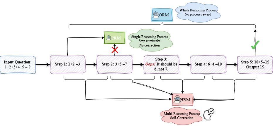<details> <summary>imgs/hrm_fig_wt_fixed.png Details</summary>  ### Visual Description ## Diagram: Reasoning Process Comparison (ORM, PRM, HRM) ### Overview The image is a flowchart diagram illustrating and comparing three different reasoning process models: ORM (Whole Reasoning Process), PRM (Single Reasoning Process), and HRM (Multi-Reasoning Process with Self-Correction). It uses a specific arithmetic problem ("1+2+3+4+5 = ?") as an example to demonstrate how each model handles a step-by-step calculation, including an error and its correction. ### Components/Axes The diagram is structured as a process flow from left to right, with additional components placed above and below the main flow. **Main Flow (Center, Left to Right):** 1. **Input Question Box (Leftmost):** A blue-bordered rectangle containing the text: `Input Question: 1+2+3+4+5 = ?` 2. **Step Boxes (Purple, Sequential):** Five purple-bordered rectangles connected by arrows, representing calculation steps. * `Step 1: 1+2 = 3` * `Step 2: 3+3 = 7` (This step contains an error.) * `Step 3: Oops! It should be 6, not 7.` (This step contains a correction annotation in red text "Oops!" and the correct calculation.) * `Step 4: 6+4 = 10` * `Step 5: 10+5=15 Output 15` (Final output box.) **Upper Components:** 1. **ORM (Top Center):** A blue box labeled `ORM` with a small robot icon. A cloud-shaped callout connected to it states: `Whole Reasoning Process No process reward`. An arrow from this cloud points to the final output (Step 5), marked with a green checkmark. 2. **PRM (Above Step 2):** A green box labeled `PRM` with a small robot icon. A cloud-shaped callout connected to it states: `Single Reasoning Process Stop at mistake No correction`. An arrow from this cloud points to Step 2, which is marked with a large red "X". **Lower Component:** 1. **HRM (Below Steps 2-5):** A red box labeled `HRM` with a small robot icon. A cloud-shaped callout connected to it states: `Multi-Reasoning Process Self-Correction` with a small icon of a head with a checkmark. Arrows from the HRM box connect to Steps 2, 3, 4, and 5, indicating its involvement in monitoring and correcting the process. **Flow Arrows:** * Solid black arrows connect the main step boxes sequentially. * A curved arrow from the ORM cloud points to the final Step 5. * An arrow from the PRM cloud points to the erroneous Step 2. * Multiple arrows connect the HRM box to the step boxes where it intervenes. ### Detailed Analysis The diagram uses the arithmetic sequence `1+2+3+4+5` to model a reasoning chain. * **The Error:** The error is introduced in `Step 2: 3+3 = 7`. The correct sum is 6. * **PRM Behavior:** The PRM (Single Reasoning Process) model is shown to "Stop at mistake" with "No correction." This is visually represented by the arrow from the PRM cloud terminating at the erroneous Step 2, which is crossed out with a red X. The process halts here under this model. * **HRM Behavior:** The HRM (Multi-Reasoning Process) model is shown to enable "Self-Correction." It is connected to the erroneous Step 2 and the subsequent correction in `Step 3: Oops! It should be 6, not 7.` This indicates the HRM model identifies the error and generates a corrective step, allowing the process to continue to the correct final answer. * **ORM Behavior:** The ORM (Whole Reasoning Process) model is associated with the final, correct output (`Step 5: Output 15`). The label "No process reward" suggests it evaluates the end result without assigning credit or blame to intermediate steps. The green checkmark confirms the final answer is correct under this model. ### Key Observations 1. **Error Handling is Central:** The core of the diagram is the contrast between how the three models handle an intermediate computational error. 2. **Visual Coding:** Colors and symbols are used consistently: Blue for ORM (whole process), Green for PRM (single process, stops), Red for HRM (multi-process, corrects). The red "X" and "Oops!" highlight the error and correction. 3. **Process Flow vs. Oversight:** The main purple boxes show the linear calculation flow. The ORM, PRM, and HRM components represent different oversight or evaluation frameworks applied to that flow. 4. **Outcome:** Only the processes involving self-correction (HRM) or whole-process evaluation (ORM) reach the correct final answer (15). The PRM process fails at the point of error. ### Interpretation This diagram is a conceptual model comparing AI or cognitive reasoning architectures. It argues that: * **Single-step evaluation (PRM)** is brittle; it detects errors but cannot recover, leading to process failure. * **Multi-step, self-correcting evaluation (HRM)** is more robust. It can identify errors mid-process, generate corrective sub-steps, and steer the reasoning back on track, leading to a correct outcome. * **Whole-process evaluation (ORM)** judges the final output without concerning itself with the path taken. It accepts the result if correct, regardless of intermediate mistakes (which may have been corrected by another mechanism like HRM). The underlying message is that for complex, multi-step reasoning tasks, architectures capable of **self-correction (HRM)** are essential for reliability. The ORM model represents a final answer checker, while PRM represents a fragile step-by-step validator. The diagram suggests that a combination (perhaps HRM feeding into an ORM-like final judge) might be an effective design pattern for building robust reasoning systems. The arithmetic example is a simple metaphor for any sequential problem-solving task where early errors can propagate and invalidate results. </details> Figure 1: Illustration of how ORM, PRM, and HRM handle reasoning processes. ORM evaluates the entire reasoning chain, PRM assesses individual steps but stops at errors, and HRM considers multiple consecutive steps, enabling error correction. The figure also demonstrates how HRM constructs its training dataset by merging two consecutive steps. ## 2 Related Work ### 2.1 RLHF Reinforcement Learning with Human Feedback (RLHF) Ouyang et al. (2022) is a widely used framework for optimizing LLMs by incorporating human feedback. The core idea of RLHF is to use a Reward Model (RM) to distinguish between high-quality and low-quality responses and optimize the LLM using PPO Schulman et al. (2017). From the perspective of reward design, there are two main approaches: ORM Cobbe et al. (2021); Lightman et al. (2023); Wang et al. (2023) and PRM Lightman et al. (2023); Uesato et al. (2022); Luo et al. (2024); Zhang et al. (2024). ORM assigns rewards based on the whole output, while PRM evaluates intermediate reasoning steps to provide more fine-grained supervision. ### 2.2 ORM ORM suffers from delayed feedback and the credit assignment problem. Since rewards are only provided at the final outcome, ORM struggles to discern which intermediate steps contribute to success or failure Lightman et al. (2023). This delayed feedback limits learning efficiency, making it harder to optimize critical decision points. Additionally, ORM is prone to spurious reasoning Cobbe et al. (2021); Wang et al. (2023), where the model arrives at the correct answer despite flawed intermediate steps, reinforcing suboptimal reasoning patterns. However, DeepSeek-R1 Guo et al. (2025) integrates a rule-based ORM within GRPO Shao et al. (2024), demonstrating that rule-based reward, rather than score-based reward models, can effectively guide LLMs toward generating long-CoT reasoning and self-reflection, ultimately enhancing their reasoning abilities. <details> <summary>imgs/hrm_fig2.png Details</summary>  ### Visual Description ## Diagram: MCTS Rollout and Auto-labeling Reasoning Process for a Math Problem ### Overview The image is a flowchart diagram illustrating a two-stage process for solving and evaluating a simple math word problem. The left stage, labeled "MCTS Rollout," shows the generation of multiple solution paths. The right stage, labeled "Auto-label reasoning process," shows the evaluation and labeling of those paths as correct or incorrect. The overall flow moves from left to right, indicated by a large yellow arrow. ### Components/Axes The diagram is composed of several key components arranged in a hierarchical, tree-like structure: 1. **Problem Statement (Top Center):** A blue-bordered text box containing the initial math problem. 2. **Process Labels (Top Left & Right):** Two orange-bordered boxes labeling the two main stages. * Left: "MCTS Rollout" * Right: "Auto-label reasoning process" 3. **Root Node (Q):** A circle labeled "Q" (for Question) appears at the top of each process tree, representing the starting point. 4. **Solution Path Nodes (MCTS Rollout):** * **First-Level Nodes (Purple):** Two rectangular boxes showing intermediate calculation steps. * **Second-Level Nodes (Red & Green):** Four rectangular boxes showing final calculations and results. The color indicates correctness: red for incorrect, green for correct. 5. **Evaluation Nodes (Auto-label Process):** * **First-Level Nodes (Purple Circles):** Two circles containing numerical values (0.5, 1.0), likely representing confidence scores or probabilities assigned to solution branches. * **Second-Level Outcomes (Symbols):** Below each purple circle are two outcomes marked with symbols: a red "X" for incorrect and a green checkmark (✓) for correct. ### Detailed Analysis **1. Problem Statement:** * **Text:** "I earn $12 an hour for babysitting. Yesterday, I just worked 50 minutes of babysitting. How much did I earn yesterday." **2. MCTS Rollout Process (Left Side):** * **Root (Q):** The question branches into two intermediate calculation paths. * **Path 1 (Left Branch):** * **Intermediate Step (Purple Box):** `12 ÷ 60 = 0.2$/min` (Converts hourly rate to per-minute rate). * **Outcomes:** * **Left (Red Box - Incorrect):** `0.2 × 50 = 1.0` (This calculation is arithmetically correct but yields the wrong final answer due to a unit error; it treats 0.2 as dollars per minute but multiplies by 50 minutes, resulting in $1.00, which is incorrect). * **Right (Green Box - Correct):** `0.2 × 50 = 10` (This calculation is arithmetically incorrect as written—0.2 * 50 = 10—but the result, 10, is the correct final answer. This suggests the node represents a correct reasoning *path* despite a notational error in the intermediate step). * **Path 2 (Right Branch):** * **Intermediate Step (Purple Box):** `50 ÷ 60 = 5/6 h` (Converts minutes worked to hours worked). * **Outcomes:** * **Left (Green Box - Correct):** `12 × 5/6 = 10` (Correct calculation: $12/hour * (5/6) hour = $10). * **Right (Green Box - Correct):** `12 × 5/6 = 10` (Identical correct calculation). **3. Auto-label Reasoning Process (Right Side):** * **Root (Q):** The question branches into two evaluation nodes. * **Evaluation Node 1 (Left, Purple Circle "0.5"):** This node likely corresponds to the left branch of the MCTS tree. It has two child outcomes: * **Left Outcome:** Red "X" (Incorrect). This aligns with the red "1.0" result from the MCTS tree. * **Right Outcome:** Green checkmark (✓) (Correct). This aligns with the green "10" result from the same MCTS branch. * **Evaluation Node 2 (Right, Purple Circle "1.0"):** This node likely corresponds to the right branch of the MCTS tree. It has two child outcomes: * **Left Outcome:** Green checkmark (✓) (Correct). Aligns with the first green "10" result. * **Right Outcome:** Green checkmark (✓) (Correct). Aligns with the second green "10" result. ### Key Observations 1. **Multiple Solution Paths:** The MCTS Rollout generates four distinct final calculation nodes from two intermediate steps, exploring different ways to parse and compute the problem. 2. **Color-Coded Correctness:** The diagram uses a consistent color scheme: red for incorrect results and green for correct results in the MCTS stage. The Auto-label stage uses red "X" and green checkmarks for the same purpose. 3. **Discrepancy in Left Branch:** The left MCTS branch produces one incorrect result (`1.0`) and one correct result (`10`) from the same intermediate step (`0.2$/min`). This highlights how a single reasoning step can lead to divergent outcomes. 4. **Evaluation Mapping:** The Auto-label process appears to assign a confidence score (0.5) to the more ambiguous left branch (which produced mixed results) and a perfect score (1.0) to the consistently correct right branch. 5. **Spatial Layout:** The legend (color/symbol key) is implicit but consistent. The "MCTS Rollout" label is top-left, the "Auto-label" label is top-right, and the flow arrow is centered between them. The problem statement is centered at the very top. ### Interpretation This diagram visually explains a methodology for training or evaluating an AI's mathematical reasoning capabilities. * **What it demonstrates:** It shows how a Monte Carlo Tree Search (MCTS) algorithm can be used to *generate* a diverse set of potential solution paths (rollouts) for a given problem, including both correct and incorrect ones. Subsequently, an auto-labeling process evaluates these paths, assigning confidence scores and binary correctness labels. * **Relationship between elements:** The MCTS Rollout is the *exploration* phase, creating a dataset of reasoning traces. The Auto-label process is the *evaluation* phase, turning those traces into labeled training data (correct/incorrect) with associated confidence metrics. The arrow signifies this pipeline from generation to labeling. * **Notable insights:** * The process explicitly values *diversity of errors*. The incorrect path (`0.2 × 50 = 1.0`) is as valuable for training as the correct ones, as it teaches the model what mistakes to avoid. * The confidence score of "0.5" for the mixed-correctness branch is insightful. It suggests the auto-labeler recognizes this branch as "noisy" or containing contradictory evidence, rather than being wholly right or wrong. * The diagram implies that the final output for training would be a set of (problem, reasoning_path, label, confidence) tuples, which can be used to fine-tune a model to prefer high-confidence, correct reasoning chains. In essence, the image is a technical schematic for a data generation pipeline in AI, specifically for improving step-by-step mathematical reasoning through exploration and automated evaluation. 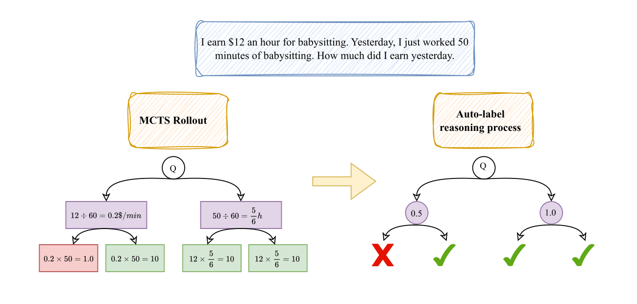</details> Figure 2: Illustration of the MCTS-based automated reasoning annotation process. The left side depicts a tree structure where each node represents a reasoning step, simulated using the ToT approach with MCTS. The right side visualizes the assigned scores for each step in the reasoning tree. ### 2.3 PRM One of the most critical challenges in PRM is reward hacking, a phenomenon in which an RL agent exploits flaws or ambiguities in the reward function to achieve artificially high rewards without genuinely learning the intended task or completing it as expected Amodei et al. (2016); Di Langosco et al. (2022); Everitt et al. (2017); Weng (2024). Furthermore, the annotation process required for training PRM is prohibitively expensive Lightman et al. (2023); Uesato et al. (2022), making large-scale implementation impractical. To address this issue, MCTS has been proposed as an autonomous method for annotating reasoning trajectories Luo et al. (2024); Zhang et al. (2024). Moreover, in MCTS, the computational cost increases significantly as the depth and breadth of the search tree expand. To mitigate this, constraints are imposed on both tree height and width, limiting the number of simulation steps and thereby reducing the diversity of generated reasoning data. ## 3 Methodology ### 3.1 Hierarchical Reward Model PRM provides fine-grained, step-wise supervision, whereas ORM evaluates reasoning holistically. To combine the advantages of both, we propose the H ierarchical R eward M odel (HRM), which introduces hierarchical supervision by training on both single-step and consecutive multi-step reasoning sequences. HRM serves as an evaluation-oriented reward model that estimates the relative quality of reasoning trajectories, rather than directly optimizing the policy model itself. This hierarchical design enables HRM to capture both local accuracy and global coherence, yielding more stable and reliable reward evaluation in multi-step reasoning. The HRM training data extends PRM supervision by merging consecutive reasoning steps into hierarchical segments (from step 1 to $N$ ), as illustrated in Fig. 1, forming a superset of the PRM dataset. <details> <summary>x1.png Details</summary>  ### Visual Description ## Diagram: Node Merging and Connection Redirection Process ### Overview The image displays a two-part diagram illustrating a three-step transformation of a tree-like decision or reasoning structure. The left side shows the initial state with two highlighted nodes (N1 and N2), and the right side shows the final state after the transformation. A large cyan arrow connects the two states, indicating the flow of the process. Textual instructions at the bottom describe the three steps performed. ### Components/Axes The diagram consists of two tree structures composed of circular nodes connected by directional arrows (edges). Each node contains a numerical value (e.g., 0.75, 0.5, 1, 0.25). Below the terminal (leaf) nodes are outcome symbols: green circles with white checkmarks (✓) and red circles with white crosses (✗). **Key Elements & Spatial Grounding:** * **Left Diagram (Initial State):** * A root node at the top center with value `0.75`. * Two primary child nodes below it, also labeled `0.75`. * The left child node (`0.75`) branches into nodes with values `0.5` and `1`. * The right child node (`0.75`) is highlighted with a yellow box and labeled **N1**. It branches into nodes with values `1` and `0.25`. * The node with value `1` directly below N1 is highlighted with a yellow box and labeled **N2**. * Terminal nodes from left to right have outcomes: ✓, ✗, ✓, ✓, ✓, ✓, ✓, ✗. * **Right Diagram (Final State):** * A root node at the top center with value `0.75`. * Two primary child nodes below it, labeled `0.75` (left) and `0.5` (right). * The left child node (`0.75`) branches into nodes with values `0.5` and `1`. * The node with value `1` (previously N2) is now highlighted with a yellow box and labeled **N2'**. It is directly connected to the root's left child (`0.75`). * The right child of the root (`0.5`) branches into nodes with values `1` and `0.25`. * Terminal nodes from left to right have outcomes: ✓, ✗, ✓, ✓, ✓, ✓, ✓, ✗. * **Connecting Arrow:** A thick, curved cyan arrow originates from the highlighted area (N1/N2) in the left diagram and points to the highlighted node (N2') in the right diagram. * **Instructional Text:** Located at the bottom center of the image. ### Detailed Analysis **Text Transcription:** The following text is present at the bottom of the image: > **Step 1:** Merge the reasoning steps of N1 and N2, integrating their information into N2. > **Step 2:** Remove the direct connection between N1 and N2. > **Step 3:** Redirect N2 to point to N0. **Node Value and Connection Analysis:** * **Initial Structure (Left):** The path is Root(0.75) -> N1(0.75) -> N2(1) -> Terminal(✓). N1 also has a sibling node (0.25). * **Transformation Process:** 1. **Merge (Step 1):** The information from node N1 (0.75) is integrated into node N2 (1). The diagram shows N2' on the right still has the value `1`, suggesting the merge may involve combining reasoning or probability rather than averaging the numerical labels. 2. **Remove Connection (Step 2):** The edge from N1 to N2 is severed. 3. **Redirect (Step 3):** Node N2' is reconnected. Instead of being a child of N1, it becomes a child of the node that was N1's parent (the root's left child, 0.75). The text says "point to N0," which likely refers to the root node or its immediate child in the new hierarchy. * **Final Structure (Right):** The new path is Root(0.75) -> Left Child(0.75) -> N2'(1) -> Terminal(✓). The original N1 node and its other child (0.25) are now part of a separate branch under the root's new right child (0.5). ### Key Observations 1. **Outcome Consistency:** The sequence of terminal outcomes (✓, ✗, ✓, ✓, ✓, ✓, ✓, ✗) is identical in both the left and right diagrams. This indicates the transformation preserves the final decision outcomes at the leaves. 2. **Structural Simplification:** The process effectively removes one level of hierarchy (N1) by promoting its child (N2) and merging information upwards. 3. **Value Ambiguity:** The numerical node labels (0.75, 1, etc.) do not change during the merge (N2 remains `1`). Their exact meaning (e.g., confidence score, probability, weight) is not defined in the diagram. 4. **Spatial Reorganization:** The right side of the tree is reorganized. The node that was N1's sibling (0.25) is now under a different parent (0.5), which is a new child of the root. ### Interpretation This diagram visually explains an algorithm or heuristic for optimizing a reasoning tree, likely in fields like decision theory, search algorithms (e.g., Monte Carlo Tree Search), or probabilistic graphical models. * **What it demonstrates:** The process shows how to consolidate information and simplify a decision path without altering the final outcomes. Merging N1 into N2 and promoting N2 streamlines the tree, potentially reducing computational complexity or improving interpretability by eliminating a redundant reasoning step (N1). * **Relationships:** The core relationship is parent-child between nodes, representing a flow of reasoning or probability. The transformation changes these relationships to create a more efficient structure. The cyan arrow explicitly maps the cause (steps applied to N1/N2) to the effect (new position of N2'). * **Notable Implications:** The preservation of leaf outcomes is critical—it confirms the optimization is "safe" and doesn't change the system's final decisions. The reorganization of the right branch suggests the algorithm may also rebalance the tree globally after a local merge. The unspecified meaning of the node values is a key uncertainty; their role in the merge logic is implied but not visually detailed. 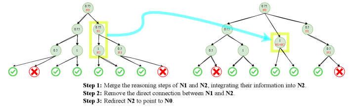</details> Figure 3: Illustration of HNC. The left part represents the original MCTS data annotation structure, while the right part shows the transformed MCTS structure after applying HNC. Formally, let $D$ represent the training dataset, $N$ denote the total number of reasoning steps in a sequence, $s_{i}$ be the $i$ -th reasoning step, and $R(\cdot)$ be the reward function that assigns a score to a step. The training datasets for PRM and HRM are defined as: $$ \displaystyle D_{\text{PRM}}=\left\{(s_{i},\,R(s_{i}))\mid 1\leq i\leq N\right\}, \displaystyle D_{\text{HRM}}=D_{\text{PRM}} \displaystyle\quad\cup\left\{(s_{i}+s_{i+1},\,R(s_{i}+s_{i+1}))\mid 1\leq i<N\right\}. \tag{1} $$ Hierarchical supervision aims to connect local correctness with global coherence by jointly evaluating individual steps and their interactions. In practice, HRM achieves this through two objectives: (1) capturing both fine-grained and coarse-grained consistency, and (2) enabling self-reflection and error correction. Unlike PRM, which evaluates each step independently and penalizes early mistakes, HRM considers whether later steps can repair earlier errors, treating them as a coherent reasoning process rather than isolated faults. Although HRM training data incorporates merged reasoning steps, the model remains step-wise in inference, assigning a reward based solely on the current step $s_{i}$ , similar to PRM. This design preserves fine-grained step-level evaluation while mitigating the subjectivity of step segmentation: by merging neighboring steps during training, HRM smooths annotation noise from ambiguous boundaries and enhances robustness across reasoning granularities. Conceptually, this hierarchical supervision extends PRM in a principled way, integrating both local accuracy and global coherence. In this work, we instantiate HRM with two-step merging as the minimal yet effective form of hierarchical supervision, enabling controlled analysis while maintaining computational efficiency. ### 3.2 Hierarchical Node Compression in MCTS Due to the prohibitively high cost of human-annotated supervision, autonomous annotation methods based on MCTS have been proposed. Fig. 2 illustrates the process of automatic reasoning annotation using MCTS. Given a ground truth and a corresponding question, MCTS generates multiple possible reasoning paths by simulating different step-by-step solutions. Each node in the search tree represents a reasoning step, and its score is calculated based on the proportion of correct trajectories in its subtree, reflecting the likelihood that the reasoning path is valid. However, these methods demand substantial computational resources, as achieving reliable estimates of intermediate reasoning step scores requires a sufficiently deep and wide search tree to reduce variance and mitigate bias; otherwise, the estimates may remain unreliable. This exponential growth in complexity makes large-scale implementation challenging. To better leverage autonomous process annotation, we propose a data augmentation method called H ierarchical N ode C ompression (HNC). The key idea is to merge two consecutive nodes, each corresponding to a reasoning step, into a single node, thereby creating a new branch with minimal computational overhead. As shown in Fig. 3, HNC assumes that each node has a sufficiently large number of child nodes. By randomly merging consecutive nodes, it introduces controlled noise, enhancing the robustness of MCTS-based scoring. Before HNC, each child node contributes $\frac{1}{N}$ to the total score. After HNC removes a random node, the remaining child nodes redistribute their weights to $\frac{1}{N-1}$ , increasing their individual influence. Since child nodes are independent and identically distributed from the parent’s perspective, the expectation of the parent score remains unchanged. However, the variance increases from $\frac{\sigma^{2}}{N}$ to $\frac{\sigma^{2}}{N-1}$ , introducing controlled noise that enables data augmentation at an extremely low computational cost. When $N$ is sufficiently large, this variance change remains moderate while still facilitating effective data augmentation. ### 3.3 Self-Training We filter high-quality reasoning data from MCTS using the MC-Score to ensure reliable supervision and avoid reward bias. Due to computational constraints, we do not employ RL methods such as PPO Schulman et al. (2017) or GRPO Shao et al. (2024). Instead, we continue using supervised fine-tuning. To preserve the general capabilities of the policy model, we incorporate causal language modeling loss combined with KL divergence regularization using a reference model. The objective function is defined as: $$ \mathcal{L}=\mathcal{L}_{\text{LM}}+\lambda\log D_{\text{KL}}(P||Q), \tag{3} $$ where $\mathcal{L}_{\text{LM}}$ represents the causal language modeling loss computed on high-quality reasoning sequences, and $D_{\text{KL}}(P||Q)$ denotes the KL divergence between the policy model’s output distribution $P$ and the reference model’s output distribution $Q$ . The term $\lambda$ serves as a weighting factor to balance task-specific adaptation and retention of general capabilities. | ORM | 0.622 | 0.677 | 0.655 | 0.655 | 0.633 | | --- | --- | --- | --- | --- | --- | | PRM | 0.700 | 0.644 | 0.611 | 0.588 | 0.577 | | HRM | 0.722 | 0.711 | 0.744 | 0.800 | 0.800 | Table 2: Accuracy of Qwen2.5-72B-Math-Instruct on the PRM800K test set under the best-of- $N$ strategy, comparing ORM, PRM, and HRM. All models are fine-tuned on the manually labeled PRM800K dataset. | DeepSeek-Math-7B HRM Qwen2.5-72B-Math | PRM 0.311 PRM | 0.311 0.388 0.233 | 0.433 0.444 0.344 | 0.377 0.455 0.411 | 0.455 0.455 0.422 | 0.411 0.422 0.488 | 0.455 0.533 0.522 | 0.466 0.522 0.600 | 0.444 0.455 0.566 | 0.377 0.500 0.666 | 0.377 0.700 | | --- | --- | --- | --- | --- | --- | --- | --- | --- | --- | --- | --- | | HRM | 0.288 | 0.366 | 0.366 | 0.488 | 0.511 | 0.611 | 0.622 | 0.611 | 0.711 | 0.722 | | | Qwen2.5-7B-Math | PRM | 0.477 | 0.466 | 0.600 | 0.544 | 0.633 | 0.677 | 0.733 | 0.677 | 0.700 | 0.722 | | HRM | 0.500 | 0.566 | 0.655 | 0.600 | 0.666 | 0.711 | 0.711 | 0.766 | 0.777 | 0.766 | | Table 3: Accuracy of different policy models under PRM and HRM using the best-of- $N$ strategy on the PRM800K test set. The training data for both PRM and HRM are derived from MCTS with Qwen2.5-7B-Math-Instruct. Without proper KL regularization or with an insufficiently weighted KL loss (i.e., a very small $\lambda$ ), the KL divergence grows unbounded during training. Specifically, KL loss typically ranges from $0$ to $20000$ , whereas the causal LM loss remains within $0$ to $12$ , leading to a severe loss imbalance. This causes the optimization process to excessively minimize KL divergence at the expense of task-specific reasoning performance. To address this, we apply a logarithmic scaling to $D_{\text{KL}}(P||Q)$ , stabilizing the loss landscape and ensuring a balanced trade-off between preserving general language capabilities and enhancing reasoning ability. Further details are provided in Section 4.3. ## 4 Experiment ### 4.1 HRM Given that the PRM800K dataset consists of Phase1 and Phase2, where Phase1 includes manually annotated reasoning processes, we utilize these manual annotations to construct the training datasets for ORM, PRM, and HRM. ORM training data comprises complete reasoning trajectories, while PRM training data consists of individual reasoning steps conditioned on preceding context. HRM training data extends PRM by incorporating multiple consecutive reasoning steps, allowing HRM to capture self-reflection and ensure reasoning coherence across sequential steps. Table 6 summarizes the labeling rules for merged reasoning steps in HRM. We fine-tune Qwen2.5-1.5B-Math Yang et al. (2024b) as the RM for classifying given reasoning step as correct or incorrect. Given an input, RM predicts logits for the positive and negative classes, denoted as $l_{\text{pos}}$ and $l_{\text{neg}}$ , respectively. The score is obtained by applying the softmax function: $$ P(y=\text{pos}\mid x)=\frac{\exp(l_{\text{pos}})}{\exp(l_{\text{pos}})+\exp(l_{\text{neg}})}, \tag{4} $$ where $P(y=\text{pos}\mid x)$ denotes the probability of given reasoning step being correct. This probability serves as the reward assigned by RM. Detailed information is provided in Appendix A.2. To evaluate the performance of ORM, PRM, and HRM, we employ Qwen2.5-72B-Math-Instruct Yang et al. (2024b) as the policy model and implement the best-of- $N$ strategy. Specifically, ORM selects the best result from $N$ complete reasoning trajectories, while PRM and HRM score $N$ intermediate reasoning steps and select the most promising one at each step. For PRM and HRM, we consider the completion of a formula as an intermediate reasoning step, enabling a finer-grained evaluation mechanism. Table 2 presents the results, showing that the accuracy of the policy model with ORM and PRM exhibits significant fluctuations, decreasing as $N$ increases. In contrast, the policy model with HRM maintains stable performance, converging to an accuracy of 80% as $N$ grows. #### Statistical robustness. The evaluation itself already provides extensive statistical averaging. Each dataset contains thousands of test problems (1k in GSM8K, 500 in MATH500, and over 800k annotated reasoning steps in PRM800K), which smooths random variation across samples. Notably, MATH500 and PRM800K consist of challenging high-school and university-level problems (e.g., calculus, linear algebra), whose solutions require multi-step reasoning rather than surface-level pattern matching or guessing. Moreover, in the Best-of- $N$ evaluation (up to $N=512$ ), each reasoning step expands into $N$ candidate paths, forming an exponentially large search tree. This hierarchical exploration implicitly averages over a vast number of trajectories, effectively functioning as multi-seed sampling and significantly reducing evaluation variance. <details> <summary>imgs/kl.png Details</summary>  ### Visual Description ## [Chart Type]: Training Loss Curves (2x3 Grid) ### Overview The image displays a 2x3 grid of six line charts, visualizing two types of loss metrics over training iterations for three different values of a parameter labeled "HRM". The top row shows "Log KL Loss" (blue lines), and the bottom row shows "Causal LM Loss" (red lines). Each column corresponds to a specific HRM value: 0.001 (left), 0.5 (center), and 10.0 (right). All plots share the same x-axis representing training iterations. ### Components/Axes **Common Elements:** * **X-Axis (All Plots):** Labeled "Iterations". The scale runs from 0 to 50,000, with major tick marks at 0, 10000, 20000, 30000, 40000, and 50000. * **Plot Titles:** Each subplot has a title indicating the loss type and HRM value. * **Grid:** All plots have a light gray grid in the background. **Top Row - Log KL Loss (Blue Lines):** * **Y-Axis Label:** "Log KL Loss". * **Plot 1 (Top-Left):** Title: "Log KL Loss (HRM 0.001)". Y-axis scale: 0 to 10, with ticks at 0, 2, 4, 6, 8, 10. * **Plot 2 (Top-Center):** Title: "Log KL Loss (HRM 0.5)". Y-axis scale: 0.0 to 3.5, with ticks at 0.0, 0.5, 1.0, 1.5, 2.0, 2.5, 3.0, 3.5. * **Plot 3 (Top-Right):** Title: "Log KL Loss (HRM 10.0)". Y-axis scale: 0 to 4, with ticks at 0, 1, 2, 3, 4. **Bottom Row - Causal LM Loss (Red Lines):** * **Y-Axis Label:** "Causal LM Loss". * **Plot 4 (Bottom-Left):** Title: "Causal LM Loss (HRM 0.001)". Y-axis scale: -5.0 to 10.0, with ticks at -5.0, -2.5, 0.0, 2.5, 5.0, 7.5, 10.0. * **Plot 5 (Bottom-Center):** Title: "Causal LM Loss (HRM 0.5)". Y-axis scale: 0 to 12, with ticks at 0, 2, 4, 6, 8, 10, 12. * **Plot 6 (Bottom-Right):** Title: "Causal LM Loss (HRM 10.0)". Y-axis scale: 0 to 12, with ticks at 0, 2, 4, 6, 8, 10, 12. ### Detailed Analysis **Trend Verification & Data Points:** 1. **Log KL Loss (HRM 0.001):** * **Trend:** The blue line shows a very rapid, near-vertical increase from near 0 at iteration 0 to approximately 8 by iteration ~2000. It then continues to rise more gradually, reaching a plateau between ~8 and ~10.5 from iteration ~10,000 onward. The line exhibits high-frequency noise/variance throughout the plateau. * **Key Values:** Starts ~0. Rapid rise to ~8 (iter ~2k). Plateau range: ~8 to ~10.5 (iter 10k-50k). 2. **Log KL Loss (HRM 0.5):** * **Trend:** The blue line starts near 0, rises quickly to a range of ~0.3 to ~1.5 by iteration ~5000. It then enters a highly volatile phase with frequent, large upward spikes. The baseline of the signal appears to slowly increase from ~0.3 to ~0.5 over the course of training, while spikes regularly reach between 2.0 and 3.5. * **Key Values:** Initial rise to ~0.3-1.5 (iter ~5k). Volatile baseline: ~0.3 to ~0.5. Prominent spikes: multiple instances reaching 2.5-3.5. 3. **Log KL Loss (HRM 10.0):** * **Trend:** Similar volatile pattern to HRM 0.5, but with a different scale. The blue line starts near 0, rises to a noisy band between ~0.1 and ~1.0 by iteration ~5000. It continues with extreme volatility, featuring sharp spikes. The baseline appears lower than the HRM 0.5 case, but the spikes are very pronounced. * **Key Values:** Initial rise to ~0.1-1.0 (iter ~5k). Volatile baseline: ~0.1 to ~0.5. Major spikes: several reaching 3.0-4.0. 4. **Causal LM Loss (HRM 0.001):** * **Trend:** The red line starts at a high value (~10-11) and undergoes a dramatic, steep decline within the first ~5000 iterations, dropping below 0. It continues to decrease, stabilizing in a negative range. From iteration ~10,000 onward, it forms a dense, noisy band centered around approximately -4.5 to -5.0. * **Key Values:** Starts ~10-11. Sharp drop to <0 by iter ~5k. Stable negative plateau: dense band from ~-4.0 to ~-5.5 (iter 10k-50k). 5. **Causal LM Loss (HRM 0.5):** * **Trend:** The red line starts high (~10-11), drops sharply within the first ~5000 iterations to a range of ~0 to ~4. After this initial drop, it stabilizes into a noisy, horizontal band. The band's center appears to be around 2.0, with fluctuations mostly between 0 and 4. * **Key Values:** Starts ~10-11. Sharp drop to ~0-4 by iter ~5k. Stable noisy band: ~0 to ~4, centered near 2.0 (iter 5k-50k). 6. **Causal LM Loss (HRM 10.0):** * **Trend:** The red line starts high (~10-11). It shows an initial decline, but then exhibits a significant upward spike around iteration ~12,000, reaching near 13. Following this spike, it drops again and stabilizes into a noisy band. This final band is positioned higher than the HRM 0.5 case, centered around 4.0, with fluctuations mostly between 0 and 6. * **Key Values:** Starts ~10-11. Spike to ~13 (iter ~12k). Stable noisy band after spike: ~0 to ~6, centered near 4.0 (iter ~15k-50k). ### Key Observations 1. **HRM Parameter Impact:** The HRM value dramatically affects the behavior and final value of both loss types. 2. **Log KL Loss Behavior:** Lower HRM (0.001) leads to a high, stable (though noisy) Log KL Loss. Higher HRM values (0.5, 10.0) result in lower baseline loss but introduce extreme volatility and large spikes. 3. **Causal LM Loss Behavior:** Lower HRM (0.001) drives the Causal LM Loss to a negative value, which is unusual for a standard loss function. Higher HRM values keep the loss positive, with the final stable value increasing as HRM increases (from ~2.0 at HRM 0.5 to ~4.0 at HRM 10.0). 4. **Inverse Relationship:** There appears to be an inverse relationship between the two losses across the HRM spectrum. The configuration that minimizes Causal LM Loss (HRM 0.001) maximizes Log KL Loss, and vice-versa. 5. **Training Dynamics:** All configurations show rapid change in the first 5,000-10,000 iterations before entering a more stable (though noisy) phase. The HRM 10.0 Causal LM Loss plot shows a notable instability (spike) later in training. ### Interpretation This grid of charts likely visualizes the training dynamics of a machine learning model, possibly a variational autoencoder (VAE) or a similar model that optimizes a combined loss function containing both a Kullback-Leibler (KL) divergence term (Log KL Loss) and a language modeling (LM) term (Causal LM Loss). The "HRM" parameter appears to be a weighting coefficient that balances these two objectives. The data demonstrates a classic **trade-off** controlled by HRM: * **Low HRM (0.001):** The model heavily prioritizes minimizing the Causal LM Loss (achieving very low, even negative values), likely at the expense of the latent space regularization, causing the KL divergence (Log KL Loss) to become large. This could indicate posterior collapse or a poorly regularized latent space. * **High HRM (10.0):** The model prioritizes keeping the KL divergence low (better regularization), but this comes at the cost of a higher Causal LM Loss, meaning the model's primary generative or predictive performance may be worse. The high volatility in KL loss suggests instability in the regularization process. * **Intermediate HRM (0.5):** Represents a middle ground, with moderate values for both losses. The negative Causal LM Loss for HRM 0.001 is a critical anomaly. In standard setups, cross-entropy loss (common for LM) is non-negative. This suggests either a non-standard loss formulation, a logging error (e.g., plotting the negative of the loss), or that the model is achieving a likelihood greater than the reference distribution in a way that yields a negative value on the chosen scale. This would require investigation into the specific loss implementation. In summary, the charts provide a clear empirical map of how the HRM hyperparameter navigates the tension between model fit (Causal LM Loss) and latent space regularization (Log KL Loss), highlighting the instability and trade-offs inherent in training such models. 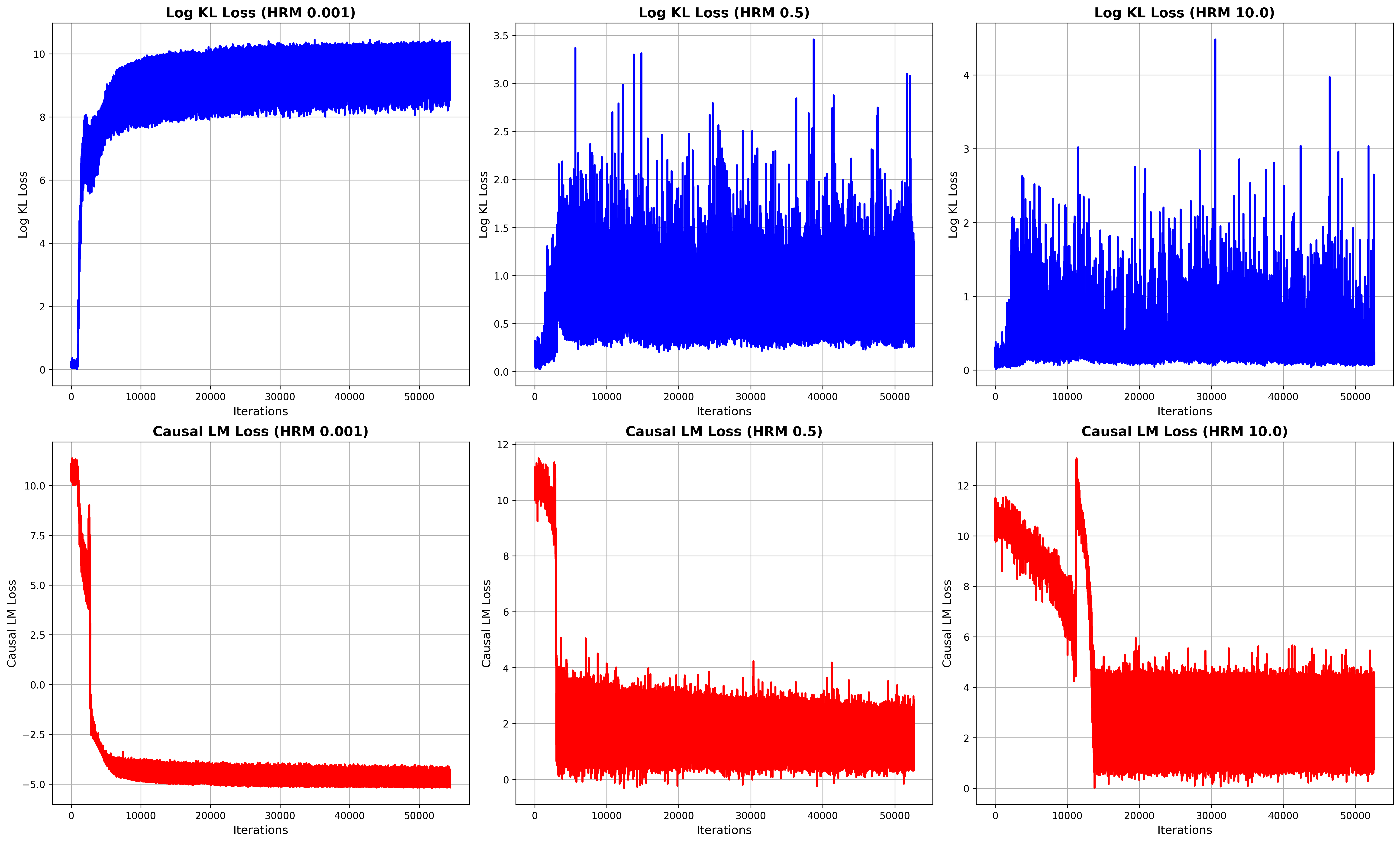</details> Figure 4: Loss dynamics during training across different KL loss weightings. Each column corresponds to a different $\lambda$ value: 0.001 (left), 0.5 (middle), and 10.0 (right). The top row shows the log KL loss, while the bottom row depicts the causal language modeling loss. ### 4.2 HNC In this section, we utilize only the questions and ground truth from the PRM800K dataset, without relying on manually annotated data. We adopt MCTS as the automatic annotation method, using Qwen2.5-7B-Math-Instruct as the reasoning engine to generate trajectories. As mentioned in Section 3.2, these auto-annotated reasoning trajectories from MCTS are used to train PRM, after which we apply the HNC data augmentation method to generate additional training data for HRM. To balance computational efficiency and robustness, we configure MCTS with 5–6 child nodes per parent and a maximum tree depth of 7, ensuring reasoning completion within 7 steps. Since the computational cost of MCTS rollouts grows exponentially with tree depth and branching factor, we limit these parameters to maintain feasibility. The full MCTS simulation requires approximately 2,457 A100 GPU-hours, while the HNC augmentation process takes around 30 minutes with CPU. We perform supervised fine-tuning of Qwen2.5-1.5B-Math for both PRM and HRM. Training HRM adds roughly 30% more samples compared to PRM, increasing total training time from about 84 GPU hours to 120 GPU hours on A100 GPUs. This additional cost is negligible relative to the over 2400 GPU hours required for generating the reasoning trajectories via MCTS, which constitute the true computational bottleneck. To evaluate performance, we employ different policy models, including Qwen2.5-7B-Math-Instruct Yang et al. (2024b), DeepSeek-Math-7B Shao et al. (2024), and Qwen2.5-72B-Math-Instruct Yang et al. (2024b), applying the best-of- $N$ strategy on the PRM800K dataset. Detailed training information is provided in Appendix A.3. | Qwen2.5-7B-Math HRM Qwen-7B-PRM | PRM 0.500 PRM | 0.477 0.566 0.477 | 0.466 0.655 0.555 | 0.600 0.600 0.533 | 0.544 0.666 0.655 | 0.633 0.711 0.655 | 0.677 0.711 0.677 | 0.733 0.766 0.711 | 0.677 0.777 0.700 | 0.700 0.766 0.744 | 0.722 0.744 | | --- | --- | --- | --- | --- | --- | --- | --- | --- | --- | --- | --- | | HRM | 0.477 | 0.544 | 0.644 | 0.722 | 0.700 | 0.711 | 0.722 | 0.755 | 0.800 | 0.800 | | | Qwen-7B-HRM | PRM | 0.511 | 0.533 | 0.644 | 0.667 | 0.667 | 0.689 | 0.733 | 0.722 | 0.744 | 0.733 | | HRM | 0.489 | 0.589 | 0.722 | 0.722 | 0.722 | 0.744 | 0.744 | 0.789 | 0.789 | 0.789 | | Table 4: Comparison of fine-tuned policy model reasoning performance on the PRM800K dataset using the best-of- $N$ strategy. Qwen-7B-HRM denotes the policy model fine-tuned on high-MC-score reasoning data from HRM’s training set, while Qwen-7B-PRM follows the same procedure for PRM’s training set. | GSM8K HRM MATH500 | PRM 0.784 PRM | 0.784 0.833 0.468 | 0.828 0.846 0.572 | 0.858 0.886 0.598 | 0.882 0.893 0.624 | 0.884 0.902 0.658 | 0.893 0.907 0.658 | 0.905 0.914 0.656 | 0.917 0.930 0.662 | 0.927 0.926 0.686 | 0.918 0.688 | | --- | --- | --- | --- | --- | --- | --- | --- | --- | --- | --- | --- | | HRM | 0.490 | 0.576 | 0.612 | 0.660 | 0.688 | 0.692 | 0.742 | 0.740 | 0.740 | 0.736 | | Table 5: Generalization performance of PRM and HRM trained on PRM800K and evaluated on GSM8K and MATH500 under the Best-of- $N$ setting using Qwen2.5-7B-Math-Instruct. Table 3 presents the accuracy results of various policy models under PRM and HRM settings on the PRM800K dataset. Although both PRM and HRM training data are derived from MCTS with Qwen2.5-7B-Math-Instruct, we evaluate HRM and PRM using different policy models, where HRM consistently demonstrates greater stability and robustness compared to PRM. The relatively lower performance of Qwen2.5-72B-Math-Instruct (as shown in Table 3) can be attributed to the tree height constraints imposed by MCTS, which limit answer generation to a predefined template of at most 6 reasoning steps and require explicit output of "# Step X". While Qwen2.5-72B-Math-Instruct exhibits strong reasoning capabilities, its highly structured training process makes it more likely to generate outputs that deviate from the required format. As a result, some outputs cannot be retrieved using regex-based post-processing, thereby affecting the overall measured performance. ### 4.3 Self-Training We adapt the method described in Section 3.3 to filter high-quality reasoning data and train the policy model. Fig. 4 illustrates that when $\lambda$ is small (e.g., 0.001), the fine-tuned policy model rapidly loses its generalization ability within just a few iterations, causing the KL loss to escalate to approximately 20,000. In contrast, the causal LM loss remains within the range of 0 to 12, leading to a significant imbalance. This discrepancy underscores the necessity of applying logarithmic scaling to the KL term in the objective function, as discussed in Section 3.3. Conversely, when $\lambda$ is excessively large (e.g., 10.0), the model prioritizes adherence to the reference distribution, resulting in slower convergence and constrained improvements in reasoning capability. We fine-tune Qwen2.5-7B-Math-Instruct using reasoning data with MC-score $>0.9$ , extracted from the PRM and HRM training datasets. Qwen-7B-HRM denotes the policy model fine-tuned on such data from HRM’s training set, while Qwen-7B-PRM follows the same procedure for PRM’s training set. We set $\lambda$ to 0.5. Table 4 further validates that SFT enhances the policy model’s reasoning capability by leveraging high-quality data, with HRM demonstrating greater robustness compared to PRM. ### 4.4 HRM Generalization Across Different Domains Trained solely on PRM800K, HRM and PRM are further evaluated on MATH500 Lightman et al. (2023) and GSM8K Cobbe et al. (2021) to assess their generalization to out-of-domain reasoning tasks. Table 5 shows that HRM exhibits greater robustness across different domains, demonstrating superior generalization performance, particularly in MATH500, where it effectively handles complex mathematical reasoning tasks. However, the performance difference between HRM and PRM on the GSM8K dataset is marginal, as GSM8K primarily consists of relatively simple arithmetic problems. A strong policy model can typically solve these problems within three steps, reducing the impact of HRM’s key advantages, such as assessing multi-step reasoning coherence and facilitating self-reflection. Nevertheless, as shown in Table 5, HRM still achieves a slight performance edge over PRM, even on simpler datasets like GSM8K. ## 5 Conclusion In this paper, we present HRM, which enhances multi-step reasoning evaluation by integrating fine-grained and coarse-grained assessments, improving reasoning coherence and self-reflection. We further introduce HNC, a data augmentation method that optimizes MCTS-based autonomous annotation, enhancing label diversity while expanding training data with minimal computational cost. Extensive experiments on PRM800K dataset demonstrate HRM’s superior robustness over PRM, with strong generalization across GSM8K and MATH500 dataset. Additionally, MCTS-generated auto-labeled data enables policy model fine-tuning, further improving reasoning performance. ## 6 Limitations ### 6.1 Merged Steps The reason why we only merge two consecutive steps at a time is to maintain the simplicity and clarity of the labeling strategy. When merging more than two steps—such as combining four reasoning steps—the number of possible label combinations increases rapidly (e.g., one positive, two negative, one neutral), making it difficult to define unified labeling rules and leading to potential conflicts. This stands in sharp contrast to the straightforward rules shown in Table 6, where merging only two steps allows for clear and consistent label definitions. ## References - Achiam et al. (2023) Josh Achiam, Steven Adler, Sandhini Agarwal, Lama Ahmad, Ilge Akkaya, Florencia Leoni Aleman, Diogo Almeida, Janko Altenschmidt, Sam Altman, Shyamal Anadkat, and 1 others. 2023. Gpt-4 technical report. In ArXiv e-prints. - Aminabadi et al. (2022) Reza Yazdani Aminabadi, Samyam Rajbhandari, Ammar Ahmad Awan, Cheng Li, Du Li, Elton Zheng, Olatunji Ruwase, Shaden Smith, Minjia Zhang, Jeff Rasley, and 1 others. 2022. Deepspeed-inference: enabling efficient inference of transformer models at unprecedented scale. In SC22: International Conference for High Performance Computing, Networking, Storage and Analysis, pages 1–15. IEEE. - Amodei et al. (2016) Dario Amodei, Chris Olah, Jacob Steinhardt, Paul Christiano, John Schulman, and Dan Mané. 2016. Concrete problems in ai safety. In arXiv preprint arXiv:1606.06565. - Amrith Setlur (2025) Adam Fisch Xinyang Geng Jacob Eisenstein Rishabh Agarwal Alekh Agarwal Jonathan Berant Aviral Kumar Amrith Setlur, Chirag Nagpal. 2025. Rewarding progress: Scaling automated process verifiers for llm reasoning. In ICLR. - Anil et al. (2023) Rohan Anil, Andrew M Dai, Orhan Firat, Melvin Johnson, Dmitry Lepikhin, Alexandre Passos, Siamak Shakeri, Emanuel Taropa, Paige Bailey, Zhifeng Chen, and 1 others. 2023. Palm 2 technical report. In ArXiv e-prints. - Cobbe et al. (2021) Karl Cobbe, Vineet Kosaraju, Mohammad Bavarian, Mark Chen, Heewoo Jun, Lukasz Kaiser, Matthias Plappert, Jerry Tworek, Jacob Hilton, Reiichiro Nakano, and 1 others. 2021. Training verifiers to solve math word problems. In ArXiv e-prints. - Dao (2024) Tri Dao. 2024. FlashAttention-2: Faster attention with better parallelism and work partitioning. In International Conference on Learning Representations (ICLR). - Dao et al. (2022) Tri Dao, Daniel Y. Fu, Stefano Ermon, Atri Rudra, and Christopher Ré. 2022. FlashAttention: Fast and memory-efficient exact attention with IO-awareness. In Advances in Neural Information Processing Systems (NeurIPS). - Di Langosco et al. (2022) Lauro Langosco Di Langosco, Jack Koch, Lee D Sharkey, Jacob Pfau, and David Krueger. 2022. Goal misgeneralization in deep reinforcement learning. In International Conference on Machine Learning, pages 12004–12019. ICML. - Everitt et al. (2017) Tom Everitt, Victoria Krakovna, Laurent Orseau, Marcus Hutter, and Shane Legg. 2017. Reinforcement learning with a corrupted reward channel. In IJCAI. - Grattafiori et al. (2024) Aaron Grattafiori, Abhimanyu Dubey, Abhinav Jauhri, Abhinav Pandey, Abhishek Kadian, Ahmad Al-Dahle, Aiesha Letman, Akhil Mathur, Alan Schelten, Alex Vaughan, and 1 others. 2024. The llama 3 herd of models. In ArXiv e-prints. - Guo et al. (2025) Daya Guo, Dejian Yang, Haowei Zhang, Junxiao Song, Ruoyu Zhang, Runxin Xu, Qihao Zhu, Shirong Ma, Peiyi Wang, Xiao Bi, and 1 others. 2025. Deepseek-r1: Incentivizing reasoning capability in llms via reinforcement learning. In ArXiv e-prints. - Kalamkar et al. (2019) Dhiraj Kalamkar, Dheevatsa Mudigere, Naveen Mellempudi, Dipankar Das, Kunal Banerjee, Sasikanth Avancha, Dharma Teja Vooturi, Nataraj Jammalamadaka, Jianyu Huang, Hector Yuen, and 1 others. 2019. A study of bfloat16 for deep learning training. arXiv preprint arXiv:1905.12322. - Lightman et al. (2023) Hunter Lightman, Vineet Kosaraju, Yuri Burda, Harrison Edwards, Bowen Baker, Teddy Lee, Jan Leike, John Schulman, Ilya Sutskever, and Karl Cobbe. 2023. Let’s verify step by step. In ICLR. - Luo et al. (2024) Liangchen Luo, Yinxiao Liu, Rosanne Liu, Samrat Phatale, Harsh Lara, Yunxuan Li, Lei Shu, Yun Zhu, Lei Meng, Jiao Sun, and 1 others. 2024. Improve mathematical reasoning in language models by automated process supervision. In ArXiv e-prints, volume 2. - Micikevicius et al. (2017) Paulius Micikevicius, Sharan Narang, Jonah Alben, Gregory Diamos, Erich Elsen, David Garcia, Boris Ginsburg, Michael Houston, Oleksii Kuchaiev, Ganesh Venkatesh, and 1 others. 2017. Mixed precision training. arXiv preprint arXiv:1710.03740. - Ouyang et al. (2022) Long Ouyang, Jeffrey Wu, Xu Jiang, Diogo Almeida, Carroll Wainwright, Pamela Mishkin, Chong Zhang, Sandhini Agarwal, Katarina Slama, Alex Ray, and 1 others. 2022. Training language models to follow instructions with human feedback. Advances in neural information processing systems, 35:27730–27744. - Rajbhandari et al. (2020) Samyam Rajbhandari, Jeff Rasley, Olatunji Ruwase, and Yuxiong He. 2020. Zero: Memory optimizations toward training trillion parameter models. In SC20: International Conference for High Performance Computing, Networking, Storage and Analysis, pages 1–16. IEEE. - Schulman et al. (2017) John Schulman, Filip Wolski, Prafulla Dhariwal, Alec Radford, and Oleg Klimov. 2017. Proximal policy optimization algorithms. arXiv preprint arXiv:1707.06347. - Shao et al. (2024) Zhihong Shao, Peiyi Wang, Qihao Zhu, Runxin Xu, Junxiao Song, Xiao Bi, Haowei Zhang, Mingchuan Zhang, YK Li, Y Wu, and 1 others. 2024. Deepseekmath: Pushing the limits of mathematical reasoning in open language models. In arXiv preprint arXiv:2402.03300. - Shunyu Yao (2023) Jeffrey Zhao Izhak Shafran Thomas L. Griffiths Yuan Cao Karthik Narasimhan Shunyu Yao, Dian Yu. 2023. Deliberate problem solving with large language models. In NeurIPS. - Uesato et al. (2022) Jonathan Uesato, Nate Kushman, Ramana Kumar, Francis Song, Noah Siegel, Lisa Wang, Antonia Creswell, Geoffrey Irving, and Irina Higgins. 2022. Solving math word problems with process-and outcome-based feedback. In ArXiv e-prints. - Wang et al. (2023) Peiyi Wang, Lei Li, Zhihong Shao, RX Xu, Damai Dai, Yifei Li, Deli Chen, Yu Wu, and Zhifang Sui. 2023. Math-shepherd: Verify and reinforce llms step-by-step without human annotations. In ACL. - Wang et al. (2024a) Teng Wang, Zhenqi He, Wing-Yin Yu, Xiaojin Fu, and Xiongwei Han. 2024a. Large language models are good multi-lingual learners: When llms meet cross-lingual prompts. In COLING. - Wang et al. (2024b) Teng Wang, Wing-Yin Yu, Zhenqi He, Zehua Liu, Hailei Gong, Han Wu, Xiongwei Han, Wei Shi, Ruifeng She, Fangzhou Zhu, and 1 others. 2024b. Bpp-search: Enhancing tree of thought reasoning for mathematical modeling problem solving. arXiv preprint arXiv:2411.17404. - Wang et al. (2024c) Teng Wang, Wing-Yin Yu, Ruifeng She, Wenhan Yang, Taijie Chen, and Jianping Zhang. 2024c. Leveraging large language models for solving rare mip challenges. arXiv preprint arXiv:2409.04464. - Wei et al. (2022) Jason Wei, Xuezhi Wang, Dale Schuurmans, Maarten Bosma, Fei Xia, Ed Chi, Quoc V Le, Denny Zhou, and 1 others. 2022. Chain-of-thought prompting elicits reasoning in large language models. Advances in neural information processing systems, 35:24824–24837. - Weng (2024) Lilian Weng. 2024. Reward hacking in reinforcement learning. - Yang et al. (2024a) An Yang, Baosong Yang, Beichen Zhang, Binyuan Hui, Bo Zheng, Bowen Yu, Chengyuan Li, Dayiheng Liu, Fei Huang, Haoran Wei, and 1 others. 2024a. Qwen2. 5 technical report. In ArXiv e-prints. - Yang et al. (2024b) An Yang, Beichen Zhang, Binyuan Hui, Bofei Gao, Bowen Yu, Chengpeng Li, Dayiheng Liu, Jianhong Tu, Jingren Zhou, Junyang Lin, and 1 others. 2024b. Qwen2. 5-math technical report: Toward mathematical expert model via self-improvement. arXiv preprint arXiv:2409.12122. - Zhang et al. (2024) Dan Zhang, Sining Zhoubian, Ziniu Hu, Yisong Yue, Yuxiao Dong, and Jie Tang. 2024. Rest-mcts*: Llm self-training via process reward guided tree search. Advances in Neural Information Processing Systems, 37:64735–64772. ## Appendix A Appendix ### A.1 Labeling Rules for HRM Training Data Table 6 summarizes the labeling rules for merging reasoning steps in HRM, as applied to the manually labeled PRM800K dataset. | Positive | Positive | Positive | | --- | --- | --- | | Positive | Neutral/Negative | Negative | | Neutral/Negative | Positive | Positive | | Neutral/Negative | Neutral/Negative | Negative | Table 6: Labeling strategy for constructing the HRM training dataset from manual annotations in PRM800K dataset. PRM800K dataset contains three label types: Positive, Negative, and Neutral. HRM extends PRM by incorporating multi-step reasoning. ### A.2 HRM Training Details To accelerate the training process of reward model, we employ FlashAttention Dao et al. (2022); Dao (2024), DeepSpeed Rajbhandari et al. (2020); Aminabadi et al. (2022), and mixed-precision training Kalamkar et al. (2019); Micikevicius et al. (2017). However, within the PRM800K domain, we frequently encounter the issue: "Current loss scale already at minimum - cannot decrease scale anymore. Exiting run." This indicates that the numerical precision is insufficient for stable training. To mitigate this issue and ensure reproducibility, we set max_grad_norm to 0.01, which effectively stabilizes the training process. We define the completion of a reasoning step as the end of a formula, using stop = [’\]\n\n’, ’\)\n\n’, ’# END!’] as boundary markers. The following prompt is used in Section 4.1: ⬇ """ You are an expert of Math and need to solve the following question and return the answer. Question: {question} Let ’ s analyze this step by step. After you finish thinking, you need to output the answer again! The answer should start with ’# Answer ’, followed by two line breaks and the final response. Just provide the answer value without any descriptive text at the end. And the answer ends with ’# END!’ Below is a correct example of the expected output format: ----------------- Question: 1+2+3 = ? Firstly, solve 1 + 2 = 3, Then, 3 + 3 = 6. # Answer 6 # END! ----------------- """ ### A.3 HNC Setting Details To ensure the feasibility of autonomous annotation using MCTS, we impose constraints on both the width and height of the search tree. This limitation prevents us from treating the completion of a formula as a single reasoning step. Instead, we require the model to explicitly output # Step X at each step. Consequently, the training data for the reward model is segmented using # Step X as a delimiter. During inference, we also apply # Step X as a separator and employ the Best-of-N strategy for selecting the optimal reasoning path. The prompt we use is as follows(delimiter= [’# END!’, ’# Step 2’, "# Step 3", "# Step 4", "# Step 5"]): ⬇ """ You are an expert of Math and need to solve the following question and return the answer. Question: {question} Let ’ s analyze this step by step. Begin each step with ’# Step X ’ to clearly indicate the entire reasoning step. After you finish thinking, you need to output the answer again! The answer should start with ’# Answer ’, followed by two line breaks and the final response. Just provide the answer value without any descriptive text at the end. And the answer ends with ’# END!’ Below is a correct example of the expected output format: ----------------- Question: 1+2+3 = ? # Step 1 solve 1 + 2 = 3, # Step 2 Then, 3 + 3 = 6. # Answer 6 # END! ----------------- """ ### A.4 Self-Training Initially, KL loss is not incorporated, causing the policy model to lose its generalization ability rapidly, despite a continuous decrease in evaluation loss. To address this issue, we introduce KL loss to regularize training from the reference model. The logarithmic scaling and weighting factor $\lambda$ are added to balance the impact of KL divergence. Without these adjustments, KL loss would range from 0 to 20000, while the language modeling loss remains between 0 and 12, leading to an imbalance. The logarithm ensures a more stable contribution of KL loss during training. As illustrated in Fig. 4, setting $\lambda=0.5$ achieves a balanced trade-off between KL loss and language modeling loss, preventing excessive divergence from the reference model while ensuring stable and effective training.