2503.14456

# ArXiv Paper 2503.14456v1 ## RWKV-7 "Goose" with Expressive Dynamic State Evolution Bo Peng 1,2, ∗ , Ruichong Zhang 3,* , Daniel Goldstein 2,4,* , Eric Alcaide 2,5 , Haowen Hou 6 , Janna Lu 4,7 , William Merrill 8 , Guangyu Song 2,9 , Kaifeng Tan 10 , Saiteja Utpala 2 , Nathan Wilce 2,4 , Johan S. Wind 11 , Tianyi Wu 12 , Daniel Wuttke 2,13 , and Christian Zhou-Zheng 2 1 RWKVProject (under Linux Foundation AI & Data), 2 EleutherAI, 3 Tsinghua University, 4 Recursal AI, 5 Dalle Molle Institute for Artificial Intelligence USI-SUPSI, 6 Guangdong Laboratory of Artificial Intelligence and Digital Economy (SZ), 7 George Mason University, 8 New York University, 9 Tano Labs, 10 Shenzhen University, 11 University of Oslo, 12 Beijing Normal University, 13 Denigma ## Abstract We present RWKV-7 "Goose", a new sequence modeling architecture, along with pre-trained language models that establish a new state-of-the-art in downstream performance at the 3 billion parameter scale on multilingual tasks, and match current SoTA English language performance despite being trained on dramatically fewer tokens than other top 3B models. Nevertheless, RWKV-7 models require only constant memory usage and constant inference time per token. RWKV-7 introduces a newly generalized formulation of the delta rule with vector-valued gating and in-context learning rates, as well as a relaxed value replacement rule. We show that RWKV-7 can perform state tracking and recognize all regular languages, while retaining parallelizability of training. This exceeds the capabilities of Transformers under standard complexity conjectures, which are limited to TC 0 . To demonstrate RWKV-7's language modeling capability, we also present an extended open source 3.1 trillion token multilingual corpus, and train four RWKV-7 models ranging from 0.19 billion to 2.9 billion parameters on this dataset. To foster openness, reproduction, and adoption, we release our models 1 and dataset component listing 2 on Hugging Face, and our training and inference code 3 on GitHub; all under the Apache 2.0 License. ∗ Equal first authorship. Others listed alphabetically. 1 Model weights at https://huggingface.co/RWKV 2 Dataset components listed at https://huggingface.co/RWKV 3 Source code at: https://github.com/RWKV/RWKV-LM ## Contents | 1 | Introduction | 3 | |-----|------------------------------------------------------------------------|-------| | 2 | Background | 4 | | 3 | Architecture | 5 | | 4 | Method | 6 | | | 4.1 Time Mixing . . . . . . . . . . . . . . . . . . . . . . . . . . | 6 | | | 4.2 MLP . . . . . . . . . . . . . . . . . . . . . . . . . . . . . . . | 9 | | 5 | RWKVWorldv3Dataset | 9 | | 6 | Pre-Trained Models | 9 | | 7 | Language Modeling Experiments | 10 | | | 7.1 LMEvaluation Harness Benchmarks . . . . . . . . . . . . | 10 | | | 7.2 Recent Internet Data Evaluation . . . . . . . . . . . . . . | 10 | | | 7.3 Associative Recall . . . . . . . . . . . . . . . . . . . . . . . | 11 | | | 7.4 Mechanistic Architecture Design . . . . . . . . . . . . . . | 12 | | | 7.5 Long Context Experiments . . . . . . . . . . . . . . . . . | 12 | | | 7.6 Evaluating State Tracking Using Group Multiplication . | 15 | | 8 | Speed and MemoryUsage | 15 | | 9 | Multimodal Experiments | 18 | | 10 | Conclusions | 19 | | | 10.1 Limitations . . . . . . . . . . . . . . . . . . . . . . . . . . . | 19 | | | 10.2 Future Work . . . . . . . . . . . . . . . . . . . . . . . . . . | 20 | | A | Author Contributions | 30 | | B | Training Dataset Details | 30 | | C | Transition Matrix Eigenvalues and Stability | 32 | | D | Expressivity of RWKV-7 | 33 | | | D.1 Warmup: Expressivity Beyond TC0 . . . . . . . . . . . . . | 34 | | | D.2 Main Result: RWKV-7 Can Recognize Any Regular Language | 34 | | | D.3 Detailed Proof of Theorem 3 . . . . . . . . . . . . . . . . | 35 | | E | Additional Architectural and Training Details | 38 | | F | Additional Architecture Discussion | 41 | | G | Pseudocode For RWKV-7 | 44 | | H | PyTorch code For Naive WKV7Kernel (Forward and Backward) | 45 | | I | Board GameModeling | 46 | | J | State Inspections | 48 | | K L | Ablation Experiments Parameters Statistics | 51 52 | | M | Token Sensitivity | | | | Initial | 52 | | Name | State Evolution | Scalars | LS | FD | DD | GE | |----------------------------------|--------------------------------------------------------------------------------------------------------------------------------------------------------------------------------------------------------------------------------------------------------------------------------------------------------------------------------------------------------------------------------------------------|---------------------|------|------|------|------| | RWKV-4 | s t = e - w ⊙ s t - 1 + e k t ⊙ v t ; s ′ t = e - w ⊙ s ′ t - 1 + e k t | | ✗ | ✓ | ✗ | ✗ | | RetNet RWKV-5 | S t = w S t - 1 + v T t k t S t = S t - 1 diag( w ) + v T k | w | ✓ | ✗ | ✗ ✗ | ✗ ✗ | | Generalized ∆ Rule RWKV-7 (ours) | t t - 1 t t t S t = S t - 1 diag( w t ) + v T t (1 - w t ) S t = w t S t - 1 + v T t k t S t = S t - 1 - a t ∇ l ( S t - 1 , k t , v t ) S t = S t - 1 ⊙ ( I - a T t k 2 t ) + ( a t x t ) T k t S t = w t S t - 1 ( I - a t k T t k t ) + a t v T t k t M t = (1 - α t ) M t - 1 + S t S t = w t S t - 1 - a t ∇ l ( M t - 1 , k t , v t ) S t = S t - 1 (diag( w t ) - z T t b t ) + v T t k t | | ✓ | ✓ ✓ | | | | Mamba | t t S t = S t - 1 exp( - ( w T t 1) ⊙ exp( A )) + ( w t ⊙ | v t ) T k t | ✓ | | ✓ | ✗ | | RWKV-6&GLA | S = S diag( w ) + v T k | | ✓ | ✓ | ✓ | ✗ | | HGRN-2 | | | ✓ | ✓ | ✓ | ✗ | | Mamba-2 a | | w t | ✓ | ✗ | ✓ | ✗ | | TTT Longhorn | | a | ✓ ✓ | ✗ ✓ | ✗ ✓ | ✓ ✗ | | Gated DeltaNet Titans a | | w t , a t w t , a t | ✓ ✓ | ✗ ✗ | ✓ ✓ | ✓ ✓ | | | S t = S t - 1 (diag( w t ) - ˆ κ T t ( a t ⊙ ˆ κ t )) + v T t k | | | | ✓ | ✓ | | | | t | ✓ ✓ | ✓ ✓ | ✓ | ✓ | Table 1: Recent RNN architectures used for language modeling. LS (Large State): matrix-valued states, or state size at least 4 times larger than the model dimension. FD (Flexible Decay): the dimension of the decay term w or wt is not smaller than the model dimension. DD (Dynamic Dependence): the decay term wt is a function over the input xt . GE (Generalized Eigenvalue): evolution matrix admits eigenvalues outside of the interval [0,1]. a Shown with mini batch size 1 for simplicity. ## 1 Introduction Autoregressive Transformers (Vaswani et al., 2023) have recently dominated sequence modeling tasks, enjoying excellent in-context processing and highly parallelizable training due to their use of softmax attention. However, softmax attention comes with quadratic computational complexity and memory usage with respect to sequence length due to its linearly growing key-value cache. For short sequences, much of this cost can be covered by modern GPU parallelism techniques, but Transformer inference becomes increasingly costly as sequence lengths grow. As a result, significant research has been conducted into the design of recurrent neural network (RNN) architectures with compressive states that afford linear computational complexity and constant memory usage, while still allowing highly parallel training. Linear attention variants (Katharopoulos et al., 2020b; Sun et al., 2023; Peng et al., 2024; Yang et al., 2023a) and State Space Models (Gu & Dao, 2023) are two of the most commonly proposed replacements satisfying these requirements. These architectures have grown more advanced, and recently many such proposals have involved some form of the delta rule, as embodied by parallelized DeltaNet (Schlag et al., 2021; Yang et al., 2024c). Such models have achieved impressive downstream performance results: ever since RWKV-4 (Peng et al., 2023), RNN models have shown increasing potential to rival Transformers given the same model size and training compute, while dramatically reducing inference costs. Wepresent a new architecture, RWKV-7 "Goose", that generalizes the delta rule for use in sequence modeling. First, we add a vector-valued state gating mechanism, enhancing expressivity and providing implicit positional encoding. Second, we expand the in-context learning rate from a scalar to become vector-valued, allowing the model to selectively replace state data on a channelwise basis. Third, we decouple the keys at which the delta rule removes from and adds to the state. Finally, we layer these innovations on top of a modified RWKV-6 architecture, inheriting important features such as token-shift, bonus, and a ReLU 2 feedforward network. We also introduce an expanded 3.1 trillion token RWKV World v3 corpus designed to provide excellent English, code, and multilingual capabilities. We use this architecture and corpus to train new state-of-the-art open-source language models, upgraded from pre-existing RWKV-5/RWKV-6 checkpoints. Our main contributions are: - The RWKV-7 "Goose" architecture , which dramatically improves downstream benchmark performance over RWKV-6 and demonstrates state-of-the-art multilingual performance at 3B scale and near SoTA English language performance, despite being trained on many fewer tokens than the top models in its class. - The RWKVWorldv3public dataset , comprised of 3.1 trillion tokens of publicly available multilingual data. - Public release of four pre-trained RWKV-7 World v3 language models , ranging from 0.19 to 2.9 billion parameters trained on 1.6 to 5.6 trillion tokens. - Public release of three pre-trained RWKV-7 Pile language models , using the GPT-NeoX tokenizer (Black et al., 2022), ranging from 0.17 to 1.47 billion parameters, useful for comparative study with other architectures. - Proofs that the generalized delta rule employed in RWKV-7 can solve problems outside of TC 0 under the widely held complexity conjecture that TC 0 ̸= NC 1 . This includes solving an S 5 state tracking problem known to be in NC 1 using only a single layer, and recognizing all regular languages using only a constant number of layers. - A method for upgrading the RWKV architecture without pre-training from scratch , producing increasingly competitive trained models at reduced computational expense. Larger datasets and RWKV-7 models are under active preparation and construction and will be released under the Apache 2 license whenever practical. ## 2 Background Linear attention's major advantage over softmax attention is that it can be formulated as a RNN with constant running time per token and constant memory usage (Katharopoulos et al., 2020a), while softmax attention takes O ( N ) time per token and O ( N ) memory with regard to sequence length. Despite this dramatic efficiency improvement, linear attention has its own significant drawbacks (Schlag et al., 2021; Han et al., 2024; Fan et al., 2025). One such issue is that linear attention numerically adds to the fixed-size state at every time-step: older state contents are never removed, only reduced by becoming a smaller proportion of the numerically increasing state. Due to limitations on the state size, eventually such a system must mix values together and muddy the outputs retrieved for a given key (Schlag et al., 2021; Yang et al., 2024b). Modern linear attention architectures like RWKV-6 (Peng et al., 2024), RetNet (Sun et al., 2023), Gated Linear Attention (Yang et al., 2023a), and Mamba 2 (Dao & Gu, 2024) use per time-step decay to remove some portion of such older values from the state in a data-dependent manner. However, decay is a blunt tool that cannot remove only the values stored at specific keys. Delta Rule. DeltaNet (Schlag et al., 2021) sidesteps the problem of numerically increasing state by partially replacing the value stored at the current key with the same amount of a new value, allowing the model to both take away old memories and add new ones on a per-key basis. It reformulates the state update as an explicit online learning problem where the goal is to retrieve the correct value as output for a given key as input. DeltaNet was the first to apply the foundational Error Correcting Delta Rule (Widrow et al., 1960) to key-value compressive states, akin to those stored in the RNN formulation of linear attention. This update rule is equivalent to a single step of stochastic gradient descent, training the state at test time to output the desired values for the keys as inputs using loss L = 1 2 ∥ ( St kt -vt ) ∥ 2 and gradient ∂ L ∂ S = Sk ⊤ k -v ⊤ k , leading to a recurrent update formula of S t = S t -1( I -β k T t kt ) + β v T t kt . The ideas behind this internal state update can be traced back to fast weights (Schmidhuber, 1992) and Hebbian learning (Hebb, 1949). There has been significant recent interest in improvements to DeltaNet, in order to bring its efficiency and downstream performance in line with Transformers while still capturing the speed and memory benefits of Linear Attention. Parallelizing DeltaNet (Yang et al., 2024c) showed that DeltaNet used diagonal plus low-rank (DPLR) state evolution like S4 (Gu et al., 2022), and could be parallelized across the time dimension, creating a path to efficiently train such models. Our work further extends that parallelization to cover the generalized delta rule formulation introduced herein, as well as the specific formula of RWKV-7. Concurrent Work. Concurrent work with our own has focused on architectural improvements beyond DeltaNet while still using the delta rule or variations thereof. Longhorn (Liu et al., 2024) employs an update rule that approximates a closed-form solution to a globally optimal update objective, applied on an otherwise unchanged Mamba architecture. Gated Delta Networks (Yang et al., 2024a) applies gating to the DeltaNet state, essentially multiplying the transition matrix by a data-dependent scalar per head. This combines the DeltaNet update rule with the scalar decay found in some modern RNNs like RetNet and Mamba-2. The delta rule gradient descent formula with dynamic weight decay wt andlearning rate at becomes St = St -1 ¡ diag( wt ) -k ⊤ t kt diag( at ) ¢ + v ⊤ t kt diag( at ). TTT (Test-Time Training) (Sun et al., 2024) and Titans (Behrouz et al., 2024) also both apply scalar decay, but eschew per-step gradient descent update rules in favor of a batched multi-timestep approach. Titans also adds momentum to the otherwise classical SGD update applied to the state. Another concurrent work with our own, Unlocking State-Tracking in Linear RNNs Through Negative Eigenvalues (Grazzi et al., 2024), has demonstrated the potential for increased expressiveness that comes from allowing the state transition matrix to contain negative eigenvalues. We show a result significantly beyond this, proving that RWKV-7 and our generalized delta rule can recognize all regular languages using only a small constant number of layers. 4 ## 3 Architecture Unlike the other work described above, RWKV-7 generalizes the delta update rule into an extended formula St = St -1(diag( wt ) + z T t bt ) + v T t kt to increase expressivity (see Table 1). This is still a diagonal plus rank one update rule, which admits efficient forms of parallelization (Yang et al., 2024c). Here, wt is a more expressive data-dependent vector-valued decay, unlike the scalar decays featured in the other works previously described. Our use of zt and bt in this extended formula permits a flexible approach to state update, while retaining the important reduction in non-SRAM memory bandwidth usage that comes from using small data-dependent vectors instead of large matrices. One example of this flexibility is the ability to use a different removal key than replacement key. This extended delta rule is flexible enough that there may be other useful formulations that fit within it beyond the formulas we have chosen for calculating zt and bt in RWKV-7. The original delta rule allowed a fixed scalar fraction of a value to be replaced from the state via its in-context learning rate parameter. RWKV-7's extended delta rule instead replaces data-dependent vector-valued amounts of the state, allowing each key channel in the state to vary independently. Weparameterize zt =-ˆ κ t and bt = ˆ κ t ⊙ at where at has elements in (0,1). This keeps the update stable (see Appendix C), while maintaining increased expressivity. We demonstrate the improved performance of these design choices via ablations in Appendix K. Previous research (Merrill et al., 2024) pointed out that Transformers and RNNs with a diagonal transition matrix could only represent functions in TC 0 . RWKV-7, however, has a non-diagonal and input-dependent transition matrix, allowing it to represent more complex functions than its predecessors. In fact, we demonstrate that RWKV-7 possesses expressive power surpassing that of TC 0 under standard complexity conjectures and can recognize all regular languages. One new component of this power, not present in the original delta rule, is the ability to represent the "copy" state transition (Lemma 3). This is a key element in our proof that RWKV-7 can recognize all regular languages with a constant number of layers. See Appendix D for proof and details. 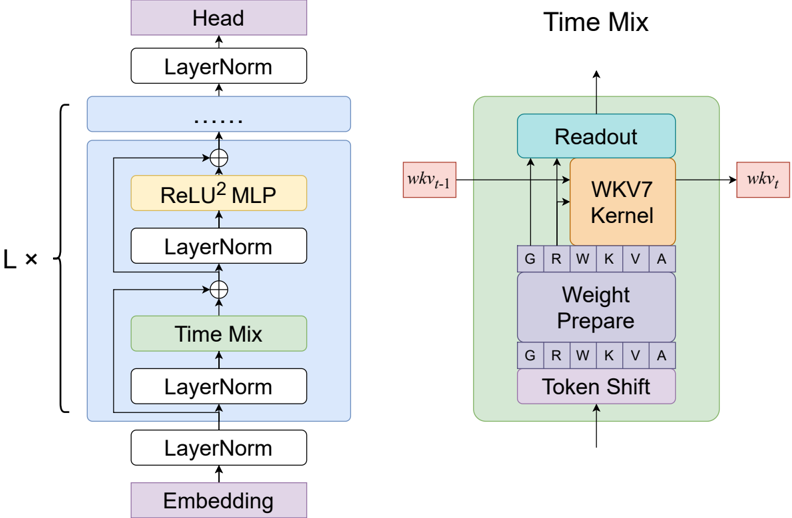Wereplace the main RWKV-6 (Peng et al., 2024) diagonal transition matrix with our extended delta rule and make several other changes to the RWKV architecture, observing significant modeling improvements. These include updates to the channel mixing module and the token shift module. We remove the data dependency of token-shift and the receptance gating of channel mixing, both of which contribute to faster training and inference. We increase the use of low-rank projections to generate more of our intermediate calculations, striking a balance between the total number of model parameters, training and inference speed, and downstream performance. 4 For now, we choose to allow only part of the range of possible negative eigenvalues in our pre-trained large language models due to experimentally observed training instabilities. Figure 1 presents the overall architecture of RWKV-7. Please refer to Appendix F for more details. Figure 1: RWKV-7's overall architecture. <details> <summary>Image 1 Details</summary>  ### Visual Description ## Diagram: Neural Network Architecture with Time Mixing Component ### Overview The image depicts a technical diagram of a neural network architecture with two primary components: a left-side recurrent processing block and a right-side "Time Mix" block. The diagram uses color-coded blocks and arrows to illustrate data flow and component relationships. ### Components/Axes **Left Flowchart (Blue Section):** - **Head** (Purple block at top) - **LayerNorm** (White block below Head) - **ReLU² MLP** (Yellow block with loop) - **Time Mix** (Green block with bidirectional arrows) - **Embedding** (Purple block at bottom) - **LayerNorm** blocks repeated in loop (marked "L x") **Right Block (Green Section):** - **Readout** (Cyan block at top) - **WKV7 Kernel** (Orange block with G/R/W/K/V/A inputs) - **Weight Prepare** (Purple block with G/R/W/K/V/A inputs) - **Token Shift** (Purple block at bottom) - Arrows show flow: Readout → WKV7 Kernel → Weight Prepare → Token Shift **Color Legend:** - Purple: Head, Embedding, Token Shift - Blue: Left flowchart background - Green: Time Mix block, right flowchart background - Yellow: ReLU² MLP - Cyan: Readout - Orange: WKV7 Kernel ### Detailed Analysis **Left Flowchart:** 1. Data enters through "Head" → LayerNorm 2. Enters loop containing: - ReLU² MLP (non-linear transformation) - LayerNorm (normalization) 3. Output merges with "Time Mix" block 4. Final LayerNorm before "Embedding" output **Right Block:** 1. "Readout" receives input from previous layer (wkv_t-1) 2. Processes through WKV7 Kernel (7x7 convolution?) 3. Weight Prepare block generates attention weights 4. Token Shift applies positional adjustments 5. Final output wkv_t ### Key Observations 1. Recurrent processing loop (L x) suggests temporal dependency modeling 2. Time Mix block connects recurrent and attention components 3. WKV7 Kernel implies specialized attention mechanism 4. Token Shift suggests positional encoding adjustments 5. Multiple LayerNorm blocks indicate careful normalization ### Interpretation This architecture combines recurrent processing (left) with attention-based time mixing (right). The ReLU² MLP loop likely handles sequential feature extraction, while the WKV7 Kernel enables efficient temporal attention. The Token Shift component suggests dynamic positional adjustments, possibly for variable-length sequences. The architecture appears designed for tasks requiring both sequential processing and temporal context awareness, such as time-series analysis or natural language understanding with temporal dependencies. </details> ## 4 Method In this section, we use D to denote the model dimension. Bold capital letters represent trainable matrices, and vectors without a subscript t are trainable parameters. The first subscript denotes sequence position and second subscript denotes layer index, where necessary. We use the convention that all vectors are row vectors unless explicitly transposed, so all matrices operate on the right side, therefore a T b is an outer product and ab T is an inner one. We use the square subscript to denote a placeholder for variable names and use the Q sign for cumulative matrix multiplication. See Appendix G for a pseudocode implementation of these formulas. ## 4.1 Time Mixing Weight Preparation Along the lines of (Peng et al., 2024), we introduce the following notation templates for common operators in the model, using the square subscript to denote a variable: $$\lvert e r p ( a , b , x ) \rvert = a + \vert b - a \vert \circ x$$ $$\forall x \in A \cap B \text { such that } f ( x ) = 0 , \forall y \in A \cap B \text { such that } f ( y ) = 1 .$$ Unless explicitly stated, all vectors appearing in this section are dimension D . Weextendtheuseoflow-rank MLP (a 2-layer MLP with small hidden dimension compared to input and output), abbreviated as loramlp, to implement data dependency using minimal parameters. The replacement key ˜ k , value v , decay w , removal key κ , in-context learning rate a , receptance r , and rwkv gate g parameters are computed as follows (outputs annotated with ▷ ): | x □ t = lerp( x t , x t - 1 , µ □ ) □∈ { r , k , v , d , a , g }, a | token shifted inputs | (3) | |-------------------------------------------------------------------------------|-------------------------------------------------------------------------------|-------| | a t = sigmoid(loramlp a (Identy, x t ,bias=True)), ▷ in-context learning rate | a t = sigmoid(loramlp a (Identy, x t ,bias=True)), ▷ in-context learning rate | (4) | | k t = x k t W k , key precursor | k t = x k t W k , key precursor | (5) | | κ t = k t ⊙ ξ , ▷ removal key | κ t = k t ⊙ ξ , ▷ removal key | (6) | | ˜ k t = k t ⊙ lerp(1, a t , α ), ▷ replacement key | ˜ k t = k t ⊙ lerp(1, a t , α ), ▷ replacement key | (7) | | ν t = sigmoid(loramlp ν (Identity, x v t ,bias=True)), value residual gate | ν t = sigmoid(loramlp ν (Identity, x v t ,bias=True)), value residual gate | (8) | | v ′ t , l = x v t W v , value precursor | v ′ t , l = x v t W v , value precursor | (9) | | v t = ( v ′ t ,0 , lerp( v ′ , v ′ , ν ), layer l ≥ 1 , | layer l = 0 ▷ value | (10) | | d t = loramlp d (tanh, x d t ,bias=True), | decay precursor | (11) | | w t = exp( - e - 0.5 sigmoid( d t )), | ▷ decay | (12) | | r t = x r t W r , | ▷ receptance | (13) | | g t = loramlp g (sigmoid, x g t ,bias=False) ▷ rwkv gate | g t = loramlp g (sigmoid, x g t ,bias=False) ▷ rwkv gate | (14) | ξ is a learned parameter representing the removal key multiplier, which transforms the original key into a version to be removed from the state. In practice, ξ lies in a range of approximately [ -5.3,9.4]. α is a learned parameter representing the replacement rate booster, which adjusts the amount added back to the state after the transition matrix is applied. Unlike r , k and v which are the main carriers of information, g , d , ν and a act like gates which control the amount of information allowed to pass. For comprehensive statistics of ξ , α and biases of dt observed in the released RWKV-7 model, including extremum values, mean measurements, and distribution trends, see Appendix L. For the computation of x □ t , we removed data dependency of linear interpolation from RWKV-6 to improve training speed. Weadapted the idea of Value Residual Learning Zhou et al. (2024) for the computation of vt , which has shown to improve the final language modeling loss. ν t represents the value residual mix, which interpolates between the layer zero and current layer value precursors: vt ,0 and vt , l . We also updated the formula for computation of wt , restricting all entries in (exp( -e -0.5 ), 1) in favor of a smaller condition number for diag( wt ), which maintains better training stability, and was beneficial to accuracy of the backward pass. The ˜ kt in the formula can be regarded as a "normalized key", a design to ensure that the state of wkv contains columns of O (1) size. Normally, we expect ˜ kt = kt ⊙ (1 -wt ), as employed in RWKV-6c (see Appendix F), so that wkv t rows are linear interpolations between wkv t -1 and v T t kt controlled by wt . However, to further enhance expressivity, we decide to decouple wt and at . We further decouple at from the amount actually added to the state, allowing the replacement rate booster α to interpolate the amount added between the normal in-context learning rate and 1.0. Importantly, all of these modifications operate on a per-channel basis. The numerical range of RWKV-7's wkv entries are generally stable as in RWKV-6c, unlike RWKV-6, where entries of the states can accumulate to thousands (see Appendix J for a state visualization). The Weighted Key Value State Evolution After weight preparation, we reshape ( r , w , ˜ k , v , κ , a ) t , splitting them to h heads, with each head sized D / h . We always assume that h is a factor of D and heads are equally split. All operations in this section are shown per-head. Before mixing in the time dimension, κ t is normalized per head: $$( 1 5 )$$ The wkv (Weighted Key Value) is a multi-headed matrix-valued state of fast weights that undergoes dynamic evolution. The evolution of wkv is crucial for encoding context information by learning at test time to map keys to values. We start by defining the WKV time mixing as the recurrence relation $$(16)$$ $$\sum _ { i = 1 } ^ { n } \sum _ { j = 1 } ^ { m } w _ { k _ { i } } w _ { l _ { j } } - ( \sum _ { i = 1 } ^ { n } \sum _ { j = 1 } ^ { m } w _ { k _ { i } } ) + ( a _ { i } c _ { j } )$$ Compared to RWKV-5 and RWKV-6, the wkv in this paper is transposed to ensure consistency with RWKV-7's code. Figure 2: A simple illustration of the update mechanism of a single head of RWKV-7's state. Note that the actual state size is 64 × 64 per head, not 4 × 4. <details> <summary>Image 2 Details</summary>  ### Visual Description ## Matrix Equation Diagram: State Update Formula ### Overview The image depicts a mathematical equation for updating a state matrix \( S_t \) using prior state \( S_{t-1} \), diagonal matrix operations, and vector interactions. The equation is structured as: \[ S_t = \left( S_{t-1} - \text{diag}(w_t) \cdot \kappa_t^T \circ (a_t \odot \kappa_t) \right) + v_t^T \tilde{\kappa}_t \] Key components include matrix subtraction, Kronecker product, and vector-matrix multiplication. ### Components/Axes - **Matrices**: - \( S_t \): Final state matrix (pink). - \( S_{t-1} \): Prior state matrix (purple). - **Diagonal Matrix**: - \( \text{diag}(w_t) \): Diagonal matrix derived from vector \( w_t \) (orange). - **Vectors**: - \( \kappa_t^T \): Transposed vector (blue). - \( v_t^T \): Transposed vector (green). - \( \tilde{\kappa}_t \): Modified vector (light blue). - **Operations**: - \( \circ \): Kronecker product (denoted by \( \circ \)). - \( \odot \): Element-wise product (denoted by \( \odot \)). ### Detailed Analysis 1. **Left Side**: - \( S_t \) (pink) is the output matrix, positioned at the far left. 2. **Right Side**: - **Subtraction Term**: - \( S_{t-1} \) (purple) is subtracted by \( \text{diag}(w_t) \cdot \kappa_t^T \circ (a_t \odot \kappa_t) \). - \( \text{diag}(w_t) \) (orange) scales \( \kappa_t^T \) (blue), which is then Kronecker-producted with \( a_t \odot \kappa_t \) (light blue). - **Addition Term**: - \( v_t^T \tilde{\kappa}_t \) (green + light blue) is added to the result of the subtraction. ### Key Observations - The equation balances prior state \( S_{t-1} \) with adjustments from \( w_t \), \( a_t \), and \( v_t \). - The Kronecker product \( \circ \) and element-wise product \( \odot \) suggest tensor-like interactions between vectors. - No numerical values are provided; the focus is on symbolic relationships. ### Interpretation This equation likely models a dynamic system where the state \( S_t \) evolves iteratively. The subtraction term refines \( S_{t-1} \) using weighted interactions (\( w_t \)) and vector operations, while the addition term introduces new information via \( v_t \) and \( \tilde{\kappa}_t \). The use of Kronecker and element-wise products implies high-dimensional data fusion or feature interaction, common in machine learning or signal processing. **Note**: The diagram lacks numerical data, so trends or outliers cannot be quantified. The structure emphasizes symbolic relationships between matrices and vectors. </details> The wkv t attention calculation can alternatively be written in a parallel manner: $$u _ { k v } = \sum _ { i = 1 } ^ { n } ( \bar { I } _ { j = i + 1 } ) - k T _ { j } ( a \circ k )$$ The recurrent transition design has parallels with Schlag et al. (2021), but crucially the transition matrix $$\sum _ { k = 1 } ^ { n } ( - \frac { 1 } { k } T _ { k } ) \left( \frac { 1 } { w _ { r } } \right) \left[ diag ( w _ { r } ) - \kappa ^ { T } _ { f } ( a _ { t } \circ k _ { r } ) \right] = I - \kappa ^ { T } _ { f } ( a _ { t } \circ k _ { r } ) = I - \frac { 1 } { w _ { r } } \left[ diag ( w _ { r } ) - \kappa ^ { T } _ { f } ( a _ { t } \circ k _ { r } ) \right]$$ is no longer a Householder matrix but a scaled approximation of it, as κ t ̸= at wt κ t . This mimics a Householder matrix but with expanded dynamics, while still having all eigenvalues in a stable range of [ -1,1] and allows the network to decay information in all subspaces if necessary. It contrasts with the case of a Householder-like matrix with learning rate ( I -av T v ), a ∈ [0,1], as used in Schlag et al. (2021); Yang et al. (2024c) where all eigenvalues are one except for the last one corresponding to 1 -a . Given these properties, we refer to wt as "in-context weight decay" and to at as "in-context learning rate" (ICLR). The RWKV-7 transition matrix, therefore, allows for both dynamic state evolution and approximation to a forget gate at the same time. See Appendix C for the details on the eigenvalue of the transition matrix, and when the transition matrix is guaranteed to be stable. The original delta rule in Schlag et al. (2021) allows partial or full removal of pre-existing values from the state at each time-step, with the amount removed being equal to the scalar a . Our formulation extends this ability by making a a vector, allowing for different removal amount per state column. WKV Bonus and Output All operations in this section are shown per-head unless otherwise specified. Receptance, which acts like the query found in transformers, is applied to the WKV state, and the result is normalized. An added bonus, the amount of which is weighted by ρ , allows the model to place extra attention on the current shifted input token without requiring it to store that token in the state. $$u _ { t } = ( r _ { t } \cdot ( p \circ k _ { t } ) ^ { n } ) v _ { t }$$ $$(bonus)$$ $$(attention result)$$ Finally, the heads are recombined via reshaping so that pt ∈ R D , gated, and transformed into the output as follows: $$o _ { 1 } = ( g _ { t } o p _ { i } ) W _ { o } e R ^ { D }$$ ## 4.2 MLP The MLP module of RWKV-7 is no longer identical to the Channel Mixing module of previous RWKV-4,5,6 architectures (Peng et al., 2024). We remove the gating matrix W r , making it a twolayer MLP . In compensation for the removed gating parameters to satisfy the equi-parameter condition, we set the hidden dimension to be 4 times the size of model dimension. $$( 2 1 )$$ $$o _ { i } ^ { \prime } = ReLU ( k _ { i } ) ^ { 2 } W _ { v } e ^ { R D }$$ ## 5 RWKVWorldv3Dataset Wetrain our models on the new RWKVWorldv3Dataset , a new multilingual 3.119 trillion token dataset drawn from a wide variety of publicly available data sources. This dataset aims to help close the gap with the amount of data used to train modern LLMs, which may consume as many as 15 - 18 trillion tokens (Qwen et al., 2025; Grattafiori et al., 2024). We select the data to approximate the distribution of our previous World datasets, including English, multilingual, and code, while slightly enhancing Chinese novels.We describe the composition of our dataset in Appendix B. ## 6 Pre-Trained Models Wehave pre-trained and publicly released seven Apache 2.0 licensed RWKV-7 models: 1. Trained on Pile: RWKV7-Pile of sizes 0.1B, 0.4B, and 1.4B 2. Trained on RWKV World V3: RWKV7-World-3 of sizes 0.1B, 0.4B, 1.5B, and 2.9B See Appendix E for detailed configurations. The RWKV-7 Pile models all use the GPT-NeoX-20B tokenizer (Black et al., 2022), and were all trained from scratch on the Pile dataset, which has 332 billion tokens. All RWKV World dataset models use the RWKV World Tokenizer. Due to compute budget constraints, the Goose World 3 0.1B and 0.4B models were trained from pre-existing RWKV-5 World v1 and v2 checkpoints, and the Goose World 3 1.5B and 2.9B models were trained from pre-existing RWKV-6 World v2.1 checkpoints. These checkpoints' parameters were then converted to the RWKV-7 format via a process described below. Once in the new format, the models are trained on either the additional full 3.1 trillion tokens of the World v3 corpus, or an equally weighted sub-sampling of it. Under this methodology, some documents were seen two or even three times. The World v1, v2, v2.1, and v3 corpora contain 0.6, 1.1, 1.4, and 3.1 trillion tokens, respectively. The amounts of training in each stage at with each successive model architecture and corpus are shown in Table 2. Table 2: Total trillions of tokens trained for all RWKV-7 World 3 models | Model | World v1 | World v2 | World v2.1 | World v3 | Total | |-------------------|--------------|--------------|--------------|--------------|---------| | RWKV7-World3-0.1B | 0.6 (RWKV-5) | | | 1.0 (RWKV-7) | 1.6 | | RWKV7-World3-0.4B | | 1.1 (RWKV-5) | | 2.0 (RWKV-7) | 3.1 | | RWKV7-World3-1.5B | | 1.1 (RWKV-6) | 1.4 (RWKV-6) | 3.1 (RWKV-7) | 5.6 | | RWKV7-World3-2.9B | | 1.1 (RWKV-6) | 1.4 (RWKV-6) | 3.1 (RWKV-7) | 5.6 | Our model format conversion process involves removing the token-shift low-rank MLPs, rescaling by half the embeddings, wkv receptance, wkv output matrix weights, and Layernorm and Groupnorm bias values. Layernorm and Groupnorm weights are clamped above zero and square rooted. We widen the FFN MLP from 3.5x (in RWKV-6) to 4x and add new small (1 × 10 -3 ) uniform initalizations in the new regions, removing the RWKV-6 FFN receptance weights. We widen the time decay Low-rank MLP and add new small (1 × 10 -4 ) uniform initializations in the new regions. We replace the gate weights with a LoRA obtained through singular value decomposition and rescaling by half. <details> <summary>Image 3 Details</summary>  ### Visual Description ## Line Chart: FLOPS vs. Average Benchmark Accuracy ### Overview The chart illustrates the relationship between training computational resources (measured in FLOPS on a logarithmic scale) and average benchmark accuracy (%) for three AI models: RWKV7-World3 2.9B, Qwen2.5 0.5B, and SmolLM2 135M. The data is plotted with three distinct lines, each representing a model's performance across increasing FLOPS. ### Components/Axes - **X-axis**: "Training FLOPS (log scale)" with values: 1E+20, 1E+21, 1E+22, 1E+23. - **Y-axis**: "Average Accuracy (%)" with values: 40%, 45%, 50%, 55%, 60%, 65%. - **Legend**: Located on the right side of the chart, associating colors with models: - **Red**: RWKV7-World3 2.9B - **Blue**: Qwen2.5 0.5B - **Green**: SmolLM2 135M ### Detailed Analysis - **Red Line (RWKV7-World3 2.9B)**: - Starts at **45%** accuracy at 1E+21 FLOPS. - Increases to **55%** at 1E+22 FLOPS. - Reaches **60%** at 1E+23 FLOPS. - **Trend**: Steady upward slope, indicating consistent improvement with more training. - **Blue Line (Qwen2.5 0.5B)**: - Starts at **50%** accuracy at 1E+22 FLOPS. - Increases to **55%** at 1E+23 FLOPS. - Reaches **60%** at 1E+23 FLOPS. - **Trend**: Slower initial growth but catches up to the red line at higher FLOPS. - **Green Line (SmolLM2 135M)**: - Starts at **45%** accuracy at 1E+22 FLOPS. - Increases to **50%** at 1E+23 FLOPS. - Reaches **55%** at 1E+23 FLOPS. - **Trend**: Gradual improvement but remains the lowest-performing model across all FLOPS. ### Key Observations 1. **Model Size vs. Accuracy**: Larger models (e.g., RWKV7-World3 2.9B) achieve higher accuracy at lower FLOPS compared to smaller models (e.g., SmolLM2 135M). 2. **Training Efficiency**: All models show improvement with increased FLOPS, but the rate of gain varies. The red line (RWKV7-World3 2.9B) demonstrates the most efficient scaling. 3. **Discrepancy**: The blue line is labeled "Qwen2.5 0.5B" in the legend but has a data point labeled "7B" in the image. This inconsistency requires clarification. ### Interpretation The chart suggests that **model size and training FLOPS are positively correlated with benchmark accuracy**. Larger models (e.g., RWKV7-World3 2.9B) achieve higher accuracy with fewer computational resources, while smaller models (e.g., SmolLM2 135M) require significantly more FLOPS to reach comparable performance. The blue line (Qwen2.5 0.5B) shows that even smaller models can improve with training, but their gains are less pronounced. The discrepancy between the blue line's label ("7B") and the legend ("Qwen2.5 0.5B") raises questions about data labeling accuracy. If the legend is correct, the blue line represents a smaller model, but its performance at 1E+23 FLOPS (60%) surpasses the red line (RWKV7-World3 2.9B) at the same FLOPS, which contradicts the expected trend. This could indicate an error in data labeling or an anomaly in the model's training dynamics. The green line (SmolLM2 135M) highlights the limitations of smaller models, as it consistently lags behind larger models in accuracy despite similar FLOPS. This underscores the trade-off between model size, computational resources, and performance in AI training. </details> <details> <summary>Image 4 Details</summary>  ### Visual Description ## Line Chart: Model/System Growth Over Time ### Overview The chart illustrates the growth trajectories of three models/systems over time, measured on a logarithmic scale (x-axis: 1E8 to 5E9) and a linear scale (y-axis: 40 to 65). Three data series are plotted with distinct colors: red (RWKV7-World3), blue (Qwen2.5), and green (SmolLM2). Each line includes labeled data points indicating metric values at specific time intervals. ### Components/Axes - **X-Axis**: Logarithmic scale labeled with 1E8, 5E8, 1E9, 5E9 (100M to 5B). - **Y-Axis**: Linear scale from 40 to 65, with increments of 5. - **Legend**: Located in the top-right corner, associating colors with models: - Red: RWKV7-World3 (2.9B) - Blue: Qwen2.5 (1.5B) - Green: SmolLM2 (1.7B) - **Data Points**: Embedded labels on lines show metric values (e.g., "0.19B", "3B"). ### Detailed Analysis 1. **Red Line (RWKV7-World3)**: - Starts at 0.19B (y=45) at 1E8. - Increases to 0.4B (y=52) at 5E8. - Rises to 1.5B (y=57) at 1E9. - Peaks at 2.9B (y=60) at 5E9. - **Trend**: Steep upward slope, indicating rapid growth. 2. **Blue Line (Qwen2.5)**: - Begins at 0.5B (y=50) at 1E8. - Jumps to 1.5B (y=55) at 5E8. - Reaches 3B (y=56) at 1E9. - Ends at 7B (y=59) at 5E9. - **Trend**: Consistent upward trajectory with accelerating growth. 3. **Green Line (SmolLM2)**: - Starts at 135M (y=45) at 1E8. - Increases to 360M (y=48) at 5E8. - Ends at 1.7B (y=52) at 5E9. - **Trend**: Gradual growth, slower than red and blue lines. ### Key Observations - **RWKV7-World3** demonstrates the highest growth rate, surpassing all others by 5E9. - **Qwen2.5** shows the largest absolute increase (0.5B to 7B) but starts later than RWKV7-World3. - **SmolLM2** begins at the lowest value (135M) but grows to 1.7B, suggesting scalability despite initial limitations. - All lines intersect at y=50 (0.5B) around 5E8, indicating convergence in metric values at this midpoint. ### Interpretation The chart highlights divergent growth patterns among the models/systems. RWKV7-World3’s exponential growth suggests superior scalability or adoption, while Qwen2.5’s late-stage acceleration may reflect strategic improvements. SmolLM2’s modest growth could indicate niche applicability or resource constraints. The convergence at 0.5B (5E8) implies a critical inflection point where all systems achieved baseline performance, but RWKV7-World3 diverged sharply afterward. This data could inform decisions on model selection, resource allocation, or competitive analysis in a technical domain. </details> Inference Active Parameters (log scale) - (b) Active Parameters vs. Average Benchmark Accuracy Figure 3: Model Comparisons across Multilingual Benchmarks ## 7 Language Modeling Experiments ## 7.1 LMEvaluation Harness Benchmarks RWKV-7 models are evaluated on a series of common English-focused and multilingual benchmarks using LMEvaluation Harness (Gao et al., 2023) as shown in Tables 3 and 4. We benchmarked RWKV-7 along with several new open models which are state-of-the-art in their parameter count ranges. All numbers are evaluated under fp32 precision with lm-eval v0.4.3 using 0-shot, except for MMLU in which case 5-shot was used. Wefind that RWKV-7 is generally able to match the English performance of Qwen2.5 (Qwen et al., 2025) with less than one third as many training tokens. Interestingly, we found that RWKV-7 models have shown giant leaps in MMLU performance compared to RWKV-6. We also find that RWKV-7-World models expand upon RWKV-6-World models already strong capabilities on multilingual benchmarks, outperforming SmolLM2 (Allal et al., 2025), Llama-3.2 (Grattafiori et al., 2024), and Qwen-2.5 (Qwen et al., 2025) by a significant margin. 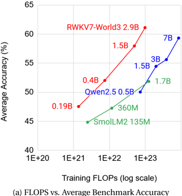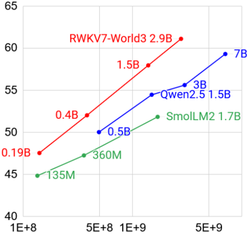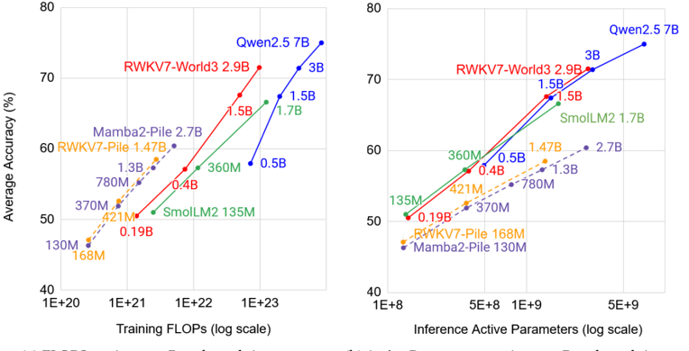In Figures 3a and 4a we plot FLOPs used to train several open models versus average accuracy across the same sets of common english and multi-lingual benchmarks. The multilingual evals show a very dramatic Pareto improvement versus the transformer models. Also note the similar english-language eval scores, but dramatically lower total FLOPs usage of RWKV7-World models versus other highly trained open transformer models. We theorize that if we were less constrained by compute and were able to train these models from scratch with the same amount of total tokens instead of from pre-trained checkpoints of earlier RWKV versions, the difference would be even more dramatic. Note that we did not plot the Llama 3.2 series of models, as they have no corresponding FLOPs amounts due to having been created via pruning and distillation from larger models. ## 7.2 Recent Internet Data Evaluation Modern large language models are trained on massive datasets. Despite careful data cleaning, benchmark data leakage remains a challenge, compromising the validity of these evaluations. To complement traditional benchmarks, we evaluated RWKV-7 Goose and other leading open-source models using temporally novel internet data, generated after the models' training periods; this data could not have appeared in the training sets, removing data leakage concerns. Specifically, we collected new data created after January 2025, including: newly submitted computer science and physics papers on arXiv, newly created Python/C++ open-source repositories on <details> <summary>Image 5 Details</summary>  ### Visual Description ## Line Chart: Model Performance vs. Training and Inference Scales ### Overview The image contains two side-by-side line charts comparing the average accuracy of different language models (LMs) as a function of **Training FLOPs** (left panel) and **Inference Active Parameters** (right panel). Both panels use a logarithmic scale for their x-axes and a linear scale for the y-axis (Average Accuracy in %). The charts highlight trade-offs between model size, computational resources, and performance. --- ### Components/Axes #### Left Panel: Training FLOPs (log scale) - **X-axis**: Training FLOPs (log scale), labeled with markers at `1E+20`, `1E+21`, `1E+22`, `1E+23`. - **Y-axis**: Average Accuracy (%), ranging from 40% to 80%. - **Legend**: Located on the right, with color-coded lines for: - **Blue**: Qwen2.5 7B - **Red**: RWKV7-World3 2.9B - **Green**: SmolLM2 1.7B - **Orange**: RWKV7-Pile 1.47B - **Purple**: Mamba2-Pile 1.3B #### Right Panel: Inference Active Parameters (log scale) - **X-axis**: Inference Active Parameters (log scale), labeled with markers at `1E+8`, `5E+8`, `1E+9`, `5E+9`. - **Y-axis**: Average Accuracy (%), same range as the left panel. - **Legend**: Same as the left panel, with identical color coding. --- ### Detailed Analysis #### Left Panel: Training FLOPs - **Qwen2.5 7B (Blue)**: - Starts at ~50% accuracy at `1E+20` FLOPs, rising to ~75% at `1E+23`. - **Trend**: Steep upward slope, indicating strong scaling with training compute. - **RWKV7-World3 2.9B (Red)**: - Begins at ~50% at `1E+20`, reaching ~70% at `1E+23`. - **Trend**: Slightly less steep than Qwen2.5 but still shows strong scaling. - **SmolLM2 1.7B (Green)**: - Starts at ~50% at `1E+20`, peaking at ~65% at `1E+22`, then plateaus. - **Trend**: Limited scaling beyond `1E+22` FLOPs. - **RWKV7-Pile 1.47B (Orange)**: - Starts at ~50% at `1E+20`, reaching ~60% at `1E+22`. - **Trend**: Moderate scaling, plateauing earlier than larger models. - **Mamba2-Pile 1.3B (Purple)**: - Starts at ~50% at `1E+20`, peaking at ~55% at `1E+22`. - **Trend**: Minimal scaling, suggesting inefficiency in training. #### Right Panel: Inference Active Parameters - **Qwen2.5 7B (Blue)**: - Starts at ~50% at `1E+8` parameters, rising to ~75% at `5E+9`. - **Trend**: Strong scaling with parameter count. - **RWKV7-World3 2.9B (Red)**: - Begins at ~50% at `1E+8`, reaching ~70% at `5E+9`. - **Trend**: Similar to Qwen2.5 but slightly less efficient. - **SmolLM2 1.7B (Green)**: - Starts at ~50% at `1E+8`, peaking at ~65% at `1E+9`, then plateaus. - **Trend**: Limited scaling beyond `1E+9` parameters. - **RWKV7-Pile 1.47B (Orange)**: - Starts at ~50% at `1E+8`, reaching ~60% at `1E+9`. - **Trend**: Moderate scaling, plateauing earlier. - **Mamba2-Pile 1.3B (Purple)**: - Starts at ~50% at `1E+8`, peaking at ~55% at `1E+9`. - **Trend**: Minimal scaling, similar to left panel. --- ### Key Observations 1. **Model Size vs. Performance**: - Larger models (e.g., Qwen2.5 7B, RWKV7-World3 2.9B) achieve higher accuracy with more training FLOPs and inference parameters. - Smaller models (e.g., Mamba2-Pile 1.3B) show limited scaling, suggesting architectural or training inefficiencies. 2. **Training vs. Inference Trade-offs**: - Models with higher training FLOPs (e.g., Qwen2.5 7B) also require more inference parameters but achieve better accuracy. - Smaller models (e.g., SmolLM2 1.7B) achieve decent accuracy with fewer resources but plateau earlier. 3. **Outliers**: - **Mamba2-Pile 1.3B** consistently underperforms despite similar training/inference scales to RWKV7-Pile 1.47B, indicating potential architectural limitations. --- ### Interpretation The charts demonstrate a clear correlation between **model size**, **training compute (FLOPs)**, and **inference efficiency**. Larger models like Qwen2.5 7B and RWKV7-World3 2.9B outperform smaller models in both training and inference, but at the cost of higher resource demands. Smaller models (e.g., SmolLM2 1.7B) offer a trade-off between performance and efficiency, suitable for resource-constrained scenarios. The plateauing trends for smaller models suggest diminishing returns beyond certain scales, highlighting the need for architectural innovations to improve scalability. The discrepancy in the left panel’s x-axis labels (e.g., `1E+20` vs. data points at `130M`) may indicate a mislabeling error, but the relative trends remain consistent. </details> - (a) FLOPS vs. Average Benchmark Accuracy - (b) Active Parameters vs. Average Benchmark Accuracy Figure 4: Model Comparisons across English-Language Benchmarks | Model (Name) | Tokens (T) | lmb.o acc ↑ | hella acc_n ↑ | piqa acc ↑ | arcE acc ↑ | arcC acc ↑ | glue a acc ↑ | WG acc ↑ | sciq acc ↑ | mmlu acc ↑ | avg acc ↑ | |---------------------|--------------|---------------|-----------------|--------------|--------------|--------------|----------------|------------|--------------|--------------|-------------| | RWKV5-World1-0.1B | 0.6 | 38.4 | 31.9 | 61.4 | 44.2 | 19.9 | 45.5 | 52.9 | 76.3 | 23.1 | 43.7 | | SmolLM2-135M | 2.0 | 42.9 | 43.1 | 68.4 | 64.4 | 28.1 | 49 | 53 | 84 | 25.8 | 51 | | RWKV7-World2.8-0.1B | 1.6 | 48.1 | 42.1 | 67.3 | 59.3 | 25.5 | 48.1 | 52.7 | 86.3 | 25.4 | 50.5 | | RWKV5-World2-0.4B | 1.1 | 54 | 40.9 | 66.5 | 54 | 24 | 50 | 53.2 | 86.9 | 23.8 | 50.4 | | SmolLM2-360M | 4.0 | 53.8 | 56.4 | 72.1 | 70.4 | 36.5 | 50.7 | 59 | 91.2 | 26.3 | 57.4 | | Qwen2.5-0.5B | 18.0 | 52.5 | 52.1 | 70.2 | 64.6 | 29.5 | 54.7 | 56.4 | 93.1 | 47.8 | 57.9 | | RWKV7-World2.9-0.4B | 3.1 | 58.6 | 56.8 | 72.9 | 68.7 | 31.9 | 49.4 | 59.9 | 89.7 | 26.1 | 57.1 | | RWKV6-World2.1-1.6B | 2.5 | 67.4 | 61.1 | 74.4 | 64.3 | 31 | 51 | 60.7 | 89.5 | 25.1 | 58.3 | | Llama3.2-1B | b 15.0 | 63 | 63.7 | 74.5 | 65.5 | 31.3 | 49.7 | 60.7 | 91.4 | 32.1 | 59.1 | | SmolLM2-1.7B | 11.0 | 67.7 | 71.5 | 77 | 77.7 | 44.7 | 51.5 | 66.1 | 93.3 | 50.3 | 66.6 | | Qwen2.5-1.5B | 18.0 | 63 | 67.7 | 75.8 | 75.5 | 41.2 | 65 | 63.4 | 94.2 | 61 | 67.4 | | RWKV7-World3-1.5B | 5.6 | 69.5 | 70.8 | 77.1 | 78.1 | 44.5 | 62.4 | 68.2 | 94.3 | 43.3 | 67.6 | | RWKV6-World2.1-3B | 2.5 | 71.7 | 68.4 | 76.4 | 71.2 | 35.6 | 56.3 | 66.3 | 92.2 | 28.3 | 62.9 | | Llama3.2-3B | b 15.0 | 70.5 | 73.6 | 76.7 | 74.5 | 42.2 | 50.7 | 69.9 | 95.7 | 56.5 | 67.8 | | Qwen2.5-3B | 18.0 | 67.1 | 73.5 | 78.6 | 77.4 | 45 | 70.2 | 68.5 | 96.2 | 65.7 | 71.4 | | RWKV7-World3-2.9B | 5.6 | 73.4 | 76.4 | 79.7 | 81 | 48.7 | 61.8 | 72.8 | 95 | 55 | 71.5 | glue a is the average accuracy of 8 subtasks: mnli , mnli\_mismatch , mrpc , qnli , qqp , rte , sst2 and wnli b Llama3.2-1B and 3B were pruned and distilled from Llama3.1-8B (Grattafiori et al., 2024) Table 3: English Focused Benchmarks, including LAMBADA ( lmb.o ) (Paperno et al., 2016), Hellswag ( hella ) (Hampel, 1974), PIQA (Bisk et al., 2020), AI2 ARC ( arcE , arcC ) (Bhakthavatsalam et al., 2021), GLUE (Wang et al., 2018), Winogrande ( WG ) (Sakaguchi et al., 2021), SciQ (Welbl et al., 2017), MMLU (Hendrycks et al., 2021). GitHub, recently published Wikipedia entries, new fiction on Archive of Our Own (Various, 2025), and recent news articles. Inspired by Delétang et al. (2024); Li et al. (2024b), we used compression rate as our evaluation metric. See Table 5 for details. Remarkably, despite being trained on significantly less data than other top models, RWKV-7 Goose showed competitive performance on this temporally novel data. ## 7.3 Associative Recall Associative recall (AR) (Arora et al., 2023) evaluates the ability of the model to recall previously encountered information within a given context. Research indicates that a model's capacity for AR can reflect its effectiveness in learning from context (Elhage et al., 2021; Olsson et al., 2022). | Model (Name) | Tokens (T) | lmb.m a ppl ↓ | lmb.m acc ↑ | pawsx acc ↑ | xcopa acc ↑ | xnli acc ↑ | xsClz acc ↑ | xwin acc ↑ | avg acc ↑ | |---------------------|--------------|-----------------|---------------|---------------|---------------|--------------|---------------|--------------|-------------| | RWKV5-World1-0.1B | 0.6 | 270 | 22 | 48.6 | 53 | 36.1 | 51.7 | 59.5 | 45.1 | | SmolLM2-135M | 2.0 | 1514 | 18.6 | 51.2 | 52.2 | 34.9 | 50.6 | 61.7 | 44.9 | | RWKV7-0.1B | 1.6 | 114 | 31.6 | 46.1 | 53.3 | 37.6 | 52.6 | 64.1 | 47.5 | | RWKV5-World2-0.4B | 1.1 | 66 | 36.8 | 49.5 | 54 | 38.5 | 54.1 | 65.6 | 49.8 | | SmolLM2-360M | 4.0 | 389 | 25.8 | 51.4 | 51.7 | 36 | 51.2 | 67.8 | 47.3 | | Qwen2.5-0.5B | 18.0 | 108 | 32.9 | 52.6 | 54.4 | 38.6 | 53.9 | 67.8 | 50 | | RWKV7-World3-0.4B | 3.1 | 52 | 39.6 | 48.7 | 55.4 | 40.3 | 55.3 | 72.9 | 52 | | RWKV6-World2.1-1.6B | 2.5 | 28 | 47.2 | 52.5 | 58.1 | 41.4 | 58.2 | 76.5 | 55.7 | | Llama3.2-1B | b 15.0 | 52 | 39 | 53.9 | 55.3 | 41.2 | 56.6 | 72.2 | 53 | | SmolLM2-1.7B | 11.0 | 85 | 37.1 | 56.5 | 53.1 | 38.1 | 54.1 | 72.8 | 52 | | Qwen2.5-1.5B | 18.0 | 49 | 40 | 55.3 | 57.4 | 40.6 | 57.7 | 75.8 | 54.5 | | RWKV7-World3-1.5B | 5.6 | 25 | 48.4 | 54.8 | 59.7 | 43.7 | 61.4 | 79.8 | 58 | | RWKV6-World2.1-3B | 2.5 | 21 | 51 | 53.4 | 60.2 | 42.7 | 61.3 | 78.8 | 57.9 | | Llama3.2-3B | b 15.0 | 30 | 45.9 | 59.9 | 58.5 | 44.2 | 60.6 | 79.2 | 58.1 | | Qwen2.5-3B | 18.0 | 36 | 43.5 | 53.3 | 59 | 38.5 | 59.6 | 79.8 | 55.6 | | RWKV7-World3-2.9B | 5.6 | 18 | 52.9 | 58.2 | 63.1 | 45.4 | 64.7 | 82.4 | 61.1 | Table 4: Multilingual Benchmarks, including LAMBADA Multilingual ( lmb.m ) (Gao et al., 2023), XCOPA (Ponti et al., 2020), XNLI (Conneau et al., 2018),XStoryCloze ( xsClz ) (Lin et al., 2022), xWinogrande ( xwin ) (Tikhonov & Ryabinin, 2021). Consequently, AR has become a standard benchmark for developing new architectural designs in language models (Fu et al., 2023; Poli et al., 2023; Lutati et al., 2023). However, training for multi-query associative recall (MQAR) is highly unstable and strongly dependent on initialization and hyperparameter settings. We observe significant variability in performance under identical configurations across different studies (Peng et al., 2024; Yang et al., 2024c; Beck et al., 2024). Wetrain two-layer RWKV-7 with MQAR and increased the difficulty by scaling the sequence length to as long as 2048. We use the RWKV-7 specific initialization, and set the ϵ of AdamW to 1 × 10 -18 to stabilize learning in later stages. Weight decay of 0.1 is only applied to weight matrices, preventing the degeneration of certain modules (such as weights and biases of LayerNorm). Interestingly, with only a WKV size of 8192, RWKV-7 is able to recall 72.93% at the setting of 256 Key-value pairs. This suggests that a total of roughly 256 × 0.7293 × log 2 (number of key tokens × number of value tokens) = 186.2 × 2 × log 2 (4096) = 4480.8 bits of information, is stored in a 8192 dimensional state, yielding an information density of 0.547 bits per dimension. ## 7.4 Mechanistic Architecture Design We evaluate RWKV-7 on the Mechanistic Architecture Design (MAD) benchmark (Poli et al., 2024), a suite of synthetic token manipulation tasks designed to probe architectural capabilities in sequence modeling, as shown in Table 7. RWKV-7 achieves the highest average score across all six tasks, outperforming previous architectures. It demonstrates perfect accuracy on In-Context and Noisy Recall tasks, matching DeltaNet while setting a new state-of-the-art for Fuzzy Recall. RWKV-7 also shows strong performance in memorization and selective copying, suggesting effective combination of attention-based and recurrent model strengths. ## 7.5 Long Context Experiments To evaluate the ability of RWKV models to retain information over long sequences, we measured loss versus sequence position (we select tokens in range [ L /2 -16384, L /2 + 16384) for document length L ) on the PG19 test set (Rae et al., 2019) for two types of RWKV7 models and their predeces- | Model | arXiv CS ↓ | arXiv Phys. ↓ | Github Python ↓ | Github C++ ↓ | AO3 Eng ↓ | BBC news ↓ | Wiki Eng ↓ | average ↓ | |-------------------|--------------|-----------------|-------------------|----------------|-------------|--------------|--------------|-------------| | Qwen2.5-1.5B | 8.12 | 8.65 | 4.42 | 4.4 | 11.76 | 9.58 | 9.49 | 8.06 | | RWKV-7 1.5B | 8.25 | 8.77 | 5.57 | 5.29 | 10.93 | 9.34 | 8.97 | 8.16 | | Llama-3.2-1B | 8.37 | 8.76 | 5.18 | 5.16 | 11.69 | 9.34 | 9.07 | 8.23 | | SmolLM2-1.7B | 8.38 | 9.04 | 5.17 | 4.94 | 11.2 | 9.4 | 9.46 | 8.23 | | Index-1.9B | 8.34 | 8.59 | 5.65 | 5.29 | 11.49 | 9.51 | 9.23 | 8.3 | | stablelm-2-1.6b | 8.58 | 9.08 | 5.54 | 5.45 | 11.42 | 9.24 | 9.06 | 8.34 | | RWKV-6 1.5B | 8.62 | 9 | 6.06 | 5.8 | 11.09 | 9.57 | 9.3 | 8.49 | | RWKV-5 1.5B | 8.77 | 9.11 | 6.2 | 5.92 | 11.25 | 9.75 | 9.5 | 8.64 | | mamba2-1.3b | 8.74 | 8.74 | 6.32 | 5.71 | 11.63 | 9.74 | 9.86 | 8.68 | | MobileLLM-1.5B | 8.82 | 9.29 | 6.79 | 6.29 | 11.59 | 9.15 | 9.22 | 8.73 | | mamba-1.4b-hf | 8.88 | 8.86 | 6.43 | 5.81 | 11.7 | 9.83 | 9.97 | 8.78 | | Zamba2-1.2B | 8.57 | 9.21 | 6.91 | 7.08 | 11.39 | 9.38 | 9.26 | 8.83 | | SmolLM-1.7B | 8.38 | 9.02 | 5.76 | 6.55 | 12.68 | 9.85 | 9.89 | 8.88 | | MobileLLM-1B | 9.03 | 9.57 | 7.03 | 6.53 | 11.86 | 9.35 | 9.43 | 8.97 | | RWKV-4 1.5B | 9.34 | 9.8 | 6.54 | 6.16 | 11.33 | 10 | 9.82 | 9 | | pythia-1.4b-v0 | 9.12 | 9.2 | 6.79 | 6.15 | 12.19 | 10.2 | 10.43 | 9.15 | | Falcon3-1B-Base | 8.6 | 9.2 | 6.92 | 7.16 | 13.04 | 10.45 | 10.75 | 9.45 | | Llama-3.2-3B | 7.78 | 8.1 | 4.15 | 4.59 | 10.9 | 8.7 | 8.28 | 7.57 | | Qwen2.5-3B | 7.79 | 8.25 | 4.15 | 4.12 | 11.23 | 9.15 | 8.96 | 7.66 | | RWKV-7 2.9B | 7.9 | 8.34 | 5.16 | 4.88 | 10.48 | 8.92 | 8.47 | 7.74 | | stablelm-3b-4e1t | 8.15 | 8.5 | 5.28 | 4.85 | 10.89 | 8.82 | 8.51 | 7.86 | | Minitron-4B-Base | 8.09 | 8.7 | 5.13 | 4.74 | 11.05 | 9.08 | 8.9 | 7.96 | | recurrentgemma-2b | 8.24 | 8.52 | 5.22 | 4.8 | 11.3 | 8.94 | 8.88 | 7.99 | | RWKV-6 3B | 8.27 | 8.58 | 5.66 | 5.39 | 10.67 | 9.17 | 8.82 | 8.08 | | gemma-2-2b | 8.39 | 8.81 | 5.36 | 5.01 | 11.35 | 8.9 | 9.03 | 8.12 | | mamba2attn-2.7b | 8.33 | 8.29 | 5.78 | 5.22 | 11.13 | 9.28 | 9.26 | 8.18 | | RWKV-5 3B | 8.42 | 8.7 | 5.78 | 5.51 | 10.83 | 9.36 | 9 | 8.23 | | mamba2-2.7b | 8.43 | 8.37 | 5.93 | 5.34 | 11.21 | 9.37 | 9.38 | 8.29 | | Zamba2-2.7B | 8.17 | 8.7 | 6.3 | 6.39 | 10.97 | 8.95 | 8.74 | 8.32 | | mamba-2.8b-hf | 8.57 | 8.52 | 6.03 | 5.46 | 11.31 | 9.49 | 9.53 | 8.41 | | RWKV-4 3B | 8.9 | 9.27 | 6.07 | 5.67 | 10.9 | 9.57 | 9.3 | 8.53 | | pythia-2.8b-v0 | 8.72 | 8.73 | 6.29 | 5.71 | 11.66 | 9.74 | 9.82 | 8.67 | Table 5: Compression rate (unit: %) compared across different language models on various data sources, including arXiv papers, GitHub repositories, AO3 fiction, and news articles created after January 2025. | Dim | WKVstate dim | (64,4) | (128,8) | (256,16) | (512,64) | (1024,128) | (2048,256) | |-------|----------------|----------|-----------|------------|------------|--------------|--------------| | 64 | 8192 | ✓ | ✓ | ✓ | 98.43 | 95.01 | 72.93 | | 128 | 16384 | ✓ | ✓ | ✓ | ✓ | ✓ | 94.97 | | 256 | 32768 | ✓ | ✓ | ✓ | ✓ | ✓ | 98.97 | | 512 | 65536 | ✓ | ✓ | ✓ | ✓ | ✓ | ✓ | Table 6: RWKV-7 MQAR test results. We use ( a , b ) to denote the sequence length and number of KV pairs respectively. A check mark ✓ indicates that the model achieves over 99% accuracy. Results are maxed over 3 different learning rate settings. 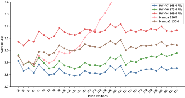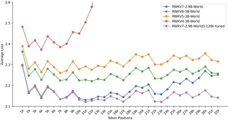sors trained on either The Pile dataset or World dataset. Despite sharing the same architecture and being pretrained on 4k context windows, models trained on different datasets exhibited different behaviors. The Pile-trained RWKV7 showed more significant loss reduction on long contexts compared to its predecessors, demonstrating effective long-context extrapolation (see Figure 5). Surprisingly, for RWKV7 trained on the World dataset, when processing contexts longer than 10k, the loss began to show an increasing trend (see Figure 6). We speculate this is because the larger dataset and model size created inductive biases that caused overfitting to specific context lengths. Further experiments showed that fine-tuning on long contexts can restore its long context capabilities. 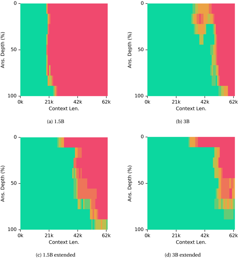To further test RWKV-7 long-context retrieval abilities, we conduct a pass-key retrieval evaluation following the approach of (Chen et al., 2024b) and plot the results in Figure 7. In this evaluation, a single sentence is repeated multiple times within a long context window, with a key phrase | Model | Compress | Fuzzy Recall | In-Context Recall | Memorize | Noisy Recall | Selective Copy | Avg | |-----------------|------------|----------------|---------------------|------------|----------------|------------------|-------| | RWKV-7 | 44.5 | 43.2 | 100 | 89.1 | 100 | 98.8 | 79.3 | | Transformer | 51.6 | 29.8 | 94.1 | 85.2 | 86.8 | 99.6 | 74.5 | | Multihead Hyena | 44.8 | 14.4 | 99 | 89.4 | 98.6 | 93 | 73.2 | | DeltaNet | 42.2 | 35.7 | 100 | 52.8 | 100 | 100 | 71.8 | | Mamba | 52.7 | 6.7 | 90.4 | 89.5 | 90.1 | 86.3 | 69.3 | | Hyena | 45.2 | 7.9 | 81.7 | 89.5 | 78.8 | 93.1 | 66 | | GLA | 38.8 | 6.9 | 80.8 | 63.3 | 81.6 | 88.6 | 60 | Results for comparison models from Yang et al. (2024c) Table 7: Results on the MAD benchmark Figure 5: PG19 loss versus sequence position for RWKV and Mamba models trained on The Pile datasets. <details> <summary>Image 6 Details</summary>  ### Visual Description ## Line Chart: Average Loss Across Token Positions for Different Models ### Overview The chart displays five data series representing average loss values across token positions (1k to 32k) for different machine learning models. The y-axis ranges from 2.7 to 3.4, with each line corresponding to a specific model configuration. ### Components/Axes - **X-axis (Token Positions)**: Labeled with increments of 1k (1k, 2k, ..., 32k). - **Y-axis (Average Loss)**: Scaled from 2.7 to 3.4 in 0.1 increments. - **Legend**: Located in the top-right corner, mapping colors to models: - Blue: RWKV7 168M Pile - Green: RWKV6 173M Pile - Red: RWKV4 169M Pile - Pink: Mamba 130M - Brown: Mamba2 130M ### Detailed Analysis 1. **RWKV7 168M Pile (Blue)**: - Starts at ~2.9 at 1k, showing a gradual downward trend to ~2.85 by 32k. - Minor fluctuations observed between 2.8 and 2.9 throughout. 2. **RWKV6 173M Pile (Green)**: - Begins at ~2.95 at 1k, fluctuates slightly upward to ~2.98 by 32k. - Stable with minor oscillations between 2.85 and 2.95. 3. **RWKV4 169M Pile (Red)**: - Starts at ~3.05 at 1k, remains relatively stable with minor fluctuations (~3.05–3.15). - Peaks at ~3.15 near 20k before stabilizing. 4. **Mamba 130M (Pink)**: - Begins at ~2.85 at 1k, sharp upward spike to ~3.35 near 18k. - Stabilizes around ~3.15 after 20k, with minor fluctuations. 5. **Mamba2 130M (Brown)**: - Starts at ~2.95 at 1k, fluctuates between ~2.9 and ~3.05. - Peaks at ~3.05 near 20k, then stabilizes around ~3.0. ### Key Observations - **RWKV4 169M Pile (Red)** exhibits the most stability, maintaining values between 3.05 and 3.15. - **Mamba 130M (Pink)** shows a sharp, anomalous increase (~2.85 → 3.35) near 18k, followed by stabilization. - **RWKV7 168M Pile (Blue)** demonstrates the most consistent downward trend (~2.9 → 2.85). - **Mamba2 130M (Brown)** and **RWKV6 173M Pile (Green)** show moderate fluctuations but remain below 3.1. ### Interpretation The data suggests performance variations across models and token positions. The RWKV4 169M Pile (red) maintains the highest average loss, indicating potential inefficiency or higher error rates. The Mamba 130M (pink) anomaly near 18k may reflect a specific issue in token processing or model behavior. The RWKV7 168M Pile (blue) shows the best performance, with a steady decline in loss, suggesting effective handling of token positions. The Mamba2 130M (brown) and RWKV6 173M Pile (green) exhibit intermediate performance, with minor fluctuations. The sharp rise in Mamba 130M highlights a critical divergence in behavior, warranting further investigation into its training dynamics or architectural differences. </details> embedded at different positions. RWKV7-World3-1.5B achieves perfect accuracy up to a context length of 19600 tokens but exhibits degradation beyond 20600 tokens. The larger RWKV7-World32.9B extends perfect retrieval up to 35000 tokens, highlighting the benefits of scaling. However, performance begins to degrade beyond this point. To explore potential improvements, we fine-tuned RWKV7-World3-1.5B and RWKV7-World3-2.9B on packed training sequences of length 128k tokens from a specially constructed dataset, which leads to further improvements in retrieval accuracy. With this fine-tuning, RWKV-7 (1.5B) reliably retrieves key phrases up to 29k tokens, and degradation is observed only around 40k tokens. RWKV-7 (2.9B) reliably retrieves the pass key up to 30k tokens, and degrades around 50k tokens. Our context length extension dataset is comprised of both public and custom sources listed in Table 8. We employed a document length-based weighting scheme to prioritize longer contexts during training. To approximate document lengths of 128,000 tokens, we used character counts of 512,000. Documents of less than 32,768 characters were assigned a weight of 1.0, while longer documents were assigned linearly increasing weights between 2.0 and 3.0, with a cap of 3.0 beyond 512,000. This method increases the inclusion of longer documents to bolster the model's handling of extended contexts while retaining shorter documents for diversity. Figure 6: PG19 loss versus sequence position for RWKV7 models and predecessors trained on the World dataset. <details> <summary>Image 7 Details</summary>  ### Visual Description ## Line Graph: Average Loss Across Token Positions ### Overview The image displays a multi-line graph comparing the average loss of five different RWKV models across token positions (1k-32k). The y-axis represents average loss values (2.1-2.6), while the x-axis shows token positions in 2k increments. Five distinct data series are plotted with unique colors and markers. ### Components/Axes - **X-axis (Token Positions)**: Labeled "Token Positions" with markers at 1k, 2k, ..., 32k intervals. - **Y-axis (Average Loss)**: Labeled "Average Loss" with increments of 0.1 from 2.1 to 2.6. - **Legend**: Located in the top-right corner, mapping colors to models: - Blue: RWKV7-2.9B-World - Green: RWKV6-3B-World - Orange: RWKV5-3B-World - Red: RWKV4-3B-World - Purple: RWKV7-2.9B-World3-128k-tuned ### Detailed Analysis 1. **RWKV4-3B-World (Red Line)**: - Starts at ~2.48 (1k) and exhibits a sharp upward spike to ~2.6 at token 12k. - Declines to ~2.42 by token 32k. - **Key Outlier**: The 12k token position shows a 0.18 loss increase compared to neighboring positions. 2. **RWKV7-2.9B-World3-128k-tuned (Purple Line)**: - Maintains the lowest average loss (~2.12-2.18) across all positions. - Shows minimal fluctuation, with a slight dip to ~2.11 at token 10k. 3. **RWKV7-2.9B-World (Blue Line)**: - Starts at ~2.3 (1k) and fluctuates between ~2.15-2.25. - Peaks at ~2.28 at token 31k before stabilizing at ~2.25 at 32k. 4. **RWKV6-3B-World (Green Line)**: - Begins at ~2.37 (1k) and trends downward to ~2.26 at 32k. - Shows periodic fluctuations, peaking at ~2.29 at token 29k. 5. **RWKV5-3B-World (Orange Line)**: - Starts at ~2.39 (1k) and trends downward to ~2.31 at 32k. - Exhibits a sawtooth pattern with peaks at tokens 18k (~2.34) and 30k (~2.33). ### Key Observations - **Performance Hierarchy**: The tuned model (purple) consistently outperforms others, maintaining ~15% lower loss than the worst-performing model (red). - **Anomaly Detection**: The red line's 12k spike suggests a potential bug or training instability in RWKV4-3B-World. - **Model Scaling**: Newer models (RWKV7 variants) generally show better loss compression than older versions (RWKV4-6). - **Positional Sensitivity**: All models exhibit increased loss at higher token positions, with RWKV4-3B-World showing the most dramatic degradation. ### Interpretation The data demonstrates significant performance disparities between RWKV model versions, with the 128k-tuned variant achieving state-of-the-art results. The red line's anomalous spike at token 12k warrants investigation into potential training data corruption or architectural limitations in the RWKV4-3B-World model. The consistent performance of the tuned model suggests that extended training on larger datasets (128k tokens) significantly improves generalization. These findings highlight the importance of model versioning and hyperparameter tuning in transformer-based architectures. </details> Table 8: Context Length Extension Dataset Components | Dataset | Type | Amount | |------------------------|--------|----------| | dclm-baseline-1.0 | Public | 25% | | fineweb-edu | Public | 15% | | fineweb | Public | 5% | | codeparrot/github-code | Public | 10% | | arXiv-CC0-v0.5 | Custom | 10% | | SuperWikiNEXT-32B | Custom | 10% | | public domain books | Custom | 15% | | the-stack (filtered) | Custom | 10% | ## 7.6 Evaluating State Tracking Using Group Multiplication 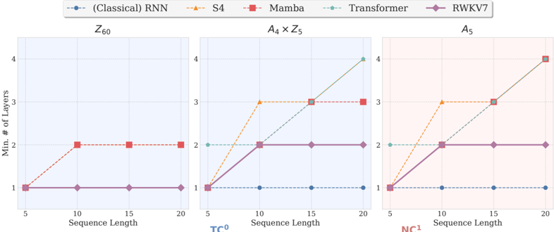Weadopt the experimental setting from Merrill et al. (2024) to evaluate the state-tracking capabilities of RWKV7 in comparison to Transformer, Mamba, S4, and classical RNN models. Given a sequence g 0, g 1, g 2,..., gn drawnfrom A 5, A 4 × Z 5, or Z 60, each step i is labeled with the cumulative product of the first i elements. Weplot the minimum number of layers required to achieve over 95% validation accuracy on group multiplication tasks, as a function of sequence length and group structure. The results are shown in Figure 8. Our findings indicate that RWKV-7 exhibits stronger state-tracking capabilities than Transformers, Mamba, and S4, though slightly weaker than classical RNNs. Figure 8 also aligns with our theory from Appendix D.2, which predicts that RWKV-7 can perform state tracking and recognize any regular language with a constant number of layers. RWKV-7 is not more expressive than classical RNNs, because classical RNNs can recognize any regular language in a single layer. Classical RNNs, while being theoretically expressive, typically suffer from gradient vanishing and memorization problems. (Zucchet & Orvieto, 2024) ## 8 Speed and Memory Usage We compare the training speed and memory usage of the RWKV-7 attention-like kernel with the RWKV-6 kernel and Flash Attention v3 (Shah et al., 2024). The "RWKV-7" kernel accelerates bfloat16 matrix multiplications with modern CUDA instructions. We also include the "RWKV-7 Figure 7: RWKV7-World3 pass-key retrieval evaluation <details> <summary>Image 8 Details</summary>  ### Visual Description ## Heatmap: Model Performance Across Context Length and Answer Depth ### Overview The image contains four heatmaps comparing model performance across varying context lengths (0k–62k tokens) and answer depths (0%–100%). Each subplot corresponds to a different model configuration: (a) 1.5B, (b) 3B, (c) 1.5B extended, and (d) 3B extended. Colors transition from green (high performance) to yellow (moderate) to red (low), indicating metric degradation. --- ### Components/Axes - **X-axis (Context Len.)**: Ranges from 0k to 62k tokens in increments of ~21k. - **Y-axis (Ans. Depth %)**: Ranges from 0% to 100% in 50% increments. - **Color Gradient**: - Green: High performance (likely accuracy/precision). - Yellow: Moderate performance. - Red: Low performance. - **Subplot Labels**: - (a) 1.5B - (b) 3B - (c) 1.5B extended - (d) 3B extended --- ### Detailed Analysis #### (a) 1.5B Model - **Green Dominance**: Left 70% of the heatmap (0k–21k context) is predominantly green, indicating stable performance at shorter contexts. - **Yellow Stripe**: A vertical yellow band (~21k–42k context) marks a performance drop. - **Red Zone**: Rightmost 20% (42k–62k context) is red, showing severe degradation at long contexts. #### (b) 3B Model - **Green Dominance**: Similar to 1.5B but with a narrower green zone (0k–21k). - **Yellow Stripe**: Broader yellow band (~21k–42k) compared to 1.5B. - **Red Zone**: Red area starts earlier (~42k) but covers less vertical space than 1.5B. #### (c) 1.5B Extended - **Green Dominance**: Slightly reduced green zone (0k–21k) compared to base 1.5B. - **Yellow Stripe**: Wider yellow band (~21k–42k) with horizontal yellow streaks at 50% and 75% answer depths. - **Red Zone**: Red area starts at 42k but extends vertically to 100% answer depth. #### (d) 3B Extended - **Green Dominance**: Minimal green (0k–21k) with a thin yellow stripe. - **Yellow Stripe**: Dominates 21k–42k context, with red streaks at 50% and 75% answer depths. - **Red Zone**: Largest red area (42k–62k context, 50%–100% answer depth), indicating severe performance collapse. --- ### Key Observations 1. **Threshold at 21k Context**: All models show a performance drop starting at ~21k tokens, marked by yellow bands. 2. **Extended Models Degrade Faster**: - 1.5B extended shows broader yellow/red zones than base 1.5B. - 3B extended has the most severe degradation (largest red zone). 3. **Answer Depth Correlation**: - Red zones expand vertically at higher answer depths (50%–100%), suggesting performance worsens with deeper reasoning. 4. **Color Consistency**: Green/yellow/red gradients align across subplots, confirming metric uniformity. --- ### Interpretation - **Context Length Limitation**: The ~21k token threshold likely reflects hardware or architectural constraints (e.g., attention mechanisms in transformers). - **Model Scaling Trade-offs**: Larger models (3B) handle shorter contexts better but fail catastrophically at longer contexts compared to smaller models (1.5B). - **Extended Model Risks**: Extended variants (c, d) exhibit amplified degradation, possibly due to increased complexity or training instability. - **Answer Depth Sensitivity**: Performance drops more sharply at higher answer depths, implying that complex reasoning tasks are more affected by context length limitations. This data highlights the trade-off between model size, context handling, and task complexity. Extended models may prioritize capacity over stability, making them less reliable for long-context tasks. </details> fp32" kernel, which is simpler and performs all its internal calculations using float32. Although the bfloat16 kernel is faster, to maximize precision, the RWKV-7 fp32 kernel was used to train the RWKV-7 World models. Our CUDA kernels are tuned for head dimension 64, as used in the RWKV-7-World models. The kernels still perform well for head dimension 128, but their efficiency drops off at larger head dimensions. There exist other RWKV-7 implementations which focus on head dimensions greater than 128. A key example is the Flash Linear Attention library (Yang & Zhang, 2024), which offers a Triton-based implementation designed for these larger configurations. Speed In Figure 9, we time the forward + backward pass of each kernel for batch size 8, head dimension 64 and model dimension 4096 (64 wkv heads) on an H100 SXM GPU, for varying sequence lengths. Although Flash Attention v3 is heavily optimized for the H100 GPU, it scales quadratically with sequence length, while the RWKV models scale linearly. This makes the RWKV models faster than attention for large sequence lengths. Furthermore, the optimized RWKV-7 kernel is about three times faster than the official RWKV-6 kernel. <details> <summary>Image 9 Details</summary>  ### Visual Description ## Line Chart: Minimum Number of Layers vs. Sequence Length for Different Architectures ### Overview The image displays three horizontal subplots comparing the minimum number of layers required for different neural network architectures (Classical RNN, S4, Mamba, Transformer, RWKV7) across varying sequence lengths. Each subplot corresponds to a distinct configuration (Z60, A₄×Z₅, A₅), with trends showing how layer requirements scale with sequence length. --- ### Components/Axes 1. **Subplots**: - **Left (Z60)**: Sequence Length (5–20) vs. Min. # of Layers (1–4). - **Middle (A₄×Z₅)**: Sequence Length (5–20) vs. Min. # of Layers (1–4). - **Right (A₅)**: Sequence Length (5–20) vs. Min. # of Layers (1–4). 2. **Axes**: - **X-axis**: "Sequence Length" (5, 10, 15, 20). - **Y-axis**: "Min. # of Layers" (1–4). 3. **Legend**: - **Colors/Markers**: - Classical RNN: Blue dashed line with circles. - S4: Orange dashed line with triangles. - Mamba: Red dashed line with squares. - Transformer: Green dashed line with diamonds. - RWKV7: Purple solid line with diamonds. --- ### Detailed Analysis #### Z60 Subplot - **Classical RNN**: Constant at 1 layer across all sequence lengths. - **S4**: Increases stepwise: 1 (5), 2 (10), 3 (15), 4 (20). - **Mamba**: Increases to 2 layers at 10, then plateaus. - **Transformer**: Increases stepwise: 1 (5), 2 (10), 3 (15), 4 (20). - **RWKV7**: Constant at 1 layer. #### A₄×Z₅ Subplot - **Classical RNN**: Constant at 1 layer. - **S4**: Increases stepwise: 1 (5), 2 (10), 3 (15), 4 (20). - **Mamba**: Increases to 2 layers at 10, then plateaus. - **Transformer**: Increases stepwise: 1 (5), 2 (10), 3 (15), 4 (20). - **RWKV7**: Constant at 1 layer. #### A₅ Subplot - **Classical RNN**: Constant at 1 layer. - **S4**: Increases stepwise: 1 (5), 2 (10), 3 (15), 4 (20). - **Mamba**: Increases to 2 layers at 10, then plateaus. - **Transformer**: Increases stepwise: 1 (5), 2 (10), 3 (15), 4 (20). - **RWKV7**: Constant at 1 layer. --- ### Key Observations 1. **Scaling Trends**: - **S4** and **Transformer** exhibit linear scaling with sequence length, requiring additional layers at every 5-unit increment. - **Mamba** shows a plateau after sequence length 10, requiring only 2 layers regardless of further increases. - **RWKV7** remains constant at 1 layer, suggesting architectural efficiency. - **Classical RNN** consistently requires 1 layer, indicating minimal scalability. 2. **Subplot Consistency**: - All subplots (Z60, A₄×Z₅, A₅) show identical trends for each architecture, implying the results are configuration-agnostic. 3. **Y-Axis Range**: - The rightmost subplot (A₅) has a y-axis labeled up to 4, matching the maximum observed value across all models. --- ### Interpretation - **Architectural Efficiency**: - **RWKV7** outperforms others by maintaining 1 layer across all sequence lengths, suggesting superior design for handling long sequences. - **S4** and **Transformer** demonstrate scalability but at the cost of increased computational complexity (more layers). - **Mamba** balances efficiency and scalability, requiring only 2 layers beyond sequence length 10. - **Classical RNN**’s inability to scale highlights its limitations in modern NLP tasks. - **Practical Implications**: - For long sequences (>10), **S4** and **Transformer** may become computationally expensive due to layer proliferation. - **RWKV7**’s constant layer requirement makes it ideal for resource-constrained environments. - **Mamba** offers a middle ground, suitable for moderate sequence lengths. - **Anomalies**: - No outliers observed; all trends align with expected architectural behaviors. - The uniformity across subplots suggests the results generalize across different configurations (Z60, A₄×Z₅, A₅). --- ### Conclusion The chart illustrates how different neural architectures scale with sequence length. **RWKV7**’s efficiency, **Mamba**’s balanced approach, and the linear scaling of **S4**/**Transformer** provide critical insights for selecting models based on computational constraints and task requirements. </details> TC 0 NC 1 Figure 8: Minimum number of layers (lower is better) required to attain > 95% validation accuracy on group multiplication problems by sequence length and group. 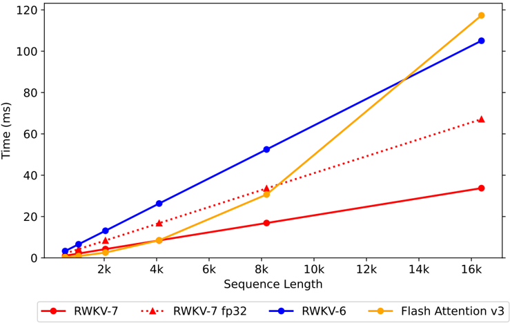<details> <summary>Image 10 Details</summary>  ### Visual Description ## Line Chart: Performance Comparison of Attention Mechanisms vs Sequence Length ### Overview The chart compares the execution time (in milliseconds) of four different attention mechanisms (RWKV-7, RWKV-7 fp32, RWKV-6, and Flash Attention v3) as sequence length increases from 2k to 16k. All lines show upward trends, with varying slopes indicating differing computational efficiencies. ### Components/Axes - **X-axis**: Sequence Length (2k, 4k, 6k, 8k, 10k, 12k, 14k, 16k) - **Y-axis**: Time (ms) (0–120 ms) - **Legend**: - Solid red: RWKV-7 - Dotted red: RWKV-7 fp32 - Solid blue: RWKV-6 - Solid orange: Flash Attention v3 - **Legend Position**: Bottom center ### Detailed Analysis 1. **RWKV-7 (Solid Red)**: - Starts at ~0 ms for 2k sequence length. - Linear increase to ~35 ms at 16k. - Steady, shallow slope. 2. **RWKV-7 fp32 (Dotted Red)**: - Starts slightly above RWKV-7 (~5 ms at 2k). - Steeper slope than RWKV-7, reaching ~65 ms at 16k. - Dotted line indicates higher time complexity. 3. **RWKV-6 (Solid Blue)**: - Starts at ~5 ms for 2k. - Linear increase to ~105 ms at 16k. - Steeper than RWKV-7 but shallower than Flash Attention v3. 4. **Flash Attention v3 (Solid Orange)**: - Starts at ~0 ms for 2k. - Sharp upward curve, surpassing RWKV-6 at ~12k. - Reaches ~115 ms at 16k, the highest among all. ### Key Observations - **Flash Attention v3** exhibits the steepest growth, becoming the slowest method at longer sequences. - **RWKV-7** maintains the slowest growth rate, suggesting better scalability. - **RWKV-7 fp32** shows intermediate performance, with a ~20 ms penalty over RWKV-7 at 16k. - All methods show linear time complexity, but with distinct constants. ### Interpretation The data suggests that **RWKV-7** is the most efficient attention mechanism for long sequences, while **Flash Attention v3** becomes increasingly inefficient as sequence length grows. The fp32 variant of RWKV-7 introduces a noticeable performance penalty, likely due to higher precision requirements. The divergence between Flash Attention v3 and RWKV-6 at 12k+ sequence lengths indicates a potential trade-off between theoretical efficiency and practical implementation costs. These trends align with known characteristics of attention mechanisms, where quadratic complexity in Flash Attention becomes prohibitive at scale, while RWKV's linear-time design offers better long-sequence performance. </details> Figure 9: Time vs. Sequence Length (H100) The forward pass of RWKV-7 is about twice as fast as the backward pass. For inference, the forward pass does not need to store the wkv state, making it faster. For example, for sequence length 16k, the forward pass without storing state takes 7.9 ms, while the forward pass with storing state takes 11.2 ms, the backward pass takes 22.5 ms, and the Flash Attention v3 forward pass takes 33.9 ms. Memory The peak training memory usages of the tested models are well described by the formulas derived below. For example, the runs in Figure 9 required peak memory within 2% of the estimates. In the tested kernels, the memory required per stored variable (e.g. q, k, or v in attention) is batch size × model dimension × sequence length × 2 bytes for bfloat16. For sequence length 1024, this is 64MB per variable. To calculate memory usage, we may use Flash Attention v3: 10 variables, RWKV-6: 10 variables, RWKV-7: 18 variables, RWKV-7 fp32: 24 variables. Flash Attention v3 requires 4 variables q, k, v and output for the forward pass, and the corresponding 4 gradients. Finally, the backward pass uses a temporary variable to accumulate the gradient of q in float32, yielding 2 variables worth of addition memory, for a total of 4+4+2 = 10. RWKV-6 requires 5 variables r, w, k, v, and output for the forward pass and also the corresponding 5 gradients for the backward pass, for a total of 10. RWKV-7uses7variables in the forward pass (r, w, k, v, -ˆ κ , ˆ κ ⊙ a , and output), and the corresponding 7 gradients. Additionally, it stores the wkv state every 16 timesteps. At head size 64, the state contributes the equivalent of 4 variables, for a total of 18. "RWKV-7 fp32" has the same 14 forward variables and gradients, but uses more memory to store the states in float32, for a total of 24 variable equivalents. Memory usage is constant for single token inference and follows the formulas above, minus the gradients and state storage. Pre-fill can easily be accomplished in a chunked manner, with memory usage growing linearly with regard to chunk size. This allows an easy trade-off for fast parallelized pre-fill, with user selectable maximum memory usage. ## 9 Multimodal Experiments In this section, we explore the capabilities of Goose when extended to handle multimodal tasks, where the model processes and integrates textual inputs with inputs from a different domain. 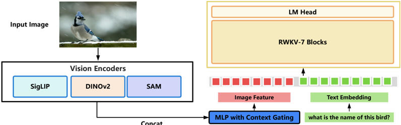<details> <summary>Image 11 Details</summary>  ### Visual Description ## Diagram: Vision-Language Model Architecture for Image Question Answering ### Overview The diagram illustrates a vision-language model architecture designed to process an input image and answer a textual question about it. The system integrates multiple vision encoders, a language model head, and a context-gating mechanism to combine visual and textual features for question answering. ### Components/Axes 1. **Left Side (Input Processing):** - **Input Image**: A photograph of a blue jay on a snowy surface. - **Vision Encoders**: Three parallel modules: - SigLIP (cyan box) - DINOv2 (peach box) - SAM (purple box) - **Concat**: A block merging outputs from all vision encoders. 2. **Right Side (Language Modeling):** - **LM Head**: A language model head (orange box). - **RWKV-7 Blocks**: A transformer-like architecture with 7 blocks (beige box). - **Image Feature**: Red squares representing visual features extracted from the input image. - **Text Embedding**: Green squares representing the textual question "what is the name of this bird?" encoded as embeddings. - **MLP with Context Gating**: A multi-layer perceptron integrating image features and text embeddings. ### Detailed Analysis - **Vision Encoders**: Three distinct models (SigLIP, DINOv2, SAM) process the input image independently, capturing different aspects of visual information (e.g., object detection, segmentation, or general feature extraction). - **Concat**: Combines multi-modal features from the three encoders into a unified representation. - **RWKV-7 Blocks**: A recurrent transformer architecture (RWKV) processes the concatenated features alongside text embeddings. The 7 blocks suggest a depth of 7 layers for sequential processing. - **MLP with Context Gating**: A non-linear integration mechanism that selectively combines image and text features, likely using attention or gating to prioritize relevant information for the question. ### Key Observations - **Multi-Modal Fusion**: The system explicitly separates visual and textual processing streams before merging them in the MLP. - **Architectural Depth**: The RWKV-7 Blocks indicate a moderately deep model for handling complex interactions between vision and language. - **Question-Specific Processing**: The text embedding directly encodes the question, enabling the model to focus on task-relevant visual features. ### Interpretation This architecture demonstrates a hybrid approach to visual question answering (VQA), leveraging multiple vision encoders to capture diverse visual cues and a language model to reason about the question. The context gating in the MLP suggests an emphasis on dynamic feature weighting, allowing the model to adaptively prioritize image regions or textual tokens relevant to the query. The use of RWKV-7 Blocks (a transformer variant with recurrent properties) may improve efficiency compared to standard transformers while maintaining contextual awareness. The absence of explicit numerical values or performance metrics implies this is a conceptual diagram rather than an empirical result. </details> Concat Figure 10: The architecture of VisualRWKV-7. The input image is processed by three vision encoders, and the obtained features are concatenated. Afterward, they are projected through an MLP with context gating to align with the dimensions of the RWKV-7 block. Finally, the image features are concatenated with the text embeddings and fed into the RWKV-7 LLM. RWKV for Image Understanding To demonstrate the modeling capabilities of RWKV-7, we constructed VisualRWKV-7 (Figure10), a visual language model based on the RWKV-7 block, to evaluate the image understanding capabilities of RWKV-7. VisualRWKV-6 (Hou et al., 2024) used the CLIP encoder, which focused on processing low-resolution images and achieved good results. VisualRWKV-7 replaces the CLIP encoder with SigLIP and DINO visual encoders, and introduced a new high-resolution SAM vision encoder, which enhances the model's supported resolution to 1024 x 1024. The experimental results of VisualRWKV-7 are shown in Table 9. The vision encoders used in both VisualRWKV-7 and VisualRWKV-6 are identical, and the training data remains consistent, aligned with the training data of LLaVA-1.5. The first stage consists of 558k alignment data, while the second stage includes 665k SFT data. VisualRWKV-7 0.1B and 0.4B outperform VisualRWKV-6 1.6B on the in-domain benchmarks VQAv2 and GQA and rapidly approach VisualRWKV-6 1.6B on two other benchmarks. The experimental results are highly compelling. With only 1/4 of the parameters (1.6B vs. 0.4B), VisualRWKV7 surpasses VisualRWKV-6 on the VQAv2 and GQA benchmarks, demonstrating the powerful modeling capabilities of RWKV-7. Table 9: A comparison of VisualRWKV-7 to other Visual Language Models across 4 distinct benchmarks. We evaluate these models on benchmarks: GQA(Hudson & Manning, 2019), SQA(Lu et al., 2022), TQA(Singh et al., 2019) and VQA(Li et al., 2023b). | Method | Vision Encoder | LLM | VQA | SQA | TQA | GQA | |--------------|-------------------|------------|-------|-------|-------|-------| | VisualRWKV-6 | SigLIP+DINOv2+SAM | RWKV6-1.6B | 73.6 | 57 | 48.7 | 58.2 | | VisualRWKV-6 | SigLIP+DINOv2+SAM | RWKV6-3.1B | 79.1 | 62.9 | 52.7 | 61 | | VisualRWKV-7 | SigLIP+DINOv2+SAM | RWKV7-0.1B | 75.2 | 50.6 | 37.9 | 59.9 | | VisualRWKV-7 | SigLIP+DINOv2+SAM | RWKV7-0.4B | 77.9 | 55 | 41.1 | 62.3 | | VisualRWKV-7 | SigLIP+DINOv2+SAM | RWKV7-1.5B | 79.8 | 59.7 | 49.5 | 63.2 | | VisualRWKV-7 | SigLIP+DINOv2+SAM | RWKV7-2.9B | 80.5 | 63.4 | 58 | 63.7 | On the out-of-domain benchmark SQA, VisualRWKV-7 2.9B also outperforms VisualRWKV-6 3.1B, indicating that VisualRWKV-7 possesses strong generalization ability. In the TextQA (TQA) benchmark, which assesses a model's associative recall, VisualRWKV-7 2.9B achieves a 5.3-point improvement over VisualRWKV-6 3.1B, further proving its superior associative recall capabilities. ## 10 Conclusions Weintroduced RWKV-7, a novel RNN architecture that pushes the boundaries of recurrent neural networks to new heights. RWKV-7 achieves state-of-the-art performance for its size across a wide range of benchmarks, demonstrating its potential to rival even highly optimized models such as Qwen2.5 despite being trained on many fewer tokens. As an RNN, RWKV-7 maintains high parameter efficiency, linear time complexity, and constant memory usage, offering a compelling alternative to traditional Transformer-based architectures. ## 10.1 Limitations Despite its strengths, the RWKV-7 architecture and models face certain limitations yet to be mitigated in future work. Numerical Precision. Weobserved that some operators, particularly the WKV7 kernel, are sensitive to the numerical precision of the implementation. This highlights the need for careful handling of numerical precision during model deployment. We also observed differences in training dynamics when using different kernels, which implies that the correct handling of precision while calculating and applying state updates is of utmost importance in this architecture. Lack of Instruction Tuning and Alignment. All RWKV-7 models presented in this work are pretrained base models and have not undergone the phase of Supervised Fine-Tuning (SFT) for instruction following nor alignment with human preferences (RLHF). Future efforts should focus on incorporating these capabilities to enhance the model's usability in real-world applications. Prompt Sensitivity. Wefound that the absence of the special token <|endoftext|> results in degraded performance of RWKV-7 models, e.g. inability to remember the first token of the input. See Appendix M for details. Compute Resources. Due to computational budget constraints, our training was limited on at most 12 × 8 = 96 Nvidia H800 GPUs. This falls short of the resources required for recent large-scale training efforts, such as DeepSeek-V3 (DeepSeek-AI et al., 2025). Additionally, we are forced to continue training from pre-existing checkpoints of earlier RWKV architectures and therefore re-use some parts of our dataset. This may limit the capabilities of our models versus pre-training from scratch. Scaling up RWKV-7 to larger sizes and datasets will require additional computational resources. ## 10.2 Future Work In addition to training larger RWKV-7 models with more tokens in the future, we also aim to explore several promising directions to further enhance the architecture and its capabilities. Speedup Techniques. A variety of speed optimization techniques were highlighted in the technical report of DeepSeek-V3 (DeepSeek-AI et al., 2025), including Dual Pipelining Mechanism, Mixture-of-Experts, Multi-Token Prediction, and FP8 Training. We are aware that many of these techniques are orthogonal to RWKV-7's architectural optimizations, therefore could be integrated to further accelerate training in later RWKV models. However, RWKV-7, like its predecessors, has been trained completely without pipeline parallelism. We also noticed that there is room for speed optimization of RWKV-7 kernels and operators. We will explore both kernel-level optimizations and distributed training strategies in the future. Incorporating Chain-of-Thought Reasoning. Webelieve that RWKV-7, as a linear RNN, is wellsuited for efficient Chain-of-Thought reasoning (Wei et al., 2022). However, this capability has been barely explored due to the lack of suitable reinforcement learning pipelines. In future work, we plan to incorporate deep thinking abilities into RWKV-7, enabling it to excel in tasks requiring multi-step logical reasoning and complex problem-solving. ## Acknowledgments Weextend our gratitude to Shenzhen Yuanshi Intelligent Co. Ltd. and Shanghai Yuanwo Intelligent Co. Ltd. for providing computational resources and their dedication to promoting and commercializing RWKV. We thank Featherless AI for their extensive experimentation with the RWKV architecture and their contributions to this paper. We are grateful to the members of the RWKV and EleutherAI Discord communities for their collaborative efforts in extending the applicability of RWKV to diverse domains. We extend a special thank you to Stella Biderman, Songlin Yang and Yu Zhang. ## References - Loubna Ben Allal, Anton Lozhkov, Elie Bakouch, Gabriel Martín Blázquez, Guilherme Penedo, Lewis Tunstall, Andrés Marafioti, Hynek Kydlíˇ cek, Agustín Piqueres Lajarín, Vaibhav Srivastav, Joshua Lochner, Caleb Fahlgren, Xuan-Son Nguyen, Clémentine Fourrier, Ben Burtenshaw, Hugo Larcher, Haojun Zhao, Cyril Zakka, Mathieu Morlon, Colin Raffel, Leandro von Werra, and Thomas Wolf. Smollm2: When smol goes big - data-centric training of a small language model, 2025. URL https://arxiv.org/abs/2502.02737 . - Simran Arora, Sabri Eyuboglu, Aman Timalsina, Isys Johnson, Michael Poli, James Zou, Atri Rudra, and Christopher Re. Zoology: Measuring and improving recall in efficient language models, 2023. - Zhangir Azerbayev, Hailey Schoelkopf, Keiran Paster, Marco Dos Santos, Stephen Marcus McAleer, Albert Q. Jiang, Jia Deng, Stella Biderman, and Sean Welleck. Llemma: An open language model for mathematics. In The Twelfth International Conference on Learning Representations , 2024. URL https://openreview.net/forum?id=4WnqRR915j . - David A. Barrington. Bounded-width polynomial-size branching programs recognize exactly those languages in nc1. Journal of Computer and System Sciences , 38(1):150-164, 1989. URL https: //www.sciencedirect.com/science/article/pii/0022000089900378 . - Maximilian Beck, Korbinian Pöppel, Markus Spanring, Andreas Auer, Oleksandra Prudnikova, Michael Kopp, Günter Klambauer, Johannes Brandstetter, and Sepp Hochreiter. xlstm: Extended long short-term memory, 2024. URL https://arxiv.org/abs/2405.04517 . - Ali Behrouz, Peilin Zhong, and Vahab Mirrokni. Titans: Learning to memorize at test time, 2024. - Loubna Ben Allal, Anton Lozhkov, Guilherme Penedo, Thomas Wolf, and Leandro von Werra. Cosmopedia, February 2024a. URL https://huggingface.co/datasets/HuggingF aceTB/cosmopedia . - Loubna Ben Allal, Anton Lozhkov, Guilherme Penedo, Thomas Wolf, and Leandro von Werra. Smollm-corpus, July 2024b. URL https://huggingface.co/datasets/HuggingFac eTB/smollm-corpus . - Sumithra Bhakthavatsalam, Daniel Khashabi, Tushar Khot, Bhavana Dalvi Mishra, Kyle Richardson, Ashish Sabharwal, Carissa Schoenick, Oyvind Tafjord, and Peter Clark. Think you have solved direct-answer question answering? try arc-da, the direct-answer ai2 reasoning challenge. arXiv preprint arXiv:2102.03315 , 2021. - Yonatan Bisk, Rowan Zellers, Jianfeng Gao, Yejin Choi, et al. Piqa: Reasoning about physical commonsense in natural language. In Proceedings of the AAAI conference on artificial intelligence , volume 34, pp. 7432-7439, 2020. - Sidney Black, Stella Biderman, Eric Hallahan, Quentin Anthony, Leo Gao, Laurence Golding, Horace He, Connor Leahy, Kyle McDonell, Jason Phang, Michael Pieler, Usvsn Sai Prashanth, Shivanshu Purohit, Laria Reynolds, Jonathan Tow, Ben Wang, and Samuel Weinbach. GPTNeoX-20B: An open-source autoregressive language model. In Angela Fan, Suzana Ilic, Thomas Wolf, and Matthias Gallé (eds.), Proceedings of BigScience Episode #5 - Workshop on Challenges & Perspectives in Creating Large Language Models , pp. 95-136, virtual+Dublin, May 2022. Association for Computational Linguistics. doi: 10.18653/v1/2022.bigscience-1.9. URL https://aclanthology.org/2022.bigscience-1.9 . - Yingfa Chen, Xinrong Zhang, Shengding Hu, Xu Han, Zhiyuan Liu, and Maosong Sun. Stuffed mamba: State collapse and state capacity of rnn-based long-context modeling, 2024a. URL https://arxiv.org/abs/2410.07145 . - Yukang Chen, Shengju Qian, Haotian Tang, Xin Lai, Zhijian Liu, Song Han, and Jiaya Jia. Longlora: Efficient fine-tuning of long-context large language models, 2024b. URL https://arxiv. org/abs/2309.12307 . - Alexis Conneau, Ruty Rinott, Guillaume Lample, Adina Williams, Samuel Bowman, Holger Schwenk, and Veselin Stoyanov. Xnli: Evaluating cross-lingual sentence representations. In Proceedings of the 2018 Conference on Empirical Methods in Natural Language Processing , pp. 2475-2485, 2018. - Tri Dao and Albert Gu. Transformers are ssms: Generalized models and efficient algorithms through structured state space duality, 2024. URL https://arxiv.org/abs/2405.210 60 . - Dao AI Lab. Causal conv1d. https://github.com/Dao-AILab/causal-conv1d , 2023. Accessed: 2025-02-26. - DeepSeek-AI, Aixin Liu, Bei Feng, Bing Xue, Bingxuan Wang, Bochao Wu, Chengda Lu, Chenggang Zhao, Chengqi Deng, Chenyu Zhang, Chong Ruan, Damai Dai, Daya Guo, Dejian Yang, Deli Chen, Dongjie Ji, Erhang Li, Fangyun Lin, Fucong Dai, Fuli Luo, Guangbo Hao, Guanting Chen, Guowei Li, H. Zhang, Han Bao, Hanwei Xu, Haocheng Wang, Haowei Zhang, Honghui Ding, Huajian Xin, Huazuo Gao, Hui Li, Hui Qu, J. L. Cai, Jian Liang, Jianzhong Guo, Jiaqi Ni, Jiashi Li, Jiawei Wang, Jin Chen, Jingchang Chen, Jingyang Yuan, Junjie Qiu, Junlong Li, Junxiao Song, Kai Dong, Kai Hu, Kaige Gao, Kang Guan, Kexin Huang, Kuai Yu, Lean Wang, Lecong Zhang, Lei Xu, Leyi Xia, Liang Zhao, Litong Wang, Liyue Zhang, Meng Li, Miaojun Wang, Mingchuan Zhang, Minghua Zhang, Minghui Tang, Mingming Li, Ning Tian, Panpan Huang, Peiyi Wang, Peng Zhang, Qiancheng Wang, Qihao Zhu, Qinyu Chen, Qiushi Du, R. J. Chen, R. L. Jin, Ruiqi Ge, Ruisong Zhang, Ruizhe Pan, Runji Wang, Runxin Xu, Ruoyu Zhang, Ruyi Chen, S. S. Li, Shanghao Lu, Shangyan Zhou, Shanhuang Chen, Shaoqing Wu, Shengfeng Ye, Shengfeng Ye, Shirong Ma, Shiyu Wang, Shuang Zhou, Shuiping Yu, Shunfeng Zhou, Shuting Pan, T. Wang, Tao Yun, Tian Pei, Tianyu Sun, W. L. Xiao, Wangding Zeng, Wanjia Zhao, Wei An, Wen Liu, Wenfeng Liang, Wenjun Gao, Wenqin Yu, Wentao Zhang, X. Q. Li, Xiangyue Jin, Xianzu Wang, Xiao Bi, Xiaodong Liu, Xiaohan Wang, Xiaojin Shen, Xiaokang Chen, Xiaokang Zhang, Xiaosha Chen, Xiaotao Nie, Xiaowen Sun, Xiaoxiang Wang, Xin Cheng, Xin Liu, Xin Xie, Xingchao Liu, Xingkai Yu, Xinnan Song, Xinxia Shan, Xinyi Zhou, Xinyu Yang, Xinyuan Li, Xuecheng Su, Xuheng Lin, Y. K. Li, Y. Q. Wang, Y. X. Wei, Y. X. Zhu, Yang Zhang, Yanhong Xu, Yanhong Xu, Yanping Huang, Yao Li, Yao Zhao, Yaofeng Sun, Yaohui Li, Yaohui Wang, Yi Yu, Yi Zheng, Yichao Zhang, Yifan Shi, Yiliang Xiong, Ying He, Ying Tang, Yishi Piao, Yisong Wang, Yixuan Tan, Yiyang Ma, Yiyuan Liu, Yongqiang Guo, Yu Wu, Yuan Ou, Yuchen Zhu, Yuduan Wang, Yue Gong, Yuheng Zou, Yujia He, Yukun Zha, Yunfan Xiong, Yunxian Ma, Yuting Yan, Yuxiang Luo, Yuxiang You, Yuxuan Liu, Yuyang Zhou, Z. F . Wu, Z. Z. Ren, Zehui Ren, Zhangli Sha, Zhe Fu, Zhean Xu, Zhen Huang, Zhen Zhang, Zhenda Xie, Zhengyan Zhang, Zhewen Hao, Zhibin Gou, Zhicheng Ma, Zhigang Yan, Zhihong Shao, Zhipeng Xu, Zhiyu Wu, Zhongyu Zhang, Zhuoshu Li, Zihui Gu, Zijia Zhu, Zijun Liu, Zilin Li, Ziwei Xie, Ziyang Song, Ziyi Gao, and Zizheng Pan. Deepseek-v3 technical report, 2025. URL https://arxiv.org/abs/2412.19437 . - Grégoire Delétang, Anian Ruoss, Paul-Ambroise Duquenne, Elliot Catt, Tim Genewein, Christopher Mattern, Jordi Grau-Moya, Li Kevin Wenliang, Matthew Aitchison, Laurent Orseau, Marcus Hutter, and Joel Veness. Language modeling is compression, 2024. URL https://arxiv.or g/abs/2309.10668 . - Nelson Elhage, Neel Nanda, Catherine Olsson, Tom Henighan, Nicholas Joseph, Ben Mann, Amanda Askell, Yuntao Bai, Anna Chen, Tom Conerly, Nova DasSarma, Dawn Drain, Deep Ganguli, Zac Hatfield-Dodds, Danny Hernandez, Andy Jones, Jackson Kernion, Liane Lovitt, Kamal Ndousse, Dario Amodei, Tom Brown, Jack Clark, Jared Kaplan, Sam McCandlish, and Chris Olah. A mathematical framework for transformer circuits. Transformer Circuits Thread , 2021. https://transformer-circuits.pub/2021/framework/index.html. - Qihang Fan, Huaibo Huang, and Ran He. Breaking the low-rank dilemma of linear attention, 2025. URL https://arxiv.org/abs/2411.07635 . - Daniel Y. Fu, Tri Dao, Khaled K. Saab, Armin W. Thomas, Atri Rudra, and Christopher Re. Hungry hungry hippos: Towards language modeling with state space models, 2023. - Leo Gao, Stella Biderman, Sid Black, Laurence Golding, Travis Hoppe, Charles Foster, Jason Phang, Horace He, Anish Thite, Noa Nabeshima, Shawn Presser, and Connor Leahy. The pile: An 800gb dataset of diverse text for language modeling, 2020. - Leo Gao, Jonathan Tow, Baber Abbasi, Stella Biderman, Sid Black, Anthony DiPofi, Charles Foster, Laurence Golding, Jeffrey Hsu, Alain Le Noac'h, Haonan Li, Kyle McDonell, Niklas Muennighoff, Chris Ociepa, Jason Phang, Laria Reynolds, Hailey Schoelkopf, Aviya Skowron, Lintang Sutawika, Eric Tang, Anish Thite, Ben Wang, Kevin Wang, and Andy Zou. A framework for few-shot language model evaluation, 12 2023. URL https://zenodo.org/records/10256836 . - Aaron Grattafiori, Abhimanyu Dubey, Abhinav Jauhri, Abhinav Pandey, Abhishek Kadian, Ahmad Al-Dahle, Aiesha Letman, Akhil Mathur, Alan Schelten, Alex Vaughan, Amy Yang, Angela Fan, Anirudh Goyal, Anthony Hartshorn, Aobo Yang, Archi Mitra, Archie Sravankumar, Artem Korenev, Arthur Hinsvark, Arun Rao, Aston Zhang, Aurelien Rodriguez, Austen Gregerson, Ava Spataru, Baptiste Roziere, Bethany Biron, Binh Tang, Bobbie Chern, Charlotte Caucheteux, Chaya Nayak, Chloe Bi, Chris Marra, Chris McConnell, Christian Keller, Christophe Touret, Chunyang Wu, Corinne Wong, Cristian Canton Ferrer, Cyrus Nikolaidis, Damien Allonsius, Daniel Song, Danielle Pintz, Danny Livshits, Danny Wyatt, David Esiobu, Dhruv Choudhary, Dhruv Mahajan, Diego Garcia-Olano, Diego Perino, Dieuwke Hupkes, Egor Lakomkin, Ehab AlBadawy, Elina Lobanova, Emily Dinan, Eric Michael Smith, Filip Radenovic, Francisco Guzmán, Frank Zhang, Gabriel Synnaeve, Gabrielle Lee, Georgia Lewis Anderson, Govind Thattai, Graeme Nail, Gregoire Mialon, Guan Pang, Guillem Cucurell, Hailey Nguyen, Hannah Korevaar, Hu Xu, Hugo Touvron, Iliyan Zarov, Imanol Arrieta Ibarra, Isabel Kloumann, Ishan Misra, Ivan Evtimov, Jack Zhang, Jade Copet, Jaewon Lee, Jan Geffert, Jana Vranes, Jason Park, Jay Mahadeokar, Jeet Shah, Jelmer van der Linde, Jennifer Billock, Jenny Hong, Jenya Lee, Jeremy Fu, Jianfeng Chi, Jianyu Huang, Jiawen Liu, Jie Wang, Jiecao Yu, Joanna Bitton, Joe Spisak, Jongsoo Park, Joseph Rocca, Joshua Johnstun, Joshua Saxe, Junteng Jia, Kalyan Vasuden Alwala, Karthik Prasad, Kartikeya Upasani, Kate Plawiak, Ke Li, Kenneth Heafield, Kevin Stone, Khalid El-Arini, Krithika Iyer, Kshitiz Malik, Kuenley Chiu, Kunal Bhalla, Kushal Lakhotia, Lauren Rantala-Yeary, Laurens van der Maaten, Lawrence Chen, Liang Tan, Liz Jenkins, Louis Martin, Lovish Madaan, Lubo Malo, Lukas Blecher, Lukas Landzaat, Luke de Oliveira, Madeline Muzzi, Mahesh Pasupuleti, Mannat Singh, Manohar Paluri, Marcin Kardas, Maria Tsimpoukelli, Mathew Oldham, Mathieu Rita, Maya Pavlova, Melanie Kambadur, Mike Lewis, Min Si, Mitesh Kumar Singh, Mona Hassan, Naman Goyal, Narjes Torabi, Nikolay Bashlykov, Nikolay Bogoychev, Niladri Chatterji, Ning Zhang, Olivier Duchenne, Onur Çelebi, Patrick Alrassy, Pengchuan Zhang, Pengwei Li, Petar Vasic, Peter Weng, Prajjwal Bhargava, Pratik Dubal, Praveen Krishnan, Punit Singh Koura, Puxin Xu, Qing He, Qingxiao Dong, Ragavan Srinivasan, Raj Ganapathy, Ramon Calderer, Ricardo Silveira Cabral, Robert Stojnic, Roberta Raileanu, Rohan Maheswari, Rohit Girdhar, Rohit Patel, Romain Sauvestre, Ronnie Polidoro, Roshan Sumbaly, Ross Taylor, Ruan Silva, Rui Hou, Rui Wang, Saghar Hosseini, Sahana Chennabasappa, Sanjay Singh, Sean Bell, Seohyun Sonia Kim, Sergey Edunov, Shaoliang Nie, Sharan Narang, Sharath Raparthy, Sheng Shen, Shengye Wan, Shruti Bhosale, Shun Zhang, Simon Vandenhende, Soumya Batra, Spencer Whitman, Sten Sootla, Stephane Collot, Suchin Gururangan, Sydney Borodinsky, Tamar Herman, Tara Fowler, Tarek Sheasha, Thomas Georgiou, Thomas Scialom, Tobias Speckbacher, Todor Mihaylov, Tong Xiao, Ujjwal Karn, Vedanuj Goswami, Vibhor Gupta, Vignesh Ramanathan, Viktor Kerkez, Vincent Gonguet, Virginie Do, Vish Vogeti, Vítor Albiero, Vladan Petrovic, Weiwei Chu, Wenhan Xiong, Wenyin Fu, Whitney Meers, Xavier Martinet, Xiaodong Wang, Xiaofang Wang, Xiaoqing Ellen Tan, Xide Xia, Xinfeng Xie, Xuchao Jia, Xuewei Wang, Yaelle Goldschlag, Yashesh Gaur, Yasmine Babaei, Yi Wen, Yiwen Song, Yuchen Zhang, Yue Li, Yuning Mao, Zacharie Delpierre Coudert, Zheng Yan, Zhengxing Chen, Zoe Papakipos, Aaditya Singh, Aayushi Srivastava, Abha Jain, Adam Kelsey, Adam Shajnfeld, Adithya Gangidi, Adolfo Victoria, Ahuva Goldstand, Ajay Menon, Ajay Sharma, Alex Boesenberg, Alexei Baevski, Allie Feinstein, Amanda Kallet, Amit Sangani, Amos Teo, Anam Yunus, Andrei Lupu, Andres Alvarado, Andrew Caples, Andrew Gu, Andrew Ho, Andrew Poulton, Andrew Ryan, Ankit Ramchandani, Annie Dong, Annie Franco, Anuj Goyal, Aparajita Saraf, Arkabandhu Chowdhury, Ashley Gabriel, Ashwin Bharambe, Assaf Eisenman, Azadeh Yazdan, Beau James, Ben Maurer, Benjamin Leonhardi, Bernie Huang, Beth Loyd, Beto De Paola, Bhargavi Paranjape, Bing Liu, Bo Wu, Boyu Ni, Braden Hancock, Bram Wasti, Brandon Spence, Brani Stojkovic, Brian Gamido, Britt Montalvo, Carl Parker, Carly Burton, Catalina Mejia, Ce Liu, Changhan Wang, Changkyu Kim, Chao Zhou, Chester Hu, Ching-Hsiang Chu, Chris Cai, Chris Tindal, Christoph Feichtenhofer, Cynthia Gao, Damon Civin, Dana Beaty, Daniel Kreymer, Daniel Li, David Adkins, David Xu, Davide Testuggine, Delia David, Devi Parikh, Diana Liskovich, Didem Foss, Dingkang Wang, Duc Le, Dustin Holland, Edward Dowling, Eissa Jamil, Elaine Montgomery, Eleonora Presani, Emily Hahn, Emily Wood, Eric-Tuan Le, Erik Brinkman, Esteban Arcaute, Evan Dunbar, Evan Smothers, Fei Sun, Felix Kreuk, Feng Tian, Filippos Kokkinos, Firat Ozgenel, Francesco Caggioni, Frank Kanayet, Frank Seide, Gabriela Medina Florez, Gabriella Schwarz, Gada Badeer, Georgia Swee, Gil Halpern, Grant Herman, Grigory Sizov, Guangyi, Zhang, Guna Lakshminarayanan, Hakan Inan, Hamid Shojanazeri, Han Zou, Hannah Wang, Hanwen Zha, Haroun Habeeb, Harrison Rudolph, Helen Suk, Henry Aspegren, Hunter Goldman, Hongyuan Zhan, Ibrahim Damlaj, Igor Molybog, Igor Tufanov, Ilias Leontiadis, Irina-Elena Veliche, Itai Gat, Jake Weissman, James Geboski, James Kohli, Janice Lam, Japhet Asher, Jean-Baptiste Gaya, Jeff Marcus, Jeff Tang, Jennifer Chan, Jenny Zhen, Jeremy Reizenstein, Jeremy Teboul, Jessica Zhong, Jian Jin, Jingyi Yang, Joe Cummings, Jon Carvill, Jon Shepard, Jonathan McPhie, Jonathan Torres, Josh Ginsburg, Junjie Wang, Kai Wu, Kam Hou U, Karan Saxena, Kartikay Khandelwal, Katayoun Zand, Kathy Matosich, Kaushik Veeraraghavan, Kelly Michelena, Keqian Li, Kiran Jagadeesh, Kun Huang, Kunal Chawla, Kyle Huang, Lailin Chen, Lakshya Garg, Lavender A, Leandro Silva, Lee Bell, Lei Zhang, Liangpeng Guo, Licheng Yu, Liron Moshkovich, Luca Wehrstedt, Madian Khabsa, Manav Avalani, Manish Bhatt, Martynas Mankus, Matan Hasson, Matthew Lennie, Matthias Reso, Maxim Groshev, Maxim Naumov, Maya Lathi, Meghan Keneally, Miao Liu, Michael L. Seltzer, Michal Valko, Michelle Restrepo, Mihir Patel, Mik Vyatskov, Mikayel Samvelyan, Mike Clark, Mike Macey, Mike Wang, Miquel Jubert Hermoso, Mo Metanat, Mohammad Rastegari, Munish Bansal, Nandhini Santhanam, Natascha Parks, Natasha White, Navyata Bawa, Nayan Singhal, Nick Egebo, Nicolas Usunier, Nikhil Mehta, Nikolay Pavlovich Laptev, Ning Dong, Norman Cheng, Oleg Chernoguz, Olivia Hart, Omkar Salpekar, Ozlem Kalinli, Parkin Kent, Parth Parekh, Paul Saab, Pavan Balaji, Pedro Rittner, Philip Bontrager, Pierre Roux, Piotr Dollar, Polina Zvyagina, Prashant Ratanchandani, Pritish Yuvraj, Qian Liang, Rachad Alao, Rachel Rodriguez, Rafi Ayub, Raghotham Murthy, Raghu Nayani, Rahul Mitra, Rangaprabhu Parthasarathy, Raymond Li, Rebekkah Hogan, Robin Battey, Rocky Wang, Russ Howes, Ruty Rinott, Sachin Mehta, Sachin Siby, Sai Jayesh Bondu, Samyak Datta, Sara Chugh, Sara Hunt, Sargun Dhillon, Sasha Sidorov, Satadru Pan, Saurabh Mahajan, Saurabh Verma, Seiji Yamamoto, Sharadh Ramaswamy, Shaun Lindsay, Shaun Lindsay, Sheng Feng, Shenghao Lin, Shengxin Cindy Zha, Shishir Patil, Shiva Shankar, Shuqiang Zhang, Shuqiang Zhang, Sinong Wang, Sneha Agarwal, Soji Sajuyigbe, Soumith Chintala, Stephanie Max, Stephen Chen, Steve Kehoe, Steve Satterfield, Sudarshan Govindaprasad, Sumit Gupta, Summer Deng, Sungmin Cho, Sunny Virk, Suraj Subramanian, Sy Choudhury, Sydney Goldman, Tal Remez, Tamar Glaser, Tamara Best, Thilo Koehler, Thomas Robinson, Tianhe Li, Tianjun Zhang, Tim Matthews, Timothy Chou, Tzook Shaked, Varun Vontimitta, Victoria Ajayi, Victoria Montanez, Vijai Mohan, Vinay Satish Kumar, Vishal Mangla, Vlad Ionescu, Vlad Poenaru, Vlad Tiberiu Mihailescu, Vladimir Ivanov, Wei Li, Wenchen Wang, Wenwen Jiang, Wes Bouaziz, Will Constable, Xiaocheng Tang, Xiaojian Wu, Xiaolan Wang, Xilun Wu, Xinbo Gao, Yaniv Kleinman, Yanjun Chen, Ye Hu, Ye Jia, Ye Qi, Yenda Li, Yilin Zhang, Ying Zhang, Yossi Adi, Youngjin Nam, Yu, Wang, Yu Zhao, Yuchen Hao, Yundi Qian, Yunlu Li, Yuzi He, Zach Rait, Zachary DeVito, Zef Rosnbrick, Zhaoduo Wen, Zhenyu Yang, Zhiwei Zhao, and Zhiyu Ma. The llama 3 herd of models, 2024. URL https://arxiv.org/abs/2407.21783 . - Riccardo Grazzi, Julien Siems, Jörg K. H. Franke, Arber Zela, Frank Hutter, and Massimiliano Pontil. Unlocking state-tracking in linear rnns through negative eigenvalues, 2024. URL https: //arxiv.org/abs/2411.12537 . - Albert Gu and Tri Dao. Mamba: Linear-time sequence modeling with selective state spaces, 2023. - Albert Gu, Karan Goel, and Christopher Re. Efficiently modeling long sequences with structured state spaces, 2022. - Frank R Hampel. The influence curve and its role in robust estimation. Journal of the american statistical association , 69(346):383-393, 1974. - Dongchen Han, Yifan Pu, Zhuofan Xia, Yizeng Han, Xuran Pan, Xiu Li, Jiwen Lu, Shiji Song, and Gao Huang. Bridging the divide: Reconsidering softmax and linear attention, 2024. URL https://arxiv.org/abs/2412.06590 . - Donald Olding Hebb. The organization of behavior: A neuropsychological theory . John Wiley & Sons, 1949. - Dan Hendrycks, Collin Burns, Steven Basart, Andy Zou, Mantas Mazeika, Dawn Song, and Jacob Steinhardt. Measuring massive multitask language understanding, 2021. URL https://ar xiv.org/abs/2009.03300 . - Roger A Horn and Charles R Johnson. Matrix analysis . Cambridge university press, 2012. - Haowen Hou, Peigen Zeng, Fei Ma, and Fei Richard Yu. Visualrwkv: Exploring recurrent neural networks for visual language models. ArXiv , abs/2406.13362, 2024. URL https://api.se manticscholar.org/CorpusID:270620870 . - Drew A. Hudson and Christopher D. Manning. Gqa: A new dataset for real-world visual reasoning and compositional question answering. 2019 IEEE/CVF Conference on Computer Vision and Pattern Recognition (CVPR) , pp. 6693-6702, 2019. URL https://api.semanticscholar. org/CorpusID:152282269 . - Jean Kaddour. The minipile challenge for data-efficient language models, 2023. - Angelos Katharopoulos, Apoorv Vyas, Nikolaos Pappas, and François Fleuret. Transformers are rnns: Fast autoregressive transformers with linear attention. In International conference on machine learning , pp. 5156-5165. PMLR, 2020a. - Angelos Katharopoulos, Apoorv Vyas, Nikolaos Pappas, and Fran¸cois Fleuret. Transformers are rnns: Fast autoregressive transformers with linear attention. Proceedings of the 37 th International Conference on Machine Learning , 2020b. - Jeffrey Li, Alex Fang, Georgios Smyrnis, Maor Ivgi, Matt Jordan, Samir Gadre, Hritik Bansal, Etash Guha, Sedrick Keh, Kushal Arora, Saurabh Garg, Rui Xin, Niklas Muennighoff, Reinhard Heckel, Jean Mercat, Mayee Chen, Suchin Gururangan, Mitchell Wortsman, Alon Albalak, Yonatan Bitton, Marianna Nezhurina, Amro Abbas, Cheng-Yu Hsieh, Dhruba Ghosh, Josh Gardner, Maciej Kilian, Hanlin Zhang, Rulin Shao, Sarah Pratt, Sunny Sanyal, Gabriel Ilharco, Giannis Daras, Kalyani Marathe, Aaron Gokaslan, Jieyu Zhang, Khyathi Chandu, Thao Nguyen, Igor Vasiljevic, Sham Kakade, Shuran Song, Sujay Sanghavi, Fartash Faghri, Sewoong Oh, Luke Zettlemoyer, Kyle Lo, Alaaeldin El-Nouby, Hadi Pouransari, Alexander Toshev, Stephanie Wang, Dirk Groeneveld, Luca Soldaini, Pang Wei Koh, Jenia Jitsev, Thomas Kollar, Alexandros G. Dimakis, Yair Carmon, Achal Dave, Ludwig Schmidt, and Vaishaal Shankar. Datacomp-lm: In search of the next generation of training sets for language models, 2024a. - Raymond Li, Loubna Ben Allal, Yangtian Zi, Niklas Muennighoff, Denis Kocetkov, Chenghao Mou, Marc Marone, Christopher Akiki, Jia Li, Jenny Chim, Qian Liu, Evgenii Zheltonozhskii, Terry Yue Zhuo, Thomas Wang, Olivier Dehaene, Mishig Davaadorj, Joel Lamy-Poirier, João Monteiro, Oleh Shliazhko, Nicolas Gontier, Nicholas Meade, Armel Zebaze, Ming-Ho Yee, Logesh Kumar Umapathi, Jian Zhu, Benjamin Lipkin, Muhtasham Oblokulov, Zhiruo Wang, Rudra Murthy, Jason Stillerman, Siva Sankalp Patel, Dmitry Abulkhanov, Marco Zocca, Manan Dey, Zhihan Zhang, Nour Fahmy, Urvashi Bhattacharyya, Wenhao Yu, Swayam Singh, Sasha Luccioni, Paulo Villegas, Maxim Kunakov, Fedor Zhdanov, Manuel Romero, Tony Lee, Nadav Timor, Jennifer Ding, Claire Schlesinger, Hailey Schoelkopf, Jan Ebert, Tri Dao, Mayank Mishra, Alex Gu, Jennifer Robinson, Carolyn Jane Anderson, Brendan Dolan-Gavitt, Danish Contractor, Siva Reddy, Daniel Fried, Dzmitry Bahdanau, Yacine Jernite, Carlos Muñoz Ferrandis, Sean Hughes, Thomas Wolf, Arjun Guha, Leandro von Werra, and Harm de Vries. Starcoder: may the source be with you!, 2023a. - Yifan Li, Yifan Du, Kun Zhou, Jinpeng Wang, Wayne Xin Zhao, and Ji rong Wen. Evaluating object hallucination in large vision-language models. In Conference on Empirical Methods in Natural Language Processing , 2023b. URL https://api.semanticscholar.org/CorpusID: 258740697 . - Yucheng Li, Yunhao Guo, Frank Guerin, and Chenghua Lin. Evaluating large language models for generalization and robustness via data compression, 2024b. URL https://arxiv.org/ab s/2402.00861 . - Xi Victoria Lin, Todor Mihaylov, Mikel Artetxe, Tianlu Wang, Shuohui Chen, Daniel Simig, Myle Ott, Naman Goyal, Shruti Bhosale, Jingfei Du, et al. Few-shot learning with multilingual generative language models. In Proceedings of the 2022 Conference on Empirical Methods in Natural Language Processing , pp. 9019-9052, 2022. - Bo Liu, Rui Wang, Lemeng Wu, Yihao Feng, Peter Stone, and Qiang Liu. Longhorn: State space models are amortized online learners, 2024. URL https://arxiv.org/abs/2407.142 07 . - Anton Lozhkov, Loubna Ben Allal, Leandro von Werra, and Thomas Wolf. Fineweb-edu: the finest collection of educational content, 2024. URL https://huggingface.co/datasets/Hu ggingFaceFW/fineweb-edu . - Pan Lu, Swaroop Mishra, Tony Xia, Liang Qiu, Kai-Wei Chang, Song-Chun Zhu, Oyvind Tafjord, Peter Clark, and A. Kalyan. Learn to explain: Multimodal reasoning via thought chains for science question answering. ArXiv , abs/2209.09513, 2022. URL https://api.semantic scholar.org/CorpusID:252383606 . - Shahar Lutati, Itamar Zimerman, and Lior Wolf. Focus your attention (with adaptive iir filters), 2023. - Sam McCandlish, Jared Kaplan, Dario Amodei, and OpenAI Dota Team. An empirical model of large-batch training. ArXiv , abs/1812.06162, 2018. URL https://api.semanticschola r.org/CorpusID:56262183 . - William Merrill, Jackson Petty, and Ashish Sabharwal. The illusion of state in state-space models. ArXiv , abs/2404.08819, 2024. URL https://api.semanticscholar.org/CorpusID: 269149086 . - Igor Molybog, Peter Albert, Moya Chen, Zachary DeVito, David Esiobu, Naman Goyal, Punit Singh Koura, Sharan Narang, Andrew Poulton, Ruan Silva, Binh Tang, Diana Liskovich, Puxin Xu, Yuchen Zhang, Melanie Kambadur, Stephen Roller, and Susan Zhang. A theory on adam instability in large-scale machine learning, 2023. URL https://arxiv.org/abs/2304.0 9871 . - Catherine Olsson, Nelson Elhage, Neel Nanda, Nicholas Joseph, Nova DasSarma, Tom Henighan, Ben Mann, Amanda Askell, Yuntao Bai, Anna Chen, Tom Conerly, Dawn Drain, Deep Ganguli, Zac Hatfield-Dodds, Danny Hernandez, Scott Johnston, Andy Jones, Jackson Kernion, Liane Lovitt, Kamal Ndousse, Dario Amodei, Tom Brown, Jack Clark, Jared Kaplan, Sam McCandlish, and Chris Olah. In-context learning and induction heads, 2022. - Denis Paperno, Germán Kruszewski, Angeliki Lazaridou, Quan Ngoc Pham, Raffaella Bernardi, Sandro Pezzelle, Marco Baroni, Gemma Boleda, and Raquel Fernández. The lambada dataset: Word prediction requiring a broad discourse context. arXiv preprint arXiv:1606.06031 , 2016. - Keiran Paster, Marco Dos Santos, Zhangir Azerbayev, and Jimmy Ba. Openwebmath: An open dataset of high-quality mathematical web text, 2023. - Bo Peng, Eric Alcaide, Quentin Anthony, Alon Albalak, Samuel Arcadinho, Stella Biderman, Huanqi Cao, Xin Cheng, Michael Chung, Leon Derczynski, Xingjian Du, Matteo Grella, Kranthi Gv, Xuzheng He, Haowen Hou, Przemyslaw Kazienko, Jan Kocon, Jiaming Kong, Bartłomiej Koptyra, Hayden Lau, Jiaju Lin, Krishna Sri Ipsit Mantri, Ferdinand Mom, Atsushi Saito, Guangyu Song, Xiangru Tang, Johan Wind, Stanisław Wo´ zniak, Zhenyuan Zhang, Qinghua Zhou, Jian Zhu, and Rui-Jie Zhu. RWKV: Reinventing RNNs for the transformer era. In Houda Bouamor, Juan Pino, and Kalika Bali (eds.), Findings of the Association for Computational Linguistics: EMNLP 2023 , pp. 14048-14077, Singapore, December 2023. Association for Computational Linguistics. doi: 10.18653/v1/2023.findings-emnlp.936. URL https://aclanthology.org/2023.find ings-emnlp.936 . - Bo Peng, Daniel Goldstein, Quentin Gregory Anthony, Alon Albalak, Eric Alcaide, Stella Biderman, Eugene Cheah, Teddy Ferdinan, Kranthi Kiran GV, Haowen Hou, Satyapriya Krishna, Ronald McClelland Jr., Niklas Muennighoff, Fares Obeid, Atsushi Saito, Guangyu Song, Haoqin Tu, Ruichong Zhang, Bingchen Zhao, Qihang Zhao, Jian Zhu, and Rui-Jie Zhu. Eagle and finch: RWKV with matrix-valued states and dynamic recurrence. In First Conference on Language Modeling , 2024. URL https://openreview.net/forum?id=soz1SEiPeq . - Michael Poli, Stefano Massaroli, Eric Nguyen, Daniel Y Fu, Tri Dao, Stephen Baccus, Yoshua Bengio, Stefano Ermon, and Christopher Ré. Hyena hierarchy: Towards larger convolutional language models. In International Conference on Machine Learning , pp. 28043-28078. PMLR, 2023. - Michael Poli, Armin W Thomas, Eric Nguyen, Pragaash Ponnusamy, Björn Deiseroth, Kristian Kersting, Taiji Suzuki, Brian Hie, Stefano Ermon, Christopher Ré, Ce Zhang, and Stefano Massaroli. Mechanistic design and scaling of hybrid architectures, 2024. URL https: //arxiv.org/abs/2403.17844 . - Edoardo Maria Ponti, Goran Glavaš, Olga Majewska, Qianchu Liu, Ivan Vuli´ c, and Anna Korhonen. XCOPA: A multilingual dataset for causal commonsense reasoning. In Bonnie Webber, Trevor Cohn, Yulan He, and Yang Liu (eds.), Proceedings of the 2020 Conference on Empirical Methods in Natural Language Processing (EMNLP) , pp. 2362-2376, Online, November 2020. Association for Computational Linguistics. doi: 10.18653/v1/2020.emnlp-main.185. URL https: //aclanthology.org/2020.emnlp-main.185 . - Qwen, :, An Yang, Baosong Yang, Beichen Zhang, Binyuan Hui, Bo Zheng, Bowen Yu, Chengyuan Li, Dayiheng Liu, Fei Huang, Haoran Wei, Huan Lin, Jian Yang, Jianhong Tu, Jianwei Zhang, Jianxin Yang, Jiaxi Yang, Jingren Zhou, Junyang Lin, Kai Dang, Keming Lu, Keqin Bao, Kexin Yang, Le Yu, Mei Li, Mingfeng Xue, Pei Zhang, Qin Zhu, Rui Men, Runji Lin, Tianhao Li, Tianyi Tang, Tingyu Xia, Xingzhang Ren, Xuancheng Ren, Yang Fan, Yang Su, Yichang Zhang, Yu Wan, Yuqiong Liu, Zeyu Cui, Zhenru Zhang, and Zihan Qiu. Qwen2.5 technical report, 2025. URL https://arxiv.org/abs/2412.15115 . - Jack W. Rae, Anna Potapenko, Siddhant M. Jayakumar, and Timothy P . Lillicrap. Compressive transformers for long-range sequence modelling, 2019. URL https://arxiv.org/abs/ 1911.05507 . - Mark Rudelson and Roman Vershynin. Sampling from large matrices: An approach through geometric functional analysis. J. ACM , 54(4):21-es, July 2007. ISSN 0004-5411. doi: 10.1145/12 55443.1255449. URL https://doi.org/10.1145/1255443.1255449 . - Keisuke Sakaguchi, Ronan Le Bras, Chandra Bhagavatula, and Yejin Choi. Winogrande: An adversarial winograd schema challenge at scale. Communications of the ACM , 64(9):99-106, 2021. - Imanol Schlag, Kazuki Irie, and Jürgen Schmidhuber. Linear transformers are secretly fast weight programmers, 2021. URL https://arxiv.org/abs/2102.11174 . - Jürgen Schmidhuber. Learning to control fast-weight memories: An alternative to dynamic recurrent networks. Neural Computation , 4(1):131-139, 1992. doi: 10.1162/neco.1992.4.1.131. - John Schultz, Jakub Adamek, Matej Jusup, Marc Lanctot, Michael Kaisers, Sarah Perrin, Daniel Hennes, Jeremy Shar, Cannada Lewis, Anian Ruoss, Tom Zahavy, Petar Veliˇ ckovi´ c, Laurel Prince, Satinder Singh, Eric Malmi, and Nenad Tomašev. Mastering board games by external and internal planning with language models, 2024. URL https://arxiv.org/abs/2412.1 2119 . - Jay Shah, Ganesh Bikshandi, Ying Zhang, Vijay Thakkar, Pradeep Ramani, and Tri Dao. Flashattention-3: Fast and accurate attention with asynchrony and low-precision. arXiv preprint arXiv:2407.08608 , 10, 2024. - Amanpreet Singh, Vivek Natarajan, Meet Shah, Yu Jiang, Xinlei Chen, Dhruv Batra, Devi Parikh, and Marcus Rohrbach. Towards vqa models that can read, 2019. - Samuel L. Smith, Pieter-Jan Kindermans, and Quoc V. Le. Don't decay the learning rate, increase the batch size. In International Conference on Learning Representations , 2018. URL https: //openreview.net/forum?id=B1Yy1BxCZ . - Daria Soboleva, Faisal Al-Khateeb, Robert Myers, Jacob R Steeves, Joel Hestness, and Nolan Dey. SlimPajama: A 627B token cleaned and deduplicated version of RedPajama. https: //www.cerebras.net/blog/slimpajama-a-627b-token-cleaned-and-ded uplicated-version-of-redpajama , June 2023. URL https://huggingface.co /datasets/cerebras/SlimPajama-627B . - Luca Soldaini, Rodney Kinney, Akshita Bhagia, Dustin Schwenk, David Atkinson, Russell Authur, Ben Bogin, Khyathi Chandu, Jennifer Dumas, Yanai Elazar, Valentin Hofmann, Ananya Harsh Jha, Sachin Kumar, Li Lucy, Xinxi Lyu, Nathan Lambert, Ian Magnusson, Jacob Morrison, Niklas Muennighoff, Aakanksha Naik, Crystal Nam, Matthew E. Peters, Abhilasha Ravichander, Kyle Richardson, Zejiang Shen, Emma Strubell, Nishant Subramani, Oyvind Tafjord, Pete Walsh, Luke Zettlemoyer, Noah A. Smith, Hannaneh Hajishirzi, Iz Beltagy, Dirk Groeneveld, Jesse Dodge, and Kyle Lo. Dolma: an Open Corpus of Three Trillion Tokens for Language Model Pretraining Research. arXiv preprint , 2024. - Yu Sun, Xinhao Li, Karan Dalal, Jiarui Xu, Arjun Vikram, Genghan Zhang, Yann Dubois, Xinlei Chen, Xiaolong Wang, Sanmi Koyejo, Tatsunori Hashimoto, and Carlos Guestrin. Learning to (learn at test time): Rnns with expressive hidden states, 2024. - Yutao Sun, Li Dong, Shaohan Huang, Shuming Ma, Yuqing Xia, Jilong Xue, Jianyong Wang, and Furu Wei. Retentive network: A successor to transformer for large language models, 2023. - Alexey Tikhonov and Max Ryabinin. It's all in the heads: Using attention heads as a baseline for cross-lingual transfer in commonsense reasoning. In Findings of the Association for Computational Linguistics: ACL-IJCNLP 2021 , pp. 3534-3546, 2021. - Oguzhan Topsakal, Colby Jacob Edell, and Jackson Bailey Harper. Evaluating large language models with grid-based game competitions: An extensible llm benchmark and leaderboard, 2024. URL https://arxiv.org/abs/2407.07796 . - Various. Archive of our own, 2025. URL https://archiveofourown.org . - Ashish Vaswani, Noam Shazeer, Niki Parmar, Jakob Uszkoreit, Llion Jones, Aidan N. Gomez, Lukasz Kaiser, and Illia Polosukhin. Attention is all you need, 2023. - Alex Wang, Amanpreet Singh, Julian Michael, Felix Hill, Omer Levy, and Samuel Bowman. Glue: A multi-task benchmark and analysis platform for natural language understanding. In Proceedings of the 2018 EMNLP Workshop BlackboxNLP: Analyzing and Interpreting Neural Networks for NLP , pp. 353-355, 2018. - Jason Wei, Maarten Bosma, Vincent Y. Zhao abd Kelvin Guu, Adams Wei Yu, Brian Lester, Nan Du, Andrew M. Dai, and Quoc V. Le. Finetuned language models are zero-shot learners, 2021. - Jason Wei, Xuezhi Wang, Dale Schuurmans, Maarten Bosma, brian ichter, Fei Xia, Ed H. Chi, Quoc V Le, and Denny Zhou. Chain of thought prompting elicits reasoning in large language models. In Alice H. Oh, Alekh Agarwal, Danielle Belgrave, and Kyunghyun Cho (eds.), Advances in Neural Information Processing Systems , 2022. URL https://openreview.net/forum ?id=\_VjQlMeSB\_J . - Johannes Welbl, Nelson F Liu, and Matt Gardner. Crowdsourcing multiple choice science questions. In Proceedings of the 3rd Workshop on Noisy User-generated Text , pp. 94-106, 2017. - Bernard Widrow, Marcian E Hoff, et al. Adaptive switching circuits. In IRE WESCON convention record , volume 4, pp. 96-104. New York, 1960. - Zhangchen Xu, Fengqing Jiang, Luyao Niu, Yuntian Deng, Radha Poovendran, Yejin Choi, and Bill Yuchen Lin. Magpie: Alignment data synthesis from scratch by prompting aligned llms with nothing, 2024. URL https://arxiv.org/abs/2406.08464 . - Takuto Yamana. Egaroucid, January 2025. URL https://www.egaroucid.nyanyan.dev/ . - Songlin Yang and Yu Zhang. Fla: A triton-based library for hardware-efficient implementations of linear attention mechanism, January 2024. URL https://github.com/fla-org/fla sh-linear-attention . - Songlin Yang, Bailin Wang, Yikang Shen, Rameswar Panda, and Yoon Kim. Gated linear attention transformers with hardware-efficient training, 2023a. - Songlin Yang, Jan Kautz, and Ali Hatamizadeh. Gated delta networks: Improving mamba2 with delta rule, 2024a. - Songlin Yang, Bailin Wang, Yikang Shen, Rameswar Panda, and Yoon Kim. Gated linear attention transformers with hardware-efficient training, 2024b. URL https://arxiv.org/abs/23 12.06635 . - Songlin Yang, Bailin Wang, Yu Zhang, Yikang Shen, and Yoon Kim. Parallelizing linear transformers with the delta rule over sequence length, 2024c. URL https://arxiv.org/abs/2406.0 6484 . - Xiaocong Yang, James Y. Huang, Wenxuan Zhou, and Muhao Chen. Parameter-efficient tuning with special token adaptation, 2023b. URL https://arxiv.org/abs/2210.04382 . - Lifan Yuan, Ganqu Cui, Hanbin Wang, Ning Ding, Xingyao Wang, Jia Deng, Boji Shan, Huimin Chen, Ruobing Xie, Yankai Lin, Zhenghao Liu, Bowen Zhou, Hao Peng, Zhiyuan Liu, and Maosong Sun. Advancing llm reasoning generalists with preference trees, 2024. - Xiang Yue, Tuney Zheng, Ge Zhang, and Wenhu Chen. Mammoth2: Scaling instructions from the web. Advances in Neural Information Processing Systems , 2024. - Rowan Zellers, Ari Holtzman, Yonatan Bisk, Ali Farhadi, and Yejin Choi. Hellaswag: Can a machine really finish your sentence?, 2019. URL https://arxiv.org/abs/1905.07830 . - Yifan Zhang, Yifan Luo, Yang Yuan, and Andrew Chi-Chih Yao. Training and evaluating language models with template-based data generation. arXiv preprint arXiv:2411.18104 , 2024. - Zhanchao Zhou, Tianyi Wu, Zhiyun Jiang, and Zhenzhong Lan. Value residual learning for alleviating attention concentration in transformers, 2024. URL https://arxiv.org/abs/2410 .17897 . - Alex Zhuang, Ge Zhang, Tianyu Zheng, Xinrun Du, Junjie Wang, Weiming Ren, Stephen W. Huang, Jie Fu, Xiang Yue, and Wenhu Chen. Structlm: Towards building generalist models for structured knowledge grounding, 2024. - Nicolas Zucchet and Antonio Orvieto. Recurrent neural networks: vanishing and exploding gradients are not the end of the story, 2024. URL https://arxiv.org/abs/2405.21064 . ## A Author Contributions BoPeng Original RWKV-7 ideas, original code, performance optimizations, original experiments, dataset composition, and trained models from 0.1B to 2.9B. Ruichong Zhang Personnel organization, wrote Sections 3, 4, 7.1, 7.3, 10 and Appendices C, E, H, J, K, M, Figures 1, 2, 11, 12, 15, 16 and Tables 1, 3, 4, 6, 13, 14, 15, 16, 17, 19. Additional contributions on implementing RWKV-7 for Flash-linear-attention and converting RWKV-7 models on HuggingFace. Daniel Goldstein Manuscript organization, initial draft sections 1, 2, 3, 4, 5, FLOPS portion of 7.1, figures 3a and 4a, and appendices B, F, G. Proofreading and revisions of full manuscript. Oversaw and chose experiments for appendix K and for pass-key in subsection 7.5. Assistance with appendix D revisions and ideas. Developed and tested initial RWKV-7 Hugging Face model code. Eric Alcaide Section 3, validation of CUDA kernels for scalable training, and manuscript proofreading. Haowen Hou Wrote Section 9, covering architectural design, coding, model training, experimental evaluation, as well as figure (Figure 10), table (Table 9), and text writing. Janna Lu Needle-in-haystack evaluations for Section 7.5, experiments for figure 4a, figure 3a, and table 17. William Merrill Developmental discussion, proofreading and revisions for appendix D. Guangyu Song Section 7.4. Experiments for 7.4 Kaifeng Tan Section 7.2, Figures 5, 6. Appendix I on board game modeling with Othello/Reversi, including training data design, model implementation, experiments, and result analysis. Saiteja Utpala Section 7.6 and state tracking experiments for Figure 8. Nathan Wilce Extended context-length dataset development and extended-length model training. Description of extended context-length dataset in 7.5 Johan S. Wind Main author of RWKV-7 CUDA kernel implementations. Experiments for Figure 9. Section 8 and Appendix D. Contributions to Appendix C. Tianyi Wu Appendix D and Appendix L. Contributions to section 4 and Appendix C (proofreading and revisions). Daniel Wuttke Constructed an itemized table of v2-v3 world datasets. Proofreading and revision of the manuscript. Contributed to Abstract, Sections 1 and B. Contributed to Tables 10, 11, 12, and 15 Performed evaluations of RWKV-7 world models and reference base models (Table 3 and 4). Christian Zhou-Zheng Experiments and writing for Appendix K and Table 18. Contributions to Sections 1 and 2. Proofreading and revisions of full manuscript. ## B Training Dataset Details The RWKV World v3 corpus builds upon the RWKV World v2 corpus (Peng et al., 2024) in two steps that we describe separately here for the purposes of reproducibility for the Goose training runs: World v2.1 adds the entries listed in Table 10 to sum to a total of approximately 1.4 trillion RWKVWorld Tokenizer tokens. World v3 adds more entries, listed in Table 11, to sum to a total of | Dataset | Domain | Dataset | Domain | |--------------------------------------------------------------------------------------------------------------------------------------------------|-----------------------------------------------------------|-----------------------------------------------------------------------------------------------------------------------------------------------------------------------------|-------------------------------------| | slimpajama C4 dolma v1.6 (reddit only) a glaive-code-assistant-v3 m-a-p_Code-Feedback cosmopedia-v0.1 SystemChat-2.0 Tess-v1.5 UltraInteract_sft | Web Forums Code Code Synthetic Instruct Instruct Instruct | Llama-3-Magpie-Pro-1M-v0.1 Magpie-Pro-MT-300K-v0.1 Magpie-Air-MT-300K-v0.1 Magpie-Qwen2-Pro-1M-v0.1 Magpie-Phi3-Pro-300K-Filtered- v1 Magpie-Gemma2-Pro-200K- Filtered-v0.1 | Align Align Align Align Align Align | Table 10: Components added into the RWKV World v2.1 dataset, their source links, and their domains. a Weadded only the reddit datasets from dolma v1.6 b DM\_math as part of The Pile was in World v2 but missed being mentioned explicitly in (Peng et al., 2024) | Dataset | Domain | Dataset | Domain | |-----------------------------------------------------------------------------------------------------------------|------------------------------------|----------------------------------------------------------------------------------|-------------------------------------------------------| | REMOVEDslimpajama parts a dclm-baseline-10-of-10 b ccnews fineweb-edu TemplateGSM open-web-math algebraic-stack | Web Web Web Web Edu Math Math Math | StarCoder c python-edu cosmopedia-v0.2 WebInstructSub Buzz-v1.2 SKGInstruct FLAN | Code Code Synthetic Forums Instruct Instruct Instruct | Table 11: Components added into the RWKV World v3 dataset, their source links, and their domains. a Weremoved the CC and C4 components of SlimPajama from the corpus for World v3 b For DCLM-baseline, we include only global-shard\_10\_of\_10 c For StarCoder, we now include all datasets, instead of just those datasets with at least 10 stars approximately 3.1 trillion tokens. In the combined corpora, all tokens are given equal weighting unless otherwise noted. Table 12: RWKV World v3 dataset component citations | SlimPajama StarCoder Cosmopedia Dolma UltraInteract Magpie FineWeb DataComp LM(DCLM) WebInstructSub StructLM TemplateGSM SmolLM Corpus FLAN OpenWebMath Algebraic-Stack | Soboleva et al. (2023) Li et al. (2023a) Ben Allal et al. (2024a) Soldaini et al. (2024) Yuan et al. (2024) Xu et al. (2024) Lozhkov et al. (2024) Li et al. (2024a) Yue et al. (2024) Zhuang et al. (2024) Zhang et al. (2024) Ben Allal et al. (2024b) Wei et al. (2021) Paster et al. (2023) Azerbayev et al. (2024) | |---------------------------------------------------------------------------------------------------------------------------------------------------------------------------|---------------------------------------------------------------------------------------------------------------------------------------------------------------------------------------------------------------------------------------------------------------------------------------------------------------------------| Most of the component data sources for the RWKV World v3 dataset are used intact, with no up- or down-sampling done so that all tokens are given equal weighting. Some sub-sampling is done for over-represented languages within a few data sources in the original World v2 corpus. All newly added tokens in v2.1 and v3 are given equal weighting. | Category | Tokens (B) | |----------------------|--------------| | Web | 1945.2 | | Books | 337.2 | | Code | 258.4 | | Science &Wiki | 222.7 | | Fiction | 192.6 | | Chat &QA&Instruction | 110 | | Math | 32.3 | | Law &Government | 19 | | Poetry &Lyrics | 1.7 | | Total | 3119.2 | Table 13: RWKV World v3 dataset categories ## C Transition Matrix Eigenvalues and Stability Weare interested in all the eigenvalues of the transition matrix At = diag( wt ) -ˆ κ T t ( at ⊙ ˆ κ t ), and when it can be stable. We drop the subscript t for statements which hold at all timesteps, to avoid clutter. Theorem 1. Let A = diag( w ) -c ˆ κ T ( a ⊙ ˆ κ ) ∈ Mm ( R ) be a matrix, where all entries of w belong to ( u , 1) , where u = exp( -e -1/2 ) = 0.5452 · · · is the clamping lower bound. Also, all entries of a are located in (0,1) , and ˆ κ is a unit row vector. When c ∈ (0,1 + u ) , the following holds: 1. The matrix A is similar to a symmetric matrix, hence similar to a diagonal matrix. 2. All eigenvalues of A lie in the interval ( -1,1) . 3. The matrix A admits at most one negative eigenvalue. 4. If further assumed that at is time-independent, then the update formula is guaranteed to be stable, i.e. there exists a time-independent constant K such that $$\vert \sum _ { i = 1 } ^ { T } A _ { t } \vert \leq K ,$$ where ∥·∥ 2 denotes the spectral norm. This hyperparameter c in the formula can be regarded as a "Global ICLR Multiplier". This hyperparameter c is set to 1 in the current implementations of RWKV-7 language modeling. Proof. ## 1. Wenotice that $$= diag ( w ) - c k ^ { T } \kappa diag ( a ) .$$ The matrix A itself is not necessarily a symmetric matrix. However, we can use the fact that diag( a ) is positive definite, so we can compute its square root. This allows us to rewrite which is a symmetric matrix. We denote this matrix by B . It has exactly the same eigenvalues as A , since it is formed by a similarity transformation of A . 2. Since B = diag( a ) 1/2 A diag( a ) -1/2 is symmetric, all eigenvalues of B (and hence A ) are real and located on the interval of $$\vert \min \{ B ^ { r } , \max \{ B ^ { r } \} \} .$$ It suffices to show that ˆ sB ˆ s T ∈ ( -1,1). This can be proved via direct expansion of B by $$s B ^ { s T } = s diag ( w ) ^ { s T } - c s ( k \diag ( a ) ^ { 2 } ) ^ { s T } \geq u ^ { s T } - c | k \diag ( a ) | ^ { 2 } > - 1 .$$ Similarly, $$\begin{aligned} s B ^ { s T } & = \frac { 1 } { 2 } \left ( \frac { 1 } { 2 } \right ) ^ { s T } - c \left ( \frac { 1 } { 2 } \right ) ^ { s T } \\ & = 1, \end{aligned}$$ which completes this part. 3. Recall B = diag( w ) -c ¡ ˆ κ diag( a ) 1/2 ¢ T ¡ ˆ κ diag( a ) 1/2 ¢ . Then B is congruent with $$1 8 - 1 0 + 9 = 1 7$$ where u = π c ˆ κ diag( a ) 1/2 diag( w ) -1/2 . Clearly, ˆ B has at most one negative eigenvalue with value 1 -∥ u ∥ 2 , and all other eigenvalues equal to 1. By Sylvester's law of inertia (Horn & Johnson, 2012), congruency preserves the number of negative eigenvalues. Hence, B also has at most one negative eigenvalue. 4. Wedrop the subscript in the time-invariant at . Since Bt = diag( a ) 1/2 At diag( a ) -1/2 is symmetric, the spectral norm of Bt is equal to the largest absolute value for eigenvalues of Bt . Weproved previously that the eigenvalues lie in ( -1,1), so ∥ Bt ∥ 2 ≤ 1. That is, Bt is a contraction matrix. Furthermore, we have Then $$\begin{aligned} \mathbb {I}_{A_t} = \mathbb {I}_{diag(a)}^{-1/2} B_{diag(a)}^{1/2} & = diag(a)^{-1/2} [ \mathbb {I}_B, \mathbb {diag}(a)^{1/2} ] \\ & = diag(a)^{-1/2} [ \mathbb {I}_B, \mathbb {diag}(a)^{1/2} ]. \end{aligned}$$ $$\vert \overline { \Gamma } _ { r = 1 } \vert _ { 2 } \leq \vert \diag ( a ) - 1 / 2 \vert _ { 2 } \leq \min ( a ) - 1 / 2 ,$$ $$\begin{aligned} A_i & = \left\{ \begin{array}{ll} \min( a )^{-1/2}, & 1 \leq i \leq n \\ 0, & i > n \end{array} \right. \end{aligned}$$ Wecan set K = min( a ) -1/2 <∞ , which is time-independent. While our stability proof only holds for time-independent at , we do not observe any problems with time-varying at in practice. We therefore put greater emphasis on the expressivity of RWKV-7, and include time-varying at . ## D Expressivity of RWKV-7 Weshow that the RWKV-7 architecture can express NC 1 -complete state tracking problems that cannot be expressed by transformers or other recurrent architectures like S4 and Mamba. We first show a particular NC 1 -complete problem that can be expressed by RWKV-7 in Section D and then generalize the argument to show that any regular language can be recognized by RWKV-7 in Section D.2. As regular language recognition can be understood to formalize finite state tracking problems, this suggests an expressivity advantage of RWKV-7 on state-tracking problems. ## D.1 Warmup: Expressivity Beyond TC 0 Recall that the RWKV-7 wkv state is, at each token, updated by multiplication with At = diag( wt ) -c ˆ κ T t ( at ⊙ ˆ κ t ), where c = 1. In the following, we will consider c = 2, and show that this yields expressivity beyond TC 0 (unless TC 0 = NC 1 ). TC 0 is the complexity class which includes transformers as well as all non-gated or diagonal SSMs (Merrill et al., 2024; Barrington, 1989). Theorem 2. RWKV-7 can solve a problem which is NC 1 -complete under AC 0 reductions. Proof. RWKV-7 can, by Lemma 2, solve the problem of tracking swaps on five elements. This problem is NC 1 -complete under AC 0 reductions (Merrill et al., 2024). Lemma1. The RWKV-7 transition matrix can represent an arbitrary swap matrix, where a swap matrix is an identity matrix with two of its rows swapped. Proof. Given indices x and y , let $$x - e _ { y } ) / \sqrt { 2 } , a _ { t } = 1 .$$ Here ei denotes the vector with 1 at position i and 0 elsewhere. Then the transition matrix becomes At = I -e T x ex -e T y ey + e T x ey + e T y ex , which is the permutation matrix which swaps indices x and y . Lemma 2 (RWKV-7 can track swaps on 5 elements) . Let a sequence of swaps on 5 elements be encoded in the format $$f ( t ) + f ( t - \mu _ { 0 } ) + f ( t + \mu _ { 0 } )$$ where # is a special beginning-of-sequence token, and [ xi ↔ yi ] is a token which denotes a swap between elements xi and yi . Then there exists a one-layer RWKV-7 model which outputs 1 if the sequence of swaps encode the identity permutation, and outputs 0 otherwise. Proof. Let the RWKV-7 model have 5 wkv heads of head dimension 5. The embedding weights and "weight preparation" part of the time mixing layer are set such that the following two properties hold: Firstly, when the model sees the special beginning-of-sequence token, the i th wkv head receives $$1 1 = 1 \div 1 = 1$$ Here ei denotes the vector with 1 at position i and 0 elsewhere. This sets the state of the i th wkv head to wkv = e T i ei , which represents state i . Secondly, when token represents a swap between tokens 1 ≤ x < y ≤ 5. In this case, using Lemma 1, all wkv heads receive $$\sqrt { 2 } , a = 1 , and v = k = 0 .$$ This changes the state to y if it was x , or x if it was y , or keeps it unchanged otherwise. To calculate the output, the i th wkv head checks whether it represents state i , by applying receptance r = ei . Finally, the MLP layer combines these outputs to check if all 5 heads agree with the identity permutation, and the output head outputs 1 if this is true, and 0 otherwise. ## D.2 Main Result: RWKV-7 Can Recognize Any Regular Language Moreover, we are able to demonstrate that RWKV-7 has the capability to recognize any regular language. The regular languages are precisely those which can be recognized by a deterministic finite automaton (DFA). It is therefore sufficient to show that RWKV-7 can simulate any DFA. We define DFAs in the usual way: Definition 1. Classically, a DFA is a tuple A = ( Q , Σ , δ , q 0, F ) where Q is a finite set of states, Σ is a finite vocabulary of tokens, δσ : Q → Q is a transition function for each token σ ∈ Σ , q 0 ∈ Q is the initial state, and F ⊆ Q is a set of accepting states. Equivalently, the DFA's computation on w ∈ Σ ∗ can be represented by matrix computations. Each δσ can be represented by a boolean matrix M σ ∈ {0,1} | Q |×| Q | , where Mw ( i , j ) = 1 iff δ w ( qj ) = qi . The initial state q 0 can be represented as a one-hot vector α ∈ {0,1} | Q | , and the set of accepting states F can be represented as a multi-hot vector ω ∈ {0,1} | Q | . For a given string w 1 · · · wT, the DFA computes $$a \cdot M _ { u } \cdots M _ { p } ^ { r }$$ We say that w ∈ L if and only if this expression evaluates to 1. For convenience, we will let n =| Q | . Having defined regular languages, we are in a position to show our main result: Theorem 3. For any regular language, there exists a 4-layer RWKV-7 model which recognizes it. To prove Theorem 3, it is sufficient to evaluate to simulate the DFA, i.e. evaluate the function α Mw 1 . . . MwT ω T . Furthermore, each DFA transition matrix M can be factored into elementary transition matrices, that the wkv heads can directly implement. However, a wkv head can only implement one elementary transition matrix per input token, but naively expanding each DFA transition gives more elementary transition matrices than tokens. Our construction therefore uses the initial RWKV-7 layers to compress blocks of n DFA transitions, such that each block yields a single, combined DFA transition matrix. This allows the wkv heads in the final layer to spend n tokens on implementing each combined DFA transition matrix. Remaining DFA transitions are handled by a large lookup table based on the last (up to) 2 n tokens. Our construction's RWKV-7 layers can be summarized as follows: 1. Check whether the current token is first, and find the parity of the current position. These preliminary quantities will be used later by the construction. 2. Calculate the current position modulo 2 n . 3. Memorize the last 2 n tokens, and apply lookup tables based on these tokens and the current position modulo 2 n . 4. Accumulate elementary transition matrices, and evaluate (1) based on the current wkv state and lookup from layer 3. In aggregate, this allows us to compute a representation of α · Mw 1 · · · MwT · ω ⊤ at token T , which means we can simulate any DFA (and thus recognize any regular language). ## D.3 Detailed Proof of Theorem 3 The proof for Theorem 3 will be broken up across many different lemmas. A single RWKV-7 wkv state transition cannot directly implement an arbitrary DFA transition. However, DFA transition matrices can be decomposed into a product a product of elementary transition matrices that can be directly simulated by wkv state transitions (cf. Lemma: 1): Lemma3. Let M be a DFA transition matrix. I.e., M has shape n × n, and contains a single 1 in each column. Then M can be factored into a product of n elementary transition matrices G 1,..., Gn. Specifically, $$M = G _ { 1 } C _ { 2 } \cdot G _ { m }$$ where each of G 1,..., Gn has one of the following forms: 1. Identity matrix. 2. Swap matrix x ↔ y; an identity matrix with rows x and y swapped. 3. Copy matrix x → y; an identity matrix with column y replaced by a copy of column x. Proof. Wewill greedily build M from the identity matrix by right-multiplying elementary transition matrices. Right-multiplying by the identity matrix does nothing, right-multiplying with a swap matrix x ↔ y swaps columns x and y , and right-multiplying with a copy matrix x → y replaces column x by a copy of column y . Weuse X to denote the current partial product of elementary transition matrices. Initially, X is the identity matrix, and the goal is to apply n transitions to make X = M . Weproceed greedily in three stages. 1. Find a column c of X which differs from column c of M , but which matches a different column c ′ of M . If no such position exists, proceed to the next stage. Otherwise, right-multiply X by a swap matrix which swaps columns c and c ′ . 2. Note that M and X differed in columns c and c ′ before the swap, but match in column c after the swap. 2. Find a column c where M and X differ. In no such column exists, proceed to the next stage. Otherwise, the previous stage has ensured that there exists a column c ′ of X , necessarily different from c , which contains a column identical to column c of M . 4. Right-multiply by a copy matrix which replaces column c of X with column c ′ of X . Note that M and X differed in column c before the move, while they agree afterwards. 3. Right-multiply by identity matrices until X is the product of n elementary transition matrices. Initially, M and X differed in at most n columns. Each subsequent right-multiplication by an elementary transition matrix reduced the number of differing columns by at least one. Thus, stages 1 and 2 required at most n multiplications. Recall that the RWKV-7 wkv state is at token index t updated by multiplication with $$A = \diag ( u , v ) - c ^ { 2 } ( h , \theta , k , l )$$ with c = 1. To simplify the presentation of the core idea, we will instead present a construction with c = 2, and then show how to remove this assumption in Section D.3. Lemma 4. For any elementary transition matrix G (in the sense of Lemma 3), there exist ndimensional vectors ˆ κ and ⃗ a, where ∥ ˆ κ ∥ = 1 , ⃗ a has elements in {0,1} , and $$C = \diag ( 1 ) - c ^ { 2 } f ( x ),$$ where c = 2 and w = 1 . Proof. Weuse ei to denote the n -dimensional vector with 1 at position i and 0 elsewhere. 1. Identity matrix: Select any length one vector ˆ κ , for example ˆ κ = e 1, and ⃗ a = 0 . π 2. Swap matrix; an identity matrix with rows x and y swapped: Select ˆ κ = ( ex -ey )/ 2 and ⃗ a = 1 . 3. Copy matrix; an identity matrix with column y replaced by a copy of column x : Select ˆ κ = ( ex -ey )/ π 2 and ⃗ a = ex . Lemma 5. There is a 1-layer RWKV-7 which outputs whether the current position is first, and whether the current position is even or odd. Proof. RWKV-7 performs a token-shift operation before the wkv heads are reached. This token shift takes as input the last token, and can therefore detect whether a previous token exists. The first layer's wkv state can track position parity by selecting ˜ k 1 = v 1 = e 1 for the first position t = 1, and subsequently letting c = 2, wt = at = 1 , ˆ κ t = e 1 and ˜ kt = vt = 0 for t ≥ 2. This leads to wkv 1 = e T 1 e 1 and subsequently wkv t = wkv t -1( I -2 e T 1 e 1) for t ≥ 2. Then wkv t = e T 1 e 1 for odd t and wkv t =-e T 1 e 1 for even t . Receptance r = e 1 can then be used to read out the sign of the wkv state, which encodes the current position's parity. Lemma6. For any positive integer n, there is a 2-layer RWKV-7 which outputs the position modulo 2 n. Proof. WeuseLemma5forthefirst layer, which tells the second layer whether the current position is first, and the parity of the current position. At the first position, set ˜ k 1 = v 1 = e 1, such that wkv 1 = e T 1 e 1. For all subsequent positions t ≥ 2, set c = 2, wt = at = 1 and ˜ kt = vt = 0 . Furthermore, set ˆ κ t = e 1 for even t and ˆ κ t = cos( π / n ) e 1 + sin( π / n ) e 2 at odd t . Then wkv T = e T 1 e 1( I -2ˆ κ T 2 ˆ κ 2)...( I -2ˆ κ T T ˆ κ T ). Note that for even t ≥ 2, the matrix ( I -2ˆ κ T t ˆ κ t )( I -2ˆ κ T t + 1 ˆ κ t + 1) rotates the first two coordinates by an angle 2 π / n . Thus, $$w k v _ { i } = \left\{ e ^ { i T ( \cos ( π t - 1 ) / n ) e _ { i } + e ^ { i T ( - \cos ( π t - 2 ) / n ) e _ { i } } , if t is odd .$$ The wkv heads are immediately followed by group normalization, which discards information about magnitudes. We therefore use 2 n wkv heads of the type above, where the k th head applies receptance r = cos( π k / n ) e 1 + sin( π k / n ) e 2. The signs of these readouts, along with the parity from the first layer, can then be combined in the subsequent MLP layer to deduce the current position module 2 n . Lemma7. Consider a lookup table Ξ which takes as key the current position modulo 2 n and the 2 n most recent tokens (padded with a special token for before-sequence tokens). There is a 3-layer RWKV-7 which produces outputs matching Ξ . Proof. We use Lemma 6 for the first two layers, such that if the current position is t , we know 1 ≤ ˜ t ≤ 2 n such that ˜ t ≡ t modulo 2 n . Recall that the wkv state is initialized to all zeros. Call the current token wt . Weapply the wkv state update $$w _ { 1 } = w _ { 2 } = 1 / ( - e ^ { i \theta } ) + e ^ { i \theta } e _ { s }$$ This can be achieved by selecting c ≥ 1, wt = 1 , at = 1 c 1 , ˜ kt = ˆ κ t = e ˜ t and v = ewt . . In words, the state update replaces the ˜ t th column of the wkv state with ewt . Hence, the wkv state stores the last 2 n tokens. Wemake n such wkv heads, where the i th wkv head applies receptance r = ei . This reads out the full state, which contains the last 2 n tokens. The model also knows the position modulo 2 n , ˜ t , from the second layer. The state and ˜ t are fed into the subsequent MLP layer, which performs the lookup into Ξ . Removing the assumption c = 2 Some of our constructions use c = 2, while the actual model uses c = 1. However, since the transition matrix is At = diag( wt ) -c ˆ κ T t ( at ⊙ ˆ κ t ), halving both c and wt simply causes At to be halved. This causes the wkv state to halve in magnitude at each token. However, since the wkv heads are immediately followed by group normalizations, the magnitude of the wkv state does not affect subsequent calculations. Additionally, since floating point numbers store a separate exponent, this rescaling only requires log-precision. The shrinking state could in principle be mismatched with the scales of vt and ˜ kt , but our constructions always satisfy vt = ˜ kt = 0 whenever c ̸= 1 is required. Wenowmoveto completing proof of the main theorem. Proof of Theorem 3. Wemust demonstrate that the RWKV-7 architecture can recognize strings in some regular language L . Consider a string w ∈ Σ ∗ and its membership in L . For any 1 ≤ t ≤ T , the current position t can be split into t = l n + ˆ t , for integers 0 ≤ l and 1 ≤ ˆ t ≤ n . We view the input sequence as blocks of length n , indexed by l . Wemakethe first three layers as in Lemma 7, and we focus on the fourth layer. Consider the wkv state update. At the first token, set v 1 = e 1 and ˜ k 1 = α (recall that α was the initial state of the DFA). All subsequent transitions t ≥ 2 set vt = ˜ kt = 0 , and use implement elementary transition matrices from Lemma 4. When l = 0 and ˆ t ≥ 2, apply the identity elementary transition matrix. Then wkv t = e T 1 α for 1 ≤ t ≤ n . Next, we describe l ≥ 1. Consider the product of DFA transitions ˜ Ml = Mw ( l -1) n + 1 . . . Mw ( l -1) n + n . This product is also a DFA transition matrix (i.e., it has a single 1 per column). Hence, Lemma 3 allows us to factor ˜ Ml = Gl ,1 Gl ,2 . . . Gl , n , where Gl ,1 , . . . , Gl , n are elementary transition matrices. Fix one such factorization for each possible DFA transition matrix. At position t = l n + ˆ t , the wkv state is right-multiplied by the elementary transition matrix Gl , ˆ t . Since Gl , ˆ t is uniquely defined by the last 2 n tokens and position modulo 2 n , it can be computed in layer 3 using Lemma 7. With this construction, $$w k v _ { t } = e ^ { i x _ { t } } , where x _ { t } = a M u$$ where as usual, empty products (such as for l ≤ 1) evaluate to identity matrices. Duplicate this construction into n wkv heads, where the i th applies receptance ei . In combination, the wkv heads read out the whole vector xt . To match the DFA evaluation formula from (1), xt can be multiplied by $$y _ { i } = G _ { 1 , i + 1 } \cdots G _ { 1 , n M _ { w _ { i } } }$$ Fortunately, this expression is a fixed function of the current position modulo 2 n and the last 2 n tokens, and can hence be found by a lookup in layer 3 by Lemma 7. The final MLP can thus output the scalar product xt y T t which is equal to (1). Hence, the model can simulate an arbitrary DFA. Thus, we have established that for any regular language L ⊆ Σ ∗ , there exists an RWKV-7 that recognizes L . ## E Additional Architectural and Training Details Architecture Diagram We provide a comprehensive architecture diagram (Figure 11) in order to help readers thoroughly understand our architecture design. Parameters and Dimensions Throughout this section, we denote by D the model dimension, L the number of layers, h = D / Dh the number of heads, and V the vocabulary size. All models are trained with head size Dh = 64, i.e., each time-mixing has h = D /64 heads with dimension 64 × 64. Pile models are trained with V = 50304 with the GPT-NeoX 20B tokenizer. World models are trained with V = 65536 with RWKV World tokenizer. Table 14: Released Goose models with parameters and state size. | Model Name | L | D | State Size (WKV + Shift) | Parameters | |-------------------|-----|------|----------------------------|--------------| | RWKV7-World3-0.1B | 12 | 768 | 589824 + 18432 | 191034624 | | RWKV7-World3-0.4B | 24 | 1024 | 1572864 + 49152 | 450767872 | | RWKV7-World3-1.5B | 24 | 2048 | 3145728 + 98304 | 1527404544 | | RWKV7-World3-2.9B | 32 | 2560 | 5242880 + 163840 | 2947735040 | RWKV-7 uses four low-rank MLPs for decay w , value residual v , in-context learning rate a and gate g respectively. The intermediate dimensions are listed in Table 15. These values are based on our mere speculation of how much information can be passed through. The number of parameters for all RWKV-7 models can be computed by the formula: $$\sum _ { i = 1 } ^ { n } ( 2 D d _ { p } + D ) . \quad ( 23 )$$ Where: - The weights of the embeddings and head, and the Layernorms beside them, yield 2 DV + 4 D parameters; Figure 11: The architecture of RWKV-7, drawn in detail. 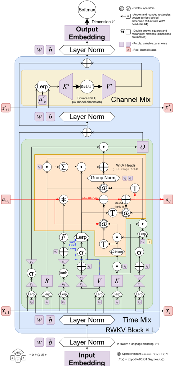<details> <summary>Image 12 Details</summary>  ### Visual Description ## Diagram: Transformer-Based Neural Network Architecture ### Overview The diagram illustrates a multi-layered neural network architecture with distinct sections for input/output embedding and intermediate processing. It features color-coded components (purple, yellow, green, orange, red, blue) representing different operations and parameters. The flow progresses vertically from bottom (Input Embedding) to top (Output Embedding), with horizontal connections indicating data flow between layers. ### Components/Axes **Legend** (top-right corner): - **Circles**: Operators (e.g., ReLU, LERP) - **Arrows/Rounded Rectangles**: Vectors/parameters (e.g., weights, biases) - **Double Arrows**: Double arrows, squares, and vectors (not specified) - **Purple Squares**: Trainable parameters - **Red Squares**: Red internal states **Key Sections**: 1. **Input Embedding** (bottom): - Layer Norm (purple) with parameters `w` (weight) and `b` (bias) - LERP operation (orange) with parameters `μ` and `k` - ReLU activation (yellow) with squared output (4x model dimension) 2. **Channel Mix** (middle-left): - `K'` and `V'` operations (orange) with ReLU activation - Layer Norm (purple) with `w` and `b` 3. **WKV Heads** (middle-center): - Multiple attention heads (orange circles) with group normalization - Operations: `F`, `T`, `R`, `V`, `K` (orange) - Group Norm (orange) and LERP (orange) blocks 4. **Time Mix** (middle-right): - `RWKV Block × L` (orange) with time-mixing operations - Layer Norm (purple) with `w` and `b` 5. **Output Embedding** (top): - Softmax function (purple) for dimensionality reduction - Layer Norm (purple) with `w` and `b` ### Detailed Analysis - **Input Embedding**: - Initial layer normalization (`w`, `b`) followed by LERP (linear interpolation) and ReLU activation. - ReLU output is squared (4x model dimension), suggesting dimensionality expansion. - **Channel Mix**: - `K'` and `V'` operations (likely key/value projections) with ReLU activation. - Layer normalization applied post-processing. - **WKV Heads**: - Multiple attention heads (`F`, `T`, `R`, `V`, `K`) with group normalization. - Complex interactions between parameters (e.g., `a_{i,j}` with red arrows) suggest cross-head dependencies. - **Time Mix**: - `RWKV Block × L` indicates recurrent or time-aware processing (e.g., for sequential data). - Layer normalization applied after time-mixing operations. - **Output Embedding**: - Final softmax layer for probability distribution over classes. - Layer normalization ensures stable gradients. ### Key Observations 1. **Color Coding**: - Purple dominates Layer Norm blocks, emphasizing their role in stabilizing training. - Orange highlights attention/head operations, critical for sequence modeling. 2. **Flow Direction**: - Vertical progression from input to output, with horizontal connections enabling cross-layer interactions (e.g., `a_{i,j}`). 3. **Complexity**: - Multiple LERP and ReLU operations suggest non-linear transformations and parameter interpolation. - Red internal states (squares) may represent intermediate activations or memory. ### Interpretation This architecture resembles a transformer variant optimized for efficiency (e.g., RWKV's recurrent design). The combination of attention heads (`WKV Heads`) and time-mixing (`Time Mix`) implies it handles sequential data (e.g., text, time series) with both local and global context awareness. The use of Layer Norm and ReLU aligns with standard practices for stable training, while the squared ReLU output in the input layer suggests dimensionality expansion for richer feature representation. The red internal states (`a_{i,j}`) likely capture cross-head interactions, critical for multi-head attention mechanisms. The diagram’s modular design (e.g., `RWKV Block × L`) indicates scalability for varying sequence lengths (`L`). </details> Table 15: Suggested Intermediate Dimensions for the low-rank MLPs for RWKV-7 models | Dimension ( D ) | d w | d a | d v | d g | |-------------------|-------|-------|-------|-------| | 768 | 64 | 64 | 32 | 128 | | 1024 | 64 | 64 | 32 | 128 | | 2048 | 96 | 96 | 64 | 256 | | 2560 | 96 | 96 | 64 | 320 | | 4096 | 128 | 128 | 96 | 480 | | 6144 | 128 | 128 | 96 | 640 | - The weights of each layer yield D ¡ 12 D + 2 ¡ dw + da + dv + dg ¢ + 19 ¢ parameters, except for the first layer; - The low-rank MLP for the value residual is not present in the first layer, subtracting (2 Ddv + D ) parameters. Parameter Initializations Proper parameter initialization is crucial for ensuring training stability and achieving optimal performance for language models. RWKV-7 employs a carefully designed initialization strategy tailored to its architecture. The detailed initialization scheme is beyond the scope here but can be found in the official code repository. We emphasize that using the recommended initialization is essential for replicating the results in this paper. Deviations from the prescribed initialization may lead to performance degradation. Dataset Loading The dataset used for pretraining consists of 3119194079123 tokens stored on disk, which are memory-mapped using the mmap mechanism. To ensure a diverse and pseudorandom sampling of training sequences, we employ a custom data loading strategy based on a mathematical function with desirable properties. Specifically, we utilize a pseudo-random number generator defined by the function f ( x ) = ax 3 over the finite field Z / p Z , where p is a prime number of the form 3 n + 2. This function is chosen because it is a bijection (full map) in Z / p Z , ensuring that all possible indices are eventually accessed exactly once within one epoch. For pretraining with a sequence length of 4096, the relative address of the k -th sample is determined as: start\_address = 4096 · ( ak 3 mod p ), end\_address = start\_address + 4097. Here, p is chosen as the largest prime of the form 3 n + 2 smaller than ⌊ dataset\_size/4096 ⌋ , yielding p = 761521949. The parameter a is set to an integer close to 0.618 p that ensures good mixing properties of the generated addresses. This approach guarantees both simple calculation and uniform access to the dataset while maintaining pseudo-randomness. By leveraging the properties of modular arithmetic and cubic mappings, we achieve a balance between computational efficiency and data diversity during pretraining. Training Details All RWKV-7 models were trained under bfloat16 format on nodes of 8 × Nvidia H800. The AdamW optimizer was configured with β 1 = 0.9, β 2 = 0.99, ϵ = 1 × 10 -18 , and a weight decay of 0.1 applied exclusively to linear layers and embedding weights. The choice of such a small ϵ value is motivated by the theory proposed by Molybog et al. (2023), which suggests that reducing ϵ can help stabilize training in large-scale models by ensuring that intermediate layers remain in a regime of active updates, thus mitigating sudden loss spikes and promoting smoother convergence. The context length for pretraining was 4096 tokens. The base decay rate w 0 parameters are placed into a special 2x learning rate multiplier grouping. Besides the traditional cosine learning rate decay schedule, we used a phased dynamic batch size scaling strategy inspired by the concept of critical batch size proposed by McCandlish et al. (2018) and similar to the approaches in Smith et al. (2018). Our strategy involves progressively increasing the batch size during training, accompanied by corresponding adjustments to the learning rate. Table 16: Training Schedules and Batch Sizes | Model | Phase | Nodes | Batch size | Proposed InitialLR | Final Loss | |-------------------|---------|---------|--------------|-----------------------|--------------| | RWKV7-World3-0.1B | 1 | 1 | 240 × 4096 | 6 × 10 - 4 | 2.5290 | | RWKV7-World3-0.4B | 1 | 1 | 240 × 4096 | 5 × 10 - 4 6 × 10 - 4 | | | | 2 | 2 | 480 × 4096 | | 2.2580 | | RWKV7-World3-1.5B | 1 | 3 | 480 × 4096 | 4 × 10 - 4 | | | | 2 | 4 | 672 × 4096 | 4.5 × 10 - 4 | | | | 3 | 6 | 1152 × 4096 | 6.1 × 10 - 4 | 1.9970 | | RWKV7-World3-2.9B | 1 | 4 | 640 × 4096 | 4 × 10 - 4 | | | | 2 | 6 | 1008 × 4096 | 5 × 10 - 4 | | | | 3 | 7 | 1120 × 4096 | 5.4 × 10 - 4 | | | | 4 | 12 | 2016 × 4096 | 8 × 10 - 4 | 1.8745 | The detailed training schedules for different model sizes are listed in Table 16. The learning rate undergoes a cosine decay schedule from the proposed initial learning rate at the beginning of the entire training run to the expected final learning rate of 1 × 10 -5 at the end of the entire run, but the implied initial rate varies across phases. This approach not only enhances training efficiency but also utilizes GPU resources economically. After smaller models complete their training, additional GPU resources become available for the later stages of training larger models. This cascading resource allocation ensures that computational power is dynamically reallocated, maximizing hardware utilization and reducing idle time. We observe extremely stable training without any loss spikes in all four runs, indicating that the likelihood of encountering such spikes during the training of a very large RWKV-7 model is minimal. See Figure 12 for the resulting learning rates and observed loss curves. Despite the general stability of our loss curves, we did sometimes observe NaN loss across a single training step, which we theorize may be due to our use of such an extremely low AdamW ϵ . When this occurs, we rewind the training to the prior checkpoint, clear optimizer states, and continue from that point. ## F Additional Architecture Discussion The following is a general overview of the RWKV-7 architecture and selected rationale for its design choices: The RWKV-7 Time Mixer begins with a feature that has been in RWKV since its inception: token shift. Token shift is a variety of 1D short convolution that is intended to allow the model to create induction heads within a single layer. At its core, token shift is just a linear interpolation between the current and prior tokens on a per channel basis, where the amount per channel is a learned parameter. Many other modern models (e.g. Mamba) have begun including short convolutions before attention replacements (See also Dao AI Lab (2023)). RWKV-6 introduced an advanced new form of token shift that was data dependent. While we found that this was beneficial in terms of loss decrease per step, we made the judgement call that the improvement in training and inference efficiency was not worthwhile. Therefore, RWKV-7 includes only the simple token shift found in RWKV-4 and RWKV-5. RWKV-7 time mixing follows the overall form of delta rule, applying an SGD-like mechanism to train the state at test time, such that when presented with a key it will respond with an appropriately matching value, like those it has been shown previously. This can be conceptualized as a simple order of operations: 1) decay the state 2) remove part of the old value located at the current key 3) add part of the new value into the current key. Then, a query (we call it receptance) is applied to Figure 12: Training loss curve for RWKV-7 World models. Blue line: loss; Red line: smoothed loss; Green line: actual learning rate; Dotted red line: learning rate schedule. 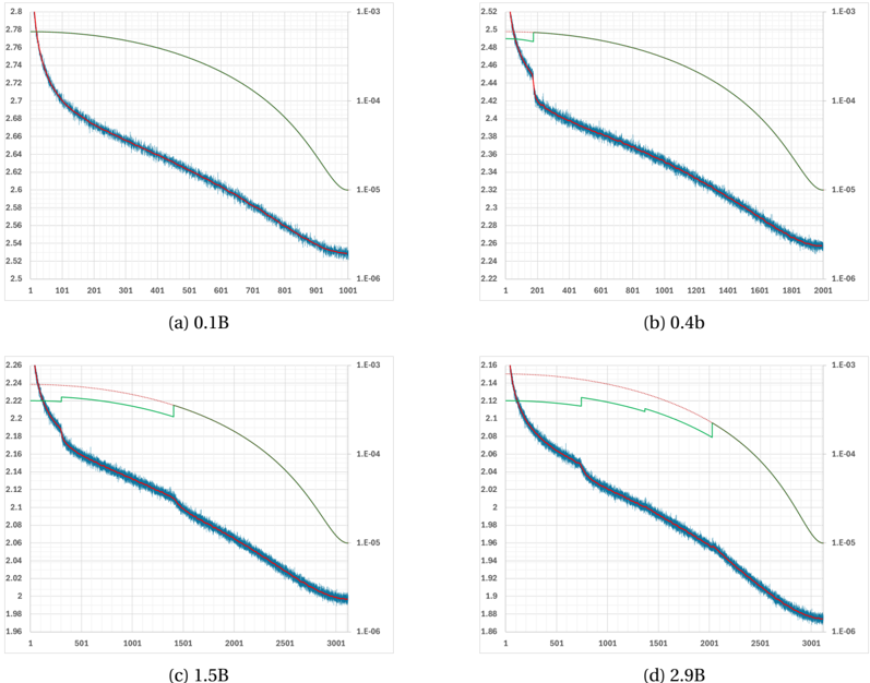<details> <summary>Image 13 Details</summary>  ### Visual Description ## Line Graphs: Model Performance Across Parameter Values ### Overview The image contains four line graphs labeled (a) 0.1B, (b) 0.4B, (c) 1.5B, and (d) 2.9B. Each graph plots "Value" (logarithmic scale: 1e-6 to 2.8) against "Time" (linear scale: 1 to 3001). Three data series are represented: Model A (blue), Model B (green), and Model C (red). All graphs share identical axis labels and legend placement (top-right), but vary in time range and value trends. --- ### Components/Axes - **Y-Axis**: "Value" (logarithmic scale: 1e-6, 1e-5, 1e-4, ..., 2.8) - **X-Axis**: "Time" (linear scale: 1, 101, 201, ..., 3001) - **Legend**: Top-right corner, labels: - Model A: Blue line - Model B: Green line - Model C: Red line --- ### Detailed Analysis #### Graph (a) 0.1B - **Model A (Blue)**: Starts at ~2.8, decreases linearly to ~2.5 over 1001 time units. - **Model B (Green)**: Sharp drop from ~2.8 to ~2.5 by time 101, then plateaus. - **Model C (Red)**: Gradual decline from ~2.8 to ~2.5 over 1001 time units. #### Graph (b) 0.4B - **Model A (Blue)**: Starts at ~2.5, decreases linearly to ~2.2 over 2001 time units. - **Model B (Green)**: Sharp drop from ~2.5 to ~2.2 by time 201, then plateaus. - **Model C (Red)**: Gradual decline from ~2.5 to ~2.2 over 2001 time units. #### Graph (c) 1.5B - **Model A (Blue)**: Starts at ~2.2, decreases linearly to ~1.9 over 3001 time units. - **Model B (Green)**: Sharp drop from ~2.2 to ~1.9 by time 301, then plateaus. - **Model C (Red)**: Gradual decline from ~2.2 to ~1.9 over 3001 time units. #### Graph (d) 2.9B - **Model A (Blue)**: Starts at ~1.9, decreases linearly to ~1.6 over 3001 time units. - **Model B (Green)**: Sharp drop from ~1.9 to ~1.6 by time 301, then plateaus. - **Model C (Red)**: Gradual decline from ~1.9 to ~1.6 over 3001 time units. --- ### Key Observations 1. **Model B (Green)** exhibits a consistent pattern: rapid initial decline followed by stabilization, regardless of parameter value. 2. **Model A (Blue)** and **Model C (Red)** show linear decay, with slower rates as parameter values increase. 3. **Parameter Correlation**: Higher parameter values (e.g., 2.9B) correlate with longer timeframes to reach plateau/stable values. 4. **Logarithmic Scale**: Y-axis compression emphasizes early-time dynamics, making late-time changes appear less pronounced. --- ### Interpretation - **Model Behavior**: Model B’s sharp drop suggests a threshold effect or rapid adaptation, while Models A and C reflect steady-state decay. - **Parameter Impact**: Larger parameters (e.g., 2.9B) delay stabilization, implying slower system response or increased complexity. - **Anomalies**: No outliers detected; all models follow predictable trends. The green line’s plateau in all graphs indicates a potential equilibrium state. - **Practical Implications**: The parameter value likely governs system sensitivity or resource allocation, with Model B optimizing for rapid initial adjustment. </details> the state in order to request the value located at a specific key. After that, the remaining operations normalize the returned values to keep numerical sizing consistent, apply gating, and recombine the heads to obtain the output. In SGD terms, the decay found in models like RWKV-7 and Gated DeltaNet can be thought of as similar to weight decay. RWKV models since RWKV-4 have employed some form of vector-valued decay on the state in place of positional encoding. We continue this tradition with RWKV-7. While vector valued decay is harder to compute efficiently than its scalar valued equivalent, it brings a significant improvement in loss per step. Many other models, like Mamba-2, make the choice to maximize training efficiency and simplify their kernels by using scalar decay, purposely trading quality for speed. We are forced to limit the maximum decay that can occur in a given time-step both in order to maintain training stability and to assist the creation of fast but numerically stable kernel implementations. We have many varieties of kernel available today, and are still working on new designs with enhanced efficiency and accuracy. Please see Parallelizing Linear Transformers with the Delta Rule over Sequence Length (Yang et al., 2024c) and its accompanying blog post series for insightful details on many components of such algorithms. We hope to be able to reduce the decay limit further in future revisions. This lower bound on the decay multiplier is expressed by the exp( -e -0.5 σ ( dt )) formula for decay. It is a rearrangement of an original source formula exp( -exp( -0.5 -softplus( dt ))). The outer exp( -exp( x )) in the original is nearly a flipped version of sigmoid, but with a better gradient. The -0.5 -softplus( dt ) is a way of limiting the inputs to this sigmoid-like function to be less than -0.5, which results in the final decay being greater than 0.545. This means that decay can remove at most 45.5% of the pre-existing values in the wkv state from one timestep to the next. More can be then removed by the delta rule mechanism. The in-context learning rate is usually equivalent to the learning rate in SGD. Ours is a bit less restrictive than the traditional delta rule or SGD would allow. We also make this data dependent and extend it to be vector-valued instead of being merely a scalar. This is allows each key channel to have its own learning rate, dependent on the current token. Note that in TTT, Gated DeltaNet, and Titans although the in-context learning rates are data dependent, they are only scalar valued. Someof the design of RWKV-7 with regard to the in-context learning rate is theoretically motivated but may not be apparent from the equations. RWKV-6c, a later v6 sub-version with no trained models but which worked well experimentally, kept its state somewhat normalized using a new design. As mentioned early in this paper and consistent with the observations in Yang et al. (2024b); Chen et al. (2024a), there is a fundamental issue with linear attention numerically growing in an unbounded fashion, and the base RWKV-6 revision has this problem. RWKV-6c, however, defeats this issue by ensuring that the amount of key added to the state is never more than the amount removed by decay. It accomplishes this by pre-multiplying the key by one minus the decay before adding it into the wkv state. Early versions of RWKV-7 attempted to use similar mathematical formulations to keep everything normalized. But experimentally we found that the model both did best and was most efficient when we allowed it enough mathematical leeway to make these decisions on its own, rather than enforcing them. So instead of pre-multiplying the key, we give the replacement key latitude in its learning rate via the replacement rate booster. Similarly, the removal key is decoupled from the replacement key. Note that the removal key is normalized. This is important in delta rule variations, because otherwise the outer product of removal key with itself would cause unwanted changes in the amount removed due to the implicit squaring of its length during that process. Another point that may not be clear upon first examination is the importance of RWKV-7 being outside of the TC 0 complexity class in which transformers, linear attention, and many varieties of SSMs lie. Consider a single layer of the Key Value Cache of a transformer. It is appended to upon each new token processed, and can never be changed. RWKV-7, however, can and does edit its state at each subsequent token. This can include simple operations like replacement, which can be viewed as functioning similarly to a transformer losing a KV Cache entry via some sparsity mechanism e.g. a sliding window. But it can also include complex operations like swapping two entries in the state; operations a transformer cannot do within its immutable KV Cache. These kinds of operations can be used to enact computations on the state itself, which lends greater computational abilities to RWKV-7 when processing a fixed set of inputs. You might think of the RWKV-7 state as being like an internal scratchpad. There are easy problems that simply cannot be solved by transformers on fixed inputs because they lack this ability. One example is that if you give a transformer an ordered set of items and a list of which ones swap places, it will not be able to tell you which item ends up in which position at the end. Both architectures gain even more power when they are allowed extra outputs (e.g. chain of thought), becoming Turing complete. But this requires costly additional inference-time computation, whereas the RWKV-7 state does not. A possible way to interpret the designation of RWKV-7 is training a model to learn (how to train an internal model). A WKV head can be viewed as a linear transformation that takes the input (receptance) r and outputs o . Every WKV head can be regarded as a linear model that can update its weights as the context progresses. The entries of WKV states are exactly the parameters of these models. After receptance is applied to the WKV state, we normalize the result on a per head basis. This has become common across many linear attention and post-linear-attention architectures. It is a way of ensuring that change in the numerical size of the state over time does not impact the model's ability to use the state. The original formulations of RWKV-4 used a denominator in place of normalization to achieve a similar effect, but it is costly, harder to code, and uses more memory. The readout part of RWKV-7 differ from RWKV-6 by the addition of the per-head ¡ r t ( ρ ⊙ ˜ kt ) T ¢ scalar gating of vt . The trainable parameter ρ resembles the design of "time-first" u term existing from RWKV-4 to RWKV-6, under the belief that the information of the current token deserves special treatment. The "time-first" term was fused inside the WKV kernel in previous architectures of RWKV, but we decide to extract this term out of the kernel to simplify the implementation of RWKV-7. ## G Pseudocode For RWKV-7 ``` ``` ``` ``` ## H PyTorch code For Naive WKV7 Kernel (Forward and Backward) ``` class WKV_Kernel(nn.Module): def __init__(self): super().__init__() def forward(self, r, w, k = None, v = None, a = None, b = None, state=None): if state is not None: torch.zeros((B, T+1, H, N, N)) return state r = r.view(B, T, H) k = k.view(B, T, H) v = v.view(B, T, H) a = a.view(B, T, H) b = b.view(B, T, H) torch.zeros((B, T+1, H, N, N)) return torch.cat([r, k, v, a, b], dim=0) ``` ``` ``` ``` ## I Board Game Modeling Previous research (Schultz et al. (2024); Topsakal et al. (2024)) has shown that board games can serve as potentially effective tools for evaluating a model's capabilities. As an RNN with powerful state tracking abilities, RWKV-v7 is highly suitable for board game modeling and conducting extended searches directly within context to find better strategies. As an early exploration, we tested RWKV-v7's board game modeling capabilities and its ability to perform in-context search on the game of Othello (Reversi). Data We designed training data that guides the model to predict legal moves, evaluate these moves, and perform Alpha-Beta pruning. Each training sample consists of three components: - Input section : Captures the game state, including the current board position, active player, and search parameters (tree depth and width settings). - Reasoning section : Varies with search settings: - -Without search (depth or width = 1): Lists legal moves and their evaluations - -With search (depth and width > 1): Performs Alpha-Beta pruning to find optimal moves All move evaluations in the reasoning section were generated using the Egaroucid engine (Yamana, 2025). - Output section : This contains the final move decision and displays the resulting board position after implementing the move. An example of our training data is shown in sample 1. ``` <input> 2 . . . . . . . . . . . . . . . . . . . . . . . . . . . . . . . ``` ``` <doc> Code Listing 1: Training Data Example RWCF7 models with 9M and 26M parameters respectively on 6 million ing (figure 13), we noticed rd state tracking capability, </doc> ``` Code Listing 1: Training Data Example Training We trained RWKV-7 models with 9M and 26M parameters respectively on 6 million samples. By tracking the loss across different token types during training (figure 13), we noticed that the model first mastered output formatting, then developed board state tracking capability, and continuously improved its evaluation accuracy throughout training. Evaluation Wecontrol the model's thinking budget by setting the width and depth of Alpha-beta pruning, and test the win rate against baseline a model (depth=1, width=1) under different budgets. As shown in figure 14, by increasing the testing budget, RWKV-7 can effectively search for better strategies, demonstrating a positive test-time scaling law on this task. ## J State Inspections Weinspected the WKV matrix states of RWKV-7 and compared them with those of RWKV-5 and RWKV-6. We analyzed the following aspects: 1. Visualization example of WKV state matrices, to better understand the structure and behavior of the matrices. 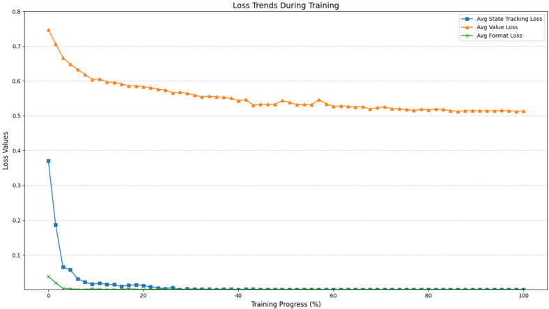Figure 13: Reversi Training loss for different token types <details> <summary>Image 14 Details</summary>  ### Visual Description ## Line Chart: Loss Trends During Training ### Overview The chart visualizes three loss metrics tracked during a training process, plotted against training progress percentage (0-100%). The y-axis represents loss values (0-0.8), while the x-axis shows training progress. Three distinct data series are represented by color-coded lines: blue (Avg State Tracking Loss), orange (Avg Value Loss), and green (Avg Format Loss). ### Components/Axes - **Title**: "Loss Trends During Training" - **X-axis**: "Training Progress (%)" with markers at 0, 20, 40, 60, 80, 100. - **Y-axis**: "Loss Values" with increments of 0.1 (0.0 to 0.8). - **Legend**: Located in the top-right corner, mapping: - Blue: Avg State Tracking Loss - Orange: Avg Value Loss - Green: Avg Format Loss ### Detailed Analysis 1. **Avg State Tracking Loss (Blue Line)**: - Starts at **~0.37** at 0% training progress. - Drops sharply to **~0.01** by 10% training progress. - Remains near-zero for the remainder of the training (0.01-0.02 range). 2. **Avg Value Loss (Orange Line)**: - Begins at **~0.75** at 0% training progress. - Gradually declines to **~0.51** by 100% training progress. - Shows minor fluctuations (e.g., slight peaks at ~0.53 between 40-60% training). 3. **Avg Format Loss (Green Line)**: - Remains consistently near **~0.005** throughout training. - No significant variation observed. ### Key Observations - **Rapid Improvement in State Tracking**: The blue line’s steep decline indicates a quick reduction in state tracking errors early in training. - **Steady Value Loss Reduction**: The orange line’s gradual decline suggests slower but consistent improvement in value-related losses. - **Negligible Format Loss**: The green line’s near-zero value implies format loss was not a significant factor during training. ### Interpretation The data suggests the model prioritizes resolving state tracking errors early, achieving near-optimal performance in this metric by 10% training progress. Value loss, while decreasing steadily, remains the dominant loss component throughout training, indicating it may be a more complex or persistent challenge. The near-zero format loss implies the model’s formatting mechanisms were either inherently robust or not a focus of the training process. The divergence between the blue and orange lines highlights differing learning dynamics: state tracking improves rapidly, while value loss requires sustained effort. This could reflect architectural choices, data complexity, or optimization priorities in the training setup. 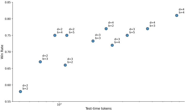</details> Figure 14: Reversi Token consumption and win rates under different search configurations <details> <summary>Image 15 Details</summary>  ### Visual Description ## ScatterPlot: Win Rate vs. Test-time Tokens ### Overview The image is a scatter plot visualizing the relationship between **Test-time tokens** (x-axis, logarithmic scale) and **Win Rate** (y-axis, linear scale). Data points are labeled with combinations of parameters `d` (depth) and `b` (breadth), with all points colored blue. The legend is positioned on the right side of the plot. --- ### Components/Axes - **X-axis (Test-time tokens)**: Logarithmic scale ranging from $10^3$ to $10^4$. Tick marks are labeled at $10^3$, $10^{3.5}$, and $10^4$. - **Y-axis (Win Rate)**: Linear scale from 0.55 to 0.85, with increments of 0.05. - **Legend**: Located on the right, associating blue color with all data points (no distinct subcategories). - **Data Points**: Labeled with `d` (depth) and `b` (breadth) values, e.g., `d=2, b=2`, `d=4, b=4`. --- ### Detailed Analysis - **Data Points**: - `d=2, b=2`: (10³, 0.58) - `d=2, b=3`: (10³.⁵, 0.67) - `d=2, b=4`: (10³.⁵, 0.75) - `d=2, b=5`: (10³.⁵, 0.75) - `d=3, b=2`: (10³.⁵, 0.66) - `d=3, b=3`: (10³.⁵, 0.73) - `d=3, b=4`: (10³.⁵, 0.72) - `d=3, b=5`: (10³.⁵, 0.75) - `d=4, b=2`: (10³.⁵, 0.77) - `d=4, b=3`: (10³.⁵, 0.76) - `d=4, b=4`: (10⁴, 0.81) - **Trends**: - **General Trend**: Win Rate increases with higher Test-time tokens (e.g., from 0.58 at $10^3$ to 0.81 at $10^4$). - **Parameter Effects**: - Higher `d` (depth) and `b` (breadth) values generally correlate with higher Win Rates (e.g., `d=4, b=4` at $10^4$ achieves 0.81). - At the same Test-time token value, combinations with higher `d` and `b` (e.g., `d=4, b=4`) outperform lower combinations (e.g., `d=2, b=3` at $10^{3.5}$ with 0.67). --- ### Key Observations 1. **Outliers**: - `d=2, b=3` at $10^{3.5}$ (0.67) and `d=3, b=2` at $10^{3.5}$ (0.66) show lower Win Rates compared to other combinations at the same token count. - `d=4, b=4` at $10^4$ (0.81) is the highest Win Rate observed. 2. **Parameter Interactions**: - Increasing `d` and `b` together improves performance, but the effect is non-linear. For example, `d=3, b=5` (0.75) at $10^{3.5}$ performs better than `d=2, b=5` (0.75) at the same token count. 3. **Logarithmic Scale**: - The x-axis’s logarithmic scale emphasizes performance differences at lower token ranges (e.g., $10^3$ vs. $10^{3.5}$). --- ### Interpretation The data suggests that **Test-time tokens** and the interplay between **depth (`d`)** and **breadth (`b`)** are critical factors in determining Win Rate. While higher token counts generally improve performance, the optimal combination of `d` and `b` depends on the scale of tokens. For instance: - At lower token ranges ($10^3$–$10^{3.5}$), smaller `d` and `b` values (e.g., `d=2, b=2`) underperform compared to larger ones. - At higher token ranges ($10^4$), larger `d` and `b` (e.g., `d=4, b=4`) achieve the highest Win Rates, indicating scalability benefits. The outliers highlight that **parameter tuning** is essential: even with more tokens, suboptimal `d` and `b` combinations can limit performance. This underscores the need for adaptive strategies that balance token count with parameter selection. </details> 2. Root Mean Square (RMS) of matrix elements, to assess the numerical stability of those WKVmatrices. 3. Stable Rank (SR) of the matrices (Rudelson & Vershynin, 2007), defined as the square of (the Frobenius norm divided by the spectral norm): $$S R ( A ) = ( \frac { 1 1 A l _ { F } ^ { 2 } } { 1 1 A l _ { 2 } ^ { 2 } } ) ^ { 2 }$$ This serves as a rough measure to the effective amount of information of the states. For this analysis, we selected 10 samples from the validation set of the PG19 dataset (Rae et al., 2019), ensuring that each sample had a sequence length of at least 8192 tokens. We tested the 1.5B parameter versions of RWKV-5, RWKV-6, and RWKV-7, plotting on the appearance, stable rank and RMS values of their WKV matrices. Figure 15: Visualization example of RWKV's WKV matrices. 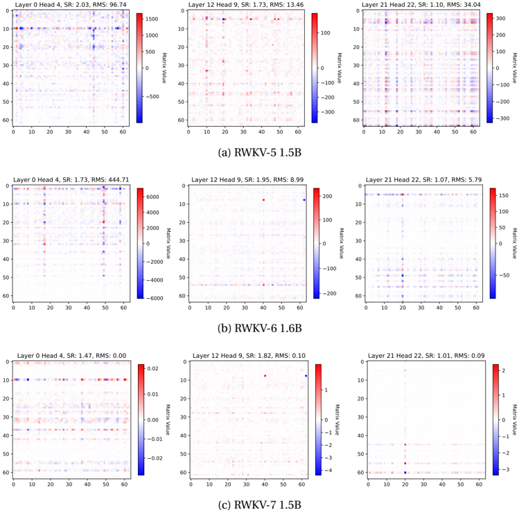<details> <summary>Image 16 Details</summary>  ### Visual Description ## Heatmap Visualization: RWKV Model Matrix Analysis ### Overview The image presents three comparative heatmap visualizations of matrix values across different RWKV model architectures (5B, 6B, 7B). Each section contains three heatmaps showing matrix values for specific layer-head combinations, with color intensity representing value magnitude and RMS (Root Mean Square) metrics indicating value distribution characteristics. ### Components/Axes **Common Elements Across All Heatmaps:** - **X-axis**: Layer indices (0, 12, 21) - **Y-axis**: Head indices (4, 9, 22) - **Color Scale**: Matrix value magnitude (blue = negative, red = positive) - **Legend**: Positioned right-aligned with color gradient from blue (-) to red (+) - **Title Format**: "Layer [X] Head [Y], SR: [Z], RMS: [W]" **Section-Specific Details:** 1. **(a) RWKV-5 1.5B** - Color Scale: -1500 to +1500 - RMS Values: 96.74 (Layer 0), 13.46 (Layer 12), 34.04 (Layer 21) - SR Values: 2.03 (Layer 0), 1.73 (Layer 12), 1.10 (Layer 21) 2. **(b) RWKV-6 1.6B** - Color Scale: -6000 to +6000 - RMS Values: 444.71 (Layer 0), 1.95 (Layer 12), 5.79 (Layer 21) - SR Values: 1.73 (Layer 0), 1.95 (Layer 12), 1.07 (Layer 21) 3. **(c) RWKV-7 1.5B** - Color Scale: -0.02 to +0.02 - RMS Values: 0.00 (Layer 0), 0.10 (Layer 12), 0.09 (Layer 21) - SR Values: 1.47 (Layer 0), 1.82 (Layer 12), 1.01 (Layer 21) ### Detailed Analysis **Section (a) RWKV-5 1.5B:** - Layer 0 shows extreme value distribution with large positive/negative spikes (e.g., Head 4: SR=2.03, RMS=96.74) - Layer 12 exhibits moderate variation (SR=1.73, RMS=13.46) - Layer 21 demonstrates reduced variability (SR=1.10, RMS=34.04) **Section (b) RWKV-6 1.6B:** - Layer 0 maintains high variability (SR=1.73, RMS=444.71) - Layer 12 shows significant improvement (SR=1.95, RMS=1.95) - Layer 21 exhibits moderate stability (SR=1.07, RMS=5.79) **Section (c) RWKV-7 1.5B:** - All layers show near-zero RMS values (<0.10) - Matrix values cluster tightly around zero (color scale compressed to ±0.02) - SR values indicate consistent scaling across layers (1.47-1.82) ### Key Observations 1. **Model Evolution Trends:** - RMS values decrease significantly from RWKV-5 to RWKV-7 (96.74 → 0.00) - SR values show inverse correlation with RMS (higher SR = lower RMS) - Layer 0 consistently shows highest variability across all models 2. **Color Pattern Analysis:** - RWKV-5 heatmaps display dominant red/blue regions indicating strong positive/negative values - RWKV-6 shows reduced color intensity compared to RWKV-5 - RWKV-7 heatmaps appear nearly uniform (minimal color variation) 3. **Layer-Specific Behavior:** - Layer 0 (input processing) maintains highest variability across all models - Layer 12 (mid-depth) shows progressive stabilization - Layer 21 (output processing) demonstrates most consistent behavior ### Interpretation The visual progression from RWKV-5 to RWKV-7 reveals significant architectural improvements in matrix stability: - **RMS Reduction**: The near-zero RMS in RWKV-7 suggests near-perfect value distribution, indicating optimized weight initialization or training - **SR Correlation**: The inverse relationship between SR and RMS implies that better scaling (lower SR) leads to more stable value distributions - **Layer Specialization**: The consistent high variability in Layer 0 across all models suggests this layer retains critical input processing characteristics that resist optimization - **Color Intensity**: The dramatic reduction in color variation from RWKV-5 to RWKV-7 visually confirms the quantitative RMS improvements These patterns suggest that later RWKV versions achieve better weight initialization or training stability, resulting in more consistent matrix value distributions while maintaining effective scaling properties. </details> Weobserved that the WKV states of RWKV-7 had significantly smaller RMS values compared to RWKV-5 and RWKV-6. The entries of the WKV matrix in RWKV-7 were consistently of order O (1) (i.e., no outliers, and does not grow over context length), whereas RWKV-5 and RWKV-6 constantly produced outliers on the order of thousands (see Figures 15 and 16). This indicates that RWKV-7 has better numerical stability during training and inference. Interestingly, the stable rank of the WKV matrix in RWKV-7 has shown to be lower than that of RWKV-5 and RWKV-6 for context longer than 32. A lower stable rank typically suggests that the matrix contains less information or has a more compressed representation. However, this observation appears to contradict the experimental results showing that RWKV-7 performs better on tasks requiring long-term memory. We hypothesize that this contradiction can be explained by RWKV7's enhanced state evolution mechanism, which enables RWKV-7 to achieve stronger information compression and utilization capabilities and allowing it to maintain important information in a more compact form. This dual capability likely contributes to both the reduced stable rank and the improved performance on memory-intensive tasks. Figure 16: The global RMS and average stable rank of WKV matrices, plotted over sequence length. 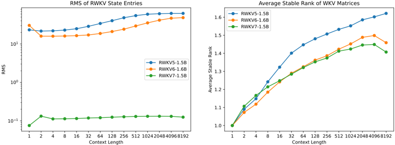<details> <summary>Image 17 Details</summary>  ### Visual Description ## Line Graphs: RMS of RWKV State Entries and Average Stable Rank of WKV Matrices ### Overview The image contains two line graphs comparing performance metrics of RWKV models (RWKV5-1.5B, RWKV6-1.6B, RWKV7-1.5B) across varying context lengths (1 to 8192 tokens). The left graph measures RMS of state entries, while the right graph tracks average stable rank of WKV matrices. Both graphs use logarithmic scales for context length and linear scales for their respective y-axes. --- ### Components/Axes #### Left Graph: RMS of RWKV State Entries - **X-axis**: Context Length (logarithmic scale: 1, 2, 4, 8, 16, 32, 64, 128, 256, 512, 1024, 2048, 4096, 8192) - **Y-axis**: RMS (logarithmic scale: 10⁻¹ to 10¹) - **Legend**: - Blue: RWKV5-1.5B - Orange: RWKV6-1.6B - Green: RWKV7-1.5B - **Positioning**: Legend in top-right corner; lines anchored to legend labels. #### Right Graph: Average Stable Rank of WKV Matrices - **X-axis**: Context Length (same logarithmic scale as left graph) - **Y-axis**: Average Stable Rank (linear scale: 1.0 to 1.6) - **Legend**: Same color coding as left graph (blue, orange, green). - **Positioning**: Legend in top-right corner; lines anchored to legend labels. --- ### Detailed Analysis #### Left Graph: RMS of RWKV State Entries - **RWKV5-1.5B (Blue)**: - Starts at ~10¹.² (≈15.85) at context length 1. - Dips slightly at context length 2 (~10¹.1, ≈12.6). - Rises steadily to ~10¹.5 (≈31.6) at 8192 tokens. - **RWKV6-1.6B (Orange)**: - Starts at ~10¹.1 (≈12.6) at context length 1. - Increases gradually to ~10¹.4 (≈25.1) at 8192 tokens. - **RWKV7-1.5B (Green)**: - Remains flat at ~10⁻¹ (≈0.1) across all context lengths. #### Right Graph: Average Stable Rank of WKV Matrices - **RWKV5-1.5B (Blue)**: - Starts at 1.0 at context length 1. - Rises sharply to 1.6 at 8192 tokens. - **RWKV6-1.6B (Orange)**: - Starts at 1.0 at context length 1. - Increases gradually to 1.5 at 8192 tokens. - **RWKV7-1.5B (Green)**: - Starts at 1.0 at context length 1. - Rises steadily to 1.4 at 8192 tokens, with a minor dip at 4096 tokens (~1.35). --- ### Key Observations 1. **RMS Trends**: - RWKV5-1.5B exhibits the highest RMS values, increasing exponentially with context length. - RWKV7-1.5B maintains near-zero RMS, suggesting stable state management. - RWKV6-1.6B shows intermediate RMS growth, slower than RWKV5-1.5B. 2. **Stable Rank Trends**: - RWKV5-1.5B has the steepest increase in stable rank, indicating reduced stability at longer contexts. - RWKV7-1.5B demonstrates the most stable behavior, with the lowest final stable rank (1.4 vs. 1.6 for RWKV5-1.5B). - RWKV6-1.6B balances growth and stability, with a moderate increase to 1.5. --- ### Interpretation 1. **Model Efficiency**: - RWKV7-1.5B’s near-zero RMS and low stable rank suggest superior state management efficiency, critical for long-context tasks. - RWKV5-1.5B’s high RMS and stable rank imply higher computational variability, potentially limiting scalability. 2. **Context Length Impact**: - All models show increased RMS and stable rank with longer contexts, but RWKV7-1.5B mitigates this effect most effectively. - The divergence in trends highlights architectural differences: RWKV7’s design likely prioritizes stability over raw capacity. 3. **Anomalies**: - RWKV7-1.5B’s slight dip in stable rank at 4096 tokens may indicate transient optimization or noise in the dataset. - RWKV5-1.5B’s sharp rise in stable rank suggests sensitivity to context length, possibly due to memory constraints. --- ### Conclusion The data underscores trade-offs between model size, stability, and context handling. RWKV7-1.5B’s performance aligns with use cases requiring long-context stability, while RWKV5-1.5B may suit scenarios prioritizing raw capacity despite higher variability. Further investigation into RWKV7’s architectural innovations (e.g., attention mechanisms, state initialization) could clarify its efficiency advantages. </details> ## K Ablation Experiments The Pile To demonstrate the architectural advantages of RWKV-7, we conducted ablation experiments by training models of three different sizes-168M, 421M, and 1.47B parameters-on the full Pile dataset (Gao et al., 2020). Table 17: English Focused Benchmarks, including LAMBADA ( lmb.o ) (Paperno et al., 2016), Hellaswag ( hella ) (Zellers et al., 2019), PIQA (Bisk et al., 2020), AI2 ARC ( arcE , arcC ) (Bhakthavatsalam et al., 2021), GLUE (Wang et al., 2018), Winogrande ( WG ) (Sakaguchi et al., 2021), SciQ (Welbl et al., 2017). | Model | Tokens (B) | lmb.o ppl ↓ | lmb.o acc ↑ | hella acc_n ↑ | piqa acc ↑ | arcE acc ↑ | arcC acc ↑ | glue acc ↑ | WG acc ↑ | sciq acc ↑ | avg acc ↑ | |------------------|--------------|---------------|---------------|-----------------|--------------|--------------|--------------|--------------|------------|--------------|-------------| | RWKV4-169M-Pile | 332 | 29.2 | 33.2 | 32.2 | 64.8 | 47.1 | 19.9 | 47.6 | 51.2 | 77.6 | 46.7 | | Pythia-160M | 300 | 37.3 | 35.4 | 30.3 | 62.3 | 43.6 | 19.5 | 46.5 | 51.3 | 75.4 | 45.5 | | Mamba-130M | 300 | 16 | 44.3 | 35.3 | 64.5 | 48 | 19.7 | 48.5 | 52.1 | 78.2 | 48.8 | | Mamba2-130M | 300 | 16.8 | 43.9 | 35.3 | 64.9 | 47.4 | 20.9 | 45.8 | 52.6 | 81 | 49 | | RWKV6-173M-Pile | 332 | 16 | 44.5 | 34.9 | 64.4 | 48.3 | 19.7 | 48.9 | 51.9 | 80.6 | 49.2 | | RWKV7-168M-Pile | 332 | 14.2 | 45.7 | 36.9 | 65.5 | 47.9 | 19.7 | 49.1 | 52.4 | 81.6 | 49.8 | | RWKV4-430M-Pile | 332 | 13.1 | 45.1 | 40.8 | 67.7 | 52.8 | 24.1 | 49.4 | 52 | 80.7 | 51.6 | | Pythia-410M | 300 | 10.8 | 51.6 | 40.6 | 66.7 | 51.9 | 21.4 | 44.1 | 53.3 | 81.5 | 51.4 | | Mamba-370M | 300 | 8.1 | 55.6 | 46.5 | 69.5 | 55 | 25 | 46.8 | 55.5 | 84.5 | 54.8 | | Mamba2-370M | 300 | 8 | 55.9 | 46.9 | 70.5 | 54.8 | 25.1 | 48.1 | 55.4 | 85.3 | 55.2 | | RWKV7-421M-Pile | 332 | 7.2 | 57.9 | 48 | 69.3 | 56.3 | 23.5 | 50.3 | 56.4 | 85.9 | 56 | | RWKV4-1.5B-Pile | 332 | 7.1 | 56.4 | 52.8 | 72.2 | 60.7 | 24.9 | 50.5 | 54.3 | 85.8 | 57.2 | | Pythia-1.4B | 300 | 6.1 | 61.7 | 52 | 70.8 | 60.5 | 26.1 | 47.7 | 57.5 | 86.6 | 57.9 | | Mamba-1.4B | 300 | 5 | 65 | 59.1 | 74.2 | 65.5 | 29.8 | 46.2 | 61.4 | 87.3 | 61.1 | | Mamba2-1.3B | 300 | 5 | 65.6 | 59.9 | 73.2 | 64.2 | 29.9 | 46.1 | 61 | 89.8 | 61.2 | | RWKV7-1.47B-Pile | 332 | 4.8 | 67 | 61.8 | 73.6 | 64.9 | 30.2 | 48 | 64.4 | 91.1 | 62.6 | These results highlight the consistent improvements brought by the RWKV-7 architecture over earlier RWKV models, even when trained on the same dataset. As all RWKV models shown were trained under identical configurations and dataset, this underscores the inherent architectural advantages of RWKV-7 over its predecessors. Notably, the performance gap sustains as the model size increases, suggesting that RWKV-7 may scale more effectively than its predecessors. Architecture Choice Ablations Weran a series of ablation experiments to validate the various improvements made in RWKV-7 versus some of the more restrictive choices seen in other DeltaNet and post-DeltaNet related work. These improvements were: - using a vector-valued decay w instead of a scalar-valued decay; - using a vector-valued in-context learning rate a instead of a scalar-valued rate; - using different removal κ and replacement ˜ k keys, instead of the same for both; and - adding the bonus term ut , j vt , j to the output step (Equation bonus). Wetrained a small 6-layer, dmodel = 768 Goose model on the 1.6B token minipile (Kaddour, 2023) dataset at context length 512 and obtained the loss results shown in Table 18. Table 18: Ablation Results for 6 layer 768 dimension Goose model | Model | Training Loss | Validation Loss | |----------------------------------------|-----------------|-------------------| | Goose | 2.834 | 2.541 | | Goose, scalar decay | 2.873 | 2.609 | | Goose, scalar in-context learning rate | 2.843 | 2.591 | | Goose, same removal/replacement keys | 2.84 | 2.56 | | Goose, no bonus term | 2.841 | 2.588 | ## L Parameters Statistics In Section 4, the actual ranges and statistical metrics of the parameters within the trained model are not specified. To facilitate a better understanding of the role of these parameters in the practical models, this appendix provides empirical statistical metrics of selected parameters from the released RWKV-7 model. 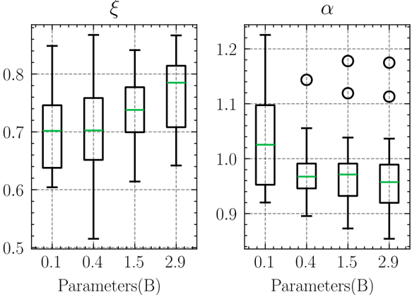Figure 17: Box Plots of ξ and α Across Models <details> <summary>Image 18 Details</summary>  ### Visual Description ## Box Plots: Comparison of ξ and α Parameters ### Overview The image contains two side-by-side box plots comparing the distributions of two parameters, ξ (left) and α (right), across four parameter categories (B = 0.1, 0.4, 1.5, 2.9). Each plot includes medians (green lines), interquartile ranges (boxes), whiskers, and outliers (open circles). The y-axes represent normalized values, with ξ ranging from 0.5–0.8 and α from 0.9–1.2. --- ### Components/Axes - **X-Axis (Parameters(B))**: - Categories: 0.1, 0.4, 1.5, 2.9 (labeled as "Parameters(B)"). - **Y-Axis (ξ)**: - Range: 0.5–0.8 (left plot). - Median (green line) and quartiles (box edges) marked. - **Y-Axis (α)**: - Range: 0.9–1.2 (right plot). - Median (green line) and quartiles (box edges) marked. - **Outliers**: - Open circles outside whiskers (1.5×IQR threshold). - **Legend**: - No explicit legend, but green lines represent medians. --- ### Detailed Analysis #### ξ (Left Plot) - **Median Trends**: - Median increases from ~0.7 (B=0.1) to ~0.75 (B=2.9). - **Spread**: - IQR widens from B=0.1 to B=2.9. - **Outliers**: - B=0.1: Outlier at ~0.85 (above upper whisker). - B=2.9: Outlier at ~0.9 (above upper whisker). #### α (Right Plot) - **Median Trends**: - Median decreases from ~1.05 (B=0.1) to ~0.95 (B=2.9). - **Spread**: - IQR narrows from B=0.1 to B=2.9. - **Outliers**: - B=0.1: Outlier at ~1.15 (above upper whisker). - B=0.4: Outlier at ~1.1 (above upper whisker). - B=1.5 and B=2.9: Outliers at ~1.15 (above upper whisker). --- ### Key Observations 1. **ξ**: - Central tendency increases with parameter B, but variability (IQR) also grows. - Outliers at extremes (B=0.1 and B=2.9) suggest rare high-value deviations. 2. **α**: - Central tendency decreases with parameter B, with tighter distributions at higher B. - Multiple outliers across all B categories, indicating persistent anomalies. --- ### Interpretation - **ξ vs. α Behavior**: - ξ exhibits a positive correlation between parameter B and central tendency, while α shows a negative correlation. This suggests opposing relationships between the parameters and their distributions. - **Outlier Patterns**: - Outliers in ξ are limited to the smallest and largest B values, whereas α outliers are widespread, hinting at systemic instability in α across all B categories. - **Practical Implications**: - For ξ, increasing B may improve typical outcomes but introduces greater variability. For α, higher B stabilizes results but does not eliminate outliers, requiring further investigation into anomalous cases. - **Data Limitations**: - Small sample sizes (implied by box plot compactness) may affect reliability of trends. </details> ## M Initial Token Sensitivity In our evaluation of LAMBADA (Paperno et al., 2016), we found that RWKV-7's performance varies significantly under different settings. After ruling out precision issues, we investigated the consistency of the input and discovered that omitting the special token <|endoftext|> at the beginning of the input caused substantial and statistically significant differences in perplexity (PPL) and accuracy (ACC) for some RWKV-7 models. Previous research highlights that Transformer models are sensitive to special tokens, and finetuning these tokens can yield notable improvements (Yang et al., 2023b). However, to our knowledge, no quantitative study has examined this effect systematically. 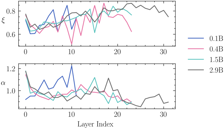Weanalyzed the cases with the largest performance discrepancies, and identified a key pattern: Figure 18: Mean ξ and α Across Layers for Different Models <details> <summary>Image 19 Details</summary>  ### Visual Description ## Line Chart: ξ and α Values Across Layer Indices ### Overview The image contains two line graphs stacked vertically, each plotting a metric (ξ and α) against a "Layer Index" (0–30). Four data series are represented by distinct colored lines, each corresponding to a specific "B" value (0.1B, 0.4B, 1.5B, 2.9B). The graphs show fluctuating trends with notable variability across layers. ### Components/Axes - **X-axis**: "Layer Index" (0–30), incrementing by 10. - **Y-axes**: - Top graph: ξ (range: 0.6–0.8). - Bottom graph: α (range: 1.0–1.2). - **Legend**: Located on the right, with four entries: - Blue: 0.1B - Pink: 0.4B - Cyan: 1.5B - Black: 2.9B ### Detailed Analysis #### Top Graph (ξ): - **Black line (2.9B)**: Most stable, with minor fluctuations. Starts near 0.75, dips to ~0.65 at layer 10, and ends ~0.7. - **Blue line (0.1B)**: Highly volatile, with sharp peaks (e.g., ~0.8 at layer 5) and troughs (e.g., ~0.6 at layer 15). - **Pink line (0.4B)**: Moderate fluctuations, peaking at ~0.75 (layer 10) and dipping to ~0.6 (layer 20). - **Cyan line (1.5B)**: Smoothest trend, starting ~0.7, peaking ~0.75 (layer 15), and ending ~0.7. #### Bottom Graph (α): - **Black line (2.9B)**: Stable, starting ~1.0, dipping to ~0.95 (layer 10), and ending ~0.9. - **Blue line (0.1B)**: Extreme volatility, peaking at ~1.2 (layer 5) and dropping to ~0.9 (layer 25). - **Pink line (0.4B)**: Erratic, with peaks (~1.1 at layer 10) and troughs (~0.95 at layer 20). - **Cyan line (1.5B)**: Moderate fluctuations, starting ~1.0, peaking ~1.1 (layer 15), and ending ~1.0. ### Key Observations 1. **Stability vs. Volatility**: The 2.9B (black) line is the most stable in both graphs, while 0.1B (blue) exhibits the highest variability. 2. **Layer-Specific Trends**: - ξ peaks for 0.1B occur at layer 5, while α peaks for 0.1B occur at layer 5. - 1.5B (cyan) shows gradual increases in ξ (layer 15) and α (layer 15). 3. **Convergence**: All lines converge near layer 30, with ξ and α values stabilizing. ### Interpretation The data suggests that higher "B" values (e.g., 2.9B) correlate with greater stability in both ξ and α metrics, while lower "B" values (e.g., 0.1B) result in pronounced fluctuations. This could indicate that "B" acts as a damping or stabilizing parameter in the system being modeled. The convergence at layer 30 implies a potential equilibrium or normalization effect at higher layer indices. The erratic behavior of 0.1B and 0.4B lines might reflect sensitivity to initial conditions or external perturbations in the system. 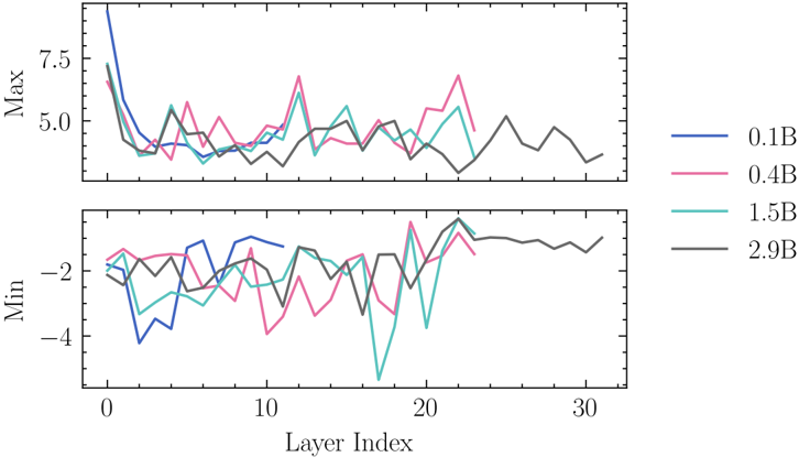</details> Figure 19: Maximum and Minimum of ξ Across Layers in Different Models <details> <summary>Image 20 Details</summary>  ### Visual Description ## Line Chart: Max and Min Values Across Layer Indices ### Overview The image contains two line charts stacked vertically, showing the maximum (top) and minimum (bottom) values of a metric across 31 layer indices (0–30). Four data series are represented by distinct colors, each corresponding to a specific "B" value (0.1B, 0.4B, 1.5B, 2.9B). The charts exhibit fluctuating trends with peaks and troughs at varying layer indices. ### Components/Axes - **X-axis (Layer Index)**: Ranges from 0 to 30 in increments of 10. - **Y-axes**: - Top plot: "Max" values (range: -4 to 7.5). - Bottom plot: "Min" values (range: -4 to 2). - **Legend**: Located on the right, mapping colors to "B" values: - Blue: 0.1B - Pink: 0.4B - Teal: 1.5B - Black: 2.9B ### Detailed Analysis #### Max Plot (Top) - **0.1B (Blue)**: Starts at ~7.5 (layer 0), drops sharply to ~4.5 by layer 5, then fluctuates between ~4 and ~6. - **0.4B (Pink)**: Begins at ~6.5 (layer 0), peaks at ~7.5 (layer 5), then oscillates between ~5 and ~7. - **1.5B (Teal)**: Starts at ~5.5 (layer 0), peaks at ~6.5 (layer 10), then fluctuates between ~4.5 and ~6. - **2.9B (Black)**: Begins at ~5 (layer 0), peaks at ~6 (layer 15), then fluctuates between ~4 and ~6. #### Min Plot (Bottom) - **0.1B (Blue)**: Starts at ~-2 (layer 0), dips to ~-4 (layer 5), then fluctuates between ~-3 and ~-1. - **0.4B (Pink)**: Begins at ~-1 (layer 0), dips to ~-3 (layer 10), then oscillates between ~-2 and ~0. - **1.5B (Teal)**: Starts at ~-2 (layer 0), dips to ~-4 (layer 15), then fluctuates between ~-3 and ~-1. - **2.9B (Black)**: Begins at ~-1 (layer 0), dips to ~-3 (layer 20), then fluctuates between ~-2 and ~0. ### Key Observations 1. **Peak/Trough Delay**: Higher "B" values (e.g., 2.9B) exhibit delayed peaks (layer 15) and troughs (layer 20) compared to lower "B" values (e.g., 0.1B peaks at layer 5). 2. **Amplitude Variation**: Lower "B" values (0.1B, 0.4B) show larger amplitude fluctuations in both Max and Min plots. 3. **Crossing Lines**: All lines intersect at multiple points, indicating no consistent dominance of a single "B" value across layers. 4. **Layer-Specific Trends**: Max values for 0.1B and 0.4B peak early (layers 5–10), while 1.5B and 2.9B peak later (layers 10–15). Min values follow a similar delayed pattern. ### Interpretation The data suggests a relationship between the "B" parameter and layer-specific performance metrics. Higher "B" values correlate with delayed peaks and troughs, potentially indicating slower convergence or layer-specific optimization dynamics. The fluctuating amplitudes imply that smaller "B" values may introduce greater variability in layer performance. The crossing lines highlight a trade-off: no single "B" value consistently outperforms others across all layers, suggesting that the optimal "B" might depend on the target layer index or application context. This could reflect architectural trade-offs in neural networks, where larger "B" values stabilize later layers at the cost of early-layer variability. </details> - The answer appears as the first word of the paragraph. - This first word does not reappear elsewhere in the text. This suggests that the model may struggle to retain the first token in memory. In the LAMBADA test set, we identified 142 such examples out of a total of 5153 questions. One example is: Beth smoothed her wiry half-black, half-gray hair from her makeup-free face. In New Mexico, the natural look was common. Standing next to Cindy Fanucci, she felt like a disaster. She hid her ragged nails under the sleeves of her sweatshirt. "Hi, I'm Cindy. It's so nice to meet you, Beth. 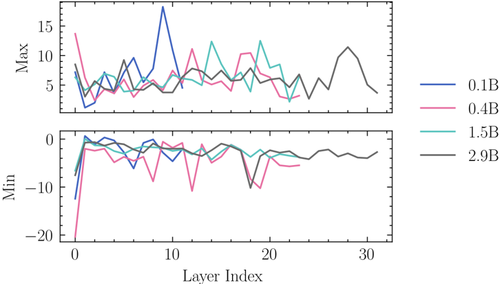" Figure 20: Maximum and Minimum of α Across Layers in Different Models <details> <summary>Image 21 Details</summary>  ### Visual Description ## Line Chart: Max and Min Values Across Layer Indices ### Overview The image contains two stacked line charts (top: "Max", bottom: "Min") showing the variation of maximum and minimum values across 31 layer indices (0–30). Four data series are represented by distinct colors (blue, pink, cyan, black), each corresponding to a specific "B" value (0.1B, 0.4B, 1.5B, 2.9B). The charts exhibit oscillatory patterns with peaks and troughs, suggesting dynamic relationships between layer indices and the measured values. ### Components/Axes - **X-axis (Layer Index)**: Ranges from 0 to 30 in integer increments. - **Y-axis (Top Chart - Max)**: Ranges from -20 to 15, labeled "Max". - **Y-axis (Bottom Chart - Min)**: Ranges from -20 to 0, labeled "Min". - **Legend**: Positioned on the right, with four entries: - Blue: 0.1B - Pink: 0.4B - Cyan: 1.5B - Black: 2.9B ### Detailed Analysis #### Max Values (Top Chart) - **0.1B (Blue)**: Peaks sharply at layer 5 (~12), then declines with minor fluctuations. Ends near 5 at layer 30. - **0.4B (Pink)**: Peaks at layer 10 (~10), followed by a gradual decline. Ends near 3 at layer 30. - **1.5B (Cyan)**: Peaks at layer 15 (~8), then stabilizes. Ends near 4 at layer 30. - **2.9B (Black)**: Peaks at layer 20 (~14), then declines. Ends near 6 at layer 30. #### Min Values (Bottom Chart) - **0.1B (Blue)**: Dips below -10 at layer 5, recovers to -2 by layer 30. - **0.4B (Pink)**: Dips to -12 at layer 10, recovers to -3 by layer 30. - **1.5B (Cyan)**: Dips to -10 at layer 15, recovers to -1 by layer 30. - **2.9B (Black)**: Dips to -8 at layer 20, recovers to 0 by layer 30. ### Key Observations 1. **Peak Alignment**: Each B value's maximum and minimum values align spatially across both charts (e.g., 0.1B peaks at layer 5 in Max and dips at layer 5 in Min). 2. **Inverse Relationship**: Higher B values (e.g., 2.9B) exhibit later-layer peaks in Max and later-layer troughs in Min compared to lower B values. 3. **Amplitude Trends**: Larger B values (1.5B, 2.9B) show smaller amplitude oscillations in both Max and Min compared to smaller B values (0.1B, 0.4B). 4. **Recovery Patterns**: All series recover toward baseline values (0 for Min, ~5 for Max) by layer 30, suggesting stabilization at higher indices. ### Interpretation The data suggests that the parameter "B" modulates the layer-specific behavior of maximum and minimum values. Larger B values delay the occurrence of extreme values (peaks/troughs) to higher layer indices, while smaller B values exhibit earlier extremes. The consistent recovery toward baseline values by layer 30 implies a convergence or stabilization effect at later layers, independent of B magnitude. The inverse relationship between B and the timing of extremes may indicate a scaling effect in the underlying system, where larger B values require deeper layers to manifest their influence. The oscillatory nature of the curves could reflect iterative processes or feedback mechanisms within the modeled system. 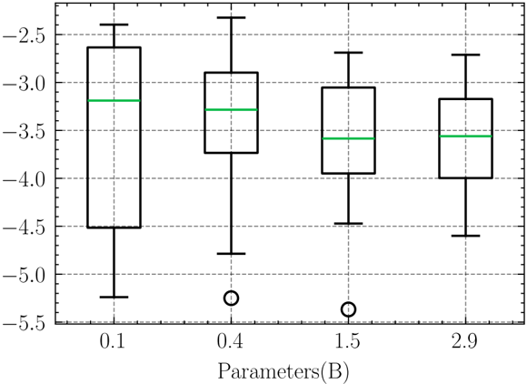</details> Figure 21: Box Plots of biases of dt Across Models <details> <summary>Image 22 Details</summary>  ### Visual Description ## Box Plot: Distribution of Parameters (B) Across Different Values ### Overview The image displays a box plot comparing the distribution of four parameter values (0.1, 0.4, 1.5, 2.9) on the x-axis against a continuous y-axis ranging from -5.5 to -2.5. Each box plot includes a green median line, whiskers, and outliers marked with open circles. The data suggests variability in central tendency and spread across parameter values. ### Components/Axes - **X-axis**: Labeled "Parameters (B)" with discrete categories: 0.1, 0.4, 1.5, 2.9. - **Y-axis**: Labeled with numerical values from -5.5 (bottom) to -2.5 (top), in increments of 0.5. - **Legend**: No explicit legend is present, but the green line within each box represents the median value. - **Outliers**: Open circles at the bottom of three box plots (0.4, 1.5, 2.9) indicate extreme low values. ### Detailed Analysis 1. **Parameter 0.1**: - Median (green line): -3.0. - Interquartile Range (IQR): -3.5 to -2.5 (box height). - Whiskers: Extend from -5.5 (outlier) to -2.5. - Outlier: Single point at -5.5. 2. **Parameter 0.4**: - Median: -3.5. - IQR: -4.0 to -3.0. - Whiskers: Extend from -5.0 (outlier) to -3.0. - Outlier: Single point at -5.0. 3. **Parameter 1.5**: - Median: -3.5. - IQR: -4.0 to -3.0. - Whiskers: Extend from -5.0 (outlier) to -3.0. - Outlier: Single point at -5.0. 4. **Parameter 2.9**: - Median: -3.5. - IQR: -4.0 to -3.0. - Whiskers: Extend from -5.0 (outlier) to -3.0. - Outlier: Single point at -5.0. ### Key Observations - **Median Trends**: The median value decreases slightly from -3.0 (0.1) to -3.5 (0.4, 1.5, 2.9), indicating a trend toward lower central tendency with increasing parameter values. - **Spread**: Parameter 0.1 exhibits the widest IQR (-1.0), while parameters 0.4, 1.5, and 2.9 have identical IQRs (-1.0). This suggests greater variability in the 0.1 group. - **Outliers**: All outliers occur at the lower end of the y-axis (-5.0 or -5.5), indicating extreme low values in three parameter groups. ### Interpretation The data demonstrates that higher parameter values (0.4, 1.5, 2.9) cluster around a median of -3.5 with consistent spread, while the lowest parameter value (0.1) has a marginally higher median (-3.0) but greater variability. The presence of outliers in three groups suggests potential anomalies or edge cases in the dataset. The consistency in medians for parameters ≥0.4 implies stabilization of the central tendency as parameter values increase, though the spread remains uniform. The extreme low outliers (-5.0/-5.5) may warrant further investigation to determine their cause or impact on the analysis. </details> Thefollowing table summarizes the performance of different models with and without the padding token <|endoftext|> : The results indicate that the inclusion of the <|endoftext|> token improves the performance of RWKV-7 very significantly, especially for small models (e.g., RWKV-7 0.1B). This finding highlights the importance of proper state initialization and context setting for RNN-based architectures like RWKV. Unexpectedly, we also found that two consecutive <|endoftext|> tokens at the beginning can further improve the performance of RWKV-7, despite that <|endoftext|> never appears consecutively in the training corpus. However, for Transformer-based models such as Qwen2.5-0.5B, we observe that the impact of the <|endoftext|> token is less pronounced, suggesting that these models may have better mechanisms for attending to the initial token. 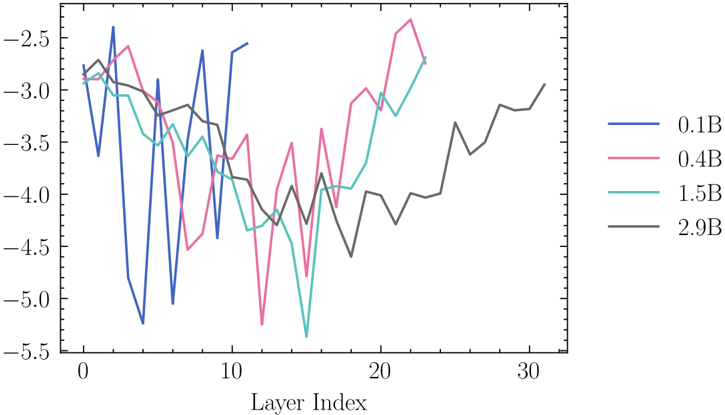Figure 22: Mean biases of dt Across Layers for Different Models <details> <summary>Image 23 Details</summary>  ### Visual Description ## Line Graph: Layer Index vs. Numerical Values ### Overview The image depicts a line graph comparing four data series across a layer index range (0–30). The y-axis represents numerical values (approximately -5.5 to -2.5), while the x-axis represents layer indices. Four distinct lines, differentiated by color and labeled with "B" values (0.1B, 0.4B, 1.5B, 2.9B), show fluctuating trends with sharp peaks and troughs. ### Components/Axes - **X-axis (Layer Index)**: Labeled "Layer Index," spanning 0 to 30 in increments of 10. - **Y-axis (Numerical Values)**: Labeled with values from -5.5 to -2.5 in increments of 0.5. - **Legend**: Positioned on the right, mapping colors to B values: - Blue: 0.1B - Pink: 0.4B - Teal: 1.5B - Black: 2.9B ### Detailed Analysis 1. **0.1B (Blue Line)**: - Starts near -2.8 at layer 0, plunges to -5.0 at layer 5, then oscillates between -3.5 and -4.5. - Sharpest dip occurs between layers 5–10, followed by erratic fluctuations. 2. **0.4B (Pink Line)**: - Begins at -2.9, drops to -4.0 at layer 5, then fluctuates between -3.0 and -4.5. - Shows a pronounced peak at layer 20 (~ -2.5) before declining. 3. **1.5B (Teal Line)**: - Starts at -3.2, dips to -4.5 at layer 10, then stabilizes between -3.0 and -4.0. - Sharpest drop occurs between layers 10–15. 4. **2.9B (Black Line)**: - Most stable series, starting at -2.8 and gradually increasing to -2.5 by layer 30. - Minimal fluctuations compared to other lines. ### Key Observations - **Volatility Correlation**: Lower B values (0.1B, 0.4B) exhibit greater volatility, with sharper dips and peaks. - **Stability Threshold**: The 2.9B line (highest B value) shows the least fluctuation, suggesting a correlation between B magnitude and stability. - **Critical Dips**: All lines except 2.9B experience significant drops between layers 5–15, potentially indicating a shared external factor. - **Recovery Patterns**: Lines recover partially after dips, but none fully return to initial values, implying cumulative effects. ### Interpretation The data suggests that higher B values (e.g., 2.9B) correlate with greater stability in layer index measurements, while lower B values (e.g., 0.1B) are more sensitive to external influences, causing erratic fluctuations. The sharp dips across all series between layers 5–15 may indicate a systemic event or threshold affecting all conditions. The gradual recovery in higher B values implies resilience or compensatory mechanisms absent in lower B scenarios. This could reflect a physical, biological, or computational system where B represents a parameter (e.g., resource allocation, energy input) modulating system behavior. 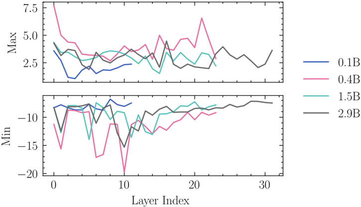</details> Figure 23: Maximum and Minimum of biases of dt Across Layers in Different Models <details> <summary>Image 24 Details</summary>  ### Visual Description ## Line Chart: Max and Min Values Across Layer Indices ### Overview The image contains a dual-axis line chart comparing maximum (top subplot) and minimum (bottom subplot) values across 31 layer indices (0–30). Four data series are represented by distinct colors, each corresponding to a specific "B" parameter value (0.1B, 0.4B, 1.5B, 2.9B). The chart emphasizes volatility patterns in both peak and trough behaviors across different configurations. ### Components/Axes - **X-axis (Layer Index)**: - Range: 0 to 30 (integer increments) - Label: "Layer Index" - **Y-axes**: - Top subplot ("Max"): - Range: -20 to 7.5 (approximate) - Label: "Max" - Bottom subplot ("Min"): - Range: -20 to 0 (approximate) - Label: "Min" - **Legend**: - Position: Right of the chart - Entries: - Blue: 0.1B - Pink: 0.4B - Teal: 1.5B - Black: 2.9B ### Detailed Analysis #### Max Subplot Trends 1. **0.1B (Blue)**: - Starts at ~5.0 (Layer 0), drops sharply to ~2.5 by Layer 5, then fluctuates between 2.0–4.0 until Layer 30. - Notable: Sharp dip at Layer 5 (~2.5), recovery to ~4.0 by Layer 10. 2. **0.4B (Pink)**: - Begins at ~7.5 (Layer 0), with extreme volatility: peaks at ~7.0 (Layer 2), troughs at ~2.0 (Layer 5), and sharp spikes to ~6.0 (Layer 15). - Ends at ~3.0 (Layer 30). 3. **1.5B (Teal)**: - Stable oscillations between 3.0–5.0, with minor dips to ~2.5 (Layer 15). - Ends at ~4.0 (Layer 30). 4. **2.9B (Black)**: - Most stable series: fluctuates between 3.0–4.5, with a gradual upward trend from ~3.5 (Layer 0) to ~4.5 (Layer 30). #### Min Subplot Trends 1. **0.1B (Blue)**: - Starts at ~-10, plunges to ~-15 (Layer 5), then stabilizes between -10 and -12. - Sharpest drop at Layer 5. 2. **0.4B (Pink)**: - Begins at ~-12, drops to ~-18 (Layer 5), then fluctuates between -14 and -16. - Sharpest drop at Layer 5. 3. **1.5B (Teal)**: - Moderate stability: oscillates between -10 and -14, with a slight recovery to ~-12 by Layer 30. 4. **2.9B (Black)**: - Smoothest series: starts at ~-10, dips to ~-12 (Layer 5), then stabilizes between -11 and -13. ### Key Observations 1. **Volatility Correlation**: - Lower B values (0.1B, 0.4B) exhibit significantly higher volatility in both Max and Min values compared to higher B values (1.5B, 2.9B). 2. **Extreme Fluctuations**: - The 0.4B series (pink) shows the most extreme peaks (~7.5) and troughs (~-18), suggesting heightened sensitivity to layer index changes. 3. **Stability Trends**: - 2.9B (black) demonstrates the most consistent behavior, with minimal deviation in both subplots. 4. **Layer 5 Anomaly**: - All series experience pronounced dips at Layer 5, indicating a potential systemic factor affecting this layer. ### Interpretation The data suggests that higher B values (e.g., 2.9B) correlate with greater stability in both maximum and minimum outcomes, likely due to optimized parameter tuning or reduced sensitivity to layer-specific variations. Conversely, lower B values (0.1B, 0.4B) display erratic behavior, with 0.4B showing the most extreme fluctuations. The consistent dip at Layer 5 across all series hints at a shared underlying mechanism or constraint in this layer. The 2.9B configuration’s stability makes it a candidate for robust applications requiring predictable performance, while the 0.4B series may require further investigation into its instability drivers. </details> As a result, for optimal performance when prompting RWKV-7, we recommend always including the <|endoftext|> token at the beginning of the prompt. For example, if you plan to use RWKV-7 as a chat assistant, consider the following structured prompt format: ``` <endoftext>|User: <Your Question> Assistant Answer> Assistant: User: <Another Question> Assistant: </doc> ``` Table 19: Performance comparison of different models with and without the <|endoftext|> token in the partial set of 142 samples from LAMBADA. Significance levels: ∗ p < 0.05, ∗∗ p < 0.01, ∗∗∗ p < 0.001, NS = Not Significant. | Model | EOSpadding | PPL | ACC(%) | Significance | |------------------|--------------|-----------|-----------|----------------| | RWKV7 World 0.1B | 0 1 | 357 16.4 | 9.2 36.6 | ∗∗∗ | | RWKV7 World 0.4B | 0 1 | 42.7 7.25 | 28.9 48.6 | ∗∗∗ | | SmolLM2 360M | 0 1 | 21.1 9.17 | 39.4 49.3 | ∗ | | Qwen2.5 0.5B | 0 1 | 12.2 7.97 | 47.9 54.9 | NS |