# Reasoning Effort and Problem Complexity: A Scaling Analysis in LLMs
**Authors**: Benjamin Estermann, ETH Zürich, &Roger Wattenhofer, ETH Zürich
Abstract
Large Language Models (LLMs) have demonstrated remarkable text generation capabilities, and recent advances in training paradigms have led to breakthroughs in their reasoning performance. In this work, we investigate how the reasoning effort of such models scales with problem complexity. We use the infinitely scalable Tents puzzle, which has a known linear-time solution, to analyze this scaling behavior. Our results show that reasoning effort scales with problem size, but only up to a critical problem complexity. Beyond this threshold, the reasoning effort does not continue to increase, and may even decrease. This observation highlights a critical limitation in the logical coherence of current LLMs as problem complexity increases, and underscores the need for strategies to improve reasoning scalability. Furthermore, our results reveal significant performance differences between current state-of-the-art reasoning models when faced with increasingly complex logical puzzles.
1 Introduction
Large language models (LLMs) have demonstrated remarkable abilities in a wide range of natural language tasks, from text generation to complex problem-solving. Recent advances, particularly with models trained for enhanced reasoning, have pushed the boundaries of what machines can achieve in tasks requiring logical inference and deduction.
<details>
<summary>extracted/6290299/Figures/tents.png Details</summary>
### Visual Description
## Grid Diagram: Forest and Field Layout
### Overview
The image is a grid diagram representing a landscape with trees and fields. The grid is 6x6, with the x-axis labeled along the bottom and the y-axis labeled along the right. The grid cells contain either a tree icon, a triangle icon, or are empty. The x-axis labels are 1, 1, 1, 2, 0, 2. The y-axis labels are 1, 1, 2, 0, 0, 3.
### Components/Axes
* **Grid:** 6x6 grid with light gray background.
* **X-axis Labels:** Located at the bottom of the grid, with values 1, 1, 1, 2, 0, 2.
* **Y-axis Labels:** Located on the right side of the grid, with values 1, 1, 2, 0, 0, 3.
* **Tree Icon:** Represents a tree, colored green.
* **Triangle Icon:** Represents a field, colored gold.
* **Light Green Cells:** Some cells have a light green background, indicating a specific area.
### Detailed Analysis or ### Content Details
The grid contains the following elements:
* **Row 1 (Y=1):**
* Column 1 (X=1): Tree icon in a light green cell.
* Column 2 (X=1): Triangle icon in a light green cell.
* Column 5 (X=0): Tree icon.
* **Row 2 (Y=1):** Empty.
* **Row 3 (Y=2):**
* Column 3 (X=1): Tree icon.
* Column 6 (X=2): Triangle icon in a light green cell.
* **Row 4 (Y=0):**
* Column 6 (X=2): Tree icon.
* **Row 5 (Y=0):**
* Column 3 (X=1): Tree icon.
* Column 6 (X=2): Tree icon.
* **Row 6 (Y=3):**
* Column 1 (X=1): Triangle icon in a light green cell.
* Column 2 (X=1): Tree icon in a light green cell.
* Column 3 (X=1): Triangle icon in a light green cell.
### Key Observations
* Trees and triangles are placed in specific cells, some with a light green background.
* The x and y axis labels have values ranging from 0 to 3.
* The distribution of trees and triangles is not uniform across the grid.
### Interpretation
The diagram likely represents a simplified model of a landscape, where trees and fields are distributed according to some underlying rule or pattern. The x and y axis labels could represent coordinates or some other spatial information. The light green cells might indicate areas of particular interest or significance. The data suggests a non-random distribution of trees and fields, possibly reflecting environmental factors or human intervention. The diagram could be used to visualize and analyze the spatial relationships between different landscape elements.
</details>
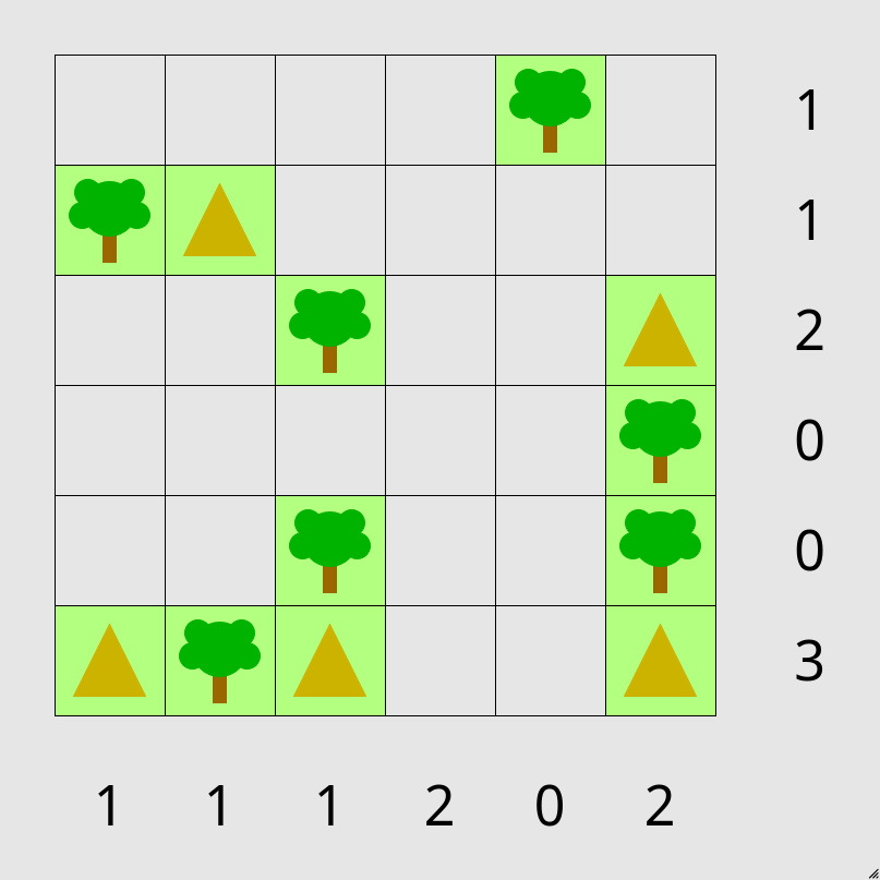
Figure 1: An example instance of a partially solved 6 by 6 tents puzzle. Tents need to be placed next to trees, away from other tents and fulfilling the row and column constraints.
A critical factor in the success of these advanced models is the ability to leverage increased computational resources at test time, allowing them to explore more intricate solution spaces. This capability raises a fundamental question: how does the ”reasoning effort” of these models scale as the complexity of the problem increases?
Understanding this scaling relationship is crucial for several reasons. First, it sheds light on the fundamental nature of reasoning within LLMs, moving beyond simply measuring accuracy on isolated tasks. By examining how the computational demands, reflected in token usage, evolve with problem difficulty, we can gain insights into the efficiency and potential bottlenecks of current LLM architectures. Second, characterizing this scaling behavior is essential for designing more effective and resource-efficient reasoning models in the future.
In this work, we address this question by investigating the scaling of reasoning effort in LLMs using a specific, infinitely scalable logic puzzle: the Tents puzzle The puzzle is available to play in the browser at https://www.chiark.greenend.org.uk/~sgtatham/puzzles/js/tents.html (see Figure 1). This puzzle offers a controlled environment for studying algorithmic reasoning, as its problem size can be systematically increased, and it possesses a known linear-time solution. Our analysis focuses on how the number of tokens used by state-of-the-art reasoning LLMs changes as the puzzle grid size grows. In addition to reasoning effort, we also evaluate the success rate across different puzzle sizes to provide a comprehensive view of their performance.
2 Related Work
The exploration of reasoning abilities in large language models (LLMs) is a rapidly evolving field with significant implications for artificial intelligence. Several benchmarks have been developed to evaluate the reasoning capabilities of LLMs across various domains. These benchmarks provide standardized tasks and evaluation metrics to assess and compare different models. Notable benchmarks include GSM8K (Cobbe et al., 2021), ARC-AGI (Chollet, 2019), GPQA (Rein et al., 2023), MMLU (Hendrycks et al., 2020), SWE-bench (Jimenez et al., 2023) and NPhard-eval (Fan et al., 2023). These benchmarks cover topics from mathematics to commonsense reasoning and coding. More recently, also math competitions such as AIME2024 (of America, 2024) have been used to evaluate the newest models. Estermann et al. (2024) have introduced PUZZLES, a benchmark focusing on algorithmic and logical reasoning for reinforcement learning. While PUZZLES does not focus on LLMs, except for a short ablation in the appendix, we argue that the scalability provided by the underlying puzzles is an ideal testbed for testing extrapolative reasoning capabilities in LLMs.
The reasoning capabilities of traditional LLMs without specific prompting strategies are quite limited (Huang & Chang, 2022). Using prompt techniques such as chain-of-thought (Wei et al., 2022), least-to-most (Zhou et al., 2022) and tree-of-thought (Yao et al., 2023), the reasoning capabilities of traditional LLMs can be greatly improved. Lee et al. (2024) have introduced the Language of Thought Hypothesis, based on the idea that human reasoning is rooted in language. Lee et al. propose to see the reasoning capabilities through three different properties: Logical coherence, compositionality and productivity. In this work we will mostly focus on the aspect of algorithmic reasoning, which falls into logical coherence. Specifically, we analyze the limits of logical coherence.
With the release of OpenAI’s o1 model, it became apparent that new training strategies based on reinforcement learning are able to boost the reasoning performance even further. Since o1, there now exist a number of different models capable of enhanced reasoning (Guo et al., 2025; DeepMind, 2025; Qwen, 2024; OpenAI, 2025). Key to the success of these models is the scaling of test-time compute. Instead of directly producing an answer, or thinking for a few steps using chain-of-thought, the models are now trained to think using several thousands of tokens before coming up with an answer.
3 Methods
3.1 The Tents Puzzle Problem
In this work, we employ the Tents puzzle, a logic problem that is both infinitely scalable and solvable in linear time See a description of the algorithm of the solver as part of the PUZZLES benchmark here: https://github.com/ETH-DISCO/rlp/blob/main/puzzles/tents.c#L206C3-L206C67, making it an ideal testbed for studying algorithmic reasoning in LLMs. The Tents puzzle, popularized by Simon Tatham’s Portable Puzzle Collection (Tatham, ), requires deductive reasoning to solve. The puzzle is played on a rectangular grid, where some cells are pre-filled with trees. The objective is to place tents in the remaining empty cells according to the following rules:
- no two tents are adjacent, even diagonally
- there are exactly as many tents as trees and the number of tents in each row and column matches the numbers around the edge of the grid
- it is possible to match all tents to trees so that each tent is orthogonally adjacent to its own tree (a tree may also be adjacent to other tents).
An example instance of the Tents puzzle is visualized in Figure 1 in the Introduction. The scalability of the puzzle is achieved by varying the grid dimensions, allowing for systematic exploration of problem complexity. Where not otherwise specified, we used the ”easy” difficulty preset available in the Tents puzzle generator, with ”tricky” being evaluated in Section A.2.1. Crucially, the Tents puzzle is designed to test extrapolative reasoning as puzzle instances, especially larger ones, are unlikely to be present in the training data of LLMs. We utilized a text-based interface for the Tents puzzle, extending the code base provided by Estermann et al. (2024) to generate puzzle instances and represent the puzzle state in a format suitable for LLMs.
Models were presented with the same prompt (detailed in Appendix A.1) for all puzzle sizes and models tested. The prompt included the puzzle rules and the initial puzzle state in a textual format. Models were tasked with directly outputting the solved puzzle grid in JSON format. This one-shot approach contrasts with interactive or cursor-based approaches previously used in (Estermann et al., 2024), isolating the reasoning process from potential planning or action selection complexities.
3.2 Evaluation Criteria
Our evaluation focuses on two key metrics: success rate and reasoning effort. Success is assessed as a binary measure: whether the LLM successfully outputs a valid solution to the Tents puzzle instance, adhering to all puzzle rules and constraints. We quantify problem complexity by the problem size, defined as the product of the grid dimensions (rows $×$ columns). To analyze the scaling of reasoning effort, we measure the total number of tokens generated by the LLMs to produce the final answer, including all thinking tokens. We hypothesize a linear scaling relationship between problem size and reasoning effort, and evaluate this hypothesis by fitting a linear model to the observed token counts as a function of problem size. The goodness of fit is quantified using the $R^{2}$ metric, where scores closer to 1 indicate that a larger proportion of the variance in reasoning effort is explained by a linear relationship with problem size. Furthermore, we analyze the percentage of correctly solved puzzles across different problem sizes to assess the performance limits of each model.
3.3 Considered Models
We evaluated the reasoning performance of the following large language models known for their enhanced reasoning capabilities: Gemini 2.0 Flash Thinking (DeepMind, 2025), OpenAI o3-mini (OpenAI, 2025), DeepSeek R1 Guo et al. (2025), and Qwen/QwQ-32B-Preview Qwen (2024).
4 Results
<details>
<summary>x1.png Details</summary>
### Visual Description
## Scatter Plot: Reasoning Tokens vs. Problem Size
### Overview
The image is a scatter plot comparing the number of reasoning tokens used by three different models (deepseek/deepseek-r1, o3-mini, and qwen/qwq-32b-preview) against the problem size. Each model has a scatter plot of data points and a fitted line, along with an R-squared value indicating the goodness of fit.
### Components/Axes
* **X-axis:** Problem Size, ranging from approximately 15 to 80 in increments of 10.
* **Y-axis:** Reasoning Tokens, ranging from 0 to 20000 in increments of 5000.
* **Legend (Top-Right):**
* Blue Circle: deepseek/deepseek-r1
* Blue Line: deepseek/deepseek-r1 fit (R2: 0.667)
* Orange Square: o3-mini
* Orange Dashed Line: o3-mini fit (R2: 0.833)
* Green Triangle: qwen/qwq-32b-preview
* Green Dash-Dot Line: qwen/qwq-32b-preview fit (R2: 0.087)
### Detailed Analysis
* **deepseek/deepseek-r1 (Blue):**
* Trend: The number of reasoning tokens generally increases with problem size.
* Data Points: At problem size ~20, reasoning tokens are around 4000-7000. At problem size ~40, reasoning tokens are around 7000-12000.
* Fitted Line: The blue line shows a positive slope.
* R-squared: 0.667
* **o3-mini (Orange):**
* Trend: The number of reasoning tokens increases with problem size.
* Data Points: At problem size ~20, reasoning tokens are around 2000-4000. At problem size ~80, reasoning tokens are around 13000-19000.
* Fitted Line: The orange dashed line shows a positive slope, steeper than deepseek/deepseek-r1.
* R-squared: 0.833
* **qwen/qwq-32b-preview (Green):**
* Trend: The number of reasoning tokens remains relatively constant with increasing problem size.
* Data Points: Reasoning tokens are clustered around 5000-7000 for problem sizes between 15 and 30.
* Fitted Line: The green dash-dot line is nearly flat.
* R-squared: 0.087
### Key Observations
* The o3-mini model has the highest R-squared value (0.833), indicating the best fit to its data.
* The qwen/qwq-32b-preview model has a very low R-squared value (0.087), suggesting a poor fit and that problem size does not strongly predict reasoning tokens for this model.
* For smaller problem sizes (around 20), o3-mini uses the fewest reasoning tokens, while qwen/qwq-32b-preview and deepseek/deepseek-r1 use a similar number of tokens.
* For larger problem sizes (around 80), o3-mini uses significantly more reasoning tokens than deepseek/deepseek-r1.
### Interpretation
The scatter plot illustrates the relationship between problem size and the number of reasoning tokens used by different models. The R-squared values indicate how well the fitted lines represent the data. The o3-mini model shows a strong positive correlation between problem size and reasoning tokens, while the qwen/qwq-32b-preview model shows almost no correlation. The deepseek/deepseek-r1 model shows a moderate positive correlation. This suggests that the o3-mini model's token usage is highly dependent on problem size, while the qwen/qwq-32b-preview model's token usage is relatively independent of problem size within the range tested. The deepseek/deepseek-r1 model falls in between these two extremes. The data suggests that o3-mini may scale its reasoning more aggressively with problem size compared to the other two models.
</details>
(a)
<details>
<summary>x2.png Details</summary>
### Visual Description
## Line Chart: Success Rate vs. Problem Size
### Overview
The image is a line chart comparing the success rates of four different models (deepseek/deepseek-r1, o3-mini, gemini-2.0-flash-thinking-exp-01-21, and qwen/qwq-32b-preview) across varying problem sizes. The x-axis represents the problem size, and the y-axis represents the success rate in percentage.
### Components/Axes
* **X-axis:** Problem Size, ranging from 20 to 120 in increments of 20.
* **Y-axis:** Success Rate (%), ranging from 0 to 100 in increments of 20.
* **Legend:** Located in the top-right corner of the chart.
* Blue line with circle markers: deepseek/deepseek-r1
* Orange dashed line with square markers: o3-mini
* Green dash-dot line with triangle markers: gemini-2.0-flash-thinking-exp-01-21
* Red dotted line with inverted triangle markers: qwen/qwq-32b-preview
### Detailed Analysis
* **deepseek/deepseek-r1 (Blue line with circle markers):**
* Trend: Starts at 100% success rate for problem size 20, remains at 100% until problem size 30, then decreases to approximately 75% at problem size 35, then decreases to approximately 52% at problem size 55, and finally drops to 0% at problem size 65 and remains at 0% for larger problem sizes.
* Data Points: (20, 100), (30, 100), (35, 75), (55, 52), (65, 0), (120, 0)
* **o3-mini (Orange dashed line with square markers):**
* Trend: Maintains a 100% success rate from problem size 20 to 40, then drops to approximately 33% at problem size 75, then increases to approximately 67% at problem size 80, then drops to 0% at problem size 100 and remains at 0% for larger problem sizes.
* Data Points: (20, 100), (40, 100), (75, 33), (80, 67), (100, 0), (120, 0)
* **gemini-2.0-flash-thinking-exp-01-21 (Green dash-dot line with triangle markers):**
* Trend: Starts at approximately 67% at problem size 20, increases to 100% at problem size 30, then drops to 0% at problem size 40 and remains at 0% for larger problem sizes.
* Data Points: (20, 67), (30, 100), (40, 0), (120, 0)
* **qwen/qwq-32b-preview (Red dotted line with inverted triangle markers):**
* Trend: Starts at approximately 67% at problem size 20, then drops to 0% at problem size 30 and remains at 0% for larger problem sizes.
* Data Points: (20, 67), (30, 0), (120, 0)
### Key Observations
* The deepseek/deepseek-r1 model shows a gradual decline in success rate as the problem size increases, eventually reaching 0%.
* The o3-mini model maintains a high success rate for smaller problem sizes but experiences a significant drop and fluctuation before ultimately failing.
* The gemini-2.0-flash-thinking-exp-01-21 model initially performs well but quickly drops to 0% success rate as the problem size increases.
* The qwen/qwq-32b-preview model has the poorest performance, dropping to 0% success rate very early on.
### Interpretation
The chart illustrates the performance of different models in relation to the problem size they are attempting to solve. The deepseek/deepseek-r1 model appears to be the most robust for moderately sized problems, while the other models either fail quickly or exhibit inconsistent performance. The data suggests that the deepseek/deepseek-r1 model is better at handling larger problem sizes compared to the other models, although its success rate eventually diminishes. The o3-mini model shows some potential for mid-sized problems, but its performance is not consistent. The gemini-2.0-flash-thinking-exp-01-21 and qwen/qwq-32b-preview models are not suitable for larger problem sizes based on this data.
</details>
(b)
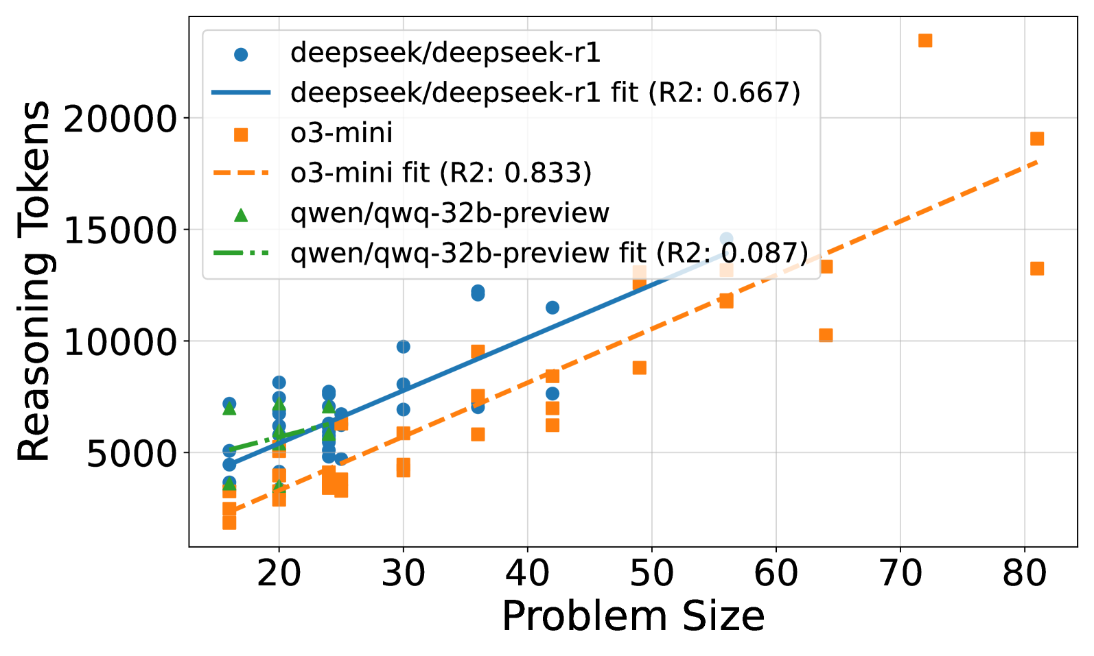
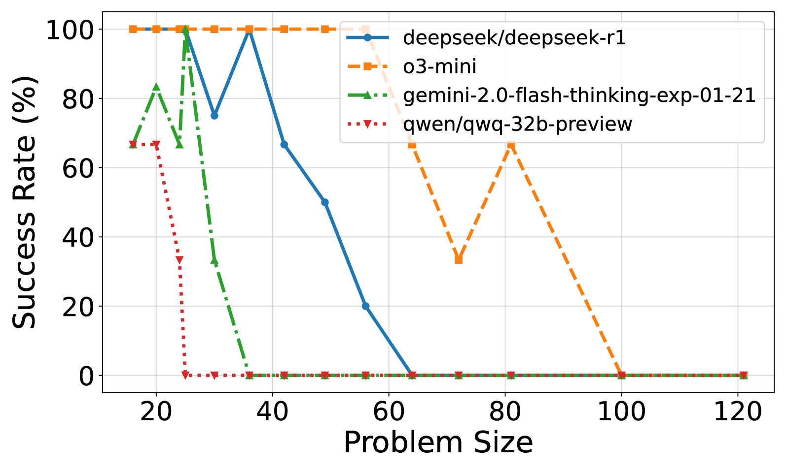
Figure 2: (a) Reasoning effort in number of reasoning tokens versus problem size for DeepSeek R1, o3-mini, and Qwen/QwQ-32B-Preview. Successful attempts only. Linear fits are added for each model. Gemini 2.0 Flash Thinking is excluded due to unknown number of thinking tokens. (b) Solved percentage versus problem size for all models. No model solved problems larger than size 100. o3-mini achieves the highest success rate, followed by DeepSeek R1 and Gemini 2.0 Flash Thinking. Qwen/QwQ-32B-Preview struggles with problem instances larger than size 20.
The relationship between reasoning effort and problem size reveals interesting scaling behaviors across the evaluated models. Figure 2(a) illustrates the scaling of reasoning effort, measured by the number of reasoning tokens, as the problem size increases for successfully solved puzzles. For DeepSeek R1 and o3-mini, we observe a roughly linear increase in reasoning effort with problem size. Notably, the slopes of the linear fits for R1 and o3-mini are very similar, suggesting comparable scaling behavior in reasoning effort for these models, although DeepSeek R1 consistently uses more tokens than o3-mini across problem sizes. Qwen/QwQ-32B-Preview shows a weaker linear correlation, likely due to the limited number of larger puzzles it could solve successfully.
The problem-solving capability of the models, shown in Figure 2(b), reveals performance limits as problem size increases. None of the models solved puzzles with a problem size exceeding 100. o3-mini demonstrates the highest overall solvability, managing to solve the largest problem instances, followed by DeepSeek R1 and Gemini 2.0 Flash Thinking. Qwen/QwQ-32B-Preview’s performance significantly degrades with increasing problem size, struggling to solve instances larger than 25.
<details>
<summary>x3.png Details</summary>
### Visual Description
## Scatter Plot: Reasoning Tokens vs. Problem Size for o3-mini
### Overview
The image is a scatter plot comparing the number of reasoning tokens used by the "o3-mini" model against the problem size. The plot distinguishes between successful and failed attempts, using blue circles for successful attempts and orange squares for failed attempts. The x-axis represents the problem size, and the y-axis represents the number of reasoning tokens.
### Components/Axes
* **Title:** There is no explicit title on the chart.
* **X-axis:**
* Label: "Problem Size"
* Scale: 0 to 400, with major ticks at 0, 100, 200, 300, and 400.
* **Y-axis:**
* Label: "Reasoning Tokens"
* Scale: 0 to 50000, with major ticks at 0, 10000, 20000, 30000, 40000, and 50000.
* **Legend:** Located in the top-right corner.
* Blue circle: "o3-mini (Successful)"
* Orange square: "o3-mini (Failed)"
### Detailed Analysis
**o3-mini (Successful) - Blue Circles:**
* **Trend:** The number of reasoning tokens generally increases with problem size for successful attempts.
* **Data Points:**
* Problem Size ~10, Reasoning Tokens ~2000
* Problem Size ~20, Reasoning Tokens ~3000
* Problem Size ~30, Reasoning Tokens ~4000
* Problem Size ~40, Reasoning Tokens ~6000
* Problem Size ~50, Reasoning Tokens ~8000
* Problem Size ~60, Reasoning Tokens ~9000
* Problem Size ~70, Reasoning Tokens ~12000
* Problem Size ~80, Reasoning Tokens ~13000
* Problem Size ~90, Reasoning Tokens ~23000
**o3-mini (Failed) - Orange Squares:**
* **Trend:** For failed attempts, the number of reasoning tokens initially increases with problem size, but then appears to decrease or plateau as the problem size increases beyond approximately 100.
* **Data Points:**
* Problem Size ~20, Reasoning Tokens ~3000
* Problem Size ~40, Reasoning Tokens ~8000
* Problem Size ~60, Reasoning Tokens ~18000
* Problem Size ~80, Reasoning Tokens ~40000
* Problem Size ~100, Reasoning Tokens ~48000
* Problem Size ~120, Reasoning Tokens ~8000
* Problem Size ~140, Reasoning Tokens ~25000
* Problem Size ~160, Reasoning Tokens ~14000
* Problem Size ~180, Reasoning Tokens ~10000
* Problem Size ~200, Reasoning Tokens ~12000
* Problem Size ~220, Reasoning Tokens ~11000
* Problem Size ~260, Reasoning Tokens ~4000
* Problem Size ~280, Reasoning Tokens ~6000
* Problem Size ~300, Reasoning Tokens ~11000
* Problem Size ~380, Reasoning Tokens ~8000
* Problem Size ~400, Reasoning Tokens ~12000
### Key Observations
* For successful attempts, there is a clear positive correlation between problem size and the number of reasoning tokens.
* For failed attempts, the relationship is more complex. Initially, the number of reasoning tokens increases with problem size, but beyond a certain point (around 100), the number of tokens used in failed attempts appears to decrease or plateau.
* There is a significant difference in the number of reasoning tokens used between successful and failed attempts for smaller problem sizes.
### Interpretation
The data suggests that for the "o3-mini" model, successful problem-solving generally requires more reasoning tokens as the problem size increases. However, when the model fails, it may be due to an inefficient use of reasoning tokens, especially for larger problem sizes. The plateau or decrease in reasoning tokens for failed attempts at larger problem sizes could indicate that the model is either giving up early or getting stuck in a loop, failing to explore the solution space effectively. The model may be more likely to fail when the problem size is larger, and the number of reasoning tokens is lower. This could be due to the model not having enough resources to solve the problem.
</details>
(a)
<details>
<summary>x4.png Details</summary>
### Visual Description
## Scatter Plot: Reasoning Tokens vs. Problem Size
### Overview
The image is a scatter plot showing the relationship between "Problem Size" and "Reasoning Tokens" for three different levels of "Reasoning Effort": low, medium, and high. Each level has a scatter plot of data points and a corresponding fitted line with an R-squared value indicating the goodness of fit.
### Components/Axes
* **X-axis:** "Problem Size", ranging from 0 to 100, with tick marks at intervals of 20.
* **Y-axis:** "Reasoning Tokens", ranging from 0 to 50000, with tick marks at intervals of 10000.
* **Legend (top-left):**
* "Reasoning Effort"
* Blue circle: "low"
* Blue solid line: "low fit (R^2: 0.489)"
* Orange square: "medium"
* Orange dashed line: "medium fit (R^2: 0.833)"
* Green triangle: "high"
* Green dash-dot line: "high fit (R^2: 0.813)"
### Detailed Analysis
* **Low Reasoning Effort (Blue):**
* Data points: Scatter points are clustered near the bottom of the chart.
* Trend: The "low fit" line is nearly flat, showing a slight positive slope.
* Data points: (20, 1000), (30, 2000), (40, 2500)
* R-squared: 0.489
* **Medium Reasoning Effort (Orange):**
* Data points: Scatter points are in the middle range of the chart.
* Trend: The "medium fit" line has a moderate positive slope.
* Data points: (20, 1000), (30, 8000), (40, 9000), (70, 22000), (80, 14000)
* R-squared: 0.833
* **High Reasoning Effort (Green):**
* Data points: Scatter points are spread across the entire range of the chart.
* Trend: The "high fit" line has a steep positive slope.
* Data points: (20, 6000), (30, 10000), (40, 12000), (50, 35000), (60, 23000), (70, 28000), (80, 50000), (90, 40000), (100, 45000)
* R-squared: 0.813
### Key Observations
* As "Problem Size" increases, "Reasoning Tokens" generally increase for all levels of "Reasoning Effort".
* The "high" reasoning effort exhibits the most significant increase in "Reasoning Tokens" as "Problem Size" increases.
* The R-squared values indicate that the fitted lines for "medium" and "high" reasoning effort are a better fit for the data than the "low" reasoning effort.
### Interpretation
The plot demonstrates that the amount of reasoning required (measured in tokens) increases with problem size. The level of reasoning effort significantly impacts the rate at which reasoning tokens increase. Problems requiring "high" reasoning effort show a much steeper increase in tokens compared to "medium" or "low" effort problems. The R-squared values suggest that a linear model is more appropriate for "medium" and "high" reasoning effort than for "low" reasoning effort, where the relationship between problem size and reasoning tokens may be more complex or less pronounced. The "low" reasoning effort shows a very weak correlation, suggesting that problem size has little impact on the number of reasoning tokens required when the reasoning effort is low.
</details>
(b)
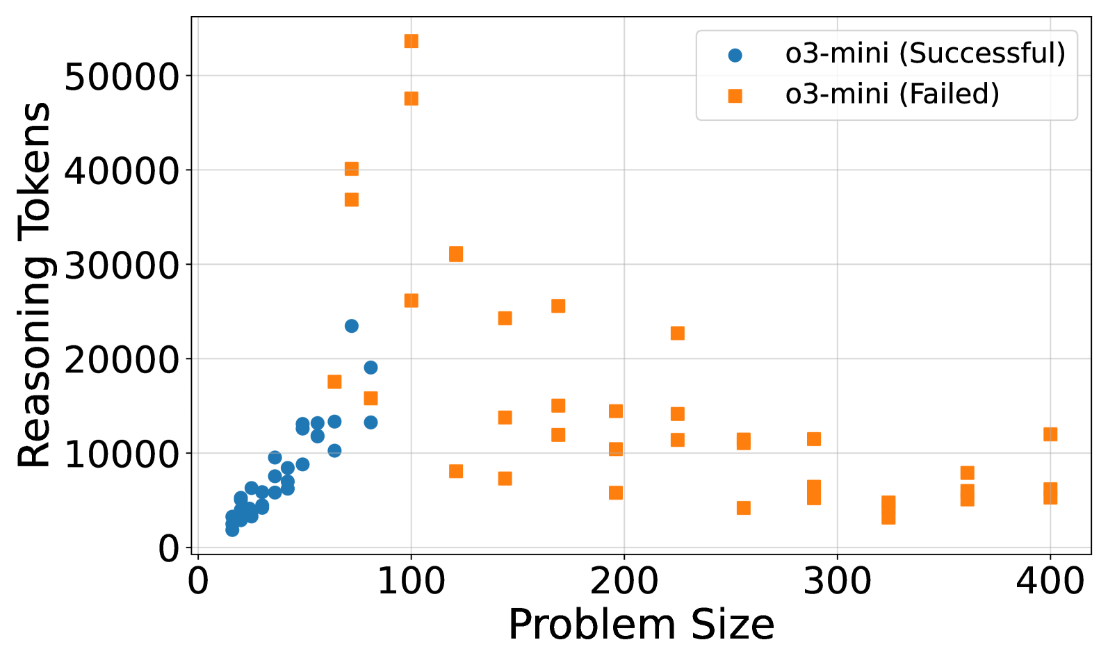
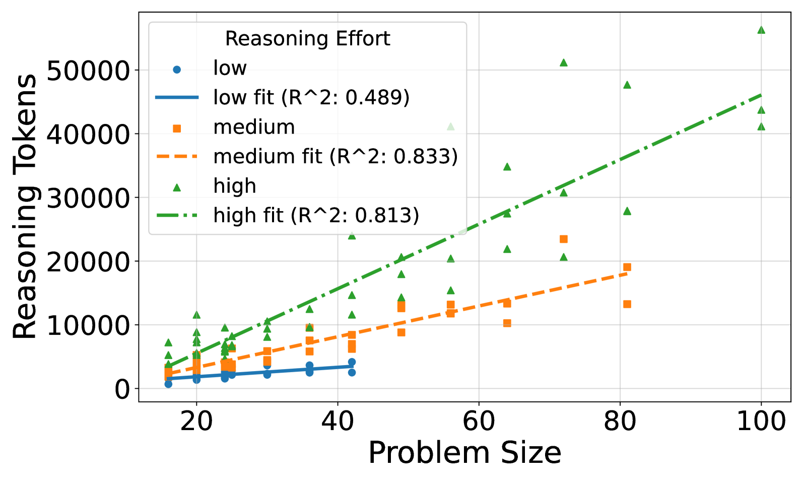
Figure 3: (a) Reasoning effort in number of reasoning tokens versus problem size for o3-mini. A peak in reasoning effort is observed around problem size 100, followed by a decline for larger problem sizes. (b) Reasoning effort in number of reasoning tokens versus problem size for o3-mini, categorized by low, medium, and high reasoning effort strategies. Steeper slopes are observed for higher reasoning effort strategies. High reasoning effort enables solving larger instances but also increases token usage for smaller, already solvable problems.
A more detailed analysis of o3-mini’s reasoning effort (Figure 3(a)) reveals a non-monotonic trend. While generally increasing with problem size initially, reasoning effort peaks around a problem size of 100. Beyond this point, the reasoning effort decreases, suggesting a potential ”frustration” effect where increased complexity no longer leads to proportionally increased reasoning in the model. The same behavior could not be observed for other models, see Section A.2.2. It would be interesting to see the effect of recent works trying to optimize reasoning length would have on these results (Luo et al., 2025).
Figure 3(b) further explores o3-mini’s behavior by categorizing reasoning effort into low, medium, and high strategies. The steepness of the scaling slope increases with reasoning effort, indicating that higher effort strategies lead to a more pronounced increase in token usage as problem size grows. While high reasoning effort enables solving larger puzzles (up to 10x10), it also results in a higher token count even for smaller problems that were already solvable with lower effort strategies. This suggests a trade-off where increased reasoning effort can extend the solvable problem range but may also introduce inefficiencies for simpler instances.
5 Conclusion
This study examined how reasoning effort scales in LLMs using the Tents puzzle. We found that reasoning effort generally scales linearly with problem size for solvable instances. Model performance varied, with o3-mini and DeepSeek R1 showing better performance than Qwen/QwQ-32B-Preview and Gemini 2.0 Flash Thinking. These results suggest that while LLMs can adapt reasoning effort to problem complexity, their logical coherence has limits, especially for larger problems. Future work should extend this analysis to a wider variety of puzzles contained in the PUZZLES benchmark to include puzzles with different algorithmic complexity. These insights could lead the way to find strategies to improve reasoning scalability and efficiency, potentially by optimizing reasoning length or refining prompting techniques. Understanding these limitations is crucial for advancing LLMs in complex problem-solving.
References
- Chollet (2019) François Chollet. On the measure of intelligence. arXiv preprint arXiv:1911.01547, 2019.
- Cobbe et al. (2021) Karl Cobbe, Vineet Kosaraju, Mohammad Bavarian, Mark Chen, Heewoo Jun, Lukasz Kaiser, Matthias Plappert, Jerry Tworek, Jacob Hilton, Reiichiro Nakano, et al. Training verifiers to solve math word problems. arXiv preprint arXiv:2110.14168, 2021.
- DeepMind (2025) DeepMind. Gemini flash thinking. https://deepmind.google/technologies/gemini/flash-thinking/, 2025. Accessed: February 6, 2025.
- Estermann et al. (2024) Benjamin Estermann, Luca A Lanzendörfer, Yannick Niedermayr, and Roger Wattenhofer. Puzzles: A benchmark for neural algorithmic reasoning. In The Thirty-eight Conference on Neural Information Processing Systems Datasets and Benchmarks Track, 2024.
- Fan et al. (2023) Lizhou Fan, Wenyue Hua, Lingyao Li, Haoyang Ling, and Yongfeng Zhang. Nphardeval: Dynamic benchmark on reasoning ability of large language models via complexity classes. arXiv preprint arXiv:2312.14890, 2023.
- Guo et al. (2025) Daya Guo, Dejian Yang, Haowei Zhang, Junxiao Song, Ruoyu Zhang, Runxin Xu, Qihao Zhu, Shirong Ma, Peiyi Wang, Xiao Bi, et al. Deepseek-r1: Incentivizing reasoning capability in llms via reinforcement learning. arXiv preprint arXiv:2501.12948, 2025.
- Hendrycks et al. (2020) Dan Hendrycks, Collin Burns, Steven Basart, Andy Zou, Mantas Mazeika, Dawn Song, and Jacob Steinhardt. Measuring massive multitask language understanding. arXiv preprint arXiv:2009.03300, 2020.
- Huang & Chang (2022) Jie Huang and Kevin Chen-Chuan Chang. Towards reasoning in large language models: A survey. arXiv preprint arXiv:2212.10403, 2022.
- Jimenez et al. (2023) Carlos E Jimenez, John Yang, Alexander Wettig, Shunyu Yao, Kexin Pei, Ofir Press, and Karthik Narasimhan. Swe-bench: Can language models resolve real-world github issues? arXiv preprint arXiv:2310.06770, 2023.
- Lee et al. (2024) Seungpil Lee, Woochang Sim, Donghyeon Shin, Wongyu Seo, Jiwon Park, Seokki Lee, Sanha Hwang, Sejin Kim, and Sundong Kim. Reasoning abilities of large language models: In-depth analysis on the abstraction and reasoning corpus. ACM Transactions on Intelligent Systems and Technology, 2024.
- Luo et al. (2025) Haotian Luo, Li Shen, Haiying He, Yibo Wang, Shiwei Liu, Wei Li, Naiqiang Tan, Xiaochun Cao, and Dacheng Tao. O1-pruner: Length-harmonizing fine-tuning for o1-like reasoning pruning. arXiv preprint arXiv:2501.12570, 2025.
- of America (2024) Mathematical Association of America. 2024 aime i problems. https://artofproblemsolving.com/wiki/index.php/2024_AIME_I, 2024. Accessed: February 6, 2025.
- OpenAI (2025) OpenAI. Openai o3 mini. https://openai.com/index/openai-o3-mini/, 2025. Accessed: February 6, 2025.
- Qwen (2024) Qwen. Qwq: Reflect deeply on the boundaries of the unknown, November 2024. URL https://qwenlm.github.io/blog/qwq-32b-preview/.
- Rein et al. (2023) David Rein, Betty Li Hou, Asa Cooper Stickland, Jackson Petty, Richard Yuanzhe Pang, Julien Dirani, Julian Michael, and Samuel R Bowman. Gpqa: A graduate-level google-proof q&a benchmark. arXiv preprint arXiv:2311.12022, 2023.
- (16) Simon Tatham. Simon tatham’s portable puzzle collection. https://www.chiark.greenend.org.uk/~sgtatham/puzzles/. Accessed: 2025-02-06.
- Wei et al. (2022) Jason Wei, Xuezhi Wang, Dale Schuurmans, Maarten Bosma, Fei Xia, Ed Chi, Quoc V Le, Denny Zhou, et al. Chain-of-thought prompting elicits reasoning in large language models. Advances in neural information processing systems, 35:24824–24837, 2022.
- Yao et al. (2023) Shunyu Yao, Dian Yu, Jeffrey Zhao, Izhak Shafran, Thomas L Griffiths, Yuan Cao, and Karthik Narasimhan. Tree of thoughts: Deliberate problem solving with large language models, may 2023. arXiv preprint arXiv:2305.10601, 14, 2023.
- Zhou et al. (2022) Denny Zhou, Nathanael Schärli, Le Hou, Jason Wei, Nathan Scales, Xuezhi Wang, Dale Schuurmans, Claire Cui, Olivier Bousquet, Quoc Le, et al. Least-to-most prompting enables complex reasoning in large language models. arXiv preprint arXiv:2205.10625, 2022.
Appendix A Appendix
A.1 Full Prompt
The full prompt used in the experiments is the following, on the example of a 4x4 puzzle:
⬇
You are a logic puzzle expert. You will be given a logic puzzle to solve. Here is a description of the puzzle:
You have a grid of squares, some of which contain trees. Your aim is to place tents in some of the remaining squares, in such a way that the following conditions are met:
There are exactly as many tents as trees.
The tents and trees can be matched up in such a way that each tent is directly adjacent (horizontally or vertically, but not diagonally) to its own tree. However, a tent may be adjacent to other trees as well as its own.
No two tents are adjacent horizontally, vertically or diagonally.
The number of tents in each row, and in each column, matches the numbers given in the row or column constraints.
Grass indicates that there cannot be a tent in that position.
You receive an array representation of the puzzle state as a grid. Your task is to solve the puzzle by filling out the grid with the correct values. You need to solve the puzzle on your own, you cannot use any external resources or run any code. Once you have solved the puzzle, tell me the final answer without explanation. Return the final answer as a JSON array of arrays.
Here is the current state of the puzzle as a string of the internal state representation:
A 0 represents an empty cell, a 1 represents a tree, a 2 represents a tent, and a 3 represents a grass patch.
Tents puzzle state:
Current grid:
[[0 0 1 0]
[0 1 0 0]
[1 0 0 0]
[0 0 0 0]]
The column constraints are the following:
[1 1 0 1]
The row constraints are the following:
[2 0 0 1]
A.2 Additional Figures
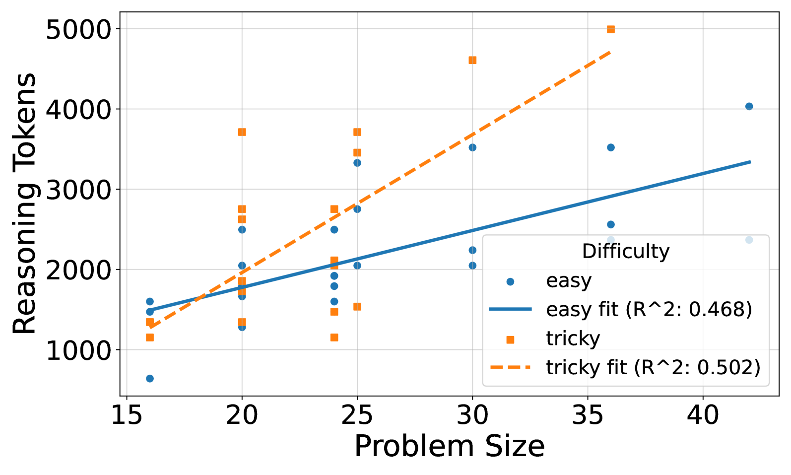
A.2.1 Easy vs. Tricky Puzzles
<details>
<summary>x5.png Details</summary>
### Visual Description
## Scatter Plot: Reasoning Tokens vs. Problem Size by Difficulty
### Overview
The image is a scatter plot showing the relationship between "Reasoning Tokens" and "Problem Size" for two categories of problem difficulty: "easy" and "tricky". The plot includes trend lines (linear fits) for each difficulty level, along with their corresponding R-squared values.
### Components/Axes
* **X-axis:** "Problem Size", ranging from 15 to 40 in increments of 5.
* **Y-axis:** "Reasoning Tokens", ranging from 1000 to 5000 in increments of 1000.
* **Data Series 1:** "easy" - represented by blue circles.
* **Data Series 2:** "tricky" - represented by orange squares.
* **Trend Line 1:** "easy fit (R^2: 0.468)" - a solid blue line.
* **Trend Line 2:** "tricky fit (R^2: 0.502)" - a dashed orange line.
* **Legend:** Located in the bottom-right corner, labeled "Difficulty", explaining the color and marker scheme for each difficulty level and their corresponding trend lines.
### Detailed Analysis
**"easy" Data Series (Blue Circles):**
* **Trend:** The "easy" data series shows a generally positive, but weak, correlation between problem size and reasoning tokens.
* **Data Points:**
* Problem Size ~15: Reasoning Tokens ~650
* Problem Size ~17: Reasoning Tokens ~1500
* Problem Size ~20: Reasoning Tokens ~1300, ~1600, ~2500
* Problem Size ~23: Reasoning Tokens ~1800, ~2000
* Problem Size ~25: Reasoning Tokens ~2000, ~3400
* Problem Size ~30: Reasoning Tokens ~2200
* Problem Size ~35: Reasoning Tokens ~3500
* Problem Size ~40: Reasoning Tokens ~4000
* Problem Size ~42: Reasoning Tokens ~2300
**"easy fit (R^2: 0.468)" Trend Line (Solid Blue):**
* The blue trend line starts at approximately 1400 Reasoning Tokens at a Problem Size of 15 and increases to approximately 3400 Reasoning Tokens at a Problem Size of 40.
**"tricky" Data Series (Orange Squares):**
* **Trend:** The "tricky" data series shows a stronger positive correlation between problem size and reasoning tokens compared to the "easy" series.
* **Data Points:**
* Problem Size ~15: Reasoning Tokens ~1200
* Problem Size ~20: Reasoning Tokens ~1700, ~2700, ~3700
* Problem Size ~23: Reasoning Tokens ~1100, ~1500
* Problem Size ~25: Reasoning Tokens ~2600
* Problem Size ~30: Reasoning Tokens ~4700
* Problem Size ~35: Reasoning Tokens ~5000
**"tricky fit (R^2: 0.502)" Trend Line (Dashed Orange):**
* The orange trend line starts at approximately 1300 Reasoning Tokens at a Problem Size of 15 and increases to approximately 4700 Reasoning Tokens at a Problem Size of 40.
### Key Observations
* The "tricky" problems generally require more reasoning tokens than the "easy" problems for a given problem size.
* The R-squared value for the "tricky" fit (0.502) is slightly higher than the R-squared value for the "easy" fit (0.468), indicating a slightly better linear fit for the "tricky" data.
* There is considerable variance in the number of reasoning tokens for both difficulty levels at each problem size.
### Interpretation
The scatter plot suggests that problem size is positively correlated with the number of reasoning tokens required to solve a problem, and that "tricky" problems generally require more reasoning tokens than "easy" problems. The relatively low R-squared values for both trend lines indicate that problem size is not the only factor influencing the number of reasoning tokens required. Other factors, such as the specific nature of the problem, likely play a significant role. The variance in reasoning tokens at each problem size further supports this conclusion.
</details>
(a)
<details>
<summary>x6.png Details</summary>
### Visual Description
## Line Chart: Success Rate vs. Problem Size by Difficulty
### Overview
The image is a line chart comparing the success rate (%) against problem size for two difficulty levels: "easy" and "tricky". The x-axis represents the problem size, ranging from 0 to 120. The y-axis represents the success rate, ranging from 0% to 100%. The chart displays how the success rate changes with increasing problem size for each difficulty level.
### Components/Axes
* **Title:** There is no explicit title on the chart.
* **X-axis:**
* Label: "Problem Size"
* Scale: 0 to 120, with tick marks at intervals of 20 (20, 40, 60, 80, 100, 120).
* **Y-axis:**
* Label: "Success Rate (%)"
* Scale: 0 to 100, with tick marks at intervals of 20 (20, 40, 60, 80, 100).
* **Legend:** Located in the top-right corner.
* Title: "Difficulty"
* Entries:
* "easy": Represented by a solid blue line with circular markers.
* "tricky": Represented by a dashed orange line with square markers.
### Detailed Analysis
* **"easy" (Blue Line):**
* Trend: The success rate starts at 100% for smaller problem sizes, remains high until a problem size of approximately 40, and then decreases to near 0% as the problem size increases further.
* Data Points:
* Problem Size 20: Success Rate 100%
* Problem Size 30: Success Rate approximately 100%
* Problem Size 40: Success Rate approximately 100%
* Problem Size 50: Success Rate approximately 67%
* Problem Size 60 and beyond: Success Rate approximately 0%
* **"tricky" (Orange Line):**
* Trend: The success rate starts high, drops significantly around a problem size of 30, and then reaches near 0% after a problem size of 40.
* Data Points:
* Problem Size 20: Success Rate 100%
* Problem Size 30: Success Rate approximately 83%
* Problem Size 40: Success Rate approximately 33%
* Problem Size 50 and beyond: Success Rate approximately 0%
### Key Observations
* For smaller problem sizes (around 20), both "easy" and "tricky" problems have a 100% success rate.
* The success rate for "tricky" problems drops off more sharply than for "easy" problems as the problem size increases.
* Beyond a problem size of 60, the success rate for both difficulty levels is approximately 0%.
### Interpretation
The chart illustrates that as the problem size increases, the success rate decreases for both "easy" and "tricky" problems. However, "tricky" problems are more sensitive to problem size, experiencing a steeper decline in success rate compared to "easy" problems. This suggests that the "tricky" problems become significantly more difficult to solve as the problem size grows, while "easy" problems maintain a higher success rate for a slightly larger range of problem sizes before also dropping to near zero. The data implies that problem size is a critical factor affecting the success rate, and the difficulty level amplifies this effect.
</details>
(b)
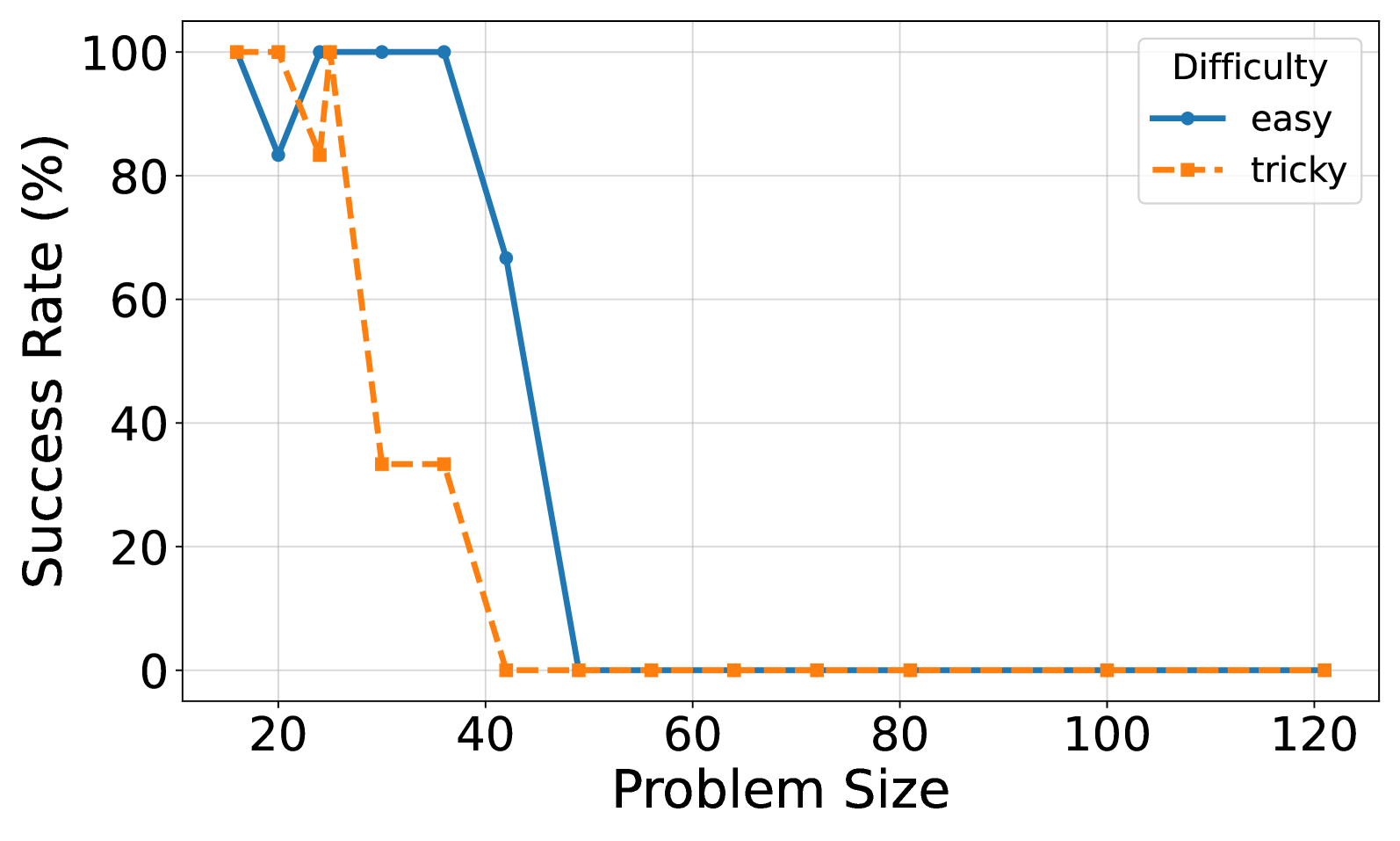
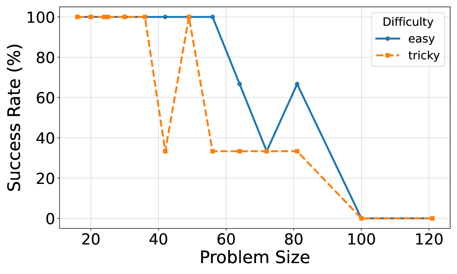
Figure 4: (a) Reasoning effort in number of reasoning tokens versus problem size for o3-mini with reasoning effort low. Successful tries only. Linear fits are added for each model. (b) Solved percentage versus problem size for o3-mini with reasoning effort low.
<details>
<summary>x7.png Details</summary>
### Visual Description
## Scatter Plot: Reasoning Tokens vs. Problem Size by Difficulty
### Overview
The image is a scatter plot showing the relationship between "Problem Size" and "Reasoning Tokens" for two difficulty levels: "easy" and "tricky". The plot includes trend lines (linear fits) for each difficulty level, along with their respective R-squared values.
### Components/Axes
* **X-axis:** "Problem Size", ranging from approximately 15 to 80 in increments of 10.
* **Y-axis:** "Reasoning Tokens", ranging from 0 to 30000 in increments of 5000.
* **Legend (top-left):**
* "Difficulty"
* Blue circle: "easy"
* Blue line: "easy fit (R^2: 0.829)"
* Orange square: "tricky"
* Orange dashed line: "tricky fit (R^2: 0.903)"
### Detailed Analysis
* **"easy" data series (blue circles):**
* Trend: Generally increasing as "Problem Size" increases.
* Data points:
* (20, ~2000)
* (25, ~3000)
* (25, ~5000)
* (30, ~4000)
* (35, ~6000)
* (40, ~7000)
* (45, ~6000)
* (50, ~9000)
* (50, ~13000)
* (55, ~12000)
* (60, ~13000)
* (65, ~12000)
* (70, ~23000)
* (80, ~13000)
* (80, ~18000)
* "easy fit (R^2: 0.829)": A blue line that represents the linear regression fit for the "easy" data points. The line starts at approximately (15, 0) and ends at approximately (80, 18000).
* **"tricky" data series (orange squares):**
* Trend: Generally increasing as "Problem Size" increases, with a steeper slope than the "easy" series.
* Data points:
* (20, ~2000)
* (20, ~4000)
* (25, ~3000)
* (25, ~5000)
* (30, ~5000)
* (30, ~8000)
* (35, ~10000)
* (40, ~12000)
* (45, ~13000)
* (50, ~13000)
* (50, ~21000)
* (55, ~17000)
* (60, ~18000)
* (70, ~33000)
* (80, ~29000)
* "tricky fit (R^2: 0.903)": An orange dashed line that represents the linear regression fit for the "tricky" data points. The line starts at approximately (15, 0) and ends at approximately (80, 30000).
### Key Observations
* Both "easy" and "tricky" problems show a positive correlation between "Problem Size" and "Reasoning Tokens".
* The "tricky" problems generally require more "Reasoning Tokens" than "easy" problems for a given "Problem Size".
* The R-squared value for the "tricky fit" (0.903) is higher than that of the "easy fit" (0.829), indicating a stronger linear relationship between "Problem Size" and "Reasoning Tokens" for "tricky" problems.
### Interpretation
The data suggests that as the size of a problem increases, the number of reasoning tokens required to solve it also increases. "Tricky" problems require more reasoning tokens than "easy" problems of the same size, indicating that they are inherently more complex and demand more cognitive resources. The higher R-squared value for the "tricky" problems suggests that the relationship between problem size and reasoning tokens is more consistent and predictable for "tricky" problems compared to "easy" problems. This could be because the "easy" problems have more variability in their structure or solution paths, leading to a less consistent relationship.
</details>
(a)
<details>
<summary>x8.png Details</summary>
### Visual Description
## Line Chart: Success Rate vs. Problem Size by Difficulty
### Overview
The image is a line chart comparing the success rate of solving problems of varying sizes, categorized by difficulty (easy and tricky). The x-axis represents the problem size, and the y-axis represents the success rate in percentage. The chart displays two lines, one for "easy" problems (solid blue) and one for "tricky" problems (dashed orange).
### Components/Axes
* **Title:** There is no explicit title on the chart.
* **X-axis:** "Problem Size", with tick marks at 20, 40, 60, 80, 100, and 120.
* **Y-axis:** "Success Rate (%)", with tick marks at 0, 20, 40, 60, 80, and 100.
* **Legend:** Located in the top-right corner, labeled "Difficulty".
* "easy": Represented by a solid blue line with circular markers.
* "tricky": Represented by a dashed orange line with square markers.
### Detailed Analysis
**Easy Problems (Solid Blue Line):**
* Trend: The success rate for easy problems remains at 100% until a problem size of approximately 60. It then decreases, rises again, and then decreases to 0% at a problem size of 100.
* Data Points:
* Problem Size 20-60: Success Rate 100%
* Problem Size 60: Success Rate ~67%
* Problem Size 80: Success Rate ~67%
* Problem Size 100-120: Success Rate 0%
**Tricky Problems (Dashed Orange Line):**
* Trend: The success rate for tricky problems remains at 100% until a problem size of approximately 40. It then fluctuates significantly before decreasing to 0% at a problem size of 100.
* Data Points:
* Problem Size 20-40: Success Rate 100%
* Problem Size 40: Success Rate ~33%
* Problem Size 60: Success Rate ~33%
* Problem Size 80: Success Rate ~33%
* Problem Size 100-120: Success Rate 0%
### Key Observations
* For smaller problem sizes (20-40), both "easy" and "tricky" problems have a 100% success rate.
* The success rate for "tricky" problems drops sharply at a problem size of 40, while the success rate for "easy" problems remains high until a problem size of 60.
* Both "easy" and "tricky" problems have a 0% success rate for problem sizes of 100 and above.
* The "easy" problem success rate peaks at problem size 80.
### Interpretation
The chart suggests that problem size significantly impacts the success rate, especially for "tricky" problems. "Easy" problems are solvable until a larger problem size is reached. Both types of problems become unsolvable as the problem size increases beyond a certain threshold (around 100). The fluctuation in the "tricky" problem success rate between problem sizes 40 and 80 indicates that other factors besides size may influence the difficulty of these problems. The data demonstrates that problem difficulty is not solely determined by size, as "tricky" problems show a more volatile success rate compared to "easy" problems.
</details>
(b)
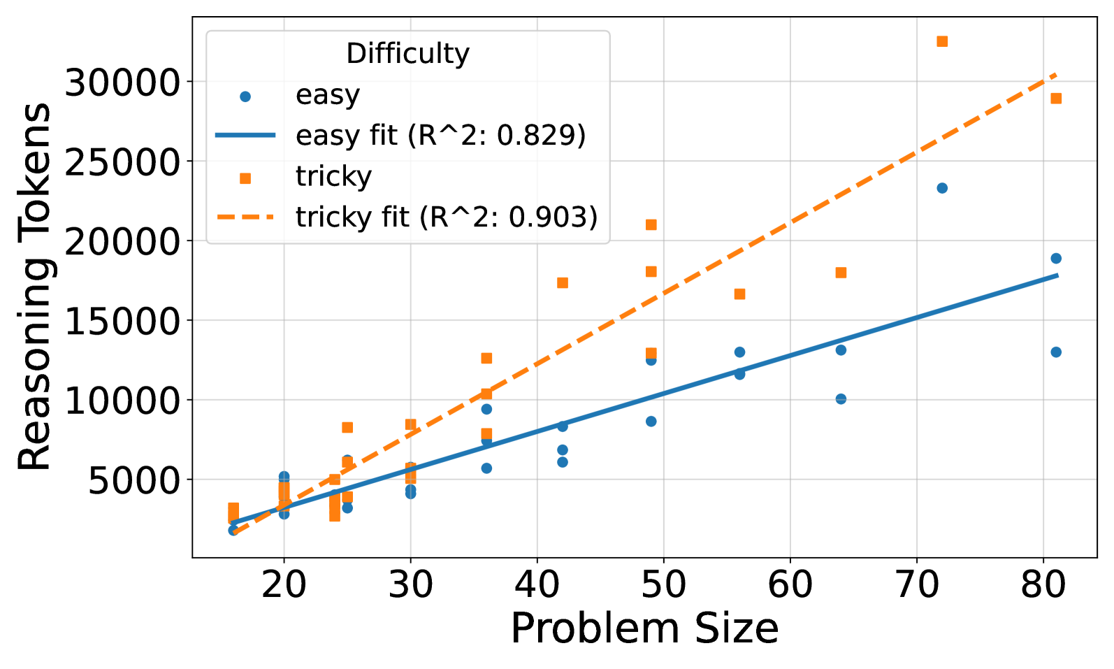
Figure 5: (a) Reasoning effort in number of reasoning tokens versus problem size for o3-mini with reasoning effort medium. Successful tries only. Linear fits are added for each model. (b) Solved percentage versus problem size for o3-mini with reasoning effort medium.
<details>
<summary>x9.png Details</summary>
### Visual Description
## Scatter Plot: Reasoning Tokens vs. Problem Size by Difficulty
### Overview
The image is a scatter plot showing the relationship between "Reasoning Tokens" and "Problem Size" for two categories of problem difficulty: "easy" and "tricky". Each category has a scatter plot of data points and a linear regression fit line with an R-squared value. The plot aims to visualize how the number of reasoning tokens changes with problem size for different difficulty levels.
### Components/Axes
* **X-axis:** "Problem Size", with a numerical scale ranging from 20 to 100 in increments of 20.
* **Y-axis:** "Reasoning Tokens", with a numerical scale ranging from 0 to 60000 in increments of 10000.
* **Legend (top-left):**
* "Difficulty"
* Blue circle: "easy"
* Solid blue line: "easy fit (R^2: 0.811)"
* Orange square: "tricky"
* Dashed orange line: "tricky fit (R^2: 0.607)"
### Detailed Analysis
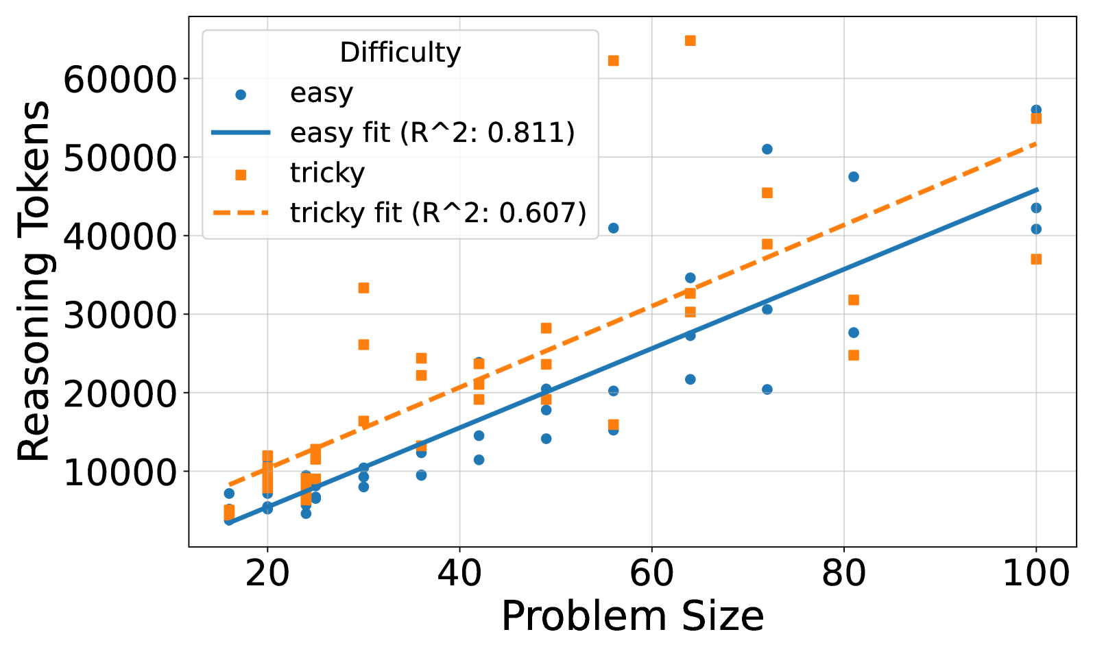
**1. Easy Problems (Blue Circles and Solid Blue Line):**
* **Trend:** The "easy" data points generally show an upward trend, indicating that as the problem size increases, the number of reasoning tokens also tends to increase.
* **Data Points:**
* At Problem Size = 20, Reasoning Tokens range from approximately 4000 to 10000.
* At Problem Size = 40, Reasoning Tokens range from approximately 8000 to 15000.
* At Problem Size = 60, Reasoning Tokens range from approximately 15000 to 22000.
* At Problem Size = 80, Reasoning Tokens range from approximately 20000 to 50000.
* At Problem Size = 100, Reasoning Tokens range from approximately 40000 to 55000.
* **Fit Line:** The solid blue line represents the linear regression fit for the "easy" data. It has an R-squared value of 0.811, indicating a strong positive linear relationship.
**2. Tricky Problems (Orange Squares and Dashed Orange Line):**
* **Trend:** The "tricky" data points also show an upward trend, but with more variability compared to the "easy" data.
* **Data Points:**
* At Problem Size = 20, Reasoning Tokens range from approximately 8000 to 12000.
* At Problem Size = 40, Reasoning Tokens range from approximately 10000 to 35000.
* At Problem Size = 60, Reasoning Tokens range from approximately 15000 to 65000.
* At Problem Size = 80, Reasoning Tokens range from approximately 25000 to 30000.
* At Problem Size = 100, Reasoning Tokens range from approximately 35000 to 55000.
* **Fit Line:** The dashed orange line represents the linear regression fit for the "tricky" data. It has an R-squared value of 0.607, indicating a moderate positive linear relationship.
### Key Observations
* Both "easy" and "tricky" problems show a positive correlation between problem size and the number of reasoning tokens.
* The "easy" problems have a higher R-squared value (0.811) compared to the "tricky" problems (0.607), suggesting a stronger linear relationship between problem size and reasoning tokens for "easy" problems.
* The "tricky" problems exhibit more variability in the number of reasoning tokens for a given problem size, as indicated by the wider spread of data points around the regression line.
* For smaller problem sizes (around 20), the reasoning tokens are similar for both easy and tricky problems. However, as the problem size increases, the "tricky" problems tend to require more reasoning tokens than the "easy" problems.
### Interpretation
The data suggests that as problem size increases, the number of reasoning tokens required to solve the problem also increases, regardless of the difficulty level. However, the relationship is stronger and more predictable for "easy" problems compared to "tricky" problems. The lower R-squared value for "tricky" problems indicates that other factors, besides problem size, may significantly influence the number of reasoning tokens required. These factors could include the specific nature of the problem, the complexity of the reasoning steps, or the presence of misleading information. The greater variability in reasoning tokens for "tricky" problems suggests that these problems may require more diverse and potentially less efficient reasoning strategies. The fact that "tricky" problems tend to require more reasoning tokens than "easy" problems as problem size increases is intuitive, as "tricky" problems likely involve more complex logic or require more steps to arrive at a solution.
</details>
(a)
<details>
<summary>x10.png Details</summary>
### Visual Description
## Line Chart: Success Rate vs. Problem Size by Difficulty
### Overview
The image is a line chart that plots the success rate (in percentage) against the problem size for two different difficulty levels: "easy" and "tricky". The chart shows how the success rate changes as the problem size increases for each difficulty level.
### Components/Axes
* **Title:** There is no explicit title on the chart.
* **X-axis:**
* Label: "Problem Size"
* Scale: 20 to 120, with tick marks at intervals of 20 (20, 40, 60, 80, 100, 120)
* **Y-axis:**
* Label: "Success Rate (%)"
* Scale: 0 to 100, with tick marks at intervals of 20 (0, 20, 40, 60, 80, 100)
* **Legend:** Located in the bottom-left corner of the chart.
* "Difficulty"
* "easy": Represented by a solid blue line with circular markers.
* "tricky": Represented by a dashed orange line with square markers.
### Detailed Analysis
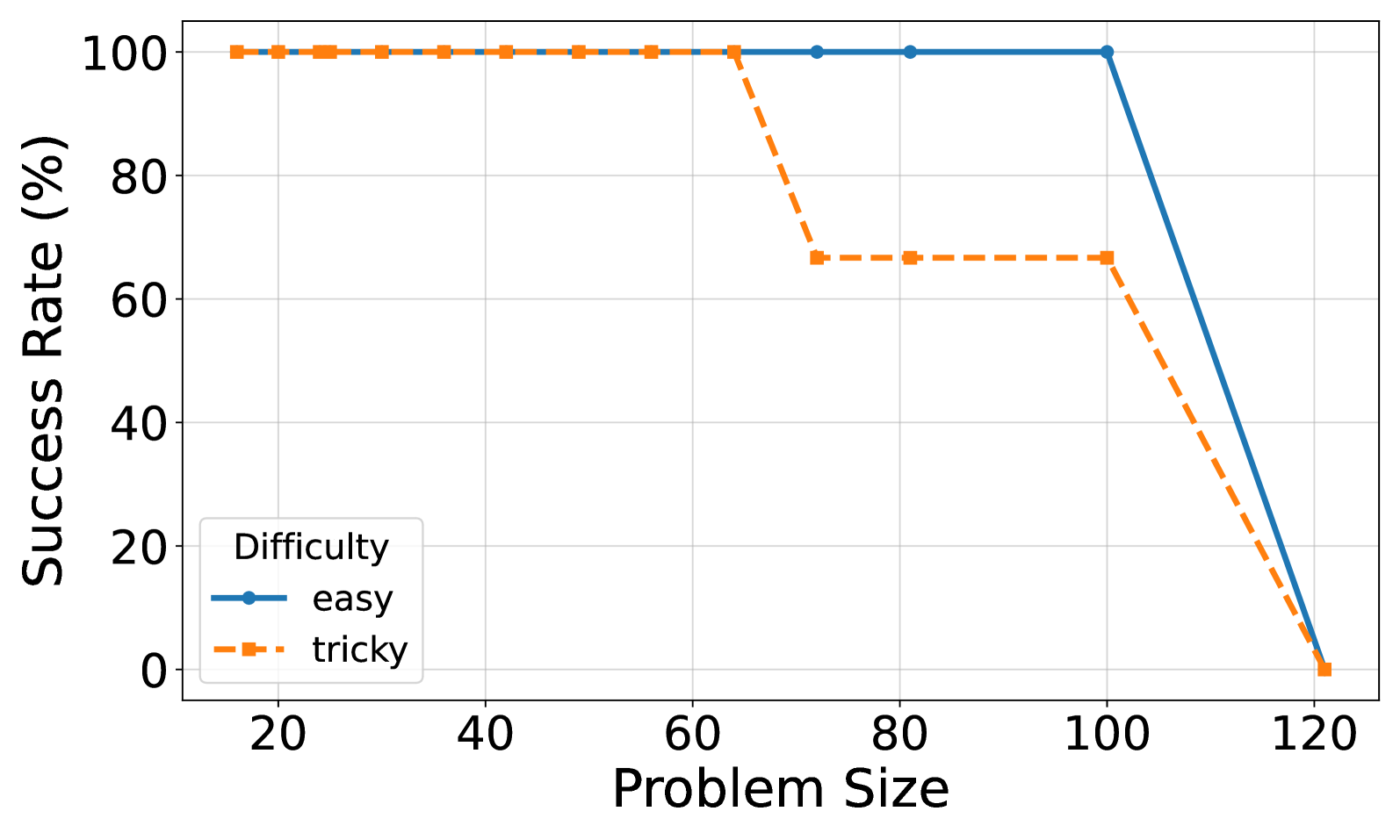
* **"easy" (blue line):**
* Trend: The success rate remains at 100% until a problem size of approximately 80. After that, it drops linearly to 0% at a problem size of 120.
* Data Points:
* Problem Size 20-80: Success Rate 100%
* Problem Size 100: Success Rate ~67%
* Problem Size 120: Success Rate 0%
* **"tricky" (orange dashed line):**
* Trend: The success rate remains at 100% until a problem size of approximately 60. It then drops to approximately 67% and remains constant until a problem size of 100, after which it drops linearly to 0% at a problem size of 120.
* Data Points:
* Problem Size 20-60: Success Rate 100%
* Problem Size 80-100: Success Rate ~67%
* Problem Size 120: Success Rate 0%
### Key Observations
* For smaller problem sizes (20-60), both difficulty levels have a 100% success rate.
* The "tricky" difficulty level experiences a drop in success rate earlier than the "easy" difficulty level.
* Both difficulty levels reach a 0% success rate at a problem size of 120.
* The "easy" difficulty maintains a 100% success rate for a longer range of problem sizes compared to the "tricky" difficulty.
### Interpretation
The chart demonstrates the relationship between problem size and success rate for different difficulty levels. It suggests that as the problem size increases, the success rate decreases, and this decrease is more pronounced for the "tricky" difficulty level. The "easy" difficulty level is more resilient to increasing problem sizes, maintaining a high success rate for a longer range. The data indicates that the "tricky" problems become difficult at a smaller problem size than the "easy" problems. The eventual convergence to 0% success rate for both difficulty levels at a problem size of 120 suggests a limit to the problem-solving capability, regardless of difficulty, as the problem size becomes sufficiently large.
</details>
(b)
Figure 6: (a) Reasoning effort in number of reasoning tokens versus problem size for o3-mini with reasoning effort high. Successful tries only. Linear fits are added for each model. (b) Solved percentage versus problem size for o3-mini with reasoning effort high.
A.2.2 Reasoning Effort for All Models
<details>
<summary>x11.png Details</summary>
### Visual Description
## Scatter Plot: Reasoning Tokens vs. Problem Size for qwen/qwq-32b-preview
### Overview
The image is a scatter plot showing the relationship between "Reasoning Tokens" and "Problem Size" for a model named "qwen/qwq-32b-preview". The plot distinguishes between successful and failed attempts using different markers: blue circles for successful attempts and orange squares for failed attempts.
### Components/Axes
* **X-axis (Horizontal):** "Problem Size". The scale ranges from 0 to 400, with tick marks at intervals of 100.
* **Y-axis (Vertical):** "Reasoning Tokens". The scale ranges from 0 to 20000, with tick marks at intervals of 5000.
* **Legend (Top-Right):**
* Blue Circle: "qwen/qwq-32b-preview (Successful)"
* Orange Square: "qwen/qwq-32b-preview (Failed)"
### Detailed Analysis
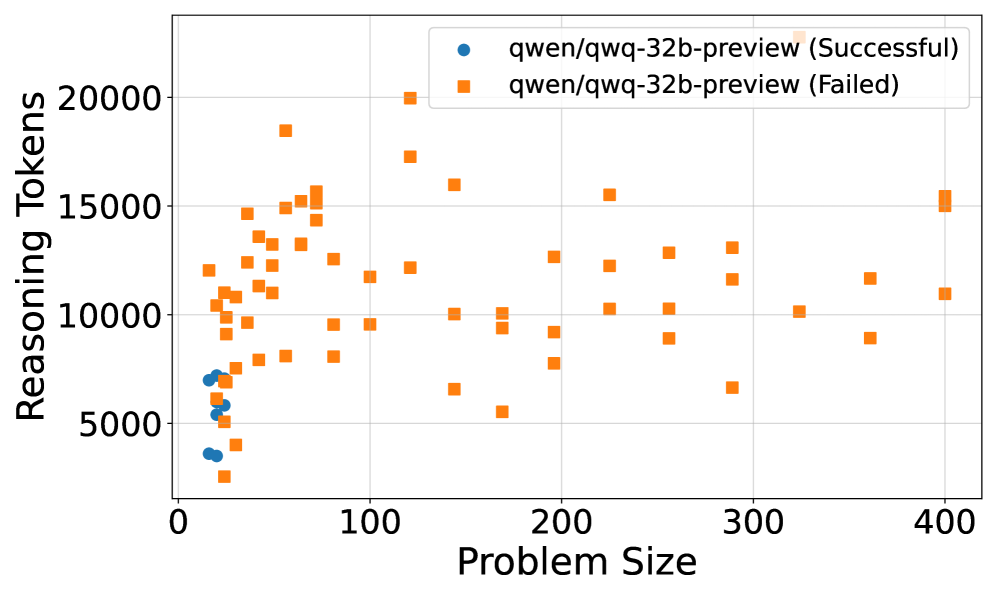
* **Successful Attempts (Blue Circles):**
* All successful attempts occur at small problem sizes, specifically below 50.
* Reasoning tokens for successful attempts range approximately from 3000 to 7000.
* The trend for successful attempts is that as problem size increases (from approximately 10 to 50), the reasoning tokens appear to increase slightly.
* Specific data points:
* Problem Size ~10, Reasoning Tokens ~3500
* Problem Size ~15, Reasoning Tokens ~5500
* Problem Size ~20, Reasoning Tokens ~5000
* Problem Size ~25, Reasoning Tokens ~7000
* Problem Size ~30, Reasoning Tokens ~6000
* **Failed Attempts (Orange Squares):**
* Failed attempts are scattered across the entire range of problem sizes (approximately 10 to 400).
* Reasoning tokens for failed attempts range approximately from 5000 to 20000.
* There is no clear trend between problem size and reasoning tokens for failed attempts. The data points appear randomly distributed.
* Specific data points:
* Problem Size ~10, Reasoning Tokens ~7000 to 16000
* Problem Size ~50, Reasoning Tokens ~8000 to 15000
* Problem Size ~100, Reasoning Tokens ~6000 to 18000
* Problem Size ~200, Reasoning Tokens ~6000 to 13000
* Problem Size ~300, Reasoning Tokens ~7000 to 13000
* Problem Size ~400, Reasoning Tokens ~12000 to 16000
### Key Observations
* The model "qwen/qwq-32b-preview" only succeeds on problems with small problem sizes (less than 50).
* The number of reasoning tokens required for successful attempts is significantly lower and more consistent than for failed attempts.
* Failed attempts show a wide range of reasoning tokens, regardless of problem size.
### Interpretation
The scatter plot suggests that the "qwen/qwq-32b-preview" model struggles with larger problem sizes. The successful attempts are clustered at low problem sizes, indicating a limitation in the model's ability to handle complex or large-scale reasoning tasks. The wide distribution of reasoning tokens for failed attempts suggests that the model's performance is inconsistent and unpredictable when it fails. The data implies that the model may require further optimization or a different approach to handle larger problem sizes effectively. The fact that successful attempts require fewer reasoning tokens could indicate that the model is more efficient when it can solve the problem, but struggles to find a solution for larger problems, leading to a higher and more variable token count.
</details>
Figure 7: Reasoning effort in tokens for Qwen QwQ.
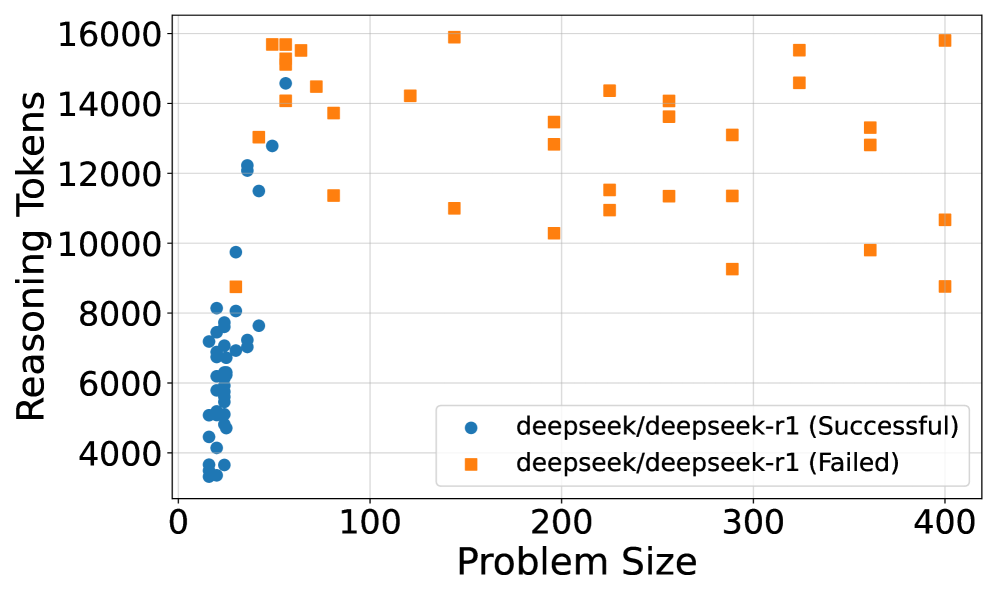
<details>
<summary>x12.png Details</summary>
### Visual Description
## Scatter Plot: Reasoning Tokens vs. Problem Size for deepseek/deepseek-r1
### Overview
The image is a scatter plot showing the relationship between "Reasoning Tokens" and "Problem Size" for the deepseek/deepseek-r1 model. The plot distinguishes between successful and failed attempts using different colored markers: blue circles for successful attempts and orange squares for failed attempts. The plot shows that successful attempts tend to cluster at smaller problem sizes, while failed attempts are scattered across a wider range of problem sizes and token counts.
### Components/Axes
* **X-axis:** Problem Size, ranging from 0 to 400. Axis markers are present at 0, 100, 200, 300, and 400.
* **Y-axis:** Reasoning Tokens, ranging from 4000 to 16000. Axis markers are present at 4000, 6000, 8000, 10000, 12000, 14000, and 16000.
* **Legend:** Located in the bottom-right corner of the plot.
* Blue circles: deepseek/deepseek-r1 (Successful)
* Orange squares: deepseek/deepseek-r1 (Failed)
### Detailed Analysis
* **deepseek/deepseek-r1 (Successful):**
* The blue circles, representing successful attempts, are concentrated at smaller problem sizes (0-100).
* The number of reasoning tokens for successful attempts generally ranges from approximately 3500 to 14500.
* The trend for successful attempts shows a slight increase in reasoning tokens as the problem size increases within the 0-100 range.
* Specific data points:
* Problem Size ~10, Reasoning Tokens ~3500
* Problem Size ~20, Reasoning Tokens ~5000
* Problem Size ~30, Reasoning Tokens ~7000
* Problem Size ~40, Reasoning Tokens ~7500
* Problem Size ~50, Reasoning Tokens ~7500
* Problem Size ~60, Reasoning Tokens ~8000
* Problem Size ~70, Reasoning Tokens ~12000
* Problem Size ~80, Reasoning Tokens ~14500
* **deepseek/deepseek-r1 (Failed):**
* The orange squares, representing failed attempts, are scattered across a wider range of problem sizes (approximately 50 to 400).
* The number of reasoning tokens for failed attempts ranges from approximately 8500 to 16000.
* There is no clear trend between problem size and reasoning tokens for failed attempts.
* Specific data points:
* Problem Size ~50, Reasoning Tokens ~15500
* Problem Size ~75, Reasoning Tokens ~14000
* Problem Size ~100, Reasoning Tokens ~11500
* Problem Size ~150, Reasoning Tokens ~14000
* Problem Size ~175, Reasoning Tokens ~11000
* Problem Size ~200, Reasoning Tokens ~13500
* Problem Size ~225, Reasoning Tokens ~11500
* Problem Size ~250, Reasoning Tokens ~14000
* Problem Size ~275, Reasoning Tokens ~9000
* Problem Size ~300, Reasoning Tokens ~11500
* Problem Size ~325, Reasoning Tokens ~14000
* Problem Size ~350, Reasoning Tokens ~13000
* Problem Size ~375, Reasoning Tokens ~10000
* Problem Size ~400, Reasoning Tokens ~9000
### Key Observations
* Successful attempts are clustered at smaller problem sizes, suggesting that the model is more likely to succeed with simpler problems.
* Failed attempts are scattered across a wider range of problem sizes, indicating that larger problem sizes do not guarantee failure, but the model's performance becomes less predictable.
* The number of reasoning tokens used in failed attempts is generally higher than in successful attempts, suggesting that the model may be using more resources when it fails.
### Interpretation
The data suggests that the deepseek/deepseek-r1 model is more effective at solving smaller problems. As the problem size increases, the model's success rate decreases, and the number of reasoning tokens used in failed attempts tends to be higher. This could indicate that the model struggles to efficiently process larger, more complex problems, leading to increased resource consumption and eventual failure. The scattering of failed attempts across a wide range of problem sizes and token counts suggests that other factors, besides problem size and token usage, may also contribute to the model's failure. Further investigation is needed to identify these factors and improve the model's performance on larger problems.
</details>
Figure 8: Reasoning effort in tokens for Deepseek R1.
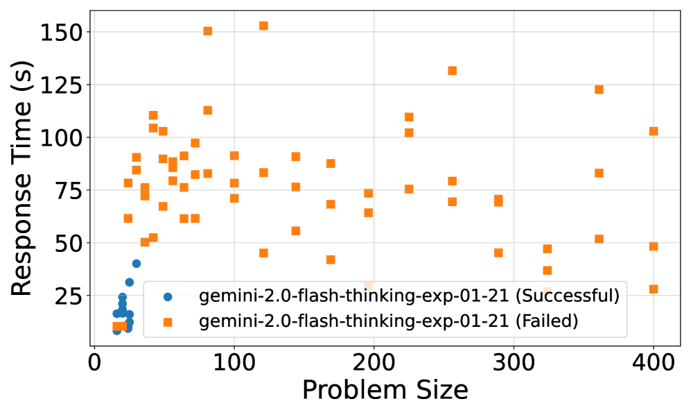
<details>
<summary>x13.png Details</summary>
### Visual Description
## Scatter Plot: Response Time vs. Problem Size
### Overview
The image is a scatter plot comparing the response time (in seconds) against the problem size for the 'gemini-2.0-flash-thinking-exp-01-21' experiment. The plot distinguishes between successful and failed attempts, with successful attempts marked in blue and failed attempts in orange.
### Components/Axes
* **X-axis:** Problem Size, ranging from 0 to 400. Axis markers are present at 0, 100, 200, 300, and 400.
* **Y-axis:** Response Time (s), ranging from 0 to 150. Axis markers are present at 0, 25, 50, 75, 100, 125, and 150.
* **Legend:** Located in the bottom-right corner.
* Blue circles: 'gemini-2.0-flash-thinking-exp-01-21 (Successful)'
* Orange squares: 'gemini-2.0-flash-thinking-exp-01-21 (Failed)'
### Detailed Analysis
* **Successful Attempts (Blue):**
* All successful attempts are clustered at the lower left of the graph, with problem sizes between 0 and approximately 50.
* Response times for successful attempts range from approximately 5 seconds to 40 seconds.
* Trend: Successful attempts are concentrated at smaller problem sizes and lower response times.
* Specific Data Points:
* (Problem Size ~10, Response Time ~10)
* (Problem Size ~10, Response Time ~15)
* (Problem Size ~10, Response Time ~20)
* (Problem Size ~20, Response Time ~10)
* (Problem Size ~20, Response Time ~25)
* (Problem Size ~30, Response Time ~35)
* (Problem Size ~50, Response Time ~40)
* **Failed Attempts (Orange):**
* Failed attempts are scattered across the plot, with problem sizes ranging from approximately 10 to 400.
* Response times for failed attempts range from approximately 10 seconds to 155 seconds.
* Trend: Failed attempts are more prevalent at larger problem sizes and higher response times, but are present across the entire problem size range.
* Specific Data Points:
* (Problem Size ~10, Response Time ~10)
* (Problem Size ~20, Response Time ~10)
* (Problem Size ~20, Response Time ~15)
* (Problem Size ~20, Response Time ~20)
* (Problem Size ~30, Response Time ~60)
* (Problem Size ~40, Response Time ~80)
* (Problem Size ~50, Response Time ~90)
* (Problem Size ~60, Response Time ~60)
* (Problem Size ~70, Response Time ~90)
* (Problem Size ~80, Response Time ~75)
* (Problem Size ~90, Response Time ~90)
* (Problem Size ~100, Response Time ~75)
* (Problem Size ~110, Response Time ~45)
* (Problem Size ~120, Response Time ~75)
* (Problem Size ~130, Response Time ~75)
* (Problem Size ~140, Response Time ~155)
* (Problem Size ~150, Response Time ~75)
* (Problem Size ~160, Response Time ~75)
* (Problem Size ~170, Response Time ~75)
* (Problem Size ~180, Response Time ~75)
* (Problem Size ~190, Response Time ~75)
* (Problem Size ~200, Response Time ~100)
* (Problem Size ~210, Response Time ~110)
* (Problem Size ~220, Response Time ~75)
* (Problem Size ~230, Response Time ~130)
* (Problem Size ~240, Response Time ~75)
* (Problem Size ~250, Response Time ~75)
* (Problem Size ~260, Response Time ~75)
* (Problem Size ~270, Response Time ~75)
* (Problem Size ~280, Response Time ~75)
* (Problem Size ~290, Response Time ~75)
* (Problem Size ~300, Response Time ~75)
* (Problem Size ~310, Response Time ~75)
* (Problem Size ~320, Response Time ~75)
* (Problem Size ~330, Response Time ~75)
* (Problem Size ~340, Response Time ~75)
* (Problem Size ~350, Response Time ~75)
* (Problem Size ~360, Response Time ~75)
* (Problem Size ~370, Response Time ~75)
* (Problem Size ~380, Response Time ~75)
* (Problem Size ~390, Response Time ~100)
* (Problem Size ~400, Response Time ~30)
### Key Observations
* Successful attempts are limited to smaller problem sizes.
* Failed attempts occur across a wide range of problem sizes and response times.
* There is a clear separation between successful and failed attempts based on problem size.
### Interpretation
The data suggests that the 'gemini-2.0-flash-thinking-exp-01-21' experiment is only successful for smaller problem sizes. As the problem size increases, the experiment is more likely to fail, and the response time tends to be higher. This could indicate a limitation in the algorithm's ability to handle larger, more complex problems within a reasonable time frame. The clustering of successful attempts at low problem sizes and response times indicates a region of efficiency for the algorithm. The scattering of failed attempts suggests that factors beyond just problem size may contribute to failures, as some failures occur even at smaller problem sizes, albeit with longer response times.
</details>
Figure 9: Reasoning effort quantified by response time for Gemini-2.0-flash-thinking.
A.3 Cost
Total cost of these experiments was around 80 USD in API credits.