# Reasoning Effort and Problem Complexity: A Scaling Analysis in LLMs
**Authors**: Benjamin Estermann, ETH Zürich, &Roger Wattenhofer, ETH Zürich
## Abstract
Large Language Models (LLMs) have demonstrated remarkable text generation capabilities, and recent advances in training paradigms have led to breakthroughs in their reasoning performance. In this work, we investigate how the reasoning effort of such models scales with problem complexity. We use the infinitely scalable Tents puzzle, which has a known linear-time solution, to analyze this scaling behavior. Our results show that reasoning effort scales with problem size, but only up to a critical problem complexity. Beyond this threshold, the reasoning effort does not continue to increase, and may even decrease. This observation highlights a critical limitation in the logical coherence of current LLMs as problem complexity increases, and underscores the need for strategies to improve reasoning scalability. Furthermore, our results reveal significant performance differences between current state-of-the-art reasoning models when faced with increasingly complex logical puzzles.
## 1 Introduction
Large language models (LLMs) have demonstrated remarkable abilities in a wide range of natural language tasks, from text generation to complex problem-solving. Recent advances, particularly with models trained for enhanced reasoning, have pushed the boundaries of what machines can achieve in tasks requiring logical inference and deduction.
<details>
<summary>extracted/6290299/Figures/tents.png Details</summary>
### Visual Description
\n
## Diagram: 6x6 Icon Grid Puzzle with Numerical Clues
### Overview
The image displays a 6x6 grid-based logic puzzle, likely a variant of "Nonograms" or "Picross," where icons (trees and triangles) are placed in some cells. Numerical clues are provided along the right (row clues) and bottom (column clues) of the grid. The grid cells are outlined in dark gray, and cells containing icons are highlighted with a light green background. The overall background is light gray.
### Components/Axes
- **Grid Structure**: 6 rows × 6 columns.
- **Icons**: Two distinct types:
- **Green Tree**: A stylized green tree with a brown trunk.
- **Yellow Triangle**: A solid yellow triangle pointing upward.
- **Numerical Clues**:
- **Right Side (Row Clues)**: Numbers aligned to the right of each row, from top to bottom: `1, 1, 2, 0, 0, 3`.
- **Bottom (Column Clues)**: Numbers aligned below each column, from left to right: `1, 1, 1, 2, 0, 2`.
- **Highlighting**: Cells containing any icon have a light green fill; empty cells have no fill (transparent/light gray).
### Detailed Analysis
**Grid Contents (Row-by-Row, Left to Right):**
- **Row 1 (Top)**: Columns 1–4: Empty. Column 5: Tree. Column 6: Empty.
- **Row 2**: Column 1: Tree. Column 2: Triangle. Columns 3–6: Empty.
- **Row 3**: Columns 1–2: Empty. Column 3: Tree. Columns 4–5: Empty. Column 6: Triangle.
- **Row 4**: Columns 1–5: Empty. Column 6: Tree.
- **Row 5**: Columns 1–2: Empty. Column 3: Tree. Columns 4–5: Empty. Column 6: Tree.
- **Row 6 (Bottom)**: Column 1: Triangle. Column 2: Tree. Column 3: Triangle. Columns 4–5: Empty. Column 6: Triangle.
**Icon Counts per Row and Column:**
- **Row Totals**:
- Row 1: 1 icon (tree).
- Row 2: 2 icons (1 tree, 1 triangle).
- Row 3: 2 icons (1 tree, 1 triangle).
- Row 4: 1 icon (tree).
- Row 5: 2 icons (2 trees).
- Row 6: 4 icons (1 tree, 3 triangles).
- **Column Totals**:
- Column 1: 2 icons (1 tree, 1 triangle).
- Column 2: 2 icons (1 tree, 1 triangle).
- Column 3: 3 icons (2 trees, 1 triangle).
- Column 4: 0 icons.
- Column 5: 1 icon (tree).
- Column 6: 4 icons (2 trees, 2 triangles).
**Clue vs. Actual Icon Count Discrepancies:**
- Row clues do not consistently match the total icon count per row (e.g., Row 2 clue is `1` but has 2 icons; Row 4 clue is `0` but has 1 icon).
- Column clues similarly show mismatches (e.g., Column 6 clue is `2` but has 4 icons).
- This suggests the clues may represent something other than total icon count, such as:
- The number of **consecutive icon groups** in that row/column.
- The count of a **specific icon type** (e.g., triangles only).
- A **separate puzzle logic** (e.g., clues for a solution state not fully shown).
### Key Observations
1. **Spatial Distribution**: Icons are clustered in the left and right columns, with column 4 completely empty.
2. **Icon Type Patterns**: Triangles appear only in columns 1, 2, 3, and 6. Trees appear in all columns except column 4.
3. **Highlight Consistency**: All cells with icons are highlighted; no empty cells are highlighted.
4. **Clue Anomalies**: The clue `0` appears for Row 4, Row 5, and Column 5, yet these rows/columns contain icons. This is a significant inconsistency if clues are meant to indicate icon presence.
### Interpretation
This image likely represents a **logic puzzle in progress or as an example**. The numerical clues are integral to solving the puzzle, but their exact meaning is ambiguous without additional context (e.g., puzzle rules). The discrepancies between clues and icon counts suggest one of the following:
- The clues indicate **groups of consecutive icons** rather than totals. For example, Row 2 has one consecutive group (tree and triangle adjacent), matching clue `1`. Row 3 has two separate groups (tree in column 3, triangle in column 6), matching clue `2`. However, Row 4 has one group but clue `0`, contradicting this.
- The clues might represent **the number of triangles per row/column**. Row 6 has three triangles, matching clue `3`. Column 6 has two triangles, matching clue `2`. But Row 2 has one triangle and clue `1`, which fits, while Row 3 has one triangle and clue `2`, which does not.
- Alternatively, this could be a **partially filled puzzle** where the icons are the solver's entries, and the clues are the original hints. The mismatches may indicate errors in the solver's placement.
The puzzle's design—with two icon types and numerical clues—implies a need to deduce correct icon placement based on constraints. The empty column 4 and clustered icons suggest strategic placement rules. For a complete understanding, the puzzle's specific ruleset (e.g., whether icons must be consecutive, whether clues count specific types, or whether there are hidden constraints) would be required.
</details>
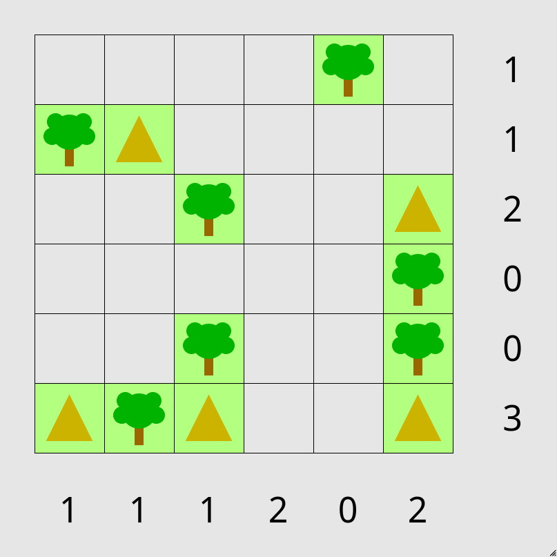
Figure 1: An example instance of a partially solved 6 by 6 tents puzzle. Tents need to be placed next to trees, away from other tents and fulfilling the row and column constraints.
A critical factor in the success of these advanced models is the ability to leverage increased computational resources at test time, allowing them to explore more intricate solution spaces. This capability raises a fundamental question: how does the ”reasoning effort” of these models scale as the complexity of the problem increases?
Understanding this scaling relationship is crucial for several reasons. First, it sheds light on the fundamental nature of reasoning within LLMs, moving beyond simply measuring accuracy on isolated tasks. By examining how the computational demands, reflected in token usage, evolve with problem difficulty, we can gain insights into the efficiency and potential bottlenecks of current LLM architectures. Second, characterizing this scaling behavior is essential for designing more effective and resource-efficient reasoning models in the future.
In this work, we address this question by investigating the scaling of reasoning effort in LLMs using a specific, infinitely scalable logic puzzle: the Tents puzzle The puzzle is available to play in the browser at https://www.chiark.greenend.org.uk/~sgtatham/puzzles/js/tents.html (see Figure 1). This puzzle offers a controlled environment for studying algorithmic reasoning, as its problem size can be systematically increased, and it possesses a known linear-time solution. Our analysis focuses on how the number of tokens used by state-of-the-art reasoning LLMs changes as the puzzle grid size grows. In addition to reasoning effort, we also evaluate the success rate across different puzzle sizes to provide a comprehensive view of their performance.
## 2 Related Work
The exploration of reasoning abilities in large language models (LLMs) is a rapidly evolving field with significant implications for artificial intelligence. Several benchmarks have been developed to evaluate the reasoning capabilities of LLMs across various domains. These benchmarks provide standardized tasks and evaluation metrics to assess and compare different models. Notable benchmarks include GSM8K (Cobbe et al., 2021), ARC-AGI (Chollet, 2019), GPQA (Rein et al., 2023), MMLU (Hendrycks et al., 2020), SWE-bench (Jimenez et al., 2023) and NPhard-eval (Fan et al., 2023). These benchmarks cover topics from mathematics to commonsense reasoning and coding. More recently, also math competitions such as AIME2024 (of America, 2024) have been used to evaluate the newest models. Estermann et al. (2024) have introduced PUZZLES, a benchmark focusing on algorithmic and logical reasoning for reinforcement learning. While PUZZLES does not focus on LLMs, except for a short ablation in the appendix, we argue that the scalability provided by the underlying puzzles is an ideal testbed for testing extrapolative reasoning capabilities in LLMs.
The reasoning capabilities of traditional LLMs without specific prompting strategies are quite limited (Huang & Chang, 2022). Using prompt techniques such as chain-of-thought (Wei et al., 2022), least-to-most (Zhou et al., 2022) and tree-of-thought (Yao et al., 2023), the reasoning capabilities of traditional LLMs can be greatly improved. Lee et al. (2024) have introduced the Language of Thought Hypothesis, based on the idea that human reasoning is rooted in language. Lee et al. propose to see the reasoning capabilities through three different properties: Logical coherence, compositionality and productivity. In this work we will mostly focus on the aspect of algorithmic reasoning, which falls into logical coherence. Specifically, we analyze the limits of logical coherence.
With the release of OpenAI’s o1 model, it became apparent that new training strategies based on reinforcement learning are able to boost the reasoning performance even further. Since o1, there now exist a number of different models capable of enhanced reasoning (Guo et al., 2025; DeepMind, 2025; Qwen, 2024; OpenAI, 2025). Key to the success of these models is the scaling of test-time compute. Instead of directly producing an answer, or thinking for a few steps using chain-of-thought, the models are now trained to think using several thousands of tokens before coming up with an answer.
## 3 Methods
### 3.1 The Tents Puzzle Problem
In this work, we employ the Tents puzzle, a logic problem that is both infinitely scalable and solvable in linear time See a description of the algorithm of the solver as part of the PUZZLES benchmark here: https://github.com/ETH-DISCO/rlp/blob/main/puzzles/tents.c#L206C3-L206C67, making it an ideal testbed for studying algorithmic reasoning in LLMs. The Tents puzzle, popularized by Simon Tatham’s Portable Puzzle Collection (Tatham, ), requires deductive reasoning to solve. The puzzle is played on a rectangular grid, where some cells are pre-filled with trees. The objective is to place tents in the remaining empty cells according to the following rules:
- no two tents are adjacent, even diagonally
- there are exactly as many tents as trees and the number of tents in each row and column matches the numbers around the edge of the grid
- it is possible to match all tents to trees so that each tent is orthogonally adjacent to its own tree (a tree may also be adjacent to other tents).
An example instance of the Tents puzzle is visualized in Figure 1 in the Introduction. The scalability of the puzzle is achieved by varying the grid dimensions, allowing for systematic exploration of problem complexity. Where not otherwise specified, we used the ”easy” difficulty preset available in the Tents puzzle generator, with ”tricky” being evaluated in Section A.2.1. Crucially, the Tents puzzle is designed to test extrapolative reasoning as puzzle instances, especially larger ones, are unlikely to be present in the training data of LLMs. We utilized a text-based interface for the Tents puzzle, extending the code base provided by Estermann et al. (2024) to generate puzzle instances and represent the puzzle state in a format suitable for LLMs.
Models were presented with the same prompt (detailed in Appendix A.1) for all puzzle sizes and models tested. The prompt included the puzzle rules and the initial puzzle state in a textual format. Models were tasked with directly outputting the solved puzzle grid in JSON format. This one-shot approach contrasts with interactive or cursor-based approaches previously used in (Estermann et al., 2024), isolating the reasoning process from potential planning or action selection complexities.
### 3.2 Evaluation Criteria
Our evaluation focuses on two key metrics: success rate and reasoning effort. Success is assessed as a binary measure: whether the LLM successfully outputs a valid solution to the Tents puzzle instance, adhering to all puzzle rules and constraints. We quantify problem complexity by the problem size, defined as the product of the grid dimensions (rows $\times$ columns). To analyze the scaling of reasoning effort, we measure the total number of tokens generated by the LLMs to produce the final answer, including all thinking tokens. We hypothesize a linear scaling relationship between problem size and reasoning effort, and evaluate this hypothesis by fitting a linear model to the observed token counts as a function of problem size. The goodness of fit is quantified using the $R^{2}$ metric, where scores closer to 1 indicate that a larger proportion of the variance in reasoning effort is explained by a linear relationship with problem size. Furthermore, we analyze the percentage of correctly solved puzzles across different problem sizes to assess the performance limits of each model.
### 3.3 Considered Models
We evaluated the reasoning performance of the following large language models known for their enhanced reasoning capabilities: Gemini 2.0 Flash Thinking (DeepMind, 2025), OpenAI o3-mini (OpenAI, 2025), DeepSeek R1 Guo et al. (2025), and Qwen/QwQ-32B-Preview Qwen (2024).
## 4 Results
<details>
<summary>x1.png Details</summary>
### Visual Description
\n
## Scatter Plot with Regression Lines: Reasoning Tokens vs. Problem Size
### Overview
The image is a scatter plot comparing the "Reasoning Tokens" (Y-axis) against "Problem Size" (X-axis) for three different AI models. Each model's data points are plotted with a unique marker, and a linear regression fit line is provided for each series. The plot includes a legend in the top-left corner identifying the models and their corresponding fit lines with R² values.
### Components/Axes
* **X-Axis:** Labeled "Problem Size". The scale runs from approximately 15 to 85, with major tick marks at 20, 30, 40, 50, 60, 70, and 80.
* **Y-Axis:** Labeled "Reasoning Tokens". The scale runs from approximately 0 to 24,000, with major tick marks at 5000, 10000, 15000, and 20000.
* **Legend (Top-Left):**
* `deepseek/deepseek-r1`: Blue circle marker.
* `deepseek/deepseek-r1 fit (R2: 0.667)`: Solid blue line.
* `o3-mini`: Orange square marker.
* `o3-mini fit (R2: 0.833)`: Dashed orange line.
* `qwen/qwq-32b-preview`: Green triangle marker.
* `qwen/qwq-32b-preview fit (R2: 0.087)`: Dash-dot green line.
### Detailed Analysis
**Data Series and Trends:**
1. **deepseek/deepseek-r1 (Blue Circles & Solid Blue Line):**
* **Trend:** The data shows a clear positive correlation. The solid blue regression line slopes upward from left to right.
* **Data Points (Approximate):** Points are clustered between Problem Sizes of ~15 to ~55. Reasoning Tokens range from ~4,500 at the low end to ~15,000 at the high end. Notable points include a cluster around (20, 5000-8000) and a high point near (55, 15000).
* **Fit:** The linear fit has an R² value of 0.667, indicating a moderately strong fit to the data.
2. **o3-mini (Orange Squares & Dashed Orange Line):**
* **Trend:** This series also shows a strong positive correlation, with a steeper slope than the deepseek-r1 line. The dashed orange regression line rises sharply.
* **Data Points (Approximate):** Points span a wider range of Problem Sizes, from ~15 to ~80. Reasoning Tokens start lower (~2,000 at Problem Size 15) but reach the highest values on the chart, with a significant outlier near (70, 23000). Other high points are near (80, 19000) and (80, 13000).
* **Fit:** The linear fit has the highest R² value of 0.833, suggesting a strong linear relationship.
3. **qwen/qwq-32b-preview (Green Triangles & Dash-Dot Green Line):**
* **Trend:** The visible data points are few and clustered in a narrow range. The green dash-dot fit line is nearly flat, showing a very weak positive slope.
* **Data Points (Approximate):** Only about 4-5 data points are visible, all located between Problem Sizes of ~15 and ~25. Their Reasoning Token values are between ~3,000 and ~7,000.
* **Fit:** The linear fit has a very low R² of 0.087, indicating the line does not explain the variance in the data well (likely due to the sparse and clustered data).
### Key Observations
* **Scaling Behavior:** Both `o3-mini` and `deepseek-r1` demonstrate that Reasoning Tokens increase with Problem Size. `o3-mini` exhibits a steeper scaling curve.
* **Data Spread:** The `o3-mini` data has the largest spread, especially at higher Problem Sizes (e.g., at Problem Size ~80, tokens range from ~13,000 to ~19,000).
* **Outlier:** A prominent outlier exists for `o3-mini` at approximately (Problem Size: 70, Reasoning Tokens: 23000), which is the highest token count on the chart.
* **Limited Data for Qwen:** The `qwen/qwq-32b-preview` model has insufficient data points across the Problem Size range to establish a reliable trend, as reflected by its poor R² value.
* **Legend Accuracy:** The colors and markers in the legend (blue circle, orange square, green triangle) correspond exactly to the data points and their respective fit lines on the plot.
### Interpretation
This chart analyzes how the computational "reasoning" effort (measured in tokens) of different AI models scales with the complexity or size of a problem. The data suggests that for the tasks measured, the `o3-mini` model's token usage is highly predictable (high R²) and scales more aggressively with problem size than `deepseek-r1`. The `deepseek-r1` model also scales positively but with more variability. The `qwen/qwq-32b-preview` model's performance is inconclusive from this data; the near-zero R² suggests either that problem size is not a primary driver of its token usage for this task range, or that the model's behavior is highly inconsistent. The outlier for `o3-mini` at Problem Size 70 could indicate a specific problem type that triggered an exceptionally long reasoning chain, or a potential anomaly in the data collection. Overall, the visualization is a tool for comparing model efficiency and predictability in resource allocation (tokens) as task difficulty increases.
</details>
(a)
<details>
<summary>x2.png Details</summary>
### Visual Description
\n
## Line Chart: AI Model Success Rate vs. Problem Size
### Overview
This is a line chart comparing the performance of four different AI models as the complexity of a task (represented by "Problem Size") increases. The chart plots "Success Rate (%)" on the vertical axis against "Problem Size" on the horizontal axis. The data suggests a general trend where model performance degrades as problem size grows, but the rate and pattern of degradation vary significantly between models.
### Components/Axes
* **X-Axis (Horizontal):** Labeled "Problem Size". The scale runs from approximately 15 to 120, with major tick marks at 20, 40, 60, 80, 100, and 120.
* **Y-Axis (Vertical):** Labeled "Success Rate (%)". The scale runs from 0 to 100, with major tick marks at 0, 20, 40, 60, 80, and 100.
* **Legend:** Located in the top-right quadrant of the chart area. It identifies four data series:
1. `deepseek/deepseek-r1`: Represented by a solid blue line with circular markers.
2. `o3-mini`: Represented by a dashed orange line with square markers.
3. `gemini-2.0-flash-thinking-exp-01-21`: Represented by a dash-dot green line with upward-pointing triangle markers.
4. `qwen/qwq-32b-preview`: Represented by a dotted red line with downward-pointing triangle markers.
### Detailed Analysis
**Data Series Trends and Approximate Points:**
1. **`deepseek/deepseek-r1` (Blue, Solid Line, Circles):**
* **Trend:** Starts at 100% success, maintains it briefly, then experiences a volatile decline with sharp drops and partial recoveries before ultimately falling to 0%.
* **Approximate Data Points:**
* Problem Size ~15: 100%
* Problem Size ~25: Drops sharply to ~75%
* Problem Size ~35: Recovers to 100%
* Problem Size ~42: Drops to ~67%
* Problem Size ~50: Drops to ~50%
* Problem Size ~57: Drops to ~20%
* Problem Size ~64 and beyond: 0%
2. **`o3-mini` (Orange, Dashed Line, Squares):**
* **Trend:** Maintains a perfect 100% success rate for the longest duration, then experiences a dramatic, non-linear collapse with a significant mid-drop recovery before finally failing completely.
* **Approximate Data Points:**
* Problem Size ~15 to ~57: Consistently 100%
* Problem Size ~64: Drops to ~67%
* Problem Size ~71: Drops further to ~33%
* Problem Size ~81: Recovers sharply to ~67%
* Problem Size ~100 and beyond: 0%
3. **`gemini-2.0-flash-thinking-exp-01-21` (Green, Dash-Dot Line, Up-Triangles):**
* **Trend:** Shows high initial volatility with a peak, followed by a very rapid and steep decline to 0%.
* **Approximate Data Points:**
* Problem Size ~15: ~67%
* Problem Size ~20: Peaks at ~83%
* Problem Size ~25: Drops to ~67%
* Problem Size ~30: Plummets to ~33%
* Problem Size ~35 and beyond: 0%
4. **`qwen/qwq-32b-preview` (Red, Dotted Line, Down-Triangles):**
* **Trend:** Begins with moderate success, then suffers the most immediate and catastrophic drop to 0%.
* **Approximate Data Points:**
* Problem Size ~15: ~67%
* Problem Size ~20: ~67%
* Problem Size ~25: Drops sharply to ~33%
* Problem Size ~30 and beyond: 0%
**Spatial Grounding & Cross-Reference:**
* The legend is positioned in the top-right, overlapping the grid lines but not obscuring critical data points.
* All line colors and marker styles in the plot area correspond exactly to their definitions in the legend.
* At Problem Size ~15, the blue (`deepseek-r1`) and orange (`o3-mini`) lines both start at 100%, while the green (`gemini`) and red (`qwen`) lines start at the same point (~67%), creating two distinct starting clusters.
* All four lines converge at 0% success rate from Problem Size ~100 onward.
### Key Observations
1. **Performance Hierarchy by Robustness:** `o3-mini` is the most robust, maintaining 100% success up to a problem size of ~57. `deepseek-r1` is next, showing resilience with recoveries until ~57. `gemini` and `qwen` are significantly less robust to increasing problem size.
2. **Pattern of Failure:** The models exhibit two distinct failure patterns: a gradual, stepped decline (`deepseek-r1`, `o3-mini`) and a rapid, near-vertical collapse (`gemini`, `qwen`).
3. **Anomalous Recovery:** The `o3-mini` model shows a notable recovery at problem size ~81 after a significant drop, which is unique among the models plotted.
4. **Convergence to Zero:** All models ultimately fail (0% success rate) for problem sizes of 100 and above, suggesting a common upper limit of capability for this specific task.
### Interpretation
This chart likely benchmarks the reasoning or problem-solving capability of different large language models (LLMs) or AI agents on tasks of varying complexity (e.g., mathematical puzzles, code generation length, logical reasoning steps).
* **What the data suggests:** The data demonstrates that model performance is not linearly related to problem complexity. There appear to be critical thresholds where capability breaks down. The `o3-mini` model's performance profile suggests it may have a more robust underlying architecture or training for this specific task type, allowing it to handle larger problems before failing. The volatile performance of `deepseek-r1` could indicate sensitivity to specific problem characteristics at certain sizes.
* **How elements relate:** The "Problem Size" is the independent variable driving the change in the dependent variable, "Success Rate." The diverging lines illustrate that different models have different scaling laws and failure modes. The legend is crucial for attributing these distinct behaviors to specific model architectures or versions.
* **Notable implications:** For practical applications, this chart implies that choosing a model depends heavily on the expected problem size. `o3-mini` would be preferred for larger, more complex tasks within its operational range. The complete failure of all models at the high end (size 100+) indicates a current frontier in AI capability for this particular benchmark. The sharp drop-offs warn that a model's performance on small problems is not a reliable indicator of its performance on large ones.
</details>
(b)
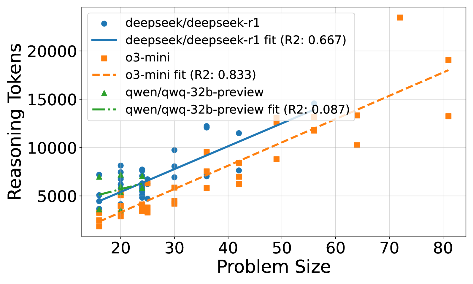
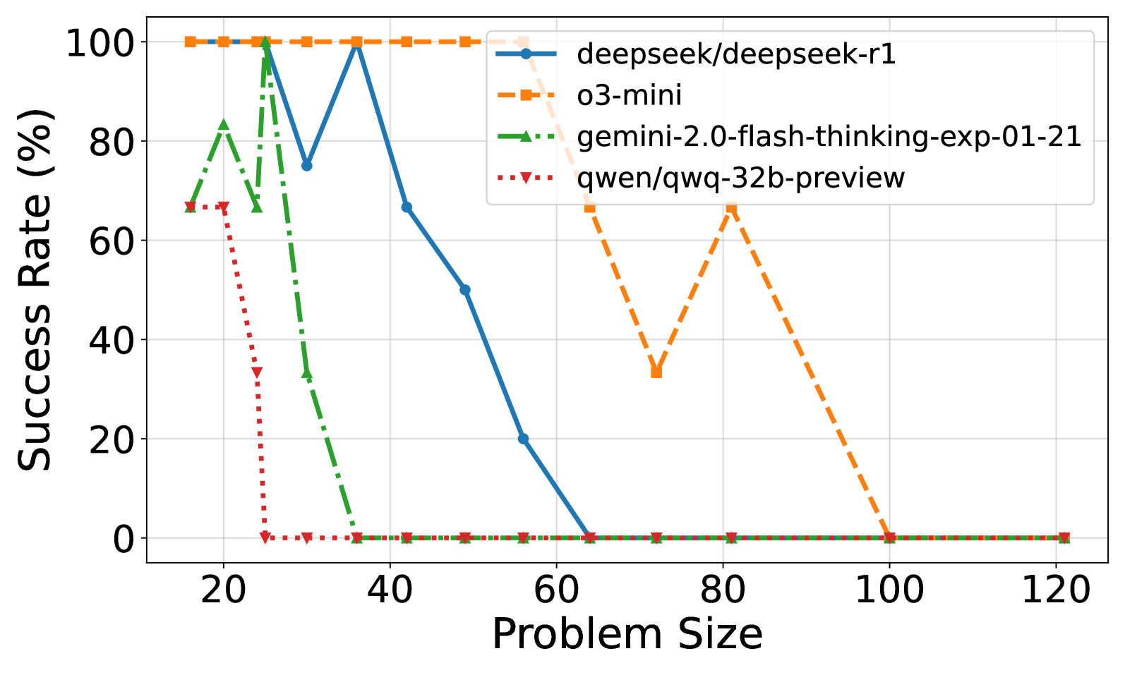
Figure 2: (a) Reasoning effort in number of reasoning tokens versus problem size for DeepSeek R1, o3-mini, and Qwen/QwQ-32B-Preview. Successful attempts only. Linear fits are added for each model. Gemini 2.0 Flash Thinking is excluded due to unknown number of thinking tokens. (b) Solved percentage versus problem size for all models. No model solved problems larger than size 100. o3-mini achieves the highest success rate, followed by DeepSeek R1 and Gemini 2.0 Flash Thinking. Qwen/QwQ-32B-Preview struggles with problem instances larger than size 20.
The relationship between reasoning effort and problem size reveals interesting scaling behaviors across the evaluated models. Figure 2(a) illustrates the scaling of reasoning effort, measured by the number of reasoning tokens, as the problem size increases for successfully solved puzzles. For DeepSeek R1 and o3-mini, we observe a roughly linear increase in reasoning effort with problem size. Notably, the slopes of the linear fits for R1 and o3-mini are very similar, suggesting comparable scaling behavior in reasoning effort for these models, although DeepSeek R1 consistently uses more tokens than o3-mini across problem sizes. Qwen/QwQ-32B-Preview shows a weaker linear correlation, likely due to the limited number of larger puzzles it could solve successfully.
The problem-solving capability of the models, shown in Figure 2(b), reveals performance limits as problem size increases. None of the models solved puzzles with a problem size exceeding 100. o3-mini demonstrates the highest overall solvability, managing to solve the largest problem instances, followed by DeepSeek R1 and Gemini 2.0 Flash Thinking. Qwen/QwQ-32B-Preview’s performance significantly degrades with increasing problem size, struggling to solve instances larger than 25.
<details>
<summary>x3.png Details</summary>
### Visual Description
## Scatter Plot: Reasoning Tokens vs. Problem Size for o3-mini
### Overview
This is a scatter plot comparing the number of "Reasoning Tokens" used against "Problem Size" for a model or system identified as "o3-mini." The data is split into two categories: successful runs and failed runs. The plot reveals a distinct separation in the distribution and behavior of these two categories.
### Components/Axes
* **Chart Type:** Scatter Plot
* **X-Axis:**
* **Label:** "Problem Size"
* **Scale:** Linear, ranging from 0 to 400.
* **Major Tick Marks:** 0, 100, 200, 300, 400.
* **Y-Axis:**
* **Label:** "Reasoning Tokens"
* **Scale:** Linear, ranging from 0 to 50,000.
* **Major Tick Marks:** 0, 10000, 20000, 30000, 40000, 50000.
* **Legend:**
* **Position:** Top-right corner of the plot area.
* **Series 1:** Blue circle marker, labeled "o3-mini (Successful)".
* **Series 2:** Orange square marker, labeled "o3-mini (Failed)".
* **Grid:** Light gray gridlines are present for both axes.
### Detailed Analysis
**1. o3-mini (Successful) - Blue Circles:**
* **Spatial Grounding & Trend:** These data points are tightly clustered in the bottom-left quadrant of the plot. The trend shows a positive correlation: as Problem Size increases from approximately 10 to 80, the Reasoning Tokens used also increase, but remain below ~25,000.
* **Data Point Distribution (Approximate):**
* Problem Size ~10-30: Tokens range from ~2,000 to ~8,000.
* Problem Size ~30-60: Tokens range from ~8,000 to ~15,000.
* Problem Size ~60-80: Tokens range from ~10,000 to ~24,000. The highest token count for a successful run is approximately 24,000 at a Problem Size of about 75.
* **Key Characteristic:** No successful runs are plotted for Problem Sizes greater than approximately 80.
**2. o3-mini (Failed) - Orange Squares:**
* **Spatial Grounding & Trend:** These points are widely dispersed across the entire plot area. There is no single clear linear trend. The distribution suggests failures can occur with both low and high token usage across a wide range of problem sizes.
* **Data Point Distribution (Approximate):**
* **High-Token Failures (Outliers):** Several failures occur at relatively small Problem Sizes (50-150) but with extremely high token counts, including the highest points on the chart: ~54,000 tokens at Problem Size ~100 and ~48,000 tokens at Problem Size ~90.
* **Mid-Range Failures:** A cluster exists between Problem Size 100-250 with token counts scattered between ~5,000 and ~30,000.
* **Large-Problem Failures:** Failures are recorded for Problem Sizes up to 400. At these larger sizes (300-400), the token counts are generally lower, mostly between ~3,000 and ~12,000.
* **Key Characteristic:** Failed runs exist across the entire spectrum of Problem Size (from ~50 to 400) and Reasoning Tokens (from ~3,000 to ~54,000).
### Key Observations
1. **Clear Separation by Problem Size:** Successful runs are confined to Problem Sizes below ~80. All runs with Problem Size >80 are failures.
2. **Inverse Relationship for Failures at Extremes:** The highest token usage (potential overthinking/inefficiency) occurs for failures on moderately sized problems (~50-150). Failures on the largest problems (~300-400) use comparatively fewer tokens.
3. **Absence of Successful Large Problems:** The chart shows no data points for successful runs on problems larger than ~80, indicating a potential capability boundary for the o3-mini model in this test.
4. **Token Usage Variability:** Failed runs exhibit vastly greater variability in token consumption compared to the more predictable, lower-token successful runs.
### Interpretation
The data suggests a strong correlation between problem complexity (size) and the model's ability to succeed, with a clear threshold around a Problem Size of 80. The "Successful" series demonstrates efficient scaling: token usage grows moderately with problem size.
The "Failed" series tells a more complex story. The cluster of high-token failures at moderate problem sizes may indicate scenarios where the model engaged in extensive but unproductive reasoning, ultimately failing. Conversely, failures at very large problem sizes with lower token counts might suggest the model gave up early or failed to initiate a sufficiently deep reasoning process.
**Peircean Investigation:** The chart acts as a sign of the model's **performance envelope**. The tight blue cluster is an *icon* of efficient, successful processing within its comfort zone. The scattered orange squares are an *index* of failure modes: some point to inefficiency (high tokens), others to insufficient effort (low tokens on large problems). The stark boundary at Problem Size ~80 is a *symbol* of a hard limit in the model's tested capability. This visualization is crucial for diagnosing whether failures stem from computational inefficiency or fundamental inability.
</details>
(a)
<details>
<summary>x4.png Details</summary>
### Visual Description
## Scatter Plot with Linear Regression Fits: Reasoning Tokens vs. Problem Size by Reasoning Effort
### Overview
This image is a scatter plot chart displaying the relationship between "Problem Size" (x-axis) and the number of "Reasoning Tokens" (y-axis) used. The data is categorized into three levels of "Reasoning Effort": low, medium, and high. Each category includes individual data points and a fitted linear regression line with its corresponding R-squared value.
### Components/Axes
* **Chart Title:** None visible.
* **X-Axis:**
* **Label:** "Problem Size"
* **Scale:** Linear, ranging from approximately 15 to 100. Major tick marks are at 20, 40, 60, 80, and 100.
* **Y-Axis:**
* **Label:** "Reasoning Tokens"
* **Scale:** Linear, ranging from 0 to over 50,000. Major tick marks are at 0, 10000, 20000, 30000, 40000, and 50000.
* **Legend:** Located in the top-left quadrant of the plot area. It defines three data series and their corresponding fit lines:
1. **low:** Blue circle marker.
2. **low fit (R^2: 0.489):** Solid blue line.
3. **medium:** Orange square marker.
4. **medium fit (R^2: 0.833):** Dashed orange line.
5. **high:** Green triangle marker.
6. **high fit (R^2: 0.813):** Dash-dot green line.
* **Grid:** A light gray grid is present in the background.
### Detailed Analysis
The analysis is segmented by the three "Reasoning Effort" categories.
**1. Low Reasoning Effort (Blue Circles & Solid Blue Line)**
* **Trend:** The data points show a very shallow, slightly positive slope. The fitted line increases minimally from left to right.
* **Data Points (Approximate):**
* At Problem Size ~18: ~1,000 tokens.
* At Problem Size ~20: ~1,500 tokens.
* At Problem Size ~25: ~2,000 tokens.
* At Problem Size ~30: ~2,500 tokens.
* At Problem Size ~35: ~3,000 tokens.
* At Problem Size ~42: ~3,500 tokens.
* **Fit Line:** The solid blue regression line starts near (18, 1000) and ends near (42, 3500). The R-squared value of 0.489 indicates a weak to moderate fit, suggesting the linear model explains less than half of the variance in the data for this category.
**2. Medium Reasoning Effort (Orange Squares & Dashed Orange Line)**
* **Trend:** The data points and the fitted line show a clear, moderate positive linear trend. The slope is steeper than the "low" effort series.
* **Data Points (Approximate):**
* At Problem Size ~18: ~2,500 tokens.
* At Problem Size ~20: ~3,000 tokens.
* At Problem Size ~25: ~4,000 tokens.
* At Problem Size ~30: ~5,500 tokens.
* At Problem Size ~35: ~7,000 tokens.
* At Problem Size ~42: ~8,500 tokens.
* At Problem Size ~50: ~9,000 tokens.
* At Problem Size ~55: ~12,000 tokens.
* At Problem Size ~64: ~10,000 tokens.
* At Problem Size ~72: ~23,000 tokens (potential outlier, high).
* At Problem Size ~80: ~13,000 tokens and ~19,000 tokens.
* **Fit Line:** The dashed orange regression line starts near (18, 2500) and ends near (80, 18000). The R-squared value of 0.833 indicates a strong fit, meaning the linear model explains a large portion of the variance.
**3. High Reasoning Effort (Green Triangles & Dash-Dot Green Line)**
* **Trend:** The data points and the fitted line show a strong, steep positive linear trend. This series has the steepest slope and the highest token counts.
* **Data Points (Approximate):** The data is more scattered, especially at higher problem sizes.
* At Problem Size ~18: ~5,000 tokens.
* At Problem Size ~20: ~7,000 tokens.
* At Problem Size ~25: ~8,000 tokens.
* At Problem Size ~30: ~10,000 tokens.
* At Problem Size ~35: ~12,000 tokens.
* At Problem Size ~42: ~15,000 tokens.
* At Problem Size ~50: ~18,000 tokens and ~20,000 tokens.
* At Problem Size ~55: ~20,000 tokens and ~24,000 tokens.
* At Problem Size ~64: ~22,000 tokens, ~28,000 tokens, and ~35,000 tokens.
* At Problem Size ~72: ~20,000 tokens, ~31,000 tokens, and ~51,000 tokens (a very high point).
* At Problem Size ~80: ~28,000 tokens, ~48,000 tokens.
* At Problem Size ~100: ~41,000 tokens, ~44,000 tokens, and ~56,000 tokens (the highest point on the chart).
* **Fit Line:** The dash-dot green regression line starts near (18, 5000) and ends near (100, 46000). The R-squared value of 0.813 indicates a strong fit, similar to the "medium" category.
### Key Observations
1. **Clear Hierarchy:** For any given Problem Size, the number of Reasoning Tokens increases systematically from Low to Medium to High effort.
2. **Increasing Slope with Effort:** The slope of the regression line becomes progressively steeper from Low to Medium to High effort, indicating that the *rate* at which token usage grows with problem size is greater for higher reasoning efforts.
3. **Variance Increases with Effort:** The scatter (vertical spread) of data points around the fit line is smallest for "low" effort and largest for "high" effort, particularly at larger problem sizes (e.g., Problem Size 72 and 100).
4. **Strong Correlation for Medium/High:** Both the "medium" and "high" effort categories show a strong linear correlation (R² > 0.8) between problem size and token usage.
5. **Potential Outliers:** The data point at Problem Size ~72 for "medium" effort (~23,000 tokens) appears high relative to its trend. The "high" effort series has several points at large problem sizes (e.g., ~51,000 at PS 72, ~56,000 at PS 100) that are significantly above the fit line.
### Interpretation
The chart demonstrates a fundamental trade-off in computational reasoning: **increased problem complexity (size) requires more processing resources (tokens), and this cost scales more aggressively when the system is configured for higher reasoning effort.**
* **Low Effort** appears to be a "baseline" mode where token usage grows slowly and unpredictably with problem size (low R²). It may represent a shallow or heuristic-based approach.
* **Medium and High Effort** modes show a predictable, linear scaling law. The strong R² values suggest these modes engage in a more systematic, depth-first reasoning process whose resource consumption can be reliably modeled.
* The **steeper slope for High Effort** implies that for complex problems, choosing a high-effort strategy incurs a multiplicative cost in tokens. This could be due to more extensive search, verification, or step-by-step explanation generation.
* The **increased variance at High Effort** for large problems suggests that the reasoning process becomes less uniform; some problems may trigger exceptionally long chains of thought, while others of similar size are solved more efficiently. This could reflect the inherent variability in problem difficulty beyond just the "size" metric.
In essence, the data suggests that "Reasoning Effort" is a critical control parameter that not only determines the absolute resource cost but also fundamentally changes how that cost scales with problem difficulty. Users or systems must balance the desire for thoroughness (high effort) against the predictable and potentially prohibitive increase in token consumption for large-scale tasks.
</details>
(b)
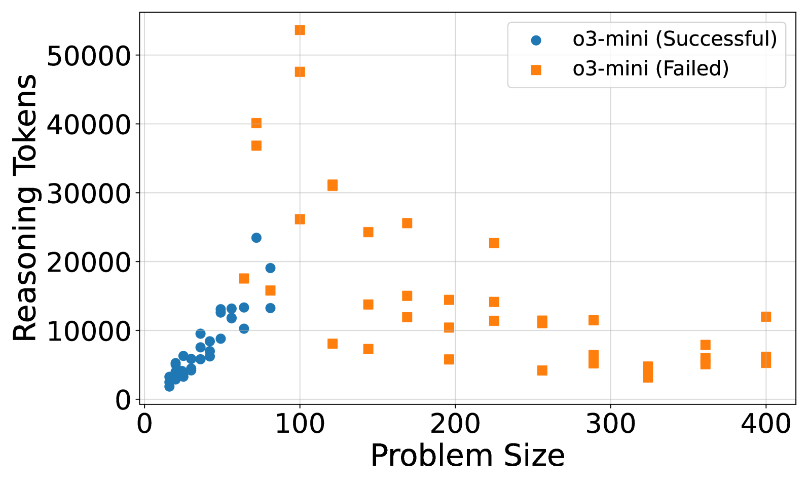
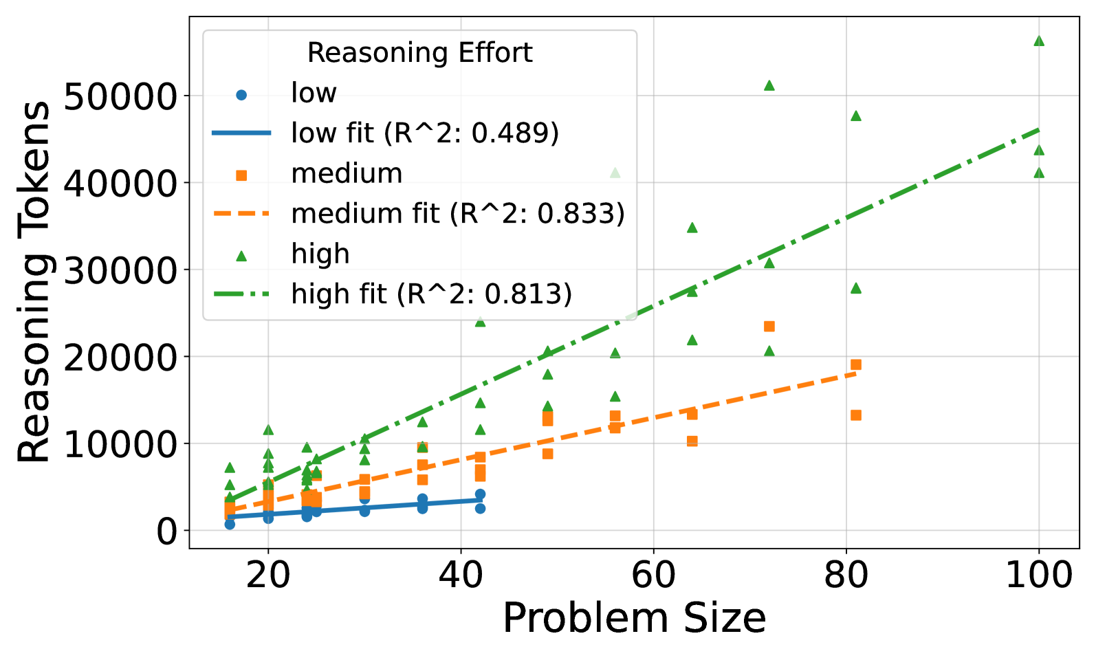
Figure 3: (a) Reasoning effort in number of reasoning tokens versus problem size for o3-mini. A peak in reasoning effort is observed around problem size 100, followed by a decline for larger problem sizes. (b) Reasoning effort in number of reasoning tokens versus problem size for o3-mini, categorized by low, medium, and high reasoning effort strategies. Steeper slopes are observed for higher reasoning effort strategies. High reasoning effort enables solving larger instances but also increases token usage for smaller, already solvable problems.
A more detailed analysis of o3-mini’s reasoning effort (Figure 3(a)) reveals a non-monotonic trend. While generally increasing with problem size initially, reasoning effort peaks around a problem size of 100. Beyond this point, the reasoning effort decreases, suggesting a potential ”frustration” effect where increased complexity no longer leads to proportionally increased reasoning in the model. The same behavior could not be observed for other models, see Section A.2.2. It would be interesting to see the effect of recent works trying to optimize reasoning length would have on these results (Luo et al., 2025).
Figure 3(b) further explores o3-mini’s behavior by categorizing reasoning effort into low, medium, and high strategies. The steepness of the scaling slope increases with reasoning effort, indicating that higher effort strategies lead to a more pronounced increase in token usage as problem size grows. While high reasoning effort enables solving larger puzzles (up to 10x10), it also results in a higher token count even for smaller problems that were already solvable with lower effort strategies. This suggests a trade-off where increased reasoning effort can extend the solvable problem range but may also introduce inefficiencies for simpler instances.
## 5 Conclusion
This study examined how reasoning effort scales in LLMs using the Tents puzzle. We found that reasoning effort generally scales linearly with problem size for solvable instances. Model performance varied, with o3-mini and DeepSeek R1 showing better performance than Qwen/QwQ-32B-Preview and Gemini 2.0 Flash Thinking. These results suggest that while LLMs can adapt reasoning effort to problem complexity, their logical coherence has limits, especially for larger problems. Future work should extend this analysis to a wider variety of puzzles contained in the PUZZLES benchmark to include puzzles with different algorithmic complexity. These insights could lead the way to find strategies to improve reasoning scalability and efficiency, potentially by optimizing reasoning length or refining prompting techniques. Understanding these limitations is crucial for advancing LLMs in complex problem-solving.
## References
- Chollet (2019) François Chollet. On the measure of intelligence. arXiv preprint arXiv:1911.01547, 2019.
- Cobbe et al. (2021) Karl Cobbe, Vineet Kosaraju, Mohammad Bavarian, Mark Chen, Heewoo Jun, Lukasz Kaiser, Matthias Plappert, Jerry Tworek, Jacob Hilton, Reiichiro Nakano, et al. Training verifiers to solve math word problems. arXiv preprint arXiv:2110.14168, 2021.
- DeepMind (2025) DeepMind. Gemini flash thinking. https://deepmind.google/technologies/gemini/flash-thinking/, 2025. Accessed: February 6, 2025.
- Estermann et al. (2024) Benjamin Estermann, Luca A Lanzendörfer, Yannick Niedermayr, and Roger Wattenhofer. Puzzles: A benchmark for neural algorithmic reasoning. In The Thirty-eight Conference on Neural Information Processing Systems Datasets and Benchmarks Track, 2024.
- Fan et al. (2023) Lizhou Fan, Wenyue Hua, Lingyao Li, Haoyang Ling, and Yongfeng Zhang. Nphardeval: Dynamic benchmark on reasoning ability of large language models via complexity classes. arXiv preprint arXiv:2312.14890, 2023.
- Guo et al. (2025) Daya Guo, Dejian Yang, Haowei Zhang, Junxiao Song, Ruoyu Zhang, Runxin Xu, Qihao Zhu, Shirong Ma, Peiyi Wang, Xiao Bi, et al. Deepseek-r1: Incentivizing reasoning capability in llms via reinforcement learning. arXiv preprint arXiv:2501.12948, 2025.
- Hendrycks et al. (2020) Dan Hendrycks, Collin Burns, Steven Basart, Andy Zou, Mantas Mazeika, Dawn Song, and Jacob Steinhardt. Measuring massive multitask language understanding. arXiv preprint arXiv:2009.03300, 2020.
- Huang & Chang (2022) Jie Huang and Kevin Chen-Chuan Chang. Towards reasoning in large language models: A survey. arXiv preprint arXiv:2212.10403, 2022.
- Jimenez et al. (2023) Carlos E Jimenez, John Yang, Alexander Wettig, Shunyu Yao, Kexin Pei, Ofir Press, and Karthik Narasimhan. Swe-bench: Can language models resolve real-world github issues? arXiv preprint arXiv:2310.06770, 2023.
- Lee et al. (2024) Seungpil Lee, Woochang Sim, Donghyeon Shin, Wongyu Seo, Jiwon Park, Seokki Lee, Sanha Hwang, Sejin Kim, and Sundong Kim. Reasoning abilities of large language models: In-depth analysis on the abstraction and reasoning corpus. ACM Transactions on Intelligent Systems and Technology, 2024.
- Luo et al. (2025) Haotian Luo, Li Shen, Haiying He, Yibo Wang, Shiwei Liu, Wei Li, Naiqiang Tan, Xiaochun Cao, and Dacheng Tao. O1-pruner: Length-harmonizing fine-tuning for o1-like reasoning pruning. arXiv preprint arXiv:2501.12570, 2025.
- of America (2024) Mathematical Association of America. 2024 aime i problems. https://artofproblemsolving.com/wiki/index.php/2024_AIME_I, 2024. Accessed: February 6, 2025.
- OpenAI (2025) OpenAI. Openai o3 mini. https://openai.com/index/openai-o3-mini/, 2025. Accessed: February 6, 2025.
- Qwen (2024) Qwen. Qwq: Reflect deeply on the boundaries of the unknown, November 2024. URL https://qwenlm.github.io/blog/qwq-32b-preview/.
- Rein et al. (2023) David Rein, Betty Li Hou, Asa Cooper Stickland, Jackson Petty, Richard Yuanzhe Pang, Julien Dirani, Julian Michael, and Samuel R Bowman. Gpqa: A graduate-level google-proof q&a benchmark. arXiv preprint arXiv:2311.12022, 2023.
- (16) Simon Tatham. Simon tatham’s portable puzzle collection. https://www.chiark.greenend.org.uk/~sgtatham/puzzles/. Accessed: 2025-02-06.
- Wei et al. (2022) Jason Wei, Xuezhi Wang, Dale Schuurmans, Maarten Bosma, Fei Xia, Ed Chi, Quoc V Le, Denny Zhou, et al. Chain-of-thought prompting elicits reasoning in large language models. Advances in neural information processing systems, 35:24824–24837, 2022.
- Yao et al. (2023) Shunyu Yao, Dian Yu, Jeffrey Zhao, Izhak Shafran, Thomas L Griffiths, Yuan Cao, and Karthik Narasimhan. Tree of thoughts: Deliberate problem solving with large language models, may 2023. arXiv preprint arXiv:2305.10601, 14, 2023.
- Zhou et al. (2022) Denny Zhou, Nathanael Schärli, Le Hou, Jason Wei, Nathan Scales, Xuezhi Wang, Dale Schuurmans, Claire Cui, Olivier Bousquet, Quoc Le, et al. Least-to-most prompting enables complex reasoning in large language models. arXiv preprint arXiv:2205.10625, 2022.
## Appendix A Appendix
### A.1 Full Prompt
The full prompt used in the experiments is the following, on the example of a 4x4 puzzle:
⬇
You are a logic puzzle expert. You will be given a logic puzzle to solve. Here is a description of the puzzle:
You have a grid of squares, some of which contain trees. Your aim is to place tents in some of the remaining squares, in such a way that the following conditions are met:
There are exactly as many tents as trees.
The tents and trees can be matched up in such a way that each tent is directly adjacent (horizontally or vertically, but not diagonally) to its own tree. However, a tent may be adjacent to other trees as well as its own.
No two tents are adjacent horizontally, vertically or diagonally.
The number of tents in each row, and in each column, matches the numbers given in the row or column constraints.
Grass indicates that there cannot be a tent in that position.
You receive an array representation of the puzzle state as a grid. Your task is to solve the puzzle by filling out the grid with the correct values. You need to solve the puzzle on your own, you cannot use any external resources or run any code. Once you have solved the puzzle, tell me the final answer without explanation. Return the final answer as a JSON array of arrays.
Here is the current state of the puzzle as a string of the internal state representation:
A 0 represents an empty cell, a 1 represents a tree, a 2 represents a tent, and a 3 represents a grass patch.
Tents puzzle state:
Current grid:
[[0 0 1 0]
[0 1 0 0]
[1 0 0 0]
[0 0 0 0]]
The column constraints are the following:
[1 1 0 1]
The row constraints are the following:
[2 0 0 1]
### A.2 Additional Figures
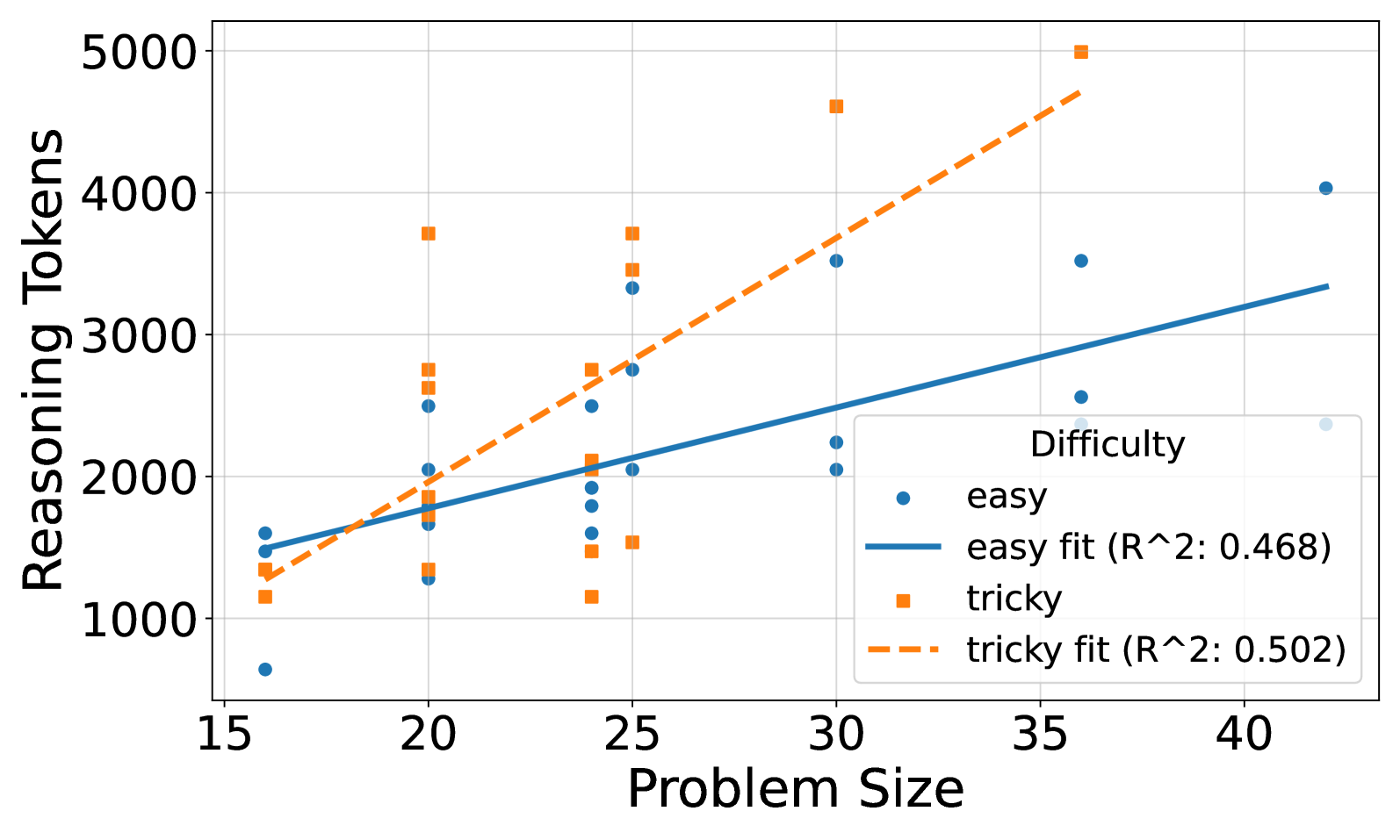
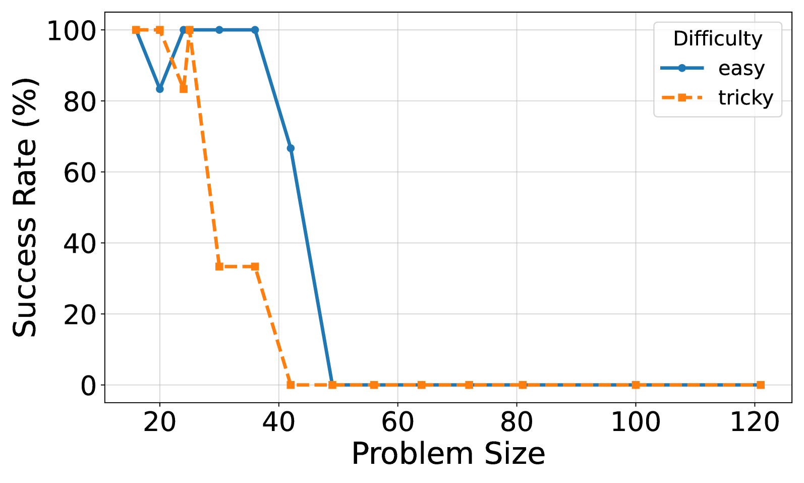
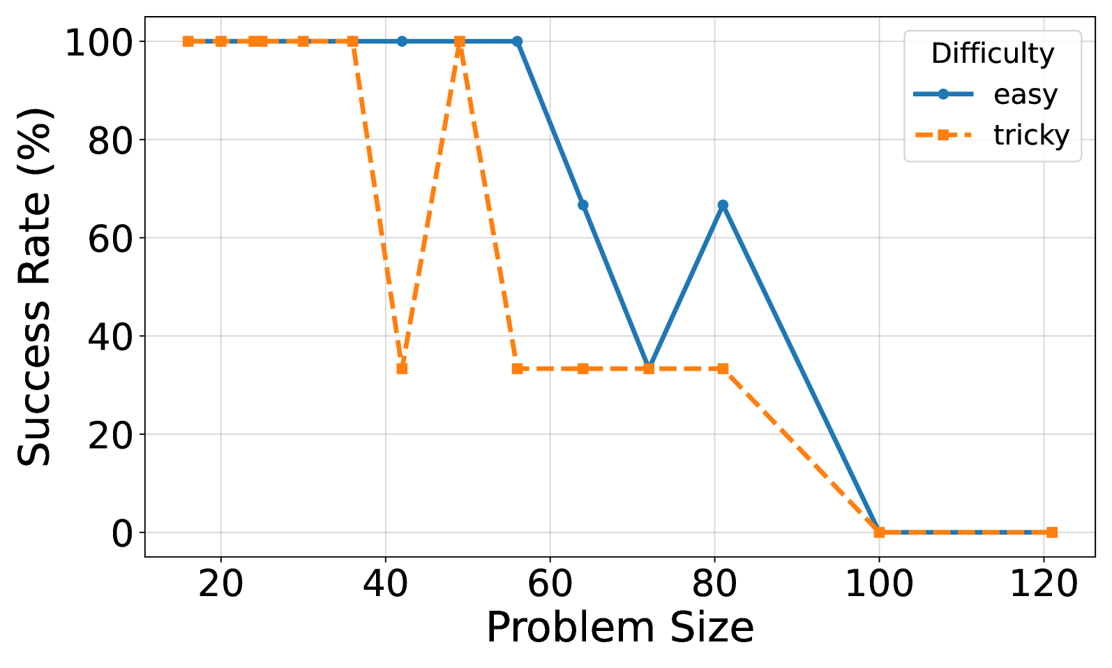
#### A.2.1 Easy vs. Tricky Puzzles
<details>
<summary>x5.png Details</summary>
### Visual Description
## Scatter Plot with Linear Regression: Reasoning Tokens vs. Problem Size by Difficulty
### Overview
This image is a scatter plot with two overlaid linear regression lines. It visualizes the relationship between "Problem Size" (x-axis) and the number of "Reasoning Tokens" (y-axis) required, categorized by problem difficulty: "easy" and "tricky". The chart suggests that as problem size increases, the reasoning tokens required also increase, with a notably steeper increase for "tricky" problems.
### Components/Axes
* **X-Axis:** Labeled "Problem Size". The scale runs from approximately 15 to 42, with major tick marks at 15, 20, 25, 30, 35, and 40.
* **Y-Axis:** Labeled "Reasoning Tokens". The scale runs from approximately 500 to 5000, with major tick marks at 1000, 2000, 3000, 4000, and 5000.
* **Legend:** Located in the bottom-right quadrant of the chart area. It contains four entries:
1. **easy:** Represented by blue circle markers (●).
2. **easy fit (R^2: 0.468):** Represented by a solid blue line.
3. **tricky:** Represented by orange square markers (■).
4. **tricky fit (R^2: 0.502):** Represented by a dashed orange line.
* **Data Series:** Two distinct series are plotted:
* **Easy Series (Blue Circles):** Data points for problems classified as "easy".
* **Tricky Series (Orange Squares):** Data points for problems classified as "tricky".
### Detailed Analysis
**Trend Verification:**
* The **blue "easy" fit line** has a positive, moderate upward slope.
* The **orange "tricky" fit line** has a positive, steeper upward slope compared to the easy line.
**Data Point Extraction (Approximate Values):**
*Points are listed from left to right along the x-axis. Values are approximate based on visual alignment with the grid.*
**Easy Series (Blue Circles):**
* At Problem Size ~16: Reasoning Tokens ~700 and ~1600.
* At Problem Size ~20: Reasoning Tokens ~1300, ~1700, ~2000, and ~2500.
* At Problem Size ~24: Reasoning Tokens ~1600, ~1800, ~1900, ~2500, and ~3300.
* At Problem Size ~25: Reasoning Tokens ~2050 and ~2750.
* At Problem Size ~30: Reasoning Tokens ~2050, ~2200, and ~3500.
* At Problem Size ~36: Reasoning Tokens ~2550 and ~3500.
* At Problem Size ~42: Reasoning Tokens ~4000.
**Tricky Series (Orange Squares):**
* At Problem Size ~16: Reasoning Tokens ~1150 and ~1350.
* At Problem Size ~20: Reasoning Tokens ~1350, ~1850, ~2650, ~2750, and ~3700.
* At Problem Size ~24: Reasoning Tokens ~1150, ~1500, ~2100, ~2750, and ~3450.
* At Problem Size ~25: Reasoning Tokens ~1550 and ~3700.
* At Problem Size ~30: Reasoning Tokens ~4600.
* At Problem Size ~36: Reasoning Tokens ~5000.
**Regression Lines:**
* The **easy fit line** starts at approximately (16, 1500) and ends near (42, 3350). Its R-squared value is 0.468.
* The **tricky fit line** starts at approximately (16, 1300) and ends near (36, 4700). Its R-squared value is 0.502.
### Key Observations
1. **Diverging Slopes:** The most prominent feature is the difference in slope between the two regression lines. The "tricky" line is significantly steeper, indicating that reasoning token count grows at a faster rate with problem size for tricky problems compared to easy ones.
2. **Variance:** Both data series show considerable vertical spread (variance) at similar problem sizes, especially in the 20-25 range. This suggests problem size alone is not the sole determinant of reasoning tokens; other factors within the "easy" or "tricky" category also play a role.
3. **Outliers:** The highest data point on the chart is an orange square (tricky) at Problem Size ~36 with ~5000 tokens. The lowest point is a blue circle (easy) at Problem Size ~16 with ~700 tokens.
4. **Model Fit:** The R-squared values (0.468 for easy, 0.502 for tricky) indicate that the linear model explains roughly 47-50% of the variance in the data. This is a moderate fit, confirming the visual scatter of points around the lines.
### Interpretation
The chart demonstrates a clear, positive correlation between problem size and the computational resources (reasoning tokens) required for an AI model to solve it. The critical insight is the interaction with problem difficulty. While both easy and tricky problems demand more resources as they grow larger, **tricky problems exhibit a much higher marginal cost per unit of size increase**. This implies that the complexity or non-obvious nature of "tricky" problems compounds the challenge posed by scale.
The moderate R-squared values suggest that "Problem Size" and "Difficulty" (as a binary category) are important but incomplete predictors. The significant scatter indicates that the specific structure or content of a problem within these categories introduces substantial variability in resource needs. For system design or cost estimation, this means planning must account not only for the scale of tasks but also for their inherent difficulty, with a non-linear scaling factor for harder problems. The data argues for difficulty-aware resource allocation and optimization strategies.
</details>
(a)
<details>
<summary>x6.png Details</summary>
### Visual Description
\n
## Line Chart: Success Rate vs. Problem Size by Difficulty
### Overview
This is a line chart comparing the percentage success rate of solving problems of two different difficulty levels ("easy" and "tricky") as the problem size increases. The chart demonstrates a clear negative correlation between problem size and success rate for both categories, with performance dropping to zero at larger sizes.
### Components/Axes
* **X-Axis:** Labeled "Problem Size". The axis displays major tick marks and labels at intervals of 20, starting at 20 and ending at 120. The scale appears linear.
* **Y-Axis:** Labeled "Success Rate (%)". The axis displays major tick marks and labels at intervals of 20, from 0 to 100. The scale is linear.
* **Legend:** Located in the top-right corner of the chart area. It is titled "Difficulty" and defines two data series:
* `easy`: Represented by a solid blue line with circular markers.
* `tricky`: Represented by a dashed orange line with square markers.
* **Grid:** A light gray grid is present, aligned with the major ticks on both axes.
### Detailed Analysis
**Data Series: "easy" (Blue, Solid Line with Circles)**
* **Trend:** The line starts at the maximum success rate, experiences a single sharp dip, recovers fully, then begins a steep, final decline to zero.
* **Data Points (Approximate):**
* Problem Size 20: 100%
* Problem Size 25: ~83%
* Problem Size 30: 100%
* Problem Size 35: 100%
* Problem Size 40: ~67%
* Problem Size 45: 0%
* Problem Sizes 50, 60, 70, 80, 100, 120: 0%
**Data Series: "tricky" (Orange, Dashed Line with Squares)**
* **Trend:** The line starts at the maximum success rate, holds for one interval, then begins a stepwise decline that is more immediate and severe than the "easy" series, reaching zero earlier.
* **Data Points (Approximate):**
* Problem Size 20: 100%
* Problem Size 25: 100%
* Problem Size 30: ~83%
* Problem Size 35: ~33%
* Problem Size 40: ~33%
* Problem Size 45: 0%
* Problem Sizes 50, 60, 70, 80, 100, 120: 0%
### Key Observations
1. **Performance Cliff:** Both difficulty levels exhibit a "cliff" where success rates plummet to 0%. For "tricky" problems, this cliff begins after size 25 and is complete by size 45. For "easy" problems, the final decline starts after size 35 and is complete by size 45.
2. **Relative Difficulty:** The "tricky" series consistently performs worse than or equal to the "easy" series at every measured problem size. The performance gap is most pronounced between sizes 30 and 40.
3. **Anomalous Dip:** The "easy" series shows a significant, isolated drop in success rate at problem size 25 (~83%) before recovering to 100% at sizes 30 and 35. This is the only non-monotonic movement in either series.
4. **Convergence to Zero:** From problem size 45 onward, both series show a 0% success rate, indicating a complete failure to solve problems of that size or larger, regardless of difficulty.
### Interpretation
The chart illustrates a scalability limit for the system or method being tested. Success is highly dependent on problem size, with a sharp phase transition from high success to complete failure.
* **The "tricky" problems** are not just harder at a given size; they cause the system to fail at smaller sizes. The system's capacity is lower for complex tasks.
* **The "easy" problems** show a more robust performance curve, maintaining perfect success for larger sizes (up to 35) before failing. The dip at size 25 is curious and may indicate a specific, non-linear challenge at that particular scale for otherwise easy problems, or it could be an artifact of the test data.
* **The universal failure at size ≥45** suggests a fundamental bottleneck—be it computational, algorithmic, or related to resource constraints—that prevents success beyond this threshold. The data implies that to handle larger problems, a fundamental change to the underlying approach is required, as incremental improvements are unlikely to overcome this hard limit.
</details>
(b)
Figure 4: (a) Reasoning effort in number of reasoning tokens versus problem size for o3-mini with reasoning effort low. Successful tries only. Linear fits are added for each model. (b) Solved percentage versus problem size for o3-mini with reasoning effort low.
<details>
<summary>x7.png Details</summary>
### Visual Description
## Scatter Plot with Trend Lines: Difficulty vs. Reasoning Tokens
### Overview
The image is a scatter plot chart displaying the relationship between "Problem Size" (x-axis) and "Reasoning Tokens" (y-axis) for two categories of problems: "easy" and "tricky". Each category has a set of data points and a corresponding linear regression trend line. The chart includes a legend, axis labels, and a grid.
### Components/Axes
* **Chart Title/Legend Title:** "Difficulty" (located in the top-left corner of the plot area).
* **X-Axis:**
* **Label:** "Problem Size"
* **Scale:** Linear, ranging from approximately 15 to 85.
* **Major Tick Marks:** 20, 30, 40, 50, 60, 70, 80.
* **Y-Axis:**
* **Label:** "Reasoning Tokens"
* **Scale:** Linear, ranging from 0 to over 30,000.
* **Major Tick Marks:** 0, 5000, 10000, 15000, 20000, 25000, 30000.
* **Legend (Top-Left):**
* **Series 1:** "easy" - Represented by blue circle markers (●).
* **Series 2:** "easy fit (R^2: 0.829)" - Represented by a solid blue line (—).
* **Series 3:** "tricky" - Represented by orange square markers (■).
* **Series 4:** "tricky fit (R^2: 0.903)" - Represented by a dashed orange line (--).
* **Grid:** Light gray grid lines are present for both major x and y ticks.
### Detailed Analysis
**Trend Verification & Data Series:**
1. **"easy" Series (Blue Circles & Solid Line):**
* **Visual Trend:** The data points show a clear upward trend. The solid blue trend line slopes upward from left to right, indicating a positive correlation between Problem Size and Reasoning Tokens for easy problems.
* **Approximate Data Points (Selected):**
* At Problem Size ~18: Reasoning Tokens ~2,000.
* At Problem Size ~30: Reasoning Tokens ~4,000.
* At Problem Size ~50: Reasoning Tokens ~8,500.
* At Problem Size ~65: Reasoning Tokens ~10,000 and ~13,000 (two points).
* At Problem Size ~81: Reasoning Tokens ~13,000 and ~19,000 (two points).
* **Fit Line:** The solid blue line represents a linear fit with an R-squared value of 0.829, suggesting a reasonably strong linear relationship.
2. **"tricky" Series (Orange Squares & Dashed Line):**
* **Visual Trend:** The data points also show a strong upward trend, generally positioned above the "easy" points for similar Problem Sizes. The dashed orange trend line slopes upward more steeply than the "easy" line.
* **Approximate Data Points (Selected):**
* At Problem Size ~18: Reasoning Tokens ~3,000.
* At Problem Size ~30: Reasoning Tokens ~5,500 and ~8,500.
* At Problem Size ~42: Reasoning Tokens ~17,500.
* At Problem Size ~49: Reasoning Tokens ~13,000, ~18,000, and ~21,000.
* At Problem Size ~72: Reasoning Tokens ~33,000 (a notable high point).
* At Problem Size ~81: Reasoning Tokens ~29,000.
* **Fit Line:** The dashed orange line represents a linear fit with an R-squared value of 0.903, indicating a very strong linear relationship, slightly stronger than for the "easy" category.
**Spatial Grounding:** The legend is positioned in the top-left quadrant of the chart area. The "tricky" data points and trend line are consistently positioned above the "easy" data points and trend line across the entire range of Problem Size, indicating higher Reasoning Token counts for "tricky" problems at any given size.
### Key Observations
1. **Positive Correlation:** Both "easy" and "tricky" problem categories show a positive, linear correlation between Problem Size and the number of Reasoning Tokens required.
2. **Differential Slope:** The slope of the "tricky" fit line is steeper than that of the "easy" fit line. This suggests that as Problem Size increases, the *additional* Reasoning Tokens required for "tricky" problems grows at a faster rate than for "easy" problems.
3. **Variance:** There is noticeable variance in the data points around the trend lines, particularly for the "tricky" category at mid-to-high Problem Sizes (e.g., around Problem Size 49 and 65).
4. **Outlier:** A single "tricky" data point at approximately Problem Size 72 has an exceptionally high Reasoning Token count (~33,000), which is the highest value on the chart.
5. **Goodness of Fit:** Both linear models fit their respective data well, with R-squared values of 0.829 ("easy") and 0.903 ("tricky").
### Interpretation
The data demonstrates that the computational effort (measured in Reasoning Tokens) required to solve a problem scales linearly with the problem's size. Crucially, the problem's difficulty category ("easy" vs. "tricky") acts as a multiplier on this scaling factor.
The steeper slope for "tricky" problems implies they are not just uniformly harder, but that their complexity compounds more severely with size. A large "tricky" problem demands a disproportionately larger reasoning overhead compared to a large "easy" problem, beyond the simple increase due to size alone. This has practical implications for resource allocation and performance prediction in systems that process such problems; one cannot extrapolate the cost of a large "tricky" problem from the cost of a small one using the same rate derived from "easy" problems. The high R-squared values suggest that Problem Size is a very reliable predictor of Reasoning Tokens within each difficulty class, making this a useful model for estimation.
</details>
(a)
<details>
<summary>x8.png Details</summary>
### Visual Description
\n
## Line Chart: Success Rate vs. Problem Size by Difficulty
### Overview
This is a line chart comparing the success rate (in percentage) of solving problems of varying sizes, categorized by two difficulty levels: "easy" and "tricky". The chart illustrates how performance degrades as problem complexity increases, with distinct patterns for each difficulty category.
### Components/Axes
* **Chart Type:** Line chart with markers.
* **X-Axis (Horizontal):** Labeled **"Problem Size"**. The axis has major tick marks and labels at intervals of 20, specifically at: 20, 40, 60, 80, 100, 120.
* **Y-Axis (Vertical):** Labeled **"Success Rate (%)"**. The axis ranges from 0 to 100, with major tick marks and labels at intervals of 20: 0, 20, 40, 60, 80, 100.
* **Legend:** Located in the **top-right corner** of the chart area. It is titled **"Difficulty"** and contains two entries:
* **"easy"**: Represented by a **solid blue line** with circular markers.
* **"tricky"**: Represented by a **dashed orange line** with square markers.
* **Grid:** A light gray grid is present in the background, aligned with the major ticks of both axes.
### Detailed Analysis
Data points are approximate, derived from visual inspection of the chart.
**1. "easy" Difficulty (Solid Blue Line with Circles):**
* **Trend:** Maintains a perfect success rate for smaller problem sizes, then experiences a sharp decline with a brief partial recovery before ultimately failing completely.
* **Data Points:**
* Problem Size ~20: Success Rate = **100%**
* Problem Size ~40: Success Rate = **100%**
* Problem Size ~60: Success Rate = **100%**
* Problem Size ~70: Success Rate ≈ **35%** (Sharp drop)
* Problem Size ~80: Success Rate ≈ **65%** (Partial recovery)
* Problem Size ~100: Success Rate = **0%**
* Problem Size ~120: Success Rate = **0%**
**2. "tricky" Difficulty (Dashed Orange Line with Squares):**
* **Trend:** Shows high volatility at mid-range problem sizes, with a sharp drop, a full recovery, and a plateau before a final decline to zero.
* **Data Points:**
* Problem Size ~20: Success Rate = **100%**
* Problem Size ~40: Success Rate = **100%**
* Problem Size ~40 (second point, slightly right): Success Rate ≈ **35%** (Sharp drop)
* Problem Size ~50: Success Rate = **100%** (Full recovery)
* Problem Size ~60: Success Rate ≈ **35%**
* Problem Size ~70: Success Rate ≈ **35%**
* Problem Size ~80: Success Rate ≈ **35%** (Plateau)
* Problem Size ~100: Success Rate = **0%**
* Problem Size ~120: Success Rate = **0%**
### Key Observations
1. **Performance Cliff:** Both difficulty levels show a complete failure (0% success) for problem sizes of 100 and above.
2. **Volatility in "tricky":** The "tricky" series exhibits a dramatic V-shaped dip and recovery between problem sizes 40 and 50, which is not present in the "easy" series.
3. **Delayed Decline for "easy":** The "easy" problems maintain a 100% success rate up to a larger problem size (~60) compared to the first drop in "tricky" problems (~40).
4. **Partial Recovery:** Only the "easy" series shows a significant partial recovery (from ~35% to ~65%) after its initial major drop.
5. **Convergent Failure:** Despite different paths, both series converge to the same 0% success rate at the largest problem sizes.
### Interpretation
The data suggests a non-linear relationship between problem size and solvability, heavily influenced by problem difficulty.
* **System Capacity Limit:** The universal drop to 0% at problem size 100 indicates a fundamental system or algorithmic limit. Beyond this threshold, the method being tested fails completely regardless of difficulty.
* **Difficulty Manifests as Instability:** The "tricky" category's volatile performance (the sharp drop and recovery) implies that certain mid-sized problems (around size 40-50) possess specific characteristics that cause catastrophic failure, which are not present in slightly smaller or larger "tricky" problems. This could point to sensitivity to particular problem structures or edge cases.
* **Robustness of "easy" Problems:** The "easy" category demonstrates greater robustness, sustaining perfect performance for larger sizes and showing a capacity for partial recovery after failure. This suggests the underlying method handles "easy" problem structures more predictably until a critical size is reached.
* **Practical Implication:** For applications using this method, problem size is a critical constraint. For "tricky" problems, sizes near 40 and beyond 80 are high-risk. For "easy" problems, sizes beyond 60 require caution, and sizes beyond 80 are likely to fail. The chart provides a clear visual guide for setting operational limits based on problem difficulty.
</details>
(b)
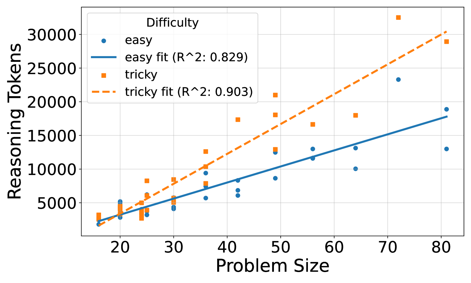
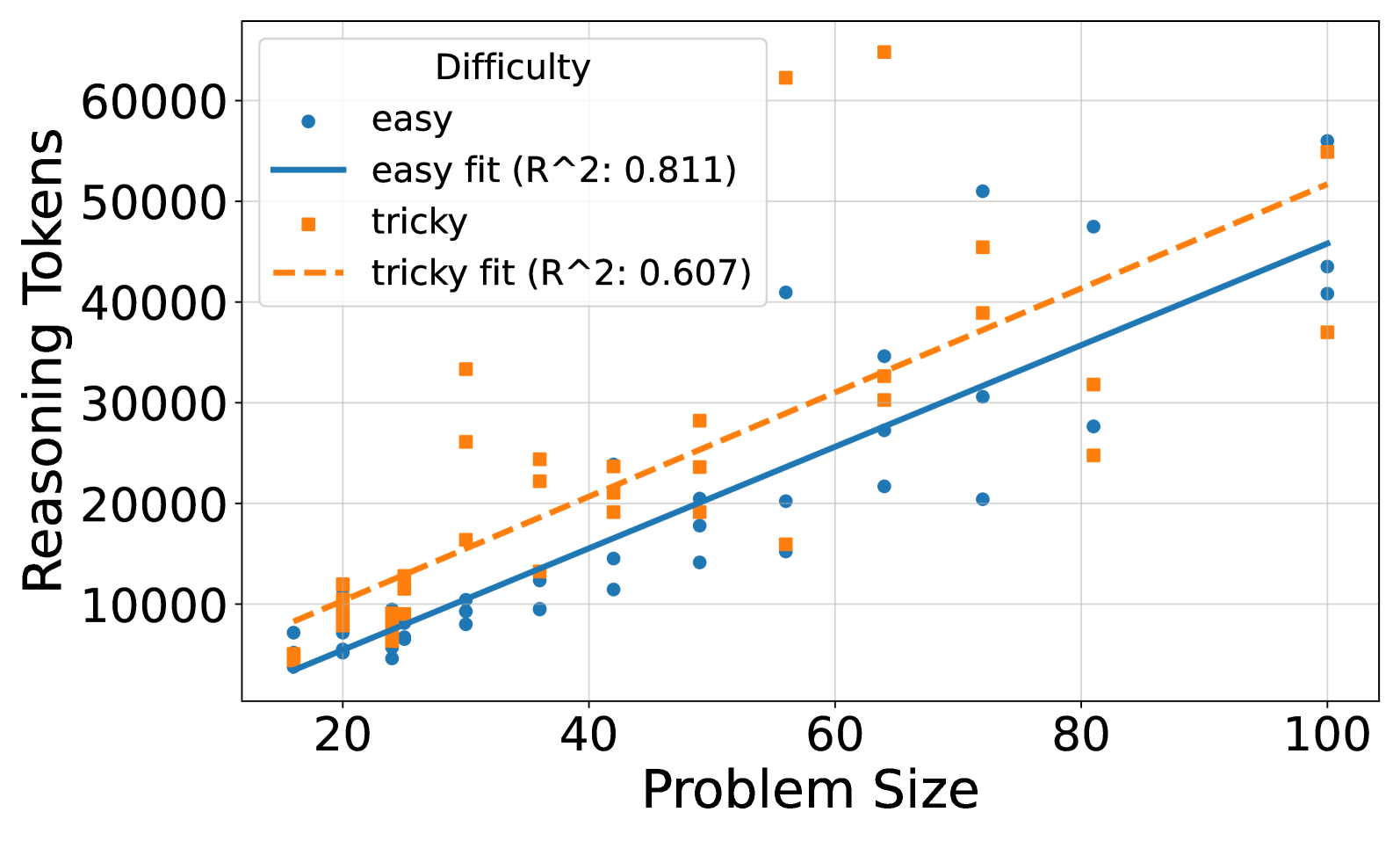
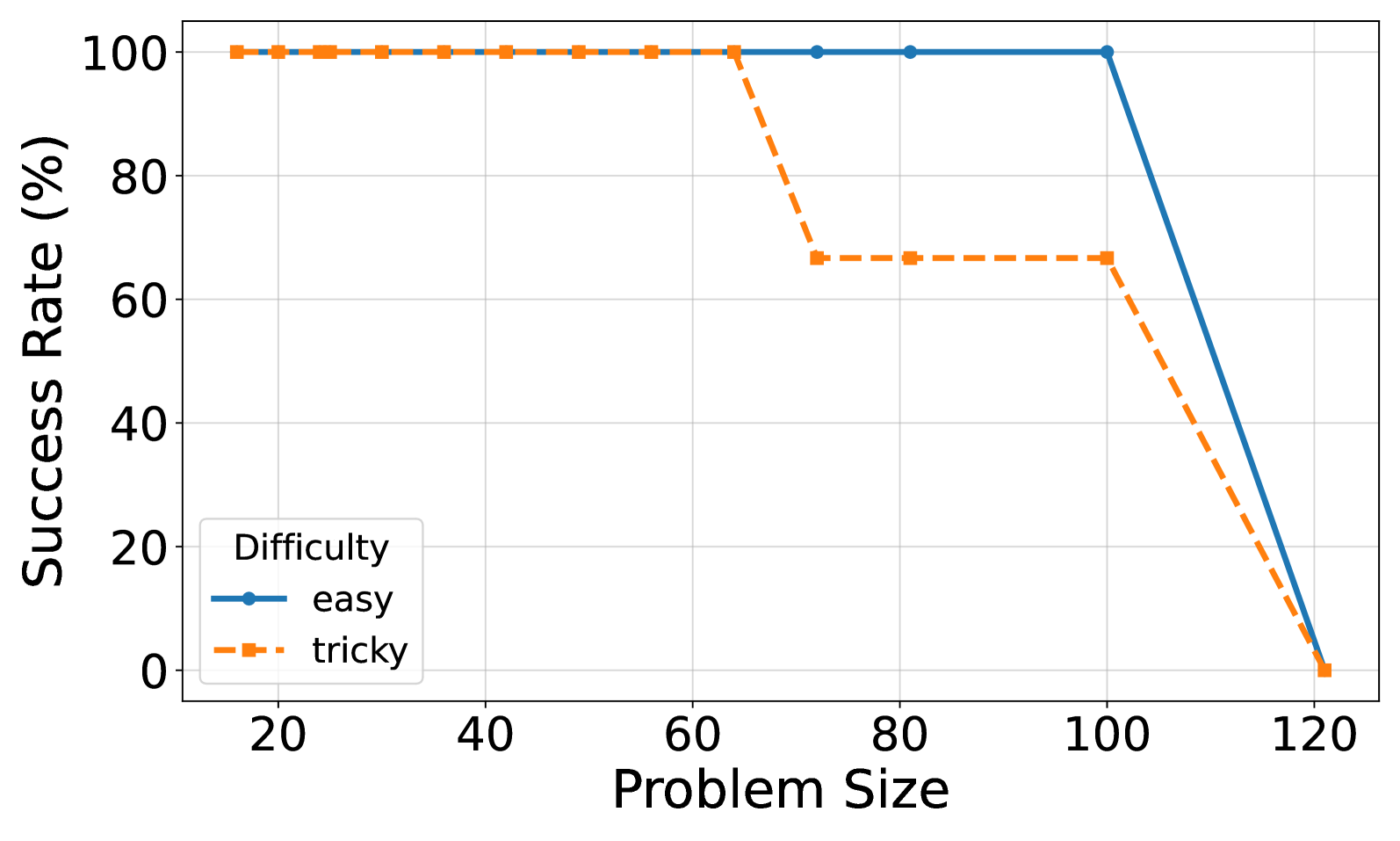
Figure 5: (a) Reasoning effort in number of reasoning tokens versus problem size for o3-mini with reasoning effort medium. Successful tries only. Linear fits are added for each model. (b) Solved percentage versus problem size for o3-mini with reasoning effort medium.
<details>
<summary>x9.png Details</summary>
### Visual Description
## Scatter Plot with Linear Regression Fits: Reasoning Tokens vs. Problem Size by Difficulty
### Overview
This image is a scatter plot chart that visualizes the relationship between "Problem Size" (x-axis) and the number of "Reasoning Tokens" (y-axis) required to solve problems. The data is categorized into two difficulty levels: "easy" and "tricky." Each category has its data points plotted and a linear regression trend line fitted to them, along with the corresponding R-squared (R²) value displayed in the legend.
### Components/Axes
* **Chart Type:** Scatter plot with overlaid linear regression lines.
* **X-Axis:**
* **Label:** "Problem Size"
* **Scale:** Linear scale ranging from approximately 15 to 100. Major tick marks are labeled at 20, 40, 60, 80, and 100.
* **Y-Axis:**
* **Label:** "Reasoning Tokens"
* **Scale:** Linear scale ranging from 0 to over 60,000. Major tick marks are labeled at 10000, 20000, 30000, 40000, 50000, and 60000.
* **Legend:**
* **Position:** Top-left corner of the plot area.
* **Title:** "Difficulty"
* **Entries:**
1. **easy:** Represented by blue circular dots (●).
2. **easy fit (R^2: 0.811):** Represented by a solid blue line (—).
3. **tricky:** Represented by orange square dots (■).
4. **tricky fit (R^2: 0.607):** Represented by a dashed orange line (---).
* **Grid:** A light gray grid is present in the background.
### Detailed Analysis
**Data Series and Trends:**
1. **"easy" Series (Blue Circles & Solid Blue Line):**
* **Trend:** The data points show a clear positive correlation. As Problem Size increases, the Reasoning Tokens required also increase. The trend is relatively consistent with moderate scatter around the fitted line.
* **Fitted Line:** The solid blue line represents a linear model fit to the "easy" data. It has a positive slope.
* **Goodness of Fit:** The R² value of 0.811 indicates that approximately 81.1% of the variance in Reasoning Tokens for "easy" problems can be explained by the linear relationship with Problem Size. This suggests a strong fit.
* **Approximate Data Points (Estimated from visual grid):**
* At Problem Size ~20: Tokens range from ~5,000 to ~8,000.
* At Problem Size ~40: Tokens range from ~10,000 to ~15,000.
* At Problem Size ~60: Tokens range from ~20,000 to ~28,000.
* At Problem Size ~80: Tokens range from ~28,000 to ~48,000.
* At Problem Size ~100: Tokens cluster around ~40,000 to ~55,000.
2. **"tricky" Series (Orange Squares & Dashed Orange Line):**
* **Trend:** This series also shows a strong positive correlation. However, the data points are more widely scattered compared to the "easy" series, indicating higher variance in the token count for a given problem size.
* **Fitted Line:** The dashed orange line represents the linear model fit for "tricky" problems. It has a steeper positive slope than the "easy" fit line.
* **Goodness of Fit:** The R² value of 0.607 indicates that about 60.7% of the variance is explained by the linear model. This is a weaker fit than for the "easy" series, consistent with the greater visual scatter.
* **Approximate Data Points (Estimated from visual grid):**
* At Problem Size ~20: Tokens range from ~5,000 to ~12,000.
* At Problem Size ~40: Tokens range from ~18,000 to ~25,000.
* At Problem Size ~60: Tokens range from ~15,000 to ~35,000 (with one notable outlier near 65,000).
* At Problem Size ~80: Tokens range from ~25,000 to ~45,000.
* At Problem Size ~100: Tokens range from ~37,000 to ~55,000.
### Key Observations
1. **Positive Correlation:** Both difficulty levels demonstrate that larger problems require more reasoning tokens.
2. **Difficulty Impact:** For any given Problem Size, the "tricky" data points and their trend line are generally positioned higher on the y-axis than the "easy" ones. This indicates that "tricky" problems consistently demand more reasoning tokens.
3. **Variance Difference:** The "tricky" series exhibits significantly greater variance (scatter) around its trend line compared to the "easy" series. This suggests that the token count for tricky problems is less predictable based solely on problem size.
4. **Outlier:** There is a prominent outlier in the "tricky" series at a Problem Size of approximately 65, with a Reasoning Token count near 65,000, which is far above the trend line and other data points in that region.
5. **Slope Comparison:** The slope of the "tricky fit" line is steeper than that of the "easy fit" line. This implies that the incremental cost (in tokens) of increasing problem size is higher for tricky problems than for easy ones.
### Interpretation
This chart provides a quantitative analysis of how computational effort (measured in reasoning tokens) scales with problem complexity (size) and inherent difficulty. The data strongly suggests that both factors are critical determinants of resource consumption.
The high R² for "easy" problems indicates a predictable, almost linear scaling law. In contrast, the lower R² and higher variance for "tricky" problems imply that other factors beyond simple size—perhaps the specific nature of the trickiness, the solution path required, or the model's specific weaknesses—play a substantial role in determining token usage. The steeper slope for tricky problems means that as problems get larger, the "penalty" for them being tricky becomes increasingly severe in terms of token cost.
The outlier in the tricky series is particularly interesting. It represents a case where a problem of moderate size required an exceptionally high number of tokens, potentially indicating a pathological case, a misleading problem statement, or a specific failure mode in the reasoning process being measured. This chart would be valuable for resource estimation, model evaluation, and understanding the limits of predictable scaling in AI reasoning tasks.
</details>
(a)
<details>
<summary>x10.png Details</summary>
### Visual Description
## Line Chart: Success Rate vs. Problem Size by Difficulty
### Overview
This is a line chart comparing the success rate (in percentage) of solving problems of varying sizes, categorized by two difficulty levels: "easy" and "tricky". The chart demonstrates how performance degrades as problem size increases, with a notably sharper decline for the "tricky" category.
### Components/Axes
* **X-Axis (Horizontal):** Labeled "Problem Size". The scale runs from approximately 15 to 120, with major tick marks at 20, 40, 60, 80, 100, and 120.
* **Y-Axis (Vertical):** Labeled "Success Rate (%)". The scale runs from 0 to 100, with major tick marks at 0, 20, 40, 60, 80, and 100.
* **Legend:** Located in the bottom-left quadrant of the chart area. It contains two entries:
* **"easy"**: Represented by a solid blue line with circular markers.
* **"tricky"**: Represented by a dashed orange line with square markers.
* **Grid:** A light gray grid is present, aligning with the major tick marks on both axes.
### Detailed Analysis
**Data Series: "easy" (Blue Solid Line with Circles)**
* **Trend:** The line remains perfectly flat at the top of the chart before a steep, near-vertical drop at the end.
* **Data Points (Approximate):**
* Problem Size ~15 to 100: Success Rate = 100%
* Problem Size 120: Success Rate = 0%
**Data Series: "tricky" (Orange Dashed Line with Squares)**
* **Trend:** The line starts flat, experiences a sharp drop to a lower plateau, holds steady, and then drops sharply again to meet the "easy" line at the final point.
* **Data Points (Approximate):**
* Problem Size ~15 to ~65: Success Rate = 100%
* Problem Size ~70: Success Rate drops sharply to ~67%
* Problem Size ~70 to 100: Success Rate holds steady at ~67%
* Problem Size 120: Success Rate = 0%
### Key Observations
1. **Performance Plateau:** Both difficulty levels maintain a 100% success rate for smaller problem sizes (up to ~65 for "tricky" and up to 100 for "easy").
2. **Differential Degradation:** The "tricky" problems show an earlier and more complex failure mode. Their success rate drops significantly at a problem size of around 70, plateaus, and then collapses. The "easy" problems maintain perfect performance much longer but then fail completely and abruptly.
3. **Convergence at Failure:** At the largest problem size shown (120), both difficulty levels have a 0% success rate, indicating a common point of total system failure or intractability.
4. **Sharp Transitions:** The changes in success rate are not gradual slopes but appear as sharp, almost step-like drops, suggesting critical thresholds in problem size.
### Interpretation
The data suggests a system or algorithm whose performance is highly reliable up to a certain problem scale, after which it fails catastrophically. The key insight is the difference in failure profiles between "easy" and "tricky" problems.
* **"Easy" problems** exhibit a **cliff-edge failure**: the system handles them perfectly until it suddenly cannot handle them at all (at size 100). This implies a hard resource limit or a fundamental algorithmic constraint that is triggered at a specific size.
* **"Tricky" problems** reveal a **two-stage failure**: an initial drop to a degraded but stable performance level (~67%), followed by a final collapse. This indicates that "tricky" problems likely exploit a specific weakness or complexity in the system that becomes active at a lower threshold (size ~70). The plateau suggests the system can still partially cope with this added complexity for a range of sizes before being overwhelmed entirely.
The chart effectively communicates that problem difficulty isn't just about a uniform lower success rate; it changes the *pattern* of failure. For practical purposes, this means the system is robust for "easy" tasks up to a known limit, but for "tricky" tasks, one must expect degraded performance much sooner, and planning should account for this two-phase degradation. The universal failure at size 120 defines the absolute upper bound of the system's capability for this class of problems.
</details>
(b)
Figure 6: (a) Reasoning effort in number of reasoning tokens versus problem size for o3-mini with reasoning effort high. Successful tries only. Linear fits are added for each model. (b) Solved percentage versus problem size for o3-mini with reasoning effort high.
#### A.2.2 Reasoning Effort for All Models
<details>
<summary>x11.png Details</summary>
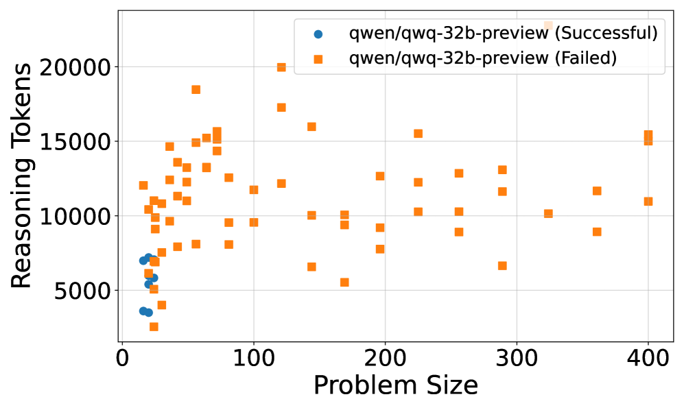
### Visual Description
## Scatter Plot: Model Performance by Problem Size and Reasoning Tokens
### Overview
This image is a scatter plot comparing the performance outcomes (Successful vs. Failed) of a specific AI model, `qwen/qwq-32b-preview`, across two metrics: "Problem Size" and "Reasoning Tokens". The plot visualizes the relationship between the complexity of a task (problem size) and the computational effort expended (reasoning tokens), categorized by the final success or failure of the model's attempt.
### Components/Axes
* **X-Axis (Horizontal):** Labeled "Problem Size". The scale runs from 0 to 400, with major tick marks at 0, 100, 200, 300, and 400.
* **Y-Axis (Vertical):** Labeled "Reasoning Tokens". The scale runs from 0 to 20,000, with major tick marks at 0, 5000, 10000, 15000, and 20000.
* **Legend:** Located in the top-right corner of the plot area.
* **Blue Circle (●):** `qwen/qwq-32b-preview (Successful)`
* **Orange Square (■):** `qwen/qwq-32b-preview (Failed)`
* **Grid:** A light gray grid is present, aiding in the estimation of data point coordinates.
### Detailed Analysis
The data is segmented into two distinct series based on the legend.
**1. Successful Attempts (Blue Circles):**
* **Trend & Placement:** These points form a tight cluster exclusively in the lower-left quadrant of the chart.
* **Data Points:** All successful attempts are confined to a narrow range.
* **Problem Size:** Approximately between 10 and 30.
* **Reasoning Tokens:** Approximately between 3,500 and 7,500.
* **Observation:** There is a positive correlation within this small cluster; as problem size increases slightly, the reasoning tokens used also increase. No successful attempts are recorded for problem sizes greater than ~30.
**2. Failed Attempts (Orange Squares):**
* **Trend & Placement:** These points are widely dispersed across the entire chart area, showing no single tight cluster.
* **Data Points:** They span the full ranges of both axes.
* **Problem Size:** From as low as ~15 to the maximum shown, 400.
* **Reasoning Tokens:** From as low as ~2,500 to the maximum shown, ~20,000.
* **Distribution:**
* A dense concentration exists for lower problem sizes (0-100), where token counts vary dramatically from ~2,500 to ~18,000.
* For larger problem sizes (100-400), the points are more sparse but still show high variability in token usage, ranging from ~5,000 to ~15,000+.
* The highest token count (≈20,000) is associated with a failed attempt at a problem size of approximately 120.
### Key Observations
1. **Clear Performance Boundary:** There is a stark, almost binary separation. Successful outcomes are strictly limited to very small problem sizes (< ~30) and moderate token usage (< ~7,500).
2. **Failure Across All Scales:** Failures occur across the entire spectrum of problem sizes, from small to large.
3. **Inefficiency in Failure:** Many failed attempts, especially at lower problem sizes, consume significantly more reasoning tokens (e.g., 10,000-18,000) than any successful attempt. This suggests a pattern of "spinning wheels" or inefficient reasoning on tasks that are ultimately not solved.
4. **No Success at Scale:** The complete absence of blue circles beyond a problem size of ~30 indicates a potential hard limit or severe degradation in the model's capability to successfully solve larger problems within this evaluation.
### Interpretation
This chart suggests a critical performance limitation for the `qwen/qwq-32b-preview` model on the evaluated task suite.
* **Capability Ceiling:** The model appears capable of solving only the simplest problems (small "Problem Size"). Its success is not just less likely but *non-existent* for more complex tasks in this dataset.
* **Resource Misallocation:** The high token counts for many failures indicate that the model often engages in extensive, yet unproductive, reasoning when it is destined to fail. This is particularly notable for small problems where it fails, using 2-3 times the tokens of a successful run.
* **Diagnostic Value:** The plot is a powerful diagnostic tool. It doesn't just show *that* the model fails on hard problems, but *how* it fails—often after expending considerable computational effort. This points to potential issues in the model's reasoning strategy, its ability to recognize dead ends, or a fundamental mismatch between its training and the nature of larger problems in this domain.
* **Actionable Insight:** To improve performance, focus should be on either: 1) Enhancing the model's core reasoning capability to handle larger problem sizes, or 2) Implementing better early-stopping or confidence-calibration mechanisms to prevent the wasteful expenditure of tokens on attempts that are unlikely to succeed.
</details>
Figure 7: Reasoning effort in tokens for Qwen QwQ.
<details>
<summary>x12.png Details</summary>
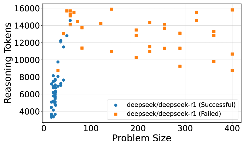
### Visual Description
\n
## Scatter Plot: Reasoning Tokens vs. Problem Size for DeepSeek-R1
### Overview
This image is a scatter plot comparing the number of "Reasoning Tokens" used against "Problem Size" for a model identified as "deepseek/deepseek-r1". The data is split into two series: successful attempts and failed attempts. The plot reveals a distinct separation in the distribution of these two outcomes based on problem size.
### Components/Axes
* **Chart Type:** Scatter Plot.
* **X-Axis:** Labeled "Problem Size". The scale runs from 0 to 400, with major tick marks at 0, 100, 200, 300, and 400.
* **Y-Axis:** Labeled "Reasoning Tokens". The scale runs from 0 to 16000, with major tick marks at 0, 2000, 4000, 6000, 8000, 10000, 12000, 14000, and 16000.
* **Legend:** Located in the bottom-right quadrant of the chart area.
* Blue Circle (●): `deepseek/deepseek-r1 (Successful)`
* Orange Square (■): `deepseek/deepseek-r1 (Failed)`
### Detailed Analysis
**1. Data Series: Successful Attempts (Blue Circles)**
* **Spatial Grounding & Trend:** This series is densely clustered in the far-left region of the chart, corresponding to low "Problem Size" values. The trend shows a steep, near-vertical increase in reasoning tokens as problem size increases from approximately 10 to 50.
* **Data Points (Approximate):**
* Problem Size Range: ~10 to ~50.
* Reasoning Tokens Range: ~3,000 to ~15,000.
* The highest token count for a successful run is approximately 14,500 at a problem size of ~50.
* The lowest token count is approximately 3,000 at a problem size of ~15.
* The majority of points are concentrated between problem sizes 20-40 and token counts 4,000-8,000.
**2. Data Series: Failed Attempts (Orange Squares)**
* **Spatial Grounding & Trend:** This series is widely dispersed across the entire x-axis. There is no single linear trend; instead, the points form a broad, scattered cloud. However, the minimum token count for failures appears to increase slightly with problem size.
* **Data Points (Approximate):**
* Problem Size Range: ~50 to 400.
* Reasoning Tokens Range: ~8,500 to ~16,000.
* Notable points include:
* A cluster of high-token failures (14,000-16,000) at low problem sizes (~50-80).
* A point at problem size ~140 with ~11,000 tokens.
* A point at problem size ~200 with ~10,200 tokens.
* The highest token count is near 16,000 at problem sizes ~140 and ~400.
* The lowest token count is approximately 8,500 at a problem size of ~400.
### Key Observations
1. **Clear Segmentation by Outcome:** There is a stark, almost complete separation between successful and failed attempts along the "Problem Size" axis. All successful attempts occur at problem sizes below ~50, while all failed attempts occur at problem sizes above ~50.
2. **Token Usage Patterns:** Successful attempts show a strong, positive correlation between problem size and token usage within their limited range. Failed attempts show high variability in token usage across all problem sizes, with no strong correlation.
3. **Overlap in Token Counts:** The token count ranges for success (~3k-15k) and failure (~8.5k-16k) overlap significantly, particularly in the 8,500-15,000 range. This indicates that high token usage alone does not predict failure; problem size is the critical dividing factor.
4. **Absence of Data:** There are no data points for successful attempts beyond a problem size of ~50, and no data points for failed attempts below a problem size of ~50.
### Interpretation
The data suggests a critical threshold in "Problem Size" around the value of 50 for the `deepseek/deepseek-r1` model under the tested conditions.
* **Performance Boundary:** The model appears capable of solving problems only up to a certain size (~50). Beyond this threshold, it consistently fails, regardless of the computational effort (reasoning tokens) expended.
* **Efficiency vs. Scale:** For small problems (size <50), the model's reasoning effort scales with problem complexity. For large problems (size >50), the model engages in extensive reasoning (often using 10,000+ tokens) but cannot achieve success, indicating a fundamental limitation in its reasoning capacity or approach for larger-scale tasks.
* **Investigative Insight:** The plot does not show *why* failures occur at large sizes. It could be due to context window limitations, error propagation in long reasoning chains, or a flaw in the model's problem-decomposition strategy for complex tasks. The high token usage in failures suggests the model is attempting to reason but is unable to converge on a correct solution. This visualization clearly identifies "Problem Size > 50" as a key area for debugging and improvement.
</details>
Figure 8: Reasoning effort in tokens for Deepseek R1.
<details>
<summary>x13.png Details</summary>
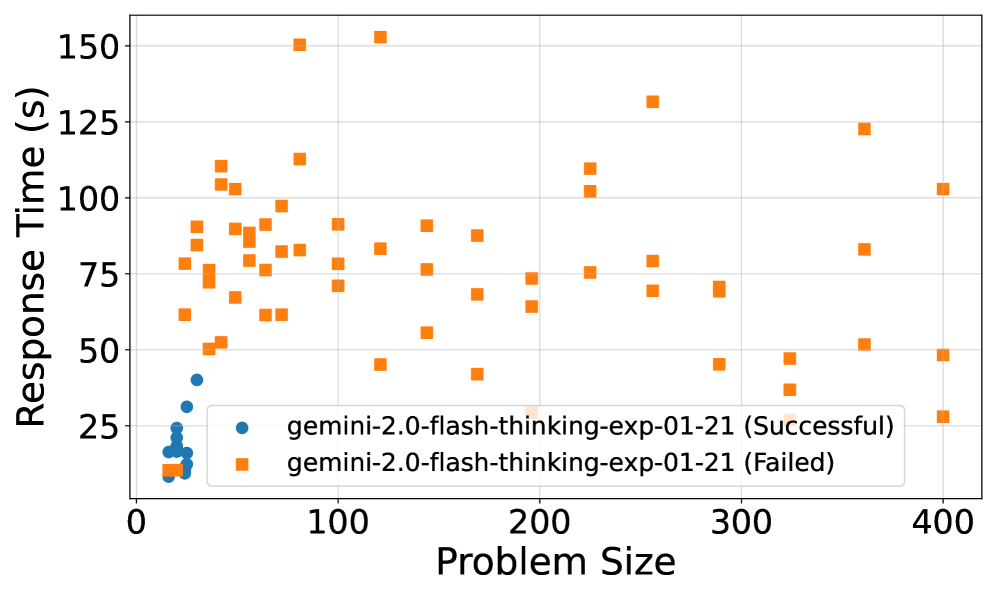
### Visual Description
\n
## Scatter Plot: Response Time vs. Problem Size for gemini-2.0-flash-thinking-exp-01-21
### Overview
This is a scatter plot comparing the response time (in seconds) against problem size for two outcome categories of a model named "gemini-2.0-flash-thinking-exp-01-21". The plot visualizes the performance distribution for successful versus failed attempts.
### Components/Axes
* **Chart Type:** Scatter Plot.
* **X-Axis:** Labeled "Problem Size". The scale runs from 0 to 400, with major tick marks at 0, 100, 200, 300, and 400.
* **Y-Axis:** Labeled "Response Time (s)". The scale runs from 0 to 150, with major tick marks at 0, 25, 50, 75, 100, 125, and 150.
* **Legend:** Located in the bottom-left quadrant of the plot area. It contains two entries:
1. A blue circle symbol labeled `gemini-2.0-flash-thinking-exp-01-21 (Successful)`.
2. An orange square symbol labeled `gemini-2.0-flash-thinking-exp-01-21 (Failed)`.
### Detailed Analysis
**Data Series 1: Successful Attempts (Blue Circles)**
* **Trend Verification:** The data points form a tight cluster with a slight upward trend, confined to the lower-left corner of the plot.
* **Spatial Grounding & Data Points:** All blue circle points are located at very low problem sizes and low response times.
* **Problem Size Range:** Approximately 10 to 40.
* **Response Time Range:** Approximately 10 to 40 seconds.
* **Cluster Density:** The points are densely packed, with many overlapping, indicating consistent performance within this narrow band. The highest response time for a successful attempt appears to be just below 40 seconds.
**Data Series 2: Failed Attempts (Orange Squares)**
* **Trend Verification:** The data points are widely scattered across the entire plot area with no single, clear linear trend. There is a broad distribution.
* **Spatial Grounding & Data Points:** Orange square points are found across the full range of problem sizes and a wide range of response times.
* **Problem Size Range:** Spans from approximately 10 to 400.
* **Response Time Range:** Spans from approximately 10 to just over 150 seconds.
* **Distribution:** There is a high density of points between problem sizes 20-150 and response times 50-110s. Points become more sparse but remain present at higher problem sizes (200-400). Several outliers exist with very high response times (e.g., ~150s at problem size ~80 and ~120).
### Key Observations
1. **Clear Separation:** There is a stark visual separation between the two outcome clusters. Successful attempts are exclusively confined to a small region of low problem size and low response time.
2. **Performance Threshold:** No successful attempts are visible for problem sizes greater than approximately 40. This suggests a potential performance or capability threshold for the model in this test.
3. **High Variability in Failures:** Failed attempts show enormous variability in both problem size and response time. A failure can occur quickly on a small problem or take a very long time on a large problem.
4. **Overlap at Low End:** At the very lowest problem sizes (~10-20) and response times (~10-20s), there is some overlap between the blue and orange markers, indicating that both successes and failures can occur under similar, minimal conditions.
### Interpretation
The data suggests a strong correlation between problem complexity (size) and the model's ability to succeed. The model "gemini-2.0-flash-thinking-exp-01-21" appears to reliably succeed only on a narrow band of small, simple problems, completing them quickly (under 40 seconds). Once the problem size exceeds a certain threshold (around 40), the model consistently fails, regardless of the time taken. The wide scatter of failed attempts indicates that failure mode is not predictable by problem size alone; some large problems fail quickly, while others take the maximum observed time. This pattern could indicate a fundamental limitation in the model's reasoning capacity or resource allocation for complex tasks, where it either solves the problem efficiently or enters a prolonged, unsuccessful processing state. The lack of any successful attempts in the mid-to-high problem size range is the most critical finding, pointing to a clear boundary in the model's effective operational domain for this specific task.
</details>
Figure 9: Reasoning effort quantified by response time for Gemini-2.0-flash-thinking.
### A.3 Cost
Total cost of these experiments was around 80 USD in API credits.