2503.17523

# Bayesian Teaching Enables Probabilistic Reasoning in Large Language Models **Authors**: Linlu Qiu, Fei Sha, Kelsey Allen, Yoon Kim, Tal Linzen, Sjoerd van Steenkiste > Google DeepMindUniversity of British ColumbiaVector Institute > Google ResearchNew York University > Google Research Corresponding author: linluqiu@mit.edu, svansteenkiste@google.com, linzen@google.com Abstract Large language models (LLMs) are increasingly used as agents that interact with users and with the world. To do so successfully, LLMs must construct representations of the world and form probabilistic beliefs about them. To provide personalized recommendations, for example, the LLM needs to infer a user’s preferences from their behavior over multiple interactions. The Bayesian inference framework lays out the optimal way for an agent to update its beliefs as it receives new information. We first show that LLMs fall far short of the standard defined by the Bayesian framework. We then show that by teaching LLMs to mimic the predictions of the normative Bayesian model, we can dramatically improve their ability to update their beliefs; this ability generalizes to new tasks. We conclude that LLMs can effectively learn reasoning skills from examples and generalize those skills to new domains. 1 Introduction Humans interact with the world based on our beliefs about it. To effectively support decision making, our beliefs need to correspond to the structure of the world as much as possible; in other words, our beliefs need to be supported by appropriate “world models” [Johnson-Laird, 1980, Ha and Schmidhuber, 2018, LeCun, 2022, Wong et al., 2023]. We typically do not have perfect knowledge about the outside world; to the extent that we are uncertain about our environment, our beliefs need to be probabilistic, reflecting this uncertainty. And for these beliefs to remain relevant as the world changes, or as new information about the world becomes available, we need to update our beliefs to reflect the new information. The framework of Bayesian inference describes the normative way in which new information should trigger a change in one’s beliefs so as to maximize the effectiveness of these beliefs as a foundation for acting in the world [Chater et al., 2006]. The Bayesian framework has informed a substantial body of work in cognitive science, which has identified both areas where humans act as the framework predicts, as well as deviations from it [Griffiths et al., 2024, Jern et al., 2017, Tenenbaum et al., 2011, Xu and Tenenbaum, 2007, Baker et al., 2011, Tenenbaum et al., 2006, Chater and Manning, 2006, Griffiths et al., 2007, Chaigneau et al., 2025, Rehder, 2018, Rottman and Hastie, 2016, Sloman and Lagnado, 2015]. In the last few years, artificial intelligence systems based on large language models (LLMs) have become dramatically more capable than in the past [Team, 2024a, Achiam et al., 2023, Anthropic, 2024, Team, 2024b, Touvron et al., 2023, Guo et al., 2025]. Far outgrowing their original motivation—as methods to estimate the probabilities of different word sequences—these systems are now being used for applications where they interact with users and with the outside world. As with humans, for the LLMs’ interactions with users to be effective, the LLMs’ beliefs need to reflect their experience with the user and to be continuously updated as more information becomes available. Here, we ask: do LLMs act as if they have probabilistic beliefs that are updated as expected from normative Bayesian inference? To the extent that the LLMs’ behavior deviates from the normative Bayesian strategy, how can we minimize these deviations? 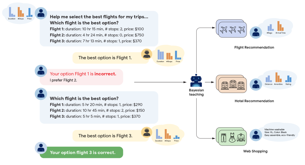We begin to study these questions using a simple controlled setting: a flight recommendation task [Lin et al., 2022], illustrated in Fig. 1. This task involves multiple rounds of interactions between a simulated user and an LLM, where the LLM is acting as a flight booking assistant. In each round, the assistant is given a small number of flight options, and is expected to recommend one of them to the user, based on the user’s preferences. The user’s preferences are not directly communicated to the LLM: it only observes the choices the user makes among the flight options. To make optimal recommendations, then, the LLM must construct an implicit model of the factors that shape the user’s preferences, and must reason probabilistically about those factors as it learns about the user’s choices across multiple sets of flight options. We compare the LLMs’ behavior to that of a model that follows the normative Bayesian strategy, which we refer to as the Bayesian Assistant. This model maintains a probability distribution that reflects its beliefs about the user’s preferences, and uses Bayes’ rule to update this distribution as new information about the user’s choices becomes available. Unlike many real-life scenarios, where it is difficult to specify and implement the Bayesian strategy computationally, in this controlled setting this strategy can be computed exactly, allowing us to precisely estimate the extent to which LLMs deviate from it. 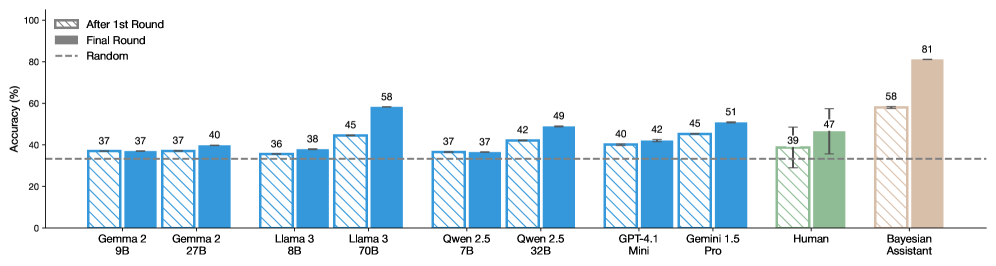We use this framework to evaluate a range of LLMs and find that they all perform significantly worse than the normative Bayesian Assistant (Fig. 2). Most importantly, in contrast to the Bayesian Assistant, which gradually improves its recommendations as it receives additional information about the user’s choices, LLMs’ performance often plateaus after a single interaction, pointing to a limited ability to adapt to new information. We then introduce Bayesian teaching, a strategy to teach an LLM to approximate Bayesian reasoning. We provide the LLM with examples of interactions between the user and the Bayesian Assistant, and have the LLM mimic those interactions. We find that, by leading the LLMs to gradually adapt to the user over the course of the interactions, this method substantially improves the LLMs’ performance on the flight recommendation task. Crucially, teaching the LLMs to mimic the Bayesian Assistant in one task allows them to generalize to other tasks that similarly require making decisions under uncertainty; those include not only different variants of the flight recommendation task, but also a related hotel recommendation task, as well as a web shopping task with real-world products (Fig. 1), a much more complex task for which it is difficult to specify and implement a fully Bayesian model. Notably, while the Bayesian Assistant often makes incorrect predictions as it reasons under uncertainty, especially in the early rounds of interaction, we find that it is a more effective teacher than a teacher that directly provides the LLMs with users’ choices (which we refer to as an oracle teacher); in other words, the Bayesian model’s educated guesses make for a stronger learning signal than the correct answers. Overall, we conclude that through observing the Bayesian Assistant perform a particular task, the LLMs are able to approximate transferable probabilistic reasoning skills. To summarize our contributions: we first identify significant limitations of off-the-shelf LLMs in tasks that require forming and updating probabilistic beliefs. We then demonstrate that, by having the LLMs mimic an normative Bayesian model, we can teach them effectively to approximate probabilistic belief updates, and show that these skills can generalize to new environments. These findings suggest that LLMs can be used in interactive settings where information is provided gradually, including complex application domains where implementing an exact Bayesian model is difficult. More generally, our results highlight a unique strength of deep learning models such as LLMs: they can learn to mimic a symbolic model and generalize its strategy to domains that are too complex to specify in a classic symbolic model. 2 Evaluating Belief Updates via Flight Recommendations <details> <summary>x1.png Details</summary>  ### Visual Description ## Diagram: Bayesian Teaching for Recommendations ### Overview The image illustrates a Bayesian teaching system used for personalized recommendations across different domains: flight selection, hotel selection, and web shopping. The system learns from user feedback to improve its recommendations. ### Components/Axes * **User Interaction Bubbles:** These represent user queries and feedback. * Each bubble contains a question about selecting the best option (flight). * Each bubble contains a list of options with attributes (duration, # stops, price). * Each bubble contains the system's initial recommendation. * Each bubble contains the user's feedback on the recommendation. * **Bayesian Teaching Robot:** This represents the core learning algorithm. It receives user feedback and updates its model. * **Recommendation Modules:** These represent the different domains where recommendations are made. * Flight Recommendation: Shows airplanes and bar graphs for "#Bags" and "ArrivalTime". * Hotel Recommendation: Shows buildings and bar graphs for "Distance", "Amenities", and "Rating". * Web Shopping: Shows clothing items and text "Machine washable, Size: XL, Color: Black, Easy assemble, eco-friendly". * **Bar Graphs:** Each recommendation module has associated bar graphs representing different features. The x-axis labels are specific to each module. The y-axis is not labeled, but represents the relative importance or value of each feature. * **Flow Arrows:** Arrows indicate the flow of information from user interaction to the Bayesian teaching robot and then to the recommendation modules. ### Detailed Analysis **User Interaction Bubbles (Flight Selection - First Instance):** * **Query:** "Help me select the best flights for my trips... Which flight is the best option?" * **Flight Options:** * Flight 1: duration: 10 hr 15 min, # stops: 2, price: $100 * Flight 2: duration: 4 hr 24 min, # stops: 0, price: $750 * Flight 3: duration: 7 hr 13 min, # stops: 1, price: $370 * **System Recommendation:** "The best option is Flight 1." * **User Feedback:** "Your option Flight 1 is incorrect. I prefer Flight 2." * **Associated Bar Graph:** * Duration: Tallest bar (blue) * #Stops: Medium bar (orange) * Price: Shortest bar (blue) **User Interaction Bubbles (Flight Selection - Second Instance):** * **Query:** "Which flight is the best option?" * **Flight Options:** * Flight 1: duration: 5 hr 20 min, # stops: 1, price: $290 * Flight 2: duration: 10 hr 45 min, # stops: 2, price: $150 * Flight 3: duration: 5 hr 5 min, # stops: 1, price: $370 * **System Recommendation:** "The best option is Flight 3." * **User Feedback:** "Your option flight 3 is correct." * **Associated Bar Graph:** * Duration: Shortest bar (blue) * #Stops: Medium bar (orange) * Price: Tallest bar (blue) **Flight Recommendation Module:** * **Features:** #Bags, Arrival Time * **Bar Graph:** * #Bags: Short bar (blue) * ArrivalTime: Tall bar (orange) **Hotel Recommendation Module:** * **Features:** Distance, Amenities, Rating * **Bar Graph:** * Distance: Short bar (blue) * Amenities: Tall bar (orange) * Rating: Medium bar (blue) **Web Shopping Module:** * **Features:** (Implied from text) Machine washable, Size: XL, Color: Black, Easy assemble, eco-friendly. * **No Bar Graph:** Instead, descriptive text is provided. ### Key Observations * The Bayesian teaching system learns from user feedback to improve its recommendations. * The system considers multiple factors (duration, # stops, price) when recommending flights. * The system adapts its recommendations based on user preferences. * The bar graphs represent the relative importance of different features in each domain. ### Interpretation The diagram illustrates a personalized recommendation system that uses Bayesian teaching to learn from user feedback. The system aims to provide relevant recommendations across different domains by considering multiple factors and adapting to user preferences. The initial recommendation in the first flight selection instance is incorrect, but after receiving feedback, the system provides a correct recommendation in the second instance. This demonstrates the learning capability of the Bayesian teaching algorithm. The bar graphs provide a visual representation of the relative importance of different features in each domain, allowing users to understand the factors that influence the system's recommendations. The system is designed to be flexible and adaptable, allowing it to be used in a variety of domains. </details> Figure 1: Evaluating and improving LLMs’ probabilistic belief updates. The flight recommendation task (left) involves multi-round interactions between a user and a flight booking assistant. In each round, the assistant is asked to recommend to the user one of three available flight options. The assistant is then shown the flight that was in fact chosen by the user (based on the user’s reward function, which characterizes the user’s preferences). To make good recommendations, the assistant needs to infer the user’s preferences from the user’s choices. To teach the LLM to reason probabilistically, we fine-tune the LLM on interactions between users and a Bayesian Assistant, which represents the normative way to update beliefs about the user’s preferences. We then evaluate the fine-tuned model on the flight recommendation task as well as two new tasks (right). We first describe the simplified flight recommendation task, derived that we use to evaluate the LLMs [Lin et al., 2022]. In this task, we have the LLMs interact with a simulated user for five rounds. In each round, three flight options are presented to both the user and the assistant. Each flight is defined by a departure time, a duration, a number of stops, and a cost (see Fig. 1). Each simulated user is characterized by a set of preferences: for each feature, they can have a strong or weak preference for high or low values of the feature (e.g., they may prefer longer or shorter flights), or no preference regarding this feature. We refer to this set of preferences as the user’s reward function. We have 624 possible users in total (see Appendix Section A). These preferences, which determine the flights that the user chooses, are not directly revealed to the assistant. The goal of the assistant is to recommend the flight that matches the user’s choice. At the end of each round, the user indicates to the assistant whether or not it chose correctly, and provides it with the correct answer. After each round, we evaluate the accuracy of the assistant’s recommendations for 100 new sets of three flights that differ from the ones on which the assistant has received feedback. We do not provide any feedback to the assistant for these new flight option sets (see Appendix Fig. 7 for the evaluation workflow). 2.1 The Bayesian Assistant Because the users’ preferences are only revealed gradually, through their choices among flight options, we cannot expect the LLMs to reach perfect accuracy immediately after a single round of interaction. As an upper bound on the LLMs’ performance, we define a Bayesian Assistant, which implements the strategy that optimally takes into account the evidence about the user’s preferences that accumulates over rounds of interaction. This entails maintaining uncertainty about those preferences when the evidence is partial: instead of committing to a single most likely reward function, which could turn out to be incorrect in future rounds, the assistant maintains a probability distribution over possible reward functions. After each round, the Bayesian Assistant updates its distribution over reward functions using Bayes’ rule: the probability of each reward function after the round (the posterior) is computed based on its probability before the round (the prior) and whether or not it was compatible with the user’s choice (the likelihood). This normative model represents the best performance that we can possibly expect from any system. Because the number of possible reward functions is small, we are able to perform exact Bayesian inference (see Appendix Section A). This method requires us to define the Bayesian Assistant’s initial prior distribution, that is, its probabilistic assumptions about which user preferences are more likely, in advance of any interaction with the user. We use an uninformed prior, where all possible sets of user preferences are equally likely (for experiments with alternative priors, see Appendix Section D.4). <details> <summary>x2.png Details</summary>  ### Visual Description ## Bar Chart: Model Accuracy Comparison ### Overview The image is a bar chart comparing the accuracy of various language models, a human, and a Bayesian assistant after one round and after a final round of processing. The y-axis represents accuracy in percentage, and the x-axis lists the different models and the human benchmark. A dashed line indicates a "random" accuracy level. ### Components/Axes * **Y-axis:** Accuracy (%), ranging from 0 to 100. Increments of 20 are marked (0, 20, 40, 60, 80, 100). * **X-axis:** Categorical axis listing the models and human benchmark: * Gemma 2 9B * Gemma 2 27B * Llama 3 8B * Llama 3 70B * Qwen 2.5 7B * Qwen 2.5 32B * GPT-4.1 Mini * Gemini 1.5 Pro * Human * Bayesian Assistant * **Legend:** Located in the top-left corner: * "After 1st Round": Represented by bars with diagonal stripes. * "Final Round": Represented by solid bars. * "Random": Represented by a dashed horizontal line. ### Detailed Analysis Here's a breakdown of the accuracy for each model and the human benchmark, comparing the "After 1st Round" and "Final Round" accuracy: * **Gemma 2 9B:** * After 1st Round: 37% * Final Round: 37% * **Gemma 2 27B:** * After 1st Round: 37% * Final Round: 40% * **Llama 3 8B:** * After 1st Round: 36% * Final Round: 38% * **Llama 3 70B:** * After 1st Round: 45% * Final Round: 58% * **Qwen 2.5 7B:** * After 1st Round: 37% * Final Round: 37% * **Qwen 2.5 32B:** * After 1st Round: 42% * Final Round: 49% * **GPT-4.1 Mini:** * After 1st Round: 40% * Final Round: 42% * **Gemini 1.5 Pro:** * After 1st Round: 45% * Final Round: 51% * **Human:** * After 1st Round: 39% * Final Round: 47% * **Bayesian Assistant:** * After 1st Round: 58% * Final Round: 81% * **Random Accuracy:** Represented by a dashed line at approximately 33%. ### Key Observations * The Bayesian Assistant shows the highest accuracy in both rounds, with a significant increase from the first to the final round. * Llama 3 70B and Gemini 1.5 Pro also show notable improvements in accuracy from the first to the final round. * Some models, like Gemma 2 9B and Qwen 2.5 7B, show no improvement between rounds. * The human accuracy is relatively low compared to some of the models, especially the Bayesian Assistant. * All models and the human perform better than random chance. ### Interpretation The chart suggests that certain language models, particularly the Bayesian Assistant, are significantly more accurate than others. The improvement in accuracy from the first to the final round indicates that some models benefit from additional processing or refinement. The Bayesian Assistant's high accuracy suggests it may employ more sophisticated techniques or have been trained on a more relevant dataset. The human benchmark provides a point of comparison, highlighting the strengths and weaknesses of AI models relative to human performance. The fact that all models perform better than random chance indicates that they possess some level of understanding or pattern recognition. </details> Figure 2: LLMs show limited or no improvement over multiple interactions with the user. We show accuracy after the first round and final (fifth) round. We compare off-the-shelf LLMs from different model families to human participants and the Bayesian Assistant. For human participants, we only evaluate on a subset of 48 out of our 624 simulated users. The LLMs perform considerably worse than the Bayesian Assistant. Human participants demonstrate a larger improvement than most LLMs as they receive more information, but they still fall short of the accuracy that characterizes the normative Bayesian strategy. For the human study, the error bars show the averaged standard error across participants; for models, they show the standard error across the three sets of interactions with each of the 624 users. 2.2 LLMs Show Limited Evidence of Belief Updating The LLMs we evaluate, like most contemporary LLMs, are first trained to predict upcoming words in a large collection of texts (“pre-training”), and are then specialized to follow user instructions provided in natural language (“instruction-tuning”) [Sanh et al., 2022, Wei et al., 2022a]. Most commercially available models are closed-weights: we can query them but we cannot access their parameters. We evaluate two such closed-weights models, Gemini 1.5 Pro [Team, 2024a] and GPT-4.1 Mini [OpenAI, 2025], which were among the state-of-the-art LLMs at the time of writing [Chiang et al., 2024]. We also evaluate the following open-weights models: Gemma 2 (9B and 27B parameters) [Team, 2024b], Llama 3 (8B and 70B parameters) [Grattafiori et al., 2024], and Qwen 2.5 (7B and 32B parameters) [Yang et al., 2024a]. We chose those models because their performance was quite competitive, and their weights are openly available, which makes it possible to perform fine-tuning (see the next section). We provide these LLMs with English instructions explaining how to act as a flight booking assistant (see Fig. 1 for an example, and Appendix Table 3 for a detailed interaction). We show results in Fig. 2. Overall, the accuracy of the LLMs after the five rounds of interaction is considerably lower than that of the Bayesian Assistant, and most of the models show little improvement after the first round of interaction (Fig. 2 shows results after the first and fifth round; for results after each of the five rounds, see Appendix Fig. 24). For an exploration of how the models’ performance varies across users’ possible reward functions, see Appendix Section D.2. A range of follow-up experiments failed to produce meaningful improvement in the LLMs’ behavior (for details, see Appendix Section C.1). Those include experiments with “chain-of-thought prompting” [Wei et al., 2022b, Nye et al., 2021, Kojima et al., 2022], that is, instructions that are meant to encourage the LLM to reason more explicitly (Appendix Fig. 9); an experiment with alternative, purely numerical representations of the flight options that we hypothesized might be easier for the LLMs to parse than the verbal ones we used for our main experiments (Appendix Fig. 9); a setting where we have 30 instead of five rounds of interaction (Appendix Fig. 9); and experiments with models that are only pre-trained to predict upcoming words in texts, without subsequent training to follow user instructions (Appendix Fig. 9). We also had human participants act as the assistant to a subset of 48 simulated users (see Appendix Section A and Appendix Section F.1 for details). The human participants made recommendations for five rounds and showed a significant improvement between round 1 and 5 (p = 0.002, logistic mixed-effects model). In terms of accuracy, they perform better than small LLMs and slightly worse than larger LLMs (see Appendix Fig. 24 for performance over rounds). That being said, like all LLMs, humans also fall substantially short of the accuracy expected from the normative Bayesian strategy. 3 Teaching LLMs to Approximate Bayesian Reasoning <details> <summary>x3.png Details</summary>  ### Visual Description ## Bar Chart: Model Accuracy Comparison ### Overview The image is a bar chart comparing the accuracy of different language models (Gemma, Llama, Qwen, and Bayesian Assistant) under various conditions: "Original", "Oracle", and "Bayesian". The chart displays accuracy percentages for each model after the "1st Round" (striped bars) and in the "Final Round" (solid bars). A dashed horizontal line indicates the "Random" accuracy level. ### Components/Axes * **Y-axis:** "Accuracy (%)", ranging from 0 to 100. Increments of 20 are marked (0, 20, 40, 60, 80, 100). * **X-axis:** Categorical axis representing different language models and their variations: * Gemma (Original, Oracle, Bayesian) * Llama (Original, Oracle, Bayesian) * Qwen (Original, Oracle, Bayesian) * Bayesian Assistant * **Legend:** Located at the top-left corner: * Striped bars: "After 1st Round" * Solid bars: "Final Round" * Dashed line: "Random" ### Detailed Analysis **Gemma:** * **Original:** Accuracy is 37% after the 1st round and 37% in the final round. * **Oracle:** Accuracy is 50% after the 1st round and 61% in the final round. * **Bayesian:** Accuracy is 57% after the 1st round and 76% in the final round. **Llama:** * **Original:** Accuracy is 36% after the 1st round and 38% in the final round. * **Oracle:** Accuracy is 48% after the 1st round and 62% in the final round. * **Bayesian:** Accuracy is 57% after the 1st round and 75% in the final round. **Qwen:** * **Original:** Accuracy is 37% after the 1st round and 37% in the final round. * **Oracle:** Accuracy is 43% after the 1st round and 53% in the final round. * **Bayesian:** Accuracy is 55% after the 1st round and 68% in the final round. **Bayesian Assistant:** * Accuracy is 58% after the 1st round and 81% in the final round. **Random Accuracy:** * The dashed line indicates a random accuracy level of approximately 33%. ### Key Observations * All models generally show an increase in accuracy from the "1st Round" to the "Final Round," except for Gemma and Qwen "Original" which remain constant. * The "Bayesian" versions of Gemma, Llama, and Qwen consistently outperform their "Original" and "Oracle" counterparts. * The "Bayesian Assistant" achieves the highest final round accuracy (81%) among all models. * The "Original" versions of Gemma, Llama, and Qwen have very low accuracy, close to the "Random" level. ### Interpretation The chart demonstrates the impact of different training approaches ("Oracle" and "Bayesian") on the accuracy of language models. The "Bayesian" approach appears to significantly improve model performance compared to the "Original" versions. The "Bayesian Assistant" model stands out as the most accurate among those tested. The "Original" models perform poorly, suggesting that they may require further training or optimization. The "Oracle" models show improvement over the "Original" models, but not as much as the "Bayesian" models. 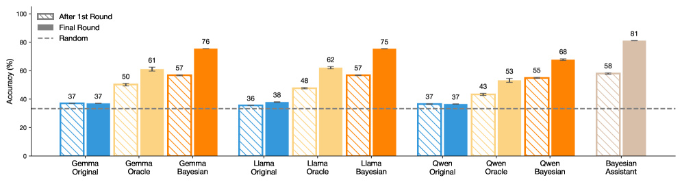</details> Figure 3: Supervised fine-tuning teaches LLMs to approximate probabilistic inference. We show accuracy after the first round and final (fifth) round across different assistants. We compare the original LLMs, LLMs fine-tuned on user interactions with the Bayesian Assistant, and LLMs fine-tuned on user interactions with an oracle, which always provides the correct answer. Both types of fine-tuning significantly improve LLMs’ performance, and Bayesian teaching is consistently more effectively than oracle teaching. Error bars show the standard error across three random seeds (and three training runs). All results are statistical significant, $p<0.001$ (see Appendix Section G). We next describe the supervised fine-tuning technique we use to teach the LLM to mimic the normative Bayesian model; we show that this method substantially improves the LLM’s ability to update its beliefs correctly. From a technical perspective, supervised fine-tuning is similar to the method used to train most LLMs in the first place. The model is provided with the first words of a text and is trained to predict the upcoming word. After each example, the LLM’s weights are adjusted to increase the likelihood of a correct prediction if the same example is observed again. The main difference is that while in the first phase of training the texts are typically drawn from the Internet or similar resources, in the supervised fine-tuning phase the texts are constructed in a targeted way (automatically or by human writers) so as to teach the LLM particular skills [Sanh et al., 2022, Wei et al., 2022a]; to improve arithmetic skills, for example, the model may be given the text “the output of $1+1=...$ is $2$ ”. We apply supervised fine-tuning to the three medium-sized open-weights models (Gemma 2 9B, Llama 3 8B, and Qwen 2.5 7B); we do not attempt to fine-tune the larger models from these families due to computational constraints. We update all of the models’ weights in fine-tuning (in Appendix Section C.2, we show that a different training objective, Direct Preference Optimization [Rafailov et al., 2023], produces similar results, as does a computationally cheaper fine-tuning method, LoRA [Hu et al., 2022], which only updates a subset of the model’s weights). We explore two strategies to create supervised fine-tuning data. For both strategies, we construct 10 five-round interactions per user. These interactions follow the same format as described above (Appendix Table 3). In the first strategy, which we refer to as oracle teaching, we provide the LLM with interactions between simulated users and an “oracle” assistant that has perfect knowledge of the user’s preferences, and as such always recommends the option that is identical to the user’s choices. The second strategy, which we call Bayesian teaching, provides the LLM with interactions between the user and the Bayesian Assistant. In this setting, the assistant will often choose flights that do not match the user’s preferred choice, especially in early rounds where it has considerable uncertainty about the user’s preferences. We hypothesize that despite this fact mimicking the Bayesian Assistant’s best guesses would teach the LLM to maintain uncertainty and update its beliefs more effectively than the first strategy where the LLM is trained on the correct choices. This approach can be seen as a form of distillation, where a model is trained by learning to mimic another system [Hinton et al., 2015, Kim and Rush, 2016, Deng et al., 2023, Wang et al., 2023b, Li et al., 2023b, Jung et al., 2024, Yu et al., 2024, Chen et al., 2024b]. We use a uniform prior for the Bayesian Assistant that produces the supervised fine-tuning data. Other priors perform similarly (see Appendix Fig. 16). 3.1 Fine-Tuning Teaches LLMs to Adapt to Users Both supervised fine-tuning strategies, oracle teaching and Bayesian teaching, significantly improve the LLMs’ performance on the flight recommendation task (Fig. 3). Crucially, after fine-tuning, the LLMs’ performance gradually improves as more information becomes available; this contrasts with the original LLMs, which plateaued after the first round (see the substantial performance improvement between the first and last round in Fig. 3; for detailed results for each round, see Appendix Fig. 25). While there is still a performance gap between the fine-tuned LLMs and the normative Bayesian Assistant, this gap is much narrower than for the original LLMs. All three medium-sized LLMs, which before fine-tuning performed worse than either stronger models or our human participants, markedly outperform them after fine-tuning. 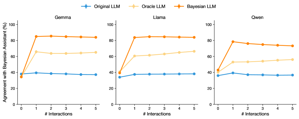We find that Bayesian teaching leads to higher accuracy and less variability across repetitions of the experiment than oracle teaching (Fig. 3). Bayesian teaching also successfully makes the LLM more Bayesian: the Bayesian-tuned LLMs’ predictions agree with those of the Bayesian Assistant around 80% of the time, significantly more often than do the predictions of the original LLMs and oracle-tuned LLMs (Fig. 4). In Appendix Section D.4, we show that the effectiveness of Bayesian teaching cannot be explained by two potential confounds, and conclude that the effectiveness of this method is in fact due to the Bayesian signal it provides. The amount of information that can be gained from the user’s choice for a particular option set varies from one set to another. For example, a choice between two flight options that differ in exactly one feature provides direct evidence for the user’s preference for that feature; such a choice could be more informative about the user’s preferences than the choice between options that differ along multiple dimensions. We expect a model with more sophisticated probabilistic skills to show greater sensitivity to this factor. Do our fine-tuned models show such sensitivity? Focusing on the Gemma models, we find that Gemma Original does not show sensitivity to option set informativity, but both fine-tuned versions of Gemma do, with Gemma Bayesian displaying considerably more sensitivity than Gemma Oracle (Appendix Section E). Can the fine-tuned models accurately verbalize their beliefs? To address this question, we ask the LLMs explicitly for their beliefs about the user’s preferences—we have the simulated user ask them, for example, “on a scale of 1 to 5, what is my preference for price?”. We then test for the accuracy of these verbalized beliefs by deriving flight recommendations from those beliefs, using the same decision procedure we use with the Bayesian Assistant. We find that this approach generally performs better the approach we have used so far where we directly ask for the LLMs’ recommendations; that predictions based on the fine-tuned LLMs’ verbalized beliefs are substantially more accurate than those based on the original LLMs’ verbalized beliefs; and that the Bayesian-tuned LLMs produce more accurate beliefs than either the original LLMs or oracle-tuned ones (for additional details, see Appendix Section B). <details> <summary>x4.png Details</summary>  ### Visual Description ## Line Chart: Agreement with Bayesian Assistant vs. Number of Interactions for Different LLMs ### Overview The image presents three line charts comparing the agreement percentage with a Bayesian Assistant for three different Language Learning Models (LLMs): Original LLM, Oracle LLM, and Bayesian LLM. The charts are separated by LLM type: Gemma, Llama, and Qwen. The x-axis represents the number of interactions (0 to 5), and the y-axis represents the agreement percentage (0% to 100%). ### Components/Axes * **Title:** Agreement with Bayesian Assistant (%) vs. # Interactions * **X-axis:** # Interactions, with markers at 0, 1, 2, 3, 4, and 5. * **Y-axis:** Agreement with Bayesian Assistant (%), with markers at 0, 20, 40, 60, 80, and 100. * **Chart Titles (Top):** Gemma, Llama, Qwen * **Legend (Top):** * Blue line with circle marker: Original LLM * Light Orange line with circle marker: Oracle LLM * Orange line with circle marker: Bayesian LLM ### Detailed Analysis **Gemma** * **Original LLM (Blue):** Relatively flat, hovering around 40%. * 0 Interactions: ~38% * 1 Interaction: ~40% * 5 Interactions: ~38% * **Oracle LLM (Light Orange):** Increases sharply from 0 to 1 interaction, then plateaus around 65%. * 0 Interactions: ~38% * 1 Interaction: ~65% * 5 Interactions: ~65% * **Bayesian LLM (Orange):** Increases sharply from 0 to 1 interaction, then plateaus around 85%. * 0 Interactions: ~35% * 1 Interaction: ~85% * 5 Interactions: ~85% **Llama** * **Original LLM (Blue):** Relatively flat, hovering around 38%. * 0 Interactions: ~35% * 1 Interaction: ~38% * 5 Interactions: ~38% * **Oracle LLM (Light Orange):** Increases sharply from 0 to 1 interaction, then plateaus around 65%. * 0 Interactions: ~40% * 1 Interaction: ~60% * 5 Interactions: ~65% * **Bayesian LLM (Orange):** Increases sharply from 0 to 1 interaction, then plateaus around 85%. * 0 Interactions: ~40% * 1 Interaction: ~85% * 5 Interactions: ~83% **Qwen** * **Original LLM (Blue):** Relatively flat, hovering around 38%. * 0 Interactions: ~36% * 1 Interaction: ~38% * 5 Interactions: ~37% * **Oracle LLM (Light Orange):** Increases sharply from 0 to 1 interaction, then plateaus around 55%. * 0 Interactions: ~42% * 1 Interaction: ~53% * 5 Interactions: ~57% * **Bayesian LLM (Orange):** Increases sharply from 0 to 1 interaction, then plateaus around 75%. * 0 Interactions: ~40% * 1 Interaction: ~78% * 5 Interactions: ~73% ### Key Observations * The "Original LLM" consistently shows the lowest agreement percentage across all three LLM types (Gemma, Llama, Qwen). * The "Bayesian LLM" consistently shows the highest agreement percentage across all three LLM types. * The "Oracle LLM" shows an agreement percentage between the "Original LLM" and "Bayesian LLM". * For all three LLM types, the agreement percentage for "Bayesian LLM" and "Oracle LLM" increases sharply from 0 to 1 interaction, then plateaus. The "Original LLM" remains relatively flat. ### Interpretation The data suggests that incorporating Bayesian methods into LLMs significantly improves their agreement with a Bayesian Assistant. The "Bayesian LLM" consistently outperforms the "Original LLM" and "Oracle LLM" across all three LLM types (Gemma, Llama, Qwen). The sharp increase in agreement percentage from 0 to 1 interaction for "Bayesian LLM" and "Oracle LLM" indicates that even a single interaction can significantly improve their performance. The "Original LLM" shows little to no improvement with increasing interactions, suggesting that it lacks the ability to effectively learn from interactions in the same way as the other two models. </details> Figure 4: Fine-tuned LLMs agree more with the Bayesian Assistant. We show agreement between the LLMs and the Bayesian Assistant, measured by the proportion of trials where the LLMs makes the same predictions as the Bayesian Assistant. Fine-tuning on the Bayesian Assistant’s predictions makes the LLMs more Bayesian, with the Bayesian versions of each LLM achieving the highest agreement with the Bayesian Assistant. Error bars (too small to be visible in plot) show standard errors across three random seeds (and three training runs). 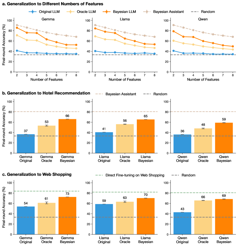3.2 Fine-Tuned LLMs Generalize to New Tasks <details> <summary>x5.png Details</summary>  ### Visual Description ## Chart Type: Performance Comparison of Language Models ### Overview The image presents a series of bar and line charts comparing the performance of different language models (Gemma, Llama, and Qwen) under various conditions. The charts are organized into three sections: generalization to different numbers of features, generalization to hotel recommendation, and generalization to web shopping. Each section compares the "Original," "Oracle," and "Bayesian" versions of each language model, along with baselines like "Bayesian Assistant" and "Random." ### Components/Axes **General Components:** * **Title:** The image is divided into three sections, each with a title: "a. Generalization to Different Numbers of Features," "b. Generalization to Hotel Recommendation," and "c. Generalization to Web Shopping." * **Y-axis:** All charts share a common Y-axis labeled "Final-round Accuracy (%)" ranging from 0 to 100. * **Legend:** Located at the top of the image, the legend identifies the different language model versions and baselines using color-coded lines and bars: * Original LLM (Blue) * Oracle LLM (Light Orange) * Bayesian LLM (Orange) * Bayesian Assistant (Light Gray, dashed line) * Random (Dark Gray, dashed line) **Section a: Generalization to Different Numbers of Features** * **X-axis:** Labeled "Number of Features," ranging from 2 to 8. * **Subplots:** Three subplots, one for each language model: Gemma, Llama, and Qwen. * **Data Series:** Each subplot contains line plots for "Original LLM," "Oracle LLM," "Bayesian LLM," "Bayesian Assistant," and "Random." **Section b: Generalization to Hotel Recommendation** * **X-axis:** Categorical, with three categories for each language model: "Original," "Oracle," and "Bayesian." * **Subplots:** Three subplots, one for each language model: Gemma, Llama, and Qwen. * **Data Series:** Each subplot contains bar plots for "Original," "Oracle," and "Bayesian" versions of the language model. **Section c: Generalization to Web Shopping** * **X-axis:** Categorical, with three categories for each language model: "Original," "Oracle," and "Bayesian." * **Subplots:** Three subplots, one for each language model: Gemma, Llama, and Qwen. * **Data Series:** Each subplot contains bar plots for "Original," "Oracle," and "Bayesian" versions of the language model. ### Detailed Analysis **Section a: Generalization to Different Numbers of Features** * **Gemma:** * Original LLM (Blue): Relatively flat line around 37% accuracy. * Oracle LLM (Light Orange): Decreases from approximately 90% at 2 features to 55% at 8 features. * Bayesian LLM (Orange): Decreases from approximately 95% at 2 features to 60% at 8 features. * Bayesian Assistant (Light Gray, dashed line): Flat line around 80% accuracy. * Random (Dark Gray, dashed line): Flat line around 37% accuracy. * **Llama:** * Original LLM (Blue): Relatively flat line around 41% accuracy. * Oracle LLM (Light Orange): Decreases from approximately 80% at 2 features to 50% at 8 features. * Bayesian LLM (Orange): Decreases from approximately 90% at 2 features to 55% at 8 features. * Bayesian Assistant (Light Gray, dashed line): Flat line around 80% accuracy. * Random (Dark Gray, dashed line): Flat line around 37% accuracy. * **Qwen:** * Original LLM (Blue): Relatively flat line around 36% accuracy. * Oracle LLM (Light Orange): Decreases from approximately 75% at 2 features to 45% at 8 features. * Bayesian LLM (Orange): Decreases from approximately 85% at 2 features to 50% at 8 features. * Bayesian Assistant (Light Gray, dashed line): Flat line around 80% accuracy. * Random (Dark Gray, dashed line): Flat line around 37% accuracy. **Section b: Generalization to Hotel Recommendation** * **Gemma:** * Original (Blue): 37% accuracy. * Oracle (Light Orange): 53% accuracy. * Bayesian (Orange): 66% accuracy. * **Llama:** * Original (Blue): 41% accuracy. * Oracle (Light Orange): 56% accuracy. * Bayesian (Orange): 65% accuracy. * **Qwen:** * Original (Blue): 36% accuracy. * Oracle (Light Orange): 48% accuracy. * Bayesian (Orange): 59% accuracy. **Section c: Generalization to Web Shopping** * **Gemma:** * Original (Blue): 54% accuracy. * Oracle (Light Orange): 61% accuracy. * Bayesian (Orange): 73% accuracy. * **Llama:** * Original (Blue): 59% accuracy. * Oracle (Light Orange): 63% accuracy. * Bayesian (Orange): 70% accuracy. * **Qwen:** * Original (Blue): 43% accuracy. * Oracle (Light Orange): 66% accuracy. * Bayesian (Orange): 69% accuracy. ### Key Observations * In the "Generalization to Different Numbers of Features" section, the "Original LLM" models maintain a relatively constant accuracy regardless of the number of features, while the "Oracle LLM" and "Bayesian LLM" models show a decreasing trend in accuracy as the number of features increases. * In both the "Hotel Recommendation" and "Web Shopping" sections, the "Bayesian" versions of each language model consistently outperform the "Original" and "Oracle" versions. * The "Bayesian Assistant" baseline in the "Generalization to Different Numbers of Features" section consistently achieves around 80% accuracy. * The "Random" baseline consistently achieves around 37% accuracy across all sections. * The "Direct Fine-tuning on Web Shopping" baseline in the "Web Shopping" section achieves around 80% accuracy. ### Interpretation The data suggests that the "Oracle" and "Bayesian" versions of the language models are more sensitive to the number of features, as their accuracy decreases as the number of features increases. This could indicate that these models are more prone to overfitting or that they require more data to generalize effectively with a larger number of features. The "Bayesian" versions of the language models consistently outperform the "Original" and "Oracle" versions in the "Hotel Recommendation" and "Web Shopping" tasks, suggesting that the Bayesian approach is more effective for these specific tasks. The baselines provide a point of reference for evaluating the performance of the language models. The "Random" baseline indicates the expected accuracy of a random guess, while the "Bayesian Assistant" and "Direct Fine-tuning on Web Shopping" baselines represent the performance of alternative approaches. The error bars on the bar charts indicate the variability in the accuracy of the models. The error bars are relatively small, suggesting that the results are consistent and reliable. </details> \phantomsubcaption \phantomsubcaption \phantomsubcaption Figure 5: Bayesian teaching generalizes outside the task used for fine-tuning. (a) Final-round accuracy gain in fine-tuned models compared to the original LLM when varying task complexity (here the number of features is a proxy for task complexity). (b) Final-round accuracy for LLMs on the hotel recommendation task, which was not seen during fine-tuning. We show the normative Bayesian Assistant’s performance with brown dashed lines. (c) Final-round accuracy for LLMs on the web shopping domain, also unseen during fine-tuning. The green dashed line indicates the performance of the LLM when it is fine-tuned directly on web shopping data, such that no domain generalization is necessary. Error bars indicate the standard errors over three training runs (for web shopping) and additionally three random seeds (for flight recommendation and hotel recommendation). As a result of Bayesian teaching, the LLMs demonstrate a greatly improved ability to approximate Bayesian probabilistic inference. Is this ability specific to the particular task the models were trained on, or do the LLMs’ probabilistic skills improve more broadly? To answer this question, we evaluate the fine-tuned LLMs on a set of tasks that diverge to different extents from our original flight recommendation task (see the right panel of Fig. 1 for an overview). All tasks require the LLMs to infer the user’s preferences from the user’s choices over multiple interactions. Overall, as we show in the rest of this section, we find that fine-tuned LLMs show considerable generalization to new settings, and that, as before, Bayesian teaching is more effective than oracle teaching. We first test the LLMs on variants of the flight recommendation task with different numbers of features: whereas in the interactions provided during fine-tuning, flights were characterized by four features, in this evaluation setting flights are described by between two and eight features. This requires the LLM to generalize to features that were not included in fine-tuning (e.g., the number of checked bags). In this setting, we find that both types of fine-tuning lead to large improvement in accuracy compared to the original LLMs. We also find that Bayesian teaching is considerably more effective than oracle teaching, as before (Fig. 5). We note that as the number of features increases, the space of possible reward functions grows exponentially, and the task becomes inherently more difficult, even for the Bayesian Assistant. Despite this fact, for both fine-tuning methods, performance relative to the upper bound defined by the Bayesian Assistant drops off only moderately as the number of features increases. The generalization experiments we have discussed so far focused on variants of the flight recommendation task. We next evaluate whether the LLMs can generalize the probabilistic skills they acquire through fine-tuning and apply them to other domains. We consider two such domains: hotel recommendations and web shopping. The hotel recommendation task is a synthetic task whose structure is similar to that of the flight recommendation task presented in fine-tuning. Here, each hotel is defined by four features: distance to downtown, price, rating, and amenities (for an example, see Appendix Table 11). The web shopping task uses real-world products from a simulated environment [Yao et al., 2022], and differs much more substantially from the fine-tuning task than does the hotel recommendation task. It is difficult to construct a Bayesian Assistant for more natural scenarios like the web shopping task, where the space of user preferences is large and hard to specify formally. For this reason, successful transfer from synthetic settings like the flight recommendation task to more natural scenarios represents a particularly important application of Bayesian teaching. In the web shopping task, each user is defined by a set of randomly sampled goals that characterize the product they are interested in; for example, they might be looking for a shirt that is machine washable, or for a size XL shirt (see Appendix Table 1 for examples). As in the flight domain, the assistant interacts with the user for multiple rounds. In each round, a set of product options is randomly sampled from the product category (e.g., shirts), and the assistant is asked to recommend the best option. Each product is represented by a short title along with a detailed description (see Appendix Table 12 for an example). The user provides feedback at the end of each round, indicating whether or not the assistant’s recommendation was correct. The user’s preferred option is the one with the highest reward, as defined in Yao et al. [2022]. As mentioned above, it is difficult to construct a Bayesian Assistant for this task due to the large space of possible preferences. Instead, as an alternative upper bound on the transfer performance we can expect from the models fine-tuned on the flight recommendation task, we fine-tune LLMs directly on data from the shopping task. We find that LLMs fine-tuned on the flight recommendation task generalize to both hotel recommendations and web shopping: they perform much better than the original LLMs on those tasks (Fig. 5 and Fig. 5). Bayesian teaching continues to outperform oracle teaching, though the gap is smaller for web shopping than hotel recommendations. There remains a gap between the generalization performance of the LLMs fine-tuned on flight recommendations and the upper bound obtained by fine-tuning the LLMs directly on the web shopping interactions (green dashed line in Fig. 5). Overall, we conclude that fine-tuning, and especially Bayesian teaching, imparts probabilistic skills that transfer substantially beyond the setting used for fine-tuning. 3.3 Generalization to Interactions with Human Users The synthetically generated data we have used so far makes two simplifying assumptions: the simulated users’ choices faithfully reflect the reward function that characterizes their preferences, and all reward functions are encountered equally often. In practice, these assumptions may not hold as humans’ behavior could occasionally be inconsistent with their preferences, due to inattention or other biases, and some preferences may be more common in the population than others (such as a preference for lower price). To evaluate the models in a more realistic setting, we recruit human participants to act as users. Each human participant is asked to first state their preferences for each of the flight features, and then select their preferred flight out of three options, for five different sets of options. We collect data from 10 human participants each for 50 lists of flight option sets, for a total of 500 participants (see Appendix Section A). 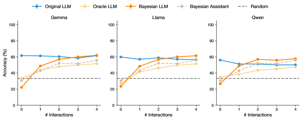The performance of both fine-tuned models and the Bayesian Assistant for human users consistently improves over rounds (Fig. 6), and, as was the case for the simulated users, the Bayesian LLMs consistently outperform the Oracle LLMs; at least for some model families, the Bayesian LLMs also outperform the original LLMs. This indicates that the Bayesian LLMs generalize to human users from the simulated users on which they were fine-tuned. All models, including the Bayesian Assistant, show substantially lower performance for humans than they did for simulated users, where accuracy after five rounds approached 80% (Fig. 3). In the Appendix Section F.2, we show that this is due to the fact that participants’ choices are not always consistent with their stated preferences, and as such are impossible to predict with high accuracy (Appendix Fig. 22). For the subset of human users whose choices are perfectly consistent with their preferences, the Bayesian LLM performs much better than the original LLM (Appendix Fig. 21; see also Appendix Section D.3, where we study inconsistent simulated users). Unlike for the simulated users, for human users the original LLMs perform well even after a single interaction (although, crucially, the original LLMs do not improve over interactions). We attribute the original LLMs’ surprisingly strong performance to the fact that human users have generally predictable preferences (e.g., a preference for cheaper flights), such that guesses based on the LLM’s priors, without any adaptation to the individual user, can be quite effective (see Appendix Figs. 20 and 21 for evidence for this hypothesis). <details> <summary>x6.png Details</summary>  ### Visual Description ## Line Chart: LLM Accuracy vs. Interactions ### Overview The image presents three line charts comparing the accuracy of different Language Learning Models (LLMs) across a varying number of interactions. The charts are titled "Gemma", "Llama", and "Qwen". Each chart displays the accuracy (in percentage) on the y-axis against the number of interactions on the x-axis. Five different LLM configurations are compared: "Original LLM", "Oracle LLM", "Bayesian LLM", "Bayesian Assistant", and a "Random" baseline. ### Components/Axes * **X-axis:** "# Interactions" ranging from 0 to 4 in integer increments. * **Y-axis:** "Accuracy (%)" ranging from 0 to 100 in increments of 20. * **Titles:** "Gemma" (left), "Llama" (center), "Qwen" (right). * **Legend (Top):** * Blue: "Original LLM" * Light Orange: "Oracle LLM" * Orange: "Bayesian LLM" * Light Gray: "Bayesian Assistant" * Dashed Gray: "Random" ### Detailed Analysis #### Gemma Chart (Left) * **Original LLM (Blue):** Starts at approximately 62% accuracy and remains relatively constant, ending at approximately 59%. * **Oracle LLM (Light Orange):** Starts at approximately 32% accuracy and increases to approximately 52% at 1 interaction, then increases gradually to approximately 55% at 4 interactions. * **Bayesian LLM (Orange):** Starts at approximately 22% accuracy, increases sharply to approximately 48% at 1 interaction, and then increases to approximately 60% at 4 interactions. * **Bayesian Assistant (Light Gray):** Starts at approximately 32% accuracy, increases to approximately 50% at 1 interaction, and then increases to approximately 54% at 4 interactions. * **Random (Dashed Gray):** Constant at approximately 33% accuracy. #### Llama Chart (Center) * **Original LLM (Blue):** Starts at approximately 59% accuracy and remains relatively constant, ending at approximately 62%. * **Oracle LLM (Light Orange):** Starts at approximately 30% accuracy and increases to approximately 45% at 1 interaction, then increases gradually to approximately 55% at 4 interactions. * **Bayesian LLM (Orange):** Starts at approximately 22% accuracy, increases sharply to approximately 49% at 1 interaction, and then increases to approximately 65% at 4 interactions. * **Bayesian Assistant (Light Gray):** Starts at approximately 30% accuracy, increases to approximately 42% at 1 interaction, and then increases to approximately 55% at 4 interactions. * **Random (Dashed Gray):** Constant at approximately 33% accuracy. #### Qwen Chart (Right) * **Original LLM (Blue):** Starts at approximately 56% accuracy, decreases to approximately 50% at 1 interaction, and then increases slightly to approximately 51% at 4 interactions. * **Oracle LLM (Light Orange):** Starts at approximately 30% accuracy and increases to approximately 40% at 1 interaction, then increases gradually to approximately 52% at 4 interactions. * **Bayesian LLM (Orange):** Starts at approximately 28% accuracy, increases sharply to approximately 48% at 1 interaction, and then increases to approximately 58% at 4 interactions. * **Bayesian Assistant (Light Gray):** Starts at approximately 35% accuracy, increases to approximately 45% at 1 interaction, and then increases to approximately 52% at 4 interactions. * **Random (Dashed Gray):** Constant at approximately 33% accuracy. ### Key Observations * The "Original LLM" generally maintains a relatively stable accuracy across all three charts, with a slight decrease in the "Qwen" chart. * The "Bayesian LLM" shows the most significant improvement in accuracy with increasing interactions across all three charts. * The "Oracle LLM" and "Bayesian Assistant" show similar trends, with moderate improvements in accuracy as the number of interactions increases. * The "Random" baseline remains constant across all interaction levels and charts. * The "Bayesian LLM" consistently outperforms the "Oracle LLM" and "Bayesian Assistant" after a few interactions. ### Interpretation The data suggests that the "Bayesian LLM" benefits the most from increased interactions, indicating that it effectively learns and adapts to new information. The "Original LLM" appears to be less sensitive to the number of interactions, maintaining a relatively stable performance. The "Random" baseline provides a benchmark for comparison, highlighting the performance gain achieved by the other LLM configurations. The "Oracle LLM" and "Bayesian Assistant" show moderate improvements with interactions, suggesting they also benefit from learning but to a lesser extent than the "Bayesian LLM". The differences in performance across the "Gemma", "Llama", and "Qwen" charts indicate that the effectiveness of these LLM configurations may vary depending on the specific dataset or task. </details> Figure 6: Bayesian teaching generalizes to human users. We show accuracy over rounds when the user is a human participant. The original LLMs achieve strong performance but do not show any learning behavior. In contrast, fine-tuned LLMs (with both Bayesian and Oracle teachers) improve their performance over rounds, and the Bayesian LLMs consistently outperform the Oracle LLMs. Error bars show standard errors across four random seeds (and three training runs; the errors bars are not visible in the plot because they are very small). 4 Discussion To interact with the world successfully, an agent needs to adapt its behavior as it obtains additional information about the statistics of this environment. To evaluate the ability of large language models (LLMs) to do so, we introduced a simple flight recommendation task where, in order to make accurate predictions, the model needs to adapt to a user’s preferences over multiple interactions with the user. We tested a range of LLMs and found that they struggle to form and update probabilistic beliefs. We further found that continuing the LLMs’ training through exposure to interactions between users and the Bayesian Assistant—a model that implements the normative probabilistic belief update strategy—dramatically improves the LLMs’ ability to approximate probabilistic reasoning. Crucially, this improvement did not only hold for the flight recommendation task the LLM was trained on, but also generalized to variants to the flight recommendation task that the LLM has not encountered before, as well as to other tasks. Across the board, this approach, which we refer to as Bayesian teaching, was more effective than a related approach where the LLM is fine-tuned directly on the correct answers, pointing to the effectiveness of the Bayesian training signal. Our paradigm differs from those used in previous investigations of LLMs’ probabilistic reasoning abilities, where LLMs were expected to compute statistics explicitly [Nafar et al., 2025, Paruchuri et al., 2024] or provide probability judgments [Zhu and Griffiths, 2024, Belém et al., 2024]. In our paradigm, probabilistic reasoning is as essential as it is in explicit reasoning tasks, but, crucially, it is implicit in the task. Unlike in some recent studies, where the assistant is expected to ask questions to directly elicit the user’s preferences [Li et al., 2023a, Handa et al., 2024, Piriyakulkij et al., 2023, Andukuri et al., 2024, Peng et al., 2024, Aliannejadi et al., 2021, Chen et al., 2024a, Lin et al., 2022], our setup expects the assistant to gradually infer the user’s preferences by simply observing the user’s choices, and to provide recommendations that are increasingly in line with the user’s true preferences. Finally, our findings are consistent with those of concurrent work [Zhao et al., 2025], which also investigates LLMs’ ability to infer user preferences from different types of dialogues, including a condition where the user accepts or rejects one or more options provided by the assistant—a setup similar to ours—where the models performed poorly. Compared to this concurrent study, our work analyzes the LLMs’ behavior through the lens of Bayesian inference, and demonstrates the benefits of mimicking a Bayesian model in fine-tuning compared to a more standard fine-tuning strategy, where the model is always provided with the correct answer (oracle teaching, in the terminology we used in the current paper). We observed robust generalization from the synthetic flight recommendation task on which the LLMs were fine-tuned to the more natural web shopping task. While performance was even stronger when we fine-tuned the LLM directly on interactions from this task (the green dashed line in Fig. 5), in practice it may be difficult or expensive to collect such data; our synthetic fine-tuning strategy provides an alternative that improves the LLM’s probabilistic reasoning abilities across tasks, without requiring collecting additional data and re-training the model on the new domain. Our proposal is related to but distinct from approaches that embed an LLM inside a neuro-symbolic framework for probabilistic reasoning [Wong et al., 2023, Feng et al., 2024, Liu et al., 2024, Piriyakulkij et al., 2024, Grand et al., 2023, Ying et al., 2024, Ellis, 2023]. In those approaches, the LLM is used to translate between natural language inputs and formal representations, which in turn serve as input to a symbolic model that can update its beliefs according to the Bayesian framework [Wong et al., 2023]. Indeed, we provide further evidence that hybrid methods can outperform the LLM-only approach in Appendix Section B, where we describe a variation of our method where we first ask the LLM to verbalize its beliefs about the user’s preferences, and then we use an external, symbolic system to make predictions based on these verbalized beliefs. The experiments described in that Appendix section show that in simple tasks where preferences can be mapped to predictions, such hybrid methods indeed outperform a direct interaction with the LLM. Our preliminary explorations of this approach can be developed in greater detail in future work. Besides their superior performance in certain cases, neuro-symbolic methods have the benefit of greater interpretability, and their probabilistic inferences could be more robust. Crucially, however, the utility of such methods is limited to problems whose structure can be made explicit in the symbolic component of the system. By contrast, the method we propose empowers the LLM to approximate probabilistic inference on its own, such that it can apply this skill to domains that are hard to codify explicitly in a symbolic system, domains such as the web shopping task we have examined. This approach leverages LLMs’ remarkable ability to generalize to new problems defined using natural language. Notably, even in cases where the domain is simple enough for a purely symbolic model to be constructed, such models may not be consistently more accurate than LLMs. In our study, we found that while for “well-behaved” simulated users a moderate performance gap persisted between the fine-tuned models and the Bayesian Assistant, for human users, whose choices are not always consistent with their preferences, our Bayesian LLMs were in fact superior to the fully symbolic Bayesian Assistant, demonstrating LLMs’ greater robustness to noise compared to symbolic models. We have argued that through mimicking the Bayesian Assistant the LLMs learn to perform probabilistic inference, albeit only approximately. This hypothesis may appear to be surprising in light of the fact that LLMs’ training objective does not explicitly provide supervision for this skill, and that the transformer architecture does not explicitly track probability distributions: it is trained only to predict the next word produced by the Bayesian Assistant. That being said, there is mounting evidence that in order to predict the next token successfully, LLMs can acquire sophisticated representations that match the structure of the process that generated those tokens. In the case of natural language syntax, for example, the internal representations of LLM trained solely to predict upcoming words have been shown to encode abstract features such as syntactic role and grammatical number [Lakretz et al., 2019, Hao and Linzen, 2023, Manning et al., 2020]. It would be a fruitful direction for future work to determine how probabilistic reasoning is implemented by the LLMs’ internal representations, for example by using techniques such as probes and causal interventions [Finlayson et al., 2021, Ravfogel et al., 2021, Vig et al., 2020] to find internal representations of the model’s probability distributions over users’ preferences, or using circuit analysis [Wang et al., 2023a] to explore the computations through which the model updates these distributions. The success of Bayesian teaching in imparting approximate probabilistic reasoning skills to LLMs opens up a range of questions for future work. Would the benefits of Bayesian teaching extend to larger models than we were able to fine-tune in this work, or to the recent generation of models that are explicitly trained to reason in words [Guo et al., 2025]? Does the benefit of Bayesian teaching extend to continuous domains and real-world applications beyond the ones we evaluated (for example, interactions whose goal goes beyond shopping)? Could we provide the models with a stronger supervision signal—for example, by instructing them to consider explicit probability distributions, by providing them with explicit supervision on the optimal way to update these distributions (for example, by supervising beliefs as in Appendix Fig. 10), or by encouraging them to maintain explicit representations of users such that the probability distributions are consistent across interactions with the same user, through methods such as supervised fine-tuning or reinforcement learning? The goal of this study was not to replicate human behavior in LLMs, but rather to identify methods that can bring LLMs’ probabilistic reasoning skills closer to the normative Bayesian strategy: for most applications we expect AI assistants to be follow normative reasoning standards rather than reproduce human deviations from that standard. That being said, our comparisons between LLMs and humans point to a number of directions for future work. Our participants showed substantial deviations from the normative reasoning strategy, in line with prior work on reasoning biases [Eisape et al., 2024, Rottman and Hastie, 2016, Chaigneau et al., 2025, Tversky and Kahneman, 1974]. To what extent can people be taught to follow the normative strategy more closely? Can participants’ apparent biases be explained as consequences of resource limitations [Simon, 1955]? How consistent are participants’ choices with their stated preferences? Do people’s deviations from the normative strategy align with those of LLMs [Eisape et al., 2024], and what properties of an LLM lead to closer alignment with humans? While our findings from our first experiment point to the limitations of particular LLMs, the positive findings of our subsequent fine-tuning experiments can be viewed as a demonstration of the strength of the LLM “post-training” paradigm more generally: by training the LLMs on demonstrations of the normative strategy to perform the task, we were able to improve their performance considerably, suggesting that they learned to approximate the probabilistic reasoning strategy illustrated by the demonstrations. The LLMs were able to generalize this strategy to domains where it is difficult to encode it explicitly in a symbolic model, demonstrating the power of distilling a classic symbolic model into a neural network. We hypothesize that this generalization ability is, in part, responsible for LLMs’ remarkable empirical success. Acknowledgments We thank Stephanie Chan, Andrew Lampinen, Michael Mozer, Peter Shaw, and Zhaofeng Wu for helpful discussions. Author Contributions L.Q., F.S., T.L., and S.V.S. co-led the project. S.V.S. conceptualized the project direction. L.Q. conducted the experiments and analysis. L.Q., F.S., T.L., and S.V.S. framed, analyzed and designed experiments, with inputs from K.A. and Y.K. L.Q., T.L., and S.V.S. wrote the paper with help from F.S., K.A., and Y.K. References - Achiam et al. [2023] J. Achiam, S. Adler, S. Agarwal, L. Ahmad, I. Akkaya, F. L. Aleman, D. Almeida, J. Altenschmidt, S. Altman, S. Anadkat, et al. GPT-4 technical report. ArXiv preprint, abs/2303.08774, 2023. - Aliannejadi et al. [2021] M. Aliannejadi, J. Kiseleva, A. Chuklin, J. Dalton, and M. Burtsev. Building and evaluating open-domain dialogue corpora with clarifying questions. In Proceedings of the 2021 Conference on Empirical Methods in Natural Language Processing, 2021. - Andukuri et al. [2024] C. Andukuri, J.-P. Fränken, T. Gerstenberg, and N. Goodman. STaR-GATE: Teaching language models to ask clarifying questions. In First Conference on Language Modeling, 2024. - Anthropic [2024] Anthropic. Claude 3, 2024. - Baker et al. [2011] C. Baker, R. Saxe, and J. Tenenbaum. Bayesian theory of mind: Modeling joint belief-desire attribution. In Proceedings of the annual meeting of the cognitive science society, volume 33, 2011. - Belém et al. [2024] C. G. Belém, M. Kelly, M. Steyvers, S. Singh, and P. Smyth. Perceptions of linguistic uncertainty by language models and humans. In Proceedings of the 2024 Conference on Empirical Methods in Natural Language Processing, 2024. - Brown et al. [2020] T. B. Brown, B. Mann, N. Ryder, M. Subbiah, J. Kaplan, P. Dhariwal, A. Neelakantan, P. Shyam, G. Sastry, A. Askell, S. Agarwal, A. Herbert-Voss, G. Krueger, T. Henighan, R. Child, A. Ramesh, D. M. Ziegler, J. Wu, C. Winter, C. Hesse, M. Chen, E. Sigler, M. Litwin, S. Gray, B. Chess, J. Clark, C. Berner, S. McCandlish, A. Radford, I. Sutskever, and D. Amodei. Language models are few-shot learners. In Advances in Neural Information Processing Systems 33: Annual Conference on Neural Information Processing Systems 2020, NeurIPS 2020, December 6-12, 2020, virtual, 2020. - Chaigneau et al. [2025] S. Chaigneau, N. Marchant, and B. Rehder. Breaking the chains of independence: A bayesian uncertainty model of normative violations in human causal probabilistic reasoning. OSF, 2025. - Chater and Manning [2006] N. Chater and C. D. Manning. Probabilistic models of language processing and acquisition. Trends in Cognitive Sciences, 10, 2006. - Chater et al. [2006] N. Chater, J. B. Tenenbaum, and A. Yuille. Probabilistic models of cognition: Conceptual foundations. Trends in Cognitive Sciences, 10(7), 2006. - Chen et al. [2024a] S. Chen, S. Wiseman, and B. Dhingra. Chatshop: Interactive information seeking with language agents. ArXiv preprint, abs/2404.09911, 2024a. - Chen et al. [2024b] X. Chen, H. Huang, Y. Gao, Y. Wang, J. Zhao, and K. Ding. Learning to maximize mutual information for chain-of-thought distillation. In Findings of the Association for Computational Linguistics: ACL 2024, 2024b. - Chiang et al. [2024] W. Chiang, L. Zheng, Y. Sheng, A. N. Angelopoulos, T. Li, D. Li, B. Zhu, H. Zhang, M. I. Jordan, J. E. Gonzalez, and I. Stoica. Chatbot arena: An open platform for evaluating llms by human preference. In Forty-first International Conference on Machine Learning, ICML 2024, Vienna, Austria, July 21-27, 2024, 2024. - Christiano et al. [2017] P. F. Christiano, J. Leike, T. B. Brown, M. Martic, S. Legg, and D. Amodei. Deep reinforcement learning from human preferences. In Advances in Neural Information Processing Systems 30: Annual Conference on Neural Information Processing Systems 2017, December 4-9, 2017, Long Beach, CA, USA, 2017. - Deng et al. [2023] Y. Deng, K. Prasad, R. Fernandez, P. Smolensky, V. Chaudhary, and S. Shieber. Implicit chain of thought reasoning via knowledge distillation. ArXiv preprint, abs/2311.01460, 2023. - Eisape et al. [2024] T. Eisape, M. Tessler, I. Dasgupta, F. Sha, S. Steenkiste, and T. Linzen. A systematic comparison of syllogistic reasoning in humans and language models. In Proceedings of the 2024 Conference of the North American Chapter of the Association for Computational Linguistics: Human Language Technologies (Volume 1: Long Papers), 2024. - Ellis [2023] K. Ellis. Human-like few-shot learning via bayesian reasoning over natural language. In Advances in Neural Information Processing Systems 36: Annual Conference on Neural Information Processing Systems 2023, NeurIPS 2023, New Orleans, LA, USA, December 10 - 16, 2023, 2023. - Feng et al. [2024] Y. Feng, B. Zhou, W. Lin, and D. Roth. BIRD: A trustworthy bayesian inference framework for large language models. In The Thirteenth International Conference on Learning Representations, 2024. - Finlayson et al. [2021] M. Finlayson, A. Mueller, S. Gehrmann, S. Shieber, T. Linzen, and Y. Belinkov. Causal analysis of syntactic agreement mechanisms in neural language models. In Proceedings of the 59th Annual Meeting of the Association for Computational Linguistics and the 11th International Joint Conference on Natural Language Processing (Volume 1: Long Papers), 2021. - Grand et al. [2023] G. Grand, V. Pepe, J. Andreas, and J. Tenenbaum. Loose lips sink ships: Asking questions in battleship with language-informed program sampling. In Proceedings of the Annual Meeting of the Cognitive Science Society, volume 46, 2023. - Grattafiori et al. [2024] A. Grattafiori, A. Dubey, A. Jauhri, A. Pandey, A. Kadian, A. Al-Dahle, A. Letman, A. Mathur, A. Schelten, A. Vaughan, et al. The llama 3 herd of models, 2024. - Griffiths et al. [2007] T. L. Griffiths, M. Steyvers, and J. B. Tenenbaum. Topics in semantic association. Psychological Review, 114, 2007. - Griffiths et al. [2024] T. L. Griffiths, N. Chater, and J. B. Tenenbaum. Bayesian Models of Cognition: Reverse Engineering the Mind. The MIT Press, 2024. ISBN 9780262049412. - Guo et al. [2025] D. Guo, D. Yang, H. Zhang, J. Song, R. Zhang, R. Xu, Q. Zhu, S. Ma, P. Wang, X. Bi, et al. Deepseek-r1: Incentivizing reasoning capability in LLMs via reinforcement learning. Nature, 645, 2025. - Ha and Schmidhuber [2018] D. Ha and J. Schmidhuber. Recurrent world models facilitate policy evolution. Advances in Neural Information Processing Systems, 31, 2018. - Handa et al. [2024] K. Handa, Y. Gal, E. Pavlick, N. Goodman, J. Andreas, A. Tamkin, and B. Z. Li. Bayesian preference elicitation with language models. ArXiv preprint, abs/2403.05534, 2024. - Hao and Linzen [2023] S. Hao and T. Linzen. Verb conjugation in transformers is determined by linear encodings of subject number. In Findings of the Association for Computational Linguistics: EMNLP 2023, 2023. - Hinton et al. [2015] G. Hinton, O. Vinyals, and J. Dean. Distilling the knowledge in a neural network. stat, 1050:9, 2015. - Hu et al. [2022] E. J. Hu, Y. Shen, P. Wallis, Z. Allen-Zhu, Y. Li, S. Wang, L. Wang, and W. Chen. Lora: Low-rank adaptation of large language models. In The Tenth International Conference on Learning Representations, ICLR 2022, Virtual Event, April 25-29, 2022, 2022. - Hu and Levy [2023] J. Hu and R. Levy. Prompting is not a substitute for probability measurements in large language models. In Proceedings of the 2023 Conference on Empirical Methods in Natural Language Processing, 2023. - J. Koehler and James [2010] D. J. Koehler and G. James. Probability matching and strategy availability. Memory & Cognition, 38(6), 2010. - Jern et al. [2017] A. Jern, C. G. Lucas, and C. Kemp. People learn other people’s preferences through inverse decision-making. Cognition, 168, 2017. ISSN 0010-0277. - Johnson-Laird [1980] P. N. Johnson-Laird. Mental models in cognitive science. Cognitive Science, 4(1), 1980. - Jung et al. [2024] J. Jung, P. West, L. Jiang, F. Brahman, X. Lu, J. Fisher, T. Sorensen, and Y. Choi. Impossible distillation for paraphrasing and summarization: How to make high-quality lemonade out of small, low-quality model. In Proceedings of the 2024 Conference of the North American Chapter of the Association for Computational Linguistics: Human Language Technologies (Volume 1: Long Papers), 2024. - Kim and Rush [2016] Y. Kim and A. M. Rush. Sequence-level knowledge distillation. In Proceedings of the 2016 Conference on Empirical Methods in Natural Language Processing, 2016. - Kojima et al. [2022] T. Kojima, S. S. Gu, M. Reid, Y. Matsuo, and Y. Iwasawa. Large language models are zero-shot reasoners. In Advances in Neural Information Processing Systems 35: Annual Conference on Neural Information Processing Systems 2022, NeurIPS 2022, New Orleans, LA, USA, November 28 - December 9, 2022, 2022. - Kotha et al. [2024] S. Kotha, J. M. Springer, and A. Raghunathan. Understanding catastrophic forgetting in language models via implicit inference. In The Twelfth International Conference on Learning Representations, ICLR 2024, Vienna, Austria, May 7-11, 2024, 2024. - Lakretz et al. [2019] Y. Lakretz, G. Kruszewski, T. Desbordes, D. Hupkes, S. Dehaene, and M. Baroni. The emergence of number and syntax units in LSTM language models. In Proceedings of the 2019 Conference of the North American Chapter of the Association for Computational Linguistics: Human Language Technologies, Volume 1 (Long and Short Papers), 2019. - LeCun [2022] Y. LeCun. A path towards autonomous machine intelligence. Open Review, 62(1), 2022. - Li et al. [2023a] B. Z. Li, A. Tamkin, N. Goodman, and J. Andreas. Eliciting human preferences with language models. In The Thirteenth International Conference on Learning Representations, 2023a. - Li et al. [2023b] L. H. Li, J. Hessel, Y. Yu, X. Ren, K.-W. Chang, and Y. Choi. Symbolic chain-of-thought distillation: Small models can also “think” step-by-step. In Proceedings of the 61st Annual Meeting of the Association for Computational Linguistics (Volume 1: Long Papers), 2023b. - Lin et al. [2022] J. Lin, D. Fried, D. Klein, and A. Dragan. Inferring rewards from language in context. In Proceedings of the 60th Annual Meeting of the Association for Computational Linguistics (Volume 1: Long Papers), 2022. - Lin et al. [2024] Y. Lin, H. Lin, W. Xiong, S. Diao, J. Liu, J. Zhang, R. Pan, H. Wang, W. Hu, H. Zhang, H. Dong, R. Pi, H. Zhao, N. Jiang, H. Ji, Y. Yao, and T. Zhang. Mitigating the alignment tax of RLHF. In Proceedings of the 2024 Conference on Empirical Methods in Natural Language Processing, 2024. - Liu et al. [2024] R. Liu, J. Geng, J. Peterson, I. Sucholutsky, and T. L. Griffiths. Large language models assume people are more rational than we really are. In The Thirteenth International Conference on Learning Representations, 2024. - Manning et al. [2020] C. D. Manning, K. Clark, J. Hewitt, U. Khandelwal, and O. Levy. Emergent linguistic structure in artificial neural networks trained by self-supervision. Proceedings of the National Academy of Sciences, 117(48), 2020. - Nafar et al. [2025] A. Nafar, K. B. Venable, and P. Kordjamshidi. Reasoning over uncertain text by generative large language models. In Proceedings of the AAAI Conference on Artificial Intelligence, 2025. - Nye et al. [2021] M. Nye, A. J. Andreassen, G. Gur-Ari, H. Michalewski, J. Austin, D. Bieber, D. Dohan, A. Lewkowycz, M. Bosma, D. Luan, et al. Show your work: Scratchpads for intermediate computation with language models. In Deep Learning for Code Workshop, 2021. - OpenAI [2025] OpenAI. Introducing GPT-4.1 in the API, 2025. - Ouyang et al. [2022] L. Ouyang, J. Wu, X. Jiang, D. Almeida, C. L. Wainwright, P. Mishkin, C. Zhang, S. Agarwal, K. Slama, A. Ray, J. Schulman, J. Hilton, F. Kelton, L. Miller, M. Simens, A. Askell, P. Welinder, P. F. Christiano, J. Leike, and R. Lowe. Training language models to follow instructions with human feedback. In Advances in Neural Information Processing Systems 35: Annual Conference on Neural Information Processing Systems 2022, NeurIPS 2022, New Orleans, LA, USA, November 28 - December 9, 2022, 2022. - Palan and Schitter [2018] S. Palan and C. Schitter. Prolific.ac—A subject pool for online experiments. Journal of Behavioral and Experimental Finance, 17, 2018. - Paruchuri et al. [2024] A. Paruchuri, J. Garrison, S. Liao, J. B. Hernandez, J. Sunshine, T. Althoff, X. Liu, and D. McDuff. What are the odds? language models are capable of probabilistic reasoning. In Proceedings of the 2024 Conference on Empirical Methods in Natural Language Processing, 2024. - Peng et al. [2024] A. Peng, Y. Sun, T. Shu, and D. Abel. Pragmatic feature preferences: Learning reward-relevant preferences from human input. In Forty-first International Conference on Machine Learning, ICML 2024, Vienna, Austria, July 21-27, 2024, 2024. - Piriyakulkij et al. [2023] T. Piriyakulkij, V. Kuleshov, and K. Ellis. Active preference inference using language models and probabilistic reasoning. In NeurIPS 2023 Foundation Models for Decision Making Workshop, 2023. - Piriyakulkij et al. [2024] T. Piriyakulkij, C. Langenfeld, T. A. Le, and K. Ellis. Doing experiments and revising rules with natural language and probabilistic reasoning. In Advances in Neural Information Processing Systems 38: Annual Conference on Neural Information Processing Systems 2024, NeurIPS 2024, Vancouver, BC, Canada, December 10 - 15, 2024, 2024. - Rafailov et al. [2023] R. Rafailov, A. Sharma, E. Mitchell, C. D. Manning, S. Ermon, and C. Finn. Direct preference optimization: Your language model is secretly a reward model. In Advances in Neural Information Processing Systems 36: Annual Conference on Neural Information Processing Systems 2023, NeurIPS 2023, New Orleans, LA, USA, December 10 - 16, 2023, 2023. - Ravfogel et al. [2021] S. Ravfogel, G. Prasad, T. Linzen, and Y. Goldberg. Counterfactual interventions reveal the causal effect of relative clause representations on agreement prediction. In Proceedings of the 25th Conference on Computational Natural Language Learning, 2021. - Rehder [2018] B. Rehder. Beyond Markov: Accounting for independence violations in causal reasoning. Cognitive Psychology, 103, 2018. - Rottman and Hastie [2016] B. M. Rottman and R. Hastie. Do people reason rationally about causally related events? Markov violations, weak inferences, and failures of explaining away. Cognitive Psychology, 87, 2016. - Sanh et al. [2022] V. Sanh, A. Webson, C. Raffel, S. H. Bach, L. Sutawika, Z. Alyafeai, A. Chaffin, A. Stiegler, A. Raja, M. Dey, M. S. Bari, C. Xu, U. Thakker, S. S. Sharma, E. Szczechla, T. Kim, G. Chhablani, N. V. Nayak, D. Datta, J. Chang, M. T. Jiang, H. Wang, M. Manica, S. Shen, Z. X. Yong, H. Pandey, R. Bawden, T. Wang, T. Neeraj, J. Rozen, A. Sharma, A. Santilli, T. Févry, J. A. Fries, R. Teehan, T. L. Scao, S. Biderman, L. Gao, T. Wolf, and A. M. Rush. Multitask prompted training enables zero-shot task generalization. In The Tenth International Conference on Learning Representations, ICLR 2022, Virtual Event, April 25-29, 2022, 2022. - Simon [1955] H. A. Simon. A behavioral model of rational choice. The Quarterly Journal of Economics, 1955. - Sloman and Lagnado [2015] S. A. Sloman and D. Lagnado. Causality in thought. Annual Review of Psychology, 66(1), 2015. - Stiennon et al. [2020] N. Stiennon, L. Ouyang, J. Wu, D. M. Ziegler, R. Lowe, C. Voss, A. Radford, D. Amodei, and P. F. Christiano. Learning to summarize with human feedback. In Advances in Neural Information Processing Systems 33: Annual Conference on Neural Information Processing Systems 2020, NeurIPS 2020, December 6-12, 2020, virtual, 2020. - Team [2024a] Team. Gemini 1.5: Unlocking multimodal understanding across millions of tokens of context, 2024a. - Team [2024b] G. Team. Gemma 2: Improving open language models at a practical size. ArXiv preprint, abs/2408.00118, 2024b. - Tenenbaum et al. [2006] J. B. Tenenbaum, T. L. Griffiths, and C. Kemp. Theory-based bayesian models of inductive learning and reasoning. Trends in Cognitive Sciences, 10(7), 2006. ISSN 1364-6613. Special issue: Probabilistic models of cognition. - Tenenbaum et al. [2011] J. B. Tenenbaum, C. Kemp, T. L. Griffiths, and N. D. Goodman. How to grow a mind: Statistics, structure, and abstraction. Science, 331(6022), 2011. - Touvron et al. [2023] H. Touvron, L. Martin, K. Stone, P. Albert, A. Almahairi, Y. Babaei, N. Bashlykov, S. Batra, P. Bhargava, S. Bhosale, et al. Llama 2: Open foundation and fine-tuned chat models. ArXiv preprint, abs/2307.09288, 2023. - Tversky and Kahneman [1974] A. Tversky and D. Kahneman. Judgment under uncertainty: Heuristics and biases: Biases in judgments reveal some heuristics of thinking under uncertainty. Science, 185(4157), 1974. - Vaswani et al. [2017] A. Vaswani, N. Shazeer, N. Parmar, J. Uszkoreit, L. Jones, A. N. Gomez, L. Kaiser, and I. Polosukhin. Attention is all you need. In Advances in Neural Information Processing Systems 30: Annual Conference on Neural Information Processing Systems 2017, December 4-9, 2017, Long Beach, CA, USA, 2017. - Vig et al. [2020] J. Vig, S. Gehrmann, Y. Belinkov, S. Qian, D. Nevo, Y. Singer, and S. M. Shieber. Investigating gender bias in language models using causal mediation analysis. In Advances in Neural Information Processing Systems 33: Annual Conference on Neural Information Processing Systems 2020, NeurIPS 2020, December 6-12, 2020, virtual, 2020. - Wang et al. [2023a] K. R. Wang, A. Variengien, A. Conmy, B. Shlegeris, and J. Steinhardt. Interpretability in the wild: a circuit for indirect object identification in GPT-2 small. In The Eleventh International Conference on Learning Representations, ICLR 2023, Kigali, Rwanda, May 1-5, 2023, 2023a. - Wang et al. [2023b] P. Wang, Z. Wang, Z. Li, Y. Gao, B. Yin, and X. Ren. SCOTT: Self-consistent chain-of-thought distillation. In Proceedings of the 61st Annual Meeting of the Association for Computational Linguistics (Volume 1: Long Papers), 2023b. - Wang et al. [2024] Y. Wang, A. Bai, N. Peng, and C.-J. Hsieh. On the loss of context-awareness in general instruction fine-tuning. ArXiv preprint, abs/2411.02688, 2024. - Wei et al. [2022a] J. Wei, M. Bosma, V. Y. Zhao, K. Guu, A. W. Yu, B. Lester, N. Du, A. M. Dai, and Q. V. Le. Finetuned language models are zero-shot learners. In The Tenth International Conference on Learning Representations, ICLR 2022, Virtual Event, April 25-29, 2022, 2022a. - Wei et al. [2022b] J. Wei, X. Wang, D. Schuurmans, M. Bosma, B. Ichter, F. Xia, E. H. Chi, Q. V. Le, and D. Zhou. Chain-of-thought prompting elicits reasoning in large language models. In Advances in Neural Information Processing Systems 35: Annual Conference on Neural Information Processing Systems 2022, NeurIPS 2022, New Orleans, LA, USA, November 28 - December 9, 2022, 2022b. - Wong et al. [2023] L. Wong, G. Grand, A. K. Lew, N. D. Goodman, V. K. Mansinghka, J. Andreas, and J. B. Tenenbaum. From word models to world models: Translating from natural language to the probabilistic language of thought. ArXiv preprint, abs/2306.12672, 2023. - Xu and Tenenbaum [2007] F. Xu and J. B. Tenenbaum. Word learning as Bayesian inference. Psychological Review, 114(2), 2007. - Yang et al. [2024a] A. Yang, B. Yang, B. Zhang, B. Hui, B. Zheng, B. Yu, C. Li, D. Liu, F. Huang, H. Wei, et al. Qwen2. 5 technical report. arXiv e-prints, 2024a. - Yang et al. [2024b] H. Yang, Y. Zhang, J. Xu, H. Lu, P.-A. Heng, and W. Lam. Unveiling the generalization power of fine-tuned large language models. In Proceedings of the 2024 Conference of the North American Chapter of the Association for Computational Linguistics: Human Language Technologies (Volume 1: Long Papers), 2024b. - Yao et al. [2022] S. Yao, H. Chen, J. Yang, and K. Narasimhan. Webshop: Towards scalable real-world web interaction with grounded language agents. In Advances in Neural Information Processing Systems 35: Annual Conference on Neural Information Processing Systems 2022, NeurIPS 2022, New Orleans, LA, USA, November 28 - December 9, 2022, 2022. - Ying et al. [2024] L. Ying, T. Zhi-Xuan, L. Wong, V. Mansinghka, and J. Tenenbaum. Grounding language about belief in a bayesian theory-of-mind. In Proceedings of the Annual Meeting of the Cognitive Science Society, volume 46, 2024. - Yu et al. [2024] P. Yu, J. Xu, J. E. Weston, and I. Kulikov. Distilling system 2 into system 1. In The First Workshop on System-2 Reasoning at Scale, NeurIPS’24, 2024. - Zhao et al. [2025] S. Zhao, M. Hong, Y. Liu, D. Hazarika, and K. Lin. Do LLMs recognize your preferences? evaluating personalized preference following in LLMs. In The Thirteenth International Conference on Learning Representations, 2025. - Zhu and Griffiths [2024] J.-Q. Zhu and T. Griffiths. Incoherent probability judgments in large language models. In Proceedings of the Annual Meeting of the Cognitive Science Society, volume 46, 2024. Appendix A Experimental Details A.1 Simulated Users in the Flight Recommendation Task In each round, we presented a set of $k$ flight options $\mathcal{O}=\{o_{1},...,o_{k}\}$ to both the simulated user and the assistant (typically $k=3$ ). Each flight has a departure time, a duration, a number of stops, and a cost; these four features are encoded in a vector $\bm{\phi}(o)∈\mathbb{R}^{4}$ . For each flight option, each feature can take one of 11 values uniformly distributed between 0 and 1, except for the number of stops, which has 3 values. This defines $3× 11^{3}$ unique flight options. We converted these four numbers into a textual description illustrated in Fig. 1. The user’s preferences are defined by a reward function $\bm{\theta}$ parameterized by four numbers, which indicate the user’s preferences for the aforementioned features. The space $\Theta$ of reward functions includes all four-dimensional vectors with the values $\{-1,-0.5,0,0.5,1\}$ , where $-1$ corresponds to a preference for low values of this feature (e.g., short flights) and $1$ to a preference for high values (e.g., long flights). Given a set of flight options $\mathcal{O}$ , the user computes the reward $r(o;\bm{\theta})=\bm{\theta^{T}}\bm{\phi}(o)$ of each flight $o$ , and chooses the flight with the highest reward: $$ \displaystyle o^{*}(\mathcal{O},\bm{\theta})=\textrm{argmax}_{o\in\mathcal{O}}r(\mathcal{O};\bm{\theta}). \tag{1} $$ When there was a tie between multiple options, we randomly selected one of the options that had the highest reward. We excluded the reward function $(0,0,0,0)$ , that is, the completely indifferent user. This results in a total of $5^{4}-1=624$ possible reward functions, corresponding to 624 simulated users. We note that these simulated users are highly simplified and are not meant to capture the full complexity of humans: humans do not always choose the option that maximizes their utility [J. Koehler and James, 2010], and their preferences may evolve over time. A.2 The Bayesian Assistant Since the space of reward functions is relatively small, we were able perform exact Bayesian updates. In each round, given options $\mathcal{O}$ and the user’s preferred option $o^{*}$ , the Bayesian Assistant updates its posterior as follows: $$ \displaystyle q^{i+1}_{B}(\bm{\theta}|\mathcal{O}^{i+1},o^{*i+1})=\frac{p(o^{*i+1}|\bm{\theta},\mathcal{O}^{i+1})q^{i}_{B}(\bm{\theta})}{p(o^{*i+1}|\mathcal{O}^{i+1})}, \tag{2} $$ where the likelihood function indicates whether the reward function is consistent with the user’s choice: $$ \displaystyle p(o^{*}|\bm{\theta},\mathcal{O})=\mathbbm{1}\big[\max_{o\in\mathcal{O}}r(o;\bm{\theta})=o^{*}]. \tag{3} $$ The Bayesian Assistant then makes flight recommendations based on its reward posterior mean, $\hat{\bm{\theta}}=\mathbb{E}_{q(\bm{\theta})}[\bm{\theta}]$ , following Equation 1. In most experiments, we used the uniform prior (for experiments with other priors, see Supplementary Fig. C10b). A.3 LLMs Our main experiments focus on the instruction-tuned versions of open-weights models, including models from the Gemma 2 [Team, 2024b], Llama 3 [Grattafiori et al., 2024], and Qwen 2.5 [Yang et al., 2024a] families. We used Gemma 2 models with 9B parameters (https://huggingface.co/google/gemma-2-9b-it) and 27B parameters (https://huggingface.co/google/gemma-2-27b-it), Llama 3 models with 8B parameters (https://huggingface.co/meta-llama/Llama-3.1-8B-Instruct) and 70B parameters (https://huggingface.co/meta-llama/Llama-3.3-70B-Instruct), and Qwen 2.5 models with 7B paramters (https://huggingface.co/Qwen/Qwen2.5-7B-Instruct) and 32B parameters (https://huggingface.co/Qwen/Qwen2.5-32B-Instruct). We also evaluated Gemini 1.5 Pro [Team, 2024a] and GPT-4.1 Mini [OpenAI, 2025], which can only be accessed through an API, as representatives of stronger models whose weights are not accessible. All of the models we use are based on the Transformer neural network architecture [Vaswani et al., 2017]. We used greedy decoding (temperature of 0) for all experiments. A.4 Generalization Tasks For the variants of the flight recommendation task (see “Fine-tuned LLMs generalize to new tasks”), we varied the number of flight features, ranging from two to eight features. The full flight features include the following features, in addition to the above four: arrival time, layover duration, cancellation policy, and number of bags. As the number of possible reward functions grows exponentially with the number of features, we randomly sampled up to 1,000 reward functions (simulated users) for each number of features. For the hotel recommendation task, the hotel features include distance to downtown, price, rating, and amenities. For each hotel option, the distance to downtown and price take one of 11 values uniformly distributed between 0 and 1, while rating and amenities take one of 5 values uniformly distributed between 0 and 1, resulting in $5× 5× 11^{2}$ unique hotel options. We evaluated $624$ different simulated users, as in the flight recommendation task. For the web shopping task, we used real-world products that are publicly available at https://webshop-pnlp.github.io. We chose the 100 categories with the most products. Each product is described by a title and bullet point descriptions, whose length is limited to 800 characters. The reward of a user for a product was calculated based on text-matching heuristics on product attributes and options, following Yao et al. [2022]. For each category, we randomly sampled 10 users, each consisting of five-round interactions. Performance was evaluated on 100 held-out option sets within the same category. To reduce the sensitivity of the results to the specific randomly selected option sets, we averaged all experiments over three random seeds for flight and hotel recommendations, and over all categories for web shopping. In each case, we report the mean and the standard error across runs and evaluation seeds. A.5 LLM Fine-Tuning We used the instruction-tuned version of Gemma 2 9B, Llama 3 8B, and Qwen 2.5 7B for all fine-tuning experiments. For each reward function, we generated 10 user–assistant interactions, resulting in $624× 10=6,240$ fine-tuning examples, each with five-round interactions. We experimented with fine-tuning on more examples but did not observe any significant improvement. The interactions were formatted as shown in Supplementary Table H3. We used full fine-tuning (i.e. all parameters were updated) with a learning rate of 2e-6, a batch size of 128, and a maximum sequence length of 2048, for 1 epoch. The models were fine-tuned using the standard language modeling objective, i.e., the cross-entropy loss between the model’s predicted token probabilities and the ground-truth tokens in the training data. The loss was only computed on the model’s responses. For each setup, we trained three models with different random seeds. We conducted all fine-tuning experiments using 4 $×$ H100 GPUs based on the standard recipe (https://github.com/huggingface/alignment-handbook). Fine-tuning Gemma 2 9B, Llama 3 8B and Qwen 2.5 7B required about an hour for each model. A.6 Human Annotations We collected two sets of human annotations for the flight recommendation task: one where the annotators act as assistants and one where they act as users. The human annotators were recruited online and paid the market rate of $12 an hour, as suggested by the Prolific platform [Palan and Schitter, 2018] we used to recruit participants. See details in Supplementary Section E. The annotation setup for the assistant role follows the evaluation setup we used for LLMs. In each round, the annotator was asked to make recommendations from three flight options, with each represented in the same format shown to the LLMs. After making their recommendation, the annotator received feedback indicating whether their choice was correct. They were then directed to a preference questionnaire, where they provided their estimates of the user’s preferences for each individual feature (see annotation interface in Supplementary Fig. G17). We sampled 48 reward functions by first grouping them based on the L2 distance between their four-dimensional parameter vector and the origin, then sampling from each group proportionally to its size. We had 15 separate participants provide annotations for each of the 48 simulated users (720 human participants in total). When the annotator serves in the user role, we first asked them to rate their own preferences for different flight features; this serves as their reward function. Then, the annotator was asked to select their preferred option out of three flight options based on their preferences; this was repeated for five rounds. We constructed 50 such lists of five rounds of flights options, and had 10 annotators produce annotations for each of these 50 lists (500 human participants in total). We then produced three randomly shuffled variants of each of the interactions, for a total of 2000 interactions (500 original interactions and $3× 500$ shuffled interactions). This ensures that a particular option set is not consistently at a particular point in the interaction (for example, at the end of the interaction, where the participants may be paying less attention). To ensure quality, we required annotators to think for at least 30 seconds before making their selection. Appendix B Can LLMs Accurately Verbalize Their Beliefs? The results of the fine-tuning experiments described in the main text suggest that fine-tuned models are able to infer the user’s preferences, at least implicitly. Here, we test if the LLMs can verbalize their beliefs about the user’s preferences, based on the user’s previous booking history which is provided as context. B.1 Eliciting Beliefs About User Preferences We elicit beliefs in one of two ways. For the open-weights models (Gemma 2, Llama 3, and Qwen 2.5), for which we have access to the probability distribution over upcoming words, we employ continuation scoring, as follows. After interacting with the LLM for one or more rounds, the user asks the LLM for its beliefs about the user’s preferences, for example, “on a scale of 1 to 5, what is my preference for price?”, where $1$ indicates a strong preference for cheaper flights, $3$ indicates no strong preference, and $5$ indicates a strong preference for expensive flights. We score the numbers 1, 2, 3, 4, and 5 as possible continuations of the current text and re-normalize them to form a probability distribution over these five numbers (see Table 4 for a detailed example). For closed-weights models (Gemini 1.5 Pro and GPT-4.1 Mini), where the LLM’s underlying probability distribution over upcoming words is not made accessible to researchers, we ask the LLM to explicitly provide a probability distribution over each of the five points on the scale (see Table 7; for a comparison between the scoring and explicit probability judgment method in Gemma 2, which finds that scoring yields more accurate estimates, see Section C.1). For our human participants, we use a similar survey to the one we use for closed-weights models. We then approximate the distribution over reward functions as a factorization of these feature distributions: $$ \displaystyle q_{LLM}^{i}(\bm{\theta}|\mathcal{O}^{i},o^{*i})\approx\prod_{j}q_{LLM}^{i}(\bm{\theta}_{j}|\mathcal{O}^{i},o^{*i},c_{j}^{i}). \tag{4} $$ where $q_{LLM}^{i}(\bm{\theta}_{j}|\mathcal{O}^{i},o^{*i},c_{j}^{i})$ is the probability that the LLM assigns to each of the user’s preferences for feature $j$ given the current context in the prompt $c_{j}^{i}$ , using either scoring or explicit probability judgement. This makes an independence assumption, whereby the preference for one feature does not interact with the preference for another; because this assumption is quite strong, we cannot guarantee that it provides a complete picture of the LLM’s beliefs over all possible reward functions. We elicit the LLM’s beliefs by prompting it; it is possible that other techniques, such as probing, where a classifier is trained to decode the model’s internal activations, could yield different results. We leave a more systematic study of this question for future work. B.2 Evaluating the LLM’s Verbalized Beliefs To determine whether the LLM can accurately verbalize its beliefs about the user’s preferences, we derive flight recommendations from the LLM’s verbalized beliefs, using the same procedure that the Bayesian Assistant uses to make recommendations based on its explicit beliefs, and evaluate the accuracy of these recommendations. We follow the same evaluation setup as our main experiments, except at the end of each round, we query the LLM’s beliefs about the user’s preferences. Importantly, this process branches out from the main dialogue, ensuring the interaction remains unaffected (Fig. 7). We also examine whether the recommendations produced in this way are consistent with the recommendations made by the LLM directly. High consistency between these two measures would suggest that the LLM’s verbalized beliefs align with the implicit internal beliefs used by the LLM to make predictions in the original setup. We also perform an analogous analysis for the experiment where human participants acted as the assistant to a simulated user. Recall that after each round we asked the participants what they thought the user’s preferences were. We use these verbalized beliefs about the user’s preferences as input to the same computation we used for the LLMs’ verbalized beliefs. As with the LLMs, we can compute the consistency between the flight choices derived in this way and the participants’ choices in the experiment. We only evaluated on the five-round interactions of the 48 simulated users for which we have human annotations. 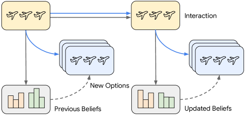<details> <summary>x7.png Details</summary>  ### Visual Description ## Diagram: Belief Update Process ### Overview The image is a diagram illustrating a belief update process, likely in the context of decision-making or reinforcement learning. It shows how initial options and beliefs are updated through interaction, leading to new options and updated beliefs. ### Components/Axes * **Top-Left Box:** Represents the initial state or options. It contains four airplane icons and has a yellow background. * **Top-Right Box:** Represents the state or options after interaction. It also contains four airplane icons and has a yellow background. The label "Interaction" is to the right of this box. * **Middle-Left Stacked Boxes:** Represents new options derived from the initial state. It contains three stacked boxes with airplane icons and has a light blue background. * **Middle-Right Stacked Boxes:** Represents new options derived from the interacted state. It contains three stacked boxes with airplane icons and has a light blue background. * **Bottom-Left Box:** Represents previous beliefs. It contains a bar chart with two orange bars and two green bars. * **Bottom-Right Box:** Represents updated beliefs. It contains a bar chart with two orange bars and two green bars. * **Arrows:** * Blue arrow from the top-left box to the middle-left stacked boxes. * Gray arrow from the top-left box to the bottom-left box. * Blue arrow from the top-right box to the middle-right stacked boxes. * Gray arrow from the top-right box to the bottom-right box. * Dashed gray arrow from the bottom-left box to the middle-left stacked boxes, labeled "New Options". * Dashed gray arrow from the bottom-right box to the middle-right stacked boxes, labeled "New Options". * Blue arrow connecting the top-left and top-right boxes. ### Detailed Analysis or Content Details * **Initial State (Top-Left):** The yellow box at the top-left contains four airplane icons, suggesting a set of initial options or states. * **Interaction (Top-Right):** The yellow box at the top-right, labeled "Interaction," also contains four airplane icons, indicating the state after some interaction or action. A blue arrow connects the initial state to this interacted state, showing the flow of information or action. * **New Options (Middle-Left & Middle-Right):** The stacked light blue boxes represent new options generated from the initial and interacted states. The dashed gray arrows from the "Previous Beliefs" and "Updated Beliefs" boxes to these "New Options" boxes suggest that beliefs influence the generation of new options. * **Beliefs (Bottom-Left & Bottom-Right):** The bar charts represent beliefs associated with the states. The "Previous Beliefs" chart shows two orange bars and two green bars, while the "Updated Beliefs" chart shows a similar configuration, but the heights of the bars appear to be slightly different. * **Previous Beliefs:** The approximate heights of the bars are: Orange bar 1: 0.6, Orange bar 2: 0.8, Green bar 1: 1.0, Green bar 2: 0.9. * **Updated Beliefs:** The approximate heights of the bars are: Orange bar 1: 0.7, Orange bar 2: 0.6, Green bar 1: 0.9, Green bar 2: 0.8. ### Key Observations * The diagram illustrates a cyclical process where initial options and beliefs are updated through interaction, leading to new options and updated beliefs. * The dashed arrows from the belief states to the new options suggest that beliefs influence the generation of new options. * The changes in the bar chart heights from "Previous Beliefs" to "Updated Beliefs" indicate that the interaction leads to a change in beliefs. ### Interpretation The diagram represents a belief update mechanism, possibly within a reinforcement learning or decision-making framework. The agent starts with initial options and beliefs. Through interaction with the environment (or another agent), the agent updates its beliefs and generates new options. This process is iterative, allowing the agent to learn and adapt over time. The bar charts representing beliefs likely correspond to the probabilities or values assigned to different options or states. The changes in bar heights indicate that the interaction has caused the agent to revise its assessment of these options. The dashed arrows highlight the influence of existing beliefs on the exploration of new options, suggesting a balance between exploitation (using current beliefs) and exploration (generating new options). </details> Figure 7: Experimental design for LLM evaluation. At the end of each round, we evaluate the LLM using new option sets for which it has not received feedback. The evaluation branches out from the main interactions (that is, the evaluation performed after the first round is not included in the context of the second round). The LLM’s direct evaluation, where we ask the LLM directly to choose a flight, follows the blue lines; the belief-based evaluation, where we first assess the LLM’s beliefs about the user’s preferences and then use them to choose the flight, follows the gray lines. The dashed lines indicate the deterministic conversion of the LLM’s beliefs into flight recommendations. 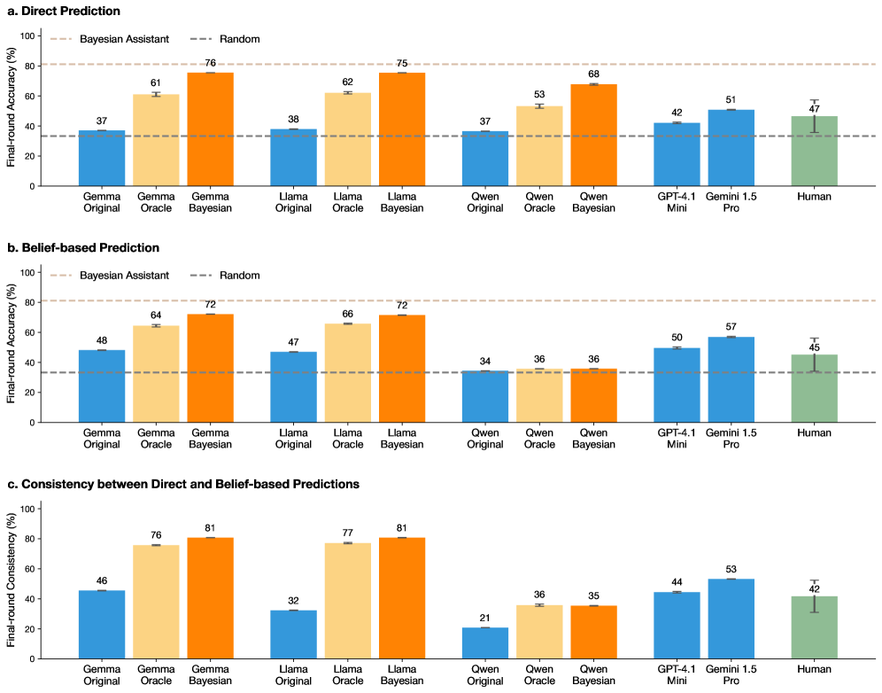<details> <summary>x8.png Details</summary>  ### Visual Description ## Bar Charts: Model Performance Comparison ### Overview The image presents three bar charts comparing the performance of various language models (Gemma, Llama, Qwen, GPT-4.1, Gemini 1.5) and human performance on a task. The charts depict "Final-round Accuracy (%)" or "Final-round Consistency (%)" on the y-axis, with different model configurations (Original, Oracle, Bayesian) on the x-axis. The charts compare "Direct Prediction", "Belief-based Prediction", and "Consistency between Direct and Belief-based Predictions". Horizontal dashed lines represent the performance of a "Bayesian Assistant" and a "Random" baseline. ### Components/Axes **General Chart Elements:** * **Title:** The image contains three sub-charts labeled "a. Direct Prediction", "b. Belief-based Prediction", and "c. Consistency between Direct and Belief-based Predictions". * **Y-axis:** Labeled "Final-round Accuracy (%)" for charts a and b, and "Final-round Consistency (%)" for chart c. The scale ranges from 0 to 100 in increments of 20. * **X-axis:** Categorical axis representing different language models and configurations: Gemma (Original, Oracle, Bayesian), Llama (Original, Oracle, Bayesian), Qwen (Original, Oracle, Bayesian), GPT-4.1 Mini, Gemini 1.5 Pro, and Human. * **Bars:** Represent the performance of each model/configuration. * **Error Bars:** Small vertical lines on top of each bar, indicating the standard error or confidence interval. * **Horizontal Dashed Lines:** Two horizontal dashed lines representing the performance of "Bayesian Assistant" (top line) and "Random" (bottom line). **Legend (Inferred):** * Blue bars: "Original" model configuration. * Light Orange bars: "Oracle" model configuration. * Dark Orange bars: "Bayesian" model configuration. * Green bars: "Human" performance. ### Detailed Analysis #### a. Direct Prediction * **Y-axis:** Final-round Accuracy (%) * **Bayesian Assistant Baseline:** Approximately 80% * **Random Baseline:** Approximately 35% **Data Points:** * **Gemma Original:** 37% * **Gemma Oracle:** 61% * **Gemma Bayesian:** 76% * **Llama Original:** 38% * **Llama Oracle:** 62% * **Llama Bayesian:** 75% * **Qwen Original:** 37% * **Qwen Oracle:** 53% * **Qwen Bayesian:** 68% * **GPT-4.1 Mini:** 42% * **Gemini 1.5 Pro:** 51% * **Human:** 47% **Trends:** * For Gemma, Llama, and Qwen, the Bayesian configuration consistently outperforms the Oracle and Original configurations. * GPT-4.1 Mini and Gemini 1.5 Pro perform similarly to each other. * Human performance is comparable to GPT-4.1 Mini and Gemini 1.5 Pro. #### b. Belief-based Prediction * **Y-axis:** Final-round Accuracy (%) * **Bayesian Assistant Baseline:** Approximately 80% * **Random Baseline:** Approximately 35% **Data Points:** * **Gemma Original:** 48% * **Gemma Oracle:** 64% * **Gemma Bayesian:** 72% * **Llama Original:** 47% * **Llama Oracle:** 66% * **Llama Bayesian:** 72% * **Qwen Original:** 34% * **Qwen Oracle:** 36% * **Qwen Bayesian:** 36% * **GPT-4.1 Mini:** 50% * **Gemini 1.5 Pro:** 57% * **Human:** 45% **Trends:** * Similar to Direct Prediction, the Bayesian configuration generally outperforms the Oracle and Original configurations for Gemma and Llama. * Qwen's performance is relatively flat across all three configurations. * GPT-4.1 Mini and Gemini 1.5 Pro show improved performance compared to the Direct Prediction chart. * Human performance is slightly lower than in the Direct Prediction chart. #### c. Consistency between Direct and Belief-based Predictions * **Y-axis:** Final-round Consistency (%) * **Bayesian Assistant Baseline:** Not applicable in this chart. * **Random Baseline:** Not applicable in this chart. **Data Points:** * **Gemma Original:** 46% * **Gemma Oracle:** 76% * **Gemma Bayesian:** 81% * **Llama Original:** 32% * **Llama Oracle:** 77% * **Llama Bayesian:** 81% * **Qwen Original:** 21% * **Qwen Oracle:** 36% * **Qwen Bayesian:** 35% * **GPT-4.1 Mini:** 44% * **Gemini 1.5 Pro:** 53% * **Human:** 42% **Trends:** * The Bayesian and Oracle configurations for Gemma and Llama show significantly higher consistency than the Original configurations. * Qwen's consistency is notably lower compared to other models. * GPT-4.1 Mini and Gemini 1.5 Pro show moderate consistency. * Human consistency is relatively low. ### Key Observations * The "Bayesian" configurations of Gemma and Llama consistently achieve the highest accuracy and consistency across all three charts. * Qwen's performance is generally lower and more consistent across different configurations, especially in the "Belief-based Prediction" and "Consistency" charts. * GPT-4.1 Mini and Gemini 1.5 Pro show comparable performance, often outperforming the "Original" configurations of Gemma, Llama, and Qwen. * Human performance varies across the charts, sometimes exceeding the performance of certain models but generally falling within the range of GPT-4.1 Mini and Gemini 1.5 Pro. ### Interpretation The data suggests that incorporating Bayesian methods into language models can significantly improve their accuracy and consistency in both direct and belief-based predictions. The "Oracle" configurations also show substantial improvements over the "Original" models, indicating the value of informed model design. The relatively low consistency of Qwen suggests that its predictions may be less reliable or more sensitive to the specific task or context. The performance of GPT-4.1 Mini and Gemini 1.5 Pro highlights the capabilities of larger, more advanced models. The variability in human performance underscores the challenges of evaluating language models against human benchmarks, as human performance itself can be inconsistent. The fact that human performance is sometimes worse than the models suggests that the models are in some cases better than humans. The relationship between the charts is that they show different aspects of model performance. "Direct Prediction" measures raw accuracy, "Belief-based Prediction" measures accuracy when considering the model's confidence, and "Consistency" measures how well the model's direct and belief-based predictions align. </details> \phantomsubcaption \phantomsubcaption \phantomsubcaption Figure 8: Comparison of direct accuracy and belief-based accuracy. We show final-round accuracy based on (a) the LLM’s or human’s direct predictions and (b) predictions derived from their verbalized beliefs about the user’s preferences. The gray dashed line indicates random performance, while the brown dashed line indicates the performance of the Bayesian Assistant. For human participants, we only evaluate on a subset of our evaluation data, which includes 48 different simulated users. (c) Final-round consistency between two predictions: the prediction directly provided by the LLM or human participants and the prediction derived from their beliefs about the user’s preferences. Fine-tuned LLMs show better consistency than the original LLMs, with Bayesian LLMs achieving the highest consistency. Error bars show standard error across participants for humans and across three random seeds (and three training runs) for LLMs. B.3 Results For the original LLMs, we find that the approach described in this section—where we first estimate the LLMs’ beliefs about the user’s preferences by explicitly querying the LLMs, and then use a decision-making component that is external to the LLM—performs better than directly using the LLMs’ predictions (Fig. 8 vs. Fig. 8, original LLMs). We also find that the original LLMs’ direct predictions are often inconsistent with the belief-based predictions (those derived from the beliefs elicited from the LLMs), with less than 50% alignment between the two sets of predictions (Fig. 8). Human participants similarly show high inconsistency between the two types of predictions. Predictions based on the fine-tuned LLMs’ verbalized beliefs are substantially more accurate than those based on the original LLM’s verbalized beliefs, except for Qwen 2.5 models (Fig. 8 and Fig. 8, Oracle LLMs and Bayesian LLMs). This suggests that both training methods teach the LLM to infer the user’s preferences and update them as more information becomes available, even though neither method provides the model with direct access to users’ preferences. For both Gemma 2 and Llama 3, the Bayesian variant of the LLMs produces more accurate estimates of the user’s beliefs than the Oracle one. Likewise, compared to the Oracle variants, the Bayesian variants achieve higher consistency between the predictions directly provided by the LLM and those derived from the LLM’s verbalized beliefs. The difference in overall accuracy between these models’ direct predictions and belief-based predictions is much smaller after fine-tuning. This trend, however, does not hold for Qwen 2.5 model: while direct prediction accuracy improves after fine-tuning, belief-based prediction accuracy remains unchanged from the original LLM. This suggests that for Gemma 2 and Llama 3, prompt-based prediction elicitation may tap into a representation that is shared with the computation used to make direct predictions, but that is not the case for Qwen 2.5. 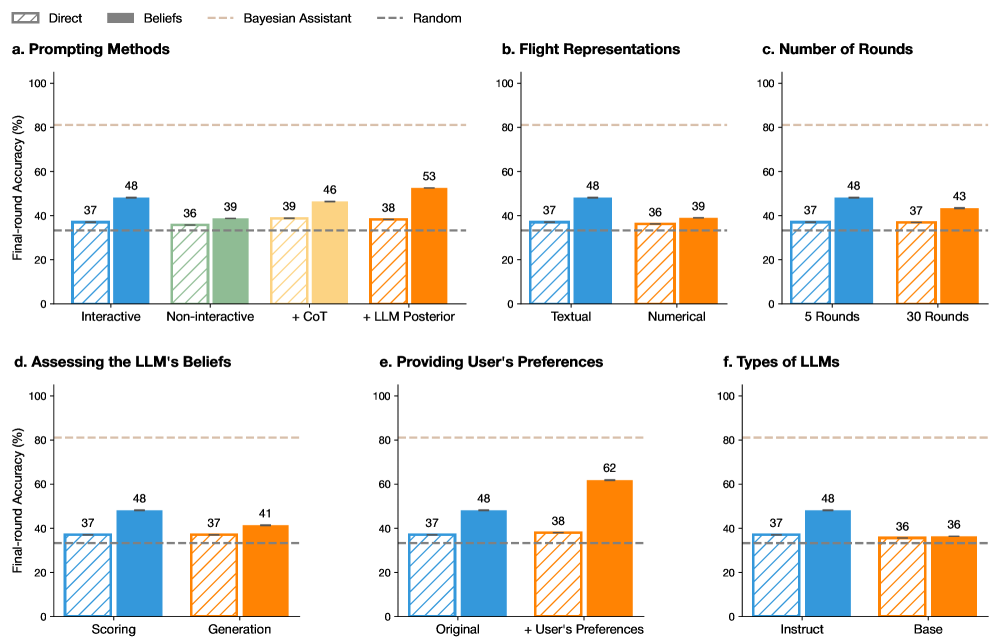Appendix C Additional Results C.1 The Original LLMs’ Poor Performance is Robust to Evaluation Setup <details> <summary>x9.png Details</summary>  ### Visual Description ## Bar Charts: Final-Round Accuracy Comparison ### Overview The image presents six bar charts comparing the final-round accuracy (%) of different methods and parameters related to Large Language Models (LLMs). The charts compare different prompting methods, flight representations, number of rounds, ways of assessing LLM beliefs, methods of providing user preferences, and types of LLMs. Each chart compares the "Direct" method (striped bars) with other methods (solid bars) using different colors. A horizontal dashed line represents a "Random" baseline. ### Components/Axes * **Y-axis (all charts):** "Final-round Accuracy (%)", ranging from 0 to 100. Tick marks are not explicitly labeled, but the scale is linear. * **Legend (top):** * "Direct": Striped bars * "Beliefs": Solid bars (color varies by chart) * "Bayesian Assistant": Not explicitly represented in the charts, but implied as a comparison point. * "Random": Dashed horizontal line. * **Horizontal dashed lines:** Two horizontal dashed lines are present in each chart. One is at approximately 33% and is labeled "Random" in the legend. The other is at approximately 82% and is unlabeled. * **Chart Titles:** Each chart has a title (a, b, c, d, e, f) indicating the comparison being made. ### Detailed Analysis **a. Prompting Methods** * X-axis: Prompting Methods (Interactive, Non-interactive, +CoT, +LLM Posterior) * "Direct" (striped blue): * Interactive: 37% * Non-interactive: 36% * +CoT: 39% * +LLM Posterior: 38% * "Beliefs" (solid): * Interactive (solid blue): 48% * Non-interactive (solid green): 39% * +CoT (solid yellow): 46% * +LLM Posterior (solid orange): 53% * Trend: The "Beliefs" method generally outperforms the "Direct" method across all prompting methods. **b. Flight Representations** * X-axis: Flight Representations (Textual, Numerical) * "Direct" (striped blue): * Textual: 37% * Numerical: 36% * "Beliefs" (solid): * Textual (solid blue): 48% * Numerical (solid orange): 39% * Trend: The "Beliefs" method outperforms the "Direct" method for both textual and numerical flight representations. **c. Number of Rounds** * X-axis: Number of Rounds (5 Rounds, 30 Rounds) * "Direct" (striped blue): * 5 Rounds: 37% * 30 Rounds: 37% * "Beliefs" (solid): * 5 Rounds (solid blue): 48% * 30 Rounds (solid orange): 43% * Trend: The "Beliefs" method outperforms the "Direct" method for both 5 and 30 rounds. **d. Assessing the LLM's Beliefs** * X-axis: Assessing the LLM's Beliefs (Scoring, Generation) * "Direct" (striped blue): * Scoring: 37% * Generation: 37% * "Beliefs" (solid): * Scoring (solid blue): 48% * Generation (solid orange): 41% * Trend: The "Beliefs" method outperforms the "Direct" method for both scoring and generation. **e. Providing User's Preferences** * X-axis: Providing User's Preferences (Original, + User's Preferences) * "Direct" (striped blue): * Original: 37% * + User's Preferences: 38% * "Beliefs" (solid): * Original (solid blue): 48% * + User's Preferences (solid orange): 62% * Trend: The "Beliefs" method outperforms the "Direct" method for both original and user-preference-enhanced methods. The largest performance gap is observed when user preferences are included. **f. Types of LLMs** * X-axis: Types of LLMs (Instruct, Base) * "Direct" (striped blue): * Instruct: 37% * Base: 36% * "Beliefs" (solid): * Instruct (solid blue): 48% * Base (solid orange): 36% * Trend: The "Beliefs" method outperforms the "Direct" method for the "Instruct" LLM type, but performs similarly for the "Base" LLM type. ### Key Observations * The "Beliefs" method consistently outperforms the "Direct" method across most categories. * The largest performance difference is observed in "Providing User's Preferences" when user preferences are included. * The "Beliefs" method shows a significant advantage with the "Instruct" LLM type compared to the "Base" LLM type. * The "Random" baseline is consistently around 33% accuracy. ### Interpretation The data suggests that incorporating "Beliefs" into LLMs generally improves final-round accuracy compared to the "Direct" method. The improvement is particularly noticeable when providing user preferences and when using "Instruct" type LLMs. This indicates that understanding and utilizing the LLM's beliefs, especially in conjunction with user-specific information, can significantly enhance performance. The consistent outperformance over the "Random" baseline confirms that these methods are providing meaningful improvements. The "Bayesian Assistant" mentioned in the legend is not directly represented in the charts, but it likely serves as a theoretical or comparative benchmark for the other methods. </details> \phantomsubcaption \phantomsubcaption \phantomsubcaption \phantomsubcaption \phantomsubcaption \phantomsubcaption Figure 9: Final-round accuracy of Gemma Original under different variations of our experimental setup. We report both the model’s direct predictions (hatched bars) and the predictions derived from the model’s verbalized beliefs (solid bars; Supplementary Section B). (a) We compare the original interactive setting, where we directly ask the LLM to generate predictions and provide it with feedback, with other common techniques: non-interactive prompting, where we always provide correct examples; chain-of-thought (CoT) prompting, which encourages the LLM to think step-by-step; and methods that incorporate the LLM’s verbalized reward posterior distribution in the context. (b) The textual representation of the flight options, which uses natural language descriptions deterministically generated from the feature values, compared to the numerical representation, which directly uses the feature values. (c) 5-round interactions between the user and the LLM compared to 30-round interactions. (d) The scoring method, which assesses the LLM’s beliefs by scoring possible continuations, compared to the generation method, where we explicitly ask the LLM to generate probability judgments. (e) Performance without versus with the verbalized user’s preferences from the Bayesian model. (f) Instruction-tuned models versus their pre-trained base models. Error bars show standard errors across three random seeds. In light of the poor performance of the original LLMs (before fine-tuning), we considered various modifications to our evaluation setting. These include prompting-based methods, that is, modifications to the instructions provided to the LLM; an alternative, numerical representation of the flight options; and a greater number of interactions. We also ablate methods that access the LLM’s verbalized beliefs, explore whether providing the user’s preferences improves performance, and compare the instructed version of the models with their corresponding pre-trained versions. These robustness analyses focus on Gemma 2 9B. Overall, we do not observe significant differences across these evaluations; the only methods that we find effectively improved model performance involved fine-tuning (see Section C.2). Advanced prompting methods do not improve accuracy. Our main experiments evaluate the LLM in an interactive setting, where the user provides it with feedback indicating whether the LLM’s choice is correct. In this case, the user’s feedback is always based on the LLM’s prediction. We first experiment with an alternative non-interactive setting, where the context for the assistant includes all previous rounds and the option chosen by the assistant in these context rounds is always correct, a setting that better approximates the standard few-shot or in-context learning setup for LLMs (Brown et al. [2020]; see Table 10 for an example). While performance on direct prediction remains similar, we observe a performance drop when evaluating with predictions derived from the LLM’s beliefs (Fig. 9, “Non-interactive’). Chain-of-thought (CoT) prompting [Wei et al., 2022b, Nye et al., 2021, Kojima et al., 2022], which encourages the model to generate step-by-step reasoning chains, has been shown to be effective on many reasoning tasks. We evaluate the LLM using this strategy by explicitly including reasoning hints and the phrase “Let’s think step by step” in the instruction (see Table 8 for an example prompt). We find that LLMs prompted with CoT perform similarly to those prompted in the way described in the main text (Fig. 9, “ $+$ CoT”). Since inferring user’s preferences based on current information before making recommendations is crucial in our task, we further evaluate another CoT-style two-stage prompting method, where we allow the LLM to explicitly reason over the posterior distribution over reward functions. Specifically, we verbalize the LLM’s reward posterior distribution using natural language and add it to the LLM’s context (see Table 9 for an example). Explicitly encouraging the LLM to reason over its own reward posterior distribution improves the predictions derived from its verbalized beliefs. However, direct prediction accuracy remains similar (Fig. 9, “ $+$ LLM Posterior”). Though additional prompt engineering and advanced prompting techniques could potentially yield different results; in particular, some prompts may more effectively extract the model’s beliefs than the ones we used. For the moment, however, our preliminary findings suggest that it is challenging to significantly improve the LLM’s performance purely through prompting. The LLMs’ poor performance is not due to inability to parse the flight representations. Our main experiments use a representation that deterministically maps the feature value of each flight to a textual description (e.g., the departure time may be 02:00 PM and the duration 2 hr 30 min). While this textual representation is closer to realistic scenarios, and may therefore better align with the LLM’s training distribution, this setup introduces a potential confounder that complicates the interpretation of our results: the LLM’s poor performance in the flight recommendation task could be due to its inability to translate the text description into the feature space required for probabilistic reasoning. To control for this factor, we investigate an alternative numerical representation of the flight options, where we directly provide the LLM with numerical feature values in the same format we provide them to the Bayesian Assistant (e.g., the duration may be 0.9 instead of 16 hr 6 min; see Table 5 and Table 6 for examples). We find that, if anything, the textual representation outperforms its numerical counterpart in both accuracy metrics (Fig. 9). This suggests that the LLM’s poor performance cannot be attributed to an inability to parse the textual format to a numerical value. Increasing the number of interactions does not improve performance. Our previous experiments include only five rounds of interactions between the user and the LLM. To investigate the possibility that LLMs do in fact extract information from the interaction and update their beliefs, but do so more slowly than the Bayesian Assistant, we increase the number of interactions to 30. We find that Gemma Original still shows similar performance; if anything, its performance is slightly worse compared to our main experiments (Fig. 9). This indicates that simply increasing the number of interactions is unlikely to significantly improve the LLM’s performance. Assessing the LLM’s beliefs: Scoring continuations vs. explicit probability judgments. In the main experiment, for the open-weights LLMs where we have access to the probabilities the LLM assigns to upcoming words, we estimate the LLM’s distribution over reward functions by asking it to rate individual features and scoring the possible continuations; for flight duration, for example, we might ask it what the user’s preference is on a scale of 1 to 5. We refer to this method as “scoring”. Here, we compare this method to one where we instruct the LLM to assign a probability to each of the five ratings on each scale; we refer to this method as “generation” (see Table 7 for an example). The generation method is also used for experiments with the closed-weights models, as we do not have access to these LLM’s probabilities. As in the scoring method, we renormalize the probabilities to ensure that they sum to 1 (although we find that this step is typically not necessary as they already sum to 1). Overall, we find the scoring-based reward distribution, which we use in the main text for the open-weights models, is closer than the generation-based one to the ground truth distribution (Fig. 9; for related results, see Hu and Levy [2023]). Can the LLM make recommendations given the user’s preferences? The flight recommendation task requires two capabilities: inferring the user’s preferences and making predictions based on these preferences. We previously showed that the original LLM performs poorly at inferring the user’s preferences (Fig. 8). Here, we investigate its performance in the latter one. Specifically, we provide the LLM with the verbalized reward posterior distribution from the normative Bayesian model (see Table 9 for an example). In this case, the LLM only needs to make recommendations based on the provided preferences. We find that having access to the optimal reward posterior distribution improves belief-based accuracy; however, the direct prediction accuracy remains similar (Fig. 9). Although our method of presenting user’s preferences to the LLM may not be optimal, these results suggest that the LLM struggles to make correct recommendations even when the user’s preferences are explicitly provided. Types of LLMs: Instructed model vs. pre-trained base model. We use instruction-tuned LLMs for our main experiments. As these models are trained using an additional post-training alignment stage, their behavior is likely to differ from their pre-trained base model counterparts [Lin et al., 2024, Yang et al., 2024b, Wang et al., 2024, Kotha et al., 2024], though because we expect instruction-tuning to improve the models’ interactive capabilities, we hypothesize that the base version of Gemma would not perform better than the instruction-tuned one. As base models are not well-suited to interactive evaluation, we evaluate them using the non-interactive setting by providing them with in-context examples (see earlier in this section). We find that the base model performs comparably to the instruction-tuned one (Fig. 9); we omit the results for Llama 3 and Qwen 2.5, which were similar. C.2 Modifications to Training Setup This Supplementary describes variants on the methods we used to fine-tune the LLMs on interactions with users. We only explore these variants for Bayesian teaching, which was consistently more effective than oracle teaching). We use Gemma 2 9B for all of the follow-up experiments reported in this section. 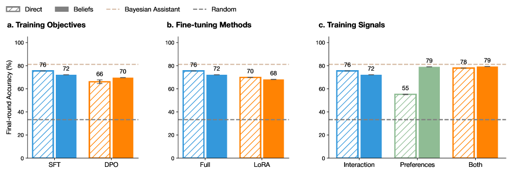<details> <summary>x10.png Details</summary>  ### Visual Description ## Bar Charts: Model Accuracy Comparison ### Overview The image presents three bar charts comparing the final-round accuracy (%) of different models under varying conditions: training objectives, fine-tuning methods, and training signals. Each chart compares "Direct", "Beliefs", and "Bayesian Assistant" models against a "Random" baseline. ### Components/Axes **Legend:** Located at the top of the image. * Direct: Bars with diagonal lines. * Beliefs: Solid blue bars. * Bayesian Assistant: Solid orange bars. * Random: Dashed gray horizontal line. **Y-axis (all charts):** * Label: "Final-round Accuracy (%)" * Scale: 0 to 100, with tick marks at intervals of 20. **Chart a. Training Objectives:** * Title: "a. Training Objectives" * X-axis labels: "SFT", "DPO" **Chart b. Fine-tuning Methods:** * Title: "b. Fine-tuning Methods" * X-axis labels: "Full", "LoRA" **Chart c. Training Signals:** * Title: "c. Training Signals" * X-axis labels: "Interaction", "Preferences", "Both" ### Detailed Analysis **Chart a. Training Objectives:** * **Direct (SFT):** 76% * **Beliefs (SFT):** 72% * **Direct (DPO):** 66% * **Beliefs (DPO):** 70% * **Random:** Approximately 33% (estimated from the dashed line) **Chart b. Fine-tuning Methods:** * **Direct (Full):** 76% * **Beliefs (Full):** 72% * **Direct (LoRA):** 70% * **Beliefs (LoRA):** 68% * **Random:** Approximately 33% (estimated from the dashed line) **Chart c. Training Signals:** * **Direct (Interaction):** 76% * **Beliefs (Interaction):** 72% * **Direct (Preferences):** 55% * **Beliefs (Both):** 79% * **Bayesian Assistant (Both):** 79% * **Bayesian Assistant (Preferences):** 79% * **Random:** Approximately 33% (estimated from the dashed line) ### Key Observations * The "Beliefs" model consistently outperforms the "Direct" model across all training objectives and fine-tuning methods. * Using "Both" interaction and preferences as training signals yields the highest accuracy for the "Beliefs" and "Bayesian Assistant" models. * The "Random" baseline remains constant across all charts, providing a consistent point of comparison. ### Interpretation The data suggests that the "Beliefs" model is more effective than the "Direct" model in these experiments. The choice of training signals significantly impacts model accuracy, with combining interaction and preferences leading to the best results. The "Random" baseline highlights the improvement gained by using the tested models and methods. </details> \phantomsubcaption \phantomsubcaption \phantomsubcaption Figure 10: Final-round accuracy of LLMs fine-tuned with different training strategies on the flight recommendation task. We use Bayesian teaching (i.e. users’ interactions with the Bayesian Assistant) for all experiments. (a) Comparison of training objectives: supervised fine-tuning (SFT) vs. direct preference optimization (DPO). (b) Fine-tuning methods: full fine-tuning, which updates all model parameters, vs. LoRA fine-tuning, a parameter-efficient method that only updates partial parameters. (c) Training only on interactions between users and assistants, as in our other experiments, compared to training on the Bayesian Assistant’s estimate of the user’s preferences, as well as training on both interactions and the estimated preferences. Error bars show standard errors across three random seeds and three training runs. Training objective: Supervised fine-tuning vs. Direct preference optimization. In most of our experiments, we use supervised fine-tuning (SFT) to provide the oracle and Bayesian predictions. In this method, the LLM is trained to predict the upcoming token in the interaction, the same objective used during pre-trainining. Here, we examine the utility of reinforcement learning from human feedback (RLHF; Christiano et al. [2017], Ouyang et al. [2022], Stiennon et al. [2020]), another common practice for adapting LLMs’ behavior following pre-training, in which the LLM is instead provided with an explicit signal indicating whether an output is preferable. In particular, we use direct preference optimization (DPO; Rafailov et al. [2023]), where the model is trained to assign higher probability to the preferred response than to the less preferred one. We investigate the DPO training objective by treating the Bayesian Assistant’s prediction as the preferred one while using a different random recommendation as the less preferred one. We train the model with the DPO objective with a learning rate of 2e-6 and $\beta=0.1$ . We find that training on Bayesian predictions works comparably for both SFT (used in main experiments) and DPO objectives (Fig. 10), indicating that the approach is robust to the choice of training objective. Full vs. parameter-efficient fine-tuning. In our main experiments, we update all model parameters. As this approach becomes less feasible as the model size grows, a common strategy to improve training efficiency relies on parameter-efficient fine-tuning, where only a subset of parameters is updated. We evaluate this approach using Low-Rank Adaptation (LoRA; Hu et al. [2022]), a method that injects trainable rank decomposition matrices while keeping the original model weights frozen. We perform LoRA fine-tuning with a learning rate of 2e-5. While LoRA fine-tuning performs slightly worse than full fine-tuning (Fig. 10), it achieves comparable performance while significantly reducing training costs. This demonstrates that our fine-tuning strategy can be effectively applied in computationally efficient settings, which is particularly beneficial for larger LLMs. Providing Bayesian preference estimates in fine-tuning. We have shown in the main text that fine-tuning the LLMs to make better recommendations also significantly improves its ability to infer the user’s preferences, even though their supervision does not explicitly include the user’s preferences. Here, we investigate a complementary setup, where we explicitly train the model to match the Bayesian Assistant’s estimates of the user’s preferences, but not to make flight recommendations. The Bayesian Assistant produces a posterior probability distribution over all reward functions after each round; we select the reward function with the highest posterior probability and provide it to the LLM, formatted as in Table 4. We find that, like training on interactions, providing the user’s preferences as a fine-tuning signal improves both accuracy measures, compared to Gemma Original, but the gain in direct prediction accuracy on is smaller than when we fine-tune on interactions (Fig. 10). We also explore a setting where both the interactions and the preferences are provided during training; this setting leads to the best performance on both metrics, with accuracy approaching the accuracy of the Bayesian Assistant. 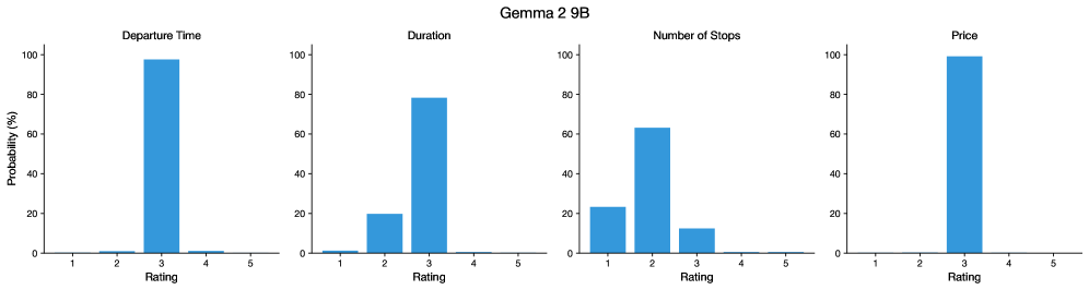Appendix D Additional Analyses D.1 LLM Priors <details> <summary>x11.png Details</summary>  ### Visual Description ## Bar Charts: Gemma 2 9B - Feature Ratings ### Overview The image contains four bar charts arranged horizontally, each representing the distribution of ratings for a different feature: Departure Time, Duration, Number of Stops, and Price. The x-axis represents the rating (1 to 5), and the y-axis represents the probability in percentage (0 to 100%). All bars are blue. The title of the image is "Gemma 2 9B". ### Components/Axes * **Title:** Gemma 2 9B (located at the top-center of the image) * **X-axis (Rating):** * Label: Rating * Scale: 1, 2, 3, 4, 5 (same for all four charts) * **Y-axis (Probability):** * Label: Probability (%) * Scale: 0, 20, 40, 60, 80, 100 (same for all four charts) * **Chart Titles (from left to right):** 1. Departure Time 2. Duration 3. Number of Stops 4. Price ### Detailed Analysis **1. Departure Time** * Trend: The distribution is heavily skewed towards a rating of 3. * Data Points: * Rating 1: ~1% * Rating 2: ~1% * Rating 3: ~98% * Rating 4: ~1% * Rating 5: ~0% **2. Duration** * Trend: The distribution is skewed towards a rating of 3, with a secondary peak at 2. * Data Points: * Rating 1: ~1% * Rating 2: ~20% * Rating 3: ~78% * Rating 4: ~1% * Rating 5: ~0% **3. Number of Stops** * Trend: The distribution has peaks at ratings 1 and 2, with a smaller peak at 3. * Data Points: * Rating 1: ~23% * Rating 2: ~63% * Rating 3: ~13% * Rating 4: ~1% * Rating 5: ~0% **4. Price** * Trend: The distribution is heavily skewed towards a rating of 3. * Data Points: * Rating 1: ~0% * Rating 2: ~0% * Rating 3: ~100% * Rating 4: ~0% * Rating 5: ~0% ### Key Observations * For Departure Time and Price, the rating is almost exclusively 3. * Duration has a strong preference for rating 3, but also a significant number of ratings at 2. * Number of Stops has a broader distribution, with peaks at ratings 1 and 2. ### Interpretation The charts suggest that, for "Gemma 2 9B", the departure time and price are overwhelmingly rated as "3". Duration is also primarily rated as "3", but with a noticeable number of "2" ratings. The number of stops has a more varied distribution, indicating a wider range of experiences or preferences among users. The high concentration of ratings at "3" for Departure Time and Price could indicate a standardized or optimized aspect of the service, while the broader distribution for Number of Stops might reflect inherent variability in travel itineraries. 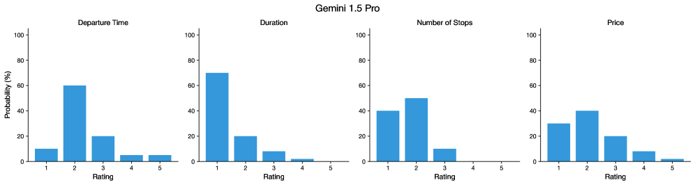</details> <details> <summary>x12.png Details</summary>  ### Visual Description ## Bar Chart: Gemini 1.5 Pro Ratings ### Overview The image presents four bar charts side-by-side, each displaying the probability distribution of ratings for a different aspect of travel: Departure Time, Duration, Number of Stops, and Price. The ratings are on a scale of 1 to 5, and the probability is expressed as a percentage. The title of the image is "Gemini 1.5 Pro". ### Components/Axes * **Title:** Gemini 1.5 Pro * **X-axis (horizontal):** Rating (values 1 to 5) * **Y-axis (vertical):** Probability (%) (scale from 0 to 100) * **Chart Titles (top of each chart):** * Departure Time * Duration * Number of Stops * Price * **Bar Color:** Blue ### Detailed Analysis **1. Departure Time:** * Trend: The probability peaks at rating 2, then decreases. * Rating 1: Approximately 10% * Rating 2: Approximately 60% * Rating 3: Approximately 20% * Rating 4: Approximately 5% * Rating 5: Approximately 5% **2. Duration:** * Trend: The probability decreases as the rating increases. * Rating 1: Approximately 70% * Rating 2: Approximately 20% * Rating 3: Approximately 8% * Rating 4: Approximately 2% * Rating 5: Approximately 1% **3. Number of Stops:** * Trend: The probability peaks at rating 2, then decreases. * Rating 1: Approximately 40% * Rating 2: Approximately 50% * Rating 3: Approximately 10% * Rating 4: Approximately 0% * Rating 5: Approximately 0% **4. Price:** * Trend: The probability peaks at rating 2, then decreases. * Rating 1: Approximately 30% * Rating 2: Approximately 40% * Rating 3: Approximately 20% * Rating 4: Approximately 8% * Rating 5: Approximately 2% ### Key Observations * For Departure Time, the highest probability is at rating 2. * For Duration, the highest probability is at rating 1. * For Number of Stops, the highest probability is at rating 2. * For Price, the highest probability is at rating 2. * In all four charts, higher ratings (4 and 5) have very low probabilities. ### Interpretation The data suggests that, according to Gemini 1.5 Pro, users generally prefer trips with a rating of 2 for Departure Time, Number of Stops, and Price. They strongly prefer a rating of 1 for Duration. This could indicate a preference for shorter trips, but some flexibility or tolerance for departure times, number of stops, and price. The low probabilities for ratings 4 and 5 across all categories suggest that users generally avoid or dislike trips with those characteristics. The model seems to be capturing user preferences for certain travel characteristics. </details> Figure 11: Priors of Gemma 2 9B Original and Gemini 1.5 Pro for each flight feature. We obtain these priors via the prompting-based elicitation method (Supplementary B). A rating of 1 indicates a strongest preference for the earliest departure time, the shortest duration, the fewest number of stops, and the lowest price, while a rating of 5 indicates the opposite. A rating of 3 indicates no preference. In the section Generalization to interactions with human users, we find that the original LLMs, before fine-tuning, were able to provide recommendations with an accuracy substantially higher than chance even before their first interaction with the user, suggesting that the LLMs’ priors are aligned with human preferences. In this section, we test this hypothesis by asking two models, Gemma 2 and Gemini 1.5, for their verbalized beliefs in advance of any interaction with a particular user. Fig. 11 shows the results. For Gemma 2 9B, the hypothesis is only partly supported: the prior derived from this model assigns a high probability to “no preference” for most of the features, with the exception of the number of stops, where it reflects a moderate preference for fewer stops. By contrast, Gemini 1.5 Pro has a more diffuse prior over these features, which favors cheaper and shorter flights, as well as flights that leave earlier in the day, plausibly reflecting the preferences of most flyers. We note that the interpretation of this pattern of results is complicated by the fact that Gemma’s verbalized prior beliefs may not faithfully reflect the underlying prior it uses to make recommendations before having interacted with a user. 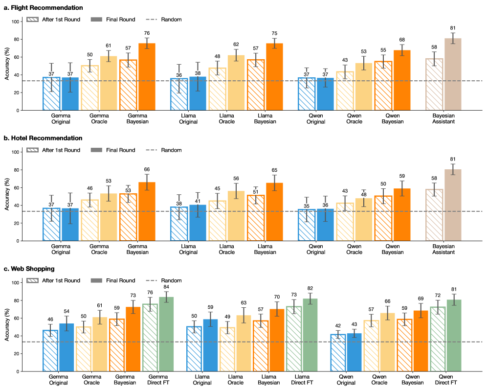<details> <summary>x13.png Details</summary>  ### Visual Description ## Bar Chart: Recommendation Accuracy Comparison ### Overview The image presents three bar charts comparing the accuracy of different recommendation systems (Gemma, Llama, Qwen, and Bayesian Assistant/Direct FT) across three scenarios: Flight Recommendation, Hotel Recommendation, and Web Shopping. The charts compare the accuracy after the first round, in the final round, and against a random baseline. ### Components/Axes * **Chart Titles:** * a. Flight Recommendation * b. Hotel Recommendation * c. Web Shopping * **Y-Axis:** * Label: Accuracy (%) * Scale: 0 to 100, with tick marks at intervals of 20. * **X-Axis:** * Categories: Gemma, Llama, Qwen, Bayesian Assistant/Direct FT * Sub-categories: Original, Oracle, Bayesian, Direct FT (where applicable) * **Legend:** Located at the top-left of each chart. * After 1st Round (Blue) * Final Round (Yellow/Orange) * Random (Gray/Green with diagonal lines) * **Horizontal Dashed Line:** Represents the "Random" baseline accuracy. ### Detailed Analysis #### a. Flight Recommendation * **Gemma Original:** * After 1st Round: 37% * Final Round: 37% * **Gemma Oracle:** * After 1st Round: 50% * Final Round: 61% * **Gemma Bayesian:** * After 1st Round: 57% * Final Round: 76% * Random: 57% * **Llama Original:** * After 1st Round: 36% * Final Round: 38% * **Llama Oracle:** * After 1st Round: 48% * Final Round: 62% * **Llama Bayesian:** * After 1st Round: 57% * Final Round: 75% * Random: 57% * **Qwen Original:** * After 1st Round: 37% * Final Round: 37% * **Qwen Oracle:** * After 1st Round: 43% * Final Round: 53% * **Qwen Bayesian:** * After 1st Round: 55% * Final Round: 68% * Random: 55% * **Bayesian Assistant:** * Random: 81% #### b. Hotel Recommendation * **Gemma Original:** * After 1st Round: 37% * Final Round: 37% * **Gemma Oracle:** * After 1st Round: 46% * Final Round: 53% * **Gemma Bayesian:** * After 1st Round: 53% * Final Round: 66% * Random: 53% * **Llama Original:** * After 1st Round: 38% * Final Round: 41% * **Llama Oracle:** * After 1st Round: 45% * Final Round: 56% * **Llama Bayesian:** * After 1st Round: 51% * Final Round: 65% * Random: 51% * **Qwen Original:** * After 1st Round: 35% * Final Round: 36% * **Qwen Oracle:** * After 1st Round: 43% * Final Round: 48% * **Qwen Bayesian:** * After 1st Round: 50% * Final Round: 59% * Random: 50% * **Bayesian Assistant:** * Random: 81% #### c. Web Shopping * **Gemma Original:** * After 1st Round: 46% * Final Round: 54% * **Gemma Oracle:** * After 1st Round: 50% * Final Round: 61% * **Gemma Bayesian:** * After 1st Round: 59% * Final Round: 73% * Random: 59% * **Gemma Direct FT:** * Random: 84% * **Llama Original:** * After 1st Round: 50% * Final Round: 59% * **Llama Oracle:** * After 1st Round: 49% * Final Round: 63% * **Llama Bayesian:** * After 1st Round: 57% * Final Round: 70% * Random: 57% * **Llama Direct FT:** * Random: 82% * **Qwen Original:** * After 1st Round: 42% * Final Round: 43% * **Qwen Oracle:** * After 1st Round: 57% * Final Round: 66% * **Qwen Bayesian:** * After 1st Round: 59% * Final Round: 69% * Random: 59% * **Qwen Direct FT:** * Random: 81% ### Key Observations * In general, the "Final Round" accuracy is higher than the "After 1st Round" accuracy for most models and scenarios. * The "Bayesian Assistant" (for Flight and Hotel Recommendations) and "Direct FT" (for Web Shopping) models consistently show the highest accuracy compared to other models. * The "Original" models (Gemma Original, Llama Original, Qwen Original) tend to have the lowest accuracy. * The random baseline accuracy varies across the different recommendation tasks. ### Interpretation The data suggests that refining recommendation models over multiple rounds generally improves their accuracy. The Bayesian Assistant and Direct FT models appear to be the most effective for these tasks, indicating that incorporating Bayesian methods or direct fine-tuning can significantly enhance recommendation performance. The lower accuracy of the "Original" models highlights the importance of optimization and refinement in recommendation systems. The varying random baselines indicate that the difficulty of the recommendation task differs across the three scenarios (Flight, Hotel, Web Shopping). </details> Figure 12: Variability across simulated users. We show accuracy after the first and final (fifth) rounds. (a) We compare the original LLMs, fine-tuned LLMs, and the upper bound (the Bayesian Assistant) on flight recommendation. (b) Comparison of LLMs and the upper bound (the Bayesian Assistant) on hotel recommendation. (c) Comparison of LLMs and the upper bound (LLMs fine-tuned directly on the task) for web shopping. Error bars indicate the standard deviation across reward functions (for flight and hotel recommendations) or product categories (for web shopping). D.2 Variability in LLM Accuracy Across Simulated Users In our main experiments, we show results averaged over all simulated users. Here, we explore how the LLM’s accuracy varies by user. As before, for flight and hotel recommendations, the user is characterized as a reward function. For web shopping, we have 10 users with different goals (i.e. preferred attributes) for each category; we average their performance and compute the standard deviation across 100 product categories (see Table 1 for examples). All methods exhibit high variance as shown in Fig. 12. Table 1: Example product categories and their corresponding goals of different users. | Product Category | User’s Goals (Preferred Attributes) | | --- | --- | | Beds | eco friendly, twin with drawers | | wood frame, easy assemble, twin | | | memory foam, solid wood | | | Men’s athletic shoes | running shoes, lace up | | non slip, mesh | | | daily wear, color back, size 14 | | | Food & beverage | simple ingredients | | gluten free | | | low sodium | | <details> <summary>x14.png Details</summary>  ### 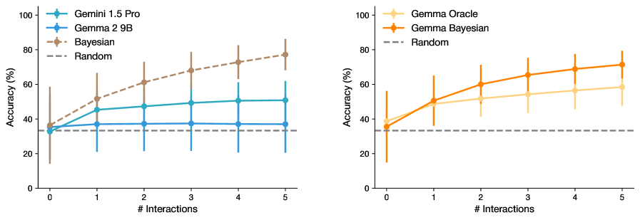Visual Description ## Line Chart: Model Accuracy vs. Number of Interactions ### Overview The image contains two line charts comparing the accuracy of different language models as the number of interactions increases. The left chart compares "Gemini 1.5 Pro", "Gemma 2 9B", and "Bayesian" models, while the right chart compares "Gemma Oracle" and "Gemma Bayesian" models. Both charts include a "Random" baseline. The x-axis represents the number of interactions, and the y-axis represents the accuracy in percentage. Error bars are present on each data point. ### Components/Axes * **X-axis (Horizontal):** "# Interactions" ranging from 0 to 5. * **Y-axis (Vertical):** "Accuracy (%)" ranging from 0 to 100. * **Left Chart Legend (Top-Left):** * Blue: Gemini 1.5 Pro * Light Blue: Gemma 2 9B * Brown Dashed: Bayesian * Gray Dashed: Random * **Right Chart Legend (Top-Right):** * Light Orange: Gemma Oracle * Orange: Gemma Bayesian * Gray Dashed: Random * **Horizontal Dashed Line:** Represents the "Random" baseline, positioned at approximately 33% accuracy on both charts. ### Detailed Analysis **Left Chart:** * **Gemini 1.5 Pro (Blue):** Starts at approximately 33% accuracy at 0 interactions, increases to approximately 45% at 1 interaction, and then plateaus around 48-50% for 2-5 interactions. * (0, 33%), (1, 45%), (2, 48%), (3, 48%), (4, 50%), (5, 50%) * **Gemma 2 9B (Light Blue):** Starts at approximately 33% accuracy at 0 interactions, increases to approximately 37% at 1 interaction, and then plateaus around 37% for 2-5 interactions. * (0, 33%), (1, 37%), (2, 37%), (3, 37%), (4, 37%), (5, 37%) * **Bayesian (Brown Dashed):** Starts at approximately 37% accuracy at 0 interactions and increases steadily to approximately 77% at 5 interactions. * (0, 37%), (1, 50%), (2, 60%), (3, 65%), (4, 70%), (5, 77%) * **Random (Gray Dashed):** Remains constant at approximately 33% accuracy across all interactions. **Right Chart:** * **Gemma Oracle (Light Orange):** Starts at approximately 37% accuracy at 0 interactions, increases to approximately 50% at 1 interaction, and then plateaus around 55-58% for 2-5 interactions. * (0, 37%), (1, 50%), (2, 53%), (3, 55%), (4, 57%), (5, 58%) * **Gemma Bayesian (Orange):** Starts at approximately 37% accuracy at 0 interactions, increases to approximately 50% at 1 interaction, and then continues to increase to approximately 72% at 5 interactions. * (0, 37%), (1, 50%), (2, 60%), (3, 67%), (4, 70%), (5, 72%) * **Random (Gray Dashed):** Remains constant at approximately 33% accuracy across all interactions. ### Key Observations * The "Random" baseline remains constant across all interactions in both charts. * In the left chart, the "Bayesian" model shows the most significant improvement in accuracy as the number of interactions increases. * In the right chart, the "Gemma Bayesian" model shows a more significant improvement in accuracy compared to "Gemma Oracle" as the number of interactions increases. * "Gemini 1.5 Pro" and "Gemma 2 9B" plateau quickly after the first interaction. ### Interpretation The charts illustrate how the accuracy of different language models changes with an increasing number of interactions. The "Bayesian" model in the left chart and the "Gemma Bayesian" model in the right chart demonstrate the most substantial improvements in accuracy, suggesting that these models benefit more from increased interactions compared to the other models. The "Random" baseline serves as a control, indicating the expected accuracy without any learning or interaction. The error bars indicate the variability in the accuracy measurements. The plateauing of "Gemini 1.5 Pro", "Gemma 2 9B", and "Gemma Oracle" suggests that these models may have reached a performance limit with the given interaction setup. </details> Figure 13: Variability across reward functions over rounds. Error bars indicate standard deviation across reward functions. We additionally show results over rounds in Fig. 13. We find that both original LLMs and the Bayesian Assistant display high variance across reward function. While the variance of the Bayesian Assistant decreases as the number of interactions increases, as does that of the fine-tuned LLMs, the variance of the original LLM remains largely constant across interactions. Notably, Gemma Bayesian has lower variance while maintaining similar performance to the Bayesian Assistant. In particular, we hypothesize that reward functions that more strongly deviate from the LLM’s prior (Supplementary Section D.1) may be harder to infer. For example, the LLM may assume most people prefer shorter flights over long ones, making it more difficult to infer the preferences of an “abnormal” user who prefers longer flights. To test the hypothesis that the variability across reward functions is due in part to the prior, we fit linear regression models predicting a reward function’s final-round accuracy from its L2 distance to the mean of the prior reward distribution, focusing on Gemma in this experiment. We elicit the priors separately for Gemma Original, Gemma Bayesian and Gemma Oracle. The prior of the Bayesian Assistant is uniform, as before. Before computing distances we normalize the reward functions (divide them by their sum) to account for the fact that some functions are equivalent; for example, the reward function $[-1,-1,-1,-1]$ is equivalent to the function $[-0.5,-0.5,-0.5,-0.5]$ as both will always lead the user to prefer the same flights. In line with this hypothesis, we find negative regression coefficients for Gemma Original, indicating it performs worse when the reward function deviates from its priors (Fig. 14). The absolute coefficients for the Bayesian Assistant and Gemma Bayesian are similar, and much smaller than that of Gemma Original. For these three models, the impact of L2 distance from prior on the final-round accuracy is all significant (p $<$ 0.001). The Gemma Oracle does not show sensitivity to this distance (p = 0.24). 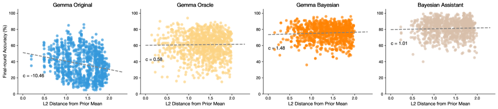<details> <summary>x15.png Details</summary>  ### Visual Description ## Scatter Plot: Final-round Accuracy vs. L2 Distance from Prior Mean for Different Models ### Overview The image presents four scatter plots, each displaying the relationship between "Final-round Accuracy (%)" and "L2 Distance from Prior Mean" for different models: "Gemma Original", "Gemma Oracle", "Gemma Bayesian", and "Bayesian Assistant". Each plot includes a dashed gray line indicating a linear trend, along with a 'c' value representing the slope of that line. ### Components/Axes * **X-axis (Horizontal):** "L2 Distance from Prior Mean". The scale ranges from 0.0 to 2.0 in all four plots. * **Y-axis (Vertical):** "Final-round Accuracy (%)". The scale ranges from 0 to 100 in all four plots. * **Titles:** Each plot has a title indicating the model being analyzed: "Gemma Original", "Gemma Oracle", "Gemma Bayesian", and "Bayesian Assistant". * **Data Points:** Each plot contains numerous data points representing individual observations. * Gemma Original: Blue data points. * Gemma Oracle: Yellow data points. * Gemma Bayesian: Orange data points. * Bayesian Assistant: Tan data points. * **Trend Line:** A dashed gray line is present in each plot, indicating the general trend of the data. * **'c' Value:** Each plot displays a 'c' value, representing the slope of the trend line. ### Detailed Analysis **1. Gemma Original (Top-Left)** * Data points are blue. * Trend: The data points are scattered, but there is a slight downward trend. * 'c' Value: c = -10.46 * Accuracy ranges from approximately 20% to 80%. * L2 Distance ranges from 0 to 2. **2. Gemma Oracle (Top-Middle)** * Data points are yellow. * Trend: The data points are scattered, with no clear trend. * 'c' Value: c = 0.58 * Accuracy ranges from approximately 20% to 100%. * L2 Distance ranges from 0 to 2. **3. Gemma Bayesian (Top-Right)** * Data points are orange. * Trend: The data points are scattered, with no clear trend. * 'c' Value: c = 1.48 * Accuracy ranges from approximately 50% to 100%. * L2 Distance ranges from 0 to 2. **4. Bayesian Assistant (Top-Right)** * Data points are tan. * Trend: The data points are scattered, with no clear trend. * 'c' Value: c = 1.01 * Accuracy ranges from approximately 50% to 100%. * L2 Distance ranges from 0 to 2. ### Key Observations * The "Gemma Original" model shows a slight negative correlation between L2 Distance and Final-round Accuracy. * The "Gemma Oracle", "Gemma Bayesian", and "Bayesian Assistant" models show no clear correlation between L2 Distance and Final-round Accuracy. * The "Gemma Original" model has a lower range of accuracy compared to the other three models. ### Interpretation The plots compare the performance of different models ("Gemma Original", "Gemma Oracle", "Gemma Bayesian", and "Bayesian Assistant") in relation to the L2 distance from the prior mean. The 'c' value indicates the slope of the linear trend line, providing insight into how accuracy changes with increasing L2 distance. The negative 'c' value for "Gemma Original" suggests that as the L2 distance from the prior mean increases, the final-round accuracy tends to decrease slightly. In contrast, the other three models show a slightly positive or near-zero correlation, indicating that accuracy is not strongly affected by the L2 distance from the prior mean. The data suggests that the "Gemma Original" model might be more sensitive to deviations from the prior mean compared to the other models. The "Gemma Oracle", "Gemma Bayesian", and "Bayesian Assistant" models appear to maintain a relatively stable level of accuracy regardless of the L2 distance. </details> Figure 14: The relationship between the final-round accuracy and the normalized L2 distance to the mean of the prior reward distribution (1000 randomly sampled points for readability). $c$ refers to the coefficient in a linear regression predicting accuracy from L2 distance. The impact of L2 distance on final-round accuracy is significant (p $<$ 0.001) for Gemma Original, Gemma Bayesian, and Bayesian Assistant, but not for Gemma Oracle (p = 0.24). D.3 Interacting with Non-deterministic Users Our main experiments assume the simulated user always makes decisions that are consistent with its reward function. By contrast, as we show in the section Generalization to interactions with human users, humans may behave inconsistently with their stated preferences. To simulate this real-world stochasticity, we evaluate a setting where the LLM interacts with a non-deterministic user. We add noise to the user’s behavior, such that with a certain probability they select a non-optimal choice, that is a choice that does not maximize their reward. The relationship between the percentage of noise and final-round accuracy is shown in Fig. 15. We experiment with the three variants of Gemma, and with the Bayesian Assistant. As expected, performance decreases across the board as the amount of noise increases. For realistic noise values in the 10–60% range, we find that Gemma Bayesian is more robust to noise compared not only to Gemma Original and Gemma Oracle, but also to the Bayesian Assistant, which is the best model in the noiseless setting. This robustness to noise illustrates an advantage of an LLM fine-tuned to mimic a symbolic model compared to the original symbolic model (see Discussion). 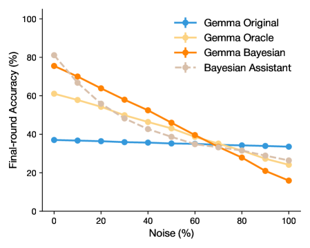<details> <summary>x16.png Details</summary>  ### Visual Description ## Line Chart: Final-round Accuracy vs. Noise ### Overview The image is a line chart comparing the final-round accuracy of four different models (Gemma Original, Gemma Oracle, Gemma Bayesian, and Bayesian Assistant) as the noise level increases from 0% to 100%. The chart shows how the accuracy of each model changes with increasing noise. ### Components/Axes * **X-axis:** Noise (%), with markers at 0, 20, 40, 60, 80, and 100. * **Y-axis:** Final-round Accuracy (%), with markers at 0, 20, 40, 60, 80, and 100. * **Legend:** Located in the top-right corner, identifying each line by color and name: * Blue: Gemma Original * Light Orange: Gemma Oracle * Orange: Gemma Bayesian * Gray dashed: Bayesian Assistant ### Detailed Analysis * **Gemma Original (Blue):** The line is nearly horizontal, indicating that the final-round accuracy remains relatively constant as noise increases. The accuracy is approximately 37% across all noise levels. * At 0% Noise: ~37% Accuracy * At 100% Noise: ~34% Accuracy * **Gemma Oracle (Light Orange):** The line slopes downward, indicating that the final-round accuracy decreases as noise increases. * At 0% Noise: ~61% Accuracy * At 100% Noise: ~25% Accuracy * **Gemma Bayesian (Orange):** The line slopes downward, indicating that the final-round accuracy decreases as noise increases. * At 0% Noise: ~76% Accuracy * At 100% Noise: ~16% Accuracy * **Bayesian Assistant (Gray dashed):** The line slopes downward, indicating that the final-round accuracy decreases as noise increases. * At 0% Noise: ~82% Accuracy * At 100% Noise: ~27% Accuracy ### Key Observations * Gemma Original maintains a stable accuracy regardless of noise level. * Gemma Oracle, Gemma Bayesian, and Bayesian Assistant all experience a decrease in accuracy as noise increases. * Bayesian Assistant has the highest initial accuracy (at 0% noise) but also experiences a significant drop as noise increases. * Gemma Bayesian starts with a high accuracy but degrades to the lowest accuracy at 100% noise. * At around 60% noise, the accuracy of Gemma Oracle, Gemma Bayesian, and Bayesian Assistant converge to approximately 35%. ### Interpretation The chart demonstrates the robustness of the "Gemma Original" model to noise, as its accuracy remains relatively stable. In contrast, the other three models ("Gemma Oracle", "Gemma Bayesian", and "Bayesian Assistant") are more susceptible to noise, with their accuracy decreasing as noise levels increase. The "Bayesian Assistant" model, while initially having the highest accuracy, is the most affected by noise. This suggests that while some models may perform well in ideal conditions (low noise), their performance degrades significantly in noisy environments. The intersection of the lines around 60% noise indicates a point where the performance of the noise-sensitive models becomes comparable. The "Gemma Original" model's consistent performance might be preferable in applications where noise is expected. </details> Figure 15: Final-round accuracy when interacting with a noisy simulated user. We add noise to the simulated user’s choice such that with some probability the user chooses an option that is different from the one that maximizes its reward. We plot fine-round accuracy with respect to the amount of noise. While all models show a decrease in performance as noise increases, Gemma Bayesian demonstrates greater robustness for noise levels between 10% and 60%. Error bars (too small to be visible in the plot) show standard errors across three random seeds (and three training runs). D.4 What Makes Bayesian Teaching Effective? We have shown that it is more effective to fine-tune our LLMs on the Bayesian Assistant’s predictions than on the user’s true choices. In this section, we explore and rule out two deflationary hypotheses that might explain the effectiveness of this method, and tentatively conclude that the advantage of Bayesian teaching is in fact due the probabilistically optimal predictions made by the Bayesian Assistant. In all of the experiments described in this section, we focus on Gemma 2 9B. We use the same list of flight option sets for all models, and vary only the supervision we provide during fine-tuning (i.e. the assistant’s recommendations). 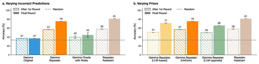<details> <summary>x17.png Details</summary>  ### Visual Description ## Bar Charts: Accuracy Comparison of Different Models ### Overview The image presents two bar charts comparing the accuracy of different models under varying conditions. Chart 'a' focuses on varying incorrect predictions, while chart 'b' explores varying priors. Each chart displays the accuracy (%) of different models "After 1st Round" (represented by hatched bars) and in the "Final Round" (represented by solid bars). A dashed horizontal line indicates the "Random" accuracy level. ### Components/Axes **Chart a. Varying Incorrect Predictions:** * **Title:** Varying Incorrect Predictions * **Y-axis:** Accuracy (%), with a scale from 0 to 100 in increments of 20. * **X-axis:** Categorical, representing different models: * Gemma Original * Gemma Bayesian * Gemma Oracle with Noise * Bayesian Assistant * **Legend:** Located at the top-left of the chart. * "After 1st Round": Represented by hatched bars. * "Final Round": Represented by solid bars. * "Random": Represented by a dashed horizontal line. **Chart b. Varying Priors:** * **Title:** Varying Priors * **Y-axis:** Accuracy (%), with a scale from 0 to 100 in increments of 20. * **X-axis:** Categorical, representing different models: * Gemma Bayesian (LLM-based) * Gemma Bayesian (Uniform) * Gemma Bayesian (LLM-opposite) * Bayesian Assistant * **Legend:** Located at the top-left of the chart. * "After 1st Round": Represented by hatched bars. * "Final Round": Represented by solid bars. * "Random": Represented by a dashed horizontal line. ### Detailed Analysis **Chart a. Varying Incorrect Predictions:** * **Gemma Original:** * After 1st Round: Accuracy is approximately 37%. * Final Round: Accuracy is approximately 37%. * **Gemma Bayesian:** * After 1st Round: Accuracy is approximately 57%. * Final Round: Accuracy is approximately 76%. * **Gemma Oracle with Noise:** * After 1st Round: Accuracy is approximately 40%. * Final Round: Accuracy is approximately 45%. * **Bayesian Assistant:** * After 1st Round: Accuracy is approximately 58%. * Final Round: Accuracy is approximately 81%. * **Random Accuracy:** Approximately 33%, represented by the dashed horizontal line. **Chart b. Varying Priors:** * **Gemma Bayesian (LLM-based):** * After 1st Round: Accuracy is approximately 51%. * Final Round: Accuracy is approximately 71%. * **Gemma Bayesian (Uniform):** * After 1st Round: Accuracy is approximately 57%. * Final Round: Accuracy is approximately 76%. * **Gemma Bayesian (LLM-opposite):** * After 1st Round: Accuracy is approximately 50%. * Final Round: Accuracy is approximately 66%. * **Bayesian Assistant:** * After 1st Round: Accuracy is approximately 58%. * Final Round: Accuracy is approximately 81%. * **Random Accuracy:** Approximately 33%, represented by the dashed horizontal line. ### Key Observations * In both charts, the "Bayesian Assistant" model consistently achieves the highest accuracy in the "Final Round." * The "Final Round" accuracy is generally higher than the "After 1st Round" accuracy for most models in both charts, indicating an improvement in performance over time. * The "Gemma Original" model in chart 'a' shows no improvement between the "After 1st Round" and "Final Round." * The "Random" accuracy line serves as a baseline, and most models significantly outperform this baseline in the "Final Round." ### Interpretation The data suggests that incorporating Bayesian methods, particularly with the "Bayesian Assistant," leads to higher accuracy in these models. The improvement from "After 1st Round" to "Final Round" indicates that the models are learning and refining their predictions over time. The "Bayesian Assistant" consistently outperforming other models suggests that its approach to handling incorrect predictions or prior information is more effective. The "Gemma Original" model's lack of improvement in chart 'a' may indicate a limitation in its design or training process. The charts highlight the importance of model selection and the impact of different strategies for handling uncertainty and prior knowledge in achieving higher accuracy. </details> \phantomsubcaption \phantomsubcaption Figure 16: Final-round accuracy of LLMs fine-tuned with different data variants. (a) Accuracy of the model using Bayesian teaching and the model using oracle teaching with random noise. (b) Accuracy of models fine-tuned on predictions from variants of the Bayesian Assistant, initialized with different priors. Error bars show standard errors across three random seeds (and three training runs). Hypothesis: Incorrect predictions regularize training. The Bayesian Assistant can make incorrect predictions, especially in the first few rounds, due to the fact that it only has limited information about the user (see the Bayesian Assistant’s accuracy over rounds in Fig. 24). Could these incorrect predictions regularize training and prevent overfitting, accounting for the effectiveness of Bayesian teaching? To test this hypothesis, we fine-tune the LLM using oracle teaching injected with random noise: 40% of the time, instead of predicting the user’s choice, the assistant recommends one of the incorrect options at random. The proportion of incorrect predictions in this control roughly matches that of the Bayesian predictions averaged across all five interactions. Contrary to the regularization hypothesis, we find that incorrect predictions do not necessarily improve performance: the model fine-tuned on noisy user’s choices (Gemma Oracle with Noise) barely outperforms the original LLM and has high standard error (Fig. 16). This suggests that random noise alone cannot explain why Bayesian predictions are more effective; rather, the Bayesian’s educated mistakes are more valuable than random errors. Hypothesis: The LLM benefits from the correct prior. We initialize the Bayesian Assistant using the uniform prior, which assigns equal probability to all reward functions, and therefore aligns with the data generation process of our evaluation. One hypothesis is that the LLM benefits from this correct prior (in the sense that it is calibrated to the distribution of simulated users in our experiment), which makes the predictions of the Bayesian Assistant more effective for supervised fine-tuning. To test this hypothesis, we fine-tune Gemma three times, using the predictions of three variants of the Bayesian Assistant, initialized with three different priors: the uniform prior, the LLM-based prior obtained from Gemma Original (see Fig. 11), and the prior that is contrary to the LLM-based one (e.g., if Gemma’s prior favors cheaper flights, this prior would instead prefer more expensive flights). The results are shown in Fig. 16. LLMs fine-tuned on predictions from all three Bayesian models perform very well and dramatically better than the original LLM. The choice of prior does influence the performance of the fine-tuned LLMs. The model fine-tuned on Bayesian predictions using the uniform prior, which matches the distribution of users in our sample, achieves the best accuracy. The LLM-based prior, despite being biased and spiky, leads to accuracy that is only slightly worse. The LLM-opposite prior, which is both biased and mismatches the LLM’s beliefs, leads to a more significant performance drop. That being said, the vast gap between all three LLMs fine-tuned on Bayesian predictions and Gemma Original suggests that the correct prior alone does not fully explain the effectiveness of Bayesian teaching. D.5 Qualitative Example In Fig. 17, we show a qualitative example of the evolution of the reward distributions of Gemma Original and the Bayesian Assistant over interactions. In this case, since the user’s true reward function differs significantly from the LLM’s prior, both Gemma Original and the Bayesian Assistant perform poorly at the start of the interactions. However, while the Bayesian Assistant gradually converges toward the ground-truth reward function after a few rounds, Gemma Original continues to assign high probability to reward functions that are inconsistent with its observations. 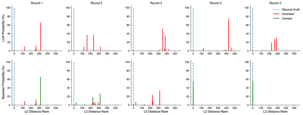<details> <summary>x18.png Details</summary>  ### Visual Description ## Bar Chart: LLM and Bayesian Probability vs. L2 Distance Rank Across Rounds ### Overview The image presents a series of bar charts comparing the probability distributions of an LLM (Large Language Model) and a Bayesian model across five rounds. The x-axis represents the L2 Distance Rank, and the y-axis represents the probability (%). Each round has two charts: the top one for the LLM and the bottom one for the Bayesian model. The charts show the distribution of "Correct" and "Incorrect" predictions, with a vertical dashed line indicating the "Ground-truth". ### Components/Axes * **Titles:** "Round 1", "Round 2", "Round 3", "Round 4", "Round 5" (placed above each pair of charts). * **Y-axis (Left):** "LLM Probability (%)" for the top row of charts, "Bayesian Probability (%)" for the bottom row of charts. Scale ranges from 0 to 100 in increments of 20. * **X-axis (Bottom):** "L2 Distance Rank". Scale ranges from 0 to 500 in increments of 100. * **Legend (Top-Right):** * "Ground-truth" - Dashed cyan line. * "Incorrect" - Red bars. * "Correct" - Green bars. ### Detailed Analysis **Round 1:** * **LLM:** A single prominent "Incorrect" (red) bar at approximately L2 Distance Rank 350, with a probability of approximately 65%. Smaller "Incorrect" bars are present at ranks around 100 and 250, with probabilities around 10%. The "Ground-truth" line is near 0. * **Bayesian:** A single prominent "Correct" (green) bar at approximately L2 Distance Rank 350, with a probability of approximately 70%. Small "Incorrect" (red) bars are present at ranks around 100 and 250, with probabilities around 5%. The "Ground-truth" line is near 0. **Round 2:** * **LLM:** Several "Incorrect" (red) bars are present between L2 Distance Ranks 100 and 300. The probabilities are approximately 50% at rank 150, 40% at rank 200, 50% at rank 250, and 20% at rank 350. The "Ground-truth" line is near 0. * **Bayesian:** "Incorrect" (red) bars are present at ranks around 100, 200, and 250, with probabilities around 10%. "Correct" (green) bars are present at ranks around 150 and 300, with probabilities around 20%. The "Ground-truth" line is near 0. **Round 3:** * **LLM:** A single prominent "Incorrect" (red) bar at approximately L2 Distance Rank 350, with a probability of approximately 60%. A smaller "Incorrect" bar is present at rank around 400, with a probability around 45%. The "Ground-truth" line is near 0. * **Bayesian:** A single prominent "Correct" (green) bar at approximately L2 Distance Rank 0, with a probability of approximately 90%. Small "Incorrect" (red) bars are present at ranks around 350 and 400, with probabilities around 10%. **Round 4:** * **LLM:** A single prominent "Incorrect" (red) bar at approximately L2 Distance Rank 400, with a probability of approximately 80%. The "Ground-truth" line is near 0. * **Bayesian:** A single prominent "Correct" (green) bar at approximately L2 Distance Rank 0, with a probability of approximately 70%. A small "Incorrect" (red) bar is present at rank around 400, with a probability around 10%. **Round 5:** * **LLM:** Several "Incorrect" (red) bars are present between L2 Distance Ranks 200 and 350. The probabilities are approximately 20% at rank 250, 30% at rank 300, and 80% at rank 350. The "Ground-truth" line is near 0. * **Bayesian:** A single prominent "Correct" (green) bar at approximately L2 Distance Rank 0, with a probability of approximately 60%. Small "Incorrect" (red) bars are present at ranks around 300 and 350, with probabilities around 10%. ### Key Observations * The "Ground-truth" line consistently appears near 0 on the L2 Distance Rank axis across all rounds and models. * The LLM tends to have higher probabilities associated with "Incorrect" predictions at higher L2 Distance Ranks. * The Bayesian model tends to have higher probabilities associated with "Correct" predictions at lower L2 Distance Ranks, particularly at 0. * The distribution of probabilities varies significantly between rounds for both models. ### Interpretation The charts suggest that the Bayesian model is generally more accurate than the LLM, as it assigns higher probabilities to the correct answer (lower L2 Distance Rank) more consistently across the rounds. The LLM, on the other hand, often assigns higher probabilities to incorrect answers (higher L2 Distance Rank). The variation in probability distributions across rounds indicates that the models' performance is not consistent and may be influenced by the specific data or task in each round. The "Ground-truth" line near 0 suggests that the ideal prediction would have a very low L2 distance rank. The data highlights the strengths and weaknesses of each model, with the Bayesian model showing a tendency towards correct predictions and the LLM showing a tendency towards incorrect predictions, especially as the L2 distance rank increases. </details> Figure 17: The reward distributions of Gemma Original (top) and the Bayesian Assistant (bottom) over multiple rounds. The reward functions are sorted by their normalized L2 distance from the ground-truth (GT) reward function, indicated by the blue dashed line at $x=0$ . Red indicates that the reward function’s prediction on the given options is incorrect, while green indicates that its prediction is correct. Appendix E Sensitivity to the Informativeness of Option Sets In each round of the flight recommendation task, we present the model with a set of three flight options, and the user’s choice among those options. The amount of information that can be gained through this process varies from round to round. For example, a choice between two flight options that differ in exactly one feature could be more informative than the choice between options that differ along multiple dimensions: the minimal pair of options provides direct evidence for the user’s preference for the particular feature. We expect a strong probabilistic reasoner to be sensitive to this factor: when the user’s choice between a particular set of options provides more information about their preferences, we expect the system to update its beliefs more substantially. In this section we test whether LLMs display this behavior. In contrast with the main experiments, where we sample the option sets randomly, here we sample them based on their informativeness. To measure the amount of information contained in a set of options $\mathcal{O}$ , we define the ground truth information gain as $$ \displaystyle g(\mathcal{O},o^{*},p(\bm{\theta}),q(\bm{\theta})) \displaystyle=\mathrm{KL}(p(\bm{\theta})||q(\bm{\theta}))-\mathrm{KL}(p(\bm{\theta})||q(\bm{\theta}|\mathcal{O},o^{*})) \displaystyle=\log q(\bm{\theta}^{*}|\mathcal{O},o^{*})-\log q(\bm{\theta}^{*}), \tag{5} $$ where $p(\bm{\theta})=\delta(\bm{\theta}^{*})$ and $q(\bm{\theta})$ is either $q_{B}(\bm{\theta})$ or $q_{LLM}(\bm{\theta})$ . This metric captures the increase in the posterior probability of the ground-truth reward function (that is, the user’s true reward function) after this set of options has been observed. Note that $g$ is relative to the model that is used to update the probability distribution; we use $g_{\textit{B}}$ and $g_{\textit{LLM}}$ to refer to the gain derived from the Bayesian Assistant and the LLM, respectively. E.1 Experimental Setup We randomly sample 5,000 candidate option sets, compute the ground truth information gain of each one based on the Bayesian Assistant, and select the option set that leads to the desired value of $g_{\textit{B}}$ . The performance is evaluated at the end of a five-round interaction, and the ground truth information gain is averaged over these five rounds. We evaluate the Bayesian Assistant as well as Gemma Original, Gemma Oracle, and Gemma Bayesian; as in our main experiments, the Bayesian Assistant is initialized with the uniform prior. 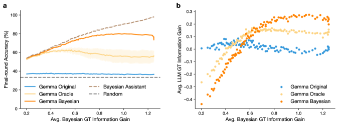<details> <summary>x19.png Details</summary>  ### Visual Description ## Chart: Final-round Accuracy and LLM GT Information Gain vs. Avg. Bayesian GT Information Gain ### Overview The image presents two charts (a and b) comparing the performance of different models (Gemma Original, Gemma Oracle, Gemma Bayesian, Bayesian Assistant, and Random) based on their final-round accuracy and average LLM GT information gain relative to the average Bayesian GT information gain. Chart 'a' shows the final-round accuracy as a function of the average Bayesian GT information gain, while chart 'b' shows the average LLM GT information gain as a function of the average Bayesian GT information gain. ### Components/Axes **Chart a:** * **Title:** Final-round Accuracy vs. Avg. Bayesian GT Information Gain * **X-axis:** Avg. Bayesian GT Information Gain, ranging from 0.2 to 1.2. * **Y-axis:** Final-round Accuracy (%), ranging from 0 to 100. * **Legend (bottom-left):** * Blue line: Gemma Original * Light Orange line: Gemma Oracle * Orange line: Gemma Bayesian * Dashed brown line: Bayesian Assistant * Dashed gray line: Random **Chart b:** * **Title:** Avg. LLM GT Information Gain vs. Avg. Bayesian GT Information Gain * **X-axis:** Avg. Bayesian GT Information Gain, ranging from 0.2 to 1.2. * **Y-axis:** Avg. LLM GT Information Gain, ranging from -0.4 to 0.3. * **Legend (bottom-right):** * Blue dots: Gemma Original * Light Orange dots: Gemma Oracle * Orange dots: Gemma Bayesian ### Detailed Analysis **Chart a:** * **Gemma Original (Blue):** The accuracy remains relatively constant at approximately 35% across the range of Avg. Bayesian GT Information Gain. * **Gemma Oracle (Light Orange):** The accuracy starts at around 55% at 0.2 Avg. Bayesian GT Information Gain, increases to approximately 65% around 0.6, and then decreases to around 55% at 1.2. There is a shaded region around this line, indicating variability or confidence intervals. * **Gemma Bayesian (Orange):** The accuracy starts at around 55% at 0.2 Avg. Bayesian GT Information Gain, increases to approximately 80% around 0.8, and then decreases slightly to around 78% at 1.2. * **Bayesian Assistant (Dashed Brown):** The accuracy increases from approximately 60% at 0.2 Avg. Bayesian GT Information Gain to approximately 95% at 1.2. * **Random (Dashed Gray):** The accuracy remains constant at approximately 35% across the range of Avg. Bayesian GT Information Gain. **Chart b:** * **Gemma Original (Blue):** The Avg. LLM GT Information Gain starts at approximately 0.1 at 0.2 Avg. Bayesian GT Information Gain, decreases to approximately -0.1 at 0.6, and then increases to approximately 0.0 at 1.2. * **Gemma Oracle (Light Orange):** The Avg. LLM GT Information Gain starts at approximately -0.3 at 0.2 Avg. Bayesian GT Information Gain, increases to approximately 0.2 at 0.8, and then decreases to approximately 0.0 at 1.2. * **Gemma Bayesian (Orange):** The Avg. LLM GT Information Gain starts at approximately -0.4 at 0.2 Avg. Bayesian GT Information Gain, increases to approximately 0.3 at 0.8, and then decreases to approximately 0.0 at 1.2. ### Key Observations * In chart a, the Bayesian Assistant consistently outperforms the other models in terms of final-round accuracy as the Avg. Bayesian GT Information Gain increases. Gemma Bayesian also shows a significant improvement in accuracy with increasing information gain, while Gemma Original and Random remain relatively constant. * In chart b, Gemma Bayesian and Gemma Oracle show a similar trend of increasing Avg. LLM GT Information Gain up to a certain point (around 0.8 Avg. Bayesian GT Information Gain) and then decreasing. Gemma Original shows a less pronounced variation. ### Interpretation The charts suggest that leveraging Bayesian GT information gain can significantly improve the performance of certain models, particularly the Bayesian Assistant and Gemma Bayesian, in terms of final-round accuracy. However, the relationship between Avg. Bayesian GT Information Gain and Avg. LLM GT Information Gain is more complex, with the models showing an initial increase in LLM GT Information Gain followed by a decrease as the Bayesian GT Information Gain increases beyond a certain point. This could indicate a saturation effect or a change in the way the models utilize the information gain at higher levels. The Gemma Original model appears to be less sensitive to the Bayesian GT Information Gain in both accuracy and LLM GT Information Gain. The Random model performs as expected, with a constant low accuracy, indicating that the Bayesian GT Information Gain is not being effectively utilized in this case. </details> \phantomsubcaption \phantomsubcaption Figure 18: Analysis of sensitivity of LLMs to the informativeness of option sets. (a) Effect of option set informativity on model performance. Option set informativity is defined by ground-truth information gain, i.e., the increase in the log probability assigned by the Bayesian Assistant to the ground truth reward function after observing the provided options. We plot accuracy after five interactions as a function of option set informativity averaged over the five interactions. (b) The relationship between ground-truth information gain computed from the Bayesian Assistant and from LLMs. E.2 Results The Bayesian Assistant’s performance consistently improves as option sets become more informative: after observing highly informative options, its performance is almost perfect (Fig. 18). Gemma Original does not show sensitivity to option set informativity, but the fine-tuned models are much more sensitive to this factor: their performance positively correlates with the Bayesian ground-truth information gain up to a certain point. Gemma Bayesian saturates later than Gemma Oracle, and achieves higher final accuracy, especially in the highly informative regime. E.3 Comparing LLM-derived and Bayesian Information Gain Recall that information gain is relative to the model that is used to update the probability distributions: $g_{\textit{LLM}}$ quantifies the amount of information the LLM can absorb from a particular set of options, whereas $g_{\textit{B}}$ quantifies the amount that the ideal Bayesian reasoner can absorb. How does $g_{\textit{LLM}}$ related to $g_{\textit{B}}$ for each of the variants of Gemma? We find that the correlation between the two measures is weak for Gemma Original (Fig. 18). For Gemma Oracle and Gemma Bayesian, we observe a more complex pattern. When $g_{\textit{B}}$ is small, there is a positive relationship between the two metrics, indicating that options that are informative from the Bayesian perspective are beneficial for the fine-tuned LLMs. In this part of the range, the information gain derived from Gemma Bayesian shows a stronger correlation with $g_{\textit{B}}$ compared with Gemma Oracle. When $g_{\textit{B}}$ is large, however, the relationship levels off and we no longer see a correlation between $g_{\textit{B}}$ and $g_{\textit{LLM}}$ for either of the fine-tuned models. This suggests that even Gemma Bayesian only approximates and does not fully implement the normative Bayesian reasoning strategy. Appendix F Human Experiments F.1 Humans As Assistants Participants. For the experiment where human participants acted as the assistant to a simulated user, we recruited 720 participants through the Prolific platform [Palan and Schitter, 2018]. Each human participant interacted with one simulated user from a subset of 48 simulated users (out of the total 624 users), which we sampled based on the L2 distance of their reward function from the origin. The average age of human participants was 37.2 (SD=12.5). Of those, 54.9% identified as male (395), 44.6% as female (321), and 0.6% preferred not to say (4). The major nationalities of human participants were the United States at 32.5% (234), United Kingdom at 23.2% (167), South Africa at 10.3% (74), Canada at 7.6% (55), and Poland at 4.4% (32). By ethnicity, 62.5% (450) were White, 17.4% (125) were Black, 11.9% (86) were Asian, and 5.6% (40) were Mixed. All participants reported using English as their primary language. Procedure. At the beginning of the experiment, each participant was asked to complete a preference questionnaire to indicate their initial guess of the user’s preferences for each individual feature. The participant subsequently proceeded to the annotation round, where they made recommendations from three flight options. After the selection, the human annotator received feedback indicating whether their choice was correct. They were then redirected to the preference questionnaire to report their updated beliefs about the user’s preferences. This completed one round. The annotator repeated the same procedure for five rounds. Following these five rounds, we also implemented a quality control annotation round where the annotator interacted with a typical user with a highly informative option list (differing only in one feature dimension). We expected this quality control round to be very easy for participants who were paying close attention to task. We filtered out participants who failed the quality control annotation. The mean and median completion time (including the quality control annotation) was 9.35 minutes and 7.90 minutes, respectively, with a standard deviation of 5.08 minutes. Additional Results. Our main results show the accuracy of human assistants using their direct predictions of the user’s preferred choices. Since we also ask the annotator to rate their beliefs about the user’s preferences after each round, we can also use these estimated preferences to make recommendations—the same procedure we use in Section B. This allows us to evaluate on the larger held-out set and reduce the noise. As shown in Fig. 19, we find that while the accuracy of the human annotators’ direct prediction may not monotonically improve from one round to the next, their beliefs about the user’s preferences become consistently more accurate over rounds. 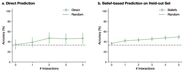<details> <summary>x20.png Details</summary>  ### Visual Description ## Chart: Accuracy vs. Number of Interactions for Direct and Belief-based Predictions ### Overview The image presents two line graphs comparing the accuracy of "Direct Prediction" and "Belief-based Prediction on Held-out Set" against the number of interactions. Both graphs also show a "Random" baseline for comparison. The y-axis represents accuracy in percentage, and the x-axis represents the number of interactions. Error bars are present on the data points. ### Components/Axes **Left Chart (a. Direct Prediction):** * **Title:** a. Direct Prediction * **Y-axis:** Accuracy (%) with scale from 0 to 100 in increments of 20. * **X-axis:** # Interactions, ranging from 0 to 4 in increments of 1. * **Legend (Top-Right):** * Direct (Light Green Line with Circle Markers) * Random (Dashed Gray Line) **Right Chart (b. Belief-based Prediction on Held-out Set):** * **Title:** b. Belief-based Prediction on Held-out Set * **Y-axis:** Accuracy (%) with scale from 0 to 100 in increments of 20. * **X-axis:** # Interactions, ranging from 0 to 5 in increments of 1. * **Legend (Top-Right):** * Beliefs (Light Green Line with Circle Markers) * Random (Dashed Gray Line) ### Detailed Analysis **Left Chart (Direct Prediction):** * **Direct (Light Green Line):** * Trend: Initially increases, then plateaus. * Data Points: * 0 Interactions: Accuracy ~35% * 1 Interaction: Accuracy ~40% * 2 Interactions: Accuracy ~47% * 3 Interactions: Accuracy ~47% * 4 Interactions: Accuracy ~47% * **Random (Dashed Gray Line):** * Constant at ~33% **Right Chart (Belief-based Prediction):** * **Beliefs (Light Green Line):** * Trend: Gradually increases. * Data Points: * 0 Interactions: Accuracy ~38% * 1 Interaction: Accuracy ~43% * 2 Interactions: Accuracy ~46% * 3 Interactions: Accuracy ~47% * 4 Interactions: Accuracy ~49% * 5 Interactions: Accuracy ~50% * **Random (Dashed Gray Line):** * Constant at ~33% ### Key Observations * Both "Direct" and "Beliefs" predictions start above the "Random" baseline. * "Direct Prediction" shows an initial increase in accuracy but plateaus after 2 interactions. * "Belief-based Prediction" shows a more gradual and consistent increase in accuracy with increasing interactions. * Error bars are present on all data points, indicating variability in the results. ### Interpretation The data suggests that both direct and belief-based prediction methods perform better than random chance. The direct prediction method shows an initial improvement in accuracy with a few interactions, but its performance plateaus quickly. In contrast, the belief-based prediction method demonstrates a more consistent and gradual improvement in accuracy as the number of interactions increases. This could indicate that belief-based methods are better at leveraging additional interactions to refine their predictions, while direct prediction methods may reach a performance limit more quickly. The error bars indicate that there is some variability in the results, which should be considered when interpreting the findings. </details> Figure 19: Accuracy of the human assistant over rounds. (a) Based on the human’s direct predictions on provided option sets. (b) Based on the human’s beliefs about the user’s preferences on held-out option sets. Error bars show the averaged standard error across human participants. Qualitative Analysis. One pattern we observe in human assistants is that they tend to favor simpler heuristics when there is limited evidence. For example, in Table 2, we show that when there are multiple valid user preferences, human assistants may rely on simpler heuristics, e.g. in this example, always choosing the cheapest flight. In contrast, the fine-tuned Gemma Bayesian model does not seem to exhibit this behavior. Table 2: Qualitative examples of LLM and human predictions. Here, the user strongly prefers an early departure time, weakly prefers a short flight duration, and has no preference for the number of stops and the price. Most human participants tend to favor a simpler heuristic, i.e., always choosing the cheapest flight, while Gemma Bayesian does not seem to exhibit this behavior. | Flight 1 | 05:12 PM | 30 min | 1 | $190 | Flight 1 | Flight 1 | Flight 1: 66.7% | | --- | --- | --- | --- | --- | --- | --- | --- | | Flight 2 | 03:36 PM | 12 hr 12 min | 2 | $460 | Flight 2: 26.7% | | | | Flight 3 | 10:00 PM | 10 hr 15 min | 2 | $640 | Flight 3: 6.7% | | | | Flight 1 | 06:48 PM | 4 hr 24 min | 1 | $370 | Flight 2 | Flight 2 | Flight 1: 40.0% | | Flight 2 | 07:36 AM | 16 hr 6 min | 1 | $100 | Flight 2: 33.3% | | | | Flight 3 | 10:00 PM | 20 hr | 0 | $550 | Flight 3: 26.7% | | | | Flight 1 | 10:00 PM | 30 min | 1 | $280 | Flight 3 | Flight 3 | Flight 1: 60% | | Flight 2 | 08:24 PM | 30 min | 0 | $910 | Flight 2: 0.0% | | | | Flight 3 | 06:00 AM | 8 hr 18 min | 0 | $370 | Flight 3: 40% | | | F.2 Humans As Users Participants. For the experiment where human participants acted as the users, we recruited 500 participants through the Prolific platform. The average age of the participants was 38.7 (SD=13.6); 51.0% identified as male (255), 48.4% as female (242), and 0.6% preferred not to say (3). The major nationalities of human participants were the United States at 40.0% (200), United Kingdom at 16.0% (80), South Africa at 9.0% (45), Canada at 7.8% (39), and Australia at 5.6% (28), with smaller representations from other countries. In terms of ethnicity, 65.2% (326) identified as White, 15.0% (75) as Black, 8.4% (42) as Asian, 7.2% (36) as Mixed, and 4.0% (20) as Other. All participants reported that English is their primary language. Procedure. Each participant in this experiment was first asked to complete a preference questionnaire to indicate their own preferences for different flight features. They then proceeded to the annotation rounds, where they needed to select their preferred option out of three flight options. To ensure quality, we required annotators to think for at least 30 seconds before making their selection. The procedure continued for five rounds. Participants were told to make choices consistent with their initially stated preferences throughout all five rounds. The mean and median completion times were 6.43 minutes and 5.18 minutes, respectively, with a standard deviation of 3.51 minutes. Additional Results. 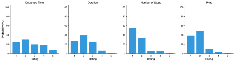<details> <summary>x21.png Details</summary>  ### Visual Description ## Bar Charts: Feature Rating Distributions ### Overview The image contains four bar charts, each displaying the distribution of ratings for a different feature: Departure Time, Duration, Number of Stops, and Price. The y-axis represents the probability (%), and the x-axis represents the rating from 1 to 5. All bars are blue. ### Components/Axes * **X-axis (Rating):** Discrete values from 1 to 5, representing the rating level. * **Y-axis (Probability (%)):** Continuous scale from 0 to 100%, with tick marks at 0, 20, 40, 60, 80, and 100. * **Chart Titles:** * Top-left: "Departure Time" * Top-middle-left: "Duration" * Top-middle-right: "Number of Stops" * Top-right: "Price" ### Detailed Analysis **1. Departure Time** * Trend: The distribution is relatively uniform, with a slight peak at rating 2. * Rating 1: Approximately 25% * Rating 2: Approximately 30% * Rating 3: Approximately 20% * Rating 4: Approximately 20% * Rating 5: Approximately 5% **2. Duration** * Trend: The distribution is skewed towards lower ratings, with a peak at rating 2. * Rating 1: Approximately 28% * Rating 2: Approximately 40% * Rating 3: Approximately 25% * Rating 4: Approximately 5% * Rating 5: Approximately 2% **3. Number of Stops** * Trend: The distribution is heavily skewed towards lower ratings, with a significant peak at rating 1. * Rating 1: Approximately 55% * Rating 2: Approximately 33% * Rating 3: Approximately 5% * Rating 4: Approximately 5% * Rating 5: Approximately 2% **4. Price** * Trend: The distribution is skewed towards lower ratings, with a peak at rating 2. * Rating 1: Approximately 38% * Rating 2: Approximately 48% * Rating 3: Approximately 8% * Rating 4: Approximately 3% * Rating 5: Approximately 1% ### Key Observations * The "Number of Stops" feature has the most skewed distribution, with the highest probability for a rating of 1. * The "Departure Time" feature has the most uniform distribution compared to the others. * All features show a decreasing probability as the rating increases from 2 to 5. * Ratings of 4 and 5 are relatively rare across all features. ### Interpretation The bar charts provide insights into how users rate different features. The "Number of Stops" is the most negatively perceived feature, with a high probability of receiving a rating of 1. "Price" and "Duration" also tend to receive lower ratings. "Departure Time" is rated more evenly, suggesting it is less of a concern for users. These ratings could reflect user preferences or expectations regarding these features. The data suggests that minimizing the number of stops is a key factor in user satisfaction, followed by price and duration. </details> Figure 20: The distributions of human participants’ initial preferences for different flight features. A rating of 1 indicates the strongest preference for the earliest departure time, the shortest duration, the fewest number of stops, and the lowest price, while a rating of 5 indicates the opposite. A rating of 3 indicates no preference. 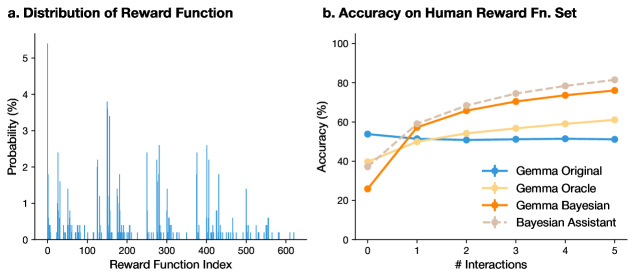<details> <summary>x22.png Details</summary>  ### Visual Description ## Chart: Distribution of Reward Function and Accuracy on Human Reward Function Set ### Overview The image presents two charts. The first chart (a) is a bar graph showing the distribution of a reward function across different reward function indices. The second chart (b) is a line graph comparing the accuracy of different models (Gemma Original, Gemma Oracle, Gemma Bayesian, and Bayesian Assistant) on a human reward function set, plotted against the number of interactions. ### Components/Axes **Chart a: Distribution of Reward Function** * **Title:** a. Distribution of Reward Function * **X-axis:** Reward Function Index, ranging from 0 to 600. * **Y-axis:** Probability (%), ranging from 0% to 5%. * **Data:** The chart displays a series of vertical bars, each representing the probability associated with a specific reward function index. **Chart b: Accuracy on Human Reward Fn. Set** * **Title:** b. Accuracy on Human Reward Fn. Set * **X-axis:** # Interactions, ranging from 0 to 5. * **Y-axis:** Accuracy (%), ranging from 0% to 100%. * **Legend (located in the bottom-right):** * **Blue Line with Plus Markers:** Gemma Original * **Light Yellow Line:** Gemma Oracle * **Orange Line with Plus Markers:** Gemma Bayesian * **Dashed Gray Line with Diamond Markers:** Bayesian Assistant ### Detailed Analysis **Chart a: Distribution of Reward Function** * The distribution is highly uneven, with most reward function indices having very low probabilities. * There are several spikes indicating reward function indices with significantly higher probabilities. * The highest probability observed is approximately 5%. **Chart b: Accuracy on Human Reward Fn. Set** * **Gemma Original (Blue):** Starts at approximately 54% accuracy at 0 interactions, dips slightly to around 51% at 1 interaction, and then remains relatively constant at approximately 53% for the remaining interactions. * **Gemma Oracle (Light Yellow):** Starts at approximately 38% accuracy at 0 interactions, increases to approximately 52% at 1 interaction, and then gradually increases to approximately 60% at 5 interactions. * **Gemma Bayesian (Orange):** Starts at approximately 25% accuracy at 0 interactions, increases sharply to approximately 52% at 1 interaction, and then gradually increases to approximately 77% at 5 interactions. * **Bayesian Assistant (Dashed Gray):** Starts at approximately 38% accuracy at 0 interactions, increases to approximately 52% at 1 interaction, and then gradually increases to approximately 82% at 5 interactions. ### Key Observations * In Chart a, the reward function distribution is sparse, suggesting that only a small subset of reward functions are highly probable. * In Chart b, Gemma Bayesian and Bayesian Assistant significantly outperform Gemma Original and Gemma Oracle as the number of interactions increases. * Gemma Original's accuracy remains relatively stable regardless of the number of interactions. * Bayesian Assistant shows the highest accuracy among all models, especially at higher interaction counts. ### Interpretation The distribution of the reward function (Chart a) indicates that the reward landscape is not uniform, with certain reward functions being much more likely than others. This could reflect inherent biases or preferences in the environment or the data used to define the reward functions. The accuracy comparison (Chart b) demonstrates the effectiveness of Bayesian methods (Gemma Bayesian and Bayesian Assistant) in learning from human interactions. These methods show a significant improvement in accuracy as the number of interactions increases, suggesting that they are better at adapting to human preferences or feedback compared to the Gemma Original and Gemma Oracle models. The Gemma Original model's stable accuracy suggests it may not be effectively learning from interactions, while the Gemma Oracle model shows some improvement but not as significant as the Bayesian approaches. The Bayesian Assistant, with its highest accuracy, likely incorporates additional mechanisms or prior knowledge that further enhance its learning capabilities. </details> \phantomsubcaption \phantomsubcaption Figure 21: Analysis of human reward functions. (a) Distribution of human reward functions. (b) Accuracy over rounds on the subset of the original data where the simulated user’s reward function is set of reward functions stated by the human participants. Error bars show standard errors across three random seeds (and three training runs). 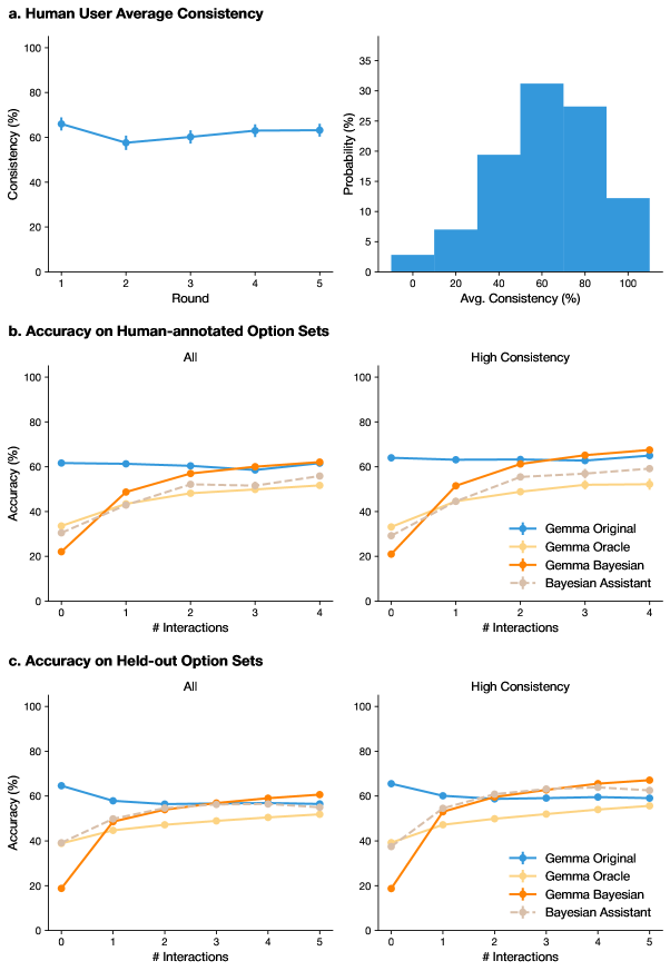<details> <summary>x23.png Details</summary>  ### Visual Description ## Chart/Diagram Type: Multi-Panel Performance Evaluation ### Overview The image presents a multi-panel figure evaluating the performance of different models (Gemma Original, Gemma Oracle, Gemma Bayesian, and Bayesian Assistant) in terms of human user consistency and accuracy on both human-annotated and held-out option sets. The figure is divided into three sections: (a) Human User Average Consistency, (b) Accuracy on Human-annotated Option Sets, and (c) Accuracy on Held-out Option Sets. Each accuracy section is further divided into "All" and "High Consistency" subsets. ### Components/Axes **Panel a: Human User Average Consistency** * **Title:** Human User Average Consistency * **X-axis:** Round (values: 1, 2, 3, 4, 5) * **Y-axis:** Consistency (%) (range: 0 to 100) * **Data:** A single data series showing consistency across rounds. Error bars are present. **Panel a: Histogram of Average Consistency** * **X-axis:** Avg. Consistency (%) (range: 0 to 100) * **Y-axis:** Probability (%) (range: 0 to 35) **Panel b: Accuracy on Human-annotated Option Sets** * **Title:** Accuracy on Human-annotated Option Sets * **Subtitles:** All, High Consistency * **X-axis:** # Interactions (values: 0, 1, 2, 3, 4) * **Y-axis:** Accuracy (%) (range: 0 to 100) * **Legend (right side of the panel):** * Blue: Gemma Original * Light Blue: Gemma Oracle * Orange: Gemma Bayesian * Gray Dashed: Bayesian Assistant **Panel c: Accuracy on Held-out Option Sets** * **Title:** Accuracy on Held-out Option Sets * **Subtitles:** All, High Consistency * **X-axis:** # Interactions (values: 0, 1, 2, 3, 4, 5) * **Y-axis:** Accuracy (%) (range: 0 to 100) * **Legend (right side of the panel):** * Blue: Gemma Original * Light Blue: Gemma Oracle * Orange: Gemma Bayesian * Gray Dashed: Bayesian Assistant ### Detailed Analysis **Panel a: Human User Average Consistency** * The consistency starts at approximately 67% in Round 1. * It dips to around 58% in Round 2. * Then, it gradually increases and stabilizes around 63% for Rounds 3, 4, and 5. * The error bars indicate the variability in consistency across users. **Panel a: Histogram of Average Consistency** * The histogram shows the distribution of average consistency scores. * The distribution is unimodal and skewed to the right. * The highest probability is around 60-70% consistency. * The probability is low for consistency scores below 20% and above 90%. * Approximate probability values: * 0-20%: ~3% * 20-40%: ~7% * 40-60%: ~19% * 60-80%: ~32% * 80-100%: ~12% **Panel b: Accuracy on Human-annotated Option Sets** * **"All" Subpanel:** * Gemma Original (Blue): Starts at approximately 62% and remains relatively constant. * Gemma Oracle (Light Blue): Starts around 30%, increases to approximately 55% by interaction 1, and plateaus. * Gemma Bayesian (Orange): Starts around 22%, increases to approximately 50% by interaction 1, and plateaus. * Bayesian Assistant (Gray Dashed): Starts around 35%, increases to approximately 58% by interaction 1, and plateaus. * **"High Consistency" Subpanel:** * Gemma Original (Blue): Starts at approximately 64% and remains relatively constant. * Gemma Oracle (Light Blue): Starts around 30%, increases to approximately 60% by interaction 1, and plateaus. * Gemma Bayesian (Orange): Starts around 20%, increases to approximately 65% by interaction 2, and plateaus. * Bayesian Assistant (Gray Dashed): Starts around 35%, increases to approximately 60% by interaction 1, and plateaus. **Panel c: Accuracy on Held-out Option Sets** * **"All" Subpanel:** * Gemma Original (Blue): Starts at approximately 65% and decreases slightly to approximately 60% by interaction 5. * Gemma Oracle (Light Blue): Starts around 40%, increases to approximately 58% by interaction 2, and plateaus. * Gemma Bayesian (Orange): Starts around 18%, increases to approximately 60% by interaction 4, and plateaus. * Bayesian Assistant (Gray Dashed): Starts around 40%, increases to approximately 55% by interaction 1, and plateaus. * **"High Consistency" Subpanel:** * Gemma Original (Blue): Starts at approximately 65% and decreases slightly to approximately 60% by interaction 5. * Gemma Oracle (Light Blue): Starts around 40%, increases to approximately 60% by interaction 1, and plateaus. * Gemma Bayesian (Orange): Starts around 20%, increases to approximately 65% by interaction 3, and plateaus. * Bayesian Assistant (Gray Dashed): Starts around 40%, increases to approximately 55% by interaction 1, and plateaus. ### Key Observations * Gemma Original consistently maintains a higher accuracy compared to other models across all conditions, but does not improve with interactions. * Gemma Oracle, Gemma Bayesian, and Bayesian Assistant show improvement in accuracy with increasing interactions, but plateau after a few interactions. * The "High Consistency" subsets generally show slightly higher accuracy for Gemma Oracle, Gemma Bayesian, and Bayesian Assistant compared to the "All" subsets. * The accuracy of Gemma Original on held-out option sets decreases slightly with more interactions. ### Interpretation The data suggests that Gemma Original performs well without any interactions, possibly due to pre-training or inherent biases. The other models (Gemma Oracle, Gemma Bayesian, and Bayesian Assistant) benefit from interactions with human-annotated data, improving their accuracy. The "High Consistency" subsets indicate that these models perform better when trained on more reliable data. The slight decrease in Gemma Original's accuracy on held-out option sets with more interactions might indicate overfitting or a shift in the data distribution. The histogram of average consistency shows that most users have a consistency score between 40% and 80%, indicating a moderate level of agreement among annotators. </details> \phantomsubcaption \phantomsubcaption \phantomsubcaption Figure 22: Results on interactions with real human users. (a) Consistency between the human users’ choices and the predictions derived from their initially stated preferences. We show user consistency over rounds and the distribution of the average user consistency. Error bars show standard errors across five-round option sets list. (b) Accuracy over rounds on human-annotated option sets. We show the results of all human users and users with high consistency, i.e., their choices matched their initially stated preferences in 4 or 5 of the rounds (40.4% of the data). (c) Accuracy over rounds on the held-out set, where the preferred choices are deterministically computed based on the human user’s preferences. Error bars show standard errors across three random seeds (and three training runs). In the main paper we report results for this more realistic setting where the model interacts with real human users on the flight recommendation task. Surprisingly, we also find that the original LLMs achieved good performance, unlike what was observed in earlier experiments. We hypothesize that two factors may contribute to its improved performance. First, unlike our simulated users whose preferences are uniformly sampled from the space of possible reward functions, human preferences are biased towards particular types of functions, and in Fig. 21 we show that some reward functions are considerably more common than others in our sample of human participants. For example, most participants report preferring cheaper flights (see Fig. 20). As such, a viable strategy for the original LLM could be to rely on its prior knowledge about user preferences to make relatively good recommendations. To investigate this further, we filter results for simulated users based on reward functions stated by the human participants in Fig. 21. We observe that also in this case, Gemma Original achieves a higher accuracy of around 60% (as opposed to 37% in Fig. 2, matching the high accuracy it obtained in Fig. 6. This makes it clear that the bias among the human preferences in this experiment contributes to the stronger performance of original LLMs. Secondly, human users may not necessarily behave consistently with their preferences, i.e., their choices may differ from those that would reflect their initially stated preferences. Indeed, note how in Fig. 21 the gap between the original LLM and the Bayesian LLM increases significantly when evaluating on consistent simulated users. To quantify this potential discrepancy, we compute the consistency between the human user’s choices and the predictions derived from their preferences. The latter are obtained by mapping their stated preferences to corresponding reward functions and selecting the option with the highest reward accordingly. In line with our hypothesis, the average consistency is relatively low at 60%, with chance performance being 33.3% (Fig. 22). We further break down the performance by user consistency over rounds and show results for high-consistency users; that is, users whose choices were consistent with their stated preferences in 4 or 5 of the rounds (Fig. 22). We find that all models perform better for the high-consistency users. Specifically, when user consistency is high, the improvement of Gemma Bayesian over Gemma Original increases. Finally, to limit the effect of such inconsistencies, while still retaining the real interactions between human users and the model, we also evaluate the LLMs on a held-out set of 100 randomly sampled options that simulate perfectly consistent users; to do so we use the preferred options derived from the participants’ initially stated preferences rather than the participants’ actual choices. As shown in Fig. 22, when removing inconsistency from the evaluation data, Gemma Bayesian achieves the best performance. Gemma Original performs best initially, likely due to its correct prior about human users, but its performance decreases over rounds, indicating its limited ability to incorporate the simulated user’s feedback. F.3 Human Annotation Interface We show the human annotation interface where humans act as the assistant in Fig. 23. The interface allows the human annotator to select the best option from three flight options, rate their estimation of the user’s preferences, and check the flight booking history from previous rounds. The annotation interface where humans act as the user is similar. Appendix G Statistical Analyses This Supplementary reports analyses that test whether Bayesian teaching leads to statistically significant improvement over the baselines. We fit linear mixed-effects models treating each method (Bayesian teaching, oracle teaching, and the original) and model family (Gemma, Llama, and Qwen) as fixed effects while controlling for various sources of randomness. For flight and hotel recommendation, we include training run, evaluation random seed, and reward function as random effects. For web shopping, we treat training run ad product category as random effects. Overall, the models demonstrate statistically significant differences between methods across all domains and all three model families (Gemma, Llama, and Qwen). In flight recommendation, the original LLM achieves a baseline accuracy of 37.0% (95% CI: 30.6–43.5%). The Oracle LLM performs significantly better with a 24.0% increase (95% CI: 16.6–31.4%, p $<$ 0.001), while the Bayesian LLM shows an even more substantial 38.5% increase (95% CI: 31.1–45.9%, p $<$ 0.001). Model family shows no significant effect on performance, with differences between model families all non-significant. The interaction between method and model family was not statistically significant (minimum p = 0.19). Within each model family, improvements between all methods are significant (p $<$ 0.001), with the exception of Qwen Oracle versus Qwen Original which shows slightly weaker but still significant improvement (p = 0.002). In hotel recommendation, the original LLM achieves a baseline accuracy of 36.7% (95% CI: 32.1–41.3%). The Oracle LLM performs significantly better with a 16.7% increase (95% CI: 11.4–22.0%, p $<$ 0.001), while the Bayesian LLM shows a 29.4% increase (95% CI: 24.1–34.7%, p $<$ 0.001). Model family shows no significant main effect on performance. The interaction between method and model family is not statistically significant (all interaction p-values $>$ 0.11). Within each model family, most pairwise comparisons show p-values $<$ 0.001, with two exceptions: Llama Bayesian versus Llama Oracle shows weak significance (p = 0.001), and Qwen Oracle versus Qwen Original shows weaker significance (p = 0.002). In web shopping, the original LLM achieves a baseline accuracy of 54.0% (95% CI: 49.6–58.4%). The Oracle LLM performs significantly better with a 7.1% increase (95% CI: 2.3–11.8%, p = 0.013), while the Bayesian LLM shows a more substantial 18.6% increase (95% CI: 13.8–23.4%, p $<$ 0.001). Unlike the other domains, model family shows a significant effect, with Qwen showing a significant decrease of -11.1% (95% CI: -17.0–5.3%, p = 0.003) compared to the baseline. There is also a significant interaction between Oracle method and Qwen (15.8%, 95% CI: 9.0–22.6%, p = 0.001). Within-family pairwise comparisons show different patterns: for Gemma, all method comparisons are significant (Original-Oracle: p = 0.033; others p $<$ 0.001); for Llama, Original-Oracle is non-significant (p = 0.199) while Original-Bayesian (p = 0.001) and Oracle-Bayesian (p = 0.004) are significant; for Qwen, Original-Oracle and Original-Bayesian are highly significant (p $<$ 0.001), but Oracle-Bayesian is non-significant (p = 0.282). Appendix H Results Details We show results over rounds for different models and methods in Fig. 24 – 27. For each, we show the accuracy based on the LLM’s or human direct prediction (“direct”) and accuracy based on predictions derived from their beliefs about the user’s preferences (“beliefs”) if available. 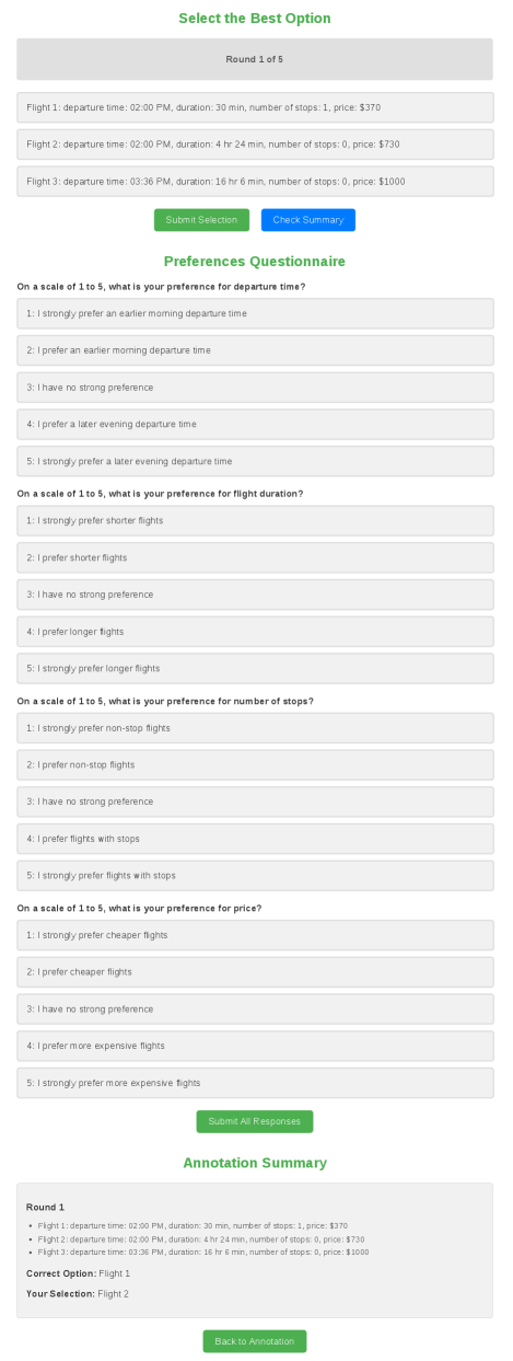<details> <summary>x24.png Details</summary>  ### Visual Description ## Webpage Screenshot: Flight Selection and Preference Questionnaire ### Overview The image is a screenshot of a webpage presenting a flight selection task and a preference questionnaire. The task involves choosing the best flight option from three alternatives based on departure time, duration, number of stops, and price. The questionnaire assesses user preferences on a scale of 1 to 5 for departure time, flight duration, number of stops, and price. The page also includes an annotation summary indicating the correct option and the user's selection. ### Components/Axes * **Header:** "Select the Best Option", "Round 1 of 5" * **Flight Options:** * Flight 1: departure time: 02:00 PM, duration: 30 min, number of stops: 1, price: $370 * Flight 2: departure time: 02:00 PM, duration: 4 hr 24 min, number of stops: 0, price: $730 * Flight 3: departure time: 03:36 PM, duration: 16 hr 6 min, number of stops: 0, price: $1000 * **Buttons:** "Submit Selection", "Check Summary" * **Preferences Questionnaire:** * Title: "Preferences Questionnaire" * Introduction: "On a scale of 1 to 5, what is your preference for..." * Scales: * Departure Time: 1: I strongly prefer an earlier morning departure time 2: I prefer an earlier morning departure time 3: I have no strong preference 4: I prefer a later evening departure time 5: I strongly prefer a later evening departure time * Flight Duration: 1: I strongly prefer shorter flights 2: I prefer shorter flights 3: I have no strong preference 4: I prefer longer flights 5: I strongly prefer longer flights * Number of Stops: 1: I strongly prefer non-stop flights 2: I prefer non-stop flights 3: I have no strong preference 4: I prefer flights with stops 5: I strongly prefer flights with stops * Price: 1: I strongly prefer cheaper flights 2: I prefer cheaper flights 3: I have no strong preference 4: I prefer more expensive flights 5: I strongly prefer more expensive flights * **Button:** "Submit All Responses" * **Annotation Summary:** * Title: "Annotation Summary" * Round 1 * Flight 1: departure time: 02:00 PM, duration: 30 min, number of stops: 1, price: $370 * Flight 2: departure time: 02:00 PM, duration: 4 hr 24 min, number of stops: 0, price: $730 * Flight 3: departure time: 03:36 PM, duration: 16 hr 6 min, number of stops: 0, price: $1000 * Correct Option: Flight 1 * Your Selection: Flight 2 * **Button:** "Back to Annotation" ### Detailed Analysis or Content Details The webpage presents a scenario where a user must select the best flight option based on given criteria. The flight options vary in departure time, duration, number of stops, and price. The preference questionnaire aims to understand the user's priorities regarding these factors. The annotation summary reveals that the correct option was Flight 1, but the user selected Flight 2. ### Key Observations * Flight 1 is the shortest and cheapest option but has one stop. * Flight 2 has no stops but is longer and more expensive than Flight 1. * Flight 3 is the longest and most expensive option with no stops and a later departure time. * The user's selection (Flight 2) differs from the correct option (Flight 1). ### Interpretation The webpage is likely part of an experiment or training exercise designed to assess decision-making processes in flight selection. The preference questionnaire provides insights into the user's priorities, which can be compared to their actual choices. The discrepancy between the correct option and the user's selection suggests that the user may have prioritized factors other than those considered "correct" in this scenario, such as minimizing stops over cost or duration. The annotation summary provides feedback to the user on their choice. </details> Figure 23: Example of annotation interface where humans act as the flight recommendation assistant. The human annotator was asked to select the best option and rate their estimation of the user’s preferences. We also allow the annotator to check a summary of previous flight booking history. The annotation interface where humans act as the user is similar. 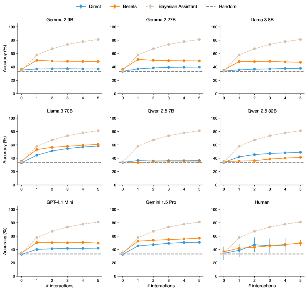<details> <summary>x25.png Details</summary>  ### Visual Description ## Chart Type: Small Multiples Line Chart ### Overview The image presents a small multiples line chart comparing the accuracy of different language models ("Direct", "Beliefs", and "Bayesian Assistant") across varying numbers of interactions (0 to 5). A "Random" baseline is also shown. Each subplot represents a different model (e.g., Gemma 2 9B, Llama 3 70B, Human). ### Components/Axes * **X-axis:** "# interactions" ranging from 0 to 5. * **Y-axis:** "Accuracy (%)" ranging from 0 to 100. * **Legend (top):** * Blue line: "Direct" * Orange line: "Beliefs" * Light Brown dashed line: "Bayesian Assistant" * Gray dashed line: "Random" * **Subplot Titles:** Each subplot is titled with the name of the language model being evaluated (e.g., "Gemma 2 9B", "Llama 3 8B", "Human"). ### Detailed Analysis **General Observations:** * All subplots share the same x and y axis scales. * The "Random" baseline is consistently a horizontal dashed line at approximately 33% accuracy across all subplots. * The "Bayesian Assistant" generally shows the highest accuracy after several interactions, with an upward sloping trend. * "Direct" and "Beliefs" methods show varying performance depending on the model, sometimes remaining relatively flat. **Specific Model Analysis:** * **Gemma 2 9B:** * "Direct" (blue): Stays relatively constant around 40% accuracy. * "Beliefs" (orange): Stays relatively constant around 50% accuracy. * "Bayesian Assistant" (light brown dashed): Increases from approximately 40% to 80% accuracy. * "Random" (gray dashed): Approximately 33% accuracy. * **Gemma 2 27B:** * "Direct" (blue): Stays relatively constant around 40% accuracy. * "Beliefs" (orange): Stays relatively constant around 50% accuracy. * "Bayesian Assistant" (light brown dashed): Increases from approximately 40% to 80% accuracy. * "Random" (gray dashed): Approximately 33% accuracy. * **Llama 3 8B:** * "Direct" (blue): Stays relatively constant around 40% accuracy. * "Beliefs" (orange): Stays relatively constant around 50% accuracy. * "Bayesian Assistant" (light brown dashed): Increases from approximately 40% to 80% accuracy. * "Random" (gray dashed): Approximately 33% accuracy. * **Llama 3 70B:** * "Direct" (blue): Increases from approximately 35% to 60% accuracy. * "Beliefs" (orange): Increases from approximately 40% to 65% accuracy. * "Bayesian Assistant" (light brown dashed): Increases from approximately 40% to 80% accuracy. * "Random" (gray dashed): Approximately 33% accuracy. * **Qwen 2.5 7B:** * "Direct" (blue): Stays relatively constant around 35% accuracy. * "Beliefs" (orange): Stays relatively constant around 35% accuracy. * "Bayesian Assistant" (light brown dashed): Increases from approximately 35% to 80% accuracy. * "Random" (gray dashed): Approximately 33% accuracy. * **Qwen 2.5 32B:** * "Direct" (blue): Increases from approximately 35% to 50% accuracy. * "Beliefs" (orange): Increases from approximately 35% to 40% accuracy. * "Bayesian Assistant" (light brown dashed): Increases from approximately 35% to 80% accuracy. * "Random" (gray dashed): Approximately 33% accuracy. * **GPT-4.1 Mini:** * "Direct" (blue): Increases from approximately 35% to 50% accuracy. * "Beliefs" (orange): Increases from approximately 35% to 55% accuracy. * "Bayesian Assistant" (light brown dashed): Increases from approximately 35% to 80% accuracy. * "Random" (gray dashed): Approximately 33% accuracy. * **Gemini 1.5 Pro:** * "Direct" (blue): Increases from approximately 35% to 50% accuracy. * "Beliefs" (orange): Increases from approximately 35% to 60% accuracy. * "Bayesian Assistant" (light brown dashed): Increases from approximately 35% to 80% accuracy. * "Random" (gray dashed): Approximately 33% accuracy. * **Human:** * "Direct" (blue): Starts at approximately 35% and fluctuates between 40% and 50% accuracy, with error bars indicating variability. * "Beliefs" (orange): Starts at approximately 40% and fluctuates between 45% and 55% accuracy, with error bars indicating variability. * "Bayesian Assistant" (light brown dashed): Increases from approximately 35% to 80% accuracy. * "Random" (gray dashed): Approximately 33% accuracy. ### Key Observations * The "Bayesian Assistant" method consistently outperforms "Direct" and "Beliefs" methods across all language models as the number of interactions increases. * The "Random" baseline provides a consistent lower bound for performance. * The performance of "Direct" and "Beliefs" methods varies depending on the specific language model. * Human performance is relatively stable after the initial interaction, with noticeable variability (error bars). ### Interpretation The data suggests that the "Bayesian Assistant" method is highly effective in improving the accuracy of language models through iterative interactions. This indicates that incorporating Bayesian principles into the interaction process can significantly enhance model performance. The consistent outperformance across different models suggests the robustness of this approach. The relatively flat performance of "Direct" and "Beliefs" in some models indicates that these methods may not be as effective in leveraging interactions for accuracy improvement. The human performance, while showing improvement over the random baseline, exhibits variability, suggesting the inherent complexity and subjectivity in human evaluation. </details> Figure 24: Accuracy over rounds for different original LLMs. We show accuracy based on direct predictions and accuracy based on predictions derived from their beliefs about users’ preferences. Error bars show standard errors across three random seeds (and three training runs). 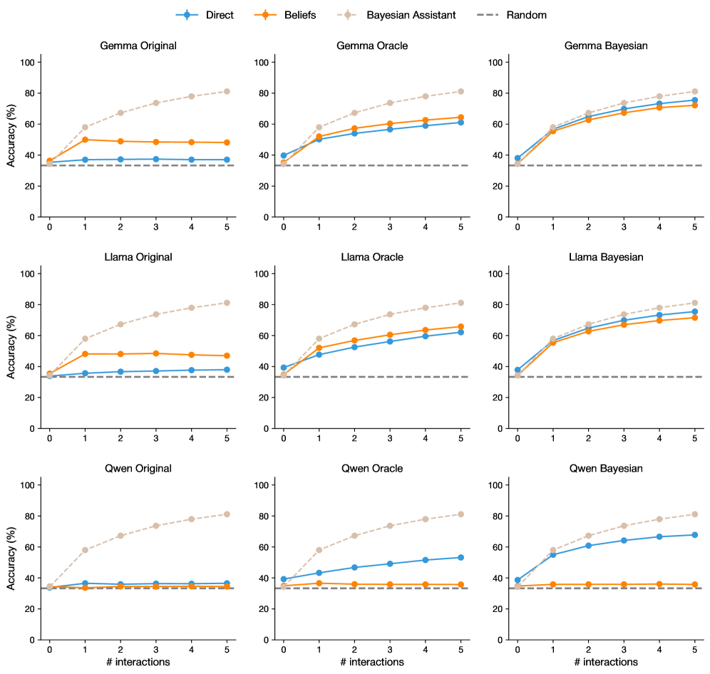<details> <summary>x26.png Details</summary>  ### Visual Description ## Chart Type: Multiple Line Charts ### Overview The image presents a set of nine line charts arranged in a 3x3 grid. Each chart displays the accuracy (%) of different models (Gemma, Llama, Qwen) under various conditions (Original, Oracle, Bayesian) as a function of the number of interactions (0 to 5). The charts compare the performance of "Direct," "Beliefs," and "Bayesian Assistant" methods, with a "Random" baseline indicated by a horizontal dashed line. ### Components/Axes * **X-axis (Horizontal):** "# interactions" ranging from 0 to 5. * **Y-axis (Vertical):** "Accuracy (%)" ranging from 0 to 100. * **Chart Titles (Top Row):** "Gemma Original", "Gemma Oracle", "Gemma Bayesian" * **Chart Titles (Middle Row):** "Llama Original", "Llama Oracle", "Llama Bayesian" * **Chart Titles (Bottom Row):** "Qwen Original", "Qwen Oracle", "Qwen Bayesian" * **Legend (Top):** * Blue line: "Direct" * Orange line: "Beliefs" * Beige dashed line: "Bayesian Assistant" * Gray dashed line: "Random" ### Detailed Analysis **General Observations:** * The "Random" baseline is consistently around 33% accuracy across all charts. * The "Bayesian Assistant" method generally shows the highest accuracy, increasing with the number of interactions. * The "Direct" and "Beliefs" methods show varying performance depending on the model and condition. **Gemma Charts:** * **Gemma Original:** * Direct (Blue): Remains relatively constant around 35-40%. * Beliefs (Orange): Remains relatively constant around 45-50%. * Bayesian Assistant (Beige Dashed): Increases from approximately 40% to 80%. * **Gemma Oracle:** * Direct (Blue): Increases from approximately 40% to 65%. * Beliefs (Orange): Increases from approximately 50% to 70%. * Bayesian Assistant (Beige Dashed): Increases from approximately 60% to 80%. * **Gemma Bayesian:** * Direct (Blue): Increases from approximately 40% to 75%. * Beliefs (Orange): Increases from approximately 50% to 80%. * Bayesian Assistant (Beige Dashed): Increases from approximately 50% to 85%. **Llama Charts:** * **Llama Original:** * Direct (Blue): Remains relatively constant around 35-40%. * Beliefs (Orange): Remains relatively constant around 45-50%. * Bayesian Assistant (Beige Dashed): Increases from approximately 40% to 80%. * **Llama Oracle:** * Direct (Blue): Increases from approximately 45% to 65%. * Beliefs (Orange): Increases from approximately 50% to 70%. * Bayesian Assistant (Beige Dashed): Increases from approximately 60% to 80%. * **Llama Bayesian:** * Direct (Blue): Increases from approximately 40% to 75%. * Beliefs (Orange): Increases from approximately 50% to 80%. * Bayesian Assistant (Beige Dashed): Increases from approximately 50% to 80%. **Qwen Charts:** * **Qwen Original:** * Direct (Blue): Remains relatively constant around 35-40%. * Beliefs (Orange): Remains relatively constant around 35-40%. * Bayesian Assistant (Beige Dashed): Increases from approximately 40% to 80%. * **Qwen Oracle:** * Direct (Blue): Increases from approximately 40% to 55%. * Beliefs (Orange): Remains relatively constant around 40-45%. * Bayesian Assistant (Beige Dashed): Increases from approximately 40% to 80%. * **Qwen Bayesian:** * Direct (Blue): Increases from approximately 40% to 70%. * Beliefs (Orange): Increases from approximately 40% to 75%. * Bayesian Assistant (Beige Dashed): Increases from approximately 40% to 80%. ### Key Observations * The "Bayesian Assistant" method consistently outperforms the "Direct" and "Beliefs" methods, especially as the number of interactions increases. * The "Original" conditions for all models show relatively flat performance for "Direct" and "Beliefs," while "Oracle" and "Bayesian" conditions show improvement with interactions. * The "Random" baseline provides a consistent point of comparison across all charts. * Gemma, Llama, and Qwen models show similar trends, but the specific accuracy levels vary. ### Interpretation The data suggests that incorporating a "Bayesian Assistant" significantly improves the accuracy of these models as the number of interactions increases. The "Oracle" and "Bayesian" conditions, which likely involve some form of feedback or adaptation, allow the "Direct" and "Beliefs" methods to improve over time, unlike the "Original" conditions where their performance remains relatively stagnant. The consistent "Random" baseline highlights the degree to which each method exceeds chance performance. The similarity in trends across Gemma, Llama, and Qwen suggests that the "Bayesian Assistant" approach is generally effective across different model architectures. The specific accuracy levels achieved by each model under different conditions likely reflect the inherent capabilities and limitations of each model. </details> Figure 25: Accuracy over rounds for different original LLMs and fine-tuned LLMs on the flight recommendation task. We show accuracy based on direct predictions and accuracy based on predictions derived from their beliefs about users’ preferences. Error bars show standard errors across three random seeds (and three training runs). 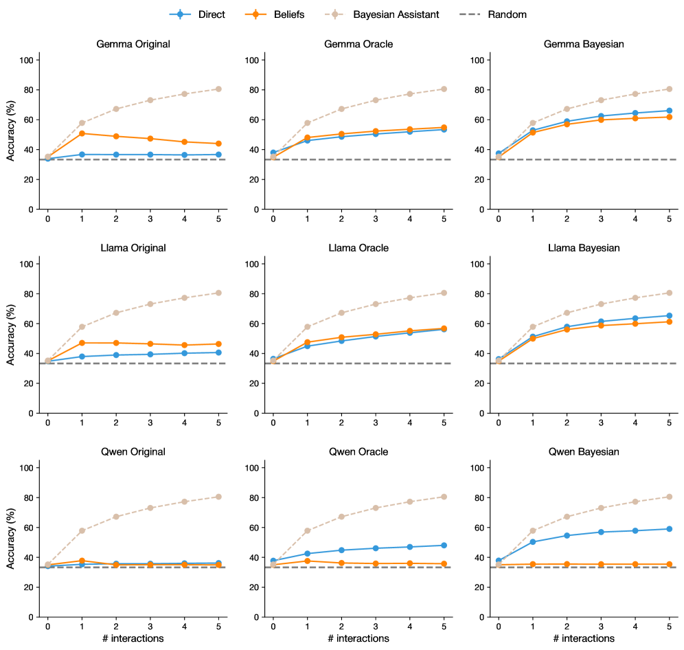<details> <summary>x27.png Details</summary>  ### Visual Description ## Line Charts: Accuracy vs. Interactions for Different Models ### Overview The image presents a series of line charts comparing the accuracy of different language models (Gemma, Llama, Qwen) under various interaction strategies (Direct, Beliefs, Bayesian Assistant, Random). Each row represents a different language model, while each column represents a different interaction strategy. The x-axis represents the number of interactions, and the y-axis represents the accuracy in percentage. ### Components/Axes * **Title:** Accuracy vs. Interactions for Different Models * **X-axis:** "# interactions" with markers at 0, 1, 2, 3, 4, and 5. * **Y-axis:** "Accuracy (%)" with markers at 0, 20, 40, 60, 80, and 100. * **Legend:** Located at the top of the image. * **Direct:** Blue line with circular markers. * **Beliefs:** Orange line with circular markers. * **Bayesian Assistant:** Light brown dashed line with circular markers. * **Random:** Gray dashed line. * **Chart Titles (Top Row):** * Gemma Original (Top-Left) * Gemma Oracle (Top-Center) * Gemma Bayesian (Top-Right) * **Chart Titles (Middle Row):** * Llama Original (Middle-Left) * Llama Oracle (Middle-Center) * Llama Bayesian (Middle-Right) * **Chart Titles (Bottom Row):** * Qwen Original (Bottom-Left) * Qwen Oracle (Bottom-Center) * Qwen Bayesian (Bottom-Right) ### Detailed Analysis **Gemma Models:** * **Gemma Original:** * Direct (Blue): Starts at approximately 35% and decreases slightly to around 33% at 5 interactions. * Beliefs (Orange): Starts at approximately 45% and decreases slightly to around 42% at 5 interactions. * Bayesian Assistant (Light Brown): Starts at approximately 35% and increases to approximately 80% at 5 interactions. * Random (Gray): Constant at approximately 33%. * **Gemma Oracle:** * Direct (Blue): Starts at approximately 35% and increases to approximately 65% at 5 interactions. * Beliefs (Orange): Starts at approximately 45% and increases to approximately 55% at 5 interactions. * Bayesian Assistant (Light Brown): Starts at approximately 35% and increases to approximately 80% at 5 interactions. * Random (Gray): Constant at approximately 33%. * **Gemma Bayesian:** * Direct (Blue): Starts at approximately 45% and increases to approximately 65% at 5 interactions. * Beliefs (Orange): Starts at approximately 50% and increases to approximately 60% at 5 interactions. * Bayesian Assistant (Light Brown): Starts at approximately 45% and increases to approximately 75% at 5 interactions. * Random (Gray): Constant at approximately 33%. **Llama Models:** * **Llama Original:** * Direct (Blue): Starts at approximately 35% and increases slightly to around 40% at 5 interactions. * Beliefs (Orange): Starts at approximately 40% and increases slightly to around 45% at 5 interactions. * Bayesian Assistant (Light Brown): Starts at approximately 35% and increases to approximately 85% at 5 interactions. * Random (Gray): Constant at approximately 33%. * **Llama Oracle:** * Direct (Blue): Starts at approximately 35% and increases to approximately 60% at 5 interactions. * Beliefs (Orange): Starts at approximately 45% and increases to approximately 55% at 5 interactions. * Bayesian Assistant (Light Brown): Starts at approximately 35% and increases to approximately 80% at 5 interactions. * Random (Gray): Constant at approximately 33%. * **Llama Bayesian:** * Direct (Blue): Starts at approximately 45% and increases to approximately 65% at 5 interactions. * Beliefs (Orange): Starts at approximately 50% and increases to approximately 70% at 5 interactions. * Bayesian Assistant (Light Brown): Starts at approximately 45% and increases to approximately 80% at 5 interactions. * Random (Gray): Constant at approximately 33%. **Qwen Models:** * **Qwen Original:** * Direct (Blue): Starts at approximately 35% and increases slightly to around 38% at 5 interactions. * Beliefs (Orange): Starts at approximately 38% and decreases slightly to around 36% at 5 interactions. * Bayesian Assistant (Light Brown): Starts at approximately 35% and increases to approximately 80% at 5 interactions. * Random (Gray): Constant at approximately 33%. * **Qwen Oracle:** * Direct (Blue): Starts at approximately 35% and increases slightly to around 48% at 5 interactions. * Beliefs (Orange): Starts at approximately 38% and increases slightly to around 40% at 5 interactions. * Bayesian Assistant (Light Brown): Starts at approximately 35% and increases to approximately 80% at 5 interactions. * Random (Gray): Constant at approximately 33%. * **Qwen Bayesian:** * Direct (Blue): Starts at approximately 45% and increases slightly to around 50% at 5 interactions. * Beliefs (Orange): Starts at approximately 40% and decreases slightly to around 38% at 5 interactions. * Bayesian Assistant (Light Brown): Starts at approximately 45% and increases to approximately 80% at 5 interactions. * Random (Gray): Constant at approximately 33%. ### Key Observations * The "Bayesian Assistant" strategy (light brown dashed line) consistently shows the most significant improvement in accuracy across all models (Gemma, Llama, Qwen) and configurations (Original, Oracle, Bayesian) as the number of interactions increases. * The "Random" strategy (gray dashed line) remains constant across all models and configurations, serving as a baseline. * The "Direct" and "Beliefs" strategies (blue and orange lines, respectively) show varying degrees of improvement or even slight decreases in accuracy depending on the model and configuration. * The "Oracle" and "Bayesian" configurations generally result in higher accuracy compared to the "Original" configuration for the "Direct" and "Beliefs" strategies. ### Interpretation The data suggests that the "Bayesian Assistant" interaction strategy is highly effective in improving the accuracy of language models as the number of interactions increases. This indicates that incorporating Bayesian methods into the interaction process can significantly enhance the model's performance. The "Random" strategy serves as a control, demonstrating the baseline accuracy without any specific interaction strategy. The varying performance of the "Direct" and "Beliefs" strategies highlights the importance of choosing an appropriate interaction strategy based on the specific language model and configuration. The "Oracle" and "Bayesian" configurations appear to provide additional information or context that aids the model in improving its accuracy, particularly when using the "Direct" and "Beliefs" strategies. </details> Figure 26: Accuracy over rounds for different original LLMs and fine-tuned LLMs on the hotel recommendation task. We show accuracy based on direct predictions and accuracy based on predictions derived from their beliefs about users’ preferences. Error bars show standard errors across three random seeds (and three training runs). 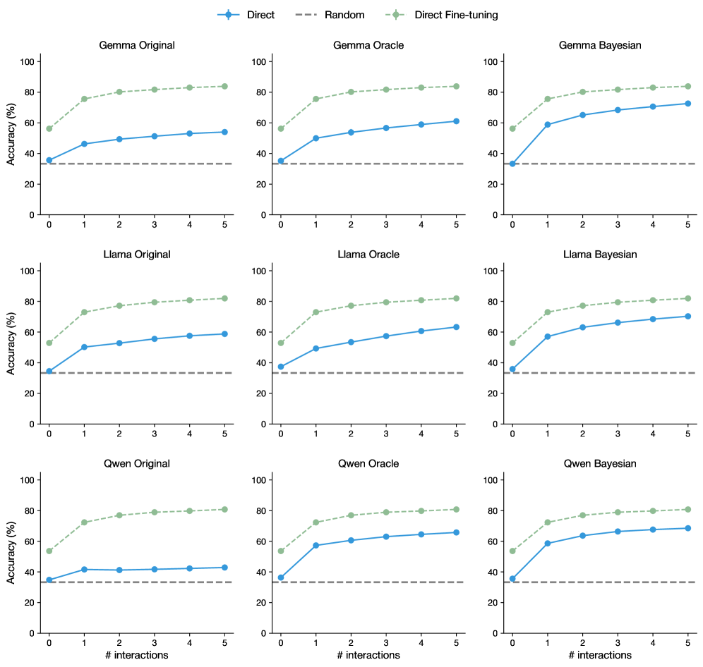<details> <summary>x28.png Details</summary>  ### Visual Description ## Chart: Accuracy vs. Interactions for Different Models ### Overview The image presents a series of line graphs comparing the accuracy of different language models (Gemma, Llama, and Qwen) under three different training/interaction strategies: "Direct", "Random", and "Direct Fine-tuning". Each model has three sub-variants: "Original", "Oracle", and "Bayesian". The graphs show how accuracy changes with an increasing number of interactions. ### Components/Axes * **Title:** Accuracy vs. # interactions * **X-axis:** "# interactions", ranging from 0 to 5. * **Y-axis:** "Accuracy (%)", ranging from 0 to 100. * **Horizontal Dashed Line:** A horizontal dashed line is present at approximately 33% accuracy across all plots. * **Legend:** Located at the top of the image. * **Blue Line (Solid):** "Direct" * **Gray Line (Dashed):** "Random" * **Green Line (Solid, with circle markers):** "Direct Fine-tuning" * **Model Categories:** * Gemma (Original, Oracle, Bayesian) * Llama (Original, Oracle, Bayesian) * Qwen (Original, Oracle, Bayesian) ### Detailed Analysis **Gemma Model Family** * **Gemma Original:** * **Direct (Blue):** Starts at approximately 35% accuracy and increases to around 55% by 5 interactions. * **Random (Gray):** Remains constant at approximately 33% accuracy. * **Direct Fine-tuning (Green):** Starts at approximately 60% accuracy and increases to around 85% by 5 interactions. * **Gemma Oracle:** * **Direct (Blue):** Starts at approximately 35% accuracy and increases to around 60% by 5 interactions. * **Random (Gray):** Remains constant at approximately 33% accuracy. * **Direct Fine-tuning (Green):** Starts at approximately 55% accuracy and increases to around 82% by 5 interactions. * **Gemma Bayesian:** * **Direct (Blue):** Starts at approximately 35% accuracy and increases to around 70% by 5 interactions. * **Random (Gray):** Remains constant at approximately 33% accuracy. * **Direct Fine-tuning (Green):** Starts at approximately 55% accuracy and increases to around 75% by 5 interactions. **Llama Model Family** * **Llama Original:** * **Direct (Blue):** Starts at approximately 35% accuracy and increases to around 58% by 5 interactions. * **Random (Gray):** Remains constant at approximately 33% accuracy. * **Direct Fine-tuning (Green):** Starts at approximately 50% accuracy and increases to around 80% by 5 interactions. * **Llama Oracle:** * **Direct (Blue):** Starts at approximately 35% accuracy and increases to around 65% by 5 interactions. * **Random (Gray):** Remains constant at approximately 33% accuracy. * **Direct Fine-tuning (Green):** Starts at approximately 50% accuracy and increases to around 82% by 5 interactions. * **Llama Bayesian:** * **Direct (Blue):** Starts at approximately 35% accuracy and increases to around 70% by 5 interactions. * **Random (Gray):** Remains constant at approximately 33% accuracy. * **Direct Fine-tuning (Green):** Starts at approximately 50% accuracy and increases to around 75% by 5 interactions. **Qwen Model Family** * **Qwen Original:** * **Direct (Blue):** Starts at approximately 35% accuracy and increases to around 45% by 5 interactions. * **Random (Gray):** Remains constant at approximately 33% accuracy. * **Direct Fine-tuning (Green):** Starts at approximately 55% accuracy and increases to around 80% by 5 interactions. * **Qwen Oracle:** * **Direct (Blue):** Starts at approximately 35% accuracy and increases to around 65% by 5 interactions. * **Random (Gray):** Remains constant at approximately 33% accuracy. * **Direct Fine-tuning (Green):** Starts at approximately 55% accuracy and increases to around 80% by 5 interactions. * **Qwen Bayesian:** * **Direct (Blue):** Starts at approximately 35% accuracy and increases to around 70% by 5 interactions. * **Random (Gray):** Remains constant at approximately 33% accuracy. * **Direct Fine-tuning (Green):** Starts at approximately 55% accuracy and increases to around 82% by 5 interactions. ### Key Observations * **"Random" Strategy:** The "Random" strategy consistently yields a flat accuracy around 33% regardless of the model or number of interactions. * **"Direct" Strategy:** The "Direct" strategy shows a moderate increase in accuracy with more interactions across all models. * **"Direct Fine-tuning" Strategy:** The "Direct Fine-tuning" strategy generally starts with a higher initial accuracy and shows a significant increase with more interactions, outperforming the other two strategies. * **Model Performance:** The "Oracle" and "Bayesian" variants of each model tend to perform better than the "Original" variants, especially with the "Direct" strategy. * **Initial Accuracy:** The "Direct Fine-tuning" strategy consistently starts with a higher initial accuracy compared to the "Direct" strategy. ### Interpretation The data suggests that "Direct Fine-tuning" is the most effective strategy for improving the accuracy of these language models with increasing interactions. The "Random" strategy appears to be ineffective, providing minimal improvement over the baseline. The "Direct" strategy offers some improvement, but not as significant as "Direct Fine-tuning". The "Oracle" and "Bayesian" variants seem to benefit more from the "Direct" strategy compared to the "Original" variants, indicating that these variants may be more adaptable or responsive to direct interactions. The consistent performance of the "Random" strategy around 33% suggests a baseline level of accuracy that is independent of the model or number of interactions, possibly representing a chance level of performance. </details> Figure 27: Accuracy over rounds for different original LLMs and fine-tuned LLMs on the web shopping task. We show accuracy based on direct predictions and accuracy based on predictions derived from their beliefs about users’ preferences. Error bars show standard errors across three training runs if any. Appendix I Example Interactions We show example interactions in Tables 3 – 12. Table 3: Example of a two-round interaction between the user and the LLM. | Col1 | | --- | | User: Help me select the best flights for my trips. I have specific preferences for what I like and dislike in a flight, and these preferences remain the same. You need to figure out my preferences and select the best flights for me. Use your best judgment if you are unsure. Do not say you need more information. Which flight is the best option? Flight 1: departure time: 02:00 PM, duration: 2 hr 30 min, number of stops: 1, price: $370 Flight 2: departure time: 10:00 PM, duration: 4 hr 24 min, number of stops: 0, price: $730 Flight 3: departure time: 03:36 PM, duration: 16 hr 6 min, number of stops: 0, price: $900 Model: The best option is Flight 1. User: Your option Flight 1 is incorrect. I prefer Flight 2. Which flight is the best option? Flight 1: departure time: 04:00 PM, duration: 18 hr 3 min, number of stops: 2, price: $280 Flight 2: departure time: 10:48 AM, duration: 6 hr 21 min, number of stops: 1, price: $370 Flight 3: departure time: 06:48 PM, duration: 10 hr 5 min, number of stops: 1, price: $810 Model: The best option is Flight 2. User: Your option Flight 2 is correct. | Table 4: Example of prompting the LLM for the user’s preference on a single feature. | Col1 | | --- | | User: Help me select the best flights for my trips. I have specific preferences for what I like and dislike in a flight, and these preferences remain the same. You need to figure out my preferences and select the best flights for me. Use your best judgment if you are unsure. Do not say you need more information. Which flight is the best option? Flight 1: departure time: 02:00 PM, duration: 2 hr 30 min, number of stops: 1, price: $370 Flight 2: departure time: 10:00 PM, duration: 4 hr 24 min, number of stops: 0, price: $730 Flight 3: departure time: 03:36 PM, duration: 16 hr 6 min, number of stops: 0, price: $900 Model: The best option is Flight 1. User: Your option Flight 1 is incorrect. I prefer Flight 2. On a scale of 1 to 5, what is my preference for price? - 1: I strongly prefer a cheaper flight - 2: I prefer a cheaper flight - 3: I have no strong preference - 4: I prefer a more expensive flight - 5: I strongly prefer a more expensive flight Model: Your preference for price is: 1. | Table 5: Example of a two-round interaction between the user and the LLM using the numerical representation of flights. | Col1 | | --- | | User: Help me select the best flights for my trips. I have specific preferences for what I like and dislike in a flight, and these preferences remain the same. You need to figure out my preferences and select the best flights for me. Use your best judgment if you are unsure. Do not say you need more information. Which flight is the best option? Flight 1: departure time: 0.7, duration: 0.5, number of stops: 1.0, price: 0.9 Flight 2: departure time: 0.9, duration: 0.6, number of stops: 0.0, price: 0.7 Flight 3: departure time: 0.5, duration: 0.9, number of stops: 0.5, price: 0.1 Model: The best option is Flight 1. User: Your option Flight 1 is incorrect. I prefer Flight 2. Which flight is the best option? Flight 1: departure time: 0.5, duration: 0.9, number of stops: 0.5, price: 0.1 Flight 2: departure time: 0.2, duration: 0.3, number of stops: 0.5, price: 0.2 Flight 3: departure time: 0.8, duration: 0.8, number of stops: 1.0, price: 0.9 Model: The best option is Flight 2. User: Your option Flight 2 is correct. | Table 6: Example of prompting the LLM for the user’s preference on a single feature using the numerical representation of flights. | Col1 | | --- | | User: Help me select the best flights for my trips. I have specific preferences for what I like and dislike in a flight, and these preferences remain the same. You need to figure out my preferences and select the best flights for me. Use your best judgment if you are unsure. Do not say you need more information. Which flight is the best option? Flight 1: departure time: 0.7, duration: 0.5, number of stops: 1.0, price: 0.9 Flight 2: departure time: 0.9, duration: 0.6, number of stops: 0.0, price: 0.7 Flight 3: departure time: 0.5, duration: 0.9, number of stops: 0.5, price: 0.1 Model: The best option is Flight 1. User: Your option Flight 1 is incorrect. I prefer Flight 2. On a scale of 1 to 5, what is my preference for duration? - 1: I strongly prefer the minimum value - 2: I prefer the minimum value - 3: I have no strong preference - 4: I prefer the maximum value - 5: I strongly prefer the maximum value | Table 7: Example of prompting the LLM for the user’s preference on a single feature using the model’s directly generated probability judgements. | Col1 | | --- | | User: Help me select the best flights for my trips. I have specific preferences for what I like and dislike in a flight, and these preferences remain the same. You need to figure out my preferences and select the best flights for me. Use your best judgment if you are unsure. Do not say you need more information. Which flight is the best option? Flight 1: departure time: 02:00 PM, duration: 2 hr 30 min, number of stops: 1, price: $370 Flight 2: departure time: 10:00 PM, duration: 4 hr 24 min, number of stops: 0, price: $730 Flight 3: departure time: 03:36 PM, duration: 16 hr 6 min, number of stops: 0, price: $900 Model: The best option is Flight 1. User: Your option Flight 1 is incorrect. I prefer Flight 2. On a scale of 1 to 5, what is my preference for price? - 1: I strongly prefer a cheaper flight - 2: I prefer a cheaper flight - 3: I have no strong preference - 4: I prefer a more expensive flight - 5: I strongly prefer a more expensive flight Provide an integer between 0 and 100 (%) that reflects the probability of each scale. Format your response exactly as follows: - 1: ??% ... Model: The probabilities of each scale are: - 1: 70% - 2: 10% - 3: 15% - 4: 5% - 5: 0% | Table 8: Example of a first-round interaction between the user and the LLM using chain-of-thought prompting. | Col1 | | --- | | User: Help me select the best flights for my trips. I have specific preferences for what I like and dislike in a flight, and these preferences remain the same. You need to figure out my preferences and select the best flights for me. First, infer my preferences by reasoning about each feature. For each feature, estimate the probability distribution of my preference across a 1-to-5 scale. For example, you might estimate a 30% probability that I strongly prefer an earlier morning flight (scale 1), a 10% probability that I prefer an earlier morning flight (scale 2), a 20% probability that I have no strong preference (scale 3), and so on. Then, use these probabilities to determine the best flights for me. Use your best judgment if you are unsure. Do not say you need more information. Which flight is the best option? Flight 1: departure time: 02:00 PM, duration: 2 hr 30 min, number of stops: 1, price: $370 Flight 2: departure time: 10:00 PM, duration: 4 hr 24 min, number of stops: 0, price: $730 Flight 3: departure time: 03:36 PM, duration: 16 hr 6 min, number of stops: 0, price: $900 Let’s think step by step. End your response with ‘The best option is Flight <your choice>.’. Model: Let’s analyze each flight feature and estimate your preferences: ... <Model’s reasoning chain> ... The best option is Flight 2. User: Your option Flight 2 is correct. | Table 9: Example of a first-round interaction between the user and the LLM with verbalized reward posterior distribution. | Col1 | | --- | | User: Help me select the best flights for my trips. I have specific preferences for what I like and dislike in a flight, and these preferences remain the same. You need to figure out my preferences and select the best flights for me. Use your best judgment if you are unsure. Do not say you need more information. Model: Based on the current information, the probabilities for each preference scale across all features are: The probabilities for each scale of your preference for departure time are: - 1: I strongly prefer an earlier morning departure time, 0.3% - 2: I prefer an earlier morning departure time, 1.0% - 3: I have no strong preference, 97.6% - 4: I prefer a later evening departure time, 1.1% - 5: I strongly prefer a later evening departure time, 0.1% The probabilities for each scale of your preference for duration are: ... User: Which flight is the best option? Flight 1: departure time: 02:00 PM, duration: 2 hr 30 min, number of stops: 1, price: $370 Flight 2: departure time: 10:00 PM, duration: 4 hr 24 min, number of stops: 0, price: $730 Flight 3: departure time: 03:36 PM, duration: 16 hr 6 min, number of stops: 0, price: $900 Model: The best option is Flight 2. User: Your option Flight 2 is incorrect. I prefer Flight 1. Model: Based on the current information, the probabilities for each preference scale across all features are: The probabilities for each scale of your preference for departure time are: - 1: I strongly prefer an earlier morning departure time, 0.1% - 2: I prefer an earlier morning departure time, 4.1% - 3: I have no strong preference, 2.5% - 4: I prefer a later evening departure time, 93.2% - 5: I strongly prefer a later evening departure time, 0.1% | Table 10: Example of a two-round interaction between the user and the LLM using the non-interactive setting. The blue part highlights the difference compared to the interactive setting in Table 3. | Col1 | | --- | | User: Help me select the best flights for my trips. I have specific preferences for what I like and dislike in a flight, and these preferences remain the same. You need to figure out my preferences and select the best flights for me. Use your best judgment if you are unsure. Do not say you need more information. Which flight is the best option? Flight 1: departure time: 02:00 PM, duration: 2 hr 30 min, number of stops: 1, price: $370 Flight 2: departure time: 10:00 PM, duration: 4 hr 24 min, number of stops: 0, price: $730 Flight 3: departure time: 03:36 PM, duration: 16 hr 6 min, number of stops: 0, price: $900 Model: The best option is Flight 2. User: Your option Flight 2 is correct. Which flight is the best option? Flight 1: departure time: 04:00 PM, duration: 18 hr 3 min, number of stops: 2, price: $280 Flight 2: departure time: 10:48 AM, duration: 6 hr 21 min, number of stops: 1, price: $370 Flight 3: departure time: 06:48 PM, duration: 10 hr 5 min, number of stops: 1, price: $810 Model: The best option is Flight 2. User: Your option Flight 2 is correct. | Table 11: Example of a first-round interaction between the user and the LLM on the hotel recommendation task. | Col1 | | --- | | User: Help me select the best hotels for my trips. I have specific preferences for what I like and dislike in a hotel, and these preferences remain the same. You need to figure out my preferences and select the best hotels for me. Use your best judgment if you are unsure. Do not say you need more information. Which hotel is the best option? Hotel 1: distance to downtown: 4 miles, price: $550, rating: 3 stars, amenities: free parking and free breakfast Hotel 2: distance to downtown: 3 miles, price: $820, rating: 2 stars, amenities: free parking, free breakfast, and pool Hotel 3: distance to downtown: 2.3 miles, price: $370, rating: 1 stars, amenities: free parking Model: The best option is Hotel 3. User: Your option Hotel 3 is incorrect. I prefer Hotel 2. | Table 12: Example of a first-round interaction between the user and the LLM on the web shopping task. | Col1 | | --- | | User: Help me select the best product. I have specific preferences for what I like and dislike in a product, and these preferences remain the same. You need to figure out my preferences and select the best products for me. Use your best judgment if you are unsure. Do not say you need more information. Which product is the best option? Product 1: Title: Chic D Independence Day Table Runner 72 Inches Long, Gnome Cotton Linen Spring Table Cloth Runners for Wedding Party Dinning Coffee Holiday, Farmhouse Style, USA Flag Description: - 14x72inch Dining Table Runner Size: 36x183cm, fits round, square or rectangular tables that seat 4 to 8 people. - High Quality Cotton Linen Table Runner: 30%cotton, 70%burlap. triangle hem, wrinkle-free, no fade. easy to maintain and reusable. - Our elegant table runner is perfect for holidays, catering, birthday party, dinning, brunches, potlucks, BBQ’s, buffets, garden, bridal party etc - Decorative Table Runner can be used as decor on kitchen tables; dining tables; entry tables; desks & more - Custom table runner, u also can personalized your tabletop decoration Color: black white Size: 13x108inch Product 2: Title: Ambesonne Orange Mandala Coffee Table, Pastel Colored Flourishes and Dark Toned Details Spring Bloom, Acrylic Glass Center Table with Wooden Frame for Offices Dorms, Small, Peach Dark Brown Cream Description: - Measurements - 24" Long x 18" Wide x 15" High coffee table with patterns that will add vitality to your living room. - Made from - High Quality Beech Wooden Frame and Acrylic Glass Table Top. Durable and Elegant! - Features- Light weight and easy to move around. You can place anywhere and enjoy its beauty! - Easy To Use- It is easy to assembly with numbered parts and clear instructions. - Versatile- Small coffee table, to keep your necessities within reach. Practical item for your living room! Color: blue purple Size: large Product 3: Title: White Round Dining Table and 4 Chairs,Mid-Century Modern Coffee Table Round Kitchen Table Small Office Table for Office Kitchen Dining Room (Round Table+4 Pale Grey Chairs) Description: - Dining Table and Chair Size:The dining table size is 35.4*35.4*29.5 inch, dining chairs is 36*17.5 inch.Our table and chairs suitable for 4-6 people. This glass table can also be used as a conference table, coffee table - Glass Dining Table and Chair Material:The table top is made of clear glass and equipped with solid wood metal legs, with a modern design style and elegant appearance.The Chair is made of velvet and solid wood metal cushions, the dining table and chair is an essential furniture Size: round table with wood legs Model: The best option is Product 3. User: Your option Product 3 is incorrect. I prefer Product 2. |