## REASONING OF LARGE LANGUAGE MODELS OVER KNOWLEDGE GRAPHS WITH SUPER-RELATIONS
Song Wang 1 † , Junhong Lin 2 , Xiaojie Guo 3 , Julian Shun 2 , Jundong Li 1 , Yada Zhu 3
1 University of Virginia, 2 MIT CSAIL, 3 IBM Research
{sw3wv,jundong}@virginia.edu
{junhong,jshun}@mit.edu {xiaojie.guo,yzhu}@ibm.com
## ABSTRACT
While large language models (LLMs) have made significant progress in processing and reasoning over knowledge graphs, current methods suffer from a high nonretrieval rate. This limitation reduces the accuracy of answering questions based on these graphs. Our analysis reveals that the combination of greedy search and forward reasoning is a major contributor to this issue. To overcome these challenges, we introduce the concept of super-relations, which enables both forward and backward reasoning by summarizing and connecting various relational paths within the graph. This holistic approach not only expands the search space, but also significantly improves retrieval efficiency. In this paper, we propose the ReKnoS framework, which aims to Re ason over Kno wledge Graphs with S uper-Relations. Our framework's key advantages include the inclusion of multiple relation paths through super-relations, enhanced forward and backward reasoning capabilities, and increased efficiency in querying LLMs. These enhancements collectively lead to a substantial improvement in the successful retrieval rate and overall reasoning performance. We conduct extensive experiments on nine real-world datasets to evaluate ReKnoS, and the results demonstrate the superior performance of ReKnoS over existing state-of-the-art baselines, with an average accuracy gain of 2.92%.
## 1 INTRODUCTION
Recent advances in large language models (LLMs) have greatly improved their ability to perform reasoning in various natural language processing tasks (Brown et al., 2020; Wei et al., 2022). However, for more complex and knowledge-intensive reasoning tasks, such as open-domain question answering (Gu et al., 2021), the knowledge stored in LLM parameters alone can be insufficient for effectively performing these tasks (Li et al., 2024). To address this limitation, recent research has explored the integration of knowledge graphs (KGs), which represent structured information as entities and relationships, to provide external knowledge that can assist LLMs in answering such questions (Sun et al., 2023; Ma et al., 2024; Xu et al., 2024; Zhang et al., 2022).
Despite this progress, effectively leveraging knowledge graphs for question answering remains challenging due to the vast amount of information in KGs and their complex structures. Existing approaches typically resort to two retrieval strategies: (1) subgraph-based reasoning (Zhang et al., 2022; Jiang et al., 2023d), which retrieves subgraphs containing task-relevant triples from the KG and uses them as input for LLMs; and (2) LLM-based reasoning (Jiang et al., 2023b; Sun et al., 2023), which involves iteratively querying LLMs to select relevant paths within KGs. While subgraphbased reasoning can efficiently retrieve structured knowledge, LLM-based reasoning benefits from the comprehension capabilities of LLMs to precisely select relevant triples, resulting in superior performance compared to subgraph-based methods (Jiang et al., 2024; Pan et al., 2024).
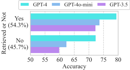
However, even with the advances in LLM-based reasoning methods, there remains a significant performance gap that is often overlooked by existing research. Specifically, current approaches exhibit a substantial non-retrieval rate, indicating that in certain cases, the LLMs fail to find a satisfactory reasoning path within the maximum allowable reasoning length. As demonstrated in Figure 1, for the recent method ToG (Sun et al., 2023) on the prevalent dataset GrailQA (Gu et al., 2021), the accuracy reduces by around 10% when the information is not retrieved from the KG.
∗ † Work done when Song Wang was visiting MIT CSAIL and the MIT-IBM AI Watson Lab.
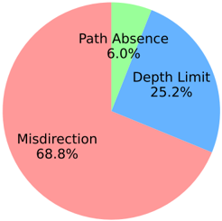
In this paper, we investigate the reasons behind retrieval failures when searching the knowledge graph, identifying two relation patterns that are often overlooked by existing works. As illustrated in Figure 2, the primary causes of non-retrieval can be classified into three categories: (1) Misdirection , where the correct path runs parallel to the retrieved path; (2) Depth Limitation , indicating that the correct path is longer than the retrieved one due to the maximum allowable length being exceeded; and (3) Path Absence , where the correct path does not exist in the knowledge graph. Notably, the first two cases account for the majority
Figure 1: The accuracy (%) of retrieved and nonretrieved samples on the GrailQA dataset.
<details>
<summary>Image 1 Details</summary>
### Visual Description
\n
## Bar Chart: Retrieval Accuracy Comparison of GPT Models
### Overview
This is a horizontal bar chart comparing the accuracy of three GPT models (GPT-4, GPT-4o-mini, and GPT-3.5) based on whether information was retrieved ("Yes" or "No"). The chart displays accuracy on the x-axis and retrieval status on the y-axis.
### Components/Axes
* **X-axis:** "Accuracy" ranging from 50 to 80, with tick marks at 55, 60, 65, 70, 75.
* **Y-axis:** "Retrieved or Not" with two categories: "Yes" and "No".
* **Legend:** Located at the top-left corner, with the following entries:
* GPT-4 (Cyan)
* GPT-4o-mini (Light Blue)
* GPT-3.5 (Lavender/Purple)
* **Data Labels:** Percentage values are displayed next to the "Yes" category bars: (54.3%).
### Detailed Analysis
The chart presents accuracy data for each model under two conditions: "Yes" (information retrieved) and "No" (information not retrieved).
**GPT-4 (Cyan):**
* **Yes:** The bar extends from approximately 72 to 79 on the accuracy scale. Estimated accuracy: 78.5 ± 1.5.
* **No:** The bar extends from approximately 69 to 72 on the accuracy scale. Estimated accuracy: 70.5 ± 1.5.
**GPT-4o-mini (Light Blue):**
* **Yes:** The bar extends from approximately 67 to 74 on the accuracy scale. Estimated accuracy: 70.5 ± 1.5.
* **No:** The bar extends from approximately 60 to 64 on the accuracy scale. Estimated accuracy: 62.0 ± 1.5.
**GPT-3.5 (Lavender/Purple):**
* **Yes:** The bar extends from approximately 67 to 73 on the accuracy scale. Estimated accuracy: 70.0 ± 1.5.
* **No:** The bar extends from approximately 57 to 61 on the accuracy scale. Estimated accuracy: 59.0 ± 1.5.
### Key Observations
* GPT-4 consistently demonstrates the highest accuracy in both "Yes" and "No" retrieval scenarios.
* GPT-4o-mini and GPT-3.5 exhibit similar accuracy levels, with GPT-4o-mini slightly outperforming GPT-3.5 in both scenarios.
* Accuracy is generally higher when information is retrieved ("Yes") compared to when it is not ("No") for all models.
* The overall accuracy difference between the models is more pronounced in the "Yes" scenario.
### Interpretation
The data suggests that GPT-4 is the most accurate model for information retrieval, regardless of whether the information is successfully retrieved or not. GPT-4o-mini offers a performance level between GPT-4 and GPT-3.5. The difference in accuracy between the "Yes" and "No" scenarios indicates that the models are more reliable when information is successfully retrieved, which is expected. The chart highlights the trade-offs between model size/complexity (GPT-4 being the largest) and accuracy. The percentage value (54.3%) next to the "Yes" category bars likely represents the overall proportion of times information was retrieved across all models, providing context for the accuracy scores. This suggests that approximately 54.3% of the time, the models were able to retrieve the requested information. The data implies that the models are more accurate when they *can* find the information, but still have limitations when they cannot.
</details>
of non-retrieval instances. Existing methods struggle with the first case because they may initially select relations that appear promising but are ultimately incorrect. In such cases, once the first step is wrong, subsequent retrieval attempts are unlikely to capture the correct path.
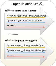
To address the issue of misdirection, we propose a novel framework ReKnoS , which aims to Re ason over Kno wledge Graphs with S uper-Relations. Super-relations are defined as a group of relations within a specific field. For example, the relation 'developer of' and 'designer of' are both under the super-relation 'video\_game', as they are in the same field of video games (shown at the bottom of Figure 3). Using super-relations allows for a more holistic approach by enhancing both the width (the number of relations covered at each step) and depth (the total length of the reasoning path). By integrating super-relations, our framework can introduce additional relational paths that were previously inaccessible, thus expanding the search space and improving retrieval rates. These super-relations effectively summarize and connect disparate parts of the graph, facilitating a more comprehensive exploration of the data. Moreover, with the summarized information within super-relations, we propose to leverage it to achieve forward reasoning and backward reasoning, which aim at exploring future paths and previous alternative paths, respectively. With the design of super-relations, our framework can represent multiple relation paths with a
Figure 2: The non-retrieval cases on the GrailQA dataset with baseline ToG (Sun et al., 2023) (maximum length of 3).
<details>
<summary>Image 2 Details</summary>
### Visual Description
\n
## Pie Chart: Distribution of Navigation Errors
### Overview
The image is a pie chart illustrating the distribution of different types of navigation errors. The chart is divided into three segments, each representing a specific error type and its corresponding percentage of the total.
### Components/Axes
The chart does not have traditional axes. It is a circular representation where the entire circle represents 100% of the navigation errors. The segments are labeled with the error type and percentage. The legend is embedded directly within the chart, with each segment labeled.
### Detailed Analysis
The pie chart shows the following distribution of navigation errors:
* **Misdirection:** This segment occupies the largest portion of the pie chart, representing approximately 68.8% of the total navigation errors. It is colored in a shade of red.
* **Depth Limit:** This segment represents 25.2% of the total errors. It is colored in a shade of blue.
* **Path Absence:** This segment is the smallest, representing 6.0% of the total errors. It is colored in a shade of green.
The percentages sum to 100% (68.8% + 25.2% + 6.0% = 100.0%).
### Key Observations
The most significant observation is the dominance of "Misdirection" as the primary cause of navigation errors, accounting for over two-thirds of all errors. "Depth Limit" is the second most frequent error, while "Path Absence" is relatively rare.
### Interpretation
The data suggests that the primary challenge in navigation is not a lack of a path ("Path Absence") or reaching a maximum depth ("Depth Limit"), but rather being led astray ("Misdirection"). This could indicate issues with the clarity of directions, misleading signage, or inaccurate mapping. The relatively low percentage of "Path Absence" suggests that paths are generally available, but the problem lies in guiding users along the correct path. The "Depth Limit" error could be related to limitations in the navigation system or the environment itself. Further investigation into the causes of "Misdirection" would likely yield the most significant improvements in navigation accuracy and user experience.
</details>
super-relation during reasoning. As such, we do not need to abandon a large number of paths during reasoning, thus significantly increasing the search space and improving the retrieval rate.
The contributions of this paper are as follows:
- Design: The use of super-relations, defined as groups of relations within a specific field, enables the inclusion of a large number of relations for efficient reasoning over knowledge graphs. Moreover, super-relations can both enhance the depth and width of various reasoning paths to deal with non-retrieval.
- Framework: We propose a novel reasoning framework ReKnoS that integrates super-relations, enabling the representation of multiple relation paths simultaneously. This approach allows for a significant expansion of the search space by incorporating diverse relational paths without discarding potentially valuable connections during reasoning. Our code is provided at https://github.com/SongW-SW/REKNOS.
- Experiments and Results: We perform experiments on nine real-world datasets and show that our approach significantly outperforms traditional reasoning methods in both retrieval success rate and search space size, improving them by an average of 25% and 87%, respectively. These results highlight the effectiveness of our design choices in addressing complex knowledge graph reasoning tasks.
## 2 RELATED WORK
Although LLMs have exhibited expressive capabilities in various natural language process tasks, such as question answering tasks (Wei et al., 2022; Wang et al., 2023), they can lack up-to-date or domainspecific knowledge (Wang et al., 2023; Jiang et al., 2023b). Recently, researchers have proposed using knowledge graphs (KGs), which provide up-to-date and structured domain-specific information, to enhance the performance of LLMs (Pan et al., 2024). As a classic example, retrieval-augmented generation (RAG) methods have been widely used to incorporate external knowledge sources as additional input to LLMs (Jiang et al., 2023e). Nevertheless, the complex structures in KGs render such retrieval more difficult and may involve unnecessary noise (Petroni et al., 2021).
Knowledge graph question answering (KGQA) focuses on answering natural language questions using structured facts from knowledge graphs (Pan et al., 2024). A central challenge lies in efficiently retrieving relevant knowledge and applying it to derive accurate answers. Recent approaches to KGQA can be divided into two main categories: (1) subgraph-based reasoning and (2) LLM-based reasoning. Subgraph-based methods, such as SR (Zhang et al., 2022), UniKGQA (Jiang et al., 2023d), and ReasoningLM (Jiang et al., 2023c), perform reasoning over retrieved subgraphs that contain task-related fact triples from the KG. However, these methods are highly dependent on the quality of the retrieved subgraphs, which may contain irrelevant information and struggle to generalize to other structures within the KG. More recently, researchers have turned to LLMs to enhance reasoning on KGs. As an early effort, StructGPT (Jiang et al., 2023b) leverages LLMs to generate executable SQL queries to reason on structured data, including databases and KGs. Think-on-Graph (ToG) (Sun et al., 2023) extends this by using LLMs to select relevant relations and entities for retrieving target answers. KG-Agent (Jiang et al., 2024) further advances this line of work by incorporating a multifunctional toolbox that dynamically selects tools to explore and reason over KGs.
## 3 PRELIMINARIES
## 3.1 KNOWLEDGE GRAPH (KG)
A knowledge graph is composed of a large set of fact triples, represented as G = {⟨ e, r, e ′ ⟩ | e, e ′ ∈ E,r ∈ R } , where E and R denote the sets of entities and relations, respectively. Each triple ⟨ e, r, e ′ ⟩ captures a factual relationship, indicating that a relation r exists between a head entity e and a tail entity e ′ . For the KGQA task studied in this work, we assume the availability of a KG that contains the entities relevant to answering the given natural language question. Our goal is to design an LLM-based framework capable of performing reasoning on the KG to retrieve the answer to the question.
## 3.2 SUPER-RELATIONS
In this paper, we introduce the concept of a super-relation to efficiently gather information from a set of more granular, detailed relations. For instance, consider a super-relation " music.featured\_artist ," which encompasses a variety of specific relations, such as " music.featured\_artist.recordings ." Iterating over each of these detailed relations can be computationally intensive. By using a higher-level super-relation like " music.featured\_artist ," we abstract and group these related relations together, allowing us to query LLMs using a single, more general relation. This abstraction reduces the complexity of handling numerous fine-grained relations while preserving the relevant information needed for reasoning. In the prevalent knowledge graph Wikidata (Vrandeˇ ci´ c & Krötzsch, 2014) that we use in this paper, relations are typically organized into a three-level hierarchy, such as "music," "featured\_artist," and "recordings." We treat the second-level relations as super-relations, which serve as a representative for related third-level relations. However, it is important to note that not all KGs are structured with such
Figure 3: An example of various super-relations R included in a super-relation set S .
<details>
<summary>Image 3 Details</summary>
### Visual Description
\n
## Diagram: Super-Relation Set Si
### Overview
The image is a diagram illustrating a "Super-Relation Set Si". It depicts two distinct relation sets, each with associated tuples, and arrows indicating a mapping or relationship between them. The diagram appears to be a conceptual representation of data relationships, likely within a database or knowledge graph context.
### Components/Axes
The diagram consists of the following components:
* **Title:** "Super-Relation Set Si" – positioned at the top-center.
* **Relation Sets:** Two rectangular blocks, one at the top and one at the bottom, representing individual relation sets.
* **Relation Labels:** Each relation set has a label of the form "R<sup>(i)</sup> = [relation name]".
* **Tuple Labels:** Within each relation set, there are labels of the form "τ<sub>i</sub> = [tuple name]".
* **Arrows:** Grey arrows with colored lines (red and blue) emanating from each relation set, indicating relationships or mappings.
* **Ellipsis:** "..." symbols indicating that there are more tuples than shown.
### Detailed Analysis or Content Details
**First Relation Set (Top):**
* **Relation Label:** R<sup>(1)</sup> = music.featured\_artist
* **Tuples:**
* τ<sub>1</sub> = music.featured\_artist.recordings (represented by a yellow line)
* τ<sub>2</sub> = music.featured\_artist.albums (represented by a blue line)
* **Arrows:** Two arrows point to the right. The first is yellow, and the second is blue.
**Second Relation Set (Bottom):**
* **Relation Label:** R<sup>(8)</sup> = computer.videogame
* **Tuples:**
* τ<sub>1</sub> = computer.videogame.designer (represented by a yellow line)
* τ<sub>2</sub> = computer.videogame.developer (represented by a blue line)
* **Arrows:** Two arrows point to the right. The first is yellow, and the second is blue.
The diagram also includes a grey background and rounded corners for the relation set blocks.
### Key Observations
* The diagram presents a consistent structure for each relation set: a relation label followed by a set of tuples.
* Each tuple is associated with a specific color (yellow or blue), which is maintained in the corresponding arrow.
* The use of superscripts (e.g., R<sup>(1)</sup>, R<sup>(8)</sup>) suggests that these are instances within a larger set of relation sets.
* The ellipsis indicates that the shown tuples are not exhaustive.
* The diagram does not contain any numerical data or quantitative measurements.
### Interpretation
The diagram illustrates a concept of "Super-Relation Sets" where each set represents a relationship between entities. The relation sets are defined by a relation name (e.g., "music.featured\_artist") and a set of tuples that specify the attributes or properties of that relationship. The arrows suggest a mapping or association between the tuples and some other entity or set of entities.
The use of different colors for the tuples and arrows could indicate different types of relationships or attributes within each relation set. For example, yellow might represent a "has-a" relationship, while blue might represent an "is-a" relationship.
The diagram is a high-level conceptual representation and does not provide specific details about the underlying data or the nature of the mappings. It serves to illustrate the structure and organization of the Super-Relation Set Si. The diagram suggests a database or knowledge graph structure where entities are related through various attributes and properties. The numbered relation sets (1 and 8) imply a larger collection of such sets, forming a comprehensive representation of interconnected data.
</details>
clear hierarchical levels. In cases where a KG lacks this inherent structure, an alternative approach
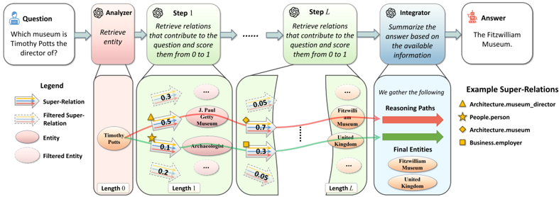
Figure 4: Overall ReKnoS framework. The LLM first extracts the query entity from the input question and then performs up to L steps of reasoning. In each step, the LLM retrieves several super-relations and scores them. Only the selected candidates will be used for further reasoning. Finally, the LLM gathers the reasoning paths and final entities to generate the final answer.
<details>
<summary>Image 4 Details</summary>
### Visual Description
## Diagram: Knowledge Graph Reasoning Process
### Overview
This diagram illustrates a multi-step process for answering a question using a knowledge graph. The process involves an Analyzer, multiple Reasoning Steps (Step 1 to Step L), an Integrator, and ultimately provides an Answer. The diagram visually represents the flow of information and relationships between entities within the knowledge graph.
### Components/Axes
The diagram is structured horizontally, representing a sequential process. Key components include:
* **Question:** "Which museum is Timothy Potts the director of?" (Top-left, within a speech bubble)
* **Analyzer:** A box labeled "Analyzer" with the text "Retrieve relations that contribute to the entity question and score them from 0 to 1".
* **Step 1 to Step L:** Multiple boxes labeled "Step 1" through "Step L", each containing a knowledge graph fragment and the text "Retrieve relations that contribute to the question and score them from 0 to 1".
* **Integrator:** A box labeled "Integrator" with the text "Summarize the answer based on the available information".
* **Answer:** "The Fitzwilliam Museum." (Top-right, within a speech bubble)
* **Legend:** Located on the bottom-left, defining the visual representation of relationships and entities.
* Orange Arrow: Super-Relation
* Light Blue Arrow: Filtered Super-Relation
* Light Green Circle: Entity
* Light Blue Circle: Filtered Entity
* **Example Super-Relations:** Located on the bottom-right, defining the color-coding for relation types.
* Yellow Triangle: Architecture.museum.director
* Red Circle: People.person
* Green Rectangle: Architecture.museum
* Blue Square: Business.employer
* **Entities:** Timothy Potts, J. Paul Getty Museum, Archaeologist, Fitzwilliam Museum, United Kingdom.
* **Reasoning Paths:** Text block stating "We gather the following Reasoning Paths".
* **Final Entities:** Fitzwilliam Museum, United Kingdom.
### Detailed Analysis or Content Details
The diagram shows the progression of reasoning through the knowledge graph.
**Step 1:**
* Timothy Potts (Entity, Light Green Circle) is connected to J. Paul Getty Museum (Entity, Light Green Circle) via a Super-Relation (Orange Arrow) with a score of 0.4.
* Timothy Potts is connected to Archaeologist (Entity, Light Green Circle) via a Super-Relation with a score of 0.1.
* Archaeologist is connected to J. Paul Getty Museum via a Super-Relation with a score of 0.2.
* Length 1 is indicated below this step.
**Step L:**
* Fitzwilliam Museum (Entity, Light Green Circle) is connected to United Kingdom (Entity, Light Green Circle) via a Super-Relation (Orange Arrow) with a score of 0.7.
* Fitzwilliam Museum is connected to an unnamed entity (Entity, Light Green Circle) via a Super-Relation with a score of 0.05.
* Length L is indicated below this step.
The connections between entities are represented by arrows with associated numerical scores (between 0 and 1). The arrows indicate the strength or relevance of the relationship. Filtered Super-Relations (Light Blue Arrows) are also present, but their specific connections are not clearly defined in the visible portion of the diagram.
### Key Observations
* The diagram demonstrates a process of iteratively refining relationships between entities to arrive at an answer.
* The scores associated with the relationships suggest varying degrees of confidence or relevance.
* The diagram highlights the importance of multiple reasoning steps (Step 1 to Step L) in complex knowledge graph queries.
* The final answer, "The Fitzwilliam Museum," is derived from the accumulated evidence gathered through the reasoning steps.
### Interpretation
The diagram illustrates a knowledge graph-based question answering system. The system begins with a natural language question and transforms it into a series of graph traversals. Each step refines the search by retrieving relevant relationships and scoring them based on their contribution to the answer. The Integrator component then synthesizes the information from all steps to provide a final answer. The use of scores suggests a probabilistic or weighted approach to reasoning, where stronger relationships contribute more to the final result. The diagram emphasizes the importance of representing knowledge as a graph and leveraging graph algorithms for complex reasoning tasks. The example super-relations provide a taxonomy of the types of relationships stored within the knowledge graph. The diagram does not provide any quantitative data about the performance of the system, but it visually conveys the underlying logic and flow of information.
</details>
involves clustering relations based on their semantic similarity and using the cluster centers as super-relations. These cluster centers must be textually coherent and meaningful to ensure they can effectively summarize the detailed relations within each cluster. In our experiments, we directly utilize the hierarchical levels.
We formally define a super-relation R as a group of more granular, detailed relations R = { r 1 , r 2 , . . . , r n } , where each r i is a specific relation on the knowledge graph. Examples are shown Figure 3. For example, if R is the super-relation "music.featured\_artist," it might include a set of relations such as R = { "music.featured\_artist.recordings" , "music.featured\_artist.albums" , . . . } .
## 3.3 SUPER-RELATION SEARCH PATHS
We first define a super-relation connection between two super-relations.
Definition 1. Super-Relation Connection. Let R 1 and R 2 be two super-relations, each consisting of multiple relations. We define R 1 → R 2 (i.e., R 1 connects to R 2 ) if and only if there exist entities e 1 , e 2 , and e 3 such that e 1 r 1 - → e 2 r 2 - → e 3 , where r 1 ∈ R 1 and r 2 ∈ R 2 .
In this manner, based on connections between super-relations, we define a super-relation path and then define a super-relation search path, where each position in the path consists of multiple super-relations.
Definition 2. Super-Relation Path. A super-relation path P = ( R 1 → R 2 → . . . → R l ) of length l consist of l super-relations that are consecutively connected.
Definition 3. Super-Relation Search Path. A super-relation search path Q l of length l consists of l super-relation sets, i.e., Q l = {S 1 , S 2 , . . . , S l } . Here S i = { R (1) i , R (2) i , . . . , R ( |S i | ) i } is a superrelation set at the i -th position in Q l . Moreover, in each super-relation set S i , there exists at least one super-relation that is connected to a super-relation in the subsequent set S i +1 , i.e.,
<!-- formula-not-decoded -->
## 4 SUPER-RELATION REASONING
Our ReKnoS framework consists of at most L reasoning steps, which is also the maximum length of search paths considered. During each reasoning step, we aim to retrieve a set of N important superrelations that are the most semantically related to the query based on the selected super-relations from previous reasoning steps. In other words, at the beginning of the l -th reasoning step, the search path Q l -1 = {S 1 , S 2 , . . . , S l -1 } is of length l -1 , i.e., containing l -1 sets of important super-relations. These super-relation sets are consecutively connected according to Definition 3, i.e., ∀ R ∈ S i , ∃ R ′ ∈ S i +1 such that R → R ′ . Our goal in this reasoning step is to select an important set of N super-relations in S l , while satisfying the condition that ∀ R ∈ S l , ∃ R ′ ∈ S l +1 such that R → R ′ . Moreover, |S i | = N for i = 1 , 2 , . . . , l . At the end of each reasoning step, the LLM will be
asked to decide whether to extract the answer from the entities or to proceed to the next reasoning step. The overall framework is illustrated in Figure 4.
## 4.1 CANDIDATE SELECTION
To select the current S l , we first need to extract any candidate super-relation R ′ that satisfies the connection requirement: ∀ R ∈ S l -1 , ∃ R ′ ∈ S l such that R → R ′ . This means that R ′ is connected by any super-relation in the last super-relation set S l -1 . Therefore, we can represent the set of candidate super-relations C l as
$$\mathcal { C } _ { l } = \{ R | \exists R ^ { \prime } \in \mathcal { S } _ { l - 1 } s u c h t h a t R ^ { \prime } \to R \} ,$$
where S l -1 is the previous super-relation set in the search path Q l -1 . This approach obtains all super-relations directly connected to the search path. As the connections are generally becoming larger as the search proceeds, it is likely that |C l | > |S l -1 | = N for l ≥ 2 . Therefore, we need to perform reasoning to filter out irrelevant super-relations in C l to obtain S l ⊆ C l .
## 4.2 SCORING
In the scoring step, we use an LLM to assign a score for each of the super-relations in C l . The scores are denoted as { s 1 l , s 2 l , . . . , s l M } , where M = |C l | . Note that this step is only needed if M > N . Based on these scores, we aim to select N super-relations with the largest scores. The scores are obtained as follows:
$$\{ s _ { l } ^ { 1 } , s _ { l } ^ { 2 } , \dots , s _ { l } ^ { M } \} = L L M ( \{ R _ { C } ^ { 1 } , R _ { C } ^ { 2 } , \dots , R _ { C } ^ { M } \} ) , w h e r e R _ { C } ^ { i } \in \mathcal { C } _ { l } , i = 1 , 2 , \dots , M .$$
The prompt to the LLM is as follows, setting N = 3 as an example:
You need to select three relations from the following candidate relations, which are the most helpful for answering the question.
```
```
Note that in the prompt, we do not explicitly inform the LLM about the super-relations in order to reduce unnecessary complexity. Following ToG, we use a human-crafted example as additional input to LLMs to guide the scoring process. Based on these scores, we select the N super-relations from C l with the highest scores. We first sort the scores in descending order:
<!-- formula-not-decoded -->
where s ( i ) l is the i -th largest score, and the corresponding super-relation is denoted as R ( i ) l .
The N selected super-relations are denoted as follows:
<!-- formula-not-decoded -->
Then, we normalize the scores of the selected super-relations so that they sum to 1 :
<!-- formula-not-decoded -->
In this way, we ensure that only the most relevant super-relations with the highest scores are considered in the next iteration, and their influence is appropriately scaled through normalization. The normalized scores { s (1) l , s (2) l , . . . , s ( N ) l } will be later used for relevant path selection in the reasoning process.
## 4.3 SCORE-BASED ENTITY EXTRACTION SELECTION
Now we have obtained the selected super-relation search path of length l , i.e., Q l = {S 1 , S 2 , . . . , S l } . Here, each super-relation set S i consists of N super-relations, i.e., S i = { R (1) i , R (2) i , . . . , R ( N ) i } .
Moreover, each super-relation R ( j ) i is associated with a score assigned during the scoring step, denoted as s ( j ) i . At this point, we need to either use the retrieved super-relations to answer the question or proceed to further increase the length of the super-relation search path.
To find the potential answers and also provide sufficient information for the LLM to decide whether to continue retrieving the super-relation search path, we propose to extract the entities at the end of Q l , i.e., entities connected by super-relations at the last step of that path. These entities will be used to prompt the LLM to decide whether the retrieved entities are sufficient for answering the query. If the LLM responds that these entities are sufficient for answering the query, we will further prompt it for the answer. On the other hand, if the LLM suggests further exploring the reasoning, we will repeat the steps described above to retrieve a longer super-relation search path Q l +1 . When l = L , we will always ask the LLM for the answer.
Super-Relation Path Selection. Due to the large number of entities connected by super-relations in Q l , we first identify K most relevant super-relation paths from Q l . Particularly, we represent a super-relation path P i derived from Q l as follows:
<!-- formula-not-decoded -->
Here, k i,j ∈ [1 , |S j | ] represents the index of the specific super-relation in the j -th position of the i -th path, such that R ( k i,j ) j ∈ S j . The set of all possible super-relation paths is denoted as P = { P 1 , P 2 , . . . , P |P| } . Notably, the number of possible super-relation paths, i.e., |P| , may vary depending on the connectivity across different super-relation sets in P l . However, P contains at least one super-relation path, i.e., |P| ≥ 1 according to the following theorem.
Theorem 4.1. A super-relation search path leads to at least one super-relation path. Given a selected super-relation search path of length l, Q l = {S 1 , S 2 , . . . , S l } , there exists at least one super-relation path of length l , i.e., P = ( R ( k 1 ) 1 → R ( k 2 ) 2 → . . . → R ( k l ) l ) , where R ( k j ) j ∈ S j and k j represents k i,j for a fixed i .
Intuitively, this theorem holds because consecutive super-relation sets, i.e., S i and S i +1 , are connected, and thus at least one super-relation in each of them is connected to each other according to Definition 3. Therefore, the consecutively connected super-relations form a super-relation path. The proof is provided in Appendix A. To select the super-relation paths that are more relevant to the input query, we propose to sum the scores of the l super-relations in each super-relation path. Specifically, for the i -th super-relation path P i = ( R ( k i, 1 ) 1 → R ( k i, 2 ) 2 → . . . → R ( k i,l ) l ) , the total score is computed as
<!-- formula-not-decoded -->
With the summed scores for these super-relation paths, we select the K super-relation paths with the largest scores. The final selected super-relation paths are as follows:
$$\mathcal { P } ^ { * } = \underset { \mathcal { P } _ { f } \subseteq P \, \colon \, | P _ { f } | \leq K } { \arg \max } \sum _ { P \in \mathcal { P } _ { f } } S c o r e ( P ) .$$
Final Entity Selection. With the relevant super-relation paths, our final goal is to extract the entities at the end of each reasoning path in P ∗ . We first introduce the following theorem for selecting specific relation paths from super-relation paths.
Theorem 4.2. For any super-relation path P = ( R ( k 1 ) 1 → R ( k 2 ) 2 → . . . → R ( k l ) l ) , there exists at least one corresponding KG reasoning path of length l , represented as e 1 r 1 - → e 2 r 2 - → · · · r l - → e l +1 , where r i ∈ R ( k i ) i is a relation chosen from the super-relation R ( k i ) i , and e 1 , e 2 , . . . , e l +1 are entities in the knowledge graph.
This theorem holds because in a super-relation path, according to Definition 2, two consecutive superrelations are connected, which leads to the connection of two relations. Therefore, the consecutively connected relations will form a relation path. The proof is provided in Appendix B. According to the
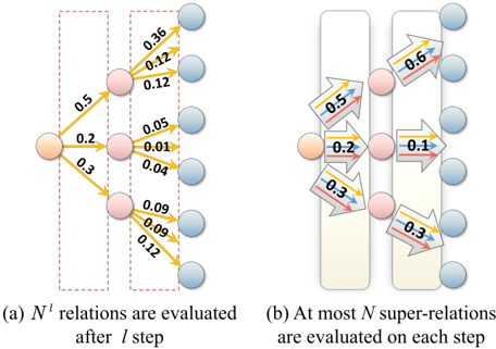
Figure 5: Number of relations need to score by the LLM in (a) the baseline ToG (Sun et al., 2023) and (b) our framework ReKnoS. The numbers on the arrows represent LLM evaluated scores and correspond to LLM computations. For clarity, we omit some of the blue nodes.
<details>
<summary>Image 5 Details</summary>
### Visual Description
## Diagram: Relation Evaluation Steps
### Overview
The image presents a comparative diagram illustrating two different approaches to relation evaluation, labeled (a) and (b). Diagram (a) shows a process where *N'* relations are evaluated after each step, while diagram (b) depicts a process evaluating at most *N* super-relations on each step. Both diagrams use node-and-arrow representations to visualize relationships and associated weights.
### Components/Axes
The diagrams consist of nodes (circles) connected by directed arrows. The arrows are labeled with numerical values representing the strength or weight of the relationship. Each diagram is enclosed in a dashed or solid rectangle, indicating the scope of evaluation. Below each diagram is a textual description of the process.
### Detailed Analysis or Content Details
**Diagram (a): N' relations are evaluated after / step**
* **Nodes:** There are 8 nodes arranged in a roughly hierarchical structure. The top node is orange, the second layer has 3 nodes (one orange, two light blue), and the bottom layer has 4 light blue nodes.
* **Arrows & Weights:**
* From the orange top node to the first light blue node: 0.5
* From the orange top node to the second light blue node: 0.2
* From the orange top node to the third light blue node: 0.3
* From the first light blue node to the first bottom node: 0.36
* From the first light blue node to the second bottom node: 0.12
* From the first light blue node to the third bottom node: 0.12
* From the second light blue node to the first bottom node: 0.05
* From the second light blue node to the second bottom node: 0.01
* From the second light blue node to the fourth bottom node: 0.04
* From the third light blue node to the third bottom node: 0.09
* From the third light blue node to the fourth bottom node: 0.09
* From the third light blue node to the first bottom node: 0.12
**Diagram (b): At most N super-relations are evaluated on each step**
* **Nodes:** There are 8 nodes arranged in two vertical columns of 4 nodes each. The top node in the left column is orange, the remaining nodes are light blue.
* **Arrows & Weights:**
* From the orange top node to the first light blue node: 0.5
* From the orange top node to the second light blue node: 0.2
* From the first light blue node to the first light blue node in the right column: 0.1
* From the second light blue node to the second light blue node in the right column: 0.3
* From the second light blue node to the third light blue node in the right column: 0.3
* From the third light blue node to the fourth light blue node in the right column: 0.6
### Key Observations
* Diagram (a) shows a branching structure where a single source node connects to multiple destination nodes, which then connect to further nodes. The weights are relatively small, and distributed across multiple paths.
* Diagram (b) shows a more streamlined structure with fewer connections. The weights are generally higher than in diagram (a).
* The text below each diagram indicates a difference in the number of relations evaluated per step. Diagram (a) evaluates *N'* relations, while diagram (b) evaluates at most *N* super-relations.
### Interpretation
The diagrams illustrate two different strategies for evaluating relationships within a network. Diagram (a) represents a more exhaustive, potentially slower approach, evaluating a larger number of individual relations (*N'*) at each step. This could be useful for identifying subtle or weak connections. Diagram (b) represents a more focused, potentially faster approach, evaluating a smaller number of stronger, "super-relations" (*N*) at each step. This could be useful for quickly identifying the most important connections.
The use of weights on the arrows suggests that the relationships are not all equal in strength. The differences in the network structure and the number of relations evaluated per step likely reflect trade-offs between accuracy, speed, and computational cost. The diagrams are likely used to compare the efficiency of different algorithms or methods for relation extraction or knowledge graph construction. The use of orange nodes may indicate a starting point or a key entity in the network.
</details>
theorem, we know that the selected super-relation path P consists of at least one valid relation path in the knowledge graph. Therefore, this relation path can be used to extract entities that contribute to answering the query.
In Figure 5, we show that for the baseline ToG, the number of LLM calls grows exponentially as l increases. However, for our framework ReKnoS, the required LLM calls at each step remain constant, indicating the efficiency of our framework. However, one challenge remains-there is a large number of entities covered by these super-relations, which can make it difficult to find the relevant ones. We describe how to address this issue below.
With these super-relation paths in P ∗ , we aim to extract the entities that satisfy the connection property of these relations. The entity set for the entire super-relation path P = ( R ( k 1 ) 1 → R ( k 2 ) 2 → . . . → R ( k l ) l ) can be expressed as
$$E _ { l } ^ { ( k _ { l } ) } = \{ e | \exists r _ { 1 } \in R _ { 1 } ^ { ( k _ { 1 } ) } , r _ { 2 } \in R _ { 2 } ^ { ( k _ { 2 } ) } , \dots , r _ { l } \in R _ { l } ^ { ( k _ { l } ) } , s u c h t a t e _ { 1 } \xrightarrow { r _ { 1 } } e _ { 2 } \xrightarrow { r _ { 2 } } \cdots \xrightarrow { r _ { l } } e \} .$$
This set E ( k l ) l contains all of the final entities that satisfy the super-relation path P . Note that although each super-relation in P can contain multiple relations, the size of E ( k l ) l should be much smaller than P ∗ , as it requires l entities on the super-relation path to be consecutively connected, which is a stricter requirement than having l super-relations consecutively connected (see Definition 1).
We use the obtained entity set E ( k l ) l along with the super-relations in P to query the LLM regarding the next step. The LLM will either output an inferred answer from E ( k l ) l or decide to continue the process by proceeding to the subsequent super-relations, i.e., repeating the process starting from Section 4.1 and increasing the super-relation path length l by 1 . Notably, when l = L , we will always ask the LLM for the answer.
## 5 EXPERIMENTS
Baselines. For baselines, we compare ReKnoS with several methods, including standard prompting (IO prompt) (Brown et al., 2020), Chain-of-Thought prompting (CoT prompt) (Wei et al., 2022), and Self-Consistency (Wang et al., 2023). Additionally, we include previous state-of-the-art (SOTA) approaches tailored for reasoning on knowledge graphs: StructGPT (Jiang et al., 2023b), Think-onGraph (ToG) (Sun et al., 2023), and KG-Agent (Jiang et al., 2024).
Datasets. To evaluate the performance of our framework on multi-hop knowledge-intensive reasoning tasks, we conduct tests using four KBQA datasets: CWQ (Talmor & Berant, 2018), WebQSP (Yih et al., 2016), GrailQA (Gu et al., 2021), and SimpleQA (Bordes et al., 2015). Among these, three are multi-hop reasoning datasets with reasoning path lengths generally larger than one, and one is singlehop reasoning (i.e., SimpleQA) with reasoning paths of length one. Additionally, we include one
Table 1: The results (Hits@1 in %) of different methods on various Datasets, using GPT-3.5 and GPT-4o-mini as the LLM. The best results are highlighted in bold.
| Dataset | WebQSP | GrailQA | CWQ | SimpleQA | WebQ | T-REx | zsRE | Creak | Hotpot QA |
|------------------|-------------|-------------|-------------|-------------|-------------|-------------|-------------|-------------|-------------|
| LLM | GPT-3.5 | GPT-3.5 | GPT-3.5 | GPT-3.5 | GPT-3.5 | GPT-3.5 | GPT-3.5 | GPT-3.5 | GPT-3.5 |
| IO | 63.3 | 29.4 | 37.6 | 20.0 | 48.7 | 33.6 | 27.7 | 89.7 | 28.9 |
| Chain-of-Thought | 62.2 | 28.1 | 38.8 | 20.3 | 48.5 | 32.0 | 28.8 | 90.1 | 34.4 |
| Self-Consistency | 61.1 | 29.6 | 45.4 | 18.9 | 50.3 | 41.8 | 45.4 | 90.8 | 35.4 |
| ToG | 76.2 | 68.7 | 57.1 | 53.6 | 54.5 | 76.4 | 88.0 | 91.2 | 35.3 |
| KG-Agent | 79.2 | 68.9 | 56.1 | 50.7 | 55.9 | 79.8 | 85.3 | 90.3 | 36.5 |
| StructGPT | 75.2 | 66.4 | 55.2 | 50.3 | 53.9 | 75.8 | 86.2 | 89.5 | 34.9 |
| ReKnoS (Ours) | 81.1 | 71.9 | 58.5 | 52.9 | 56.7 | 78.9 | 88.7 | 91.7 | 37.2 |
| LLM | GPT-4o-mini | GPT-4o-mini | GPT-4o-mini | GPT-4o-mini | GPT-4o-mini | GPT-4o-mini | GPT-4o-mini | GPT-4o-mini | GPT-4o-mini |
| ToG | 80.7 | 79.7 | 65.4 | 66.1 | 57.0 | 77.2 | 87.9 | 95.6 | 38.9 |
| KG-Agent | 81.2 | 77.5 | 67.0 | 67.9 | 56.2 | 80.6 | 86.5 | 96.1 | 40.1 |
| StructGPT | 79.5 | 78.2 | 64.7 | 63.0 | 54.5 | 76.6 | 88.1 | 94.9 | 38.5 |
| ReKnoS (Ours) | 83.8 | 80.5 | 66.8 | 67.2 | 57.6 | 78.5 | 88.4 | 96.7 | 40.8 |
open-domain QA dataset, WebQ (Berant et al., 2013), two slot-filling datasets, T-REx (Elsahar et al., 2018) and Zero-Shot RE (Petroni et al., 2021), one multi-hop complex QA dataset, HotpotQA (Yang et al., 2018), and one fact-checking dataset, Creak (Onoe et al., 2021). For the larger datasets, GrailQA and SimpleQA, 1,000 samples were randomly selected for testing to reduce computational overhead. For all of the datasets, we use exact match accuracy (Hits@1) as our evaluation metric, consistent with prior studies (Li et al., 2024; Jiang et al., 2023b). We use Freebase (Bollacker et al., 2008) as the KG for CWQ, WebQSP, GrailQA, SimpleQA, and WebQ. We use Wikidata (Vrandeˇ ci´ c &Krötzsch, 2014) as the KG for T-REx, Zero-Shot RE, HotpotQA, and Creak. The implementation details are provided in Appendix C.
Due to space constraints, some experimental results and discussions are deferred to Appendix D.
## 5.1 COMPARATIVE RESULTS
The Hits@1 performance of our ReKnoS framework is evaluated on both GPT-3.5 and GPT-4o-mini across multiple datasets, as shown in Table 1. The results highlight several key insights. First, our framework consistently outperforms the baselines across most datasets, particularly in more complex datasets like GrailQA and CWQ . On GrailQA , for example, our framework achieves an accuracy of 71.9% on GPT-3.5 and 80.5% on GPT-4o-mini, compared to the best baseline ( KG-Agent ) with 68.9% and 77.5% accuracy, respectively. This improvement can be attributed to our model's more effective integration of reasoning mechanisms and structured knowledge representation, which are critical for answering more complex questions.
On simpler datasets, such as SimpleQA and WebQ , our approach also shows competitive performance. Although the margin of improvement is smaller compared to other baselines, our framework still surpasses them. For example, on GPT-3.5, our framework achieves 52.9% accuracy on SimpleQA , which is higher than KG-Agent 's 50.7% accuracy, demonstrating the robustness of our framework even on tasks that may not demand intricate reasoning chains.
Furthermore, we observe that the performance gap between our framework and the baselines becomes more pronounced when transitioning from GPT-3.5 to GPT-4o-mini. On CWQ , for instance, our framework improves from 58.5% (GPT-3.5) to 66.8% (GPT-4o-mini) accuracy, while the bestperforming baseline ( KG-Agent ) improves from 56.1% to 67.0% accuracy. This suggests that our framework better leverages the increased reasoning and understanding capabilities of GPT-4o-mini, particularly in datasets that require multi-step reasoning, such as CWQ and GrailQA . Moreover, we also observe that the baseline KG-Agent performs better on SimpleQA and T-REx using the GPT-4o-mini LLM. This is potentially due to the advanced tool-using capabilities of GPT-4o-mini that can benefit KG-Agent, which performs reasoning over KGs with a specialized toolbox.
In conclusion, our results demonstrate the effectiveness and adaptability of our approach across a range of datasets, consistently outperforming state-of-the-art baselines. The transition to more
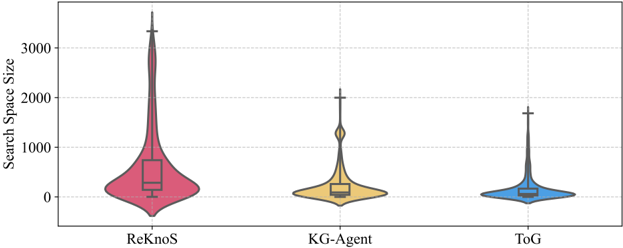
Figure 6: The size of the search space (i.e., the number of fact triples encountered during searching) of different methods on dataset GrailQA using GPT-3.5. The shape denotes the distribution of the search space sizes across all samples.
<details>
<summary>Image 6 Details</summary>
### Visual Description
\n
## Chart: Search Space Size Comparison
### Overview
The image presents a comparative analysis of the search space size for three different methods: ReKnoS, KG-Agent, and ToG. The data is visualized using violin plots with box plots overlaid, indicating the distribution of search space sizes for each method.
### Components/Axes
* **X-axis:** Method Name (ReKnoS, KG-Agent, ToG)
* **Y-axis:** Search Space Size (Scale ranges from approximately 0 to 3200, with increments of 500)
* **Violin Plots:** Represent the distribution of search space sizes for each method.
* **Box Plots:** Overlaid on the violin plots, showing the median, quartiles, and outliers.
### Detailed Analysis
The chart displays the distribution of search space sizes for each method.
* **ReKnoS (Red):** The violin plot is widest and extends to the highest values. The median search space size appears to be around 600-700. The interquartile range (IQR) is substantial, indicating a wide spread of values. The "whiskers" extend to approximately 2500-3000, with some outliers reaching the maximum value of the y-axis (approximately 3200).
* **KG-Agent (Yellow):** The violin plot is narrower than ReKnoS, and the distribution is centered at a lower value. The median search space size is approximately 800-900. The IQR is smaller than ReKnoS, suggesting less variability. The whiskers extend to approximately 1800-2000.
* **ToG (Blue):** The violin plot is the narrowest, indicating the most concentrated distribution. The median search space size is approximately 900-1000. The IQR is the smallest of the three methods, indicating the least variability. The whiskers extend to approximately 1500-1800.
### Key Observations
* ReKnoS has the largest search space size, with the widest distribution and highest outliers.
* KG-Agent has a moderate search space size, with a narrower distribution than ReKnoS.
* ToG has the smallest search space size, with the most concentrated distribution.
* The distributions are not symmetrical for any of the methods.
### Interpretation
The data suggests that ReKnoS explores a significantly larger search space compared to KG-Agent and ToG. This could be due to the method's inherent design or the specific problem it is applied to. A larger search space can potentially lead to better solutions but also increases computational cost. KG-Agent and ToG appear to be more focused in their search, potentially sacrificing exploration for efficiency. The narrow distributions of KG-Agent and ToG suggest more consistent performance, while the wider distribution of ReKnoS indicates greater variability in search space size. The presence of outliers in ReKnoS suggests that, in some cases, the search space can become exceptionally large. This could be a potential area for optimization or further investigation. The differences in search space size could be related to the complexity of the problem being solved, the effectiveness of the search algorithms, or the quality of the knowledge representation used by each method.
</details>
advanced language models like GPT-4o-mini further amplifies our model's strengths, especially in datasets that require deeper reasoning and knowledge inference.
## 5.2 EFFECT OF BACKBONE MODELS
In this subsection, we conduct experiments to compare the performance of ReKnoS and the recent baseline ToG using different backbone models to study the impact of model parameter sizes. Notably, we consider the following LLMs in addition to the two LLMs used in Sec. 5.1: Llama-2-7B (Touvron et al., 2023), Mistral-7B (Jiang et al., 2023a), Llama-3-8B (Dubey et al., 2024), and GPT4 (Anand et al., 2023). As seen in Table 2, the performance of ReKnoS varies depending on the choice of the underlying backbone model. First, smaller models, like Llama-2-7B, generally achieve worse results than larger models on all datasets. Nevertheless, the performance improvement of ReKnoS over ToG is more sig-
Table 2: Results (Hits@1 in %) of ReKnoS and ToG on various backbone models on four datasets.
| Model | WebQSP | GrailQA | CWQ | SimpleQA |
|---------|--------------|--------------|--------------|--------------|
| | Llama-2-7B | Llama-2-7B | Llama-2-7B | Llama-2-7B |
| ToG | 61.2 | 60.3 | 49.8 | 35.7 |
| ReKnoS | 64.7 | 62.2 | 51.2 | 41.0 |
| | Mistral-2-7B | Mistral-2-7B | Mistral-2-7B | Mistral-2-7B |
| ToG | 61.9 | 62.6 | 50.3 | 39.2 |
| ReKnoS | 62.5 | 64.3 | 53.1 | 45.3 |
| | Llama-3-8B | Llama-3-8B | Llama-3-8B | Llama-3-8B |
| ToG | 64.4 | 63.9 | 53.2 | 42.7 |
| ReKnoS | 67.9 | 65.8 | 56.7 | 46.4 |
| | GPT-4 | GPT-4 | GPT-4 | GPT-4 |
| ToG | 82.6 | 81.4 | 67.6 | 66.7 |
| ReKnoS | 84.9 | 82.7 | 68.2 | 69.3 |
nificant on smaller models, compared to large models like GPT-4. This indicates that our framework is significantly better for smaller models that could be easily deployed, making our framework more practical. Moreover, our framework consistently outperforms ToG on models of various parameter sizes, indicating the advantage of our framework in helping smaller models solve complex tasks. Finally, GPT-4, as expected, provides the highest performance across all datasets. This further underscores the potential of more advanced models like GPT-4 to handle complex, multi-step reasoning tasks and diverse queries, outperforming smaller and less sophisticated models. Nevertheless, smaller models with higher efficiency are valuable in simpler tasks when the inference latency is important.
## 5.3 SUPER-RELATION ANALYSIS
In this subsection, we investigate how the incorporation of super-relations contributes to improved accuracy and running time. As an example, we present the size of the search space of different methods on dataset GrailQA in Figure 6. We observe that our method has the largest search space, with nearly 42% and 55% improvements in average size over the state-of-the-art methods KG-Agent and ToG, respectively. This indicates that with super-relations, we can significantly increase the search space size when we perform reasoning on a KG. As a consequence, our method can encounter more fact triples and is more likely to retrieve the correct one for answering the question.
## 5.4 EFFICIENCY ANALYSIS
LLM calls are the dominant part of the computation; we hence separately analyze LLM calls here. The LLM operations typically require the most time and computational resources in such frameworks, especially when compared to other processes like preprocessing or document retrieval.
Let N and L represent the search width and length, respectively. In each reasoning step, ReKnoS calls the LLM twice, where
Table 3: Comparison of the average number of calls, query times (in seconds), and Hits@1 on the WebQSP and GrailQA datasets using GPT-3.5.
| Model | WebQSP | WebQSP | WebQSP | GrailQA | GrailQA | GrailQA |
|-----------|----------|----------|----------|-----------|-----------|-----------|
| Model | # Calls | Time | Hits@1 | # Calls | Time | Hits@1 |
| ToG | 15.3 | 4.9 | 76.2 | 18.9 | 6.8 | 68.7 |
| StructGPT | 11.0 | 2.0 | 75.2 | 13.3 | 3.5 | 66.4 |
| ReKnoS | 7.2 | 3.7 | 81.1 | 10.2 | 5.1 | 71.9 |
the first one is to score the super-relations, and the second one is to determine whether to proceed to the next reasoning step. Therefore, in this manner, ReKnoS calls the LLM (2 L ∗ +1) times per question, where L ∗ is the final number of reasoning steps used and the other one is to answer the final question. Note that the value of L ∗ can be smaller than the value of L .
The significant advantage of ReKnoS lies in the fact that the number of calls is independent of the width N as we utilize the concept of super-relations. In contrast, ToG searches for each path individually, and the resulting total number of LLM calls is upper bounded by 2 LN +1 (ToG calls the LLM twice at each reasoning step for each relation, while also requiring a final call for the answer). This reliance on N significantly increases the number of LLM calls needed.
We show the number of LLM calls, average query times, and Hits@1 for the different methods in Table 3. As seen in the table, ReKnoS achieves the lowest average number of LLM calls while maintaining superior performance, underscoring both its efficiency and effectiveness. Although StructGPT is faster in terms of query times, it suffers from lower accuracy. This trade-off between speed and accuracy further highlights the balance ReKnoS achieves, as it maintains high accuracy without excessively increasing the number of LLM calls.
## 5.5 HYPER-PARAMETER ANALYSIS
Here, we evaluate how hyper-parameters affect the performance of ReKnoS . We present the results of our framework in Table 4 with different values of L and N . From the results, we see that increasing both L and N leads to better performance. This is because, with larger values of L and N , our framework can retrieve and store more information in the super-relation search path Q , which can contain up to NL
Table 4: Accuracy and the retrieval rate (Ret.) of ReKnoS with different hyper-parameters using GPT-3.5.
| Setting | N = 1 | N = 1 | N = 3 | N = 3 | N = 5 | N = 5 |
|-----------|---------|---------|---------|---------|---------|---------|
| | Hits@1 | Ret. | Hits@1 | Ret. | Hits@1 | Ret. |
| L = 1 | 75.3 | 57.0 | 79.2 | 69.2 | 79.8 | 71.3 |
| L = 3 | 76.2 | 64.3 | 81.1 | 69.8 | 81.8 | 76.6 |
| L = 5 | 77.3 | 68.6 | 82.1 | 72.9 | 82.2 | 76.9 |
super-relations. It is noteworthy that decreasing N from 3 to 1 causes a considerable drop in accuracy. The reduction in Hits@1 is substantial. For example, when L = 3 , Hits@1 drops from 81.1% with N = 3 to 76.2% with N = 1 . This indicates that N plays a crucial role in the framework's performance, as having fewer super-relations reduces the amount of information available for reasoning, leading to less effective answers.
## 6 CONCLUSION
This paper introduces the ReKnoS framework, which leverages super-relations to involve a large number of relations during reasoning in knowledge graphs. By enabling the representation and exploration of multiple relation paths simultaneously, our approach significantly expands the search space of reasoning paths over knowledge graphs without sacrificing potentially valuable information. Extensive experiments demonstrate the effectiveness of our method, showing that ReKnoS achieves substantial improvements over state-of-the-art baselines. These results underscore the potential of super-relations in advancing complex reasoning tasks in knowledge graph applications. In future work, we will apply our work to knowledge graphs of other domains and types.
## ACKNOWLEDGEMENTS
This work is supported in part by the MIT-IBM AI Watson Lab, National Science Foundation (NSF) under grants CCF-1845763, CCF-2316235, and CCF-2403237, IIS-2006844, IIS-2144209, IIS2223769, CNS-2154962, BCS-2228534, and CMMI-2411248; the Commonwealth Cyber Initiative (CCI) under grant VV-1Q24-011; Google Faculty Research Award; and Google Research Scholar Award.
## REFERENCES
- Yuvanesh Anand, Zach Nussbaum, Brandon Duderstadt, Benjamin Schmidt, and Andriy Mulyar. GPT4all: Training an assistant-style chatbot with large scale data distillation from GPT-3.5-turbo. GitHub , 2023.
- Jonathan Berant, Andrew Chou, Roy Frostig, and Percy Liang. Semantic parsing on freebase from question-answer pairs. In Conference on Empirical Methods in Natural Language Processing , pp. 1533-1544, 2013.
- Kurt Bollacker, Colin Evans, Praveen Paritosh, Tim Sturge, and Jamie Taylor. Freebase: a collaboratively created graph database for structuring human knowledge. In ACM SIGMOD International Conference on Management of Data , pp. 1247-1250, 2008.
- Antoine Bordes, Nicolas Usunier, Sumit Chopra, and Jason Weston. Large-scale simple question answering with memory networks. arXiv preprint arXiv:1506.02075 , 2015.
- Tom Brown, Benjamin Mann, Nick Ryder, Melanie Subbiah, Jared D Kaplan, Prafulla Dhariwal, Arvind Neelakantan, Pranav Shyam, Girish Sastry, Amanda Askell, et al. Language models are few-shot learners. Advances in Neural Information Processing Systems , 33:1877-1901, 2020.
- Mohammad Dehghan, Mohammad Alomrani, Sunyam Bagga, David Alfonso-Hermelo, Khalil Bibi, Abbas Ghaddar, Yingxue Zhang, Xiaoguang Li, Jianye Hao, Qun Liu, Jimmy Lin, Boxing Chen, Prasanna Parthasarathi, Mahdi Biparva, and Mehdi Rezagholizadeh. EWEK-QA : Enhanced web and efficient knowledge graph retrieval for citation-based question answering systems. In Proceedings of the 62nd Annual Meeting of the Association for Computational Linguistics (Volume 1: Long Papers) , pp. 14169-14187. Association for Computational Linguistics, 2024.
- Abhimanyu Dubey, Abhinav Jauhri, Abhinav Pandey, Abhishek Kadian, Ahmad Al-Dahle, Aiesha Letman, Akhil Mathur, Alan Schelten, Amy Yang, Angela Fan, et al. The Llama 3 herd of models. arXiv preprint arXiv:2407.21783 , 2024.
- Hady Elsahar, Pavlos Vougiouklis, Arslen Remaci, Christophe Gravier, Jonathon Hare, Frederique Laforest, and Elena Simperl. T-REx: A large scale alignment of natural language with knowledge base triples. In Proceedings of the Eleventh International Conference on Language Resources and Evaluation , 2018.
- Yu Gu, Sue Kase, Michelle Vanni, Brian Sadler, Percy Liang, Xifeng Yan, and Yu Su. Beyond IID: three levels of generalization for question answering on knowledge bases. In Proceedings of the Web Conference , pp. 3477-3488, 2021.
- Albert Q Jiang, Alexandre Sablayrolles, Arthur Mensch, Chris Bamford, Devendra Singh Chaplot, Diego de las Casas, Florian Bressand, Gianna Lengyel, Guillaume Lample, Lucile Saulnier, et al. Mistral 7b. arXiv preprint arXiv:2310.06825 , 2023a.
- Jinhao Jiang, Kun Zhou, Zican Dong, Keming Ye, Wayne Xin Zhao, and Ji-Rong Wen. StructGPT: A general framework for large language model to reason over structured data. In Conference on Empirical Methods in Natural Language Processing , pp. 9237-9251, 2023b.
- Jinhao Jiang, Kun Zhou, Wayne Xin Zhao, Yaliang Li, and Ji-Rong Wen. ReasoningLM: Enabling structural subgraph reasoning in pre-trained language models for question answering over knowledge graph. In Conference on Empirical Methods in Natural Language Processing , pp. 3721-3735, 2023c.
- Jinhao Jiang, Kun Zhou, Xin Zhao, and Ji-Rong Wen. UniKGQA: Unified retrieval and reasoning for solving multi-hop question answering over knowledge graph. In The Eleventh International Conference on Learning Representations , 2023d.
- Jinhao Jiang, Kun Zhou, Wayne Xin Zhao, Yang Song, Chen Zhu, Hengshu Zhu, and Ji-Rong Wen. KG-Agent: An efficient autonomous agent framework for complex reasoning over knowledge graph. arXiv preprint arXiv:2402.11163 , 2024.
- Zhengbao Jiang, Frank Xu, Luyu Gao, Zhiqing Sun, Qian Liu, Jane Dwivedi-Yu, Yiming Yang, Jamie Callan, and Graham Neubig. Active retrieval augmented generation. In Proceedings of the Conference on Empirical Methods in Natural Language Processing , pp. 7969-7992, 2023e.
- Xingxuan Li, Ruochen Zhao, Yew Ken Chia, Bosheng Ding, Shafiq Joty, Soujanya Poria, and Lidong Bing. Chain-of-knowledge: Grounding large language models via dynamic knowledge adapting over heterogeneous sources. In The Twelfth International Conference on Learning Representations , 2024.
- Linhao Luo, Yuan-Fang Li, Reza Haf, and Shirui Pan. Reasoning on graphs: Faithful and interpretable large language model reasoning. In The Twelfth International Conference on Learning Representations , 2024.
- Shengjie Ma, Chengjin Xu, Xuhui Jiang, Muzhi Li, Huaren Qu, and Jian Guo. Think-on-Graph 2.0: Deep and interpretable large language model reasoning with knowledge graph-guided retrieval. arXiv preprint arXiv:2407.10805 , 2024.
- Costas Mavromatis and George Karypis. GNN-RAG: Graph neural retrieval for large language model reasoning. arXiv preprint arXiv:2405.20139 , 2024.
- Todor Mihaylov, Peter Clark, Tushar Khot, and Ashish Sabharwal. Can a suit of armor conduct electricity? a new dataset for open book question answering. In Proceedings of the Conference on Empirical Methods in Natural Language Processing , pp. 2381-2391, 01 2018.
- Yasumasa Onoe, Michael J. Q. Zhang, Eunsol Choi, and Greg Durrett. CREAK: A dataset for commonsense reasoning over entity knowledge. In Proceedings of the Neural Information Processing Systems Track on Datasets and Benchmarks , 2021.
- OpenAI. ChatGPT: Optimizing language models for dialogue., 2022.
- Shirui Pan, Linhao Luo, Yufei Wang, Chen Chen, Jiapu Wang, and Xindong Wu. Unifying large language models and knowledge graphs: A roadmap. IEEE Transactions on Knowledge and Data Engineering , 2024.
- Fabio Petroni, Aleksandra Piktus, Angela Fan, Patrick Lewis, Majid Yazdani, Nicola De Cao, James Thorne, Yacine Jernite, Vladimir Karpukhin, Jean Maillard, Vassilis Plachouras, Tim Rocktaschel, and Sebastian Riedel. KILT: a benchmark for knowledge intensive language tasks. In NAACL-HLT , pp. 2523-2544, 2021.
- Robyn Speer, Joshua Chin, and Catherine Havasi. ConceptNet 5.5: An open multilingual graph of general knowledge. In Proceedings of the AAAI conference on artificial intelligence , volume 31, 2017.
- Jiashuo Sun, Chengjin Xu, Lumingyuan Tang, Sai Wang, Chen Lin, Yeyun Gong, Lionel M. Ni, Heung yeung Shum, and Jian Guo. Think-on-Graph: Deep and responsible reasoning of large language model on knowledge graph. In International Conference on Learning Representations , 2023.
- Alon Talmor and Jonathan Berant. The Web as a knowledge-base for answering complex questions. In Conference of the North American Chapter of the Association for Computational Linguistics: Human Language Technologies, Volume 1 (Long Papers) , pp. 641-651, 2018.
- Hugo Touvron, Louis Martin, Kevin Stone, Peter Albert, Amjad Almahairi, Yasmine Babaei, Nikolay Bashlykov, Soumya Batra, Prajjwal Bhargava, Shruti Bhosale, et al. Llama 2: Open foundation and fine-tuned chat models. arXiv preprint arXiv:2307.09288 , 2023.
- Denny Vrandeˇ ci´ c and Markus Krötzsch. Wikidata: a free collaborative knowledgebase. Communications of the ACM , 57(10):78-85, 2014.
- Xuezhi Wang, Jason Wei, Dale Schuurmans, Quoc V. Le, Ed H. Chi, Sharan Narang, Aakanksha Chowdhery, and Denny Zhou. Self-consistency improves chain of thought reasoning in language models. In The Eleventh International Conference on Learning Representations , 2023.
- Jason Wei, Xuezhi Wang, Dale Schuurmans, Maarten Bosma, Fei Xia, Ed Chi, Quoc V Le, Denny Zhou, et al. Chain-of-thought prompting elicits reasoning in large language models. Advances in Neural Information Processing Systems , 35:24824-24837, 2022.
- Ran Xu, Hejie Cui, Yue Yu, Xuan Kan, Wenqi Shi, Yuchen Zhuang, Wei Jin, Joyce Ho, and Carl Yang. Knowledge-infused prompting: Assessing and advancing clinical text data generation with large language models. In Findings of the Association for Computational Linguistics: ACL 2024 , pp. 15496-15523, 2024.
- Zhilin Yang, Peng Qi, Saizheng Zhang, Yoshua Bengio, William Cohen, Ruslan Salakhutdinov, and Christopher D Manning. HotpotQA: A dataset for diverse, explainable multi-hop question answering. In Conference on Empirical Methods in Natural Language Processing , 2018.
- Wen-tau Yih, Matthew Richardson, Christopher Meek, Ming-Wei Chang, and Jina Suh. The value of semantic parse labeling for knowledge base question answering. In Proceedings of the 54th Annual Meeting of the Association for Computational Linguistics (Volume 2: Short Papers) , pp. 201-206, 2016.
- Jing Zhang, Xiaokang Zhang, Jifan Yu, Jian Tang, Jie Tang, Cuiping Li, and Hong Chen. Subgraph retrieval enhanced model for multi-hop knowledge base question answering. In Proceedings of the 60th Annual Meeting of the Association for Computational Linguistics (Volume 1: Long Papers) , pp. 5773-5784, 2022.
- Yuyu Zhang, Hanjun Dai, Zornitsa Kozareva, Alexander Smola, and Le Song. Variational reasoning for question answering with knowledge graph. In Proceedings of the AAAI Conference on Artificial Intelligence , volume 32, 2018.
## A PROOF OF THEOREM 4.1
Theorem 4.1. A super-relation search path leads to at least one super-relation path. Given a selected super-relation search path of length l , Q l = {S 1 , S 2 , . . . , S l } , there exists at least one super-relation path of length l , i.e., P = ( R ( k 1 ) 1 → R ( k 2 ) 2 → . . . → R ( k l ) l ) , where R ( k j ) j ∈ S j and k j represents k i,j for a fixed i .
Proof. Let Q l = {S 1 , S 2 , . . . , S l } represent a super-relation search path consisting of l super-relation sets, as per Definition 3. Each super-relation set S i = { R (1) i , R (2) i , . . . , R ( |S i | ) i } contains multiple super-relations.
According to Definition 3, in each super-relation set S i , there exists at least one super-relation R ∈ S i that connects to a super-relation in the next set S i +1 . In other words,
$$\forall R \in { \mathcal { S } } _ { i } , \exists R ^ { \prime } \in { \mathcal { S } } _ { i + 1 } s u c h t h a t \, R \to R ^ { \prime } .$$
This ensures that there are connected super-relations between consecutive sets.
We prove the theorem using induction. As the base case, we observe that according to Definition 3, there exists a super-relation super-relation R ( k 1 ) 1 ∈ S 1 and another super-relation R ( k 2 ) 2 ∈ S 2 such that:
$$R _ { 1 } ^ { ( k _ { 1 } ) } \rightarrow R _ { 2 } ^ { ( k _ { 2 } ) } .$$
As the inductive hypothesis, suppose that for a super-relation search path of length l -1 , where l > 2 , there exists at least one super-relation path of length l -1 . We take one such path ( R ( k 1 ) 1 → R ( k 2 ) 2 → . . . → R ( k l -1 ) l -1 ) , where R ( k j ) j ∈ S j . We take the last super-relation on such
a path, R ( k l -1 ) l -1 ∈ S l -1 . By Definition 3, we know that there exists a connected super-relation R ( k l ) l ∈ S l such that:
$$R _ { l - 1 } ^ { ( k _ { l - 1 } ) } \rightarrow R _ { l } ^ { ( k _ { l } ) } .$$
Then, we can form the super-relation path P = ( R ( k 1 ) 1 → R ( k 2 ) 2 → . . . → R ( k l -1 ) l -1 → R ( k l ) l ) . Thus, we have that every super-relation search path leads to at least one super-relation path, as required.
## B PROOF OF THEOREM 4.2
Theorem 4.2. For any super-relation path P = ( R ( k 1 ) 1 → R ( k 2 ) 2 → . . . → R ( k l ) l ) , there exists at least one corresponding KG reasoning path of length l , represented as e 1 r 1 - → e 2 r 2 - → · · · r l - → e l +1 , where r i ∈ R ( k i ) i is a relation chosen from the super-relation R ( k i ) i , and e 1 , e 2 , . . . , e l +1 are entities in the knowledge graph.
Proof. Given a super-relation path P = ( R ( k 1 ) 1 → R ( k 2 ) 2 → . . . → R ( k l ) l ) , we need to show that there exists a corresponding reasoning path in the knowledge graph such that
$$e _ { 1 } \xrightarrow { r _ { 1 } } e _ { 2 } \xrightarrow { r _ { 2 } } \cdots \xrightarrow { r _ { l } } e _ { l + 1 } ,$$
where each r i is a relation from the super-relation R ( k i ) i , and the entities e 1 , e 2 , . . . , e l +1 are KG entities.
From Definition 1, we know that each super-relation R i is composed of multiple relations, i.e., R i = { r 1 , r 2 , . . . } , where r j is a standard binary relation between two entities in the knowledge graph. The super-relation R ( k 1 ) 1 connects to R ( k 2 ) 2 , denoted as R ( k 1 ) 1 → R ( k 2 ) 2 , if there exist entities e 1 , e 2 , and e 3 such that
$$e _ { 1 } \xrightarrow { r _ { 1 } } e _ { 2 } \xrightarrow { r _ { 2 } } e _ { 3 } ,$$
where r 1 ∈ R ( k 1 ) 1 and r 2 ∈ R ( k 2 ) 2 .
According to Definition 2, a super-relation path P = ( R ( k 1 ) 1 → R ( k 2 ) 2 → . . . → R ( k l ) l ) consists of l consecutive super-relations that are connected. This means that for each consecutive pair of super-relations R ( k i ) i and R ( k i +1 ) i +1 , there exist entities e i , e i +1 , and e i +2 such that
$$e _ { i } \xrightarrow { r _ { i } } e _ { i + 1 } \xrightarrow { r _ { i + 1 } } e _ { i + 2 } ,$$
where r i ∈ R ( k i ) i and r i +1 ∈ R ( k i +1 ) i +1 .
We proceed by induction on the length l of the super-relation path.
Base Case ( l = 1 ): For a super-relation path of length 1 , P = ( R ( k 1 ) 1 ) , we have the super-relation r 1 ∈ R ( k 1 ) 1 and two entities e 1 and e 2 such that
$$e _ { 1 } \xrightarrow { r _ { 1 } } e _ { 2 } .$$
This forms a valid KG reasoning path of length 1 .
Our inductive hypothesis is that for a super-relation path of length l -1 , P = ( R ( k 1 ) 1 → R ( k 2 ) 2 → . . . → R ( k l -1 ) l -1 ) (for l > 2 ), there exists a corresponding KG reasoning path
$$e _ { 1 } \xrightarrow { r _ { 1 } } e _ { 2 } \xrightarrow { r _ { 2 } } \cdots \xrightarrow { r _ { l - 1 } } e _ { l } ,$$
where each r i ∈ R ( k i ) i is chosen from the respective super-relation.
Table 5: Evaluation results (Part 1) with average accuracy and standard deviations over five runs.
| Model | WebQSP | GrailQA | CWQ | SimpleQA | WebQ |
|---------------|------------|------------|------------|------------|------------|
| ToG | 76.4 ± 2.0 | 68.9 ± 1.5 | 56.2 ± 1.8 | 53.7 ± 0.9 | 54.1 ± 2.5 |
| KG-Agent | 78.6 ± 1.9 | 69.4 ± 2.1 | 56.4 ± 1.2 | 52.5 ± 2.7 | 55.1 ± 2.0 |
| ReKnoS (Ours) | 81.0 ± 1.0 | 71.2 ± 1.5 | 57.7 ± 0.9 | 54.1 ± 1.0 | 56.5 ± 1.2 |
Table 6: Evaluation results (Part 2) with average accuracy and standard deviations over five runs.
| Model | T-REx | zsRE | Creak | Hotpot QA |
|---------------|------------|------------|------------|-------------|
| ToG | 76.0 ± 1.3 | 87.5 ± 1.0 | 91.3 ± 2.8 | 35.6 ± 2.3 |
| KG-Agent | 78.9 ± 0.8 | 86.8 ± 1.5 | 90.3 ± 2.5 | 36.5 ± 1.1 |
| ReKnoS (Ours) | 79.8 ± 1.1 | 88.3 ± 0.7 | 91.9 ± 0.9 | 37.1 ± 1.4 |
Now, consider a super-relation path of length l , P = ( R ( k 1 ) 1 → R ( k 2 ) 2 → . . . → R ( k l -1 ) l -1 → R ( k l ) l ) . From Definition 1, the super-relation R ( k l -1 ) l -1 → R ( k l ) l exists if and only if there exist entities e l and e l +1 such that where r l ∈ R ( k l ) l .
Thus, the extended path is
$$e _ { l } \xrightarrow { r _ { l } } e _ { l + 1 } ,$$
<!-- formula-not-decoded -->
which forms a valid KG reasoning path of length l , as required.
## C IMPLEMENTATION DETAILS
Since our framework is flexible and can be applied to any LLMs, in our experiments, we mainly consider two large LLMs: GPT-3.5 (ChatGPT) (OpenAI, 2022) and GPT-4o-mini (Anand et al., 2023). We additionally consider Llama-2-7B (Touvron et al., 2023), Mistral-7B (Jiang et al., 2023a), Llama-3-8B (Dubey et al., 2024), and GPT-4 (Anand et al., 2023) in Sec. 5.2. We run all of our experiments on one NVIDIA A6000 GPU with 48GB of memory. Across all datasets and methods, we set the width N to 3 and the maximum length L to 3. When prompting the LLM to score super-relations, we use 3 examples as in-context learning demonstrations, following the existing work on ToG (Sun et al., 2023). The starting entities of each query are provided in the datasets.
## D ADDITIONAL RESULTS AND DISCUSSIONS
## D.1 ADDITIONAL EVALUATION ANALYSIS
Following the settings of ToG and KG-Agent, we initially did not run multiple rounds of evaluation. To strengthen our analysis, we conducted five additional experimental runs and report the average results along with standard deviations. This ensures that our observed improvements are statistically significant. The results are shown in Table 5 and Table 6.
From these results, we observe slight variations across multiple rounds of experiments. However, ReKnoS consistently achieves the best performance compared to the two state-of-the-art baselines, highlighting its effectiveness and robustness.
## D.2 COMPARISON WITH SUBGRAPH-BASED REASONING METHODS
To further evaluate the effectiveness of our proposed ReKnoS framework, we conduct additional experiments comparing with subgraph-based reasoning methods SR (Zhang et al., 2022) and UniKGQA (Jiang et al., 2023d).
Table 7: Performance comparison of subgraph-based reasoning methods and ReKnoS on benchmark KGQA datasets.
| Model | WebQSP | GrailQA | CWQ | SimpleQA |
|---------|----------|-----------|-------|------------|
| SR | 68.9 | 65.2 | 50.2 | 48.7 |
| UniKGQA | 75.1 | 68.1 | 50.7 | 50.5 |
| ReKnoS | 81.1 | 71.9 | 58.5 | 52.9 |
Table 8: Performance comparison of Hits@1 and F1 scores on the WebQSP, GrailQA, and CWQ datasets.
| Model | WebQSP | WebQSP | GrailQA | GrailQA | CWQ | CWQ |
|----------|----------|----------|-----------|-----------|--------|-------|
| | Hits@1 | F1 | Hits@1 | F1 | Hits@1 | F1 |
| ToG | 76.2 | 64.3 | 68.7 | 66.6 | 57.4 | 54.5 |
| KG-Agent | 79.2 | 77.1 | 68.9 | 65.3 | 56.1 | 52.6 |
| ReKnoS | 81.1 | 79.5 | 71.9 | 70.2 | 58.5 | 56.8 |
Experimental Setup. While our primary focus is on reasoning methods specifically tailored for large language models (LLMs), we recognize the value of including subgraph-based reasoning baselines to provide a more comprehensive evaluation. Unlike ReKnoS , which leverages superrelations to enhance retrieval and reasoning efficiency for LLMs, subgraph-based approaches operate with different objectives. For instance, UniKGQA employs RoBERTa as its encoder, whereas LLM-based methods such as ToG utilize powerful models like GPT-3.5. Despite these fundamental differences, we report the performance of these approaches on four benchmark datasets: WebQSP, GrailQA, CWQ, and SimpleQA. For SR and UniKGQA, we follow the experimental settings in the original papers, and we use GPT-3.5 for our framework.
Results and Discussion. Table 7 presents the comparison between ReKnoS and the subgraph-based reasoning methods. Our method achieves superior performance across all datasets, demonstrating the effectiveness of leveraging super-relations in KGQA. Notably, ReKnoS outperforms UniKGQA by 6.0% , 3.8% , 7.8% , and 2.4% on WebQSP, GrailQA, CWQ, and SimpleQA, respectively while outperforming SR by even more. These results reinforce our argument that reasoning methods designed for LLMs can effectively enhance knowledge graph-based question answering.
## D.3 ANALYSIS OF HITS@1 VS. F1 METRIC
To comprehensively evaluate the effectiveness of our proposed ReKnoS framework, we compare the use of the Hits@1 and F1 metrics in knowledge graph question answering (KGQA) tasks.
Motivation. While Hits@1 is commonly used in KGQA benchmarks, the F1 metric may provide additional insights, especially when multiple valid answers exist for a given question. However, we follow the existing work on ToG (Sun et al., 2023) in primarily reporting Hits@1, as certain datasets in our evaluation, such as T-REx and zsRE , do not involve multiple correct answers per question, making the F1 metric less meaningful in these cases. For single-answer tasks, Hits@1 remains the most reliable evaluation metric.
Experimental Results. Despite the above considerations, we acknowledge the value of the F1 metric in datasets where multiple answers exist. Thus, we report both Hits@1 and F1 scores for the state-of-the-art models across three datasets: WebQSP , GrailQA , and CWQ . The results are summarized in Table 8. We use GPT-3.5 for this experiment.
Discussion. From the results in Table 8, we observe that a stronger baseline like KG-Agent does not always maintain better F1 scores. Interestingly, the relatively weaker baseline ToG can demonstrate a more complete answer set, which is useful in scenarios where answer coverage is more critical than strict correctness. Notably, ReKnoS consistently outperforms both baselines, achieving the best
Table 9: Comparison of ReKnoS with additional baselines.
| Model | WebQSP | WebQSP | GrailQA | GrailQA |
|---------|----------|----------|-----------|-----------|
| | Hits@1 | F1 | Hits@1 | F1 |
| RoG | 80.0 | 70.8 | 57.8 | 56.2 |
| GNN-RAG | 82.8 | 73.5 | 62.8 | 60.4 |
| ReKnoS | 81.1 | 79.5 | 58.5 | 56.8 |
Table 10: Distribution of non-retrieval cases across datasets.
| Dataset | Path Absence | Depth Limit | Misdirection |
|-----------|----------------|---------------|----------------|
| GrailQA | 6.0% | 25.2% | 68.8% |
| CWQ | 9.2% | 43.1% | 47.7% |
| WebQSP | 11.6% | 15.9% | 72.5% |
performance across both the Hits@1 and F1 metrics, demonstrating its ability to effectively balance precision and completeness.
These findings highlight that while Hits@1 is appropriate for single-answer tasks, F1 can be an important complementary metric for tasks with multiple correct answers.
## D.4 COMPARISON WITH ADDITIONAL BASELINES
In this subsection, we consider additional baselines that are applicable to the task that we focus on. These methods provide interesting perspectives.
- RoG (Luo et al., 2024): RoG is a reasoning framework that enhances LLMs with knowledge graphs by using a planning-retrieval-reasoning approach, where relation paths generated from KGs guide the retrieval of valid reasoning paths, enabling faithful, interpretable, and state-of-the-art KG reasoning. This method uses LLaMA2-Chat-7B as the LLM backbone, fine-tuned on the training split of WebQSP, CWQ, and Freebase for 3 epochs.
- GNN-RAG (Mavromatis & Karypis, 2024): GNN-RAG is a novel RAG framework that combines the reasoning capabilities of Graph Neural Networks (GNNs) with the language understanding abilities of LLMs by extracting KG reasoning paths from a dense subgraph and verbalizing them for LLM-based KGQA. This method uses LLaMA2-Chat-7B as the LLM backbone.
We also considered EWEK-QA (Dehghan et al., 2024), which is an enhanced citation-based QA system that improves knowledge extraction by combining an adaptive Web retriever with efficient knowledge graph (KG) integration. However, this method primarily focuses on citation-based question answering, which diverges from the scope of our work. Additionally, its performance has been reported in Jiang et al. (2024) to be inferior to the baselines that we included. Therefore, we did not include this method in the experiments.
From the results presented in Table 9, we observe that GNN-RAG generally achieves better results than ReKnoS on both datasets. This demonstrates the importance of exploiting the structural information in knowledge graphs to extract useful knowledge. Nevertheless, despite the strong performance of RoG and GNN-RAG, they require fine-tuning on white-box LLMs, which can be infeasible in specific scenarios where computational resources are scarce. On the other hand, the advantage of ReKnoS is that any black-box LLM can be easily plugged in to the framework.
## D.5 BREAKDOWN OF NON-RETRIEVAL CASES ON ADDITIONAL DATASETS
In this subsection, we include the breakdown of non-retrieval cases across two additional datasets: WebQSP and CWQ. The results are shown in Table 10. From the results, we observe that the reasons for non-retrieval cases are distributed differently across datasets. However, the majority of cases still fall under Misdirection , which ReKnoS is designed to address.
Table 11: Evaluation results on datasets without using built-in super-relations.
| Method | CWQ | WebQSP | OBQA | MetaQA |
|----------------------------------------|-------|----------|--------|----------|
| StructGPT | 55.2 | 75.2 | 77.2 | 81.2 |
| ToG | 56.2 | 76.4 | 81 | 87.2 |
| ReKnoS (without given super-relations) | 57.6 | 76.9 | 85.3 | 92.5 |
Table 12: Comparison of StructGPT implementations with different numbers of selected relations per step. We include the results for ToG and ReKnoS for reference.
| Model | WebQSP | WebQSP | WebQSP | GrailQA | GrailQA | GrailQA |
|-------------------------|----------|----------|----------|-----------|-----------|-----------|
| | # Calls | Time | Hits@1 | # Calls | Time | Hits@1 |
| ToG | 15.3 | 4.9 | 76.2 | 18.9 | 6.8 | 68.7 |
| StructGPT (3 Relations) | 11.0 | 2.0 | 75.2 | 13.3 | 3.5 | 66.4 |
| StructGPT (1 Relation) | 3.8 | 1.1 | 72.7 | 4.2 | 1.0 | 61.7 |
| ReKnoS | 7.2 | 3.7 | 81.1 | 10.2 | 5.1 | 71.9 |
## D.6 APPLICABILITY BEYOND THE WIKIDATA KNOWLEDGE GRAPH
To further demonstrate the robustness of our method, we conducted additional experiments on two datasets with different knowledge graphs:
OBQA (OpenBookQA) (Mihaylov et al., 2018) is a multiple-choice question-answering task designed to assess commonsense knowledge. The utilized KG is ConceptNet (Speer et al., 2017), a comprehensive knowledge base covering diverse aspects of everyday knowledge, such as <"rabbit", CapableOf, "move fast"> . MetaQA (MoviE Text Audio QA) (Zhang et al., 2018) is a dataset focused on the movie domain, featuring questions where the answer entities can be located up to three hops from the topic entities within a movie KG derived from OMDb.
Both OBQA and MetaQA do not have built-in super-relations. In addition, we removed predefined super-relations from CWQ and WebQSP. The results are shown in Table 11.
The results validate that our approach is effective even in scenarios where super-relations must be derived dynamically via clustering, without reliance on predefined super-relations. This further reinforces the generalizability and robustness of ReKnoS across diverse KG structures.
## D.7 ANALYSIS OF LLM CALLS IN STRUCTGPT
In this subsection, we modified the StructGPT implementation by modifying the number of selected relations per step. The original StructGPT implementation selects only one relation at a time, whereas our modified implementation selects three relations per step, aligning with ToG and ReKnoS. This modification allows StructGPT to explore a broader set of candidate relations, thereby improving accuracy (Hits@1). However, it also increases the number of LLM calls and query time compared to its original implementation.
To provide a clearer comparison, we present an analysis of the trade-offs between the original StructGPT implementation (selecting 1 relation) and our modified implementation (selecting 3 relations). The results are summarized in Table 12.
The results illustrate the trade-offs in StructGPT. When selecting only one relation per step, the method reduces query time and the number of LLM calls, but at the cost of slightly lower accuracy (Hits@1). Conversely, when selecting three relations, StructGPT achieves higher accuracy but requires more calls and query time.
Table 13: Performance comparison with and without explicit scoring criteria.
| Model | WebQSP | GrailQA | CWQ |
|------------------------------------|----------|-----------|-------|
| ReKnoS | 81 | 71.2 | 57.7 |
| ReKnoS (Explicit Scoring Criteria) | 81.9 | 72.5 | 58.2 |
## D.8 BENEFITS OF EXPLICIT CRITERIA
In this subsection, we integrate explicit scoring criteria to enhance the interoperability of our framework. We replace the manual example with the following scoring criteria, which serve as a guideline for the LLMs:
- [0.8 - 1.0]: Highly Relevant
- -There is a strong logical connection between the relation and the query.
- [0.6 - 0.8]: Strongly Related
- -The relation aligns well with the query and provides substantial relevant information , but it may lack some precision.
- [0.4 - 0.6]: Moderately Related
- -The relation is partially relevant and may provide general background information or indirect support for the query.
- [0.2 - 0.4]: Weakly Related
- -The relation has a tenuous connection to the query, providing limited or peripheral information .
- [0.0 - 0.2]: Irrelevant
- -The relation is unrelated or only tangentially related to the query.
By providing this guideline as an additional input to the LLM, we conduct further experiments and obtain the results shown in Table 13. The results indicate that incorporating explicit scoring criteria improves performance across all three datasets. This suggests that a well-defined guideline can enhance the model's ability to distinguish between different levels of relevance, thereby improving both interpretability and accuracy.
## D.9 MITIGATING HALLUCINATION
In this subsection, we discuss the mitigation of the risk of hallucination in our framework. Our framework ensures that all selected super-relations exist within the knowledge graph. First, the candidate selection step explicitly filters super-relations to include only those that are directly connected to previously selected relations in the KG. This design ensures that the reasoning process remains grounded in the structure of the KG and prevents the hallucination of non-existent relations from influencing the retrieval process. Second, during the scoring step, the LLM is tasked with ranking super-relations for their relevance, but these candidates are pre-selected based on their existence and connectivity in the KG. As a result, any hallucinated suggestions by the LLM are naturally excluded from the retrieval pipeline.