# AI-Newton: A Concept-Driven Physical Law Discovery System without Prior Physical Knowledge
**Authors**: You-Le Fang, Dong-Shan Jian, Xiang Li, Yan-Qing Ma
> School of Physics, Peking University, Beijing 100871, China
> School of Physics, Peking University, Beijing 100871, China Center for High Energy Physics, Peking University, Beijing 100871, China
(December 11, 2025)
## Abstract
While current AI-driven methods excel at deriving empirical models from individual experiments, a significant challenge remains in uncovering the common fundamental physics that underlie these models—a task at which human physicists are adept. To bridge this gap, we introduce AI-Newton, a novel framework for concept-driven scientific discovery. Our system autonomously derives general physical laws directly from raw, multi-experiment data, operating without supervision or prior physical knowledge. Its core innovations are twofold: (1) proposing interpretable physical concepts to construct laws, and (2) progressively generalizing these laws to broader domains. Applied to a large, noisy dataset of mechanics experiments, AI-Newton successfully rediscovers foundational and universal laws, such as Newton’s second law, the conservation of energy, and the universal gravitation. This work represents a significant advance toward autonomous, human-like scientific discovery.
Introduction. — For centuries, the ultimate goal of fundamental physics research has been to describe a wide range of phenomena through a small number of discovered laws. Advances in artificial intelligence (AI) have made AI-driven scientific discovery a highly promising new paradigm [1]. Although AI has achieved remarkable results in tackling domain-specific challenges [2, 3], the ultimate aspiration from a paradigm-shifting perspective still lies in developing reliable AI systems capable of autonomous scientific discovery directly from a large collection of raw data without supervision [4, 5].
Current approaches to automated physics discovery focus on individual experiments, employing either neural network (NN)-based methods [6, 7, 8, 9, 10, 11, 12, 13, 14, 15, 16, 17, 18, 19, 20, 21, 22, 23, 24, 25] or symbolic techniques [26, 27, 28, 29, 30, 31, 32, 33]. By analyzing data from a single experiment, these methods can construct a specific model capable of predicting future data from the same experiment; if sufficiently simple, such a model may even be expressed in symbolic form [34, 35, 36]. Although these methods represent a crucial and successful stage towards automated scientific discovery, they have not yet reached a discovery capacity comparable to that of human physicists.
Human scientists advance further by discerning common patterns across specific models from different experiments and, on that basis, formulating general models that account for data from all such experiments. For instance, Newtonian mechanics provides a unifying and interpretable framework by defining meaningful physical concepts and formulating general laws that are valid across diverse phenomena. Therefore, a central challenge for the AI-driven physics discovery field is to evolve beyond problem-specific model fitting towards AI systems capable of discovering knowledge that is inherently generalizable and universally applicable.
In this Letter, we present AI-Newton, a concept-driven discovery system, which is designed for the critical question: how to extract concepts and general laws from problem-specific models. AI-Newton integrates an autonomous discovery workflow which is fundamentally built upon plausible reasoning and physical concepts. Given a collection of physical experiments, AI-Newton can gradually formulate a set of general laws applicable across a wide problem scope with neither supervision nor any prior physical knowledge. As a proof-of-concept implementation Code available at https://github.com/Science-Discovery/AI-Newton, by applying it to 46 different classical mechanics experiments, it can rediscover Newton’s second law, energy conservation, law of gravitation and others in classical mechanics.
<details>
<summary>overview.png Details</summary>

### Visual Description
## Diagram: Autonomous Scientific Discovery Workflow
### Overview
The image is a technical flowchart illustrating a closed-loop system for autonomous scientific discovery. It depicts the flow of information between three primary bases: an **Experiment base** (left, green), an **Autonomous discovery workflow** (center, pink), and a **Theory base** (right, blue). The diagram shows how experimental data is processed through a series of computational steps to extract concepts and laws, which then populate a theoretical framework, which in turn informs future experiments.
### Components/Axes
The diagram is organized into three vertical sections, each with a distinct background color and containing labeled boxes and arrows.
**1. Experiment base (Left, Green Background)**
* **Title:** "Experiment base" (top-left).
* **Components:**
* A large rounded rectangle labeled **"Experiment 1"**. Inside, it lists:
* "Physical objects"
* "Geometric information"
* "Experimental parameters"
* "Space-time coordinates"
* "Data generator"
* Below it, a smaller rounded rectangle labeled **"Experiment 2"**.
* A vertical ellipsis ("⋮") indicating a sequence.
* A final rounded rectangle labeled **"Experiment N"**.
* **Outgoing Flow:** A thick, white arrow labeled **"Experiments"** points from the "Experiment 1" box to the central workflow.
**2. Autonomous discovery workflow (Center, Pink Background)**
* **Title:** "Autonomous discovery workflow" (top-center).
* **Components (Top to Bottom):**
* **Selection:** A purple box with a dashed **orange/gold border**. Subtext: "One experiment", "A few concepts".
* **Search of physical laws:** A purple box with a dashed **grey border**. Subtext: "Extension of general laws", "Direct search of specific laws".
* **Simplification and classification:** A purple box with a dashed **red border**.
* **Extraction of concepts and general laws:** A purple box with a dashed **blue border**.
* **Internal Flow:** Vertical white arrows connect the boxes in a top-down sequence: Selection → Search → Simplification → Extraction.
* **External Interactions:**
* Receives "Experiments" from the left.
* Sends "Concepts" and "Laws" (via a white arrow) to the Theory base on the right.
* Receives "Concepts" and "Laws" (via a white arrow) back from the Theory base.
**3. Theory base (Right, Blue Background)**
* **Title:** "Theory base" (top-right).
* **Components (Top to Bottom):**
* **Symbols:** A blue box.
* **Concepts:** A blue box. Subtext: "Dynamical concepts", "Intrinsic concepts", "Universal constants".
* **Laws:** A blue box. Subtext: "Specific laws", "General laws".
* **Internal Relationships:**
* Between "Symbols" and "Concepts": Two vertical arrows. A downward arrow labeled **"represent"** and an upward arrow labeled **"extract"**.
* Between "Concepts" and "Laws": Two vertical arrows. A downward arrow labeled **"represent"** and an upward arrow labeled **"extract"**.
**4. Legend (Bottom)**
A horizontal legend explains the meaning of the dashed border colors used in the central workflow:
* **Orange/Gold dashed border:** "Recommendation engine"
* **Grey dashed border:** "Symbolic regression"
* **Red dashed border:** "Differential algebra & variable control"
* **Blue dashed border:** "Plausible reasoning"
### Detailed Analysis
The diagram details a multi-stage pipeline for automated scientific reasoning:
1. **Input:** The process begins with raw experimental data ("Experiments") from the Experiment base.
2. **Selection (Recommendation engine):** The first stage selects a single experiment and a few relevant concepts to focus on.
3. **Law Search (Symbolic regression):** The core discovery phase searches for physical laws, either by extending known general laws or directly searching for specific ones.
4. **Refinement (Differential algebra & variable control):** The discovered laws undergo simplification and classification.
5. **Output & Integration (Plausible reasoning):** The final stage extracts refined concepts and general laws. These are sent to populate the Theory base.
6. **Theory Base Structure:** The Theory base is hierarchical. **Symbols** represent **Concepts**, which in turn represent **Laws**. The upward "extract" arrows suggest that concepts can be extracted from symbols, and laws can be extracted from concepts, mirroring the discovery process.
7. **Closed Loop:** The Theory base feeds "Concepts" and "Laws" back into the workflow (specifically to the "Search of physical laws" stage), creating a continuous, iterative cycle where existing theory guides the discovery of new theory from new experiments.
### Key Observations
* The workflow is explicitly modular, with each stage associated with a specific computational technique (e.g., symbolic regression, differential algebra).
* The "Theory base" is not a static repository but an active participant in the loop, providing the conceptual and legal framework for interpreting new experiments.
* The process is designed to handle multiple experiments (Experiment 1 to N), suggesting scalability.
* The distinction between "Specific laws" and "General laws" in the Theory base, and the corresponding "Extension of general laws" vs. "Direct search of specific laws" in the workflow, indicates a nuanced approach to law discovery.
### Interpretation
This diagram represents a sophisticated framework for **automated or AI-driven scientific discovery**. It conceptualizes science not as a linear process but as a closed-loop system where experiment and theory co-evolve.
* **The Core Idea:** The system aims to mimic the scientific method autonomously. It takes empirical data, uses it to hypothesize laws (via symbolic regression), refines those hypotheses, and integrates them into a growing body of knowledge (the theory base). This new knowledge then informs the selection and interpretation of future experiments.
* **Role of AI:** The labeled techniques (Recommendation engine, Symbolic regression, etc.) point to the use of machine learning and symbolic AI to perform tasks traditionally done by human scientists: selecting promising research directions, formulating mathematical models, and logically organizing knowledge.
* **Significance:** Such a system could accelerate scientific discovery by automating the labor-intensive process of moving from data to theory. It highlights the importance of not just finding patterns in data (symbolic regression) but also of logically structuring and simplifying the discovered knowledge (differential algebra, plausible reasoning) to make it coherent and generalizable.
* **Underlying Philosophy:** The bidirectional "represent/extract" arrows in the Theory base suggest a deep, two-way relationship between observation (symbols/data), conceptualization, and law formulation. Discovery is portrayed as both a bottom-up (extract) and top-down (represent) process.
</details>
Figure 1: AI-Newton’s experiment base, theory base, and autonomous discovery workflow.
Knowledge base and knowledge representation. — AI-Newton contains an experiment base and a theory base, as shown in Fig. 1. The experiment base stores physical experiments and corresponding simulated data generators. The inputs for each experiment include only the physical objects involved, geometric information, experimental parameters, and space-time coordinates, which define an experiment. To emphasize that no prior physical knowledge is used, all other concepts, such as mass or energy, are autonomously discovered in AI-Newton. The output of each experiment is simulated data with statistical errors.
The theory base stores physical knowledge explicitly in an interconnected library of symbols, concepts, and laws. This design mirrors how human physicists construct concise, universal laws from conceptual building blocks. In contrast to prior work, which interprets latent features in NNs as physical concepts [37, 23, 38], AI-Newton represents concepts and laws in an explicit, symbolic form. This greatly enhances interpretability and makes the acquired knowledge easier to transfer to new problems. Moreover, the introduction of powerful intermediate concepts allows complex physical laws to be expressed concisely, which in turn makes them more amenable to discovery through techniques like symbolic regression (SR) [26, 27, 28, 29, 30, 31, 32, 33, 34, 35, 36]. Initially, the concept layer contains only space-time coordinates; new concepts are autonomously defined and registered using a dedicated physical domain-specific language (DSL). (See Supplemental Materials (SMs) [39] for details.)
A robust knowledge representation is crucial because our goal is for the AI to discover generalizable knowledge across diverse systems, which requires transferring knowledge between different problems. To achieve this, we designed a physical DSL with a well-defined structure. This DSL not only formulates equations but also encodes the properties of physical objects and the relationships between physical quantities. For instance, given the known concepts of coordinate $x$ and time $t$ , the velocity of a ball can be defined in the DSL as:
$$
C_{1}:=\forall i\text{: Ball},\,\mathrm{d}x[i]/\mathrm{d}t, \tag{1}
$$
where $i$ indexes the balls and $C_{1}$ denotes the symbol of velocity, with the subscript $1$ varying across tests. In addition to dynamical concepts like velocity, the system also automatically identifies two other types: intrinsic concepts (e.g., mass, spring constant), which depend solely on specific physical objects, and universal constants (e.g., the gravitational constant), which are independent of all other quantities. Both are defined by documenting their measurement procedures. For example, mass of a ball could be defined as:
$$
\begin{split}C_{2}:=&\forall i\text{: Ball},\text{Intrinsic}[\\
&\text{ExpName}(o_{1}\rightarrow i,o_{2}\to s),\text{L}[s]-\text{L}_{0}[s]],\end{split} \tag{2}
$$
where ExpName is the name of an experiment. In this experiment, the measured ball $i$ is suspended from a fixed spring $s$ , and the spring elongation $\text{L}[s]-\text{L}_{0}[s]$ serves as the measurement of the mass. Recording the measurement procedures of intrinsic concepts is essential, since it allows the value of an intrinsic property to be retrieved by invoking its defining experiment, ensuring conceptual consistency across different problems.
These explicit concepts serve as the building blocks for the laws layer, which stores discovered physical laws, such as conserved quantities and dynamical equations. The laws are categorized into specific laws (valid for one experiment with specific forms) and general laws (valid across diverse experiments with general forms). Within this framework, prior research in AI-driven physics discovery has concentrated on identifying specific laws. The introduction of general laws enables AI-Newton to simultaneously describe physics in various complex systems with compact and concise formulations. For instance, consider a system with a ball on an inclined plane connected to a fixed end via a spring. By applying the general law discovered by AI-Newton (Newton’s second law in the $x$ -direction):
$$
\forall i:\text{Ball},\,m_{i}a_{i,x}+(\nabla_{i}V_{g})_{x}+(\nabla_{i}V_{k})_{x}=0, \tag{3}
$$
the more complex dynamical equation of the ball can be concretely derived as:
$$
\begin{split}&ma_{x}-\frac{c_{x}c_{z}}{c_{x}^{2}+c_{y}^{2}+c_{z}^{2}}mg\\
+&\frac{\left[\left(c_{y}^{2}+c_{z}^{2}\right)x-c_{x}\left(c_{y}y+c_{z}z\right)\right]}{\left(c_{x}^{2}+c_{y}^{2}+c_{z}^{2}\right)L}k\Delta{L}=0,\end{split} \tag{4}
$$
where $(c_{x},c_{y},c_{z})$ is the normal vector defining the inclined plane. For multi-object systems, concrete dynamical equations can be much more complex than the general laws, making them hard to be obtained using previous symbolic approaches. These cases highlight the efficacy of our concept-driven hierarchical approach.
Autonomous discovery workflow. — The autonomous discovery workflow in AI-Newton continuously distill knowledge—expressed as physical concepts and laws—from experimental data, as shown in Fig. 1. Plausible reasoning, a method based on rational inference from partial evidence [40, 41], is the key to discovering knowledge. Unlike deductive logic, it produces contextually reasonable rather than universally certain conclusions, mirroring scientific practice where hypotheses precede rigorous verification.
The workflow initiates each trial by selecting an experiment and a few concepts from the theory base. This selection is governed by a recommendation engine that integrates a UCB-inspired value function [42, 43, 44, 45, 46] with a dynamically adapted NN. The NN’s architecture is updated in real-time to favor configurations that lead to efficient knowledge extraction. This mechanism enables the system to emulate human-like learning, naturally balancing the trade-off between exploration and exploitation.
To ensure the workflow establishes foundational knowledge before tackling complex experiments, we introduce an era-control strategy. Within a given era, every trial must conclude within a specific wall-clock time limit. If no new knowledge is acquired after a sufficient number of trials, the system advances to a new era with an exponentially increased time limit. Consequently, this strategy keeps the system focused on simpler experiments in the early phases. (See SMs [39] for more details.)
The next step of each trial is to explore new laws from the selected experiment and concepts. Specific laws can be discovered through direct searching for relations among the selected concepts within the allowed operational space, which is nothing but SR. Our SR implementation combines direct instantiation-verification and PCA-based differential polynomial regression [47, 48, 49, 50]. Furthermore, new general laws may emerge by extending existing ones through plausible reasoning. The core idea of plausible reasoning here is that, if a general law holds across multiple experiments but fails in the current one, there is a possibility to derive a valid modified law by adding simple terms to the original formulation via SR. For instance, while kinetic energy conservation governs elastic collisions, it fails in spring systems. Through plausible reasoning, AI-Newton introduces additional terms (elastic potential) to restore conservation. Mirroring human research practice, the system heuristically leverages existing general laws and selected concepts to search for physical laws that explain new experimental data.
The aforementioned process may generate redundant knowledge causing an explosion in both the theory base and search space that severely hinders continuous discovery under limited resources. To address this, AI-Newton simplifies physical laws into minimal representations in each trial. For the example shown in this paper, we employ the Rosenfeld Gröbner algorithm [51, 52, 53, 54] from differential algebra to perform the simplification (See SMs [39] for more details). Furthermore, through controlled-variable analysis, AI-Newton numerically identifies the dependencies of relations on physical objects and experimental parameters, using these dependencies as the basis for classification.
After identifying new laws, AI-Newton extracts new concepts from the processed results through plausible reasoning: a conserved quantity in the current experiment suggests broader utility, triggering its extraction as a new concept. Similarly, it proposes new general laws from directly-searched specific laws that also hold in multiple other experiments. All accumulated knowledge are updated to the theory base.
<details>
<summary>test_cases.png Details</summary>
### Visual Description
## Diagram: Physics Experiment Schematics and Derived Laws
### Overview
The image is a three-column educational or scientific diagram illustrating the relationship between physical objects, experimental setups, and the fundamental physical laws derived from them. The left column shows 3D renderings of basic physical objects. The middle column presents schematic line drawings of various experiments involving these objects, numbered (1) through (9). The right column lists the "Discovered important general laws" with their corresponding mathematical equations. The entire diagram is in English.
### Components/Axes
The diagram is organized into three distinct vertical sections:
1. **Left Column: "Physical objects"**
* Contains three rendered images:
* Top: A smooth, grey sphere.
* Middle: A metallic coil spring.
* Bottom: A grey wedge or inclined plane.
2. **Middle Column: "Schematic of experiments"**
* This section is a grid of nine schematic drawings, separated by horizontal and vertical lines and numbered (1) to (9).
* **(1)** A single circle (particle) moving right, with a spring below it also moving right.
* **(2)** Three rows of particle interactions: two particles moving toward each other; two particles with arrows indicating a back-and-forth collision; three particles in a line with alternating motion arrows.
* **(3)** Three horizontal setups of particles connected by springs, showing longitudinal oscillations (arrows indicate compression/extension).
* **(4)** Two setups of particles connected by springs in non-linear arrangements (a line and a triangle), with arrows indicating rotational or complex vibrational motion.
* **(5)** A diagram labeled "gravity near Earth's surface". It shows two particles falling vertically downward (straight arrows) and one following a parabolic trajectory (curved arrow) towards a hatched ground line.
* **(6)** A particle rolling down a triangular wedge (inclined plane).
* **(7)** Four pendulums of varying lengths and angles, suspended from a ceiling, with arrows indicating swing motion.
* **(8)** A particle attached to a spring, rolling down an inclined plane.
* **(9)** Located in the right column, but visually part of the experiment schematics. It shows three diagrams of particle systems (two, three, and four particles) with dotted lines connecting them and curved arrows around each particle, labeled "universal gravitation".
3. **Right Column: "Discovered important general laws"**
* **Energy conservation**
* Primary Equation: `∑_{κ ∈ {x,y,z}} T_κ + ∑_{λ ∈ {k,g,G}} δ_λ V_λ = const.,`
* Definition: "where T_κ and V_λ are defined as:"
* **T_κ** (Kinetic Energy): `T_κ = ∑_{i ∈ Particles} m_i v_{i,κ}^2,`
* **V_k** (Spring Potential Energy): `V_k = ∑_{i ∈ Springs} k_i (L_i - L_{0,i})^2,`
* **V_g** (Gravitational Potential Energy near Earth): `V_g = ∑_{i ∈ Particles} 2 m_i g z_i,`
* **V_G** (Universal Gravitational Potential Energy): `V_G = ∑_{i,j ∈ Particles} 2 ( - (G m_i m_j) / r_{ij} ).`
* **Newton's second law**
* Equation: `2 a_κ + ∑_{λ ∈ {k,g,G}} δ_λ ( (1/m) (∂V_λ)/(∂κ) ) = 0, κ ∈ {x, y, z}.`
* Footnote: `( δ_λ = 0 or 1, determined spontaneously during instantiation as specific laws in experiments)`
### Detailed Analysis
The diagram creates a direct mapping between concrete experiments and abstract physical laws.
* **Experiments (1)-(4)** involve particles and springs, leading to the definitions of kinetic energy (`T_κ`) and spring potential energy (`V_k`).
* **Experiments (5) & (6)** involve gravity near Earth's surface (falling, inclined plane), corresponding to the gravitational potential energy term `V_g`.
* **Experiments (7) & (8)** combine elements: pendulums (gravity + rotation) and a mass-spring on an incline (gravity + spring force).
* **Experiment (9)** explicitly illustrates "universal gravitation" between multiple particles, corresponding to the potential energy term `V_G`.
* The **Energy Conservation** law is presented as a universal sum, where the coefficients `δ_λ` (0 or 1) act as switches, activating the relevant potential energy terms (`V_k`, `V_g`, `V_G`) based on the specific experimental setup.
* **Newton's Second Law** is presented in a generalized form, where the acceleration `a_κ` is balanced by the gradient of the active potential energies, scaled by mass.
### Key Observations
1. **Hierarchical Structure:** The diagram flows from concrete (objects) to abstract (schematics) to universal (mathematical laws).
2. **Unification of Forces:** The equations unify spring force, near-Earth gravity, and universal gravitation under a single framework of potential energy (`V_λ`).
3. **The Role of δ_λ:** The footnote is critical. It states that `δ_λ` is not a fixed constant but is "determined spontaneously during instantiation." This means the specific laws (e.g., Hooke's Law, Newton's Law of Gravitation) emerge from the general equations based on the experimental context.
4. **Mathematical Notation:** The equations use summation notation over defined sets (Particles, Springs) and indices (i, j, κ, λ). The kinetic energy `T_κ` is defined per spatial dimension (x, y, z).
### Interpretation
This diagram is a pedagogical tool demonstrating the process of scientific induction in classical mechanics. It argues that by studying simple, idealized experiments with basic objects (spheres, springs, wedges), one can derive general, mathematically precise laws that govern a wide range of physical phenomena.
The core message is the **unifying power of energy conservation and Newtonian dynamics**. The same fundamental equations, with slight modifications (the `δ_λ` switches), can describe a particle colliding, a spring oscillating, an apple falling, or planets orbiting. The "discovery" is not of separate rules for each scenario, but of a single, adaptable framework.
The inclusion of the `δ_λ` parameter is particularly insightful. It moves beyond simply listing laws (Hooke's, Newton's, etc.) and instead presents them as specific cases of a more general principle. This reflects a deeper, more theoretical understanding of physics, where the presence or absence of a type of force (elastic, gravitational) is a condition applied to a universal equation. The diagram effectively visualizes how empirical observation (the experiments) leads to theoretical abstraction (the laws).
</details>
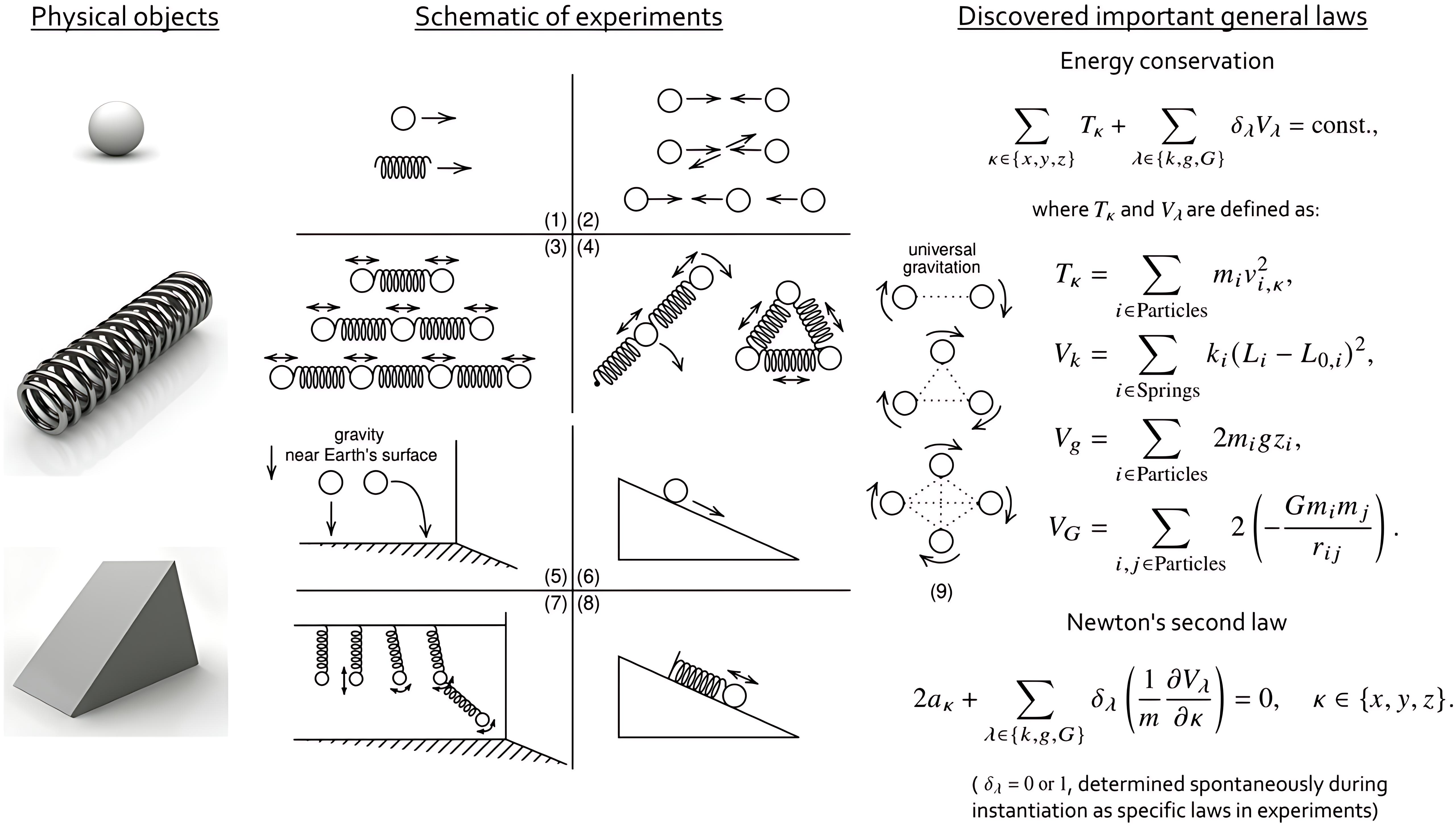
Figure 2: Schematic of tested experiments and main general laws discovered. Some complex configurations are omitted for clarity. See text for details.
Rediscovering Laws of Newtonian Mechanics. — To evaluate AI-Newton’s performance, we apply it to Newtonian mechanics problems, focusing on a set of 46 predefined experiments. These experiments involve three primary types of physical objects: balls (either small balls or celestial bodies), springs, and inclined planes. The experiments are designed to investigate both isolated and coupled systems, as illustrated in Fig. 2, including:
1. Free motion of individual balls and springs;
1. Elastic collision of balls;
1. Coupled systems demonstrating translational vibrations, rotational oscillations, and pendulum-like motions;
1. Gravity-related problems, such as projectile motion and motion on inclined planes, along with complex spring-ball systems;
1. Celestial mechanics problems involving gravitational interactions.
The complexities of experiments are systematically increased by varying the number of physical objects and spatial dimensions, encompassing high-degree-of-freedom problems such as coupled oscillations of chained 2-ball-2-spring systems on inclined planes, rotational dynamics of 4-ball-4-spring systems, and other complex configurations. To simulate realistic experimental conditions, all test data are generated by solving differential equations and incorporating Gaussian-distributed errors. This comprehensive experimental setup covers three types of forces in Newtonian mechanics, elastic forces, gravity near Earth’s surface, and universal gravitational forces, while incorporating realistic measurement uncertainties. In this way, it enables rigorous evaluation of AI-Newton’s capability to discover physical laws from noisy experimental data.
We evaluated the performance of our proof-of-concept implementation on an Intel Xeon Platinum 8370C (128 threads @ 3.500GHz) platform with NVIDIA A40 GPU, configured with 64 cores for parallel processing. With max trials set to 1200 and an average runtime of 48 hours, the system demonstrated robust knowledge discovery capabilities, identifying approximately 90 physical concepts and 50 general laws on average across the test cases. The discoveries include significant general laws such as energy conservation and Newton’s second law along with their relevant concepts, as shown in Fig. 2, providing complete explanatory for all experiments covering systems from simple to high-degree-of-freedom complex configurations.
<details>
<summary>knowledge_progression.png Details</summary>
### Visual Description
## Horizontal Dot Plot with Error Bars: Concept Acquisition Timeline
### Overview
The image is a horizontal dot plot with error bars, illustrating the approximate number of trials required to acquire or master a series of related concepts. The concepts are listed vertically, and the number of trials is plotted on the horizontal axis. The background is segmented into six vertical, shaded regions labeled with Roman numerals (I-VI), representing distinct trial ranges or stages.
### Components/Axes
* **Vertical Axis (Y-axis):** Labeled **"Concepts"**. It lists 14 distinct concepts, ordered from bottom to top. The concepts are represented by symbols, likely variables from a scientific or mathematical domain:
* `m`, `v`, `k`, `g`, `a`, `T`, `P`, `V_k`, `V_g`, `F_k`, `F_g`, `G, V_G`, `F_G`.
* **Horizontal Axis (X-axis):** Labeled **"Number of trials"**. The scale runs from 0 to approximately 900, with major tick marks at 0, 100, 200, 300, 400, 500, 600, 700, and 800.
* **Data Series:** Each concept has a single data point represented by a black dot (likely the mean or median), with horizontal error bars (likely representing standard deviation, range, or confidence interval).
* **Background Regions (Stages):** The plot area is divided into six vertical bands of varying green shades, labeled with large, faint Roman numerals:
* **I:** Darkest green, spanning approximately 0 to 150 trials.
* **II:** Medium-dark green, spanning approximately 150 to 200 trials.
* **III:** Medium green, spanning approximately 200 to 275 trials.
* **IV:** Light-medium green, spanning approximately 275 to 450 trials.
* **V:** Light green, spanning approximately 450 to 650 trials.
* **VI:** Lightest green, spanning approximately 650 to 900 trials.
### Detailed Analysis
The following table reconstructs the approximate data points and their associated error ranges, read from the chart. Values are estimated based on visual alignment with the x-axis.
| Concept | Approx. Mean Trials | Approx. Error Bar Range (Min to Max) | Visual Trend & Stage |
| :--- | :--- | :--- | :--- |
| **m** | 50 | 0 to 100 | Lowest trial count. Within Stage I. |
| **v** | 70 | 30 to 110 | Slightly higher than `m`. Within Stage I. |
| **k** | 80 | 40 to 120 | Slightly higher than `v`. Within Stage I. |
| **g** | 220 | 150 to 300 | Significant jump. Spans Stages II and III. |
| **a** | 250 | 200 to 300 | Slightly higher than `g`. Within Stage III. |
| **T** | 300 | 280 to 320 | Narrow error bar, indicating consistency. At the boundary of Stages III and IV. |
| **P** | 350 | 280 to 420 | Wider error bar. Within Stage IV. |
| **V_k** | 400 | 300 to 480 | Within Stage IV. |
| **V_g** | 420 | 320 to 480 | Slightly higher than `V_k`. Within Stage IV. |
| **F_k** | 450 | 400 to 500 | At the boundary of Stages IV and V. |
| **F_g** | 500 | 420 to 580 | Within Stage V. |
| **G, V_G** | 750 | 650 to 850 | Large jump. Two concepts grouped together. Within Stage VI. |
| **F_G** | 800 | 700 to 900 | Highest trial count. Within Stage VI. |
**Trend Verification:** There is a clear, positive correlation between the vertical position of the concept (from `m` to `F_G`) and the number of trials required. The line formed by the data points slopes consistently upward from left to right.
### Key Observations
1. **Hierarchical Learning:** The concepts appear to be ordered in a hierarchy of increasing complexity or dependency. Foundational concepts (`m`, `v`, `k`) require the fewest trials (<100), while the most advanced concepts (`G, V_G`, `F_G`) require the most (>700).
2. **Stage Grouping:** The Roman numeral stages group concepts by trial ranges. Stage I contains the three simplest concepts. Stages IV and V contain the bulk of the intermediate concepts. Stage VI contains only the two most complex entries.
3. **Variable Precision:** The width of the error bars varies significantly. Concepts like `T` have very narrow bars, suggesting highly consistent acquisition times. Concepts like `g`, `P`, and `F_g` have wide bars, indicating high variability in the number of trials needed.
4. **Concept Grouping:** The label `G, V_G` indicates that these two concepts are either learned simultaneously or are so closely related that they are measured as a single unit in this analysis.
### Interpretation
This chart visualizes a **learning or skill acquisition timeline** for a set of interrelated concepts, likely from a domain like physics (given symbols for mass, velocity, gravity, force, etc.). The data suggests a structured, sequential learning path:
* **Foundation (Stage I):** Basic parameters (`m`, `v`, `k`) are acquired quickly and with relatively low variability.
* **Intermediate Development (Stages II-V):** More complex relationships and derived quantities (`g`, `a`, `T`, `P`, various `V` and `F` terms) require progressively more trials. The increasing width of some error bars here may reflect individual differences in learning these more abstract concepts.
* **Advanced Mastery (Stage VI):** The most complex, possibly integrative concepts (`G, V_G`, `F_G`) represent a significant leap in difficulty, requiring an order of magnitude more trials than the foundational concepts. The grouping of `G` and `V_G` hints at a strong conceptual link, perhaps representing a unified principle (like gravitational potential and its associated vector).
The overarching narrative is one of **cumulative complexity**. Mastery of later concepts is likely dependent on the solid acquisition of earlier ones, explaining the steep, non-linear increase in trials. The stages (I-VI) may correspond to formal levels of education, training modules, or natural breakpoints in the learning process. The chart effectively argues that advanced expertise in this domain is not just marginally harder, but requires a vastly greater investment of practice or exposure.
</details>
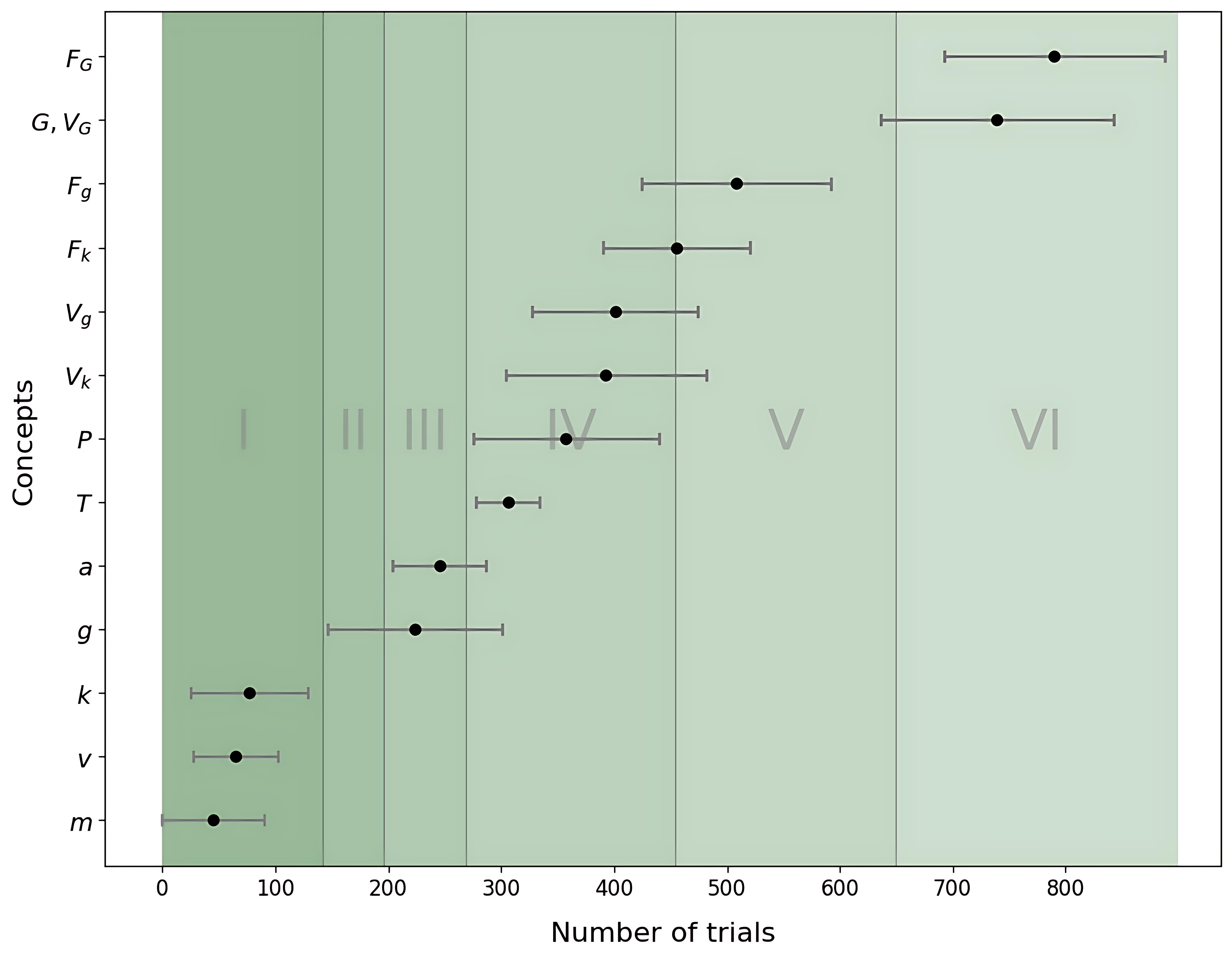
Figure 3: Statistical analysis of concept discovery timing on 10 test cases, recording the mean and standard deviation of discovery timings for key concepts. Number of trials means the number of analysis trial attempt has been done, not distinguishing which experiment. Roman numerals (I, II, …) in the background indicate the eras defined by the era-control strategy.
Statistical discovery progression on 10 test cases is illustrated in Fig. 3, showing the timing distribution of important concept discoveries. This discovery progression exhibits an incremental pattern, where AI-Newton first explores simple concepts (e.g., mass) before advancing to more complex ones (e.g., force). For instance, gravitational acceleration $g$ is defined as a constant by analyzing free-fall or projectile motion, where the vertical acceleration $a_{z}$ of the ball is invariant. In experiments with elastic collisions between balls, conservation of kinetic energy $T$ is discovered and proposed as a general law. Through plausible reasoning, elastic potential energy $V_{k}$ , gravitational potential energy near Earth’s surface $V_{g}$ , and universal gravitational potential energy $V_{G}$ are progressively defined when trying to apply the conservation of kinetic energy to inelastic experiments. These are then incorporated with kinetic energy conservation to ultimately formulate the complete law of energy conservation. The discovery of Newton’s second law follows an analogous progression: it is first proposed in a simple experimental context and then generalized through plausible reasoning.
It is important to emphasize that the system is able to independently discover and unify fundamental concepts from disparate physical contexts. For instance, AI-Newton can derive the concept of ‘mass’ through two distinct experimental routes: from the static elongation of a spring under gravity (defining gravitational mass, $m_{g}$ ) and from the experiment of a horizontal spring-mass oscillation system (defining inertial mass, $m_{i}$ ). Critically, the system then autonomously verify the numerical equivalence of $m_{g}$ and $m_{i}$ , effectively indicating a cornerstone of general relativity—the weak equivalence principle—from raw data alone.
Summary. — We introduce AI-Newton, a novel framework for the autonomous discovery of general physical laws from raw data across a large set of experiments, without supervision or pre-existing physical knowledge. This approach transcends current AI-driven methods, which are limited to extracting specific laws from individual experiments. Our main contributions are based on plausible reasoning, enabling us to: (1) propose physical concepts from the extracted laws; and (2) extend an existing general law by adding new terms, thereby adapting it to describe a wider range of experiments. Introducing interpretable physical concepts allows discovered laws to remain concise, making them more tractable for SR to identify. Furthermore, iteratively constructing general laws from existing ones enables a gradual, scalable discovery process. Applied to a large, noisy dataset of mechanics experiments, AI-Newton successfully rediscovers foundational laws, including Newton’s second law, the conservation of energy, and the law of universal gravitation. This work thus offers a promising pathway toward building AI systems capable of contributing to frontier scientific research.
As a first step, we employ AI-Newton to rediscover known physical laws—a task where direct reliance on large language models (LLMs) is unsuitable, as they already possess this knowledge. In future applications to frontier science, however, the DSL, the recommendation engine and the plausible reasoning components of the framework could be replaced or augmented by LLMs. This integration would grant the system direct access to all existing knowledge, enabling a more informed and efficient discovery process.
Acknowledgements. We would like to thank Hong-Fei Zhang for early participant of the project and many valuable discussions. This work is supported by the National Natural Science Foundation of China (No. 12325503), and the High-performance Computing Platform of Peking University.
## References
- [1] Y. Xu, X. Liu, X. Cao, C. Huang, E. Liu, S. Qian, X. Liu, Y. Wu, F. Dong, C.-W. Qiu, et al., Artificial intelligence: A powerful paradigm for scientific research, The Innovation 2 (2021) .
- [2] H. Wang, T. Fu, Y. Du, W. Gao, K. Huang, Z. Liu, P. Chandak, S. Liu, P. Van Katwyk, A. Deac, et al., Scientific discovery in the age of artificial intelligence, Nature 620 (2023) 47–60.
- [3] X. Zhang, L. Wang, J. Helwig, Y. Luo, C. Fu, Y. Xie, M. Liu, Y. Lin, Z. Xu, K. Yan, et al., Artificial intelligence for science in quantum, atomistic, and continuum systems, Foundations and Trends® in Machine Learning 18 (2025) 385–912.
- [4] C. Lu, C. Lu, R. T. Lange, J. Foerster, J. Clune, and D. Ha, The ai scientist: Towards fully automated open-ended scientific discovery, [arXiv:2408.06292].
- [5] C. K. Reddy and P. Shojaee, Towards scientific discovery with generative ai: Progress, opportunities, and challenges, Proceedings of the AAAI Conference on Artificial Intelligence 39 (Apr., 2025) 28601–28609.
- [6] M. Schmidt and H. Lipson, Distilling free-form natural laws from experimental data, science 324 (2009) 81–85.
- [7] S. Brunton, J. Proctor, and J. Kutz, Discovering governing equations from data: Sparse identification of nonlinear dynamical systems, Proceedings of the National Academy of Sciences 113 (09, 2015) 3932–3937.
- [8] K. Champion, B. Lusch, J. N. Kutz, and S. L. Brunton, Data-driven discovery of coordinates and governing equations, Proceedings of the National Academy of Sciences 116 (2019) 22445–22451.
- [9] T. Wu and M. Tegmark, Toward an artificial intelligence physicist for unsupervised learning, Physical Review E 100 (2019) 033311.
- [10] S. Greydanus, M. Dzamba, and J. Yosinski, Hamiltonian neural networks. Curran Associates Inc., Red Hook, NY, USA, 2019.
- [11] M. Cranmer, S. Greydanus, S. Hoyer, P. Battaglia, D. Spergel, and S. Ho, Lagrangian neural networks, [arXiv:2003.04630].
- [12] B. M. De Silva, D. M. Higdon, S. L. Brunton, and J. N. Kutz, Discovery of physics from data: Universal laws and discrepancies, Frontiers in artificial intelligence 3 (2020) 25.
- [13] Z. Liu and M. Tegmark, Machine learning conservation laws from trajectories, Physical Review Letters 126 (2021) 180604.
- [14] G. E. Karniadakis, I. G. Kevrekidis, L. Lu, P. Perdikaris, S. Wang, and L. Yang, Physics-informed machine learning, Nature Reviews Physics 3 (2021) 422–440.
- [15] Z. Liu, V. Madhavan, and M. Tegmark, Machine learning conservation laws from differential equations, Physical Review E 106 (2022) 045307.
- [16] G. Camps-Valls, A. Gerhardus, U. Ninad, G. Varando, G. Martius, E. Balaguer-Ballester, R. Vinuesa, E. Diaz, L. Zanna, and J. Runge, Discovering causal relations and equations from data, Physics Reports 1044 (2023) 1–68.
- [17] C. Cornelio, S. Dash, V. Austel, T. R. Josephson, J. Goncalves, K. L. Clarkson, N. Megiddo, B. El Khadir, and L. Horesh, Combining data and theory for derivable scientific discovery with ai-descartes, Nature Communications 14 (2023) 1777.
- [18] P. Lemos, N. Jeffrey, M. Cranmer, S. Ho, and P. Battaglia, Rediscovering orbital mechanics with machine learning, Machine Learning: Science and Technology 4 (2023) 045002.
- [19] Z. Liu, P. O. Sturm, S. Bharadwaj, S. J. Silva, and M. Tegmark, Interpretable conservation laws as sparse invariants, Phys. Rev. E 109 (Feb, 2024) L023301.
- [20] R. Cory-Wright, C. Cornelio, S. Dash, B. El Khadir, and L. Horesh, Evolving scientific discovery by unifying data and background knowledge with ai hilbert, Nature Communications 15 (2024) 5922.
- [21] D. Zheng, V. Luo, J. Wu, and J. B. Tenenbaum, Unsupervised learning of latent physical properties using perception-prediction networks, [arXiv:1807.09244].
- [22] M. Tegmark, Latent Representations of Dynamical Systems: When Two is Better Than One, [arXiv:1902.03364].
- [23] R. Iten, T. Metger, H. Wilming, L. Del Rio, and R. Renner, Discovering physical concepts with neural networks, Physical review letters 124 (2020) 010508.
- [24] B. Chen, K. Huang, S. Raghupathi, I. Chandratreya, Q. Du, and H. Lipson, Automated discovery of fundamental variables hidden in experimental data, Nature Computational Science 2 (2022) 433–442.
- [25] Q. Li, T. Wang, V. Roychowdhury, and M. K. Jawed, Metalearning generalizable dynamics from trajectories, Physical Review Letters 131 (2023) 067301.
- [26] S.-M. Udrescu and M. Tegmark, Ai feynman: A physics-inspired method for symbolic regression, Science Advances 6 (2020) eaay2631.
- [27] S.-M. Udrescu, A. Tan, J. Feng, O. Neto, T. Wu, and M. Tegmark, Ai feynman 2.0: Pareto-optimal symbolic regression exploiting graph modularity, Advances in Neural Information Processing Systems 33 (2020) 4860–4871.
- [28] T. Bendinelli, L. Biggio, and P.-A. Kamienny, Controllable neural symbolic regression, in International Conference on Machine Learning, pp. 2063–2077, PMLR. 2023.
- [29] W. Tenachi, R. Ibata, and F. I. Diakogiannis, Deep symbolic regression for physics guided by units constraints: toward the automated discovery of physical laws, The Astrophysical Journal 959 (2023) 99.
- [30] Y. Tian, W. Zhou, M. Viscione, H. Dong, D. Kammer, and O. Fink, Interactive symbolic regression with co-design mechanism through offline reinforcement learning, Nature Communications 16 (04, 2025) .
- [31] M. Cranmer, Interpretable machine learning for science with pysr and symbolicregression. jl, [arXiv:2305.01582].
- [32] M. Du, Y. Chen, Z. Wang, L. Nie, and D. Zhang, Large language models for automatic equation discovery of nonlinear dynamics, Physics of Fluids 36 (2024) .
- [33] B. Romera-Paredes, M. Barekatain, A. Novikov, M. Balog, M. P. Kumar, E. Dupont, F. J. Ruiz, J. S. Ellenberg, P. Wang, O. Fawzi, et al., Mathematical discoveries from program search with large language models, Nature 625 (2024) 468–475.
- [34] M. Valipour, B. You, M. Panju, and A. Ghodsi, Symbolicgpt: A generative transformer model for symbolic regression, arXiv:2106.14131 (2021) .
- [35] X. Chu, H. Zhao, E. Xu, H. Qi, M. Chen, and H. Shao, Neural symbolic regression using control variables, [arXiv:2306.04718].
- [36] S. Mežnar, S. Džeroski, and L. Todorovski, Efficient generator of mathematical expressions for symbolic regression, Machine Learning 112 (2023) 4563–4596.
- [37] C. Wang, H. Zhai, and Y.-Z. You, Emergent schrödinger equation in an introspective machine learning architecture, Science Bulletin 64 (2019) 1228–1233.
- [38] B.-B. Li, Y. Gu, and S.-F. Wu, Discover physical concepts and equations with machine learning, [arXiv:2412.12161].
- [39] “See the arXiv supplemental material for details on the domain-specific language, recommendation engine, and computational engine.”.
- [40] G. Pólya, Mathematics and plausible reasoning: Induction and analogy in mathematics, vol. 1. Princeton University Press, 1990.
- [41] G. Pólya, Mathematics and Plausible Reasoning: Patterns of plausible inference, vol. 2. Princeton University Press, 1990.
- [42] T. Lai and H. Robbins, Asymptotically efficient adaptive allocation rules, Adv. Appl. Math. 6 (Mar., 1985) 4–22.
- [43] T. L. Lai, Adaptive treatment allocation and the multi-armed bandit problem, The Annals of Statistics 15 (1987) 1091–1114. http://www.jstor.org/stable/2241818.
- [44] R. Agrawal, Sample mean based index policies by o (log n) regret for the multi-armed bandit problem, Advances in applied probability 27 (1995) 1054–1078.
- [45] M. N. Katehakis and H. Robbins, Sequential choice from several populations., Proceedings of the National Academy of Sciences 92 (1995) 8584–8585.
- [46] P. Auer, Using confidence bounds for exploitation-exploration trade-offs, Journal of Machine Learning Research 3 (2002) 397–422. https://www.jmlr.org/papers/volume3/auer02a/auer02a.pdf.
- [47] K. Pearson, Liii. on lines and planes of closest fit to systems of points in space, The London, Edinburgh, and Dublin Philosophical Magazine and Journal of Science 2 (1901) 559–572.
- [48] L. Wang, Discovering phase transitions with unsupervised learning, Phys. Rev. B 94 (Nov, 2016) 195105.
- [49] H. Kiwata, Deriving the order parameters of a spin-glass model using principal component analysis, Physical Review E 99 (2019) 063304.
- [50] D. Yevick, Conservation laws and spin system modeling through principal component analysis, Computer Physics Communications 262 (2021) 107832.
- [51] F. Boulier, D. Lazard, F. Ollivier, and M. Petitot, Representation for the radical of a finitely generated differential ideal, in Proceedings of the 1995 international symposium on Symbolic and algebraic computation, ISSAC ’95, pp. 158–166. Association for Computing Machinery, New York, NY, USA, 1995.
- [52] F. Boulier, D. Lazard, F. Ollivier, and M. Petitot, Computing representations for radicals of finitely generated differential ideals, Applicable Algebra in Engineering, Communication and Computing 20 (2009) 73–121.
- [53] Maplesoft, Differential algebra in maple, Maplesoft Help Center (2024) . https://cn.maplesoft.com/support/help/Maple/view.aspx?path=DifferentialAlgebra.
- [54] Maplesoft, Maple 2024, 2024. https://www.maplesoft.com/products/maple/.