# SymDQN: Symbolic Knowledge and Reasoning in Neural Network-based Reinforcement Learning
**Authors**:
- Ivo Amador
- Nina Gierasimczuk (Technical University of Denmark)
- ivo.amador@gmail.com, nigi@dtu.dk
## Abstract
We propose a learning architecture that allows symbolic control and guidance in reinforcement learning with deep neural networks. We introduce SymDQN, a novel modular approach that augments the existing Dueling Deep Q-Networks (DuelDQN) architecture with modules based on the neuro-symbolic framework of Logic Tensor Networks (LTNs). The modules guide action policy learning and allow reinforcement learning agents to display behavior consistent with reasoning about the environment. Our experiment is an ablation study performed on the modules. It is conducted in a reinforcement learning environment of a 5x5 grid navigated by an agent that encounters various shapes, each associated with a given reward. The underlying DuelDQN attempts to learn the optimal behavior of the agent in this environment, while the modules facilitate shape recognition and reward prediction. We show that our architecture significantly improves learning, both in terms of performance and the precision of the agent. The modularity of SymDQN allows reflecting on the intricacies and complexities of combining neural and symbolic approaches in reinforcement learning.
## 1 Introduction
Despite its rapidly growing impact on society, Artificial Intelligence technologies are tormented by reliability issues, such as lack of interpretability, propagation of biases, difficulty in generalizing across domains, and susceptibility to adversarial attacks. A possible way towards more interpretable, controlled and guided algorithms leads through the field of neuro-symbolic AI, which explores new ways of integrating symbolic, logic-based knowledge in neural networks (NNs). In particular, the framework of Logic Tensor Networks (LTNs, for short) Serafini and d’Avila Garcez (2016); Badreddine et al. (2022) enhances learning by interpreting first-order logic formulas concretely on data used by NNs algorithms. Such formulas express properties of data and, given a fuzzy semantics, can be integrated into the loss function, thus guiding the learning process.
In this paper, we apply LTNs to a reinforcement learning problem. By integrating LTNs in the training process, our learning agent uses logic to learn the structure of the environment, to predict how different objects in the environment interact with each other, and to guide its actions by performing elementary reasoning about rewards. We investigate how such integration affects learning performance of a robust, established and well-studied framework of Dueling Deep Q-Network (DuelDQN, for short) Wang et al. (2016). The structure of the paper is as follows. In Section 2 we briefly recall Logic Tensor Networks and elements of the underlying Real Logic. In Section 3 we introduce our methodology: the SymDQN architecture and its training process. We follow up with the presentation of the experiment in Section 4. We discuss of the results in Section 5. Section 6 concludes and outlines directions for future work.
#### Related Work
Since its conception, the framework of LTNs has been applied in various domains. In computer vision, LTNs were used to inject prior knowledge about object relationships and properties, improving interpretability and accuracy in object detection Donadello et al. (2017). Their addition to convolutional neural networks improves the robustness on noisy data Manigrasso et al. (2021). They enhance the accuracy in reasoning tasks in open-world and closed-world scenarios Wagner and d’Avila Garcez (2022). In Bianchi and Hitzler (2019), LTNs are leveraged for deductive reasoning tasks. Finally, in learning by reinforcement LTNs were used to integrate prior knowledge into reinforcement learning agents improving both the learning rate and robustness to environmental changes Badreddine and Spranger (2019). The latter work is similar to ours in the choice of tools, but it differs in its methodology. In Badreddine and Spranger (2019), LTN is a separate pre-training module which interacts with DuelDQN only by creating inputs. In contrast, our SymDQN integrates LTN in the training process (making it learn alongside DuelDQN).
Our work uses logic to adjust elements of a reinforcement learning framework. In that, it is related to reward shaping approaches, where the learner is given external symbolic information about the environment, e.g., in the form of linear time logic formulas (also known as restraining bolts) in Giacomo et al. (2019) or of an induced automaton in Furelos-Blanco et al. (2021). In a way, the LTN approach is similar: logical formulas adjust the reinforcement learning process. However, our technique is a more distributed form of reward shaping. First, the formulas of Real Logic are used as guides to obtain a symbolic representation of the environment, then to predict immediate rewards from encountering the objects of the environment. Finally, a logical formula is used to help the learner align the $q$ -values (the agent’s long term policy) with the predicted immediate rewards of symbolically represented objects. In other words, we restrain the reinforcement learner by expecting it to reason about its behavior as it learns, and we investigate the impact of this restriction on learning precision and performance. We will come back to this issue in Section 5.1, after we have detailed all the components.
## 2 Real Logic
Real Logic is the basis of the functioning of LTNs. In this section we provide a rudimentary introduction (for a full exposition consult Badreddine et al. (2022)). Let us start with a simple example.
**Example 1**
*Consider two datasets: a data set of humans (with two features: age and gender), and a dataset of pets (with three features: height, weight and color). Assume that Alice appears in the data set of humans (for instance as a five year old female), and Max and Mittens are listed in a dataset of pets. To be able to talk about Alice, Max and Mittens, we need a logical language that includes constants referring to objects (particular rows of the datasets). Note that such constants can be of different types —in our example humans consists of two, while pets are composed of three features.*
The signature of the language of Real Logic $\mathcal{L}$ contains a set $\mathcal{C}$ of constant symbols, a set $\mathcal{F}$ of function symbols, a set $\mathcal{P}$ of predicate symbols, and a set $\mathcal{X}$ of variable symbols. Let $\mathcal{D}$ be a non-empty set of domain symbols (that represent types). Domain symbols are used by functions $\mathbf{D}$ , $\mathbf{D_{in}}$ , and $\mathbf{D_{out}}$ which for a given element of the signature output its type, in the following way. $\mathbf{D}:\mathcal{X}\cup\mathcal{C}\rightarrow\mathcal{D}$ specifies the types for variables and constants; $\mathbf{D_{in}}:\mathcal{F}\cup\mathcal{P}\rightarrow\mathcal{D}^{\ast}$ specifies the types of the sequence of arguments allowed by function and predicate symbols ( $\mathcal{D}^{\ast}$ stands for the set of all finite sequences of elements from $\mathcal{D}$ ); $\mathbf{D_{out}}:\mathcal{F}\rightarrow\mathcal{D}$ specifies the type of the range of a function symbol.
**Example 2**
*Continuing Example 1, let the language of pet-ownership $\mathcal{L}_{pets}$ have the signature consisting of the set of constants $\mathcal{C}=\{\textsc{Alice},\textsc{Max},\textsc{Mit}\}$ , a set of function symbols $\mathcal{F}=\{\textsc{owner}\}$ , a set of predicate symbols $\mathcal{P}=\{\textsc{isOwner}\}$ , and two variable symbols $\mathcal{X}=\{\textsc{pet},\textsc{person}\}$ . Further, we have two domain symbols, one for the domain of humans and one for pets, $\mathcal{D}=\{H,P\}$ . Then, our domain functions can be defined in the following way. $\mathbf{D}(\textsc{Alice})=H$ (Alice is a constant of type $H$ ), $\mathbf{D}(\textsc{Max})=\mathbf{D}(\textsc{Mit})=P$ (Max and Mittens are of type $P$ ). Further, each dataset will have its own variable: $\mathbf{D}(\textsc{pet})=P$ , $\mathbf{D}(\textsc{person})=H$ . We also need to specify inputs for predicates: $\mathbf{D_{in}}(\textsc{isOwner})=HP$ (isOwner is a predicate taking two arguments, a human and a pet). Finally, for functions, we need both the input and the output types: $\mathbf{D_{in}}(\textsc{owner})=P$ , and $\mathbf{D_{out}}(\textsc{owner})=H$ (owner takes as input a pet and outputs the human who owns it).*
The language of Real Logic corresponds to first-order logic, and so it allows for more complex expressions. The set of terms consists of constants, variables, and function symbols and is defined in the following way: each $t\in X\cup C$ is a term of domain $\mathbf{D}(t)$ ; if $t_{1},\ldots,t_{n}$ are terms, then $t_{1}\ldots t_{n}$ is a term of the domain $\mathbf{D}(t_{1})...\mathbf{D}(t_{n})$ ; if $t$ is a term of the domain $\mathbf{D_{in}}(f)$ , then $f(t)$ is a term of the domain $\mathbf{D_{out}}(f)$ . Finally, the formulae of Real Logic are as follows: $t_{1}=t_{2}$ is an atomic formula for any terms $t_{1}$ and $t_{2}$ with $\mathbf{D}(t_{1})=\mathbf{D}(t_{2})$ ; $P(t)$ is an atomic formula if $\mathbf{D}(t)=\mathbf{D_{in}}(P)$ ; if $\varphi$ and $\psi$ are formulae and $x_{1},\ldots,x_{n}$ are variable symbols, then $\neg\varphi$ , $\varphi\wedge\psi$ , $\varphi\vee\psi$ , $\varphi\rightarrow\psi$ , $\varphi\leftrightarrow\psi$ , $\forall x_{1}\ldots x_{n}\varphi$ and $\exists x_{1}\ldots x_{n}\varphi$ are formulae.
Let us turn to the semantics of Real Logic. Domain symbols allow grounding the logic in numerical, data-driven representations—to be precise, Real Logic is grounded in tensors in the field of real numbers. Tensor grounding is the key concept that allows the interplay of Real Logic with Neural Networks. It refers to the process of mapping high-level symbols to tensor representations, allowing integration of reasoning and differentiable functions. A grounding $\mathcal{G}$ assigns to each domain symbol $D\in\mathcal{D}$ a set of tensors $\mathcal{G}(D)\subseteq\bigcup_{n_{1}\ldots n_{d}\in\mathbb{N}^{\ast}}\mathbb{ R}^{n_{1}\times\ldots\times n_{d}}$ . For every $D_{1}\ldots D_{n}\in\mathcal{D}^{\ast}$ , $\mathcal{G}(D_{1}\ldots D_{n})=\mathcal{G}(D_{1})\times\ldots\times\mathcal{G} (D_{n})$ . Given a language $\mathcal{L}$ , a grounding $\mathcal{G}$ of $\mathcal{L}$ assigns to each constant symbol $c$ , a tensor $\mathcal{G}(c)$ in the domain $\mathcal{G}(\mathbf{D}(c))$ ; to a variable $x$ it assigns a finite sequence of tensors $d_{1}\ldots d_{k}$ , each in $\mathcal{G}(\mathbf{D}(x))$ , representing the instances of $x$ ; to a function symbol $f$ it assigns a function taking tensors from $\mathcal{G}(\mathbf{D_{in}}(f))$ as input, and producing a tensor in $\mathcal{G}(\mathbf{D_{out}}(f))$ as output; to a predicate symbol $P$ it assigns a function taking tensors from $\mathcal{G}(\mathbf{D_{in}}(P))$ as input, and producing a truth-degree in the interval $[0,1]$ as output.
In other words, $\mathcal{G}$ assigns to a variable a concatenation of instances in the domain of the variable. The treatment of free variables in Real Logic is analogous, departing from the usual interpretation of free variables in FOL. Thus, the application of functions and predicates to terms with free variables results in point-wise application of the function or predicate to the string representing all instances of the variable (see p. 5 of Badreddine et al. (2022) for examples). Semantically, logical connectives are fuzzy operators applied recursively to the suitable subformulas: conjunction is a t-norm, disjunction is a t-conorm, and for implication and negation—its fuzzy correspondents. The semantics for formulae with quantifiers ( $\forall$ and $\exists$ ) is given by symmetric and continuous aggregation operators $Agg:\bigcup_{n\in N}[0,1]^{n}\rightarrow[0,1]$ . Intuitively, quantifiers reduce the dimensions associated with the quantified variables.
**Example 3**
*Continuing our running example, we could enrich our signature with predicates $Dog$ and $Cat$ . Then, $Dog(Max)$ might return $0.8$ , while $Dog(Mit)$ might return $0.3$ , indicating that Max is likely a dog, while Mittens is not. In practice, the truth degrees for these atomic formulas could be obtained for example by a Multi-layer Perceptron (MLP), followed by a sigmoid function, taking the object’s features as input and returning a value in $[0,1]$ . For a new function symbol $age$ , $age(Max)$ could be an MLP, taking Max’s features, and outputting a scalar representing Max’s age. An example of a formula could be $Dog(Max)\vee Cat(Max)$ , which could return $0.95$ indicating that Max is almost certainly either a dog or a cat. A formula with a universal quantifier could be used to express that Alice owns all of the cats $\forall pet(Cat(pet)\rightarrow isOwner(Alice,pet))$ .*
Real Logic allows some flexibility in the choice of appropriate fuzzy operators for the semantics of connectives and quantifiers. However, note that not all fuzzy operators are suitable for differentiable learning van Krieken et al. (2022). In Appendix B of Badreddine et al. (2022), the authors discuss some particularly suitable fuzzy operators. In this work, we follow their recommendation and adopt the Product Real Logic semantics (product t-norm for conjunction, standard negation, the Reichenbach implication, p-mean for the existential, and p-mean error for the universal quantifier).
LTNs make use of Real Logic—they learns parameters that maximize the aggregated satisfiability of the formulas in the so-called knowledge base containing formulas of Real Logic. The framework is the basis of the PyTorch implementation of the LTN framework, known as LTNtorch library Carraro (2022). In our experiments we make substantial use of that tool.
## 3 Methodology
### 3.1 The game
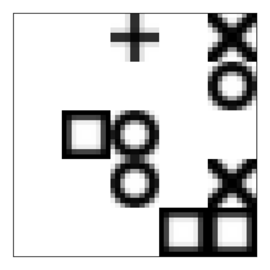
The environment used for the experiments was a custom Gymnasium Towers et al. (2024) environment ShapesGridEnv designed for the experiments in Badreddine and Spranger (2019), see Fig. 1. The game is played on an image showing a 5x5 grid with cells occupied by one agent, represented by the symbol ‘+’, and a number of other objects: circles, squares, and crosses. The agent moves across the board (up, right, down, left) and when it enters a space occupied by an object, it ‘consumes’ that object. Each object shape is associated with a reward. The agent’s goal is to maximize its cumulative reward throughout an episode. An episode terminates when either all shapes with positive reward have been consumed, or when a predefined number of steps has been reached.
<details>
<summary>extracted/6333762/fig-env.png Details</summary>
### Visual Description
## Diagram: 3x3 Grid Pattern Analysis
### Overview
The image displays a 3x3 grid containing various geometric symbols. The grid is not explicitly drawn with lines, but the arrangement of the symbols implies a matrix structure. The symbols are monochromatic (black on white) and appear to be pixelated or low-resolution icons.
### Components/Axes
The image is a 3x3 matrix. We can define the positions using (Row, Column) coordinates, where (1,1) is top-left and (3,3) is bottom-right.
* **Grid Structure:** 3 rows, 3 columns.
* **Symbols Used:**
* **Plus Sign (+):** A cross shape.
* **X:** A diagonal cross.
* **Square:** A hollow box.
* **Circle:** A hollow ring.
* **Empty:** No symbol present.
### Detailed Analysis
The following table maps the symbols to their respective positions in the 3x3 grid:
| | Column 1 | Column 2 | Column 3 |
| :--- | :--- | :--- | :--- |
| **Row 1** | [Empty] | Plus Sign (+) | X |
| **Row 2** | Square | Circle | Circle |
| **Row 3** | [Empty] | Square | X |
* **Row 1:** The first cell is empty. The second cell contains a plus sign. The third cell contains an X.
</details>
Figure 1: ShapesGridEnv environment
We chose this environment because of its simplicity, and because it allows comparing our setting with that of Badreddine and Spranger (2019). The environment is very flexible in its parameters: density (the minimum and maximum amount of shapes initiated, in our case max is $18$ ), rewards (in our case the reward for a cross is +1, for a circle is -1 and for a square is 0), colors (in our case the background is white and objects are black), episode maximum length (for us it is 50). Altering the environment configurations allows investigating the adaptability of the learner in Badreddine and Spranger (2019).
### 3.2 The Model
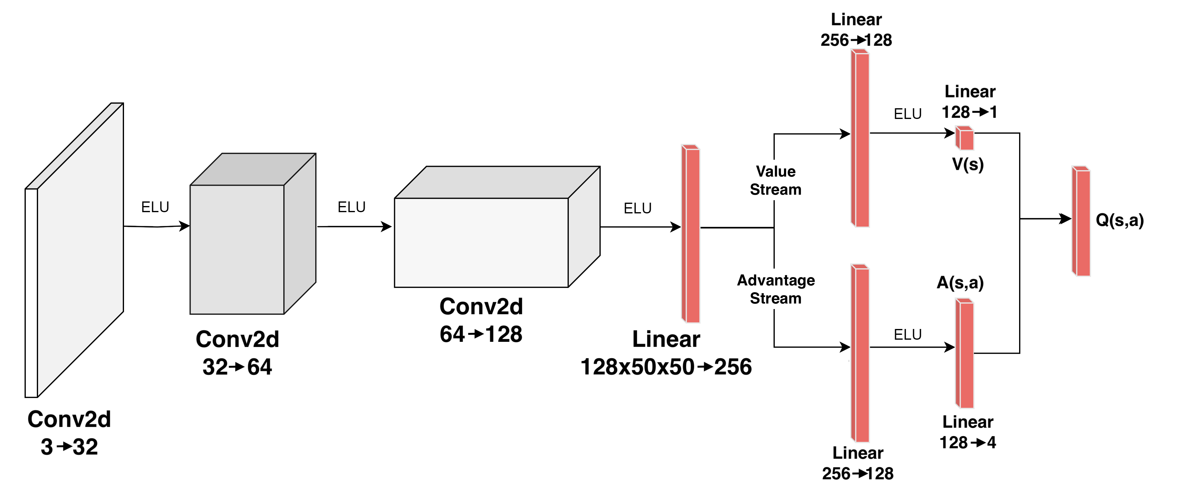
A suitable approach to learning to play such a game could be the existing Dueling Deep Q-Network (DuelDQN) Wang et al. (2015). The architecture is composed of several convolutional layers, which extract relevant features from the raw image input, and then pass them to the two main components, a Value Stream and an Advantage Stream (see Fig. 2). The Value Stream estimates how good it is for the agent to be in the given state, while the Advantage Stream estimates how good it is to perform each action in that given state. The two streams are then combined to calculate the final output.
<details>
<summary>extracted/6333762/dueldqn_parameters.png Details</summary>
### Visual Description
## Diagram: Dueling Deep Q-Network (Dueling DQN) Architecture
### Overview
The image illustrates the architectural flow of a Dueling Deep Q-Network (Dueling DQN), a type of reinforcement learning model. The diagram depicts a sequential processing pipeline that begins with an input layer, proceeds through three convolutional layers, flattens the data, and then bifurcates into two distinct processing streams—the "Value Stream" and the "Advantage Stream"—before merging into a final output layer representing the Q-value.
### Components/Axes
The diagram is structured as a left-to-right flow chart.
* **Input/Convolutional Layers:** Represented by 3D blocks of varying sizes.
* **Activation Functions:** Labeled as "ELU" (Exponential Linear Unit) on the arrows connecting the layers.
* **Linear/Fully Connected Layers:** Represented by vertical red bars.
* **Streams:** Two parallel paths labeled "Value Stream" and "Advantage Stream."
* **Output:** The final node labeled "Q(s,a)."
### Detailed Analysis
#### Region 1: Convolutional Feature Extraction (Left)
* **Input Layer:** Labeled "Conv2d 3→32". This is a flat rectangle, suggesting an input image with 3 channels (likely RGB).
* **Transition:** An arrow labeled "ELU" connects the input to the next layer.
* **Second Layer:** Labeled "Conv2d 32→64". Represented as a 3D block.
* **Transition:** An arrow labeled "ELU" connects this to the next layer.
* **Third Layer:** Labeled "Conv2d 64→128". Represented as a larger 3D block.
* **Transition:** An arrow labeled "ELU" connects this to the flattening layer.
#### Region 2: Flattening and Bifurcation (Center)
* **Flattening Layer:** Labeled "Linear 128x50x50→256". This is a tall, thin red vertical bar, indicating the transition from 3D feature maps to a 1D vector.
* **Split:** The flow branches into two parallel paths:
* **Top Path (Value Stream):**
* "Linear 256→128": A vertical red bar.
* "ELU": Activation function.
* "Linear 128→1": A vertical red bar.
* **Output:** "V(s)" (State Value).
* **Bottom Path (Advantage Stream):**
* "Linear 256→128": A vertical red bar.
* "ELU": Activation function.
* "Linear 128→4": A vertical red bar.
* **Output:** "A(s,a)" (Action Advantage).
#### Region 3: Output Integration (Right)
* **Final Merge:** The outputs from the Value Stream (V(s)) and the Advantage Stream (A(s,a)) converge into a final vertical red bar.
* **Final Output:** Labeled "Q(s,a)".
### Key Observations
* **Activation Consistency:** The diagram explicitly uses "ELU" (Exponential Linear Unit) as the activation function between every major layer transition.
* **Dimensionality:** The "Linear 128x50x50→256" label indicates that the feature map entering the fully connected layers has a spatial resolution of 50x50 with 128 channels.
* **Action Space:** The "Linear 128→4" in the Advantage Stream indicates that the environment has a discrete action space of 4 possible actions.
* **Value vs. Advantage:** The Value Stream outputs a single scalar (1), representing the value of the state, while the Advantage Stream outputs a vector of size 4, representing the relative advantage of each action.
### Interpretation
This diagram represents a **Dueling DQN architecture**, which is designed to improve the stability and efficiency of reinforcement learning agents.
* **Why it matters:** In standard DQN architectures, the network estimates the Q-value for every action directly. However, in many states, the choice of action does not significantly impact the outcome. The Dueling architecture addresses this by decoupling the estimation of the state value (V(s))—how good it is to be in a particular state—from the advantage of each action (A(s,a))—how much better one action is compared to others in that state.
* **Peircean Investigative Insight:** The "4" in the Advantage Stream is the most critical variable for the environment's complexity; it implies the agent is navigating a 4-action environment (e.g., Up, Down, Left, Right). The "1" in the Value Stream confirms that the state value is a single scalar, which is then combined with the advantage vector to produce the final Q-values. The use of ELU suggests a preference for handling negative inputs more gracefully than standard ReLU, which is common in deep reinforcement learning to prevent "dying neurons."
</details>
Figure 2: Network Architecture of DuelDQN, with the convolutional layers in white, and the dense layers in red
The DuelDQN architecture will be our starting point. We will extend it with new symbolic, cognitively-motivated components:
- shape recognition (ShapeRecognizer),
- reward prediction (RewardPredictor),
- action reasoning (ActionReasoner), and
- action filtering (ActionFilter).
In the following, we will discuss each component in more detail.
#### ShapeRecognizer
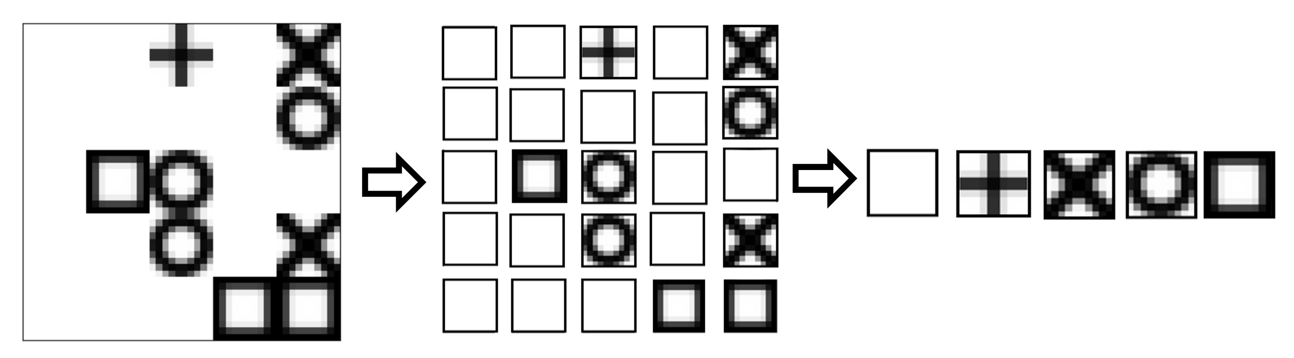
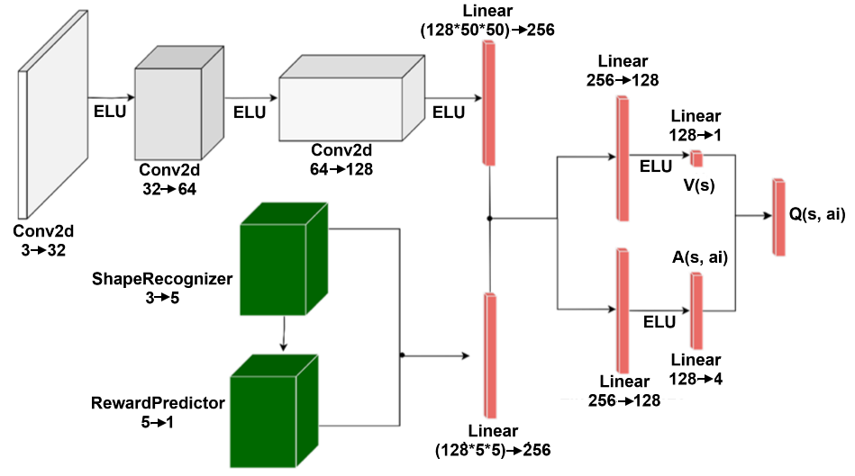
The function of ShapeRecognizer is to estimate the likelihood of a certain observation to be of a given unique kind. ShapeRecognizer is comprised of one pre-processing function, which divides the initial raw image into 25 patches. Each patch is then processed by a Convolutional Neural Network (CNN), which then outputs a 5-dimensional tensor.
The numbers chosen for the number of patches and the output dimension are an instance of soft knowledge injection, as the environment represents a 5x5 grid, and dividing it into 25 patches immediately separates the content of each cell in the grid. As for the output size, 5 is the number of different objects that each patch might contain: empty, agent, circle, cross, square. This allows the agent to perform a multi-label classification on each object type. The theoretical intention of this module is to give the agent a possibility of symbolic understanding of the different entities in the environment, by labeling their types.
Given the simple nature of the ShapesGridEnv, representing the environment is very easy. The state is composed of $25$ positions, with each position being occupied by one of five shapes (empty, agent, circle, square, cross), which results in the state space of size $25^{5}$ . To generate this representation, we start by instantiating five one-hot representations of the classes, which are stored in the LTN Variable $shape\_types$ . Then, for each state that the agent is in, it keeps in memory all the different patches that it has seen and a list of all the patches that are present in the current state.
<details>
<summary>extracted/6333762/unique_patch.png Details</summary>
### Visual Description
## Diagram: Symbol Sorting and Categorization Process
### Overview
The image illustrates a three-stage process involving a 5x5 grid of symbols. The process begins with an unsorted 5x5 grid of mixed symbols, transitions to a 5x5 grid where the symbols are organized or grouped, and concludes with a 1x5 row that acts as a legend or summary of the unique symbol types present in the grids.
### Components/Axes
* **Left Grid (Input):** A 5x5 matrix containing a mix of four distinct symbols and empty cells.
* **Middle Grid (Processed):** A 5x5 matrix containing the same symbols as the left grid, but rearranged into a structured, grouped format.
* **Right Row (Legend/Summary):** A 1x5 horizontal sequence displaying the unique symbols found in the grids, ordered from left to right: [Empty Square, Plus, Cross, Circle, Filled Square].
* **Arrows:** Two large arrows pointing from left to right, indicating the flow of the transformation process.
### Detailed Analysis
#### 1. Left Grid (Input)
The grid contains 25 cells. The distribution of symbols is as follows:
* **Plus (+):** 1 instance (Row 1, Column 3)
* **Cross (X):** 3 instances (Row 1, Column 5; Row 2, Column 5; Row 4, Column 5)
* **Circle (O):** [Description truncated in source]
</details>
Figure 3: The process of obtaining unique labels
Once the variables have been set up, the ShapeRecognizer module can be used to estimate the likelihood of a grid cell containing a given unique shape. To guide its learning, the aggregated satisfiability of three axioms is maximized. The axioms represent the first instance of actual knowledge injection in the system:
$$
\forall s\ \exists l\ IS(s,l)
$$
$$
\neg\exists s\ l_{1}\ l_{2}\ (IS(s,l_{1})\wedge IS(s,l_{2})\wedge(l_{1}\neq l_
{2}))
$$
$$
\forall s_{1}\ s_{2}\ l\ ((IS(s_{1},l)\wedge(s_{1}\neq s_{2}))\rightarrow\neg
IS
(s_{2},l)
$$
In the above formulas, $s$ stands for a shape, $l$ stands for a label and $IS(x,y)$ stands for $x$ has label $y$ . A1 says that every shape has a label; A2 says that no shape has two different labels; A3 says that different shapes cannot have the same label. At each step of every episode, the aggregated satisfaction (truth) degree of these axioms is calculated, and its inverse, $1-AggSat(A1,A2,A3)$ , is used as a loss to train the agent.
Intuitively, ShapeRecognizer gives the learner a way to distinguish between different shapes. In that, our approach is somewhat similar to the framework of semi-supervised symbol grounding Umili et al. (2023).
#### RewardPredictor
Once the environment is symbolically represented, we will make the agent understand the properties of different objects and their dynamics. The only truly dynamic element in the environment is the agent itself—nothing else moves. The agent can move to a cell that was previously occupied by a different shape, which results in the shape being consumed, and the agent being rewarded with the value of the respective shape. Hence, there are three key pieces of knowledge that the learner must acquire to successfully navigate the environment. It must identify which shape represents the agent, it must understand how each action influences the future position of the agent, and it must associate each shape with its respective reward.
The task of self-recognition can be approached in numerous ways, depending on the information we have about the environment, and on our understanding of its dynamics. In our approach, leveraging the ShapeRecognizer, in each episode we count the occurrences of each shape in the environment and add it to a variable that keeps track of this shape’s count over time. The agent is the only shape that has a constant, and equal to one, number of appearances in the environment. This approach is enough to quickly determine with confidence which shape represents the agent. This step demonstrates a specific advantage of using the neuro-symbolic framework. Our reinforcement learning agent is now equipped with memory of the previous states of the environment (i.e., the count of shapes) which can then be used to make decisions or to further process symbolic knowledge.
Understanding the impact of different actions is crucial for the agent to make informed decisions in the environment. Each action represents a direction (up, right, down, left) and taking the action will lead to one of two outcomes. If the agent is at the edge of the environment and attempts to move against the edge, it will remain in the same cell, otherwise, the agent will move one cell in the given direction. Given the simplicity of this dynamics, a function has been defined that takes as input a position and an action, outputting the resulting position.
Our RewardPredictor is a Multi-layer Perceptron (MLP), which takes as input a ShapeRecognizer ’s prediction and outputs one scalar. The main intention of this module is to train to predict the reward associated with each object shape, using the symbolic representations generated by the ShapeRecognizer paired with high-level reasoning on the training procedure. This module intends to give the agent a way of knowing on a high level the reward associated with any shape, and consequently with any action.
In reinforcement learning environments, agents learn action policies by maximizing their expected rewards. When building an agent that symbolically represents and reasons about the environment, one of the key elements is the agent’s ability to understand how to obtain rewards. Given that the agent has the capability of identifying the shapes in the grid, recognizing its own shape, and calculating the position it will take given an action, it can now determine the shape that will be consumed by that action. By using the RewardPredictor module and passing it this shape, the agent obtains a prediction of the reward associated with that shape. Over time, by calculating the loss between that prediction and the actual reward obtained after taking an action, the module learns to accurately predict the reward associated with every shape.
#### ActionReasoner
Once the agent can predict the expected reward of its own actions, we can then guide its policy learning so that it acts in the way (it expects) will give the highest immediate reward. To achieve this, we specify an axiom to ensure that the $q-$ value outputs of the Q-Network are in alignment with the predicted rewards. To achieve this, the expected reward of all the possible actions is calculated by using the RewardPredictor and the $q-$ values are calculated by calling the SymDQN. Our axiom expresses the following condition: if the reward prediction of action $a_{1}$ is higher than the reward prediction of action $a_{2}$ , then the $q-$ value of $a_{1}$ must also be higher than the $q-$ value of $a_{2}$ . The learning is then guided by the LTN framework with the following formula of Real Logic used in the loss function.
$$
\forall\ \textup{Diag}((r_{1},q_{1}),(r_{2},q_{2}))(r_{1}>r_{2}):(q_{1}>q_{2})
$$
Two standard operators of Real Logic Badreddine et al. (2022) are applied in this axiom: $Diag$ and guarded quantification with the condition $(r_{1}>r_{2})$ . Firstly, the $Diag$ operator restricts the range of the quantifier, which will then not run through all the pairs from $\{r_{1},r_{2},q_{1},q_{2}\}$ , but only the pairs of (reward, $q$ -value) that correspond to the same actions. Specifically, when $r_{1}$ corresponds to the predicted reward of action ‘up’, then $q_{1}$ corresponds to $q$ -value of action ‘up’. Secondly, we use guarded quantification, restricting the range of the quantifier to only those cases in which $(r_{1}>r_{2})$ . If we had used implication, with the antecedent $(r_{1}>r_{2})$ false, the whole condition would evaluate to true. This is problematic when the majority of pairs do not fulfill the antecedent. In such a case the universal quantifier evaluates to true for most of the instances, even if the important ones, with antecedent true, are false. Guarded quantification gives a satisfaction degree that is much closer to the value we are interested in.
#### ActionFilter
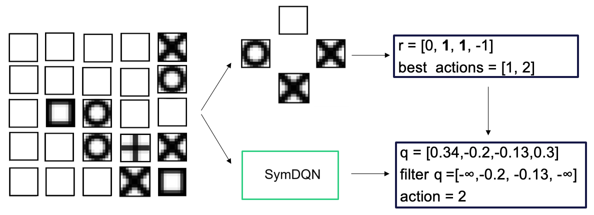
Our learner can now predict the reward for each shape. For each action in a given state, it then knows what shapes could be consumed and what is their corresponding immediate reward. ActionFilter eliminates the actions for which the difference between their reward and the maximum immediately obtainable reward in that state is under a predefined threshold (we set it at 0.5). This allows a balance between the strictness of symbolic selection of immediately best actions and the information about rewards available in the network as a whole. This is represented in Fig. 4.
<details>
<summary>extracted/6333762/fig-action-filter.png Details</summary>
### Visual Description
## Diagram: SymDQN Decision Process
### Overview
The image illustrates a decision-making process within a Reinforcement Learning (RL) framework, specifically utilizing a "SymDQN" (Symmetry-aware Deep Q-Network) approach. The diagram depicts a state-space representation (a 5x5 grid), a set of potential action outcomes (a diamond-shaped icon cluster), and the mathematical filtering process used to select the optimal action based on rewards and Q-values.
### Components/Axes
* **Left Region (Grid World):** A 5x5 grid containing various symbols.
* The grid contains empty squares, circles, crosses (X), and a plus sign.
* A specific cell at row 3, column 2 is highlighted with a thicker border, likely representing the current agent position.
* **Center Region (Action Outcomes):** A diamond-shaped cluster of four icons representing the potential next states resulting from four possible actions (Up, Left, Right, Down).
* **Top:** Empty square.
* **Left:** Circle pattern.
* **Right:** X pattern.
* **Bottom:** X pattern.
* **Right Region (Decision Logic):** Two stacked rectangular boxes containing mathematical vectors.
* **Top Box:** Contains reward vector `r` and the identified `best actions`.
* **Bottom Box:** Contains Q-value vector `q`, the `filter q` operation, and the final selected `action`.
* **Connectivity:** Arrows indicate the flow of information from the grid to the action outcomes, and from the action outcomes/SymDQN module to the decision logic boxes.
### Detailed Analysis
#### 1. Grid State
The 5x5 grid serves as the environment state.
* **Agent Position:** Row 3, Column 2 (thick border).
* **Other notable features:**
* Row 1, Col 5: X
* Row 2, Col 5: Circle
* Row 3, Col 3: Circle
* Row 4, Col 3: Circle
* Row 4, Col 4: Plus
* Row 4, Col 5: X
* Row 5, Col 4: X
#### 2. Decision Logic (Right Boxes)
The logic follows a specific filtering process to determine the optimal action:
* **Reward Vector (`r`):** `[0, 1, 1, -1]`
* This vector represents the immediate reward associated with each of the four actions (indices 0, 1, 2, 3).
* **Best Actions:** The indices with the maximum reward (1) are `[1, 2]`.
* **Q-Value Vector (`q`):** `[0.34, -0.2, -0.13, 0.3]`
* This vector represents the predicted future value of taking each action.
* **Filtering Process (`filter q`):**
* The algorithm applies a mask to the Q-values based on the `best actions` identified from the reward vector.
* Indices not in `best actions` (0 and 3) are set to negative infinity (`-∞`).
* Resulting vector: `[-∞, -0.2, -0.13, -∞]`
* **Action Selection:**
* The agent selects the action corresponding to the maximum value in the filtered vector.
* Comparing `-0.2` (index 1) and `-0.13` (index 2), `-0.13` is the higher value.
* **Final Action:** `2`
### Key Observations
* **Symmetry Awareness:** The "SymDQN" label suggests the algorithm is designed to exploit symmetries in the environment. The filtering process effectively restricts the agent's choice to only those actions that yield the maximum immediate reward, regardless of the Q-values of other actions.
* **Logic Flow:** The diagram demonstrates a "constrained optimization" approach. Even though index 0 and index 3 have high Q-values (0.34 and 0.3 respectively), they are ignored because their immediate reward (`r`) is lower than the maximum.
* **Action Selection:** The final selection of `action = 2` is a tie-break between two equally rewarding actions (1 and 2) based on which has the higher Q-value.
### Interpretation
This diagram visualizes how a SymDQN agent prioritizes immediate reward signals to constrain its policy search. By calculating `best actions` based on the reward vector `r` and using that to filter the Q-values, the agent ensures it does not pursue high-Q-value actions that are suboptimal in terms of immediate reward. This is a method to enforce safety or goal-directed behavior in reinforcement learning, ensuring the agent focuses on the most promising immediate paths before considering long-term value estimates.
</details>
Figure 4: The process of action filtering
ActionFilter severely restricts action choice. We prevented it from forcing the outcomes by switching it off during the training period. When the agent is actually running in the environment, the ActionFilter is used to optimize decision making. Further strategies on how this dynamic might be implemented in training must be studied, as we want to maintain the asymptotic optimality of DuelDQNs, while enhancing them with reasoning, when relevant.
With ShapeRecognizer, RewardPredictor, ActionReasoner and ActionFilter integrated with the original DuelDQN, the complete architecture of SymDQN can be seen in Fig. 5.
<details>
<summary>extracted/6333762/SymDQN_arch.png Details</summary>
### Visual Description
## Diagram: Neural Network Architecture (Dueling DQN with Auxiliary Reward Prediction)
### Overview
The image displays a deep reinforcement learning neural network architecture. The diagram is composed of two primary processing streams: a top visual processing pipeline (grey blocks) and a bottom auxiliary task pipeline (green blocks). These streams converge into a Dueling DQN (Deep Q-Network) structure, which splits into Value ($V(s)$) and Advantage ($A(s, ai)$) streams before merging into a final output ($Q(s, ai)$).
### Components/Axes
* **Grey Cubes:** Convolutional layers (`Conv2d`).
* **Green Cubes:** Auxiliary task modules (`ShapeRecognizer`, `RewardPredictor`).
* **Red Bars:** Fully connected (`Linear`) layers.
* **Labels:** `ELU` (Exponential Linear Unit) activation functions.
* **Flow:** The diagram flows from left to right.
### Detailed Analysis
#### 1. Top Branch (Visual Processing Pipeline)
Located in the upper-left to center-left region, this branch processes visual input through a series of convolutional layers:
* **Input:** `Conv2d 3->32` (Grey cube).
* **Activation:** `ELU` (arrow).
* **Layer 2:** `Conv2d 32->64` (Grey cube).
* **Activation:** `ELU` (arrow).
* **Layer 3:** `Conv2d 64->128` (Grey cube).
* **Activation:** `ELU` (arrow).
* **Flattening/Linear:** `Linear (128*50*50)->256` (Tall red bar).
#### 2. Bottom Branch (Auxiliary Task Pipeline)
Located in the lower-left region, this branch processes auxiliary information:
* **Module 1:** `ShapeRecognizer 3->5` (Green cube).
* **Module 2:** `RewardPredictor 5->1` (Green cube).
* **Linear:** `Linear (128*5*5)->256` (Tall red bar, bottom-center).
#### 3. Dueling DQN Structure (Right Side)
The output of the top branch (the first red bar) splits at a junction point (indicated by a dot).
* **Top Path (Value Stream):**
* `Linear 256->128` (Red bar).
* `ELU` (Activation).
* `Linear 128->1` (Small red bar).
* **Output:** `V(s)` (Value of state).
* **Bottom Path (Advantage Stream):**
* `Linear 256->128` (Red bar).
* *Note:* The output from the bottom branch (`Linear (128*5*5)->256`) feeds into this specific `Linear 256->128` layer.
* `ELU` (Activation).
* `Linear 128->4` (Small red bar).
* **Output:** `A(s, ai)` (Advantage of action $i$ in state $s$).
#### 4. Final Output
* The `V(s)` and `A(s, ai)` streams merge into a final node: `Q(s, ai)` (Red bar, far right).
### Key Observations
* **Architecture Type:** This is a Dueling DQN architecture, which is designed to decouple the estimation of the state value ($V$) and the advantage of each action ($A$).
* **Auxiliary Task:** The inclusion of the `ShapeRecognizer` and `RewardPredictor` (green blocks) suggests this model uses auxiliary tasks to improve feature representation learning, likely to speed up convergence or improve sample efficiency.
* **Data Flow:** The auxiliary task (RewardPredictor) is injected into the Advantage stream, suggesting the auxiliary information is specifically used to help the model distinguish between the relative benefits of different actions.
### Interpretation
This diagram represents a sophisticated reinforcement learning agent. By separating the network into a visual encoder (top) and an auxiliary task (bottom), the model learns a more robust representation of the environment.
The "Dueling" aspect is critical: by splitting the final layers into $V(s)$ and $A(s, ai)$, the network can learn which states are valuable without needing to learn the effect of each action for every state. This is particularly useful in environments where many actions have the same effect, or where the value of the state is independent of the actions taken. The auxiliary `RewardPredictor` likely acts as a regularizer or a feature-enhancer, forcing the network to learn features that are predictive of rewards, which helps the agent focus on relevant visual information.
</details>
Figure 5: SymDQN network architecture integrating DuelDQN with ShapeRecognizer and RewardPredictor modules
## 4 The experiment
By comparing the baseline DuelDQN model with our SymDQN model, this study attempts to answer the following questions:
1. Does the SymDQN converge to a stable action policy faster than the baseline DuelDQN?
1. Does the SymDQN outperform the baseline DuelDQN in average reward accumulation?
1. Is SymDQN more precise in its performance than DuelDQN, i.e., is it better at avoiding shapes with negative rewards?
In the experiment, we analyze the impact that each individual modification has on the performance of the SymDQN, comparing them between each other and the baseline DuelDQN. We hence consider five experimental conditions:
DuelDQN: the baseline model-no symbolic components;
SymDQN: DuelDQN enriched with ShapeRecognizer (that uses A1-A3) and with RewardPredictor;
SymDQN(AR): SymDQN with ActionReasoner (that uses the axiom A4);
SymDQN(AF): SymDQN with ActionFilter;
SymDQN(AR,AF): SymDQN enriched with both ActionReasoner and ActionFilter.
Our experiment runs through $250$ epochs, after which the empirically observed rate of learning of all the variations is no longer significant. Each epoch contains $50$ episodes of training, and then the agent’s performance is evaluated as the average score of $50$ new episodes. The score is defined as the ratio of the actual score and the maximum score obtainable in a given episode. The other performance measure we look at is the percentage of the negative-reward objects consumed. The hardware and software specification and the hyperparameters of the experiment can be found in the Appendix A.
## 5 Results
In this section, we will report on the results of our ablation study, which isolates the impact of each component on the agent’s performance. We will first focus on the obtained score comparison among different experimental conditions, and later we will report on the precision of the agent.
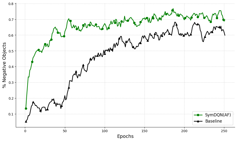
We first compare our best-performing condition, SymDQN(AF) with the baseline learning of the pure non-symbolic DuelDQN, see Fig. 6.
<details>
<summary>extracted/6333762/SymDQNAF-DuelingDQN.png Details</summary>
### Visual Description
## Line Chart: Performance Comparison of SymDQN(AF) vs. Baseline
### Overview
The image is a line chart illustrating the performance of two models, "SymDQN(AF)" and "Baseline," over 250 training epochs. The Y-axis represents the percentage of "Negative Objects" (likely a performance metric, such as detection rate or avoidance success), while the X-axis represents the training time in "Epochs." The chart demonstrates that SymDQN(AF) learns significantly faster and maintains a higher performance level than the Baseline throughout the training process.
### Components/Axes
* **X-Axis:** Labeled "Epochs," ranging from 0 to 250, with major grid lines every 50 units.
* **Y-Axis:** Labeled "% Negative Objects," ranging from 0.1 to 0.8, with major grid lines every 0.1 units.
* **Legend:** Located in the bottom-right corner of the plot area.
* **Green line with circle markers:** Labeled "SymDQN(AF)."
* **Black line with triangle markers:** Labeled "Baseline."
* **Grid:** A light gray dashed grid overlays the plot area to assist in reading values.
### Detailed Analysis
#### Trend Verification
* **SymDQN(AF) (Green Line):** Exhibits a very steep, rapid upward trend from the start (Epoch 0) until approximately Epoch 20. Following this, the slope decreases, transitioning into a gradual, sustained upward trend with minor fluctuations until the end of the training period.
* **Baseline (Black Line):** Exhibits a very slow, shallow upward trend from Epoch 0 to Epoch 50. Between Epoch 50 and Epoch 100, the slope increases significantly (acceleration phase). From Epoch 100 to 250, the trend continues to rise but at a slower, more volatile rate.
#### Data Points (Approximate Values)
| Epoch | SymDQN(AF) Value | Baseline Value |
| :--- | :--- | :--- |
| 0 | ~0.14 | ~0.05 |
| 50 | ~0.60 | ~0.15 |
| 100 | ~0.65 | ~0.45 |
| 150 | ~0.68 | ~0.55 |
| 200 | ~0.72 | ~0.60 |
| 250 | ~0.70 | ~0.60 |
### Key Observations
* **Performance Gap:** SymDQN(AF) consistently outperforms the Baseline. At no point does the Baseline overtake or match the SymDQN(AF) performance.
* **Learning Efficiency:** SymDQN(AF) reaches a performance level of ~0.50 by Epoch 20. The Baseline does not reach this same level of ~0.50 until approximately Epoch 110, indicating a significant lag in learning speed.
* **Volatility:** Both models exhibit increased volatility (fluctuations in the line) in the latter half of the training (post-Epoch 150), suggesting that neither model has reached a perfectly stable convergence point by Epoch 250.
* **Peak Performance:** SymDQN(AF) peaks slightly above 0.75 around Epoch 180, while the Baseline peaks near 0.68 around Epoch 180.
### Interpretation
The data strongly suggests that the "SymDQN(AF)" architecture is superior to the "Baseline" in this specific task. The primary advantage is sample efficiency; the model achieves high performance very early in the training process.
The "Baseline" model appears to struggle initially, suggesting it may have difficulty learning the underlying patterns of the data or environment without the specific enhancements provided by the "AF" (likely "Attention Function" or similar) component in SymDQN. The fact that both lines remain volatile at the end of the 250 epochs suggests that the training process is still active and that further training might yield higher results, though the performance gap between the two models appears to be stabilizing rather than closing.
</details>
Figure 6: SymDQN(AF) (in green) vs. DuelDQN (in black): $x$ -axis represents epochs and $y$ -axis represents the ratio of obtained score in the episode and the maximum obtainable score in that episode.
Clearly, the performance of the SymDQN agent equipped with ActionFilter is superior to DuelDQN both in terms of quicker convergence (high initial learning rate) and overall end performance.
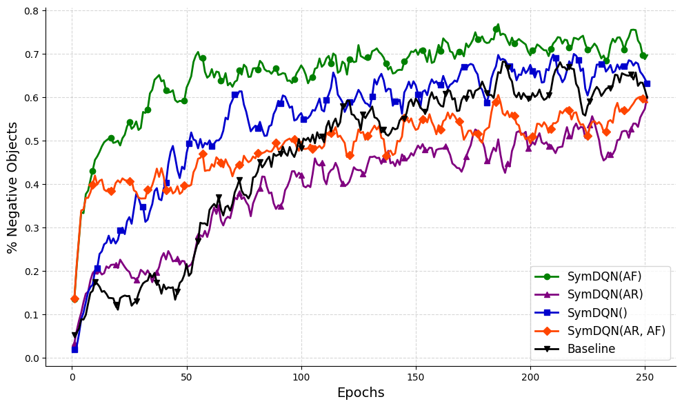
Let us now look at different versions of our SymDQN to better understand what contributes to its performance. In Fig. 7 we show the performance of all four versions of SymDQN.
<details>
<summary>extracted/6333762/SymDQN_performance_new.png Details</summary>
### Visual Description
## Line Chart: Performance Comparison of SymDQN Variants
### Overview
This image displays a line chart comparing the performance of five different reinforcement learning models, labeled as variants of "SymDQN" and a "Baseline," over the course of 250 training epochs. The Y-axis represents the "% Negative Objects" (presumably a metric of success or task completion), while the X-axis represents the training time in "Epochs."
### Components/Axes
* **X-Axis:** Labeled "Epochs," ranging from 0 to 250, with major grid lines every 50 epochs.
* **Y-Axis:** Labeled "% Negative Objects," ranging from 0.0 to 0.8, with major grid lines every 0.1 units.
* **Legend:** Located in the bottom-right quadrant of the chart.
* **SymDQN(AF):** Green line with circle markers.
* **SymDQN(AR):** Purple line with triangle markers.
* **SymDQN():** Blue line with square markers.
* **SymDQN(AR, AF):** Orange line with diamond markers.
* **Baseline:** Black line with inverted triangle markers.
### Detailed Analysis
The chart tracks the performance of five models. Below is the trend analysis for each series:
* **SymDQN(AF) (Green, Circles):**
* **Trend:** This model shows the most rapid initial growth and maintains the highest performance throughout the duration of the training.
* **Values:** It starts at approximately 0.15 at epoch 0, climbs steeply to ~0.5 by epoch 20, and continues a steady, fluctuating upward trend, peaking near 0.75 around epoch 180, before settling near 0.7 at epoch 250.
* **SymDQN() (Blue, Squares):**
* **Trend:** Shows a strong, consistent upward trajectory.
* **Values:** Starts near 0.02, rises to ~0.3 by epoch 30, and continues to climb, reaching ~0.6 by epoch 150. It fluctuates between 0.6 and 0.7 for the remainder of the training, ending near 0.63.
* **Baseline (Black, Inverted Triangles):**
* **Trend:** Starts with the lowest performance but exhibits a very strong, consistent upward slope, eventually overtaking the orange and purple lines.
* **Values:** Starts near 0.05, remains low until epoch 50 (~0.25), then accelerates significantly, reaching ~0.6 by epoch 250.
* **SymDQN(AR, AF) (Orange, Diamonds):**
* **Trend:** Starts with a very strong initial jump but plateaus earlier than the other models.
* **Values:** Starts at ~0.15, jumps to ~0.4 by epoch 10. It continues a slow, steady climb, reaching ~0.5 by epoch 100, and ends near 0.6 at epoch 250.
* **SymDQN(AR) (Purple, Triangles):**
* **Trend:** Generally the lowest performing model for the majority of the training duration.
* **Values:** Starts near 0.02, rises to ~0.2 by epoch 10, and maintains a slow, steady growth, ending near 0.58 at epoch 250.
### Key Observations
* **Dominance of AF:** The "AF" component appears to be the primary driver of high performance, as the `SymDQN(AF)` model is consistently the top performer.
* **Early vs. Late Performance:** The `SymDQN(AR, AF)` model demonstrates excellent "cold start" performance (rising quickly in the first 10 epochs) but fails to maintain that lead, being overtaken by the `SymDQN(AF)` and `SymDQN()` models.
* **Baseline Competitiveness:** The `Baseline` model is surprisingly robust, starting from the bottom but showing a consistent learning curve that eventually matches or exceeds the `SymDQN(AR)` and `SymDQN(AR, AF)` variants.
### Interpretation
The data suggests that the "AF" modification is highly beneficial for the model's ability to identify or process "Negative Objects." Conversely, the "AR" modification, when used alone (`SymDQN(AR)`), appears to hinder performance compared to the baseline.
The combination of both (`SymDQN(AR, AF)`) results in a model that learns very quickly initially but suffers from a lower performance ceiling compared to the `SymDQN(AF)` variant. This implies a potential trade-off: "AR" might help with early-stage exploration or stability, but "AF" is necessary for achieving higher accuracy in the later stages of training. The `Baseline` model's steady performance suggests that the `SymDQN` modifications (specifically AR) might introduce some instability or slower convergence in the mid-to-late training phases.
</details>
Figure 7: All versions of SymDQN: SymDQN(AF) (in green), SymDQN(AR,AF) (in red), SymDQN (in blue) and SymDQN(AR) (in purple); the $x$ -axis represents epochs and the $y$ -axis represents the ratio of obtained score in the episode and the maximum obtainable score in that episode. We report in standard deviations in the Appendix.
From this graph, we can conclude that the presence of ActionReasoner, despite giving a slight boost in the initial learning rate, hampers the overall performance of the agent (red and purple graphs). On the other hand, the presence of ActionFilter improves the initial performance (green and red).
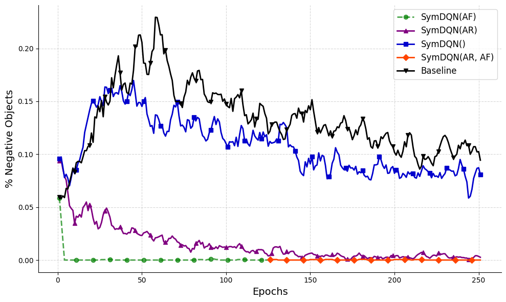
Let us now move to another performance measure: the precision of the agent in avoiding objects of the shape associated with negative rewards. We now compare all five experimental conditions, see Fig. 8.
<details>
<summary>extracted/6333762/precision_new.png Details</summary>
### Visual Description
## Line Chart: Training Performance Comparison (% Negative Objects)
### Overview
This chart illustrates the training performance of five different configurations of a "SymDQN" model compared to a "Baseline" model. The metric being tracked is the percentage of "Negative Objects" generated over 250 training epochs. The chart demonstrates how different architectural or algorithmic modifications (AF, AR) affect the model's tendency to produce negative objects during the learning process.
### Components/Axes
* **X-Axis:** Labeled "Epochs," ranging from 0 to 250, with major grid lines every 50 epochs.
* **Y-Axis:** Labeled "% Negative Objects," ranging from 0.00 to 0.20+, with major grid lines every 0.05.
* **Legend:** Located in the top-right corner.
* **SymDQN(AF):** Green dashed line with circle markers.
* **SymDQN(AR):** Purple solid line with triangle markers.
* **SymDQN():** Blue solid line with square markers.
* **SymDQN(AR, AF):** Orange solid line with diamond markers.
* **Baseline:** Black solid line with inverted triangle markers.
### Detailed Analysis
The following trends are observed for each data series:
* **Baseline (Black, Inverted Triangles):**
* **Trend:** Starts at ~0.06, rises sharply to a peak of ~0.23 at approximately epoch 60. Following this peak, it exhibits a gradual downward trend, ending at ~0.10 by epoch 250.
* **Performance:** This configuration consistently produces the highest percentage of negative objects throughout the training duration.
* **SymDQN() (Blue, Squares):**
* **Trend:** Starts at ~0.09, rises to a peak of ~0.17 at epoch 40. It then fluctuates with a downward trend, ending at ~0.08 by epoch 250.
* **Performance:** Performs better than the Baseline but still maintains a significant percentage of negative objects.
* **SymDQN(AR) (Purple, Triangles):**
* **Trend:** Starts at ~0.09, drops sharply to ~0.05 by epoch 10. It then exhibits a slow, steady decay, approaching 0.00 by the end of the training (epoch 250).
* **Performance:** Shows significant improvement over the Baseline and the standard SymDQN() configuration.
* **SymDQN(AF) (Green, Circles):**
* **Trend:** Starts at ~0.06, drops immediately to 0.00 by epoch 5, and remains at 0.00 for the duration of the training.
* **Performance:** Highly effective at eliminating negative objects almost immediately.
* **SymDQN(AR, AF) (Orange, Diamonds):**
* **Trend:** Remains at 0.00 throughout the entire training process.
* **Performance:** Identical to SymDQN(AF) in terms of eliminating negative objects, maintaining a 0.00 rate from the start.
### Key Observations
* **Dominance of AF:** The inclusion of "AF" (likely Action Filtering or a similar constraint) appears to be the primary factor in eliminating negative objects. Both configurations containing "AF" (`SymDQN(AF)` and `SymDQN(AR, AF)`) achieve near-zero negative objects.
* **Baseline Instability:** The Baseline model is highly unstable, peaking early (epoch 60) and failing to converge to a low error rate, suggesting it lacks the constraints necessary to avoid negative object generation.
* **AR Impact:** The "AR" configuration (`SymDQN(AR)`) provides a gradual improvement over the standard `SymDQN()` but is not as immediately effective as the "AF" configurations.
### Interpretation
The data suggests that the "SymDQN" architecture is significantly more robust than the "Baseline" when it comes to avoiding the generation of "Negative Objects."
The most critical finding is the efficacy of the "AF" component. Whether used alone or in combination with "AR," the "AF" component effectively forces the model to avoid negative objects almost instantly (within 5 epochs). The "AR" component alone (`SymDQN(AR)`) provides a learning-based reduction, where the model gradually learns to avoid negative objects over time, whereas "AF" appears to act as a hard constraint or a highly effective filter. The "Baseline" and standard "SymDQN()" models struggle significantly, indicating that without these specific modifications, the model is prone to generating undesirable outputs.
</details>
Figure 8: Agent’s precision in all conditions: SymDQN(AF) (in green), SymDQN(AR,AF) (in red), SymDQN(AR) (in purple); SymDQN (in blue); DuelDQN (in black): the $x$ -axis represents epochs and the $y$ -axis represents the percentage of negative-reward objects consumed by the agent. Note that the green and red lines overlap.
While the presence of ActionReasoner (in purple) allows a significant improvement of precision, it’s the ActionFilter that eradicates negative rewards completely (red and green graphs). The baseline DuelDQN and the pure SymDQN perform similarly, not being able to learn to avoid negative rewards completely.
### 5.1 Interpretation and Discussion
The integration of symbolic knowledge into reinforcement learning, as demonstrated by SymDQN, provides several insights into the potential of neuro-symbolic approaches in AI. The ability of SymDQN to extract and utilize key environmental features drives a significant boost in initial learning rate and overall performance, suggesting that symbolic representations can provide a valuable advantage to neural networks, enabling them to rapidly leverage the features for better decision-making. The ActionFilter provides a dramatic enhancement in early-stage performance, allowing the model to make good decisions as soon as the symbolic representation is available. By leveraging the symbolic representation and understanding of the environment, ActionFilter prunes sub-optimal actions, aligning the agent’s behavior with a symbolic understanding of the environment. The role of ActionReasoner is less clear: while providing a slight boost in initial performance, it hampers the overall learning rate. It seems that by forcing the model output to comply with the logical axiom, it diminishes its ability to capture information that is not described by the logical formulas.
The two components, ActionReasoner and ActionFilter use symbolic information to adjust (the impact of) $q$ -values and could be seen as a form of reward shaping. ActionReasoner uses the axiom (A4) to align $q$ -values with predicted immediate rewards. As we can see in Fig. 7, this ‘reward shaping’ process is detrimental to the overall performance. A possible reason for that can be illustrated in the following example. Let’s assume the agent is separated from a multitude of positive shapes by a thin wall of negative shapes. A long-term perspective of sacrificing some reward by crossing over the wall can be blocked by attaching too much value to the immediate punishment. Note, however, that although ineffective, this ‘reward shaping’ makes the agent more cautious/precise (see Fig. 7). While ActionFilter does not shape the reward function directly (as it is turned off in the training phase), it performs reasoning based on rewards (Fig. 4). In a given state it eliminates the possibility of executing actions for which $q$ -values and immediate rewards differ too drastically.
The advantages of SymDQN come with trade-offs. The computational cost introduced by the additional components is non-trivial, and the logical constraints imposed on the learning might hamper performance in more complex environments. In that, the use of LTNs in reinforcement learning sheds light on the ‘thinking fast and slow’ effects in learning. Firstly, the use of axioms (A1)-(A3) in ShapeRecognizer gives a sharp increase in the initial performance due to the understanding of the environment structure (Fig. 8). Apart from that, adjusting the reward function with ActionReasoner and ActionFilter will increase precision (as normally assumed about the System 2 type of behavior), but it can also hamper the overall performance, like it does in the case of ActionReasoner (see Fig. 7).
## 6 Conclusions and Future Work
This research introduces a novel modular approach to integrating symbolic knowledge with deep reinforcement learning through the implementation of SymDQN. We contribute to the field of Neuro-Symbolic AI in several ways. Firstly, we demonstrate a successful integration of LTNs into reinforcement learning, a promising and under-explored research direction. This integration touches on key challenges: interpretability, alignment, and knowledge injection. Secondly, SymDQN augments reinforcement learning through symbolic environment representation, modeling of object relationships and dynamics, and guiding action based on symbolic knowledge, effectively improving both initial learning rates and the end performance of the reinforcement learning agents. These contributions advance the field of neuro-symbolic AI, bridging the gap between symbolic reasoning and deep learning systems. Our findings demonstrate the potential of integrative approaches in creating more aligned, controllable and interpretable models for safe and reliable AI systems.
### 6.1 Future Work
We see several potential avenues for future research.
Enhancing Environment Representation It is easy to see that the ShapeRecognizer can be adapted to any grid-like environment. It could also be further developed to represent more complex environments symbolically, e.g., by integrating a more advanced object-detection component (e.g., Faster-LTN Manigrasso et al. (2021)). With the addition of precise bounding box detection and multi-class labeling, the component could be extended to also perform hierarchical representations, e.g., recognizing independent objects and their parts or constructing abstract taxonomies.
Automatic Axiom Discovery The investigation of automatic axiom discovery through iterative learning, or meta-learning, is an interesting direction that opens the doors to knowledge extraction from a model (see, e.g., Hasanbeig et al. (2021); Umili et al. (2021); Meli et al. (2024)). Theoretically, given enough time and randomization, Q-learning converges to optimal decision policy in any environment, and so the iterative development and assessment of axioms might allow us to extract knowledge from deep learning systems that outperform human experts.
Broader Evaluation While a version of SymDQN was shown to be advantageous, it was only tested in a single, simple environment. A broader suite of empirical experiments in more complex environments, such as Atari games or Pac-Man, is necessary to understand the generalization capabilities of the findings. These environments provide more complex and diverse challenges, potentially offering deeper insights into the advantages of SymDQN.
## Appendix A Appendix
#### Hardware and software specifications
The experiments, hyper-parameter tuning, and model variation comparisons were performed on a computing center machine (Tesla V100 with either 16 or 32GB). The coding environment used was Python 3.9.5 and Pytorch 2.3.1 with Cuda Toolkit 12.1. To integrate LTNs, the LTNtorch Carraro (2022) library was used, a PyTorch implementation by Tommaso Carraro. For experiment tracking, the ClearMl Platform cle (2023) was used. The code is provided as a separate .zip file.
#### Hyperparameters
The hyper-parameters used for training were: explore steps: 25000, update steps: 1000, initial epsilon: 0.95, end epsilon: 0.05, memory capacity: 1000, batch size: 16, gamma: 0.99, learning rate: 0.0001, maximum gradient norm: 1. Semantics of quantifiers in LTN used $p=8$ .
#### Standard deviations
Performance was assessed through 5 independent experimental runs per configuration. Each run evaluated 50 distinct environments to calculate average scores per epoch; ( $\ast$ ) stands for SymDQN( $\ast$ ), values for epochs 50, 150, 250 (smoothed, rolling window 5). First table: overall performance (rewards, r) and standard deviations (sd). Second table: ratio of negative shapes collected (inverse of precision, p) and sd.
| (AF) (AR) () | 0.65 0.26 0.43 | 0.03 0.03 0.05 | 0.70 0.47 0.65 | 0.01 0.01 0.02 | 0.71 0.53 0.66 | 0.01 0.04 0.02 |
| --- | --- | --- | --- | --- | --- | --- |
| (AR,AF) | 0.40 | 0.02 | 0.53 | 0.02 | 0.59 | 0.02 |
| DuelDQN | 0.24 | 0.06 | 0.57 | 0.02 | 0.64 | 0.01 |
| (AF) (AR) () | 0.00 0.02 0.17 | 0.00 0.00 0.02 | 0.00 0.01 0.12 | 0.00 0.00 0.02 | 0.00 0.00 0.08 | 0.00 0.00 0.00 |
| --- | --- | --- | --- | --- | --- | --- |
| (AR,AF) | 0.00 | 0.00 | 0.00 | 0.00 | 0.00 | 0.00 |
| DDQN | 0.19 | 0.03 | 0.14 | 0.01 | 0.10 | 0.00 |
## References
- Badreddine and Spranger (2019) Samy Badreddine and Michael Spranger. Injecting prior knowledge for transfer learning into reinforcement learning algorithms using logic tensor networks. CoRR, abs/1906.06576, 2019.
- Badreddine et al. (2022) Samy Badreddine, Artur d’Avila Garcez, Luciano Serafini, and Michael Spranger. Logic tensor networks. Artificial Intelligence, 303:103649, 2022.
- Bianchi and Hitzler (2019) Federico Bianchi and Pascal Hitzler. On the capabilities of logic tensor networks for deductive reasoning. In AAAI Spring Symposium Combining Machine Learning with Knowledge Engineering, 2019.
- Carraro (2022) Tommaso Carraro. LTNtorch: PyTorch implementation of Logic Tensor Networks, mar 2022.
- cle (2023) ClearML - your entire mlops stack in one open-source tool, 2023. Software available from http://github.com/allegroai/clearml.
- Donadello et al. (2017) Ivan Donadello, Luciano Serafini, and Artur d’Avila Garcez. Logic tensor networks for semantic image interpretation. In Proceedings of the Twenty-Sixth International Joint Conference on Artificial Intelligence, IJCAI-17, pages 1596–1602, 2017.
- Furelos-Blanco et al. (2021) Daniel Furelos-Blanco, Mark Law, Anders Jonsson, Krysia Broda, and Alessandra Russo. Induction and exploitation of subgoal automata for reinforcement learning. J. Artif. Intell. Res., 70:1031–1116, 2021.
- Giacomo et al. (2019) Giuseppe De Giacomo, Luca Iocchi, Marco Favorito, and Fabio Patrizi. Foundations for restraining bolts: Reinforcement learning with ltlf/ldlf restraining specifications. In J. Benton, Nir Lipovetzky, Eva Onaindia, David E. Smith, and Siddharth Srivastava, editors, Proceedings of the Twenty-Ninth International Conference on Automated Planning and Scheduling, ICAPS 2019, Berkeley, CA, USA, July 11-15, 2019, pages 128–136. AAAI Press, 2019.
- Hasanbeig et al. (2021) Mohammadhosein Hasanbeig, Natasha Yogananda Jeppu, Alessandro Abate, Tom Melham, and Daniel Kroening. Deepsynth: Automata synthesis for automatic task segmentation in deep reinforcement learning. In Thirty-Fifth AAAI Conference on Artificial Intelligence, AAAI 2021, Thirty-Third Conference on Innovative Applications of Artificial Intelligence, IAAI 2021, The Eleventh Symposium on Educational Advances in Artificial Intelligence, EAAI 2021, Virtual Event, February 2-9, 2021, pages 7647–7656. AAAI Press, 2021.
- Manigrasso et al. (2021) Francesco Manigrasso, Filomeno Davide Miro, Lia Morra, and Fabrizio Lamberti. Faster-LTN: A neuro-symbolic, end-to-end object detection architecture. In Igor Farkaš, Paolo Masulli, Sebastian Otte, and Stefan Wermter, editors, Artificial Neural Networks and Machine Learning – ICANN 2021, pages 40–52, Cham, 2021. Springer International Publishing.
- Meli et al. (2024) Daniele Meli, Alberto Castellini, and Alessandro Farinelli. Learning logic specifications for policy guidance in pomdps: an inductive logic programming approach. Journal of Artificial Intelligence Research, 79:725–776, February 2024.
- Serafini and d’Avila Garcez (2016) Luciano Serafini and Artur S. d’Avila Garcez. Logic tensor networks: Deep learning and logical reasoning from data and knowledge. CoRR, abs/1606.04422, 2016.
- Towers et al. (2024) Mark Towers, Jordan K. Terry, Ariel Kwiatkowski, John U. Balis, Gianluca de Cola, Tristan Deleu, Manuel Goulão, Andreas Kallinteris, Arjun KG, Markus Krimmel, Rodrigo Perez-Vicente, Andrea Pierré, Sander Schulhoff, Jun Jet Tai, Andrew Tan Jin Shen, and Omar G. Younis. Gymnasium, June 2024.
- Umili et al. (2021) Elena Umili, Emanuele Antonioni, Francesco Riccio, Roberto Capobianco, Daniele Nardi, Giuseppe De Giacomo, et al. Learning a symbolic planning domain through the interaction with continuous environments. In Workshop on Bridging the Gap Between AI Planning and Reinforcement Learning (PRL), workshop at ICAPS 2021, 2021.
- Umili et al. (2023) Elena Umili, Roberto Capobianco, and Giuseppe De Giacomo. Grounding LTLf Specifications in Image Sequences. In Proceedings of the 20th International Conference on Principles of Knowledge Representation and Reasoning, pages 668–678, 8 2023.
- van Krieken et al. (2022) Emile van Krieken, Erman Acar, and Frank van Harmelen. Analyzing differentiable fuzzy logic operators. Artificial Intelligence, 302:103602, 2022.
- Wagner and d’Avila Garcez (2022) Benedikt Wagner and Artur S. d’Avila Garcez. Neural-symbolic reasoning under open-world and closed-world assumptions. In Proceedings of the AAAI 2022 Spring Symposium on Machine Learning and Knowledge Engineering for Hybrid Intelligence (AAAI-MAKE 2022), 2022.
- Wang et al. (2015) Ziyu Wang, Nando de Freitas, and Marc Lanctot. Dueling network architectures for deep reinforcement learning. CoRR, abs/1511.06581, 2015.
- Wang et al. (2016) Ziyu Wang, Tom Schaul, Matteo Hessel, Hado Van Hasselt, Marc Lanctot, and Nando De Freitas. Dueling network architectures for deep reinforcement learning. In Proceedings of the 33rd International Conference on International Conference on Machine Learning - Volume 48, ICML’16, pages 1995–2003. JMLR.org, 2016.