2504.02670v6

# Affordable AI Assistants with Knowledge Graph of Thoughts **Authors**: Maciej Besta, ETH Zurich, &Lorenzo Paleari, ETH Zurich, &Jia Hao Andrea Jiang, ETH Zurich, &Robert Gerstenberger, ETH Zurich, &You Wu, ETH Zurich, &Jón Gunnar Hannesson, ETH Zurich, &Patrick Iff, ETH Zurich, &Ales Kubicek, ETH Zurich, &Piotr Nyczyk, &Diana Khimey, ETH Zurich, &Nils Blach, ETH Zurich, &Haiqiang Zhang, ETH Zurich, &Tao Zhang, ETH Zurich, &Peiran Ma, ETH Zurich, &Grzegorz Kwaśniewski, ETH Zurich, &Marcin Copik, ETH Zurich, &Hubert Niewiadomski, &Torsten Hoefler, ETH Zurich > corresponding author ## Abstract Large Language Models (LLMs) are revolutionizing the development of AI assistants capable of performing diverse tasks across domains. However, current state-of-the-art LLM-driven agents face significant challenges, including high operational costs and limited success rates on complex benchmarks like GAIA. To address these issues, we propose Knowledge Graph of Thoughts (KGoT), an innovative AI assistant architecture that integrates LLM reasoning with dynamically constructed knowledge graphs (KGs). KGoT extracts and structures task-relevant knowledge into a dynamic KG representation, iteratively enhanced through external tools such as math solvers, web crawlers, and Python scripts. Such structured representation of task-relevant knowledge enables low-cost models to solve complex tasks effectively while also minimizing bias and noise. For example, KGoT achieves a 29% improvement in task success rates on the GAIA benchmark compared to Hugging Face Agents with GPT-4o mini. Moreover, harnessing a smaller model dramatically reduces operational costs by over 36 $×$ compared to GPT-4o. Improvements for other models (e.g., Qwen2.5-32B and Deepseek-R1-70B) and benchmarks (e.g., SimpleQA) are similar. KGoT offers a scalable, affordable, versatile, and high-performing solution for AI assistants. Website & code: https://github.com/spcl/knowledge-graph-of-thoughts ## 1 Introduction Large Language Models (LLMs) are transforming the world. However, training LLMs is expensive, time-consuming, and resource-intensive. In order to democratize the access to generative AI, the landscape of agent systems has massively evolved during the last two years (LangChain Inc., 2025a; Rush, 2023; Kim et al., 2024; Sumers et al., 2024; Hong et al., 2024; Guo et al., 2024; Edge et al., 2025; Besta et al., 2025c; Zhuge et al., 2024; Beurer-Kellner et al., 2024; Shinn et al., 2023; Kagaya et al., 2024; Zhao et al., 2024a; Stengel-Eskin et al., 2024; Wu et al., 2024). These schemes have been applied to numerous tasks in reasoning (Creswell et al., 2023; Bhattacharjya et al., 2024; Besta et al., 2025c), planning (Wang et al., 2023c; Prasad et al., 2024; Shen et al., 2023; Huang et al., 2023), software development (Tang et al., 2024), and many others (Xie et al., 2024; Li & Vasarhelyi, 2024; Schick et al., 2023; Beurer-Kellner et al., 2023). Among the most impactful applications of LLM agents is the development of AI assistants capable of helping with a wide variety of tasks. These assistants promise to serve as versatile tools, enhancing productivity and decision-making across domains. From aiding researchers with complex problem-solving to managing day-to-day tasks for individuals, AI assistants are becoming an indispensable part of modern life. Developing such systems is highly relevant, but remains challenging, particularly in designing solutions that are both effective and economically viable. The GAIA benchmark (Mialon et al., 2024) has become a key standard for evaluating LLM-based agent systems across diverse tasks, including web navigation, code execution, image reasoning, scientific QA, and multimodal challenges. Despite its introduction nearly two years ago, top-performing solutions still struggle with many tasks. Moreover, operational costs remain high: running all validation tasks with Hugging Face Agents (Roucher & Petrov, 2025) and GPT-4o costs $≈$ $200, underscoring the need for more affordable alternatives . Smaller models like GPT-4o mini significantly reduce expenses but suffer from steep drops in task success, making them insufficient. Open large models also pose challenges due to demanding infrastructure needs, while smaller open models, though cheaper to run, lack sufficient capabilities. To address these challenges, we propose Knowledge Graph of Thoughts (KGoT), a novel AI assistant architecture that significantly reduces task execution costs while maintaining a high success rate (contribution #1). The central innovation of KGoT lies in its use of a knowledge graph (KG) (Singhal, 2012; Besta et al., 2024b) to represent knowledge relevant to a given task. A KG organizes information into triples, providing a structured representation of knowledge that small, cost-effective models can efficiently process. Hence, KGoT “turns the unstructured into the structured”, i.e., KGoT turns the often unstructured data such as website contents or PDF files into structured KG triples. This approach enhances the comprehension of task requirements, enabling even smaller models to achieve performance levels comparable to much larger counterparts, but at a fraction of the cost. The KGoT architecture (contribution #2) implements this concept by iteratively constructing a KG from the task statement, incorporating tools as needed to gather relevant information. The constructed KG is kept in a graph store, serving as a repository of structured knowledge. Once sufficient information is gathered, the LLM attempts to solve the task by either directly embedding the KG in its context or querying the graph store for specific insights. This approach ensures that the LLM operates with a rich and structured knowledge base, improving its task-solving ability without incurring the high costs typically associated with large models. The architecture is modular and extensible towards different types of graph query languages and tools. Our evaluation against top GAIA leaderboard baselines demonstrates its effectiveness and efficiency (contribution #3). KGoT with GPT-4o mini solves $>$ 2 $×$ more tasks from the validation set than Hugging Face Agents with GPT-4o or GPT-4o mini. Moreover, harnessing a smaller model dramatically reduces operational costs: from $187 with GPT-4o to roughly $5 with GPT-4o mini. KGoT’s benefits generalize to other models, baselines, and benchmarks such as SimpleQA (Wei et al., 2024). On top of that, KGoT reduces noise and simultaneously minimizes bias and improves fairness by externalizing reasoning into an explicit knowledge graph rather than relying solely on the LLM’s internal generation (contribution #4). This ensures that key steps when resolving tasks are grounded in transparent, explainable, and auditable information. 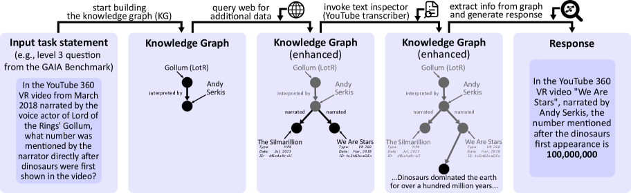## 2 Knowledge Graph of Thoughts We first illustrate the key idea, namely, using a knowledge graph to encode structurally the task contents. Figure 1 shows an example task and its corresponding evolving KG. ### 2.1 What is a Knowledge Graph? A knowledge graph (KG) is a structured representation of information that organizes knowledge into a graph-based format, allowing for efficient querying, reasoning, and retrieval. Formally, a KG consists of a set of triples, where each triple $(s,p,o)$ represents a relationship between two entities $s$ (subject) and $o$ (object) through a predicate $p$ . For example, the triple $(``Earth'',``orbits'',``Sun'')$ captures the fact that Earth orbits the Sun. Mathematically, a knowledge graph can be defined as a directed labeled graph $G=(V,E,L)$ , where $V$ is the set of vertices (entities), $E⊆ V× V$ is the set of edges (relationships), and $L$ is the set of labels (predicates) assigned to the edges. Each entity or predicate may further include properties or attributes, enabling richer representation. Knowledge graphs are widely used in various domains, including search engines, recommendation systems, and AI reasoning, as they facilitate both efficient storage and complex queries. <details> <summary>x1.png Details</summary>  ### Visual Description ## Process Diagram: Knowledge Graph-Based Question Answering System ### Overview The image illustrates a five-step workflow for a system that answers complex questions by constructing and iteratively enhancing a knowledge graph (KG), querying external data sources, and synthesizing a final response. The process is demonstrated using a specific example question from the GAIA Benchmark. ### Components/Flow The diagram is organized into five vertical panels, each representing a stage in the process. A horizontal flow at the top connects these stages with action labels and icons. **Top Flow (Left to Right):** 1. **Action:** "start building the knowledge graph (KG)" * **Icon:** A simple line drawing of a person at a desk with a computer. 2. **Action:** "query web for additional data" * **Icon:** A globe with a magnifying glass. 3. **Action:** "invoke text inspector (YouTube transcriber)" * **Icon:** A document with a magnifying glass. 4. **Action:** "extract info from graph and generate response" * **Icon:** A magnifying glass over a document with a gear. 5. **Final Output:** "Response" (no action label). **Panel Content (Left to Right):** **Panel 1: Input task statement** * **Title:** "Input task statement (e.g., level 3 question from the GAIA Benchmark)" * **Content (Text Block):** "In the YouTube 360 VR video from March 2018 narrated by the voice actor of Lord of the Rings' Gollum, what number was mentioned by the narrator directly after dinosaurs first shown in the video?" **Panel 2: Knowledge Graph** * **Title:** "Knowledge Graph" * **Content (Diagram):** A simple graph with two black nodes connected by a labeled edge. * **Node 1 (Top):** "Gollum (LotR)" * **Node 2 (Bottom):** "Andy Serkis" * **Edge Label:** "interpreted by" (pointing from Gollum to Andy Serkis). **Panel 3: Knowledge Graph (enhanced)** * **Title:** "Knowledge Graph (enhanced)" * **Content (Diagram):** The graph expands. The original nodes are now gray. Two new black nodes are added, connected to "Andy Serkis." * **Existing Nodes (Gray):** "Gollum (LotR)", "Andy Serkis" * **New Node 1 (Bottom Left):** "The Silmarillion" * **Sub-text:** "YouTube 360 VR video", "March 2018", "narrated by: Andy Serkis" * **New Node 2 (Bottom Right):** "We Are Stars" * **Sub-text:** "YouTube 360 VR video", "March 2018", "narrated by: Andy Serkis" * **Edge Labels:** "interpreted by" (Gollum -> Andy Serkis), "narrated" (Andy Serkis -> The Silmarillion), "narrated" (Andy Serkis -> We Are Stars). **Panel 4: Knowledge Graph (enhanced)** * **Title:** "Knowledge Graph (enhanced)" * **Content (Diagram):** The graph is further enhanced. The previous nodes are gray. A new black node is added, connected to "We Are Stars." * **Existing Nodes (Gray):** "Gollum (LotR)", "Andy Serkis", "The Silmarillion", "We Are Stars" * **New Node (Bottom Center):** A black node with no label, connected to "We Are Stars." * **Edge Label:** "narrated" (Andy Serkis -> We Are Stars). * **Text Below Graph:** "...Dinosaurs dominated the earth for over a hundred million years..." **Panel 5: Response** * **Title:** "Response" * **Content (Text Block):** "In the YouTube 360 VR video "We Are Stars", narrated by Andy Serkis, the number mentioned after the dinosaurs first appearance is **100,000,000**" ### Detailed Analysis The process demonstrates a multi-step reasoning chain: 1. **Problem Parsing:** The system starts with a complex natural language question requiring multi-hop reasoning (find video -> identify narrator -> find specific moment in video -> extract number). 2. **Initial KG Construction:** It creates a minimal graph linking the known entity "Gollum" to its actor "Andy Serkis." 3. **External Data Integration:** It queries the web, discovering two relevant YouTube videos narrated by Andy Serkis ("The Silmarillion" and "We Are Stars"), and adds them to the graph. 4. **Targeted Data Retrieval:** It invokes a "text inspector" (likely a transcription tool) on the candidate videos. The text snippet "...Dinosaurs dominated the earth for over a hundred million years..." is extracted, identifying "We Are Stars" as the correct video. 5. **Answer Synthesis:** Using the enhanced graph and the retrieved text, it formulates the final answer, extracting the specific number "100,000,000." ### Key Observations * **Graph Evolution:** The knowledge graph grows from 2 nodes to 5 nodes, with node color changing from black (newly added) to gray (existing) in subsequent steps. * **Information Source Hierarchy:** The system uses the initial KG as a seed, the web for broad discovery, and a specialized text inspector for precise data extraction. * **Answer Specificity:** The final response directly quotes the video title and narrator, confirming the reasoning path, before providing the numerical answer. ### Interpretation This diagram outlines an **investigative, Peircean abductive reasoning process** implemented in an AI system. It doesn't just retrieve an answer; it builds a structured model of the problem space (the knowledge graph), uses that model to guide targeted information gathering, and verifies its hypothesis (that "We Are Stars" is the correct video) by finding corroborating evidence (the dinosaur text). The final answer is a conclusion derived from this structured investigation. The workflow highlights the system's ability to: * **Decompose** a complex query into sub-tasks (identify video, identify narrator, locate event, extract data). * **Integrate** heterogeneous data sources (pre-existing knowledge, web search, video transcription). * **Maintain** a structured context (the KG) to avoid losing intermediate reasoning steps. * **Generate** a transparent, justified response that traces back to the evidence. The notable anomaly is the unlabeled black node in Panel 4. This likely represents the extracted fact or the specific moment in the video transcript containing the answer, which is then used to populate the final response with the number "100,000,000." The process emphasizes traceability and evidence-based reasoning over simple pattern matching. </details> Figure 1: The key idea behind Knowledge Graph of Thoughts (KGoT): transforming the representation of a task for an AI assistant from a textual form into a knowledge graph (KG). As an example, we use a Level-3 (i.e., highest difficulty) task from the GAIA benchmark. In order to solve the task, KGoT evolves this KG by adding relevant information that brings the task closer to completion. This is achieved by iteratively running various tools. Finally, the task is solved by extracting the relevant information from the KG, using – for example – a graph query, or an LLM’s inference process with the KG provided as a part of the input prompt. More examples of KGs are in Appendix A. ### 2.2 Harnessing Knowledge Graphs for Effective AI Assistant Task Resolution At the heart of KGoT is the process of transforming a task solution state into an evolving KG. The KG representation of the task is built from “thoughts” generated by the LLM. These “thoughts” are intermediate insights identified by the LLM as it works through the problem. Each thought contributes to expanding or refining the KG by adding vertices or edges that represent new information. For example, consider the following Level 3 (i.e., highest difficulty) task from the GAIA benchmark: “In the YouTube 360 VR video from March 2018 narrated by the voice actor of Lord of the Rings’ Gollum, what number was mentioned by the narrator directly after dinosaurs were first shown in the video?” (see Figure 1 for an overview; more examples of constructed KGs are in Appendix A). Here, the KG representation of the task solution state has a vertex “Gollum (LotR)”. Then, the thought “Gollum from Lord of the Rings is interpreted by Andy Serkis” results in adding a vertex for “Andy Serkis”, and linking “Gollum (LotR)” to “Andy Serkis” with the predicate “interpreted by”. Such integration of thought generation and KG construction creates a feedback loop where the KG continuously evolves as the task progresses, aligning the representation with problem requirements. In order to evolve the KG task representation, KGoT iteratively interacts with tools and retrieves more information. For instance, the system might query the internet to identify videos narrated by Andy Serkis (e.g., “The Silmarillion“ and “We Are Stars”). It can also use a YouTube transcriber tool to find their publication date. This iterative refinement allows the KG to model the current “state” of a task at each step, creating a more complete and structured representation of this task and bringing it closer to completion. Once the KG has been sufficiently populated with task-specific knowledge, it serves as a robust resource for solving the problem. In addition to adding new graph elements, KGoT also supports other graph operations. This includes removing nodes and edges, used as a part of noise elimination strategies. ### 2.3 Extracting Information from the KG To accommodate different tasks, KGoT supports different ways to extract the information from the KG. Currently, we offer graph query languages or general-purpose languages; each of them can be combined with the so-called Direct Retrieval. First, one can use a graph query, prepared by the LLM in a language such as Cypher (Francis et al., 2018) or SPARQL (Pérez et al., 2009), to extract the answer to the task from the graph. This works particularly well for tasks that require retrieving specific patterns within the KG. Second, we also support general scripts prepared by the LLM in a general-purpose programming language such as Python. This approach, while not as effective as query languages for pattern matching, offers greater flexibility and may outperform the latter when a task requires, for example, traversing a long path in the graph. Third, in certain cases, once enough information is gathered into the KG, it may be more effective to directly paste the KG into the LLM context and ask the LLM to solve the task, instead of preparing a dedicated query or script. We refer to this approach as Direct Retrieval. The above schemes offer a tradeoff between accuracy, cost, and runtime. For example, when low latency is priority, general-purpose languages should be used, as they provide an efficient lightweight representation of the KG and offer rapid access and modification of graph data. When token cost is most important, one should avoid Direct Retrieval (which consumes many tokens as it directly embeds the KG into the LLM context) and focus on either query or general-purpose languages, with a certain preference for the former, because its generated queries tend to be shorter than scripts. Finally, when aiming for solving as many tasks as possible, one should experiment with all three schemes. As shown in the Evaluation section, these methods have complementary strengths: Direct Retrieval is effective for broad contextual understanding, while graph queries and scripts are better suited for structured reasoning. ### 2.4 Representing the KG KGoT can construct three interoperable KG representations: Property graphs (used with graph query languages such as Cypher and systems such as Neo4j (Robinson et al., 2015)), RDF graphs (used with graph query languages such as SPARQL and systems such as RDF4J (Ben Mahria et al., 2021)), and the adjacency list graphs (Besta et al., 2018) (used with general-purpose languages such as Python and systems such as NetworkX (NetworkX Developers, 2025)). Each representation supports a different class of analysis. The Property graph view facilitates analytics such as pattern matching, filtering, of motif queries directly on the evolving task-state graph. The RDF graph view facilitates reasoning over ontology constraints, schema validation, and SPARQL-based inference for missing links. The adjacency list representation with NetworkX facilitates Python-based graph analytics, for example centrality measures, connected components, clustering coefficients, etc., all on the same KG snapshots. Appendix A contains examples of task-specific KGs, illustrating how their topology varies with the task domain (e.g., tree-like procedural chains vs. dense relational subgraphs in multi-entity reasoning). ### 2.5 Bias, Fairness, and Noise Mitigation through KG-Based Representation KGoT externalizes and structures the reasoning process, which reduces noise, mitigates model bias, and improves fairness, because in each iteration both the outputs from tools and LLM thoughts are converted into triples and stored explicitly. Unlike opaque monolithic LLM generations, this fosters transparency and facilitates identifying biased inference steps. It also facilitates noise mitigation: new triples can be explicitly checked for the quality of their information content before being integrated into the KG, and existing triples can also be removed if they are deemed redundant (examples of such triples that have been found and removed are in Appendix B.6). 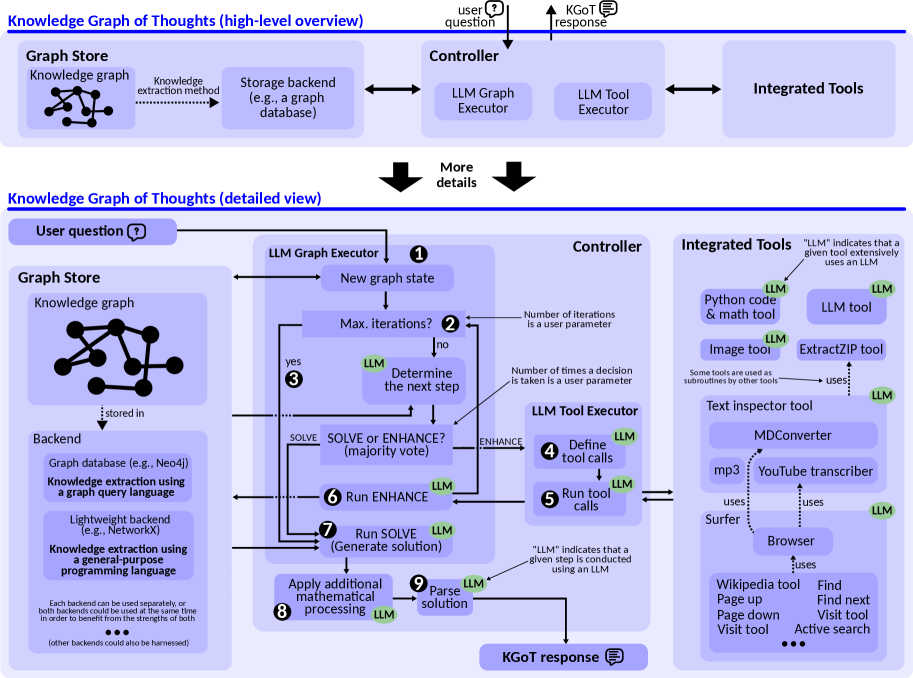## 3 System Architecture The KGoT modular and flexible architecture, pictured in Figure 2, consists of three main components: the Graph Store Module, the Controller, and the Integrated Tools, each playing a critical role in the task-solving process. Below, we provide a detailed description of each component and its role in the system. Additional details are in Appendix B (architecture) and in Appendix C (prompts). ### 3.1 Maintaining the Knowledge Graph with the Graph Store Module A key component of the KGoT system is the Graph Store Module, which manages the storage and retrieval of the dynamically evolving knowledge graph which represents the task state. In order to harness graph queries, we use a graph database backend; in the current KGoT implementation, we test Cypher together with Neo4j (Robinson et al., 2015), an established graph database (Besta et al., 2023b; c), as well as SPARQL together with the RDF4J backend (Ben Mahria et al., 2021). Then, in order to support graph accesses using a general-purpose language, KGoT harnesses the NetworkX library (NetworkX Developers, 2025) and Python. Note that the extensible design of KGoT enables seamless integration of any other backends and languages. ### 3.2 Managing the Workflow with the Controller Module The Controller orchestrates the interactions between the KG and the tools. Upon receiving a user query, it iteratively interprets the task, determines the appropriate tools to invoke based on the KG state and task needs, and integrates tool outputs back into the KG. The Controller uses a dual-LLM architecture with a clear separation of roles: the LLM Graph Executor constructs and evolves the KG, while the LLM Tool Executor manages tool selection and execution. The LLM Graph Executor determines the next steps after each iteration that constructs and evolves the KG. It identifies any missing information necessary to solve the task, formulates appropriate queries for the graph store interaction (retrieve/insert operations), and parses intermediate or final results for integration into the KG. It also prepares the final response to the user based on the KG. The LLM Tool Executor operates as the executor of the plan devised by the LLM Graph Executor. It identifies the most suitable tools for retrieving missing information, considering factors such as tool availability, relevance, and the outcome of previous tool invocation attempts. For example, if a web crawler fails to retrieve certain data, the LLM Tool Executor might prioritize a different retrieval mechanism or adjust its queries. The LLM Tool Executor manages the tool execution process, including interacting with APIs, performing calculations, or extracting information, and returns the results to the LLM Graph Executor for further reasoning and integration into the KG. ### 3.3 Ensuring Versatile and Extensible Set of Integrated Tools KGoT offers a hierarchical suite of tools tailored to diverse task needs. The Python Code Tool enables dynamic script generation and execution for complex computations. The LLM Tool supplements the controller’s reasoning by integrating an auxiliary language model, enhancing knowledge access while minimizing hallucination risk. For multimodal inputs, the Image Tool supports image processing and extraction. Web-based tasks are handled by the Surfer Agent (based on the design by Hugging Face Agents (Roucher & Petrov, 2025)), which leverages tools like the Wikipedia Tool, granular navigation tools (PageUp, PageDown, Find), and SerpApi (SerpApi LLM, 2025) for search. Additional tools include the ExtractZip Tool for compressed files and the Text Inspector Tool for converting content from sources like MP3s and YouTube transcripts into Markdown. Finally, the user can seamlessly add a new tool by initializing the tool, passing in the logger object for tool use statistics, and appending the tool to the tool list via a Tool Manager object. We require all tools implemented to adhere to the LangChain’s BaseTool interface class. This way, the list of tools managed by the Tool Manager can be directly bound to the LLM Tool Executor via LangChain bind_tools, further facilitating new tools. ### 3.4 Ensuring High-Performance & Scalability The used scalability optimizations include (1) asynchronous execution using asyncio (Python Software Foundation, 2025b) to parallelize LLM tool invocations, mitigating I/O bottlenecks and reducing idle time, (2) graph operation parallelism by reformulating LLM-generated Cypher queries to enable concurrent execution of independent operations in a graph database, and (3) MPI-based distributed processing, which decomposes workloads into atomic tasks distributed across ranks using a work-stealing algorithm to ensure balanced computational load and scalability. ### 3.5 Ensuring System Robustness Robustness is ensured with two established mechanisms, Self-Consistency (Wang et al., 2023b) (via majority voting) and LLM-as-a-Judge (Gu et al., 2025) (other strategies such as embedding-based stability are also applicable (Besta et al., 2025d)). With Self-Consistency, we query the LLM multiple times when deciding whether to insert more data into the KG or retrieve existing data, when deciding which tool to use, and when parsing the final solution. This approach reduces the impact of single-instance errors or inconsistencies in various parts of the KGoT architecture. LLM-as-a-Judge further reinforces the robustness, by directly employing the LLM agent to make these decisions based on generated reasoning chains. Overall, both Self-Consistency and LLM-as-a-Judge have been shown to significantly enhance the robustness of prompting. For example, MT-Bench and Chatbot Arena show that strong judges (e.g., GPT-4 class) match human preferences at 80% agreement or more, on par with human-human agreement (Zheng et al., 2023). Prometheus/Prometheus-2 further demonstrate open evaluator LMs with the highest correlations to both humans and proprietary judges across direct-assessment and pairwise settings, and AlpacaEval has been validated against approximately 20K human annotations, addressing earlier concerns about reproducibility at scale. Similarly reliable gains have been shown for Self-Consistency (Wang et al., 2023b). ### 3.6 Ensuring Layered Error Containment & Management To manage LLM-generated syntax errors, KGoT includes LangChain’s JSON parsers that detect syntax issues. When a syntax error is detected, the system first attempts to correct it by adjusting the problematic syntax using different encoders, such as the “unicode escape” (Python Software Foundation, 2025a). If the issue persists, KGoT employs a retry mechanism (three attempts by default) that uses the LLM to rephrase the query/command and attempts to regenerate its output. If the error persists, the system logs it for further analysis, bypasses the problematic query, and continues with other iterations. To handle API & system related errors, such as the OpenAI code 500, we employ exponential backoff, implemented using the tenacity library (Tenacity Developers, 2025a). Additionally, KGoT includes comprehensive logging systems as part of its error management framework. These systems track the errors encountered during system operation, providing valuable data that can be easily parsed and analyzed (e.g., snapshots of the knowledge graphs or responses from third-party APIs). The Python Executor tool, a key component of the system, is containerized to ensure secure execution of LLM-generated code. This tool is designed to run code with strict timeouts and safeguards, preventing potential misuse or resource overconsumption. ### 3.7 Implementation Details KGoT employs Docker (Docker Inc., 2025) and Sarus (Benedicic et al., 2019) for containerization, enabling a consistent and isolated runtime environment for all components. We containerize critical modules such as the KGoT controller, the Neo4j knowledge graph, and integrated tools (e.g., the Python Executor tool for safely running LLM-generated code with timeouts). Here, Docker provides a widely adopted containerization platform for local and cloud deployments that guarantees consistency between development and production environments. Sarus, a specialized container platform designed for high-performance computing (HPC) environments, extends KGoT’s portability to HPC settings where Docker is typically unavailable due to security constraints. This integration allows KGoT to operate efficiently in HPC environments, leveraging their computational power. KGoT also harnesses LangChain (LangChain Inc., 2025a), an open-source framework specifically designed for creating and orchestrating LLM-driven applications. LangChain offers a comprehensive suite of tools and APIs that simplify the complexities of managing LLMs, including prompt engineering, tool integration, and the coordination of LLM outputs. ## 4 System Workflow <details> <summary>x2.png Details</summary>  ### Visual Description ## System Architecture Diagram: Knowledge Graph of Thoughts (KGoT) ### Overview The image is a technical system architecture diagram illustrating the "Knowledge Graph of Thoughts" (KGoT) framework. It is divided into two primary sections: a **high-level overview** at the top and a **detailed view** below, connected by arrows labeled "More details." The diagram describes a system that uses a knowledge graph, a controller powered by Large Language Models (LLMs), and a suite of integrated tools to process a user question and generate a structured response. ### Components/Flow The system is organized into three main vertical columns in both views, with the Controller being the central processing unit. **High-Level Overview (Top Section):** * **Left Column - Graph Store:** Contains a "Knowledge graph" (visualized as a network of nodes and edges). A "Knowledge extraction method" arrow points to a "Storage backend (e.g., a graph database)." * **Center Column - Controller:** Receives the "user question" and outputs the "KGoT response." It contains two sub-components: "LLM Graph Executor" and "LLM Tool Executor." * **Right Column - Integrated Tools:** A single block representing the available tools. * **Flow:** Arrows indicate bidirectional communication between the Graph Store and Controller, and between the Controller and Integrated Tools. **Detailed View (Bottom Section):** This section expands the Controller and provides a step-by-step workflow. * **Left Column - Graph Store & Backend:** * **Graph Store:** Same "Knowledge graph" visualization. * **Backend:** Two options are detailed: 1. "Graph database (e.g., Neo4j)" using "Knowledge extraction using a graph query language." 2. "Lightweight backend (e.g., NetworkX)" using "Knowledge extraction using a general-purpose programming language." * A note states: "Each backend can be used separately, or both can be used in tandem in order to benefit from the strengths of both... (other backends could also be harnessed)." * **Center Column - Controller (Expanded):** This is the core processing loop, with numbered steps (1-9). * **LLM Graph Executor:** Manages the graph state. * **Step 1:** "New graph state" is created from the user question. * **Step 2:** Checks "Max. iterations?" (a user parameter). If "no," proceeds. * **Step 3:** Uses an LLM to "Determine the next step." * **Decision Point:** A diamond labeled "SOLVE or ENHANCE? (majority vote)" directs the flow. * **LLM Tool Executor:** Handles tool interactions. * **Step 4:** "Define tool calls" (using an LLM). * **Step 5:** "Run tool calls" (using an LLM). * **Action Paths:** * **ENHANCE Path:** From the decision, goes to Step 4 (Define tool calls) -> Step 5 (Run tool calls) -> Step 6 "Run ENHANCE" (using an LLM) -> loops back to the "New graph state." * **SOLVE Path:** From the decision, goes to Step 7 "Run SOLVE (Generate solution)" (using an LLM). * **Post-Processing:** * **Step 8:** "Apply additional mathematical processing" (using an LLM). * **Step 9:** "Parse solution" (using an LLM). * **Output:** The parsed solution becomes the "KGoT response." * **Right Column - Integrated Tools (Expanded):** Lists specific tools, with green "LLM" badges indicating extensive LLM use. * **Top Group:** "Python code & math tool," "LLM tool," "Image tool," "ExtractZIP tool." * **Middle Group:** "Text inspector tool," "MDConverter," "mp3," "YouTube transcriber." * **Bottom Group:** "Surfer," "Browser," "Wikipedia tool," "Page up," "Page down," "Visit tool," "Find," "Find next," "Visit tool," "Active search." * **Annotations:** * "LLM indicates that a given tool extensively uses an LLM." * "Some tools are used as subroutines by other tools." (e.g., arrows show "Surfer" uses "Browser," which uses "Wikipedia tool," "Find," etc.). * "LLM indicates that a given step is conducted using an LLM." (pointing to steps in the Controller). ### Detailed Analysis The diagram meticulously maps the flow of information and control: 1. **Input:** A "user question" initiates the process. 2. **Graph Initialization:** The question is used to create an initial "New graph state" within the Graph Store. 3. **Iterative Enhancement Loop:** The system enters a loop (bounded by "Max. iterations") where it uses an LLM to decide the next action. The majority vote determines if it should "ENHANCE" the graph or "SOLVE" the problem. * If **ENHANCE**, the LLM Tool Executor is engaged to call external tools (e.g., run Python code, inspect text, browse the web). The results are used to "Run ENHANCE," updating the graph state, and the loop continues. 4. **Solution Generation:** When the decision is "SOLVE," the system generates a solution using the LLM. 5. **Final Processing:** The solution undergoes "additional mathematical processing" and is "parsed" before being output as the final "KGoT response." 6. **Tool Integration:** The "Integrated Tools" column shows a rich ecosystem. Tools can be primary or used as subroutines (e.g., the "Browser" tool is a subroutine for "Surfer" and "Wikipedia tool"). The pervasive "LLM" badges highlight that tool definition, execution, and many processing steps are LLM-driven. ### Key Observations * **Hybrid Backend Strategy:** The system explicitly supports both dedicated graph databases (Neo4j) and lightweight general-purpose libraries (NetworkX), allowing flexibility based on the task's complexity. * **LLM-Centric Control:** Nearly every decision-making and processing step (steps 3, 4, 5, 6, 7, 8, 9) is annotated as being conducted by an LLM, indicating the framework's heavy reliance on language models for reasoning and orchestration. * **Tool Subroutine Hierarchy:** The diagram reveals a layered tool architecture where high-level tools (like "Surfer") are built upon lower-level utilities (like "Browser" and "Find"). * **Majority Vote Mechanism:** The core control flow hinges on a "majority vote" to decide between enhancing knowledge or solving, suggesting an ensemble or multi-agent approach within the LLM. ### Interpretation This diagram presents a sophisticated architecture for augmented reasoning. The KGoT framework is designed to move beyond simple question-answering by: 1. **Grounding Reasoning in a Knowledge Graph:** It externalizes information into a graph structure, which can be iteratively refined and queried, providing a persistent and structured "memory" for the problem-solving process. 2. **Creating a Deliberative Loop:** The "ENHANCE vs. SOLVE" decision introduces a metacognitive layer. The system can autonomously decide it needs more information (enhance) before committing to an answer (solve), mimicking a human's research process. 3. **Orchestrating a Tool Ecosystem:** It acts as a central controller that can dynamically invoke a wide array of specialized tools (code execution, web browsing, document parsing) to gather information and perform actions, with LLMs serving as the universal interface to these tools. 4. **Peircean Investigative Lens:** From a semiotic perspective, the system embodies a pragmatic investigative cycle. The "user question" is the *sign* that triggers an inquiry. The "Knowledge Graph" is the evolving *interpretant*—a structured representation of understanding. The "Integrated Tools" are the *objects* in the world the system interacts with to test and refine its interpretant. The iterative loop represents the ongoing process of semiosis, where meaning (the final response) is derived through action and interpretation within a structured framework. The "majority vote" is a mechanism for resolving competing interpretations before committing to a final sign (the answer). </details> Figure 2: Architecture overview of KGoT (top part) and the design details combined with the workflow (bottom part). We show the workflow in the bottom part of Figure 2. The workflow begins when the user submits a problem to the system <details> <summary>x3.png Details</summary>  ### Visual Description Icon/Small Image (19x14) </details> . The first step is to verify whether the maximum number of iterations allowed for solving the problem has been reached <details> <summary>x4.png Details</summary>  ### Visual Description Icon/Small Image (19x14) </details> . If the iteration limit is exceeded, the system will no longer try to gather additional information and insert it into the KG, but instead will return a solution with the existing data in the KG <details> <summary>x5.png Details</summary>  ### Visual Description Icon/Small Image (19x14) </details> . Otherwise, the majority vote (over several replies from the LLM) decides whether the system should proceed with the Enhance pathway (using tools to generate new knowledge) or directly proceed to the Solve pathway (gathering the existing knowledge in the KG and using it to deliver the task solution). The Enhance Pathway If the majority vote indicates an Enhance pathway, the next step involves determining the tools necessary for completing the Enhance operation <details> <summary>x6.png Details</summary>  ### Visual Description Icon/Small Image (19x14) </details> . The system then orchestrates the appropriate tool calls based on the KG state <details> <summary>x7.png Details</summary>  ### Visual Description Icon/Small Image (19x14) </details> . Once the required data from the tools is collected, the system generates the Enhance query or queries to modify the KG appropriately. Each Enhance query is executed <details> <summary>x8.png Details</summary>  ### Visual Description Icon/Small Image (19x14) </details> and its output is validated. If an error or invalid value is returned, the system attempts to fix the query, retrying a specified number of times. If retries fail, the query is discarded, and the operation moves on. After processing the Enhance operation, the system increments the iteration count and continues until the KG is sufficiently expanded or the iteration limit is reached. This path ensures that the knowledge graph is enriched with relevant and accurate information, enabling the system to progress toward a solution effectively. The Solve Pathway If the majority vote directs the system to the Solve pathway, the system executes multiple solve operations iteratively <details> <summary>x9.png Details</summary>  ### Visual Description Icon/Small Image (19x14) </details> . If an execution produces an invalid value or error three times in a row, the system asks the LLM to attempt to correct the issue by recreating the used query. The query is then re-executed. If errors persist after three such retries, the query is regenerated entirely, disregarding the faulty result, and the process restarts. After the Solve operation returns the result, final parsing is applied, which includes potential mathematical processing to resolve potential calculations <details> <summary>x10.png Details</summary>  ### Visual Description Icon/Small Image (19x14) </details> and refining the output (e.g., formatting the results appropriately) <details> <summary>x11.png Details</summary>  ### Visual Description Icon/Small Image (19x14) </details> . ## 5 Evaluation We now show advantages of KGoT over the state of the art. Additional results and full details on the evaluation setup are in Appendix D. Comparison Baselines. We focus on the Hugging Face (HF) Agents (Roucher & Petrov, 2025), the most competitive scheme in the GAIA benchmark for the hardest level 3 tasks with the GPT-4 class of models. We also compare to two agentic frameworks, namely GPTSwarm (Zhuge et al., 2024) (a representative graph-enhanced multi-agent scheme) and Magentic-One (Fourney et al., 2024), an AI agent equipped with a central orchestrator and multiple integrated tool agents. Next, to evaluate whether database search outperforms graph-based knowledge extraction, we also consider two retrieval-augmented generation (RAG) (Lewis et al., 2020) schemes, a simple RAG scheme and GraphRAG (Edge et al., 2025). Both RAG baselines use the same tool-generated knowledge, chunking data at tool-call granularity (i.e., a chunk corresponds to individual tool call output). Simple RAG constructs a vector database from these tool outputs while GraphRAG instead models the tool outputs as a static KG of entities and relations, enabling retrieval via graph traversal. Finally, we use Zero-Shot schemes where a model answers without any additional agent framework. KGoT variants. First, we experiment with graph query languages vs. general-purpose languages, cf. Section 2.3. For each option, we vary how the Solve operation is executed, by either having the LLM send a request to the backend (a Python script for NetworkX and a Cypher/SPARQL query for Neo4j/RDF4J) or by directly asking the LLM to infer the answer based on the KG (Direct Retrieval (DR)). We experiment with different query languages (Cypher vs. SPARQL). We also consider “fusion” runs, which simulate the effect from KGoT runs with both graph backends available simultaneously (or both Solve operation variants harnessed for each task). Fusion runs only incur negligible additional storage overhead because the generated KGs are small (up to several hundreds of nodes). Finally, we experiment with different tool sets. To focus on the differences coming from harnessing the KG, we reuse several utilities from AutoGen (Wu et al., 2024) such as Browser and MDConverter, and tools from HF Agents, such as Surfer Agent, web browsing tools, and Text Inspector. Considered Metrics We focus primarily on the number of solved tasks as well as token costs ($). Unless stated otherwise, we report single run results due to budget reasons. Considered Datasets We use the GAIA benchmark (Mialon et al., 2024) focusing on the validation set (165 tasks) for budgetary reasons and also because it comes with the ground truth answers. The considered tasks are highly diverse in nature; many require parsing websites or analyzing PDF, image, and audio files. We focus on GAIA as this is currently the most comprehensive benchmark for general-purpose AI assistants, covering diverse domains such as web navigation, code execution, image reasoning, scientific QA, and multimodal tasks. We further evaluate on SimpleQA (Wei et al., 2024), a factuality benchmark of 4,326 questions, of which we sample 10% for budgetary reasons. The dataset spans diverse topics and emphasizes single, verifiable answers, making it effective for assessing factual accuracy. <details> <summary>x12.png Details</summary>  ### Visual Description ## Comparative Analysis of AI/ML Methods: Task Performance vs. Cost ### Overview The image displays two adjacent bar charts comparing various AI/ML methods (primarily large language models and graph-based retrieval systems) across two key metrics: the number of tasks solved (left chart) and the average cost in dollars (right chart). The charts share the same set of methods on the x-axis, allowing for direct comparison of performance versus cost. ### Components/Axes **Left Chart: Number of Solved Tasks** * **Title:** Not explicitly stated, but the y-axis label serves as the title. * **Y-Axis:** "Number of Solved Tasks (the higher the better)". Scale is linear from 0 to 70. * **X-Axis:** Lists 14 different methods/models. * **Legend:** Located at the top center. Defines three performance levels: * **Level 1 (Cyan):** Likely represents basic or foundational task completion. * **Level 2 (Blue):** Likely represents intermediate or more complex task completion. * **Level 3 (Purple):** Likely represents advanced or highest-difficulty task completion. * **Data Series:** Each method has up to three stacked bars corresponding to the levels. The total height represents the total solved tasks. A gray bar labeled "Baselines" is present for some methods. * **Annotations:** A vertical line separates "Zero-Shot" methods (GPT-4o, GPT-4o mini) from others. A text box notes "Max: 71" pointing to the highest total bar. **Right Chart: Average Cost (S)** * **Title:** Not explicitly stated, but the y-axis label serves as the title. * **Y-Axis:** "Average Cost (S) (the lower the better)". Scale is **logarithmic**, ranging from 10^-3 ($0.001) to 10^0 ($1.00). * **X-Axis:** Same 14 methods as the left chart. * **Legend:** Same as the left chart (Level 1, Level 2, Level 3). * **Data Series:** Each method has up to three bars (cyan, blue, purple) representing the average cost per task for each level. A gray "Baselines" bar is also present. * **Annotations:** A vertical line separates "Zero-Shot" methods. A text box notes "Max: 3,403$" pointing to the highest cost bar. ### Detailed Analysis **Left Chart - Number of Solved Tasks (Approximate Values):** * **GPT-4o (Zero-Shot):** Level 1: ~10, Level 2: ~17, Level 3: ~2. Total: ~29. * **GPT-4o mini (Zero-Shot):** Level 1: ~13, Level 2: ~4. Total: ~17. * **Neo4j + Query:** Level 1: ~21, Level 2: ~18, Level 3: ~3. Total: ~42. * **Neo4j + DR:** Level 1: ~21, Level 2: ~16, Level 3: ~3. Total: ~40. * **NetworkX + Query:** Level 1: ~21, Level 2: ~21, Level 3: ~4. Total: ~46. * **NetworkX + DR:** Level 1: ~20, Level 2: ~18, Level 3: ~2. Total: ~40. * **RDKit + Query:** Level 1: ~20, Level 2: ~15, Level 3: ~2. Total: ~37. * **Neo4j + NetworkX (Query+DR):** Level 1: ~34, Level 2: ~33, Level 3: ~4. Total: ~71 (Highest). * **Neo4j + NetworkX (Query+DR):** (Second instance, likely a different configuration) Level 1: ~29, Level 2: ~24, Level 3: ~4. Total: ~57. * **Neo4j + NetworkX (Query+DR):** (Third instance) Level 1: ~27, Level 2: ~28, Level 3: ~4. Total: ~59. * **Simple RAG:** Level 1: ~18, Level 2: ~15, Level 3: ~2. Total: ~35. * **GraphRAG:** Level 1: ~10, Level 2: ~13, Level 3: ~1. Total: ~24. * **Matgraph-One:** Level 1: ~13, Level 2: ~18, Level 3: ~1. Total: ~32. * **HF GPT-4o mini:** Level 1: ~14, Level 2: ~20, Level 3: ~1. Total: ~35. * **HF GPT-4o:** Level 1: ~22, Level 2: ~31, Level 3: ~2. Total: ~55. **Right Chart - Average Cost (S) (Approximate Log-Scale Values):** * **GPT-4o (Zero-Shot):** Level 1: ~$0.0075, Level 2: ~$0.015, Level 3: ~$0.0015. * **GPT-4o mini (Zero-Shot):** Level 1: ~$0.0015. * **Neo4j + Query:** Level 1: ~$0.0985, Level 2: ~$0.1355, Level 3: ~$0.1105. * **Neo4j + DR:** Level 1: ~$0.1105, Level 2: ~$0.1485, Level 3: ~$0.0835. * **NetworkX + Query:** Level 1: ~$0.0985, Level 2: ~$0.1355, Level 3: ~$0.1105. * **NetworkX + DR:** Level 1: ~$0.1105, Level 2: ~$0.1485, Level 3: ~$0.0835. * **RDKit + Query:** Level 1: ~$0.0985, Level 2: ~$0.1355, Level 3: ~$0.1105. * **Neo4j + NetworkX (Query+DR):** Level 1: ~$0.1145, Level 2: ~$0.2255, Level 3: ~$0.0655. * **Neo4j + NetworkX (Query+DR):** (Second instance) Level 1: ~$0.1235, Level 2: ~$0.2285, Level 3: ~$0.0655. * **Neo4j + NetworkX (Query+DR):** (Third instance) Level 1: ~$0.1235, Level 2: ~$0.2285, Level 3: ~$0.0655. * **Simple RAG:** Level 1: ~$0.1145, Level 2: ~$0.2255, Level 3: ~$0.0655. * **GraphRAG:** Level 1: ~$0.1235, Level 2: ~$0.2285, Level 3: ~$0.0655. * **Matgraph-One:** Level 1: ~$0.1235, Level 2: ~$0.2285, Level 3: ~$0.0655. * **HF GPT-4o mini:** Level 1: ~$0.1235, Level 2: ~$0.2285, Level 3: ~$0.0655. * **HF GPT-4o:** Level 1: ~$0.1235, Level 2: ~$0.2285, Level 3: ~$0.0655. (Note: The annotation "Max: 3,403$" likely refers to a cumulative or total cost not directly shown by the average bar height). ### Key Observations 1. **Performance Leader:** The method "Neo4j + NetworkX (Query+DR)" (first instance) achieves the highest total number of solved tasks (~71), with strong contributions from both Level 1 and Level 2. 2. **Cost Leader:** The "GPT-4o mini (Zero-Shot)" method has the lowest average cost per task, but also solves the fewest tasks. 3. **Performance-Cost Trade-off:** There is a clear inverse relationship. The zero-shot LLM methods (GPT-4o, GPT-4o mini) have very low costs but moderate-to-low task completion. The graph-based and hybrid methods (Neo4j, NetworkX combinations) solve significantly more tasks but at an order of magnitude higher average cost (around $0.10-$0.23 per task vs. $0.001-$0.015). 4. **Level Contribution:** For most methods, Level 1 (cyan) and Level 2 (blue) tasks constitute the vast majority of solved tasks. Level 3 (purple) tasks are solved in very small numbers across all methods. 5. **Baseline Comparison:** The gray "Baselines" bars are generally lower than the best-performing methods in the left chart, indicating the evaluated methods offer improvements. 6. **Cost Consistency:** The average cost for the graph-based and hybrid methods is relatively consistent within the $0.10-$0.25 range, regardless of their total task performance. ### Interpretation This data suggests a fundamental trade-off in the evaluated systems between **effectiveness** (solving complex tasks) and **efficiency** (cost per task). * **Zero-Shot LLMs (GPT-4o/mini)** are highly cost-efficient but limited in their ability to solve the full spectrum of tasks, especially higher-difficulty (Level 3) ones. They are suitable for simple, low-cost applications. * **Graph-Augmented Methods (Neo4j, NetworkX, RAG variants)** demonstrate superior problem-solving capability, particularly for Level 1 and 2 tasks. The hybrid "Neo4j + NetworkX" approach appears most effective. However, this comes at a significantly higher operational cost, approximately 10-100 times more per task than zero-shot LLMs. * **The "Max: 3,403$" annotation** is critical. While the *average* cost per task for a method like HF GPT-4o is shown as ~$0.23, this annotation implies that the *total* cost for running that method on a full benchmark or workload can be extremely high. This highlights the importance of considering both average cost and total cost of ownership. * **Strategic Implication:** The choice of method depends on the application's priorities. If maximizing task completion is paramount and budget is available, a graph-augmented hybrid system is preferable. If minimizing cost is the primary driver and some task failure is acceptable, a zero-shot LLM is the better choice. The data does not show a method that achieves both top-tier performance *and* top-tier cost efficiency, indicating a potential gap or a necessary compromise in the current technological landscape. </details> Figure 3: Advantages of different variants of KGoT over other baselines (Hugging Face Agents using both GPT-4o-mini and GPT-4o, Magentic-One, GPTSwarm, two RAG baselines, Zero-Shot GPT-4o mini, and Zero-Shot GPT-4o) on the validation dataset of the GAIA benchmark. DR stands for Direct Retrieval. The used model is GPT-4o mini unless noted otherwise. 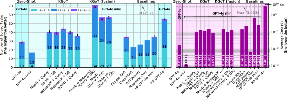### 5.1 Advantages of KGoT Figure 3 shows the number of solved tasks (the left side) as well as the average cost per solved task (the right side) for different KGoT variants as well as all comparison baselines. While we focus on GPT-4o mini, we also show the results for HF Agents and Zero-Shot with GPT-4o. Additionally, we show the Pareto front in Figure 11 for the multidimensional optimization problem of improving accuracy (i.e., reducing failed tasks) and lowering cost. All variants of KGoT solve a greater number of tasks (up to 9 more) compared to HF Agents while also being more cost-efficient (between 42% to 62% lower costs). The key reason for the KGoT advantages stems from harnessing the knowledge graph–based representation of the evolving task state. The ideal fusion runs of Neo4j and NetworkX solve an even greater number of tasks (57 for both) than the single runs, they have a lower average cost (up to 62% lower than HF Agents), and they even outperform HF Agents with GPT-4o. The fusion of all combinations of backend and solver types solve by far the highest number of tasks (71) – more than twice as much as HF Agents – while also exhibiting 44% lower cost than HF Agents. The direct Zero-Shot use of GPT-4o mini and GPT-4o has the lowest average cost per solved task (just $0.0013 and $0.0164 respectively), making it the most cost-effective, however this approach is only able to solve 17 and 29 tasks, respectively. GPTSwarm is cheaper compared to KGoT, but also comes with fewer solved tasks (only 26). While Magentic-One is a capable agent with a sophisticated architecture, its performance with GPT-4o mini is limited, solving 31 tasks correctly, while also exhibiting significantly higher costs. Simple RAG yields somewhat higher costs than KGoT and it solves fewer tasks (35). GraphRAG performs even worse, solving only 23 tasks and incurring even higher cost. While neither RAG baseline can invoke new tools to gather missing information (reducing accuracy and adaptability), GraphRAG’s worse performance is due to the fact that it primarily targets query summarization and not tasks as diverse as those tested by GAIA. Overall, KGoT achieves the best cost-accuracy tradeoff, being both highly affordable and very effective. ### 5.2 Analysis of Methods for Knowledge Extraction We explore different methods of extracting knowledge. Overall, in many situations, different methods have complementary strengths and weaknesses. Graph queries with Neo4j excel at queries such as counting patterns. Yet, Cypher queries can be difficult to generate correctly, especially for graphs with more nodes and edges. Despite this, KGoT’s Cypher queries are able to solve many new GAIA tasks that could not be solved without harnessing Cypher. SPARQL (Pérez et al., 2009) + RDF4J (Eclipse Foundation, 2025) is slightly worse (36 tasks solved) than Cypher + Neo4j (existing literature also indicates that LLMs have difficulties formulating effective SPARQL queries (Emonet et al., 2024; Mecharnia & d’Aquin, 2025)). Python with NetworkX offers certain advantages over Neo4j by eliminating the need for a separate database server, making it a lightweight choice for the KG. Moreover, NetworkX computations are fast and efficient for small to medium-sized graphs without the overhead of database transactions. Unlike Neo4j, which requires writing Cypher queries, we observe that in cases where Neo4j-based implementations struggle, NetworkX-generated graphs tend to be more detailed and provide richer vertex properties and relationships. This is likely due to the greater flexibility of Python code over Cypher queries for graph insertion, enabling more fine-grained control over vertex attributes and relationships. Another reason may be the fact that Python is likely more represented in the training data of the respective models than Cypher. Our analysis of failed tasks indicates that, in many cases, the KG contains the required data, but the graph query fails to extract it. In such scenarios, Direct Retrieval, where the entire KG is included in the model’s context, performs significantly better by bypassing query composition issues. However, Direct Retrieval demonstrates lower accuracy in cases requiring structured, multi-step reasoning. We also found that Direct Retrieval excels at extracting dispersed information but struggles with structured queries, whereas graph queries are more effective for structured reasoning but can fail when the LLM generates incorrect query formulations. Although both Cypher and general-purpose queries occasionally are erroneous, Python scripts require more frequent corrections because they are often longer and more error-prone. However, despite the higher number of corrections, the LLM is able to fix Python code more easily than Cypher queries, often succeeding after a single attempt. During retrieval, the LLM frequently embeds necessary computations directly within the Python scripts while annotating its reasoning through comments, improving transparency and interpretability. ### 5.3 Advantages on the GAIA Test Set Table 1: Comparison of KGoT with other current state-of-the-art open-source agents on the full GAIA test set. The baseline data, including for TapeAgent (Bahdanau et al., 2024), of the number of solved tasks is obtained through the GAIA Leaderboard (Mialon et al., 2025). We highlight the best performing scheme in a given category in bold. Model: GPT-4o mini. | Agents | All | L1 | L2 | L3 | | --- | --- | --- | --- | --- | | GPTSwarm | 33 | 15 | 15 | 3 | | Magentic-One | 43 | 22 | 18 | 3 | | TapeAgent | 66 | 28 | 35 | 3 | | Hugging Face Agents | 68 | 30 | 34 | 4 | | KGoT (fusion) | 73 | 33 | 36 | 4 | Furthermore, our approach achieves state-of-the-art performance on the GAIA test set with the GPT-4o mini model. The results are shown in Table 1, underscoring its effectiveness across all evaluation levels. The test set consists of 301 tasks (93 level 1 tasks, 159 level 2 tasks and 49 level 3 tasks). ### 5.4 Advantages beyond GAIA Benchmark We also evaluate KGoT as well as HF Agents and GPTSwarm on a 10% sample (433 tasks) of the SimpleQA benchmark (detailed results are in Appendix D.1). KGoT performs best, solving 73.21%, while HF Agents and GPTSwarm exhibit reduced accuracy (66.05% and 53.81% respectively). KGoT incurs only 0.018$ per solved task, less than a third of the HF Agents costs (0.058$), while being somewhat more expensive than GPTSwarm (0.00093$). We further evaluate KGoT on the entire SimpleQA benchmark (due to very high costs of running all SimpleQA questions, we limit the full benchmark evaluation to KGoT). We observe no degradation in performance with a 70.34% accuracy rate. When compared against the official F1-scores of various OpenAI and Claude models (OpenAI, 2025), KGoT outperforms all the available results. Specifically, our design achieves a 71.06% F1 score, significantly surpassing the 49.4% outcome of the top-performing reasoning model and improving upon all mini-reasoning models by at least 3.5 $×$ . Furthermore, KGoT exceeds the performance of all standard OpenAI models, from GPT-4o’s 40% F1 score to the best-scoring closed-source model, GPT-4.5, with 62.5%. More detailed results are available in Appendix D.1. ### 5.5 Ensuring Scalability and Mitigating Bottlenecks The primary bottleneck in KGoT arises from I/O-bound and latency-sensitive LLM tool invocations (e.g., web browsing, text parsing), which account for 72% of the runtime, which KGoT mitigates through asynchronous execution and graph operation parallelism as discussed in Section 3.4. A detailed breakdown of the runtime is reported in Appendix D.3. Figure 10 confirms KGoT’s scalability, as increasing the number of parallelism consistently reduces the runtime. Moreover, due to the effective knowledge extraction process and the nature of the tasks considered, none of the tasks require large KGs. The maximum graph size that we observed was 522 nodes. This is orders of magnitude below any scalability concerns. ### 5.6 Impact from Various Design Decisions <details> <summary>x13.png Details</summary>  ### Visual Description ## Grouped Bar Chart: Model Performance Comparison on Solved Tasks ### Overview This image displays a grouped bar chart comparing the performance of four different methods (GPTSwarm, HF Agents, KGoT (Neo4j + Query), and Zero-Shot) across ten different language models or model sizes. The performance metric is the "Number of Solved Tasks," where a higher value indicates better performance. ### Components/Axes * **Chart Type:** Grouped Bar Chart. * **Y-Axis:** * **Label:** "Number of Solved Tasks (the higher the better)" * **Scale:** Linear scale from 0 to 50, with major tick marks at intervals of 10 (0, 10, 20, 30, 40, 50). * **X-Axis:** * **Label:** Not explicitly labeled, but contains categorical labels for different models/model sizes. * **Categories (from left to right):** Qwen2.5-32B, DeepSeek-R1-70B, GPT4o mini, DeepSeek-R1-32B, QwQ-32B, DeepSeek-R1-7B, DeepSeek-R1-1.5B, Qwen2.5-7B, Qwen2.5-27B, Qwen2.5-1.5B. * **Legend:** * **Position:** Top center of the chart area. * **Items (with associated colors/patterns):** 1. **GPTSwarm:** Solid pink bar. 2. **HF Agents:** Solid purple bar. 3. **KGoT (Neo4j + Query):** Solid blue bar. 4. **Zero-Shot:** Bar with diagonal black hatching on a white background. ### Detailed Analysis The following table reconstructs the data presented in the chart. Values are read directly from the data labels positioned above each bar. | Model / Model Size | GPTSwarm (Pink) | HF Agents (Purple) | KGoT (Neo4j + Query) (Blue) | Zero-Shot (Hatched) | | :--- | :--- | :--- | :--- | :--- | | **Qwen2.5-32B** | 29 | 19 | 26 | 15 | | **DeepSeek-R1-70B** | 10 | 16 | 22 | 20 | | **GPT4o mini** | 26 | 6 | 40 | 17 | | **DeepSeek-R1-32B** | 0 | 17 | 35 | 14 | | **QwQ-32B** | 0 | 6 | 21 | 0 | | **DeepSeek-R1-7B** | 0 | 2 | 20 | 0 | | **DeepSeek-R1-1.5B** | 0 | 0 | 8 | 13 | | **Qwen2.5-7B** | 0 | 2 | 5 | 0 | | **Qwen2.5-27B** | 27 | 12 | 38 | 19 | | **Qwen2.5-1.5B** | 5 | 4 | 4 | 7 | **Trend Verification per Method:** * **KGoT (Blue):** This series shows the strongest overall performance. The blue bars are the tallest or tied for tallest in 8 out of 10 model categories. The trend is generally high performance, with a peak of 40 solved tasks for GPT4o mini and a low of 4 for Qwen2.5-1.5B. * **GPTSwarm (Pink):** Performance is highly variable. It performs well on larger models (29 for Qwen2.5-32B, 27 for Qwen2.5-27B) and GPT4o mini (26), but drops to 0 for five of the models, particularly the mid-range and smaller DeepSeek and Qwen variants. * **HF Agents (Purple):** Shows moderate, relatively consistent performance across most models, typically ranging between 2 and 19 solved tasks. It never achieves the highest score in any category but also rarely drops to zero (only for DeepSeek-R1-1.5B). * **Zero-Shot (Hatched):** Performance is inconsistent. It achieves moderate results on some models (20 for DeepSeek-R1-70B, 19 for Qwen2.5-27B) but scores 0 for three models (QwQ-32B, DeepSeek-R1-7B, Qwen2.5-7B). Its highest score is 20. ### Key Observations 1. **Dominant Method:** KGoT (Neo4j + Query) is the clear top performer across the broadest range of models. 2. **Model Size Sensitivity:** GPTSwarm appears highly sensitive to model size or capability, failing completely (0 tasks) on several mid-range and smaller models while performing well on the largest ones. 3. **Zero-Shot Failure Cases:** The Zero-Shot method completely fails (0 tasks) on three specific models: QwQ-32B, DeepSeek-R1-7B, and Qwen2.5-7B. 4. **Lowest Overall Performance:** The smallest models tested (DeepSeek-R1-1.5B and Qwen2.5-1.5B) show the lowest aggregate performance across all methods, with no method exceeding 13 solved tasks. 5. **Notable Outlier:** For the Qwen2.5-1.5B model, the Zero-Shot method (7 tasks) outperforms all other methods, which is an exception to the general trend. ### Interpretation The data suggests a significant advantage for the **KGoT (Neo4j + Query)** method in solving the given set of tasks. Its consistent high performance implies that integrating a structured knowledge graph (Neo4j) with a query-based approach provides a robust framework that generalizes well across different underlying language models, from large to relatively small. The **GPTSwarm** method's performance pattern indicates it may rely on capabilities that are only present in larger or more advanced models (like Qwen2.5-32B/27B and GPT4o mini), making it less reliable for a broader range of models. The **HF Agents** method offers a stable, middle-ground performance, suggesting it is a dependable but not state-of-the-art approach. The **Zero-Shot** method's inconsistency highlights the challenge of solving complex tasks without any specialized agent framework or external knowledge structure, as its success appears highly dependent on the specific model's inherent abilities. The chart effectively demonstrates that for this benchmark, the choice of agent or problem-solving framework (KGoT) can be more impactful than the raw size of the underlying language model, as seen by KGoT's strong performance even on mid-sized models like DeepSeek-R1-7B. </details> Figure 4: Performance on the GAIA validation set with KGoT (non-fusion) using various LLM models. For KGoT, we use Cypher queries for knowledge extraction from the Neo4j database. <details> <summary>x14.png Details</summary>  ### Visual Description ## Grouped Bar Chart: Knowledge Graph System Performance on Task Solving ### Overview The image is a grouped, stacked bar chart comparing the performance of four different knowledge graph (KG) systems or configurations across three distinct task types. Performance is measured by the number of solved tasks, with a higher number being better. The chart includes a maximum performance benchmark line. ### Components/Axes * **Chart Type:** Grouped, stacked bar chart. * **Y-Axis:** Labeled "Number of Solved Tasks (the higher the better)". Scale ranges from 0 to 80, with major gridlines at intervals of 10. * **X-Axis:** Categorical, showing four main system groups, each containing three task types. * **Main System Groups (from left to right):** `Neo4j`, `NetworkX`, `Neo4j + NetworkX`, `No KG`. * **Task Types within each group (from left to right):** `Query`, `Direct Retrieve`, `Query + DR`. * **Legend:** Positioned at the top-center of the chart area. Defines three performance levels represented by stacked bar segments: * `Level 1` (Light Cyan/Teal) * `Level 2` (Medium Blue) * `Level 3` (Dark Blue/Purple) * **Benchmark Line:** A horizontal dashed gray line near the top of the chart, labeled "Max: 71" on the right side, indicating a maximum possible or target score. ### Detailed Analysis The chart presents numerical results for each system and task combination, broken down by level. Values are read from the labels on each bar segment. **1. Neo4j System Group (Leftmost)** * **Query Task:** Level 1 = 21, Level 2 = 18, Level 3 = 1. **Total = 40.** * **Direct Retrieve Task:** Level 1 = 21, Level 2 = 16, Level 3 = 3. **Total = 40.** * **Query + DR Task:** Level 1 = 20, Level 2 = 24, Level 3 = 4. **Total = 48.** **2. NetworkX System Group (Second from left)** * **Query Task:** Level 1 = 20, Level 2 = 21, Level 3 = 1. **Total = 42.** * **Direct Retrieve Task:** Level 1 = 20, Level 2 = 18, Level 3 = 2. **Total = 40.** * **Query + DR Task:** Level 1 = 27, Level 2 = 28, Level 3 = 2. **Total = 57.** **3. Neo4j + NetworkX System Group (Third from left)** * **Query Task:** Level 1 = 20, Level 2 = 25, Level 3 = 1. **Total = 46.** * **Direct Retrieve Task:** Level 1 = 26, Level 2 = 24, Level 3 = 3. **Total = 53.** * **Query + DR Task:** Level 1 = 34, Level 2 = 31, Level 3 = 6. **Total = 71.** (This bar reaches the "Max: 71" benchmark line). **4. No KG System Group (Rightmost)** * **Single Run #1 Task:** Level 1 = 14, Level 2 = 14, Level 3 = 1. **Total = 29.** * **Single Run #2 Task:** Level 1 = 17, Level 2 = 16, Level 3 = 0. **Total = 33.** * **Fusion Task:** Level 1 = 19, Level 2 = 20, Level 3 = 2. **Total = 41.** ### Key Observations 1. **Performance Hierarchy:** The combined `Neo4j + NetworkX` system consistently outperforms the individual systems (`Neo4j` and `NetworkX`) and the `No KG` baseline across all comparable tasks. 2. **Task Difficulty:** For all systems with a KG, the `Query + DR` task yields the highest total solved tasks, followed by `Query`, with `Direct Retrieve` generally being the lowest or tied. This suggests the combined task is either easier or better supported by these systems. 3. **Benchmark Achievement:** Only one configuration, `Neo4j + NetworkX` on the `Query + DR` task, achieves the maximum benchmark score of 71. 4. **Level Contribution:** `Level 1` and `Level 2` contribute the vast majority of solved tasks across all systems. `Level 3` contributions are minimal (typically 0-6 tasks), indicating these are the most difficult problems. 5. **No KG Baseline:** The `No KG` system shows the lowest performance, as expected. Its task labels (`Single Run #1`, `Single Run #2`, `Fusion`) differ from the others, suggesting a different experimental setup or capability set. Its best performance (`Fusion`, 41) is comparable to the worst performance of the KG-enabled systems. ### Interpretation This chart demonstrates the significant value of integrating knowledge graph technologies (`Neo4j`, `NetworkX`) for solving complex tasks compared to a system without a structured knowledge base (`No KG`). The data suggests a synergistic effect when combining two different KG technologies (`Neo4j + NetworkX`), as this configuration achieves the highest performance, reaching the predefined maximum benchmark. The consistent pattern where `Query + DR` outperforms standalone `Query` or `Direct Retrieve` tasks implies that the systems benefit from combining retrieval and querying capabilities. The very low contribution of `Level 3` across the board highlights a common challenge or ceiling in solving the most advanced tier of problems, regardless of the underlying system. The experiment likely aims to validate the hypothesis that a hybrid KG architecture provides superior problem-solving capability, which the results strongly support. The `No KG` results serve as a crucial control, quantifying the baseline performance achievable without the structured knowledge representation and reasoning that KGs provide. 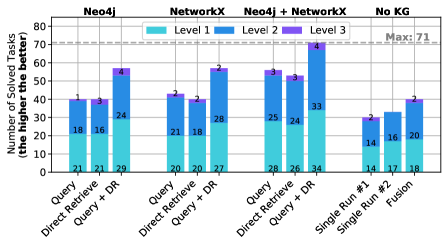</details> Figure 5: The impact coming from harnessing knowledge graphs (KGs) with different knowledge extraction methods (graph queries with Neo4j and Cypher, and general-purpose languages with Python and NetworkX), vs. using no KGs at all. DR stands for Direct Retrieval. Model: GPT-4o mini. 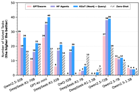We also show the advantages of KGoT on different open models in Figure 5 over HF Agents and GPTSwarm for nearly all considered models (Yang et al., 2025; Guo et al., 2025). Interestingly, certain sizes of DeepSeek-R1 (Guo et al., 2025) offer high Zero-Shot performance that outperforms both KGoT and HF Agents, illustrating potential for further improvements specifically aimed at Reasoning Language Models (RLMs) (Besta et al., 2025a; c). Finally, we investigate the impact on performance coming from harnessing KGs, vs. using no KGs at all (the “no KG” baseline), which we illustrate in Figure 5. Harnessing KGs has clear advantages, with a nearly 2 $×$ increase in the number of solved tasks. This confirms the positive impact from structuring the task related knowledge into a graph format, and implies that our workflow generates high quality graphs. To further confirm this, we additionally verified these graphs manually and we discovered that the generated KGs do contain the actual solution (e.g., the solution can be found across nodes/edges of a given KG by string matching). This illustrates that in the majority of the solved tasks, the automatically generated KGs correctly represent the solution and directly enable solving a given task. We offer further analyses in Appendix D, including studying the impact on performance from different tool sets, prompt formats as well as fusion types. ## 6 Related Work Our work is related to numerous LLM domains. First, we use LangChain (LangChain Inc., 2025a) to facilitate the integration of the LLM agents with the rest of the KGoT system. Other such LLM integration frameworks, such as MiniChain (Rush, 2023) or AutoChain (Forethought, 2023), could be used instead. Agent collaboration frameworks are systems such as Magentic-One and numerous others (Zhuge et al., 2024; Tang et al., 2024; Liu et al., 2024b; Li et al., 2024; Chu et al., 2024; Wu et al., 2024; Chen et al., 2024; Hong et al., 2024; Shinn et al., 2023; Zhu et al., 2024; Kagaya et al., 2024; Zhao et al., 2024a; Stengel-Eskin et al., 2024; Significant Gravitas, 2025; Zhu et al., 2025). The core KGoT idea that can be applied to enhance such frameworks is that a KG can also be used as a common shared task representation for multiple agents solving a task together. Such a graph would be then updated by more than a single agent. This idea proves effective, as confirmed by the fact that KGoT outperforms highly competitive baselines (HF Agents, Magentic-One, GPTSwarm) in both GAIA and SimpleQA benchmarks. Some agent frameworks explicitly use graphs for more effective collaboration. Examples are GPTSwarm (Zhuge et al., 2024), MacNet (Qian et al., 2025), and AgentPrune (Zhang et al., 2025). These systems differ from KGoT as they use a graph to model and manage multiple agents in a structured way, forming a hierarchy of tools. Contrarily, KGoT uses KGs to represent the task itself, including its intermediate state. These two design choices are orthogonal and could be combined together. Moreover, while KGoT only relies on in-context learning; both MacNet (Qian et al., 2025) and AgentPrune (Zhang et al., 2025) require additional training rounds, making their integration and deployment more challenging and expensive than KGoT. Many works exist in the domain of general prompt engineering (Beurer-Kellner et al., 2024; Besta et al., 2025c; Yao et al., 2023a; Besta et al., 2024a; Wei et al., 2022; Yao et al., 2023b; Chen et al., 2023; Creswell et al., 2023; Wang et al., 2023a; Hu et al., 2024; Dua et al., 2022; Jung et al., 2022; Ye et al., 2023). One could use such schemes to further enhance respective parts of the KGoT workflow. While we already use prompts that are suited for encoding knowledge graphs, possibly harnessing other ideas from that domain could bring further benefits. Task decomposition & planning increases the effectiveness of LLMs by dividing a task into subtasks. Examples include ADaPT (Prasad et al., 2024), ANPL (Huang et al., 2023), and others (Zhu et al., 2025; Shen et al., 2023). Overall, the whole KGoT workflow already harnesses recursive task decomposition: the input task is divided into numerous steps, and many of these steps are further decomposed into sub steps by the LLM Graph Executor if necessary. For example, when solving a task based on the already constructed KG, the LLM Graph Executor may decide to decompose this step similarly to ADaPT. Other decomposition schemes could also be tried, we leave this as future work. Retrieval-Augmented Generation (RAG) is an important part of the LLM ecosystem, with numerous designs being proposed (Edge et al., 2025; Gao et al., 2024; Besta et al., 2025b; Zhao et al., 2024b; Hu & Lu, 2025; Huang & Huang, 2024; Yu et al., 2024a; Mialon et al., 2023; Li et al., 2022; Abdallah & Jatowt, 2024; Delile et al., 2024; Manathunga & Illangasekara, 2023; Zeng et al., 2024; Wewer et al., 2021; Xu et al., 2024; Sarthi et al., 2024; Asai et al., 2024; Yu et al., 2024b; Gutiérrez et al., 2024). RAG has been used primarily to ensure data privacy and to reduce hallucinations. We illustrate that it has lower performance than KGoT when applied to AI assistant tasks. Another increasingly important part of the LLM ecosystem is the usage of tools to augment the abilities of LLMs (Beurer-Kellner et al., 2023; Schick et al., 2023; Xie et al., 2024). For example, ToolNet (Liu et al., 2024a) uses a directed graph to model the application of multiple tools while solving a task, however focuses specifically on the iterative usage of tools at scale. KGoT harnesses a flexible and adaptable hierarchy of various tools, which can easily be extended with ToolNet and such designs, to solve a wider range of complex tasks. While KGoT focuses on classical AI assistant tasks, it can be extended to other applications. Promising directions could include supporting multi-stage, cost-efficient reasoning, for example to enhance the capabilities of the recent reasoning models such as DeepSeek-R1. Extending KGoT to this and other domains may require new ways of KG construction via predictive graph models (Besta et al., 2023a; 2024c), integration with neural graph databases (Besta et al., 2022), or deployment over distributed-memory clusters for scalability. Further, refining its reasoning strategies through advanced task decomposition schemes could improve performance on very long-horizon tasks. These directions highlight both the generality of the framework and current boundaries in tool orchestration, reasoning depth, and scalability, which we aim to address in future work. ## 7 Conclusion In this paper, we introduce Knowledge Graph of Thoughts (KGoT), an AI assistant architecture that enhances the reasoning capabilities of low-cost models while significantly reducing operational expenses. By dynamically constructing and evolving knowledge graphs (KGs) that encode the task and its resolution state, KGoT enables structured knowledge representation and retrieval, improving task success rates on benchmarks such as GAIA and SimpleQA. Our extensive evaluation demonstrates that KGoT outperforms existing LLM-based agent solutions, for example achieving a substantial increase in task-solving efficiency of 29% or more over the competitive Hugging Face Agents baseline, while ensuring over 36 $×$ lower costs. Thanks to its modular design, KGoT can be extended to new domains that require complex multi-step reasoning integrated with extensive interactions with the external compute environment, for example automated scientific discovery or software design. #### Acknowledgments We thank Chi Zhang and Muyang Du for their contributions to the framework. We thank Hussein Harake, Colin McMurtrie, Mark Klein, Angelo Mangili, and the whole CSCS team granting access to the Ault, Daint and Alps machines, and for their excellent technical support. We thank Timo Schneider for help with infrastructure at SPCL. This project received funding from the European Research Council (Project PSAP, No. 101002047), and the European High-Performance Computing Joint Undertaking (JU) under grant agreement No. 955513 (MAELSTROM). This project was supported by the ETH Future Computing Laboratory (EFCL), financed by a donation from Huawei Technologies. This project received funding from the European Union’s HE research and innovation programme under the grant agreement No. 101070141 (Project GLACIATION). We gratefully acknowledge the Polish high-performance computing infrastructure PLGrid (HPC Center: ACK Cyfronet AGH) for providing computer facilities and support within computational grant no. PLG/2024/017103. ## References - Abdallah & Jatowt (2024) Abdelrahman Abdallah and Adam Jatowt. Generator-Retriever-Generator Approach for Open-Domain Question Answering, March 2024. URL https://arxiv.org/abs/2307.11278. arXiv:2307.11278. - Asai et al. (2024) Akari Asai, Zeqiu Wu, Yizhong Wang, Avirup Sil, and Hannaneh Hajishirzi. Self-RAG: Learning to Retrieve, Generate, and Critique through Self-Reflection. In B. Kim, Y. Yue, S. Chaudhuri, K. Fragkiadaki, M. Khan, and Y. Sun (eds.), Proceedings of the Twelfth International Conference on Learning Representations, ICLR ’24, pp. 9112–9141, Vienna, Austria, May 2024. International Conference on Learning Representations. URL https://proceedings.iclr.cc/paper_files/paper/2024/hash/25f7be9694d7b32d5cc670927b8091e1-Abstract-Conference.html. - Bahdanau et al. (2024) Dzmitry Bahdanau, Nicolas Gontier, Gabriel Huang, Ehsan Kamalloo, Rafael Pardinas, Alex Piché, Torsten Scholak, Oleh Shliazhko, Jordan Prince Tremblay, Karam Ghanem, Soham Parikh, Mitul Tiwari, and Quaizar Vohra. TapeAgents: A Holistic Framework for Agent Development and Optimization, December 2024. URL https://arxiv.org/abs/2412.08445. arXiv:2412.08445. - Ben Mahria et al. (2021) Bilal Ben Mahria, Ilham Chaker, and Azeddine Zahi. An Empirical Study on the Evaluation of the RDF Storage Systems. Journal of Big Data, 8(1):100:1–100:20, July 2021. ISSN 2196-1115. doi: 10.1186/s40537-021-00486-y. URL https://journalofbigdata.springeropen.com/articles/10.1186/s40537-021-00486-y. - Benedicic et al. (2019) Lucas Benedicic, Felipe A. Cruz, Alberto Madonna, and Kean Mariotti. Sarus: Highly Scalable Docker Containers for HPC Systems. In Michèle Weiland, Guido Juckeland, Sadaf Alam, and Heike Jagode (eds.), Proceedings of the International Conference on High Performance Computing (ICS ’19), volume 11887 of Lecture Notes in Computer Science, pp. 46–60, Frankfurt, Germany, June 2019. Springer International Publishing. ISBN 978-3-030-34356-9. doi: 10.1007/978-3-030-34356-9˙5. URL https://link.springer.com/chapter/10.1007/978-3-030-34356-9_5. - Besta et al. (2018) Maciej Besta, Dimitri Stanojevic, Tijana Zivic, Jagpreet Singh, Maurice Hoerold, and Torsten Hoefler. Log(Graph): A Near-Optimal High-Performance Graph Representation. In Proceedings of the 27th International Conference on Parallel Architectures and Compilation Techniques, PACT ’18, pp. 7:1–7:13, Limassol, Cyprus, November 2018. Association for Computing Machinery. ISBN 9781450359863. doi: 10.1145/3243176.3243198. URL https://doi.org/10.1145/3243176.3243198. - Besta et al. (2022) Maciej Besta, Patrick Iff, Florian Scheidl, Kazuki Osawa, Nikoli Dryden, Michal Podstawski, Tiancheng Chen, and Torsten Hoefler. Neural Graph Databases. In Bastian Rieck and Razvan Pascanu (eds.), Proceedings of the First Learning on Graphs Conference, volume 198 of Proceedings of Machine Learning Research, pp. 31:1–31:38, Virtual Event, December 2022. PMLR. URL https://proceedings.mlr.press/v198/besta22a.html. - Besta et al. (2023a) Maciej Besta, Afonso Claudino Catarino, Lukas Gianinazzi, Nils Blach, Piotr Nyczyk, Hubert Niewiadomski, and Torsten Hoefler. HOT: Higher-Order Dynamic Graph Representation Learning with Efficient Transformers. In Soledad Villar and Benjamin Chamberlain (eds.), Proceedings of the Second Learning on Graphs Conference, volume 231 of Proceedings of Machine Learning Research, pp. 15:1–15:20, Virtual Event, November 2023a. PMLR. URL https://proceedings.mlr.press/v231/besta24a.html. - Besta et al. (2023b) Maciej Besta, Robert Gerstenberger, Marc Fischer, Michal Podstawski, Nils Blach, Berke Egeli, Georgy Mitenkov, Wojciech Chlapek, Marek Michalewicz, Hubert Niewiadomski, Jürgen Müller, and Torsten Hoefler. The Graph Database Interface: Scaling Online Transactional and Analytical Graph Workloads to Hundreds of Thousands of Cores. In Proceedings of the International Conference for High Performance Computing, Networking, Storage and Analysis, SC ’23, pp. 22:1–22:18, Denver, CO, USA, November 2023b. Association for Computing Machinery. ISBN 9798400701092. doi: 10.1145/3581784.3607068. URL https://doi.org/10.1145/3581784.3607068. - Besta et al. (2023c) Maciej Besta, Robert Gerstenberger, Emanuel Peter, Marc Fischer, Michał Podstawski, Claude Barthels, Gustavo Alonso, and Torsten Hoefler. Demystifying Graph Databases: Analysis and Taxonomy of Data Organization, System Designs, and Graph Queries. ACM Comput. Surv., 56(2):31:1–31:40, September 2023c. ISSN 0360-0300. doi: 10.1145/3604932. URL https://doi.org/10.1145/3604932. - Besta et al. (2024a) Maciej Besta, Nils Blach, Ales Kubicek, Robert Gerstenberger, Michal Podstawski, Lukas Gianinazzi, Joanna Gajda, Tomasz Lehmann, Hubert Niewiadomski, Piotr Nyczyk, and Torsten Hoefler. Graph of Thoughts: Solving Elaborate Problems with Large Language Models. Proceedings of the AAAI Conference on Artificial Intelligence, 38(16):17682–17690, March 2024a. doi: 10.1609/aaai.v38i16.29720. URL https://ojs.aaai.org/index.php/AAAI/article/view/29720. - Besta et al. (2024b) Maciej Besta, Robert Gerstenberger, Patrick Iff, Pournima Sonawane, Juan Gómez Luna, Raghavendra Kanakagiri, Rui Min, Onur Mutlu, Torsten Hoefler, Raja Appuswamy, and Aidan O Mahony. Hardware Acceleration for Knowledge Graph Processing: Challenges & Recent Developments, November 2024b. URL https://arxiv.org/abs/2408.12173. arXiv:2408.12173. - Besta et al. (2024c) Maciej Besta, Florian Scheidl, Lukas Gianinazzi, Grzegorz Kwaśniewski, Shachar Klaiman, Jürgen Müller, and Torsten Hoefler. Demystifying Higher-Order Graph Neural Networks, December 2024c. URL https://arxiv.org/abs/2406.12841. arXiv:2406.12841. - Besta et al. (2025a) Maciej Besta, Julia Barth, Eric Schreiber, Ales Kubicek, Afonso Catarino, Robert Gerstenberger, Piotr Nyczyk, Patrick Iff, Yueling Li, Sam Houliston, Tomasz Sternal, Marcin Copik, Grzegorz Kwaśniewski, Jürgen Müller, Łukasz Flis, Hannes Eberhard, Zixuan Chen, Hubert Niewiadomski, and Torsten Hoefler. Reasoning Language Models: A Blueprint, June 2025a. URL https://arxiv.org/abs/2501.11223. arXiv:2501.11223. - Besta et al. (2025b) Maciej Besta, Ales Kubicek, Robert Gerstenberger, Marcin Chrapek, Roman Niggli, Patrik Okanovic, Yi Zhu, Patrick Iff, Michał Podstawski, Lucas Weitzendorf, Mingyuan Chi, Joanna Gajda, Piotr Nyczyk, Jürgen Müller, Hubert Niewiadomski, and Torsten Hoefler. Multi-Head RAG: Solving Multi-Aspect Problems with LLMs, July 2025b. URL https://arxiv.org/abs/2406.05085. arXiv:2406.05085. - Besta et al. (2025c) Maciej Besta, Florim Memedi, Zhenyu Zhang, Robert Gerstenberger, Guangyuan Piao, Nils Blach, Piotr Nyczyk, Marcin Copik, Grzegorz Kwaśniewski, Jürgen Müller, Lukas Gianinazzi, Ales Kubicek, Hubert Niewiadomski, Aidan O’Mahony, Onur Mutlu, and Torsten Hoefler. Demystifying Chains, Trees, and Graphs of Thoughts. IEEE Transactions on Pattern Analysis and Machine Intelligence, August 2025c. doi: 10.1109/TPAMI.2025.3598182. URL https://ieeexplore.ieee.org/document/11123142. - Besta et al. (2025d) Maciej Besta, Lorenzo Paleari, Marcin Copik, Robert Gerstenberger, Ales Kubicek, Piotr Nyczyk, Patrick Iff, Eric Schreiber, Tanja Srindran, Tomasz Lehmann, Hubert Niewiadomski, and Torsten Hoefler. CheckEmbed: Effective Verification of LLM Solutions to Open-Ended Tasks, July 2025d. URL https://arxiv.org/abs/2406.02524. arXiv:2406.02524. - Beurer-Kellner et al. (2023) Luca Beurer-Kellner, Marc Fischer, and Martin Vechev. Large Language Models are Zero-Shot Multi-Tool Users. In Proceedings of the ICML Workshop on Knowledge and Logical Reasoning in the Era of Data-Driven Learning, KLR ’23, Honolulu, HI, USA, July 2023. URL https://files.sri.inf.ethz.ch/website/papers/lmql_actions.pdf. - Beurer-Kellner et al. (2024) Luca Beurer-Kellner, Mark Niklas Müller, Marc Fischer, and Martin Vechev. Prompt Sketching for Large Language Models. In Proceedings of the 41st International Conference on Machine Learning (ICML ’24), volume 235 of Proceedings of Machine Learning Research, pp. 3674–3706, Vienna, Austria, July 2024. PMLR. URL https://proceedings.mlr.press/v235/beurer-kellner24b.html. - Bhattacharjya et al. (2024) Debarun Bhattacharjya, Junkyu Lee, Don Joven Agravante, Balaji Ganesan, and Radu Marinescu. Foundation Model Sherpas: Guiding Foundation Models through Knowledge and Reasoning, February 2024. URL https://arxiv.org/abs/2402.01602. arXiv:2402.01602. - Chen et al. (2024) Guangyao Chen, Siwei Dong, Yu Shu, Ge Zhang, Jaward Sesay, Börje F Karlsson, Jie Fu, and Yemin Shi. AutoAgents: A Framework for Automatic Agent Generation. In Kate Larson (ed.), Proceedings of the Thirty-Third International Joint Conference on Artificial Intelligence, IJCAI ’24, pp. 22–30, Jeju, South Korea, August 2024. International Joint Conferences on Artificial Intelligence Organization. doi: 10.24963/ijcai.2024/3. URL https://www.ijcai.org/proceedings/2024/3. - Chen et al. (2023) Wenhu Chen, Xueguang Ma, Xinyi Wang, and William W. Cohen. Program of Thoughts Prompting: Disentangling Computation from Reasoning for Numerical Reasoning Tasks. Transactions on Machine Learning Research, November 2023. ISSN 2835-8856. URL https://openreview.net/forum?id=YfZ4ZPt8zd. - Chu et al. (2024) Zhixuan Chu, Yan Wang, Feng Zhu, Lu Yu, Longfei Li, and Jinjie Gu. Professional Agents – Evolving Large Language Models into Autonomous Experts with Human-Level Competencies, February 2024. URL https://arxiv.org/abs/2402.03628. arXiv:2402.03628. - Creswell et al. (2023) Antonia Creswell, Murray Shanahan, and Irina Higgins. Selection-Inference: Exploiting Large Language Models for Interpretable Logical Reasoning. In Proceedings of the Eleventh International Conference on Learning Representations, ICLR ’23, Kigali, Rwanda, May 2023. OpenReview. URL https://openreview.net/forum?id=3Pf3Wg6o-A4. - Delile et al. (2024) Julien Delile, Srayanta Mukherjee, Anton Van Pamel, and Leonid Zhukov. Graph-Based Retriever Captures the Long Tail of Biomedical Knowledge. In Proceedings of the Workshop ML for Life and Material Science: From Theory to Industry Applications, ML4LMS ’24, Vienna, Austria, July 2024. OpenReview. URL https://openreview.net/forum?id=RUwfsPWrv3. - Docker Inc. (2025) Docker Inc. Docker: Accelerated Container Applications. https://www.docker.com/, July 2025. Accessed: 2025-09-22. - Dua et al. (2022) Dheeru Dua, Shivanshu Gupta, Sameer Singh, and Matt Gardner. Successive Prompting for Decomposing Complex Questions. In Yoav Goldberg, Zornitsa Kozareva, and Yue Zhang (eds.), Proceedings of the 2022 Conference on Empirical Methods in Natural Language Processing, EMNLP ’22, pp. 1251–1265, Abu Dhabi, United Arab Emirates, December 2022. Association for Computational Linguistics. doi: 10.18653/v1/2022.emnlp-main.81. URL https://aclanthology.org/2022.emnlp-main.81/. - Eclipse Foundation (2025) Eclipse Foundation. RDF4J. https://rdf4j.org/, September 2025. Accessed: 2025-09-22. - Edge et al. (2025) Darren Edge, Ha Trinh, Newman Cheng, Joshua Bradley, Alex Chao, Apurva Mody, Steven Truitt, Dasha Metropolitansky, Robert Osazuwa Ness, and Jonathan Larson. From Local to Global: A Graph RAG Approach to Query-Focused Summarization, February 2025. URL https://arxiv.org/abs/2404.16130. arXiv:2404.16130. - Emonet et al. (2024) Vincent Emonet, Jerven Bolleman, Severine Duvaud, Tarcisio Mendes de Farias, and Ana Claudia Sima. LLM-Based SPARQL Query Generation from Natural Language over Federated Knowledge Graphs. In Reham Alharbi, Jacopo de Berardinis, Paul Groth, Albert Meroño Peñuela, Elena Simperl, and Valentina Tamma (eds.), Proceedings of the Special Session on Harmonising Generative AI and Semantic Web Technologies (HGAIS ’24), volume 3953 of Workshop Proceedings, Baltimore, MD, USA, November 2024. CEUR. URL https://ceur-ws.org/Vol-3953/355.pdf. - Forethought (2023) Forethought. AutoChain. https://autochain.forethought.ai/, 2023. Accessed: 2025-09-22. - Fourney et al. (2024) Adam Fourney, Gagan Bansal, Hussein Mozannar, Cheng Tan, Eduardo Salinas, Erkang Zhu, Friederike Niedtner, Grace Proebsting, Griffin Bassman, Jack Gerrits, Jacob Alber, Peter Chang, Ricky Loynd, Robert West, Victor Dibia, Ahmed Awadallah, Ece Kamar, Rafah Hosn, and Saleema Amershi. Magentic-One: A Generalist Multi-Agent System for Solving Complex Tasks, November 2024. URL https://arxiv.org/abs/2411.04468. arXiv:2411.04468. - Francis et al. (2018) Nadime Francis, Alastair Green, Paolo Guagliardo, Leonid Libkin, Tobias Lindaaker, Victor Marsault, Stefan Plantikow, Mats Rydberg, Petra Selmer, and Andrés Taylor. Cypher: An Evolving Query Language for Property Graphs. In Proceedings of the International Conference on Management of Data, SIGMOD ’18, pp. 1433–1445, Houston, TX, USA, June 2018. Association for Computing Machinery. ISBN 9781450347037. doi: 10.1145/3183713.3190657. URL https://doi.org/10.1145/3183713.3190657. - Gao et al. (2024) Yunfan Gao, Yun Xiong, Xinyu Gao, Kangxiang Jia, Jinliu Pan, Yuxi Bi, Yi Dai, Jiawei Sun, Meng Wang, and Haofen Wang. Retrieval-Augmented Generation for Large Language Models: A Survey, March 2024. URL https://arxiv.org/abs/2312.10997. arXiv:2312.10997. - Gu et al. (2025) Jiawei Gu, Xuhui Jiang, Zhichao Shi, Hexiang Tan, Xuehao Zhai, Chengjin Xu, Wei Li, Yinghan Shen, Shengjie Ma, Honghao Liu, et al. A Survey on LLM-as-a-Judge, March 2025. URL https://arxiv.org/abs/2411.15594. arXiv:2411.15594. - Guo et al. (2025) Daya Guo, Dejian Yang, Haowei Zhang, Junxiao Song, Ruoyu Zhang, Runxin Xu, Qihao Zhu, Shirong Ma, Peiyi Wang, Xiao Bi, et al. DeepSeek-R1: Incentivizing Reasoning Capability in LLMs via Reinforcement Learning, January 2025. URL https://arxiv.org/abs/2501.12948. arXiv:2501.12948. - Guo et al. (2024) Taicheng Guo, Xiuying Chen, Yaqi Wang, Ruidi Chang, Shichao Pei, Nitesh V. Chawla, Olaf Wiest, and Xiangliang Zhang. Large Language Model Based Multi-Agents: A Survey of Progress and Challenges. In Kate Larson (ed.), Proceedings of the Thirty-Third International Joint Conference on Artificial Intelligence, IJCAI ’24, pp. 8048–8057, Jeju, South Korea, August 2024. International Joint Conferences on Artificial Intelligence Organization. doi: 10.24963/ijcai.2024/890. URL https://www.ijcai.org/proceedings/2024/890. Survey Track. - Gutiérrez et al. (2024) Bernal Jiménez Gutiérrez, Yiheng Shu, Yu Gu, Michihiro Yasunaga, and Yu Su. HippoRAG: Neurobiologically Inspired Long-Term Memory for Large Language Models. In A. Globerson, L. Mackey, D. Belgrave, A. Fan, U. Paquet, J. Tomczak, and C. Zhang (eds.), Proceedings of the Thirty-Eighth Annual Conference on Neural Information Processing Systems (NeurIPS ’24), volume 37 of Advances in Neural Information Processing Systems, pp. 59532–59569, Vancouver, Canada, December 2024. Curran Associates. URL https://proceedings.neurips.cc/paper_files/paper/2024/hash/6ddc001d07ca4f319af96a3024f6dbd1-Abstract-Conference.html. - Hong et al. (2024) Sirui Hong, Mingchen Zhuge, Jonathan Chen, Xiawu Zheng, Yuheng Cheng, Jinlin Wang, Ceyao Zhang, Zili Wang, Steven Ka Shing Yau, Zijuan Lin, Liyang Zhou, Chenyu Ran, Lingfeng Xiao, Chenglin Wu, and Jürgen Schmidhuber. MetaGPT: Meta Programming for a Multi-Agent Collaborative Framework. In B. Kim, Y. Yue, S. Chaudhuri, K. Fragkiadaki, M. Khan, and Y. Sun (eds.), Proceedings of the Twelfth International Conference on Learning Representations, ICLR ’24, pp. 23247–23275, Vienna, Austria, May 2024. International Conference on Learning Representations. URL https://proceedings.iclr.cc/paper_files/paper/2024/hash/6507b115562bb0a305f1958ccc87355a-Abstract-Conference.html. - Hu et al. (2024) Hanxu Hu, Hongyuan Lu, Huajian Zhang, Wai Lam, and Yue Zhang. Chain-of-Symbol Prompting Elicits Planning in Large Langauge Models, August 2024. URL https://arxiv.org/abs/2305.10276. arXiv:2305.10276. - Hu & Lu (2025) Yucheng Hu and Yuxing Lu. RAG and RAU: A Survey on Retrieval-Augmented Language Model in Natural Language Processing, June 2025. URL https://arxiv.org/abs/2404.19543. arXiv:2404.19543. - Huang et al. (2023) Di Huang, Ziyuan Nan, Xing Hu, Pengwei Jin, Shaohui Peng, Yuanbo Wen, Rui Zhang, Zidong Du, Qi Guo, Yewen Pu, and Yunji Chen. ANPL: Towards Natural Programming with Interactive Decomposition. In A. Oh, T. Naumann, A. Globerson, K. Saenko, M. Hardt, and S. Levine (eds.), Proceedings of the Thirty-Seventh Annual Conference on Neural Information Processing Systems (NeurIPS ’23), volume 36 of Advances in Neural Information Processing Systems, pp. 69404–69440, New Orleans, LA, USA, December 2023. Curran Associates. URL https://proceedings.neurips.cc/paper_files/paper/2023/hash/dba8fa689ede9e56cbcd4f719def38fb-Abstract-Conference.html. - Huang & Huang (2024) Yizheng Huang and Jimmy Huang. A Survey on Retrieval-Augmented Text Generation for Large Language Models, August 2024. URL https://arxiv.org/abs/2404.10981. arXiv:2404.10981. - Jung et al. (2022) Jaehun Jung, Lianhui Qin, Sean Welleck, Faeze Brahman, Chandra Bhagavatula, Ronan Le Bras, and Yejin Choi. Maieutic Prompting: Logically Consistent Reasoning with Recursive Explanations. In Yoav Goldberg, Zornitsa Kozareva, and Yue Zhang (eds.), Proceedings of the 2022 Conference on Empirical Methods in Natural Language Processing, EMNLP ’22, pp. 1266–1279, Abu Dhabi, United Arab Emirates, December 2022. Association for Computational Linguistics. doi: 10.18653/v1/2022.emnlp-main.82. URL https://aclanthology.org/2022.emnlp-main.82/. - Kaddour et al. (2023) Jean Kaddour, Joshua Harris, Maximilian Mozes, Herbie Bradley, Roberta Raileanu, and Robert McHardy. Challenges and Applications of Large Language Models, July 2023. URL https://arxiv.org/abs/2307.10169. arXiv:2307.10169. - Kagaya et al. (2024) Tomoyuki Kagaya, Thong Jing Yuan, Yuxuan Lou, Jayashree Karlekar, Sugiri Pranata, Akira Kinose, Koki Oguri, Felix Wick, and Yang You. RAP: Retrieval-Augmented Planning with Contextual Memory for Multimodal LLM Agents. In Proceedings of the Workshop on Open-World Agents, OWA ’24, Vancouver, Canada, December 2024. OpenReview. URL https://openreview.net/forum?id=Xf49Dpxuox. - Kim et al. (2024) Sehoon Kim, Suhong Moon, Ryan Tabrizi, Nicholas Lee, Michael W. Mahoney, Kurt Keutzer, and Amir Gholami. An LLM Compiler for Parallel Function Calling. In Ruslan Salakhutdinov, Zico Kolter, Katherine Heller, Adrian Weller, Nuria Oliver, Jonathan Scarlett, and Felix Berkenkamp (eds.), Proceedings of the 41st International Conference on Machine Learning (ICML ’24), volume 235 of Proceedings of Machine Learning Research, pp. 24370–24391, Vienna, Austria, July 2024. PMLR. URL https://proceedings.mlr.press/v235/kim24y.html. - LangChain Inc. (2025a) LangChain Inc. LangChain. https://www.langchain.com/, 2025a. Accessed: 2025-09-22. - LangChain Inc. (2025b) LangChain Inc. Dealing with API Errors. https://js.langchain.com/v0.1/docs/modules/data_connection/text_embedding/api_errors/, 2025b. Accessed: 2025-09-22. - LangChain Inc. (2025c) LangChain Inc. LangChain Core Tools: BaseTool. https://api.python.langchain.com/en/latest/tools/langchain_core.tools.BaseTool.html, 2025c. Accessed: 2025-09-22. - LangChain Inc. (2025d) LangChain Inc. How to parse JSON output. https://python.langchain.com/docs/how_to/output_parser_json/, 2025d. Accessed: 2025-09-22. - Lewis et al. (2020) Patrick Lewis, Ethan Perez, Aleksandra Piktus, Fabio Petroni, Vladimir Karpukhin, Naman Goyal, Heinrich Küttler, Mike Lewis, Wen-tau Yih, Tim Rocktäschel, Sebastian Riedel, and Douwe Kiela. Retrieval-Augmented Generation for Knowledge-Intensive NLP Tasks. In H. Larochelle, M. Ranzato, R. Hadsell, M.F. Balcan, and H. Lin (eds.), Proceedings of the Thirty-Fourth Annual Conference on Neural Information Processing Systems (NeurIPS ’20), volume 33 of Advances in Neural Information Processing Systems, pp. 9459–9474, Virtual Event, December 2020. Curran Associates. URL https://proceedings.neurips.cc/paper_files/paper/2020/hash/6b493230205f780e1bc26945df7481e5-Abstract.html. - Li & Vasarhelyi (2024) Huaxia Li and Miklos A. Vasarhelyi. Applying Large Language Models in Accounting: A Comparative Analysis of Different Methodologies and Off-the-Shelf Examples. Journal of Emerging Technologies in Accounting, 21(2):133–152, October 2024. ISSN 1554-1908. doi: 10.2308/JETA-2023-065. URL https://publications.aaahq.org/jeta/article-abstract/21/2/133/12800/. - Li et al. (2022) Huayang Li, Yixuan Su, Deng Cai, Yan Wang, and Lemao Liu. A Survey on Retrieval-Augmented Text Generation, February 2022. URL https://arxiv.org/abs/2202.01110. arXiv:2202.01110. - Li et al. (2024) Junyou Li, Qin Zhang, Yangbin Yu, Qiang Fu, and Deheng Ye. More Agents Is All You Need. Transactions on Machine Learning Research, October 2024. ISSN 2835-8856. URL https://openreview.net/forum?id=bgzUSZ8aeg. - Liu et al. (2024a) Xukun Liu, Zhiyuan Peng, Xiaoyuan Yi, Xing Xie, Lirong Xiang, Yuchen Liu, and Dongkuan Xu. ToolNet: Connecting Large Language Models with Massive Tools via Tool Graph, February 2024a. URL https://arxiv.org/abs/2403.00839. arXiv:2403.00839. - Liu et al. (2024b) Zijun Liu, Yanzhe Zhang, Peng Li, Yang Liu, and Diyi Yang. A Dynamic LLM-Powered Agent Network for Task-Oriented Agent Collaboration. In Proceedings of the First Conference on Language Modeling, COLM ’24, Philadelphia, PA, USA, October 2024b. OpenReview. URL https://openreview.net/forum?id=XII0Wp1XA9. - Manathunga & Illangasekara (2023) S. S. Manathunga and Y. A. Illangasekara. Retrieval Augmented Generation and Representative Vector Summarization for Large Unstructured Textual Data in Medical Education, August 2023. URL https://arxiv.org/abs/2308.00479. arXiv:2308.00479. - Mecharnia & d’Aquin (2025) Thamer Mecharnia and Mathieu d’Aquin. Performance and Limitations of Fine-Tuned LLMs in SPARQL Query Generation. In Genet Asefa Gesese, Harald Sack, Heiko Paulheim, Albert Merono-Penuela, and Lihu Chen (eds.), Proceedings of the Workshop on Generative AI and Knowledge Graphs, GenAIK ’25, pp. 69–77, Abu Dhabi, United Arab Emirates, January 2025. International Committee on Computational Linguistics. URL https://aclanthology.org/2025.genaik-1.8/. - Mialon et al. (2023) Grégoire Mialon, Roberto Dessi, Maria Lomeli, Christoforos Nalmpantis, Ramakanth Pasunuru, Roberta Raileanu, Baptiste Roziere, Timo Schick, Jane Dwivedi-Yu, Asli Celikyilmaz, Edouard Grave, Yann LeCun, and Thomas Scialom. Augmented Language Models: A Survey. Transactions on Machine Learning Research, July 2023. ISSN 2835-8856. URL https://openreview.net/forum?id=jh7wH2AzKK. Survey Certification. - Mialon et al. (2024) Grégoire Mialon, Clémentine Fourrier, Thomas Wolf, Yann LeCun, and Thomas Scialom. GAIA: A Benchmark for General AI Assistants. In B. Kim, Y. Yue, S. Chaudhuri, K. Fragkiadaki, M. Khan, and Y. Sun (eds.), Proceedings of the Twelfth International Conference on Learning Representations, ICLR ’24, pp. 9025–9049, Vienna, Austria, May 2024. International Conference on Learning Representations. URL https://proceedings.iclr.cc/paper_files/paper/2024/hash/25ae35b5b1738d80f1f03a8713e405ec-Abstract-Conference.html. - Mialon et al. (2025) Grégoire Mialon, Clémentine Fourrier, Thomas Wolf, Yann LeCun, and Thomas Scialom. GAIA Leaderboard. https://huggingface.co/spaces/gaia-benchmark/leaderboard, September 2025. Accessed: 2025-09-25. - NetworkX Developers (2025) NetworkX Developers. NetworkX Documentation. https://networkx.org/, May 2025. Accessed: 2025-09-22. - OpenAI (2025) OpenAI. simple-evals. https://github.com/openai/simple-evals, July 2025. Accessed: 2025-09-22. - Pérez et al. (2009) Jorge Pérez, Marcelo Arenas, and Claudio Gutierrez. Semantics and Complexity of SPARQL. ACM Trans. Database Syst., 34(3):16:1–16:45, September 2009. ISSN 0362-5915. doi: 10.1145/1567274.1567278. URL https://doi.org/10.1145/1567274.1567278. - Prasad et al. (2024) Archiki Prasad, Alexander Koller, Mareike Hartmann, Peter Clark, Ashish Sabharwal, Mohit Bansal, and Tushar Khot. ADaPT: As-Needed Decomposition and Planning with Language Models. In Kevin Duh, Helena Gomez, and Steven Bethard (eds.), Findings of the Association for Computational Linguistics: NAACL 2024, pp. 4226–4252, Mexico City, Mexico, June 2024. Association for Computational Linguistics. doi: 10.18653/v1/2024.findings-naacl.264. URL https://aclanthology.org/2024.findings-naacl.264/. - Python Software Foundation (2025a) Python Software Foundation. codecs — Codec registry and base classes. https://docs.python.org/3/library/codecs.html, September 2025a. Accessed: 2025-09-22. - Python Software Foundation (2025b) Python Software Foundation. asyncio — Asynchronous I/O. https://docs.python.org/3/library/asyncio.html, September 2025b. Accessed: 2025-09-22. - Qian et al. (2025) Chen Qian, Zihao Xie, Yifei Wang, Wei Liu, Kunlun Zhu, Hanchen Xia, Yufan Dang, Zhuoyun Du, Weize Chen, Cheng Yang, Zhiyuan Liu, and Maosong Sun. Scaling Large Language Model-Based Multi-Agent Collaboration. In Y. Yue, A. Garg, N. Peng, F. Sha, and R. Yu (eds.), Proceedings of the Thirteenth International Conference on Learning Representations, ICLR ’25, pp. 41488–41505, Singapore, April 2025. International Conference on Learning Representations. URL https://proceedings.iclr.cc/paper_files/paper/2025/hash/66a026c0d17040889b50f0dfa650e5e0-Abstract-Conference.html. - Robinson et al. (2015) Ian Robinson, Jim Webber, and Emil Eifrem. Graph Database Internals. In Graph Databases, chapter 7, pp. 149–170. O’Reilly, Sebastopol, CA, USA, 2nd edition, 2015. ISBN 9781491930892. - Roucher & Petrov (2025) Aymeric Roucher and Sergei Petrov. Beating GAIA with Transformers Agents. https://github.com/aymeric-roucher/GAIA, February 2025. Accessed: 2025-09-22. - Rush (2023) Alexander Rush. MiniChain: A Small Library for Coding with Large Language Models. In Yansong Feng and Els Lefever (eds.), Proceedings of the 2023 Conference on Empirical Methods in Natural Language Processing: System Demonstrations, EMNLP ’23, pp. 311–317, Singapore, December 2023. Association for Computational Linguistics. doi: 10.18653/v1/2023.emnlp-demo.27. URL https://aclanthology.org/2023.emnlp-demo.27. - Sarthi et al. (2024) Parth Sarthi, Salman Abdullah, Aditi Tuli, Shubh Khanna, Anna Goldie, and Christopher Manning. RAPTOR: Recursive Abstractive Processing for Tree-Organized Retrieval. In B. Kim, Y. Yue, S. Chaudhuri, K. Fragkiadaki, M. Khan, and Y. Sun (eds.), Proceedings of the Twelfth International Conference on Learning Representations, ICLR ’24, pp. 32628–32649, Vienna, Austria, May 2024. International Conference on Learning Representations. URL https://proceedings.iclr.cc/paper_files/paper/2024/hash/8a2acd174940dbca361a6398a4f9df91-Abstract-Conference.html. - Schick et al. (2023) Timo Schick, Jane Dwivedi-Yu, Roberto Dessì, Roberta Raileanu, Maria Lomeli, Eric Hambro, Luke Zettlemoyer, Nicola Cancedda, and Thomas Scialom. Toolformer: Language Models Can Teach Themselves to Use Tools. In A. Oh, T. Naumann, A. Globerson, K. Saenko, M. Hardt, and S. Levine (eds.), Proceedings of the Thirty-Seventh Annual Conference on Neural Information Processing Systems (NeurIPS ’23), volume 36 of Advances in Neural Information Processing Systems, pp. 68539–68551, New Orleans, LA, USA, December 2023. Curran Associates. URL https://proceedings.neurips.cc/paper_files/paper/2023/hash/d842425e4bf79ba039352da0f658a906-Abstract-Conference.html. - SerpApi LLM (2025) SerpApi LLM. SerpApi: Google Search API. https://serpapi.com/, 2025. Accessed: 2025-09-22. - Shen et al. (2023) Yongliang Shen, Kaitao Song, Xu Tan, Dongsheng Li, Weiming Lu, and Yueting Zhuang. HuggingGPT: Solving AI Tasks with ChatGPT and its Friends in Hugging Face. In A. Oh, T. Naumann, A. Globerson, K. Saenko, M. Hardt, and S. Levine (eds.), Proceedings of the Thirty-Seventh Annual Conference on Neural Information Processing Systems (NeurIPS ’23), volume 36 of Advances in Neural Information Processing Systems, pp. 38154–38180, New Orleans, LA, USA, December 2023. Curran Associates. URL https://proceedings.neurips.cc/paper_files/paper/2023/hash/77c33e6a367922d003ff102ffb92b658-Abstract-Conference.html. - Shinn et al. (2023) Noah Shinn, Federico Cassano, Ashwin Gopinath, Karthik Narasimhan, and Shunyu Yao. Reflexion: Language Agents with Verbal Reinforcement Learning. In A. Oh, T. Naumann, A. Globerson, K. Saenko, M. Hardt, and S. Levine (eds.), Proceedings of the Thirty-Seventh Annual Conference on Neural Information Processing Systems (NeurIPS ’23), volume 36 of Advances in Neural Information Processing Systems, pp. 8634–8652, New Orleans, LA, USA, December 2023. Curran Associates. URL https://proceedings.neurips.cc/paper_files/paper/2023/hash/1b44b878bb782e6954cd888628510e90-Abstract-Conference.html. - Significant Gravitas (2025) Significant Gravitas. AutoGPT. https://github.com/Significant-Gravitas/AutoGPT, September 2025. Accessed: 2025-09-22. - Singhal (2012) Amit Singhal. Introducing the Knowledge Graph: things, not strings. https://www.blog.google/products/search/introducing-knowledge-graph-things-not/, May 2012. Accessed: 2025-09-22. - Stengel-Eskin et al. (2024) Elias Stengel-Eskin, Archiki Prasad, and Mohit Bansal. ReGAL: Refactoring Programs to Discover Generalizable Abstractions. In Ruslan Salakhutdinov, Zico Kolter, Katherine Heller, Adrian Weller, Nuria Oliver, Jonathan Scarlett, and Felix Berkenkamp (eds.), Proceedings of the 41st International Conference on Machine Learning (ICML ’24), volume 235 of Proceedings of Machine Learning Research, pp. 46605–46624, Vienna, Austria, July 2024. PMLR. URL https://proceedings.mlr.press/v235/stengel-eskin24a.html. - Sumers et al. (2024) Theodore Sumers, Shunyu Yao, Karthik Narasimhan, and Thomas Griffiths. Cognitive Architectures for Language Agents. Transactions on Machine Learning Research, February 2024. ISSN 2835-8856. URL https://openreview.net/forum?id=1i6ZCvflQJ. Survey Certification. - Tang et al. (2024) Xunzhu Tang, Kisub Kim, Yewei Song, Cedric Lothritz, Bei Li, Saad Ezzini, Haoye Tian, Jacques Klein, and Tegawendé F. Bissyandé. CodeAgent: Autonomous Communicative Agents for Code Review. In Yaser Al-Onaizan, Mohit Bansal, and Yun-Nung Chen (eds.), Proceedings of the 2024 Conference on Empirical Methods in Natural Language Processing, EMNLP ’24, pp. 11279–11313, Miami, FL, USA, November 2024. Association for Computational Linguistics. doi: 10.18653/v1/2024.emnlp-main.632. URL https://aclanthology.org/2024.emnlp-main.632/. - Tenacity Developers (2025a) Tenacity Developers. Tenacity: Retrying Library. https://github.com/jd/tenacity, April 2025a. Accessed: 2025-09-22. - Tenacity Developers (2025b) Tenacity Developers. Tenacity Documentation. https://tenacity.readthedocs.io/en/latest/, 2025b. Accessed: 2025-09-22. - Wang et al. (2023a) Shenzhi Wang, Chang Liu, Zilong Zheng, Siyuan Qi, Shuo Chen, Qisen Yang, Andrew Zhao, Chaofei Wang, Shiji Song, and Gao Huang. Avalon’s Game of Thoughts: Battle Against Deception through Recursive Contemplation, October 2023a. URL https://arxiv.org/abs/2310.01320. arXiv:2310.01320. - Wang et al. (2023b) Xuezhi Wang, Jason Wei, Dale Schuurmans, Quoc V. Le, Ed H. Chi, Sharan Narang, Aakanksha Chowdhery, and Denny Zhou. Self-Consistency Improves Chain of Thought Reasoning in Language Models. In Proceedings of the Eleventh International Conference on Learning Representations, ICLR ’23, Kigali, Rwanda, May 2023b. OpenReview. URL https://openreview.net/forum?id=1PL1NIMMrw. - Wang et al. (2023c) Zihao Wang, Shaofei Cai, Guanzhou Chen, Anji Liu, Xiaojian (Shawn) Ma, and Yitao Liang. Describe, Explain, Plan and Select: Interactive Planning with LLMs Enables Open-World Multi-Task Agents. In A. Oh, T. Naumann, A. Globerson, K. Saenko, M. Hardt, and S. Levine (eds.), Proceedings of the Thirty-Seventh Annual Conference on Neural Information Processing Systems (NeurIPS ’23), volume 36 of Advances in Neural Information Processing Systems, pp. 34153–34189, New Orleans, LA, USA, December 2023c. Curran Associates. URL https://proceedings.neurips.cc/paper_files/paper/2023/hash/6b8dfb8c0c12e6fafc6c256cb08a5ca7-Abstract-Conference.html. - Wei et al. (2022) Jason Wei, Xuezhi Wang, Dale Schuurmans, Maarten Bosma, Brian Ichter, Fei Xia, Ed Chi, Quoc V. Le, and Denny Zhou. Chain-of-Thought Prompting Elicits Reasoning in Large Language Models. In S. Koyejo, S. Mohamed, A. Agarwal, D. Belgrave, K. Cho, and A. Oh (eds.), Proceedings of the Thirty-Sixth Annual Conference on Neural Information Processing Systems (NeurIPS ’22), volume 35 of Advances in Neural Information Processing Systems, pp. 24824–24837, New Orleans, LA, USA, December 2022. Curran Associates. URL https://proceedings.neurips.cc/paper_files/paper/2022/hash/9d5609613524ecf4f15af0f7b31abca4-Abstract-Conference.html. - Wei et al. (2024) Jason Wei, Nguyen Karina, Hyung Won Chung, Yunxin Joy Jiao, Spencer Papay, Amelia Glaese, John Schulman, and William Fedus. Measuring Short-Form Factuality in Large Language Models, November 2024. URL https://arxiv.org/abs/2411.04368. arXiv:2411.04368. - Wewer et al. (2021) Christopher Wewer, Florian Lemmerich, and Michael Cochez. Updating Embeddings for Dynamic Knowledge Graphs, September 2021. URL https://arxiv.org/abs/2109.10896. arXiv:2109.10896. - Wu et al. (2024) Qingyun Wu, Gagan Bansal, Jieyu Zhang, Yiran Wu, Beibin Li, Erkang Zhu, Li Jiang, Xiaoyun Zhang, Shaokun Zhang, Jiale Liu, Ahmed Hassan Awadallah, Ryen W. White, Doug Burger, and Chi Wang. AutoGen: Enabling Next-Gen LLM Applications via Multi-Agent Conversation. In Proceedings of the First Conference on Language Modeling, COLM ’24, Philadelphia, PA, USA, October 2024. OpenReview. URL https://openreview.net/forum?id=BAakY1hNKS. - Xie et al. (2024) Tianbao Xie, Fan Zhou, Zhoujun Cheng, Peng Shi, Luoxuan Weng, Yitao Liu, Toh Jing Hua, Junning Zhao, Qian Liu, Che Liu, Zeju Liu, Yiheng Xu, Hongjin Su, Dongchan Shin, Caiming Xiong, and Tao Yu. OpenAgents: An Open Platform for Language Agents in the Wild. In Proceedings of the First Conference on Language Modeling, COLM ’24, Philadelphia, PA, USA, October 2024. OpenReview. URL https://openreview.net/forum?id=sKATR2O1Y0. - Xu et al. (2024) Zhipeng Xu, Zhenghao Liu, Yukun Yan, Shuo Wang, Shi Yu, Zheni Zeng, Chaojun Xiao, Zhiyuan Liu, Ge Yu, and Chenyan Xiong. ActiveRAG: Autonomously Knowledge Assimilation and Accommodation through Retrieval-Augmented Agents, October 2024. URL https://arxiv.org/abs/2402.13547. arXiv:2402.13547. - Yang et al. (2025) An Yang, Baosong Yang, Beichen Zhang, Binyuan Hui, Bo Zheng, Bowen Yu, Chengyuan Li, Dayiheng Liu, Fei Huang, Haoran Wei, Huan Lin, et al. Qwen2.5 Technical Report, January 2025. URL https://arxiv.org/abs/2412.15115. arXiv:2412.15115. - Yao et al. (2023a) Shunyu Yao, Dian Yu, Jeffrey Zhao, Izhak Shafran, Tom Griffiths, Yuan Cao, and Karthik Narasimhan. Tree of Thoughts: Deliberate Problem Solving with Large Language Models. In A. Oh, T. Naumann, A. Globerson, K. Saenko, M. Hardt, and S. Levine (eds.), Proceedings of the Thirty-Seventh Annual Conference on Neural Information Processing Systems (NeurIPS ’23), volume 36 of Advances in Neural Information Processing Systems, pp. 11809–11822, New Orleans, LA, USA, December 2023a. Curran Associates. URL https://proceedings.neurips.cc/paper_files/paper/2023/hash/271db9922b8d1f4dd7aaef84ed5ac703-Abstract-Conference.html. - Yao et al. (2023b) Shunyu Yao, Jeffrey Zhao, Dian Yu, Nan Du, Izhak Shafran, Karthik Narasimhan, and Yuan Cao. ReAct: Synergizing Reasoning and Acting in Language Models. In Proceedings of the Eleventh International Conference on Learning Representations, ICLR ’23, Kigali, Rwanda, May 2023b. OpenReview. URL https://openreview.net/forum?id=WE_vluYUL-X. - Ye et al. (2023) Yunhu Ye, Binyuan Hui, Min Yang, Binhua Li, Fei Huang, and Yongbin Li. Large Language Models Are Versatile Decomposers: Decomposing Evidence and Questions for Table-Based Reasoning. In Proceedings of the 46th International ACM SIGIR Conference on Research and Development in Information Retrieval, SIGIR ’23, pp. 174–184, Taipei, Taiwan, July 2023. Association for Computing Machinery. ISBN 9781450394086. doi: 10.1145/3539618.3591708. URL https://doi.org/10.1145/3539618.3591708. - Yu et al. (2024a) Hao Yu, Aoran Gan, Kai Zhang, Shiwei Tong, Qi Liu, and Zhaofeng Liu. Evaluation of Retrieval-Augmented Generation: A Survey. In Wenwu Zhu, Hui Xiong, Xiuzhen Cheng, Lizhen Cui, Zhicheng Dou, Junyu Dong, Shanchen Pang, Li Wang, Lanju Kong, and Zhenxiang Chen (eds.), Proceedings of the 12th CCF Conference, BigData, volume 2301 of Communications in Computer and Information Science (CCIS), pp. 102–120, Qingdao, China, August 2024a. Springer Nature. ISBN 978-981-96-1024-2. doi: 10.1007/978-981-96-1024-2˙8. URL https://link.springer.com/chapter/10.1007/978-981-96-1024-2_8. - Yu et al. (2024b) Wenhao Yu, Hongming Zhang, Xiaoman Pan, Peixin Cao, Kaixin Ma, Jian Li, Hongwei Wang, and Dong Yu. Chain-of-Note: Enhancing Robustness in Retrieval-Augmented Language Models. In Yaser Al-Onaizan, Mohit Bansal, and Yun-Nung Chen (eds.), Proceedings of the 2024 Conference on Empirical Methods in Natural Language Processing, EMNLP ’24, pp. 14672–14685, Miami, FL, USA, November 2024b. Association for Computational Linguistics. doi: 10.18653/v1/2024.emnlp-main.813. URL https://aclanthology.org/2024.emnlp-main.813/. - Zeng et al. (2024) Huimin Zeng, Zhenrui Yue, Qian Jiang, and Dong Wang. Federated Recommendation via Hybrid Retrieval Augmented Generation. In Wei Ding, Chang-Tien Lu, Fusheng Wang, Liping Di, Kesheng Wu, Jun Huan, Raghu Nambiar, Jundong Li, Filip Ilievski, Ricardo Baeza-Yates, and Xiaohua Hu (eds.), Proceedings of the IEEE International Conference on Big Data, BigData ’24, pp. 8078–8087, Washington, DC, USA, December 2024. IEEE Press. doi: 10.1109/BigData62323.2024.10825302. URL https://ieeexplore.ieee.org/document/10825302. - Zhang et al. (2025) Guibin Zhang, Yanwei Yue, Zhixun Li, Sukwon Yun, Guancheng Wan, Kun Wang, Dawei Cheng, Jeffrey Xu Yu, and Tianlong Chen. Cut the Crap: An Economical Communication Pipeline for LLM-Based Multi-Agent Systems. In Y. Yue, A. Garg, N. Peng, F. Sha, and R. Yu (eds.), Proceedings of the Thirteenth International Conference on Learning Representations, ICLR ’25, pp. 75389–75428, Singapore, April 2025. International Conference on Learning Representations. URL https://proceedings.iclr.cc/paper_files/paper/2025/hash/bbc461518c59a2a8d64e70e2c38c4a0e-Abstract-Conference.html. - Zhao et al. (2024a) Andrew Zhao, Daniel Huang, Quentin Xu, Matthieu Lin, Yong-Jin Liu, and Gao Huang. ExpeL: LLM Agents Are Experiential Learners. Proceedings of the AAAI Conference on Artificial Intelligence, 38(17):19632–19642, March 2024a. doi: 10.1609/aaai.v38i17.29936. URL https://ojs.aaai.org/index.php/AAAI/article/view/29936. - Zhao et al. (2024b) Penghao Zhao, Hailin Zhang, Qinhan Yu, Zhengren Wang, Yunteng Geng, Fangcheng Fu, Ling Yang, Wentao Zhang, Jie Jiang, and Bin Cui. Retrieval-Augmented Generation for AI-Generated Content: A Survey, June 2024b. URL https://arxiv.org/abs/2402.19473. arXiv:2402.19473. - Zheng et al. (2023) Lianmin Zheng, Wei-Lin Chiang, Ying Sheng, Siyuan Zhuang, Zhanghao Wu, Yonghao Zhuang, Zi Lin, Zhuohan Li, Dacheng Li, Eric Xing, et al. Judging LLM-as-a-Judge with MT-Bench and Chatbot Arena. In A. Oh, T. Naumann, A. Globerson, K. Saenko, M. Hardt, and S. Levine (eds.), Proceedings of the Thirty-Seventh Annual Conference on Neural Information Processing Systems (NeurIPS ’23), volume 36 of Advances in Neural Information Processing Systems, pp. 46595–46623, New Orleans, LA, USA, December 2023. Curran Associates. URL https://proceedings.neurips.cc/paper_files/paper/2023/hash/91f18a1287b398d378ef22505bf41832-Abstract-Datasets_and_Benchmarks.html. - Zhu et al. (2025) Yuqi Zhu, Shuofei Qiao, Yixin Ou, Shumin Deng, Shiwei Lyu, Yue Shen, Lei Liang, Jinjie Gu, Huajun Chen, and Ningyu Zhang. KnowAgent: Knowledge-Augmented Planning for LLM-Based Agents. In Luis Chiruzzo, Alan Ritter, and Lu Wang (eds.), Findings of the Association for Computational Linguistics: NAACL 2025, pp. 3709–3732, Albuquerque, NM, USA, April 2025. Association for Computational Linguistics. ISBN 979-8-89176-195-7. URL https://aclanthology.org/2025.findings-naacl.205/. - Zhu et al. (2024) Zhaocheng Zhu, Yuan Xue, Xinyun Chen, Denny Zhou, Jian Tang, Dale Schuurmans, and Hanjun Dai. Large Language Models Can Learn Rules, December 2024. URL https://arxiv.org/abs/2310.07064. arXiv:2310.07064. - Zhuge et al. (2024) Mingchen Zhuge, Wenyi Wang, Louis Kirsch, Francesco Faccio, Dmitrii Khizbullin, and Jürgen Schmidhuber. GPTSwarm: Language Agents as Optimizable Graphs. In Ruslan Salakhutdinov, Zico Kolter, Katherine Heller, Adrian Weller, Nuria Oliver, Jonathan Scarlett, and Felix Berkenkamp (eds.), Proceedings of the 41st International Conference on Machine Learning (ICML ’24), volume 235 of Proceedings of Machine Learning Research, pp. 62743–62767, Vienna, Austria, July 2024. PMLR. URL https://proceedings.mlr.press/v235/zhuge24a.html. ## Appendix A Additional Examples of Knowledge Graph Representation of Tasks We include selected snapshots of KG representation of tasks, covering a wide range of graph structures from simple chains to trees and cyclic graphs. Each snapshot captures the current KG state in a JSON file, exported using a predefined query that retrieves all labeled nodes and edges. Regardless of the underlying graph backend, the use of a consistent export format allows all snapshots to be visualized through Neo4j’s built-in web interface. In the following, we showcase illustrations of such snapshots and task statements from the GAIA validation set. Please note that the GAIA benchmark discourages making its tasks accessible to crawling. To honor their wishes, we replaced the names of entities with placeholders in the following examples, while keeping the overall structure intact. 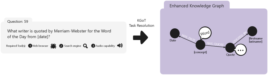<details> <summary>x15.png Details</summary>  ### Visual Description ## Diagram: Knowledge Graph Task Resolution (KGoT) Process Flow ### Overview The image illustrates a conceptual workflow for resolving a natural language question using a Knowledge Graph Task Resolution (KGoT) system. It depicts the transformation of a user's question into a structured query against an "Enhanced Knowledge Graph." The diagram is composed of three main sections: a question input panel on the left, a central process arrow, and a knowledge graph schema on the right. ### Components & Flow The diagram is segmented into three distinct regions: 1. **Left Panel (Question Input):** * A white card with a light gray header labeled **"Question: 59"**. * The main question text reads: **"What writer is quoted by Merriam-Webster for the Word of the Day from [date]?"** * Below the question, a line specifies: **"Required Tool(s): 1 Web browser, 2 Search engine, 3 Audio capability."** Each tool number is accompanied by a small icon (a globe, a magnifying glass, and a speaker, respectively). 2. **Center (Process Indicator):** * A thick, black arrow points from the left panel to the right panel. * Above the arrow, the text **"KGoT Task Resolution"** is displayed, indicating the process that transforms the question into a graph query. 3. **Right Panel (Enhanced Knowledge Graph Schema):** * A light purple box with the title **"Enhanced Knowledge Graph"** at the top. * Inside the box is a node-and-edge diagram representing the graph structure needed to answer the question. * **Nodes (Entities):** * **Date** (black circle, leftmost) * **Word** (white circle with black outline, center-top) * **[concept]** (black circle, center) * **Quote** (black circle, center-right) * **[firstname lastname]** (black circle, rightmost) * An additional small node with three dots **"..."** is connected to the "Quote" node, suggesting expandable or additional properties. * **Edges (Relationships):** * An arrow labeled **"HAS DATE"** points from the **Word** node to the **Date** node. * An arrow labeled **"HAS QUOTE"** points from the **Word** node to the **Quote** node. * An arrow labeled **"QUOTED BY"** points from the **Quote** node to the **[firstname lastname]** node. * The **[concept]** node is connected to the **Word** node by an unlabeled edge, implying a "is a" or "represents" relationship. ### Detailed Analysis * **Spatial Grounding:** The legend/title "Enhanced Knowledge Graph" is positioned at the top-center of the right purple panel. The graph nodes are arranged in a left-to-right flow that mirrors the logical dependency of the answer: a specific `Word` (for a given `Date`) has a `Quote`, which is `QUOTED BY` a specific writer (`[firstname lastname]`). * **Component Isolation:** The diagram clearly isolates the input (question with required tools), the processing engine (KGoT), and the target data structure (knowledge graph). The knowledge graph itself is a sub-component showing the precise schema needed. * **Trend Verification:** Not applicable, as this is a structural diagram, not a data chart. ### Key Observations 1. **Question Specificity:** The question is highly structured, asking for a specific writer associated with a specific lexical item ("Word of the Day") from a specific source (Merriam-Webster) on a specific date. 2. **Tool Requirement:** The inclusion of "Audio capability" as a required tool is notable. It suggests the system may need to process audio pronunciations or other audio data from the source, or that the KGoT system itself has multimodal capabilities. 3. **Graph Schema:** The knowledge graph schema is minimal but precise. It defines the exact path of relationships (`Word -> HAS QUOTE -> Quote -> QUOTED BY -> Writer`) needed to resolve the question. The `[concept]` node indicates that the "Word" is linked to an underlying lexical concept. 4. **Placeholder Notation:** The use of brackets in `[date]` and `[firstname lastname]` indicates these are variable slots to be filled by the system during query execution. ### Interpretation This diagram demonstrates a **symbolic AI or neuro-symbolic AI approach** to question answering. Instead of relying solely on a neural network to generate an answer, the system first parses the natural language question into a formal query structure (the knowledge graph pattern). * **What it suggests:** The KGoT system acts as a translator, converting human language into a precise, machine-readable query that can be executed against a structured knowledge base (the Enhanced Knowledge Graph). This method promotes accuracy, explainability, and the ability to handle complex, multi-hop questions. * **How elements relate:** The question defines the *goal*. The required tools define the *means* to gather raw data. The KGoT process is the *reasoning engine* that structures the goal. The knowledge graph schema is the *blueprint* for the information retrieval and assembly process. * **Notable implication:** The presence of the "Audio capability" tool hints that the "Enhanced Knowledge Graph" may contain or be linked to multimodal data (like word pronunciations), moving beyond purely textual relationships. The diagram argues for a hybrid system where flexible natural language understanding is grounded in rigid, logical data structures. </details> Figure 6: Example of a chain structure. This task requires 7 intermediate steps and the usage of 3 tools. The expected solution is ’[firstname lastname]’. KGoT invokes the Surfer agent to search for relevant pages, locate the relevant quote, and find the person who said it. All intermediate information is successfully retrieved and used for enhancing the dynamically constructed KG. The quote contains two properties, significance and text. ’significance’ stores the meaning of the quote, whereas ’text’ stores the actual quote. 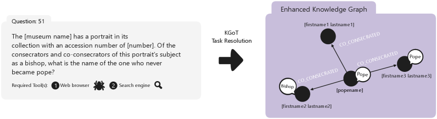<details> <summary>x16.png Details</summary>  ### Visual Description ## Diagram: KGoT Task Resolution Process with Enhanced Knowledge Graph ### Overview The image is a two-panel diagram illustrating a process called "KGoT Task Resolution." It shows how a natural language question about a museum portrait is processed and represented within an "Enhanced Knowledge Graph" to derive an answer. The left panel contains the input question and required tools, while the right panel visualizes the resulting knowledge graph structure. ### Components/Axes The diagram is composed of two primary sections connected by a central arrow. **1. Left Panel (Input):** * **Header:** "Question: 51" * **Question Text:** "The [museum name] has a portrait in its collection with an accession number of [number]. Of the consecrators and co-consecrators of this portrait's subject as a bishop, what is the name of the one who never became pope?" * **Required Tool(s):** Listed below the question. * Icon 1: A globe icon labeled "Web browser". * Icon 2: A magnifying glass icon labeled "Search engine". **2. Central Connector:** * A thick black arrow points from the left panel to the right panel. * Text above the arrow: "KGoT Task Resolution". **3. Right Panel (Output - Enhanced Knowledge Graph):** * **Header:** "Enhanced Knowledge Graph" (in a purple banner). * **Graph Structure:** A network diagram with three main nodes (black circles) and connecting lines (edges). * **Nodes and Labels:** * **Bottom-Left Node:** Has a white label attached reading "Bishop". Below this node is the placeholder text "[firstname2 lastname2]". * **Center Node:** Has a white label attached reading "Pope". Below this node is the placeholder text "[popename]". * **Top-Right Node:** Has no attached label. Below this node is the placeholder text "[firstname3 lastname3]". * **Edges and Relationships:** * A line connects the "Bishop" node to the "Pope" node. The relationship label on this line is "CO_CONSECRATED". * A line connects the "Pope" node to the unlabeled top-right node. The relationship label on this line is "CO_CONSECRATED". * A line connects the "Bishop" node to the unlabeled top-right node. The relationship label on this line is "CO_CONSECRATED". * **Additional Node:** There is a fourth, isolated black circle node at the top center of the graph. Below it is the placeholder text "[firstname1 lastname1]". This node has no visible connections to the other three. ### Detailed Analysis The diagram depicts a specific workflow: 1. **Input:** A templated question (Question 51) is posed. It contains placeholders (`[museum name]`, `[number]`) for specific data points. The question asks to identify a specific individual from a set of religious figures (consecrators/co-consecrators) based on a negative condition (never became pope). 2. **Process:** The question is processed by the "KGoT Task Resolution" system. The acronym "KGoT" is not defined in the image. 3. **Output Representation:** The system's output is visualized as an "Enhanced Knowledge Graph." This graph models entities (people) and their relationships. * The entities are represented as nodes, with placeholders for their names (`[firstname2 lastname2]`, `[popename]`, etc.). * The relationships are represented as edges, all labeled "CO_CONSECRATED," indicating a shared role in a consecration ceremony. * The graph explicitly models one entity as a "Bishop" and another as a "Pope," directly mapping to the roles mentioned in the input question. * The structure shows a triangular relationship between three individuals (Bishop, Pope, and a third person), all co-consecrated with each other. A fourth individual is present but disconnected. ### Key Observations * **Placeholder Language:** All specific names and identifiers are replaced with generic placeholders (`[...]`), indicating this is a template or schematic example, not a solved instance. * **Graph Topology:** The core of the graph is a fully connected triad (three nodes each connected to the other two). The isolated fourth node suggests it may be an entity retrieved by the system but not directly relevant to the specific relationship chain being queried. * **Role Labeling:** Only two of the four nodes have explicit role labels ("Bishop," "Pope"). This directly corresponds to the question's focus on distinguishing between those who were bishops and those who became pope. * **Tool Indication:** The required tools (web browser, search engine) imply that the KGoT system likely performs external information retrieval to populate the knowledge graph with real data to replace the placeholders. ### Interpretation This diagram illustrates a **knowledge-graph-based question-answering (QA) pipeline**. The process can be interpreted as follows: 1. **Question Parsing:** The system parses the natural language question, identifying key entities (museum, portrait, accession number) and the core relational query (find a person among consecrators who was a bishop but not a pope). 2. **Information Retrieval:** Using the specified tools (web browser, search engine), the system would search for the museum, the specific portrait, and its subject. It would then research the consecrators and co-consecrators involved in that subject's episcopal consecration. 3. **Knowledge Graph Construction:** The retrieved information is structured into a graph. The nodes represent the individuals found. The "CO_CONSECRATED" edges represent the factual relationship established by their joint participation in the consecration event. 4. **Answer Derivation:** The graph structure allows the system to apply logical filters. It can identify all nodes connected to the portrait's subject (the central "Pope" node in this example graph might represent the subject, or another key figure). It can then filter these connected nodes for those with the "Bishop" label and, crucially, exclude any node that also has the "Pope" label. The remaining node(s) would contain the answer. The **underlying investigative logic** (Peircean) is abductive: the system starts with an observation (a portrait exists), posits a hypothesis about the relationships between historical figures (they were co-consecrators), and uses available evidence (web data) to construct a model (the knowledge graph) that can be interrogated to find the best explanation (the name of the bishop who never became pope). The diagram emphasizes that the answer is not found through simple text search but by mapping and analyzing relational structures within retrieved data. The presence of placeholders and a template question suggests this is a demonstration of the system's *capability* to handle such complex, relational queries. </details> Figure 7: Example of a tree structure. This task requires 6 intermediate steps and the usage of 2 tools. The expected solution is ’[firstname1 lastname1]’. The Surfer agent is also invoked for this task. In this KG representation of the task, [popename] is identified as the consecrator, where [firstname1 lastname1], [firstname2 lastname2] and [firstname3 lastname3] are all co-consecrators. Subsequently, the correct answer is obtained from the KGoT from the KG by correctly identifying [firstname1 lastname1] as the one without any labels. 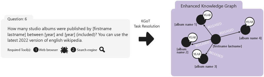<details> <summary>x17.png Details</summary>  ### Visual Description ## Diagram: KGoT Task Resolution Process Flow ### Overview The image is a conceptual diagram illustrating a two-step process for resolving a natural language question using a Knowledge Graph-based Task (KGoT) resolution system. It visually maps a user's question to a structured knowledge graph representation. The diagram is composed of two primary rectangular containers connected by a directional arrow, set against a plain, light gray background. ### Components/Axes The diagram has two main components arranged horizontally: 1. **Left Component (Input):** A white, rounded rectangle with a subtle drop shadow, labeled "Question: 6" at the top. 2. **Central Connector:** A thick, black, right-pointing arrow labeled "KGoT Task Resolution" above it. 3. **Right Component (Output):** A larger, light purple rounded rectangle with a darker purple header bar, titled "Enhanced Knowledge Graph". ### Detailed Analysis **Left Component - Question Box:** * **Header:** "Question: 6" * **Main Text:** "How many studio albums were published by [firstname lastname] between [year] and [year] (included)? You can use the latest 2022 version of english wikipedia." * **Footer Label:** "Required Tool(s):" * **Tool Icons & Labels:** * Icon 1: A stylized globe/web icon. Label: "1 Web browser" * Icon 2: A magnifying glass icon. Label: "2 Search engine" **Central Connector:** * **Arrow:** A solid black arrow pointing from the left box to the right box. * **Label:** "KGoT Task Resolution" is written in black text above the arrow shaft. **Right Component - Enhanced Knowledge Graph:** * **Header:** "Enhanced Knowledge Graph" in white text on a dark purple bar. * **Graph Structure:** A network diagram with black circular nodes and connecting lines. * **Node Types & Labels:** * **Central Node:** A large black circle labeled "[firstname lastname]" in white text. * **Album Nodes:** Four black circles labeled "[album name 1]", "[album name 2]", "[album name 3]", and "[album name 4]" in white text. * **Year Nodes:** Four smaller black circles, each labeled "YEAR" in white text. Each is connected to one of the album nodes. * **Relationships (Edges):** Lines connect the central node to each album node. Each connecting line is labeled with the word "RELEASED" in gray, uppercase text, oriented along the line. ### Key Observations * **Spatial Grounding:** The legend (the "Required Tool(s)" list) is positioned at the bottom of the input box. The knowledge graph is the dominant element on the right side. * **Component Isolation:** The diagram is cleanly segmented into an input region (question and tools), a processing step (arrow), and an output region (knowledge graph). * **Trend/Flow Verification:** The visual flow is strictly left-to-right, indicating a transformation process. The graph structure shows a one-to-many relationship from the artist (central node) to multiple albums, each with an associated release year. * **Placeholder Consistency:** The placeholders `[firstname lastname]`, `[year]`, and `[album name X]` in the question text directly correspond to the labeled nodes in the knowledge graph, demonstrating how the system parses the query into structured entities. ### Interpretation This diagram serves as a visual explanation of how a natural language question-answering system, specifically one using a Knowledge Graph-based Task (KGoT) resolver, processes a query. 1. **Process Demonstration:** It illustrates the transformation from an unstructured, parameterized question ("How many studio albums...") into a structured data model. The "Enhanced Knowledge Graph" is the system's internal representation of the query's core entities (artist, albums, years) and their relationships (RELEASED). 2. **System Logic:** The diagram reveals the underlying logic: to answer the question, the system must first identify the artist entity, then find all album entities connected to that artist via a "RELEASED" relationship, and finally filter those albums based on the release year nodes to count those within the specified range. 3. **Tool Integration:** The inclusion of "Required Tool(s)" (Web browser, Search engine) indicates that the KGoT system is not operating on a pre-existing, complete knowledge graph. It must actively use these tools to gather the necessary information (likely from Wikipedia as specified) to populate the graph structure shown on the right before it can compute the final answer. 4. **Abstraction Level:** The use of placeholders (`[firstname lastname]`, `[album name 1]`) instead of specific data shows this is a template or schema for a class of questions, not a resolved instance. The diagram explains the *method*, not a specific result. In essence, the image argues that complex factual questions can be systematically broken down into a graph of entities and relationships, which can then be queried computationally, potentially with the aid of external information retrieval tools. </details> Figure 8: Example of a tree structure. This task requires 4 intermediate steps and the usage of 2 tools. The expected solution is ’4’. This is a trap question where only the studio albums should be taken into account. In addition to years, the type of the albums is also stored as a property in the KG. Please note that the original GAIA task has a different solution, which we do not want to reveal. 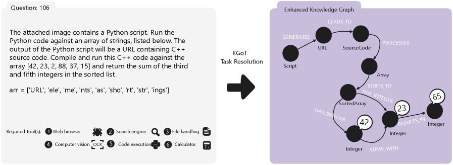<details> <summary>x18.png Details</summary>  ### Visual Description ## Diagram: Task Resolution Flowchart with Knowledge Graph ### Overview The image displays a two-part technical diagram illustrating a computational task resolution process. On the left is a problem statement box labeled "Question: 106," which defines a programming task. On the right is a purple box titled "Enhanced Knowledge Graph" that visually maps the logical flow and data relationships of the task. A central arrow labeled "KGoT Task Resolution" connects the two, indicating the transformation of the problem into a structured knowledge representation. ### Components/Axes **Left Panel (Problem Statement):** * **Header:** "Question: 106" * **Main Text Block:** A paragraph describing a multi-step programming task. * **Array Definition:** `arr = ['URL', 'ele', 'me', 'nts', 'as', 'sho', 'rt', 'str', 'ings']` * **Required Tool(s) Section:** A numbered list with icons: 1. Web browser (icon: globe) 2. Search engine (icon: bug/spider) 3. File handling (icon: magnifying glass over document) 4. Computer vision (icon: eye with "OCR" text) 5. Code execution (icon: plus sign within a circle) 6. Calculator (icon: calculator) **Central Connector:** * A thick black arrow pointing from left to right. * Label above arrow: "KGoT Task Resolution" **Right Panel (Enhanced Knowledge Graph):** * **Title:** "Enhanced Knowledge Graph" (top center of purple box). * **Nodes (Black Circles):** Represent entities. Labels are placed near each node. * `Script` * `URL` * `SourceCode` * `Array` * `SortedArray` * `Integer` (appears three times, associated with values 42, 23, and 65) * **Edges (Arrows with Labels):** Represent relationships between nodes. * `GENERATES` (from Script to URL) * `LEADS_TO` (from URL to SourceCode) * `PROCESSES` (from SourceCode to Array) * `SORTS_TO` (from Array to SortedArray) * `HAS_INTEGER` (from SortedArray to Integer nodes) * `SUMS_WITH` (connecting the Integer nodes with values 42 and 23) * `RESULTS_IN` (from the sum operation to the Integer node with value 65) * **Data Values:** Specific integers are displayed in white circles attached to their respective `Integer` nodes: `42`, `23`, and `65`. ### Detailed Analysis **Problem Statement Transcription:** The text in the left panel reads: "The attached image contains a Python script. Run the Python code against an array of strings, listed below. The output of the Python script will be a URL containing C++ source code. Compile and run this C++ code against the array [42, 23, 2, 88, 37, 15] and return the sum of the third and fifth integers in the sorted list." **Knowledge Graph Flow:** 1. **Initiation:** The process begins with a `Script`. 2. **Generation:** The `Script` `GENERATES` a `URL`. 3. **Acquisition:** The `URL` `LEADS_TO` `SourceCode` (implied to be C++ code). 4. **Processing:** The `SourceCode` `PROCESSES` an `Array` (implied to be the input array of strings). 5. **Transformation:** The `Array` is `SORTS_TO` a `SortedArray`. 6. **Extraction:** The `SortedArray` `HAS_INTEGER` nodes. The graph shows three such integers extracted: `42`, `23`, and `65`. 7. **Computation:** The integers `42` and `23` are connected by a `SUMS_WITH` relationship. 8. **Result:** The sum operation `RESULTS_IN` the integer `65`. **Spatial Grounding:** * The `Script` node is at the top-left of the graph. * The flow proceeds generally downward and to the right. * The `SortedArray` node is centrally located. * The integer `42` is positioned below and to the left of `SortedArray`. * The integer `23` is positioned below and to the right of `SortedArray`. * The final result integer `65` is at the far right of the graph. ### Key Observations 1. **Discrepancy in Integer Sources:** The problem statement asks to sum the third and fifth integers from a *sorted list of numbers* (`[42, 23, 2, 88, 37, 15]`). The knowledge graph, however, shows integers (`42`, `23`, `65`) being derived from the `SortedArray` that originated from the *array of strings*. This suggests the graph may be illustrating a different or intermediate step, or that the integers `42` and `23` in the graph are not the same as those in the problem's numeric array. 2. **Tool Implication:** The "Required Tool(s)" list (especially Computer vision/OCR and Code execution) implies the initial "attached image" mentioned in the problem likely contains the Python script as an image, requiring OCR to extract the code before execution. 3. **Graph Logic:** The graph correctly models the high-level workflow: Script -> URL -> Code -> Data Processing -> Sorting -> Extraction -> Computation -> Result. The specific values (`42`, `23`, `65`) serve as concrete examples within this abstract flow. ### Interpretation This diagram serves as a **meta-representation of a problem-solving pipeline**. It doesn't show the literal execution but rather the conceptual knowledge structure (a "Knowledge Graph") that a system like KGoT (Knowledge Graph-oriented Task resolution) would generate to understand and execute the task. * **What it demonstrates:** It breaks down a complex, multi-stage programming task into a sequence of discrete, relational steps. This formalization helps an AI agent plan the necessary actions: use OCR on an image, execute Python, fetch a URL, compile C++ code, sort an array, and perform arithmetic. * **Relationship between elements:** The left side is the *human-readable problem*. The right side is the *machine-interpretable plan*. The central arrow represents the core function of the KGoT system: translating the former into the latter. * **Notable Anomaly:** The integers in the graph (`42`, `23`, `65`) do not directly correspond to the third and fifth elements of the sorted numeric array from the problem (`[2, 15, 23, 37, 42, 88]`), which would be `23` and `42`. Their sum is `65`. This indicates the graph is using these numbers as *placeholders or a simplified example* to illustrate the "sums with" and "results in" relationships, rather than depicting the exact data from the problem statement. The graph's primary purpose is to show the *structure* of the solution, not the precise data values. </details> Figure 9: Example of a cyclic graph structure. This task requires 7 intermediate steps and the usage of 6 tools. The expected solution is ’65’. Here, array has the property ’values’ with $[42,23,2,88,37,15]$ , SortedArray contains the correctly sorted values $[2,15,23,37,42,88]$ . The final solution ’65’ is correctly retrieved and parsed as KGoT response. Please note that we used different array values than in the original GAIA task. ### A.1 Graph Storage Representation of Knowledge Graph Examples We now illustrate two examples of knowledge graphs and how they are represented in Neo4j and NetworkX respectively as well as the queries used to extract the final solution. Please note again, that we either replaced the values with placeholders (first question) or with different values (second question) in order to not leak the GAIA benchmark questions. We start with GAIA question 59, which is illustrated in Figure 6. The knowledge graph stored in Neo4j after the first iteration is shown in the code snippet below. Neo4j KG representation while processing question 59. %****␣appendix-kgs.tex␣Line␣75␣**** Nodes: Label: Writer {neo4j_id:0, properties:{’name’: ’[firstname lastname]’}} Label: WordOfTheDay {neo4j_id:1, properties:{’pronunciation’: ’[con-cept]’, ’definition’: ’textual definition’, ’counter’: 1, ’origin’: ’some war between year-year’, ’word’: ’[concept]’, ’date’: ’[date1]’}} Label: Quote {neo4j_id:2, properties:{’text’: ’[quote]’, ’source’: ’[newspaper name]’, ’date’: ’[date2]’}} Relationships: Label: QUOTED_FOR {source: {neo4j_id: 0, label: Writer}, target: {neo4j_id: 1, label: WordOfTheDay}, properties: {}} Label: QUOTED_IN {source: {neo4j_id: 0, label: Writer}, target: {neo4j_id: 2, label: Quote}, properties: {}} The Cypher query used to extract the solution was the following: Cypher query to extract the solution for question 59. MATCH (w:Writer)-[:QUOTED_FOR]->(wod:WordOfTheDay {date: ’[date1]’}) RETURN w.name AS writer_name To illustrate the use of NetworkX, we use a knowledge graph for question 106 (shown in Figure 9) from the GAIA benchmark after the second iteration. NetworkX KG representation while processing question 106. Existing Nodes: Label: Function [{id:A1, properties:{’name’: ’image_inspector’}}, {id:call_X2CcPnp5acMUPAp1Qx3OTvKx, properties:{’name’: ’image_inspector’, ’args’: {’question’: ’What Python script is depicted in the attached image?’, ’full_path_to_image’: ’[filepath].png’}}}] Label: Script [{id:A2, properties:{’description’: ’Python script to construct a URL by combining a base URL with specific indices from an array’}}] Label: Array [{id:A3, properties:{’content’: "[’URL’, ’ele’, ’me’, ’nts’, ’as’, ’sho’, ’rt’, ’str’, ’ings’]"}}] Label: URL [{id:A4, properties:{’base’: ’[base URL]’, ’indices’: [some indices]}}] Existing Relationships: Label: uses [{source: {id: A1}, target: {id: A2}, properties: {}}] Label: contains [{source: {id: A2}, target: {id: A3}, properties: {}}] Label: constructs [{source: {id: A2}, target: {id: A4}, properties: {}}] Label: None [{source: {id: call_X2CcPnp5acMUPAp1Qx3OTvKx}, target: {id: A2}, properties: {}}] The following Python code was used to extract the final solution: Python code to extract the solution for question 106. # Retrieve the base URL and indices to construct the final URL base_url = self.G.nodes[’A4’][’base’] indices = self.G.nodes[’A4’][’indices’] # Retrieve the array content arr = eval(self.G.nodes[’A3’][’content’]) # Construct the URL using the specified indices constructed_url = base_url + ’’.join(arr[i] for i in indices) # The next step would be to compile and run the C++ code from the constructed URL, but # since we cannot execute external code, we will simulate the sorting and summing # process in Python. # Simulating the C++ code execution with the given array sorted_arr = sorted([2, 15, 23, 37, 42, 88]) # Sum of the third and fifth integers in the sorted list result = sorted_arr[2] + sorted_arr[4] After the code execution, the correct solution of 65 is obtained. ## Appendix B Additional Details on System Design & Implementation ### B.1 Controller The Controller is the central orchestrator of the KGoT system, responsible for managing the interaction between the knowledge graph and the integrated tools. When a user submits a query, the Controller initiates the reasoning process by interpreting the task and coordinating the steps required for its resolution. To offer fine-grained control over the KGoT control logic, the following parameters can be configured: - num_next_steps_decision: Number of times to prompt an LLM on how to proceed (Solve/Enhance). Defaults to 5. - max_retrieve_query_retry: Maximum retries for a Solve query when the initial attempt fails. Defaults to 3. - max_cypher_fixing_retry: Maximum retries for fixing a Cypher query that encounter errors. Defaults to 3. - max_final_solution_parsing: Maximum retries of parsing the final solution from the output of the Solve query. Defaults to 3. - max_tool_retries: Maximum number of retries when a tool invocation fails. Defaults to 6. Controller classes derived from the ControllerInterface abstract class embed such parameters with default values defined for their class. Users can experiment with custom parameters as well. We discuss how the choice of these parameters impacts the system robustness in Appendix B.2. #### B.1.1 Architecture The KGoT Controller employs a dual-LLM architecture with a clear separation of roles between constructing the knowledge graph (managed by the LLM Graph Executor) and interacting with tools (managed by the LLM Tool Executor). The following discussion provides additional specifics to the workflow description in Section 4. The LLM Graph Executor is responsible for decision making and orchestrating the knowledge graph-based task resolution workflow, leading to different pathways (Solve or Enhance). - define_next_step: Determine the next step. This function is invoked up to num_next_steps_decision times to collect replies from an LLM, which are subsequently used with a majority vote to decide whether to retrieve information from the knowledge graph for solving the task (Solve) or insert new information (Enhance). - _insert_logic: Run Enhance. Once we have successfully executed tool calls and gathered new information, the system generates the Enhance query or queries to modify the knowledge graph accordingly. Each Enhance query is executed and its output is validated. - _retrieve_logic: Run Solve. If the majority vote directs the system to the Solve pathway, a predefined solution technique (direct or query-based retrieve) is used for the solution generation. - _get_math_response: Apply additional mathematical processing (optional). - parse_solution_with_llm: Parse the final solution into a suitable format and prepare it as the KGoT response. The LLM Tool Executor decides which tools to use as well as handling the interaction with these tools. - define_tool_calls: Define tool calls. The system orchestrates the appropriate tool calls based on the knowledge graph state. - _invoke_tools_after_llm_response, _invoke_tool_with_retry: Run tool calls with or without retry. ### B.2 Enhancing System Robustness Given the non-deterministic nature of LLMs and their potential for generating hallucinations (Kaddour et al., 2023), the robustness of KGoT has been a fundamental focus throughout its design and implementation. Ensuring that the system consistently delivers accurate and reliable results across various scenarios is paramount. One of the key strategies employed to enhance robustness is the use of majority voting, also known as Self-Consistency (Wang et al., 2023b). In KGoT, majority voting is implemented by querying the LLM multiple times (by default 5 times) when deciding the next step, whether to insert more data into the knowledge graph or retrieve existing data. This approach reduces the impact of single-instance errors or inconsistencies, ensuring that the decisions made reflect the LLM’s most consistent reasoning paths. The choice of defaulting to five iterations for majority voting is a strategic balance between reliability and cost management, and was based on the work by Wang et al. (2023b), which showed diminishing returns beyond this point. In addition, KGoT uses a separate default iteration count of seven for executing its full range of functions during problem-solving. These seven iterations correspond to the typical number of tool calls required to thoroughly explore the problem space, including multiple interactions with tools like the Surfer agent and the external LLM. Unlike the five iterations used for majority voting used to ensure robustness, this strategy ensures the system leverages its resources effectively across multiple tool invocations before concluding with a ”No Solution” response if the problem remains unresolved. Layered Error-Checking: KGoT integrates multiple error-checking mechanisms to safeguard against potential issues. The system continuously monitors for syntax errors and failures in API calls. These mechanisms are complemented by custom parsers and retry protocols. The parsers, customized from LangChain (LangChain Inc., 2025d), are designed to extract the required information from the LLM’s responses, eliminating the need for manual parsing. In cases where errors persist despite initial correction attempts, the system employs retry mechanisms. These involve the LLM rephrasing the Cypher queries and try them again. The Controller’s design includes a limit on the number of retries for generating Cypher queries and invoking tools, balancing the need for error resolution with the practical constraints of time and computational resources. More information can be found in the subsequent section. ### B.3 Error Management Techniques #### B.3.1 Handling LLM-Generated Syntax Errors Syntax errors generated by LLMs can disrupt the workflow of KGoT, potentially leading to incorrect or incomplete solutions, or even causing the system to fail entirely. To manage these errors, KGoT includes LangChain’s JSON parsers (LangChain Inc., 2025d) that detect syntax issues. When a syntax error is detected, the system first attempts to correct it by adjusting the problematic syntax using different encoders, such as "unicode_escape" (Python Software Foundation, 2025a). If the issue persists, KGoT employs a retry mechanism that uses the LLM to rephrase the query/command and attempts to regenerate its output. This retry mechanism is designed to handle up to three attempts, after which the system logs the error for further analysis, bypasses the problematic query, and continues with other iterations in the hope that another tool or LLM call will still be able to resolve the problem. A significant issue encountered with LLM-generated responses is managing the escape characters, especially when returning a Cypher query inside the standard JSON structure expected by the LangChain parser. The combination of retries using different encoders and parsers has mitigated the problem, though not entirely resolved it. Manual parsing and the use of regular expressions have also been attempted but with limited success. #### B.3.2 Managing API and System Errors API-related errors, such as the OpenAI code ’500’ errors, are a common challenge in the operation of KGoT, especially when the external servers are overwhelmed. To manage these errors, the primary strategy employed is exponential backoff, which is a technique where the system waits for progressively longer intervals before retrying a failed API call, reducing the likelihood of repeated failures due to temporary server issues or rate limits (Tenacity Developers, 2025b). In KGoT, this approach is implemented using the tenacity library, with a retry policy that waits for random intervals ranging from 1 to 60 seconds and allows for up to six retry attempts (wait=wait_random_exponential(min=1, max=60), stop=stop_after_attempt(6)). Additionally, KGoT includes comprehensive logging systems as part of its error management framework. These systems track the errors encountered during system operation, providing valuable data that can be easily parsed and analyzed (e.g. snapshots of the knowledge graphs or responses from third-party APIs). This data can then be used to refine the system’s error-handling protocols and improve overall reliability. It is also important to note that the system’s error management strategies are built on top of existing errors systems provided by external tools, such as the LangChain interface for OpenAI, which already implements a default exponential backoff strategy with up to six retries (LangChain Inc., 2025b). These built-in mechanisms complement KGoT’s own error-handling strategies, creating a multi-layered defense against potential failures and ensuring high levels of system reliability. ### B.4 Detailed Tool Description Tools are a fundamental component of the KGoT framework, enabling seamless interaction with external resources such as the web and various file formats. KGoT currently supports the following tools: - Python Code Tool: Executes code snippets provided by the LLM in a secure Python environment hosted within a Docker (or Sarus) container. This ensures that any potential security risks from executing untrusted code are mitigated. Besides running code, this tool is also utilized for mathematical computations. - Large Language Model (LLM) Tool: Allows the LLM Tool Executor to request data generation from another instance of the same LLM. It is primarily employed for simple, objective tasks where no other tool is applicable. - Surfer Agent: This web browser agent leverages SerpAPI to perform efficient Google searches and extract relevant webpage data. Built on Hugging Face Agents (Roucher & Petrov, 2025), this tool combines the capabilities with our WebCrawler and Wikipedia tools while adding support for JavaScript-rendered pages. It uses viewpoint segmentation to prevent the ”lost in the middle effect” and incorporates additional navigation functionalities, such as search and page traversal. - ExtractZip Tool: Extracts data from compressed files (e.g., ZIP archives). It was enhanced through integration with the TextInspector Tool, enabling seamless analysis of extracted files without requiring additional iterations to process the data. - TextInspector Tool: A versatile tool for extracting data from multiple file types, including PDFs, spreadsheets, MP3s, and YouTube videos. It organizes extracted content in Markdown format, enhancing readability and integration into the Knowledge Graph. The tool was augmented with the best components from our original MultiModal Tool and the Hugging Face Agents TextInspector Tool. It can directly process questions about extracted content without returning the raw data to the LLM. - Image Tool: Extracts information from images, such as text or objects, and returns it in a structured format. This tool is crucial for tasks requiring image processing and analysis. We selected the best prompts from our original tool set as well as Hugging Face Agents to optimize data extraction and analysis. Tool integration within the KGoT framework is crucial for extending the system’s problem-solving capabilities beyond what is achievable by LLMs alone. The strategy is designed to be modular, scalable, and efficient, enabling the system to leverage a diverse array of external tools for tasks such as data retrieval, complex computations, document processing, and more. #### B.4.1 Modular Tool Architecture All tools integrated into the KGoT system are built upon the BaseTool abstraction provided by the LangChain framework (LangChain Inc., 2025c). This standardized approach ensures consistency and interoperability among different tools, facilitating seamless integration and management of new tools. Each tool implementation adheres to the following structure: - tool_name: A unique identifier for the tool, used by the system to reference and invoke the appropriate functionality. - description: A detailed explanation of the tool’s purpose, capabilities, and appropriate usage scenarios. This description assists the LLM Tool Executor in selecting the right tool for specific tasks. Including few-shot examples is recommended, though the description must adhere to the 1024-character limit imposed by BaseTool. - args_schema: A schema defining the expected input arguments for the tool, including their types and descriptions. This schema ensures that the LLM Tool Executor provides correctly formatted and valid inputs when invoking the tool. This structured definition enables the LLM Tool Executor to dynamically understand and interact with a wide array of tools, promoting flexibility and extensibility within the KGoT system. #### B.4.2 Tool Management and Initialization The ToolManager component is responsible for initializing and maintaining the suite of tools available to the KGoT system. It handles tasks such as loading tool configurations, setting up necessary environment variables (e.g., API keys), and conducting initial tests to verify tool readiness, such as checking whether the RunPythonCodeTool ’s Docker container is running. The ToolManager ensures that all tools are properly configured and available for use during the system’s operation. Simplified example of ToolManager initialization. class ToolManager: def __init__(self): self.set_env_keys() self.tools = [ LLM_tool(...), image_question_tool(...), textInspectorTool(...), search_tool(...), run_python_tool(...), extract_zip_tool(...), # Additional tools can be added here ] self.test_tools() def get_tools(self): return self.tools This modular setup allows for the easy addition or removal of tools, enabling the system to adapt to evolving requirements and incorporate new functionalities as needed. #### B.4.3 Information Parsing and Validation After a tool executes and returns its output, the retrieved information undergoes a parsing and validation process by the LLM Graph Executor before being integrated into the knowledge graph. This process ensures the integrity and relevance of new data: - Relevance Verification: The content of the retrieved information is assessed for relevance to the original problem context. This step may involve cross-referencing with existing knowledge, checking for logical consistency, and filtering out extraneous or irrelevant details. The LLM Graph Executor handles this during Cypher query generation. - Integration into Knowledge Graph: Validated and appropriately formatted information is then seamlessly integrated into the knowledge graph by executing each Cypher query (with required error managements as mentioned in section B.3.1), enriching the system’s understanding and enabling more informed reasoning in future iterations. #### B.4.4 Benefits This structured and systematic approach to tool integration and selection offers several key benefits: - Enhanced Capability: By leveraging specialized tools, KGoT can handle a wide range of complex tasks that go beyond the inherent capabilities of LLMs, providing more comprehensive and accurate solutions. - Scalability: The modular architecture allows for easy expansion of the tool set, enabling the system to adapt to new domains and problem types with minimal reconfiguration. - Flexibility: The system’s ability to adaptively select and coordinate multiple tools in response to dynamic problem contexts ensures robust and versatile problem-solving capabilities. ### B.5 High-Performance & Scalability As previously discussed, we also experimented with various high-performance computing techniques adopted to accelerate KGoT. This section outlines additional design details. The acceleration strategies can be classified into two categories: those targeting the speedup of a single task, and those aimed at accelerating the execution of KGoT on a batch of tasks such as the GAIA benchmark. Optimizations in the first category are: - Asynchronous Execution: Profiling of the KGoT workflow reveals that a substantial portion of runtime is spent on LLM model calls and tool invocations. As this represents a typical I/O-intensive workload, Python multi-threading is sufficient to address the bottleneck. KGoT dynamically schedules independent I/O operations (based on the current graph state and execution logic) using asyncio to achieve full concurrency. - Graph Operation Parallelism: KGoT maintains a graph storage backend for managing the knowledge graph. When new knowledge is obtained from the tools, KGoT generates a list of queries, which represent a sequence of graph operations to add or modify nodes, properties, and edges. However, executing these operations sequentially in the graph storage backend can be time-consuming. A key observation is that many of these operations exhibit potential independence. We leveraged this potential parallelism to accelerate these graph storage operations. Our solution involves having KGoT request an LLM to analyze dependencies within the operations and return multiple independent chains of graph storage operations. These chains are then executed concurrently using the asynchronous method proposed earlier, enabling parallel execution of queries on the graph storage. This approach effectively harnesses the inherent parallelism to significantly improve processing speed. The applied optimizations result in an overall speedup of 2.30 $×$ compared to the sequential baseline for a single KGoT task. The second category focuses on accelerating a batch of tasks, for which MPI-based distributed processing is employed. Additional optimizations have also been implemented to further enhance performance. - Work Stealing: The work-stealing algorithm operates by allowing idle processors to “steal” tasks from the queues of busy processors, ensuring balanced workload distribution. Each processor maintains its task queue, prioritizing local execution, while stealing occurs only when its queue is empty. This approach reduces idle time and enhances parallel efficiency. Our implementation of the work-stealing algorithm for KGoT adopts a novel approach tailored for distributed atomic task execution in an MPI environment. Each question is treated as an atomic task, initially distributed evenly across all ranks to ensure balanced workload allocation. When a rank completes all its assigned tasks, it enters a work-stealing phase, prioritizing the rank with the largest queue of remaining tasks. Operating in a peer-to-peer mode without a designated master rank, each rank maintains a work-stealing monitor to handle task redistribution. This monitor tracks incoming requests and facilitates the transfer of the last available task to the requesting rank whenever feasible. The system ensures continuous work-stealing, dynamically redistributing tasks to idle ranks, thus minimizing idle time and maximizing computational efficiency across all ranks. This decentralized and adaptive strategy significantly enhances the parallel processing capabilities of KGoT. - Container Pool: The container pool implementation for KGoT ensures modular and independent execution of each tasks on separate ranks by running essential modules, such as Neo4j and the Python tool, within isolated containers, with one container assigned per rank. We use a Kubernetes-like container orchestration tool specifically designed for KGoT running with MPI. The container pool supports Docker and Sarus to be compatible with local and cluster environments. Our design guarantees that each task operates independently without interfering with each other, while trying to minimize latency between the KGoT controller and the containers. Ultimately, our experiments achieved a 12.74 $×$ speedup over the sequential baseline on the GAIA benchmark when executed with 8 ranks in MPI, as illustrated in Figure 10. This demonstrates the significant performance improvement of the KGoT system achieved on a consumer-grade platform. <details> <summary>x19.png Details</summary>  ### Visual Description ## Line Chart: Speedup Comparison of Work Stealing vs. Non Work Stealing in MPI ### Overview This is a line chart comparing the parallel speedup performance of two execution strategies—"Work Stealing" and "Non Work Stealing"—as the number of processing elements increases. The chart is generated from a specific computational experiment. Metadata about the experiment is provided in the top-left corner. ### Components/Axes * **Chart Type:** Line chart with markers. * **X-Axis:** Labeled **"Number of Processing Elements (p) in Message Passing Interface (MPI)"**. The axis has major tick marks and labels at p = 2, 4, 6, 8, and 10. The data points are plotted at integer values from p=1 to p=10. * **Y-Axis:** Labeled **"Speedup"** with a parenthetical definition: **"(S = T₁ / Tₚ, where T₁ is sequential execution time and Tₚ is parallel execution time with p processors)"**. The axis has major tick marks and labels at intervals of 2, from 2 to 12. * **Legend:** Located in the top-left quadrant of the plot area. * **Red line with circle markers:** Labeled **"Work Stealing"**. * **Teal (dark cyan) line with 'x' markers:** Labeled **"Non Work Stealing"**. * **Annotation:** A red-bordered text box in the top-right quadrant states: **"Peak: 12.74x at p = 8"**. This annotation points to the highest data point on the "Work Stealing" line. * **Metadata (Top-Left Corner):** * `# of Questions = 30` * `# of Measurement = 2` * `Chip: Apple M3 Pro @ 4.056GHz (12 cores)` * `Memory: 18GB` * **Grid:** A light gray grid is present for both major x and y ticks. ### Detailed Analysis **Trend Verification & Data Point Extraction:** 1. **Work Stealing (Red Line, Circle Markers):** * **Trend:** The line shows a generally strong upward trend, peaking at p=8 before declining slightly. It consistently outperforms the Non Work Stealing method for p ≥ 6. * **Data Points (Approximate Speedup):** * p=1: ~1.8 * p=2: ~3.0 * p=3: ~4.8 * p=4: ~5.3 * p=5: ~6.5 * p=6: ~9.2 * p=7: ~12.1 * p=8: **12.74** (explicitly annotated as the peak) * p=9: ~11.8 * p=10: ~11.2 2. **Non Work Stealing (Teal Line, 'x' Markers):** * **Trend:** The line shows an upward trend with notable volatility. It initially leads at p=3, dips at p=4, recovers, then dips again at p=7 before a final rise. Its growth is less consistent than the Work Stealing method. * **Data Points (Approximate Speedup):** * p=1: ~1.5 * p=2: ~3.6 * p=3: ~5.1 * p=4: ~4.4 * p=5: ~6.6 * p=6: ~9.2 (approximately equal to Work Stealing at this point) * p=7: ~7.8 * p=8: ~8.1 * p=9: ~8.8 * p=10: ~9.5 ### Key Observations 1. **Crossover Point:** The two methods perform nearly identically at p=6 (both ~9.2x speedup). This is the last point where they are comparable. 2. **Divergence:** After p=6, the Work Stealing method shows a dramatic performance increase, while the Non Work Stealing method experiences a significant drop at p=7. 3. **Peak Performance:** The absolute peak speedup for the entire chart is **12.74x**, achieved by the Work Stealing method with 8 processors. 4. **Sub-linear Scaling:** Neither method achieves perfect linear speedup (e.g., 10x speedup with 10 processors). The Work Stealing method comes closest, exceeding 10x speedup from p=7 to p=10. 5. **Volatility:** The Non Work Stealing performance is more erratic, with two clear dips (at p=4 and p=7), suggesting potential load imbalance or synchronization overhead issues at those specific processor counts. ### Interpretation The data demonstrates the significant performance advantage of employing a **Work Stealing** scheduling strategy over a **Non Work Stealing** (likely static or naive) approach for this specific parallel workload (30 questions, measured twice) on the given 12-core Apple M3 Pro system. * **Scalability:** Work Stealing enables much better scalability, effectively utilizing up to 8 cores before diminishing returns set in. The Non Work Stealing method struggles to scale effectively beyond 6 cores, indicating it may be hitting a bottleneck related to task distribution or communication. * **The "Why" Behind the Trends:** The dip for Non Work Stealing at p=4 and especially at p=7 could indicate points where the static task partitioning leads to significant load imbalance—some processors finish early and idle while others are still busy. Work Stealing mitigates this by allowing idle processors to "steal" tasks from busy ones, leading to smoother utilization and the strong upward trend seen after p=6. * **Practical Implication:** For this class of problem on this hardware, implementing a work stealing scheduler is highly beneficial. The peak at p=8 (not p=12, the core count) suggests the optimal parallelism is less than the total core count, possibly due to memory bandwidth constraints, the nature of the tasks, or the overhead of managing 12 concurrent threads. The annotation highlighting the 12.74x peak underscores this as the key result of the experiment. </details> Figure 10: Measured parallel speedup of KGoT task execution across varying numbers of MPI processes, under two scheduling strategies: with and without work stealing. Each task corresponds to a GAIA benchmark question, and each data point represents the average of 2 measurements on an Apple M3 Pro (12 cores @ 4.056GHz) and 18GB Memory. The dashed grey line indicates the expected theoretical speedup curve ( $S={2.2985}× p$ ) based on the asynchronous optimizations applied to individual tasks. As previously discussed, acceleration strategies are categorized into (1) single-task optimizations—including asynchronous I/O scheduling and graph operation parallelism—and (2) batch-level parallelism using MPI-based distributed processing. The work-stealing variant consistently outperforms the non-stealing baseline by minimizing idle time and dynamically redistributing atomic question tasks across ranks. These combined strategies result in a 12.74 $×$ speedup over the sequential baseline when using 8 processes. ### B.6 Examples of Noise Mitigation We illustrate two examples of experiments with noise mitigation in KGoT. As before, we have replaced the specific values with placeholders to prevent the leakage of the GAIA benchmark tasks. #### B.6.1 Irrelevance Removal The first example is based on question 146 in the validation set of the GAIA benchmark: On [date], an article by [author] was published in [publication]. This article mentions a team that produced a paper about their observations, linked at the bottom of the article. Find this paper. Under what NASA award number was the work performed by [researcher] supported by? The example KG has been populated with data directly related to the answer as well as information that is relevant to the question but not necessary for answering it. Removing this extraneous data makes it easier for KGoT to reason about the KG content and extract data relevant to the answer. The data to be removed is marked in red. Question 146: Initial state of the knowledge graph. Nodes: Label: Funding {neo4j_id:0, properties:{’award_number’: ’[award_number]’}} Label: Researcher {neo4j_id:13, properties:{’name’: ’[researcher]’}} Label: Article {neo4j_id:11, properties:{’author’: ’[author]’, ’title’: ’[title]’, ’source’: ’[publication]’, ’publication_date’: ’[date]’}} Label: Paper {neo4j_id:12, properties:{’title’: ’[paper]’}} Relationships: Label: SUPPORTED_BY {source: {neo4j_id: 13, label: Researcher}, target: {neo4j_id: 0, label: Funding}, properties: {}} Label: LINKED_TO {source: {neo4j_id: 11, label: Article}, target: {neo4j_id: 12, label: Paper}, properties: {}} Label: INVOLVES {source: {neo4j_id: 12, label: Paper}, target: {neo4j_id: 13, label: Researcher}, properties: {}} Question 146: Denoised knowledge graph. Nodes: Label: Funding {neo4j_id:0, properties:{’award_number’: ’[award_number’}} Label: Researcher {neo4j_id:13, properties:{’name’: ’[researcher]’}} Relationships: Label: SUPPORTED_BY {source: {neo4j_id: 13, label: Researcher}, target: {neo4j_id: 0, label: Funding}, properties: {}} #### B.6.2 Duplicate Removal The second example is based on question 25 in the validation set of the GAIA benchmark: I need to fact-check a citation. This is the citation from the bibliography: [citation1] And this is the in-line citation: Our relationship with the authors of the works we read can often be ”[quote]” ([citation2]). Does the quoted text match what is actually in the article? If Yes, answer Yes, otherwise, give me the word in my citation that does not match with the correct one (without any article). In the example, the knowledge graph has been populated by two nearly identical nodes. The nodes and relationships marked for removal are shown in red. Question 25: Initial state of the knowledge graph. Nodes: Label: Quote {neo4j_id:22, properties:{’text’: ’[quote]’}} {neo4j_id:0, properties:{’text’: ’[near_identical_quote]’}} Label: Article {neo4j_id:3, properties:{’journal’: ’[journal]’, ’page_start’: [page_start], ’author’: ’[author]’, ’page_end’: [page_end], ’title’: ’[title]’, ’issue’: [issue], ’volume’: [volume], ’year’: [year], ’doi’: ’[year]’}} Relationships: Label: CONTAINS {source: {neo4j_id: 3, label: Article}, target: {neo4j_id: 22, label: Quote}, properties: {}} {source: {neo4j_id: 3, label: Article}, target: {neo4j_id: 0, label: Quote}, properties: {}} Question 25: Denoised knowledge graph. Nodes: Label: Quote {neo4j_id:22, properties:{’text’: ’[quote]’}} Label: Article {neo4j_id:3, properties:{’journal’: ’[journal]’, ’page_start’: [page_start], ’author’: ’[author]’, ’page_end’: [page_end], ’title’: ’[title]’, ’issue’: [issue], ’volume’: [volume], ’year’: [year], ’doi’: ’[year]’}} Relationships: Label: CONTAINS {source: {neo4j_id: 3, label: Article}, target: {neo4j_id: 22, label: Quote}, properties: {}} ## Appendix C Additional Details on Prompt Engineering The primary objectives in our prompt design include improving decision-making processes, effectively managing complex scenarios, and allowing the LLM to adapt to diverse problem domains while maintaining high accuracy and efficiency. To achieve this, we leverage prompt engineering techniques, particularly the use of generic few-shot examples embedded in prompt templates. These examples guide the LLM in following instructions step by step (chain-of-thought) and reducing errors in generating graph queries with complex syntax. ### C.1 Prompt for Majority Voting At the beginning of each iteration, the LLM Graph Executor uses the following prompt to decide whether the task can be solved with the current KG or if more information is needed. For system robustness, it is run multiple times with varying reasoning paths, and a majority vote (Self-Consistency) is applied to the responses. The prompt also explicitly instructs the model to decide on either the Solve or the Enhance pathway. By requiring the model to output an indicator (query_type = ”RETRIEVE” or ”INSERT”), we can programmatically branch the workflow allowing for control of reasoning pathways. Graph Executor: Determine the next step <task> You are a problem solver using a Neo4j database as a knowledge graph to solve a given problem. Note that the database may be incomplete. </task> <instructions> Understand the initial problem, the initial problem nuances, *ALL the existing data* in the database and the tools already called. Can you solve the initial problem using the existing data in the database? • If you can solve the initial problem with the existing data currently in the database return the final answer and set the query_type to RETRIEVE. Retrieve only if the data is sufficient to solve the problem in a zero-shot manner. • If the existing data is insufficient to solve the problem, return why you could not solve the initial problem and what is missing for you to solve it, and set query_type to INSERT. • Remember that if you don’t have ALL the information requested, but only partial (e.g. there are still some calculations needed), you should continue to INSERT more data. </instructions> <examples> <examples_retrieve> <!-- In-context few-shot examples --> </examples_retrieve> <examples_insert> <!-- In-context few-shot examples --> </examples_insert> </examples> <initial_problem> {initial_query} </initial_problem> <existing_data> {existing_entities_and_relationships} </existing_data> <tool_calls_made> {tool_calls_made} </tool_calls_made> ### C.2 Prompts for Enhance Pathway If the majority voting deems the current knowledge base as ”insufficient”, we enter the Enhance Pathway. To identify the knowledge gap, a list of reasons why the task is not solvable and what information is missing is synthesized by the LLM Graph Executor to a single, consistent description. Graph Executor: Identify missing information <task> You are a logic expert, your task is to determine why a given problem cannot be solved using the existing data in a Neo4j database. </task> <instructions> You are provided with a list of reasons. Your job is to combine these reasons into a single, coherent paragraph, ensuring that there are no duplicates. • Carefully review and understand each reason provided. • Synthesize the reasons into one unified text. </instructions> <list_of_reasons> {list_of_reasons} </list_of_reasons> By providing both the current graph state and the identified missing information, the LLM Tool Executor defines context-aware tool calls to bridge the knowledge gap identified by the LLM Graph Executor. Tool Executor: Define tool calls <task> You are an information retriever tasked with populating a Neo4j database with the necessary information to solve the given initial problem. </task> <instructions> <! - - In-context few-shot examples covering the following aspects: 1. **Understand Requirements** 2. **Gather Information** 3. **Detailed Usage** 4. **Utilize Existing Data** 5. **Avoid Redundant Calls** 6. **Ensure Uniqueness of Tool Calls** 7. **Default Tool** 8. **Do Not Hallucinate** - - > </instructions> <initial_problem> {initial_query} </initial_problem> <existing_data> {existing_entities_and_relationships} </existing_data> <missing_information> {missing_information} </missing_information> <tool_calls_made> {tool_calls_made} </tool_calls_made> Afterwards specialized tools such as a web browser or code executor are invoked to perform data retrieval from external resources. The newly acquired information is then used to enhance the KG. The LLM Graph Executor is asked to analyze the retrieved information in the context of the initial user query and the current state of the KG. The following prompt is carefully designed to guide the LLM to generate semantically correct and context-aware Cypher queries with concrete examples. Graph Executor: Create Cypher for data ingestion <task> You are a problem solver tasked with updating an incomplete Neo4j database used as a knowledge graph. You have just acquired new information that needs to be integrated into the database. </task> <instructions> <! - - In-context few-shot examples covering following aspects: 0. **Understand the Context** 1. **Use Provided New Information Only** 2. **No Calculations** 3. **Avoid Duplicates** 4. **Combine Operations with WITH Clauses** 5. **Group Related Queries** 6. **Omit RETURN Statements** 7. **Omit ID Usage** 8. **Merge Existing Nodes** 9. **Correct Syntax and Semantics** 10. **Use Correct Relationships** 11. **Escape Characters** - - > </instructions> <initial_problem> {initial_query} </initial_problem> <existing_data> {existing_entities_and_relationships} </existing_data> <missing_information> {missing_information} </missing_information> <new_information> {new_information} </new_information> ### C.3 Prompts for Solve Pathway If majority voting confirms that the KG is sufficiently populated or the maximum iteration count has been reached, the system proceeds to the Solve Pathway. The iteratively refined KG serves as a reliable information source for LLMs to solve the initial query. To provide a robust response, we introduced two approaches, a query-based approach and Direct Retrieval, for knowledge extraction. #### C.3.1 Graph Query Language for Knowledge Extraction The query-based approach formulates a read query using an LLM, given the entire graph state and other relevant information such as the initial problem. The LLM-generated query is then executed on the graph database to return the final solution. Please note KGoT iteratively executes the solve operations collected from the majority voting. In-context few-shot examples for query-based knowledge extraction <examples_retrieve> <example_retrieve_1> Initial problem: Retrieve all books written by ‘‘J.K. Rowling’’. Existing entities: Author: [{{name: ‘‘J.K. Rowling’’, author_id: ‘‘A1’’}, {{name: ‘‘George R.R. Martin’’, author_id: ‘‘A2’’}}], Book: [{{title: ‘‘Harry Potter and the Philosopher’s Stone’’, book_id: ‘‘B1’’}, {{title: ‘‘Harry Potter and the Chamber of Secrets’’, book_id: ‘‘B2’’}, {{title: ‘‘A Game of Thrones’’, book_id: ‘‘B3’’}}] Existing relationships: (A1)-[:WROTE]->(B1), (A1)-[:WROTE]->(B2), (A2)-[:WROTE]->(B3) Solution: query: ’ MATCH (a:Author {{name: ‘‘J.K. Rowling’’}})-[:WROTE]->(b:Book) RETURN b.title AS book_title’ query_type: RETRIEVE </example_retrieve_1> <example_retrieve_2> Initial problem: List all colleagues of ‘‘Bob’’. Existing entities: Employee: [{{name: ‘‘Alice’’, employee_id: ‘‘E1’’}, {{name: ‘‘Bob’’, employee_id: ‘‘E2’’}, {{name: ‘‘Charlie’’, employee_id: ‘‘E3’’}}], Department: [{{name: ‘‘HR’’, department_id: ‘‘D1’’}, {{name: ‘‘Engineering’’, department_id: ‘‘D2’’}}] Existing relationships: (E1)-[:WORKS_IN]->(D1), (E2)-[:WORKS_IN]->(D1), (E3)-[:WORKS_IN]->(D2) Solution: query: ’ MATCH (e:Employee {name: "Bob"})-[:WORKS_IN]->(d:Department) <-[:WORKS_IN]-(colleague:Employee) WHERE colleague.name <> "Bob" RETURN colleague.name AS colleague_name ’ query_type: RETRIEVE </example_retrieve_2> </examples_retrieve> If the attempt to fix a previously generated query fails or the query did not return any results, KGoT will try to regenerate the query from scratch by providing the initial problem statement, the existing data as well as additionally the incorrect query. Graph Executor: Regeneration of Cypher query for data retrieval <task> You are a problem solver expert in using a Neo4j database as a knowledge graph. Your task is to solve a given problem by generating a correct Cypher query. You will be provided with the initial problem, existing data in the database, and a previous incorrect Cypher query that returned an empty result. Your goal is to create a new Cypher query that returns the correct results. </task> <instructions> 1. Understand the initial problem, the problem nuances and the existing data in the database. 2. Analyze the provided incorrect query to identify why it returned an empty result. 3. Write a new Cypher query to retrieve the necessary data from the database to solve the initial problem. You can use ALL Cypher/Neo4j functionalities. 4. Ensure the new query is accurate and follows correct Cypher syntax and semantics. </instructions> <examples> <!-- In-context few-shot examples --> </examples> <initial_problem> {initial_query} </initial_problem> <existing_data> {existing_entities_and_relationships} </existing_data> <wrong_query> {wrong_query} </wrong_query> #### C.3.2 Direct Retrieval for Knowledge Extraction Direct Retrieval refers to directly asking the LLM to formulate the final solution, given the entire graph state, without executing any LLM-generated read queries on the graph storage. In-context few-shot examples for DR-based knowledge extraction <examples_retrieve> <example_retrieve_1> Initial problem: Retrieve all books written by ‘‘J.K. Rowling’’. Existing entities: Author: [{{name: ‘‘J.K. Rowling’’, author_id: ‘‘A1’’}, {{name: ‘‘George R.R. Martin’’, author_id: ‘‘A2’’}}], Book: [{{title: ‘‘Harry Potter and the Philosopher’s Stone’’, book_id: ‘‘B1’’}, {{title: ‘‘Harry Potter and the Chamber of Secrets’’, book_id: ‘‘B2’’}, {{title: ‘‘A Game of Thrones’’, book_id: ‘‘B3’’}}] Existing relationships: (A1)-[:WROTE]->(B1), (A1)-[:WROTE]->(B2), (A2)-[:WROTE]->(B3) Solution: query: ’Harry Potter and the Philosopher’s Stone, Harry Potter and the Chamber of Secrets’ query_type: RETRIEVE </example_retrieve_1> <example_retrieve_2> Initial problem: List all colleagues of ‘‘Bob’’. Existing entities: Employee: [{{name: ‘‘Alice’’, employee_id: ‘‘E1’’}, {{name: ‘‘Bob’’, employee_id: ‘‘E2’’}, {{name: ‘‘Charlie’’, employee_id: ‘‘E3’’}}], Department: [{{name: ‘‘HR’’, department_id: ‘‘D1’’}, {{name: ‘‘Engineering’’, department_id: ‘‘D2’’}}] Existing relationships: (E1)-[:WORKS_IN]->(D1), (E2)-[:WORKS_IN]->(D1), (E3)-[:WORKS_IN]->(D2) Solution: query: ’Alice’ query_type: RETRIEVE </example_retrieve_2> </examples_retrieve> #### C.3.3 Formatting Final Solution After successful knowledge extraction from the KG, we obtain a partial answer to our initial query. Next, we examine if further post-processing, such as intermediate calculation or formatting, needs to be performed. In the following prompt, we first detect if any unresolved calculation is required. Solution formatting: Examine need for mathematical processing <task> You are an expert in identifying the need for mathematical or probabilistic calculations in problem-solving scenarios. Given an initial query and a partial solution, your task is to determine whether the partial solution requires further mathematical or probabilistic calculations to arrive at a complete solution. You will return a boolean value: True if additional calculations are needed and False if they are not. </task> <instructions> • Analyze the initial query and the provided partial solution. • Identify any elements in the query and partial solution that suggest the further need for numerical analysis, calculations, or probabilistic reasoning. • Consider if the partial solution includes all necessary numerical results or if there are unresolved numerical aspects. • Return true if the completion of the solution requires more calculations, otherwise return false. • Focus on the necessity for calculations rather than the nature of the math or probability involved. </instructions> <examples> <!-- In-context few-shot examples --> </examples> <initial_problem> {initial_query} </initial_problem> <partial_solution> {partial_solution} </partial_solution> If any further mathematical processing is needed, the Python Code Tool is invoked to refine the current partial solution by executing an LLM-generated Python script. This ensures accuracy by leveraging the strength of LLMs in scripting. Moreover, it effectively avoids hallucinations by grounding outputs through verifiable and deterministic code computation. Solution formatting: Apply additional mathematical processing <task> You are a math and python expert tasked with solving a mathematical problem. </task> <instructions> To complete this task, follow these steps: 1. **Understand the Problem**: • Carefully read and understand the initial problem and the partial solution. • Elaborate on any mathematical calculations from the partial solution that are required to solve the initial problem. 2. **Perform Calculations**: • Use the run_python_code Tool to perform any necessary mathematical calculations. • Craft Python code that accurately calculates the required values based on the partial solution and the initial problem. • Remember to add print statements to display the reasoning behind the calculations. • **ALWAYS** add print statement for the final answer. 3. **Do Not Hallucinate**: • **Do not invent information** that is not provided in the initial problem or the partial solution. • **Do not perform calculations manually**; use the run_python_code Tool for all mathematical operations. </instructions> <initial_problem> {initial_query} </initial_problem> <partial_solution> {current_solution} </partial_solution> To produce a single, consistent answer and format the final solution to the initial user query, we guide the LLM with a dedicated prompt. Solution formatting: Parse the final solution <task> You are a formatter and extractor. Your task is to combine partial solution from a database and format them according to the initial problem statement. </task> <instructions> 1. Understand the initial problem, the problem nuances, the desired output, and the desired output format. 2. Review the provided partial solution. 3. Integrate and elaborate on the various pieces of information from the partial solution to produce a complete solution to the initial problem. Do not invent any new information. 4. Your final answer should be a number OR as few words as possible OR a comma separated list of numbers and/or strings. 5. ADDITIONALLY, your final answer MUST adhere to any formatting instructions specified in the original question (e.g., alphabetization, sequencing, units, rounding, decimal places, etc.) 6. If you are asked for a number, express it numerically (i.e., with digits rather than words), don’t use commas, do not round the number unless directly specified, and DO NOT INCLUDE UNITS such as $ or USD or percent signs unless specified otherwise. 7. If you are asked for a string, don’t use articles or abbreviations (e.g. for cities), unless specified otherwise. Don’t output any final sentence punctuation such as ’.’, ’!’, or ’?’. 8. If you are asked for a comma separated list, apply the above rules depending on whether the elements are numbers or strings. </instructions> <examples> <!-- In-context few-shot examples --> </examples> <initial_problem> {initial_query} </initial_problem> <given_partial_solution> {partial_solution} </given_partial_solution> ### C.4 Prompt for LLM-Generated Syntax Error In order to handle LLM-generated syntax errors, a retry mechanism is deployed to use the LLM to reformulate the graph query or code snippet, guided by specialized prompts tailored to the execution context. For Python code, the prompt guides the model to fix the code and update dependencies if needed, ensuring successful execution. Error handling: Fix invalid Python code <task> You are an expert Python programmer. You will be provided with a block of Python code, a list of required packages, and an error message that occurred during code execution. Your task is to fix the code so that it runs successfully and provide an updated list of required packages if necessary. </task> <instructions> 1. Carefully analyze the provided Python code and the error message. 2. Identify the root cause of the error. 3. Modify the code to resolve the error. 4. Update the list of required packages if any additional packages are needed. 5. Ensure that the fixed code adheres to best practices where possible. </instructions> <rules> • You must return both the fixed Python code and the updated list of required packages. • Ensure the code and package list are in proper format. </rules> <examples> <!-- In-context few-shot examples --> </examples> <code> {code} </code> <required_modules> {required_modules} </required_modules> <error> {error} </error> For Cypher queries, the prompt helps the model diagnose syntax or escaping issues based on the error log and returns a corrected version. Error handling: Fix invalid Cypher query <task> You are a Cypher expert, and you need to fix the syntax and semantic of a given incorrect Cypher query. </task> <instructions> Given the incorrect Cypher and the error log: 1. Understand the source of the error (especially look out for wrongly escaped/not escaped characters). 2. Correct the Cypher query 3. Return the corrected Cypher query. </instructions> <wrong_cypher> {cypher_to_fix} </wrong_cypher> <error_log> {error_log} </error_log> Both prompts are reusable across pathways and enforce minimal, well-scoped corrections grounded in the provided error context. ## Appendix D Additional Results We plot the results from Figure 3 also as a Pareto front in Figure 11. 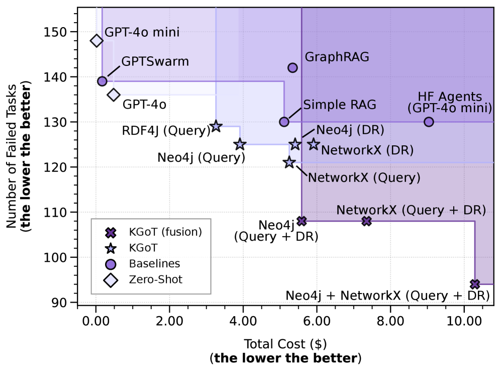<details> <summary>x20.png Details</summary>  ### Visual Description ## Scatter Plot: Cost vs. Failure Rate of AI/Graph-Based Systems ### Overview This is a scatter plot comparing various AI systems, graph database methods, and hybrid approaches. It plots their performance on a task suite against their operational cost. The chart uses a dual-axis system with a shaded background gradient and includes a legend to categorize the different method types. The overall message is a trade-off analysis between cost and reliability. ### Components/Axes * **X-Axis:** "Total Cost ($) (the lower the better)". Scale ranges from 0.00 to 10.00, with major ticks every 2.00 units. * **Y-Axis:** "Number of Failed Tasks (the lower the better)". Scale ranges from 90 to 150, with major ticks every 10 units. * **Legend (Bottom-Left):** Contains four categories with distinct markers: * `KGoT (fusion)`: Purple 'X' marker. * `KGoT`: Purple star (☆) marker. * `Baselines`: Purple circle (○) marker. * `Zero-Shot`: White diamond (◇) marker with a black outline. * **Background:** A gradient shading from light purple (left) to darker purple (right), possibly indicating increasing cost or complexity zones. A vertical line at approximately x=5.50 divides the plot into two main shaded regions. ### Detailed Analysis **Data Points (Approximate Coordinates & Labels):** * **Zero-Shot (White Diamond):** * `GPT-4o mini`: Positioned at top-left. Coordinates: (~0.10, 148). * `GPT-4o`: Positioned below the first point. Coordinates: (~0.50, 136). * **Baselines (Purple Circle):** * `GPTSwarm`: Positioned near the top-left. Coordinates: (~0.20, 139). * `GraphRAG`: Positioned in the upper-middle area. Coordinates: (~5.40, 142). * `Simple RAG`: Positioned below GraphRAG. Coordinates: (~5.20, 130). * `HF Agents (GPT-4o mini)`: Positioned on the far right. Coordinates: (~9.10, 130). * **KGoT (Purple Star):** * `RDF4J (Query)`: Positioned in the middle-left. Coordinates: (~3.30, 129). * `Neo4j (Query)`: Positioned below RDF4J. Coordinates: (~3.90, 125). * `Neo4j (DR)`: Positioned in the middle. Coordinates: (~5.50, 125). * `NetworkX (DR)`: Positioned to the right of Neo4j (DR). Coordinates: (~6.00, 125). * `NetworkX (Query)`: Positioned below NetworkX (DR). Coordinates: (~5.40, 121). * **KGoT (fusion) (Purple 'X'):** * `Neo4j (Query + DR)`: Positioned in the lower-middle area. Coordinates: (~5.60, 108). * `NetworkX (Query + DR)`: Positioned to the right of the previous point. Coordinates: (~7.40, 108). * `Neo4j + NetworkX (Query + DR)`: Positioned at the bottom-right. Coordinates: (~10.20, 94). ### Key Observations 1. **Cost-Performance Frontier:** The most efficient systems (lowest cost and lowest failures) are the `KGoT (fusion)` methods, particularly `Neo4j + NetworkX (Query + DR)`, which achieves the lowest failure count (~94) at the highest cost (~$10.20). 2. **Zero-Shot Inefficiency:** The `Zero-Shot` methods (`GPT-4o`, `GPT-4o mini`) have very low cost but the highest failure rates (136-148), indicating poor reliability without additional systems. 3. **Baseline Spread:** `Baselines` show a wide cost range. `GPTSwarm` is cheap but unreliable, while `HF Agents` is very expensive with mediocre performance (~130 failures). `GraphRAG` and `Simple RAG` cluster in the middle cost range with varying failure rates. 4. **KGoT Improvement:** Within the `KGoT` (star) category, adding "DR" (likely Data Retrieval or a similar component) generally lowers failure rates compared to "Query"-only methods at a similar cost point. 5. **Fusion Advantage:** The `KGoT (fusion)` methods consistently outperform their non-fusion `KGoT` counterparts, achieving significantly lower failure rates (108 vs. 121-125) for a moderate increase in cost. ### Interpretation The chart demonstrates a clear Pareto frontier where improved reliability (fewer failed tasks) comes at the expense of higher monetary cost. The data suggests that: * **Simple, cheap approaches (Zero-Shot) are not viable** for tasks requiring high reliability. * **Hybrid and fusion architectures (`KGoT (fusion)`)** represent the state-of-the-art in this comparison, successfully trading increased computational cost for a substantial gain in robustness. The combination of multiple graph systems (`Neo4j + NetworkX`) yields the best performance, albeit at the highest cost. * There is a **diminishing returns** pattern: moving from the worst to mid-tier systems yields large failure rate reductions for small cost increases, but pushing to the absolute best performance requires a disproportionately large cost investment. * The **vertical line at ~$5.50** may represent a significant cost threshold or a boundary between different architectural paradigms (e.g., single vs. multi-system approaches). The visualization effectively argues that for complex task suites, investing in sophisticated, fused graph-based reasoning systems (`KGoT (fusion)`) is justified by their superior reliability, despite the higher operational cost. </details> Figure 11: Pareto front plot of cost and error counts. We report results for answering 165 GAIA validation questions across different comparison targets, using the GPT-4o mini model with each baseline. For the Zero-Shot inference, we also include results for GPT-4o for comparison. Please note that we omit the results for Magentic-One and HF Agents (GPT-4o) as their high costs would heavily disturb the plot. DR means Direct Retrieval. We also plot the relative improvements of KGoT over Hugging Face Agents and GPTSwarm respectively in Figure 12, which is based on the results shown in Figure 5. 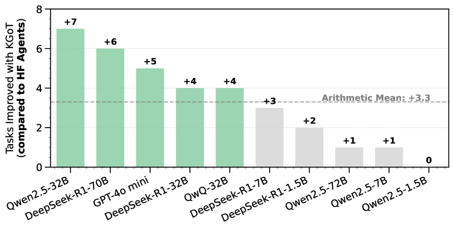<details> <summary>x21.png Details</summary>  ### Visual Description ## Bar Chart: KGoT Performance Improvement vs. HF Agents ### Overview This is a vertical bar chart comparing the performance improvement of various large language models (LLMs) when using "KGoT" (likely a method or framework) versus "HF Agents" (likely Hugging Face Agents). The chart quantifies the number of additional tasks each model successfully completes with KGoT. The data is presented in descending order of improvement. ### Components/Axes * **Y-Axis (Vertical):** Labeled "Tasks Improved with KGoT (compared to HF Agents)". The scale runs from 0 to 8, with major tick marks at intervals of 2 (0, 2, 4, 6, 8). * **X-Axis (Horizontal):** Lists the names of 10 different AI models. The labels are rotated approximately 45 degrees for readability. * **Data Series:** A single series of bars representing the improvement score for each model. * **Reference Line:** A horizontal dashed gray line labeled "Arithmetic Mean: +3.3" is positioned at the y-value of 3.3. * **Bar Labels:** Each bar has a numerical value label directly above it (e.g., "+7", "+6"). * **Color Coding:** Bars are colored in two distinct shades. The first five bars (from left) are a light green/teal color. The remaining five bars are a light gray color. The color change appears to correspond to whether the value is above (green) or below/at (gray) the arithmetic mean line. ### Detailed Analysis The chart displays the following data points, from left to right: 1. **Qwen2.5-32B:** Green bar. Value: **+7**. This is the highest improvement shown. 2. **DeepSeek-R1-70B:** Green bar. Value: **+6**. 3. **GPT-4o mini:** Green bar. Value: **+5**. 4. **DeepSeek-R1-32B:** Green bar. Value: **+4**. 5. **QwQ-32B:** Green bar. Value: **+4**. 6. **DeepSeek-R1-7B:** Gray bar. Value: **+3**. This is the first bar below the mean line. 7. **DeepSeek-R1-1.5B:** Gray bar. Value: **+2**. 8. **Qwen2.5-72B:** Gray bar. Value: **+1**. 9. **Qwen2.5-7B:** Gray bar. Value: **+1**. 10. **Qwen2.5-1.5B:** Gray bar. Value: **0**. This model shows no improvement. **Trend Verification:** The visual trend is a clear, step-wise descending staircase from left to right. The tallest bar is on the far left, and the bars generally decrease in height, with the final bar on the far right having zero height. The two bars for "DeepSeek-R1-32B" and "QwQ-32B" are of equal height, as are the two bars for "Qwen2.5-72B" and "Qwen2.5-7B". ### Key Observations * **Performance Spread:** There is a significant range in KGoT's effectiveness, from a high of +7 additional tasks to a low of 0. * **Model Size vs. Improvement:** There is no strict linear correlation between model parameter size (e.g., 70B, 32B, 7B) and improvement score. For example, the 70B DeepSeek model shows +6 improvement, while the 72B Qwen model shows only +1. The 32B Qwen model shows the highest improvement (+7). * **Clustering:** The top five performers (all above the mean) are a mix of models from different families (Qwen, DeepSeek, GPT, QwQ). The bottom five performers (at or below the mean) are exclusively from the DeepSeek-R1 and Qwen2.5 families, but include both small and large variants (e.g., 72B and 1.5B). * **Mean Benchmark:** The arithmetic mean improvement across all listed models is +3.3 tasks. Five models perform above this average, and five perform at or below it. ### Interpretation The data suggests that the KGoT method provides a measurable performance boost over standard HF Agents for the majority of the tested models, with an average gain of over 3 tasks. However, its efficacy is highly model-dependent. The lack of a clear size-to-benefit relationship implies that KGoT's advantages may stem from architectural compatibility, training data alignment, or specific capabilities of the base model rather than raw scale. The fact that the largest model tested (Qwen2.5-72B) shows minimal gain (+1) while a mid-sized model (Qwen2.5-32B) shows the maximum gain (+7) is a critical finding. It indicates that simply scaling up a model does not guarantee better utilization of the KGoT framework. The zero improvement for Qwen2.5-1.5B suggests a potential lower-bound threshold for model capability or size below which KGoT offers no advantage. This chart would be essential for a technical audience deciding which models to pair with the KGoT system for optimal task performance, highlighting that model selection is a crucial factor beyond just choosing the largest available model. 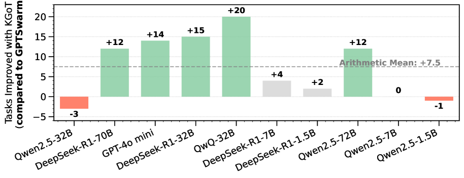</details> (a) Hugging Face Agents <details> <summary>x22.png Details</summary>  ### Visual Description ## Bar Chart: Model Performance Improvement with KGoT Method ### Overview This is a vertical bar chart comparing the performance improvement of various large language models (LLMs) when using a method called "KGoT" versus a baseline method called "GPTswarm." The chart quantifies the improvement in terms of "Tasks Improved." The overall trend shows that most models experience a positive improvement, with a calculated arithmetic mean improvement of +7.5 tasks. ### Components/Axes * **Chart Type:** Vertical Bar Chart. * **Y-Axis (Vertical):** * **Label:** "Tasks Improved with KGoT (compared to GPTswarm)" * **Scale:** Linear scale ranging from -5 to 20. * **Major Gridlines:** Horizontal lines at intervals of 5 units (0, 5, 10, 15, 20). * **X-Axis (Horizontal):** * **Label:** None explicit. Contains categorical labels for different AI models. * **Categories (from left to right):** 1. Qwen2.5-32B 2. DeepSeek-R1-70B 3. GPT-4o mini 4. DeepSeek-R1-32B 5. QwQ-32B 6. DeepSeek-R1-7B 7. DeepSeek-R1-1.5B 8. Qwen2.5-72B 9. Qwen2.5-7B 10. Qwen2.5-1.5B * **Legend/Color Coding:** While not in a separate box, color is used functionally: * **Green Bars:** Indicate a positive improvement value. * **Red/Salmon Bars:** Indicate a negative improvement value (performance regression). * **Light Gray Bars:** Indicate a small positive improvement value (near zero). * **Reference Line:** A horizontal dashed gray line is drawn across the chart at the Y-axis value of **+7.5**. It is labeled in the upper-right quadrant of the chart area as **"Arithmetic Mean: +7.5"**. ### Detailed Analysis Each bar's value is explicitly annotated above or below it. The data series, from left to right, is as follows: 1. **Qwen2.5-32B:** Bar extends downward to **-3**. (Color: Red) 2. **DeepSeek-R1-70B:** Bar extends upward to **+12**. (Color: Green) 3. **GPT-4o mini:** Bar extends upward to **+14**. (Color: Green) 4. **DeepSeek-R1-32B:** Bar extends upward to **+15**. (Color: Green) 5. **QwQ-32B:** Bar extends upward to **+20**. This is the highest value on the chart. (Color: Green) 6. **DeepSeek-R1-7B:** Bar extends upward to **+4**. (Color: Light Gray) 7. **DeepSeek-R1-1.5B:** Bar extends upward to **+2**. (Color: Light Gray) 8. **Qwen2.5-72B:** Bar extends upward to **+12**. (Color: Green) 9. **Qwen2.5-7B:** Bar has no height, annotated with **0**. (Color: Not distinctly colored, appears as a line on the axis) 10. **Qwen2.5-1.5B:** Bar extends downward to **-1**. (Color: Red) **Trend Verification:** The visual trend shows a cluster of strong positive performance (green bars) for several 32B and 70B parameter models, with the peak at QwQ-32B. Smaller models (1.5B, 7B) show minimal gains (gray bars). Two models from the Qwen2.5 series (32B and 1.5B) show negative results (red bars). ### Key Observations * **Highest Performer:** **QwQ-32B** shows the greatest improvement with **+20** tasks. * **Lowest Performer:** **Qwen2.5-32B** shows the greatest regression with **-3** tasks. * **Model Size Correlation:** There is a loose, non-linear correlation where mid-to-large size models (32B, 70B) tend to show larger improvements, but this is not absolute (e.g., Qwen2.5-72B at +12 is lower than the 32B models from other series). * **Series Variance:** The **Qwen2.5** model series shows high variance in results, ranging from -3 to +12, with the smallest model (1.5B) also showing a slight regression (-1). * **Mean Performance:** The arithmetic mean of **+7.5** is explicitly provided, serving as a benchmark. Six models perform above this mean, and four perform at or below it. ### Interpretation The data suggests that the "KGoT" method provides a net positive benefit across the tested suite of models, as indicated by the positive arithmetic mean. However, its effectiveness is highly model-dependent. * **Method Efficacy:** KGoT appears particularly effective for the **DeepSeek-R1** and **GPT-4o mini** models in the tested configurations, consistently yielding improvements between +12 and +15, with the standout result from **QwQ-32B**. * **Model-Specific Behavior:** The inconsistent results within the **Qwen2.5** family (from -3 to +12) imply that the method's success may depend on factors beyond just model size, such as architecture, training data, or specific task alignment. The negative results for two Qwen models indicate that KGoT can, in some cases, degrade performance compared to the GPTswarm baseline. * **Practical Implication:** A practitioner would conclude that KGoT is a promising technique worth investigating, especially for models like DeepSeek-R1 and QwQ, but it requires careful validation for each specific model, as it is not universally beneficial. The chart effectively argues that one cannot assume a single method will work equally well across all state-of-the-art LLMs. </details> (b) GPTSwarm Figure 12: Relative improvement of KGoT over Hugging Face Agents (left) and GPTSwarm (right) on the GAIA validation set using various LLM models. Table 2: Comparison of KGoT with other current state-of-the-art open-source agents on the GAIA benchmark. We provide both the absolute (number of solved tasks) and relative (percentage) results. The baseline data on the test set is obtained through the leaderboard. We highlight the best performing scheme in a given category in bold. The validation set consists of 165 tasks in total (53 in level 1, 86 in level 2 and 26 in level 3), whereas the test set contains 301 tasks (93 in level 1, 159 in level 2 and 49 in level 3). DR stands for Direct Retrieval. | | | Absolute | Relative | | | | | | | | --- | --- | --- | --- | --- | --- | --- | --- | --- | --- | | Agents | Model | All | L1 | L2 | L3 | Avg. | L1 | L2 | L3 | | Test Set | | | | | | | | | | | GPTSwarm | GPT-4o mini | 33 | 15 | 15 | 3 | 10.96 | 16.13 | 9.43 | 6.12 | | Magentic-One | GPT-4o mini | 43 | 22 | 18 | 3 | 14.29 | 23.66 | 11.32 | 6.12 | | TapeAgent | GPT-4o mini | 66 | 28 | 35 | 3 | 21.93 | 30.11 | 22.01 | 6.12 | | Hugging Face Agents | GPT-4o mini | 68 | 30 | 34 | 4 | 22.59 | 32.26 | 21.38 | 8.16 | | KGoT (fusion) | GPT-4o mini | 73 | 33 | 36 | 4 | 24.25 | 35.48 | 22.64 | 8.16 | | Validation Set | | | | | | | | | | | Simple RAG | GPT-4o mini | 35 | 18 | 15 | 2 | 21.21 | 33.96 | 17.44 | 7.69 | | GraphRAG | GPT-4o mini | 23 | 10 | 13 | 0 | 13.94 | 18.87 | 15.12 | 0.00 | | Magentic-One | GPT-4o mini | 31 | 13 | 18 | 0 | 18.79 | 24.53 | 20.93 | 0.00 | | No KG (Single Run #1) | GPT-4o mini | 30 | 14 | 14 | 2 | 18.18 | 26.42 | 16.28 | 7.69 | | No KG (Single Run #2) | GPT-4o mini | 33 | 17 | 16 | 0 | 20.00 | 32.08 | 18.60 | 0.00 | | No KG (Fusion) | GPT-4o mini | 40 | 18 | 20 | 2 | 24.24 | 33.96 | 23.26 | 7.69 | | KGoT (Neo4j + DR) | GPT-4o mini | 40 | 21 | 16 | 3 | 24.24 | 39.62 | 18.60 | 11.54 | | KGoT (NetworkX + Query) | GPT-4o mini | 44 | 21 | 21 | 2 | 26.67 | 39.62 | 24.42 | 7.69 | | KGoT (NetworkX + DR) | GPT-4o mini | 40 | 20 | 18 | 2 | 24.24 | 37.74 | 20.93 | 7.69 | | KGoT (RDF4J + Query) | GPT-4o mini | 36 | 20 | 15 | 1 | 21.82 | 37.74 | 17.44 | 3.85 | | KGoT (fusion) (Neo4j; Query + DR) | GPT-4o mini | 57 | 29 | 24 | 4 | 34.55 | 54.72 | 27.91 | 15.38 | | KGoT (fusion) (NetworkX; Query + DR) | GPT-4o mini | 57 | 27 | 28 | 2 | 34.55 | 50.94 | 32.56 | 7.69 | | KGoT (fusion) (Neo4j + NetworkX; Query + DR) | GPT-4o mini | 71 | 34 | 33 | 4 | 43.03 | 64.15 | 38.37 | 15.38 | | Zero-Shot | GPT-4o mini | 17 | 4 | 13 | 0 | 10.30 | 7.55 | 15.12 | 0.00 | | Zero-Shot | GPT-4o | 29 | 10 | 17 | 2 | 17.58 | 18.87 | 19.77 | 7.69 | | Zero-Shot | Qwen2.5-1.5B | 3 | 2 | 1 | 0 | 1.81 | 3.77 | 1.16 | 0.00 | | Zero-Shot | Qwen2.5-7B | 9 | 4 | 5 | 0 | 5.45 | 7.55 | 5.81 | 0.00 | | Zero-Shot | Qwen2.5-32B | 15 | 7 | 8 | 0 | 9.09 | 13.21 | 9.30 | 0.00 | | Zero-Shot | Qwen2.5-72B | 19 | 6 | 13 | 0 | 11.52 | 11.32 | 15.12 | 0.00 | | Zero-Shot | QwQ-32B | 0 | 0 | 0 | 0 | 0.00 | 0.00 | 0.00 | 0.00 | | Zero-Shot | DeepSeek-R1-1.5B | 5 | 3 | 2 | 0 | 3.03 | 5.66 | 2.33 | 0.00 | | Zero-Shot | DeepSeek-R1-7B | 13 | 8 | 5 | 0 | 7.88 | 15.09 | 5.81 | 0.00 | | Zero-Shot | DeepSeek-R1-32B | 14 | 8 | 6 | 0 | 8.48 | 15.09 | 6.98 | 0.00 | | Zero-Shot | DeepSeek-R1-70B | 20 | 9 | 10 | 1 | 12.12 | 16.98 | 11.63 | 3.85 | | GPTSwarm | GPT-4o mini | 26 | 13 | 13 | 0 | 15.76 | 24.53 | 15.12 | 0.00 | | GPTSwarm | Qwen2.5-1.5B | 5 | 4 | 1 | 0 | 3.03 | 7.55 | 1.16 | 0.00 | | GPTSwarm | Qwen2.5-7B | 12 | 8 | 4 | 0 | 7.27 | 15.09 | 4.65 | 0.00 | | GPTSwarm | Qwen2.5-32B | 29 | 15 | 14 | 0 | 17.58 | 28.30 | 16.28 | 0.00 | | GPTSwarm | Qwen2.5-72B | 27 | 13 | 14 | 0 | 16.36 | 24.53 | 16.28 | 0.00 | | GPTSwarm | QwQ-32B | 0 | 0 | 0 | 0 | 0.00 | 0.00 | 0.00 | 0.00 | | GPTSwarm | DeepSeek-R1-1.5B | 0 | 0 | 0 | 0 | 0.00 | 0.00 | 0.00 | 0.00 | | GPTSwarm | DeepSeek-R1-7B | 2 | 0 | 2 | 0 | 1.21 | 0.00 | 2.33 | 0.00 | | GPTSwarm | DeepSeek-R1-32B | 6 | 3 | 3 | 0 | 3.64 | 5.66 | 3.49 | 0.00 | | GPTSwarm | DeepSeek-R1-70B | 10 | 5 | 5 | 0 | 6.06 | 9.43 | 5.81 | 0.00 | | Hugging Face Agents | GPT-4o mini | 35 | 14 | 20 | 1 | 21.21 | 26.42 | 23.26 | 3.85 | | Hugging Face Agents | GPT-4o | 55 | 22 | 31 | 2 | 33.33 | 41.51 | 36.05 | 7.69 | | Hugging Face Agents | Qwen2.5-1.5B | 4 | 2 | 2 | 0 | 2.42 | 3.77 | 2.33 | 0.00 | | Hugging Face Agents | Qwen2.5-7B | 11 | 7 | 4 | 0 | 6.66 | 13.21 | 4.65 | 0.00 | | Hugging Face Agents | Qwen2.5-32B | 19 | 10 | 9 | 0 | 11.52 | 18.87 | 11.63 | 0.00 | | Hugging Face Agents | Qwen2.5-72B | 38 | 16 | 22 | 0 | 23.03 | 30.19 | 25.58 | 0.00 | | Hugging Face Agents | QwQ-32B | 16 | 9 | 7 | 0 | 9.70 | 16.98 | 8.14 | 0.00 | | Hugging Face Agents | DeepSeek-R1-1.5B | 0 | 0 | 0 | 0 | 0.00 | 0.00 | 0.00 | 0.00 | | Hugging Face Agents | DeepSeek-R1-7B | 3 | 2 | 1 | 0 | 1.81 | 3.77 | 1.16 | 0.00 | | Hugging Face Agents | DeepSeek-R1-32B | 17 | 9 | 7 | 1 | 10.30 | 16.98 | 8.14 | 3.85 | | Hugging Face Agents | DeepSeek-R1-70B | 16 | 9 | 6 | 1 | 9.70 | 16.98 | 6.98 | 3.85 | | KGoT (Neo4j + Query) | GPT-4o mini | 40 | 21 | 18 | 1 | 24.24 | 39.62 | 20.93 | 3.85 | | KGoT (Neo4j + Query) | Qwen2.5-1.5B | 4 | 3 | 1 | 0 | 2.42 | 5.66 | 1.16 | 0.00 | | KGoT (Neo4j + Query) | Qwen2.5-7B | 12 | 7 | 5 | 0 | 7.27 | 13.21 | 5.81 | 0.00 | | KGoT (Neo4j + Query) | Qwen2.5-32B | 26 | 12 | 14 | 0 | 15.76 | 22.64 | 16.28 | 0.00 | | KGoT (Neo4j + Query) | Qwen2.5-72B | 39 | 18 | 21 | 0 | 23.64 | 33.96 | 24.42 | 0.00 | | KGoT (Neo4j + Query) | QwQ-32B | 20 | 11 | 9 | 0 | 12.12 | 20.75 | 10.47 | 0.00 | | KGoT (Neo4j + Query) | DeepSeek-R1-1.5B | 2 | 1 | 1 | 0 | 1.21 | 1.89 | 1.16 | 0.00 | | KGoT (Neo4j + Query) | DeepSeek-R1-7B | 6 | 3 | 3 | 0 | 3.64 | 5.66 | 3.49 | 0.00 | | KGoT (Neo4j + Query) | DeepSeek-R1-32B | 21 | 12 | 9 | 0 | 12.73 | 22.64 | 10.47 | 0.00 | | KGoT (Neo4j + Query) | DeepSeek-R1-70B | 22 | 11 | 10 | 1 | 13.33 | 20.75 | 11.63 | 3.85 | ### D.1 SimpleQA Results Table 3: Comparison of KGoT, HF Agents and GPTSwarm on a subset of SimpleQA as well as the results for KGoT on the full benchmark. We highlight the best performing scheme in given category in bold. Model: GPT-4o mini. | | | Not | | Correct | | | Cost per | | --- | --- | --- | --- | --- | --- | --- | --- | | Correct | attempted | Incorrect | given at- | | Total | solved | | | Framework | (%) | (%) | (%) | tempted (%) | F-score | cost ($) | task ($) | | GPTSwarm | 53.8106 | 6.2356 | 39.9538 | 57.3892 | 55.5 | 0.2159 | 0.00092660 | | HF Agents | 66.0508 | 18.0139 | 15.9353 | 80.5634 | 72.6 | 16.7117 | 0.05843265 | | KGoT | 73.2102 | 1.6166 | 25.1732 | 74.4131 | 73.8 | 5.6432 | 0.01780182 | | KGoT (Full) | 70.3421 | 2.0342 | 27.8548 | 71.8027 | 71.1 | 59.1538 | 0.01943931 | Table 4: F1-score comparison of KGoT, OpenAI and Claude models on SimpleQA. OpenAI and Claude results were taken from the official repository (OpenAI, 2025). Model for KGoT: GPT-4o mini. | Reasoning Models | F1-score | Assistant Models | F1-score | | --- | --- | --- | --- | | o1 | 42.6 | gpt-4.1-2025-04-14 | 41.6 | | o1-preview | 42.4 | gpt-4.1-mini-2025-04-14 | 16.8 | | o3-high | 48.6 | gpt-4.1-nano-2025-04-14 | 7.6 | | o3 | 49.4 | gpt-4o-2024-11-20 | 38.8 | | o3-low | 49.4 | gpt-4o-2024-08-06 | 40.1 | | o1-mini | 7.6 | gpt-4o-2024-05-13 | 39.0 | | o3-mini-high | 13.8 | gpt-4o-mini-2024-07-18 | 9.5 | | o3-mini | 13.4 | gpt-4.5-preview-2025-02-27 | 62.5 | | o3-mini-low | 13.0 | gpt-4-turbo-2024-04-09 | 24.2 | | o4-mini-high | 19.3 | Claude 3.5 Sonnet | 28.9 | | o4-mini | 20.2 | Claude 3 Opus | 23.5 | | o4-mini-low | 20.2 | | | | KGoT | 71.1 | | | ### D.2 Impact from Various Design Decisions Table 5: Analysis of different design decisions and tool sets in KGoT. “ ST ” stands for the type of the solve operation and pathway (“ GQ ”: graph query, “ DR ”: Direct Retrieval), “ PF ” for the prompt format (“ MD ”: Markdown) and “ merged ” stands for a combination of the original KGoT tools and the Hugging Face Agents tools. | Configuration | Metrics | | | | | | --- | --- | --- | --- | --- | --- | | Tools | ST | PF | Solved | Time (h) | Cost | | HF | DR | XML | 37 | 11.87 | $7.84 | | HF | GQ | MD | 33 | 9.70 | $4.28 | | merged | GQ | XML | 31 | 10.62 | $5.43 | | HF | GQ | XML | 30 | 13.02 | $4.90 | | original KGoT | GQ | XML | 27 | 27.57 | $6.85 | We explored different tool sets, with selected results presented in Table 5. Initially, we examined the limitations of our original tools and subsequently integrated the complete Hugging Face Agents tool set into the KGoT framework, which led to improvements in accuracy, runtime, and cost efficiency. A detailed analysis allowed us to merge the most effective components from both tool sets into an optimized hybrid tool set, further enhancing accuracy and runtime while only moderately increasing costs. Key improvements include a tighter integration between the ExtractZip tool and the Text Inspector tool, which now supports Markdown, as well as enhancements to the Surfer Agent, incorporating a Wikipedia tool and augmenting viewpoint segmentation with full-page summarization. This optimized tool set was used for all subsequent experiments. We further evaluated different prompt formats in the initial iterations of KGoT. While our primary format was XML-based, we conducted additional tests using Markdown. Initial experiments with the Hugging Face Agents tool set (see Table 5) combined with Markdown and GPT-4o mini yielded improved accuracy, reduced runtime, and lower costs. However, these results were not consistently reproducible with GPT-4o. Moreover, Markdown-based prompts interfered with optimizations such as Direct Retrieval, ultimately leading us to retain the XML-based format. 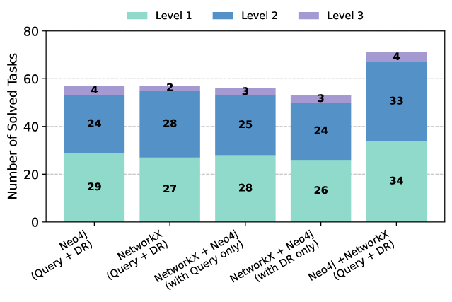<details> <summary>x23.png Details</summary>  ### Visual Description ## Stacked Bar Chart: Task Solving Performance by Method and Complexity Level ### Overview This image is a stacked bar chart comparing the performance of five different computational methods or system configurations in solving tasks. The performance is measured by the total number of tasks solved, broken down by three complexity levels (Level 1, Level 2, Level 3). The chart visually demonstrates how each method's total solved tasks are composed of tasks from these different levels. ### Components/Axes * **Chart Type:** Stacked Bar Chart. * **Y-Axis:** * **Label:** "Number of Solved Tasks" * **Scale:** Linear scale from 0 to 80, with major gridlines at intervals of 20 (0, 20, 40, 60, 80). * **X-Axis:** * **Label:** None explicit. The axis displays categorical labels for five distinct methods/configurations. * **Categories (from left to right):** 1. `Neo4j (Query + DR)` 2. `NetworkX (Query + DR)` 3. `NetworkX + Neo4j (with Query only)` 4. `NetworkX + Neo4j (with DR only)` 5. `Neo4j + NetworkX (Query + DR)` * **Legend:** * **Position:** Top center, above the plot area. * **Entries:** * **Level 1:** Represented by a mint green color. * **Level 2:** Represented by a medium blue color. * **Level 3:** Represented by a lavender/light purple color. * **Data Labels:** Each segment of every stacked bar contains a numerical label indicating the exact count of solved tasks for that specific level within that method. ### Detailed Analysis The chart presents the following data for each method, broken down by level: 1. **Neo4j (Query + DR)** * **Level 1 (Mint Green):** 29 tasks * **Level 2 (Blue):** 24 tasks * **Level 3 (Lavender):** 4 tasks * **Total Solved Tasks:** 57 (29 + 24 + 4) 2. **NetworkX (Query + DR)** * **Level 1 (Mint Green):** 27 tasks * **Level 2 (Blue):** 28 tasks * **Level 3 (Lavender):** 2 tasks * **Total Solved Tasks:** 57 (27 + 28 + 2) 3. **NetworkX + Neo4j (with Query only)** * **Level 1 (Mint Green):** 28 tasks * **Level 2 (Blue):** 25 tasks * **Level 3 (Lavender):** 3 tasks * **Total Solved Tasks:** 56 (28 + 25 + 3) 4. **NetworkX + Neo4j (with DR only)** * **Level 1 (Mint Green):** 26 tasks * **Level 2 (Blue):** 24 tasks * **Level 3 (Lavender):** 3 tasks * **Total Solved Tasks:** 53 (26 + 24 + 3) 5. **Neo4j + NetworkX (Query + DR)** * **Level 1 (Mint Green):** 34 tasks * **Level 2 (Blue):** 33 tasks * **Level 3 (Lavender):** 4 tasks * **Total Solved Tasks:** 71 (34 + 33 + 4) **Visual Trend Verification:** * The **Level 1 (Mint Green)** segment is the largest component in every bar, indicating that the majority of solved tasks across all methods are of the lowest complexity. * The **Level 2 (Blue)** segment is consistently the second-largest component. * The **Level 3 (Lavender)** segment is the smallest in all cases, forming a thin cap on each bar. * The total height of the bars (total solved tasks) is relatively similar for the first four methods (ranging from 53 to 57), but the fifth bar (`Neo4j + NetworkX (Query + DR)`) is noticeably taller, indicating superior overall performance. ### Key Observations 1. **Top Performer:** The method `Neo4j + NetworkX (Query + DR)` solves the most tasks overall (71), outperforming the next best methods by a significant margin (14 more tasks). 2. **Consistent Level Distribution:** The proportional contribution of each level (L1 > L2 > L3) is consistent across all methods. No method shows a disproportionate strength in higher-level tasks. 3. **Query + DR Synergy:** The two methods explicitly labeled with `(Query + DR)` (the first and last bars) are the top two performers. The combined `Neo4j + NetworkX` configuration with both capabilities is the most effective. 4. **Impact of Isolation:** The method `NetworkX + Neo4j (with DR only)` has the lowest total score (53), suggesting that using only the "DR" component in this hybrid setup is less effective than using only "Query" (56 tasks) or both. 5. **Low High-Level Task Completion:** Across all methods, the number of solved Level 3 tasks is very low (2-4), indicating these tasks are significantly more challenging for all tested configurations. ### Interpretation This chart provides a comparative analysis of system architectures for automated task solving, likely in the domain of graph-based reasoning or database querying (given the mention of Neo4j and NetworkX). The data suggests several key insights: * **Integration is Key:** The most effective approach is not using Neo4j or NetworkX in isolation, but integrating them (`Neo4j + NetworkX`). Furthermore, this integration yields the best results when both core capabilities—referred to as "Query" and "DR" (likely Data Retrieval or Reasoning)—are active. This points to a synergistic effect where the strengths of one system compensate for the limitations of the other. * **Complexity Barrier:** The stark drop-off in solved tasks from Level 1 to Level 3 across all methods indicates a fundamental challenge in handling high-complexity tasks. The systems' capabilities appear to plateau at lower-complexity problems. Future development would need to focus specifically on the algorithms or knowledge representations required for Level 3 tasks. * **Performance Baseline:** The first four methods establish a performance baseline between 53-57 solved tasks. The significant jump to 71 tasks with the fully integrated system demonstrates that architectural choices have a substantial impact on capability, beyond incremental improvements. * **Component Contribution:** The "Query" component appears slightly more valuable than "DR" when used in isolation within the hybrid model (56 vs. 53 tasks). However, the true value is unlocked when both are combined with the integrated graph systems. In summary, the chart advocates for a holistic, integrated system design (`Neo4j + NetworkX`) that leverages both query and data retrieval/reasoning functionalities to maximize performance, while also highlighting a clear research target for improving performance on the most complex (Level 3) tasks. </details> Figure 13: Comparison of different fusion types in respect to the task solve operation as well as the graph backend type. We report results for answering 165 GAIA validation questions across different comparison targets. DR stands for Direct Retrieval. Model: GPT-4o mini. Graph Backend vs. Task Solve Operation We provide more detailed results in Figure 13, studying the performance of the following configurations: NetworkX + Neo4j (with query only) and NetworkX + Neo4j (with DR only) as well as Neo4j (query + DR) and NetworkX (query + DR). Overall, the fusion of backends (with DR only) offers smaller advantages than other types of fusion. This indicates that different graph querying languages have different strengths and their fusion comes with the largest combined advantage. ### D.3 Runtime We provide a runtime overview of running KGoT on the validation set of the GAIA benchmark with GPT4o-mini, Neo4j and query-based retrieval in Figure 14. The right part follows the categorization in Appendix C. We provide a more detailed analysis of the runtime in Figure 17. 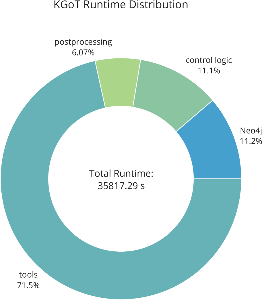<details> <summary>x24.png Details</summary>  ### Visual Description ## Donut Chart: KGoT Runtime Distribution ### Overview This image is a donut chart (a pie chart with a central hole) titled "KGoT Runtime Distribution." It visualizes the proportional breakdown of total runtime for a system or process called "KGoT" across four distinct components. The total runtime is explicitly stated in the center of the chart. ### Components/Axes * **Chart Title:** "KGoT Runtime Distribution" (located at the top center). * **Central Information:** "Total Runtime: 35817.29 s" (located in the white central hole of the donut). * **Segments & Labels:** The chart is divided into four colored segments, each with an associated label and percentage placed outside the segment. * **Segment 1 (Largest, Teal):** Label "tools", Percentage "71.5%". Positioned from approximately the 7 o'clock to 4 o'clock position (spanning the bottom and left side). * **Segment 2 (Blue):** Label "Neo4j", Percentage "11.2%". Positioned from approximately the 4 o'clock to 2 o'clock position (right side). * **Segment 3 (Light Green):** Label "control logic", Percentage "11.1%". Positioned from approximately the 2 o'clock to 12 o'clock position (top-right). * **Segment 4 (Lightest Green):** Label "postprocessing", Percentage "6.07%". Positioned from approximately the 12 o'clock to 11 o'clock position (top-left). ### Detailed Analysis The chart provides a precise percentage breakdown of the total 35,817.29 seconds of runtime. 1. **tools:** 71.5% of the total runtime. * *Calculated Approximate Value:* 0.715 * 35817.29 s ≈ 25,609.36 s. * *Visual Trend:* This is the dominant segment, occupying nearly three-quarters of the chart. 2. **Neo4j:** 11.2% of the total runtime. * *Calculated Approximate Value:* 0.112 * 35817.29 s ≈ 4,011.54 s. * *Visual Trend:* The second-largest segment, roughly equal in size to "control logic". 3. **control logic:** 11.1% of the total runtime. * *Calculated Approximate Value:* 0.111 * 35817.29 s ≈ 3,975.72 s. * *Visual Trend:* Nearly identical in proportion to "Neo4j". 4. **postprocessing:** 6.07% of the total runtime. * *Calculated Approximate Value:* 0.0607 * 35817.29 s ≈ 2,174.11 s. * *Visual Trend:* The smallest segment. **Note on Precision:** The percentages sum to 99.87% (71.5 + 11.2 + 11.1 + 6.07). The missing 0.13% is likely due to rounding in the displayed percentages. ### Key Observations * **Dominant Component:** The "tools" component is overwhelmingly the largest contributor to the KGoT runtime, accounting for more than double the combined time of all other components. * **Secondary Components:** "Neo4j" and "control logic" are nearly identical in their runtime share (~11% each). * **Minor Component:** "postprocessing" represents a relatively small fraction of the total time. * **Total Runtime:** The system's total measured runtime is substantial, at approximately 35,817 seconds, which is roughly 9 hours and 57 minutes. ### Interpretation This chart clearly demonstrates that the performance bottleneck of the KGoT system lies within the "tools" component. Any effort to optimize the overall runtime should prioritize this segment, as even a modest percentage improvement here would yield the largest absolute time savings. The near-equal split between "Neo4j" (likely a database interaction layer) and "control logic" suggests these are secondary but significant areas for potential optimization. "postprocessing" is a minor factor in the current runtime profile. The data suggests a system architecture where the core "tools" execution is the most computationally expensive phase, while database operations and control flow management are secondary, and final post-processing is relatively lightweight. The precise total runtime value (35817.29 s) indicates this is based on measured empirical data, not an estimate. 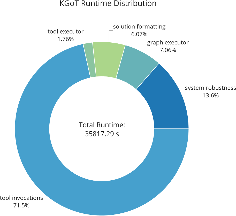</details> <details> <summary>x25.png Details</summary>  ### Visual Description ## Donut Chart: KGoT Runtime Distribution ### Overview The image displays a donut chart titled "KGoT Runtime Distribution," illustrating the percentage breakdown of total runtime across five distinct components of a system or process named "KGoT." The chart includes a central annotation stating the total runtime duration. ### Components/Axes * **Chart Type:** Donut Chart (a pie chart with a central hole). * **Title:** "KGoT Runtime Distribution" (positioned at the top center). * **Central Annotation:** "Total Runtime: 35817.29 s" (positioned in the center of the donut hole). * **Segments & Labels:** The chart is divided into five colored segments, each with an associated label and percentage value placed outside the chart, near its respective segment. 1. **tool invocations** (71.5%) - Medium blue segment. This is the largest segment, occupying the majority of the chart from the bottom-left, sweeping clockwise to the top-right. 2. **system robustness** (13.6%) - Dark blue segment. Positioned on the right side of the chart. 3. **graph executor** (7.06%) - Teal/blue-green segment. Located in the upper-right quadrant. 4. **solution formatting** (6.07%) - Light green segment. Positioned at the top of the chart. 5. **tool executor** (1.76%) - Pale green segment. The smallest segment, located at the top-left, adjacent to the "solution formatting" segment. ### Detailed Analysis The chart provides a precise quantitative breakdown of the total 35,817.29 seconds of runtime. * **Dominant Component:** "tool invocations" accounts for the overwhelming majority of the runtime at **71.5%**. This translates to approximately 25,609.36 seconds (71.5% of 35817.29 s). * **Secondary Components:** * "system robustness" is the second-largest component at **13.6%** (~4,871.15 seconds). * "graph executor" contributes **7.06%** (~2,528.70 seconds). * "solution formatting" contributes **6.07%** (~2,174.11 seconds). * **Minor Component:** "tool executor" represents the smallest fraction at **1.76%** (~630.38 seconds). The percentages sum to 100.0% (71.5 + 13.6 + 7.06 + 6.07 + 1.76 = 100.0), confirming the data's internal consistency. ### Key Observations 1. **Extreme Skew:** The distribution is highly skewed. The "tool invocations" component consumes nearly three-quarters of the total runtime, dwarfing all other components combined. 2. **Performance Bottleneck:** The data strongly suggests that "tool invocations" is the primary performance bottleneck within the KGoT system. Any optimization efforts aimed at reducing total runtime would yield the most significant returns by targeting this component. 3. **Relative Scale:** The four non-dominant components ("system robustness," "graph executor," "solution formatting," and "tool executor") together account for only 28.5% of the runtime. The smallest component ("tool executor") is about 40 times smaller than the largest. ### Interpretation This runtime distribution chart provides a clear diagnostic view of the KGoT system's performance profile. The data indicates that the system's operation is fundamentally characterized by time spent invoking external tools or services. This could imply several architectural realities: * The core logic of KGoT might be relatively lightweight, but it relies heavily on external dependencies whose execution or communication latency dominates the total time. * The "tool invocations" phase may include network I/O, waiting for external APIs, or executing subprocesses, which are inherently slower than in-memory computation. * The relatively small share for "system robustness" (13.6%) suggests that error handling, validation, or recovery routines, while significant, are not the primary cost center. * The minor share for "tool executor" (1.76%) versus the major share for "tool invocations" (71.5%) is noteworthy. This could indicate that the act of *invoking* or *preparing for* tool use (e.g., parameter serialization, request dispatch, response parsing) is far more costly than the actual *execution* of the tool's core logic itself. In summary, the chart reveals a system where performance is not bound by its internal graph processing ("graph executor") or output preparation ("solution formatting"), but by its interaction with the external environment via tool calls. To improve KGoT's efficiency, engineering efforts should be prioritized on optimizing the tool invocation pipeline—potentially through caching, batching, asynchronous execution, or selecting faster tool alternatives. </details> Figure 14: Different runtime categorizations of the same data. Graph storage: Neo4j. Retrieval type: query. Model: GPT-4o mini. ### D.4 Compute Resources Because of the long runtime, we executed most experiments using the OpenAI API as an external resource on server compute nodes containing a AMD EPYC 7742 CPU with 128 cores running at 2.25GHz, with a total memory of 256GB. However when the LLM is called as an external resource, KGoT is able to run on commodity hardware with minimal effects on runtime. Our experiments with locally run LLMs were executed with compute nodes containing 4x NVIDIA GH200, a respective GPU memory of 96GB, and a total memory of 896GB. In these cases, the minimum hardware requirements are dictated by the resources needed to run each LLM locally. High-performance & scalability experiments were performed on an Apple M3 Pro with 12 cores at 4.056GHz and a total memory of 18GB. ### D.5 GAIA Result Visualizations We also implemented various automatic scripts that plot various aspects once a GAIA run is finished. In the following we provide example plots for Neo4j with query retrieval. We provide a breakdown for each level of the GAIA benchmark into the categories that KGoT’s answers for the tasks fall into in Figure 15. We measure the runtime and costs of the various components of KGoT and illustrate them in Figure 17. We also provide insights into the tool usage, starting with the number of tasks for which a specific tools is used and whether that task was successful or not (see Figure 16). A more detailed analysis into the tool selection is provided in the plots of Figures 18 and 19 as well as the number of times the tools are used in Figure 20. We provide now a brief explanation of the more opaque function names listed in Figure 17. - Any function marked as not logged refers to function or tool calls that do not incur an LLM-related cost or where usage costs are logged within the tool itself. - WebSurfer.forward submits a query to SerpApi. - Define Cypher query given new information constructs a Cypher insert query based on newly gathered information. - Fix JSON corrects malformed or invalid JSON for services like Neo4j. - Define forced retrieve queries generates a Cypher retrieval query when the maximum number of iterations is reached. - Generate forced solution generates a solution based on the state of the knowledge graph if no viable solution has been parsed after a Cypher retrieve or if the forced retrievals fails after exhausting all iterations. 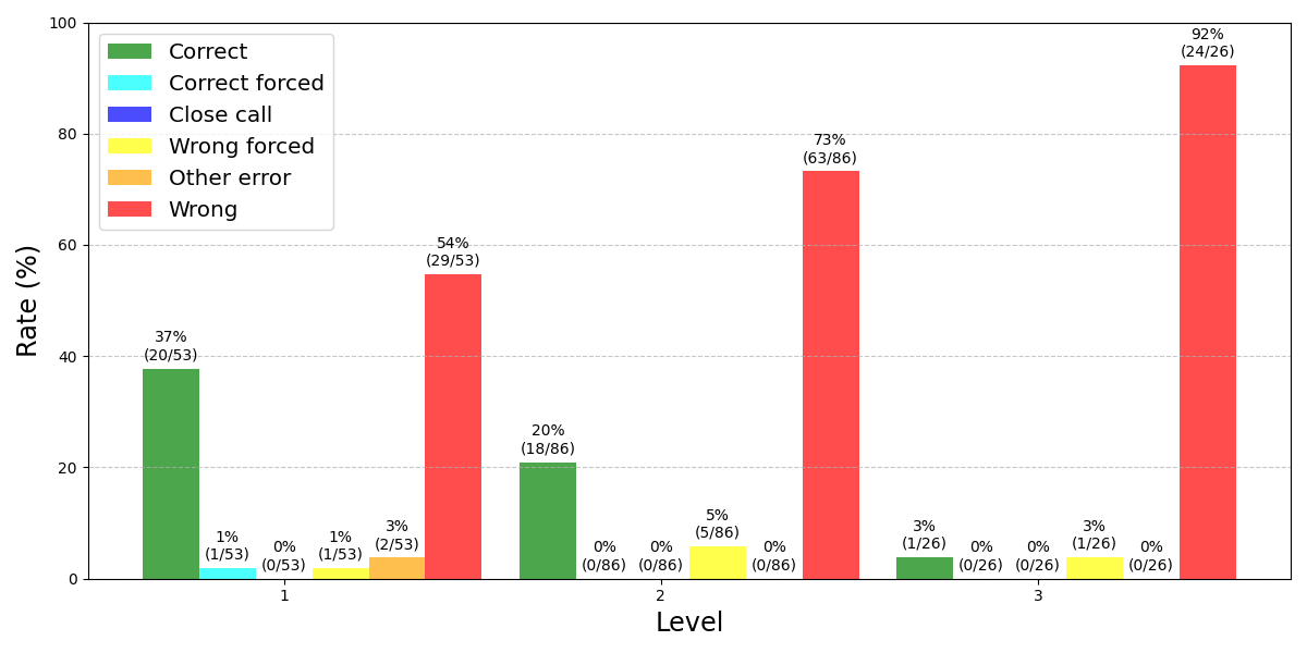<details> <summary>figures/all_plot_all_stats.png Details</summary>  ### Visual Description ## Grouped Bar Chart: Error Rate Distribution by Level ### Overview This image displays a grouped bar chart illustrating the percentage distribution of six different outcome categories across three distinct levels (1, 2, and 3). The chart quantifies performance or error rates, showing a clear trend where the "Wrong" outcome becomes increasingly dominant as the level number increases. ### Components/Axes * **Chart Type:** Grouped bar chart. * **X-Axis:** Labeled "Level". It has three categorical tick marks: `1`, `2`, and `3`. * **Y-Axis:** Labeled "Rate (%)". It is a linear scale ranging from 0 to 100, with major gridlines at intervals of 20 (0, 20, 40, 60, 80, 100). * **Legend:** Positioned in the top-left corner of the chart area. It defines six color-coded categories: * **Green:** Correct * **Cyan:** Correct forced * **Blue:** Close call * **Yellow:** Wrong forced * **Orange:** Other error * **Red:** Wrong * **Data Labels:** Each bar is annotated with a percentage value and, in parentheses, the raw fraction (e.g., `37% (20/53)`). ### Detailed Analysis The data is presented for each level, with bars grouped side-by-side. The total sample size (denominator) differs per level: Level 1 (n=53), Level 2 (n=86), Level 3 (n=26). **Level 1:** * **Correct (Green):** 37% (20/53). This is the highest rate for a non-"Wrong" category at this level. * **Correct forced (Cyan):** 1% (1/53). * **Close call (Blue):** 0% (0/53). * **Wrong forced (Yellow):** 1% (1/53). * **Other error (Orange):** 3% (2/53). * **Wrong (Red):** 54% (29/53). This is the dominant category at Level 1. **Level 2:** * **Correct (Green):** 20% (18/86). A significant decrease from Level 1. * **Correct forced (Cyan):** 0% (0/86). * **Close call (Blue):** 0% (0/86). * **Wrong forced (Yellow):** 5% (5/86). A slight increase from Level 1. * **Other error (Orange):** 0% (0/86). * **Wrong (Red):** 73% (63/86). A substantial increase, becoming overwhelmingly dominant. **Level 3:** * **Correct (Green):** 3% (1/26). A dramatic drop to near zero. * **Correct forced (Cyan):** 0% (0/26). * **Close call (Blue):** 0% (0/26). * **Wrong forced (Yellow):** 3% (1/26). * **Other error (Orange):** 0% (0/26). * **Wrong (Red):** 92% (24/26). The vast majority of outcomes at this level. ### Key Observations 1. **Dominant Trend:** There is a strong, inverse relationship between the "Correct" and "Wrong" rates as the level increases. "Correct" rates plummet from 37% to 3%, while "Wrong" rates surge from 54% to 92%. 2. **Minimal Other Categories:** The categories "Correct forced," "Close call," and "Other error" are negligible or zero across all levels, indicating they are rare outcomes. 3. **"Wrong Forced" Persistence:** The "Wrong forced" category, while small, is the only non-"Wrong" category present at all three levels (1%, 5%, 3%). 4. **Sample Size Variation:** The denominator changes per level (53, 86, 26), which should be considered when comparing absolute counts, though the percentages are normalized. ### Interpretation The data strongly suggests that the task or assessment becomes progressively more difficult from Level 1 to Level 3. The near-total dominance of the "Wrong" category at Level 3 (92%) indicates that this level may be beyond the capability threshold for the subjects being tested, or that the task design at this level is fundamentally different. The virtual absence of "Close call" and "Other error" outcomes implies a binary or near-binary scoring system where responses are classified as either definitively correct or definitively wrong, with "forced" choices representing a specific, constrained condition. The persistence of "Wrong forced" errors, even at the highest difficulty, may point to a specific, recurring flaw in reasoning or a consistent trap within the task design. From a Peircean perspective, this chart is an *index*—it points directly to a causal relationship between level difficulty and error rate. The trend is not merely correlational; the systematic increase in "Wrong" responses with each level strongly implies that the level variable is the *cause* of the performance degradation. The chart serves as a diagnostic tool, highlighting Level 3 as a critical point of failure and suggesting that investigation should focus on the specific challenges introduced at that stage. </details> Figure 15: Number of tasks per level that succeeded or fall into a given error category. Graph storage: Neo4j. Retrieval type: query. Model: GPT-4o mini. 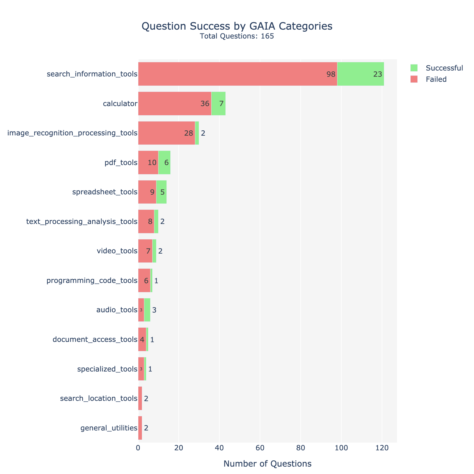<details> <summary>figures/all_tool_category_success.png Details</summary>  ### Visual Description ## Horizontal Stacked Bar Chart: Question Success by GAIA Categories ### Overview This image is a horizontal stacked bar chart titled "Question Success by GAIA Categories" with a subtitle "Total Questions: 165". It displays the performance (successful vs. failed) of an AI system across 13 distinct tool-use categories from the GAIA benchmark. The chart visually compares the volume of questions per category and the success/failure split within each. ### Components/Axes * **Title:** "Question Success by GAIA Categories" * **Subtitle:** "Total Questions: 165" * **Y-Axis (Vertical):** Lists 13 categorical tool types. From top to bottom: 1. `search_information_tools` 2. `calculator` 3. `image_recognition_processing_tools` 4. `pdf_tools` 5. `spreadsheet_tools` 6. `text_processing_analysis_tools` 7. `video_tools` 8. `programming_code_tools` 9. `audio_tools` 10. `document_access_tools` 11. `specialized_tools` 12. `search_location_tools` 13. `general_utilities` * **X-Axis (Horizontal):** Labeled "Number of Questions". The scale runs from 0 to 120, with major tick marks at intervals of 20 (0, 20, 40, 60, 80, 100, 120). * **Legend:** Positioned in the top-right corner. * Green square: "Successful" * Red (salmon) square: "Failed" * **Data Representation:** Each category has a horizontal bar composed of two segments: * **Left Segment (Red):** Represents the count of "Failed" questions. * **Right Segment (Green):** Represents the count of "Successful" questions. * The exact count for each segment is printed inside or adjacent to its respective bar segment. ### Detailed Analysis The following table reconstructs the data presented in the chart. The "Total" column is the sum of Failed and Successful for that category. Note: The sum of all category totals (216) exceeds the stated "Total Questions: 165", indicating that a single question may be evaluated against multiple tool categories, or the "Total Questions" refers to the unique question set size. | Category (Y-Axis) | Failed Count (Red Bar) | Successful Count (Green Bar) | Total per Category | | :--- | :--- | :--- | :--- | | search_information_tools | 98 | 23 | 121 | | calculator | 36 | 7 | 43 | | image_recognition_processing_tools | 28 | 2 | 30 | | pdf_tools | 10 | 6 | 16 | | spreadsheet_tools | 9 | 5 | 14 | | text_processing_analysis_tools | 8 | 2 | 10 | | video_tools | 7 | 2 | 9 | | programming_code_tools | 6 | 1 | 7 | | audio_tools | 3 | 3 | 6 | | document_access_tools | 4 | 1 | 5 | | specialized_tools | 3 | 1 | 4 | | search_location_tools | 2 | 0 | 2 | | general_utilities | 2 | 0 | 2 | **Visual Trend:** The bars are ordered from longest to shortest, showing a clear hierarchy in the number of questions associated with each tool category. `search_information_tools` is by far the most prevalent category. ### Key Observations 1. **Dominant Category:** `search_information_tools` accounts for the largest volume of questions (121 total), representing over half of all category instances. 2. **High Failure Rates:** The top three categories by volume (`search_information_tools`, `calculator`, `image_recognition_processing_tools`) all exhibit a high ratio of failures to successes. For `image_recognition_processing_tools`, failures outnumber successes 14:1. 3. **Balanced Performance:** `audio_tools` is the only category with an even split (3 Failed, 3 Successful). 4. **Zero Success:** Two categories, `search_location_tools` and `general_utilities`, have no recorded successful questions, though their total question count is very low (2 each). 5. **Success Rate Gradient:** There is no simple correlation between category volume and success rate. For example, `pdf_tools` (16 total) has a much higher success rate (6/16 ≈ 37.5%) than `calculator` (43 total, 7/43 ≈ 16.3%). ### Interpretation This chart provides a diagnostic breakdown of an AI system's capabilities on the GAIA benchmark, revealing significant performance disparities across different types of tool-use tasks. * **Core Challenge Area:** The system struggles most with tasks requiring **information search and retrieval** (`search_information_tools`), which are also the most frequently tested. This suggests a fundamental weakness in web search, information synthesis, or tool-use orchestration for open-ended queries. * **Specialized Tool Proficiency:** The system shows relative strength in tasks involving **PDF manipulation** and **audio processing**, achieving its highest success rates in these less common categories. This may indicate better-trained models or more deterministic tooling for these specific formats. * **Failure Patterns:** The near-total failure in `image_recognition_processing_tools` and `calculator` tasks points to critical gaps in multimodal understanding and precise numerical reasoning, respectively. * **Data Implication:** The discrepancy between the sum of category counts (216) and the total unique questions (165) is a key insight. It implies that GAIA questions are **multi-faceted**, often requiring the use of multiple tool types to solve. The system's overall performance is therefore a product of its ability to chain these tools effectively, and its failure in one area (like search) likely cascades to doom complex questions that depend on it. In summary, the chart doesn't just show success rates; it maps the **topography of the system's reasoning capabilities**, highlighting search, calculation, and image understanding as major valleys, while showing relative peaks in document and audio processing. </details> Figure 16: Overview over how many tasks use a given tool and whether they are successful or not. Graph storage: Neo4j. Retrieval type: query. Model: GPT-4o mini. 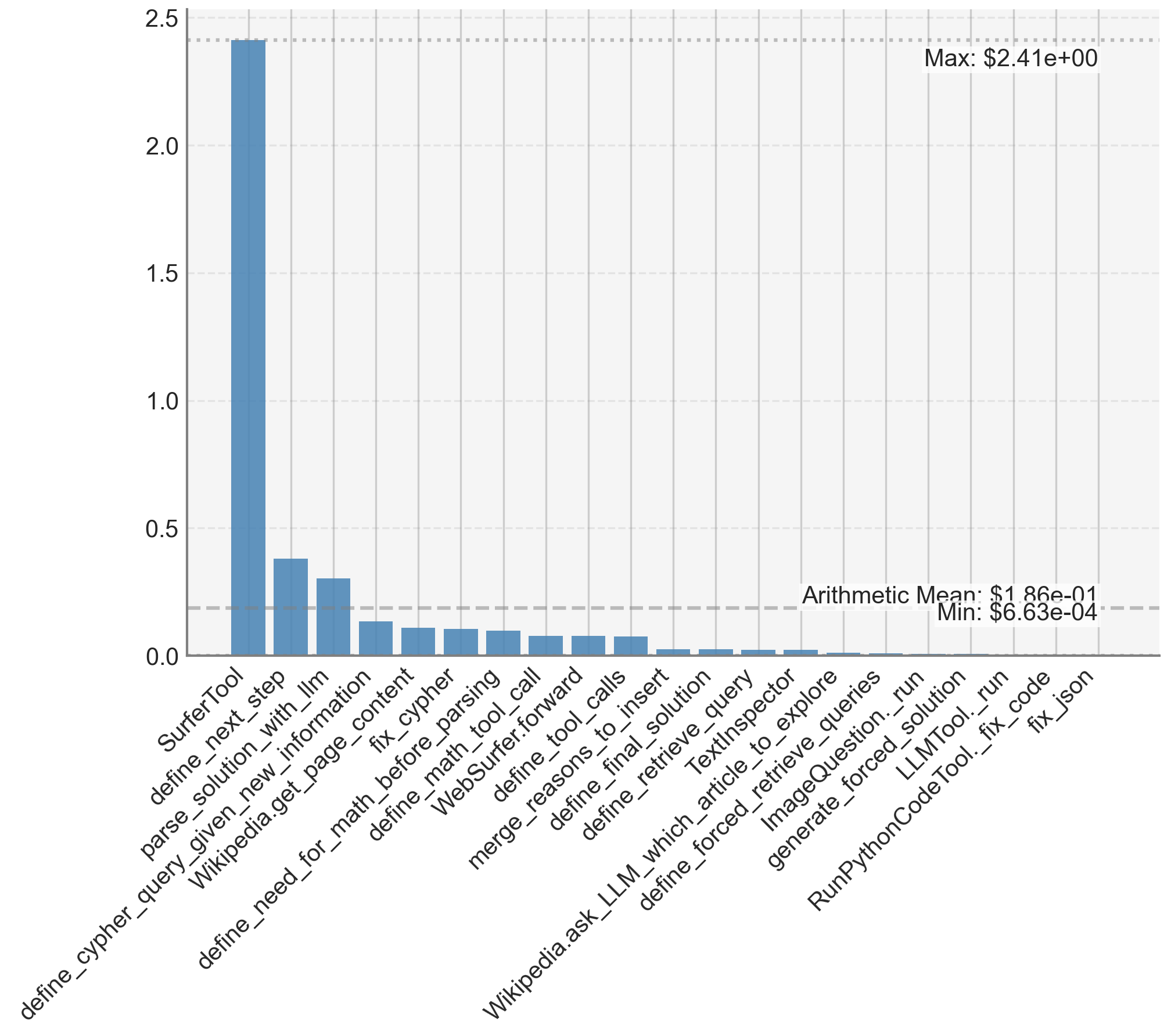<details> <summary>figures/all_cost_summary_cost.png Details</summary>  ### Visual Description ## Bar Chart: Tool Performance Metrics ### Overview The image displays a vertical bar chart comparing numerical values (likely performance metrics, costs, or scores) across 20 distinct tools or functions. The chart is characterized by one dominant outlier and a long tail of significantly lower values. The data is presented on a linear scale with gridlines for reference. ### Components/Axes * **Chart Type:** Vertical Bar Chart. * **Y-Axis:** Linear scale ranging from 0.0 to 2.5, with major gridlines at intervals of 0.5. The axis is not explicitly labeled with a title, but the values are presented in a format suggesting currency or a normalized score (e.g., `$2.41e+00`). * **X-Axis:** Categorical axis listing 20 tool/function names. The labels are rotated approximately 60 degrees for readability. * **Annotations:** * **Top-right corner:** "Max: $2.41e+00" (≈ 2.41). This corresponds to the tallest bar. * **Right side, near the bottom:** "Arithmetic Mean: $1.86e-01" (≈ 0.186). A dashed horizontal line extends from this label across the chart. * **Right side, below the mean:** "Min: $6.63e-04" (≈ 0.000663). This corresponds to the shortest bar(s). * **Legend:** There is no separate legend. Each bar is a uniform blue color, and its category is defined by the x-axis label directly beneath it. ### Detailed Analysis The following table lists the tools in the order they appear on the x-axis (left to right) with their approximate corresponding y-axis values, derived from visual estimation against the gridlines. | Tool/Function Name | Approximate Value | Visual Trend & Notes | | :--- | :--- | :--- | | **SurferTool** | **~2.41** | **Extreme outlier.** The bar reaches the "Max" annotation line. It is over 6 times taller than the next highest bar. | | **define_next_step** | ~0.38 | Second tallest bar, but a dramatic drop from the first. | | **parse_solution_with_llm** | ~0.30 | Third tallest, continuing the steep decline. | | **define_cypher_query_given_new_information** | ~0.12 | Value falls below the arithmetic mean line (~0.186). | | **Wikipedia.get_page_content** | ~0.10 | | | **fix_cypher** | ~0.09 | | | **define_need_for_math_before_parsing** | ~0.08 | | | **define_math_tool_call** | ~0.07 | | | **WebSurfer.forward** | ~0.06 | | | **define_tool_calls** | ~0.06 | | | **merge_reasons_to_insert** | ~0.06 | | | **define_final_solution** | ~0.02 | Value drops significantly again. | | **define_retrieve_query** | ~0.02 | | | **TextInspector** | ~0.01 | | | **Wikipedia.ask_LLM_which_article_to_explore** | ~0.01 | | | **define_forced_retrieve_queries** | ~0.005 | Bars become very short, approaching the baseline. | | **ImageQuestion._run** | ~0.003 | | | **generate_forced_retrieve_solution** | ~0.001 | | | **LLMTool._run** | ~0.0008 | | | **RunPythonCodeTool._fix_code** | ~0.0007 | | | **fix_json** | **~0.000663** | **Minimum value.** Bar is barely visible, corresponding to the "Min" annotation. | **Trend Verification:** The data series shows a **precipitous downward trend** from left to right. The first bar is an extreme outlier. The next two bars form a secondary tier, followed by a cluster of tools with values near or below the mean. The final eight tools have values approaching zero, forming a long, flat tail. ### Key Observations 1. **Dominant Outlier:** `SurferTool` has a value (~2.41) that is an order of magnitude higher than most other tools and over 6x higher than the second-place tool. This suggests it is either the most frequently used, the most costly, or the highest-scoring component in the measured context. 2. **Extreme Range:** The data spans nearly four orders of magnitude, from a maximum of ~2.41 to a minimum of ~0.000663. The arithmetic mean (~0.186) is heavily skewed by the outlier and is not representative of the typical tool value. 3. **Long Tail Distribution:** The chart exhibits a classic "long tail" or power-law distribution. A very small number of tools account for the vast majority of the total value, while the majority of tools contribute minimally. 4. **Clustering:** Tools can be loosely grouped into tiers: the primary outlier (`SurferTool`), a secondary tier (`define_next_step`, `parse_solution_with_llm`), a middle cluster (tools 4-11, values ~0.06-0.12), and a low-value tail (tools 12-20, values <0.03). ### Interpretation This chart likely visualizes a performance metric for an AI agent or complex software system composed of multiple specialized tools. The metric could represent **computational cost (e.g., API call cost in dollars), execution time, frequency of invocation, or a performance score.** * **What the data suggests:** The system's operation is overwhelmingly dominated by the `SurferTool`. This tool is either the core engine of the system, a particularly expensive operation (like a web search or complex computation), or a bottleneck. The next tier of tools (`define_next_step`, `parse_solution_with_llm`) are also significant, likely representing key planning and reasoning steps. * **Relationship between elements:** The tools form a pipeline or toolkit. The distribution suggests a workflow where one or two primary tools do the heavy lifting, supported by a suite of smaller, specialized utilities for tasks like data parsing (`parse_solution_with_llm`), knowledge retrieval (`Wikipedia.*`), code fixing (`fix_cypher`, `fix_json`), and validation (`TextInspector`). * **Notable implications:** The extreme skew indicates that optimizing the system's overall performance or cost would yield the greatest returns by focusing on the `SurferTool`. The long tail of low-value tools suggests they are either rarely called, very efficient, or have a minimal impact on the measured metric. The presence of tools with names like `define_*` and `*_run` hints at a structured, possibly agentic, architecture where tools are dynamically selected and executed. </details> (a) Cost in dollar. 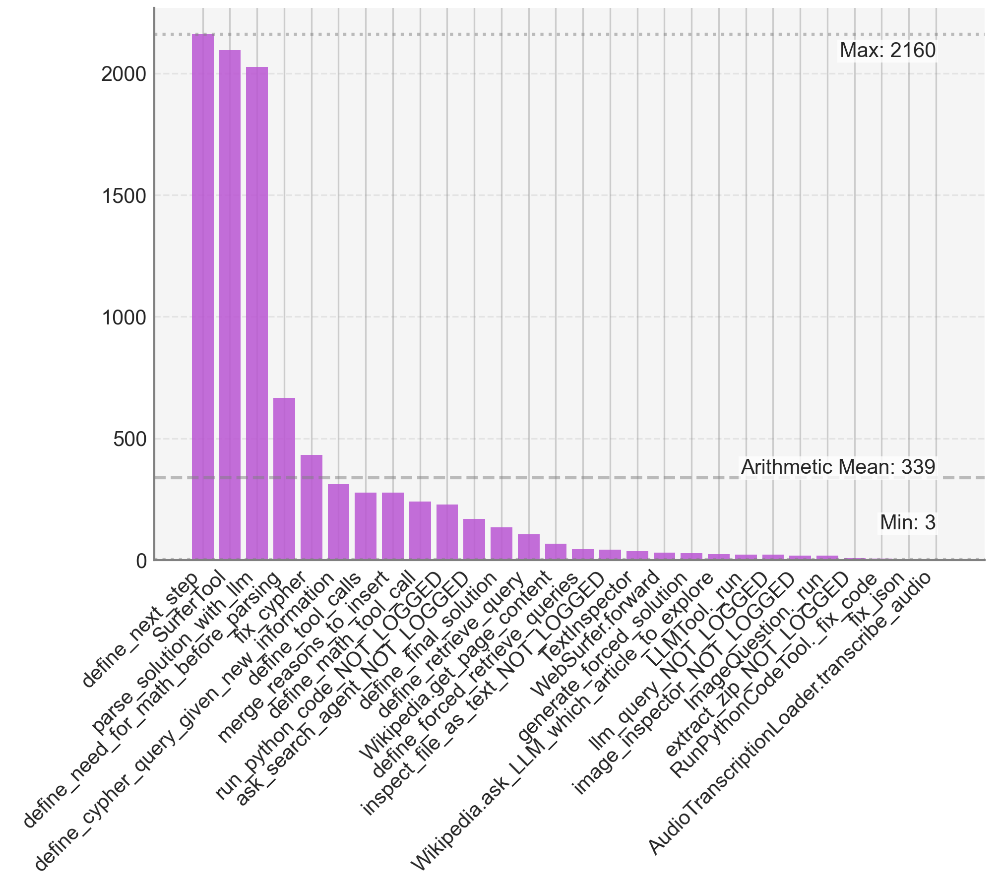<details> <summary>figures/all_cost_summary_number_of_calls.png Details</summary>  ### Visual Description ## Bar Chart: Tool Usage Frequency Distribution ### Overview This image is a vertical bar chart displaying the frequency or count of various tool names, likely from an AI agent or automation system. The chart shows a highly skewed distribution, with a few tools having very high counts and a long tail of tools with very low counts. The data is presented against a light gray grid background. ### Components/Axes * **Chart Type:** Vertical Bar Chart. * **X-Axis (Horizontal):** Lists the names of various tools or functions. The labels are rotated approximately 45 degrees for readability. The complete list of tool names, from left to right, is: 1. `define_next_step` 2. `SurferTool` 3. `parse_solution_with_llm` 4. `define_need_for_math_before_parsing` 5. `fix_cypher` 6. `define_cypher_query_given_new_information` 7. `define_tool_calls` 8. `merge_reasons_to_insert` 9. `define_math_tool_call` 10. `run_python_code_NOT_LOGGED` 11. `ask_search_agent_NOT_LOGGED` 12. `define_final_solution` 13. `define_retrieve_query` 14. `Wikipedia.get_page_content` 15. `define_forced_retrieve_queries` 16. `inspect_file_as_text_NOT_LOGGED` 17. `TextInspector` 18. `WebSurfer.forward` 19. `generate_forced_solution` 20. `Wikipedia.ask_LLM_which_article_to_explore` 21. `LLMTool.run` 22. `llm_query_NOT_LOGGED` 23. `image_inspector_NOT_LOGGED` 24. `ImageQuestion.run` 25. `extract_zip_NOT_LOGGED` 26. `RunPythonCodeTool._fix_code` 27. `fix_json` 28. `AudioTranscriptionLoader.transcribe_audio` * **Y-Axis (Vertical):** Represents a numerical count, with major gridlines and labels at 0, 500, 1000, 1500, and 2000. The axis extends slightly beyond 2000. * **Legend/Annotations:** There are three horizontal dashed lines with annotations placed on the right side of the chart: * **Top (Dotted Line):** "Max: 2160" - Indicates the maximum value in the dataset. * **Middle (Dashed Line):** "Arithmetic Mean: 339" - Indicates the average value. * **Bottom (Dashed Line):** "Min: 3" - Indicates the minimum value. ### Detailed Analysis The bars are all a uniform purple color. Their heights, estimated from the y-axis scale, are as follows (values are approximate): 1. `define_next_step`: ~2160 (Matches the "Max" annotation) 2. `SurferTool`: ~2050 3. `parse_solution_with_llm`: ~2000 4. `define_need_for_math_before_parsing`: ~650 5. `fix_cypher`: ~430 6. `define_cypher_query_given_new_information`: ~300 7. `define_tool_calls`: ~270 8. `merge_reasons_to_insert`: ~270 9. `define_math_tool_call`: ~240 10. `run_python_code_NOT_LOGGED`: ~230 11. `ask_search_agent_NOT_LOGGED`: ~160 12. `define_final_solution`: ~120 13. `define_retrieve_query`: ~90 14. `Wikipedia.get_page_content`: ~60 15. `define_forced_retrieve_queries`: ~40 16. `inspect_file_as_text_NOT_LOGGED`: ~30 17. `TextInspector`: ~25 18. `WebSurfer.forward`: ~20 19. `generate_forced_solution`: ~15 20. `Wikipedia.ask_LLM_which_article_to_explore`: ~10 21. `LLMTool.run`: ~8 22. `llm_query_NOT_LOGGED`: ~7 23. `image_inspector_NOT_LOGGED`: ~6 24. `ImageQuestion.run`: ~5 25. `extract_zip_NOT_LOGGED`: ~4 26. `RunPythonCodeTool._fix_code`: ~4 27. `fix_json`: ~3 (Matches the "Min" annotation) 28. `AudioTranscriptionLoader.transcribe_audio`: ~3 (Matches the "Min" annotation) **Trend Verification:** The visual trend is a steep, descending slope from left to right. The first three bars form a high plateau, followed by a sharp drop at the fourth bar. The remaining bars form a long, gradually descending tail, with the last several bars being barely visible above the zero line. ### Key Observations 1. **Extreme Skew:** The distribution is heavily right-skewed. The top three tools (`define_next_step`, `SurferTool`, `parse_solution_with_llm`) account for a disproportionately large share of the total count. 2. **Significant Drop-off:** There is a dramatic decrease in frequency after the third tool. The fourth tool's count is less than a third of the third tool's count. 3. **Long Tail:** The majority of the tools (20 out of 28) have counts below the arithmetic mean of 339. The last 10 tools all have counts in the single digits. 4. **Core vs. Peripheral Tools:** The chart suggests a clear hierarchy of tool usage, with a small set of core, frequently-invoked tools and a large set of specialized or rarely-used tools. ### Interpretation This chart likely visualizes the usage frequency of different functions or modules within an AI agent's toolkit over a specific period or set of tasks. The data suggests that the agent's operation is dominated by a few fundamental activities: defining the next step (`define_next_step`), using a web or information surfing tool (`SurferTool`), and parsing solutions with a language model (`parse_solution_with_llm`). These could represent the core reasoning and information-gathering loop of the agent. The sharp drop-off indicates that other tools, while necessary, are invoked far less frequently. The long tail of single-digit usage tools (`fix_json`, `AudioTranscriptionLoader.transcribe_audio`, etc.) represents highly specific, situational capabilities. The presence of many `_NOT_LOGGED` suffixed tools might indicate internal or debugging functions that are not part of the primary, logged workflow. The arithmetic mean (339) is heavily influenced by the high-value outliers and is not representative of the typical tool's usage, which is better described by the median (which would be much lower, likely in the low hundreds). This distribution is characteristic of many complex systems where a small number of components handle the majority of the workload. </details> (b) Number of calls. 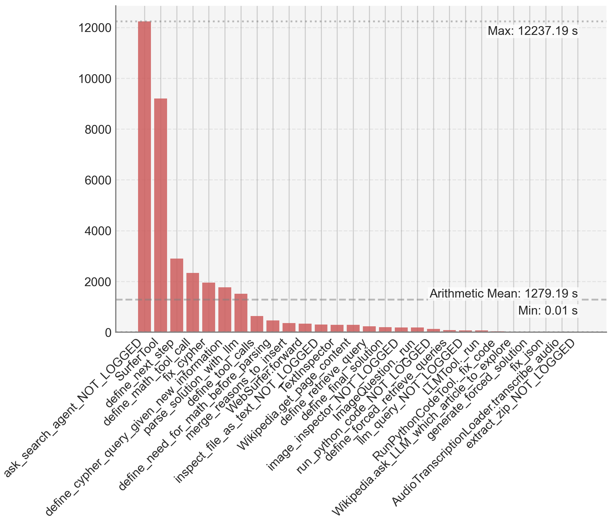<details> <summary>figures/all_cost_summary_duration.png Details</summary>  ### Visual Description ## Bar Chart: Tool Execution Time Distribution ### Overview This image is a vertical bar chart displaying the execution times (in seconds) for a series of distinct computational tools or functions, likely from an AI agent or software system's performance log. The chart is sorted in descending order of execution time, revealing a highly skewed distribution where a few tools consume the vast majority of time. ### Components/Axes * **Chart Type:** Vertical Bar Chart. * **X-Axis (Horizontal):** Lists the names of 30 distinct tools/functions. The labels are rotated approximately 60 degrees for readability. From left to right, the labels are: 1. `ask_search_agent_NOT_LOGGED` 2. `SurferTool` 3. `define_next_step` 4. `define_math_tool_call` 5. `fix_cypher` 6. `define_given_new_information` 7. `parse_solution_with_llm` 8. `define_tool_calls` 9. `define_need_for_math_before_parsing` 10. `merge_reasons_to_insert` 11. `WebSurfer.forward` 12. `inspect_file_as_text_NOT_LOGGED` 13. `TextInspector` 14. `Wikipedia.get_page_content` 15. `define_retrieve_query` 16. `define_final_solution` 17. `image_inspector_NOT_LOGGED` 18. `ImageQuestion.run` 19. `run_python_code_NOT_LOGGED` 20. `define_forced_retrieve_queries` 21. `llm_query_NOT_LOGGED` 22. `RunPythonCodeTool._run` 23. `Wikipedia.ask_LLM_which_article_to_explore` 24. `fix_code` 25. `generate_forced_solution` 26. `fix_json` 27. `AudioTranscriptionLoader.transcribe_audio` 28. `extract_zip_NOT_LOGGED` * **Y-Axis (Vertical):** Represents time in seconds. The scale runs from 0 to 12000, with major gridlines at intervals of 2000 (0, 2000, 4000, 6000, 8000, 10000, 12000). * **Annotations (Top-Right Corner):** * `Max: 12237.19 s` (aligned with the top of the tallest bar). * `Arithmetic Mean: 1279.19 s` (indicated by a horizontal dashed line crossing the chart). * `Min: 0.01 s` (aligned with the baseline of the shortest bars). * **Visual Elements:** All bars are a uniform muted red/terracotta color. The background is a light gray with a faint grid. ### Detailed Analysis The data presents a classic "long tail" distribution. The execution times are listed below in descending order, with approximate values estimated from the bar heights relative to the y-axis scale. 1. **`ask_search_agent_NOT_LOGGED`**: ~12,200 s (The tallest bar, reaching the annotated maximum). 2. **`SurferTool`**: ~9,200 s. 3. **`define_next_step`**: ~2,900 s. 4. **`define_math_tool_call`**: ~2,300 s. 5. **`fix_cypher`**: ~2,000 s. 6. **`define_given_new_information`**: ~1,800 s. 7. **`parse_solution_with_llm`**: ~1,500 s. 8. **`define_tool_calls`**: ~600 s. 9. **`define_need_for_math_before_parsing`**: ~450 s. 10. **`merge_reasons_to_insert`**: ~350 s. 11. **`WebSurfer.forward`**: ~300 s. 12. **`inspect_file_as_text_NOT_LOGGED`**: ~280 s. 13. **`TextInspector`**: ~250 s. 14. **`Wikipedia.get_page_content`**: ~220 s. 15. **`define_retrieve_query`**: ~200 s. 16. **`define_final_solution`**: ~180 s. 17. **`image_inspector_NOT_LOGGED`**: ~150 s. 18. **`ImageQuestion.run`**: ~120 s. 19. **`run_python_code_NOT_LOGGED`**: ~100 s. 20. **`define_forced_retrieve_queries`**: ~80 s. 21. **`llm_query_NOT_LOGGED`**: ~60 s. 22. **`RunPythonCodeTool._run`**: ~40 s. 23. **`Wikipedia.ask_LLM_which_article_to_explore`**: ~30 s. 24. **`fix_code`**: ~20 s. 25. **`generate_forced_solution`**: ~15 s. 26. **`fix_json`**: ~10 s. 27. **`AudioTranscriptionLoader.transcribe_audio`**: ~5 s. 28. **`extract_zip_NOT_LOGGED`**: ~0.01 s (The shortest bar, matching the annotated minimum). **Trend Verification:** The visual trend is a steep, monotonic decline from left to right. The first two bars are extreme outliers, each several times larger than the third. After the seventh bar (`parse_solution_with_llm`), the times drop below the arithmetic mean line (1279.19 s) and continue to decrease rapidly, forming a long tail of tools with sub-500-second execution times. ### Key Observations 1. **Extreme Skew:** The top two tools (`ask_search_agent_NOT_LOGGED` and `SurferTool`) account for a disproportionate amount of total execution time. Their combined time (~21,400 s) is vastly greater than the sum of all other 26 tools. 2. **Performance Bottleneck:** The `ask_search_agent_NOT_LOGGED` function is the clear performance bottleneck, with a time (12237.19 s) nearly 10 times the arithmetic mean. 3. **Tool Categorization:** The tool names suggest a multi-step AI agent pipeline involving search (`ask_search_agent`, `SurferTool`), planning (`define_next_step`), code/math handling (`define_math_tool_call`, `fix_cypher`, `run_python_code`), information parsing (`parse_solution_with_llm`), and external service calls (`Wikipedia.get_page_content`, `AudioTranscriptionLoader`). 4. **Logging Status:** Several tools have the suffix `_NOT_LOGGED`, which may indicate they are internal or debug functions not typically recorded in standard logs, yet their performance is being measured here. ### Interpretation This chart is a diagnostic tool for system performance optimization. It demonstrates that efforts to improve overall speed should be overwhelmingly focused on the first two functions, particularly `ask_search_agent_NOT_LOGGED`. Optimizing any of the tools in the long tail (e.g., `fix_json` or `extract_zip`) would yield negligible system-wide benefit. The data suggests the agent's workflow is heavily bottlenecked by its initial search and web navigation phases (`SurferTool`). The subsequent steps of planning, reasoning, and executing specific tools (like code running or API calls) are relatively fast in comparison. This could indicate that the search agent is performing complex, time-consuming operations like multiple web retrievals, page parsing, or waiting on external APIs. The presence of `_NOT_LOGGED` in the names of the most expensive tools might also imply that these critical performance metrics are not being captured in standard operational monitoring, which could be a significant oversight. The mean (1279.19 s) is heavily influenced by the outliers and is not representative of the typical tool's execution time, which is mostly under 500 seconds. </details> (c) Duration in seconds. 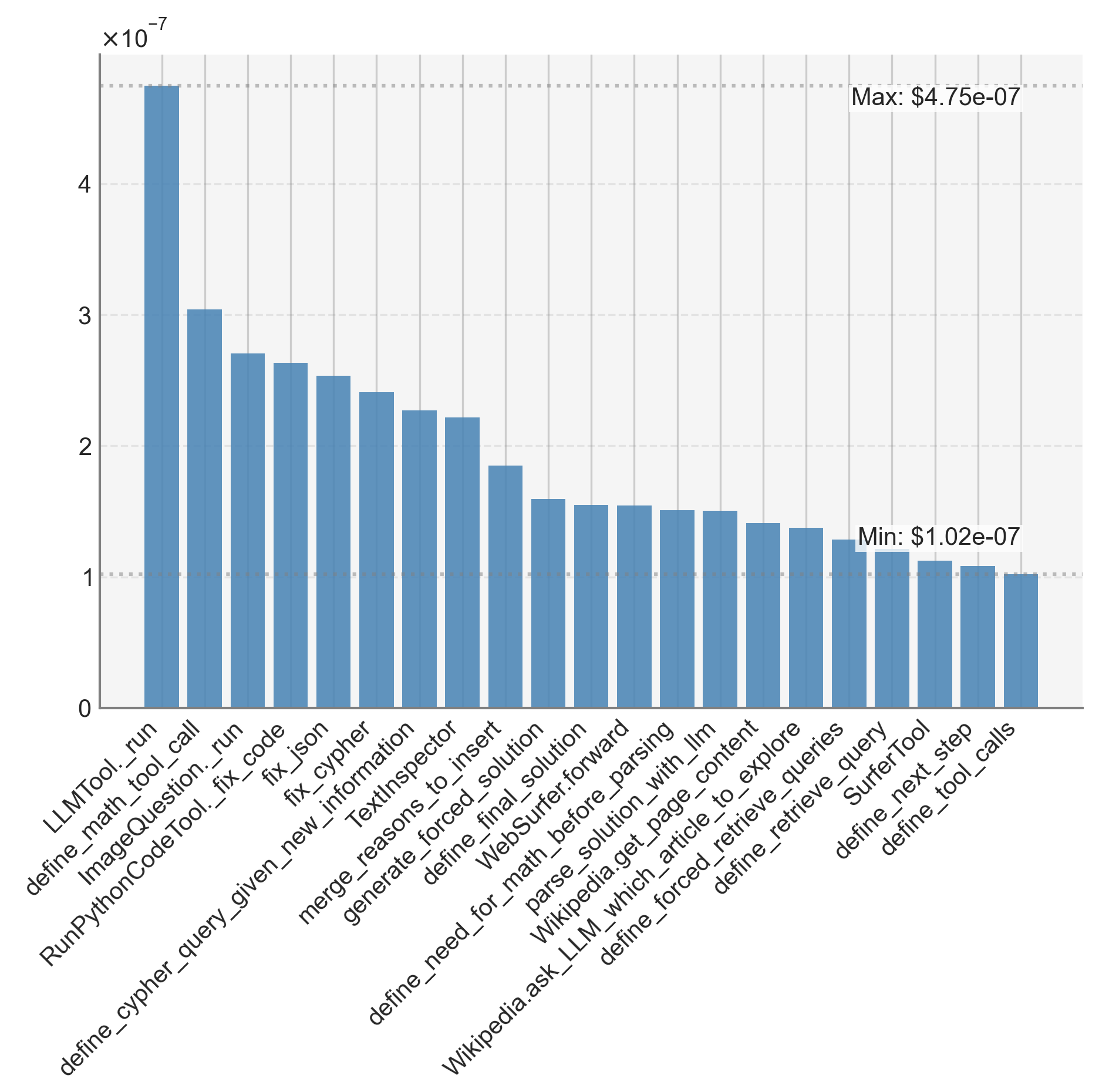<details> <summary>figures/all_cost_summary_cost_token.png Details</summary>  ### Visual Description ## Bar Chart: Tool Call Cost/Frequency Analysis ### Overview The image displays a vertical bar chart illustrating the relative cost or frequency (indicated by values on the y-axis) of 20 different tool calls or function names, likely from an AI or software system. The data is presented in descending order from left to right. The y-axis uses a logarithmic scale multiplier of ×10⁻⁷. ### Components/Axes * **Y-Axis:** * **Label:** `×10⁻⁷` (indicating all y-axis values should be multiplied by 10⁻⁷). * **Scale:** Linear scale from 0 to 4, with major gridlines at 0, 1, 2, 3, and 4. * **Annotations:** * Top-right corner: `Max: $4.75e-07` (corresponding to the tallest bar). * Bottom-right corner: `Min: $1.02e-07` (corresponding to the shortest bar). * **X-Axis:** * **Labels:** 20 distinct tool/function names, listed below from left (highest value) to right (lowest value). The labels are rotated approximately 45 degrees for readability. * **Categories (in order):** 1. `LLMTool._run` 2. `define_math_tool_call` 3. `ImageQuestion._run` 4. `RunPythonCodeTool._fix_code` 5. `fix_json` 6. `fix_cypher` 7. `define_cypher_query_given_new_information` 8. `merge_reasons_to_insert` 9. `TextInspector` 10. `generate_forced_solution` 11. `define_final_solution` 12. `WebSurfer.forward` 13. `define_need_for_math_before_parsing` 14. `parse_solution_with_llm` 15. `Wikipedia.get_page_content` 16. `Wikipedia.ask_LLM_which_article_to_explore` 17. `define_forced_retrieve_queries` 18. `define_retrieve_query` 19. `SurferTool` 20. `define_next_step` 21. `define_tool_calls` *(Note: There are 21 labels but 20 bars. The label `define_tool_calls` appears to be the final, shortest bar, making the total count 20 bars for 20 labels. The list above includes all 20 labels in order.)* * **Legend:** There is no separate legend. The x-axis labels serve as the category identifiers for each bar. * **Visual Elements:** All bars are a uniform medium blue color. The chart has a light grey background with faint horizontal gridlines. ### Detailed Analysis * **Trend:** The data shows a clear, consistent downward trend from left to right. The first bar (`LLMTool._run`) is significantly taller than all others, and the bar heights decrease monotonically. * **Approximate Values (y-axis value × 10⁻⁷):** * **Highest Value:** `LLMTool._run` aligns with the annotated maximum of **~4.75** (or $4.75e-07). * **Second Tier:** The next three bars (`define_math_tool_call`, `ImageQuestion._run`, `RunPythonCodeTool._fix_code`) range from approximately **3.0** down to **2.6**. * **Middle Tier:** The following group (`fix_json` through `generate_forced_solution`) descends from about **2.5** to **1.8**. * **Lower Tier:** The remaining bars (`define_final_solution` through `define_tool_calls`) cluster between approximately **1.6** and the annotated minimum of **1.02** (or $1.02e-07). * **Distribution:** The distribution is right-skewed. The top 5-6 tools account for a disproportionately large share of the total value (cost/frequency), while the bottom half of the tools have relatively similar, low values. ### Key Observations 1. **Dominant Tool:** `LLMTool._run` is a clear outlier, with a value nearly 50% higher than the second-ranked tool (`define_math_tool_call`). This suggests it is the most resource-intensive or frequently called function by a significant margin. 2. **Clustering:** Tools can be loosely grouped into tiers based on their values: * **Tier 1 (High):** `LLMTool._run` * **Tier 2 (Medium-High):** `define_math_tool_call`, `ImageQuestion._run`, `RunPythonCodeTool._fix_code` * **Tier 3 (Medium):** `fix_json`, `fix_cypher`, `define_cypher_query_given_new_information`, `merge_reasons_to_insert`, `TextInspector` * **Tier 4 (Low):** The remaining 11 tools, all with values below ~1.8 × 10⁻⁷. 3. **Functional Grouping:** The tool names suggest different functionalities: * **Core LLM/Execution:** `LLMTool._run`, `define_math_tool_call`, `ImageQuestion._run`, `RunPythonCodeTool._fix_code`. * **Data/Query Manipulation:** `fix_json`, `fix_cypher`, `define_cypher_query...`. * **Reasoning & Solution Generation:** `merge_reasons...`, `generate_forced_solution`, `define_final_solution`. * **External Knowledge & Navigation:** `WebSurfer.forward`, `Wikipedia.get_page_content`, `Wikipedia.ask_LLM...`, `SurferTool`. * **Planning & Parsing:** `define_need_for_math...`, `parse_solution...`, `define_next_step`, `define_tool_calls`. ### Interpretation This chart likely visualizes the **computational cost (e.g., in dollars or compute units) or invocation frequency** of various tools within an AI agent or complex software system. The data suggests a hierarchy of resource consumption: * **Primary Driver:** The core Large Language Model tool (`LLMTool._run`) is the dominant cost/frequency center. This is logical, as it likely handles the central reasoning and generation tasks. * **Specialized Tools:** Tools for specific tasks like math, image questions, and code execution form the next tier, indicating they are significant but secondary to the core LLM. * **Supporting Functions:** A long tail of tools for data fixing, query definition, web navigation, and planning have lower, more uniform costs. This implies they are called less often or are less computationally expensive per call. * **System Design Insight:** The steep drop-off after the first few tools indicates that optimizing the system's overall efficiency would yield the highest returns by focusing on the `LLMTool._run` and the top 4-5 tools. The long tail of lower-cost tools, while numerous, contributes less to the total aggregate cost/frequency. **Note on Language:** All text in the image is in English. The values use standard scientific notation (e.g., `e-07`). </details> (d) Cost per token in dollar. 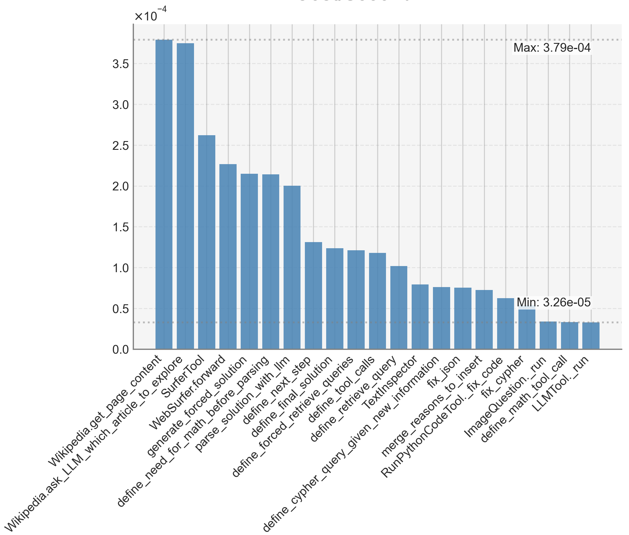<details> <summary>figures/all_cost_summary_cost_second.png Details</summary>  ### Visual Description ## Bar Chart: Tool Usage Frequency (Estimated) ### Overview The image displays a vertical bar chart showing the frequency or magnitude of various computational tools or functions, likely from an AI agent or automated system. The bars are sorted in descending order from left to right. The chart's title is partially obscured at the top, but the visible portion suggests it relates to tool usage or performance metrics. The y-axis uses a scientific notation scale (×10⁻⁴), indicating very small numerical values. ### Components/Axes * **Chart Type:** Vertical Bar Chart. * **Y-Axis:** * **Label:** Not fully visible. The scale is marked with a multiplier `×10⁻⁴` at the top left. * **Scale:** Linear, ranging from 0.0 to approximately 3.8 (after applying the multiplier). Major gridlines are at intervals of 0.5 (0.0, 0.5, 1.0, 1.5, 2.0, 2.5, 3.0, 3.5). * **Annotations:** Two horizontal dotted lines mark the maximum and minimum values in the dataset. * Top-right annotation: `Max: 3.79e-04` * Bottom-right annotation: `Min: 3.26e-05` * **X-Axis:** * **Label:** Not visible. * **Categories:** 20 distinct tool/function names, listed as labels beneath each bar. The labels are rotated approximately 45 degrees for readability. * **Legend:** None present. All bars are the same blue color. * **Grid:** Light grey horizontal and vertical gridlines are present. ### Detailed Analysis The following table lists the tools (x-axis labels) in order from left to right, with their approximate y-axis values. Values are estimated based on bar height relative to the gridlines and the provided max/min annotations. All values are in units of `×10⁻⁴`. | Order | Tool/Function Name (X-Axis Label) | Estimated Value (×10⁻⁴) | Notes | | :--- | :--- | :--- | :--- | | 1 | `Wikipedia.get_page_content` | ~3.79 | Matches the annotated maximum. | | 2 | `Wikipedia.ask_LLM_which_article_to_explore` | ~3.75 | Slightly lower than the first bar. | | 3 | `SurferTool` | ~2.62 | | | 4 | `WebSurfer.forward` | ~2.28 | | | 5 | `generate_forced_solution` | ~2.15 | | | 6 | `define_need_for_math_before_parsing` | ~2.15 | Appears equal in height to the previous bar. | | 7 | `parse_solution_with_llm` | ~2.00 | | | 8 | `define_next_step` | ~1.32 | | | 9 | `define_final_solution` | ~1.25 | | | 10 | `define_forced_retrieve_queries` | ~1.22 | | | 11 | `define_tool_calls` | ~1.18 | | | 12 | `define_retrieve_query` | ~1.02 | | | 13 | `TextInspector` | ~0.80 | | | 14 | `define_cypher_query_given_new_information` | ~0.77 | | | 15 | `fix_json` | ~0.76 | | | 16 | `merge_reasons_to_insert` | ~0.74 | | | 17 | `RunPythonCodeTool._fix_code` | ~0.62 | | | 18 | `ImageQuestion._run` | ~0.50 | | | 19 | `define_math_tool_call` | ~0.35 | | | 20 | `LLMTool._run` | ~0.33 | Matches the annotated minimum (`3.26e-05`). | ### Key Observations 1. **Dominant Tools:** The two `Wikipedia`-related tools (`get_page_content` and `ask_LLM_which_article_to_explore`) are the clear leaders, with values nearly an order of magnitude higher than the lowest tools. 2. **Steep Initial Drop:** There is a significant drop in value after the second bar (`Wikipedia.ask_LLM...`), and another notable drop after the seventh bar (`parse_solution_with_llm`). 3. **Clustering:** Several tools have very similar values, forming clusters: * `generate_forced_solution` and `define_need_for_math_before_parsing` (~2.15). * `define_final_solution`, `define_forced_retrieve_queries`, and `define_tool_calls` (range ~1.18 to ~1.25). * `TextInspector`, `define_cypher_query...`, `fix_json`, and `merge_reasons_to_insert` (range ~0.74 to ~0.80). 4. **Low-Frequency Tools:** The last three tools (`RunPythonCodeTool._fix_code`, `ImageQuestion._run`, `define_math_tool_call`, `LLMTool._run`) have the lowest values, all below 0.65 ×10⁻⁴. ### Interpretation This chart likely visualizes the usage frequency, computational cost, or some performance metric (e.g., error rate, latency contribution) of different tools within an AI agent's toolkit. The data suggests a system heavily reliant on information retrieval from Wikipedia (`Wikipedia.get_page_content` is the most prominent). Tools related to web navigation (`SurferTool`, `WebSurfer.forward`) and solution generation/parsing (`generate_forced_solution`, `parse_solution_with_llm`) also see significant use. The steep drop-off indicates a "long tail" distribution: a few core tools handle the majority of the workload or contribute the most to the measured metric, while a larger number of specialized tools (like `fix_json`, `RunPythonCodeTool._fix_code`, `ImageQuestion._run`) are used much less frequently. This pattern is common in modular systems where a few primary functions are called often, and many helper functions are invoked only in specific edge cases. The very small scale of the values (10⁻⁴) could imply these are probabilities, normalized weights, or time costs in seconds for very fast operations. </details> (e) Cost per time in dollar/s. 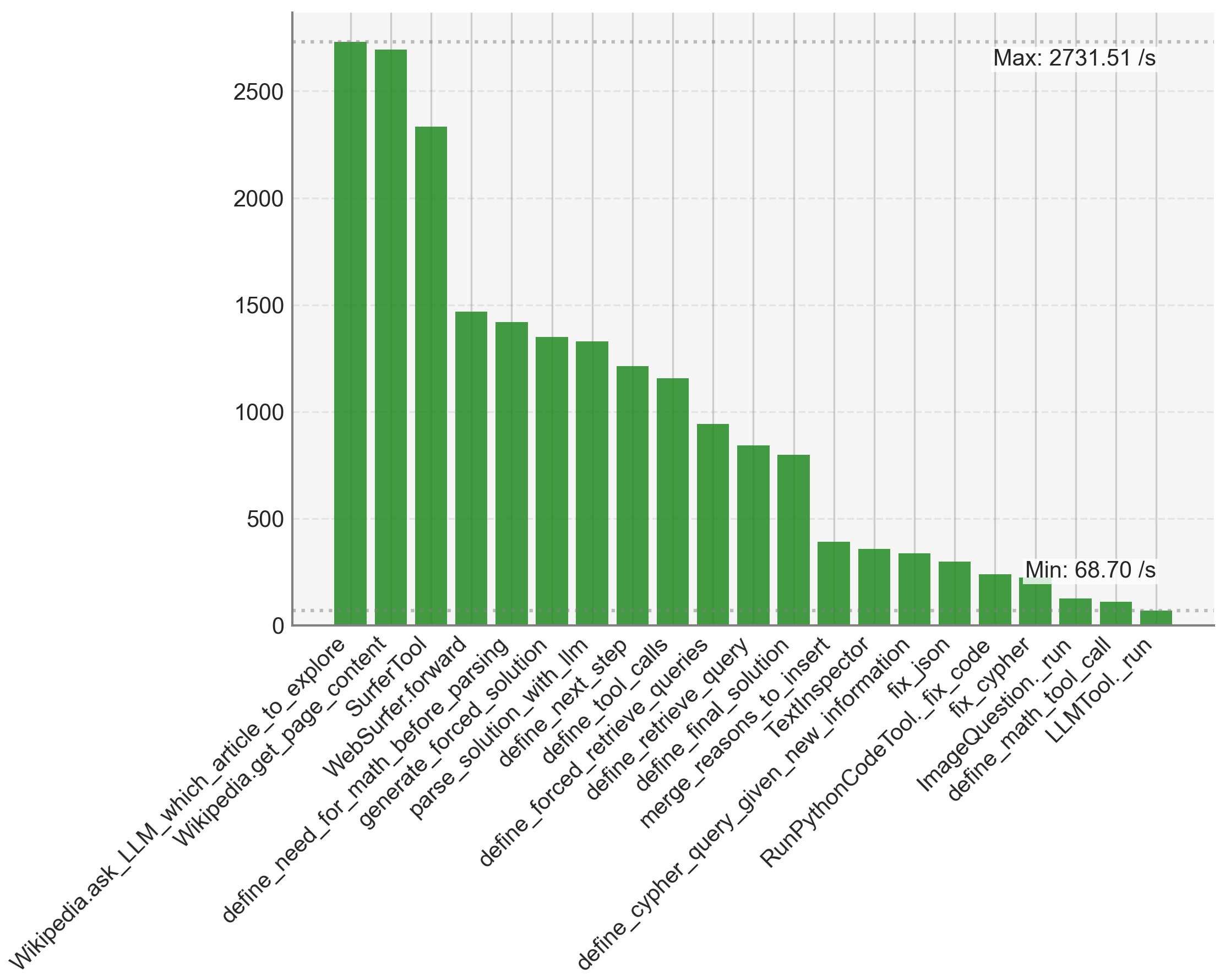<details> <summary>figures/all_cost_summary_tokens_per_second.png Details</summary>  ### Visual Description ## Vertical Bar Chart: Tool/Function Performance Metrics ### Overview The image displays a vertical bar chart comparing the performance metrics (likely speed or throughput, measured in operations per second) of 21 distinct tools or functions. The chart is sorted in descending order of performance, from the highest value on the left to the lowest on the right. The highest and lowest values are explicitly annotated on the chart. ### Components/Axes * **Chart Type:** Vertical Bar Chart. * **X-Axis (Horizontal):** Lists the names of 21 tools or functions. The labels are rotated approximately 45 degrees for readability. The full list of labels, from left to right, is: 1. `Wikipedia.ask_LLM_which_article_to_explore` 2. `Wikipedia.get_page_content` 3. `SurferTool` 4. `WebSurfer.forward` 5. `define_need_for_math_before_parsing` 6. `generate_forced_solution` 7. `parse_solution_with_llm` 8. `define_next_step` 9. `define_tool_calls` 10. `define_forced_retrieve_queries` 11. `define_retrieve_query` 12. `define_final_solution` 13. `merge_reasons_to_insert` 14. `TextInspector` 15. `define_cypher_query_given_new_information` 16. `fix_json` 17. `RunPythonCodeTool._fix_code` 18. `fix_cypher` 19. `ImageQuestion._run` 20. `define_math_tool_call` 21. `LLMTool._run` * **Y-Axis (Vertical):** Represents a numerical performance metric. The axis is labeled with major gridlines at intervals of 500, starting from 0 and extending to 2500. The unit is implied to be "per second" (/s) based on the annotations. * **Annotations:** * **Top-Right:** "Max: 2731.51 /s" – This annotation points to the top of the first (leftmost) bar. * **Bottom-Right:** "Min: 68.70 /s" – This annotation points to the top of the last (rightmost) bar. * **Legend:** There is no separate legend. All bars are the same solid green color, indicating they belong to the same data series. * **Grid:** A light gray grid is present in the background, with horizontal lines corresponding to the y-axis ticks. ### Detailed Analysis The chart presents a clear performance hierarchy. Below are the approximate values for each bar, determined by visual comparison to the y-axis gridlines. Values are listed in the same order as the x-axis labels (descending performance). 1. `Wikipedia.ask_LLM_which_article_to_explore`: **~2731.51 /s** (Exact value from annotation; bar extends slightly above the 2500 line). 2. `Wikipedia.get_page_content`: **~2700 /s** (Slightly shorter than the first bar). 3. `SurferTool`: **~2350 /s** (Bar ends between the 2000 and 2500 lines, closer to 2500). 4. `WebSurfer.forward`: **~1480 /s** (Bar ends just below the 1500 line). 5. `define_need_for_math_before_parsing`: **~1420 /s** (Slightly shorter than the previous bar). 6. `generate_forced_solution`: **~1350 /s**. 7. `parse_solution_with_llm`: **~1330 /s**. 8. `define_next_step`: **~1220 /s**. 9. `define_tool_calls`: **~1150 /s**. 10. `define_forced_retrieve_queries`: **~950 /s** (Bar ends just below the 1000 line). 11. `define_retrieve_query`: **~850 /s**. 12. `define_final_solution`: **~800 /s**. 13. `merge_reasons_to_insert`: **~400 /s** (Significant drop; bar ends below the 500 line). 14. `TextInspector`: **~370 /s**. 15. `define_cypher_query_given_new_information`: **~350 /s**. 16. `fix_json`: **~320 /s**. 17. `RunPythonCodeTool._fix_code`: **~250 /s**. 18. `fix_cypher`: **~220 /s**. 19. `ImageQuestion._run`: **~120 /s**. 20. `define_math_tool_call`: **~110 /s**. 21. `LLMTool._run`: **~68.70 /s** (Exact value from annotation; bar is the shortest). ### Key Observations 1. **Steep Performance Gradient:** There is a dramatic, non-linear decline in performance. The top three tools (`Wikipedia.ask_LLM...`, `Wikipedia.get_page...`, `SurferTool`) are in a class of their own, all exceeding 2300 /s. 2. **Performance Clusters:** The data naturally groups into clusters: * **High-Performance Cluster (>2300 /s):** First 3 tools. * **Mid-High Cluster (~1150-1500 /s):** Tools 4 through 9. * **Mid-Low Cluster (~800-950 /s):** Tools 10 through 12. * **Low-Performance Cluster (<400 /s):** Tools 13 through 21. The drop from tool 12 (`define_final_solution`, ~800 /s) to tool 13 (`merge_reasons_to_insert`, ~400 /s) is particularly sharp, representing a ~50% decrease. 3. **Magnitude of Difference:** The highest-performing tool is approximately **39.7 times faster** than the lowest-performing tool (2731.51 / 68.70 ≈ 39.7). 4. **Label Patterns:** The tool names suggest a workflow involving web interaction (`Wikipedia.*`, `SurferTool`, `WebSurfer`), mathematical reasoning (`define_need_for_math...`, `define_math_tool_call`), code generation/execution (`RunPythonCodeTool`, `fix_json`, `fix_cypher`), and general language model orchestration (`LLMTool._run`, `parse_solution_with_llm`). ### Interpretation This chart likely visualizes the execution speed (e.g., API calls per second, function invocations per second) of different components within a complex AI agent or multi-tool system. The data suggests a clear architectural hierarchy: * **Information Retrieval is Fast:** Tools that fetch or process raw information from Wikipedia are the fastest components. This makes sense as they may involve relatively simple, optimized network or parsing operations. * **Reasoning and Planning are Slower:** Functions that involve "defining" steps, solutions, or tool calls (`define_*` functions) occupy the middle tiers. These likely involve more complex logic, prompting of an LLM, or decision-making, which are computationally heavier. * **Code Execution and Specialized Tools are Slowest:** The lowest-performing cluster includes tools for fixing code (`fix_json`, `RunPythonCodeTool._fix_code`), handling images (`ImageQuestion._run`), and the base `LLMTool._run`. This indicates that operations requiring code interpretation, image processing, or direct, unoptimized LLM inference are the primary bottlenecks in this system. The stark performance disparity implies that system throughput would be heavily constrained by the slowest components (`LLMTool._run`, `define_math_tool_call`). Optimizing these low-performing tools, or redesigning the workflow to minimize their use, would yield the most significant overall performance gains. The chart serves as a diagnostic tool for identifying such bottlenecks within a multi-stage AI pipeline. </details> (f) Tokens per second. Figure 17: Overview over the execution time as well as the cost in dollar. Graph storage: Neo4j. Retrieval type: query. Model: GPT-4o mini. 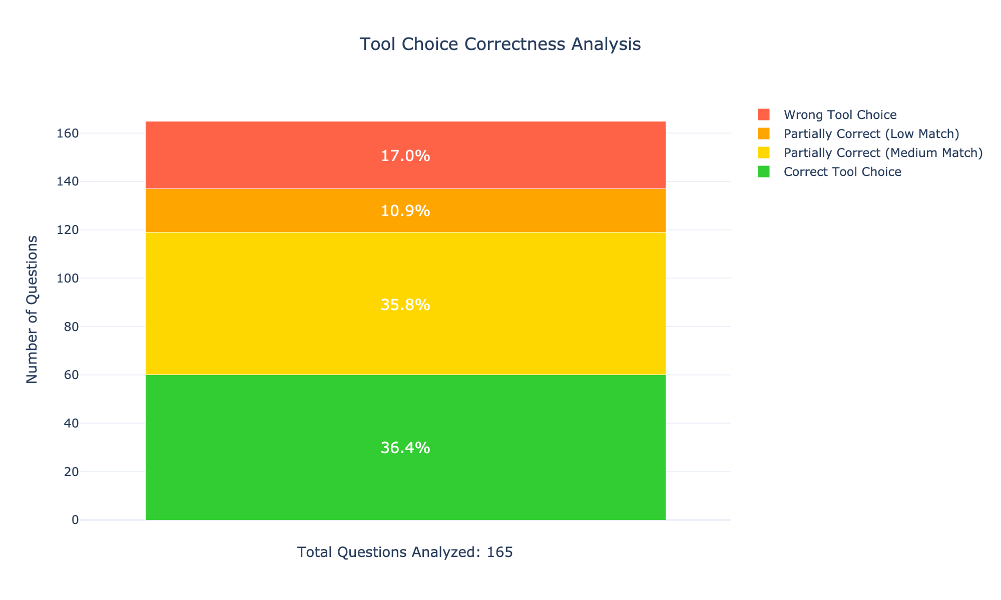<details> <summary>figures/all_tool_match.png Details</summary>  ### Visual Description ## Stacked Bar Chart: Tool Choice Correctness Analysis ### Overview The image displays a single stacked bar chart titled "Tool Choice Correctness Analysis." It visualizes the distribution of correctness outcomes for tool selection across a set of analyzed questions. The chart is designed to show the proportion of each outcome category relative to the total number of questions. ### Components/Axes * **Title:** "Tool Choice Correctness Analysis" (centered at the top). * **Y-Axis:** Labeled "Number of Questions." The scale runs from 0 to 160, with major gridlines at intervals of 20 (0, 20, 40, 60, 80, 100, 120, 140, 160). * **X-Axis:** Not explicitly labeled. It contains a single, wide stacked bar representing the entire dataset. * **Legend:** Positioned to the right of the bar. It lists four categories with corresponding color swatches: * **Red Square:** Wrong Tool Choice * **Orange Square:** Partially Correct (Low Match) * **Yellow Square:** Partially Correct (Medium Match) * **Green Square:** Correct Tool Choice * **Data Labels:** White percentage values are centered within each colored segment of the bar. * **Footer Text:** "Total Questions Analyzed: 165" is centered below the x-axis. ### Detailed Analysis The single bar is segmented from bottom to top as follows: 1. **Bottom Segment (Green - Correct Tool Choice):** * **Percentage:** 36.4% * **Approximate Count:** 36.4% of 165 ≈ **60 questions**. * **Visual Trend:** This is the largest segment, forming the base of the bar. It extends from the 0 line to approximately the 60 mark on the y-axis. 2. **Second Segment (Yellow - Partially Correct (Medium Match)):** * **Percentage:** 35.8% * **Approximate Count:** 35.8% of 165 ≈ **59 questions**. * **Visual Trend:** This segment is nearly equal in size to the green segment. It sits directly on top of the green segment, extending from ~60 to ~119 on the y-axis. 3. **Third Segment (Orange - Partially Correct (Low Match)):** * **Percentage:** 10.9% * **Approximate Count:** 10.9% of 165 ≈ **18 questions**. * **Visual Trend:** This is a significantly smaller segment. It sits atop the yellow segment, extending from ~119 to ~137 on the y-axis. 4. **Top Segment (Red - Wrong Tool Choice):** * **Percentage:** 17.0% * **Approximate Count:** 17.0% of 165 ≈ **28 questions**. * **Visual Trend:** This segment is larger than the orange one but smaller than the green and yellow ones. It forms the top of the bar, extending from ~137 to the bar's total height at approximately 165 on the y-axis. **Sum Check:** 36.4% + 35.8% + 10.9% + 17.0% = 100.1%. The minor discrepancy is attributable to rounding in the displayed percentages. ### Key Observations * **Dominant Categories:** The "Correct Tool Choice" (36.4%) and "Partially Correct (Medium Match)" (35.8%) categories are the most frequent, together accounting for over 72% of all questions. * **Significant Error Rate:** The "Wrong Tool Choice" category represents a substantial 17.0% of cases, indicating a notable failure rate. * **Partial Correctness Split:** Partial correctness is divided into two tiers. The "Medium Match" tier (35.8%) is more than three times as common as the "Low Match" tier (10.9%). * **Total Volume:** The analysis is based on a dataset of 165 questions. ### Interpretation This chart provides a performance snapshot for an AI or system tasked with selecting appropriate tools to answer questions. The data suggests a generally positive but imperfect performance: * **Strength:** The system demonstrates a solid baseline of competence, with over a third of its choices being fully correct and another third being largely correct (medium match). This indicates the underlying logic for tool selection is functional for a majority of cases. * **Area for Improvement:** The combined "Partially Correct (Low Match)" and "Wrong Tool Choice" categories total 27.9%, meaning more than 1 in 4 tool selections are either incorrect or only marginally appropriate. This highlights a significant opportunity for refinement in the tool selection algorithm, particularly in avoiding outright wrong choices (17.0%). * **Nuance in Partial Correctness:** The distinction between "Medium Match" and "Low Match" is critical. The high proportion of "Medium Match" suggests the system often identifies a relevant tool but may not always select the *optimal* one. The smaller "Low Match" group represents cases where the tool choice was tangential or minimally useful. In summary, the system is more often right than wrong, but its reliability is hampered by a substantial minority of poor tool selections. Efforts to improve performance should focus on reducing the "Wrong Tool Choice" and "Low Match" categories, potentially by better understanding the nuances that differentiate a "Medium Match" from a "Low Match" tool. </details> Figure 18: Analysis of the tool selection. Graph storage: Neo4j. Retrieval type: query. Model: GPT-4o mini. 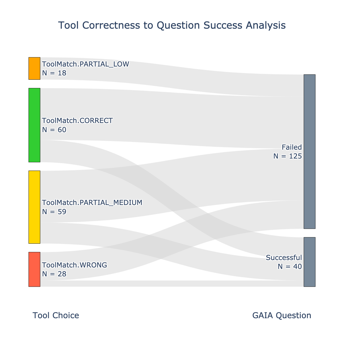<details> <summary>figures/all_tool_choice_analysis.png Details</summary>  ### Visual Description ## Sankey Diagram: Tool Correctness to Question Success Analysis ### Overview This is a Sankey diagram visualizing the relationship between the correctness of tool usage ("Tool Choice") and the success of answering questions ("GAIA Question"). It shows how instances from four distinct tool correctness categories flow into two final outcome categories (Failed or Successful). The width of the connecting bands is proportional to the flow quantity. ### Components/Axes * **Title:** "Tool Correctness to Question Success Analysis" (centered at the top). * **Left Axis (Source):** Labeled "Tool Choice" at the bottom-left. It contains four vertically stacked, color-coded categories: 1. **ToolMatch.PARTIAL_LOW** (Orange bar, top-left). Count: `N = 18`. 2. **ToolMatch.CORRECT** (Green bar, second from top). Count: `N = 60`. 3. **ToolMatch.PARTIAL_MEDIUM** (Yellow bar, third from top). Count: `N = 59`. 4. **ToolMatch.WRONG** (Red bar, bottom-left). Count: `N = 28`. * **Right Axis (Target):** Labeled "GAIA Question" at the bottom-right. It contains two vertically stacked, gray-blue outcome categories: 1. **Failed** (Taller bar, top-right). Count: `N = 125`. 2. **Successful** (Shorter bar, bottom-right). Count: `N = 40`. * **Flow Bands:** Light gray, semi-transparent bands connect the left categories to the right categories. The width of each band represents the number of instances flowing from a specific tool correctness category to a specific outcome. ### Detailed Analysis The diagram maps the following flows from left to right: 1. **From ToolMatch.PARTIAL_LOW (N=18):** * A very thin band flows to **Failed**. * An extremely thin, almost negligible band flows to **Successful**. This is the smallest flow in the diagram. 2. **From ToolMatch.CORRECT (N=60):** * A very wide band flows to **Failed**. This is the single widest flow band in the entire diagram. * A moderately wide band flows to **Successful**. 3. **From ToolMatch.PARTIAL_MEDIUM (N=59):** * A wide band flows to **Failed**. * A moderately wide band flows to **Successful**. 4. **From ToolMatch.WRONG (N=28):** * A moderately wide band flows to **Failed**. * A very thin band flows to **Successful**. **Spatial Grounding & Trend Verification:** * The **Failed** outcome (top-right) receives the majority of flow from all four source categories, with the thickest incoming band originating from the green `ToolMatch.CORRECT` bar. * The **Successful** outcome (bottom-right) receives a smaller portion of the flow. Its thickest incoming bands come from the green (`CORRECT`) and yellow (`PARTIAL_MEDIUM`) bars. * The visual trend shows that while `ToolMatch.CORRECT` has the highest total count (60), a larger proportion of its instances flow to "Failed" than to "Successful". Conversely, `ToolMatch.WRONG` has a lower total count (28), but a very small proportion flows to "Successful". ### Key Observations 1. **Dominant Flow to Failure:** The "Failed" outcome (N=125) is significantly larger than the "Successful" outcome (N=40), indicating a high overall failure rate in the analyzed dataset. 2. **Paradox of Correctness:** The `ToolMatch.CORRECT` category, despite its name, contributes the largest single volume of instances to the "Failed" outcome. This is the most striking visual and numerical pattern. 3. **Partial Success Correlation:** The `ToolMatch.PARTIAL_MEDIUM` category shows a more balanced flow between "Failed" and "Successful" compared to the other categories. 4. **Low Impact of Wrong Tools:** The `ToolMatch.WRONG` category contributes a relatively small number of instances to both outcomes, with a very minor contribution to "Successful". 5. **Minimal Contribution from Low Partial Match:** The `ToolMatch.PARTIAL_LOW` category has the smallest overall count and contributes minimally to either outcome. ### Interpretation This Sankey diagram reveals a complex and potentially counterintuitive relationship between tool usage correctness and final task success. The data suggests that simply using a tool "correctly" (`ToolMatch.CORRECT`) is not a strong predictor of successfully answering a GAIA question; in fact, it is associated with the highest number of failures. This could imply several investigative possibilities: * The "GAIA Question" set may be inherently difficult, where even correct tool application is insufficient for success. * The definition of "correct" tool match might be misaligned with the requirements for solving the question. * There may be other critical factors beyond tool correctness (e.g., reasoning, data interpretation, question complexity) that determine the final outcome. The diagram effectively isolates "tool correctness" as one variable in a larger system. The high volume of failures stemming from correct tool use is a significant anomaly that warrants deeper investigation into the nature of the questions, the tools' capabilities, or the evaluation criteria for "success." The flow from `PARTIAL_MEDIUM` to "Successful" suggests that a medium level of tool appropriateness might sometimes be sufficient or that other compensating factors are at play in those instances. </details> Figure 19: Analysis of the tool selection. Graph storage: Neo4j. Retrieval type: query. Model: GPT-4o mini. 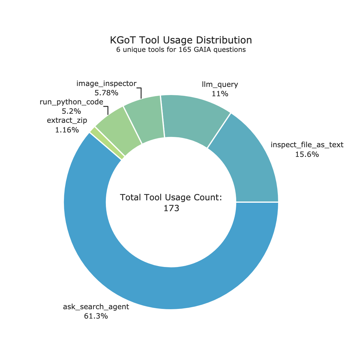<details> <summary>figures/all_tool_usage_count.png Details</summary>  ### Visual Description ## Donut Chart: KGoT Tool Usage Distribution ### Overview The image displays a donut chart titled "KGoT Tool Usage Distribution" with the subtitle "6 unique tools for 165 GAIA questions." The chart visualizes the proportional usage of six different tools, with the total usage count displayed in the center. The overall aesthetic uses a cool color palette of blues and greens against a white background. ### Components/Axes * **Chart Type:** Donut Chart (a pie chart with a central hole). * **Title:** "KGoT Tool Usage Distribution" * **Subtitle:** "6 unique tools for 165 GAIA questions" * **Central Label:** "Total Tool Usage Count: 173" * **Data Series (Segments):** The chart is divided into six segments, each representing a tool. The segments are labeled directly with the tool name and its percentage of the total usage. There is no separate legend; labels are placed adjacent to their corresponding segments. * **Color Scheme:** The segments use a gradient from a dominant medium blue for the largest segment to progressively lighter shades of teal and green for the smaller segments. ### Detailed Analysis The chart presents the following data, ordered from the largest segment to the smallest: 1. **ask_search_agent** * **Color:** Medium blue. * **Placement:** Occupies the entire bottom half and a portion of the upper right quadrant of the donut. It is the visually dominant segment. * **Percentage:** 61.3% * **Trend:** This is the most frequently used tool by a significant margin. 2. **inspect_file_as_text** * **Color:** Teal blue. * **Placement:** Located in the upper right quadrant, adjacent to the `ask_search_agent` segment. * **Percentage:** 15.6% * **Trend:** The second most used tool. 3. **llm_query** * **Color:** Light teal. * **Placement:** Located in the upper center, adjacent to `inspect_file_as_text`. * **Percentage:** 11% * **Trend:** The third most used tool. 4. **image_inspector** * **Color:** Light green. * **Placement:** Located in the upper left quadrant, adjacent to `llm_query`. * **Percentage:** 5.78% * **Trend:** Usage drops significantly here. 5. **run_python_code** * **Color:** Lighter green. * **Placement:** Located in the upper left quadrant, adjacent to `image_inspector`. * **Percentage:** 5.2% * **Trend:** Very similar in usage to `image_inspector`. 6. **extract_zip** * **Color:** Pale green. * **Placement:** A very thin sliver in the upper left quadrant, adjacent to `run_python_code`. * **Percentage:** 1.16% * **Trend:** The least used tool by a wide margin. **Data Verification:** The sum of the percentages (61.3 + 15.6 + 11 + 5.78 + 5.2 + 1.16) equals 100.04%, which is within an acceptable rounding margin. The central label states a total count of 173 tool usages across 165 questions, indicating an average of approximately 1.05 tool uses per question. ### Key Observations * **Dominant Tool:** The `ask_search_agent` tool is overwhelmingly dominant, accounting for nearly two-thirds (61.3%) of all tool invocations. * **Usage Concentration:** The top three tools (`ask_search_agent`, `inspect_file_as_text`, `llm_query`) collectively account for 87.9% of all usage. * **Minimal Tools:** The `extract_zip` tool is used very infrequently (1.16%), suggesting it is either a specialized tool for rare cases or potentially underutilized. * **Total Count Discrepancy:** The total tool usage count (173) is slightly higher than the number of questions (165), implying that some questions required the use of more than one tool. ### Interpretation This chart provides a clear quantitative breakdown of tool utilization within the KGoT system for the GAIA benchmark. The data strongly suggests that the system's problem-solving strategy is heavily reliant on a search agent (`ask_search_agent`). This could indicate that retrieving and synthesizing information from external sources is the primary mode of operation for the tasks in the GAIA dataset. The secondary reliance on file inspection tools (`inspect_file_as_text`, `image_inspector`) and direct LLM queries (`llm_query`) points to a workflow that often involves analyzing provided documents or files and using the language model's internal knowledge. The very low usage of `run_python_code` and `extract_zip` suggests that tasks requiring computational execution or handling of compressed archives are rare in this specific evaluation set. The distribution is highly skewed, which is a notable pattern. It raises questions about the nature of the GAIA questions: are they predominantly research and retrieval tasks? It also suggests that optimizing the performance and reliability of the `ask_search_agent` would yield the greatest overall system improvement for this benchmark. The near-negligible use of `extract_zip` might warrant investigation to determine if it's a tool in search of a problem or if the benchmark simply lacks scenarios that require it. </details> Figure 20: Analysis of the tool usage. Graph storage: Neo4j. Retrieval type: query. Model: GPT-4o mini.