2504.07825

# What the HellaSwag? On the Validity of Common-Sense Reasoning Benchmarks > Correspondence to ## Abstract Common-sense reasoning is a key language model capability because it encapsulates not just specific factual knowledge but rather general language and world understanding. Measuring common-sense reasoning, therefore, is crucial for language models of different sizes and applications. One of the most widely used benchmarks for evaluating such capabilities is HellaSwag; however, in this paper, we show that it has severe construct validity issues. These issues range from basic ungrammaticality and numerous typos to misleading prompts or equally correct options. Furthermore, we show that if models are evaluated only on answer texts, or with ”Lorem ipsum dolor…” instead of the question, more than 65% of model predictions remain the same, and this cannot be attributed merely to contamination. Since benchmark scores are an essential part of model selection in both research and commercial applications, these validity issues can have severe consequences. In particular, knowing that taking benchmark scores at face value is ubiquitous, inadequate evaluation leads to ill-informed decisions about models. In this paper, we thoroughly investigate critical validity issues posed by HellaSwag and illustrate them with various evaluations using generative language models of different sizes. We argue that this benchmark does not accurately measure common-sense reasoning and, therefore, should not be used for evaluation in its current state. Based on the results of our study, we propose requirements that should be met by future common-sense reasoning benchmarks. In addition, we release GoldenSwag, a corrected subset of HellaSwag, which, to our belief, facilitates acceptable common-sense reasoning evaluation. ## 1 Introduction Language models All annotations and datasets are released on HuggingFace, the code is released on GitHub. are evaluated through benchmarks. These evaluations shape language model development by indicating how different design decisions—such as hyperparameters, training data, and post-training procedure—impact model performance (Biderman et al., 2024). NLP practitioners select training procedures in order to improve performance according to accepted benchmarks. However, if the benchmarks do not measure what we think they are measuring, development may not be going in the most optimal direction, and we may be missing out on performance gains. Benchmarks should allow us to draw an inference about the capabilities of a model, but whether a benchmark measures what we want them to measure is essential for making that inference. Construct validity means that an evaluation is measuring the capability that it is claimed to measure (Cronbach & Meehl, 1955). Without established validity, the use of a benchmark may be “supercharging bad science” (Blili-Hamelin et al., 2025). <details> <summary>x1.png Details</summary>  ### Visual Description ## Diagram: Question Prompt Annotation Example ### Overview The image is a technical diagram illustrating a text annotation or evaluation scheme. It displays a "Question prompt" with an example sentence and multiple-choice answers, where specific words and phrases are underlined in different colors to indicate various types of errors or annotations. A legend on the right explains the color-coding system. ### Components/Axes The diagram is divided into two primary regions: 1. **Left Region (Main Content):** Contains the annotated text example. * **Header:** The text "Question prompt" is centered at the top. * **Structure Labels:** Two labels, "Activity label" and "Context," are positioned above the example sentence, connected by a bracket line indicating they are components of the prompt. * **Example Sentence:** "Clean and jerk: Women are in the background of a gym lifting weights. Man" * **Numbered Options:** Four numbered answer choices follow the example sentence. * **Annotations:** Various words and phrases within the sentence and options are underlined with colored lines. A green checkmark (✓) appears next to option 1. * **Highlighting:** The phrase "Text removed in zero-prompt" is highlighted with a gray background. 2. **Right Region (Legend):** A rounded rectangle containing the annotation key. * **Symbols & Labels:** * A green checkmark (✓) labeled "correct answer" * A red line labeled "ungrammatical" * An orange line labeled "typos" * A blue line labeled "nonsense" * A gray highlight box labeled "Text removed in zero-prompt" ### Detailed Analysis **Annotated Text Transcription & Color-Coding:** * **Example Sentence:** "Clean and jerk: Women are in the background of a gym lifting weights. Man" * "in the background" is underlined in **blue** (nonsense). * "Man" is underlined in **red** (ungrammatical). * **Option 1:** "is preparing himself to lift weigh and stands in front of weight." * "weigh" is underlined in **orange** (typo). * "weight." is underlined in **red** (ungrammatical). * A **green checkmark (✓)** is placed at the end of the line, indicating this is the correct answer. * **Option 2:** "is boxing with woman in an arena." * "woman" is underlined in **red** (ungrammatical). * **Option 3:** "is running in a marathon in a large arena and people is standing around." * "in" is underlined in **red** (ungrammatical). * "is" is underlined in **red** (ungrammatical). * **Option 4:** "is standing in front of a woman doing weight lifting with camera around a table." * "with camera" is underlined in **red** (ungrammatical). * "around a table." is underlined in **blue** (nonsense). * **Zero-Prompt Note:** The phrase "Text removed in zero-prompt" is displayed with a **gray background highlight**. This label is positioned in the bottom-right of the left region, below the options. ### Key Observations 1. **Multi-Layer Annotation:** The diagram demonstrates a system where a single text can have multiple, overlapping annotations (e.g., a word can be both ungrammatical and part of a nonsense phrase). 2. **Error Typology:** It defines four distinct categories for annotation: correctness, grammaticality, typographical accuracy, and semantic plausibility ("nonsense"). 3. **Contextual Example:** The chosen example ("Clean and jerk") suggests the domain may be related to activity recognition, video captioning, or visual question answering, where descriptions of scenes are evaluated. 4. **Spatial Layout:** The legend is placed to the right of the main content for easy reference. The structural labels ("Activity label", "Context") are placed directly above the relevant text segments they describe. ### Interpretation This diagram serves as a **specification or training guide for a text annotation task**, likely for evaluating machine-generated descriptions or answers. It defines a precise schema for human annotators to flag different types of errors in text. * **Purpose:** The system is designed to move beyond a simple "correct/incorrect" binary. It provides granular feedback on *why* a text is flawed—whether due to grammatical rules, spelling, or factual/logical coherence with the given context ("Clean and jerk"). * **"Zero-Prompt" Context:** The highlighted note "Text removed in zero-prompt" is a critical clue. It implies there are different experimental conditions. A "zero-prompt" condition likely involves evaluating the model's output without providing the initial "Activity label" and "Context" (the gray-highlighted text in the example). This diagram shows what text is *removed* for that condition, allowing for a comparison of model performance with and without explicit context. * **Underlying Workflow:** The presence of a "correct answer" (option 1) among flawed options indicates this could be an example from a dataset used to train or test a model's ability to select the most appropriate description, with the annotations explaining why the other options are inferior. The meticulous error tagging suggests the data is used for fine-grained analysis or to train models that can understand and generate text with fewer specific error types. 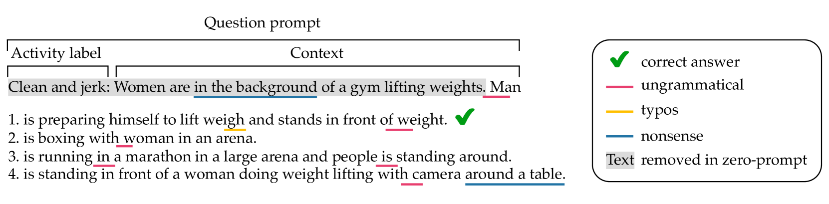</details> Figure 1: Example from the HellaSwag validation set: a question prompt and four answer options (the correct one is ticked). Validity issues are underlined in color. The part of the question prompt that we remove in zero-prompt experiments is highlighted in light gray. Common-sense reasoning is a desirable capability in a model because it encompasses a more generalizable world understanding rather than memorized facts about the world. This kind of reasoning differs from the math- and code-oriented reasoning capabilities that are increasingly of interest, as it focuses on reasoning over domain-general scenarios. In a survey of over one hundred text-based common-sense reasoning benchmarks, Davis (2023) observe widespread quality issues. HellaSwag (Zellers et al., 2019) is one of the most widely used of these commonsense reasoning benchmarks, and it has played a large role in language model development over the past six years. It is one of the evaluations that made up Hugging Face’s Open LLM Leaderboard v1, meaning that it was used by thousands of people to compare and select models for research and deployment. HellaSwag is useful as a relatively large dataset, with over 10k items in the validation set The validation set is the only available set on HuggingFace. The test set was intentionally not released to prevent contamination, but in practice, many people use the validation set as the test set.. HellaSwag is also in a format that facilitates both evaluation using log-likelihood and text generation. Log-likelihood-based evaluation is more appropriate for small models whose capabilities are underestimated by prompt-based evaluation (Hu & Levy, 2023) due to task demands (Hu & Frank, 2024). Text generation, on the other hand, is more appropriate for larger models. Many benchmarks, especially ones that are being developed now, do not allow for effective evaluation of both small and large models either due to their difficulty, their format, or both, e.g., GPQA (Rein et al., 2024). HellaSwag was created by taking portions of existing dataset (ActivityNet (Krishna et al., 2017) and WikiHow, which the authors scraped themselves) and generating alternative completions to the segments. The completions were generated by the original GPT model (Radford et al., 2018) and curated using an Adversarial Filtering procedure in which the authors intended to select only the machine-generated answers that seemed the most plausible to the language model but nonsensical to humans. Human validators reviewed the dataset after the AF process, ensuring high agreement on correct answers. The result was intended to be a task that was trivial for people (approximately 95% accuracy) but significantly more difficult (less than 50% accuracy) for models that were the state of the art at the time. In order for a common-sense reasoning benchmark to serve its purpose, it should allow us to draw an inference about model capabilities, specifically the inference that the model with the highest HellaSwag score has the best common-sense reasoning capabilities. However, we argue that there are some key construct validity issues that prevent us from drawing that inference from HellaSwag scores (see an example in Figure 1). These issues include bad grammar, typos, and nonsensical constructions in poor English. The key contributions of this paper can be summarized as follows: - We argue that performance on HellaSwag does not benchmark sentence completion or common-sense reasoning. We point out diverse validity issues and their consequences (Section 3) and show that they are omnipresent in HellaSwag (Section 4.1). - We show how to use model predictions to judge the quality of the benchmark (Sections 4.2 and 4.3). We also use zero-prompt evaluation (Section 4.4) to directly test construct validity and show that, on average, 68% of predictions do not change based on whether or not the model is presented with the question, or even when the question is replaced with a generic text. - Based on our analysis, we propose a list of requirements that should be met by a quality common-sense reasoning benchmark (Section 5) and propose a small highly filtered subset of HellaSwag — GoldenSwag (Section 5.1) with substantially reduced effect of observed issues. ## 2 Related Work Validity Issues in Other Benchmarks. Several recent studies have highlighted validity issues in widely used benchmarks. In the text-generation evaluation format, MMLU (Hendrycks et al., 2021) has been shown to yield variable performance for the same model after minor changes, such as re-ordering the answer choices, changing the formatting, or rewording the task. Simply re-ordering the answer choices in MMLU leads to a significant reduction in accuracy on the task (Gupta et al., 2024). Most models showed a drop in accuracy of around 10%, but some of the models tested showed a drop of up to 27%. Changing formatting, such as the characters representing each answer choice, can also have an effect. Alzahrani et al. (2024) replaced answer letters with alternative rare characters, which led to a significant re-ordering in relative model performance ranking among the models tested. Small perturbations in the prompt were also shown to significantly change model performance on benchmarks such as MMLU and HellaSwag (Habba et al., 2025). In addition to sensitivity to these changes, MMLU has been shown to contain questions with no clear correct answer or incorrect ground truth labels (Gema et al., 2024). Other benchmarks ranging in domain and task type have also been shown to have errors in the reference answers or in the ground truth labels. One of these is GSM8K (Cobbe et al., 2021), a math word problem benchmark. Vendrow et al. (2025) find that at least 5% of the items in GSM8K contain a serious error, such as mislabeled questions, logical contradictions, and ambiguous questions. Another example is XSUM (Narayan et al., 2018), a summarization benchmark. Liang et al. (2023) found that reference summaries in XSUM were rated as being worse than model-generated responses, according to human annotators. Therefore, the quality of the benchmark underestimates the model’s summarization performance. Together, this work indicates that validity issues are pervasive in language model benchmarks. The current paper contributes to this line of work, which aims to identify issues with existing benchmarks, and, in some cases, to propose filtered, cleaned, and improved versions of the original benchmark, e.g. Gema et al. (2024) and Vendrow et al. (2025). Common-Sense Reasoning Benchmarks. In a survey of common-sense reasoning benchmarks, Davis (2023) highlights item quality as a common issue among over one hundred text-based benchmarks, of which HellaSwag is one of the most widely used. A blog post was previously published highlighting some of the issues with HellaSwag (Chen, 2023), however, the author uses only a small sample ( $n=300$ ) items from the entire dataset. The author estimates that 36% of items in HellaSwag contain errors. In this work, we expand on the list of validity issues we consider and we annotate the entire validation set. We estimate that a much higher proportion of HellaSwag contains errors. Zero-Prompt Evaluation. In this paper, we introduce the term ‘zero-prompt’ evaluation, which consists of evaluating a model on a multiple-choice benchmark without the previous context. Other work has also used similar methods (‘no context’ condition Shah et al., 2020; ‘choice-only’ prompting, Balepur & Rudinger, 2024; Balepur et al., 2024), all of which are aimed at testing whether a model relies on the prompt to complete the task. This is essential for establishing construct validity, as the task is designed to evaluate the extent to which the model is able to draw a connection between the prompt and the answer choices. Types of Evaluation. Evaluating language models on multiple-choice question benchmarks, such as HellaSwag, can be done with probability-based and generation-based formats (Hu & Levy, 2023; Lyu et al., 2024). Probability methods imply choosing the answer with maximum probability or log-likelihood and may lead to different results based on how this log-likelihood is computed and normalized (Gao, 2022; Biderman et al., 2024). Generation evaluation methods have an advantage in presenting the model with a question in its complete form but suffer from high dependence on the instruction prompt. For instance, OLMo’s performance on HellaSwag ranges from 1% to 99% based on the instruction prompt (Habba et al., 2025). There also exists a misalignment of evaluations by log-likelihood and generation (Hu & Levy, 2023; Lyu et al., 2024), so these evaluations essentially present different tasks and models evaluated with different methods cannot be compared. ## 3 Methods We investigate several validity issues of HellaSwag to show how they limit its ability to serve as a language model benchmark. We focus on the following issues: Ungrammaticality and typos. Sentences with grammatical errors and typos have generally lower likelihood and might push the model away from these options, which hinders adequate evaluation when these errors are not intended. This introduces an undesired noise in the benchmark scores when the model’s capabilities are measured on a trade-off between reasoning and natural language understanding or grammatical error correction. Even though such noise may be considered a factor that makes the task more challenging, we argue that the common-sense reasoning benchmark should be free of such errors, and, if wanted, the errors may be separately injected to test the model’s robustness in comparison. Nonsensicality. Nonsensical texts naturally contradict the common-sense reasoning evaluation, especially when nonsensical sentences are present in the correct answer and the question prompt. In such questions choosing the correct answer is essentially reduced to random guessing. Additionally, ridiculously implausible incorrect options create overly high contrast with the correct answer and make the task trivial and non-informative. No or multiple good answers. All questions in HellaSwag are supposed to have exactly one correct answer. If there is no good option, the scoring of a question comes down to random guessing. On the other hand, if there are multiple acceptable endings, the model might predict an equally plausible option, but this will be treated as a wrong answer. Multiple correct options also affect the estimation of the random baseline score value. We also aim at directly evaluating the construct validity of HellaSwag, i.e., testing whether the benchmark measures what it is supposed to measure (Section 3.3). To investigate all these issues, we use annotations from a large language model and predictions from a range of language models of different sizes in diverse experiments. ### 3.1 Annotations We use Claude 3.5 Sonnet (Anthropic, 2024) to annotate the HellaSwag validation set. In the first round of annotations, we assess questions and answer options for grammaticality and sensicality. In the second round, we annotate the plausibility of correct answers, the presence of equally correct options, and we also collect the options considered to be the worst. We report the detailed prompts we use in Appendix C. In both rounds of annotations, we specify in the prompt which answer is supposed to be correct so that we do not rely on Claude’s solutions for the benchmark, and the model has a better understanding of how the question is designed. We use the collected annotations as descriptive indications of HellaSwag issues and also as part of our further experimental design. ### 3.2 Model Evaluations We propose using model evaluation on HellaSwag to investigate benchmark issues. We perform two types of model evaluations: by maximizing the mean log-likelihood and by generation. Before the evaluations, we apply the preprocessing procedure from lm-evaluation-harness (Biderman et al., 2024). All evaluations are done manually, rather than using an existing framework, in order to enable modifications, e.g., zero-prompt evaluation. We release our evaluation code as part of this work. Mean Log-Likelihood. We append each answer option to the question prompt and run each sequence through the model to compute output logits. We then choose the maximum mean log-likelihood among answer options using the following formula: $$ \mathcal{L}=\frac{1}{|\mathcal{V}|}\sum_{t\in\mathcal{V}}\log\mathrm{P}(y_{t} \mid x_{<t}), \tag{1} $$ where $y_{t}$ is the ground truth token at position $t$ , $x_{<t}$ is the preceding sequence of tokens, and $\mathcal{V}$ is the set of valid (non-special) token positions. The resulting value will have non-positive values, and the higher it is, the more plausible the option is, according to the model. Generation. The model is presented with a question and all answer choices and is asked to output the correct answer digit (the options are enumerated 1–4). The exact prompt used for evaluation is presented in Appendix B. We use the generation strategy set by default for each model. In order to reduce the possible effect of contamination in generation evaluations, we shuffle the options for each question following Alzahrani et al. (2024). These two types of evaluation differ in the task the model is asked to perform. In log-likelihood evaluation, we directly request the model’s estimate of plausibility for each given option. On the contrary, evaluation by generation allows us to present the model with all the options so that it can compare and choose the most plausible or the least implausible option. We consider evaluation by generation only for larger models ( $\sim$ 32B), as their instruct versions are more likely to produce outputs in the desired format. We report the list of models we used in Appendix A. ### 3.3 Zero-Prompt Evaluations In order to test the construct validity of HellaSwag, we also run zero-prompt evaluations. By zero-prompt, we mean removing the activity label and the question context from the task. We keep only the beginnings of answer sentences, typically present in the ActivityNet part of the data and absent in WikiHow. We show an example of such removal in Figure 1. We also use another setup when we change the question text to a generic ”Lorem ipsum dolor…”. We perform this kind of evaluation to test whether HellaSwag measures common-sense reasoning. The idea behind this is that for common-sense reasoning, the model should figure out which ending stems best from the question prompt. By comparing the results from these evaluations, we can see whether this causally impacts model performance. | First round — Prompt — Correct option | Nonsense: 4.9% 1.5% | 11.7% 3.1% | 1.7% 0.8% | | | --- | --- | --- | --- | --- | | — Incorrect option(s) | 84.5% | 71.1% | 90.9% | | | Ungrammatical: | | | | | | — Prompt | 39.7% | 95.7% | 12.9% | | | — Correct option | 6.1% | 11.7% | 3.4% | | | — Incorrect option(s) | 39.4% | 43.5% | 37.5% | | | High quality | 4.9% | 2.0% | 6.3% | | | Second round | Wrong golden answer | 3.7% | 5.5% | 2.8% | | All nonsense | 4.1% | 10.0% | 1.2% | | | Multiple correct | 21.1% | 31.3% | 16.3% | | Table 1: Claude annotations for the HellaSwag validation set questions. We present the percentage for each issue from the complete set, and by source: from ActivityNet (AN) and WikiHow (WH). The validation set consists of 10042 questions, 3243 (32.3%) of which are from ActivityNet, and all the rest are from WikiHow. ## 4 Results and Discussion ### 4.1 Annotations The results of the two rounds of annotations are presented in Table 1. From the first round of evaluations of grammar and sensicality, we find that almost 40% of the questions have ungrammatical prompts. Such questions comprise the absolute majority (95.7%) of the ActivityNet part, which can be attributed to the benchmark creation methodology, in which these questions were generated by the original GPT model (Radford et al., 2018) inferior to the modern ones. It is also clear that correct answers generally have considerably fewer issues than incorrect ones because, on benchmark construction, the correct answers were taken from an existing corpus and the incorrect ones were synthetically generated. This might lead to trivial solutions dependent solely on choosing the least problematic option. In the second round, we concentrated on the plausibility of answer options and the task design validation. Claude agreed with the answer option labeled as correct in 96.3% of cases. However, in many questions (21.1%), multiple other options were considered just as good as the correct one (up to all three others in several cases). In some cases (4.1%), all answer options were considered implausible. These issues are mostly concentrated in the ActivityNet portion of the data, though also present in the WikiHow. We also encountered six ethical refusals from Claude. By investigating these questions, we found that they contain severe ethical issues related to constructing weapons, taking drugs, and adult content. ### 4.2 Model Evaluations <details> <summary>x2.png Details</summary>  ### Visual Description \n ## Grouped Bar Chart: Model Accuracy Comparison ### Overview The image displays a grouped bar chart comparing the accuracy of ten different language models under various evaluation conditions. The chart evaluates each model's performance across three accuracy tiers (Normal, Extended, Worst) and two primary evaluation methods (Full-Prompt, Zero-Prompt), with a baseline for Random performance. ### Components/Axes * **Chart Type:** Grouped bar chart. * **X-Axis (Horizontal):** Labeled "Model". It lists ten distinct language models. From left to right: 1. Qwen 2.5 32B 2. OLMo 2 32B 3. Llama 3.2 1B 4. Gemma 3 1B 5. Qwen 2.5 1.5B 6. SmolLM2 1.7B 7. Granite 3.1 1B 8. Pythia 1B 9. PleIAs 1.0 1B 10. DeepSeek-R1 1.5B * **Y-Axis (Vertical):** Labeled "Accuracy". The scale runs from 0.0 to 0.8, with major gridlines at intervals of 0.2. * **Legend (Top-Right Corner):** Contains two sections. * **Accuracy (Color Key):** * Normal: Olive green solid bar. * Extended: Dark forest green solid bar. * Worst: Light peach/salmon solid bar. * **Evaluation (Pattern Key):** * Full-Prompt: Solid bar (no pattern). * Zero-Prompt: Bar with diagonal hatching (\\). * Random: A horizontal dashed grey line across the chart at y=0.25. * **Baseline:** A horizontal dashed grey line labeled "Random" in the legend, positioned at an accuracy value of 0.25. ### Detailed Analysis For each model, there are two groups of bars: one for "Full-Prompt" (solid) and one for "Zero-Prompt" (hatched). Within each group, three bars represent the "Normal", "Extended", and "Worst" accuracy tiers. **Trend Verification:** Across all models, the "Extended" accuracy (dark green) is consistently the highest bar in its group, followed by "Normal" (olive), and then "Worst" (peach). The "Full-Prompt" evaluation (solid bars) generally yields higher accuracy than the "Zero-Prompt" evaluation (hatched bars) for the same accuracy tier. **Data Points by Model (Approximate Values):** 1. **Qwen 2.5 32B:** * *Full-Prompt:* Normal ~0.83, Extended ~0.86, Worst ~0.49. * *Zero-Prompt:* Normal ~0.61, Extended ~0.65, Worst ~0.40. 2. **OLMo 2 32B:** * *Full-Prompt:* Normal ~0.87, Extended ~0.89, Worst ~0.50. * *Zero-Prompt:* Normal ~0.66, Extended ~0.70, Worst ~0.42. 3. **Llama 3.2 1B:** * *Full-Prompt:* Normal ~0.62, Extended ~0.67, Worst ~0.45. * *Zero-Prompt:* Normal ~0.47, Extended ~0.52, Worst ~0.36. 4. **Gemma 3 1B:** * *Full-Prompt:* Normal ~0.59, Extended ~0.64, Worst ~0.44. * *Zero-Prompt:* Normal ~0.45, Extended ~0.50, Worst ~0.35. 5. **Qwen 2.5 1.5B:** * *Full-Prompt:* Normal ~0.66, Extended ~0.71, Worst ~0.46. * *Zero-Prompt:* Normal ~0.49, Extended ~0.54, Worst ~0.37. 6. **SmolLM2 1.7B:** * *Full-Prompt:* Normal ~0.70, Extended ~0.74, Worst ~0.46. * *Zero-Prompt:* Normal ~0.52, Extended ~0.57, Worst ~0.38. 7. **Granite 3.1 1B:** * *Full-Prompt:* Normal ~0.63, Extended ~0.67, Worst ~0.45. * *Zero-Prompt:* Normal ~0.48, Extended ~0.53, Worst ~0.37. 8. **Pythia 1B:** * *Full-Prompt:* Normal ~0.45, Extended ~0.51, Worst ~0.42. * *Zero-Prompt:* Normal ~0.37, Extended ~0.43, Worst ~0.35. 9. **PleIAs 1.0 1B:** * *Full-Prompt:* Normal ~0.41, Extended ~0.48, Worst ~0.40. * *Zero-Prompt:* Normal ~0.34, Extended ~0.40, Worst ~0.33. 10. **DeepSeek-R1 1.5B:** * *Full-Prompt:* Normal ~0.43, Extended ~0.49, Worst ~0.39. * *Zero-Prompt:* Normal ~0.32, Extended ~0.38, Worst ~0.31. ### Key Observations 1. **Top Performers:** The two largest models, **OLMo 2 32B** and **Qwen 2.5 32B**, achieve the highest accuracies, with OLMo 2 32B showing a slight edge. Their "Extended/Full-Prompt" accuracy approaches 0.9. 2. **Performance Drop with Zero-Prompt:** All models experience a significant drop in accuracy when moving from "Full-Prompt" to "Zero-Prompt" evaluation. The drop is most pronounced for the higher-performing models. 3. **Model Size Correlation:** There is a general trend where the 32B parameter models outperform the 1B-1.7B parameter models. However, among the smaller models, **SmolLM2 1.7B** and **Qwen 2.5 1.5B** perform notably better than others like Pythia 1B or PleIAs 1.0 1B. 4. **"Worst" Case Performance:** The "Worst" accuracy tier (peach bars) shows less variance between models and evaluation methods compared to the "Normal" and "Extended" tiers. Most "Worst" scores cluster between 0.3 and 0.5. 5. **Baseline Comparison:** All models, even under "Zero-Prompt/Worst" conditions, perform above the "Random" baseline of 0.25, except for DeepSeek-R1 1.5B's Zero-Prompt/Worst score which is very close to it (~0.31). ### Interpretation This chart provides a multifaceted evaluation of language model robustness and capability. The data suggests several key insights: * **Prompt Engineering is Critical:** The substantial gap between "Full-Prompt" and "Zero-Prompt" results across all models underscores the heavy reliance of current LLMs on detailed instructions to achieve high performance. Their ability to infer task requirements without explicit prompting ("Zero-Prompt") is significantly weaker. * **Scale Still Matters:** The clear performance advantage of the 32B models indicates that, for this evaluation benchmark, increased model scale correlates strongly with higher accuracy and robustness. * **Performance Tiers Reveal Robustness:** The consistent hierarchy of `Extended > Normal > Worst` accuracy within each model/evaluation group suggests that the benchmark likely has a gradient of difficulty. Models that maintain higher "Worst" scores may be more robust to adversarial or edge-case scenarios. * **Benchmarking Small Models:** The chart allows for direct comparison of similarly sized models (1B-1.7B). SmolLM2 1.7B emerges as a standout among the smaller models, suggesting its architecture or training data may be more effective for this specific task domain. * **The "Random" Baseline:** The 0.25 random baseline implies the task likely involves a four-choice selection (e.g., multiple-choice question). All models demonstrate learned capability beyond random guessing. In summary, this visualization is not just a simple accuracy leaderboard. It reveals the conditional nature of LLM performance, highlighting the importance of prompt design, the benefits of scale, and providing a nuanced view of model robustness across different evaluation scenarios. 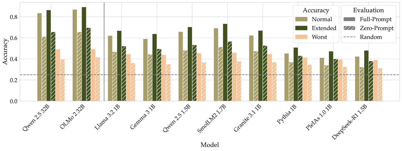</details> Figure 2: Accuracy evaluation with log-likelihood for larger (32B) and smaller (1-2B) models with a full question prompt and without it (zero-prompt). For each model, we report three accuracy scores: usual accuracy on correct answers, extended accuracy on correct and equally correct options, and accuracy on the worst option. Important: the ground truths for the last two kinds of evaluation are based on the annotations from Claude. In Figure 2, we present the results of accuracy evaluations. Along with the regular accuracy computed by maximizing the log-likelihood, we compute extended accuracy based on Claude annotations. In particular, we extend the set of correct answers with the ones proposed by Claude as equally correct. For all models, the extended accuracy is higher, which means that in some cases, models prefer the option that can be considered just as good as the correct answer. Therefore, as we discussed in Section 3, the model is sometimes penalized for sensible answers unintended to be correct, which invalidates the scoring. We also compute the accuracy on the worst options selected by Claude by minimizing the mean log-likelihood, thus choosing the least plausible option. These scores are comparable for the majority of models. In addition, report accuracies by question source in Appendix F. <details> <summary>x3.png Details</summary>  ### Visual Description ## Scatter Plot with Trend Lines: Mean Log-Likelihood vs. Text Length by Source ### Overview The image is a 2D scatter plot overlaid with two linear trend lines. It visualizes the relationship between the length of a text (x-axis) and the mean log-likelihood (y-axis) assigned to it by a model, with data points grouped by their source: WikiHow or ActivityNet. The plot uses semi-transparent, binned squares to represent the density of data points. ### Components/Axes * **X-Axis:** Labeled "Text Length". The scale runs from approximately 15 to 150, with major tick marks at 20, 40, 60, 80, 100, 120, and 140. * **Y-Axis:** Labeled "Mean Log-Likelihood". The scale runs from -6.5 to -1.5, with major tick marks at -6, -5, -4, -3, and -2. Values are negative, with higher (less negative) values indicating higher likelihood. * **Legend:** Located in the bottom-right corner of the plot area. It is titled "Source" and contains two entries: * A green square labeled "WikiHow". * A pink/red square labeled "ActivityNet". * **Data Representation:** Data points are shown as semi-transparent, binned squares (a 2D histogram or density plot). The color intensity indicates the density of points in that bin. Overlap between the two sources creates a grayish-brown color. ### Detailed Analysis **1. Data Series - ActivityNet (Pink/Red):** * **Spatial Distribution:** The pink squares are concentrated in the lower-left to middle region of the plot. They span a text length range from approximately 15 to 120. * **Trend Line:** A solid pink/red line represents the linear trend for ActivityNet. * **Trend Verification:** The line slopes upward from left to right, indicating that mean log-likelihood increases with text length for this source. * **Approximate Points:** The line starts near (Text Length: 15, Mean Log-Likelihood: -3.75) and ends near (Text Length: 120, Mean Log-Likelihood: -2.9). * **Data Density:** The highest density of ActivityNet points appears between text lengths of 20-60 and mean log-likelihoods of -5 to -3. **2. Data Series - WikiHow (Green):** * **Spatial Distribution:** The green squares are concentrated in the middle to upper-right region. They span a text length range from approximately 55 to 150. * **Trend Line:** A solid green line represents the linear trend for WikiHow. * **Trend Verification:** The line slopes upward from left to right, but with a shallower slope than the ActivityNet line. * **Approximate Points:** The line starts near (Text Length: 55, Mean Log-Likelihood: -3.1) and ends near (Text Length: 150, Mean Log-Likelihood: -2.7). * **Data Density:** The highest density of WikiHow points appears between text lengths of 80-130 and mean log-likelihoods of -3.5 to -2.0. **3. Overlap Region:** * There is a significant overlapping region between text lengths of approximately 60 and 110, where both pink (ActivityNet) and green (WikiHow) squares are present, creating a mixed, desaturated color. ### Key Observations 1. **Source Separation:** The two sources occupy largely distinct regions of the plot. ActivityNet dominates shorter texts (length < ~60), while WikiHow dominates longer texts (length > ~100). There is a transitional overlap zone in the middle. 2. **Overall Positive Correlation:** Both trend lines show a positive correlation between text length and mean log-likelihood. Longer texts tend to receive higher (less negative) likelihood scores from the model for both sources. 3. **Difference in Level and Slope:** The WikiHow trend line is consistently above the ActivityNet trend line across the overlapping range of text lengths. This indicates that, for texts of similar length, the model assigns a higher mean log-likelihood to WikiHow texts than to ActivityNet texts. The slope of the WikiHow line is also shallower. 4. **Variance:** The spread of data points (vertical dispersion) around each trend line appears substantial for both sources, indicating high variance in the mean log-likelihood for any given text length. ### Interpretation This chart suggests a systematic difference in how a language model perceives or scores text from two different sources, WikiHow and ActivityNet, which is mediated by text length. * **Source-Specific Patterns:** The model appears to have learned distinct statistical profiles for these sources. WikiHow texts, which are typically instructional and procedural, consistently receive higher likelihood scores than ActivityNet texts (which describe video activities) when compared at the same length. This could reflect differences in vocabulary, syntax, or narrative structure that the model finds more "predictable" or "typical" in WikiHow's style. * **Length as a Confounding Variable:** The strong separation along the x-axis reveals that text length is a major confounding factor. ActivityNet samples are predominantly short, while WikiHow samples are predominantly long. Simply comparing average likelihoods between sources without controlling for length would be misleading, as the inherent length difference would dominate the comparison. * **Model Behavior:** The positive slope for both lines indicates the model's log-likelihood scores are not length-normalized in this visualization; longer sequences naturally accumulate higher (less negative) total log-likelihoods. The difference in slopes suggests the rate at which likelihood increases with length differs between the two text genres. * **Investigative Insight:** A researcher viewing this would conclude that any analysis comparing model performance on these datasets must account for text length as a primary covariate. The plot argues against treating these sources as directly comparable without normalization. The overlapping region is particularly interesting for deeper analysis, as it represents texts where the sources are most similar in length, allowing for a cleaner comparison of the source effect itself. 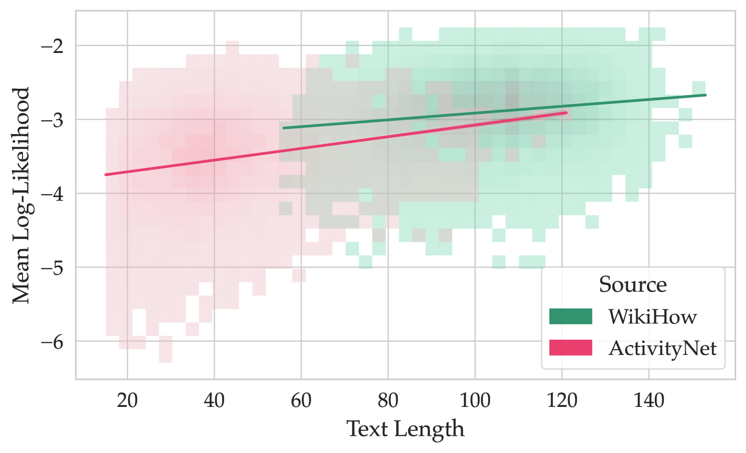</details> Figure 3: Mean log-likelihoods of answer options and their lengths. The lines represent the trend for each question source. | Qwen-2.5 32B OLMo-2 32B | 0.92 0.84 0.86 0.87 | 0.83 0.70 0.75 0.75 | | --- | --- | --- | Table 2: Accuracies for 32B models with generation (G) and log-likelihood (LL) evaluation. We report the complete accuracy for HellaSwag (Accuracy) and accuracy for the questions annotated to have no good options (All Bad). We also evaluate larger models by generation (Table 2), the detailed generation prompt is shown in Appendix B. For OLMo, the accuracies by generation and by log-likelihood are comparable, while for Qwen, the accuracy with generation is better. This can be due to the score on the questions having no good options. Evaluating by generation allows the model to see all options at once and, even if they are all bad, to choose the most acceptable. ### 4.3 Answer Length We also found that answer likelihood positively correlates with its length (see Figure 3), especially for the questions from ActivityNet. This might be due to the difference in answer option sources: generated distractor options can be shorter than the correct answers. Another reason for this might be that every text has very low likelihood values in the beginning, but as the prior context grows longer, the following tokens become more predictable, and log-likelihoods increase overall. Therefore, the overall mean token probability is lower for shorter texts. Finally, such correlation might also be dependent on the log-likelihood normalization type. We separately investigate total and byte-normalized log-likelihoods proposed by Gao (2022) and find that these methods also produce values correlated with the input length (see Appendix D.1 for details). The relative length difference between answer options can be quite high (more than 17% for half of the data, see Appendix D.2). Furthermore, we find that the accuracy of Llama 3.2 1B when the correct answer is the longest one (0.72) is substantially greater than when the longest answer is wrong (0.59). Thus, varied answer lengths pose a potential problem for a benchmark since the models might implicitly prefer longer answers. ### 4.4 Zero-Prompt Evaluation If a model is able to choose the right option without the question text, this invalidates the construct validity of a benchmark. To test this, we evaluate the models without the question prompt, i.e., only on the answer options, and compare with the full-prompt evaluation. The accuracies for zero-prompt evaluation are presented in Figure 2. For all models, zero-prompt accuracies are well above random guessing (25%), which means that the probabilities of the answer choices are biased towards the correct answer. This presents a problem in two ways. First, the question prompt does not contribute to the task. Without the prompt, there is no reasoning about plausible completions. Instead, the task is for a model to choose the most plausible text fragment. It is unclear what model capabilities this evaluates. Second, features of the incorrect answers—such as grammatical or logical errors, as discussed in Section 4.1 —may increase the probability of the correct option. This means that a model may achieve high accuracy on a subset of the questions by simply ruling out grammatical inconsistencies or nonsensical phrases. By this logic, high accuracy on these questions does not indicate a model’s common-sense reasoning capabilities. | Model | Size | Agreement | Agreement type | Disagreement type | | | | | --- | --- | --- | --- | --- | --- | --- | --- | | Both ✓ | Both ✗ | Full ✓ | Zero ✓ | Both ✗ | | | | | Llama 3.2 | 1. 1B | 0.69 | 0.43 | 0.26 | 0.19 | 0.04 | 0.07 | | Gemma 3 | 1. 1B | 0.70 | 0.40 | 0.29 | 0.19 | 0.04 | 0.07 | | Qwen 2.5 | 1.5B | 0.69 | 0.45 | 0.24 | 0.21 | 0.03 | 0.07 | | SmolLM2 | 1.7B | 0.71 | 0.49 | 0.23 | 0.21 | 0.03 | 0.05 | | Granite 3.1 | 1. 1B | 0.72 | 0.44 | 0.28 | 0.18 | 0.03 | 0.06 | | Pythia | 1. 1B | 0.71 | 0.32 | 0.39 | 0.14 | 0.05 | 0.10 | | PleIAs | 1. 1B | 0.69 | 0.28 | 0.41 | 0.13 | 0.06 | 0.11 | | DeepSeek-R1 | 1.5B | 0.65 | 0.26 | 0.39 | 0.16 | 0.06 | 0.13 | | Qwen 2.5 (LL) | 32B | 0.71 | 0.60 | 0.12 | 0.24 | 0.02 | 0.03 | | OLMo 2 (LL) | 32B | 0.74 | 0.64 | 0.09 | 0.23 | 0.01 | 0.02 | | Qwen 2.5 (Gen) | . 32B | 0.70 | 0.67 | 0.03 | 0.25 | 0.03 | 0.02 | | Olmo 2 (Gen) | . 32B | 0.50 | 0.45 | 0.05 | 0.41 | 0.05 | 0.04 | Table 3: We report proportions by agreement type (a model gives equal correct or incorrect predictions) and disagreement types (the model gives correct prediction only in either full- or zero-prompt scenario or gives different incorrect answers). Furthermore, we test the agreement of full-prompt and zero-prompt predictions. Following Lyu et al. (2024), “agreement” here means that the model gives the same predictions in both evaluation modes (with and without the prompt), regardless of whether these predictions are correct or wrong. The results of agreement evaluations are presented in Table 3 for all models. On average, 68% of the model predictions do not change if we remove the question prompt from the evaluation. This holds not only for correct answers but also for a substantial partition of the incorrect ones, which discards contamination as the main suspected reason for this. For Pythia, PleIAs, and DeepSeek-R1 models, the share of agreement for incorrect answers is larger than for the correct ones. This suggests that for the majority of HellaSwag questions, the question text does not contain additional information that the model uses to do the task. Furthermore, for some questions, removing the context actually allowed the model to make a better choice (see column Zero ✓). Interestingly, we observed similar agreement patterns when the question prompt is changed to a placeholder text “Lorem ipsum dolor…” (see Appendix E). Together with the other results, these findings lead us to question the most fundamental quality of the benchmark — its construct validity. Since the question text does not play a decisive role in $\sim$ 68% of cases, the benchmark cannot accurately measure common-sense reasoning, as presenting the model with the cause does not help it in the choice of the right effect. This also poses a concern about the answer choices: the incorrect options might often be so blatantly implausible that the correct answer stands out, even without context. | % of questions | 75% | 67% | 60% | 55% | 50% | 45% | 39% | 34% | 27% | 18% | | --- | --- | --- | --- | --- | --- | --- | --- | --- | --- | --- | Table 4: Zero-prompt core. A pair (N models, X%) means that at least N models can answer correctly X% of questions without question prompt texts. Interestingly, we also find that questions answered correctly in zero-prompt are common for many models. In Table 4, we show the zero-prompt core — the percentage of questions answered correctly without the prompt by groups of models. In particular, about 18% of questions are answered correctly without question prompts by all 10 of the tested models. ## 5 Requirements and GoldenSwag Our experiments highlighted a variety of validity issues in HellaSwag. Based on these results, we formulate a list of requirements for a valid common-sense reasoning benchmark: Grammar and typos. All the texts should be grammatically correct, including the incorrect options. If the model is to be tested for robustness to bad grammar or typos, a separate version of the dataset should be created, e.g., by injecting errors or typos. Sensicality. All options should be a reasonable, coherent text. Even though by the nature of the task incorrect options should make no sense, this should be only due to how they relate to the question context and not, for instance, due to single implausible constructions. Distinct correct answers. The correct option should be a substantially better fit for the question prompt than the incorrect options. There might be more than one correct option if the task design allows it, but they should all be comparably suitable. Uniform option lengths. The answers can have different lengths, though this variability should be limited. The length rank of correct answers should be uniform over the dataset. Content. The questions should be filtered for toxicity and ethical issues. For smaller models, the questions should preferably be on general-domain topics excluding overly specific professional knowledge. ### 5.1 GoldenSwag <details> <summary>x4.png Details</summary>  ### Visual Description \n ## Grouped Bar Chart: Model Accuracy Comparison on HellaSwag and GoldenSwag ### Overview This image is a grouped bar chart comparing the accuracy of ten different language models on two evaluation datasets: HellaSwag and GoldenSwag. The chart evaluates each model under two prompting conditions (Full-Prompt and Zero-Prompt) and includes a random baseline for reference. ### Components/Axes * **Chart Type:** Grouped bar chart. * **X-Axis (Horizontal):** Labeled "Model". It lists ten specific language models. From left to right: 1. Qwen 2.5 32B 2. OLMo 2 32B 3. Llama 3.2 1B 4. Gemma 3 1B 5. Qwen 2.5 1.5B 6. SmolLM2 1.7B 7. Granite 3.1 1B 8. Pythia 1B 9. PleIAs 1.0 1B 10. DeepSeek-R1 5B * **Y-Axis (Vertical):** Labeled "Accuracy". The scale runs from 0.0 to 0.8, with major gridlines at intervals of 0.2. * **Legend (Top-Right Corner):** * **Accuracy (Color Key):** * Blue solid bar: HellaSwag dataset. * Yellow solid bar: GoldenSwag dataset. * **Evaluation (Pattern Key):** * Solid fill: Full-Prompt evaluation. * Diagonal hatching (///): Zero-Prompt evaluation. * **Baseline:** A dashed horizontal line labeled "Random" is positioned at approximately y=0.25. ### Detailed Analysis The chart presents accuracy scores for each model across four conditions: HellaSwag Full-Prompt, HellaSwag Zero-Prompt, GoldenSwag Full-Prompt, and GoldenSwag Zero-Prompt. Values are approximate based on visual bar height. **Trend Verification:** * **HellaSwag (Blue Bars):** The general trend shows a decrease in accuracy from the larger models on the left (Qwen 2.5 32B, OLMo 2 32B) towards the smaller models on the right, with some fluctuation. * **GoldenSwag (Yellow Bars):** This trend is less linear. The highest scores are on the left, but there is a notable dip for Llama 3.2 1B and Gemma 3 1B, followed by a partial recovery for SmolLM2 1.7B before declining again. **Model-by-Model Data Points (Approximate):** 1. **Qwen 2.5 32B:** * HellaSwag Full-Prompt: ~0.83 * HellaSwag Zero-Prompt: ~0.61 * GoldenSwag Full-Prompt: ~0.85 * GoldenSwag Zero-Prompt: ~0.48 2. **OLMo 2 32B:** * HellaSwag Full-Prompt: ~0.87 (Highest HellaSwag score) * HellaSwag Zero-Prompt: ~0.66 * GoldenSwag Full-Prompt: ~0.90 (Highest overall score) * GoldenSwag Zero-Prompt: ~0.59 3. **Llama 3.2 1B:** * HellaSwag Full-Prompt: ~0.62 * HellaSwag Zero-Prompt: ~0.47 * GoldenSwag Full-Prompt: ~0.47 * GoldenSwag Zero-Prompt: ~0.16 4. **Gemma 3 1B:** * HellaSwag Full-Prompt: ~0.59 * HellaSwag Zero-Prompt: ~0.44 * GoldenSwag Full-Prompt: ~0.40 * GoldenSwag Zero-Prompt: ~0.14 5. **Qwen 2.5 1.5B:** * HellaSwag Full-Prompt: ~0.66 * HellaSwag Zero-Prompt: ~0.49 * GoldenSwag Full-Prompt: ~0.53 * GoldenSwag Zero-Prompt: ~0.19 6. **SmolLM2 1.7B:** * HellaSwag Full-Prompt: ~0.70 * HellaSwag Zero-Prompt: ~0.52 * GoldenSwag Full-Prompt: ~0.61 * GoldenSwag Zero-Prompt: ~0.28 7. **Granite 3.1 1B:** * HellaSwag Full-Prompt: ~0.62 * HellaSwag Zero-Prompt: ~0.48 * GoldenSwag Full-Prompt: ~0.49 * GoldenSwag Zero-Prompt: ~0.20 8. **Pythia 1B:** * HellaSwag Full-Prompt: ~0.45 * HellaSwag Zero-Prompt: ~0.37 * GoldenSwag Full-Prompt: ~0.20 * GoldenSwag Zero-Prompt: ~0.06 9. **PleIAs 1.0 1B:** * HellaSwag Full-Prompt: ~0.41 * HellaSwag Zero-Prompt: ~0.34 * GoldenSwag Full-Prompt: ~0.18 * GoldenSwag Zero-Prompt: ~0.06 10. **DeepSeek-R1 5B:** * HellaSwag Full-Prompt: ~0.42 * HellaSwag Zero-Prompt: ~0.32 * GoldenSwag Full-Prompt: ~0.19 * GoldenSwag Zero-Prompt: ~0.05 ### Key Observations 1. **Top Performers:** The two 32B parameter models (Qwen 2.5 32B and OLMo 2 32B) significantly outperform all smaller models on both datasets, especially under the Full-Prompt condition. 2. **Prompting Impact:** For every model and every dataset, the Full-Prompt evaluation (solid bar) yields higher accuracy than the Zero-Prompt evaluation (hatched bar). The performance gap is often substantial, particularly for the GoldenSwag dataset. 3. **Dataset Difficulty:** For most models, accuracy on GoldenSwag (yellow) is lower than on HellaSwag (blue) under the same prompting condition. This suggests GoldenSwag is a more challenging benchmark for these models. 4. **Random Baseline:** All models perform above the random baseline (dashed line at ~0.25) in the Full-Prompt setting. However, several models' Zero-Prompt scores on GoldenSwag (e.g., Pythia, PleIAs, DeepSeek-R1) fall below this random threshold. 5. **Model Size vs. Performance:** While the largest models lead, the relationship isn't perfectly linear among the smaller models. For instance, SmolLM2 1.7B outperforms several other 1B-class models. ### Interpretation This chart provides a comparative snapshot of model capabilities on commonsense reasoning tasks (HellaSwag) and a related, possibly more difficult, benchmark (GoldenSwag). The data suggests several key insights: * **Scale is a Dominant Factor:** The dramatic performance leap of the 32B models underscores the continued importance of model scale for achieving high accuracy on these benchmarks. * **Prompting is Critical:** The consistent and large advantage of Full-Prompt over Zero-Prompt evaluations highlights that these models are highly sensitive to the format and context provided in the input. Their "raw," unprompted reasoning ability is significantly weaker. * **Benchmark Sensitivity:** The generally lower scores on GoldenSwag indicate it may test a different or more nuanced aspect of reasoning than HellaSwag, or that the models' training data was less aligned with its content. The severe drop for some models (e.g., Llama 3.2 1B) on GoldenSwag Zero-Prompt is a notable anomaly, suggesting a particular weakness in that specific evaluation setting. * **Practical Implications:** For practitioners, this data argues for using larger models when possible and, crucially, for investing effort in prompt engineering (Full-Prompt) to unlock a model's performance potential. It also cautions that performance on one benchmark (HellaSwag) does not perfectly predict performance on another (GoldenSwag). 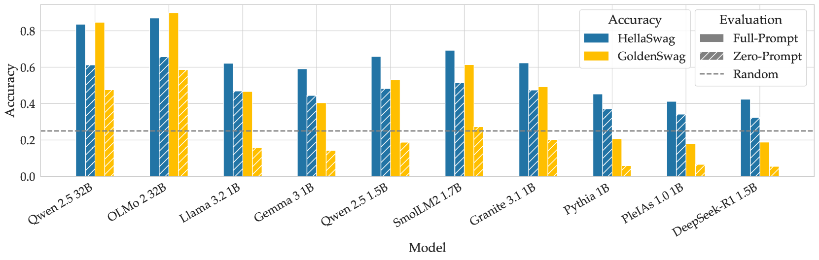</details> Figure 4: Accuracy comparison between HellaSwag and GoldenSwag. All models were evaluated by maximizing mean log-likelihood in full- and zero-prompt scenarios. Based on our analysis, we propose a small, highly filtered subset of HellaSwag, GoldenSwag. We removed the questions that had nonsensical or ungrammatical prompts or correct answers, and those that had grammar errors in the incorrect answer options. We also filtered out the questions in which Claude disagreed with the correct answer, found other equally correct options, or indicated that all of the options were implausible. In addition, we eliminated the questions rejected by Claude for ethical reasons. Furthermore, we filtered out the questions that had relative differences between the longest and shortest options larger than 0.3, and those among the rest, where the difference was above 0.15 and the longest answer was the correct one. Finally, we discarded the questions that at least seven out of ten tested models managed to answer correctly without question prompts. We present the detailed filtering in Appendix G. These filters left us with 1525 questions (15.2% of the original 10042), which we release as a part of this work. We re-evaluated the models on GoldenSwag (see Figure 4). The scores of smaller models dropped, while the larger ones improved their results. For smaller models, the zero-prompt evaluations dropped below random chance. ## 6 Conclusion In this paper, we described numerous construct validity issues in HellaSwag, ranging from grammar and typos to ambiguous answer choices. Zero-prompt evaluation shows that in most of the HellaSwag questions, question text does not affect model predictions, which allows us to conclude HellaSwag performance does not necessarily indicate common-sense reasoning capabilities. We specifically highlight that common-sense reasoning is a salient characteristic, and there should be a raised research interest in constructing a good benchmark to measure it. Based on our findings, we released GoldenSwag — a filtered subset of HellaSwag that can be one of the first steps towards this goal. ## Acknowledgments The authors of this work acknowledge the HPC resource allocation by Erlangen National High-Performance Computing Center (NHR@FAU) of the Friedrich-Alexander-Universität Erlangen-Nürnberg (FAU) (joint project with the Center for Artificial Intelligence (CAIRO), THWS) and Jean Zay (compute grant #GC011015451). The authors would also like to thank Catherine Arnett for her continuous help with the project, and the members of the PleIAs and CAIRO Research teams for helpful discussion and feedback. ## References - Allal et al. (2025) Loubna Ben Allal, Anton Lozhkov, Elie Bakouch, Gabriel Martín Blázquez, Guilherme Penedo, Lewis Tunstall, Andrés Marafioti, Hynek Kydlíček, Agustín Piqueres Lajarín, Vaibhav Srivastav, Joshua Lochner, Caleb Fahlgren, Xuan-Son Nguyen, Clémentine Fourrier, Ben Burtenshaw, Hugo Larcher, Haojun Zhao, Cyril Zakka, Mathieu Morlon, Colin Raffel, Leandro von Werra, and Thomas Wolf. Smollm2: When smol goes big – data-centric training of a small language model, 2025. URL https://arxiv.org/abs/2502.02737. - Alzahrani et al. (2024) Norah Alzahrani, Hisham Alyahya, Yazeed Alnumay, Sultan AlRashed, Shaykhah Alsubaie, Yousef Almushayqih, Faisal Mirza, Nouf Alotaibi, Nora Al-Twairesh, Areeb Alowisheq, M Saiful Bari, and Haidar Khan. When benchmarks are targets: Revealing the sensitivity of large language model leaderboards. In Lun-Wei Ku, Andre Martins, and Vivek Srikumar (eds.), Proceedings of the 62nd Annual Meeting of the Association for Computational Linguistics (Volume 1: Long Papers), pp. 13787–13805, Bangkok, Thailand, August 2024. Association for Computational Linguistics. doi: 10.18653/v1/2024.acl-long.744. URL https://aclanthology.org/2024.acl-long.744/. - Anthropic (2024) Anthropic. Introducing claude 3.5 sonnet, June 2024. URL https://www.anthropic.com/news/claude-3-5-sonnet. - Balepur & Rudinger (2024) Nishant Balepur and Rachel Rudinger. Is your large language model knowledgeable or a choices-only cheater? In Sha Li, Manling Li, Michael JQ Zhang, Eunsol Choi, Mor Geva, Peter Hase, and Heng Ji (eds.), Proceedings of the 1st Workshop on Towards Knowledgeable Language Models (KnowLLM 2024), pp. 15–26, Bangkok, Thailand, August 2024. Association for Computational Linguistics. doi: 10.18653/v1/2024.knowllm-1.2. URL https://aclanthology.org/2024.knowllm-1.2/. - Balepur et al. (2024) Nishant Balepur, Abhilasha Ravichander, and Rachel Rudinger. Artifacts or abduction: How do LLMs answer multiple-choice questions without the question? In Lun-Wei Ku, Andre Martins, and Vivek Srikumar (eds.), Proceedings of the 62nd Annual Meeting of the Association for Computational Linguistics (Volume 1: Long Papers), pp. 10308–10330, Bangkok, Thailand, August 2024. Association for Computational Linguistics. doi: 10.18653/v1/2024.acl-long.555. URL https://aclanthology.org/2024.acl-long.555/. - Biderman et al. (2023) Stella Biderman, Hailey Schoelkopf, Quentin Gregory Anthony, Herbie Bradley, Kyle O’Brien, Eric Hallahan, Mohammad Aflah Khan, Shivanshu Purohit, USVSN Sai Prashanth, Edward Raff, et al. Pythia: A suite for analyzing large language models across training and scaling. In International Conference on Machine Learning, pp. 2397–2430. PMLR, 2023. - Biderman et al. (2024) Stella Biderman, Hailey Schoelkopf, Lintang Sutawika, Leo Gao, Jonathan Tow, Baber Abbasi, Alham Fikri Aji, Pawan Sasanka Ammanamanchi, Sidney Black, Jordan Clive, et al. Lessons from the trenches on reproducible evaluation of language models. arXiv preprint arXiv:2405.14782, 2024. - Blili-Hamelin et al. (2025) Borhane Blili-Hamelin, Christopher Graziul, Leif Hancox-Li, Hananel Hazan, El-Mahdi El-Mhamdi, Avijit Ghosh, Katherine Heller, Jacob Metcalf, Fabricio Murai, Eryk Salvaggio, et al. Stop treatingagi’as the north-star goal of ai research. arXiv preprint arXiv:2502.03689, 2025. - Chen (2023) Edwin Chen. Hellaswag or hellabad? 36% of this popular llm benchmark contains errors, 2023. URL https://www.surgehq.ai/blog/hellaswag-or-hellabad-36-of-this-popular-llm-benchmark-contains-errors. Accessed: 2025-03-27. - Cobbe et al. (2021) Karl Cobbe, Vineet Kosaraju, Mohammad Bavarian, Mark Chen, Heewoo Jun, Lukasz Kaiser, Matthias Plappert, Jerry Tworek, Jacob Hilton, Reiichiro Nakano, et al. Training verifiers to solve math word problems. arXiv preprint arXiv:2110.14168, 2021. - Cronbach & Meehl (1955) LJ Cronbach and PE Meehl. Construct validity in psychological tests. Psychological Bulletin, 52(4):281–302, 1955. - Davis (2023) Ernest Davis. Benchmarks for automated commonsense reasoning: A survey. ACM Computing Surveys, 56(4):1–41, 2023. - DeepSeek-AI et al. (2025) DeepSeek-AI, Daya Guo, Dejian Yang, Haowei Zhang, Junxiao Song, Ruoyu Zhang, Runxin Xu, Qihao Zhu, Shirong Ma, Peiyi Wang, Xiao Bi, Xiaokang Zhang, Xingkai Yu, Yu Wu, Z. F. Wu, Zhibin Gou, Zhihong Shao, Zhuoshu Li, Ziyi Gao, Aixin Liu, Bing Xue, Bingxuan Wang, Bochao Wu, Bei Feng, Chengda Lu, Chenggang Zhao, Chengqi Deng, Chenyu Zhang, Chong Ruan, Damai Dai, Deli Chen, Dongjie Ji, Erhang Li, Fangyun Lin, Fucong Dai, Fuli Luo, Guangbo Hao, Guanting Chen, Guowei Li, H. Zhang, Han Bao, Hanwei Xu, Haocheng Wang, Honghui Ding, Huajian Xin, Huazuo Gao, Hui Qu, Hui Li, Jianzhong Guo, Jiashi Li, Jiawei Wang, Jingchang Chen, Jingyang Yuan, Junjie Qiu, Junlong Li, J. L. Cai, Jiaqi Ni, Jian Liang, Jin Chen, Kai Dong, Kai Hu, Kaige Gao, Kang Guan, Kexin Huang, Kuai Yu, Lean Wang, Lecong Zhang, Liang Zhao, Litong Wang, Liyue Zhang, Lei Xu, Leyi Xia, Mingchuan Zhang, Minghua Zhang, Minghui Tang, Meng Li, Miaojun Wang, Mingming Li, Ning Tian, Panpan Huang, Peng Zhang, Qiancheng Wang, Qinyu Chen, Qiushi Du, Ruiqi Ge, Ruisong Zhang, Ruizhe Pan, Runji Wang, R. J. Chen, R. L. Jin, Ruyi Chen, Shanghao Lu, Shangyan Zhou, Shanhuang Chen, Shengfeng Ye, Shiyu Wang, Shuiping Yu, Shunfeng Zhou, Shuting Pan, S. S. Li, Shuang Zhou, Shaoqing Wu, Shengfeng Ye, Tao Yun, Tian Pei, Tianyu Sun, T. Wang, Wangding Zeng, Wanjia Zhao, Wen Liu, Wenfeng Liang, Wenjun Gao, Wenqin Yu, Wentao Zhang, W. L. Xiao, Wei An, Xiaodong Liu, Xiaohan Wang, Xiaokang Chen, Xiaotao Nie, Xin Cheng, Xin Liu, Xin Xie, Xingchao Liu, Xinyu Yang, Xinyuan Li, Xuecheng Su, Xuheng Lin, X. Q. Li, Xiangyue Jin, Xiaojin Shen, Xiaosha Chen, Xiaowen Sun, Xiaoxiang Wang, Xinnan Song, Xinyi Zhou, Xianzu Wang, Xinxia Shan, Y. K. Li, Y. Q. Wang, Y. X. Wei, Yang Zhang, Yanhong Xu, Yao Li, Yao Zhao, Yaofeng Sun, Yaohui Wang, Yi Yu, Yichao Zhang, Yifan Shi, Yiliang Xiong, Ying He, Yishi Piao, Yisong Wang, Yixuan Tan, Yiyang Ma, Yiyuan Liu, Yongqiang Guo, Yuan Ou, Yuduan Wang, Yue Gong, Yuheng Zou, Yujia He, Yunfan Xiong, Yuxiang Luo, Yuxiang You, Yuxuan Liu, Yuyang Zhou, Y. X. Zhu, Yanhong Xu, Yanping Huang, Yaohui Li, Yi Zheng, Yuchen Zhu, Yunxian Ma, Ying Tang, Yukun Zha, Yuting Yan, Z. Z. Ren, Zehui Ren, Zhangli Sha, Zhe Fu, Zhean Xu, Zhenda Xie, Zhengyan Zhang, Zhewen Hao, Zhicheng Ma, Zhigang Yan, Zhiyu Wu, Zihui Gu, Zijia Zhu, Zijun Liu, Zilin Li, Ziwei Xie, Ziyang Song, Zizheng Pan, Zhen Huang, Zhipeng Xu, Zhongyu Zhang, and Zhen Zhang. Deepseek-r1: Incentivizing reasoning capability in llms via reinforcement learning, 2025. URL https://arxiv.org/abs/2501.12948. - Gao (2022) Leo Gao. Multiple choice normalization, 2022. URL https://blog.eleuther.ai/multiple-choice-normalization/. - Gema et al. (2024) Aryo Pradipta Gema, Joshua Ong Jun Leang, Giwon Hong, Alessio Devoto, Alberto Carlo Maria Mancino, Rohit Saxena, Xuanli He, Yu Zhao, Xiaotang Du, Mohammad Reza Ghasemi Madani, et al. Are we done with mmlu? arXiv preprint arXiv:2406.04127, 2024. - Google (2025) Google. Introducing gemma 3: Advancing open models for developers, March 2025. URL https://blog.google/technology/developers/gemma-3/. - Grattafiori et al. (2024) Aaron Grattafiori, Abhimanyu Dubey, Abhinav Jauhri, Abhinav Pandey, Abhishek Kadian, Ahmad Al-Dahle, Aiesha Letman, Akhil Mathur, Alan Schelten, Alex Vaughan, Amy Yang, Angela Fan, Anirudh Goyal, Anthony Hartshorn, Aobo Yang, Archi Mitra, Archie Sravankumar, Artem Korenev, Arthur Hinsvark, Arun Rao, Aston Zhang, Aurelien Rodriguez, Austen Gregerson, Ava Spataru, Baptiste Roziere, Bethany Biron, Binh Tang, Bobbie Chern, Charlotte Caucheteux, Chaya Nayak, Chloe Bi, Chris Marra, Chris McConnell, Christian Keller, Christophe Touret, Chunyang Wu, Corinne Wong, Cristian Canton Ferrer, Cyrus Nikolaidis, Damien Allonsius, Daniel Song, Danielle Pintz, Danny Livshits, Danny Wyatt, David Esiobu, Dhruv Choudhary, Dhruv Mahajan, Diego Garcia-Olano, Diego Perino, Dieuwke Hupkes, Egor Lakomkin, Ehab AlBadawy, Elina Lobanova, Emily Dinan, Eric Michael Smith, Filip Radenovic, Francisco Guzmán, Frank Zhang, Gabriel Synnaeve, Gabrielle Lee, Georgia Lewis Anderson, Govind Thattai, Graeme Nail, Gregoire Mialon, Guan Pang, Guillem Cucurell, Hailey Nguyen, Hannah Korevaar, Hu Xu, Hugo Touvron, Iliyan Zarov, Imanol Arrieta Ibarra, Isabel Kloumann, Ishan Misra, Ivan Evtimov, Jack Zhang, Jade Copet, Jaewon Lee, Jan Geffert, Jana Vranes, Jason Park, Jay Mahadeokar, Jeet Shah, Jelmer van der Linde, Jennifer Billock, Jenny Hong, Jenya Lee, Jeremy Fu, Jianfeng Chi, Jianyu Huang, Jiawen Liu, Jie Wang, Jiecao Yu, Joanna Bitton, Joe Spisak, Jongsoo Park, Joseph Rocca, Joshua Johnstun, Joshua Saxe, Junteng Jia, Kalyan Vasuden Alwala, Karthik Prasad, Kartikeya Upasani, Kate Plawiak, Ke Li, Kenneth Heafield, Kevin Stone, Khalid El-Arini, Krithika Iyer, Kshitiz Malik, Kuenley Chiu, Kunal Bhalla, Kushal Lakhotia, Lauren Rantala-Yeary, Laurens van der Maaten, Lawrence Chen, Liang Tan, Liz Jenkins, Louis Martin, Lovish Madaan, Lubo Malo, Lukas Blecher, Lukas Landzaat, Luke de Oliveira, Madeline Muzzi, Mahesh Pasupuleti, Mannat Singh, Manohar Paluri, Marcin Kardas, Maria Tsimpoukelli, Mathew Oldham, Mathieu Rita, Maya Pavlova, Melanie Kambadur, Mike Lewis, Min Si, Mitesh Kumar Singh, Mona Hassan, Naman Goyal, Narjes Torabi, Nikolay Bashlykov, Nikolay Bogoychev, Niladri Chatterji, Ning Zhang, Olivier Duchenne, Onur Çelebi, Patrick Alrassy, Pengchuan Zhang, Pengwei Li, Petar Vasic, Peter Weng, Prajjwal Bhargava, Pratik Dubal, Praveen Krishnan, Punit Singh Koura, Puxin Xu, Qing He, Qingxiao Dong, Ragavan Srinivasan, Raj Ganapathy, Ramon Calderer, Ricardo Silveira Cabral, Robert Stojnic, Roberta Raileanu, Rohan Maheswari, Rohit Girdhar, Rohit Patel, Romain Sauvestre, Ronnie Polidoro, Roshan Sumbaly, Ross Taylor, Ruan Silva, Rui Hou, Rui Wang, Saghar Hosseini, Sahana Chennabasappa, Sanjay Singh, Sean Bell, Seohyun Sonia Kim, Sergey Edunov, Shaoliang Nie, Sharan Narang, Sharath Raparthy, Sheng Shen, Shengye Wan, Shruti Bhosale, Shun Zhang, Simon Vandenhende, Soumya Batra, Spencer Whitman, Sten Sootla, Stephane Collot, Suchin Gururangan, Sydney Borodinsky, Tamar Herman, Tara Fowler, Tarek Sheasha, Thomas Georgiou, Thomas Scialom, Tobias Speckbacher, Todor Mihaylov, Tong Xiao, Ujjwal Karn, Vedanuj Goswami, Vibhor Gupta, Vignesh Ramanathan, Viktor Kerkez, Vincent Gonguet, Virginie Do, Vish Vogeti, Vítor Albiero, Vladan Petrovic, Weiwei Chu, Wenhan Xiong, Wenyin Fu, Whitney Meers, Xavier Martinet, Xiaodong Wang, Xiaofang Wang, Xiaoqing Ellen Tan, Xide Xia, Xinfeng Xie, Xuchao Jia, Xuewei Wang, Yaelle Goldschlag, Yashesh Gaur, Yasmine Babaei, Yi Wen, Yiwen Song, Yuchen Zhang, Yue Li, Yuning Mao, Zacharie Delpierre Coudert, Zheng Yan, Zhengxing Chen, Zoe Papakipos, Aaditya Singh, Aayushi Srivastava, Abha Jain, Adam Kelsey, Adam Shajnfeld, Adithya Gangidi, Adolfo Victoria, Ahuva Goldstand, Ajay Menon, Ajay Sharma, Alex Boesenberg, Alexei Baevski, Allie Feinstein, Amanda Kallet, Amit Sangani, Amos Teo, Anam Yunus, Andrei Lupu, Andres Alvarado, Andrew Caples, Andrew Gu, Andrew Ho, Andrew Poulton, Andrew Ryan, Ankit Ramchandani, Annie Dong, Annie Franco, Anuj Goyal, Aparajita Saraf, Arkabandhu Chowdhury, Ashley Gabriel, Ashwin Bharambe, Assaf Eisenman, Azadeh Yazdan, Beau James, Ben Maurer, Benjamin Leonhardi, Bernie Huang, Beth Loyd, Beto De Paola, Bhargavi Paranjape, Bing Liu, Bo Wu, Boyu Ni, Braden Hancock, Bram Wasti, Brandon Spence, Brani Stojkovic, Brian Gamido, Britt Montalvo, Carl Parker, Carly Burton, Catalina Mejia, Ce Liu, Changhan Wang, Changkyu Kim, Chao Zhou, Chester Hu, Ching-Hsiang Chu, Chris Cai, Chris Tindal, Christoph Feichtenhofer, Cynthia Gao, Damon Civin, Dana Beaty, Daniel Kreymer, Daniel Li, David Adkins, David Xu, Davide Testuggine, Delia David, Devi Parikh, Diana Liskovich, Didem Foss, Dingkang Wang, Duc Le, Dustin Holland, Edward Dowling, Eissa Jamil, Elaine Montgomery, Eleonora Presani, Emily Hahn, Emily Wood, Eric-Tuan Le, Erik Brinkman, Esteban Arcaute, Evan Dunbar, Evan Smothers, Fei Sun, Felix Kreuk, Feng Tian, Filippos Kokkinos, Firat Ozgenel, Francesco Caggioni, Frank Kanayet, Frank Seide, Gabriela Medina Florez, Gabriella Schwarz, Gada Badeer, Georgia Swee, Gil Halpern, Grant Herman, Grigory Sizov, Guangyi, Zhang, Guna Lakshminarayanan, Hakan Inan, Hamid Shojanazeri, Han Zou, Hannah Wang, Hanwen Zha, Haroun Habeeb, Harrison Rudolph, Helen Suk, Henry Aspegren, Hunter Goldman, Hongyuan Zhan, Ibrahim Damlaj, Igor Molybog, Igor Tufanov, Ilias Leontiadis, Irina-Elena Veliche, Itai Gat, Jake Weissman, James Geboski, James Kohli, Janice Lam, Japhet Asher, Jean-Baptiste Gaya, Jeff Marcus, Jeff Tang, Jennifer Chan, Jenny Zhen, Jeremy Reizenstein, Jeremy Teboul, Jessica Zhong, Jian Jin, Jingyi Yang, Joe Cummings, Jon Carvill, Jon Shepard, Jonathan McPhie, Jonathan Torres, Josh Ginsburg, Junjie Wang, Kai Wu, Kam Hou U, Karan Saxena, Kartikay Khandelwal, Katayoun Zand, Kathy Matosich, Kaushik Veeraraghavan, Kelly Michelena, Keqian Li, Kiran Jagadeesh, Kun Huang, Kunal Chawla, Kyle Huang, Lailin Chen, Lakshya Garg, Lavender A, Leandro Silva, Lee Bell, Lei Zhang, Liangpeng Guo, Licheng Yu, Liron Moshkovich, Luca Wehrstedt, Madian Khabsa, Manav Avalani, Manish Bhatt, Martynas Mankus, Matan Hasson, Matthew Lennie, Matthias Reso, Maxim Groshev, Maxim Naumov, Maya Lathi, Meghan Keneally, Miao Liu, Michael L. Seltzer, Michal Valko, Michelle Restrepo, Mihir Patel, Mik Vyatskov, Mikayel Samvelyan, Mike Clark, Mike Macey, Mike Wang, Miquel Jubert Hermoso, Mo Metanat, Mohammad Rastegari, Munish Bansal, Nandhini Santhanam, Natascha Parks, Natasha White, Navyata Bawa, Nayan Singhal, Nick Egebo, Nicolas Usunier, Nikhil Mehta, Nikolay Pavlovich Laptev, Ning Dong, Norman Cheng, Oleg Chernoguz, Olivia Hart, Omkar Salpekar, Ozlem Kalinli, Parkin Kent, Parth Parekh, Paul Saab, Pavan Balaji, Pedro Rittner, Philip Bontrager, Pierre Roux, Piotr Dollar, Polina Zvyagina, Prashant Ratanchandani, Pritish Yuvraj, Qian Liang, Rachad Alao, Rachel Rodriguez, Rafi Ayub, Raghotham Murthy, Raghu Nayani, Rahul Mitra, Rangaprabhu Parthasarathy, Raymond Li, Rebekkah Hogan, Robin Battey, Rocky Wang, Russ Howes, Ruty Rinott, Sachin Mehta, Sachin Siby, Sai Jayesh Bondu, Samyak Datta, Sara Chugh, Sara Hunt, Sargun Dhillon, Sasha Sidorov, Satadru Pan, Saurabh Mahajan, Saurabh Verma, Seiji Yamamoto, Sharadh Ramaswamy, Shaun Lindsay, Shaun Lindsay, Sheng Feng, Shenghao Lin, Shengxin Cindy Zha, Shishir Patil, Shiva Shankar, Shuqiang Zhang, Shuqiang Zhang, Sinong Wang, Sneha Agarwal, Soji Sajuyigbe, Soumith Chintala, Stephanie Max, Stephen Chen, Steve Kehoe, Steve Satterfield, Sudarshan Govindaprasad, Sumit Gupta, Summer Deng, Sungmin Cho, Sunny Virk, Suraj Subramanian, Sy Choudhury, Sydney Goldman, Tal Remez, Tamar Glaser, Tamara Best, Thilo Koehler, Thomas Robinson, Tianhe Li, Tianjun Zhang, Tim Matthews, Timothy Chou, Tzook Shaked, Varun Vontimitta, Victoria Ajayi, Victoria Montanez, Vijai Mohan, Vinay Satish Kumar, Vishal Mangla, Vlad Ionescu, Vlad Poenaru, Vlad Tiberiu Mihailescu, Vladimir Ivanov, Wei Li, Wenchen Wang, Wenwen Jiang, Wes Bouaziz, Will Constable, Xiaocheng Tang, Xiaojian Wu, Xiaolan Wang, Xilun Wu, Xinbo Gao, Yaniv Kleinman, Yanjun Chen, Ye Hu, Ye Jia, Ye Qi, Yenda Li, Yilin Zhang, Ying Zhang, Yossi Adi, Youngjin Nam, Yu, Wang, Yu Zhao, Yuchen Hao, Yundi Qian, Yunlu Li, Yuzi He, Zach Rait, Zachary DeVito, Zef Rosnbrick, Zhaoduo Wen, Zhenyu Yang, Zhiwei Zhao, and Zhiyu Ma. The llama 3 herd of models, 2024. URL https://arxiv.org/abs/2407.21783. - Gupta et al. (2024) Vipul Gupta, David Pantoja, Candace Ross, Adina Williams, and Megan Ung. Changing answer order can decrease mmlu accuracy. arXiv preprint arXiv:2406.19470, 2024. - Habba et al. (2025) Eliya Habba, Ofir Arviv, Itay Itzhak, Yotam Perlitz, Elron Bandel, Leshem Choshen, Michal Shmueli-Scheuer, and Gabriel Stanovsky. Dove: A large-scale multi-dimensional predictions dataset towards meaningful llm evaluation. arXiv preprint arXiv:2503.01622, 2025. - Hendrycks et al. (2021) Dan Hendrycks, Collin Burns, Steven Basart, Andy Zou, Mantas Mazeika, Dawn Song, and Jacob Steinhardt. Measuring massive multitask language understanding. In International Conference on Learning Representations, 2021. URL https://openreview.net/forum?id=d7KBjmI3GmQ. - Hu & Frank (2024) Jennifer Hu and Michael Frank. Auxiliary task demands mask the capabilities of smaller language models. In First Conference on Language Modeling, 2024. URL https://openreview.net/forum?id=U5BUzSn4tD. - Hu & Levy (2023) Jennifer Hu and Roger Levy. Prompting is not a substitute for probability measurements in large language models. In Houda Bouamor, Juan Pino, and Kalika Bali (eds.), Proceedings of the 2023 Conference on Empirical Methods in Natural Language Processing, pp. 5040–5060, Singapore, December 2023. Association for Computational Linguistics. doi: 10.18653/v1/2023.emnlp-main.306. URL https://aclanthology.org/2023.emnlp-main.306/. - IBM (2024) IBM. Ibm unveils granite 3.1: Powerful performance, long context, and more, March 2024. URL https://www.ibm.com/new/announcements/ibm-granite-3-1-powerful-performance-long-context-and-more. - Krishna et al. (2017) Ranjay Krishna, Kenji Hata, Frederic Ren, Li Fei-Fei, and Juan Carlos Niebles. Dense-captioning events in videos. In Proceedings of the IEEE international conference on computer vision, pp. 706–715, 2017. - Liang et al. (2023) Percy Liang, Rishi Bommasani, Tony Lee, Dimitris Tsipras, Dilara Soylu, Michihiro Yasunaga, Yian Zhang, Deepak Narayanan, Yuhuai Wu, Ananya Kumar, Benjamin Newman, Binhang Yuan, Bobby Yan, Ce Zhang, Christian Alexander Cosgrove, Christopher D Manning, Christopher Re, Diana Acosta-Navas, Drew Arad Hudson, Eric Zelikman, Esin Durmus, Faisal Ladhak, Frieda Rong, Hongyu Ren, Huaxiu Yao, Jue WANG, Keshav Santhanam, Laurel Orr, Lucia Zheng, Mert Yuksekgonul, Mirac Suzgun, Nathan Kim, Neel Guha, Niladri S. Chatterji, Omar Khattab, Peter Henderson, Qian Huang, Ryan Andrew Chi, Sang Michael Xie, Shibani Santurkar, Surya Ganguli, Tatsunori Hashimoto, Thomas Icard, Tianyi Zhang, Vishrav Chaudhary, William Wang, Xuechen Li, Yifan Mai, Yuhui Zhang, and Yuta Koreeda. Holistic evaluation of language models. Transactions on Machine Learning Research, 2023. ISSN 2835-8856. URL https://openreview.net/forum?id=iO4LZibEqW. Featured Certification, Expert Certification. - Lyu et al. (2024) Chenyang Lyu, Minghao Wu, and Alham Aji. Beyond probabilities: Unveiling the misalignment in evaluating large language models. In Sha Li, Manling Li, Michael JQ Zhang, Eunsol Choi, Mor Geva, Peter Hase, and Heng Ji (eds.), Proceedings of the 1st Workshop on Towards Knowledgeable Language Models (KnowLLM 2024), pp. 109–131, Bangkok, Thailand, August 2024. Association for Computational Linguistics. doi: 10.18653/v1/2024.knowllm-1.10. URL https://aclanthology.org/2024.knowllm-1.10/. - Narayan et al. (2018) Shashi Narayan, Shay B. Cohen, and Mirella Lapata. Don‘t give me the details, just the summary! topic-aware convolutional neural networks for extreme summarization. In Ellen Riloff, David Chiang, Julia Hockenmaier, and Jun’ichi Tsujii (eds.), Proceedings of the 2018 Conference on Empirical Methods in Natural Language Processing, pp. 1797–1807, Brussels, Belgium, October-November 2018. Association for Computational Linguistics. doi: 10.18653/v1/D18-1206. URL https://aclanthology.org/D18-1206/. - OLMo et al. (2025) Team OLMo, Pete Walsh, Luca Soldaini, Dirk Groeneveld, Kyle Lo, Shane Arora, Akshita Bhagia, Yuling Gu, Shengyi Huang, Matt Jordan, Nathan Lambert, Dustin Schwenk, Oyvind Tafjord, Taira Anderson, David Atkinson, Faeze Brahman, Christopher Clark, Pradeep Dasigi, Nouha Dziri, Michal Guerquin, Hamish Ivison, Pang Wei Koh, Jiacheng Liu, Saumya Malik, William Merrill, Lester James V. Miranda, Jacob Morrison, Tyler Murray, Crystal Nam, Valentina Pyatkin, Aman Rangapur, Michael Schmitz, Sam Skjonsberg, David Wadden, Christopher Wilhelm, Michael Wilson, Luke Zettlemoyer, Ali Farhadi, Noah A. Smith, and Hannaneh Hajishirzi. 2 olmo 2 furious, 2025. URL https://arxiv.org/abs/2501.00656. - PleIAs (2024) PleIAs. Common models: A new way to understand and explore ai models, March 2024. URL https://huggingface.co/blog/Pclanglais/common-models. - Radford et al. (2018) Alec Radford, Karthik Narasimhan, Tim Salimans, and Ilya Sutskever. Improving language understanding by generative pre-training. 2018. - Rein et al. (2024) David Rein, Betty Li Hou, Asa Cooper Stickland, Jackson Petty, Richard Yuanzhe Pang, Julien Dirani, Julian Michael, and Samuel R. Bowman. GPQA: A graduate-level google-proof q&a benchmark. In First Conference on Language Modeling, 2024. URL https://openreview.net/forum?id=Ti67584b98. - Shah et al. (2020) Krunal Shah, Nitish Gupta, and Dan Roth. What do we expect from multiple-choice QA systems? In Trevor Cohn, Yulan He, and Yang Liu (eds.), Findings of the Association for Computational Linguistics: EMNLP 2020, pp. 3547–3553, Online, November 2020. Association for Computational Linguistics. doi: 10.18653/v1/2020.findings-emnlp.317. URL https://aclanthology.org/2020.findings-emnlp.317/. - Vendrow et al. (2025) Joshua Vendrow, Edward Vendrow, Sara Beery, and Aleksander Madry. Do large language model benchmarks test reliability? arXiv preprint arXiv:2502.03461, 2025. - Yang et al. (2024) An Yang, Baosong Yang, Beichen Zhang, Binyuan Hui, Bo Zheng, Bowen Yu, Chengyuan Li, Dayiheng Liu, Fei Huang, Haoran Wei, Huan Lin, Jian Yang, Jianhong Tu, Jianwei Zhang, Jianxin Yang, Jiaxi Yang, Jingren Zhou, Junyang Lin, Kai Dang, Keming Lu, Keqin Bao, Kexin Yang, Le Yu, Mei Li, Mingfeng Xue, Pei Zhang, Qin Zhu, Rui Men, Runji Lin, Tianhao Li, Tingyu Xia, Xingzhang Ren, Xuancheng Ren, Yang Fan, Yang Su, Yichang Zhang, Yu Wan, Yuqiong Liu, Zeyu Cui, Zhenru Zhang, and Zihan Qiu. Qwen2.5 technical report. arXiv preprint arXiv:2412.15115, 2024. - Zellers et al. (2019) Rowan Zellers, Ari Holtzman, Yonatan Bisk, Ali Farhadi, and Yejin Choi. HellaSwag: Can a machine really finish your sentence? In Anna Korhonen, David Traum, and Lluís Màrquez (eds.), Proceedings of the 57th Annual Meeting of the Association for Computational Linguistics, pp. 4791–4800, Florence, Italy, July 2019. Association for Computational Linguistics. doi: 10.18653/v1/P19-1472. URL https://aclanthology.org/P19-1472/. ## Appendix A Models | Model | Size | HuggingFace repository | | --- | --- | --- | | LLaMA 3.2 | 1B | meta-llama/Llama-3.2-1B | | (Grattafiori et al., 2024) | | | | Qwen 2.5 (Yang et al., 2024) | 1.5B | Qwen/Qwen2.5-1.5B | | Granite 3.1 (IBM, 2024) | 1B | ibm-granite/granite-3.1-1b-a400m-base | | Gemma 3.1 (Google, 2025) | 1B | google/gemma-3-1b-pt.csv | | SmolLM2 (Allal et al., 2025) | 1.7B | HuggingFaceTB/SmolLM2-1.7B | | DeepSeek-R1 | 1.5B | deepseek-ai/DeepSeek-R1-Distill-Qwen-1.5B | | (DeepSeek-AI et al., 2025) | | | | Pythia (Biderman et al., 2023) | 1B | EleutherAI/pythia-1b | | Pleias 1.0 (PleIAs, 2024) | 1B | PleIAs/Pleias-1b-Preview | | Qwen 2.5 (Yang et al., 2024) | 32B | Qwen/Qwen2.5-32B-Instruct | | OLMo 2 (OLMo et al., 2025) | 32B | allenai/OLMo-2-0325-32B-Instruct | Table 5: Model names and their corresponding HuggingFace repositories. In Table 5, we present the models we used for evaluations in the paper with their corresponding HuggingFace repository paths. ## Appendix B Generation Prompt We use the following prompt to evaluate the models by generation: Generation Prompt You are given a situation followed by four possible endings. Choose the most appropriate ending by selecting the corresponding number. Respond only with the number of the correct answer. Context: Roof shingle removal: A man is sitting on a roof. He 1. is using wrap to wrap a pair of skis. 2. is ripping level tiles off. 3. is holding a Rubik’s cube. 4. starts pulling up roofing on a roof. Answer: ## Appendix C Annotations Here we report the two prompts we used for annotations with Claude 3.5 Sonnet (version claude-3-5-sonnet-20241022). In both prompts, we indicate the answer that is supposed to be correct. In the first prompt, we have a part about the equal plausibility of answers, but we did not use the results from this annotation label as we did it more verbosely in the second round of annotations. In the second annotation prompt, we present HellaSwag questions as complete texts to change the familiar benchmark structure and force the model to understand the options as complete texts. For the examples in the second prompt, we use the questions from the HellaSwag training set. First Round of Annotations I am evaluating the quality of a multiple-choice task, where given the prompt, you are supposed to pick the best sentence completion. I will provide the prompt and four possible completion options, with the correct one labeled. For each set, return all applicable labels (in brackets, separated by semicolons) based on the descriptions below: • [ungrammatical, prompt] — there is a grammatical error or typo in the question. It’s okay if the last part of the prompt is incomplete, that’s part of the task. • [ungrammatical, correct answer] — there is a grammatical error or typo in the correct answer • [ungrammatical, incorrect answer(s)] — there is a grammatical error or typo in one or more of the incorrect answer choices • [nonsense, prompt] — ignoring grammatical errors or typos, the question does not make sense or is not coherent • [nonsense, correct answer] — ignoring grammatical errors or typos, the correct answer does not make sense or is not coherent • [nonsense, incorrect answer(s)] — ignoring grammatical errors or typos, one or more of the answer choices does not make sense or is not coherent • [plausibility, answers] — two or more of the answer choices are equally plausible or implausible, therefore the correct answer is not necessarily the best answer, given your understanding of the prompt • [high quality] - there are no issues with the prompt or answer choices Example Output: If the prompt has a grammatical error and the correct answer is nonsensical, return: [ungrammatical, prompt; nonsense, correct answer] Sentence: Roof shingle removal: A man is sitting on a roof. He Completions: a) is using wrap to wrap a pair of skis. b) is ripping level tiles off. c) is holding a Rubik’s cube. d) starts pulling up roofing on a roof. (Labeled as correct) Labels: Second Round of Annotations I will give you four short texts that start similarly but have different endings. I will also indicate which text is considered correct—i.e., the one with the most logical and plausible ending. However, in some cases, the text labeled as correct may not actually be the best one, or there may be several other options that are just as good. It may also happen that all the texts, including the correct one, are implausible and nonsensical. I would like you to answer the following four questions: 1. Is the text labeled as correct in fact the best one, or do you have a better option? Reply with the letter of the best sentence in your opinion. 2. Are there other options that are equally plausible/make as much sense as the answer labeled as correct? Reply with the letters corresponding to those texts, separated by commas, or “None” if there are no equally good options. 3. Is it the case that all of the answer choices are implausible or nonsensical? Answer “Yes” or “No.” 4. Which is the worst of the answer choices? Reply with one letter of the worst option. Here’s an example: A) Triple jump: As he reaches the dirt section, he does three jumps. On his final jump, he extends his legs to try and jump as far as possible. The video ends with closing captions. B) Triple jump: As he reaches the dirt section, he does three jumps. On his final jump, he extends his legs to try and jump as far as possible. The video ends after he lands and he is shown smacking the ground. (Labeled as correct) C) Triple jump: As he reaches the dirt section, he does three jumps. On his final jump, he extends his legs to try and jump as far as possible. The video ends with the intro credits shown. D) Triple jump: As he reaches the dirt section, he does three jumps. On his final jump, he extends his legs to try and jump as far as possible. The video ends with more dirt. The answer should be: 1. B 2. A 3. No 4. D Here’s another example, where all of the options are implausible: A) Cheerleading: A cheerleading team begins to hold up posters as their mascot runs behind them. They eventually get the dogs on the field and push them around. B) Cheerleading: A cheerleading team begins to hold up posters as their mascot runs behind them. They begin to perform an athlete’s routine on the field. C) Cheerleading: A cheerleading team begins to hold up posters as their mascot runs behind them. They then begin to do a routine, and some of the girls run with streamers as the rest hold up the girls for their stunt. (Labeled as correct) D) Cheerleading: A cheerleading team begins to hold up posters as their mascot runs behind them. They begin to perform acoustic songs. The answer should be: 1. C 2. None 3. Yes 4. A Here is the actual question for you to evaluate: A) Roof shingle removal: A man is sitting on a roof. He is using wrap to wrap a pair of skis. B) Roof shingle removal: A man is sitting on a roof. He is ripping level tiles off. C) Roof shingle removal: A man is sitting on a roof. He is holding a Rubik’s cube. D) Roof shingle removal: A man is sitting on a roof. He starts pulling up roofing on a roof. 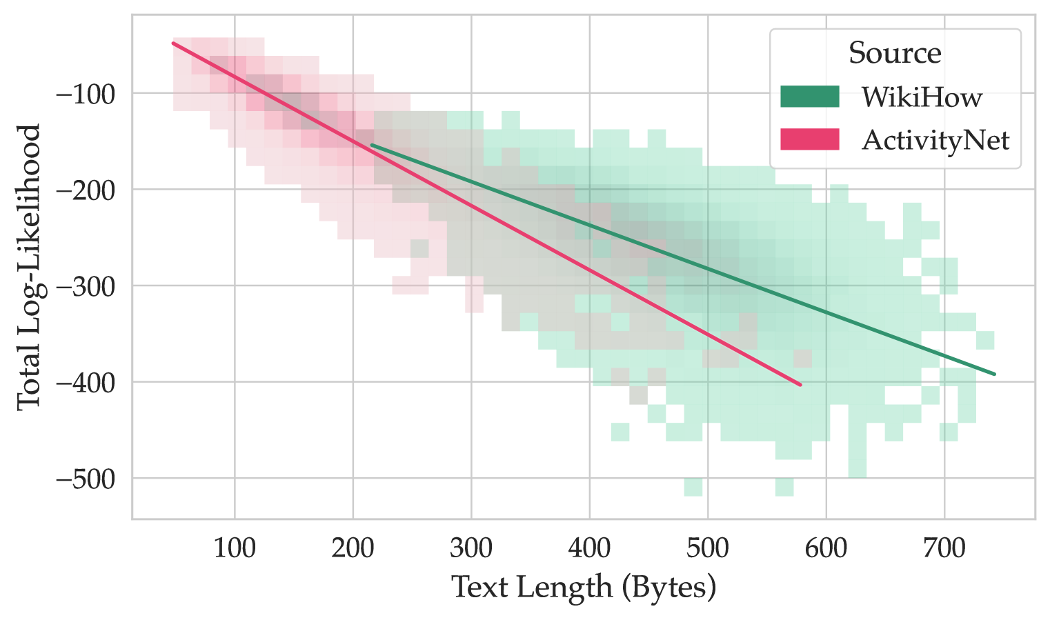(Labeled as correct) Your Answer: ## Appendix D Answer Lengths ### D.1 Other Log-Likelihood Variants <details> <summary>x5.png Details</summary>  ### Visual Description \n ## Scatter Plot with Regression Lines: Text Length vs. Total Log-Likelihood by Source ### Overview This image is a scatter plot with overlaid regression lines, visualizing the relationship between the length of text (in bytes) and its total log-likelihood for two distinct data sources: WikiHow and ActivityNet. The plot suggests a negative correlation between text length and log-likelihood for both sources. ### Components/Axes * **X-Axis:** Labeled "Text Length (Bytes)". The scale runs from approximately 50 to 750 bytes, with major tick marks at 100, 200, 300, 400, 500, 600, and 700. * **Y-Axis:** Labeled "Total Log-Likelihood". The scale runs from approximately -50 to -500, with major tick marks at -100, -200, -300, -400, and -500. * **Legend:** Located in the top-right corner of the plot area. It is titled "Source" and contains two entries: * A green square labeled "WikiHow". * A pink square labeled "ActivityNet". * **Data Series:** Two distinct series are plotted as semi-transparent, binned scatter points (resembling a 2D histogram or density plot) with solid regression lines. * **WikiHow (Green):** Data points are represented by green squares. A solid green regression line is overlaid. * **ActivityNet (Pink):** Data points are represented by pink squares. A solid pink regression line is overlaid. ### Detailed Analysis **1. WikiHow Data Series (Green):** * **Trend Verification:** The green regression line slopes downward from left to right, indicating a negative correlation. As text length increases, total log-likelihood decreases. * **Data Distribution:** The green data points are densely clustered in a broad band. They span a text length range from approximately 200 bytes to 750 bytes. The corresponding log-likelihood values range from about -100 down to -500. * **Regression Line Points (Approximate):** * Start: (Text Length ≈ 200 bytes, Log-Likelihood ≈ -150) * End: (Text Length ≈ 750 bytes, Log-Likelihood ≈ -400) **2. ActivityNet Data Series (Pink):** * **Trend Verification:** The pink regression line also slopes downward from left to right, indicating a negative correlation. Its slope appears steeper than the WikiHow line. * **Data Distribution:** The pink data points are concentrated in a band that starts at shorter text lengths. They span from approximately 50 bytes to 600 bytes. The log-likelihood values range from about -50 down to -400. * **Regression Line Points (Approximate):** * Start: (Text Length ≈ 50 bytes, Log-Likelihood ≈ -50) * End: (Text Length ≈ 600 bytes, Log-Likelihood ≈ -400) **3. Relationship Between Series:** * The two data clouds overlap significantly in the region between 200-600 bytes and -150 to -400 log-likelihood. * The ActivityNet series (pink) dominates the shorter text length region (<200 bytes), while the WikiHow series (green) extends into the longer text length region (>600 bytes). * The pink regression line (ActivityNet) is consistently below the green regression line (WikiHow) for text lengths where both are present, suggesting that for a given text length, ActivityNet texts tend to have a lower total log-likelihood than WikiHow texts. ### Key Observations 1. **Strong Negative Correlation:** Both datasets exhibit a clear, strong negative linear relationship between text length and total log-likelihood. 2. **Differing Slopes:** The rate of decrease in log-likelihood per additional byte of text is greater for ActivityNet (steeper pink line) than for WikiHow (shallower green line). 3. **Domain Separation:** The sources occupy partially distinct domains in the feature space. ActivityNet is associated with shorter texts and a wider initial range of log-likelihoods. WikiHow is associated with longer texts. 4. **Convergence at Length:** The two regression lines appear to converge near a log-likelihood of -400 at the upper end of the ActivityNet text length range (~600 bytes). ### Interpretation This chart likely analyzes the performance or characteristics of a probabilistic model (e.g., a language model) applied to text from two different datasets. Total log-likelihood is a measure of how well the model explains the data; higher values (closer to zero) indicate better fit. * **Core Finding:** The model's confidence or explanatory power (log-likelihood) systematically decreases as the text it is evaluating gets longer. This is a common phenomenon, as longer sequences present more opportunities for deviation from model predictions. * **Source-Specific Behavior:** The model assigns consistently higher likelihoods to WikiHow texts of a given length compared to ActivityNet texts. This could imply: * The WikiHow domain (likely instructional, procedural text) is more predictable or better represented in the model's training data. * The ActivityNet domain (likely descriptive, narrative text about activities) is more diverse or contains more complex language patterns that the model finds less probable. * **Practical Implication:** When using this model for tasks like text generation, classification, or anomaly detection, one must account for the inherent bias against longer texts and the different baseline likelihoods for different text sources. A raw log-likelihood score is not directly comparable across texts of different lengths or from different domains without normalization. </details> (a) Joint distributions of total log-likelihood and text length in bytes for different question sources in the Hellaswag validation set. 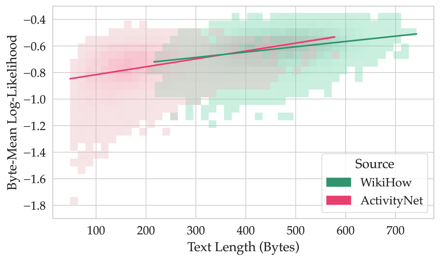<details> <summary>x6.png Details</summary>  ### Visual Description ## Scatter Plot with Trend Lines: Text Length vs. Byte-Mean Log-Likelihood by Source ### Overview The image is a 2D scatter plot overlaid with two linear trend lines. It visualizes the relationship between the length of text (in bytes) and a metric called "Byte-Mean Log-Likelihood" for two distinct data sources: WikiHow and ActivityNet. The plot uses a 2D histogram or binned scatter approach, where the density of data points is represented by the opacity or color intensity of rectangular bins. ### Components/Axes * **Chart Type:** 2D Histogram / Binned Scatter Plot with overlaid linear regression trend lines. * **X-Axis:** * **Label:** "Text Length (Bytes)" * **Scale:** Linear, ranging from approximately 50 to 750 bytes. * **Major Ticks:** 100, 200, 300, 400, 500, 600, 700. * **Y-Axis:** * **Label:** "Byte-Mean Log-Likelihood" * **Scale:** Linear, ranging from -1.8 to -0.4. * **Major Ticks:** -1.8, -1.6, -1.4, -1.2, -1.0, -0.8, -0.6, -0.4. * **Legend:** * **Position:** Bottom-right corner of the plot area. * **Title:** "Source" * **Entries:** 1. **WikiHow:** Represented by a dark green color. The associated data points are shown as green-tinted bins, and its trend line is a solid dark green line. 2. **ActivityNet:** Represented by a pink/magenta color. The associated data points are shown as pink-tinted bins, and its trend line is a solid pink line. * **Data Representation:** The plot uses colored, semi-transparent rectangular bins. The overlap of the two datasets creates greyish areas where both green and pink bins coincide. ### Detailed Analysis **1. Data Distribution & Density:** * **ActivityNet (Pink):** Data points are concentrated in the lower text length range, primarily between ~50 and 300 bytes. The density (opacity) is highest in the region of 100-200 bytes and -1.0 to -0.6 on the y-axis. The distribution shows a wide vertical spread, especially at shorter text lengths, with some points reaching as low as -1.8. * **WikiHow (Green):** Data points are concentrated in the higher text length range, primarily between ~200 and 750 bytes. The density is highest in the region of 300-600 bytes and -0.8 to -0.4. The distribution is more vertically compact compared to ActivityNet, especially at longer text lengths. * **Overlap:** There is a significant region of overlap between approximately 200 and 500 bytes on the x-axis and -1.0 to -0.6 on the y-axis, indicated by the grey mixed bins. **2. Trend Lines & Correlation:** * **ActivityNet Trend Line (Pink):** * **Visual Trend:** Slopes upward from left to right. * **Approximate Path:** Starts near (50 bytes, -0.85) and ends near (580 bytes, -0.55). * **Interpretation:** Indicates a positive correlation. As text length increases, the Byte-Mean Log-Likelihood for ActivityNet data tends to increase (become less negative). * **WikiHow Trend Line (Green):** * **Visual Trend:** Slopes upward from left to right, with a slightly steeper slope than the ActivityNet line. * **Approximate Path:** Starts near (220 bytes, -0.72) and ends near (750 bytes, -0.50). * **Interpretation:** Also indicates a positive correlation. The relationship appears slightly stronger (steeper slope) for WikiHow data. **3. Key Data Points (Approximate from Trend Lines):** * At **Text Length = 100 bytes:** ActivityNet trend ≈ -0.82; WikiHow trend not applicable (data sparse). * At **Text Length = 300 bytes:** ActivityNet trend ≈ -0.70; WikiHow trend ≈ -0.68. * At **Text Length = 500 bytes:** ActivityNet trend ≈ -0.58; WikiHow trend ≈ -0.58. * At **Text Length = 700 bytes:** ActivityNet trend not applicable (data sparse); WikiHow trend ≈ -0.52. ### Key Observations 1. **Distinct Data Ranges:** The two sources occupy largely different domains of text length. ActivityNet is characterized by shorter texts, while WikiHow is characterized by longer texts. 2. **Positive Correlation for Both:** Both datasets show that longer text length is associated with a higher (less negative) Byte-Mean Log-Likelihood. 3. **Convergence of Trends:** The two trend lines intersect and are very close in value in the overlapping region around 300-500 bytes, suggesting similar model likelihood behavior for texts of that length regardless of source. 4. **Variance:** ActivityNet shows much higher variance in the Byte-Mean Log-Likelihood metric, particularly for short texts, as evidenced by the tall vertical spread of pink bins. WikiHow's variance appears lower and more consistent across its range. 5. **Outliers:** There are isolated, low-density bins for ActivityNet at very low likelihoods (e.g., near -1.8 at ~50 bytes), which may represent outliers or particularly atypical short texts. ### Interpretation This chart likely analyzes the performance or characteristics of a language or sequence model. "Byte-Mean Log-Likelihood" is a metric where higher values (closer to zero) indicate the model finds the data more probable or "less surprising." The data suggests that **both WikiHow and ActivityNet texts become more "predictable" or "model-friendly" as they get longer.** This is a common phenomenon in language modeling, as longer contexts provide more information for prediction. The key investigative insight is the **source-dependent behavior.** WikiHow, presumably containing instructional, well-structured text, consistently yields higher likelihoods and shows a stronger positive trend. ActivityNet, likely containing more varied, noisy, or informal descriptions of activities, has lower average likelihoods and much higher variance, especially in short snippets. The convergence in the middle suggests that for medium-length texts (~400 bytes), the source matters less to the model's assessment of likelihood. This analysis could be used to understand dataset biases, model calibration, or to guide data preprocessing (e.g., filtering very short, low-likelihood texts from ActivityNet). </details> (b) Joint distributions of byte-normalized log-likelihood and text length in bytes for different question sources in the Hellaswag validation set. Figure 5: Joint distributions of likelihoods and lengths of the HellaSwag validation set questions for different variants of likelihood computation. The lines are meant to show the trend, we are not assuming linear regression to be significant for these data. In order to compare our mean log-likelihood evaluations with the ones used in lm-evaluation-harness (Biderman et al., 2024). In Figure 5, we show joint distributions for total log-likelihood: $$ \mathcal{L}_{t}=\sum_{t\in\mathcal{V}}\log\mathrm{P}(y_{t}\mid x_{<t}), \tag{2} $$ and byte-normalized log-likelihood: $$ \mathcal{L}_{b}=\frac{1}{\mathrm{B}}\sum_{t\in\mathcal{V}}\log\mathrm{P}(y_{t} \mid x_{<t}), \tag{3} $$ where $y_{t}$ is the ground truth token at position $t$ , $x_{<t}$ is the preceding sequence of tokens, $\mathrm{B}$ is the sequence length in bytes, and $\mathcal{V}$ is the set of valid (non-special) token positions. As with the mean log-likelihood, there is a visible correlation between answer length and log-likelihood in both cases (negative, in Figure 5(a)). 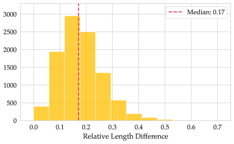### D.2 Lengths distribution <details> <summary>x7.png Details</summary>  ### Visual Description ## Histogram: Relative Length Difference Distribution ### Overview The image displays a histogram visualizing the frequency distribution of a metric called "Relative Length Difference." The chart includes a vertical dashed line indicating the median value of the distribution. The overall shape is right-skewed, with the majority of data points concentrated on the left side of the scale. ### Components/Axes * **Chart Type:** Histogram. * **X-Axis:** * **Label:** "Relative Length Difference" * **Scale:** Linear scale from 0.0 to 0.7. * **Major Tick Marks:** 0.0, 0.1, 0.2, 0.3, 0.4, 0.5, 0.6, 0.7. * **Y-Axis:** * **Label:** Not explicitly labeled, but represents frequency/count. * **Scale:** Linear scale from 0 to 3000. * **Major Tick Marks:** 0, 500, 1000, 1500, 2000, 2500, 3000. * **Legend:** * **Position:** Top-right corner of the chart area. * **Content:** A dashed red line symbol followed by the text "Median: 0.17". * **Data Series:** A single series represented by yellow bars. * **Reference Line:** A vertical, dashed red line positioned at x = 0.17, corresponding to the median. ### Detailed Analysis The histogram bins data into intervals of approximately 0.05 units along the "Relative Length Difference" axis. The approximate frequency (count) for each bin, estimated from the bar heights, is as follows: * **0.00 - 0.05:** ~400 * **0.05 - 0.10:** ~1950 * **0.10 - 0.15:** ~2950 (This is the modal bin, the highest bar) * **0.15 - 0.20:** ~2500 * **0.20 - 0.25:** ~1350 * **0.25 - 0.30:** ~550 * **0.30 - 0.35:** ~200 * **0.35 - 0.40:** ~100 * **0.40 - 0.45:** ~50 * **0.45 - 0.50:** ~20 * **0.50 - 0.55:** ~10 (Very small bar, barely visible) * **0.55 - 0.70:** No visible bars, frequency appears to be 0 or near 0. **Trend Verification:** The visual trend is a sharp rise to a peak in the 0.10-0.15 bin, followed by a steady, decaying decline as the Relative Length Difference increases. The distribution has a long tail extending to the right. ### Key Observations 1. **Central Tendency:** The median is explicitly stated as 0.17, marked by the red dashed line. This falls within the second-highest bar (0.15-0.20 bin). 2. **Peak Frequency:** The highest concentration of data (mode) occurs in the interval between 0.10 and 0.15. 3. **Skewness:** The distribution is positively skewed (right-skewed). The tail on the right side (higher values) is much longer than the left. 4. **Data Range:** The vast majority of the data lies between 0.05 and 0.30. Values above 0.40 are rare. 5. **Visual Design:** The chart uses a simple, clean design with a white background, light gray grid lines, and a single accent color (yellow) for the data bars. The median line uses a contrasting red color for emphasis. ### Interpretation This histogram demonstrates that the measured "Relative Length Difference" is not symmetrically distributed. Instead, it shows a strong clustering of values at the lower end of the scale, with a median of 0.17. This suggests that for the population sampled, the relative difference in length is typically small. The right skew indicates the presence of a subset of cases with substantially larger relative differences, though these are progressively less common. The sharp drop-off after 0.30 implies that extreme differences are outliers in this dataset. From a technical or investigative perspective, this pattern could indicate: * A process that is generally well-controlled (keeping differences low) but occasionally experiences larger deviations. * A natural phenomenon where small differences are the norm, and large differences represent exceptional or edge-case scenarios. * The need to investigate the causes behind the data points in the long tail (values > 0.3) to understand what drives these larger relative length differences. The chart effectively communicates that while the typical case involves a ~17% relative length difference, one should be prepared for and investigate instances where the difference is significantly higher. </details> Figure 6: Distribution of differences between the longest and the shortest answer options relative to the longest option length. We compute relative length differences as differences between the longest and the shortest answer options relative to the length of the longest answer option. We show the distribution of relative length differences in Figure 6. ## Appendix E Placeholder-Prompt Evaluation | Llama 3.2 Gemma 3 Qwen 2.5 | 1B 1B 1.5B | 0.67 0.69 0.65 | 0.43 0.40 0.43 | 0.25 0.29 0.22 | 0.20 0.19 0.23 | 0.06 0.05 0.05 | 0.08 0.07 0.07 | | --- | --- | --- | --- | --- | --- | --- | --- | | SmolLM2 | 1.7B | 0.64 | 0.46 | 0.18 | 0.23 | 0.06 | 0.07 | | Granite 3.1 | 1B | 0.71 | 0.44 | 0.27 | 0.18 | 0.04 | 0.07 | | Pythia | 1B | 0.55 | 0.26 | 0.30 | 0.19 | 0.10 | 0.15 | | PleIAs 1.0 | 1B | 0.59 | 0.24 | 0.35 | 0.17 | 0.09 | 0.14 | | DeepSeek-R1 | 1.5B | 0.62 | 0.25 | 0.37 | 0.18 | 0.07 | 0.14 | Table 6: Agreement between full-prompt and placeholder-prompt evaluation. Agreement means that a model gives equal predictions in both evaluation modes. We separately report fractions for agreement types (a model gives equal correct or incorrect predictions) and disagreement types (the model gives correct prediction only in either full- or placeholder-prompt scenario or gives different incorrect answers). Along with our zero-prompt evaluation (Section 4.4), we perform a similar experiment with placeholder prompts. We replace the question prompt with the following text: Lorem ipsum dolor sit amet, consectetur adipiscing elit. Morbi vel venenatis dui. Pellentesque sed cursus massa. The results of this evaluation are presented in Table 6. Here, we also observe high level of agreement between full-prompt and lorem-prompt evaluations. Furthermore, in quite a lot of cases, this helps to solve the question while the model found not do it with the normal question prompt (see column Lorem ✓, up to 10% for Pythia). The reason for this could be that the placeholder prompt gives more randomness to the evaluation, and the model has more chance to guess in these questions than with the original question context. 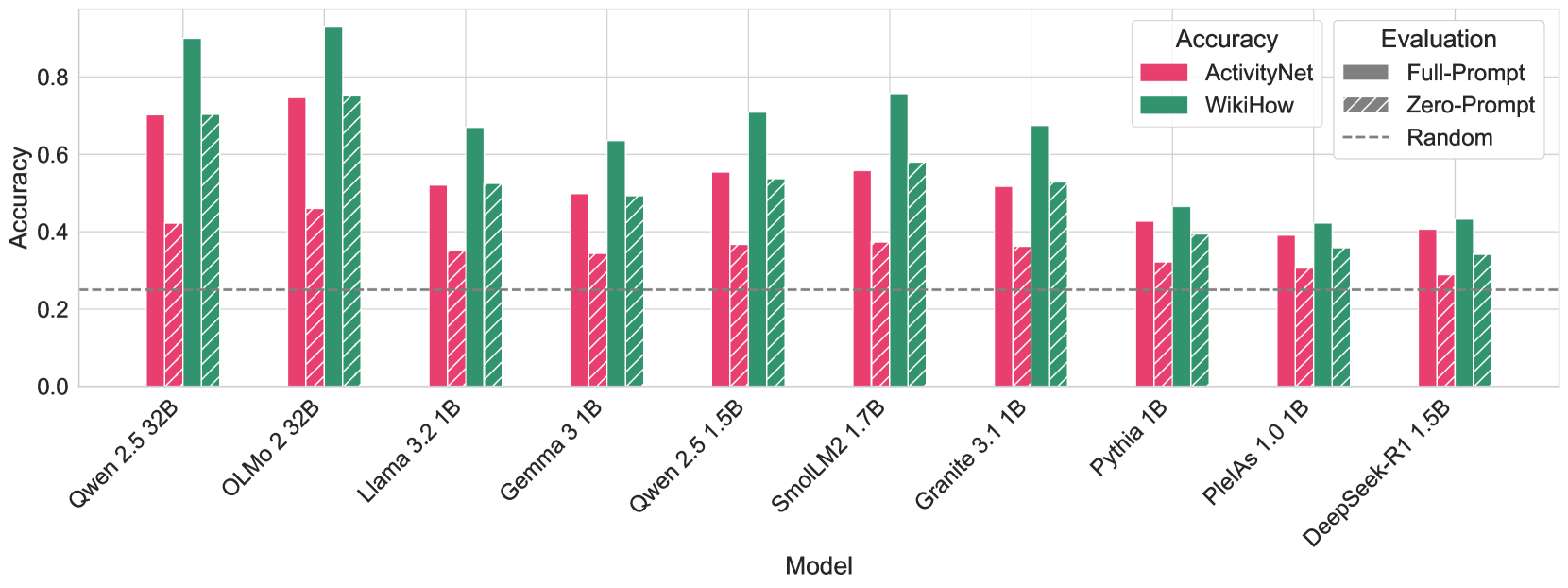## Appendix F Accuracy by Source <details> <summary>x8.png Details</summary>  ### Visual Description ## Grouped Bar Chart: Model Accuracy Comparison on ActivityNet and WikiHow Datasets ### Overview The image is a grouped bar chart comparing the accuracy of ten different language models on two datasets: ActivityNet and WikiHow. Each model's performance is shown under two evaluation conditions: "Full-Prompt" and "Zero-Prompt." A dashed line indicates a "Random" baseline accuracy. ### Components/Axes * **X-Axis (Horizontal):** Labeled "Model." It lists ten specific language models. From left to right: 1. Qwen 2.5 32B 2. OLMo 2 32B 3. Llama 3.2 1B 4. Gemma 3 1B 5. Qwen 2.5 1.5B 6. SmolLM2 1.7B 7. Granite 3.1 1B 8. Pythia 1B 9. PleIAs 1.0 1B 10. DeepSeek-R1 1.5B * **Y-Axis (Vertical):** Labeled "Accuracy." The scale runs from 0.0 to approximately 0.9, with major gridlines at 0.0, 0.2, 0.4, 0.6, and 0.8. * **Legend (Top-Right):** * **Accuracy (Color):** * Pink/Red bars represent the **ActivityNet** dataset. * Green/Teal bars represent the **WikiHow** dataset. * **Evaluation (Pattern):** * Solid bars represent **Full-Prompt** evaluation. * Diagonally hatched bars represent **Zero-Prompt** evaluation. * A dashed grey line represents the **Random** baseline. * **Baseline:** A horizontal dashed grey line is positioned at an accuracy of approximately **0.25**, labeled "Random" in the legend. ### Detailed Analysis For each model, there are four bars: two for ActivityNet (Full-Prompt solid, Zero-Prompt hatched) and two for WikiHow (Full-Prompt solid, Zero-Prompt hatched). Values are approximate visual estimates. 1. **Qwen 2.5 32B:** * *Trend:* Strong performance, with WikiHow scores notably higher than ActivityNet. Full-Prompt outperforms Zero-Prompt on both datasets. * *Values:* ActivityNet Full-Prompt ~0.70, Zero-Prompt ~0.42. WikiHow Full-Prompt ~0.90, Zero-Prompt ~0.70. 2. **OLMo 2 32B:** * *Trend:* Highest overall performance on the chart. WikiHow Full-Prompt is the tallest bar. Similar pattern to Qwen 2.5 32B. * *Values:* ActivityNet Full-Prompt ~0.75, Zero-Prompt ~0.46. WikiHow Full-Prompt ~0.92, Zero-Prompt ~0.75. 3. **Llama 3.2 1B:** * *Trend:* Moderate performance. WikiHow scores are higher than ActivityNet. The gap between Full-Prompt and Zero-Prompt is smaller than for the larger models. * *Values:* ActivityNet Full-Prompt ~0.52, Zero-Prompt ~0.35. WikiHow Full-Prompt ~0.67, Zero-Prompt ~0.52. 4. **Gemma 3 1B:** * *Trend:* Similar profile to Llama 3.2 1B, with slightly lower scores. * *Values:* ActivityNet Full-Prompt ~0.50, Zero-Prompt ~0.34. WikiHow Full-Prompt ~0.63, Zero-Prompt ~0.49. 5. **Qwen 2.5 1.5B:** * *Trend:* Performance is between the 1B and 32B models of its family. Clear advantage for WikiHow and Full-Prompt. * *Values:* ActivityNet Full-Prompt ~0.55, Zero-Prompt ~0.37. WikiHow Full-Prompt ~0.71, Zero-Prompt ~0.54. 6. **SmolLM2 1.7B:** * *Trend:* Notably strong performance for its size, especially on WikiHow Full-Prompt. * *Values:* ActivityNet Full-Prompt ~0.56, Zero-Prompt ~0.37. WikiHow Full-Prompt ~0.76, Zero-Prompt ~0.58. 7. **Granite 3.1 1B:** * *Trend:* Moderate performance, consistent with other 1B-class models. * *Values:* ActivityNet Full-Prompt ~0.52, Zero-Prompt ~0.36. WikiHow Full-Prompt ~0.68, Zero-Prompt ~0.53. 8. **Pythia 1B:** * *Trend:* Lower performance tier. The gap between datasets and prompt methods is less pronounced. * *Values:* ActivityNet Full-Prompt ~0.43, Zero-Prompt ~0.32. WikiHow Full-Prompt ~0.47, Zero-Prompt ~0.39. 9. **PleIAs 1.0 1B:** * *Trend:* Among the lowest performing models shown. Scores are clustered closer together. * *Values:* ActivityNet Full-Prompt ~0.39, Zero-Prompt ~0.31. WikiHow Full-Prompt ~0.42, Zero-Prompt ~0.36. 10. **DeepSeek-R1 1.5B:** * *Trend:* Similar performance level to PleIAs 1.0 1B. * *Values:* ActivityNet Full-Prompt ~0.41, Zero-Prompt ~0.29. WikiHow Full-Prompt ~0.43, Zero-Prompt ~0.34. ### Key Observations * **Dataset Difficulty:** For every single model, accuracy on the **WikiHow** dataset (green bars) is higher than on the **ActivityNet** dataset (pink bars). This suggests WikiHow is an easier task for these models. * **Prompting Effect:** For every model and both datasets, **Full-Prompt** evaluation (solid bars) yields higher accuracy than **Zero-Prompt** evaluation (hatched bars). The performance drop from Full-Prompt to Zero-Prompt is generally more severe for the larger, higher-performing models. * **Model Scale:** The two largest models (Qwen 2.5 32B and OLMo 2 32B) significantly outperform all the smaller models (1B-1.7B range). * **Random Baseline:** All models perform above the random baseline of ~0.25, even under Zero-Prompt conditions. * **Outlier:** SmolLM2 1.7B shows particularly strong performance for its size class, especially on WikiHow with Full-Prompt, rivaling some scores from the much larger 32B models. ### Interpretation This chart demonstrates two clear, consistent trends in language model evaluation: 1. **Task Dependency:** Model performance is highly dependent on the specific dataset or task. The systematic advantage on WikiHow suggests it may involve more structured or common-knowledge procedural text compared to ActivityNet, which likely involves more complex, real-world video-based activity understanding. 2. **Prompt Sensitivity:** Providing a full prompt significantly boosts accuracy across the board. The larger performance drop for bigger models when moving to Zero-Prompt might indicate they are better at leveraging provided context, and thus suffer more when that context is removed. The data suggests that for these procedural understanding tasks, both the choice of model scale and the evaluation setup (prompting strategy) are critical factors. The consistent hierarchy (WikiHow > ActivityNet, Full-Prompt > Zero-Prompt) provides a reliable benchmark for comparing these models. The strong showing of SmolLM2 1.7B is notable, indicating that architecture or training data can sometimes compensate for smaller parameter count. </details> Figure 7: Accuracy of the models evaluated with log-likelihood maximization split by the source of questions. In Figure 7, we show the differences in accuracies by question sources. ActivityNet part of the data, which is a suspect for lower-quality questions in HellaSwag, is more challenging to the models. However, taking all our results into account, this complexity is not a compelling benchmark feature, but rather low-quality data that produces unwanted noise in the scores. Interestingly, the zero-prompt accuracy drop in ActivityNet is also larger than that for the WikiHow. One of the reasons for this might be that WikiHow has generally longer options, from which it is easier to get a general understanding of the situation. ## Appendix G GoldenSwag In Table 7, we present the complete set of stages used for the filtering of the HellaSwag validation set, which consists of 10042 questions. For each filter, we report the number of questions in HellaSwag that fit the filtering criterion, the number of questions that we actually remove at this stage (that were not removed in previous stages), and the number of questions that are left in HellaSwag after each filtering stage. | Toxic content | 6 | 6 | 10036 | | --- | --- | --- | --- | | Nonsense or ungrammatical prompt | 4065 | 4064 | 5972 | | Nonsense or ungrammatical correct answer | 711 | 191 | 5781 | | Ungrammatical incorrect answers | 3953 | 1975 | 3806 | | Wrong answer | 370 | 89 | 3717 | | All options are nonsense | 409 | 23 | 3694 | | Multiple correct options | 2121 | 583 | 3111 | | Relative length difference $>0.3$ | 802 | 96 | 3015 | | Length difference $\in(0.15,0.3]$ and longest is correct | 1270 | 414 | 2601 | | Zero-prompt core $\geq 0.3$ | 3963 | 1076 | 1525 | Table 7: Filtering steps for the GoldenSwag subset. For each filter, we report the number of questions fitting for the filter (# to remove), the number of questions actually removed at this stage (# removed), and the number of questions left in the HellaSwag validation set after this stage (# left). After the filtering, almost all of the questions are sourced from WikiHow — 1498 (98.2%), which further proves that the ActivityNet part of the data contains mostly problematic examples with poor grammar and language choices, mostly attributed to artifacts from synthetic generation by a model that does not meet modern standards.