## Scaling Laws for Native Multimodal Models
Mustafa Shukor 2
Enrico Fini 1
Victor Guilherme Turrisi da Costa 1
Matthieu Cord 2
Joshua Susskind 1
Alaaeldin El-Nouby 1
1 Apple
2 Sorbonne University
## Abstract
Building general-purpose models that can effectively perceive the world through multimodal signals has been a long-standing goal. Current approaches involve integrating separately pre-trained components, such as connecting vision encoders to LLMs and continuing multimodal training. While such approaches exhibit remarkable sample efficiency, it remains an open question whether such late-fusion architectures are inherently superior. In this work, we revisit the architectural design of native multimodal models (NMMs)-those trained from the ground up on all modalities-and conduct an extensive scaling laws study, spanning 457 trained models with different architectures and training mixtures. Our investigation reveals no inherent advantage to late-fusion architectures over early-fusion ones, which do not rely on image encoders or tokenizers. On the contrary, early-fusion exhibits stronger performance at lower parameter counts, is more efficient to train, and is easier to deploy. Motivated by the strong performance of the early-fusion architectures, we show that incorporating Mixture of Experts (MoEs) allows models to learn modality-specific weights, significantly benefiting performance. 10 18 2 3 Validation Loss
## 1. Introduction
Multimodality provides a rich signal for perceiving and understanding the world. Advances in vision [23, 52, 55, 80] and language models [3, 19, 67] have enabled the development of powerful multimodal models that understand language, images, and audio. A common approach involves grafting separately pre-trained unimodal models, such as connecting a vision encoder to the input layer of an LLM [6, 9, 35, 43, 62, 64, 73, 78].
Although this seems like a convenient approach, it remains an open question whether such late-fusion strategies are inherently optimal for understanding multimodal signals. Moreover, with abundant multimodal data available, initializing from unimodal pre-training is potentially detrimental, as it may introduce biases that prevent the model
<details>
<summary>Image 1 Details</summary>
### Visual Description
## Chart: Validation Loss and N/D vs. FLOPs
### Overview
The image presents two line charts comparing the performance of "Early," "Late," and "MoE" models. The top chart shows Validation Loss as a function of FLOPs (Floating Point Operations Per Second), while the bottom chart shows the ratio N/D as a function of FLOPs. Both charts use a logarithmic scale for the x-axis (FLOPs).
### Components/Axes
**Top Chart:**
* **Y-axis:** "Validation Loss" (linear scale, range approximately 2 to 4)
* **X-axis:** "FLOPs" (logarithmic scale, range 10^18 to 10^24)
* **Legend (top-right):**
* Orange dotted line: "Early: L ∝ C^-0.0492"
* Blue dotted line: "Late: L ∝ C^-0.0494"
* Green dotted line: "MoE: L ∝ C^-0.0474"
**Bottom Chart:**
* **Y-axis:** "N/D" (linear scale, range approximately 0 to 4 * 10^-2)
* **X-axis:** "FLOPs" (logarithmic scale, range 10^18 to 10^24)
* **Legend (top-right):**
* Orange dotted line: "Early: N/D ∝ C^0.053"
* Blue dotted line: "Late: N/D ∝ C^0.076"
* Green dotted line: "MoE: N/D ∝ C^-0.312"
### Detailed Analysis
**Top Chart (Validation Loss vs. FLOPs):**
* **Early (Orange):** The validation loss decreases as FLOPs increase. At 10^18 FLOPs, the validation loss is approximately 3.7. At 10^24 FLOPs, the validation loss is approximately 2.0.
* **Late (Blue):** The validation loss decreases as FLOPs increase. At 10^18 FLOPs, the validation loss is approximately 3.6. At 10^24 FLOPs, the validation loss is approximately 2.0.
* **MoE (Green):** The validation loss decreases as FLOPs increase. At 10^18 FLOPs, the validation loss is approximately 3.5. At 10^24 FLOPs, the validation loss is approximately 1.9.
**Bottom Chart (N/D vs. FLOPs):**
* **Early (Orange):** The N/D ratio increases as FLOPs increase. At 10^18 FLOPs, the N/D ratio is approximately 0.012. At 10^24 FLOPs, the N/D ratio is approximately 0.018.
* **Late (Blue):** The N/D ratio increases as FLOPs increase. At 10^18 FLOPs, the N/D ratio is approximately 0.014. At 10^24 FLOPs, the N/D ratio is approximately 0.028.
* **MoE (Green):** The N/D ratio decreases as FLOPs increase. At 10^18 FLOPs, the N/D ratio is approximately 0.048. At 10^24 FLOPs, the N/D ratio is approximately 0.001.
### Key Observations
* In the top chart, all three models ("Early," "Late," and "MoE") show a decrease in validation loss as FLOPs increase, indicating improved performance with more computation.
* In the bottom chart, the "Early" and "Late" models show an increase in the N/D ratio as FLOPs increase, while the "MoE" model shows a significant decrease in the N/D ratio as FLOPs increase.
* The "MoE" model has the lowest validation loss at higher FLOPs.
### Interpretation
The charts suggest that increasing FLOPs generally leads to a decrease in validation loss for all three models, indicating better model performance. However, the behavior of the N/D ratio differs significantly between the "MoE" model and the "Early" and "Late" models. The decreasing N/D ratio for the "MoE" model as FLOPs increase could indicate a more efficient use of computational resources or a different scaling behavior compared to the other models. The "MoE" model appears to be the most effective in reducing validation loss at higher FLOPs, suggesting it may be a more scalable architecture for this particular task. The relationships L ∝ C^-0.0492, L ∝ C^-0.0494, L ∝ C^-0.0474, N/D ∝ C^0.053, N/D ∝ C^0.076, and N/D ∝ C^-0.312 describe the power-law scaling of Validation Loss (L) and N/D with respect to FLOPs (C) for each model.
</details>
C
-
C
-
C
.
-
.
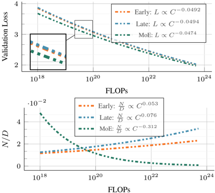
Figure 1. Scaling properties of Native Multimodal Models. Based on the scaling laws study in § 3.1, we observe: (1) early and late fusion models provide similar validation loss L when trained with the same compute budget C (FLOPs); (2) This performance is achieved via a different trade-off between parameters N and number of training tokens D , where early-fusion models requires fewer parameters. (3) Sparse early-fusion models achieve lower loss and require more training tokens for a given FLOP budget.
from fully leveraging cross-modality co-dependancies. An additional challenge is scaling such systems; each component (e.g., vision encoder, LLM) has its own set of hyperparameters, pre-training data mixtues, and scaling properties with respect to the amount of data and compute applied. A more flexible architecture might allow the model to dynamically allocate its capacity across modalities, simplifying scaling efforts.
In this work, we focus on the scaling properties of native multimodal models trained from the ground up on multimodal data. We first investigate whether the commonly adopted late-fusion architectures hold an intrinsic advantage by comparing them to early-fusion models, which process raw multimodal inputs without relying on dedicated vision encoders. We conduct scaling experiments on early and late fusion architectures, deriving scaling laws to pre-
.
dict their performance and compute-optimal configurations. Our findings indicate that late fusion offers no inherent advantage when trained from scratch. Instead, early-fusion models are more efficient and are easier to scale. Furthermore, we observe that native multimodal models follow scaling laws similar to those of LLMs [26], albeit with slight variations in scaling coefficients across modalities and datasets. Our results suggest that model parameters and training tokens should be scaled roughly equally for optimal performance. Moreover, we find that different multimodal training mixtures exhibit similar overall trends, indicating that our findings are likely to generalize to a broader range of settings.
While our findings favor early fusion, multimodal data is inherently heterogeneous, suggesting that some degree of parameter specialization may still offer benefits. To investigate this, we explore leveraging Mixture of Experts (MoEs) [59], a technique that enables the model to dynamically allocate specialized parameters across modalities in a symmetric and parallel manner, in contrast to late-fusion models, which are asymmetric and process data sequentially. Training native multimodal models with MoEs results in significantly improved performance and therefore, faster convergence. Our scaling laws for MoEs suggest that scaling number of training tokens is more important than the number of active parameters. This unbalanced scaling is different from what is observed for dense models, due to the higher number of total parameters for sparse models. In addition, Our analysis reveals that experts tend to specialize in different modalities, with this specialization being particularly prominent in the early and last layers.
## 1.1. Summary of our findings
Our findings can be summarized as follows:
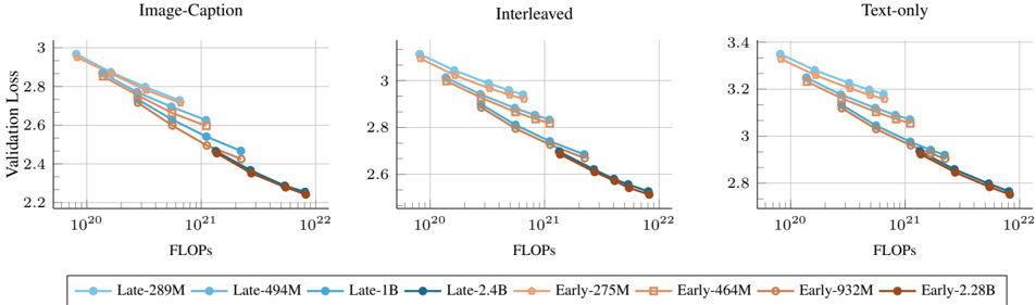
Native Early and Late fusion perform on par: Early fusion models trained from scratch perform on par with their late-fusion counterparts, with a slight advantage to earlyfusion models for low compute budgets (Figure 3). Furthermore, our scaling laws study indicates that the computeoptimal models for early and late fusion perform similarly as the compute budget increases (Figure 1 Top).
NMMs scale similarly to LLMs: The scaling laws of native multimodal models follow similar laws as text-only LLMs with slightly varying scaling exponents depending on the target data type and training mixture (Table 2).
Late-fusion requires more parameters: Computeoptimal late-fusion models require a higher parameters-todata ratio when compared to early-fusion (Figure 1 bottom). Sparsity significantly benefits early-fusion NMMs: Sparse NMMs exhibit significant improvements compared to their dense counterparts at the same inference cost (Figure 10). Furthermore, they implicitly learn modalityspecific weights when trained with sparsity (Figure 12). In
Table 1. Definitions of the expressions used throughout the paper.
| Expression | Definition |
|--------------|-------------------------------------------------------------------------------------------------------------------|
| N | Number of parameters in the multimodal decoder. For MoEs this refers to the active parameters only. |
| D | Total number of multimodal tokens. |
| N v | Number of parameters in the vision-specific encoder. Only exists in late-fusion architectures. |
| D v | Number of vision-only tokens. |
| C | Total number of FLOPs, estimated as C = 6 ND for early-fusion and C = 6( N v D v + ND ) for late-fusion. |
| L | Validation loss measured as the average over interleaved image- text, image-caption, and text-only data mixtures. |
addition, compute-optimal models rely more on scaling the number of training tokens than the number of active parameters as the compute-budget grows (Figure 1 Bottom).
Modality-agnostic routing beats Modality-aware routing for Sparse NMMs: Training sparse mixture of experts with modality-agnostic routing consistently outperforms models with modality-aware routing (Figure 11).
## 2. Preliminaries
## 2.1. Definitions
Native Multimodal Models (NMMs): Models that are trained from scratch on all modalities simultaneously without relying on pre-trained LLMs or vision encoders. Our focus is on the representative image and text modalities, where the model processes both text and images as input and generates text as output.
Early fusion: Enabling multimodal interaction from the beginning, using almost no modality-specific parameters ( e.g ., except a linear layer to patchify images). Using a single transformer model, this approach processes raw multimodal input-tokenized text and continuous image patches-with no image discretization. In this paper, we refer to the main transformer as the decoder.
Late fusion: Delaying the multimodal interaction to deeper layers, typically after separate unimodal components has processed that process each modality independently (e.g., a vision encoder connected to a decoder).
Modality-agnostic routing: In sparse mixture-of-experts, modality-agnostic routing refers to relying on a learned router module that is trained jointly with the model.
Modality-aware routing: Routing based on pre-defined rules such as routing based on the modality type ( e.g ., vision-tokens, token-tokens).
## 2.2. Scaling Laws
We aim to understand the scaling properties of NMMs and how different architectural choices influence trade-offs. To this end, we analyze our models within the scaling laws framework proposed by Hoffmann et al. [26], Kaplan et al. [31]. We compute FLOPs based on the total number of parameters, using the approximation C = 6 ND , as adopted in prior work [2, 26]. However, we modify this estimation to suit our setup: for late-fusion models, FLOPs is computed
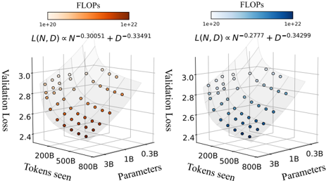
Figure 2. Scaling laws for early-fusion and late-fusion native multimodal models. Each point represents a model (300M to 3B parameters) trained on varying number of tokens (250M to 400B). We report the average cross-entropy loss on the validation sets of interleaved (Obelics), Image-caption (HQITP), and text-only data (DCLM).
<details>
<summary>Image 2 Details</summary>
### Visual Description
## 3D Scatter Plots: Validation Loss vs. Tokens Seen and Parameters
### Overview
The image presents two 3D scatter plots, each visualizing the relationship between validation loss, tokens seen, and the number of parameters. The plots differ in the exponents used in the formula L(N, D) ∝ N^exponent + D^exponent, and the color of the data points represents the FLOPs (Floating Point Operations per second).
### Components/Axes
**Left Plot:**
* **X-axis:** Tokens seen, labeled with values 200B, 500B, 800B, and 3B.
* **Y-axis:** Validation Loss, ranging from 2.4 to 3.0.
* **Z-axis:** Parameters, labeled with values 0.3B, 1B, and 3B.
* **Color Legend (Top-Left):** FLOPs, ranging from 1e+20 (light orange) to 1e+22 (dark orange).
* **Formula:** L(N, D) ∝ N^-0.30051 + D^-0.33491
**Right Plot:**
* **X-axis:** Tokens seen, labeled with values 200B, 500B, 800B, and 3B.
* **Y-axis:** Validation Loss, ranging from 2.4 to 3.0.
* **Z-axis:** Parameters, labeled with values 0.3B, 1B, and 3B.
* **Color Legend (Top-Right):** FLOPs, ranging from 1e+20 (light blue) to 1e+22 (dark blue).
* **Formula:** L(N, D) ∝ N^-0.2777 + D^-0.34299
### Detailed Analysis
**Left Plot (Orange):**
* **Trend:** The validation loss generally decreases as both tokens seen and parameters increase, forming a curved surface.
* **Data Points:**
* At 200B tokens seen and 0.3B parameters, validation loss ranges from approximately 2.8 to 3.0 (light orange, lower FLOPs).
* At 3B tokens seen and 3B parameters, validation loss is approximately 2.4 to 2.6 (dark orange, higher FLOPs).
* The lowest validation loss values (darkest orange) are clustered towards the higher tokens seen and higher parameter values.
**Right Plot (Blue):**
* **Trend:** Similar to the left plot, the validation loss decreases as both tokens seen and parameters increase.
* **Data Points:**
* At 200B tokens seen and 0.3B parameters, validation loss ranges from approximately 2.8 to 3.0 (light blue, lower FLOPs).
* At 3B tokens seen and 3B parameters, validation loss is approximately 2.4 to 2.6 (dark blue, higher FLOPs).
* The lowest validation loss values (darkest blue) are clustered towards the higher tokens seen and higher parameter values.
### Key Observations
* Both plots show a similar trend: increasing tokens seen and parameters leads to lower validation loss.
* The color gradient indicates that higher FLOPs are generally associated with lower validation loss, especially at higher tokens seen and parameter values.
* The exponents in the formulas for L(N, D) are slightly different between the two plots, which may contribute to subtle differences in the shape of the curved surface and the distribution of data points.
### Interpretation
The plots demonstrate the relationship between model size (parameters), training data size (tokens seen), computational cost (FLOPs), and model performance (validation loss). The data suggests that increasing both the size of the model and the amount of training data generally leads to improved performance, as indicated by the lower validation loss. The color gradient further suggests that achieving lower validation loss often requires higher computational cost (FLOPs). The difference in exponents between the two plots could represent different optimization strategies or model architectures, leading to slightly different trade-offs between model size, data size, and computational cost.
</details>
as 6( N v D v + ND ) . We consider a setup where, given a compute budget C , our goal is to predict the model's final performance, as well as determine the optimal number of parameters or number of training tokens. Consistent with prior studies on LLM scaling [26], we assume a power-law relationship between the final model loss and both model size ( N ) and training tokens ( D ):
<!-- formula-not-decoded -->
Here, E represents the lowest achievable loss on the dataset, while A N α captures the effect of increasing the number of parameters, where a larger model leads to lower loss, with the rate of improvement governed by α . Similarly, B D β accounts for the benefits of a higher number of tokens, with β determining the rate of improvement. Additionally, we assume a linear relationship between compute budget (FLOPs) and both N and D ( C ∝ ND ). This further leads to power-law relationships detailed in Appendix C.7.
## 2.3. Experimental setup
Our models are based on the autoregressive transformer architecture [71] with SwiGLU FFNs [58] and QK-Norm [17] following Li et al. [39]. In early-fusion models, image patches are linearly projected to match the text token dimension, while late-fusion follows the CLIP architecture [55]. We adopt causal attention for text tokens and bidirectional attention for image tokens, we found this to work better. Training is conducted on a mixture of public and private multimodal datasets, including DCLM [39], Obelics [34], DFN [21], COYO [11], and a private collection of HighQuality Image-Text Pairs (HQITP). Images are resized to 224×224 resolution with a 14×14 patch size. We use a context length of 1k for the multimodal sequences. For training efficiency, we train our models with bfloat16 , Fully Sharded Data Parallel (FSDP) [82], activation checkpointing, and gradient accumulation. We also use se-
Table 2. Scaling laws for native multimodal models . We report the scaling laws results for early and late fusion models. We fit the scaling laws for different target data types as well as their average loss (A VG).
| L = E + A N α + B D β | N ∝ C a | N ∝ C a | D ∝ C b | D ∝ C b | L ∝ C c | L ∝ C c | D ∝ N d | D ∝ N d |
|--------------------------|---------------|-----------|-----------|-----------|-----------|-----------|-----------|---------------|
| Model | Data | E | α | β | a | b | c | d |
| GPT3 [10] | Text | - | - | - | - | - | -0.048 | |
| Chinchilla [26] | Text | 1.693 | 0.339 | 0.285 | 0.46 | 0.54 | - | |
| NMM(early-fusion) | Text | 2.222 | 0.3084 | 0.3375 | 0.5246 | 0.4774 | -0.0420 | 0.9085 0.9187 |
| | Image-Caption | 1.569 | 0.3111 | 0.3386 | 0.5203 | 0.4785 | -0.0610 | |
| | Interleaved | 1.966 | 0.2971 | 0.338 | 0.5315 | 0.4680 | -0.0459 | 0.8791 |
| | AVG | 1.904 | 0.301 | 0.335 | 0.5262 | 0.473 | -0.0492 | 0.8987 |
| NMM(late-fusion) | AVG | 1.891 | 0.2903 | 0.3383 | 0.6358 | 0.4619 | -0.0494 | 0.6732 |
| Sparse NMM(early-fusion) | AVG | 2.158 | 0.710 | 0.372 | 0.361 | 0.656 | -0.047 | 1.797 |
quence packing for the image captioning dataset to reduce the amount of padded tokens. Similar to previous works [2, 5, 26], we evaluate performance on held-out subsets of interleaved (Obelics), Image-caption (HQITP), and text-only data (DCLM). Further implementation details are provided in Appendix A.
## 3. Scaling native multimodal models
In this section, we present a scaling laws study of native multimodal models, examining various architectural choices § 3.1, exploring different data mixtures § 3.2, analyzing the practical trade-offs between late and early fusion NMMs, and comparing the performance of native pretraining and continual pre-training of NMMs § 3.3.
Setup. We train models ranging from 0.3B to 4B active parameters, scaling the width while keeping the depth constant. For smaller training token budgets, we reduce the warm-up phase to 1K steps while maintaining 5K steps for larger budgets. Following H¨ agele et al. [25], models are trained with a constant learning rate, followed by a cooldown phase using an inverse square root scheduler. The cool-down phase spans 20% of the total steps spent at the constant learning rate. To estimate the scaling coefficients in Eq 1, we apply the L-BFGS algorithm [51] and Huber loss [28] (with δ = 10 -3 ), performing a grid search over initialization ranges.
## 3.1. Scaling laws of NMMs
Scaling laws for early-fusion and late-fusion models. Figure 2 (left) presents the final loss averaged across interleaved, image-caption, and text datasets for early-fusion NMMs. The lowest-loss frontier follows a power law as a function of FLOPs. Fitting the power law yields the expression L ∝ C -0 . 049 , indicating the rate of improvement with increasing compute. When analyzing the scaling laws per data type ( e.g ., image-caption, interleaved, text), we observe that the exponent varies (Table 2). For instance, the model achieves a higher rate of improvement for image-
Figure 3. Early vs late fusion: scaling training FLOPs. We compare early and late fusion models when scaling both the number of model parameters and the number of training tokens. Overall, early fusion shows a slight advantage, especially at smaller model sizes, and the gap decreases when scaling the number of parameters N .
<details>
<summary>Image 3 Details</summary>
### Visual Description
## Line Charts: Validation Loss vs. FLOPs for Different Input Types
### Overview
The image presents three line charts comparing the validation loss of different models against the number of floating-point operations (FLOPs) used during training. The charts are titled "Image-Caption", "Interleaved", and "Text-only", representing different input types used for training. Each chart displays multiple lines, each representing a different model size, with the model sizes ranging from 275M to 2.4B parameters. The x-axis represents FLOPs on a logarithmic scale, and the y-axis represents validation loss.
### Components/Axes
* **Titles:**
* Left Chart: "Image-Caption"
* Middle Chart: "Interleaved"
* Right Chart: "Text-only"
* **X-axis (Horizontal):**
* Label: "FLOPs"
* Scale: Logarithmic, with markers at 10^20, 10^21, and 10^22.
* **Y-axis (Vertical):**
* Label: "Validation Loss"
* Scale: Linear.
* Left Chart: Ranges from 2.2 to 3.0, with tick marks at intervals of 0.2.
* Middle Chart: Ranges from 2.6 to 3.4, with tick marks at intervals of 0.2.
* Right Chart: Ranges from 2.8 to 3.4, with tick marks at intervals of 0.2.
* **Legend (Bottom):**
* "Late-289M" (light blue, circle marker)
* "Late-494M" (light blue, square marker)
* "Late-1B" (light blue, no marker)
* "Late-2.4B" (dark blue, circle marker)
* "Early-275M" (light orange, circle marker)
* "Early-464M" (light orange, square marker)
* "Early-932M" (light orange, no marker)
* "Early-2.28B" (brown, circle marker)
### Detailed Analysis
**General Trend:** All lines in all three charts show a downward trend, indicating that validation loss decreases as the number of FLOPs increases. This suggests that the models generally improve with more training.
**Image-Caption Chart:**
* **Late-289M (light blue, circle):** Starts at approximately 2.9 and decreases to around 2.3.
* **Late-494M (light blue, square):** Starts at approximately 2.9 and decreases to around 2.3.
* **Late-1B (light blue, no marker):** Starts at approximately 2.8 and decreases to around 2.3.
* **Late-2.4B (dark blue, circle):** Starts at approximately 2.7 and decreases to around 2.3.
* **Early-275M (light orange, circle):** Starts at approximately 2.9 and decreases to around 2.3.
* **Early-464M (light orange, square):** Starts at approximately 2.8 and decreases to around 2.3.
* **Early-932M (light orange, no marker):** Starts at approximately 2.7 and decreases to around 2.3.
* **Early-2.28B (brown, circle):** Starts at approximately 2.7 and decreases to around 2.2.
**Interleaved Chart:**
* **Late-289M (light blue, circle):** Starts at approximately 3.1 and decreases to around 2.6.
* **Late-494M (light blue, square):** Starts at approximately 3.0 and decreases to around 2.6.
* **Late-1B (light blue, no marker):** Starts at approximately 3.0 and decreases to around 2.6.
* **Late-2.4B (dark blue, circle):** Starts at approximately 2.9 and decreases to around 2.6.
* **Early-275M (light orange, circle):** Starts at approximately 3.1 and decreases to around 2.6.
* **Early-464M (light orange, square):** Starts at approximately 3.0 and decreases to around 2.6.
* **Early-932M (light orange, no marker):** Starts at approximately 2.9 and decreases to around 2.6.
* **Early-2.28B (brown, circle):** Starts at approximately 2.9 and decreases to around 2.5.
**Text-only Chart:**
* **Late-289M (light blue, circle):** Starts at approximately 3.3 and decreases to around 2.9.
* **Late-494M (light blue, square):** Starts at approximately 3.3 and decreases to around 2.9.
* **Late-1B (light blue, no marker):** Starts at approximately 3.2 and decreases to around 2.9.
* **Late-2.4B (dark blue, circle):** Starts at approximately 3.1 and decreases to around 2.9.
* **Early-275M (light orange, circle):** Starts at approximately 3.3 and decreases to around 2.9.
* **Early-464M (light orange, square):** Starts at approximately 3.2 and decreases to around 2.9.
* **Early-932M (light orange, no marker):** Starts at approximately 3.1 and decreases to around 2.9.
* **Early-2.28B (brown, circle):** Starts at approximately 3.0 and decreases to around 2.8.
### Key Observations
* The "Text-only" chart generally shows higher validation loss values compared to the "Image-Caption" and "Interleaved" charts, suggesting that models trained solely on text data perform worse than those trained with image and caption data.
* The "Image-Caption" chart shows the lowest validation loss values, indicating that this input type leads to the best model performance.
* The "Early-2.28B" model (brown line) consistently achieves the lowest validation loss across all three charts, suggesting that larger models trained early in the process perform better.
* The validation loss decreases more rapidly in the beginning and then plateaus as FLOPs increase, indicating diminishing returns from additional training.
### Interpretation
The data suggests that incorporating image information into the training process (as seen in "Image-Caption" and "Interleaved" charts) leads to better model performance compared to using text data alone ("Text-only" chart). The "Image-Caption" input type appears to be the most effective. Furthermore, larger models (like "Early-2.28B") tend to achieve lower validation loss, indicating better generalization. The diminishing returns observed with increasing FLOPs suggest that there is a point beyond which additional training provides minimal improvement in validation loss. The "Early" vs "Late" training regime seems to have a significant impact, with "Early" models generally performing better, especially the largest one.
</details>
caption data ( L ∝ C -0 . 061 ) when compared to interleaved documents ( L ∝ C -0 . 046 ).
To model the loss as a function of the number of training tokens D and model parameters N , we fit the parametric function in Eq 1, obtaining scaling exponents α = 0 . 301 and β = 0 . 335 . These describe the rates of improvement when scaling the number of model parameters and training tokens, respectively. Assuming a linear relationship between compute, N , and D ( i.e ., C ∝ ND ), we derive the law relating model parameters to the compute budget (see Appendix C for details). Specifically, for a given compute budget C , we compute the corresponding model size N at logarithmically spaced D values and determine N opt , the parameter count that minimizes loss. Repeating this across different FLOPs values produces a dataset of ( C, N opt ) , to which we fit a power law predicting the compute-optimal model size as a function of compute: N ∗ ∝ C 0 . 526 .
Similarly, we fit power laws to estimate the computeoptimal training dataset size as a function of compute and model size:
<!-- formula-not-decoded -->
These relationships allow practitioners to determine the optimal model and dataset size given a fixed compute budget. When analyzing by data type, we find that interleaved data benefits more from larger models ( a = 0 . 532 ) compared to image-caption data ( a = 0 . 520 ), whereas the opposite trend holds for training tokens.
We conduct a similar study on late-fusion models in Figure 2 (right) and observe comparable scaling behaviors. In particular, the loss scaling exponent ( c = -0 . 0494 ) is nearly identical to that of early fusion ( c = -0 . 0492 ). This trend is evident in Figure 3, where early fusion outperforms late fusion at smaller model scales, while both architectures converge to similar performance at larger model sizes. We also observe similar trends when varying late-fusion con-
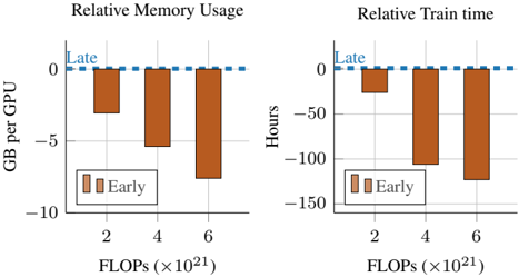
Figure 4. Early vs late: pretraining efficiency. Early-fusion is faster to train and consumes less memory. Models are trained on 16 H100 GPUs for 160k steps (300B tokens).
<details>
<summary>Image 4 Details</summary>
### Visual Description
## Bar Charts: Relative Memory Usage and Relative Train Time
### Overview
The image contains two bar charts comparing "Early" and "Late" training strategies. The left chart shows "Relative Memory Usage" in GB per GPU, while the right chart shows "Relative Train time" in hours. Both charts have FLOPs (x10^21) on the x-axis.
### Components/Axes
**Left Chart: Relative Memory Usage**
* **Title:** Relative Memory Usage
* **Y-axis:** GB per GPU
* Scale: -10 to 0
* Markers: -10, -5, 0
* **X-axis:** FLOPs (x10^21)
* Categories: 2, 4, 6
* **Legend:**
* "Early": Brown bars
* **Horizontal Line:** Dashed blue line at 0, labeled "Late"
**Right Chart: Relative Train time**
* **Title:** Relative Train time
* **Y-axis:** Hours
* Scale: -150 to 0
* Markers: -150, -100, -50, 0
* **X-axis:** FLOPs (x10^21)
* Categories: 2, 4, 6
* **Legend:**
* "Early": Brown bars
* **Horizontal Line:** Dashed blue line at 0, labeled "Late"
### Detailed Analysis
**Left Chart: Relative Memory Usage**
* **Early (Brown Bars):**
* At 2 FLOPs: Approximately -3 GB per GPU
* At 4 FLOPs: Approximately -5.5 GB per GPU
* At 6 FLOPs: Approximately -8 GB per GPU
* Trend: Memory usage decreases (becomes more negative) as FLOPs increase.
**Right Chart: Relative Train time**
* **Early (Brown Bars):**
* At 2 FLOPs: Approximately -30 GB per GPU
* At 4 FLOPs: Approximately -105 GB per GPU
* At 6 FLOPs: Approximately -130 GB per GPU
* Trend: Train time decreases (becomes more negative) as FLOPs increase.
### Key Observations
* In both charts, the "Early" training strategy consistently uses less memory and takes less time than the "Late" strategy (represented by the 0 line).
* The difference between "Early" and "Late" becomes more pronounced as FLOPs increase.
### Interpretation
The charts suggest that the "Early" training strategy is more efficient in terms of both memory usage and training time compared to the "Late" strategy. The efficiency gain of the "Early" strategy increases with higher computational demands (FLOPs). This could be due to the "Early" strategy optimizing resource allocation or convergence speed as the complexity of the training task grows. The data implies that for computationally intensive tasks, adopting the "Early" training strategy could lead to significant resource savings and faster training cycles.
</details>
figurations, such as using a smaller vision encoder with a larger text decoder Appendix B.
Scaling laws of NMMs vs LLMs. Upon comparing the scaling law coefficients of our NMMs to those reported for text-only LLMs ( e.g ., GPT-3, Chinchilla), we find them to be within similar ranges. In particular, for predicting the loss as a function of compute, GPT-3 [10] follows L ∝ C -0 . 048 , while our models follow L ∝ C -0 . 049 , suggesting that the performance of NMMs adheres to similar scaling laws as LLMs. Similarly, our estimates of the α and β parameters in Eq 1 ( α = 0 . 301 , β = 0 . 335 ) closely match those reported by Hoffmann et al. [26] ( α = 0 . 339 , β = 0 . 285 ). Likewise, our computed values of a = 0 . 526 and b = 0 . 473 align closely with a = 0 . 46 and b = 0 . 54 from [26], reinforcing the idea that, for native multimodal models, the number of training tokens and model parameters should be scaled proportionally. However, since the gap between a and b is smaller than in LLMs, this principle holds even more strongly for NMMs. Additionally, as a = 0 . 526 is greater than b = 0 . 473 in our case, the optimal model size for NMMs is larger than that of LLMs,
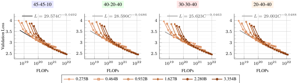
Figure 5. Scaling laws with different training mixtures. Early-fusion models follow similar scaling trends when changing the pretraining mixtures. However, increasing the image captions leads to a higher scaling exponent norm (see Table 3).
<details>
<summary>Image 5 Details</summary>
### Visual Description
## Chart: Validation Loss vs. FLOPs for Different Model Configurations
### Overview
The image presents four line charts comparing validation loss against FLOPs (Floating Point Operations Per Second) for different model configurations. Each chart represents a different configuration, labeled as "45-45-10", "40-20-40", "30-30-40", and "20-40-40". Each chart contains multiple lines, each representing a different model size, ranging from 0.275B to 3.354B parameters. The x-axis (FLOPs) is on a logarithmic scale.
### Components/Axes
* **X-axis:** FLOPs (Floating Point Operations Per Second). Logarithmic scale from approximately 10^19 to 10^22.
* **Y-axis:** Validation Loss. Linear scale from 2.5 to 4.0.
* **Chart Titles (Top):**
* Top-left: "45-45-10" (Blue text)
* Top-middle-left: "40-20-40" (Green text)
* Top-middle-right: "30-30-40" (Pink text)
* Top-right: "20-40-40" (Yellow-Orange text)
* **Legend (Bottom):**
* 0.275B (Light Brown, circle markers)
* 0.464B (Light Brown, square markers)
* 0.932B (Light Brown, diamond markers)
* 1.627B (Brown, triangle markers)
* 2.280B (Dark Brown, circle markers)
* 3.354B (Dark Brown, no marker)
* **Trendline:** Each chart has a black trendline represented by the equation L = aC^-b, where 'L' is the validation loss, 'C' is the FLOPs, and 'a' and 'b' are constants specific to each configuration.
### Detailed Analysis
**Chart 1: 45-45-10**
* Equation: L = 29.574C^-0.0492
* 0.275B: Starts at approximately (10^19, 3.6), decreases to (10^22, 2.6)
* 0.464B: Starts at approximately (10^19, 3.7), decreases to (10^22, 2.7)
* 0.932B: Starts at approximately (10^19, 3.8), decreases to (10^22, 2.7)
* 1.627B: Starts at approximately (10^19, 3.9), decreases to (10^22, 2.8)
* 2.280B: Starts at approximately (10^19, 4.0), decreases to (10^22, 2.8)
* 3.354B: Starts at approximately (10^19, 4.1), decreases to (10^22, 2.9)
**Chart 2: 40-20-40**
* Equation: L = 28.590C^-0.0486
* 0.275B: Starts at approximately (10^19, 3.8), decreases to (10^22, 2.5)
* 0.464B: Starts at approximately (10^19, 3.9), decreases to (10^22, 2.6)
* 0.932B: Starts at approximately (10^19, 4.0), decreases to (10^22, 2.7)
* 1.627B: Starts at approximately (10^19, 4.1), decreases to (10^22, 2.8)
* 2.280B: Starts at approximately (10^19, 4.2), decreases to (10^22, 2.9)
* 3.354B: Starts at approximately (10^19, 4.3), decreases to (10^22, 3.0)
**Chart 3: 30-30-40**
* Equation: L = 25.623C^-0.0463
* 0.275B: Starts at approximately (10^19, 3.7), decreases to (10^22, 2.6)
* 0.464B: Starts at approximately (10^19, 3.8), decreases to (10^22, 2.7)
* 0.932B: Starts at approximately (10^19, 3.9), decreases to (10^22, 2.8)
* 1.627B: Starts at approximately (10^19, 4.0), decreases to (10^22, 2.9)
* 2.280B: Starts at approximately (10^19, 4.1), decreases to (10^22, 3.0)
* 3.354B: Starts at approximately (10^19, 4.2), decreases to (10^22, 3.1)
**Chart 4: 20-40-40**
* Equation: L = 29.002C^-0.0488
* 0.275B: Starts at approximately (10^19, 3.8), decreases to (10^22, 2.6)
* 0.464B: Starts at approximately (10^19, 3.9), decreases to (10^22, 2.7)
* 0.932B: Starts at approximately (10^19, 4.0), decreases to (10^22, 2.8)
* 1.627B: Starts at approximately (10^19, 4.1), decreases to (10^22, 2.9)
* 2.280B: Starts at approximately (10^19, 4.2), decreases to (10^22, 3.0)
* 3.354B: Starts at approximately (10^19, 4.3), decreases to (10^22, 3.1)
### Key Observations
* **General Trend:** For all configurations and model sizes, the validation loss decreases as FLOPs increase. The rate of decrease diminishes as FLOPs increase, indicating diminishing returns.
* **Model Size Impact:** Larger models (higher parameter counts) generally exhibit higher validation loss for a given FLOP count, but also tend to achieve lower final validation loss as FLOPs increase significantly.
* **Configuration Impact:** The "45-45-10" configuration appears to have a slightly lower validation loss compared to the other configurations for similar FLOPs and model sizes.
* **Trendline Fit:** The trendlines provide a reasonable approximation of the overall trend, but they do not perfectly capture the behavior of individual model sizes.
### Interpretation
The charts illustrate the relationship between computational effort (FLOPs) and model performance (validation loss) for different model configurations and sizes. The data suggests that increasing FLOPs generally leads to improved model performance, but the benefit diminishes as FLOPs increase. Larger models tend to have higher initial validation loss but can achieve lower final validation loss with sufficient computational resources. The specific configuration "45-45-10" may be more efficient in terms of validation loss compared to the others. The equations provided above each chart, L = aC^-b, are power law models that describe the relationship between validation loss (L) and FLOPs (C). The exponent 'b' indicates the rate at which validation loss decreases with increasing FLOPs. A smaller absolute value of 'b' indicates a slower rate of decrease.
</details>
Table 3. Scaling laws for different training mixtures . Earlyfusion models. C-I-T refer to image-caption, interleaved and text while the optimal number of training tokens is lower, given a fixed compute budget.
| | C-I-T (%) | I/T ratio | E | α | β | a | b | d | c |
|----|-------------|-------------|-------|-------|-------|-------|-------|-------|---------|
| 1 | 45-45-10 | 1.19 | 1.906 | 0.301 | 0.335 | 0.527 | 0.474 | 0.901 | -0.0492 |
| 2 | 40-20-40 | 0.65 | 1.965 | 0.328 | 0.348 | 0.518 | 0.486 | 0.937 | -0.0486 |
| 3 | 30-30-40 | 0.59 | 1.847 | 0.253 | 0.338 | 0.572 | 0.428 | 0.748 | -0.0463 |
| 4 | 20-40-40 | 0.49 | 1.836 | 0.259 | 0.354 | 0.582 | 0.423 | 0.726 | -0.0488 |
Compute-optimal trade-offs for early vs. late fusion NMMs. While late- and early-fusion models reduce loss at similar rates with increasing FLOPs, we observe distinct trade-offs in their compute-optimal models. Specifically, N opt is larger for late-fusion models, whereas D opt is larger for early-fusion models. This indicates that, given a fixed compute budget, late-fusion models require a higher number of parameters, while early-fusion models benefit more from a higher number of training tokens. This trend is also reflected in the lower N opt D opt ∝ C 0 . 053 for early fusion compared to N opt D opt ∝ C 0 . 076 for late fusion. As shown in Figure 1 (bottom), when scaling FLOPs, the number of parameters of early fusion models becomes significantly lower, which is crucial for reducing inference costs and, consequently, lowering serving costs after deployment.
Early-fusion is more efficient to train. We compare the training efficiency of lateand early-fusion architectures. As shown in Figure 4, early-fusion models consume less memory and train faster under the same compute budget. This advantage becomes even more pronounced as compute increases, highlighting the superior training efficiency of early fusion while maintaining comparable performance to late fusion at scale. Notably, for the same FLOPs, latefusion models have a higher parameter count and higher effective depth ( i.e ., additional vision encoder layers alongside decoder layers) compared to early-fusion models.
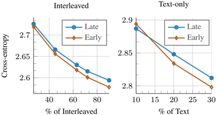
Figure 7. Early vs late fusion: changing the training mixture. Wevary the training mixtures and plot the final training loss. Early fusion models attain a favorable performance when increasing the proportion of interleaved documents and text-only data.
<details>
<summary>Image 6 Details</summary>
### Visual Description
## Line Charts: Cross-Entropy vs. Percentage of Interleaved/Text
### Overview
The image presents two line charts comparing "Late" and "Early" models in terms of cross-entropy. The left chart shows the relationship between cross-entropy and the percentage of interleaved data, while the right chart shows the relationship between cross-entropy and the percentage of text-only data. Both charts display two data series: "Late" and "Early."
### Components/Axes
**Left Chart (Interleaved):**
* **Title:** Interleaved
* **Y-axis:** Cross-entropy
* Scale ranges from approximately 2.58 to 2.78.
* **X-axis:** % of Interleaved
* Scale: 40, 60, 80
* **Legend:** Located in the top-right corner of the chart.
* Blue line with circle markers: Late
* Brown line with diamond markers: Early
**Right Chart (Text-only):**
* **Title:** Text-only
* **Y-axis:** Cross-entropy
* Scale ranges from approximately 2.78 to 2.9.
* **X-axis:** % of Text
* Scale: 10, 20, 30
* **Legend:** Located in the top-right corner of the chart.
* Blue line with circle markers: Late
* Brown line with diamond markers: Early
### Detailed Analysis
**Left Chart (Interleaved):**
* **Late (Blue):** The line slopes downward.
* At 40% Interleaved, Cross-entropy ≈ 2.73
* At 60% Interleaved, Cross-entropy ≈ 2.63
* At 80% Interleaved, Cross-entropy ≈ 2.59
* **Early (Brown):** The line slopes downward.
* At 40% Interleaved, Cross-entropy ≈ 2.66
* At 60% Interleaved, Cross-entropy ≈ 2.62
* At 80% Interleaved, Cross-entropy ≈ 2.57
**Right Chart (Text-only):**
* **Late (Blue):** The line slopes downward.
* At 10% Text, Cross-entropy ≈ 2.88
* At 20% Text, Cross-entropy ≈ 2.85
* At 30% Text, Cross-entropy ≈ 2.80
* **Early (Brown):** The line slopes downward.
* At 10% Text, Cross-entropy ≈ 2.89
* At 20% Text, Cross-entropy ≈ 2.83
* At 30% Text, Cross-entropy ≈ 2.79
### Key Observations
* In both charts, cross-entropy decreases as the percentage of interleaved or text-only data increases.
* The "Early" model generally has a slightly lower cross-entropy than the "Late" model for both interleaved and text-only data.
* The decrease in cross-entropy appears to be more pronounced in the "Text-only" chart compared to the "Interleaved" chart.
### Interpretation
The charts suggest that increasing the percentage of interleaved or text-only data improves the performance of both "Late" and "Early" models, as indicated by the decrease in cross-entropy. The "Early" model seems to perform slightly better than the "Late" model under both conditions. The more significant drop in cross-entropy in the "Text-only" chart might indicate that the models benefit more from increasing the percentage of text-only data compared to interleaved data. This could be due to the nature of the task or the specific characteristics of the models.
</details>
## 3.2. Scaling laws for different data mixtures
We investigate how variations in the training mixture affect the scaling laws of native multimodal models. To this end, we study four different mixtures that reflect common community practices [34, 41, 46, 81], with Image CaptionInterleaved-Text ratios of 45-45-10 (our default setup), 30-30-40 , 40-20-40 , and 20-40-40 . For each mixture, we conduct a separate scaling study by training 76 different models, following our setup in § 3.1. Overall, Figure 5 shows that different mixtures follow similar scaling trends; however, the scaling coefficients vary depending on the mixture (Table 3). Interestingly, increasing the proportion of image-caption data (mixtures 1 and 2) leads to lower a and higher b , whereas increasing the ratio of interleaved and text data (mixtures 3 and 4) have the opposite effect. Notably, image-caption data contains more image tokens than text tokens; therefore, increasing its proportion results in more image tokens, while increasing interleaved and text data increases text token counts. This suggests that, when image tokens are prevalent, training for longer decreases the loss faster than increasing the model size. We also found that for a fixed model size, increasing text-only and interleaved data ratio is in favor of early-fusion Figure 7.
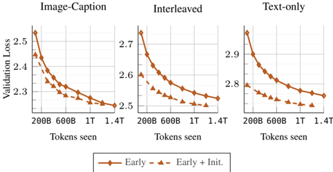
Figure 8. Early native vs initializing from LLMs: initializing from pre-trained models and scaling training tokens. We compare training with and without initializing from DCLM-1B.
<details>
<summary>Image 7 Details</summary>
### Visual Description
## Chart: Validation Loss vs. Tokens Seen for Different Training Methods
### Overview
The image presents three line charts comparing the validation loss of a model trained with different data interleaving methods (Image-Caption, Interleaved, and Text-only) against the number of tokens seen during training. Two training strategies are compared: "Early" and "Early + Init."
### Components/Axes
* **X-axis (horizontal):** "Tokens seen" with markers at 200B, 600B, 1T, and 1.4T.
* **Y-axis (vertical):** "Validation Loss" with a scale ranging from approximately 2.3 to 2.5 for "Image-Caption", 2.5 to 2.7 for "Interleaved", and 2.7 to 2.9 for "Text-only".
* **Titles:** "Image-Caption", "Interleaved", and "Text-only" are the titles for the three charts, respectively.
* **Legend (bottom):**
* Solid brown line with diamond markers: "Early"
* Dashed brown line with triangle markers: "Early + Init."
### Detailed Analysis
**1. Image-Caption Chart:**
* **Early (solid brown line, diamond markers):** The validation loss starts at approximately 2.5 and decreases to about 2.5 over the range of tokens seen.
* 200B: ~2.5
* 600B: ~2.35
* 1T: ~2.27
* 1.4T: ~2.25
* **Early + Init. (dashed brown line, triangle markers):** The validation loss starts at approximately 2.45 and decreases to about 2.25 over the range of tokens seen.
* 200B: ~2.45
* 600B: ~2.3
* 1T: ~2.27
* 1.4T: ~2.25
**2. Interleaved Chart:**
* **Early (solid brown line, diamond markers):** The validation loss starts at approximately 2.7 and decreases to about 2.52 over the range of tokens seen.
* 200B: ~2.72
* 600B: ~2.6
* 1T: ~2.55
* 1.4T: ~2.52
* **Early + Init. (dashed brown line, triangle markers):** The validation loss starts at approximately 2.6 and decreases to about 2.5 over the range of tokens seen.
* 200B: ~2.6
* 600B: ~2.53
* 1T: ~2.5
* 1.4T: ~2.5
**3. Text-only Chart:**
* **Early (solid brown line, diamond markers):** The validation loss starts at approximately 2.92 and decreases to about 2.75 over the range of tokens seen.
* 200B: ~2.92
* 600B: ~2.85
* 1T: ~2.78
* 1.4T: ~2.75
* **Early + Init. (dashed brown line, triangle markers):** The validation loss starts at approximately 2.8 and decreases to about 2.7 over the range of tokens seen.
* 200B: ~2.8
* 600B: ~2.75
* 1T: ~2.72
* 1.4T: ~2.7
### Key Observations
* In all three charts, the "Early" training strategy consistently shows a higher validation loss compared to the "Early + Init." strategy across all token counts.
* The validation loss decreases as the number of tokens seen increases for both training strategies in all three charts.
* The "Text-only" chart exhibits the highest validation loss values compared to the "Image-Caption" and "Interleaved" charts.
* The "Image-Caption" chart exhibits the lowest validation loss values compared to the "Interleaved" and "Text-only" charts.
* The rate of decrease in validation loss diminishes as the number of tokens seen increases, suggesting diminishing returns with more training data.
### Interpretation
The data suggests that initializing the model ("Early + Init.") leads to a lower validation loss compared to training from scratch ("Early"). This indicates that pre-training or using a good initialization point can improve model performance.
The different data interleaving methods ("Image-Caption", "Interleaved", "Text-only") impact the validation loss. "Image-Caption" results in the lowest validation loss, suggesting that incorporating image captions during training is beneficial. "Text-only" results in the highest validation loss, implying that relying solely on text data might not be as effective.
The decreasing validation loss with increasing tokens seen demonstrates that the model learns as it is exposed to more data. However, the diminishing rate of decrease suggests that there is a point of diminishing returns, where adding more training data provides less significant improvements in performance.
The relative performance of the different training methods and data interleaving strategies can inform decisions about how to train the model most effectively.
</details>
## 3.3. Native multimodal pre-training vs . continual training of LLMs
In this section, we compare training natively from scratch to continual training after initializing from a pre-trained LLM. We initialize the model from DCLM-1B [21] that is trained on more than 2T tokens. Figure 8 shows that native multimodal models can close the gap with initialized models when trained for longer. Specifically, on image captioning data, the model requires fewer than 100B multimodal tokens to reach comparable performance. However, on interleaved and text data, the model may need longer training-up to 1T tokens. Considering the cost of pre-training, these results suggest that training natively could be a more efficient approach for achieving the same performance on multimodal benchmarks.
## 4. Towards multimodal specialization
Previously, we demonstrated that early-fusion models achieve performance on par with late-fusion models under a fixed compute budget. However, multimodal data is inherently heterogeneous, and training a unified model to fit such diverse distributions may be suboptimal. Here, we argue for multimodal specialization within a unified architecture. Ideally, the model should implicitly adapt to each modality, for instance, by learning modality-specific weights or specialized experts. Mixture of Experts is a strong candidate for this approach, having demonstrated effectiveness in LLMs. In this section, we highlight the advantages of sparse earlyfusion models over their dense counterparts.
Setup. Our sparse models are based on the dropless-MoE implementation of Gale et al. [24], which eliminates token dropping during training caused by expert capacity constraints. We employ a topk expert-choice routing mechanism, where each token selects its topk experts among the E available experts. Specifically, we set k = 1 and E = 8 , as we find this configuration to work effectively. Additionally, we incorporate an auxiliary load-balancing loss [59] with a weight of 0.01 to ensure a balanced expert utilization.
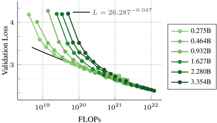
Figure 9. Scaling laws for sparse early-fusion NMMs. We report the final validation loss averaged across interleaved, imagecaptions and text data.
<details>
<summary>Image 8 Details</summary>
### Visual Description
## Log-Log Plot: Validation Loss vs. FLOPs for Varying Model Sizes
### Overview
The image is a log-log plot showing the relationship between validation loss and FLOPs (floating point operations per second) for different model sizes. The plot illustrates how validation loss decreases as FLOPs increase, with different lines representing models of varying sizes (0.275B to 3.354B parameters). A power-law fit is also shown on the plot.
### Components/Axes
* **X-axis:** FLOPs (Floating Point Operations Per Second), logarithmic scale from 10^19 to 10^22.
* **Y-axis:** Validation Loss, linear scale from approximately 2.5 to 4.5.
* **Legend:** Located on the right side of the plot, indicating the model size corresponding to each line color. The model sizes are:
* 0.275B (lightest green)
* 0.464B (light green)
* 0.932B (medium green)
* 1.627B (green)
* 2.280B (dark green)
* 3.354B (darkest green)
* **Power-Law Fit:** A black line representing the power-law fit to the data, with the equation L = 26.287 * FLOPs^(-0.047).
### Detailed Analysis
* **0.275B (lightest green):** Starts at approximately (10^19, 4.2) and decreases to approximately (10^22, 2.5).
* **0.464B (light green):** Starts at approximately (10^19, 3.9) and decreases to approximately (10^22, 2.4).
* **0.932B (medium green):** Starts at approximately (10^19, 3.7) and decreases to approximately (10^22, 2.3).
* **1.627B (green):** Starts at approximately (10^19, 3.5) and decreases to approximately (10^22, 2.2).
* **2.280B (dark green):** Starts at approximately (10^19, 3.3) and decreases to approximately (10^22, 2.1).
* **3.354B (darkest green):** Starts at approximately (10^19, 3.2) and decreases to approximately (10^22, 2.0).
All lines show a decreasing trend, indicating that as FLOPs increase, validation loss decreases. The rate of decrease appears to slow down as FLOPs increase, suggesting diminishing returns.
### Key Observations
* **Trend:** All model sizes exhibit a decreasing validation loss as FLOPs increase.
* **Model Size Impact:** Larger models (higher parameter count) generally have lower validation loss for a given number of FLOPs.
* **Power-Law Fit:** The black line represents a power-law fit to the data, suggesting a relationship of the form L = a * FLOPs^b, where 'a' and 'b' are constants. The equation provided is L = 26.287 * FLOPs^(-0.047).
* **Log-Log Scale:** The use of a log-log scale allows for the visualization of a wide range of FLOPs values and highlights the power-law relationship.
### Interpretation
The plot demonstrates the relationship between model size, computational effort (FLOPs), and validation loss. The data suggests that increasing the model size and/or the number of FLOPs used during training leads to a reduction in validation loss, indicating improved model performance. The power-law fit suggests that there is a predictable relationship between FLOPs and validation loss, which can be used to estimate the expected performance of a model given a certain computational budget. The diminishing returns observed at higher FLOPs suggest that there may be a point beyond which increasing FLOPs yields only marginal improvements in validation loss. The different curves for different model sizes indicate that larger models generally achieve lower validation loss for a given number of FLOPs, highlighting the importance of model size in achieving good performance.
</details>
Following Abnar et al. [2], we compute training FLOPs as 6 ND , where N represents the number of active parameters.
## 4.1. Sparse vs dense NMMs when scaling FLOPs
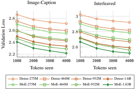
We compare sparse MoE models to their dense counterparts by training models with different numbers of active parameters and varying amounts of training tokens. Figure 10 shows that, under the same inference cost (or number of active parameters), MoEs significantly outperform dense models. Interestingly, this performance gap is more pronounced for smaller model sizes. This suggests that MoEs enable models to handle heterogeneous data more effectively and specialize in different modalities. However, as dense models become sufficiently large, the gap between the two architectures gradually closes.
## 4.2. Scaling laws for sparse early-fusion models
We train different models (ranging from 300M to 3.4B active parameters) on varying amounts of tokens (ranging from 250M to 600B) and report the final loss in Figure 9. We fit a power law to the convex hull of the lowest loss as a function of compute (FLOPs). Interestingly, the exponent ( -0 . 048 ) is close to that of dense NMMs ( -0 . 049 ), indicating that both architectures scale similarly. However, the multiplicative constant is smaller for MoEs ( 27 . 086 ) compared to dense models ( 29 . 574 ), revealing lower loss. Additionally, MoEs require longer training to reach saturation compared to dense models (Appendix C for more details). We also predict the coefficients of Eq 1 by considering N as the number of active parameters. Table 2 shows significantly higher α compared to dense models. Interestingly, b is significantly higher than a , revealing that the training tokens should be scaled at a higher rate than the number of parameters when training sparse NMMs. We also experiment with a scaling law that takes into account the sparsity [2] and reached similar conclusions Appendix C.7.
## 4.3. Modality-aware vs . Modality-agnostic routing
Another alternative to MoEs is modality-aware routing, where multimodal tokens are assigned to experts based on
Figure 10. MoE vs Dense: scaling training FLOPs. We compare MoE and dense early-fusion models when scaling both the amount of training tokens and model sizes. MoEs beat dense models when matching the number of active parameters.
<details>
<summary>Image 9 Details</summary>
### Visual Description
## Chart: Validation Loss vs. Tokens Seen
### Overview
The image presents two line charts comparing the validation loss of different model architectures (Dense and MoE) with varying parameter sizes (275M, 464M, 932M, 1.6B) as a function of the number of tokens seen during training. The left chart is labeled "Image-Caption" and the right chart is labeled "Interleaved". Both charts share the same x and y axes.
### Components/Axes
* **Title (Left Chart):** Image-Caption
* **Title (Right Chart):** Interleaved
* **Y-axis Label:** Validation Loss
* Scale: 2.2 to 3.0, with tick marks at 2.2, 2.4, 2.6, 2.8, and 3.0.
* **X-axis Label:** Tokens seen
* Scale: 100B to 400B, with tick marks at 100B, 200B, 300B, and 400B.
* **Legend (Bottom):**
* Dense-275M (light brown, circle marker)
* Dense-464M (light brown, square marker)
* Dense-932M (light brown, no marker)
* Dense-1.6B (brown, diamond marker)
* MoE-275M (light green, circle marker)
* MoE-464M (light green, square marker)
* MoE-932M (light green, no marker)
* MoE-1.63B (dark green, diamond marker)
### Detailed Analysis
**Image-Caption Chart (Left)**
* **Dense-275M (light brown, circle):** Starts at approximately 2.85 at 100B tokens and decreases to approximately 2.72 at 400B tokens.
* **Dense-464M (light brown, square):** Starts at approximately 2.78 at 100B tokens and decreases to approximately 2.70 at 400B tokens.
* **Dense-932M (light brown, no marker):** Starts at approximately 2.65 at 100B tokens and decreases to approximately 2.58 at 400B tokens.
* **Dense-1.6B (brown, diamond):** Starts at approximately 2.52 at 100B tokens and decreases to approximately 2.42 at 400B tokens.
* **MoE-275M (light green, circle):** Starts at approximately 2.72 at 100B tokens and decreases to approximately 2.60 at 400B tokens.
* **MoE-464M (light green, square):** Starts at approximately 2.65 at 100B tokens and decreases to approximately 2.52 at 400B tokens.
* **MoE-932M (light green, no marker):** Starts at approximately 2.50 at 100B tokens and decreases to approximately 2.38 at 400B tokens.
* **MoE-1.63B (dark green, diamond):** Starts at approximately 2.40 at 100B tokens and decreases to approximately 2.20 at 400B tokens.
**Interleaved Chart (Right)**
* **Dense-275M (light brown, circle):** Starts at approximately 3.00 at 100B tokens and decreases to approximately 2.80 at 400B tokens.
* **Dense-464M (light brown, square):** Starts at approximately 2.88 at 100B tokens and decreases to approximately 2.75 at 400B tokens.
* **Dense-932M (light brown, no marker):** Starts at approximately 2.75 at 100B tokens and decreases to approximately 2.65 at 400B tokens.
* **Dense-1.6B (brown, diamond):** Starts at approximately 2.68 at 100B tokens and decreases to approximately 2.55 at 400B tokens.
* **MoE-275M (light green, circle):** Starts at approximately 2.80 at 100B tokens and decreases to approximately 2.70 at 400B tokens.
* **MoE-464M (light green, square):** Starts at approximately 2.72 at 100B tokens and decreases to approximately 2.60 at 400B tokens.
* **MoE-932M (light green, no marker):** Starts at approximately 2.60 at 100B tokens and decreases to approximately 2.48 at 400B tokens.
* **MoE-1.63B (dark green, diamond):** Starts at approximately 2.50 at 100B tokens and decreases to approximately 2.30 at 400B tokens.
### Key Observations
* In both charts, validation loss generally decreases as the number of tokens seen increases.
* For both Dense and MoE architectures, larger models (higher parameter counts) tend to have lower validation loss.
* The MoE-1.63B model consistently exhibits the lowest validation loss across both charts.
* The "Interleaved" chart generally shows higher validation loss values compared to the "Image-Caption" chart for all models.
### Interpretation
The charts suggest that increasing the number of tokens seen during training improves the validation loss for all models. Furthermore, larger models, particularly the MoE-1.63B model, achieve lower validation loss, indicating better performance. The difference in validation loss between the "Image-Caption" and "Interleaved" charts suggests that the training data distribution or task setup in the "Interleaved" scenario is more challenging, leading to higher loss values. The MoE models generally outperform the Dense models, indicating that the Mixture of Experts architecture is more effective for this task.
</details>
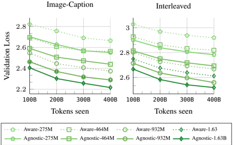
their modalities, similar to previous works [7, 75]. We train models with distinct image and text experts in the form of FFNs, where image tokens are processed only by the image FFN and text tokens only by the text FFN. Compared to modality-aware routing, MoEs exhibit significantly better performance on both image-caption and interleaved data as presented in Figure 11.
## 4.4. Emergence of expert specialization and sharing
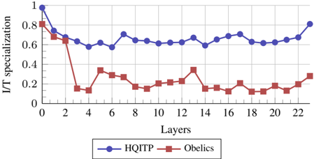
We investigate multimodal specialization in MoE architectures. In Figure 13, we visualize the normalized number of text and image tokens assigned to each expert across layers. To quantify this specialization, we compute a specialization score, defined as the average, across all experts within a layer, of 1 -H ( p ) , where H is the binary entropy of each expert's text/image token distribution. We plot this specialization score in Figure 12. Higher specialization scores indicate a tendency for experts to focus on either text or image tokens, while lower scores indicate a shared behavior. These visualizations provide clear evidence of modalityspecific experts, particularly in the early layers. Furthermore, the specialization score decreases as the number of layers increases, before rising again in the last layers. This suggests that early and final layers exhibit higher modality specialization compared to mid-layers. This behavior is intuitive, as middle layers are expected to hold higherlevel features that may generalize across modalities, and consistent with findings in [61] that shows increasing alignment between modalities across layers. The emergence of both expert specialization and cross-modality sharing in our modality-agnostic MoE, suggests it may be a preferable approach compared to modality-aware sparsity. All data displayed here is from an early-fusion MoE model with 1B active parameters trained for 300B tokens.
Table 4. Supervised finetuning on the LLaVA mixture. All models are native at 1.5B scale and pre-trained on 300B tokens.
| | Accuracy | Accuracy | Accuracy | Accuracy | Accuracy | Accuracy | CIDEr | CIDEr |
|--------------|------------|------------|------------|------------|------------|------------|---------|----------|
| | AVG | VQAv2 | TextVQA | OKVQA | GQA | VizWiz | COCO | TextCaps |
| Late-fusion | 46.8 | 69.4 | 25.8 | 50.1 | 65.8 | 22.8 | 70.7 | 50.9 |
| Early-fusion | 47.6 | 69.3 | 28.1 | 52.1 | 65.4 | 23.2 | 72.0 | 53.8 |
| Early-MoEs | 48.2 | 69.8 | 30.0 | 52.1 | 65.4 | 23.6 | 69.6 | 55.7 |
Figure 11. Modality-aware vs modality agnostic routing for sparse NMMs. We compare modality-agnostic routing with modality-aware routing when scaling both the amount of training tokens and model sizes.
<details>
<summary>Image 10 Details</summary>
### Visual Description
## Line Charts: Validation Loss vs. Tokens Seen
### Overview
The image presents two line charts comparing the validation loss of "Aware" and "Agnostic" models with varying parameter sizes (275M, 464M, 932M, and 1.63B) against the number of tokens seen during training. The left chart is labeled "Image-Caption," and the right chart is labeled "Interleaved." Both charts share the same x and y axes, allowing for a direct comparison of the models' performance under different training conditions.
### Components/Axes
* **Titles:** "Image-Caption" (left chart), "Interleaved" (right chart)
* **Y-axis Label:** "Validation Loss"
* Scale: 2.2 to 2.8 for "Image-Caption", 2.6 to 3.0 for "Interleaved"
* **X-axis Label:** "Tokens seen"
* Scale: 100B, 200B, 300B, 400B
* **Legend:** Located at the bottom of the image.
* Aware-275M (light green, dotted line, circle marker)
* Aware-464M (light green, dotted line, square marker)
* Aware-932M (light green, dotted line, no marker)
* Aware-1.63 (light green, dotted line, diamond marker)
* Agnostic-275M (dark green, solid line, circle marker)
* Agnostic-464M (dark green, solid line, square marker)
* Agnostic-932M (dark green, solid line, no marker)
* Agnostic-1.63B (dark green, solid line, diamond marker)
### Detailed Analysis
#### Image-Caption Chart
* **Aware-275M:** (light green, dotted line, circle marker) Starts at approximately 2.8, decreases to about 2.7 by 400B tokens.
* **Aware-464M:** (light green, dotted line, square marker) Starts at approximately 2.7, decreases to about 2.65 by 400B tokens.
* **Aware-932M:** (light green, dotted line, no marker) Starts at approximately 2.6, decreases to about 2.5 by 400B tokens.
* **Aware-1.63:** (light green, dotted line, diamond marker) Starts at approximately 2.45, decreases to about 2.4 by 400B tokens.
* **Agnostic-275M:** (dark green, solid line, circle marker) Starts at approximately 2.6, decreases to about 2.4 by 400B tokens.
* **Agnostic-464M:** (dark green, solid line, square marker) Starts at approximately 2.5, decreases to about 2.3 by 400B tokens.
* **Agnostic-932M:** (dark green, solid line, no marker) Starts at approximately 2.4, decreases to about 2.25 by 400B tokens.
* **Agnostic-1.63B:** (dark green, solid line, diamond marker) Starts at approximately 2.45, decreases to about 2.2 by 400B tokens.
#### Interleaved Chart
* **Aware-275M:** (light green, dotted line, circle marker) Starts at approximately 3.05, decreases to about 2.9 by 400B tokens.
* **Aware-464M:** (light green, dotted line, square marker) Starts at approximately 2.9, decreases to about 2.8 by 400B tokens.
* **Aware-932M:** (light green, dotted line, no marker) Starts at approximately 2.8, decreases to about 2.7 by 400B tokens.
* **Aware-1.63:** (light green, dotted line, diamond marker) Starts at approximately 2.7, decreases to about 2.6 by 400B tokens.
* **Agnostic-275M:** (dark green, solid line, circle marker) Starts at approximately 2.7, decreases to about 2.5 by 400B tokens.
* **Agnostic-464M:** (dark green, solid line, square marker) Starts at approximately 2.7, decreases to about 2.45 by 400B tokens.
* **Agnostic-932M:** (dark green, solid line, no marker) Starts at approximately 2.6, decreases to about 2.35 by 400B tokens.
* **Agnostic-1.63B:** (dark green, solid line, diamond marker) Starts at approximately 2.65, decreases to about 2.2 by 400B tokens.
### Key Observations
* In both charts, the "Agnostic" models generally exhibit lower validation loss compared to the "Aware" models for a given parameter size.
* Larger parameter sizes (1.63B) tend to result in lower validation loss compared to smaller parameter sizes (275M, 464M, 932M) for both "Aware" and "Agnostic" models.
* The "Interleaved" training method generally results in higher validation loss compared to the "Image-Caption" training method for both "Aware" and "Agnostic" models.
* The validation loss decreases as the number of tokens seen increases for all models and training methods.
### Interpretation
The data suggests that "Agnostic" models are more effective than "Aware" models in terms of validation loss, indicating better generalization performance. Increasing the parameter size of the models also improves performance, as expected. The "Image-Caption" training method appears to be more effective than the "Interleaved" method, possibly due to the nature of the training data or the learning dynamics induced by the different training approaches. The decreasing validation loss with more tokens seen indicates that the models are learning and improving their performance as they are exposed to more data. The "Agnostic-1.63B" model trained with the "Image-Caption" method achieves the lowest validation loss, suggesting it is the most effective configuration among those tested.
</details>
## 5. Evaluation on downstream tasks with SFT
Following previous work on scaling laws, we primarily rely on validation losses. However, we generally find that this evaluation correlates well with performance on downstream tasks. To validate this, we conduct a multimodal instruction tuning stage (SFT) on the LLaVA mixture [43] and report accuracy and CIDEr scores across several VQA and captioning tasks. Table 4 confirms the ranking of different model configurations. Specifically, early fusion outperforms late fusion, and MoEs outperform dense models. However, since the models are relatively small (1.5B scale), trained from scratch, and fine-tuned on a small dataset, the overall scores are lower than the current state of the art. Further implementation details can be found in Appendix A.
## 6. Related work
Large multimodal models. A long-standing research goal has been to develop models capable of perceiving the world through multiple modalities, akin to human sensory experience. Recent progress in vision and language processing has shifted the research focus from smaller, taskspecific models toward large, generalist models that can handle diverse inputs [29, 67]. Crucially, pre-trained vision and language backbones often require surprisingly little adaptation to enable effective cross-modal communication [32, 47, 62, 68, 69]. Simply integrating a vision encoder with either an encoder-decoder architecture [45, 48, 63, 72]
Figure 12. MoE specialization score. Entropy-based image/text specialization score (as described in § 4.4) across layers for two data sources: HQITP and Obelics. HQITP has a more imbalanced image-to-text token distribution, resulting in generally higher specialization. Despite this difference, both data sources exhibit a similar trend: the specialization score decreases in the early layers before increasing again in the final layers.
<details>
<summary>Image 11 Details</summary>
### Visual Description
## Line Chart: I/T Specialization vs. Layers
### Overview
The image is a line chart comparing the I/T specialization of two entities, "HQITP" and "Obelics," across different layers. The x-axis represents the layers, and the y-axis represents the I/T specialization, ranging from 0 to 1.
### Components/Axes
* **X-axis:** "Layers," with numerical markers at 0, 2, 4, 6, 8, 10, 12, 14, 16, 18, 20, and 22.
* **Y-axis:** "I/T specialization," with numerical markers at 0, 0.2, 0.4, 0.6, 0.8, and 1.
* **Legend:** Located at the bottom of the chart.
* Blue line with circular markers: "HQITP"
* Red line with square markers: "Obelics"
### Detailed Analysis
* **HQITP (Blue line, circular markers):**
* Trend: Generally decreasing from layer 0 to layer 4, then relatively stable with minor fluctuations from layer 4 to layer 22.
* Data Points:
* Layer 0: approximately 0.98
* Layer 2: approximately 0.65
* Layer 4: approximately 0.59
* Layer 6: approximately 0.61
* Layer 8: approximately 0.64
* Layer 10: approximately 0.63
* Layer 12: approximately 0.59
* Layer 14: approximately 0.63
* Layer 16: approximately 0.69
* Layer 18: approximately 0.63
* Layer 20: approximately 0.62
* Layer 22: approximately 0.72
* **Obelics (Red line, square markers):**
* Trend: Decreasing sharply from layer 0 to layer 4, then relatively stable with minor fluctuations from layer 4 to layer 22.
* Data Points:
* Layer 0: approximately 0.83
* Layer 2: approximately 0.68
* Layer 4: approximately 0.13
* Layer 6: approximately 0.32
* Layer 8: approximately 0.20
* Layer 10: approximately 0.15
* Layer 12: approximately 0.34
* Layer 14: approximately 0.18
* Layer 16: approximately 0.13
* Layer 18: approximately 0.18
* Layer 20: approximately 0.14
* Layer 22: approximately 0.28
### Key Observations
* HQITP consistently maintains a higher I/T specialization compared to Obelics across all layers.
* Obelics experiences a significant drop in I/T specialization between layers 2 and 4.
* Both HQITP and Obelics show relatively stable I/T specialization after layer 4, with minor fluctuations.
### Interpretation
The chart suggests that HQITP is more specialized than Obelics across the layers examined. The sharp decline in Obelics' I/T specialization between layers 2 and 4 indicates a significant shift or change in its processing or function within those layers. The relatively stable I/T specialization after layer 4 for both entities suggests that their specialization levels reach a steady state after the initial layers. The data could represent the specialization of different neural network architectures or different processing units within a system.
</details>
or a decoder-only LLM has yielded highly capable multimodal systems [1, 6, 9, 13, 16, 35, 43, 49, 64, 73, 78, 83]. This late-fusion approach, where modalities are processed separately before being combined, is now well-understood, with established best practices for training effective models [34, 41, 46, 81]. In contrast, early-fusion models [8, 18, 66], which combine modalities at an earlier stage, remain relatively unexplored, with only a limited number of publicly released models [8, 18]. Unlike [18, 66], our models utilize only a single linear layer and rely exclusively on a nexttoken prediction loss. Furthermore, we train our models from scratch on all modalities without image tokenization.
Native Multimodal Models. We define native multimodal models as those trained from scratch on all modalities simultaneously [67] rather than adapting LLMs to accommodate additional modalities. Due to the high cost of training such models, they remain relatively underexplored, with most relying on late-fusion architectures [27, 79]. Some multimodal models trained from scratch [4, 66, 76] relax this constraint by utilizing pre-trained image tokenizers such as [20, 70] to convert images into discrete tokens, integrating them into the text vocabulary. This approach enables models to understand and generate text and images, facilitating a more seamless multimodal learning process.
Scaling laws. Scaling law studies aim to predict how model performance scales with training compute. Early works [26, 31] found that LLM performance follows a power-law relationship with compute, enabling the compute-optimal estimation of the number of model parameters and training tokens at scale for a given budget. Similar research has extended these findings to sparse Mixture of Experts (MoE) models, considering factors such as sparsity, number of experts, and routing granularity [15, 33, 74]. Scaling laws have also been observed across various domains, including image models [23], video models [56], protein LLMs [14], and imitation learning [54]. However, few stud-
Figure 13. MoE specialization frequency. Percentage of text and image tokens routed to each expert on interleaved data from Obelics. Experts are ordered for better visualization. The first layer shows the highest amount of unimodal experts.
<details>
<summary>Image 12 Details</summary>
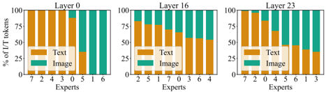
### Visual Description
## Bar Chart: Percentage of Image/Text Tokens by Expert and Layer
### Overview
The image presents three bar charts, each representing a different layer (0, 16, and 23). Each chart shows the percentage of Image and Text tokens for different "Experts" (numbered 0-7). The y-axis represents the percentage of Image/Text tokens, ranging from 0% to 100%. The x-axis represents the different experts.
### Components/Axes
* **Titles:**
* Top-left chart: "Layer 0"
* Top-middle chart: "Layer 16"
* Top-right chart: "Layer 23"
* **Y-axis:** "% of I/T tokens" (ranging from 0 to 100 in increments of 25)
* **X-axis:** "Experts" (categorical, numbered differently for each layer)
* **Legend:** Located within each chart.
* Orange: "Text"
* Teal: "Image"
### Detailed Analysis
**Layer 0**
* Experts (x-axis): 7, 2, 4, 3, 0, 5, 1, 6
* Trend: Experts 7, 2, 4, 3, and 0 are dominated by Text tokens. Experts 5, 1, and 6 are dominated by Image tokens.
* Data Points:
* Expert 7: Text ~100%, Image ~0%
* Expert 2: Text ~100%, Image ~0%
* Expert 4: Text ~100%, Image ~0%
* Expert 3: Text ~100%, Image ~0%
* Expert 0: Text ~90%, Image ~10%
* Expert 5: Text ~30%, Image ~70%
* Expert 1: Text ~0%, Image ~100%
* Expert 6: Text ~0%, Image ~100%
**Layer 16**
* Experts (x-axis): 2, 5, 1, 7, 0, 3, 6, 4
* Trend: Experts 2, 5, 1, 7, 0, 3, 6, and 4 have a mix of Text and Image tokens.
* Data Points:
* Expert 2: Text ~80%, Image ~20%
* Expert 5: Text ~80%, Image ~20%
* Expert 1: Text ~75%, Image ~25%
* Expert 7: Text ~70%, Image ~30%
* Expert 0: Text ~65%, Image ~35%
* Expert 3: Text ~40%, Image ~60%
* Expert 6: Text ~30%, Image ~70%
* Expert 4: Text ~20%, Image ~80%
**Layer 23**
* Experts (x-axis): 7, 2, 0, 4, 5, 6, 1, 3
* Trend: Experts 7, 2, 0, 4, 5, 6, 1, and 3 have a mix of Text and Image tokens.
* Data Points:
* Expert 7: Text ~95%, Image ~5%
* Expert 2: Text ~90%, Image ~10%
* Expert 0: Text ~80%, Image ~20%
* Expert 4: Text ~60%, Image ~40%
* Expert 5: Text ~55%, Image ~45%
* Expert 6: Text ~30%, Image ~70%
* Expert 1: Text ~20%, Image ~80%
* Expert 3: Text ~20%, Image ~80%
### Key Observations
* In Layer 0, some experts are highly specialized in either Text or Image tokens.
* In Layers 16 and 23, the distribution of Text and Image tokens is more balanced across experts.
* The expert order on the x-axis changes between layers.
### Interpretation
The charts illustrate how different "experts" within a model (likely a neural network) process image and text tokens at different layers. Layer 0 shows a clear specialization, with some experts focusing almost exclusively on text and others on images. As the data progresses through the network (Layers 16 and 23), the experts become more balanced in their processing of both types of tokens. This suggests that the model is integrating information from both modalities as it goes deeper. The changing order of experts on the x-axis between layers might indicate a re-organization or re-weighting of expert contributions as the model processes the data.
</details>
ies have investigated scaling laws for multimodal models. Notably, Aghajanyan et al. [5] examined multimodal models that tokenize modalities into discrete tokens and include multimodal generation. In contrast, we focus on studying early-fusion models that take raw multimodal inputs and are trained on interleaved multimodal data.
Mixture of experts (MoEs). MoEs [59] scale model capacity efficiently by sparsely activating parameters, enabling large models with reduced per-sample compute. While widely studied in LLMs [22, 30, 36, 37, 42, 65, 77, 84], MoEs remain underexplored in multimodal settings. Prior work has examined contrastive models [50], late-fusion LLMs [38, 40], and modality-specific experts [7, 12, 60]. We focus on analyzing MoEs in early-fusion multimodal models.
## 7. Limitations
Our study finds that scaling law coefficients are broadly consistent across training mixtures, though a broader exploration is needed to validate this observation. While validation loss scales predictably with compute, the extent to which this correlates with downstream performance remains unclear and warrants further investigation. The accuracy of scaling law predictions improves with higher FLOPs, but their extrapolation to extreme model sizes is still an open question (Appendix D for more details).
## 8. Conclusion
We explore various strategies for compute-optimal pretraining of native multimodal models. We found the NMMs follow similar scaling laws to those of LLMs. Contrary to common belief, we find no inherent advantage in adopting late-fusion architectures over early-fusion ones. While both architectures exhibit similar scaling properties, early-fusion models are more efficient to train and outperform latefusion models at lower compute budgets. Furthermore, we show that sparse architectures encourage modality-specific specialization, leading to performance improvements while maintaining the same inference cost.
## Acknowledgment
We thank Philipp Dufter, Samira Abnar, Xiujun Li, Zhe Gan, Alexander Toshev, Yinfei Yang, Dan Busbridge, and Jason Ramapuram for many fruitful discussions. We thank Denise Hui, and Samy Bengio for infra and compute support. Finally, we thank, Louis B´ ethune, Pierre Ablin, Marco Cuturi, and the MLR team at Apple for their support throughout the project.
## References
- [1] Marah Abdin, Jyoti Aneja, Hany Awadalla, Ahmed Awadallah, Ammar Ahmad Awan, Nguyen Bach, Amit Bahree, Arash Bakhtiari, Jianmin Bao, Harkirat Behl, et al. Phi-3 technical report: A highly capable language model locally on your phone. arXiv preprint arXiv:2404.14219 , 2024. 8
- [2] Samira Abnar, Harshay Shah, Dan Busbridge, Alaaeldin Mohamed Elnouby Ali, Josh Susskind, and Vimal Thilak. Parameters vs flops: Scaling laws for optimal sparsity for mixture-of-experts language models. arXiv preprint arXiv:2501.12370 , 2025. 2, 3, 6, 18, 20
- [3] Josh Achiam, Steven Adler, Sandhini Agarwal, Lama Ahmad, Ilge Akkaya, Florencia Leoni Aleman, Diogo Almeida, Janko Altenschmidt, Sam Altman, Shyamal Anadkat, et al. Gpt-4 technical report. arXiv preprint arXiv:2303.08774 , 2023. 1
- [4] Armen Aghajanyan, Bernie Huang, Candace Ross, Vladimir Karpukhin, Hu Xu, Naman Goyal, Dmytro Okhonko, Mandar Joshi, Gargi Ghosh, Mike Lewis, et al. Cm3: A causal masked multimodal model of the internet. arXiv preprint arXiv:2201.07520 , 2022. 8
- [5] Armen Aghajanyan, Lili Yu, Alexis Conneau, Wei-Ning Hsu, Karen Hambardzumyan, Susan Zhang, Stephen Roller, Naman Goyal, Omer Levy, and Luke Zettlemoyer. Scaling laws for generative mixed-modal language models. In International Conference on Machine Learning , pages 265-279. PMLR, 2023. 3, 8
- [6] Jean-Baptiste Alayrac, Jeff Donahue, Pauline Luc, Antoine Miech, Iain Barr, Yana Hasson, Karel Lenc, Arthur Mensch, Katherine Millican, Malcolm Reynolds, et al. Flamingo: a visual language model for few-shot learning. Advances in neural information processing systems , 35:23716-23736, 2022. 1, 8
- [7] Hangbo Bao, Wenhui Wang, Li Dong, Qiang Liu, Owais Khan Mohammed, Kriti Aggarwal, Subhojit Som, and Furu Wei. Vlmo: Unified vision-language pretraining with mixture-of-modality-experts. arXiv preprint arXiv:2111.02358 , 2021. 7, 8
- [8] Rohan Bavishi, Erich Elsen, Curtis Hawthorne, Maxwell Nye, Augustus Odena, Arushi Somani, and Sa˘ gnak Tas ¸ırlar. Introducing our multimodal models, 2023. 8
- [9] Lucas Beyer, Andreas Steiner, Andr´ e Susano Pinto, Alexander Kolesnikov, Xiao Wang, Daniel Salz, Maxim Neumann, Ibrahim Alabdulmohsin, Michael Tschannen, Emanuele Bugliarello, et al. Paligemma: A versatile 3b vlm for transfer. arXiv preprint arXiv:2407.07726 , 2024. 1, 8
- [10] Tom Brown, Benjamin Mann, Nick Ryder, Melanie Subbiah, Jared D Kaplan, Prafulla Dhariwal, Arvind Neelakantan, Pranav Shyam, Girish Sastry, Amanda Askell, et al. Language models are few-shot learners. Advances in neural information processing systems , 33:1877-1901, 2020. 3, 4
- [11] Minwoo Byeon, Beomhee Park, Haecheon Kim, Sungjun Lee, Woonhyuk Baek, and Saehoon Kim. Coyo700m: Image-text pair dataset. https://github.com/ kakaobrain/coyo-dataset , 2022. 3, 13
- [12] Junyi Chen, Longteng Guo, Jia Sun, Shuai Shao, Zehuan Yuan, Liang Lin, and Dongyu Zhang. Eve: Efficient visionlanguage pre-training with masked prediction and modalityaware moe. In Proceedings of the AAAI Conference on Artificial Intelligence , pages 1110-1119, 2024. 8
- [13] Zhe Chen, Jiannan Wu, Wenhai Wang, Weijie Su, Guo Chen, Sen Xing, Muyan Zhong, Qinglong Zhang, Xizhou Zhu, Lewei Lu, et al. Internvl: Scaling up vision foundation models and aligning for generic visual-linguistic tasks. In Proceedings of the IEEE/CVF Conference on Computer Vision and Pattern Recognition , pages 24185-24198, 2024. 8
- [14] Xingyi Cheng, Bo Chen, Pan Li, Jing Gong, Jie Tang, and Le Song. Training compute-optimal protein language models. bioRxiv , 2024. 8
- [15] Aidan Clark, Diego de Las Casas, Aurelia Guy, Arthur Mensch, Michela Paganini, Jordan Hoffmann, Bogdan Damoc, Blake Hechtman, Trevor Cai, Sebastian Borgeaud, et al. Unified scaling laws for routed language models. In International conference on machine learning , pages 4057-4086. PMLR, 2022. 8
- [16] Wenliang Dai, Nayeon Lee, Boxin Wang, Zhuolin Yang, Zihan Liu, Jon Barker, Tuomas Rintamaki, Mohammad Shoeybi, Bryan Catanzaro, and Wei Ping. Nvlm: Open frontier-class multimodal llms. arXiv preprint arXiv:2409.11402 , 2024. 8
- [17] Mostafa Dehghani, Josip Djolonga, Basil Mustafa, Piotr Padlewski, Jonathan Heek, Justin Gilmer, Andreas Peter Steiner, Mathilde Caron, Robert Geirhos, Ibrahim Alabdulmohsin, et al. Scaling vision transformers to 22 billion parameters. In International Conference on Machine Learning , pages 7480-7512. PMLR, 2023. 3
- [18] Haiwen Diao, Yufeng Cui, Xiaotong Li, Yueze Wang, Huchuan Lu, and Xinlong Wang. Unveiling encoder-free vision-language models. arXiv preprint arXiv:2406.11832 , 2024. 8
- [19] Abhimanyu Dubey, Abhinav Jauhri, Abhinav Pandey, Abhishek Kadian, Ahmad Al-Dahle, Aiesha Letman, Akhil Mathur, Alan Schelten, Amy Yang, Angela Fan, et al. The llama 3 herd of models. arXiv preprint arXiv:2407.21783 , 2024. 1
- [20] Patrick Esser, Robin Rombach, and Bjorn Ommer. Taming transformers for high-resolution image synthesis. In Proceedings of the IEEE/CVF Conference on Computer Vision and Pattern Recognition (CVPR) , pages 12873-12883, 2021. 8
- [21] Alex Fang, Albin Madappally Jose, Amit Jain, Ludwig Schmidt, Alexander Toshev, and Vaishaal Shankar. Data filtering networks. arXiv preprint arXiv:2309.17425 , 2023. 3, 6, 13
- [22] William Fedus, Barret Zoph, and Noam Shazeer. Switch transformers: Scaling to trillion parameter models with simple and efficient sparsity. Journal of Machine Learning Research , 23(120):1-39, 2022. 8
- [23] Enrico Fini, Mustafa Shukor, Xiujun Li, Philipp Dufter, Michal Klein, David Haldimann, Sai Aitharaju, Victor Guilherme Turrisi da Costa, Louis B´ ethune, Zhe Gan, Alexander T Toshev, Marcin Eichner, Moin Nabi, Yinfei Yang, Joshua M. Susskind, and Alaaeldin El-Nouby. Multimodal autoregressive pre-training of large vision encoders, 2024. 1, 8
- [24] Trevor Gale, Deepak Narayanan, Cliff Young, and Matei Zaharia. Megablocks: Efficient sparse training with mixtureof-experts. Proceedings of Machine Learning and Systems , 5:288-304, 2023. 6
- [25] Alexander H¨ agele, Elie Bakouch, Atli Kosson, Loubna Ben Allal, Leandro Von Werra, and Martin Jaggi. Scaling laws and compute-optimal training beyond fixed training durations. arXiv preprint arXiv:2405.18392 , 2024. 3
- [26] Jordan Hoffmann, Sebastian Borgeaud, Arthur Mensch, Elena Buchatskaya, Trevor Cai, Eliza Rutherford, Diego de Las Casas, Lisa Anne Hendricks, Johannes Welbl, Aidan Clark, et al. Training compute-optimal large language models. In Proceedings of the 36th International Conference on Neural Information Processing Systems , pages 3001630030, 2022. 2, 3, 4, 8, 17
- [27] Shaohan Huang, Li Dong, Wenhui Wang, Yaru Hao, Saksham Singhal, Shuming Ma, Tengchao Lv, Lei Cui, Owais Khan Mohammed, Barun Patra, et al. Language is not all you need: Aligning perception with language models. Advances in Neural Information Processing Systems , 36:72096-72109, 2023. 8
- [28] Peter J. Huber. Robust Estimation of a Location Parameter , pages 492-518. Springer New York, New York, NY, 1992. 3
- [29] Aaron Hurst, Adam Lerer, Adam P Goucher, Adam Perelman, Aditya Ramesh, Aidan Clark, AJ Ostrow, Akila Welihinda, Alan Hayes, Alec Radford, et al. Gpt-4o system card. arXiv preprint arXiv:2410.21276 , 2024. 7
- [30] Albert Q Jiang, Alexandre Sablayrolles, Antoine Roux, Arthur Mensch, Blanche Savary, Chris Bamford, Devendra Singh Chaplot, Diego de las Casas, Emma Bou Hanna, Florian Bressand, et al. Mixtral of experts. arXiv preprint arXiv:2401.04088 , 2024. 8
- [31] Jared Kaplan, Sam McCandlish, Tom Henighan, Tom B Brown, Benjamin Chess, Rewon Child, Scott Gray, Alec Radford, Jeffrey Wu, and Dario Amodei. Scaling laws for neural language models. arXiv preprint arXiv:2001.08361 , 2020. 2, 8, 15
- [32] Jing Yu Koh, Ruslan Salakhutdinov, and Daniel Fried. Grounding language models to images for multimodal inputs and outputs. In International Conference on Machine Learning , pages 17283-17300. PMLR, 2023. 7
- [33] Jakub Krajewski, Jan Ludziejewski, Kamil Adamczewski, Maciej Pi´ oro, Michał Krutul, Szymon Antoniak, Kamil Ciebiera, Krystian Kr´ ol, Tomasz Odrzyg´ o´ zd´ z, Piotr Sankowski, et al. Scaling laws for fine-grained mixture of experts. arXiv preprint arXiv:2402.07871 , 2024. 8, 18
- [34] Hugo Laurenc ¸on, Lucile Saulnier, L´ eo Tronchon, Stas Bekman, Amanpreet Singh, Anton Lozhkov, Thomas Wang, Siddharth Karamcheti, Alexander Rush, Douwe Kiela, et al. Obelics: An open web-scale filtered dataset of interleaved image-text documents. Advances in Neural Information Processing Systems , 36, 2024. 3, 5, 8, 13
- [35] Hugo Laurenc ¸on, L´ eo Tronchon, Matthieu Cord, and Victor Sanh. What matters when building vision-language models? arXiv preprint arXiv:2405.02246 , 2024. 1, 8
- [36] Dmitry Lepikhin, HyoukJoong Lee, Yuanzhong Xu, Dehao Chen, Orhan Firat, Yanping Huang, Maxim Krikun, Noam Shazeer, and Zhifeng Chen. Gshard: Scaling giant models with conditional computation and automatic sharding. arXiv preprint arXiv:2006.16668 , 2020. 8
- [37] Mike Lewis, Shruti Bhosale, Tim Dettmers, Naman Goyal, and Luke Zettlemoyer. Base layers: Simplifying training of large, sparse models. In International Conference on Machine Learning , pages 6265-6274. PMLR, 2021. 8
- [38] Dongxu Li, Yudong Liu, Haoning Wu, Yue Wang, Zhiqi Shen, Bowen Qu, Xinyao Niu, Guoyin Wang, Bei Chen, and Junnan Li. Aria: An open multimodal native mixture-ofexperts model. arXiv preprint arXiv:2410.05993 , 2024. 8
- [39] Jeffrey Li, Alex Fang, Georgios Smyrnis, Maor Ivgi, Matt Jordan, Samir Gadre, Hritik Bansal, Etash Guha, Sedrick Keh, Kushal Arora, et al. Datacomp-lm: In search of the next generation of training sets for language models. arXiv preprint arXiv:2406.11794 , 2024. 3, 13, 15
- [40] Bin Lin, Zhenyu Tang, Yang Ye, Jiaxi Cui, Bin Zhu, Peng Jin, Junwu Zhang, Munan Ning, and Li Yuan. Moe-llava: Mixture of experts for large vision-language models. arXiv preprint arXiv:2401.15947 , 2024. 8
- [41] Ji Lin, Hongxu Yin, Wei Ping, Pavlo Molchanov, Mohammad Shoeybi, and Song Han. Vila: On pre-training for visual language models. In Proceedings of the IEEE/CVF Conference on Computer Vision and Pattern Recognition , pages 26689-26699, 2024. 5, 8
- [42] Aixin Liu, Bei Feng, Bing Xue, Bingxuan Wang, Bochao Wu, Chengda Lu, Chenggang Zhao, Chengqi Deng, Chenyu Zhang, Chong Ruan, et al. Deepseek-v3 technical report. arXiv preprint arXiv:2412.19437 , 2024. 8
- [43] Haotian Liu, Chunyuan Li, Yuheng Li, and Yong Jae Lee. Improved baselines with visual instruction tuning. In Proceedings of the IEEE/CVF Conference on Computer Vision and Pattern Recognition , pages 26296-26306, 2024. 1, 7, 8
- [44] Ilya Loshchilov and Frank Hutter. Decoupled weight decay regularization. arXiv preprint arXiv:1711.05101 , 2017. 13
- [45] Jiasen Lu, Christopher Clark, Rowan Zellers, Roozbeh Mottaghi, and Aniruddha Kembhavi. Unified-io: A unified model for vision, language, and multi-modal tasks. In The Eleventh International Conference on Learning Representations , 2022. 7
- [46] Brandon McKinzie, Zhe Gan, Jean-Philippe Fauconnier, Sam Dodge, Bowen Zhang, Philipp Dufter, Dhruti Shah, Xianzhi Du, Futang Peng, Anton Belyi, et al. Mm1: methods, analysis and insights from multimodal llm pre-training. In European Conference on Computer Vision , pages 304-323. Springer, 2025. 5, 8, 13
- [47] Jack Merullo, Louis Castricato, Carsten Eickhoff, and Ellie Pavlick. Linearly mapping from image to text space. In The Eleventh International Conference on Learning Representations , 2023. 7
- [48] David Mizrahi, Roman Bachmann, Oguzhan Kar, Teresa Yeo, Mingfei Gao, Afshin Dehghan, and Amir Zamir. 4m: Massively multimodal masked modeling. Advances in Neural Information Processing Systems , 36:58363-58408, 2023. 7
- [49] Seungwhan Moon, Andrea Madotto, Zhaojiang Lin, Tushar Nagarajan, Matt Smith, Shashank Jain, Chun-Fu Yeh, Prakash Murugesan, Peyman Heidari, Yue Liu, et al. Anymal: An efficient and scalable any-modality augmented language model. In Proceedings of the 2024 Conference on Empirical Methods in Natural Language Processing: Industry Track , pages 1314-1332, 2024. 8
- [50] Basil Mustafa, Carlos Riquelme, Joan Puigcerver, Rodolphe Jenatton, and Neil Houlsby. Multimodal contrastive learning with limoe: the language-image mixture of experts. Advances in Neural Information Processing Systems , 35:95649576, 2022. 8
- [51] Jorge Nocedal. Updating quasi newton matrices with limited storage. Mathematics of Computation , 35(151):951958, 1980. 3
- [52] Maxime Oquab, Timoth´ ee Darcet, Th´ eo Moutakanni, Huy Vo, Marc Szafraniec, Vasil Khalidov, Pierre Fernandez, Daniel Haziza, Francisco Massa, Alaaeldin El-Nouby, et al. Dinov2: Learning robust visual features without supervision. arXiv preprint arXiv:2304.07193 , 2023. 1
- [53] Tim Pearce and Jinyeop Song. Reconciling kaplan and chinchilla scaling laws. arXiv preprint arXiv:2406.12907 , 2024. 15
- [54] Tim Pearce, Tabish Rashid, Dave Bignell, Raluca Georgescu, Sam Devlin, and Katja Hofmann. Scaling laws for pre-training agents and world models. arXiv preprint arXiv:2411.04434 , 2024. 8
- [55] Alec Radford, Jong Wook Kim, Chris Hallacy, Aditya Ramesh, Gabriel Goh, Sandhini Agarwal, Girish Sastry, Amanda Askell, Pamela Mishkin, Jack Clark, et al. Learning transferable visual models from natural language supervision. In International conference on machine learning , pages 8748-8763. PMLR, 2021. 1, 3, 15
- [56] Jathushan Rajasegaran, Ilija Radosavovic, Rahul Ravishankar, Yossi Gandelsman, Christoph Feichtenhofer, and Jitendra Malik. An empirical study of autoregressive pretraining from videos. arXiv preprint arXiv:2501.05453 , 2025. 8
- [57] Kanchana Ranasinghe, Brandon McKinzie, Sachin Ravi, Yinfei Yang, Alexander Toshev, and Jonathon Shlens. Perceptual grouping in contrastive vision-language models. In Proceedings of the IEEE/CVF International Conference on Computer Vision , pages 5571-5584, 2023. 13
- [58] Noam Shazeer. Glu variants improve transformer. arXiv preprint arXiv:2002.05202 , 2020. 3
- [59] Noam Shazeer, Azalia Mirhoseini, Krzysztof Maziarz, Andy Davis, Quoc Le, Geoffrey Hinton, and Jeff Dean. Outrageously large neural networks: The sparsely-gated mixture-
of-experts layer. arXiv preprint arXiv:1701.06538 , 2017. 2, 6, 8
- [60] Sheng Shen, Zhewei Yao, Chunyuan Li, Trevor Darrell, Kurt Keutzer, and Yuxiong He. Scaling vision-language models with sparse mixture of experts. In The 2023 Conference on Empirical Methods in Natural Language Processing , 2023. 8
- [61] Mustafa Shukor and Matthieu Cord. Implicit multimodal alignment: On the generalization of frozen llms to multimodal inputs. Advances in Neural Information Processing Systems , 37:130848-130886, 2024. 7
- [62] Mustafa Shukor, Corentin Dancette, and Matthieu Cord. epalm: Efficient perceptual augmentation of language models. In Proceedings of the IEEE/CVF International Conference on Computer Vision , pages 22056-22069, 2023. 1, 7
- [63] Mustafa Shukor, Corentin Dancette, Alexandre Rame, and Matthieu Cord. Unival: Unified model for image, video, audio and language tasks. Transactions on Machine Learning Research Journal , 2023. 7
- [64] Mustafa Shukor, Dana Aubakirova, Francesco Capuano, Pepijn Kooijmans, Steven Palma, Adil Zouitine, Michel Aractingi, Caroline Pascal, Martino Russi, Andres Marafioti, et al. Smolvla: A vision-language-action model for affordable and efficient robotics. arXiv preprint arXiv:2506.01844 , 2025. 1, 8
- [65] Xingwu Sun, Yanfeng Chen, Yiqing Huang, Ruobing Xie, Jiaqi Zhu, Kai Zhang, Shuaipeng Li, Zhen Yang, Jonny Han, Xiaobo Shu, et al. Hunyuan-large: An open-source moe model with 52 billion activated parameters by tencent. arXiv preprint arXiv:2411.02265 , 2024. 8
- [66] Chameleon Team. Chameleon: Mixed-modal early-fusion foundation models. arXiv preprint arXiv:2405.09818 , 2024. 8
- [67] Gemini Team, Rohan Anil, Sebastian Borgeaud, JeanBaptiste Alayrac, Jiahui Yu, Radu Soricut, Johan Schalkwyk, Andrew M Dai, Anja Hauth, Katie Millican, et al. Gemini: a family of highly capable multimodal models. arXiv preprint arXiv:2312.11805 , 2023. 1, 7, 8
- [68] Maria Tsimpoukelli, Jacob L Menick, Serkan Cabi, SM Eslami, Oriol Vinyals, and Felix Hill. Multimodal few-shot learning with frozen language models. Advances in Neural Information Processing Systems , 34:200-212, 2021. 7
- [69] Th´ eophane Vallaeys, Mustafa Shukor, Matthieu Cord, and Jakob Verbeek. Improved baselines for data-efficient perceptual augmentation of llms. arXiv preprint arXiv:2403.13499 , 2024. 7
- [70] Aaron van den Oord, Oriol Vinyals, and koray kavukcuoglu. Neural discrete representation learning. In Advances in Neural Information Processing Systems . Curran Associates, Inc., 2017. 8
- [71] A Vaswani. Attention is all you need. Advances in Neural Information Processing Systems , 2017. 3
- [72] Peng Wang, An Yang, Rui Men, Junyang Lin, Shuai Bai, Zhikang Li, Jianxin Ma, Chang Zhou, Jingren Zhou, and Hongxia Yang. Ofa: Unifying architectures, tasks, and modalities through a simple sequence-to-sequence learning framework. In International conference on machine learning , pages 23318-23340. PMLR, 2022. 7
- [73] Peng Wang, Shuai Bai, Sinan Tan, Shijie Wang, Zhihao Fan, Jinze Bai, Keqin Chen, Xuejing Liu, Jialin Wang, Wenbin Ge, et al. Qwen2-vl: Enhancing vision-language model's perception of the world at any resolution. arXiv preprint arXiv:2409.12191 , 2024. 1, 8
- [74] Siqi Wang, Zhengyu Chen, Bei Li, Keqing He, Min Zhang, and Jingang Wang. Scaling laws across model architectures: A comparative analysis of dense and MoE models in large language models. In Proceedings of the 2024 Conference on Empirical Methods in Natural Language Processing , pages 5583-5595, Miami, Florida, USA, 2024. Association for Computational Linguistics. 8, 18
- [75] Wenhui Wang, Hangbo Bao, Li Dong, Johan Bjorck, Zhiliang Peng, Qiang Liu, Kriti Aggarwal, Owais Khan Mohammed, Saksham Singhal, Subhojit Som, et al. Image as a foreign language: Beit pretraining for all vision and visionlanguage tasks. arXiv preprint arXiv:2208.10442 , 2022. 7
- [76] Xinlong Wang, Xiaosong Zhang, Zhengxiong Luo, Quan Sun, Yufeng Cui, Jinsheng Wang, Fan Zhang, Yueze Wang, Zhen Li, Qiying Yu, et al. Emu3: Next-token prediction is all you need. arXiv preprint arXiv:2409.18869 , 2024. 8
- [77] Tianwen Wei, Bo Zhu, Liang Zhao, Cheng Cheng, Biye Li, Weiwei L¨ u, Peng Cheng, Jianhao Zhang, Xiaoyu Zhang, Liang Zeng, et al. Skywork-moe: A deep dive into training techniques for mixture-of-experts language models. arXiv preprint arXiv:2406.06563 , 2024. 8
- [78] Le Xue, Manli Shu, Anas Awadalla, Jun Wang, An Yan, Senthil Purushwalkam, Honglu Zhou, Viraj Prabhu, Yutong Dai, Michael S Ryoo, et al. xgen-mm (blip-3): A family of open large multimodal models. arXiv preprint arXiv:2408.08872 , 2024. 1, 8
- [79] Jiahui Yu, Zirui Wang, Vijay Vasudevan, Legg Yeung, Mojtaba Seyedhosseini, and Yonghui Wu. Coca: Contrastive captioners are image-text foundation models. Transactions on Machine Learning Research , 2022. 8
- [80] Xiaohua Zhai, Basil Mustafa, Alexander Kolesnikov, and Lucas Beyer. Sigmoid loss for language image pre-training. In Proceedings of the IEEE/CVF International Conference on Computer Vision , pages 11975-11986, 2023. 1
- [81] Haotian Zhang, Mingfei Gao, Zhe Gan, Philipp Dufter, Nina Wenzel, Forrest Huang, Dhruti Shah, Xianzhi Du, Bowen Zhang, Yanghao Li, et al. Mm1. 5: Methods, analysis & insights from multimodal llm fine-tuning. arXiv preprint arXiv:2409.20566 , 2024. 5, 8
- [82] Yanli Zhao, Andrew Gu, Rohan Varma, Liang Luo, ChienChin Huang, Min Xu, Less Wright, Hamid Shojanazeri, Myle Ott, Sam Shleifer, et al. Pytorch fsdp: experiences on scaling fully sharded data parallel. arXiv preprint arXiv:2304.11277 , 2023. 3
- [83] Deyao Zhu, Jun Chen, Xiaoqian Shen, Xiang Li, and Mohamed Elhoseiny. MiniGPT-4: Enhancing vision-language understanding with advanced large language models. In The Twelfth International Conference on Learning Representations , 2024. 8
- [84] Barret Zoph, Irwan Bello, Sameer Kumar, Nan Du, Yanping Huang, Jeff Dean, Noam Shazeer, and William Fedus. Stmoe: Designing stable and transferable sparse expert models. arXiv preprint arXiv:2202.08906 , 2022. 8
## Scaling Laws for Native Multimodal Models
## Supplementary Material
This supplementary material is organized as follows:
- Appendix A: contains the implementation details and the hyperparameters used to train our models.
- Appendix B: contains detailed comparison between early and late fusion models.
- Appendix C: contains more details about scaling laws derivation, evaluation and additional results.
- Appendix D: contains discussion about the paper limitations.
- Appendix E: contains more results about MoEs and modality specialization.
| Data type | dataset | #samples | sampling prob. |
|---------------|--------------|------------|------------------|
| | DFN [21] | 2B | 27% |
| Image-Caption | COYO [11] | 600M | 11.25% |
| | HQITP[57] | 400M | 6.75% |
| Interleaved | Obelics [34] | 141M Docs | 45% |
| Text | DCLM [39] | 6.6T Toks | 10% |
## A. Experimental setup
In Table 6, we show the pre-training hyperparameters for different model configurations used to derive the scaling laws. The number of parameters ranges from 275M to 3.7B, with model width increasing accordingly, while the depth remains fixed at 24 layers. Learning rates vary by model size, decreasing as the model scales up. Based on empirical experiments and estimates similar to [46], we found these values to be effective in our setup. Training is optimized using a fully decoupled AdamW optimizer with momentum values β 1 = 0 . 9 , β 2 = 0 . 95 , and a weight decay of 1 e -4 . The batch size is set to 2k samples, which account for 2M tokens, given 1k context length. Gradient clipping is set to 1.0, with a maximum warmup duration of 5k iterations, adjusted for shorter training runs: 1k and 2.5k warmup steps for models trained between 1k-4k and 5k-15k steps, respectively. For MoEs, we found that longer warmup is significantly better, so we adopt a 2.5k warmup for all runs under 20k steps. We use a constant learning rate schedule with cooldown during the final 20% of training, gradually reducing to zero following an inverse square root schedule. For vision processing, image inputs are divided into (14 , 14) patches, with augmentations including Random Resized Crop (resizing images to 224px with a scale range of [0.4, 1.0]) and Random Horizontal Flip with a probability of 0.5. We train our models on mixture of interleaved, image captions and text only data Table 5. For late fusion models, we found that using smaller learning rate for the vision encoder significantly boost the performance Table 8, and when both the encoder and decoder are initialized (Appendix B.7) we found that freezing the vision encoder works best Table 7.
Table 5. Pre-training data mixture. Unless otherwise specified, the training mixture contains 45%, 45% and 10% of image captions, interleaved documents and text-only data.
| Early-fusion | | | | | | | |
|-------------------------------------------------------------------------------------------------------------------------|---------------------------------------------------|---------------|---------------|---------------|---------------|---------------|---------------|
| Params width depth | 275M 800 | 468M 1088 | 932M 1632 | 1.63B 2208 24 | 2.28B 2624 | 3.35B 3232 | 3.35B 3232 |
| Learning rate | | | 5e-4 | 4.2e-4 | | 3.5e-4 | 3.5e-4 |
| Late-fusion | 1.5e-3 | 1.5e-3 | | | 4e-4 | | |
| Params vision encoder | | | | | | | |
| width vision encoder depth | 289M 384 | 494M 512 | 1B 768 | 1.75B 1024 | 2.43B 1184 | 3.7B | 3.7B |
| width depth | 768 | 1024 | 1536 | 24 2048 24 | 2464 | 3072 | 3072 |
| Early-fusion MoEs Active Params width | | | 5e-4 | | | | |
| Learning rate | 1.5e-3 | 1.5e-3 | | 4.2e-4 | 3.8e-4 | 3.3e-4 | 3.3e-4 |
| depth | 275M 800 | 468M 1088 | 932M 1632 | 1.63B 2208 24 | 2.28B 2624 | 3.35B 3232 | 3.35B 3232 |
| Learning rate Training tokens Optimizer | 1.5e-3 2.5B-600B decoupled β 1 = 0 . 9 ,β 2 = 0 . | 1.5e-3 | 5e-4 | 4.2e-4 | 4e-4 | 3.5e-4 | 3.5e-4 |
| Optimizer Momentum Minimum Learning rate Weight decay Batch size Patch size Gradient clipping MAximum Warmup iterations | Fully 0 1e-4 | | | | | | |
| | AdamW [44] 95 | AdamW [44] 95 | AdamW [44] 95 | AdamW [44] 95 | AdamW [44] 95 | AdamW [44] 95 | AdamW [44] 95 |
| | 2k 14) | 2k 14) | 2k 14) | 2k 14) | 2k 14) | 2k 14) | 2k 14) |
| | (14, 1.0 | (14, 1.0 | (14, 1.0 | (14, 1.0 | (14, 1.0 | (14, 1.0 | (14, 1.0 |
| | 5k | 5k | 5k | 5k | 5k | 5k | 5k |
| Augmentations: | | | | | | | |
| RandomResizedCrop | | | | | | | |
| | 224px | 224px | 224px | 224px | 224px | 224px | 224px |
| | [0.4, 1.0] | [0.4, 1.0] | [0.4, 1.0] | [0.4, 1.0] | [0.4, 1.0] | [0.4, 1.0] | [0.4, 1.0] |
| size | | | | | | | |
| scale | | | | | | | |
| | p = 0 . 5 | p = 0 . 5 | p = 0 . 5 | p = 0 . 5 | p = 0 . 5 | p = 0 . 5 | p = 0 . 5 |
| RandomHorizontalFlip | | | | | | | |
Table 6. Pre-training hyperparameters We detail the hyperaparmeters used for pre-training different model configurations to derive scaling laws.
Table 7. Vision encoder scaler. Freezing the vision encoder works best when initializing late-fusion models with pre-trained models.
| Vision encoder lr scaler | Interleaved (CE) | Image-Caption (CE) | Text (CE) | AVG (CE) | AVG (SFT) (Acc) |
|----------------------------|--------------------|----------------------|-------------|------------|-------------------|
| 1 | 2.521 | 2.15 | 2.867 | 2.513 | 43.49 |
| 0.1 | 2.502 | 2.066 | 2.862 | 2.477 | 52.27 |
| 0.01 | 2.502 | 2.066 | 2.859 | 2.476 | 53.76 |
| 0.001 | 2.513 | 2.066 | 2.857 | 2.479 | - |
| 0 (frozen) | 2.504 | 2.061 | 2.856 | 2.474 | 54.14 |
<details>
<summary>Image 13 Details</summary>
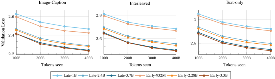
### Visual Description
## Line Charts: Validation Loss vs. Tokens Seen for Different Training Strategies
### Overview
The image presents three line charts comparing the validation loss of different language models as a function of the number of tokens seen during training. The charts are grouped by training strategy: "Image-Caption", "Interleaved", and "Text-only". Each chart displays the performance of six different model configurations, distinguished by color-coded lines. The x-axis represents the number of tokens seen (in billions), and the y-axis represents the validation loss.
### Components/Axes
* **Titles:**
* Top-left chart: "Image-Caption"
* Top-middle chart: "Interleaved"
* Top-right chart: "Text-only"
* **X-axis:** "Tokens seen" with markers at 100B, 200B, 300B, and 400B.
* **Y-axis:** "Validation Loss" with markers ranging from 2.2 to 2.6 for "Image-Caption", 2.6 to 2.8 for "Interleaved", and 2.8 to 3.0 for "Text-only".
* **Legend:** Located at the bottom of the image.
* Light Blue: "Late-1B"
* Tan: "Late-2.4B"
* Dark Blue: "Late-3.7B"
* Light Orange: "Early-932M"
* Orange: "Early-2.28B"
* Brown: "Early-3.3B"
### Detailed Analysis
**Chart 1: Image-Caption**
* **Late-1B (Light Blue):** Starts at approximately 2.62 and decreases to approximately 2.45.
* **Late-2.4B (Tan):** Starts at approximately 2.48 and decreases to approximately 2.30.
* **Late-3.7B (Dark Blue):** Starts at approximately 2.42 and decreases to approximately 2.26.
* **Early-932M (Light Orange):** Starts at approximately 2.45 and decreases to approximately 2.28.
* **Early-2.28B (Orange):** Starts at approximately 2.38 and decreases to approximately 2.25.
* **Early-3.3B (Brown):** Starts at approximately 2.40 and decreases to approximately 2.24.
**Chart 2: Interleaved**
* **Late-1B (Light Blue):** Starts at approximately 2.82 and decreases to approximately 2.70.
* **Late-2.4B (Tan):** Starts at approximately 2.72 and decreases to approximately 2.60.
* **Late-3.7B (Dark Blue):** Starts at approximately 2.65 and decreases to approximately 2.55.
* **Early-932M (Light Orange):** Starts at approximately 2.70 and decreases to approximately 2.60.
* **Early-2.28B (Orange):** Starts at approximately 2.68 and decreases to approximately 2.58.
* **Early-3.3B (Brown):** Starts at approximately 2.65 and decreases to approximately 2.53.
**Chart 3: Text-only**
* **Late-1B (Light Blue):** Starts at approximately 3.05 and decreases to approximately 2.90.
* **Late-2.4B (Tan):** Starts at approximately 2.95 and decreases to approximately 2.80.
* **Late-3.7B (Dark Blue):** Starts at approximately 2.90 and decreases to approximately 2.75.
* **Early-932M (Light Orange):** Starts at approximately 2.92 and decreases to approximately 2.78.
* **Early-2.28B (Orange):** Starts at approximately 2.88 and decreases to approximately 2.75.
* **Early-3.3B (Brown):** Starts at approximately 2.85 and decreases to approximately 2.73.
### Key Observations
* In all three charts, the validation loss decreases as the number of tokens seen increases. This indicates that the models are learning as they are exposed to more data.
* The "Late-1B" model consistently has the highest validation loss across all three training strategies.
* The "Early-3.3B" model generally has the lowest validation loss, indicating better performance.
* The "Text-only" training strategy results in the highest validation loss values compared to "Image-Caption" and "Interleaved".
* The "Image-Caption" training strategy results in the lowest validation loss values compared to "Interleaved" and "Text-only".
### Interpretation
The data suggests that the "Early-3.3B" model configuration is the most effective in terms of minimizing validation loss, regardless of the training strategy used. The "Text-only" training strategy appears to be the least effective, possibly indicating that incorporating image data (as in "Image-Caption" and "Interleaved") improves model performance. The consistent decrease in validation loss with increasing tokens seen confirms the expected learning behavior of the models. The differences in performance between the "Early" and "Late" models, as well as the impact of different training strategies, highlight the importance of model architecture and training data composition in achieving optimal results.
</details>
Figure 14. Early vs late fusion: scaling training FLOPs. We compare early and late fusion models when scaling both the model size and the number of training tokens. The gap decreases mainly due to scaling models size.
Figure 15. Early vs late fusion: changing the training mixture. Wevary the training mixtures and plot the final training loss. Early fusion models become better when increasing the proportion of interleaved documents. Early and late fusion has 1.63B and 1.75B parameters respectively.
<details>
<summary>Image 14 Details</summary>
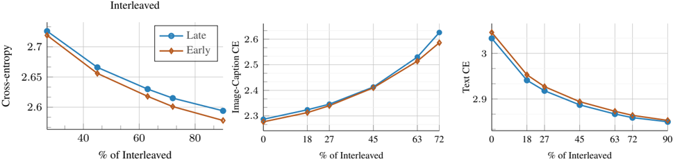
### Visual Description
## Chart: Interleaved Performance Metrics
### Overview
The image presents three line charts comparing the performance of "Late" and "Early" models across varying percentages of interleaved data. The charts depict Cross-entropy, Image-Caption Cross-entropy (CE), and Text Cross-entropy (CE) as a function of the percentage of interleaved data.
### Components/Axes
**General Layout:**
* The image contains three separate line charts arranged horizontally.
* Each chart has a horizontal axis representing "% of Interleaved" and a vertical axis representing a different performance metric.
* A legend in the top-center distinguishes between the "Late" (blue line with circle markers) and "Early" (brown line with diamond markers) models.
**Chart 1: Cross-entropy**
* **Y-axis:** "Cross-entropy" ranging from 2.6 to 2.7. Axis markers at 2.6, 2.65, and 2.7.
* **X-axis:** "% of Interleaved" ranging from 40 to 80. Axis markers at 40, 60, and 80.
* **Legend:** Located at the top-center of the image. "Late" is represented by a blue line with circle markers. "Early" is represented by a brown line with diamond markers.
**Chart 2: Image-Caption CE**
* **Y-axis:** "Image-Caption CE" ranging from 2.3 to 2.6. Axis markers at 2.3, 2.4, 2.5, and 2.6.
* **X-axis:** "% of Interleaved" ranging from 0 to 72. Axis markers at 0, 18, 27, 45, 63, and 72.
* **Legend:** Located at the top-center of the image. "Late" is represented by a blue line with circle markers. "Early" is represented by a brown line with diamond markers.
**Chart 3: Text CE**
* **Y-axis:** "Text CE" ranging from 2.8 to 3.1. Axis markers at 2.9 and 3.
* **X-axis:** "% of Interleaved" ranging from 0 to 90. Axis markers at 0, 18, 27, 45, 63, 72, and 90.
* **Legend:** Located at the top-center of the image. "Late" is represented by a blue line with circle markers. "Early" is represented by a brown line with diamond markers.
### Detailed Analysis
**Chart 1: Cross-entropy**
* **Late (Blue):** The line slopes downward.
* At 40% Interleaved, Cross-entropy is approximately 2.72.
* At 60% Interleaved, Cross-entropy is approximately 2.63.
* At 80% Interleaved, Cross-entropy is approximately 2.61.
* **Early (Brown):** The line slopes downward.
* At 40% Interleaved, Cross-entropy is approximately 2.71.
* At 60% Interleaved, Cross-entropy is approximately 2.65.
* At 80% Interleaved, Cross-entropy is approximately 2.59.
**Chart 2: Image-Caption CE**
* **Late (Blue):** The line slopes upward.
* At 0% Interleaved, Image-Caption CE is approximately 2.29.
* At 18% Interleaved, Image-Caption CE is approximately 2.31.
* At 27% Interleaved, Image-Caption CE is approximately 2.34.
* At 45% Interleaved, Image-Caption CE is approximately 2.41.
* At 63% Interleaved, Image-Caption CE is approximately 2.51.
* At 72% Interleaved, Image-Caption CE is approximately 2.65.
* **Early (Brown):** The line slopes upward.
* At 0% Interleaved, Image-Caption CE is approximately 2.28.
* At 18% Interleaved, Image-Caption CE is approximately 2.31.
* At 27% Interleaved, Image-Caption CE is approximately 2.35.
* At 45% Interleaved, Image-Caption CE is approximately 2.40.
* At 63% Interleaved, Image-Caption CE is approximately 2.53.
* At 72% Interleaved, Image-Caption CE is approximately 2.58.
**Chart 3: Text CE**
* **Late (Blue):** The line slopes downward.
* At 0% Interleaved, Text CE is approximately 3.05.
* At 18% Interleaved, Text CE is approximately 2.94.
* At 27% Interleaved, Text CE is approximately 2.91.
* At 45% Interleaved, Text CE is approximately 2.87.
* At 63% Interleaved, Text CE is approximately 2.84.
* At 72% Interleaved, Text CE is approximately 2.83.
* At 90% Interleaved, Text CE is approximately 2.81.
* **Early (Brown):** The line slopes downward.
* At 0% Interleaved, Text CE is approximately 3.03.
* At 18% Interleaved, Text CE is approximately 2.95.
* At 27% Interleaved, Text CE is approximately 2.90.
* At 45% Interleaved, Text CE is approximately 2.85.
* At 63% Interleaved, Text CE is approximately 2.83.
* At 72% Interleaved, Text CE is approximately 2.82.
* At 90% Interleaved, Text CE is approximately 2.81.
### Key Observations
* For Cross-entropy (Chart 1), both "Late" and "Early" models show a decrease in Cross-entropy as the percentage of interleaved data increases.
* For Image-Caption CE (Chart 2), both "Late" and "Early" models show an increase in Image-Caption CE as the percentage of interleaved data increases.
* For Text CE (Chart 3), both "Late" and "Early" models show a decrease in Text CE as the percentage of interleaved data increases.
* The "Late" and "Early" models perform similarly across all three metrics, with slight variations.
### Interpretation
The charts suggest that interleaving data has a varying impact on different aspects of model performance. As the percentage of interleaved data increases:
* Overall Cross-entropy decreases, which could indicate better overall model performance or generalization.
* Image-Caption CE increases, which might suggest that the model struggles more with image-caption alignment when data is interleaved.
* Text CE decreases, which could indicate improved text processing or understanding.
The similar performance of "Late" and "Early" models suggests that the timing of the model's processing (early vs. late) does not significantly affect its performance in these interleaved scenarios. The specific reasons for these trends would require further investigation into the model architectures and the nature of the interleaved data.
</details>
Table 8. Vision encoder scaler. Reducing the learning rate for the vision encoder is better when training late-fusion models from scratch.
| Vision encoder lr scaler | Interleaved (CE) | Image-Caption (CE) | Text (CE) | AVG (CE) | AVG (SFT) (Acc) |
|----------------------------|--------------------|----------------------|-------------|------------|-------------------|
| 0.1 | 2.674 | 2.219 | 3.072 | 2.655 | 34.84 |
| 0.01 | 2.672 | 2.197 | 3.071 | 2.647 | 38.77 |
| 0.001 | 2.674 | 2.218 | 3.073 | 2.655 | 38.46 |
## B. Late vs early fusion
This section provides additional comparison between early and late fusion models.
## B.1. Scaling FLOPs
Figure 14 compares early-fusion and late-fusion models when scaling FLOPs. Specifically, for each model size, we train multiple models using different amounts of training tokens. The performance gap between the two approaches mainly decreases due to increasing model sizes rather than increasing the number of training tokens. Despite the decreasing gap, across all the models that we train, earlyfusion consistently outperform late-fusion.
## B.2. Changing the training data mixture
Weanalyze how the performance gap between early and late fusion models changes with variations in the training data mixture. As shown in Figure 16 and Figure 15, when fixing the model size, increasing the ratio of text and interleaved data favors early fusion. Interestingly, the gap remains largely unchanged for other data types. We also observe interference effects between different data types. Specifically, increasing the amount of interleaved data negatively impacts performance on image captions and vice versa. Additionally, increasing the proportion of text-only data slightly improves interleaved performance but increases loss on image captions. Overall, we find that text-only and interleaved data are correlated across different setups.
## B.3. Scaling image resolution is in favor of earlyfusion
We examine how both architectures perform with varying image resolution. We fix the number of model parameters to 1.63B and 1.75B for early and late fusion respecively. All models are trained for 100K steps or 200B tokens. Since
Figure 16. Early vs late fusion: changing the amount of text-only data in the training mixture (isoFLOPs). We vary the ratio of text-only data and plot the final training loss. The gap increases with the text data ratio in favor of early fusion model. Early fusion has 1.63B parameters and late fusion 1.75B parameters.
<details>
<summary>Image 15 Details</summary>
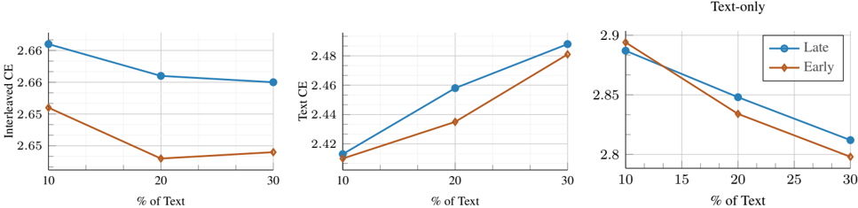
### Visual Description
## Line Charts: Performance Comparison of "Late" and "Early" Strategies
### Overview
The image presents three line charts comparing the performance of "Late" and "Early" strategies across different percentages of text. The charts are titled "Interleaved CE", "Text CE", and "Text-only". Each chart plots the performance metric (CE - Cross Entropy) against the percentage of text, ranging from 10% to 30%. The "Late" strategy is represented by a blue line with circular markers, while the "Early" strategy is represented by a brown line with diamond markers.
### Components/Axes
* **X-axis (all charts):** "% of Text", with tick marks at 10, 20, and 30. The "Text-only" chart has additional tick marks at 15 and 25.
* **Y-axis (left chart):** "Interleaved CE", ranging from approximately 2.65 to 2.66.
* **Y-axis (middle chart):** "Text CE", ranging from approximately 2.42 to 2.48.
* **Y-axis (right chart):** No label, but the chart is titled "Text-only", ranging from approximately 2.8 to 2.9.
* **Legend (top-right of the rightmost chart):**
* Blue line with circular markers: "Late"
* Brown line with diamond markers: "Early"
### Detailed Analysis
**Chart 1: Interleaved CE**
* **Late (Blue):** The line starts at approximately 2.662 at 10% text, decreases to approximately 2.661 at 20% text, and remains relatively constant at approximately 2.660 at 30% text.
* **Early (Brown):** The line starts at approximately 2.652 at 10% text, decreases to approximately 2.648 at 20% text, and increases slightly to approximately 2.649 at 30% text.
**Chart 2: Text CE**
* **Late (Blue):** The line starts at approximately 2.415 at 10% text, increases to approximately 2.458 at 20% text, and continues to increase to approximately 2.480 at 30% text.
* **Early (Brown):** The line starts at approximately 2.410 at 10% text, increases to approximately 2.433 at 20% text, and continues to increase to approximately 2.470 at 30% text.
**Chart 3: Text-only**
* **Late (Blue):** The line starts at approximately 2.890 at 10% text, decreases to approximately 2.850 at 20% text, and continues to decrease to approximately 2.815 at 30% text.
* **Early (Brown):** The line starts at approximately 2.885 at 10% text, decreases to approximately 2.830 at 20% text, and continues to decrease to approximately 2.800 at 30% text.
### Key Observations
* In the "Interleaved CE" chart, the "Late" strategy consistently outperforms the "Early" strategy, although the difference is minimal. Both strategies show a slight decrease in CE as the percentage of text increases.
* In the "Text CE" chart, both strategies show an increasing trend in CE as the percentage of text increases. The "Late" strategy consistently outperforms the "Early" strategy.
* In the "Text-only" chart, both strategies show a decreasing trend in CE as the percentage of text increases. The "Late" strategy consistently outperforms the "Early" strategy.
### Interpretation
The charts compare the performance of "Late" and "Early" strategies under different conditions ("Interleaved CE", "Text CE", and "Text-only") with varying percentages of text. The "Late" strategy generally outperforms the "Early" strategy across all conditions.
* **Interleaved CE:** The slight decrease in CE with increasing text percentage suggests that both strategies benefit marginally from more text when the context is interleaved.
* **Text CE:** The increasing CE with increasing text percentage suggests that both strategies perform better with more text when focusing solely on text-based cross-entropy.
* **Text-only:** The decreasing CE with increasing text percentage suggests that both strategies benefit from more text when the model is trained on text only.
The consistent outperformance of the "Late" strategy suggests that processing text later in the model architecture is generally more effective than processing it early, regardless of the specific condition. The magnitude of the performance difference varies depending on the condition, with the "Text CE" chart showing the most significant difference between the two strategies.
</details>
Figure 17. Early vs late fusion: training with different image resolutions (isoFLOPs). For the same training FLOPs we vary the image resolution (and thus the number of image tokens) during training and report the final training loss. Increasing resolution, hurts the performance on text and interleaved documents, while helping image captioning. The gap stays almost the same on text and interleaved data while slightly increase on image captioning in favor of early fusion.
<details>
<summary>Image 16 Details</summary>
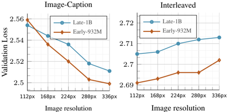
### Visual Description
## Chart Type: Line Graphs Comparing Validation Loss vs. Image Resolution
### Overview
The image presents two line graphs side-by-side, comparing the validation loss of two models, "Late-1B" and "Early-932M," across different image resolutions. The left graph is titled "Image-Caption," and the right graph is titled "Interleaved." Both graphs share the same x-axis (Image resolution) and y-axis (Validation Loss), but display different trends for the two models.
### Components/Axes
* **X-axis (Image resolution):** Categorical axis with values 112px, 168px, 224px, 280px, and 336px.
* **Y-axis (Validation Loss):** Numerical axis.
* Left graph ("Image-Caption"): Ranges from approximately 2.50 to 2.56.
* Right graph ("Interleaved"): Ranges from approximately 2.69 to 2.72.
* **Legend:** Present in both graphs.
* Blue line with circle markers: "Late-1B"
* Brown/Orange line with diamond markers: "Early-932M"
* **Titles:**
* Left graph: "Image-Caption"
* Right graph: "Interleaved"
### Detailed Analysis
**Left Graph ("Image-Caption"):**
* **Late-1B (Blue):** The line slopes downward.
* 112px: Approximately 2.555
* 168px: Approximately 2.545
* 224px: Approximately 2.537
* 280px: Approximately 2.518
* 336px: Approximately 2.512
* **Early-932M (Brown/Orange):** The line slopes downward.
* 112px: Approximately 2.56
* 168px: Approximately 2.537
* 224px: Approximately 2.52
* 280px: Approximately 2.503
* 336px: Approximately 2.498
**Right Graph ("Interleaved"):**
* **Late-1B (Blue):** The line slopes slightly upward.
* 112px: Approximately 2.704
* 168px: Approximately 2.706
* 224px: Approximately 2.712
* 280px: Approximately 2.713
* 336px: Approximately 2.714
* **Early-932M (Brown/Orange):** The line slopes upward.
* 112px: Approximately 2.691
* 168px: Approximately 2.693
* 224px: Approximately 2.696
* 280px: Approximately 2.696
* 336px: Approximately 2.702
### Key Observations
* In the "Image-Caption" scenario, both models exhibit a decrease in validation loss as image resolution increases.
* In the "Interleaved" scenario, both models exhibit an increase in validation loss as image resolution increases, but the increase is more pronounced for "Early-932M."
* The "Early-932M" model has a higher validation loss than the "Late-1B" model at the lowest resolution (112px) in the "Image-Caption" scenario, but the "Early-932M" model has a lower validation loss than the "Late-1B" model at all resolutions in the "Interleaved" scenario.
### Interpretation
The graphs suggest that the performance of the "Late-1B" and "Early-932M" models is affected differently by image resolution depending on the task ("Image-Caption" vs. "Interleaved"). For "Image-Caption," higher resolution images lead to lower validation loss for both models, indicating improved performance. However, for "Interleaved," higher resolution images lead to higher validation loss, suggesting a potential overfitting or difficulty in processing higher resolution images for this specific task. The "Early-932M" model seems to be more sensitive to changes in image resolution in the "Interleaved" scenario compared to the "Late-1B" model. The difference in trends between the two tasks highlights the importance of considering the specific task when evaluating model performance across different image resolutions.
</details>
the patch size remains constant, increasing the resolution results in a higher number of visual tokens. For all resolutions, we maintain the same number of text tokens. As shown in Figure 17, the early-fusion model consistently outperforms the late-fusion model across resolutions, particularly for multimodal data, with the performance gap widening at higher resolutions. Additionally, we observe that the loss on text and interleaved data increases as resolution increases.
## B.4. Early-fusion is consistently better when matching the late-fusion model size
In this section, we compare the late-fusion model with different configurations of early-fusion one. Specifically, we train early-fusion models that match the late-fusion model in total parameters (Params), text model size (Text), and FLOPs (FLOPs), assuming 45-45-10 training mixture. As shown in Figure 18, early fusion consistently outperforms late fusion when normalized by total parameters, followed by normalization by FLOPs. When matching the text model size, early fusion performs better at higher ratios of interleaved data.
## B.5. Different late-fusion configuration
We examine how this scaling changes with different latefusion configurations. Instead of scaling both the vision and text models equally, as done in the main paper, we fix the vision encoder size to 300M and scale only the text model. Figure 19 shows that late-fusion models lag behind at smaller model sizes, with the gap closing significantly as the text model scales. This suggests that allocating more parameters to shared components is more beneficial, further supporting the choice of early-fusion models.
## B.6. Different context lengths
In the paper, we use a 1k context length following [31]. Also following, this paper, we ignore the context length effect, as the model dimension dominates the training compute estimate. Moreover, [53] empirically found that scaling coefficients are robust to context length. Nevertheless, Our initial experiments (Figure 20) indicate that scaling the context length did not significantly affect the comparison between late and early fusion.
## B.7. Initializing from LLM and CLIP
We study the case where both late and early fusion models are initialized from pre-trained models, specifically DCLM1B [39] and CLIP-ViT-L [55] for late fusion. Interestingly, Figure 21 shows that for text and interleaved multimodal documents, early fusion can match the performance of late fusion when trained for longer. However, closing the gap on image caption data remains more challenging. Notably, when considering the overall training cost, including that of pre-trained models, early fusion requires significantly longer training to compensate for the vision encoder's pretraining cost.
<details>
<summary>Image 17 Details</summary>
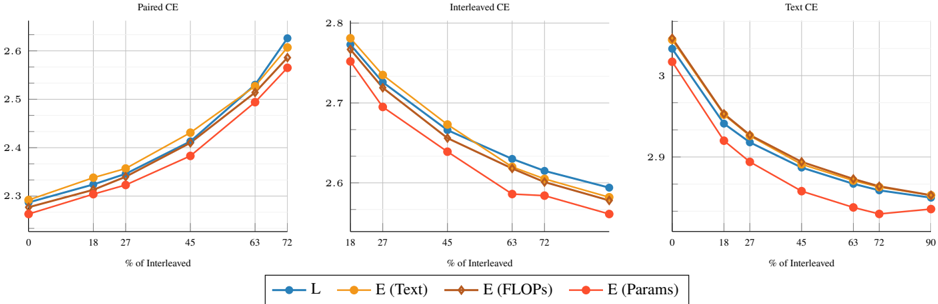
### Visual Description
## Line Charts: Cross Entropy vs. % of Interleaved Data
### Overview
The image presents three line charts comparing the cross-entropy (CE) for different data interleaving strategies. The charts are titled "Paired CE", "Interleaved CE", and "Text CE". Each chart plots the cross-entropy value against the percentage of interleaved data, ranging from 0% to 72% for the first two charts and 0% to 90% for the third. Four different data series are compared: 'L', 'E (Text)', 'E (FLOPs)', and 'E (Params)'.
### Components/Axes
* **Titles:**
* Left Chart: "Paired CE"
* Middle Chart: "Interleaved CE"
* Right Chart: "Text CE"
* **X-axis:** "% of Interleaved"
* Left Chart: Values at 0, 18, 27, 45, 63, 72
* Middle Chart: Values at 18, 27, 45, 63, 72
* Right Chart: Values at 0, 18, 27, 45, 63, 72, 90
* **Y-axis:** Cross Entropy (CE)
* Left Chart: Scale from 2.3 to 2.6
* Middle Chart: Scale from 2.6 to 2.8
* Right Chart: Scale from 2.8 to 3.0
* **Legend:** Located at the bottom of the image.
* Blue line: "L"
* Yellow line: "E (Text)"
* Brown line: "E (FLOPs)"
* Red line: "E (Params)"
### Detailed Analysis
#### Paired CE (Left Chart)
* **L (Blue):** The line slopes upward.
* 0%: ~2.28
* 18%: ~2.32
* 27%: ~2.34
* 45%: ~2.40
* 63%: ~2.50
* 72%: ~2.60
* **E (Text) (Yellow):** The line slopes upward.
* 0%: ~2.29
* 18%: ~2.35
* 27%: ~2.36
* 45%: ~2.44
* 63%: ~2.54
* 72%: ~2.65
* **E (FLOPs) (Brown):** The line slopes upward.
* 0%: ~2.27
* 18%: ~2.31
* 27%: ~2.35
* 45%: ~2.42
* 63%: ~2.52
* 72%: ~2.58
* **E (Params) (Red):** The line slopes upward.
* 0%: ~2.26
* 18%: ~2.30
* 27%: ~2.31
* 45%: ~2.38
* 63%: ~2.50
* 72%: ~2.52
#### Interleaved CE (Middle Chart)
* **L (Blue):** The line slopes downward.
* 18%: ~2.78
* 27%: ~2.74
* 45%: ~2.68
* 63%: ~2.62
* 72%: ~2.60
* **E (Text) (Yellow):** The line slopes downward.
* 18%: ~2.79
* 27%: ~2.75
* 45%: ~2.68
* 63%: ~2.62
* 72%: ~2.60
* **E (FLOPs) (Brown):** The line slopes downward.
* 18%: ~2.76
* 27%: ~2.72
* 45%: ~2.66
* 63%: ~2.59
* 72%: ~2.58
* **E (Params) (Red):** The line slopes downward.
* 18%: ~2.70
* 27%: ~2.68
* 45%: ~2.62
* 63%: ~2.58
* 72%: ~2.54
#### Text CE (Right Chart)
* **L (Blue):** The line slopes downward.
* 0%: ~3.02
* 18%: ~2.95
* 27%: ~2.92
* 45%: ~2.88
* 63%: ~2.86
* 72%: ~2.84
* 90%: ~2.83
* **E (Text) (Yellow):** The line slopes downward.
* 0%: ~3.03
* 18%: ~2.96
* 27%: ~2.93
* 45%: ~2.89
* 63%: ~2.86
* 72%: ~2.84
* 90%: ~2.83
* **E (FLOPs) (Brown):** The line slopes downward.
* 0%: ~3.01
* 18%: ~2.94
* 27%: ~2.91
* 45%: ~2.87
* 63%: ~2.85
* 72%: ~2.83
* 90%: ~2.82
* **E (Params) (Red):** The line slopes downward.
* 0%: ~2.98
* 18%: ~2.88
* 27%: ~2.83
* 45%: ~2.78
* 63%: ~2.75
* 72%: ~2.74
* 90%: ~2.73
### Key Observations
* In the "Paired CE" chart, all lines show an increasing trend in cross-entropy as the percentage of interleaved data increases.
* In the "Interleaved CE" and "Text CE" charts, all lines show a decreasing trend in cross-entropy as the percentage of interleaved data increases.
* The "E (Params)" series (red line) consistently has the lowest cross-entropy values in all three charts, especially as the percentage of interleaved data increases in the "Interleaved CE" and "Text CE" charts.
* The "E (Text)" series (yellow line) and "L" series (blue line) are very close to each other in all three charts.
* The "E (FLOPs)" series (brown line) is generally between the "E (Text)" and "E (Params)" series.
### Interpretation
The charts suggest that interleaving data has different effects on cross-entropy depending on the type of data being considered (Paired, Interleaved, or Text). For "Paired CE", interleaving seems to worsen the cross-entropy, while for "Interleaved CE" and "Text CE", it improves the cross-entropy. The "E (Params)" series consistently performs the best (lowest cross-entropy) as the percentage of interleaved data increases for "Interleaved CE" and "Text CE", indicating that this configuration might be more robust or efficient when dealing with interleaved data. The close proximity of the "E (Text)" and "L" series suggests that these two configurations behave similarly with respect to data interleaving.
</details>
Figure 18. Early vs late fusion: changing the training mixture and early-fusion configuration. We vary the training mixtures and plot the final training loss for different configuration of early fusion models. For the same number of total parameters early fusion consistently outperform late fusion.
<details>
<summary>Image 18 Details</summary>
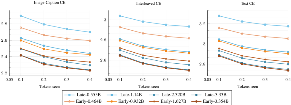
### Visual Description
## Line Charts: Cross Entropy (CE) vs. Tokens Seen for Different Training Strategies
### Overview
The image presents three line charts comparing the cross-entropy (CE) loss against the number of tokens seen during training for different training strategies. The charts are titled "Image-Caption CE," "Interleaved CE," and "Text CE," representing different training data compositions. Each chart plots the CE loss for models trained with "Early" and "Late" strategies, further differentiated by the number of parameters (0.464B to 3.354B). The x-axis represents "Tokens seen," ranging from 0.05 to 0.4, while the y-axis represents the CE loss.
### Components/Axes
* **Titles:**
* Left Chart: Image-Caption CE
* Middle Chart: Interleaved CE
* Right Chart: Text CE
* **X-axis:**
* Label: Tokens seen
* Scale: 0.05, 0.1, 0.2, 0.3, 0.4
* **Y-axis:**
* Left Chart Scale: 2.2, 2.4, 2.6, 2.8
* Middle Chart Scale: 2.6, 2.8, 3
* Right Chart Scale: 2.8, 3, 3.2
* **Legend:** Located at the bottom of the image, applies to all three charts.
* Blue (circle markers): Late-0.555B
* Light Blue (circle markers): Late-1.14B
* Teal (circle markers): Late-2.320B
* Dark Teal (circle markers): Late-3.33B
* Light Orange (diamond markers): Early-0.464B
* Orange (diamond markers): Early-0.932B
* Brown (diamond markers): Early-1.627B
* Dark Brown (diamond markers): Early-3.354B
### Detailed Analysis
**Image-Caption CE (Left Chart):**
* **Late-0.555B (Blue, circle markers):** Decreases from approximately 2.92 at 0.05 tokens to 2.72 at 0.4 tokens.
* **Late-1.14B (Light Blue, circle markers):** Decreases from approximately 2.75 at 0.05 tokens to 2.58 at 0.4 tokens.
* **Late-2.320B (Teal, circle markers):** Decreases from approximately 2.62 at 0.05 tokens to 2.45 at 0.4 tokens.
* **Late-3.33B (Dark Teal, circle markers):** Decreases from approximately 2.5 at 0.05 tokens to 2.3 at 0.4 tokens.
* **Early-0.464B (Light Orange, diamond markers):** Decreases from approximately 2.75 at 0.05 tokens to 2.65 at 0.4 tokens.
* **Early-0.932B (Orange, diamond markers):** Decreases from approximately 2.6 at 0.05 tokens to 2.5 at 0.4 tokens.
* **Early-1.627B (Brown, diamond markers):** Decreases from approximately 2.42 at 0.05 tokens to 2.3 at 0.4 tokens.
* **Early-3.354B (Dark Brown, diamond markers):** Decreases from approximately 2.4 at 0.05 tokens to 2.25 at 0.4 tokens.
**Interleaved CE (Middle Chart):**
* **Late-0.555B (Blue, circle markers):** Decreases from approximately 3.05 at 0.05 tokens to 2.85 at 0.4 tokens.
* **Late-1.14B (Light Blue, circle markers):** Decreases from approximately 2.9 at 0.05 tokens to 2.7 at 0.4 tokens.
* **Late-2.320B (Teal, circle markers):** Decreases from approximately 2.75 at 0.05 tokens to 2.6 at 0.4 tokens.
* **Late-3.33B (Dark Teal, circle markers):** Decreases from approximately 2.65 at 0.05 tokens to 2.5 at 0.4 tokens.
* **Early-0.464B (Light Orange, diamond markers):** Decreases from approximately 2.9 at 0.05 tokens to 2.8 at 0.4 tokens.
* **Early-0.932B (Orange, diamond markers):** Decreases from approximately 2.8 at 0.05 tokens to 2.7 at 0.4 tokens.
* **Early-1.627B (Brown, diamond markers):** Decreases from approximately 2.65 at 0.05 tokens to 2.55 at 0.4 tokens.
* **Early-3.354B (Dark Brown, diamond markers):** Decreases from approximately 2.65 at 0.05 tokens to 2.5 at 0.4 tokens.
**Text CE (Right Chart):**
* **Late-0.555B (Blue, circle markers):** Decreases from approximately 3.3 at 0.05 tokens to 3.1 at 0.4 tokens.
* **Late-1.14B (Light Blue, circle markers):** Decreases from approximately 3.15 at 0.05 tokens to 2.95 at 0.4 tokens.
* **Late-2.320B (Teal, circle markers):** Decreases from approximately 3.0 at 0.05 tokens to 2.85 at 0.4 tokens.
* **Late-3.33B (Dark Teal, circle markers):** Decreases from approximately 2.9 at 0.05 tokens to 2.75 at 0.4 tokens.
* **Early-0.464B (Light Orange, diamond markers):** Decreases from approximately 3.2 at 0.05 tokens to 3.1 at 0.4 tokens.
* **Early-0.932B (Orange, diamond markers):** Decreases from approximately 3.05 at 0.05 tokens to 2.95 at 0.4 tokens.
* **Early-1.627B (Brown, diamond markers):** Decreases from approximately 2.9 at 0.05 tokens to 2.8 at 0.4 tokens.
* **Early-3.354B (Dark Brown, diamond markers):** Decreases from approximately 2.85 at 0.05 tokens to 2.7 at 0.4 tokens.
### Key Observations
* In all three charts, the CE loss decreases as the number of tokens seen increases, indicating that the models are learning.
* For both "Early" and "Late" strategies, models with more parameters (higher B value) generally have lower CE loss, suggesting better performance.
* The "Text CE" chart shows the highest CE loss values, followed by "Interleaved CE," and then "Image-Caption CE," indicating that training on text alone might be more challenging than training with image-caption pairs or interleaved data.
* The "Late" training strategy generally results in higher CE loss compared to the "Early" strategy for the same number of parameters and tokens seen.
### Interpretation
The charts demonstrate the impact of training strategy (Early vs. Late), model size (number of parameters), and training data composition (Image-Caption, Interleaved, Text) on the cross-entropy loss during model training. The consistent downward trend of all lines indicates that the models are learning from the data. The lower CE loss for larger models suggests that increasing model capacity improves performance. The differences in CE loss across the three charts highlight the importance of the training data composition, with image-caption pairs potentially providing a more effective training signal than text alone. The "Late" training strategy's higher CE loss could indicate a slower or less efficient learning process compared to the "Early" strategy.
</details>
Figure 19. Early vs late fusion: scaling training FLOPs while fixing the vision encoder size. We compare early and late fusion models when scaling both the amount of training tokens and model sizes. For late fusion mdoels, we fix the vision encoder size (300M) and scale the text model (250M, 834M, 2B, 3B). The gap between early and late get tighter when scaling the text model.
Figure 20. Early vs late fusion with different context lengths.
<details>
<summary>Image 19 Details</summary>
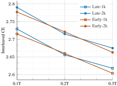
### Visual Description
## Line Chart: Interleaved CE vs. Time
### Overview
The image is a line chart comparing the Interleaved Cross-Entropy (CE) over time for "Early" and "Late" models, each with two different configurations (1k and 2k). The x-axis represents time, and the y-axis represents the Interleaved CE value.
### Components/Axes
* **X-axis:** Time, labeled as "0.1T", "0.2T", and "0.3T".
* **Y-axis:** Interleaved CE, ranging from 2.6 to 2.8 with increments of 0.05.
* **Legend (Top-Right):**
* Blue Square: "Late-1k"
* Blue Circle: "Late-2k"
* Brown Square: "Early-1k"
* Brown Circle: "Early-2k"
### Detailed Analysis
* **Late-1k (Blue Square):**
* Trend: Decreasing.
* Data Points:
* 0.1T: ~2.73
* 0.2T: ~2.65
* 0.3T: ~2.62
* **Late-2k (Blue Circle):**
* Trend: Decreasing.
* Data Points:
* 0.1T: ~2.79
* 0.2T: ~2.72
* 0.3T: ~2.67
* **Early-1k (Brown Square):**
* Trend: Decreasing.
* Data Points:
* 0.1T: ~2.72
* 0.2T: ~2.65
* 0.3T: ~2.60
* **Early-2k (Brown Circle):**
* Trend: Decreasing.
* Data Points:
* 0.1T: ~2.77
* 0.2T: ~2.72
* 0.3T: ~2.66
### Key Observations
* All four data series show a decreasing trend in Interleaved CE as time increases.
* The "Late-2k" model consistently has the highest Interleaved CE values across all time points.
* The "Early-1k" model consistently has the lowest Interleaved CE values across all time points.
* The "Late" models (1k and 2k) generally have higher Interleaved CE values than the "Early" models (1k and 2k) at each time point.
* The difference in Interleaved CE between the "1k" and "2k" configurations is more pronounced in the "Late" models than in the "Early" models.
### Interpretation
The data suggests that the Interleaved CE decreases over time for both "Early" and "Late" models, indicating that the models are improving their performance as they are trained or used for a longer duration. The "Late" models, particularly the "Late-2k" configuration, exhibit higher Interleaved CE values, suggesting that they might be more complex or have a different learning rate compared to the "Early" models. The "Early-1k" model shows the lowest Interleaved CE, indicating it might be the simplest or most optimized configuration among the four. The consistent decrease in Interleaved CE across all models implies that the models are learning and adapting to the data over time. The difference between the "1k" and "2k" configurations suggests that the model complexity or capacity plays a role in the Interleaved CE performance.
</details>
Figure 21. Early vs late fusion when initializing the encoder and decoder. Early-fusion can match the performance of latefusion models when trained for longer. However, the gap is bigger on image-caption data.
<details>
<summary>Image 20 Details</summary>
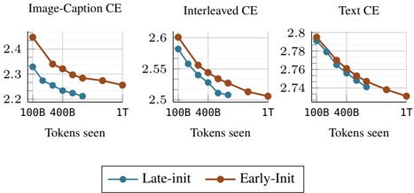
### Visual Description
## Chart Type: Multiple Line Charts Comparing Cross-Entropy (CE) Loss
### Overview
The image presents three line charts comparing the cross-entropy (CE) loss for different training strategies: "Image-Caption CE", "Interleaved CE", and "Text CE". Each chart plots the CE loss against the number of tokens seen during training, comparing "Late-init" and "Early-Init" approaches.
### Components/Axes
* **Titles (Top):**
* Left: "Image-Caption CE"
* Middle: "Interleaved CE"
* Right: "Text CE"
* **X-axis (Horizontal):** "Tokens seen" with markers at "100B", "400B", and "1T" (Trillion).
* **Y-axis (Vertical):** Cross-Entropy (CE) Loss. The scales vary slightly between charts:
* Image-Caption CE: Ranges from approximately 2.2 to 2.45.
* Interleaved CE: Ranges from approximately 2.5 to 2.6.
* Text CE: Ranges from approximately 2.74 to 2.8.
* **Legend (Bottom):**
* Blue line with circle markers: "Late-init"
* Brown line with circle markers: "Early-Init"
### Detailed Analysis
**1. Image-Caption CE**
* **Late-init (Blue):** The line slopes downward, indicating decreasing CE loss as more tokens are seen.
* 100B Tokens: CE loss ≈ 2.33
* 400B Tokens: CE loss ≈ 2.25
* 1T Tokens: CE loss ≈ 2.22
* **Early-Init (Brown):** The line also slopes downward.
* 100B Tokens: CE loss ≈ 2.45
* 400B Tokens: CE loss ≈ 2.33
* 1T Tokens: CE loss ≈ 2.26
**2. Interleaved CE**
* **Late-init (Blue):** The line slopes downward.
* 100B Tokens: CE loss ≈ 2.57
* 400B Tokens: CE loss ≈ 2.52
* 1T Tokens: CE loss ≈ 2.50
* **Early-Init (Brown):** The line slopes downward.
* 100B Tokens: CE loss ≈ 2.60
* 400B Tokens: CE loss ≈ 2.54
* 1T Tokens: CE loss ≈ 2.51
**3. Text CE**
* **Late-init (Blue):** The line slopes downward.
* 100B Tokens: CE loss ≈ 2.79
* 400B Tokens: CE loss ≈ 2.75
* 1T Tokens: CE loss ≈ 2.74
* **Early-Init (Brown):** The line slopes downward.
* 100B Tokens: CE loss ≈ 2.80
* 400B Tokens: CE loss ≈ 2.76
* 1T Tokens: CE loss ≈ 2.74
### Key Observations
* In all three charts, both "Late-init" and "Early-Init" strategies show a decrease in CE loss as the number of tokens seen increases.
* The "Early-Init" strategy generally starts with a higher CE loss than the "Late-init" strategy, but the difference diminishes as more tokens are seen.
* The "Text CE" chart has the highest CE loss values compared to the other two charts.
* The "Image-Caption CE" chart has the lowest CE loss values compared to the other two charts.
### Interpretation
The charts suggest that both "Late-init" and "Early-Init" strategies benefit from increased training data (more tokens seen), as indicated by the decreasing CE loss. The "Early-Init" strategy might initially perform worse, but the performance gap narrows with more training. The different CE loss values across the three charts ("Image-Caption CE", "Interleaved CE", and "Text CE") likely reflect the inherent difficulty or characteristics of each training task. The "Text CE" task appears to be the most challenging, while "Image-Caption CE" is the least, based on the relative CE loss values.
</details>
## C. Scaling laws
<!-- formula-not-decoded -->
Following [26], we determine the parameters that minimize the following objective across all our runs i :
<!-- formula-not-decoded -->
We perform this optimization across various initialization ranges and select the parameters that achieve the lowest loss across all initializations. Specifically, our grid search spans { 0 , 0 . 5 , 2 . 5 } for α and β , { 0 , 5 , 10 , ..., 30 } for a and b , and {-1 , -0 . 5 , 1 , 0 . 5 } for e . We use the L-BFGS algorithm with δ = 1 e -3 .
<!-- formula-not-decoded -->
While these equations have a closed-form solution [26] for early-fusion models that can be derived from Eq 1, this is not the case for late-fusion models without specifying either the vision encoder or text model size. To ensure a fair comparison, we derive these equations for both models, by performing linear regression in log space. We found that the regression is very close to the coefficient found with closed-form derivation Table 9. For instance, to derive N = K a C a , given a FLOP budget C and a set of linearly spaced tokens D i ranging from 10B to 600B, we compute the model size for each D i as N i = C 6 D for early fusion and N i = C 6 D + 0 . 483 ∗ N v for late fusion (for the 45-45-10 mixture, D v = 0 . 544 D , thus C = 6 D (0 . 544 N v + N t ) ). We then apply Eq 1 to obtain the loss for each model size and select N that has the minimum loss. We repeat this for all FLOP values corresponding to our runs, resulting in a set of points ( C, N opt ) that we use to regress a and K a . We follow a similar procedure to find b and d . For late-fusion models, we regress a linear model to determine N v given N . Notably, even though we maintain a fixed width ratio for late-fusion models, this approach is more accurate, as embedding layers prevent a strictly fixed ratio between text and vision model sizes. We present the regression results in Figure 22.
Table 9. Scaling laws parameters for early-fusion. Doing regression to derive the scaling laws coefficients leads to very close results to using the closed-form solution.
| Model | a | b | d | n | dn |
|-------------|---------|---------|---------|---------|----------|
| Closed form | 0.52649 | 0.47351 | 0.89938 | 1.11188 | -0.05298 |
| Regression | 0.52391 | 0.47534 | 0.90052 | 1.10224 | -0.04933 |
## C.3. Fitting L ∝ C c
To determine the relationship between the final model loss and the compute budget C , we begin by interpolating the points corresponding to the same model size and compute the convex hull that covers the minimum loss achieved by all runs for each FLOP. This results in a continuous mapping from the FLOPs to the lowest loss. We consider a range of FLOPs, excluding very small values ( ≤ 3 e 19 ), and construct a dataset of ( C, L ) for linearly spaced compute C . Using this data, we find the linear relationship between L and C in the log space and deduce the exponent c . We visualize the results in Figure 26.
Figure 22. Regression results of the scaling laws coefficients. our estimation of the scaling coefficients is close to the closed form solution.
<details>
<summary>Image 21 Details</summary>
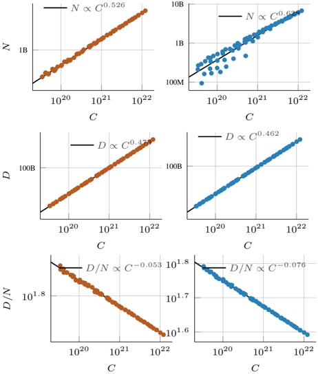
### Visual Description
## Chart: Relationships between N, D, and C
### Overview
The image presents six scatter plots arranged in a 3x2 grid. Each plot illustrates the relationship between two variables, with a power-law fit overlaid. The plots on the left are in a brownish-orange color, while the plots on the right are in blue. The x-axis represents 'C' in all plots, while the y-axes represent 'N', 'D', and 'D/N' from top to bottom.
### Components/Axes
* **X-axis (C):** The x-axis is labeled 'C' and uses a logarithmic scale ranging from approximately 10^20 to 10^22 in all six plots.
* **Y-axis (Left Column):**
* Top plot: Labeled 'N', logarithmic scale from approximately 1B.
* Middle plot: Labeled 'D', logarithmic scale from approximately 100B.
* Bottom plot: Labeled 'D/N', linear scale from approximately 10^1.6 to 10^1.8.
* **Y-axis (Right Column):**
* Top plot: Labeled 'N', logarithmic scale from approximately 100M to 10B.
* Middle plot: Labeled 'D', logarithmic scale from approximately 100B.
* Bottom plot: Labeled 'D/N', linear scale from approximately 10^1.6 to 10^1.8.
* **Data Points:** The data points are represented as circles. The left column uses brownish-orange circles, and the right column uses blue circles.
* **Power-Law Fit:** Each plot includes a black line representing a power-law fit to the data. The equations for these fits are displayed on each plot.
### Detailed Analysis
**Top Row: N vs. C**
* **Left Plot (Brownish-Orange):**
* Equation: N ∝ C^0.526
* Trend: The data points show a clear upward trend, closely following the power-law fit.
* Y-axis ranges from 1B
* **Right Plot (Blue):**
* Equation: N ∝ C^0.626
* Trend: The data points show an upward trend, but with more scatter compared to the left plot.
* Y-axis ranges from 100M to 10B.
**Middle Row: D vs. C**
* **Left Plot (Brownish-Orange):**
* Equation: D ∝ C^0.472
* Trend: The data points show a strong upward trend, closely aligned with the power-law fit.
* Y-axis ranges from 100B
* **Right Plot (Blue):**
* Equation: D ∝ C^0.462
* Trend: The data points show a strong upward trend, closely aligned with the power-law fit.
* Y-axis ranges from 100B
**Bottom Row: D/N vs. C**
* **Left Plot (Brownish-Orange):**
* Equation: D/N ∝ C^-0.053
* Trend: The data points show a slight downward trend, following the power-law fit.
* Y-axis ranges from 10^1.6 to 10^1.8
* **Right Plot (Blue):**
* Equation: D/N ∝ C^-0.076
* Trend: The data points show a slight downward trend, following the power-law fit.
* Y-axis ranges from 10^1.6 to 10^1.8
### Key Observations
* The relationships between N, D, and C are well-approximated by power laws.
* The exponents in the power-law fits vary slightly between the left and right columns.
* The plots of D/N vs. C show a negative exponent, indicating an inverse relationship.
* The scatter in the N vs. C plot (right column) is more pronounced than in the other plots.
### Interpretation
The plots suggest that N and D both increase with C, following power-law relationships. The exponents indicate the rate at which they increase. The negative exponents in the D/N vs. C plots suggest that as C increases, the ratio of D to N decreases. The difference in exponents and scatter between the left and right columns might indicate different underlying conditions or datasets. The data demonstrates the relationships between these variables and provides a basis for further analysis and modeling.
</details>
## C.4. Scaling laws for different target data type
In Figure 27, we derive the scaling laws for different target data types. In general, we observe that the model learns image captioning faster than interleaved data, as indicated by the higher absolute value of the scaling exponent (e.g., 0.062 vs 0.046), despite using the same data ratio for captioning and interleaved data (45% each). Additionally, we find that the model learns more slowly on textonly data, likely due to the smaller amount of text-only data (10%). Across model configurations, we find that early fusion scales similarly to late fusion on image captioning but has a lower multiplicative constant (49.99 vs 47.97). For MoEs, the model learns faster but exhibits a higher multiplicative constant. On text and interleaved data, early and late fusion models scale similarly and achieve comparable
Figure 23. Observed vs predicted loss. We visualize the loss predicted by our scaling laws (Eq 1) and the actual loss achived by each run.
<details>
<summary>Image 22 Details</summary>
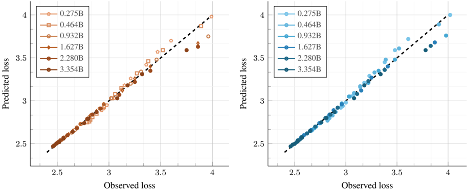
### Visual Description
## Scatter Plot: Predicted Loss vs. Observed Loss
### Overview
The image contains two scatter plots, each comparing predicted loss against observed loss for different model sizes. The left plot uses shades of brown, while the right plot uses shades of blue to represent different model sizes. A dashed black line, representing perfect prediction (predicted loss equals observed loss), is overlaid on both plots.
### Components/Axes
* **X-axis (Observed loss):** Both plots share the same x-axis, labeled "Observed loss," ranging from approximately 2.3 to 4.0, with gridlines at intervals of 0.5.
* **Y-axis (Predicted loss):** Both plots share the same y-axis, labeled "Predicted loss," ranging from approximately 2.3 to 4.0, with gridlines at intervals of 0.5.
* **Legend (Left Plot):** Located in the top-left corner of the left plot. It indicates the model sizes represented by different shades of brown:
* Lightest Brown (circle): 0.275B
* Light Brown (square): 0.464B
* Medium Light Brown (circle with line): 0.932B
* Medium Dark Brown (diamond): 1.627B
* Dark Brown (triangle): 2.280B
* Darkest Brown (circle): 3.354B
* **Legend (Right Plot):** Located in the top-left corner of the right plot. It indicates the model sizes represented by different shades of blue:
* Lightest Blue (circle): 0.275B
* Light Blue (circle): 0.464B
* Medium Light Blue (circle): 0.932B
* Medium Dark Blue (circle): 1.627B
* Dark Blue (circle): 2.280B
* Darkest Blue (circle): 3.354B
* **Dashed Line:** A dashed black line runs diagonally across each plot, representing the ideal scenario where predicted loss equals observed loss.
### Detailed Analysis
**Left Plot (Brown Shades):**
* **0.275B (Lightest Brown, circle):** The data points generally follow the dashed line, indicating good prediction accuracy. Observed loss ranges from approximately 2.4 to 3.9, and predicted loss ranges from approximately 2.4 to 4.0.
* **0.464B (Light Brown, square):** The data points generally follow the dashed line, indicating good prediction accuracy. Observed loss ranges from approximately 2.4 to 3.9, and predicted loss ranges from approximately 2.4 to 3.9.
* **0.932B (Medium Light Brown, circle with line):** The data points generally follow the dashed line, indicating good prediction accuracy. Observed loss ranges from approximately 2.4 to 3.9, and predicted loss ranges from approximately 2.4 to 3.9.
* **1.627B (Medium Dark Brown, diamond):** The data points generally follow the dashed line, indicating good prediction accuracy. Observed loss ranges from approximately 2.4 to 3.9, and predicted loss ranges from approximately 2.4 to 3.9.
* **2.280B (Dark Brown, triangle):** The data points generally follow the dashed line, indicating good prediction accuracy. Observed loss ranges from approximately 2.4 to 3.9, and predicted loss ranges from approximately 2.4 to 3.9.
* **3.354B (Darkest Brown, circle):** The data points generally follow the dashed line, indicating good prediction accuracy. Observed loss ranges from approximately 2.4 to 3.9, and predicted loss ranges from approximately 2.4 to 3.9.
**Right Plot (Blue Shades):**
* **0.275B (Lightest Blue, circle):** The data points generally follow the dashed line, indicating good prediction accuracy. Observed loss ranges from approximately 2.4 to 3.9, and predicted loss ranges from approximately 2.4 to 3.9.
* **0.464B (Light Blue, circle):** The data points generally follow the dashed line, indicating good prediction accuracy. Observed loss ranges from approximately 2.4 to 3.9, and predicted loss ranges from approximately 2.4 to 3.9.
* **0.932B (Medium Light Blue, circle):** The data points generally follow the dashed line, indicating good prediction accuracy. Observed loss ranges from approximately 2.4 to 3.9, and predicted loss ranges from approximately 2.4 to 3.9.
* **1.627B (Medium Dark Blue, circle):** The data points generally follow the dashed line, indicating good prediction accuracy. Observed loss ranges from approximately 2.4 to 3.9, and predicted loss ranges from approximately 2.4 to 3.9.
* **2.280B (Dark Blue, circle):** The data points generally follow the dashed line, indicating good prediction accuracy. Observed loss ranges from approximately 2.4 to 3.9, and predicted loss ranges from approximately 2.4 to 3.9.
* **3.354B (Darkest Blue, circle):** The data points generally follow the dashed line, indicating good prediction accuracy. Observed loss ranges from approximately 2.4 to 3.9, and predicted loss ranges from approximately 2.4 to 3.9.
### Key Observations
* Both plots show a strong correlation between predicted loss and observed loss across all model sizes.
* The data points cluster closely around the dashed line, indicating that the models are generally accurate in their predictions.
* There is no clear trend indicating that larger model sizes consistently perform better or worse than smaller model sizes.
* The shapes of the data points in the left plot are different, while the shapes of the data points in the right plot are the same.
### Interpretation
The scatter plots demonstrate the performance of different model sizes in predicting loss. The close alignment of data points with the dashed line suggests that all model sizes are reasonably accurate. The absence of a clear performance difference between model sizes implies that increasing model size may not necessarily lead to significant improvements in prediction accuracy for this particular task or dataset. The use of different colors (browns vs. blues) likely serves to visually distinguish the two plots, possibly representing different experimental conditions or model architectures, while the shapes in the left plot may represent different training parameters.
</details>
performance. However, MoEs demonstrate better overall performance while learning slightly more slowly.
## C.5. Scaling laws for different training mixtures
We investigate how the scaling laws change when modifying the training mixtures. Specifically, we vary the ratio of image caption, interleaved, and text-only data and report the results in Figure 28. Overall, we observe similar scaling trends, with only minor changes in the scaling coefficients. Upon closer analysis, we find that increasing the ratio of a particular data type in the training mixture, leads to a corresponding increase in its scaling exponent. For instance, increasing the ratio of image captions from 30% to 40% raises the absolute value of the exponent from 0.056 to 0.061. However, for text-only data, we do not observe significant changes in the scaling coefficients when varying its proportion in the training mixture.
Table 10. Scaling laws prediction errors. We report the mean square error, R2 and mean absolute error for the loss prediction for held-in and held-out (8B model) data.
| Parameter | MSE | R2 | MAE (%) |
|-------------|--------|--------|-----------|
| Held-in | 0.0029 | 0.9807 | 0.8608 |
| Held-out | 0.0004 | 0.9682 | 0.553 |
Table 11. Scaling laws sensitivity. We report the mean and standard deviation after bootstrapping with 100 iterations.
| Model | E | α | β | a | b | d |
|---------|---------|---------|---------|---------|---------|---------|
| Avg | 1.80922 | 0.29842 | 0.33209 | 0.54302 | 0.48301 | 0.92375 |
| Std | 0.33811 | 0.10101 | 0.02892 | 0.08813 | 0.05787 | 0.23296 |
## C.6. Scaling laws evaluation
For each model size and number of training tokens, we compute the loss using the estimated functional form in Eq 1 and compare it to the actual loss observed in our runs. Figure 23, Figure 24, and Table 10 visualizes these comparisons, showing that our estimation is highly accurate, particularly for lower loss values and larger FLOPs. We also assess our scaling laws in an extrapolation setting, predicting performance beyond the model sizes used for fitting. Notably, our approach estimates the performance of an 8B model with reasonable accuracy.
Additionally, we conduct a sensitivity analysis using bootstrapping. Specifically, we sample P points with replacement ( P being the total number of trained models) and re-estimate the scaling law coefficients. This process is repeated 100 times, and we report the mean and standard deviation of each coefficient. Table 11 shows that our estimation is more precise for β than for α , primarily due to the smaller number of model sizes relative to the number of different token counts used to derive the scaling laws.
## C.7. Scaling laws for sparse NMMs.
Similar to dense models, we fit a parametric loss function (Eq 1) to predict the loss of sparse NMMs based on the number of parameters and training tokens, replacing the total parameter count with the number of active parameters. While incorporating sparsity is standard when deriving scaling laws for MoEs [2, 33, 74], we focus on deriving scaling laws specific to the sparsity level used in our MoE setup. This yields coefficients that are implicitly conditioned on the sparsity configuration.
We also experiment with a sparsity-aware formulation of the scaling law as proposed in [2], and observe consistent
.
464M
932M
1.63B
2.28B
<details>
<summary>Image 23 Details</summary>
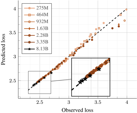
### Visual Description
## Scatter Plot: Predicted Loss vs. Observed Loss for Different Model Sizes
### Overview
The image is a scatter plot comparing predicted loss against observed loss for various model sizes, ranging from 275M to 8.13B parameters. The plot includes a dashed diagonal line, representing perfect prediction. The data points are clustered around this line, with some deviation, particularly for smaller model sizes. An inset provides a zoomed-in view of the data points at higher loss values.
### Components/Axes
* **X-axis (Observed loss):** Ranges from approximately 2.3 to 4.0, with gridlines at intervals of 0.5.
* **Y-axis (Predicted loss):** Ranges from approximately 2.3 to 4.0, with gridlines at intervals of 0.5.
* **Legend (Top-Left):**
* 275M (Light Brown, Circle): Lightest shade of brown, circle marker.
* 464M (Light Brown, Square): Slightly darker shade of brown, square marker.
* 932M (Medium Brown, Pentagon): Medium shade of brown, pentagon marker.
* 1.63B (Medium Brown, Diamond): Medium shade of brown, diamond marker.
* 2.28B (Dark Brown, Circle): Darker shade of brown, circle marker.
* 3.35B (Dark Brown, Circle): Darkest shade of brown, circle marker.
* 8.13B (Black, Star): Black, star marker.
* **Diagonal Line:** Dashed black line representing perfect prediction (predicted loss = observed loss).
### Detailed Analysis
* **275M (Light Brown, Circle):** The data points are scattered around the diagonal line, with a tendency to underestimate the loss, especially at higher observed loss values.
* Observed loss range: ~2.4 to ~3.8
* Predicted loss range: ~2.4 to ~3.7
* **464M (Light Brown, Square):** Similar to 275M, the data points are scattered, with underestimation at higher observed loss values.
* Observed loss range: ~2.4 to ~3.8
* Predicted loss range: ~2.4 to ~3.7
* **932M (Medium Brown, Pentagon):** The data points are closer to the diagonal line compared to 275M and 464M.
* Observed loss range: ~2.4 to ~3.8
* Predicted loss range: ~2.4 to ~3.8
* **1.63B (Medium Brown, Diamond):** The data points are even closer to the diagonal line than 932M.
* Observed loss range: ~2.4 to ~3.8
* Predicted loss range: ~2.4 to ~3.8
* **2.28B (Dark Brown, Circle):** The data points are tightly clustered around the diagonal line.
* Observed loss range: ~2.4 to ~3.8
* Predicted loss range: ~2.4 to ~3.8
* **3.35B (Dark Brown, Circle):** The data points are very close to the diagonal line.
* Observed loss range: ~2.4 to ~3.8
* Predicted loss range: ~2.4 to ~3.8
* **8.13B (Black, Star):** The data points are almost perfectly aligned with the diagonal line.
* Observed loss range: ~2.4 to ~3.8
* Predicted loss range: ~2.4 to ~3.8
### Key Observations
* As the model size increases, the predicted loss becomes more aligned with the observed loss.
* Smaller models (275M, 464M) tend to underestimate the loss, especially at higher observed loss values.
* Larger models (2.28B, 3.35B, 8.13B) provide more accurate predictions, with the 8.13B model showing near-perfect alignment.
* The inset highlights the clustering of data points for larger models at higher loss values.
### Interpretation
The scatter plot demonstrates the relationship between model size and prediction accuracy. Smaller models exhibit greater deviation between predicted and observed loss, indicating lower accuracy. As the model size increases, the predictions become more accurate, converging towards the ideal scenario represented by the diagonal line. This suggests that larger models are better at capturing the underlying patterns in the data and making more accurate predictions. The 8.13B model performs exceptionally well, indicating that it has sufficient capacity to model the data effectively. The underestimation of loss by smaller models could be attributed to their limited capacity to capture the complexity of the data.
</details>
that techniques for extending context length could be beneficial.
Scaling laws for multimodal MoEs models. For MoEs, we consider only a single configuration (top-1 routing with 8 experts). We found this configuration to work reasonably well in our setup, and follow a standard MoEs implementation. However, the findings may vary when optimizing more the MoE architecture or exploring different load-balancing, routing strategies or different experts implementations.
## E. Mixture of experts and modality-specific specialization
## 3 . 5 E.1. MoEs configuration
Observed loss We experiment with different MoEs configuration by changing the number of experts and the top-k. We report a sample of these experiments in Table 13.
.
Figure 24. Observed vs predicted loss. We visualize the loss predicted by our scaling laws Eq 1 and the actual loss achieved by each run. We can reliably predict the performance of models larger (8B params) than those used to fit the scaling laws.
trends (Table 12). In particular, the exponents associated with model size ( N ) are substantially larger than those for training tokens ( β ), reinforcing the importance of scaling model size in sparse architectures. Additionally, we observe that the terms governing the scaling of active parameters decompose into two components.
## D. Discussion and Limitations
Scaling laws for multimodal data mixtures. Our scaling laws study spans different model configurations and training mixtures. While results suggest that the scaling law coefficients remain largely consistent across mixtures, a broader exploration of mixture variations is needed to validate this observation and establish a unified scaling law that accounts for this factor.
Scaling laws and performance on downstream tasks. Similar to previous scaling law studies, our analysis focuses on pretraining performance as measured by the validation loss. However, the extent to which these findings translate to downstream performance remains an open question and requires further investigation.
Extrapolation to larger scales. The accuracy of scaling law predictions improves with increasing FLOPs Appendix C. Furthermore, we validate our laws when extrapolating to larger model sizes (Appendix C.6). However, whether these laws can be reliably extrapolated to extremely large model sizes remains an open question.
High resolution and early-fusion models. Training earlyfusion models with high-resolution inputs leads to a significant increase in vision tokens. While pooling techniques have been widely adopted for late-fusion models, alternative approaches may be necessary for early fusion. Given the similarity of early-fusion models to LLMs, it appears
## E.2. MoEs specialization
Figure 25. Modality-specific specialization. We visualize the experts specialization to text and image modalities. Models are evaluated on Obelics.
<details>
<summary>Image 24 Details</summary>
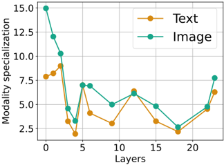
### Visual Description
## Line Chart: Modality Specialization vs. Layers
### Overview
The image is a line chart comparing the modality specialization of "Text" and "Image" across different layers. The x-axis represents the layers, and the y-axis represents modality specialization.
### Components/Axes
* **X-axis:** Layers, ranging from 0 to 22.
* **Y-axis:** Modality specialization, ranging from 2.5 to 15.0.
* **Legend:** Located in the top-right corner.
* **Text:** Represented by an orange line.
* **Image:** Represented by a teal line.
### Detailed Analysis
* **Text (Orange Line):**
* Starts at approximately 8.0 at layer 0.
* Increases slightly to approximately 9.0 at layer 1.
* Decreases sharply to approximately 3.0 at layer 4.
* Increases to approximately 4.0 at layer 7.
* Decreases to approximately 3.0 at layer 11.
* Increases to approximately 6.0 at layer 13.
* Decreases to approximately 3.0 at layer 17.
* Decreases to approximately 2.0 at layer 20.
* Increases to approximately 7.0 at layer 23.
* **Image (Teal Line):**
* Starts at approximately 15.0 at layer 0.
* Decreases to approximately 12.0 at layer 1.
* Decreases to approximately 10.0 at layer 2.
* Decreases sharply to approximately 4.0 at layer 4.
* Increases to approximately 7.0 at layer 5.
* Decreases to approximately 6.0 at layer 10.
* Increases to approximately 6.0 at layer 13.
* Decreases to approximately 5.0 at layer 16.
* Decreases to approximately 2.0 at layer 20.
* Increases to approximately 8.0 at layer 23.
### Key Observations
* The "Image" modality specialization starts much higher than the "Text" modality specialization.
* Both modalities experience a significant drop in specialization around layer 4.
* The "Image" modality specialization generally remains higher than the "Text" modality specialization, except for a brief period around layer 13.
* Both modalities show an increase in specialization towards the end of the layers.
### Interpretation
The chart illustrates how the specialization of text and image modalities changes across different layers of a model. The initial high specialization of the "Image" modality suggests that the early layers are more focused on processing visual information. The subsequent drop in both modalities around layer 4 could indicate a point where the model begins to integrate information from both modalities. The overall trend suggests that the model gradually refines its specialization as it progresses through the layers, with both modalities becoming more specialized towards the end. The fluctuations in specialization may reflect the model's adaptation to different types of input or tasks.
</details>
We investigate multimodal specialization in MoE architectures. We compute a specialization score as the average difference between the number of text/images tokens assigned to each expert and a uniform assignment ( 1 /E ). Additionally, we visualize the normalized number of text and image tokens assigned to each expert across layers. Figure 25 shows clear modality-specific experts, particularly in the early layers. Furthermore, the specialization score decreases as the number of layers increases but rises again in the very last layers. This suggests that early and final layers require more modality specialization compared to midlayers. Additionally, we observe several experts shared between text and image modalities, a phenomenon not present in hard-routed or predefined modality-specific experts.
| L ( N,D ) = E + A N α + B D β | L ( N,D ) = E + A N α + B D β | L ( N,D ) = E + A N α + B D β | vs | vs | L ( N,D,S ) = A N α + B D β + C (1 - S ) λ + d (1 - S ) δ N γ + E | L ( N,D,S ) = A N α + B D β + C (1 - S ) λ + d (1 - S ) δ N γ + E | L ( N,D,S ) = A N α + B D β + C (1 - S ) λ + d (1 - S ) δ N γ + E | L ( N,D,S ) = A N α + B D β + C (1 - S ) λ + d (1 - S ) δ N γ + E | L ( N,D,S ) = A N α + B D β + C (1 - S ) λ + d (1 - S ) δ N γ + E | L ( N,D,S ) = A N α + B D β + C (1 - S ) λ + d (1 - S ) δ N γ + E |
|---------------------------------|---------------------------------|---------------------------------|------|--------|---------------------------------------------------------------------|---------------------------------------------------------------------|---------------------------------------------------------------------|---------------------------------------------------------------------|---------------------------------------------------------------------|---------------------------------------------------------------------|
| Model | E | A | B | α | β | λ | δ | γ | C | d |
| L ( N,D ) (Eq 1) | 2.158 | 381773 | 4659 | 0.710 | 0.372 | - | - | - | - | - |
| L ( N,D,S ) [2] | 1.0788 | 1 | 4660 | 0.5890 | 0.3720 | 0.2 | 0.2 | 0.70956 | 1.0788 | 381475 |
Table 12. Scaling laws for sparse native multimodal models .
Table 13. SFT results with different MoEs configurations. .
| | Accuracy | Accuracy | Accuracy | Accuracy | Accuracy | Accuracy | CIDEr | CIDEr |
|-----------------------|------------|------------|------------|------------|------------|------------|---------|----------|
| | AVG | VQAv2 | TextVQA | OKVQA | GQA | VizWiz | COCO | TextCaps |
| 4-E-top-1 | 40.0552 | 64.068 | 14.284 | 41.948 | 61.46 | 18.516 | 62.201 | 34.08 |
| 8-E-top-1 | 41.6934 | 65.684 | 17.55 | 42.908 | 63.26 | 19.065 | 67.877 | 39.63 |
| 8-E-top-2 | 42.8546 | 66.466 | 19.162 | 45.344 | 63.94 | 19.361 | 65.988 | 41.649 |
| 8-E-top-2 finegrained | 39.904 | 62.76 | 15.58 | 41.88 | 61.6 | 17.7 | 57.52 | 35.42 |
Figure 26. Scaling laws for native multimodal models. From left to right: late-fusion (dense), early-fusion (dense) and early-fusion MoEs. The scaling exponents are very close for all models. However, MoEs leads to overall lower loss (smaller multiplicative constant) and takes longer to saturate.
<details>
<summary>Image 25 Details</summary>
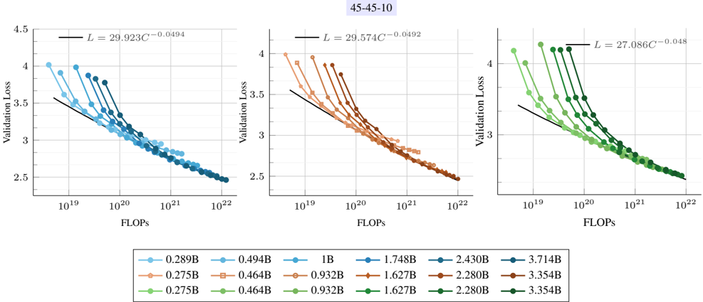
### Visual Description
## Scatter Plot: Validation Loss vs. FLOPS for Different Model Sizes
### Overview
The image presents three scatter plots arranged horizontally, each displaying the relationship between validation loss and FLOPS (Floating Point Operations Per Second) for different model sizes. Each plot contains multiple data series, each representing a specific model size, and a black line representing a power law fit. The plots share the same axes and general structure, but differ in the range of model sizes they depict. The title "45-45-10" is present at the top of the image.
### Components/Axes
* **Title:** 45-45-10 (located at the top-center of the image)
* **X-axis (Horizontal):** FLOPS (Floating Point Operations Per Second). The scale is logarithmic, ranging from approximately 10<sup>19</sup> to 10<sup>22</sup>.
* **Y-axis (Vertical):** Validation Loss. The scale is linear, ranging from 2.5 to 4.5.
* **Data Series:** Each plot contains multiple data series, each represented by a different color and marker. Each series represents a different model size (in billions of parameters, denoted as 'B').
* **Power Law Fit:** Each plot includes a black line representing a power law fit to the data. The equation for the power law is displayed on each plot in the form L = aC<sup>-b</sup>, where L is the validation loss, C is the FLOPS, and a and b are constants.
* **Legend:** Located at the bottom of the image, the legend maps the colors and markers to the corresponding model sizes.
### Detailed Analysis
**Plot 1 (Left):**
* **Power Law Fit:** L = 29.923C<sup>-0.0494</sup>
* **Data Series (from top-left to bottom-right):**
* Light Blue: 0.289B. Starts at approximately (10<sup>19</sup>, 4.0) and decreases to (10<sup>22</sup>, 2.6).
* Orange: 0.275B. Starts at approximately (10<sup>19</sup>, 3.9) and decreases to (10<sup>22</sup>, 2.6).
* Green: 0.275B. Starts at approximately (10<sup>19</sup>, 3.8) and decreases to (10<sup>22</sup>, 2.5).
* Blue: 0.494B. Starts at approximately (10<sup>19</sup>, 3.8) and decreases to (10<sup>22</sup>, 2.6).
* Brown: 0.464B. Starts at approximately (10<sup>19</sup>, 3.7) and decreases to (10<sup>22</sup>, 2.6).
* Dark Green: 0.464B. Starts at approximately (10<sup>19</sup>, 3.6) and decreases to (10<sup>22</sup>, 2.5).
**Plot 2 (Center):**
* **Power Law Fit:** L = 29.574C<sup>-0.0492</sup>
* **Data Series (from top-left to bottom-right):**
* Light Blue: 1B. Starts at approximately (10<sup>19</sup>, 4.0) and decreases to (10<sup>22</sup>, 2.6).
* Orange: 0.932B. Starts at approximately (10<sup>19</sup>, 3.9) and decreases to (10<sup>22</sup>, 2.6).
* Green: 0.932B. Starts at approximately (10<sup>19</sup>, 3.8) and decreases to (10<sup>22</sup>, 2.5).
* Blue: 1.748B. Starts at approximately (10<sup>19</sup>, 3.7) and decreases to (10<sup>22</sup>, 2.6).
* Brown: 1.627B. Starts at approximately (10<sup>19</sup>, 3.6) and decreases to (10<sup>22</sup>, 2.6).
* Dark Green: 1.627B. Starts at approximately (10<sup>19</sup>, 3.5) and decreases to (10<sup>22</sup>, 2.5).
**Plot 3 (Right):**
* **Power Law Fit:** L = 27.086C<sup>-0.048</sup>
* **Data Series (from top-left to bottom-right):**
* Light Blue: 2.430B. Starts at approximately (10<sup>19</sup>, 4.2) and decreases to (10<sup>22</sup>, 2.6).
* Orange: 2.280B. Starts at approximately (10<sup>19</sup>, 4.0) and decreases to (10<sup>22</sup>, 2.6).
* Green: 2.280B. Starts at approximately (10<sup>19</sup>, 3.9) and decreases to (10<sup>22</sup>, 2.5).
* Blue: 3.714B. Starts at approximately (10<sup>19</sup>, 3.8) and decreases to (10<sup>22</sup>, 2.6).
* Brown: 3.354B. Starts at approximately (10<sup>19</sup>, 3.7) and decreases to (10<sup>22</sup>, 2.6).
* Dark Green: 3.354B. Starts at approximately (10<sup>19</sup>, 3.6) and decreases to (10<sup>22</sup>, 2.5).
### Key Observations
* **Inverse Relationship:** There is a clear inverse relationship between FLOPS and validation loss. As FLOPS increase, validation loss decreases.
* **Power Law Behavior:** The power law fit suggests that the relationship between FLOPS and validation loss can be modeled by a power law function.
* **Model Size Impact:** For a given FLOPS value, larger models (higher 'B' value) tend to have lower validation loss.
* **Saturation:** The validation loss appears to saturate at higher FLOPS values, meaning that increasing FLOPS beyond a certain point yields diminishing returns in terms of reducing validation loss.
* **Similar Trends:** The trends are very similar across the three plots, suggesting that the relationship between FLOPS and validation loss is consistent across different ranges of model sizes.
* **Power Law Exponents:** The exponents in the power law fits are similar across the three plots (-0.0494, -0.0492, -0.048), suggesting a similar rate of decrease in validation loss with increasing FLOPS.
### Interpretation
The plots demonstrate the relationship between computational effort (FLOPS) and model performance (validation loss) for different model sizes. The data suggests that increasing the computational effort invested in training a model leads to a reduction in validation loss, following a power law relationship. Furthermore, larger models tend to achieve lower validation loss for a given amount of computation. The saturation effect indicates that there are limits to the benefits of increasing FLOPS, and that other factors, such as model architecture or training data, may become more important at higher levels of computation. The consistency of the trends across the three plots suggests that these relationships are robust and generalizable across different model size ranges. The title "45-45-10" likely refers to specific experimental parameters or configurations used in the study.
</details>
Figure 27. Scaling laws for native multimodal models. From top to bottom: late-fusion (dense), early-fusion (dense) and early-fusion MoEs. From left to right: cross-entropy on the validation set of image-caption, interleaved and text-only data.
<details>
<summary>Image 26 Details</summary>
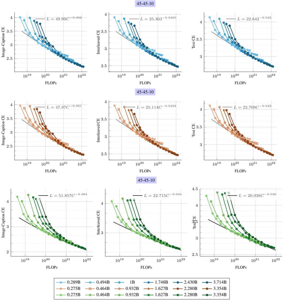
### Visual Description
## Chart: Performance Curves for Different Tasks
### Overview
The image presents a series of performance curves, plotting the relationship between computational cost (FLOPS) and cross-entropy loss (CE) for different tasks: Image-Caption, Interleaved, and Text. Each plot shows multiple curves, each representing a different model size, ranging from 0.275B to 3.714B parameters. The plots are arranged in a 3x3 grid, with each row representing a different task and each column representing a different performance metric. The title "45-45-10" appears above the middle column of plots.
### Components/Axes
* **X-axis:** FLOPS (Floating Point Operations Per Second) on a logarithmic scale from 10^19 to 10^22.
* **Y-axis:** Cross-Entropy (CE) Loss. The range varies slightly between plots, but generally spans from approximately 2 to 4.5.
* **Titles:**
* Left Column: "Image-Caption CE"
* Middle Column: "Interleaved CE"
* Right Column: "Text CE"
* **Legend:** Located at the bottom of the image.
* `0.289B` (lightest shade in each color group)
* `0.494B` (second lightest shade in each color group)
* `1B` (third lightest shade in each color group)
* `1.748B` (middle shade in each color group)
* `2.430B` (second darkest shade in each color group)
* `3.714B` (darkest shade in each color group)
* `0.275B` (lightest shade in each color group)
* `0.464B` (second lightest shade in each color group)
* `0.932B` (third lightest shade in each color group)
* `1.627B` (middle shade in each color group)
* `2.280B` (second darkest shade in each color group)
* `3.354B` (darkest shade in each color group)
* **Regression Lines:** Each plot contains a black line representing a power-law fit to the data. The equation for each line is displayed on the plot in the form "L = a\*C^(-b)", where L is the loss, C is the compute (FLOPS), and a and b are constants.
* **Title:** The title "45-45-10" is present above the Interleaved CE plots.
### Detailed Analysis
**Row 1: Image-Caption CE, Interleaved CE, Text CE (Blue)**
* **Image-Caption CE:**
* Trend: The curves generally slope downwards, indicating decreasing loss with increasing FLOPS.
* Equation: L = 49.99\*C^(-0.062)
* Data Points: The curves are clustered, with the largest model (3.714B) achieving the lowest loss for a given FLOPS.
* **Interleaved CE:**
* Trend: The curves generally slope downwards, indicating decreasing loss with increasing FLOPS.
* Equation: L = 25.303\*C^(-0.0460)
* Data Points: The curves are clustered, with the largest model (3.714B) achieving the lowest loss for a given FLOPS.
* **Text CE:**
* Trend: The curves generally slope downwards, indicating decreasing loss with increasing FLOPS.
* Equation: L = 22.642\*C^(-0.042)
* Data Points: The curves are clustered, with the largest model (3.714B) achieving the lowest loss for a given FLOPS.
**Row 2: Image-Caption CE, Interleaved CE, Text CE (Brown)**
* **Image-Caption CE:**
* Trend: The curves generally slope downwards, indicating decreasing loss with increasing FLOPS.
* Equation: L = 47.97\*C^(-0.061)
* Data Points: The curves are clustered, with the largest model (3.354B) achieving the lowest loss for a given FLOPS.
* **Interleaved CE:**
* Trend: The curves generally slope downwards, indicating decreasing loss with increasing FLOPS.
* Equation: L = 25.114\*C^(-0.0458)
* Data Points: The curves are clustered, with the largest model (3.354B) achieving the lowest loss for a given FLOPS.
* **Text CE:**
* Trend: The curves generally slope downwards, indicating decreasing loss with increasing FLOPS.
* Equation: L = 22.709\*C^(-0.042)
* Data Points: The curves are clustered, with the largest model (3.354B) achieving the lowest loss for a given FLOPS.
**Row 3: Image-Caption CE, Interleaved CE, Text CE (Green)**
* **Image-Caption CE:**
* Trend: The curves generally slope downwards, indicating decreasing loss with increasing FLOPS.
* Equation: L = 51.857\*C^(-0.064)
* Data Points: The curves are clustered, with the largest model (3.354B) achieving the lowest loss for a given FLOPS.
* **Interleaved CE:**
* Trend: The curves generally slope downwards, indicating decreasing loss with increasing FLOPS.
* Equation: L = 22.715\*C^(-0.044)
* Data Points: The curves are clustered, with the largest model (3.354B) achieving the lowest loss for a given FLOPS.
* **Text CE:**
* Trend: The curves generally slope downwards, indicating decreasing loss with increasing FLOPS.
* Equation: L = 20.036\*C^(-0.040)
* Data Points: The curves are clustered, with the largest model (3.354B) achieving the lowest loss for a given FLOPS.
### Key Observations
* **Power-Law Relationship:** The relationship between FLOPS and CE loss appears to follow a power-law distribution, as indicated by the fitted lines.
* **Model Size Impact:** Larger models (higher number of parameters) generally achieve lower CE loss for a given number of FLOPS.
* **Task-Specific Performance:** The specific values of CE loss and the coefficients in the power-law equations vary depending on the task (Image-Caption, Interleaved, Text).
* **Color Grouping:** Each row has a distinct color scheme (blue, brown, green), but the significance of this grouping is not immediately apparent from the image alone.
### Interpretation
The data suggests that increasing the computational cost (FLOPS) during training leads to a reduction in cross-entropy loss for all three tasks (Image-Caption, Interleaved, and Text). Furthermore, larger models tend to perform better (lower loss) for a given amount of computation. The power-law relationship indicates diminishing returns, meaning that the reduction in loss becomes smaller as the amount of computation increases. The task-specific differences in performance suggest that some tasks are inherently easier to learn than others, or that the models are better suited to some tasks than others. The "45-45-10" title might refer to a specific experimental setup or configuration used to generate these results, but without further context, its meaning is unclear. The color grouping of the rows might represent different datasets, training regimes, or model architectures, but this requires additional information to confirm.
</details>
Figure 28. Scaling laws for early-fusion native multimodal models. Our runs across different training mixtures (Image-captionInterleaved-Text) and FLOPs. We visulize the final validation loss on 3 data types: HQITP (left), Obelics (middle) and DCLM (right).
<details>
<summary>Image 27 Details</summary>
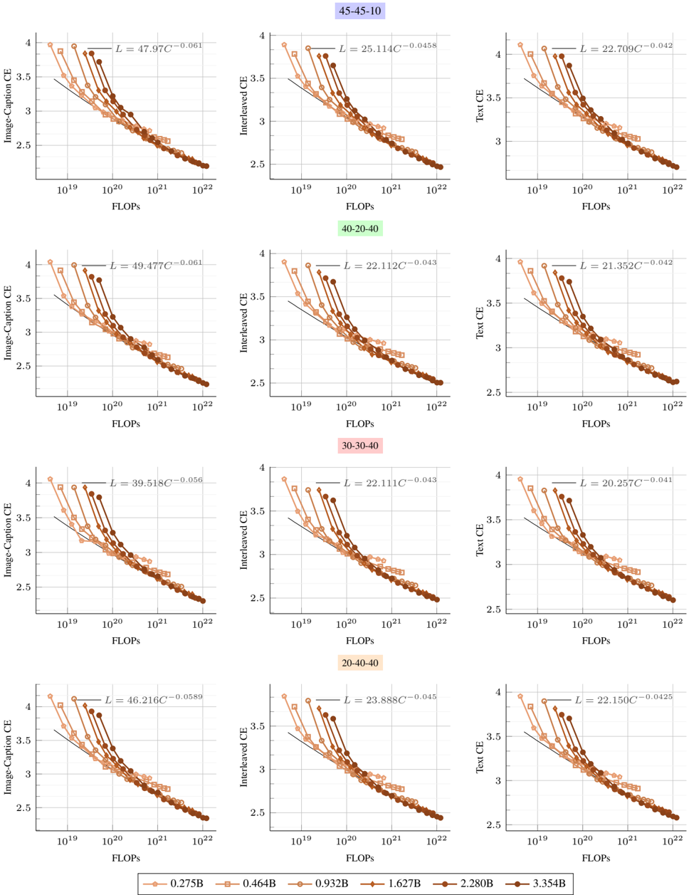
### Visual Description
## Chart: Performance vs. Compute for Different Data Mixes
### Overview
The image presents a series of scatter plots showing the relationship between performance (CE - Cross Entropy) and compute (FLOPS - Floating Point Operations Per Second) for different data mixes. Each plot represents a different data mix configuration (45-45-10, 40-20-40, 30-30-40, 20-40-40), and within each plot, different lines represent different model sizes. The plots are arranged in a 2x3 grid.
### Components/Axes
* **X-axis (FLOPS):** Represents the computational cost in Floating Point Operations Per Second. The scale is logarithmic, ranging from approximately 10^19 to 10^22.
* **Y-axis (Image-Caption CE, Interleaved CE, Text CE):** Represents the cross-entropy loss, a measure of performance. The scale ranges from 2.5 to 4.0. The Y-axis label varies depending on the column: "Image-Caption CE" for the first column, "Interleaved CE" for the second column, and "Text CE" for the third column.
* **Data Series:** Each line on the plot represents a different model size, indicated by the legend at the bottom. The model sizes are 0.275B, 0.464B, 0.932B, 1.627B, 2.280B, and 3.354B.
* **Titles:** Each plot has a title indicating the data mix configuration (e.g., 45-45-10, 40-20-40, etc.).
* **Trend Lines:** Each plot includes a black trend line, with an equation of the form L = aC^(-b), where L is the loss, C is the compute, and a and b are constants.
### Detailed Analysis
**Plot 1: 45-45-10, Image-Caption CE**
* Trend: As FLOPS increase, Image-Caption CE decreases.
* Equation: L = 47.97C^(-0.061)
* Data Points:
* 0.275B (lightest color): Starts at approximately (10^19, 4.0), ends around (10^22, 2.4)
* 0.464B: Starts at approximately (10^19, 3.8), ends around (10^22, 2.3)
* 0.932B: Starts at approximately (10^19, 3.6), ends around (10^22, 2.3)
* 1.627B: Starts at approximately (10^19, 3.4), ends around (10^22, 2.2)
* 2.280B: Starts at approximately (10^19, 3.2), ends around (10^22, 2.2)
* 3.354B (darkest color): Starts at approximately (10^19, 3.0), ends around (10^22, 2.1)
**Plot 2: 45-45-10, Interleaved CE**
* Trend: As FLOPS increase, Interleaved CE decreases.
* Equation: L = 25.114C^(-0.0458)
* Data Points:
* 0.275B: Starts at approximately (10^19, 4.0), ends around (10^22, 2.5)
* 0.464B: Starts at approximately (10^19, 3.7), ends around (10^22, 2.4)
* 0.932B: Starts at approximately (10^19, 3.5), ends around (10^22, 2.4)
* 1.627B: Starts at approximately (10^19, 3.3), ends around (10^22, 2.3)
* 2.280B: Starts at approximately (10^19, 3.1), ends around (10^22, 2.3)
* 3.354B: Starts at approximately (10^19, 2.9), ends around (10^22, 2.2)
**Plot 3: 45-45-10, Text CE**
* Trend: As FLOPS increase, Text CE decreases.
* Equation: L = 22.709C^(-0.042)
* Data Points:
* 0.275B: Starts at approximately (10^19, 4.0), ends around (10^22, 2.5)
* 0.464B: Starts at approximately (10^19, 3.7), ends around (10^22, 2.4)
* 0.932B: Starts at approximately (10^19, 3.5), ends around (10^22, 2.4)
* 1.627B: Starts at approximately (10^19, 3.3), ends around (10^22, 2.3)
* 2.280B: Starts at approximately (10^19, 3.1), ends around (10^22, 2.3)
* 3.354B: Starts at approximately (10^19, 2.9), ends around (10^22, 2.2)
**Plot 4: 40-20-40, Image-Caption CE**
* Trend: As FLOPS increase, Image-Caption CE decreases.
* Equation: L = 49.477C^(-0.061)
* Data Points:
* 0.275B: Starts at approximately (10^19, 4.0), ends around (10^22, 2.4)
* 0.464B: Starts at approximately (10^19, 3.8), ends around (10^22, 2.3)
* 0.932B: Starts at approximately (10^19, 3.6), ends around (10^22, 2.3)
* 1.627B: Starts at approximately (10^19, 3.4), ends around (10^22, 2.2)
* 2.280B: Starts at approximately (10^19, 3.2), ends around (10^22, 2.2)
* 3.354B: Starts at approximately (10^19, 3.0), ends around (10^22, 2.1)
**Plot 5: 40-20-40, Interleaved CE**
* Trend: As FLOPS increase, Interleaved CE decreases.
* Equation: L = 22.112C^(-0.043)
* Data Points:
* 0.275B: Starts at approximately (10^19, 4.0), ends around (10^22, 2.5)
* 0.464B: Starts at approximately (10^19, 3.7), ends around (10^22, 2.4)
* 0.932B: Starts at approximately (10^19, 3.5), ends around (10^22, 2.4)
* 1.627B: Starts at approximately (10^19, 3.3), ends around (10^22, 2.3)
* 2.280B: Starts at approximately (10^19, 3.1), ends around (10^22, 2.3)
* 3.354B: Starts at approximately (10^19, 2.9), ends around (10^22, 2.2)
**Plot 6: 40-20-40, Text CE**
* Trend: As FLOPS increase, Text CE decreases.
* Equation: L = 21.352C^(-0.042)
* Data Points:
* 0.275B: Starts at approximately (10^19, 4.0), ends around (10^22, 2.5)
* 0.464B: Starts at approximately (10^19, 3.7), ends around (10^22, 2.4)
* 0.932B: Starts at approximately (10^19, 3.5), ends around (10^22, 2.4)
* 1.627B: Starts at approximately (10^19, 3.3), ends around (10^22, 2.3)
* 2.280B: Starts at approximately (10^19, 3.1), ends around (10^22, 2.3)
* 3.354B: Starts at approximately (10^19, 2.9), ends around (10^22, 2.2)
**Plot 7: 30-30-40, Image-Caption CE**
* Trend: As FLOPS increase, Image-Caption CE decreases.
* Equation: L = 39.518C^(-0.056)
* Data Points:
* 0.275B: Starts at approximately (10^19, 4.0), ends around (10^22, 2.4)
* 0.464B: Starts at approximately (10^19, 3.8), ends around (10^22, 2.3)
* 0.932B: Starts at approximately (10^19, 3.6), ends around (10^22, 2.3)
* 1.627B: Starts at approximately (10^19, 3.4), ends around (10^22, 2.2)
* 2.280B: Starts at approximately (10^19, 3.2), ends around (10^22, 2.2)
* 3.354B: Starts at approximately (10^19, 3.0), ends around (10^22, 2.1)
**Plot 8: 30-30-40, Interleaved CE**
* Trend: As FLOPS increase, Interleaved CE decreases.
* Equation: L = 22.111C^(-0.043)
* Data Points:
* 0.275B: Starts at approximately (10^19, 4.0), ends around (10^22, 2.5)
* 0.464B: Starts at approximately (10^19, 3.7), ends around (10^22, 2.4)
* 0.932B: Starts at approximately (10^19, 3.5), ends around (10^22, 2.4)
* 1.627B: Starts at approximately (10^19, 3.3), ends around (10^22, 2.3)
* 2.280B: Starts at approximately (10^19, 3.1), ends around (10^22, 2.3)
* 3.354B: Starts at approximately (10^19, 2.9), ends around (10^22, 2.2)
**Plot 9: 30-30-40, Text CE**
* Trend: As FLOPS increase, Text CE decreases.
* Equation: L = 20.257C^(-0.041)
* Data Points:
* 0.275B: Starts at approximately (10^19, 4.0), ends around (10^22, 2.5)
* 0.464B: Starts at approximately (10^19, 3.7), ends around (10^22, 2.4)
* 0.932B: Starts at approximately (10^19, 3.5), ends around (10^22, 2.4)
* 1.627B: Starts at approximately (10^19, 3.3), ends around (10^22, 2.3)
* 2.280B: Starts at approximately (10^19, 3.1), ends around (10^22, 2.3)
* 3.354B: Starts at approximately (10^19, 2.9), ends around (10^22, 2.2)
**Plot 10: 20-40-40, Image-Caption CE**
* Trend: As FLOPS increase, Image-Caption CE decreases.
* Equation: L = 46.216C^(-0.0589)
* Data Points:
* 0.275B: Starts at approximately (10^19, 4.0), ends around (10^22, 2.4)
* 0.464B: Starts at approximately (10^19, 3.8), ends around (10^22, 2.3)
* 0.932B: Starts at approximately (10^19, 3.6), ends around (10^22, 2.3)
* 1.627B: Starts at approximately (10^19, 3.4), ends around (10^22, 2.2)
* 2.280B: Starts at approximately (10^19, 3.2), ends around (10^22, 2.2)
* 3.354B: Starts at approximately (10^19, 3.0), ends around (10^22, 2.1)
**Plot 11: 20-40-40, Interleaved CE**
* Trend: As FLOPS increase, Interleaved CE decreases.
* Equation: L = 23.888C^(-0.045)
* Data Points:
* 0.275B: Starts at approximately (10^19, 4.0), ends around (10^22, 2.5)
* 0.464B: Starts at approximately (10^19, 3.7), ends around (10^22, 2.4)
* 0.932B: Starts at approximately (10^19, 3.5), ends around (10^22, 2.4)
* 1.627B: Starts at approximately (10^19, 3.3), ends around (10^22, 2.3)
* 2.280B: Starts at approximately (10^19, 3.1), ends around (10^22, 2.3)
* 3.354B: Starts at approximately (10^19, 2.9), ends around (10^22, 2.2)
**Plot 12: 20-40-40, Text CE**
* Trend: As FLOPS increase, Text CE decreases.
* Equation: L = 22.150C^(-0.0425)
* Data Points:
* 0.275B: Starts at approximately (10^19, 4.0), ends around (10^22, 2.5)
* 0.464B: Starts at approximately (10^19, 3.7), ends around (10^22, 2.4)
* 0.932B: Starts at approximately (10^19, 3.5), ends around (10^22, 2.4)
* 1.627B: Starts at approximately (10^19, 3.3), ends around (10^22, 2.3)
* 2.280B: Starts at approximately (10^19, 3.1), ends around (10^22, 2.3)
* 3.354B: Starts at approximately (10^19, 2.9), ends around (10^22, 2.2)
### Key Observations
* **Inverse Relationship:** There is a clear inverse relationship between FLOPS and CE. As the computational cost increases, the cross-entropy loss decreases, indicating improved performance.
* **Model Size Impact:** Larger models (higher number of parameters) generally achieve lower CE (better performance) for a given amount of compute.
* **Data Mix Impact:** The data mix configuration influences the overall performance. The equations for the trend lines vary across different data mixes, suggesting that some mixes are more efficient than others.
* **Similar Trends:** The trends are qualitatively similar across different data mixes and CE types (Image-Caption, Interleaved, Text).
### Interpretation
The data suggests that increasing computational resources (FLOPS) and model size leads to improved performance, as measured by cross-entropy loss. The specific data mix used during training also plays a role in the final performance, as evidenced by the different trend line equations. The consistent trends across different CE types indicate that the observed relationships are robust and not specific to a particular task. The equations provided allow for a quantitative comparison of the efficiency of different data mixes. The plots demonstrate the trade-off between compute, model size, and performance, which is a crucial consideration in machine learning model development.
</details>