# A functional limit theorem for a dynamical system with an observable maximised on a Cantor set
**Authors**: Raquel Couto, Ana Cristina Moreira Freitas, Jorge Milhazes Freitas, Mike Todd
> Raquel Couto Centro de Matemática & Faculdade de Ciências da Universidade do Porto Rua do Campo Alegre 687 4169-007 Porto Portugal
> Ana Cristina Moreira Freitas Centro de Matemática & Faculdade de Economia da Universidade do Porto Rua Dr. Roberto Frias 4200-464 Porto Portugal http://www.fep.up.pt/docentes/amoreira/
> Jorge Milhazes Freitas Centro de Matemática & Faculdade de Ciências da Universidade do Porto Rua do Campo Alegre 687 4169-007 Porto Portugal http://www.fc.up.pt/pessoas/jmfreita/
> Mike Todd Mathematical Institute University of St Andrews North Haugh St Andrews KY16 9SS Scotland https://mtoddm.github.io/
(Date: January 17, 2026)
## Abstract
We consider heavy-tailed observables maximised on a dynamically defined Cantor set and prove convergence of the associated point processes as well as functional limit theorems. The Cantor structure, and its connection to the dynamics, causes clustering of large observations: this is captured in the ‘decorations’ on our point processes and functional limits, an application of the theory developed in a paper by the latter three authors.
Key words and phrases: Functional limit theorems, point processes, Lévy processes with decorations, extremal processes, clustering, Cantor sets, hitting times
2020 Mathematics Subject Classification: 37A25, 37A50, 37B20, 60F17, 60G55, 60G70
All authors were partially financed by Portuguese public funds through FCT – Fundação para a Ciência e a Tecnologia, I.P., in the framework of the projects PTDC/MAT-PUR/4048/2021, 2022.07167.PTDC and UID/00144 - Centro de Matemática da Universidade do Porto. RC was supported by an FCT scholarship with Reference Number PD/BD/150456/2019.
## 1. Introduction
Understanding the statistical properties of extreme events in dynamical systems is crucial across various scientific disciplines, notably in climate dynamics where accurate predictions of rare but impactful phenomena are paramount. This paper extends the study of extreme value theory and sums of heavy tailed observables which are maximised on fractal sets, paying particular attention to the clustering profiles of extreme observations.
The motivations to consider fractal maximal sets stem, in particular, from meteorology where the appearance of critical regions with a complex multifractal structure is common, such as in [FMAY17], where the anomalies for the precipitation frequency data are consistent with an underlying fractal or, in [FAMR19], where it was observed that the enhancement of greenhouse gases carries the attractor towards some sort of lower dimensional fractal structure. As for the relevance of understanding clustering, we mention its crucial role for assessing compound risks, such in the case of the 2022 European drought addressed in [FPB23].
The study of rare events for observables with fractal maximal sets is quite recent in the dynamical systems framework ([MP16, FFRS20, FFS21]). In these papers, the main results prove the existence of distributional limits for the partial maxima of stochastic processes arising from uniformly expanding systems with these observables, which, of course, is related to the elapsed time the orbits take to enter small vicinities of the maximal fractal sets (see [FFT10, FFT11]).
Here, we generalise these results and prove the convergence of decorated point processes of rare events, which provide a more refined approach, aimed at better characterising how extreme events cluster and how their cumulative impact can be quantified. In particular, using the tools developed in [FFT25], we will also prove the existence of enriched functional limits for sums of heavy tailed observables with such fractal maximal sets. We note that the theory in [FFT25] is related to ideas in stochastic processes where richer spaces for the limiting process to converge in were developed, such as in [BPS18] (see [FFT25] for a fuller historical account).
We recall that the study sums of heavy tailed stochastic processes is closely intertwined with the extremal properties of the process because the behaviour of the sum is dominated by that of the extreme observations among the summands ([LWZ81]). In particular, in order to prove convergence to a stable law or to a corresponding Lévy process, the convergence of point processes is usually at the core of the approach (see for example [T10, JPZ20, FFT25, CKM24], in the dynamical setting, or earlier works [D83, R87, DH95] in the more classical statistical setting).
Dynamically generated heavy tailed stochastic processes can occur either because the observable is unbounded with a polynomial type of spike on the maximal set, or because the dynamics has some some source of non-hyperbolicity, like an indifferent periodic point or a cusp, where the dynamics is severely decelerated so that, after inducing, there is a piling of observations that aggregate making the induced observable heavy tailed. To our knowledge, the sources of heavy tailed behaviour in the literature have been taken either finite or at most countable, which is one of the reasons for the interest in considering fractal sets.
In order to be able to give concrete formulae and describe the point processes, particularly their decorations, we will consider uniformly hyperbolic systems (Markov full branched linear maps) and observables maximised on dynamically generated Cantor sets associated to these maps. We remark that although we work with simple models, they capture the essence of the limiting behaviour and we believe that the spirit of our findings should prevail in more general settings, where closed formulas would be impossible to obtain.
One of the highlights of this paper lies in the construction of an observable function maximised on Cantor sets that still has a continuous distribution function. This is achieved by considering a carefully designed symbolic distance to the maximal set, which is necessary to apply the theory developed in [FFT25] to obtain enriched functional limit theorems and the convergence of decorated point process of rare events. This contrasts with the Cantor ladder type of observables considered in [MP16, FFRS20, FFS21], which give rise to discrete distributions.
The formal statements of the main results involve introducing objects and notations that would overload this introduction and for this reason we defer it to Section 4.1. Nonetheless, in the following subsections we will give an informal version of these results.
### 1.1. Enriched functional limit theorems
We will consider a finite full-branched interval map and a corresponding dynamically defined Cantor set. Then, defining an observable maximised on this Cantor set, we obtain a sequence of stationary random variables $X_0,X_1,…$ with an $α$ -heavy tail and prove a suitable functional limit theorem, namely find limits of
$$
S_n(t)=∑_i=0^\lfloor nt\rfloor-1\dfrac{1}{n^\frac{1{α}}}X_i, t∈[0,1].
$$
We will see that the limit, which will live in the space $F^\prime$ of decorated càdlàg functions, introduced in [FFT25], can be seen as an $α$ stable Lévy process, denoted by $V$ , with decorations at each jump, which capture the excursion performed by the finite time process $S_n$ , when a cluster of abnormally high observations occurs (note that these correspond to visits of the orbit to close vicinities of the maximal (Cantor) set). In this case, the compatibility between the systems considered and the structure of the maximal (Cantor) set imply that the decoration corresponding to the jumping time, $s$ , can be described by a càdlàg function of the form:
$$
e_V^s(t)=V(s^-)+U^-\frac{1{α}}\displaystyle∑_0≤ j≤\lfloor\tan(π t/2)\rfloor(1-θ)^\frac{j{α}}, t∈[0,1]
$$
where $0<θ<1$ is the extremal index, which gives the reciprocal of the average number of abnormal observations within a cluster and, in this case, is related to the decay rate of the measure of the iterative approximations of the maximal (Cantor) set, during its construction. In the case of the ternary Cantor set, $θ=2/3$ .
### 1.2. Point processes with decorations
The convergence of enriched functional limit theorems is derived from the convergence of point processes with decorations. Point processes are a very powerful tool to study rare events and, in particular, sums of heavy tailed observations. An illustration of their convenience is the fact that the Lévy processes obtained here can be written as an integral with respect to a Poisson random measure that underlies the limiting point process.
The construction of the point processes is based on splitting $n$ observations into $k_n$ blocks of size $r_n$ , where both $(k_n)_n,(r_n)_n$ diverge. Then we consider a point process with a time component keeping record of each block and a decoration consisting of a vector of increasing length with all block observations conveniently normalised:
$$
N_n=∑_i=1^∞δ_≤ft(i/k_{n,X_n,i\right)},
$$
where $X_n,i=≤ft(n(X_(i-1)r_{n})^-α,n(X_(i-1)r_{n+1})^-α,…,n(X_r_{n-1})^-α\right)$ .
The main result establishes that these point processes after embedded in a proper space converge to a limiting process that can be written as a bidimensional Poisson process with Lebesgue intensity measure decorated with a bi-infinite sequence, which in this case is equal to $(1-θ)^j$ for all $j≥ 0$ and $∞$ for all $j≤-1$ .
### 1.3. Structure of the paper
In Section 2 we outline our class of interval maps and the observables we will use, which are maximised on a dynamically defined Cantor set. In Section 3 we explain the theory of functional limit theorems for heavy tailed systems with clustering. This involved defining sequence spaces $l_∞^+,\tilde{l}_∞^+$ aligned to a ‘block structure’, defining the anchored tail process, defining the dependence conditions $\D_q_{n}^*$ and $\D_q_{n}^{^\prime*}$ , defining Rare Events Point Processes and explaining what the enriched functional limit theorem in [FFT25] is. In Section 4 we apply this theory to our class of examples. This long section is broken down into the statement of the main theorems, defining our constants and normalisation sequences, the extremal index, checking the dependence requirements, showing the anchored tail process is well defined and finally dealing with the small jumps condition in the case $1<α<2$ , using ideas from [CNT25].
## 2. A Fractal Maximal Set
We divide $[0,1]$ into interleaved domains $I_i$ and $J_i$ , on each of which we define linear bijections to $[0,1]$ : the former intervals will define our dynamical attractor.
Let $0≤ a_0<a_1<⋯<a_2k_{I-1}≤ 1$ and $I_i=[a_2(i-1),a_2i-1]$ for $i=1,…,k_I$ . Next define $J_1,…,J_k_{J}$ be the complementary (open) intervals in order where $k_J∈\{k_I-1,k_I,k_I+1\}$ . So $k_J=k_I-1$ if $a_0=0$ and $a_2k_{I-1}=1$ ; $k_J=k_I+1$ if $a_0>0$ and $a_2k_{I-1}<1$ ; and $k_J=k_I$ in the other two cases. Let $\hat{k}:=k_I+k_J$ . Writing the $I_i$ and $J_i$ s together in order, given $1≤ k≤\hat{k}$ it will sometimes be convenient to let $(I,J)_k$ be the $k$ -th interval in this list, so either some $I_i$ or some $J_i$ . Moreover, let $I_I$ be the indices $k$ where $(I,J)_k=I_i$ for some $i$ and $I_J$ be the indices $k$ where $(I,J)_k=J_i$ for some $i$ (note $\{1,…,\hat{k}\}=I_I∪I_J$ ).
Let $g_i:I_i→[0,1]$ and $h_j:J_j→(0,1)$ be linear bijections (making the obvious change if $J_1$ contains 0 and/or $J_k_{J}$ contains 1). We also assume that $|I_i|,|J_i|≤ 1/2$ so that the derivatives of $g_i,h_i$ are greater than or equal to two. Let $m_i$ denote the absolute value of the derivative of $g_i$ and let $G:[0,1]→[0,1]$ be such that the restriction of $G$ to $I_i$ is $g_i$ and to $J_i$ is $h_j$ .
The collection of the intervals $I_i$ and $J_j$ , with $i=1,…,k_I$ and $j=1,…,k_J$ forms a measurable partition of $[0,1]$ that we denote by $P$ . Then we define by recursion the sequence of partitions $P^n=\bigvee_j=0^n-1G^-j(P)$ , given by the $n$ -th join of $P$ . The elements of $P^n$ are called $n$ -cylinders and $n$ will be referred to as the depth of the cylinder $ω∈P^n$ . Note that, since $G$ is linearly expanding and full-branched, if $ω_n(x)$ denotes the element of $P^n$ that contains $x$ then $G^n(ω_n(x))=[0,1]$ and $∩_n∈ℕω_n(x)=\{x\}$ .
Let $Λ_0=[0,1]$ and, for all $n∈ℕ$ , define
$$
Λ_n:=\bigcup_i=1^k_Ig_i^-1(Λ_n-1)
$$
and
$$
Λ:=\displaystyle\bigcap_n∈ℕΛ_n.
$$
So $Λ$ can be thought of as a dynamically defined Cantor set.
A natural example of such a system, is for $k=2$ , $I_1=≤ft[0,\dfrac{1}{3}\right]$ , $J_1=≤ft(\dfrac{1}{3},\dfrac{2}{3}\right)$ , $I_2=≤ft[\dfrac{2}{3},1\right]$ and $g_1(x)=3x$ , $h_1(x)=3x-1$ and $g_2(x)=3x-2$ . Then $Λ$ here is the ternary/middle- $\frac{1}{3}$ Cantor set.
It is always the case that $([0,1],B_[0,1],\mathfrak{m},G)$ , where $\mathfrak{m}$ denotes the Lebesgue measure on $[0,1]$ , is a probability preserving dynamical system. We will define an observable on this system so that the theory from [FFT25] applies, and whose maximal set is precisely $Λ$ . For that, we define a distance on $[0,1]$ as follows.
Let $Σ=Σ_\hat{k}=\{1,…,\hat{k}\}^ℕ$ and let $σ:Σ→Σ$ be the left-shift map. For $x∈[0,1]$ , let $\underline{x}=(x_1,x_2…)∈Σ$ be defined by $x_i=k∈\{1,…,\hat{k}\}$ if $G^i-1(x)∈(I,J)_k$ . Observe that $x∈Λ\iff\underline{x}=(x_1,x_2,…)$ where $x_i∈I_I$ for all $i∈ℕ$ .
**Definition 2.1**
*Let $\underline{x}=(x_1,x_2,…)∈Σ$ . Let $I_x=\{i∈ℕ:x_i∈I_J\}$ . Let
$$
ψ(x)=∑_i∈I_x2^-i.
$$*
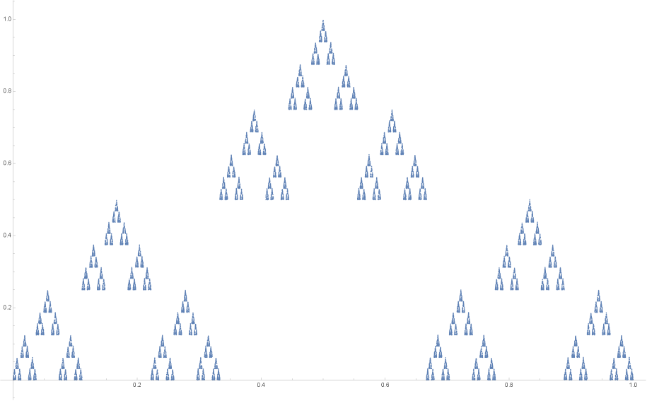
$ψ$ provides us with a notion of distance to $Λ$ such that the earlier a point exits the dynamical construction of $Λ$ (in the sense of (2.1)) the bigger the corresponding distance to $Λ$ . We will also view $ψ$ is a $[0,1]$ -valued random variable defined on $([0,1],B[0,1],\mathfrak{m})$ .
<details>
<summary>x1.png Details</summary>
### Visual Description
## Mathematical Plot: Sierpinski Triangle Fractal
### Overview
The image displays a two-dimensional scatter plot on a unit square coordinate system (0.0 to 1.0 on both axes). The plot visualizes a self-similar fractal pattern, specifically the Sierpinski triangle. The pattern is rendered using discrete blue points against a light gray background. The structure is characterized by recursive triangular clusters, where each larger triangle is composed of three smaller, identical triangles.
### Components/Axes
* **X-Axis (Horizontal):** Ranges from 0.0 to 1.0.
* Major ticks are present at intervals of 0.2.
* **Y-Axis (Vertical):** Ranges from 0.0 to 1.0.
* Major ticks are present at intervals of 0.2.
</details>
Figure 1. Graph of the function $ψ$ for the ternary Cantor set.
**Lemma 2.2**
*1. $ψ(x)=0\iff x∈Λ$ ;
1. $ψ(x)<2^-n\iff x∈Λ_n∖\{p_1,\dots,p_k_{I^n}\}$ , where
$$
\{p_1,\dots,p_k_{I^n}\}=≤ft\{x∈[0,1]:x_i∈I_I for all i=1,… n, and x_i∈I_J for i≥ n+1\right\};
$$
1. for $F:[0,1]→[0,1]$ the distribution function of $ψ$ ,
1. $F$ is strictly increasing on $[0,1]$ ;
1. $F(2^-n)=|Λ_n|=λ^n$ for $λ:=≤ft|∪_i=1^I_II_i\right|=∑_i=1^I_I\frac{1}{m_i}$ ;
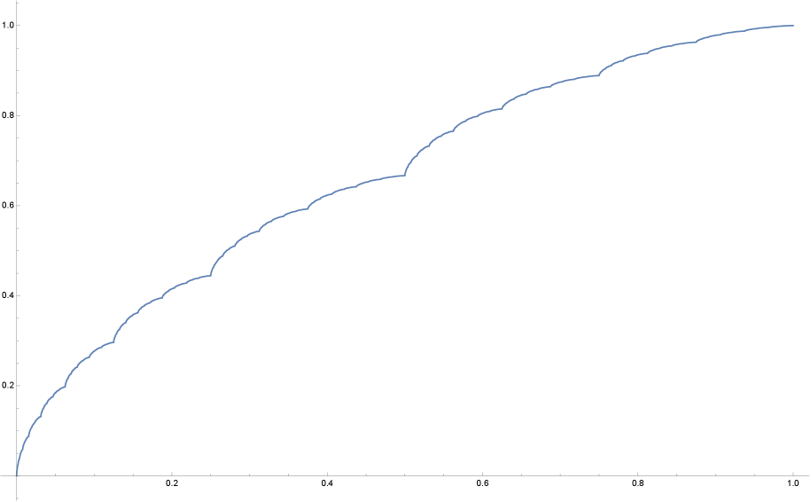
1. we can view $F∘ψ$ as a uniformly distributed random variable.*
* Proof*
The proofs of (a) and (b) are immediate. For (c) the strict increasing property follows from the definition of $ψ$ and (ii) follows from (b). (iii) is a standard fact in probability, which results from observing that $ℙ≤ft(F∘ψ≤ z\right)=ℙ≤ft(ψ≤ F^-1(z)\right)=F(F^-1(z))=z.$ ∎
<details>
<summary>x2.png Details</summary>
### Visual Description
## Mathematical Plot: The Cantor Function (Devil's Staircase)
### Overview
The image displays a mathematical plot of a continuous, monotonically increasing function defined on the interval [0, 1]. The curve exhibits a recursive, fractal-like structure, commonly known as the "Devil's Staircase" or the Cantor function.
### Components/Axes
* **X-Axis (Horizontal):** Represents the domain, ranging from 0.0 to 1.0. Major tick marks are present at 0.2, 0.4, 0.6, 0.8, and 1.0.
* **Y-Axis (Vertical):** Represents the range, ranging from 0.0 to 1.0. Major tick marks are present at 0.2, 0.4, 0.6, 0.8, and 1.0.
* **Data Series:** A single, continuous blue line plotted against the axes.
* **Background:** A uniform, light-gray field.
### Detailed Analysis
* **Trend Verification:** The line originates at the origin (0,0) and terminates at the coordinate (1,1). The function is monotonically increasing; it never decreases.
* **Visual Structure:** The curve is composed of a series of "steps" or plateaus. Upon closer inspection, these steps are self-similar; the pattern of the curve at a large scale is repeated at smaller scales.
* **Key Data Points:**
* **Start:** (0, 0)
* **Midpoint:** (0.5, 0.5)
* **End:** (1, 1)
* **Quarter points:** The curve passes through approximately (0.25, 0.25) and (0.75, 0.75), though the fractal nature means the "flat" sections are dense.
### Key Observations
* **Fractal Nature:** The curve is a classic example of a fractal. It is continuous everywhere but differentiable almost nowhere.
* **"Flat" Regions:** The curve appears to have horizontal segments. In the mathematical definition of the Cantor function, the derivative is zero almost everywhere, meaning the function is "flat" on the complement of the Cantor set.
* **Symmetry:** The function exhibits point symmetry about the center point (0.5, 0.5).
### Interpretation
This plot represents the Cantor function, a counter-intuitive mathematical object.
* **Mathematical Significance:** It is a standard example in real analysis used to demonstrate that a function can be continuous and non-decreasing, yet have a derivative of zero almost everywhere.
* **"Devil's Staircase":** The name arises because the function appears to be a staircase (a series of flat steps), yet it is continuous. It effectively "climbs" from 0 to 1 without ever having a positive slope in the traditional sense over the majority of its domain.
* **Application:** This type of function is often used to illustrate the limitations of the Fundamental Theorem of Calculus, as it is a function that is not the integral of its derivative (since the derivative is 0 almost everywhere, but the function changes from 0 to 1).
</details>
Figure 2. Graph of the the distribution function of $ψ$ for the ternary Cantor set.
We may now define our observable.
**Definition 2.3**
*For $α∈(0,2)$ , let
$$
φ_α(x):=(F∘ψ(x))^-\frac{1{α}}.
$$
where $F:[0,1]→[0,1]$ is the distribution function of $ψ$ . Moreover, define
$$
X_n:=φ_α∘ G^n
$$
for all $n∈ℕ_0$ .*
Note that since $G$ is $\mathfrak{m}$ -invariant, $X_n$ is a stationary process.
**Lemma 2.4**
*1. $φ_α(x)=∞$ iff $x∈Λ$ ;
1. if $x∈Λ_n∖\{p_1,\dots,p_k_{I^n}\}$ and $y∈Λ_n+1$ then $φ_α(x)<φ_α(y)$ ;
1. $\{X_n>u\}=\{ψ∘ G^n<F^-1(u^-α)\}$ ;
1. if $u^\prime>u$ then $\mathfrak{m}\{X_n>u^\prime\}<\mathfrak{m}\{X_n>u\}$ .*
* Proof*
Parts (a), (b) and (c) are immediate from the definition. Part (d) then follows from part (b) along with Lemma 2.2 (c). ∎
## 3. General theory of functional limit theorems
In this section we present a simplified version of the theory in [FFT25] which, to fit with our application outlined above, deals with real non-negative random variables $X_0,X_1,…$ distributed according to $ℙ$ , defined via a dynamical system $f:[0,1]→[0,1]$ with invariant probability measure $μ$ and an observable $φ:[0,1]→[0,∞]$ with $X_n=φ∘ f^n-1$ (hence $ℙ(X>u)=μ(φ>u)$ , but we will also write this as $μ(X>u)$ ).
We define sequences $(k_n)_n∈ℕ$ , $(r_n)_n∈ℕ$ , $(t_n)_n∈ℕ$ , $(q_n)_n$ , which we assume to be such that
$$
k_n,r_n,t_n\xrightarrow[n→∞]{}∞ where k_n· t_n=o(n),k_n· r_n∼ n and q_n=o(r_n).
$$
As in [FFT25, (3.2), (3.3)], these relate to a blocking argument with $k_n$ blocks of size $\lfloor n/k_n\rfloor$ , where $t_n$ is a time gap inserted to achieve asymptotic independence of the blocks, while $q_n$ is the clustering run length, i.e., all abnormal observations occurring within a time difference of at most $q_n$ units between each other belong to the same cluster. In most dynamical applications $q_n=q$ for all $n∈ℕ$ , such as when the observable is maximised at a single periodic point of period $p$ , in which case $q_n=p$ (see [FFT12]). In fact, we will see that, in this paper, for our applications we only require $q_n=1$ . We assume for each $τ≥ 0$ there is $(u_n(τ))_n$ such that
$$
\lim_n→∞nℙ(X_0>u_n(τ))=τ,\lim_τ_{1→ 0,τ_2→∞}ℙ≤ft(u_n(τ_1)<X_0<u_n(τ_2)\right)=1
$$
and that $u_n:[0,∞]→[0,∞]$ is bijective.
We say that $X_0$ has $α$ -regularly varying tails if there is a sequence $(\mathfrak{a}_n)_n$ such that for any $y>0$ ,
$$
\lim_n→∞nℙ(X_0>y\mathfrak{a}_n)=y^-α.
$$
Define
$$
U_n(τ):=\{X_0>u_n(τ)\}.
$$
### 3.1. Sequence spaces and the anchored tail process
For $i<j∈\{0,…,n\}$ we will use the notation
$$
X_n^i,j:=≤ft(u_n^-1(X_i),…,u_n^-1(X_j-1)\right), X_n,i:=X_n^(i-1)r_n,ir_n.
$$
Define
| | $\displaystyle l_∞^+$ | $\displaystyle:=≤ft\{x=(x_j)_j∈(0,∞]^ℤ\colon \lim_|j|→∞x_j=∞\right\}.$ | |
| --- | --- | --- | --- |
Note that we can embed $∪_n∈ℕ(0,∞]^n$ into $l_∞^+$ by adding a sequence of $∞$ before and after the $n$ entrances of any element of $(0,∞]^n$ For example, $X_n^i,j$ can be seen as an element of $l_∞^+$ by identifying it with
$$
≤ft(…,∞,∞,u_n^-1(X_i),…,{u_n^-1(X_j-1)},∞,∞,…\right).
$$
We can define the left shift $σ$ on this space, which moves every element one place to the left. We define the quotient space $\tilde{l}_∞^+=l_∞^+/{∼}$ where $∼$ is the equivalence relation defined by $x∼y$ if and only if there exists $k∈ℤ$ such that $σ^k(x)=y$ . Also let $\tilde{π}$ denote the natural projection from $l_∞^+$ to $\tilde{l}_∞^+$ , which assigns to each element $x$ of $l_∞^+$ the corresponding equivalence class $\tilde{π}(x)=\tilde{x}$ in $\tilde{l}_∞^+$ . Given any vector $v$ of $(0,∞]^m$ , for some $m∈ℕ$ , we write $\tilde{π}(v)$ for the projection of the natural embedding of $v$ into $l_∞^+$ to the quotient space $\tilde{l}_∞^+$ . Namely,
$$
\tilde{π}(X_n^i,j)=\tilde{π}≤ft(≤ft(…,∞,∞,u_n^-1(X_i),…,{u_n^-1(X_j-1)},∞,∞,…\right)\right).
$$
We let $\tilde{∞}∈\tilde{l}_∞^+$ be the sequence where all terms are $∞$ .
We will assume in the theory, and prove in practice, the existence of a process $(Y_j)_j∈ℤ∈ l_∞^+$ satisfying the following assumptions:
1. $L≤ft(\frac{1}{τ}X_n^r_n+s,r_n+t \middle| X_r_{n}>u_n(τ)\right)\xrightarrow[n→∞]{}L≤ft((Y_j)_j=s,\dots,t\right),$ for all $s<t∈ℤ$ and all $τ>0$ ;
1. the process $(Θ_j)_j∈ℤ$ given by $Θ_j=\frac{Y_j}{Y_0}$ is independent of $Y_0$ ;
1. $\lim_|j|→∞Y_j=∞$ a.s.;
1. $ℙ≤ft(∈f_j≤-1Y_j≥ 1\right)>0$ .
Here $(r_n)_n$ is assumed to satisfy (3.1): in our applications it is the sequence appearing in $\D_q_{n}^*$ and $\D^{^\prime*}_q_{n}$ below. We call this the transformed tail process.
We can then define:
**Definition 3.1**
*Assuming the existence of a sequence $(Y_j)_j∈ℤ$ satisfying conditions (1)–(4), we define the transformed anchored tail process $(Z_j)_j∈ℤ$ as a sequence of random numbers satisfying
$$
L≤ft((Z_j)_j∈ℤ\right)=L≤ft((Y_j)_j∈ℤ \middle| ∈f_j≤-1Y_j≥ 1\right).
$$*
The anchor $Z_0$ was chosen so that it marks the beginning of a new cluster. We consider a polar decomposition of the transformed anchored tail process by defining the random variable $L_Z$ and the process $(Q_j)_j∈ℤ$ by
$$
L_Z:=∈f_j∈ℤZ_j Q_j:=\frac{Z_j}{L_Z}.
$$
### 3.2. The $\D_q_{n}^*$ and $\D_q_{n}^{^\prime*}$ conditions and the extremal index
For $B⊂[0,1]$ , $J$ a subset of $[0,∞)$ and $q∈ℕ$ define
$$
\mathscr{W}_J(B):=\bigcap_i∈ J∩ℕ_0f^-i(B^c), \mathscr{W}_J^c(B):=(\mathscr{W}_J(B))^c=\bigcup_i∈ J∩ℕ_0f^-i(B),
$$
and
$$
B^(q):=B∩\bigcap_i=1^qf^-i(B^c), B^(0):=B. \tag{0}
$$
Now let $E$ be an element of the ring generated by the half open intervals of $[0,1]$ so that $E=∪_\ell=1^NJ_\ell=∪_\ell=1^N[a_\ell,b_\ell)$ and for each $\ell=1,…,N$ , let $A_\ell$ be an element of the ring generated by the half open intervals of $[0,∞)$ so that $A_\ell=∪_s=1^n_\ell[{τ_s^\prime\prime},τ^\prime_s)$ for some $n_\ell∈ℕ$ and some $τ_1^\prime\prime<τ_1^\prime<τ_2^\prime\prime<⋯<τ_n_{\ell}^\prime\prime<τ_n_{\ell}^\prime$ .
Given $E$ and $A_\ell$ as above, define
$$
J_n,\ell:=k_nr_nJ_\ell:=[k_nr_na_\ell,k_nr_nb_\ell), A_n,\ell:=\bigcup_s=1^n_\ell≤ft\{u_n^-1(X_0)∈[τ^\prime\prime_s,τ^\prime_s)\right\}=\bigcup_s=1^n_\ellU_n(τ^\prime_s)∖ U_n(τ_s^\prime\prime)
$$
Condition $\D_q_{n}^*$ . We say that $\D_q_{n}^*$ holds for the sequence ${X}_0,{X}_1,\dots$ if there exist sequences $(k_n)_n∈ℕ,(r_n)_n∈ℕ,(t_n)_n∈ℕ$ and $(q_n)_n∈ℕ$ as defined in (3.1), such that for every $N,t,n∈ℕ$ and every $J_\ell,A_\ell$ as above, for $\ell=1,\dots,N$ , we have
$$
≤ft\lvertℙ≤ft(A_n,\ell^(q_n)∩\bigcap_i=\ell^N\mathscr{W}_J_{n,i}≤ft(A_n,i^(q_n)\right)\right)-ℙ≤ft(A_n,\ell^(q_n)\right)ℙ≤ft(\bigcap_i=\ell^N\mathscr{W}_J_{n,i}≤ft(A_n,i^(q_n)\right)\right)\right\rvert≤γ(n,t_n)
$$
where $\min\{J_n,\ell∩ℕ_0\}≥ t_n+q_n$ and $\lim_n→∞nγ(n,t_n)=0$ .
Condition $\D_q_{n}^{^\prime*}$ . We say that $\D_q_{n}^{^\prime*}$ holds for the sequence ${X}_0,{X}_1,\dots$ if there exist sequences $(k_n)_n∈ℕ,(r_n)_n∈ℕ,(t_n)_n∈ℕ$ and $(q_n)_n∈ℕ$ as defined in (3.1), such that for every $A_1=∪_s=1^N_1[{τ^\prime\prime}_s,τ^\prime_s)$ ,
$$
\lim_n→∞nℙ≤ft(A_n,1^(q_n)∩\mathscr{W}^c_[q_{n+1,r_n)}≤ft(A_n,1\right)\right)=0.
$$
**Remark 3.2**
*Note that if $(q_n)_n∈ℕ$ and $(\tilde{q}_n)_n∈ℕ$ are two sequences satisfying (3.1) and $q_n≤\tilde{q}_n$ , for all $n∈ℕ$ . Then $\D^\prime_q_{n}$ implies $\D^\prime_\tilde{q_n}$ . As observed in [AFF20, Remark 2.11], one should try first to find the smallest constant sequence $q_n=q$ that makes $\D_q_{n}^{^\prime*}$ hold, establishing, in this way, the run length. We will see that here we can actually take $q_n=1$ for all $n∈ℕ$ .*
If, for all $τ>0$ , the following limit exists:
$$
θ=\lim_n→∞\frac{ℙ(U_n^(q_n)(τ))}{ℙ(U_n(τ))},
$$
then we call $θ$ the extremal index.
### 3.3. Complete convergence of the Rare Events Point Processes
As mentioned above, at the core of all convergence results stated and mentioned in this paper is the convergence of the so-called Rare Events Point Processes (REPP), which are spatio-temporal clustering processes that keep record of the cluster profiles and their time occurrences:
$$
N_n=∑_i=1^∞δ_≤ft(i/k_{n,\tilde{π}(X_n,i)\right)}.
$$
The complete convergence of these REPP follows from [FFT25, Theorem 3.18], which assuming that the transformed anchored tail process exists and is well defined (see Definition 3.1) and that conditions $\D_q_{n}^*$ and $\D_q_{n}^*^{\prime}$ are satisfied, states that $N_n$ given in (3.7) converges weakly in the space of boundedly finite point measures on $ℝ_0^+×\tilde{l}_∞^+∖\{\tilde{∞}\}$ with weak # topology (see [FFT25, Appendix C] for details) to the Poisson process with decorations, which can be written as:
$$
N=∑_i=1^∞δ_(T_{i,U_i\tilde{Q}_i)},
$$
where $T_i$ and $U_i$ are independently (of $i$ and of each other) distributed according to $Leb$ and $θ Leb$ respectively, for $θ$ as in (3.6), and $(\tilde{Q}_i)_i∈ℕ$ is an i.i.d sequence such that each $\tilde{Q}_i∈\tilde{l}_∞^+∖\{\tilde{∞}\}$ has the same distribution as $\tilde{π}((Q_j)_j∈ℤ)$ , where the bi-infinite sequence $(Q_j)_j$ is as in (3.4).
### 3.4. Enriched functional limit theorem
For processes $X_0,X_1,…$ with $α$ -regularly varying tails, for which we can prove the convergence of the REPP defined above, applying [FFT25, Theorem 2.5], we obtain an enriched functional limit theorem (FLT) for the normalised sums:
$$
S_n(t)=∑_i=0^\lfloor nt\rfloor-1\dfrac{1}{\mathfrak{a}_n}X_i-tc_n, t∈[0,1],
$$
where the sequence $(c_n)_n∈ℕ$ is such that $c_n=0$ if $0<α<1$ and
$$
c_n=\frac{n}{\mathfrak{a}_n}E≤ft(X_0{\mathbbm{1}}_|X_{0|≤\mathfrak{a}_n}\right), for 1<α<2.
$$
In order to guarantee the existence of a limit for the càdàg function $S_n(t)$ , which sometimes is not possible with any of the Skorohod metrics in $D([0,1])$ , the space of càdàg functions on $[0,1]$ , and to keep the information regarding the excursions performed by finite time process during a cluster of abnormal observations that gets collapsed on the same discontinuity of the limit process, in [FFT25], the authors introduced the enriched space $F^\prime([0,1])$ as the space of triplets $(v,S^v,\{e_v^s\}_s∈ S^v)$ , where $v$ is the main càdàg function, $S^v$ a set containing all its discontinuities and $e_v^s$ a decorating excursion associated to each element of $S^v$ . This excursion is an element of $\tilde{D}([0,1])$ , the equivalence space of càdàg functions on $[0,1]$ , where two elements are identified if there is a strictly continuous time reparametrisation that sends one into another. We refer to [FFT25, Section 2.3.1] for the details about this space, the corresponding metric and notions of convergence there.
From [FFT25, Theorem 2.5], in the case $0<α<1$ , we obtain that the càdàg function $S_n(t)$ embedded in the space $F^\prime$ converges to $(V,disc(V),(e_V^s)_s∈disc(V))$ , where $V$ is an $α$ -stable Lévy process on $[0,1]$ , which can be written as:
$$
V(t)=∑_T_{i≤ t}∑_j∈ℤU_i^-\frac{1{α}}Q_i,j
$$
and the excursions are given by
$$
e_V^T_i(t)=V(T_i^-)+U_i^-\frac{1{α}}\displaystyle∑_j≤\lfloor\tan(π(t-\frac{1{2}))\rfloor}Q_i,j, t∈[0,1]
$$
where $Q_i,j=\tilde{Q}_i,j^-\frac{1{α}}$ (zero if $\tilde{Q}_i,j=∞$ ), with $\tilde{Q}_i=≤ft(\tilde{Q}_i,j\right)_j$ , $T_i$ and $U_i$ as in $N$ in (3.8).
In the case $1<α<2$ , we need the next two extra conditions to hold. Namely, for all $δ>0$
$$
\lim_ε→ 0\limsup_n→∞ℙ≤ft(\max_1≤ k≤ n≤ft\|∑_j=1^k≤ft(X_j{\mathbbm{1}}_|X_{j|≤ε a_n}\right)-E≤ft(X_j{\mathbbm{1}}_|X_{j|≤ε a_n}\right)\right\|≥δ a_n\right)=0
$$
and, moreover,
$$
E≤ft(≤ft(∑_j∈ℤ\|Q_j)\|\right)^α\right)<∞.
$$
Then, under these two assumptions as well, $S_n(t)$ converges to $(V,disc(V),(e_V^s)_s∈disc(V))$ in $F^\prime$ , where $V$ has the more complicated expression:
$$
\displaystyle V(t) \displaystyle=\lim_ε→ 0\Bigg(∑_T_{i≤ t}∑_j∈ℤU_i^-\frac{1{α}}Q_i,j{\mathbbm{1}}_\{|U_{i^-\frac{1{α}}Q_i,j|>ε\}} \displaystyle\hskip 128.0374pt-tθ∫_0^+∞E\Bigg(y∑_j∈ℤQ_j{\mathbbm{1}}_\{ε<y|Q_j|≤ 1\}\Bigg)d(-y^-α)\Bigg),
$$
while $e_V^T_i(t)$ is again as in (3.11).
## 4. Application of the theory to our examples
We apply the theory described above to the setting described in Section 2. In particular, we have now all the tools and notation introduced in order to state our main results.
### 4.1. Statement of main results
We begin with the convergence of the REPP.
**Theorem 4.1**
*Let $G$ be as defined in Section 2, let $φ_α$ be as in Definition 2.3 and $X_0,X_1,…$ , as in (2.5). We consider the REPP
$$
N_n=∑_i=1^∞δ_≤ft(\frac{i{k_n},\tilde{π}≤ft(≤ft(n(X_(i-1)r_{n})^-α,n(X_(i-1)r_{n+1})^-α,…,n(X_ir_{n-1})^-α\right)\right)\right)},
$$
where the sequences $(k_n)_n,(r_n)_n$ are as described in (3.1). Then $N_n$ converges in the weak # topology to a process $N$ which can be written as in (3.8), where $Q_j=(1-θ)^-j$ for all $j≥ 0$ , $Q_j=∞$ for all $j≤-1$ and
$$
θ=1-\displaystyle∑_i=1^I_I\dfrac{1}{m_i}=1-λ.
$$*
From the convergence of the REPP and [FFT25, Theorem 2.5], we obtain the following enriched functional limit theorem.
**Theorem 4.2**
*Under the same assumptions of the previous theorem, we consider the heavy tailed sums:
$$
S_n(t)=∑_i=0^\lfloor nt\rfloor-1\dfrac{1}{n^\frac{1{α}}}X_i-tc_n, t∈[0,1],
$$
where $c_n=0$ , when $0<α<1$ and is given by (3.9), when $1<α<2$ . Then, the process $S_n(t)$ converges in $F^\prime$ to $(V,disc(V),(e_V^s)_s∈disc(V))$ , where $V$ is as described in (3.10), when $0<α<1$ , or as in (3.14), when $1<α<2$ , and the excursions can be written as
$$
e_V^T_i(t)=V(T_i^-)+U_i^-\frac{1{α}}∑_0≤ j≤\lfloor\tan(π t/2)\rfloor(1-θ)^\frac{j{α}}, t∈[0,1].
$$*
**Remark 4.3**
*In light of [FFRS20], for $M$ equal to the middle- $\frac{1}{3}$ Cantor set then $θ<1$ if and only if, among the class of maps $mx\mod 1$ , $m≥ 2$ , we restrict to $m=3^k$ , $k∈ℕ$ . Hence, an extremal index strictly less than $1$ is obtained if and only if the dynamics is somehow compatible with the construction of the middle- $\frac{1}{3}$ Cantor set. We proceed with the computation of the extremal index in the greater generality of $Λ$ dynamically defined by $G$ and for our observable $φ_α$ which is different from the one used in [FFRS20].*
The rest of this section is dedicated to the proof of Theorem 4.1, which essentially means checking that we have the right normalisations, that all conditions of [FFT25, Theorem 3.18], [FFT25, Theorem 2.5] described in Sections 3.3 and 3.4 hold, and computing the extremal index and the transformed anchored tail process.
### 4.2. Tuning constants and normalising sequences
**Lemma 4.4**
*$X_n$ have $α$ -regularly varying tails.*
* Proof*
We wish to find $(\mathfrak{a}_n)_n∈ℕ$ such that $\lim_n→∞nℙ(X_0>y\mathfrak{a}_n)=y^-α.$ Since from Lemma 2.4,
$$
\{X_0>y\mathfrak{a}_n\}=\{F∘ψ<y^-α\mathfrak{a}_n^-α\},
$$
it follows that
$$
ℙ(X_0>y\mathfrak{a}_n)=ℙ(F∘ψ<y^-α\mathfrak{a}_n^-α)=y^-α\mathfrak{a}_n^-α.
$$
Hence we conclude that $\mathfrak{a}_n=n^\frac{1{α}}$ for all $n∈ℕ$ . ∎
In particular, this lemma means for each $τ>0$ we can define $(u_n(τ))_n$ so that
$$
\lim_n→∞nℙ(X_0>u_n(τ))=τ, so u_n(τ)=≤ft(\frac{n}{τ}\right)^\frac{1{α}} and u_n^-1(z)=nz^-α.
$$
We next give a geometric description of this set. By Lemma 2.2 and (4.1) there are $a_i=a_i(n,τ)∈\{0,1\}$ so that,
$$
F^-1((u_n(τ))^-α)=F^-1≤ft(\frac{τ}{n}\right)=∑_i∈ℕa_i2^-i=∑_j∈J_n,τ2^-j=:u_n,τ
$$
where $J_n,τ=\{i∈ℕ:a_i=1\}$ .
Let
$$
j_n,τ=j_n,τ^1:=\min\{j:j∈J_n,τ\} and j_n,τ^\ell+1=\min\{j>j_n,τ^\ell\colon j∈J_n,τ\}, for all \ell∈ℕ.
$$
If, for some $\ell>1$ , we have $a_i=0$ for all $i≥ j_n,r^\ell$ , then we set $j_n,r^s=∞$ for all $s≥\ell$ . Note that Lemma 2.2 (c)(ii) implies that $j_n,τ$ grows logarithmically in $n$ (i.e., , $\limsup_n→∞\frac{j_n,τ}{\log n}<∞$ ). Moreover, by Lemma 2.4,
$$
\begin{split}U_n(τ)=\{X_0>u_n(τ)\}=\{ψ<u_n,τ\}=Λ_j_{n,τ}∪ H^(j_n,τ)\end{split}
$$
where $H^(j_n,τ)$ denotes a subset of $Λ_j_{n,τ-1}∖Λ_j_{n,τ}$ .
**Remark 4.5**
*Recall Lemma 2.2 (b) to justify the appearance of $Λ_j_{n,τ}$ . Observe that $u_n,τ=2^-j_n,τ+δ$ with $δ≤ 2^-j_n,τ$ , so, in particular, $H^(j_n,τ)=∅$ if $δ=0$ (which means that $j_n,τ^\ell=∞$ for all $\ell≥ 2$ ) and $H^(j_n,τ)=Λ_j_{n,τ-1}∖(Λ_j_{n,τ}∪\{p_1,\dots,p_k_{I^j_n,τ}\})$ , if $δ=2^-j_n,τ$ and where the $p_i$ s are as in Lemma 2.2. Now, $H^(j_n,τ)$ can be further decomposed into
$$
H^(j_n,τ)=Λ^\prime_j_{n,τ^2-j_n,τ}∪ H^(j_n,τ^{2)},
$$
where $Λ^\prime_j_{n,τ^2-j_n,τ}$ is homothetic to $Λ_j_{n,τ^2-j_n,τ}$ , which was rescaled to fit the corresponding connected components of $Λ_j_{n,τ-1}∖Λ_j_{n,τ}$ , and $H^(j_n,τ^{2)}$ is a subset of $Λ^\prime_j_{n,τ^2-j_n,τ}∖Λ^\prime_j_{n,τ^2-j_n,τ-1}$ . Note that $Λ^\prime_j_{n,τ^2-j_n,τ}$ can be written as a union of $j_n,τ^2$ -cylinders. This procedure can be repeated to obtain approximations of $H^(j_n,τ)$ by unions of cylinders of greater and greater depth.*
### 4.3. Extremal Index
Recall that
$$
\begin{split}U_n^(q)(τ)&=\{X_0(x)>u_n(τ),X_1≤ u_n(τ),\dots,X_q≤ u_n(τ)\}\\
&=\{ψ<u_n,τ,ψ∘ G≥ u_n,τ,\dots,ψ∘ G^q≥ u_n,τ\}.\end{split}
$$
Observe that for $n$ sufficiently large, we have
$$
\begin{split}U_n^(1)(τ)&=\{ψ<u_n,τ,ψ∘ G≥ u_n,τ\}\\
&=≤ft(Λ_j_{n,τ}∪ H^(j_n,τ)\right)∩ G^-1([0,1]∖(Λ_j_{n,τ}∪ H^(j_n,τ)))\\
&=H^(j_n,τ)∪(Λ_j_{n,τ}∩ G^-1((Λ_j_{n,τ-1}∖Λ_j_{n,τ})∖ H^(j_n,τ)))\end{split} \tag{1}
$$
Now, observing that the points of $U_n^(1)(τ)$ are sent by $G$ into the holes of smaller and smaller generation in the construction of $Λ$ , it follows that $U_n^(1)(τ)=U_n^(2)(τ)=U_n^(3)(τ)=…$ . In light of Remark 3.2, this means that $q_n=1$ is then a natural choice to prove condition $\D_q_{n}^{^\prime*}$ , which is indeed established in Section 4.4.
The extremal index $θ$ can be written as
$$
θ=\lim_n→∞\dfrac{\mathfrak{m}(U_n^(1)(τ))}{\mathfrak{m}(U_n(τ))} \tag{1}
$$
provided the limit exists.
**Proposition 4.6**
*For $G$ as defined in Section 2 and observable $φ_α$ as given in Definition 2.3, the extremal index is $θ=1-\displaystyle∑_i=1^I_I\dfrac{1}{m_i}=1-λ$ .*
* Proof*
Let $u_n,τ∈[2^-j,2^-j+1)$ . Then, $j_n,τ=j$ and, by (4.3), $U_n(τ)=Λ_j∪ H^(j)$ so that
$$
\mathfrak{m}(U_n(τ))=\mathfrak{m}(Λ_j)+κ\mathfrak{m}(Λ_j-1∖Λ_j)
$$
where $κ∈[0,1]$ since $H^(j)$ is a fraction of $Λ_j-1∖Λ_j$ . Now, by (4.4),
$$
U_n^(1)(τ)=H^(j)∪(Λ_j∩ G^-1((Λ_j-1∖Λ_j)∖ H^(j))) \tag{1}
$$
and we have
$$
\mathfrak{m}(U_n^(1)(τ))=κ\mathfrak{m}(Λ_j-1∖Λ_j)+(1-κ)\mathfrak{m}(Λ_j∖Λ_j+1) \tag{1}
$$
where $κ$ is the same as in (4.5) (in particular, observe that the second summand reflects the fact that only a fraction of $Λ_j∖Λ_j+1$ , whose measure is $(1-κ)\mathfrak{m}(Λ_j∖Λ_j+1)$ , is iterated in one time step to the complement of $H^(j)$ in $Λ_j-1∖Λ_j$ ). (4.5) can be rewritten
$$
\mathfrak{m}(U_n(τ))=≤ft(∑_i=1^I_I\dfrac{1}{m_i}\right)\mathfrak{m}(Λ_j-1)+κ≤ft(1-∑_i=1^I_I\dfrac{1}{m_i}\right)\mathfrak{m}(Λ_j-1)=λ\mathfrak{m}(Λ_j-1)+κ≤ft(1-λ\right)\mathfrak{m}(Λ_j-1)
$$ and (4.6) can be rewritten
$$
\mathfrak{m}(U_n^(1)(τ))=κ≤ft(1-λ\right)\mathfrak{m}(Λ_j-1)+(1-κ)≤ft(1-λ\right)λ\mathfrak{m}(Λ_j-1) \tag{1}
$$ Finally,
$$
\begin{split}θ_n=\dfrac{\mathfrak{m}(U_n^(1)(τ))}{\mathfrak{m}(U_n(τ))}&=\dfrac{κ≤ft(1-\displaystyleλ\right)+(1-κ)≤ft(1-λ\right)λ}{λ+κ≤ft(1-λ\right)}=\dfrac{κ≤ft(1-λ\right)≤ft(1-λ\right)+≤ft(1-λ\right)λ}{λ+κ≤ft(1-λ\right)}\\
&=≤ft(1-λ\right)\dfrac{κ≤ft(1-λ\right)+λ}{λ+κ≤ft(1-\displaystyleλ\right)}=1-\displaystyleλ\end{split} \tag{1}
$$ Therefore, $θ=\displaystyle\lim_n→∞θ_n=1-\displaystyleλ$ . ∎
**Remark 4.7**
*Observe that with $Λ$ equal to the middle- $\frac{1}{3}$ Cantor set as described in Section 2 we obtain $θ=\dfrac{1}{3}$ .*
### 4.4. Dependence requirements
In order to prove that the conditions $\D_q_{n}$ and $\D^\prime_q_{n}$ from Section 3.2 hold in our setting we will approximate the sets $A_n,\ell^(q_n)$ by a union of cylinders of controlled depth and then use the excellent mixing properties on cylinders in the spirit of [HP14, DHY21, BF24], for example.
Since $A_n,\ell^(q_n)$ is itself a finite union of sets of the form $U_n(τ^\prime,τ^\prime\prime):=U_n(τ^\prime)∖ U_n(τ^\prime\prime)$ , for $τ^\prime\prime<τ^\prime$ , we restrict the analysis to these building blocks in order to simplify the already heavy notation.
Since
$$
\begin{split}U_n(τ^\prime,τ^\prime\prime)&=≤ft(Λ_j_{n,τ^\prime}∪ H^(j_n,τ^{\prime)}\right)∖≤ft(Λ_j_{n,τ^\prime\prime}∪ H^(j_n,τ^{\prime\prime)}\right)\\
&=H^(j_n,τ^{\prime)}∪≤ft(Λ_j_{n,τ^\prime}∖≤ft(Λ_j_{n,τ^\prime\prime}∪ H^(j_n,τ^{\prime\prime)}\right)\right),\end{split}
$$
$U_n(τ^\prime,τ^\prime\prime)$ is made up of holes in the dynamical construction of $Λ$ (i.e. subsets of the form $Λ_k∖Λ_k+1$ where $k∈ℕ$ ), where $j_n,τ^\prime$ is as in (4.2). Moreover, as observed earlier, for $n$ sufficiently large,
$$
\begin{split}U_n(τ^\prime,τ^\prime\prime)^(q)&=U_n(τ^\prime,τ^\prime\prime)∩ G^-1(U_n(τ^\prime,τ^\prime\prime))^c∩\dots∩ G^-q(U_n(τ^\prime,τ^\prime\prime))^c\\
&=U_n(τ^\prime,τ^\prime\prime)∩ G^-1(U_n(τ^\prime,τ^\prime\prime))^c\end{split}
$$
so, in particular, taking $q_n=1$ for all $n∈ℕ$ is the natural choice to prove condition $\D_q_{n}^{^\prime*}$ , which is established in 4.4.
Combining (4.7) and (4.8), we obtain
$$
U_n(τ^\prime,τ^\prime\prime)^(1)=H^(j_n,τ^{\prime)} \bigcup≤ft\{≤ft((Λ_j_{n,τ^\prime}∖Λ_j_{n,τ^\prime\prime})∖ H^(j_n,τ^{\prime\prime)}\right)∩ G^-1≤ft((Λ_j_{n,τ^\prime-1}∖Λ_j_{n,τ^\prime})∖ H^(j_n,τ^{\prime)}\right)\right\}. \tag{1}
$$
For a Borel set $A⊂[0,1]$ and $j∈ℕ$ , we define
$$
Υ^+(A,j):=\bigcup_ω∈P_j\colonω∩ A≠∅ω and Υ^-(A,j):=\bigcup_ω∈P_j\colonω⊂ Aω.
$$
They are the approximations of $A$ from above and below by $j$ -cylinders.
**Lemma 4.8**
*Let $U_n(τ^\prime,τ^\prime\prime)^(1)$ be given and let $j_n,τ^\prime$ be associated to this set as in (4.2). Let $Γ_n^+=Υ^+(U_n(τ^\prime,τ^\prime\prime)^(1),2j_n,τ^\prime)$ and $Γ_n^-=Υ^-(U_n(τ^\prime,τ^\prime\prime)^(1),2j_n,τ^\prime)$ be the respective outer and inner approximations by unions of $(2j_n,τ^\prime)$ -cylinders. Then there exists $(ρ_n)_n$ such that
$$
\dfrac{\mathfrak{m}(Γ_n^+∖Γ_n^-)}{\mathfrak{m}≤ft(U_n(τ^\prime,τ^\prime\prime)^(1)\right)}≤ρ_n \tag{1}
$$
where $\displaystyle\lim_n→∞ρ_n=0$ .*
* Proof*
We write
$$
U_n(τ^\prime,τ^\prime\prime)^(1)=H^(j_n,τ^{\prime)}∪ K \tag{1}
$$
where $K⊂Λ_j_{n,τ^\prime}∖Λ_j_{n,τ^\prime+1}$ . Therefore,
$$
\begin{split}\mathfrak{m}≤ft(U_n(τ^\prime,τ^\prime\prime)^(1)\right)&=β\mathfrak{m}(Λ_j_{n,τ^\prime-1}∖Λ_j_{n,τ^\prime})+γ\mathfrak{m}(Λ_j_{n,τ^\prime}∖Λ_j_{n,τ^\prime+1})\\
&=β≤ft(1-λ\right)\mathfrak{m}(Λ_j_{n,τ^\prime-1})+γ≤ft(1-λ\right)\mathfrak{m}(Λ_j_{n,τ^\prime})\\
&=β≤ft(1-λ\right)\mathfrak{m}(Λ_j_{n,τ^\prime-1})+γ≤ft(1-λ\right)λ\mathfrak{m}(Λ_j_{n,τ^\prime-1})\\
&=≤ft(β≤ft(1-λ\right)+γ≤ft(1-λ\right)λ\right)\mathfrak{m}(Λ_j_{n,τ^\prime-1})\\
&=≤ft(βθ+γθ(1-θ)\right)λ^j_n,τ^{\prime-1}\end{split} \tag{1}
$$
where $β,γ∈[0,1]$ and $θ$ is as in Proposition 4.6 (as $H^(j_n,τ^{\prime)}$ is a fraction of $Λ_j_{n,τ^\prime-1}∖Λ_j_{n,τ^\prime}$ while $K$ is a fraction of $Λ_j_{n,τ^\prime}∖Λ_j_{n,τ^\prime+1}$ ). Observe that the larger the set $H^(j_n,τ^{\prime)}$ is, the smaller the set $K$ is and vice-versa. This means that, in particular, $β$ and $γ$ cannot be simultaneously equal to $0$ or to $1$ . On the other hand, taking into consideration the definition of the function $ψ$ and of the approximating cylinders, as well as the fact that $G$ is a full branched Markov linear map (which, in particular, means that there exist $\tilde{C}>0$ and $0<η<1$ such that $\mathfrak{m}(ω)≤\tilde{C}η^n$ , for all $n∈ℕ$ and $ω∈P^n$ ), we claim that
$$
\mathfrak{m}(Γ_n^+∖Γ_n^-)≤ Cη^2j_n,τ^{\prime}, for some C>0.
$$
To see this, we start by noting that since $K$ is a preimage of the complement of $H^(j_n,τ^{\prime)}$ in $Λ_j_{n,τ^\prime-1}∖Λ_j_{n,τ^\prime}$ , we only need to check that $\mathfrak{m}≤ft(Υ^+(H^(j_n,τ^{\prime)},2j_n,τ^\prime)∖Υ^-(H^(j_n,τ^{\prime)},2j_n,τ^\prime)\right)≤ Cη^2j_n,τ^{\prime}$ for some $C>0$ . Recalling Remark 4.5, assume first that $j_n,τ^\prime^2>2j_n,τ^\prime$ . This means that $H^(j_n,τ^{\prime)}⊂Λ_j_{n,τ^\prime}^\prime$ , where $Λ_j_{n,τ^\prime}^\prime$ is homothetic to $Λ_j_{n,τ^\prime}$ , which was scaled to fit in one the the holes of $Λ_j_{n,τ^\prime}$ that comprise $Λ_j_{n,τ^\prime-1}∖Λ_j_{n,τ^\prime}$ in order to give rise to $Λ_j_{n,τ^\prime}^\prime$ . Hence, since $∅⊂Υ^-(H^(j_n,τ^{\prime)}⊂Υ^+(H^(j_n,τ^{\prime)}⊂Λ_j_{n,τ^\prime}^\prime$ , we have that
$$
\mathfrak{m}≤ft(Υ^+(H^(j_n,τ^{\prime)},2j_n,τ^\prime)∖Υ^-(H^(j_n,τ^{\prime)},2j_n,τ^\prime)\right)≤\mathfrak{m}(Λ_j_{n,τ^\prime}^\prime)≤ Cη^2j_n,τ^{\prime},
$$
for some $C>0$ . Now, if $j_n,τ^\prime^2≤ 2j_n,τ^\prime$ , we decompose the set $H^(j_n,τ^{\prime)}=Λ^\prime_j_{n,τ^2-j_n,τ}∪ H^(j_n,τ^{2)}$ further, as in Remark 4.5. Then, observe that $Λ^\prime_j_{n,τ^2-j_n,τ}$ can clearly be written as a union of cylinders of $P^2j_n,τ^{\prime}$ , which means that we only need to estimate the measure of $Υ^+(H^(j_n,τ^{2)},2j_n,τ^\prime)∖Υ^-(H^(j_n,τ^{2)},2j_n,τ^\prime)$ . We now consider the case $j_n,τ^\prime^3≤ 2j_n,τ^\prime$ , which will lead us to the same conclusion, as before, and otherwise proceed to another decomposition of $H^(j_n,τ^{2)}$ until we end by exhaustion. The result now follows from gathering estimates (4.10) and (4.11). ∎
It is a direct consequence of Lemma 4.8 that the REPP counting the number of hits to $U_n(τ^\prime,τ^\prime\prime)^(1)$ converges if and only if the REPP counting the number of hits to either $Γ_n^+$ or $Γ_n^-$ converges, and the limits are the same (see [BF24, Lemma 3.13], for example).
As a result, we only need to check that the conditions $\D_q_{n}^*$ and $\D^{^\prime*}_q_{n}$ are verified for the cylinder approximating sets. To this end, we next define a strong form of mixing, which is a property of the maps we are considering here.
**Definition 4.9**
*Let $(X,B_X,μ,f)$ be a probability preserving system. Let $F_0,k$ denote the $σ$ -algebra generated by $P^k$ . $(X,B_X,μ,f)$ is exponentially $φ$ -mixing if there exist $C,c>0$ such that for every $H∈F_0,k$ and every $A∈B_X$
$$
\lvertμ(H∩ f^-(t+k)(A))-μ(H)μ(A)\rvert≤ C{\rm e}^-ctμ(A).
$$*
We remark that $G$ is exponentially $φ$ -mixing, see for example [AN05, Theorem 1]. Recall that, as observed above, we only need to check the conditions $\D_q_{n}^*$ , $\D_q_{n}^{^\prime*}$ , where the set $A_n,\ell^(q_n)$ is replaced by the approximations $Γ_n^+$ and $Γ_n^-$ . In what follows, we will only check such conditions for $Γ_n^+$ , but the argument applies with minor adjustments to $Γ_n^-$ .
* Proof of ConditionДqn∗\D_{q_{n}}^{*}*
We need to control:
$$
E_n:=≤ft\lvert\mathfrak{m}≤ft(Γ_n^+∩\bigcap_i=\ell^N\mathscr{W}_J_{n,i}≤ft(Γ_n^+\right)\right)-\mathfrak{m}≤ft(Γ_n^+\right)\mathfrak{m}≤ft(\bigcap_i=\ell^N\mathscr{W}_J_{n,i}≤ft(Γ_n^+\right)\right)\right\rvert
$$ We start by noting that $E_n≤ 2\mathfrak{m}(Γ_n^+)$ . Also, observe that $Γ_n^+∈F_0,2j_{n,τ^\prime}$ . Assuming that $t>2j_n,τ^\prime$ and writing (4.12) with $H=Γ_n^+$ and $f^-(t-2j_n,τ^{\prime)+2j_n,τ^\prime}(A)=\bigcap_i=l^m\mathscr{W}_J_{n,i}(Γ_n^+)$ , we estimate $E_n≤ C{\rm e}^-c(t-2j_n,τ^{\prime)}$ . Hence, we can set $γ(n,t)=\max≤ft\{2,C{\rm e}^-c(t-2j_n,τ^{\prime)}\right\}$ . Since $j_n,τ^\prime$ grows logarithmically in $n$ , we can choose $t_n=o(n)$ and satisfying conditions (3.1) so that $\lim_n→∞nγ(n,t_n)=0$ . ∎
* Proof of ConditionДqn∗′\D_{q_{n}}^{{}^{\prime}*}*
We start by noting that, by construction, the points of $U_n(τ^\prime,τ^\prime\prime)^(1)$ are sent by $G$ into the holes that appeared in the $(j_n,τ^\prime-1)$ -th and/or the $(j_n,τ^\prime-2)$ -th step of the construction of $Λ$ and then they are sent successively by $G$ to lower and lower ranked holes in the construction until they reach the first holes of the construction and only then can they return to $U_n(τ^\prime,τ^\prime\prime)^(1)$ . Using this fact and the exponential $φ$ mixing property of $G$ , we have:
$$
\begin{split}&n\mathfrak{m}≤ft(Γ_n^+∩\mathscr{W}^c_[q_{n+1,r_n)}≤ft(A_n,(\bar{τ_i)_i,N}\right)\right)≤ n∑_j=j_{n,τ^\prime-1}^r_n-1\mathfrak{m}≤ft(Γ_n^+∩ f^-j≤ft(Γ_n^+\right)\right)\\
&≤ n∑_j=j_{n,τ^\prime-1}^2j_n,τ^{\prime}\mathfrak{m}≤ft(Γ_n^+∩ f^-j≤ft(Γ_n^+\right)\right)+n∑_j=2j_{n,τ^\prime}^r_n-1\mathfrak{m}≤ft(Γ_n^+∩ f^-j≤ft(Γ_n^+\right)\right)\\
&≤ n∑_j=j_{n,τ^\prime-1}^2j_n,τ^{\prime}\mathfrak{m}≤ft(Γ_n^+∩ f^-j≤ft(Γ_n^+\right)\right)+n∑_j=2j_{n,τ^\prime}^r_n-1\mathfrak{m}(Γ_n^+)\mathfrak{m}(Γ_n^+)+n\mathfrak{m}(Γ_n^+)∑_j=2j_{n,τ^\prime}^r_n-1C{\rm e}^-cj\\
&≤ n∑_j=j_{n,τ^\prime-1}^2j_n,τ^{\prime}\mathfrak{m}≤ft(Υ^+(U_n(τ^\prime,τ^\prime\prime)^(1),j)∩ f^-j≤ft(Γ_n^+\right)\right)+\tilde{C}\frac{n^2≤ft(\mathfrak{m}(Γ_n^+)\right)^2}{k_n}+\hat{C}n\mathfrak{m}(Γ_n^+)∑_j=2j_{n,τ^\prime}^∞C{\rm e}^-cj,\end{split} \tag{1}
$$
for some $\tilde{C},\hat{C}>0$ . The second term goes to $0$ by (3.2), Lemma 4.8 and the fact that $k_n→∞$ . The third term goes to $0$ by (3.2) and the fact that $j_n,τ^\prime→∞$ . Now, to handle the first term, we write $Υ^+(U_n(τ^\prime,τ^\prime\prime)^(1),j)=\bigcup_ω∈P_j\colonω⊂Υ^+(U_n(τ^\prime,τ^\prime\prime)^(1),j)ω$ , where the union is disjoint. Since $G$ is a full branched linear Markovian map, we have
$$
\mathfrak{m}≤ft(ω∩ f^-j≤ft(Γ_n^+\right)\right)≤ C\mathfrak{m}(ω)\mathfrak{m}≤ft(Γ_n^+\right).
$$
It follows that
$$
\begin{split}n∑_j=j_{n,τ^\prime-1}^2j_n,τ^{\prime}&\mathfrak{m}≤ft(Υ^+(U_n(τ^\prime,τ^\prime\prime)^(1),j)∩ f^-j≤ft(Γ_n^+\right)\right)\\
&≤ n∑_j=j_{n,τ^\prime-1}^2j_n,τ^{\prime}∑_ω∈P_j\colonω⊂Υ^+(U_n(τ^\prime,τ^\prime\prime)^(1),j)\mathfrak{m}≤ft(ω∩ f^-j≤ft(Γ_n^+\right)\right)\\
&≤ n∑_j=j_{n,τ^\prime-1}^2j_n,τ^{\prime}∑_ω∈P_j\colonω⊂Υ^+(U_n(τ^\prime,τ^\prime\prime)^(1),j)C\mathfrak{m}(ω)\mathfrak{m}≤ft(Γ_n^+\right)\\
&≤ Cn∑_j=j_{n,τ^\prime-1}^2j_n,τ^{\prime}\mathfrak{m}≤ft(Υ^+(U_n(τ^\prime,τ^\prime\prime)^(1),j)\right)\mathfrak{m}≤ft(Γ_n^+\right)≤\hat{C}\frac{j_n,τ^\prime}{n}\xrightarrow[n→∞]{}0\end{split} \tag{1}
$$
∎
### 4.5. Anchored tail process
We will see that for our $G$ and $φ_α$ the Cantor set $Λ$ behaves like a fixed point.
**Proposition 4.10**
*Let $G$ be as defined in Section 2 and let $φ_α$ be as in Definition 2.3. Then, the anchored tail process is (a.s.) the bi-infinite sequence $(Z_j)_j∈ℤ$ with entry $U.(1-θ)^-j$ at $j∈ℕ_0$ and $∞$ otherwise, where $U$ is uniformly distributed on $[0,1]$ and $θ$ is the extremal index (cf. Proposition 4.6).*
* Proof*
We check that the process $(Y_j)_j∈ℤ$ is (a.s.) the bi-infinite sequence with:
1. entry $U$ at $j=0$ ;
1. entries $U.(1-θ)^-j$ for all positive indices $j$ ;
1. $∞$ for all negative indices $j$ except, possibly, $U.(1-θ)^-j$ at $j≥-m$ for some $m∈ℕ$ ;
where $U$ is uniformly distributed on $[0,1]$ . Observe that $U.(1-θ)^-j<1$ for all $j<0$ . Therefore, if $(Y_j)_j∈ℤ$ is as described by (i)-(iii) then $(Z_j)_j∈ℤ$ is as in the statement of the theorem. We must check that conditions (1)-(4) in Section 3.1 are satisfied for $(Y_j)_j∈ℤ$ as given by (i)-(iii). Conditions (2) and (3) are straightforward. As for condition (4), $Y_j≥ 1$ for all $j≤-1$ implies that the hit to $Λ_j_{n,τ}∪ H^(j_n,τ)$ at time $r_n$ is the first hit to that same neighbourhood of $Λ$ (i.e. there is no hit to $Λ_j_{n,τ}∪ H^(j_n,τ)$ before time $r_n$ given that there is a hit to $Λ_j_{n,τ}∪ H^(j_n,τ)$ at time $r_n$ - recall, from (4.3), that $\{X_r_{n}>u_n(τ)\}=G^-r_n(Λ_j_{n,τ}∪ H^(j_n,τ))$ ). Since
$$
\dfrac{\mathfrak{m}(G^-r_n(Λ_j_{n,τ}∪ H^(j_n,τ))∩ G^-(r_n-1)([0,1]∖(Λ_j_{n,τ}∪ H^(j_n,τ))))}{\mathfrak{m}(G^-r_n(Λ_j_{n,τ}∪ H^(j_n,τ)))}>0,
$$
condition (4) is satisfied. So, we check that condition (1) holds. Recall that $u_n^-1(X_j)=≤ft(\dfrac{X_j}{\mathfrak{a}_n}\right)^-α$ . Therefore,
$$
≤ft\{\dfrac{1}{τ}u_n^-1(X_r_{n+j})\>\middle|\>X_r_{n}>u_n(τ)\right\}=≤ft\{\dfrac{1}{τ}≤ft(\dfrac{X_r_{n+j}}{\mathfrak{a}_n}\right)^-α\>\middle|\>X_r_{n}>u_n(τ)\right\}.
$$ Now, $\{x∈[0,1]:X_r_{n}(x)>u_n(τ)\}=G^-r_n(Λ_j_{n,τ}∪ H^(j_n,τ))$ . First note that for $t∈[0,1]$ , $ℙ(Y_0≤ t)=ℙ(F∘ψ≤ t)=t$ by Lemma 2.2 (c)(iii), so we write this uniform distribution by $U$ . For $j≥ 1$ , if $G^r_n(x)∈Λ_j_{n,τ}∪ H^(j_n,τ)$ then $G^r_n+j(x)∈Λ_j_{n,τ-j}∪ H^(j_n,τ-j)$ provided $j_n,τ-j≥ 0$ , in which case $ψ(G^r_n+j(x))=2^jψ(G^r_n(x))$ giving
$$
\begin{split}\dfrac{F(ψ(G^r_n+j(x)))}{F(ψ(G^r_n(x)))}=\dfrac{ℙ(ψ≤ψ(G^r_n+j(x)))}{ℙ(ψ≤ψ(G^r_n(x)))}=\dfrac{\mathfrak{m}(Λ_j_{n,τ-j}∪ H^(j_n,τ-j))}{\mathfrak{m}(Λ_j_{n,τ}∪ H^(j_n,τ))}&=≤ft(\displaystyle∑_i=1^k\dfrac{1}{m_i}\right)^-j\\
&=(1-θ)^-j\end{split}
$$ We have
$$
\lim_n→∞ℙ≤ft(≤ft\{\dfrac{u_n^-1(X_r_{n+j})}{u_n^-1(X_r_{n})}=(1-θ)^-j\>\middle|\>X_r_{n}>u_n(τ)\right\}\right)=1
$$
(since $j_n,τ-j≥ 0$ when $n→∞$ ). We may write
$$
\begin{split}&\hskip-28.45274pt\lim_n→∞ℙ≤ft\{\dfrac{1}{τ}u_n^-1(X_r_{n+j})=s\>\middle|\>X_r_{n}>u_n(τ)\right\}\\
&=\lim_n→∞ℙ≤ft\{\dfrac{u_n^-1(X_r_{n+j})}{u_n^-1(X_r_{n})}\dfrac{u_n^-1(X_r_{n})}{τ}=s\>\middle|\>X_r_{n}>u_n(τ)\right\}\end{split}
$$
which, by (2) in in Section 3.1 holds, gives $L(Y_j)=L(Θ_jY_0)=(1-θ)^-j.U$ (a.s.). Let $j<0$ . If $G^r_n(x)∈Λ_j_{n,τ}∪ H^(j_n,τ)$ then $G^r_n+j(x)∈Λ_j_{n,τ-j}∪ H^(j_n,τ-j)$ for an at most finite number of indices $j≥-m$ where $m∈ℕ$ . In words, a hit, at time $r_n$ , to the approximation (of $Λ$ ) $Λ_j_{n,τ}∪ H^(j_n,τ)$ can only be preceded by a finite number of hits to the finer approximations $Λ_j_{n,τ-j}∪ H^(j_n,τ-j)$ , as, otherwise, the point would be in $Λ$ . This leads to $Y_j=U.(1-θ)^-j$ for an at most finite number of indices $j≥-m$ where $m∈ℕ$ . If $G^r_n(x)∈Λ_j_{n,τ}∪ H^(j_n,τ)$ is such that $G^r_n+k(x)∈[0,1]∖Λ_1$ for some $k∈K⊆\{1,\dots,-j\}$ , we have
$$
\dfrac{ψ(G^r_n+j(x))}{ψ(G^r_n(x))}=\dfrac{∑_k∈K2^-k+2^jψ(G^r_n(x))}{ψ(G^r_n(x))}
$$
so that
$$
\dfrac{F(ψ(G^r_n+j(x)))}{F(ψ(G^r_n(x)))}=\dfrac{\mathfrak{m}([0,1]∖Λ_1)}{\mathfrak{m}(Λ_j_{n,τ}∪ H^(j_n,τ))}.
$$ This leads to
$$
\lim_n→∞ℙ≤ft\{\dfrac{u_n^-1(X_r_{n+j})}{u_n^-1(X_r_{n})}=∞\>\middle|\>X_r_{n}>u_n(τ)\right\}=1.
$$
So, $Y_j=∞$ . ∎
### 4.6. The $1<α<2$ case
To prove our result in the case $1<α<2$ , we are required to satisfy the small jumps condition (3.12) and we will also need to check that the sequence $(Q_j)_j∈ℤ$ , obtained from the spectral decomposition of the transformed anchored tail process, satisfies the assumption (3.13). Since we have geometric decay of $Q_j$ (from geometric growth of $(\tilde{Q}_i,j)_j$ ), this latter condition holds in our case.
For the small jumps condition, we will now follow the proof strategy of [CNT25]. Note that they did not cover the case $α=1$ , so we will also omit this. As is well known (see [D83]), to show (3.12) it is sufficient to show that for $Y_j=X_j{\bf 1}_X_{j≤ε\mathfrak{a}_n}-E≤ft(X_j{\bf 1}_X_{j≤ε\mathfrak{a}_n}\right)$ , that
$$
\lim_ε→ 0\limsup_n→∞\frac{n}{\mathfrak{a}_n^2}∑_j=1^n\max≤ft\{0,E(Y_1Y_j)\right\}=0.
$$
As in [CNT25], we define $φ_n,ε=φ_α·{\bf 1}_φ_{α≤ε\mathfrak{a}_n}$ and it is sufficient to show that
$$
\lim_ε→ 0\limsup_n→∞\frac{n}{\mathfrak{a}_n^2}∑_j=1^n∫|φ_n,ε|·|φ_n,ε∘ G^j|\penalty 10000 d\mathfrak{m}=0.
$$
In that paper they use the decay of correlations against $BV$ , which we also have here. By Lemma 2.2 (c)(ii) that the set $\{φ_α<t\}=Λ_k$ for $k≈\frac{-α\log t}{\logλ}$ , so the complexity here is polynomial. That is, there exists $β>1$ such that
$$
\|{\bf 1}_\{φ_{α<t\}}\|_BV≤ Kt^β.
$$
This is useful for us since if we have exponential decay of correlations at rate $θ$ , as in [CNT25] we need only show
$$
\lim_ε→ 0\limsup_n→∞\frac{n}{\mathfrak{a}_n^2}∑_j=1^b\log n∫|φ_n,ε|·|φ_n,ε∘ G^j|\penalty 10000 d\mathfrak{m}=0
$$
since we can choose $b$ large enough so that
$$
\frac{n}{\mathfrak{a}_n^2}\|φ_n,ε\|_BV\|φ_n,ε\|_L^1e^-cj≤sssim\frac{n}{\mathfrak{a}_n^2}(\mathfrak{a}_nε)^β+1e^-θ j≈ n^1+\frac{1{α}(β-1)}e^-θ j
$$
is bounded for $j=b\log n$ .
For the rest of the argument, we can follow the steps of the proof of [CNT25, Theorem 8.1]. For the estimates (II) and (III) there, the argument is identical. For (I) we observe that in the setting of this paper we are always in Case 1, and the derivative is constant 3, so we get an exponentially decaying constant in front of $∫φ_n,ε^2\penalty 10000 d\mathfrak{m}$ , so the proof then follows.
### 4.7. Conclusion of Theorem 4.1
We have shown that our observable has regularly varying tails, a well-defined anchored process, that the system satisfies the relevant dependence/mixing conditions and in the case $1<α<2$ , we have the required small jumps condition. Hence Theorem 4.1 (and hence, as in [FFT25], also Theorem 4.2) is proved.
## References
- [AN05] J. Aaronson and H. Nakada. On the mixing coefficients of piecewise monotonic maps. volume 148, pages 1–10. 2005. Probability in mathematics.
- [AFF20] M. Abadi, A. C. M. Freitas, and J. M. Freitas. Dynamical counterexamples regarding the extremal index and the mean of the limiting cluster size distribution. J. Lond. Math. Soc. (2), 102(2):670–694, 2020.
- [BF24] D. Bansard-Tresse and J. M. Freitas. Inducing techniques for quantitative recurrence and applications to misiurewicz maps and doubly intermittent maps. to appear in Ann. Inst. Henri Poincaré Probab. Stat., 2024.
- [BPS18] B. Basrak, H. Planinić, and P. Soulier. An invariance principle for sums and record times of regularly varying stationary sequences. Probab. Theory Related Fields, 172, 869–914, 2018.
- [CKM24] I. Chevyrev, A. Korepanov, and I. Melbourne. Superdiffusive limits beyond the Marcus regime for deterministic fast-slow systems. Commun. Am. Math. Soc., 4:746–786, 2024.
- [CNT25] A. Chen, M. Nicol, A. Török, Birkhoff sum convergence of Fréchet observables to stable laws for Gibbs-Markov systems and applications, to appear in Nonlinearity.
- [DHY21] C. Davis, N. Haydn, and F. Yang. Escape rate and conditional escape rate from a probabilistic point of view. Ann. Henri Poincaré, 22(7):2195–2225, 2021.
- [D83] R. A. Davis. Stable limits for partial sums of dependent random variables. Ann. Probab., 11(2):262–269, 1983.
- [DH95] R. A. Davis and T. Hsing. Point process and partial sum convergence for weakly dependent random variables with infinite variance. Ann. Probab., 23(2):879–917, 1995.
- [FAMR19] D. Faranda, M. C. Alvarez-Castro, G. Messori, D. Rodrigues, and P. Yiou. The hammam effect or how a warm ocean enhances large scale atmospheric predictability. Nature Communications, 10(1):1316, 2019.
- [FMAY17] D. Faranda, G. Messori, M. C. Alvarez-Castro, and P. Yiou. Dynamical properties and extremes of northern hemisphere climate fields over the past 60 years. Nonlinear Processes in Geophysics, 24(4):713–725, 2017.
- [FPB23] D. Faranda, S. Pascale, and B. Bulut. Persistent anticyclonic conditions and climate change exacerbated the exceptional 2022 european-mediterranean drought. Environmental Research Letters, 18(3):034030, 2023.
- [FFRS20] A. C. M. Freitas, J. M. Freitas, F. B. Rodrigues, and J. V. Soares. Rare events for Cantor target sets. Comm. Math. Phys., 378(1):75–115, 2020.
- [FFS21] A. C. M. Freitas, J. M. Freitas, and J. V. Soares. Rare events for product fractal sets. J. Phys. A, 54(34):Paper No. 345202, 30, 2021.
- [FFT10] A. C. M. Freitas, J. M. Freitas, and M. Todd. Hitting time statistics and extreme value theory. Probab. Theory Related Fields, 147(3-4):675–710, 2010.
- [FFT11] A. C. M. Freitas, J. M. Freitas, and M. Todd. Extreme value laws in dynamical systems for non-smooth observations. J. Stat. Phys., 142(1):108–126, 2011.
- [FFT12] A. C. M. Freitas, J. M. Freitas, and M. Todd. The extremal index, hitting time statistics and periodicity. Adv. Math., 231(5):2626–2665, 2012.
- [FFT25] A.C.M. Freitas, J.M. Freitas, M. Todd, Enriched functional limit theorems for dynamical systems, to appear in Ann. Scuola Norm. Sup. Pisa Cl. Sci.
- [HP14] N. T. A. Haydn and Y. Psiloyenis. Return times distribution for Markov towers with decay of correlations. Nonlinearity, 27(6):1323–1349, 2014.
- [JPZ20] P. Jung, F. Pène, and H.-K. Zhang. Convergence to $α$ -stable Lévy motion for chaotic billiards with several cusps at flat points. Nonlinearity, 33(2):807–839, 2020.
- [LWZ81] R. LePage, M. Woodroofe, and J. Zinn. Convergence to a stable distribution via order statistics. Ann. Probab., 9(4):624–632, 1981.
- [MP16] G. Mantica and L. Perotti. Extreme value laws for fractal intensity functions in dynamical systems: Minkowski analysis. J. Phys. A, 49(37):374001, 21, 2016.
- [R87] S. I. Resnick. Extreme values, regular variation, and point processes, volume 4 of Applied Probability. A Series of the Applied Probability Trust. Springer-Verlag, New York, 1987.
- [T10] M. Tyran-Kamińska. Weak convergence to Lévy stable processes in dynamical systems. Stoch. Dyn., 10(2):263–289, 2010.