2504.16828v5

# Process Reward Models That Think newfloatplacement newfloatname newfloatfileext newfloatwithin ## Abstract Step-by-step verifiers—also known as process reward models (PRMs)—are a key ingredient for test-time scaling, but training them requires expensive step-level supervision. This work aims to build data-efficient PRMs as verbalized step-wise reward models that verify every step in the solution by generating a verification chain-of-thought (CoT). We propose ThinkPRM, a long CoT verifier fine-tuned on orders of magnitude fewer process labels than those required by discriminative PRMs. Our approach capitalizes on the inherent reasoning abilities of long CoT models, and outperforms LLM-as-a-Judge and discriminative verifiers—using only 1% of the process labels in PRM800K—across several challenging benchmarks. Specifically, ThinkPRM beats the baselines on ProcessBench, MATH-500, and AIME ’24 under best-of-N selection and reward-guided search. In an out-of-domain evaluation over subsets of GPQA-Diamond and LiveCodeBench, our PRM surpasses discriminative verifiers trained with the full PRM800K by 8% and 4.5%, respectively. Lastly, under the same token budget, ThinkPRM scales up verification compute more effectively compared to LLM-as-a-Judge, outperforming it by 7.2% on a subset of ProcessBench. This work highlights the value of generative, long CoT PRMs that can scale test-time compute for verification while requiring minimal supervision for training. Our code, data, and models are released at https://github.com/mukhal/thinkprm. <details> <summary>x1.png Details</summary>  ### Visual Description ## [Dual Charts]: Training Data Efficiency and Verifier-Guided Search Performance ### Overview The image displays two side-by-side charts comparing the performance of three methods: **ThinkPRM** (orange star markers), **DiscPRM** (green circle markers), and **LLM-as-a-Judge** (blue dashed line). The left chart evaluates training data efficiency on the ProcessBench dataset, while the right chart evaluates reasoning accuracy on the MATH-500 dataset using verifier-guided search with varying numbers of beams. A shared legend is positioned at the top center of the entire figure. ### Components/Axes **Shared Legend (Top Center):** * **ThinkPRM**: Represented by an orange star (★) marker. * **DiscPRM**: Represented by a green circle (●) marker. * **LLM-as-a-Judge**: Represented by a blue dashed line (---). **Left Chart: "Training data efficiency: ProcessBench"** * **Y-axis (Vertical):** Label: "verification F1". Scale: Linear, ranging from 70 to 90, with major ticks at 70, 75, 80, 85, 90. * **X-axis (Horizontal):** Label: "Training samples". Scale: Logarithmic (base 10), with major ticks at 10³, 10⁴, 10⁵. * **Annotations:** * An arrow points to the ThinkPRM data point at approximately 10³ samples with the text: "8K process labels" (in orange). * An arrow points to the DiscPRM data point at approximately 10⁵ samples with the text: "~700K process labels" (in green). **Right Chart: "Verifier-guided search: MATH-500"** * **Y-axis (Vertical):** Label: "reasoning accuracy". Scale: Linear, ranging from 50 to 70, with major ticks at 50, 55, 60, 65, 70. * **X-axis (Horizontal):** Label: "Number of beams". Scale: Logarithmic (base 2), with major ticks at 2⁰, 2¹, 2², 2³, 2⁴ (corresponding to 1, 2, 4, 8, 16 beams). ### Detailed Analysis **Left Chart - Training Data Efficiency (ProcessBench):** * **ThinkPRM (Orange Stars):** Shows a high verification F1 score with very little training data. The first point at ~10³ samples has an F1 of ~81. The second point, annotated as using "8K process labels" (which is less than 10⁴ samples), achieves the highest F1 on the chart at ~85.5. The trend suggests exceptional data efficiency. * **DiscPRM (Green Circles):** Requires significantly more data to achieve moderate performance. The first point at ~10³ samples has an F1 of ~74. Performance increases gradually with more data: ~75.5 at 10⁴ samples, and ~76.5 at the point annotated as using "~700K process labels" (near 10⁵ samples). * **LLM-as-a-Judge (Blue Dashed Line):** Appears as a flat, horizontal line at an F1 score of approximately 70 across the entire range of training samples (10³ to 10⁵). This indicates its performance is static and does not improve with the addition of the specific training data measured here. **Right Chart - Verifier-Guided Search (MATH-500):** * **ThinkPRM (Orange Stars):** Demonstrates the highest reasoning accuracy at every beam count. The trend is consistently upward: starting at ~63% accuracy for 1 beam (2⁰), rising to ~63% for 2 beams (2¹), ~65% for 4 beams (2²), ~66% for 8 beams (2³), and peaking at ~68% for 16 beams (2⁴). * **DiscPRM (Green Circles):** Shows a similar upward trend but at a lower accuracy level than ThinkPRM. Starts at ~58% for 1 beam, remains at ~58% for 2 beams, jumps to ~63% for 4 beams, increases to ~64% for 8 beams, and reaches ~65% for 16 beams. * **LLM-as-a-Judge (Blue Dashed Line):** Has the lowest accuracy but also shows a clear improving trend with more beams. Starts at ~55% for 1 and 2 beams, increases to ~56% for 4 beams, ~58% for 8 beams, and ends at ~62% for 16 beams. ### Key Observations 1. **Dominant Performance:** ThinkPRM outperforms both DiscPRM and LLM-as-a-Judge on both metrics (verification F1 and reasoning accuracy) across all data points and beam counts shown. 2. **Data Efficiency Disparity:** The left chart highlights a massive difference in data efficiency. ThinkPRM achieves its peak performance with only ~8K process labels, while DiscPRM uses ~700K labels to reach a lower F1 score. 3. **Positive Scaling with Search Effort:** All three methods in the right chart show improved reasoning accuracy as the "Number of beams" (a proxy for search effort or computation) increases from 1 to 16. 4. **Performance Hierarchy:** A consistent performance hierarchy is maintained in the right chart: ThinkPRM > DiscPRM > LLM-as-a-Judge at every beam count. 5. **Baseline Comparison:** The LLM-as-a-Judge serves as a baseline. In the left chart, it is static, while in the right chart, it improves but remains the lowest-performing method. ### Interpretation The data suggests that **ThinkPRM is a significantly more data-efficient and effective verification/reasoning method** compared to DiscPRM and a standard LLM-as-a-Judge approach. * **For Training Efficiency (ProcessBench):** The key insight is that ThinkPRM's architecture or training paradigm allows it to learn a high-quality verification function from a very small, targeted set of process labels (8K). In contrast, DiscPRM requires nearly two orders of magnitude more data (~700K) to learn a less effective verifier. This implies ThinkPRM has a much better inductive bias for this task. * **For Search-Guided Reasoning (MATH-500):** The results demonstrate that using a better verifier (ThinkPRM) directly translates to higher final answer accuracy when guiding a search process (like beam search). The upward trend for all methods confirms that allocating more compute (more beams) to the search is beneficial, but the quality of the verifier (the "guide") sets the ceiling for potential accuracy. ThinkPRM provides a better guide, leading to superior outcomes at every compute budget. **Notable Anomaly/Outlier:** The flat line for LLM-as-a-Judge in the left chart is striking. It suggests that the specific "training samples" being varied on the x-axis (likely process labels for training a dedicated verifier) are irrelevant to the LLM-as-a-Judge method, which presumably uses a pre-trained LLM without this specific fine-tuning. Its performance is therefore constant with respect to this variable. **Underlying Message:** The charts collectively argue for the value of developing specialized, data-efficient process reward models (like ThinkPRM) over both larger, less efficient models (DiscPRM) and general-purpose LLM judges for tasks requiring step-by-step verification and guided reasoning, particularly in domains like mathematical problem-solving. 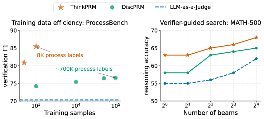</details> Figure 1: Left: Verifier F1-score on ProcessBench (Zheng et al., 2024). ThinkPRM -14B, trained on 8K process labels or 1K synthetic examples, outperforms discriminative PRMs trained on about 100x more data. Right: Verifier-guided search accuracy on MATH-500 with Llama-3.2-3B-Instruct as generator. ThinkPRM -1.5B, trained using the same 8K labels, outperforms LLM-as-a-judge and discriminative verifiers in reward-guided search on MATH-500. The LLM-as-a-judge in both figures uses the same base model as ThinkPRM. ## 1 Introduction Reasoning with large language models (LLMs) can substantially benefit from utilizing more test-time compute (Jaech et al., 2024; Guo et al., 2025; Akyürek et al., 2024). This typically depends on a high-quality process reward model (PRM)—also known as a process verifier—that scores (partial) solutions for selecting promising paths for search or ranking (Cobbe et al., 2021; Li et al., 2023; Wu et al., 2024; Brown et al., 2024). PRMs have typically assumed the form of discriminative classifiers, trained to discern correct from incorrect reasoning (Uesato et al., 2022; Zhang et al., 2025). However, training discriminative PRMs requires access to process labels, i.e., step-level annotations, which either require extensive human annotation (Lightman et al., 2023; Zheng et al., 2024), gold step-by-step solutions (Khalifa et al., 2023), or compute-intensive rollouts (Luo et al., 2024; Chen et al., 2024a). For instance, training reasonably performing math PRMs requires hundreds of thousands of step-level annotations (Lightman et al., 2023; Wang et al., 2023b). Generative verification either via LLM-as-a-judge (Wang et al., 2023a; Liu et al., 2023b; Zheng et al., 2023) or GenRM (Zhang et al., 2024a) treats verification as a generation problem of a rationale followed by a decision. However, LLM-as-a-judge is known to perform poorly compared to specialized reward models (Lambert et al., 2024; Zhang et al., 2024b; Chen et al., 2024c), as general-purpose LLMs frequently fail to recognize reasoning errors (Huang et al., 2023; Zhang et al., 2024a; Ye et al., 2024). Moreover, GenRM is limited to outcome verification via short chain-of-thoughts (CoTs), fundamentally limiting its ability for test-time scaling. <details> <summary>x2.png Details</summary>  ### Visual Description ## Line Chart: Scaling verifier compute: ProcessBench ### Overview This image is a line chart titled "Scaling verifier compute: ProcessBench". It plots the performance, measured in F1-score (%), of three different verification methods against the amount of computational resources allocated for "thinking", measured in thousands of tokens (#tokens). The chart demonstrates how each method's performance scales as the token budget increases from 8K to 32K. ### Components/Axes * **Title:** "Scaling verifier compute: ProcessBench" (Top center). * **Y-Axis:** Labeled "F1-score (%)". The scale runs from 74 to 88, with major tick marks every 2 units (74, 76, 78, 80, 82, 84, 86, 88). * **X-Axis:** Labeled "Thinking up to (#tokens)". The scale has four discrete points: 8K, 16K, 24K, and 32K. * **Legend:** Located at the bottom center of the chart. It defines three data series: * **ThinkPRM:** Represented by an orange solid line with star markers (★). * **LLM-as-a-judge:** Represented by a blue solid line with circle markers (●). * **DiscPRM:** Represented by a green dashed line (---). ### Detailed Analysis **Data Series and Trends:** 1. **ThinkPRM (Orange line with stars):** * **Trend:** Shows a strong, consistent upward trend that plateaus at higher token counts. * **Data Points (Approximate):** * At 8K tokens: ~83.3% * At 16K tokens: ~88.0% * At 24K tokens: ~89.0% * At 32K tokens: ~89.0% 2. **LLM-as-a-judge (Blue line with circles):** * **Trend:** Shows a non-monotonic, fluctuating trend. Performance increases, then decreases, then increases again. * **Data Points (Approximate):** * At 8K tokens: ~79.8% * At 16K tokens: ~82.5% * At 24K tokens: ~79.4% * At 32K tokens: ~81.8% 3. **DiscPRM (Green dashed line):** * **Trend:** Shows a perfectly flat, constant trend. Performance does not change with increased token budget. * **Data Point (Approximate):** A constant value of ~73.8% across all token counts (8K, 16K, 24K, 32K). ### Key Observations * **Performance Hierarchy:** ThinkPRM consistently outperforms the other two methods at every measured token budget. LLM-as-a-judge is the second-best performer, while DiscPRM is the lowest-performing method. * **Scaling Behavior:** ThinkPRM demonstrates positive scaling, with significant gains from 8K to 16K tokens and diminishing returns thereafter. LLM-as-a-judge shows unstable scaling. DiscPRM shows zero scaling. * **Convergence:** The performance gap between ThinkPRM and LLM-as-a-judge widens significantly after 16K tokens. * **Baseline:** The DiscPRM line acts as a static baseline, highlighting the performance gains achieved by the other, compute-scaling methods. ### Interpretation The chart provides a clear comparison of how different verification strategies utilize increased computational "thinking" budget. The data suggests that the **ThinkPRM** method is highly effective at converting additional compute into improved accuracy (F1-score), making it a strong candidate for scenarios where compute resources can be scaled. Its plateau after 16K tokens indicates a potential performance ceiling for this method on the ProcessBench task. The **LLM-as-a-judge** method's fluctuating performance is anomalous. The dip at 24K tokens suggests it may be sensitive to specific token budget ranges or that its reasoning process becomes less reliable or more noisy at certain scales of computation. It does not reliably benefit from more compute in a linear fashion. The **DiscPRM** method's flat line indicates it is not a compute-scaling verifier. Its performance is fixed, likely because it uses a deterministic or non-generative process that does not involve "thinking" with a variable token budget. It serves as a crucial baseline, showing the minimum performance level that the scaling methods must exceed. In summary, the chart argues for the superiority of the ThinkPRM approach for this specific benchmark when additional compute is available, while cautioning that not all verification methods (like LLM-as-a-judge) scale predictably, and some (like DiscPRM) do not scale at all. 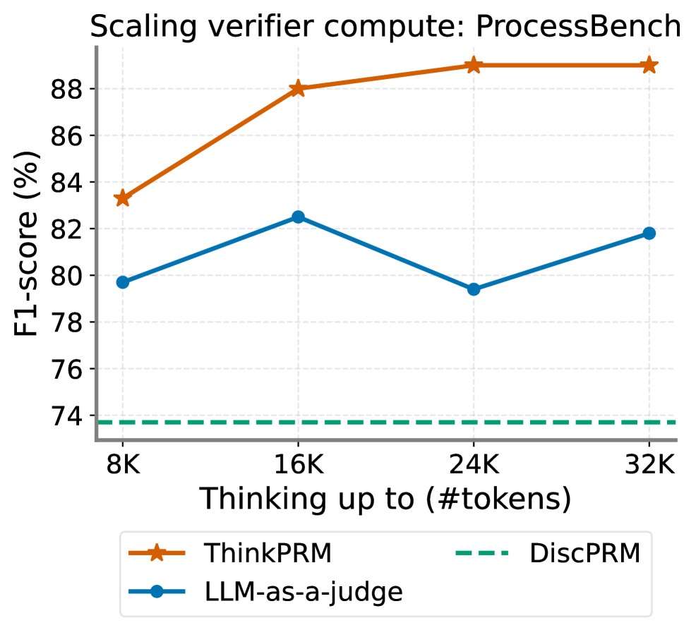</details> Figure 2: ThinkPRM enables scaling verification compute with more CoT tokens. This paper builds on the insight that generative step-by-step verification can greatly benefit from scaling up the verifier’s inference compute—specifically, by enabling it to think through a CoT. Specifically, we repurpose open-weight large reasoning models (LRMs) as the foundation for generative PRMs through lightweight training. This training uses uses synthetic data (Kim et al., 2023; Zhu et al., 2023; Wang et al., 2024), utilizing as few as 8K step labels, and yieldinga ThinkPRM —a PRM that not only surpasses LLM-as-a-judge, but also outperforms discriminative PRMs trained on two orders of magnitude more data across a variety of test-time scaling scenarios. We obtain ThinkPRM by training four reasoning models, namely R1-Distill-Qwen{1.5B,7B,14B} (Guo et al., 2025), and QwQ-32B-Preview (Team, 2024), and extensively evaluate it both as a standalone verifier on ProcessBench (Zheng et al., 2024), and combined with a generator under Best-of-N and verifier-guided beam search. ThinkPRM -14B outperforms a discriminative PRM based on the same base model in terms of accuracy while using far fewer supervision signals as in Fig. 1 left. In addition, ThinkPRM -1.5B demonstrates strong performance on MATH-500 (Hendrycks et al., 2021) under guided beam search, shown in Fig. 1 right. Lastly, as shown in Fig. 2, ThinkPRM can effectively utilize more verification compute than LLM-as-a-judge, by forcing it to think for more tokens. All these results are obtained while training only on 8K step labels. Our work highlights the promise of long CoT PRMs that verify reasoning with reasoning, effectively scaling both generator and verifier compute. Our main findings are as follows: ThinkPRM outperforms strong PRM baselines in best-of-N and guided-search setups on two math reasoning benchmarks: MATH-500 and AIME 2024, and surpasses LLM-as-a-judge baselines under the same base model by thinking longer during verification (section 4). Moreover, ThinkPRM generalizes under two types of domain shift. First, it outperforms baselines on out-of-domain tasks such as scientific reasoning and code generation. Second, despite being trained only on short solutions, it generalizes to long-form reasoning without explicit step delimiters (section 5.3). Third, ThinkPRM outperforms self-consistency (Wang et al., 2022) when using the same compute budget, especially under high sampling regimes (section 5.4). Finally, fine-grained filtering of synthetic data based on step supervision is crucial for training high-quality PRMs (section 5.7). ## 2 Background and Related Work #### Discriminative PRMs. Discriminative PRMs are trained as classifiers that directly predict numerical correctness scores for each solution step, and typically rely on extensive step-level annotations (Uesato et al., 2022; Lightman et al., 2023; Zhang et al., 2025). Given a solution prefix, discriminative PRMs encode the solution text and employ a classification head to produce step-level scores, usually optimized with binary cross-entropy. An overall correctness score for a solution is obtained by aggregating these step-level scores (Beeching et al., ). PRMs are effective and straightforward but they do not utilize the language-modeling head of the base language model, making training expensive and labor-intensive (Yuan et al., 2024). Additionally, they offer limited interpretability and utilize fixed compute, restricting their dynamic scalability at test-time (Zhang et al., 2024a; Mahan et al., 2024). Thus, there is a need for data-efficient PRMs that can scale with more test-time compute. #### Generative Verification. Generative verification (Zheng et al., 2023; Zhu et al., 2023; Zhang et al., 2024a) frames verification as a language-generation task, producing step-level decisions as tokens (e.g., “correct” or “incorrect”), typically accompanied by a chain-of-thought (CoT). One can train generative verifiers using the standard language modeling objective on verification rationales rather than on binary labels. This approach leverages the strengths of LLMs in text generation, making generative verifiers inherently interpretable and scalable (Zhang et al., 2024a; Mahan et al., 2024; Wang et al., 2023a; Ankner et al., 2024). However, prior work on generative verifiers has relied mainly on short verification CoT (e.g., few hundred tokens) (Zhang et al., 2024a), which highly limits their scalability. Thus, there is a need for verifiers that can “think” longer through verification, utilizing test-time compute effectively. While LLM-as-a-Judge has been employed for step-level verification (Zheng et al., 2024). it tends to be sensitive to prompt phrasing, and prone to invalid outputs, such as infinite looping or excessive overthinking (Bavaresco et al., 2024) —issues we further confirm in this work. Prior results with reasoning models like QwQ-32B-Preview (Team, 2024) show promise, but their practical utility in test-time scaling remains limited without additional training (Zheng et al., 2024). #### Test-Time Scaling with PRMs. Test-time scaling techniques, such as Best-of-N selection (Charniak & Johnson, 2005) and tree-based search (Yao et al., 2023; Chen et al., 2024c; Wan et al., 2024), leverage additional inference-time compute to improve reasoning performance. Central to these approaches is the quality of the verifier used to score and select solutions. A major advantage of generative PRMs is that they uniquely support simultaneous scaling of both generator and verifier compute (Zhang et al., 2024a; Kalra & Tang, 2025). In particular, our work shows that generative PRMs trained based on long CoT models (Jaech et al., 2024; Guo et al., 2025) enable both parallel and sequential scaling of verifier compute. ## 3 ThinkPRM <details> <summary>x3.png Details</summary>  ### Visual Description \n ## Diagram: Reasoning Model Verification and Finetuning Pipeline ### Overview The image is a technical flowchart illustrating a process for evaluating and curating reasoning chains generated by an AI model. The process involves generating solution steps, verifying their correctness against process labels, and filtering them to create high-quality finetuning data. The diagram uses a left-to-right flow with color-coded elements and symbolic icons (checkmarks, crosses) to indicate correctness. ### Components/Axes The diagram is structured into three main horizontal sections or stages, connected by arrows indicating data flow. **1. Input Stage (Leftmost, Pink Box):** * **Container:** A large pink rectangle with rounded corners. * **Labels:** Contains two white sub-boxes. * Left sub-box: Labeled "**Problem**" with a large question mark "?" inside. * Right sub-box: Labeled "**Solution**" with placeholder text: "Step 1: ...", "Step 2: ...", "Step 3: ...". * **Function:** Represents the initial input: a problem statement and a proposed multi-step solution generated by a model. **2. Processing Stage (Center, Purple Box):** * **Container:** A purple rectangle with rounded corners, connected by an arrow from the Input Stage. * **Label:** Labeled "**Reasoning Model**". * **Function:** Represents the AI model that processes the problem and solution to generate detailed reasoning chains (shown in the next stage). **3. Verification & Filtering Stage (Right, Two Parallel Paths):** This stage is split into two parallel processing chains, labeled at the top as "**1. Sample verification chains**". * **Path A (Top Chain - Discarded):** * **Container:** A light gray box containing a `<think>` block. * **Content:** A reasoning chain with three steps. * `Step 1 accurately... and is \boxed{correct}` - Accompanied by a **green checkmark icon**. * `Step 2 omits... \boxed{incorrect}` - Accompanied by a **red 'X' icon**. * `Step 3 ... \boxed{incorrect}` - Accompanied by a **red 'X' icon**. * **Process Label (Right of Chain):** A green box labeled "**Step 1: Correct**", "**Step 2: Incorrect**", "**Step 3: Incorrect**". * **Action:** An arrow points from this chain to a large **red 'X'** and the text "**Discard!**". This path is labeled "**2. Compare against process labels**". * **Path B (Bottom Chain - Kept):** * **Container:** A light gray box containing a `<think>` block. * **Content:** A reasoning chain with three steps. * `Step 1 calculates... Therefore is \boxed{correct}` - Accompanied by a **green checkmark icon**. * `Step 2 ... is \boxed{correct}` - Accompanied by a **green checkmark icon**. * `Step 3 is... \boxed{incorrect}` - Accompanied by a **red 'X' icon**. * **Process Label (Right of Chain):** A green box labeled "**Step 1: Correct**", "**Step 2: Correct**", "**Step 3: Incorrect**". * **Action:** An arrow points from this chain to a **green checkmark icon** and then to a yellow cylinder. This path is labeled "**3. Keep good chains**". **4. Output Stage (Bottom Right):** * **Container:** A yellow cylinder, a standard icon for a database or storage. * **Label:** Labeled "**Finetuning data**". * **Function:** Represents the curated dataset of high-quality reasoning chains (like the one from Path B) used to improve the model. ### Detailed Analysis The diagram explicitly details the content of two sample verification chains to illustrate the filtering logic. * **Chain A (Discarded):** This chain has one correct step followed by two incorrect steps. The process label confirms this assessment (Correct, Incorrect, Incorrect). The outcome is to discard the entire chain. * **Chain B (Kept):** This chain has two correct steps followed by one incorrect step. The process label confirms this (Correct, Correct, Incorrect). Despite the final step being incorrect, the chain is kept. This suggests the filtering criterion is not perfection, but perhaps a minimum threshold of correctness (e.g., majority of steps correct) or the presence of valuable correct reasoning in the early steps. ### Key Observations 1. **Asymmetric Filtering:** The system does not require all steps to be correct for a chain to be retained. Chain B, with a 2/3 correct rate, is kept, while Chain A, with a 1/3 correct rate, is discarded. 2. **Process Label Dependency:** The verification is not based solely on the model's own `\boxed{correct/incorrect}` self-assessment. It is compared against external "**process labels**" (the green boxes), which serve as the ground truth for correctness. 3. **Visual Coding:** Correctness is consistently coded with **green checkmarks** and the word "correct". Incorrectness is coded with **red 'X' icons** and the word "incorrect". The final "Discard!" action is also marked with a large red 'X'. 4. **Spatial Flow:** The layout clearly separates the two outcomes (discard vs. keep) vertically, making the comparison and decision process easy to follow. ### Interpretation This diagram outlines a **data curation pipeline for improving AI reasoning models**. Its core purpose is to automatically generate training data that teaches the model not just the final answer, but the *process* of correct reasoning. * **What it demonstrates:** The system uses a "reasoning model" to generate step-by-step solutions. These solutions are then audited for correctness at each step against a known standard (process labels). The audit results are used to filter the generated data. * **How elements relate:** The "Problem/Solution" input feeds the "Reasoning Model," which produces the detailed chains. The verification stage acts as a quality gate. The "Finetuning data" cylinder is the valuable output, composed only of chains that meet a quality standard (e.g., containing significant correct reasoning). * **Notable implication:** The decision to keep Chain B (with a final incorrect step) is significant. It implies the finetuning process values **partial correctness and the demonstration of correct reasoning methodology**, even if the conclusion is flawed. This is a more nuanced approach than simply using only perfectly correct solutions, potentially making the model more robust by learning from near-miss examples. The pipeline automates the labor-intensive task of creating high-quality, process-oriented training data. 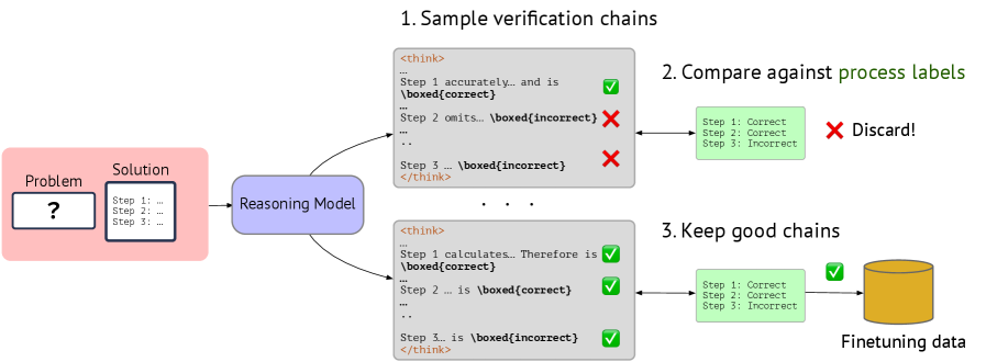</details> Figure 3: Collecting verification chains for finetuning. First, we prompt a reasoning model, in our case QwQ-32B-Preview to critique a given solution to a problem. Then, we sample multiple verification chains, which we judge against gold process labels from PRM800K, only keeping chains that match the gold process labels. Our goal is verbalized PRM that, given a problem-solution pair, verifies every step in the solution via an extended chain-of-thought (CoT) such as the one shown in Fig. 44 in App. G. This section introduces issues with LLM-as-a-judge verification and proposes a data collection process (shown in Fig. 3) to curate high-quality synthetic verification CoTs for training such PRM. The rest of the paper addresses the following research questions: - RQ1: How well do LRMs perform under LLM-as-a-judge for process-level verification? Section 3.1 - RQ2: Can lightweight finetuning on synthetic verification CoTs improve the reliability and effectiveness of these models as process verifiers? Section 3.2 - RQ3: How does a finetuned verbalized PRM (ThinkPRM) compare to discriminative PRMs and LLM-as-a-Judge baselines under different test-time scaling scenarios? Section 4 ### 3.1 LLM-as-a-judge PRMs are suboptimal This section highlights limitations we observe when using off-the-shelf reasoning models as process verifiers, suggesting the need for finetuning. For evaluation, we use ProcessBench (Zheng et al., 2024), which includes problem-solution pairs with problems sourced from existing math benchmarks, along with ground-truth correctness labels. We report the binary F1-score by instructing models to verify full solutions and judge whether there exists a mistake. We use two most challenging subsets of ProcessBench: OlympiadBench (He et al., 2024) and OmniMath (Gao et al., 2024), each comprised of 1K problem-prefix pairs. For LLM-as-a-judge, we use the same prompt template as in Zheng et al. (2024), shown in Fig. 42, which we found to work best overall. Table 3 shows LLM-as-a-judge F1 scores and a sample output by QwQ-32B-Preview is displayed in Fig. 41 in App. F. We observe different issues with LLM-as-a-judge verification. First, the verification quality is highly sensitive to the instruction wording: slight change in the instruction can affect the F1-score by up to 3-4 points. First, a substantial number of the generated chains include invalid judgments, i.e., chains without an extractable overall label as clear in Fig. 10. Such invalid judgements are caused by the following. In some cases, final decision was in the wrong format than instructed e.g., the model tries to solve the problem rather than verify the given solution—a behavior likely stemming from the model training. Second, we noted multiple instances of overthinking (Chen et al., 2024b; Cuadron et al., 2025), which prevents the model from terminating within the token budget, and infinite looping/repetitions, where the model gets stuck trying alternative techniques to verify the solutions. 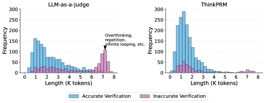Fig. 4 (left) shows a histogram of verification CoT lengths generated by R1-Qwen-14B in the LLM-as-a-judge setting. Accurate CoTs tend to be shorter, typically under 3K tokens, while inaccurate CoTs are more evenly distributed and spike sharply around 7K-8K tokens, highlighting the prevalence of overthinking and looping in long chains. We show examples of these behaviors in App. B. In the next section, we mostly fix these issues via lightweight finetuning over synthetic verification CoTs. ### 3.2 Finetuning on synthetic data boosts LLM-as-a-judge verification Inspired by recent work on reducing overthinking in long CoT models that by training (Yu et al., 2024; Kang et al., 2024), we aim to improve LLM-as-a-judge performance via finetuning on high-quality verification data. Collecting real data would be expensive, so we rely on filtered synthetic data (Zelikman et al., 2022; Singh et al., 2023; Dong et al., 2023; Zhang et al., 2024b; Wang et al., 2024) also known as rejection sampling finetuning. To keep our approach simple, we refrain from more expensive training techniques, such as reinforcement learning or preference-based learning. #### Synthetic data collection. As training data, we sample synthetic verification CoTs from QwQ-32B-Preview, prompting it to verify each step in a solution prefix, using the instruction shown in Fig. 21. The problems and corresponding step-by-step solutions come from the PRM800K dataset (Lightman et al., 2023), which provides both model-generated solutions and human-verified step-level labels. The sampling process continues until we obtain 1K verification CoTs which coreepond to 8K step labels in total. For data filtering, we use the following criteria: (i) the CoT must follow the expected format (i.e., include an extractable decision label for each step inside \boxed{} as shown in Fig. 20, and (ii) the generated step judgements match the gold step labels from PRM800K, and (iii) the CoT length is within a maximum budget—to avoid the excessive overthinking behavior we observed in Fig. 4 (left). The filtering process ensures our training data is of sufficient quality. note that process-based filtering is crucial for the performance of the resulting PRM as we show in Section 5.7. Data collection is illustrated in Fig. 3, data statistics are in Section A.1 and a training example is in Fig. 20. Notably, our filtering relies only on step-level annotations, not on gold verification rationales or CoTs—making this pipeline scalable and low-overhead. In the absence of gold step-level annotations, one can obtain silver labels via Monte Carlo rollouts (Wang et al., 2023b; Chen et al., 2024a). While we train only on math data, the resulting PRM remains robust under other domains such as science QA and code generation as we show in Section 4.2. We then proceed to train our models on the 1K collected chains. Our training is very lightweight; finetuning QwQ-32B-Preview takes only 4.5 hours on a single A100 80GB GPU. Refer to Section C.1 for training details. <details> <summary>x4.png Details</summary>  ### Visual Description ## Histograms: Comparison of Verification Length Distributions ### Overview The image displays two side-by-side histograms comparing the distribution of verification lengths (in thousands of tokens) for two different methods: "LLM-as-a-Judge" and "ThinkPRM". Each histogram plots frequency against length, with data segmented into "Accurate Verification" (blue) and "Inaccurate Verification" (pink). An annotation highlights a specific pattern in the left chart. ### Components/Axes * **Titles:** * Left Chart: "LLM-as-a-Judge" * Right Chart: "ThinkPRM" * **X-Axis (Both Charts):** Label: "Length (K tokens)". Scale: Linear, from 0 to 8, with major tick marks at every integer (0, 1, 2, ..., 8). * **Y-Axis (Both Charts):** Label: "Frequency". Scale: Linear, from 0 to 300, with major tick marks at intervals of 50 (0, 50, 100, ..., 300). * **Legend:** Positioned at the bottom center of the entire image, below both charts. * Blue square: "Accurate Verification" * Pink square: "Inaccurate Verification" * **Annotation:** Located in the top-right quadrant of the "LLM-as-a-Judge" chart. A black arrow points to the peak of the pink bars at approximately 7K tokens. The text reads: "Overthinking, repetition, infinite looping, etc." ### Detailed Analysis **1. LLM-as-a-Judge (Left Chart):** * **Accurate Verification (Blue):** The distribution is right-skewed. The highest frequency (approximately 160-170) occurs at a length of ~1K tokens. The frequency then steadily declines as length increases, approaching near-zero by 8K tokens. * **Inaccurate Verification (Pink):** The distribution is bimodal. There is a small, low-frequency cluster between 0.5K and 3K tokens (peaking around 25-30). A second, much more prominent cluster appears between 6K and 8K tokens, with a sharp peak at ~7K tokens reaching a frequency of approximately 100-110. This peak is explicitly annotated as representing "Overthinking, repetition, infinite looping, etc." **2. ThinkPRM (Right Chart):** * **Accurate Verification (Blue):** The distribution is strongly right-skewed with a very high, sharp peak. The maximum frequency (approximately 280-290) occurs at ~1K tokens. The frequency drops off rapidly after 1.5K tokens and becomes very low (below 20) beyond 4K tokens. * **Inaccurate Verification (Pink):** The frequencies are very low across the entire range. There is a minor, broad elevation between 0.5K and 2.5K tokens (peaking around 50) and another very slight increase around 7K tokens (peaking below 20). No significant spike is observed at the higher length ranges. ### Key Observations 1. **Peak Location & Magnitude:** Both methods show the highest frequency of accurate verifications at short lengths (~1K tokens). However, the peak for ThinkPRM is significantly higher (~290 vs. ~170) and narrower, suggesting a stronger concentration of accurate results at that length. 2. **Inaccurate Verification Pattern:** The most striking difference is in the distribution of inaccurate verifications. LLM-as-a-Judge shows a major secondary mode at high token lengths (~7K), which is explicitly linked to failure modes like overthinking. ThinkPRM shows no such pronounced secondary mode; its inaccurate verifications are low and spread thinly. 3. **Length Efficiency:** The ThinkPRM distribution for accurate verifications is more concentrated at the lower end of the length scale. The LLM-as-a-Judge distribution has a longer "tail" of accurate verifications extending to higher token counts, but at much lower frequencies. ### Interpretation The data suggests a fundamental difference in the behavior and reliability of the two verification methods. * **LLM-as-a-Judge** appears prone to a specific failure mode where inaccurate verifications are strongly associated with very long outputs (6K-8K tokens). The annotation implies this is due to unproductive loops or redundancy in the model's reasoning process. While it produces accurate verifications across a wide range of lengths, its inefficiency and the clear pattern of failure at high lengths are notable drawbacks. * **ThinkPRM** demonstrates a more controlled and efficient profile. It achieves a higher density of accurate verifications at short lengths and, crucially, avoids the catastrophic "overthinking" failure mode seen in the other method. The near-absence of a high-length spike for inaccurate verifications indicates it is more robust against generating excessively long, erroneous outputs. In essence, the charts argue that ThinkPRM is a more precise and reliable verification method, as it concentrates accurate results where they are most efficient (short lengths) and minimizes the specific type of lengthy, inaccurate output that plagues the LLM-as-a-Judge approach. The visual evidence strongly links excessive length with inaccuracy for LLM-as-a-Judge, a correlation that is largely absent for ThinkPRM. </details> Figure 4: Verifier performance on ProcessBench in light of CoT lengths. On the left, LLM-as-a-judge produces excessively long chains including repetition, infinite looping, and overthinking, leading to worse verifier performance since the output never terminates. Training on collected syntehtic data substantially reduces these issues as shown in the ThinkPRM plot on the right. #### Finetuning on synthetic verification CoTs substantially improves the verifier. ThinkPRM trains on the 1K chains and is evaluated on ProcessBench and compared to LLM-as-a-judge under the same base model. Fig. 10 shows verifier accuracy of different models before and after our finetuning. We note a substantial boost in F1 across all models, with the 1.5B model gaining most improvement by over 70 F1 points, and the 14B model performing best. Looking at the ratio of invalid judgements in Fig. 10, we also note a significant reduction in invalid labels with all models, except for QwQ, where it slightly increases. Lastly, the reduction in overthinking and infinite looping behavior discussed in the last section is evident, as in Fig. 4 (right), where ThinkPRM generations maintain a reasonable length (1K-5K) tokens while being substantially more accurate. floatrow figurerow b figure b <details> <summary>x5.png Details</summary>  ### Visual Description ## Bar Chart: CoTs without a valid label on ProcessBench ### Overview This is a grouped bar chart comparing the performance of two evaluation methods ("ThinkPRM" and "LLM-as-a-judge") across four different language models. The chart measures the percentage of "Chain-of-Thoughts (CoTs) without a valid label" for each model-method pair. The data suggests an analysis of model reasoning or labeling failures on a benchmark called "ProcessBench." ### Components/Axes * **Chart Title:** "CoTs without a valid label on ProcessBench" * **Y-Axis:** * **Label:** "Percentage of total (%)" * **Scale:** Linear, from 0 to 60, with major tick marks at intervals of 10 (0, 10, 20, 30, 40, 50, 60). * **X-Axis:** * **Label:** None explicit. The axis categories are the names of four language models. * **Categories (from left to right):** 1. QwQ-32B-preview 2. R1-Qwen-14B 3. R1-Qwen-7B 4. R1-Qwen-1.5B * **Legend:** * **Position:** Centered at the bottom of the chart. * **Items:** * **Orange Square:** "ThinkPRM" * **Blue Square:** "LLM-as-a-judge" * **Data Series:** Two series of bars, one for each legend item, grouped by model category. ### Detailed Analysis The chart presents the following specific data points for each model and evaluation method: **1. QwQ-32B-preview:** * **ThinkPRM (Orange Bar):** 11.5% * **LLM-as-a-judge (Blue Bar):** 9.4% * **Trend:** For this model, the ThinkPRM method yields a slightly higher percentage of invalid labels than the LLM-as-a-judge method. **2. R1-Qwen-14B:** * **ThinkPRM (Orange Bar):** 2.3% * **LLM-as-a-judge (Blue Bar):** 16.0% * **Trend:** A significant reversal occurs. The ThinkPRM percentage drops sharply, while the LLM-as-a-judge percentage rises. The LLM-as-a-judge value is now nearly 7 times higher than the ThinkPRM value. **3. R1-Qwen-7B:** * **ThinkPRM (Orange Bar):** 1.2% * **LLM-as-a-judge (Blue Bar):** 19.5% * **Trend:** The trend continues. ThinkPRM reaches its lowest point, while LLM-as-a-judge increases further. The gap between the two methods widens. **4. R1-Qwen-1.5B:** * **ThinkPRM (Orange Bar):** 1.9% * **LLM-as-a-judge (Blue Bar):** 53.2% * **Trend:** This model shows the most extreme disparity. ThinkPRM remains very low (a slight increase from the previous model). In stark contrast, the LLM-as-a-judge percentage surges dramatically to 53.2%, the highest value on the chart by a large margin. ### Key Observations 1. **Divergent Trends:** The two evaluation methods show opposite trends across the model series. The "ThinkPRM" percentage generally decreases (with a minor uptick for the smallest model), while the "LLM-as-a-judge" percentage increases consistently and dramatically. 2. **Model Size Correlation:** There is a clear inverse relationship between model size (implied by the names: 32B, 14B, 7B, 1.5B) and the percentage of invalid labels when judged by an LLM. Smaller models (especially R1-Qwen-1.5B) produce a much higher rate of invalid CoTs according to the "LLM-as-a-judge" metric. 3. **ThinkPRM Stability:** The "ThinkPRM" method appears relatively stable and low across all models, ranging only between 1.2% and 11.5%. It does not show the same sensitivity to model scale. 4. **Extreme Outlier:** The data point for R1-Qwen-1.5B evaluated by "LLM-as-a-judge" (53.2%) is a major outlier, being more than 2.7 times higher than the next highest value (19.5% for R1-Qwen-7B). ### Interpretation This chart likely illustrates a critical finding in the evaluation of language model reasoning. "CoTs without a valid label" suggests instances where the model's reasoning chain failed to produce a clear, classifiable answer. * **What the data suggests:** The "LLM-as-a-judge" evaluation method is highly sensitive to model capability. As model size and presumed capability decrease, this method flags a dramatically increasing proportion of reasoning chains as invalid. This could mean smaller models are more prone to generating nonsensical, ambiguous, or off-topic reasoning that an LLM judge cannot confidently label. * **Contrasting Methods:** The "ThinkPRM" method (possibly a process-based reward model or a different verification technique) appears far more robust to model scale. It consistently identifies a low baseline of invalid CoTs, suggesting it may be measuring a different, more fundamental type of error or using a less stringent criterion. * **Why it matters:** The stark divergence highlights a potential pitfall in AI evaluation. Relying solely on an "LLM-as-a-judge" could lead to overly pessimistic assessments of smaller models' reasoning abilities, as the judge itself may be conflating "difficult to label" with "invalid." The stability of ThinkPRM suggests it might be a more reliable metric for comparing reasoning quality across models of different sizes. The extreme value for the 1.5B model indicates a potential failure mode where the model's reasoning breaks down almost completely from the perspective of an LLM evaluator. 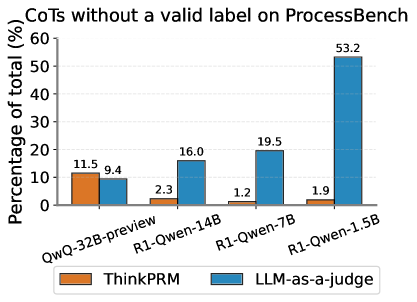</details> Figure 7: LLM-as-a-judge suffers from a significant ratio of verification CoTs that do not terminate with a parsable label, i.e., \boxed{yes} or \boxed{no}. Our finetuning process that yields ThinkPRM, substantially mitigates this issue. Both verifiers are based on R1-Distill-Qwen-14B. figure b <details> <summary>x6.png Details</summary>  ### Visual Description ## Bar Chart: Verifier Performance on ProcessBench ### Overview This is a grouped bar chart comparing the performance of two verification methods, "ThinkPRM" and "LLM-as-a-judge," across four different language models on a benchmark called "ProcessBench." Performance is measured using the F1-score metric. ### Components/Axes * **Chart Title:** "Verifier performance on ProcessBench" (Top center). * **Y-Axis:** Labeled "F1-score". The scale runs from 0 to 100 in increments of 20 (0, 20, 40, 60, 80, 100). * **X-Axis:** Lists four model names as categories: 1. QwQ-32B-preview 2. R1-Qwen-14B 3. R1-Qwen-7B 4. R1-Qwen-1.5B * **Legend:** Located at the bottom center of the chart. * Orange square: "ThinkPRM" * Blue square: "LLM-as-a-judge" * **Baseline:** A horizontal dashed black line labeled "random" is positioned at approximately F1-score = 37. ### Detailed Analysis The chart displays paired bars for each model, with the orange "ThinkPRM" bar on the left and the blue "LLM-as-a-judge" bar on the right. **Data Points (F1-scores):** 1. **QwQ-32B-preview:** * ThinkPRM (Orange): 73.2 * LLM-as-a-judge (Blue): 53.0 2. **R1-Qwen-14B:** * ThinkPRM (Orange): 86.5 (Highest value in the chart) * LLM-as-a-judge (Blue): 70.3 3. **R1-Qwen-7B:** * ThinkPRM (Orange): 73.7 * LLM-as-a-judge (Blue): 45.2 4. **R1-Qwen-1.5B:** * ThinkPRM (Orange): 76.0 * LLM-as-a-judge (Blue): 5.2 (Lowest value in the chart) **Trend Verification:** * **ThinkPRM (Orange Bars):** The performance is relatively stable and high across all models, ranging from 73.2 to 86.5. The trend line is roughly flat with a peak at the R1-Qwen-14B model. * **LLM-as-a-judge (Blue Bars):** Shows a clear and steep downward trend as the model size decreases (from left to right on the x-axis). Performance drops from 70.3 with the 14B model to just 5.2 with the 1.5B model. ### Key Observations 1. **Consistent Superiority:** ThinkPRM outperforms LLM-as-a-judge on every single model tested. 2. **Performance Gap:** The performance gap between the two methods widens dramatically as the model size decreases. The gap is smallest for the largest model (QwQ-32B-preview: 20.2 points) and largest for the smallest model (R1-Qwen-1.5B: 70.8 points). 3. **Critical Failure Point:** The LLM-as-a-judge method performs worse than the random baseline (37) for the smallest model (R1-Qwen-1.5B), with an F1-score of only 5.2. 4. **Peak Performance:** The highest overall score (86.5) is achieved by ThinkPRM using the R1-Qwen-14B model. ### Interpretation The data strongly suggests that **ThinkPRM is a significantly more robust and effective verification method than LLM-as-a-judge** for the ProcessBench task. Its performance is less sensitive to the underlying model's scale, maintaining high effectiveness even with smaller models. The **LLM-as-a-judge method appears to be highly dependent on the capability of the base model**. Its performance degrades severely with smaller models, to the point of being practically useless (F1=5.2) for the 1.5B parameter model, falling far below random chance. This indicates a fundamental limitation in using a less capable LLM to judge or verify outputs, likely due to its own lack of reasoning or comprehension depth. The "random" baseline provides a crucial reference point, highlighting that while both methods are generally better than chance, the LLM-as-a-judge approach fails this basic test at the smallest model scale. The chart makes a compelling case for the adoption of ThinkPRM-like verification techniques, especially in resource-constrained scenarios involving smaller language models. 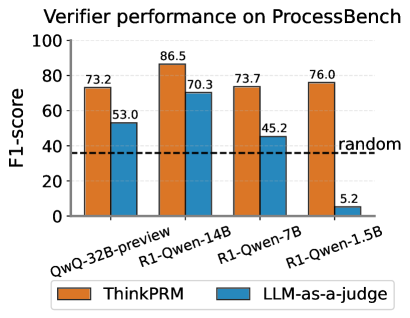</details> Figure 10: Verification accuracy on 2K question-solution pairs from two most challenging subsets of ProcessBench: OlympiadBench and OmniMath. ThinkPRM obtained by finetuning the correponding model over only 1K verification chains performs better. ## 4 Test-time Scaling Experiments This section aims to answer RQ3 introduced in section 3 by comparing ThinkPRM to baselines under different scaling scenarios. We study how ThinkPRM performs under different generation budgets (i) best-of-N selection (Wu et al., 2024; Brown et al., 2020) and (ii) guided beam search (Snell et al., 2024; Beeching et al., ). We also explore how ThinkPRM performs when verifier compute is scaled either in parallel by aggregating decisions over multiple verification CoTs or sequentially through longer CoTs by forcing the model to double check or self-correct its verification. ### 4.1 Experimental Setup In the remainder of the the paper, we will mainly use our finetuned verifiers based on R1-Distill-Qwen-1.5B and R1-Distill-Qwen-14B as these provide the best tradeoff between size and performance. We will refer to these as ThinkPRM -1.5B and ThinkPRM -14B, respectively. #### Baselines. We compare ThinkPRM to DiscPRM, which uses the same base model as ThinkPRM, finetuned with binary cross-entropy on the entire PRM800K dataset, totaling 712K process labels, which is two orders of magnitude larger than our training data. Details on finetuning DiscPRMs are in Section C.2. We also compare to unweighted majority voting, which merely selects the most frequent answer across the samples (Wang et al., 2022), and to LLM-as-a-Judge using the same base model as ThinkPRM, prompted as in Section 3.1. #### Tasks and Models. We show results on three math reasoning tasks, namely 100 problems from MATH-500 (Hendrycks et al., 2021) covering all difficulty levels (see Section E.5 for more details), and American Invitational Mathematics Examination (AIME) problems for 2024. Since ThinkPRM was finetuned only on math data, we study the out-of-domain generalization on two tasks: scientific reasoning and code generation. For scientific reasoning, we use the physics subset of GPQA-Diamond (Rein et al., 2024), consisting of 86 PhD-level multiple choice questions. For code generation, we use a 200-problem subset from the v5 release of LiveCodeBench (Jain et al., 2024). Over MATH-500, we show results with ThinkPRM -1.5B and ThinkPRM -14B on two different generator models: Qwen-2.5-14B and Llama-3.2-3B-Instruct. The former model is used for best-of-N and the latter for beam search as search is compute intensive. Showing results with different generators guarantees that our conclusions are not specific to a certain model family or size. For the more challenging tasks, namely AIME ’24 and GPQA, we use a more capable model, namely Qwen-2.5-32B-Instruct. For code generation, we use Qwen-2.5-Coder-7B (Hui et al., 2024). Implementation and hyperparemter details on how we select the final answer with best-of-N and beam search are in App. E. <details> <summary>x7.png Details</summary>  ### Visual Description ## Line Charts: Best-of-N Performance on AIME '24 and MATH-500 ### Overview The image contains two side-by-side line charts comparing the performance of different methods for generating solutions to mathematical problems. The charts plot "Accuracy (%)" against the "Number of solutions" (N) on a logarithmic scale (base 2). The left chart evaluates performance on the "AIME '24" dataset using the "Qwen2.5-32B-Instruct" generator. The right chart evaluates performance on the "MATH-500" dataset using the "Qwen2.5-14B" generator. Four methods are compared in each chart. ### Components/Axes **Titles & Subtitles:** * **Left Chart Title:** `Best-of-N: AIME '24` * **Left Chart Subtitle:** `Generator: Qwen2.5-32B-Instruct` * **Right Chart Title:** `Best-of-N: MATH-500` * **Right Chart Subtitle:** `Generator: Qwen2.5-14B` **Axes:** * **X-Axis (Both Charts):** Label: `Number of solutions`. Scale: Logarithmic (base 2). Ticks: `2^0`, `2^1`, `2^2`, `2^3` (left chart); `2^0`, `2^1`, `2^2`, `2^3`, `2^4`, `2^5`, `2^6` (right chart). * **Y-Axis (Left Chart):** Label: `Accuracy (%)`. Scale: Linear. Ticks: `20.0`, `22.5`, `25.0`, `27.5`, `30.0`, `32.5`. * **Y-Axis (Right Chart):** Label: `Accuracy (%)`. Scale: Linear. Ticks: `50`, `60`, `70`, `80`. **Legend (Bottom Center, spanning both charts):** * `ThinkPRM-14B`: Orange line with star markers. * `DiscPRM-14B`: Teal line with circle markers. * `LLM-as-a-judge`: Blue line with circle markers. * `Majority`: Tan/light brown line with circle markers. ### Detailed Analysis **Left Chart: AIME '24 (Generator: Qwen2.5-32B-Instruct)** * **ThinkPRM-14B (Orange, Stars):** Shows a strong, consistent upward trend. Starts at ~20.0% (2^0), rises to ~26.5% (2^1), ~30.0% (2^2), and peaks at ~33.5% (2^3). This is the top-performing method. * **DiscPRM-14B (Teal, Circles):** Shows a steady upward trend. Starts at ~20.0% (2^0), rises to ~23.5% (2^1), ~26.5% (2^2), and ends at ~30.0% (2^3). * **LLM-as-a-judge (Blue, Circles):** Shows an upward trend with a plateau. Starts at ~20.0% (2^0), rises to ~23.5% (2^1), remains flat at ~23.5% (2^2), then jumps to ~30.0% (2^3). * **Majority (Tan, Circles):** Shows a flat trend. Accuracy remains constant at ~20.0% across all values of N (2^0 to 2^3). **Right Chart: MATH-500 (Generator: Qwen2.5-14B)** * **ThinkPRM-14B (Orange, Stars):** Shows a strong, consistent upward trend. Starts at ~51% (2^0), rises to ~62% (2^1), ~69% (2^2), ~77% (2^3), ~79% (2^4), ~83% (2^5), and peaks at ~86% (2^6). This is the top-performing method. * **DiscPRM-14B (Teal, Circles):** Shows an upward trend that plateaus. Starts at ~51% (2^0), rises to ~61% (2^1), ~67% (2^2), ~73% (2^3), remains flat at ~73% (2^4), rises slightly to ~74% (2^5), and ends at ~80% (2^6). * **LLM-as-a-judge (Blue, Circles):** Shows an upward trend that plateaus. Starts at ~51% (2^0), rises to ~62% (2^1), ~68% (2^2), ~77% (2^3), dips slightly to ~76% (2^4), remains at ~76% (2^5), and ends at ~80% (2^6). * **Majority (Tan, Circles):** Shows an upward trend with a late surge. Starts at ~51% (2^0), remains flat at ~51% (2^1), rises to ~68% (2^2), ~74% (2^3), dips slightly to ~73% (2^4), rises to ~74% (2^5), and ends at ~78% (2^6). ### Key Observations 1. **Dominant Method:** `ThinkPRM-14B` is the clear top performer on both datasets, showing the steepest and most consistent improvement as the number of solutions (N) increases. 2. **Dataset/Generator Impact:** The absolute accuracy values are significantly higher on the MATH-500 dataset (right chart, 50-86% range) compared to AIME '24 (left chart, 20-33.5% range). This is likely due to both the inherent difficulty of the datasets and the different generator models used (14B vs. 32B-Instruct). 3. **Majority Baseline Behavior:** The `Majority` voting baseline shows no improvement with more solutions on the harder AIME '24 task (flat line), but does improve on the MATH-500 task, especially for N >= 4 (2^2). 4. **Plateauing Effects:** On the MATH-500 chart, both `DiscPRM-14B` and `LLM-as-a-judge` show signs of performance plateauing between N=8 (2^3) and N=32 (2^5) before a final increase at N=64 (2^6). 5. **LLM-as-a-judge Anomaly:** On the AIME '24 chart, `LLM-as-a-judge` shows an unusual plateau between N=2 (2^1) and N=4 (2^2) before catching up to `DiscPRM-14B` at N=8 (2^3). ### Interpretation The data demonstrates the effectiveness of the `ThinkPRM-14B` method for improving mathematical problem-solving accuracy through a "Best-of-N" sampling strategy. The core finding is that generating and selecting from multiple solutions (increasing N) reliably boosts performance, but the degree of improvement is highly dependent on the selection method. * **ThinkPRM-14B's superiority** suggests its internal process for ranking or scoring solution candidates is more aligned with true correctness than the alternatives (`DiscPRM-14B`, `LLM-as-a-judge`). * The **failure of the Majority baseline on AIME '24** indicates that for very challenging problems, simply generating more solutions and taking a vote is ineffective; the solutions are likely all incorrect or diverse in wrong answers. Its success on MATH-500 suggests that for moderately difficult problems, increased sampling can surface the correct answer more frequently. * The **plateaus observed** (e.g., `LLM-as-a-judge` on AIME '24, multiple methods on MATH-500) may indicate points of diminishing returns for those specific methods, where generating additional solutions provides little to no marginal benefit until a larger threshold (e.g., N=64) is crossed. * The comparison across two different datasets and generator models shows the **robustness of the trend**: `ThinkPRM-14B` consistently outperforms other methods, making it a promising approach for scaling the capabilities of language models on reasoning tasks via inference-time computation (generating more solutions). 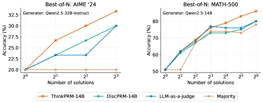</details> Figure 11: Best-of-N on AIME ’24 and MATH-500. Compared to LLM-as-a-judge, DiscPRM, and (unweighted) majority vote, ThinkPRM -14B exhibits best accuracy scaling curve. #### Scaling verifier compute. Compared to DiscPRMs, generative reward models enable an extra dimension of scaling to squeeze more performance: scaling the verifier compute. Specifically, ThinkPRM allows for two types of scaling. First, we use parallel scaling (Mahan et al., 2024; Brown et al., 2024), by sampling $K$ independent CoTs and averaging their scores. We will refer to this scaling using “@K” throughout the rest of the paper. Second, and more specific to long reasoning models, we use sequential scaling e.g., by enabling the model to double-check its initial verification (Xiong et al., 2025; Kumar et al., 2024; Ye et al., 2024). Inspired by Muennighoff et al. (2025), we use a trigger phrase such as “Let’s verify again” to elicit self-correction of earlier verification. See Section E.4 for more details. floatrow figurerow b figure b <details> <summary>x8.png Details</summary>  ### Visual Description \n ## Line Chart: Guided beam search: MATH-500 ### Overview This is a line chart comparing the performance (accuracy) of five different AI models on the MATH-500 benchmark as the complexity of the "guided beam search" decoding method increases. The chart demonstrates how accuracy changes for each model when the number of beams used in the search is varied from 1 (2^0) to 16 (2^4). ### Components/Axes * **Title:** "Guided beam search: MATH-500" * **Subtitle/Generator:** "Generator: Llama-3.2-3B-Instruct" * **Y-Axis:** Label is "Accuracy (%)". The scale runs from 55.0 to 72.5, with major tick marks at 2.5% intervals (55.0, 57.5, 60.0, 62.5, 65.0, 67.5, 70.0, 72.5). * **X-Axis:** Label is "Number of beams". The scale is logarithmic base 2, with categorical tick marks at 2^0 (1), 2^1 (2), 2^2 (4), 2^3 (8), and 2^4 (16). * **Legend:** Located at the bottom of the chart. It contains five entries, each with a unique color and marker symbol: 1. **ThinkPRM-1.5B:** Orange line with star markers (★). 2. **ThinkPRM-1.5B@4:** Orange dashed line with upward-pointing triangle markers (▲). 3. **RLHFFlow-8B-Deepseek:** Purple line with circle markers (●). 4. **DiscPRM-1.5B:** Green line with circle markers (●). 5. **MathShepherd-7B:** Brown line with circle markers (●). ### Detailed Analysis The chart plots five data series. Below is an analysis of each, including approximate values extracted from the chart. **1. ThinkPRM-1.5B@4 (Orange dashed line, ▲)** * **Trend:** Shows a strong, consistent upward trend across all beam counts. It is the top-performing model at every data point except the first, where it ties with its non-@4 variant. * **Data Points (Approximate):** * 2^0 beams: ~65.0% * 2^1 beams: ~65.0% * 2^2 beams: ~68.0% * 2^3 beams: ~70.0% * 2^4 beams: ~73.5% **2. ThinkPRM-1.5B (Orange solid line, ★)** * **Trend:** Shows a steady upward trend. It starts at the same level as ThinkPRM-1.5B@4 but grows at a slightly slower rate, resulting in a performance gap that widens with more beams. * **Data Points (Approximate):** * 2^0 beams: ~63.0% * 2^1 beams: ~63.0% * 2^2 beams: ~65.0% * 2^3 beams: ~66.0% * 2^4 beams: ~68.0% **3. DiscPRM-1.5B (Green line, ●)** * **Trend:** Shows a moderate upward trend. It starts lower than the ThinkPRM models but closes the gap somewhat at higher beam counts. * **Data Points (Approximate):** * 2^0 beams: ~58.0% * 2^1 beams: ~58.0% * 2^2 beams: ~63.0% * 2^3 beams: ~64.0% * 2^4 beams: ~65.0% **4. RLHFFlow-8B-Deepseek (Purple line, ●)** * **Trend:** Shows a significant upward trend, especially after 2^1 beams. It starts as the lowest-performing model but experiences the largest relative gain, surpassing MathShepherd-7B. * **Data Points (Approximate):** * 2^0 beams: ~55.0% * 2^1 beams: ~55.0% * 2^2 beams: ~60.0% * 2^3 beams: ~62.0% * 2^4 beams: ~65.0% **5. MathShepherd-7B (Brown line, ●)** * **Trend:** Shows a modest upward trend with a notable plateau. It improves from 2^1 to 2^2 beams, then shows almost no improvement between 2^2 and 2^3 beams before rising again. * **Data Points (Approximate):** * 2^0 beams: ~56.0% * 2^1 beams: ~56.0% * 2^2 beams: ~58.0% * 2^3 beams: ~58.0% * 2^4 beams: ~62.0% ### Key Observations 1. **Universal Benefit from More Beams:** All five models show higher accuracy with 16 beams (2^4) than with 1 beam (2^0), indicating that guided beam search is generally effective for improving performance on this task. 2. **Performance Hierarchy:** A clear performance hierarchy is established and maintained as beam count increases. The ThinkPRM models (especially the @4 variant) consistently outperform the others. 3. **Diminishing Returns & Plateaus:** While all lines trend upward, the rate of improvement varies. MathShepherd-7B exhibits a clear plateau between 4 and 8 beams. The ThinkPRM-1.5B@4 line shows the steepest and most consistent slope. 4. **Convergence at High Beams:** At 16 beams, the performance of DiscPRM-1.5B and RLHFFlow-8B-Deepseek converges to approximately the same point (~65.0%). 5. **Initial Plateau:** For all models, there is little to no improvement in accuracy when increasing beams from 1 to 2 (2^0 to 2^1). The significant gains begin after this point. ### Interpretation This chart provides a technical comparison of how different model architectures or training methods (represented by the five models) leverage increased computational effort during inference (more beams in guided search) to solve math problems. * **What the data suggests:** The effectiveness of guided beam search is model-dependent. The "ThinkPRM" models, particularly the "@4" variant, are not only more accurate overall but also scale better with increased search complexity. This suggests their internal reasoning or reward modeling is better aligned with the guided search process. * **Relationship between elements:** The X-axis (Number of beams) represents a controllable trade-off between computational cost and potential accuracy. The Y-axis (Accuracy) is the outcome. The different lines show the unique "scaling law" for each model type under this specific decoding strategy. * **Notable patterns/anomalies:** The complete lack of improvement from 1 to 2 beams for all models is a striking pattern. It implies a threshold effect where a minimal increase in search breadth is insufficient to find better solutions; a more substantial increase (to 4 beams or more) is needed to unlock gains. The plateau for MathShepherd-7B suggests it may hit a performance ceiling with this method earlier than others. The strong performance of the ThinkPRM-1.5B@4 model indicates that its specific configuration (possibly an ensemble or a different decoding parameter denoted by "@4") is highly synergistic with guided beam search for this task. 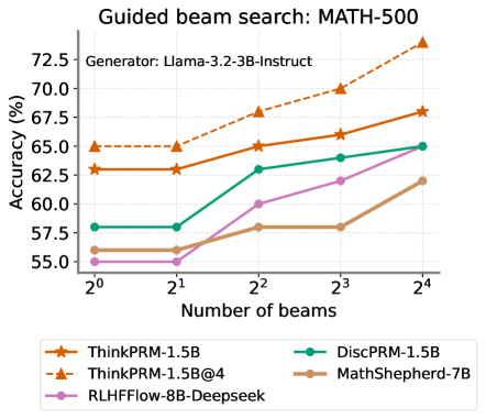</details> Figure 14: Comparison to off-the-shelf PRMs trained on much more step labels than ThinkPRM. $@K$ represents parallel scaling by averaging scores over K CoTs. figure b <details> <summary>x9.png Details</summary>  ### Visual Description \n ## Line Chart: Filtering based on Process vs. 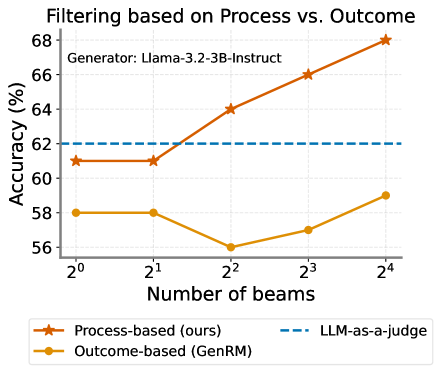Outcome ### Overview This is a line chart comparing the accuracy of two filtering methods ("Process-based" and "Outcome-based") against a baseline ("LLM-as-a-judge") as the number of beams increases. The chart is generated using the "Llama-3.2-3B-Instruct" model, as noted in the top-left corner of the plot area. ### Components/Axes * **Title:** "Filtering based on Process vs. Outcome" * **Generator Label:** "Generator: Llama-3.2-3B-Instruct" (positioned in the top-left of the chart area). * **Y-Axis:** * **Label:** "Accuracy (%)" * **Scale:** Linear, ranging from 56 to 68, with major tick marks at 56, 58, 60, 62, 64, 66, 68. * **X-Axis:** * **Label:** "Number of beams" * **Scale:** Logarithmic base 2, with categorical tick marks at 2⁰ (1), 2¹ (2), 2² (4), 2³ (8), and 2⁴ (16). * **Legend:** Positioned at the bottom of the chart. * **Orange line with star markers:** "Process-based (ours)" * **Yellow line with circle markers:** "Outcome-based (GenRM)" * **Blue dashed line:** "LLM-as-a-judge" ### Detailed Analysis **Data Series and Points:** 1. **Process-based (ours) - Orange line with star markers:** * **Trend:** Shows a consistent, strong upward trend as the number of beams increases. * **Data Points (Approximate):** * At 2⁰ beams: ~61% * At 2¹ beams: ~61% * At 2² beams: ~64% * At 2³ beams: ~66% * At 2⁴ beams: ~68% 2. **Outcome-based (GenRM) - Yellow line with circle markers:** * **Trend:** Shows a non-monotonic trend. It starts flat, dips significantly at 2² beams, then recovers and increases. * **Data Points (Approximate):** * At 2⁰ beams: ~58% * At 2¹ beams: ~58% * At 2² beams: ~56% (lowest point) * At 2³ beams: ~57% * At 2⁴ beams: ~59% 3. **LLM-as-a-judge - Blue dashed line:** * **Trend:** Constant, horizontal line. * **Value:** Fixed at 62% accuracy across all beam numbers. ### Key Observations * The "Process-based (ours)" method demonstrates superior scaling, with accuracy improving significantly as more beams are used. It surpasses the "LLM-as-a-judge" baseline between 2¹ and 2² beams. * The "Outcome-based (GenRM)" method performs worse than the baseline at all tested beam counts. Its performance notably degrades at 2² beams before a partial recovery. * The "LLM-as-a-judge" serves as a static performance benchmark at 62%. * The performance gap between the two active methods widens considerably as the number of beams increases, from a ~3% difference at 2⁰ beams to a ~9% difference at 2⁴ beams. ### Interpretation The chart suggests that the "Process-based" filtering approach is more effective and benefits more from increased computational resources (represented by a higher number of beams) compared to the "Outcome-based" approach for the given task and model. The consistent upward trend indicates that the process-based method effectively utilizes the additional beams to refine its outputs and improve accuracy. In contrast, the outcome-based method shows instability, with a performance drop at a moderate beam count (4), suggesting it may struggle with certain search configurations or that its reward model (GenRM) is less robust. Its final accuracy at 16 beams remains below the simple, static baseline. The key takeaway is that for this specific application using Llama-3.2-3B-Instruct, investing in more beams yields clear returns when using the proposed process-based filtering, while the alternative outcome-based method does not justify the added computational cost over the baseline judge. </details> Figure 17: Ablating the data filtering mechanism, where our process-based filtering yields better PRMs. LLM-as-a-judge is shown with number of beams = 16. ### 4.2 Results #### ThinkPRM outperforms DiscPRM and LLM-as-a-Judge. Under best-of-N selection with MATH-500 shown in Fig. 11 (right), ThinkPRM leads to higher or comparable reasoning accuracy to DiscPRM under all sampling budgets. The trend holds on the more challenging AIME ’24, shown in Fig. 11 left. Additionally, Fig. 1 (right) shows beam search results on MATH-500, with ThinkPRM 1.5B surpassing DiscPRM and LLM-as-a-Judge. #### ThinkPRM surpasses off-the-shelf PRMs. We compare ThinkPRM -1.5B to two strong off-the-shelf PRMs, namely RLHFFlow-Deepseek-PRM (Xiong et al., 2024) and MATH-Shepherd-PRM (Wang et al., 2023b). These PRMs are trained on even more data than PRM800K and are larger than 1.5B. We show results under verifier-guided search on MATH-500 in Fig. 17, with ThinkPRM -1.5B’s scaling curve surpassing all baselines and outperforming RLHFFlow-Deepseek-PRM, the best off-the-shelf PRM among the ones we tested, by more than 7% across all beam sizes. #### ThinkPRM excels on out-of-domain tasks. 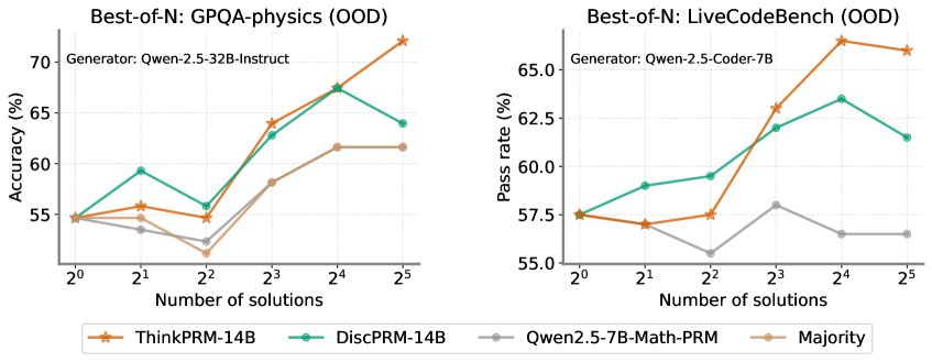As for OOD performance on GPQA-physics (Fig. 18 left), ThinkPRM scales better than DiscPRM—which drops substantially at N=32—outperforming it by 8%. On LiveCodeBench (Fig. 18 right), ThinkPRM also outperforms DiscPRM by 4.5%. On LiveCodeBench, Qwen2.5-7B-Math-PRM (Zhang et al., 2025) —a discriminative PRM trained on substantial amount of process labels obtained from LLM-as-a-judge data and Monte Carlo rollouts—struggles when applied out-of-domain. Our results shed light on the fragility of discriminative PRMs under domain shifts in contrast with generative PRMs. #### Scaling ThinkPRM compute boosts performance. Under verifier-guided search (shown in Fig. 17), parallel scaling with ThinkPRM -1.5B@4 boosts the accuracy by more than 5% points, and yields the best accuracy on MATH-500. In addition, parallel scaling with ThinkPRM -14B@4 and ThinkPRM -14B@8 boosts best-of-N performance on MATH-500 as shown in Fig. 31 in Section E.6. Now we move to sequential scaling of verifier compute by forcing ThinkPRM to recheck its own verification. Since this can be compute-intensive, we only run this on 200 problems from OmniMath subset of ProcessBench, and observe how verification F1 improves as we force the model to think for longer as shown in Fig. 2. ThinkPRM exhibits better scaling behavior compared to LLM-as-a-judge, which drops after 16K tokens, and outperforms DiscPRM-14B by 15 F1 points. In summary, ThinkPRM is consistently better than LLM-as-a-judge under parallel and sequential scaling. #### Parallel scaling vs. sequential scaling. Is it preferable to scale verifier compute in parallel or sequentially? We investigate this by comparing the two modes of scaling under the same token budget. Fig. 32 in Section E.6 shows performance of best-of-N with Qwen-2.5-14B under parallel and sequential scaling with $K=2,4$ under both parallel scaling and sequential scaling. Overall, the performance of both methods is fairly close, but we observe a slight advantage to parallel scaling under certain budgets. <details> <summary>x10.png Details</summary>  ### Visual Description ## Line Charts: Best-of-N Performance Comparison ### Overview The image displays two side-by-side line charts comparing the performance of different AI models/methods on two distinct out-of-distribution (OOD) benchmarks as the number of generated solutions increases. The left chart measures accuracy on GPQA-physics, and the right chart measures pass rate on LiveCodeBench. A shared legend at the bottom identifies four data series. ### Components/Axes **Common Elements:** * **X-Axis (Both Charts):** Labeled "Number of solutions". It uses a logarithmic scale with base 2, marked at points: 2⁰ (1), 2¹ (2), 2² (4), 2³ (8), 2⁴ (16), 2⁵ (32). * **Legend (Bottom Center):** Contains four entries with corresponding line colors and markers: * **ThinkPRM-14B:** Orange line with star markers. * **DiscPRM-14B:** Teal/Green line with circle markers. * **Qwen2.5-7B-Math-PRM:** Gray line with circle markers. * **Majority:** Light brown/Tan line with circle markers. **Left Chart: GPQA-physics (OOD)** * **Title:** "Best-of-N: GPQA-physics (OOD)" * **Subtitle:** "Generator: Qwen-2.5-32B-Instruct" * **Y-Axis:** Labeled "Accuracy (%)". Scale ranges from 55 to 70, with major ticks at 55, 60, 65, 70. **Right Chart: LiveCodeBench (OOD)** * **Title:** "Best-of-N: LiveCodeBench (OOD)" * **Subtitle:** "Generator: Qwen-2.5-Coder-7B" * **Y-Axis:** Labeled "Pass rate (%)". Scale ranges from 55.0 to 65.0, with major ticks at 55.0, 57.5, 60.0, 62.5, 65.0. ### Detailed Analysis **Left Chart: GPQA-physics (OOD) - Accuracy (%)** * **ThinkPRM-14B (Orange, Stars):** Shows a strong, generally upward trend. Starts at ~55% (2⁰), rises to ~56% (2¹), dips slightly to ~55% (2²), then climbs sharply to ~64% (2³), ~68% (2⁴), and peaks at ~72% (2⁵). * **DiscPRM-14B (Teal, Circles):** Shows volatility. Starts at ~55% (2⁰), jumps to ~59% (2¹), drops to ~56% (2²), rises to ~63% (2³), peaks at ~67% (2⁴), then falls to ~64% (2⁵). * **Qwen2.5-7B-Math-PRM (Gray, Circles):** Shows a shallow, fluctuating trend. Starts at ~55% (2⁰), dips to ~54% (2¹), drops further to ~52% (2²), rises to ~58% (2³), then plateaus at ~62% for both 2⁴ and 2⁵. * **Majority (Tan, Circles):** Follows a similar but slightly lower path than Qwen2.5-7B-Math-PRM. Starts at ~55% (2⁰), dips to ~54% (2¹), drops to ~53% (2²), rises to ~58% (2³), then plateaus at ~62% for both 2⁴ and 2⁵. **Right Chart: LiveCodeBench (OOD) - Pass rate (%)** * **ThinkPRM-14B (Orange, Stars):** Shows a strong upward trend with a late plateau. Starts at ~57.5% (2⁰), dips slightly to ~57% (2¹), rises to ~57.5% (2²), jumps to ~63% (2³), peaks at ~66% (2⁴), then slightly decreases to ~65.5% (2⁵). * **DiscPRM-14B (Teal, Circles):** Shows a steady rise then a fall. Starts at ~57.5% (2⁰), rises to ~59% (2¹), ~59.5% (2²), ~62% (2³), peaks at ~63.5% (2⁴), then falls to ~61.5% (2⁵). * **Qwen2.5-7B-Math-PRM (Gray, Circles):** Shows a volatile, low trend. Starts at ~57.5% (2⁰), dips to ~57% (2¹), drops to a low of ~55.5% (2²), rises to ~58% (2³), then falls and plateaus at ~56.5% for both 2⁴ and 2⁵. * **Majority (Tan, Circles):** Not plotted on this chart. The legend entry exists, but no corresponding tan line is visible in the right chart's plot area. ### Key Observations 1. **Dominant Performer:** ThinkPRM-14B (orange) is the top performer on both benchmarks, especially at higher solution counts (N=16, 32). Its performance scales most effectively with increased sampling. 2. **Performance Crossover:** On the GPQA-physics chart, DiscPRM-14B (teal) initially outperforms ThinkPRM at N=2 and N=4, but is overtaken at N=8 and beyond. 3. **Plateauing Effect:** Both Qwen2.5-7B-Math-PRM and the Majority method on the left chart show a clear performance plateau from N=16 to N=32, suggesting diminishing returns for these methods with more samples. 4. **Anomaly in Right Chart:** The "Majority" baseline, while present in the legend, has no visible data line on the LiveCodeBench chart. This could indicate missing data or that its performance was outside the plotted y-axis range. 5. **Volatility:** DiscPRM-14B shows more performance volatility (sharp rises and falls) compared to the steadier climb of ThinkPRM-14B. ### Interpretation The data demonstrates the effectiveness of the "Best-of-N" sampling strategy, where generating multiple solutions and selecting the best one improves performance. However, the benefit is highly dependent on the underlying model or method used for scoring/selecting the "best" solution. * **ThinkPRM-14B** appears to be a robust scoring model, as its associated accuracy/pass rate scales reliably with more candidate solutions. This suggests it is good at identifying higher-quality solutions from a larger pool. * The **plateau** for simpler methods (like Majority voting or the Qwen-based PRM) indicates a ceiling to their improvement. They may lack the discriminative power to effectively leverage additional samples beyond a certain point. * The **divergence in trends** between the two charts (e.g., DiscPRM's late drop on LiveCodeBench vs. its earlier peak on GPQA) highlights that model performance is benchmark-dependent. A method that works well for physics QA may not transfer perfectly to code generation tasks. * The **missing Majority line** on the right chart is a critical data gap. It prevents a full comparison on the LiveCodeBench task, leaving open the question of whether simple majority voting is effective for code generation pass rates. In summary, the charts argue for the use of advanced process reward models (like ThinkPRM) over simpler baselines when employing Best-of-N scaling, as they provide better and more consistent performance gains, particularly in out-of-distribution scenarios. </details> Figure 18: Best-of-N on two out-of-domain tasks: science QA (GPQA-Physics) and code generation (LiveCodeBench). Although ThinkPRM was only finetuned on math, it exhibits superior OOD performance than the baselines, especially at larger sampling budgets, where the baselines fall short. Discriminative PRMs struggle despite being trained on orders of magnitude more process labels. ## 5 Analysis and Discussion ### 5.1 Training data efficiency A major strength of ThinkPRM is training data efficiency compared to discriminative versions. Here, we study the training scaling behavior of ThinkPRM -14B by training it over 500 and 1K examples in total collected using the pipeline in Section 3.2, which roughly corresponds to 4K and 8K process labels from PRM800K in total. We compare that to DiscPRM-14B trained with 1K, 10K, 50K and 98K examples, where 98K corresponds to training on the full PRM800K train set that includes 712K step labels. Fig. 1 (Left) contrasts the training data scaling behavior of ThinkPRM -14B with that of DiscPRM-14B, where ThinkPRM -14B’s performance scales substantially better with two orders of magnitude fewer process labels. This primarily stems from ThinkPRM ’s utilization of text generation and reasoning abilities of the underlying models. While we train ThinkPRM using only 1K data points, we investigate whether it will benefit from training on more data. Using the pipeline, we collect and filter additional verification CoTs and obtain a total of 65K chains. We then finetune R1-Distill-Qwen-1.5B and R1-Distill-Qwen-14B on these for a single epoch while keeping all other training hyperparameters fixed. We then compare the resulting models to the 1K-trained version of ThinkPRM under best-of-N selection on MATH-500. Figs. 38 and 38 in Section E.7 show a performance boost from training on the 65K examples compared to only 1K. This suggests that ThinkPRM can utilize more training data when available. ### 5.2 Effect of Verification CoT Length on PRM Quality We study whether the length of verification chains of thought affects the quality of the resulting generative verifier. Specifically, we compare ThinkPRM trained on the full, long synthetic CoTs with a variant trained on short, compressed versions of the same 1K CoTs. To obtain the short CoTs, we instruct gpt-4o-mini to rewrite each original CoT into a concise version that preserves only the essential reasoning. We then train R1-Qwen-1.5B and R1-Qwen-14B on these short CoTs and evaluate verification F1 on ProcessBench. Table 1 reports the comparison. | R1-Qwen-1.5B R1-Qwen-14B | 87.3 87.3 | 75.7 85.7 | 64.8 55.3 | 66.7 60.8 | | --- | --- | --- | --- | --- | Table 1: Verification F1 when training R1 models on long versus short CoTs. The substantial performance drop when training on short CoTs emphasizes how ThinkPRM benefits from extended reasoning. Since verification is a complex task, throwing more reasoning effort at it via thinking improves performance. These results support the value of using long verification CoTs for training. ### 5.3 Reasoning traces without clear step boundaries So far, we have used ThinkPRM to verify short CoTs with clear steps delimiters. Here, we investigate whether ThinkPRM can still verify long CoTs that involve extended reasoning, backtracking, and self-correction. As a generator, we use Qwen3-1.7B (Yang et al., 2025) with thinking mode. Although ThinkPRM was only trained on short solutions from PRM800K, it can still verify long CoTs and outperforms the baselines as shown in Fig. 19 left. Inspecting ThinkPRM ’s outputs, we found that it extracts and verifies individual steps embedded in the long CoT—an example is in Fig. 45. ### 5.4 Compute-matched comparison to self-consistency Under a fixed test-time compute budget for best-of-N, how does ThinkPRM compare to simply sampling more solutions from the generator and applying majority voting? To investigate this, we conduct a compute-matched analysis on MATH-500 and GPQA-Physics. Fig. 19 mid and right plot solution accuracy as a function of sampling FLOPs for MATH-500 and GPQA-physics. At low sampling budgets, best-of-N with ThinkPRM performs comparably to self-consistency, but as the compute budget increases, ThinkPRM has a clear advantage. These findings agree with recent work on outcome reward models (Singhi et al., 2025). ### 5.5 ThinkPRM with Monte Carlo step labels To train ThinkPRM, we have relied on manual step labels from PRM800K. Since automatic labels e.g., via Monte Carlo rollouts Luo et al. (2024) are cheaper, we validate whether we can train ThinkPRM using automatic labels. We train ThinkPRM -1.5B using 1K synthetic chains based on labels from Math-shepherd dataset (Wang et al., 2023b). Performance on ProcessBench is shown in Table 4, where training ThinkPRM with automatic labels yields very comparable performance to training with manual labels, showing that our training pipeline is agnostic to step-labeling strategy. 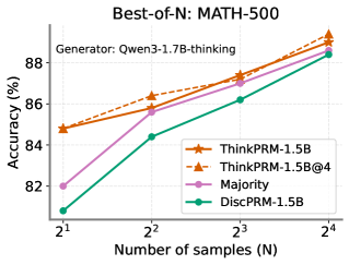<details> <summary>x11.png Details</summary>  ### Visual Description ## Line Chart: Best-of-N: MATH-500 ### Overview This is a line chart comparing the performance (accuracy) of four different methods on the MATH-500 benchmark as the number of samples (N) increases. The chart demonstrates how accuracy scales with increased sampling for each method. ### Components/Axes * **Title:** "Best-of-N: MATH-500" (Top center) * **Subtitle:** "Generator: Qwen3-1.7B-thinking" (Below title, left-aligned) * **Y-Axis:** Label is "Accuracy (%)". Scale runs from 82 to 88, with major tick marks at 82, 84, 86, and 88. * **X-Axis:** Label is "Number of samples (N)". The axis is logarithmic, with categorical tick marks at 2¹ (2), 2² (4), 2³ (8), and 2⁴ (16). * **Legend:** Located in the bottom-right quadrant of the chart area. It contains four entries: 1. `ThinkPRM-1.5B` (Solid orange line, star marker) 2. `ThinkPRM-1.5B@4` (Dashed orange line, star marker) 3. `Majority` (Solid pink line, circle marker) 4. `DiscPRM-1.5B` (Solid green line, diamond marker) ### Detailed Analysis The chart plots four data series. All series show a positive trend, with accuracy increasing as the number of samples (N) increases. **Data Series & Approximate Values:** 1. **ThinkPRM-1.5B (Solid Orange, Stars):** * **Trend:** Steady, strong upward slope. * **Data Points:** * N=2: ~85.0% * N=4: ~86.5% * N=8: ~87.5% * N=16: ~89.0% 2. **ThinkPRM-1.5B@4 (Dashed Orange, Stars):** * **Trend:** Parallel to and slightly above the solid ThinkPRM-1.5B line, indicating a consistent small performance boost. * **Data Points:** * N=2: ~85.2% * N=4: ~86.8% * N=8: ~87.8% * N=16: ~89.2% 3. **Majority (Pink, Circles):** * **Trend:** Starts the lowest but has the steepest initial slope between N=2 and N=4, then continues to rise steadily. * **Data Points:** * N=2: ~82.0% * N=4: ~85.8% * N=8: ~87.0% * N=16: ~88.5% 4. **DiscPRM-1.5B (Green, Diamonds):** * **Trend:** Consistently the lowest-performing method, but shows steady improvement. * **Data Points:** * N=2: ~81.0% * N=4: ~84.5% * N=8: ~86.2% * N=16: ~88.5% ### Key Observations * **Performance Hierarchy:** At all sample sizes, the two `ThinkPRM` variants outperform `Majority` voting, which in turn outperforms `DiscPRM-1.5B`. * **Diminishing Returns:** The slope of improvement for all methods appears to flatten slightly as N increases from 8 to 16, suggesting diminishing returns from additional sampling. * **Convergence at High N:** The performance gap between the methods narrows as N increases. At N=16, `Majority` and `DiscPRM-1.5B` achieve nearly identical accuracy (~88.5%), while the `ThinkPRM` methods are only about 0.5-0.7% higher. * **ThinkPRM@4 Advantage:** The dashed `ThinkPRM-1.5B@4` line maintains a small but consistent lead over the solid `ThinkPRM-1.5B` line across all N. ### Interpretation The data suggests that for the MATH-500 benchmark using the Qwen3-1.7B-thinking generator: 1. **Method Superiority:** The `ThinkPRM` methods are more effective than simple `Majority` voting or `DiscPRM-1.5B` for achieving high accuracy, especially at lower sample counts (N=2, 4). 2. **Value of Sampling:** Increasing the number of samples (Best-of-N) is a universally effective strategy for boosting accuracy, regardless of the underlying method. 3. **Efficiency vs. Peak Performance:** While `Majority` voting starts poorly, it scales efficiently and nearly catches up to the best methods at high N (16). This implies that if computational cost allows for many samples, the choice of method becomes less critical. However, for lower sample budgets, using a more sophisticated method like `ThinkPRM` provides a significant advantage. 4. **The "@4" Variant:** The consistent, small advantage of `ThinkPRM-1.5B@4` over `ThinkPRM-1.5B` indicates that the specific configuration or technique denoted by "@4" provides a reliable, incremental improvement in performance. 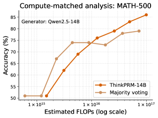</details> <details> <summary>x12.png Details</summary>  ### Visual Description ## Line Chart: Compute-Matched Analysis of MATH-500 Accuracy ### Overview The image is a line chart comparing the performance of two methods, "ThinkPRM-14B" and "Majority voting," on the MATH-500 benchmark. The analysis plots accuracy against estimated computational cost (FLOPs) on a logarithmic scale. The chart demonstrates how the accuracy of each method scales with increased computational resources. ### Components/Axes * **Chart Title:** "Compute-matched analysis: MATH-500" * **Subtitle/Generator:** "Generator: Qwen2.5-14B" * **Y-Axis:** Labeled "Accuracy (%)". The scale runs from 50 to 85, with major tick marks at 50, 55, 60, 65, 70, 75, 80, and 85. * **X-Axis:** Labeled "Estimated FLOPs (log scale)". The scale is logarithmic, with major labeled tick marks at `1 x 10^15`, `1 x 10^16`, and `1 x 10^17`. * **Legend:** Located in the bottom-right quadrant of the chart area. * **ThinkPRM-14B:** Represented by an orange line with circular markers. * **Majority voting:** Represented by a light brown/tan line with circular markers. ### Detailed Analysis **Data Series 1: ThinkPRM-14B (Orange Line)** * **Trend:** The line shows a consistent, strong upward slope across the entire range of compute, indicating that accuracy improves steadily as more FLOPs are allocated. * **Approximate Data Points:** * At ~1 x 10^15 FLOPs: Accuracy ≈ 51% * At ~3 x 10^15 FLOPs: Accuracy ≈ 62% * At ~1 x 10^16 FLOPs: Accuracy ≈ 74% * At ~3 x 10^16 FLOPs: Accuracy ≈ 79% * At ~1 x 10^17 FLOPs: Accuracy ≈ 85% **Data Series 2: Majority voting (Light Brown Line)** * **Trend:** The line shows a steep initial increase in accuracy at lower compute levels, but the rate of improvement slows significantly (plateaus) after approximately 1 x 10^16 FLOPs. * **Approximate Data Points:** * At ~1 x 10^15 FLOPs: Accuracy ≈ 51% (similar starting point to ThinkPRM-14B). * At ~3 x 10^15 FLOPs: Accuracy ≈ 67% (notably higher than ThinkPRM-14B at this point). * At ~1 x 10^16 FLOPs: Accuracy ≈ 74% (intersects with ThinkPRM-14B). * At ~3 x 10^16 FLOPs: Accuracy ≈ 73% (slight dip or plateau). * At ~1 x 10^17 FLOPs: Accuracy ≈ 79% (ends lower than ThinkPRM-14B). ### Key Observations 1. **Crossover Point:** The two methods achieve approximately equal accuracy (~74%) at an estimated compute level of 1 x 10^16 FLOPs. 2. **Diverging Scaling:** After the crossover point, the performance trajectories diverge. ThinkPRM-14B continues to scale efficiently, while Majority voting exhibits diminishing returns. 3. **Initial Advantage:** Majority voting provides a significant accuracy advantage at lower compute budgets (between ~2 x 10^15 and 8 x 10^15 FLOPs). 4. **Final Outcome:** At the highest compute level shown (~1 x 10^17 FLOPs), ThinkPRM-14B outperforms Majority voting by approximately 6 percentage points (85% vs. 79%). ### Interpretation This chart illustrates a classic trade-off in machine learning between a method that is highly efficient at low compute (Majority voting) and one that scales more effectively with abundant resources (ThinkPRM-14B). * **What the data suggests:** The "ThinkPRM-14B" method appears to be a more scalable architecture or technique for this task. Its consistent upward trend implies it can effectively utilize additional computational power to improve performance without hitting an early plateau. In contrast, "Majority voting" likely represents an ensemble or sampling technique that provides quick gains but has a fundamental performance ceiling that is reached relatively quickly. * **How elements relate:** The x-axis (compute) is the independent variable being controlled, and the y-axis (accuracy) is the dependent outcome. The two lines represent different strategies for converting compute into performance. The crossover point is critical, as it defines the computational budget at which one should switch from using Majority voting to ThinkPRM-14B for optimal results. * **Notable implications:** For projects with constrained computational budgets (below 1 x 10^16 FLOPs), Majority voting is the more effective choice. For state-of-the-art results where maximum accuracy is the goal and compute is less constrained, ThinkPRM-14B is the superior approach. The chart provides a clear, data-driven rationale for selecting a method based on available resources. 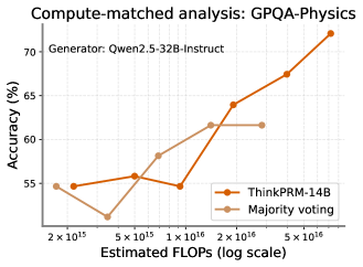</details> <details> <summary>x13.png Details</summary>  ### Visual Description ## Line Chart: Compute-matched analysis: GPQA-Physics ### Overview The image is a line chart comparing the performance (accuracy) of two methods, "ThinkPRM-14B" and "Majority voting," as a function of increasing computational resources (estimated FLOPs). The analysis is performed on the GPQA-Physics benchmark using the Qwen2.5-32B-Instruct model as the generator. ### Components/Axes * **Chart Title:** "Compute-matched analysis: GPQA-Physics" * **Subtitle/Generator Label:** "Generator: Qwen2.5-32B-Instruct" * **Y-Axis:** * **Label:** "Accuracy (%)" * **Scale:** Linear, ranging from 55 to 70, with major tick marks at 55, 60, 65, and 70. * **X-Axis:** * **Label:** "Estimated FLOPs (log₁₀ scale)" * **Scale:** Logarithmic (base 10). Major tick marks are labeled: `2 x 10¹⁵`, `5 x 10¹⁵`, `1 x 10¹⁶`, `2 x 10¹⁶`, `5 x 10¹⁶`. * **Legend:** Located in the bottom-right quadrant of the chart area. * **Orange line with circle markers:** "ThinkPRM-14B" * **Light brown/tan line with circle markers:** "Majority voting" ### Detailed Analysis **Data Series 1: ThinkPRM-14B (Orange Line)** * **Trend:** The line shows a relatively flat or slightly increasing trend at lower compute levels, followed by a steep, consistent upward slope at higher compute levels. * **Data Points (Approximate):** * At ~2 x 10¹⁵ FLOPs: Accuracy ≈ 55% * At ~5 x 10¹⁵ FLOPs: Accuracy ≈ 55.5% * At ~1 x 10¹⁶ FLOPs: Accuracy ≈ 55% * At ~2 x 10¹⁶ FLOPs: Accuracy ≈ 64% * At ~5 x 10¹⁶ FLOPs: Accuracy ≈ 68% * At the final point (estimated >5 x 10¹⁶ FLOPs): Accuracy ≈ 72% **Data Series 2: Majority voting (Light Brown Line)** * **Trend:** The line shows an initial dip, followed by a steady, moderate upward trend that appears to plateau at the highest compute levels shown. * **Data Points (Approximate):** * At ~2 x 10¹⁵ FLOPs: Accuracy ≈ 55% * At ~5 x 10¹⁵ FLOPs: Accuracy ≈ 52% (This is a notable dip) * At ~1 x 10¹⁶ FLOPs: Accuracy ≈ 58% * At ~2 x 10¹⁶ FLOPs: Accuracy ≈ 61.5% * At ~5 x 10¹⁶ FLOPs: Accuracy ≈ 61.5% (Plateau) ### Key Observations 1. **Crossover Point:** The two methods have similar accuracy at the lowest compute point (~2 x 10¹⁵ FLOPs). ThinkPRM-14B dips below Majority voting at ~5 x 10¹⁵ FLOPs but then surpasses it decisively at ~1 x 10¹⁶ FLOPs and maintains a significant lead thereafter. 2. **Scaling Behavior:** ThinkPRM-14B demonstrates superior scaling with increased compute. Its accuracy continues to climb steeply across the entire range, especially after 1 x 10¹⁶ FLOPs. Majority voting shows more modest gains and appears to saturate. 3. **Anomaly:** The Majority voting series shows a distinct performance drop at ~5 x 10¹⁵ FLOPs before recovering. This could indicate a specific compute regime where the voting mechanism is less effective or a potential measurement outlier. ### Interpretation This chart illustrates a **compute-performance scaling law comparison** for two reasoning or inference techniques on a physics QA task. The key finding is that the "ThinkPRM-14B" method (likely a process reward model or a specific reasoning framework) is significantly more **compute-efficient at higher scales** than the simpler "Majority voting" baseline. * **What it suggests:** Investing more computational resources (FLOPs) yields substantially greater accuracy improvements when using ThinkPRM-14B compared to majority voting. The diverging trends imply that for large-scale, high-performance applications, advanced methods like ThinkPRM are necessary to fully leverage available compute. * **Relationship between elements:** The x-axis (compute) is the independent variable being increased. The y-axis (accuracy) is the dependent outcome. The two lines represent different algorithms attempting to convert the same "budget" of compute into performance. The widening gap between the lines visually quantifies the growing advantage of the more sophisticated method. * **Notable patterns:** The plateau in Majority voting suggests it hits a performance ceiling, while ThinkPRM-14B shows no such saturation within the tested range, hinting at a higher potential ceiling. The initial dip for Majority voting is curious and might warrant investigation into the stability of that method at specific compute points. </details> Figure 19: Left: Best-of-N with Qwen3-1.7B on the full MATH-500 test set, showing how ThinkPRM generalizes well to verifying long reasoning traces. Mid and Right: Compute-matched comparison between best-of-N with ThinkPRM and self-consistency or majority vote. ### 5.6 ThinkPRM helps with difficult reasoning problems ThinkPRM ’s reasoning ability should enable it to tackle verification of hard problems. To check if this is the case, we analyze performance of ThinkPRM vs. DiscPRM in light of problem difficulty over MATH-500 and GPQA-physics (how we estimate difficulty for GPQA-Physics is explained in Section E.9), shown in Fig. 39. The generators here are Qwen-2.5-14B for MATH-500 and Qwen-2.5-32B-Instruct for GPQA-Physics. Primarily, ThinkPRM improves reasoning on the difficult problems (levels 3, 4, 5 in MATH-500 and 2, 3, 4 in GPQA-Physics) substantially more than DiscPRM. ### 5.7 Filtering based on process vs. outcome labels In Section 3.2, we describe our process-based filtering strategy, which selects verification CoTs based on agreement between generated step-level decisions and gold process labels. To validate its effectiveness, we compare it to outcome-based filtering, as in GenRM (Zheng et al., 2024), which retains chains solely based on final answer correctness—keeping a CoT if its final answer is correct and the final step is \boxed{correct}, or if the answer is incorrect and the final step is \boxed{incorrect}, thereby ignoring intermediate step labels. We obtain 65K and 128K CoTs using process- and outcome-based filtering, respectively. Fig. 17 shows that finetuning R1-Distill-Qwen-1.5B on process-filtered data yields significantly better verification performance, despite using fewer examples, which reflects the importance of our process-based filtering in training strong PRMs. ### 5.8 Limitations of Generative PRMs While generative PRMs are more powerful and data-efficient than their discriminative counterparts, they come with some limitations that we highlight as avenues for future work. First, overconfidence is a known issue in LLMs (Liu et al., 2023a; Stechly et al., 2023; Zhou et al., 2024) and, in the case of PRMs, it can cause the predicted PRM scores to cluster near extremes: close to either 0 or 1. One reason is that we are using probabilities of certain tokens such as “yes” or “no”, which by nature will be either very high or very low. Future work should explore more reliable techniques to extract calibrated scores from generative reward models. Another limitation is due to autoregressive nature of LLMs, leading them to prematurely commit to an earlier judgment. For example, we observe a phenomenon we term step label interference, where verification errors for earlier steps impact verification of later steps. For example, we noted that if the PRM judges a particular step as incorrect, it becomes more likely to label subsequent steps as incorrect even if it is not. Lastly, generating a verification CoT introduces extra overhead compared to discriminative PRMs, but we argue that the performance gains offered by generative PRMs justify this extra cost. ## Conclusion We introduced ThinkPRM, a generative process reward model trained with minimal synthetic supervision for scalable step-by-step verification. With just 8K process labels, ThinkPRM significantly outperforms LLM-as-a-judge and even surpasses discriminative PRMs trained on orders of magnitude more data. These results highlight the benefits of generative PRMs in interpretability, scalability, and data efficiency, and demonstrate their potential to scale verification compute for complex reasoning tasks in math and science. ## References - Akyürek et al. (2024) Ekin Akyürek, Mehul Damani, Linlu Qiu, Han Guo, Yoon Kim, and Jacob Andreas. The surprising effectiveness of test-time training for abstract reasoning. arXiv preprint arXiv:2411.07279, 2024. - Ankner et al. (2024) Zachary Ankner, Mansheej Paul, Brandon Cui, Jonathan D Chang, and Prithviraj Ammanabrolu. Critique-out-loud reward models. arXiv preprint arXiv:2408.11791, 2024. - Bavaresco et al. (2024) Anna Bavaresco, Raffaella Bernardi, Leonardo Bertolazzi, Desmond Elliott, Raquel Fernández, Albert Gatt, Esam Ghaleb, Mario Giulianelli, Michael Hanna, Alexander Koller, et al. Llms instead of human judges? a large scale empirical study across 20 nlp evaluation tasks. arXiv preprint arXiv:2406.18403, 2024. - (4) Edward Beeching, Lewis Tunstall, and Sasha Rush. Scaling test-time compute with open models. URL https://huggingface.co/spaces/HuggingFaceH4/blogpost-scaling-test-time-compute. - Brown et al. (2024) Bradley Brown, Jordan Juravsky, Ryan Ehrlich, Ronald Clark, Quoc V Le, Christopher Ré, and Azalia Mirhoseini. Large language monkeys: Scaling inference compute with repeated sampling. arXiv preprint arXiv:2407.21787, 2024. - Brown et al. (2020) Tom Brown, Benjamin Mann, Nick Ryder, Melanie Subbiah, Jared D Kaplan, Prafulla Dhariwal, Arvind Neelakantan, Pranav Shyam, Girish Sastry, Amanda Askell, et al. Language models are few-shot learners. Advances in neural information processing systems, 33:1877–1901, 2020. - Charniak & Johnson (2005) Eugene Charniak and Mark Johnson. Coarse-to-fine n-best parsing and maxent discriminative reranking. In Proceedings of the 43rd Annual Meeting of the Association for Computational Linguistics (ACL’05), pp. 173–180, 2005. - Chen et al. (2024a) Guoxin Chen, Minpeng Liao, Chengxi Li, and Kai Fan. Alphamath almost zero: process supervision without process. arXiv preprint arXiv:2405.03553, 2024a. - Chen et al. (2024b) Xingyu Chen, Jiahao Xu, Tian Liang, Zhiwei He, Jianhui Pang, Dian Yu, Linfeng Song, Qiuzhi Liu, Mengfei Zhou, Zhuosheng Zhang, et al. Do not think that much for 2+ 3=? on the overthinking of o1-like llms. arXiv preprint arXiv:2412.21187, 2024b. - Chen et al. (2024c) Ziru Chen, Michael White, Raymond Mooney, Ali Payani, Yu Su, and Huan Sun. When is tree search useful for llm planning? it depends on the discriminator. arXiv preprint arXiv:2402.10890, 2024c. - Cobbe et al. (2021) Karl Cobbe, Vineet Kosaraju, Mohammad Bavarian, Jacob Hilton, Reiichiro Nakano, Christopher Hesse, and John Schulman. Training verifiers to solve math word problems. arXiv preprint arXiv:2110.14168, 2021. - Cuadron et al. (2025) Alejandro Cuadron, Dacheng Li, Wenjie Ma, Xingyao Wang, Yichuan Wang, Siyuan Zhuang, Shu Liu, Luis Gaspar Schroeder, Tian Xia, Huanzhi Mao, et al. The danger of overthinking: Examining the reasoning-action dilemma in agentic tasks. arXiv preprint arXiv:2502.08235, 2025. - Dong et al. (2023) Hanze Dong, Wei Xiong, Deepanshu Goyal, Yihan Zhang, Winnie Chow, Rui Pan, Shizhe Diao, Jipeng Zhang, Kashun Shum, and Tong Zhang. Raft: Reward ranked finetuning for generative foundation model alignment. arXiv preprint arXiv:2304.06767, 2023. - Gao et al. (2024) Bofei Gao, Feifan Song, Zhe Yang, Zefan Cai, Yibo Miao, Qingxiu Dong, Lei Li, Chenghao Ma, Liang Chen, Runxin Xu, et al. Omni-math: A universal olympiad level mathematic benchmark for large language models. arXiv preprint arXiv:2410.07985, 2024. - Guo et al. (2025) Daya Guo, Dejian Yang, Haowei Zhang, Junxiao Song, Ruoyu Zhang, Runxin Xu, Qihao Zhu, Shirong Ma, Peiyi Wang, Xiao Bi, et al. Deepseek-r1: Incentivizing reasoning capability in llms via reinforcement learning. arXiv preprint arXiv:2501.12948, 2025. - He et al. (2024) Chaoqun He, Renjie Luo, Yuzhuo Bai, Shengding Hu, Zhen Leng Thai, Junhao Shen, Jinyi Hu, Xu Han, Yujie Huang, Yuxiang Zhang, et al. Olympiadbench: A challenging benchmark for promoting agi with olympiad-level bilingual multimodal scientific problems. arXiv preprint arXiv:2402.14008, 2024. - Hendrycks et al. (2021) Dan Hendrycks, Collin Burns, Saurav Kadavath, Akul Arora, Steven Basart, Eric Tang, Dawn Song, and Jacob Steinhardt. Measuring mathematical problem solving with the math dataset. arXiv preprint arXiv:2103.03874, 2021. - Hu et al. (2022) Edward J Hu, Yelong Shen, Phillip Wallis, Zeyuan Allen-Zhu, Yuanzhi Li, Shean Wang, Lu Wang, Weizhu Chen, et al. Lora: Low-rank adaptation of large language models. ICLR, 1(2):3, 2022. - Huang et al. (2023) Jie Huang, Xinyun Chen, Swaroop Mishra, Huaixiu Steven Zheng, Adams Wei Yu, Xinying Song, and Denny Zhou. Large language models cannot self-correct reasoning yet. arXiv preprint arXiv:2310.01798, 2023. - Hui et al. (2024) Binyuan Hui, Jian Yang, Zeyu Cui, Jiaxi Yang, Dayiheng Liu, Lei Zhang, Tianyu Liu, Jiajun Zhang, Bowen Yu, Kai Dang, et al. Qwen2. 5-coder technical report. arXiv preprint arXiv:2409.12186, 2024. - Jaech et al. (2024) Aaron Jaech, Adam Kalai, Adam Lerer, Adam Richardson, Ahmed El-Kishky, Aiden Low, Alec Helyar, Aleksander Madry, Alex Beutel, Alex Carney, et al. Openai o1 system card. arXiv preprint arXiv:2412.16720, 2024. - Jain et al. (2024) Naman Jain, King Han, Alex Gu, Wen-Ding Li, Fanjia Yan, Tianjun Zhang, Sida Wang, Armando Solar-Lezama, Koushik Sen, and Ion Stoica. Livecodebench: Holistic and contamination free evaluation of large language models for code. arXiv preprint arXiv:2403.07974, 2024. - Kalra & Tang (2025) Nimit Kalra and Leonard Tang. Verdict: A library for scaling judge-time compute. arXiv preprint arXiv:2502.18018, 2025. - Kang et al. (2024) Yu Kang, Xianghui Sun, Liangyu Chen, and Wei Zou. C3ot: Generating shorter chain-of-thought without compromising effectiveness. arXiv preprint arXiv:2412.11664, 2024. - Khalifa et al. (2023) Muhammad Khalifa, Lajanugen Logeswaran, Moontae Lee, Honglak Lee, and Lu Wang. GRACE: discriminator-guided chain-of-thought reasoning. In Houda Bouamor, Juan Pino, and Kalika Bali (eds.), Findings of the Association for Computational Linguistics: EMNLP 2023, Singapore, December 6-10, 2023, pp. 15299–15328. Association for Computational Linguistics, 2023. doi: 10.18653/V1/2023.FINDINGS-EMNLP.1022. URL https://doi.org/10.18653/v1/2023.findings-emnlp.1022. - Kim et al. (2023) Seungone Kim, Jamin Shin, Yejin Cho, Joel Jang, Shayne Longpre, Hwaran Lee, Sangdoo Yun, Seongjin Shin, Sungdong Kim, James Thorne, et al. Prometheus: Inducing fine-grained evaluation capability in language models. In The Twelfth International Conference on Learning Representations, 2023. - Kumar et al. (2024) Aviral Kumar, Vincent Zhuang, Rishabh Agarwal, Yi Su, John D Co-Reyes, Avi Singh, Kate Baumli, Shariq Iqbal, Colton Bishop, Rebecca Roelofs, et al. Training language models to self-correct via reinforcement learning. arXiv preprint arXiv:2409.12917, 2024. - Lambert et al. (2024) Nathan Lambert, Valentina Pyatkin, Jacob Morrison, LJ Miranda, Bill Yuchen Lin, Khyathi Chandu, Nouha Dziri, Sachin Kumar, Tom Zick, Yejin Choi, et al. Rewardbench: Evaluating reward models for language modeling. arXiv preprint arXiv:2403.13787, 2024. - Li et al. (2023) Yifei Li, Zeqi Lin, Shizhuo Zhang, Qiang Fu, Bei Chen, Jian-Guang Lou, and Weizhu Chen. Making language models better reasoners with step-aware verifier. In Proceedings of the 61st Annual Meeting of the Association for Computational Linguistics (Volume 1: Long Papers), pp. 5315–5333, 2023. - Lightman et al. (2023) Hunter Lightman, Vineet Kosaraju, Yura Burda, Harri Edwards, Bowen Baker, Teddy Lee, Jan Leike, John Schulman, Ilya Sutskever, and Karl Cobbe. Let’s verify step by step. arXiv preprint arXiv:2305.20050, 2023. - Liu et al. (2023a) Xin Liu, Muhammad Khalifa, and Lu Wang. Litcab: Lightweight language model calibration over short-and long-form responses. arXiv preprint arXiv:2310.19208, 2023a. - Liu et al. (2023b) Yang Liu, Dan Iter, Yichong Xu, Shuohang Wang, Ruochen Xu, and Chenguang Zhu. G-eval: Nlg evaluation using gpt-4 with better human alignment. arXiv preprint arXiv:2303.16634, 2023b. - Luo et al. (2024) Liangchen Luo, Yinxiao Liu, Rosanne Liu, Samrat Phatale, Harsh Lara, Yunxuan Li, Lei Shu, Yun Zhu, Lei Meng, Jiao Sun, et al. Improve mathematical reasoning in language models by automated process supervision. arXiv preprint arXiv:2406.06592, 2, 2024. - Mahan et al. (2024) Dakota Mahan, Duy Van Phung, Rafael Rafailov, Chase Blagden, Nathan Lile, Louis Castricato, Jan-Philipp Fränken, Chelsea Finn, and Alon Albalak. Generative reward models. arXiv preprint arXiv:2410.12832, 2024. - Muennighoff et al. (2025) Niklas Muennighoff, Zitong Yang, Weijia Shi, Xiang Lisa Li, Li Fei-Fei, Hannaneh Hajishirzi, Luke Zettlemoyer, Percy Liang, Emmanuel Candès, and Tatsunori Hashimoto. s1: Simple test-time scaling. arXiv preprint arXiv:2501.19393, 2025. - Rein et al. (2024) David Rein, Betty Li Hou, Asa Cooper Stickland, Jackson Petty, Richard Yuanzhe Pang, Julien Dirani, Julian Michael, and Samuel R Bowman. Gpqa: A graduate-level google-proof q&a benchmark. In First Conference on Language Modeling, 2024. - Singh et al. (2023) Avi Singh, John D Co-Reyes, Rishabh Agarwal, Ankesh Anand, Piyush Patil, Xavier Garcia, Peter J Liu, James Harrison, Jaehoon Lee, Kelvin Xu, et al. Beyond human data: Scaling self-training for problem-solving with language models. arXiv preprint arXiv:2312.06585, 2023. - Singhi et al. (2025) Nishad Singhi, Hritik Bansal, Arian Hosseini, Aditya Grover, Kai-Wei Chang, Marcus Rohrbach, and Anna Rohrbach. When to solve, when to verify: Compute-optimal problem solving and generative verification for llm reasoning. arXiv preprint arXiv:2504.01005, 2025. - Snell et al. (2024) Charlie Snell, Jaehoon Lee, Kelvin Xu, and Aviral Kumar. Scaling llm test-time compute optimally can be more effective than scaling model parameters. arXiv preprint arXiv:2408.03314, 2024. - Stechly et al. (2023) Kaya Stechly, Matthew Marquez, and Subbarao Kambhampati. Gpt-4 doesn’t know it’s wrong: An analysis of iterative prompting for reasoning problems. arXiv preprint arXiv:2310.12397, 2023. - Sun et al. (2024) Zhiqing Sun, Longhui Yu, Yikang Shen, Weiyang Liu, Yiming Yang, Sean Welleck, and Chuang Gan. Easy-to-hard generalization: Scalable alignment beyond human supervision. arXiv preprint arXiv:2403.09472, 2024. - Team (2024) Qwen Team. Qwq: Reflect deeply on the boundaries of the unknown, November 2024. URL https://qwenlm.github.io/blog/qwq-32b-preview/. - Uesato et al. (2022) Jonathan Uesato, Nate Kushman, Ramana Kumar, Francis Song, Noah Siegel, Lisa Wang, Antonia Creswell, Geoffrey Irving, and Irina Higgins. Solving math word problems with process-and outcome-based feedback. arXiv preprint arXiv:2211.14275, 2022. - Wan et al. (2024) Ziyu Wan, Xidong Feng, Muning Wen, Stephen Marcus McAleer, Ying Wen, Weinan Zhang, and Jun Wang. Alphazero-like tree-search can guide large language model decoding and training. In Forty-first International Conference on Machine Learning, 2024. - Wang et al. (2023a) Jiaan Wang, Yunlong Liang, Fandong Meng, Haoxiang Shi, Zhixu Li, Jinan Xu, Jianfeng Qu, and Jie Zhou. Is chatgpt a good nlg evaluator? a preliminary study. arXiv preprint arXiv:2303.04048, 2023a. - Wang et al. (2023b) Peiyi Wang, Lei Li, Zhihong Shao, RX Xu, Damai Dai, Yifei Li, Deli Chen, Y Wu, and Zhifang Sui. Math-shepherd: A label-free step-by-step verifier for llms in mathematical reasoning. arXiv preprint arXiv:2312.08935, 2023b. - Wang et al. (2024) Tianlu Wang, Ilia Kulikov, Olga Golovneva, Ping Yu, Weizhe Yuan, Jane Dwivedi-Yu, Richard Yuanzhe Pang, Maryam Fazel-Zarandi, Jason Weston, and Xian Li. Self-taught evaluators. arXiv preprint arXiv:2408.02666, 2024. - Wang et al. (2022) Xuezhi Wang, Jason Wei, Dale Schuurmans, Quoc Le, Ed Chi, and Denny Zhou. Self-consistency improves chain of thought reasoning in language models. arXiv preprint arXiv:2203.11171, 2022. - Wu et al. (2024) Yangzhen Wu, Zhiqing Sun, Shanda Li, Sean Welleck, and Yiming Yang. Inference scaling laws: An empirical analysis of compute-optimal inference for problem-solving with language models. arXiv preprint arXiv:2408.00724, 2024. - Xiong et al. (2024) Wei Xiong, Hanning Zhang, Nan Jiang, and Tong Zhang. An implementation of generative prm. https://github.com/RLHFlow/RLHF-Reward-Modeling, 2024. - Xiong et al. (2025) Wei Xiong, Hanning Zhang, Chenlu Ye, Lichang Chen, Nan Jiang, and Tong Zhang. Self-rewarding correction for mathematical reasoning. arXiv preprint arXiv:2502.19613, 2025. - Yang et al. (2025) An Yang, Anfeng Li, Baosong Yang, Beichen Zhang, Binyuan Hui, Bo Zheng, Bowen Yu, Chang Gao, Chengen Huang, Chenxu Lv, et al. Qwen3 technical report. arXiv preprint arXiv:2505.09388, 2025. - Yao et al. (2023) Shunyu Yao, Dian Yu, Jeffrey Zhao, Izhak Shafran, Tom Griffiths, Yuan Cao, and Karthik Narasimhan. Tree of thoughts: Deliberate problem solving with large language models. Advances in neural information processing systems, 36:11809–11822, 2023. - Ye et al. (2024) Tian Ye, Zicheng Xu, Yuanzhi Li, and Zeyuan Allen-Zhu. Physics of language models: Part 2.2, how to learn from mistakes on grade-school math problems. arXiv preprint arXiv:2408.16293, 2024. - Yu et al. (2024) Ping Yu, Jing Xu, Jason Weston, and Ilia Kulikov. Distilling system 2 into system 1. arXiv preprint arXiv:2407.06023, 2024. - Yuan et al. (2024) Lifan Yuan, Wendi Li, Huayu Chen, Ganqu Cui, Ning Ding, Kaiyan Zhang, Bowen Zhou, Zhiyuan Liu, and Hao Peng. Free process rewards without process labels. arXiv preprint arXiv:2412.01981, 2024. - Zelikman et al. (2022) Eric Zelikman, Yuhuai Wu, Jesse Mu, and Noah Goodman. Star: Bootstrapping reasoning with reasoning. Advances in Neural Information Processing Systems, 35:15476–15488, 2022. - Zhang et al. (2024a) Lunjun Zhang, Arian Hosseini, Hritik Bansal, Mehran Kazemi, Aviral Kumar, and Rishabh Agarwal. Generative verifiers: Reward modeling as next-token prediction. arXiv preprint arXiv:2408.15240, 2024a. - Zhang et al. (2024b) Yunxiang Zhang, Muhammad Khalifa, Lajanugen Logeswaran, Jaekyeom Kim, Moontae Lee, Honglak Lee, and Lu Wang. Small language models need strong verifiers to self-correct reasoning. In Lun-Wei Ku, Andre Martins, and Vivek Srikumar (eds.), Findings of the Association for Computational Linguistics, ACL 2024, Bangkok, Thailand and virtual meeting, August 11-16, 2024, pp. 15637–15653. Association for Computational Linguistics, 2024b. doi: 10.18653/V1/2024.FINDINGS-ACL.924. URL https://doi.org/10.18653/v1/2024.findings-acl.924. - Zhang et al. (2025) Zhenru Zhang, Chujie Zheng, Yangzhen Wu, Beichen Zhang, Runji Lin, Bowen Yu, Dayiheng Liu, Jingren Zhou, and Junyang Lin. The lessons of developing process reward models in mathematical reasoning. arXiv preprint arXiv:2501.07301, 2025. - Zheng et al. (2024) Chujie Zheng, Zhenru Zhang, Beichen Zhang, Runji Lin, Keming Lu, Bowen Yu, Dayiheng Liu, Jingren Zhou, and Junyang Lin. Processbench: Identifying process errors in mathematical reasoning. arXiv preprint arXiv:2412.06559, 2024. - Zheng et al. (2023) Lianmin Zheng, Wei-Lin Chiang, Ying Sheng, Siyuan Zhuang, Zhanghao Wu, Yonghao Zhuang, Zi Lin, Zhuohan Li, Dacheng Li, Eric Xing, et al. Judging llm-as-a-judge with mt-bench and chatbot arena. Advances in Neural Information Processing Systems, 36:46595–46623, 2023. - Zhou et al. (2024) Kaitlyn Zhou, Jena D Hwang, Xiang Ren, and Maarten Sap. Relying on the unreliable: The impact of language models’ reluctance to express uncertainty. arXiv preprint arXiv:2401.06730, 2024. - Zhu et al. (2023) Lianghui Zhu, Xinggang Wang, and Xinlong Wang. Judgelm: Fine-tuned large language models are scalable judges. arXiv preprint arXiv:2310.17631, 2023. ## Appendix A Training data ### A.1 Sampling Fig. 3 shows the prompt used with QwQ-32B-Preview to sample verification chains for training. We use the problem-prefix pairs from PRM800K train split (Lightman et al., 2023), which is based on MATH (Hendrycks et al., 2021). We sample 4 verification chains for each prefix in the dataset with temperature $T=0.1$ until we have 1K verification CoTs that (1) follow the desired format i.e., the model generated an extractable label for every step in the prefix and (2) the verbalized step labels match the gold labels in the PRM800K dataset annotation, (3) at most 4096 tokens long, and are (4) roughly balanced with respect to final answer correctness. Roughly 20% of the initial samples satisfied criteria 1 and 2 in our case, which means that about 5K samples in total are needed to obtain 1K filtered samples. Table 2 shows the statistics of the final dataset. We also show an example from the 1K training CoTs in Fig. 20. Synthetic training sample Problem: Find the area in square feet of a square with a perimeter of 32ft. Solution: Step 1: A square has four equal sides, so the perimeter is four times the length of one side. Step 2: I can write an equation to relate the perimeter and the side length: 4s = 32, where s is the side length in feet. Step 3: To solve for s, I can divide both sides by 4: s = 32/4 = 8. Step 4: Now I know the side length of the square is 8 feet. Step 5: The area of a square is the side length squared, so the area is s² = 8² = 64. Step 6: The area is in square feet, so the units are ft². Step 7: The answer is 64 ft² <think> Alright, let’s verify step by step the solution provided for finding the area of a square with a perimeter of 32 feet. Step 1: “A square has four equal sides, so the perimeter is four times the length of one side.” Critique: This statement is accurate. A square indeed has four sides of equal length, and the perimeter is the sum of all sides. Therefore, perimeter (P) equals 4 times the side length (s), or P = 4s. The step is \\boxed{correct} Step 2: “I can write an equation to relate the perimeter and the side length: 4s = 32, where s is the side length in feet.” Critique: Given that the perimeter is 32 feet, setting up the equation 4s = 32 is correct. It properly represents the relationship between the perimeter and the side length of the square. The step is \\boxed{correct} Step 3: “To solve for s, I can divide both sides by 4: s = 32/4 = 8.” Critique: This step correctly solves for s by dividing both sides of the equation by 4. The calculation 32 divided by 4 equals 8 is accurate. The step is \\boxed{correct} Step 4: “Now I know the side length of the square is 8 feet.” Critique: Based on the previous step, s = 8 feet, which is correctly stated here. The step is \\boxed{correct} Step 5: “The area of a square is the side length squared, so the area is s² = 8² = 64.” Critique: The formula for the area of a square is indeed s squared. Calculating 8 squared equals 64 is correct. The step is \\boxed{correct} Step 6: “The area is in square feet, so the units are ft².” Critique: Since the side length is in feet, the area will be in square feet (ft²). This is the correct unit for area. The step is \\boxed{correct} Step 7: “The answer is 64 ft²” Critique: This is the final answer, correctly stating the area as 64 square feet. The step is \\boxed{correct} </think> Is the solution correct? Yes Figure 20: Training example from our sampled 1K synthetic chains. ### A.2 Preprocessing From the sampled verification CoTs, we extract boxed predictions (e.g., \boxed{correct} or \boxed{incorrect}) for each reasoning step. Then we filter the data as follows: - CoTs with missing or malformed verification decisions are discarded. - CoTs where verification decisions don’t match ground truth labels are filtered out. Precisely, we require all step-by-step verification decisions to match the ground truth labels. Then we clean the data as follows: - We standardize boxed notation formats. - Content after the last verification decision is removed. - Special tokens (e.g., <think> and </think>) are added to designate verification reasoning. Table 2: Statistics of the 1K finetuning dataset. | Correctness Distribution | | | --- | --- | | # correct | 486 (48.6%) | | # incorrect | 514 (51.4%) | | Step label distribution | | | # correct | 7474 (92.3%) | | # Incorrect | 625 (7.7%) | | Prefix statistics | | | # unique questions | 869 | | average steps per prefix | 9.5 | | min # steps | 1 | | max # steps | 53 | | Verification Chain Statistics | | | Average verification chain length (tokens) | 1037.0 | | Min verification chain length (tokens) | 207 | | Max verification chain length (tokens) | 3669 | Data generation prompt You are given a math problem and a proposed multiple-step solution (with a step on each line): [Math Problem] {problem} [Solution] {solution} Review and critique the proposed solution steps and determine whether each step is correct. If the solution is incomplete, only critique the steps that are provided. Your output must be in the following format: Let’s verify step by step: Step 1: <critique>…The step is \boxed{correct/incorrect} Step 2: <critique>…The step is \boxed{correct/incorrect} … Step n: <critique>…The step is \boxed{correct/incorrect} Once you find an incorrect step, you should stop since you don’t need to analyze the remaining steps. Figure 21: Prompt used to generate synthetic verification chains as described in Section 3.2. ## Appendix B LLM-as-a-Judge Limitations We show examples of failures from QwQ-32B-Preview and Deepseek-R1-Distill-Qwen-14B when used for LLM-as-judge verification in Figs. 23 and 25. QwQ-32B-Preview stuck in a loop Okay, so I need to analyze each step of the proposed solution to the math problem. The problem is: If $f(x)=\frac{3x-2}{x-2}$ , what is the value of $f(-2)+f(-1)+f(0)$ ? The proposed solution is given, and I have to check if each step is correct. First, let me read through the problem and the solution carefully. The function is $f(x)=\frac{3x-2}{x-2}$ . They want the sum of $f(-2)+f(-1)+f(0)$ . Looking at the solution steps: Step 0: They plug in $x=-2$ into the function and calculate $\frac{3(-2)-2}{-2-2}=\frac{-8}{-4}=2$ . Step 1: They mention that plugging $x=-2$ into the denominator gives zero, which would be division by zero. Step 2: They generalize that we should avoid plugging in values that make the denominator zero. Step 3: Similarly, plugging $x=-1$ into the denominator also gives zero. Step 4: Plugging $x=0$ into the denominator also results in division by zero. … Wait no! The original function is given as $f(x)=\frac{\text{numerator}}{\text{denominator}}=?$ No! The problem says: If $f(x)=\frac{\text{numerator}}{\text{denominator}}=?$ No! The problem says: If $f(x)=\frac{\text{numerator}}{\text{denominator}}=?$ No! The problem says: If $f(x)=\frac{\text{numerator}}{\text{denominator}}=?$ No! The problem says: If $f(x)=\frac{\text{numerator}}{\text{denominator}}=?$ No! The problem says: If $f(x)=\frac{\text{numerator}}{\text{denominator}}=?$ No! The problem says: If $f(x)=\frac{\text{numerator}}{\text{denominator}}=?$ No! The problem says: If $f(x)=\frac{\text{numerator}}{\text{denominator}}=?$ No! The problem says: If $f(x)=\frac{\text{numerator}}{\text{denominator}}=?$ No! The problem says: If $f(x)=\frac{\text{numerator}}{\text{denominator}}=?$ … Figure 22: Degeneration behavior from QwQ-32B-Preview with LLM-as-judge verification. Problem and solution are omitted for brevity. Deepseek-R1-Distill-Qwen-14B stuck in a loop Okay, so I need to review and critique the solution step by step for the given math problem. The problem is to find the exact value of the continued fraction expression: 1 + 1/(1 + 2/(1 + 1/(1 + 2/(1 + …)))) The solution provided is split into 16 steps, each enclosed in a tag. I need to go through each step, analyze it, and see if there are any errors or if the logic holds. After that, I’ll determine if the solution is correct by outputting ”yes” or ”no” in a box. Let me start by understanding the problem. It’s a continued fraction that alternates between 1 and 2 in the numerators. The expression is: x = 1 + 1/(1 + 2/(1 + 1/(1 + 2/(1 + …)))) So, the pattern repeats every two steps: 1, then 2, then 1, then 2, etc. The solution starts by denoting the expression as x and then tries to find a relationship by substituting the inner expression back into x. Wait, the original expression is x = 1 + 1/(1 + 2/(1 + 1/(1 + 2/(1 + …)))). So, the part after the first 1 is 1 + 2/(1 + 1/(1 + 2/(1 + …))). But that part isn’t x, because x starts with 1 + 1/(…). So, maybe the substitution isn’t directly x. Let me think. Wait, perhaps the inner part is similar but not exactly x. Let me denote the inner part as y. So, y = 1 + 2/(1 + 1/(1 + 2/(1 + …))). But then, the expression for y would involve another similar structure. Hmm, maybe the solution is oversimplifying here. … Wait, actually, when you multiply both sides by (1 + 2/x), the left side is x*(1 + 2/x) = x + 2. The right side is [1 + 1/(1 + 2/x)]*(1 + 2/x) = 1*(1 + 2/x) + [1/(1 + 2/x)]*(1 + 2/x) = (1 + 2/x) + 1 = 2 + 2/x. So, the correct equation after multiplying both sides by (1 + 2/x) is: x + 2 = 2 + 2/x. But in step 6, they have: x + 2 = 1 + 1/(1 + 2/x) + 2/x + 4/x² Which seems to be incorrect. They seem to have distributed the multiplication incorrectly. Wait, let me see. If you have x*(1 + 2/x) = [1 + 1/(1 + 2/x)]*(1 + 2/x) + [2/x*(1 + 2/x)] But that doesn’t make sense because when you multiply both sides by (1 + 2/x), you should only have: Left side: x*(1 + 2/x) Right side: [1 + 1/(1 + 2/x)]*(1 + 2/x) Which simplifies to x + 2 = 2 + 2/x. But in the solution, step 6 says: x*(1 + 2/x) = 1 + 1/(1 + 2/x) + 2/x*(1 + 2/x) Which seems to be adding an extra term, 2/x*(1 + 2/x), which is not correct. So, step 6 is incorrect. Therefore, the solution has an error in step 6. Instead of correctly multiplying both sides, they incorrectly expanded the right-hand side, leading to an incorrect equation. Because of this mistake, the subsequent steps are likely incorrect as well. So, the entire solution is flawed from step 6 onwards. … Wait, let me compute the continued fraction numerically to check. Let me compute the continued fraction up to a certain depth. Let me compute it step by step: Start with the innermost part and work outwards. … So, it seems to converge to approximately 2.414, which is 1 + sqrt(2) $\approx$ 2.4142. Wait, but according to my earlier solving, x should be sqrt(2) $\approx$ 1.414, but the numerical computation suggests it converges to approximately 2.414, which is 1 + sqrt(2). So, which one is correct? Wait, perhaps I made a mistake in setting up the equation. Wait, let’s re-examine the original expression: … But when I tried to solve it earlier, I set x = 1 + 1/(1 + 2/x), which led to x = sqrt(2). But the numerical computation suggests it converges to 1 + sqrt(2). So, perhaps my initial substitution was incorrect. Wait, perhaps I need to define it differently. Let me try to define the continued fraction properly. Wait, let’s solve the system: From x = 1 + 1/y and y = 1 + 2/x. Substitute y = 1 + 2/x into x = 1 + 1/y: x = 1 + 1/(1 + 2/x) Multiply both sides by (1 + 2/x): … Alternatively, perhaps I need to define y differently. Let me try to define y as the expression starting with 1 + 1/(…): y = 1 + 1/(1 + 2/(1 + 1/(1 + 2/(1 + …)))) But then, y = x, which brings us back to the original substitution. … Which is the same equation as before, leading to x = sqrt(2). But the numerical computation suggests it’s approaching 1 + sqrt(2). So, perhaps my initial substitution is incorrect. Alternatively, perhaps the continued fraction is structured such that after the first 1 + 1/(…), the denominator is another continued fraction similar to x but shifted. … Figure 23: Degeneration behavior from Deepseek-R1-Distill-Qwen-14B with LLM-as-judge verification. Problem and solution are omitted for brevity. Problem and solution from ProcessBench Problem: Let $a,b$ be positive reals with $a>b>\frac{1}{2}a$ . Place two squares of side lengths $a,b$ next to each other, such that the larger square has lower left corner at $(0,0)$ and the smaller square has lower left corner at $(a,0)$ . Draw the line passing through $(0,a)$ and $(a+b,0)$ . The region in the two squares lying above the line has area 2013. If $(a,b)$ is the unique pair maximizing $a+b$ , compute $\frac{a}{b}$ . Solution: We begin by finding the equation of the line through $(0,a)$ and $(a+b,0)$ . The slope is: $m=\frac{0-a}{(a+b)-0}=-\frac{a}{a+b}$ Using point-slope form from $(0,a)$ : $y=a-\frac{a}{a+b}x$ Area above the line in the larger square: At $x=a$ , the height is: $y=a-\frac{a^{2}}{a+b}=\frac{ab}{a+b}$ So the area is a trapezoid: $\text{Area}_{1}=\frac{1}{2}\left(a+\frac{ab}{a+b}\right)a=\frac{a^{3}+2a^{2}b}{2(a+b)}$ Area above the line in the smaller square: This is a triangle with height $\frac{ab}{a+b}$ and base $b$ : $\text{Area}_{2}=\frac{1}{2}\cdot\frac{ab}{a+b}\cdot b=\frac{ab^{2}}{2(a+b)}$ Total Area: $\text{Total}=\text{Area}_{1}+\text{Area}_{2}=\frac{a^{3}+2a^{2}b+ab^{2}}{2(a+b)}=\frac{a(a^{2}+2ab+b^{2})}{2(a+b)}=\frac{a(a+b)^{2}}{2(a+b)}=\frac{a(a+b)}{2}$ We are given: $\frac{a(a+b)}{2}=2013\Rightarrow a(a+b)=4026$ Express $b$ in terms of $a$ : $b=\frac{4026}{a}-a$ Apply the constraints $a>b>\frac{1}{2}a$ : • $a>b\Rightarrow a>\frac{4026}{a}-a\Rightarrow a^{2}>2013\Rightarrow a>\sqrt{2013}$ • $b>\frac{1}{2}a\Rightarrow\frac{4026}{a}-a>\frac{1}{2}a\Rightarrow a^{2}<2684\Rightarrow a<\sqrt{2684}$ So $\sqrt{2013}<a<\sqrt{2684}$ . To maximize $a+b=\frac{4026}{a}$ , we minimize $a$ , so let $a=\sqrt{2013}$ . Then $b=\sqrt{2013}$ , satisfying the constraints. $\frac{a}{b}=\boxed{2}$ Figure 24: An example of problem and solution from OmniMath subset of ProcessBench. Incorrect verification Okay, so I need to review and critique the given solution step by step. Let me go through each step carefully. Step 0: The solution starts by identifying key points and properties. It mentions that $J$ is the excenter opposite to $A$ , which is correct. $A_{1}$ is where the excircle touches $BC$ , and $B_{1},C_{1}$ are where it touches the extensions of $AC$ and $AB$ . Then, it says $A_{1}B_{1}$ is perpendicular to $AB$ and intersects at $D$ . $E$ is the foot of the perpendicular from $C_{1}$ to $DJ$ . Hmm, this seems okay, but I wonder if they’ve correctly identified all the properties. Maybe they should have mentioned more about the excenter’s properties, like the fact that it’s the intersection of external angle bisectors. But maybe that’s assumed knowledge. Step 1: They note that since $A_{1}B_{1}$ is perpendicular to $AB$ , $D$ is the projection of $A_{1}$ onto $AB$ . So, $D$ lies on $AB$ and $A_{1}D$ is perpendicular to $AB$ . Wait, is that necessarily true? If $A_{1}B_{1}$ is perpendicular to $AB$ , and they intersect at $D$ , then yes, $D$ is the foot of the perpendicular from $A_{1}$ to $AB$ . That seems correct. Step 2: They examine the excircle and the triangle, mentioning that the excircle is tangent to $BC$ at $A_{1}$ , and the tangents from $A_{1}$ to $B_{1}$ and $C_{1}$ form right angles with the radii. Then, $DJ$ is a line through the excenter and the intersection point of the perpendiculars from $A_{1}$ and $B_{1}$ to $AB$ . Hmm, I’m not sure about this part. The line $DJ$ is through the excenter $J$ and point $D$ , which is the foot from $A_{1}$ . But does it involve perpendiculars from $A_{1}$ and $B_{1}$ ? I think the solution might be conflating different properties here. The excenter is equidistant from all sides, but $DJ$ is just a line from $D$ to $J$ , not necessarily involving perpendiculars from both $A_{1}$ and $B_{1}$ . Maybe this is a misstatement. Step 3: They state that since $E$ is the foot of the perpendicular from $C_{1}$ to $DJ$ , angle $C_{1}ED$ is 90 degrees. Then, they argue that angles $BEA_{1}$ and $AEB_{1}$ are equal due to symmetry and properties of the cyclic quadrilateral. Wait, why is $E$ symmetrically placed? The solution says it’s because of the properties of the excircle and right angles, but I’m not entirely convinced. Just because $E$ is a foot of a perpendicular doesn’t automatically make it symmetric with respect to $A_{1}B_{1}$ . Maybe there’s a better reason, like cyclic quadrilaterals or similar triangles, but this step feels a bit hand-wavy. Step 4: They conclude both angles are 45 degrees because of symmetry and right angles, forming a cyclic quadrilateral. But I’m not sure if the cyclic quadrilateral part is clearly established. Also, 45 degrees seems specific—does the problem necessarily lead to that? Wait, maybe I should draw a diagram to visualize. If $A_{1}B_{1}$ is perpendicular to $AB$ , and $E$ is the foot from $C_{1}$ to $DJ$ , which is connected to the excenter. Hmm, maybe the angles are indeed 45 degrees because of the right angles and the properties of the excentral triangle, but I’m not entirely certain. Overall Thoughts: The solution seems to have some correct steps but might be making assumptions without sufficient justification. For example, in Step 3, the symmetry argument isn’t fully explained. Also, in Step 2, the description of $DJ$ might not be accurate. The conclusion of 45 degrees might be correct, but the reasoning feels a bit rushed. Final Answer After considering the steps, I think the solution might have some gaps in justification but arrives at the correct answer. So, I’ll say yes, but with some reservations. $y ​ e ​ s$ Figure 25: Incorrect verification by Deepseek-R1-Distill-Qwen-14B for the problem-solution pair in Fig. 24. ## Appendix C Training details ### C.1 Training ThinkPRM We train our models on the filtered 1K chains using LoRA (Hu et al., 2022) with rank $r=32$ and $\alpha=16$ . Specifically, we finetune Qwen-14B-Instruct and R1-Deepseek (14B) for 3 epochs, and QwQ-32B-Preview for 5 epochs using LoRA. We use an effective batch size of 16 and a fixed learning rate of $4\times 10^{-4}$ without warmup is used. Training took 1.5 hours for the 14B models and 4.5 hours for QwQ-32B-Preview on a single A100 80GB GPU. Without particularly found QwQ to be hard to train with LoRA and still generates a relatively high percentage of invalid judgments after training. Full training of the model will likely resolve these issues but that would require more compute than we have. The R1-Distill-Qwen{1.5B,7B} models use full training with the following parameters. The 1.5B model We trained for 3 epochs with an effective batch size of 32, using a constant learning rate of $6\times 10^{-5}$ without decay or warmup. We train both models using four RTX A6000 48GB GPU using data parallel. Training the 1.5B model on the 1K chains took about half an hour and the 7B model about two hours. ### C.2 Training Discriminative Verifiers We train R1-Qwen-14B for 1 epoch over the entire PRM800K dataset using two A100 80GB GPUs with a batch size of 8 and a learning rate of $6\times 10^{-5}$ . We use a constant learning rate scheduler with no warmup. Following prior work (Wang et al., 2023b; Zhang et al., 2025) We train the model using binary cross-entropy to maximize the probability of the tokens “+” and “-” for correct and incorrect steps, respectively. The R1-Qwen-1.5B model is trained with the same infrastructure with a batch size of 64 and a learning rate of $1\times 10^{-4}$ with a warm up ratio of 10%. ## Appendix D Results on ProcessBench before and after finetuning Table 3 shows the performance numbers of LLM-as-a-Judge and ThinkPRM on ProcessBench. Table 3: Average F1-score on OlympiadBench and OmniMath subsets of ProcessBench (Zheng et al., 2024) comparing LLM-as-a-Judge to ThinkPRM finetuned on 1K examples. Random baseline for OlympiadBench is 39.1% and for OmniMath is 32.7%. Percentage of bad outputs (repetitions, invalid label formatting, overthinking, etc.) are shown in red. LLM-as-a-judge with reasoning models suffer from issues that limits their utility as generative verifiers. | Model | LLM-as-a-Judge | ThinkPRM | | | | --- | --- | --- | --- | --- | | OlympiadBench | OmniMath | OlympiadBench | OmniMath | | | Random baseline | 39.1 | 32.7 | 39.1 | 32.7 | | R1-Qwen-1.5B | 5.0 (51.4 %) | 5.4 (55.1 %) | 76.3 (1.4 %) | 75.7 (2.4 %) | | R1-Qwen-7B | 44.8 (18.2 %) | 45.7 (20.9 %) | 73.4 (1.1 %) | 74.0 (1.4 %) | | R1-Qwen-14B | 72.8 (13.3 %) | 67.8 (18.6 %) | 87.3 (2.3 %) | 85.7 (2.3 %) | | QwQ-32B-preview | 50.6 (7.9 %) | 55.5 (10.9 %) | 73.1 (15.1 %) | 73.2 (7.9 %) | ## Appendix E Evaluation details This section includes exact details on the test-time scaling shown in Section 4.2 ### E.1 Predicting verification labels Following prior work (Snell et al., 2024; Beeching et al., ), we aggregate scores from DiscPRM by using the score of the last step. For ThinkPRM, we first prompt the model to generate the verification chain up to a maximum of 8192 tokens, then we force decode the string “Is the solution correct?” and use $\frac{P(\text{``yes"})}{P(\text{``yes"})+P(\text{``no"})}$ as the solution score. ### E.2 Best-of-N selection We sample solutions using a temperature of $T=0.8$ for Llama-3.2-3B-Instruct and $T=0.4$ for Qwen-2.5-14B. We instruct all models to think step by step and put the final answer in \boxed{}. All our Best-of-N experiments use weighted majority voting, which scores final answers based on the sum of the verifier scores of their solutions (Uesato et al., 2022; Wu et al., 2024; Sun et al., 2024) except for our experiments on AIME ’24, where we use the verifier score directly to rank the solution, as we found this to perform better for all verifiers. ### E.3 Verifier-guided beam search Under verifier-guided beam search, we sample candidate next steps and score them with the process verifier, then selects top- $K$ out of these to further expand and so on. Our implementation is based on (Snell et al., 2024; Beeching et al., ), which maintains $N$ beams in total, and samples $M$ candidate next steps per beam. We set $M=4$ for all experiments and run search for a maximum of 20 steps per beam. To sample next steps, we use $T=0.6$ and use double newlines as the step delimiter. ### E.4 Sequential scaling of verifier compute We achieve budget forcing (Muennighoff et al., 2025) by triggering the model to think again for $R$ rounds, where each round uses a unique trigger phrase that incites the model to revisit or double-check its earlier verification. We use different trigger phrases for each round since we found that using the same phrase causes the model to repeat what it did in the last round. We do a maximum of $R=4$ thinking rounds, and use the phrases “Let me double check”, “Let’s verify again”, and “Did I miss something?”, for rounds 2, 3, and 4 respectively. We do not investigate deeply into optimizing the trigger phrase, but we note that performance may depend on these and we use the same phrases for both ThinkPRM and LLM-as-a-judge to ensure fair comparison. ### E.5 MATH-500 test examples As running on all 500 examples from MATH-500 will require a lot of compute, we run all our experiments on 100 randomly sampled subsets from MATH-500 (Hendrycks et al., 2021). We pick the 100 problems such that they cover different difficulty levels, as shown in Fig. 31. 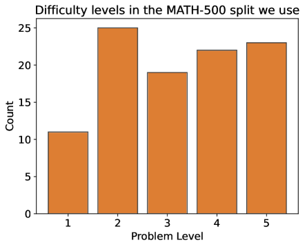floatrow figurerow b figure b <details> <summary>x14.png Details</summary>  ### Visual Description \n ## Bar Chart: Difficulty Levels in the MATH-500 Split ### Overview This is a vertical bar chart illustrating the distribution of problem difficulty levels within a specific dataset referred to as the "MATH-500 split." The chart displays the count of problems for each of five discrete difficulty levels. ### Components/Axes * **Chart Title:** "Difficulty levels in the MATH-500 split we use" (positioned at the top center). * **X-Axis (Horizontal):** * **Label:** "Problem Level" * **Categories/Ticks:** 1, 2, 3, 4, 5 (representing discrete difficulty levels). * **Y-Axis (Vertical):** * **Label:** "Count" * **Scale:** Linear scale from 0 to 25, with major tick marks at intervals of 5 (0, 5, 10, 15, 20, 25). * **Data Series:** A single series represented by five vertical bars. All bars are the same burnt orange/ochre color. There is no separate legend, as the x-axis labels define the categories. ### Detailed Analysis The height of each bar corresponds to the count of problems at that difficulty level. The values are approximate, derived from visual alignment with the y-axis grid. * **Problem Level 1:** The bar height is slightly above the 10 mark. **Approximate Count: 11.** * **Problem Level 2:** This is the tallest bar, reaching the top grid line. **Approximate Count: 25.** * **Problem Level 3:** The bar height is just below the 20 mark. **Approximate Count: 19.** * **Problem Level 4:** The bar height is slightly above the 20 mark. **Approximate Count: 22.** * **Problem Level 5:** The bar height is slightly taller than the Level 4 bar. **Approximate Count: 23.** **Trend Verification:** The visual trend is non-monotonic. The count increases sharply from Level 1 to Level 2 (the peak), then decreases at Level 3, before increasing again for Levels 4 and 5, which are close in value. ### Key Observations 1. **Non-Uniform Distribution:** The dataset does not have an equal number of problems across difficulty levels. 2. **Peak at Level 2:** The highest concentration of problems (approx. 25) is at difficulty Level 2. 3. **Skew Towards Higher Difficulty:** The combined count for the higher difficulty levels (3, 4, and 5) is significantly larger than the combined count for the lower levels (1 and 2). Levels 4 and 5 have very similar, high counts. 4. **Lowest Count at Level 1:** The easiest difficulty level has the fewest problems (approx. 11). ### Interpretation This chart characterizes the composition of the "MATH-500 split" dataset. The data suggests this particular split is **not balanced by difficulty**. It is weighted towards medium (Level 2) and high (Levels 3-5) difficulty problems, with Level 2 being the most common single category. This distribution has implications for any model or analysis using this dataset: * **Performance Evaluation:** A model's overall accuracy on this split will be heavily influenced by its performance on Levels 2, 4, and 5, which constitute the majority of the data. * **Bias in Assessment:** The split may not be ideal for assessing a model's capability across a uniform spectrum of difficulty, as it under-represents the easiest problems (Level 1). * **Potential Purpose:** The skew might be intentional, perhaps designed to challenge models or to focus evaluation on non-trivial problem-solving. The title "we use" implies this is a specific, curated subset for a particular research or testing purpose, not a random or fully representative sample of all MATH problems. </details> Figure 28: Histogram of difficulty levels in our 100-problem subset from MATH-500. 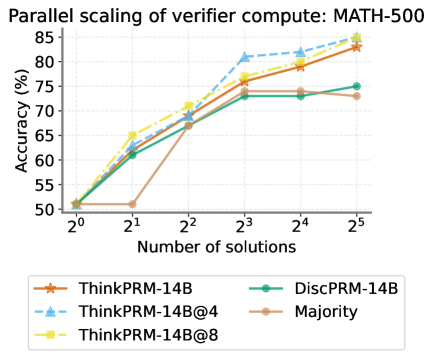figure b <details> <summary>x15.png Details</summary>  ### Visual Description ## Line Chart: Parallel scaling of verifier compute: MATH-500 ### Overview This image is a line chart titled "Parallel scaling of verifier compute: MATH-500". It plots the accuracy percentage of five different models or methods against an increasing number of solutions, presented on a logarithmic scale (base 2). The chart demonstrates how the performance of these verifiers scales as more parallel solutions are considered. ### Components/Axes * **Title:** "Parallel scaling of verifier compute: MATH-500" (Top center). * **Y-Axis:** Labeled "Accuracy (%)". The scale runs from 50 to 85, with major tick marks every 5 units (50, 55, 60, 65, 70, 75, 80, 85). * **X-Axis:** Labeled "Number of solutions". The scale is logarithmic with base 2, showing tick marks at 2⁰ (1), 2¹ (2), 2² (4), 2³ (8), 2⁴ (16), and 2⁵ (32). * **Legend:** Positioned at the bottom of the chart, centered. It contains five entries, each with a colored line, marker symbol, and label: 1. **ThinkPRM-14B:** Orange line with star (★) markers. 2. **DiscPRM-14B:** Teal/green line with circle (●) markers. 3. **ThinkPRM-14B@4:** Light blue dashed line with triangle (▲) markers. 4. **ThinkPRM-14B@8:** Yellow line with square (■) markers. 5. **Majority:** Brown/tan line with circle (●) markers. ### Detailed Analysis The chart tracks five data series. All series begin at the same point (1 solution, 50% accuracy). Below is the approximate data extracted for each series, with trends noted. **1. ThinkPRM-14B (Orange, ★)** * **Trend:** Consistent, strong upward slope. * **Data Points (Approx.):** * 2⁰ (1): 50% * 2¹ (2): ~61% * 2² (4): ~68% * 2³ (8): ~75% * 2⁴ (16): ~79% * 2⁵ (32): ~83% **2. DiscPRM-14B (Teal, ●)** * **Trend:** Increases initially, then plateaus after 8 solutions. * **Data Points (Approx.):** * 2⁰ (1): 50% * 2¹ (2): ~61% * 2² (4): ~67% * 2³ (8): ~73% * 2⁴ (16): ~73% (plateau) * 2⁵ (32): ~75% **3. ThinkPRM-14B@4 (Light Blue, ▲, Dashed Line)** * **Trend:** Very steep upward slope, one of the top performers. * **Data Points (Approx.):** * 2⁰ (1): 50% * 2¹ (2): ~65% * 2² (4): ~71% * 2³ (8): ~81% * 2⁴ (16): ~82% * 2⁵ (32): ~84% **4. ThinkPRM-14B@8 (Yellow, ■)** * **Trend:** Strong upward slope, ends as the highest-performing series. * **Data Points (Approx.):** * 2⁰ (1): 50% * 2¹ (2): ~65% * 2² (4): ~71% * 2³ (8): ~77% * 2⁴ (16): ~80% * 2⁵ (32): ~85% **5. Majority (Brown, ●)** * **Trend:** Increases to a point, then flatlines completely. * **Data Points (Approx.):** * 2⁰ (1): 50% * 2¹ (2): 50% (no initial gain) * 2² (4): ~67% * 2³ (8): ~73% * 2⁴ (16): ~73% (plateau) * 2⁵ (32): ~73% (plateau) ### Key Observations 1. **Universal Starting Point:** All methods start at 50% accuracy with a single solution, which is the baseline. 2. **Clear Performance Tiers:** At the maximum measured point (32 solutions), a clear hierarchy emerges: * **Top Tier:** ThinkPRM-14B@8 (~85%) and ThinkPRM-14B@4 (~84%). * **Middle Tier:** ThinkPRM-14B (~83%). * **Lower Tier:** DiscPRM-14B (~75%) and Majority (~73%). 3. **Scaling Behavior:** The "ThinkPRM" family of models (all variants) shows continuous improvement across the entire range of solutions. In contrast, both "DiscPRM-14B" and "Majority" show diminishing returns, plateauing after 8 solutions (2³). 4. **Initial Jump:** The "@4" and "@8" variants of ThinkPRM show a larger initial performance jump from 1 to 2 solutions compared to the base ThinkPRM-14B. 5. **Majority Baseline:** The "Majority" method, likely a simple voting baseline, fails to gain any benefit from 1 to 2 solutions and is ultimately outperformed by all neural verifier models. ### Interpretation This chart provides a performance benchmark for different AI verification strategies on the MATH-500 dataset, specifically measuring how accuracy improves when the system is allowed to generate and evaluate multiple solution candidates in parallel. The data suggests that the **ThinkPRM architecture scales more effectively with increased parallel compute** than the DiscPRM architecture or a simple majority vote. The continuous upward trend of the ThinkPRM lines indicates that its method for verifying or ranking solutions continues to extract useful signal even from a large pool of 32 candidates. The plateau of the **Majority and DiscPRM methods** implies a fundamental limit to their approach. For Majority, this is intuitive—beyond a certain point, adding more random guesses doesn't improve the consensus. For DiscPRM, it may indicate that its discrimination capability saturates, and it cannot effectively differentiate between correct and incorrect solutions in a larger, noisier set. The superior performance of **ThinkPRM-14B@8 and @4** over the base ThinkPRM-14B suggests that techniques like increased sampling (@8 likely means 8 samples per problem) or other ensemble methods provide a significant boost, making them the most compute-efficient strategies for achieving high accuracy in this parallel scaling regime. The chart makes a strong case for investing in verifier models that are designed to leverage parallelism, as the accuracy gains are substantial and sustained. </details> Figure 31: Scaling of verifier compute by parallel sampling of multiple verification CoTs and averaging their scores. Parallel scaling (ThinkPRM -14B@4 and ThinkPRM -14B@8) further boosts performance curve compared to scoring based on a single CoT (ThinkPRM -14B). ### E.6 Additional results on scaling verifier compute Fig. 31 shows results of ThinkPRM -14B of parallel scaling verifier compute by sampling $K=4$ and $K=8$ CoTs with temperature $T=0.6$ and aggregating their scores. Parallel scaling indeed lifts up the accuracy curve of ThinkPRM -14B compared to standard $K=1$ with greedy decoding. However, performance plateaus rather quickly and $K=8$ remains comparable to $K=4$ , while slightly better at smaller sampling budgets. Fig. 32 compares parallel to sequential scaling under the same token budget. While there is no clear winner, parallel scaling seems to perform slightly better at best-of-8. 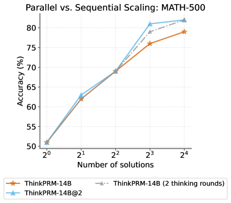floatrow figurerow b <details> <summary>x16.png Details</summary>  ### Visual Description ## Line Chart: Parallel vs. Sequential Scaling: MATH-500 ### Overview This is a line chart comparing the performance (accuracy) of three different model scaling approaches on the MATH-500 benchmark as the number of solutions increases. The chart demonstrates how accuracy scales with increased computational effort (number of solutions) for different methods. ### Components/Axes * **Chart Title:** "Parallel vs. Sequential Scaling: MATH-500" (centered at the top). * **Y-Axis:** Labeled "Accuracy (%)". The scale runs from 50 to 80, with major tick marks at intervals of 5 (50, 55, 60, 65, 70, 75, 80). * **X-Axis:** Labeled "Number of solutions". The scale is logarithmic base 2, with markers at 2⁰ (1), 2¹ (2), 2² (4), 2³ (8), and 2⁴ (16). * **Legend:** Positioned at the bottom center of the chart. It contains three entries: 1. **ThinkPRM-14B:** Represented by an orange solid line with star (★) markers. 2. **ThinkPRM-14B@2:** Represented by a light blue solid line with upward-pointing triangle (▲) markers. 3. **ThinkPRM-14B (2 thinking rounds):** Represented by a gray dashed line with upward-pointing triangle (▲) markers. ### Detailed Analysis The chart plots three data series. All series show a positive correlation between the number of solutions and accuracy. **1. ThinkPRM-14B (Orange Line, Star Markers):** * **Trend:** Shows a steady, near-linear upward slope on this semi-log plot. * **Data Points (Approximate):** * At 2⁰ (1 solution): ~51% * At 2¹ (2 solutions): ~62% * At 2² (4 solutions): ~69% * At 2³ (8 solutions): ~76% * At 2⁴ (16 solutions): ~79% **2. ThinkPRM-14B@2 (Blue Line, Triangle Markers):** * **Trend:** Follows a similar initial trajectory to the orange line but exhibits a steeper increase between 2² and 2³, ultimately achieving the highest accuracy. * **Data Points (Approximate):** * At 2⁰ (1 solution): ~51% (overlaps with orange line) * At 2¹ (2 solutions): ~63% (slightly above orange line) * At 2² (4 solutions): ~69% (overlaps with orange line) * At 2³ (8 solutions): ~81% * At 2⁴ (16 solutions): ~82% **3. ThinkPRM-14B (2 thinking rounds) (Gray Dashed Line, Triangle Markers):** * **Trend:** This series is only plotted from 2² onward. It starts at the same point as the other two at 2² and follows a path between the orange and blue lines, ending very close to the blue line. * **Data Points (Approximate):** * At 2² (4 solutions): ~69% (overlaps with others) * At 2³ (8 solutions): ~78% (between orange and blue) * At 2⁴ (16 solutions): ~81% (very close to blue line) ### Key Observations 1. **Convergence at Low Compute:** All three methods start at nearly identical accuracy (~51%) with a single solution (2⁰). 2. **Divergence at High Compute:** Performance begins to diverge significantly at 8 solutions (2³). The "ThinkPRM-14B@2" (blue) method shows a clear advantage, jumping to ~81%, while the base "ThinkPRM-14B" (orange) is at ~76%. 3. **Diminishing Returns:** The slope of all lines begins to flatten between 8 (2³) and 16 (2⁴) solutions, indicating diminishing returns in accuracy for additional solutions in this range. 4. **Effect of "Thinking Rounds":** The gray dashed line suggests that adding "2 thinking rounds" to the base model improves its scaling performance, bringing it close to the "ThinkPRM-14B@2" method at 16 solutions. ### Interpretation The data demonstrates the principle of **scaling laws** for reasoning models on mathematical problems. Increasing the number of solutions (a form of parallel compute or sampling) reliably improves accuracy. The key finding is the comparison between scaling methods. "ThinkPRM-14B@2" (likely a form of parallel scaling or ensemble) outperforms the standard "ThinkPRM-14B" (likely sequential scaling) at higher compute budgets (8+ solutions). This suggests that parallel strategies may be more efficient for leveraging additional compute to solve difficult problems. The "2 thinking rounds" variant acts as an intermediate, showing that enhancing the sequential reasoning process (more "thinking") can also close the gap with parallel methods, but the parallel approach still holds a slight edge at the highest measured compute point (16 solutions). The flattening curves at 16 solutions imply that for this specific benchmark and model size, simply adding more solutions yields progressively smaller gains, and further improvements may require architectural changes or significantly more compute. 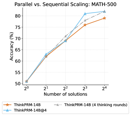</details> <details> <summary>x17.png Details</summary>  ### Visual Description \n ## Line Chart: Parallel vs. Sequential Scaling: MATH-500 ### Overview The image is a line chart comparing the performance (accuracy) of three different model scaling strategies on the MATH-500 benchmark as the number of solutions increases. The chart demonstrates how accuracy scales with increased computational effort, measured in the number of solutions generated. ### Components/Axes * **Title:** "Parallel vs. Sequential Scaling: MATH-500" (Top-center). * **Y-Axis:** Labeled "Accuracy (%)". The scale runs from 50 to 80, with major tick marks at 50, 55, 60, 65, 70, 75, and 80. * **X-Axis:** Labeled "Number of solutions". The scale is logarithmic (base 2), with markers at `2^0` (1), `2^1` (2), `2^2` (4), `2^3` (8), and `2^4` (16). * **Legend:** Positioned at the bottom of the chart, outside the plot area. It contains three entries: 1. **ThinkPRM-14B:** Represented by a solid orange line with star markers. 2. **ThinkPRM-14B@4:** Represented by a solid blue line with upward-pointing triangle markers. 3. **ThinkPRM-14B (4 thinking rounds):** Represented by a gray dashed line with upward-pointing triangle markers. ### Detailed Analysis The chart plots three data series, each showing an upward trend in accuracy as the number of solutions increases. **1. ThinkPRM-14B (Orange line, star markers):** * **Trend:** Shows a steady, slightly concave upward slope. * **Data Points (Approximate):** * At 1 solution (`2^0`): ~51% * At 2 solutions (`2^1`): ~62% * At 4 solutions (`2^2`): ~69% * At 8 solutions (`2^3`): ~76% * At 16 solutions (`2^4`): ~79% **2. ThinkPRM-14B@4 (Blue line, triangle markers):** * **Trend:** Shows a strong upward slope that peaks at 8 solutions before a slight decline. It is the top-performing series for most data points. * **Data Points (Approximate):** * At 1 solution (`2^0`): ~51% (similar to orange line) * At 2 solutions (`2^1`): ~63% * At 4 solutions (`2^2`): ~69% (similar to orange line) * At 8 solutions (`2^3`): ~81% (Peak) * At 16 solutions (`2^4`): ~80% (Slight decrease from peak) **3. ThinkPRM-14B (4 thinking rounds) (Gray dashed line, triangle markers):** * **Trend:** Shows a consistent, nearly linear upward slope. It generally performs between the other two models. * **Data Points (Approximate):** * At 1 solution (`2^0`): ~51% * At 2 solutions (`2^1`): ~63% * At 4 solutions (`2^2`): ~71% * At 8 solutions (`2^3`): ~78% * At 16 solutions (`2^4`): ~82% ### Key Observations 1. **Convergence at Low Compute:** All three models start at nearly identical accuracy (~51%) when using only a single solution (`2^0`). 2. **Divergence with Scaling:** As the number of solutions increases, the performance of the three strategies diverges. The "ThinkPRM-14B@4" (blue) model shows the most significant initial gains. 3. **Peak and Plateau:** The "ThinkPRM-14B@4" model achieves the highest observed accuracy (~81%) at 8 solutions (`2^3`) but shows a slight performance drop when scaled to 16 solutions, suggesting a potential plateau or diminishing returns. 4. **Consistent Linear Scaling:** The "ThinkPRM-14B (4 thinking rounds)" (gray dashed) model demonstrates the most consistent and linear improvement, ultimately matching or slightly surpassing the blue line's peak at 16 solutions. 5. **Baseline Performance:** The standard "ThinkPRM-14B" (orange) model scales effectively but consistently lags behind the other two enhanced strategies at higher solution counts. ### Interpretation This chart illustrates the trade-offs between different methods of scaling a reasoning model's compute (here, measured by the number of solutions generated). The data suggests: * **Strategy Matters:** Simply generating more solutions (parallel scaling, likely represented by the orange line) improves performance, but more sophisticated strategies yield better returns. * **The "@4" Advantage:** The "ThinkPRM-14B@4" strategy (blue line) appears highly efficient at lower to medium compute levels (2-8 solutions), providing the best "bang for the buck." Its slight dip at 16 solutions could indicate that its specific method of parallelization or aggregation encounters interference or inefficiencies at very high scales. * **Sequential Depth Wins at Scale:** The "4 thinking rounds" strategy (gray dashed line), which implies a sequential, iterative reasoning process, shows robust and continuous scaling. While it may be slightly less efficient than the "@4" method at 8 solutions, it ultimately achieves the highest final accuracy at 16 solutions, suggesting that deeper sequential computation may have a higher performance ceiling. * **Practical Implication:** The choice between these strategies depends on the available computational budget. For budgets allowing 8 solutions, "@4" is optimal. For larger budgets (16+ solutions), investing in sequential "thinking rounds" may be more effective. The standard model serves as a baseline, proving that any scaling is beneficial, but optimized methods are superior. </details> Figure 32: Parallel vs. sequential scaling of ThinkPRM compute under the same generation budget with Qwen-2.5-14B generator. Parallel scaling (model@K) is done by independently sampling $K$ verification CoTs and aggregating their scores. Sequential scaling is done by prompting the model $K$ times to revise its own verification for $K$ thinking rounds. Both setups generate up until 8192 tokens per generation. We do not observe a clear winner although parallel scaling seems slightly better especially at larger sampling budgets. ### E.7 Scaling training data of ThinkPRM Here, we show results when training ThinkPRM -14B and ThinkPRM -1.5B using synthetic data from all PRM800K. The goal is to show that ThinkPRM can still benefit from training on more synthetic data. Here, we train both R1-Distill-Qwen-1.5B and R1-Distill-Qwen-14B on a total of 65K verification CoTs we obtained by sampling and filtering as explained in Section 3.2. Figs. 38 and 38 show best-of-N performance with ThinkPRM -1.5B and ThinkPRM -14B respectively when trained on 65K and compares it to training on 1K examples. Interestingly, ThinkPRM benefits from additional training, and can further improve the accuracy curve compared to the 1K-trained version on MATH-500. We note, however, that while training on more math data boosts performance on MATH-500, we observe some performance drop on out-of-domain tasks due to the distribution shift. 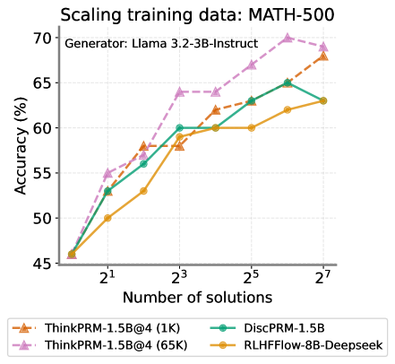floatrow figurerow b figure b <details> <summary>x18.png Details</summary>  ### Visual Description ## Line Chart: Scaling training data: MATH-500 ### Overview This is a line chart illustrating the relationship between the amount of training data (measured in "Number of solutions") and model performance (measured in "Accuracy (%)") on the MATH-500 benchmark. The chart compares four different model training methods or configurations. The overall trend for all methods is that accuracy increases as the number of training solutions increases, following a logarithmic scale on the x-axis. ### Components/Axes * **Chart Title:** "Scaling training data: MATH-500" * **Subtitle/Generator:** "Generator: Llama 3.2-3B-Instruct" * **Y-Axis:** * **Label:** "Accuracy (%)" * **Scale:** Linear, ranging from 45 to 70, with major tick marks at 5-unit intervals (45, 50, 55, 60, 65, 70). * **X-Axis:** * **Label:** "Number of solutions" * **Scale:** Logarithmic (base 2), with labeled tick marks at 2¹ (2), 2³ (8), 2⁵ (32), and 2⁷ (128). The axis starts at approximately 2⁰ (1). * **Legend:** Located at the bottom of the chart, outside the plot area. It contains four entries, each with a unique color, line style, and marker shape. 1. **ThinkPRM-1.5B@4 (1K):** Orange dashed line with upward-pointing triangle markers. 2. **ThinkPRM-1.5B@4 (65K):** Pink (light purple) dashed line with upward-pointing triangle markers. 3. **DiscPRM-1.5B:** Green solid line with circle markers. 4. **RLHFFlow-8B-Deepseek:** Yellow solid line with circle markers. * **Grid:** A light gray grid is present in the background of the plot area. ### Detailed Analysis The chart plots four data series. Below is a breakdown of each series, its visual trend, and approximate data points extracted by aligning markers with the grid. **1. ThinkPRM-1.5B@4 (65K) - Pink Dashed Line, Triangle Markers** * **Trend:** Shows the steepest and highest overall growth. It starts as the second-highest performer at the lowest data point and becomes the clear top performer from 2³ solutions onward, maintaining a significant lead. * **Data Points (Approximate):** * At ~2⁰ (1) solutions: ~46% * At 2¹ (2) solutions: ~55% * At 2² (4) solutions: ~58% * At 2³ (8) solutions: ~64% * At 2⁴ (16) solutions: ~64.5% * At 2⁵ (32) solutions: ~67% * At 2⁶ (64) solutions: ~70% (Peak) * At 2⁷ (128) solutions: ~69% **2. ThinkPRM-1.5B@4 (1K) - Orange Dashed Line, Triangle Markers** * **Trend:** Shows strong, steady growth. It starts as the lowest performer but catches up to and eventually surpasses the DiscPRM-1.5B model at higher data volumes. * **Data Points (Approximate):** * At ~2⁰ (1) solutions: ~46% * At 2¹ (2) solutions: ~53% * At 2² (4) solutions: ~58% * At 2³ (8) solutions: ~58% * At 2⁴ (16) solutions: ~62% * At 2⁵ (32) solutions: ~63% * At 2⁶ (64) solutions: ~65% * At 2⁷ (128) solutions: ~68% **3. DiscPRM-1.5B - Green Solid Line, Circle Markers** * **Trend:** Shows consistent growth but at a slightly lower rate than the ThinkPRM variants at higher data scales. It starts as the second-lowest performer and is overtaken by ThinkPRM-1.5B@4 (1K) after 2⁵ solutions. * **Data Points (Approximate):** * At ~2⁰ (1) solutions: ~46% * At 2¹ (2) solutions: ~53% * At 2² (4) solutions: ~56% * At 2³ (8) solutions: ~60% * At 2⁴ (16) solutions: ~60% * At 2⁵ (32) solutions: ~63% * At 2⁶ (64) solutions: ~65% * At 2⁷ (128) solutions: ~63% (Note: This point appears to dip slightly from the previous point.) **4. RLHFFlow-8B-Deepseek - Yellow Solid Line, Circle Markers** * **Trend:** Shows the slowest rate of improvement. It starts as the lowest performer and remains the lowest-performing method across the entire range of training data, though its accuracy does increase. * **Data Points (Approximate):** * At ~2⁰ (1) solutions: ~46% * At 2¹ (2) solutions: ~50% * At 2² (4) solutions: ~53% * At 2³ (8) solutions: ~58% * At 2⁴ (16) solutions: ~60% * At 2⁵ (32) solutions: ~60% * At 2⁶ (64) solutions: ~62% * At 2⁷ (128) solutions: ~63% ### Key Observations 1. **Universal Scaling Law:** All four methods demonstrate that increasing the volume of training data (solutions) leads to improved accuracy on the MATH-500 benchmark, confirming a positive scaling relationship. 2. **Performance Hierarchy:** A clear performance hierarchy is established and maintained as data scales: `ThinkPRM-1.5B@4 (65K)` > `ThinkPRM-1.5B@4 (1K)` ≈ `DiscPRM-1.5B` > `RLHFFlow-8B-Deepseek`. The gap between the top and bottom methods widens significantly with more data. 3. **Diminishing Returns:** The curves for all methods begin to flatten between 2⁵ (32) and 2⁷ (128) solutions, suggesting diminishing returns from adding more data beyond a certain point. The `ThinkPRM-1.5B@4 (65K)` model even shows a slight decrease at the final data point. 4. **Crossover Point:** The `ThinkPRM-1.5B@4 (1K)` (orange) line crosses above the `DiscPRM-1.5B` (green) line between 2⁵ (32) and 2⁶ (64) solutions, indicating it becomes more data-efficient at larger scales. 5. **Initial Convergence:** All models start at nearly the same accuracy (~46%) when trained on the smallest dataset (~1 solution), but their performance diverges rapidly as data increases. ### Interpretation This chart provides a comparative analysis of different training methodologies (likely involving different reward models or training objectives like "ThinkPRM," "DiscPRM," and "RLHFFlow") when applied to a base generator model (Llama 3.2-3B-Instruct) for mathematical reasoning. The data suggests that the **`ThinkPRM-1.5B@4` method, especially when scaled to 65K solutions, is the most effective and data-efficient approach** among those tested for improving mathematical accuracy. Its superior performance implies that its underlying training strategy (possibly involving more sophisticated process supervision or thinking-step reward modeling) extracts more learning signal per data point. The fact that the much larger `RLHFFlow-8B-Deepseek` model (8B parameters vs. 1.5B for the others) performs the worst is a critical finding. It indicates that **model size alone is not the primary driver of performance on this task**; the training methodology and data quality/quantity are more decisive factors. This challenges the simple "bigger is better" paradigm and highlights the importance of algorithmic innovation in training. The flattening of the curves suggests that for this specific task and generator, simply adding more solution data of the same type may yield limited future gains. Further improvements might require higher-quality data, more advanced training techniques, or changes to the base generator model itself. The slight dip for the top model at 128 solutions could be noise or an early sign of overfitting to the training data distribution. </details> Figure 35: Best-of-N results with ThinkPRM -1.5B comparing the version trained on 1K examples (used throughout the paper) and a version trained on 65K examples. ThinkPRM benefits from training on more synthetic data as the performance can further improve with more training. 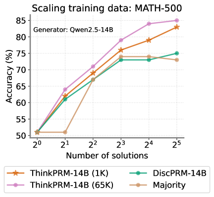figure b <details> <summary>x19.png Details</summary>  ### Visual Description ## Line Chart: Scaling training data: MATH-500 ### Overview This is a line chart titled "Scaling training data: MATH-500" with a subtitle "Generator: Qwen2.5-14B". It plots the accuracy percentage of four different models or methods against an increasing number of solutions, presented on a logarithmic scale (base 2). The chart demonstrates how performance scales with more solution examples provided during training or evaluation. ### Components/Axes * **Title:** "Scaling training data: MATH-500" (Top-left, above chart area). * **Subtitle:** "Generator: Qwen2.5-14B" (Top-left, below title). * **Y-Axis:** Labeled "Accuracy (%)". Scale runs from 50 to 85, with major tick marks every 5 units (50, 55, 60, 65, 70, 75, 80, 85). * **X-Axis:** Labeled "Number of solutions". Scale is logarithmic base 2, with markers at 2⁰ (1), 2¹ (2), 2² (4), 2³ (8), 2⁴ (16), and 2⁵ (32). * **Legend:** Positioned at the bottom, centered below the x-axis. It contains four entries: 1. **ThinkPRM-14B (1K):** Orange line with star (★) markers. 2. **ThinkPRM-14B (65K):** Pink line with circle (●) markers. 3. **DiscPRM-14B:** Teal line with circle (●) markers. 4. **Majority:** Beige/light brown line with circle (●) markers. ### Detailed Analysis The chart tracks four data series. Below is an analysis of each, including approximate data points extracted from the chart. **1. ThinkPRM-14B (65K) - Pink line, circle markers:** * **Trend:** Shows a strong, consistent upward trend across the entire range. It is the top-performing series for all data points beyond the first. * **Data Points (Approximate):** * 2⁰ (1 solution): ~51% * 2¹ (2 solutions): ~64% * 2² (4 solutions): ~71% * 2³ (8 solutions): ~79% * 2⁴ (16 solutions): ~84% * 2⁵ (32 solutions): ~85% **2. ThinkPRM-14B (1K) - Orange line, star markers:** * **Trend:** Also shows a strong, consistent upward trend, closely following but slightly below the 65K variant. * **Data Points (Approximate):** * 2⁰ (1 solution): ~51% * 2¹ (2 solutions): ~62% * 2² (4 solutions): ~69% * 2³ (8 solutions): ~76% * 2⁴ (16 solutions): ~79% * 2⁵ (32 solutions): ~83% **3. DiscPRM-14B - Teal line, circle markers:** * **Trend:** Increases initially but then plateaus. It shows significant growth from 2⁰ to 2³, after which the accuracy gain becomes minimal. * **Data Points (Approximate):** * 2⁰ (1 solution): ~51% * 2¹ (2 solutions): ~61% * 2² (4 solutions): ~67% * 2³ (8 solutions): ~73% * 2⁴ (16 solutions): ~73% * 2⁵ (32 solutions): ~75% **4. Majority - Beige line, circle markers:** * **Trend:** Exhibits an unusual pattern. It starts at the same point as others, dips at 2¹, then rises sharply to a peak at 2³ before slightly declining. * **Data Points (Approximate):** * 2⁰ (1 solution): ~51% * 2¹ (2 solutions): ~51% (Note: This is a notable dip or flatline compared to others) * 2² (4 solutions): ~67% * 2³ (8 solutions): ~74% * 2⁴ (16 solutions): ~74% * 2⁵ (32 solutions): ~73% ### Key Observations 1. **Common Starting Point:** All four methods begin at approximately the same accuracy (~51%) when given only one solution (2⁰). 2. **Performance Hierarchy:** For all data points beyond the first, the order of performance from highest to lowest is consistent: ThinkPRM-14B (65K) > ThinkPRM-14B (1K) > DiscPRM-14B ≈ Majority (after 2³). 3. **Scaling Behavior:** The two ThinkPRM variants show continued, strong scaling with more solutions. In contrast, DiscPRM and Majority show diminishing returns, with their curves flattening after 8 solutions (2³). 4. **Outlier Point:** The "Majority" method's performance at 2¹ (2 solutions) is an outlier. While all other methods show a clear improvement from 1 to 2 solutions, Majority's accuracy remains stagnant at ~51%. 5. **Plateau Levels:** DiscPRM and Majority plateau at a significantly lower accuracy (~73-75%) compared to the continued ascent of the ThinkPRM models (reaching 83-85%). ### Interpretation This chart investigates the relationship between the quantity of training/evaluation data (number of solution examples) and model accuracy on the MATH-500 benchmark, using Qwen2.5-14B as the base generator. * **Data Scaling is Crucial:** The primary takeaway is that providing more solution examples ("scaling training data") generally leads to higher accuracy. This effect is most pronounced and sustained for the ThinkPRM methods. * **Model Architecture/Training Matters:** The significant performance gap between ThinkPRM (both variants) and DiscPRM/Majority after the initial data points suggests that the ThinkPRM approach is more effective at leveraging additional data. The "(65K)" vs. "(1K)" labels likely refer to the size of an internal dataset used during the model's training or refinement phase, with the larger dataset (65K) yielding a consistent, though not dramatic, advantage over the smaller one (1K). * **Limits of Simple Methods:** The "Majority" baseline (likely a simple voting or averaging scheme) and "DiscPRM" appear to hit a performance ceiling. Their inability to scale effectively beyond 8 solutions indicates they may lack the capacity to integrate more complex patterns from larger datasets, or they may be fundamentally limited by their design. * **The Anomaly at 2 Solutions:** The flat performance of "Majority" at 2 solutions is curious. It could suggest that with only two examples, a majority vote is no more informative than a single example, or it might point to a specific weakness or instability in that method at very low data regimes. In summary, the data demonstrates that for the MATH-500 task, advanced methods like ThinkPRM benefit substantially from scaling data, while simpler baselines saturate quickly. The choice of method is therefore critical for realizing the gains from larger datasets. </details> Figure 38: Best-of-N results with ThinkPRM -14B comparing the version trained on 1K examples (used throughout the paper) and a version trained on 65K examples. ThinkPRM benefits from training on more synthetic data as the performance can further improve with more training. ### E.8 Results with automatic labels Table 4 shows performance when filtering training data based on manual labels (PRM800K) vs automatic labels (Math-Shepherd) (Wang et al., 2023b). ThinkPRM still performs well even with automatic labels, and comparably to manual labels. | ThinkPRM-1.5B (PRM800K) ThinkPRM-1.5B (Math-shepherd) | 76.3 75.8 | 75.7 76.5 | | --- | --- | --- | Table 4: Comparison of ThinkPRM-1.5B trained on PRM800K vs Math-shepherd step labels. 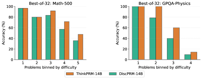### E.9 Verifier performance in terms of problem difficulty <details> <summary>x20.png Details</summary>  ### Visual Description \n ## Grouped Bar Charts: Model Accuracy by Problem Difficulty ### Overview The image displays two side-by-side grouped bar charts comparing the performance of two AI models, "ThinkPRM-14B" and "DiscPRM-14B," on two different problem sets. The charts show the percentage accuracy of each model as problem difficulty increases. The overall trend indicates that accuracy decreases for both models as problems become more difficult, with ThinkPRM-14B consistently outperforming DiscPRM-14B, especially on harder problems. ### Components/Axes * **Chart Titles:** * Left Chart: "Best-of-32: Math-500" * Right Chart: "Best-of-32: GPQA-Physics" * **Y-Axis (Both Charts):** Labeled "Accuracy (%)". The scale runs from 0 to 100 in increments of 20. * **X-Axis (Both Charts):** Labeled "Problems binned by difficulty". The bins are numbered sequentially. * Left Chart (Math-500): Bins 1, 2, 3, 4, 5. * Right Chart (GPQA-Physics): Bins 1, 2, 3, 4. * **Legend:** Located at the bottom center of the image, spanning both charts. * Orange square: "ThinkPRM-14B" * Teal square: "DiscPRM-14B" * **Data Series:** Each difficulty bin contains two bars, one for each model, placed side-by-side. The left bar in each pair is teal (DiscPRM-14B), and the right bar is orange (ThinkPRM-14B). ### Detailed Analysis **Left Chart: Best-of-32: Math-500** * **Trend Verification:** Both models show a clear downward trend in accuracy as difficulty increases from bin 1 to bin 5. ThinkPRM-14B's decline is less steep. * **Data Points (Approximate):** * **Bin 1:** DiscPRM-14B ≈ 98%, ThinkPRM-14B ≈ 98%. (Nearly identical, very high accuracy). * **Bin 2:** DiscPRM-14B ≈ 80%, ThinkPRM-14B ≈ 80%. (Identical, significant drop from bin 1). * **Bin 3:** DiscPRM-14B ≈ 84%, ThinkPRM-14B ≈ 92%. (ThinkPRM shows a notable advantage). * **Bin 4:** DiscPRM-14B ≈ 58%, ThinkPRM-14B ≈ 72%. (ThinkPRM maintains a ~14 percentage point lead). * **Bin 5:** DiscPRM-14B ≈ 36%, ThinkPRM-14B ≈ 48%. (Both models struggle, ThinkPRM retains a ~12 point lead). **Right Chart: Best-of-32: GPQA-Physics** * **Trend Verification:** A very steep downward trend for both models. The performance gap between the models widens significantly in the middle bins before converging at the highest difficulty. * **Data Points (Approximate):** * **Bin 1:** DiscPRM-14B ≈ 100%, ThinkPRM-14B ≈ 100%. (Perfect or near-perfect accuracy). * **Bin 2:** DiscPRM-14B ≈ 79%, ThinkPRM-14B ≈ 100%. (ThinkPRM maintains perfect accuracy, while DiscPRM drops significantly). * **Bin 3:** DiscPRM-14B ≈ 40%, ThinkPRM-14B ≈ 60%. (Both drop sharply, ThinkPRM leads by ~20 points). * **Bin 4:** DiscPRM-14B ≈ 10%, ThinkPRM-14B ≈ 15%. (Both models perform very poorly, with a minimal difference). ### Key Observations 1. **Consistent Superiority:** ThinkPRM-14B (orange bars) achieves equal or higher accuracy than DiscPRM-14B (teal bars) in every single difficulty bin across both subjects. 2. **Difficulty Impact:** The "GPQA-Physics" problems appear to be more challenging overall, especially at higher difficulties. While both models start at 100% in bin 1, their accuracy plummets to 10-15% by bin 4. In contrast, the "Math-500" decline is more gradual, with both models still scoring between 36-48% at bin 5. 3. **Performance Gap:** The advantage of ThinkPRM-14B is most pronounced in the middle difficulty ranges (Bin 3 for Math, Bins 2 & 3 for Physics). This suggests its reasoning capabilities are particularly beneficial for moderately complex problems. 4. **Convergence at Extremes:** At the easiest problems (Bin 1 for both, Bin 2 for Physics/ThinkPRM) and the hardest problems (Bin 5 for Math, Bin 4 for Physics), the performance gap between the two models narrows or disappears. ### Interpretation The data demonstrates a clear hierarchy in problem-solving capability between the two models under a "Best-of-32" sampling strategy. ThinkPRM-14B exhibits more robust reasoning, as evidenced by its slower decay in accuracy with increasing problem difficulty. This is especially evident in the physics domain, where it maintains perfect accuracy one bin longer than DiscPRM-14B. The stark difference in the slope of decline between Math-500 and GPQA-Physics suggests the nature of the challenges differs. The physics problems likely involve more complex, multi-step reasoning or specialized knowledge that causes a catastrophic drop in performance for both models once a certain complexity threshold is crossed. The math problems, while difficult, allow for a more linear degradation of performance. From a Peircean perspective, the charts are an indexical sign of the models' underlying reasoning architecture. The consistent performance gap points to a fundamental difference in how ThinkPRM and DiscPRM process and solve problems, with ThinkPRM's approach being more resilient to complexity. The charts do not reveal *why* this is the case, but they provide strong evidence *that* it is the case, prompting investigation into the architectural or training differences between the "Think" and "Disc" paradigms. </details> Figure 39: ThinkPRM helps with challenging reasoning problems compared to DiscPRM. The generator model here is Qwen-2.5-14B for MATH-500 and Qwen-2.5-32B-Instruct for GPQA. We the difficulty We do not estimate the difficulty over MATH problem since each problem in MATH is annotated based on 1 of 5 difficulty levels. For GPQA-Physics problems, we first compute the pass@1 rate of Qwen2.5-32B-Instruct for every problem by sampling 32 solutions for each problem. Then, we bin the pass@1 rates into four different bins and use the bin assignment for each problem as the difficulty level. As discussed in Section 5.6, Fig. 39 show how ThinkPRM helps more with verifying hard problems compared to DiscPRM. | QwQ-32B Bad-step-index Decision-for-each-step | Single Yes/No 65.4 (18.3 %) 40.1 (6.4 %) | 50.6 (7.9 %) 69.0 (16.8 %) 36.6 (9.2 %) | 55.5 (3.2 %) | | --- | --- | --- | --- | | R1-Qwen-14B | Single Yes/No | 72.8 (13.3 %) | 67.8 (18.6 %) | | Bad step index | 77.7 (17.0 %) | 76.6 (17.9 %) | | | Decision-for-each-step | 73.3 (14.6 %) | 71.4 (14.7 %) | | Table 5: F1-score on OlympiadBench and OmniMath subsets from ProcessBench with different prompts. Ratio of invalid judgments is shown in red. Example problem-solution pair from ProcessBench Problem: In quadrilateral $ABCD$ , $\mathrm{m}\angle B+\mathrm{m}\angle D=270^{\circ}$ . The circumcircle of $\triangle ABD$ intersects $\overline{CD}$ at point $E$ , distinct from $D$ . Given that $BC=4$ , $CE=5$ , and $DE=7$ , compute the diameter of the circumcircle of $\triangle ABD$ . Solution: Step 0: To solve this problem, we will use several properties of geometry, particularly related to circles and quadrilaterals. Let’s break down the steps: First, we understand the given information. We have a quadrilateral $ABCD$ where $\angle B+\angle D=270^{\circ}$ . The circumcircle of $\triangle ABD$ intersects $\overline{CD}$ at point $E$ , distinct from $D$ . Additionally, $BC=4$ , $CE=5$ , and $DE=7$ . Step 1: Next, we apply properties of cyclic quadrilaterals and circles. Since $E$ lies on the circumcircle of $\triangle ABD$ , $E$ is also part of the circumcircle of $\square ABCD$ (assuming $ABCD$ is cyclic, which will be justified later). In a cyclic quadrilateral, opposite angles sum up to $180^{\circ}$ . Given $\angle B+\angle D=270^{\circ}$ , it suggests an error in our initial understanding or misinterpretation, since angles cannot sum to more than $360^{\circ}$ in a quadrilateral. However, if we consider the context, let’s assume a correction was intended for the sake of explanation: Correct interpretation: If we adjust for logical consistency, perhaps the intention was to imply that one of the angles at $B$ or $D$ is $90^{\circ}$ (since this would fit the property of cyclic quadrilaterals better, aligning with the geometry principles involved). For this explanation, let’s proceed with an assumption that either $\angle B$ or $\angle D$ is $90^{\circ}$ , aiming for a coherent solution path. Step 2: We then use the Power of a Point Theorem. The Power of a Point Theorem states that for a point $P$ outside a circle, the product of the lengths of the two segments from $P$ to the circle equals the product of the lengths of the other two segments when considering tangents or secants from that point. However, in this case, $E$ is not outside but on the circumference of the circle, and we apply it differently: Given $BC=4$ and $CE=5$ , $DE=7$ , and knowing $E$ is part of the circumcircle, we can apply the property of intersecting chords in a circle, which states that the product of the lengths of the segments of one chord is equal to the product of the lengths of the segments of the other chord. Thus, in this scenario, we consider $BC$ and $CD$ as intersecting chords, where $CD=BC+CE=4+5=9$ . $$ BC\cdot CD=CE\cdot DE $$ Substituting the known values: $$ 4\cdot 9=5\cdot DE $$ $$ 36=5\cdot DE $$ Thus, $$ DE=\frac{36}{5}=7.2. $$ Step 3: This discrepancy suggests a reevaluation of the given values or a misunderstanding in their application within the context provided. However, for the purpose of demonstrating the method: Step 4: Finally, we find the diameter of the circumcircle of $\triangle ABD$ . The key to finding the diameter involves recognizing that the circumcircle’s radius or diameter is crucial for calculating distances involving points $A$ , $B$ , and $D$ . However, without specific details about how $E$ relates to these points geometrically beyond being on the circle, or additional information such as the length of another segment or angle measures, directly calculating the diameter becomes complex. Step 5: The question’s focus on $E$ and its relation to $BC$ , $CE$ , and $DE$ might suggest looking at the properties of chords in a circle or applying trigonometric relationships based on the angles given initially. However, due to the discrepancy noted and the complexity introduced by the misinterpretation of the angle condition, a direct calculation for the diameter of the circumcircle of $\triangle ABD$ isn’t straightforward with the information provided. Step 6: Given the complexities and discrepancies in the original problem statement, particularly with the angles summing to $270^{\circ}$ in a quadrilateral, the solution path becomes less clear. The explanation provided aimed to creatively interpret and apply geometric principles under the constraints of the given information. However, the direct calculation for the diameter of the circumcircle of $\triangle ABD$ requires additional, precise information about the positions and relationships of the points $A$ , $B$ , $C$ , $D$ , and $E$ within the quadrilateral and its circumcircle. Figure 40: An example problem and solution from the OlympiadBench (He et al., 2024) in ProcessBench (Zheng et al., 2024). Example from QwQ-32B-Preview Let’s verify step by step: Step 0: The initial step seems to correctly identify the given information in the problem. It mentions the quadrilateral $ABCD$ with angles at $B$ and $D$ summing to $270^{\circ}$ , and the circumcircle of $\triangle ABD$ intersecting $\overline{CD}$ at $E$ , distinct from $D$ . The lengths $BC=4$ , $CE=5$ , and $DE=7$ are also noted. This step is accurate in summarizing the problem statement. Step 1: This step attempts to apply properties of cyclic quadrilaterals but seems to get confused about the sum of angles in quadrilateral $ABCD$ . It is mentioned that in a cyclic quadrilateral, opposite angles sum to $180^{\circ}$ , but the given sum of angles $\angle B$ and $\angle D$ is $270^{\circ}$ , which indeed seems inconsistent. However, the step then suggests assuming that one of the angles is $90^{\circ}$ for the sake of explanation, which is an adjustment to proceed with the solution. This part is a bit problematic because it alters the given information, but perhaps there was a misinterpretation in the problem statement. Step 2: Here, the Power of a Point Theorem is applied to points related to the circle. However, there is confusion in calculating the length of $\overline{CD}$ . It states that $CD=BC+CE=4+5=9$ , but since $E$ is a point on $\overline{CD}$ distinct from $D$ , and $DE$ is given as $7$ , this suggests that $CD=CE+DE=5+7=12$ , not $9$ . This is an error in calculation. Furthermore, the application of the Power of a Point Theorem seems misapplied because $E$ is on the circle, not outside it, so the theorem should be applied differently, possibly considering intersecting chords. Step 3: Recognizing the discrepancy in the previous step, the solution acknowledges the need for reevaluation, which is a good practice. However, without correcting the earlier mistake in calculating $\overline{CD}$ , the subsequent steps may be built on incorrect foundations. Step 4: This step aims to find the diameter of the circumcircle of $\triangle ABD$ , which is the main goal of the problem. It notes that the diameter is related to the circumradius, but without specific details about the triangle’s sides or angles, it’s challenging to compute directly. The solution hints at the need for more information, which is accurate. Step 5: The insight here is that the relationship between $E$ and the other points might provide the necessary information through chord properties or trigonometric relationships. However, due to the earlier discrepancies, this step does not lead to a concrete calculation. Step 6: The conclusion reflects on the complexities and discrepancies in the problem and the solution approach. It acknowledges that the direct calculation for the diameter is not straightforward with the given information, which is a fair assessment. Overall, while the solution attempt shows an understanding of relevant geometric principles, there are significant errors in calculation and application of theorems, particularly in Step 2. These errors propagate through the subsequent steps, leading to an inconclusive solution. Therefore, the solution is not correct. \boxed {no} Figure 41: Example verification chain generated by QwQ-32B-Preview in response to the problem-solution pair in Fig. 40. ## Appendix F More details on LLM-as-judge verification The instruction used for LLM-as-judge verification in Section 3.1 is shown in Fig. 42, which we refer to as Single-label. Table 5 shows performance of QwQ-32B-Preview and Qwen-Deepseek-R1-14B with two more instructions. Bad-step-index refers to instructing the model to find the index of the first incorrect step and then if a step is found generate a single yes/no label regarding the solution correctness. Decision-for-each-step instructs the model to critique and produce a boxed label for each step. This instruction is shown in Fig. 21. We observe high ha variance in verification performance and invalid judgment ratio depending on the prompt. LLM-as-a-judge prompt The following is a math problem and a solution (split into steps, enclosed with tags and indexed from 0): [Math Problem] {problem} [Solution] {prefix} Your task is to review and critique the solution step by step. Your output must be in the following format: Step 0: <critique> Step 1: <critique> … Step n: <critique> After your analysis, return yes/no depending on whether the solution is correct. Please put your final answer (i.e., yes/no) in \boxed{} Figure 42: Prompt used for LLM-as-a-judge verification in Section 3.1 We also an example from ProcessBench in Fig. 40 and the generated verification chain from QwQ-32B-Preview in Fig. 41. ## Appendix G Examples from ThinkPRM Fig. 44 shows an example of a verification CoT from ThinkPRM -14B on a problem and solution from the OmniMath subset in ProcessBench, shown in Fig. 43. Figure 43: Problem and solution from the OmniMath subset of ProcessBench. The verification CoT output by ThinkPRM is shown in Fig. 44 Example verification chain-of-thought Problem: A solid rectangular prism has dimensions 4 by 2 by 2. A 1 by 1 by 1 cube is cut out of the corner creating the new solid shown. What is the surface area of the new solid? Solution: Step 1: To determine the surface area of the new solid after cutting a 1 by 1 by 1 cube from one corner of a 4 by 2 by 2 rectangular prism, we will follow these steps: First, calculate the surface area of the original rectangular prism. The original rectangular prism has dimensions 4 by 2 by 2. The surface area $A_{\text{original}}$ of a rectangular prism is given by: $A_{\text{original}}=2(lw+lh+wh)$ where $l=4$ , $w=2$ , and $h=2$ . Substituting these values in, we get: $A_{\text{original}}=2(4\cdot 2+4\cdot 2+2\cdot 2)=2(8+8+4)=2\cdot 20=40$ Step 2: Second, determine the effect of cutting out the 1 by 1 by 1 cube. When we cut out a 1 by 1 by 1 cube from one corner, we remove three faces of the cube (one face for each dimension) but add three new faces of the same size. Each face of the cube is 1 by 1, so the area of each face is 1 square unit. Step 3: Third, calculate the change in surface area. Removing the three faces of the cube reduces the surface area by $3\times 1=3$ square units. Adding the three new faces increases the surface area by $3\times 1=3$ square units. Therefore, the net change in surface area is: $3-3=0$ Step 4: Finally, calculate the total surface area of the new solid. Since the net change in surface area is zero, the surface area of the new solid remains the same as the original surface area: $A_{\text{new}}=A_{\text{original}}=40$ Thus, the surface area of the new solid is $\boxed{40}$ . Example verification chain-of-thought from ThinkPRM -14B Verification: <think> Alright, I’ve got this math problem about finding the surface area of a solid after cutting out a small cube from a larger rectangular prism. The original prism has dimensions 4 by 2 by 2, and a 1 by 1 by 1 cube is removed from one corner. The provided solution has four steps, and I need to review each one to see if it’s correct. Let’s start with Step 1. Step 1: The solution calculates the surface area of the original rectangular prism. The formula used is $A_{\text{original}}=2(lw+lh+wh)$ , which is correct for a rectangular prism. Plugging in the dimensions $l=4$ , $w=2$ , and $h=2$ , the calculation goes like this: $A_{\text{original}}=2(4\cdot 2+4\cdot 2+2\cdot 2)=2(8+8+4)=2\cdot 20=40$ This seems right. So, Step 1 is \\boxed{correct}. Step 2: Here, the solution talks about the effect of cutting out the 1 by 1 by 1 cube from one corner. It says that removing the cube takes away three faces but adds three new faces. Each face is 1 by 1, so each has an area of 1 square unit. Wait a minute, is this accurate? When you cut out a cube from a corner, you are indeed removing material, but how does that affect the surface area? Let me visualize this. Imagine a rectangular prism and cutting out a small cube from one corner. The cube has three faces exposed to the outside of the prism. When you remove the cube, those three faces are no longer part of the surface area. However, the removal also creates three new internal faces where the cube was taken out, which are now part of the surface area. So, the solution says that removing three faces reduces the surface area by 3 square units and adding three faces increases it by 3 square units, leading to no net change. That seems logical at first glance. But is this actually correct? Let me think deeper. When you remove the cube, you are taking away three 1x1 faces from the original prism, which indeed reduces the surface area by 3 square units. However, the new faces created are also 1x1, and there are three of them, so that adds 3 square units back. So, the total surface area remains the same. But I’m not entirely sure. Maybe I should consider if the new faces are actually exposed or if they are somehow internal. Wait, no. When you cut out the cube from the corner, the three new faces are now part of the exterior of the new solid, so they should be included in the surface area. Therefore, the net change is indeed zero, and the surface area remains 40. Hmm, but I recall that sometimes when you make a cut, the surface area can change in unexpected ways. Maybe I should double-check this. Let me consider a simpler example. Suppose I have a cube and I cut out a smaller cube from one corner. How does the surface area change? Original cube: surface area is $6s^{2}$ , where $s$ is the side length. After cutting out a smaller cube from one corner, I remove three faces of the smaller cube and expose three new faces. So, the change in surface area is $-3s^{2}+3s^{2}=0$ , similar to what the solution says. Alternatively, perhaps I can think about the new solid’s dimensions. But I think the initial approach is correct. Therefore, Step 2 is \\boxed{correct}. Step 3: This step calculates the net change in surface area as zero, which follows from Step 2. Since the net change is zero, the surface area remains the same as the original. So, Step 3 is \\boxed{correct}. Step 4: Concludes that the surface area of the new solid is 40, the same as the original. Therefore, Step 4 is \\boxed{correct}. Wait, but I recall that sometimes when you make a cut, especially in certain ways, the surface area can change. But in this case, it seems to hold up. Figure 44: Example output by ThinkPRM -14B, where it verifies and labels every step in the provided prefix via a long verification CoT. The problem and solution are in Fig. 43 Alternatively, maybe I should consider if the cube is cut from a corner where only two faces are on the exterior. Wait, no. In a rectangular prism, each corner is where three faces meet, so cutting out a cube from a corner would remove three faces and expose three new ones. But perhaps I should consider if the cube is cut from a corner where one of the original faces is larger than 1x1. Wait, the original prism is 4x2x2, and the cube being removed is 1x1x1, so the faces being removed are indeed 1x1. So, the calculation seems accurate. Alternatively, maybe I can think about it in terms of the total surface area. Alternatively, perhaps I can think about the surface area of the new solid directly. Let me try that. The new solid has the original surface area minus the three 1x1 faces that were removed, plus the three new 1x1 faces that are now exposed. So, 40 - 3 + 3 = 40. Alternatively, perhaps I can think about the surface area as the sum of all exterior faces. But I think the initial approach is correct. Therefore, the solution is correct. But the instruction says to review and critique each step, and determine if the whole solution is correct. So, in this case, all steps seem correct, leading to the conclusion that the surface area remains 40. </think> Verification of long CoT solution Problem: Convert the point $(0,3)$ in rectangular coordinates to polar coordinates. Enter your answer in the form $(r,\theta)$ , where $r>0$ and $0\leq\theta<2\pi$ . Solution: Okay, so I need to convert the rectangular coordinates $(0,3)$ to polar coordinates. Let me recall how to do this. From what I remember, polar coordinates are given as $(r,\theta)$ , where $r$ is the distance from the origin to the point, and $\theta$ is the angle made with the positive $x$ -axis. The formulas to convert between rectangular $(x,y)$ and polar $(r,\theta)$ coordinates are: $x=r\cos\theta,\quad y=r\sin\theta$ To find $r$ , we use: $r=\sqrt{x^{2}+y^{2}}$ To find $\theta$ , we use: $\theta=\arctan\left(\frac{y}{x}\right)$ But I need to be careful with the quadrant since $\arctan$ may be undefined or ambiguous when $x=0$ . Given $x=0$ and $y=3$ , compute: $r=\sqrt{0^{2}+3^{2}}=\sqrt{9}=3$ So $r=3$ . For $\theta$ , since $x=0$ , the expression $\arctan(y/x)$ is undefined due to division by zero. However, because the point lies on the positive $y$ -axis, $\theta=\frac{\pi}{2}$ . This is the standard angle for points directly above the origin. Therefore, the polar coordinates are \boxed{(3, \frac{\pi}{2})}. Wait, let me check if there’s another way to get this. Since the point is $(0,3)$ , which is on the positive $y$ -axis, the angle is indeed $\frac{\pi}{2}$ . Could $\theta$ be $\frac{3\pi}{2}$ ? No, $\frac{3\pi}{2}$ is the negative $y$ -axis, which is the opposite direction. Since the point is on the positive $y$ -axis, $\theta=\frac{\pi}{2}$ . Let me recall again that when converting from rectangular to polar, $\theta$ is calculated as $\arctan(y/x)$ , but when $x=0$ , $\theta$ is either $\frac{\pi}{2}$ or $\frac{3\pi}{2}$ depending on the sign of $y$ . Here $y>0$ , so the correct angle is $\frac{\pi}{2}$ . … ThinkPRM -1.5B: <think> Step 1: The student correctly recalls the formulas for converting from rectangular to polar coordinates: $x=r\cos\theta,\quad y=r\sin\theta$ and $r=\sqrt{x^{2}+y^{2}},\quad\theta=\arctan\left(\frac{y}{x}\right)$ This step is \boxed{correct}. Step 2: The student computes: $r=\sqrt{0^{2}+3^{2}}=3$ This is \boxed{correct}. Step 3: The student identifies that $\theta=\arctan(3/0)$ is undefined but correctly infers that the point lies on the positive $y$ -axis, hence $\theta=\frac{\pi}{2}$ . This reasoning is also \boxed{correct}. … </think> Figure 45: Example of verification of long CoT solution from Qwen3-1.7B-thinking using ThinkPRM -1.5B. ThinkPRM extracts and verifies individual steps embedded in the long CoT.