2504.21261

# Multi-Domain Causal Discovery in Bijective Causal Models \clearauthor \Name Kasra Jalaldoust \Email kasra@cs.columbia.edu \addr Department of Computer Science, Columbia University and \Name Saber Salehkaleybar \Email s.salehkaleybar@liacs.leidenuniv.nl \addr Leiden Institute of Advanced Computer Science (LIACS), Leiden University and \Name Negar Kiyavash \Email negar.kiyavash@epfl.ch \addr College of Management of Technology, École Polytechnique Fédérale de Lausanne (EPFL) Abstract We consider the problem of causal discovery (a.k.a., causal structure learning) in a multi-domain setting. We assume that the causal functions are invariant across the domains, while the distribution of the exogenous noise may vary. Under causal sufficiency (i.e., no confounders exist), we show that the causal diagram can be discovered under less restrictive functional assumptions compared to previous work. What enables causal discovery in this setting is bijective generation mechanisms (BGM), which ensures that the functional relation between the exogenous noise $E$ and the endogenous variable $Y$ is bijective and differentiable in both directions at every level of the cause variable $X=x$ . BGM generalizes a variety of models including additive noise model, LiNGAM, post-nonlinear model, and location-scale noise model. Further, we derive a statistical test to find the parents set of the target variable. Experiments on various synthetic and real-world datasets validate our theoretical findings. 1 Introduction Recovering causal relations is central to many scientific fields. Causal relationships between random variables are commonly represented by a graph called causal diagram in which a directed edge from variable $X$ to variable $Y$ , if $X$ is a direct cause of $Y$ . Performing controlled experiments can recover the causal relationships, however, it is not always possible to perform controlled experiments due to technical or ethical considerations. This limits us to use the observational data that is collected passively from the variables in the system in order to recover the causal diagram. From the observational data, without parametric assumptions, the true causal diagram can be identified up to a Markov equivalence class (MEC), which is the class of graphs representing the same set of conditional independence relations among the observed variables (Pearl, 2009a). In order to identify the MEC, one can use constraint-based algorithms such IC and IC* Pearl (2009a), PC, FCI Spirtes et al. (2000) or score-based methods such as greedy equivalence search Chickering (2003). Moreover, within the framework of structural causal models (SCM), the true graph can be recovered uniquely by considering some additional assumptions on the data generation mechanisms such as non-Gaussianity of noise Shimizu et al. (2006), or non-linearity of functional relations Hoyer et al. (2009). The aforementioned results rely on Markovianity assumption, which states that there exist no exogenous variables that affect multiple endogenous variables, i.e., no confounders; throughout this paper we assume Markovianity. In recent years, causal discovery using data collected from multiple domains has gained attention (Jaber et al., 2020; Perry et al., 2022; Huang et al., 2019a; Peters et al., 2016b; Mooij et al., 2020; Yang et al., 2018; Squires et al., 2020). This setting is commonly formulated as having i.i.d samples of the variables across different domains, such that the causal modules may change across datasets, and these changes may or may not be known to the learner. As an example from applications, in (Ackerer et al., 2020) heteroskedasticity has been observed in food expenditure as a function of income for Belgian working class households. From the methods, Peters et al. (2016a) introduced the notion of “invariant prediction”, where it is assumed that for every domain $e∈\mathcal{E}$ , the response variable $Y^{i}$ has a fixed set of predictors $X_{S^{*}},S^{*}⊂\{1,2,...,p\}$ as its “invariant" predictors, such that the residual distribution is invariant across the domains when $X_{S^{*}}$ is the set of explanatory variables. The task is then finding the set of covariates $S^{*}$ using observations from multiple domains. Although, correctly recovering the set $S^{*}$ is contingent on (1) having access to large enough set of domains and (2) invariance of the mechanism that determines $Y$ based on $X_{S^{*}}$ across all domains. The proposed method searches exhaustively over all possible subsets of the covariates, thus, has high computational and statistical complexity. The output is guaranteed to be contained by $X_{S^{*}}$ with high probability, however, exact recovery requires further assumptions on diversity of the domains. Later, Heinze-Deml et al. (2017) extended this work to non-linear functional relations, yet still assuming additive noise. Pfister et al. (2019) used invariant causal prediction assumption to handle sequentially ordered data where heterogeneity stems from the varying index of the datapoints. Ghassami et al. (2017) considered invariance of functional relations between variables and their parents in the linear SCM while the distribution of exogenous noises may vary among the domains. The authors introduced a notion of completeness of causal discovery for this setting and proposed a complete algorithm which is computationally intensive. They also presented a heuristic algorithm that improved upon the complete baseline in computational complexity. Huang et al. (2019b) (and previously, Zhang et al. (2017)), proposed a more generalized model for the multi-domain causal discovery problem where the changes in causal mechanisms are modeled by adding deterministic functions from the domain index $C$ to the parameters of causal mechanisms. The variable $C$ itself is also modeled as a random variable in the proposed SCM. It is assumed that the parameters of the functional relation of variable $V_{i}$ , denoted by $\theta_{i}(C)$ , change independently from the other variables’ parameters. However, this assumption may be violated as $\theta_{i}(C)$ and $\theta_{j}(C)$ are deterministic functions of the same random variable $C$ , and they are unlikely to be independent unless one of them is constant. Ghassami et al. (2018) proposed a method to identify the causal relation between two random variables in linear SCM where the causal coefficients and/or the distribution of exogenous noises may vary. They also extend this method for a network of variables in linear SCM. The noise model we consider in this work was introduced by Nasr-Esfahany et al. (2023) as bijective generateion mechanisms (BGM) for the purpose of couterfactual identification, where the graph is assumed to be known; in our analysis, we study a complementary task that is the identification of the graph itself under BGM assumption. Immer et al. (2023) and Strobl and Lasko (2023) showed that location-scale noise model is identifiable, though their analysis is limited to bivariate case with both $X,Y$ being real-valued; On the other hand, our noise model is less restrictive, since the location-scale is a special case in our model, although we require observations from more than one domain to make inferences. An extension of LiNGAM known as multi-group LiNGAM (MGL) is implemented for multi-domain setting. (Guo et al., 2023) introduce the "Causal de Finetti" framework, demonstrating how exchangeable data and the independent causal mechanism assumption can be leveraged to uniquely identify invariant causal structures using multi-domain data. (Reizinger et al., 2025) introduce an Identifiable Exchangeable Mechanisms framework that unifies causal discovery, independent component analysis, and causal representation learning by relaxing the conditions for identifying causal structures in exchangeable data. Another method for multi-domain causal discovery is ORION by (Mian et al., 2023), which uses minimum description length (MDL) principles to jointly discover causal networks and sources of heterogeneity across multiple environments that are modeled as hard and soft interventions. Contribution We present a causal discovery algorithm for the multi-domain setting under Markovianity assumption under Bijective generation mechanism (BGM) that generalizes some of the existing noise models including additive noise model (Hoyer et al., 2009), LiNGAM (Shimizu et al., 2006), post-nonlinear noise model (Zhang and Hyvarinen, 2012), and location-scale noise model (Immer et al., 2023; Strobl and Lasko, 2023). Since BGM does not require the exogenous noise to be additive, it captures cases with complex dependencies between the exogenous and endogenous variables, including the case of discrete observables. These dependencies often exist in real-world applications and can cause the methods which are based on independence of the regression residual and the cause to fail. We construct statistical tests to recover the true parent set of a target variable among a set of covariates and prove its soundness under BGM assumptions. Finally, we extend our results to multivariate and mixed-type data in the multi-domain setting. The structure of this paper is as follows: In Section 3, we present our assumptions and the theoretical guarantees for discovery of the parent set, and propose a statistical testing scheme. We also present the extensions of our results to multivariate and mixed-type data setting. In Section 4, we describe our causal discovery algorithm and heuristics supported by our findings in Section 3. In Section 5 we provide experiment results and compare our method with previous work. 2 Preliminaries Here we provide the background and notation necessary for the other sections. **Definition 1** *A Structural Causal Model is defined by the set of observable variables $\mathbf{V}=\{V_{1},V_{2},...,V_{n}\}$ , a set of mutually independent exogenous variables $\mathbf{E}=\{E_{1},E_{2},...,E_{n}\}$ , a set of functions (i.e., causal mechanisms) $\mathscr{F}=\{f_{1},f_{2},...,f_{n}\}$ , and a probability measure $\mathbb{P}$ . In a Markovian SCM, $V_{i}← f_{i}(\mathbf{PA}_{i},E_{i})$ , where $\mathbf{PA}_{i}⊂eq\mathbf{V}\setminus\{V_{i}\}$ is called the parents of $V_{i}$ . Moreover, the causal graph $G$ is constructed over the vertex set $\mathbf{V}$ by adding directed edges from every $V^{\prime}∈\mathbf{PA}_{i}$ to $V_{i}$ . We assume that the SCM is non-recursive, i.e., $\mathscr{G}$ is acyclic.* In this paper, we first restrict ourselves to a bivariate case with the causal diagram $X→ Y$ which indicates that $Y← f(X,E)$ , and then we extend the results to the multivariate case. Due to Markovianity (a.k.a. causal sufficiency), we assume that $X,E$ are independent random variables. The sets $\mathcal{X}$ , $\mathcal{Y},$ and $\mathcal{E}$ denote the support of $X,Y,E$ , respectively. There exists a variety of models for multi-domain causal discovery in the literature (Jaber et al., 2020; Perry et al., 2022; Huang et al., 2019a; Peters et al., 2016b; Mooij et al., 2020; Yang et al., 2018; Squires et al., 2020). In order to identify the causal structure uniquely, most of these methods not only assume Markovianity, but also require that either the functional relations $f_{i}$ or the distribution of exogenous variables $P(E)$ are invariant across the different domains. Furthermore, as discussed in the related work, each approach asserts additional assumptions about the noise models, some more restrictive than others. To model a multi-domain setting, we assume that the distribution of variables in each domain is governed by a probability measure; the set of these probability measures is denoted by $\mathcal{M}=\{\mathbb{P}^{1},\mathbb{P}^{2},...,\mathbb{P}^{m}\}$ , where $\mathbb{P}^{i}$ corresponds to the $i$ -th domain. We assume that these probability measures are defined over the same $\sigma$ -algebra $\Sigma$ so that for each $\mathbb{P}^{i}∈\mathcal{M}$ , the triple $(\Omega,\Sigma,\mathbb{P}^{i})$ is a probability space. Random variables $X,Y,E$ can have different distributions under each probability measure, but the distribution of $Y$ depends on the distributions of $X$ and $E$ through the function $f:\mathcal{X}×\mathcal{E}→\mathcal{Y}$ that we assume to be invariant across the domains. For each random variable $V:\Omega→\mathcal{V}$ (such as $X$ and $Y$ ) and a value $v∈\mathcal{V}$ (such as $x∈\mathcal{X}$ ), we denote the distribution under $\mathbb{P}^{i}∈\mathcal{M}$ as $p^{i}_{V}(v)$ . Similarly, for a pair of random variables $V,W∈\mathbf{V}$ , we denote the distribution of $V$ conditional on $W$ as $p^{i}_{V|W}(v|w)$ . For multivariate functions like $g:\mathcal{A}×\mathcal{B}→\mathcal{C}$ , and the points $a∈\mathcal{A},b∈\mathcal{B}$ , we write $g(·,b)$ or $g(a,·)$ to denote the functional $g_{b}:\mathcal{A}→\mathcal{C}$ and $g_{a}:\mathcal{B}→\mathcal{C}$ , respectively, which are defined as $g_{b}(a)=g_{a}(b)=g(a,b)$ . We view conditional probability densities as multivariate functions defined over the support of the random variables. 3 Identification Result We assume that the joint density function $p^{i}_{X,Y}$ exists under each $\mathbb{P}^{i}∈\mathcal{M}$ . In addition, we assume the set of probability measures $\mathcal{M}$ are mutually absolutely continuous, i.e., each subset of the sample space either has zero probability under every $\mathbb{P}^{i}∈\mathcal{M}$ , or it has a positive probability under every $\mathbb{P}^{i}∈\mathcal{M}$ ; This assumption is known as positivity, it simplifies the results and the notation, and is standard in the literature (Rosenbaum and Rubin, 1983; Pearl, 2009b; Shpitser and Pearl, 2008; Peters et al., 2016b; Dawid, 2010; Imbens and Rubin, 2015). Thus, under positivity assumption, the densities $\{p^{i}_{X,Y}\}_{i=1}^{m}$ would all have the same support. We also assume that the function $f:\mathcal{X}×\mathcal{E}→\mathcal{Y}$ to be invariant across the domains. We assume Markovianity, i.e., causal sufficiency in all domains, that is $E\mathchoice{\mathrel{\hbox to0.0pt{$\displaystyle\perp$\hss}\mkern 2.0mu{% \displaystyle\perp}}}{\mathrel{\hbox to0.0pt{$\textstyle\perp$\hss}\mkern 2.0% mu{\textstyle\perp}}}{\mathrel{\hbox to0.0pt{$\scriptstyle\perp$\hss}\mkern 2.% 0mu{\scriptstyle\perp}}}{\mathrel{\hbox to0.0pt{$\scriptscriptstyle\perp$\hss}% \mkern 2.0mu{\scriptscriptstyle\perp}}}X$ in under every $\mathbb{P}^{i}∈\mathcal{M}$ , or equivalently, $p^{i}_{E|X}(e|x)=p^{i}_{E}(e)$ for all values of the noise $E=e$ . This assumption is also known as the principle of independent mechanisms is commonly imposed in the literature of multi-domain or single-domain causal discovery (Schölkopf et al., 2012; Peters et al., 2017; Lemeire and Janzing, 2013). **Definition 2** *A fixed-cause functional at $x∈\mathcal{X}$ is denoted by $f(x,·)$ which represents the functional relation between the exogenous noise $E$ and the effect variable $Y$ , for a specific value of cause, $x$ .* Table 1: Noise Models | Additive noise model LiNGAM Post-nonlinear model | $f(X,E)=g(X)+E$ $f(X,E)=\beta.X+E$ $f(X,E)=h(g(X)+E)$ | Affine: $g(x)+E$ Affine: $\beta.x+E$ monotone $\circ$ affine: $h(g(x)+E)$ | | --- | --- | --- | | location-scale noise model | $f(X,E)=g(X)+h(X)E$ | Affine : $g(x)+h(x)E$ | **Definition 3** *A bijective function $g:\mathcal{A}→\mathcal{B}$ is a diffeomorphism if it is differentiable and also has a differentiable inverse.* Below, we introduce the key assumption we use in this paper. **Assumption 1 (bijective generation mechanisms)** *For every $x∈\mathcal{X}$ , we assume that the fixed-cause functional $f(x,·)$ is a diffeomorphism.* Notably BGM extends all classical noise models in the Table 1, since they all satisfy this Assumption 1. There are some recent works on learning causal directions by considering additional assumptions on the data generation mechansims. For example, in the CdF theorem (bivariate case) (Guo et al., 2023), it is assumed that there are two latent random variables corresponding to the causal mechanisms generating the cause and effect (given the cause). However, our approach does not take a Bayesian perspective and does not require such latent variables. Another line of research relies on nonlinear ICA, which often imposes additional assumptions on exogenous noise, such as the “variability" assumption (Hyvarinen et al., 2019). In contrast, our work does not require these assumptions. For instance, in (Reizinger et al., 2023), Assumption 2(v) states that the conditional distribution of certain pairs of exogenous noises must follow a von Mises-Fisher distribution. We are given $n_{i}$ i.i.d. samples $\{(x^{i}_{l},y^{i}_{l})\}_{l=1}^{n_{i}}$ for each $\mathbb{P}^{i}∈\mathcal{M}$ , and our task is to decide whether $X→ Y$ is a valid causal diagram under BGM. 3.1 Necessary Conditions Implied by BGM **Definition 4** *Define $\tilde{Y}_{x}$ as a $\mathcal{Y}$ -valued random variable with the same distribution as $Y$ conditioned on $X=x$ , under each $\mathbb{P}^{i}∈\mathcal{M}$ . More precisely, for each measurable subset $u⊂\mathcal{Y}$ and for each $1≤ e≤ m$ , we have $$ \mathbb{P}^{i}(\tilde{Y}_{x}\in u)=\mathbb{P}^{i}(Y\in u|X=x). \tag{1} $$ Since we assumed the joint probability density function $p_{X,Y}$ exists, this is equivalent to $$ p^{i}_{\tilde{Y}_{x}}(y)=p^{i}_{Y|X}(y|x), \tag{2} $$ for each $1≤ e≤ m$ and each $y∈\mathcal{Y}$ .* **Definition 5 (Identical r.v.s)** *Consider two $\mathcal{V}$ -valued random variables $V$ and $V^{\prime}$ . $V$ and $V^{\prime}$ are “identical" (denoted by $V\overset{I}{=}V^{\prime}$ ) if for every $\mathbb{P}^{i}∈\mathcal{M}$ and for each $u⊂\mathcal{V}$ , $$ \mathbb{P}^{i}(V\in u)=\mathbb{P}^{i}(V^{\prime}\in u). \tag{3} $$* **Definition 6 (Similar r.v.s)** *Let $A$ and $B$ be two $\mathcal{A}$ -valued and $\mathcal{B}$ -valued random variables, respectively. $A$ is “similar" to $B$ (denoted by $A\sim B$ ) if and only if there exists a diffeomorphism $g:\mathcal{A}→\mathcal{B}$ such that $B\overset{I}{=}g(A)$ .* For any random variable $V$ and diffeomorphism $g$ , density function of $W=g(V)$ under $\mathbb{P}^{i}∈\mathcal{M}$ is $p^{i}_{W}(w)=\frac{p^{i}_{V}(g^{-1}(w))}{|det(J_{g}(g^{-1}(w)))|}$ , where $J_{g}$ denotes the Jacobian matrix of the $g$ at each point in the support of $V$ . As $g$ is a diffeomorphism, the matrix $J_{g}$ exists and is non-zero at every point of support of $\mathcal{V}$ (Stark and Woods, 1986). Thus, for any pair of similar random variable random variables $A\sim B$ (Definition 6), we have $$ \frac{p^{1}_{A}(g^{-1}(b))}{p^{1}_{B}(b)}=\frac{p^{2}_{A}(g^{-1}(b))}{p^{2}_{B% }(b)}=\dots=\frac{p^{m}_{A}(g^{-1}(b))}{p^{m}_{B}(b)}. \tag{4} $$ It can be easily shown that in a single-domain setting, any two continuous probability density functions can be transformed into each other by diffeomorphisms Nelsen (2007). Therefore, similarity of two random variables is trivially true as long as $|\mathcal{M}|=1$ . However, in a multi-domain setting, i.e., $|\mathcal{M}|>1$ , similarity of random variables would be a non-trivial relation. Below, we prove a property that holds under BGM which would in turn enable causal discovery. **Proposition 1** *Assumption 1 holds if and only if $$ \forall a,b\in\mathcal{X}:\tilde{Y}_{a}\sim\tilde{Y}_{b}. \tag{5} $$ We call this property “pairwise similarity of conditionals".* To further elaborate on the above, we note that similarity of random variables requires existence of a diffeomorphism that transforms one to the other. In a multi-domain setting, not every two continuous random variables are similar, and therefore, we can test this property. According to Proposition 1, in a bijective generation mechanisms (i.e., Assumption 1), the variables that represent the conditional distributions of the effect variable $Y$ are all similar. Proposition 1 can be used as a basis to reject $X→ Y$ as follows: if we find $a,b∈\mathcal{X}$ such that $\tilde{Y}_{a}\not\sim\tilde{Y}_{b}$ , that is $\tilde{Y}_{b}\not\overset{I}{=}g(\tilde{Y}_{a})$ for any diffeomorphism $g:\mathcal{Y}→\mathcal{Y}$ , we can reject $X→ Y$ . Note that verifying pairwise similarity of conditionals, even for a single pair $a,b∈\mathcal{X}$ , is intractable in this way since there are countless candidates diffeomorphisms that one must consider. In fact, Proposition 1 is just an identifiability result and it does not provide a method on how to test for pairwise similarity property. Next, we introduce a practical method for statistically testing pairwise similarity of conditionals. 3.2 Statistical Tests for Similarity First, we introduce a probabilistic indicator of similarity. Next, we propose an algorithm by which we can measure this indicator using finite samples. 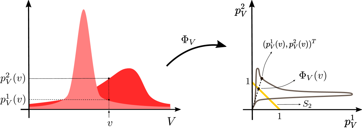According to Eq. (4), for any two similar random variables $A$ and $B$ such that $B=g(A)$ , the vectors $(p^{1}_{A}(g^{-1}(b)),·s,p^{m}_{A}(g^{-1}(b)))^{T}$ and $(p^{1}_{B}(b),·s,p^{m}_{B}(b))^{T}$ are aligned. Based on this observation, we define the following vector representation associated with random variables. **Definition 7** *Consider $\mathcal{V}$ -valued random variable $V$ . The density-vectorization associated with $V$ , $\Phi_{V}:\mathcal{V}→ S_{m}$ , is defined as $$ \Phi_{V}(v)=\frac{h}{\|h\|_{1}}, \tag{6} $$ where $S_{m}$ is the simplex in $m$ -dimensional space and $$ h=(p^{1}_{V}(v),p^{2}_{V}(v),\dots,p^{m}_{V}(v))^{T}, \tag{7} $$ for every $v∈\mathcal{V}$ .* In words, the density-vectorization operator takes as input a point in the support of $V$ , concatenates the density of $V$ across the domains into a vector of $m$ entries, and then normalizes it so that they sum up to one. The reason for using this operator is to summarize the relative density of $V$ in each point of the support, since this quantity turns out to be an important invariant of this setting that we leverage for identification. <details> <summary>x1.png Details</summary>  ### Visual Description \n ## Diagram: Phase Space Transformation ### Overview The image presents two diagrams illustrating a transformation, denoted as Φ_V, within a phase space. The left diagram depicts a distribution of p_V²(v) and p_V¹(v) as a function of velocity (v) and volume (V). The right diagram shows the transformation of this distribution in a space defined by p_V¹ and p_V². ### Components/Axes **Left Diagram:** * **X-axis:** Labeled "V" (Volume). * **Y-axis:** Labeled "p_V²(v)" (top) and "p_V¹(v)" (bottom). * **Vertical dashed line:** Marked with "v" (Velocity). * **Shaded Area:** Represents a distribution, peaking around a specific velocity 'v'. **Right Diagram:** * **X-axis:** Labeled "p_V¹". Scale ranges from approximately 0.5 to 1.5. * **Y-axis:** Labeled "p_V²". Scale ranges from approximately 0.5 to 1.5. * **Lines:** Several gray lines representing the transformation Φ_V(v). * **Yellow Line:** A single line representing the transformation Φ_V(v) with a highlighted segment. * **Black Line:** A line labeled "S₂". * **Text:** "(p_V¹(v), p_V²(v))^T" positioned near the top of the diagram. * **Arrow:** A curved arrow labeled "Φ_V" indicating the direction of the transformation. ### Detailed Analysis or Content Details **Left Diagram:** The distribution p_V¹(v) and p_V²(v) is approximately symmetric around the velocity 'v'. The peak of the distribution is located at approximately V = 1 and p_V²(v) = 1.5, and p_V¹(v) = 0.5. The distribution extends to lower values of p_V¹(v) and higher values of p_V²(v). **Right Diagram:** The gray lines representing Φ_V(v) appear to be curves that originate near (1,1) and bend upwards. The yellow line highlights a specific instance of the transformation. The highlighted segment starts at approximately (1, 1) and extends to approximately (1.2, 1.3). The line labeled S₂ is a vertical line at p_V¹ = 1. The text "(p_V¹(v), p_V²(v))^T" indicates a vector representation of the phase space coordinates. ### Key Observations * The transformation Φ_V maps points from the left diagram's distribution to curves in the right diagram's phase space. * The highlighted segment of Φ_V(v) suggests a specific trajectory or evolution of the system. * The line S₂ might represent a constraint or boundary condition within the phase space. * The distribution on the left is being mapped to a set of curves on the right. ### Interpretation The diagrams illustrate a transformation of a probability distribution in phase space. The left diagram shows the initial distribution of momentum components (p_V¹ and p_V²) as a function of velocity and volume. The right diagram shows how this distribution is transformed by Φ_V, mapping points in the original phase space to curves. This transformation could represent the evolution of a system over time, or a change in its state due to external forces. The line S₂ could represent a conserved quantity or a constraint on the system's motion. The vector notation "(p_V¹(v), p_V²(v))^T" suggests a mathematical formulation of the phase space coordinates. The diagrams are likely part of a theoretical framework describing the dynamics of a physical system, potentially in statistical mechanics or thermodynamics. </details> Figure 1: Left: Density functions $p^{1}_{V},p^{2}_{V}$ for random variable $V$ . Values of density functions at point $v$ are also shown in this plot. Right: Points on the gray curve are vectorization of values of density functions $p^{1}_{V},p^{2}_{V}$ for each point $v$ in $\mathbb{R}$ . Projecting the density vector $(p^{1}_{V}(v),p^{2}_{V}(v))^{T}$ on the simplex $S_{2}$ yields $\Phi_{V}(v)$ which is shown on the plot. **Definition 8** *Random variable $\Psi_{V}:\Omega→ S_{m}$ is called the “special random variable" associated with $V$ and it is defined as $\Psi_{V}:=\Phi_{V}(V)$ . Note that $\Phi_{V}$ is a deterministic function, but $\Psi_{V}$ is a random variable as it is a deterministic image of $V$ .* **Proposition 2** *Consider $A$ and $B$ , two $\mathcal{A}$ -valued and $\mathcal{B}$ -valued random variables, respectively. If $A\sim B$ , then $\Psi_{A}\overset{I}{=}\Psi_{B}$ .* In words, if two random variables are similar, then the special random variables associated with them are identical. Note that this result does not introduce an equivalent condition for similarity of random variables; instead, it is a necessary condition, and can be used to reject the hypothesis of similarity whenever the latter condition about special random variables is violated We conjecture that $\Psi_{A}\overset{I}{=}\Psi_{B}$ is a sufficient condition for $A$ and $B$ to be similar. We could not generate any counter-examples, but could not prove the statement either.. That being said, in case the distribution of variables does not change between the domains, then the density-vectorization operator collapses all points of the support to the point $\underbrace{\langle\frac{1}{m},\frac{1}{m},...,\frac{1}{m}\rangle}_{m\text{ % times}}$ . This implies that $\Psi_{V}$ is a constant, thus would be independent of all random variables. Therefore, if the distribution of variables in different domains are identical then the tests would be uninformative since no hypothesis may be rejected. Proposition 1 implies that Assumption 1 is equivalent to pairwise similarity of conditionals. Moreover, according to Proposition 2, Assumption 1 implies that for every pair of values $a,b∈\mathcal{X}$ , the special random variables associated with $\tilde{Y}_{a}$ and $\tilde{Y}_{b}$ are identical. Hence, if there exists $a,b∈\mathcal{X}$ for which $\Psi_{\tilde{Y}_{a}}\overset{I}{\not=}\Psi_{\tilde{Y}_{b}}$ , then $X\not→ Y$ under our assumptions. Motivated by this observation, we design a statistical test to reject pairwise similarity, thus, the causal diagram $X→ Y$ under BGM. **Definition 9** *Let $\Gamma_{X→ Y}$ be an $S_{m}$ -valued random variable obtained by taking a random sample $x∈\mathcal{X}$ according to the distribution of $X$ (in each domain), and then drawing a random sample from $\Psi_{\tilde{Y}_{x}}$ . More formally, $$ \Gamma_{X\to Y}:=\Psi_{\tilde{Y}_{X}}=\Phi_{\tilde{Y}_{X}}(\tilde{Y}_{X}). \tag{8} $$* **Proposition 3** *For every $a,b∈\mathcal{X}$ , $\Psi_{\tilde{Y}_{a}}\overset{I}{=}\Psi_{\tilde{Y}_{b}}$ if and only if $$ \Gamma_{X\to Y}\mathchoice{\mathrel{\hbox to0.0pt{$\displaystyle\perp$\hss}% \mkern 2.0mu{\displaystyle\perp}}}{\mathrel{\hbox to0.0pt{$\textstyle\perp$% \hss}\mkern 2.0mu{\textstyle\perp}}}{\mathrel{\hbox to0.0pt{$\scriptstyle\perp% $\hss}\mkern 2.0mu{\scriptstyle\perp}}}{\mathrel{\hbox to0.0pt{$% \scriptscriptstyle\perp$\hss}\mkern 2.0mu{\scriptscriptstyle\perp}}}X,\text{ % under each }\mathbb{P}^{i}\in\mathcal{M}. \tag{9} $$* **Corollary 1** *Combining the latter with Propositions 1 and 2 implies that we can reject the causal direction $X→ Y$ if data does not statistically admit the above independence relation under some $\mathbb{P}^{i}∈\mathcal{M}$ . Since if $\Gamma_{X→ Y}\not\mathchoice{\mathrel{\hbox to0.0pt{$\displaystyle\perp$\hss% }\mkern 2.0mu{\displaystyle\perp}}}{\mathrel{\hbox to0.0pt{$\textstyle\perp$% \hss}\mkern 2.0mu{\textstyle\perp}}}{\mathrel{\hbox to0.0pt{$\scriptstyle\perp% $\hss}\mkern 2.0mu{\scriptstyle\perp}}}{\mathrel{\hbox to0.0pt{$% \scriptscriptstyle\perp$\hss}\mkern 2.0mu{\scriptscriptstyle\perp}}}X,\text{ % under some }\mathbb{P}^{i}∈\mathcal{M}$ , then there would be some $a,b∈\mathcal{X}$ such that $\Psi_{\tilde{Y}_{a}}\overset{I}{=}\Psi_{\tilde{Y}_{b}}$ does not hold. Thus, based on Proposition 2, $\tilde{Y}_{a}$ and $\tilde{Y}_{b}$ are not similar which violates Assumption 1 according to Proposition 1.* Based on the above corollary, we state our main result as follows: **Theorem 1** *Under Assumption 1 and for continuous random variables $X$ and $Y$ , the causal diagram $X→ Y$ can be rejected if $\Gamma_{X→ Y}\not\mathchoice{\mathrel{\hbox to0.0pt{$\displaystyle\perp$\hss% }\mkern 2.0mu{\displaystyle\perp}}}{\mathrel{\hbox to0.0pt{$\textstyle\perp$% \hss}\mkern 2.0mu{\textstyle\perp}}}{\mathrel{\hbox to0.0pt{$\scriptstyle\perp% $\hss}\mkern 2.0mu{\scriptstyle\perp}}}{\mathrel{\hbox to0.0pt{$% \scriptscriptstyle\perp$\hss}\mkern 2.0mu{\scriptscriptstyle\perp}}}X,\text{ % for some }\mathbb{P}^{i}∈\mathcal{M}$ .* In what follows, we describe two extensions to our model. First, we discuss how our results extends to discrete case. Second, we discuss the extension to network of multiple variables. In these extensions, we modify both some of our assumptions in Section 3 as well as our theoretical results to cover the extended settings Our finding could be expressed in measure theoretic language where the continuous and discrete cases (as well as the cases which are neither continuous nor discrete) can be unified. To make the presentation accessible to a larger audience, we decided to adopt the current presentation which avoids complex notation and technical discussions in measure theoretic formalism.. 3.3 Discrete Case Assume that $E$ , and consequently $Y$ , are discrete random variables Since we assume that $f(x,·)$ is a bijective function from $\mathcal{E}$ to $\mathcal{Y}$ , $Y$ should take discrete values.. Continuity and differentiability are not defined for mappings between discrete sets. Thus, we replace Assumption 1 with the following assumption: **Assumption 2** *For every $x∈\mathcal{X}$ , the fixed-cause functional $f(x,·)$ is bijective.* Akin to Definition 6, discrete variables $A,B$ are similar (denote it by $A\sim B$ ), if and only if there exists a bijection $g$ such that $B\overset{I}{=}g(A)$ . **Proposition 4** *For discrete-valued $E$ , under Assumption 2, there is no causal direction from $X$ to $Y$ if $\Gamma_{X→ Y}\not\mathchoice{\mathrel{\hbox to0.0pt{$\displaystyle\perp$\hss% }\mkern 2.0mu{\displaystyle\perp}}}{\mathrel{\hbox to0.0pt{$\textstyle\perp$% \hss}\mkern 2.0mu{\textstyle\perp}}}{\mathrel{\hbox to0.0pt{$\scriptstyle\perp% $\hss}\mkern 2.0mu{\scriptstyle\perp}}}{\mathrel{\hbox to0.0pt{$% \scriptscriptstyle\perp$\hss}\mkern 2.0mu{\scriptscriptstyle\perp}}}X,\text{ % for some }\mathbb{P}^{i}∈\mathcal{M}$ .* In words, we can still test the causal diagram $X→ Y$ using the same exact method described for the continuous case. 3.4 Multivariate Case In this subsection, we extend our results to a setting with more than two observed variables by extending the Assumption 1 to the multivariate case as follows. **Assumption 3** *For every value of $V_{i}$ ’s parents like $pa_{i}$ , we assume that the fixed-cause functional $f_{i}(pa_{i},·)$ is a diffeomorphism.* Notably Assumption 3 is an extension of Assumption 1 for each endogenous variable. **Proposition 5** *Under Assumption 3, if for each variable $V_{i}$ , its conditional density function given any subset of variables $\mathbf{S}⊂\mathbf{V}$ is continuous in all domains, then $\mathbf{S}≠\mathbf{PA}_{i}$ if $$ \Gamma_{\mathbf{PA}_{i}\to V_{i}}\not\mathchoice{\mathrel{\hbox to0.0pt{$% \displaystyle\perp$\hss}\mkern 2.0mu{\displaystyle\perp}}}{\mathrel{\hbox to0.% 0pt{$\textstyle\perp$\hss}\mkern 2.0mu{\textstyle\perp}}}{\mathrel{\hbox to0.0% pt{$\scriptstyle\perp$\hss}\mkern 2.0mu{\scriptstyle\perp}}}{\mathrel{\hbox to% 0.0pt{$\scriptscriptstyle\perp$\hss}\mkern 2.0mu{\scriptscriptstyle\perp}}}% \mathbf{PA}_{i},\text{ for some }\mathbb{P}_{i}\in\mathcal{M}. \tag{10} $$* In words, the conditional independence test in Eq. 10 can be used as a basis for rejecting the hypothesis of a certain set being the parent set of $V_{i}$ . Similarly, note that this result can be extended to mixed-type (continuous or discrete) multivariable case. In what follows, we construct the discovery routine based on our findings. 4 Algorithm We assume that in each domain, there are $n_{e}$ i.i.d. samples drawn from $\mathbb{P}_{i}∈\mathcal{M}$ . Denote these observations as $\{(x^{i}_{l},y^{i}_{l})\}_{l=1}^{n_{e}}$ . To cover the discrete extension from Subsection 3.3, we use the general term “distribution” to refer density functions in continuous settings and probability mass functions in discrete settings. 4.1 Sampling From $\Gamma_{X→ Y}$ In Subsection 3.4 we propose the algorithm in the general multivariate case. If the conditional distribution functions $\{p^{i}_{Y|X}\}_{i=1}^{m}$ were available, we could obtain random samples from $\Gamma_{X→ Y}$ under each of the probability measure as followings. Note that $\tilde{Y}_{X}$ (Definition 9) and $Y$ are identically distributed, since the subscript $X$ is randomized. For a datapoint $(x,y)$ from say domain $e$ , we form the vector $w=(p^{1}_{Y|X}(y|x),p^{2}_{Y|X}(y|x),...,p^{i}_{Y|X}(y|x))^{T}$ and project it on $S_{m}$ (the simplex in $m$ dimensions) to obtain $\gamma:=\frac{w}{\|w\|_{1}}$ , which would be identically distributed as $\Gamma_{X→ Y}$ under $\mathbb{P}^{i}$ . When the true conditional distribution functions are not available, assuming we have enough samples from the joint observations of $X$ and $Y$ , we estimate the conditional distribution function $p^{i}_{Y|X}$ in each of the domains: $\hat{p}^{i}_{Y|X}$ . We performed this estimation using np package in R Hayfield and Racine (2008) in our implementation, and the code is available in the supplementary material. Using these estimated conditionals, we can obtain joint samples of $(\Gamma_{X→ Y},Y)$ as described above for each domain. Upon consistent estimation of the conditional distributions, this sampling routine yields “approximately accurately distributed” samples as $(\gamma,x)$ . As the size of data increases (in all domains), we obtain more accurate samples of $(\Gamma_{X→ Y},X)$ , as we can estimate the conditional distributions more accurately across the domains. 4.2 Inference As described in Subsection 4.1, we can obtain samples of $\Gamma_{X→ Y}$ in each domain. Using these samples, we perform an independence test to evaluate $\Gamma_{X→ Y}\mathchoice{\mathrel{\hbox to0.0pt{$\displaystyle\perp$\hss}% \mkern 2.0mu{\displaystyle\perp}}}{\mathrel{\hbox to0.0pt{$\textstyle\perp$% \hss}\mkern 2.0mu{\textstyle\perp}}}{\mathrel{\hbox to0.0pt{$\scriptstyle\perp% $\hss}\mkern 2.0mu{\scriptstyle\perp}}}{\mathrel{\hbox to0.0pt{$% \scriptscriptstyle\perp$\hss}\mkern 2.0mu{\scriptscriptstyle\perp}}}X\text{ % under each }\mathbb{P}^{i}$ . In our implementation, we used d-variable HSIC test Pfister et al. (2018) provided in dHSIC package in R. According to Theorem 1, we shall reject $X→ Y$ if this independence relation is rejected under any probability measure $\mathbb{P}^{i}∈\mathcal{M}$ . To aggregate the results of these $m$ independence tests (one in each of the $m$ domains), we consider the minimum $p$ -values of the independence tests performed in each of the domains. This ensure that the output of the aggregation is small whenever the independence relation is rejected in at least one domain. Without further assumptions about the data generation mechanism, the true causal structure is identifiable up to Markov equivalence classes (skeleton The skeleton of a directed graph $G$ is an undirected graph which does not take the direction of edges of $G$ into account. and v-structures of the causal graph) (Peters et al., 2017). As we are mainly concerned with orienting the undirected edges of the skeleton graph, we seek to find the set of parents of the nodes in the graph. Let $V$ denote a variable in the SCM, and $\mathbf{A}$ , the set of all the variables adjacent to $V$ . Clearly, parents of $V$ denoted by $PA(V)$ (or for short $\mathbf{PA}$ ) is a subset of $\mathbf{A}$ . Let $L(\mathbf{S})$ be the minimum p-value of testing $\Gamma_{\mathbf{S}→ V}\mathchoice{\mathrel{\hbox to0.0pt{$\displaystyle\perp% $\hss}\mkern 2.0mu{\displaystyle\perp}}}{\mathrel{\hbox to0.0pt{$\textstyle% \perp$\hss}\mkern 2.0mu{\textstyle\perp}}}{\mathrel{\hbox to0.0pt{$% \scriptstyle\perp$\hss}\mkern 2.0mu{\scriptstyle\perp}}}{\mathrel{\hbox to0.0% pt{$\scriptscriptstyle\perp$\hss}\mkern 2.0mu{\scriptscriptstyle\perp}}}V$ over all of the domains. If $L(\mathbf{S})$ is lower than some threshold $c$ , then there is enough evidence that at least in one domain, the independence relation $\Gamma_{\mathbf{S}→ V}\mathchoice{\mathrel{\hbox to0.0pt{$\displaystyle\perp% $\hss}\mkern 2.0mu{\displaystyle\perp}}}{\mathrel{\hbox to0.0pt{$\textstyle% \perp$\hss}\mkern 2.0mu{\textstyle\perp}}}{\mathrel{\hbox to0.0pt{$% \scriptstyle\perp$\hss}\mkern 2.0mu{\scriptstyle\perp}}}{\mathrel{\hbox to0.0% pt{$\scriptscriptstyle\perp$\hss}\mkern 2.0mu{\scriptscriptstyle\perp}}}V$ is violated. As a result of Theorem 1, if $L(\mathbf{S})<c$ , we conclude that $\mathbf{S}≠\mathbf{PA}$ . In order to obtain a single subset of $\mathbf{A}$ as the inferred parent set, we propose the following methods: H1: Compute $L(\mathbf{S})$ for all $\mathbf{S}⊂\mathbf{A}$ . To ensure that $\mathbf{PA}$ is contained in the output, return $$ \mathbf{\hat{PA}}:=\bigcup_{\mathbf{S}\subset\mathbf{A}:L(\mathbf{S})>c}% \mathbf{S}. \tag{11} $$ H2: If we know the size of the parent set apriori or have a bound on it, it suffices to explore subsets with that size or up to that bound, and return the subset with maximum value of $L$ . 5 Experiments Next, we evaluate the performance of proposed methods, and we explore use of our algorithms in synthetic and real data, and compare it with related work. 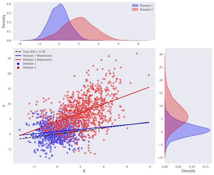5.1 Synthetic Data We used a heteroscedastic noise model to generate our synthetic data in two domains. In this model, variable $Y$ is determined by the value of its parent $X$ and an exogenous noise $E$ by the following equation $$ Y=f(X)+g(X)E, \tag{12} $$ where we assumed $f(X):=\alpha^{T}X$ , and $g(X)$ was randomly selected with equal probability from $\sqrt{|\beta^{T}X|+1}$ or $\log(|\beta^{T}X|+2)$ , respectively. We focused on the setting discussed in Subsection 4.2, in which we observe variables $\mathbf{A}\cup\{V\}$ , and the value of each variable is determined by the value of its parents according to Eq. (12). The coefficients $\alpha$ and $\beta$ for each structural equation were drawn randomly from $\mathcal{N}(0,0.05)$ and $\textit{unif}([-2,-1]\cup[1,2])$ , respectively. We considered two domains and in both domains, the exogenous noise was assumed normal. Let $\mu_{e}$ and $\sigma_{e}$ be the mean and the standard deviation of exogenous noise in domain $e∈\{1,2\}$ , respectively. We drew $\mu_{1}$ randomly from $\mathcal{N}(0,1)$ and $\sigma_{1}$ was set to 2. We also set the parameters in the second domain to $\mu_{2}=\mu_{1}+\text{{unif}}(\{-3,3\})$ and $\sigma_{2}=\sigma_{1}\text{{unif}}([\frac{2}{3},\frac{3}{2}])$ . An instance of the data in bivariate case is shown in Figure 2. <details> <summary>extracted/6400390/figs/bivariate-data.png Details</summary>  ### Visual Description ## Scatter Plot with Regression Lines and Density Plots: Domain Adaptation ### Overview The image presents a scatter plot visualizing two datasets ("Domain 1" and "Domain 2") with their respective linear regression lines. Superimposed on the scatter plot are density plots showing the distribution of each domain along the x-axis, and a marginal density plot along the y-axis. A dashed black line represents the "True f(x) = 0.5X" function, serving as a ground truth for comparison. The plot appears to demonstrate a domain adaptation scenario, where a model trained on one domain (Domain 1) is attempting to generalize to another (Domain 2). ### Components/Axes * **X-axis:** Labeled "X", ranging approximately from -3 to 8. * **Y-axis:** Labeled "Y", ranging approximately from -10 to 30. * **Density Plots:** Two density plots are positioned at the top of the image, representing the distribution of Domain 1 (blue) and Domain 2 (red) along the X-axis. A marginal density plot is positioned on the right side of the image, representing the distribution of both domains along the Y-axis. * **Legend:** Located in the top-right corner, with the following entries: * "Domain 1" (Blue) * "Domain 2" (Red) * "True f(x) = 0.5X" (Black dashed line) * "Domain 1 Regression" (Blue line) * "Domain 2 Regression" (Red line) ### Detailed Analysis **Scatter Plot Data:** * **Domain 1 (Blue):** Approximately 100 data points are scattered, primarily clustered around the line of regression. The points are distributed roughly between X = -2 and X = 3, and Y = -5 to 5. * **Domain 2 (Red):** Approximately 100 data points are scattered, also clustered around its regression line. The points are distributed roughly between X = 2 and X = 8, and Y = 5 to 25. **Regression Lines:** * **Domain 1 Regression (Blue):** The blue regression line has a positive slope, but is relatively shallow. It starts around Y = -1 when X = -2, and reaches approximately Y = 3 when X = 3. * **Domain 2 Regression (Red):** The red regression line has a steeper positive slope than the blue line. It starts around Y = 5 when X = 2, and reaches approximately Y = 20 when X = 8. * **True f(x) = 0.5X (Black Dashed):** This line has a moderate positive slope. It passes through the origin (0,0) and appears to be a reference for the expected relationship between X and Y. **Density Plots:** * **Domain 1 (Blue):** The density plot is centered around X = 0, with a peak density around X = 0.5. It extends from approximately X = -2 to X = 2. * **Domain 2 (Red):** The density plot is centered around X = 4, with a peak density around X = 4. It extends from approximately X = 2 to X = 8. * **Y-axis Density Plot:** The density plot is bimodal, with peaks around Y = 0 and Y = 10. ### Key Observations * The two domains have different distributions along the X-axis, as evidenced by the separate density plots. * The regression lines for each domain differ in slope, indicating different relationships between X and Y in each domain. * The Domain 2 regression line is steeper than the Domain 1 regression line. * The "True f(x) = 0.5X" line falls between the two regression lines, closer to the Domain 1 regression line. * There is a clear separation between the data points of Domain 1 and Domain 2 in the scatter plot. ### Interpretation This visualization likely demonstrates a domain adaptation problem in regression. The "True f(x) = 0.5X" represents the underlying relationship between X and Y. Domain 1 appears to be more closely aligned with this true function, while Domain 2 exhibits a different relationship. The differing regression lines suggest that a model trained on Domain 1 would not generalize well to Domain 2, and vice versa. The density plots highlight the distributional shift between the two domains, which is a common challenge in domain adaptation. The bimodal distribution on the Y-axis suggests a potential confounding factor or a more complex relationship between X and Y than a simple linear model can capture. The plot illustrates the need for techniques to mitigate the effects of domain shift and improve generalization performance. </details> Figure 2: 1000 datapoints in two domains, the marginals of $X$ and $Y$ , the regression lines in each domain, and the true invariant component $f$ . We compared the proposed methods with ICP (Peters et al., 2016a), NLICP (Heinze-Deml et al., 2017), MC (Ghassami et al., 2018), IB (Ghassami et al., 2018), LRE (Ghassami et al., 2017), CD-NOD (Huang et al., 2019b), CdF (Guo et al., 2023), and multi-group LiNGAM (MGL) (Shimizu, 2012) which have been proposed previously for the multi-domain setting. ICP method assumes that the target variable is a linear function of a subset of predictors, where the coefficients may change across the domains while the distribution of additive exogenous noise is assumed to be invariant. Non-linear ICP allows the functional relation to be non-linear. LRE considers invariant linear functional relations while the distribution of additive exogenous noise might change among the domains. IB and MC extend LRE so that neither distribution of noise nor the linear functional relation is assumed to be invariant. CD-NOD recovers causal relations based on the assumption of independent changes of conditional probability $\mathbb{P}($ cause $|$ effect $)$ . In our experiments, we also considered LiNGAM (Shimizu et al., 2006) which is a causal discovery algorithm in single domain setting and assumes linear functional relations with additive non-Gaussian noise. We evaluated the performance of our algorithms as well as previous work in two cases (each case comprised of 100 instances of synthetic dataset). We tuned the hyper-parameters of all algorithms (e.g. $c$ for our algorithm) with a training dataset before each experiment, and evaluated the performance on another testing dataset. In both experiments, H2 was initially fed with the size of true parent set. The code is made available here: https://github.com/jalaldoust/MD-BGM. | Alg. Acc. | H1 82% | ICP 43% | NLICP 51% | LiNGAM 66% | MC 62% | IB 59% | LRE 43% | CD-NOD 10% | CdF 49% | MGL 63% | | --- | --- | --- | --- | --- | --- | --- | --- | --- | --- | --- | Table 2: Bivariate case: Accuracy of algorithms on detection of causal direction between two variables. Bivariate case. In this case, $|\mathbf{A}|=1$ . The adjacent variable was set as the parent of $V$ with probability $\frac{1}{2}$ . We generated $1000$ samples in each of the domains. Accuracy of the algorithms are reported in Table 2. The proposed method (H1) indeed achieves the highest accuracy. It is worth to note that since we used only 100 instances of the problem, the standard deviation of the accuracies is no more than $5\%$ , which still deems our algorithm as the most accurate with high confidence. 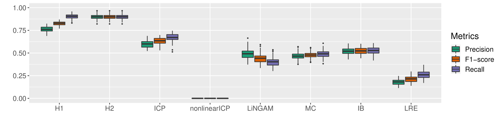Multivariate case. In this case, $|\mathbf{A}|$ was selected uniformly at random from $\{2,3,4,5\}$ , and we picked $|\mathbf{PA}|$ uniformly from $\{1,2,...,|\mathbf{A}|\}$ . We considered the fully connected skeleton among the variables $\mathbf{A}\cup\{V\}$ and the parents were determined according to a random topological order. We generated $10000$ samples in each of the domains and evaluated Precision, Recall, and F1-score for each of the algorithms. We repeated this procedure 100 times. Figure 3 depicts the performances of the various algorithms we compared. H1 outperformed all other algorithms with 20% margin of F1-score. H2 which has the advantage of prior knowledge about the size of parent set, has 12% improvement in precision over H1. (Please note that CD-NOD algorithm does not return any output in a reasonable time for the size of parents greater than one. Thus, its performance is reported only in the bivariate case). 5.2 Real World Data CollegeDistance dataset. We considered educational attainment data (Rouse, 1995) which was collected from approximately 1100 high-school students. The data contains 13 features including gender, race, base year composite test score, family income, etc. As in Peters et al. (2016a) and Ghassami et al. (2017), we split the observations into two groups (treated as two domains). This is done based on the distance to the closest 4-year college where the first group contains students within the 10 miles radius. The target variable is the number of years of education. We run our method for $100$ trials and in about $80\%$ of the executions, the set with greatest value of $L(\mathbf{S})$ was $\mathbf{S}=\{$ race $\}$ . Thus, this variable was returned as the parent set of the target variable. This variable along with three other candidates was also selected in Ghassami et al. (2017) as the parent set. <details> <summary>x2.png Details</summary>  ### Visual Description \n ## Box Plot: Performance Metrics Comparison ### Overview The image presents a box plot comparing the performance of several methods (H1, H2, ICP, nonlinearICP, LiNGAM, MC, IB, LRE) across three metrics: Precision, F1-score, and Recall. The y-axis represents the metric value, ranging from 0.0 to 1.0. Each method has three corresponding box plots, one for each metric. ### Components/Axes * **X-axis:** Method names: H1, H2, ICP, nonlinearICP, LiNGAM, MC, IB, LRE. * **Y-axis:** Metric Value (ranging from approximately 0.0 to 1.0). * **Legend (top-right):** * Precision (Teal/Cyan) * F1-score (Orange/Brown) * Recall (Yellow/Gold) * **Data Representation:** Box plots showing the distribution of each metric for each method. Each box plot displays the median, quartiles, and outliers. ### Detailed Analysis Let's analyze each method and metric individually, referencing the legend colors to ensure accuracy. **H1:** * Precision (Teal): Median around 0.72, IQR from approximately 0.65 to 0.80. * F1-score (Orange): Median around 0.85, IQR from approximately 0.78 to 0.92. * Recall (Yellow): Median around 0.75, IQR from approximately 0.65 to 0.85. **H2:** * Precision (Teal): Median around 0.85, IQR from approximately 0.80 to 0.90. * F1-score (Orange): Median around 0.90, IQR from approximately 0.85 to 0.95. * Recall (Yellow): Median around 0.85, IQR from approximately 0.80 to 0.90. **ICP:** * Precision (Teal): Median around 0.65, IQR from approximately 0.55 to 0.75. * F1-score (Orange): Median around 0.70, IQR from approximately 0.60 to 0.80. * Recall (Yellow): Median around 0.60, IQR from approximately 0.50 to 0.70. **nonlinearICP:** * Precision (Teal): Median around 0.50, IQR from approximately 0.40 to 0.60. * F1-score (Orange): Median around 0.55, IQR from approximately 0.45 to 0.65. * Recall (Yellow): Median around 0.50, IQR from approximately 0.40 to 0.60. **LiNGAM:** * Precision (Teal): Median around 0.40, IQR from approximately 0.30 to 0.50. * F1-score (Orange): Median around 0.40, IQR from approximately 0.30 to 0.50. * Recall (Yellow): Median around 0.40, IQR from approximately 0.30 to 0.50. **MC:** * Precision (Teal): Median around 0.50, IQR from approximately 0.40 to 0.60. * F1-score (Orange): Median around 0.50, IQR from approximately 0.40 to 0.60. * Recall (Yellow): Median around 0.50, IQR from approximately 0.40 to 0.60. **IB:** * Precision (Teal): Median around 0.55, IQR from approximately 0.45 to 0.65. * F1-score (Orange): Median around 0.55, IQR from approximately 0.45 to 0.65. * Recall (Yellow): Median around 0.55, IQR from approximately 0.45 to 0.65. **LRE:** * Precision (Teal): Median around 0.25, IQR from approximately 0.20 to 0.30. * F1-score (Orange): Median around 0.30, IQR from approximately 0.25 to 0.35. * Recall (Yellow): Median around 0.20, IQR from approximately 0.15 to 0.25. ### Key Observations * H2 consistently demonstrates the highest performance across all three metrics. * LRE consistently exhibits the lowest performance across all three metrics. * Precision, F1-score, and Recall tend to be correlated; methods with high F1-score generally also have high Precision and Recall. * The spread of the box plots (IQR) indicates the variability in performance for each method. H2 has the smallest spread, suggesting more consistent performance. * Outliers are present in several box plots, indicating some instances where the performance deviates significantly from the typical range. ### Interpretation The box plots provide a comparative analysis of the performance of different methods in a task where Precision, F1-score, and Recall are key evaluation metrics. H2 appears to be the most robust and reliable method, consistently achieving high scores and exhibiting low variability. LRE, on the other hand, performs poorly and is likely unsuitable for this task. The correlation between the three metrics suggests that improving one metric generally leads to improvements in the others. The presence of outliers highlights the potential for occasional performance fluctuations, which may warrant further investigation. The data suggests that the choice of method significantly impacts performance, and H2 is the preferred option based on these results. The differences in performance could be due to the underlying assumptions of each method, the characteristics of the data, or the specific implementation details. Further analysis could involve investigating the reasons for the poor performance of LRE and the consistent success of H2. </details> Figure 3: Multivariate case: Performance of our methods (H1 and H2) as well as previous work. Adult dataset. This dataset is available at UCI Machine Learning Repository Dua and Graff (2017) and contains census information. We pre-processed the data by filtering or transforming some of the features before feeding them to our causal discovery algorithm. We chose sex as the domain variable, and working hour per week as the target variable. We considered the following features: age, race, marital status, level of education, level of income, work class, and country. Among these variables, the maximum value of $L(\mathbf{S})$ was achieved by $\mathbf{S}=\{\text{country}\}$ . This is not surprising since working policy in each country has a direct impact on the working hour per week. 5.3 Limitations Our algorithm has few practical limitations. First, accurately estimating the density in each environment may require large amounts of data, and the minimum required data grows exponentially with the dimensionality of the variables unless additional assumptions are imposed. Second, our framework requires domain indices to be integers, and the causal discovery task depends on having sufficient data in all domains. Consequently, our method is most effective when the number of domains is small relative to the dataset size. Third, the computational cost is significant due to the combinatorial search over parent sets, computation of test statistics, and execution of independence tests. A theoretical limitation of our approach is that we do not claim completeness of the discovery algorithm—while we guarantee soundness (i.e., once a non-parent is identified, it is truly a non-parent), we do not ensure that all non-parents are rejected. Since completeness is not the focus of this work, the discussion of necessary faithfulness assumptions remains an open question. 6 Conclusion We studied causal discovery problem in multi-domain setting with invariant causal relations and varying noise distribution. We presented an identifiablity result assuming bijective generation mechanisms, which is less restrictive than previous approaches, and holds in several classical models. We defined similarity relation between random variables in settings with multiple probability measures and we introduced an independence relation which necessarily holds in case of causation. We compared the performance of our approach with previous work and in our experiments our method out performed them with a high margin. Future work includes extension of results to non-stationary time-series and applications in sequential decision-making. References - Ackerer et al. (2020) Damien Ackerer, Natasa Tagasovska, and Thibault Vatter. Deep smoothing of the implied volatility surface. Advances in Neural Information Processing Systems, 33:11552–11563, 2020. - Chickering (2003) David Maxwell Chickering. Optimal structure identification with greedy search. J. Mach. Learn. Res., 3(null):507–554, March 2003. ISSN 1532-4435. 10.1162/153244303321897717. URL https://doi.org/10.1162/153244303321897717. - Dawid (2010) A. Philip Dawid. Beware of the dag! In Proceedings of the Nineteenth Annual Conference on Uncertainty in Artificial Intelligence, 2010. - Dua and Graff (2017) Dheeru Dua and Casey Graff. UCI machine learning repository, 2017. URL http://archive.ics.uci.edu/ml. - Ghassami et al. (2017) AmirEmad Ghassami, Saber Salehkaleybar, Negar Kiyavash, and Kun Zhang. Learning causal structures using regression invariance. In I. Guyon, U. V. Luxburg, S. Bengio, H. Wallach, R. Fergus, S. Vishwanathan, and R. Garnett, editors, Advances in Neural Information Processing Systems 30, pages 3011–3021. Curran Associates, Inc., 2017. URL http://papers.nips.cc/paper/6894-learning-causal-structures-using-regression-invariance.pdf. - Ghassami et al. (2018) AmirEmad Ghassami, Negar Kiyavash, Biwei Huang, and Kun Zhang. Multi-domain causal structure learning in linear systems. In Advances in neural information processing systems, pages 6266–6276, 2018. - Guo et al. (2023) Siyuan Guo, Viktor Tóth, Bernhard Schölkopf, and Ferenc Huszár. Causal de finetti: On the identification of invariant causal structure in exchangeable data. In Thirty-seventh Conference on Neural Information Processing Systems, 2023. URL https://openreview.net/forum?id=o4RtDFMSNL. - Hayfield and Racine (2008) Tristen Hayfield and Jeffrey Racine. Nonparametric econometrics: The np package. Journal of Statistical Software, Articles, 27(5):1–32, 2008. ISSN 1548-7660. 10.18637/jss.v027.i05. URL https://www.jstatsoft.org/v027/i05. - Heinze-Deml et al. (2017) Christina Heinze-Deml, Jonas Peters, and Nicolai Meinshausen. Invariant causal prediction for nonlinear models. Journal of Causal Inference, 6, 06 2017. 10.1515/jci-2017-0016. - Hoyer et al. (2009) Patrik O Hoyer, Dominik Janzing, Joris M Mooij, Jonas Peters, and Bernhard Schölkopf. Nonlinear causal discovery with additive noise models. In Advances in neural information processing systems, pages 689–696, 2009. - Huang et al. (2019a) Biwei Huang, Kun Zhang, Mingming Gong, and Clark Glymour. Causal discovery and forecasting in nonstationary environments with state-space models. In Proceedings of the 36th International Conference on Machine Learning, volume 97, pages 2901–2910. PMLR, 2019a. - Huang et al. (2019b) Biwei Huang, Kun Zhang, Jiji Zhang, Joseph Ramsey, Ruben Sanchez-Romero, Clark Glymour, and Bernhard Schölkopf. Causal discovery from heterogeneous/nonstationary data. arXiv preprint arXiv:1903.01672, 2019b. - Hyvarinen et al. (2019) Aapo Hyvarinen, Hiroaki Sasaki, and Richard Turner. Nonlinear ica using auxiliary variables and generalized contrastive learning. In The 22nd international conference on artificial intelligence and statistics, pages 859–868. PMLR, 2019. - Imbens and Rubin (2015) Guido W Imbens and Donald B Rubin. Causal inference for statistics, social, and biomedical sciences: An introduction. Cambridge University Press, 2015. - Immer et al. (2023) Alexander Immer, Christoph Schultheiss, Julia E Vogt, Bernhard Schölkopf, Peter Bühlmann, and Alexander Marx. On the identifiability and estimation of causal location-scale noise models. In International Conference on Machine Learning, pages 14316–14332. PMLR, 2023. - Jaber et al. (2020) Amin Jaber, Murat Kocaoglu, Karthikeyan Shanmugam, and Elias Bareinboim. Causal discovery from soft interventions with unknown targets: Characterization and learning. In Advances in Neural Information Processing Systems, volume 33, pages 9551–9561. Curran Associates, Inc., 2020. - Lemeire and Janzing (2013) Jan Lemeire and Dominik Janzing. Revisiting causal discovery by assuming the independence of cause and mechanism. In Proceedings of the 29th Conference on Uncertainty in Artificial Intelligence (UAI), 2013. - Mian et al. (2023) Osman Mian, Michael Kamp, and Jilles Vreeken. Information-theoretic causal discovery and intervention detection over multiple environments. In Proceedings of the AAAI Conference on Artificial Intelligence, volume 37, pages 9171–9179, 2023. - Mooij et al. (2020) Joris M Mooij, Sara Magliacane, and Tom Claassen. Joint causal inference from multiple contexts. Journal of Machine Learning Research, 21(99):1–108, 2020. - Nasr-Esfahany et al. (2023) Arash Nasr-Esfahany, Mohammad Alizadeh, and Devavrat Shah. Counterfactual identifiability of bijective causal models. In International Conference on Machine Learning, pages 25733–25754. PMLR, 2023. - Nelsen (2007) Roger B Nelsen. An introduction to copulas. Springer Science & Business Media, 2007. - Pearl (2009a) Judea Pearl. Causality. Cambridge University Press, 2009a. 10.1017/CBO9780511803161. - Pearl (2009b) Judea Pearl. Causal inference in statistics: An overview. Statistics Surveys, 3:96–146, 2009b. - Perry et al. (2022) Ronan Perry, Julius von Kügelgen, and Bernhard Schölkopf. Causal discovery in heterogeneous environments under the sparse mechanism shift hypothesis. In Advances in Neural Information Processing Systems, volume 35, pages 10904–10917. Curran Associates, Inc., 2022. - Peters et al. (2016a) J. Peters, P. Bühlmann, and N. Meinshausen. Causal inference using invariant prediction: identification and confidence intervals. Journal of the Royal Statistical Society, Series B (Statistical Methodology), 78(5):947–1012, 2016a. URL http://arxiv.org/abs/1501.01332. (with discussion). - Peters et al. (2017) J. Peters, D. Janzing, and B. Schölkopf. Elements of Causal Inference: Foundations and Learning Algorithms. MIT Press, Cambridge, MA, USA, 2017. - Peters et al. (2016b) Jonas Peters, Peter Bühlmann, and Nicolai Meinshausen. Causal inference using invariant prediction: identification and confidence intervals. Journal of the Royal Statistical Society: Series B (Statistical Methodology), 78(5):947–1012, 2016b. - Pfister et al. (2018) Niklas Pfister, Peter Bühlmann, Bernhard Schölkopf, and Jonas Peters. Kernel-based tests for joint independence. Journal of the Royal Statistical Society: Series B (Statistical Methodology), 80(1):5–31, 2018. - Pfister et al. (2019) Niklas Pfister, Peter Bühlmann, and Jonas Peters. Invariant causal prediction for sequential data. Journal of the American Statistical Association, 114(527):1264–1276, 2019. 10.1080/01621459.2018.1491403. URL https://doi.org/10.1080/01621459.2018.1491403. - Reizinger et al. (2023) Patrik Reizinger, Yash Sharma, Matthias Bethge, Bernhard Schölkopf, Ferenc Huszár, and Wieland Brendel. Jacobian-based causal discovery with nonlinear ica. Transactions on Machine Learning Research, 2023. - Reizinger et al. (2025) Patrik Reizinger, Siyuan Guo, Ferenc Huszár, Bernhard Schölkopf, and Wieland Brendel. Identifiable exchangeable mechanisms for causal structure and representation learning. In The Thirteenth International Conference on Learning Representations, 2025. URL https://openreview.net/forum?id=k03mB41vyM. - Rosenbaum and Rubin (1983) Paul R Rosenbaum and Donald B Rubin. The central role of the propensity score in observational studies for causal effects. Biometrika, 70(1):41–55, 1983. - Rouse (1995) Cecilia Elena Rouse. Democratization or diversion? the effect of community colleges on educational attainment. Journal of Business & Economic Statistics, 13(2):217–224, 1995. - Schölkopf et al. (2012) Bernhard Schölkopf, Dominik Janzing, and Jonas Peters. Semi-supervised learning, causality, and the conditional independence assumption. In Proceedings of the 15th International Conference on Artificial Intelligence and Statistics (AISTATS), 2012. - Shimizu (2012) Shohei Shimizu. Joint estimation of linear non-gaussian acyclic models. Neurocomputing, 81:104–107, 2012. - Shimizu et al. (2006) Shohei Shimizu, Patrik O. Hoyer, Aapo Hyvärinen, and Antti Kerminen. A linear non-gaussian acyclic model for causal discovery. J. Mach. Learn. Res., 7:2003–2030, December 2006. ISSN 1532-4435. - Shpitser and Pearl (2008) Ilya Shpitser and Judea Pearl. Complete identification methods for the causal hierarchy. Journal of Machine Learning Research, 9:1941–1979, 2008. - Spirtes et al. (2000) Peter Spirtes, Clark N Glymour, Richard Scheines, and David Heckerman. Causation, prediction, and search. MIT press, 2000. - Squires et al. (2020) Chandler Squires, Yuhao Wang, and Caroline Uhler. Permutation-based causal structure learning with unknown intervention targets. Proceedings of the 36th Conference on Uncertainty in Artificial Intelligence, 124:909–918, 2020. - Stark and Woods (1986) Henry Stark and John W. Woods, editors. Probability, Random Processes, and Estimation Theory for Engineers. Prentice-Hall, Inc., USA, 1986. ISBN 013711706X. - Strobl and Lasko (2023) Eric V Strobl and Thomas A Lasko. Identifying patient-specific root causes with the heteroscedastic noise model. Journal of Computational Science, 72:102099, 2023. - Yang et al. (2018) Karren D Yang, Ari Katcoff, and Caroline Uhler. Characterizing and learning equivalence classes of causal dags under interventions. Proceedings of the 35th International Conference on Machine Learning, 80:5541–5550, 2018. - Zhang and Hyvarinen (2012) Kun Zhang and Aapo Hyvarinen. On the identifiability of the post-nonlinear causal model, 2012. - Zhang et al. (2017) Kun Zhang, Biwei Huang, Jiji Zhang, Clark Glymour, and Bernhard Schölkopf. Causal discovery from nonstationary/heterogeneous data: Skeleton estimation and orientation determination. In Proceedings of the Twenty-Sixth International Joint Conference on Artificial Intelligence, IJCAI-17, pages 1347–1353, 2017. 10.24963/ijcai.2017/187. URL https://doi.org/10.24963/ijcai.2017/187. Appendix **Remark 1** *Suppose $g,f:\mathcal{A}→\mathcal{B}$ are diffeomorphisms. Then $g^{-1}$ and $g$ o $f$ are also diffeomorphisms.* **Lemma 1** *Similarity is an equivalence relation. **Proof .1** *We should check the three properties of equivalence relations. Consider random variables $A$ , $B$ , and $C$ taking value in $\mathcal{A}$ , $\mathcal{B}$ , and $\mathcal{C}$ , respectively. Assume that $A\sim B$ and $B\sim C$ . Claim: $\sim$ is reflective. Define $g:\mathcal{A}→\mathcal{A}$ such that $∀ x∈\mathcal{A}:g(x)=x$ . It is bijective and continuously differentiable. Hence, it is a diffeomorphism. By Definition 6, $A\sim A$ . Claim: $\sim$ is symmetric. As $A\sim B$ , from Definition 6, there exists a diffeomorphism $g$ such that $g(A)\overset{I}{=}B$ . From Definition 5, for every $e$ and every $u⊂\mathcal{B}$ $$ \mathbb{P}^{i}(g(A)\in u)=\mathbb{P}^{i}(B\in u). \tag{13} $$ Note that $g$ is a diffeomorphism, so $g^{-1}$ exists. Let $w$ be an arbitrary subset of $\mathcal{A}$ . Let $u=g(w)$ , hence $w=g^{-1}(u)$ . $$ \displaystyle\mathbb{P}^{i}(A\in w) \displaystyle=\mathbb{P}^{i}(A\in g^{-1}(u)) \displaystyle=\mathbb{P}^{i}(g(A)\in u) \displaystyle=\mathbb{P}^{i}(B\in u) \displaystyle=\mathbb{P}^{i}(g^{-1}(B)\in g^{-1}(u)) \displaystyle=\mathbb{P}^{i}(g^{-1}(B)\in w). \tag{14} $$ Form Remark 1, we know that $g^{-1}$ is a diffeomorphims. As the choice of $w$ was arbitrary, from Definitions 5 and 6, we have $$ B\sim A. \tag{19} $$ Claim: $\sim$ is transitive. Similarly, for every $e$ and every $u⊂\mathcal{B}$ $$ \mathbb{P}^{i}(g(A)\in u)=\mathbb{P}^{i}(B\in u). \tag{20} $$ Also, for every $e$ and every $q⊂\mathcal{C}$ , $$ \mathbb{P}^{i}(f(B)\in q)=\mathbb{P}^{i}(C\in q). \tag{21} $$ Note that both $g$ and $f$ are diffeomorphisms. Thus, they are invertible. Consider $q⊂\mathcal{C}$ arbitrarily. Let $u=f^{-1}(q)$ and $w=g^{-1}(u)$ . $$ \displaystyle\mathbb{P}^{i}((f\circ g)(A)\in q) \displaystyle=\mathbb{P}^{i}(g(A)\in f^{-1}(q)) \displaystyle=\mathbb{P}^{i}(g(A)\in u) \displaystyle=\mathbb{P}^{i}(B\in u) \displaystyle=\mathbb{P}^{i}(f(B)\in f(u)) \displaystyle=\mathbb{P}^{i}(f(B)\in q) \displaystyle=\mathbb{P}^{i}(C\in q) \tag{22} $$ From Remark 1, we know that $f\circ g$ is a diffeomorphism. Therefore, $$ A\sim C. \tag{28} $$** Proof of Proposition 1 Claim: Assumption 1 holds $\Rightarrow∀ a,b∈\mathcal{X}:\tilde{Y}_{a}\sim\tilde{Y}_{b}$ . Fix the domain variable $e$ and consider $x∈\mathcal{X}$ arbitrarily. As a result of Assumption 1, $f(x,·)$ is invertible, and we have $$ p^{i}_{(Y|X)}(y|x)=p^{i}_{(E|X)}(f(x,\cdot)^{-1}(y)|x)=p^{i}_{E}(f(x,\cdot)^{-% 1}(y)), \tag{29} $$ where the first equation is because of the model $Y=f(X,E)$ , and the second one is due to $X\mathchoice{\mathrel{\hbox to0.0pt{$\displaystyle\perp$\hss}\mkern 2.0mu{% \displaystyle\perp}}}{\mathrel{\hbox to0.0pt{$\textstyle\perp$\hss}\mkern 2.0% mu{\textstyle\perp}}}{\mathrel{\hbox to0.0pt{$\scriptstyle\perp$\hss}\mkern 2.% 0mu{\scriptstyle\perp}}}{\mathrel{\hbox to0.0pt{$\scriptscriptstyle\perp$\hss}% \mkern 2.0mu{\scriptscriptstyle\perp}}}E$ . Let $g:=f(x,·)$ which is a diffeomorphism, according to Assumption 1. As $Y=f(X,E)$ , we have $$ \tilde{Y}_{x}\overset{I}{=}g(E). \tag{30} $$ Note that $\tilde{Y}_{x}$ is a random variable which has the same distribution as $Y$ given $X=x$ . According to Definition 6, $$ \forall x\in\mathcal{X}:E\sim\tilde{Y}_{x}. \tag{31} $$ By Lemma 1, similarity is an equivalence relation, so we have $$ \forall a,b\in\mathcal{X}:\tilde{Y}_{a}\sim\tilde{Y}_{b}. \tag{32} $$ Claim: $∀ a,b∈\mathcal{X}:\tilde{Y}_{a}\sim\tilde{Y}_{b}\Rightarrow$ Assumption 1 holds. Fix arbitrary $x_{0}∈\mathcal{X}$ . Define $\tilde{E}$ an independent random variable which is identically distributed as $\tilde{Y}_{x_{0}}$ ( $E\overset{I}{=}\tilde{Y}_{x_{0}}$ ). Define $\tilde{f}$ so that $\tilde{f}(x,·):=g_{x}$ where $g_{x}$ is the diffeomorphism which forms the similarity between $\tilde{Y}_{x}$ and $\tilde{Y}_{x_{0}}$ (Definition 1). Assumption 1 holds for $\tilde{f}$ . Proof of Proposition 2 Fix the domain index $e$ and consider $s⊂ S_{m}$ arbitrarily. Note that the events $\Psi_{A}∈ s$ and $\Psi_{B}∈ s$ should both be measurable under $\mathbb{P}^{i}$ , as we intend to show $$ \mathbb{P}^{i}(\Psi_{A}\in s)=\mathbb{P}^{i}(\Psi_{B}\in s), \tag{33} $$ which results in $\Psi_{A}\overset{I}{=}\Psi_{B}$ (Definition 5). Let $\alpha=\Phi^{-1}_{A}(s)$ and $\beta=\Phi^{-1}_{B}(s)$ . Note that $\alpha⊂\mathcal{A}$ and $\beta⊂\mathcal{B}$ . As $A\sim B$ , according to Definition 6 $$ \exists\text{ diffeomorphism }g:\mathcal{A}\to\mathcal{B}\text{ such that }g(A% )\overset{I}{=}B \tag{34} $$ Consider $a∈\alpha$ arbitrarily. Let $b=g(a)$ . We have $$ \displaystyle\Phi_{B}(b) \displaystyle=c.(p^{1}_{B}(b),p^{2}_{B}(b),\dots,p^{m}_{B}(b)) \displaystyle=c.\frac{1}{|det(J_{g}(a))|}.(p^{1}_{A}(a),p^{2}_{A}(a),\dots,p^{% m}_{A}(a)) \displaystyle=c^{\prime}.(p^{1}_{A}(a),p^{2}_{A}(a),\dots,p^{m}_{A}(a)), \tag{35} $$ where (35) holds according to Definition 7 and (36) holds due to (4). As we defined $\alpha$ , we have $$ \Phi_{A}(a)=c^{\prime\prime}.(p^{1}_{A}(a),p^{2}_{A}(a),\dots,p^{m}_{A}(a))\in s. \tag{38} $$ Note that we also have $$ \Phi_{B}(b)=c^{\prime}.(p^{1}_{A}(a),p^{2}_{A}(a),\dots,p^{m}_{A}(a))\in s. \tag{39} $$ Thus, $\Phi_{B}(b)$ and $\Phi_{A}(a)$ are proportional with factor $\frac{c^{\prime}}{c^{\prime\prime}}$ . As they are both in $S_{m}$ , this is possible only if $c^{\prime\prime}=c^{\prime}$ and $\Phi_{B}(b)=\Phi_{A}(a)$ . Because the choice of $a$ was arbitrary, we have $$ g(\alpha)\subset\beta. \tag{40} $$ According to Lemma 1, $A\sim B\Rightarrow B\sim A$ . Therefore, with the same arguments in the reverse direction, we get $$ g^{-1}(\beta)\subset\alpha, \tag{41} $$ which results in $$ g(\alpha)=\beta. \tag{42} $$ Finally, $$ \displaystyle\mathbb{P}^{i}(\Psi_{A}\in s) \displaystyle=\mathbb{P}^{i}(A\in\alpha) \displaystyle=\mathbb{P}^{i}(g(A)\in g(\alpha)) \displaystyle=\mathbb{P}^{i}(g(A)\in\beta) \displaystyle=\mathbb{P}^{i}(B\in\beta) \displaystyle=\mathbb{P}^{i}(\Psi_{B}\in s), \tag{43} $$ where (46) follows from $g(A)\overset{I}{=}B$ which is imposed by $A\sim B$ . Proof of Proposition 3 Claim: If for every $a,b∈\mathcal{X}$ , $\Psi_{\tilde{Y}_{a}}\overset{I}{=}\Psi_{\tilde{Y}_{b}}$ , then $\Gamma_{X→ Y}\mathchoice{\mathrel{\hbox to0.0pt{$\displaystyle\perp$\hss}% \mkern 2.0mu{\displaystyle\perp}}}{\mathrel{\hbox to0.0pt{$\textstyle\perp$% \hss}\mkern 2.0mu{\textstyle\perp}}}{\mathrel{\hbox to0.0pt{$\scriptstyle\perp% $\hss}\mkern 2.0mu{\scriptstyle\perp}}}{\mathrel{\hbox to0.0pt{$% \scriptscriptstyle\perp$\hss}\mkern 2.0mu{\scriptscriptstyle\perp}}}X$ , under each $\mathbb{P}^{i}∈\mathcal{M}$ . Fix the domain index $e$ . Consider any $s⊂ S_{m}$ arbitrarily. Consider $a,b∈\mathcal{X}$ arbitrarily. Then, $$ \displaystyle\mathbb{P}^{i}(\Gamma_{X\to Y}\in s|X=a) \displaystyle=\mathbb{P}^{i}(\Psi_{\tilde{Y}_{X}}\in s|X=a) \displaystyle=\mathbb{P}^{i}(\Psi_{\tilde{Y}_{a}}\in s) \displaystyle=\mathbb{P}^{i}(\Psi_{\tilde{Y}_{b}}\in s) \displaystyle=\mathbb{P}^{i}(\Psi_{\tilde{Y}_{X}}\in s|X=b) \displaystyle=\mathbb{P}^{i}(\Gamma_{X\to Y}\in s|X=b), \tag{48} $$ where (48) is from Definition 9 and (49) is from imposing the condition $X=a$ . Moreover, (50) is from the assumption $\Psi_{\tilde{Y}_{a}}\overset{I}{=}\Psi_{\tilde{Y}_{b}}$ and Definition 5. As the distribution of $\Gamma_{X→ Y}$ is invariant for every condition on $X$ , we conclude $\Gamma_{X→ Y}\mathchoice{\mathrel{\hbox to0.0pt{$\displaystyle\perp$\hss}% \mkern 2.0mu{\displaystyle\perp}}}{\mathrel{\hbox to0.0pt{$\textstyle\perp$% \hss}\mkern 2.0mu{\textstyle\perp}}}{\mathrel{\hbox to0.0pt{$\scriptstyle\perp% $\hss}\mkern 2.0mu{\scriptstyle\perp}}}{\mathrel{\hbox to0.0pt{$% \scriptscriptstyle\perp$\hss}\mkern 2.0mu{\scriptscriptstyle\perp}}}X$ under $\mathbb{P}^{i}$ and as the choice of $e$ was arbitrary, this holds for every $e$ . Claim: If $\Gamma_{X→ Y}\mathchoice{\mathrel{\hbox to0.0pt{$\displaystyle\perp$\hss}% \mkern 2.0mu{\displaystyle\perp}}}{\mathrel{\hbox to0.0pt{$\textstyle\perp$% \hss}\mkern 2.0mu{\textstyle\perp}}}{\mathrel{\hbox to0.0pt{$\scriptstyle\perp% $\hss}\mkern 2.0mu{\scriptstyle\perp}}}{\mathrel{\hbox to0.0pt{$% \scriptscriptstyle\perp$\hss}\mkern 2.0mu{\scriptscriptstyle\perp}}}X$ , under each $\mathbb{P}^{i}∈\mathcal{M}$ , then for every $a,b∈\mathcal{X}$ , $\Psi_{\tilde{Y}_{a}}\overset{I}{=}\Psi_{\tilde{Y}_{b}}$ . Fix the domain index $e$ . Consider any $s⊂ S_{m}$ arbitrarily. Consider $a,b∈\mathcal{X}$ arbitrarily. Then, $$ \displaystyle\mathbb{P}^{i}(\Psi_{\tilde{Y}_{a}}\in s) \displaystyle=\mathbb{P}^{i}(\Psi_{\tilde{Y}_{X}}\in s|X=a) \displaystyle=\mathbb{P}^{i}(\Gamma_{X\to Y}\in s|X=a) \displaystyle=\mathbb{P}^{i}(\Gamma_{X\to Y}\in s|X=b) \displaystyle=\mathbb{P}^{i}(\Psi_{\tilde{Y}_{b}}\in s). \tag{53} $$ Due to arbitrary choice of $s$ , according to Definition 5, we have $$ \Psi_{\tilde{Y}_{a}}\overset{I}{=}\Psi_{\tilde{Y}_{b}} \tag{57} $$ Proof of Theorem 1 In continuous case, we have Assumption 1, along with other technical assumptions mentioned in the Section 3. Proposition 1 states that under this set of assumptions, if $X$ causes $Y$ in our model, we have $$ \forall a,b\in\mathcal{X}:\tilde{Y}_{a}\sim\tilde{Y}_{b}. \tag{58} $$ Proposition 2 states that for every two similar random variables $A\sim B$ , the corresponding special random variables are identical, i.e., $$ \Psi_{A}\overset{I}{=}\Psi_{B}. \tag{59} $$ Being identical means that they have the same distribution function under every measure $\mathbb{P}^{i}∈\mathcal{M}$ . From these two results, we can imply the following condition from our set of assumptions, in case of $X$ causing $Y$ in our model. $$ \forall a,b\in\mathcal{X}:\Psi_{\tilde{Y}_{a}}\overset{I}{=}\Psi_{\tilde{Y}_{b% }}. \tag{60} $$ Proposition 3 states that from the condition (60), we can imply the following independence criterion in all domains (i.e., for every $\mathbb{P}^{i}∈\mathcal{M}$ ): $$ \Gamma_{X\to Y}\mathchoice{\mathrel{\hbox to0.0pt{$\displaystyle\perp$\hss}% \mkern 2.0mu{\displaystyle\perp}}}{\mathrel{\hbox to0.0pt{$\textstyle\perp$% \hss}\mkern 2.0mu{\textstyle\perp}}}{\mathrel{\hbox to0.0pt{$\scriptstyle\perp% $\hss}\mkern 2.0mu{\scriptstyle\perp}}}{\mathrel{\hbox to0.0pt{$% \scriptscriptstyle\perp$\hss}\mkern 2.0mu{\scriptscriptstyle\perp}}}X. \tag{61} $$ Therefore, our set of assumptions implies that if the causal direction is from $X$ to $Y$ , then the above independence should hold in all domains. As a result, violation of this independence criterion in at least one of the domains, rejects the hypothesis that $X$ causes $Y$ . Proof of Proposition 4 We should prove equivalent results from Propositions 1, 2, and 3 for the discrete case. We define a discrete notion of similarity. $$ A\overset{d}{\sim}B\iff\exists\text{ bijective }g\text{ such that }g(A)% \overset{I}{=}B. \tag{62} $$ Note that Definition 5 should not be changed as it work in both discrete and continuous cases. We state our identifiability result in discrete case as follows: Assumption 2 holds if and only if $∀ a,b∈\mathcal{X}:\tilde{Y}_{a}\overset{d}{\sim}\tilde{Y}_{b}$ . The same reasoning in the proof of Proposition 1 yields this result. The result equivalent to Proposition 2 is as follows: For any two discrete-valued random variables $A$ and $B$ , if $A\overset{d}{\sim}B$ , then $\Psi_{A}\overset{I}{=}\Psi_{B}$ . To prove this result, it suffices to change the proof of Proposition 2 by replacing $|det(J_{g}(a))|$ with $1$ (in Equation (36)), and use $p^{i}_{V}$ to denote the probability mass function (instead of probability density function). Finally, we state the result equivalent to Proposition 3, for discrete case: In the discrete case, for every $a,b∈\mathcal{X}$ , we have $\Psi_{\tilde{Y}_{a}}\overset{I}{=}\Psi_{\tilde{Y}_{b}}$ if and only if $\Gamma_{X→ Y}\mathchoice{\mathrel{\hbox to0.0pt{$\displaystyle\perp$\hss}% \mkern 2.0mu{\displaystyle\perp}}}{\mathrel{\hbox to0.0pt{$\textstyle\perp$% \hss}\mkern 2.0mu{\textstyle\perp}}}{\mathrel{\hbox to0.0pt{$\scriptstyle\perp% $\hss}\mkern 2.0mu{\scriptstyle\perp}}}{\mathrel{\hbox to0.0pt{$% \scriptscriptstyle\perp$\hss}\mkern 2.0mu{\scriptscriptstyle\perp}}}X$ . The exact same reasoning in Proposition 3 works for proving this result. Finally, Proposition 4 is proved in the same way as Theorem 1. Proof of Proposition 5 Proposition 5 is a restatement of Theorem 1 for multivariate case. By setting $X:=\mathbf{PA}_{i}$ and $Y:=V_{i}$ , the result is immediately implied from Theorem 1.