2505.02216v2

# LLM-Guided Probabilistic Program Induction for POMDP Model Estimation ## Abstract Partially Observable Markov Decision Processes (POMDPs) model decision making under uncertainty. While there are many approaches to approximately solving POMDPs, we aim to address the problem of learning such models. In particular, we are interested in a subclass of POMDPs wherein the components of the model, including the observation function, reward function, transition function, and initial state distribution function, can be modeled as low-complexity probabilistic graphical models in the form of a short probabilistic program. Our strategy to learn these programs uses an LLM as a prior, generating candidate probabilistic programs that are then tested against the empirical distribution and adjusted through feedback. We experiment on a number of classical toy POMDP problems, simulated MiniGrid domains, and two real mobile-base robotics search domains involving partial observability. Our results show that using an LLM to guide in the construction of a low-complexity POMDP model can be more effective than tabular POMDP learning, behavior cloning, or direct LLM planning. Keywords: POMDPs, LLMs, Probabilistic Program, Induction ## 1 Introduction Decision making under uncertainty is a central challenge in robotics, autonomous systems, and artificial intelligence more broadly. Partially Observable Markov Decision Processes (POMDPs) provide a principled framework for modeling and solving such problems by explicitly representing uncertainty in state perception, transitions, and rewards. Many prior works have used the POMDP formulation to solve real-world problems such as intention-aware decision-making for autonomous vehicles [1], collaborative control of smart assistive wheelchairs [2], robotic manipulation in cluttered environments [3], and generalized object search [4]. Despite their conceptual clarity, practical application of POMDPs is bottlenecked by difficulties in specifying accurate models of environments, which requires careful engineering and a thorough understanding of the theory and available solvers. In this work, we address the critical challenge of learning interpretable, low-complexity POMDP models directly from data. We specifically target a class of POMDPs whose components, namely the observation function, reward function, transition dynamics, and initial state distribution, can be succinctly represented as probabilistic graphical models encoded by short probabilistic programs. To efficiently identify these programs, we leverage recent advancements in Large Language Models (LLMs) to serve as informative priors, generating candidate probabilistic programs. These candidates are evaluated against empirical observations and iteratively refined through LLM-generated feedback. We evaluate our approach across several domains including classical POMDP problems, minigrid navigation and manipulation problems, and a real-world robotics setting involving a mobile-base robot searching for a target object. Our experimental results demonstrate that guiding model construction with an LLM significantly enhances sample efficiency compared to traditional tabular model or behavior learning methods and achieves greater accuracy than directly querying an LLM. ## 2 Related Work Learning world models for partially observable decision-making is a form of model-based reinforcement learning [5], for which there are many methods. In this section, we focus on methods that emphasize extreme data efficiency through the use of explicit models and representations, such as probabilistic programs, that facilitate efficient learning. Additionally, we discuss methods that use LLMs to synthesize and refine these models, enabling the integration of human priors and domain-specific constraints to create world models for downstream solvers. POMDP Model Learning A substantial body of research has addressed the challenge of learning Partially Observable Markov Decision Process (POMDP) models from experience. For example, Mossel and Roch [6] provide an average-case complexity result showing that estimating the parameters of certain Hidden Markov Models, an essential subproblem in POMDP learning, is computationally intractable in general. Despite these challenges, several approaches have made significant progress by introducing tractability under specific assumptions. Bayesian methods, such as Bayes-Adaptive POMDPs [7], incorporate model uncertainty directly into decision-making by unifying model learning, information gathering, and exploitation. This, however, increases the overall complexity of the POMDP. In contrast, spectral techniques like Predictive State Representations (PSRs) [8] offer computational efficiency by bypassing full Bayesian inference, although they require strong structural assumptions and extensive exploratory data. Recent work on optimism-based exploration algorithms has yielded theoretical guarantees for efficient learning in specific POMDP subclasses, even though these methods can be challenging to apply directly to real-world, complex domains [9]. Additionally, apprenticeship learning approaches estimate POMDP parameters by leveraging expert demonstrations, assuming that expert behavior encapsulates informative state-transition dynamics [10]. Such methods help reduce the burden of exploration but are sensitive to the quality of the expert demonstrations. In dialogue systems, for instance, these techniques have successfully learned user models without relying on manual annotations [11]. Probabilistic Program Induction. Probabilistic programming provides a powerful framework for modeling complex systems using concise, symbolic representations [12, 13, 14]. Several works in probabilistic program induction have demonstrated that such representations can lead to markedly improved data efficiency and enable few-shot learning, in stark contrast to more data-intensive conventional methods [15, 16]. Nonetheless, the vast search space inherent to probabilistic programs can be a major computational bottleneck. Recent advances have attempted to address this issue by integrating language models with probabilistic programming, thereby infusing human priors into the model discovery process [17, 18, 19]. LLM Model Learning for Decision-Making. The application of large language models (LLMs) to world-modeling for decision-making is an emerging and rapidly evolving area. Prior work has primarily focused on fully observable settings, where transition dynamics and reward structures are represented using frameworks such as PDDL or code-based models [20, 21]. Other approaches have utilized code-based representations as constraints or as part of optimization frameworks [22, 23, 24]. To our knowledge, our work is the first to extend these techniques to the POMDP setting, thereby addressing the additional complexities introduced by partial observability. ## 3 Background ### 3.1 Partially Observable Markov Decision Processes Partially Observable Markov Decision Processes (POMDPs) provide a principled framework for sequential decision making under uncertainty. A POMDP is defined by the tuple $(\mathcal{S},\mathcal{A},\mathcal{O},\mathcal{T},\mathcal{Z},\mathcal{R},\gamma)$ , where $\mathcal{S}$ , $\mathcal{A}$ , and $\mathcal{O}$ denote the state, action, and observation spaces, respectively. In this work we assume all these spaces are discrete, but the POMDP formulation supports continuous spaces in general. $\mathcal{T}(s_{t+1}\mid s_{t},a_{t})$ indicates the distribution over next states expected when taking action $a_{t}$ in state $s_{t}$ . The observation model $\mathcal{Z}(o_{t}\mid s_{t+1},a_{t})$ represents the distribution over observations expected when executing action $a_{t}$ resulting in a subsequent state $s_{t+1}$ . $\mathcal{R}(s_{t},a_{t},s_{t+1})$ is the reward function. Lastly, $\gamma\in(0,1)$ is the discount factor which weighs the value of current rewards over future ones. Since the agent does not have direct access to the true state $s_{t}$ , it maintains a belief $b_{t}(s)$ , or a probability distribution over possible states, which must be updated for replanning after each action is taken and new observation received. Given an action and observation, a belief can be updated via particle filtering [25]. We use particle filtering as our belief-updating mechanism across all domains. 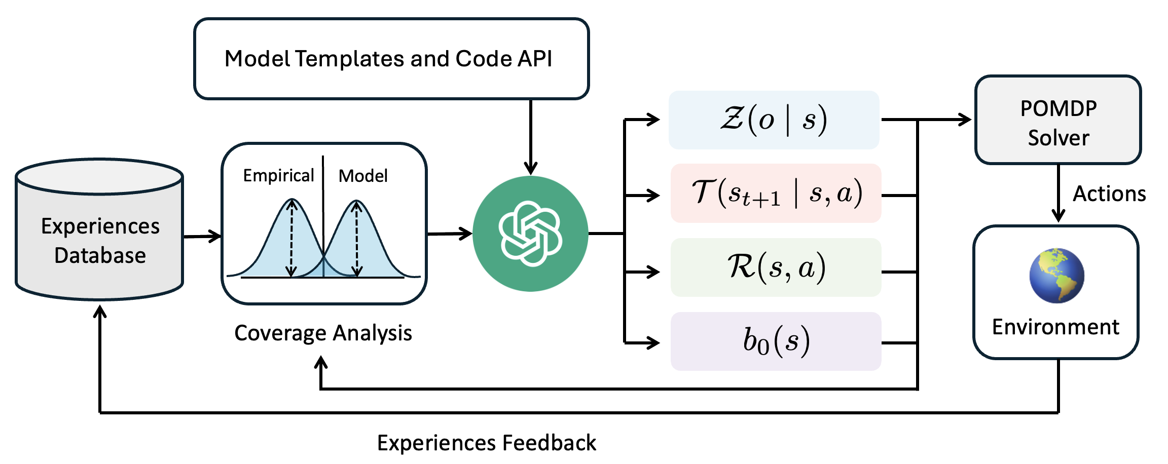<details> <summary>extracted/6430121/figures/arch.png Details</summary>  ### Visual Description ## Diagram: System Architecture for Model-Based Reinforcement Learning with Experience Feedback ### Overview The image is a technical flowchart diagram illustrating a closed-loop system for decision-making or reinforcement learning. It depicts how an "Experiences Database" feeds into a "Coverage Analysis" module, which is then processed by a central AI component (represented by a green circular icon) to generate the parameters of a Partially Observable Markov Decision Process (POMDP). These parameters are used by a "POMDP Solver" to select actions for an "Environment," with the resulting experiences looping back to the database. The diagram emphasizes a cycle of experience collection, model analysis, planning, and execution. ### Components/Axes The diagram is organized into several interconnected blocks and flows. There are no traditional chart axes. The key components, their labels, and spatial relationships are: 1. **Top Input Block (Top-Center):** * **Label:** `Model Templates and Code API` * **Description:** A rectangular box with a dark border. An arrow points downward from this block to the central AI icon. 2. **Experience Source (Left):** * **Label:** `Experiences Database` * **Description:** A cylinder icon representing a database. An arrow points rightward to the "Coverage Analysis" block. A feedback arrow from the bottom of the diagram points upward into this database. 3. **Analysis Module (Center-Left):** * **Label:** `Coverage Analysis` * **Description:** A rectangular block containing a plot. The plot shows two overlapping bell curves (distributions). The left curve is labeled `Empirical` and the right curve is labeled `Model`. Dashed vertical lines indicate the peaks of each distribution. An arrow points rightward from this block to the central AI icon. 4. **Central Processing Unit (Center):** * **Description:** A green circular icon containing a white, intricate knot or brain-like symbol. This is the central processing node. It receives inputs from "Model Templates and Code API" and "Coverage Analysis." It outputs four arrows to the right. 5. **POMDP Parameter Blocks (Center-Right):** * These are four colored, rounded rectangles stacked vertically, each containing a mathematical function. They are the outputs of the central AI. * **Top (Light Blue):** `Z(o | s)` - Observation model. * **Second (Light Pink):** `T(s_{t+1} | s, a)` - Transition model. * **Third (Light Green):** `R(s, a)` - Reward function. * **Bottom (Light Purple):** `b_0(s)` - Initial belief state. * **Spatial Grounding:** All four blocks are aligned vertically to the right of the central AI icon. Arrows from each point rightward to the "POMDP Solver." 6. **Solver (Right):** * **Label:** `POMDP Solver` * **Description:** A rectangular box. It receives inputs from the four POMDP parameter blocks. An arrow labeled `Actions` points downward from this block to the "Environment." 7. **Environment (Bottom-Right):** * **Label:** `Environment` * **Description:** A rectangular box containing a globe icon (Earth). It receives `Actions` from the solver. An arrow labeled `Experiences Feedback` originates from this block and travels leftward along the bottom of the diagram, then upward to the "Experiences Database." 8. **Feedback Loop (Bottom):** * **Label:** `Experiences Feedback` * **Description:** A long arrow running along the bottom edge of the diagram, connecting the "Environment" back to the "Experiences Database." A secondary branch of this feedback arrow points upward to the "Coverage Analysis" block. ### Detailed Analysis The diagram details a specific workflow: 1. **Data Flow:** The process begins with historical data in the `Experiences Database`. This data is analyzed in the `Coverage Analysis` module, which visually compares the distribution of empirical data against a model's predictions (the two bell curves). 2. **Model Generation:** The central AI (green icon) uses the results of the coverage analysis, along with predefined `Model Templates and Code API`, to construct or refine a POMDP model. It outputs the four core components of a POMDP: * `Z(o | s)`: The probability of making observation `o` given state `s`. * `T(s_{t+1} | s, a)`: The probability of transitioning to state `s_{t+1}` from state `s` after taking action `a`. * `R(s, a)`: The immediate reward received for taking action `a` in state `s`. * `b_0(s)`: The initial probability distribution over states (belief state). 3. **Planning and Execution:** The `POMDP Solver` uses these four parameters to compute optimal `Actions`. These actions are executed in the `Environment`. 4. **Learning Loop:** The outcomes of these actions in the environment generate new experiences. This `Experiences Feedback` is sent back to update the `Experiences Database` and is also used directly by the `Coverage Analysis` module, creating a closed loop for continuous learning and model improvement. ### Key Observations * The system is explicitly designed for **Partially Observable** environments, as indicated by the POMDP framework and the inclusion of an observation model `Z(o | s)` and a belief state `b_0(s)`. * The `Coverage Analysis` component is critical. Its visual depiction suggests the system's goal is to align the model's predictions with real-world empirical data, likely to identify and correct model inaccuracies or areas where the model is uncertain. * The feedback loop is dual-purpose: it populates the database for future analysis and provides immediate feedback to the coverage analysis, enabling rapid model adjustment. * The central AI icon acts as a **model constructor or refiner**, not just a solver. It translates analysis and templates into a formal mathematical model. ### Interpretation This diagram represents a sophisticated, adaptive model-based reinforcement learning system. The core innovation appears to be the integration of a dedicated **coverage analysis** step that explicitly compares model and data distributions. This suggests the system is designed to be **self-aware of its model's limitations**. The workflow implies a Peircean investigative cycle: 1. **Abduction:** The `Coverage Analysis` identifies a discrepancy (the gap between the `Empirical` and `Model` curves), posing a question about the model's accuracy. 2. **Deduction:** The central AI, using templates, hypothesizes a new or updated POMDP model (`Z, T, R, b_0`) that might better explain the data. 3. **Induction:** The `POMDP Solver` tests this hypothesis by generating actions in the `Environment`. The resulting `Experiences Feedback` provides new data to validate or refute the model's predictions in the next cycle. The system matters because it moves beyond simply using a fixed model for planning. It creates a framework for **continuous model discovery and validation** grounded in experience. This is crucial for deploying AI in complex, real-world environments where the initial model is likely to be incomplete or incorrect. The "Model Templates and Code API" input suggests this process can be guided by human knowledge or prior architectures, making it a hybrid of data-driven and knowledge-driven learning. </details> Figure 1: An architecture diagram for our POMDP coder method The objective of a POMDP is to find a policy $\pi$ that maximizes the expected discounted reward: $$ \max_{\pi}\;\mathbb{E}_{b_{0},\pi}\left[\sum_{t=0}^{\infty}\gamma^{t}\sum_{s \in\mathcal{S}}b_{t}(s)\sum_{s^{\prime}\in\mathcal{S}}\mathcal{T}(s^{\prime} \mid s,a_{t})\,\mathcal{R}(s,a_{t},s^{\prime})\right] $$ To illustrate the POMDP formulation and serve as a running example, consider the classic Tiger problem [26]. An agent faces two doors: one hides a tiger, the other a treasure. The true state $s$ consisting of the the tiger’s location is hidden. The agent can listen to receive a noisy observation $o$ of which door the tiger is behind, or open a door to gain a reward or incur a penalty. An ideal policy is to wait long enough to be confident in the tiger’s location before opening the door with the treasure. ### 3.2 Probabilistic Programs Probabilistic programming offers an expressive and concise way to represent complex probabilistic models as executable code. In our work, each component of the POMDP including the initial state model, transition dynamics, observation function, and reward structure is encoded as a short probabilistic program. We leverage Pyro [12], a flexible probabilistic programming framework built on Python, to specify these models. Pyro enables us to define generative models with inherent stochastic behavior. In our tiger problem example, the below implementation would be a correct probabilistic program for the observation model. [fontsize=, breaklines, tabsize=4, bgcolor=LightGray]python def tiger_observation_func(state: TigerState, act: TigerActions): if act != TigerActions.LISTEN: return TigerObservation(NONE) correct = bool(pyro.sample(”listen_correct”, Bernoulli(torch.tensor(0.85)))) tiger_left = state.tiger_location == 0 hear_left = (correct and tiger_left) or (not correct and not tiger_left) return TigerObservation(HEAR_LEFT if hear_left else HEAR_RIGHT) ### 3.3 POMDP Solvers While traditional offline solvers aim to compute a global policy over the entire belief space [27, 28, 29], these methods often face scalability challenges in high-dimensional or continuous environments. In contrast, online solvers focus on finding a solution from a specific initial belief and replan after every step as new observations become available. Online approaches such as Partially Observable Monte Carlo Planning (POMCP) [30, 31] and Partially Observable Upper Confidence Trees (POUCT) [32] combine Monte Carlo sampling with tree search to approximate optimal policies in real time. Additionally, determinized belief space planners simplify the stochastic nature of the problem by converting it into a deterministic surrogate, thereby enabling rapid replanning [33, 34, 35]. In our work, we adopt the determinized belief space planning approach due to its computational efficiency in larger problems. Please refer to Appendix C for specifics on our solver implementation. ## 4 POMDP Coder In our approach, which we call POMDP Coder, we decompose the problem into two major components: learning the probabilistic models that define the POMDP and using these learned models for online planning. The first part involves leveraging a Large Language Model (LLM) to generate, refine, and validate candidate probabilistic programs that represent the initial state, transition, observation, and reward functions. The second component uses these models within an online POMDP solver along with the current belief to find optimal actions to take in the environment. We assume the agent is provided access to an initial set of ten human-generated demonstrations $\mathcal{D}$ , where each demonstration consists of $(s_{t},a_{t},o_{t},s_{t+1})$ transitions. Since we are learning models instead of policies, there are no assumptions made about the quality of these demonstrations. However, we do make an assumption of post-hoc full observability [36]. That is, we assume the agent gets access to the intermediate states after an episode has terminated (see Section 7 for details). Additionally POMDP Coder is provided a code-based API defining the structure of the state, action, and observation space. Below is an example for the Tiger domain. [fontsize=, breaklines, tabsize=4, bgcolor=LightGray]python class TigerActions(enum.IntEnum): OPEN_LEFT = 0, OPEN_RIGHT = 1, LISTEN = 2 class TigerObservation(Observation): obs: int # 0 = hear left, 1 = hear right, 2 = none class TigerState(State): tiger_location: int # 0 = left, 1 = right 1: Input: A demo dataset $\mathcal{D}$ , max episodes $E$ , num particles $N$ , empty models $\theta=\emptyset$ 2: for $\text{episode}=1$ to $E$ do 3: $\theta=(\theta_{\text{trans}},\theta_{\text{rew}},\theta_{\text{obs}},\theta_{ \text{init}})\leftarrow\texttt{LearnModels}(\mathcal{D},\theta)$ $\triangleright$ Update all models using $\mathcal{D}$ 4: $b\leftarrow N\text{ samples from }\theta_{\text{init}}$ 5: while episode not terminated do 6: $a\leftarrow\texttt{POMDPSolver}(b,\theta)$ $\triangleright$ Plan best next action, see Appendix C 7: Execute $a$ in the world, observe $o$ 8: $b\leftarrow\texttt{ParticleFilter}(b,a,o,\theta)$ $\triangleright$ Update belief 9: Append $(a,o)$ to trajectory $\tau$ 10: end while 11: $\mathcal{D}\leftarrow\mathcal{D}\cup\tau$ $\triangleright$ Update demo data with new trajectory 12: end for 13: return $\theta$ Algorithm 1 POMDP Coder Given these inputs, POMDP Coder proceeds as outlined in Algorithm 1. It proposes an initial set of models that comprise the POMDP problem (Line 3), using a learning procedure detailed in Section 4.1. After an initial set of models is decided on, these models are passed to a POMDP solver along with the initial belief (Line 6) to find an optimal first action to take in the environment (Line 7). After an action is taken and an observation received, the belief is updated using particle filtering to form a new belief (Line 8). This process continues until the episode terminates or times out. Lastly, at the end of each episode, the trajectory is added to the dataset (Line 8) and the learning process repairs any inaccuracies that the previous model may have had under the new data (Line 3). ### 4.1 Learning Models We aim to learn four core components of a POMDP: the initial state distribution $P(s_{0})$ , the transition model $P(s_{t+1}\mid s_{t},a_{t})$ , the observation model $P(o_{t}\mid s_{t+1},a_{t})$ , and the reward model $R(s_{t},a_{t},s_{t+1})$ . Each of these components is expressed as a short probabilistic program. The objective of our learning procedure is to maximize a dataset coverage metric, which we define to be the proportion of data in $\mathcal{D}$ that has support under the model as follows: $$ \text{coverage}(P_{\theta},\mathcal{D})\;=\;\frac{1}{|\mathcal{D}|}\sum_{i=1}^ {|\mathcal{D}|}\mathbf{1}\!\Bigl{[}\,P_{\theta}\bigl{(}y_{i}\mid x_{i}\bigr{)} >0\,\Bigr{]}. $$ Although we experimented with other metrics such distributional distance metrics, we found that those were more prone to overfitting and less interpretable to an LLM than binary coverage feedback. Still, the coverage metric has its own limitations, which we discuss in Section 7. Our approach to learning these models builds on strategies previously developed for reward model learning [37], but extends them to the more general setting of POMDP model learning across multiple stochastic components (transition, observation, initial state, and reward), replaces accuracy with coverage, and introduces the notion of a testing and training split to avoid overfitting. At its core, our model learning strategy uses two operations: (1) LLM program proposal given a model function template and a set of examples from the database and and (2) LLM program repair given a previous model and set of examples that the previous model failed to cover. We run a stochastic procedure for sampling which program to repair next, which is biased toward repairing programs that have high coverage. The pseudocode and additional details can be found in the Appendix B. ## 5 Experiments ### 5.1 Simulated Experiments Simulated experiments were conducted on two categories of problems: classical POMDP problems from the literature and MiniGrid tasks. The classical POMDP problems serve as simplified benchmarks that capture the core challenges of decision making under uncertainty while keeping the problem domains small and tractable. In addition to the tiger problem, we evaluate on the rock sample problem [38]. <details> <summary>x1.png Details</summary>  ### Visual Description ## Diagram Series: Grid-Based Puzzle Level Layouts ### Overview The image displays a horizontal sequence of five distinct grid-based diagrams, each representing a different puzzle or game level layout. Each diagram is a rectangular grid composed of colored tiles and is labeled with a title below it. The diagrams appear to illustrate different environmental mechanics or challenges, likely from a puzzle game or a level design document. ### Components/Axes * **Structure:** Five separate grid diagrams arranged horizontally. * **Common Elements:** * **Grid:** Each diagram is a grid of square tiles (approximately 8x8 or similar). * **Tile Types (by color/pattern):** * **Black:** Solid, impassable walls or obstacles. * **Gray:** Open, passable floor or ground. * **Dark Blue with Diagonal Stripes:** A distinct terrain type, possibly water, void, or a special boundary. * **Green with Red Triangle:** A special tile, likely representing the player character, start point, or an interactive element. The red triangle points in a direction (down, up, right). * **Orange with Black Wavy Lines:** A hazard tile, explicitly labeled as "Lava." * **Labels:** Each diagram has a text label centered beneath it: "Empty", "Corners", "Lava", "Unlock", "Rooms". ### Detailed Analysis **Panel 1: "Empty"** * **Layout:** A large, roughly rectangular black area occupies the center-left. Gray floor surrounds it. A column of blue-striped tiles runs along the far left edge. * **Key Element:** The green/red triangle tile is located in the bottom-right quadrant on a gray tile. The triangle points downward. **Panel 2: "Corners"** * **Layout:** The black area forms a more complex, angular shape. Blue-striped tiles are prominent in the top-left and top-right corners, creating a framed effect. * **Key Element:** The green/red triangle tile is positioned in the top-left corner on a gray tile. The triangle points upward. **Panel 3: "Lava"** * **Layout:** Features a vertical column of orange "Lava" tiles running down the center. Black walls are on either side. Blue-striped tiles are present on the left and right edges. * **Key Element:** The green/red triangle tile is in the bottom-right corner, adjacent to the lava column. The triangle points downward. **Panel 4: "Unlock"** * **Layout:** Shows two main black rectangular areas separated by a narrow gray corridor. A single vertical blue line (possibly a door or barrier) is visible in the corridor. Blue-striped tiles are at the top and bottom edges. * **Key Element:** The green/red triangle tile is located in the right-hand black area, on a gray tile within it. The triangle points to the right. **Panel 5: "Rooms"** * **Layout:** The most complex layout, featuring multiple distinct black "rooms" connected by narrow gray corridors. The blue-striped tiles form a large outer boundary. * **Key Element:** The green/red triangle tile is situated inside a small, central black room. The triangle points upward. ### Key Observations 1. **Progression of Complexity:** The diagrams show a clear increase in structural complexity from "Empty" (simple block) to "Rooms" (multiple interconnected chambers). 2. **Mechanic Introduction:** Each panel introduces or highlights a specific game mechanic: basic navigation ("Empty"), angular movement ("Corners"), environmental hazard ("Lava"), a gating mechanism ("Unlock"), and multi-room exploration ("Rooms"). 3. **Player Start Position:** The green tile's location and orientation change in each diagram, suggesting different starting scenarios or objectives for each level. 4. **Consistent Visual Language:** The color and pattern coding for walls, floors, hazards, and the player is consistent across all five diagrams. ### Interpretation This image is a technical or design document illustrating a set of foundational puzzle templates or level archetypes. The diagrams are not random; they are carefully constructed to teach or test specific player skills and understanding of game rules. * **"Empty"** teaches basic movement and goal identification (reach the green tile?). * **"Corners"** introduces navigation around obstacles with diagonal boundaries. * **"Lava"** adds a dynamic hazard, requiring pathfinding that avoids a specific tile type. * **"Unlock"** implies a conditional progression mechanic (e.g., finding a key to remove the blue barrier). * **"Rooms"** combines previous elements into a more complex spatial reasoning challenge involving exploration and possibly backtracking. The sequence suggests a pedagogical or iterative design approach, where each level builds upon the mechanics introduced in the previous ones. The consistent use of the green/red triangle tile anchors the player's perspective across all varying environments. This is likely a reference for developers, artists, or testers to understand the core puzzle logic of a game. 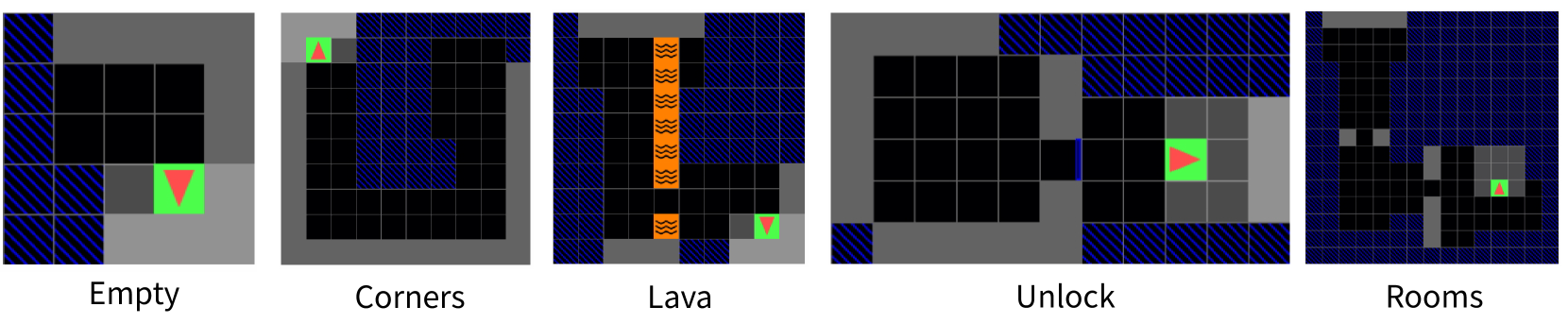</details> Figure 2: A visualization of the final belief state for each of the MiniGrid tasks. The green square is the goal, the red triangle is the agent, and the blue squares are places that the agent has not viewed. MiniGrid is a set of minimalistic gridworld tasks for testing navigation and planning under partial observability originally designed for reinforcement learning [39]. We evaluate on five of these environments. In the empty environment, the agent is deterministically placed in the top left cell of a 5×5 grid and must navigate to the green square in the bottom right. In the corners environment, the agent is randomly positioned with an arbitrary orientation in a 10×10 grid while the green square appears in a randomly selected corner. In the lava environment, the agent starts in the upper left corner of a 10×10 grid that features a randomly positioned column of lava with a gap forming a narrow passage to the green square. In the unlock environment, the agent is randomly placed in the left room of a two-room layout, must collect a randomly placed key to open a locked door, and then proceeds to the green square fixed at the center of the right room. In the rooms environment, the agent is initialized in the upper right-hand corner of a multi-room setting and must traverse through the rooms to reach the green square randomly located in the bottom right room. Each MiniGrid environment is modified from the original implementation [39]. This modification demonstrates the ability of our method to generalize to new environments not seen during LLM pretraining. ### 5.2 Baselines In our experiments, we evaluate our method against several diverse baselines to comprehensively assess its performance in partially observable environments. One baseline, termed the oracle, uses POMDP models that are hardcoded to exactly match the true dynamics of the environment, thereby serving as an upper-bound on achievable performance. In contrast, the random baseline takes actions arbitrarily at every step, establishing a lower-bound benchmark for comparison. Another baseline, referred to as direct LLM, involves querying a large language model for the next action at each decision point. In this setup, the LLM is provided with all the same information provided to POMDP Coder during model learning. The exact prompt template used for this method is detailed in Appendix E.4. Next, our evaluation includes a behavior cloning baseline, where a policy is constructed by mapping states to actions using a dictionary learned from the demonstration dataset. In addition, we consider a tabular baseline in which the POMDP models are learned as conditional probability tables derived from counts in the demonstration dataset. Lastly, we test against two ablations of POMDP Coder. The first is the offline only ablation which only makes use of the human demonstrations and does not update the model with its own experiences. Conversely, the online only ablation does not make use of the expert demonstrations, learning only from its own experiences. 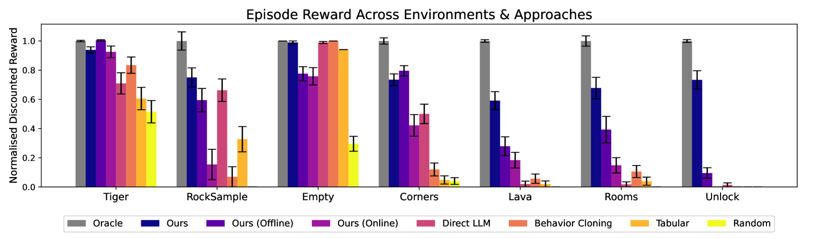### 5.3 Simulation Results We evaluate various methods using expected discounted reward defined in Section 3.1, measuring both total cumulative reward and efficiency. The results of our evaluations can be seen in Figure 3. We see POMDP Coder match or outperform all baseline methods across all domains. We observe that the behavior cloning and tabular baselines were fundamentally limited in their ability to generalize. This is because the set of possible initial states for many tasks was orders of magnitude larger than the training set. In contrast, the probabilistic programs written by POMDP Coder use symbolic abstraction to cover large portions of the state and observation spaces, allowing them to generalize to new situations. While the direct LLM approach was sometimes effective, such as in the rock sample domain, it frequently got stuck in infinite loops, failing to understand constraints such as obstacle obstruction despite the examples of collision it had access to in the dataset. POMDP Coder outperformed both the online-only and offline-only ablations across most environments. A common failure mode of the offline-only ablation was missing transitions outside expert demonstrations. For example, it will run into lava without knowing it causes death. In contrast, the online-only ablation struggled to discover informative actions due to inefficient random exploration. For instance, in the unlock environment, if the agent never used the key, the model failed to learn that behavior, and random actions rarely uncovered it. In addition to success metrics, we record some additional runtime statistics such as the number of candidate programs generated during offline and online learning in Table 2 as well as the training and testing coverage scores after offline model learning in Table 3. <details> <summary>x2.png Details</summary>  ### Visual Description ## Bar Chart: Episode Reward Across Environments & Approaches ### Overview This is a grouped bar chart comparing the performance of eight different algorithmic approaches across seven distinct reinforcement learning environments. Performance is measured by "Normalised Discounted Reward," a metric scaled between 0.0 and 1.0, where higher values indicate better performance. Each environment cluster contains eight bars, one for each approach, with error bars indicating variability. ### Components/Axes * **Chart Title:** "Episode Reward Across Environments & Approaches" * **Y-Axis:** * **Label:** "Normalised Discounted Reward" * **Scale:** Linear, from 0.0 to 1.0, with major tick marks at 0.0, 0.2, 0.4, 0.6, 0.8, and 1.0. * **X-Axis:** * **Label:** Environment names. * **Categories (from left to right):** Tiger, RockSample, Empty, Corners, Lava, Rooms, Unlock. * **Legend:** Positioned at the bottom of the chart, centered. It maps colors to approach names: * **Grey:** Oracle * **Dark Blue:** Ours * **Purple:** Ours (Offline) * **Magenta:** Ours (Online) * **Pink:** Direct LLM * **Salmon/Orange-Red:** Behavior Cloning * **Orange:** Tabular * **Yellow:** Random ### Detailed Analysis Performance is analyzed per environment cluster, moving left to right. Approximate values are estimated from the bar heights relative to the y-axis. **1. Tiger:** * **Trend:** Oracle, Ours, and Ours (Online) perform best, near the maximum reward. Performance generally decreases across the remaining approaches. * **Approximate Values:** * Oracle: ~1.0 * Ours: ~0.95 * Ours (Offline): ~0.92 * Ours (Online): ~0.92 * Direct LLM: ~0.70 * Behavior Cloning: ~0.82 * Tabular: ~0.60 * Random: ~0.52 **2. RockSample:** * **Trend:** Oracle is highest. "Ours" and "Ours (Online)" show moderate performance. "Ours (Offline)" and "Direct LLM" are notably lower. "Behavior Cloning" is very low. * **Approximate Values:** * Oracle: ~1.0 * Ours: ~0.75 * Ours (Offline): ~0.60 * Ours (Online): ~0.66 * Direct LLM: ~0.15 * Behavior Cloning: ~0.08 * Tabular: ~0.33 * Random: ~0.0 (near zero) **3. Empty:** * **Trend:** A high-performance cluster. Oracle, Ours, Ours (Online), and Tabular all achieve near-maximum reward. Ours (Offline) is slightly lower. Random is the only low-performing approach. * **Approximate Values:** * Oracle: ~1.0 * Ours: ~0.99 * Ours (Offline): ~0.76 * Ours (Online): ~0.99 * Direct LLM: ~1.0 * Behavior Cloning: ~0.94 * Tabular: ~0.94 * Random: ~0.28 **4. Corners:** * **Trend:** Oracle is highest. "Ours" and "Ours (Online)" are the next best group. Performance drops significantly for the remaining approaches. * **Approximate Values:** * Oracle: ~1.0 * Ours: ~0.72 * Ours (Offline): ~0.79 * Ours (Online): ~0.49 * Direct LLM: ~0.50 * Behavior Cloning: ~0.12 * Tabular: ~0.05 * Random: ~0.05 **5. Lava:** * **Trend:** Oracle is highest. "Ours" is the only other approach with substantial reward. All other approaches perform very poorly, near zero. * **Approximate Values:** * Oracle: ~1.0 * Ours: ~0.59 * Ours (Offline): ~0.28 * Ours (Online): ~0.18 * Direct LLM: ~0.03 * Behavior Cloning: ~0.05 * Tabular: ~0.03 * Random: ~0.02 **6. Rooms:** * **Trend:** Oracle is highest. "Ours" shows moderate performance. All other approaches have low to very low rewards. * **Approximate Values:** * Oracle: ~1.0 * Ours: ~0.68 * Ours (Offline): ~0.39 * Ours (Online): ~0.15 * Direct LLM: ~0.03 * Behavior Cloning: ~0.11 * Tabular: ~0.05 * Random: ~0.02 **7. Unlock:** * **Trend:** Oracle is highest. "Ours" is the only other approach with a significant reward. All other approaches perform at or near zero. * **Approximate Values:** * Oracle: ~1.0 * Ours: ~0.73 * Ours (Offline): ~0.09 * Ours (Online): ~0.01 * Direct LLM: ~0.02 * Behavior Cloning: ~0.0 * Tabular: ~0.0 * Random: ~0.0 ### Key Observations 1. **Oracle Dominance:** The "Oracle" approach (grey bar) consistently achieves the maximum normalized reward (~1.0) across all seven environments, serving as an upper-bound benchmark. 2. **"Ours" Consistency:** The "Ours" approach (dark blue) is the most consistent non-oracle performer, maintaining moderate to high rewards in every environment. 3. **Environment Difficulty:** There is a clear gradient in task difficulty. "Empty" appears to be the easiest, with six of eight approaches scoring above 0.75. "Lava," "Rooms," and "Unlock" appear to be the hardest, with only Oracle and "Ours" achieving meaningful rewards. 4. **Approach Variability:** The performance of approaches like "Direct LLM," "Behavior Cloning," and "Tabular" is highly environment-dependent. They perform well in "Empty" but fail in "Lava" or "Unlock." 5. **"Random" Baseline:** The "Random" approach (yellow) performs poorly across all environments, as expected, confirming the tasks require learned policy. ### Interpretation This chart demonstrates the comparative efficacy of different learning paradigms in varied reinforcement learning settings. The "Oracle" represents an idealized upper bound, likely using perfect model knowledge. The strong, consistent performance of "Ours" suggests it is a robust method that generalizes well across diverse task structures (from navigation in "Empty" to complex manipulation in "Unlock"). The data highlights a key challenge in AI: methods that excel in simple or specific domains (like "Tabular" in "Empty") often fail to transfer to more complex, sparse-reward environments. The significant drop-off for most methods in "Lava," "Rooms," and "Unlock" indicates these environments pose fundamental challenges related to exploration, long-term planning, or partial observability that only the most sophisticated approaches ("Oracle" and "Ours") can handle. The chart argues for the development of generalizable algorithms, as specialized techniques show brittle performance. </details> Figure 3: Experimental results for the MiniGrid and Classical POMDP domains. We show the expected discounted returns ( $\gamma=0.98$ ) of each method across five learning seeds with ten episodes per seed. The error bars show standard error across all episodes. We normalize the expected discounted returns by the performance of Oracle. ### 5.4 Real Robot Experiments Our real robot experiments are conducted using a Boston Dynamics Spot robot. The robot carries an in-hand camera mounted on a 6-DoF arm at its back. April tags are distributed throughout the area, enabling precise localization. The goal is for the robot to find an pick up an apple placed within the scene. Before any demonstrations are gathered, we construct a map of the empty room by scanning it with PolyCam [40]. This scan is used to construct a scene representation that includes an object-centric scene graph, encoding “on” relationships derived from geometric cues, and an occupancy grid delineating forbidden zones corresponding to physical obstacles. For each real-world task, ten demonstrations are collected by commanding the robot via keyboard. The agent’s action space is discretized into fixed theta rotations to the left and right and movements in the four cardinal directions. Objects are detected online using Grounding SAM, an open vocabulary object detector [41, 42, 43]. 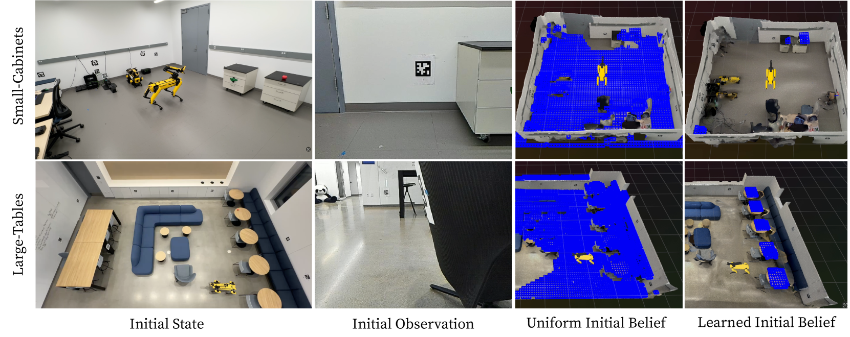We test our method in two distinct spaces. The first is a small, closed-off room, as shown in the top row of Figure 4, which contains a few tables, chairs, and drawer cabinets. The second is a large, open lobby area depicted in the bottom row of Figure 4, furnished with more than twenty pieces of furniture. Within these environments, task distributions are defined by varying the location of the apple. In the Small-Cabinets configuration, which takes place in the small room, the apple is consistently placed on top of one of the three drawer cabinets for each demonstration. In the Large-Tables setting within the large room, the apple is positioned on one of the five round tables. Our approach is compared against a subset of baselines evaluated in Section 5.2. The evaluation includes behavior cloning, direct LLM execution, and a hardcoded uniform baseline that assumes the object is placed uniformly throughout the search space. Although the uniform baseline requires additional task-specific human input and is not strictly an apples-to-apples comparison, it demonstrates that our method can outperform a naively designed initial state distribution. The results shown in Table 1 demonstrate that POMDP Coder achieves more efficient and accurate exploration by understanding and generalizing trends in initial state distribution seen in the training data. Specifically, our approach learns that objects are always on top of objects of a particular class, and constructs an initial state distribution that captures that without overfitting to specific initial states. <details> <summary>x3.png Details</summary>  ### Visual Description ## Diagram: Robotic Belief State Visualization in Indoor Environments ### Overview The image is a composite diagram arranged in a 2x4 grid. It illustrates a robotic perception or mapping experiment conducted in two distinct indoor environments. The experiment tracks the state of a yellow quadruped robot (resembling a Boston Dynamics Spot) and its surroundings across four stages: the initial physical state, an initial camera observation, an initial uniform belief state, and a final learned belief state. The visualization compares how the robot's internal model of the world (its "belief") evolves from a generic, uniform assumption to a learned, environment-specific model. ### Components/Axes **Row Labels (Vertical Axis - Left Side):** * **Top Row:** "Small-Cabinets" * **Bottom Row:** "Large-Tables" **Column Labels (Horizontal Axis - Bottom):** 1. **Initial State:** A wide-angle, third-person photograph of the physical environment. 2. **Initial Observation:** A first-person perspective image, likely from the robot's onboard camera. 3. **Uniform Initial Belief:** A 3D visualization (voxel grid) representing the robot's initial, uninformative guess about the environment's occupancy. 4. **Learned Initial Belief:** A 3D visualization representing the robot's updated, learned model of the environment after processing observations. **Visual Elements:** * **Robot:** A yellow, four-legged robot appears in all "Initial State" panels and in the "Learned Initial Belief" visualizations. * **Environment Objects:** Includes cabinets, tables, chairs, sofas, doors, walls, and floor markings. * **AprilTag:** A fiducial marker (black and white square pattern) is visible on a wall in the "Initial Observation" panel for the "Small-Cabinets" row. * **3D Visualizations (Columns 3 & 4):** Use a grid of blue cubes (voxels) to represent occupied or explored space. The background is a dark grid plane. The robot model is rendered in yellow within this space. ### Detailed Analysis **Row 1: Small-Cabinets Environment** * **Initial State:** Shows a lab-like room with grey flooring and white walls. The yellow robot is positioned centrally. To the right are two small, white mobile cabinets with black tops. A red object sits on one cabinet. A door is visible in the background. Various cables and equipment are on the floor to the left. * **Initial Observation:** A close-up, first-person view focusing on a white wall. An AprilTag is affixed to the wall. The edge of a white cabinet is visible on the right. The floor is grey. * **Uniform Initial Belief:** A top-down, isometric 3D view. The entire floor area is covered in a dense, uniform grid of blue voxels, indicating the robot initially assumes the entire space is equally likely to be occupied or unexplored. The yellow robot model is placed in the center. The walls are rendered as grey boundaries. * **Learned Initial Belief:** The same 3D view, but the blue voxel grid is now sparse and structured. Voxels are clustered around the actual locations of the cabinets, the door frame, and other obstacles. The floor area is largely clear of blue voxels, indicating the robot has learned these are free spaces. The robot's position is updated. **Row 2: Large-Tables Environment** * **Initial State:** Shows a lounge or break room. A large, blue, L-shaped sofa dominates the center, surrounded by several small, round, light-wood tables. A long, rectangular wooden table is against the left wall. The yellow robot is near the sofa. The floor is a polished, light-colored material. * **Initial Observation:** A first-person view from a low angle, looking past a black office chair. In the background, a panda plush toy is visible on the floor near a doorway. The environment appears bright. * **Uniform Initial Belief:** Similar to the first row, the 3D view shows a near-complete, uniform coverage of blue voxels across the floor plan, representing an uninformed prior belief. * **Learned Initial Belief:** The blue voxels are now precisely localized. They form clear outlines corresponding to the positions of the sofa, the round tables, and the long table against the wall. The open floor spaces are free of voxels. The robot's model now accurately reflects the cluttered layout of the lounge. ### Key Observations 1. **Contrast in Environments:** The "Small-Cabinets" environment is sparse and utilitarian, while the "Large-Tables" environment is cluttered with furniture. 2. **Belief Evolution:** The core visual narrative is the dramatic transformation from the "Uniform Initial Belief" (a solid blue floor) to the "Learned Initial Belief" (a structured, obstacle-aware map). This demonstrates the process of perceptual learning. 3. **Spatial Accuracy:** In the "Learned Initial Belief" panels, the blue voxels align well with the physical objects seen in the "Initial State" photos, indicating successful mapping. 4. **Role of Observation:** The "Initial Observation" panels provide the specific, first-person visual data (like the AprilTag) that likely seeds or calibrates the belief-updating process. ### Interpretation This diagram visually documents a robotic system's capability to build an accurate internal model (a belief state) of its environment from sensory data. The "Uniform Initial Belief" represents a state of maximum uncertainty or a generic prior assumption. The "Learned Initial Belief" represents the posterior belief after Bayesian or similar updating, where the model has incorporated observations to identify free space and obstacles. The experiment highlights the importance of **active perception**. The robot doesn't just passively receive data; its belief state is a structured representation that it can use for planning navigation or manipulation tasks. The inclusion of two very different environments (sparse vs. cluttered) suggests the method is being tested for robustness across scenarios. The presence of the AprilTag implies the system may use known markers for localization or to ground its perceptual learning. Ultimately, the image serves as a qualitative result, showing that the learning algorithm successfully moves the robot's understanding from a blank slate to a useful, environment-specific map. </details> Figure 4: The two real-world experimental setups wherein a robot is searching for an apple in a partially observable world. The blue cells represent the robot’s belief about where the apple could be in the world. In the uniform initial belief, the robot thinks the apple could be anywhere it has not looked yet. The learned initial belief found by POMDP Coder has a narrower initial belief leading to more efficient exploration. $$ \textbf{0.89}\pm{\textbf{0.09}}\;(10) 0.68\pm{0.21}\;(10) 0.25\pm{0.42}\;(3) 0.28\pm{0.39}\;(4) 0.35\pm{0.41}\;(5) \textbf{0.73}\pm{\textbf{0.08}}\;(10) 0.40\pm{0.26}\;(8) 0.15\pm{0.32}\;(2) 0.13\pm{0.28}\;(2) 0.13\pm{0.22}\;(3) \tag{10} $$ Table 1: Real-world experiment results on the small room domain in the top row of Figure 4 and the large room domain in the bottom row of Figure 4. The table shows the mean and standard deviation of expected discounted reward (with $\gamma=0.98$ ) under the ground-truth reward model (1 if the agent is holding the apple and 0 otherwise) along with the number of successes over ten runs in parenthesis. ## 6 Discussion In this work, we have presented a novel approach to learning interpretable, low-complexity POMDP models by integrating LLM-guided probabilistic program induction with online planning. Our method leverages large language models to generate and iteratively refine candidate probabilistic programs that capture the dynamics, observation functions, initial state distributions, and reward structures of complex environments. Experimental results on simulated MiniGrid domains and real-world robotics scenarios demonstrate that our approach can significantly enhance sample efficiency and predictive accuracy compared to traditional tabular learning methods, behavior cloning, or direct LLM planning. Our findings further suggest that environments represented with structured scene graphs and other rich input representations can be better modeled by learning a world model within which a reasoning agent can operate, rather than by directly learning a policy that maps observation histories to actions or by attempting to apply a language model in a zero-shot setting. This is particularly evident in large, partially observable worlds where the belief space is considerably more complex and challenging to cover with training examples than the space of states itself. The use of code to represent these models is especially advantageous, as language models are adept at generating concise, executable snippets that can be interpreted, debugged, and evaluated post-hoc, thus providing an additional layer of transparency and robustness in model evaluation. ## 7 Limitations Despite these promising results, several limitations remain. Our approach currently relies on human expertise to design the underlying representation over which the world model is learned, which may constrain its applicability to domains where such structured representations are not readily available. Additionally, due to our post-hoc observability assumption, collecting datasets outside of a simulator requires one of the following: human state annotation, complete robot exploration after the episode, or third-party perspectives such as externally mounted cameras. In our real robot experiments, this was not a challenge because the only state variability was in the position of the goal object, which is fully determined upon completion of the task. More complex problems with multiple dimensions of both task-relevant and task-irrelevant uncertainty would require more than just the agent’s perspective. Alleviating this assumption may require jointly reasoning about the interrelated structure of the constituent models, and is a valuable direction for future work. Moreover, the particle filter employed in our current implementation does not scale well to arbitrarily large state spaces. Future work may address this limitation by incorporating more advanced inference techniques, such as factored particle filters or other scalable methods, to improve performance in high-dimensional settings. Another area for improvement is in the sometimes overly broad distributions proposed by the LLM due to the coverage metric indirectly rewarding broader distributions. While this doesn’t make the problem infeasible, it can lead to less efficient behavior. A direction for future work could be to use inference methods on the hidden variables of the proposed probabilistic program to strike a balance between the empirical distribution and the overly broad model distribution. Lastly, our study focuses exclusively on discrete state and action spaces, despite robotics tasks requiring search over continuous spaces such as grasps and poses. Extending our learning strategy and adopting continuous-space POMDP solvers would broaden our framework to these domains, enabling more complex manipulation and navigation tasks. Ultimately, our work opens up exciting avenues for combining the strengths of probabilistic programming and large language models to construct robust, interpretable models for decision-making under uncertainty. ## References - Song et al. [2016] W. Song, G. Xiong, and H. Chen. Intention-aware autonomous driving decision-making in an uncontrolled intersection. Mathematical Problems in Engineering, 2016:1–15, 01 2016. doi: 10.1155/2016/1025349. - Ghorbel et al. [2018] M. Ghorbel, J. Pineau, R. Gourdeau, S. Javdani, and S. Srinivasa. A decision-theoretic approach for the collaborative control of a smart wheelchair. International Journal of Social Robotics, 10, 01 2018. doi: 10.1007/s12369-017-0434-7. - Pajarinen and Kyrki [2017] J. Pajarinen and V. Kyrki. Robotic manipulation of multiple objects as a pomdp. Artificial Intelligence, 247:213–228, 2017. ISSN 0004-3702. doi: https://doi.org/10.1016/j.artint.2015.04.001. URL https://www.sciencedirect.com/science/article/pii/S0004370215000570. Special Issue on AI and Robotics. - Zheng et al. [2023] K. Zheng, A. Paul, and S. Tellex. A system for generalized 3d multi-object search. In 2023 IEEE International Conference on Robotics and Automation (ICRA), pages 1638–1644, 2023. doi: 10.1109/ICRA48891.2023.10161387. - Moerland et al. [2020] T. M. Moerland, J. Broekens, and C. M. Jonker. Model-based reinforcement learning: A survey. CoRR, abs/2006.16712, 2020. URL https://arxiv.org/abs/2006.16712. - Mossel and Roch [2005] E. Mossel and S. Roch. Learning nonsingular phylogenies and hidden markov models. CoRR, abs/cs/0502076, 2005. URL http://arxiv.org/abs/cs/0502076. - Ross et al. [2007] S. Ross, B. Chaib-draa, and J. Pineau. Bayes-adaptive pomdps. In J. Platt, D. Koller, Y. Singer, and S. Roweis, editors, Advances in Neural Information Processing Systems, volume 20. Curran Associates, Inc., 2007. URL https://proceedings.neurips.cc/paper_files/paper/2007/file/3b3dbaf68507998acd6a5a5254ab2d76-Paper.pdf. - Boots et al. [2009] B. Boots, S. M. Siddiqi, and G. J. Gordon. Closing the learning-planning loop with predictive state representations, 2009. URL https://arxiv.org/abs/0912.2385. - Jin et al. [2020] C. Jin, S. M. Kakade, A. Krishnamurthy, and Q. Liu. Sample-efficient reinforcement learning of undercomplete pomdps. CoRR, abs/2006.12484, 2020. URL https://arxiv.org/abs/2006.12484. - Makino and Takeuchi [2012] T. Makino and J. Takeuchi. Apprenticeship learning for model parameters of partially observable environments, 2012. URL https://arxiv.org/abs/1206.6484. - Thomson et al. [2010] B. Thomson, F. Jurčíček, M. Gašić, S. Keizer, F. Mairesse, K. Yu, and S. Young. Parameter learning for pomdp spoken dialogue models. In 2010 IEEE Spoken Language Technology Workshop, pages 271–276, 2010. doi: 10.1109/SLT.2010.5700863. - Bingham et al. [2018] E. Bingham, J. P. Chen, M. Jankowiak, F. Obermeyer, N. Pradhan, T. Karaletsos, R. Singh, P. A. Szerlip, P. Horsfall, and N. D. Goodman. Pyro: Deep universal probabilistic programming. CoRR, abs/1810.09538, 2018. URL http://arxiv.org/abs/1810.09538. - Cusumano-Towner et al. [2019] M. F. Cusumano-Towner, F. A. Saad, A. K. Lew, and V. K. Mansinghka. Gen: a general-purpose probabilistic programming system with programmable inference. In Proceedings of the 40th ACM SIGPLAN Conference on Programming Language Design and Implementation, PLDI 2019, page 221–236, New York, NY, USA, 2019. Association for Computing Machinery. ISBN 9781450367127. doi: 10.1145/3314221.3314642. URL https://doi.org/10.1145/3314221.3314642. - Goodman et al. [2012] N. D. Goodman, V. Mansinghka, D. M. Roy, K. A. Bonawitz, and J. B. Tenenbaum. Church: a language for generative models. CoRR, abs/1206.3255, 2012. URL http://arxiv.org/abs/1206.3255. - Ellis et al. [2020] K. Ellis, C. Wong, M. I. Nye, M. Sablé-Meyer, L. Cary, L. Morales, L. B. Hewitt, A. Solar-Lezama, and J. B. Tenenbaum. Dreamcoder: Growing generalizable, interpretable knowledge with wake-sleep bayesian program learning. CoRR, abs/2006.08381, 2020. URL https://arxiv.org/abs/2006.08381. - Lake et al. [2015] B. M. Lake, R. Salakhutdinov, and J. B. Tenenbaum. Human-level concept learning through probabilistic program induction. Science, 350(6266):1332–1338, 2015. doi: 10.1126/science.aab3050. URL https://doi.org/10.1126/science.aab3050. - Li et al. [2024] M. Y. Li, E. B. Fox, and N. D. Goodman. Automated statistical model discovery with language models, 2024. URL https://arxiv.org/abs/2402.17879. - Wong et al. [2023] L. Wong, G. Grand, A. K. Lew, N. D. Goodman, V. K. Mansinghka, J. Andreas, and J. B. Tenenbaum. From word models to world models: Translating from natural language to the probabilistic language of thought, 2023. URL https://arxiv.org/abs/2306.12672. - Grand et al. [2024] G. Grand, V. Pepe, J. Andreas, and J. B. Tenenbaum. Loose lips sink ships: Asking questions in battleship with language-informed program sampling, 2024. URL https://arxiv.org/abs/2402.19471. - Liang et al. [2025] Y. Liang, N. Kumar, H. Tang, A. Weller, J. B. Tenenbaum, T. Silver, J. F. Henriques, and K. Ellis. Visualpredicator: Learning abstract world models with neuro-symbolic predicates for robot planning, 2025. URL https://arxiv.org/abs/2410.23156. - Tang et al. [2024] H. Tang, D. Key, and K. Ellis. Worldcoder, a model-based llm agent: Building world models by writing code and interacting with the environment, 2024. URL https://arxiv.org/abs/2402.12275. - Curtis et al. [2024] A. Curtis, N. Kumar, J. Cao, T. Lozano-Pérez, and L. P. Kaelbling. Trust the proc3s: Solving long-horizon robotics problems with llms and constraint satisfaction, 2024. URL https://arxiv.org/abs/2406.05572. - Hao et al. [2024] Y. Hao, Y. Chen, Y. Zhang, and C. Fan. Large language models can plan your travels rigorously with formal verification tools. In arxiv preprint, 2024. URL https://arxiv.org/abs/2404.11891. - Ye et al. [2024] X. Ye, Q. Chen, I. Dillig, and G. Durrett. Satlm: Satisfiability-aided language models using declarative prompting. Advances in Neural Information Processing Systems (NeurIPS), 2024. URL https://arxiv.org/pdf/2305.09656. - Thrun et al. [2005] S. Thrun, W. Burgard, and D. Fox. Probabilistic Robotics (Intelligent Robotics and Autonomous Agents). The MIT Press, 2005. ISBN 0262201623. - Kaelbling et al. [1998] L. P. Kaelbling, M. L. Littman, and A. R. Cassandra. Planning and acting in partially observable stochastic domains. Artificial Intelligence, 101(1):99–134, 1998. ISSN 0004-3702. doi: https://doi.org/10.1016/S0004-3702(98)00023-X. URL https://www.sciencedirect.com/science/article/pii/S000437029800023X. - Mundhenk et al. [1997] M. Mundhenk, J. Goldsmith, and E. Allender. The complexity of policy evaluation for finite-horizon partially-observable markov decision processes. In I. Prívara and P. Ružička, editors, Mathematical Foundations of Computer Science 1997, pages 129–138, Berlin, Heidelberg, 1997. Springer Berlin Heidelberg. ISBN 978-3-540-69547-9. - Littman [1995] M. Littman. The witness algorithm: Solving partially observable markov decision processes. 02 1995. - Cassandra et al. [2013] A. R. Cassandra, M. L. Littman, and N. L. Zhang. Incremental pruning: A simple, fast, exact method for partially observable markov decision processes. CoRR, abs/1302.1525, 2013. URL http://arxiv.org/abs/1302.1525. - Silver and Veness [2010] D. Silver and J. Veness. Monte-Carlo planning in large POMDPs. In J. Lafferty, C. Williams, J. Shawe-Taylor, R. Zemel, and A. Culotta, editors, Advances in Neural Information Processing Systems, volume 23. Curran Associates, Inc., 2010. - Curtis et al. [2022] A. Curtis, L. Kaelbling, and S. Jain. Task-directed exploration in continuous pomdps for robotic manipulation of articulated objects, 2022. URL https://arxiv.org/abs/2212.04554. - Sunberg and Kochenderfer [2017] Z. Sunberg and M. J. Kochenderfer. POMCPOW: an online algorithm for pomdps with continuous state, action, and observation spaces. CoRR, abs/1709.06196, 2017. URL http://arxiv.org/abs/1709.06196. - Yoon et al. [2007] S. W. Yoon, A. Fern, and R. Givan. Ff-replan: A baseline for probabilistic planning. In International Conference on Automated Planning and Scheduling, 2007. URL https://api.semanticscholar.org/CorpusID:15013602. - Kaelbling and Lozano-Perez [2013] L. Kaelbling and T. Lozano-Perez. Integrated task and motion planning in belief space. The International Journal of Robotics Research, 32:1194–1227, 08 2013. doi: 10.1177/0278364913484072. - Curtis et al. [2024] A. Curtis, G. Matheos, N. Gothoskar, V. Mansinghka, J. Tenenbaum, T. Lozano-Pérez, and L. P. Kaelbling. Partially observable task and motion planning with uncertainty and risk awareness, 2024. URL https://arxiv.org/abs/2403.10454. - Pinto et al. [2017] L. Pinto, M. Andrychowicz, P. Welinder, W. Zaremba, and P. Abbeel. Asymmetric actor critic for image-based robot learning. CoRR, abs/1710.06542, 2017. URL http://arxiv.org/abs/1710.06542. - Tang et al. [2024] H. Tang, K. Hu, J. P. Zhou, S. Zhong, W.-L. Zheng, X. Si, and K. Ellis. Code repair with llms gives an exploration-exploitation tradeoff. In A. Globerson, L. Mackey, D. Belgrave, A. Fan, U. Paquet, J. Tomczak, and C. Zhang, editors, Advances in Neural Information Processing Systems, volume 37, pages 117954–117996. Curran Associates, Inc., 2024. URL https://proceedings.neurips.cc/paper_files/paper/2024/file/d5c56ec4f69c9a473089b16000d3f8cd-Paper-Conference.pdf. - Smith and Simmons [2012] T. Smith and R. G. Simmons. Heuristic search value iteration for pomdps. CoRR, abs/1207.4166, 2012. URL http://arxiv.org/abs/1207.4166. - Chevalier-Boisvert et al. [2023] M. Chevalier-Boisvert, B. Dai, M. Towers, R. de Lazcano, L. Willems, S. Lahlou, S. Pal, P. S. Castro, and J. Terry. Minigrid & miniworld: Modular & customizable reinforcement learning environments for goal-oriented tasks. CoRR, abs/2306.13831, 2023. - Polycam [2025] Polycam. Polycam – capture and share 3d models, 2025. URL https://poly.cam/. Accessed: 2025-04-30. - Liu et al. [2023] S. Liu, Z. Zeng, T. Ren, F. Li, H. Zhang, J. Yang, C. Li, J. Yang, H. Su, J. Zhu, et al. Grounding dino: Marrying dino with grounded pre-training for open-set object detection. arXiv preprint arXiv:2303.05499, 2023. - Ren et al. [2024] T. Ren, S. Liu, A. Zeng, J. Lin, K. Li, H. Cao, J. Chen, X. Huang, Y. Chen, F. Yan, Z. Zeng, H. Zhang, F. Li, J. Yang, H. Li, Q. Jiang, and L. Zhang. Grounded sam: Assembling open-world models for diverse visual tasks, 2024. - Smith and Simmons [2012] T. Smith and R. G. Simmons. Heuristic search value iteration for pomdps. CoRR, abs/1207.4166, 2012. URL http://arxiv.org/abs/1207.4166. ## Appendix A Code Release The full implementation, including all code, trained models, and experiment configurations, will be released publicly upon publication to ensure reproducibility and facilitate future research. ## Appendix B Model Learning The learning algorithm follows the pseudocode in Algorithm 2. Firstly, in order to mitigate overfitting to spurious patterns, we split the demonstration dataset into separate training and test sets (Line 3). Given the training set and a code-based interface that specifies how states, actions, and observations are represented, we query an LLM to propose an initial code snippet for a given component (Line 4, see Appendix E.2 for prompt). 1: Input: demonstration dataset $\mathcal{D}$ , initial model $\theta_{\text{prev}}$ , budget $N$ 2: Output: Learned model $\theta_{\text{new}}$ 3: Split $\mathcal{D}$ into $\mathcal{D}_{\text{train}},\mathcal{D}_{\text{test}}$ 4: if $\theta=\emptyset$ then $\theta_{\text{prev}}\leftarrow\text{LLM Init using }\mathcal{D}_{\text{train}}$ $\triangleright$ Appendix E.2 5: $\text{coverage},\mathcal{D}_{\text{errors}}\leftarrow\texttt{Eval}(\theta_{ \text{prev}},\mathcal{D}_{\text{test}},\mathcal{D}_{\text{train}})$ $\triangleright$ Discrepancy between model & empirical 6: $\text{beta}\leftarrow\text{Beta}(1+C\cdot\text{coverage},1+C\cdot(1-\text{ coverage}))$ 7: $\mathcal{M}\leftarrow\{(\theta_{\text{prev}},\text{beta},\mathcal{D}_{\text{ errors}})\}$ 8: while $\text{coverage}<1.0$ and $\text{iterations}<M$ do 9: $(\theta_{\text{new}},\text{Beta}(\alpha,\beta),\mathcal{D}_{\text{errors}}) \leftarrow\text{argmax}_{\mathcal{M}}(p\sim\text{beta})$ $\triangleright$ Thompson sampling 10: $\theta_{\text{new}}^{\prime}\leftarrow$ LLM refinement using $\theta_{\text{new}}$ and $\mathcal{D}_{\text{errors}}$ $\triangleright$ Appendix E.3 11: $\text{coverage}^{\prime},\mathcal{D}_{\text{errors}}^{\prime}\leftarrow\texttt {Eval}(\theta_{\text{new}},\mathcal{D}_{\text{test}},\mathcal{D}_{\text{train}})$ 12: $\text{beta}^{\prime}\leftarrow\text{Beta}(\alpha+C\cdot\text{coverage}^{\prime },\beta+C\cdot(1-\text{coverage}^{\prime}))$ 13: insert $(\theta_{\text{new}}^{\prime},\text{beta}^{\prime},\text{coverage}^{\prime})$ into $\mathcal{M}$ 14: end while 15: return $\text{argmax}_{\mathcal{M}}(\text{coverage})[0]$ $\triangleright$ Return the model with the best overall coverage Algorithm 2 LearnModel Following the initial candidate model proposal, we evaluate them against the empirical conditional probability distributions observed in the demonstration data (Line 5). Determining if a particular outcome is possible under an arbitrary code model is not analytically possible in most probabilistic programming languages, including Pyro, so we use Monte Carlo approximation of the model density. Any empirical sample that is never produced is treated as a failure and recorded in an error set $\mathcal{D}_{\text{errors}}$ . During evaluation, we estimate the model’s coverage on a combination of the training and testing sets, evaluating models based on their ability to generalize beyond the training examples (Line 5). We proceed with an iterative learning procedure that uses a Thompson sampling exploration strategy to build out a tree of candidate models. In addition to a candidate code block, each node contains a Beta distribution capturing uncertainty over its true coverage performance. Initially, the root node contains the LLM’s first code proposal evaluated against the data (Line 7). At each iteration, we select a node to expand using Thompson sampling: we sample from each node’s Beta distribution and pick the node with the highest sampled value (Line 9). The selected node is refined by prompting the LLM with its associated training set coverage mismatch errors $\mathcal{D}_{\text{errors}}$ , encouraging the LLM to generate a corrected or improved version of the model (Line 10, see Appendix E.3 for prompt). This produces a child node with updated code, which is re-evaluated to obtain new train and test coverage statistics (Line 11). The parent’s Beta distribution is updated using a smoothing constant $C$ to encourage stable learning from finite samples, and the child node is added to the tree (Line 13). This iterative process continues until the overall coverage across the empirical distribution is sufficiently high, or until a pre-defined iteration budget is exhausted. Ultimately, we return the candidate model with the highest empirical coverage among all nodes (Line 26). ## Appendix C Belief-Space Planner 1: Input: initial belief $b_{0}$ , models $\mathcal{T}$ , $\mathcal{O}$ , $\mathcal{R}$ , horizon $H$ , hyper-parameters $\lambda,\alpha$ 2: Output: best first action $a^{\ast}$ 3: $\text{Open}\leftarrow\{(b_{0},g{=}0)\}$ , Closed $\leftarrow\emptyset$ , Cost $\leftarrow\{b_{0}:0\}$ 4: while Open $\neq\emptyset$ and iterations $<H$ do 5: $(b,g)\leftarrow\text{pop\_lowest}(\text{Open})$ 6: if $b$ is terminal then 7: continue 8: end if 9: if $b\in$ Closed then 10: continue 11: end if 12: add $b$ to Closed 13: for each action $a\in\mathcal{A}$ do 14: Draw $n$ state particles $s^{\prime}\sim\mathcal{T}(s,a)$ for $s\sim b$ 15: Draw observations $o\sim\mathcal{O}(s^{\prime},a)$ 16: Form child belief $b^{\prime}=\texttt{Branch}(b,a,o)$ 17: $\hat{r}\leftarrow\mathbb{E}_{s,s^{\prime}}[\mathcal{R}(s,a,s^{\prime})]$ 18: $\hat{p}\leftarrow\Pr[o\mid b,a]$ , $\hat{h}\leftarrow H(b^{\prime})$ 19: $g^{\prime}\leftarrow g-\hat{r}-\lambda\log\hat{p}+\alpha\hat{h}+\text{cost}(a)$ 20: if $b^{\prime}\notin$ Cost or $g^{\prime}<\text{Cost}[b^{\prime}]$ then 21: $\text{Cost}[b^{\prime}]\leftarrow g^{\prime}$ 22: insert $(b^{\prime},g^{\prime})$ into Open 23: end if 24: end for 25: end while 26: return first action in the path to the node in Open $\cup$ Closed with minimal $g$ Algorithm 3 BeliefPlanner Our online planning routine conducts forward search directly in belief space, determinizing the stochastic dynamics to enable an A*-style expansion strategy that balances exploitation (reward) and exploration (information gain). Algorithm 3 provides the complete procedure. We begin by inserting the initial belief $b_{0}$ into an open priority queue with zero cost-to-come and initializing an empty closed set (Line 3). Each queue element stores the belief, its cumulative cost $g$ , and bookkeeping metadata such as depth. During each iteration (Line 4), we pop the node with the lowest priority value; if it is terminal or has already been expanded (i.e., in the closed set), we skip further expansion (Lines 6 – 9). Otherwise, for every action $a$ (Line 13), we draw next-state particles from the transition model $\mathcal{T}$ (Line 14) and sample the corresponding observations through the observation model $\mathcal{O}$ (Line 15). Conditioning on the sampled observation yields a child belief $b^{\prime}$ (Line 16). We estimate the expected reward $\hat{r}$ under $\mathcal{R}$ , the likelihood $\hat{p}$ of the observation, and the entropy $\hat{h}$ of $b^{\prime}$ (Lines 17 – 18). These statistics define the child’s cost $$ g^{\prime}\;=\;g\;-\;\hat{r}\;-\;\lambda\log\hat{p}\;+\;\alpha\hat{h}\;+\; \text{cost}(a), $$ where $\lambda$ and $\alpha$ trade off risk sensitivity and information gain (Line 19). The child node is inserted into the queue only if it is not yet discovered or has a lower cumulative cost than a previously seen version (Line 20). The process continues until the queue is empty or a computational budget is exhausted. Finally, we return the first action in the path from $b_{0}$ to the node with the minimum accumulated cost (Line 26), thereby maximizing the composite objective of long-term reward, low risk, and maximal information gathering. While this planner is similar in many ways to POUCT [32], it has the additional feature that enables graph-based search rather than strictly tree-based search, which proved computationally necessary for many of our larger MiniGrid problems. It is important to note that this planner is not optimal, but it suffices for all of the problems we tested, and can easily be substituted for other planning methods in the POMDP Coder framework. ## Appendix D Hyperparameters Table D shows the hyperparameters used per domain for both planning and learning. The planning hyperparameters (in grey) were tuned to work best for the ground truth models used in oracle. With the exception of Thompson smoothing coefficient which was selected based on [37], the other hyperparameters were selected to be as large as possible under computational and budgetary constraints. | Hyperparameter | Classical | MiniGrid | Spot Robot | | --- | --- | --- | --- | | gray!10 Action cost penalty | 0.01 | 0.01 | 0.01 | | gray!10 $\alpha$ (Entropy coefficient) | 0.0 | 0.0 | 1.0 | | gray!10 $\lambda$ (log-prob reward shaping) | 0.1 | 0.1 | 0.1 | | gray!10 Rollouts per stochastic model query | 5 | 1 | 1 | | gray!10 $H$ (Max expansions) | 50 | 5000 | 5000 | | $N$ (Num initial particles), | 50 | 10 | 10 | | Max particle rejuvenations, | 2,500,00 | 500,000 | 25,000 | | $M$ Max refinements | 25 | 25 | 25 | | $C$ Thompson smoothing | 25 | 25 | 25 | | $ND$ (# datapoints shown - initial, E.2) | 5 | 5 | 5 | | $NC$ (# conditions shown - refinement, E.3) | 5 | 5 | 5 | | $NS$ (# samples per condition - refinement, E.3) | 5 | 5 | 5 | ## Appendix E Prompts ### E.1 Function Templates [fontsize=, breaklines, tabsize=4, bgcolor=LightGray]python def initial_func(empty_state:MiniGridState): ””” Input: empty_state (MiniGridState): An empty state with only the walls filled into the grid Returns: state (MiniGridState): the initial state of the environment ””” raise NotImplementedError [fontsize=, breaklines, tabsize=4, bgcolor=LightGray]python def observation_func(state, action, empty_obs): ””” Args: state (MiniGridState): the state of the environment action (int): the previous action that was taken empty_obs (MiniGridObservation): an empty observation that needs to be filled and returned Returns: obs (MiniGridObservation): observation of the agent ””” raise NotImplementedError [fontsize=, breaklines, tabsize=4, bgcolor=LightGray]python def reward_func(state, action, next_state): ””” Args: state (MiniGridState): the state of the environment action (int): the action to be executed next_state (MiniGridState): the next state of the environment Returns: reward (float): the reward of that state done (bool): whether the episode is done ””” raise NotImplementedError [fontsize=, breaklines, tabsize=4, bgcolor=LightGray]python def transition_func(state, action): ””” Args: state (MiniGridState): the state of the environment action (int): action to be taken in state ‘state‘ Returns: new_state (MiniGridState): the new state of the environment ””” raise NotImplementedError ### E.2 Initial Prompt [fontsize=, breaklines, tabsize=4, bgcolor=LightGray]text You are a robot exploring its environment. Environment Description: env_description Goal Description: goal_description Your goal is to model the what_to_model. You need to implement the python code to model the world, as seen in the provided experiences. Please follow the template to implement the code. The code needs to be directly runnable model_input and return model_output. Below are a few samples from the environment distribution. These are only samples from a larger distribution that your should model. exp Here is the template for the model_name function. Please implement the reward function following the template. The code needs to be directly runnable. “‘ code_api code_template “‘ Explain what you believe is the what_to_model in english. Additionally, please implement code to model the logic of the world. Please implement the code following the template. Only output the definition for ‘ model_name ‘. You must implement the ‘ model_name ‘ function. Create any helper function inside the scope of ‘ model_name ‘. Do not create any helper function outside the scope of ‘ model_name ‘. Do not output examples usage. Do not create any new classes. Do not rewrite existing classes. Do not import any new modules from anywhere. Do not overfit to the specific samples. Put the ‘ model_name ‘ function in a python code block. Implement any randomness with ‘pyro.sample‘ ### E.3 Refinement Prompt [fontsize=, breaklines, tabsize=4, bgcolor=LightGray]text You are a robot exploring its environment. env_description Your goal is to model what_to_model of the world in python. You have tried it before and came up with one partially correct solution, but it is not perfect. The observed distribution disagrees with the generated model in several cases. You need to improve your code to come closer to the true distribution. Environment Description: env_description Goal Description: goal_description Here is a solution you came up with before. “‘ code_api code “‘ experiences Explain what you believe is what_to_model in english, then improve your code to better model the true distribution. Please implement the code for the following the template. You must implement the ‘ model_name ‘ function. The code needs to be directly runnable model_input and return model_output. Do not output examples. Do not create any new classes. Do not rewrite existing classes. Do not import any new modules from anywhere. Do not list out specific indices that overfit to the examples, but include ranges. Put the ‘ model_name ‘ function in a python code block. Implement any randomness with ‘pyro.sample‘ The experiences in the refinement prompt are structured as follows. First, we sample conditions for which there is coverage less than 1. For example, in the transition model $P(s_{t+1}|s_{t},a_{t})$ , we search through the set of $(s_{t},a_{t})$ tuples in the database and we find the set of those tuples where the distribution over $(s_{t+1})$ contains at least 1 element that can not be achieved by the LLM-generated model. We select out $NC$ of those conditions. Then, given those conditions, we select $NS$ samples that were not covered by the model to show as examples to the LLM. An example template for a single condition and an $NS=3$ is shown below. The values we used for $NC$ , $NS$ are in Table D. [fontsize=, breaklines, tabsize=4, bgcolor=LightGray]text Here are some samples from the real world that were impossible under your model condition -¿ dataset_outcome condition -¿ dataset_outcome condition -¿ dataset_outcome And here are some samples from your code under the same conditions condition -¿ model_outcome condition -¿ model_outcome condition -¿ model_outcome ### E.4 Direct LLM Baseline Prompt [fontsize=, breaklines, tabsize=4, bgcolor=LightGray]text You are a robot exploring its environment. env_description Your goal is to predict the next best action to take to reach the goal and maximize reward. Here is the template for the reward function. Please implement the reward function following the template. The code needs to be directly runnable on the inputs of (state) and return (reward) in python. “‘ code_api “‘ Here are some example rollouts from the environment exp Here is the current episode history for the task that you are doing right now current_episode Output the next aciton in the form where you fill in ¡action-here¿ with the action that is best for reaching the goal and maximizing reward. For example, your code will look like this: “‘ next_action:int = 0 “‘ The action should be an integer with no additional code. Explan your reasoning in one sentence. ### E.5 Runtime Statistics | Offline Transition Online Transition Offline Reward | $2.00\,\pm\,0.00$ $0.00\,\pm\,0.00$ $2.40\,\pm\,0.24$ | $2.60\,\pm\,0.24$ $0.06\,\pm\,0.06$ $11.80\,\pm\,4.33$ | $2.20\,\pm\,0.20$ $0.00\,\pm\,0.00$ $2.00\,\pm\,0.00$ | $2.00\,\pm\,0.00$ $0.00\,\pm\,0.00$ $2.00\,\pm\,0.00$ | $2.00\,\pm\,0.00$ $0.00\,\pm\,0.00$ $2.20\,\pm\,0.20$ | $2.60\,\pm\,0.24$ $0.00\,\pm\,0.00$ $2.00\,\pm\,0.00$ | $4.60\,\pm\,0.81$ $0.40\,\pm\,0.15$ $2.20\,\pm\,0.20$ | | --- | --- | --- | --- | --- | --- | --- | --- | | Online Reward | $0.05\,\pm\,0.05$ | $0.05\,\pm\,0.05$ | $0.00\,\pm\,0.00$ | $0.00\,\pm\,0.00$ | $0.19\,\pm\,0.09$ | $0.00\,\pm\,0.00$ | $0.00\,\pm\,0.00$ | | Offline Observation | $2.20\,\pm\,0.20$ | $5.80\,\pm\,1.46$ | $10.40\,\pm\,4.01$ | $7.80\,\pm\,4.61$ | $2.40\,\pm\,0.24$ | $17.25\,\pm\,5.71$ | $15.00\,\pm\,3.63$ | | Online Observation | $0.00\,\pm\,0.00$ | $0.00\,\pm\,0.00$ | $0.05\,\pm\,0.05$ | $0.08\,\pm\,0.06$ | $0.00\,\pm\,0.00$ | $0.28\,\pm\,0.17$ | $0.05\,\pm\,0.05$ | | Offline Initial | $2.00\,\pm\,0.00$ | $2.60\,\pm\,0.24$ | $2.00\,\pm\,0.00$ | $2.80\,\pm\,0.37$ | $22.60\,\pm\,3.40$ | $1.75\,\pm\,0.25$ | $18.80\,\pm\,4.59$ | | Online Initial | $0.00\,\pm\,0.00$ | $0.02\,\pm\,0.02$ | $0.00\,\pm\,0.00$ | $0.17\,\pm\,0.09$ | $0.86\,\pm\,0.21$ | $0.06\,\pm\,0.06$ | $0.49\,\pm\,0.15$ | Table 2: The average and standard deviation of the number of nodes, or LLM-generated candidate programs, sampled during the online and offline phases of model learning. | Transition Train Transition Test Reward Train | $1.00\,\pm\,0.00$ $1.00\,\pm\,0.00$ $1.00\,\pm\,0.00$ | $1.00\,\pm\,0.00$ $1.00\,\pm\,0.00$ $0.99\,\pm\,0.01$ | $1.00\,\pm\,0.00$ $1.00\,\pm\,0.00$ $1.00\,\pm\,0.00$ | $1.00\,\pm\,0.00$ $1.00\,\pm\,0.00$ $1.00\,\pm\,0.00$ | $1.00\,\pm\,0.00$ $1.00\,\pm\,0.00$ $1.00\,\pm\,0.00$ | $1.00\,\pm\,0.00$ $1.00\,\pm\,0.00$ $1.00\,\pm\,0.00$ | $1.00\,\pm\,0.00$ $1.00\,\pm\,0.00$ $1.00\,\pm\,0.00$ | | --- | --- | --- | --- | --- | --- | --- | --- | | Reward Test | $1.00\,\pm\,0.00$ | $0.99\,\pm\,0.01$ | $1.00\,\pm\,0.00$ | $1.00\,\pm\,0.00$ | $1.00\,\pm\,0.00$ | $1.00\,\pm\,0.00$ | $1.00\,\pm\,0.00$ | | Observation Train | $1.00\,\pm\,0.00$ | $1.00\,\pm\,0.00$ | $0.92\,\pm\,0.08$ | $0.81\,\pm\,0.19$ | $1.00\,\pm\,0.00$ | $0.94\,\pm\,0.06$ | $0.94\,\pm\,0.06$ | | Observation Test | $1.00\,\pm\,0.00$ | $1.00\,\pm\,0.00$ | $0.92\,\pm\,0.08$ | $0.88\,\pm\,0.12$ | $1.00\,\pm\,0.00$ | $0.93\,\pm\,0.06$ | $0.94\,\pm\,0.06$ | | Initial Train | $1.00\,\pm\,0.00$ | $1.00\,\pm\,0.00$ | $1.00\,\pm\,0.00$ | $1.00\,\pm\,0.00$ | $0.68\,\pm\,0.16$ | $0.75\,\pm\,0.25$ | $0.88\,\pm\,0.12$ | | Initial Test | $1.00\,\pm\,0.00$ | $1.00\,\pm\,0.00$ | $1.00\,\pm\,0.00$ | $1.00\,\pm\,0.00$ | $0.56\,\pm\,0.18$ | $0.75\,\pm\,0.25$ | $0.24\,\pm\,0.19$ | Table 3: The average and standard deviation of coverages achieved after the offline model learning step has completed running split into training and testing coverages.