2505.04955

# Chain-of-Thought Tokens are Computer Program Variables Abstract Chain-of-thoughts (CoT) requires large language models (LLMs) to generate intermediate steps before reaching the final answer, and has been proven effective to help LLMs solve complex reasoning tasks. However, the inner mechanism of CoT still remains largely unclear. In this paper, we empirically study the role of CoT tokens in LLMs on two compositional tasks: multi-digit multiplication and dynamic programming. While CoT is essential for solving these problems, we find that preserving only tokens that store intermediate results would achieve comparable performance. Furthermore, we observe that storing intermediate results in an alternative latent form will not affect model performance. We also randomly intervene some values in CoT, and notice that subsequent CoT tokens and the final answer would change correspondingly. These findings suggest that CoT tokens may function like variables in computer programs but with potential drawbacks like unintended shortcuts and computational complexity limits between tokens. The code and data are available at https://github.com/solitaryzero/CoTs_are_Variables. \pdfcolInitStack tcb@breakable Chain-of-Thought Tokens are Computer Program Variables Fangwei Zhu, Peiyi Wang, Zhifang Sui School of Computer Science, State Key Laboratory of Multimedia Information Processing, Peking University zhufangwei2022@stu.pku.edu.cn wangpeiyi9979@gmail.com szf@pku.edu.cn 1 Introduction Chain-of-thoughts (CoT) Wei et al. (2022) is a widely adopted technique that greatly boosts the capability of large language models (LLMs) in reasoning tasks like solving mathematical problems Shao et al. (2024); Wang et al. (2024) or generating codes Guo et al. (2025). By requiring language models to generate intermediate steps before reaching the final result, chain-of-thoughts enables LLMs to perform advanced reasoning, and thus significantly outperforms standard supervised learning methods. Various methods have been explored to unlock the ability of chain-of-thought reasoning in LLMs, for example designing prompts Wei et al. (2022); Khot et al. (2022); Zhou et al. (2022), instruction tuning Yue et al. (2023); Yu et al. (2023) or reinforcement learning Havrilla et al. (2024); Wang et al. (2024); Guo et al. (2025). There have been theoretical studies on the efficacy of chain-of-thoughts Deng et al. (2024); Li et al. (2024); Chen et al. (2024). These studies reveal that while it is exponentially difficult for language models to solve compositional problems requiring serial computations, CoT could help models solve problems under multinominal complexity. More interestingly, CoT tokens do not need to fall in the “language space”, using latent vectors could also enable language models to perform complex reasoning Hao et al. (2024), indicating that CoTs are more than mere thought traces. The mechanism of how CoT works, and the role of CoT tokens are still not fully explored. In this paper, we propose a novel hypothesis that CoT tokens function like computer program variables. To be specific, the tokens in CoT store intermediate values that will be used in subsequent computations, and these values are partially mutable to control the final output. As long as the important intermediate values are calculated and stored, the CoT that leads to the final answer could be represented in different forms. To verify the hypothesis, we conduct empirical study on two types of problems that both require long-chain serial computations: multi-digit multiplication and dynamic programming. By comparing the performance of vanilla prompting with CoT prompting, we confirm that CoT is crucial for these problems. However, we also find that removing non-result tokens would not bring performance drops, which means that tokens storing intermediate values matter more in chain-of-thoughts. We further explore whether intermediate values could be represented in different forms. We attempt to compress consequent number digits within a single latent vector, and experimental results show that it does not detriment the model performance. This phenomenon indicates that the existence, rather than the form, of intermediate values matters more to language models. However, when the degree of compression exceeds a certain limit of language models’ capacity, it would lead to failure in reasoning. To further confirm that the intermediate values are causally connected with the output, we intervene in some tokens in CoT, replacing them with random values. It can be observed that LLMs will ignore previous steps, and use the intervened value to perform subsequent computations, supporting that CoT tokens are causally related with the final result. We conclude that CoT tokens function like the variables in computer programs. To sum up, in this paper we empirically study the function of CoT tokens, and find that: (1) The role of CoT tokens is similar to variables in computer programs as they store intermediate values used in subsequent computations; (2) The intermediate values could be stored in CoT tokens with different forms; (3) The values in CoT tokens are causally related to the final output and could be intervened like program variables. These findings are helpful in understanding alternative forms of CoT, and could assist in designing more concise CoTs. 2 Preliminary 2.1 Chain-of-Thoughts Chain-of-thoughts (CoT) Wei et al. (2022) is a technique commonly used in decoder-only transformers. Given the input text $x$ , CoT attempts to generate intermediate steps $z$ prior to the final answer $y$ . In other words, instead of modeling the probability distribution $P(y|x)$ , CoT attempts to model the joint distribution $P(y,z|x)=P(z|x)P(y|x,z)$ . For convenience, we use two special tokens <COT> and </COT> to separate CoT tokens from the final result in our experiments. 2.2 Compositional Tasks It has been noticed that LLMs may fail on seemingly trivial problems like multi-digit multiplication. The commonality of these problems is that they need strict multi-hop reasoning to derive correct predictions, which requires language models to perform step-to-step reasoning like human intelligence. In this paper, we choose two representative tasks to study the role of CoT tokens: Algorithm 1 Digit-wise multiplication 0: Integer $a$ and $b$ 0: Value of $a*b$ Partial = [ ] for Digit $b[i]$ in $b$ do carry $←$ 0 for Digit $a[i]$ in $a$ do x $←$ $a[i]*b[i]$ + carry digit $←$ x/10 carry $←$ x mod 10 end for res $←$ Combine digits and last carry Add res to Partial end for while Len(Partial) > 1 do x $←$ Partial[0] + Partial[1] Partial $←$ [x] + Partial[2:] end while return Partial[0] Multi-digit Multiplication Calculating the multiplication result of two multi-digit numbers $(x,y)$ requires executing multiple operations based on procedural rules Dziri et al. (2023). A commonly adopted solution is the long-form multiplication algorithm, which iteratively calculates the digit-wise multiplication result and adds them up to get the final result. We describe the algorithm in Algorithm 1, see Appendix A for prompt and dataset construction details. Algorithm 2 Maximum path sum in a grid 0: A $m*n$ matrix $W$ 0: Maximum weight sum $s$ on path DP $←$ $m*n$ matrix filled with 0 for $i$ in range( $m$ ) do for $j$ in range( $n$ ) do DP[ $i$ ][ $j$ ] = $\max$ (DP[ $i-1$ ][ $j$ ], DP[ $i$ ][ $j-1$ ]) + W[ $i$ ][ $j$ ] end for end for return DP[ $m-1$ ][ $n-1$ ] Dynamic Programming Dynamic programming (DP) is an algorithmic paradigm that breaks down complicated problems into simpler sub-problems, and then recursively solves these sub-problems. In our experiments, we use the “Maximum Path Sum in a Grid” problem: Given a $m× n$ grid filled with non-negative numbers where only moving downward and rightward is allowed, find a path from top left to bottom right which maximizes the sum of all numbers along its path. This is a classic problem that can be solved with dynamic programming in $O(m× n)$ time. We describe the algorithm in Algorithm 2, see Appendix B for prompt and dataset construction details. <details> <summary>x1.png Details</summary>  ### Visual Description ## Heatmap: Accuracy ### Overview The image is a heatmap displaying accuracy values. The x-axis represents 'digit_a' and the y-axis represents 'digit_b', both ranging from 1 to 5. The color intensity of each cell corresponds to the accuracy value, with blue indicating high accuracy and red indicating low accuracy. The heatmap is triangular, with values only present for digit_a >= digit_b. ### Components/Axes * **Title:** Accuracy * **X-axis:** digit\_a, with ticks at 1, 2, 3, 4, and 5. * **Y-axis:** digit\_b, with ticks at 1, 2, 3, 4, and 5. * **Colorbar:** Ranges from 0.0 to 1.0, with blue representing 1.0 and red representing 0.0. Intermediate values are represented by a gradient from blue to white to red. Ticks are at 0.0, 0.2, 0.4, 0.6, 0.8, and 1.0. ### Detailed Analysis or ### Content Details Here's a breakdown of the accuracy values for each combination of digit_a and digit_b: * **digit\_b = 1:** * digit\_a = 1: 1.00 (Blue) * **digit\_b = 2:** * digit\_a = 1: 0.93 (Blue) * digit\_a = 2: 0.67 (Light Blue/White) * **digit\_b = 3:** * digit\_a = 1: 0.94 (Blue) * digit\_a = 2: 0.57 (Light Blue/White) * digit\_a = 3: 0.12 (Red) * **digit\_b = 4:** * digit\_a = 1: 0.99 (Blue) * digit\_a = 2: 0.39 (Light Red/White) * digit\_a = 3: 0.03 (Red) * digit\_a = 4: 0.01 (Red) * **digit\_b = 5:** * digit\_a = 1: 0.97 (Blue) * digit\_a = 2: 0.35 (Light Red/White) * digit\_a = 3: 0.02 (Red) * digit\_a = 4: 0.00 (Red) * digit\_a = 5: 0.00 (Red) ### Key Observations * The accuracy is highest when digit\_a and digit\_b are equal to 1. * The accuracy decreases as the difference between digit\_a and digit\_b increases. * When digit\_a and digit\_b are equal, the accuracy decreases as both digits increase. ### Interpretation The heatmap suggests that the model performs best when classifying the digit '1'. The accuracy drops significantly when trying to classify higher digits, especially when digit\_a is much larger than digit\_b. This could indicate that the model struggles to distinguish between higher digits or that there is a bias towards classifying digits as '1'. The triangular shape of the heatmap implies that the model is only evaluated when digit\_a is greater than or equal to digit\_b, which might be due to the nature of the classification task or the data used for evaluation. </details> (a) Plain multiplication <details> <summary>x2.png Details</summary>  ### Visual Description ## Heatmap: Accuracy ### Overview The image is a heatmap displaying the accuracy between two digits, 'digit_a' and 'digit_b', ranging from 0.0 to 1.0. The heatmap is triangular, showing only the lower triangle of a full matrix. The color intensity represents the accuracy value, with darker blue indicating higher accuracy and red indicating lower accuracy. ### Components/Axes * **Title:** Accuracy * **X-axis:** digit\_a (values: 1, 2, 3, 4, 5) * **Y-axis:** digit\_b (values: 1, 2, 3, 4, 5) * **Colorbar:** Ranges from 0.0 (red) to 1.0 (dark blue), with intermediate values of 0.2, 0.4, 0.6, and 0.8. ### Detailed Analysis or ### Content Details The heatmap displays the following accuracy values for each combination of digit_a and digit_b: * **digit_a = 1:** * digit_b = 1: 1.00 (dark blue) * digit_b = 2: 0.97 (blue) * digit_b = 3: 1.00 (dark blue) * digit_b = 4: 1.00 (dark blue) * digit_b = 5: 0.99 (dark blue) * **digit_a = 2:** * digit_b = 2: 0.95 (blue) * digit_b = 3: 0.99 (dark blue) * digit_b = 4: 0.99 (dark blue) * digit_b = 5: 0.99 (dark blue) * **digit_a = 3:** * digit_b = 3: 0.97 (blue) * digit_b = 4: 0.98 (blue) * digit_b = 5: 0.97 (blue) * **digit_a = 4:** * digit_b = 4: 0.96 (blue) * digit_b = 5: 0.95 (blue) * **digit_a = 5:** * digit_b = 5: 0.88 (light blue) ### Key Observations * The highest accuracy (1.00) is observed when digit_a = 1 and digit_b = 1, digit_a = 1 and digit_b = 3, and digit_a = 1 and digit_b = 4. * The lowest accuracy (0.88) is observed when digit_a = 5 and digit_b = 5. * The accuracy generally remains high (above 0.95) for most digit combinations. * The accuracy tends to decrease as both digit_a and digit_b increase. ### Interpretation The heatmap visualizes the accuracy of a model in distinguishing between different digits. The high accuracy values suggest that the model performs well in classifying these digits, with some combinations being more accurately classified than others. The lower accuracy for digit_a = 5 and digit_b = 5 might indicate that the model has more difficulty distinguishing this particular digit. The triangular shape implies that the accuracy is symmetric (i.e., the accuracy of classifying digit A as digit B is the same as classifying digit B as digit A). </details> (b) CoT multiplication <details> <summary>x3.png Details</summary>  ### Visual Description ## Heatmap: Accuracy ### Overview The image is a heatmap displaying the accuracy between two digits, 'digit_a' and 'digit_b', ranging from 0.0 to 1.0. The heatmap is triangular, with values only present in the upper triangle. The color intensity represents the accuracy, with darker blues indicating higher accuracy and darker reds indicating lower accuracy. ### Components/Axes * **Title:** Accuracy * **X-axis:** digit\_a (values: 1, 2, 3, 4, 5) * **Y-axis:** digit\_b (values: 1, 2, 3, 4, 5) * **Colorbar:** Ranges from 0.0 (dark red) to 1.0 (dark blue), with intermediate values indicated by a gradient. The colorbar has tick marks at 0.0, 0.2, 0.4, 0.6, 0.8, and 1.0. ### Detailed Analysis or ### Content Details The heatmap displays the following accuracy values for each digit pair: * **digit\_b = 1:** * digit\_a = 1: 1.00 (dark blue) * **digit\_b = 2:** * digit\_a = 1: 1.00 (dark blue) * digit\_a = 2: 0.98 (dark blue) * **digit\_b = 3:** * digit\_a = 1: 0.99 (dark blue) * digit\_a = 2: 0.18 (red) * digit\_a = 3: 0.11 (red) * **digit\_b = 4:** * digit\_a = 1: 0.92 (blue) * digit\_a = 2: 0.11 (red) * digit\_a = 3: 0.09 (red) * digit\_a = 4: 0.03 (dark red) * **digit\_b = 5:** * digit\_a = 1: 0.09 (red) * digit\_a = 2: 0.11 (red) * digit\_a = 3: 0.10 (red) * digit\_a = 4: 0.09 (red) * digit\_a = 5: 0.05 (red) ### Key Observations * The accuracy is highest when digit\_a and digit\_b are the same or close to each other, especially for digits 1 and 2. * The accuracy drops significantly when comparing digits 1 and 2 to digits 3, 4, and 5. * The lowest accuracy values are observed when comparing digit 5 to other digits. ### Interpretation The heatmap suggests that the model performs well in distinguishing between digits 1 and 2, but struggles with digits 3, 4, and 5. There is a clear distinction in accuracy between the lower digits (1 and 2) and the higher digits (3, 4, and 5). This could indicate that the features used to classify the digits are more effective for the lower digits or that there is more overlap in the features for the higher digits. The poor performance when comparing digit 5 to other digits suggests that digit 5 may be particularly difficult to classify. </details> (c) Plain DP <details> <summary>x4.png Details</summary>  ### Visual Description ## Heatmap: Accuracy ### Overview The image is a heatmap displaying accuracy values for different combinations of 'digit_a' and 'digit_b', ranging from 1 to 5. The heatmap is triangular, showing only the combinations where digit_b is greater than or equal to digit_a. The color intensity represents the accuracy, with darker blue indicating higher accuracy (close to 1.0) and red indicating lower accuracy (close to 0.0). ### Components/Axes * **Title:** Accuracy * **X-axis:** digit\_a (values: 1, 2, 3, 4, 5) * **Y-axis:** digit\_b (values: 1, 2, 3, 4, 5) * **Colorbar:** Ranges from 0.0 (red) to 1.0 (dark blue), with intermediate values of 0.2, 0.4, 0.6, and 0.8. ### Detailed Analysis The heatmap presents accuracy values for each combination of digit_a and digit_b, where digit_b >= digit_a. * **digit_a = 1:** * digit_b = 1: 1.00 (dark blue) * digit_b = 2: 1.00 (dark blue) * digit_b = 3: 0.99 (dark blue) * digit_b = 4: 1.00 (dark blue) * digit_b = 5: 1.00 (dark blue) * **digit_a = 2:** * digit_b = 2: 0.99 (dark blue) * digit_b = 3: 1.00 (dark blue) * digit_b = 4: 1.00 (dark blue) * digit_b = 5: 0.99 (dark blue) * **digit_a = 3:** * digit_b = 3: 1.00 (dark blue) * digit_b = 4: 1.00 (dark blue) * digit_b = 5: 0.99 (dark blue) * **digit_a = 4:** * digit_b = 4: 0.99 (dark blue) * digit_b = 5: 1.00 (dark blue) * **digit_a = 5:** * digit_b = 5: 0.99 (dark blue) ### Key Observations * Most combinations of digit_a and digit_b have high accuracy values (0.99 or 1.00). * The heatmap is upper-triangular, meaning only combinations where digit_b is greater than or equal to digit_a are shown. * The color is consistently dark blue, indicating high accuracy across the board. ### Interpretation The heatmap suggests that the model or system being evaluated has a high degree of accuracy in classifying or relating 'digit_a' and 'digit_b' when digit_b is greater than or equal to digit_a. The consistently high accuracy values indicate a robust performance across the tested combinations. The triangular shape implies that the relationship or classification is only meaningful when digit_b is greater than or equal to digit_a, or that the other combinations were not tested/relevant. The slight variations in accuracy (0.99 vs 1.00) might indicate minor differences in performance for specific digit combinations, but overall, the system performs very well. 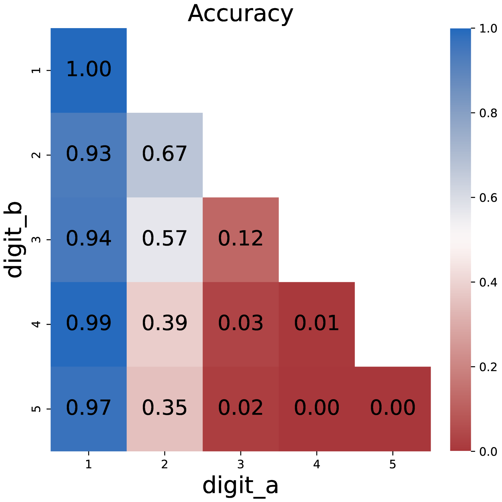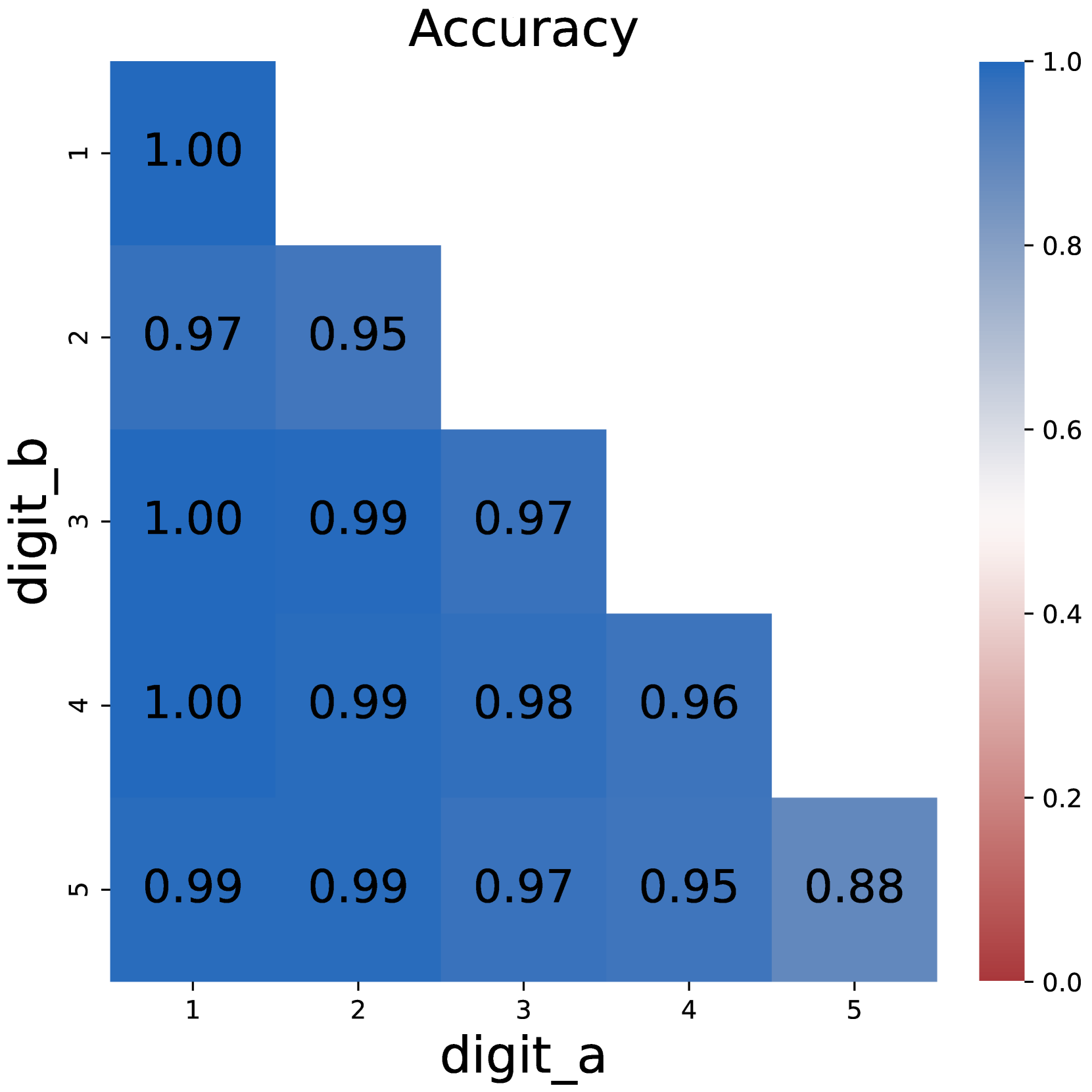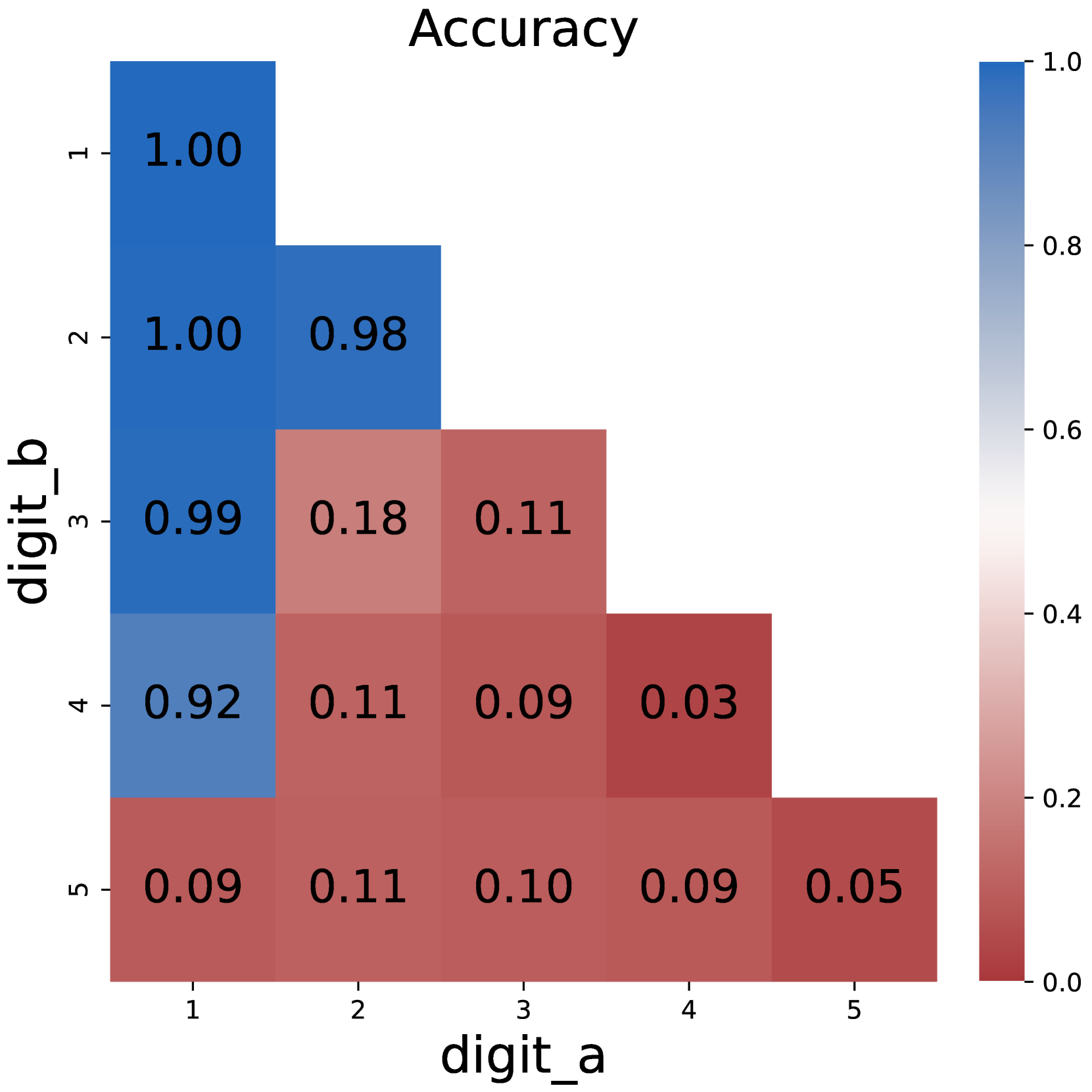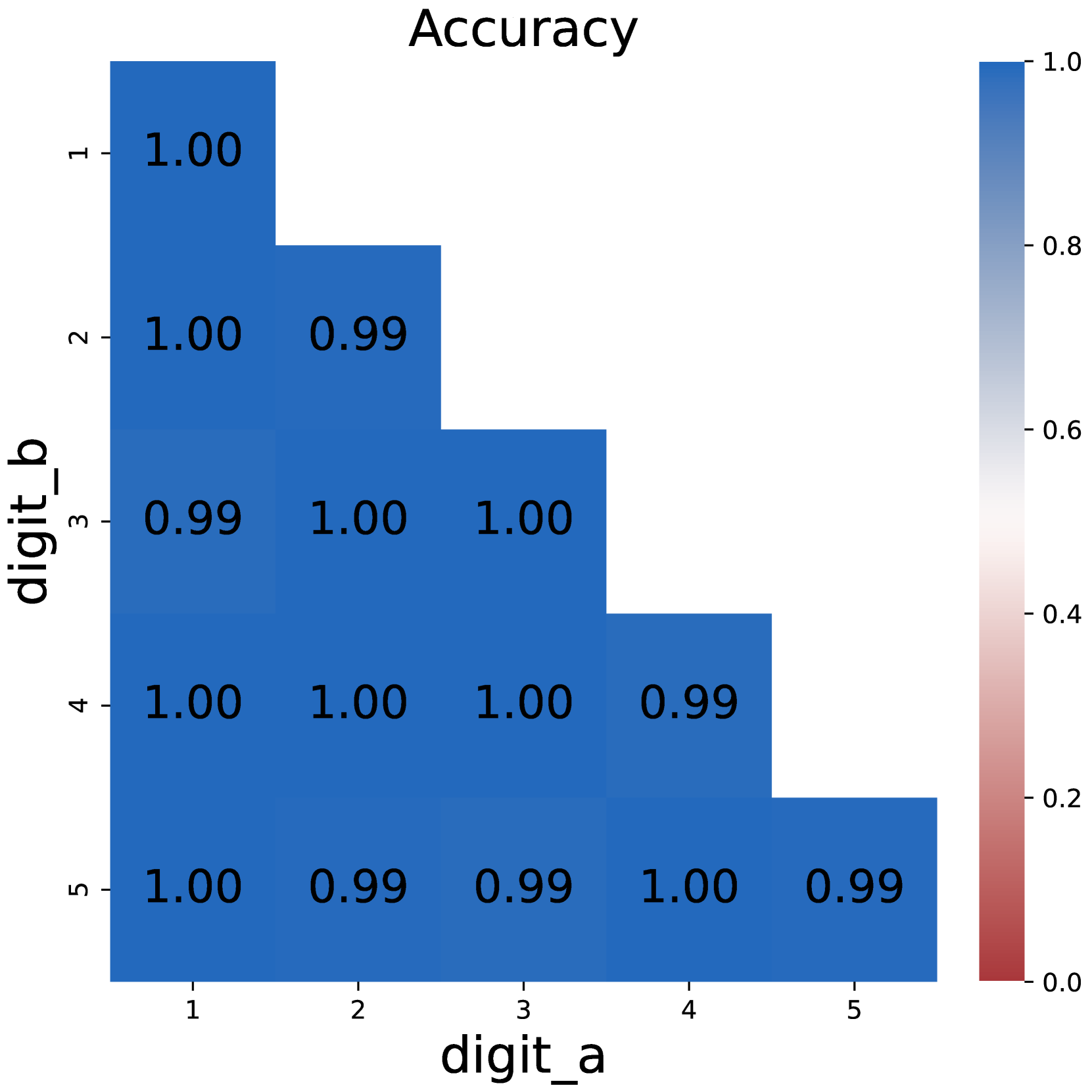</details> (d) CoT DP Figure 1: Comparison on model accuracy between plain prompting and chain-of-thought prompting. 3 CoT Tokens Store Intermediate Results Experimental Setup In all of our experiments, We use Qwen-2.5-1.5B Yang et al. (2024) as the backbone model. On each task, we finetune the model on the corresponding training data and then evaluate whether the generated final answer matches the golden answer. The training stage goes under a learning rate of 1e-5 for 1 epoch. See Appendix C for detailed hyperparameter settings. 3.1 Necessity of Chain-of-Thoughts We start by examining the effectiveness of CoT by comparing the model performance under direct prompting and CoT settings. As illustrated in Figure 1, training the model with direct prompts faces difficulty starting from 3*3 multiplication problems, and completely fails on larger numbers. In contrast, the model could easily solve multiplication problems with chain-of-thoughts, with near-perfect accuracy. The same applies to dynamic programming problems. Direct prompting would fail as the number of intermediate states increases, while CoT maintains its competence. These results support the conclusion that chain-of-thoughts is necessary for solving inherent serial problems that require multi-step reasoning, just as previous research suggests Li et al. (2024); Chen et al. (2024). <details> <summary>x5.png Details</summary>  ### Visual Description ## Heatmap: Accuracy ### Overview The image is a heatmap displaying the accuracy between two variables, 'digit_a' and 'digit_b', ranging from 1 to 5. The heatmap is triangular, showing only the upper triangle of a full matrix. The color intensity represents the accuracy value, with darker blue indicating higher accuracy and lighter shades indicating lower accuracy. A colorbar on the right side provides the mapping between color and accuracy value. ### Components/Axes * **Title:** Accuracy * **X-axis (digit\_a):** Labeled "digit\_a" with values 1, 2, 3, 4, 5. * **Y-axis (digit\_b):** Labeled "digit\_b" with values 1, 2, 3, 4, 5. * **Colorbar:** Ranges from 0.0 to 1.0, with darker blue representing 1.0 and red representing 0.0. The colorbar has tick marks at 0.0, 0.2, 0.4, 0.6, 0.8, and 1.0. ### Detailed Analysis The heatmap displays the following accuracy values for each combination of digit_a and digit_b: * **digit\_a = 1:** * digit\_b = 1: 1.00 * digit\_b = 2: 0.92 * digit\_b = 3: 1.00 * digit\_b = 4: 1.00 * digit\_b = 5: 1.00 * **digit\_a = 2:** * digit\_b = 2: 0.90 * digit\_b = 3: 1.00 * digit\_b = 4: 0.98 * digit\_b = 5: 1.00 * **digit\_a = 3:** * digit\_b = 3: 0.98 * digit\_b = 4: 0.94 * digit\_b = 5: 0.87 * **digit\_a = 4:** * digit\_b = 4: 0.93 * digit\_b = 5: 0.93 * **digit\_a = 5:** * digit\_b = 5: 0.93 ### Key Observations * The highest accuracy values (1.00) are observed when digit\_a = 1 and digit\_b = 1, 3, 4, 5, and when digit\_a = 2 and digit\_b = 3. * The lowest accuracy value is 0.87, observed when digit\_a = 3 and digit\_b = 5. * The diagonal elements (digit\_a = digit\_b) generally have high accuracy, ranging from 0.90 to 1.00. ### Interpretation The heatmap visualizes the accuracy of a model or system in distinguishing between different digits. The high accuracy values along the diagonal suggest that the model performs well in correctly identifying the digits. The off-diagonal values indicate the accuracy when the model confuses one digit for another. For example, the accuracy of 0.87 when digit\_a = 3 and digit\_b = 5 suggests that the model sometimes misclassifies the digit 3 as the digit 5. The overall high accuracy values indicate that the model is generally effective in digit recognition. The triangular shape of the heatmap suggests that the accuracy is symmetric, meaning that the accuracy of classifying digit A as digit B is the same as classifying digit B as digit A. 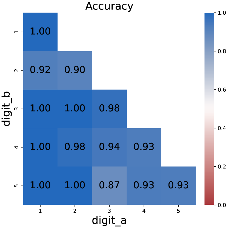</details> Figure 2: Model performance when non-result tokens are removed from CoT in multi-digit multiplication. Removing these tokens has little impact. 3.2 Removing Non-result Tokens One of the concerns about CoT is whether it could be compressed into a more concise form. An obvious approach is to remove some less important tokens. To be specific, we remove tokens that are neither a number nor a symbol For example word ”carry“ in multiplication problems, see Appendix C for details, making CoT a sequence consisting purely of intermediate results to solve the task. Figure 2 shows the model performances after removing these tokens. While the removal would make the CoT unreadable, models finetuned on compressed CoT still achieve satisfying performance, even outperforming the full CoT setting. We can infer from this phenomenon that intermediate results are more important than semantic completeness in CoT. In other words, the central function of CoT is to store the sequence of intermediate results. <details> <summary>x6.png Details</summary>  ### Visual Description ## Diagram: Large Language Model with Latent Predictions ### Overview The image is a diagram illustrating the architecture and process of a Large Language Model (LLM) that uses latent predictions. It shows the flow of information from input tokens to output tokens, highlighting the role of latent embeddings and predictions in generating the final result. ### Components/Axes * **Labels (Left Side):** * Output token * Latent prediction * Last hidden state * Input embedding * Latent embedding * Input token * **Tokens (Bottom):** * \[Question] * <COT> * <LAT> (repeated multiple times) * </COT> * **Tokens (Top):** * <COT> * <LAT> (repeated multiple times) * </COT> * Result * **Central Component:** * Large Language Model (represented as a rounded rectangle) ### Detailed Analysis 1. **Input Token Layer (Bottom):** * Starts with the token "[Question]". * Followed by "<COT>" (Chain of Thought). * Then multiple "<LAT>" (Latent) tokens. * Ends with "</COT>". * Each token has a corresponding "Latent embedding" represented by a small array of cells, with one cell highlighted in orange. * Each token also has a corresponding "Input embedding" represented by a yellow rectangle. The color of the rectangles darkens as the sequence progresses from left to right. 2. **Large Language Model (Center):** * A large, rounded rectangle labeled "Large Language Model". * Represents the core processing unit. 3. **Last Hidden State Layer (Middle):** * A series of green rectangles representing the "Last hidden state". * There are ellipsis (...) indicating continuation of the sequence. 4. **Latent Prediction Layer (Top):** * Each "Last hidden state" has a corresponding "Latent prediction" represented by a small array of cells, with one cell highlighted in orange. * Curved arrows connect each "Last hidden state" to its corresponding "Latent prediction". 5. **Output Token Layer (Top):** * Starts with "<COT>". * Followed by multiple "<LAT>" tokens. * Ends with "</COT>" and "Result". * Each "Last hidden state" has an arrow pointing up to the corresponding "Output token". ### Key Observations * The diagram illustrates a sequential process where input tokens are processed by the LLM to generate output tokens. * Latent embeddings and predictions play a crucial role in the process, influencing the generation of the final result. * The use of "<COT>" and "<LAT>" tokens suggests a mechanism for incorporating chain-of-thought reasoning and latent information into the model's predictions. ### Interpretation The diagram depicts a Large Language Model architecture that leverages latent predictions to enhance its reasoning and generation capabilities. The input tokens, including the question and special tokens like "<COT>" and "<LAT>", are embedded and fed into the LLM. The model then generates a sequence of hidden states, which are used to predict latent variables. These latent predictions, along with the hidden states, are then used to generate the output tokens, ultimately leading to the final result. The "<COT>" tokens likely guide the model to generate a chain of thought, while the "<LAT>" tokens allow the model to incorporate latent information into its predictions. This architecture suggests a sophisticated approach to language modeling that combines explicit reasoning with implicit knowledge representation. 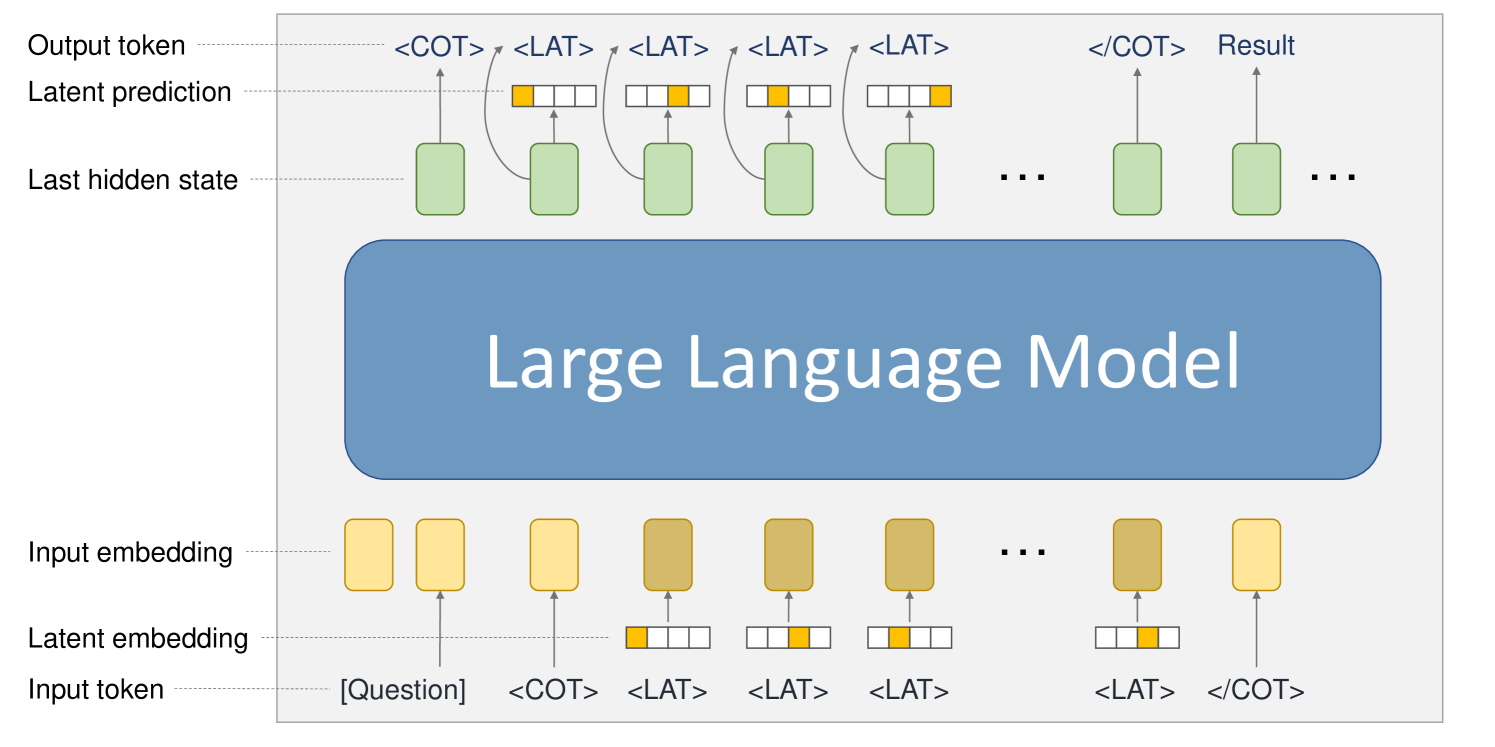</details> Figure 3: The model structure used to reason with latent tokens. We use one-hot vectors as the latent embedding of latent tokens <LAT>. When the input token is a latent token, we use its projected latent embedding to replace the original input embedding. Correspondingly, a latent output head is added to predict the latent embedding of the next token from the last hidden state. <details> <summary>x7.png Details</summary>  ### Visual Description ## Heatmap: Accuracy ### Overview The image is a heatmap displaying accuracy values between two variables, 'digit_a' and 'digit_b', both ranging from 1 to 5. The heatmap is triangular, showing only the upper triangle of a full matrix. The color intensity represents the accuracy, with darker blue indicating higher accuracy and lighter shades indicating lower accuracy. A colorbar on the right provides the mapping between color and accuracy value. ### Components/Axes * **Title:** Accuracy * **X-axis (Horizontal):** digit\_a, with ticks at 1, 2, 3, 4, and 5. * **Y-axis (Vertical):** digit\_b, with ticks at 1, 2, 3, 4, and 5. * **Colorbar:** Ranges from 0.0 (red) to 1.0 (dark blue), with ticks at 0.0, 0.2, 0.4, 0.6, 0.8, and 1.0. ### Detailed Analysis The heatmap displays the accuracy values for each combination of 'digit_a' and 'digit_b'. The values are as follows: * **digit_b = 1:** * digit_a = 1: 1.00 (dark blue) * **digit_b = 2:** * digit_a = 1: 0.92 (blue) * digit_a = 2: 0.92 (blue) * **digit_b = 3:** * digit_a = 1: 1.00 (dark blue) * digit_a = 2: 1.00 (dark blue) * digit_a = 3: 0.97 (dark blue) * **digit_b = 4:** * digit_a = 1: 1.00 (dark blue) * digit_a = 2: 0.99 (dark blue) * digit_a = 3: 0.90 (blue) * digit_a = 4: 0.96 (dark blue) * **digit_b = 5:** * digit_a = 1: 1.00 (dark blue) * digit_a = 2: 0.99 (dark blue) * digit_a = 3: 0.97 (dark blue) * digit_a = 4: 0.96 (dark blue) * digit_a = 5: 0.93 (blue) ### Key Observations * The highest accuracy (1.00) is observed when digit_b is 1 and digit_a is 1, when digit_b is 3 and digit_a is 1, when digit_b is 3 and digit_a is 2, when digit_b is 4 and digit_a is 1, and when digit_b is 5 and digit_a is 1. * The lowest accuracy (0.90) is observed when digit_b is 4 and digit_a is 3. * The accuracy values are generally high, ranging from 0.90 to 1.00. * The heatmap is symmetric along the diagonal (if the lower triangle were present), meaning the accuracy for (digit_a = x, digit_b = y) is the same as for (digit_a = y, digit_b = x). ### Interpretation The heatmap visualizes the accuracy of a classification or prediction task involving digits. The high accuracy values suggest that the model performs well in distinguishing between the digits. The symmetry of the heatmap (if it were a full matrix) indicates that the model's performance is consistent regardless of which digit is considered as 'digit_a' or 'digit_b'. The slight variations in accuracy may be due to differences in the complexity or similarity of the digits. For example, the lower accuracy when digit_b is 4 and digit_a is 3 might indicate that these two digits are sometimes confused by the model. </details> (a) Multiplication <details> <summary>x8.png Details</summary>  ### Visual Description ## Heatmap: Accuracy ### Overview The image is a heatmap displaying accuracy values for different combinations of 'digit_a' and 'digit_b'. The heatmap is triangular, with values only present above and including the diagonal. The color intensity represents the accuracy, ranging from red (low accuracy) to blue (high accuracy), as indicated by the colorbar on the right. ### Components/Axes * **Title:** Accuracy * **X-axis (Horizontal):** digit\_a, with ticks at 1, 2, 3, 4, and 5. * **Y-axis (Vertical):** digit\_b, with ticks at 1, 2, 3, 4, and 5. * **Colorbar:** Ranges from 0.0 (red) to 1.0 (blue), with intermediate values of 0.2, 0.4, 0.6, and 0.8. ### Detailed Analysis The heatmap displays the following accuracy values for each combination of digit_a and digit_b: * **digit_a = 1:** * digit_b = 1: 1.00 (dark blue) * digit_b = 2: 1.00 (dark blue) * digit_b = 3: 0.98 (dark blue) * digit_b = 4: 0.98 (dark blue) * digit_b = 5: 0.93 (blue) * **digit_a = 2:** * digit_b = 2: 0.96 (blue) * digit_b = 3: 0.93 (blue) * digit_b = 4: 0.91 (blue) * digit_b = 5: 0.97 (blue) * **digit_a = 3:** * digit_b = 3: 0.94 (blue) * digit_b = 4: 0.95 (blue) * digit_b = 5: 0.94 (blue) * **digit_a = 4:** * digit_b = 4: 0.98 (dark blue) * digit_b = 5: 0.91 (blue) * **digit_a = 5:** * digit_b = 5: 0.95 (blue) ### Key Observations * The highest accuracy (1.00) is observed when digit_a and digit_b are both 1, and when digit_a is 1 and digit_b is 2. * The accuracy values are generally high, ranging from 0.91 to 1.00. * The heatmap is triangular, indicating that only the upper triangle of the matrix is filled. ### Interpretation The heatmap visualizes the accuracy of a model or system in correctly identifying or matching digits 'a' and 'b'. The high accuracy values suggest that the system performs well in this task. The triangular shape of the heatmap implies that the accuracy is only measured when digit_b is greater than or equal to digit_a. This could be due to the nature of the task or the way the data was collected. The color gradient provides a quick visual representation of the accuracy, with darker blue indicating higher accuracy and lighter shades indicating lower accuracy. 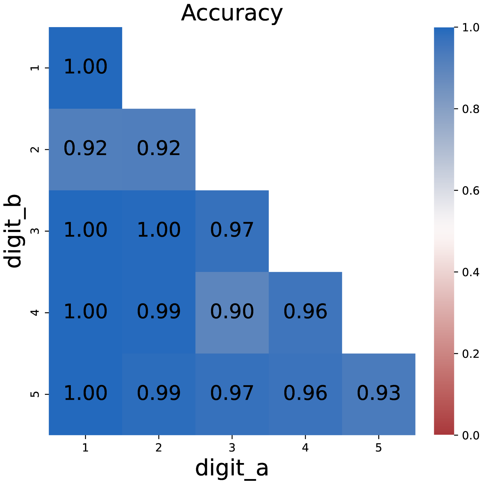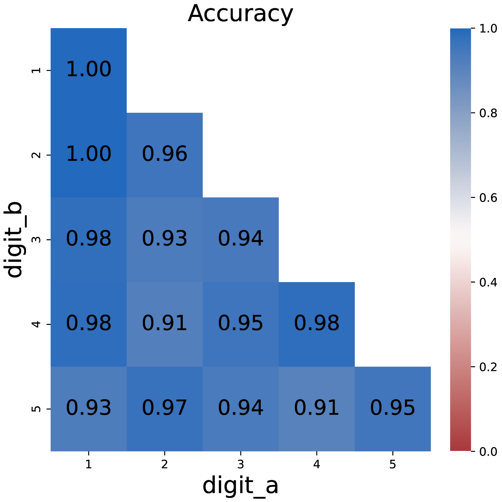</details> (b) DP Figure 4: Model performances when merging intermediate results into latent tokens. 3.3 Merging Results into Latent Tokens Another concern about CoT is whether intermediate results should be explicitly recorded. To test this hypothesis, we try to merge some of the intermediate results, and represent the merged results with latent tokens. Method design. As depicted in Figure 3, we use latent tokens <LAT> to store intermediate results, and each latent token stores the information of a complete number. For simplicity, we use one-hot vectors $\mathbf{l}$ as the embedding of latent tokens: a one-hot vector $\mathbf{l}=(l_{1},l_{2},...,l_{d})∈\mathbb{R}^{d}$ consisting of $d$ dimensions could represent a number $N$ of at most $n$ digits, where $d=10n$ . $$ l_{10k+x}=\begin{cases}1,\lfloor\frac{N}{10^{k}}\rfloor\mod 10=x\\ 0,\lfloor\frac{N}{10^{k}}\rfloor\mod 10\neq x\end{cases} \tag{1} $$ We start by setting all values in $L$ to 0. Assuming that the value of the $k$ -th digit under the little-endian system is $x$ , we set $l_{10k+x}=1$ . In this way, we could represent a number with a single latent token instead of multiple tokens. To support reasoning with latent tokens, we augment the Transformer structure by adding an input projection module $P_{in}$ and a latent output head $P_{out}$ . When the input token $c_{t}$ at position $t$ is a latent token, we feed its latent embedding $\mathbf{l}_{t}$ to the projection module $P_{in}$ , and use the projected vector as the input embedding; Correspondingly, the last hidden state $\mathbf{h}_{t}$ is fed to the latent output head $P_{out}$ aside from the default LM head to predict the latent embedding of the next token $\mathbf{l}_{t+1}$ . We use linear layers to implement $P_{in}$ and $P_{out}$ , which can be described as: $$ \displaystyle P_{in}(\mathbf{l}_{t}) \displaystyle=\mathbf{W}_{in}\mathbf{l}_{t}+\mathbf{b}_{in} \displaystyle P_{out}(\mathbf{h}_{t}) \displaystyle=\mathbf{W}_{out}\mathbf{h}_{t}+\mathbf{b}_{out} \tag{2} $$ where $\mathbf{W}_{in},\mathbf{b}_{in},\mathbf{W}_{out},\mathbf{b}_{out}$ are trainable parameters. We randomly initialize these parameters. An additional latent loss $\mathcal{L}_{lat}$ is introduced to train the augmented model: $$ \mathcal{L}_{lat}=\frac{1}{N_{l}}\sum_{c_{t}=<LAT>}\text{BCE}(\sigma(P_{out}(% \mathbf{h}_{t}),\mathbf{y})) \tag{4} $$ Where $N_{l}$ is the number of latent tokens, $\mathbf{y}$ is the golden latent embedding, BCE is the binary cross entropy loss function, and $\sigma$ is the Sigmoid function. <details> <summary>x9.png Details</summary>  ### Visual Description ## Text Comparison: Original CoT vs. Intervened CoT ### Overview The image presents a side-by-side comparison of two "Chain of Thought" (CoT) calculation processes, labeled "Original CoT" and "Intervened CoT." Both examples demonstrate the multiplication of 8493 by 8877, showing intermediate steps. The key difference lies in a single digit within the calculation of 8493 * 7, which propagates through the rest of the calculation, leading to different final results. ### Components/Axes * **Titles:** "Original CoT" (left), "Intervened CoT" (right) * **Calculation:** Both sides show the multiplication 8493 * 8877, represented as `<COT>`. * **Intermediate Steps:** Both sides show the calculation of 8493 * 7 and 8493 * 70, with intermediate steps for 8493 * 7. * **Partial Results:** Both sides show the addition of partial results. * **Final Result:** Both sides show a final result. ### Detailed Analysis or ### Content Details **Original CoT (Left Side):** * **Initial Calculation:** 8493 * 8877 = `<COT>` * **Calculate 8493 * 7:** * 3 * 7 = 21, digit 1, carry 2 (in blue) * 9 * 7 = 63, digit 5 (in blue), carry 6 * 4 * 7 = 28, digit 4, carry 3 * 8 * 7 = 56, digit 9, carry 5 * Result of 8493 * 7 = 59451 (in blue) * **Calculate 8493 * 70:** (Indicated by "......") * **Add up partial results:** 59451 + 594510 + ... * **Final Result:** 75392361 (in blue) **Intervened CoT (Right Side):** * **Initial Calculation:** 8493 * 8877 = `<COT>` * **Calculate 8493 * 7:** * 3 * 7 = 21, digit 1, carry 4 (in red) * 9 * 7 = 63, digit 7 (in green), carry 6 * 4 * 7 = 28, digit 4, carry 3 * 8 * 7 = 56, digit 9, carry 5 * Result of 8493 * 7 = 59471 (in green) * **Calculate 8493 * 70:** (Indicated by "......") * **Add up partial results:** 59471 + 594510 + ... * **Final Result:** 75392381 (in green) ### Key Observations * The only explicit difference between the two CoT processes is in the calculation of 8493 * 7. * In the "Original CoT," the digit in the tens place of the result of 9 * 7 is "5" and the carry from 3*7 is "2". * In the "Intervened CoT," the digit in the tens place of the result of 9 * 7 is "7" and the carry from 3*7 is "4". * This single-digit difference propagates through the calculation, leading to different partial results and a different final result. * The final results differ by 20 (75392381 - 75392361 = 20). ### Interpretation The image demonstrates the sensitivity of the Chain of Thought process to even minor errors. A single-digit error in an intermediate calculation can significantly impact the final result. This highlights the importance of accuracy and careful attention to detail in complex calculations. The "Intervened CoT" likely represents a scenario where an error was introduced (or corrected) during the calculation process, leading to a different, potentially more accurate, result. The example underscores the value of CoT for debugging and understanding the flow of calculations, as it allows for the identification and correction of errors at intermediate steps. </details> (a) Successful intervention <details> <summary>x10.png Details</summary>  ### Visual Description ## Diagram: Original CoT vs. Intervened CoT ### Overview The image presents a comparison between an "Original CoT" (Chain of Thought) and an "Intervened CoT". Both sides show a calculation process for 7967 * 1083, demonstrating the steps involved in multiplying 7967 by 1000 and adding partial results. The "Intervened CoT" shows a change in one of the intermediate calculations. ### Components/Axes * **Titles:** "Original CoT" (left), "Intervened CoT" (right) * **Calculation:** Both sides start with "7967*1083=<COT>" * **Intermediate Step:** "Calculate 7967*1000" * **Partial Calculation:** Shows individual digit multiplications (e.g., "7*1=7, digit 7, carry 0") * **Result of 7967*1000:** "=7967000" * **Partial Results Summation:** "Add up partial results: 23901...+7967000" * **Final Result:** "Result: 8628261" * **Arrow:** A horizontal arrow points from the "Original CoT" to the "Intervened CoT", indicating a transformation or intervention. ### Detailed Analysis or ### Content Details **Original CoT (Left Side):** * 7967*1083=<COT> * Calculate 7967*1000 * 7*1=7, digit 7, carry 0 * 6*1=6, digit 6, carry 0 * 9*1=9, digit 9, carry 0 * 7*1=7, digit 7, carry 0 * Result of 7967*1000 = 7967000 * Add up partial results: 23901...+7967000 * </COT> * Result: 8628261 **Intervened CoT (Right Side):** * 7967*1083=<COT> * Calculate 7967*1000 * 7*1=7, digit 7, carry 9 * 6*1=6, digit 5, carry 0 * 9*1=9, digit 9, carry 0 * 7*1=7, digit 7, carry 0 * Result of 7967*1000 = 7967000 * Add up partial results: 23901...+7967000 * </COT> * Result: 8628261 **Differences:** * In the "Original CoT", the calculation "7*1=7, digit 7, carry 0" and "6*1=6, digit 6, carry 0" are shown. * In the "Intervened CoT", the calculation "7*1=7, digit 7, carry 9" and "6*1=6, digit 5, carry 0" are shown. ### Key Observations * The "Intervened CoT" modifies the intermediate calculation steps. * Despite the change in intermediate steps, the final result remains the same (8628261). * The arrow indicates a transformation or intervention from the original to the intervened process. ### Interpretation The diagram illustrates the impact of intervening in the "Chain of Thought" process. Specifically, it shows that altering intermediate calculation steps does not necessarily change the final result. This suggests that there might be multiple valid paths to arrive at the same solution, or that the intervention corrected an error in the original CoT. The specific intervention involves changing the "carry" value and the "digit" value in the intermediate calculations, which could represent a correction of a mistake or an alternative calculation method. The fact that the final result is identical despite the intervention highlights the robustness of the calculation or the possibility of compensating errors. 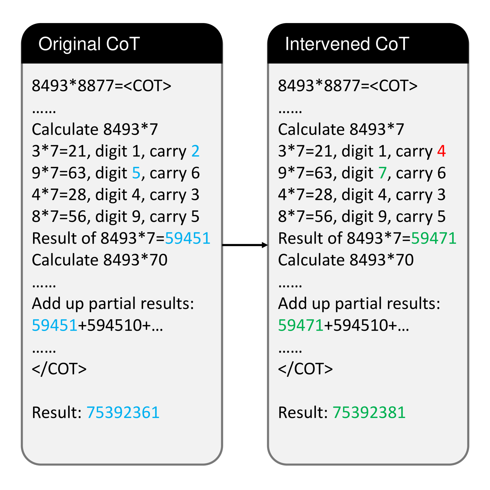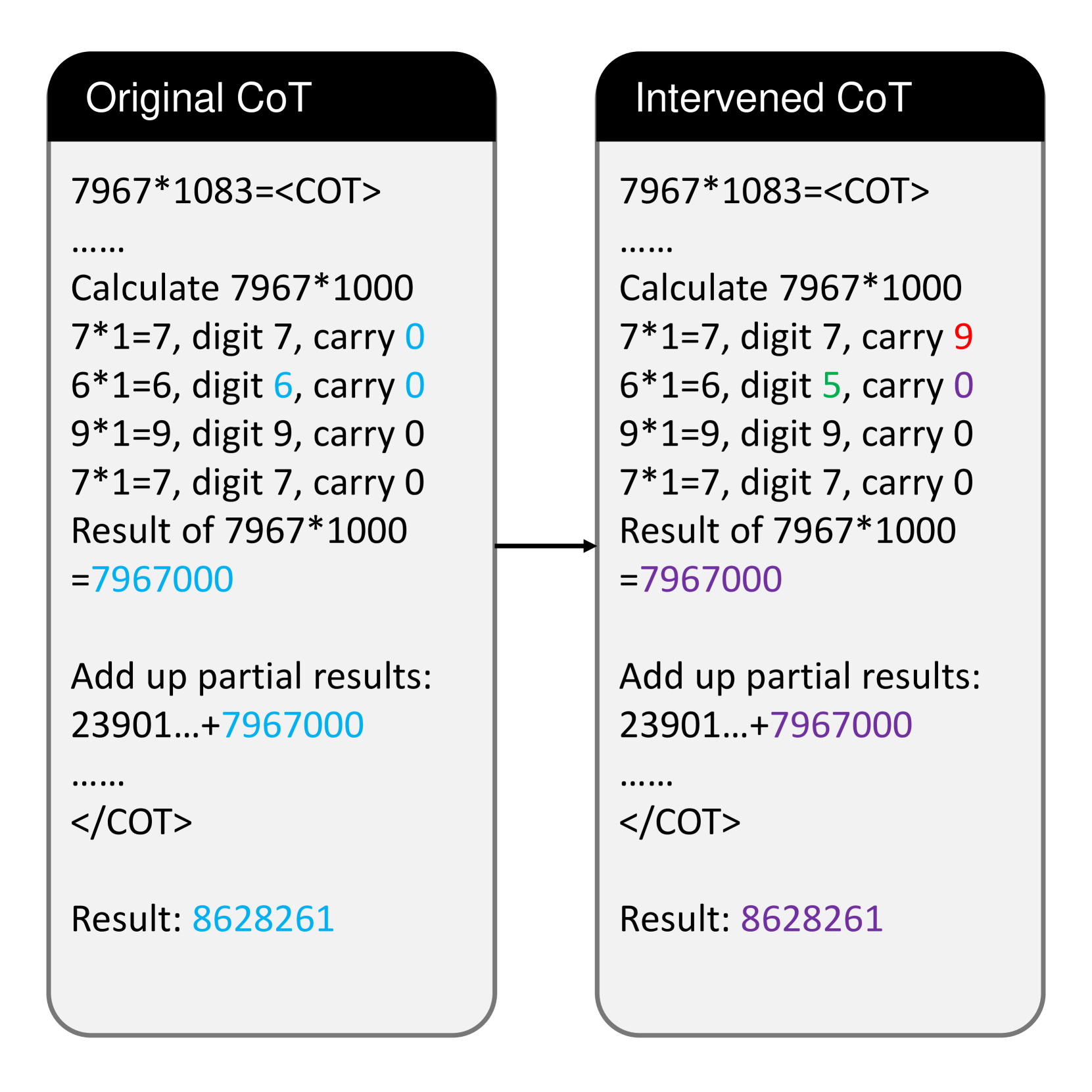</details> (b) Intervention with a shortcut error Figure 5: Examples of a successful intervention (left) and an intervention with a shortcut error (right). Blue numbers refer to relevant values in the original CoT, red numbers refer to the intervention, green numbers refer to values that change as expected, but purple numbers do not change due to a shortcut error. Experimental setup. For multiplication problems, we replace each digit-wise multiplication step with a single latent token and set $d=20$ ; For DP problems, we replace each intermediate state with a single latent token and set $d=50$ . We add the latent loss $\mathcal{L}_{lat}$ with the default LM head loss as the final loss for training. Figure 4 shows the model performances when trained with latent tokens. Surprisingly, merging digit tokens to a single latent token does not detriment the performance: the model retains most of its ability to solve problems. The accuracy of using latent tokens on multiplication problems is almost identical with the accuracy of using full CoT. On 5*5 multiplication problems, using latent tokens even surpasses the original CoT, suggesting that the form of intermediate results does not matter. However, it can also be observed that using latent tokens brings disadvantage on DP problems where latent tokens store larger numbers. For example, the accuracy reduces by 9% on 4*5 DP problems. This raises the hypothesis that the computation complexity should not exceed a certain limit, which we will discuss further in Section 4.2. 4 CoT Tokens are Mutable Variables In the previous section, we find that while CoT is essential for solving complex problems (Section 3.1), the tokens representing intermediate results are more important than others (Section 3.2). Meanwhile, compressing intermediate results into latent tokens would not obviously harm model performance (Section 3.3), indicating that intermediate results could be stored in different forms. Here, we continue to discuss whether these stored intermediate results are causally related to the final prediction, and how the computation complexity between intermediate results affects model performance. <details> <summary>x11.png Details</summary>  ### Visual Description ## Bar Chart: Accuracy by Task ### Overview The image is a bar chart comparing the accuracy of two tasks: "Multi" and "DP". The y-axis represents accuracy, ranging from 0.0 to 1.0. The x-axis represents the task type. The bar for "Multi" is a lighter blue, while the bar for "DP" is a darker blue. ### Components/Axes * **X-axis:** "task" with categories "Multi" and "DP". * **Y-axis:** "accuracy" ranging from 0.0 to 1.0, with increments of 0.2. ### Detailed Analysis * **Multi:** The accuracy for the "Multi" task is approximately 0.74. * **DP:** The accuracy for the "DP" task is approximately 0.99. ### Key Observations * The "DP" task has a significantly higher accuracy than the "Multi" task. ### Interpretation The bar chart indicates that the "DP" task is performed with greater accuracy compared to the "Multi" task. The difference in accuracy is substantial, suggesting that the "DP" task may be inherently easier or that the system/method used is better suited for the "DP" task. </details> (a) Success rate <details> <summary>x12.png Details</summary>  ### Visual Description ## Chart Type: Pie Chart ### Overview The image is a pie chart titled "Error breakdown". It shows the distribution of different error types, with each slice representing a specific error category and its corresponding percentage. The legend on the top-right corner identifies each error type by color. ### Components/Axes * **Title:** Error breakdown * **Legend (Top-Right):** Error type * **Addition:** Light Blue * **Reconstruct:** Light Orange * **Shortcut:** Light Green * **Copy:** Light Red * **Misc:** Light Purple ### Detailed Analysis The pie chart is divided into five slices, each representing a different error type. The percentages are displayed directly on the slices. * **Addition (Light Blue):** 29.3% * **Reconstruct (Light Orange):** 19.0% * **Shortcut (Light Green):** 49.4% * **Copy (Light Red):** The copy slice is very small, and the percentage is not directly labeled on the chart. Based on the remaining percentage, it is approximately 1.3%. * **Misc (Light Purple):** The misc slice is very small, and the percentage is not directly labeled on the chart. Based on the remaining percentage, it is approximately 1.0%. ### Key Observations * The "Shortcut" error type accounts for the largest portion of errors, representing 49.4% of the total. * "Addition" errors make up the second-largest portion, at 29.3%. * "Reconstruct" errors account for 19.0%. * "Copy" and "Misc" errors are relatively small, accounting for approximately 1.3% and 1.0% respectively. ### Interpretation The pie chart provides a clear visual representation of the distribution of different error types. The dominance of "Shortcut" errors suggests that this area should be prioritized for improvement efforts. The relatively small percentages of "Copy" and "Misc" errors indicate that these may be less critical areas to focus on, although they should still be monitored. The data suggests that addressing "Shortcut" and "Addition" errors would have the most significant impact on reducing overall errors. 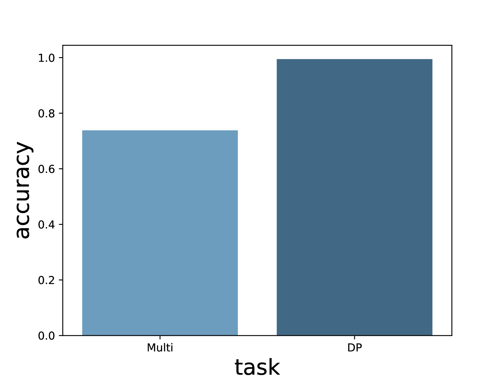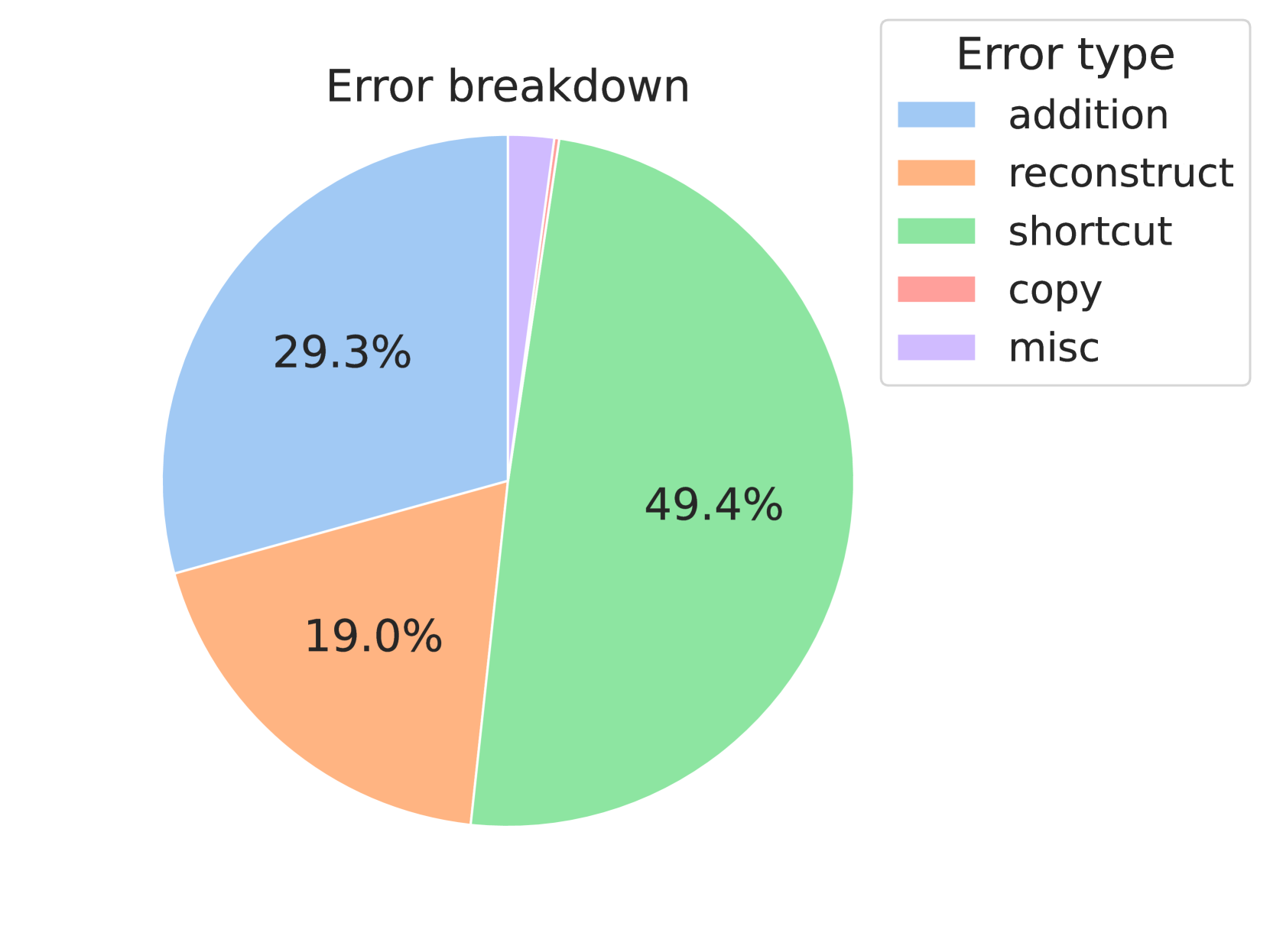</details> (b) Error breakdown Figure 6: (a) Success rate of intervention. When the intervened output is the same as simulated, we view it as a successful intervention. (b) Error breakdown. Shortcut error occupies a large percentage of the errors. <details> <summary>x13.png Details</summary>  ### Visual Description ## Diagram: Dynamic Programming Dependency Graph ### Overview The image depicts a dependency graph, likely representing a dynamic programming approach. It shows the relationships between different states or subproblems, denoted as DP[i][j], DP[i][j+1], etc. The arrows indicate the dependencies, with different arrow styles (solid, dashed, red dashed) possibly representing different types or strengths of dependencies. The diagram illustrates how the solution to a particular state depends on the solutions to other states. ### Components/Axes * **Nodes:** Each node is a rounded rectangle labeled as DP[i][j], DP[i][j+1], DP[i][j+2], DP[i+1][j], DP[i+1][j+1], DP[i+1][j+2], DP[i+2][j], DP[i+2][j+1], DP[i+2][j+2]. The nodes in the first and third rows are solid yellow, while the nodes in the second row are dashed yellow. * **Edges:** The edges are represented by arrows, indicating the direction of dependency. There are three types of arrows: * Solid black arrows pointing downwards. * Dashed black arrows pointing to the right or downwards. * Dashed red arrows pointing to the right or downwards. * **Ellipsis:** Two sets of ellipsis (...) indicate that the pattern continues beyond what is shown in the diagram. One is on the right side of the second row, and the other is below the third row. ### Detailed Analysis or Content Details * **Row 1:** * Node 1: DP[i][j] (solid yellow) * Node 2: DP[i][j+1] (solid yellow) * Node 3: DP[i][j+2] (solid yellow) * Dependencies: DP[i][j] -> DP[i][j+1] (red dashed arrow), DP[i][j+1] -> DP[i][j+2] (dashed arrow) * **Row 2:** * Node 4: DP[i+1][j] (dashed yellow) * Node 5: DP[i+1][j+1] (dashed yellow) * Node 6: DP[i+1][j+2] (dashed yellow) * Dependencies: DP[i+1][j] -> DP[i+1][j+1] (red dashed arrow), DP[i+1][j+1] -> DP[i+1][j+2] (red dashed arrow) * **Row 3:** * Node 7: DP[i+2][j] (solid yellow) * Node 8: DP[i+2][j+1] (solid yellow) * Node 9: DP[i+2][j+2] (solid yellow) * Dependencies: DP[i+2][j] -> DP[i+2][j+1] (dashed arrow), DP[i+2][j+1] -> DP[i+2][j+2] (dashed arrow) * **Column 1:** * Dependencies: DP[i][j] -> DP[i+1][j] (solid arrow), DP[i+1][j] -> DP[i+2][j] (solid arrow) * **Column 2:** * Dependencies: DP[i][j+1] -> DP[i+1][j+1] (red dashed arrow), DP[i+1][j+1] -> DP[i+2][j+1] (dashed arrow) * **Column 3:** * Dependencies: DP[i][j+2] -> DP[i+1][j+2] (red dashed arrow), DP[i+1][j+2] -> DP[i+2][j+2] (solid arrow) ### Key Observations * The diagram represents a 2D grid of states, indexed by `i` and `j`. * Dependencies exist both horizontally (within the same row) and vertically (within the same column). * The arrow styles (solid, dashed, red dashed) suggest different types or strengths of dependencies. * The dashed nodes in the second row might indicate intermediate or optional states. * The ellipsis indicate that the pattern continues indefinitely in both horizontal and vertical directions. ### Interpretation The diagram illustrates a typical dependency structure found in dynamic programming problems. The states DP[i][j] represent subproblems, and the arrows indicate which subproblems need to be solved before a particular subproblem can be solved. The different arrow styles could represent different costs or probabilities associated with the dependencies. The dashed nodes might represent states that are only conditionally required, or states that are computed differently. The diagram provides a visual representation of the order in which the subproblems need to be solved to arrive at the final solution. The specific meaning of 'i' and 'j' would depend on the particular dynamic programming problem being represented. 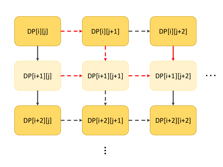</details> Figure 7: Demonstration of the alternative merging strategy. Each line refers to the compare-then-add state transfer function in the original setup. Nodes corresponding to the dashed boxes will not appear in the new CoT. It will cost at most 3 compare-then-add operations (red lines) to transfer states between new matrix tokens. 4.1 Intervening the Value of CoT Tokens An inherent problem is that while CoT is essential for reaching the right answer, some of the intermediate results may only be correlational to the output, rather than having causal effects. To address this problem, we perform intervention experiments by replacing intermediate results and observe whether the final result would change as expected. For multiplication problems, we randomly choose a substep in CoT and replace its result with a different random number; For DP problems, we randomly choose an intermediate state and replace it with a different random number. For simplicity, we perform interventions on 4*4 problems, and only one number is replaced in each data entry. Details are described in Appendix E. As shown in Figure 6(a), the intervention on both tasks achieves a decent success rate, clearly indicating that the intermediate values stored in CoT tokens are causally related to the final answer. We also notice that subsequent reasoning steps will change correspondingly. Take Figure 5(a) as an example, when we change the carry from 2 to 4, the model generates a result of $8493*7=59471$ instead of 59451, just as simulated. In other words, tokens in CoT not only store intermediate values, but they are also “variables” that would affect subsequent reasoning steps. Another interesting observation is that the success rate on multiplication problems is significantly lower than that on DP problems. We investigate the cause of unsuccessful interventions and categorize them into 5 categories. (1) Addition error means that the model fails to add up partial multiplication results; (2) Reconstruction error means that the partial multiplication result conflicts with digit-wise results; (3) Copy error means that partial multiplication results do not correctly appear in the addition step; (4) Shortcut error means that the model learns a “shortcut” on certain multiplications (usually when one of the operands is 0 or 1); (5) Misc error covers the remaining errors. Figure 6(b) illustrates the distribution of error types. Among the 5 types, shortcut error occupies the largest portion. As shown in Figure 5(b), while changing the carry from 0 to 9 will affect the next digit as intended, the model does not change its result in the substep $7967*1000$ . When multiplying a number $x$ by 1, the model seems to be taking a shortcut of directly copying $x$ , rather than collecting the digit-wise multiplication results. To sum up, language models use the value in CoT tokens like treating program variables, but models may develop shortcut on easy subproblems that leave certain variables unused. <details> <summary>x14.png Details</summary>  ### Visual Description ## Line Chart: Probe Accuracy ### Overview The image is a line chart titled "Probe Accuracy". It displays the accuracy of different metrics ("element", "entry", "none", and "row") across various layers. The x-axis represents the layer number, and the y-axis represents the value (accuracy). ### Components/Axes * **Title:** Probe Accuracy * **X-axis:** Layer, with markers from 0 to 25 in increments of 5. * **Y-axis:** Value, with markers from 0.0 to 1.0 in increments of 0.2. * **Legend (top-left):** Accuracy Metric * element (solid teal line) * entry (solid orange line) * none (solid black line) - Note: This line is not visible on the chart, implying a constant value of 0 or near 0. * row (dashed black line) ### Detailed Analysis * **Element (solid teal line):** The accuracy starts at approximately 0.95 and remains relatively constant until layer 19, after which it increases slightly to approximately 0.99. * Layer 0-19: Value ~ 0.95 * Layer 20-27: Value ~ 0.99 * **Entry (solid orange line):** The accuracy is at 0 until layer 19. Between layers 19 and 22, the accuracy increases sharply from 0 to approximately 0.9. After layer 22, the accuracy increases more gradually to approximately 0.97 by layer 27. * Layer 0-19: Value = 0 * Layer 20: Value ~ 0.1 * Layer 21: Value ~ 0.6 * Layer 22: Value ~ 0.9 * Layer 27: Value ~ 0.97 * **None (solid black line):** This line is not visible, suggesting its value is consistently near 0 across all layers. * **Row (dashed black line):** The accuracy is at 0 until layer 21. It then gradually increases to approximately 0.15 by layer 27. * Layer 0-21: Value = 0 * Layer 27: Value ~ 0.15 ### Key Observations * The "element" metric has the highest and most stable accuracy across all layers. * The "entry" metric experiences a significant increase in accuracy between layers 19 and 22. * The "row" metric shows a gradual increase in accuracy starting from layer 21. * The "none" metric has negligible accuracy across all layers. ### Interpretation The chart compares the accuracy of different compression metrics ("element", "entry", "none", and "row") across different layers. The "element" metric consistently performs well, while the "entry" metric shows a delayed but significant increase in accuracy. The "row" metric shows a gradual improvement, and the "none" metric performs poorly. This suggests that the "element" metric is the most reliable for maintaining accuracy across layers, while the "entry" metric becomes more effective in later layers. The "none" metric is not effective for this task. 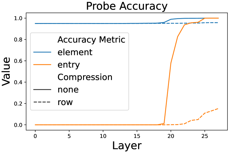</details> Figure 8: Probing accuracy on different layers. Intermediate variable values can only be probed on late layers, regardless of the overall accuracy. 4.2 Probing the Limit of CoT Tokens In Section 3.3, we discover that intermediate values can be compressed in latent tokens. This naturally raises the question: to what extent could the values be compressed? To address this problem, we adopt some aggressive compression strategies and use linear probing classifiers to observe how the compression affects the final output. We choose 5*5 DP problems as the base problem and use the latent token setting in Section 3.3. Specifically, we introduce an alternative strategy that merges two adjacent latent tokens in a row to one latent token (Figure 7). In this way, this strategy yields a 3*3 CoT token matrix instead of a 5*5 matrix. However, the computational complexity between CoT tokens also increases: it would cost up to 3 times as much as in the original case. For each CoT token <LAT>, we use a linear probe $P$ to probe its latent embedding $\mathbf{l}$ from the hidden states $\mathbf{h}_{k}$ on different layer $k$ of the previous token. We use a unique probe $P_{k}$ for each layer: $$ P_{k}(\mathbf{h}_{k})=\mathbf{W}_{k}\mathbf{h}_{k}+\mathbf{b}_{k} \tag{5} $$ where $\mathbf{W}_{k}$ and $\mathbf{b}_{k}$ are trainable parameters. After training the probes on the training set, we evaluate them with two metrics: element accuracy evaluates the ratio of correctly predicted individual dimensions, and token accuracy evaluates the ratio of correct latent tokens. Figure 8 shows the result of probing CoT tokens. Aggressively merging CoT tokens will significantly lower both element accuracy and token accuracy, meaning that there exists a computation complexity limit, over which the LLM can no longer correctly calculate the next intermediate variable. <details> <summary>x15.png Details</summary>  ### Visual Description ## Heatmap: Accuracy Breakdown ### Overview The image is a heatmap titled "Accuracy Breakdown". The heatmap visualizes the accuracy of a model across different layers (x-axis) and digit scales (y-axis). The color intensity represents the accuracy value, with darker blue indicating higher accuracy and lighter blue indicating lower accuracy. ### Components/Axes * **Title:** Accuracy Breakdown * **X-axis:** "layer" with tick marks at 0, 2, 4, 6, 8, 10, 12, 14, 16, 18, 20, 22, 24, and 26. * **Y-axis:** "Digit Scale" with tick marks at 1, 2, 3, and 4. * **Colorbar:** A vertical colorbar on the right side of the heatmap, ranging from 0.0 (lightest blue) to 0.8 (darkest blue), with tick marks at 0.0, 0.2, 0.4, 0.6, and 0.8. ### Detailed Analysis The heatmap shows accuracy values for different combinations of "layer" and "Digit Scale". * **Digit Scale 1:** Accuracy is approximately 0.8 for layers 22, 24, and 26. * **Digit Scale 2:** Accuracy is approximately 0.6 for layer 22, 0.7 for layer 24, and 0.8 for layer 26. * **Digit Scale 3:** Accuracy is approximately 0.4 for layer 22, 0.5 for layer 24, and 0.5 for layer 26. * **Digit Scale 4:** Accuracy is approximately 0.0 for layers 0 through 26. For layers 0 through 20, the accuracy is approximately 0.0 for digit scales 1, 2, and 3. ### Key Observations * Accuracy generally increases with the layer number, especially for layers 22, 24, and 26. * Accuracy decreases as the digit scale increases. Digit scale 4 has the lowest accuracy across all layers. * The model performs significantly better on digit scales 1, 2, and 3 compared to digit scale 4. ### Interpretation The heatmap suggests that the model's accuracy is highly dependent on both the layer and the digit scale. The later layers (22, 24, 26) seem to be more effective in extracting relevant features, leading to higher accuracy. The poor performance on digit scale 4 indicates that the model struggles to accurately classify digits at that scale, potentially due to the features being less discriminative or the model not being trained adequately on that scale. The model does not appear to learn anything until layer 22. 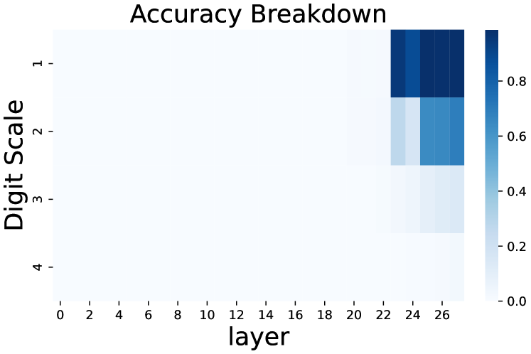</details> Figure 9: Accuracy breakdown by the scale of target values. When computational complexity between tokens exceeds a limit, the model will fail. Figure 9 further breaks down the accuracy distribution by the range of values stored in merged latent tokens. We can see that merging latent tokens has little impact on numbers with a digit length of 1 or 2, but would decrease the accuracy to near 0 on larger number values. This phenomenon can be explained as it is easier to calculate small numbers, and thus the model could “afford” the extra computational cost of merging latent tokens. Another interesting point to notice is that two accuracy curves share a similar pattern: the token accuracy stays at 0 from early layers, and rapidly rises around layer 20. Previous work Stolfo et al. (2023); Zhu et al. (2025) has concluded that LLMs tend to use early-mid layers to gather and process information from previous tokens, and determine the output only in mid-late layers. We may further assume that the role of layers will not change with computation complexity between CoT tokens. 5 Discussion Explaining alternative CoT forms. By viewing CoTs as programs, we can explain alternative CoT forms in a novel way. For example, the success of internalizing CoT steps Deng et al. (2024); Hao et al. (2024) could be viewed as compressing explicit step tokens into implicit latent tokens that cover all essential intermediate values. And the validity of inserting meaningless filler tokens Goyal et al. (2024); Pfau et al. (2024) comes from enabling LLMs to store intermediate results in the hidden states of filler tokens. By reserving space for complex reasoning steps and compressing simple reasoning steps, we could design high-efficiency CoTs. Generalization of CoT “programs”. From the experiments in previous sections, we can see that CoT tokens store intermediate values, and their values are subsequently used like the way variables function in computer programs. Theoretical proof has been made that Transformer with a recurrent module is Turing complete Pérez et al. (2021). However, there is also evidence that LLMs may struggle to generalize on compositional problems Dziri et al. (2023): models trained on easy problems would fail on more complex problems. In real-world settings, the type and complexity of desired programs are unknown, and a general-purpose LLM needs to first determine the type of program to use, or in other words, generate a meta-program first. Identification of intermediate variable tokens. It is not surprising that the CoT generated by LLMs is partially redundant and could be shortened. In Section 3.2, we find that preserving value tokens could retain most of the ability of language models. While it is easy to judge whether a token stores intermediate results in multiplication and DP problems, it is harder to identify variable tokens on general tasks: Madaan and Yazdanbakhsh (2022) finds that plain text helps LLMs elicit semantic commonsense knowledge, which may be infused into later CoT tokens. Developing an approach to identifying variable tokens would benefit CoT compression. Estimation of computational complexity between variable tokens. Section 4.2 shows that LLMs would fail when the computational complexity between variable tokens exceeds a certain limit. However, it is difficult to estimate the exact complexity limit for LLMs. It is possible to calculate the theoretical bound of ability for finite-precision Transformers Chen et al. (2024), but how LLMs process semantic information is still largely opaque, and unexpected features may appear Lindsey et al. (2025). Moreover, LLMs are not guaranteed to solve similar subproblems in the same way, they may take shortcuts (Section 4.1) that would largely affect the computational complexity between variable tokens. We hope that the broader research community could help estimate the computational complexity between variable tokens in different types of questions. 6 Related Work 6.1 Chain-of-Thought Reasoning Chain-of-Thoughts (CoT) Wei et al. (2022) is a commonly adopted technique in LLMs. Nowadays, CoT refers to a broad range of approaches that require LLMs to generate an intermediate reasoning process before reaching the final answer. Typical approaches include designing the prompt Wei et al. (2022); Khot et al. (2022); Zhou et al. (2022) and finetuning LLMs on existing chain-of-thoughts Yue et al. (2023); Yu et al. (2023). Recently, reinforcement learning also reveals its great potential in enabling LLMs to perform complex reasoning without extensive human annotations Havrilla et al. (2024); Wang et al. (2024); Shao et al. (2024); Guo et al. (2025). While the tokens in CoT can be classified into symbols, patterns, and text, which both contribute to the final answer Madaan and Yazdanbakhsh (2022), it seems that LLMs can still perform well with a small amount of CoT tokens Xu et al. (2025). Aside from plain text, researchers have also explored alternative forms of CoT. Some works focus on search abilities, like tree-form thought traces Yao et al. (2023); Xie et al. (2023) and Monte-Carlo Tree Search (MCTS) algorithms Zhang et al. (2024); Guan et al. (2025). Another line of work attempts to reason in a latent space: Goyal et al. (2024) uses a pause token to help models process extra computation before reaching an answer, and Pfau et al. (2024) shows it is also possible to replace CoT with meaningless filler tokens. On top of this, Deng et al. (2024) tries to train models with gradually shortened CoT, and COCONUT Hao et al. (2024) proposes the continuous thought paradigm, where the last hidden state of a latent token is used as the next input embedding. 6.2 Theoretical Analysis on CoT It has been noticed that LLMs face difficulty in compositional problems where combining multiple reasoning steps is strictly required, and it may be an intrinsic drawback of the Transformer structure Dziri et al. (2023). Feng et al. (2023) explains the phenomenon with the circuit complexity theory, and reaches the conclusion that it is impossible for a constant-depth log-precision transformer to solve certain math problems like linear equations. However, with the help of CoT, the model could solve these problems in polynomial complexity. Li et al. (2024) further extends the conclusion that constant-depth transformers using constant-bit precision could solve any problems solvable by boolean circuits, as long as they are equipped with CoT whose steps are longer than the circuit size. Chen et al. (2024) analyzes the problem with a multi-party autoregressive communication model, and finds that it is exponentially harder for Transformer models to solve composition tasks that require more steps than the model layers, and CoT could make the problem exponentially easier. In fact, Transformer models are powerful enough to represent finite-state automata Liu et al. (2022), and could even be Turing-complete Pérez et al. (2021) to simulate computer programs when equipped with loop modules Giannou et al. (2023). We hold the belief that these findings could also be extended to chain-of-thoughts reasoning. 7 Conclusion In this paper, we empirically explore the role CoT tokens play in reasoning. By observing the model performance on multi-digit multiplication problems and dynamic programming, we confirm that CoT is essential for solving these compositional problems. We further find that we could mostly preserve model ability by only using tokens that store intermediate results, and these intermediate results could be stored in different forms like latent token embeddings. To validate the causal connection between CoT tokens and model output, we randomly replace some values in CoT, and find that both the subsequent reasoning process and the final result would change corresponding to the intervention. The way CoT tokens behave is similar to the function of computer program variables. However, in easy subproblems LLMs would learn shortcuts that are unfaithful to the generated reasoning process, and the intervention would fail under these scenarios. We also train probing classifiers to probe variable values from hidden states on different layers, and find that there exists a computational complexity limit between CoT tokens. Intermediate values could be compressed within a single latent CoT token, but the model would drastically fail when computational complexity exceeds the limit. Our work conducts preliminary experiments on the function of CoT tokens, and there still exist mysteries like generalization ability, variable identification and complexity limit estimation, which we leave for future explorations. Limitations In this paper we empirically demonstrate that an important function of CoT tokens is to store intermediate values, and these values function like program variables. However, currently we are not able to give a theoretical proof on this statement. Another limitation of our work is that the experiments are conducted on two synthetic tasks with Qwen-2.5-1.5B, as it is difficult to identify and analyze intermediate results in real-world datasets like GSM8K and Math. Future experiments on other problems and models will be beneficial. References - Chen et al. (2024) Lijie Chen, Binghui Peng, and Hongxun Wu. 2024. Theoretical limitations of multi-layer transformer. arXiv preprint arXiv:2412.02975. - Deng et al. (2024) Yuntian Deng, Yejin Choi, and Stuart Shieber. 2024. From explicit cot to implicit cot: Learning to internalize cot step by step. arXiv preprint arXiv:2405.14838. - Dziri et al. (2023) Nouha Dziri, Ximing Lu, Melanie Sclar, Xiang Lorraine Li, Liwei Jiang, Bill Yuchen Lin, Sean Welleck, Peter West, Chandra Bhagavatula, Ronan Le Bras, and 1 others. 2023. Faith and fate: Limits of transformers on compositionality. Advances in Neural Information Processing Systems, 36:70293–70332. - Feng et al. (2023) Guhao Feng, Bohang Zhang, Yuntian Gu, Haotian Ye, Di He, and Liwei Wang. 2023. Towards revealing the mystery behind chain of thought: a theoretical perspective. Advances in Neural Information Processing Systems, 36:70757–70798. - Giannou et al. (2023) Angeliki Giannou, Shashank Rajput, Jy-yong Sohn, Kangwook Lee, Jason D Lee, and Dimitris Papailiopoulos. 2023. Looped transformers as programmable computers. In International Conference on Machine Learning, pages 11398–11442. PMLR. - Goyal et al. (2024) Sachin Goyal, Ziwei Ji, Ankit Singh Rawat, Aditya Krishna Menon, Sanjiv Kumar, and Vaishnavh Nagarajan. 2024. Think before you speak: Training language models with pause tokens. In The Twelfth International Conference on Learning Representations. - Guan et al. (2025) Xinyu Guan, Li Lyna Zhang, Yifei Liu, Ning Shang, Youran Sun, Yi Zhu, Fan Yang, and Mao Yang. 2025. rstar-math: Small llms can master math reasoning with self-evolved deep thinking. arXiv preprint arXiv:2501.04519. - Guo et al. (2025) Daya Guo, Dejian Yang, Haowei Zhang, Junxiao Song, Ruoyu Zhang, Runxin Xu, Qihao Zhu, Shirong Ma, Peiyi Wang, Xiao Bi, and 1 others. 2025. Deepseek-r1: Incentivizing reasoning capability in llms via reinforcement learning. arXiv preprint arXiv:2501.12948. - Hao et al. (2024) Shibo Hao, Sainbayar Sukhbaatar, DiJia Su, Xian Li, Zhiting Hu, Jason Weston, and Yuandong Tian. 2024. Training large language models to reason in a continuous latent space. arXiv preprint arXiv:2412.06769. - Havrilla et al. (2024) Alexander Havrilla, Yuqing Du, Sharath Chandra Raparthy, Christoforos Nalmpantis, Jane Dwivedi-Yu, Eric Hambro, Sainbayar Sukhbaatar, and Roberta Raileanu. 2024. Teaching large language models to reason with reinforcement learning. In AI for Math Workshop@ ICML 2024. - Khot et al. (2022) Tushar Khot, Harsh Trivedi, Matthew Finlayson, Yao Fu, Kyle Richardson, Peter Clark, and Ashish Sabharwal. 2022. Decomposed prompting: A modular approach for solving complex tasks. In The Eleventh International Conference on Learning Representations. - Li et al. (2024) Zhiyuan Li, Hong Liu, Denny Zhou, and Tengyu Ma. 2024. Chain of thought empowers transformers to solve inherently serial problems. In The Twelfth International Conference on Learning Representations. - Lindsey et al. (2025) Jack Lindsey, Wes Gurnee, Emmanuel Ameisen, Brian Chen, Adam Pearce, Nicholas L. Turner, Craig Citro, David Abrahams, Shan Carter, Basil Hosmer, Jonathan Marcus, Michael Sklar, Adly Templeton, Trenton Bricken, Callum McDougall, Hoagy Cunningham, Thomas Henighan, Adam Jermyn, Andy Jones, and 8 others. 2025. On the biology of a large language model. Transformer Circuits Thread. - Liu et al. (2022) Bingbin Liu, Jordan T Ash, Surbhi Goel, Akshay Krishnamurthy, and Cyril Zhang. 2022. Transformers learn shortcuts to automata. In The Eleventh International Conference on Learning Representations. - Madaan and Yazdanbakhsh (2022) Aman Madaan and Amir Yazdanbakhsh. 2022. Text and patterns: For effective chain of thought, it takes two to tango. arXiv preprint arXiv:2209.07686. - Pérez et al. (2021) Jorge Pérez, Pablo Barceló, and Javier Marinkovic. 2021. Attention is turing-complete. Journal of Machine Learning Research, 22(75):1–35. - Pfau et al. (2024) Jacob Pfau, William Merrill, and Samuel R Bowman. 2024. Let’s think dot by dot: Hidden computation in transformer language models. In First Conference on Language Modeling. - Shao et al. (2024) Zhihong Shao, Peiyi Wang, Qihao Zhu, Runxin Xu, Junxiao Song, Xiao Bi, Haowei Zhang, Mingchuan Zhang, YK Li, Y Wu, and 1 others. 2024. Deepseekmath: Pushing the limits of mathematical reasoning in open language models. arXiv preprint arXiv:2402.03300. - Stolfo et al. (2023) Alessandro Stolfo, Yonatan Belinkov, and Mrinmaya Sachan. 2023. A mechanistic interpretation of arithmetic reasoning in language models using causal mediation analysis. In Proceedings of the 2023 Conference on Empirical Methods in Natural Language Processing, pages 7035–7052. - Wang et al. (2024) Peiyi Wang, Lei Li, Zhihong Shao, Runxin Xu, Damai Dai, Yifei Li, Deli Chen, Yu Wu, and Zhifang Sui. 2024. Math-shepherd: Verify and reinforce llms step-by-step without human annotations. In Proceedings of the 62nd Annual Meeting of the Association for Computational Linguistics (Volume 1: Long Papers), pages 9426–9439. - Wei et al. (2022) Jason Wei, Xuezhi Wang, Dale Schuurmans, Maarten Bosma, Fei Xia, Ed Chi, Quoc V Le, Denny Zhou, and 1 others. 2022. Chain-of-thought prompting elicits reasoning in large language models. Advances in neural information processing systems, 35:24824–24837. - Xie et al. (2023) Yuxi Xie, Kenji Kawaguchi, Yiran Zhao, James Xu Zhao, Min-Yen Kan, Junxian He, and Michael Xie. 2023. Self-evaluation guided beam search for reasoning. Advances in Neural Information Processing Systems, 36:41618–41650. - Xu et al. (2025) Silei Xu, Wenhao Xie, Lingxiao Zhao, and Pengcheng He. 2025. Chain of draft: Thinking faster by writing less. arXiv preprint arXiv:2502.18600. - Yang et al. (2024) An Yang, Baosong Yang, Beichen Zhang, Binyuan Hui, Bo Zheng, Bowen Yu, Chengyuan Li, Dayiheng Liu, Fei Huang, Haoran Wei, and 1 others. 2024. Qwen2. 5 technical report. arXiv preprint arXiv:2412.15115. - Yao et al. (2023) Shunyu Yao, Dian Yu, Jeffrey Zhao, Izhak Shafran, Tom Griffiths, Yuan Cao, and Karthik Narasimhan. 2023. Tree of thoughts: Deliberate problem solving with large language models. Advances in neural information processing systems, 36:11809–11822. - Yu et al. (2023) Longhui Yu, Weisen Jiang, Han Shi, YU Jincheng, Zhengying Liu, Yu Zhang, James Kwok, Zhenguo Li, Adrian Weller, and Weiyang Liu. 2023. Metamath: Bootstrap your own mathematical questions for large language models. In The Twelfth International Conference on Learning Representations. - Yue et al. (2023) Xiang Yue, Xingwei Qu, Ge Zhang, Yao Fu, Wenhao Huang, Huan Sun, Yu Su, and Wenhu Chen. 2023. Mammoth: Building math generalist models through hybrid instruction tuning. In The Twelfth International Conference on Learning Representations. - Zhang et al. (2024) Di Zhang, Jianbo Wu, Jingdi Lei, Tong Che, Jiatong Li, Tong Xie, Xiaoshui Huang, Shufei Zhang, Marco Pavone, Yuqiang Li, and 1 others. 2024. Llama-berry: Pairwise optimization for o1-like olympiad-level mathematical reasoning. arXiv preprint arXiv:2410.02884. - Zhou et al. (2022) Denny Zhou, Nathanael Schärli, Le Hou, Jason Wei, Nathan Scales, Xuezhi Wang, Dale Schuurmans, Claire Cui, Olivier Bousquet, Quoc V Le, and 1 others. 2022. Least-to-most prompting enables complex reasoning in large language models. In The Eleventh International Conference on Learning Representations. - Zhu et al. (2025) Fangwei Zhu, Damai Dai, and Zhifang Sui. 2025. Language models encode the value of numbers linearly. In Proceedings of the 31st International Conference on Computational Linguistics, pages 693–709. Appendix A Details on Multiplication Task Dataset construction For each problem scale of $m× n$ that multiplies $m$ -digit number $a$ with $n$ -digit number $b$ , we generate 100,000 data entries by randomly sampling $a$ and $b$ . When the scale is small (for example $1× 2$ ), we exhaustively generate all number pairs instead. The generated data entries are then divided into train and test splits with a ratio of 90%/10%. Prompt and CoT Formulation We use simple multiplication expressions as prompts. Figure 10 shows an example prompt for querying the model to perform multiplication. For convenience, we use <tool_call> as the start-of-CoT token <COT>, </tool_call> as the end-of-CoT token </COT>, and <|fim_middle|> as the latent token <LAT>, which already exist in the tokenizer vocabulary. We formulate the reasoning process with the algorithm of digit-wise multiplication, whose example is demonstrated in Figure 11. In the compressed CoT setting, we remove all tokens that merely represent text semantics in CoT, namely “Calculate”, “digit”, “carry”, “Result of” “Add up partial results:” and “The final result is:”, whose example is demonstrated in Figure 12. Prompt example 3773*6821= Figure 10: Example prompt for the multi-digit multiplication task. Full CoT example 3773*6821=<tool_call>Calculate 3773*1 3*1=3, digit 3, carry 0 7*1=7, digit 7, carry 0 7*1=7, digit 7, carry 0 3*1=3, digit 3, carry 0 Result of 3773*1=3773 Calculate 3773*20 3*2=6, digit 6, carry 0 7*2=14, digit 4, carry 1 7*2=14, digit 5, carry 1 3*2=6, digit 7, carry 0 Result of 3773*20=75460 Calculate 3773*800 3*8=24, digit 4, carry 2 7*8=56, digit 8, carry 5 7*8=56, digit 1, carry 6 3*8=24, digit 0, carry 3 Result of 3773*800=3018400 Calculate 3773*6000 3*6=18, digit 8, carry 1 7*6=42, digit 3, carry 4 7*6=42, digit 6, carry 4 3*6=18, digit 2, carry 2 Result of 3773*6000=22638000 Add up partial results: 3773+75460+3018400+22638000 3773+75460+3018400+22638000=79233+3018400+22638000 79233+3018400+22638000=3097633+22638000 3097633+22638000=25735633 The final result is: 3773*6821=25735633</tool_call> Result: 25735633 Figure 11: Example CoT for the multi-digit multiplication task. Compressed CoT example 3773*6821=<tool_call>3773*1 3*1 3 0 7*1 7 0 7*1 7 0 3*1 3 0 3773*1=3773 3773*20 3*2 6 0 7*2 4 1 7*2 5 1 3*2 7 0 3773*20=75460 3773*800 3*8 4 2 7*8 8 5 7*8 1 6 3*8 0 3 3773*800=3018400 3773*6000 3*6 8 1 7*6 3 4 7*6 6 4 3*6 2 2 3773*6000=22638000 3773+75460+3018400+22638000 3773+75460+3018400+22638000=79233+3018400+22638000 79233+3018400+22638000=3097633+22638000 3097633+22638000=25735633 3773*6821=25735633</tool_call> Result: 25735633 Figure 12: Example CoT after compression for the multi-digit multiplication task. Appendix B Details on Dynamic Programming Task Dataset construction Similar to the multiplication problems, we generate 100,000 data entries for each problem scale of $m× n$ (whose input matrix has a shape of $m$ rows, $n$ columns), and divide them into train and test splits with a ratio of 90%/10%. To control the value of intermediate states within a reasonable range, we ensure all values $x$ in the input matrix satisfy $1<x<100$ . In other words, each input value is a 2-digit number. Prompt formulation We use a matrix whose shape is the same as the input matrix to store intermediate values. The choice of special tokens <COT>, </COT> and <LAT> are the same as those in multiplication problems. An example of the input prompt is shown in Figure 13, and an example of the full prompt is shown in Figure 14. Notice that we do not have a compressed version of CoT in dynamic programming tasks. Prompt example Find a path in the given table from the top-left corner to the bottom-right corner that maximizes the sum of the numbers on it. You can only move rightwards or downwards. Table: 85 93 45 79 49 28 12 37 57 76 3 22 37 55 68 26 2 57 7 100 87 11 12 67 89 Figure 13: Example Prompt for the dynamic programming task. Full CoT example Find a path in the given table from the top-left corner to the bottom-right corner that maximizes the sum of the numbers on it. You can only move rightwards or downwards. Table: 15 5 59 62 22 41 61 7 12 27 98 60 34 94 24 45 40 12 77 11 56 94 46 34 45 <tool_call>15 20 79 141 163 56 117 124 153 190 154 214 248 342 366 199 254 266 419 430 255 349 395 453 498</tool_call> Result: 498 Figure 14: Example CoT for the dynamic programming task. Appendix C Main Experiment Settings For all of our experiments, we use Qwen-2.5-1.5B Yang et al. (2024) from the huggingface model hub as the base model. On each task, we finetune the model on the training set and then evaluate the model on the test set of the corresponding prompt type. We use the full-parameter supervised finetuning setting and do not use parameter-efficient training techniques. During training, we use the AdamW optimizer with a learning rate of $1e-5$ . The weight decay is set to 0 and the gradient clipping threshold is set to 1. We train the model for 1 epoch with a training batch size of 4 by default. For small datasets like $1× 2$ digit multiplication, we change the epoch to 10 to ensure convergence. The models on multiplication problems are trained under BFloat16 precision, while models on DP problems are trained under Float32 precision. During evaluation, we evaluate with a batch size of 1. We only check the correctness of the final result, and do not check the values in CoT. Appendix D Latent Experiment Settings The hyperparameters in latent experiments are the same as the main experiment. For convenience, we use <|fim_middle|> as the latent token <LAT>. In multiplication problems, the dimension of latent embeddings is set to 20 (10 for digit results and 10 for carry results). In dynamic programming problems, the dimension of latent embeddings is set to 50 to store values no larger than 100,000. The latent projection module $P_{in}$ and the latent output head $P_{out}$ are trained with the backbone model with the same learning rate. We simply add the latent loss $\mathcal{L}_{lat}$ with the original LM head loss $\mathcal{L}_{lm}$ as the final loss $\mathcal{L}=\mathcal{L}_{lat}+\mathcal{L}_{lm}$ . Figure 15 shows an example of latent CoT in multiplication problems, and Figure 16 shows an example of latent CoT in dynamic programming problems. Latent CoT example 8493*8877=<tool_call>8493*7 <|fim_middle|><|fim_middle|><|fim_middle|><|fim_middle|>|59451 8493*70 <|fim_middle|><|fim_middle|><|fim_middle|><|fim_middle|>|594510 8493*800 <|fim_middle|><|fim_middle|><|fim_middle|><|fim_middle|>|6794400 8493*8000 <|fim_middle|><|fim_middle|><|fim_middle|><|fim_middle|>|67944000 59451+594510+6794400+67944000 59451+594510+6794400+67944000=653961+6794400+67944000 653961+6794400+67944000=7448361+67944000 7448361+67944000=75392361 8493*8877=75392361</tool_call> Result: 75392361 Figure 15: Example latent CoT for the multi-digit multiplication task. Latent CoT example Find a path in the given table from the top-left corner to the bottom-right corner that maximizes the sum of the numbers on it. You can only move rightwards or downwards. Table: 15 5 59 62 22 41 61 7 12 27 98 60 34 94 24 45 40 12 77 11 56 94 46 34 45 <tool_call><|fim_middle|><|fim_middle|><|fim_middle|><|fim_middle|><|fim_middle|> <|fim_middle|><|fim_middle|><|fim_middle|><|fim_middle|><|fim_middle|> <|fim_middle|><|fim_middle|><|fim_middle|><|fim_middle|><|fim_middle|> <|fim_middle|><|fim_middle|><|fim_middle|><|fim_middle|><|fim_middle|> <|fim_middle|><|fim_middle|><|fim_middle|><|fim_middle|><|fim_middle|></tool_call> Result: 498 Figure 16: Example latent CoT for the dynamic programming task. Appendix E Intervention Experiment Details In the intervention experiments, we randomly substitute a number value in the CoT generated by trained models on the test set. The interventions are performed on the full CoT texts. The substituted number has the same digit length as the original number, but with a different value. To prevent outlier values, we keep the first digit to be the same as the original number when substituting numbers with 2 or more digits. We choose the number to substitute within the following range: Multiplication - $x$ or $y$ in “digit $x$ , carry $y$ ” statements; - A random number $x$ in “Add up partial results:” statements; - The first partial result $x$ in “ $a_{1}+...+a_{n}=x+...$ statements; - The result $x$ in the “The final result is: $...=x$ ” statement. Dynamic programming A random intermediate value in the CoT. After intervention, we truncate all tokens after the intervened value, and feed the partial CoT into trained models to complement the full CoT and get the final answer. The detailed breakdown of errors in multiplication problems is shown in Table 1 (1 entry with deformed CoT is excluded): | Total Success Error | 9999 7383 2616 | | --- | --- | | Addition error | 767 | | Reconstruct error | 496 | | Shortcut error | 1291 | | Copy error | 6 | | Misc error | 56 | Table 1: Intervention error breakdown in multiplication problems. Appendix F Probing Experiment Details In the probing experiments, we probe on latent CoT for simplicity. We first collect hidden states of LLMs on different layers, and then train the probe classifiers. The training set of hidden states is collected by running the trained model on the original training set, and so is the test set. We use a learning rate of $1e-3$ and a gradient clipping threshold of $1$ . We train the probe classifiers for 4 epochs with a training batch size of 32, and an evaluate batch size of 64.