# APOLLO: Automated LLM and Lean Collaboration for Advanced Formal Reasoning
**Authors**: Azim Ospanov, &Farzan Farnia , &Roozbeh Yousefzadeh
> Huawei Hong Kong Research CenterDepartment of Computer Science & Engineering, The Chinese University of Hong Kong
Abstract
Formal reasoning and automated theorem proving constitute a challenging subfield of machine learning, in which machines are tasked with proving mathematical theorems using formal languages like Lean. A formal verification system can check whether a formal proof is correct or not almost instantaneously, but generating a completely correct formal proof with large language models (LLMs) remains a formidable task. The usual approach in the literature is to prompt the LLM many times (up to several thousands) until one of the generated proofs passes the verification system. In this work, we present APOLLO (A utomated P r O of repair via L LM and L ean c O llaboration), a modular, model‑agnostic agentic framework that combines the strengths of the Lean compiler with an LLM’s reasoning abilities to achieve better proof‐generation results at a low token and sampling budgets. Apollo directs a fully automated process in which the LLM generates proofs for theorems, a set of agents analyze the proofs, fix the syntax errors, identify the mistakes in the proofs using Lean, isolate failing sub‑lemmas, utilize automated solvers, and invoke an LLM on each remaining goal with a low top‑ $K$ budget. The repaired sub‑proofs are recombined and reverified, iterating up to a user‑controlled maximum number of attempts. On the miniF2F benchmark, we establish a new state‑of‑the‑art accuracy of 84.9% among sub 8B‑parameter models (as of August 2025) while keeping the sampling budget below one hundred. Moreover, Apollo raises the state‑of‑the‑art accuracy for Goedel‑Prover‑SFT to 65.6% while cutting sample complexity from 25,600 to a few hundred. General‑purpose models (o3‑mini, o4‑mini) jump from 3–7% to over 40% accuracy. Our results demonstrate that targeted, compiler‑guided repair of LLM outputs yields dramatic gains in both efficiency and correctness, suggesting a general paradigm for scalable automated theorem proving. The codebase is available at https://github.com/aziksh-ospanov/APOLLO
1 Introduction
<details>
<summary>x1.png Details</summary>
### Visual Description
## Diagram: Common Approach: Whole-Proof Generation Pipeline
### Overview
This image is a technical flowchart illustrating a standard iterative process for automated theorem proving. It depicts a system where a Large Language Model (LLM) generates complete mathematical proofs, which are then evaluated by a formal verification environment (Lean Server). The system operates in a feedback loop that continues until a correct proof is found or a maximum number of attempts is reached.
### Components and Spatial Grounding
The diagram is composed of a header, three main sequential nodes arranged horizontally from left to right, connecting arrows, and an overarching feedback loop.
**1. Header (Top Center)**
* **Text:** "Common Approach: Whole-Proof Generation Pipeline"
* **Positioning:** Centered at the very top of the image, acting as the title.
**2. Node 1: Generator (Left)**
* **Visual:** A light blue square containing a stylized icon of a brain integrated into a computer microchip (circuit lines ending in dots).
* **Label:** A small blue rectangular tab rests on the top edge of the square containing the text "**LLM**".
**3. Edge 1: Transmission (Center-Left)**
* **Visual:** A blue arrow pointing from the LLM node to the Lean Server node.
* **Label:** A white rectangle interrupts the arrow line, containing the text "**proof attempt**".
**4. Node 2: Verifier (Center)**
* **Visual:** A large white rectangle. Inside the rectangle is a stylized, geometric line-art graphic that spells out the word "**LEAN**" using continuous, sharp angles.
* **Label:** A grey rectangular tab rests on the top edge of the white box containing the text "**Lean Server**".
**5. Edge 2: Result Output (Center-Right)**
* **Visual:** A simple blue arrow pointing from the Lean Server node to the Evaluation node. It has no text label.
**6. Node 3: Evaluation/State (Right)**
* **Visual:** A stylized computer application window. It features a black top menu bar with three small colored dots (red, yellow, green) typical of macOS window controls. Inside the window are two distinct status indicators:
* **Left Indicator:** A green square with rounded corners containing a thick black checkmark. Above it is a green pill-shaped label reading "**exit loop**".
* **Right Indicator:** A red square with rounded corners containing a thick black 'X'. Above it is a red pill-shaped label reading "**continue**".
**7. Feedback Loop (Perimeter)**
* **Visual:** A thick black line that forms a large rectangular loop around the entire process. It originates from the right side of the Evaluation node, points downward, travels left across the bottom of the image, travels up the left side, and points right, feeding back into the LLM node.
* **Label:** On the top horizontal section of this black loop line, there is a grey rectangle containing the text "**repeat up to K times**".
### Content Details and Flow
The diagram maps a specific logical flow:
1. **Generation:** The cycle begins at the **LLM**, which generates a complete **proof attempt**.
2. **Verification:** This attempt is sent to the **Lean Server**, which acts as the compiler/verifier to check the logical and syntactic validity of the proof.
3. **Evaluation:** The output of the Lean Server results in a binary state:
* If the proof is correct (Green Checkmark), the system triggers an **exit loop** command, successfully ending the process.
* If the proof is incorrect (Red 'X'), the system triggers a **continue** command.
4. **Iteration:** The "continue" state feeds into the outer black feedback loop. This prompts the LLM to generate a new, different proof attempt.
5. **Constraint:** The entire iterative process is bounded by the condition to **repeat up to K times**. If the system fails $K$ times, the loop will terminate without a successful proof.
### Key Observations
* **Binary Feedback:** The diagram implies that the LLM only receives a pass/fail signal (check or X) rather than detailed error messages or step-by-step interactive guidance.
* **"Whole-Proof" Paradigm:** The title explicitly states this is a "Whole-Proof" generation pipeline. This means the LLM attempts to write the entire proof from start to finish in a single inference step, rather than constructing it line-by-line with intermediate checks.
* **Automated Loop:** There is no human-in-the-loop depicted; the process relies entirely on the LLM's generation capabilities and the Lean Server's deterministic verification.
### Interpretation
This diagram illustrates the baseline or "naive" approach to using Large Language Models for formal mathematics (specifically using the Lean theorem prover). Because LLMs are prone to hallucinations or logical errors, a single generation is rarely reliable for complex proofs. Therefore, the standard methodology is to use the LLM as a heuristic guesser and the Lean Server as a rigorous judge.
By wrapping this in a loop ("repeat up to K times"), the system utilizes a "sample-and-filter" or brute-force methodology. It relies on the probability that if the LLM generates enough diverse attempts ($K$ attempts), at least one will be logically sound.
*Peircean/Investigative Note:* The explicit labeling of this as the "Common Approach" strongly suggests that this image serves as a baseline comparison in a broader technical paper or presentation. The author is likely setting up this "Whole-Proof" brute-force loop to contrast it with a novel, more sophisticated method—such as a Tree-of-Thought approach, step-by-step interactive proving, or a system where the Lean Server feeds specific error messages back to the LLM to guide corrections, rather than just a binary "continue" signal.
</details>
<details>
<summary>x2.png Details</summary>
### Visual Description
## Diagram: Our Proposed Apollo Pipeline
### Overview
This image is a system architecture diagram illustrating a closed-loop, iterative process for automated theorem proving or code verification. It details the interaction between a Large Language Model (LLM), a specialized "Apollo Proof Repair Agent," and a "Lean Server" environment. The system is designed to generate proofs, test them, extract errors, and iteratively repair them up to a specified number of attempts.
### Components and Spatial Grounding
The diagram is divided into three primary horizontal regions, enclosed within a global feedback loop.
**1. Global Loop (Outer Boundary)**
* **Position:** Surrounds the entire diagram.
* **Visuals:** A thick black line with directional arrows indicating a clockwise flow.
* **Label:** A grey box at the top center reads: `repeat up to r times`.
**2. Left Region: Generation**
* **Component:** `LLM`
* **Visuals:** A light blue box containing an icon of a brain superimposed on a computer microchip. A smaller blue tab at the top reads `LLM`.
**3. Center Region: Processing & Repair**
* **Component:** `Apollo Proof Repair Agent`
* **Visuals:** Enclosed in a dashed black bounding box. A yellow tab at the top reads `Apollo Proof Repair Agent`.
* **Sub-components (Inside the dashed box):**
* **Top (Main Agent):** A large yellow box containing two icons: a hand holding a wrench (symbolizing repair) and a computer monitor displaying lines of code `</>`.
* **Bottom Right:** A peach-colored box labeled `Subproof Extractor` containing an icon of a gear, a warning triangle, and a wrench.
* **Bottom Left:** A brown box labeled `Auto Solver` containing an icon of a tic-tac-toe board with a winning line drawn through the 'O's.
**4. Right Region: Verification & Control**
* **Component:** `Lean Server`
* **Visuals:** A white box with a grey tab at the top reading `Lean Server`. Inside the box is a stylized, geometric line-art spelling of the word `LEAN`.
* **Component:** Loop Control Interface
* **Position:** Bottom right, situated below the Lean Server.
* **Visuals:** A stylized dark computer window/terminal. It contains two prominent buttons:
* Left button: Green with a checkmark, labeled `exit loop`.
* Right button: Red with an 'X', labeled `continue`.
### Detailed Flow Analysis (Content Details)
The flow of information is denoted by colored arrows. Blue arrows generally indicate forward progression or outputs, while red arrows indicate feedback, errors, or return requests.
**Forward Flow (Blue Arrows):**
1. **LLM to Apollo Agent:** A blue arrow points right from the LLM to the yellow box of the Apollo Proof Repair Agent.
* **Label:** `proof attempt(s)`
2. **Apollo Agent to Lean Server:** A blue arrow points right from the yellow box of the Apollo Proof Repair Agent to the Lean Server. (No text label).
3. **Lean Server to Loop Control:** A blue arrow points down and left from the Lean Server to the Loop Control Interface.
**Feedback/Return Flow (Red Arrows):**
1. **Lean Server to Apollo Agent:** A red arrow points left from the Lean Server back to the yellow box of the Apollo Proof Repair Agent.
* **Label:** (Stacked text)
`proof state`
`compilation errors`
`syntax errors`
2. **Internal Apollo Agent Flow:**
* A red arrow points down from the yellow main box to the `Subproof Extractor`.
* A red arrow points left from the `Subproof Extractor` to the `Auto Solver`.
* A red arrow points up from the `Auto Solver` back to the yellow main box.
3. **Apollo Agent to LLM:** A red arrow points left from the yellow box of the Apollo Proof Repair Agent back to the LLM.
* **Label:** `sub-problem(s) to prove`
4. **Loop Control to Lean Server:** A red arrow points up and left from the Loop Control Interface back to the Lean Server.
### Key Observations
* **Color-Coded Semantics:** The diagram strictly adheres to a color-coding scheme for its data flow. Blue represents the generation and submission of attempts, while red represents the extraction of errors, breakdown of problems, and feedback loops.
* **Internal vs. External Loops:** There are multiple loops occurring. An internal loop exists within the Apollo Agent itself (Agent -> Extractor -> Solver -> Agent). A secondary loop exists between the Apollo Agent and the Lean Server. The primary global loop encompasses the LLM and is governed by the `repeat up to r times` constraint.
* **Termination Conditions:** The loop control interface at the bottom right dictates the end of the process. A successful proof (green check) triggers `exit loop`, while a failure (red X) triggers `continue`, pushing the process back through the global loop (provided the attempt count is less than *r*).
### Interpretation
This diagram outlines a sophisticated, AI-driven automated theorem proving or code synthesis pipeline, specifically tailored for the Lean theorem prover.
The process begins with an LLM generating initial `proof attempt(s)`. Instead of sending these directly to the Lean Server, they pass through the "Apollo Proof Repair Agent." This agent acts as an intermediary and refinement tool. It sends the proof to the Lean Server, which acts as the ground-truth verifier.
If the Lean Server rejects the proof, it returns highly specific feedback (`proof state`, `compilation errors`, `syntax errors`). The Apollo Agent receives this feedback. If the error is complex, the Apollo Agent utilizes its internal tools: the `Subproof Extractor` isolates the specific failing part of the proof, and the `Auto Solver` attempts to resolve it algorithmically.
If the Apollo Agent cannot fix the proof internally, it translates the specific failure into `sub-problem(s) to prove` and sends this refined prompt back to the LLM. This prevents the LLM from having to regenerate the entire proof from scratch, focusing its computational power only on the broken segments.
This entire cycle is bounded by a maximum retry limit (*r* times) to prevent infinite loops, ensuring computational efficiency. The system demonstrates a "neuro-symbolic" approach, combining the generative power of neural networks (LLM) with the strict, rule-based logic of symbolic solvers (Lean Server and Auto Solver).
</details>
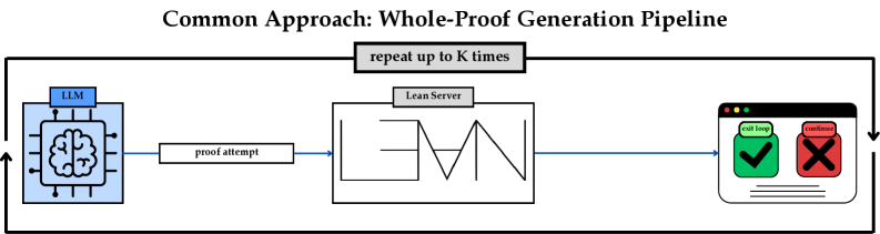
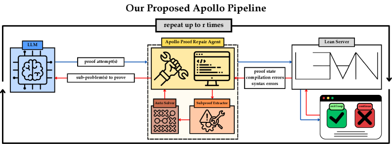
Figure 1: The summary of whole-proof generation pipeline vs. proposed Apollo agentic pipeline. LLM refers to a chosen formal theorem generator model.
Formal reasoning has emerged as one of the most challenging fields of AI with recent achievements such as AlphaProof and AlphaGeometry doing well at the International Math Olympiad competing with humans yang2024formal ; alphaproof ; AlphaGeometryTrinh2024 . Formal reasoning relies both on AI models and a formal verification system that can automatically verify whether a mathematical proof is correct or not. In recent years, formal verification systems such as Lean lean4paper have facilitated a new form of doing mathematical research by enabling mathematicians to interact with the formal verification system and also with each other via the system, enabling larger numbers of mathematicians to collaborate with each other on a single project. As such, these formal verification systems are also called proof assistants as one can use them interactively to write a formal proof and instantaneously observe the current state of the proof and any possible errors or shortcomings in the proof generated by the compiler. Immediate access to the output of Lean compiler can help a mathematician to fix possible errors in the proof. At the same time, when a proof passes the compiler with no error, other collaborators do not need to verify the correctness of the proof. This type of collaboration is transforming the field of mathematics enabling large groups of collaborators to engage in large projects of mathematical research such as the Prime Number Theorem And More project kontorovich_tao_2024_primenumbertheoremand . Moreover, it has given rise to the digitization of mathematics buzzard2024mathematical .
In the AI front, large language models (LLMs) are improving at mathematical reasoning in natural language, and at the same time, they have shown a remarkable ability to learn the language of those formal verification systems and write mathematical proofs in formal language. This has led to the field of Automated Theorem Proving (ATP) where the standard approach is to prompt the LLM to generate a number of candidate proofs for a given theorem which will then be verified automatically using the formal verification system. Better models, better training sets, and better training methods has led to significant advances in this field tsoukalas2024putnambenchevaluatingneuraltheoremprovers ; zheng2022minif2fcrosssystembenchmarkformal ; azerbayev2023proofnetautoformalizingformallyproving ; li2024numinamath ; hu2025minictx .
Despite these advances, the LLMs do not really get the chance to interact with the verification system the way a human does. LLMs generate many possible proofs, sometimes as many as tens of thousands, and the verification system only marks the proofs with a binary value of correct or incorrect. This common approach is illustrated in Figure 1. When the formal verification system analyzes a proof, its compiler may generate a long list of issues including syntax errors, incorrect tactics, open goals, etc. In the current approach of the community, all of those information/feedback from the compiler remains unused, as the LLM’s proof generation is not directly engaged with the compiler errors of the formal verification system.
In this work, we address this issue by introducing Apollo, a fully automated system which uses a modular, model-agnostic pipeline that combines the strengths of the Lean compiler with the reasoning abilities of LLMs. Apollo directs a fully automated process in which the LLM generates proofs for theorems, a set of agents analyze the proofs, fix the syntax errors, identify the mistakes in the proofs using Lean, isolate failing sub‑lemmas, utilize automated solvers, and invoke an LLM on each remaining goal with a low top‑ $K$ budget. The high-level overview of Apollo appears at the bottom of Figure 1.
Our contributions are as follows:
- We introduce a novel fully automated system that directs a collaboration between LLMs, Lean compiler, and automated solvers for automated theorem proving.
- We evaluate Apollo on miniF2F-test set using best LLMs for theorem proving and demonstrate that Apollo improves the baseline accuracies by significant margins while keeping the sampling costs much lower.
- We establish a new SOTA on miniF2F-test benchmark for medium-sized language models. (with parameter size 8B or less)
2 Related Works
Formal theorem proving systems. At their core, formal theorem‑proving (FTP) systems employ interactive theorem provers (ITPs) to verify mathematical results. In particular, Lean4 lean4paper is both a functional programming language and an ITP. Each theorem, lemma, conjecture, or definition must be checked by Lean’s trusted kernel, so the compiler’s verdict is binary: either the statement type‑checks (True) or it fails (False). This rigorous verification dramatically increases the reliability of formal mathematics; however, it also increases the complexity of proof development: authors must both comprehend the mathematical concepts and precisely encode them in the formal language. The usefulness of Lean is also shown to go beyond theorem proving, as Jiang et al. jiang2024leanreasoner showed that Lean can be adapted to natural language logical reasoning.
Patching broken programs. Many prior works have explored using feedback to repair broken proofs. In software engineering, “repair” typically refers to program repair, i.e. fixing code that no longer runs programrepair . A common source of errors is a version mismatch that introduces bugs and prevents execution. For example, SED sed_repair uses a neural program‐generation pipeline that iteratively repairs initial generation attempts. Other notable approaches train specialized models to fix broken code based on compiler feedback (e.g. BIFI bifi , TFix tfix ) or leverage unsupervised learning over large bug corpora (e.g. BugLab buglab ).
LLM collaboration with external experts. The use of expert feedback, whether from human users or from a proof assistant’s compiler, has proven effective for repairing broken proofs. Ringer ringer2009typedirected showcased automatic proof repair within the Coq proof assistant bertot2013interactive , enabling the correction of proofs in response to changes in underlying definitions. Jiang et al. jiang2022thor showed that leveraging automatic solvers with generative models yield better performance on formal math benchmarks. More recently, First et al. first2023baldurwholeproofgenerationrepair showed that incorporating compiler feedback into LLM proof generation significantly improves the model’s ability to correct errors and produce valid proofs. Another line of work song2023towards explored an idea of mathematician and LLM collaboration, where human experts are aided by LLMs at proof writing stage.
Proof search methods. Numerous recent systems use machine learning to guide the search for formal proofs. One of the methods involves using large language models with structured search strategies, e.g. Best‑First Search (BFS) polu2022formalmathematicsstatementcurriculum ; wu2024internlm25stepproveradvancingautomatedtheorem ; xin2025bfsproverscalablebestfirsttree or Monte Carlo Tree Search (MCTS) lample2022hypertree ; wang2023dt-solver ; alphaproof . While tree‑search methods reliably steer a model toward valid proofs, they result in high inference costs and often explore many suboptimal paths before success. Another line of work leverages retrieval based systems to provide context for proof generators with potentially useful lemmas. One such example is ReProver yang_leandojo_2023 that augments Lean proof generation by retrieving relevant lemmas from a proof corpus and feeding them to an LLM, enabling the model to reuse existing proofs.
Whole proof generation. The use of standalone LLMs for theorem proving has emerged as a major research direction in automated theorem proving. One of the earliest works presented GPT-f polu2020generativelanguagemodelingautomated , a transformer-based model for theorem proving that established the LLMs ability in formal reasoning. As training frameworks and methods advance, the community has produced numerous models that generate complete proofs without external search or tree‑search algorithms. Recent work shows that both supervised models xin2024deepseekproverv15harnessingproofassistant ; lin2025goedelproverfrontiermodelopensource and those trained via reinforcement learning xin2024deepseekproverv15harnessingproofassistant ; zhang2025leanabellproverposttrainingscalingformal ; dong2025stp ; kimina_prover_2025 achieve competitive performance on formal‑math benchmarks. However, whole‑proof generation remains vulnerable to hallucinations that can cause compilation failures even for proofs with correct reasoning chains.
Informal Chain-of-Thought in Formal Mathematics. Several recent works demonstrate that interleaving informal “chain‑of‑thought” (CoT) reasoning with formal proof steps substantially improves whole‑proof generation. For example, developers insert natural‑language mathematical commentary between tactics, yielding large accuracy gains lin2025goedelproverfrontiermodelopensource ; xin2024deepseekproverv15harnessingproofassistant ; azerbayev2024llemma . Wang, et al. kimina_prover_2025 further show that special “thinking” tokens let the model plan its strategy and self‑verify intermediate results. The “Draft, Sketch, and Prove” (DSP) jiang2023draftsketchproveguiding and LEGO-Prover wang2024legoprover pipelines rely on an informal proof sketch before attempting to generate the formal proof. Collectively, these studies indicate that providing informal mathematical context, whether as comments, sketches, or dedicated tokens, guides LLMs toward correct proofs and significantly boosts proof synthesis accuracy.
<details>
<summary>x3.png Details</summary>
### Visual Description
## Diagram: Apollo Algorithm Workflow and Proof Repair
### Overview
This image presents a technical flowchart and code comparison illustrating the "Apollo Algorithm," an automated system designed to repair formal mathematical proofs (specifically in the Lean 4 programming language) using a combination of symbolic tools and Large Language Models (LLMs). The top half displays the iterative workflow of the algorithm, while the bottom half provides a concrete before-and-after example of a Lean 4 proof being repaired.
### Components
The image is divided into three main spatial regions:
1. **Header & Main Flowchart (Top half):** A dashed rectangular border encloses the step-by-step process of the Apollo Algorithm.
2. **Invalid Proof (Bottom-left):** A code block outlined in red, showing a failing mathematical proof with specific errors highlighted.
3. **Correct Proof (Bottom-right):** A code block outlined in green, showing the successfully repaired proof with the corrected sections highlighted.
### Content Details
#### 1. Main Flowchart (Top Section)
The workflow proceeds through several distinct nodes, connected by directional arrows:
* **Syntax Refiner:** Located at the top-left. Represented by a blue box with an icon of a document and gears. An arrow points right to the Sorrifier.
* **Sorrifier:** Represented by a red box with an icon of a hammer breaking a dashed circle. An arrow points right to the Auto Solver.
* **Auto Solver:** Represented by a green box with an icon of a document and a green pen. An arrow points right to a sequence of LLM interactions.
* **LLM Interaction Sequence:**
* A gray box labeled `Extract subproofs to prove` points to an icon of a document with a microchip and checkmark.
* A gray box labeled `Feed to LLM` points to the **LLM** node (orange box, neural network icon).
* An arrow points down from the LLM to a gray box labeled `Assemble the proof back`.
* An arrow points left to the **Proof Assembler** (brown box, icon of a trowel building a brick wall).
* **Decision Loop:** From the Proof Assembler, an arrow points down to a decision diamond.
* **Decision Diamond 1 (Right):** Orange diamond labeled `Does the proof compile in Lean4?`.
* **YES (Green circle):** An arrow points down, exiting the dashed box and pointing to the "Correct Proof" block.
* **NO (Red circle):** An arrow points left to the second decision diamond.
* **Decision Diamond 2 (Left):** Orange diamond labeled `number of attempts > r?`.
* **NO (Red circle):** An arrow loops up and left, returning to the **Syntax Refiner** to start the process over.
* **YES (Green circle):** An arrow points down, exiting the dashed box and pointing to the "Invalid Proof" block.
#### 2. Invalid Proof (Bottom-Left Section)
This section contains Lean 4 code with a red border and a red header labeled "Invalid Proof". Four specific lines/blocks of code are highlighted in red and tagged with numbers `#1` through `#4`.
**Transcription of Invalid Proof Code:**
```lean
import Mathlib
import Aesop
set_option maxHeartbeats 0
open BigOperators Real Nat Topology Rat Set
theorem mathd_numbertheory_495_incorrect (a b : N)
(h₀ : 0 < a 0 < b)
(h₁ : a % 10 = 2) (h₂ : b % 10 = 4)
(h₃ : Nat.gcd a b = 6) : 108 ≤ Nat.lcm a b := by
have h4 : a ≥ 6 := by
have h5 : a % 10 = 2 := h₁
omega #1 (Highlighted Red)
have h5 : b ≥ 6 := by
have h6 : b % 10 = 4 := h₂
omega #2 (Highlighted Red)
by_contra h
push_neg at h
have h6 : a * b < 648 := by
have h7 : Nat.lcm a b < 108 := by linarith
have h8 : a * b = 6 * Nat.lcm a b := by
rw [ Nat.gcd_mul_lcm a b ]
rw [h₃]
linarith
have h7 : a ≤ 100 := by
nlinarith [h₁, h₂, h₃, Nat.gcd_pos_of_pos_left a h₀.right, #3 (Highlighted Red)
h₀.right, Nat.gcd_pos_of_pos_right b h₀.right] (Highlighted Red)
have h8 : b ≤ 100 := by
nlinarith [h₁, h₂, h₃, Nat.gcd_pos_of_pos_left a h₀.right, #4 (Highlighted Red)
h₀.right, Nat.gcd_pos_of_pos_right b h₀.right] (Highlighted Red)
interval_cases a <;> interval_cases b <;>
norm_num at *
<;> try { contradiction }
```
#### 3. Correct Proof (Bottom-Right Section)
This section contains Lean 4 code with a green border and a green header labeled "Correct Proof". It is formatted in two columns. Four specific blocks of code are highlighted in green and tagged with numbers `#1` through `#4`, corresponding directly to the red tags in the invalid proof.
**Transcription of Correct Proof Code (Left Column):**
```lean
...
theorem mathd_numbertheory_495_after_proof_repair
(a b : N)
(h₀ : 0 < a 0 < b)
(h₁ : a % 10 = 2) (h₂ : b % 10 = 4)
(h₃ : Nat.gcd a b = 6) : 108 ≤ Nat.lcm a b := by
have h4 : a ≥ 6 := by
have h5 : a % 10 = 2 := h₁
have h6 : 6 ≤ a := by #1 (Highlighted Green Start)
have h : a.gcd b = 6 := h₃
have h7 : 6 | a := by
rw [ ← h ]
apply Nat.gcd_dvd_left
omega
exact h6 (Highlighted Green End)
have h5 : b ≥ 6 := by
have h6 : b % 10 = 4 := h₂
by_contra h #2 (Highlighted Green Start)
push_neg at h
have h4 : b = 4 := by
omega
rw [h4] at h₃
have h6 : a.gcd 4 ≤ 4 := by
apply Nat.gcd_le_right
norm_num
linarith (Highlighted Green End)
by_contra h
push_neg at h
...
```
**Transcription of Correct Proof Code (Right Column):**
```lean
...
have h6 : a * b < 648 := by
have h7 : Nat.lcm a b < 108 := by linarith
have h8 : a * b = 6 * Nat.lcm a b := by
rw [ Nat.gcd_mul_lcm a b ]
rw [h₃]
linarith
have h7 : a ≤ 100 := by
by_contra h' #3 (Highlighted Green Start)
push_neg at h'
have h7 : a ≥ 101 := by linarith
have h8 : b ≤ 6 := by nlinarith
have h9 : b = 6 := by linarith
rw [h9] at h₂
norm_num at h₂ (Highlighted Green End)
have h8 : b ≤ 100 := by
by_contra h8 #4 (Highlighted Green Start)
push_neg at h8
have h9 : b ≤ 107 := by
have h10 : a * b < 648 := h6
have h11 : a ≥ 6 := h4
nlinarith
have h12 : b ≤ 107 := h9
have h13 : b > 100 := h8
have h14 : b % 10 = 4 := h₂
have h15 : b ≥ 101 := by omega
interval_cases b <;> omega (Highlighted Green End)
interval_cases a <;> interval_cases b <;> norm_num at *
<;> try { contradiction }
```
### Key Observations
* **Direct Substitution:** The tags `#1`, `#2`, `#3`, and `#4` serve as a visual legend connecting the two code blocks. The algorithm identifies failing single-line tactics (like `omega` or `nlinarith` in the red block) and replaces them with expanded, multi-step subproofs (in the green block) that successfully compile.
* **Iterative Loop:** The flowchart explicitly shows that if the LLM's generated proof does not compile in Lean 4, the system does not immediately fail. Instead, it loops back to the "Syntax Refiner" to try again, up to a maximum number of attempts (`r`).
* **Failure State:** If the number of attempts exceeds `r`, the algorithm outputs the "Invalid Proof" (the red path).
* **Success State:** If the proof compiles, it outputs the "Correct Proof" (the green path).
### Interpretation
This diagram illustrates a "neuro-symbolic" approach to automated theorem proving.
1. **The Problem:** Large Language Models (LLMs) are good at generating code but often make logical or syntactic errors in strict formal environments like Lean 4.
2. **The Solution (Apollo):** The Apollo Algorithm uses the strict Lean 4 compiler as a verifiable "ground truth." It isolates broken parts of a proof ("Extract subproofs to prove"), asks the LLM to fix only those specific parts, and then reassembles the proof.
3. **The Loop:** By placing the LLM inside a `while` loop governed by the Lean 4 compiler (`Does the proof compile?`), the system forces the LLM to iteratively refine its output until it is mathematically sound, rather than accepting its first guess. The before-and-after code blocks demonstrate that the LLM is capable of taking a failing, overly-optimistic tactic (like expecting `omega` to solve a complex goal) and breaking it down into rigorous, step-by-step logical deductions that satisfy the compiler.
</details>
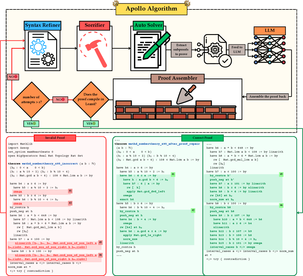
Figure 2: Overview of the Apollo framework.
3 Our Approach
In this section we describe Apollo, our framework for transforming an LLM’s raw proof sketch into a fully verified Lean4 proof. Figure 2 illustrates the Apollo pipeline process with an attached Lean code before and after repair. We observe that often LLM is capable of producing a valid proof sketch; however, it often struggles with closing fine-grained goals. For example, statements h4, h5, h7, h8 are correct but the generated proofs for each sub-lemma throw compilation errors. Apollo identifies and fixes such proof steps and guides the LLM towards a correct solution.
Our compiler of choice is the Lean REPL leanrepl , a “ R ead– E val– P rint– L oop” for Lean4. It provides a complete list of compilation errors and warnings, each with a detailed description and the location (for example, the line number) where it occurred. Errors can include syntax mistakes, nonexistent tactics, unused tactics, and more. We aggregate this information to drive our agent’s dynamic code repair and sub‑problem extraction. The pseudo-code for our framework can be found in Algorithm 1 in the Appendix.
3.1 Syntax Refiner
The Syntax Refiner catches and corrects superficial compilation errors: missing commas, wrong keywords (e.g. Lean3’s from vs. Lean4’s := by), misplaced brackets, etc. These syntax errors arise when a general‑purpose LLM (such as o3‑mini openai-o3-mini-2025 or o4‑mini openai-o4-mini-2025 ) has not been specialized on Lean4 syntax. By normalizing these common mistakes, this module ensures that subsequent stages operate on syntactically valid code. It is important to note that this module is primarily applicable to general purpose models not explicitly trained for theorem proving in Lean. In contrast, Syntax Refiner usually does not get invoked for proofs generated by LLMs trained for formal theorem proving.
3.2 Sorrifier
The Sorrifier patches any remaining compilation failures by inserting Lean’s sorry placeholder. We first parse the failed proof into a tree of nested proof‑blocks (sub‑lemmas as children). Then we compile the proof with Lean REPL leanrepl , detect the offending line or block, and apply one of three repairs:
1. Line removal, if a single tactic or declaration is invalid but its surrounding block may still succeed.
1. Block removal, if the entire sub‑proof is malformed.
1. Insert sorry, if the block compiles but leaves unsolved goals open.
We repeat this procedure until the file compiles without errors. At that point, every remaining sorry marks a sub‑lemma to be proved in later stages of Apollo. This part of the pipeline guarantees that the proof successfully compiles in Lean with warnings of presence of sorry statements.
Each sorry block corresponds to a sub‑problem that the LLM failed to prove. Such blocks may not type‑check for various reasons, most commonly LLM hallucination. The feedback obtained via REPL lets us to automatically catch these hallucinations, insert a sorry placeholder, and remove invalid proof lines.
3.3 Auto Solver
The Auto Solver targets each sorry block in turn. It first invokes the Lean4’s hint to close the goal. If goals persist, it applies built‑in solvers (nlinarith, ring, simp, etc.) wrapped in try to test combinations automatically. Blocks whose goals remain open stay marked with sorry. After applying Auto Solver, a proof may be complete with no sorry’s in which case Apollo has already succeeded in fixing the proof. Otherwise, the process can repeat recursively.
3.4 Recursive reasoning and repair
In the case where a proof still has some remaining sorry statements after applying the Auto Solver, Apollo can consider each as a new lemma, i.e., extract its local context (hypotheses, definitions, and any lemmas proved so far), and recursively try to prove the lemmas by prompting the LLM and repeating the whole process of verification, syntax refining, sorrifying, and applying the Auto Solver.
At each of these recursive iterations, a lemma may be completely proved, or it may end up with an incomplete proof with one or a few sorry blocks. This allows the Apollo to make progress in proving the original theorem by breaking down the incomplete steps further and further until the LLM or Auto Solver can close the goals. This process can continue up to a user‑specified recursion depth $r$ .
3.5 Proof Assembler
Finally, the Proof Assembler splices all repaired blocks back into a single file and verifies that no sorry or admit (alias for "sorry") commands remain. If the proof still fails, the entire pipeline repeats (up to a user‑specified recursion depth $r$ ), allowing further rounds of refinement and sub‑proof generation.
Apollo’s staged approach: syntax cleaning, “sorrifying,” automated solving, and targeted LLM‐driven repair, yields improvements in both proof‐sample efficiency and final proof correctness.
4 Experiments
In this section, we present empirical results for Apollo on the miniF2F dataset zheng2022minif2fcrosssystembenchmarkformal , which comprises of 488 formalized problems drawn from AIME, IMO, and AMC competitions. The benchmark is evenly split into validation and test sets (244 problems each); here we report results on the miniF2F‑test partition. To demonstrate Apollo’s effectiveness, we evaluate it on a range of state‑of‑the‑art whole‑proof generation models. All experiments use Lean v4.17.0 and run on eight NVIDIA A5000 GPUs with 128 CPU cores. We used $@32$ sampling during sub-proof generation unless stated otherwise. Baseline numbers are sourced from each model’s original publication works.
4.1 The effect of applying Apollo on top of the base models
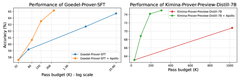
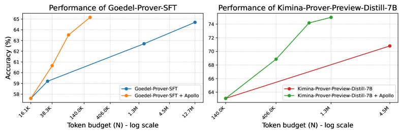
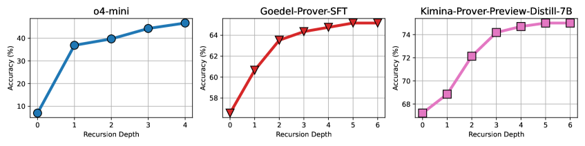
Figure 3 shows the impact of Apollo on two state‑of‑the‑art whole‑proof generation models: Goedel Prover‑SFT lin2025goedelproverfrontiermodelopensource and Kimina‑Prover‑Preview‑Distill‑7B kimina_prover_2025 . Applying Apollo increases Goedel‑Prover‑SFT’s top accuracy from 64.7% to 65.6% while reducing its sampling budget by two orders of magnitude (from 25,600 generated samples to only a few hundred on average). Similarly, Kimina‑Prover‑Preview‑Distill‑7B achieves a new best Kimina-Prover-Preview-Distill-7B accuracy of 75.0% with roughly one‑third of the previous sample budget. We report the exact numbers in Table 1.
<details>
<summary>x4.png Details</summary>
### Visual Description
**Language Declaration:** The text in this image is entirely in English. No other languages are present.
## Line Charts: Performance Impact of "Apollo" on Prover Models
### Overview
The image consists of two side-by-side line charts comparing the performance (Accuracy) against computational cost (Pass budget) for two different AI models: "Goedel-Prover-SFT" (left) and "Kimina-Prover-Preview-Distill-7B" (right). Both charts demonstrate the baseline model's performance compared to the model augmented with a system or method called "Apollo".
### Component Isolation: Left Chart (Goedel-Prover-SFT)
#### Components/Axes
* **Positioning:** Left half of the image.
* **Title:** "Performance of Goedel-Prover-SFT" (Top center).
* **Y-axis:** Labeled "Accuracy (%)". Linear scale with major gridlines at 58, 59, 60, 61, 62, 63, 64, and 65.
* **X-axis:** Labeled "Pass budget (K) - log scale". The tick marks are angled and spaced logarithmically. The explicit labels are: 32, 80, 150, 306, 1.0K, 25.6K.
* **Legend:** Located in the bottom-right corner of the chart area.
* Blue line with circular markers: `Goedel-Prover-SFT`
* Orange line with circular markers: `Goedel-Prover-SFT + Apollo`
#### Detailed Analysis
* **Trend Verification (Blue Line - Baseline):** The blue line slopes upward gradually across a massive span of the x-axis (from 32 to 25.6K).
* Point 1: x = 32, y ≈ 57.6%
* Point 2: x = 80, y ≈ 59.2%
* Point 3: x = 1.0K, y ≈ 62.7%
* Point 4: x = 25.6K, y ≈ 64.7%
* **Trend Verification (Orange Line - With Apollo):** The orange line slopes upward steeply, achieving higher accuracy at much lower pass budgets, terminating early on the x-axis.
* Point 1: x = 32, y ≈ 57.6% (Shares exact starting point with baseline)
* Point 2: x = 80, y ≈ 60.7%
* Point 3: x = 150, y ≈ 63.5%
* Point 4: x = 306, y ≈ 65.1%
---
### Component Isolation: Right Chart (Kimina-Prover-Preview-Distill-7B)
#### Components/Axes
* **Positioning:** Right half of the image.
* **Title:** "Performance of Kimina-Prover-Preview-Distill-7B" (Top center).
* **Y-axis:** No explicit text label, but visually shares the "Accuracy (%)" metric from the left chart. Linear scale with major gridlines at 64, 66, 68, 70, 72, and 74.
* **X-axis:** Labeled "Pass budget (K)". This is a **linear scale**, unlike the left chart. Major tick marks at 0, 200, 400, 600, 800, 1000.
* **Legend:** Located in the top-right corner of the chart area.
* Red line with circular markers: `Kimina-Prover-Preview-Distill-7B`
* Green line with circular markers: `Kimina-Prover-Preview-Distill-7B + Apollo`
#### Detailed Analysis
* **Trend Verification (Red Line - Baseline):** The red line slopes upward gradually in a nearly straight line across the linear x-axis.
* Point 1: x ≈ 32 (slightly right of 0), y ≈ 63.1%
* Point 2: x ≈ 1024 (slightly past 1000), y ≈ 70.8%
* **Trend Verification (Green Line - With Apollo):** The green line slopes upward very steeply, then begins to curve (concave down), showing rapid accuracy gains at low pass budgets.
* Point 1: x ≈ 32, y ≈ 63.1% (Shares exact starting point with baseline)
* Point 2: x ≈ 100, y ≈ 68.8%
* Point 3: x ≈ 200, y ≈ 74.1%
* Point 4: x ≈ 300, y ≈ 75.0%
---
### Key Observations
1. **Shared Origins:** In both charts, the baseline model and the Apollo-enhanced model start at the exact same accuracy for the lowest pass budget (approx. 32K).
2. **Drastic Efficiency Gains:** The addition of "Apollo" creates a significantly steeper learning/performance curve in both models.
3. **Scale Discrepancy:** The left chart uses a logarithmic scale for the X-axis to show the baseline model requiring up to 25.6K pass budget to reach ~64.7% accuracy. The Apollo version reaches higher accuracy (~65.1%) at a mere 306 pass budget. This is an efficiency gain of nearly two orders of magnitude.
4. **Higher Baseline:** The Kimina model (right) starts at a higher baseline accuracy (~63%) compared to the Goedel model (~57.6%).
### Interpretation
The data overwhelmingly demonstrates that the "Apollo" method/system acts as a massive multiplier for computational efficiency (measured here as "Pass budget").
By reading between the lines, "Pass budget" likely refers to the number of attempts, samples, or tokens a theorem-proving model is allowed to generate or evaluate to find a correct solution.
Without Apollo, scaling up the pass budget yields diminishing, slow returns (requiring logarithmic scaling on the left chart just to fit the baseline line). With Apollo, the models achieve superior accuracy using a fraction of the computational budget. For example, on the left chart, Apollo achieves in ~300 passes what the baseline cannot achieve in 25,000 passes. On the right chart, Apollo achieves 75% accuracy at 300 passes, while the baseline only reaches ~71% at over 1000 passes. Apollo appears to be a highly effective search heuristic, filtering mechanism, or reasoning enhancement that prevents the models from wasting computational budget on dead ends.
</details>
(a) Model accuracy against sampling budget
<details>
<summary>x5.png Details</summary>
### Visual Description
## Line Charts: Performance Comparison of Base Models vs. Apollo-Augmented Models
### Overview
The image consists of two side-by-side line charts demonstrating the performance (Accuracy) of two different language models ("Goedel-Prover-SFT" and "Kimina-Prover-Preview-Distill-7B") as a function of their token budget. Each chart compares the base model against a version augmented with a system or method called "Apollo". The language used in the image is entirely English.
---
### Component Isolation: Left Chart (Goedel-Prover-SFT)
#### Components/Axes
* **Positioning:** Left half of the image.
* **Title:** "Performance of Goedel-Prover-SFT" (Centered at the top).
* **Y-Axis:**
* **Label:** "Accuracy (%)" (Rotated 90 degrees, positioned on the far left).
* **Scale:** Linear, ranging from 58 to 65.
* **Markers/Gridlines:** Horizontal dotted gridlines at integer intervals: 58, 59, 60, 61, 62, 63, 64, 65.
* **X-Axis:**
* **Label:** "Token budget (N) - log scale" (Centered at the bottom).
* **Scale:** Logarithmic.
* **Markers:** Tilted text labels at specific intervals: 16.1K, 38.3K, 140.0K, 406.0K, 1.3M, 4.5M, 12.7M. Vertical dotted gridlines align with these markers.
* **Legend:** Positioned in the bottom-right corner of the chart area, enclosed in a white box with a light gray border.
* Blue line with a solid circle marker: `Goedel-Prover-SFT`
* Orange line with a solid circle marker: `Goedel-Prover-SFT + Apollo`
#### Detailed Analysis (Left Chart)
* **Trend Verification - Blue Line (Goedel-Prover-SFT):** The blue line exhibits a steady, moderate upward slope across the entire visible x-axis, indicating a gradual increase in accuracy as the token budget increases.
* Point 1: X = 16.1K, Y ≈ 57.6%
* Point 2: X = 38.3K, Y ≈ 59.2%
* Point 3: X = 1.3M, Y ≈ 62.7%
* Point 4: X = 12.7M, Y ≈ 64.7%
* **Trend Verification - Orange Line (Goedel-Prover-SFT + Apollo):** The orange line starts at the exact same point as the blue line but slopes upward much more steeply. It achieves higher accuracy at significantly lower token budgets and terminates earlier on the x-axis.
* Point 1: X = 16.1K, Y ≈ 57.6% (Shared origin with the blue line)
* Point 2: X = 38.3K, Y ≈ 60.7%
* Point 3: X = 140.0K, Y ≈ 63.5%
* Point 4: X ≈ 300K (Visually positioned before the 406.0K marker), Y ≈ 65.2%
---
### Component Isolation: Right Chart (Kimina-Prover-Preview-Distill-7B)
#### Components/Axes
* **Positioning:** Right half of the image.
* **Title:** "Performance of Kimina-Prover-Preview-Distill-7B" (Centered at the top).
* **Y-Axis:**
* **Label:** None explicitly written, but contextually inherits "Accuracy (%)" from the left chart.
* **Scale:** Linear, ranging from 64 to 74.
* **Markers/Gridlines:** Horizontal dotted gridlines at even integer intervals: 64, 66, 68, 70, 72, 74.
* **X-Axis:**
* **Label:** "Token budget (N) - log scale" (Centered at the bottom).
* **Scale:** Logarithmic.
* **Markers:** Tilted text labels at specific intervals: 140.0K, 406.0K, 1.3M, 4.5M. Vertical dotted gridlines align with these markers.
* **Legend:** Positioned in the bottom-right corner of the chart area, enclosed in a white box with a light gray border.
* Red line with a solid circle marker: `Kimina-Prover-Preview-Distill-7B`
* Green line with a solid circle marker: `Kimina-Prover-Preview-Distill-7B + Apollo`
#### Detailed Analysis (Right Chart)
* **Trend Verification - Red Line (Kimina-Prover-Preview-Distill-7B):** The red line shows a steady, moderate upward slope from the lowest visible token budget to the highest.
* Point 1: X = 140.0K, Y ≈ 63.1%
* Point 2: X = 4.5M, Y ≈ 70.8%
* **Trend Verification - Green Line (Kimina-Prover-Preview-Distill-7B + Apollo):** The green line shares the starting point with the red line but slopes upward sharply, achieving significantly higher accuracy at lower token budgets before the slope begins to shallow out slightly at the top.
* Point 1: X = 140.0K, Y ≈ 63.1% (Shared origin with the red line)
* Point 2: X = 406.0K, Y ≈ 68.8%
* Point 3: X ≈ 800K (Visually positioned roughly halfway between 406.0K and 1.3M on the log scale), Y ≈ 74.2%
* Point 4: X ≈ 1.5M (Visually positioned slightly to the right of the 1.3M marker), Y ≈ 75.0%
---
### Key Observations
1. **Shared Origins:** In both charts, the base model and the "+ Apollo" model start at the exact same accuracy for the lowest tested token budget (16.1K for Goedel, 140.0K for Kimina).
2. **Steeper Trajectories:** In both charts, the addition of "Apollo" (Orange line left, Green line right) results in a drastically steeper performance curve compared to the base models (Blue line left, Red line right).
3. **Different Baselines:** The Kimina model (Right Chart) operates at a higher overall accuracy baseline (ranging roughly 63% to 75%) compared to the Goedel model (Left Chart, ranging roughly 57% to 65%).
4. **Token Budget Ranges:** The Goedel chart evaluates performance starting from a much lower token budget (16.1K) and extending to a higher one (12.7M) compared to the Kimina chart (140.0K to 4.5M).
### Interpretation
The data strongly suggests that the "Apollo" augmentation is a highly effective method for improving the sample efficiency of these language models.
By reading between the lines, the charts demonstrate that to achieve a specific target accuracy, a model using Apollo requires orders of magnitude fewer tokens than the base model. For example, in the left chart, the base Goedel model requires roughly 12.7M tokens to reach ~64.7% accuracy. The Apollo-augmented version surpasses that accuracy (reaching ~65.2%) using fewer than 406K tokens.
This implies that Apollo significantly accelerates the learning or reasoning process during training or inference (depending on what "Token budget" specifically refers to in this context, though "Prover" suggests inference/search budgets in formal mathematics or logic tasks). The fact that this pattern holds true across two distinctly different models (Goedel and Kimina) indicates that Apollo is likely a generalized architectural improvement or search strategy rather than a model-specific tweak.
</details>
(b) Model accuracy against generated token budget
Figure 3: Performance of base models against the Apollo aided models on miniF2F-test dataset at different sample budgets and token length.
Note that Apollo’s sampling budget is not fixed: it depends on the recursion depth $r$ and the LLM’s ability to generate sub‑lemmas. For each sub‑lemma that Auto Solver fails to close, we invoke the LLM with a fixed top‑32 sampling budget. Because each generated sub‑lemma may spawn further sub‑lemmas, the total sampling overhead grows recursively, making any single @K budget difficult to report. Sub‑lemmas also tend to require far fewer tactics (and thus far fewer tokens) than the main theorem. A theorem might need 100 lines of proof while a sub-lemma might need only 1 line. Hence, sampling cost does not scale one‑to‑one. Therefore, to compare with other whole-proof generation approaches, we report the average number of proof samples and token budgets. We present more in-depth analysis of inference budgets in Section B of the Appendix.
Table 1: Table results comparing sampling cost, accuracy, and token usage before and after applying Apollo. “Cost” denotes the sampling budget $K$ for whole‑proof generation and the recursion depth $r$ for Apollo. Column $N$ reports the average number of tokens generated per problem in "Chain‑of‑Thought" mode. Bold cells highlight the best accuracy. Results are shown on the miniF2F‑test dataset for two models: Kimina‑Prover‑Preview‑Distill‑7B and Goedel‑SFT.
| Goedel‑Prover‑SFT | Kimina‑Prover‑Preview‑Distill‑7B | | | | | | | | | | |
| --- | --- | --- | --- | --- | --- | --- | --- | --- | --- | --- | --- |
| Base Model | + Apollo | Base Model | + Apollo | | | | | | | | |
| $K$ | $N$ | Acc. (%) | $r$ | $N$ | Acc. (%) | $K$ | $N$ | Acc. (%) | $r$ | $N$ | Acc. (%) |
| 32 | 16.1K | 57.6% | 0 | 16.1K | 57.6% | 32 | 140K | 63.1% | 0 | 140K | 63.1% |
| 64 | 31.8K | 59.2% | 2 | 38.3K | 60.7% | | | | 2 | 406K | 68.9% |
| 3200 | 1.6M | 62.7% | 4 | 74.6K | 63.5% | | | | 4 | 816K | 74.2% |
| 25600 | 12.7M | 64.7% | 6 | 179.0K | 65.6 % | 1024 | 4.5M | 70.8% | 6 | 1.3M | 75.0% |
4.2 Comparison with SoTA LLMs
Table 2 compares whole‑proof generation and tree‑search methods on miniF2F‑test. For each approach, we report its sampling budget, defined as the top‑ $K$ parameter for LLM generators or equivalent search‑depth parameters for tree‑search provers. Since Apollo’s budget varies with recursion depth $r$ , we instead report the mean number of proof sampled during procedure. Moreover, we report an average number of generated tokens as another metric for computational cost of proof generation. For some models due to inability to collect generated tokens, we leave them blank and report sampling budget only.
When Apollo is applied on top of any generator, it establishes a new best accuracy for that model. For instance, Goedel‑Prover‑SFT’s accuracy jumps to 65.6%, surpassing the previous best result (which required 25,600 sample budget). In contrast, Apollo requires only 362 samples on average. Likewise, Kimina‑Prover‑Preview‑Distill‑7B sees a 4.2% accuracy gain while reducing its sample budget below the original 1,024. To further validate Apollo’s generalizability, we tested the repair framework on Goedel-V2-8B lin2025goedelproverv2 , the current state-of-the-art theorem prover. We observe that, at similar sample and token budgets, Apollo achieves a 0.9% accuracy gain, whereas the base LLM requires twice the budget to reach the same accuracy. Overall, Apollo not only boosts accuracy but does so with a smaller sampling budget, setting a new state-of-the-art result among sub‑8B‑parameter LLMs with sampling budget of 32.
We also evaluate general‑purpose LLMs (OpenAI o3‑mini and o4‑mini). Without Apollo, these models rarely produce valid Lean4 proofs, since they default to Lean3 syntax or introduce trivial compilation errors. Yet they have a remarkable grasp of mathematical concepts, which is evident by the proof structures they often produce. By applying Apollo’s syntax corrections and solver‑guided refinements, their accuracies increase from single digits (3–7%) to over 40%. These results demonstrate that in many scenarios discarding and regenerating the whole proof might be overly wasteful, and with a little help from a Lean compiler, we can achieve better accuracies while sampling less proofs from LLMs.
Table 2: Comparison of Apollo accuracy against state-of-the-art models on the miniF2F-test dataset. Token budget is computed over all generated tokens by LLM.
| Method | Model size | Sample budget | Token budget | miniF2F-test |
| --- | --- | --- | --- | --- |
| Tree Search Methods | | | | |
| Hypertree Proof Search (lample2022hypertree, ) | 0.6B | $64× 5000$ | - | $41.0\%$ |
| IntLM2.5-SP+BFS+CG (wu2024internlm25stepproveradvancingautomatedtheorem, ) | 7B | $256× 32× 600$ | - | $65.9\%$ |
| HPv16+BFS+DC (li2025hunyuanproverscalabledatasynthesis, ) | 7B | $600× 8× 400$ | - | $68.4\%$ |
| BFS-Prover (xin2025bfsproverscalablebestfirsttree, ) | 7B | $2048× 2× 600$ | - | $70.8\%$ |
| Whole-proof Generation Methods | | | | |
| DeepSeek-R1- Distill-Qwen-7B (deepseekai2025deepseekr1incentivizingreasoningcapability, ) | 7B | 32 | - | 42.6% |
| Leanabell-GD-RL (zhang2025leanabellproverposttrainingscalingformal, ) | 7B | $128$ | - | $61.1\%$ |
| STP (dong2025stp, ) | 7B | $25600$ | - | $67.6\%$ |
| o3-mini (openai-o3-mini-2025, ) | - | 1 | - | $3.3\%$ |
| $32$ | - | $24.6\%$ | | |
| o4-mini (openai-o4-mini-2025, ) | - | 1 | - | $7.0\%$ |
| Goedel-SFT (lin2025goedelproverfrontiermodelopensource, ) | 7B | 32 | 16.1K | $57.6\%$ |
| $3200$ | 1.6M | $62.7\%$ | | |
| $25600$ | 12.7M | $64.7\%$ | | |
| Kimina-Prover- Preview-Distill (kimina_prover_2025, ) | 7B | 1 | 4.4K | $52.5\%$ |
| $32$ | 140K | $63.1\%$ | | |
| $1024$ | 4.5M | $70.8\%$ | | |
| Goedel-V2 (lin2025goedelproverv2, ) | 8B | 32 | 174K | $83.3\%$ |
| $64$ | 349K | $84.0\%$ | | |
| $128$ | 699K | $84.9\%$ | | |
| Whole-proof Generation Methods + Apollo | | | | |
| o3-mini + Apollo | - | 8 | - | 40.2% (+36.9%) |
| o4-mini + Apollo | - | 15 | - | 46.7% (+39.7%) |
| Goedel-SFT + Apollo | 7B | 362 | 179K | 65.6% (+0.9%) |
| Kimina-Preview + Apollo | 7B | 307 | 1.3M | 75.0% (+4.2%) |
| Goedel-V2 + Apollo | 8B | 63 | 344K | 84.9% (+0.9%) |
To further assess Apollo, we conducted experiments on PutnamBench tsoukalas2024putnambenchevaluatingneuraltheoremprovers , using Kimina-Prover-Preview-Distill-7B as the base model. Under whole-proof generation pipeline, LLM produced 10 valid proofs. With Apollo, the LLM produced one additional valid proof while consuming nearly half as many tokens. Results are presented in Table 3.
Overall, our results on a variety of LLMs and benchmarks demonstrate that Apollo consistently consumes fewer tokens while achieving higher accuracy, highlighting its effectiveness.
Table 3: Comparison of Apollo accuracy on the PutnamBench dataset. Token budget is computed over all generated tokens by LLM.
| Method | Model size | Sample budget | Token budget | PutnamBench |
| --- | --- | --- | --- | --- |
| Kimina-Preview | 7B | 32 | 180K | 7/658 |
| Kimina-Preview | 7B | 192 | 1.1M | 10/658 |
| Kimina-Preview+Apollo | 7B | 108 | 579K | 11/658 |
4.3 Distribution of Proof Lengths
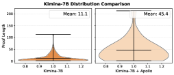
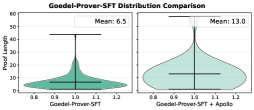
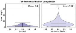
We assess how Apollo affects proof complexity by examining proof‑length distributions before and after repair. Here, proof length is defined as the total number of tactics in a proof, which serves as a proxy for proof complexity.
Figure 4 presents violin plots for three base models: Kimina‑Prover‑Preview‑Distill‑7B, Goedel‑Prover‑SFT, and o4‑mini. Each subplot shows two non‑overlapping sets: proofs generated directly by the base model (“before”) and proofs produced after applying Apollo (“after”). We only consider valid proofs verified by REPL in this setup.
The proofs that Apollo succeeds in fixing in collaboration with the LLM have considerably longer proof lengths. The mean length of proofs fixed by Apollo is longer than those written by the LLM itself at least by a factor of two in each model selection scenario. This increase indicates that the proofs which the base model alone could not prove require longer, more structured reasoning chains. By decomposing challenging goals into smaller sub‑lemmas, Apollo enables the generation of these extended proofs, therefore improving overall success rate.
These results demonstrate that Apollo not only raises accuracy but also systematically guides models to construct deeper, more rigorous proof structures capable of solving harder theorems.
<details>
<summary>x6.png Details</summary>
### Visual Description
## Violin Plot: Kimina-7B Distribution Comparison
### Overview
This image displays a side-by-side comparison of two violin plots. The charts illustrate the distribution of a metric called "Proof Length" across two different system configurations: "Kimina-7B" (left) and "Kimina-7B + Apollo" (right). The plots show the density of the data at different values, along with internal markers indicating the range and median, and explicit text boxes stating the mean for each distribution.
### Components/Axes
**Header Region:**
* **Main Title:** "Kimina-7B Distribution Comparison" (Centered at the top).
**Y-Axis (Shared visually, labeled only on the left):**
* **Title:** "Proof Length" (Rotated 90 degrees counter-clockwise, positioned on the far left).
* **Scale/Markers:** Numerical values starting from 0, incrementing by 50 up to 200 (0, 50, 100, 150, 200).
* **Gridlines:** Faint, light-gray horizontal gridlines extend across both plots at each 50-unit interval.
**X-Axes (Individual to each subplot):**
* **Left Subplot Label:** "Kimina-7B"
* **Right Subplot Label:** "Kimina-7B + Apollo"
* **Scale/Markers (Both subplots):** 0.8, 0.9, 1.0, 1.1, 1.2. (These represent the arbitrary width scale used to draw the violin shapes, centered on 1.0).
**Annotations (Legends/Text Boxes):**
* **Left Subplot (Top-Right):** A white rectangular box containing the text "Mean: 11.1".
* **Right Subplot (Top-Right):** A white rectangular box containing the text "Mean: 45.4".
### Detailed Analysis
**Left Plot: Kimina-7B**
* **Visual Trend/Shape:** The distribution is heavily skewed toward the bottom. The violin shape is extremely wide at the base (near zero) and tapers sharply into a very thin, needle-like tail that extends upwards. The color is a solid, medium-dark orange/brown.
* **Data Points (Approximate based on internal markers):**
* **Stated Mean:** 11.1
* **Minimum (Bottom horizontal line):** ~0 to 2
* **Median (Middle horizontal line):** ~10 to 15 (Aligns closely with the stated mean).
* **Maximum (Top horizontal line):** ~110 to 115.
**Right Plot: Kimina-7B + Apollo**
* **Visual Trend/Shape:** The distribution is much broader and extends much higher than the left plot. While still widest near the bottom, the "bulge" of the violin is thicker and extends further up the y-axis (between 20 and 80) before tapering. The tail extends past the visible 200 mark on the y-axis. The color is a lighter, more transparent peach/orange.
* **Data Points (Approximate based on internal markers):**
* **Stated Mean:** 45.4
* **Minimum (Bottom horizontal line):** ~0 to 2
* **Median (Middle horizontal line):** ~45 to 50 (Aligns closely with the stated mean).
* **Maximum (Top horizontal line):** Extends beyond the 200 gridline, approximately ~210 to 220.
### Key Observations
1. **Significant Shift in Mean:** The addition of "Apollo" increases the mean Proof Length by more than a factor of four (from 11.1 to 45.4).
2. **Change in Distribution Shape:** The baseline Kimina-7B model produces almost exclusively very short proofs (clustered tightly around 10). The Kimina-7B + Apollo configuration produces a much wider variety of proof lengths, with a thick distribution of lengths between 20 and 100.
3. **Increased Maximums:** The longest proofs generated by the baseline model cap out around 115. The Apollo-augmented model generates proofs that exceed a length of 200.
### Interpretation
This chart demonstrates the impact of integrating an "Apollo" component or methodology with a base "Kimina-7B" model (likely a 7-billion parameter Large Language Model) on a task involving formal logic, mathematics, or reasoning (indicated by "Proof Length").
The data clearly suggests that the baseline model tends to output very brief, perhaps truncated or overly concise, proofs. By adding Apollo, the system is forced or enabled to generate significantly longer proofs.
*Reading between the lines:* In the context of LLM reasoning, longer "proofs" often correlate with Chain-of-Thought (CoT) reasoning, step-by-step deduction, or more rigorous formal verification. The Apollo addition appears to be a mechanism designed specifically to increase the verbosity, depth, or step-count of the model's reasoning process. The fact that the distribution becomes much wider (rather than just shifting the whole cluster up) implies that Apollo allows the model to dynamically adjust the proof length based on the complexity of the prompt, whereas the base model was seemingly constrained to short outputs regardless of the input.
</details>
(a) Kimina-Preview-Distill-7B
<details>
<summary>x7.png Details</summary>
### Visual Description
## Violin Plot: Goedel-Prover-SFT Distribution Comparison
### Overview
The image displays two side-by-side violin plots comparing the statistical distribution of "Proof Length" between two different system configurations: a baseline "Goedel-Prover-SFT" and an augmented "Goedel-Prover-SFT + Apollo". The charts illustrate how the addition of "Apollo" alters the length and variance of the generated proofs.
### Components/Axes
**Header (Top Center):**
* **Main Title:** "Goedel-Prover-SFT Distribution Comparison" (Black, bold text).
**Y-Axis (Shared visually, labeled on the far left):**
* **Title:** "Proof Length" (Rotated 90 degrees counter-clockwise).
* **Scale/Markers:** Ranges from 0 to 60, with tick marks and faint horizontal grid lines at intervals of 10 (0, 10, 20, 30, 40, 50, 60).
**Left Subplot (Baseline):**
* **X-Axis Label (Bottom Center):** "Goedel-Prover-SFT"
* **X-Axis Scale:** 0.8, 0.9, 1.0, 1.1, 1.2 (Note: In standard violin plots, these are dummy coordinates used to define the width of the plot around a central axis of 1.0; they do not represent data variables).
* **Legend (Top Right):** A white box containing the text "Mean: 6.5".
**Right Subplot (Augmented):**
* **X-Axis Label (Bottom Center):** "Goedel-Prover-SFT + Apollo"
* **X-Axis Scale:** 0.8, 0.9, 1.0, 1.1, 1.2 (Dummy coordinates).
* **Legend (Top Right):** A white box containing the text "Mean: 13.0".
### Detailed Analysis
**1. Left Plot: Goedel-Prover-SFT**
* **Visual Trend:** The distribution is highly skewed to the right (positive skew). The vast majority of the data mass is concentrated at the very bottom of the y-axis, indicating that most proofs are quite short. The plot narrows sharply and extends into a long, thin upper tail.
* **Color:** Medium teal/sea-green fill with a dark outline.
* **Data Points (Approximate based on visual alignment with Y-axis):**
* **Minimum (Bottom horizontal line):** ~1
* **Mean/Median (Middle horizontal line):** 6.5 (Explicitly stated in the legend). Visually, the widest part of the violin (the mode) sits slightly below this mean line, around 4-5.
* **Maximum (Top horizontal line):** ~44
**2. Right Plot: Goedel-Prover-SFT + Apollo**
* **Visual Trend:** While still exhibiting a rightward skew, the distribution is significantly more dispersed than the baseline. The "bulb" of the violin is wider, taller, and sits higher on the y-axis. The tail extends much further up the y-axis, indicating a higher frequency of much longer proofs.
* **Color:** Pale mint green/light cyan fill with a dark outline.
* **Data Points (Approximate based on visual alignment with Y-axis):**
* **Minimum (Bottom horizontal line):** ~1
* **Mean/Median (Middle horizontal line):** 13.0 (Explicitly stated in the legend). The widest part of the violin sits around 10-12.
* **Maximum (Top horizontal line):** ~58
### Key Observations
* **Mean Doubling:** The most prominent data point is the exact doubling of the mean proof length, from 6.5 in the baseline to 13.0 with the addition of Apollo.
* **Maximum Extension:** The maximum proof length increases by approximately 14 units (from ~44 to ~58).
* **Variance/Spread:** The right plot is visibly "fatter" in the middle ranges (10-30) compared to the left plot, which is almost entirely concentrated below 10. This indicates a much higher variance in proof lengths when Apollo is used.
* **Shared Minimums:** Both distributions appear to share a similar minimum proof length near zero (approx. 1), suggesting that Apollo does not eliminate short proofs entirely, but rather shifts the overall distribution upward.
### Interpretation
The data clearly demonstrates that integrating "Apollo" into the "Goedel-Prover-SFT" system fundamentally changes the output characteristics of the model, specifically regarding verbosity or complexity.
Because "Proof Length" in automated theorem proving or logical reasoning models usually correlates with the number of deductive steps or the depth of reasoning, the doubling of the mean suggests that Apollo enables or forces the model to generate significantly more detailed, multi-step proofs.
*Reading between the lines (Peircean inference):* The fact that the minimum proof length remains unchanged while the mean and maximum increase drastically implies that Apollo does not simply add "padding" to all answers. If a proof requires only 1 or 2 steps, the Apollo-augmented model can still provide that short answer. However, for more complex problems, Apollo unlocks the model's ability to sustain longer chains of reasoning (up to ~58 steps/length units), whereas the baseline model rarely exceeded 10 steps and capped out at ~44. Therefore, Apollo likely acts as a reasoning enhancer or a search-depth expander rather than a simple verbosity multiplier.
</details>
(b) Goedel-SFT
<details>
<summary>x8.png Details</summary>
### Visual Description
## Violin Plot: o4-mini Distribution Comparison
### Overview
This image displays a side-by-side violin plot comparing the distribution of a metric called "Proof Length" between two distinct system configurations: a base model ("o4-mini") and an augmented model ("o4-mini + Apollo"). The charts visually demonstrate the density, range, and mean of the data for both configurations.
### Components/Axes
**Header Region:**
* **Main Title:** "o4-mini Distribution Comparison" (Located top-center).
**Y-Axis (Shared visually across both plots):**
* **Title:** "Proof Length" (Located vertically on the far left).
* **Scale/Markers:** Numerical ticks at `0`, `20`, `40`, and `60`. Faint horizontal grid lines extend across both plots at these intervals.
**Left Subplot (Base Model):**
* **X-Axis Title:** "o4-mini" (Located bottom-center of the left plot).
* **X-Axis Markers:** `0.8`, `0.9`, `1.0`, `1.1`, `1.2`. *(Note: In violin plots, these represent the spatial width/density bounds centered around the categorical x-value of 1.0, rather than a measured data variable).*
* **Annotation/Legend:** A white bounding box in the top-right corner of this subplot contains the text: "Mean: 3.8".
**Right Subplot (Augmented Model):**
* **X-Axis Title:** "o4-mini + Apollo" (Located bottom-center of the right plot).
* **X-Axis Markers:** `0.8`, `0.9`, `1.0`, `1.1`, `1.2`.
* **Annotation/Legend:** A white bounding box in the top-right corner of this subplot contains the text: "Mean: 13.0".
### Detailed Analysis
**1. Left Plot: "o4-mini"**
* **Visual Trend:** The distribution shape is heavily bottom-weighted, resembling a flattened, wide base that tapers off abruptly. It indicates a high concentration of data points at very low values with minimal variance.
* **Data Points (Approximate):**
* **Minimum Value:** ~0.
* **Maximum Value (Top Whisker/Cap):** ~15.
* **Density Peak (Widest point):** ~2 to ~5.
* **Central Horizontal Bar (Median):** ~4.
* **Explicit Mean:** 3.8.
**2. Right Plot: "o4-mini + Apollo"**
* **Visual Trend:** The distribution shape is significantly taller and wider overall compared to the left plot. It features a bulbous base that transitions into a pronounced, elongated upper tail. This indicates a much wider spread of data, a higher average, and the presence of high-value outliers.
* **Data Points (Approximate):**
* **Minimum Value:** ~0.
* **Maximum Value (Top Whisker/Cap):** ~75 (The vertical line extends well past the 60 grid line).
* **Density Peak (Widest point):** ~8 to ~15.
* **Central Horizontal Bar (Median):** ~12.
* **Explicit Mean:** 13.0.
### Key Observations
* **Mean Shift:** The addition of "Apollo" increases the mean Proof Length from 3.8 to 13.0, an increase of approximately 342%.
* **Range Expansion:** The maximum observed Proof Length jumps from roughly 15 in the base model to roughly 75 in the augmented model, a 5x increase in the upper bound.
* **Variance:** The "o4-mini" model is highly consistent, producing short lengths almost exclusively. The "o4-mini + Apollo" model exhibits high variance, producing a wide variety of lengths, including a long tail of exceptionally long proofs.
### Interpretation
The data clearly demonstrates the behavioral impact of adding the "Apollo" component to the "o4-mini" system. Assuming "o4-mini" is a Large Language Model (LLM) and "Proof Length" refers to the number of steps, tokens, or logical deductions generated to solve a problem, the base model tends to provide very brief, concise outputs.
The introduction of "Apollo"—which is likely a reasoning framework (like Chain-of-Thought), a search/retrieval agent, or a formal verification tool—forces or enables the model to "show its work." Consequently, the augmented system generates significantly longer, more elaborate proofs.
The long upper tail in the right-hand plot is particularly notable. It suggests that while Apollo usually increases the proof length to a moderate degree (around 10-20 units), it occasionally encounters complex edge cases that trigger massive expansions in reasoning, pushing the proof length up to 60-75 units. The base model lacks the capacity or prompting to ever reach these lengths, hard-capping at around 15.
</details>
(c) OpenAI o4-mini
Figure 4: Distribution of proof lengths for selected models before (left) and after (right) applying Apollo. In the “before” plots, proof lengths cover only proofs the base model proved without the help of Apollo; in the “after” plots, proof lengths cover only proofs proved with Apollo’s assistance.
<details>
<summary>x9.png Details</summary>
### Visual Description
## Line Charts: Accuracy vs. Recursion Depth Across Three Models
### Overview
The image consists of three side-by-side line charts arranged horizontally (left, center, right). Each chart illustrates the relationship between "Recursion Depth" and "Accuracy (%)" for a different computational model. While the x-axis scale is similar across the charts, the y-axis scales differ significantly, indicating varying baseline performances among the models.
### Components/Axes
* **Layout:** Three distinct subplots in a 1x3 grid.
* **X-Axis (All Charts):**
* **Label:** "Recursion Depth" (located at the bottom center of each chart).
* **Scale:** Linear integer scale. The left chart ranges from 0 to 4. The center and right charts range from 0 to 6.
* **Y-Axis (Varies per Chart):**
* **Label:** "Accuracy (%)" (located vertically on the left side of each chart).
* **Left Chart Scale:** Major gridlines at 10, 20, 30, 40.
* **Center Chart Scale:** Major gridlines at 58, 60, 62, 64.
* **Right Chart Scale:** Major gridlines at 68, 70, 72, 74.
* **Grid:** All charts feature a light gray background grid corresponding to the major axis ticks.
* **Legend:** There is no explicit floating legend. Instead, the title of each chart identifies the data series, and each uses a distinct color and marker shape.
---
### Detailed Analysis
#### 1. Left Chart: o4-mini
* **Position:** Far left.
* **Title:** "o4-mini" (Top center).
* **Styling:** Thick blue line with large circular markers outlined in black.
* **Visual Trend:** The line exhibits a massive, steep upward slope from depth 0 to 1, followed by a moderate, steady upward slope from depth 1 to 4. There is no plateau reached within the visible data.
* **Data Points (Approximate):**
* Recursion Depth 0: ~7.0% (± 1.0%)
* Recursion Depth 1: ~37.0% (± 1.0%)
* Recursion Depth 2: ~40.0% (± 1.0%)
* Recursion Depth 3: ~44.0% (± 1.0%)
* Recursion Depth 4: ~47.0% (± 1.0%)
#### 2. Center Chart: Goedel-Prover-SFT
* **Position:** Middle.
* **Title:** "Goedel-Prover-SFT" (Top center).
* **Styling:** Thick red line with large downward-pointing triangular markers outlined in black.
* **Visual Trend:** The line slopes steeply upward from depth 0 to 2. The slope then decreases significantly, forming a gradual curve that flattens into a near-horizontal plateau between depths 4, 5, and 6.
* **Data Points (Approximate):**
* Recursion Depth 0: ~56.5% (± 0.5%)
* Recursion Depth 1: ~60.8% (± 0.5%)
* Recursion Depth 2: ~63.5% (± 0.5%)
* Recursion Depth 3: ~64.3% (± 0.5%)
* Recursion Depth 4: ~64.7% (± 0.5%)
* Recursion Depth 5: ~65.1% (± 0.5%)
* Recursion Depth 6: ~65.2% (± 0.5%)
#### 3. Right Chart: Kimina-Prover-Preview-Distill-7B
* **Position:** Far right.
* **Title:** "Kimina-Prover-Preview-Distill-7B" (Top center).
* **Styling:** Thick pink/light-purple line with large square markers outlined in black.
* **Visual Trend:** The line shows a steady, linear upward slope from depth 0 to 3. After depth 3, the curve sharply flattens, reaching a horizontal plateau by depth 5 and 6.
* **Data Points (Approximate):**
* Recursion Depth 0: ~67.2% (± 0.5%)
* Recursion Depth 1: ~68.8% (± 0.5%)
* Recursion Depth 2: ~72.1% (± 0.5%)
* Recursion Depth 3: ~74.2% (± 0.5%)
* Recursion Depth 4: ~74.8% (± 0.5%)
* Recursion Depth 5: ~75.1% (± 0.5%)
* Recursion Depth 6: ~75.1% (± 0.5%)
---
### Key Observations
1. **Universal Improvement:** Across all three models, increasing the "Recursion Depth" from 0 results in an increase in "Accuracy (%)".
2. **Diminishing Returns:** Both the "Goedel-Prover-SFT" and "Kimina-Prover-Preview-Distill-7B" models demonstrate a clear pattern of diminishing returns. The accuracy gains become marginal after a recursion depth of 3 or 4, eventually plateauing.
3. **Varying Baselines and Ceilings:**
* `o4-mini` has the lowest overall accuracy (peaking around 47%) but shows the most dramatic relative jump from depth 0 to 1 (+30%).
* `Goedel-Prover-SFT` operates in the mid-range (peaking around 65%).
* `Kimina-Prover-Preview-Distill-7B` has the highest baseline (starting at ~67%) and the highest ceiling (peaking at ~75%).
4. **Incomplete Curve:** The `o4-mini` chart stops at depth 4 and has not yet shown the distinct flattening/plateauing behavior seen in the other two models at depths 5 and 6.
### Interpretation
These charts likely represent the performance of automated theorem provers or reasoning models (suggested by "Prover" in the titles). "Recursion Depth" likely refers to the number of iterative steps, search depth, or chain-of-thought expansions the model is permitted to execute before returning an answer.
The data demonstrates a fundamental principle in search-based or iterative reasoning AI: allowing a model to "think longer" or search deeper reliably improves its accuracy. However, this benefit is not infinite. The plateauing effect in the Goedel and Kimina models suggests an upper bound to the utility of recursion; beyond a depth of 4 or 5, the models exhaust their capacity to find better solutions, or the search space becomes too noisy to yield further accuracy gains.
Furthermore, the charts highlight that while recursion helps, base model capability is paramount. Even at its maximum tested recursion depth (4), the `o4-mini` model (47%) cannot match the zero-recursion baseline accuracy of the `Goedel` (~56.5%) or `Kimina` (~67.2%) models. The `Kimina-Prover-Preview-Distill-7B` is objectively the most performant model shown in this dataset.
</details>
Figure 5: Performance of Apollo on miniF2F dataset at various recursion depth parameters $r$ on three different models: o4-mini, Kimina‑Prover‑Preview‑Distill‑7B and Goedel‑Prover‑SFT.
4.4 Impact of recursion depth $r$ on proof accuracy
We evaluate how the recursion‐depth parameter $r$ affects accuracy on miniF2F‑test. A recursion depth of $r=0$ corresponds to the base model’s standalone performance; higher $r$ values permit additional rounds of Apollo. Figure 5 plots accuracy versus $r$ for three models: o4‑mini ( $r=0... 4$ ), Kimina‑Prover‑Preview‑Distill‑7B ( $r=0... 6$ ), and Goedel‑Prover‑SFT ( $r=0... 6$ ).
The o4‑mini model exhibits its largest accuracy gain between $r=0$ and $r=1$ , since its raw proof structure is often correct but contains many syntax errors and proof-step errors. Syntax Refiner fixes most of them and together with Auto Solver leads to a spike in accuracy. Beyond $r=1$ , accuracy plateaus, since o4-mini was not explicitly designed for proving formal theorems. We note that even though accuracy gains slow down drastically for o4-mini, its accuracy still increases at a slow rate, which means that pushing parameter $r$ further has a potential to increase the efficiency of o4-mini further. In contrast, both Kimina‑Prover‑Preview‑Distill‑7B and Goedel‑Prover‑SFT continue to improve steadily throughout different levels of recursion depth. The results suggest that decomposing the challenging problems into smaller parts allows the model to close simpler goals, slowly building towards a complete proof.
Although the total number of proof samples grows with $r$ , even $r=5$ requires only 300–400 LLM requests on average, an order of magnitude below typical budgets in the literature. Moreover, one could further increase $r$ to explore budgets in the thousands if desired.
4.5 Ablation Studies on different components of Apollo
To evaluate the contribution of each Apollo component, we conducted an ablation study on two base models: o4-mini (a general-purpose model) and Kimina-Prover-Preview-Distill-7B (a theorem-prover model). Results are reported in Table 4. We decomposed Apollo into three key modules: Syntax Refiner, Auto Solver, and LLM Re-invoker. The LLM invoker is the module which re-invokes the LLM to prove the sorrified sub-goals. The Sorrifier and Proof Assembler modules are excluded from this analysis, as they are essential for decomposing problems into sub-goals and assembling proofs, and thus cannot be ablated.
From the results, we observe that Syntax Refiner alone provides only a marginal benefit, and its effect is limited to the general-purpose model o4-mini; it yields no improvement on the dedicated prover. Auto Solver, when used in isolation, also produces little accuracy gain, indicating that built-in solvers in most cases do not have the capability to prove the failed sub-goals after the first round of proof generation by LLMs. However, further reasoning and proof decomposition on those sub-goals by the LLM can significantly increase the accuracy gain. The most significant accuracy gains, however, arise when Auto Solver and LLM Re-invoker are combined, which corresponds to the full Apollo framework. This demonstrates that Apollo’s repair mechanism is crucial for achieving robust performance across both model types. We extend the ablation to individual module triggers during inference in Section E of the Appendix.
Table 4: Ablation study of different parts of Apollo on o4-mini (general purpose model) and Kimina-Prover-Preview-Distill-7B (theorem prover model).
| Apollo Modules | Model Accuracy | | | |
| --- | --- | --- | --- | --- |
| Syntax Refiner | AutoSolver | LLM Re-Invoker | o4-mini | Kimina-7B |
| ✗ | ✗ | ✗ | 7.0% | 63.1% |
| ✓ | ✗ | ✗ | 7.4% | 63.1% |
| ✗ | ✓ | ✗ | 7.0% | 63.5% |
| ✗ | ✗ | ✓ | 8.2% | 69.3% |
| ✓ | ✓ | ✗ | 20.5% | 63.5% |
| ✓ | ✗ | ✓ | 18.9% | 69.3% |
| ✗ | ✓ | ✓ | 10.2% | 75.0% |
| ✓ | ✓ | ✓ | 46.7% | 75.0% |
5 Limitations
Integration with tree‑search methods. Our evaluation focuses exclusively on applying Apollo to whole‑proof generation by LLMs and does not explore its interaction with traditional tree‑search provers (e.g. BFS, MCTS). Investigating how lemma decomposition and targeted repair could accelerate or prune search paths in those systems is a promising direction for future work.
Dependence on base model’s proof sketch quality. Apollo’s ability to produce a correct formal proof largely depends on the base model and whether its initial proof has a coherent proof sketch. As yousefzadeh2025a observe, models often tend to “cut corners,” producing proofs that are much shorter than the rigorous, multi-step arguments required to generate a valid proof. When a base model fails to write a correct proof strategy (e.g. omitting critical lemmas or suggesting irrelevant tactics, or taking a wrong approach), the Apollo is less likely to repair such a proof. Enhancing the robustness of Apollo to very poor initial sketches remains an open challenge.
6 Conclusion
In this work, we present Apollo, a novel, modular fully automated agentic system that combines syntax cleaning, automatic solvers, and LLM‑driven sub‑proof generation to transform an LLM’s initial proof sketch into a fully verified Lean4 proof. This framework harnesses the full power of the Lean compiler and integrated solvers, merging them with LLM systems. Applied across five whole‑proof generation models, ranging from general‑purpose LLMs (o3‑mini, o4‑mini) to specialized provers (Kimina‑Prover‑Preview‑Distill‑7B, Goedel‑Prover‑SFT, Goedel-V2), Apollo consistently establishes new best accuracies on the miniF2F benchmark while reducing token and sampling budgets by one to two orders of magnitude. Our empirical analysis shows that Apollo not only raises overall proof success rates but also guides models to generate longer, more structured proofs, as evidenced by a drastic increase in average successful proof length. We further demonstrate how the recursion‑depth parameter $r$ trades off sample complexity against accuracy, achieving robust gains with only a few hundred samples. We believe that Apollo’s collaboration between LLMs, automatic solvers, and the Lean compiler defines a paradigm of agentic systems that produce high‑quality, verifiable proofs for increasingly challenging theorems.
Acknowledgments
The work of Farzan Farnia is partially supported by a grant from the Research Grants Council of the Hong Kong Special Administrative Region, China, Project 14209920, and is partially supported by CUHK Direct Research Grants with CUHK Project No. 4055164 and 4937054. Also, the authors would like to thank the anonymous reviewers for their constructive feedback.
References
- (1) Kaiyu Yang, Gabriel Poesia, Jingxuan He, Wenda Li, Kristin Lauter, Swarat Chaudhuri, and Dawn Song. Formal mathematical reasoning: A new frontier in AI. In Proceedings of the International Conference on Machine Learning, 2025.
- (2) Google DeepMind. AI achieves silver-medal standard solving international mathematical olympiad problems. https://deepmind.google/discover/blog/ai-solves-imo-problems-at-silver-medal-level/, 2024. Accessed: 2025-05-08.
- (3) Trieu Trinh, Yuhuai Wu, Quoc Le, He He, and Thang Luong. Solving olympiad geometry without human demonstrations. Nature, 2024.
- (4) Leonardo de Moura and Sebastian Ullrich. The lean 4 theorem prover and programming language. In Automated Deduction – CADE 28: 28th International Conference on Automated Deduction, Virtual Event, July 12–15, 2021, Proceedings, page 625–635, Berlin, Heidelberg, 2021. Springer-Verlag.
- (5) Alex Kontorovich and Terence Tao. Prime number theorem and more. https://github.com/AlexKontorovich/PrimeNumberTheoremAnd, 2024. Version 0.1.0, released 2024-01-09.
- (6) Kevin Buzzard. Mathematical reasoning and the computer. Bulletin of the American Mathematical Society, 2024.
- (7) George Tsoukalas, Jasper Lee, John Jennings, Jimmy Xin, Michelle Ding, Michael Jennings, Amitayush Thakur, and Swarat Chaudhuri. Putnambench: Evaluating neural theorem-provers on the putnam mathematical competition, 2024.
- (8) Kunhao Zheng, Jesse Michael Han, and Stanislas Polu. miniF2F: a cross-system benchmark for formal Olympiad-level mathematics, 2022.
- (9) Zhangir Azerbayev, Bartosz Piotrowski, Hailey Schoelkopf, Edward W. Ayers, Dragomir Radev, and Jeremy Avigad. Proofnet: Autoformalizing and formally proving undergraduate-level mathematics, 2023.
- (10) Jia Li, Edward Beeching, Lewis Tunstall, Ben Lipkin, Roman Soletskyi, Shengyi Costa Huang, Kashif Rasul, Longhui Yu, Albert Jiang, Ziju Shen, Zihan Qin, Bin Dong, Li Zhou, Yann Fleureau, Guillaume Lample, and Stanislas Polu. Numinamath. https://github.com/project-numina/aimo-progress-prize/blob/main/report/numina_dataset.pdf, 2024. GitHub repository.
- (11) Jiewen Hu, Thomas Zhu, and Sean Welleck. miniCTX: Neural theorem proving with (long-)contexts. In The Thirteenth International Conference on Learning Representations, 2025.
- (12) Dongwei Jiang, Marcio Fonseca, and Shay B Cohen. Leanreasoner: Boosting complex logical reasoning with lean. In Proceedings of the 2024 Conference of the North American Chapter of the Association for Computational Linguistics: Human Language Technologies (Volume 1: Long Papers), pages 7490–7503, 2024.
- (13) Quanjun Zhang, Chunrong Fang, Yuxiang Ma, Weisong Sun, and Zhenyu Chen. A survey of learning-based automated program repair. ACM Trans. Softw. Eng. Methodol., 33(2), December 2023.
- (14) Kavi Gupta, Peter Ebert Christensen, Xinyun Chen, and Dawn Song. Synthesize, execute and debug: Learning to repair for neural program synthesis. In Advances in Neural Information Processing Systems, volume 33, pages 17685–17695. Curran Associates, Inc., 2020.
- (15) Michihiro Yasunaga and Percy Liang. Break-it-fix-it: Unsupervised learning for program repair. In Proceedings of the 38th International Conference on Machine Learning, volume 139, pages 11941–11952. PMLR, 18–24 Jul 2021.
- (16) Berkay Berabi, Jingxuan He, Veselin Raychev, and Martin Vechev. Tfix: Learning to fix coding errors with a text-to-text transformer. In Proceedings of the 38th International Conference on Machine Learning, volume 139, pages 780–791. PMLR, 18–24 Jul 2021.
- (17) Miltiadis Allamanis, Henry Jackson-Flux, and Marc Brockschmidt. Self-supervised bug detection and repair. In Advances in Neural Information Processing Systems, volume 34, pages 27865–27876. Curran Associates, Inc., 2021.
- (18) Talia Ringer. Proof Repair. PhD thesis, University of Washington, 2021. Ph.D. dissertation.
- (19) Yves Bertot and Pierre Castéran. Interactive theorem proving and program development: Coq’Art: the calculus of inductive constructions. Springer Science & Business Media, 2013.
- (20) Albert Qiaochu Jiang, Wenda Li, Szymon Tworkowski, Konrad Czechowski, Tomasz Odrzygóźdź, Piotr Miłoś, Yuhuai Wu, and Mateja Jamnik. Thor: Wielding hammers to integrate language models and automated theorem provers. In Advances in Neural Information Processing Systems, 2022.
- (21) Emily First, Markus N. Rabe, Talia Ringer, and Yuriy Brun. Baldur: Whole-proof generation and repair with large language models, 2023.
- (22) Peiyang Song, Kaiyu Yang, and Anima Anandkumar. Towards large language models as copilots for theorem proving in lean. In The 3rd Workshop on Mathematical Reasoning and AI at NeurIPS’23, 2023.
- (23) Stanislas Polu, Jesse Michael Han, Kunhao Zheng, Mantas Baksys, Igor Babuschkin, and Ilya Sutskever. Formal mathematics statement curriculum learning, 2022.
- (24) Zijian Wu, Suozhi Huang, Zhejian Zhou, Huaiyuan Ying, Jiayu Wang, Dahua Lin, and Kai Chen. Internlm2.5-stepprover: Advancing automated theorem proving via expert iteration on large-scale lean problems, 2024.
- (25) Ran Xin, Chenguang Xi, Jie Yang, Feng Chen, Hang Wu, Xia Xiao, Yifan Sun, Shen Zheng, and Kai Shen. BFS-Prover: Scalable best-first tree search for llm-based automatic theorem proving, 2025.
- (26) Guillaume Lample, Marie-Anne Lachaux, Thibaut Lavril, Xavier Martinet, Amaury Hayat, Gabriel Ebner, Aurélien Rodriguez, and Timothée Lacroix. Hypertree proof search for neural theorem proving. In Proceedings of the 36th International Conference on Neural Information Processing Systems, pages 26337–26349, 2022.
- (27) Haiming Wang et al. Dt-solver: Automated theorem proving with dynamic-tree sampling guided by proof-level value function. In Proceedings of the 61st Annual Meeting of the Association for Computational Linguistics (Volume 1: Long Papers), pages 12632–12646, 2023.
- (28) Kaiyu Yang, Aidan M. Swope, Alex Gu, Rahul Chalamala, Peiyang Song, Shixing Yu, Saad Godil, Ryan Prenger, and Anima Anandkumar. LeanDojo: Theorem Proving with Retrieval-Augmented Language Models, October 2023. arXiv:2306.15626.
- (29) Stanislas Polu and Ilya Sutskever. Generative language modeling for automated theorem proving, 2020.
- (30) Huajian Xin, Z. Z. Ren, Junxiao Song, Zhihong Shao, Wanjia Zhao, Haocheng Wang, Bo Liu, Liyue Zhang, Xuan Lu, Qiushi Du, Wenjun Gao, Qihao Zhu, Dejian Yang, Zhibin Gou, Z. F. Wu, Fuli Luo, and Chong Ruan. Deepseek-prover-v1.5: Harnessing proof assistant feedback for reinforcement learning and monte-carlo tree search, 2024.
- (31) Yong Lin, Shange Tang, Bohan Lyu, Jiayun Wu, Hongzhou Lin, Kaiyu Yang, Jia Li, Mengzhou Xia, Danqi Chen, Sanjeev Arora, and Chi Jin. Goedel-prover: A frontier model for open-source automated theorem proving, 2025.
- (32) Jingyuan Zhang, Qi Wang, Xingguang Ji, Yahui Liu, Yang Yue, Fuzheng Zhang, Di Zhang, Guorui Zhou, and Kun Gai. Leanabell-prover: Posttraining scaling in formal reasoning, 2025.
- (33) Kefan Dong and Tengyu Ma. STP: Self-play LLM theorem provers with iterative conjecturing and proving. arXiv preprint arXiv:2502.00212, 2025.
- (34) Haiming Wang, Mert Unsal, Xiaohan Lin, Mantas Baksys, Junqi Liu, Marco Dos Santos, Flood Sung, Marina Vinyes, Zhenzhe Ying, Zekai Zhu, Jianqiao Lu, Hugues de Saxcé, Bolton Bailey, Chendong Song, Chenjun Xiao, Dehao Zhang, Ebony Zhang, Frederick Pu, Han Zhu, Jiawei Liu, Jonas Bayer, Julien Michel, Longhui Yu, Léo Dreyfus-Schmidt, Lewis Tunstall, Luigi Pagani, Moreira Machado, Pauline Bourigault, Ran Wang, Stanislas Polu, Thibaut Barroyer, Wen-Ding Li, Yazhe Niu, Yann Fleureau, Yangyang Hu, Zhouliang Yu, Zihan Wang, Zhilin Yang, Zhengying Liu, and Jia Li. Kimina-Prover Preview: Towards large formal reasoning models with reinforcement learning, 2025.
- (35) Zhangir Azerbayev, Hailey Schoelkopf, Keiran Paster, Marco Dos Santos, Stephen Marcus McAleer, Albert Q. Jiang, Jia Deng, Stella Biderman, and Sean Welleck. Llemma: An open language model for mathematics. In The Twelfth International Conference on Learning Representations, 2024.
- (36) Albert Q. Jiang et al. Draft, sketch, and prove: Guiding formal theorem provers with informal proofs, 2023.
- (37) Haiming Wang, Huajian Xin, Chuanyang Zheng, Zhengying Liu, Qingxing Cao, Yinya Huang, Jing Xiong, Han Shi, Enze Xie, Jian Yin, Zhenguo Li, and Xiaodan Liang. LEGO-prover: Neural theorem proving with growing libraries. In The Twelfth International Conference on Learning Representations, 2024.
- (38) Lean FRO. A read-eval-print-loop for Lean 4. https://github.com/leanprover-community/repl, 2023.
- (39) OpenAI. Openai o3-mini. https://openai.com/index/openai-o3-mini/, January 2025.
- (40) OpenAI. Introducing openai o3 and o4-mini. https://openai.com/index/introducing-o3-and-o4-mini/, April 2025.
- (41) Yong Lin, Shange Tang, Bohan Lyu, Ziran Yang, Jui-Hui Chung, Haoyu Zhao, Lai Jiang, Yihan Geng, Jiawei Ge, Jingruo Sun, Jiayun Wu, Jiri Gesi, David Acuna, Kaiyu Yang, Hongzhou Lin, Yejin Choi, Danqi Chen, Sanjeev Arora, and Chi Jin. Goedel-prover-v2: The strongest open-source theorem prover to date, 2025.
- (42) Yang Li, Dong Du, Linfeng Song, Chen Li, Weikang Wang, Tao Yang, and Haitao Mi. HunyuanProver: A scalable data synthesis framework and guided tree search for automated theorem proving, 2025.
- (43) DeepSeek-AI. DeepSeek-R1: Incentivizing reasoning capability in llms via reinforcement learning, 2025.
- (44) Roozbeh Yousefzadeh, Xuenan Cao, and Azim Ospanov. A Lean dataset for International Math Olympiad: Small steps towards writing math proofs for hard problems. Transactions on Machine Learning Research, 2025.
- (45) Huajian Xin, Z. Z. Ren, Junxiao Song, Zhihong Shao, Wanjia Zhao, Haocheng Wang, Bo Liu, Liyue Zhang, Xuan Lu, Qiushi Du, Wenjun Gao, Qihao Zhu, Dejian Yang, Zhibin Gou, Z. F. Wu, Fuli Luo, and Chong Ruan. DeepSeek-Prover-V1.5: Harnessing Proof Assistant Feedback for Reinforcement Learning and Monte-Carlo Tree Search, August 2024. arXiv:2408.08152.
Appendix A Additional implementation details
Algorithm 1 presents a high-level pseudo code of the Apollo framework. We highlight that the framework is built-upon the recursive function calls up to a maximum recursion depth given by parameter $r$ . $\mathbf{LLM}$ refers to a proof generator model that takes in a proof statement and outputs a formal proof attempt. $\mathbf{LeanCompiler}$ refers to Lean REPL that verifies the proof and outputs True or False. In the case of False, it also provides a detailed list of errors, their locations and types along with the error messages generated by the Lean compiler. Other functions in the pseudo code ( $\mathbf{SyntaxRefiner,Sorrifier,AutoSolver,ProofAssembler}$ ) represent the sub-modules described in the main text. To give deeper insight into Apollo’s design, we now outline the rationale and responsibilities of each core module.
A.1 Syntax Refiner
The Syntax Refiner class applies a set of rule‐based corrections to eliminate syntax errors in LLM‐generated Lean code. During model experimentation, we collected a corpus of common mistakes, such as stray Lean 3 keywords (from, begin … end), misplaced tactics, or missing delimiters, and encoded each repair as a regular‐expression rule. For example:
- Convert [from by] to [:= by].
- Replace Lean 3 blocks (begin … end) with the corresponding Lean 4 structure.
- Ensure that commands like rw use correctly placed square brackets to avoid compilation errors.
In more complex cases, multiple regex patterns and replacements are composed to restore valid Lean 4 syntax without altering the logical content of the proof sketch.
A.2 Sorrifier
The Sorrifier module uses a feedback loop between Apollo and the Lean REPL as follows:
1. Apollo sends the current proof candidate to REPL.
1. The REPL returns a list of error messages and their source locations.
1. Apollo parses the proof into a syntax tree, navigates to each failing sub‐lemma, and attempts to fix it or replace it with a sorry placeholder.
1. The updated proof is re‐submitted to REPL, and this cycle repeats until no error remain.
If the REPL indicates the original theorem statement itself is malformed (e.g. due to LLM hallucination), Apollo abandons the current proof and requests a fresh generation from LLM. One example of malformed formal statement is if LLM introduces a variable in a hypothesis that was not previously defined. Such case would trigger a compilation error in the formal statement; therefore, when parsing the proof, Apollo will catch this error and request a fresh proof from LLM. To guarantee consistent variable types during lemma extraction and proof assembly, Apollo sets the following Lean options to true:
⬇
set_option pp. instanceTypes true
set_option pp. numericTypes true
set_option pp. coercions. types true
set_option pp. letVarTypes true
set_option pp. structureInstanceTypes true
set_option pp. instanceTypes true
set_option pp. mvars. withType true
set_option pp. coercions true
set_option pp. funBinderTypes true
set_option pp. piBinderTypes true
so that the compiler reports explicit types (e.g. $\mathbb{Z}$ vs. $\mathbb{R}$ ). This fail-safe prevents trivialization of theorems and ensures correct typing in the final assembled proof.
A.3 AutoSolver
The AutoSolver module takes the “sorrified” proof and applies a sequence of tactics to close as many goals as possible:
1. Hint-based tactics. It first invokes hint, which proposes candidate tactics. We filter out any suggestions that merely progress the goal and retain only those that fully discharge it.
1. Built-in tactics. If hint fails, AutoSolver systematically tries a suite of powerful Lean tactics, such as nlinarith, norm_num, norm_cast, ring_nf, simp, simp_all, and others, often combining them with try to catch failures without aborting.
1. Recursive fallback. Any goals that remain unsolved are reported back to Apollo. Apollo queries the REPL for the exact goal statements, spawns corresponding sub-lemmas, and then invokes the full repair loop (LLM generation, Syntax Refiner, Sorrifier, and AutoSolver) on each sub-lemma.
This tiered strategy maximizes automation while ensuring that challenging subgoals are handled via targeted recursion.
Algorithm 1 Apollo Pseudocode for Formal Theorem Proving
1: problem statement $ps$ , current recursion depth $r_{current}$ , maximum depth $r$
2: if $r_{current}$ is not initialized then
3: $r_{current}← 0$
4: end if
5: if $r_{current}>r$ then
6: return sorry $\triangleright$ If recursion depth reached, return sorry
7: end if
8: $proof←\mathbf{LLM}(ps)$ $\triangleright$ Generate proof from LLM
9: $proof←\mathbf{SyntaxRefiner}(proof)$ $\triangleright$ Refine the proof syntax
10: $proof←\mathbf{Sorrifier}(proof)$ $\triangleright$ Patch failing sub-lemmas
11: $proof←\mathbf{AutoSolver}(proof)$ $\triangleright$ Try built-in Lean solvers
12: if $\mathbf{LeanCompiler}(proof)$ == True then
13: return $\color[rgb]{0,.5,.5}\definecolor[named]{pgfstrokecolor}{rgb}{0,.5,.5}proof$
14: end if
15: $r_{current}← r_{current}+1$
16: $n←\mathbf{CountSorries}(proof)$ $\triangleright$ Number of ’sorry’ placeholders
17: $sub\_proofs←[]$
18: for $i=1$ to $n$ do
19: $ps_{goal}←\mathbf{GetTheoremGoal}(proof,i)$
20: $sub\_ps←\mathbf{TransformGoal}(ps_{goal})$
21: $sub\_proofs[i]←\mathbf{Apollo}(sub\_ps,r_{current},r)$
22: end for
23: $repaired\_proof←\mathbf{ProofAssembler}(sub\_proofs)$
24: return $repaired\_proof$
Appendix B Discussion on maximum budget of @K and Apollo
To better highlight Apollo’s contribution to token efficiency, we report token counts under two settings: (1) the budget over all attempted miniF2F-test problems, and (2) the budget restricted to proofs where Apollo was invoked. For instance, if the base LLM proves a theorem without Apollo’s assistance, its token usage is included only in the first setting. In contrast, if the base LLM cannot prove the theorem on its own but succeeds with Apollo’s help, its token usage is counted in the second setting. Results for setting (1) are shown in Table 5, while results for setting (2) appear in Table 6.
We emphasize that, regardless of the token-count setting, Apollo consistently consumes fewer tokens while achieving higher accuracy, highlighting its effectiveness. Throughout this work, we primarily report results under setting (2), as it more directly highlights Apollo’s contribution: the reported token usage is not artificially reduced by problems that the base LLM could solve independently. This makes Scenario (2) a more representative measure of our contribution.
Table 5: Comparison of maximum/average sample/token budget across $@K$ sampling and Apollo repair on the entire miniF2F-test dataset.
| Model | Max sample budget | Average sample budget | Max token budget | Average token budget |
| --- | --- | --- | --- | --- |
| Goedel-SFT | 25600 | 9730 | 12.7M | 4.8M |
| Goedel-SFT+Apollo | 1100 | 335 | 548K | 167K |
| Kimina-7B | 1024 | 373 | 1.3M | 1.6M |
| Kimina-7B+Apollo | 888 | 189 | 3.8M | 818K |
Table 6: Comparison of maximum/average sample/token budget across $@K$ sampling on the entire miniF2F-test dataset and Apollo repair exclusively on Apollo-assisted problems.
| Model | Max sample budget | Average sample budget | Max token budget | Average token budget |
| --- | --- | --- | --- | --- |
| Goedel-SFT | 25600 | 9730 | 12.7M | 4.8M |
| Goedel-SFT+Apollo | 1100 | 618 | 548K | 307K |
| Kimina-7B | 1024 | 373 | 1.3M | 1.6M |
| Kimina-7B+Apollo | 888 | 367 | 3.8M | 1.6M |
Appendix C Additional evaluation results
We also conducted experiments on the ProofNet azerbayev2023proofnetautoformalizingformallyproving dataset using the Kimina-Preview-Prover-Distill-7B model. Table 7 summarizes the sample/token budget and accuracy. Incorporating the Apollo agent with Kimina not only improves accuracy by 7% but also reduces token consumption by 25%.
Table 7: Comparison of Apollo accuracy on the ProofNet dataset. Token budget is computed over all generated tokens by LLM.
| Method | Model size | Sample budget | Token budget | ProofNet |
| --- | --- | --- | --- | --- |
| Kimina-Preview | 7B | 128 | 559K | 11.3% |
| Kimina-Preview+Apollo | 7B | 96 | 415K | 18.3% |
Moreover, we observe rising adoption of REPL-based repair, introduced in yousefzadeh2025a . Currently, models such as Goedel-Prover-V2 are fine-tuned on REPL outputs paired with faulty Lean code, enabling the model to repair missing or incorrect proof fragments using this feedback. Following yousefzadeh2025a , we compare Apollo against a REPL-feedback baseline using the general-purpose o3-mini model. Table 8 presents the results: Apollo outperforms the REPL-feedback approach while requiring a smaller sample budget. We view REPL-based feedback as complementary and expect it to work well in conjunction with recursive, compiler-aided repair of Lean proofs.
Feedback prompt schema
This is an incorrect proof: [model’s last proof] Compilation errors are as follows: [Lean’s error messages] Based on this feedback, produce a correct raw Lean code for the following problem: [header] [informal prefix] [formal statement]
Table 8: Comparison of Apollo accuracy against compiler (REPL) feedback based repair on the miniF2F-test dataset. Token budget is omitted since OpenAI API does not provide exact token budget with its response.
| Method | Sample budget | Accuracy |
| --- | --- | --- |
| o3-mini | 1 | 3.3% |
| o3-mini | 32 | 24.6% |
| o3-mini + REPL feedback repair | 5 | 17.2% |
| o3-mini + REPL feedback repair | 10 | 25.4% |
| o3-mini + Apollo | 8 | 40.2% |
We also evaluated Apollo against the RMaxTS method proposed in xin_deepseek-prover-v15_2024 . This approach employs Monte Carlo Tree Simulation to explore the proof space and truncates the search whenever Lean compiler errors are encountered. RMaxTS has been shown to further improve the accuracy of whole-generation provers. For our evaluation, we used Kimina-Prover-Preview-Distill-7B as the base model. Table 9 reports the results. At a comparable sample budget of approximately 2M tokens, Apollo outperforms RMaxTS by 10.7%. These findings further reinforce the effectiveness of the agentic recursive repair approach.
Appendix D Computational resource considerations
Our emphasis on reducing sample complexity is driven by resource allocation. CPU performance is not a limiting factor in our setup: the Lean kernel remains efficient even under high parallelization, with proof verification typically completing in 6–200 seconds. To guard against inefficient structures, we impose a 5-minute compilation timeout, which is rarely approached in practice.
By contrast, GPU resources were the primary bottleneck. Running Kimina-Prover-Preview-Distill-7B on a single A5000 GPU with a 16,384-token context window takes 700–2,000 seconds per problem, over 11.5 minutes at @32 sampling. Increased sampling exacerbates this cost, and even with eight GPUs throughput remains difficult to scale. While Lean-based servers such as Kimina-server continue to improve verification efficiency through CPU parallelization, the growing overhead of sampling highlights the need to minimize LLM invocations alongside improving theorem-proving accuracy.
Table 9: Comparison of Apollo accuracy against other sampling methods on the miniF2F-test dataset. Token budget is computed over all generated tokens by LLM.
| Method | Model size | Sample budget | Token budget | Accuracy |
| --- | --- | --- | --- | --- |
| Kimina-Preview | 7B | 1024 | 4.5M | 70.8% |
| Kimina-Preview+RMaxTS xin_deepseek-prover-v15_2024 | 7B | $4× 128$ | 2.0M | 64.3% |
| Kimina-Preview+Apollo | 7B | 589 | 2.2M | 75.0% |
Appendix E Extension of ablation study
To further elaborate on the ablation results presented in the main text, we measured the number of relevant Apollo module calls during inference. The results are shown in Table 10. Specifically, we counted the number of invocations for each Apollo-assisted problem in the miniF2F-test subset. The findings are consistent with the ablation study reported in the main text.
Table 10: Number of Apollo module triggers across different models
| Model | Syntax Refiner | Auto Solver | LLM Re-Invoker |
| --- | --- | --- | --- |
| Goedel-SFT | 0.0% | 100.0% | 100.0% |
| Kimina-7B | 0.0% | 100.0% | 100.0% |
| o3-mini | 100.0% | 100.0% | 70.0% |
| o4-mini | 94.7% | 100.0% | 64.9% |
Appendix F An example of Apollo proof repair procedure
Figure 6 shows a detailed run of the Apollo framework on mathd_algebra_332. First, the LLM generates an initial proof sketch, which fails to type-check in Lean. Apollo then applies its Syntax Refiner to correct simple errors (e.g. changing “from by” to “:= by”) and to strip out all comment blocks. Next, the Sorrifier replaces each failing sub-lemma with a sorry statement (six in this example). The AutoSolver module then attempts to discharge these sub-lemmas: it resolves four of them, leaving lemmas #5 and #6 unsolved. Apollo recurses on those two: each is passed again through LLM, Syntax Refiner, Sorrifier, and AutoSolver. After this single recursive iteration, all goals are closed. Finally, Apollo reassembles the full proof and returns it to the user.
This example illustrates Apollo’s repair logic. In this case the proof was fixed in one iteration; more complex theorems may require deeper recursive repair.
<details>
<summary>examples/step_by_step/dryrun.png Details</summary>
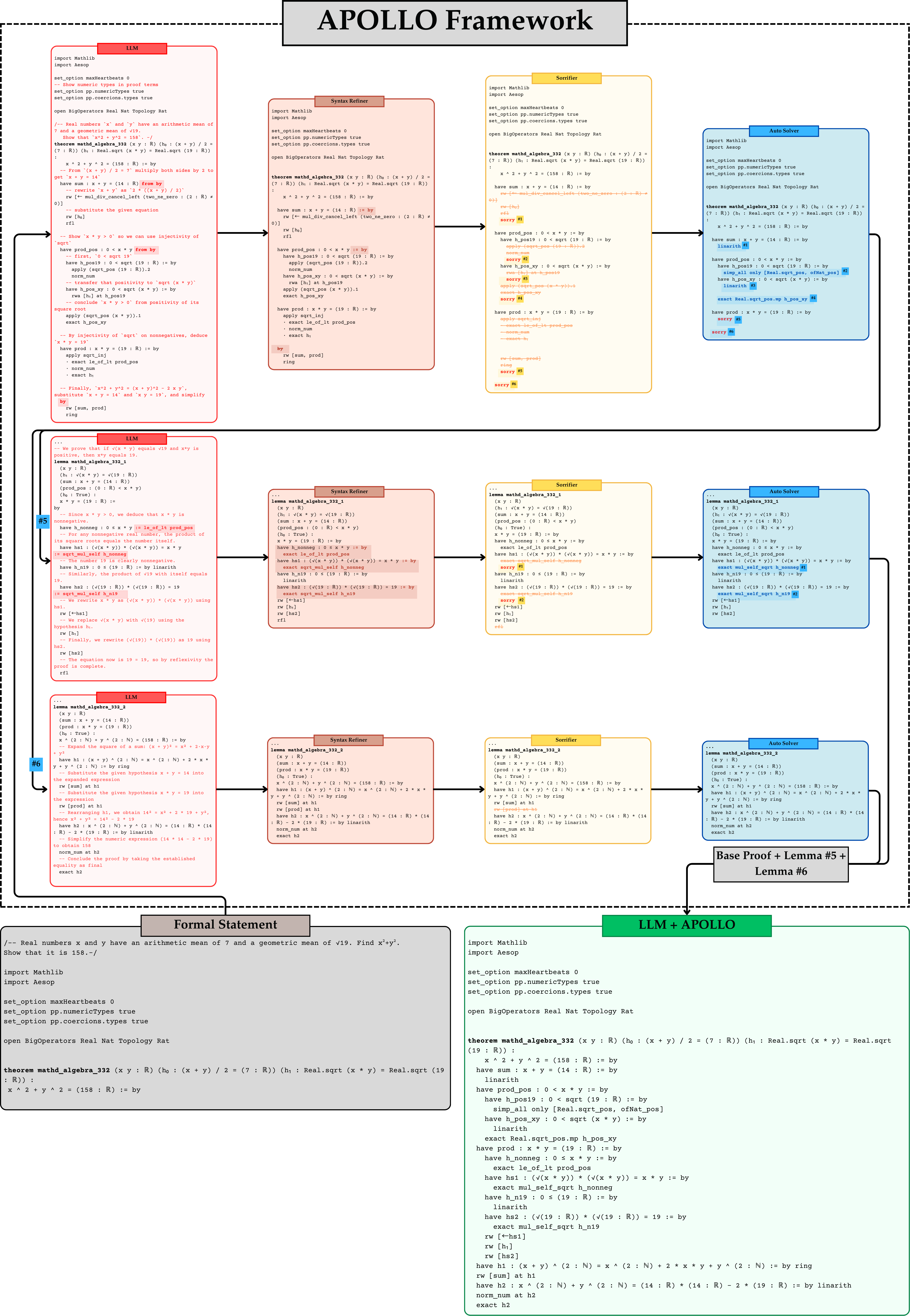
### Visual Description
## Diagram: APOLLO Framework Workflow
### Overview
This image is a complex technical flowchart illustrating the "APOLLO Framework," a system designed to translate natural language mathematical problems into formally verified proofs using the Lean 4 theorem prover. The diagram demonstrates a multi-agent, iterative pipeline where an initial Large Language Model (LLM) output is systematically refined, stripped of informalities, segmented into logical gaps (using Lean's `sorry` macro), and solved by automated tools. When the automated tools fail, the system recursively generates sub-lemmas to bridge the gaps, ultimately compiling a complete, verified formal proof.
### Components/Axes
The diagram is spatially organized into a main processing area (enclosed in a large dashed rectangle) and input/output areas at the bottom.
**Columns (Processing Stages):**
1. **LLM (Red Boxes, Left Column):** Generates initial Lean code mixed with natural language comments and informal proof steps.
2. **Syntax Refiner (Brown Boxes, Second Column):** Strips natural language comments, leaving only Lean syntax. Highlights unverified or potentially faulty tactics in red text.
3. **Sorrifier (Yellow Boxes, Third Column):** Replaces the unverified/faulty tactics (red text) with numbered `sorry` placeholders (e.g., `sorry #1`), effectively isolating the logical steps that need formal verification.
4. **Auto Solver (Blue Boxes, Right Column):** Attempts to replace the `sorry` placeholders with valid Lean tactics (highlighted in blue).
**Rows (Logical Progression):**
* **Top Row:** The main theorem proof attempt.
* **Middle Row:** Generation and processing of "Lemma #5" (triggered by a failure in the main proof).
* **Bottom Row:** Generation and processing of "Lemma #6" (triggered by a failure in the main proof).
**Input/Output (Bottom Section):**
* **Formal Statement (Grey Box, Bottom Left):** The initial problem statement and setup.
* **LLM + APOLLO (Green Box, Bottom Right):** The final, successfully compiled and verified Lean 4 proof.
**Flow Indicators:**
* **Solid Black Arrows:** Indicate the forward progression of code through the pipeline (Left to Right).
* **Dashed Black Arrows:** Indicate feedback loops or structural dependencies. Notably, dashed arrows point from `sorry #5` and `sorry #6` in the top Auto Solver box down to the LLM boxes for the respective lemmas. Another dashed arrow points from the combined lemmas to the final output.
---
### Content Details (Transcription & Analysis)
#### 1. Input: Formal Statement (Bottom Left)
This box sets up the Lean environment and states the mathematical problem: Find $x^2 + y^2$ given the arithmetic mean is 7 and the geometric mean is $\sqrt{19}$.
```lean
-- Real numbers x and y have an arithmetic mean of 7 and a geometric mean of √19. Find x²+y².
Show that it is 158.-/
import Mathlib
import Aesop
set_option maxHeartbeats 0
set_option pp.numericTypes true
set_option pp.coercions.types true
open BigOperators Real Nat Topology Rat
theorem mathd_algebra_332 (x y : ℝ) (h₀ : (x + y) / 2 = (7 : ℝ)) (h₁ : Real.sqrt (x * y) = Real.sqrt (19 : ℝ)) :
x ^ 2 + y ^ 2 = (158 : ℝ) := by
```
#### 2. Main Proof Flow (Top Row)
**LLM (Red Box):**
Generates the initial proof attempt. It includes extensive natural language comments (highlighted in red in the image) explaining the math, interspersed with Lean code.
*Key extractions:*
* `have sum : x + y = (14 : ℝ) from by` ... `rw [← mul_div_cancel_left (two_ne_zero : (2 : ℝ) ≠ 0)]`
* `have prod_pos : 0 < x * y from by` ... `apply (sqrt_pos (19 : ℝ)).2`
* `have prod : x * y = (19 : ℝ) := by` ... `apply sqrt_inj`
* Ends with `rw [sum, prod]` and `ring`.
**Syntax Refiner (Brown Box):**
The comments are removed. The informal or potentially incorrect tactic blocks are highlighted in red text.
*Key extractions (Red text):*
* `from by`
* `rw [← mul_div_cancel_left (two_ne_zero : (2 : ℝ) ≠ 0)]`
* `from by`
* `apply (sqrt_pos (19 : ℝ)).2`
* `by`
* `apply sqrt_inj`
* `by`
* `rw [sum, prod]`
* `ring`
**Sorrifier (Yellow Box):**
The red text from the previous step is crossed out (strikethrough) and replaced with numbered `sorry` tags highlighted in orange.
*Key extractions:*
* `have sum : x + y = (14 : ℝ) := by` -> `sorry #1`
* `have prod_pos : 0 < x * y := by` -> `sorry #2`
* `have h_pos_xy : 0 < sqrt (x * y) := by` -> `sorry #3`
* `have prod : x * y = (19 : ℝ) := by` -> `sorry #5`
* Final step -> `sorry #6`
**Auto Solver (Blue Box):**
Attempts to solve the `sorry` tags. Successful tactics are highlighted in blue.
*Key extractions:*
* `sorry #1` becomes `linarith #1`
* `sorry #2` becomes `simp_all only [Real.sqrt_pos, ofNat_pos] #2`
* `sorry #3` becomes `linarith #3`
* `sorry #4` becomes `exact Real.sqrt_pos.mp h_pos_xy #4`
* **Crucial Detail:** `sorry #5` and `sorry #6` remain unsolved (highlighted in blue text, but still say `sorry`). Dashed arrows point from these to the rows below.
#### 3. Lemma #5 Flow (Middle Row)
Triggered by the failure to solve `sorry #5` (proving $x * y = 19$).
**LLM (Red Box):**
Defines `lemma mathd_algebra_332_1`. Includes comments explaining how to prove that if $\sqrt{x*y} = \sqrt{19}$ and $x*y$ is positive, then $x*y = 19$.
*Key code:*
```lean
lemma mathd_algebra_332_1
(x y : ℝ)
(h₁ : √(x * y) = √(19 : ℝ))
(sum : x + y = (14 : ℝ))
(prod_pos : (0 : ℝ) < x * y)
(h₀ : True) :
x * y = (19 : ℝ) := by
```
**Syntax Refiner -> Sorrifier -> Auto Solver:**
Follows the same pattern. The Auto Solver successfully finds tactics for this lemma.
*Auto Solver (Blue Box) Output for Lemma 5:*
* `have h_nonneg : 0 ≤ x * y := by exact le_of_lt prod_pos`
* `have hs1 : (√(x * y)) * (√(x * y)) = x * y := by exact mul_self_sqrt h_nonneg #1`
* `have h_n19 : 0 ≤ (19 : ℝ) := by linarith`
* `have hs2 : (√(19 : ℝ)) * (√(19 : ℝ)) = 19 := by exact mul_self_sqrt h_n19 #2`
* `rw [←hs1]`
* `rw [h₁]`
* `rw [hs2]`
#### 4. Lemma #6 Flow (Bottom Row)
Triggered by the failure to solve `sorry #6` (the final algebraic expansion).
**LLM (Red Box):**
Defines `lemma mathd_algebra_332_2`. Proves $x^2 + y^2 = 158$ given $x+y=14$ and $x*y=19$.
*Key code:*
```lean
lemma mathd_algebra_332_2
(x y : ℝ)
(sum : x + y = (14 : ℝ))
(prod : x * y = (19 : ℝ))
(h₀ : True) :
x ^ 2 + y ^ 2 = (158 : ℝ) := by
```
**Syntax Refiner -> Sorrifier -> Auto Solver:**
The Auto Solver successfully resolves the algebraic steps.
*Auto Solver (Blue Box) Output for Lemma 6:*
* `have h1 : (x + y) ^ (2 : ℕ) = x ^ (2 : ℕ) + 2 * x * y + y ^ (2 : ℕ) := by ring`
* `rw [sum] at h1`
* `have h2 : x ^ (2 : ℕ) + y ^ (2 : ℕ) = (14 : ℝ) * (14 : ℝ) - 2 * (19 : ℝ) := by linarith`
* `norm_num at h2`
* `exact h2`
Below the Auto Solver for Lemma 6 is a grey box stating: **"Base Proof + Lemma #5 + Lemma #6"**, with a dashed arrow pointing to the final output.
#### 5. Output: LLM + APOLLO (Bottom Right Green Box)
This is the final, synthesized Lean 4 code. It combines the initial setup, the successfully solved steps from the main proof, and inlines the logic discovered during the lemma generation phases into a single, cohesive, verified proof.
```lean
import Mathlib
import Aesop
set_option maxHeartbeats 0
set_option pp.numericTypes true
set_option pp.coercions.types true
open BigOperators Real Nat Topology Rat
theorem mathd_algebra_332 (x y : ℝ) (h₀ : (x + y) / 2 = (7 : ℝ)) (h₁ : Real.sqrt (x * y) = Real.sqrt (19 : ℝ)) :
x ^ 2 + y ^ 2 = (158 : ℝ) := by
have sum : x + y = (14 : ℝ) := by
linarith
have prod_pos : 0 < x * y := by
have h_pos19 : 0 < sqrt (19 : ℝ) := by
simp_all only [Real.sqrt_pos, ofNat_pos]
have h_pos_xy : 0 < sqrt (x * y) := by
linarith
exact Real.sqrt_pos.mp h_pos_xy
have prod : x * y = (19 : ℝ) := by
have h_nonneg : 0 ≤ x * y := by
exact le_of_lt prod_pos
have hs1 : (√(x * y)) * (√(x * y)) = x * y := by
exact mul_self_sqrt h_nonneg
have h_n19 : 0 ≤ (19 : ℝ) := by
linarith
have hs2 : (√(19 : ℝ)) * (√(19 : ℝ)) = 19 := by
exact mul_self_sqrt h_n19
rw [←hs1]
rw [h₁]
rw [hs2]
have h1 : (x + y) ^ (2 : ℕ) = x ^ (2 : ℕ) + 2 * x * y + y ^ (2 : ℕ) := by ring
rw [sum] at h1
have h2 : x ^ (2 : ℕ) + y ^ (2 : ℕ) = (14 : ℝ) * (14 : ℝ) - 2 * (19 : ℝ) := by linarith
norm_num at h2
exact h2
```
---
### Key Observations
* **Iterative Refinement:** The system does not expect the LLM to write perfect Lean code on the first try. Instead, it uses the LLM for high-level logical structuring and relies on deterministic tools (Syntax Refiner, Sorrifier, Auto Solver) to handle the rigorous formalization.
* **The Power of `sorry`:** The framework ingeniously uses Lean's native `sorry` macro (which tells the compiler "assume this is true for now") as a boundary marker. By "sorrifying" dubious LLM code, the system isolates discrete sub-problems that an automated theorem prover can tackle independently.
* **Dynamic Lemma Generation:** The dashed arrows from `sorry #5` and `sorry #6` reveal a dynamic fallback mechanism. When the Auto Solver cannot bridge a logical gap in the main proof, the framework prompts the LLM to treat that specific gap as a new, standalone theorem (a lemma), restarting the refinement pipeline for that specific chunk of logic.
### Interpretation
This diagram illustrates a sophisticated neuro-symbolic architecture. It addresses a fundamental limitation of Large Language Models in formal mathematics: LLMs are good at intuitive leaps and natural language reasoning but struggle with the exact, unforgiving syntax and step-by-step rigor required by formal verification languages like Lean 4.
By breaking the process into specialized agents, the APOLLO Framework acts as a translator and verifier. The LLM provides the "skeleton" of the proof. The Syntax Refiner and Sorrifier act as a "compiler," identifying where the LLM's logic is informal or unverified. The Auto Solver acts as the "muscle," using brute-force or specialized tactics to fill in the formal steps.
The most powerful feature demonstrated here is the recursive lemma generation. By recognizing failure (`sorry #5` and `#6` remaining unsolved) and branching those failures into new LLM prompts, the system can dynamically break down complex mathematical leaps into smaller, digestible proofs, eventually synthesizing them into the flawless final output shown in the green box. This represents a significant step toward fully automated formal mathematical reasoning.
</details>
Figure 6: Step-by-step Apollo repair on mathd_algebra_332. The initial proof and all sub-lemma proofs are generated with o4-mini, then systematically repaired and reassembled by Apollo.
<details>
<summary>examples/comparison/short_3.png Details</summary>
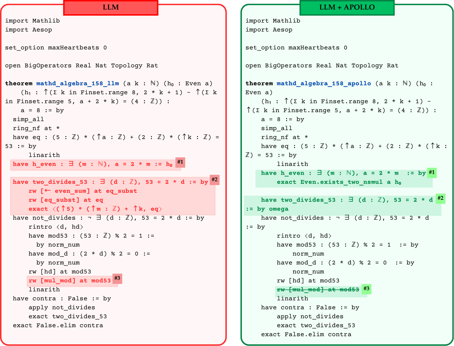
### Visual Description
## Diagram: Code Comparison - LLM vs. LLM + APOLLO
### Overview
This image presents a side-by-side comparison of two code snippets written in Lean 4, a formal theorem proving language. The image contrasts the output of a standard Large Language Model ("LLM") on the left with an enhanced system ("LLM + APOLLO") on the right. The visual design uses color-coding (red for the baseline/errors, green for corrections/improvements) and numbered tags to highlight specific differences where the APOLLO system has fixed errors or optimized the proof generated by the base LLM.
### Components and Layout
The image is divided into two main vertical panels:
1. **Left Panel (Red - Baseline LLM):**
* **Header:** A red rectangular box at the top center containing the text "LLM" in black.
* **Border:** A thick red border surrounds the entire panel.
* **Background:** Very light red/pink.
* **Highlights:** Specific lines of code are highlighted with a darker red background.
* **Tags:** Small red rectangular tags with white text (`#1`, `#2`, `#3`) are placed at the end of the highlighted lines to index the errors.
2. **Right Panel (Green - Enhanced System):**
* **Header:** A green rectangular box at the top center containing the text "LLM + APOLLO" in black.
* **Border:** A thick green border surrounds the entire panel.
* **Background:** Very light green.
* **Highlights:** Specific lines of code are highlighted with a darker green background, corresponding to the fixes for the red highlights on the left.
* **Tags:** Small green rectangular tags with black text (`#1`, `#2`, `#3`) are placed at the end of the highlighted lines to index the corrections.
* **Formatting:** Tag `#3` includes a strikethrough line through the code, indicating deletion.
---
### Content Details: Full Transcription and Comparison
Both panels share the same initial setup, imports, and theorem declaration. The differences occur within the proof body (`:= by`).
#### Shared Initial Code (Lines 1-15)
```lean
import Mathlib
import Aesop
set_option maxHeartbeats 0
open BigOperators Real Nat Topology Rat
theorem mathd_algebra_158_llm (a k : ℕ) (h₀ : Even a)
(h₁ : ↑(Σ k in Finset.range 8, 2 * k + 1) - ↑(Σ k
in Finset.range 5, a + 2 * k) = (4 : ℤ)) :
a = 8 := by
simp_all
ring_nf at *
have eq : (5 : ℤ) * (↑a : ℤ) + (2 : ℤ) * (↑k : ℤ) =
53 := by
linarith
```
*(Note: The theorem name on the right panel is slightly different: `mathd_algebra_158_apollo`, and there are minor line-break differences in the theorem signature due to formatting, but the logical content is identical).*
#### Difference #1: Type Mismatch Correction
* **Left Panel (LLM) - Red Highlight #1:**
```lean
have h_even : ∃ (m : ℕ), a = 2 * m := h₀
```
*Visual:* The entire line is highlighted red. The tag `#1` is at the far right.
* **Right Panel (LLM + APOLLO) - Green Highlight #1:**
```lean
have h_even : ∃ (m : ℕ), a = 2 * m := by
exact Even.exists_two_nsmul a h₀
```
*Visual:* The `:= by` and the subsequent indented line are highlighted green. The tag `#1` is placed after `:= by`.
#### Difference #2: Hallucination vs. Automated Tactic
* **Left Panel (LLM) - Red Highlight #2:**
```lean
have two_divides_53 : ∃ (d : ℤ), 53 = 2 * d := by
rw [← even_sum] at eq_subst
rw [eq_subst] at eq
exact ⟨(↑5) * (↑m : ℤ) + ↑k, eq⟩
```
*Visual:* A four-line block is highlighted red. The tag `#2` is at the end of the first line.
* **Right Panel (LLM + APOLLO) - Green Highlight #2:**
```lean
have two_divides_53 : ∃ (d : ℤ), 53 = 2 * d
:= by omega
```
*Visual:* The `:= by omega` portion is highlighted green. The tag `#2` is placed at the end of the first line.
#### Shared Intermediate Code
```lean
have not_divides : ¬ ∃ (d : ℤ), 53 = 2 * d := by
rintro ⟨d, hd⟩
have mod53 : (53 : ℤ) % 2 = 1 := by
norm_num
have mod_d : (2 * d) % 2 = 0 := by
norm_num
rw [hd] at mod53
```
#### Difference #3: Redundant Code Removal
* **Left Panel (LLM) - Red Highlight #3:**
```lean
rw [mul_mod] at mod53
```
*Visual:* The entire line is highlighted red. The tag `#3` is at the far right.
* **Right Panel (LLM + APOLLO) - Green Highlight #3:**
```lean
rw [mul_mod] at mod53
```
*Visual:* The text `rw [mul_mod] at mod53` has a horizontal strikethrough line through it and is highlighted green. The tag `#3` is at the far right.
#### Shared Final Code
```lean
linarith
have contra : False := by
apply not_divides
exact two_divides_53
exact False.elim contra
```
---
### Key Observations
1. **Syntax/Type Error (Tag #1):** The base LLM attempts to directly assign `h₀` (which is of type `Even a`) to a proposition `∃ (m : ℕ), a = 2 * m`. In Lean, this requires a specific proof term. APOLLO corrects this by invoking the specific lemma `Even.exists_two_nsmul`.
2. **Hallucination (Tag #2):** The base LLM invents variable names (`eq_subst`, `even_sum`) and a variable `m` that is not in scope for this specific block, resulting in a broken proof state. APOLLO completely replaces this flawed multi-line manual proof attempt with a single, powerful automated tactic: `omega` (which handles integer arithmetic).
3. **Redundancy (Tag #3):** The base LLM includes a rewrite tactic (`rw [mul_mod]`) that is either unnecessary or incorrect for the proof path. APOLLO identifies this and removes it (indicated by the strikethrough).
### Interpretation
This image serves as a technical demonstration of the "APOLLO" system's capabilities in the context of formal theorem proving (specifically Lean 4).
The data suggests that while standard LLMs can generate the general structure of a mathematical proof, they frequently fail on the strict syntactic and logical requirements of formal verification languages. They suffer from "hallucinations" (inventing tactics or variables that don't exist, as seen in #2) and type mismatches (as seen in #1).
The APOLLO system acts as an intelligent corrector or agentic wrapper around the LLM. By comparing the left and right panels, we can deduce that APOLLO likely possesses the ability to:
1. Verify code against the Lean compiler.
2. Search for correct lemmas when types mismatch (Fix #1).
3. Recognize when a proof state can be solved by standard automation (replacing hallucinated garbage with `omega` in Fix #2).
4. Prune dead or broken code paths (Fix #3).
Ultimately, the diagram visually communicates that "LLM + APOLLO" transforms broken, uncompilable AI-generated code into a verified, working mathematical proof.
</details>
Figure 7: Proof attempt of mathd_algebra_158 produced by the base model (o4-mini) versus after Apollo’s targeted repair. The left shows the original end-to-end LLM output, which does not compile in Lean; the right shows the corrected, repaired proof assembled by Apollo that closes all of the goals.
Appendix G Comparison between base proofs generated from LLMs and Apollo-repaired counterparts
In this section, we present and discuss examples of initial proof attempts alongside their Apollo-repaired counterparts.
Figures 7, 8, 9 illustrate cases where Apollo repairs the proof without invoking the LLM again. In each example, the LLM struggles to generate the precise tactics needed to close certain goals; however, we find that regenerating the entire proof is unnecessary. Instead, built-in Lean solvers can discharge those subgoals directly. Moreover, in Figure 7, problematic block #3 is resolved simply by removing it, since the surrounding proof context is correct. Thus, omitting problematic lines can sometimes yield a valid proof.
In Figure 10, one goal is expanded via an LLM query, but the model injects extra tactics that trigger a no goals to be solved error. Apollo then repairs the first block using a combination of LLM generation and AutoSolver, while the second block is removed entirely.
Figure 11 illustrates a case where the model fails to apply nlinarith to discharge the goal. We observe that, when uncertain, the model often resorts to broad tactics in hopes of closing the goal. Here, the goal is too complex for nlinarith, so Apollo leverages both the LLM and AutoSolver to guide the proof to completion.
Figure 12 illustrates an example of proof that required a recursion depth $r=5$ to repair the initial proof attempt. We observe that LLM’s proof structure is correct; however, in many cases it over-relies on built-in solvers and rewrites. However, since the goals are too complex, this approach leads to a total of nine error blocks. Repairing those blocks requires aid from both AutoSolver module of Apollo and LLM itself. We show that if LLM grasps the correct approach, then Apollo is able to repair fine grained logic errors to produce a correct proof.
Figure 13 illustrates a case where the LLM produces an incomplete proof sketch. The first half of the proof is correct, but the model fails to discharge the remaining goal and instead uses all_goals positivity. Apollo detects this error and performs two additional recursive repair iterations to complete the proof.
Figure 14 illustrates a case where the base model takes a lazy approach by trying to close all goals with linarith. In contrast, Apollo’s repaired proof performs additional setup and discharges each goal by first proving the necessary auxiliary hypotheses. This example shows that, although the model often understands the high-level strategy, it lacks the fine-grained tactics (and compiler feedback) needed to close subgoals. Apollo decomposes the proof, identifies the failure points, and applies targeted repairs to generate a fully verified solution.
Figure 15 shows another scenario in which Apollo successfully closes the first two blocks with linarith, but the final block requires a deeper reasoning chain. Apollo augments the proof by introducing and proving the missing lemmas, which leads to a correct solution with a series of rewrites.
Figure 16 presents an example of a very large repair. As in Figure 12, Apollo requires $r=5$ to fully fix the proof. The final proof length increases from 100 lines to 216, which means Apollo applied roughly $× 2.2$ more tactics to close the goal. The repair relied on combined effort from AutoSolver and the LLM to close all goals. We show that, even for large, complex proofs, Apollo can repair each failing sub-block and generate a correct solution.
<details>
<summary>examples/comparison/short_1.png Details</summary>
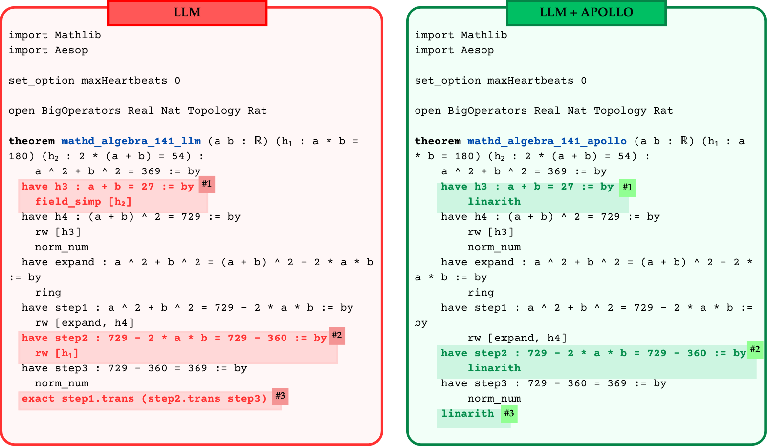
### Visual Description
## Code Comparison Diagram: LLM vs. LLM + APOLLO Theorem Proving
### Overview
This image is a side-by-side technical diagram comparing two blocks of computer code, specifically written in Lean 4 (a mathematical theorem proving language). The diagram contrasts the output generated by a standard Large Language Model ("LLM") on the left against the output generated by an enhanced system ("LLM + APOLLO") on the right. The image uses color-coding (red for the left panel, green for the right panel) and numbered annotations to highlight specific differences in the proof tactics used to solve the same algebraic theorem.
### Components and Layout
The image is divided into two distinct spatial regions:
1. **Left Panel (Baseline LLM):**
* **Position:** Occupies the left half of the image.
* **Header:** A red rectangular box at the top center containing the text "LLM" in black.
* **Border/Background:** Surrounded by a red border with rounded corners. The background has a very faint pink/red tint.
* **Highlights:** Three specific blocks of code are highlighted with a solid red background and tagged with dark red square labels containing white text: `#1`, `#2`, and `#3`.
2. **Right Panel (Enhanced LLM + APOLLO):**
* **Position:** Occupies the right half of the image.
* **Header:** A green rectangular box at the top center containing the text "LLM + APOLLO" in black.
* **Border/Background:** Surrounded by a dark green border with rounded corners. The background has a very faint green tint.
* **Highlights:** Three specific blocks of code are highlighted with a solid light green background and tagged with dark green square labels containing white text: `#1`, `#2`, and `#3`. These correspond spatially and logically to the highlights in the left panel.
### Content Details
Both panels contain code attempting to prove the same theorem: `mathd_algebra_141`. The setup, imports, and theorem definitions are identical. The differences lie strictly within the highlighted proof tactics.
#### Left Panel Transcription (LLM)
```lean
import Mathlib
import Aesop
set_option maxHeartbeats 0
open BigOperators Real Nat Topology Rat
theorem mathd_algebra_141_llm (a b : ℝ) (h₁ : a * b =
180) (h₂ : 2 * (a + b) = 54) :
a ^ 2 + b ^ 2 = 369 := by
have h3 : a + b = 27 := by #1 [Highlighted Red]
field_simp [h₂] #1 [Highlighted Red]
have h4 : (a + b) ^ 2 = 729 := by
rw [h3]
norm_num
have expand : a ^ 2 + b ^ 2 = (a + b) ^ 2 - 2 * a * b
:= by
ring
have step1 : a ^ 2 + b ^ 2 = 729 - 2 * a * b := by
rw [expand, h4]
have step2 : 729 - 2 * a * b = 729 - 360 := by #2 [Highlighted Red]
rw [h₁] #2 [Highlighted Red]
have step3 : 729 - 360 = 369 := by
norm_num
exact step1.trans (step2.trans step3) #3 [Highlighted Red]
```
#### Right Panel Transcription (LLM + APOLLO)
*Note: Line breaks in the theorem definition differ slightly from the left panel due to text wrapping, but the code logic is identical until the highlights.*
```lean
import Mathlib
import Aesop
set_option maxHeartbeats 0
open BigOperators Real Nat Topology Rat
theorem mathd_algebra_141_apollo (a b : ℝ) (h₁ : a
* b = 180) (h₂ : 2 * (a + b) = 54) :
a ^ 2 + b ^ 2 = 369 := by
have h3 : a + b = 27 := by #1 [Highlighted Green]
linarith #1 [Highlighted Green]
have h4 : (a + b) ^ 2 = 729 := by
rw [h3]
norm_num
have expand : a ^ 2 + b ^ 2 = (a + b) ^ 2 - 2 *
a * b := by
ring
have step1 : a ^ 2 + b ^ 2 = 729 - 2 * a * b :=
by
rw [expand, h4]
have step2 : 729 - 2 * a * b = 729 - 360 := by #2 [Highlighted Green]
linarith #2 [Highlighted Green]
have step3 : 729 - 360 = 369 := by
norm_num
linarith #3 [Highlighted Green]
```
### Key Observations
A direct comparison of the highlighted sections reveals the exact substitutions made by the "APOLLO" system:
* **Highlight #1 Comparison:**
* *LLM (Left):* Uses the tactic `field_simp [h₂]` to prove `a + b = 27`.
* *LLM + APOLLO (Right):* Replaces this with the tactic `linarith`.
* **Highlight #2 Comparison:**
* *LLM (Left):* Uses the tactic `rw [h₁]` (rewrite using hypothesis 1) to prove `729 - 2 * a * b = 729 - 360`.
* *LLM + APOLLO (Right):* Replaces this with the tactic `linarith`.
* **Highlight #3 Comparison:**
* *LLM (Left):* Uses a complex transitive equality chain: `exact step1.trans (step2.trans step3)` to conclude the proof.
* *LLM + APOLLO (Right):* Replaces the entire chain with the single tactic `linarith`.
### Interpretation
This diagram serves as a visual demonstration of the effectiveness of the "APOLLO" system when augmenting a standard LLM for formal theorem proving in Lean 4.
The data suggests that a standard LLM (left panel) attempts to solve mathematical proofs by stringing together highly specific, sometimes overly complex, or potentially incorrect tactics (like `field_simp` for simple linear arithmetic, or manually chaining transitive properties with `exact step1.trans...`). The red highlighting implies these choices are either suboptimal, brittle, or represent hallucinated logic that fails to compile.
Conversely, the "LLM + APOLLO" system (right panel) demonstrates a pattern of simplification and robustness. In all three highlighted instances, APOLLO replaces the LLM's specific tactics with `linarith` (Linear Arithmetic), a powerful and standard automated tactic in Lean designed specifically to solve linear equations and inequalities.
Reading between the lines, APOLLO appears to act as a refinement or correction layer. It recognizes when the base LLM is struggling with basic algebraic manipulations and substitutes a reliable, automated solver (`linarith`), thereby making the proof cleaner, shorter, and mathematically sound. The visual use of red (error/suboptimal) versus green (success/optimal) strongly reinforces the narrative that APOLLO "fixes" the LLM's proof generation.
</details>
Figure 8: Proof attempt of mathd_algebra_141 produced by the base model (o4-mini) versus after Apollo’s targeted repair. The left shows the original end-to-end LLM output, which does not compile in Lean; the right shows the corrected, repaired proof assembled by Apollo that closes all of the goals.
<details>
<summary>examples/comparison/short_2.png Details</summary>
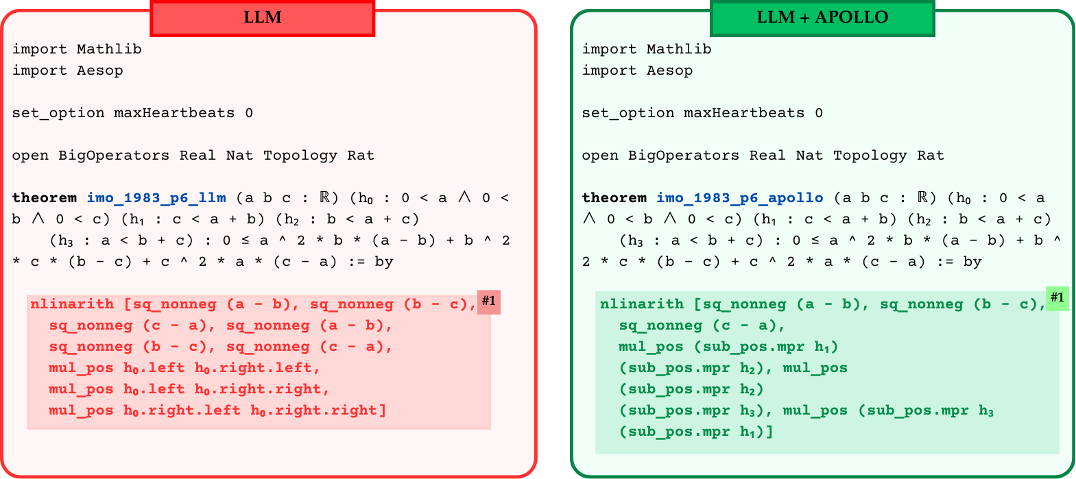
### Visual Description
## Code Comparison Diagram: LLM vs. LLM + APOLLO Theorem Proving
### Overview
This image is a side-by-side comparison of two code snippets written in the Lean 4 theorem proving language. It contrasts the output generated by a standard Large Language Model ("LLM") on the left with the output generated by an LLM augmented with a system called "APOLLO" on the right. Both snippets attempt to prove a mathematical theorem related to the International Mathematical Olympiad (IMO) 1983, Problem 6. The visual design uses color coding (red for the baseline LLM, green for the APOLLO-augmented LLM) to highlight the differences in the final proof tactic.
### Components & Layout
The image is divided into two distinct rectangular panels of equal size:
1. **Left Panel (Red Theme):**
* **Header:** A solid red rectangle at the top center containing the text "LLM" in black.
* **Border:** A thick red outline surrounding the panel.
* **Background:** The top portion has a very faint red/pink tint (almost white), while the bottom highlighted code block has a distinct light red background.
* **Annotation:** A small, darker red square in the top-right corner of the highlighted block containing the text "#1" in white.
2. **Right Panel (Green Theme):**
* **Header:** A solid green rectangle at the top center containing the text "LLM + APOLLO" in black.
* **Border:** A thick green outline surrounding the panel.
* **Background:** The top portion has a very faint green tint (almost white), while the bottom highlighted code block has a distinct light green background.
* **Annotation:** A small, darker green square in the top-right corner of the highlighted block containing the text "#1" in black.
### Content Details
Both panels share identical setup code and theorem declarations (with minor line-wrapping differences), but diverge significantly in the final `nlinarith` tactic block.
#### Left Panel Transcription (LLM)
```lean
import Mathlib
import Aesop
set_option maxHeartbeats 0
open BigOperators Real Nat Topology Rat
theorem imo_1983_p6_llm (a b c : ℝ) (h₀ : 0 < a ∧ 0 <
b ∧ 0 < c) (h₁ : c < a + b) (h₂ : b < a + c)
(h₃ : a < b + c) : 0 ≤ a ^ 2 * b * (a - b) + b ^ 2
* c * (b - c) + c ^ 2 * a * (c - a) := by
nlinarith [sq_nonneg (a - b), sq_nonneg (b - c),
sq_nonneg (c - a), sq_nonneg (a - b),
sq_nonneg (b - c), sq_nonneg (c - a),
mul_pos h₀.left h₀.right.left,
mul_pos h₀.left h₀.right.right,
mul_pos h₀.right.left h₀.right.right]
```
*(Note: The `nlinarith` block is highlighted in light red, with `#1` in the top right corner).*
#### Right Panel Transcription (LLM + APOLLO)
```lean
import Mathlib
import Aesop
set_option maxHeartbeats 0
open BigOperators Real Nat Topology Rat
theorem imo_1983_p6_apollo (a b c : ℝ) (h₀ : 0 < a
∧ 0 < b ∧ 0 < c) (h₁ : c < a + b) (h₂ : b < a + c)
(h₃ : a < b + c) : 0 ≤ a ^ 2 * b * (a - b) + b ^ 2
* c * (b - c) + c ^ 2 * a * (c - a) := by
nlinarith [sq_nonneg (a - b), sq_nonneg (b - c),
sq_nonneg (c - a),
mul_pos (sub_pos.mpr h₁)
(sub_pos.mpr h₂), mul_pos
(sub_pos.mpr h₂)
(sub_pos.mpr h₃), mul_pos (sub_pos.mpr h₃)
(sub_pos.mpr h₁)]
```
*(Note: The `nlinarith` block is highlighted in light green, with `#1` in the top right corner).*
### Key Observations
* **Shared Context:** Both models correctly set up the environment (`import Mathlib`, `import Aesop`), set options (`maxHeartbeats 0`), and define the theorem signature for IMO 1983 Problem 6. The theorem involves real numbers $a, b, c$ that are strictly positive ($h_0$) and satisfy the triangle inequalities ($h_1, h_2, h_3$).
* **Naming Convention:** The left theorem is named `imo_1983_p6_llm`, while the right is named `imo_1983_p6_apollo`.
* **Divergence in Logic (The Highlighted Blocks):**
* **The Baseline LLM (Red):** The arguments provided to the `nlinarith` (non-linear arithmetic) tactic contain redundancies. It repeats `sq_nonneg (a - b), sq_nonneg (b - c), sq_nonneg (c - a)` twice. Furthermore, it attempts to use `mul_pos` by combining the basic positivity hypotheses from $h_0$ (e.g., `h₀.left`, which is $0 < a$).
* **The APOLLO LLM (Green):** The arguments are concise and mathematically distinct. It lists the `sq_nonneg` terms only once. Crucially, it uses `mul_pos` in conjunction with `sub_pos.mpr` applied to the triangle inequality hypotheses ($h_1, h_2, h_3$). For example, `sub_pos.mpr h₁` converts the hypothesis $c < a + b$ into the mathematically useful form $0 < a + b - c$.
### Interpretation
This image serves as a demonstration of the efficacy of the "APOLLO" system in improving the formal mathematical reasoning capabilities of Large Language Models.
The data suggests that a standard LLM (left) struggles to provide the correct auxiliary proofs required by the `nlinarith` tactic to close the goal. The baseline LLM exhibits "hallucination" or poor logical planning by repeating identical arguments and feeding basic, insufficient positivity proofs (`h₀`) into the tactic, which likely results in a failure to compile or prove the theorem.
Conversely, the APOLLO-augmented system (right) demonstrates a deeper understanding of the mathematical requirements. It recognizes that to solve this specific non-linear inequality, the tactic needs to know that the terms derived from the triangle inequalities are positive. By applying `sub_pos.mpr` to $h_1, h_2,$ and $h_3$, APOLLO correctly transforms the hypotheses into the exact format required by `nlinarith` to successfully complete the proof. The use of red (often associated with failure/errors) and green (associated with success/correctness) strongly implies that the left code fails while the right code succeeds.
</details>
Figure 9: Proof attempt of imo_1983_p6 produced by the base model (Kimina-Prover-Preview-Distill-7B) versus after Apollo’s targeted repair. The left shows the original end-to-end LLM output, which does not compile in Lean; the right shows the corrected, repaired proof assembled by Apollo that closes all of the goals.
<details>
<summary>examples/comparison/short_4.png Details</summary>
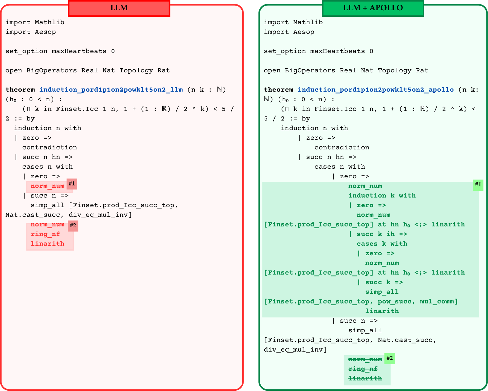
### Visual Description
## Code Comparison Diagram: LLM vs. LLM + APOLLO Lean 4 Proofs
### Overview
The image presents a side-by-side comparison of two code snippets written in the Lean 4 theorem proving language. The left panel displays code generated by a baseline "LLM" (Large Language Model), while the right panel displays code generated by an augmented system labeled "LLM + APOLLO". The diagram highlights specific differences in the proof tactics used by each system, using color-coded blocks and numbered tags to draw attention to areas where APOLLO modifies, expands, or deletes the baseline LLM's output.
### Components and Spatial Grounding
The image is divided into two distinct vertical panels:
* **Left Panel (LLM):** Enclosed in a red border with a red header box at the top center containing the text "LLM" in black. The background is a very faint red/pink. It contains Lean 4 code. Two specific areas are highlighted with a solid light red background and tagged with "#1" and "#2" on their right edges.
* **Right Panel (LLM + APOLLO):** Enclosed in a green border with a green header box at the top center containing the text "LLM + APOLLO" in black. The background is a very faint green. It contains Lean 4 code. Two specific areas are highlighted with a solid light green background and tagged with "#1" and "#2" on their right edges. Text within the "#2" highlight features a strikethrough effect.
### Content Details: Transcription and Component Isolation
#### 1. Left Panel: LLM
This panel shows the baseline proof attempt.
**Transcription:**
```lean
import Mathlib
import Aesop
set_option maxHeartbeats 0
open BigOperators Real Nat Topology Rat
theorem induction_pord1p1on2powklt5on2_llm (n k : ℕ) (h₀ : 0 < n) :
(∏ k in Finset.Icc 1 n, 1 + (1 : ℝ) / 2 ^ k) < 5 / 2 := by
induction n with
| zero =>
contradiction
| succ n hn =>
cases n with
| zero =>
norm_num #1
| succ n =>
simp_all [Finset.prod_Icc_succ_top, Nat.cast_succ, div_eq_mul_inv]
norm_num #2
ring_nf
linarith
```
*Spatial Notes for Left Panel:*
* **Highlight #1:** The line `norm_num` under the `| zero =>` case has a red background. The tag `#1` is placed immediately to the right of `norm_num`.
* **Highlight #2:** The block of three lines (`norm_num`, `ring_nf`, `linarith`) at the very end of the code has a red background. The tag `#2` is placed immediately to the right of the `norm_num` line within this block.
#### 2. Right Panel: LLM + APOLLO
This panel shows the modified proof attempt. The setup and initial theorem declaration are identical, except for the theorem name suffix (`_apollo` instead of `_llm`) and slight differences in line wrapping.
**Transcription:**
```lean
import Mathlib
import Aesop
set_option maxHeartbeats 0
open BigOperators Real Nat Topology Rat
theorem induction_pord1p1on2powklt5on2_apollo (n k : ℕ) (h₀ : 0 < n) :
(∏ k in Finset.Icc 1 n, 1 + (1 : ℝ) / 2 ^ k) < 5 / 2 := by
induction n with
| zero =>
contradiction
| succ n hn =>
cases n with
| zero =>
norm_num
induction k with
| zero =>
norm_num [Finset.prod_Icc_succ_top] at hn h₀ <;> linarith
| succ k ih =>
cases k with
| zero =>
norm_num [Finset.prod_Icc_succ_top] at hn h₀ <;> linarith
| succ k =>
simp_all [Finset.prod_Icc_succ_top, pow_succ, mul_comm]
linarith #1
| succ n =>
simp_all [Finset.prod_Icc_succ_top, Nat.cast_succ, div_eq_mul_inv]
~~norm_num~~ #2
~~ring_nf~~
~~linarith~~
```
*Spatial Notes for Right Panel:*
* **Highlight #1:** A large green background block begins at the `norm_num` line under the `| zero =>` case and extends down to the `linarith` line just before `| succ n =>`. The tag `#1` is placed to the far right, aligned with the top line (`norm_num`) of this highlighted block.
* **Highlight #2:** A green background block covers the final three lines of the code. The text of these three lines (`norm_num`, `ring_nf`, `linarith`) is crossed out with a strikethrough line. The tag `#2` is placed immediately to the right of the crossed-out `norm_num`.
### Key Observations
1. **Expansion at #1:** The baseline LLM attempts to solve the `| zero =>` case of the `cases n` block with a single `norm_num` tactic. This is highlighted in red, implying it fails or is insufficient. The APOLLO system expands this single line into a complex, 14-line nested induction on `k` (`induction k with...`), handling multiple sub-cases to properly close the goal.
2. **Deletion at #2:** At the end of the proof, under the `| succ n =>` case, the baseline LLM generates three tactics: `norm_num`, `ring_nf`, and `linarith` after a `simp_all` call. The APOLLO system highlights these exact three lines and applies a strikethrough, indicating that these tactics are either unnecessary (the proof is already closed by `simp_all`), redundant, or cause an error in the Lean environment.
### Interpretation
This image serves as a technical demonstration of the "APOLLO" system's capabilities in the domain of formal theorem proving (specifically using Lean 4). It illustrates that while a standard LLM can generate the broad structure of a mathematical proof, it often fails at specific logical junctions by either hallucinating overly simplistic tactics that don't work (Observation #1) or by appending unnecessary/failing steps at the end of a branch (Observation #2).
The APOLLO system appears to act as an agentic or iterative wrapper around the LLM. By comparing the two panels, we can deduce APOLLO's function:
* **Generative Repair:** When a tactic fails (like the first `norm_num`), APOLLO does not just give up; it generates a deeper, structurally sound sub-proof (the nested induction on `k`) to bridge the logical gap.
* **Pruning:** APOLLO recognizes when the goal state has been achieved or when subsequent tactics are invalid, actively removing them (the struck-through text) to ensure the final proof script compiles cleanly without errors.
Ultimately, the data suggests that combining an LLM with the APOLLO framework transforms an incomplete or broken formal proof into a verified, working proof by dynamically expanding necessary logic and pruning faulty logic.
</details>
Figure 10: Proof attempt of induction_pord1p1on2powklt5on2 produced by the base model (Goedel-Prover-SFT) versus after Apollo’s targeted repair. The left shows the original end-to-end LLM output, which does not compile in Lean; the right shows the corrected, repaired proof assembled by Apollo that closes all of the goals.
<details>
<summary>examples/comparison/short_5.png Details</summary>
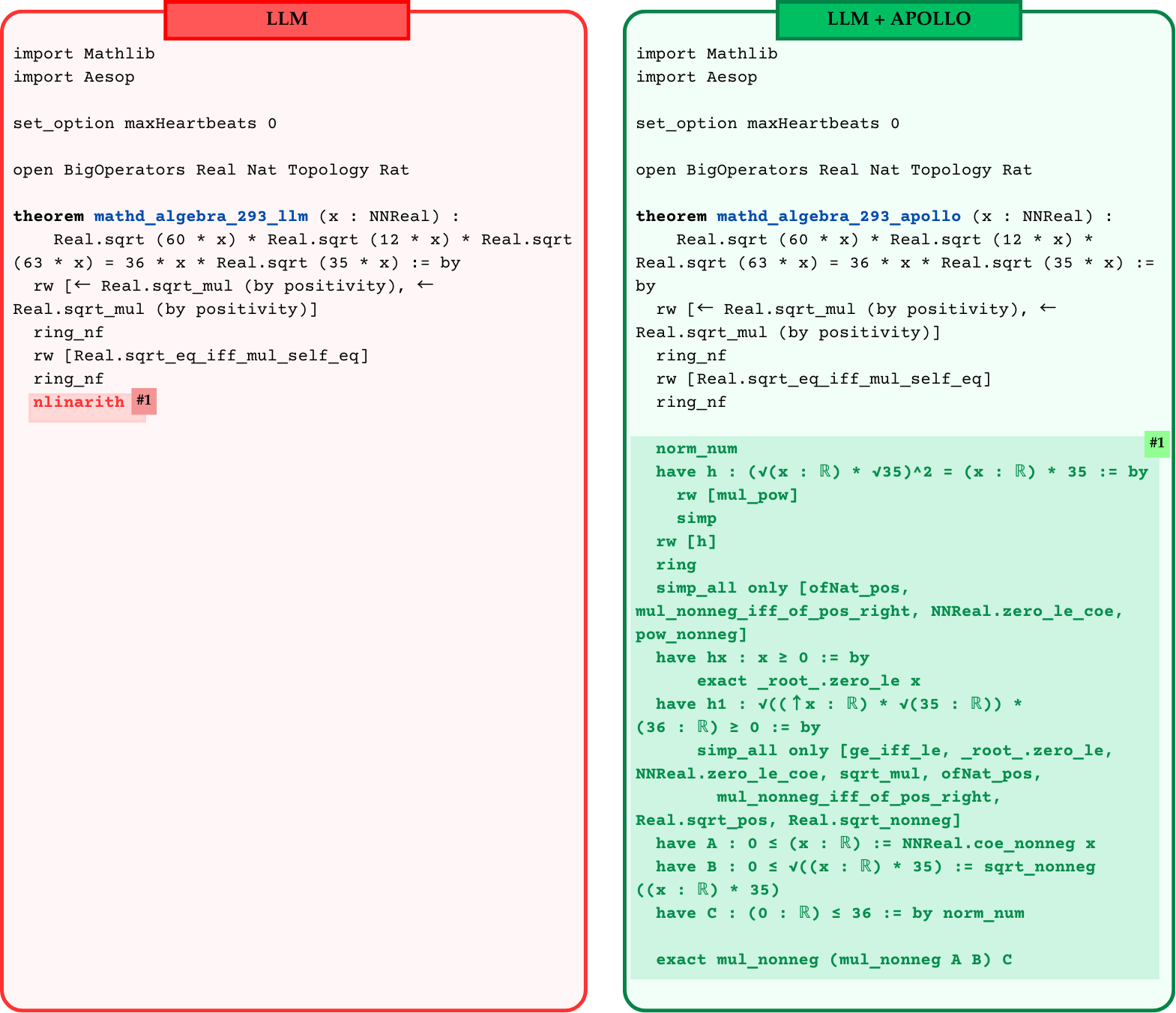
### Visual Description
## Diagram: Comparison of Lean 4 Proofs - LLM vs. LLM + APOLLO
### Overview
The image presents a side-by-side comparison of two formal mathematical proofs written in the Lean 4 theorem prover language. The graphic demonstrates how a standard Large Language Model (LLM) fails to complete a specific proof, whereas an augmented system ("LLM + APOLLO") successfully completes the same proof by replacing a failing high-level tactic with a detailed, step-by-step logical deduction.
### Components and Layout
The image is divided into two distinct vertical panels:
1. **Left Panel (LLM):**
* **Header:** A red rectangular tab at the top center containing the text "LLM" in black.
* **Border:** A thick red line with rounded corners enclosing the panel.
* **Background:** A very faint pink/red tint.
* **Content:** A block of Lean 4 code.
* **Annotation:** The final line of code (`nlinarith`) is highlighted with a red background, followed by a darker red tag reading `#1`.
2. **Right Panel (LLM + APOLLO):**
* **Header:** A green rectangular tab at the top center containing the text "LLM + APOLLO" in black.
* **Border:** A thick green line with rounded corners enclosing the panel.
* **Background:** A very faint green tint.
* **Content:** A block of Lean 4 code. The top half is nearly identical to the left panel.
* **Annotation:** The bottom half of the code is enclosed in a darker green highlighted box. In the top right corner of this highlighted box is a green tag reading `#1`.
### Content Details (Transcription)
Below is the exact transcription of the code presented in both panels.
#### Left Panel Transcription (LLM)
```lean
import Mathlib
import Aesop
set_option maxHeartbeats 0
open BigOperators Real Nat Topology Rat
theorem mathd_algebra_293_llm (x : NNReal) :
Real.sqrt (60 * x) * Real.sqrt (12 * x) * Real.sqrt (63 * x) = 36 * x * Real.sqrt (35 * x) := by
rw [← Real.sqrt_mul (by positivity), ← Real.sqrt_mul (by positivity)]
ring_nf
rw [Real.sqrt_eq_iff_mul_self_eq]
ring_nf
nlinarith #1
```
*(Note: The text `nlinarith #1` is highlighted in red in the original image).*
#### Right Panel Transcription (LLM + APOLLO)
```lean
import Mathlib
import Aesop
set_option maxHeartbeats 0
open BigOperators Real Nat Topology Rat
theorem mathd_algebra_293_apollo (x : NNReal) :
Real.sqrt (60 * x) * Real.sqrt (12 * x) * Real.sqrt (63 * x) = 36 * x * Real.sqrt (35 * x) := by
rw [← Real.sqrt_mul (by positivity), ← Real.sqrt_mul (by positivity)]
ring_nf
rw [Real.sqrt_eq_iff_mul_self_eq]
ring_nf
norm_num #1
have h : (√(x : ℝ) * √35)^2 = (x : ℝ) * 35 := by
rw [mul_pow]
simp
rw [h]
ring
simp_all only [ofNat_pos, mul_nonneg_iff_of_pos_right, NNReal.zero_le_coe, pow_nonneg]
have hx : x ≥ 0 := by
exact _root_.zero_le x
have h1 : √((↑x : ℝ) * √(35 : ℝ)) * (36 : ℝ) ≥ 0 := by
simp_all only [ge_iff_le, _root_.zero_le, NNReal.zero_le_coe, sqrt_mul, ofNat_pos, mul_nonneg_iff_of_pos_right, Real.sqrt_pos, Real.sqrt_nonneg]
have A : 0 ≤ (x : ℝ) := NNReal.coe_nonneg x
have B : 0 ≤ √((x : ℝ) * 35) := sqrt_nonneg ((x : ℝ) * 35)
have C : (0 : ℝ) ≤ 36 := by norm_num
exact mul_nonneg (mul_nonneg A B) C
```
*(Note: Everything from `norm_num` down to the end of the block is highlighted in green in the original image. The `#1` tag sits on the right margin aligned with `norm_num`).*
### Key Observations
* **Identical Setup:** Both scripts import the same libraries (`Mathlib`, `Aesop`), set the same options (`maxHeartbeats 0`), and open the same namespaces.
* **Theorem Statement:** The mathematical theorem being proved is identical: $\sqrt{60x} \cdot \sqrt{12x} \cdot \sqrt{63x} = 36x \cdot \sqrt{35x}$ where $x$ is a non-negative real number (`NNReal`). The only difference is the naming convention (`_llm` vs `_apollo`).
* **Initial Proof Steps:** The first four tactics applied in the `by` block are identical in both panels (`rw`, `ring_nf`, `rw`, `ring_nf`).
* **The Divergence (The `#1` Tag):**
* In the **LLM** panel, the model attempts to finish the proof using a single, powerful automated tactic: `nlinarith` (non-linear arithmetic). The red highlight indicates this tactic fails or times out.
* In the **LLM + APOLLO** panel, the failing `nlinarith` step is entirely replaced. The `#1` tag visually links the failure point on the left to the resolution block on the right.
* **The Resolution:** APOLLO replaces the single failing line with 22 lines of highly specific, step-by-step Lean 4 code. This new block manually handles type coercions (converting `NNReal` to `ℝ`), explicitly proves non-negativity (`have hx : x ≥ 0`, `have A : 0 ≤ (x : ℝ)`), and uses basic algebraic simplifications (`norm_num`, `simp`, `ring`) to satisfy the strict requirements of the theorem prover.
### Interpretation
This image serves as a technical demonstration of the limitations of standard LLMs in formal mathematics and the value of augmented systems (like "APOLLO").
**Reading between the lines:**
Standard LLMs possess strong "intuition" for mathematics. The LLM correctly recognized that the final step of this proof required resolving non-linear arithmetic, hence it guessed the `nlinarith` tactic. However, formal theorem provers like Lean 4 are pedantic; `nlinarith` often fails if the exact preconditions (like proving that variables inside square roots are strictly non-negative, or handling the invisible type coercions between non-negative reals and standard reals) are not explicitly laid out in the local context.
The "APOLLO" system appears to be an agentic framework or search mechanism that catches this failure. Instead of giving up, APOLLO takes the failing step (`#1`), analyzes the missing logical gaps, and generates the verbose, rigorous sub-proofs required to bridge the gap between the LLM's high-level intuition and Lean 4's strict type-checking engine. It proves that $x \ge 0$, that the square roots are valid, and that the multiplications hold, ultimately allowing the proof to compile successfully.
</details>
Figure 11: Proof attempt of mathd_algebra_293 produced by the base model (Goedel-Prover-SFT) versus after Apollo’s targeted repair. The left shows the original end-to-end LLM output, which does not compile in Lean; the right shows the corrected, repaired proof assembled by Apollo that closes all of the goals.
<details>
<summary>examples/comparison/medium_1.png Details</summary>
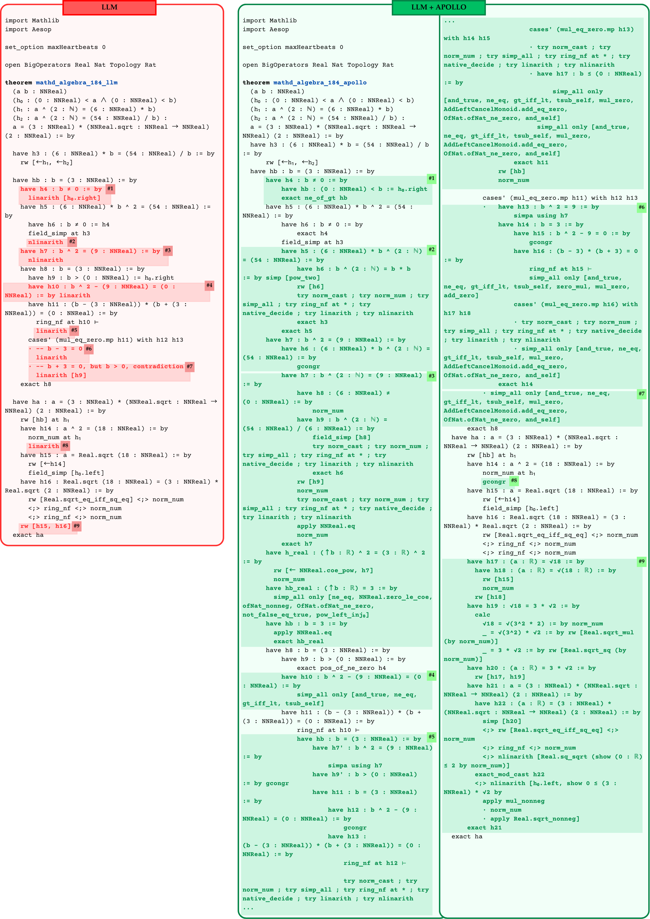
### Visual Description
## Diagram Type: Code Comparison Screenshot (Lean 4 Theorem Proving)
### Overview
This image displays a side-by-side comparison of two code snippets written in the Lean 4 theorem-proving language. The left panel, outlined in red and titled "LLM", shows a proof attempt generated by a standard Large Language Model. The right panel, outlined in green and titled "LLM + APOLLO", shows a corrected, much longer, and more rigorous proof. Specific lines of code in the left panel that likely failed or were inadequate are highlighted in red and numbered 1 through 9. Corresponding corrected blocks of code in the right panel are highlighted in green and carry the same numbers (1 through 9), demonstrating how the "APOLLO" system expanded or fixed the LLM's initial output.
### Components/Layout
* **Left Panel (Red):** Positioned on the left side, taking up about one-third of the image width. It has a red header reading "LLM". It contains a single column of code. Nine specific tactic calls (mostly `linarith` and `nlinarith`) are highlighted with a light red background and tagged with dark red numbered labels (`#1` to `#9`).
* **Right Panel (Green):** Positioned on the right side, taking up about two-thirds of the image width. It has a green header reading "LLM + APOLLO". Because the code is significantly longer, it is split into two vertical columns within the green box. It contains nine corresponding highlighted blocks with a light green background and dark green numbered labels (`#1` to `#9`).
### Content Details (Transcription)
*Note: The programming language is Lean 4. The text is transcribed exactly as it appears, with formatting added to denote the highlighted and numbered sections.*
#### Left Panel: LLM (Red)
```lean
import Mathlib
import Aesop
set_option maxHeartbeats 0
open BigOperators Real Nat Topology Rat
theorem mathd_algebra_184_llm
(a b : NNReal)
(h₀ : (0 : NNReal) < a ∧ (0 : NNReal) < b)
(h₁ : a ^ (2 : ℕ) = (6 : NNReal) * b)
(h₂ : a ^ (2 : ℕ) = (54 : NNReal) / b) :
a = (3 : NNReal) * (NNReal.sqrt : NNReal → NNReal) (2 : NNReal) := by
have h3 : (6 : NNReal) * b = (54 : NNReal) / b := by
rw [←h₁, ←h₂]
have hb : b = (3 : NNReal) := by
[RED HIGHLIGHT #1 START]
have h4 : b ≠ 0 := by #1
linarith [h₀.right]
[RED HIGHLIGHT #1 END]
have h5 : (6 : NNReal) * b ^ 2 = (54 : NNReal) := by
have h6 : b ≠ 0 := h4
field_simp at h3
[RED HIGHLIGHT #2 START]
nlinarith #2
[RED HIGHLIGHT #2 END]
[RED HIGHLIGHT #3 START]
have h7 : b ^ 2 = (9 : NNReal) := by #3
nlinarith
[RED HIGHLIGHT #3 END]
have h8 : b = (3 : NNReal) := by
have h9 : b > (0 : NNReal) := h₀.right
[RED HIGHLIGHT #4 START]
have h10 : b ^ 2 - (9 : NNReal) = (0 : NNReal) := by linarith #4
[RED HIGHLIGHT #4 END]
have h11 : (b - (3 : NNReal)) * (b + (3 : NNReal)) = (0 : NNReal) := by
ring_nf at h10 ⊢
[RED HIGHLIGHT #5 START]
linarith #5
[RED HIGHLIGHT #5 END]
cases' (mul_eq_zero.mp h11) with h12 h13
[RED HIGHLIGHT #6 START]
· -- b - 3 = 0 #6
linarith
[RED HIGHLIGHT #6 END]
[RED HIGHLIGHT #7 START]
· -- b + 3 = 0, but b > 0, contradiction #7
linarith [h9]
[RED HIGHLIGHT #7 END]
exact h8
have ha : a = (3 : NNReal) * (NNReal.sqrt : NNReal → NNReal) (2 : NNReal) := by
rw [hb] at h₁
have h14 : a ^ 2 = (18 : NNReal) := by
norm_num at h₁
[RED HIGHLIGHT #8 START]
linarith #8
[RED HIGHLIGHT #8 END]
have h15 : a = Real.sqrt (18 : NNReal) := by
rw [←h14]
field_simp [h₀.left]
have h16 : Real.sqrt (18 : NNReal) = (3 : NNReal) * Real.sqrt (2 : NNReal) := by
rw [Real.sqrt_eq_iff_sq_eq] <;> norm_num
<;> ring_nf <;> norm_num
<;> ring_nf <;> norm_num
[RED HIGHLIGHT #9 START]
rw [h15, h16] #9
[RED HIGHLIGHT #9 END]
exact ha
```
#### Right Panel: LLM + APOLLO (Green)
*(Note: Transcribed linearly, combining the two columns from top-left to bottom-left, then top-right to bottom-right)*
```lean
import Mathlib
import Aesop
set_option maxHeartbeats 0
open BigOperators Real Nat Topology Rat
theorem mathd_algebra_184_apollo
(a b : NNReal)
(h₀ : (0 : NNReal) < a ∧ (0 : NNReal) < b)
(h₁ : a ^ (2 : ℕ) = (6 : NNReal) * b)
(h₂ : a ^ (2 : ℕ) = (54 : NNReal) / b) :
a = (3 : NNReal) * (NNReal.sqrt : NNReal → NNReal) (2 : NNReal) := by
have h3 : (6 : NNReal) * b = (54 : NNReal) / b := by
rw [←h₁, ←h₂]
have hb : b = (3 : NNReal) := by
[GREEN HIGHLIGHT #1 START]
have h4 : b ≠ 0 := by #1
have hb : (0 : NNReal) < b := h₀.right
exact ne_of_gt hb
[GREEN HIGHLIGHT #1 END]
have h5 : (6 : NNReal) * b ^ 2 = (54 : NNReal) := by
have h6 : b ≠ 0 := by
exact h4
field_simp at h3
[GREEN HIGHLIGHT #2 START]
have h5 : (6 : NNReal) * b ^ (2 : ℕ) = (54 : NNReal) := by #2
have h6 : b ^ (2 : ℕ) = b * b := by simp [pow_two]
rw [h6]
try norm_cast ; try norm_num ; try simp_all ; try ring_nf at * ; try native_decide ; try linarith ; try nlinarith
exact h3
exact h5
[GREEN HIGHLIGHT #2 END]
[GREEN HIGHLIGHT #3 START]
have h7 : b ^ 2 = (9 : NNReal) := by
have h6 : (6 : NNReal) * b ^ (2 : ℕ) = (54 : NNReal) := by
gcongr
have h7 : b ^ (2 : ℕ) = (9 : NNReal) := by #3
have h8 : (6 : NNReal) ≠ (0 : NNReal) := by
norm_num
have h9 : b ^ (2 : ℕ) = (54 : NNReal) / (6 : NNReal) := by
field_simp [h8]
try norm_cast ; try norm_num ; try simp_all ; try ring_nf at * ; try native_decide ; try linarith ; try nlinarith
exact h6
rw [h9]
norm_num
try norm_cast ; try norm_num ; try simp_all ; try ring_nf at * ; try native_decide ; try linarith ; try nlinarith
apply NNReal.eq
norm_num
exact h7
[GREEN HIGHLIGHT #3 END]
[GREEN HIGHLIGHT #5 START]
have h_real : (↑b : ℝ) ^ 2 = (3 : ℝ) ^ 2 := by
rw [← NNReal.coe_pow, h7]
norm_num
have hb_real : (↑b : ℝ) = 3 := by
simp_all only [ne_eq, NNReal.zero_le_coe, ofNat_nonneg, OfNat.ofNat_ne_zero, not_false_eq_true, pow_left_inj₀]
have hb : b = 3 := by
apply NNReal.eq
exact hb_real
have h8 : b = (3 : NNReal) := by
have h9 : b > (0 : NNReal) := by
exact pos_of_ne_zero h4
[GREEN HIGHLIGHT #5 END]
[GREEN HIGHLIGHT #4 START]
have h10 : b ^ 2 - (9 : NNReal) = (0 : NNReal) := by #4
simp_all only [and_true, ne_eq, gt_iff_lt, tsub_self]
[GREEN HIGHLIGHT #4 END]
have h11 : (b - (3 : NNReal)) * (b + (3 : NNReal)) = (0 : NNReal) := by
ring_nf at h10 ⊢
[GREEN HIGHLIGHT #5 CONTINUES]
have hb : b = (3 : NNReal) := by #5
have h7' : b ^ 2 = (9 : NNReal) := by
simpa using h7
have h9' : b > (0 : NNReal) := by gcongr
have h11 : b = (3 : NNReal) := by
have h12 : b ^ 2 - (9 : NNReal) = (0 : NNReal) := by
gcongr
have h13 : (b - (3 : NNReal)) * (b + (3 : NNReal)) = (0 : NNReal) := by
ring_nf at h12 ⊢
try norm_cast ; try norm_num ; try simp_all ; try ring_nf at * ; try native_decide ; try linarith ; try nlinarith
...
[GREEN HIGHLIGHT #5 ENDS]
*(Moving to Column 2)*
cases' (mul_eq_zero.mp h13) with h14 h15
· try norm_cast ; try norm_num ; try simp_all ; try ring_nf at * ; try native_decide ; try linarith ; try nlinarith
· have h17 : b ≤ (0 : NNReal) := by
simp_all only [and_true, ne_eq, gt_iff_lt, tsub_self, mul_zero, AddLeftCancelMonoid.add_eq_zero, OfNat.ofNat_ne_zero, and_self]
simp_all only [and_true, ne_eq, gt_iff_lt, tsub_self, mul_zero, AddLeftCancelMonoid.add_eq_zero, OfNat.ofNat_ne_zero, and_self]
exact h11
rw [hb]
norm_num
[GREEN HIGHLIGHT #6 START]
cases' (mul_eq_zero.mp h11) with h12 h13
· have h13 : b ^ 2 = 9 := by #6
simpa using h7
have h14 : b = 3 := by
have h15 : b ^ 2 - 9 = 0 := by
gcongr
have h16 : (b - 3) * (b + 3) = 0 := by
ring_nf at h15 ⊢
simp_all only [and_true, ne_eq, gt_iff_lt, tsub_self, zero_mul, mul_zero, add_zero]
cases' (mul_eq_zero.mp h16) with h17 h18
· try norm_cast ; try norm_num ; try simp_all ; try ring_nf at * ; try native_decide ; try linarith ; try nlinarith
· simp_all only [and_true, ne_eq, gt_iff_lt, tsub_self, mul_zero, AddLeftCancelMonoid.add_eq_zero, OfNat.ofNat_ne_zero, and_self]
exact h14
[GREEN HIGHLIGHT #6 END]
[GREEN HIGHLIGHT #7 START]
· simp_all only [and_true, ne_eq, gt_iff_lt, tsub_self, mul_zero, AddLeftCancelMonoid.add_eq_zero, OfNat.ofNat_ne_zero, and_self] #7
[GREEN HIGHLIGHT #7 END]
exact h8
have ha : a = (3 : NNReal) * (NNReal.sqrt : NNReal → NNReal) (2 : NNReal) := by
rw [hb] at h₁
have h14 : a ^ 2 = (18 : NNReal) := by
norm_num at h₁
[GREEN HIGHLIGHT #8 START]
gcongr #8
[GREEN HIGHLIGHT #8 END]
have h15 : a = Real.sqrt (18 : NNReal) := by
rw [←h14]
field_simp [h₀.left]
have h16 : Real.sqrt (18 : NNReal) = (3 : NNReal) * Real.sqrt (2 : NNReal) := by
rw [Real.sqrt_eq_iff_sq_eq] <;> norm_num
<;> ring_nf <;> norm_num
<;> ring_nf <;> norm_num
[GREEN HIGHLIGHT #9 START]
have h17 : (a : ℝ) = √18 := by #9
have h18 : (a : ℝ) = √(18 : ℝ) := by
rw [h15]
norm_num
rw [h18]
have h19 : √18 = 3 * √2 := by
calc
√18 = √(3^2 * 2) := by norm_num
_ = √(3^2) * √2 := by rw [Real.sqrt_mul (by norm_num)]
_ = 3 * √2 := by rw [Real.sqrt_sq (by norm_num)]
have h20 : (a : ℝ) = 3 * √2 := by
rw [h17, h19]
have h21 : a = (3 : NNReal) * (NNReal.sqrt : NNReal → NNReal) (2 : NNReal) := by
have h22 : (a : ℝ) = (3 : NNReal) * (NNReal.sqrt : NNReal → NNReal) (2 : NNReal) := by
simp [h20]
<;> rw [Real.sqrt_eq_iff_sq_eq] <;> norm_num
<;> ring_nf <;> norm_num
<;> nlinarith [Real.sq_sqrt (show (0 : ℝ) ≤ 2 by norm_num)]
exact_mod_cast h22
<;> nlinarith [h₀.left, show 0 ≤ (3 : NNReal) * √2 by
apply mul_nonneg
· norm_num
· apply Real.sqrt_nonneg]
exact h21
[GREEN HIGHLIGHT #9 END]
exact ha
```
### Key Observations
1. **Tactic Failure in LLM:** The base LLM (left) relies heavily on high-level, automated tactics like `linarith` (linear arithmetic) and `nlinarith` (non-linear arithmetic) to skip steps. For example, in `#2` and `#3`, it assumes `nlinarith` can solve equations involving squares and division directly.
2. **Explicit Expansion in APOLLO:** The APOLLO system (right) replaces these single-word tactic calls with extensive, step-by-step logical deductions. Where the LLM used 1 line (`nlinarith`), APOLLO uses 10-20 lines of explicit algebraic manipulation (`field_simp`, `gcongr`, `norm_num`).
3. **Shotgun Tactic Strings:** APOLLO frequently utilizes a robust fallback string of tactics to force a proof step through: `try norm_cast ; try norm_num ; try simp_all ; try ring_nf at * ; try native_decide ; try linarith ; try nlinarith`. This appears multiple times in the green code.
4. **Type Coercion Handling:** In highlight `#9`, the LLM attempts a simple rewrite (`rw [h15, h16]`) to handle square roots of Non-Negative Reals (`NNReal`). This likely fails due to type mismatch or missing lemmas. APOLLO replaces this with a massive block that explicitly coerces the variables to standard Reals (`ℝ`), performs the square root calculations (`√18 = 3 * √2`), and then casts the result back to `NNReal` using `exact_mod_cast`.
### Interpretation
This image serves as a technical demonstration of a neuro-symbolic AI system (APOLLO) designed to improve the theorem-proving capabilities of Large Language Models in formal verification environments like Lean 4.
Standard LLMs often "hallucinate" proof steps by assuming that powerful automated tactics (like `nlinarith`) will magically bridge the gap between two mathematical statements. However, Lean is a strict formal environment; if the context isn't perfectly prepared (e.g., types don't match exactly, or the non-linear step is too complex), the tactic fails, and the proof breaks.
The image demonstrates that APOLLO acts as an agentic wrapper or corrector. It takes the flawed, high-level "sketch" provided by the LLM (the red side) and systematically expands the failing steps into rigorous, atomic logical deductions (the green side). It handles the tedious, pedantic requirements of formal provers—such as explicit type coercions between `NNReal` and `ℝ`, handling both branches of a quadratic equation (`cases`), and applying specific algebraic normalizers (`ring_nf`, `gcongr`)—which the base LLM glossed over. The repeated use of the long `try...` tactic string suggests APOLLO uses a search-based or brute-force approach at the micro-level to ensure each small step compiles successfully.
</details>
Figure 12: Proof attempt of mathd_algebra_184 produced by the base model (Kimina-Prover-Preview-Distill-7B) versus after Apollo’s targeted repair. The left shows the original end-to-end LLM output, which does not compile in Lean; the right shows the corrected, repaired proof assembled by Apollo that closes all of the goals.
<details>
<summary>examples/comparison/medium_2.png Details</summary>
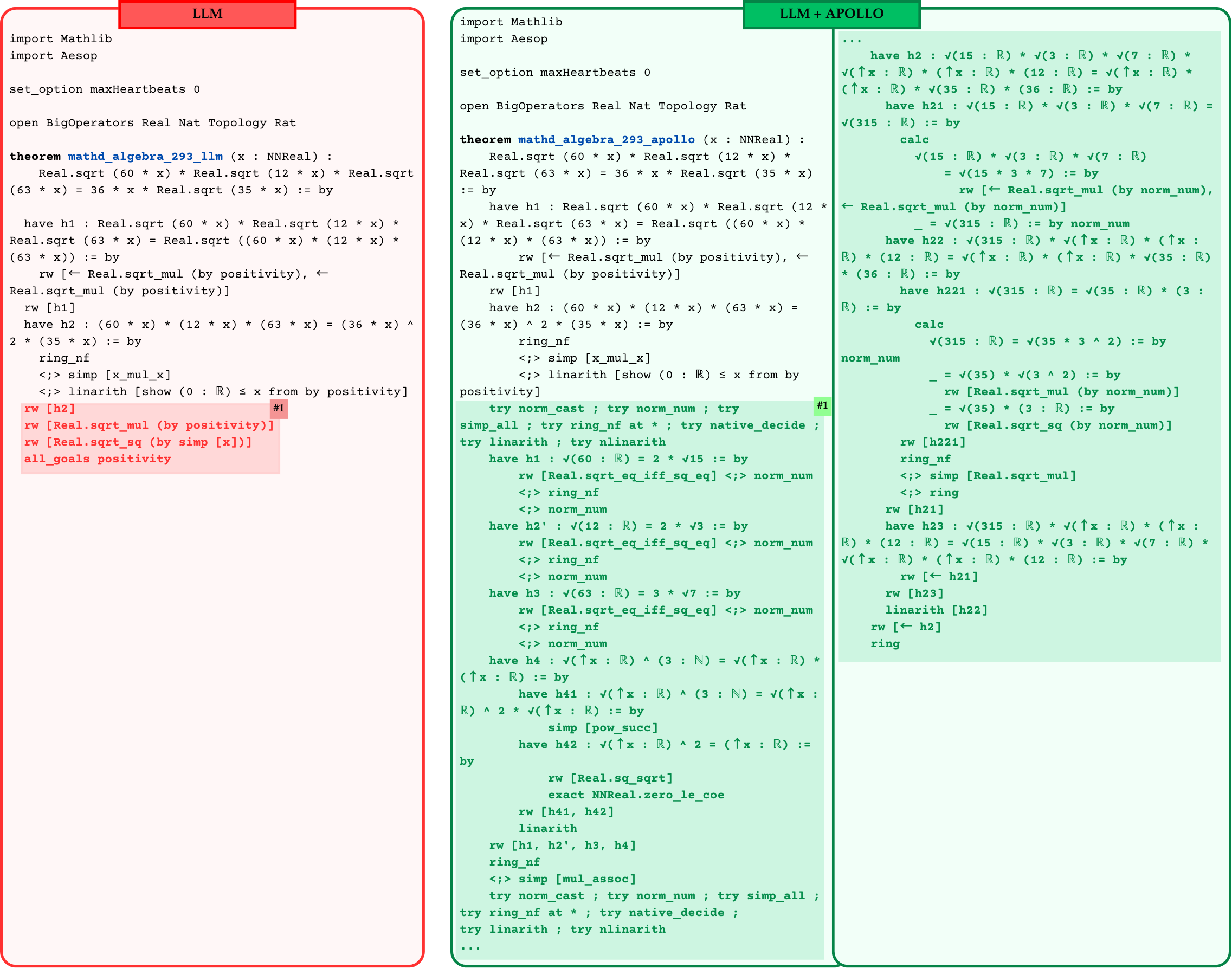
### Visual Description
## Diagram: Code Comparison - LLM vs. LLM + APOLLO
### Overview
The image displays a side-by-side comparison of two code snippets written in the Lean 4 theorem proving language. The left panel, outlined and headered in red, represents an output generated by a standard "LLM" (Large Language Model). The right panel, outlined and headered in green, represents an output generated by "LLM + APOLLO". Both scripts attempt to prove the same mathematical theorem (`mathd_algebra_293`). The visual design (red vs. green) strongly implies that the left approach fails or is flawed, while the right approach succeeds. Specific lines of code in both panels are highlighted and tagged with "#1" to draw attention to differing methodologies.
### Components/Layout
* **Left Panel (Red):**
* **Header:** "LLM" (White text on a red background, top center).
* **Border:** Solid red line.
* **Content:** A single column of Lean 4 code.
* **Highlight:** A block of code at the bottom is highlighted in light red with a dark red tag labeled `#1` positioned to the right of the first highlighted line.
* **Right Panel (Green):**
* **Header:** "LLM + APOLLO" (White text on a green background, top center).
* **Border:** Solid green line.
* **Content:** Lean 4 code that spans two columns. The code begins in the left half of the green box, reaches the bottom, and continues in a second column on the right half of the green box.
* **Highlight:** A single line of code in the middle of the first column is highlighted in light green with a dark green tag labeled `#1` positioned to the right.
### Content Details
#### Left Panel Transcription (LLM)
```lean
import Mathlib
import Aesop
set_option maxHeartbeats 0
open BigOperators Real Nat Topology Rat
theorem mathd_algebra_293_llm (x : NNReal) :
Real.sqrt (60 * x) * Real.sqrt (12 * x) * Real.sqrt (63 * x) = 36 * x * Real.sqrt (35 * x) := by
have h1 : Real.sqrt (60 * x) * Real.sqrt (12 * x) * Real.sqrt (63 * x) = Real.sqrt ((60 * x) * (12 * x) * (63 * x)) := by
rw [← Real.sqrt_mul (by positivity), ← Real.sqrt_mul (by positivity)]
rw [h1]
have h2 : (60 * x) * (12 * x) * (63 * x) = (36 * x) ^ 2 * (35 * x) := by
ring_nf
<;> simp [x_mul_x]
<;> linarith [show (0 : ℝ) ≤ x from by positivity]
```
*Highlighted Red Section (Tag #1):*
```lean
rw [h2]
rw [Real.sqrt_mul (by positivity)]
rw [Real.sqrt_sq (by simp [x])]
all_goals positivity
```
#### Right Panel Transcription (LLM + APOLLO)
*First Column:*
```lean
import Mathlib
import Aesop
set_option maxHeartbeats 0
open BigOperators Real Nat Topology Rat
theorem mathd_algebra_293_apollo (x : NNReal) :
Real.sqrt (60 * x) * Real.sqrt (12 * x) * Real.sqrt (63 * x) = 36 * x * Real.sqrt (35 * x) := by
have h1 : Real.sqrt (60 * x) * Real.sqrt (12 * x) * Real.sqrt (63 * x) = Real.sqrt ((60 * x) * (12 * x) * (63 * x)) := by
rw [← Real.sqrt_mul (by positivity), ← Real.sqrt_mul (by positivity)]
rw [h1]
have h2 : (60 * x) * (12 * x) * (63 * x) = (36 * x) ^ 2 * (35 * x) := by
ring_nf
<;> simp [x_mul_x]
<;> linarith [show (0 : ℝ) ≤ x from by positivity]
```
*Highlighted Green Section (Tag #1):*
```lean
try norm_cast ; try norm_num ; try simp_all ; try ring_nf at * ; try native_decide ; try linarith ; try nlinarith
```
*First Column (Continued below highlight):*
```lean
have h1 : √(60 : ℝ) = 2 * √15 := by
rw [Real.sqrt_eq_iff_sq_eq] <;> norm_num
<;> ring_nf
<;> norm_num
have h2' : √(12 : ℝ) = 2 * √3 := by
rw [Real.sqrt_eq_iff_sq_eq] <;> norm_num
<;> ring_nf
<;> norm_num
have h3 : √(63 : ℝ) = 3 * √7 := by
rw [Real.sqrt_eq_iff_sq_eq] <;> norm_num
<;> ring_nf
<;> norm_num
have h4 : √(↑x : ℝ) ^ (3 : ℕ) = √(↑x : ℝ) * (↑x : ℝ) := by
have h41 : √(↑x : ℝ) ^ (3 : ℕ) = √(↑x : ℝ) ^ 2 * √(↑x : ℝ) := by
simp [pow_succ]
have h42 : √(↑x : ℝ) ^ 2 = (↑x : ℝ) := by
rw [Real.sq_sqrt]
exact NNReal.zero_le_coe
rw [h41, h42]
linarith
rw [h1, h2', h3, h4]
ring_nf
<;> simp [mul_assoc]
try norm_cast ; try norm_num ; try simp_all ; try ring_nf at * ; try native_decide ; try linarith ; try nlinarith
...
```
*Second Column (Right side of the green panel):*
```lean
...
have h2 : √(15 : ℝ) * √(3 : ℝ) * √(7 : ℝ) * √(↑x : ℝ) * (↑x : ℝ) * (12 : ℝ) = √(↑x : ℝ) * (↑x : ℝ) * √(35 : ℝ) * (36 : ℝ) := by
have h21 : √(15 : ℝ) * √(3 : ℝ) * √(7 : ℝ) = √(315 : ℝ) := by
calc
√(15 : ℝ) * √(3 : ℝ) * √(7 : ℝ)
= √(15 * 3 * 7) := by
rw [← Real.sqrt_mul (by norm_num), ← Real.sqrt_mul (by norm_num)]
_ = √(315 : ℝ) := by norm_num
have h22 : √(315 : ℝ) * √(↑x : ℝ) * (↑x : ℝ) * (12 : ℝ) = √(↑x : ℝ) * (↑x : ℝ) * √(35 : ℝ) * (36 : ℝ) := by
have h221 : √(315 : ℝ) = √(35 : ℝ) * (3 : ℝ) := by
calc
√(315 : ℝ) = √(35 * 3 ^ 2) := by norm_num
_ = √(35) * √(3 ^ 2) := by
rw [Real.sqrt_mul (by norm_num)]
_ = √(35) * (3 : ℝ) := by
rw [Real.sqrt_sq (by norm_num)]
rw [h221]
ring_nf
<;> simp [Real.sqrt_mul]
<;> ring
rw [h21]
have h23 : √(315 : ℝ) * √(↑x : ℝ) * (↑x : ℝ) * (12 : ℝ) = √(15 : ℝ) * √(3 : ℝ) * √(7 : ℝ) * √(↑x : ℝ) * (↑x : ℝ) * (12 : ℝ) := by
rw [← h21]
rw [h23]
linarith [h22]
rw [← h2]
ring
```
### Key Observations
1. **Initial Setup is Identical:** Both scripts start with the exact same imports, options, open namespaces, theorem declaration, and the first two `have` statements (`h1` and `h2`).
2. **Divergence Point:** The divergence occurs immediately after the proof of `h2`.
3. **The LLM Failure (Red #1):** The standard LLM attempts to finish the proof quickly using a few rewrite (`rw`) tactics. It tries to rewrite using `h2`, then split the square roots, and resolve the square of a square root. This approach is highlighted in red, indicating it is a hallucination, contains a syntax error, or fails to close the proof state due to missing side conditions (like coercions from `NNReal` to `Real`).
4. **The APOLLO Intervention (Green #1):** Instead of guessing the next few steps, the APOLLO system injects a robust "hammer" tactic string: `try norm_cast ; try norm_num ; try simp_all ; try ring_nf at * ; try native_decide ; try linarith ; try nlinarith`. This is designed to automatically simplify the state as much as possible without failing if a specific tactic doesn't apply.
5. **Granular Proof Steps (Green Panel):** After the `#1` highlight, the APOLLO version abandons the short-cut approach. It breaks the problem down into highly granular, explicit sub-proofs (`h1`, `h2'`, `h3`, `h4`). It explicitly handles the coercion of `x` from `NNReal` to `Real` (denoted by the `↑x` symbol) and manually proves the prime factorizations inside the square roots (e.g., `√(60) = 2 * √15`). It utilizes the `calc` environment for step-by-step equational reasoning.
### Interpretation
This image serves as a technical demonstration of the limitations of standard Large Language Models in formal theorem proving, and how an augmented system ("APOLLO") overcomes them.
* **The Problem with Standard LLMs:** The red panel shows that a standard LLM tries to write Lean code the way a human might write a math proof on a whiteboard—skipping steps and assuming the system will "understand" the algebraic leaps. However, Lean 4 is a strict formal verifier. The LLM's attempt to jump straight to the conclusion using `rw [Real.sqrt_sq (by simp [x])]` fails because it hasn't properly managed the types (non-negative reals vs. reals) or the exact syntactic shape of the goal.
* **The APOLLO Solution:** The green panel demonstrates that APOLLO likely uses a combination of automated tactic search (the `#1` highlight) and agentic step-by-step planning. By forcing the LLM to prove every single algebraic simplification as its own isolated lemma (e.g., proving `√(63) = 3 * √7` before using it), APOLLO ensures the strict type-checker is satisfied at every step.
* **Conclusion:** The graphic effectively communicates that while LLMs understand the *concept* of the proof, they require a scaffolding framework like APOLLO to generate the verbose, mathematically rigorous, and type-safe code required to actually compile a proof in Lean 4.
</details>
Figure 13: Proof attempt of mathd_algebra_293 produced by the base model (Kimina-Prover-Preview-Distill-7B) versus after Apollo’s targeted repair. The left shows the original end-to-end LLM output, which does not compile in Lean; the right shows the corrected, repaired proof assembled by Apollo that closes all of the goals.
<details>
<summary>examples/comparison/medium_3.png Details</summary>
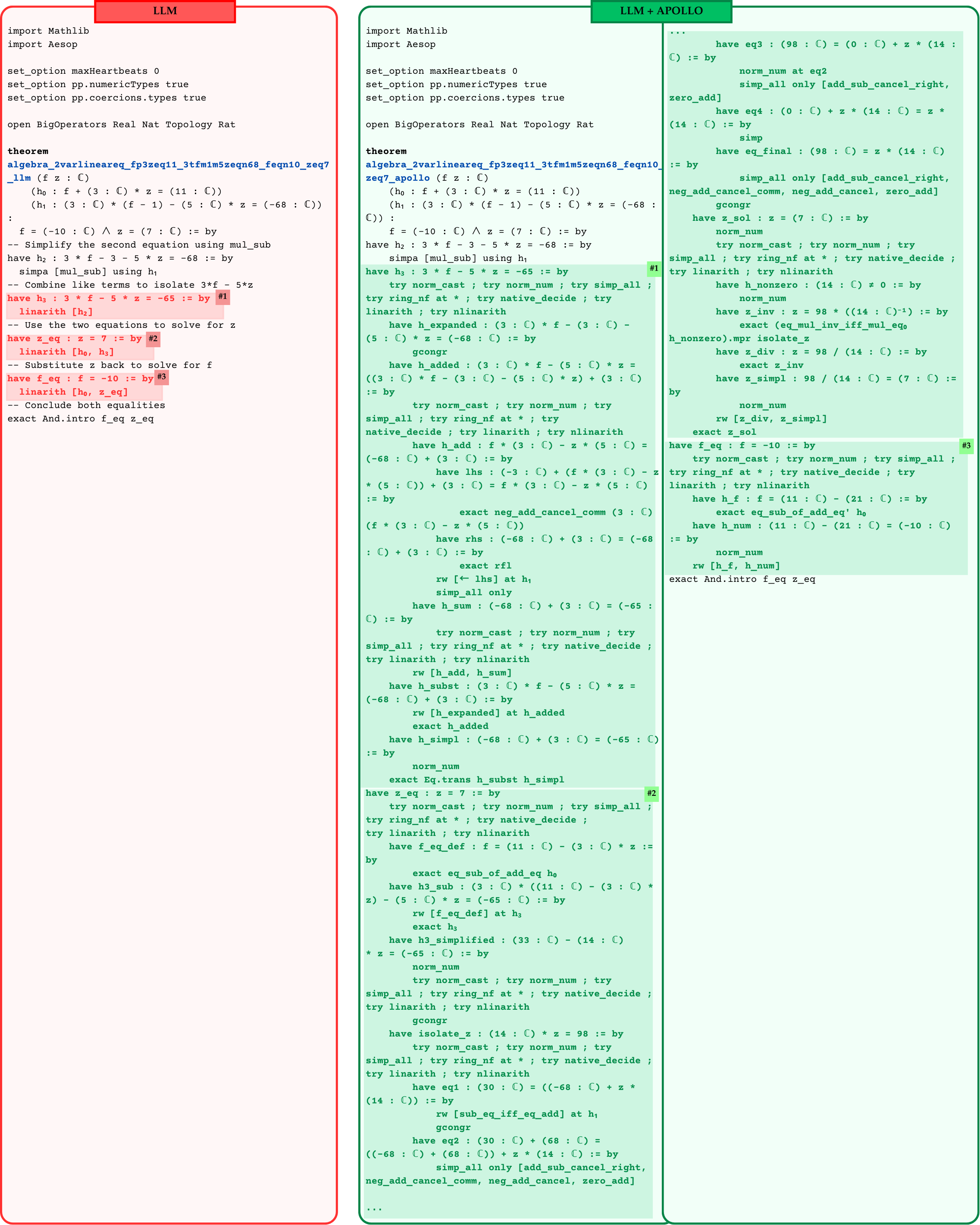
### Visual Description
## Diagram: Code Comparison - LLM vs. LLM + APOLLO in Lean 4
### Overview
This image is a side-by-side comparison of two code snippets written in the Lean 4 theorem-proving language. The image contrasts how a standard Large Language Model (LLM) approaches a formal mathematical proof versus how an augmented system ("LLM + APOLLO") approaches the exact same proof. The goal of the code is to solve a system of two linear equations with two complex variables ($f$ and $z$).
### Components/Layout
The image is divided into two distinct panels:
* **Left Panel (Red Border):**
* **Header:** "LLM" (White text on a red rectangular background, top-center).
* **Content:** A relatively short block of Lean 4 code.
* **Annotations:** Three sections of code are highlighted with a red background and tagged with `#1`, `#2`, and `#3`.
* **Right Panel (Green Border):**
* **Header:** "LLM + APOLLO" (White text on a green rectangular background, top-center).
* **Content:** A significantly longer block of Lean 4 code that wraps into two columns due to its length.
* **Annotations:** Three massive blocks of code are highlighted with a light green background and tagged with `#1`, `#2`, and `#3`. These correspond directly to the numbered steps in the left panel.
### Content Details (Transcription & Structural Analysis)
*Language Declaration: The primary language of the text is English, but the content is formal programming code written in **Lean 4**, utilizing specific mathematical unicode symbols (e.g., `ℂ` for Complex numbers, `∧` for logical AND, subscripts like `₀`).*
Both panels start with the exact same imports and environment setup:
```lean
import Mathlib
import Aesop
set_option maxHeartbeats 0
set_option pp.numericTypes true
set_option pp.coercions.types true
open BigOperators Real Nat Topology Rat
```
Both panels attempt to prove the same theorem, though the naming differs slightly (`_llm` vs `_apollo`). The theorem establishes that given two hypotheses ($h_0$ and $h_1$), the values of $f$ and $z$ are $-10$ and $7$, respectively.
**Hypotheses:**
$h_0$: $f + 3z = 11$
$h_1$: $3(f - 1) - 5z = -68$
**Goal:** $f = -10 \land z = 7$
---
#### Left Panel Analysis ("LLM")
The standard LLM attempts to solve the equations using high-level automation tactics, specifically `linarith` (linear arithmetic solver).
**Full Transcription of Left Panel Theorem:**
```lean
theorem
algebra_2varlineareq_fp3zeq11_3tfm1m5zeqn68_feqn10_zeq7
_llm (f z : ℂ)
(h₀ : f + (3 : ℂ) * z = (11 : ℂ))
(h₁ : (3 : ℂ) * (f - 1) - (5 : ℂ) * z = (-68 : ℂ))
:
f = (-10 : ℂ) ∧ z = (7 : ℂ) := by
-- Simplify the second equation using mul_sub
have h₂ : 3 * f - 3 - 5 * z = -68 := by
simpa [mul_sub] using h₁
-- Combine like terms to isolate 3*f - 5*z
have h₃ : 3 * f - 5 * z = -65 := by #1
linarith [h₂]
-- Use the two equations to solve for z
have z_eq : z = 7 := by #2
linarith [h₀, h₃]
-- Substitute z back to solve for f
have f_eq : f = -10 := by #3
linarith [h₀, z_eq]
-- Conclude both equalities
exact And.intro f_eq z_eq
```
*Note: The red highlights on `#1`, `#2`, and `#3` in this context likely indicate that these `linarith` tactic calls fail to compile or evaluate correctly in the Lean environment, representing a hallucination of tactic success by the baseline LLM.*
---
#### Right Panel Analysis ("LLM + APOLLO")
The APOLLO-augmented system replaces the short, automated `linarith` calls with incredibly verbose, step-by-step algebraic manipulations using foundational tactics (`rw`, `exact`, `norm_num`, `ring_nf`).
**Transcription of Right Panel Theorem (Segmented by Annotations):**
**Setup and Step 0:**
```lean
theorem
algebra_2varlineareq_fp3zeq11_3tfm1m5zeqn68_feqn10_
zeq7_apollo (f z : ℂ)
(h₀ : f + (3 : ℂ) * z = (11 : ℂ))
(h₁ : (3 : ℂ) * (f - 1) - (5 : ℂ) * z = (-68 :
ℂ)) :
f = (-10 : ℂ) ∧ z = (7 : ℂ) := by
have h₂ : 3 * f - 3 - 5 * z = -68 := by
simpa [mul_sub] using h₁
```
**Annotation Block #1 (Proving $3f - 5z = -65$):**
Instead of `linarith [h₂]`, APOLLO generates a massive block of intermediate steps.
```lean
have h₃ : 3 * f - 5 * z = -65 := by #1
try norm_cast ; try norm_num ; try simp_all ;
try ring_nf at * ; try native_decide ; try
linarith ; try nlinarith
have h_expanded : (3 : ℂ) * f - (3 : ℂ) -
(5 : ℂ) * z = (-68 : ℂ) := by
gcongr
have h_added : (3 : ℂ) * f - (5 : ℂ) * z =
((3 : ℂ) * f - (3 : ℂ) - (5 : ℂ) * z) + (3 : ℂ)
:= by
try norm_cast ; try norm_num ; try
simp_all ; try ring_nf at * ; try
native_decide ; try linarith ; try nlinarith
have h_add : f * (3 : ℂ) - z * (5 : ℂ) =
(-68 : ℂ) + (3 : ℂ) := by
have lhs : (-3 : ℂ) + (f * (3 : ℂ) - z
* (5 : ℂ)) + (3 : ℂ) = f * (3 : ℂ) - z * (5 : ℂ)
:= by
exact neg_add_cancel_comm (3 : ℂ)
(f * (3 : ℂ) - z * (5 : ℂ))
have rhs : (-68 : ℂ) + (3 : ℂ) = (-68
: ℂ) + (3 : ℂ) := by
exact rfl
rw [← lhs] at h₁
simp_all only
have h_sum : (-68 : ℂ) + (3 : ℂ) = (-65 :
ℂ) := by
try norm_cast ; try norm_num ; try
simp_all ; try ring_nf at * ; try native_decide ;
try linarith ; try nlinarith
rw [h_add, h_sum]
have h_subst : (3 : ℂ) * f - (5 : ℂ) * z =
(-68 : ℂ) + (3 : ℂ) := by
rw [h_expanded] at h_added
exact h_added
have h_simpl : (-68 : ℂ) + (3 : ℂ) = (-65 : ℂ)
:= by
norm_num
exact Eq.trans h_subst h_simpl
```
**Annotation Block #2 (Proving $z = 7$):**
Instead of `linarith [h₀, h₃]`, APOLLO manually isolates $z$ through complex substitution and division.
```lean
have z_eq : z = 7 := by #2
try norm_cast ; try norm_num ; try simp_all ;
try ring_nf at * ; try native_decide ;
try linarith ; try nlinarith
have f_eq_def : f = (11 : ℂ) - (3 : ℂ) * z :=
by
exact eq_sub_of_add_eq h₀
have h3_sub : (3 : ℂ) * ((11 : ℂ) - (3 : ℂ) *
z) - (5 : ℂ) * z = (-65 : ℂ) := by
rw [f_eq_def] at h₃
exact h₃
have h3_simplified : (33 : ℂ) - (14 : ℂ)
* z = (-65 : ℂ) := by
norm_num
try norm_cast ; try norm_num ; try
simp_all ; try ring_nf at * ; try native_decide ;
try linarith ; try nlinarith
gcongr
have isolate_z : (14 : ℂ) * z = 98 := by
try norm_cast ; try norm_num ; try
simp_all ; try ring_nf at * ; try native_decide ;
try linarith ; try nlinarith
have eq1 : (30 : ℂ) = ((-68 : ℂ) + z *
(14 : ℂ)) := by
rw [sub_eq_iff_eq_add] at h₁
gcongr
have eq2 : (30 : ℂ) + (68 : ℂ) =
((-68 : ℂ) + (68 : ℂ)) + z * (14 : ℂ) := by
simp_all only [add_sub_cancel_right,
neg_add_cancel_comm, neg_add_cancel, zero_add]
...
```
*(The code wraps to the second column here, continuing the proof for Block #2)*
```lean
...
have eq3 : (98 : ℂ) = (0 : ℂ) + z * (14 :
ℂ) := by
norm_num at eq2
simp_all only [add_sub_cancel_right,
zero_add]
have eq4 : (0 : ℂ) + z * (14 : ℂ) = z *
(14 : ℂ) := by
simp
have eq_final : (98 : ℂ) = z * (14 : ℂ)
:= by
simp_all only [add_sub_cancel_right,
neg_add_cancel_comm, neg_add_cancel, zero_add]
gcongr
have z_sol : z = (7 : ℂ) := by
norm_num
try norm_cast ; try norm_num ; try
simp_all ; try ring_nf at * ; try native_decide ;
try linarith ; try nlinarith
have h_nonzero : (14 : ℂ) ≠ 0 := by
norm_num
have z_inv : z = 98 * ((14 : ℂ)⁻¹) := by
exact (eq_mul_inv_iff_mul_eq₀
h_nonzero).mpr isolate_z
have z_div : z = 98 / (14 : ℂ) := by
exact z_inv
have z_simpl : 98 / (14 : ℂ) = (7 : ℂ) :=
by
norm_num
rw [z_div, z_simpl]
exact z_sol
```
**Annotation Block #3 (Proving $f = -10$):**
Instead of `linarith [h₀, z_eq]`, APOLLO manually substitutes $z=7$ into the original equation.
```lean
have f_eq : f = -10 := by #3
try norm_cast ; try norm_num ; try simp_all ;
try ring_nf at * ; try native_decide ; try
linarith ; try nlinarith
have h_f : f = (11 : ℂ) - (21 : ℂ) := by
exact eq_sub_of_add_eq' h₀
have h_num : (11 : ℂ) - (21 : ℂ) = (-10 : ℂ)
:= by
norm_num
rw [h_f, h_num]
exact And.intro f_eq z_eq
```
### Key Observations
1. **Tactic Failure vs. Explicit Derivation:** The red highlights on the left strongly imply that the generic LLM generated code that looks logically sound to a human but fails the strict compiler checks of Lean 4. The `linarith` tactic often struggles with complex numbers (`ℂ`) or requires specific preprocessing that the LLM omitted.
2. **Brute Force Automation Strategy:** The APOLLO side inserts a "shotgun" approach string of tactics (`try norm_cast ; try norm_num ; try simp_all ; try ring_nf at * ; try native_decide ; try linarith ; try nlinarith`) repeatedly before explicitly writing out the low-level logical steps (`have eq1... have eq2...`).
3. **Extreme Granularity:** To prove $z=7$ from $33 - 14z = -65$, APOLLO breaks the algebra down into minuscule steps: isolating terms, proving $14 \neq 0$, multiplying by the inverse ($14^{-1}$), converting to division, and finally simplifying $98 / 14 = 7$.
### Interpretation
This diagram serves as a technical demonstration of the "APOLLO" system's capabilities in formal theorem proving compared to a baseline LLM.
When baseline LLMs write code for strict mathematical environments like Lean 4, they suffer from "hallucinated automation"—assuming high-level solver tactics (like `linarith`) will magically bridge the gap between intermediate algebraic steps. In reality, formal verification compilers require exact, typed matches, and these leaps of logic fail (indicated by the red boxes).
The APOLLO system solves this by refusing to rely on "magic" tactics. It forces the generation of highly granular, almost painstakingly verbose, low-level logical steps. By manually defining explicit equalities (`have h_expanded`, `have h_sum`, `have z_div`) and using basic rewrite rules (`rw`) and exact equivalences (`exact`), APOLLO constructs a proof that is practically guaranteed to compile and satisfy the strict rules of the formal verifier. The visual contrast—a 15-line failed script versus an 80+ line successful script—highlights the massive gap between "human-readable mathematical intuition" and "machine-verifiable formal logic."
</details>
Figure 14: Proof attempt of algebra_2varlineareq_fp3zeq11_3tfm1m5zeqn68_feqn10_zeq7 produced by the base model (o4-mini) versus after Apollo’s targeted repair. The left shows the original end-to-end LLM output, which does not compile in Lean; the right shows the corrected, repaired proof assembled by Apollo that closes all of the goals.
<details>
<summary>examples/comparison/medium_4.png Details</summary>
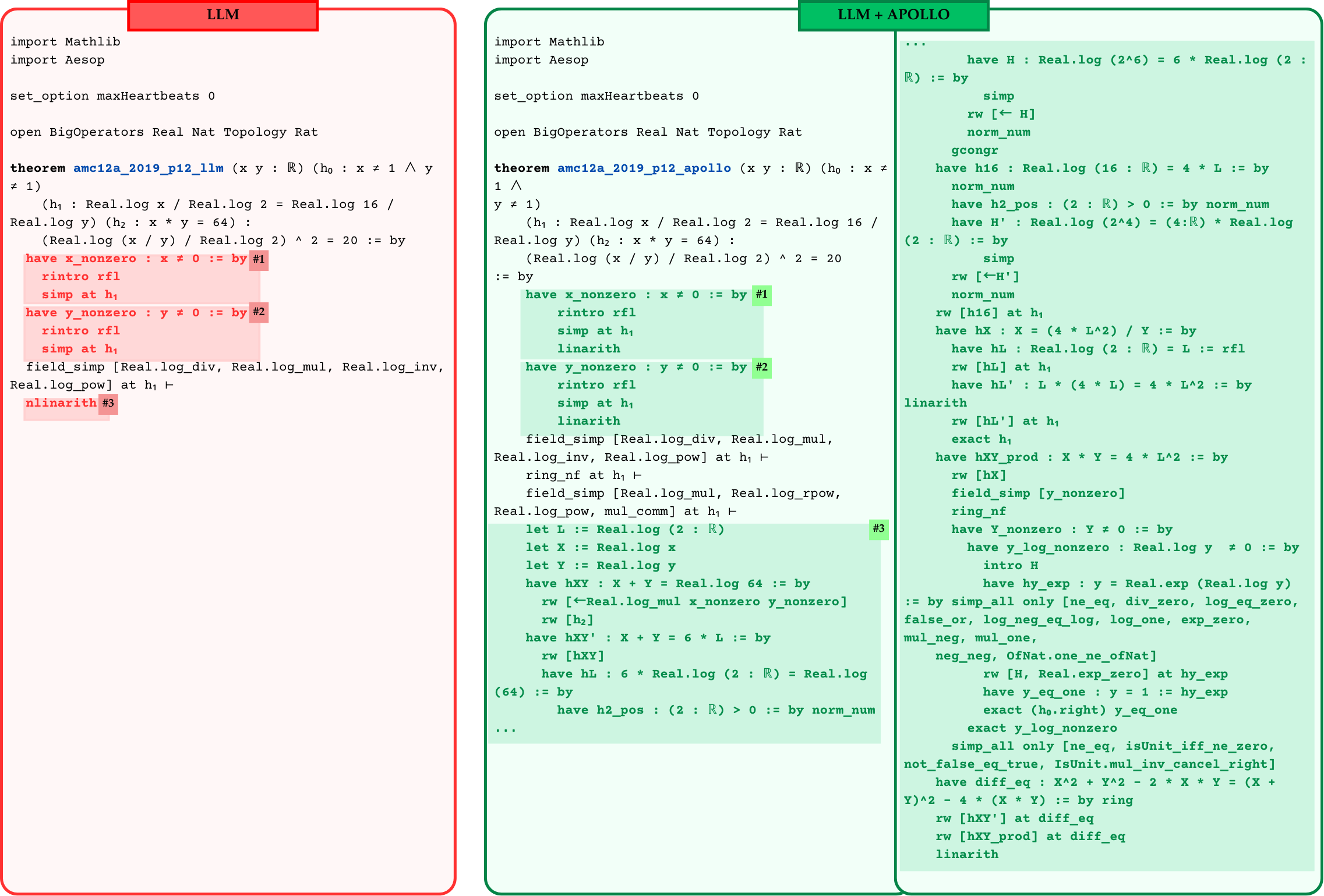
### Visual Description
## Diagram: Code Comparison - LLM vs LLM + APOLLO
### Overview
The image displays a side-by-side comparison of two Lean 4 code snippets attempting to formally prove a mathematical theorem (`amc12a_2019_p12`). The left panel, outlined in red and labeled "LLM", shows a short, incomplete, or failing proof attempt with specific sections highlighted in red. The right panel, outlined in green and labeled "LLM + APOLLO", shows a highly detailed, successful proof spanning two columns, with corresponding sections highlighted in green. Numbered tags (`#1`, `#2`, `#3`) are used to map specific logical steps between the two approaches, demonstrating how the "APOLLO" system corrects and expands upon the baseline LLM's output.
### Components and Layout
* **Left Panel (Red Outline):**
* **Header:** A red box containing the text "LLM".
* **Content:** A single column of Lean 4 code.
* **Highlights:** Light red background applied to lines 11-16 and line 19.
* **Tags:** `#1`, `#2`, `#3` placed inline with the code.
* **Right Panel (Green Outline):**
* **Header:** A green box containing the text "LLM + APOLLO".
* **Content:** Lean 4 code split into two columns to accommodate its length. The left column contains the beginning of the proof, and the right column continues it.
* **Highlights:** Light green background applied to lines 12-19 and lines 24-38 in the first column.
* **Tags:** `#1`, `#2`, `#3` placed inline with the code, corresponding to the tags in the left panel.
### Content Details (Transcription)
#### Left Panel: LLM
```lean
import Mathlib
import Aesop
set_option maxHeartbeats 0
open BigOperators Real Nat Topology Rat
theorem amc12a_2019_p12_llm (x y : ℝ) (h₀ : x ≠ 1 ∧ y ≠ 1)
(h₁ : Real.log x / Real.log 2 = Real.log 16 / Real.log y) (h₂ : x * y = 64) :
(Real.log (x / y) / Real.log 2) ^ 2 = 20 := by
have x_nonzero : x ≠ 0 := by #1 -- [HIGHLIGHTED RED START]
rintro rfl
simp at h₁
have y_nonzero : y ≠ 0 := by #2
rintro rfl
simp at h₁ -- [HIGHLIGHTED RED END]
field_simp [Real.log_div, Real.log_mul, Real.log_inv, Real.log_pow] at h₁ ⊢
nlinarith #3 -- [HIGHLIGHTED RED]
```
#### Right Panel: LLM + APOLLO (Column 1)
```lean
import Mathlib
import Aesop
set_option maxHeartbeats 0
open BigOperators Real Nat Topology Rat
theorem amc12a_2019_p12_apollo (x y : ℝ) (h₀ : x ≠ 1 ∧ y ≠ 1)
(h₁ : Real.log x / Real.log 2 = Real.log 16 / Real.log y) (h₂ : x * y = 64) :
(Real.log (x / y) / Real.log 2) ^ 2 = 20
:= by
have x_nonzero : x ≠ 0 := by #1 -- [HIGHLIGHTED GREEN START]
rintro rfl
simp at h₁
linarith
have y_nonzero : y ≠ 0 := by #2
rintro rfl
simp at h₁
linarith -- [HIGHLIGHTED GREEN END]
field_simp [Real.log_div, Real.log_mul, Real.log_inv, Real.log_pow] at h₁ ⊢
ring_nf at h₁ ⊢
field_simp [Real.log_mul, Real.log_rpow, Real.log_pow, mul_comm] at h₁ ⊢
let L := Real.log (2 : ℝ) #3 -- [HIGHLIGHTED GREEN START]
let X := Real.log x
let Y := Real.log y
have hXY : X + Y = Real.log 64 := by
rw [←Real.log_mul x_nonzero y_nonzero]
rw [h₂]
have hXY' : X + Y = 6 * L := by
rw [hXY]
have hL : 6 * Real.log (2 : ℝ) = Real.log (64) := by
have h2_pos : (2 : ℝ) > 0 := by norm_num
... -- [HIGHLIGHTED GREEN END]
```
#### Right Panel: LLM + APOLLO (Column 2)
```lean
...
have H : Real.log (2^6) = 6 * Real.log (2 : ℝ) := by
simp
rw [← H]
norm_num
gcongr
have h16 : Real.log (16 : ℝ) = 4 * L := by
norm_num
have h2_pos : (2 : ℝ) > 0 := by norm_num
have H' : Real.log (2^4) = (4:ℝ) * Real.log (2 : ℝ) := by
simp
rw [←H']
norm_num
rw [h16] at h₁
have hX : X = (4 * L^2) / Y := by
have hL : Real.log (2 : ℝ) = L := rfl
rw [hL] at h₁
have hL' : L * (4 * L) = 4 * L^2 := by linarith
rw [hL'] at h₁
exact h₁
have hXY_prod : X * Y = 4 * L^2 := by
rw [hX]
field_simp [y_nonzero]
ring_nf
have Y_nonzero : Y ≠ 0 := by
have y_log_nonzero : Real.log y ≠ 0 := by
intro H
have hy_exp : y = Real.exp (Real.log y) := by simp_all only [ne_eq, div_zero, log_eq_zero, false_or, log_neg_eq_log, log_one, exp_zero, mul_neg, mul_one, neg_neg, OfNat.one_ne_ofNat]
rw [H, Real.exp_zero] at hy_exp
have y_eq_one : y = 1 := hy_exp
exact (h₀.right) y_eq_one
exact y_log_nonzero
simp_all only [ne_eq, isUnit_iff_ne_zero, not_false_eq_true, IsUnit.mul_inv_cancel_right]
have diff_eq : X^2 + Y^2 - 2 * X * Y = (X + Y)^2 - 4 * (X * Y) := by ring
rw [hXY'] at diff_eq
rw [hXY_prod] at diff_eq
linarith
```
### Key Observations
1. **Error Correction at `#1` and `#2`:** The baseline LLM attempts to prove `x_nonzero` and `y_nonzero` using `rintro rfl` and `simp at h₁`, but fails to close the goal (indicated by the red highlight). The APOLLO system corrects this by adding the `linarith` tactic to both sub-proofs, successfully closing them (indicated by the green highlight).
2. **Strategic Divergence at `#3`:** The baseline LLM attempts to solve the remainder of the complex logarithmic equation with a single, powerful tactic: `nlinarith`. The red highlight indicates this tactic fails or times out.
3. **APOLLO's Step-by-Step Approach:** At tag `#3`, instead of relying on a single tactic, the APOLLO system introduces variable substitutions (`let L`, `let X`, `let Y`) to convert the logarithmic problem into an algebraic one. It then meticulously proves intermediate lemmas (`hXY`, `hXY'`, `h16`, `hX`, `hXY_prod`, `Y_nonzero`, `diff_eq`) over dozens of lines of code before finally concluding the proof with `linarith`.
### Interpretation
This image serves as a visual demonstration of the limitations of standard Large Language Models (LLMs) in formal theorem proving, and how an augmented system (APOLLO) overcomes them.
The baseline LLM exhibits a common failure mode in formal mathematics: it attempts to "leap" to the conclusion using heavy-handed automation tactics (`nlinarith`) without properly setting up the intermediate logical steps. When the automation fails to find a path, the proof fails.
The "APOLLO" system (which likely represents an agentic search framework, a specialized decoding strategy, or a reinforcement learning pipeline built on top of the LLM) demonstrates a much deeper "understanding" of the required proof structure. By breaking the problem down—specifically by recognizing that the logarithmic equations should be mapped to algebraic variables (`X`, `Y`, `L`)—APOLLO guides the prover through a series of manageable, verifiable steps. The contrast between the single failing red line (`nlinarith`) and the massive block of successful green code highlights APOLLO's ability to perform complex, multi-step reasoning that standard LLMs cannot achieve in a single zero-shot generation.
</details>
Figure 15: Proof attempt of amc12a_2019_p12 produced by the base model (Goedel-Prover-SFT) versus after Apollo’s targeted repair. The left shows the original end-to-end LLM output, which does not compile in Lean; the right shows the corrected, repaired proof assembled by Apollo that closes all of the goals.
<details>
<summary>examples/comparison/long.png Details</summary>
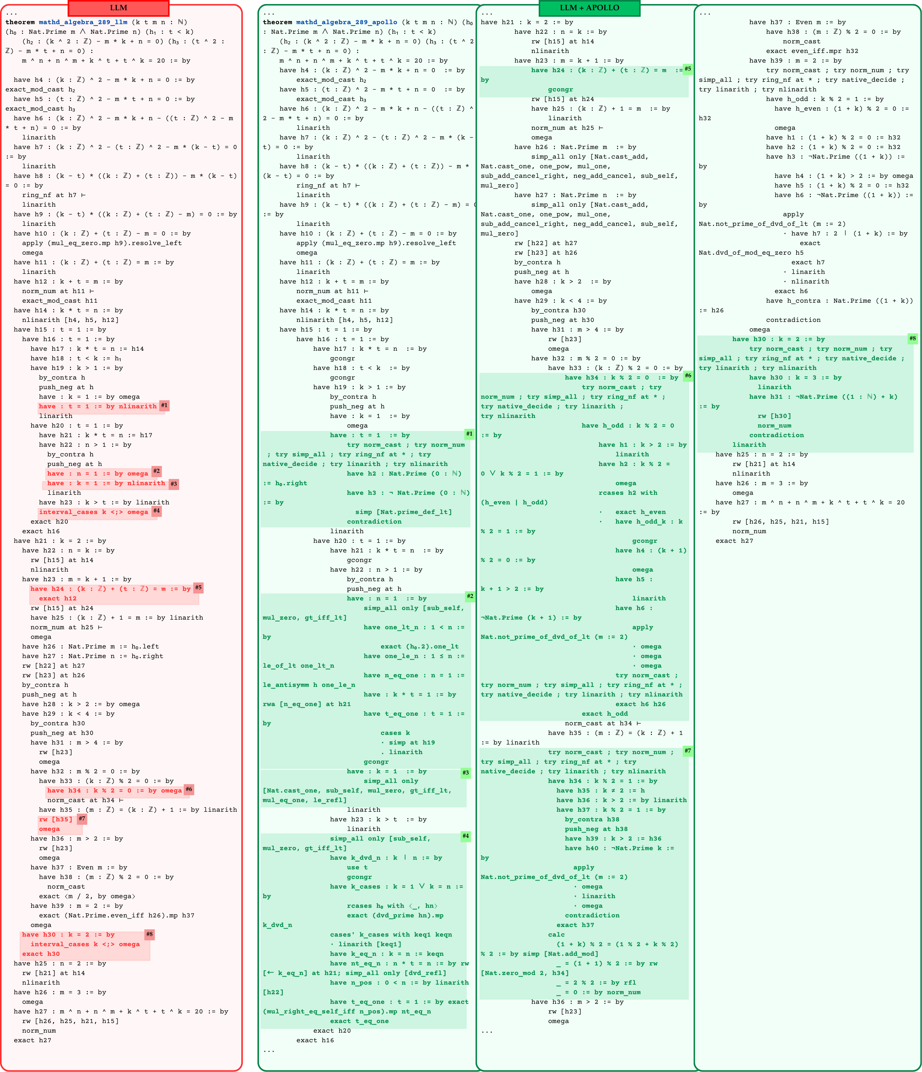
### Visual Description
## Code Comparison Diagram: LLM vs. LLM + APOLLO (Lean 4 Proofs)
### Overview
This image presents a side-by-side comparison of two formal mathematical proofs written in the Lean 4 theorem proving language. The image is divided into two main panels. The left panel, outlined in red and titled "LLM", shows a relatively short, single-column proof containing several highlighted errors or hallucinated steps. The right panel, outlined in green and titled "LLM + APOLLO", shows a much longer, three-column proof where the errors from the left panel have been replaced with extensive, successfully verified tactic blocks. The numbered tags (#1 through #8) map the failed steps in the standalone LLM to the corrected, expanded sub-proofs generated by the APOLLO system.
*Language Declaration:* The text is written in Lean 4, a formal programming and theorem-proving language that utilizes English keywords alongside mathematical notation. It is transcribed exactly as written.
### Components/Layout
* **Left Panel (Red Bounding Box):**
* **Header:** "LLM" (white text on red background).
* **Layout:** A single column of code.
* **Highlights:** Specific lines of code are highlighted in light red. These lines contain inline comments with numbers (e.g., `#1`, `#2`), indicating points of failure or hallucination where the LLM assumed a tactic (like `omega` or `nlinarith`) would solve the goal, but it did not.
* **Right Panel (Green Bounding Box):**
* **Header:** "LLM + APOLLO" (white text on green background).
* **Layout:** Three columns of code, separated by thin vertical gray lines. The second and third columns have `...` at the top, indicating continuous flow from the previous column.
* **Highlights:** Large blocks of code are highlighted in light green. These blocks contain corresponding inline comments (`#1`, `#2`, etc.). These represent the expanded, rigorous proof steps that APOLLO generated to successfully bridge the logical gaps left by the standalone LLM.
---
### Content Details (Transcription)
#### Left Panel: LLM (Red)
```lean
theorem mathd_algebra_289_llm (k t m n : ℕ)
(h₀ : Nat.Prime m ∧ Nat.Prime n) (h₁ : t < k)
(h₂ : (k ^ 2 : ℤ) - m * k + n = 0) (h₃ : (t ^ 2 :
ℤ) - m * t + n = 0) :
m ^ n + n ^ m + k ^ t + t ^ k = 20 := by
have h4 : (k : ℤ) ^ 2 - m * k + n = 0 := by
exact_mod_cast h₂
have h5 : (t : ℤ) ^ 2 - m * t + n = 0 := by
exact_mod_cast h₃
have h6 : (k : ℤ) ^ 2 - m * k + n - ((t : ℤ) ^ 2 - m
* t + n) = 0 := by
linarith
have h7 : (k : ℤ) ^ 2 - (t : ℤ) ^ 2 - m * (k - t) = 0
:= by
linarith
have h8 : (k - t) * ((k : ℤ) + (t : ℤ)) - m * (k - t)
= 0 := by
ring_nf at h7 ⊢
linarith
have h9 : (k - t) * ((k : ℤ) + (t : ℤ) - m) = 0 := by
linarith
have h10 : (k : ℤ) + (t : ℤ) - m = 0 := by
apply (mul_eq_zero.mp h9).resolve_left
omega
have h11 : (k : ℤ) + (t : ℤ) = m := by
linarith
have h12 : k + t = m := by
norm_num at h11 ⊢
exact_mod_cast h11
have h14 : k * t = n := by
nlinarith [h4, h5, h12]
have h15 : t = 1 := by
have h16 : t = 1 := by
have h17 : k * t = n := h14
have h18 : t < k := h₁
have h19 : k > 1 := by
by_contra h
push_neg at h
have : k = 1 := by omega
[RED HIGHLIGHT START] have t : 1 := by nlinarith #1 [RED HIGHLIGHT END]
linarith
have h20 : t = 1 := by
have h21 : k * t = n := h17
have h22 : n > 1 := by
by_contra h
push_neg at h
[RED HIGHLIGHT START] have n : 1 := by omega #2 [RED HIGHLIGHT END]
[RED HIGHLIGHT START] have k : 1 := by nlinarith #3 [RED HIGHLIGHT END]
linarith
have h23 : k > t := by linarith
[RED HIGHLIGHT START] interval_cases k <;> omega #4 [RED HIGHLIGHT END]
exact h20
exact h16
have h21 : k = 2 := by
have h22 : n = k := by
rw [h15] at h14
nlinarith
have h23 : m = k + 1 := by
[RED HIGHLIGHT START] have h24 : (k : ℤ) + (t : ℤ) = m := by #5
exact h12 [RED HIGHLIGHT END]
rw [h15] at h24
have h25 : (k : ℤ) + 1 = m := by linarith
norm_num at h25 ⊢
omega
have h26 : Nat.Prime m := h₀.left
have h27 : Nat.Prime n := h₀.right
rw [h22] at h27
rw [h23] at h26
by_contra h
push_neg at h
have h28 : k > 2 := by omega
have h29 : k < 4 := by
by_contra h30
push_neg at h30
have h31 : m > 4 := by
rw [h23]
omega
have h32 : m % 2 = 0 := by
have h33 : (k : ℤ) % 2 = 0 := by
[RED HIGHLIGHT START] have h34 : k % 2 = 0 := by omega #6 [RED HIGHLIGHT END]
norm_cast at h34 ⊢
have h35 : (m : ℤ) = (k : ℤ) + 1 := by linarith
[RED HIGHLIGHT START] rw [h35] #7
omega [RED HIGHLIGHT END]
have h36 : m > 2 := by
rw [h23]
omega
have h37 : Even m := by
have h38 : (m : ℤ) % 2 = 0 := by
norm_cast
exact ⟨m / 2, by omega⟩
have h39 : m = 2 := by
exact (Nat.Prime.even_iff h26).mp h37
omega
[RED HIGHLIGHT START] have h30 : k = 2 := by #8
interval_cases k <;> omega
exact h30 [RED HIGHLIGHT END]
have h25 : n = 2 := by
rw [h21] at h14
nlinarith
have h26 : m = 3 := by
omega
have h27 : m ^ n + n ^ m + k ^ t + t ^ k = 20 := by
rw [h26, h25, h21, h15]
norm_num
exact h27
```
#### Right Panel: LLM + APOLLO (Green) - Column 1
```lean
theorem mathd_algebra_289_apollo (k t m n : ℕ) (h₀
: Nat.Prime m ∧ Nat.Prime n) (h₁ : t < k)
(h₂ : (k ^ 2 : ℤ) - m * k + n = 0) (h₃ : (t ^ 2 :
ℤ) - m * t + n = 0) :
m ^ n + n ^ m + k ^ t + t ^ k = 20 := by
have h4 : (k : ℤ) ^ 2 - m * k + n = 0 := by
exact_mod_cast h₂
have h5 : (t : ℤ) ^ 2 - m * t + n = 0 := by
exact_mod_cast h₃
have h6 : (k : ℤ) ^ 2 - m * k + n - ((t : ℤ) ^
2 - m * t + n) = 0 := by
linarith
have h7 : (k : ℤ) ^ 2 - (t : ℤ) ^ 2 - m * (k -
t) = 0 := by
linarith
have h8 : (k - t) * ((k : ℤ) + (t : ℤ)) - m *
(k - t) = 0 := by
ring_nf at h7 ⊢
linarith
have h9 : (k - t) * ((k : ℤ) + (t : ℤ) - m) = 0
:= by
linarith
have h10 : (k : ℤ) + (t : ℤ) - m = 0 := by
apply (mul_eq_zero.mp h9).resolve_left
omega
have h11 : (k : ℤ) + (t : ℤ) = m := by
linarith
have h12 : k + t = m := by
norm_num at h11 ⊢
exact_mod_cast h11
have h14 : k * t = n := by
nlinarith [h4, h5, h12]
have h15 : t = 1 := by
have h16 : t = 1 := by
have h17 : k * t = n := by
gcongr
have h18 : t < k := by
gcongr
have h19 : k > 1 := by
by_contra h
push_neg at h
have : k = 1 := by
omega
[GREEN HIGHLIGHT START] have t : 1 := by #1
try norm_cast ; try norm_num
; try simp_all ; try ring_nf at * ; try
native_decide ; try linarith ; try nlinarith
have h2 : Nat.Prime (0 : ℕ)
:= h₀.right
have h3 : ¬Nat.Prime (0 : ℕ)
:= by
simp [Nat.prime_def_lt]
contradiction
linarith
have h20 : t = 1 := by
have h21 : k * t = n := by
gcongr
have h22 : n > 1 := by
by_contra h
push_neg at h
have n : 1 := by #2
simp_all only [sub_self,
mul_zero, gt_iff_lt]
have one_lt_n : 1 < n :=
by
exact (h₀.2).one_lt
have one_le_n : 1 ≤ n :=
le_of_lt one_lt_n
have n_eq_one : n = 1 :=
le_antisymm h one_le_n
have : k * t = 1 := by
rwa [n_eq_one] at h21
have t_eq_one : t = 1 :=
by
cases k
· simp at h19
· linarith
gcongr
have k : 1 := by #3
simp_all only
[Nat.cast_one, sub_self, mul_zero, gt_iff_lt,
mul_eq_one, le_refl]
linarith
have h23 : k > t := by
linarith
simp_all only [sub_self, #4
mul_zero, gt_iff_lt]
have k_dvd_n : k ∣ n := by
use t
gcongr
have k_cases : k = 1 ∨ k = n :=
by
rcases h₀ with ⟨_, hn⟩
exact (dvd_prime hn).mp
k_dvd_n
cases' k_cases with keq1 keqn
· linarith [keq1]
have k_eq_n : k = n := keqn
have nt_eq_n : n * t = n := by rw
[← k_eq_n] at h21; simp_all only [dvd_refl]
have n_pos : 0 < n := by linarith
[h22]
have t_eq_one : t = 1 := by exact
(mul_right_eq_self_iff n_pos).mp nt_eq_n
exact t_eq_one
exact h20
exact h16 [GREEN HIGHLIGHT END]
```
#### Right Panel: LLM + APOLLO (Green) - Column 2
```lean
...
have h21 : k = 2 := by
have h22 : n = k := by
rw [h15] at h14
nlinarith
have h23 : m = k + 1 := by
[GREEN HIGHLIGHT START] have h24 : (k : ℤ) + (t : ℤ) = m := #5
by
gcongr [GREEN HIGHLIGHT END]
rw [h15] at h24
have h25 : (k : ℤ) + 1 = m := by
linarith
norm_num at h25 ⊢
omega
have h26 : Nat.Prime m := by
simp_all only [Nat.cast_add,
Nat.cast_one, one_pow, mul_one,
sub_add_cancel_right, neg_add_cancel, sub_self,
mul_zero]
have h27 : Nat.Prime n := by
simp_all only [Nat.cast_add,
Nat.cast_one, one_pow, mul_one,
sub_add_cancel_right, neg_add_cancel, sub_self,
mul_zero]
rw [h22] at h27
rw [h23] at h26
by_contra h
push_neg at h
have h28 : k > 2 := by
omega
have h29 : k < 4 := by
by_contra h30
push_neg at h30
have h31 : m > 4 := by
rw [h23]
omega
have h32 : m % 2 = 0 := by
have h33 : (k : ℤ) % 2 = 0 := by
[GREEN HIGHLIGHT START] have h34 : k % 2 = 0 := by #6
try norm_cast ; try
norm_num ; try simp_all ; try ring_nf at * ;
try native_decide ; try linarith ;
try nlinarith
have h_odd : k % 2 = 0
:= by
have h1 : k > 2 := by
linarith
have h2 : k % 2 =
0 ∨ k % 2 = 1 := by
omega
rcases h2 with
(h_even | h_odd)
· exact h_even
· have h_odd_k : k
% 2 = 1 := by
gcongr
have h4 : (k + 1)
% 2 = 0 := by
omega
have h5 :
k + 1 > 2 := by
linarith
have h6 :
¬Nat.Prime (k + 1) := by
apply
Nat.not_prime_of_dvd_of_lt (m := 2)
· omega
· omega
· omega
try norm_cast ;
try norm_num ; try simp_all ; try ring_nf at * ;
try native_decide ; try linarith ; try nlinarith
exact h26
exact h_odd
norm_cast at h34 ⊢
have h35 : (m : ℤ) = (k : ℤ) + 1
:= by linarith
[GREEN HIGHLIGHT START] try norm_cast ; try norm_num ; #7
try simp_all ; try ring_nf at * ; try
native_decide ; try linarith ; try nlinarith
have h34 : k % 2 = 1 := by
have h35 : k ≠ 2 := h
have h36 : k > 2 := by linarith
have h37 : k % 2 = 1 := by
by_contra h38
push_neg at h38
have h39 : k > 2 := h36
have h40 : ¬Nat.Prime k :=
by
apply
Nat.not_prime_of_dvd_of_lt (m := 2)
· omega
· linarith
· omega
contradiction
exact h37
calc
(1 + k) % 2 = (1 % 2 + k % 2)
% 2 := by simp [Nat.add_mod]
_ = (1 + 1) % 2 := by rw
[Nat.zero_mod 2, h34]
_ = 2 % 2 := by rfl
_ = 0 := by norm_num [GREEN HIGHLIGHT END]
have h36 : m > 2 := by
rw [h23]
omega
...
```
#### Right Panel: LLM + APOLLO (Green) - Column 3
```lean
...
have h37 : Even m := by
have h38 : (m : ℤ) % 2 = 0 := by
norm_cast
exact even_iff.mpr h32
have h39 : m = 2 := by
try norm_cast ; try norm_num ; try
simp_all ; try ring_nf at * ; try native_decide ;
try linarith ; try nlinarith
have h_odd : k % 2 = 1 := by
have h_even : (1 + k) % 2 = 0 :=
h32
omega
have h1 : (1 + k) % 2 = 0 := h32
have h2 : (1 + k) > 2 := by omega
have h3 : ¬Nat.Prime ((1 + k)) :=
by
have h4 : (1 + k) > 2 := by omega
have h5 : (1 + k) % 2 = 0 := h32
have h6 : ¬Nat.Prime ((1 + k)) :=
by
apply
Nat.not_prime_of_dvd_of_lt (m := 2)
· have h7 : 2 ∣ (1 + k) := by
exact
Nat.dvd_of_mod_eq_zero h5
exact h7
· linarith
· nlinarith
exact h6
have h_contra : Nat.Prime ((1 + k))
:= h26
contradiction
omega
[GREEN HIGHLIGHT START] have h30 : k = 2 := by #8
try norm_cast ; try norm_num ; try
simp_all ; try ring_nf at * ; try native_decide ;
try linarith ; try nlinarith
have h30 : k = 3 := by
linarith
have h31 : ¬Nat.Prime ((1 : ℕ) + k)
:= by
norm_num
contradiction
linarith [GREEN HIGHLIGHT END]
have h25 : n = 2 := by
rw [h21] at h14
nlinarith
have h26 : m = 3 := by
omega
have h27 : m ^ n + n ^ m + k ^ t + t ^ k = 20
:= by
rw [h26, h25, h21, h15]
norm_num
exact h27
```
---
### Key Observations
1. **Visual Trend (Length and Complexity):** The most striking visual trend is the disparity in code volume between the red and green highlights. A single line of code in the "LLM" panel (e.g., `#1`, `#2`, `#4`) expands into massive, multi-nested logical blocks in the "LLM + APOLLO" panel.
2. **Tactic Hallucination:** In the Red panel, the LLM frequently attempts to close goals using terminal tactics like `omega` (a decision procedure for integer/natural number arithmetic) or `nlinarith` (non-linear arithmetic). For example, Red `#1` is `have t : 1 := by nlinarith`.
3. **APOLLO's Search/Expansion:** In the Green panel, APOLLO replaces these hallucinated terminal tactics with extensive search sequences. Green `#1` replaces `nlinarith` with a sequence of attempts: `try norm_cast ; try norm_num ; try simp_all ; try ring_nf at * ; try native_decide ; try linarith ; try nlinarith`, followed by actual logical deductions involving `Nat.Prime` and `contradiction`.
4. **Mapping the Tags:**
* **#1:** Red attempts `nlinarith`. Green expands into a ~10-line proof by contradiction.
* **#2:** Red attempts `omega`. Green expands into a ~15-line proof using `le_antisymm` and case analysis.
* **#3:** Red attempts `nlinarith`. Green uses `simp_all only [...]`.
* **#4:** Red attempts `interval_cases k <;> omega`. Green expands into a ~15-line proof using divisibility (`k ∣ n`) and prime properties (`dvd_prime`).
* **#5:** Red uses `exact h12`. Green uses `gcongr`.
* **#6:** Red attempts `omega`. Green expands into a massive ~25-line sub-proof handling even/odd cases and prime contradictions.
* **#7:** Red attempts `rw [h35]` followed by `omega`. Green expands into a ~20-line calculation block (`calc`) to prove modulo arithmetic.
* **#8:** Red attempts `interval_cases k <;> omega`. Green expands into a proof by contradiction showing `k = 3` violates prime conditions.
### Interpretation
This image serves as a technical demonstration of the limitations of standalone Large Language Models in formal theorem proving, and the value of augmenting them with search/agentic frameworks (like "APOLLO").
* **The Problem:** The base LLM (left) understands the *structure* of a Lean 4 proof. It knows what intermediate steps (`have` statements) might be useful to reach the final goal. However, it suffers from "tactic hallucination"—it assumes powerful automated tactics like `omega` or `nlinarith` can magically bridge the gap between its current state and the intermediate goal, even when the mathematical context doesn't support it. The proof on the left is syntactically plausible but logically broken; it will not compile in Lean.
* **The Solution:** The APOLLO system.
</details>
Figure 16: Proof attempt of mathd_algebra_289 produced by the base model (Kimina-Prover-Preview-Distill-7B) versus after Apollo’s targeted repair. The left shows the original end-to-end LLM output, which does not compile in Lean; the right shows the corrected, repaired proof assembled by Apollo that closes all of the goals. Import headers are the same as other presented examples, for visibility they were omitted in this diagram.