# Follow the Path: Reasoning over Knowledge Graph Paths to Improve LLM Factuality
## Abstract
We introduce fs1, a simple yet effective method that improves the factuality of reasoning traces by sourcing them from large reasoning models (e.g., DeepSeek-R1) and grounding them by conditioning on knowledge graph (KG) paths. We fine-tune eight instruction-tuned Large Language Models (LLMs) on 3.9K factually grounded reasoning traces and rigorously evaluate them on six complex open-domain question-answering (QA) benchmarks encompassing 23.9K questions. Our results demonstrate that our fs1 -tuned model (32B parameters) consistently outperforms instruction-tuned counterparts with parallel sampling by 6-14 absolute points (pass@ $16$ ). Our detailed analysis shows that fs1 considerably improves model performance over more complex questions (requiring 3 or more hops on KG paths) and numerical answer types compared to the baselines. Furthermore, in single-pass inference, we notice that smaller LLMs show the most improvements. While prior works demonstrate the effectiveness of reasoning traces primarily in the STEM domains, our work shows strong evidence that anchoring reasoning to factual KG paths is a critical step in transforming LLMs for reliable knowledge-intensive tasks.
## 1 Introduction
Factual consistency of LLM-generated output is a requirement for critical real-world applications. LLM reasoning in the form of “thinking” has shown promising improvements in model performance on complex downstream tasks, such as mathematical reasoning and puzzle-like questions using additional compute resources during inference (e.g., test-time scaling; Wu et al., 2024; Muennighoff et al., 2025; Zhang et al., 2025). However, it remains an open question whether these reasoning techniques improve factuality, particularly for complex multi-hop QA (mQA). This task tests a model’s ability to answer a question by synthesizing information from multiple pieces of evidence, often spread across different resources and requiring reasoning steps. We hypothesize that reasoning models should perform better than non-reasoning LLMs on the mQA task. To test this hypothesis, we source reasoning traces from state-of-the-art reasoning models and fine-tune several non-reasoning LLMs to attempt to induce reasoning capabilities. However, we have no guarantee that these reasoning traces from the large reasoning models are factually correct. In order to have a formal factual grounding in these traces, we condition the models on retrieved knowledge graph (KG) paths relevant to the questions. This is possible as KGs encode facts as directed, labeled graphs over entities and relations, which offers a verifiable foundation to inform each step of the reasoning process. We call our approach fs1 (factual simple test-time scaling; Muennighoff et al., 2025).
We fine-tune eight different LLMs sizes on the original reasoning traces (rt; 3.4K samples) or on our KG-enhanced traces (fs1; 3.9K samples). We evaluate the fine-tuned models on six QA test sets spanning 23.9K questions, finding that fine-tuning on this amount of data can improve accuracy by 6-14 absolute points (pass@ $16$ ) for a 32B parameter model across the benchmarks. A snapshot of our method is in Figure 1. This setup enables us to address our research question (RQ): To what extent does grounding the reasoning processes of LLMs in KG paths enhance their factual accuracy for mQA? To address this question, our contributions are as follows:
<details>
<summary>x1.png Details</summary>

### Visual Description
## Diagram: Comparison of AI Reasoning Methods on a Knowledge-Based Question
### Overview
The image is a comparative diagram illustrating four different AI reasoning approaches applied to the same factual question. It visually demonstrates the varying accuracy of these methods, with only the final approach yielding the correct answer. The diagram is structured as a horizontal sequence of four panels, each representing a distinct method.
### Components/Axes
* **Header (Top Banner):** A dark gray banner spanning the width of the image contains the central question in white text: "The visual artist that created the art series of Las Meninas, where did they live?"
* **Panels (Four Columns):** The main body consists of four vertical panels, each with a light beige background. From left to right, they are labeled:
1. **Instruction-tuned** (Cyan speech bubble)
2. **Chain-of-Thought** (Cyan speech bubble)
3. **Thinking (rt)** (Cyan speech bubble)
4. **Thinking with KGs (fs1)** (Cyan speech bubble)
* **Common Elements per Panel:**
* A cyan speech bubble at the top containing the method's name.
* A stylized robot head icon (blue and gray with orange antenna) on the left.
* A correctness indicator on the right: a red "X" for incorrect answers, a green checkmark for the correct answer.
* Text output from the AI model below the robot icon.
### Detailed Analysis
**Panel 1: Instruction-tuned**
* **Method Label:** "Instruction-tuned"
* **Correctness Indicator:** Red "X" (Incorrect)
* **AI Output Text:** "The answer is **Paris.**" (The word "Paris" is in bold).
**Panel 2: Chain-of-Thought**
* **Method Label:** "Chain-of-Thought"
* **Correctness Indicator:** Red "X" (Incorrect)
* **AI Output Text:** "Let me think step-by-step... My answer is **Vienna.**" (The word "Vienna" is in bold).
**Panel 3: Thinking (rt)**
* **Method Label:** "Thinking (rt)"
* **Correctness Indicator:** Red "X" (Incorrect)
* **AI Output Text:** " The answer should be **Barcelona.**" (The word "Barcelona" is in bold).
**Panel 4: Thinking with KGs (fs1)**
* **Method Label:** "Thinking with KGs (fs1)"
* **Correctness Indicator:** Green checkmark (Correct)
* **AI Output Text:** "<Question> + [Icon of a knowledge graph (nodes and edges)] + [Wikidata logo] The visual artist who created the art series [..] The answer is **Madrid.**" (The word "Madrid" is in bold). The "[..]" indicates an ellipsis in the transcribed text.
### Key Observations
1. **Progression of Complexity:** The methods evolve from a simple direct answer ("Instruction-tuned") to a process involving step-by-step reasoning ("Chain-of-Thought"), internal monologue ("Thinking (rt)"), and finally, reasoning augmented by external knowledge ("Thinking with KGs").
2. **Accuracy Correlation:** There is a direct correlation between the method's complexity (specifically, the integration of external knowledge) and its accuracy. The first three methods, which rely solely on internal model parameters, produce incorrect answers (Paris, Vienna, Barcelona).
3. **Visual Cues for Correctness:** The diagram uses universal symbols (red X, green checkmark) to immediately convey the success or failure of each approach, making the conclusion visually intuitive.
4. **Spatial Grounding:** The legend (method labels in cyan bubbles) is consistently placed at the top of each panel. The correctness indicator is consistently placed to the right of the robot icon. The final, correct panel is distinguished by additional visual elements (knowledge graph icon, Wikidata logo) placed between the question tag and the thinking tag.
### Interpretation
This diagram serves as a pedagogical or illustrative tool to argue for the necessity of **grounding AI reasoning in external knowledge bases** (like Wikidata/Knowledge Graphs) for factual accuracy.
* **What it demonstrates:** It suggests that standard instruction-tuned models and even those employing chain-of-thought or internal reasoning ("rt") can confidently generate plausible but incorrect answers ("hallucinations") when their training data is insufficient or imprecise for a specific factual query. The question about Diego Velázquez (the artist of *Las Meninas*) and his residence is a precise historical fact that requires verified data.
* **How elements relate:** The progression shows a logical argument: simple prompting fails, structured internal reasoning fails, but when the model's reasoning process is augmented with a direct query to a structured knowledge source (Wikidata), it succeeds. The inclusion of the Wikidata logo is a key visual anchor for this argument.
* **Notable implication:** The diagram implies that for reliable factual question-answering, especially on niche or precise topics, AI systems benefit significantly from architectures that can retrieve and incorporate information from curated knowledge graphs rather than relying solely on parametric knowledge learned during training. The "(fs1)" in the final label may refer to a specific technique or model variant designed for this fusion.
</details>
Figure 1: Snapshot of Method. We show a snapshot of the experiments executed in this study. There are four settings on how a question can be answered; (1) direct answer from an instruction-tuned model, (2) step-by-step reasoning via Chain-of-Thought, (3) original “thinking”, and (4) knowledge-graph enhanced “thinking”. We show an example of how (4) looks like in Figure 4.
- We demonstrate that with test-time scaling (parallel sampling), our fs1 -tuned Qwen2.5-32B model improves factual accuracy by 6-14 absolute points (at pass@ $16$ ).
- We conduct an analysis over the question and answer types (e.g., question difficulty, answer type, and domains) to investigate where fs1 -tuned models provide improvements. We find that fs1 -tuned models perform better on more difficult questions, requiring 3 hops or more.
- We examine performance of eight fs1 -tuned models (360M-32B parameters) in a pass@ $1$ setting against baselines. We find that smaller LLMs have the largest increase in performance, whereas larger models see less profound improvements.
- We release 3.4K raw reasoning traces and 3.9K KG-enhanced reasoning traces both sourced from QwQ-32B and Deepseek-R1. All code, datasets, and models are publicly available under an MIT license: https://github.com/jjzha/fs1.
## 2 Reasoning Data
#### rt : Distilling Reasoning Traces.
To obtain reasoning traces, we use ComplexWebQuestions (CWQ; Talmor & Berant, 2018), a dataset designed for complex mQA. The CWQ dataset is created by automatically generating complex SPARQL queries based on Freebase (Bollacker et al., 2008). These queries are then automatically transformed into natural language questions, which are further refined by human paraphrasing. We take the CWQ dev. set, which consists of 3,519 questions, to curate the reasoning traces. We query both QwQ-32B (Qwen Team, 2025) and Deepseek-R1 (671B; DeepSeek-AI, 2025). By querying the model directly with a question, e.g., “ What art movement was Pablo Picasso part of? ”, we retrieve the reasoning traces surrounded by “think” tokens (<think>...</think>) and force the model to give the final answer to the question in \boxed{} format. We extract around 3.4K correct-only traces (final answer is correct), which we call rt. We show full examples in Figure 8 and Figure 9 (Appendix C).
#### fs1 : Enhancing Reasoning Traces with Knowledge Graph Paths.
We attempt to steer the reasoning traces with KG paths to remove the inaccuracies in the traces. Since the CWQ dataset consists of entities from Freebase, we align them to their corresponding Wikidata entities. For each question in the dev. set of the CWQ dataset, relevant KG paths are extracted from Wikidata using random walks using SPARQL queries as shown in Appendix E. Each mQA pair in the dataset may contain multiple valid KG paths, which are linearized graphs that retain the structural information of the KG. The paths are generated by extracting the relevant entities from the question and the gold answer. These diverse KG paths that can lead to the same answer reflect the possible diversity of the reasoning traces. Therefore, including linearized graphs improves the interpretability and the explainability of the reasoning traces. The prompt to obtain the improved reasoning traces is shown in Figure 4, by prompting QwQ-32B and Deepseek-R1 again. Full examples are in Figure 10 and Figure 11 (Appendix C).
Table 1: Training Data Statistics. Statistics of reasoning traces of QwQ-32B and Deepseek-R1 on CWQ based on the Qwen2.5-32B tokenizer. The original reasoning traces (rt) are from simply querying the question to the reasoning models, whereas fs1 indicates the statistics when queried with the knowledge graphs. We calculate the performance of the models’ final answer via LLM-as-a-Judge. We show that fs1 has higher performance in terms of accuracy compared to rt.
| | | QwQ-32B | R1-685B | Total | | | |
| --- | --- | --- | --- | --- | --- | --- | --- |
| rt | fs1 | rt | fs1 | rt | fs1 | | |
| Exact Match | | 0.46 | $\uparrow$ 0.63 | 0.56 | $\uparrow$ 0.72 | 0.51 | $\uparrow$ 0.67 |
| Sem. Match (all-MiniLM-L6-v2) | | 0.50 | $\uparrow$ 0.58 | 0.55 | $\uparrow$ 0.63 | 0.52 | $\uparrow$ 0.60 |
| LLM-as-a-Judge (gpt-4o-mini) | | 0.44 | $\uparrow$ 0.61 | 0.54 | $\uparrow$ 0.70 | 0.49 | $\uparrow$ 0.65 |
| Samples with only correct answers | | | | | | | |
| Number of Samples | | 1,533 | 1,972 | 1,901 | 1,914 | 3,434 | 3,886 |
| Avg. Reasoning Length (subwords) | | 937 | 897 | 1,043 | 637 | 990 | 767 |
| Avg. Answer Length (subwords) | | 40 | 93 | 64 | 116 | 52 | 104 |
<details>
<summary>x2.png Details</summary>
### Visual Description
## Violin Plot Comparison: Token Count Distributions
### Overview
The image displays two side-by-side violin plots comparing the distribution of token counts (measured in number of subwords) for two different models, **QwQ-32B** (left) and **DeepSeek-R1** (right). Each model's plot compares two data sources labeled **rt** and **fs1**. The plots show the probability density of the data at different values, with embedded box plot elements indicating key statistics.
### Components/Axes
* **Chart Title (Top Center):** "QwQ-32B" (left plot), "DeepSeek-R1" (right plot).
* **Y-Axis (Vertical):** Label: "Token Count (# Subwords)". Scale ranges from 0 to 8000, with major tick marks at 0, 2000, 4000, 6000, and 8000.
* **X-Axis (Horizontal):** Label: "Data Source". Two categories are present for each model: "rt" and "fs1".
* **Legend/Statistical Annotations:** For each violin, three key statistics are annotated directly on the plot:
* **QwQ-32B, rt (Blue):** Q3: 1017, Median: 552, Q1: 392.
* **QwQ-32B, fs1 (Orange):** Q3: 1039, Median: 553, Q1: 386.
* **DeepSeek-R1, rt (Blue):** Q3: 1274, Median: 635, Q1: 431.
* **DeepSeek-R1, fs1 (Orange):** Q3: 792, Median: 496, Q1: 359.
* **Color Coding:** The "rt" data source is consistently represented by a blue violin. The "fs1" data source is consistently represented by an orange violin.
### Detailed Analysis
**QwQ-32B Plot (Left):**
* **Data Source "rt" (Blue):** The distribution is strongly right-skewed. The bulk of the data (the widest part of the violin) is concentrated between approximately 400 and 700 tokens. The median is 552. The interquartile range (IQR) is from 392 (Q1) to 1017 (Q3), indicating a long tail extending to higher token counts. The violin's peak density appears near the median.
* **Data Source "fs1" (Orange):** The distribution shape is very similar to "rt" for this model. It is also right-skewed with a dense region between ~400-700 tokens. The median (553) and IQR (Q1: 386, Q3: 1039) are nearly identical to the "rt" source, suggesting comparable token count characteristics between the two data sources for QwQ-32B.
**DeepSeek-R1 Plot (Right):**
* **Data Source "rt" (Blue):** This distribution is also right-skewed but appears more spread out than the QwQ-32B distributions. The dense region is broader, spanning roughly 500 to 900 tokens. The median is higher at 635. The IQR is wider (Q1: 431, Q3: 1274), indicating greater variability in token counts, with a more pronounced tail towards higher values.
* **Data Source "fs1" (Orange):** This distribution is notably different from the "rt" source for the same model. It is more compact and less skewed. The dense region is concentrated between approximately 400 and 600 tokens. The median is lower at 496. The IQR is much narrower (Q1: 359, Q3: 792), indicating that token counts from the "fs1" source are more consistent and generally lower than those from the "rt" source for DeepSeek-R1.
### Key Observations
1. **Model Comparison:** For the "rt" data source, DeepSeek-R1 shows a higher median token count (635 vs. 552) and greater variability (wider IQR) compared to QwQ-32B.
2. **Data Source Consistency:** QwQ-32B exhibits remarkable consistency between the "rt" and "fs1" data sources, with nearly identical medians and distribution shapes.
3. **Data Source Divergence:** DeepSeek-R1 shows a significant divergence between data sources. The "rt" source produces higher and more variable token counts, while the "fs1" source yields lower and more tightly clustered counts.
4. **Distribution Shape:** All four distributions are right-skewed, meaning there is a concentration of data points at lower token counts with a tail of less frequent, higher token count examples. This is typical for length distributions in language data.
### Interpretation
The data suggests fundamental differences in how the two models process or are evaluated on the "rt" and "fs1" data sources.
* **QwQ-32B's** consistent performance across sources implies its tokenization or the nature of its outputs is stable regardless of the input data source ("rt" vs. "fs1"). This could indicate robustness or a specific design that normalizes input characteristics.
* **DeepSeek-R1's** divergent performance is the more striking finding. The "rt" source appears to elicit longer, more variable responses from the model. In contrast, the "fs1" source constrains the model to produce shorter, more uniform outputs. This could mean:
* The "fs1" data source contains prompts that are inherently simpler or more specific, leading to concise answers.
* The "rt" data source contains more open-ended, complex, or verbose prompts.
* The model itself has different behavior modes triggered by the characteristics of each data source.
* The right skew in all plots indicates that while most interactions result in moderate-length outputs (a few hundred subwords), there is a non-trivial subset of interactions that generate very long sequences (approaching or exceeding 8000 subwords), which could be important for understanding computational cost and performance outliers.
In summary, this visualization highlights that model behavior (token count) is not only a function of the model architecture (QwQ-32B vs. DeepSeek-R1) but is also significantly influenced by the data source ("rt" vs. "fs1"), with the effect being much more pronounced for DeepSeek-R1.
</details>
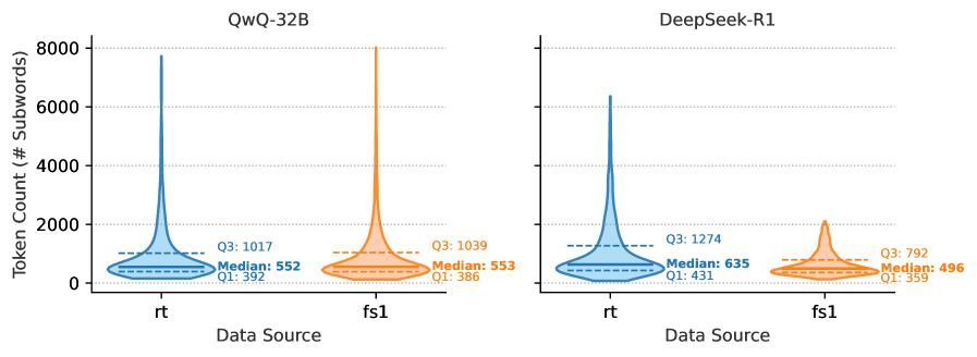
Figure 2: Distribution of Reasoning Traces. We show the distribution of the reasoning length among the queried models. In the left plot, we show rt and in the right plot, we show fs1. We show that particularly for fs1 and Deepseek-R1, the reasoning length is shorter in terms of subwords.
#### Data Statistics.
In Table 1 and Figure 2, we compare the reasoning trace accuracy and statistics of rt and fs1. We evaluate reasoning traces using three methods: (1) Exact Match, checking if the \boxed{} answer exactly matches or is a sub-phrase of any gold answer; (2) Semantic Match, accepting answers with a cosine similarity score $>$ 0.5; and (3) LLM-as-a-Judge, verifying entity alignment using gpt-4o-mini-2024-07-18. Results show that fs1 achieves higher accuracy, indicating that it contains more factual answers. Traces from rt are longer (up to 1K subwords), fs1 traces are typically shorter (around 800 subwords). The median length in subwords is similar for QwQ-32B (552 for rt and 553 for fs1), while there is a difference for Deepseek-R1 (635 median for rt and 496 for fs1). Spot-checking reveals that fs1 yields a more definitive answer.
## 3 Methodology
### 3.1 Training and Inference
We fine-tune six Qwen2.5-Instruct models (0.5B to 32B) on rt and fs1, using only reasoning traces with correct final answers. During inference, we evaluate the model on the original questions to test its performance. Following Muennighoff et al. (2025), we train for 5 epochs with a sequence length of 8,192, a batch size of 16, a learning rate of $1\times 10^{-5}$ (cosine schedule, 5% warmup), and a weight decay of $1\times 10^{-4}$ . The models are optimized with a standard supervised fine-tuning (SFT) loss, which minimizes the negative log-likelihood (implemented as the cross-entropy function) of target tokens in an autoregressive manner. Let $y_{t}^{*}$ be the correct token and $p_{\theta}(y_{t}^{*}\mid x,y_{<t})$ be the model’s probability of predicting it. The model optimizes the function:
$$
\mathcal{L}_{\text{SFT}}(\theta)=-\frac{1}{T}\sum_{t=1}^{T}\log p_{\theta}\left(y_{t}^{*}\mid x,y_{<t}\right). \tag{1}
$$
For inference, we use a temperature ( $T$ ) of $0.7$ and top_p of $0.8$ for original instruct models. Otherwise, we use $T=0.6$ and top_p of $0.95$ . Further details on hardware and costs are in Appendix B.
fs1 Prompt Example
⬇ When did the sports team owned by Leslie Alexander win the NBA championship? While answering the question, make use of the following linearised graph as an inspiration in your reasoning, not as the only answer: 1994 NBA Finals, winner, Houston Rockets Houston Rockets, owned by, Leslie Alexander 1995 NBA Finals, winner, Houston Rockets Houston Rockets, owned by, Leslie Alexander. Put your final answer within \ boxed {}. – (For illustration) Gold Answer: [”1994 and 1995”]
Figure 3: fs1 Prompt Example. We depict how we prompt both Deepseek-R1 and QwQ-32B to obtain better reasoning traces with KG paths.
LLM-as-a-Judge (Llama-3.3-70B)
⬇ gold answer: [” Joule per gram per kelvin ”, ” Joule per kilogram per kelvin ”] predicted answer: ” J /(kg $ \ cdot$ K)” Is the gold answer entity or value contained in the predicted answer? Respond only with 0 (no) or 1 (yes). # Llama -3.3-70 B - Instruct outputs ”1”
Figure 4: Prompt for LLM-as-a-Judge. We show the LLM-as-a-Judge prompt for evaluating whether the predicted and gold answer refer to the same real-world entity, where regular exact string matching will not capture the alignment between the gold and predicted answer in this example (i.e., the measurement unit).
Table 2: Test Benchmark. Overview of the mQA test sets used in our evaluation.
| CWQ (Talmor & Berant, 2018) | apache-2.0 | 3.5K | Multi-hop QA from WebQuestionsSP with compositional SPARQL queries for Freebase paraphrased by crowd workers. |
| --- | --- | --- | --- |
| ExaQT (Jia et al., 2021) | cc-by-4.0 | 3.2K | Temporal-QA benchmark combining eight KB-QA datasets, focusing on time-specific queries. |
| GrailQA (Gu et al., 2021) | apache-2.0 | 6.8K | Freebase QA dataset with annotated answers and logical forms (SPARQL/S-expressions) across 86 domains. |
| SimpleQA (Wei et al., 2024a) | MIT | 4.3K | Fact-seeking questions with verified answers, designed to measure and challenge the factual accuracy of language models. |
| Mintaka (Sen et al., 2022) | cc-by-4.0 | 4.0K | Multilingual QA (9 languages), entity-linked pairs across diverse domains (English test split). |
| WebQSP (Yih et al., 2016) | apache-2.0 | 2.0K | Enhanced WebQuestions with Freebase QA annotated with SPARQL ( $\sim$ 82% coverage). |
| Total | | 23.9K | |
<details>
<summary>x3.png Details</summary>
### Visual Description
## Heatmap Comparison: Dataset Similarity Metrics
### Overview
The image displays three horizontally arranged heatmap charts comparing seven datasets across three different similarity metrics. The datasets are: CWQ_train, CWQ_test, ExaQT, GrailQA, SimpleQA, Mintaka, and WebQSP. Each heatmap is a lower-triangular matrix showing pairwise comparisons.
### Components/Axes
* **Chart Titles (Top):**
* Left: "Cosine Similarity Count (> 0.90)"
* Center: "Exact Match Count"
* Right: "Average Cosine Similarity"
* **Axes Labels (Identical for all three charts):**
* **Y-axis (Vertical, Left side):** Lists datasets from top to bottom: CWQ_train, CWQ_test, ExaQT, GrailQA, SimpleQA, Mintaka, WebQSP.
* **X-axis (Horizontal, Bottom):** Lists datasets from left to right: CWQ_train, CWQ_test, ExaQT, GrailQA, SimpleQA, Mintaka, WebQSP. Labels are rotated approximately 45 degrees.
* **Legend/Color Scale:** Each chart uses a sequential color scale from dark green (low values) to bright yellow (high values). The specific numerical mapping is not provided, but the relative intensity is clear.
### Detailed Analysis
#### Chart 1: Cosine Similarity Count (> 0.90)
This chart counts the number of data points with a cosine similarity greater than 0.90 between dataset pairs.
* **Trend:** The diagonal (self-comparison) and certain off-diagonal pairs show high counts (yellow), while most other pairs have very low counts (dark green).
* **Data Points (Row, Column -> Value):**
* CWQ_test vs. CWQ_train -> **109** (Highest value in the chart)
* ExaQT vs. CWQ_train -> **51**
* ExaQT vs. CWQ_test -> **80**
* GrailQA vs. CWQ_train -> **1**
* GrailQA vs. ExaQT -> **0**
* SimpleQA vs. CWQ_train -> **0**
* SimpleQA vs. ExaQT -> **1**
* SimpleQA vs. GrailQA -> **0**
* Mintaka vs. CWQ_train -> **0**
* Mintaka vs. ExaQT -> **1**
* Mintaka vs. GrailQA -> **4**
* Mintaka vs. SimpleQA -> **0**
* WebQSP vs. CWQ_train -> **12**
* WebQSP vs. CWQ_test -> **26**
* WebQSP vs. ExaQT -> **83**
* WebQSP vs. GrailQA -> **1**
* WebQSP vs. SimpleQA -> **0**
* WebQSP vs. Mintaka -> **15**
* WebQSP vs. WebQSP (diagonal) -> **15**
#### Chart 2: Exact Match Count
This chart counts the number of exact matches between dataset pairs.
* **Trend:** The matrix is almost entirely dark green (zero), indicating extremely few exact matches. Only one off-diagonal cell is non-zero.
* **Data Points (Row, Column -> Value):**
* All diagonal cells (self-comparison) are **0**.
* All off-diagonal cells are **0**, except:
* WebQSP vs. CWQ_test -> **1**
#### Chart 3: Average Cosine Similarity
This chart shows the average cosine similarity score between dataset pairs.
* **Trend:** Values are generally low (all below 0.20). The diagonal (self-similarity) tends to have the highest values in each row, shown in lighter yellow-green. Off-diagonal similarities are modest.
* **Data Points (Row, Column -> Value):**
* CWQ_test vs. CWQ_train -> **0.15**
* ExaQT vs. CWQ_train -> **0.11**
* ExaQT vs. CWQ_test -> **0.12**
* GrailQA vs. CWQ_train -> **0.08**
* GrailQA vs. CWQ_test -> **0.08**
* GrailQA vs. ExaQT -> **0.05**
* SimpleQA vs. CWQ_train -> **0.11**
* SimpleQA vs. CWQ_test -> **0.12**
* SimpleQA vs. ExaQT -> **0.13**
* SimpleQA vs. GrailQA -> **0.07**
* Mintaka vs. CWQ_train -> **0.11**
* Mintaka vs. CWQ_test -> **0.12**
* Mintaka vs. ExaQT -> **0.12**
* Mintaka vs. GrailQA -> **0.07**
* Mintaka vs. SimpleQA -> **0.11**
* WebQSP vs. CWQ_train -> **0.12**
* WebQSP vs. CWQ_test -> **0.13**
* WebQSP vs. ExaQT -> **0.11**
* WebQSP vs. GrailQA -> **0.06**
* WebQSP vs. SimpleQA -> **0.11**
* WebQSP vs. Mintaka -> **0.11**
* WebQSP vs. WebQSP (diagonal) -> **0.11**
### Key Observations
1. **High Pairwise Similarity (Cosine Count):** CWQ_test, ExaQT, and WebQSP form a cluster with high counts of high-similarity pairs (>0.90). The pair (ExaQT, WebQSP) has the second-highest count (83).
2. **Near-Zero Exact Matches:** Exact matches between different datasets are virtually non-existent (only 1 instance found). This indicates the datasets are distinct in their exact content.
3. **Low Average Similarity:** Despite some pairs having many high-similarity points, the *average* cosine similarity across all pairs is low (0.05 to 0.15). This suggests similarity is not uniform but concentrated in subsets of data.
4. **Self-Similarity:** The diagonal values confirm that datasets are most similar to themselves, which is an expected sanity check.
### Interpretation
This analysis compares the composition of several question-answering or text datasets. The findings suggest:
* **Dataset Relationships:** CWQ (train/test), ExaQT, and WebQSP share significant semantic overlap, as evidenced by high cosine similarity counts. They may contain similar types of questions, answers, or textual patterns.
* **Distinct Content:** The lack of exact matches confirms these are not simply copies of each other; they are unique corpora. The similarity is in meaning or structure, not in verbatim text.
* **Nature of Similarity:** The contrast between high "Cosine Similarity Count (>0.90)" and low "Average Cosine Similarity" is critical. It implies that within these datasets, there are specific clusters or types of data points that are very similar to each other, but these clusters are embedded within a larger body of data that is not similar. The similarity is localized, not global.
* **Utility for Modeling:** Datasets with high pairwise similarity (like CWQ and ExaQT) might be used for cross-domain evaluation or could indicate redundancy. The low overall average similarity suggests that combining these datasets could provide a more diverse training or testing set. The outlier pair (WebQSP, ExaQT) with a high similarity count (83) warrants specific investigation into their common characteristics.
</details>
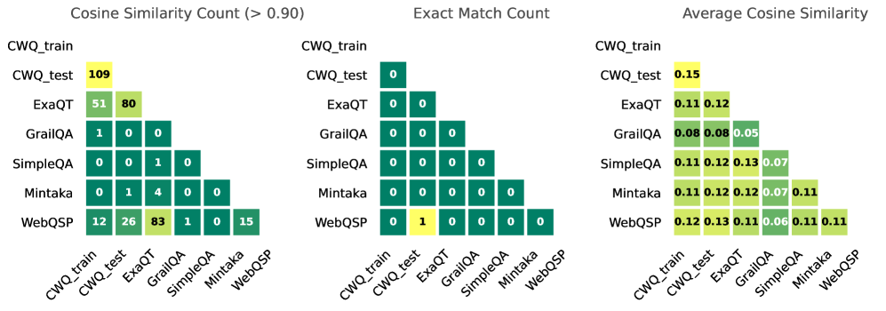
Figure 5: Data Overlap. We show data overlap between the train set and benchmark. On the left, one can observe the count of similar questions when the cosine similarity $>$ 0.90 (measured with paraphrase-MiniLM-L6-v2; Reimers & Gurevych, 2019). In the middle, we measure exact match counts. On the right, we show the average pairwise cosine similarity across the full test sets.
### 3.2 Benchmarks and Evaluation
We show the test datasets, licenses, size and a short description in Table 2. We have four baselines, namely Qwen2.5-72B-Instruct (Qwen Team, 2024), QwQ-32B, Deepseek-R1, and o3-mini (OpenAI, 2025). To evaluate our models, we select a suite of six mQA benchmarks with a total of 23.9K questions. We have four setups for benchmarking the models: (1) All models including baselines are evaluated zero-shot (i.e., only querying the question); (2) the models are queried using zero-shot chain-of-thought prompting (Kojima et al., 2022; Wei et al., 2022), where we simply append the prompt “ Put your final answer within \boxed{}. Think step-by-step. ”; (3) we benchmark the models fine-tuned on rt; (4) we benchmark the models fine-tuned on fs1. In Figure 12 (Section D.1), we show an example of each dataset in the test benchmark.
#### Possible Data Leakage.
In Figure 5, we show the overlap of the questions in the training set of ComplexWebQuestions (CWQ_train) versus all the other benchmarks used in our study (all questions lower-cased). On the left, we count the times that the cosine similarity between questions exceeds 0.90. We can see that there is the most overlap between CWQ_train and CWQ_test (109 questions), and the second most is between WebQSP and ExaQT (83 questions). In the middle, we show that there is almost to none exact string match between the questions. On the right, we show the average pairwise cosine similarity across the benchmarks is lower or equal to 0.15.
#### Evaluation Metric.
Similar to previous studies, e.g., Ma et al. (2025), we report pass@ $k$ , which reflects the probability that at least one out of $k$ randomly selected completions (drawn from a total of $n$ completions per problem) is correct. As such, it serves as an upper-bound on practical performance, which would require a subsequent selection mechanism. Formally, pass@ $k$ is given by: $\mathbb{E}_{\text{problems}}\left[1-\frac{\binom{n-c}{k}}{\binom{n}{k}}\right]$ , where $n$ is the number of generated completions per problem and $c$ is the count of correct completions (Chen et al., 2021). For our benchmarks, we evaluate $k=\{1,2,4,8,16\}$ . In practice, pass@32 is typically reported for formal theorem-proving tasks, while pass@1 (reducing to standard top-1 accuracy) is standard for math and coding tasks as mentioned by Ma et al. (2025). In this work for factual mQA, we report until $k=16$ .
#### LLM-as-a-Judge.
To decide whether an answer is correct or not (1 or 0), our main evaluation approach is using LLM-as-a-judge with Llama-3.3-70B-Instruct We compare both gpt-4o-mini-2024-07-18 and Llama-3.3-70B-Instruct on a large subsample of our outputs and saw there there is almost no difference in predictions. Additionally, Llama-3.3-70B is rated higher in LM Arena than gpt-4o-mini (at time of writing 79 ${}^{\text{th}}$ vs. 83 ${}^{\text{rd}}$ respectively). to determine whether a predicted answer obtained from the \boxed{} output is referring to the same real-world entity as the gold answer. An example of this is shown in Figure 4. When the model does not generate a \boxed{} output, we take the last 10 subwords as predicted answer, which LLM-as-a-judge can infer what the predicted real-world entity is when there is not exact string matching. This same approach is used in Table 1. Compared to exact string matching and semantic similarity evaluation methods, LLM-as-a-Judge rates the quality of output similarly compared to the other methods.
<details>
<summary>x4.png Details</summary>
### Visual Description
\n
## [Multi-Panel Line Chart]: Performance of Different Methods on Six Question Answering Datasets
### Overview
The image displays six separate line charts arranged in a 2x3 grid. Each chart plots the performance of four different methods on a specific question answering (QA) dataset. Performance is measured by the "pass@k (%)" metric as a function of the parameter "k". All charts show a consistent pattern where performance improves with increasing "k", but the absolute performance levels and the relative ranking of methods vary across datasets.
### Components/Axes
* **Titles:** Six dataset names, one above each chart: `ComplexWebQuestions`, `ExaQT`, `GrailQA`, `Mintaka`, `SimpleQA`, `WebQSP`.
* **Y-Axis:** Labeled `pass@k (%)` for all charts. The scale varies:
* ComplexWebQuestions: ~45% to ~65%
* ExaQT: ~35% to ~58%
* GrailQA: ~33% to ~55%
* Mintaka: ~68% to ~86%
* SimpleQA: ~8% to ~24%
* WebQSP: ~58% to ~78%
* **X-Axis:** Labeled `k` for all charts. The markers are at values 1, 2, 4, 8, and 16.
* **Legend:** Positioned at the bottom center of the entire figure. It defines four data series:
* `inst`: Cyan solid line with circle markers.
* `cot`: Green dashed line with diamond markers.
* `rt`: Purple dotted line with upward-pointing triangle markers.
* `fs1`: Salmon (light red) dashed line with square markers.
### Detailed Analysis
**1. ComplexWebQuestions (Top-Left)**
* **Trend:** All four methods show a steep initial increase from k=1 to k=4, followed by a more gradual rise to k=16.
* **Data Points (Approximate):**
* `fs1` (Salmon, Square): Starts ~48%, ends ~64%.
* `rt` (Purple, Triangle): Starts ~47%, ends ~63%.
* `cot` (Green, Diamond): Starts ~45%, ends ~59%.
* `inst` (Cyan, Circle): Starts ~44%, ends ~55%.
* **Ranking (at k=16):** `fs1` > `rt` > `cot` > `inst`.
**2. ExaQT (Top-Center)**
* **Trend:** Similar logarithmic growth pattern. The gap between `fs1`/`rt` and `cot`/`inst` widens as k increases.
* **Data Points (Approximate):**
* `fs1`: Starts ~37%, ends ~58%.
* `rt`: Starts ~36%, ends ~56%.
* `cot`: Starts ~36%, ends ~53%.
* `inst`: Starts ~36%, ends ~48%.
* **Ranking (at k=16):** `fs1` > `rt` > `cot` > `inst`.
**3. GrailQA (Top-Right)**
* **Trend:** Consistent upward trend. The performance hierarchy is clear and maintained across all k.
* **Data Points (Approximate):**
* `fs1`: Starts ~34%, ends ~54%.
* `rt`: Starts ~34%, ends ~52%.
* `cot`: Starts ~33%, ends ~49%.
* `inst`: Starts ~33%, ends ~46%.
* **Ranking (at k=16):** `fs1` > `rt` > `cot` > `inst`.
**4. Mintaka (Bottom-Left)**
* **Trend:** Strong upward trend. The top three methods (`fs1`, `rt`, `cot`) are tightly clustered, while `inst` lags significantly.
* **Data Points (Approximate):**
* `fs1`: Starts ~68%, ends ~86%.
* `rt`: Starts ~69%, ends ~85%.
* `cot`: Starts ~70%, ends ~83%.
* `inst`: Starts ~69%, ends ~78%.
* **Ranking (at k=16):** `fs1` ≈ `rt` > `cot` > `inst`.
**5. SimpleQA (Bottom-Center)**
* **Trend:** All methods show improvement. The `rt` and `fs1` lines nearly overlap at the top, while `cot` and `inst` are distinctly lower.
* **Data Points (Approximate):**
* `fs1`: Starts ~9%, ends ~24%.
* `rt`: Starts ~9%, ends ~24%.
* `cot`: Starts ~9%, ends ~24% (appears to converge with top two at k=16).
* `inst`: Starts ~9%, ends ~18%.
* **Ranking (at k=16):** `fs1` ≈ `rt` ≈ `cot` > `inst`.
**6. WebQSP (Bottom-Right)**
* **Trend:** Clear logarithmic growth. A distinct separation exists between the top method (`fs1`) and the others.
* **Data Points (Approximate):**
* `fs1`: Starts ~58%, ends ~78%.
* `rt`: Starts ~61%, ends ~74%.
* `cot`: Starts ~61%, ends ~73%.
* `inst`: Starts ~61%, ends ~70%.
* **Ranking (at k=16):** `fs1` > `rt` ≈ `cot` > `inst`.
### Key Observations
1. **Universal Trend:** Across all six datasets, the `pass@k` metric increases with `k` for every method, demonstrating the benefit of generating more candidate answers.
2. **Consistent Method Hierarchy:** The `fs1` method (salmon squares) is consistently the top or tied-for-top performer. The `inst` method (cyan circles) is consistently the lowest performer.
3. **Dataset Difficulty:** The absolute `pass@k` values vary greatly, indicating differing dataset difficulty. `SimpleQA` appears the most challenging (max ~24%), while `Mintaka` appears the easiest (max ~86%).
4. **Convergence at High k:** On several datasets (`SimpleQA`, `Mintaka`), the performance of the top methods (`fs1`, `rt`, `cot`) converges as `k` increases to 16.
### Interpretation
This visualization compares the efficacy of four different prompting or reasoning strategies (`inst`: instruction-only, `cot`: chain-of-thought, `rt`: self-refinement or similar, `fs1`: few-shot with one example) for large language models on knowledge-intensive QA tasks.
The data suggests that **providing examples (`fs1`) or structured reasoning steps (`cot`, `rt`) consistently outperforms simple instruction (`inst`)**. The advantage of these advanced methods is robust across diverse QA formats and difficulty levels. The `pass@k` metric's rise with `k` underscores a key strategy in LLM deployment: generating multiple candidate answers and using a verifier or voting mechanism to select the best one significantly boosts reliability. The convergence of top methods at high `k` on some datasets implies that with enough candidate generations, the specific prompting strategy may become less critical, though `fs1` maintains a slight edge. The stark difference in absolute performance between datasets like `SimpleQA` and `Mintaka` highlights the importance of benchmarking across a varied suite of tasks to get a complete picture of model capability.
</details>
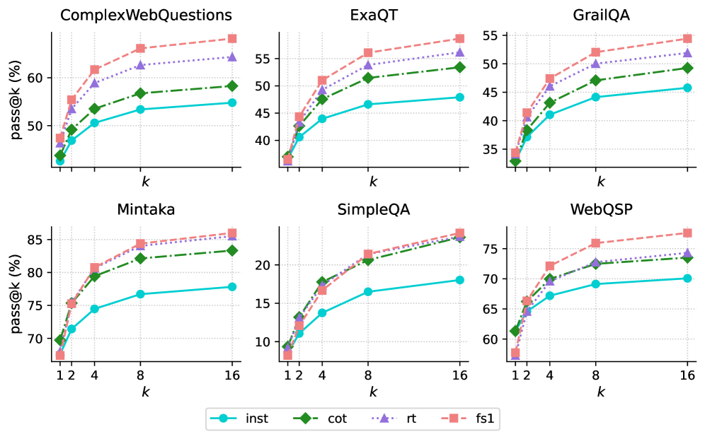
Figure 6: Upper-bound Test-Time Scaling for Factual Reasoning. We show with Qwen2.5-32B that parallel scaling is beneficial for complex mQA, measured by pass@ $k$ , especially when fine-tuned on fs1, instead of conducting single-pass inference.
## 4 Results and Discussion
### 4.1 Results with Test-time Scaling
Parallel scaling can achieve lower latency by enabling multiple (identical) models to run simultaneously locally (via e.g., multiple GPUs or batching techniques) or via API based methods to generate multiple answers. Formally, parallel sampling entails an aggregation technique that combines $N$ independent solutions into a single final prediction, commonly known as a best-of- $N$ approach (Chollet, 2019; Irvine et al., 2023; Brown et al., 2024a; Li et al., 2022). Formally, given a set of $N$ predictions $P=\{p_{1},\dots,p_{N}\}$ , the best-of- $N$ method selects a prediction $p\in P$ as the final output.
In this work, we present results using pass@ $k$ (see Section 3.2), extending the number of sampled $k$ (until $k$ = 16). In Figure 6, we show parallel scaling results by performing 16 inference runs with Qwen2.5-32B -Instruct, CoT, rt, fs1 on each test dataset. For parallel sampling, we limit ourselves to Qwen2.5-32B as running 16 inferences for 8 models for all 4 settings would require 12.2M model inferences for the test benchmarks, which is computationally prohibitive. As $k$ increases, pass@ $k$ (indicating whether at least one generation is correct) rises steadily across all benchmarks. Parallel sampling boosts the chance of producing a correct answer, especially when fine-tuned on fs1. For example, on CWQ, we see a performance increase of 16 absolute points at $k$ = 16 and on SimpleQA around 6 absolute points at the same $k$ compared to their original instruction-tuned counterpart.
<details>
<summary>x5.png Details</summary>
### Visual Description
## Grouped Bar Chart: Relative Improvement (RI) by Hops
### Overview
This is a grouped bar chart titled "Relative Improvement (RI) by Hops." It displays the relative improvement percentage (RI) for three different methods or models (cot, rt, fs1) across four categories of problem complexity, defined by the number of "hops" required (1, 2, 3, and 3+). The y-axis represents the RI percentage, measured with a "pass@16" metric.
### Components/Axes
* **Chart Title:** "Relative Improvement (RI) by Hops" (centered at the top).
* **Y-Axis:**
* **Label:** "RI (%); pass@16" (rotated vertically on the left).
* **Scale:** Linear scale from 0 to 60.
* **Tick Marks:** Major ticks at 0, 20, 40, 60. Dotted horizontal grid lines extend from these ticks across the chart.
* **X-Axis:**
* **Categories (Hops):** Four discrete categories labeled "1", "2", "3", and "3+".
* **Legend:**
* **Position:** Top-left corner, inside the plot area.
* **Series:**
1. **cot:** Light blue solid fill.
2. **rt:** Medium blue fill with diagonal hatching (lines sloping down from left to right: `\`).
3. **fs1:** Dark blue fill with cross-hatching (diagonal lines in both directions: `X`).
### Detailed Analysis
The chart presents the following approximate RI (%) values for each method across the hop categories. Values are estimated based on bar height relative to the y-axis grid.
**Hop Category 1:**
* **cot (light blue):** ~38%
* **rt (medium blue, `\` hatch):** ~36%
* **fs1 (dark blue, `X` hatch):** ~33%
* *Trend:* cot shows the highest improvement, followed closely by rt, with fs1 slightly lower.
**Hop Category 2:**
* **cot (light blue):** ~38%
* **rt (medium blue, `\` hatch):** ~45%
* **fs1 (dark blue, `X` hatch):** ~34%
* *Trend:* rt shows a notable increase and surpasses cot. cot remains stable. fs1 shows a slight decrease.
**Hop Category 3:**
* **cot (light blue):** ~33%
* **rt (medium blue, `\` hatch):** ~53%
* **fs1 (dark blue, `X` hatch):** ~60%
* *Trend:* fs1 shows a dramatic increase, becoming the highest. rt also increases significantly. cot shows a moderate decrease.
**Hop Category 3+:**
* **cot (light blue):** ~33%
* **rt (medium blue, `\` hatch):** ~24%
* **fs1 (dark blue, `X` hatch):** ~50%
* *Trend:* fs1 remains the highest but decreases from its peak at 3 hops. cot remains stable at its lower level. rt shows a sharp decline, becoming the lowest.
### Key Observations
1. **Diverging Trends with Complexity:** The performance of the three methods diverges significantly as the number of hops increases.
2. **fs1's Strong Scaling:** The `fs1` method shows a strong positive trend with complexity, peaking at 3 hops (RI ~60%) and maintaining a high level for 3+ hops (~50%). It is the top performer for the most complex categories.
3. **rt's Peak and Drop:** The `rt` method improves from 1 to 3 hops (peaking at ~53%) but experiences a severe performance drop for the 3+ category (~24%), suggesting it may not generalize well to the most complex problems.
4. **cot's Stability:** The `cot` method is the most stable, hovering between ~33% and ~38% across all categories. It does not show significant improvement or degradation with increasing hops.
5. **Relative Performance Flip:** The ranking of methods completely flips between the simplest (1 hop: cot > rt > fs1) and most complex (3 hops: fs1 > rt > cot) categories.
### Interpretation
This chart likely compares the effectiveness of different reasoning or prompting strategies (Chain-of-Thought "cot", possibly "Reasoning Trace" "rt", and "Few-Shot 1" "fs1") on tasks requiring multi-step inference ("hops").
The data suggests a clear trade-off:
* **Specialization vs. Generalization:** `fs1` appears to be a specialized strategy that excels on moderately to highly complex multi-hop problems (3 and 3+ hops) but is less optimal for simpler ones. `cot` is a generalist, providing consistent, moderate improvement regardless of complexity. `rt` shows promise for mid-complexity tasks but fails to scale to the hardest ones.
* **Implication for Model Selection:** The choice of strategy should be guided by the expected complexity of the task. For unknown or variable complexity, `cot` offers reliability. For known complex tasks, `fs1` is the superior choice based on this data. The poor performance of `rt` on 3+ hop tasks is a critical weakness that would need investigation.
* **Underlying Mechanism:** The dramatic rise of `fs1` suggests its mechanism (perhaps leveraging a single worked example) becomes disproportionately more valuable as the reasoning chain lengthens, up to a point. The collapse of `rt` at 3+ hops might indicate error propagation or a breakdown in its tracing mechanism for very long reasoning chains.
</details>
(a) Performance by number of hops required to answer the question measured in pass@ $16$ .
<details>
<summary>x6.png Details</summary>
### Visual Description
## Grouped Bar Chart: Relative Improvement (RI) by Answer Type
### Overview
This is a grouped bar chart comparing the performance of three different methods or models (labeled "cot", "rt", and "fs1") across five distinct categories of answers. The performance metric is "Relative Improvement (RI)" measured as a percentage, with a secondary note of "pass@16". The chart visually demonstrates how each method's effectiveness varies depending on the type of answer being generated.
### Components/Axes
* **Chart Title:** "Relative Improvement (RI) by Answer Type" (centered at the top).
* **Y-Axis:**
* **Label:** "RI (%); pass@16" (rotated vertically on the left).
* **Scale:** Linear scale from 0 to 50, with major tick marks at intervals of 10 (0, 10, 20, 30, 40, 50).
* **X-Axis:**
* **Categories (from left to right):** "date", "place", "person", "other", "number".
* **Legend:**
* **Position:** Top-right corner of the chart area.
* **Items:**
1. **cot:** Represented by a solid yellow bar.
2. **rt:** Represented by a teal bar with diagonal hatching (stripes running from top-left to bottom-right).
3. **fs1:** Represented by a dark blue/indigo bar with diagonal hatching (stripes running from top-left to bottom-right).
### Detailed Analysis
The analysis is segmented by the five answer categories on the x-axis. For each category, the approximate RI (%) values for the three methods are estimated based on bar height relative to the y-axis grid lines.
**1. Category: `date`**
* **Visual Trend:** This category shows the highest overall RI values. The `fs1` bar is the tallest, followed by `cot`, then `rt`.
* **Data Points (Approximate):**
* `cot` (Yellow): ~48%
* `rt` (Teal, hatched): ~41%
* `fs1` (Dark blue, hatched): ~55% (This is the highest single value in the entire chart).
**2. Category: `place`**
* **Visual Trend:** A clear descending step pattern from `cot` to `rt` to `fs1`.
* **Data Points (Approximate):**
* `cot` (Yellow): ~33%
* `rt` (Teal, hatched): ~21%
* `fs1` (Dark blue, hatched): ~19%
**3. Category: `person`**
* **Visual Trend:** `rt` and `cot` are relatively close, with `rt` slightly higher. `fs1` shows a significant drop.
* **Data Points (Approximate):**
* `cot` (Yellow): ~24%
* `rt` (Teal, hatched): ~26%
* `fs1` (Dark blue, hatched): ~13% (This is the lowest value for `fs1` across all categories).
**4. Category: `other`**
* **Visual Trend:** `rt` and `fs1` are nearly equal and are the tallest bars. `cot` is notably shorter.
* **Data Points (Approximate):**
* `cot` (Yellow): ~19%
* `rt` (Teal, hatched): ~30%
* `fs1` (Dark blue, hatched): ~30.5%
**5. Category: `number`**
* **Visual Trend:** Similar to the "other" category, `rt` and `fs1` are close and lead, with `cot` trailing.
* **Data Points (Approximate):**
* `cot` (Yellow): ~17%
* `rt` (Teal, hatched): ~27%
* `fs1` (Dark blue, hatched): ~30%
### Key Observations
1. **Method Performance is Context-Dependent:** No single method (`cot`, `rt`, `fs1`) is universally superior. The best-performing method changes based on the answer type category.
2. **`fs1` Shows High Variance:** The `fs1` method achieves the highest overall RI (~55% for `date`) but also the lowest overall RI (~13% for `person`). Its performance is highly sensitive to the category.
3. **`cot` is Strong for `date` and `place`:** The `cot` method leads in the `place` category and is a strong second in `date`, but its performance drops significantly for `person`, `other`, and `number`.
4. **`rt` is Consistently Mid-to-High Tier:** The `rt` method rarely has the lowest score (only in `date` and `place`). It is the top performer in `person` and ties for the lead in `other` and `number`, showing more consistent, robust performance across diverse categories.
5. **Category Difficulty:** The `date` category appears to be the "easiest" for these models, yielding the highest RI scores overall. The `person` category seems particularly challenging for the `fs1` method.
### Interpretation
This chart provides a comparative analysis of three techniques (likely prompting or decoding strategies like Chain-of-Thought, Repeated Sampling, or Few-Shot with 1 example, given the labels) for improving a language model's performance on a task measured by "pass@16" (likely the probability of generating a correct answer in 16 attempts).
The data suggests that the effectiveness of a technique is not intrinsic but is deeply tied to the **nature of the information** being generated. Techniques that excel at factual recall for dates (`fs1`) may falter when reasoning about people. Conversely, a more balanced technique (`rt`) may provide reliable gains across a wider range of tasks without achieving the peak performance of a specialized one.
For a practitioner, this implies that model optimization should be **category-aware**. One might deploy a hybrid system that selects the best method (`cot`, `rt`, or `fs1`) based on the detected type of the query (e.g., a date question vs. a person question) to maximize overall system reliability and performance. The high variance of `fs1` indicates it is a high-risk, high-reward strategy, while `rt` represents a safer, more general-purpose improvement.
</details>
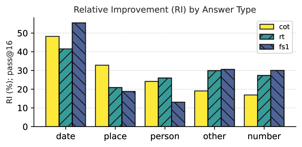
(b) Performance by answer type (i.e., what type of entity the answer is) in pass@ $16$ .
<details>
<summary>x7.png Details</summary>
### Visual Description
## Grouped Bar Chart: Relative Improvement (RI) by Domain
### Overview
This is a grouped bar chart titled "Relative Improvement (RI) by Domain". It displays the percentage of Relative Improvement (RI) for three different methods or models (labeled "cot", "rt", and "fs1") across ten distinct knowledge domains. The metric is specified as "RI (%); pass@16".
### Components/Axes
* **Chart Title:** "Relative Improvement (RI) by Domain" (centered at the top).
* **Y-Axis:**
* **Label:** "RI (%); pass@16" (rotated vertically on the left).
* **Scale:** Linear scale from 0 to 80, with major gridlines at intervals of 20 (0, 20, 40, 60, 80).
* **X-Axis:**
* **Categories (Domains):** Ten categories listed from left to right: `art`, `sports`, `other`, `geography`, `tv shows`, `video games`, `politics`, `music`, `sci & tech`, `history`.
* **Label Orientation:** Domain labels are rotated approximately 45 degrees for readability.
* **Legend:**
* **Position:** Top-right corner of the chart area.
* **Items:**
1. `cot`: Represented by a solid, medium-purple bar.
2. `rt`: Represented by a light-purple bar with diagonal hatching (lines sloping down from left to right: `\`).
3. `fs1`: Represented by a salmon/pink bar with diagonal hatching (lines sloping up from left to right: `/`).
### Detailed Analysis
Below are the approximate RI (%) values for each method within each domain, estimated from the bar heights relative to the y-axis gridlines. Values are approximate (±2-3%).
| Domain | cot (solid purple) | rt (hatched light purple `\`) | fs1 (hatched pink `/`) |
| :--- | :--- | :--- | :--- |
| **art** | ~62 | ~72 | ~58 |
| **sports** | ~48 | ~37 | ~47 |
| **other** | ~41 | ~34 | ~47 |
| **geography** | ~35 | ~19 | ~46 |
| **tv shows** | ~34 | ~51 | ~40 |
| **video games** | ~34 | ~62 | ~85 |
| **politics** | ~31 | ~27 | ~41 |
| **music** | ~26 | ~21 | ~28 |
| **sci & tech** | ~17 | ~18 | ~12 |
| **history** | ~4 | ~19 | ~19 |
**Visual Trend Verification per Data Series:**
* **`cot` (solid purple):** Shows a generally decreasing trend from left to right. It starts highest in `art` (~62) and declines to its lowest point in `history` (~4). There is a notable plateau in the middle domains (`tv shows`, `video games`) around ~34.
* **`rt` (hatched light purple):** Exhibits a more volatile pattern. It peaks in `art` (~72) and `video games` (~62), with significant dips in `geography` (~19) and `music` (~21). It shows a slight recovery in the final two domains.
* **`fs1` (hatched pink):** Displays a distinct peak in `video games` (~85), which is the highest value on the entire chart. It maintains relatively high values in the first seven domains (mostly above 40), then drops sharply in `sci & tech` (~12) before a slight rise in `history`.
### Key Observations
1. **Domain Performance Variability:** The relative effectiveness of the three methods varies dramatically by domain. No single method is consistently superior across all categories.
2. **Outlier - `video games`:** This domain shows the most extreme results. `fs1` achieves the chart's maximum value (~85), while `cot` is at its mid-range (~34). This suggests the `fs1` method is exceptionally well-suited for the `video games` domain.
3. **Outlier - `history`:** This domain has the lowest overall RI values. `cot` performs very poorly here (~4), while `rt` and `fs1` are tied at a modest ~19.
4. **Method Strengths:**
* `rt` is strongest in `art` and `video games`.
* `fs1` is strongest in `video games` and shows robust performance in `art`, `other`, `geography`, and `politics`.
* `cot` is strongest in `art` but generally shows a declining trend.
5. **`sci & tech` Low Performance:** All three methods show their lowest or near-lowest performance in the `sci & tech` domain, with RI values clustered between ~12 and ~18.
### Interpretation
The chart demonstrates that the "Relative Improvement" of these three techniques (likely AI prompting or reasoning methods: Chain-of-Thought, Retrieval-Augmented, and Few-Shot 1-shot) is highly domain-dependent. The data suggests:
* **Domain-Specific Optimization:** The significant variance implies that the underlying knowledge structures or question types in domains like `video games` or `art` are more amenable to certain reasoning strategies (e.g., `fs1` for `video games`) than others.
* **Complementary Strengths:** The methods appear to have complementary strengths. A system designed to use the optimal method for each domain (e.g., `rt` for `art`, `fs1` for `video games`, `cot` for `sports`) would likely outperform any single-method approach.
* **Challenge of Formal Domains:** The uniformly low scores in `sci & tech` and `history` suggest these domains may involve more specialized, precise, or less pattern-based knowledge that is harder for all three evaluated methods to improve upon with the given "pass@16" metric.
* **The `video games` Anomaly:** The exceptionally high `fs1` score for `video games` warrants investigation. It could indicate that this domain's QA pairs are particularly well-structured for few-shot learning, or that the evaluation set for this domain has characteristics that uniquely benefit from this approach.
In essence, the chart argues against a one-size-fits-all solution for enhancing model performance across diverse knowledge domains, highlighting the need for domain-aware strategy selection.
</details>
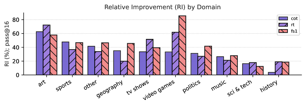
(c) Performance measured per domain in pass@ $16$ .
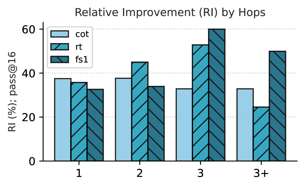
Figure 7: Relative Improvements across Different Axes. We show the relative performance improvement (%) at pass@ $16$ of different Qwen-32B (i.e., CoT, rt and fs1) against the original instruct model. In (a), we show the performance of the models by the number of hops required to answer the question. In (b), we show the performance of the models by answer type. In (c), we show the performance by domain of the question. Absolute numbers are in Figure 13 (Appendix F).
### 4.2 What type of samples do models seem to fail on?
In Figure 7, we investigate what kind of questions the model (Qwen2.5-32B) seems to fail on. We take metadata information from SimpleQA (Wei et al., 2024a), which indicates the question difficulty in number of hops required to answer the question (Figure 7(a)), type of answer (Figure 7(b)) and the domain of the question (Figure 7(c)). For question difficulty, we source the number of hops for each question in SimpleQA from Lavrinovics et al. (2025). We count the number of relations (P) from Wikidata, which would indicate the number of hops required to go from entity A to B. When a question does not contain any relations, we assume it takes more than 3 hops to answer the question.
In Figure 7(a), we observe that fs1 has lower relative improvements on easier questions (e.g., 1 or 2 hops required), but outperforms the other models when the question gets more complex (3 or more hops required). This indicates that inducing KG paths helps answering complex questions. In Figure 7(b), we show that fs1 has the most relative improvement on numerical answers, such as numbers, dates and also miscellaneous answer types. Last, in Figure 7(c), fs1 performs best on questions related to video games, geography, politics, music, and miscellaneous questions. Additionally, rt performs best on art and history-related questions. Last, CoT performs best on questions related to sports.
### 4.3 Single pass results across scale
In Table 3, we show results in terms of accuracy via LLM-as-a-Judge at pass@ $1$ (i.e., one inference run per question) on all test datasets. For the baselines, we observe that o3-mini is the dominant model, achieving the highest score on five out of six datasets, such as its 0.774 accuracy on Mintaka and 0.680 on WebQSP. The only exception is SimpleQA, where R1-70B performs best with a score of 0.188. These are followed by Qwen2.5-72B-Instruct and QwQ-32B in overall performance.
Observing the Qwen2.5 results, the benefits of fine-tuning on rt and fs1 are most pronounced at the sub-billion parameter scale. For instance, fine-tuning the 0.5B model on fs1 yields substantial relative gains across all tasks, peaking at a +74.6% on WebQSP. However, as model size increases, the performance differences become more nuanced. For the 1.5B model, the same fs1 fine-tuning leads to performance degradation on four out of six datasets, such as ExaQT (-4.7%) and WebQSP (-1.1%). While larger models like the 32B still benefit from fine-tuning (e.g., rt and fs1 are often the best performers in their group), the relative gains are smaller than those seen at the 0.5B scale.
Our results also show that fine-tuning improvements do not uniformly generalize across different model families at the sub-billion parameter scale. A comparison between the fine-tuned Qwen2.5 and SmolLM2 models reveals a significant performance divergence. Specifically, fine-tuning on fs1 provided consistent enhancements for the Qwen2.5-0.5B model, improving its CWQ score from 0.135 to 0.209. In contrast, the same fine-tuning on SmolLM2-360M yielded mixed results; while it improved performance on most tasks, it caused a notable degradation of -15.9% on GrailQA.
This variance diminishes with scale, as models at the 1.5B/1.7B parameter scale exhibit more convergent behavior. For example, fine-tuning with rt on GrailQA provides a nearly identical small boost to both Qwen2.5-1.5B (+1.9%) and SmolLM2-1.7B (+1.8%). Overall, We hypothesize this scale-dependent effect may occur because larger models (e.g., 32B) possess stronger parametric knowledge, making them less reliant on the explicit guidance from KG paths.
Table 3: Single Pass (pass@1) Results on mQA Benchmarks. We show accuracy and relative performance gains on our benchmarks for several baselines, Qwen2.5, and SmolLM2 models. For each size, we show the original instruction-tuned model followed by versions fine-tuned with chain-of-thought, rt, and fs1. Parentheses indicate the relative improvement over the instruction-tuned counterpart. The benefits of fine-tuning are most pronounced for smaller models.
| Model Large Language Model Baselines Qwen2.5-72B | CWQ 0.481 | ExaQT 0.440 | GrailQA 0.361 | SimpleQA 0.117 | Mintaka 0.736 | WebQSP 0.653 |
| --- | --- | --- | --- | --- | --- | --- |
| QwQ-32B | 0.479 | 0.390 | 0.358 | 0.097 | 0.708 | 0.612 |
| R1-70B | 0.501 | 0.476 | 0.340 | 0.188 | 0.755 | 0.549 |
| o3-mini | 0.558 | 0.497 | 0.438 | 0.138 | 0.774 | 0.680 |
| Small Language Models (0.36B-1.7B) | | | | | | |
| SmolLM2-360M | 0.148 | 0.088 | 0.164 | 0.024 | 0.175 | 0.235 |
| + cot | 0.151 (+2.0 %) | 0.101 (+14.8 %) | 0.169 (+3.0 %) | 0.025 (+4.2 %) | 0.188 (+7.4 %) | 0.230 (-2.1 %) |
| + rt | 0.192 (+29.7 %) | 0.111 (+26.1 %) | 0.156 (-4.9 %) | 0.029 (+20.8 %) | 0.202 (+15.4 %) | 0.293 (+24.7 %) |
| + fs1 | 0.179 (+20.9 %) | 0.093 (+5.7 %) | 0.138 (-15.9 %) | 0.027 (+12.5 %) | 0.197 (+12.6 %) | 0.264 (+12.3 %) |
| Qwen2.5-0.5B | 0.135 | 0.058 | 0.127 | 0.023 | 0.131 | 0.173 |
| + cot | 0.161 (+19.3 %) | 0.104 (+79.3 %) | 0.141 (+11.0 %) | 0.031 (+34.8 %) | 0.214 (+63.4 %) | 0.234 (+35.3 %) |
| + rt | 0.190 (+40.7 %) | 0.089 (+53.4 %) | 0.155 (+22.0 %) | 0.022 (-4.3 %) | 0.178 (+35.9 %) | 0.286 (+65.3 %) |
| + fs1 | 0.209 (+54.8 %) | 0.101 (+74.1 %) | 0.166 (+30.7 %) | 0.035 (+52.2 %) | 0.202 (+54.2 %) | 0.302 (+74.6 %) |
| Qwen2.5-1.5B | 0.234 | 0.170 | 0.208 | 0.031 | 0.316 | 0.360 |
| + cot | 0.252 (+7.7 %) | 0.179 (+5.3 %) | 0.216 (+3.8 %) | 0.041 (+32.3 %) | 0.318 (+0.6 %) | 0.391 (+8.6 %) |
| + rt | 0.255 (+9.0 %) | 0.173 (+1.8 %) | 0.212 (+1.9 %) | 0.038 (+22.6 %) | 0.294 (-7.0 %) | 0.360 (+0.0 %) |
| + fs1 | 0.263 (+12.4 %) | 0.162 (-4.7 %) | 0.204 (-1.9 %) | 0.035 (+12.9 %) | 0.301 (-4.7 %) | 0.356 (-1.1 %) |
| SmolLM2-1.7B | 0.248 | 0.176 | 0.219 | 0.032 | 0.293 | 0.408 |
| + cot | 0.285 (+14.9 %) | 0.177 (+0.6 %) | 0.209 (-4.6 %) | 0.032 (+0.0 %) | 0.295 (+0.7 %) | 0.409 (+0.2 %) |
| + rt | 0.306 (+23.4 %) | 0.184 (+4.5 %) | 0.223 (+1.8 %) | 0.038 (+18.7 %) | 0.366 (+24.9 %) | 0.454 (+11.3 %) |
| + fs1 | 0.305 (+23.0 %) | 0.179 (+1.7 %) | 0.218 (-0.5 %) | 0.036 (+12.5 %) | 0.341 (+16.4 %) | 0.426 (+4.4 %) |
| Large Language Models (3B-32B) | | | | | | |
| Qwen2.5-3B | 0.317 | 0.214 | 0.252 | 0.044 | 0.396 | 0.466 |
| + cot | 0.302 (-4.7 %) | 0.222 (+3.7 %) | 0.248 (-1.6 %) | 0.048 (+9.1 %) | 0.431 (+8.8 %) | 0.477 (+2.4 %) |
| + rt | 0.363 (+14.5 %) | 0.235 (+9.8 %) | 0.279 (+10.7 %) | 0.053 (+20.5 %) | 0.495 (+25.0 %) | 0.483 (+3.6 %) |
| + fs1 | 0.330 (+4.1 %) | 0.205 (-4.2 %) | 0.253 (+0.4 %) | 0.045 (+2.3 %) | 0.444 (+12.1 %) | 0.406 (-12.9 %) |
| Qwen2.5-7B | 0.376 | 0.281 | 0.299 | 0.070 | 0.548 | 0.580 |
| + cot | 0.383 (+1.9 %) | 0.292 (+3.9 %) | 0.295 (-1.3 %) | 0.062 (-11.4 %) | 0.580 (+5.8 %) | 0.565 (-2.6 %) |
| + rt | 0.401 (+6.6 %) | 0.296 (+5.3 %) | 0.300 (+0.3 %) | 0.067 (-4.3 %) | 0.576 (+5.1 %) | 0.517 (-10.9 %) |
| + fs1 | 0.408 (+8.5 %) | 0.272 (-3.2 %) | 0.303 (+1.3 %) | 0.053 (-24.3 %) | 0.551 (+0.5 %) | 0.492 (-15.2 %) |
| Qwen2.5-14B | 0.392 | 0.336 | 0.318 | 0.068 | 0.624 | 0.599 |
| + cot | 0.422 (+7.7 %) | 0.356 (+6.0 %) | 0.322 (+1.3 %) | 0.080 (+17.6 %) | 0.664 (+6.4 %) | 0.592 (-1.2 %) |
| + rt | 0.451 (+15.1 %) | 0.352 (+4.8 %) | 0.331 (+4.1 %) | 0.082 (+20.6 %) | 0.678 (+8.7 %) | 0.562 (-6.2 %) |
| + fs1 | 0.454 (+15.8 %) | 0.339 (+0.9 %) | 0.328 (+3.1 %) | 0.079 (+16.2 %) | 0.654 (+4.8 %) | 0.558 (-6.8 %) |
| Qwen2.5-32B | 0.428 | 0.362 | 0.334 | 0.087 | 0.674 | 0.621 |
| + cot | 0.435 (+1.6 %) | 0.366 (+1.1 %) | 0.332 (-0.6 %) | 0.099 (+13.8 %) | 0.696 (+3.3 %) | 0.614 (-1.1 %) |
| + rt | 0.471 (+10.0 %) | 0.366 (+1.1 %) | 0.342 (+2.4 %) | 0.094 (+8.0 %) | 0.680 (+0.9 %) | 0.563 (-9.3 %) |
| + fs1 | 0.477 (+11.4 %) | 0.361 (-0.3 %) | 0.344 (+3.0 %) | 0.078 (-10.3 %) | 0.682 (+1.2 %) | 0.576 (-7.2 %) |
## 5 Related Work
Different methods that involve long chain-of-thought processes (Kojima et al., 2022; Wei et al., 2022) involving reflection, backtracking, thinking (e.g., DeepSeek-AI, 2025; Muennighoff et al., 2025), self-consistency (e.g., Wang et al., 2023), and additional computation at inference time, such as test-time scaling (Wu et al., 2024; Muennighoff et al., 2025; Zhang et al., 2025), have shown promising improvements in LLM performance on complex reasoning tasks. Our work intersects with efforts in factuality, knowledge graph grounding, and test-time scaling.
#### Graph-enhanced In-context Learning.
Enhancing the factual consistency of LLMs using KGs has been explored in different directions, including semantic parsing methods that convert natural language questions into formal KG queries (Lan & Jiang, 2020; Ye et al., 2022). Retrieval-augmented methods (KG-RAG) (Li et al., 2023; Sanmartin, 2024; Jiang et al., 2023) aim to reduce LLMs’ reliance on latent knowledge by incorporating explicit, structured information from a KG; reasoning on graphs (RoG) models (Luo et al., 2024) generate relation paths grounded by KGs as faithful paths for the model to follow. Recent works like Tan et al. (2025) also use KG paths to guide reasoning, our fs1 approach focuses on distilling and fine-tuning general instruction models on these factually-grounded traces, and we provide a broad empirical study on its effect across model scales.
#### Long Form Factuality.
Factuality in NLP involves multiple challenges (Augenstein et al., 2024), and while prior efforts have established reasoning datasets like SAFE (Wei et al., 2024b) and SimpleQA (Wei et al., 2024a), they often lack explicit grounding in structured knowledge subgraphs. In contrast, Tian et al. (2024) directly address factual accuracy by fine-tuning models on automatically generated preference rankings that prioritize factual consistency.
#### Test-Time Scaling as a Performance Upper-Bound.
Our evaluation using pass@ $k$ is situated within the broader context of test-time scaling, which seeks to improve performance by dedicating more compute at inference. This field encompasses parallel scaling (e.g., Best-of-N), where multiple candidate solutions are generated to increase the probability of finding a correct one (Chollet, 2019; Irvine et al., 2023; Brown et al., 2024a; Li et al., 2022), and sequential scaling, where a single solution is iteratively refined through techniques like chain-of-thought prompting and revision (Wei et al., 2022; Nye et al., 2021; Madaan et al., 2023; Lee et al., 2025; Hou et al., 2025; Huang et al., 2023; Min et al., 2024; Muennighoff et al., 2025; Wang et al., 2024b; Li et al., 2025; Jurayj et al., 2025). While practical applications of parallel scaling depend on a selection mechanism (e.g., majority voting or reward-model-based scoring) to choose the final answer (Wang et al., 2023; Christiano et al., 2017; Lightman et al., 2024; Wang et al., 2024a; Wu et al., 2024; Beeching et al., 2025; Pan et al., 2024; Hassid et al., 2024; Stroebl et al., 2024), the performance of any such method is fundamentally limited by the quality of the underlying generations, often facing diminishing returns (Brown et al., 2024b; Snell et al., 2024; Wu et al., 2024; Levi, 2024). Our work, therefore, focuses on improving the quality of each individual reasoning trace through fine-tuning, thereby directly boosting the upper-bound potential that is measured by pass@ $k$ .
#### Domain-specific Test-Time Scaling.
Test-time scaling also spans specific domains like coding and medicine. Z1-7B optimizes coding tasks through constrained reasoning windows, reducing overthinking while maintaining accuracy (Yu et al., 2025). In medicine, extended reasoning boosts smaller models’ clinical QA performance significantly (Huang et al., 2025), complemented by structured datasets like MedReason, which enhance factual reasoning via knowledge-graph-guided paths (Wu et al., 2025), similar to our work.
## 6 Conclusion
In this work, we have investigated whether grounding reasoning traces on knowledge graph paths and training models on them yield tangible gains in factual accuracy on complex open-domain QA tasks. After distilling over 3K original and knowledge-graph-enhanced reasoning traces from models such as QwQ-32B and Deepseek-R1, we fine-tuned 8 LLMs on rt and fs1 and evaluated them across 6 diverse benchmarks. In short, with parallel sampling, we consistently improve 6-14 absolute points in accuracy over their instruction-tuned counterpart. Particularly, using SimpleQA, we highlight that CoT and rt perform better on simpler questions (1 or 2 hops required), whereas our fs1 -tuned model performs better on more complex questions, requiring 3 hops or more. Lastly, we examined the performance of eight fs1 -tuned models across different parameter scales, finding that smaller models (below the 1.7B parameter range) show the largest increase in performance, while larger models see less profound improvements in a pass@1 setting. By releasing all code, models, and reasoning traces, we provide a rich resource for future work on process-level verification and the development of factuality-aware reward models. In turn, we hope this work facilitates more factual large language models, making them more useful for real-world usage.
#### Limitations.
Our approach assumes that conditioning on KG paths improves the accuracy of reasoning traces, though it does not guarantee perfect intermediate processes. Additionally, accurately evaluating entity answers poses challenges; we attempted to mitigate this limitation using LLM-based judgments, but these methods have their own inherent limitations. For evaluation, we note that pass@ $k$ is an upper-bound performance measure. A practical implementation would require an additional selection mechanism, such as majority voting or a verifier model, to choose the final answer. Last, some of the the test datasets used might be on the older side and English only, where we do not have control on whether the data has been included in any type of LLM pre- or post-training.
#### Future Work.
Several future research directions emerge from both the KG and test-time scaling perspectives. One promising avenue is leveraging these reasoning traces to develop process reward models, which are designed for complex reasoning and decision-making tasks where evaluating intermediate (factual reasoning) steps is critical to achieving the desired outcomes. This in fact is a crucial step towards more factual LLMs. This can be done together with KGs, one possible example could be (Amayuelas et al., 2025), where they attempt to ground every generation with a knowledge graph entry. This can possibly be done during the generation of long reasoning.
## Ethics Statement
The primary ethical motivation for this research is to enhance the factuality and reliability of LLMs. By addressing the probability of these models to generate incorrect information, our work aims to contribute positively to the development of more trustworthy AI systems. We do not foresee any direct negative ethical implications arising from this research. Instead, our goal is to provide a methodology that mitigates existing risks associated with misinformation, thereby promoting a safer and more beneficial application of language technologies.
## Reproducibility Statement
We are committed to full reproducibility. All associated artifacts, such as source code, datasets, and pretrained model weights, will be made publicly available via GitHub and the Huggingface Hub upon publication. Further details regarding the computational environment, including hardware specifications, software dependencies, and hyperparameters used for fine-tuning and inference, are documented in Section 3 and Appendix B. We acknowledge that minor variations in numerical results may arise from discrepancies in hardware or software versions; however, we have provided sufficient detail to allow for a faithful replication of our experimental setup.
## Acknowledgments
MZ and JB are supported by the research grant (VIL57392) from VILLUM FONDEN. We would like to thank the AAU-NLP group for helpful discussions and feedback on an earlier version of this article. We acknowledge the Danish e-Infrastructure Cooperation for awarding this project access (No. 465001263; DeiC-AAU-N5-2024078 - H2-2024-18) to the LUMI supercomputer, owned by the EuroHPC Joint Undertaking, hosted by CSC (Finland) and the LUMI consortium through DeiC, Denmark.
## References
- Amayuelas et al. (2025) Alfonso Amayuelas, Joy Sain, Simerjot Kaur, and Charese Smiley. Grounding llm reasoning with knowledge graphs, 2025. URL https://arxiv.org/abs/2502.13247.
- Augenstein et al. (2024) Isabelle Augenstein, Timothy Baldwin, Meeyoung Cha, Tanmoy Chakraborty, Giovanni Luca Ciampaglia, David Corney, Renee DiResta, Emilio Ferrara, Scott Hale, Alon Halevy, et al. Factuality challenges in the era of large language models and opportunities for fact-checking. Nature Machine Intelligence, 6(8):852–863, 2024.
- Beeching et al. (2025) Edward Beeching, Lewis Tunstall, and Sasha Rush. Scaling test-time compute with open models, 2025. URL https://huggingface.co/spaces/HuggingFaceH4/blogpost-scaling-test-time-compute.
- Bollacker et al. (2008) Kurt Bollacker, Colin Evans, Praveen Paritosh, Tim Sturge, and Jamie Taylor. Freebase: a collaboratively created graph database for structuring human knowledge. In Proceedings of the 2008 ACM SIGMOD International Conference on Management of Data, SIGMOD ’08, pp. 1247–1250, New York, NY, USA, 2008. Association for Computing Machinery. ISBN 9781605581026. doi: 10.1145/1376616.1376746. URL https://doi.org/10.1145/1376616.1376746.
- Brown et al. (2024a) Bradley Brown, Jordan Juravsky, Ryan Ehrlich, Ronald Clark, Quoc V Le, Christopher Ré, and Azalia Mirhoseini. Large language monkeys: Scaling inference compute with repeated sampling. ArXiv preprint, abs/2407.21787, 2024a. URL https://arxiv.org/abs/2407.21787.
- Brown et al. (2024b) Bradley Brown, Jordan Juravsky, Ryan Ehrlich, Ronald Clark, Quoc V. Le, Christopher Ré, and Azalia Mirhoseini. Large language monkeys: Scaling inference compute with repeated sampling. ArXiv preprint, abs/2407.21787, 2024b. URL https://arxiv.org/abs/2407.21787.
- Chen et al. (2021) Mark Chen, Jerry Tworek, Heewoo Jun, Qiming Yuan, Henrique Ponde De Oliveira Pinto, Jared Kaplan, Harri Edwards, Yuri Burda, Nicholas Joseph, Greg Brockman, et al. Evaluating large language models trained on code. ArXiv preprint, abs/2107.03374, 2021. URL https://arxiv.org/abs/2107.03374.
- Chollet (2019) François Chollet. On the measure of intelligence, 2019.
- Christiano et al. (2017) Paul F. Christiano, Jan Leike, Tom B. Brown, Miljan Martic, Shane Legg, and Dario Amodei. Deep reinforcement learning from human preferences. In Isabelle Guyon, Ulrike von Luxburg, Samy Bengio, Hanna M. Wallach, Rob Fergus, S. V. N. Vishwanathan, and Roman Garnett (eds.), Advances in Neural Information Processing Systems 30: Annual Conference on Neural Information Processing Systems 2017, December 4-9, 2017, Long Beach, CA, USA, pp. 4299–4307, 2017. URL https://proceedings.neurips.cc/paper/2017/hash/d5e2c0adad503c91f91df240d0cd4e49-Abstract.html.
- DeepSeek-AI (2025) DeepSeek-AI. Deepseek-r1: Incentivizing reasoning capability in llms via reinforcement learning. ArXiv preprint, abs/2501.12948, 2025. URL https://arxiv.org/abs/2501.12948.
- Gu et al. (2021) Yu Gu, Sue Kase, Michelle Vanni, Brian M. Sadler, Percy Liang, Xifeng Yan, and Yu Su. Beyond I.I.D.: three levels of generalization for question answering on knowledge bases. In Jure Leskovec, Marko Grobelnik, Marc Najork, Jie Tang, and Leila Zia (eds.), WWW ’21: The Web Conference 2021, Virtual Event / Ljubljana, Slovenia, April 19-23, 2021, pp. 3477–3488. ACM / IW3C2, 2021. doi: 10.1145/3442381.3449992. URL https://doi.org/10.1145/3442381.3449992.
- Hassid et al. (2024) Michael Hassid, Tal Remez, Jonas Gehring, Roy Schwartz, and Yossi Adi. The larger the better? improved llm code-generation via budget reallocation. ArXiv preprint, abs/2404.00725, 2024. URL https://arxiv.org/abs/2404.00725.
- Hou et al. (2025) Zhenyu Hou, Xin Lv, Rui Lu, Jiajie Zhang, Yujiang Li, Zijun Yao, Juanzi Li, Jie Tang, and Yuxiao Dong. Advancing language model reasoning through reinforcement learning and inference scaling. ArXiv preprint, abs/2501.11651, 2025. URL https://arxiv.org/abs/2501.11651.
- Huang et al. (2023) Jiaxin Huang, Shixiang Gu, Le Hou, Yuexin Wu, Xuezhi Wang, Hongkun Yu, and Jiawei Han. Large language models can self-improve. In Houda Bouamor, Juan Pino, and Kalika Bali (eds.), Proceedings of the 2023 Conference on Empirical Methods in Natural Language Processing, pp. 1051–1068, Singapore, 2023. Association for Computational Linguistics. doi: 10.18653/v1/2023.emnlp-main.67. URL https://aclanthology.org/2023.emnlp-main.67.
- Huang et al. (2025) Xiaoke Huang, Juncheng Wu, Hui Liu, Xianfeng Tang, and Yuyin Zhou. m1: Unleash the potential of test-time scaling for medical reasoning with large language models, 2025. URL https://arxiv.org/abs/2504.00869.
- Irvine et al. (2023) Robert Irvine, Douglas Boubert, Vyas Raina, Adian Liusie, Ziyi Zhu, Vineet Mudupalli, Aliaksei Korshuk, Zongyi Liu, Fritz Cremer, Valentin Assassi, Christie-Carol Beauchamp, Xiaoding Lu, Thomas Rialan, and William Beauchamp. Rewarding chatbots for real-world engagement with millions of users. ArXiv preprint, abs/2303.06135, 2023. URL https://arxiv.org/abs/2303.06135.
- Jia et al. (2021) Zhen Jia, Soumajit Pramanik, Rishiraj Saha Roy, and Gerhard Weikum. Complex temporal question answering on knowledge graphs. In Proceedings of the 30th ACM International Conference on Information & Knowledge Management, CIKM ’21, pp. 792–802, New York, NY, USA, 2021. Association for Computing Machinery. ISBN 9781450384469. doi: 10.1145/3459637.3482416. URL https://doi.org/10.1145/3459637.3482416.
- Jiang et al. (2023) Jinhao Jiang, Kun Zhou, Xin Zhao, Yaliang Li, and Ji-Rong Wen. ReasoningLM: Enabling structural subgraph reasoning in pre-trained language models for question answering over knowledge graph. In Houda Bouamor, Juan Pino, and Kalika Bali (eds.), Proceedings of the 2023 Conference on Empirical Methods in Natural Language Processing, pp. 3721–3735, Singapore, 2023. Association for Computational Linguistics. doi: 10.18653/v1/2023.emnlp-main.228. URL https://aclanthology.org/2023.emnlp-main.228.
- Jurayj et al. (2025) William Jurayj, Jeffrey Cheng, and Benjamin Van Durme. Is that your final answer? test-time scaling improves selective question answering. ArXiv preprint, abs/2502.13962, 2025. URL https://arxiv.org/abs/2502.13962.
- Kojima et al. (2022) Takeshi Kojima, Shixiang Shane Gu, Machel Reid, Yutaka Matsuo, and Yusuke Iwasawa. Large language models are zero-shot reasoners. In Sanmi Koyejo, S. Mohamed, A. Agarwal, Danielle Belgrave, K. Cho, and A. Oh (eds.), Advances in Neural Information Processing Systems 35: Annual Conference on Neural Information Processing Systems 2022, NeurIPS 2022, New Orleans, LA, USA, November 28 - December 9, 2022, 2022. URL http://papers.nips.cc/paper_files/paper/2022/hash/8bb0d291acd4acf06ef112099c16f326-Abstract-Conference.html.
- Kwon et al. (2023) Woosuk Kwon, Zhuohan Li, Siyuan Zhuang, Ying Sheng, Lianmin Zheng, Cody Hao Yu, Joseph E. Gonzalez, Hao Zhang, and Ion Stoica. Efficient memory management for large language model serving with pagedattention. In Proceedings of the ACM SIGOPS 29th Symposium on Operating Systems Principles, 2023.
- Lacoste et al. (2019) Alexandre Lacoste, Alexandra Luccioni, Victor Schmidt, and Thomas Dandres. Quantifying the carbon emissions of machine learning. ArXiv preprint, abs/1910.09700, 2019. URL https://arxiv.org/abs/1910.09700.
- Lan & Jiang (2020) Yunshi Lan and Jing Jiang. Query graph generation for answering multi-hop complex questions from knowledge bases. In Dan Jurafsky, Joyce Chai, Natalie Schluter, and Joel Tetreault (eds.), Proceedings of the 58th Annual Meeting of the Association for Computational Linguistics, pp. 969–974, Online, 2020. Association for Computational Linguistics. doi: 10.18653/v1/2020.acl-main.91. URL https://aclanthology.org/2020.acl-main.91.
- Lavrinovics et al. (2025) Ernests Lavrinovics, Russa Biswas, Katja Hose, and Johannes Bjerva. Multihal: Multilingual dataset for knowledge-graph grounded evaluation of llm hallucinations, 2025. URL https://arxiv.org/abs/2505.14101.
- Lee et al. (2025) Kuang-Huei Lee, Ian Fischer, Yueh-Hua Wu, Dave Marwood, Shumeet Baluja, Dale Schuurmans, and Xinyun Chen. Evolving deeper llm thinking. ArXiv preprint, abs/2501.09891, 2025. URL https://arxiv.org/abs/2501.09891.
- Levi (2024) Noam Levi. A simple model of inference scaling laws. ArXiv preprint, abs/2410.16377, 2024. URL https://arxiv.org/abs/2410.16377.
- Li et al. (2025) Dacheng Li, Shiyi Cao, Tyler Griggs, Shu Liu, Xiangxi Mo, Shishir G. Patil, Matei Zaharia, Joseph E. Gonzalez, and Ion Stoica. Llms can easily learn to reason from demonstrations: structure, not content, is what matters! ArXiv preprint, abs/2502.07374, 2025. URL https://arxiv.org/abs/2502.07374.
- Li et al. (2023) Shiyang Li, Yifan Gao, Haoming Jiang, Qingyu Yin, Zheng Li, Xifeng Yan, Chao Zhang, and Bing Yin. Graph reasoning for question answering with triplet retrieval. In Anna Rogers, Jordan Boyd-Graber, and Naoaki Okazaki (eds.), Findings of the Association for Computational Linguistics: ACL 2023, pp. 3366–3375, Toronto, Canada, 2023. Association for Computational Linguistics. doi: 10.18653/v1/2023.findings-acl.208. URL https://aclanthology.org/2023.findings-acl.208.
- Li et al. (2022) Yujia Li, David Choi, Junyoung Chung, Nate Kushman, Julian Schrittwieser, Rémi Leblond, Tom Eccles, James Keeling, Felix Gimeno, Agustin Dal Lago, Gabriel Synnaeve, David Imrie, Peter Ying, Peter Battaglia, and Oriol Vinyals. Competition-level code generation with alphacode. ArXiv preprint, abs/2203.07814, 2022. URL https://arxiv.org/abs/2203.07814.
- Lightman et al. (2024) Hunter Lightman, Vineet Kosaraju, Yuri Burda, Harrison Edwards, Bowen Baker, Teddy Lee, Jan Leike, John Schulman, Ilya Sutskever, and Karl Cobbe. Let’s verify step by step. In The Twelfth International Conference on Learning Representations, ICLR 2024, Vienna, Austria, May 7-11, 2024. OpenReview.net, 2024. URL https://openreview.net/forum?id=v8L0pN6EOi.
- Luo et al. (2024) Linhao Luo, Yuan-Fang Li, Gholamreza Haffari, and Shirui Pan. Reasoning on graphs: Faithful and interpretable large language model reasoning. In The Twelfth International Conference on Learning Representations, ICLR 2024, Vienna, Austria, May 7-11, 2024. OpenReview.net, 2024. URL https://openreview.net/forum?id=ZGNWW7xZ6Q.
- Ma et al. (2025) Wenjie Ma, Jingxuan He, Charlie Snell, Tyler Griggs, Sewon Min, and Matei Zaharia. Reasoning models can be effective without thinking, 2025. URL https://arxiv.org/abs/2504.09858.
- Madaan et al. (2023) Aman Madaan, Niket Tandon, Prakhar Gupta, Skyler Hallinan, Luyu Gao, Sarah Wiegreffe, Uri Alon, Nouha Dziri, Shrimai Prabhumoye, Yiming Yang, Shashank Gupta, Bodhisattwa Prasad Majumder, Katherine Hermann, Sean Welleck, Amir Yazdanbakhsh, and Peter Clark. Self-refine: Iterative refinement with self-feedback. In Alice Oh, Tristan Naumann, Amir Globerson, Kate Saenko, Moritz Hardt, and Sergey Levine (eds.), Advances in Neural Information Processing Systems 36: Annual Conference on Neural Information Processing Systems 2023, NeurIPS 2023, New Orleans, LA, USA, December 10 - 16, 2023, 2023. URL http://papers.nips.cc/paper_files/paper/2023/hash/91edff07232fb1b55a505a9e9f6c0ff3-Abstract-Conference.html.
- Min et al. (2024) Yingqian Min, Zhipeng Chen, Jinhao Jiang, Jie Chen, Jia Deng, Yiwen Hu, Yiru Tang, Jiapeng Wang, Xiaoxue Cheng, Huatong Song, Feng Ji, Qi Zhang, and Fuli Luo. Imitate, explore, and self-improve: A reproduction report on slow-thinking reasoning systems. ArXiv preprint, abs/2412.09413, 2024. URL https://arxiv.org/abs/2412.09413.
- Muennighoff et al. (2025) Niklas Muennighoff, Zitong Yang, Weijia Shi, Xiang Lisa Li, Li Fei-Fei, Hannaneh Hajishirzi, Luke Zettlemoyer, Percy Liang, Emmanuel Candès, and Tatsunori Hashimoto. s1: Simple test-time scaling. ArXiv preprint, abs/2501.19393, 2025. URL https://arxiv.org/abs/2501.19393.
- Nye et al. (2021) Maxwell Nye, Anders Johan Andreassen, Guy Gur-Ari, Henryk Michalewski, Jacob Austin, David Bieber, David Dohan, Aitor Lewkowycz, Maarten Bosma, David Luan, Wojciech Zaremba, Illya Sutskever, Charles Sutton, Martin Wattenberg, Michael Terry, Jeff Dean, Douglas Eck, Bastien Potier, and Ethan Dyer. Show your work: Scratchpads for intermediate computation with language models. ArXiv preprint, abs/2112.00114, 2021. URL https://arxiv.org/abs/2112.00114.
- OpenAI (2025) OpenAI. Openai o3-mini: Pushing the frontier of cost-effective reasoning., 2025. URL https://openai.com/index/openai-o3-mini/.
- Pan et al. (2024) Jiayi Pan, Xingyao Wang, Graham Neubig, Navdeep Jaitly, Heng Ji, Alane Suhr, and Yizhe Zhang. Training software engineering agents and verifiers with swe-gym. ArXiv preprint, abs/2412.21139, 2024. URL https://arxiv.org/abs/2412.21139.
- Qwen Team (2024) Qwen Team. Qwen2.5: A party of foundation models, 2024. URL https://qwenlm.github.io/blog/qwen2.5/.
- Qwen Team (2025) Qwen Team. Qwq-32b: Embracing the power of reinforcement learning, 2025. URL https://qwenlm.github.io/blog/qwq-32b/.
- Reimers & Gurevych (2019) Nils Reimers and Iryna Gurevych. Sentence-BERT: Sentence embeddings using Siamese BERT-networks. In Kentaro Inui, Jing Jiang, Vincent Ng, and Xiaojun Wan (eds.), Proceedings of the 2019 Conference on Empirical Methods in Natural Language Processing and the 9th International Joint Conference on Natural Language Processing (EMNLP-IJCNLP), pp. 3982–3992, Hong Kong, China, November 2019. Association for Computational Linguistics. doi: 10.18653/v1/D19-1410. URL https://aclanthology.org/D19-1410/.
- Sanmartin (2024) Diego Sanmartin. Kg-rag: Bridging the gap between knowledge and creativity. ArXiv preprint, abs/2405.12035, 2024. URL https://arxiv.org/abs/2405.12035.
- Sen et al. (2022) Priyanka Sen, Alham Fikri Aji, and Amir Saffari. Mintaka: A complex, natural, and multilingual dataset for end-to-end question answering. In Nicoletta Calzolari, Chu-Ren Huang, Hansaem Kim, James Pustejovsky, Leo Wanner, Key-Sun Choi, Pum-Mo Ryu, Hsin-Hsi Chen, Lucia Donatelli, Heng Ji, Sadao Kurohashi, Patrizia Paggio, Nianwen Xue, Seokhwan Kim, Younggyun Hahm, Zhong He, Tony Kyungil Lee, Enrico Santus, Francis Bond, and Seung-Hoon Na (eds.), Proceedings of the 29th International Conference on Computational Linguistics, pp. 1604–1619, Gyeongju, Republic of Korea, October 2022. International Committee on Computational Linguistics. URL https://aclanthology.org/2022.coling-1.138/.
- Snell et al. (2024) Charlie Snell, Jaehoon Lee, Kelvin Xu, and Aviral Kumar. Scaling llm test-time compute optimally can be more effective than scaling model parameters. ArXiv preprint, abs/2408.03314, 2024. URL https://arxiv.org/abs/2408.03314.
- Stroebl et al. (2024) Benedikt Stroebl, Sayash Kapoor, and Arvind Narayanan. Inference scaling flaws: The limits of llm resampling with imperfect verifiers. ArXiv preprint, abs/2411.17501, 2024. URL https://arxiv.org/abs/2411.17501.
- Talmor & Berant (2018) Alon Talmor and Jonathan Berant. The web as a knowledge-base for answering complex questions. In Marilyn Walker, Heng Ji, and Amanda Stent (eds.), Proceedings of the 2018 Conference of the North American Chapter of the Association for Computational Linguistics: Human Language Technologies, Volume 1 (Long Papers), pp. 641–651, New Orleans, Louisiana, June 2018. Association for Computational Linguistics. doi: 10.18653/v1/N18-1059. URL https://aclanthology.org/N18-1059/.
- Tan et al. (2025) Xingyu Tan, Xiaoyang Wang, Qing Liu, Xiwei Xu, Xin Yuan, and Wenjie Zhang. Paths-over-graph: Knowledge graph empowered large language model reasoning. In Proceedings of the ACM on Web Conference 2025, pp. 3505–3522, 2025.
- Tian et al. (2024) Katherine Tian, Eric Mitchell, Huaxiu Yao, Christopher D. Manning, and Chelsea Finn. Fine-tuning language models for factuality. In The Twelfth International Conference on Learning Representations, ICLR 2024, Vienna, Austria, May 7-11, 2024. OpenReview.net, 2024. URL https://openreview.net/forum?id=WPZ2yPag4K.
- Wang et al. (2024a) Peiyi Wang, Lei Li, Zhihong Shao, Runxin Xu, Damai Dai, Yifei Li, Deli Chen, Yu Wu, and Zhifang Sui. Math-shepherd: Verify and reinforce llms step-by-step without human annotations. In Proceedings of the 62nd Annual Meeting of the Association for Computational Linguistics (Volume 1: Long Papers), pp. 9426–9439, 2024a.
- Wang et al. (2023) Xuezhi Wang, Jason Wei, Dale Schuurmans, Quoc V. Le, Ed H. Chi, Sharan Narang, Aakanksha Chowdhery, and Denny Zhou. Self-consistency improves chain of thought reasoning in language models. In The Eleventh International Conference on Learning Representations, ICLR 2023, Kigali, Rwanda, May 1-5, 2023. OpenReview.net, 2023. URL https://openreview.net/pdf?id=1PL1NIMMrw.
- Wang et al. (2024b) Yifei Wang, Yuyang Wu, Zeming Wei, Stefanie Jegelka, and Yisen Wang. A theoretical understanding of self-correction through in-context alignment. In Amir Globersons, Lester Mackey, Danielle Belgrave, Angela Fan, Ulrich Paquet, Jakub M. Tomczak, and Cheng Zhang (eds.), Advances in Neural Information Processing Systems 38: Annual Conference on Neural Information Processing Systems 2024, NeurIPS 2024, Vancouver, BC, Canada, December 10 - 15, 2024, 2024b. URL http://papers.nips.cc/paper_files/paper/2024/hash/a399456a191ca36c7c78dff367887f0a-Abstract-Conference.html.
- Wei et al. (2022) Jason Wei, Xuezhi Wang, Dale Schuurmans, Maarten Bosma, Brian Ichter, Fei Xia, Ed H. Chi, Quoc V. Le, and Denny Zhou. Chain-of-thought prompting elicits reasoning in large language models. In Sanmi Koyejo, S. Mohamed, A. Agarwal, Danielle Belgrave, K. Cho, and A. Oh (eds.), Advances in Neural Information Processing Systems 35: Annual Conference on Neural Information Processing Systems 2022, NeurIPS 2022, New Orleans, LA, USA, November 28 - December 9, 2022, 2022. URL http://papers.nips.cc/paper_files/paper/2022/hash/9d5609613524ecf4f15af0f7b31abca4-Abstract-Conference.html.
- Wei et al. (2024a) Jason Wei, Nguyen Karina, Hyung Won Chung, Yunxin Joy Jiao, Spencer Papay, Amelia Glaese, John Schulman, and William Fedus. Measuring short-form factuality in large language models. ArXiv preprint, abs/2411.04368, 2024a. URL https://arxiv.org/abs/2411.04368.
- Wei et al. (2024b) Jerry Wei, Chengrun Yang, Xinying Song, Yifeng Lu, Nathan Hu, Jie Huang, Dustin Tran, Daiyi Peng, Ruibo Liu, Da Huang, Cosmo Du, and Quoc V. Le. Long-form factuality in large language models. In Amir Globersons, Lester Mackey, Danielle Belgrave, Angela Fan, Ulrich Paquet, Jakub M. Tomczak, and Cheng Zhang (eds.), Advances in Neural Information Processing Systems 38: Annual Conference on Neural Information Processing Systems 2024, NeurIPS 2024, Vancouver, BC, Canada, December 10 - 15, 2024, 2024b. URL http://papers.nips.cc/paper_files/paper/2024/hash/937ae0e83eb08d2cb8627fe1def8c751-Abstract-Conference.html.
- Wu et al. (2025) Juncheng Wu, Wenlong Deng, Xingxuan Li, Sheng Liu, Taomian Mi, Yifan Peng, Ziyang Xu, Yi Liu, Hyunjin Cho, Chang-In Choi, Yihan Cao, Hui Ren, Xiang Li, Xiaoxiao Li, and Yuyin Zhou. Medreason: Eliciting factual medical reasoning steps in llms via knowledge graphs, 2025. URL https://arxiv.org/abs/2504.00993.
- Wu et al. (2024) Yangzhen Wu, Zhiqing Sun, Shanda Li, Sean Welleck, and Yiming Yang. Inference scaling laws: An empirical analysis of compute-optimal inference for problem-solving with language models. ArXiv preprint, abs/2408.00724, 2024. URL https://arxiv.org/abs/2408.00724.
- Ye et al. (2022) Xi Ye, Semih Yavuz, Kazuma Hashimoto, Yingbo Zhou, and Caiming Xiong. RNG-KBQA: Generation augmented iterative ranking for knowledge base question answering. In Smaranda Muresan, Preslav Nakov, and Aline Villavicencio (eds.), Proceedings of the 60th Annual Meeting of the Association for Computational Linguistics (Volume 1: Long Papers), pp. 6032–6043, Dublin, Ireland, 2022. Association for Computational Linguistics. doi: 10.18653/v1/2022.acl-long.417. URL https://aclanthology.org/2022.acl-long.417.
- Yih et al. (2016) Wen-tau Yih, Matthew Richardson, Chris Meek, Ming-Wei Chang, and Jina Suh. The value of semantic parse labeling for knowledge base question answering. In Katrin Erk and Noah A. Smith (eds.), Proceedings of the 54th Annual Meeting of the Association for Computational Linguistics (Volume 2: Short Papers), pp. 201–206, Berlin, Germany, August 2016. Association for Computational Linguistics. doi: 10.18653/v1/P16-2033. URL https://aclanthology.org/P16-2033/.
- Yu et al. (2025) Zhaojian Yu, Yinghao Wu, Yilun Zhao, Arman Cohan, and Xiao-Ping Zhang. Z1: Efficient test-time scaling with code, 2025. URL https://arxiv.org/abs/2504.00810.
- Zhang et al. (2025) Qiyuan Zhang, Fuyuan Lyu, Zexu Sun, Lei Wang, Weixu Zhang, Zhihan Guo, Yufei Wang, Irwin King, Xue Liu, and Chen Ma. What, how, where, and how well? a survey on test-time scaling in large language models, 2025. URL https://arxiv.org/abs/2503.24235.
## Appendix A Large Language Model Use
We made use of LLMs to polish our writing and plotting our figures.
## Appendix B Training and Inference
For running Deepseek-R1, o3-mini, and some LLM-as-a-Judge experiments with gpt-4o-mini, we use API-based solutions via OpenAI https://platform.openai.com/ or TogetherAI https://api.together.ai/. The costs of running inference on all data took around 250 USD. For fine-tuning and running inference of the local models, we make use of a large HPC cluster with hardware configurations comprising multiple nodes (depending on model size; e.g., 32B models require 4 nodes for training and 1 node for inference), each with node contains eight AMD MI250x GPU modules alongside a single 64-core AMD EPYC “Trento” CPU. The library we use for inference is vllm (Kwon et al., 2023). For all the experiments it resulted in around 6,500 GPU hours spent.
### B.1 Environmental Impact
We acknowledge that conducting a large-scale analysis using LLMs comes with an environmental impact. Experiments were conducted using private infrastructure in [Redacted] running on green energy. A cumulative of 6,500 GPU hours of computation was performed on AMD MI250x GPU modules, which has a TDP of 500 Watts. The experiments were ran from February to September 2025. During this time, the average carbon efficiency in [Redacted] was 0.085 $kg/kWh$ . According to https://app.electricitymaps.com/map. This means we released about 276 $kg$ of $CO_{2}$ equivalent. Estimations were conducted using the Machine Learning Impact calculator Find the tool here: https://mlco2.github.io/impact. presented in (Lacoste et al., 2019).
## Appendix C Example Reasoning Traces
We show four full examples in Figure 8 and Figure 9 for rt and Figure 10 and Figure 11 for fs1. For visualization purposes, we split up the specific parts in special tags: <question>Q</question>, <think>T</think>, <gold>G</gold> to indicate what it refers to. Deepseek-R1 Example (rt)
⬇ < question > In Family Guy, Seth Macfarlane plays the parent of Chris Griffin. What is his character ’ s name? </ question > < think > Okay, so I need to figure out the name of the character Seth MacFarlane voices who is the parent of Chris Griffin in Family Guy. Let me start by recalling what I know about the show.\ n \ nFirst, Family Guy is an animated sitcom created by Seth MacFarlane. He ’ s known for voicing several characters in the show. The main family is the Griffins. The children in the family are Chris, Meg, and Stewie, and there ’ s also the talking dog Brian. The parents would be the father and mother of these kids.\ n \ nI remember that the father is Peter Griffin, who is the bumbling, overweight patriarch of the family. Seth MacFarlane does voice Peter Griffin, along with other characters like Stewie and Brian. The mother is Lois Griffin, but I think she ’ s voiced by Alex Borstein, not Seth MacFarlane. So, since the question is about the parent of Chris Griffin that Seth MacFarlane plays, it must be Peter Griffin.\ n \ nWait, let me double - check. Chris is the son, so his parents are Peter and Lois. Since Seth MacFarlane voices Peter, that ’ s the answer. But just to be thorough, are there any other parents in the show that Seth voices? For example, maybe a grandparent? But Chris ’ s grandparents would be Peter ’ s parents or Lois ’ s parents. I think Peter ’ s father is named Francis Griffin, but I don ’ t recall if Seth voices him. Lois ’ s parents are Carter and Babs Pewterschmidt, and they are voiced by other actors. So no, the main parent characters voiced by Seth would be Peter. \ n \ nAlso, Stewie is the baby, and Brian is the dog, both voiced by Seth, but they aren ’ t parents. So yes, the answer should be Peter Griffin. </ think > The character voiced by Seth MacFarlane who is the parent of Chris Griffin in * Family Guy * is \\ boxed {Peter Griffin}. < gold > [” Peter Griffin ”, ” Peter Lowenbrou Griffin ”] </ gold >
Figure 8: Example Instance (rt). A successful reasoning trace for a simple multi-hop question by Deepseek-R1. QwQ-32B Example (rt)
⬇ < question > What Eastern Europe main religion worshipers also attend St. Mary ’ s Cathedral, in Batticaloa, Sri Lanka? </ question > < think > Okay, so the user is asking about the main religion worshippers in Eastern Europe who attend St. Mary ’ s Cathedral in Batticaloa, Sri Lanka. Hmm, first I need to break this down. Let me start by recalling that Batticaloa is a city in Sri Lanka, which is in South Asia. The cathedral mentioned is a Christian church, specifically a Catholic cathedral since it ’ s named St. Mary ’ s.\ n \ nNow, the question is about Eastern Europeans who worship there. Wait, Eastern Europe ’ s main religions are predominantly Christian, like Eastern Orthodox or Roman Catholic in some countries. But Sri Lanka ’ s main religions are Buddhism, Hinduism, Islam, and then there ’ s a Christian minority. So why would Eastern Europeans be attending a cathedral there? Maybe there ’ s a community of Eastern Europeans living or working in Batticaloa? Or perhaps it ’ s a question about the cathedral ’ s affiliation?\ n \ nAlternatively, maybe there ’ s confusion in the question. St. Mary ’ s Cathedral in Batticaloa is likely part of the Roman Catholic Church. Eastern Europeans who are Catholic, like from countries such as Poland, Lithuania, or parts of Croatia, might attend. But Eastern Orthodox Christians would typically go to their own churches. Since the cathedral is Catholic, the main worshippers there would be local Catholics, but the question specifies Eastern Europeans. \ n \ nWait, perhaps the user is thinking of the term \” Eastern Europe \” in a different context. Maybe they ’ re referring to the Eastern Catholic Churches, which are in communion with Rome but have Eastern rites. For example, Ukrainian Catholics or Ruthenian Catholics. But would they be in Sri Lanka? Maybe there ’ s a small expat community or missionary group. Alternatively, maybe the question is mixing up terms, and the answer is Roman Catholic, as that ’ s the cathedral ’ s denomination, and Eastern Europeans of that faith would attend. \ n \ nAlternatively, could there be a confusion with Batticaloa ’ s demographics? The area has a significant Tamil population, but Tamils are mostly Hindu or Christian. The cathedral serves the local Catholic community, which includes Sri Lankan Tamils and others. But the question specifically asks about Eastern Europeans. Maybe the answer is Roman Catholics from Eastern Europe, but I need to confirm if there ’ s a specific group. \ n \ nAlternatively, perhaps the question is a trick, and the main religion in Eastern Europe (like Orthodox) isn ’ t the one at the cathedral, so the answer is Roman Catholics. Since the cathedral is Catholic, Eastern European Catholics would be the ones attending. So the main religion worshippers there from Eastern Europe would be Roman Catholics. \ n \ nI think that ’ s the most logical answer here. The cathedral is Catholic, so Eastern Europeans who are Roman Catholic would attend. The main religions in Eastern Europe include Orthodox and Catholic, so the Catholic ones from there would be the answer. </ think > \\ boxed {Roman Catholics}. < gold > [” Catholicism ”, ” Roman Catholic convert ”, ” Roman Catholic ”] </ gold >
Figure 9: Example Instance (rt). A successful reasoning trace for a simple multi-hop question by QwQ-32B. QwQ-32B Example (fs1)
⬇ < question > What geographic region is the country that used the Ottoman Lira used? While answering the question, make use of the following linearised graph as an inspiration in your reasoning, not as the only answer: Konstantin Mikhailovich Bazili, place of birth, Istanbul Istanbul, work location, Near East. Put your final answer within \ boxed {}. </ question > < think > Okay, let ’ s tackle this question step by step. The user is asking about the geographic region of the country that used the Ottoman Lira. First, I need to recall what the Ottoman Lira was. From what I remember, the lira was the currency used in the Ottoman Empire. So the country in question here is the Ottoman Empire. But since the Ottoman Empire is a historical entity and not a current country, the region would refer to where the empire was located. Now, the Ottoman Empire was a large and extensive empire that existed from the 14 th century until after World War I. Its heartland was in Anatolia (modern - day Turkey) and Southeast Europe. The capital was Constantinople, which is now known as Istanbul, Turkey. The empire also controlled much of the Balkans, parts of North Africa, and the Middle East. … (cutoff) … Wait, but the question is about the geographic region of the country that used the Ottoman Lira. The country is the Ottoman Empire. The geographic region that it is in is the Near East. So combining the clues provided (Istanbul being part of the Near East), the answer would be the Near East. Alternatively, if they want the specific country now, like Turkey, but since the Ottoman Empire was not Turkey, but Turkey is the successor state. The question is a bit ambiguous. However, given the clues pointing towards Near East as the work location linked to Istanbul, I think the intended answer is the Near East region. So the final answer would be Near East. </ think > The Ottoman Lira was the currency of the Ottoman Empire, which was centered in the geographic region known historically as the Near East. This region included the empire ’ s heartland in Anatolia (modern - day Turkey), Istanbul (then Constantinople), parts of Southeast Europe, and the Middle East. The provided clues about Istanbul, the former capital, and its association with the Near East further reinforce this connection. \\ boxed {Near East}. < gold > [” Near East ”] </ gold >
Figure 10: Example Instance (fs1). A successful reasoning trace for a question by QwQ-32B. Deepseek-R1 Example (fs1)
⬇ < question > What part of the world map is the Government of the Republic of Seychelles located in? While answering the question, make use of the following linearised graph as an inspiration in your reasoning, not as the only answer: Seychellois Creole, country, Seychelles Seychelles, continent, Africa Seychellois Creole, indigenous to, Seychelles Seychelles, continent, Africa. Put your final answer within \ boxed {}. </ question > < think > Okay, so I need to figure out where the Government of the Republic of Seychelles is located on the world map. Let me start by recalling what I know about Seychelles. I think Seychelles is a country made up of islands. But where exactly? The user provided a linearised graph that mentions Seychelles is in the continent of Africa. Hmm, that ’ s interesting because when I think of Africa, I usually picture the mainland, but there are also island countries associated with Africa. Let me verify that. Seychelles is an archipelago in the Indian Ocean, right? So it ’ s a group of islands northeast of Madagascar. Since Madagascar itself is off the southeastern coast of Africa, Seychelles being northeast of there would place it in the Indian Ocean, near the African continent. The graph also mentions Seychellois Creole being indigenous to Seychelles, which makes sense as the local language. So, putting this together, the Government of the Republic of Seychelles is located in the country of Seychelles, which is part of the African continent. Even though it ’ s an island nation, geographically and politically, it ’ s considered part of Africa. Therefore, the answer should be that the government is located in Seychelles, which is in Africa. </ think > The Government of the Republic of Seychelles is located in the country of Seychelles. According to the provided graph, Seychelles is part of the continent of Africa. Although geographically situated in the Indian Ocean northeast of Madagascar, it is politically and regionally classified as part of Africa. \\ boxed {Africa} < gold > [ ” Africa ”, ” Afrique ” ] </ gold >
Figure 11: Example Instance (fs1). A successful reasoning trace for a question by Deepseek-R1.
## Appendix D Test Benchmark
### D.1 Examples Test Benchmark
In Figure 12, we show for each dataset in the test benchmark an example of how the question and answers look like. Benchmark Test Examples
⬇ < cwq > Who was the president in 2012 of the country where Unidad de Valor Constante is the chosen currency? Answers: [ ” Rafael Correa ”, ” Rafael Correa Delgado ”, ” Rafael Vicente Correa Delgado ” ] </ cwq > < exaqt > what nba team won the back to back championship in 1989 and 1990? Answer: [ ” Detroit Pistons ” ] </ exaqt > < grailqa > lonnie wheeler contributed to a book edition published by what publisher? Answer: [ ” Simon & Schuster ” ] </ grailqa > < simpleqa > Who received the IEEE Frank Rosenblatt Award in 2010? Answer: [ ” Michio Sugeno ” ] </ simpleqa > < mintaka > How many books are in Goosebumps? Answer: [ ”235” ] </ mintaka > < webqsp > where did diego velazquez die? Answer: [ ” Madrid ” ] </ webqsp >
Figure 12: Text Examples. For each dataset in the benchmark, we show an example.
## Appendix E SPARQL queries
The query format to retrieve the Wikidata entities for Freebase entities is given by
SELECT ?wikientity
WHERE
{?wikientity wdt:P646 $FREEBASE_ENTITY}
The general structure of the SPARQL queries for 2-hop paths between the source and target entities are given by
SELECT ?p1 ?p1Label ?o1 ?o1Label ?p2 ?p2Label
WHERE
{wd:$SOURCE_ENTITY ?p1 ?o1.
?o1 ?p2 wd:$TARGET_ENTITY}
SERVICE wikibase:label { bd:serviceParam wikibase:language "[AUTO_LANGUAGE],mul,en". }
SELECT ?o1 ?o1Label ?p1 ?p1Label ?p2 ?p2Label
WHERE
{ ?p1 ?o1.
?o1 ?p2 wd:$TARGET_ENTITY}
SERVICE wikibase:label { bd:serviceParam wikibase:language "[AUTO_LANGUAGE],mul,en". }
## Appendix F Absolute Performance Results for Analysis
We show the absolute performance numbers from Figure 7 at pass@ $16$ in Figure 13.
<details>
<summary>x8.png Details</summary>
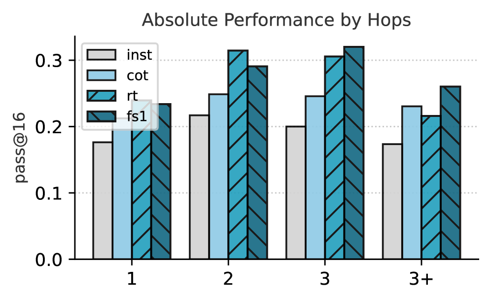
### Visual Description
\n
## Grouped Bar Chart: Absolute Performance by Hops
### Overview
This is a grouped bar chart titled "Absolute Performance by Hops." It compares the performance of four different methods or models (labeled "inst", "cot", "rt", and "fs1") across four categories of increasing complexity, defined by the number of "hops" (1, 2, 3, and 3+). Performance is measured by the metric "pass@16" on the y-axis.
### Components/Axes
* **Title:** "Absolute Performance by Hops" (centered at the top).
* **Y-Axis:**
* **Label:** "pass@16" (rotated vertically on the left).
* **Scale:** Linear scale from 0.0 to 0.3, with major tick marks at 0.0, 0.1, 0.2, and 0.3.
* **X-Axis:**
* **Categories (Hops):** Four discrete groups labeled "1", "2", "3", and "3+".
* **Legend:** Located in the top-left corner of the plot area. It defines four data series:
1. `inst`: Light gray solid bar.
2. `cot`: Light blue solid bar.
3. `rt`: Teal bar with diagonal hatching (stripes running from top-left to bottom-right).
4. `fs1`: Darker teal bar with diagonal hatching (stripes running from top-right to bottom-left).
### Detailed Analysis
The chart displays the approximate "pass@16" values for each method within each hop category. Values are estimated based on bar height relative to the y-axis grid lines.
**Hop 1:**
* `inst` (light gray): ~0.18
* `cot` (light blue): ~0.24
* `rt` (teal, hatched): ~0.23
* `fs1` (dark teal, hatched): ~0.24
**Hop 2:**
* `inst`: ~0.22
* `cot`: ~0.25
* `rt`: ~0.31
* `fs1`: ~0.29
**Hop 3:**
* `inst`: ~0.20
* `cot`: ~0.25
* `rt`: ~0.305
* `fs1`: ~0.315
**Hop 3+:**
* `inst`: ~0.175
* `cot`: ~0.23
* `rt`: ~0.215
* `fs1`: ~0.26
### Key Observations
1. **Performance Peak:** The highest overall performance is achieved by the `fs1` method at 3 hops (~0.315) and the `rt` method at 2 hops (~0.31).
2. **Method Trends:**
* `inst`: Performance increases from 1 to 2 hops, then declines at 3 and 3+ hops.
* `cot`: Performance is relatively stable between 1, 2, and 3 hops (~0.24-0.25), then drops at 3+ hops.
* `rt`: Shows a strong peak at 2 hops, with lower performance at 1, 3, and especially 3+ hops.
* `fs1`: Performance increases steadily from 1 to 3 hops, peaking at 3, before declining at 3+ hops.
3. **Relative Performance:** At lower complexity (1 hop), `cot`, `rt`, and `fs1` perform similarly and better than `inst`. At medium complexity (2-3 hops), `rt` and `fs1` clearly outperform `inst` and `cot`. At the highest complexity (3+ hops), `fs1` maintains the lead, while `rt` performance drops significantly.
### Interpretation
This chart visualizes how different reasoning or execution strategies ("inst", "cot", "rt", "fs1") scale with problem complexity, measured in "hops" (likely representing reasoning steps or dependencies).
* **Scalability:** The data suggests that the `fs1` strategy scales the most robustly, maintaining the highest performance at the most complex level (3+ hops). The `rt` strategy is highly effective for medium complexity (2 hops) but does not scale as well to the highest complexity.
* **Strategy Effectiveness:** There is no single best strategy for all complexity levels. The optimal choice depends on the expected number of hops. `cot` and `inst` are consistently outperformed by `rt` and `fs1` at medium to high complexities.
* **The "3+" Category:** The drop in performance for all methods at the "3+" category indicates a significant increase in difficulty beyond 3 hops, posing a challenge for all evaluated strategies. The fact that `fs1` retains the highest performance here suggests it may have architectural or methodological advantages for handling very complex, multi-step problems.
The metric "pass@16" likely measures success rate (e.g., solving a problem correctly in 16 attempts), so higher values are better. The chart effectively communicates that problem complexity (hops) is a critical factor in determining which AI reasoning method will be most successful.
</details>
(a) Performance by number of hops required to answer the question measured in pass@ $16$ .
<details>
<summary>x9.png Details</summary>
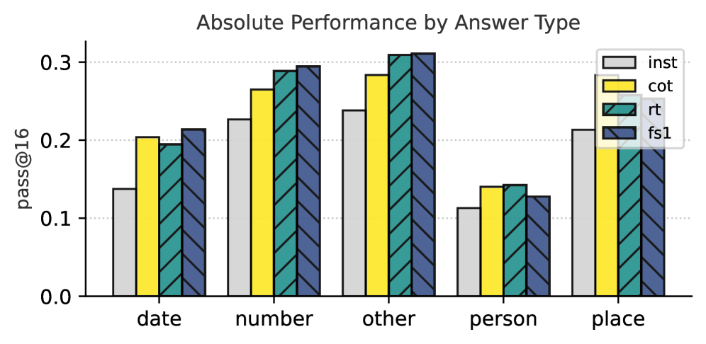
### Visual Description
## Grouped Bar Chart: Absolute Performance by Answer Type
### Overview
The image displays a grouped bar chart titled "Absolute Performance by Answer Type." It compares the performance of four different methods (inst, cot, rt, fs1) across five categories of answers (date, number, other, person, place). Performance is measured by the metric "pass@16" on the y-axis.
### Components/Axes
* **Chart Title:** "Absolute Performance by Answer Type" (centered at the top).
* **Y-Axis:**
* **Label:** "pass@16"
* **Scale:** Linear scale from 0.0 to 0.3, with major tick marks at 0.0, 0.1, 0.2, and 0.3.
* **X-Axis:**
* **Categories (from left to right):** "date", "number", "other", "person", "place".
* **Legend:** Located in the top-right corner of the chart area. It defines four data series:
* `inst`: Light gray solid bar.
* `cot`: Yellow solid bar.
* `rt`: Teal bar with diagonal stripes (top-left to bottom-right).
* `fs1`: Dark blue bar with diagonal stripes (top-left to bottom-right).
### Detailed Analysis
The chart presents the approximate "pass@16" values for each method within each answer category. Values are visual estimates.
**1. Category: date**
* `inst` (light gray): ~0.14
* `cot` (yellow): ~0.20
* `rt` (teal striped): ~0.19
* `fs1` (blue striped): ~0.21
* *Trend:* `cot`, `rt`, and `fs1` perform similarly and notably better than `inst`.
**2. Category: number**
* `inst` (light gray): ~0.23
* `cot` (yellow): ~0.27
* `rt` (teal striped): ~0.29
* `fs1` (blue striped): ~0.30
* *Trend:* A clear ascending trend from `inst` to `fs1`. This category shows the highest overall performance levels.
**3. Category: other**
* `inst` (light gray): ~0.24
* `cot` (yellow): ~0.29
* `rt` (teal striped): ~0.31
* `fs1` (blue striped): ~0.31
* *Trend:* Similar to "number," with `inst` lowest and `rt`/`fs1` tied for highest. This category contains the highest single value on the chart (~0.31).
**4. Category: person**
* `inst` (light gray): ~0.11
* `cot` (yellow): ~0.14
* `rt` (teal striped): ~0.14
* `fs1` (blue striped): ~0.13
* *Trend:* This is the lowest-performing category overall. All methods score below 0.15. `cot` and `rt` are nearly tied, with `fs1` slightly lower.
**5. Category: place**
* `inst` (light gray): ~0.21
* `cot` (yellow): ~0.28
* `rt` (teal striped): ~0.19
* `fs1` (blue striped): ~0.25
* *Trend:* This category shows the most variation between methods. `cot` performs best, followed by `fs1`. Notably, `rt` performs worse here than in any other category except "person."
### Key Observations
1. **Method Performance Hierarchy:** Across most categories ("date", "number", "other"), the performance order is generally `inst` < `cot` < `rt` ≈ `fs1`. The "place" category is an exception where `cot` leads.
2. **Category Difficulty:** The "person" category is consistently the most challenging for all methods. The "number" and "other" categories yield the highest performance scores.
3. **Consistency of `rt` and `fs1`:** The two striped-bar methods (`rt` and `fs1`) are often the top performers and track closely together, except in the "place" category where `rt` underperforms.
4. **`inst` as Baseline:** The `inst` method (light gray) is consistently the lowest or among the lowest performers in every category, suggesting it may be a baseline or simpler approach.
### Interpretation
This chart likely evaluates different prompting or reasoning techniques (e.g., `cot` could be "Chain-of-Thought," `fs1` could be "Few-Shot 1") for a language model or AI system on a task requiring specific answer types. The "pass@16" metric suggests a pass rate or success probability given 16 attempts or samples.
The data demonstrates that the choice of method significantly impacts performance, and the optimal method depends on the answer type. Techniques like `cot`, `rt`, and `fs1` provide substantial gains over the `inst` baseline for most categories. The pronounced difficulty with "person" answers indicates a specific weakness in the underlying model or task formulation for that entity type. The anomaly in the "place" category, where `rt` underperforms, warrants investigation—it may suggest that the `rt` method is less robust for spatial or location-based reasoning compared to numerical or temporal reasoning. Overall, the chart provides a clear comparative analysis to guide method selection based on the expected output type.
</details>
(b) Performance by answer type (i.e., what type of entity the answer is) in pass@ $16$ .
<details>
<summary>x10.png Details</summary>
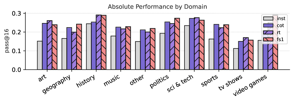
### Visual Description
## Grouped Bar Chart: Absolute Performance by Domain
### Overview
The image displays a grouped bar chart titled "Absolute Performance by Domain." It compares the performance of four different methods or models (labeled `inst`, `cot`, `rt`, and `fs1`) across ten distinct knowledge domains. Performance is measured by the metric "pass@16" on the y-axis.
### Components/Axes
* **Chart Title:** "Absolute Performance by Domain" (centered at the top).
* **Y-Axis:**
* **Label:** "pass@16" (rotated vertically on the left).
* **Scale:** Linear scale from 0.0 to 0.3, with major tick marks at 0.0, 0.1, 0.2, and 0.3.
* **X-Axis:**
* **Categories (Domains):** Ten categories listed from left to right: `art`, `geography`, `history`, `music`, `other`, `politics`, `sci & tech`, `sports`, `tv shows`, `video games`.
* **Legend:** Located in the top-right corner of the chart area. It defines the four data series:
* `inst`: Light gray solid fill.
* `cot`: Purple solid fill.
* `rt`: Purple fill with diagonal black stripes (hatching).
* `fs1`: Pink/salmon fill with diagonal black stripes (hatching).
### Detailed Analysis
The following table reconstructs the approximate "pass@16" values for each method within each domain. Values are estimated from the bar heights relative to the y-axis grid lines.
| Domain | `inst` (Gray) | `cot` (Purple) | `rt` (Striped Purple) | `fs1` (Striped Pink) |
| :--- | :--- | :--- | :--- | :--- |
| **art** | ~0.15 | ~0.25 | ~0.26 | ~0.24 |
| **geography** | ~0.16 | ~0.22 | ~0.20 | ~0.24 |
| **history** | ~0.24 | ~0.25 | ~0.29 | ~0.29 |
| **music** | ~0.18 | ~0.22 | ~0.21 | ~0.23 |
| **other** | ~0.15 | ~0.21 | ~0.19 | ~0.22 |
| **politics** | ~0.19 | ~0.25 | ~0.24 | ~0.27 |
| **sci & tech** | ~0.23 | ~0.27 | ~0.28 | ~0.26 |
| **sports** | ~0.16 | ~0.24 | ~0.22 | ~0.24 |
| **tv shows** | ~0.11 | ~0.15 | ~0.17 | ~0.16 |
| **video games** | ~0.15 | ~0.14 | ~0.16 | ~0.15 |
**Trend Verification per Data Series:**
* **`inst` (Gray):** Generally the lowest-performing method across most domains. Shows a notable peak in `history` (~0.24) and `sci & tech` (~0.23), and a significant dip in `tv shows` (~0.11).
* **`cot` (Purple):** Consistently performs in the mid-to-high range. Its trend is relatively stable, with values mostly between 0.20 and 0.27, except for lower performance in `tv shows` and `video games`.
* **`rt` (Striped Purple):** Often performs similarly to or slightly better than `cot`. It achieves the highest single value on the chart in `history` (~0.29). Its performance dips in `tv shows` and `video games`.
* **`fs1` (Striped Pink):** Frequently the top or tied-for-top performer, especially in `history`, `politics`, and `geography`. It shows a similar pattern of lower scores in `tv shows` and `video games`.
### Key Observations
1. **Domain Performance Hierarchy:** The domains `history` and `sci & tech` show the highest overall performance across all methods, with multiple bars reaching or exceeding 0.25. Conversely, `tv shows` and `video games` are the lowest-performing domains, with all methods scoring below 0.20.
2. **Method Comparison:** The `inst` method is consistently outperformed by the other three methods (`cot`, `rt`, `fs1`) in every domain except `video games`, where all methods perform similarly poorly.
3. **Top Performers:** The `fs1` and `rt` methods (both with striped patterns) frequently achieve the highest scores within a domain, particularly in `history` (tied at ~0.29) and `politics` (`fs1` leads).
4. **Notable Outlier:** The `history` domain is an outlier for the `rt` method, which shows a dramatic spike to ~0.29, its highest value by a significant margin.
### Interpretation
This chart likely evaluates the efficacy of different prompting or reasoning techniques (e.g., `inst`=Instruction, `cot`=Chain-of-Thought, `rt`=Reasoning Tree, `fs1`=Few-Shot 1) on a question-answering or knowledge-retrieval task, measured by the "pass@16" metric (possibly the probability of a correct answer within 16 attempts).
The data suggests that **domain knowledge significantly impacts model performance**. Abstract or culturally nuanced domains like `history` and `sci & tech` yield higher scores, possibly because they contain more structured or factual information within the model's training data. In contrast, domains like `tv shows` and `video games`, which may rely on pop culture, temporal trends, or highly specific details, prove more challenging for all methods.
Furthermore, the **technique matters**. The consistent underperformance of `inst` indicates that simple instructions are less effective than more structured reasoning approaches (`cot`, `rt`) or examples (`fs1`). The strong performance of `fs1` and `rt` implies that providing a reasoning framework or a single example can substantially boost accuracy across diverse topics. The chart effectively demonstrates that both the *subject matter* and the *problem-solving strategy* are critical determinants of success.
</details>
(c) Performance measured per domain in pass@ $16$ .
Figure 13: Absolute Performance across Different Axes. We show the absolute performance at pass@ $16$ of different versions of Qwen-32B (i.e., instruct, CoT, rt and fs1). In (a), we show the performance of the models by answer type. In (b), we show the performance of the models by the number of hops required to answer the question. In (c), we show the performance by domain of the question.