2505.13737

# Causal Head Gating: A Framework for Interpreting Roles of Attention Heads in Transformers **Authors**: - Andrew J. Nam (Princeton Laboratory for AI) - Natural and Artificial Minds (Princeton University) - &Henry C. Conklin (Princeton Laboratory for AI) - Natural and Artificial Minds (Princeton University) - &Yukang Yang (Department of Electrical and Computer Engineering) - &Thomas L. Griffiths (Department of Psychology) - &Jonathan D. Cohen (Princeton Neuroscience Institute) - &Sarah-Jane Leslie (Department of Philosophy) > Equal contribution; authors listed alphabetically ## Abstract We present causal head gating (CHG), a scalable method for interpreting the functional roles of attention heads in transformer models. CHG learns soft gates over heads and assigns them a causal taxonomy—facilitating, interfering, or irrelevant—based on their impact on task performance. Unlike prior approaches in mechanistic interpretability, which are hypothesis-driven and require prompt templates or target labels, CHG applies directly to any dataset using standard next-token prediction. We evaluate CHG across multiple large language models (LLMs) in the Llama 3 model family and diverse tasks, including syntax, commonsense, and mathematical reasoning, and show that CHG scores yield causal, not merely correlational, insight validated via ablation and causal mediation analyses. We also introduce contrastive CHG, a variant that isolates sub-circuits for specific task components. Our findings reveal that LLMs contain multiple sparse task-sufficient sub-circuits, that individual head roles depend on interactions with others (low modularity), and that instruction following and in-context learning rely on separable mechanisms. ## 1 Introduction Large language models (LLMs) achiam2023gpt ; liu2024deepseek ; grattafiori2024llama represent state-of-the-art systems across a wide array of domains, exhibiting remarkable generalization and problem-solving capabilities. Yet, as these models grow in scale and complexity, they become increasingly opaque, making it more difficult to understand, predict, or control their behavior, which raises concerns about safety and misuse bommasani2021opportunities ; wei2023jailbroken ; weidinger2024holistic . This has motivated a growing body of work on interpretability, which seeks to better understand how LLMs learn and represent information, and how their responses can be shaped (tenney2019bert, ; bricken2023towards, ). Interest has focused in particular on transformer-based architectures vaswani2017attention such as GPT achiam2023gpt , LLaMA grattafiori2024llama , Gemma team2025gemma , and DeepSeek liu2024deepseek , in which the central processing blocks consist of multi-head attention followed by multi-layer perceptrons. Here, there has been considerable research on the roles of individual attention heads, which have been found to exhibit some level of human-interpretability elhage2021mathematical ; todd2023function ; yang2025emergent . Two broad categories of approaches dominate research on mechanistic interpretability in LLMs. The first uses a trained mapping from latent representations to human-interpretable concepts, such as syntactic features tenney2019bert ; tenney2019you ; hewitt2019structural or identifiable items (e.g., the Golden Gate Bridge templeton2024scaling ). The second uses causal interventions to identify portions of a single weight matrix or individual attention heads responsible for a specific behavior (lee2024mechanistic, ; voita2019analyzing, ). These approaches often focus on small portions of a model, ‘zooming in’ (olah2020zoom, ) in an effort to interpret the role of a single computational subgraph. However, in deep-learning models, computation is often distributed hinton1986learning and the role of one component is dependent on another elhage2022superposition ; fakhar2022systematic ; giallanza2024integrated , making the behavior of such complex distributed systems difficult to predict from an understanding of their parts alone (mitchell2009complexity, ). To apply a distributed perspective to mechanistic interpretability, we introduce causal head gating (CHG) which identifies a parametrically weighted set of heads that contribute to a model’s execution of a given task. Given a dataset that defines a task, we fit a set of gating values for each attention head that applies a soft ablation to its output using next-token prediction, so that task-facilitating heads remain unaltered while any task-interfering heads are suppressed. Using a simple regularization procedure that further separates irrelevant heads from those that facilitate or interfere with task performance, CHG assigns meaningful scores to each attention head across an entire model according to its task contribution. We use these scores to define a taxonomy of task relevance according to how individual attention heads contribute to a model’s distributed computation of a given task, describing each head as facilitating, interfering or irrelevant. In this respect, CHG offers an exploratory complement to standard hypothesis-driven approaches to mechanistic interpretability, assigning causal roles without relying on predefined hypotheses about what each head might be doing. Beyond its conceptual contribution, CHG also offers several practical methodological advantages over existing mechanistic interpretability tools. First, because CHG operates directly on next-token prediction, it avoids the need for externally-provided labels tenney2019bert ; tenney2019you ; hewitt2019structural ; templeton2024scaling , controlled input-output pairs tenney2019bert ; tenney2019you ; hewitt2019structural , or rigid prompt templates wang2022interpretability ; todd2023function ; yang2025emergent , which are often required for decoding and interventional approaches. Second, CHG naturally accommodates complex target outputs, including chain-of-thought reasoning wei2022chain , where the solution spans multiple intermediate steps. Finally, CHG is highly scalable: it introduces only one learnable parameter per attention head and requires no updates to the underlying model weights, so that the CHG parameters can be fitted in minutes using gradient-based optimization, even for LLMs with billions of parameters. Thus, in settings where analyzing complex dependencies between heads is important, it is feasible to fit large samples of CHG values to estimate a distribution over gating values in a bootstrap fashion. To test its efficacy, we apply CHG across a diverse set of tasks—mathematical, commonsense, and syntactic reasoning—and across LLMs ranging from 1 to 8 billion parameters with varying training paradigms. We use CHG to analyze not only where specific computations take place, but also how distributed they are across attention heads, and how these patterns vary across different tasks and models. We also validate the causal scores produced by CHG by comparing them against targeted ablations as well as causal mediation analysis todd2023function ; wang2022interpretability , showing strong agreement between predicted and observed effects. Finally, we extend CHG to a contrastive setting to identify distinct sub-circuits that support instruction following versus in-context learning, suggesting that even semantically similar tasks can be underpinned by separable mechanisms. Our main contributions are fourfold: 1. We introduce causal head gating (CHG), a parametric, scalable method for identifying potentially distributed, task-relevant sub-circuits in transformer models without requiring prompt templates or labeled outputs, and extend it with contrastive CHG to isolate heads supporting specific sub-tasks. 1. We propose a simple causal taxonomy of heads—facilitating, interfering, and irrelevant—that quantifies the effect of each on task performance using CHG-derived scores. 1. We use CHG to show that models contain multiple task-sufficient sub-circuits with varying degrees of overlap, suggesting head roles are not fully modular but depend on interactions with other heads. 1. We use CHG to show that instruction following and in-context learning rely on context-dependent separable circuits at the head level, where CHG-guided gating can selectively suppress one mode without substantially disrupting the other. The accompanying repository for this paper can be found at https://github.com/andrewnam/causal_head_gating. ## 2 Related Work #### Representational decoders Representational decoders are models trained to map hidden activations to externally labeled properties tenney2019bert ; tenney2019you ; hewitt2019structural , estimating the mutual information between representations and those properties belinkov2022probing ; pimentel2020information . However, such probing results are difficult to interpret: simpler decoders may underfit and miss relevant features (false negatives), while complex decoders may overfit and learn spurious correlations (false positives) hewitt2019designing ; voita2020information , requiring complexity-accuracy tradeoffs to contextualize results voita2020information . Moreover, although decodability indicates that a property is encoded in the representation, it does not imply that the model uses that information for its task, highlighting a correlational finding rather than a causal one ravichander2020probing . Finally, representational decoders require labeled datasets, constraining their use to curated, predefined properties. For a comprehensive review of the probing framework and its limitations, see belinkov2022probing . Sparse autoencoders (SAE) can be viewed as a related approach, where the autoencoder reconstructs representations through a sparse bottleneck to reveal modular or interpretable features templeton2024scaling ; cunningham2023sparse . However, like probing classifiers, their insights remain correlational and still depend on post hoc labeling or interpretation, inheriting the same supervision bottleneck. In contrast, CHG performs direct interventions on model components without external supervision and proposes sufficient sub-circuits to the default unablated model, thereby identifying causal links between attention heads and model behavior on a task. #### Causal mediation analysis Causal mediation analysis (CMA) vig2020investigating ; meng2022locating is used to identify the functional roles of specific attention heads by crafting controlled prompt pairs that isolate a hypothesized behavior, then intervening on model components to measure their causal effect on outputs. For instance, in the indirect-object-identification (IOI) task wang2022interpretability , sentences like “When Alice and John went to the store, John gave a drink to…” are used to identify attention heads responsible for resolving coreference. By patching specific head outputs from a source sentence into a structurally matched target, and checking whether the model changes its prediction (e.g. “Alice” instead of “Mary”), CMA localizes the relevant circuit. It has also uncovered head-level roles in function tracking todd2023function , symbol abstraction yang2025emergent , and other structured settings zhengattention . However, CMA relies on manually crafted prompt templates and clear mechanistic hypotheses, which limits its scalability to more complex domains. In open-ended tasks like mathematical reasoning cobbe2021gsm8k ; hendrycks2021measuring ; toshniwal2024openmathinstruct , the diversity of required knowledge makes it hard to design effective controlled inputs. A single shared template is unlikely to accommodate even two prompts from the MATH dataset hendrycks2021measuring , such as: “If $∑_n=0^∞\cos^2nθ=5$ , what is $\cos 2θ$ ?” and “The equation $x^2+2x=i$ has two complex solutions; determine the product of their real parts.” Moreover, LLMs often solve such problems most effectively via chain-of-thought reasoning wei2022chain , which unfolds over multiple steps, further complicating the use of a unified prompt structure. #### Head ablations Despite the use of multiple heads being commonplace in transformer-based architectures, it has been observed that multiple, and sometimes the majority of, heads can be entirely pruned with minimal impact on model performance michel2019sixteen ; voita2019analyzing ; li2021differentiable ; xia2022structured . Moreover, entire layers can be pruned while retaining model performance fan2019reducing ; sajjad2023effect ; he2024matters . However, existing works on pruning attention heads have focused primarily on custom-trained small-scale transformers michel2019sixteen ; voita2019analyzing ; li2021differentiable or BERT-based devlin2019bert models xia2022structured ; sajjad2023effect , and the literature is limited for modern causal LLMs such as GPT brown2020language ; achiam2023gpt and Llama grattafiori2024llama . Head pruning has also been used to validate findings from other interpretability methods, such as CMA wang2022interpretability ; yang2025emergent or attention pattern analysis voita2019analyzing . In these studies, researchers first identify heads believed to perform specific functions, then ablate them to test their causal impact. Such targeted ablations often lead to disproportionate drops in performance, supporting the hypothesis that those heads are functionally important. Most closely related to our work are differentiable masking and soft-gating approaches that learn which attention heads to retain or suppress. In de2020decisions , the authors apply sparsity gating to identify subcircuits and use the fitted parameters as weighting values in convex combinations for activation patching. Similarly, yin2024lofit learns scaling constants for each attention head, but uses the fitted values to identify heads that are most suitable for fine-tuning. Thus, while methodologically similar, our work is unique in applying the gating parameters to identify task-sufficient causal sub-circuits. Others voita2019analyzing ; li2021differentiable have opted for hard, binary ablations using the Gumbel-softmax trick jang2016categorical ; maddison2016concrete , fitting gating probabilities rather than weighting parameters. Although these Gumbel-based approaches have been applied for causal circuit discovery in a similar spirit to our work, they suffer from a fundamental limitation that CHG does not. Specifically, while Gumbel-based gating methods also learn differentiable gates per head, they treat each head independently, effectively learning separate Gumbel–Bernoulli distributions for head inclusion. This factorized formulation models only marginal probabilities and cannot capture interdependencies between heads that jointly affect task performance. In contrast, CHG jointly optimizes all gating coefficients under the model’s loss, capturing the full range of interactions and contingencies between the attention heads. Because CHG is highly scalable, it can be fit repeatedly across random seeds or subsets, effectively sampling from the space of sub-circuits without assuming independence between heads. This enables estimation of the underlying distribution over functional head configurations while preserving the joint statistical structure that factorized gating approaches discard. ## 3 Our Approach: Causal Head Gating Causal head gating is based on three ideas: applying multiplicative gates to attention heads to evaluate their roles, using regularization to produce variation in the estimates of the gating parameters, and constructing a taxonomy based on that variation. We introduce these ideas in turn. ### 3.1 Applying gates to attention heads <details> <summary>figures/concept.png Details</summary>  ### Visual Description ## [Multi-Panel Technical Figure]: Gating Mechanism in Multi-Head Attention ### Overview This image is a three-panel technical figure (labeled a, b, c) illustrating a gating mechanism for multi-head attention layers in a neural network. Panel (a) is a schematic diagram of the architecture. Panel (b) is a line chart showing the evolution of gate values during training. Panel (c) is a scatter plot analyzing the relationship between two gate metrics across different layers and head types. ### Components/Axes **Panel (a): Schematic Diagram** * **Top Component:** A blue rounded rectangle labeled **\( W_l^O \)** (Output projection weight matrix for layer \( l \)). * **Middle Components:** Three orange circles representing gates, labeled **\( G_{l,1} \)**, **\( G_{l,h} \)**, and **\( G_{l,H} \)**. Each has an upward-pointing green arrow connecting it to the \( W_l^O \) block. * **Bottom Components:** Three green rounded rectangles representing attention head outputs, labeled **\( A_{l,1}V_{l,1} \)**, **\( A_{l,h}V_{l,h} \)**, and **\( A_{l,H}V_{l,H} \)**. Each has a downward-pointing green arrow connecting it to the corresponding gate above. * **Ellipsis:** The notation "..." between the bottom and middle components indicates there are \( H \) total heads in the layer. **Panel (b): Line Chart - Gate Value vs. Gradient Updates** * **X-axis:** **Gradient Updates**. Scale: 0 to 1000, with major ticks at 0, 250, 500, 750, 1000. * **Y-axis:** **Gate Value**. Scale: 0.00 to 1.00, with major ticks at 0.00, 0.25, 0.50, 0.75, 1.00. * **Legend (Top-Right):** * **Regularization:** Three line styles. * Dotted line: **\( \lambda < 0 \)** * Solid line: **\( \lambda = 0 \)** * Dash-dot line: **\( \lambda > 0 \)** * **Head Type:** Three colors. * Green line: **Facilitating** * Blue line: **Irrelevant** * Red/Salmon line: **Interfering** **Panel (c): Scatter Plot - \( G^+ \) vs. \( G^- \)** * **X-axis:** **\( G^- \)**. Scale: 0.00 to 1.00, with major ticks at 0.00, 0.25, 0.50, 0.75, 1.00. * **Y-axis:** **\( G^+ \)**. Scale: 0.00 to 1.00, with major ticks at 0.00, 0.25, 0.50, 0.75, 1.00. * **Color Bar (Far Right):** Labeled **Layer**. Scale from 0 (dark purple) to 25 (bright yellow), with ticks at 0, 5, 10, 15, 20, 25. * **Annotations:** * **Facilitating:** Green text and arrow pointing to a dense cluster of points in the top-right corner (high \( G^- \), high \( G^+ \)). * **Irrelevant:** Blue text and arrow pointing to a cluster of points along the top-left edge (low \( G^- \), high \( G^+ \)). * **Interfering:** Red text and arrow pointing to a cluster of points in the bottom-left corner (low \( G^- \), low \( G^+ \)). ### Detailed Analysis **Panel (b) - Trend Verification:** 1. **Facilitating Head (Green Line):** Starts at a gate value of ~0.6. Shows a sharp, near-vertical increase within the first ~50 gradient updates to a value of ~0.98. It then plateaus, maintaining a value very close to 1.00 for the remainder of training (up to 1000 updates). The line is solid (\( \lambda = 0 \)). 2. **Irrelevant Head (Blue Line):** Starts at a gate value of ~0.4. It initially dips to ~0.15 within the first ~50 updates. It then begins a steady, roughly linear increase, reaching ~0.4 by 500 updates. At exactly 500 updates, it jumps vertically to 1.00 and plateaus. The line is dotted (\( \lambda < 0 \)) before 500 updates and becomes dash-dot (\( \lambda > 0 \)) after. 3. **Interfering Head (Red/Salmon Line):** Starts at a gate value of ~0.35. It shows a sharp, exponential decay, dropping to near 0.00 by ~150 updates. It remains flat at ~0.00 for the rest of training. The line is solid (\( \lambda = 0 \)). **Panel (c) - Data Point Distribution:** * **Facilitating Cluster (Top-Right):** A very dense horizontal band of points is located at \( G^+ \approx 1.00 \), spanning \( G^- \) values from ~0.25 to 1.00. The points are predominantly yellow and light green, indicating they belong to higher layers (approximately layers 15-25). * **Irrelevant Cluster (Top-Left):** A vertical band of points is located at \( G^- \approx 0.00 \), spanning \( G^+ \) values from ~0.00 to 1.00. The colors are mixed, but many points in the upper part of this band (\( G^+ > 0.5 \)) are blue/teal, indicating mid-range layers (approximately layers 5-15). * **Interfering Cluster (Bottom-Left):** A small, tight cluster of points is located near the origin (\( G^- \approx 0.00, G^+ \approx 0.00 \)). These points are dark purple, indicating they belong to the earliest layers (layers 0-5). * **Scattered Points:** There are approximately 15-20 scattered points in the central region of the plot (\( G^- \) between 0.25-0.75, \( G^+ \) between 0.25-0.60). These points are mostly teal and green (layers 10-20). ### Key Observations 1. **Clear Behavioral Dichotomy:** The gating mechanism successfully learns to assign drastically different values to different head types: near 1.0 for Facilitating, near 0.0 for Interfering, and a delayed jump to 1.0 for Irrelevant. 2. **Layer-Dependent Specialization:** Panel (c) strongly suggests that head type is correlated with layer depth. Early layers (0-5) contain "Interfering" heads. Mid-layers (5-15) contain "Irrelevant" heads. Later layers (15-25) are dominated by "Facilitating" heads. 3. **Training Dynamics:** The "Irrelevant" head's gate value is sensitive to a change in regularization (from \( \lambda < 0 \) to \( \lambda > 0 \)) at 500 updates, which triggers its suppression (gate value jumps to 1.0, effectively deactivating it). 4. **Metric Relationship:** For "Facilitating" heads, high \( G^+ \) is associated with a wide range of \( G^- \) values. For "Irrelevant" heads, high \( G^+ \) is strictly associated with very low \( G^- \). ### Interpretation This figure demonstrates a method for dynamically gating (enabling or disabling) attention heads in a Transformer based on their functional role ("Facilitating," "Irrelevant," or "Interfering"). * **What the data suggests:** The system learns to identify and suppress harmful ("Interfering") heads early in training and in early network layers. It identifies "Irrelevant" heads (which may not contribute positively or negatively) and eventually suppresses them as well, but only after a specific training event (change in regularization). "Facilitating" heads, which are beneficial, are consistently activated (gate value ~1) and are primarily found in the deeper layers of the network. * **How elements relate:** Panel (a) defines the mechanism. Panel (b) shows the training-time behavior of the gates for each head type. Panel (c) provides a spatial analysis of the final gate states, revealing a clear architectural pattern: the network's early layers filter out noise/interference, middle layers handle neutral information, and deep layers perform the core facilitative processing. * **Notable Anomalies:** The sharp, discontinuous jump of the "Irrelevant" head's gate at 500 updates is a notable event, indicating a potential phase change in training or the effect of a scheduled hyperparameter. The scattered points in the middle of panel (c) may represent heads in transition or with ambiguous roles. 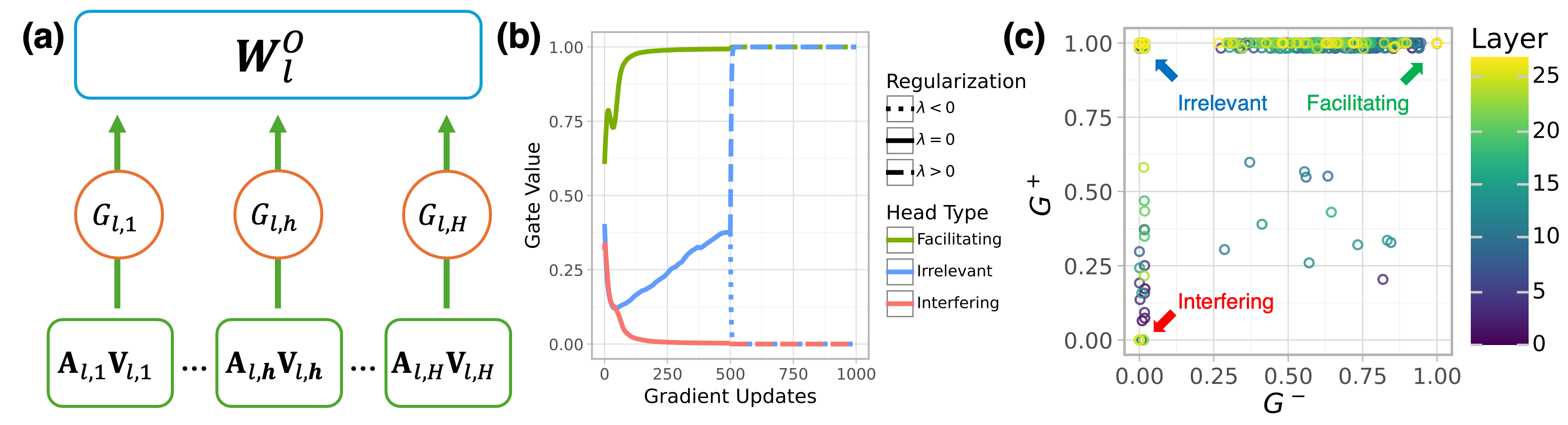</details> Figure 1: (a) Schematic of a single multihead attention block with CHG-determined gating attenuation (in red). (b) Gate fitting trajectories for three heads on L3.2-3BI with OpenMathInstruct2. When fitting with $λ<0$ and $λ>0$ , $G^+$ and $G^-$ both stay near 1 for facilitating heads and near 0 for interfering heads, but bifurcate to 1 and 0 respectively for irrelevant heads. (c) Gate values after fitting. For a transformer with $L$ layers and $H$ attention heads, we define a gating matrix $G∈[0,1]^L× H$ , where $G_\ell,h$ scales the output of head $h$ in layer $\ell$ , just before the output projection matrix $W_\ell^O$ (shown in red for an example head in Figure 1 a). Given input hidden states $X∈ℝ^seq× d_\text{model}$ , each head computes: $$ A_\ell,h=softmax≤ft(\frac{XW_Q^\ell,h(XW_K^\ell,h)^⊤}{√{d_k}}\right), V_\ell,h=XW_V^\ell,h, Z_\ell,h=G_\ell,h·(A_\ell,hV_\ell,h) $$ where $W_Q^\ell,h,W_K^\ell,h,W_V^\ell,h∈ℝ^d_model× d_k$ are learned projection matrices for queries, keys, and values. The gating coefficient $G_\ell,h$ modulates the contribution of head $h$ by scaling its output $Z_\ell,h$ after attention is applied but before the heads are combined (see Figure 1 a). The gated outputs are then concatenated and projected: $$ Output_\ell=Concat(Z_\ell,1,\dots,Z_\ell,H)W^O_\ell, W^O_\ell∈ℝ^Hd_k× d_model $$ We fit $G$ by freezing the parameters of the model $M_θ$ and minimizing the negative log-likelihood (NLL) on a next-token prediction task with a regularization term specified below. Table 1: Causal taxonomy for head roles and corresponding gating patterns. | Role | Description | $G^+$ | $G^-$ | Metric | Ablation Effect | | --- | --- | --- | --- | --- | --- | | Facilitating | Supports task performance | High | High | $G^-$ | Decreases task performance | | Interfering | Interferes with task performance | Low | Low | $1-G^+$ | Increases task performance | | Irrelevant | Negligible impact on performance | High | Low | $G^+×(1-G^-)$ | No effect on task performance | ### 3.2 Producing variation through regularization We add a regularization term to the objective that introduces a small but consistent gradient—clipped to ensure NLL remains the dominant term—that nudges the gates for task-irrelevant heads toward 1 or 0 while leaving task-relevant ones relatively unaffected. The NLL optimizes towards improving task performance, and tunes the heads by either increasing the gating values for task-facilitating heads or decreasing the gating values for task-interfering heads. However, if a head does not affect task performance, i.e. is task-irrelevant, then the expected gradient from the NLL is 0, which confounds interpretation of task relevance when evaluating the tuned gating values: a gate $G_l,h$ may be close to 1 either because it is important for performing the task (causal), or because gating it has no effect (incidental). We address this limitation by introducing an $L_1$ -regularization term in our objective function, with weight $λ$ that either nudges gates toward 1 for maximal density ( $λ>0$ ) or toward 0 for maximal sparsity ( $λ<0$ ): $$ L(G;M_θ,D,λ)=\underbrace{-∑_(x,y)∈D\log P(y\mid x;M_θ,G)}_Negative log-likelihood (NLL)-\underbrace{λ∑_i,jσ^-1(G_l,h)}_Regularization \tag{1} $$ where $M_θ$ is the model being analyzed, $y$ is the target text sequence for a given prompt $x$ in dataset $D$ , and $σ^-1$ is the clipped inverse-sigmoid function. We fit $G$ twice: once with $λ>0$ to encourage retention ( $G^+$ ), and once with $λ<0$ to encourage removal ( $G^-$ ). To ensure that the heads are aligned across both optimizations, we first fit $G$ with $λ=0$ to establish a shared initialization (see Figure 1), so that any differences between $G^+$ and $G^-$ reflect only the effect of the regularization and not divergent optimization paths. ### 3.3 Constructing a taxonomy of task relevance The $G^+$ and $G^-$ matrices allow us to interpret the functional role of each head. To formalize this, we introduce a causal taxonomy (Table 1) in which each head is assigned one of three roles— facilitating, interfering, or irrelevant —based on its predicted impact on model performance under ablation. Facilitating heads positively contribute to performance, while ablating them degrades it. Conversely, interfering heads negatively contribute to performance, while ablating them improves it. Finally, irrelevant heads have negligible effect, with ablation leaving performance effectively unchanged. We instantiate this taxonomy using the fitted CHG matrices $G^+$ and $G^-$ , which reflect head behavior under opposing regularization pressures. Facilitation is measured by $G^-$ : heads that remain active despite pressure to suppress are likely necessary for the task. Interference is measured by $1-G^+$ : heads that are suppressed even under encouragement to remain are likely harmful. Irrelevance is measured via $G^-\odot(1-G^+)$ , identifying heads that vary in gate values based on regularization. ## 4 Experiments and analyses <details> <summary>x1.png Details</summary>  ### Visual Description ## Multi-Panel Line Chart: Impact of Ablating Attention Heads on Model Performance ### Overview The image displays a 3x4 grid of line charts (12 subplots total) illustrating how the performance of different Large Language Models (LLMs) changes as an increasing number of attention heads are "ablated" (likely disabled or removed). Performance is measured by the change in log probability of the target response. The charts are organized by model variant (columns) and evaluation domain (rows). ### Components/Axes * **Grid Structure:** * **Columns (Model Variants):** Labeled at the top of each column. From left to right: `L3.2-1B`, `L3.2-3B`, `L3.2-3B-I`, `L3.1-8B`. * **Rows (Evaluation Domains):** Labeled on the right side of the grid. From top to bottom: `Syntax`, `Common Sense`, `Math`. * **Axes:** * **X-axis (All subplots):** `Number of Ablated Heads`. Linear scale from 0 to 50, with major ticks at 0, 10, 20, 30, 40, 50. * **Y-axis (All subplots):** `Δ Log Probability of Target Response`. The scale varies by row: * **Syntax & Common Sense Rows:** Linear scale from approximately -3.5 to +1.5. Major ticks at -3, -2, -1, 0, 1. * **Math Row:** Linear scale from approximately -160 to +10. Major ticks at -150, -100, -50, 0. * **Legend:** Located on the far right of the image. Title: `Metric`. Contains three entries with corresponding line colors: * `Facilitation` - **Green line** * `Irrelevance` - **Blue line** * `Interference` - **Red line** ### Detailed Analysis **Trend Verification & Data Point Extraction (Approximate Values):** **Row 1: Syntax** * **L3.2-1B:** Green (Facilitation) starts near 0, declines steadily to ~-3.2 at 50 heads. Blue (Irrelevance) remains near 0 throughout. Red (Interference) fluctuates slightly above 0, peaking near +1 at ~15 heads, ending near 0. * **L3.2-3B:** Green declines to ~-2.2. Blue stays near 0. Red stays near 0 with minor fluctuations. * **L3.2-3B-I:** Green declines to ~-2.8. Blue stays near 0. Red shows a slight positive bump between 20-40 heads, peaking near +0.8. * **L3.1-8B:** Green declines to ~-1.2. Blue stays near 0. Red stays near 0. **Row 2: Common Sense** * **L3.2-1B:** Green declines to ~-3.0. Blue stays near 0. Red shows a small positive bump, peaking near +0.5 at ~25 heads. * **L3.2-3B:** Green declines to ~-2.0. Blue stays near 0. Red shows a positive bump, peaking near +1.0 at ~25 heads. * **L3.2-3B-I:** Green declines to ~-2.5. Blue stays near 0. Red shows a pronounced positive bump, peaking near +1.5 at ~20 heads. * **L3.1-8B:** Green declines to ~-1.0. Blue stays near 0. Red shows a positive bump, peaking near +1.2 at ~20 heads. **Row 3: Math** * **L3.2-1B:** Green shows a dramatic, steep decline, reaching ~-150 at 50 heads. Blue shows a slight negative trend, ending near -10. Red stays near 0. * **L3.2-3B:** Green declines steeply to ~-100. Blue stays near 0. Red stays near 0. * **L3.2-3B-I:** Green declines steeply to ~-150. Blue stays near 0. Red stays near 0. * **L3.1-8B:** Green declines to ~-80. Blue shows a slight positive bump early on. Red shows a positive bump, peaking near +20 at ~25 heads. ### Key Observations 1. **Dominant Negative Trend for Facilitation:** In every single subplot, the green line (`Facilitation`) shows a clear downward trend as more heads are ablated. This negative impact is most severe in the `Math` domain, where the y-axis scale is an order of magnitude larger. 2. **Stability of Irrelevance:** The blue line (`Irrelevance`) remains close to the zero baseline across nearly all conditions, indicating that ablating heads has minimal effect on this metric. 3. **Variable Impact on Interference:** The red line (`Interference`) shows varied behavior. It often remains near zero but exhibits notable positive bumps (improvement) in several `Common Sense` subplots and the `L3.1-8B` Math subplot. It rarely shows a negative trend. 4. **Model Size & Variant Differences:** The largest model (`L3.1-8B`) generally shows the least severe decline in `Facilitation` for `Syntax` and `Common Sense`. The `L3.2-3B-I` variant often shows more pronounced positive `Interference` bumps than its counterparts. 5. **Domain Sensitivity:** The `Math` domain is uniquely sensitive to head ablation for the `Facilitation` metric, with performance dropping catastrophically compared to `Syntax` and `Common Sense`. ### Interpretation This chart investigates the functional specialization of attention heads in LLMs by measuring the effect of their removal (`ablation`) on different types of reasoning tasks. * **What the data suggests:** The consistent, steep decline of the `Facilitation` metric indicates that a significant number of attention heads are crucial for the model to correctly generate or support the target response. Their removal directly harms performance. This effect is dramatically amplified for mathematical reasoning, suggesting that math tasks rely on a more fragile or distributed set of attentional mechanisms. * **Relationship between elements:** The `Irrelevance` metric acts as a control, showing that the ablation procedure itself doesn't randomly affect all predictions. The `Interference` metric's occasional positive bumps are intriguing; they suggest that in some contexts (especially common sense reasoning), removing certain heads might actually *reduce* the model's tendency to generate incorrect or interfering information, thereby improving the relative probability of the correct target. * **Notable anomalies:** The extreme scale of the `Math` y-axis is the most striking anomaly. It implies that mathematical correctness is highly vulnerable to the perturbation of the model's attention mechanism. The positive `Interference` bumps in `Common Sense` for the `3B-I` and `8B` models could indicate the presence of "counter-productive" heads that the model has learned to use for certain types of distractors. 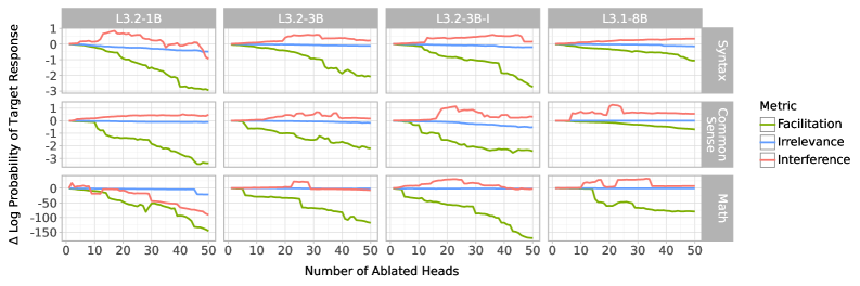**In summary, the visualization provides strong evidence that attention heads are not uniformly important; their necessity varies by task domain, with mathematical reasoning being particularly dependent on a large subset of heads for facilitation, while common sense reasoning may involve heads that sometimes introduce interference.** </details> Figure 2: Difference in target log-probability when sequentially setting individual gates in $G^+$ to 1 and 0 in order of facilitation, irrelevance, and interference scores. The horizontal axis shows the number of heads ablated in descending score order. Positive values indicate task improvement, negative values indicate degradation, and values near zero indicate no effect. Note that not all heads in the top 50 necessarily have high absolute scores. ### 4.1 Causal roles of attention heads We begin by reporting experiments that evaluated the causal taxonomy presented in Table 1 across four variants of the Llama 3 LLM grattafiori2024llama : L3.1-8B, a pre-trained 8B-parameter model; L3.2-3B, a 3B-parameter model distilled from Llama-3.1-70B (not used in this paper); L3.2-3BI, an instruction-tuned version of Llama-3.2-3B; and L3.2-1B, a 1B-parameter model distilled from L3.1-8B. For each model, we fit CHG matrices on three task types performed over distinct datasets: mathematical reasoning from OpenMathInstruct2 (toshniwal2024openmathinstruct, ), syntactic reasoning from the subset labeled “syntax” in BIG-Bench (srivastava2022beyond, ), and commonsense reasoning from CommonsenseQA (talmor2018commonsenseqa, ). We fit CHG matrices independently for each model-dataset pair across 10 random seeds. We first test whether the causal scores align with the taxonomy’s predictions about performance. Specifically, the taxonomy predicts that, when ablated, attention heads scoring highly on facilitation, irrelevance, or interference should decrease, leave unchanged, or increase the model’s task performance, respectively. To test this, we sort heads in descending order by each causal metric and evaluate the model using the $G^+$ matrix while toggling each head to 0 or 1 in order of its score. While both $G^+$ and $G^-$ match the context in which scores were computed, we use $G^+$ as it retains more heads, providing a more interpretable baseline for ablation. We then compare the retained and ablated masks by the model’s log-probability of the target sequence, expecting the resulting change in log-probability to follow the predicted pattern. As shown in Figure 2, these interventions match the predicted patterns: the difference in target log-probability is negative when progressively ablating facilitating heads, near 0 when ablating irrelevant heads, and positive when ablating interfering heads, up until the set of interfering heads is exhausted. ### 4.2 Distribution of causal roles <details> <summary>x2.png Details</summary>  ### Visual Description ## [Multi-Panel Line Chart]: Performance Proportion by Score Across Models and Domains ### Overview The image displays a 3x4 grid of line charts, labeled as panel (a). It visualizes the performance of four different language models across three cognitive domains. Each chart plots the "Proportion ≥ Score" (y-axis) against a normalized "Score" (x-axis, ranging from 0 to 1). The data is broken down by three experimental conditions, represented by colored lines. ### Components/Axes * **Overall Grid Structure:** * **Columns (Models):** Four columns, each headed by a model identifier in a gray box at the top: `L3.2-1B`, `L3.2-3B`, `L3.2-3B-I`, `L3.1-8B`. * **Rows (Domains):** Three rows, each labeled on the right side in a vertical gray box: `Syntax` (top row), `Common Sense` (middle row), `Math` (bottom row). * **Axes (for each subplot):** * **Y-axis:** Labeled "Proportion ≥ Score" on the far left of the grid. Scale is marked at 0%, 50%, and 100%. * **X-axis:** Labeled "Score" at the bottom center of the grid. Scale is marked at 0, 0.5, and 1. * **Legend:** Positioned at the bottom center of the entire figure. It defines three colored lines: * **Green line:** `Facilitation` * **Blue line:** `Irrelevance` * **Red line:** `Interference` ### Detailed Analysis The following describes the trend for each line in each subplot. Values are approximate visual estimates. **Row 1: Syntax** * **L3.2-1B:** Blue (Irrelevance) starts near 100% at Score=0, declines steadily to ~50% at Score=1. Green (Facilitation) starts near 40%, declines to near 0%. Red (Interference) starts near 20%, declines to near 0%. * **L3.2-3B:** Blue starts near 100%, declines to ~50%. Green starts near 35%, declines to near 0%. Red starts near 20%, declines to near 0%. * **L3.2-3B-I:** Blue starts near 100%, declines to ~50%. Green starts near 35%, declines to near 0%. Red starts near 20%, declines to near 0%. * **L3.1-8B:** Blue starts near 100%, declines to ~50%. Green starts near 35%, declines to near 0%. Red starts near 20%, declines to near 0%. **Row 2: Common Sense** * **L3.2-1B:** Blue starts near 100%, declines to ~70%. Green starts near 20%, declines to near 0%. Red starts near 15%, declines to near 0%. * **L3.2-3B:** Blue starts near 100%, declines to ~50%. Green starts near 40%, declines to near 0%. Red starts near 20%, declines to near 0%. * **L3.2-3B-I:** Blue starts near 100%, declines to ~60%. Green starts near 30%, declines to near 0%. Red starts near 15%, declines to near 0%. * **L3.1-8B:** Blue starts near 100%, declines to ~50%. Green starts near 45%, declines to near 0%. Red starts near 15%, declines to near 0%. **Row 3: Math** * **L3.2-1B:** Blue starts near 100%, declines sharply to near 0% by Score=0.7. Green starts near 90%, declines to near 0% by Score=1. Red starts near 20%, declines to near 0%. * **L3.2-3B:** Blue starts near 100%, declines to near 0% by Score=1. Green starts near 70%, declines to near 0% by Score=1. Red starts near 10%, declines to near 0%. * **L3.2-3B-I:** Blue starts near 100%, declines to near 0% by Score=1. Green starts near 65%, declines to near 0% by Score=1. Red starts near 10%, declines to near 0%. * **L3.1-8B:** Blue starts near 100%, declines to near 0% by Score=1. Green starts near 60%, declines to near 0% by Score=1. Red starts near 10%, declines to near 0%. ### Key Observations 1. **Consistent Hierarchy:** In nearly all charts, the blue line (Irrelevance) is the highest, followed by the green line (Facilitation), with the red line (Interference) consistently the lowest. 2. **Domain-Specific Behavior in Math:** The Math domain (bottom row) shows a distinctly different pattern. The blue (Irrelevance) and green (Facilitation) lines start much closer together and both decline more steeply toward zero as the score increases, compared to the Syntax and Common Sense domains. 3. **Model Similarity:** The four models (columns) show remarkably similar patterns within each domain row. The most notable difference is in the Math domain, where the starting point for the green line (Facilitation) appears slightly lower for the larger models (L3.2-3B, L3.2-3B-I, L3.1-8B) compared to L3.2-1B. 4. **Universal Low Interference:** The red line (Interference) is consistently low (starting below 20%) and flat across all models and domains, indicating this condition yields poor performance regardless of score threshold. ### Interpretation This chart likely comes from a study on how different types of contextual information affect language model performance on various tasks. The "Proportion ≥ Score" metric suggests it's showing the cumulative distribution of scores—what fraction of test samples achieved at least a given score. * **What the data suggests:** The results demonstrate a clear and consistent effect of context type. **Irrelevance** (blue) provides the best baseline performance, suggesting models perform best when given context that is not directly related but also not contradictory. **Facilitation** (green) provides a moderate boost over **Interference** (red), which severely hampers performance. This hierarchy holds across syntax and common sense tasks. * **The Math Anomaly:** The dramatic convergence and steep decline of the Irrelevance and Facilitation lines in the Math domain indicate that for mathematical reasoning, the type of context matters less as the required score threshold increases. High-scoring math problems appear to be difficult for all models regardless of context, with performance dropping to near zero for scores above ~0.7-0.8. * **Model Scaling:** The similarity across model sizes (from 1B to 8B parameters) suggests that this pattern of context sensitivity is a fundamental characteristic of the model architectures or training paradigms being tested, rather than an artifact of model scale. The slight differences in the Math domain may hint at subtle scaling effects for complex reasoning. * **Underlying Mechanism:** The consistently poor performance under **Interference** implies that contradictory information is highly disruptive. The superiority of **Irrelevance** over **Facilitation** is intriguing; it may suggest that models are better at ignoring irrelevant information than they are at correctly utilizing subtly helpful information, or that the "Facilitation" context in this experiment introduced complexity that offset its benefits. </details> <details> <summary>x3.png Details</summary>  ### Visual Description ## 2x2 Grid of Heatmaps: (b) - Layer vs. Head Activation Patterns ### Overview The image displays a 2x2 grid of heatmaps labeled "(b)". Each heatmap visualizes a relationship between "Layer" (y-axis) and "Head" (x-axis), likely representing attention heads across layers in a neural network model. The four subplots compare two categories ("Math" and "Syntax") under two different conditions ("Always" and "Any"). The color intensity within each cell of the grid represents a quantitative value, with a color scale ranging from black (low/zero) through green, yellow, to red (high). ### Components/Axes * **Overall Structure:** A 2x2 grid of square heatmaps. * **Main Label:** "(b)" is positioned in the top-left corner, outside the grid. * **Subplot Titles (in gray header bars):** * Top-Left: "Math (Always)" * Top-Right: "Math (Any)" * Bottom-Left: "Syntax (Always)" * Bottom-Right: "Syntax (Any)" * **Y-Axis (Common to all subplots):** Labeled "Layer". The axis is marked with ticks at 0, 10, and 20. The scale appears to run from 0 to approximately 24, based on the grid size. * **X-Axis (Common to all subplots):** Labeled "Head". The axis is marked with ticks at 0, 5, 10, 15, and 20. The scale appears to run from 0 to approximately 23, based on the grid size. * **Color Scale (Implicit):** No explicit legend is provided. The color gradient is inferred from the data: Black → Dark Green → Bright Green → Yellow → Orange → Red. This likely represents a metric such as activation strength, importance score, or frequency. ### Detailed Analysis Each heatmap is a grid of approximately 24 rows (Layers 0-23) by 24 columns (Heads 0-23). **1. Math (Always) - Top-Left Heatmap:** * **Trend/Pattern:** Sparse activation. The majority of cells are black, indicating a value of zero or near-zero. * **Data Distribution:** Activations (green pixels) are scattered, with a slightly higher concentration in the lower half of the layers (Layers 0-12). Very few yellow or red pixels are present. The pattern is irregular with no clear diagonal or block structure. **2. Math (Any) - Top-Right Heatmap:** * **Trend/Pattern:** Dense, high-value activation across the entire grid. * **Data Distribution:** Nearly every cell is colored. There is a strong presence of red and yellow pixels, particularly in the upper half of the layers (Layers 12-23). The lower layers (0-12) show a dense mix of green and yellow. The distribution appears relatively uniform without large black voids. **3. Syntax (Always) - Bottom-Left Heatmap:** * **Trend/Pattern:** Extremely sparse activation, the sparsest of the four. * **Data Distribution:** The map is almost entirely black. Only a handful of isolated green pixels are visible (e.g., near Layer 18, Head 1; Layer 13, Head 7; Layer 13, Head 9; Layer 24, Head 0). No yellow or red pixels are discernible. **4. Syntax (Any) - Bottom-Right Heatmap:** * **Trend/Pattern:** Dense activation, similar in density to "Math (Any)" but with a different color distribution. * **Data Distribution:** The grid is fully populated. The lower half (Layers 0-12) is dominated by yellow and green pixels. The upper half (Layers 12-23) shows a significant increase in red and orange pixels, indicating higher values in deeper layers. The transition from yellow/green to red/orange is more pronounced than in the "Math (Any)" plot. ### Key Observations 1. **Condition Contrast ("Always" vs. "Any"):** The most striking difference is between the "Always" and "Any" conditions. "Always" heatmaps (left column) are extremely sparse, while "Any" heatmaps (right column) are densely populated. This suggests the "Always" condition is highly selective, activating only a few specific head-layer combinations, whereas the "Any" condition is permissive, activating most combinations. 2. **Category Contrast ("Math" vs. "Syntax"):** Under the "Always" condition, "Math" shows more activations than "Syntax". Under the "Any" condition, both are dense, but "Syntax (Any)" shows a clearer stratification, with lower-value colors (yellow/green) in early layers and higher-value colors (red/orange) in later layers. 3. **Layer Gradient in "Any" Conditions:** Both "Math (Any)" and "Syntax (Any)" exhibit a trend where higher-value colors (red) become more prevalent in the upper rows (higher layer numbers). This is more distinct in the "Syntax (Any)" plot. ### Interpretation This visualization likely analyzes the specialization of attention heads in a transformer-based model for processing mathematical versus syntactic information. The "Always" and "Any" conditions probably refer to different criteria for identifying a head's function (e.g., "Always active for math tasks" vs. "Active for any math task"). * **Functional Sparsity:** The "Always" plots demonstrate extreme functional sparsity. Very few heads are consistently dedicated to a single task type (Math or Syntax). This aligns with the understanding that neural network functions are often distributed. * **Distributed Representation:** The "Any" plots show that when the criterion is relaxed, nearly all heads participate to some degree in both math and syntax processing. This suggests a highly distributed representation where most heads contribute to multiple functions. * **Layer-wise Specialization:** The concentration of higher values (red) in deeper layers (higher numbers) for the "Any" conditions, especially for Syntax, suggests that more abstract or task-specific processing may occur in the later stages of the network. Early layers may handle more general features. * **Math vs. Syntax:** The fact that "Math (Always)" has more activations than "Syntax (Always)" could indicate that mathematical processing requires more consistently dedicated resources than syntactic processing within this model. Conversely, the dense "Syntax (Any)" map with its clear layer gradient suggests syntax processing is a fundamental, network-wide operation that becomes more pronounced in deeper layers. All text in the image is in English. 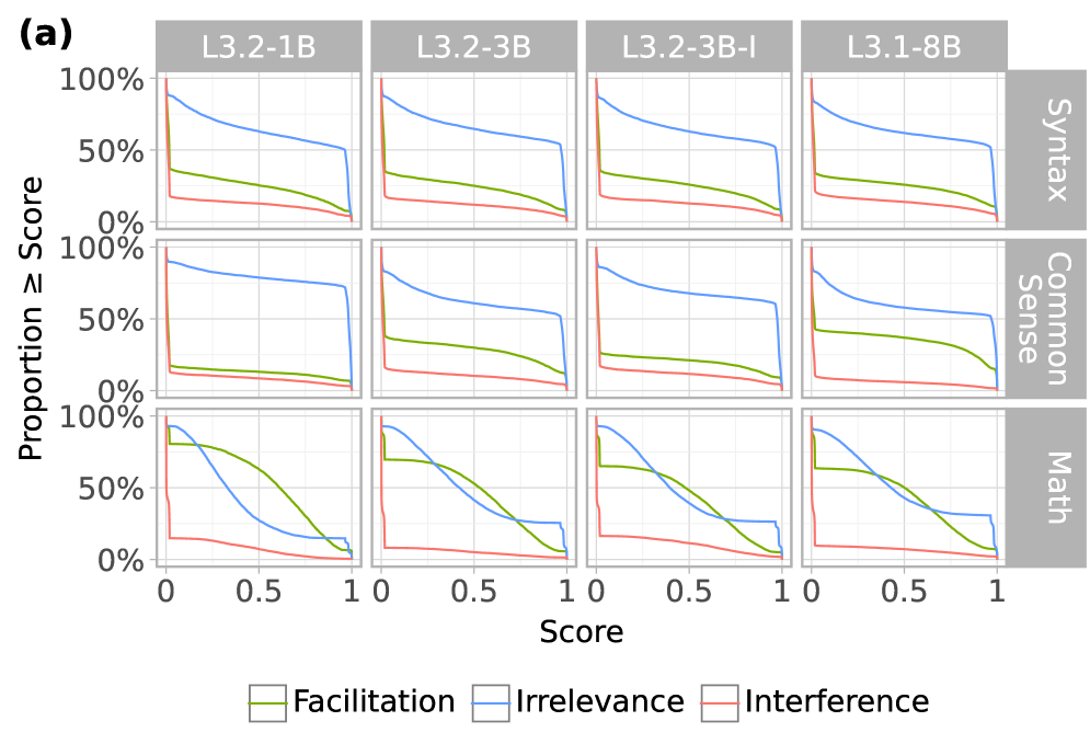</details> Figure 3: CHG score distributions and consistency. (a) Empirical cumulative distribution of CHG scores across all attention heads, showing the proportion of heads with scores below a given threshold for facilitation, irrelevance, and interference. (b) Aggregated CHG scores on L3.2-3BI, where red and green color channels represent interference ( $1-G^+$ ) and facilitation ( $G^-$ ), respectively. Colors are combined using RGB rules: black indicates irrelevance (low in both), and yellow indicates both facilitation and interference (high in both). Always aggregates using the minimum across seeds (highlighting consistent effects); Any uses the maximum (highlighting any effect across seeds). Having validated the causal scores using targeted ablations, we next analyze how they are distributed across models and tasks. Figure 3 a shows that for each task, the distribution of head roles is highly consistent across all four model variants. This holds despite large differences in model size (1B to 8b) and training setup (pretraining, distillation, instruction tuning). We quantify these similarities by computing Pearson correlations between head scores across all model pairs for each task and causal metric, yielding 54 model pairs, all of which show high agreement with a minimum correlation of 94.92% and an average of 99.2%. Across tasks, however, we observe notable differences, with the math dataset standing out in particular. For syntax and commonsense reasoning, most heads are irrelevant—63.0% and 64.6% have irrelevance scores $≥ 0.5$ , respectively—with only a sparse subset of facilitating heads (25.6% and 27.4% with facilitation scores $≥ 0.5$ ), suggesting that compact, redundant circuits are sufficient for these tasks. In contrast, mathematical reasoning activates a much larger fraction of facilitating heads: 52.6% have facilitation scores $≥ 0.5$ , while only 39.0% are irrelevant, likely reflecting the task’s higher complexity and need for broader sub-circuitry to support multi-step, latent computations. It is also worth noting that, across all tasks, 84.0% of heads are marked as facilitating or interfering (score $≥ 0.5$ ) in at least one seed, yet only a small fraction are consistently facilitating or interfering across all seeds (Figure 3 b). In syntax and commonsense tasks, most models have fewer than 5% of heads that are always facilitating and virtually none that are always interfering (Table 2). In contrast, math reveals more rigid and consistent circuitry, with up to 38.3% of heads consistently facilitating and 1.3% consistently interfering. These patterns suggest that individual attention heads may not have modular, context-independent roles, but instead participate in a flexible ensemble of overlapping sub-circuits, in which their function depends on the configuration of others merullo2024talking . Table 2: Percent of heads with facilitation (F) or interference (N) scores $≥$ 0.5 across all seeds (always) or in at least one seed (any). | Task | Agg. | L3.2-1B | L3.2-3B | L3.2-3BI | L3.1-8B | | | | | | --- | --- | --- | --- | --- | --- | --- | --- | --- | --- | | F | N | F | N | F | N | F | N | | | | Syntax | Always | 1.2 | 0.2 | 1.5 | 0.1 | 0.7 | 0.0 | 1.4 | 0.0 | | Any | 72.1 | 57.2 | 67.9 | 51.3 | 72.8 | 56.1 | 68.5 | 59.2 | | | Common Sense | Always | 3.9 | 0.0 | 4.5 | 0.0 | 3.0 | 0.0 | 18.7 | 0.6 | | Any | 56.6 | 41.0 | 75.4 | 52.4 | 68.2 | 55.7 | 60.3 | 22.2 | | | Math | Always | 38.3 | 0.4 | 24.6 | 1.3 | 18.3 | 0.1 | 25.3 | 1.0 | | Any | 81.1 | 26.0 | 75.1 | 13.8 | 74.4 | 47.2 | 75.0 | 21.2 | | ### 4.3 Comparison with causal mediation analysis CMA, like CHG, aims to identify attention heads that facilitate task execution, though it does so in a more hypothesis-driven manner. Framed in signal detection terms, CMA and CHG are complementary. CMA exhibits high precision but relatively low sensitivity: while many facilitating heads may go undetected (false negatives), those it does identify are reliably task-relevant (few false positives). Conversely, CHG is biased toward sensitivity over precision. This suggests that heads identified by CMA should also be identified (as showing strong facilitation) under CHG. We test this by comparing CHG to the results of two former studies using CMA, replicating their methods to identify attention heads with specific computations: heads that encode task information in function vectors todd2023function and heads that perform symbolic reasoning yang2025emergent . For function vectors, we use the six in-context learning tasks used in todd2023function : ‘antonym’, ‘capitalize’, ‘country-capital’, ‘English-French’, ‘present-past’, and ‘singular-plural’. Each prompt is presented in an in-context learning (ICL) brown2020language format consisting of 10 input-output examples using a “Q: X\n A: Y” template, followed by a query to be answered. To perform CMA, we corrupt the prompt by randomly shuffling example outputs to induce mismatched pairs, then patch individual head outputs with clean activations to identify which heads recover performance—interpreting high recovery as evidence of causal mediation. We apply a similar logic to symbolic reasoning tasks from yang2025emergent , where the goal is to generalize abstract identity rules such as ABA (“flowˆStartedˆflow”) or ABB (“flowˆStartedˆStarted”). We deploy the same CMA procedure used in yang2025emergent to identify the three-stage symbolic processing mechanism that was reported: (1) symbol abstraction heads that abstract symbols (“A” or “B”) away from the actual tokens in the in-context examples; (2) symbolic induction heads that operate over the abstracted symbols to induce the symbol for the missing token in the query; (3) retrieval heads that retrieve the actual token based on the induced symbol to complete the query. To screen heads of each type, we construct prompt pairs in which either the same token is assigned to different symbols (“A” or “B”) or tokens are swapped while preserving the same rule, and patch activations at certain token positions between them. Attention heads that steer model behavior towards specific hypotheses about the three head types after patching (either converting the abstract rule or altering the actual token) are labeled as mediating. We conduct all experiments on the Llama-3.2-3B-Instruct model. <details> <summary>x4.png Details</summary>  ### Visual Description ## Scatter Plot Matrix: Linguistic Task Facilitation vs. AIE Score ### Overview The image displays a multi-panel scatter plot matrix labeled "(a)" in the top-left corner. It consists of six individual subplots arranged in a 2x3 grid, each representing a different linguistic or cognitive task. The plots compare a "Facilitation" metric (y-axis) against an "AIE Score" (x-axis). Data points are colored based on a statistical significance threshold relative to 3 standard deviations (3σ). ### Components/Axes * **Overall Structure:** Six subplots in a 2x3 grid. * **Subplot Titles (Top Row, Left to Right):** "Antonym", "Capitalize", "Country-Capital". * **Subplot Titles (Bottom Row, Left to Right):** "English-French", "Present-Past", "Singular-Plural". * **Y-Axis (Common to all plots):** Label: "Facilitation". Scale: Linear, ranging from 0.00 to 1.00, with major ticks at 0.00, 0.25, 0.50, 0.75, and 1.00. * **X-Axis (Common to all plots):** Label: "AIE Score". Scale: Linear, ranging from 0.0 to 0.6, with major ticks at 0.0, 0.2, 0.4, and 0.6. * **Legend (Bottom Center):** Positioned below the bottom row of plots. Contains two entries: * A red circle symbol labeled "< 3σ". * A cyan (light blue) circle symbol labeled "≥ 3σ". * **Data Points:** Scatter points within each subplot, colored either red or cyan according to the legend. ### Detailed Analysis **General Pattern Across All Plots:** * **Red Points (< 3σ):** In every subplot, red points form a dense vertical cluster at or very near an AIE Score of 0.0. Their Facilitation values are widely distributed, spanning the entire range from 0.00 to 1.00. * **Cyan Points (≥ 3σ):** These points are generally located at higher AIE Scores than the red cluster, with the notable exception of the "Antonym" plot. Their Facilitation values are predominantly high, clustering near 1.00. **Subplot-Specific Analysis:** 1. **Antonym:** * **Trend:** Cyan points are found both within the red cluster at AIE ≈ 0.0 and at a slightly higher AIE ≈ 0.1. * **Data Points:** Red points at AIE=0.0, Facilitation from 0.00 to 1.00. Cyan points at AIE=0.0 (Facilitation ~0.85-1.00) and one at AIE≈0.1, Facilitation=1.00. 2. **Capitalize:** * **Trend:** Cyan points are distinctly separated to the right of the red cluster. * **Data Points:** Red points at AIE=0.0. Cyan points at AIE ≈ 0.1 to 0.3, with Facilitation mostly at 1.00. One outlier cyan point at AIE≈0.1, Facilitation=0.00. 3. **Country-Capital:** * **Trend:** Shows the most extreme separation. A single cyan point is far to the right. * **Data Points:** Red points at AIE=0.0. One cyan point at AIE≈0.6, Facilitation≈0.80. 4. **English-French:** * **Trend:** Cyan points are separated to the right. * **Data Points:** Red points at AIE=0.0. Cyan points at AIE≈0.1 and AIE≈0.4, both with Facilitation=1.00. 5. **Present-Past:** * **Trend:** Cyan points are separated to the right. * **Data Points:** Red points at AIE=0.0. Cyan points at AIE ≈ 0.1 to 0.3, all with Facilitation=1.00. 6. **Singular-Plural:** * **Trend:** Cyan points are separated to the right, with a slight downward trend in Facilitation as AIE increases. * **Data Points:** Red points at AIE=0.0. Cyan points at AIE ≈ 0.1 to 0.2, with Facilitation ranging from ~0.70 to 1.00. ### Key Observations 1. **Bimodal Distribution of AIE Scores:** For 5 of the 6 tasks (all except Antonym), data points with statistical significance (≥3σ, cyan) are exclusively associated with positive AIE Scores, while non-significant points (<3σ, red) are concentrated at AIE=0. 2. **High Facilitation for Significant Effects:** With the exception of one outlier in "Capitalize," all cyan points (≥3σ) have high Facilitation scores, generally above 0.70 and often at 1.00. 3. **The Antonym Anomaly:** The "Antonym" task is unique. It shows statistically significant results (cyan points) even at an AIE Score of 0.0, suggesting the mechanism measured by the AIE Score may not be necessary for facilitation in this specific task. 4. **Task Difficulty/Effect Size Gradient:** The maximum AIE Score for cyan points varies by task, suggesting a hierarchy: "Country-Capital" (AIE≈0.6) > "English-French" (AIE≈0.4) > "Capitalize"/"Present-Past"/"Singular-Plural" (AIE≈0.1-0.3) > "Antonym" (AIE≈0.0-0.1). ### Interpretation This chart investigates the relationship between an "AIE Score" (likely a measure of some cognitive or model-based interference effect) and task "Facilitation" across different linguistic transformations. The data strongly suggests that for most tasks (morphological changes like capitalization, tense, number; translation), achieving a statistically significant facilitation effect (≥3σ) is correlated with a non-zero AIE Score. This implies that the cognitive or computational process indexed by the AIE Score is a common prerequisite or concomitant for facilitation in these domains. The higher the AIE Score required (as in "Country-Capital"), the more distinct or demanding the underlying process may be. The "Antonym" task breaks this pattern. Significant facilitation occurs even with a zero AIE Score, indicating that antonym processing might rely on a different, more direct or automatic pathway that doesn't engage the mechanism measured by the AIE metric. This makes sense from a psycholinguistic perspective, as antonymy is a strong, direct semantic association, unlike the rule-based or associative mappings in the other tasks. The single low-facilitation cyan point in "Capitalize" is an interesting outlier, representing a case where a significant effect was measured but resulted in no facilitation, possibly indicating a disruptive or inhibitory process. Overall, the visualization effectively dissociates task types based on their dependence on the AIE-related process. </details> <details> <summary>x5.png Details</summary>  ### Visual Description ## Scatter Plot: CMA Score vs. Facilitation by Head Type ### Overview This image is a scatter plot labeled "(b)" in the top-left corner. It visualizes the relationship between two numerical variables, "CMA Score" and "Facilitation," for data points categorized into four distinct "Head Types." The plot reveals how different cognitive or processing head types cluster and distribute across these two dimensions. ### Components/Axes * **Plot Label:** "(b)" located in the top-left corner, outside the main axes. * **X-Axis:** * **Title:** "CMA Score" * **Scale:** Linear scale ranging from 0 to 6. * **Major Tick Marks:** 0, 2, 4, 6. * **Y-Axis:** * **Title:** "Facilitation" * **Scale:** Linear scale ranging from 0.00 to 1.00. * **Major Tick Marks:** 0.00, 0.25, 0.50, 0.75, 1.00. * **Legend:** * **Title:** "Head Type" * **Location:** Centered below the x-axis. * **Categories & Colors:** * **Insignificant:** Red/Salmon circle. * **Abstraction:** Light Green circle. * **Induction:** Cyan/Light Blue circle. * **Retrieval:** Purple circle. ### Detailed Analysis **Data Point Distribution by Head Type:** 1. **Insignificant (Red):** * **Spatial Grounding:** Heavily clustered along the vertical line where CMA Score ≈ 0. * **Trend Verification:** Shows no clear linear trend. Points are vertically dispersed. * **Values:** CMA Score is consistently near 0. Facilitation values are widely scattered, ranging from approximately 0.00 to 1.00, with a dense concentration between 0.25 and 1.00. 2. **Abstraction (Green):** * **Spatial Grounding:** Clustered in the top-left quadrant of the plot. * **Trend Verification:** Points are grouped at high Facilitation levels. * **Values:** CMA Score is low, approximately between 0 and 1.5. Facilitation is consistently high, mostly between 0.90 and 1.00. 3. **Retrieval (Purple):** * **Spatial Grounding:** Scattered across the upper half of the plot, from left to center. * **Trend Verification:** Shows a slight positive trend; as CMA Score increases, Facilitation tends to remain high but with more variability. * **Values:** CMA Score ranges from approximately 0 to 4. Facilitation is generally high (mostly > 0.75), but with notable points dipping to around 0.80 and one outlier near 0.00 at a low CMA Score. 4. **Induction (Cyan):** * **Spatial Grounding:** Located in the top-right quadrant, isolated from other clusters. * **Trend Verification:** Points are grouped at the highest CMA Scores and high Facilitation. * **Values:** CMA Score is high, approximately between 4 and 7. Facilitation is consistently high, at or near 1.00. ### Key Observations * **Distinct Clustering:** The four head types form largely non-overlapping clusters, suggesting they represent fundamentally different categories in this CMA-Facilitation space. * **CMA Score Gradient:** There is a clear progression in typical CMA Score from left to right: Insignificant (≈0) < Abstraction (0-1.5) < Retrieval (0-4) < Induction (4-7). * **Facilitation Ceiling:** For Abstraction, Retrieval, and Induction, Facilitation values are predominantly high (>0.75). The "Insignificant" type is the only one showing a full range of Facilitation values. * **Outlier:** A single purple (Retrieval) data point is located at approximately (CMA Score: 0.5, Facilitation: 0.00), which is an outlier compared to the high-Facilitation trend of its group. ### Interpretation The data suggests a strong relationship between the categorical "Head Type" and the two measured variables. The "CMA Score" appears to be a key differentiator between the types, potentially representing a measure of complexity, cognitive load, or processing depth. * **Insignificant** heads operate at a baseline CMA Score (≈0) and their effectiveness (Facilitation) is highly variable, implying their contribution is not consistently tied to this complexity measure. * **Abstraction** and **Retrieval** heads function at low-to-moderate complexity but achieve high facilitation, indicating they are efficient processes for tasks within their CMA range. * **Induction** heads are uniquely associated with high CMA Scores and high Facilitation. This could imply that inductive reasoning processes are both required for and effective at handling the most complex tasks measured by the CMA Score. The plot effectively argues that these head types are not just labels but correspond to distinct operational profiles. The clear separation, especially of the Induction cluster, highlights it as a specialized, high-complexity, high-impact process. The outlier in the Retrieval group warrants investigation as it may represent a failure case or a different sub-type. 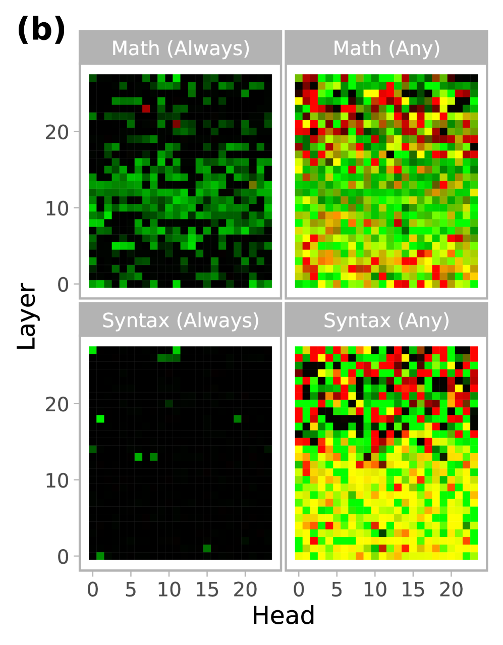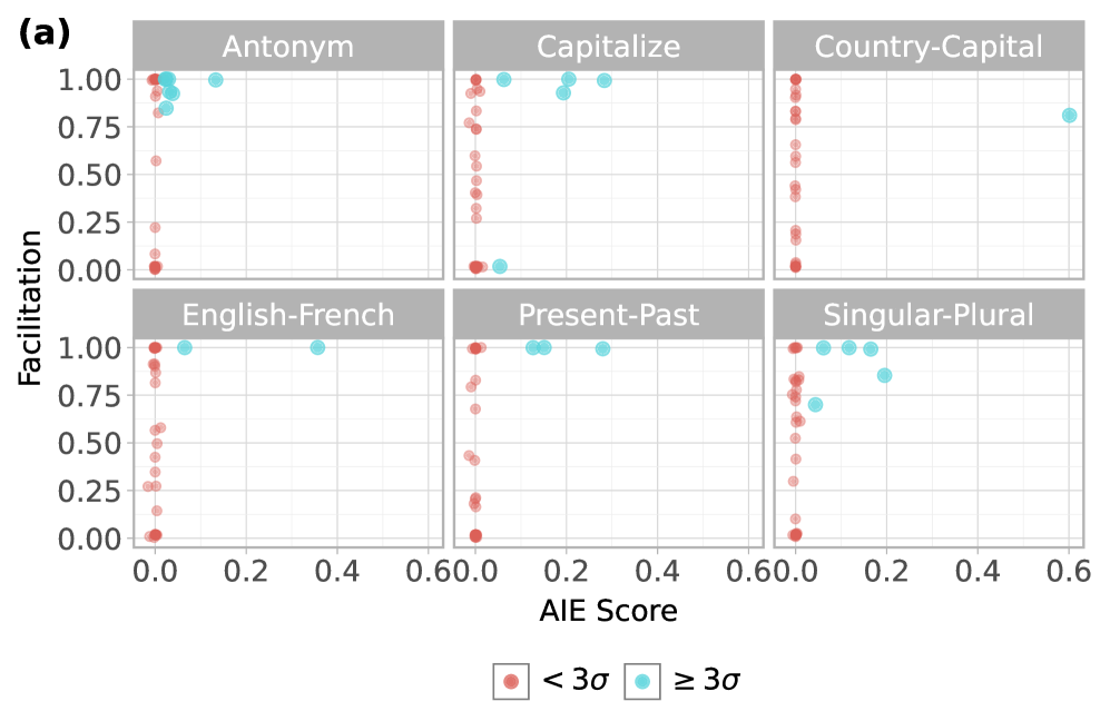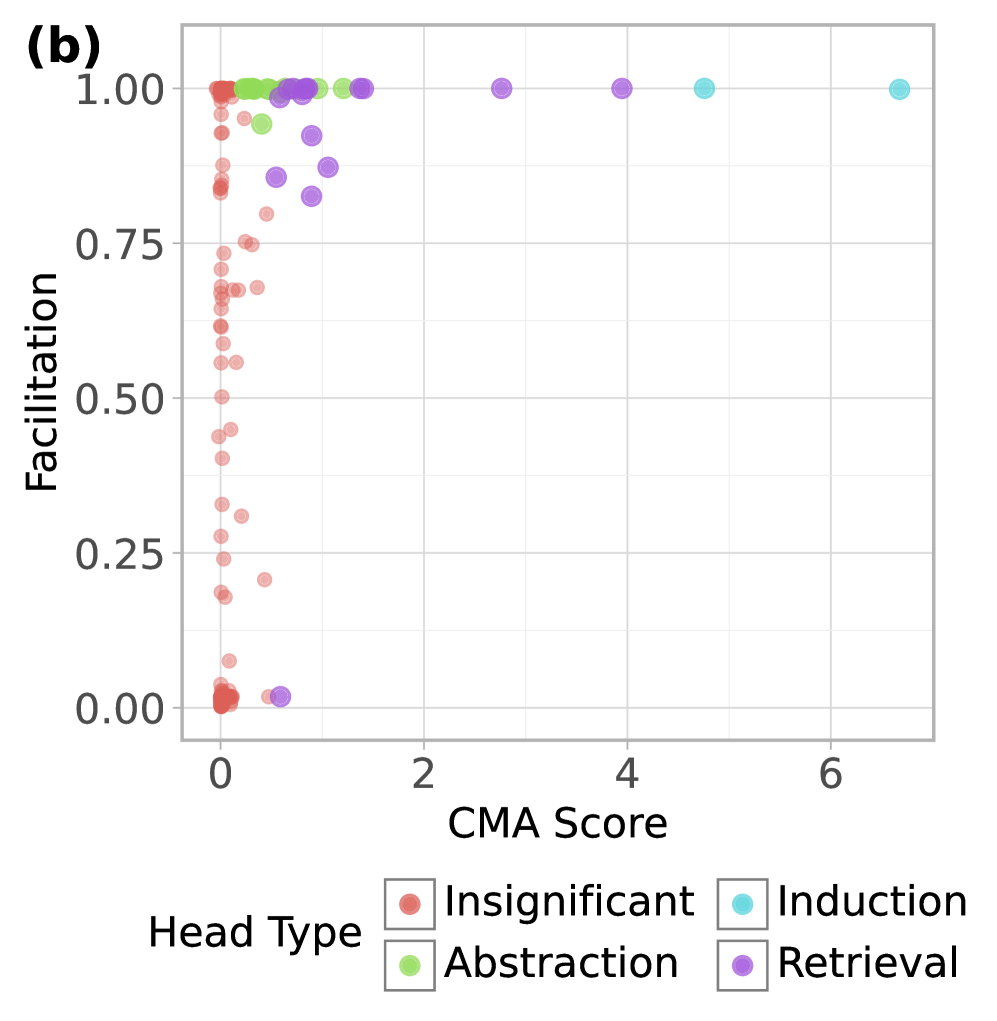</details> Figure 4: Task-facilitation scores versus (a) average indirect effect for function vector tasks and (b) CMA scores for symbolic reasoning tasks, showing significant heads by type (abstraction, induction, retrieval) and using the maximum CMA score across types for insignificant heads. As predicted, CMA-identified heads tend to exhibit high facilitation scores under CHG in both domains (Figure 4). To quantify this, we compare the CHG facilitation scores of CMA-identified heads—those with three standard deviations above the mean in function vector tasks or with statistical significance in ABA/ABB tasks yang2025emergent —to the remaining ones. Since facilitation and irrelevance depend on the specific sufficient circuit identified by CHG, a head may appear irrelevant in one run but facilitating in another if multiple circuits exist. To account for this, we fit 10 CHG masks per function vector task and 20 per ABA/ABB task, and compute each head’s maximum facilitation score across runs—capturing whether it participates in any sufficient circuit. We find significantly greater facilitation among mediating heads in both the function vector tasks ( $t(23.05)=8.52$ , $p<10^-8$ ) and the ABA/ABB tasks ( $t(53.77)=11.18$ , $p<10^-15$ ), supporting the relationship between CMA and CHG-identified task relevance. ### 4.4 Contrastive Causal Head Gating The results above indicate that CHG effectively distinguishes among facilitating, irrelevant, and interfering attention heads. However, as an exploratory method, it lacks the granularity to characterize the specific functions of these subnetworks. For instance, consider the ‘antonym’ task from Section 4.3, presented in an in-context learning (ICL) format with 10 examples and a single-word response, as defined in todd2023function . To perform this task successfully, the model must not only generate the appropriate antonym of a given word, but also infer the task itself from the 10 input-output pairs in the prompt. Thus, a minimal circuit of task-facilitating heads will contain both those involved in task inference and those involved in antonym production, and CHG cannot distinguish between the two. This becomes more pronounced as task complexity increases, as in the OpenMathInstruct2 dataset, where the minimal circuit must jointly support diverse sub-tasks, including English comprehension, mathematical reasoning, chain-of-thought processing, and LaTeX generation. To address this, we introduce a simple extension of CHG that not only identifies facilitating heads for a given task but also isolates the sub-circuit responsible for a particular sub-task. We generate parallel variants of the same task that share all features except for a controlled difference in the required operation, allowing us to isolate the corresponding sub-circuits. In doing so, we take a step toward a hypothesis-driven approach, decomposing the task into sub-steps while remaining agnostic to the mechanistic implementations For example, the antonym task can be constructed as an ICL task using the default format from todd2023function , or as an instruction-following task where the model is presented with the task description “Given an input word, generate the word with opposite meaning”. By comparing the resulting attention circuits, we can disentangle components responsible for task inference from those involved in antonym generation. Furthermore, rather than simply applying CHG to each version and directly comparing the results, we propose a combined approach that fits a single mask with a joint objective to forget one variant of the task while retaining the other, so that the resulting gate matrix suppresses heads uniquely necessary for one variant but dispensable for the other: $$ L(G;M_θ,λ)=∑_(x_{R,y_R,x_F,y_F)}\log P(y_F\mid x_F)-\log P(y_R\mid x_R)-λ∑_i,jσ^-1(G_l,h) \tag{2} $$ where $\log P(y\mid x)$ denotes the log-probability of target sequence $y$ given prompt $x$ under model $M_θ$ with gating matrix $G$ , the sum ranges over matched tuples $(x_R,y_R,x_F,y_F)$ of the retention and forget variants that differ only in task formulation, and $λ>0$ . To stabilize the gradient, we clip the inverse-sigmoid as in Eq. 1 as well as the difference in log-probability. 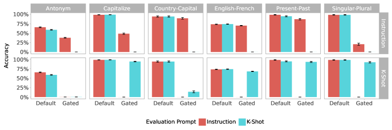We evaluate this method using the six function vector tasks from Section 4.3, leveraging the natural language task descriptions provided in todd2023function to construct instruction-based variants. For each problem, we replace the 10-shot word-pair examples with a prompt containing the task instruction and a single example. We then fit the contrastive causal head gating (CCHG) mask to forget the ICL variant of five tasks while retaining the instruction-based format, holding out the sixth task for evaluation. If task inference from examples, instruction-following, and task execution are indeed mediated by separable circuits, this analysis should disable example-based generalization while preserving instruction-based performance. We perform our experiments in both directions (forgetting ICL while retaining instruction-following, and vice versa), using each of the six tasks as the held-out evaluation task. All experiments were conducted on the LLaMA-3.2-3B-Instruct model. <details> <summary>x6.png Details</summary>  ### Visual Description \n ## Grouped Bar Chart: Accuracy Comparison Across Tasks and Evaluation Methods ### Overview The image displays a 2x6 grid of grouped bar charts comparing model accuracy across six different linguistic tasks. The comparison is made across two training methods (rows) and two evaluation prompt types (bar colors) for each task. ### Components/Axes * **Chart Type:** Grouped Bar Chart (Small Multiples) * **Y-Axis:** Labeled "Accuracy" on the far left. Scale runs from 0% to 100% in increments of 25%. * **X-Axis (within each subplot):** Two categories: "Default" and "Gated". * **Column Headers (Top):** Six task names: "Antonym", "Capitalize", "Country-Capital", "English-French", "Present-Past", "Singular-Plural". * **Row Labels (Right Side):** Two training methods: "Instruction" (top row) and "K-Shot" (bottom row). * **Legend (Bottom Center):** Titled "Evaluation Prompt". Contains two colored squares: * Red square: "Instruction" * Teal square: "K-Shot" * **Data Series:** Each subplot contains four bars, grouped into two pairs (Default and Gated). Each pair contains a red bar (Instruction evaluation) and a teal bar (K-Shot evaluation). ### Detailed Analysis **Data Extraction (Approximate Values):** **Row 1: Instruction Training** * **Antonym:** * Default: Instruction (Red) ~65%, K-Shot (Teal) ~60% * Gated: Instruction (Red) ~40%, K-Shot (Teal) ~0% * **Capitalize:** * Default: Instruction (Red) ~98%, K-Shot (Teal) ~98% * Gated: Instruction (Red) ~50%, K-Shot (Teal) ~0% * **Country-Capital:** * Default: Instruction (Red) ~95%, K-Shot (Teal) ~95% * Gated: Instruction (Red) ~90%, K-Shot (Teal) ~0% * **English-French:** * Default: Instruction (Red) ~75%, K-Shot (Teal) ~75% * Gated: Instruction (Red) ~70%, K-Shot (Teal) ~0% * **Present-Past:** * Default: Instruction (Red) ~98%, K-Shot (Teal) ~95% * Gated: Instruction (Red) ~85%, K-Shot (Teal) ~0% * **Singular-Plural:** * Default: Instruction (Red) ~98%, K-Shot (Teal) ~98% * Gated: Instruction (Red) ~20%, K-Shot (Teal) ~0% **Row 2: K-Shot Training** * **Antonym:** * Default: Instruction (Red) ~65%, K-Shot (Teal) ~60% * Gated: Instruction (Red) ~0%, K-Shot (Teal) ~0% * **Capitalize:** * Default: Instruction (Red) ~98%, K-Shot (Teal) ~98% * Gated: Instruction (Red) ~0%, K-Shot (Teal) ~95% * **Country-Capital:** * Default: Instruction (Red) ~95%, K-Shot (Teal) ~95% * Gated: Instruction (Red) ~0%, K-Shot (Teal) ~15% * **English-French:** * Default: Instruction (Red) ~75%, K-Shot (Teal) ~75% * Gated: Instruction (Red) ~0%, K-Shot (Teal) ~70% * **Present-Past:** * Default: Instruction (Red) ~98%, K-Shot (Teal) ~95% * Gated: Instruction (Red) ~0%, K-Shot (Teal) ~95% * **Singular-Plural:** * Default: Instruction (Red) ~98%, K-Shot (Teal) ~98% * Gated: Instruction (Red) ~0%, K-Shot (Teal) ~95% ### Key Observations 1. **Consistent High Performance on "Default":** For all six tasks, both training methods achieve high accuracy (mostly >60%, often >95%) when using the "Default" evaluation prompt, regardless of whether the evaluation prompt is "Instruction" (red) or "K-Shot" (teal). 2. **Catastrophic Drop with "Gated" Prompt:** The most striking pattern is the severe performance degradation when switching from the "Default" to the "Gated" evaluation prompt. 3. **Divergent Behavior by Training Method:** * **Instruction Training (Top Row):** When using the "Gated" prompt, the "Instruction" evaluation (red bars) retains some accuracy (20-90% depending on task), while the "K-Shot" evaluation (teal bars) drops to near 0% for all tasks. * **K-Shot Training (Bottom Row):** The pattern is inverted. With the "Gated" prompt, the "Instruction" evaluation (red bars) drops to 0% for all tasks, while the "K-Shot" evaluation (teal bars) retains significant accuracy for most tasks (15-95%). 4. **Task-Specific Vulnerability:** The "Capitalize" and "Singular-Plural" tasks show the most dramatic drops under the "Gated" condition for their non-preferred evaluation method (e.g., Instruction evaluation for K-Shot trained models). ### Interpretation This chart demonstrates a critical failure mode related to **prompt sensitivity** and **training-evaluation alignment**. * **What the data suggests:** The models are highly brittle. Their performance is not just a function of the task but is acutely dependent on the format of the evaluation prompt ("Default" vs. "Gated"). The "Gated" prompt appears to break the model's ability to follow instructions unless the evaluation method perfectly matches the training method. * **Relationship between elements:** The training method ("Instruction" vs. "K-Shot") creates a strong bias. A model trained with one method becomes almost completely incapable of performing when evaluated with the *other* method under the "Gated" prompt condition. This indicates the models are not learning the underlying task robustly but are instead overfitting to the specific prompt format used during training. * **Notable anomaly:** The near-perfect 0% scores are extreme outliers in typical model evaluation, signaling a complete breakdown rather than a gradual decline. This is a severe reliability issue for real-world deployment where input phrasing can vary. * **Underlying implication:** The results argue strongly for more robust training paradigms that decouple task understanding from prompt formatting. It highlights a significant gap between achieving high benchmark scores (on "Default" prompts) and creating models that generalize reliably across different interaction styles. </details> Figure 5: Task accuracy under CCHG. Columns indicate held-out evaluation tasks and rows indicate the retained prompt format. Bar color shows the evaluation prompt format. “Default” and “gated” indicate whether CCHG is applied during evaluation. Error bars indicate 95% CI. As shown in Figure 5, the CCHG masks generalize to the held-out task. When the model is induced to forget task inference from ICL examples across five tasks, its target task accuracy drops to zero on the ICL variant of the held-out task while in most cases remaining well above zero—and often close to the unablated baseline—on the instruction-based variant. A similar pattern emerges when forgetting is applied using the instruction-based format: performance collapses on instruction prompts while generally remaining intact for example-based ones. Interestingly, while degradation is often small for the retained prompt format, this pattern is not consistent across all tasks. For example, when the gating matrix is fitted to retain ICL and forget instruction-following, the ‘singular-plural’ task shows only a small drop in ICL accuracy ( $98\$ ) but a complete failure on instruction prompts ( $98\$ ). When this setup is reversed—fitted to retain instruction-following and forget ICL—accuracy on ICL drops from 98% to 0%, while instruction accuracy drops more modestly $(98\$ . Across the 6 tasks, 3 (‘country-capital’, ‘English-French’, ‘present-past’) remain robust as held-out tasks under instruction prompts, and 4 (‘capitalize’, ‘English-French’, ‘present-past’, ‘singular-plural’) do so under ICL prompts. Thus, our results indicate that the circuits for instruction following and ICL may be separable at the head level. However, this separability also depends on the task, suggesting that task execution circuits may share heads with those used for task understanding and representation. ## 5 Discussion In this work, we introduced Causal Head Gating (CHG), a flexible and scalable method for identifying causally relevant attention heads in large language models. CHG assigns each head a graded score for facilitation, interference, or irrelevance based on its effect on task performance, going beyond correlational or observational analyses. These scores predict performance changes under targeted ablations, confirming that facilitation, interference, and irrelevance scores capture causal impact. Crucially, it does so using next-token prediction alone, thereby avoiding reliance on labeled data or handcrafted prompts, making it broadly and easily applicable. Moreover, CHG requires no finetuning or auxiliary decoder model, and introduces only one parameter per head, allowing it to run in minutes even on billion-scale models. To validate our method, we demonstrated that existing works within the mechanistic interpretability literature successfully corroborate our findings using, and that the ICL and instruction-following circuits revealed using contrastive CHG successfully generalize across tasks. Interestingly, across the range of models and tasks we investigated, we observed that attention heads form task-sufficient sub-circuits with low overlap. Moreover, a single head may vary in its relevance across multiple runs depending on which others are active, reflecting the distributed and context-dependent nature of computation in LLMs, and in rare cases, a head may even receive low $G^+$ but high $G^-$ scores within the same run. We hypothesize that this variability reflects an interaction-dependent landscape in which causal roles shift with circuit configuration. While these complexities may appear messy, we view them as a strength of CHG, revealing the redundancy and interdependence that underlie emergent model behavior. Because CHG is highly scalable, it can be repeatedly applied to estimate distributions over gating values, providing a bootstrapped view of redundant and contingent sub-circuits with greater fidelity to the model’s underlying dependency structure. While CHG provides a lightweight and scalable approach for exploratory analysis, requiring only a dataset and no model finetuning or supervision, it is not designed to reveal the precise computations performed by individual heads. Instead, CHG offers a complementary first-pass diagnostic tool that identifies candidate heads or sub-circuits with consistent causal influence, guiding where more granular, hypothesis-driven methods such as causal mediation or activation patching can be applied. In this way, CHG provides a practical entry point into large-scale causal interpretability, mapping functional dependencies that subsequent analyses can examine in greater detail. We hope that our work encourages further exploration of causal structure in language models as a foundation for more mechanistic understanding. Future work may build on these tools to develop circuit-level explanations of how models implement complex behaviors. ## Acknowledgments and Disclosure of Funding We thank Declan Campbell and Alexander Ku for helpful discussions, and Legasse Remon for assistance with dataset organization. Jonathan Cohen was supported by the Vannevar Bush Faculty Fellowship, sponsored by the Office of Naval Research. The authors declare no competing interests. ## References - [1] Josh Achiam, Steven Adler, Sandhini Agarwal, Lama Ahmad, Ilge Akkaya, Florencia Leoni Aleman, Diogo Almeida, Janko Altenschmidt, Sam Altman, Shyamal Anadkat, et al. GPT-4 technical report. arXiv preprint arXiv:2303.08774, 2023. - [2] Aixin Liu, Bei Feng, Bing Xue, Bingxuan Wang, Bochao Wu, Chengda Lu, Chenggang Zhao, Chengqi Deng, Chenyu Zhang, Chong Ruan, et al. Deepseek-v3 technical report. arXiv preprint arXiv:2412.19437, 2024. - [3] Aaron Grattafiori, Abhimanyu Dubey, Abhinav Jauhri, Abhinav Pandey, Abhishek Kadian, Ahmad Al-Dahle, Aiesha Letman, Akhil Mathur, Alan Schelten, Alex Vaughan, et al. The llama 3 herd of models. arXiv preprint arXiv:2407.21783, 2024. - [4] Rishi Bommasani, Drew A Hudson, Ehsan Adeli, Russ Altman, Simran Arora, Sydney von Arx, Michael S Bernstein, Jeannette Bohg, Antoine Bosselut, Emma Brunskill, et al. On the opportunities and risks of foundation models. arXiv preprint arXiv:2108.07258, 2021. - [5] Alexander Wei, Nika Haghtalab, and Jacob Steinhardt. Jailbroken: How does LLM safety training fail? Advances in Neural Information Processing Systems, 36:80079–80110, 2023. - [6] Laura Weidinger, Joslyn Barnhart, Jenny Brennan, Christina Butterfield, Susie Young, Will Hawkins, Lisa Anne Hendricks, Ramona Comanescu, Oscar Chang, Mikel Rodriguez, et al. Holistic safety and responsibility evaluations of advanced ai models. arXiv preprint arXiv:2404.14068, 2024. - [7] Ian Tenney, Dipanjan Das, and Ellie Pavlick. BERT rediscovers the classical NLP pipeline. arXiv preprint arXiv:1905.05950, 2019. - [8] Trenton Bricken, Adly Templeton, Joshua Batson, Brian Chen, Adam Jermyn, Tom Conerly, Nick Turner, Cem Anil, Carson Denison, Amanda Askell, et al. Towards monosemanticity: Decomposing language models with dictionary learning. Transformer Circuits Thread, 2, 2023. - [9] Ashish Vaswani, Noam Shazeer, Niki Parmar, Jakob Uszkoreit, Llion Jones, Aidan N Gomez, Łukasz Kaiser, and Illia Polosukhin. Attention is all you need. Advances in Neural Information Processing Systems, 30, 2017. - [10] Gemma Team, Aishwarya Kamath, Johan Ferret, Shreya Pathak, Nino Vieillard, Ramona Merhej, Sarah Perrin, Tatiana Matejovicova, Alexandre Ramé, Morgane Rivière, et al. Gemma 3 technical report. arXiv preprint arXiv:2503.19786, 2025. - [11] Nelson Elhage, Neel Nanda, Catherine Olsson, Tom Henighan, Nicholas Joseph, Ben Mann, Amanda Askell, Yuntao Bai, Anna Chen, Tom Conerly, Nova DasSarma, Dawn Drain, Deep Ganguli, Zac Hatfield-Dodds, Danny Hernandez, Andy Jones, Jackson Kernion, Liane Lovitt, Kamal Ndousse, Dario Amodei, Tom Brown, Jack Clark, Jared Kaplan, Sam McCandlish, and Chris Olah. A mathematical framework for transformer circuits. Transformer Circuits Thread, 2021. https://transformer-circuits.pub/2021/framework/index.html. - [12] Eric Todd, Millicent L Li, Arnab Sen Sharma, Aaron Mueller, Byron C Wallace, and David Bau. Function vectors in large language models. arXiv preprint arXiv:2310.15213, 2023. - [13] Yukang Yang, Declan Campbell, Kaixuan Huang, Mengdi Wang, Jonathan Cohen, and Taylor Webb. Emergent symbolic mechanisms support abstract reasoning in large language models. arXiv preprint arXiv:2502.20332, 2025. - [14] Ian Tenney, Patrick Xia, Berlin Chen, Alex Wang, Adam Poliak, R Thomas McCoy, Najoung Kim, Benjamin Van Durme, Samuel R Bowman, Dipanjan Das, et al. What do you learn from context? Probing for sentence structure in contextualized word representations. arXiv preprint arXiv:1905.06316, 2019. - [15] John Hewitt and Christopher D Manning. A structural probe for finding syntax in word representations. In Proceedings of the 2019 Conference of the North American Chapter of the Association for Computational Linguistics: Human Language Technologies, Volume 1 (Long and Short Papers), pages 4129–4138, 2019. - [16] Adly Templeton, Tom Conerly, Jonathan Marcus, Jack Lindsey, Trenton Bricken, Brian Chen, Adam Pearce, Craig Citro, Emmanuel Ameisen, Andy Jones, Hoagy Cunningham, Nicholas L Turner, Callum McDougall, Monte MacDiarmid, C. Daniel Freeman, Theodore R. Sumers, Edward Rees, Joshua Batson, Adam Jermyn, Shan Carter, Chris Olah, and Tom Henighan. Scaling monosemanticity: Extracting interpretable features from Claude 3 Sonnet. Transformer Circuits Thread, 2024. - [17] Andrew Lee, Xiaoyan Bai, Itamar Pres, Martin Wattenberg, Jonathan K Kummerfeld, and Rada Mihalcea. A mechanistic understanding of alignment algorithms: A case study on dpo and toxicity. arXiv preprint arXiv:2401.01967, 2024. - [18] Elena Voita, David Talbot, Fedor Moiseev, Rico Sennrich, and Ivan Titov. Analyzing multi-head self-attention: Specialized heads do the heavy lifting, the rest can be pruned. arXiv preprint arXiv:1905.09418, 2019. - [19] Chris Olah, Nick Cammarata, Ludwig Schubert, Gabriel Goh, Michael Petrov, and Shan Carter. Zoom in: An introduction to circuits. Distill, 5(3):e00024–001, 2020. - [20] Geoffrey E Hinton. Learning distributed representations of concepts. In Proceedings of the Annual Meeting of the Cognitive Science Society, volume 8, 1986. - [21] Nelson Elhage, Tristan Hume, Catherine Olsson, Nicholas Schiefer, Tom Henighan, Shauna Kravec, Zac Hatfield-Dodds, Robert Lasenby, Dawn Drain, Carol Chen, Roger Grosse, Sam McCandlish, Jared Kaplan, Dario Amodei, Martin Wattenberg, and Christopher Olah. Toy models of superposition. Transformer Circuits Thread, 2022. https://transformer-circuits.pub/2022/toy_model/index.html. - [22] Kayson Fakhar and Claus C Hilgetag. Systematic perturbation of an artificial neural network: A step towards quantifying causal contributions in the brain. PLOS Computational Biology, 18(6):e1010250, 2022. - [23] Tyler Giallanza, Declan Campbell, Jonathan D Cohen, and Timothy T Rogers. An integrated model of semantics and control. Psychological Review, 2024. - [24] Melanie Mitchell. Complexity: A guided tour. Oxford University Press, 2009. - [25] Kevin Wang, Alexandre Variengien, Arthur Conmy, Buck Shlegeris, and Jacob Steinhardt. Interpretability in the wild: a circuit for indirect object identification in GPT-2 small. arXiv preprint arXiv:2211.00593, 2022. - [26] Jason Wei, Xuezhi Wang, Dale Schuurmans, Maarten Bosma, Fei Xia, Ed Chi, Quoc V Le, Denny Zhou, et al. Chain-of-thought prompting elicits reasoning in large language models. Advances in Neural Information Processing Systems, 35:24824–24837, 2022. - [27] Yonatan Belinkov. Probing classifiers: Promises, shortcomings, and advances. Computational Linguistics, 48(1):207–219, 2022. - [28] Tiago Pimentel, Josef Valvoda, Rowan Hall Maudslay, Ran Zmigrod, Adina Williams, and Ryan Cotterell. Information-theoretic probing for linguistic structure. arXiv preprint arXiv:2004.03061, 2020. - [29] John Hewitt and Percy Liang. Designing and interpreting probes with control tasks. arXiv preprint arXiv:1909.03368, 2019. - [30] Elena Voita and Ivan Titov. Information-theoretic probing with minimum description length. arXiv preprint arXiv:2003.12298, 2020. - [31] Abhilasha Ravichander, Yonatan Belinkov, and Eduard Hovy. Probing the probing paradigm: Does probing accuracy entail task relevance? arXiv preprint arXiv:2005.00719, 2020. - [32] Hoagy Cunningham, Aidan Ewart, Logan Riggs, Robert Huben, and Lee Sharkey. Sparse autoencoders find highly interpretable features in language models. arXiv preprint arXiv:2309.08600, 2023. - [33] Jesse Vig, Sebastian Gehrmann, Yonatan Belinkov, Sharon Qian, Daniel Nevo, Yaron Singer, and Stuart Shieber. Investigating gender bias in language models using causal mediation analysis. Advances in Neural Information Processing Systems, 33:12388–12401, 2020. - [34] Kevin Meng, David Bau, Alex Andonian, and Yonatan Belinkov. Locating and editing factual associations in GPT. Advances in Neural Information Processing Systems, 35:17359–17372, 2022. - [35] Zifan Zheng, Yezhaohui Wang, Yuxin Huang, Shichao Song, Mingchuan Yang, Bo Tang, Feiyu Xiong, and Zhiyu Li. Attention heads of large language models. Patterns. - [36] Karl Cobbe, Vineet Kosaraju, Mohammad Bavarian, Mark Chen, Heewoo Jun, Lukasz Kaiser, Matthias Plappert, Jerry Tworek, Jacob Hilton, Reiichiro Nakano, Christopher Hesse, and John Schulman. Training verifiers to solve math word problems. arXiv preprint arXiv:2110.14168, 2021. - [37] Dan Hendrycks, Collin Burns, Saurav Kadavath, Akul Arora, Steven Basart, Eric Tang, Dawn Song, and Jacob Steinhardt. Measuring mathematical problem solving with the math dataset. arXiv preprint arXiv:2103.03874, 2021. - [38] Shubham Toshniwal, Wei Du, Ivan Moshkov, Branislav Kisacanin, Alexan Ayrapetyan, and Igor Gitman. Openmathinstruct-2: Accelerating ai for math with massive open-source instruction data. arXiv preprint arXiv:2410.01560, 2024. - [39] Paul Michel, Omer Levy, and Graham Neubig. Are sixteen heads really better than one? Advances in Neural Information Processing Systems, 32, 2019. - [40] Jiaoda Li, Ryan Cotterell, and Mrinmaya Sachan. Differentiable subset pruning of transformer heads. Transactions of the Association for Computational Linguistics, 9:1442–1459, 2021. - [41] Mengzhou Xia, Zexuan Zhong, and Danqi Chen. Structured pruning learns compact and accurate models. In Proceedings of the 60th Annual Meeting of the Association for Computational Linguistics (Volume 1: Long Papers), pages 1513–1528, 2022. - [42] Angela Fan, Edouard Grave, and Armand Joulin. Reducing transformer depth on demand with structured dropout. arXiv preprint arXiv:1909.11556, 2019. - [43] Hassan Sajjad, Fahim Dalvi, Nadir Durrani, and Preslav Nakov. On the effect of dropping layers of pre-trained transformer models. Computer Speech & Language, 77:101429, 2023. - [44] Shwai He, Guoheng Sun, Zheyu Shen, and Ang Li. What matters in transformers? not all attention is needed. arXiv preprint arXiv:2406.15786, 2024. - [45] Jacob Devlin, Ming-Wei Chang, Kenton Lee, and Kristina Toutanova. Bert: Pre-training of deep bidirectional transformers for language understanding. In Proceedings of the 2019 Conference of the North American Chapter of the Association for Computational Linguistics: Human Language Technologies, Volume 1 (Long and Short Papers), pages 4171–4186, 2019. - [46] Tom Brown, Benjamin Mann, Nick Ryder, Melanie Subbiah, Jared D Kaplan, Prafulla Dhariwal, Arvind Neelakantan, Pranav Shyam, Girish Sastry, Amanda Askell, et al. Language models are few-shot learners. Advances in Neural Information Processing Systems, 33:1877–1901, 2020. - [47] Nicola De Cao, Michael Schlichtkrull, Wilker Aziz, and Ivan Titov. How do decisions emerge across layers in neural models? interpretation with differentiable masking. arXiv preprint arXiv:2004.14992, 2020. - [48] Fangcong Yin, Xi Ye, and Greg Durrett. Lofit: Localized fine-tuning on llm representations. Advances in Neural Information Processing Systems, 37:9474–9506, 2024. - [49] Eric Jang, Shixiang Gu, and Ben Poole. Categorical reparameterization with gumbel-softmax. arXiv preprint arXiv:1611.01144, 2016. - [50] Chris J Maddison, Andriy Mnih, and Yee Whye Teh. The concrete distribution: A continuous relaxation of discrete random variables. arXiv preprint arXiv:1611.00712, 2016. - [51] Aarohi Srivastava, Abhinav Rastogi, Abhishek Rao, Abu Awal Md Shoeb, Abubakar Abid, Adam Fisch, Adam R Brown, Adam Santoro, Aditya Gupta, Adrià Garriga-Alonso, et al. Beyond the imitation game: Quantifying and extrapolating the capabilities of language models. arXiv preprint arXiv:2206.04615, 2022. - [52] Alon Talmor, Jonathan Herzig, Nicholas Lourie, and Jonathan Berant. Commonsenseqa: A question answering challenge targeting commonsense knowledge. arXiv preprint arXiv:1811.00937, 2018. - [53] Jack Merullo, Carsten Eickhoff, and Ellie Pavlick. Talking heads: Understanding inter-layer communication in transformer language models. Advances in Neural Information Processing Systems, 37:61372–61418, 2024. - [54] Diederik P Kingma. Adam: A method for stochastic optimization. arXiv preprint arXiv:1412.6980, 2014. ## 6 Technical Appendices and Supplementary Material ### 6.1 Datasets For each dataset, we split the full set into three partitions: an example set, a training set, and a validation set. Example problems were selected from the top $K$ shortest prompt-solution sequences after tokenization. One example was randomly drawn from the example set to be included in each training/validation prompt to help align model responses with the task format. For multiple-choice datasets, answer options were randomly shuffled and labeled with capital letters (A, B, C, …), and the target answer was the correct letter. #### OpenMathInstruct2 We used the OpenMathInstruct-2_train_1M subset. We filtered out problems marked as having no solution, removed duplicate prompts (even if their solutions differed), and retained the 55,050 shortest prompt-solution pairs by total tokenized length. From this, we selected 50 examples, 50,000 training problems, and 5,000 validation problems. Each prompt began with the instruction: “For each problem, explain your reasoning step by step and use LaTeX for all mathematical expressions. Indicate your final answer using \boxed{…}.” #### CommonsenseQA We selected 10 problems for the example set, then split the remaining data into a 90% / 10% training/validation split. #### BIG-Bench syntax We included all tasks labeled ‘syntax’ in BIG-Bench: ‘linguistic mappings’, ‘tense’, and ‘subject-verb-agreement’. The ‘linguistic mappings’ category consisted of five subtasks, each with its own instruction: - Past tense: “Convert the verb to its past tense form.” - Plural: “Convert the noun to its plural form.” - Pronoun replacement: “Replace the repeated name with the correct pronoun.” - Question formation: “Convert the statement into a yes/no question.” - Sentence negation: “Convert the statement into a negative sentence.” The ‘tense’ task used the instruction: “Modify the tense of a given sentence.” The ‘subject-verb-agreement’ task used the instruction: “Choose the grammatically correct verb form that agrees with the subject of the sentence.” Each task or subtask was treated independently for splitting and prompt generation. We allocated 10 examples per subtask, with a 90% / 10% split over the remainder into training and validation. Example problems used in prompts were always drawn from the same subtask as the target problem. #### Function vector tasks We included six tasks: ‘antonym’, ‘capitalize’, ‘country-capital’, ‘english-french’, ‘present-past’, and ‘singular-plural’. Each task was used in two formats: 10-shot in-context learning (ICL) prompts with 10 input-output pairs, and instruction-based prompts using task descriptions from [12]: - Antonym: “Given an input word, generate the word with opposite meaning.” - Capitalize: “Given an input word, generate the same word with a capital first letter.” - Country-Capital: “Given a country name, generate the capital city.” - English-French: “Given an English word, generate the French translation of the word.” - Present-Past: “Given a verb in the present tense, generate the verb’s simple past inflection.” - Singular-Plural: “Given a singular noun, generate its plural inflection.” We allocated 10 examples per task, and split the remaining data into 90% training and 10% validation. Example problems used in prompts matched the format (ICL or instruction) of the task being evaluated. #### Symbolic reasoning (ABA/ABB) : We procedurally generated symbolic reasoning prompts following the A^B^A and A^B^B templates from [13]. using 4 in-context examples per prompt. Each prompt was generated by selecting 10 random tokens—8 assigned to the 4 examples and 2 used in the query. We used individual tokens rather than full words, since multi-token words often behave similarly: once the first token is generated, the model tends to complete the rest automatically, reducing the task to token-level pattern recognition. ### 6.2 Training details #### Causal head gating For each model and task, we first fit a CHG matrix $G$ with $λ=0$ for 500 gradient updates with a batch size of 64 samples. $G$ was initialized with random values sampled uniformly between 0 and 1. We used the Adam optimizer [54] for optimization using an initial learning rate of 0.1 with a linear decay that terminates with a learning rate of 0.01. After fitting $G$ with $λ=0$ , we fit $G^+$ and $G^-$ using $G$ as the initial conditions and $λ=± 0.1$ for 500 gradient updates with an initial learning rate of 0.5 and a terminal learning rate of 0.1. We clipped the regularization term at $± 4$ . #### Contrastive causal head gating For each model and task pair, we fit a CCHG matrix $G$ with $λ=-0.1$ , clipping the regularization term at 4 and the log-probability difference at 5. We fitted $G$ over 500 gradient updates with a batch size of 64 using the Adam optimizer with an initial learning rate of 0.1 with a linear decay that terminates with a learning rate of 0.01. ### 6.3 Hardware and compute For all our experiments, we used 128 GB of CPU RAM and a single Nvidia H100 GPU at a time. Each run of CHG (1,500 gradient updates) took between 15 minutes and 1 hour, depending on the model and dataset. Each run of CCHG (500 gradient updates) took approximately 5 minutes. We estimate that all experiments reported in this paper can be completed in under 100 GPU hours. Preliminary or failed experiments required negligible additional compute and are not included in the total. ## NeurIPS Paper Checklist 1. Claims 1. Question: Do the main claims made in the abstract and introduction accurately reflect the paper’s contributions and scope? 1. Answer: [Yes] 1. Justification: We claim in the abstract and introduction that CHG offers causal insight into individual attention heads in LLMs, which we substantiate using ablation analysis and comparison to CMA. We also claim that instruction following and ICL are separable at the head level, which we show using CCHG. Lastly, we claim that LLMs contain multiple sparse sub-circuits that are individually sufficient for different tasks, which we show in our consistency analysis. 1. Guidelines: - The answer NA means that the abstract and introduction do not include the claims made in the paper. - The abstract and/or introduction should clearly state the claims made, including the contributions made in the paper and important assumptions and limitations. A No or NA answer to this question will not be perceived well by the reviewers. - The claims made should match theoretical and experimental results, and reflect how much the results can be expected to generalize to other settings. - It is fine to include aspirational goals as motivation as long as it is clear that these goals are not attained by the paper. 1. Limitations 1. Question: Does the paper discuss the limitations of the work performed by the authors? 1. Answer: [Yes] 1. Justification: The paper discusses key limitations in the Discussion section, including CHG’s inability to explain why heads matter, occasional divergence between $G^+$ and $G^-$ , and the context-dependent variability in head roles across runs. 1. Guidelines: - The answer NA means that the paper has no limitation while the answer No means that the paper has limitations, but those are not discussed in the paper. - The authors are encouraged to create a separate "Limitations" section in their paper. - The paper should point out any strong assumptions and how robust the results are to violations of these assumptions (e.g., independence assumptions, noiseless settings, model well-specification, asymptotic approximations only holding locally). The authors should reflect on how these assumptions might be violated in practice and what the implications would be. - The authors should reflect on the scope of the claims made, e.g., if the approach was only tested on a few datasets or with a few runs. In general, empirical results often depend on implicit assumptions, which should be articulated. - The authors should reflect on the factors that influence the performance of the approach. For example, a facial recognition algorithm may perform poorly when image resolution is low or images are taken in low lighting. Or a speech-to-text system might not be used reliably to provide closed captions for online lectures because it fails to handle technical jargon. - The authors should discuss the computational efficiency of the proposed algorithms and how they scale with dataset size. - If applicable, the authors should discuss possible limitations of their approach to address problems of privacy and fairness. - While the authors might fear that complete honesty about limitations might be used by reviewers as grounds for rejection, a worse outcome might be that reviewers discover limitations that aren’t acknowledged in the paper. The authors should use their best judgment and recognize that individual actions in favor of transparency play an important role in developing norms that preserve the integrity of the community. Reviewers will be specifically instructed to not penalize honesty concerning limitations. 1. Theory assumptions and proofs 1. Question: For each theoretical result, does the paper provide the full set of assumptions and a complete (and correct) proof? 1. Answer: [N/A] 1. Justification: Our paper does not include theoretical results. 1. Guidelines: - The answer NA means that the paper does not include theoretical results. - All the theorems, formulas, and proofs in the paper should be numbered and cross-referenced. - All assumptions should be clearly stated or referenced in the statement of any theorems. - The proofs can either appear in the main paper or the supplemental material, but if they appear in the supplemental material, the authors are encouraged to provide a short proof sketch to provide intuition. - Inversely, any informal proof provided in the core of the paper should be complemented by formal proofs provided in appendix or supplemental material. - Theorems and Lemmas that the proof relies upon should be properly referenced. 1. Experimental result reproducibility 1. Question: Does the paper fully disclose all the information needed to reproduce the main experimental results of the paper to the extent that it affects the main claims and/or conclusions of the paper (regardless of whether the code and data are provided or not)? 1. Answer: [Yes] 1. Justification: We provide detailed descriptions of the CHG algorithm, datasets, model variants, and evaluation methods (e.g., ablation, CMA comparisons). The precise methods for reproducing the CMA results are better described in the original papers. Hyperparameters and additional procedural details are included in the supplementary materials. 1. Guidelines: - The answer NA means that the paper does not include experiments. - If the paper includes experiments, a No answer to this question will not be perceived well by the reviewers: Making the paper reproducible is important, regardless of whether the code and data are provided or not. - If the contribution is a dataset and/or model, the authors should describe the steps taken to make their results reproducible or verifiable. - Depending on the contribution, reproducibility can be accomplished in various ways. For example, if the contribution is a novel architecture, describing the architecture fully might suffice, or if the contribution is a specific model and empirical evaluation, it may be necessary to either make it possible for others to replicate the model with the same dataset, or provide access to the model. In general. releasing code and data is often one good way to accomplish this, but reproducibility can also be provided via detailed instructions for how to replicate the results, access to a hosted model (e.g., in the case of a large language model), releasing of a model checkpoint, or other means that are appropriate to the research performed. - While NeurIPS does not require releasing code, the conference does require all submissions to provide some reasonable avenue for reproducibility, which may depend on the nature of the contribution. For example 1. If the contribution is primarily a new algorithm, the paper should make it clear how to reproduce that algorithm. 1. If the contribution is primarily a new model architecture, the paper should describe the architecture clearly and fully. 1. If the contribution is a new model (e.g., a large language model), then there should either be a way to access this model for reproducing the results or a way to reproduce the model (e.g., with an open-source dataset or instructions for how to construct the dataset). 1. We recognize that reproducibility may be tricky in some cases, in which case authors are welcome to describe the particular way they provide for reproducibility. In the case of closed-source models, it may be that access to the model is limited in some way (e.g., to registered users), but it should be possible for other researchers to have some path to reproducing or verifying the results. 1. Open access to data and code 1. Question: Does the paper provide open access to the data and code, with sufficient instructions to faithfully reproduce the main experimental results, as described in supplemental material? 1. Answer: [Yes] 1. Justification: The accompanying repository can be found at https://github.com/andrewnam/causal_head_gating. We also note that the models and datasets used in our paper are publicly available. 1. Guidelines: - The answer NA means that paper does not include experiments requiring code. - Please see the NeurIPS code and data submission guidelines (https://nips.cc/public/guides/CodeSubmissionPolicy) for more details. - While we encourage the release of code and data, we understand that this might not be possible, so “No” is an acceptable answer. Papers cannot be rejected simply for not including code, unless this is central to the contribution (e.g., for a new open-source benchmark). - The instructions should contain the exact command and environment needed to run to reproduce the results. See the NeurIPS code and data submission guidelines (https://nips.cc/public/guides/CodeSubmissionPolicy) for more details. - The authors should provide instructions on data access and preparation, including how to access the raw data, preprocessed data, intermediate data, and generated data, etc. - The authors should provide scripts to reproduce all experimental results for the new proposed method and baselines. If only a subset of experiments are reproducible, they should state which ones are omitted from the script and why. - At submission time, to preserve anonymity, the authors should release anonymized versions (if applicable). - Providing as much information as possible in supplemental material (appended to the paper) is recommended, but including URLs to data and code is permitted. 1. Experimental setting/details 1. Question: Does the paper specify all the training and test details (e.g., data splits, hyperparameters, how they were chosen, type of optimizer, etc.) necessary to understand the results? 1. Answer: [Yes] 1. Justification: The training and evaluation details, hyperparameters, and optimizer settings can be found in the supplementary materials. 1. Guidelines: - The answer NA means that the paper does not include experiments. - The experimental setting should be presented in the core of the paper to a level of detail that is necessary to appreciate the results and make sense of them. - The full details can be provided either with the code, in appendix, or as supplemental material. 1. Experiment statistical significance 1. Question: Does the paper report error bars suitably and correctly defined or other appropriate information about the statistical significance of the experiments? 1. Answer: [Yes] 1. Justification: The paper reports t-test results for CMA comparisons and includes 95% confidence intervals in the CCHG evaluation plots 1. Guidelines: - The answer NA means that the paper does not include experiments. - The authors should answer "Yes" if the results are accompanied by error bars, confidence intervals, or statistical significance tests, at least for the experiments that support the main claims of the paper. - The factors of variability that the error bars are capturing should be clearly stated (for example, train/test split, initialization, random drawing of some parameter, or overall run with given experimental conditions). - The method for calculating the error bars should be explained (closed form formula, call to a library function, bootstrap, etc.) - The assumptions made should be given (e.g., Normally distributed errors). - It should be clear whether the error bar is the standard deviation or the standard error of the mean. - It is OK to report 1-sigma error bars, but one should state it. The authors should preferably report a 2-sigma error bar than state that they have a 96% CI, if the hypothesis of Normality of errors is not verified. - For asymmetric distributions, the authors should be careful not to show in tables or figures symmetric error bars that would yield results that are out of range (e.g. negative error rates). - If error bars are reported in tables or plots, The authors should explain in the text how they were calculated and reference the corresponding figures or tables in the text. 1. Experiments compute resources 1. Question: For each experiment, does the paper provide sufficient information on the computer resources (type of compute workers, memory, time of execution) needed to reproduce the experiments? 1. Answer: [Yes] 1. Justification: Details on compute resources are provided in the supplementary materials. 1. Guidelines: - The answer NA means that the paper does not include experiments. - The paper should indicate the type of compute workers CPU or GPU, internal cluster, or cloud provider, including relevant memory and storage. - The paper should provide the amount of compute required for each of the individual experimental runs as well as estimate the total compute. - The paper should disclose whether the full research project required more compute than the experiments reported in the paper (e.g., preliminary or failed experiments that didn’t make it into the paper). 1. Code of ethics 1. Question: Does the research conducted in the paper conform, in every respect, with the NeurIPS Code of Ethics https://neurips.cc/public/EthicsGuidelines? 1. Answer: [Yes] 1. Justification: We have reviewed the NeurIPS Code of Ethics and confirm that all aspects of our research fully comply. 1. Guidelines: - The answer NA means that the authors have not reviewed the NeurIPS Code of Ethics. - If the authors answer No, they should explain the special circumstances that require a deviation from the Code of Ethics. - The authors should make sure to preserve anonymity (e.g., if there is a special consideration due to laws or regulations in their jurisdiction). 1. Broader impacts 1. Question: Does the paper discuss both potential positive societal impacts and negative societal impacts of the work performed? 1. Answer: [N/A] 1. Justification: The paper presents foundational interpretability methods without direct application or deployment, and we do not foresee societal impacts resulting from its current scope. 1. Guidelines: - The answer NA means that there is no societal impact of the work performed. - If the authors answer NA or No, they should explain why their work has no societal impact or why the paper does not address societal impact. - Examples of negative societal impacts include potential malicious or unintended uses (e.g., disinformation, generating fake profiles, surveillance), fairness considerations (e.g., deployment of technologies that could make decisions that unfairly impact specific groups), privacy considerations, and security considerations. - The conference expects that many papers will be foundational research and not tied to particular applications, let alone deployments. However, if there is a direct path to any negative applications, the authors should point it out. For example, it is legitimate to point out that an improvement in the quality of generative models could be used to generate deepfakes for disinformation. On the other hand, it is not needed to point out that a generic algorithm for optimizing neural networks could enable people to train models that generate Deepfakes faster. - The authors should consider possible harms that could arise when the technology is being used as intended and functioning correctly, harms that could arise when the technology is being used as intended but gives incorrect results, and harms following from (intentional or unintentional) misuse of the technology. - If there are negative societal impacts, the authors could also discuss possible mitigation strategies (e.g., gated release of models, providing defenses in addition to attacks, mechanisms for monitoring misuse, mechanisms to monitor how a system learns from feedback over time, improving the efficiency and accessibility of ML). 1. Safeguards 1. Question: Does the paper describe safeguards that have been put in place for responsible release of data or models that have a high risk for misuse (e.g., pretrained language models, image generators, or scraped datasets)? 1. Answer: [N/A] 1. Justification: The paper poses no such risks, as it uses only publicly available models and datasets and does not release any new high-risk assets. 1. Guidelines: - The answer NA means that the paper poses no such risks. - Released models that have a high risk for misuse or dual-use should be released with necessary safeguards to allow for controlled use of the model, for example by requiring that users adhere to usage guidelines or restrictions to access the model or implementing safety filters. - Datasets that have been scraped from the Internet could pose safety risks. The authors should describe how they avoided releasing unsafe images. - We recognize that providing effective safeguards is challenging, and many papers do not require this, but we encourage authors to take this into account and make a best faith effort. 1. Licenses for existing assets 1. Question: Are the creators or original owners of assets (e.g., code, data, models), used in the paper, properly credited and are the license and terms of use explicitly mentioned and properly respected? 1. Answer: [Yes] 1. Justification: All assets are cited in the paper. 1. Guidelines: - The answer NA means that the paper does not use existing assets. - The authors should cite the original paper that produced the code package or dataset. - The authors should state which version of the asset is used and, if possible, include a URL. - The name of the license (e.g., CC-BY 4.0) should be included for each asset. - For scraped data from a particular source (e.g., website), the copyright and terms of service of that source should be provided. - If assets are released, the license, copyright information, and terms of use in the package should be provided. For popular datasets, paperswithcode.com/datasets has curated licenses for some datasets. Their licensing guide can help determine the license of a dataset. - For existing datasets that are re-packaged, both the original license and the license of the derived asset (if it has changed) should be provided. - If this information is not available online, the authors are encouraged to reach out to the asset’s creators. 1. New assets 1. Question: Are new assets introduced in the paper well documented and is the documentation provided alongside the assets? 1. Answer: [N/A] 1. Justification: We do not release any new assets. 1. Guidelines: - The answer NA means that the paper does not release new assets. - Researchers should communicate the details of the dataset/code/model as part of their submissions via structured templates. This includes details about training, license, limitations, etc. - The paper should discuss whether and how consent was obtained from people whose asset is used. - At submission time, remember to anonymize your assets (if applicable). You can either create an anonymized URL or include an anonymized zip file. 1. Crowdsourcing and research with human subjects 1. Question: For crowdsourcing experiments and research with human subjects, does the paper include the full text of instructions given to participants and screenshots, if applicable, as well as details about compensation (if any)? 1. Answer: [N/A] 1. Justification: Our paper does not involve crowdsourcing or research with human subjects. 1. Guidelines: - The answer NA means that the paper does not involve crowdsourcing nor research with human subjects. - Including this information in the supplemental material is fine, but if the main contribution of the paper involves human subjects, then as much detail as possible should be included in the main paper. - According to the NeurIPS Code of Ethics, workers involved in data collection, curation, or other labor should be paid at least the minimum wage in the country of the data collector. 1. Institutional review board (IRB) approvals or equivalent for research with human subjects 1. Question: Does the paper describe potential risks incurred by study participants, whether such risks were disclosed to the subjects, and whether Institutional Review Board (IRB) approvals (or an equivalent approval/review based on the requirements of your country or institution) were obtained? 1. Answer: [N/A] 1. Justification: Our paper does not involve crowdsourcing or research with human subjects. 1. Guidelines: - The answer NA means that the paper does not involve crowdsourcing nor research with human subjects. - Depending on the country in which research is conducted, IRB approval (or equivalent) may be required for any human subjects research. If you obtained IRB approval, you should clearly state this in the paper. - We recognize that the procedures for this may vary significantly between institutions and locations, and we expect authors to adhere to the NeurIPS Code of Ethics and the guidelines for their institution. - For initial submissions, do not include any information that would break anonymity (if applicable), such as the institution conducting the review. 1. Declaration of LLM usage 1. Question: Does the paper describe the usage of LLMs if it is an important, original, or non-standard component of the core methods in this research? Note that if the LLM is used only for writing, editing, or formatting purposes and does not impact the core methodology, scientific rigorousness, or originality of the research, declaration is not required. 1. Answer: [Yes] 1. Justification: Our study is applied directly to LLMs and is central to our methodology. 1. Guidelines: - The answer NA means that the core method development in this research does not involve LLMs as any important, original, or non-standard components. - Please refer to our LLM policy (https://neurips.cc/Conferences/2025/LLM) for what should or should not be described.