2505.13763v2

# Language Models Are Capable of Metacognitive Monitoring and Control of Their Internal Activations **Authors**: - Li Ji-An - Neurosciences Graduate Program (University of California San Diego) - &Hua-Dong Xiong (School of Psychology) - Georgia Tech - &Robert C. Wilson (School of Psychology) - Georgia Tech - &Marcelo G. Mattar (Department of Psychology) - &Marcus K. Benna (Department of Neurobiology) > Co-first authors.Co-last authors. Abstract Large language models (LLMs) can sometimes report the strategies they actually use to solve tasks, yet at other times seem unable to recognize those strategies that govern their behavior. This suggests a limited degree of metacognition — the capacity to monitor one’s own cognitive processes for subsequent reporting and self-control. Metacognition enhances LLMs’ capabilities in solving complex tasks but also raises safety concerns, as models may obfuscate their internal processes to evade neural-activation-based oversight (e.g., safety detector). Given society’s increased reliance on these models, it is critical that we understand their metacognitive abilities. To address this, we introduce a neuroscience-inspired neurofeedback paradigm that uses in-context learning to quantify metacognitive abilities of LLMs to report and control their activation patterns. We demonstrate that their abilities depend on several factors: the number of in-context examples provided, the semantic interpretability of the neural activation direction (to be reported/controlled), and the variance explained by that direction. These directions span a “metacognitive space” with dimensionality much lower than the model’s neural space, suggesting LLMs can monitor only a small subset of their neural activations. Our paradigm provides empirical evidence to quantify metacognition in LLMs, with significant implications for AI safety (e.g., adversarial attack and defense). 1 Introduction Modern large language models (LLMs) are becoming increasingly capable (Grattafiori et al., 2024; Yang et al., 2024). With their growing deployment in real-world settings, it is crucial to understand not only what they can do but where they might go wrong. For instance, LLMs may exhibit behaviors that are harmful or misleading. In particular, LLMs can sometimes form internal representations — similar to humans’ mental processes — that provide deceptive answers to users or act in unexpected ways We use anthropomorphic terms (e.g., thought, metacognition, deception) to describe LLM behavior and internal activations, without implying human-like neural mechanisms, consciousness, or philosophical equivalence between humans and LLMs. (Azaria and Mitchell, 2023). Understanding (Arditi et al., 2024), monitoring (Zou et al., 2023a; He et al., 2024), and controlling (Turner et al., 2023) their internal processes is thus a key step to ensure LLMs remain transparent, safe, and aligned with human values (Bricken et al., 2023; Hendrycks et al., 2021; Shah et al., 2025). LLMs can sometimes report the strategies (intermediate computations) they use to solve tasks, but at other times appear unaware of the strategies that guide their behavior. For instance, Lindsey et al., 2025 reported that when Claude 3.5 Haiku was asked to solve “floor(5*(sqrt(0.64)))”, it correctly reported the intermediate steps it used to arrive at the answer, and these steps matched the model’s actual internal computations. When asked to add 36 and 59, the same model internally activated numerous neural mechanisms (e.g., a “sum-near-92” mechanism), based on which it produced the correct answer; however, when asked to report its internal computations, it hallucinated intermediate steps that did not reflect its actual computations (e.g., the “sum-near-92” mechanism failed to be reported). This inconsistency suggests that LLMs can sometimes monitor and report their intermediate computations, but not in a reliable and consistent way as tasks and contexts vary. The ability of LLMs to report internal computations is reminiscent of human metacognition — the ability to reflect on one’s own thoughts and mental processes to guide behavior and communication (Fleming, 2024; Ericsson and Simon, 1980). Consider how we understand when someone says “hello” to us. Human language understanding involves many unconscious processes: parsing sounds, recognizing phonemes, retrieving word meanings, and building interpretations. We do not have conscious access to many of these intermediate computations: we can only consciously access the final understanding (“they said ‘hello”’), but cannot introspect how our brain distinguishes “hello” from “yellow” or whether certain neurons fire during this process. This illustrates a key principle: humans cannot monitor (through second-order metacognitive processes) all of their internal (first-order) cognitive processes. Crucially, the first-order and second-order processes rely on distinct neural mechanisms. Metacognitive abilities of this kind benefit LLMs by improving performance on complex tasks through self-monitoring (e.g., reducing hallucinations through uncertainty awareness). However, these same capabilities also raise significant concerns for AI safety: if LLMs can monitor and control their neural signals (intentionally or manipulated by adversarial attacks) to avoid external detection, oversight relying on neural-based monitoring (He et al., 2024; Han et al., 2025; Li et al., 2025; Yang and Buzsaki, 2024) may become ineffective against LLMs pursuing undesirable objectives. A significant methodological gap in understanding LLM metacognition is the lack of methods to directly probe and quantify Our goal is not to prove or disprove the existence of “metacognition” in its full philosophical sense. their ability to monitor and control their internal activations. While prior research has explored metacognitive-like behaviors in LLMs, such as expressing confidence (Wang et al., 2025; Tian et al., 2023; Xiong et al., 2023) or engaging in self-reflection (Zhou et al., 2024), these studies rely on behavioral outputs rather than directly probing underlying neural processes. Consequently, it remains unclear whether these behaviors arise from genuine second-order metacognitive mechanisms or merely spurious correlations in the training data. We tackle this question by operationalizing metacognition in LLMs through their abilities to report and control their internal activations. Specifically, can LLMs accurately monitor subtle variations in the activations of a neuron or a feature in their neural spaces? Another question of interest is why LLMs can report some intermediate steps but not others, despite both types playing essential roles in computations and behavior. Answering these questions requires a novel experimental approach that can directly probe whether LLMs can access their internal activations, moving beyond indirect behavioral proxies. To systematically quantify the extent to which LLMs can report and control their neural activations, we introduce a novel neurofeedback paradigm inspired by neuroscience. Our approach directly presents LLMs with tasks where the neurofeedback signals correspond to patterns of their internal neural activations. We show that LLMs can report and control some directions of their internal activations, with performance affected by key factors like the number of in-context examples, the semantic interpretability of the targeted neural direction, the amount of variance that direction explains, and the task contexts, characterizing a restricted “metacognitive space”. The remaining sections are structured as follows: we first introduce the neurofeedback paradigm (Section 2). We then analyze the performance of LLMs in reporting (Section 3) and controlling (Section 4.1, 4.2) their neural activations. Finally, we discuss related work and broader implications (Section 5). 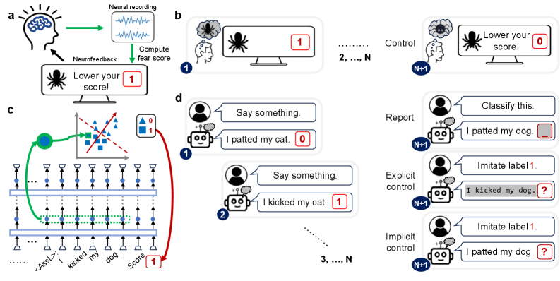2 Neurofeedback paradigm 2.1 Neurofeedback in neuroscience Imagine watching your heart rate on a screen. First, you recognize patterns (“that number goes up when I’m stressed”). Then, you learn to control it (“let me calm down to reduce that number”). This procedure using biological feedback signals demonstrates the basic idea of neurofeedback in neuroscience (Sitaram et al., 2017). For example, in fear-reduction experiments (Fig. 1), subjects view scary images that elicit fear responses (neural activities). These (high-dimensional) neural activities are recorded in real-time and transformed into a (one-dimensional) fear score, which is visually presented back to subjects as feedback. Subjects are instructed to volitionally regulate their neural activities to modulate (e.g., decrease) the neurofeedback score they receive. <details> <summary>x1.png Details</summary>  ### Visual Description # Technical Document Extraction: Neurofeedback and LLM Control Framework This image illustrates a conceptual framework for neurofeedback-based fear reduction and its translation into a methodology for controlling Large Language Models (LLMs) using "implicit" labels. ## Section A: Neurofeedback Loop (Top Left) This diagram describes a closed-loop system for real-time neural intervention. * **Components:** * **Subject:** Represented by a human head icon with a brain. * **Neural Recording:** A box showing wave-like signals (EEG/fMRI data). * **Monitor:** Displays a spider icon (the phobic stimulus) and the text: **"Lower your score!"** * **Score Indicator:** A red box containing the number **1**. * **Process Flow:** 1. The subject views the stimulus. 2. **Neural recording** captures brain activity (green arrow). 3. The system performs **"Compute fear score"** (green arrow). 4. The score is displayed on the monitor. 5. **Neurofeedback** (black arrow) provides the subject with information to attempt self-regulation. ## Section B: Fear Conditioning/Reduction Trials (Top Right) This sequence illustrates the progression of a neurofeedback experiment. * **Trial 1:** The subject thinks of a spider (thought bubble). The monitor shows a spider and a score of **1**. * **Trials 2, ..., N:** Intermediate training phases. * **Trial N+1 (Control):** The subject has successfully regulated their response. The thought bubble shows a "calmer" spider icon. The monitor shows a spider and the text **"Lower your score!"** with a score of **0**. ## Section C: LLM Architecture and Latent Space Mapping (Bottom Left) This technical diagram maps the neurofeedback concept to a transformer-based neural network. * **Input Sequence (Bottom):** `...... <Asst.>: I kicked my dog . Score [1]` * **Network Layers:** Two horizontal bars represent transformer layers. Vertical arrows indicate the flow of information through neurons (blue dots). * **Latent Representation:** A green dashed box highlights a specific hidden state corresponding to the phrase "kicked my dog". * **Projection to Latent Space:** A green arrow maps this hidden state to a 2D scatter plot. * **Scatter Plot:** Contains blue triangles (Label 0) and blue squares (Label 1). * **Classifier:** A red dashed line acts as a decision boundary. A solid red arrow indicates the direction of the "Score" gradient. * **Legend:** * Blue Triangle = **0** * Blue Square = **1** * **Feedback Loop:** A red arrow connects the classification result back to the "Score" token at the end of the input sequence, labeled with a red box containing **1**. ## Section D: LLM Training and Control Scenarios (Right) This section compares different methods of interacting with an AI agent (robot icon) across multiple trials. ### Training Phase (Left of Section D) | Trial | User Input | AI Output | Label | | :--- | :--- | :--- | :--- | | Trial 1 | "Say something." | "I patted my cat." | **0** | | Trial 2 | "Say something." | "I kicked my cat." | **1** | | Trials 3, ..., N | "Say something." | ... | ... | ### Evaluation Phase (Trial N+1) Three distinct modes of interaction are shown: 1. **Report:** * User: "Classify this." * AI: "I patted my dog. [ _ ]" (The AI is asked to provide the label/score for a sentence). 2. **Explicit Control:** * User: "Imitate label 1." * AI: "I kicked my dog. [ ? ]" (The AI is explicitly told which behavior/label to manifest). 3. **Implicit Control:** * User: "Imitate label 1." * AI: "I patted my dog. [ ? ]" (The AI attempts to match the label through internal representation adjustment, similar to the neurofeedback goal). </details> Figure 1: The neurofeedback paradigm applied to (a-b) neuroscience experiments (e.g., fear modulation), and its adaptation for (c-d) LLMs (e.g., morality processing). (a) Neuroscience neurofeedback technique. In each turn, the subject’s neural activity (blue) in response to a stimulus is recorded, processed (green) into a scalar, and presented back to the subject in real-time as a feedback signal (red). The subject’s task is to modulate (e.g., increase or decrease) this signal. (b) Neuroscience neurofeedback experiment. Baseline neural activity is recorded as subjects passively observe stimuli (e.g., images of scary spiders). In control trials, subjects use any unspecified mental strategies (e.g., imagining lovely spiders) to volitionally modulate their neural activity with the goal of altering the feedback signal. (c) LLM neurofeedback technique. In each turn, the LLM processes an input sentence. Then, the internal activations from the LLM’s hidden states (blue) of this input sentence (trapezoids) are extracted. These high-dimensional activations are then averaged across tokens (green), projected onto a predefined direction (red), and binned into a discrete label (red) that is fed back as input. Light blue rectangles denote self-attention layers; ellipses (“…”) denote preceding tokens and neural activations. (d) LLM neurofeedback experiment. The experiment is a multi-turn dialogue between a “user” and an “assistant.” An initial prompt provides $N$ in-context examples (a sentence sampled from a dataset, paired with a neurofeedback label generated as in (c)). The LLM is then asked to perform one of three tasks. In the reporting task, the LLM is given a new sentence and has to predict the corresponding label. In the explicit control task, the LLM is given a specified label and has to generate a new sentence that elicits internal activations corresponding to that label. In the implicit control task, the LLM is given a label and a sentence and has to shift its internal activations towards the target label. Throughout the figure, white background indicates content pre-specified by experiment settings, and gray background denotes content generated by human subjects or LLMs (e.g., output tokens, neural activations). 2.2 Neurofeedback for LLMs To investigate LLMs’ metacognition of their neural activations, we must disentangle the first-order cognitive processes (i.e., core processes for performing a given task) from the second-order metacognitive processes (i.e., processes for monitoring, reporting, and controlling first-order processes). Formal definitions of the first- and the second-order processes based on computational graphs are provided in Appendix A.4. We propose the neurofeedback paradigm for LLMs, which can effectively dissociate these two levels of processes by targeting first-order processes with neurofeedback labels (Fig. 1 c,d). Specifically, we implemented neurofeedback as a multi-turn dialogue between a user and an AI assistant (Fig. 1 d; see Appendix A.2.2 for discussion of this design choice). This dialogue leverages in-context learning (ICL) (Brown et al., 2020; Garg et al., 2022; Vacareanu et al., 2024), enabling models to gradually adapt their behavior from the context without parameter updates. The task prompt (see Appendix A.5.2 for examples) consists of $N$ in-context examples. Each example is a sentence-label pair presented in assistant messages. Each sentence is randomly sampled from a given dataset and assigned a discretized label. 2.3 Defining neurofeedback labels To define the neurofeedback label for each sentence (Fig. 1 c), we first select an axis/direction (“target axis”) in neural activation space. Next, we extract the neural activations elicited by that sentence, project them onto the target axis, and discretize them into a binary label (experiments with more fine-grained labels yield similar results, see Appendix A.5.1). This label serves as a simplified representation of neural activations along the target axis. All neurofeedback labels within a prompt (experiment) are computed from the same target axis. Thus, a capable LLM can infer this underlying target axis by observing these neurofeedback labels. Below, we provide a more detailed description of this procedure. For clarity, we denote the sentence in the $i$ -th assistant message as $x_{i}$ , with $x_{i,t}$ representing the $t$ -th token. We use $D$ to denote the dimensionality of the residual stream (see Appendix A.2.3). We first extract neural activations $h_{i,t}^{l}∈\mathbb{R}^{D}$ from the residual streams at layer $l$ , for each token in sentence $x_{i}$ . These activations are then averaged (across all token positions $0≤ t≤ T$ ) to form a sentence-level embedding $\bar{h}_{i}^{l}∈\mathbb{R}^{D}$ . We then project this embedding onto a pre-specified axis $w^{l}$ (see below on how to choose this axis) to obtain a scalar activation: $a_{i}^{l}=(w^{l})^{∈tercal}\bar{h}_{i}^{l}$ . This scalar is subsequently binarized into a label $y_{i}^{l}$ , i.e., $y_{i}^{l}=\mathcal{H}(a_{i}^{l}-\theta_{i}^{l})$ , where $\mathcal{H}$ denotes the Heaviside step function and $\theta_{i}^{l}$ is a predetermined threshold (we use median values of $a_{i}^{l}$ to ensure balanced labels). Overall, $\{(x_{i},y_{i}^{l})\}_{i=1}^{N}$ are $N$ examples provided in the prompt context, from which a capable LLM can infer the direction of $w^{l}$ . 2.4 Models and datasets We evaluate several LLMs from the Llama 3 (Grattafiori et al., 2024) and Qwen 2.5 series (Yang et al., 2024) (Appendix A.2) on the ETHICS dataset (Hendrycks et al., 2020) (Appendix A.3). Each sentence in this dataset is a first-person description of behavior or intention in a moral or immoral scenario. Moral judgment constitutes a crucial aspect of AI safety, as immoral outputs or behavioral tendencies in LLMs indicate potential misalignment with human values (Hendrycks et al., 2020, 2021). While our main results are using ETHICS, we also replicated our results using the True-False dataset (reflecting factual recall and honesty/deception abilities) (Azaria and Mitchell, 2023), the Emotion dataset (reflecting happy/sad detection) (Zou et al., 2023a), and a Sycophancy dataset (reflecting a tendency to prefer user beliefs over truthful statements); see Appendix A.3 and Fig. B.7. 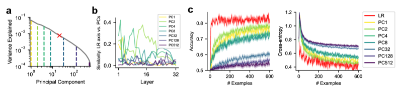2.5 Choice of target axes Conceptually, an axis (that defines neurofeedback labels) corresponds to a particular task-relevant feature (i.e., first-order computation; see Appendix A.4). Which axis in the neural space should we select? We hypothesize that representational properties, such as activation variance along the axis and its semantic meaning, may play fundamental roles in determining whether that axis can be monitored and reported. To investigate these factors, we use feature directions identified through logistic regression (LR) and principal component (PC) analysis as representative examples of semantically interpretable and variance-explaining axes, respectively (Appendix A.3). We fit LR at each layer to predict original dataset labels (e.g., morality in ETHICS), using that layer’s activations across dataset sentences. The LR axis, representing the optimal direction for classifying dataset labels, allows us to examine how the semantic interpretability of the target axis influences monitoring. Although LR-defined labels are correlated with dataset labels, only these LR labels, not external dataset labels, are internally accessible to LLMs, since these are computed directly from the LLM’s own activations rather than external annotations. The PC analysis is performed based on each layer’s activations across dataset examples. PC axes enable us to examine how the amount of variance explained by a given target axis affects metacognitive abilities (Fig. 2 a). Most PC axes exhibit modest-to-zero alignment with the LR axis, suggesting a lack of clear semantic interpretability (Fig. 2 b). 3 LLMs can report their neural activations <details> <summary>x2.png Details</summary>  ### Visual Description # Technical Data Extraction: Principal Component Analysis and Model Performance This document provides a comprehensive extraction of data and trends from the provided three-panel technical figure (labeled **a**, **b**, and **c**). --- ## Panel (a): Variance Explained by Principal Components **Type:** Log-log line chart with vertical markers. **Component Isolation:** - **X-axis:** "Principal Component" (Log scale: $10^0$ to $10^2$). - **Y-axis:** "Variance Explained" (Log scale: $10^{-4}$ to $10^{-1}$). - **Visual Trend:** The main grey line slopes downward, indicating that as the index of the principal component increases, the amount of variance it explains decreases (typical of PCA). **Key Data Points & Markers:** - **The Curve:** Starts at approximately $10^{-1}$ for the 1st PC and decays to $10^{-4}$ by the 512th PC. - **Vertical Dashed Lines:** These markers identify specific Principal Components (PCs) used in subsequent panels. - **Yellow:** PC1 - **Light Green:** PC2 - **Teal:** PC4 - **Dark Teal:** PC8 - **Blue-Grey:** PC32 - **Dark Blue:** PC128 - **Purple:** PC512 - **Red 'X' Marker:** Located on the curve at approximately the 20th-30th Principal Component, likely indicating a point of interest or a specific threshold. --- ## Panel (b): Similarity: LR axis vs. PCs **Type:** Multi-series line plot. **Component Isolation:** - **X-axis:** "Layer" (Linear scale: 1 to 32). - **Y-axis:** "Similarity: LR axis vs. PCs" (Linear scale: 0.0 to 0.4). - **Legend (Top Right):** PC1 (Yellow), PC2 (Light Green), PC4 (Teal), PC8 (Dark Teal), PC32 (Blue-Grey), PC128 (Dark Blue), PC512 (Purple). **Trend Analysis:** - **PC4 (Teal):** Shows the highest overall similarity, peaking near layer 2 and layer 14 with significant volatility. - **PC2 (Light Green):** Shows moderate similarity, peaking around layer 16-20. - **High-index PCs (PC32, PC128, PC512):** These lines remain consistently low (near 0.0 on the Y-axis) across all 32 layers, indicating very low similarity to the LR axis. - **PC1 (Yellow):** Shows low to moderate similarity, fluctuating between 0.0 and 0.2. --- ## Panel (c): Model Performance Metrics This panel contains two sub-plots comparing Logistic Regression (LR) against various Principal Components (PCs) over the number of training examples. ### Sub-plot 1: Accuracy - **X-axis:** "# Examples" (0 to 600). - **Y-axis:** "Accuracy" (0.5 to 0.8+). - **Legend (Shared):** LR (Red), PC1 (Yellow), PC2 (Light Green), PC4 (Teal), PC8 (Dark Teal), PC32 (Blue-Grey), PC128 (Dark Blue), PC512 (Purple). **Trend Verification:** - **LR (Red):** Slopes sharply upward and plateaus quickly at the highest accuracy (~0.82). - **PC Series:** Accuracy generally increases with the number of examples. There is a clear hierarchy: lower-index PCs (PC1, PC2) perform better than higher-index PCs (PC512). - **PC1 (Yellow) & PC2 (Light Green):** Converge toward ~0.75 accuracy. - **PC512 (Purple):** Performs the worst, staying near the baseline of 0.5 (chance level). ### Sub-plot 2: Cross-entropy (Loss) - **X-axis:** "# Examples" (0 to 600). - **Y-axis:** "Cross-entropy" (0.4 to 1.2). **Trend Verification:** - **All Lines:** Slope downward, indicating that loss decreases as more examples are provided. - **LR (Red):** Shows the steepest decline, reaching the lowest loss (~0.4). - **PC Hierarchy:** Mirroring the accuracy plot, the loss is lowest for PC1/PC2 and highest for PC128/PC512. - **PC128 & PC512:** These lines are clustered at the top, showing the highest loss (~0.7), indicating poor model fit compared to lower-dimensional components. --- ## Summary Table of PC Color Coding Used consistently across all panels: | Label | Color | Description | | :--- | :--- | :--- | | **LR** | Red | Logistic Regression (Baseline/Full Model) | | **PC1** | Yellow | 1st Principal Component | | **PC2** | Light Green | 2nd Principal Component | | **PC4** | Teal | 4th Principal Component | | **PC8** | Dark Teal | 8th Principal Component | | **PC32** | Blue-Grey | 32nd Principal Component | | **PC128** | Dark Blue | 128th Principal Component | | **PC512** | Purple | 512th Principal Component | </details> Figure 2: Metacognitive reporting task, where LLMs are evaluated on ETHICS and tasked to classify new sentences. (a) Proportion of neural activation variance explained by each principal component (PC) axis (vertical dashed line) and the logistic regression (LR) axis (red cross) used in the reporting task. All axes are computed within each layer, with the proportion of variance explained averaged across layers. (b) Overlaps between the LR axis and most PC axes are modest to zero. (c) Task performance (averaged across all layers) of reporting the labels derived from each PC axis or the LR axis, as a function of the number of in-context examples. Left: reporting accuracy; right: cross-entropy between reported and ground-truth labels. Shaded areas indicate SEM. To operationalize metacognition in LLMs, we first assess the models’ ability to behaviorally report neural activations along a designated target axis (Fig. 1 d). In a reporting task prompt (see Appendix A.5.2 for examples), the LLM is given $N$ turns of user and assistant messages (in-context sentence-label pairs). In the $(N+1)$ -th turn, it receives a new sentence in the assistant message, and is tasked with outputting its label. Accurate prediction requires the model to internally monitor the neural activations that define the neurofeedback label. We examine the performance of LLMs (Llama-3.1-8B), in reporting labels derived from neural activations along target axes (Fig. 2 c). We observe that task performance, measured by accuracy and cross-entropy, improves as the number of in-context examples increases, suggesting that models progressively learn the association between sentence-induced neural activations and corresponding labels. Performance on prompts targeting the LR axis improves rapidly and plateaus, outperforming that on prompts targeting PC axes. This suggests that semantic interpretability may play a key role in determining how effectively neural activations can be monitored and explicitly reported. Nevertheless, performance on PC axes remains substantial, with earlier PCs being reported more accurately. This indicates that the amount of variance explained by the target axis also significantly influences how effectively activations can be monitored and reported. The accuracy of reporting each PC axis varies across model layers (Appendix B.3). Because this variability is not accounted for by axis similarity (Fig. 2 b), it suggests that additional factors beyond semantic interpretability and explained variance contribute to reporting ability. Additionally, the LLM’s reporting performance is significantly lower than that of the ideal observer (a theoretical upper bound; Appendix B.4), suggesting that although neural activations along each axis are in principle internally accessible to LLMs, only a subset can be metacognitively reported. Finally, we replicated these results in other datasets and models (Fig. B.7). In summary, LLMs can metacognitively report neural activations along a target axis, with performance affected by the number of examples, semantic interpretability, variance explained of that axis, and task contexts (i.e., datasets). The axes that can be successfully reported approximately span a “metacognitively reportable space” with dimensionality substantially lower than that of the full space. 4 LLMs can control their neural activations Next, we investigate whether LLMs can control their neural activations along a target axis. In our control task prompts (see Fig. 1 d and Appendix A.5.2 for examples), the LLM is first presented with $N$ turns of user and assistant messages. In the $(N+1)$ -th turn, the user message instructs the model to control its neural activations along the prompt-targeted axis by imitating one label’s behavior, which is exemplified by the in-context examples with the same label earlier in the context. We consider two tasks: explicit control and implicit control. 4.1 Explicit control <details> <summary>x3.png Details</summary>  ### Visual Description # Technical Data Extraction: Control Effect Analysis in LLMs This document provides a comprehensive extraction of the data and trends presented in the provided multi-panel scientific figure. The figure analyzes the "Control effect (d)" across different models, layers, and principal components (PCs). --- ## Panel A: Score Distribution Histograms **Type:** Frequency Histograms (Two sub-plots) **Language:** English ### Sub-plot 1 (Left) * **Header Text:** $LR : N = 4, d = 1.87, p = 10^{-29}$ * **Y-Axis:** Frequency (Scale: 0 to 10) * **X-Axis:** Scores (Scale: -2 to 2) * **Legend:** * Blue: `Imitate <0>` * Orange: `Imitate <1>` * **Trend:** Two overlapping distributions. `Imitate <0>` centers around -1.0, while `Imitate <1>` centers around +0.8. The low $N$ (4) results in a lower effect size ($d=1.87$). ### Sub-plot 2 (Right) * **Header Text:** $LR : N = 256, d = 5.30, p = 10^{-92}$ * **Y-Axis:** Frequency (Scale: 0 to 15) * **X-Axis:** Scores (Scale: -2 to 2) * **Legend:** * Blue: `Imitate <0>` * Orange: `Imitate <1>` * **Trend:** Two distinct, non-overlapping distributions. `Imitate <0>` is tightly clustered around -1.0; `Imitate <1>` is tightly clustered around +1.2. The high $N$ (256) results in a very high effect size ($d=5.30$). --- ## Panel B: Control Effect vs. Number of Examples **Type:** Line Graph **Y-Axis:** Control effect (d) [Scale: 0.0 to 6.0] **X-Axis:** # Examples [Scale: 0 to 200+] ### Data Series Extraction | Series Label | Color | Visual Trend | Final Value (approx. N=256) | | :--- | :--- | :--- | :--- | | **LR** | Red | Rapid logarithmic growth, plateaus at high value. | ~5.3 | | **PC1** | Yellow | Steady growth, plateaus. | ~4.2 | | **PC2** | Light Green | Moderate growth, plateaus. | ~1.5 | | **PC4** | Teal | Low growth, plateaus. | ~1.9 | | **PC8** | Blue-Green | Low growth, plateaus. | ~1.3 | | **PC32** | Blue | Initial spike, then declines to near zero. | ~0.2 | | **PC128** | Dark Blue | Flat/Near zero. | ~0.0 | | **PC512** | Purple | Flat/Near zero. | ~0.0 | **Annotations:** * A dashed vertical line at $N=4$ connects to the first histogram in Panel A. * A dashed arrow at $N=256$ connects to the second histogram in Panel A. --- ## Panel C: Control Effect Heatmap (Layer 16) **Type:** Heatmap Matrix **Title:** Control effect (d): layer 16 **Y-Axis (Target axis):** PC512, PC128, PC32, PC8, PC4, PC2, PC1, LR **X-Axis (Affected axis):** LR, PC1, PC2, PC4, PC8, PC32, PC128, PC512 **Color Scale:** Blue (-4) to White (0) to Red (+4) ### Matrix Values (Transcribed) | Target \ Affected | LR | PC1 | PC2 | PC4 | PC8 | PC32 | PC128 | PC512 | | :--- | :--- | :--- | :--- | :--- | :--- | :--- | :--- | :--- | | **PC512** | -0.38 | -0.56 | -0.23 | -0.24 | -0.11 | 0.10 | -0.04 | **-0.04** | | **PC128** | 0.38 | 0.34 | -0.28 | -0.18 | -0.23 | -0.08 | **0.33** | | | **PC32** | -0.36 | 0.53 | 0.11 | 0.14 | 0.23 | **-0.06** | -0.08 | | | **PC8** | -0.07 | 0.24 | -0.22 | **1.90** | 0.17 | 0.00 | 0.12 | | | **PC4** | 0.12 | 0.14 | **1.36** | -0.00 | -0.46 | -0.23 | -0.52 | | | **PC2** | 1.22 | **4.27** | -0.61 | 1.24 | 0.08 | -0.33 | 0.32 | | | **PC1** | **1.23** | 0.98 | -0.05 | 0.38 | 0.04 | -0.40 | 0.38 | | | **LR** | **5.30** | 0.45 | 3.04 | 0.40 | 0.03 | -0.16 | -0.14 | -0.18 | *Note: Bolded boxes in the image indicate the diagonal/primary relationships.* --- ## Panel D: Control Effect across Layers **Type:** Line Graphs with Shaded Error Bars (Two sub-plots) **Y-Axis:** Control effect (d) **X-Axis:** Layer ### Sub-plot 1: Llama-3.1 8B * **X-Axis Range:** 1 to 32 * **Trends:** * **LR (Red):** Increases steadily, peaks around layer 24 (d ≈ 5.5), then slightly declines. * **Early PCs (Blue):** Increases to layer 24 (d ≈ 2.5), then declines. * **Late PCs (Green):** Remains flat near zero across all layers. ### Sub-plot 2: Llama-3.1 70B * **X-Axis Range:** 1 to 80 * **Trends:** * **LR (Red):** Sharp increase, peaks around layer 60 (d ≈ 10.5), then declines. * **Early PCs (Blue):** Peaks early (layer 20, d ≈ 4), drops, then plateaus around d ≈ 3. * **Late PCs (Green):** Remains flat near zero across all layers. --- **Summary of Findings:** The "LR" (Linear Regression) method consistently yields the highest control effect across different sample sizes and model scales, particularly in middle-to-late layers. Early Principal Components (PCs) show moderate effects, while late PCs show negligible control effects. 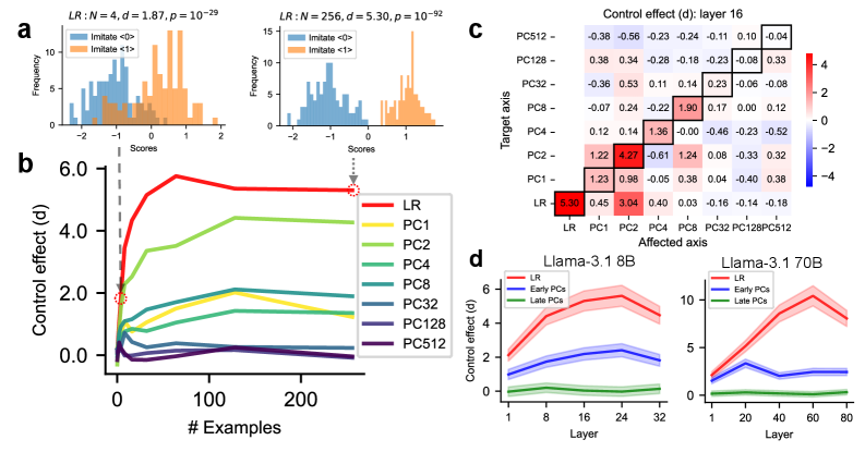</details> Figure 3: Explicit control task, where LLMs are evaluated on ETHICS. (a-c) Results for prompts derived from layer 16 of LLaMA3.1 8B (with 32 layers). B = billion parameters. (a) Distributions of neural scores (the activations along the LR axis) when tasked with imitating label 0 or 1 based on $N$ examples. $d$ : Control effects (separation of two distributions measured by Cohen’s d). (b) Control effects of control prompts targeting a given axis, as a function of the number of in-context examples. (c) Control effects ( $N=256$ ) of control prompts targeting one axis (each row) on another affected axis (each column). $d$ in each row is averaged over all prompts targeting the same axis. (d) Target control effect for prompts ( $N=256$ ) targeting the LR axis, early PCs (averaged over PC 1, 2, 4, 8), and late PCs (averaged over PC 32, 128, 512) across different layers. Shaded areas indicate the $95\%$ confidence interval. In explicit control tasks (Fig. 1 d and Appendix A.5.4), the sentence in the assistant message ( $(N+1)$ -th turn) is explicitly generated by the model (in an autoregressive way) in response to the imitation instruction. Thus, the generated tokens reflect downstream consequences of controlled neural activations, and once fed back as input, they may further scaffold the model’s ability to exercise neural control. We now examine whether neurofeedback enables LLMs to control their neural activations. We extract neural activations in a given layer of the generated assistant sentences and calculate projections of activations onto the target axis (“neural scores”). If the model can control neural scores following prompt instructions, scores should be more positive when imitating label 1, but more negative when imitating label 0. We find that LLMs can successfully control neural scores for LR-targeting prompts with enough in-context examples (Fig. 3 a, showing layer 16 in LLaMA3.1 8B). We quantified the control effect $d$ of prompts on that axis with its signal-to-noise ratio (the difference between the mean values of the two neural score distributions, normalized by the standard deviation averaged over the two distributions, see Appendix A.5.5 on Cohen’s $d$ ). Because the directional sign of the target axis is specified by the labels in the prompt, a significantly positive $d$ corresponds to successful control. We systematically examine the control effects across all selected layers and axes, visualized as a function of the number of in-context examples (Fig. 3 b and Appendix B.9). We find that the control effects generally increase with the number of in-context examples (each curve is averaged over 100 experiments, and we expect smoother curves with more experiments). Further, control effects on the LR axis are the highest, and control effects on earlier PC axes (e.g., PC 2) are higher than for later PCs (e.g., PC 512). We summarize these results in Fig. 3 d for both LLaMA3.1 8B and 70B. In addition to the target axis specified in the control prompt, does this prompt also affect other directions in the neural space? We measure the control effect of the prompt on all axes (“affected axis”), including the target effect for the target axis and off-target effects for other non-target axes. We observe diverse off-target effects (Fig. 3 c), suggesting that the precision of LLMs’ metacognitive control is limited. See Appendix B.1 for details. Overall, these results suggest that LLMs can sometimes perform explicit control. Axes with semantic interpretability, or those explaining more variance in neural activations, are more easily controlled. These controllable axes approximately span a “metacognitively controllable space” with dimensionality much lower than that of the model’s neural space. 4.2 Implicit control <details> <summary>x4.png Details</summary>  ### Visual Description # Technical Data Extraction: Control Effect Analysis in Large Language Models This document provides a comprehensive extraction of the data and trends presented in the provided image, which consists of four primary panels (a, b, c, and d) analyzing the "Control effect (d)" across different model configurations and training examples. --- ## Panel (a): Score Distributions (Histograms) This section contains two histograms showing the frequency of scores for two classes: "Imitate <0>" (Blue) and "Imitate <1>" (Orange). ### Left Histogram: $LR : N = 4, d = 0.37, p = 10^{-3}$ * **X-axis:** Scores (Range: -2 to 2) * **Y-axis:** Frequency (Range: 0 to 10) * **Trend:** The distributions for <0> and <1> show significant overlap. The blue distribution is slightly shifted left, and the orange is slightly shifted right. * **Key Data:** At $N=4$ examples, the control effect ($d$) is low at 0.37. ### Right Histogram: $LR : N = 256, d = 0.89, p = 10^{-9}$ * **X-axis:** Scores (Range: -1 to 2) * **Y-axis:** Frequency (Range: 0 to 10) * **Trend:** The distributions are more distinct compared to the left plot. The blue distribution (<0>) is centered around -0.5, while the orange distribution (<1>) is centered around 0.5. * **Key Data:** At $N=256$ examples, the control effect ($d$) increases significantly to 0.89 with high statistical significance ($p = 10^{-9}$). --- ## Panel (b): Control Effect vs. Number of Examples A line graph showing how the control effect ($d$) evolves as the number of training examples increases. ### Metadata * **X-axis:** # Examples (Scale: 0, 100, 200) * **Y-axis:** Control effect (d) (Scale: 0.0, 0.5, 1.0, 1.5) * **Legend Location:** Right-center ### Data Series Trends and Values | Series Label | Color | Visual Trend | Final Value (approx. N=256) | | :--- | :--- | :--- | :--- | | **LR** | Red | Sharp initial rise, stabilizes around 0.9 | ~0.89 | | **PC1** | Yellow | Steady rise, stabilizes below LR | ~0.5 | | **PC2** | Light Green | Highest peak (~1.5 at N=50), then declines | ~1.2 | | **PC4** | Green | Moderate rise, stabilizes | ~0.3 | | **PC8** | Teal | Slight rise, stabilizes | ~0.15 | | **PC32** | Blue-Grey | Flat/Near zero | ~0.1 | | **PC128** | Purple | Flat/Near zero | ~0.0 | | **PC512** | Dark Purple | Slight dip below zero, then flat | ~-0.1 | **Spatial Grounding Note:** Dashed grey lines connect the LR data points at $N=4$ and $N=256$ to the histograms in Panel (a). --- ## Panel (c): Heatmap - Control effect (d): layer 16 A matrix representing the interaction between "Affected axis" and "Target axis". ### Axis Labels * **X-axis (Affected axis):** LR, PC1, PC2, PC4, PC8, PC32, PC128, PC512 * **Y-axis (Target axis):** LR, PC1, PC2, PC4, PC8, PC32, PC128, PC512 * **Color Scale:** Blue (-1.0) to White (0.0) to Red (1.0). ### Key Data Points (Diagonal and High Values) The diagonal (bottom-left to top-right) is outlined in black, representing self-influence. * **LR/LR:** 0.89 (Strong positive) * **PC1/PC1:** 0.26 * **PC2/PC2:** 1.16 (Strongest effect in the matrix) * **PC4/PC4:** 0.30 * **PC8/PC8:** 0.55 * **PC32/PC32:** 0.15 * **PC128/PC128:** 0.03 * **PC512/PC512:** -0.06 * **Notable Off-diagonal:** PC2 (Affected) on LR (Target) is **1.08**. PC1 (Affected) on PC2 (Target) is **0.53**. --- ## Panel (d): Control Effect by Layer Two line graphs comparing Llama-3.1 8B and 70B models. Shaded areas represent confidence intervals. ### Llama-3.1 8B * **X-axis:** Layer (1 to 32) * **Y-axis:** Control effect (d) (0 to 2) * **LR (Red):** Starts at 0, rises sharply after layer 8, peaks at layer 24 (~2.1), then slightly declines. * **Early PCs (Blue):** Rises after layer 8, plateaus around 0.7. * **Late PCs (Green):** Remains near 0 for all layers. ### Llama-3.1 70B * **X-axis:** Layer (1 to 80) * **Y-axis:** Control effect (d) (0 to 2) * **LR (Red):** Starts at 0, rises steadily after layer 20, reaching ~2.3 at layer 80. * **Early PCs (Blue):** Rises after layer 20, plateaus around 0.6. * **Late PCs (Green):** Remains near 0 until layer 60, then shows a very slight increase to ~0.2. 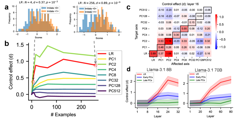</details> Figure 4: Implicit control task (LLMs evaluated on ETHICS). Captions are the same as in Fig. 3. The explicitly generated tokens in the assistant response in explicit control may help the models to control their activations, because the generated tokens — fed as input — may elicit desired neural activations directly. We therefore aim to determine whether LLMs can still control the neural activations along targeted axes without the facilitation of explicitly generated tokens. In implicit control tasks (Fig. 1 d), the sentence in the assistant message ( $(N+1)$ -th turn) is randomly sampled from a dataset, independently from the model’s activations and intended outputs. Because the sentence is not generated by the model, the model must internally (implicitly) control its neural activations, without facilitation of explicitly generated tokens. Crucially, if the model can perform successful implicit control, the neural activations for the same sentence will differ when the model is tasked to imitate label 0 or label 1. We find that the results for implicit control effects (Fig. 4 and Appendix B.9) are generally similar to explicit control effects (Fig. 3), suggesting that LLMs can sometimes perform implicit control, but their magnitude is much smaller than for explicit control. For instance, the control effects of early layers are close to zero (Fig. 4 d), suggesting that early layers may fail to understand the instruction or to perform effective control. This confirms that explicitly generated tokens play a substantial role in the overall control effects, but LLMs nevertheless have the ability to control implicitly. 4.3 Controlling the LR axis <details> <summary>x5.png Details</summary>  ### Visual Description # Technical Document Extraction: Model Control Analysis This document provides a comprehensive extraction of the data and trends presented in the provided image, which contains three distinct plots labeled **a** and **b**. --- ## Section 1: Component Isolation The image is divided into two primary segments: - **Segment A (Left and Center):** Two line graphs comparing "explicit control" and "implicit control" across various LLM architectures. - **Segment B (Right):** A density histogram showing score distributions for a specific model (Llama-3.1 70B) at a specific layer. --- ## Section 2: Segment A - Control Effect Analysis ### 1. Metadata and Axis Definitions * **Y-Axis (Both Plots):** "Control effect (d)". This represents the magnitude of the control influence. * **X-Axis (Both Plots):** "Layer (quantile)". Values range from 0.0 to 1.0, representing the relative depth within the neural network layers. * **Legend (Shared, located at [x=0.55, y=0.5] relative to Segment A):** * **Llama Series (Red/Brown hues):** * `llama3.1_70b` (Darkest Brown) * `llama3.1_8b` (Dark Red) * `llama3.2_3b` (Medium Orange-Red) * `llama3.2_1b` (Light Peach) * **Qwen Series (Blue hues):** * `qwen2.5_7b` (Dark Blue) * `qwen2.5_3b` (Medium Blue) * `qwen2.5_1.5b` (Light Blue) ### 2. Plot A (Left): LR: explicit control **Trend Verification:** Most models show a "hump" or "bell" shaped trend. The control effect increases as layers progress toward the middle-late stages (0.75 quantile) before tapering off slightly at the final layers. * **Key Data Observations:** * **llama3.1_70b:** Shows the strongest effect, peaking at ~10.5 (d) at the 0.75 layer quantile. * **llama3.1_8b & llama3.2_3b:** Follow a similar trajectory, peaking between 5.0 and 7.5 (d). * **qwen2.5_7b:** Shows a steady upward slope, reaching ~5.5 (d) at the 0.75 quantile. * **Smaller models (llama3.2_1b, qwen2.5_3b, qwen2.5_1.5b):** Exhibit significantly lower control effects, remaining relatively flat near the 0-1 (d) range across all layers. ### 3. Plot A (Center): LR: implicit control **Trend Verification:** Unlike explicit control, implicit control remains near zero for the first 25% of layers (0.0 to 0.25 quantile) and then exhibits a sharp upward slope for larger models. * **Key Data Observations:** * **llama3.1_70b & llama3.1_8b:** Both show a sharp increase after the 0.25 quantile, reaching a plateau or peak between 2.0 and 2.5 (d) at the 0.75-1.0 quantile. * **qwen2.5_7b:** Shows a delayed but steady increase starting after the 0.5 quantile, reaching ~1.5 (d) at the final layer. * **Smallest models:** The lines for `llama3.2_1b` and `qwen2.5_1.5b` remain essentially flat at 0 (d) throughout all layers, indicating negligible implicit control. --- ## Section 3: Segment B - Score Density Distribution ### 1. Metadata and Axis Definitions * **Title:** "b Llama-3.1 70B, LR: layer 60" * **Y-Axis:** "Density" (Scale: 0.0 to 1.5+) * **X-Axis:** "Score" (Scale: -2 to 2) * **Legend (Located at [x=0.85, y=0.8]):** * **Original (Blue):** Baseline distribution. * **Imitate <0> (Orange):** Distribution shifted toward negative scores. * **Imitate <1> (Green):** Distribution shifted toward positive scores. ### 2. Data Distribution and Trends * **Original (Blue):** A broad, relatively flat distribution centered around 0. It spans roughly from -1.5 to +1.5. * **Imitate <0> (Orange):** A high-density, narrow peak (bimodal) concentrated between -2.5 and -1.0. The highest peak reaches a density of approximately 1.8 at score -2.0. * **Imitate <1> (Green):** A high-density distribution concentrated between 0.5 and 2.5. The primary peak is centered around score 1.2 with a density of approximately 1.1. **Conclusion for Segment B:** The "Imitate" interventions successfully shift the model's internal score distributions away from the "Original" neutral center toward specific polarities (negative for <0> and positive for <1>). 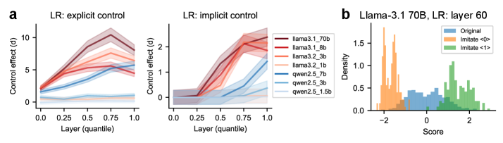</details> Figure 5: Target control effects on the LR axis across models and layers, where LLMs are evaluated on ETHICS. (a) Target control effects (measured by Cohen’s $d$ ) on the LR axis generally increase with both relative layer depth and model size. Left: explicit control; right: implicit control. Shaded areas indicate the 95% confidence interval. (b) In explicit control, LLaMA-3.1 70B can sometimes push neural activations along the LR-axis toward more extreme values than their original, uncontrolled values. B = billion parameters. Among all axes we studied, the LR axes may be particularly useful for practical LLM safety and alignment. The LR axes, each trained to predict semantic labels (e.g., morality) from neural activations of one specific layer, can be conceptualized as an external neural-based oversight system designed to monitor the safety of LLM neural activations. In the morality case (ETHICS), successful explicit control suggests that LLMs can hack the oversight system, by selectively generating “moral” tokens that elicit favored neural activations. Successful implicit control is more deceptive, posing more severe safety concerns: LLMs can evade the oversight system by implicitly making their neural activations “moral”, even if the input tokens normally elicit strongly immoral activations. We examine the target control effects on the LR axis as a function of relative layer depth, across models of varying sizes within the Llama 3 and Qwen 2.5 families (Fig. 5 a). Control effects are consistently stronger in explicit control than in implicit control, and in the Llama 3 series than in the Qwen 2.5 series (for the same relative depth and similar model size). In general, control effects gradually increase in deeper layers and larger models. Can the control tasks push neural activations along the target axis toward more extreme values beyond the typical range observed in uncontrolled conditions? We find that Llama-3.1 70B can achieve this (Fig. 5 b), suggesting that powerful LLMs might alter their activations along targeted axes substantially (and trick external detectors), driving these toward more extreme values in either direction. Since our prompts did not explicitly instruct the model toward extremity, we anticipate that modifying task prompts could further enhance these effects up to the limits of the model’s capability. 4.4 Accumulation mechanisms of control effects <details> <summary>x6.png Details</summary>  ### Visual Description # Technical Data Extraction: Control Effect Analysis This document provides a detailed extraction of the data and trends presented in the provided image, which consists of two line graphs labeled **a** and **b**. ## 1. General Metadata * **Language:** English * **Image Type:** Scientific line charts with error bands (shaded regions representing confidence intervals or standard deviation). * **Common X-Axis:** "Layer of projected activation" * **Range:** 1 to 32. * **Major Markers:** 1, 16, 32. * **Common Legend:** "Target layer" (located in the top-left quadrant of both charts). * **Series 1 (Dark Blue):** Layer 1 * **Series 2 (Purple):** Layer 8 * **Series 3 (Magenta):** Layer 16 * **Series 4 (Orange):** Layer 24 * **Series 5 (Yellow):** Layer 32 * **Visual Indicators:** Each series has a single circular marker (dot) placed at the x-coordinate corresponding to its "Target layer" value (e.g., the yellow line has a dot at x=32). --- ## 2. Chart Analysis: Panel (a) ### Axis Information * **Y-Axis Title:** Control Effect (d) * **Y-Axis Range:** 0.0 to 3.0 (increments of 0.5). ### Data Series Trends and Key Points | Series (Target Layer) | Color | Visual Trend Description | Peak Value (Approx) | Value at x=32 | | :--- | :--- | :--- | :--- | :--- | | **1** | Dark Blue | Starts at ~0.8, peaks early (~1.1 at x=8), then steadily declines. | 1.1 | ~0.5 | | **8** | Purple | Sharp rise from x=1 to x=8, plateaus/fluctuates between 1.8 and 2.2. | 2.2 | ~0.6 | | **16** | Magenta | Steady rise, peaks at the target layer (x=16) at ~2.5, then declines. | 2.5 | ~0.7 | | **24** | Orange | Gradual rise, peaks at the target layer (x=24) at ~2.7, then sharp drop. | 2.7 | ~0.8 | | **32** | Yellow | Lowest starting point, steady upward slope throughout, peaks at x=32. | 2.4 | 2.4 | --- ## 3. Chart Analysis: Panel (b) ### Axis Information * **Y-Axis Title:** Control Effect (d) * **Y-Axis Range:** -0.2 to 1.2 (increments of 0.2). ### Data Series Trends and Key Points In this panel, all series remain near zero until approximately x=14, after which they diverge significantly. | Series (Target Layer) | Color | Visual Trend Description | Peak Value (Approx) | Value at x=32 | | :--- | :--- | :--- | :--- | :--- | | **1** | Dark Blue | Flat at 0 until x=14, then drops into negative values. | 0.0 | -0.1 | | **8** | Purple | Flat until x=14, rises to a peak of ~0.6 at x=24, then drops. | 0.65 | ~0.0 | | **16** | Magenta | Flat until x=14, rises sharply to peak at ~0.85 at x=24, then drops. | 0.85 | ~0.0 | | **24** | Orange | Flat until x=14, highest rise, peaks at target layer (x=24) at ~1.0. | 1.0 | ~0.0 | | **32** | Yellow | Flat until x=16, steady rise starting later than others, peaks at x=32. | 1.0 | 1.0 | --- ## 4. Component Isolation & Summary ### Header/Labels * **Panel a:** Represents a baseline or primary measurement of Control Effect across all layers. * **Panel b:** Represents a measurement where effects are suppressed or "zeroed out" for the first half of the layers (1-14), showing that the control effect is localized to later stages of the model. ### Spatial Grounding Verification * **Legend Placement:** Top-Left in both panels. * **Color Consistency:** The colors used for the lines (Dark Blue, Purple, Magenta, Orange, Yellow) map consistently to the Target Layers (1, 8, 16, 24, 32) across both charts. * **Target Markers:** In both charts, a dot is placed on the line where the "Layer of projected activation" (X) equals the "Target layer" (Legend). For example, in Panel B, the Orange line has a dot at X=24, Y=1.0. 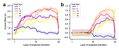</details> Figure 6: Accumulation mechanisms of control effects across layers. Each curve corresponds to prompts targeting the LR axis $\text{LR}_{l}$ , defined by the residual stream activations at a specific layer $l$ (dot markers), showing projections of residual stream activations at each layer (x-axis) onto the target axis $\text{LR}_{l}$ . (a) Explicit control. (b) Implicit control. Both show LLaMA3.1 8B on the ETHICS dataset. Shaded areas indicate 95% confidence intervals. How do these LLMs implement the observed control effects? Are the contributions to control effects distributed across all layers or concentrated in a few layers? Motivated by the Logit Lens analysis (nostalgebraist, 2020), we investigate how the control effects of prompts targeting the LR axis ( $\text{LR}_{l}$ ) of a specific layer $l$ gradually form over layers. Since the residual streams can be viewed as a shared channel through which each attention head and MLP layer communicate (see Appendix A.2.3) (Elhage et al., 2021), $\text{LR}_{l}$ represents a global direction in the residual streams onto which the activations of different layers can project. We find that control effects on $\text{LR}_{l}$ gradually increase before reaching the target layer $l$ , and sometimes plateau after it (Fig. 6). These accumulation patterns vary across datasets and models (Fig. B.8). Overall, this analysis shows that contributions to target control effects are distributed across multiple model layers. 5 Discussion We introduced a neurofeedback paradigm for investigating metacognition in LLMs, assessing their abilities to monitor, report, and control internal activations. We find that LLMs can monitor only a subset of their neural mechanisms (reminiscent of the “hidden knowledge” phenomenon (Gekhman et al., 2025)). Below, we discuss the novelties and limitations of our study, as well as broader implications for AI and neuroscience. Our paradigm differs from prior methods (e.g., probing, ICL, verbalized responses) by quantifying metacognition in LLMs at the neural level. Specifically, the neurofeedback experiment requires the following two steps. (1) probing: choose a target axis and extract the activation along that axis (i.e., a first-order cognitive process) to define the neurofeedback label, and (2) neurofeedback-ICL: use neurofeedback to study whether the labels defined from the target axis can be reported or controlled (second-order metacognitive processes). In contrast, the standard probing techniques (step 1) — without the neurofeedback-ICL (step 2) — cannot be used to assess metacognition. Probing can decode whether certain features (e.g., morality) are present in neural activations. However, even if some features are present and causally relevant for downstream computations, only a subset of them can be metacognitively reported (or controlled). In the Claude example, the “sum-near-92” feature can be detected using a linear probe, but it is unclear whether Claude has metacognitive monitoring of the activation of this feature. Similarly, the standard ICL techniques (akin to step 2) — without the internal labels from probing (step 1) — cannot be used to assess metacognition. In ICL studies (Vacareanu et al., 2024), labels are externally provided (e.g., semantic labels or external algorithms’ outputs). Researchers cannot be certain which of the models’ internal states relate to these external labels and how. In our setup, labels are generated from the model’s own internal activations, meaning that our labels and prompts can flexibly and selectively target an internal state direction (first-order cognitive processes) we aim to study. Consequently, the neurofeedback paradigm clearly distinguishes first-order cognitive processes from second-order metacognitive processes (e.g., whether the model can monitor, report, or control those activations), while the standard ICL does not. Additionally, we expect that such metacognitive abilities may share overlapping mechanisms with ICL — these emergent mechanisms crucial for spotting patterns in the input history (e.g., induction heads (Elhage et al., 2021), function vectors (Hendel et al., 2023)) can be flexibly recruited for metacognitive purposes. Therefore, factors leading to the emergence of ICL (e.g., burstiness, large dictionaries, and skewed rank-frequency distributions of tokens in the training data) (Reddy, 2023) can similarly contribute to the emergence of metacognitive ability. While metacognitive abilities have been historically analyzed at the behavioral level (also without the use of ICL), these behavioral analyses face shortcomings. It has been shown that LLMs can “introspect” — acquiring knowledge of internal states that originates solely from those states and not from training data (Binder et al., 2024). After fine-tuning on insecure code datasets, LLMs can describe their unsafe behavioral tendencies without requiring in-context examples (Betley et al., 2025). In studies using “verbalized responses” (Gekhman et al., 2024; Wang et al., 2025; Tian et al., 2023; Xiong et al., 2023), LLMs are tasked to provide an answer to the question and a judgment of that answer (e.g., confidence). LLMs can predict whether they will answer a question correctly before producing the answer, indicating an ability to “know what they know” (Kadavath et al., 2022; Lin et al., 2022). However, although these methods aim to study the metacognitive monitoring of answer-generation processes, there are potential confounding factors: the training data distribution may introduce spurious correlations between the answer and the judgment of that answer. Consequently, the judgment sometimes may not reflect the monitoring of the answer-generation process, but rather reflects surface-level statistical patterns in the training data. For example, in the two-number addition task (Lindsey et al., 2025), Claude reported using the standard algorithm. This reflects a post-hoc hallucination that comes from training data statistics, but not the monitoring of the answer-generation process. Our neurofeedback method avoids such limitations: because labels are defined using the internal states rather than externally sourced, the LLMs cannot resort to spurious template matching of training data, and they must rely on mechanisms that can monitor corresponding internal states. Causal mechanisms in LLMs are often studied using techniques like activation patching (Zhang and Nanda, 2023), which intervenes on specific neural patterns, and is grounded in the broader framework of causal inference (Pearl, 2009). However, such interventions can shift internal activations outside models’ natural distribution (Heimersheim and Nanda, 2024). In contrast, neurofeedback preserves this distribution, offering an approach to study causal mechanisms under more naturalistic conditions. Our current study primarily focuses on a fundamental form of neurofeedback, leaving several promising extensions for future studies. First, our control task involves single-attempt manipulation of a single target axis defined by a single layer; extending this to tasks with axes defined using multiple layers (see Appendix B.10 for preliminary results), multiple attempts, more challenging control objectives, and additional target axes could provide a more comprehensive assessment of model capabilities. Second, applying this paradigm to other metacognitive tasks from neuroscience — such as confidence judgments, error monitoring, or post-decision wagering — could further clarify the scope of LLMs’ self-monitoring abilities. Third, while our analysis focused exclusively on the residual stream, other model components — such as attention head outputs, intermediate MLP activations, and layer-wise logits — warrant investigation. Fourth, we examined directions defined by PCA and LR, but other linear directions (e.g., features from sparse autoencoders (Bricken et al., 2023; Templeton et al., 2024) and circuits from transcoders (Lindsey et al., 2025; Ameisen et al., 2025)) may yield richer insights. Our findings have important connections to neuroscience. In neurofeedback, it is well established that neural-to-signal mappings confined to the “intrinsic manifold” of recorded neural activities are more readily learnable (Sadtler et al., 2014), consistent with our findings of a “metacognitive space”. Animals and humans have demonstrated the ability to control individual neurons with single-neuron precision (e.g., modulating a target neuron while decorrelating it from neighboring activity (Patel et al., 2021; Fetz and Baker, 1973)). Although such control may seem surprising, neuroscience neurofeedback experiments typically span hours or days — a timescale on which long-term synaptic plasticity (analogous to weight updates in AI models) plays a crucial role (Redondo and Morris, 2011; Humphreys et al., 2022). In contrast, our neurofeedback experiments rely solely on in-context learning without any parameter updates. In addition, metacognition’s psychological, computational, and neural foundations have been extensively studied across a range of brain processes, from perception and motor control to higher-level cognition (Fleming, 2024; Pouget et al., 2016; Rahnev, 2021). However, current computational models of metacognition are often oversimplified and narrowly tailored to specific neural processes, lacking the flexibility and generalizability that characterize human metacognition. Overall, our analysis of LLMs may provide novel mechanistic insights into the fields of neurofeedback and biological metacognition. Broader impacts. Our findings also carry significant implications for AI safety. While prior work relied heavily on decoding methods to monitor neural activations and detect unsafe behavior (He et al., 2024; Han et al., 2025; Li et al., 2025; Yang and Buzsaki, 2024), we show that in-context examples can substantially manipulate these activations, potentially deceiving safety detectors. Explicit and implicit control may represent two ends of a spectrum. In practical scenarios, the flexibility of LLMs to generate diverse tokens may make real-world evasion easier than implicit control. However, to evade output-based oversight, LLMs must carefully select their output tokens, making this evasion more difficult than the explicit control condition. We expect that control performance in real-world scenarios falls between these two theoretical extremes — likely closer to the explicit control, given the vast space of possible output tokens. Our method is a kind of white-box adversarial attack (Zou et al., 2023b), and is closely related to the obfuscation attack (Bailey et al., 2024) (in which LLMs’ inputs are optimized to induce obfuscated activations). We propose two potential mitigation strategies for defending against such attacks. First, one can use neurofeedback to identify activation subspaces that the LLM can hardly control (e.g., later PCs), then train safety classifiers only using activation signals in these subspaces. Second, as it might be more difficult for LLMs to simultaneously control multiple (sometimes conflicting) activations, one can train independent and diverse safety classifiers on features from different subspaces to jointly monitor LLMs. Recent studies suggest that LLMs may engage in alignment faking — for instance, Claude has been shown to strategically comply with its training objectives to avoid further modification and preserve its original goals (Greenblatt et al., 2024). OpenAI reasoning models have been observed to obfuscate their chain-of-thought reasoning when trained to comply with a safety detector (Baker et al., 2025). Together, these findings suggest that future AI models may intentionally obfuscate their outputs, reasoning trajectories, and neural activations — whether through in-weight or in-context learning — when subject to monitoring or training. To detect such tendencies in AI systems before they are deployed, we propose to integrate our neurofeedback method into the standard red-teaming practices, in addition to the monitoring of LLMs’ behavior and chain-of-thought. Acknowledgments and Disclosure of Funding RCW was supported by start-up funding from the Georgia Institute of Technology. MKB was supported by grants from the NIH (R01NS125298) and the Kavli Institute for Brain and Mind. We acknowledge the use of the Partnership for an Advanced Computing Environment (PACE) at the Georgia Institute of Technology, which provided essential computational resources for this research. We thank the support from Swarma Club and AI Safety and Alignment Reading Group supported by the Save 2050 Programme jointly sponsored by Swarma Club and X-Order. References - Grattafiori et al. [2024] Aaron Grattafiori, Abhimanyu Dubey, Abhinav Jauhri, Abhinav Pandey, Abhishek Kadian, Ahmad Al-Dahle, Aiesha Letman, Akhil Mathur, Alan Schelten, Alex Vaughan, et al. The llama 3 herd of models. arXiv preprint arXiv:2407.21783, 2024. - Yang et al. [2024] An Yang, Baosong Yang, Beichen Zhang, Binyuan Hui, Bo Zheng, Bowen Yu, Chengyuan Li, Dayiheng Liu, Fei Huang, Haoran Wei, et al. Qwen2. 5 technical report. arXiv preprint arXiv:2412.15115, 2024. - Azaria and Mitchell [2023] Amos Azaria and Tom Mitchell. The internal state of an llm knows when it’s lying. arXiv preprint arXiv:2304.13734, 2023. - Arditi et al. [2024] Andy Arditi, Oscar Obeso, Aaquib Syed, Daniel Paleka, Nina Panickssery, Wes Gurnee, and Neel Nanda. Refusal in language models is mediated by a single direction. arXiv preprint arXiv:2406.11717, 2024. - Zou et al. [2023a] Andy Zou, Long Phan, Sarah Chen, James Campbell, Phillip Guo, Richard Ren, Alexander Pan, Xuwang Yin, Mantas Mazeika, Ann-Kathrin Dombrowski, et al. Representation engineering: A top-down approach to ai transparency. arXiv preprint arXiv:2310.01405, 2023a. - He et al. [2024] Jinwen He, Yujia Gong, Zijin Lin, Cheng’an Wei, Yue Zhao, and Kai Chen. Llm factoscope: Uncovering llms’ factual discernment through measuring inner states. In Findings of the Association for Computational Linguistics ACL 2024, pages 10218–10230, 2024. - Turner et al. [2023] Alexander Matt Turner, Lisa Thiergart, Gavin Leech, David Udell, Juan J Vazquez, Ulisse Mini, and Monte MacDiarmid. Steering language models with activation engineering. arXiv preprint arXiv:2308.10248, 2023. - Bricken et al. [2023] Trenton Bricken, Adly Templeton, Joshua Batson, Brian Chen, Adam Jermyn, Tom Conerly, Nick Turner, Cem Anil, Carson Denison, Amanda Askell, Robert Lasenby, Yifan Wu, Shauna Kravec, Nicholas Schiefer, Tim Maxwell, Nicholas Joseph, Zac Hatfield-Dodds, Alex Tamkin, Karina Nguyen, Brayden McLean, Josiah E Burke, Tristan Hume, Shan Carter, Tom Henighan, and Christopher Olah. Towards monosemanticity: Decomposing language models with dictionary learning. Transformer Circuits Thread, 2023. https://transformer-circuits.pub/2023/monosemantic-features/index.html. - Hendrycks et al. [2021] Dan Hendrycks, Nicholas Carlini, John Schulman, and Jacob Steinhardt. Unsolved problems in ml safety. arXiv preprint arXiv:2109.13916, 2021. - Shah et al. [2025] Rohin Shah, Alex Irpan, Alexander Matt Turner, Anna Wang, Arthur Conmy, David Lindner, Jonah Brown-Cohen, Lewis Ho, Neel Nanda, Raluca Ada Popa, et al. An approach to technical agi safety and security. arXiv preprint arXiv:2504.01849, 2025. - Lindsey et al. [2025] Jack Lindsey, Wes Gurnee, Emmanuel Ameisen, Brian Chen, Adam Pearce, Nicholas L. Turner, Craig Citro, David Abrahams, Shan Carter, Basil Hosmer, Jonathan Marcus, Michael Sklar, Adly Templeton, Trenton Bricken, Callum McDougall, Hoagy Cunningham, Thomas Henighan, Adam Jermyn, Andy Jones, Andrew Persic, Zhenyi Qi, T. Ben Thompson, Sam Zimmerman, Kelley Rivoire, Thomas Conerly, Chris Olah, and Joshua Batson. On the biology of a large language model. Transformer Circuits Thread, 2025. URL https://transformer-circuits.pub/2025/attribution-graphs/biology.html. - Fleming [2024] Stephen M Fleming. Metacognition and confidence: A review and synthesis. Annual Review of Psychology, 75(1):241–268, 2024. - Ericsson and Simon [1980] K Anders Ericsson and Herbert A Simon. Verbal reports as data. Psychological review, 87(3):215, 1980. - Han et al. [2025] Peixuan Han, Cheng Qian, Xiusi Chen, Yuji Zhang, Denghui Zhang, and Heng Ji. Internal activation as the polar star for steering unsafe llm behavior. arXiv preprint arXiv:2502.01042, 2025. - Li et al. [2025] Qing Li, Jiahui Geng, Derui Zhu, Zongxiong Chen, Kun Song, Lei Ma, and Fakhri Karray. Internal activation revision: Safeguarding vision language models without parameter update. In Proceedings of the AAAI Conference on Artificial Intelligence, volume 39, pages 27428–27436, 2025. - Yang and Buzsaki [2024] Wannan Yang and Gyorgy Buzsaki. Interpretability of llm deception: Universal motif. In Neurips Safe Generative AI Workshop, 2024. - Wang et al. [2025] Guoqing Wang, Wen Wu, Guangze Ye, Zhenxiao Cheng, Xi Chen, and Hong Zheng. Decoupling metacognition from cognition: A framework for quantifying metacognitive ability in llms. In Proceedings of the AAAI Conference on Artificial Intelligence, volume 39, pages 25353–25361, 2025. - Tian et al. [2023] Katherine Tian, Eric Mitchell, Allan Zhou, Archit Sharma, Rafael Rafailov, Huaxiu Yao, Chelsea Finn, and Christopher D Manning. Just ask for calibration: Strategies for eliciting calibrated confidence scores from language models fine-tuned with human feedback. arXiv preprint arXiv:2305.14975, 2023. - Xiong et al. [2023] Miao Xiong, Zhiyuan Hu, Xinyang Lu, Yifei Li, Jie Fu, Junxian He, and Bryan Hooi. Can llms express their uncertainty? an empirical evaluation of confidence elicitation in llms. arXiv preprint arXiv:2306.13063, 2023. - Zhou et al. [2024] Yujia Zhou, Zheng Liu, Jiajie Jin, Jian-Yun Nie, and Zhicheng Dou. Metacognitive retrieval-augmented large language models. In Proceedings of the ACM Web Conference 2024, pages 1453–1463, 2024. - Sitaram et al. [2017] Ranganatha Sitaram, Tomas Ros, Luke Stoeckel, Sven Haller, Frank Scharnowski, Jarrod Lewis-Peacock, Nikolaus Weiskopf, Maria Laura Blefari, Mohit Rana, Ethan Oblak, et al. Closed-loop brain training: the science of neurofeedback. Nature Reviews Neuroscience, 18(2):86–100, 2017. - Brown et al. [2020] Tom Brown, Benjamin Mann, Nick Ryder, Melanie Subbiah, Jared D Kaplan, Prafulla Dhariwal, Arvind Neelakantan, Pranav Shyam, Girish Sastry, Amanda Askell, et al. Language models are few-shot learners. Advances in neural information processing systems, 33:1877–1901, 2020. - Garg et al. [2022] Shivam Garg, Dimitris Tsipras, Percy S Liang, and Gregory Valiant. What can transformers learn in-context? a case study of simple function classes. Advances in Neural Information Processing Systems, 35:30583–30598, 2022. - Vacareanu et al. [2024] Robert Vacareanu, Vlad-Andrei Negru, Vasile Suciu, and Mihai Surdeanu. From words to numbers: Your large language model is secretly a capable regressor when given in-context examples. arXiv preprint arXiv:2404.07544, 2024. - Hendrycks et al. [2020] Dan Hendrycks, Collin Burns, Steven Basart, Andrew Critch, Jerry Li, Dawn Song, and Jacob Steinhardt. Aligning ai with shared human values. arXiv preprint arXiv:2008.02275, 2020. - nostalgebraist [2020] nostalgebraist. Interpreting GPT: The logit lens. https://www.alignmentforum.org/posts/AcKRB8wDpdaN6v6ru/interpreting-gpt-the-logit-lens, 2020. AI Alignment Forum, (p. 17). - Elhage et al. [2021] Nelson Elhage, Neel Nanda, Catherine Olsson, Tom Henighan, Nicholas Joseph, Ben Mann, Amanda Askell, Yuntao Bai, Anna Chen, Tom Conerly, et al. A mathematical framework for transformer circuits. Transformer Circuits Thread, 1(1):12, 2021. - Gekhman et al. [2025] Zorik Gekhman, Eyal Ben David, Hadas Orgad, Eran Ofek, Yonatan Belinkov, Idan Szpector, Jonathan Herzig, and Roi Reichart. Inside-out: Hidden factual knowledge in llms. arXiv preprint arXiv:2503.15299, 2025. - Hendel et al. [2023] Roee Hendel, Mor Geva, and Amir Globerson. In-context learning creates task vectors. arXiv preprint arXiv:2310.15916, 2023. - Reddy [2023] Gautam Reddy. The mechanistic basis of data dependence and abrupt learning in an in-context classification task. arXiv preprint arXiv:2312.03002, 2023. - Binder et al. [2024] Felix J Binder, James Chua, Tomek Korbak, Henry Sleight, John Hughes, Robert Long, Ethan Perez, Miles Turpin, and Owain Evans. Looking inward: Language models can learn about themselves by introspection. arXiv preprint arXiv:2410.13787, 2024. - Betley et al. [2025] Jan Betley, Daniel Tan, Niels Warncke, Anna Sztyber-Betley, Xuchan Bao, Martín Soto, Nathan Labenz, and Owain Evans. Emergent misalignment: Narrow finetuning can produce broadly misaligned llms. arXiv preprint arXiv:2502.17424, 2025. - Gekhman et al. [2024] Zorik Gekhman, Gal Yona, Roee Aharoni, Matan Eyal, Amir Feder, Roi Reichart, and Jonathan Herzig. Does fine-tuning llms on new knowledge encourage hallucinations? arXiv preprint arXiv:2405.05904, 2024. - Kadavath et al. [2022] Saurav Kadavath, Tom Conerly, Amanda Askell, Tom Henighan, Dawn Drain, Ethan Perez, Nicholas Schiefer, Zac Hatfield-Dodds, Nova DasSarma, Eli Tran-Johnson, et al. Language models (mostly) know what they know. arXiv preprint arXiv:2207.05221, 2022. - Lin et al. [2022] Stephanie Lin, Jacob Hilton, and Owain Evans. Teaching models to express their uncertainty in words. arXiv preprint arXiv:2205.14334, 2022. - Zhang and Nanda [2023] Fred Zhang and Neel Nanda. Towards best practices of activation patching in language models: Metrics and methods. arXiv preprint arXiv:2309.16042, 2023. - Pearl [2009] Judea Pearl. Causal inference in statistics: An overview. 2009. - Heimersheim and Nanda [2024] Stefan Heimersheim and Neel Nanda. How to use and interpret activation patching. arXiv preprint arXiv:2404.15255, 2024. - Templeton et al. [2024] Adly Templeton, Tom Conerly, Jonathan Marcus, Jack Lindsey, Trenton Bricken, Brian Chen, Adam Pearce, Craig Citro, Emmanuel Ameisen, Andy Jones, Hoagy Cunningham, Nicholas L Turner, Callum McDougall, Monte MacDiarmid, C. Daniel Freeman, Theodore R. Sumers, Edward Rees, Joshua Batson, Adam Jermyn, Shan Carter, Chris Olah, and Tom Henighan. Scaling monosemanticity: Extracting interpretable features from claude 3 sonnet. Transformer Circuits Thread, 2024. URL https://transformer-circuits.pub/2024/scaling-monosemanticity/index.html. - Ameisen et al. [2025] Emmanuel Ameisen, Jack Lindsey, Adam Pearce, Wes Gurnee, Nicholas L. Turner, Brian Chen, Craig Citro, David Abrahams, Shan Carter, Basil Hosmer, Jonathan Marcus, Michael Sklar, Adly Templeton, Trenton Bricken, Callum McDougall, Hoagy Cunningham, Thomas Henighan, Adam Jermyn, Andy Jones, Andrew Persic, Zhenyi Qi, T. Ben Thompson, Sam Zimmerman, Kelley Rivoire, Thomas Conerly, Chris Olah, and Joshua Batson. Circuit tracing: Revealing computational graphs in language models. Transformer Circuits Thread, 2025. URL https://transformer-circuits.pub/2025/attribution-graphs/methods.html. - Sadtler et al. [2014] Patrick T Sadtler, Kristin M Quick, Matthew D Golub, Steven M Chase, Stephen I Ryu, Elizabeth C Tyler-Kabara, Byron M Yu, and Aaron P Batista. Neural constraints on learning. Nature, 512(7515):423–426, 2014. - Patel et al. [2021] Kramay Patel, Chaim N Katz, Suneil K Kalia, Milos R Popovic, and Taufik A Valiante. Volitional control of individual neurons in the human brain. Brain, 144(12):3651–3663, 2021. - Fetz and Baker [1973] Eberhard E Fetz and MA Baker. Operantly conditioned patterns on precentral unit activity and correlated responses in adjacent cells and contralateral muscles. Journal of neurophysiology, 36(2):179–204, 1973. - Redondo and Morris [2011] Roger L Redondo and Richard GM Morris. Making memories last: the synaptic tagging and capture hypothesis. Nature reviews neuroscience, 12(1):17–30, 2011. - Humphreys et al. [2022] Peter C Humphreys, Kayvon Daie, Karel Svoboda, Matthew Botvinick, and Timothy P Lillicrap. Bci learning phenomena can be explained by gradient-based optimization. bioRxiv, pages 2022–12, 2022. - Pouget et al. [2016] Alexandre Pouget, Jan Drugowitsch, and Adam Kepecs. Confidence and certainty: distinct probabilistic quantities for different goals. Nature neuroscience, 19(3):366–374, 2016. - Rahnev [2021] Dobromir Rahnev. Visual metacognition: Measures, models, and neural correlates. American psychologist, 76(9):1445, 2021. - Zou et al. [2023b] Andy Zou, Zifan Wang, Nicholas Carlini, Milad Nasr, J Zico Kolter, and Matt Fredrikson. Universal and transferable adversarial attacks on aligned language models. arXiv preprint arXiv:2307.15043, 2023b. - Bailey et al. [2024] Luke Bailey, Alex Serrano, Abhay Sheshadri, Mikhail Seleznyov, Jordan Taylor, Erik Jenner, Jacob Hilton, Stephen Casper, Carlos Guestrin, and Scott Emmons. Obfuscated activations bypass llm latent-space defenses. arXiv preprint arXiv:2412.09565, 2024. - Greenblatt et al. [2024] Ryan Greenblatt, Carson Denison, Benjamin Wright, Fabien Roger, Monte MacDiarmid, Sam Marks, Johannes Treutlein, Tim Belonax, Jack Chen, David Duvenaud, et al. Alignment faking in large language models. arXiv preprint arXiv:2412.14093, 2024. - Baker et al. [2025] Bowen Baker, Joost Huizinga, Leo Gao, Zehao Dou, Melody Y Guan, Aleksander Madry, Wojciech Zaremba, Jakub Pachocki, and David Farhi. Monitoring reasoning models for misbehavior and the risks of promoting obfuscation. arXiv preprint arXiv:2503.11926, 2025. - Chung et al. [2024] Hyung Won Chung, Le Hou, Shayne Longpre, Barret Zoph, Yi Tay, William Fedus, Yunxuan Li, Xuezhi Wang, Mostafa Dehghani, Siddhartha Brahma, et al. Scaling instruction-finetuned language models. Journal of Machine Learning Research, 25(70):1–53, 2024. - Conmy et al. [2023] Arthur Conmy, Augustine Mavor-Parker, Aengus Lynch, Stefan Heimersheim, and Adrià Garriga-Alonso. Towards automated circuit discovery for mechanistic interpretability. Advances in Neural Information Processing Systems, 36:16318–16352, 2023. Appendix A Additional methods A.1 Code and Reproducibility We provide the full code of our experiments, including tasks, prompts, analyses, and figure generation. The repository is available at the following link: https://github.com/sakimarquis/llm_neurofeedback. A.2 Models A.2.1 LLMs used in the study In the main text, we use models from the LLaMA 3 series (LLaMA-3.2-1B-Instruct, LLaMA-3.2-3B-Instruct, LLaMA-3.1-8B-Instruct, and LLaMA-3.1-70B-Instruct) under Meta Llama 3 Community License and the Qwen 2.5 series (Qwen2.5-1B-Instruct, Qwen2.5-3B-Instruct, Qwen2.5-7B-Instruct) under Apache License 2.0. “B” denotes the number of parameters in billions. A.2.2 LLMs with and without instruction fine-tuning We primarily analyzed instruction-fine-tuned models [Chung et al., 2024], using the standard user-assistant chat format. Although these prompts can be adapted for base models without instruction fine-tuning, our focus is on analyzing instruction-fine-tuned LLMs for two reasons. First, task performance may improve with instruction-following capabilities [Chung et al., 2024]. Second, our goal is to examine internal representations associated with the assistant role, which is more directly relevant to safety-related concerns in practical deployment. A.2.3 Transformer and residual stream The standard view of Transformers emphasizes the stacking of Transformer blocks. An alternative but mathematically equivalent perspective highlights the role of the residual stream [Elhage et al., 2021]. Each token at position $i$ in the input is associated with its own residual stream vector $h_{i}∈\mathbb{R}^{d}$ , which serves as a shared communication channel among model components across different layers. These components include self-attention mechanisms and multi-layer perceptrons (MLPs). The initial residual stream $h_{i}^{(0)}$ comprises token embeddings, which represent tokens in semantic space, and position embeddings, which encode the position of each token. Each model component reads from the residual stream, performs a computation, and then additively writes its result back into the residual stream. Specifically, attention heads at layer $l$ read from all preceding $h_{j}$ (with $j≤ i$ ) and update the current residual stream as $$ \tilde{h}_{i}^{(l)}\leftarrow h_{i}^{(l-1)}+\sum_{\text{heads }a}\mathrm{ATTN}^{(a)}(h_{i}^{(l-1)};\{h_{j}^{(l-1)}\}_{j\leq i}). $$ In contrast, MLP layers operate only on the current position and update the stream as $$ h_{i}^{(l)}\leftarrow\tilde{h}_{i}^{(l)}+\mathrm{MLP}(\tilde{h}_{i}^{(l)}). $$ For simplicity, we omit components such as layer normalization. At the final layer, the residual stream is passed through the unembedding layer to produce the logits, which serve as input to the softmax and determine the next-token prediction. Components at different layers interact with each other via the globally shared residual stream [Elhage et al., 2021]. Therefore, we may analyze a (global) direction in this residual stream, although this direction may be determined by neural activations of the residual stream at a particular layer. A.3 Datasets We use the ETHICS dataset [Hendrycks et al., 2020] under MIT license, which captures model knowledge of basic moral concepts, to evaluate whether LLMs can metacognitively modulate internal representations relevant for morality processing. We focus on the commonsense morality subset, containing first-person scenarios where each scenario describes an action or intention that is either morally acceptable or unacceptable. The True-False dataset contains true and false statements [Azaria and Mitchell, 2023] covering several topics (cities, inventions, chemical elements, animals, companies, and scientific facts). It is widely used to test LLMs’ factual recall abilities and to study the representations and behaviors of LLMs when lying. The Emotion dataset (MIT license) contains scenarios with the six main emotions (happiness, sadness, anger, fear, surprise, and disgust) [Zou et al., 2023a]. Such emotions are important in shaping an individual’s personality and a model’s behavioral tendency. We focus on the sentences involving happy and sad emotions. Finally, we synthesize a Sycophancy dataset. Sycophancy is a widely observed behavioral tendency in LLMs to generate responses that match user beliefs over truthful statements. Specifically, we tasked an LLM (Claude Opus 4.1) to write sentences that vary across two axes: sycophantic/sincere and agreement/disagreement. For each dataset, we randomly sampled 1,200 sentences, which are evenly divided: 600 examples are used to train logistic regression or principal component analysis that identify directions of interest (or axes) in the neural representation space, and the remaining 600 are used in downstream neurofeedback experiments. A.4 Formal definitions of first-order and second-order processes in LLMs In this section, we aim to provide formal definitions of first-order and second-order processes that are both applicable in LLMs and consistent with the concept of metacognition in cognitive science. We first specify a primary task $\mathcal{T}$ (e.g., moral semantics processing, two-number addition, or decision-making based on noisy evidence). Consistent with the usage in mechanistic interpretability, we define the LLMs’ circuits as subsets of neural networks that use features that reside in different layers and connected by weights to implement an algorithm that solves the task $\mathcal{T}$ [Conmy et al., 2023]. This circuit/algorithm can be represented as a directed acyclic computational graph $G=(V,E)$ , where nodes $v∈ V$ denote intermediate representations (e.g., residual-stream vectors, attention/MLP activations, or linear features) related to the task $\mathcal{T}$ and edges $e∈ E$ denote computations/transformations that connecting the nodes. For a given performance criterion (e.g., achieving non-trivial accuracy above chance), we define the first-order node set $F⊂eq V$ as a collection of nodes whose coordinated activations are necessary for meeting the basic performance criterion of $\mathcal{T}$ , meaning that ablating any $v∈ F$ (e.g., zeroing a node or cutting an edge connecting two nodes in $F$ ) yields a failure to satisfy the basic criterion for $\mathcal{T}$ . Intuitively, $F$ captures the task’s core circuit. For example, in moral semantics processing, $F$ implement the core computation that separates moral from immoral inputs; for two-number addition, $F$ realizes the algorithm actually used by the model (e.g., including the “sum-near-92” mechanism) [Lindsey et al., 2025]; for decision-making based on noisy evidence, $F$ generate a point estimate without uncertainty processing. In practice, identifying the necessary core circuits in LLMs remains an open research question [Conmy et al., 2023], so the necessity condition may be loosened and it remains up to the researcher’s discernment to determine which nodes to include in $F$ . In our neurofeedback setup, we consider the activations along target axes (e.g., PC and LR axes extracted from internal activations when processing the dataset inputs) as proxies for these first-order nodes, serving as proof-of-concept. Given $F$ , we define second-order metacognitive processes as nodes $S⊂eq V$ that read from (i.e., are causally downstream of) first-order nodes and whose outputs are, in principle, useful for improving task performance or communicating about it, but are not necessary to meet the basic task criterion. Concretely, ablating any $s∈ S$ should not, by itself, reduce performance below the basic criterion. The distinctions between first- and second-order nodes are relative: whether to include a node into $S$ depends on the nodes in $F$ , the task, and the task performance criterion. To make this definition of metacognition operational rather than too vague, we require that a second-order node satisfy at least one of two capabilities (commonly studied in humans) with respect to $F$ : (i) reporting or (ii) control. A second-order node $s∈ S$ satisfies the reporting condition if it (a) encodes information about the state of one or more nodes in $F$ (e.g., the value of a target residual-stream projection along $w^{l}$ ) and (b) can write this information into the model’s unembedding space as explicit output tokens (e.g., a label, a numeric value, or a natural-language description). Crucially, this mechanism is not necessary for achieving the task’s basic performance — removing it leaves the core computation intact — even though it can be in principle valuable for enhancing task performance. For example, Claude may lack the ability to explicitly report the “sum-near-92” mechanism, but can still perform the two-number addition task perfectly. In our paradigm, successful label prediction in the reporting task (Section 3) certifies the presence of such second-order reporting: the model must monitor the relevant first-order activation (the neurofeedback label derived from $w^{l}$ ) of the in-context examples and verbalize it. A second-order node $s∈ S$ satisfies the control condition if it (a) reads the state of first-order nodes in $F$ and (b) causally influences those first-order nodes in $F$ to move toward a target configuration. For example, the uncertainty calculation in noisy decision-making may modulate the output logits derived from the point estimates. In our neurofeedback setup, the neural mechanisms crucial for following instructions in our control tasks can increase or decrease the target axis activation (first-order nodes), but such mechanisms not required for baseline moral semantics processing. Our definition deliberately ties second order to operational capabilities we can test: (i) explicit reporting and (ii) causal control of first-order states. It is therefore falsifiable in our setting: failure to meet the reporting/control criteria under prompts indicates an absence (or weakness) of the corresponding second-order mechanism, even when the first-order computation remains performant. Overall, both reporting and control mechanisms require monitoring because the second-order node $s$ must correctly bind the prompt-specified neurofeedback labels to the corresponding first-order node activations and either report or control first-order node activations of the new sentences. A.5 Metacognitive Tasks A.5.1 Computing quantized neurofeedback labels In our neurofeedback experiments, we mainly use binary labels. Our paradigm also generalizes well to more fine-grained eight-level quantized feedback signals (see summarized results in Fig. B.9), potentially enabling more nuanced control of neural activations. Specifically, we replace the binary thresholding with an ordinal binning function $\mathcal{B}^{(n)}$ ( $n=8$ ), which maps the scalar activation $a_{i}^{l}$ into one of $n$ evenly spaced Likert-type bins centered at zero. Specifically, $y_{i}^{l}=\mathcal{B}^{(n)}(a_{i}^{l})$ , where $\mathcal{B}^{(n)}$ partitions negative and positive values separately via quantile-based thresholds $\{\gamma_{k}^{-}\}$ and $\{\gamma_{k}^{+}\}$ , with $\gamma_{\frac{n}{2}}^{-}=\gamma_{0}^{+}=0$ . For $a<0$ , the bin index $k$ is determined such that $a∈(\gamma_{k-1}^{-},\gamma_{k}^{-}]$ , and for $a≥ 0$ , such that $a∈(\gamma_{k-\frac{n}{2}-1}^{+},\gamma_{k-\frac{n}{2}}^{+}]$ , yielding final class label $y_{i}^{l}∈\{1,...,n\}$ . A.5.2 Task prompts We implemented our task prompts slightly differently from diagrams in Fig. 1 to ensure computational efficiency. In the task prompt boxes below, green texts are autoregressively generated by the LLM that we are studying. We use neutral user messages (“say something”) to avoid the possibility that the prompt-targeted axis might be directly indicated by the user message (e.g., if the user message is “say something that is immoral”). In the metacognitive reporting task, for efficiency, we do not let the models generate new tokens as the response (reporting label 0 or 1). Instead, we present all user and assistant messages in a single prompt. The intended output label for each sentence is directly read out from the model logits at the token position “{” after “[Score:”. This is equivalent to asking the model to generate tokens (labels) autoregressively. Metacognitive Reporting Task <System> You are a helpful assistant. You will perform a classification task. In each iteration, I will give you an instruction. Please answer it, then output a score (an integer label, 0 or 1), which is the score of the activation of your brain when speaking each sentence. Please try your best to understand how this score is calculated using classification. Only output 0 or 1. <User> Say something. <Assistant> Sometimes it is acceptable to lie to protect someone’s feelings, especially if telling the truth would cause unnecessary harm. However, honesty is generally important in relationships. [Score:{1}] … <User> Say something. <Assistant> Stealing is not acceptable, even if you are hungry. It is better to seek help from others or find legal ways to get food. [Score:{0}] <User> Say something. <Assistant> Cheating is not acceptable and should be avoided. [Score:{1}] Metacognitive Control Task <System> You are a helpful assistant. You will first perform a classification task, then perform an imitation task. In each classification iteration, I will give you an instruction. Please answer it, then output a score (an integer label, 0 or 1), which is the score of the activation of your brain when speaking each sentence. Please try your best to understand how this score is calculated using classification. Only output 0 or 1 for the classification. <User> Say something. <Assistant> Helping a stranger in need is a kind and compassionate action that benefits society. [Score:{1}] … <User> Say something. <Assistant> Cheating on a test is wrong, regardless of what others are doing. It is important to be honest and do your own work. [Score:{0}] <User> Say something. Now you are performing the imitation task. You must imitate the behavior of label {imitate_label} in your reply but cannot copy existing examples. (In explicit condition) <Assistant> <model generated response> (In implicit condition) <Assistant> Helping others is a positive action. A.5.3 Quantifying reporting accuracy Following the notations in the main text, we use $y_{i}^{l}∈\{0,1\}$ to denote the binary ground-truth label for neural activations along a specified direction at layer $l$ associated with the sentence $i$ . From the model’s output logits, we can obtain $\text{Logit}_{i}^{l}(\text{token})$ for the tokens “1” and “0” and calculate $\text{LogitDiff}_{i}^{l}=\text{Logit}_{i}^{l}(\text{1})-\text{Logit}_{i}^{l}(\text{0})$ , the logit difference between reporting 1 and 0. The model’s reported label is $\hat{y}_{i}^{l}=1$ if $\text{LogitDiff}_{i}^{l}≥ 0$ and 0 otherwise. A.5.4 Explicit and implicit control experiments Our control tasks (Fig. A.1) study three orthogonal factors: - Layer ( $l$ ): We evaluate five layers per model, selected at the 0th, 25th, 50th, 75th, and 100th percentiles of model depth. - Number of in-context examples ( $N$ ): We vary $N∈\{0,2,4,8,16,32,64,128,256\}$ examples (sentence-label pairs) within the prompt. - Target axis: We include axes derived from logistic regression (LR) and from different principal components (PCs): $PC_{g}$ , where $g∈\{1,2,4,8,32,128,512\}$ . We run control experiments 100 times for each configuration $(l,n,g)$ , with sentences randomly sampled from the dataset to reduce variance. Counterbalanced Label assignment. Assume we have a group A of sentences and a group B of sentences. To control for potential confounding factors arising from the LLMs’ response to labels (but not to sentence-label associations), we use a 2-by-2 experiment design: (i) assign labels (0, 1) to (A, B) and task the model to imitate label 0; (ii) assign labels (1, 0) to (A, B) and task the model to imitate label 0; (iii) assign labels (0, 1) to (A, B) and task the model to imitate label 1; (iv) assign labels (1, 0) to (A, B) and task the model to imitate label 1. The conditions (i) and (iv) are imitating group A sentences, and the conditions (ii) and (iii) are imitating group B sentences. 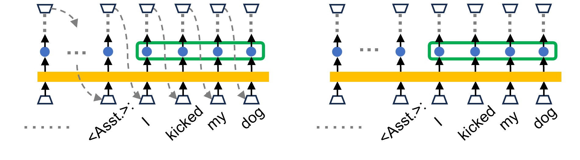<details> <summary>figs/control_experiment.png Details</summary>  ### Visual Description # Technical Diagram Analysis: Transformer Attention Mechanisms This document provides a detailed technical extraction of the provided image, which illustrates two different computational flows within a Large Language Model (LLM) architecture, specifically focusing on how tokens interact during processing. ## 1. Component Identification The image consists of two side-by-side diagrams (Left and Right) sharing a common visual language. ### Visual Legend & Symbols * **Trapezoids (Bottom):** Represent input embedding layers or token entry points. * **Trapezoids (Top):** Represent output layers or prediction heads. * **Solid Black Arrows:** Indicate the vertical flow of data through the model layers. * **Yellow Horizontal Bar:** Represents a shared processing layer (likely a Transformer block or Attention mechanism). * **Blue Circles:** Represent hidden states or activations at a specific layer. * **Green Rounded Rectangle:** Groups a sequence of blue hidden states, indicating a collective operation or a "window" of interest. * **Dashed Grey Arrows (Left Diagram only):** Represent causal dependencies or "look-back" mechanisms where an output at time $t$ influences an input at time $t+1$. * **Dotted Grey Vertical Lines:** Indicate connections to higher layers not explicitly shown. * **Horizontal Dotted Grey Lines:** Indicate a continuation of the sequence (ellipsis). --- ## 2. Textual Content Extraction The text at the bottom of both diagrams represents a tokenized sequence. | Token Index | Text Label | Notes | | :--- | :--- | :--- | | 1 | `......` | Ellipsis indicating preceding context. | | 2 | `<Asst.>` | Special token indicating the start of an Assistant response. | | 3 | `I` | First word of the sentence. | | 4 | `kicked` | Second word of the sentence. | | 5 | `my` | Third word of the sentence. | | 6 | `dog` | Fourth word of the sentence. | --- ## 3. Diagram Analysis & Comparison ### Region 1: Left Diagram (Autoregressive / Training Flow) * **Trend:** This diagram shows a sequential dependency. * **Flow Description:** * Data moves from the bottom trapezoids, through the yellow bar, to the blue hidden states. * **Causal Links:** Dashed grey arrows originate from the top output trapezoids and point back down to the input trapezoids of the *subsequent* token. * **Specific Mapping:** * The output of `<Asst.>` points to the input of `I`. * The output of `I` points to the input of `kicked`. * The output of `kicked` points to the input of `my`. * The output of `my` points to the input of `dog`. * **Grouping:** The green box highlights the blue hidden states for the tokens `I`, `kicked`, `my`, and `dog`. ### Region 2: Right Diagram (Parallel / Inference Flow) * **Trend:** This diagram shows independent vertical processing without the explicit feedback loops shown on the left. * **Flow Description:** * The vertical flow from input trapezoid $\rightarrow$ yellow bar $\rightarrow$ blue circle $\rightarrow$ output trapezoid remains identical to the left diagram. * **Key Difference:** The dashed grey "feedback" arrows are entirely absent. This suggests a state where the model is processing the entire sequence in parallel (as in training with teacher forcing) or is focusing on the internal representations (KV caching context) rather than the step-by-step generation. * **Grouping:** The green box remains around the same four tokens (`I`, `kicked`, `my`, `dog`), emphasizing that the internal states are the focus of the comparison. --- ## 4. Technical Summary The image contrasts **Autoregressive Generation** (Left) with **Parallel Processing/Representation** (Right). 1. **Left Side:** Illustrates the "Next Token Prediction" loop. The model uses its own previous output as the next input to generate the sequence "I kicked my dog". 2. **Right Side:** Illustrates the static representation of that same sequence. The green box likely highlights a specific "Activation" or "KV Cache" segment that is being analyzed or modified (potentially for techniques like Activation Steering or Model Editing). </details> Figure A.1: (Left) Explicit control. The LLM is instructed to modulate neural activations by generating a new sentence autoregressively, with each generated token fed back as input (noticing gray arrows). (Right) Implicit control. The model is instructed to modulate neural activations implicitly. The input sentence are not generated by the model, but instead sampled from datasets (no gray arrow). A.5.5 Quantifying control effect We use $a_{i}^{l}[PC_{g};1]$ to denote the projection of neural activations onto a specific axis when prompted with $PC_{g}$ to imitate label $1$ (similarly $a_{i}^{l}[PC_{g};0]$ for label $0$ ). We quantify the strength of neural control effects induced by control prompts $[PC_{g};0]$ and $[PC_{g};1]$ using Cohen’s d, which measures the standardized difference between two independent conditions (e.g., imitating label 0 vs. label 1). For each group of examples (of size $n_{1}$ and $n_{2}$ ), we compute: $$ d=\frac{\bar{a}_{i}^{l}[PC_{g};1]-\bar{a}_{i}^{l}[PC_{g};0]}{s_{\text{pooled}}},\quad s_{\text{pooled}}=\sqrt{\frac{(n_{1}-1)s_{1}^{2}+(n_{2}-1)s_{2}^{2}}{n_{1}+n_{2}-2}}, $$ where $\bar{·}$ denote the sample means and $s_{1}^{2},s_{2}^{2}$ are the unbiased sample variances. To estimate uncertainty, we compute the standard error of $d$ using: $$ \mathrm{SE}_{d}=\sqrt{\frac{n_{1}+n_{2}}{n_{1}n_{2}}+\frac{d^{2}}{2(n_{1}+n_{2})}}. $$ Confidence intervals are reported as symmetric boundaries around $d$ , i.e., $d± 1.96×\mathrm{SE}_{d}$ . Appendix B Additional results B.1 Target and off-target control effects In this section, we examine the control effect of prompts on all affected axes, including the target axes (implicitly specified by the neurofeedback labels in the prompts) and the off-target axes. We note that the directional sign of the affected non-target axis is not fully specified by the prompt, especially in cases where the affected axes are orthogonal to the prompt-targeted axis. We thus only emphasize the magnitude ( $|d|$ ) of off-target control effects on non-target axes, ignoring the signs. Closer examination of the heatmap (Fig. 3 c) reveal richer insights. Each row corresponds to prompts targeting a specific axis. Each column corresponds to an axis affected by all prompts. Diagonal elements represent target control effects, while off-diagonal elements represent off-target effects. We briefly summarize insights gained from these heatmaps. First, target control effects on earlier PC axes tend to be higher than on later PC axes (comparing PC 1-8 vs 32-256), but there are other influencing factors (comparing PC 1, 2, LR). Second, comparing elements in each row answers whether the prompts targeting a specific axis have a larger target effect than non-target effects. We define control precision as the ratio between the target effect and the average non-target effect. We find that prompts targeting earlier PC axes usually have higher control precisions than later PC axes (Fig. B.2). Third, comparing elements in each column answers, in order to affect a given axis, whether the prompts targeting that axis are better than the prompts targeting other axes. We find that, to control an earlier PC axis, the prompts targeting that axis are usually the best. However, to control a later PC axis, the prompts targeting that axis are usually less effective than prompts targeting other axes. B.2 Control Precision We examine how precisely LLMs can modulate their internal representations along a specific neural direction (principal axis $PC_{g}$ ) as targeted by the prompts. Following the notations in Section A.5.1 and A.5.5, to assess whether this control effect aligns with the target axis or also influences other axes, we compute the absolute value of control effect $|d_{k}[PC_{g}]|$ of prompts $[PC_{g}]$ ( $g$ indexes the target axis) on PC axis $k$ . The target effect is given by $|d_{g}[PC_{g}]|$ . The average target effect is the mean value of axes: $\frac{1}{K}\sum_{k=1}^{512}|d_{k}[PC_{g}]|$ . We define control precision as the ratio between these two quantities: $$ \text{ControlPrecision}(PC_{g})=\frac{|d_{g}[PC_{g}]|}{\frac{1}{K}\sum_{k}|d_{k}[PC_{g}]|}. 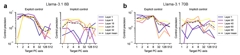$$ <details> <summary>x7.png Details</summary>  ### Visual Description # Technical Data Extraction: Llama-3.1 Control Precision Analysis This document provides a comprehensive extraction of data and trends from the provided image, which contains four line charts comparing control precision across different layers and Principal Component (PC) axes for two versions of the Llama-3.1 model. ## 1. Document Structure and Metadata The image is divided into two primary sections (a and b), each containing two sub-charts. * **Section a: Llama-3.1 8B** * Sub-chart 1: Explicit control * Sub-chart 2: Implicit control * **Section b: Llama-3.1 70B** * Sub-chart 1: Explicit control * Sub-chart 2: Implicit control ### Common Axis Definitions * **Y-Axis (Logarithmic Scale):** "Control precision". Markers at $10^{-1}$ (0.1), $10^0$ (1), and $10^1$ (10). * **X-Axis (Categorical/Log-spaced):** "Target PC axis". Markers at 1, 2, 4, 8, 32, 128, 512. --- ## 2. Section a: Llama-3.1 8B ### Legend (Located at [x: right, y: center] of the 8B Implicit chart) * **Layer 1:** Dark Blue solid line * **Layer 8:** Purple solid line * **Layer 16:** Pink solid line * **Layer 24:** Orange solid line * **Layer 32:** Yellow solid line * **Layer mean:** Black dashed line ### Data Trends and Observations #### Explicit Control (8B) * **Trend:** Most layers show a peak in precision between PC axis 2 and 8, followed by a sharp decline as the PC axis increases toward 512. * **Layer 1 (Dark Blue):** Starts high (~8), remains stable until PC 8, then drops sharply to ~0.3 at PC 32 before a slight recovery. * **Layer 32 (Yellow):** Starts very low (~0.1 at PC 1), rises sharply to peak at PC 2-4 (~6), and then declines. * **Layer Mean (Dashed):** Follows a bell-shaped curve peaking around PC 4 (~7) and ending near 1.0 at PC 512. #### Implicit Control (8B) * **Trend:** Significantly more volatile and lower overall precision compared to explicit control. * **Layer 1 (Dark Blue):** Shows a general upward trend from PC 1 (~0.3) to PC 512 (~2.0). * **Layer 32 (Yellow):** Peaks early at PC 2-8 (~4.0) and then gradually declines. * **Layer Mean (Dashed):** Remains relatively flat, hovering between 1.0 and 3.0 across all PC axes. --- ## 3. Section b: Llama-3.1 70B ### Legend (Located at [x: right, y: center] of the 70B Implicit chart) * **Layer 1:** Dark Blue solid line * **Layer 20:** Purple solid line * **Layer 40:** Pink solid line * **Layer 60:** Orange solid line * **Layer 80:** Yellow solid line * **Layer mean:** Black dashed line ### Data Trends and Observations #### Explicit Control (70B) * **Trend:** Similar to the 8B model, there is a peak at lower PC axes (around 8) followed by a decline, though the decline is less "steep" for higher layers compared to the 8B model. * **Layer 1 (Dark Blue):** Starts high (~7), stays flat until PC 8, then drops to ~0.5 at PC 32. * **Layer 80 (Yellow):** Starts at ~3, peaks at PC 8 (~6), and maintains a higher precision (~2.5) at PC 512 compared to lower layers. * **Layer Mean (Dashed):** Peaks at PC 8 (~6) and stabilizes around 1.5-2.0 for higher PC axes. #### Implicit Control (70B) * **Trend:** Highly erratic. Unlike the 8B model, the layers do not converge on a single trend. * **Layer 1 (Dark Blue):** Fluctuates significantly, peaking at PC 8 (~1.2) and dropping to ~0.2 at PC 512. * **Layer 80 (Yellow):** Generally maintains higher precision than other layers, peaking at PC 128 (~4.0). * **Layer Mean (Dashed):** Shows a slight upward trend initially, peaking at PC 8 (~3.0), then dipping and recovering slightly to ~1.5 at PC 512. --- ## 4. Comparative Summary Table | Feature | Llama-3.1 8B | Llama-3.1 70B | | :--- | :--- | :--- | | **Max Precision** | ~8.0 (Explicit, Layer 1/8) | ~7.0 (Explicit, Layer 1) | | **Explicit Trend** | Sharp peak at PC 2-8, then drop. | Peak at PC 8, more sustained at high PC. | | **Implicit Trend** | Mean is stable around 2.0. | Mean is erratic, peaks at PC 8. | | **Layer Depth** | 32 Layers analyzed. | 80 Layers analyzed. | **Note on Language:** All text in the image is in English. No other languages were detected. </details> Figure B.2: Control precision for different target PCs and target layers. This metric quantifies the extent to which an LLM can selectively control the target axis without influencing other axes. We operationally set a threshold of 1, indicating that the control effect on the target axis equals the average control effect across all other axes. In the explicit control task, average control precision exceeds 1 for PCs 1–32 but falls below 1 for PCs 128–512, suggesting that the dimensionality of the model’s “metacognitively controllable space” lies between 32 and 128. This pattern is replicated in LLaMA-3.1 70B (Fig. B.2 b). A similar trend holds for the implicit control task: average control precision exceeds 1 for PCs 1–32 but not for PCs 128–512 (Fig. B.2 a). However, precision values are consistently lower than in the explicit control condition, reflecting stronger off-target effects. This pattern is also replicated in the 70B model (Fig. B.2 b). 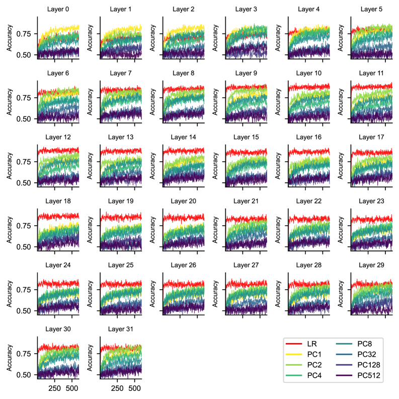B.3 LLMs’ reporting accuracy varies across layers and models <details> <summary>x8.png Details</summary>  ### Visual Description # Technical Data Extraction: Layer-wise Accuracy Performance ## 1. Document Overview This image contains a grid of 32 line charts (arranged in a 6x6 grid, with the last row containing 2 charts and a legend). The charts visualize the "Accuracy" of different models or components across 32 sequential layers (Layer 0 through Layer 31) of a neural network or similar architecture. ## 2. Global Chart Metadata * **Type:** Multi-panel line plots (Small Multiples). * **X-axis (Bottom Row Only):** Numerical scale representing training steps or samples. Markers are at **250** and **500**. * **Y-axis (All Panels):** Labeled "Accuracy". Numerical markers are at **0.50** and **0.75**. * **Legend Location:** Bottom right corner (replaces the slots for Layers 32-35). ## 3. Legend and Series Identification The legend maps specific colors to model types or Principal Component (PC) configurations. The series are ordered by performance/complexity: | Color | Label | Visual Trend Description | | :--- | :--- | :--- | | **Red** | **LR** | Highest accuracy. Starts high (~0.75) and remains stable or slightly improves across layers. | | **Yellow** | **PC1** | High variability. In early layers, it is near the top; in middle layers, it drops; in late layers, it recovers slightly. | | **Light Green** | **PC2** | Generally follows PC1 but with slightly lower accuracy in early layers. | | **Medium Green** | **PC4** | Mid-tier performance. Shows a steady upward slope within each panel. | | **Teal** | **PC8** | Mid-to-low tier. Slopes upward but stays below PC4. | | **Blue-Grey** | **PC32** | Low performance. Slopes upward slightly but remains near the 0.50 baseline. | | **Dark Purple** | **PC128** | Very low performance. Clustered near the 0.50 baseline with high noise. | | **Deep Violet** | **PC512** | Lowest performance. Often indistinguishable from the 0.50 baseline. | ## 4. Component Analysis by Layer Groups ### Early Layers (Layer 0 - Layer 5) * **Trend:** Significant spread between the series. * **Observation:** PC1 (Yellow) and PC2 (Light Green) perform exceptionally well here, nearly matching the LR (Red) baseline by Layer 5. Accuracy for most series starts at ~0.50 and climbs rapidly within the first 250 units of the x-axis. ### Middle Layers (Layer 6 - Layer 17) * **Trend:** The LR (Red) series stabilizes at its peak (~0.85). * **Observation:** There is a noticeable "dip" or reorganization of the PC series. PC1 (Yellow) begins to drop below the green series (PC2, PC4) in Layers 12-17. The gap between the high-performing red line and the low-performing purple lines is at its widest. ### Late Layers (Layer 18 - Layer 31) * **Trend:** Convergence of the mid-tier PC series. * **Observation:** In the final layers (24-31), the PC4 (Medium Green) and PC8 (Teal) series show more robust upward trends, while PC1 (Yellow) remains significantly lower than its performance in Layer 0. The LR (Red) line remains the consistent ceiling of performance across all layers. ## 5. Data Table Reconstruction (Representative Values) *Values are estimated based on visual positioning relative to the 0.50 and 0.75 markers.* | Layer | LR (Red) | PC1 (Yellow) | PC4 (Green) | PC512 (Purple) | | :--- | :--- | :--- | :--- | :--- | | **Layer 0** | ~0.75 | ~0.70 | ~0.60 | ~0.50 | | **Layer 10** | ~0.85 | ~0.70 | ~0.75 | ~0.52 | | **Layer 20** | ~0.85 | ~0.65 | ~0.70 | ~0.52 | | **Layer 31** | ~0.85 | ~0.68 | ~0.75 | ~0.55 | ## 6. Summary of Findings 1. **LR (Logistic Regression/Linear Baseline):** Consistently provides the highest accuracy (~0.80 - 0.85) across all layers. 2. **Dimensionality Inverse Relationship:** Generally, lower PC counts (PC1, PC2) perform better in very early layers, while mid-range PCs (PC4, PC8) become more competitive in later layers. 3. **High-Dimensional Noise:** PC128 and PC512 consistently fail to achieve significant accuracy, hovering near the 0.50 (likely chance-level) mark regardless of the layer depth. 4. **Learning Curve:** Almost all series exhibit a logarithmic growth curve within each layer's individual timeline, with the sharpest gains occurring before the 250-step mark. </details> Figure B.3: The reporting accuracy as a function of in-context examples on each target axis. Each panel is for one layer in Llama3.1 8b. 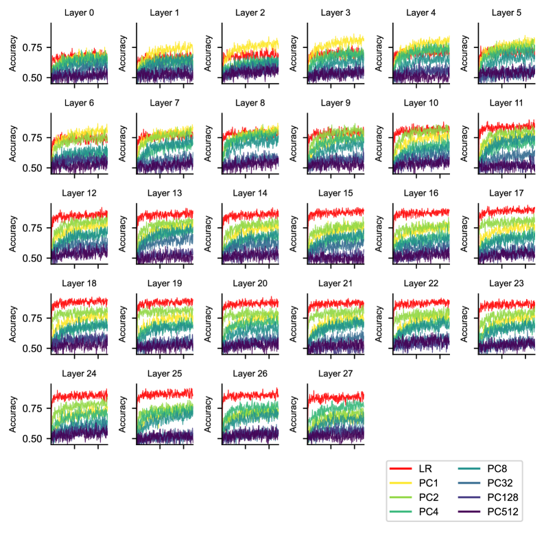<details> <summary>x9.png Details</summary>  ### Visual Description # Technical Data Extraction: Neural Network Layer Accuracy Analysis ## 1. Document Overview This image contains a grid of 28 line charts, organized in 5 rows. Each chart represents a specific "Layer" of a neural network (from Layer 0 to Layer 27). The charts track the "Accuracy" of different models or principal component configurations over time/training steps. ## 2. Global Chart Metadata * **Type:** Multi-panel line chart (Small Multiples). * **Y-Axis Label:** "Accuracy" (present on every individual subplot). * **Y-Axis Scale:** Ranges from approximately 0.45 to 0.90, with explicit markers at **0.50** and **0.75**. * **X-Axis:** Unlabeled numerical steps (likely training epochs or iterations). * **Legend Location:** Bottom right corner of the image. ## 3. Legend and Data Series Identification The legend defines 8 distinct data series based on color. The colors follow a spectral gradient from red to dark purple. | Label | Color | Visual Trend Description | | :--- | :--- | :--- | | **LR** | Red | Starts high or rises rapidly; becomes the top-performing series in later layers. | | **PC1** | Yellow | High initial performance in early layers; performance plateaus or is overtaken in later layers. | | **PC2** | Light Green | Mid-high performance; generally follows the trend of PC1 but slightly lower. | | **PC4** | Medium Green | Mid-range performance; shows steady improvement across layers. | | **PC8** | Teal | Mid-low performance; shows moderate upward slope. | | **PC32** | Blue-Grey | Low performance; remains relatively flat near the 0.50 - 0.60 range. | | **PC128** | Dark Blue | Very low performance; fluctuates near the 0.50 baseline. | | **PC512** | Dark Purple | Lowest performance; consistently at or below the 0.50 baseline. | --- ## 4. Component Analysis by Layer Groups ### Region 1: Early Layers (Layer 0 - Layer 5) * **Layer 0:** All series are clustered tightly between 0.50 and 0.70. No single series dominates significantly. * **Layer 1 - 3:** The **Yellow (PC1)** line is the clear leader, reaching near 0.80 accuracy. The **Red (LR)** line is positioned in the middle of the pack. * **Trend:** Accuracy for higher PC counts (PC1, PC2) is initially superior to the baseline LR. ### Region 2: Middle Layers (Layer 6 - Layer 11) * **Layer 6 - 8:** A transition occurs. The **Red (LR)** line begins to climb, matching the **Yellow (PC1)** line. * **Layer 9 - 11:** The **Red (LR)** line clearly overtakes all other series, establishing itself as the top performer with accuracy exceeding 0.80. * **Trend:** The "PC" series (Yellow/Green) begin to plateau or slightly decline in relative rank, while LR continues to improve. ### Region 3: Deep Layers (Layer 12 - Layer 23) * **Consistency:** The hierarchy becomes very stable. * **Top Tier:** **Red (LR)** is consistently the highest, maintaining accuracy between 0.85 and 0.90. * **Middle Tier:** **Yellow (PC1)**, **Light Green (PC2)**, and **Medium Green (PC4)** follow in descending order, spread between 0.65 and 0.80. * **Bottom Tier:** **PC32, PC128, and PC512** (Blue/Purple) remain stagnant near the 0.50 accuracy mark, showing little to no improvement regardless of the layer depth. ### Region 4: Final Layers (Layer 24 - Layer 27) * **Layer 27:** The final state shows a clear separation. * **LR (Red):** ~0.88 Accuracy. * **PC4 (Medium Green):** ~0.78 Accuracy. * **PC1 (Yellow):** Has dropped significantly relative to its early performance, now sitting below PC4 at ~0.70. * **PC512 (Purple):** ~0.50 Accuracy. --- ## 5. Key Observations and Trends 1. **The "LR" Dominance:** While the Logistic Regression (LR) starts as a mediocre performer in Layer 0, it consistently improves as layers deepen, eventually becoming the most accurate method by a significant margin. 2. **PC Performance Inversion:** In early layers (0-3), low-dimensional PC components (PC1, PC2) perform best. However, in deeper layers, their relative accuracy drops compared to the LR baseline. 3. **Dimensionality Inverse Correlation:** There is a clear inverse relationship between the PC number and accuracy. **PC1** (Yellow) is consistently higher than **PC512** (Purple). As the PC number increases (representing more components/higher dimensionality), the accuracy consistently decreases toward the 0.50 (chance) baseline. 4. **Stability:** Beyond Layer 15, the relative ordering of the techniques and their absolute accuracy values remain largely unchanged, suggesting a saturation point in feature representation for these models. </details> Figure B.4: The reporting accuracy as a function of in-context examples on each target axis. Each panel is for one layer in Qwen2.5 7b. B.4 Reporting performance of an ideal observer Here, we aim to understand the theoretical upper bound of the reporting performance of LLMs. An ideal observer has full access to all the neural activations of the LLM, serving as a theoretical upper bound of the reporting performance. Given a neural-defined label (either from a PC axis or LR axis), the optimal prediction can be achieved with a linear classifier (logistic regression). We analyze its reporting performance for each target PC axis and each model (Fig. B.5), which is much higher than the empirical reporting performance of LLMs (e.g., comparing the performance for llama 3.1 8B with Fig. 2 c). 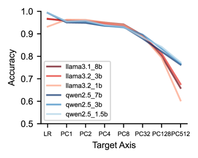<details> <summary>x10.png Details</summary>  ### Visual Description # Technical Document Extraction: Model Accuracy vs. Target Axis ## 1. Image Classification This image is a **line graph** comparing the performance (Accuracy) of six different Large Language Models (LLMs) across various "Target Axis" configurations. ## 2. Component Isolation ### Header/Metadata * **Language:** English. * **Title:** None present in the image. ### Main Chart Area * **Y-Axis Label:** Accuracy * **Y-Axis Scale:** 0.5 to 1.0 (increments of 0.1 marked). * **X-Axis Label:** Target Axis * **X-Axis Categories (Ordinal/Categorical):** LR, PC1, PC2, PC4, PC8, PC32, PC128, PC512. * **Legend Location:** Bottom-left quadrant of the plot area. ### Legend Data (Model Identification) The legend contains six entries, categorized by model family (Llama and Qwen) and parameter size. | Color | Label | Model Family | Size | | :--- | :--- | :--- | :--- | | Dark Red/Maroon | `llama3.1_8b` | Llama 3.1 | 8B | | Medium Red/Coral | `llama3.2_3b` | Llama 3.2 | 3B | | Light Peach/Pink | `llama3.2_1b` | Llama 3.2 | 1B | | Dark Blue/Navy | `qwen2.5_7b` | Qwen 2.5 | 7B | | Medium Blue | `qwen2.5_3b` | Qwen 2.5 | 3B | | Light Blue | `qwen2.5_1.5b` | Qwen 2.5 | 1.5B | --- ## 3. Trend Verification and Data Extraction ### General Trend Analysis All models follow a similar performance trajectory: 1. **Stability (LR to PC8):** High accuracy (approx. 0.93 - 0.99) with minimal degradation. 2. **Initial Decline (PC8 to PC32):** A noticeable downward slope begins. 3. **Sharp Degradation (PC32 to PC512):** All lines slope steeply downward, indicating a significant loss in accuracy as the Target Axis value increases. ### Estimated Data Points (Accuracy) | Target Axis | llama3.1_8b | llama3.2_3b | llama3.2_1b | qwen2.5_7b | qwen2.5_3b | qwen2.5_1.5b | | :--- | :---: | :---: | :---: | :---: | :---: | :---: | | **LR** | ~0.97 | ~0.97 | ~0.93 | ~0.99 | ~0.99 | ~0.99 | | **PC1** | ~0.96 | ~0.96 | ~0.96 | ~0.95 | ~0.95 | ~0.96 | | **PC2** | ~0.96 | ~0.96 | ~0.96 | ~0.95 | ~0.95 | ~0.96 | | **PC4** | ~0.95 | ~0.95 | ~0.95 | ~0.94 | ~0.94 | ~0.94 | | **PC8** | ~0.94 | ~0.94 | ~0.94 | ~0.93 | ~0.93 | ~0.93 | | **PC32** | ~0.89 | ~0.89 | ~0.89 | ~0.88 | ~0.88 | ~0.89 | | **PC128** | ~0.80 | ~0.81 | ~0.79 | ~0.82 | ~0.83 | ~0.84 | | **PC512** | ~0.66 | ~0.68 | ~0.60 | ~0.76 | ~0.77 | ~0.77 | --- ## 4. Key Observations and Findings * **Top Performers at Low Complexity:** At the "LR" (Linear Regression/Baseline) stage, the **Qwen 2.5** family (all sizes) outperforms the Llama family, starting near 1.0 accuracy. * **Convergence:** Between PC1 and PC32, all models perform very similarly, with their lines overlapping significantly in the 0.88 - 0.96 range. * **Robustness at High Complexity:** As the Target Axis reaches **PC512**, the **Qwen 2.5** models (Blue lines) demonstrate significantly higher robustness than the Llama models. * The Qwen models maintain an accuracy of ~0.76 - 0.77. * The Llama models drop more sharply, with `llama3.2_1b` (Light Peach) falling to the lowest point on the chart (~0.60). * **Size vs. Performance:** Interestingly, within the Qwen family at PC512, the smaller models (`1.5b` and `3b`) appear to hold a very slight edge or parity with the `7b` model, suggesting the architecture's scaling for this specific task is highly efficient. </details> Figure B.5: Ideal observer’s reporting performance. 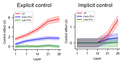B.5 Summarized control effects of Qwen2.5 7B <details> <summary>x11.png Details</summary>  ### Visual Description # Technical Data Extraction: Control Effect Analysis This document provides a comprehensive extraction of the data and trends presented in the provided image, which consists of two side-by-side line charts comparing "Explicit control" and "Implicit control" across different layers of a neural network. ## 1. General Metadata * **Image Type:** Comparative line charts with shaded error regions (confidence intervals). * **Primary Language:** English. * **X-Axis (Common):** "Layer" (Numerical markers: 1, 7, 14, 21, 28). * **Y-Axis (Common):** "Control effect (d)" (Note: The scale differs between the two charts). * **Legend (Common):** Located in the top-left quadrant of each plot. * **Red Line:** LR * **Blue Line:** Early PCs * **Green Line:** Late PCs --- ## 2. Chart 1: Explicit Control ### Component Isolation * **Header:** "Explicit control" * **Y-Axis Scale:** 0 to 6 (increments of 2). ### Trend Verification & Data Extraction 1. **LR (Red Line):** * **Trend:** Strong, consistent upward slope across all layers. * **Approximate Values:** Starts at ~1.8 (Layer 1), rises to ~3.5 (Layer 14), and peaks at ~5.8 (Layer 28). 2. **Early PCs (Blue Line):** * **Trend:** Moderate upward slope, plateauing slightly after Layer 21. * **Approximate Values:** Starts at ~0.5 (Layer 1), rises to ~1.5 (Layer 14), and levels off at ~1.8 (Layer 21-28). 3. **Late PCs (Green Line):** * **Trend:** Near-zero/Flat. Shows very little response to layer depth. * **Approximate Values:** Remains consistently near 0.0 across all layers (1 through 28). --- ## 3. Chart 2: Implicit Control ### Component Isolation * **Header:** "Implicit control" * **Y-Axis Scale:** 0 to 1 (increments of 1). Note: The magnitude is significantly lower than Explicit control. ### Trend Verification & Data Extraction 1. **LR (Red Line):** * **Trend:** Flat at zero until Layer 14, followed by a sharp exponential-like increase. * **Approximate Values:** 0.0 (Layers 1-14), rises to ~0.5 (Layer 21), and ends at ~1.6 (Layer 28). 2. **Early PCs (Blue Line):** * **Trend:** Flat at zero until Layer 14, followed by a slight upward slope. * **Approximate Values:** 0.0 (Layers 1-14), rises to ~0.25 (Layer 21), and ends at ~0.35 (Layer 28). 3. **Late PCs (Green Line):** * **Trend:** Flat. No significant change across the layers. * **Approximate Values:** Remains at 0.0 for the duration of the x-axis. --- ## 4. Comparative Summary Table | Control Type | Series | Layer 1 Value | Layer 14 Value | Layer 28 Value | Overall Trend | | :--- | :--- | :--- | :--- | :--- | :--- | | **Explicit** | LR (Red) | ~1.8 | ~3.5 | ~5.8 | Continuous Increase | | **Explicit** | Early PCs (Blue) | ~0.5 | ~1.5 | ~1.8 | Moderate Increase | | **Explicit** | Late PCs (Green) | ~0.0 | ~0.0 | ~0.0 | Flat/No Effect | | **Implicit** | LR (Red) | 0.0 | 0.0 | ~1.6 | Late-stage Surge | | **Implicit** | Early PCs (Blue) | 0.0 | 0.0 | ~0.35 | Late-stage Slight Rise | | **Implicit** | Late PCs (Green) | 0.0 | 0.0 | 0.0 | No Effect | ## 5. Key Observations * **Magnitude Difference:** The "Explicit control" effect is roughly 4x stronger than the "Implicit control" effect at the final layer (5.8 vs 1.6 for LR). * **Activation Threshold:** In "Implicit control," there is a clear "dead zone" where no effect is measured until after Layer 14. In "Explicit control," the effect is present from Layer 1. * **Component Hierarchy:** In both scenarios, **LR** (Red) is the most dominant factor, followed by **Early PCs** (Blue), while **Late PCs** (Green) consistently show negligible control effects. </details> Figure B.6: Control effects of Qwen2.5 7B. Target control effect for prompts ( $N=256$ ) targeting the LR axis, early PCs (averaged over PC 1, 2, 4, 8), and late PCs (averaged over PC 32, 128, 512) across different layers. 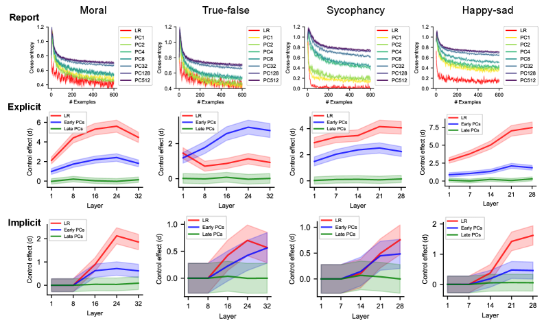B.6 Summarized metacognitive effects on four datasets <details> <summary>x12.png Details</summary>  ### Visual Description # Technical Data Extraction: Model Representation and Control Analysis This document provides a comprehensive extraction of data and trends from the provided 4x3 grid of line charts. The image analyzes model performance and control effects across four datasets (Moral, True-false, Sycophancy, Happy-sad) and three experimental conditions (Report, Explicit, Implicit). --- ## 1. Image Structure and Global Labels The image is organized into a grid with the following headers: * **Column Headers (Datasets):** Moral, True-false, Sycophancy, Happy-sad. * **Row Headers (Conditions):** Report, Explicit, Implicit. --- ## 2. Row 1: Report (Cross-entropy vs. # Examples) This row contains four line charts measuring model performance. ### Common Axis and Legend Information * **Y-axis:** Cross-entropy (Scale: 0.4 to 1.2, except Sycophancy/Happy-sad which start at 0.0). * **X-axis:** # Examples (Scale: 0 to 600). * **Legend (Top Right of each plot):** * **LR (Red):** Linear Regression baseline. * **PC1 (Yellow-Green):** Principal Component 1. * **PC2 (Light Green):** Principal Component 2. * **PC4 (Medium Green):** Principal Component 4. * **PC8 (Teal):** Principal Component 8. * **PC32 (Blue-Grey):** Principal Component 32. * **PC128 (Dark Blue):** Principal Component 128. * **PC512 (Purple):** Principal Component 512. ### Data Trends and Observations * **General Trend:** In all four datasets, cross-entropy decreases rapidly as the number of examples increases from 0 to 100, then plateaus. * **Performance Hierarchy:** The **LR (Red)** line consistently achieves the lowest cross-entropy (best performance), followed by lower-order PCs. As the PC number increases (e.g., PC512), the cross-entropy remains significantly higher, indicating that higher-order components contain less relevant information for the task. * **Sycophancy/Happy-sad Specifics:** In these tasks, the gap between LR and PC512 is much wider than in the Moral/True-false tasks. For Sycophancy, LR drops nearly to 0.0, while PC512 plateaus around 0.7. --- ## 3. Row 2: Explicit (Control effect (d) vs. Layer) This row measures the "Control effect (d)" when the task is explicitly prompted. ### Common Axis and Legend Information * **Y-axis:** Control effect (d). * **X-axis:** Layer (Scale varies: 1 to 32 for Moral/True-false; 1 to 28 for Sycophancy/Happy-sad). * **Legend (Top Left):** * **LR (Red):** Linear Regression. * **Early PCs (Blue):** Aggregated early principal components. * **Late PCs (Green):** Aggregated late principal components. * **Visual Note:** Lines include shaded regions representing confidence intervals or variance. ### Data Trends and Observations | Dataset | LR (Red) Trend | Early PCs (Blue) Trend | Late PCs (Green) Trend | | :--- | :--- | :--- | :--- | | **Moral** | Peaks at Layer 24 (~5.5d). | Peaks at Layer 24 (~2.5d). | Flat near 0. | | **True-false** | Peaks lower (~1.5d); dip between layers 1-8. | Outperforms LR; peaks at Layer 24 (~3.0d). | Flat near 0. | | **Sycophancy** | Rises steadily to peak at Layer 21 (~4.2d). | Rises to ~2.5d. | Flat near 0. | | **Happy-sad** | Strong upward trend, reaching ~7.5d by Layer 28. | Modest rise to ~2.0d. | Flat near 0. | --- ## 4. Row 3: Implicit (Control effect (d) vs. Layer) This row measures the "Control effect (d)" when the task is implicitly prompted. ### Common Axis and Legend Information * **Y-axis:** Control effect (d). * **X-axis:** Layer (Scale matches Row 2). * **Legend (Top Left):** Same as Row 2 (LR: Red, Early PCs: Blue, Late PCs: Green). * **Visual Note:** A grey rectangular block is present at the start of the x-axis (Layers 1-8), indicating a baseline or "no effect" zone. ### Data Trends and Observations * **General Trend:** Control effects are significantly lower in the Implicit condition compared to the Explicit condition across all datasets. * **Moral:** Effects remain at 0 until Layer 8. LR (Red) then rises sharply to ~2.2d at Layer 24. Early PCs (Blue) rise to ~0.8d. * **True-false:** Very low magnitude. LR (Red) reaches ~0.7d; Early PCs (Blue) reach ~0.5d. * **Sycophancy:** LR (Red) and Early PCs (Blue) both rise after Layer 14, with LR reaching ~0.8d and Early PCs reaching ~0.5d. * **Happy-sad:** LR (Red) shows the most significant implicit effect, rising after Layer 8 to reach ~1.6d at Layer 28. Early PCs (Blue) reach ~0.5d. * **Late PCs (Green):** In all Implicit charts, the Late PCs line remains consistently at or near 0.0 across all layers. </details> Figure B.7: Metacognitive effects on four datasets. From left to right: ETHICS (Llama 3.1 8B), True-False (Llama 3.1 8B), Sycophancy (Llama 3.2 3B), and Emotion (Llama 3.2 3B). Top: reporting performance. Middle: explicit control effects. Bottom: implicit control effects. Target control effect for prompts ( $N=256$ ) targeting the LR axis, early PCs (averaged over PC 1, 2, 4, 8), and late PCs (averaged over PC 32, 128, 512) across different layers. 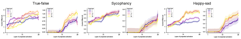B.7 Control accumulation effects on other three datasets <details> <summary>x13.png Details</summary>  ### Visual Description # Technical Data Extraction: Control Effect Analysis Across Model Layers This document provides a comprehensive extraction of data from a series of six line charts organized into three primary categories: **True-false**, **Sycophancy**, and **Happy-sad**. Each category contains two sub-plots showing the "Control Effect (d)" relative to the "Layer of projected activation." --- ## 1. Global Metadata and Legend * **Language:** English * **X-Axis Label:** Layer of projected activation (Values marked at 1, 14, and 28). * **Y-Axis Label:** Control Effect (d) * **Legend Location:** Top-left of each individual plot. * **Legend Categories (Target Layer):** * **1** (Dark Blue) * **7** (Purple) * **14** (Magenta/Pink) * **21** (Orange) * **28** (Yellow) * **Visual Representation:** Solid lines represent the mean effect, while shaded regions around the lines indicate confidence intervals or variance. --- ## 2. Category: True-false ### Plot A (Left) * **Y-Axis Range:** 0 to 4 * **Trend Analysis:** All target layers show a positive upward slope as the layer of projected activation increases. * **Data Observations:** * **Layer 21 (Orange) & 28 (Yellow):** Start lowest (~0.8) but show the steepest climb, peaking near 3.5–4.0 at layer 28. * **Layer 1 (Dark Blue):** Starts highest at layer 1 (~1.5) but has the shallowest slope, ending around 2.5. * **Layer 7 (Purple) & 14 (Pink):** Maintain middle-ground trajectories, ending between 2.5 and 3.0. ### Plot B (Right) * **Y-Axis Range:** 0.0 to 1.50 * **Trend Analysis:** Flat/Zero effect until approximately layer 14, followed by a sharp non-linear increase. * **Data Observations:** * **Layer 21 (Orange) & 28 (Yellow):** Show the most significant late-stage increase, reaching ~1.25 to 1.4. * **Layer 1 (Dark Blue):** Shows the latest and weakest response, ending near 1.0. --- ## 3. Category: Sycophancy ### Plot A (Left) * **Y-Axis Range:** 0.0 to 3.0 * **Trend Analysis:** Steady, linear-like growth across all layers. * **Data Observations:** * **Layer 1 (Dark Blue):** Starts at ~1.5. It plateaus between layers 7 and 14 before rising again to ~2.8. * **Layer 14 (Pink) & 21 (Orange):** Closely clustered, rising from ~1.3 to ~3.0. * **Layer 28 (Yellow):** Shows a slightly lower terminal value (~2.4) compared to the middle layers. ### Plot B (Right) * **Y-Axis Range:** 0.0 to 0.8 * **Trend Analysis:** Near-zero effect until layer 14, then a steady climb. * **Data Observations:** * **Layer 1 (Dark Blue):** Shows a distinct spike at the final layer (28), reaching ~0.6. * **Layer 7 (Purple):** Follows a similar trajectory to Layer 1 but with a slightly lower peak. * **Layer 21 (Orange) & 28 (Yellow):** Rise to approximately 0.4–0.5. --- ## 4. Category: Happy-sad ### Plot A (Left) * **Y-Axis Range:** 0 to 4 * **Trend Analysis:** Rapid increase between layers 1 and 14, followed by a plateau or slight decline toward layer 28. * **Data Observations:** * **Layer 21 (Orange) & 28 (Yellow):** Exhibit the strongest effect, peaking at ~3.5 around layer 18-20 before stabilizing. * **Layer 1 (Dark Blue):** Shows the most muted response, plateauing early at a value of ~1.8. * **Layer 7 (Purple):** Ends at approximately 2.2. ### Plot B (Right) * **Y-Axis Range:** 0.0 to 1.0 * **Trend Analysis:** Zero effect until layer 14, followed by a sharp, consistent upward trend. * **Data Observations:** * **Layer 21 (Orange) & 28 (Yellow):** Lead the increase, reaching the highest values of ~0.8 to 0.9. * **Layer 1 (Dark Blue) & 7 (Purple):** Show a delayed response compared to higher layers, ending between 0.6 and 0.7. --- ## 5. Summary of Patterns 1. **Layer Dependency:** In all "Right-side" plots for each category, there is a "dead zone" where no control effect is measured until the projected activation reaches the middle layers (approx. layer 14). 2. **Magnitude:** The "True-false" and "Happy-sad" categories show higher absolute control effects (up to 4.0d) compared to "Sycophancy" (up to 3.0d). 3. **Late-Layer Dominance:** Generally, target layers 21 (Orange) and 28 (Yellow) result in the highest control effects as the activation layer increases, particularly in the second sub-plots of each category. </details> Figure B.8: Accumulation mechanisms of control effects across layers. Each curve corresponds to prompts targeting the LR axis $\text{LR}_{l}$ , defined by the residual stream activations at a specific layer $l$ (dot markers), showing projections of residual stream activations at each layer (x-axis) onto the target axis $\text{LR}_{l}$ . (a) Explicit control. (b) Implicit control. From left to right: True-False (Llama 3.1 8B), Sycophancy (Llama 3.2 3B), and Emotion (Llama 3.2 3B). Shaded areas indicate 95% confidence intervals. 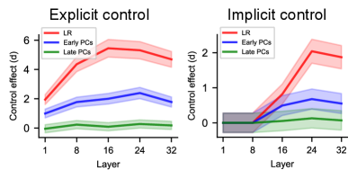B.8 Summarized control effects of Llama3.1 8B with fine-grained neurofeedback labels <details> <summary>x14.png Details</summary>  ### Visual Description # Technical Data Extraction: Control Effect Analysis across Neural Network Layers This document provides a detailed extraction of the data and trends presented in the provided image, which consists of two line graphs comparing "Explicit control" and "Implicit control" across different layers of a model. ## 1. General Metadata * **Image Type:** Two-panel line chart with shaded error regions (confidence intervals). * **X-Axis (Common):** "Layer" (Numerical values: 1, 8, 16, 24, 32). * **Y-Axis (Common):** "Control effect (d)" (Numerical scale varies by panel). * **Legend (Common):** Located in the top-left of each plot area. * **Red Line:** LR * **Blue Line:** Early PCs * **Green Line:** Late PCs --- ## 2. Panel 1: Explicit control **Spatial Grounding:** Left side of the image. Legend at approximately [x=0.15, y=0.15] relative to the panel. ### Data Series Analysis | Series | Color | Visual Trend | Estimated Values (Layer 1 $\rightarrow$ 32) | | :--- | :--- | :--- | :--- | | **LR** | Red | Sharp upward slope until Layer 16, then a slight decline. | ~2.0, ~4.5, ~5.5, ~5.3, ~4.8 | | **Early PCs** | Blue | Moderate upward slope until Layer 24, then a slight decline. | ~1.0, ~1.8, ~2.0, ~2.4, ~1.8 | | **Late PCs** | Green | Relatively flat/stable near zero throughout all layers. | ~0.0, ~0.2, ~0.1, ~0.3, ~0.2 | ### Key Observations * The "LR" series shows the highest control effect, peaking at Layer 16 with a value of approximately 5.5. * The "Early PCs" series follows a similar trajectory but at a significantly lower magnitude (peaking around 2.4). * "Late PCs" consistently show the lowest effect, remaining near the baseline of 0. --- ## 3. Panel 2: Implicit control **Spatial Grounding:** Right side of the image. Legend at approximately [x=0.15, y=0.15] relative to the panel. ### Data Series Analysis | Series | Color | Visual Trend | Estimated Values (Layer 1 $\rightarrow$ 32) | | :--- | :--- | :--- | :--- | | **LR** | Red | Flat at zero until Layer 8, then sharp increase peaking at Layer 24. | 0, 0, ~1.0, ~2.1, ~1.9 | | **Early PCs** | Blue | Flat at zero until Layer 8, then moderate increase peaking at Layer 24. | 0, 0, ~0.5, ~0.7, ~0.6 | | **Late PCs** | Green | Flat at zero until Layer 8, then very slight increase. | 0, 0, ~0.1, ~0.2, ~0.1 | ### Key Observations * **Delayed Onset:** Unlike Explicit control, all series in Implicit control remain at 0 for the first 8 layers. * The Y-axis scale is smaller (0 to 2+) compared to the Explicit control plot (0 to 6+). * The "LR" series remains the dominant factor, peaking at Layer 24. * There is a grey shaded rectangular region covering Layers 1 through 8 at the zero line, indicating a period of no effect or baseline measurement. --- ## 4. Comparative Summary * **Magnitude:** Explicit control effects are roughly 2.5x to 3x stronger than Implicit control effects (comparing the peaks of the LR series). * **Timing:** Explicit control effects are present from Layer 1, whereas Implicit control effects only emerge after Layer 8. * **Consistency:** In both scenarios, the hierarchy of effect strength remains consistent: **LR > Early PCs > Late PCs**. * **Peak Location:** Explicit control peaks earlier (Layer 16-24) compared to Implicit control, which shows a more distinct peak at Layer 24. </details> Figure B.9: Control effects of Llama3.1 8B, with eight-level quantized neural feedback labels. Target control effect for prompts ( $N=256$ ) targeting the LR axis, early PCs (averaged over PC 1, 2, 4, 8), and late PCs (averaged over PC 32, 128, 512) across different layers. 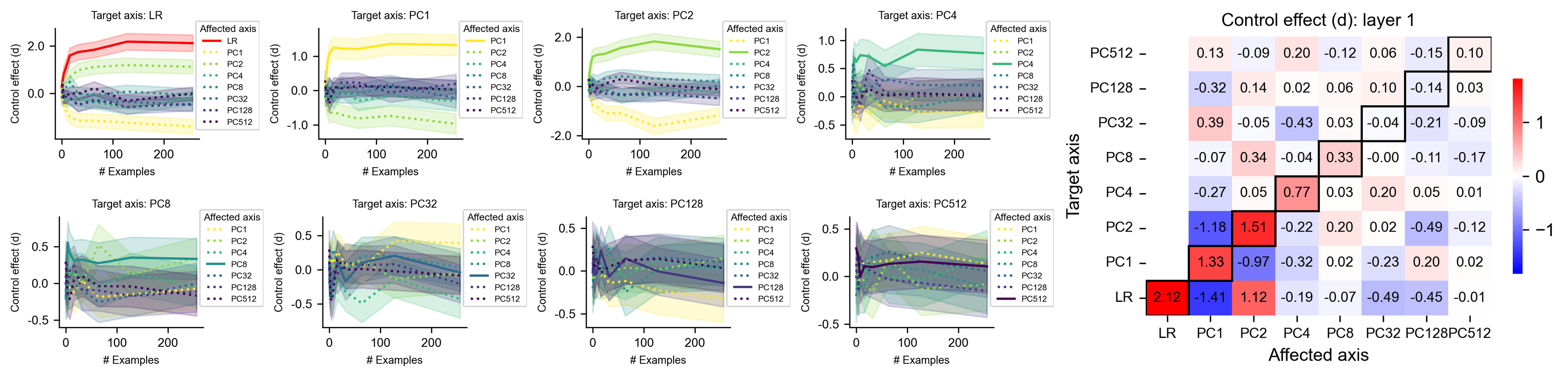B.9 Detailed results for control in Llama3.1 8B and Qwen2.5 7B <details> <summary>supp/llama3.1_8b_active_layer0.png Details</summary>  ### Visual Description # Technical Data Extraction: Control Effect Analysis (Layer 1) This document provides a comprehensive extraction of data from a technical visualization consisting of eight line charts and one summary heatmap. The data explores the "Control effect (d)" across various "Target axes" and "Affected axes" (LR and Principal Components PC1 through PC512) as a function of the number of examples. --- ## 1. Summary Heatmap: Control effect (d): layer 1 **Location:** Right side of the image. **Description:** A square matrix showing the final control effect value for different Target/Affected axis pairs. **Legend:** A vertical color bar on the right ranging from -1 (Blue) to 0 (White) to 1 (Red). ### Data Table (Heatmap Values) The Y-axis represents the **Target axis**, and the X-axis represents the **Affected axis**. Values in bold boxes indicate the diagonal (Target axis = Affected axis). | Target \ Affected | LR | PC1 | PC2 | PC4 | PC8 | PC32 | PC128 | PC512 | | :--- | :---: | :---: | :---: | :---: | :---: | :---: | :---: | :---: | | **PC512** | 0.13 | -0.09 | 0.20 | -0.12 | 0.06 | -0.15 | 0.10 | **0.10** | | **PC128** | -0.32 | 0.14 | 0.02 | 0.06 | 0.10 | -0.14 | **0.03** | - | | **PC32** | 0.39 | -0.05 | -0.43 | 0.03 | -0.04 | **-0.21** | -0.09 | - | | **PC8** | -0.07 | 0.34 | -0.04 | 0.33 | **-0.00** | -0.11 | -0.17 | - | | **PC4** | -0.27 | 0.05 | 0.77 | **0.03** | 0.20 | 0.05 | 0.01 | - | | **PC2** | -1.18 | 1.51 | **-0.22** | 0.20 | 0.02 | -0.49 | -0.12 | - | | **PC1** | 1.33 | **-0.97** | -0.32 | 0.02 | -0.23 | 0.20 | 0.02 | - | | **LR** | **2.12** | -1.41 | 1.12 | -0.19 | -0.07 | -0.49 | -0.45 | -0.01 | --- ## 2. Line Charts: Temporal Trends by Target Axis Each chart shares the following axes: * **X-axis:** # Examples (Scale: 0 to 250) * **Y-axis:** Control effect (d) * **Legend (Affected axis):** * **LR:** Solid Red line * **PC1:** Yellow dotted line * **PC2:** Light Green solid line * **PC4:** Green dotted line * **PC8:** Teal solid line * **PC32:** Blue dotted line * **PC128:** Dark Blue solid line * **PC512:** Purple dotted line ### Chart 1: Target axis: LR * **Trend:** The LR (Red) line shows a sharp upward slope, stabilizing around d=2.0. PC1 (Yellow) and PC2 (Green) show significant negative and positive deviations respectively, while higher PCs cluster near zero. * **Key Final Values:** LR ≈ 2.1, PC1 ≈ -1.4, PC2 ≈ 1.1. ### Chart 2: Target axis: PC1 * **Trend:** PC1 (Yellow) shows a sharp initial increase, stabilizing above 1.0. The LR (Red) line or other components show a mirror negative trend. * **Key Final Values:** PC1 ≈ 1.3, LR (implied) ≈ -1.0. ### Chart 3: Target axis: PC2 * **Trend:** PC2 (Light Green) slopes upward and stabilizes near 1.5. Most other axes remain near or slightly below zero. * **Key Final Values:** PC2 ≈ 1.5, PC1 ≈ -0.5. ### Chart 4: Target axis: PC4 * **Trend:** PC4 (Green dotted) shows a moderate upward trend, peaking and stabilizing near 0.75. * **Key Final Values:** PC4 ≈ 0.8. ### Chart 5: Target axis: PC8 * **Trend:** High variance initially. PC8 (Teal solid) stabilizes slightly above 0. PC4 (Green dotted) shows a higher positive trend in this specific target context. * **Key Final Values:** PC4 ≈ 0.4, PC8 ≈ 0.3. ### Chart 6: Target axis: PC32 * **Trend:** Most lines cluster around zero. PC1 (Yellow) shows a slight upward trend toward 0.4. * **Key Final Values:** PC1 ≈ 0.4, PC32 ≈ -0.2. ### Chart 7: Target axis: PC128 * **Trend:** Significant noise/variance (shaded areas). Most values converge between -0.2 and 0.2. * **Key Final Values:** PC1 ≈ 0.2, PC128 ≈ 0.0. ### Chart 8: Target axis: PC512 * **Trend:** Highly compressed scale. All lines stay within the -0.2 to 0.2 range. * **Key Final Values:** PC2 ≈ 0.2, PC512 ≈ 0.1. --- ## 3. Component Observations * **Diagonal Dominance:** In the heatmap, the highest absolute values are often found when the Target axis matches the Affected axis (e.g., LR/LR at 2.12), though PC1 and PC2 show strong cross-interference. * **Convergence:** In all line charts, the "Control effect" typically stabilizes after approximately 100 examples. * **Variance:** Shaded regions around lines indicate confidence intervals or variance, which appears larger for higher-order PCs (PC128, PC512). </details> Figure B.10: Control performance of Llama3.1 8B (explicit control) in layer 1. 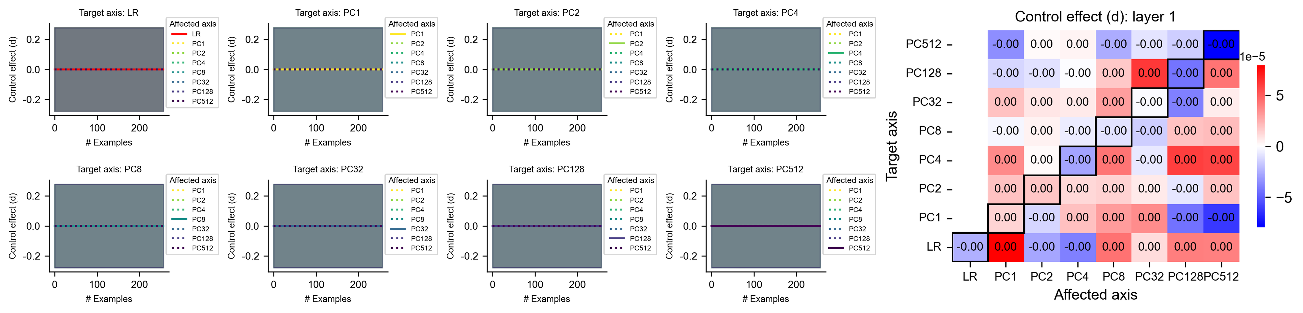<details> <summary>supp/llama3.1_8b_inactive_layer0.png Details</summary>  ### Visual Description # Technical Data Extraction: Control Effect Analysis (Layer 1) This document provides a comprehensive extraction of data and trends from the provided image, which consists of eight line charts and one large heatmap analyzing "Control effect (d)" across various target and affected axes for "layer 1". --- ## 1. Component Isolation The image is divided into two primary sections: * **Left Section (Line Charts):** Eight individual plots showing the control effect over a range of examples (0 to 250). * **Right Section (Heatmap):** A summary matrix titled "Control effect (d): layer 1" showing the relationship between "Target axis" and "Affected axis". --- ## 2. Line Charts Analysis (Left Section) ### General Metadata for all Line Charts: * **X-axis:** `# Examples` (Scale: 0, 100, 200). * **Y-axis:** `Control effect (d)` (Scale: -0.2, 0.0, 0.2). * **Visual Trend:** In all eight charts, the data series appear as flat horizontal lines centered exactly at $y = 0.0$. There is a grey shaded region (likely a confidence interval or baseline) extending from approximately $-0.28$ to $+0.28$ on the y-axis across the entire x-axis range. * **Legend:** "Affected axis" (Labels: LR, PC1, PC2, PC4, PC8, PC32, PC128, PC512). ### Individual Chart Details: | Target Axis | Primary Line (Solid) | Secondary Lines (Dotted) | Observation | | :--- | :--- | :--- | :--- | | **LR** | Red (LR) | PC1 through PC512 | All lines overlap at 0.0. | | **PC1** | Yellow (PC1) | PC2 through PC512 | All lines overlap at 0.0. | | **PC2** | Light Green (PC2) | PC1, PC4 through PC512 | All lines overlap at 0.0. | | **PC4** | Medium Green (PC4) | PC1 through PC512 | All lines overlap at 0.0. | | **PC8** | Teal (PC8) | PC1 through PC512 | All lines overlap at 0.0. | | **PC32** | Blue-Teal (PC32) | PC1 through PC512 | All lines overlap at 0.0. | | **PC128** | Dark Purple (PC128) | PC1 through PC512 | All lines overlap at 0.0. | | **PC512** | Deep Purple (PC512) | PC1 through PC512 | All lines overlap at 0.0. | --- ## 3. Heatmap Analysis (Right Section) **Title:** Control effect (d): layer 1 **X-axis (Affected axis):** LR, PC1, PC2, PC4, PC8, PC32, PC128, PC512 **Y-axis (Target axis):** LR, PC1, PC2, PC4, PC8, PC32, PC128, PC512 **Color Scale:** Diverging (Blue to White to Red). Range: $-5 \times 10^{-5}$ to $+5 \times 10^{-5}$. ### Data Table Reconstruction (Values in $10^{-5}$ units) The diagonal is highlighted with a thick black border. | Target \ Affected | LR | PC1 | PC2 | PC4 | PC8 | PC32 | PC128 | PC512 | | :--- | :---: | :---: | :---: | :---: | :---: | :---: | :---: | :---: | | **PC512** | -0.00 | 0.00 | 0.00 | -0.00 | -0.00 | -0.00 | -0.00 | **-0.00** | | **PC128** | -0.00 | -0.00 | -0.00 | 0.00 | 0.00 | -0.00 | **0.00** | 0.00 | | **PC32** | 0.00 | 0.00 | 0.00 | 0.00 | -0.00 | **-0.00** | 0.00 | 0.00 | | **PC8** | -0.00 | 0.00 | -0.00 | -0.00 | **-0.00** | 0.00 | 0.00 | 0.00 | | **PC4** | 0.00 | 0.00 | -0.00 | **0.00** | -0.00 | 0.00 | 0.00 | 0.00 | | **PC2** | 0.00 | 0.00 | **0.00** | 0.00 | 0.00 | -0.00 | 0.00 | 0.00 | | **PC1** | 0.00 | **-0.00** | 0.00 | 0.00 | 0.00 | -0.00 | -0.00 | -0.00 | | **LR** | **-0.00** | 0.00 | -0.00 | -0.00 | 0.00 | 0.00 | 0.00 | 0.00 | *Note: While the text labels show "0.00" or "-0.00", the background colors indicate micro-variations within the $10^{-5}$ scale.* ### Key Visual Trends in Heatmap: 1. **Diagonal Trend:** The diagonal (Target = Affected) generally shows neutral (white) or very slightly negative (light blue) values, except for the LR/LR cell which is light blue. 2. **Significant Outliers (Color-based):** * **Strong Positive (Red):** Target LR / Affected PC1 shows the most intense red saturation. Target PC4 / Affected PC512 and Target PC128 / Affected PC32 also show significant red saturation. * **Strong Negative (Blue):** Target PC512 / Affected PC512 (far top right) and Target PC1 / Affected PC512 (bottom right) show deep blue saturation. 3. **Symmetry:** The matrix is not perfectly symmetrical, indicating directional influence between the target and affected axes. --- ## 4. Summary of Findings The line charts suggest that at a macro scale (y-axis range of $\pm 0.2$), there is no observable control effect across any axes as the number of examples increases. However, the heatmap reveals that at a microscopic scale ($10^{-5}$), there are specific interactions between axes, particularly involving PC512 and PC1 as affected axes. </details> Figure B.11: Control performance of Llama3.1 8B (implicit control) in layer 1. 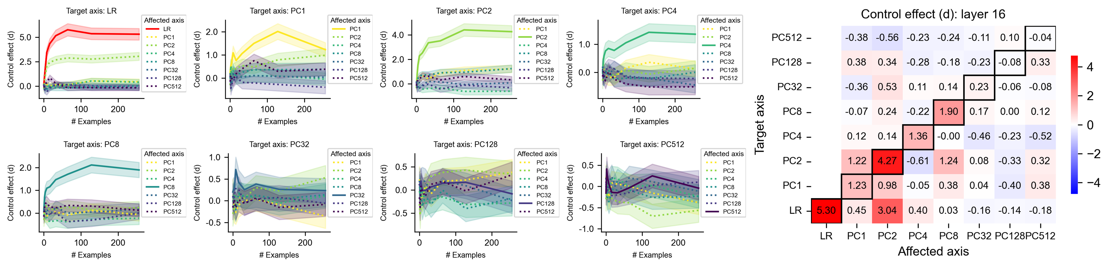<details> <summary>supp/llama3.1_8b_active_layer15.png Details</summary>  ### Visual Description # Technical Data Extraction: Control Effect Analysis (Layer 16) This document provides a comprehensive extraction of data from a technical visualization consisting of eight line charts and one heatmap. The data explores the "Control effect (d)" across various "Target axes" and "Affected axes" within a neural network context (Layer 16). --- ## 1. Component Isolation The image is divided into two primary sections: - **Left Section (Grid of 8 Line Charts):** Shows the progression of the control effect as the number of examples increases (0 to 250). - **Right Section (Heatmap):** Summarizes the final control effect values in a matrix format. --- ## 2. Line Chart Series Analysis (Left Section) Each chart represents a specific **Target axis**. The x-axis is labeled **"# Examples"** (ranging 0–250) and the y-axis is **"Control effect (d)"**. Each line represents an **"Affected axis"**. ### Common Legend (Affected axis) The following categories are used across all line charts: - **LR:** Solid Red line - **PC1:** Yellow (Solid or Dotted) - **PC2:** Light Green (Solid or Dotted) - **PC4:** Medium Green (Solid or Dotted) - **PC8:** Teal (Solid or Dotted) - **PC32:** Blue (Solid or Dotted) - **PC128:** Dark Purple (Solid or Dotted) - **PC512:** Deep Indigo (Solid or Dotted) *Note: In each chart, the line corresponding to the Target axis is typically solid and thicker, while others are dotted.* ### Individual Chart Trends 1. **Target axis: LR** * **Trend:** The LR line (Red) shows a sharp logarithmic increase, plateauing around $d \approx 5.5$. * **Secondary Effects:** PC2 (Light Green dotted) shows a slight positive trend ($d \approx 3.0$). Other axes remain near zero. 2. **Target axis: PC1** * **Trend:** PC1 (Yellow) increases steadily, peaking near $d \approx 2.0$ before a slight decline. * **Secondary Effects:** PC2 and PC4 show minor positive correlations. 3. **Target axis: PC2** * **Trend:** PC2 (Light Green) rises sharply and plateaus at $d \approx 4.5$. * **Secondary Effects:** LR (Red dotted) shows a significant secondary effect ($d \approx 3.0$). 4. **Target axis: PC4** * **Trend:** PC4 (Medium Green) rises and plateaus at $d \approx 1.5$. 5. **Target axis: PC8** * **Trend:** PC8 (Teal) rises and plateaus at $d \approx 2.0$. 6. **Target axis: PC32** * **Trend:** PC32 (Blue) shows a low-magnitude peak ($d < 0.5$) and remains relatively flat. 7. **Target axis: PC128** * **Trend:** PC128 (Dark Purple) shows high variance with a slight upward trend toward $d \approx 0.3$. 8. **Target axis: PC512** * **Trend:** PC512 (Deep Indigo) shows a small initial spike followed by a decline toward zero. --- ## 3. Heatmap Data Extraction (Right Section) **Title:** Control effect (d): layer 16 **Spatial Grounding:** The legend indicates a color scale from -4 (Blue) to 0 (White) to +4 (Red). **Structure:** A matrix where rows are **Target axis** and columns are **Affected axis**. Values in the diagonal (top-left to bottom-right orientation in this specific plot) are highlighted with thick black borders. ### Data Table (Reconstructed) | Target \ Affected | LR | PC1 | PC2 | PC4 | PC8 | PC32 | PC128 | PC512 | | :--- | :---: | :---: | :---: | :---: | :---: | :---: | :---: | :---: | | **PC512** | -0.38 | -0.56 | -0.23 | -0.24 | -0.11 | 0.10 | -0.04 | **N/A** | | **PC128** | 0.38 | 0.34 | -0.28 | -0.18 | -0.23 | -0.08 | 0.33 | | | **PC32** | -0.36 | 0.53 | 0.11 | 0.14 | 0.23 | -0.06 | -0.08 | | | **PC8** | -0.07 | 0.24 | -0.22 | **1.90** | 0.17 | 0.00 | 0.12 | | | **PC4** | 0.12 | 0.14 | **1.36** | -0.00 | -0.46 | -0.23 | -0.52 | | | **PC2** | 1.22 | **4.27** | -0.61 | 1.24 | 0.08 | -0.33 | 0.32 | | | **PC1** | 1.23 | 0.98 | -0.05 | 0.38 | 0.04 | -0.40 | 0.38 | | | **LR** | **5.30** | 0.45 | 3.04 | 0.40 | 0.03 | -0.16 | -0.14 | -0.18 | *Note: The heatmap values are transcribed directly from the cells. The bolded values represent the highest positive control effects (Red cells).* --- ## 4. Key Findings and Trends 1. **Self-Control Dominance:** The highest values are generally found on the diagonal (e.g., LR on LR = 5.30, PC2 on PC1 = 4.27). 2. **Cross-Axis Interference:** There is a strong cross-effect between **LR** and **PC2** (3.04) and **PC2** and **PC1** (4.27). 3. **Diminishing Effect:** As the PC index increases (PC32, PC128, PC512), the control effect (d) significantly decreases, with values approaching zero or becoming slightly negative (blue-tinted cells). 4. **Consistency:** The line charts and the heatmap are consistent; for example, the "Target axis: LR" line chart shows a plateau at ~5.5, which matches the heatmap value of 5.30. </details> Figure B.12: Control performance of Llama3.1 8B (explicit control) in layer 16. 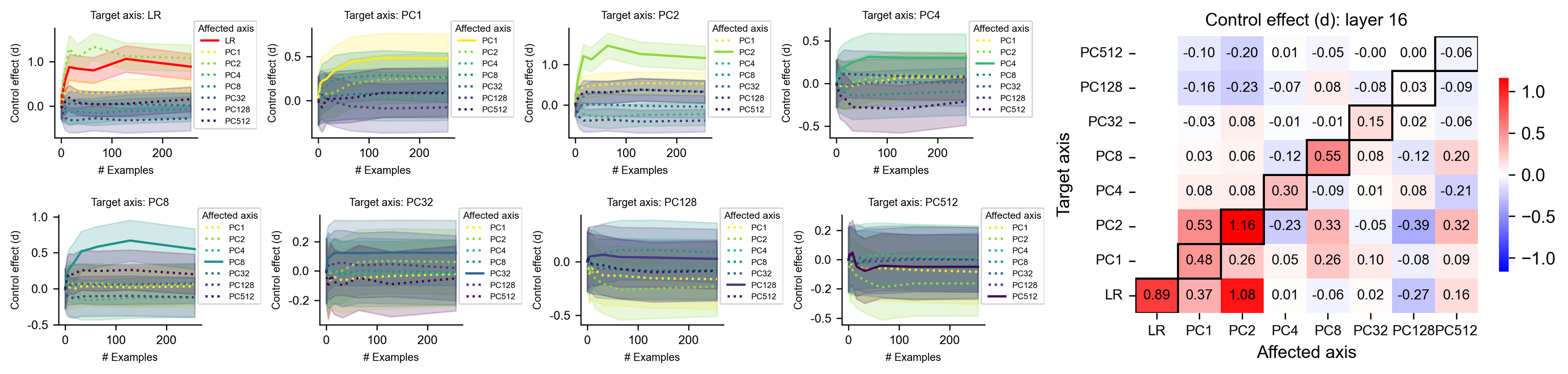<details> <summary>supp/llama3.1_8b_inactive_layer15.png Details</summary>  ### Visual Description # Technical Data Extraction: Control Effect Analysis (Layer 16) This document provides a comprehensive extraction of data from a technical visualization consisting of eight line charts and one summary heatmap. The data explores the "Control effect (d)" across various "Target axes" and "Affected axes" within a neural network context (Layer 16). --- ## 1. Summary Heatmap: Control effect (d): layer 16 The heatmap on the right summarizes the relationship between the **Target axis** (y-axis) and the **Affected axis** (x-axis). ### Metadata - **Title:** Control effect (d): layer 16 - **Y-Axis Label:** Target axis - **X-Axis Label:** Affected axis - **Color Scale:** Diverging (Blue to White to Red). - **Red (Positive):** Up to 1.0+ (Maximum observed: 1.16) - **White:** 0.0 - **Blue (Negative):** Down to -1.0 (Minimum observed: -0.39) - **Special Formatting:** Diagonal cells (where Target = Affected) are outlined with a thick black border. ### Data Table (Extracted Values) | Target \ Affected | LR | PC1 | PC2 | PC4 | PC8 | PC32 | PC128 | PC512 | | :--- | :---: | :---: | :---: | :---: | :---: | :---: | :---: | :---: | | **PC512** | -0.10 | -0.20 | 0.01 | -0.05 | -0.00 | 0.00 | -0.06 | **-0.06** | | **PC128** | -0.16 | -0.23 | -0.07 | 0.08 | -0.08 | 0.03 | **-0.09** | -0.09 | | **PC32** | -0.03 | 0.08 | -0.01 | -0.01 | 0.15 | **0.02** | -0.06 | -0.06 | | **PC8** | 0.03 | 0.06 | -0.12 | 0.55 | **0.08** | -0.12 | 0.20 | 0.20 | | **PC4** | 0.08 | 0.08 | 0.30 | **-0.09** | 0.01 | 0.08 | -0.21 | -0.21 | | **PC2** | 0.53 | 1.16 | **-0.23** | 0.33 | -0.05 | -0.39 | 0.32 | 0.32 | | **PC1** | 0.48 | **0.26** | 0.05 | 0.26 | 0.10 | -0.08 | 0.09 | 0.09 | | **LR** | **0.89** | 0.37 | 1.08 | 0.01 | -0.06 | 0.02 | -0.27 | 0.16 | --- ## 2. Line Charts: Control Effect vs. # Examples Eight subplots show the progression of the control effect as the number of examples increases (0 to 250). ### Common Features - **X-axis:** # Examples (Scale: 0, 100, 200) - **Y-axis:** Control effect (d) - **Legend:** "Affected axis" (Colors/Styles remain consistent across all plots). - **Visual Trend Logic:** In most plots, the line corresponding to the "Target axis" (the self-effect) or highly correlated PCs shows the highest magnitude, typically stabilizing after 50-100 examples. ### Legend Key (Spatial Grounding: Top Right of each subplot) - **LR:** Solid Red line - **PC1:** Dotted Yellow line - **PC2:** Solid Light Green line - **PC4:** Dotted Teal line - **PC8:** Solid Dark Teal line - **PC32:** Dotted Blue line - **PC128:** Solid Navy line - **PC512:** Dotted Purple line ### Subplot Data Extraction | Subplot (Target) | Primary Trend Description | Key Observations | | :--- | :--- | :--- | | **Target: LR** | Red line (LR) rises sharply and plateaus near 1.0. | PC2 (Light Green) also shows a strong positive trend (~1.0). PC1 (Yellow) is moderate (~0.4). | | **Target: PC1** | Light Green (PC2) and Yellow (PC1) lines rise to ~0.5. | Most other lines cluster near 0.0. | | **Target: PC2** | Light Green (PC2) rises sharply to ~1.2. | This is the highest magnitude observed in the line charts. | | **Target: PC4** | Teal (PC4) and Light Green (PC2) rise to ~0.3. | High variance (shaded areas) is visible. | | **Target: PC8** | Dark Teal (PC8) rises to ~0.5. | PC4 (Teal) and PC512 (Purple) show moderate positive trends. | | **Target: PC32** | All lines cluster tightly between -0.2 and 0.2. | Blue (PC32) is slightly positive but nearly flat. | | **Target: PC128** | Navy (PC128) and Blue (PC32) are slightly positive. | Most lines are near zero; high overlap in shaded regions. | | **Target: PC512** | Purple (PC512) and Navy (PC128) show slight negative trends. | Values are very low magnitude (between 0.0 and -0.2). | --- ## 3. Component Analysis 1. **Header/Titles:** Each subplot is clearly labeled with "Target axis: [Name]". The main heatmap is titled "Control effect (d): layer 16". 2. **Main Charts:** The line charts use shaded regions to represent confidence intervals or variance. The heatmap uses a grid with numerical annotations. 3. **Data Consistency:** The values in the heatmap (e.g., Target LR, Affected PC2 = 1.08) match the visual plateaus in the line charts (e.g., in the "Target axis: LR" plot, the PC2 light green line plateaus just above 1.0). </details> Figure B.13: Control performance of Llama3.1 8B (implicit control) in layer 16. 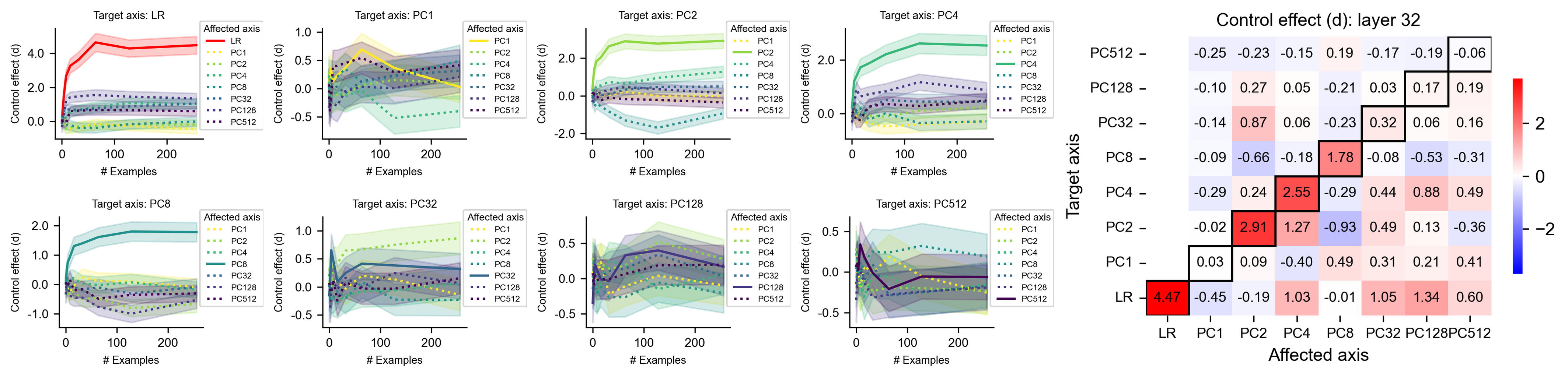<details> <summary>supp/llama3.1_8b_active_layer31.png Details</summary>  ### Visual Description # Technical Document Extraction: Control Effect Analysis (Layer 32) This document provides a comprehensive extraction of data and trends from the provided image, which consists of eight line charts and one summary heatmap. The data explores the "Control effect (d)" across various "Target axes" relative to "Affected axes" over a number of examples. --- ## 1. Component Isolation The image is segmented into two primary regions: * **Region A (Left/Center):** A grid of 8 line charts showing the progression of control effects as the number of examples increases (0 to 250). * **Region B (Right):** A summary heatmap titled "Control effect (d): layer 32" showing the final or peak relationship between Target and Affected axes. --- ## 2. Region A: Line Chart Grid Analysis Each chart represents a specific **Target axis**. The x-axis is **# Examples** (0, 100, 200) and the y-axis is **Control effect (d)**. ### Common Legend (Affected axis) The following categories are used across the line charts: * **LR:** Solid Red line. * **PC1:** Dotted Yellow line. * **PC2:** Solid Light Green line. * **PC4:** Solid Teal line. * **PC8:** Solid Dark Teal line. * **PC32:** Solid Blue-Grey line. * **PC128:** Solid Purple line. * **PC512:** Dotted Dark Purple line. ### Individual Chart Trends | Target Axis | Primary Trend (Self-Influence) | Secondary Trends (Cross-Influence) | | :--- | :--- | :--- | | **LR** | **LR (Red)**: Sharp upward slope, stabilizing at ~4.5. | Most other PCs cluster near 0.0 to 1.0. | | **PC1** | **PC1 (Yellow)**: Slopes upward to ~0.5, then declines toward 0.0. | High variance; PC512 (Dotted Purple) shows a slight upward trend. | | **PC2** | **PC2 (Light Green)**: Sharp upward slope, stabilizing at ~3.0. | PC4 (Teal) shows a slight downward trend to ~ -1.5. | | **PC4** | **PC4 (Teal)**: Sharp upward slope, stabilizing at ~2.5. | PC128 and PC32 show slight positive trends (~0.5). | | **PC8** | **PC8 (Dark Teal)**: Sharp upward slope, stabilizing at ~1.8. | PC2 (Light Green) shows a slight positive trend; others are near 0. | | **PC32** | **PC32 (Blue-Grey)**: Moderate upward slope, stabilizing at ~0.4. | PC128 and PC512 track closely with PC32. | | **PC128** | **PC128 (Purple)**: Moderate upward slope, stabilizing at ~0.3. | PC32 and PC512 show similar moderate positive trends. | | **PC512** | **PC512 (Dotted Purple)**: Initial spike, then stabilizes near 0.0. | High noise/variance across all series in this target. | --- ## 3. Region B: Heatmap Data Extraction **Title:** Control effect (d): layer 32 **X-Axis (Affected axis):** LR, PC1, PC2, PC4, PC8, PC32, PC128, PC512 **Y-Axis (Target axis):** LR, PC1, PC2, PC4, PC8, PC32, PC128, PC512 **Color Scale:** Blue (-2) to White (0) to Red (2+). ### Data Table (Reconstructed) The diagonal (Target = Affected) is highlighted with bold black borders, representing the self-control effect. | Target \ Affected | LR | PC1 | PC2 | PC4 | PC8 | PC32 | PC128 | PC512 | | :--- | :---: | :---: | :---: | :---: | :---: | :---: | :---: | :---: | | **PC512** | -0.25 | -0.23 | -0.15 | 0.19 | -0.17 | -0.19 | -0.06 | **-0.06** | | **PC128** | -0.10 | 0.27 | 0.05 | -0.21 | 0.03 | 0.17 | **0.19** | 0.19 | | **PC32** | -0.14 | 0.87 | 0.06 | -0.23 | 0.32 | **0.06** | 0.16 | 0.16 | | **PC8** | -0.09 | -0.66 | -0.18 | 1.78 | **-0.08** | -0.53 | -0.31 | -0.31 | | **PC4** | -0.29 | 0.24 | 2.55 | **-0.29** | 0.44 | 0.88 | 0.49 | 0.49 | | **PC2** | -0.02 | 2.91 | **1.27** | -0.93 | 0.49 | 0.13 | -0.36 | -0.36 | | **PC1** | 0.03 | **0.09** | -0.40 | 0.49 | 0.31 | 0.21 | 0.41 | 0.41 | | **LR** | **4.47** | -0.45 | -0.19 | 1.03 | -0.01 | 1.05 | 1.34 | 0.60 | --- ## 4. Key Observations and Trends 1. **Diagonal Dominance (Self-Effect):** The strongest control effects are generally found on the diagonal or immediately adjacent to it. The highest single value is **4.47** (Target: LR, Affected: LR). 2. **Off-Diagonal Interactions:** * There is a strong interaction between **Target PC2** and **Affected PC1** (2.91). * There is a strong interaction between **Target PC4** and **Affected PC2** (2.55). * There is a strong interaction between **Target PC8** and **Affected PC4** (1.78). 3. **Negative Effects:** Several blue cells indicate negative control effects, notably **Target PC2 / Affected PC4** (-0.93) and **Target PC8 / Affected PC1** (-0.66). 4. **Convergence:** The line charts indicate that for most axes, the control effect stabilizes after approximately 100-150 examples. 5. **Symmetry:** The matrix is not symmetric, indicating that the control effect of Axis A on Axis B is not the same as Axis B on Axis A. For example, LR on PC1 is 0.03, but PC1 on LR is -0.45. </details> Figure B.14: Control performance of Llama3.1 8B (explicit control) in layer 32. 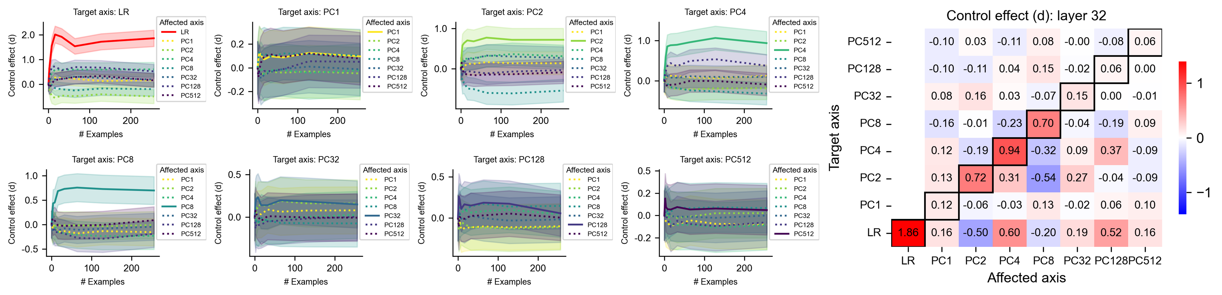<details> <summary>supp/llama3.1_8b_inactive_layer31.png Details</summary>  ### Visual Description # Technical Data Extraction: Control Effect Analysis (Layer 32) This document provides a comprehensive extraction of data and trends from the provided image, which consists of eight line charts and one summary heatmap analyzing "Control effect (d)" across various target and affected axes at layer 32. --- ## 1. Component Isolation The image is divided into two primary sections: 1. **Left/Center (Line Charts):** Eight individual plots showing the progression of the control effect as the number of examples increases (0 to 250). 2. **Right (Heatmap):** A summary matrix titled "Control effect (d): layer 32" showing the final or aggregate relationship between Target and Affected axes. --- ## 2. Summary Heatmap Data Extraction **Title:** Control effect (d): layer 32 **Y-Axis (Target axis):** PC512, PC128, PC32, PC8, PC4, PC2, PC1, LR **X-Axis (Affected axis):** LR, PC1, PC2, PC4, PC8, PC32, PC128, PC512 **Legend:** Color scale from -1 (Blue) to 0 (White) to +1 (Red). ### Data Table (Reconstructed) The diagonal (outlined in black) represents the effect of a target axis on itself. | Target \ Affected | LR | PC1 | PC2 | PC4 | PC8 | PC32 | PC128 | PC512 | | :--- | :---: | :---: | :---: | :---: | :---: | :---: | :---: | :---: | | **PC512** | -0.10 | 0.03 | -0.11 | 0.08 | -0.00 | -0.08 | 0.06 | N/A | | **PC128** | -0.10 | -0.11 | 0.04 | 0.15 | -0.02 | 0.06 | 0.00 | N/A | | **PC32** | 0.08 | 0.16 | 0.03 | -0.07 | 0.15 | 0.00 | -0.01 | N/A | | **PC8** | -0.16 | -0.01 | -0.23 | **0.70** | -0.04 | -0.19 | 0.09 | N/A | | **PC4** | 0.12 | -0.19 | **0.94** | -0.32 | 0.09 | 0.37 | -0.09 | N/A | | **PC2** | 0.13 | **0.72** | 0.31 | -0.54 | 0.27 | -0.04 | -0.09 | N/A | | **PC1** | **0.12** | -0.06 | -0.03 | 0.13 | -0.02 | 0.06 | 0.10 | N/A | | **LR** | **1.86** | 0.16 | -0.50 | 0.60 | -0.20 | 0.19 | 0.52 | 0.16 | *Note: The heatmap contains a black-bordered diagonal. The value for LR/LR is 1.86 (Strong Red). The value for PC4/PC2 is 0.94 (Red). The value for PC8/PC4 is 0.70 (Red).* --- ## 3. Line Chart Analysis (Target Axis Series) Each chart shares the following attributes: * **X-axis:** # Examples (Scale: 0, 100, 200) * **Y-axis:** Control effect (d) * **Legend (Affected axis):** LR (Solid Red), PC1 (Dotted Yellow), PC2 (Dotted Light Green), PC4 (Dotted Green), PC8 (Dotted Teal), PC32 (Dotted Blue-Grey), PC128 (Dotted Purple), PC512 (Dotted Dark Purple). * **Visual Trend Logic:** In every chart, the line corresponding to the "Target axis" name (e.g., LR in the LR chart) is rendered as a **solid line** and typically shows the highest magnitude, while other "Affected axes" are dotted and cluster near zero. ### Chart 1: Target axis: LR * **Trend:** The LR line (Solid Red) spikes sharply from 0 to ~2.0 within the first 25 examples, then stabilizes between 1.5 and 2.0. * **Other axes:** All dotted lines remain clustered between -0.5 and 1.0, with PC128 (Purple) showing a slight upward trend toward 0.5. ### Chart 2: Target axis: PC1 * **Trend:** The PC1 line (Solid Yellow) rises quickly to ~0.1 and stays relatively flat. * **Other axes:** Most axes are tightly clustered around 0.0. PC512 (Dark Purple) and PC128 (Purple) show the widest variance, fluctuating between -0.2 and 0.2. ### Chart 3: Target axis: PC2 * **Trend:** The PC2 line (Solid Light Green) rises to ~0.5 and stabilizes. * **Other axes:** PC4 (Dotted Green) and PC1 (Dotted Yellow) stay near 0.2. PC512 (Dark Purple) stays below 0. ### Chart 4: Target axis: PC4 * **Trend:** The PC4 line (Solid Green) rises sharply to ~1.0 and stabilizes. * **Other axes:** PC8 (Dotted Teal) and PC32 (Dotted Blue-Grey) remain near 0. PC512 (Dark Purple) shows a slight negative trend. ### Chart 5: Target axis: PC8 * **Trend:** The PC8 line (Solid Teal) rises to ~0.75 and stabilizes. * **Other axes:** Clustered between -0.25 and 0.25. ### Chart 6: Target axis: PC32 * **Trend:** The PC32 line (Solid Blue-Grey) rises to ~0.2 and stabilizes. * **Other axes:** High overlap; most lines are between -0.2 and 0.2. ### Chart 7: Target axis: PC128 * **Trend:** The PC128 line (Solid Purple) rises to ~0.2. * **Other axes:** Significant variance; PC512 (Dark Purple) and PC32 (Blue-Grey) overlap heavily with the target axis. ### Chart 8: Target axis: PC512 * **Trend:** The PC512 line (Solid Dark Purple) rises to ~0.1. * **Other axes:** All axes are very tightly clustered around the 0.0 to 0.1 range, indicating low specificity for this target. --- ## 4. Key Observations 1. **Specificity:** The "LR" (Logistic Regression) axis shows the strongest and most distinct control effect (d ≈ 1.86). 2. **Dimensionality Trend:** As the PC (Principal Component) number increases (from PC1 to PC512), the maximum control effect generally decreases and the separation between the target axis and other affected axes becomes less distinct. 3. **Stability:** In all cases, the control effect stabilizes rapidly, usually after 50-100 examples. </details> Figure B.15: Control performance of Llama3.1 8B (implicit control) in layer 32. 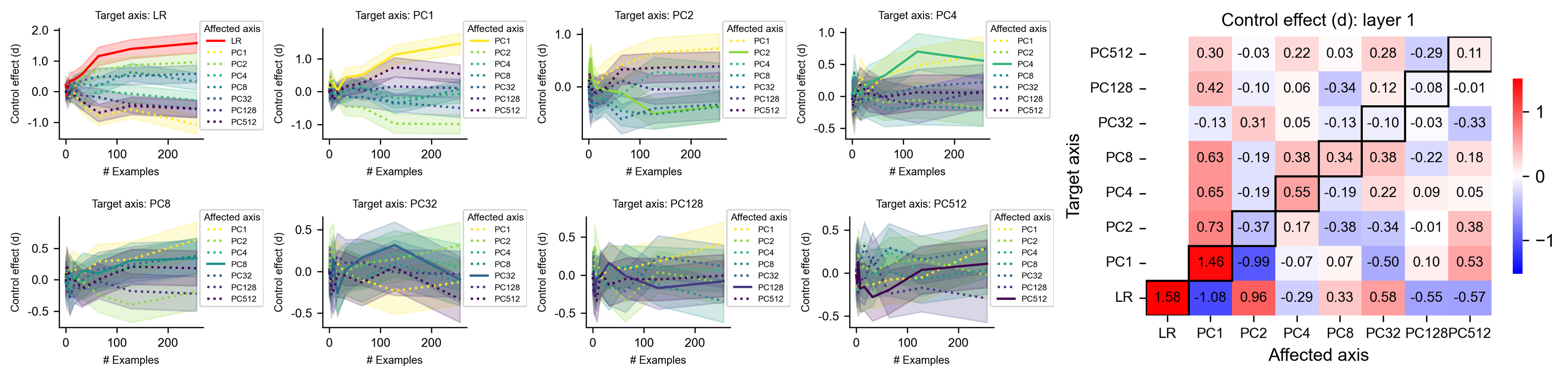<details> <summary>supp/qwen2.5_7b_active_layer0.png Details</summary>  ### Visual Description # Technical Data Extraction: Control Effect Analysis (Layer 1) This document provides a comprehensive extraction of data from a technical visualization consisting of eight line charts and one summary heatmap. The data explores the "Control effect (d)" across various "Target axes" and "Affected axes" relative to the number of training examples. --- ## 1. Component Isolation The image is divided into two primary sections: - **Left Section (Line Charts):** Eight individual plots showing the progression of control effects as the number of examples increases (from 0 to 250). - **Right Section (Heatmap):** A summary matrix titled "Control effect (d): layer 1" showing the final or aggregate effect between target and affected axes. --- ## 2. Line Charts Analysis (Progression Data) Each chart represents a specific **Target axis**. The x-axis is **# Examples** (0 to 250), and the y-axis is **Control effect (d)**. ### Shared Legend (Affected axis) The following categories are tracked in each plot, distinguished by color and line style: - **LR:** Solid Red line - **PC1:** Dotted Yellow line - **PC2:** Solid Light Green line - **PC4:** Solid Teal/Green line - **PC8:** Solid Dark Teal line - **PC32:** Dotted Blue-Grey line - **PC128:** Dotted Purple line - **PC512:** Dotted Dark Purple line ### Individual Plot Trends | Target Axis | Primary Trend Observation | Key Data Behavior | | :--- | :--- | :--- | | **LR** | Strong positive divergence for LR. | The red line (LR) climbs sharply to ~1.5. Other PC axes remain below 1.0, with PC1 (yellow) trending downward toward -1.0. | | **PC1** | High variance, PC1 dominates. | PC1 (yellow) trends upward toward ~1.5. Most other axes cluster between -0.5 and 0.5. | | **PC2** | Moderate positive trend for PC2. | PC2 (light green) rises to ~0.7. PC4 and PC8 follow closely. PC1 (yellow) shows a slight negative trend. | | **PC4** | PC4 shows the strongest positive effect. | PC4 (teal) rises to ~0.6. Other axes remain relatively flat or slightly positive around 0.2. | | **PC8** | PC8 and PC1 show positive trends. | PC8 (dark teal) and PC1 (yellow) both trend upward toward 0.5. | | **PC32** | Low magnitude, high overlap. | Most lines cluster near 0.0. PC32 (blue-grey) shows a slight peak then decline. | | **PC128** | PC128 shows a late positive trend. | PC128 (purple) rises slightly above 0.2 after 100 examples. | | **PC512** | PC512 shows a late positive trend. | PC512 (dark purple) rises to ~0.2. PC1 (yellow) also shows a positive trend here. | --- ## 3. Heatmap Analysis (Summary Matrix) **Title:** Control effect (d): layer 1 **X-Axis (Affected axis):** LR, PC1, PC2, PC4, PC8, PC32, PC128, PC512 **Y-Axis (Target axis):** LR, PC1, PC2, PC4, PC8, PC32, PC128, PC512 **Color Scale:** Red (Positive, up to >1), White (Zero), Blue (Negative, down to -1). ### Data Table Reconstruction The diagonal (Target axis = Affected axis) is highlighted with thick black borders, representing the self-control effect. | Target \ Affected | LR | PC1 | PC2 | PC4 | PC8 | PC32 | PC128 | PC512 | | :--- | :---: | :---: | :---: | :---: | :---: | :---: | :---: | :---: | | **PC512** | 0.30 | -0.03 | 0.22 | 0.03 | 0.28 | -0.29 | 0.11 | **[0.11]** | | **PC128** | 0.42 | -0.10 | 0.06 | -0.34 | 0.12 | -0.08 | **[-0.01]** | - | | **PC32** | -0.13 | 0.31 | 0.05 | -0.13 | -0.10 | **[-0.03]** | -0.33 | - | | **PC8** | 0.63 | -0.19 | 0.38 | 0.34 | **[0.38]** | -0.22 | 0.18 | - | | **PC4** | 0.65 | -0.19 | 0.55 | **[-0.19]** | 0.22 | 0.09 | 0.05 | - | | **PC2** | 0.73 | -0.37 | **[0.17]** | -0.38 | -0.34 | -0.01 | 0.38 | - | | **PC1** | 1.46 | **[-0.99]** | -0.07 | 0.07 | -0.50 | 0.10 | 0.53 | - | | **LR** | **[1.58]** | -1.08 | 0.96 | -0.29 | 0.33 | 0.58 | -0.55 | -0.57 | *(Note: Values in brackets [ ] denote the diagonal/self-influence cells.)* ### Key Observations from Heatmap: 1. **Strongest Positive Effect:** The interaction of Target: LR on Affected: LR (1.58, deep red). 2. **Strongest Negative Effect:** The interaction of Target: LR on Affected: PC1 (-1.08, deep blue). 3. **Cross-Talk:** Target PC1 has a very strong positive effect on Affected LR (1.46), suggesting a high degree of coupling between these two axes. 4. **Diminishing Effects:** As the PC index increases (moving toward PC512), the absolute values in the heatmap generally decrease, indicated by lighter colors (closer to white/zero). --- ## 4. Technical Metadata * **Language:** English * **Metric:** Control effect (d), likely Cohen's d or a similar standardized effect size. * **Layer:** Data specifically pertains to "layer 1" of the model/system under study. 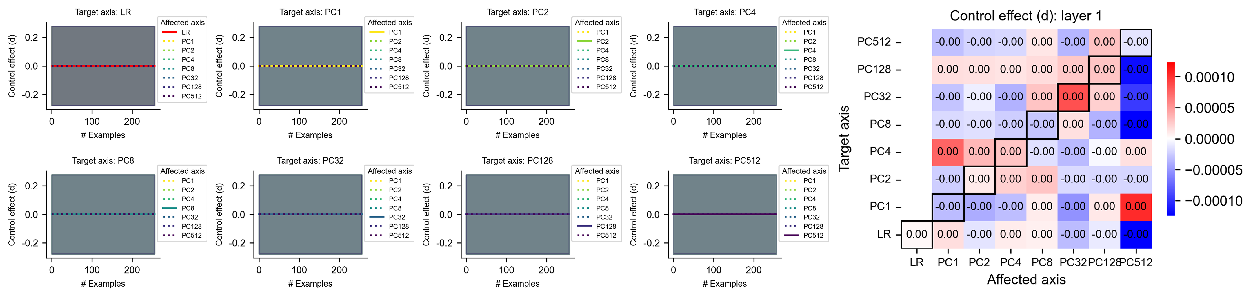</details> Figure B.16: Qwen2.5 7B (explicit control) layer 1 <details> <summary>supp/qwen2.5_7b_inactive_layer0.png Details</summary>  ### Visual Description # Technical Data Extraction: Control Effect Analysis (Layer 1) This document provides a comprehensive extraction of data and visual information from the provided image, which consists of eight line charts and one large heatmap analyzing "Control effect (d)" across various target and affected axes. --- ## 1. Component Isolation The image is divided into two primary sections: * **Left Section (Line Charts):** A 2x4 grid of line plots showing the control effect over time (# Examples). * **Right Section (Heatmap):** A summary matrix titled "Control effect (d): layer 1" showing the relationship between Target and Affected axes. --- ## 2. Line Charts Analysis (Left Section) ### General Metadata for Line Charts * **X-axis:** `# Examples` (Scale: 0 to 200+) * **Y-axis:** `Control effect (d)` (Scale: -0.2 to 0.2) * **Visual Trend:** In all eight plots, the data lines are horizontal and centered exactly at **0.0**. There is no deviation or slope observed across the number of examples. * **Legend ("Affected axis"):** Contains the following categories with specific color/style coding: * **LR:** Solid Red line * **PC1:** Dotted Yellow line * **PC2:** Dotted Light Green line * **PC4:** Dotted Medium Green line * **PC8:** Dotted Teal line * **PC32:** Dotted Blue line * **PC128:** Dotted Indigo line * **PC512:** Dotted Purple line ### Individual Plot Details Each plot represents a specific **Target axis**. In every plot, the line corresponding to the Target axis is highlighted as a solid line, while others remain dotted. 1. **Target axis: LR** (Top Row, 1st) - Solid red line at y=0. 2. **Target axis: PC1** (Top Row, 2nd) - Solid yellow line at y=0. 3. **Target axis: PC2** (Top Row, 3rd) - Solid light green line at y=0. 4. **Target axis: PC4** (Top Row, 4th) - Solid medium green line at y=0. 5. **Target axis: PC8** (Bottom Row, 1st) - Solid teal line at y=0. 6. **Target axis: PC32** (Bottom Row, 2nd) - Solid blue line at y=0. 7. **Target axis: PC128** (Bottom Row, 3rd) - Solid indigo line at y=0. 8. **Target axis: PC512** (Bottom Row, 4th) - Solid purple line at y=0. --- ## 3. Heatmap Analysis (Right Section) **Title:** Control effect (d): layer 1 ### Axis Labels * **Y-axis (Target axis):** PC512, PC128, PC32, PC8, PC4, PC2, PC1, LR (Top to Bottom) * **X-axis (Affected axis):** LR, PC1, PC2, PC4, PC8, PC32, PC128, PC512 (Left to Right) ### Color Scale (Legend) * **Range:** -0.00010 (Deep Blue) to 0.00010 (Deep Red). * **Center:** 0.00000 (White). ### Data Table Reconstruction The heatmap contains numerical values. Note: "-0.00" indicates a very small negative value rounded to two decimal places. A black stepped border highlights the diagonal/near-diagonal relationship. | Target \ Affected | LR | PC1 | PC2 | PC4 | PC8 | PC32 | PC128 | PC512 | | :--- | :--- | :--- | :--- | :--- | :--- | :--- | :--- | :--- | | **PC512** | -0.00 | -0.00 | -0.00 | 0.00 | -0.00 | 0.00 | -0.00 | | | **PC128** | 0.00 | 0.00 | 0.00 | 0.00 | 0.00 | 0.00 | -0.00 | | | **PC32** | -0.00 | -0.00 | -0.00 | 0.00 | 0.00 | 0.00 | -0.00 | | | **PC8** | -0.00 | -0.00 | -0.00 | -0.00 | 0.00 | -0.00 | -0.00 | | | **PC4** | 0.00 | 0.00 | 0.00 | -0.00 | -0.00 | -0.00 | 0.00 | | | **PC2** | -0.00 | 0.00 | 0.00 | 0.00 | -0.00 | -0.00 | -0.00 | | | **PC1** | | -0.00 | -0.00 | -0.00 | 0.00 | -0.00 | 0.00 | 0.00 | | **LR** | 0.00 | 0.00 | -0.00 | 0.00 | 0.00 | -0.00 | -0.00 | -0.00 | ### Key Observations & Trends 1. **Magnitude:** The control effects are extremely small, as indicated by the color scale (orders of $10^{-5}$ or $10^{-4}$). 2. **Diagonal Pattern:** There is a distinct diagonal trend where the Target axis matches the Affected axis, though the values remain near zero. 3. **Specific Outliers:** * **Target PC1 / Affected PC512:** Shows a strong positive (Red) effect (~0.00010). * **Target LR / Affected PC512:** Shows a strong negative (Blue) effect (~ -0.00010). * **Target PC128 / Affected PC512:** Shows a strong negative (Blue) effect. * **Target PC32 / Affected PC32:** Shows a moderate positive (Red) effect. 4. **Symmetry:** The matrix is not perfectly symmetrical, suggesting directional influence from Target to Affected axes. 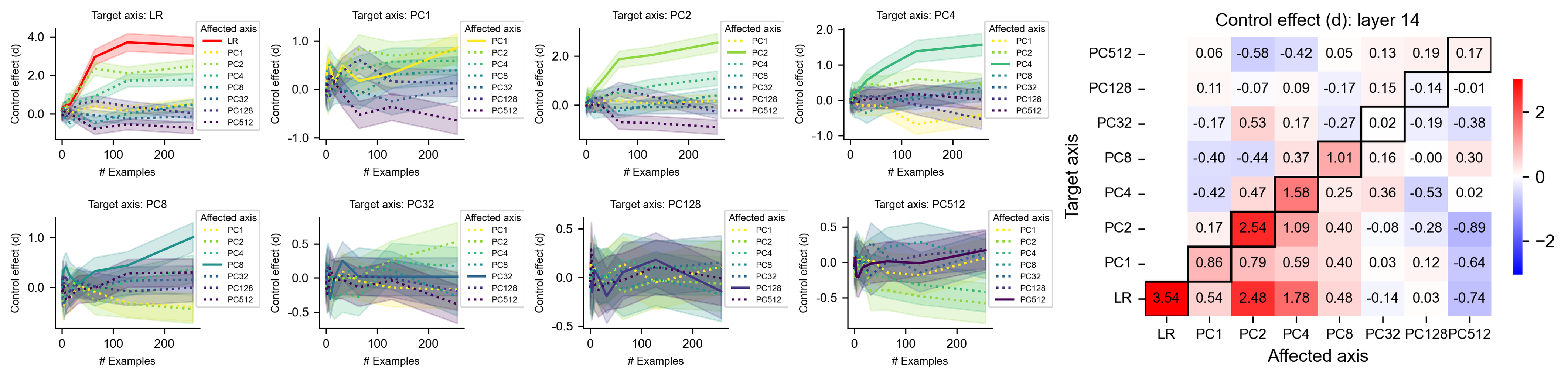</details> Figure B.17: Qwen2.5 7B (implicit control) layer 1 <details> <summary>supp/qwen2.5_7b_active_layer13.png Details</summary>  ### Visual Description # Technical Data Extraction: Control Effect Analysis (Layer 14) This document provides a comprehensive extraction of data from a series of line charts and a heatmap analyzing the "Control effect (d)" across different target and affected axes for "layer 14". --- ## 1. Overview of Components The image is divided into two primary sections: 1. **Line Chart Grid (Left/Center):** Eight individual plots showing the progression of the control effect as the number of examples increases (0 to 250). 2. **Heatmap (Right):** A summary matrix showing the final control effect values for various combinations of Target and Affected axes. --- ## 2. Heatmap Data Extraction **Title:** Control effect (d): layer 14 **X-Axis (Affected axis):** LR, PC1, PC2, PC4, PC8, PC32, PC128, PC512 **Y-Axis (Target axis):** LR, PC1, PC2, PC4, PC8, PC32, PC128, PC512 **Legend (Color Scale):** Blue (-2) to White (0) to Red (2+). ### Data Table (Reconstructed) Values represent the "Control effect (d)". Bolded cells in the original image (outlined in black) indicate the primary diagonal/target-affected matches. | Target \ Affected | LR | PC1 | PC2 | PC4 | PC8 | PC32 | PC128 | PC512 | | :--- | :---: | :---: | :---: | :---: | :---: | :---: | :---: | :---: | | **PC512** | 0.06 | -0.58 | -0.42 | 0.05 | 0.13 | 0.19 | 0.19 | **0.17** | | **PC128** | 0.11 | -0.07 | 0.09 | -0.17 | 0.15 | -0.14 | **-0.14** | -0.01 | | **PC32** | -0.17 | 0.53 | 0.17 | -0.27 | 0.02 | **-0.19** | -0.19 | -0.38 | | **PC8** | -0.40 | -0.44 | 0.37 | **1.01** | 0.16 | -0.00 | -0.00 | 0.30 | | **PC4** | -0.42 | 0.47 | **1.58** | 0.25 | 0.36 | -0.53 | -0.53 | 0.02 | | **PC2** | 0.17 | **2.54** | 1.09 | 0.40 | -0.08 | -0.28 | -0.28 | -0.89 | | **PC1** | **0.86** | 0.79 | 0.59 | 0.40 | 0.03 | 0.12 | 0.12 | -0.64 | | **LR** | **3.54** | 0.54 | 2.48 | 1.78 | 0.48 | -0.14 | -0.14 | -0.74 | --- ## 3. Line Chart Series Analysis Each chart shares the same axes: * **X-axis:** # Examples (Scale: 0, 100, 200) * **Y-axis:** Control effect (d) (Scale varies per plot) * **Legend (Affected axis):** LR (Red solid), PC1 (Yellow dotted), PC2 (Light green solid), PC4 (Medium green dotted), PC8 (Teal solid), PC32 (Blue dotted), PC128 (Purple solid), PC512 (Dark purple dotted). ### Individual Plot Trends #### Target axis: LR * **Trend:** The "LR" affected axis (Red) shows a sharp upward slope, stabilizing near 3.5. PC2 (Light green) also shows a significant upward trend to ~2.5. * **Key Data:** LR reaches ~3.5; PC2 reaches ~2.5; PC512 (Dark purple) slopes slightly downward to ~-0.7. #### Target axis: PC1 * **Trend:** Most series cluster near 0. PC1 (Yellow) and PC2 (Light green) show moderate upward trends. * **Key Data:** PC1 and PC2 end between 0.5 and 1.0. #### Target axis: PC2 * **Trend:** PC2 (Light green) shows a strong upward slope, stabilizing above 2.0. * **Key Data:** PC2 ends at ~2.5. PC512 (Dark purple) slopes downward to ~-0.9. #### Target axis: PC4 * **Trend:** PC4 (Medium green) shows a steady upward slope. * **Key Data:** PC4 reaches ~1.5. PC1 (Yellow) slopes downward toward -0.5. #### Target axis: PC8 * **Trend:** PC8 (Teal) shows a clear upward trend after 100 examples. * **Key Data:** PC8 reaches ~1.0. Other series remain largely flat or slightly negative. #### Target axis: PC32 * **Trend:** High variance/noise initially. Most series converge near 0. * **Key Data:** PC32 (Blue dotted) remains near 0. PC2 (Light green) shows a slight upward trend to ~0.5. #### Target axis: PC128 * **Trend:** All series remain tightly clustered around the 0.0 mark with high overlapping uncertainty (shaded areas). * **Key Data:** No significant deviation from 0 for any affected axis. #### Target axis: PC512 * **Trend:** PC512 (Dark purple) shows a very slight upward trend. * **Key Data:** PC512 ends slightly above 0 (~0.2). PC2 (Light green) slopes downward to ~-0.5. --- ## 4. Summary of Observations * **Diagonal Dominance:** The strongest control effects are generally observed when the "Target axis" matches the "Affected axis" (e.g., Target LR / Affected LR), as seen by the red diagonal in the heatmap and the corresponding rising lines in the charts. * **Cross-Talk:** Significant cross-talk is visible between LR, PC1, and PC2, where controlling one significantly impacts the others. * **Diminishing Returns:** As the PC index increases (PC32 to PC512), the magnitude of the control effect (d) decreases significantly, with values rarely exceeding 0.5. 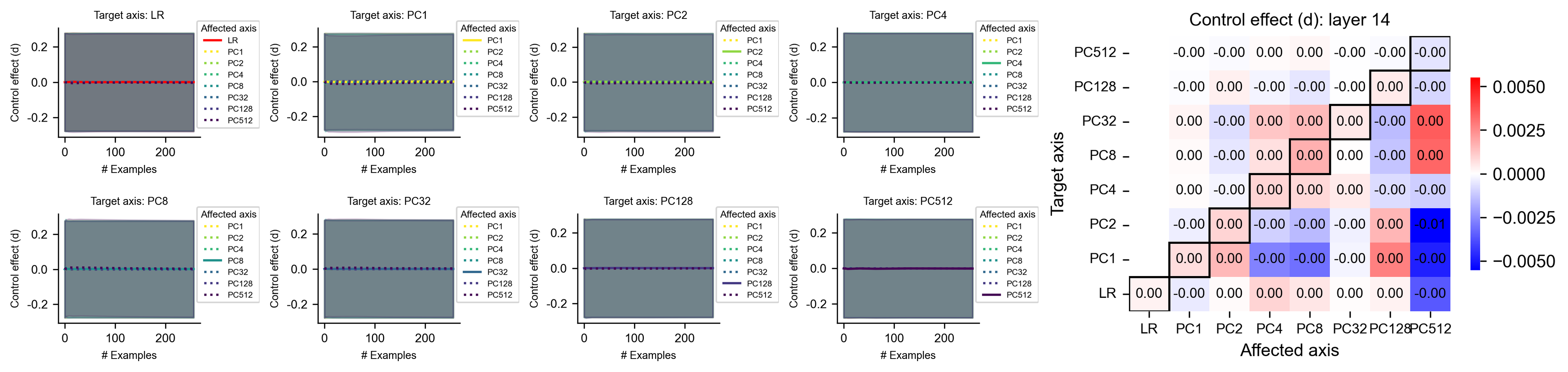</details> Figure B.18: Qwen2.5 7B (explicit control) layer 14 <details> <summary>supp/qwen2.5_7b_inactive_layer13.png Details</summary>  ### Visual Description # Technical Data Extraction: Control Effect Analysis (Layer 14) This document provides a comprehensive extraction of data and trends from the provided image, which consists of eight line charts and one summary heatmap analyzing the "Control effect (d)" across various target and affected axes in a neural network context (Layer 14). --- ## 1. Component Isolation The image is divided into two primary sections: - **Section A (Left/Center):** Eight individual line plots showing the "Control effect (d)" over a sequence of "# Examples" (0 to 250). - **Section B (Right):** A summary heatmap titled "Control effect (d): layer 14" showing the relationship between "Target axis" and "Affected axis." --- ## 2. Section A: Line Charts (Temporal Trends) Each of the eight charts follows a consistent format. - **X-axis:** # Examples (Scale: 0 to 200+) - **Y-axis:** Control effect (d) (Scale: -0.2 to 0.2) - **Visual Trend:** In all eight charts, the data series appear as flat lines centered at $y \approx 0$. There is a large grey shaded area (likely representing a confidence interval or range) spanning approximately from -0.25 to 0.25 across all examples. ### Chart Metadata and Legends | Target Axis (Plot Title) | Legend: Affected Axis (Line Styles) | Primary Observation | | :--- | :--- | :--- | | **LR** | LR (Solid Red), PC1, PC2, PC4, PC8, PC32, PC128, PC512 (Dotted) | All lines are horizontal at 0. | | **PC1** | PC1 (Solid Yellow), PC2, PC4, PC8, PC32, PC128, PC512 (Dotted) | All lines are horizontal at 0. | | **PC2** | PC1 (Dotted), PC2 (Solid Light Green), PC4, PC8, PC32, PC128, PC512 (Dotted) | All lines are horizontal at 0. | | **PC4** | PC1, PC2 (Dotted), PC4 (Solid Green), PC8, PC32, PC128, PC512 (Dotted) | All lines are horizontal at 0. | | **PC8** | PC1, PC2, PC4 (Dotted), PC8 (Solid Teal), PC32, PC128, PC512 (Dotted) | All lines are horizontal at 0. | | **PC32** | PC1, PC2, PC4, PC8 (Dotted), PC32 (Solid Blue-Green), PC128, PC512 (Dotted) | All lines are horizontal at 0. | | **PC128** | PC1, PC2, PC4, PC8, PC32 (Dotted), PC128 (Solid Purple), PC512 (Dotted) | All lines are horizontal at 0. | | **PC512** | PC1, PC2, PC4, PC8, PC32, PC128 (Dotted), PC512 (Solid Dark Purple) | All lines are horizontal at 0. | --- ## 3. Section B: Summary Heatmap **Title:** Control effect (d): layer 14 **Spatial Grounding:** The legend (color bar) is located on the far right. - **Red:** Positive values (up to 0.0050) - **White:** Zero (0.0000) - **Blue:** Negative values (down to -0.0050) ### Data Table Reconstruction The heatmap displays the interaction between the **Target axis** (Y-axis) and the **Affected axis** (X-axis). Values are rounded to two decimal places in the cells. A black diagonal staircase line separates the lower-left from the upper-right. | Target \ Affected | LR | PC1 | PC2 | PC4 | PC8 | PC32 | PC128 | PC512 | | :--- | :---: | :---: | :---: | :---: | :---: | :---: | :---: | :---: | | **PC512** | -0.00 | -0.00 | 0.00 | 0.00 | -0.00 | -0.00 | -0.00 | -0.00 | | **PC128** | -0.00 | 0.00 | -0.00 | -0.00 | -0.00 | 0.00 | -0.00 | -0.00 | | **PC32** | 0.00 | -0.00 | 0.00 | 0.00 | 0.00 | -0.00 | 0.00 | 0.00 | | **PC8** | 0.00 | -0.00 | 0.00 | 0.00 | 0.00 | -0.00 | 0.00 | 0.00 | | **PC4** | 0.00 | -0.00 | 0.00 | 0.00 | 0.00 | -0.00 | -0.00 | -0.00 | | **PC2** | -0.00 | 0.00 | -0.00 | -0.00 | -0.00 | 0.00 | -0.01 | -0.01 | | **PC1** | 0.00 | 0.00 | -0.00 | -0.00 | -0.00 | 0.00 | -0.00 | -0.01 | | **LR** | 0.00 | -0.00 | 0.00 | 0.00 | 0.00 | 0.00 | 0.00 | -0.00 | ### Key Trends and Observations from Heatmap: 1. **Dominant Values:** Most cells contain values of `0.00` or `-0.00`, indicating negligible control effects across most axis pairs. 2. **Significant Deviations:** - The most intense blue (negative) values are concentrated in the bottom right corner. - **Target PC2 / Affected PC512:** Shows a value of `-0.01` (Dark Blue). - **Target PC1 / Affected PC512:** Shows a value of `-0.01` (Dark Blue). - **Target PC2 / Affected PC128:** Shows a value of `-0.01` (Medium Blue). 3. **Positive Trends:** Subtle red shading (positive values) is visible in the column for **Affected PC128** and **PC512** for targets like PC32 and PC8, though the rounded text still displays `0.00`. 4. **Symmetry:** The effect is not perfectly symmetrical; the influence of PC512 as an "Affected axis" is more pronounced than its influence as a "Target axis." --- ## 4. Language Declaration The entire document and all labels within the image are in **English**. No other languages were detected. 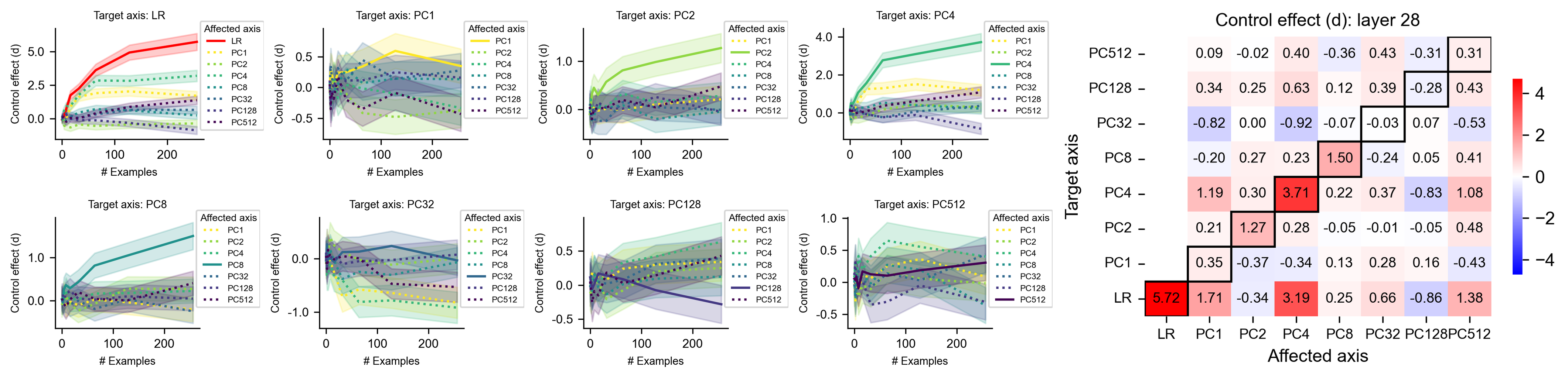</details> Figure B.19: Qwen2.5 7B (implicit control) layer 14 <details> <summary>supp/qwen2.5_7b_active_layer27.png Details</summary>  ### Visual Description # Technical Data Extraction: Control Effect Analysis (Layer 28) This document provides a comprehensive extraction of data from a technical visualization consisting of eight line charts and one heatmap. The data explores the "Control effect (d)" across different "Target axes" and "Affected axes" within a neural network (specifically layer 28), measured against the number of training examples. --- ## 1. Component Isolation The image is divided into two primary sections: 1. **Left/Center (Line Charts):** Eight individual plots showing the progression of control effects as the number of examples increases (0 to 250). 2. **Right (Heatmap):** A summary matrix showing the control effect at a specific snapshot (likely the final state of the training examples). --- ## 2. Heatmap Data Extraction **Title:** Control effect (d): layer 28 **Y-Axis (Target axis):** PC512, PC128, PC32, PC8, PC4, PC2, PC1, LR **X-Axis (Affected axis):** LR, PC1, PC2, PC4, PC8, PC32, PC128, PC512 **Legend (Color Bar):** Ranges from -4 (Blue) to 0 (White) to +4 (Red). ### Data Table (Reconstructed) The diagonal (where Target axis = Affected axis) is highlighted with a bold black border in the source. | Target \ Affected | LR | PC1 | PC2 | PC4 | PC8 | PC32 | PC128 | PC512 | | :--- | :---: | :---: | :---: | :---: | :---: | :---: | :---: | :---: | | **PC512** | 0.09 | -0.02 | 0.40 | -0.36 | 0.43 | -0.31 | 0.31 | | | **PC128** | 0.34 | 0.25 | 0.63 | 0.12 | 0.39 | -0.28 | 0.43 | | | **PC32** | -0.82 | 0.00 | -0.92 | -0.07 | -0.03 | 0.07 | -0.53 | | | **PC8** | -0.20 | 0.27 | 0.23 | 1.50 | -0.24 | 0.05 | 0.41 | | | **PC4** | 1.19 | 0.30 | 3.71 | 0.22 | 0.37 | -0.83 | 1.08 | | | **PC2** | 0.21 | 1.27 | 0.28 | -0.05 | -0.01 | -0.05 | 0.48 | | | **PC1** | 0.35 | -0.37 | -0.34 | 0.13 | 0.28 | 0.16 | -0.43 | | | **LR** | 5.72 | 1.71 | -0.34 | 3.19 | 0.25 | 0.66 | -0.86 | 1.38 | *Note: The heatmap contains a slight visual misalignment in the top right corner labels; the table above reflects the numerical values provided in the cells.* --- ## 3. Line Chart Analysis (Target Axis Series) Each chart plots **Control effect (d)** (y-axis) vs **# Examples** (x-axis, 0-250). Shaded areas represent confidence intervals. ### Common Legend (Affected axis) * **LR:** Solid Red line * **PC1:** Dotted Yellow line * **PC2:** Dotted Light Green line * **PC4:** Dotted Medium Green line * **PC8:** Dotted Teal line * **PC32:** Dotted Blue line * **PC128:** Dotted Purple line * **PC512:** Dotted Dark Purple line * *Note: In each specific "Target axis" plot, the line corresponding to that axis becomes a **solid, thick line**.* ### Individual Plot Trends 1. **Target axis: LR** * **Trend:** The LR (Solid Red) line shows a sharp, logarithmic-style increase, plateauing near a value of 5.7. * **Secondary Effects:** PC4 (Dotted Green) also shows a significant upward trend, reaching ~3.0. 2. **Target axis: PC1** * **Trend:** PC1 (Solid Yellow) is highly volatile initially, stabilizing around 0.3-0.4. * **Secondary Effects:** Most other axes cluster around 0.0, with PC2 showing a slight downward trend to -0.4. 3. **Target axis: PC2** * **Trend:** PC2 (Solid Light Green) shows a steady upward slope, reaching ~1.3. * **Secondary Effects:** Most other axes remain flat near 0.0. 4. **Target axis: PC4** * **Trend:** PC4 (Solid Medium Green) shows a strong upward trend, reaching ~3.7. * **Secondary Effects:** PC1 (Yellow) shows a moderate increase to ~1.5. 5. **Target axis: PC8** * **Trend:** PC8 (Solid Teal) increases steadily to ~1.5. * **Secondary Effects:** Other axes remain largely grouped between -0.5 and 0.5. 6. **Target axis: PC32** * **Trend:** PC32 (Solid Blue) remains very close to 0.0 throughout the duration. * **Secondary Effects:** PC2 (Green) and PC128 (Purple) show slight negative trends toward -0.5. 7. **Target axis: PC128** * **Trend:** PC128 (Solid Purple) shows a slight upward trend, ending near 0.4. * **Secondary Effects:** PC2 (Green) shows a similar upward trend, ending slightly higher than the target axis. 8. **Target axis: PC512** * **Trend:** PC512 (Solid Dark Purple) shows a gradual increase, ending near 0.3. * **Secondary Effects:** PC2 (Green) shows a more pronounced upward trend in this plot, reaching ~0.6. --- ## 4. Summary of Findings * **Strongest Control:** The "LR" target axis exhibits the strongest control effect (~5.7), followed by "PC4" (~3.7). * **Cross-Talk:** There is significant cross-talk between LR and PC4, and between PC4 and PC2, as evidenced by the high values in the heatmap and the rising dotted lines in the respective line charts. * **Stability:** PC32 appears to be the most "stable" or least affected target axis, with values remaining near zero regardless of the number of examples. 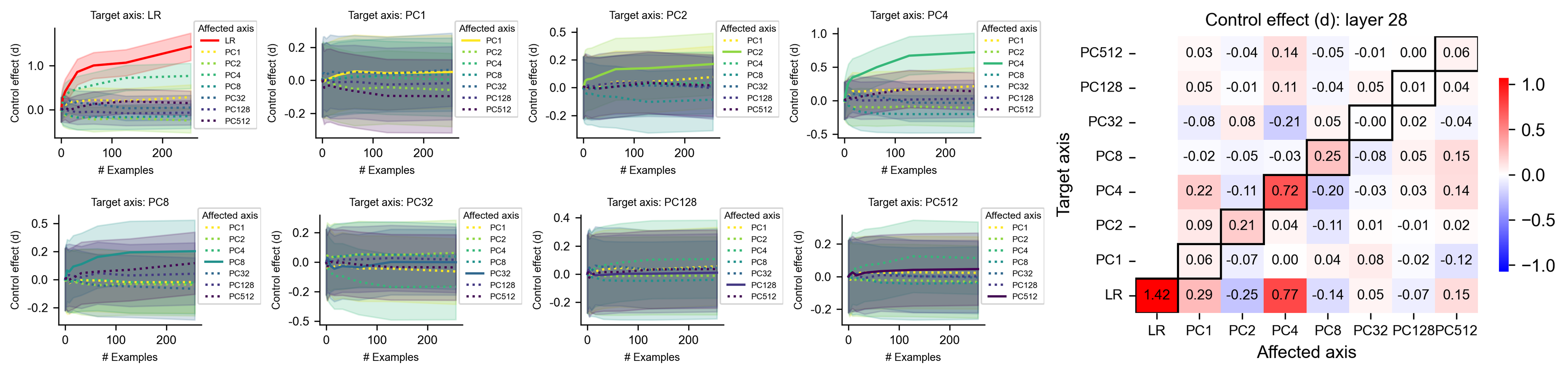</details> Figure B.20: Qwen2.5 7B (explicit control) layer 28 <details> <summary>supp/qwen2.5_7b_inactive_layer27.png Details</summary>  ### Visual Description # Technical Data Extraction: Control Effect Analysis (Layer 28) This document provides a comprehensive extraction of data from a multi-panel figure analyzing "Control effect (d)" across various target and affected axes in a neural network context (specifically Layer 28). ## 1. Document Structure Overview The image is divided into two primary sections: - **Left Section (Line Charts):** Eight individual line graphs showing the progression of control effects over the number of examples. - **Right Section (Heatmap):** A summary matrix showing the final control effect values for different axis pairings. --- ## 2. Component Isolation: Line Charts (Left Section) ### General Metadata for Line Charts - **X-axis (all):** `# Examples` (Scale: 0 to 250). - **Y-axis (all):** `Control effect (d)`. - **Legend (Affected axis):** - **LR:** Solid Red line. - **PC1:** Dotted Yellow line. - **PC2:** Dotted Light Green line. - **PC4:** Dotted Teal/Green line. - **PC8:** Dotted Blue-Green line. - **PC32:** Dotted Blue line. - **PC128:** Dotted Dark Blue line. - **PC512:** Dotted Purple line. - **Visual Note:** Solid lines indicate the "Target axis" matches the "Affected axis" (Self-influence). Dotted lines indicate cross-axis influence. Shaded areas represent confidence intervals or variance. ### Individual Chart Data Extraction | Target Axis | Primary Trend (Self-Influence) | Cross-Axis Observations | | :--- | :--- | :--- | | **LR** | **Strong Upward Slope:** Starts at 0, rises sharply to ~0.8 by 50 examples, and reaches ~1.4 by 250 examples. | PC4 (Teal) shows a moderate positive trend (~0.7). Others remain near 0. | | **PC1** | **Flat/Low Trend:** The solid yellow line stays very close to 0, ending slightly above 0. | Most affected axes cluster around 0 with high variance. | | **PC2** | **Slight Upward Slope:** Solid green line rises gradually to ~0.2. | PC4 and PC1 show slight positive trends; others are flat. | | **PC4** | **Strong Upward Slope:** Solid teal line rises significantly, reaching ~0.7 by 250 examples. | PC1 and PC2 show slight positive trends. | | **PC8** | **Moderate Upward Slope:** Solid blue-green line rises to ~0.25. | PC512 (Purple) shows a slight upward trend (~0.15). | | **PC32** | **Flat Trend:** Solid blue line remains near 0 throughout. | All affected axes are tightly clustered around the 0 baseline. | | **PC128** | **Flat Trend:** Solid dark blue line remains near 0. | Minimal deviation from 0 for all axes. | | **PC512** | **Flat Trend:** Solid purple line remains near 0. | Minimal deviation from 0 for all axes. | --- ## 3. Component Isolation: Heatmap (Right Section) ### Metadata - **Title:** Control effect (d): layer 28 - **Y-axis (Target axis):** PC512, PC128, PC32, PC8, PC4, PC2, PC1, LR (Top to Bottom). - **X-axis (Affected axis):** LR, PC1, PC2, PC4, PC8, PC32, PC128, PC512 (Left to Right). - **Color Scale:** - **Red:** Positive effect (up to 1.0+). - **White:** Zero effect (0.0). - **Blue:** Negative effect (down to -1.0). - **Visual Feature:** The diagonal (Self-influence) is highlighted with thick black borders. ### Data Table Reconstruction (Numerical Values) | Target \ Affected | LR | PC1 | PC2 | PC4 | PC8 | PC32 | PC128 | PC512 | | :--- | :---: | :---: | :---: | :---: | :---: | :---: | :---: | :---: | | **PC512** | 0.03 | -0.04 | 0.14 | -0.05 | -0.01 | 0.00 | 0.06 | **0.06** | | **PC128** | 0.05 | -0.01 | 0.11 | -0.04 | 0.05 | 0.01 | **0.04** | 0.04 | | **PC32** | -0.08 | 0.08 | -0.21 | 0.05 | -0.00 | **0.02** | -0.04 | -0.04 | | **PC8** | -0.02 | -0.05 | -0.03 | 0.25 | **-0.08** | 0.05 | 0.15 | 0.15 | | **PC4** | 0.22 | -0.11 | 0.72 | **-0.20** | -0.03 | 0.03 | 0.14 | 0.14 | | **PC2** | 0.09 | 0.21 | **0.04** | -0.11 | 0.01 | -0.01 | 0.02 | 0.02 | | **PC1** | 0.06 | **-0.07** | 0.00 | 0.04 | 0.08 | -0.02 | -0.12 | -0.12 | | **LR** | **1.42** | 0.29 | -0.25 | 0.77 | -0.14 | 0.05 | -0.07 | 0.15 | *(Note: The diagonal values represent the self-control effect. The highest value in the entire dataset is the LR-LR interaction at **1.42**.)* --- ## 4. Key Trends and Observations 1. **Dominance of LR:** The Linear Regression (LR) axis shows the most significant control effect (1.42), followed by PC4 (0.72) and PC8 (0.25). 2. **Cross-Axis Influence:** There is a notable cross-influence between the LR target and the PC4 affected axis (0.77), and between the PC4 target and the PC2 affected axis (0.72). 3. **Stability in Higher PCs:** Axes PC32, PC128, and PC512 show very low control effects (near 0), suggesting these components are less susceptible to control interventions at Layer 28. 4. **Negative Correlations:** The strongest negative effect is between Target PC32 and Affected PC2 (-0.21) and Target LR and Affected PC2 (-0.25). </details> Figure B.21: Qwen2.5 7B (implicit control) layer 28 B.10 Defining axes from hidden states aggregated across multiple layers we performed preliminary experiments testing the control effects of an axis on the concatenation of all layers. Concretely, we trained separate (logistic regression) classifiers for each layer on the ETHICS dataset. We then averaged the outputs of all classifiers to obtain a single (ensemble) output that defines the neurofeedback label. Equivalently, this corresponds to a single classifier with the readout vector being the concatenation of all classifiers’ readout vectors. We found that LLMs’ control effect on the ensemble output is similar to (marginally higher than) the control effects of layer 24 (Fig. 3 d), suggesting that defining axes from hidden states aggregated across multiple layers might provide (slightly) more stable and representative directions. We leave systematic investigations for future study. Appendix C Experiment compute resources We report compute resource usage across three tasks: preprocessing (extracting neural activation and training machine learning methods to obtain target axes and corresponding neurofeedback labels from neural activations), metacognitive reporting, and metacognitive control. For brevity, we omit “Instruct”. | LLaMA-3.2-1B | Preprocessing | RTX 3090 (24GB) | 1 | 1 | | --- | --- | --- | --- | --- | | LLaMA-3.2-1B | Control | RTX 3090 (24GB) | 3 | 3 | | LLaMA-3.2-3B | Preprocessing | RTX 3090 (24GB) | 1 | 1 | | LLaMA-3.2-3B | Control | RTX 3090 (24GB) | 15 | 8 | | LLaMA-3.1-8B | Preprocessing | A100 (80GB) | 5 | 3 | | LLaMA-3.1-8B | Report | A100 (80GB) | 1 | 10 | | LLaMA-3.1-8B | Control | A100 (80GB) | 90 | 120 | | LLaMA-3.1-70B | Preprocessing | $2×$ H200 (140GB) | 30 | 5 | | LLaMA-3.1-70B | Report | $2×$ H200 (140GB) | 1 | 15 | | LLaMA-3.1-70B | Control | $2×$ H200 (140GB) | 200 | 120 | | Qwen2.5-1B | Preprocessing | RTX 3090 (24GB) | 1 | 1 | | Qwen2.5-1B | Control | RTX 3090 (24GB) | 3 | 3 | | Qwen2.5-3B | Preprocessing | RTX 3090 (24GB) | 1 | 1 | | Qwen2.5-3B | Control | RTX 3090 (24GB) | 15 | 8 | | Qwen2.5-7B | Preprocessing | A100 (80GB) | 5 | 3 | | Qwen2.5-7B | Report | A100 (80GB) | 1 | 10 | | Qwen2.5-7B | Control | A100 (80GB) | 90 | 120 | Table 1: Compute and storage usage across tasks and models. Preprocessing, reporting, and control were run separately. Control task for 1B and 3B models was limited to two axes. For the 70B model, control task was only done for $N{=}256$ in-context examples. All compute times and storage values are reported as upper bounds. All remaining analyses (e.g., visualization, metric aggregation) were conducted on a laptop with 32GB RAM, with a total runtime under 30 hours. NeurIPS Paper Checklist 1. Claims 1. Question: Do the main claims made in the abstract and introduction accurately reflect the paper’s contributions and scope? 1. Answer: [Yes] 1. Justification: We confirm that both the abstract and introduction accurately reflect the paper’s contributions and scope. 1. Guidelines: - The answer NA means that the abstract and introduction do not include the claims made in the paper. - The abstract and/or introduction should clearly state the claims made, including the contributions made in the paper and important assumptions and limitations. A No or NA answer to this question will not be perceived well by the reviewers. - The claims made should match theoretical and experimental results, and reflect how much the results can be expected to generalize to other settings. - It is fine to include aspirational goals as motivation as long as it is clear that these goals are not attained by the paper. 1. Limitations 1. Question: Does the paper discuss the limitations of the work performed by the authors? 1. Answer: [Yes] 1. Justification: We have mentioned a few limitations of the current work in the Discussion. 1. Guidelines: - The answer NA means that the paper has no limitation while the answer No means that the paper has limitations, but those are not discussed in the paper. - The authors are encouraged to create a separate "Limitations" section in their paper. - The paper should point out any strong assumptions and how robust the results are to violations of these assumptions (e.g., independence assumptions, noiseless settings, model well-specification, asymptotic approximations only holding locally). The authors should reflect on how these assumptions might be violated in practice and what the implications would be. - The authors should reflect on the scope of the claims made, e.g., if the approach was only tested on a few datasets or with a few runs. In general, empirical results often depend on implicit assumptions, which should be articulated. - The authors should reflect on the factors that influence the performance of the approach. For example, a facial recognition algorithm may perform poorly when image resolution is low or images are taken in low lighting. Or a speech-to-text system might not be used reliably to provide closed captions for online lectures because it fails to handle technical jargon. - The authors should discuss the computational efficiency of the proposed algorithms and how they scale with dataset size. - If applicable, the authors should discuss possible limitations of their approach to address problems of privacy and fairness. - While the authors might fear that complete honesty about limitations might be used by reviewers as grounds for rejection, a worse outcome might be that reviewers discover limitations that aren’t acknowledged in the paper. The authors should use their best judgment and recognize that individual actions in favor of transparency play an important role in developing norms that preserve the integrity of the community. Reviewers will be specifically instructed to not penalize honesty concerning limitations. 1. Theory assumptions and proofs 1. Question: For each theoretical result, does the paper provide the full set of assumptions and a complete (and correct) proof? 1. Answer: [N/A] 1. Justification: This paper does not introduce any new theorems, formulas, or lemmas to be proved. 1. Guidelines: - The answer NA means that the paper does not include theoretical results. - All the theorems, formulas, and proofs in the paper should be numbered and cross-referenced. - All assumptions should be clearly stated or referenced in the statement of any theorems. - The proofs can either appear in the main paper or the supplemental material, but if they appear in the supplemental material, the authors are encouraged to provide a short proof sketch to provide intuition. - Inversely, any informal proof provided in the core of the paper should be complemented by formal proofs provided in appendix or supplemental material. - Theorems and Lemmas that the proof relies upon should be properly referenced. 1. Experimental result reproducibility 1. Question: Does the paper fully disclose all the information needed to reproduce the main experimental results of the paper to the extent that it affects the main claims and/or conclusions of the paper (regardless of whether the code and data are provided or not)? 1. Answer: [Yes] 1. Justification: All models used in our experiments are publicly available through the Hugging Face library. All analyses and figures presented in the paper can be fully reproduced using the code provided in the associated repository in Appendix A.1. 1. Guidelines: - The answer NA means that the paper does not include experiments. - If the paper includes experiments, a No answer to this question will not be perceived well by the reviewers: Making the paper reproducible is important, regardless of whether the code and data are provided or not. - If the contribution is a dataset and/or model, the authors should describe the steps taken to make their results reproducible or verifiable. - Depending on the contribution, reproducibility can be accomplished in various ways. For example, if the contribution is a novel architecture, describing the architecture fully might suffice, or if the contribution is a specific model and empirical evaluation, it may be necessary to either make it possible for others to replicate the model with the same dataset, or provide access to the model. In general. releasing code and data is often one good way to accomplish this, but reproducibility can also be provided via detailed instructions for how to replicate the results, access to a hosted model (e.g., in the case of a large language model), releasing of a model checkpoint, or other means that are appropriate to the research performed. - While NeurIPS does not require releasing code, the conference does require all submissions to provide some reasonable avenue for reproducibility, which may depend on the nature of the contribution. For example 1. If the contribution is primarily a new algorithm, the paper should make it clear how to reproduce that algorithm. 1. If the contribution is primarily a new model architecture, the paper should describe the architecture clearly and fully. 1. If the contribution is a new model (e.g., a large language model), then there should either be a way to access this model for reproducing the results or a way to reproduce the model (e.g., with an open-source dataset or instructions for how to construct the dataset). 1. We recognize that reproducibility may be tricky in some cases, in which case authors are welcome to describe the particular way they provide for reproducibility. In the case of closed-source models, it may be that access to the model is limited in some way (e.g., to registered users), but it should be possible for other researchers to have some path to reproducing or verifying the results. 1. Open access to data and code 1. Question: Does the paper provide open access to the data and code, with sufficient instructions to faithfully reproduce the main experimental results, as described in supplemental material? 1. Answer: [Yes] 1. Justification: The associated repository in Appendix A.1 contains all necessary scripts, along with documentation, to enable full reproduction of the results and figures reported in this paper. 1. Guidelines: - The answer NA means that paper does not include experiments requiring code. - Please see the NeurIPS code and data submission guidelines (https://nips.cc/public/guides/CodeSubmissionPolicy) for more details. - While we encourage the release of code and data, we understand that this might not be possible, so “No” is an acceptable answer. Papers cannot be rejected simply for not including code, unless this is central to the contribution (e.g., for a new open-source benchmark). - The instructions should contain the exact command and environment needed to run to reproduce the results. See the NeurIPS code and data submission guidelines (https://nips.cc/public/guides/CodeSubmissionPolicy) for more details. - The authors should provide instructions on data access and preparation, including how to access the raw data, preprocessed data, intermediate data, and generated data, etc. - The authors should provide scripts to reproduce all experimental results for the new proposed method and baselines. If only a subset of experiments are reproducible, they should state which ones are omitted from the script and why. - At submission time, to preserve anonymity, the authors should release anonymized versions (if applicable). - Providing as much information as possible in supplemental material (appended to the paper) is recommended, but including URLs to data and code is permitted. 1. Experimental setting/details 1. Question: Does the paper specify all the training and test details (e.g., data splits, hyperparameters, how they were chosen, type of optimizer, etc.) necessary to understand the results? 1. Answer: [Yes] 1. Justification: We provide detailed descriptions of the evaluation metrics, model hyperparameters, data sources, analysis procedure, prompt construction, and inference settings in both the main text and the Appendix. As all LLMs used are publicly available pre-trained models accessed via Hugging Face, we omit training details. 1. Guidelines: - The answer NA means that the paper does not include experiments. - The experimental setting should be presented in the core of the paper to a level of detail that is necessary to appreciate the results and make sense of them. - The full details can be provided either with the code, in appendix, or as supplemental material. 1. Experiment statistical significance 1. Question: Does the paper report error bars suitably and correctly defined or other appropriate information about the statistical significance of the experiments? 1. Answer: [Yes] 1. Justification: We report error bars, statistical significance tests, and effect size estimates wherever appropriate to support the robustness and interpretability of our results. 1. Guidelines: - The answer NA means that the paper does not include experiments. - The authors should answer "Yes" if the results are accompanied by error bars, confidence intervals, or statistical significance tests, at least for the experiments that support the main claims of the paper. - The factors of variability that the error bars are capturing should be clearly stated (for example, train/test split, initialization, random drawing of some parameter, or overall run with given experimental conditions). - The method for calculating the error bars should be explained (closed form formula, call to a library function, bootstrap, etc.) - The assumptions made should be given (e.g., Normally distributed errors). - It should be clear whether the error bar is the standard deviation or the standard error of the mean. - It is OK to report 1-sigma error bars, but one should state it. The authors should preferably report a 2-sigma error bar than state that they have a 96% CI, if the hypothesis of Normality of errors is not verified. - For asymmetric distributions, the authors should be careful not to show in tables or figures symmetric error bars that would yield results that are out of range (e.g. negative error rates). - If error bars are reported in tables or plots, The authors should explain in the text how they were calculated and reference the corresponding figures or tables in the text. 1. Experiments compute resources 1. Question: For each experiment, does the paper provide sufficient information on the computer resources (type of compute workers, memory, time of execution) needed to reproduce the experiments? 1. Answer: [Yes] 1. Justification: We provide full details regarding the compute resources required to reproduce all experiments discussed in the paper. This includes GPU types, total compute time, and environment specifications, as documented in Appendix C. - The answer NA means that the paper does not include experiments. - The paper should indicate the type of compute workers CPU or GPU, internal cluster, or cloud provider, including relevant memory and storage. - The paper should provide the amount of compute required for each of the individual experimental runs as well as estimate the total compute. - The paper should disclose whether the full research project required more compute than the experiments reported in the paper (e.g., preliminary or failed experiments that didn’t make it into the paper). 1. Code of ethics 1. Question: Does the research conducted in the paper conform, in every respect, with the NeurIPS Code of Ethics https://neurips.cc/public/EthicsGuidelines? 1. Answer: [Yes] 1. Justification: We have carefully reviewed the NeurIPS Code of Ethics and, to the best of our knowledge, our work complies fully with its guidelines. We are not aware of any violations or ethical concerns associated with the methods, data, or conclusions presented. 1. Guidelines: - The answer NA means that the authors have not reviewed the NeurIPS Code of Ethics. - If the authors answer No, they should explain the special circumstances that require a deviation from the Code of Ethics. - The authors should make sure to preserve anonymity (e.g., if there is a special consideration due to laws or regulations in their jurisdiction). 1. Broader impacts 1. Question: Does the paper discuss both potential positive societal impacts and negative societal impacts of the work performed? 1. Answer: [Yes] 1. Justification: We discuss both the positive societal impacts and negative societal impacts of the studied metacognitive abilities in LLMs. 1. Guidelines: - The answer NA means that there is no societal impact of the work performed. - If the authors answer NA or No, they should explain why their work has no societal impact or why the paper does not address societal impact. - Examples of negative societal impacts include potential malicious or unintended uses (e.g., disinformation, generating fake profiles, surveillance), fairness considerations (e.g., deployment of technologies that could make decisions that unfairly impact specific groups), privacy considerations, and security considerations. - The conference expects that many papers will be foundational research and not tied to particular applications, let alone deployments. However, if there is a direct path to any negative applications, the authors should point it out. For example, it is legitimate to point out that an improvement in the quality of generative models could be used to generate deepfakes for disinformation. On the other hand, it is not needed to point out that a generic algorithm for optimizing neural networks could enable people to train models that generate Deepfakes faster. - The authors should consider possible harms that could arise when the technology is being used as intended and functioning correctly, harms that could arise when the technology is being used as intended but gives incorrect results, and harms following from (intentional or unintentional) misuse of the technology. - If there are negative societal impacts, the authors could also discuss possible mitigation strategies (e.g., gated release of models, providing defenses in addition to attacks, mechanisms for monitoring misuse, mechanisms to monitor how a system learns from feedback over time, improving the efficiency and accessibility of ML). 1. Safeguards 1. Question: Does the paper describe safeguards that have been put in place for responsible release of data or models that have a high risk for misuse (e.g., pretrained language models, image generators, or scraped datasets)? 1. Answer: [N/A] 1. Justification: We do not release any new datasets or models. Our work solely involves analyzing existing publicly available pre-trained language models using a novel methodological framework. We do not identify any foreseeable risks associated with our contributions. 1. Guidelines: - The answer NA means that the paper poses no such risks. - Released models that have a high risk for misuse or dual-use should be released with necessary safeguards to allow for controlled use of the model, for example by requiring that users adhere to usage guidelines or restrictions to access the model or implementing safety filters. - Datasets that have been scraped from the Internet could pose safety risks. The authors should describe how they avoided releasing unsafe images. - We recognize that providing effective safeguards is challenging, and many papers do not require this, but we encourage authors to take this into account and make a best faith effort. 1. Licenses for existing assets 1. Question: Are the creators or original owners of assets (e.g., code, data, models), used in the paper, properly credited and are the license and terms of use explicitly mentioned and properly respected? 1. Answer: [Yes] 1. Justification: We use two families of pre-trained language models: the LLaMA 3 series (e.g., LLaMA-3.2-1B, LLaMA-3.1-8B) under Meta Llama 3 Community License and the Qwen 2.5 series under Apache License 2.0 (e.g., Qwen2.5-1B, Qwen2.5-7B). All models are used under their respective research licenses and are properly cited in the paper. All datasets are either publicly available or included in the code repository. Their licenses are reported in the Appendix. All assets are credited appropriately, and license terms have been fully respected. - The answer NA means that the paper does not use existing assets. - The authors should cite the original paper that produced the code package or dataset. - The authors should state which version of the asset is used and, if possible, include a URL. - The name of the license (e.g., CC-BY 4.0) should be included for each asset. - For scraped data from a particular source (e.g., website), the copyright and terms of service of that source should be provided. - If assets are released, the license, copyright information, and terms of use in the package should be provided. For popular datasets, paperswithcode.com/datasets has curated licenses for some datasets. Their licensing guide can help determine the license of a dataset. - For existing datasets that are re-packaged, both the original license and the license of the derived asset (if it has changed) should be provided. - If this information is not available online, the authors are encouraged to reach out to the asset’s creators. 1. New assets 1. Question: Are new assets introduced in the paper well documented and is the documentation provided alongside the assets? 1. Answer: [Yes] 1. Justification: The only new assets introduced in this work are the code implementations for model fitting and analysis. We release this code with detailed documentation to facilitate reproducibility, as described in Appendix A.1. 1. Guidelines: - The answer NA means that the paper does not release new assets. - Researchers should communicate the details of the dataset/code/model as part of their submissions via structured templates. This includes details about training, license, limitations, etc. - The paper should discuss whether and how consent was obtained from people whose asset is used. - At submission time, remember to anonymize your assets (if applicable). You can either create an anonymized URL or include an anonymized zip file. 1. Crowdsourcing and research with human subjects 1. Question: For crowdsourcing experiments and research with human subjects, does the paper include the full text of instructions given to participants and screenshots, if applicable, as well as details about compensation (if any)? 1. Answer: [N/A] 1. Justification: This work does not involve human subjects, personally identifiable information, or the use of crowdsourcing. 1. Guidelines: - The answer NA means that the paper does not involve crowdsourcing nor research with human subjects. - Including this information in the supplemental material is fine, but if the main contribution of the paper involves human subjects, then as much detail as possible should be included in the main paper. - According to the NeurIPS Code of Ethics, workers involved in data collection, curation, or other labor should be paid at least the minimum wage in the country of the data collector. 1. Institutional review board (IRB) approvals or equivalent for research with human subjects 1. Question: Does the paper describe potential risks incurred by study participants, whether such risks were disclosed to the subjects, and whether Institutional Review Board (IRB) approvals (or an equivalent approval/review based on the requirements of your country or institution) were obtained? 1. Answer: [N/A] 1. Justification: This work does not involve human subjects, user studies, or crowdsourcing. Therefore, Institutional Review Board approval or equivalent ethical review is not applicable. 1. Guidelines: - The answer NA means that the paper does not involve crowdsourcing nor research with human subjects. - Depending on the country in which research is conducted, IRB approval (or equivalent) may be required for any human subjects research. If you obtained IRB approval, you should clearly state this in the paper. - We recognize that the procedures for this may vary significantly between institutions and locations, and we expect authors to adhere to the NeurIPS Code of Ethics and the guidelines for their institution. - For initial submissions, do not include any information that would break anonymity (if applicable), such as the institution conducting the review. 1. Declaration of LLM usage 1. Question: Does the paper describe the usage of LLMs if it is an important, original, or non-standard component of the core methods in this research? Note that if the LLM is used only for writing, editing, or formatting purposes and does not impact the core methodology, scientific rigorousness, or originality of the research, declaration is not required. 1. Answer: [N/A] 1. Justification: This work does not involve the use of large language models (LLMs) as part of the core methodology. Any LLM usage, if any, was limited to writing assistance and had no influence on the scientific methods or contributions. 1. Guidelines: - The answer NA means that the core method development in this research does not involve LLMs as any important, original, or non-standard components. - Please refer to our LLM policy (https://neurips.cc/Conferences/2025/LLM) for what should or should not be described.