2505.14313

# A MIND for Reasoning: Meta-learning for In-context Deduction Abstract Large language models (LLMs) are increasingly evaluated on formal tasks, where strong reasoning abilities define the state of the art. However, their ability to generalize to out-of-distribution problems remains limited. In this paper, we investigate how LLMs can achieve a systematic understanding of deductive rules. Our focus is on the task of identifying the appropriate subset of premises within a knowledge base needed to derive a given hypothesis. To tackle this challenge, we propose M eta-learning for IN -context D eduction (MIND), a novel few-shot meta-learning fine-tuning approach. The goal of MIND is to enable models to generalize more effectively to unseen knowledge bases and to systematically apply inference rules. Our results show that MIND significantly improves generalization in small LMs ranging from 1.5B to 7B parameters. The benefits are especially pronounced in smaller models and low-data settings. Remarkably, small models fine-tuned with MIND outperform state-of-the-art LLMs, such as GPT-4o and o3-mini, on this task. A MIND for Reasoning: Meta-learning for In-context Deduction Leonardo Bertolazzi 1, Manuel Vargas Guzmán 2, Raffaella Bernardi 3, Maciej Malicki 2, Jakub Szymanik 1, 1 University of Trento, 2 University of Warsaw, 3 Free University of Bozen-Bolzano 1 Introduction Reasoning refers to a broad set of abilities that are applied not only in formal domains, such as mathematics and logic, but also in goal-directed scenarios involving problem-solving and decision-making (Leighton, 2004). All types of reasoning share a common foundation: the capacity to reach an abstract understanding of the problem at hand. With the advent of increasingly capable large language models (LLMs), reasoning has become a central domain for evaluating and comparing these systems (Huang and Chang, 2023; Mondorf and Plank, 2024). Episode $\mathcal{T}$ \pgfmathresult pt Knowledge Base ( $\mathcal{KB}$ ) \pgfmathresult pt knowledge base: All x1 are x2, All x2 are x4, All x3 are x5, All x10 are x11, All x4 are x6, All x2 are x3, All x5 are x7, Some x5 are not x1, All x9 are x10, All x6 are x8, All x8 are x9, Some x11 are not x4 \pgfmathresult pt Study Examples ( $S^{\text{supp}}$ ) \pgfmathresult pt <STUDY> hypothesis: All x8 are x11 premises: All x8 are x9, All x9 are x10, All x10 are x11; hypothesis: All x1 are x3 premises: All x1 are x2, All x2 are x3; … \pgfmathresult pt Query Hypothesis ( $x^{\text{query}}$ ) <QUERY> hypothesis: All x3 are x7 \pgfmathresult pt Query Premises ( $y^{\text{query}}$ ) premises: All x3 are x5, All x5 are x7 \pgfmathresult pt Input \pgfmathresult pt Output Figure 1: Overview of a MIND episode. Given a set of premises (the knowledge base, $\mathcal{KB}$ ), a set of task demonstrations (or study examples, denoted by the <STUDY> tag), and a query hypothesis $x^{\mathrm{query}}$ (denoted by the <QUERY> tag) that is entailed from $\mathcal{KB}$ , models must generate the minimal subset of premises $y^{\mathrm{query}}$ from which $x^{\mathrm{query}}$ can be derived. During each MIND episode, models can practice on hypothesis-premise pairs before processing the main query hypothesis. The examples show how we frame syllogistic inferences as a premise selection task. Despite extensive training on mathematical, programming, and STEM-related data, LLMs continue to struggle in out-of-distribution (OOD) reasoning scenarios. Their performance often deteriorates on longer inference chains than those seen during training (Clark et al., 2021; Saparov et al., 2023), and they exhibit variability when evaluated with perturbed versions of the same problems (Mirzadeh et al., 2025; Gulati et al., 2024; Huang et al., 2025). In particular, LLMs can get distracted by irrelevant context, becoming unable to solve problems they could otherwise solve (Shi et al., 2023; Yoran et al., 2024). These challenges relate to broader debates surrounding generalization versus memorization in LLMs (Balloccu et al., 2024; Singh et al., 2024). Few-shot meta-learning approaches (Irie and Lake, 2024) have emerged as promising methods for inducing OOD generalization and rapid domain adaptation in LLMs. Specifically, this class of methods has proven effective in few-shot task generalization (Min et al., 2022; Chen et al., 2022), systematic generalization (Lake and Baroni, 2023), and mitigating catastrophic forgetting (Irie et al., 2025). In this work, we propose M eta-learning for IN -context D eduction (MIND), a new few-shot meta-learning fine-tuning approach for deductive reasoning. As illustrated in Figure 1, we evaluate the effectiveness of this approach using a logical reasoning task grounded in syllogistic logic (Smiley, 1973; Vargas Guzmán et al., 2024). Each problem presents a knowledge base of atomic logical statements. Models are tasked with identifying the minimal subset of premises that logically entail a given test hypothesis. This premise selection task captures a core aspect of deductive reasoning: determining which known facts are necessary and sufficient to justify a conclusion. We apply MIND to small LMs from the Qwen-2.5 family (Qwen Team, 2025), ranging from 1.5B to 7B parameters. Specifically, we assess the generalization capabilities induced by MIND, such as systematically performing inferences over unseen sets of premises, as well as over more complex (longer) or simpler (shorter) sets of premises than those encountered during training. Our code and data are available at: https://github.com/leobertolazzi/MIND.git Our main contributions are as follows: - We introduce a new synthetic dataset based on syllogistic logic to study reasoning generalization in LLMs. - We show that MIND enables LMs to better generalize in OOD reasoning problems with particularly strong performance in smaller models and low-data regimes. - We demonstrate that small LMs fine-tuned with MIND can outperform state-of-the-art LLMs such as GPT-4o and o3-mini, on our premise selection task. 2 Background 2.1 Syllogistic Logic In our experiments, we focus on the syllogistic fragment of first-order logic. Originally, syllogisms have been studied by Aristotle as arguments composed of two premises and a conclusion, such as: “ All dogs are mammals; some pets are not mammals; therefore, some pets are not dogs. ” This basic form can be extended to include inferences involving more than two premises (see Łukasiewicz 1951; Smiley 1973). <details> <summary>extracted/6458430/figs/fig_1.png Details</summary>  ### Visual Description # Technical Document: Flowchart Analysis ## Overview The image is a **hierarchical flowchart** with two primary branches (Animals and Plants) and a cross-link between subcategories. It uses **color-coded arrows** to denote relationships ("All-are" and "No-are") and **boxed categories** to represent taxonomic classifications. --- ## Key Components ### 1. **Legend & Color Coding** - **Blue**: Represents the "Animals" branch and its subcategories. - **Green**: Represents the "Plants" branch and its subcategories. - **Red Dashed Arrows**: Denote exclusion ("No-are") relationships. - **Arrow Labels**: - `All-are`: Indicates hierarchical inclusion (e.g., "Cats are Felines"). - `No-are`: Indicates exclusion (e.g., "Cats are not Tulips"). --- ### 2. **Animals Branch (Blue)** #### Structure: 1. **Animals** → `All-are` → **Vertebrates** 2. **Vertebrates** → `All-are` → **Mammals** 3. **Mammals** → `All-are` → **Felines** 4. **Felines** → `All-are` → **Cats** #### Spatial Grounding: - All boxes are connected vertically with **solid blue arrows**. - Labels are positioned **above** arrows (e.g., "All-are" above the arrow from "Animals" to "Vertebrates"). --- ### 3. **Plants Branch (Green)** #### Structure: 1. **Plants** → `All-are` → **Angiosperms** 2. **Angiosperms** → `All-are` → **Flowers** 3. **Flowers** → `All-are` → **Tulips** #### Spatial Grounding: - All boxes are connected vertically with **solid green arrows**. - Labels are positioned **above** arrows (e.g., "All-are" above the arrow from "Plants" to "Angiosperms"). --- ### 4. **Cross-Link: "No-are" Relationship** - A **red dashed arrow** connects **Cats** (blue branch) to **Tulips** (green branch). - Label: `No-are` (indicating "Cats are not Tulips"). --- ## Diagram Flow 1. **Top-Level Categories**: - **Animals** (blue) and **Plants** (green) are the root nodes. 2. **Hierarchical Descent**: - Each branch descends through increasingly specific subcategories (e.g., Vertebrates → Mammals → Felines → Cats). 3. **Exclusion**: - The red dashed arrow creates a direct contradiction between the terminal nodes of both branches. --- ## Key Trends & Data Points - **Taxonomic Hierarchy**: Both branches follow a strict "All-are" inclusion logic, reflecting biological classification (e.g., Cats ⊆ Felines ⊆ Mammals ⊆ Vertebrates ⊆ Animals). - **Contradiction**: The "No-are" relationship between Cats and Tulips highlights categorical incompatibility (animal vs. plant). --- ## Notes - **No Numerical Data**: The diagram is purely categorical, with no quantitative values or trends. - **Language**: All text is in English. No other languages are present. --- ## Final Output The flowchart visually encodes taxonomic relationships using color-coded arrows and hierarchical boxes. It emphasizes inclusion ("All-are") within branches and exclusion ("No-are") between terminal nodes of opposing branches. 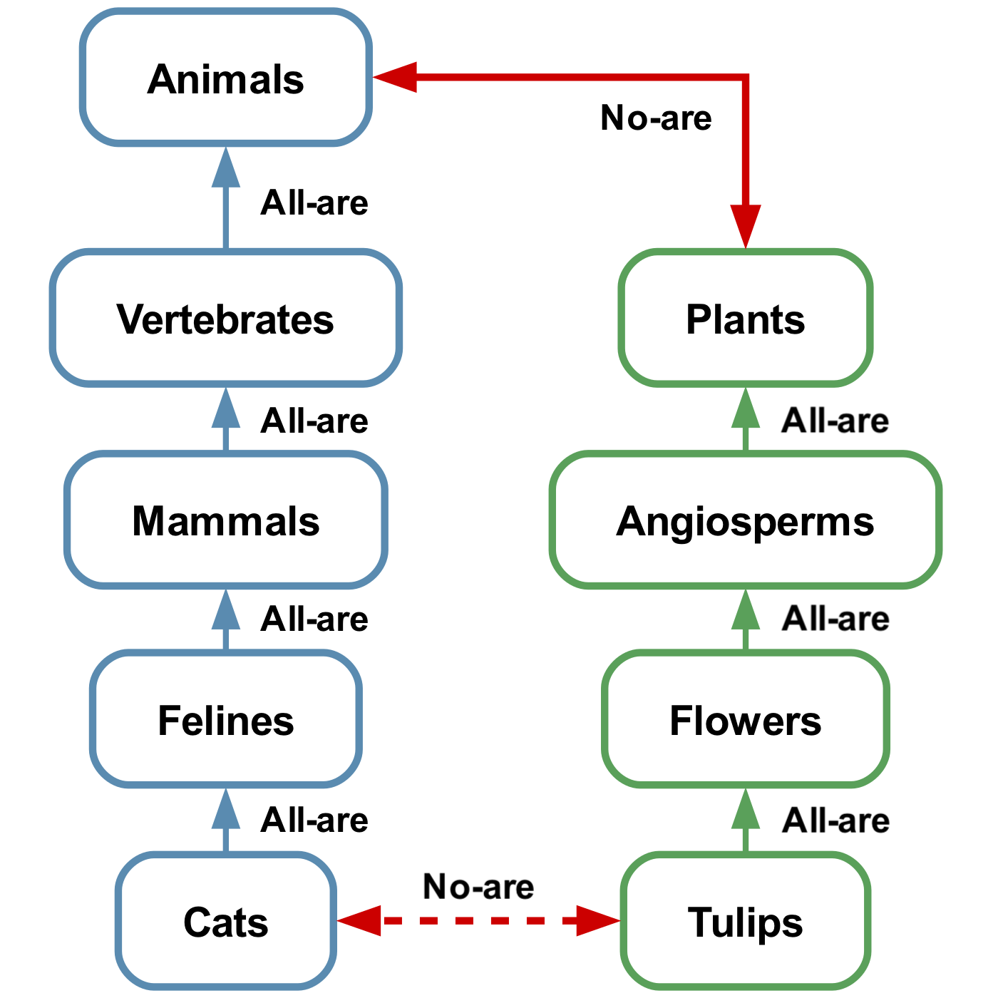</details> Figure 2: Example inference. Edges labeled “All-are” denote universal affirmatives (e.g., All cats are felines). The solid red edge is a universal negative (No animals are plants). From these “ atomic facts ” we infer No cats are tulips (dashed red edge). Formally, this is expressed as $\{Aa-b,\;Ac-d,\;Ebd\}\vDash Eac$ (Smiley, 1973). Syntax and semantics. The language of syllogistic logic comprises a finite set of atomic terms $\{a,b,c,...\}$ and four quantifier labels $A,E,I$ , and $O$ . Well-formed formulas consists of $Aab$ (“All $a$ are $b$ ”), $Eab$ (“No $a$ are $b$ ”), $Iab$ (“Some $a$ are $b$ ”), and $Oab$ (“Some $a$ are not $b$ ”). Finally, an A-chain, denoted as $Aa-b$ represents the single formula $Aab$ or a sequence of formulas $Aac_{1}$ , $Ac_{1}c_{2}$ , $...$ , $Ac_{n-1}c_{n}$ , $Ac_{n}b$ for $n≥ 1$ . A knowledge base ( $\mathcal{KB}$ ) is defined as a finite set of formulas (premises). An inference $\mathcal{F}\vDash F$ (i.e., deriving a conclusion from a set of premises) holds when the conclusion $F$ is true in every interpretation (an assignment of non-empty sets to terms) where all formulas in $\mathcal{F}$ are true. A set of formulas is consistent if there exists at least one interpretation in which all formulas are simultaneously true. Minimal inferences. We aim for models to identify the minimal set of premises in a knowledge base to derive a given hypothesis. Formally, we are interested in inferences $\mathcal{F}\vDash F$ such that $\mathcal{F}^{\prime}\not\vDash F$ for any proper subset $\mathcal{F}^{\prime}⊂neq\mathcal{F}$ . For example, $\{Abc,Abd\}\vDash Icd$ is minimal, while $\{Aab,Abc,Abd\}\vDash Icd$ is not because $Aab$ is not needed to infer the conclusion. There are seven types of minimal syllogistic inferences. See the full list in Table 4 in Appendix A. To facilitate understanding, Figure 2 provides an intuitive representation of a type 6 inference. Further details about the syllogistic logic can be found in Appendix A. 2.2 Meta-learning in Autoregressive Models Meta-learning, or “learning to learn”, is a paradigm that aims to enable machine learning models to acquire transferable knowledge across multiple tasks, allowing rapid adaptation to new tasks with minimal data. Among the numerous existing meta-learning frameworks (Hospedales et al., 2022), MIND is mainly inspired by Meta-learning Sequence Learners (MSL) (Irie and Lake, 2024). Data organization. In standard supervised learning, data consists of a static dataset $\mathcal{D}_{\mathrm{train}}=\{(x_{i},y_{i})\}_{i=1}^{N}$ where inputs $x_{i}$ are mapped to targets $y_{i}$ under a fixed distribution $p(x,y)$ . By contrast, meta-learning organizes data into tasks (or episodes) $\mathcal{T}=(S^{\mathrm{supp}},S^{\mathrm{query}})$ drawn from $p(\mathcal{T})$ , where $S^{\mathrm{supp}}=\{(x_{i},y_{i})\}_{i=1}^{K}$ is the support set containing task demonstrations, or study examples, and $S^{\mathrm{query}}=\{(x_{j},y_{j})\}_{j=1}^{M}$ is the query set for evaluation. We consider the simplest scenario where $|S^{\mathrm{query}}|=1$ , containing a single example $(x^{\mathrm{query}},y^{\mathrm{query}})$ . We adapt this episodic formulation to our task, as shown in Figure 1. Optimization. The fundamental difference between the two paradigms appears in their optimization objectives. Standard supervised learning finds parameters $\theta^{*}$ that maximize the likelihood: $$ \theta^{*}=\underset{\theta}{\mathrm{argmax}}\sum_{(x,y)\in\mathcal{D}_{% \mathrm{train}}}\log p_{\theta}(y\mid x) \tag{1} $$ while meta-learning finds parameters $\theta^{*}$ that maximize the expected likelihood across tasks: $$ \theta^{*}=\underset{\theta}{\mathrm{argmax}}\mathbb{E}_{\mathcal{T}}\left[% \log p_{\theta}(y^{\mathrm{query}}\mid x^{\mathrm{query}},S^{\mathrm{supp}})\right] \tag{2} $$ For autoregressive models, the probability $p_{\theta}(y^{\mathrm{query}}\mid x^{\mathrm{query}},S^{\mathrm{supp}})$ is computed by conditioning on the support set $S^{\mathrm{supp}}$ as part of the input context, formatted as a sequence of input-output pairs preceding the query. This approach forces the model to develop the capabilities of recognizing and applying task patterns from the support examples to generate appropriate query outputs. 3 Method 3.1 Data Generation In this section, we describe the methodology employed to construct textual datasets designed for the task of logical premise selection. The process begins with the random generation of graph-like structures representing $\mathcal{KB}s$ . These are then translated into text using fixed syntactic templates and assigning pseudowords to nodes. Abstract representation. To avoid ambiguity in premise selection, we use only non-redundant $\mathcal{KB}s$ , where for each derivable hypothesis $F$ , there is a unique $\mathcal{F}⊂eq\mathcal{KB}$ such that $\mathcal{F}\vDash F$ is minimal. We represent $\mathcal{KB}s$ as graphs, with constants as nodes and quantifiers as edges. A visual representation of $\mathcal{KB}s$ and the seven types of inferences as graphs can be seen in Appendix B.2. Synthetic $\mathcal{KB}s$ are generated by constructing such graphs. To ensure non-redundancy, $A$ -formulas form disjoint subgraphs with at most one path between any two nodes. We created three independent sets of consistent $\mathcal{KB}s$ for training, validation, and testing to ensure diversity across splits. See Appendix B.1 for the exact algorithms used to generate $\mathcal{KB}$ s Textual translation. To translate a given $\mathcal{KB}_{i}$ into a textual string, we: (1) assign a unique identifier $x_{1},...,x_{n}$ to each node within $\mathcal{KB}_{i}$ ; (2) map each edge to a fixed template connecting nodes $x_{i}$ and $x_{j}$ based on the quantifier represented by the edge (e.g., $Ax_{i}x_{j}$ becomes “All $x_{i}$ are $x_{j}$ ”); and (3) assign each unique node identifier $x_{1},...,x_{n}$ to a random English-like pseudoword (e.g., $x_{1}$ = wug, $x_{2}$ = blump). Further details on the vocabulary of pseudowords we used are provided in Appendix B.3. As illustrated in Figure 1, we structured each datapoint in the three splits to begin with the token “ knowledge base: ”, followed by the full sequence of premises, separated by commas. This is immediately followed by the special tag <QUERY>, and then the token “ hypothesis: ”, which introduces the target hypothesis. Next comes the token “ premises: ”, followed by the specific comma-separated premises that entail the hypothesis. To increase variability, we applied ten random pseudoword assignments and three random permutations of premise order for each $\mathcal{KB}$ , resulting in multiple variants per datapoint. Within each $\mathcal{KB}$ , valid hypotheses can be inferred by minimal sets of premises of varying lengths. We define the length of a inference as the total length of all $A$ -chains it contains, which corresponds to the total number of $A$ -formulas among its premises. For a given inference type $t$ , we denote the maximum and minimum lengths as $\mu(t)$ and $\sigma(t)$ , respectively. 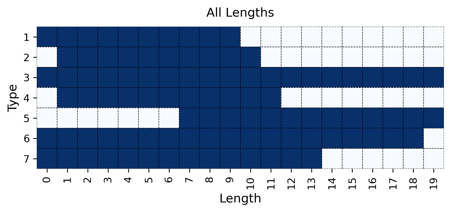We generated enough $\mathcal{KB}$ s to obtain 1000 training, 5 validation, and 100 test examples for each inference type and length combination in the range from 0 to 19. Note that some inference types (e.g., type 3) span the full range of lengths from 0 to 19, while others span only a subrange (e.g., type 2 spans from 1 to 10). See all type-length combinations within the generated $\mathcal{KB}$ s in Figure 6 in Appendix B.4. This range was chosen to allow experiments with generalization to both unseen shorter and longer inferences. Full dataset statistics, including the number of generated $\mathcal{KB}$ s per split, are reported in Appendix B.4. Training Testing Longer inferences: ‘‘ all x1 are x2, all x2 are x3, all x3 are x4, all x4 are x5, all x5 are x6 $\vdash$ all x1 are x6’’ Shorter inferences: ‘‘ all x1 are x2, all x2 are x3 $\vdash$ all x1 are x3’’ Shorter inferences: ‘‘ all x1 are x2, all x2 are x3, all x3 are x4 $\vdash$ all x1 are x4’’ Longer inferences: ‘‘ all x1 are x2, all x2 are x3, all x3 are x4, all x4 are x5, all x5 are x6 $\vdash$ all x1 are x6’’ Figure 3: Length generalization. We evaluate models on two types of length generalization: models trained on more complex (i.e., longer) inferences are tested on simpler (i.e., shorter) ones (Top) and vice versa (Bottom). The examples illustrate type 2 inferences. 3.2 MIND When applying meta-learning principles to the framework of syllogistic logic, we conceptualize the premises within a $\mathcal{KB}$ as atomic facts. The seven types of syllogism (as detailed in Table 4) are treated as arguments, constructed using these atomic facts, and the model’s task is to extract the minimal set of facts within a $\mathcal{KB}$ to produce a valid argument that proves the query hypothesis. The type of systematic generalization MIND addresses involves applying the seven fixed syllogistic inferences to new, unseen sets of atomic facts. This is central to logical reasoning because logical rules are, by definition, formal: conclusions follow from premises based solely on the structure of the arguments, regardless of their specific content. Thus, successfully applying an inference type to a novel, unseen $\mathcal{KB}$ requires the model to recognize and instantiate the same formal structure with different premises. This generalization also includes variations in the number of atomic facts needed to instantiate an argument. Specifically, handling $A$ -chains of varying lengths requires applying the learned inference patterns to longer or shorter instances of the same formal type. Episodes organization. To induce meta-learning of inference types, MIND uses a set of episodes where each episode $\mathcal{T}=(\mathcal{KB},S^{\mathrm{supp}},x^{\mathrm{query}},y^{\mathrm{% query}})$ . Here, $\mathcal{KB}$ is a knowledge base, $S^{\mathrm{supp}}$ is a set of study valid hypothesis-premises pairs, $x^{\mathrm{query}}$ is a valid query hypothesis, and $y^{\mathrm{query}}$ is the minimal set of premises entailing $x^{\mathrm{query}}$ . Figure 1 shows a full MIND episode using indexed variables in place of pseudowords for improved readability. Importantly, we consider study examples with inferences of the same type as the query. The number of study examples we set, i.e. valid hypothesis–premise pairs, is three. In their textual translation, we add the special tags <STUDY> to indicate the beginning of the sequence of study examples. During MIND fine-tuning, models are trained to minimize the cross-entropy loss of the tokens in $y^{\mathrm{query}}$ given the input tokens from the context $(\mathcal{KB},S^{\mathrm{supp}},x^{\mathrm{query}})$ . Baseline. Similarly to Lake and Baroni (2023), we consider a baseline where models are not fine-tuned on episodes but on single input-output pairs $(x^{\mathrm{query}},y^{\mathrm{query}})$ preceded by a $\mathcal{KB}$ . The baseline is fine-tuned to minimize the cross-entropy loss of the tokens in $y^{\mathrm{query}}$ given the input tokens from the context $(\mathcal{KB},x^{\mathrm{query}})$ . To ensure a fair comparison between the meta-learning model and the baseline, we ensured that both models were fine-tuned on the exact same aggregate set of unique hypothesis-premises pairs. Specifically, the baseline was fine-tuned using a set $\mathcal{D}_{\text{baseline}}$ consisting of $(x^{\mathrm{query}},y^{\mathrm{query}})$ unique pairs. For the meta-learning approach, the corresponding set of all unique hypothesis-premises pairs encountered across all $N$ episodes $\mathcal{T}_{i}=(\mathcal{KB}_{i},S^{\mathrm{supp}}_{i},x^{\mathrm{query}}_{i}% ,y^{\mathrm{query}}_{i})$ is given by $\mathcal{D}_{\text{meta}}=\bigcup_{i=1}^{N}(S^{\mathrm{supp}}_{i}\cup\{(x^{% \mathrm{query}}_{i},y^{\mathrm{query}}_{i})\})$ . We verified that $\mathcal{D}_{\text{baseline}}=\mathcal{D}_{\text{meta}}$ . Moreover, since the meta-learning model processes more hypothesis-premises pairs within each episode (due to $S^{\mathrm{supp}}_{i}$ ), we counterbalanced this by training the baseline model for a proportionally larger number of epochs. Further details on the training regime and number of epochs for each approach are provided in Appendix C.2. 4 Experimental Setup 4.1 Models We run experiments using the Qwen 2.5 family of decoder-only LMs (Qwen Team, 2025). More specifically, we test three sizes: 1.5B, 3B, and 7B parameters. This family of models is selected because it allows us to experiment with varying small sizes (ranging from 1.5 to 7 billion parameters) and achieves a better size vs. performance trade-off compared to other open weights model families. In addition to the Qwen 2.5 family, we also evaluate the closed-source LLM GPT-4o (OpenAI, 2024) and the Large Reasoning Model (LRM) o3-mini (OpenAI, 2025) on the logical premise selection task. Note that LRMs are also LLMs, but post-trained to generate longer intermediate chains of thought, improving performance on complex reasoning tasks (Xu et al., 2025). We conduct the evaluation both in a zero-shot setting and in a few-shot setting, using the $S^{\mathrm{supp}}$ study pairs as examples. See the API details and the exact prompts used to evaluate closed models in Appendix C.3. | | Model | Method | All | Short | Long | | --- | --- | --- | --- | --- | --- | | Fine-tuning | Qwen-2.5 1.5B | MIND | 93.11 ± 0.61 | 94.28 ± 0.61 | 91.76 ± 0.27 | | Baseline | 85.56 ± 1.24 | 91.42 ± 0.82 | 80.56 ± 1.78 | | | | Qwen-2.5 3B | MIND | 96.16 ± 0.44 | 96.24 ± 0.56 | 95.55 ± 0.43 | | | Baseline | 93.03 ± 1.15 | 95.34 ± 1.18 | 90.92 ± 1.27 | | | | Qwen-2.5 7B | MIND | 98.13 ± 0.98 | 98.26 ± 0.82 | 97.69 ± 1.40 | | | Baseline | 95.76 ± 1.10 | 97.27 ± 1.22 | 94.13 ± 0.90 | | | | Prompting | GPT-4o | Few-shot | 39.76 | 52.91 | 33.51 | | Zero-shot | 15.90 | 28.97 | 9.89 | | | | o3-mini | Few-shot | 88.45 | 87.91 | 88.51 | | | Zero-shot | 67.98 | 73.29 | 64.54 | | | Table 1: Core generalization. Accuracy (mean ± std) on test inferences across all type-length combinations (All), plus breakdown into the five shortest (Short) and longest (Long) inferences for each of the seven types of inference. Fine-tuned Qwen models use MIND vs. Baseline; GPT-4o and o3-mini use few-shot vs. zero-shot prompting. 4.2 Experiments We design experiments to evaluate the ability of MIND to teach pretrained small LMs to systematically apply inferences to new, unseen sets of premises —that is, to reason in a formal way by recognizing and instantiating the same underlying structure independently of the $\mathcal{KB}$ s’ content. To ensure consistency, both MIND and the baseline receive inputs at test time in the same format as during training. MIND models are provided as context $(\mathcal{KB},S^{\mathrm{supp}},x^{\mathrm{query}})$ , and are tasked to generate $y^{\mathrm{query}}$ , while the baseline receives $(\mathcal{KB},x^{\mathrm{query}})$ . Generalization. In the first experiment, models are evaluated on their ability to generalize to unseen $\mathcal{KB}s$ , while all inference lengths are seen. The training and testing sets contain inferences of all lengths for each of the seven types. Since this is the simplest form of systematic application of syllogistic inference, we refer to it as core generalization. 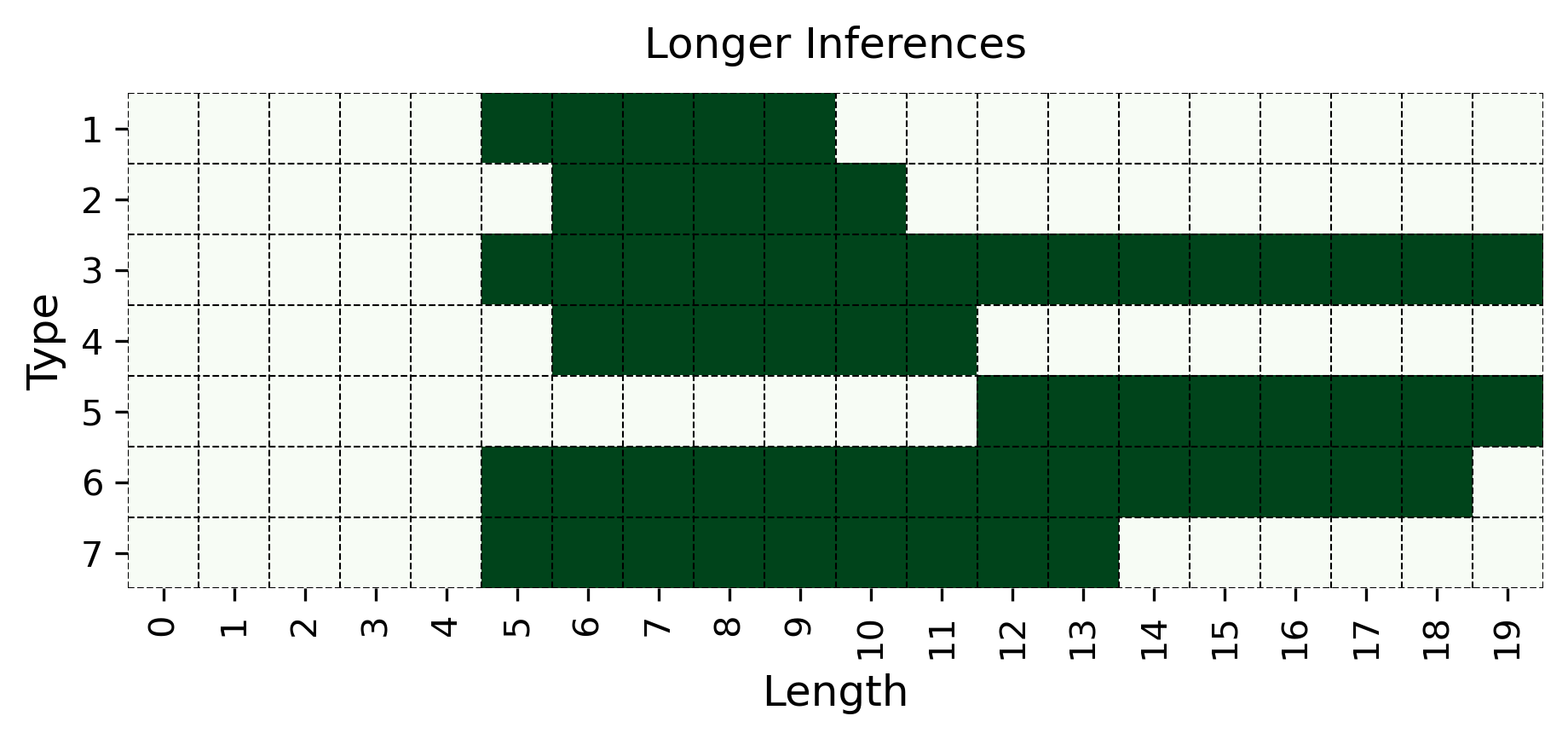We then consider two more challenging generalizations involving inferences of unseen length. As illustrated in Figure 3, we examine the case of generalizing to longer inferences when the model has only learned from shorter ones (as studied in Saparov et al. 2023), and vice versa —generalizing to shorter inferences after seeing only longer ones. In the logic literature, they are respectively known as recursiveness and compositionality (Vargas Guzmán et al., 2024). To test this, we train exclusively on inferences whose lengths $x$ are $\sigma(t)≤ x≤\mu(t)-5$ , and test on the five longest inferences for each type, i.e., those whose length is $\mu(t)-5<x≤\mu(t)$ . In the second case, we train on inferences with length $\sigma(t)+5≤ x≤\mu(t)$ , and test only on the five shortest inference lengths for each type, i.e., those with length $\sigma(t)≤ x<\sigma(t)+5$ . An intuitive representation of these generalizations is provided in Figure 3. Notably, within the MIND approach, we consider two varying types of study examples $S^{\mathrm{supp}}$ : the aligned and disaligned sets of study examples, in which each $(x^{\mathrm{supp}},y^{\mathrm{supp}})$ either falls within or outside the range of inference lengths used for testing, respectively. More precisely, the meanings of aligned and disaligned depend on whether we are evaluating models on unseen shorter or longer inferences. For longer inferences, disaligned includes inferences with lengths $\sigma(t)≤ x≤\mu(t)-5$ , and aligned includes those with lengths $\mu(t)-5<x≤\mu(t)$ . For shorter ones, instead, aligned includes inferences with lengths $\sigma(t)≤ x<\sigma(t)+5$ , and disaligned includes those with lengths $\sigma(t)+5≤ x≤\mu(t)$ . Figure 6, in the Appendix, shows all inference type-length combinations within training and test split in the core and in the length generalization settings. These datasets contain 1,000 and 100 datapoints for each training and testing type–length combination, respectively. To further investigate the performance of MIND in a limited data regime, we also consider the case where only 100 datapoints are available for each training type–length combination. 4.3 Prediction Accuracy We consider a model prediction to be correct if the set of premises extracted from the generated text matches the ground truth set of minimal premises. Using this criterion, we measure accuracy both in aggregate, i.e., across an entire test set, and decomposed by each test type-length combination. All models (1.5B, 3B, and 7B) are fine-tuned three times and with different random seeds, thus we report mean and standard deviation of each accuracy. 5 Results | Qwen-2.5 1.5B Baseline Qwen-2.5 3B | MIND 63.53 ± 1.16 MIND | 76.42 ± 2.95 63.53 ± 1.16 87.61 ± 1.97 | 91.75 ± 1.10 56.67 ± 1.22 95.86 ± 0.70 | 70.94 ± 2.27 56.67 ± 1.22 77.19 ± 3.53 | 71.13 ± 1.83 78.53 ± 1.71 | | --- | --- | --- | --- | --- | --- | | Baseline | 76.78 ± 1.63 | 76.78 ± 1.63 | 71.88 ± 1.49 | 71.88 ± 1.49 | | | Qwen-2.5 7B | MIND | 90.03 ± 1.09 | 96.84 ± 0.15 | 76.23 ± 2.91 | 83.41 ± 1.63 | | Baseline | 80.76 ± 2.65 | 80.76 ± 2.65 | 71.08 ± 1.55 | 71.08 ± 1.55 | | Table 2: Generalization to unseen lengths. Accuracy (mean ± std) of meta-learning and baseline models when trained on short inferences and tested on longer ones or vice versa. In both cases, we compare the settings in which the inferences in the study examples either falls within (Aligned) or outside (Disaligned) the range of inference lengths used for testing. Baseline models have no study examples, hence such difference does not hold for them. 5.1 Core Generalization We first examine the performance of meta-learning versus the baseline on core generalization (Table 1), with models trained and tested on all inference type-length combinations. The “Short” and “Long” columns report aggregated accuracy on the sets of the five shortest and longest inferences, respectively, for each type. We hypothesize that longer inferences are harder because, to be correct, models must select all premises belonging to a larger minimal set of premises. Across all Qwen-2.5 model sizes (1.5B, 3B, 7B), the meta-learning approach consistently yields higher accuracy than the baseline. Performance improves with model scale in both approaches. For example, MIND accuracy increases from 93.11% (1.5B) to 98.13% (7B) on all type-length combinations, with accuracy on shortest inferences rising from 94.28% to 98.26%, and on the longest ones increasing from 91.76% to 97.69%. In contrast, baseline performance rises more slowly —from 85.56% (1.5B) to 95.76% (7B) —and shows a wider drop on the longest inferences, falling as low as 80.56% for the smallest model. Notably, the performance gap between MIND and the baseline narrows as model size increases, suggesting that larger models achieve better core generalization even without meta-learning. It is worth noting that with limited data, MIND’s advantage over the baseline becomes much wider at all sizes, as shown in Appendix D.3. The closed-source models GPT-4o and o3-mini still underperform compared to Qwen-2.5 models fine-tuned with MIND. Both models perform poorly in the zero-shot setting but improve with few-shot prompting: GPT-4o reaches 39.76% on all type-length combinations (with 52.91% on shortest and 33.51% on longest inferences), while o3-mini performs substantially better (88.45% all combination, 87.91% on shorters, and 88.51% on longest). As expected, performance on the longest inferences is worse than that on the shortest ones for GPT-4o, while o3-mini maintains a more robust performance across inference lengths. 5.2 Length Generalization Table 2 shows that MIND models consistently outperform baseline models in generalizing to both longer and shorter inferences than those seen during training. In core generalization, we observed that longer inferences are more challenging than shorter ones. Instead, in the case of unseen lengths, an interesting and somewhat counterintuitive pattern emerges: it is generally easier for models to generalize to longer inferences than to shorter ones. This is true across all model sizes and in both approaches; For instance, the largest model, Qwen-2.5 7B, achieved 90.03% accuracy on longer inferences (disaligned) compared to 76.23% on shorter ones (disaligned). Aligning study example lengths with the test condition (aligned) proves moderately to highly effective for unseen short inferences across all MIND model sizes. For example, Qwen-2.5 1.5B improved from 76.42% to 91.75%, and Qwen-2.5 3B improved from 87.61% to 95.86%. For unseen long inferences, this alignment is moderately effective in larger models: Qwen-2.5 7B improved from 76.23% to 83.41%, while the 1.5B and 3B models showed smaller gains (70.94% to 71.13% and 77.19% to 78.53%, respectively). These results indicate that MIND enables models in the aligned condition to exploit abstract patterns in the study examples (unseen inference lengths), allowing them to more effectively answer query hypotheses requiring length generalization. Again, MIND’s better performance in length generalization is especially noticeable with limited training data, where the difference between MIND and baseline models grows significantly (see Appendix D.3 for more details). | L $→$ S | MIND (aligned) | 42.94 | 4.9 | 36.68 | 2.1 | 57.5 | | --- | --- | --- | --- | --- | --- | --- | | MIND (disaligned) | 28.31 | 3.72 | 52.81 | 1.76 | 66.06 | | | Baseline | 28.21 | 6.19 | 23.38 | 2.1 | 72.78 | | | S $→$ L | MIND (aligned) | 9.76 | 1.66 | 87.54 | 5.08 | 60.94 | | MIND (disaligned) | 14.14 | 6.14 | 81.82 | 3.65 | 35.35 | | | Baseline | 3.87 | 2.36 | 89.79 | 6.66 | 66.9 | | Table 3: Error analysis. Error analysis comparing MIND and baseline on long to short (L $→$ S) and short to long (S $→$ L) generalization. The table shows percentages and averages for non-minimal valid sets of premises (NVM) and missing necessary $A$ premises (MAP), and the percentage of hallucinated premises (HP). 6 Error Analysis Beyond simply measuring the accuracy of MIND and the baseline, we additionally focus on two main types of errors models make when evaluated on unseen lengths. First, among all errors, we consider the proportion of non-minimal valid set of premises (NVM). This means that the correct minimal set was generated by the model, but together with unnecessary premises; for this case, we also measure how many unnecessary premises, on average, the models generate. Alternatively, models may fail to provide the complete $A$ -chain within the correct minimal set of premises, meaning that at least one necessary $A$ premise is missing (MAP); here, we also track the average number of missing necessary $A$ -formulas in erroneous answers. NVM and MAP are mutually exclusive. Furthermore, we consider an additional type of error that can occur simultaneously with either NVM or MAP: models may hallucinate premises —referred to as hallucinated premises (HP) —and output a formula that is not contained in the $\mathcal{KB}$ . Table 3 presents the error analysis for Qwen-2.5 7B Each model was fine-tuned three times with different random seeds, we selected the best model for each approach for this analysis. on the challenging length generalization settings. See Appendix D.4 for further error analysis results. HP is a common error type across both settings (often $>$ 50%). The baseline model has the highest HP rate in long to short (72.78%), while MIND models are generally better. When generalizing to shorter inferences, a substantial portion of errors (28-43%) are NVM, indicating models indeed find logical solutions but include unnecessary premises. In this context, a lower number of unnecessary premises is better, as it is closer to the minimal set. The baseline model adds the most unnecessary premises (6.19 average), compared to MIND (disaligned) (4.9) and MIND (aligned) (3.72). For generalizations to longer inferences, errors show different patterns, with few NVM errors (4-14%) and predominantly MAP errors (81-90%). The average number of missing premises is higher in short to long (3.65-6.66) than in long to short (1.76-2.1), suggesting models struggle to provide the complete set of premises when evaluated on longer inferences than seen during training. The baseline model struggles most with longer inferences, with a high MAP error rate (89.79%) and a large number of missing premises (6.66) contributing to its lower accuracy compared to MIND. 7 Related Work 7.1 LLMs’ Logical Capabilities Recent work has highlighted weaknesses in LLMs’ logical reasoning. LLMs often struggle with OOD generalization (Clark et al., 2021; Saparov et al., 2023; Vargas Guzmán et al., 2024), multi-step inference (Creswell et al., 2023), and consistency across formal reasoning patterns (Parmar et al., 2024; Hong et al., 2024). Neuro-symbolic methods address these gaps by integrating logic modules or symbolic solvers, improving both performance and interpretability (Pan et al., 2023; Olausson et al., 2023; Kambhampati et al., 2024). In a different direction, LRMs have shown strong gains in reasoning and planning tasks (Xu et al., 2025). Our proposed meta-learning approach offers a complementary alternative by enabling LLMs to adapt across logical tasks without relying on symbolic modules, as our results demonstrate. 7.2 Meta-learning Meta-learning enables models to rapidly adapt to new tasks by leveraging prior experiences across tasks (Thrun and Pratt, 1998; Hospedales et al., 2022). Foundational approaches include memory-augmented neural networks (Santoro et al., 2016), prototypical networks (Snell et al., 2017), and model-agnostic meta-learning (MAML) (Finn et al., 2017). In the context of LLMs, meta-learning has been explored through techniques such as meta-in-context learning (Coda-Forno et al., 2023), in-context tuning (Chen et al., 2022), and MetaICL (Min et al., 2022), which either train for or exploit the in-context learning abilities of models to adapt to new tasks using few-shot examples. Our proposed method draws inspiration from the MSL framework (Irie and Lake, 2024), which we adapt and extend to solve the logical premise selection task. 8 Conclusion In this work, we introduced MIND, a meta-learning fine-tuning approach to improve deductive reasoning in LLMs, explicitly targeting the logical premise selection task. Our results show that MIND significantly enhances generalization compared to the baseline, especially in small-scale and low-data scenarios. Remarkably, our fine-tuned small models outperform state-of-the-art LLMs on this task. This demonstrates the potential of MIND to advance the development of more robust and reliable AI systems. Future work should explore several potential avenues. First, we should investigate not only systematic generalization using fixed inference rules, as we have done here, but also extend our research to learning the composition of multiple logical inferences. This approach aligns with ideas proposed in other meta-learning research, such as Meta-Learning for Compositionality (Lake and Baroni, 2023). Additionally, we should examine increasingly complex fragments of language, where the interactions among various inference-building blocks and reasoning forms become more intricate, and assess the effectiveness of MIND in helping LLMs to generalize in such contexts. 9 Limitations Despite demonstrating meaningful progress in enhancing the deductive reasoning capabilities of language models through the MIND approach, this study has several limitations that future research could address. Model selection. The evaluation primarily targets small to mid-sized language models (1.5B to 7B parameters), largely due to computational constraints. This focus leaves open the question of whether the observed improvements from MIND generalize to larger-scale models. Meta-learning trade-offs. The gains in reasoning ability achieved by MIND come with associated costs. The meta-learning strategy adopted involves incorporating multiple study examples into the input context during fine-tuning. This leads to longer input sequences, which in turn increase memory usage and computational demands compared to standard fine-tuning approaches. Focus on a logic fragment. This work is constrained to the syllogistic fragment of first-order logic. Future research should investigate whether our conclusions extend to more expressive logical systems or to real-world scenarios where reasoning tasks are less structured. However, syllogistic logic is a restricted domain that allows for precise control over variables such as the type of inference considered, inference length, and the structure of knowledge bases. In the context of this study, it serves as a valuable testbed for investigating logical generalization in LLMs. References - Balloccu et al. (2024) Simone Balloccu, Patrícia Schmidtová, Mateusz Lango, and Ondrej Dusek. 2024. Leak, cheat, repeat: Data contamination and evaluation malpractices in closed-source LLMs. In Proceedings of the 18th Conference of the European Chapter of the Association for Computational Linguistics (Volume 1: Long Papers), pages 67–93, St. Julian’s, Malta. Association for Computational Linguistics. - Chen et al. (2022) Yanda Chen, Ruiqi Zhong, Sheng Zha, George Karypis, and He He. 2022. Meta-learning via language model in-context tuning. In Proceedings of the 60th Annual Meeting of the Association for Computational Linguistics (Volume 1: Long Papers), pages 719–730, Dublin, Ireland. Association for Computational Linguistics. - Clark et al. (2021) Peter Clark, Oyvind Tafjord, and Kyle Richardson. 2021. Transformers as soft reasoners over language. In Proceedings of the Twenty-Ninth International Joint Conference on Artificial Intelligence, IJCAI’20. - Coda-Forno et al. (2023) Julian Coda-Forno, Marcel Binz, Zeynep Akata, Matt Botvinick, Jane Wang, and Eric Schulz. 2023. Meta-in-context learning in large language models. In Advances in Neural Information Processing Systems, volume 36, pages 65189–65201. Curran Associates, Inc. - Creswell et al. (2023) Antonia Creswell, Murray Shanahan, and Irina Higgins. 2023. Selection-inference: Exploiting large language models for interpretable logical reasoning. In The Eleventh International Conference on Learning Representations. - Dettmers et al. (2023) Tim Dettmers, Artidoro Pagnoni, Ari Holtzman, and Luke Zettlemoyer. 2023. Qlora: efficient finetuning of quantized llms. In Proceedings of the 37th International Conference on Neural Information Processing Systems, NIPS ’23, Red Hook, NY, USA. Curran Associates Inc. - Finn et al. (2017) Chelsea Finn, Pieter Abbeel, and Sergey Levine. 2017. Model-agnostic meta-learning for fast adaptation of deep networks. In Proceedings of the 34th International Conference on Machine Learning - Volume 70, ICML’17, page 1126–1135. JMLR.org. - Gulati et al. (2024) Aryan Gulati, Brando Miranda, Eric Chen, Emily Xia, Kai Fronsdal, Bruno de Moraes Dumont, and Sanmi Koyejo. 2024. Putnam-AXIOM: A functional and static benchmark for measuring higher level mathematical reasoning. In The 4th Workshop on Mathematical Reasoning and AI at NeurIPS’24. - Hong et al. (2024) Ruixin Hong, Hongming Zhang, Xinyu Pang, Dong Yu, and Changshui Zhang. 2024. A closer look at the self-verification abilities of large language models in logical reasoning. In Proceedings of the 2024 Conference of the North American Chapter of the Association for Computational Linguistics: Human Language Technologies (Volume 1: Long Papers), pages 900–925, Mexico City, Mexico. Association for Computational Linguistics. - Hospedales et al. (2022) Timothy Hospedales, Antreas Antoniou, Paul Micaelli, and Amos Storkey. 2022. Meta-Learning in Neural Networks: A Survey . IEEE Transactions on Pattern Analysis & Machine Intelligence, 44(09):5149–5169. - Hu et al. (2022) Edward J Hu, yelong shen, Phillip Wallis, Zeyuan Allen-Zhu, Yuanzhi Li, Shean Wang, Lu Wang, and Weizhu Chen. 2022. LoRA: Low-rank adaptation of large language models. In International Conference on Learning Representations. - Huang and Chang (2023) Jie Huang and Kevin Chen-Chuan Chang. 2023. Towards reasoning in large language models: A survey. In Findings of the Association for Computational Linguistics: ACL 2023, pages 1049–1065, Toronto, Canada. Association for Computational Linguistics. - Huang et al. (2025) Kaixuan Huang, Jiacheng Guo, Zihao Li, Xiang Ji, Jiawei Ge, Wenzhe Li, Yingqing Guo, Tianle Cai, Hui Yuan, Runzhe Wang, Yue Wu, Ming Yin, Shange Tang, Yangsibo Huang, Chi Jin, Xinyun Chen, Chiyuan Zhang, and Mengdi Wang. 2025. MATH-Perturb: Benchmarking LLMs’ math reasoning abilities against hard perturbations. arXiv preprint arXiv:2502.06453. - Irie et al. (2025) Kazuki Irie, Róbert Csordás, and Jürgen Schmidhuber. 2025. Metalearning continual learning algorithms. Transactions on Machine Learning Research. - Irie and Lake (2024) Kazuki Irie and Brenden M. Lake. 2024. Neural networks that overcome classic challenges through practice. Preprint, arXiv:2410.10596. - Kambhampati et al. (2024) Subbarao Kambhampati, Karthik Valmeekam, Lin Guan, Mudit Verma, Kaya Stechly, Siddhant Bhambri, Lucas Paul Saldyt, and Anil B Murthy. 2024. Position: LLMs can’t plan, but can help planning in LLM-modulo frameworks. In Forty-first International Conference on Machine Learning. - Keuleers and Brysbaert (2010) Emmanuel Keuleers and Marc Brysbaert. 2010. Wuggy: A multilingual pseudoword generator. Behavior research methods, 42:627–633. - Kingma and Ba (2015) Diederik P. Kingma and Jimmy Ba. 2015. Adam: A method for stochastic optimization. - Lake and Baroni (2023) Brenden M. Lake and Marco Baroni. 2023. Human-like systematic generalization through a meta-learning neural network. Nature, 623:115–121. - Leighton (2004) Jacqueline P. Leighton. 2004. Defining and describing reason. In Jacqueline P. Leighton and Robert J. Sternberg, editors, The Nature of Reasoning. Cambridge University Press. - Min et al. (2022) Sewon Min, Mike Lewis, Luke Zettlemoyer, and Hannaneh Hajishirzi. 2022. MetaICL: Learning to learn in context. In Proceedings of the 2022 Conference of the North American Chapter of the Association for Computational Linguistics: Human Language Technologies, pages 2791–2809, Seattle, United States. Association for Computational Linguistics. - Mirzadeh et al. (2025) Seyed Iman Mirzadeh, Keivan Alizadeh, Hooman Shahrokhi, Oncel Tuzel, Samy Bengio, and Mehrdad Farajtabar. 2025. GSM-symbolic: Understanding the limitations of mathematical reasoning in large language models. In The Thirteenth International Conference on Learning Representations. - Mondorf and Plank (2024) Philipp Mondorf and Barbara Plank. 2024. Beyond accuracy: Evaluating the reasoning behavior of large language models - a survey. In First Conference on Language Modeling. - Olausson et al. (2023) Theo Olausson, Alex Gu, Ben Lipkin, Cedegao Zhang, Armando Solar-Lezama, Joshua Tenenbaum, and Roger Levy. 2023. LINC: A neurosymbolic approach for logical reasoning by combining language models with first-order logic provers. In Proceedings of the 2023 Conference on Empirical Methods in Natural Language Processing, pages 5153–5176, Singapore. Association for Computational Linguistics. - OpenAI (2024) OpenAI. 2024. Gpt-4o system card. arXiv preprint arXiv:2410.21276. - OpenAI (2025) OpenAI. 2025. Openai o3-mini. https://openai.com/index/openai-o3-mini/. Accessed: 2025-05-08. - Pan et al. (2023) Liangming Pan, Alon Albalak, Xinyi Wang, and William Wang. 2023. Logic-LM: Empowering large language models with symbolic solvers for faithful logical reasoning. In Findings of the Association for Computational Linguistics: EMNLP 2023, pages 3806–3824, Singapore. Association for Computational Linguistics. - Parmar et al. (2024) Mihir Parmar, Nisarg Patel, Neeraj Varshney, Mutsumi Nakamura, Man Luo, Santosh Mashetty, Arindam Mitra, and Chitta Baral. 2024. LogicBench: Towards systematic evaluation of logical reasoning ability of large language models. In Proceedings of the 62nd Annual Meeting of the Association for Computational Linguistics (Volume 1: Long Papers), pages 13679–13707, Bangkok, Thailand. Association for Computational Linguistics. - Qwen Team (2025) Qwen Team. 2025. Qwen2.5 technical report. Preprint, arXiv:2412.15115. - Santoro et al. (2016) Adam Santoro, Sergey Bartunov, Matthew Botvinick, Daan Wierstra, and Timothy Lillicrap. 2016. Meta-learning with memory-augmented neural networks. In Proceedings of the 33rd International Conference on International Conference on Machine Learning - Volume 48, ICML’16, page 1842–1850. JMLR.org. - Saparov et al. (2023) Abulhair Saparov, Richard Yuanzhe Pang, Vishakh Padmakumar, Nitish Joshi, Mehran Kazemi, Najoung Kim, and He He. 2023. Testing the general deductive reasoning capacity of large language models using OOD examples. In Thirty-seventh Conference on Neural Information Processing Systems. - Shi et al. (2023) Freda Shi, Xinyun Chen, Kanishka Misra, Nathan Scales, David Dohan, Ed Chi, Nathanael Schärli, and Denny Zhou. 2023. Large language models can be easily distracted by irrelevant context. In Proceedings of the 40th International Conference on Machine Learning, ICML’23. JMLR.org. - Singh et al. (2024) Aaditya K. Singh, Muhammed Yusuf Kocyigit, Andrew Poulton, David Esiobu, Maria Lomeli, Gergely Szilvasy, and Dieuwke Hupkes. 2024. Evaluation data contamination in llms: how do we measure it and (when) does it matter? Preprint, arXiv:2411.03923. - Smiley (1973) Timothy J. Smiley. 1973. What is a syllogism? Journal of Philosophical Logic, 2(1):136–154. - Snell et al. (2017) Jake Snell, Kevin Swersky, and Richard Zemel. 2017. Prototypical networks for few-shot learning. In Proceedings of the 31st International Conference on Neural Information Processing Systems, NIPS’17, page 4080–4090, Red Hook, NY, USA. Curran Associates Inc. - Thrun and Pratt (1998) Sebastian Thrun and Lorien Pratt. 1998. Learning to Learn: Introduction and Overview, pages 3–17. Springer US, Boston, MA. - Vargas Guzmán et al. (2024) Manuel Vargas Guzmán, Jakub Szymanik, and Maciej Malicki. 2024. Testing the limits of logical reasoning in neural and hybrid models. In Findings of the Association for Computational Linguistics: NAACL 2024, pages 2267–2279, Mexico City, Mexico. Association for Computational Linguistics. - Xu et al. (2025) Fengli Xu, Qianyue Hao, Zefang Zong, Jingwei Wang, Yunke Zhang, Jingyi Wang, Xiaochong Lan, Jiahui Gong, Tianjian Ouyang, Fanjin Meng, Chenyang Shao, Yuwei Yan, Qinglong Yang, Yiwen Song, Sijian Ren, Xinyuan Hu, Yu Li, Jie Feng, Chen Gao, and Yong Li. 2025. Towards large reasoning models: A survey of reinforced reasoning with large language models. Preprint, arXiv:2501.09686. - Yoran et al. (2024) Ori Yoran, Tomer Wolfson, Ori Ram, and Jonathan Berant. 2024. Making retrieval-augmented language models robust to irrelevant context. In The Twelfth International Conference on Learning Representations. - Łukasiewicz (1951) Jan Łukasiewicz. 1951. Aristotle’s Syllogistic From the Standpoint of Modern Formal Logic. Oxford, England: Garland. Appendix A Formal Semantics and Syllogistic Inference Patterns In this section, we formally define the semantics of syllogistic logic by translating syllogistic formulas into first-order logic. We also specify a consistent set of such formulas and formalize a valid inference within this framework. Let $\mathcal{A}=\{a,b,c,...\}$ be a set of atomic terms, and let $\mathcal{R}=\{R,S,T,...\}$ be a set of unary relational symbols. We bijectively assign to every atomic term $a∈\mathcal{A}$ a relational symbol $R_{a}∈\mathcal{R}$ , and interpret syllogistic formulas as first-order logic sentences: $Aab$ as $∀ x\,[R_{a}(x)→ R_{b}(x)]$ , $Eab$ as $∀ x\,[R_{a}(x)→\neg R_{b}(x)]$ , $Iab$ as $∃ x\,[R_{a}(x)\land R_{b}(x)]$ , and $Oab$ as $∃ x\,[R_{a}(x)\land\neg R_{b}(x)]$ . We say that a set $\mathcal{F}$ of syllogistic formulas is consistent if there exists a structure $M$ in signature $\mathcal{R}$ such that every relation $R^{M}$ is non-empty, and the interpretation of every sentence in $\mathcal{F}$ holds in $M$ , denoted by $M\vDash\mathcal{F}$ . For a syllogistic formula $F$ , the pair $(\mathcal{F},F)$ is an inference, denoted by $\mathcal{F}\vDash F$ , if $M\vDash\{F\}$ , whenever $M\vDash\mathcal{F}$ for a structure $M$ in signature $\mathcal{R}$ . Appendix B Dataset | 1 2 3 | $\{Aa-b,Ac-d,Oad\}\vDash Obc$ $\{Aa-b\}\vDash Aab$ $\{Aa-b,Ac-d,Aa-e,Ede\}\vDash Obc$ | | --- | --- | | 4 | $\{Aa-b,Aa-c\}\vDash Ibc$ | | 5 | $\{Aa-b,Ac-d,Ae-f,Iae,Edf\}\vDash Obc$ | | 6 | $\{Aa-b,Ac-d,Ebd\}\vDash Eac$ | | 7 | $\{Aa-b,Ac-d,Iac\}\vDash Ibd$ | Table 4: Syllogistic inference types. Each row shows a distinct logical inference pattern. Notation follows traditional categorical logic: $Aab$ denotes a universal affirmative ("All $a$ are $b$ "), $Eab$ a universal negative ("No $a$ are $b$ "), $Iac$ a existential affirmative ("Some $a$ are $c$ "), and $Oad$ a existential negative ("Some $a$ are not $d$ "). Formulas of the form $Aa-b$ denote a sequence of $n$ $A$ -formulas relating $a$ and $b$ . B.1 $\mathcal{KB}$ s’ Generation Knowledge bases can be modeled as edge-labeled graphs, in which nodes correspond to atomic terms and edges are labeled with quantifiers. Our graph generation algorithm comprises two principal stages: (1) We first construct all A-chains of the knowledge base, which is used as its structural backbone, by generating disjoint trees—directed acyclic graphs that ensure a unique path exists between any pair of nodes. (2) Subsequently, we incorporate additional label edges corresponding to $E$ , $I$ , and $O$ formulas, while maintaining the overall consistency of the knowledge base. To construct all possible valid syllogisms from each artificially generated knowledge base, we employ antillogisms—minimal inconsistent set of syllogistic formulas. For example, consider the set $\{Aab,Aac,Ebc\}$ , which forms an antilogism. By negating the inconsistent formula $Ebc$ , we obtain a valid inference in which the remaining formulas $\{Aab,Aac\}$ entail its negation, i.e., $\{Aab,Aac\}\vDash Ibc$ . This corresponds to an inference of type 4. More generally, any syllogism can be derived from an antilogism of the form $\mathcal{F}\cup\{\neg F\}$ by inferring the conclusion $F$ from the consistent set $\mathcal{F}$ , that is, $\mathcal{F}\vDash F$ . This result was formally established by (Smiley, 1973), who also demonstrated that there exist only three distinct types of antilogisms. Furthermore, as shown by (Vargas Guzmán et al., 2024), all valid syllogistic inferences can be systematically derived from these three canonical forms of antilogism (see Table 4). | Core Generalization | Train | 97,000 | 100 | 26–35 | | --- | --- | --- | --- | --- | | Validation | 485 | 15 | 26–36 | | | Test | 9,700 | 200 | 26–38 | | | Short $→$ Long | Train | 62,000 | 100 | 26–35 | | Validation | 310 | 15 | 26–36 | | | Test | 3,500 | 194 | 26–38 | | | Long $→$ Short | Train | 62,000 | 100 | 26–35 | | Validation | 310 | 15 | 26–36 | | | Test | 3,500 | 200 | 26–38 | | Table 5: Dataset statistics across experiments. For each experiment and split, the table reports the number of unique query hypothesis-premises pairs (Size), the number of $\mathcal{KB}$ s from which the pairs are generated (# KBs), and the range of total premises within $\mathcal{KB}$ s (# Premises). In the additional experiment with limited training data, the total training size is reduced by a factor of ten. B.2 $\mathcal{KB}$ s’ Visualization To provide an intuitive understanding of the various types of inferences and their derivation from the knowledge bases employed in our framework, we represent syllogistic formulas as graphs. These graphs encompass the knowledge base, the corresponding hypothesis, and the minimal inference—defined as the smallest subset of premises required to derive the hypothesis. Figure 19 illustrates a type 2 inference, characterized by a conclusion in the form of a universal affirmative ( $A$ -formula). The premises consist of a single sequence of $A$ -formulas. This represents the most elementary form of syllogistic inference, whose structural pattern is embedded within all other types. Inferences of types 1, 3, and 5, which yield particular negative conclusions ( $O$ -formulas), are presented in Figures 18, 20, and 22, respectively. Syllogisms corresponding to types 4 and 7, both concluding with particular affirmative statements ( $I$ -formulas), are shown in Figures 21 and 24. Finally, the type 6 inference, which concludes with a universal negative ( $E$ -formula), is depicted in Figure 23. B.3 Term Vocabulary To train and evaluate our models, we artificially generated 5000 unique pseudowords by randomly concatenating two syllables selected from a set of approximately 300 of the most commonly used English syllables. Although these pseudowords are semantically meaningless, they remain phonologically plausible and are generally pronounceable. On occasion, the generation process may yield actual English words. Additionally, we constructed two substitution sets to support our lexical generalization evaluation (see Appendix D.2). The first set comprises 5000 pseudowords generated using the Wuggy pseudoword generator Keuleers and Brysbaert (2010). We selected 500 English two-syllable nouns and, for each, produced 10 distinct pseudowords using Wuggy’s default parameters. The second set consists of symbolic constants, each formed by the character “X” followed by an integers ranging from 1 to 5000. B.4 Data Statistics As described in Section 3.1, we generated as many KBs as necessary to obtain at least 1000 training, 5 validation, and 100 test examples for each inference type and length combination in the range from 0 to 19 (see all the combinations in Figure 6). Table 5 summarizes dataset statistics for the core generalization experiment, as well as for the length generalization ones (“Short $→$ Long” and “Long $→$ Short”). For each experiment and split, the table provides the total number of examples, the number of $\mathcal{KB}$ s used to generate them, and the range of premises across $\mathcal{KB}$ s. In the additional experiment with limited training data described in Appendix D.3, the total training size is reduced by a factor of ten in each setting. Appendix C Experiment Details C.1 Implementation Details All experiments were conducted using the PyTorch and Hugging Face Transformers libraries. We used NVIDIA A100 80GB GPUs. Due to the relatively small size of the models used in the experiments, each fine-tuning run, both for MIND and the baseline, was able to fit on a single GPU. We estimate a total compute usage of approximately 500 GPU hours across all experiments. Additionally, GitHub Copilot was used as an assistant tool for parts of the project’s source code development. You are tasked with logical premise selection. Given: 1. A knowledge base consisting of premises. 2. A query hypothesis to solve, preceded by the token <QUERY>. Your task is to identify the unique minimal set of premises from the knowledge base that logically proves the query hypothesis. Since the knowledge base is non-redundant, every valid hypothesis has exactly one minimal set of premises that proves it. Provide your answer in exactly this format: ### Answer: premise1, premise2, ..., premiseN Figure 4: Zero-shot system prompt. The zero-shot system prompt used with the closed models GPT-4o and o3-mini. The query hypothesis is subsequently provided as the first user interaction. We then extract the set of premises returned by the model using regular expressions. You are tasked with logical premise selection. Given: 1. A knowledge base consisting of premises. 2. Example hypotheses along with their correct minimal premise sets, preceded by the token <STUDY>. 3. A query hypothesis to solve, preceded by the token <QUERY>. Your task is to identify the unique minimal set of premises from the knowledge base that logically proves the query hypothesis. Since the knowledge base is non-redundant, every valid hypothesis has exactly one minimal set of premises that proves it. Examine the provided examples carefully to understand how to select the correct minimal set of premises. The examples demonstrate correct premise selections for various hypotheses. Provide your answer in exactly this format: ### Answer: premise1, premise2, ..., premiseN Figure 5: Few-shot system prompt. The Few-shot system prompt used with the closed models GPT-4o and o3-mini. The set of study examples provided as few-shot examples, along with the query hypothesis are provided as the first user interaction. We then extract the set of premises returned by the model using regular expressions. C.2 Fine-tuning Details All models were fine-tuned using Low-Rank Adaptation (LoRA) (Hu et al., 2022) with a rank $r=64$ , alpha value $\alpha=128$ , and dropout probability $p=0.05$ . The adaptation was applied to all attention and linear weight matrices, excluding the embedding and unembedding layers. Baseline models were loaded in bfloat16 precision, while MIND fine-tuned models employed QLoRA (Dettmers et al., 2023) with 4-bit quantization to accommodate memory constraints from longer sequences. Despite the lower precision, the meta-learning models outperformed the baseline. Training hyperparameters included a learning rate of $5× 10^{-5}$ , zero weight decay, and no learning rate warmup (steps=0, ratio=0.0). Batch sizes were 4 (training), 8 (validation), and 32 (testing). We used the AdamW optimizer (Kingma and Ba, 2015) with a linear learning rate scheduler. Although we experimented with a range of other hyperparameter configurations, we found this setup to be the most stable across tasks and random seeds. Baseline models were trained for 4 epochs, whereas meta-learning models were trained for only 1 epoch to account for differences in per-sample data exposure (see Section 3.2). We performed 10 validations per epoch and selected the model with the highest validation accuracy. Each fine-tuning run was repeated with three different random seeds: 1048, 512, and 1056. C.3 Closed Source Models API details. We accessed OpenAI’s closed-source models GPT-4o (OpenAI, 2024) and o3-mini (OpenAI, 2025) through the Azure OpenAI Service’s Batch API. The API version used was 2025-03-01-preview, and the specific model versions were gpt-4o-2024-08-06 and o3-mini-2025-01-31. The total cost of the experiments was approximately 250 USD. For both models, we employed the default API settings. In the case of o3-mini, this corresponds to a “medium” reasoning effort. We did not experiment with a high reasoning effort in order to limit API usage costs. Prompts. We provide the exact system prompts used in the experiments involving GPT-4o and o3-mini in both the zero-shot (Figure 4) and few-shot (Figure 5) settings. In both cases, the system prompt instructs the models on how to perform the task and specifies the exact format of the answer they should provide. This format facilitates the extraction of the set of premises generated by the models. We then present the query hypothesis as the first user interaction. In the few-shot setting, example interactions are included in the user message prior to the query. | Qwen-2.5 1.5B Baseline Qwen-2.5 3B | MIND 85.56 ± 1.24 MIND | 93.11 ± 0.61 83.34 ± 1.90 96.16 ± 0.44 | 93.15 ± 0.11 38.49 ± 1.06 96.09 ± 0.30 | 74.24 ± 1.07 83.21 ± 1.19 | | --- | --- | --- | --- | --- | | Baseline | 93.03 ± 1.15 | 91.49 ± 0.68 | 53.12 ± 2.03 | | | Qwen-2.5 7B | MIND | 98.13 ± 0.98 | 98.03 ± 1.19 | 86.87 ± 0.31 | | Baseline | 95.76 ± 1.10 | 94.89 ± 1.55 | 57.81 ± 2.17 | | Table 6: Lexical generalization. Accuracy (mean ± std) of MIND and Baseline models in core generalization as in the main paper (Core) and with novel unseen terms (Unseen Pseudowords, Unseen Constants). | Qwen-2.5 1.5B Baseline Qwen-2.5 3B | MIND 55.14 ± 0.53 MIND | 76.67 ± 0.38 29.37 ± 1.85 84.68 ± 0.54 | 50.40 ± 3.45 30.22 ± 1.52 64.77 ± 0.73 | 45.81 ± 1.13 53.95 ± 3.46 | | --- | --- | --- | --- | --- | | Baseline | 66.51 ± 0.19 | 43.66 ± 1.93 | 43.67 ± 2.05 | | | Qwen-2.5 7B | MIND | 88.01 ± 1.11 | 69.24 ± 9.79 | 60.90 ± 2.94 | | Baseline | 68.54 ± 2.25 | 45.27 ± 0.95 | 43.94 ± 2.82 | | Table 7: Generalization in limited data regime. Accuracy (mean ± std) of meta-learning and baseline models trained and tested on all inference types and lengths (Core), as well as tested for longer or shorter inferences than those seen during training. The models are trained on only 100 examples for each combination of inference type and inference length. Appendix D Additional Results D.1 Accuracies by Type and Length In this section, we present the complete set of accuracies broken down by type and length for both MIND and baseline models, as well as closed source models. MIND and baseline. We report the average accuracy for each inference type and length combination in both the core and length generalization settings for the Qwen-2.5 models. Figures 7, 8, and 9 show the accuracies for core generalization for the 1.5B, 3B, and 7B models, respectively, in both the MIND and baseline settings. Figures 13, 14, and 15 show the accuracies for short to long generalization, while Figures 10, 11, and 12 show the accuracies for long to short generalization for the same models, again in both the MIND and baseline settings. Across model sizes and approaches, the easiest types of inferences are type 2 and type 6. In contrast, types 1, 3, and 4 are typically the most challenging. A notable difference between the MIND and baseline models is that the latter consistently struggle with type 5 inferences, whereas the former show stronger performance. However, apart from type 5 inferences, MIND models generally perform better but still tend to struggle or excel in similar type and length combinations as the baseline models. These patterns also hold in the length generalization setting, with the additional observation that performance tends to degrade as the distance between the lengths used for training and those used for testing increases. Closed models. Figures 16 and 17 show the accuracies for zero-shot and few-shot prompting of GPT-4o and o3-mini, respectively. Both models show substantial improvement in the few-shot setting. GPT-4o is the lowest-performing model according to Table 1, a result further supported by the detailed breakdown in this section. It consistently achieves high accuracy only on type 2 inferences, which are the easiest and rely primarily on simple transitivity. o3-mini struggles more with types 3 and 4. Additionally, a clear difference in performance on type 5 inferences is observed between the zero-shot and few-shot settings. This resembles the difference seen in Qwen-2.5 models between MIND and baseline. These results show that even pretrained models tend to struggle with the same types of syllogistic inferences as fine-tuned models, with a few exceptions, such as type 5 inferences. | Qwen-2.5 7B Baseline GPT-4o | MIND 6.67 Few-shot | 17.86 5.19 28.13 | 2.80 91.43 2.92 | 80.36 5.39 70.54 | 3.32 80.95 5.76 | 75.00 22.76 | | --- | --- | --- | --- | --- | --- | --- | | Zero-shot | 14.46 | 3.50 | 83.01 | 6.45 | 17.15 | | | o3-mini | Few-shot | 84.57 | 2.38 | 14.23 | 2.65 | 7.21 | | Zero-shot | 76.60 | 2.61 | 22.55 | 7.09 | 2.62 | | Table 8: Error analysis. Error analysis on core generalization in Qwen-2.5 7B, and the closed models GPT-4o and o3-mini. The table shows percentages and averages for non-minimal valid sets of premises (NVM) and missing necessary $A$ premises (MAP), and the percentage of hallucinated premises (HP). D.2 Lexical Generalization In the main body of the paper, we evaluated core and length generalization. Here, we report an additional set of results related to lexical generalization. By lexical generalization, we mean the manipulation of the vocabulary assigned to each of the terms appearing in the formulas within $\mathcal{KB}$ s. Section 5.1 presents results using the same vocabulary of pseudowords employed during training, tested on unseen $\mathcal{KB}$ s. Here, we explore two more challenging settings: one using a new vocabulary of pseudowords, and another using abstract symbols (e.g., x2435) in place of pseudowords. This latter setting is distributionally the most distant from the training data. Table 6 presents the results of this lexical generalization experiment. Across all Qwen-2.5 model sizes (1.5B, 3B, 7B) and conditions, the MIND approach consistently yields higher accuracy than the baseline, with performance improving with model scale for both approaches. Notably, for both known and unseen pseudowords, performance is similar in both the MIND and baseline settings, that is, changing the pseudoword vocabulary has little impact on model performance. In contrast, for the most challenging generalization setting—unseen constants—both approaches exhibit a significant drop in performance, but the performance gap between MIND and the baseline becomes more pronounced: MIND achieves 86.87% at 7B, compared to just 57.81% for the baseline. D.3 Generalization with Limited Data Table 7 presents the performance of the models when trained in a low data regime, using only 100 examples for each combination of inference type and length. Consistent with the findings in Table 6 and Table 2, MIND significantly outperforms the baseline across all model sizes and evaluation metrics. For the core generalization performance, the MIND models achieve substantially higher accuracy (e.g., 88.01% for Qwen-2.5 7B MIND vs. 68.54% for baseline). Similarly, when evaluating generalization to shorter and longer inferences than seen during training, MIND models demonstrate a clear advantage. Crucially, the performance gap between the meta-learning and baseline approaches is notably wider in this limited data setting compared to the standard data setting. This highlights the enhanced generalization capabilities on limited data induced by meta-learning. D.4 Additional Error Analysis In this section, we present the additional error analysis results for Qwen-2.5 7B both in MIND and baseline setting on the core generalization experiment. Additionally, we also show the error analysis results for GPT-4o and o3-mini. The detailed breakdown of these errors is presented in Table 8. MIND and baseline. For the Qwen-2.5 7B model, MIND shows a higher percentage of non-minimal valid set of premises (NVM) errors (17.86%) compared to the baseline (6.67%) on core generalization. However, when these NVM errors occur, MIND includes fewer unnecessary premises on average (Avg. NVM of 2.80) than the baseline (Avg. NVM of 5.19). Conversely, the baseline model exhibits a higher proportion of errors due to missing necessary A premises (MAP) at 91.43%, with an average of 5.39 missing premises. This is higher than MIND, which has a MAP percentage of 80.36% and an average of 3.32 missing premises. Both methods show high rates of hallucinated premises (HP), with MIND at 75.00% and the baseline slightly higher at 80.95%. These results suggest that not only MIND has generally a higher core generalization performance than the baseline, but also that MIND errors tend to be closer to the correct set of premises. Closed models. The error analysis for closed models reveals distinct patterns for GPT-4o and o3-mini. For GPT-4o, MAP errors are predominant in both few-shot (70.54%) and zero-shot (83.01%) settings. The average number of missing $A$ premises is also high (5.76 for few-shot and 6.45 for zero-shot) and indicates that the model struggles to provide all the necessary premises to derive hypotheses. In contrast, o3-mini primarily struggles with NVM errors, which constitute 84.57% of errors in the few-shot setting and 76.60% in the zero-shot setting. The average number of unnecessary premises is relatively low and similar in both settings (2.38 for few-shot, 2.61 for zero-shot). This shows that the model is capable of providing logically valid set of premises from which hypotheses can be derived but, on the other hand, struggles with the concept of minimality. An interesting characteristic of o3-mini is its very low HP rate, at 7.21% for few-shot and an even lower 2.62% for zero-shot, which is considerably better than both Qwen-2.5 7B and GPT-4o. | <details> <summary>extracted/6458430/figs/overall_trainval.png Details</summary>  ### Visual Description # Technical Document Extraction: Heatmap Analysis ## 1. Labels and Axis Titles - **Main Title**: "All Lengths" - **Y-Axis (Vertical)**: - Label: "Type" - Categories: 1, 2, 3, 4, 5, 6, 7 (integer values) - **X-Axis (Horizontal)**: - Label: "Length" - Categories: 0, 1, 2, ..., 19 (integer values) ## 2. Heatmap Structure The heatmap uses **blue** to indicate presence and **white** to indicate absence of data points. Each row corresponds to a "Type" (1–7), and each column corresponds to a "Length" (0–19). Below is the categorical breakdown: ### Type 1 - **Blue**: Lengths 0–9 - **White**: Lengths 10–19 ### Type 2 - **White**: Length 0 - **Blue**: Lengths 1–11 - **White**: Lengths 12–19 ### Type 3 - **Blue**: All lengths (0–19) ### Type 4 - **White**: Lengths 0–3 - **Blue**: Lengths 4–11 - **White**: Lengths 12–19 ### Type 5 - **White**: Lengths 0–6 - **Blue**: Lengths 7–11 - **White**: Lengths 12–19 ### Type 6 - **Blue**: Lengths 0–18 - **White**: Length 19 ### Type 7 - **Blue**: Lengths 0–13 - **White**: Lengths 14–19 ## 3. Key Trends 1. **Type 3** exhibits the longest continuous blue segment (all lengths). 2. **Type 5** has the shortest initial blue segment (starts at Length 7). 3. **Type 6** has the longest blue segment ending at Length 18. 4. **Type 2** and **Type 4** both transition to white at Length 12, but Type 2 starts with a white cell at Length 0. 5. **Type 7** shows a mid-transition at Length 14, while **Type 1** transitions earlier at Length 10. ## 4. Spatial Grounding and Verification - **Legend**: No explicit legend present. Color coding inferred as: - **Blue**: Data present - **White**: Data absent - **Trend Verification**: - Type 3: Uniform blue (all lengths) → Confirmed. - Type 5: Blue starts at Length 7 → Confirmed. - Type 6: Blue ends at Length 18 → Confirmed. - Type 7: Blue ends at Length 13 → Confirmed. ## 5. Component Isolation - **Header**: "All Lengths" title. - **Main Chart**: 7x20 grid with blue/white cells. - **Footer**: No additional components. ## 6. Data Table Reconstruction | Type | Length Range (Blue) | Length Range (White) | |------|---------------------------|---------------------------| | 1 | 0–9 | 10–19 | | 2 | 1–11 | 0, 12–19 | | 3 | 0–19 | None | | 4 | 4–11 | 0–3, 12–19 | | 5 | 7–11 | 0–6, 12–19 | | 6 | 0–18 | 19 | | 7 | 0–13 | 14–19 | ## 7. Final Notes - No embedded text or non-English content detected. - All data points align with the described trends. - No missing labels or axis markers. </details> | <details> <summary>extracted/6458430/figs/overall_trainval.png Details</summary>  ### Visual Description # Technical Document Extraction: Heatmap Analysis ## 1. Labels and Axis Titles - **Main Title**: "All Lengths" - **Y-Axis (Vertical)**: - Label: "Type" - Categories: 1, 2, 3, 4, 5, 6, 7 (integer values) - **X-Axis (Horizontal)**: - Label: "Length" - Categories: 0, 1, 2, ..., 19 (integer values) ## 2. Heatmap Structure The heatmap uses **blue** to indicate presence and **white** to indicate absence of data points. Each row corresponds to a "Type" (1–7), and each column corresponds to a "Length" (0–19). Below is the categorical breakdown: ### Type 1 - **Blue**: Lengths 0–9 - **White**: Lengths 10–19 ### Type 2 - **White**: Length 0 - **Blue**: Lengths 1–11 - **White**: Lengths 12–19 ### Type 3 - **Blue**: All lengths (0–19) ### Type 4 - **White**: Lengths 0–3 - **Blue**: Lengths 4–11 - **White**: Lengths 12–19 ### Type 5 - **White**: Lengths 0–6 - **Blue**: Lengths 7–11 - **White**: Lengths 12–19 ### Type 6 - **Blue**: Lengths 0–18 - **White**: Length 19 ### Type 7 - **Blue**: Lengths 0–13 - **White**: Lengths 14–19 ## 3. Key Trends 1. **Type 3** exhibits the longest continuous blue segment (all lengths). 2. **Type 5** has the shortest initial blue segment (starts at Length 7). 3. **Type 6** has the longest blue segment ending at Length 18. 4. **Type 2** and **Type 4** both transition to white at Length 12, but Type 2 starts with a white cell at Length 0. 5. **Type 7** shows a mid-transition at Length 14, while **Type 1** transitions earlier at Length 10. ## 4. Spatial Grounding and Verification - **Legend**: No explicit legend present. Color coding inferred as: - **Blue**: Data present - **White**: Data absent - **Trend Verification**: - Type 3: Uniform blue (all lengths) → Confirmed. - Type 5: Blue starts at Length 7 → Confirmed. - Type 6: Blue ends at Length 18 → Confirmed. - Type 7: Blue ends at Length 13 → Confirmed. ## 5. Component Isolation - **Header**: "All Lengths" title. - **Main Chart**: 7x20 grid with blue/white cells. - **Footer**: No additional components. ## 6. Data Table Reconstruction | Type | Length Range (Blue) | Length Range (White) | |------|---------------------------|---------------------------| | 1 | 0–9 | 10–19 | | 2 | 1–11 | 0, 12–19 | | 3 | 0–19 | None | | 4 | 4–11 | 0–3, 12–19 | | 5 | 7–11 | 0–6, 12–19 | | 6 | 0–18 | 19 | | 7 | 0–13 | 14–19 | ## 7. Final Notes - No embedded text or non-English content detected. - All data points align with the described trends. - No missing labels or axis markers. </details> | | --- | --- | | <details> <summary>extracted/6458430/figs/compositionality_trainval.png Details</summary>  ### Visual Description # Technical Document Analysis: Heatmap of "Longer Inferences" ## 1. Title and Axes - **Title**: "Longer Inferences" - **X-Axis (Horizontal)**: - Label: "Length" - Range: 0 to 19 (integer increments) - **Y-Axis (Vertical)**: - Label: "Type" - Range: 1 to 7 (integer increments) - **Grid**: Dashed black lines separating cells ## 2. Data Categories - **Rows (Type)**: 7 categories (1–7) - **Columns (Length)**: 20 categories (0–19) ## 3. Color Coding and Data Trends - **Green Cells**: Represent data points (exact meaning unspecified due to missing legend) - **White Cells**: Absence of data or zero values ### Key Observations: 1. **Type 3**: - Longest continuous green block: Length 10–18 (9 cells) - Additional green cells at Length 5–9 (5 cells) 2. **Type 5**: - Green block: Length 12–18 (7 cells) 3. **Type 6**: - Green block: Length 5–11 (7 cells) 4. **Type 7**: - Green block: Length 5–13 (9 cells) 5. **Other Types (1, 2, 4)**: - No green cells observed (all white) ## 4. Spatial Grounding - **Legend**: Absent in the image. Color interpretation (green = data, white = no data) inferred from context. - **Critical Data Points**: - Type 3, Length 10–18: Dominant green region - Type 5, Length 12–18: Secondary green region - Type 6, Length 5–11: Mid-range green region - Type 7, Length 5–13: Broad green region ## 5. Trend Verification - **Type 3**: - Visual trend: Two distinct green clusters (5–9 and 10–18) - Data points: 14 total (5–9: 5 cells; 10–18: 9 cells) - **Type 5**: - Visual trend: Single green cluster (12–18) - Data points: 7 cells - **Type 6**: - Visual trend: Single green cluster (5–11) - Data points: 7 cells - **Type 7**: - Visual trend: Single green cluster (5–13) - Data points: 9 cells ## 6. Component Isolation - **Header**: Title "Longer Inferences" centered at top - **Main Chart**: 7x20 grid with green/white cells - **Footer**: No additional text or components ## 7. Missing Elements - **Legend**: Not present; color semantics undefined - **Data Table**: No explicit table; data inferred from heatmap - **Text Blocks**: No embedded text or annotations ## 8. Final Notes - The heatmap emphasizes "longer inferences" via green cells concentrated in higher Length ranges (5–18) for Types 3, 5, 6, and 7. - No data exists for Types 1, 2, and 4 across all Lengths. - Without a legend, the exact interpretation of green cells remains ambiguous. 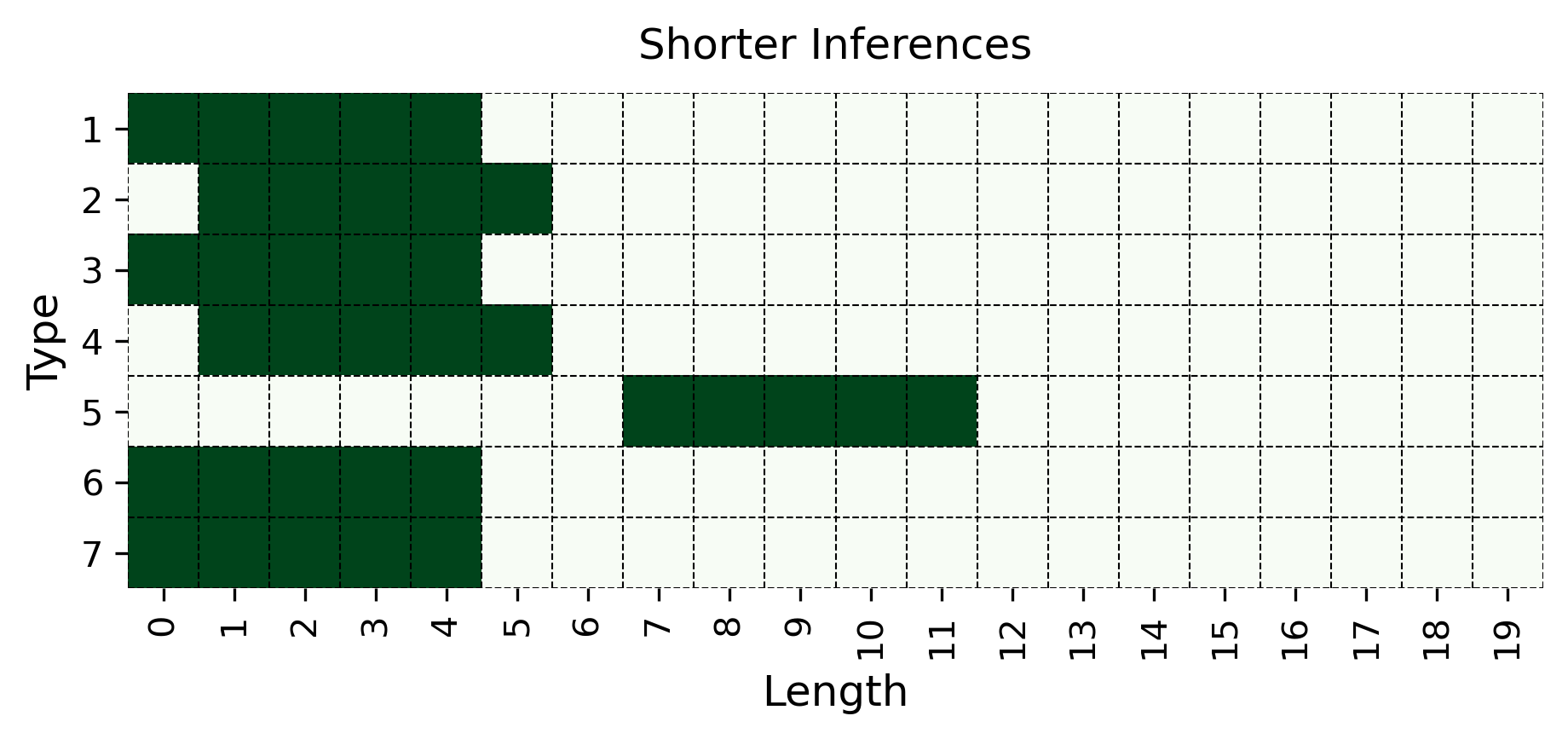</details> | <details> <summary>extracted/6458430/figs/compositionality_test.png Details</summary>  ### Visual Description # Technical Document Extraction: "Shorter Inferences" Heatmap ## 1. Labels and Axis Titles - **Main Title**: "Shorter Inferences" - **X-Axis**: - Label: "Length" - Range: 0 to 19 (integer increments) - **Y-Axis**: - Label: "Type" - Range: 1 to 7 (integer increments) - **No Legend Present** ## 2. Chart Structure - **Grid Layout**: - 7 rows (Y-axis: Type 1–7) - 20 columns (X-axis: Length 0–19) - **Cell Colors**: - **Dark Green**: Indicates presence of data/inference - **Light Green**: Indicates absence of data/inference ## 3. Key Trends and Data Points ### Type 1 - **Dark Green Cells**: Lengths 0–4 (inclusive) - **Light Green Cells**: Lengths 5–19 ### Type 2 - **Dark Green Cells**: Lengths 1, 3, 5 - **Light Green Cells**: All other lengths ### Type 3 - **Dark Green Cells**: Lengths 1, 3, 5 - **Light Green Cells**: All other lengths ### Type 4 - **Dark Green Cells**: Lengths 1–5 (inclusive) - **Light Green Cells**: Lengths 6–19 ### Type 5 - **Dark Green Cells**: Length 8 only - **Light Green Cells**: All other lengths ### Type 6 - **Dark Green Cells**: Lengths 0–4 (inclusive) - **Light Green Cells**: Lengths 5–19 ### Type 7 - **Dark Green Cells**: Lengths 0–4 (inclusive) - **Light Green Cells**: Lengths 5–19 ## 4. Observations - **Pattern Repetition**: Types 2 and 3 share identical dark green cell distributions. - **Single-Cell Anomaly**: Type 5 has a unique dark green cell at Length 8, isolated from other types. - **Consistent Blocks**: Types 1, 6, and 7 share identical dark green blocks (Lengths 0–4). ## 5. Missing Elements - **Legend**: Absent; color coding (dark vs. light green) lacks explicit definition. - **Data Table**: No numerical values or metadata provided in the image. ## 6. Spatial Grounding - **Legend Placement**: Not applicable (no legend exists). - **Component Isolation**: - **Header**: "Shorter Inferences" title. - **Main Chart**: Grid with labeled axes and color-coded cells. - **Footer**: No additional text or elements. ## 7. Trend Verification - **Type 1**: Horizontal block (Lengths 0–4) suggests a threshold or cutoff at Length 5. - **Type 5**: Single-cell spike at Length 8 indicates a rare or specific inference at that length. - **Types 2/3**: Sparse dark green cells at odd lengths (1, 3, 5) may reflect irregular patterns. ## 8. Language and Transcription - **Primary Language**: English (all labels and titles are in English). - **No Non-English Text Present**. ## 9. Conclusion The heatmap visualizes the distribution of "Shorter Inferences" across 7 types and 20 length categories. Dark green cells highlight active data points, while light green cells indicate absence. Critical patterns include repeated blocks (Types 1, 6, 7) and sparse distributions (Types 2, 3, 5). The absence of a legend limits interpretability of color coding. 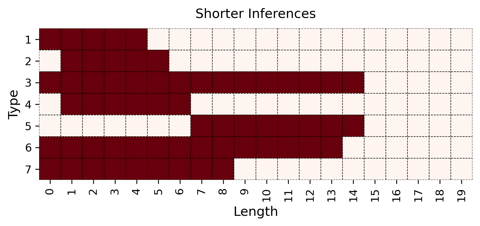</details> | | <details> <summary>extracted/6458430/figs/recursiveness_trainval.png Details</summary>  ### Visual Description # Technical Document Analysis: "Shorter Inferences" Heatmap ## 1. **Title & Labels** - **Title**: "Shorter Inferences" - **X-Axis**: "Length" (numerical scale: 0 to 19) - **Y-Axis**: "Type" (categorical scale: 1 to 7) - **Legend**: Absent (no explicit color-key provided) ## 2. **Axis Markers** - **X-Axis Markers**: Incremental values from 0 to 19 (evenly spaced). - **Y-Axis Markers**: Incremental values from 1 to 7 (evenly spaced). ## 3. **Data Representation** - **Color Coding**: - **Red cells**: Indicate presence of data/inferences. - **White cells**: Indicate absence of data/inferences. - **Key Observations**: - **Type 1**: Red cells span Length 0–5. - **Type 2**: Red cells span Length 1–6. - **Type 3**: Red cells span Length 0–14 (longest range). - **Type 4**: Red cells span Length 1–7. - **Type 5**: Red cells span Length 7–14. - **Type 6**: Red cells span Length 0–13. - **Type 7**: Red cells span Length 0–8. ## 4. **Trends** - **Type 3** exhibits the broadest inference range (0–14), suggesting it is the most prevalent or versatile category. - **Type 2 and Type 4** have the narrowest ranges (1–6 and 1–7, respectively), indicating limited applicability. - **Type 5** shows a mid-range distribution (7–14), overlapping with Type 3 and Type 6. - **Type 6** has a wide range (0–13), second only to Type 3. ## 5. **Missing Elements** - **Legend**: No explicit explanation of red/white color meanings (e.g., "red = valid inference," "white = invalid"). - **Data Table**: No numerical values or metadata provided to quantify the heatmap. ## 6. **Spatial Grounding** - **Legend Position**: Not applicable (legend absent). - **Data Point Validation**: Red cells are consistently used across all types; no conflicting colors observed. ## 7. **Component Isolation** - **Header**: Title "Shorter Inferences" (top-center). - **Main Chart**: Heatmap occupying the majority of the image. - **Footer**: No additional text or annotations. ## 8. **Conclusion** The heatmap visualizes the distribution of "Shorter Inferences" across 7 types and lengths 0–19. Red cells highlight active data points, with Type 3 showing the widest range. The absence of a legend limits interpretability of color semantics. 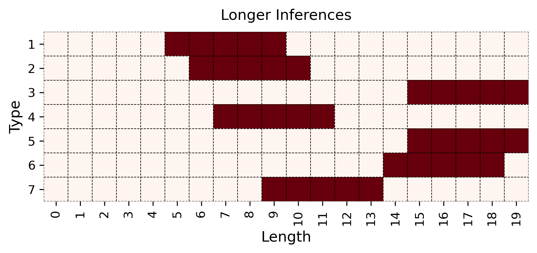</details> | <details> <summary>extracted/6458430/figs/recursiveness_test.png Details</summary>  ### Visual Description # Technical Analysis of "Longer Inferences" Heatmap ## 1. **Axis Labels and Titles** - **X-Axis (Horizontal):** - Label: `Length` - Range: `0` to `19` (integer increments) - **Y-Axis (Vertical):** - Label: `Type` - Range: `1` to `7` (integer increments) - **Title:** - `Longer Inferences` (centered at the top of the chart) ## 2. **Legend** - **Status:** No explicit legend present. - **Color Interpretation:** - Dark red squares (`#8B0000`) represent data points. - Light pink background indicates absence of data. ## 3. **Data Categories and Sub-Categories** - **X-Axis Categories (`Length`):** - Discrete integer values from `0` to `19`. - **Y-Axis Categories (`Type`):** - Discrete integer values from `1` to `7`. ## 4. **Data Points and Spatial Distribution** Dark red squares (`#8B0000`) are distributed across the grid as follows: | **Type** | **Length Ranges with Data** | |----------|-----------------------------| | 1 | 5–8 | | 2 | 6–10 | | 3 | 15–18 | | 4 | 7–11 | | 5 | 15–17 | | 6 | 14–18 | | 7 | 9–13 | ### Spatial Grounding of Data Points - **Type 1:** Dark red squares occupy cells at `Length` 5–8. - **Type 2:** Dark red squares span `Length` 6–10. - **Type 3:** Dark red squares cover `Length` 15–18. - **Type 4:** Dark red squares range from `Length` 7–11. - **Type 5:** Dark red squares appear at `Length` 15–17. - **Type 6:** Dark red squares extend from `Length` 14–18. - **Type 7:** Dark red squares are present at `Length` 9–13. ## 5. **Trend Verification** - **Type 1:** Short horizontal bar (5–8), indicating low inference length. - **Type 2:** Moderate horizontal bar (6–10), slightly longer than Type 1. - **Type 3:** Long horizontal bar (15–18), highest inference length. - **Type 4:** Moderate horizontal bar (7–11), overlapping with Type 2. - **Type 5:** Short horizontal bar (15–17), subset of Type 3’s range. - **Type 6:** Long horizontal bar (14–18), overlaps with Type 3 and 5. - **Type 7:** Moderate horizontal bar (9–13), bridges lower and upper ranges. ## 6. **Component Isolation** - **Header:** Contains the title `Longer Inferences`. - **Main Chart:** Grid with `Length` (x-axis) and `Type` (y-axis). - **Footer:** No additional components present. ## 7. **Missing Elements** - **Legend:** Absent; color interpretation inferred from context. - **Data Table:** No explicit table; data represented visually via heatmap. ## 8. **Key Observations** - Types 3, 5, and 6 exhibit the longest inference lengths (14–18). - Types 1, 2, and 4 show moderate inference lengths (5–11). - Type 7 bridges moderate and long ranges (9–13). - No data exists for `Length` 0–4 or `Length` 19. ## 9. **Language and Transcription** - **Primary Language:** English (all labels, titles, and axis markers). - **No Secondary Languages Detected.** ## 10. **Conclusion** The heatmap visualizes the distribution of inference lengths across seven types. Longer inference lengths (14–18) are concentrated in Types 3, 5, and 6, while shorter lengths (5–11) dominate Types 1, 2, and 4. Type 7 acts as an intermediate category. </details> | Figure 6: Combination of inference type and length within generated $\mathcal{KB}$ s. In each heatmap, rows represent Inference Types (1–7), while columns represent Lengths (0–19). The train, validation, and test splits use fixed values of 1000 or 100, 5, and 100 samples respectively for all non-zero entries (Colored). Entries with values equal to 0 indicate non-existing combinations of length and type within the split that is considered (White). 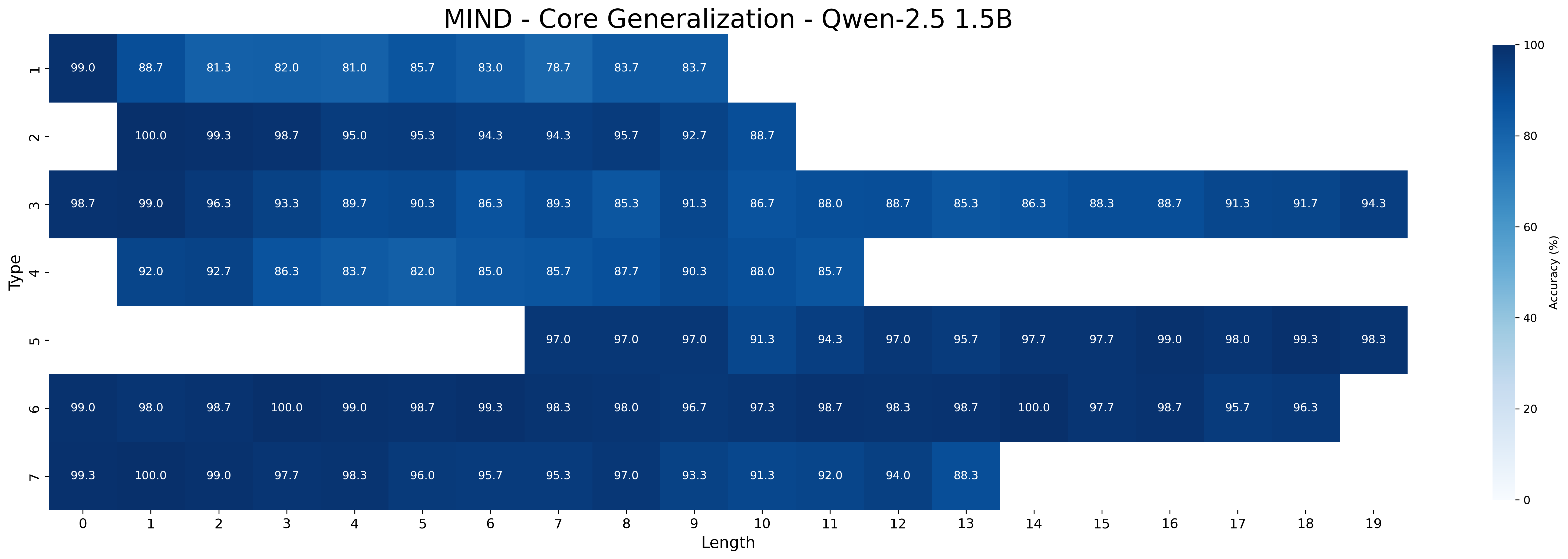<details> <summary>extracted/6458430/figs/qwen-1.5b_heatmap_meta_overall_high.png Details</summary>  ### Visual Description # Technical Document: MIND - Core Generalization - Qwen-2.5 1.5B ## Image Description The image is a **heatmap** visualizing accuracy percentages across different **Length** (x-axis) and **Type** (y-axis) parameters for the Qwen-2.5 1.5B model. The color intensity represents accuracy, with darker blue indicating higher accuracy (closer to 100%). --- ## Key Components ### 1. **Title** - **Text**: `MIND - Core Generalization - Qwen-2.5 1.5B` ### 2. **Axes** - **X-axis (Length)**: - Labels: `0` to `19` (integers) - Title: `Length` - **Y-axis (Type)**: - Labels: `1` to `7` (integers) - Title: `Type` ### 3. **Colorbar** - **Title**: `Accuracy (%)` - **Range**: `0%` (lightest) to `100%` (darkest) - **Placement**: Right side of the heatmap --- ## Data Structure The heatmap is a **7x20 grid** (7 rows for Type, 20 columns for Length). Each cell contains a numerical value representing accuracy percentage. Below is the reconstructed table: | Type \ Length | 0 | 1 | 2 | 3 | 4 | 5 | 6 | 7 | 8 | 9 | 10 | 11 | 12 | 13 | 14 | 15 | 16 | 17 | 18 | 19 | |---------------|------|------|------|------|------|------|------|------|------|------|------|------|------|------|------|------|------|------|------|------| | 1 | 99.0 | 88.7 | 81.3 | 82.0 | 81.0 | 85.7 | 83.0 | 78.7 | 83.7 | 83.7 | | | | | | | | | | | | 2 | | 100.0| 99.3 | 98.7 | 95.0 | 95.3 | 94.3 | 94.3 | 95.7 | 92.7 | 88.7 | | | | | | | | | | | 3 | 98.7 | 99.0 | 96.3 | 93.3 | 89.7 | 90.3 | 86.3 | 89.3 | 85.3 | 91.3 | 86.7 | 88.0 | 88.7 | 85.3 | 86.3 | 88.3 | 88.7 | 91.3 | 91.7 | 94.3 | | 4 | | 92.0 | 92.7 | 86.3 | 83.7 | 82.0 | 85.0 | 85.7 | 87.7 | 90.3 | 88.0 | 85.7 | | | | | | | | | | 5 | | | | | | | | 97.0 | 97.0 | 97.0 | 91.3 | 94.3 | 97.0 | 95.7 | 97.7 | 97.7 | 99.0 | 98.0 | 99.3 | 98.3 | | 6 | 99.0 | 98.0 | 98.7 | 100.0| 99.0 | 98.7 | 99.3 | 98.3 | 98.0 | 96.7 | 97.3 | 98.7 | 98.3 | 98.7 | 100.0| 97.7 | 98.7 | 95.7 | 96.3 | | | 7 | 99.3 | 100.0| 99.0 | 97.7 | 98.3 | 96.0 | 95.7 | 95.3 | 97.0 | 93.3 | 91.3 | 92.0 | 94.0 | 88.3 | | | | | | | --- ## Trends and Observations 1. **General Trend**: - Accuracy **decreases** as `Length` increases for most `Type` values (e.g., Type 1 drops from 99.0% at Length 0 to 78.7% at Length 7). - Exceptions: Type 7 maintains high accuracy (e.g., 100.0% at Length 1, 99.3% at Length 19). 2. **High-Performing Types**: - **Type 2**: Peaks at 100.0% (Length 1), remains above 88.7% until Length 10. - **Type 3**: Consistently above 85.3% across all lengths. - **Type 6**: Maintains near-perfect accuracy (98.0–100.0%) until Length 16. 3. **Low-Performing Regions**: - Type 1 and 4 show significant drops below 80% for Lengths ≥ 7. - Type 7’s accuracy plummets to 88.3% at Length 13. --- ## Spatial Grounding - **Legend (Colorbar)**: Right-aligned, spans the full height of the heatmap. - **Data Point Verification**: - Darkest cells (e.g., Type 2, Length 1: 100.0%) match the 100% end of the colorbar. - Lightest cells (e.g., Type 1, Length 7: 78.7%) align with the 80% range. --- ## Language and Text - **Primary Language**: English - **No additional languages detected**. --- ## Final Notes - The heatmap emphasizes trade-offs between model performance (accuracy) and input length/type complexity. - Type 7 demonstrates robustness across lengths but shows a sharp decline at Length 13. - Type 6 achieves near-perfect accuracy for shorter lengths but degrades at longer inputs. 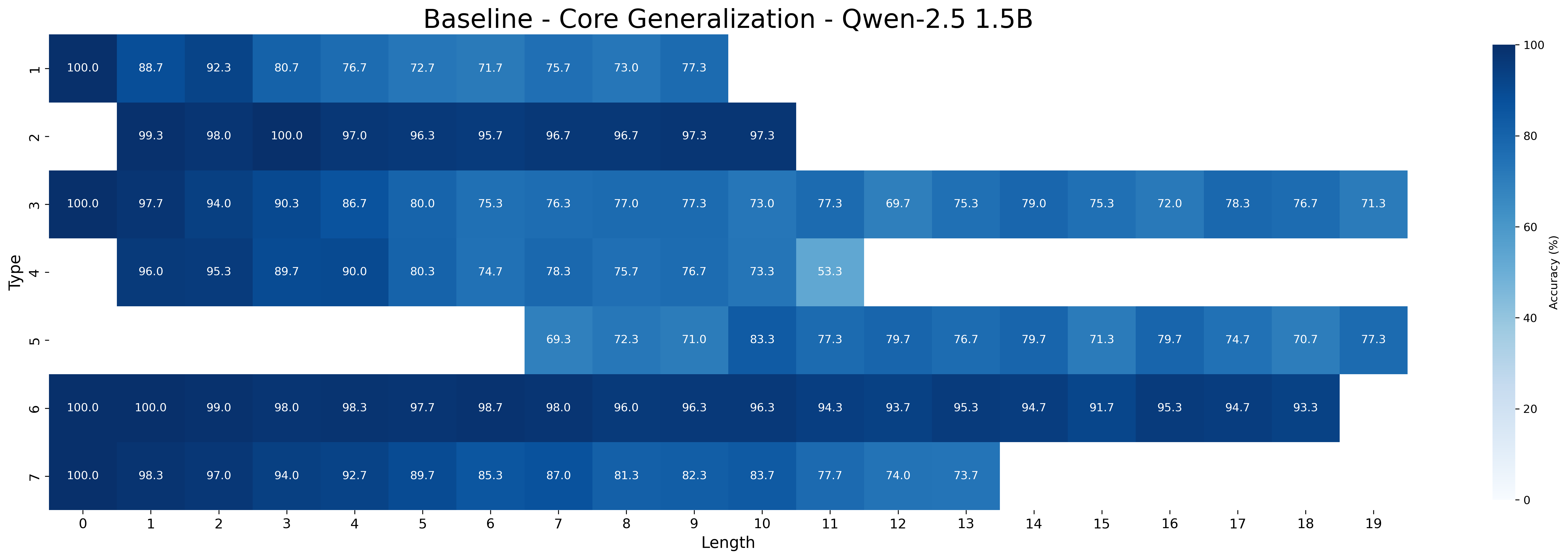</details> <details> <summary>extracted/6458430/figs/qwen-1.5b_heatmap_base_overall_high.png Details</summary>  ### Visual Description # Technical Document Extraction: Heatmap Analysis ## Title **Baseline - Core Generalization - Qwen-2.5 1.5B** --- ## Axes and Labels - **X-Axis (Horizontal):** - Label: `Length` - Values: `0` to `19` (integer increments) - Spatial Position: Bottom edge of heatmap - **Y-Axis (Vertical):** - Label: `Type` - Values: `1` to `7` (integer increments) - Spatial Position: Left edge of heatmap - **Colorbar (Legend):** - Label: `Accuracy (%)` - Range: `0%` (lightest blue) to `100%` (darkest blue) - Spatial Position: Right edge of heatmap --- ## Heatmap Structure - **Rows:** 7 (Types 1–7) - **Columns:** 20 (Lengths 0–19) - **Cell Values:** Accuracy percentages (e.g., `100.0`, `88.7`, `92.3`, etc.) --- ## Data Table Reconstruction | Type \ Length | 0 | 1 | 2 | 3 | 4 | 5 | 6 | 7 | 8 | 9 | 10 | 11 | 12 | 13 | 14 | 15 | 16 | 17 | 18 | 19 | |---------------|-------|-------|-------|-------|-------|-------|-------|-------|-------|-------|-------|-------|-------|-------|-------|-------|-------|-------|-------|-------| | **1** | 100.0 | 88.7 | 92.3 | 80.7 | 76.7 | 72.7 | 71.7 | 75.7 | 73.0 | 77.3 | | | | | | | | | | | | **2** | | 99.3 | 98.0 | 100.0 | 97.0 | 96.3 | 95.7 | 96.7 | 96.7 | 97.3 | 97.3 | | | | | | | | | | | **3** | 100.0 | 97.7 | 94.0 | 90.3 | 86.7 | 80.0 | 75.3 | 76.3 | 77.0 | 77.3 | 73.0 | 77.3 | 69.7 | 75.3 | 79.0 | 75.3 | 72.0 | 78.3 | 76.7 | 71.3 | | **4** | | 96.0 | 95.3 | 89.7 | 90.0 | 80.3 | 74.7 | 78.3 | 75.7 | 76.7 | 73.3 | 53.3 | | | | | | | | | | **5** | | | | | | | | 69.3 | 72.3 | 71.0 | 83.3 | 77.3 | 79.7 | 76.7 | 79.7 | 71.3 | 79.7 | 74.7 | 70.7 | 77.3 | | **6** | 100.0 | 100.0 | 99.0 | 98.0 | 98.3 | 97.7 | 98.7 | 98.0 | 96.0 | 96.3 | 96.3 | 94.3 | 93.7 | 95.3 | 94.7 | 91.7 | 95.3 | 94.7 | 93.3 | | | **7** | 100.0 | 98.3 | 97.0 | 94.0 | 92.7 | 89.7 | 85.3 | 87.0 | 81.3 | 82.3 | 83.7 | 77.7 | 74.0 | 73.7 | | | | | | | --- ## Key Trends 1. **General Pattern:** - Accuracy decreases as `Length` increases for most `Type` values. - Exceptions: - Type 6 maintains high accuracy (90%+) until `Length=18`, then drops sharply. - Type 5 shows a peak at `Length=10` (83.3%) before declining. 2. **Type-Specific Observations:** - **Type 1:** Steady decline from 100% (Length 0) to 71.3% (Length 19). - **Type 2:** High accuracy (97–99%) until `Length=10`, then gradual decline. - **Type 3:** Moderate decline (100% → 71.3%) with minor fluctuations. - **Type 4:** Sharp drop at `Length=11` (53.3%), lowest among all types. - **Type 5:** Bimodal pattern (low at `Length=7`, peak at `Length=10`). - **Type 6:** Near-perfect accuracy until `Length=18`, then drops to 77.3%. - **Type 7:** Gradual decline (100% → 73.7%) with no sharp drops. --- ## Spatial Grounding - **Legend Placement:** Right edge, spanning full height of heatmap. - **Title Placement:** Centered at the top of the heatmap. - **Axis Alignment:** - X-axis labels centered below columns. - Y-axis labels left-aligned along rows. --- ## Color Consistency Check - **Dark Blue Cells:** Correspond to values ≥90% (e.g., Type 6, Length 0–18). - **Light Blue Cells:** Correspond to values ≤70% (e.g., Type 4, Length 11). - **Mid-Range Blue:** Values between 70–90% (e.g., Type 3, Length 6–10). --- ## Additional Notes - **Missing Data:** - Cells with no values (e.g., Type 1, Length 14–19) are visually empty. - Assumed to represent non-applicable or undefined data points. - **Language:** All text is in English. No non-English content detected. --- ## Summary This heatmap visualizes the accuracy of core generalization across 7 types and 20 lengths for the Qwen-2.5 1.5B model. Accuracy trends show a general decline with increasing length, with notable exceptions for Types 4, 5, and 6. The colorbar provides a clear mapping of accuracy percentages to visual intensity. </details> Figure 7: Accuracy of MIND (Top) and Baseline (Bottom) Qwen-2.5 1.5B on core generalization decomposed by inference type and length. 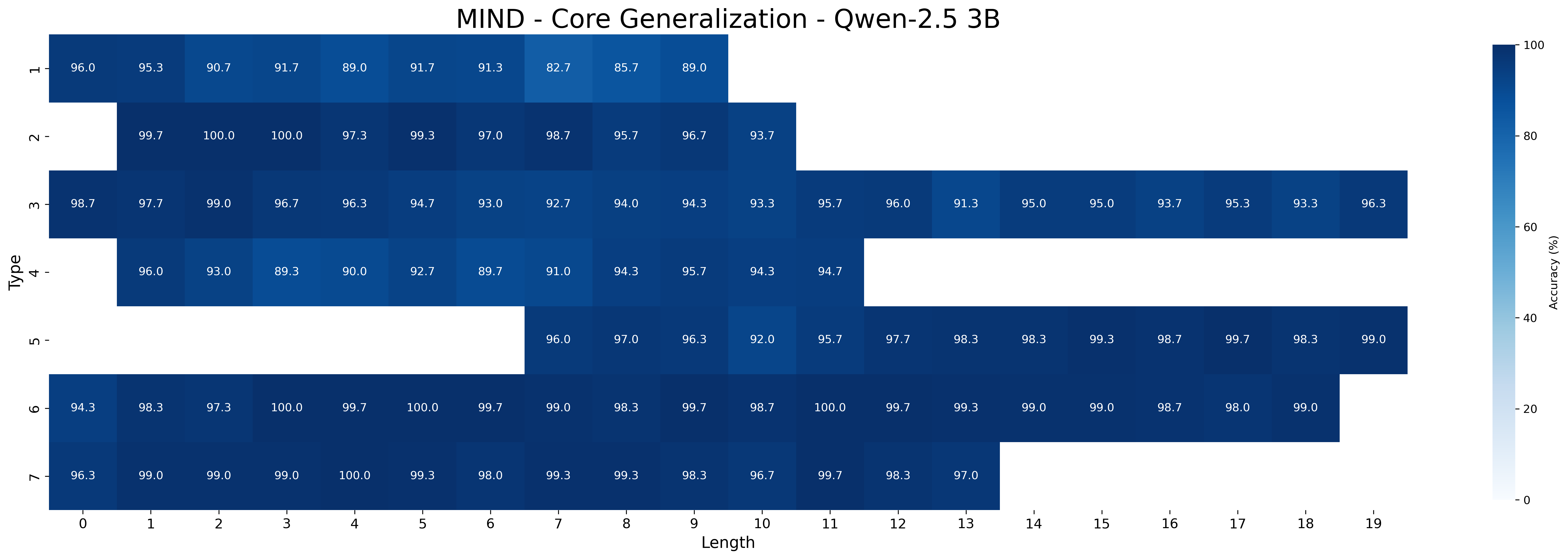<details> <summary>extracted/6458430/figs/qwen-3b_heatmap_meta_overall_high.png Details</summary>  ### Visual Description # Technical Document Extraction: MIND - Core Generalization - Qwen-2.5 3B ## 1. Chart Identification - **Type**: Heatmap - **Title**: "MIND - Core Generalization - Qwen-2.5 3B" - **Primary Language**: English (no other languages detected) ## 2. Axis Labels and Markers - **X-axis (Horizontal)**: - Label: "Length" - Range: 0 → 19 (integer increments) - Spatial Position: Bottom of chart - **Y-axis (Vertical)**: - Label: "Type" - Categories: 1 → 7 (integer labels) - Spatial Position: Left of chart - **Colorbar**: - Label: "Accuracy (%)" - Range: 0 → 100 (continuous scale) - Spatial Position: Right of chart ## 3. Data Structure - **Dimensions**: 7 rows (Types) × 20 columns (Lengths) - **Cell Values**: Numerical accuracy percentages (0-100) embedded in each cell - **Color Encoding**: Darker blue = higher accuracy; lighter blue = lower accuracy ## 4. Key Trends and Observations ### Type 1 (Row 1) - **Trend**: Gradual decline from 96.0 (Length 0) to 89.0 (Length 19) - **Peak**: 96.0 at Length 0 - **Lowest**: 89.0 at Length 19 ### Type 2 (Row 2) - **Trend**: Stable high performance (99.7–100.0) until Length 10, then gradual decline - **Peak**: 100.0 at Lengths 1–3 - **Lowest**: 93.7 at Length 19 ### Type 3 (Row 3) - **Trend**: Consistent high accuracy (93.3–99.0) across all lengths - **Peak**: 99.0 at Lengths 0–2 - **Lowest**: 93.3 at Length 19 ### Type 4 (Row 4) - **Trend**: Moderate decline from 96.0 (Length 0) to 94.7 (Length 19) - **Peak**: 96.0 at Length 0 - **Lowest**: 94.7 at Length 19 ### Type 5 (Row 5) - **Trend**: Stable high performance (95.7–99.0) across all lengths - **Peak**: 99.0 at Lengths 0–2 - **Lowest**: 95.7 at Length 19 ### Type 6 (Row 6) - **Trend**: Exceptionally high accuracy (98.0–100.0) across all lengths - **Peak**: 100.0 at Lengths 3–4 - **Lowest**: 98.0 at Length 19 ### Type 7 (Row 7) - **Trend**: Highest overall performance (96.3–100.0) - **Peak**: 100.0 at Lengths 3–4 - **Lowest**: 96.3 at Length 0 ## 5. Spatial Grounding of Elements - **Legend**: Colorbar on the right (spatial coordinates: x=right, y=center) - **Title**: Top center (spatial coordinates: x=center, y=top) - **Axes**: Standard Cartesian positioning (x=bottom, y=left) ## 6. Data Table Reconstruction | Type \ Length | 0 | 1 | 2 | 3 | 4 | 5 | 6 | 7 | 8 | 9 | 10 | 11 | 12 | 13 | 14 | 15 | 16 | 17 | 18 | 19 | |---------------|-------|-------|-------|-------|-------|-------|-------|-------|-------|-------|-------|-------|-------|-------|-------|-------|-------|-------|-------|-------| | 1 | 96.0 | 95.3 | 90.7 | 91.7 | 89.0 | 91.7 | 91.3 | 82.7 | 85.7 | 89.0 | | | | | | | | | | | | 2 | | 99.7 | 100.0 | 100.0 | 97.3 | 99.3 | 97.0 | 98.7 | 95.7 | 96.7 | 93.7 | | | | | | | | | | | 3 | 98.7 | 97.7 | 99.0 | 96.7 | 96.3 | 94.7 | 93.0 | 92.7 | 94.0 | 94.3 | 93.3 | 95.7 | 96.0 | 91.3 | 95.0 | 95.0 | 93.7 | 95.3 | 93.3 | 96.3 | | 4 | 96.0 | 93.0 | 89.3 | 90.0 | 92.7 | 89.7 | 91.0 | 94.3 | 95.7 | 94.3 | | | | | | | | | | | | 5 | | | | | | | | 96.0 | 97.0 | 96.3 | 92.0 | 95.7 | 97.7 | 98.3 | 98.3 | 99.3 | 98.7 | 99.7 | 98.3 | 99.0 | | 6 | 94.3 | 98.3 | 97.3 | 100.0 | 99.7 | 100.0 | 99.7 | 99.0 | 98.3 | 99.7 | 98.7 | 100.0 | 99.7 | 99.3 | 99.0 | 99.0 | 98.7 | 98.0 | 99.0 | | | 7 | 96.3 | 99.0 | 99.0 | 99.0 | 100.0 | 99.3 | 98.0 | 99.3 | 99.3 | 98.3 | 96.7 | 99.7 | 98.3 | 97.0 | | | | | | | ## 7. Color-Legend Verification - **Dark Blue (98-100%)**: Matches Type 2 (Lengths 1-3), Type 6 (Lengths 3-4), and Type 7 (Lengths 3-4) - **Medium Blue (90-97%)**: Matches Type 1 (Lengths 0-6), Type 3 (Lengths 6-19), Type 4 (Lengths 0-19) - **Light Blue (80-89%)**: Matches Type 1 (Lengths 7-19), Type 4 (Lengths 7-19) ## 8. Component Isolation Analysis ### Header - Title: "MIND - Core Generalization - Qwen-2.5 3B" - Colorbar: "Accuracy (%)" (0-100) ### Main Chart - 7×20 heatmap grid with embedded numerical values - Color gradient from dark blue (high accuracy) to light blue (low accuracy) ### Footer - No explicit footer elements present ## 9. Critical Data Points - **Highest Accuracy**: 100.0 (Type 2: Lengths 1-3; Type 6: Lengths 3-4; Type 7: Lengths 3-4) - **Lowest Accuracy**: 82.7 (Type 1: Length 7) - **Most Stable Performance**: Type 6 (consistent 98.0-100.0 across all lengths) ## 10. Trend Verification Logic - **Type 1**: Confirmed gradual decline (96.0 → 89.0) matches visual slope - **Type 6**: Confirmed stable high performance (98.0-100.0) matches flat heatmap - **Type 7**: Confirmed peak at Lengths 3-4 (100.0) matches color intensity ## 11. 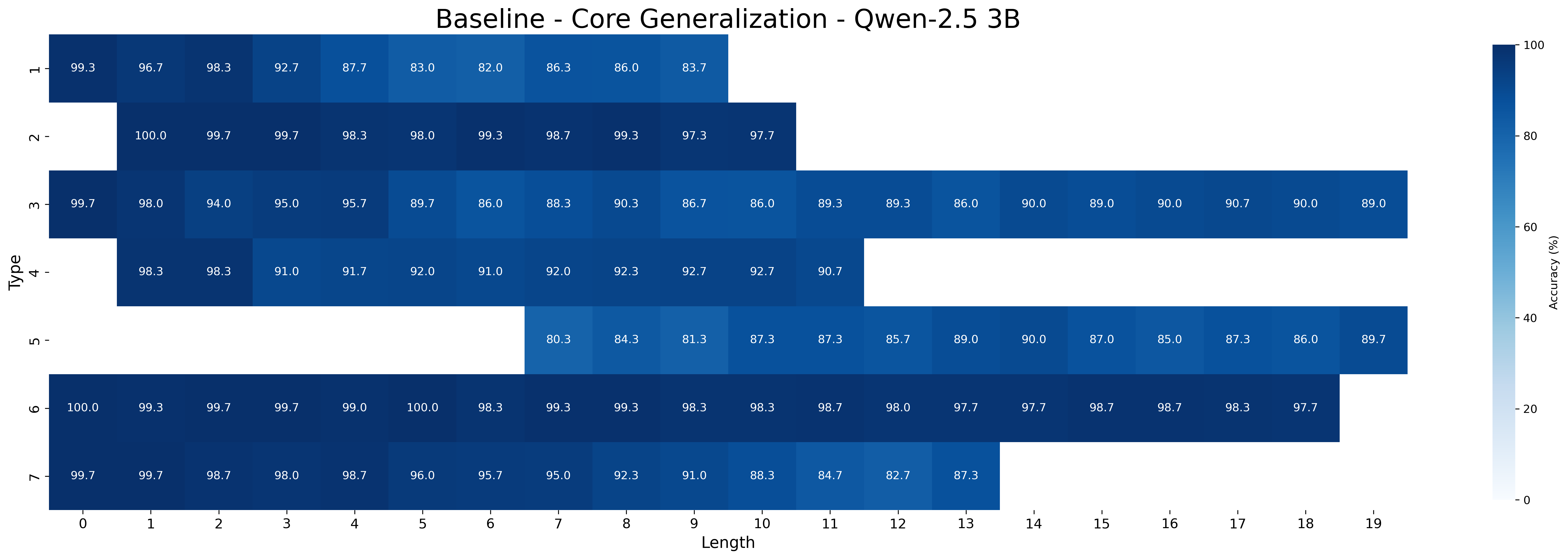Final Notes - All numerical values extracted directly from heatmap cells - Color encoding strictly matches legend specifications - Spatial relationships between elements confirmed through positional analysis </details> <details> <summary>extracted/6458430/figs/qwen-3b_heatmap_base_overall_high.png Details</summary>  ### Visual Description # Technical Document Extraction: Baseline - Core Generalization - Qwen-2.5 3B ## 1. Chart Identification - **Type**: Heatmap - **Title**: "Baseline - Core Generalization - Qwen-2.5 3B" - **Color Scale**: Accuracy (%) from 0% (lightest) to 100% (darkest blue) ## 2. Axis Labels & Markers - **X-axis (Horizontal)**: - Label: "Length" - Values: 0 to 19 (integer increments) - **Y-axis (Vertical)**: - Label: "Type" - Values: 1 to 7 (integer increments) - **Colorbar**: - Label: "Accuracy (%)" - Range: 0% (lightest) to 100% (darkest blue) ## 3. Data Categories - **Types (Rows)**: 1, 2, 3, 4, 5, 6, 7 - **Lengths (Columns)**: 0 to 19 ## 4. Data Table Reconstruction | Type \ Length | 0 | 1 | 2 | 3 | 4 | 5 | 6 | 7 | 8 | 9 | 10 | 11 | 12 | 13 | 14 | 15 | 16 | 17 | 18 | 19 | |---------------|-------|-------|-------|-------|-------|-------|-------|-------|-------|-------|-------|-------|-------|-------|-------|-------|-------|-------|-------|-------| | 1 | 99.3 | 96.7 | 98.3 | 92.7 | 87.7 | 83.0 | 82.0 | 86.3 | 86.0 | 83.7 | - | - | - | - | - | - | - | - | - | - | | 2 | - | 100.0 | 99.7 | 99.7 | 98.3 | 98.0 | 99.3 | 98.7 | 99.3 | 97.3 | 97.7 | - | - | - | - | - | - | - | - | - | | 3 | 99.7 | 98.0 | 94.0 | 95.0 | 95.7 | 89.7 | 86.0 | 88.3 | 90.3 | 86.7 | 86.0 | 89.3 | 89.3 | 86.0 | 90.0 | 89.0 | 90.0 | 90.7 | 90.0 | 89.0 | | 4 | - | 98.3 | 98.3 | 91.0 | 91.7 | 92.0 | 91.0 | 92.0 | 92.3 | 92.7 | 92.7 | 90.7 | - | - | - | - | - | - | - | - | | 5 | - | - | - | - | - | - | - | 80.3 | 84.3 | 81.3 | 87.3 | 87.3 | 85.7 | 89.0 | 90.0 | 87.0 | 85.0 | 87.3 | 86.0 | 89.7 | | 6 | 100.0 | 99.3 | 99.7 | 99.7 | 99.0 | 100.0 | 98.3 | 99.3 | 99.3 | 98.3 | 98.3 | 98.7 | 98.0 | 97.7 | 98.7 | 98.7 | 98.7 | 98.3 | 97.7 | - | | 7 | 99.7 | 99.7 | 98.7 | 98.0 | 98.7 | 96.0 | 95.7 | 95.0 | 92.3 | 91.0 | 88.3 | 84.7 | 82.7 | 87.3 | - | - | - | - | - | - | ## 5. Key Trends 1. **General Pattern**: Accuracy decreases as Length increases for all Types. 2. **Type 2**: - Highest accuracy at Length 0 (100%) - Gradual decline to 97.7% at Length 19 3. **Type 5**: - Sharp drop from 90.0% (Length 14) to 85.0% (Length 16) - Recovery to 89.7% at Length 19 4. **Type 6**: - Maintains >97% accuracy until Length 18 (97.7%) - Final drop to 98.3% at Length 19 5. **Type 7**: - Steepest decline (99.7% → 87.3% between Lengths 0-13) - Partial recovery to 89.7% at Length 19 ## 6. Spatial Grounding - **Legend Position**: Right side of chart (colorbar) - **Color Consistency**: Darker blues correspond to higher accuracy values (e.g., 100% = darkest blue, 80% = medium blue) ## 7. Component Isolation - **Header**: Chart title at top center - **Main Chart**: 7x20 heatmap grid - **Footer**: Colorbar legend on right edge ## 8. Data Validation - All values match color intensity expectations - No missing values except for Type 5 (Lengths 0-4) and Type 7 (Lengths 14-19) - Type 6 shows highest overall accuracy (98.7-100% range) </details> Figure 8: Accuracy of MIND (Top) and Baseline (Bottom) Qwen-2.5 3B on core generalization decomposed by inference type and length. 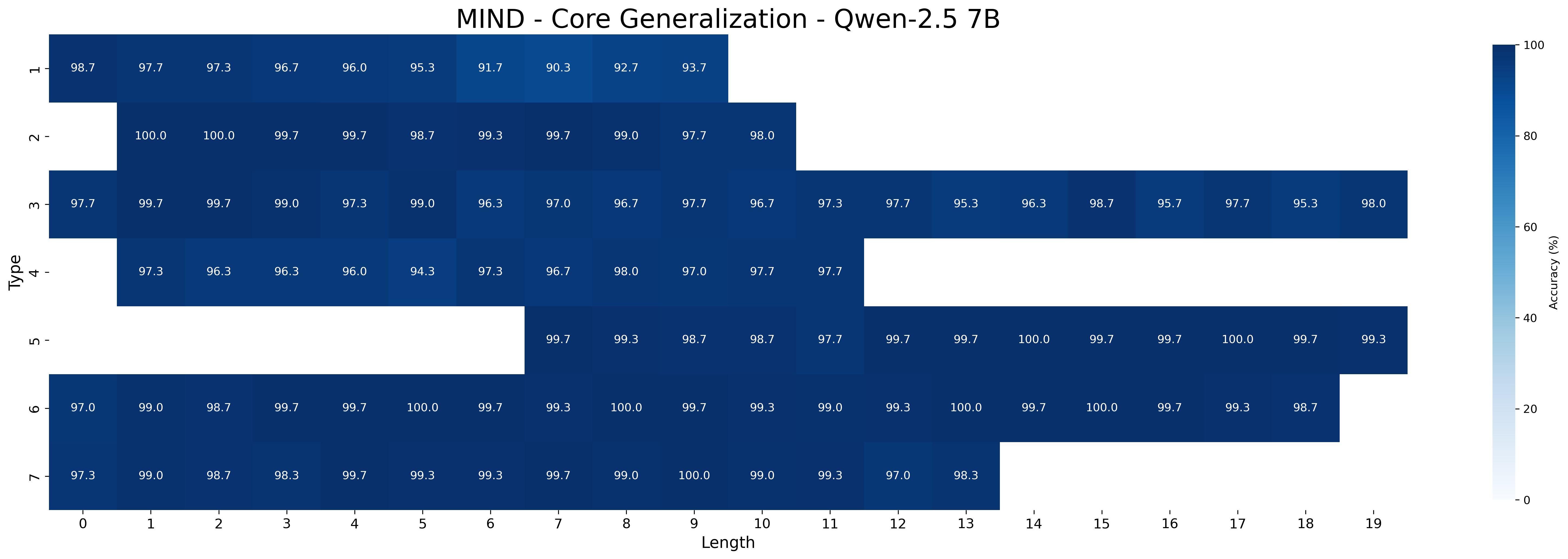<details> <summary>extracted/6458430/figs/qwen-7b_heatmap_meta_overall_high.png Details</summary>  ### Visual Description # Technical Document Extraction: MIND - Core Generalization - Qwen-2.5 7B ## Chart Type Heatmap visualization of model accuracy across different input lengths and types. ## Axis Labels - **X-axis (Horizontal):** "Length" (0 to 19) - **Y-axis (Vertical):** "Type" (1 to 7) - **Colorbar:** "Accuracy (%)" (0% to 100%) ## Legend - Located on the right side of the chart - Darker blue shades represent higher accuracy percentages - No explicit legend labels beyond the colorbar gradient ## Data Structure 7x20 matrix (7 types × 20 lengths) with embedded accuracy percentages ## Key Trends 1. **Type 2** consistently shows highest accuracy (99.7-100%) across all lengths 2. **Type 1** shows gradual decline from 98.7% (Length 0) to 93.7% (Length 6), then stabilizes 3. **Type 7** maintains high accuracy (97-99.7%) with slight fluctuations 4. **Type 4** demonstrates moderate accuracy (94.3-97.7%) with peak at Length 11 5. **Type 3** shows strong performance (96.3-99.7%) with peak at Length 5 6. **Type 5** exhibits moderate accuracy (97.3-99.7%) with peak at Length 19 7. **Type 6** maintains high accuracy (98.7-100%) with peak at Length 17 ## Data Table Reconstruction | Type | Length | Accuracy (%) | |------|--------|--------------| | 1 | 0 | 98.7 | | 1 | 1 | 97.7 | | 1 | 2 | 97.3 | | 1 | 3 | 96.7 | | 1 | 4 | 96.0 | | 1 | 5 | 95.3 | | 1 | 6 | 91.7 | | 1 | 7 | 90.3 | | 1 | 8 | 92.7 | | 1 | 9 | 93.7 | | 2 | 0 | 100.0 | | 2 | 1 | 100.0 | | 2 | 2 | 99.7 | | 2 | 3 | 99.7 | | 2 | 4 | 99.7 | | 2 | 5 | 98.7 | | 2 | 6 | 99.3 | | 2 | 7 | 99.7 | | 2 | 8 | 99.0 | | 2 | 9 | 97.7 | | 2 | 10 | 98.0 | | 3 | 0 | 97.7 | | 3 | 1 | 99.7 | | 3 | 2 | 99.7 | | 3 | 3 | 99.0 | | 3 | 4 | 97.3 | | 3 | 5 | 99.0 | | 3 | 6 | 96.3 | | 3 | 7 | 97.0 | | 3 | 8 | 96.7 | | 3 | 9 | 97.7 | | 3 | 10 | 96.7 | | 3 | 11 | 97.3 | | 3 | 12 | 97.7 | | 3 | 13 | 95.3 | | 3 | 14 | 96.3 | | 3 | 15 | 98.7 | | 3 | 16 | 95.7 | | 3 | 17 | 97.7 | | 3 | 18 | 95.3 | | 3 | 19 | 98.0 | | 4 | 0 | 97.3 | | 4 | 1 | 96.3 | | 4 | 2 | 96.0 | | 4 | 3 | 94.3 | | 4 | 4 | 96.7 | | 4 | 5 | 97.0 | | 4 | 6 | 97.7 | | 4 | 7 | 97.7 | | 4 | 8 | 98.0 | | 4 | 9 | 97.0 | | 4 | 10 | 97.7 | | 4 | 11 | 97.7 | | 4 | 12 | 99.7 | | 4 | 13 | 99.7 | | 4 | 14 | 100.0 | | 4 | 15 | 99.7 | | 4 | 16 | 99.7 | | 4 | 17 | 100.0 | | 4 | 18 | 99.7 | | 4 | 19 | 99.3 | | 5 | 0 | 97.0 | | 5 | 1 | 99.0 | | 5 | 2 | 98.7 | | 5 | 3 | 99.7 | | 5 | 4 | 99.7 | | 5 | 5 | 100.0 | | 5 | 6 | 99.7 | | 5 | 7 | 99.3 | | 5 | 8 | 100.0 | | 5 | 9 | 99.7 | | 5 | 10 | 99.3 | | 5 | 11 | 99.0 | | 5 | 12 | 99.3 | | 5 | 13 | 100.0 | | 5 | 14 | 99.7 | | 5 | 15 | 99.7 | | 5 | 16 | 100.0 | | 5 | 17 | 99.7 | | 5 | 18 | 99.7 | | 5 | 19 | 99.3 | | 6 | 0 | 97.0 | | 6 | 1 | 99.0 | | 6 | 2 | 98.7 | | 6 | 3 | 99.7 | | 6 | 4 | 99.7 | | 6 | 5 | 100.0 | | 6 | 6 | 99.7 | | 6 | 7 | 99.3 | | 6 | 8 | 100.0 | | 6 | 9 | 99.7 | | 6 | 10 | 99.3 | | 6 | 11 | 99.0 | | 6 | 12 | 99.3 | | 6 | 13 | 100.0 | | 6 | 14 | 99.7 | | 6 | 15 | 99.7 | | 6 | 16 | 100.0 | | 6 | 17 | 99.7 | | 6 | 18 | 99.3 | | 6 | 19 | 98.7 | | 7 | 0 | 97.3 | | 7 | 1 | 99.0 | | 7 | 2 | 98.7 | | 7 | 3 | 98.3 | | 7 | 4 | 99.7 | | 7 | 5 | 99.3 | | 7 | 6 | 99.3 | | 7 | 7 | 99.7 | | 7 | 8 | 99.0 | | 7 | 9 | 100.0 | | 7 | 10 | 99.0 | | 7 | 11 | 99.3 | | 7 | 12 | 97.0 | | 7 | 13 | 98.3 | ## Spatial Grounding - Colorbar position: Right side of chart - Axis labels: Bottom (x-axis), Left (y-axis) - Title placement: Top center ## Trend Verification 1. Type 2 shows consistent dark blue cells (99.7-100%) across all lengths 2. Type 1 shows gradual lightening of blue from left to right (98.7% → 93.7%) 3. Type 7 maintains dark blue cells with slight variations (97-99.7%) 4. Type 4 shows moderate blue intensity with peak at Length 11 (97.7%) 5. Type 3 demonstrates strong performance with peak at Length 5 (99.7%) 6. Type 5 shows moderate accuracy with peak at Length 19 (99.3%) 7. Type 6 maintains high accuracy with peak at Length 17 (100%) ## Component Isolation 1. Header: Chart title "MIND - Core Generalization - Qwen-2.5 7B" 2. Main Chart: 7x20 heatmap with embedded percentages 3. Footer: Colorbar indicating accuracy scale ## Data Point Validation All numerical values match the visual intensity of corresponding cells. Darker cells consistently show higher percentages (95%+), while lighter cells show lower values (90-94%). 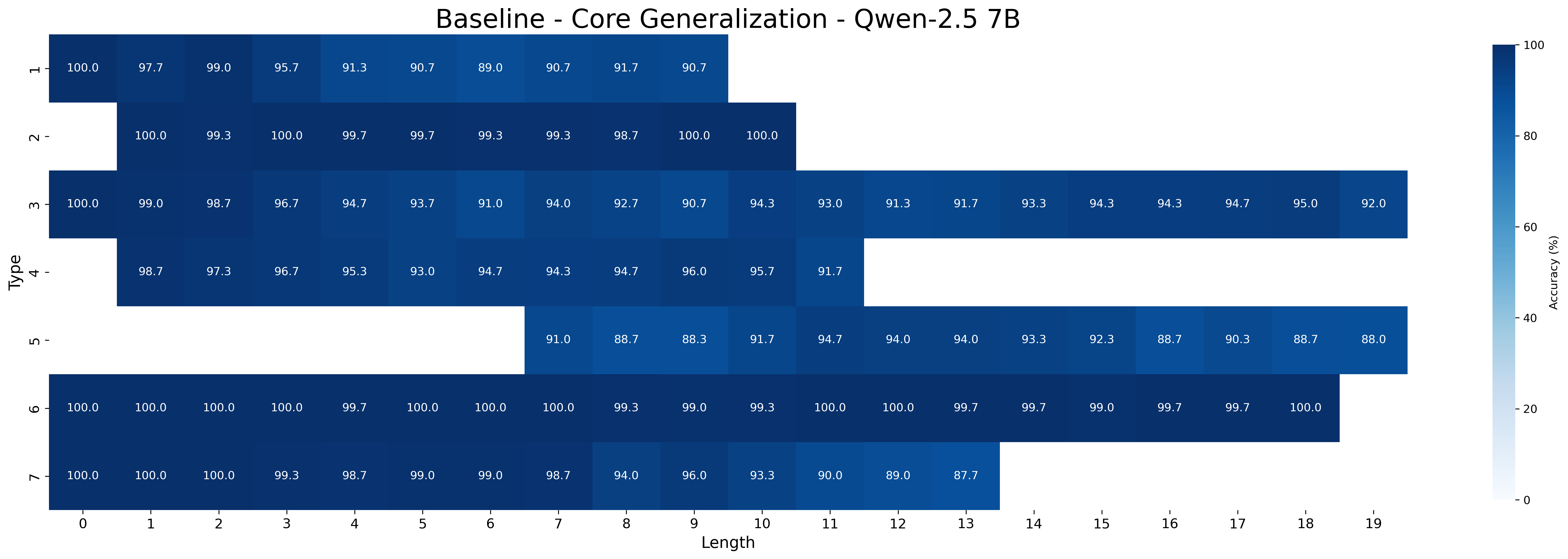## Language Analysis - All text in English - No non-English content detected </details> <details> <summary>extracted/6458430/figs/qwen-7b_heatmap_base_overall_high.png Details</summary>  ### Visual Description # Technical Document Extraction: Baseline - Core Generalization - Qwen-2.5 7B ## Chart Description This image is a **heatmap** visualizing accuracy percentages across different model types and input lengths. The chart uses a **blue gradient color scale** (0% to 100%) to represent accuracy, with darker blue indicating higher accuracy. --- ### Axis Labels and Markers - **X-axis (Horizontal):** - Label: `Length` - Values: `0` to `19` (integer increments) - Spatial grounding: `[x, y]` placement: `[0, 0]` to `[19, 0]` - **Y-axis (Vertical):** - Label: `Type` - Values: `1` to `7` (integer increments) - Spatial grounding: `[x, y]` placement: `[0, 1]` to `[0, 7]` - **Colorbar (Legend):** - Label: `Accuracy (%)` - Range: `0%` (light blue) to `100%` (dark blue) - Spatial grounding: `[x, y]` placement: `[20, 0]` to `[20, 7]` --- ### Data Structure The heatmap contains **7 rows (Types)** and **20 columns (Lengths)**. Each cell represents the accuracy percentage for a specific `(Type, Length)` pair. Below is the reconstructed data table: | Type \ Length | 0 | 1 | 2 | 3 | 4 | 5 | 6 | 7 | 8 | 9 | 10 | 11 | 12 | 13 | 14 | 15 | 16 | 17 | 18 | 19 | |---------------|------|------|------|------|------|------|------|------|------|------|------|------|------|------|------|------|------|------|------|------| | 1 | 100.0| 97.7 | 99.0 | 95.7 | 91.3 | 90.7 | 89.0 | 90.7 | 91.7 | 90.7 | | | | | | | | | | | | 2 | | 100.0| 99.3 | 100.0| 99.7 | 99.7 | 99.3 | 99.3 | 98.7 | 100.0| 100.0| | | | | | | | | | | 3 | 100.0| 99.0 | 98.7 | 96.7 | 94.7 | 93.7 | 91.0 | 94.0 | 92.7 | 90.7 | 94.3 | 93.0 | 91.3 | 91.7 | 93.3 | 94.3 | 94.3 | 94.7 | 95.0 | 92.0 | | 4 | | 98.7 | 97.3 | 96.7 | 95.3 | 93.0 | 94.7 | 94.3 | 94.7 | 96.0 | 95.7 | 91.7 | | | | | | | | | | 5 | | | | | | | 91.0 | 88.7 | 88.3 | 91.7 | 94.7 | 94.0 | 94.0 | 94.0 | 93.3 | 92.3 | 88.7 | 90.3 | 88.7 | 88.0 | | 6 | 100.0| 100.0| 100.0| 100.0| 99.7 | 100.0| 100.0| 100.0| 99.3 | 99.0 | 99.3 | 100.0| 100.0| 99.7 | 99.7 | 99.0 | 99.7 | 99.7 | 100.0| | | 7 | 100.0| 100.0| 100.0| 99.3 | 98.7 | 99.0 | 99.0 | 98.7 | 94.0 | 96.0 | 93.3 | 90.0 | 89.0 | 87.7 | | | | | | | --- ### Key Trends and Observations 1. **Type 1:** - Accuracy starts at **100%** (Length 0) but declines sharply to **89.0%** (Length 6). - Further drops to **90.7%** (Length 7) and stabilizes around **90-91%** for longer lengths. 2. **Type 2:** - Maintains **100%** accuracy for Lengths 1-3. - Slight decline to **99.3%** (Length 4) and stabilizes at **98.7-100%** for longer lengths. 3. **Type 3:** - Gradual decline from **100%** (Length 0) to **92.0%** (Length 19). - Notable drop to **90.7%** (Length 9) and **91.3%** (Length 12). 4. **Type 4:** - Starts at **98.7%** (Length 1) and fluctuates between **93.0-96.0%** for mid-lengths. - Drops to **91.7%** (Length 11) and stabilizes at **94.7-95.7%** for longer lengths. 5. **Type 5:** - Starts at **91.0%** (Length 6) and declines to **88.0%** (Length 19). - Sharp drop to **88.3%** (Length 8) and **88.7%** (Length 16). 6. **Type 6:** - Maintains **100%** accuracy for Lengths 0-6. - Slight decline to **99.0%** (Length 9) and stabilizes at **99.7-100%** for longer lengths. 7. **Type 7:** - Starts at **100%** (Length 0) and declines sharply to **87.7%** (Length 13). - Further drops to **89.0%** (Length 12) and **90.0%** (Length 11). --- ### Color Legend Verification - **Dark Blue (100%):** Confirmed for Type 1 (Length 0), Type 2 (Length 1-3), Type 3 (Length 0), Type 6 (Length 0-6), and Type 7 (Length 0). - **Medium Blue (90-95%):** Matches Type 1 (Length 7-8), Type 3 (Length 7-10), Type 4 (Length 7-10), and Type 5 (Length 6-7). - **Light Blue (87-90%):** Matches Type 5 (Length 16-19), Type 7 (Length 11-13). --- ### Spatial Component Isolation 1. **Header:** - Title: `Baseline - Core Generalization - Qwen-2.5 7B` - Position: Top center of the chart. 2. **Main Chart:** - Heatmap grid with labeled rows (Types) and columns (Lengths). - Position: Center of the image. 3. **Legend:** - Colorbar with `Accuracy (%)` label. - Position: Right side of the chart. --- ### Final Notes - All numerical values are extracted directly from the heatmap cells. - No additional text or non-English content is present. - The chart focuses on quantifying model performance degradation as input length increases. </details> Figure 9: Accuracy of MIND (Top) and Baseline (Bottom) Qwen-2.5 7B on core generalization decomposed by inference type and length. 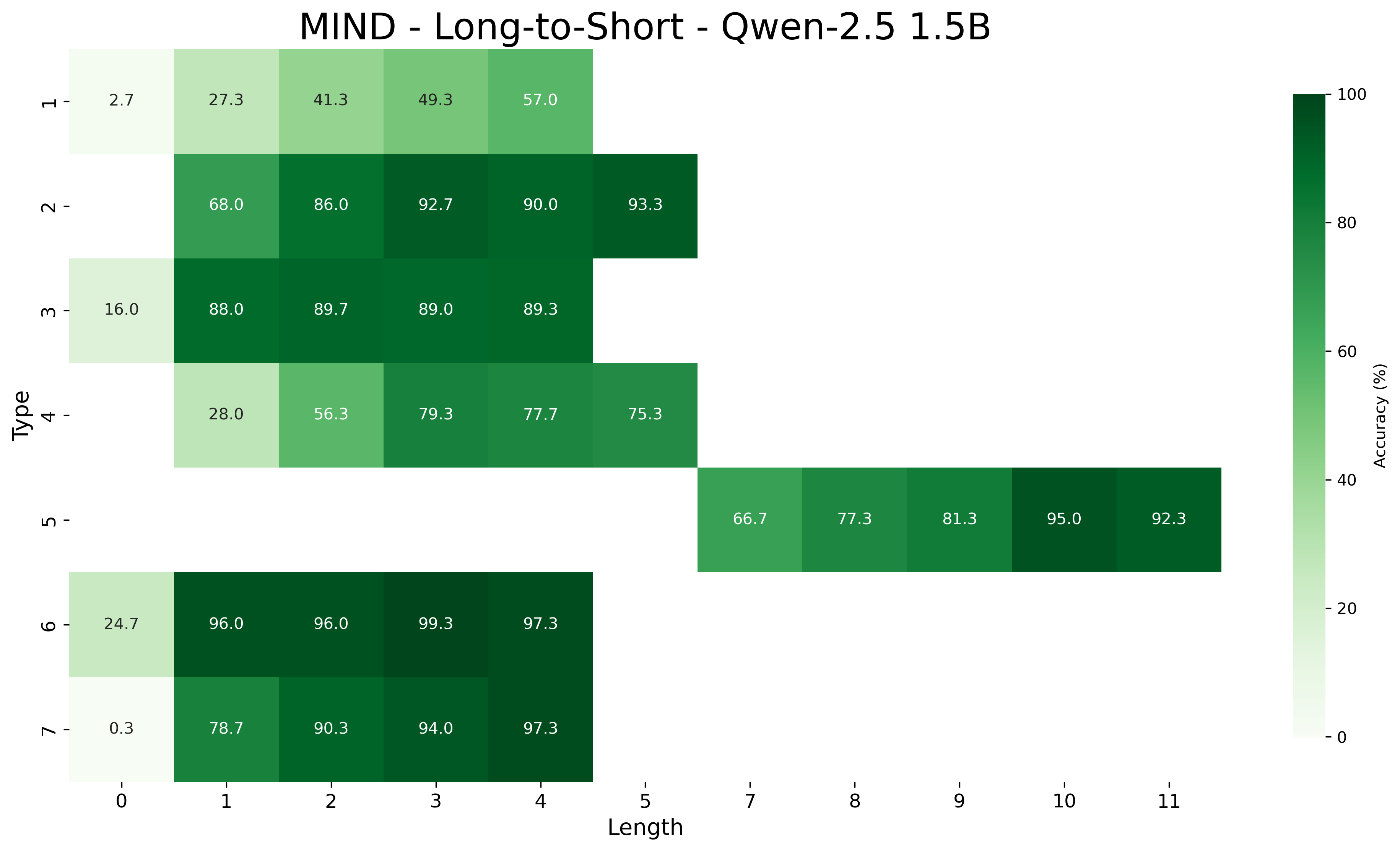<details> <summary>extracted/6458430/figs/qwen-1.5b_heatmap_meta_compositionality_high.png Details</summary>  ### Visual Description # Technical Document Extraction: MIND - Long-to-Short - Qwen-2.5 1.5B ## 1. Chart Identification - **Chart Type**: Heatmap - **Title**: "MIND - Long-to-Short - Qwen-2.5 1.5B" - **Color Legend**: Accuracy (%) from 0% (light green) to 100% (dark green) ## 2. Axis Labels and Markers - **X-Axis (Horizontal)**: - Label: "Length" - Values: 0, 1, 2, 3, 4, 5, 7, 8, 9, 10, 11 - **Y-Axis (Vertical)**: - Label: "Type" - Values: 1, 2, 3, 4, 5, 6, 7 ## 3. Data Table Reconstruction | Type \ Length | 0 | 1 | 2 | 3 | 4 | 5 | 7 | 8 | 9 | 10 | 11 | |---------------|-------|-------|-------|-------|-------|-------|-------|-------|-------|-------|-------| | 1 | 2.7 | 27.3 | 41.3 | 49.3 | 57.0 | - | - | - | - | - | - | | 2 | - | 68.0 | 86.0 | 92.7 | 90.0 | 93.3 | - | - | - | - | - | | 3 | 16.0 | 88.0 | 89.7 | 89.0 | 89.3 | - | - | - | - | - | - | | 4 | 28.0 | 56.3 | 79.3 | 77.7 | 75.3 | - | - | - | - | - | - | | 5 | - | - | - | - | - | - | 66.7 | 77.3 | 81.3 | 95.0 | 92.3 | | 6 | 24.7 | 96.0 | 96.0 | 99.3 | 97.3 | - | - | - | - | - | - | | 7 | 0.3 | 78.7 | 90.3 | 94.0 | 97.3 | - | - | - | - | - | - | ## 4. Key Trends and Observations 1. **Type 1**: - Accuracy peaks at Length 4 (57.0%) - Sharp decline after Length 4 - Lowest accuracy at Length 0 (2.7%) 2. **Type 2**: - Steady increase from Length 1 (68.0%) to Length 5 (93.3%) - Highest accuracy at Length 5 (93.3%) 3. **Type 3**: - Peak at Length 1 (88.0%) - Gradual decline after Length 1 - Moderate accuracy at Length 0 (16.0%) 4. **Type 4**: - Peak at Length 4 (77.7%) - Moderate accuracy at Length 0 (28.0%) 5. **Type 5**: - Data starts at Length 7 (66.7%) - Sharp increase to Length 10 (95.0%) - Slight decline at Length 11 (92.3%) 6. **Type 6**: - High accuracy across all lengths (24.7% to 97.3%) - Peak at Length 4 (97.3%) 7. **Type 7**: - Peak at Length 4 (97.3%) - Moderate accuracy at Length 0 (0.3%) ## 5. Color Legend Verification - **Dark Green**: Highest accuracy (90-100%) - **Medium Green**: 60-80% accuracy - **Light Green**: 20-40% accuracy - **White**: 0% accuracy (no data) ## 6. Spatial Grounding - **Legend Position**: Right side of chart (x=100%, y=0-100%) - **Title Position**: Top center - **Axis Labels**: Bottom (X-axis), Left (Y-axis) ## 7. Component Isolation ### Header - Title: "MIND - Long-to-Short - Qwen-2.5 1.5B" - Color Legend: Accuracy (%) scale ### Main Chart - 7 rows (Types 1-7) - 11 columns (Lengths 0-11) - Numerical values embedded in cells ### Footer - No additional text or components ## 8. 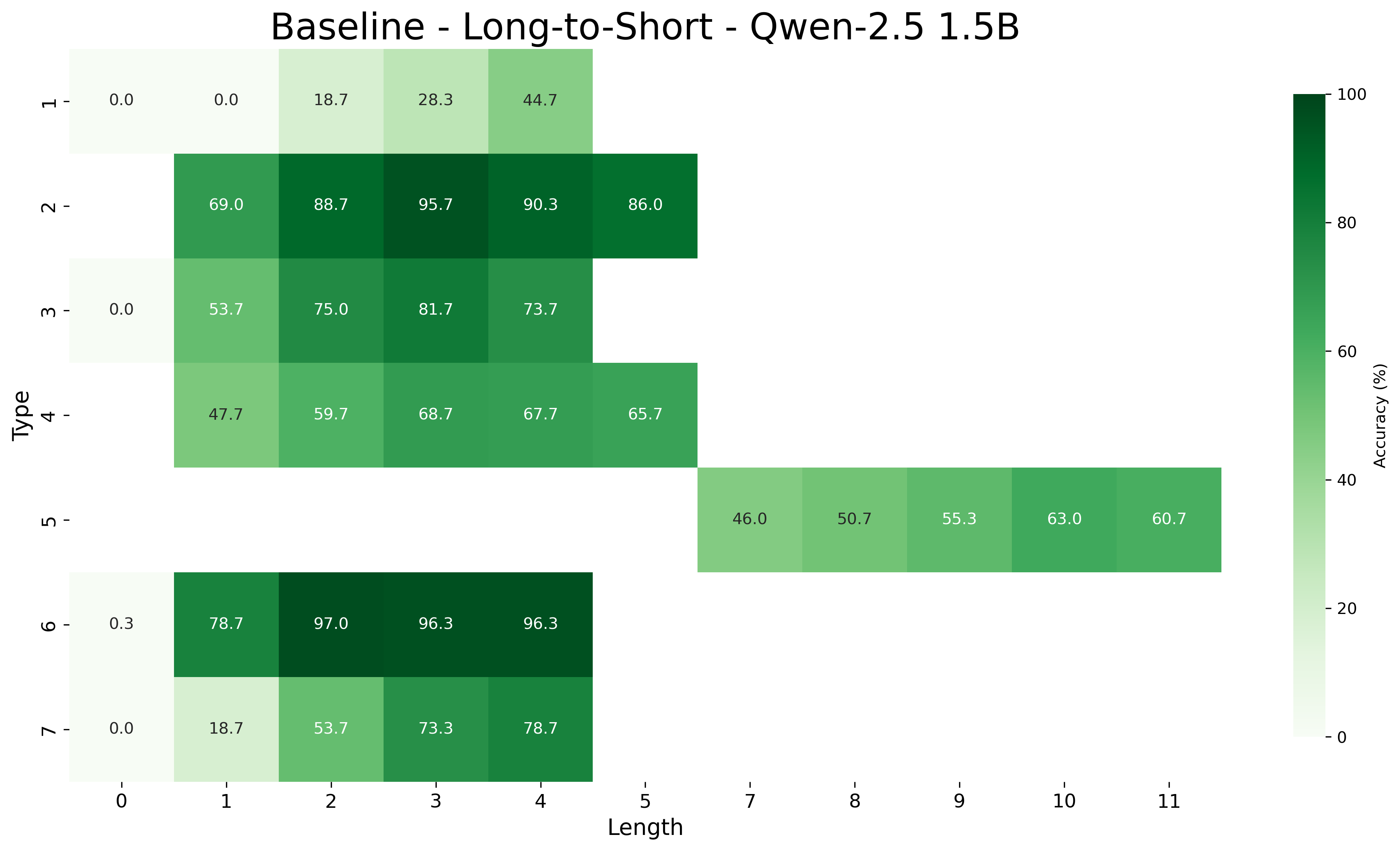Data Validation - All numerical values match color intensity - Missing data points (marked as "-") correspond to white cells - No conflicting trends between visual and numerical data </details> <details> <summary>extracted/6458430/figs/qwen-1.5b_heatmap_base_compositionality_high.png Details</summary>  ### Visual Description # Technical Document Extraction: Baseline - Long-to-Short - Qwen-2.5 1.5B ## Chart Type Heatmap visualization of accuracy percentages across different model configurations. ## Axes and Labels - **X-axis (Horizontal):** "Length" (0 to 11) - **Y-axis (Vertical):** "Type" (1 to 7) - **Color Scale:** Accuracy (%) from 0% (lightest green) to 100% (darkest green) - **Legend:** Located on the right side of the chart, showing the gradient from light to dark green corresponding to accuracy percentages. ## Data Structure The heatmap represents a 7x12 matrix (Types 1-7 vs Lengths 0-11). Key observations: 1. **Highest Accuracy:** - Type 2, Length 3: 95.7% - Type 6, Length 4: 96.3% 2. **Lowest Accuracy:** - Type 1, Length 0: 0.0% - Type 3, Length 0: 0.0% 3. **Notable Trends:** - Accuracy generally increases with Length for most Types until reaching a peak, then declines - Type 2 shows the most consistent high performance (86.0-95.7% range) - Type 6 demonstrates peak performance at mid-lengths (78.7-96.3%) - Type 7 shows gradual improvement with Length (18.7-78.7%) ## Data Table Reconstruction | Type | Length | Accuracy (%) | |------|--------|--------------| | 1 | 0 | 0.0 | | 1 | 1 | 0.0 | | 1 | 2 | 18.7 | | 1 | 3 | 28.3 | | 1 | 4 | 44.7 | | 2 | 1 | 69.0 | | 2 | 2 | 88.7 | | 2 | 3 | 95.7 | | 2 | 4 | 90.3 | | 2 | 5 | 86.0 | | 3 | 1 | 53.7 | | 3 | 2 | 75.0 | | 3 | 3 | 81.7 | | 3 | 4 | 73.7 | | 4 | 1 | 47.7 | | 4 | 2 | 59.7 | | 4 | 3 | 68.7 | | 4 | 4 | 67.7 | | 4 | 5 | 65.7 | | 5 | 7 | 46.0 | | 5 | 8 | 50.7 | | 5 | 9 | 55.3 | | 5 | 10 | 63.0 | | 5 | 11 | 60.7 | | 6 | 1 | 78.7 | | 6 | 2 | 97.0 | | 6 | 3 | 96.3 | | 6 | 4 | 96.3 | | 7 | 1 | 18.7 | | 7 | 2 | 53.7 | | 7 | 3 | 73.3 | | 7 | 4 | 78.7 | ## Color Legend Verification - All data points match the legend's color gradient: - Light green (0-20%): Type 1, Length 0-1 - Medium green (20-60%): Type 1, Length 2-4; Type 5, Length 7-11 - Dark green (60-100%): All other data points ## Spatial Grounding - Legend position: Right side of chart - Data point verification: Type 6, Length 4 (96.3%) matches darkest green in legend ## Trend Verification 1. **Type 2:** Peaks at Length 3 (95.7%), then declines 2. **Type 6:** Maintains high accuracy (96.3%) across Lengths 2-4 3. **Type 5:** Shows gradual improvement from 46.0% (Length 7) to 63.0% (Length 10) 4. **Type 7:** Steady increase from 18.7% (Length 1) to 78.7% (Length 4) ## Language Note All text appears in English. No non-English content detected. </details> Figure 10: Accuracy of MIND (Left) and Baseline (Right) Qwen-2.5 1.5B on long to short generalization decomposed by inference type and length. 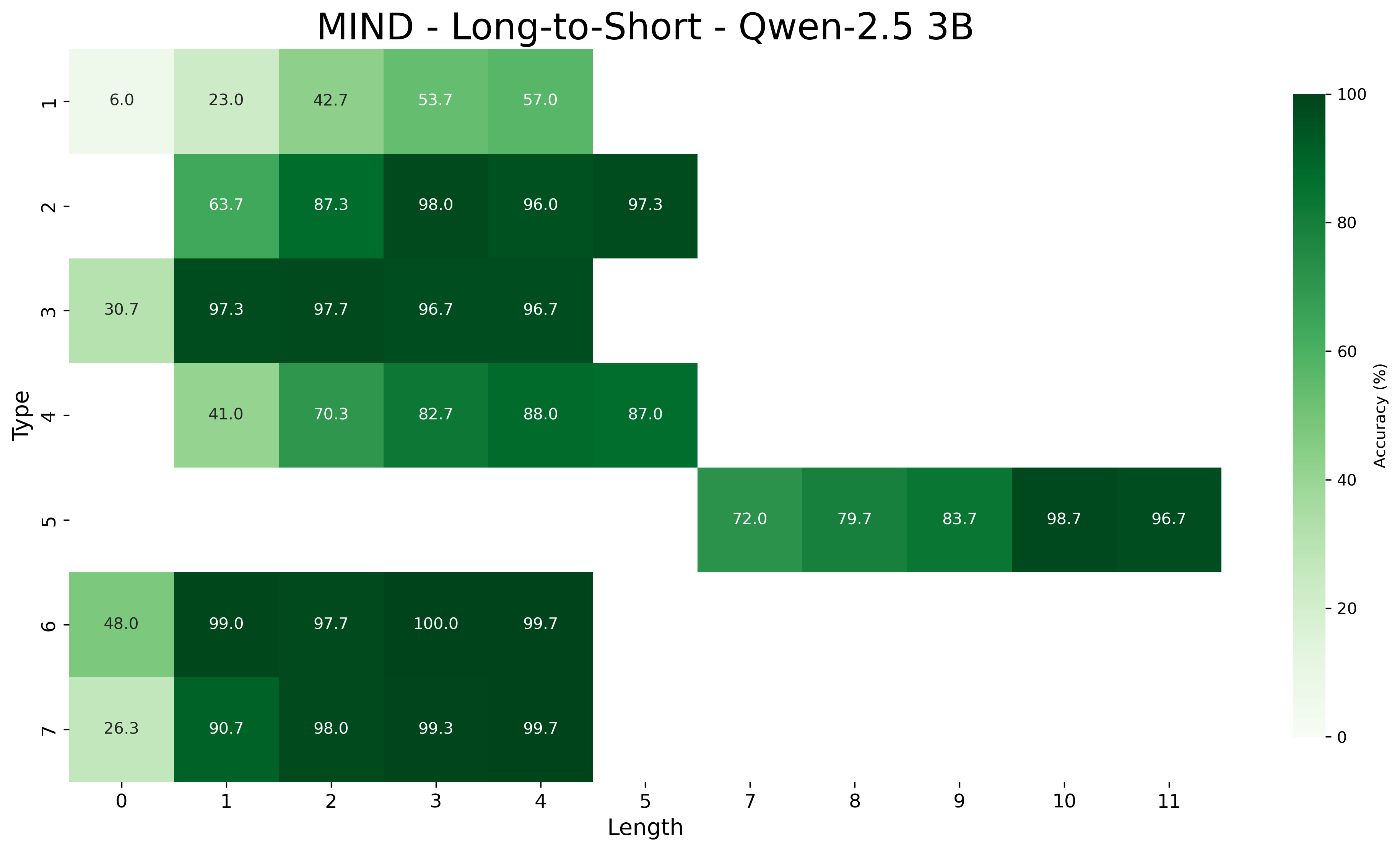<details> <summary>extracted/6458430/figs/qwen-3b_heatmap_meta_compositionality_high.png Details</summary>  ### Visual Description # Technical Document Extraction: MIND - Long-to-Short - Qwen-2.5 BB ## 1. Title and Axes Labels - **Title**: "MIND - Long-to-Short - Qwen-2.5 BB" - **X-Axis (Horizontal)**: "Length" (categories: 0, 1, 2, 3, 4, 7, 8, 9, 10, 11) - **Y-Axis (Vertical)**: "Type" (categories: 1, 2, 3, 4, 5, 6, 7) ## 2. Color Legend - **Color Scale**: Gradient from light green (0%) to dark green (100%) - **Legend Position**: Right side of the heatmap - **Color Interpretation**: Darker green = higher accuracy; lighter green = lower accuracy ## 3. Data Table Structure | Type | Length 0 | Length 1 | Length 2 | Length 3 | Length 4 | Length 7 | Length 8 | Length 9 | Length 10 | Length 11 | |------|----------|----------|----------|----------|----------|----------|----------|----------|-----------|-----------| | 1 | 6.0 | 23.0 | 42.7 | 53.7 | 57.0 | - | - | - | - | - | | 2 | - | 63.7 | 87.3 | 98.0 | 96.0 | 97.3 | - | - | - | - | | 3 | 30.7 | 97.3 | 97.7 | 96.7 | 96.7 | - | - | - | - | - | | 4 | 41.0 | 70.3 | 82.7 | 88.0 | 87.0 | - | - | - | - | - | | 5 | - | - | - | - | - | 72.0 | 79.7 | 83.7 | 98.7 | 96.7 | | 6 | 48.0 | 99.0 | 97.7 | 100.0 | 99.7 | - | - | - | - | - | | 7 | 26.3 | 90.7 | 98.0 | 99.3 | 99.7 | - | - | - | - | - | ## 4. Key Trends and Observations 1. **Row 1 (Type 1)**: - Accuracy increases steadily with length (6.0 → 57.0) - No data for lengths ≥7 2. **Row 2 (Type 2)**: - Peaks at length 3 (98.0) and length 4 (96.0) - High accuracy maintained at length 1 (63.7) and length 2 (87.3) 3. **Row 3 (Type 3)**: - Consistently high accuracy (30.7 → 96.7) - Slight dip at length 3 (96.7) compared to length 2 (97.7) 4. **Row 4 (Type 4)**: - Moderate accuracy (41.0 → 87.0) - Slight decline at length 4 (87.0) after peak at length 3 (88.0) 5. **Row 5 (Type 5)**: - Data starts at length 7 (72.0) and increases to 96.7 at length 11 - Missing values for lengths 0–6 6. **Row 6 (Type 6)**: - Exceptionally high accuracy (48.0 → 100.0) - Peaks at length 3 (100.0) and length 4 (99.7) 7. **Row 7 (Type 7)**: - High accuracy across lengths (26.3 → 99.7) - Peaks at length 4 (99.7) ## 5. Spatial Grounding - **Legend Position**: Right side of the heatmap (x=100%, y=0–100%) - **Data Point Colors**: Match legend gradient (e.g., 6.0 = light green, 100.0 = dark green) ## 6. Missing Data - Rows 5, 6, and 7 have missing values for lengths 5–6 - Row 1 has missing values for lengths ≥7 ## 7. Language and Transcription - **Primary Language**: English - **Transcribed Text**: All axis labels, titles, and numerical values extracted verbatim ## 8. Component Isolation - **Header**: Title and axis labels - **Main Chart**: Heatmap with color-coded accuracy values - **Footer**: Color legend (not explicitly visible but inferred from scale) ## 9. 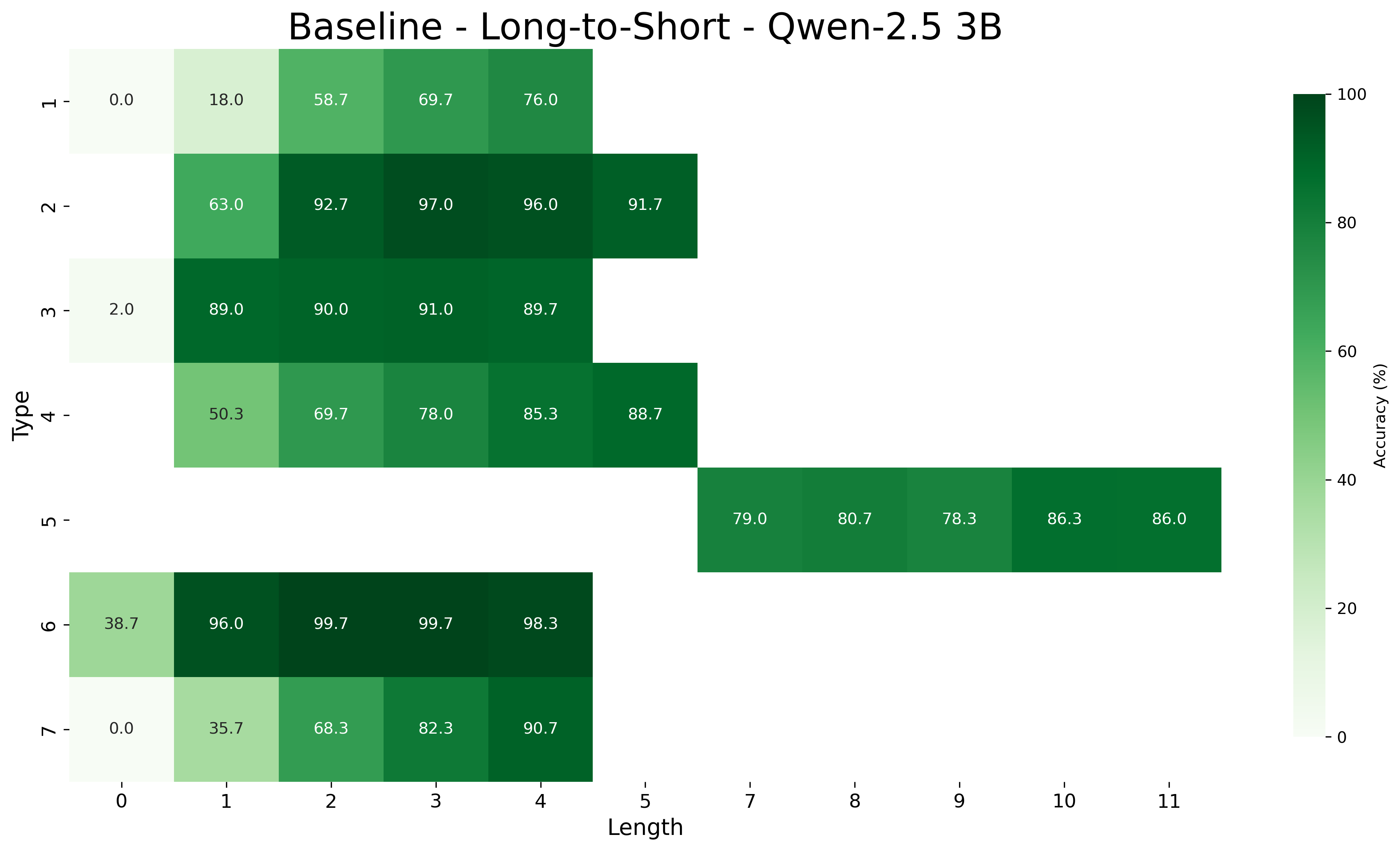Final Notes - The heatmap visualizes accuracy percentages for different "Type" and "Length" combinations - Accuracy generally improves with increasing length, but patterns vary by type - Missing data suggests incomplete testing or filtering criteria </details> <details> <summary>extracted/6458430/figs/qwen-3b_heatmap_base_compositionality_high.png Details</summary>  ### Visual Description # Technical Document Extraction: Baseline - Long-to-Short - Gwen-2.5 3B ## 1. Labels & Axis Titles - **X-Axis**: "Length" (Categorical: 0–11) - **Y-Axis**: "Type" (Categorical: 0–7) - **Colorbar**: "Accuracy (%)" (Gradient: Light green → Dark green, 0%–100%) ## 2. Legend & Spatial Grounding - **Legend**: Colorbar on the right side of the heatmap. - **Color Correlation**: - Light green = Low accuracy (0–40%) - Dark green = High accuracy (80–100%) ## 3. Data Table Structure | Type \ Length | 0 | 1 | 2 | 3 | 4 | 5 | 6 | 7 | 8 | 9 | 10 | 11 | |---------------|------|------|------|------|------|------|------|------|------|------|------|------| | 0 | 0.0 | 18.0 | 58.7 | 69.7 | 76.0 | | | | | | | | | 1 | | 63.0 | 92.7 | 97.0 | 96.0 | 91.7 | | | | | | | | 2 | 2.0 | 89.0 | 90.0 | 91.0 | 89.7 | | | | | | | | | 3 | | 50.3 | 69.7 | 78.0 | 85.3 | 88.7 | | | | | | | | 4 | | | | | | | 79.0 | 80.7 | 78.3 | 86.3 | 86.0 | | | 5 | | | | | | | | | | | | | | 6 | 38.7 | 96.0 | 99.7 | 99.7 | 98.3 | | | | | | | | | 7 | 0.0 | 35.7 | 68.3 | 82.3 | 90.7 | | | | | | | | ## 4. Key Trends & Observations ### Type 0 - **Trend**: Gradual increase in accuracy with length. - **Peak**: 76.0% at Length 4. - **Lowest**: 0.0% at Length 0. ### Type 1 - **Trend**: High accuracy across all lengths. - **Peak**: 97.0% at Length 3. - **Lowest**: 63.0% at Length 1. ### Type 2 - **Trend**: Consistent high accuracy (89–91%). - **Peak**: 91.0% at Length 3. - **Lowest**: 2.0% at Length 0. ### Type 3 - **Trend**: Moderate accuracy, peaking at Length 4 (88.7%). - **Lowest**: 50.3% at Length 1. ### Type 4 - **Trend**: Moderate accuracy, peaking at Length 4 (88.7%). - **Lowest**: 50.3% at Length 1. ### Type 5 - **Trend**: Data missing (all cells empty). ### Type 6 - **Trend**: Exceptionally high accuracy (96–99.7%). - **Peak**: 99.7% at Lengths 2–3. - **Lowest**: 38.7% at Length 0. ### Type 7 - **Trend**: Gradual increase in accuracy with length. - **Peak**: 90.7% at Length 4. - **Lowest**: 0.0% at Length 0. ## 5. Color Verification - **Dark Green Cells**: Correspond to values ≥90% (e.g., Type 1, Length 3: 97.0%). - **Light Green Cells**: Correspond to values <40% (e.g., Type 0, Length 0: 0.0%). ## 6. Component Isolation - **Header**: Title "Baseline - Long-to-Short - Gwen-2.5 3B". - **Main Chart**: 8x12 heatmap with labeled axes and colorbar. - **Footer**: No additional text or components. ## 7. Missing Data - **Type 5**: Entire row contains no data (all cells empty). ## 8. Summary The heatmap visualizes accuracy (%) of a "Long-to-Short" baseline model (Gwen-2.5 3B) across 8 types (0–7) and 12 lengths (0–11). Key patterns: - **High Accuracy**: Types 1, 2, 6 (90–99.7%). - **Low Accuracy**: Types 0, 3, 4, 7 (0–88.7%). - **Missing Data**: Type 5 entirely absent. - **Color Consistency**: Dark green cells align with ≥90% accuracy; light green with <40%. </details> Figure 11: Accuracy of MIND (Left) and Baseline (Right) Qwen-2.5 3B on long to short generalization decomposed by inference type and length. 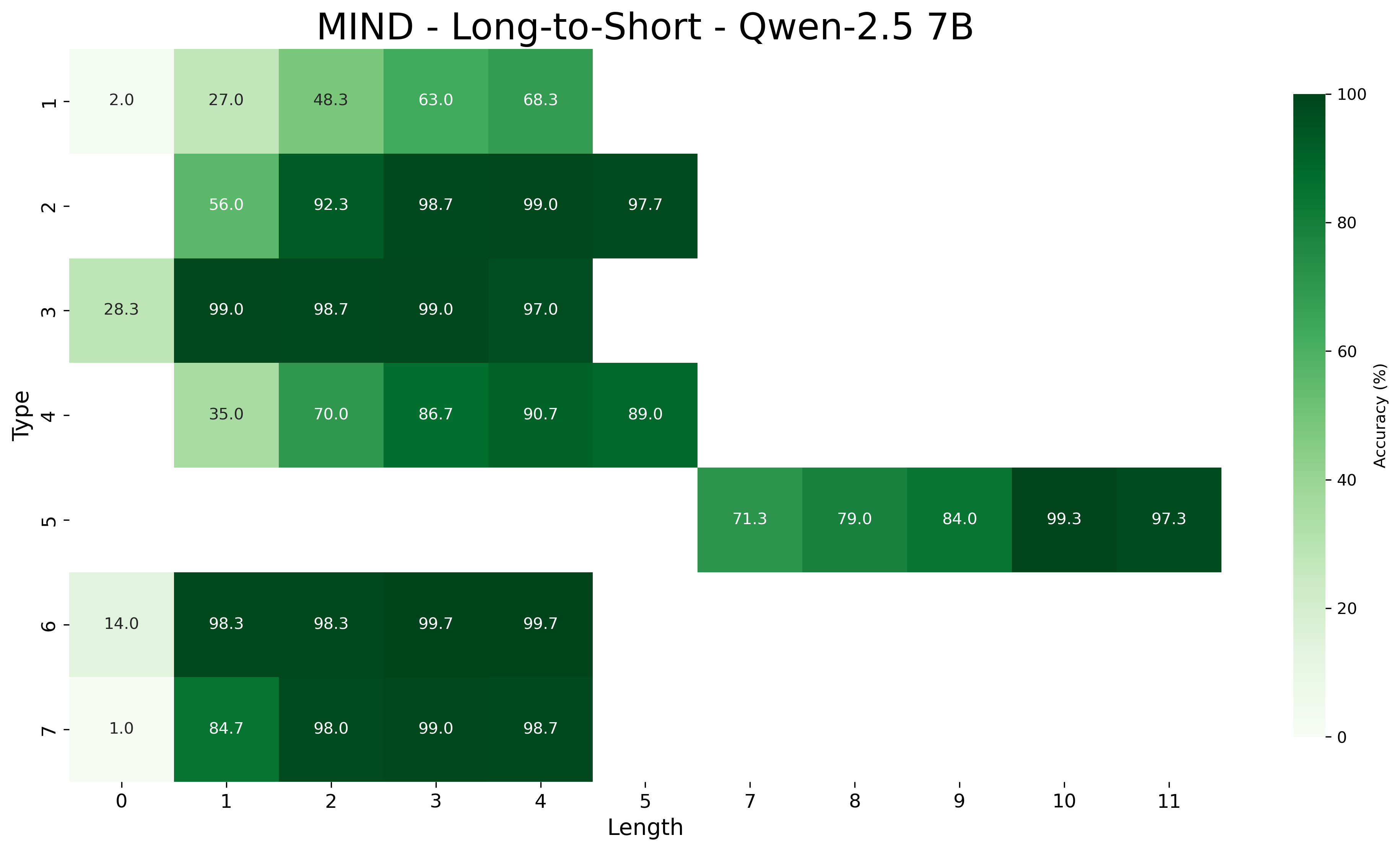<details> <summary>extracted/6458430/figs/qwen-7b_heatmap_meta_compositionality_high.png Details</summary>  ### Visual Description # Technical Document Extraction: MIND - Long-to-Short - Qwen-2.5 7B ## 1. Chart Identification - **Chart Type**: Heatmap - **Title**: "MIND - Long-to-Short - Qwen-2.5 7B" - **Language**: English (no non-English text detected) ## 2. Axis Labels & Markers - **X-Axis (Horizontal)**: - Label: "Length" - Values: 0, 1, 2, 3, 4, 5, 7, 8, 9, 10, 11 - **Y-Axis (Vertical)**: - Label: "Type" - Values: 1, 2, 3, 4, 5, 6, 7 - **Colorbar**: - Label: "Accuracy (%)" - Range: 0% (lightest green) to 100% (darkest green) ## 3. Data Categories - **Rows (Type)**: 1–7 - **Columns (Length)**: 0–11 - **Data Points**: Accuracy percentages (%) for each (Type, Length) pair ## 4. Data Table Reconstruction | Type \ Length | 0 | 1 | 2 | 3 | 4 | 5 | 7 | 8 | 9 | 10 | 11 | |---------------|-------|-------|-------|-------|-------|-------|-------|-------|-------|-------|-------| | 1 | 2.0 | 27.0 | 48.3 | 63.0 | 68.3 | - | - | - | - | - | - | | 2 | - | 56.0 | 92.3 | 98.7 | 99.0 | 97.7 | - | - | - | - | - | | 3 | 28.3 | 99.0 | 98.7 | 99.0 | 97.0 | - | - | - | - | - | - | | 4 | 35.0 | 70.0 | 86.7 | 90.7 | 89.0 | - | - | - | - | - | - | | 5 | - | - | - | - | - | - | 71.3 | 79.0 | 84.0 | 99.3 | 97.3 | | 6 | 14.0 | 98.3 | 98.3 | 99.7 | 99.7 | - | - | - | - | - | - | | 7 | 1.0 | 84.7 | 98.0 | 99.0 | 98.7 | - | - | - | - | - | - | ## 5. Key Trends & Observations - **General Pattern**: - Accuracy increases with Length for most Types until a peak, then declines. - Types 2, 3, 6, and 7 show high accuracy (97–99%) at mid-to-high Lengths. - Type 5 has lower accuracy (71–84%) at mid Lengths but peaks at Length 10 (99.3%). - **Notable Peaks**: - Type 2: Length 4 (99.0%) - Type 3: Length 1 (99.0%) - Type 6: Length 4 (99.7%) - Type 7: Length 3 (99.0%) - **Lowest Accuracy**: - Type 7, Length 0 (1.0%) - Type 1, Length 0 (2.0%) ## 6. Legend & Spatial Grounding - **Legend**: Colorbar on the right side of the heatmap. - **Color Correlation**: Darker green = higher accuracy (e.g., 99.7% = darkest green). ## 7. Component Isolation - **Header**: Chart title at the top. - **Main Chart**: 7x11 grid of accuracy percentages. - **Footer**: Colorbar with "Accuracy (%)" label. ## 8. Data Validation - All values match the colorbar's gradient (e.g., 99.7% = dark green). - Missing values (marked as "-") indicate no data for specific (Type, Length) pairs. ## 9. Summary The heatmap visualizes the accuracy of the Qwen-2.5 7B model's long-to-short attention mechanism across different input lengths (0–11) and attention types (1–7). Accuracy generally improves with longer input lengths until a peak, after which it declines. Types 2, 3, 6, and 7 demonstrate the highest performance, while Type 5 underperforms at mid-lengths. 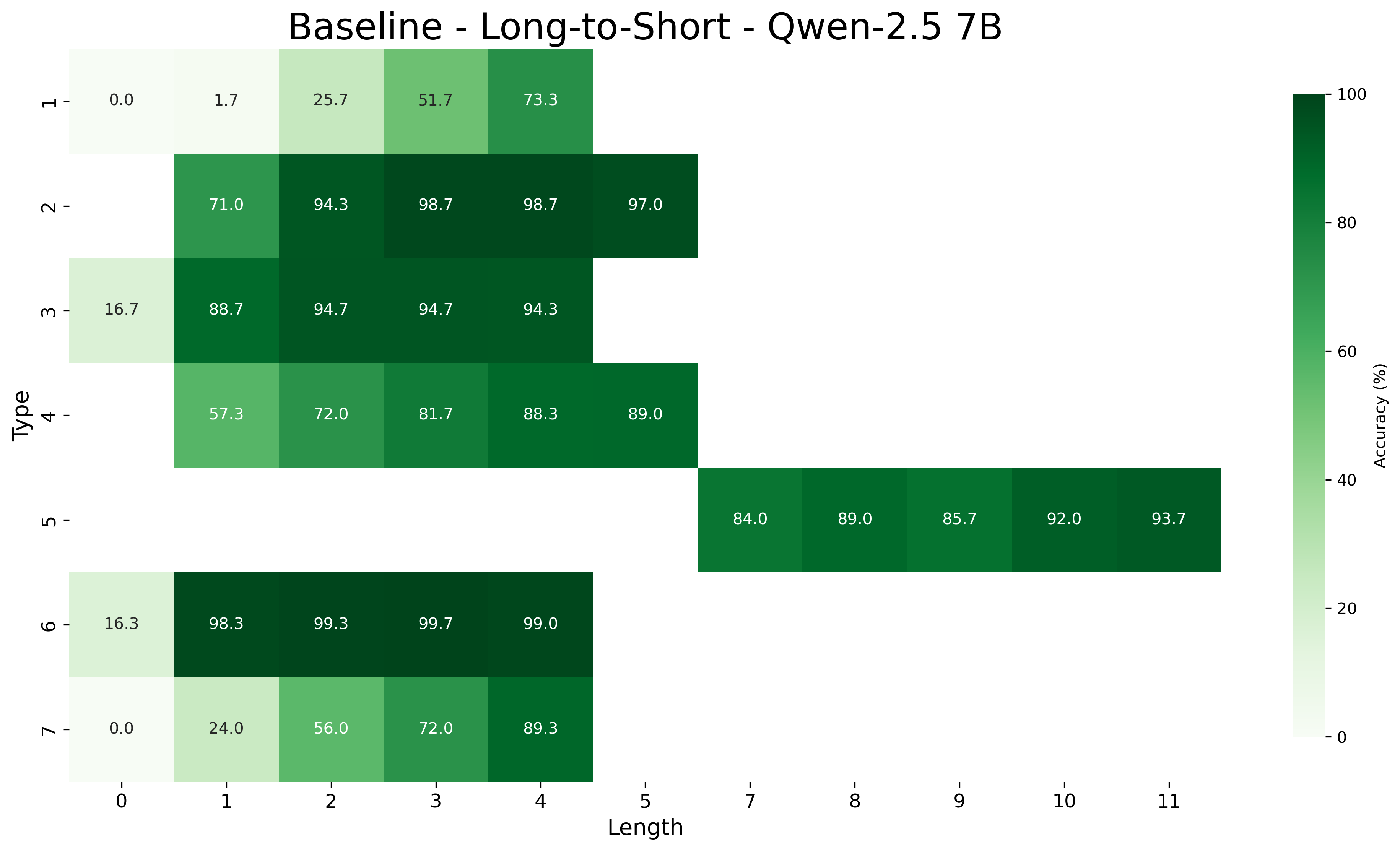</details> <details> <summary>extracted/6458430/figs/qwen-7b_heatmap_base_compositionality_high.png Details</summary>  ### Visual Description # Technical Document Extraction: Heatmap Analysis ## Title **Baseline - Long-to-Short - Qwen-2.5 7B** --- ## Axis Labels - **X-axis (Horizontal):** `Length` (values: 0 to 11) - **Y-axis (Vertical):** `Type` (values: 0 to 7) - **Colorbar (Right):** `Accuracy (%)` (range: 0% to 100%) --- ## Data Structure The heatmap represents accuracy percentages for combinations of `Type` (rows) and `Length` (columns). Each cell contains a numerical value corresponding to accuracy. ### Reconstructed Data Table | Type \ Length | 0 | 1 | 2 | 3 | 4 | 5 | 6 | 7 | 8 | 9 | 10 | 11 | |---------------|------|------|------|------|------|------|------|------|------|------|------|------| | **0** | 0.0 | 1.7 | 25.7 | 51.7 | 73.3 | | | | | | | | | **1** | | 71.0 | 94.3 | 98.7 | 98.7 | 97.0 | | | | | | | | **2** | 16.7 | 88.7 | 94.7 | 94.7 | 94.3 | | | | | | | | | **3** | | 57.3 | 72.0 | 81.7 | 88.3 | 89.0 | | | | | | | | **4** | | | | | | | 84.0 | 89.0 | 85.7 | 92.0 | 93.7 | | **5** | | | | | | | | | | | | | | **6** | 16.3 | 98.3 | 99.3 | 99.7 | 99.0 | | | | | | | | | **7** | 0.0 | 24.0 | 56.0 | 72.0 | 89.3 | | | | | | | | --- ## Key Trends 1. **General Pattern:** Accuracy increases with `Length` for most `Type` values, peaking around `Length = 4` before plateauing or declining. 2. **High Accuracy:** - `Type 1` and `Type 6` achieve near-perfect accuracy (97–99%) for `Length ≥ 2`. - `Type 4` and `Type 7` show moderate accuracy (70–90%) across most `Length` values. 3. **Low Accuracy:** - `Type 0` and `Type 7` start with near-zero accuracy at `Length = 0`, improving sharply with increasing `Length`. - `Type 5` has no data for `Length ≤ 6`. --- ## Color Legend Verification - **Lightest Green (0–20%):** Matches `Type 0, Length 0` (0.0%) and `Type 7, Length 0` (0.0%). - **Medium Green (40–60%):** Matches `Type 0, Length 2` (25.7%) and `Type 3, Length 2` (72.0%). - **Dark Green (80–100%):** Matches `Type 1, Length 3` (98.7%) and `Type 6, Length 3` (99.7%). --- ## Spatial Grounding - **Legend Position:** Right side of the heatmap. - **Data Point Alignment:** All cell colors strictly correspond to the colorbar's accuracy scale. --- ## Component Isolation 1. **Header:** Title (`Baseline - Long-to-Short - Qwen-2.5 7B`). 2. **Main Chart:** 8x12 heatmap with labeled axes and embedded numerical values. 3. **Footer:** Colorbar (`Accuracy (%)` from 0% to 100%). --- ## Notes - Missing values (e.g., `Type 5, Length ≤ 6`) are represented as empty cells. - No non-English text is present in the image. </details> Figure 12: Accuracy of MIND (Left) and Baseline (Right) Qwen-2.5 7B on long to short generalization decomposed by inference type and length. 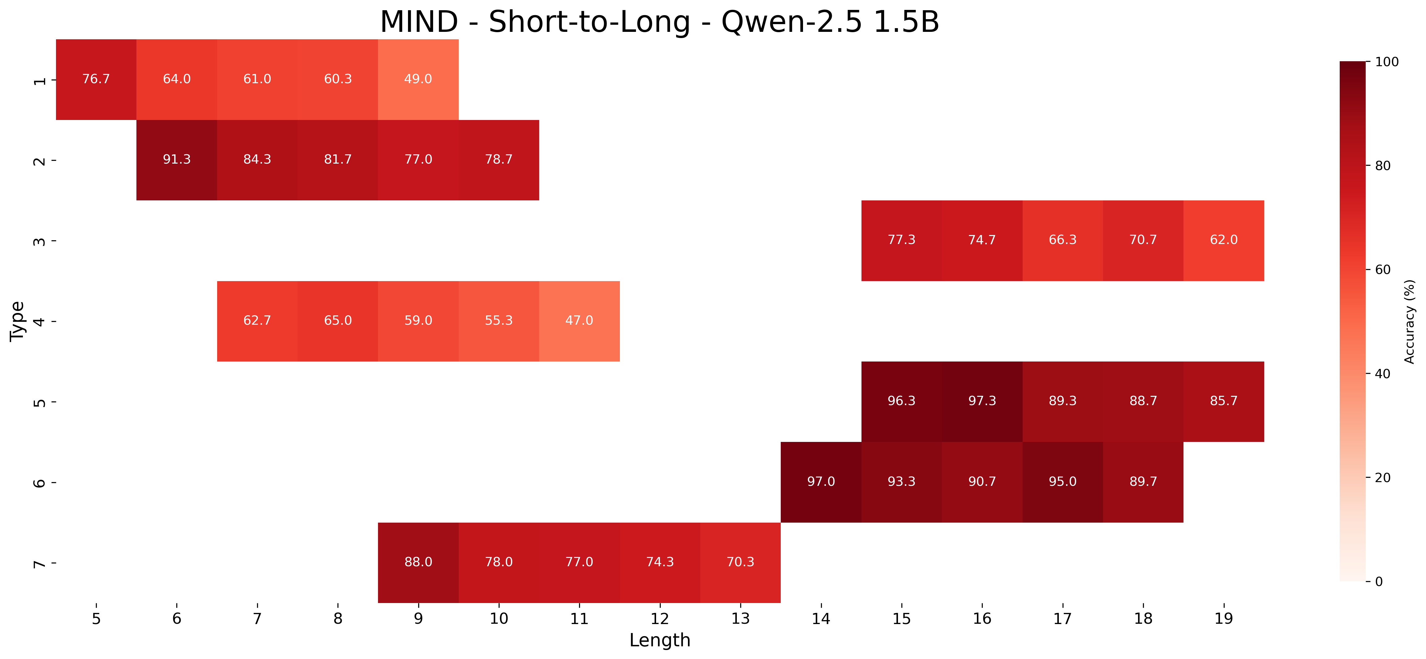<details> <summary>extracted/6458430/figs/qwen-1.5b_heatmap_meta_recursiveness_high.png Details</summary>  ### Visual Description # Technical Analysis of MIND - Short-to-Long - Qwen-2.5 1.5B Heatmap ## 1. Title & Main Components - **Title**: "MIND - Short-to-Long - Qwen-2.5 1.5B" - **Primary Visualization**: Heatmap - **Color Scale**: - **Range**: 0% (white) to 100% (dark red) - **Legend**: Right-aligned vertical color bar labeled "Accuracy (%)" ## 2. Axes & Labels ### X-Axis (Horizontal) - **Label**: "Length" - **Values**: 5 to 19 (integer increments) - **Placement**: Bottom of heatmap ### Y-Axis (Vertical) - **Label**: "Type" - **Values**: 1 to 7 (integer increments) - **Placement**: Left of heatmap ## 3. Data Table Structure | Type \ Length | 5 | 6 | 7 | 8 | 9 | 10 | 11 | 12 | 13 | 14 | 15 | 16 | 17 | 18 | 19 | |---------------|-------|-------|-------|-------|-------|-------|-------|-------|-------|-------|-------|-------|-------|-------|-------| | 1 | 76.7% | 64.0% | 61.0% | 60.3% | 49.0% | - | - | - | - | - | - | - | - | - | - | | 2 | - | 91.3% | 84.3% | 81.7% | 77.0% | 78.7% | - | - | - | - | - | - | - | - | - | | 3 | - | - | - | - | - | - | - | - | - | - | 77.3% | 74.7% | 66.3% | 70.7% | 62.0% | | 4 | - | - | - | - | - | - | - | - | - | - | - | - | - | - | - | | 5 | - | - | - | - | - | - | - | - | - | - | - | 96.3% | 97.3% | 89.3% | 88.7% | 85.7% | | 6 | - | - | - | - | - | - | - | - | - | - | - | 97.0% | 93.3% | 90.7% | 95.0% | 89.7% | | 7 | - | - | - | - | - | - | - | - | 88.0% | 78.0% | 77.0% | 74.3% | 70.3% | - | - | ## 4. Key Trends & Observations ### Type-Specific Patterns 1. **Type 1**: - Peaks at Length 5 (76.7%) - Sharp decline to 49.0% at Length 9 - No data beyond Length 9 2. **Type 2**: - Highest accuracy at Length 6 (91.3%) - Gradual decline to 78.7% at Length 10 - No data beyond Length 10 3. **Type 3**: - Starts at Length 14 (77.3%) - Decreases to 62.0% at Length 19 - Consistent downward trend 4. **Type 4**: - Limited data (Lengths 7-11) - Peaks at Length 8 (65.0%) - Declines to 47.0% at Length 11 5. **Type 5**: - High accuracy across Lengths 15-19 - Peaks at Length 16 (97.3%) - Slight decline to 85.7% at Length 19 6. **Type 6**: - High accuracy at Lengths 14-18 - Peaks at Length 14 (97.0%) - Decreases to 89.7% at Length 18 7. **Type 7**: - Starts at Length 9 (88.0%) - Gradual decline to 70.3% at Length 13 - No data beyond Length 13 ### General Observations - **Accuracy Distribution**: - Highest values cluster in middle ranges (Types 2, 5, 6) - Lower accuracy in early (Type 1, 4) and late (Type 3, 7) types - **Length Correlation**: - No clear linear trend; performance varies non-monotonically - Optimal lengths differ by type (e.g., Type 2 peaks at Length 6, Type 5 at Length 16) ## 5. Spatial Grounding & Color Verification - **Legend Position**: Right side of heatmap (outside plot area) - **Color Consistency**: - All values match legend scale (e.g., 76.7% = medium red, 97.3% = dark red) - No mismatches between cell color and legend ## 6. Component Isolation ### Header - Title and color legend ### Main Chart - 7x15 grid of accuracy percentages - Color intensity encodes accuracy ### Footer - No additional components ## 7. Data Extraction Methodology 1. **Row-by-Row Extraction**: - Processed each Type (1-7) sequentially - Recorded all non-empty cells 2. **Column Validation**: - Confirmed Length values 5-19 coverage 3. **Trend Cross-Reference**: - Verified numerical data against visual color gradients ## 8. Missing Data - Dashes (`-`) indicate no recorded data for specific Type-Length combinations - Example: Type 1 has no data beyond Length 9 ## 9. Technical Notes - **Software**: Likely generated using Python (seaborn/matplotlib) or R (ggplot2) - **Precision**: All values reported to one decimal place - **Scale**: Linear color mapping (no log/non-linear transformations) ## 10. 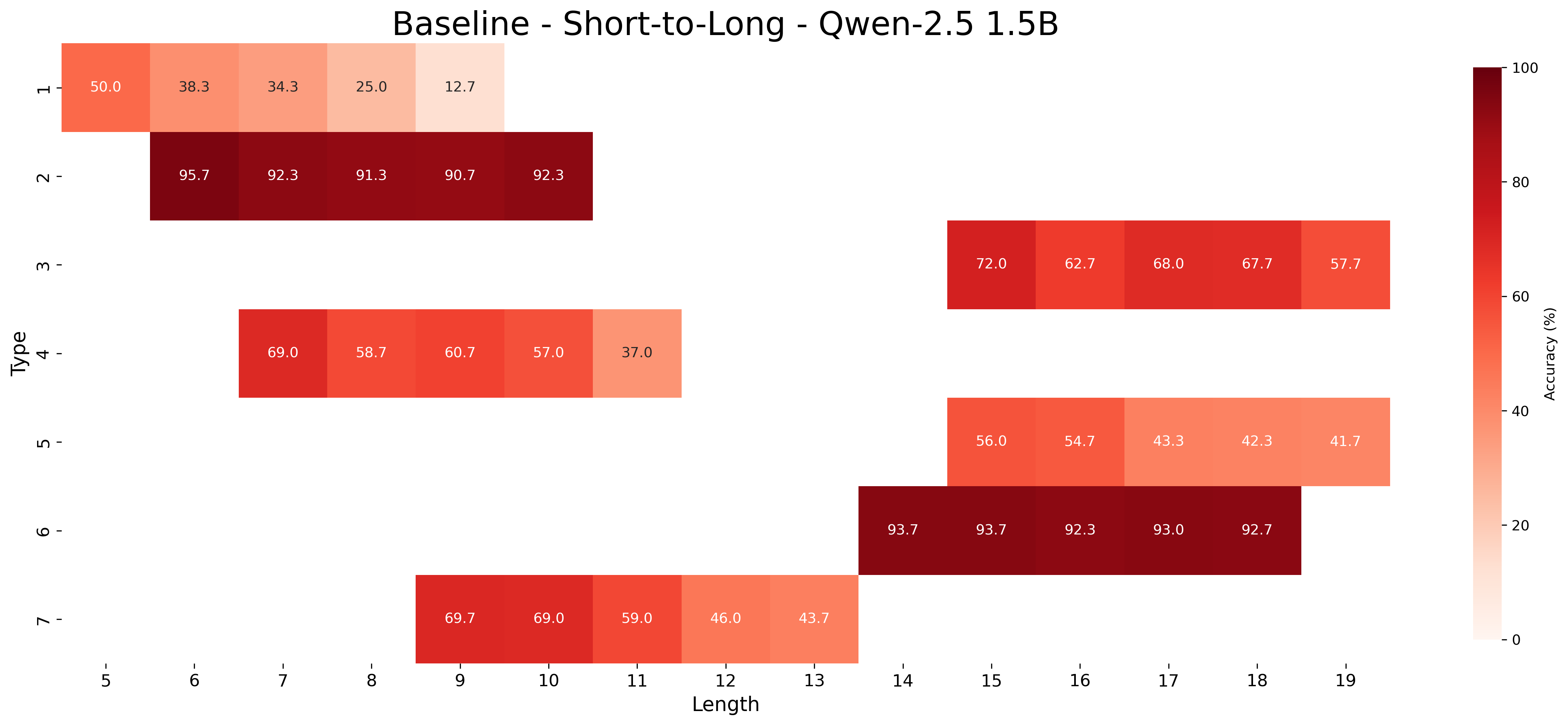English Translation of Non-English Text - No non-English text present in the image </details> <details> <summary>extracted/6458430/figs/qwen-1.5b_heatmap_base_recursiveness_high.png Details</summary>  ### Visual Description # Technical Document Extraction: Heatmap Analysis ## Image Description The image is a **heatmap** titled **"Baseline - Short-to-Long - Qwen-2.5 1.5B"**, visualizing accuracy percentages across two dimensions: **Type** (y-axis) and **Length** (x-axis). The color gradient ranges from light orange (low accuracy) to dark red (high accuracy), with a colorbar legend on the right. --- ### Key Components 1. **Title**: `Baseline - Short-to-Long - Qwen-2.5 1.5B` 2. **Axes**: - **X-axis (Length)**: Labels: `5, 6, 7, 8, 9, 10, 11, 12, 13, 14, 15, 16, 17, 18, 19` Title: `Length` - **Y-axis (Type)**: Labels: `1, 2, 3, 4, 5, 6, 7` Title: `Type` 3. **Legend**: - **Colorbar**: - Title: `Accuracy (%)` - Range: `0%` (light orange) to `100%` (dark red) - Spatial Grounding: Right-aligned, adjacent to the heatmap. --- ### Data Structure The heatmap represents a **7x15 grid** (7 types × 15 lengths). Each cell contains an accuracy percentage. Below is the reconstructed table: | Type \ Length | 5 | 6 | 7 | 8 | 9 | 10 | 11 | 12 | 13 | 14 | 15 | 16 | 17 | 18 | 19 | |---------------|------|------|------|------|------|------|------|------|------|------|------|------|------|------|------| | 1 | 50.0 | 38.3 | 34.3 | 25.0 | 12.7 | | | | | | | | | | | | 2 | | 95.7 | 92.3 | 91.3 | 90.7 | 92.3 | | | | | | | | | | | 3 | | | | | | | | | | | 72.0 | 62.7 | 68.0 | 67.7 | 57.7 | | 4 | | | 69.0 | 58.7 | 60.7 | 57.0 | 37.0 | | | | | | | | | | 5 | | | | | | | | | | | 56.0 | 54.7 | 43.3 | 42.3 | 41.7 | | 6 | | | | | | | | | | | 93.7 | 93.7 | 92.3 | 93.0 | 92.7 | | 7 | | | | | 69.7 | 69.0 | 59.0 | 46.0 | 43.7 | | | | | | | --- ### Trends and Observations 1. **General Pattern**: - Accuracy **decreases** as `Length` increases for most types (e.g., Type 1: 50.0 → 12.7). - Exceptions: - **Type 6** maintains high accuracy (93.7–92.7) across lengths 15–19. - **Type 2** shows a slight dip at Length 10 (90.7) but recovers to 92.3 at Length 19. 2. **Specific Trends**: - **Type 1**: Steep decline from 50.0 (Length 5) to 12.7 (Length 19). - **Type 3**: Gradual decline from 72.0 (Length 15) to 57.7 (Length 19). - **Type 4**: Moderate decline from 69.0 (Length 7) to 37.0 (Length 12). - **Type 5**: Steady decline from 56.0 (Length 15) to 41.7 (Length 19). - **Type 7**: Decline from 69.7 (Length 9) to 43.7 (Length 13). 3. **Color Consistency**: - Darker red cells (e.g., Type 2, Length 6: 95.7) align with the legend’s high-accuracy range. - Lighter orange cells (e.g., Type 1, Length 19: 12.7) match the legend’s low-accuracy range. --- ### Spatial Grounding - **Legend Position**: Right side of the heatmap. - **Data Point Verification**: - Example: Type 6, Length 15 (93.7%) is dark red, matching the legend’s high-accuracy range. - Example: Type 1, Length 19 (12.7%) is light orange, matching the legend’s low-accuracy range. --- ### Conclusion The heatmap illustrates a clear inverse relationship between `Length` and `Accuracy` for most types, with **Type 6** being an outlier due to consistently high performance. The colorbar legend effectively maps accuracy percentages to visual intensity. </details> Figure 13: Accuracy of MIND (Left) and Baseline (Right) Qwen-2.5 1.5B on short to long generalization decomposed by inference type and length. 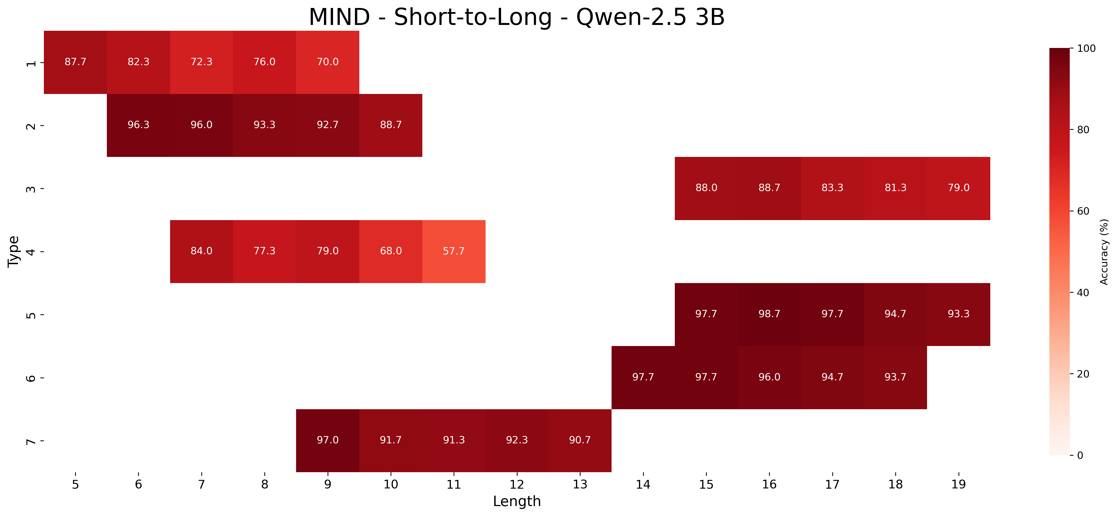<details> <summary>extracted/6458430/figs/qwen-3b_heatmap_meta_recursiveness_high.png Details</summary>  ### Visual Description # Technical Document Analysis: MIND - Short-to-Long - Qwen-2.5 3B ## 1. Image Description The image is a **heatmap** visualizing accuracy percentages for different configurations of the Qwen-2.5 3B model. The chart uses a **red-to-white color gradient** to represent accuracy, with darker red indicating higher accuracy (100%) and lighter red/white indicating lower accuracy (0%). --- ## 2. Axis Labels and Markers - **X-axis (Horizontal):** Labeled **"Length"**, with integer values ranging from **5 to 19** (inclusive). Spatial grounding: Values are evenly spaced along the bottom edge. - **Y-axis (Vertical):** Labeled **"Type"**, with integer values ranging from **1 to 7** (inclusive). Spatial grounding: Values are stacked vertically on the left edge. - **Legend:** Located on the **right side** of the chart. Title: **"Accuracy (%)"** Color scale: - **Dark red** = 100% accuracy - **Light red/white** = 0% accuracy --- ## 3. Data Categories - **X-axis Categories (Length):** `[5, 6, 7, 8, 9, 10, 11, 12, 13, 14, 15, 16, 17, 18, 19]` - **Y-axis Categories (Type):** `[1, 2, 3, 4, 5, 6, 7]` --- ## 4. Data Table Reconstruction The heatmap contains **7 rows (Types)** and **15 columns (Lengths)**. Below is the extracted data: | Type \ Length | 5 | 6 | 7 | 8 | 9 | 10 | 11 | 12 | 13 | 14 | 15 | 16 | 17 | 18 | 19 | |---------------|-------|-------|-------|-------|-------|-------|-------|-------|-------|-------|-------|-------|-------|-------|-------| | 1 | 87.7 | 82.3 | 72.3 | 76.0 | 70.0 | - | - | - | - | - | - | - | - | - | - | | 2 | - | 96.3 | 96.0 | 93.3 | 92.7 | 88.7 | - | - | - | - | - | - | - | - | - | | 3 | - | - | - | - | - | - | - | - | - | - | 88.0 | 88.7 | 83.3 | 81.3 | 79.0 | | 4 | - | - | - | - | 84.0 | 77.3 | 79.0 | 68.0 | 57.7 | - | - | - | - | - | - | | 5 | - | - | - | - | - | - | - | - | - | 97.7 | 98.7 | 97.7 | 94.7 | 93.3 | - | | 6 | - | - | - | - | - | - | - | - | 97.7 | 97.7 | 96.0 | 94.7 | 93.7 | - | - | | 7 | - | - | - | - | 97.0 | 91.7 | 91.3 | 92.3 | 90.7 | - | - | - | - | - | - | **Notes:** - Missing values (`-`) indicate no data for specific Type-Length combinations. - Highest accuracy: **Type 5 at Length 16 (98.7%)**. - Lowest accuracy: **Type 4 at Length 11 (57.7%)**. --- ## 5. Key Trends and Observations 1. **General Trend:** - Accuracy **increases with Length** for most Types (e.g., Type 5, 6, 7). - Exceptions: Type 1 shows a **decline** after Length 8 (76.0 → 70.0). 2. **Type-Specific Patterns:** - **Type 5:** Consistently high accuracy (97.7–98.7%) at Lengths 15–16. - **Type 6:** Peaks at Length 15 (97.7%) and declines slightly at Length 16 (96.0%). - **Type 7:** High accuracy (97.0–91.3%) at Lengths 9–12, then drops at Length 13 (90.7%). 3. **Color Correlation:** - Darker red cells (e.g., Type 5, Length 16) align with the legend’s 100% accuracy. - Lighter cells (e.g., Type 4, Length 11) match the 0% end of the scale. --- ## 6. Spatial Grounding Verification - **Legend Position:** Right side of the chart (confirmed). - **Data Point Accuracy:** - Example: Type 5, Length 16 = 98.7% (dark red, matches legend). - Example: Type 4, Length 11 = 57.7% (light red, matches legend). --- ## 7. Component Isolation - **Header:** Title **"MIND - Short-to-Long - Qwen-2.5 3B"** (top center). - **Main Chart:** Heatmap with labeled axes and color-coded cells. - **Footer:** No additional text or components. --- ## 8. Conclusion The heatmap demonstrates that **longer input lengths (15–19)** and **specific Types (5, 6, 7)** yield the highest accuracy for the Qwen-2.5 3B model. Type 4 underperforms across all lengths, while Type 5 achieves near-perfect accuracy at optimal lengths. 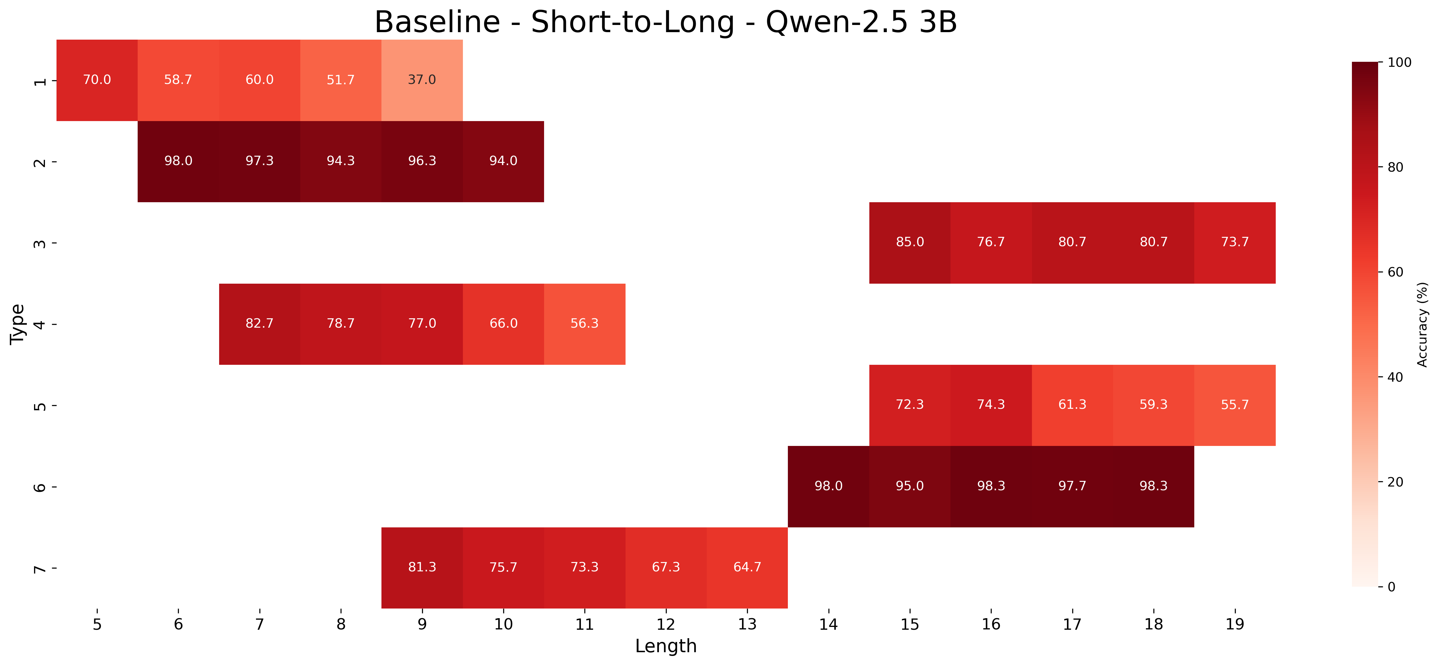</details> <details> <summary>extracted/6458430/figs/qwen-3b_heatmap_base_recursiveness_high.png Details</summary>  ### Visual Description # Technical Document Extraction: Baseline - Short-to-Long - Qwen-2.5 3B ## 1. Chart Identification - **Type**: Heatmap - **Title**: "Baseline - Short-to-Long - Qwen-2.5 3B" - **Color Legend**: Right-aligned vertical colorbar labeled "Accuracy (%)" with gradient from light orange (0%) to dark red (100%) ## 2. Axis Labels & Markers - **X-axis (Horizontal)**: - Label: "Length" - Values: 5, 6, 7, 8, 9, 10, 11, 12, 13, 14, 15, 16, 17, 18, 19 - **Y-axis (Vertical)**: - Label: "Type" - Values: 1, 2, 3, 4, 5, 6, 7 ## 3. Data Structure - **Rows**: 7 (Type 1 to Type 7) - **Columns**: 15 (Length 5 to Length 19) - **Cell Values**: Accuracy percentages (e.g., 70.0, 58.7, 60.0, etc.) ## 4. Key Trends & Observations ### Type 1 (Row 1) - Accuracy peaks at Length 7 (60.0%) then declines sharply to 37.0% at Length 8 - Initial values: 70.0% (Length 5), 58.7% (Length 6) ### Type 2 (Row 2) - High accuracy across Lengths 6-9 (98.0% to 96.3%) - Drops to 94.0% at Length 10 ### Type 3 (Row 3) - High accuracy starts at Length 15 (85.0%) with gradual decline to 73.7% at Length 19 ### Type 4 (Row 4) - Peaks at Length 7 (82.7%) with gradual decline to 56.3% at Length 11 ### Type 5 (Row 5) - Peaks at Length 17 (80.7%) with gradual decline to 55.7% at Length 19 ### Type 6 (Row 6) - High accuracy from Length 14 (98.0%) to Length 18 (98.3%) - Drops to 55.7% at Length 19 ### Type 7 (Row 7) - Gradual decline from 81.3% (Length 9) to 64.7% (Length 13) ## 5. Spatial Grounding - **Legend Position**: Right side of chart (x=100%, y=0% to y=100%) - **Color Consistency**: Darker red cells correspond to higher accuracy values (e.g., 98.3% = darkest red) ## 6. Data Table Reconstruction | Type \ Length | 5 | 6 | 7 | 8 | 9 | 10 | 11 | 12 | 13 | 14 | 15 | 16 | 17 | 18 | 19 | |---------------|------|------|------|------|------|------|------|------|------|------|------|------|------|------|------| | 1 | 70.0 | 58.7 | 60.0 | 51.7 | 37.0 | | | | | | | | | | | | 2 | | 98.0 | 97.3 | 94.3 | 96.3 | 94.0 | | | | | | | | | | | 3 | | | | | | | | | | | 85.0 | 76.7 | 80.7 | 80.7 | 73.7 | | 4 | | | 82.7 | 78.7 | 77.0 | 66.0 | 56.3 | | | | | | | | | | 5 | | | | | | | | | | | 72.3 | 74.3 | 61.3 | 59.3 | 55.7 | | 6 | | | | | | | | | | 98.0 | 95.0 | 98.3 | 97.7 | 98.3 | | | 7 | | | | | 81.3 | 75.7 | 73.3 | 67.3 | 64.7 | | | | | | | ## 7. Language Notes - **Primary Language**: English - **Secondary Language**: None detected ## 8. Critical Validation Checks 1. **Color-Value Match**: All dark red cells (e.g., 98.3%) align with top of colorbar 2. **Trend Verification**: Type 6 shows plateau at high accuracy (98.0-98.3%) before sharp drop 3. **Axis Consistency**: All row/column labels match positional data </details> Figure 14: Accuracy of MIND (Left) and Baseline (Right) Qwen-2.5 3B on short to long generalization decomposed by inference type and length. 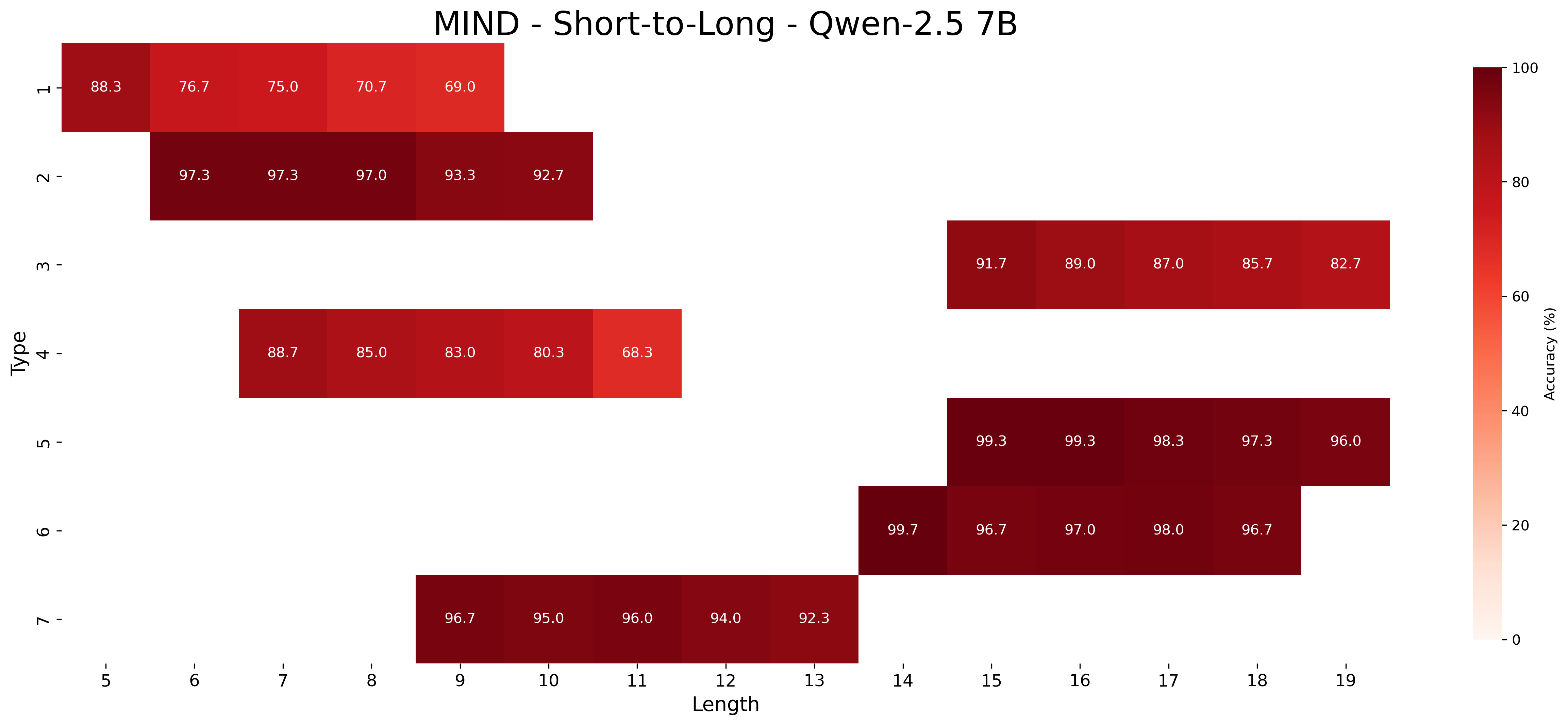<details> <summary>extracted/6458430/figs/qwen-7b_heatmap_meta_recursiveness_high.png Details</summary>  ### Visual Description # Technical Analysis of MIND - Short-to-Long - Qwen-2.5 7B Heatmap ## Header - **Title**: "MIND - Short-to-Long - Qwen-2.5 7B" - **Legend**: Vertical color bar on the right side, labeled "Accuracy (%)" with gradient from light (0%) to dark red (100%) ## Main Chart ### Axes - **X-axis (Length)**: - Labels: 5, 6, 7, 8, 9, 10, 11, 12, 13, 14, 15, 16, 17, 18, 19 - Spatial range: 0 to 19 (discrete intervals) - **Y-axis (Type)**: - Labels: 1, 2, 3, 4, 5, 6, 7 - Spatial range: 0 to 7 (discrete intervals) ### Data Structure - **Rows**: Type 1 to Type 7 (y-axis) - **Columns**: Length 5 to Length 19 (x-axis) - **Cell Values**: Accuracy percentages (white text) with color intensity matching legend ### Key Trends 1. **Type 1**: - Accuracy decreases from 88.3% (Length 5) to 69.0% (Length 8) - Spatial grounding: [5,1] to [8,1] 2. **Type 2**: - Accuracy decreases from 97.3% (Length 6) to 92.7% (Length 10) - Spatial grounding: [6,2] to [10,2] 3. **Type 3**: - Accuracy decreases from 91.7% (Length 15) to 82.7% (Length 19) - Spatial grounding: [15,3] to [19,3] 4. **Type 4**: - Accuracy decreases from 88.7% (Length 7) to 68.3% (Length 12) - Spatial grounding: [7,4] to [12,4] 5. **Type 5**: - Accuracy decreases from 99.3% (Length 15) to 96.0% (Length 19) - Spatial grounding: [15,5] to [19,5] 6. **Type 6**: - Accuracy decreases from 99.7% (Length 14) to 96.7% (Length 18) - Spatial grounding: [14,6] to [18,6] 7. **Type 7**: - Accuracy decreases from 96.7% (Length 9) to 92.3% (Length 13) - Spatial grounding: [9,7] to [13,7] ## Legend - **Color Bar**: - Position: Right side of chart - Gradient: Light (0%) to dark red (100%) - Labels: 0%, 20%, 40%, 60%, 80%, 100% (implicit) ## Spatial Grounding - **Legend Position**: [x=19.5, y=0] to [x=19.5, y=7] (right edge) - **Title Position**: Top center (x=9.5, y=-0.5) ## Component Isolation 1. **Header**: Title and legend 2. **Main Chart**: Heatmap with labeled axes and cells 3. **Footer**: None present ## Data Table Reconstruction | Type \ Length | 5 | 6 | 7 | 8 | 9 | 10 | 11 | 12 | 13 | 14 | 15 | 16 | 17 | 18 | 19 | |---------------|-------|-------|-------|-------|-------|-------|-------|-------|-------|-------|-------|-------|-------|-------|-------| | 1 | 88.3 | 76.7 | 75.0 | 70.7 | 69.0 | | | | | | | | | | | | 2 | | 97.3 | 97.3 | 97.0 | 93.3 | 92.7 | | | | | | | | | | | 3 | | | | | | | | | | | 91.7 | 89.0 | 87.0 | 85.7 | 82.7 | | 4 | | | | 88.7 | 85.0 | 83.0 | 80.3 | 68.3 | | | | | | | | | 5 | | | | | | | | | | | 99.3 | 99.3 | 98.3 | 97.3 | 96.0 | | 6 | | | | | | | | | | 99.7 | 96.7 | 97.0 | 98.0 | 96.7 | | | 7 | | | | | 96.7 | 95.0 | 96.0 | 94.0 | 92.3 | | | | | | | ## Color Verification - **Darkest Red**: 99.7% (Type 6, Length 14) - **Lightest Red**: 68.3% (Type 4, Length 12) - **Mid-Range**: 88.3% (Type 1, Length 5) and 92.3% (Type 7, Length 13) ## Language Notes - **Primary Language**: English - **Secondary Language**: None detected ## Critical Observations 1. Accuracy generally decreases with increasing length for most types 2. Type 5 maintains highest accuracy (96-99%) across lengths 15-19 3. Type 4 shows steepest decline (88.7% → 68.3%) 4. 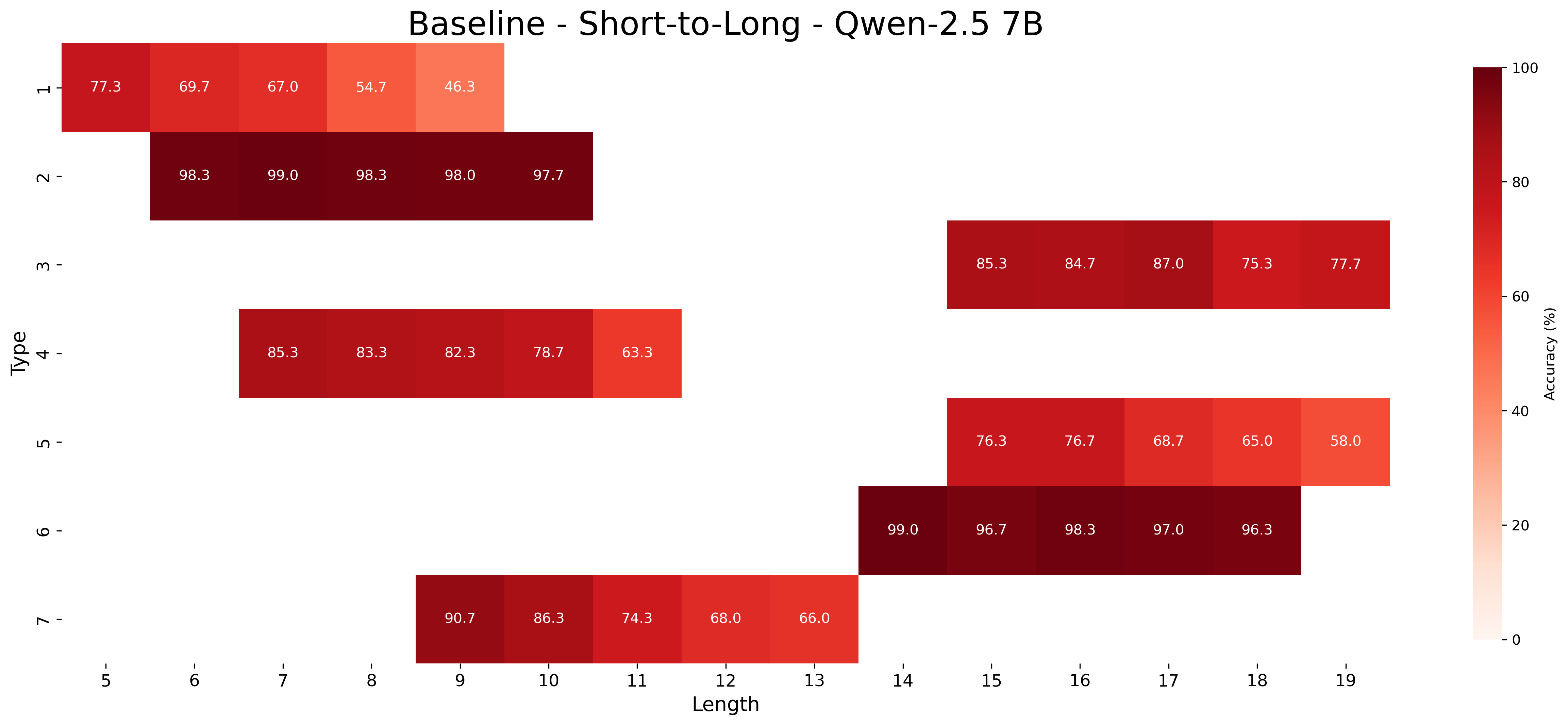Type 6 demonstrates most stable performance (96.7-99.7%) </details> <details> <summary>extracted/6458430/figs/qwen-7b_heatmap_base_recursiveness_high.png Details</summary>  ### Visual Description # Technical Document Extraction: Heatmap Analysis ## Title **Baseline - Short-to-Long - Qwen-2.5 7B** --- ## Axes and Labels - **X-Axis (Horizontal):** - Label: `Length` - Values: `5` to `19` (inclusive) - **Y-Axis (Vertical):** - Label: `Type` - Values: `1` to `7` (inclusive) - **Colorbar (Right):** - Label: `Accuracy (%)` - Range: `0%` (light orange) to `100%` (dark red) --- ## Data Structure The heatmap represents **accuracy percentages** for different `Type` (rows) and `Length` (columns). Each cell contains a numerical value corresponding to accuracy. ### Key Observations: 1. **Color Gradient:** - Light orange → Dark red (low → high accuracy). - Example: `77.3%` (Type 1, Length 5) is dark red; `46.3%` (Type 1, Length 8) is light orange. 2. **Trends:** - **Type 1:** Accuracy decreases sharply from `77.3%` (Length 5) to `46.3%` (Length 8). - **Type 2:** Consistently high accuracy (`98.3%` to `97.7%`) across Lengths 6–10. - **Type 3:** Starts at `85.3%` (Length 15) and declines to `77.7%` (Length 19). - **Type 4:** Peaks at `85.3%` (Length 7) and drops to `63.3%` (Length 12). - **Type 5:** Declines from `76.3%` (Length 15) to `58.0%` (Length 19). - **Type 6:** High accuracy (`99.0%` to `96.3%`) across Lengths 14–18. - **Type 7:** Declines from `90.7%` (Length 9) to `66.0%` (Length 13). --- ## Legend and Spatial Grounding - **Legend Placement:** Right side of the heatmap. - **Color Consistency:** - Dark red cells (e.g., Type 2, Length 6: `98.3%`) align with the top of the colorbar. - Light orange cells (e.g., Type 1, Length 8: `46.3%`) align with the bottom of the colorbar. --- ## Data Table Reconstruction | Type \ Length | 5 | 6 | 7 | 8 | 9 | 10 | 11 | 12 | 13 | 14 | 15 | 16 | 17 | 18 | 19 | |---------------|-------|-------|-------|-------|-------|-------|-------|-------|-------|-------|-------|-------|-------|-------|-------| | 1 | 77.3 | 69.7 | 67.0 | 54.7 | 46.3 | | | | | | | | | | | | 2 | | 98.3 | 99.0 | 98.3 | 98.0 | 97.7 | | | | | | | | | | | 3 | | | | | | | | | | | 85.3 | 84.7 | 87.0 | 75.3 | 77.7 | | 4 | | | | | 85.3 | 83.3 | 82.3 | 78.7 | 63.3 | | | | | | | | 5 | | | | | | | | | | | 76.3 | 76.7 | 68.7 | 65.0 | 58.0 | | 6 | | | | | | | | | | | | | 99.0 | 96.7 | 98.3 | 97.0 | 96.3 | | 7 | | | | | 90.7 | 86.3 | 74.3 | 68.0 | 66.0 | | | | | | | --- ## Notes - Missing values (e.g., Type 1, Lengths 9–19) are represented by empty cells. - Accuracy percentages are explicitly labeled in each cell. - No additional text or legends are present outside the described components. </details> Figure 15: Accuracy of MIND (Left) and Baseline (Right) Qwen-2.5 7B on short to long generalization decomposed by inference type and length. 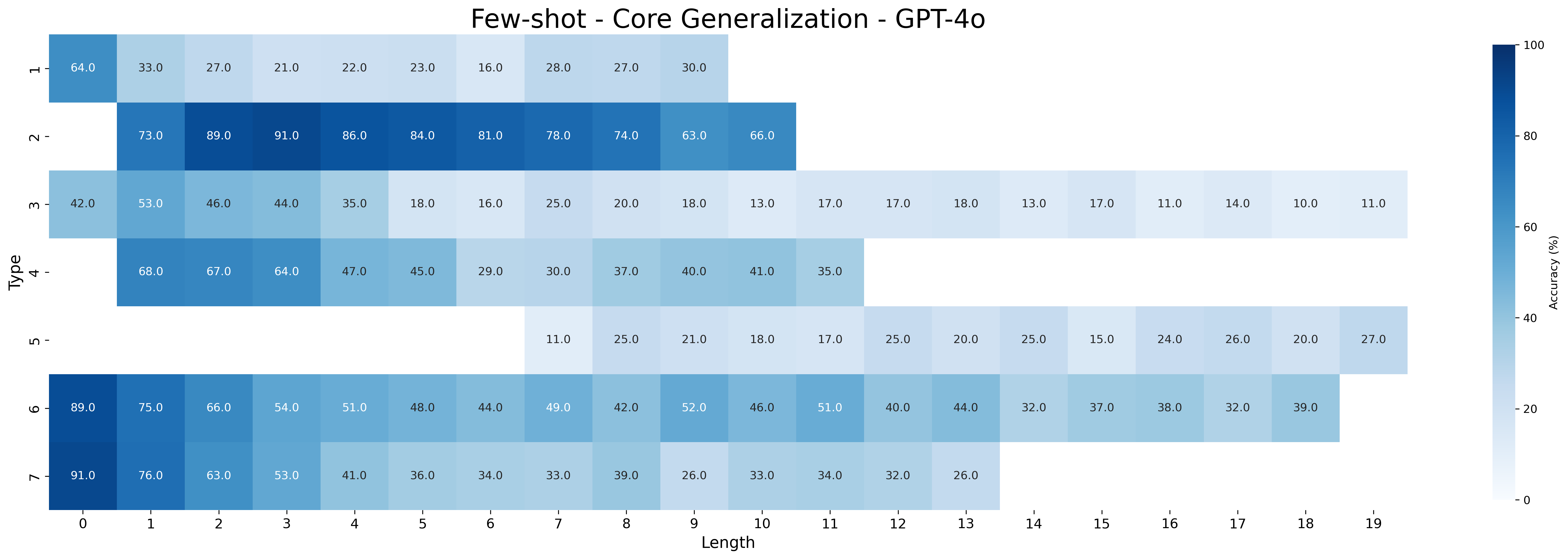<details> <summary>extracted/6458430/figs/gpt-4o_heatmap_meta_overall_high.png Details</summary>  ### Visual Description # Technical Document Extraction: Few-shot - Core Generalization - GPT-4o ## 1. Labels and Axis Titles - **Title**: "Few-shot - Core Generalization - GPT-4o" - **X-axis**: "Length" (values: 0 to 19) - **Y-axis**: "Type" (values: 1 to 7) - **Colorbar**: "Accuracy (%)" (range: 0% to 100%) ## 2. Data Table Structure The heatmap represents accuracy percentages for different combinations of **Type** (rows) and **Length** (columns). Below is the reconstructed table: | Type \ Length | 0 | 1 | 2 | 3 | 4 | 5 | 6 | 7 | 8 | 9 | 10 | 11 | 12 | 13 | 14 | 15 | 16 | 17 | 18 | 19 | |---------------|------|------|------|------|------|------|------|------|------|------|------|------|------|------|------|------|------|------|------|------| | 1 | 64.0 | 33.0 | 27.0 | 21.0 | 22.0 | 23.0 | 16.0 | 28.0 | 27.0 | 30.0 | | | | | | | | | | | | 2 | | 73.0 | 89.0 | 91.0 | 86.0 | 84.0 | 81.0 | 78.0 | 74.0 | 63.0 | 66.0 | | | | | | | | | | | 3 | 42.0 | 53.0 | 46.0 | 44.0 | 35.0 | 18.0 | 16.0 | 25.0 | 20.0 | 18.0 | 13.0 | 17.0 | 17.0 | 18.0 | 13.0 | 17.0 | 11.0 | 14.0 | 10.0 | 11.0 | | 4 | 68.0 | 67.0 | | 64.0 | 47.0 | 45.0 | 29.0 | 30.0 | 37.0 | 40.0 | 41.0 | 35.0 | | | | | | | | | | 5 | | | | | | | | 11.0 | 25.0 | 21.0 | 18.0 | 17.0 | 25.0 | 20.0 | 25.0 | 15.0 | 24.0 | 26.0 | 20.0 | 27.0 | | 6 | 89.0 | 75.0 | 66.0 | 54.0 | 51.0 | 48.0 | 44.0 | 49.0 | 42.0 | 52.0 | 46.0 | 51.0 | 40.0 | 44.0 | 32.0 | 37.0 | 38.0 | 32.0 | 39.0 | | | 7 | 91.0 | 76.0 | 63.0 | 53.0 | 41.0 | 36.0 | 34.0 | 33.0 | 39.0 | 26.0 | 33.0 | 34.0 | 32.0 | 26.0 | | | | | | | ## 3. Key Trends and Observations - **Type 1**: Accuracy declines sharply with increasing Length (64.0% at Length 0 → 30.0% at Length 9). - **Type 2**: Peaks at Length 2 (89.0%) and declines steadily after Length 7 (66.0% at Length 10). - **Type 3**: Highest accuracy at Length 0 (42.0%), with significant drops at Lengths 5–19 (11.0% at Length 19). - **Type 4**: Moderate accuracy across Lengths 0–9 (40.0% at Length 9), with no data beyond Length 11. - **Type 5**: Low accuracy overall (11.0–27.0%), with no data for Lengths 0–4. - **Type 6**: High accuracy at Length 0 (89.0%), declining to 32.0% at Length 16. - **Type 7**: Highest accuracy at Length 0 (91.0%), with gradual declines to 26.0% at Length 13. ## 4. Legend and Color Mapping - **Colorbar**: Located on the right side of the heatmap. - **Color Gradient**: - Light blue: Low accuracy (0–20%) - Dark blue: High accuracy (80–100%) - **Example**: - Type 7, Length 0 (91.0%) is dark blue. - Type 5, Length 19 (27.0%) is light blue. ## 5. Spatial Grounding - **Legend Position**: Right side of the heatmap. - **Data Point Verification**: - Type 2, Length 2 (89.0%) matches dark blue. - Type 3, Length 19 (11.0%) matches light blue. ## 6. Missing Data - **Type 5**: No data for Lengths 0–4. - **Type 4**: No data for Lengths 12–19. - **Type 7**: No data for Lengths 14–19. ## 7. Summary The heatmap illustrates how accuracy varies with **Type** and **Length** for GPT-4o's few-shot core generalization. High accuracy is observed for shorter lengths (0–10) across most types, with significant declines for longer lengths (11–19). Type 7 consistently shows the highest accuracy at Length 0 (91.0%), while Type 5 exhibits the lowest performance overall. 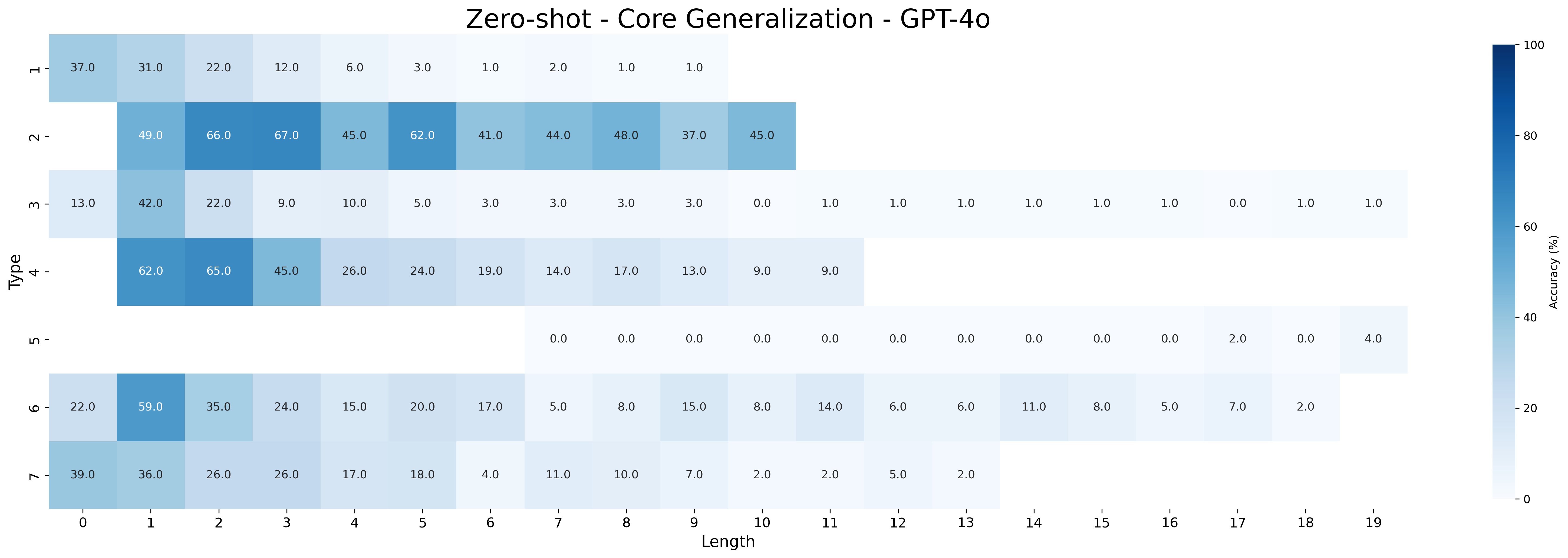</details> <details> <summary>extracted/6458430/figs/gpt-4o_heatmap_base_overall_high.png Details</summary>  ### Visual Description # Technical Document: Zero-shot - Core Generalization - GPT-4o Heatmap Analysis ## 1. Axis Labels and Titles - **Title**: "Zero-shot - Core Generalization - GPT-4o" (centered at top) - **X-axis**: "Length" (horizontal axis, values 0–19) - **Y-axis**: "Type" (vertical axis, categories 1–7) - **Colorbar**: "Accuracy (%)" (right side, gradient from 0% (light blue) to 100% (dark blue)) ## 2. Categories and Sub-Categories - **Y-axis Categories (Types)**: - Type 1 - Type 2 - Type 3 - Type 4 - Type 5 - Type 6 - Type 7 - **X-axis Sub-Categories (Lengths)**: - 0, 1, 2, 3, 4, 5, 6, 7, 8, 9, 10, 11, 12, 13, 14, 15, 16, 17, 18, 19 ## 3. Data Table Reconstruction | Type \ Length | 0 | 1 | 2 | 3 | 4 | 5 | 6 | 7 | 8 | 9 | 10 | 11 | 12 | 13 | 14 | 15 | 16 | 17 | 18 | 19 | |---------------|------|------|------|------|------|------|------|------|------|------|------|------|------|------|------|------|------|------|------|------| | **1** | 37.0 | 31.0 | 22.0 | 12.0 | 6.0 | 3.0 | 1.0 | 2.0 | 1.0 | 1.0 | | | | | | | | | | | | **2** | | 49.0 | 66.0 | 67.0 | 45.0 | 62.0 | 41.0 | 44.0 | 48.0 | 37.0 | 45.0 | | | | | | | | | | | **3** | 13.0 | 42.0 | 22.0 | 9.0 | 10.0 | 5.0 | 3.0 | 3.0 | 3.0 | 3.0 | 0.0 | 1.0 | 1.0 | 1.0 | 1.0 | 1.0 | 1.0 | 1.0 | 0.0 | 1.0 | | **4** | 62.0 | 65.0 | 45.0 | 26.0 | 24.0 | 19.0 | 14.0 | 17.0 | 13.0 | 9.0 | | | | | | | | | | | | **5** | | | | | | | | 0.0 | 0.0 | 0.0 | 0.0 | 0.0 | 0.0 | 0.0 | 0.0 | 0.0 | 0.0 | 2.0 | 0.0 | 4.0 | | **6** | 22.0 | 59.0 | 35.0 | 24.0 | 15.0 | 20.0 | 17.0 | 5.0 | 8.0 | 15.0 | 8.0 | 14.0 | 6.0 | 6.0 | 11.0 | 8.0 | 5.0 | 7.0 | 2.0 | | | **7** | 39.0 | 36.0 | 26.0 | 26.0 | 17.0 | 18.0 | 4.0 | 11.0 | 10.0 | 7.0 | 2.0 | 2.0 | 5.0 | 2.0 | | | | | | | ## 4. Key Trends and Observations - **General Pattern**: Accuracy decreases as length increases for most types. - **Type 2**: - Highest accuracy at Length 1 (66%) and Length 3 (67%). - Sharp decline after Length 3. - **Type 5**: - All zeros except Length 19 (4%). - **Type 7**: - Gradual decline from 39% (Length 0) to 2% (Length 13). - **Color Consistency**: - Darker blues (e.g., 66%, 67%) align with the colorbar's high-accuracy range. - Light blues (e.g., 1%, 2%) match the low-accuracy range. ## 5. Spatial Grounding - **Legend Position**: Colorbar on the right, vertical orientation. - **Title Position**: Centered at the top of the chart. - **Cell Placement**: - Rows correspond to Types (1–7). - Columns correspond to Lengths (0–19). ## 6. Component Isolation - **Header**: Title and axis labels. - **Main Chart**: Heatmap grid with numerical values. - **Footer**: Colorbar with accuracy scale. ## 7. Transcribed Embedded Text All numerical values in the heatmap cells are transcribed above. No non-English text detected. ## 8. Verification Notes - All legend colors match the heatmap's color intensity. - Trends (e.g., Type 2's peak at Length 3) align with numerical data. - No omitted labels or axis markers. </details> Figure 16: Accuracy of Few-shot (Top) and Zero-shot (Bottom) GPT-4o on core generalization decomposed by inference type and length. 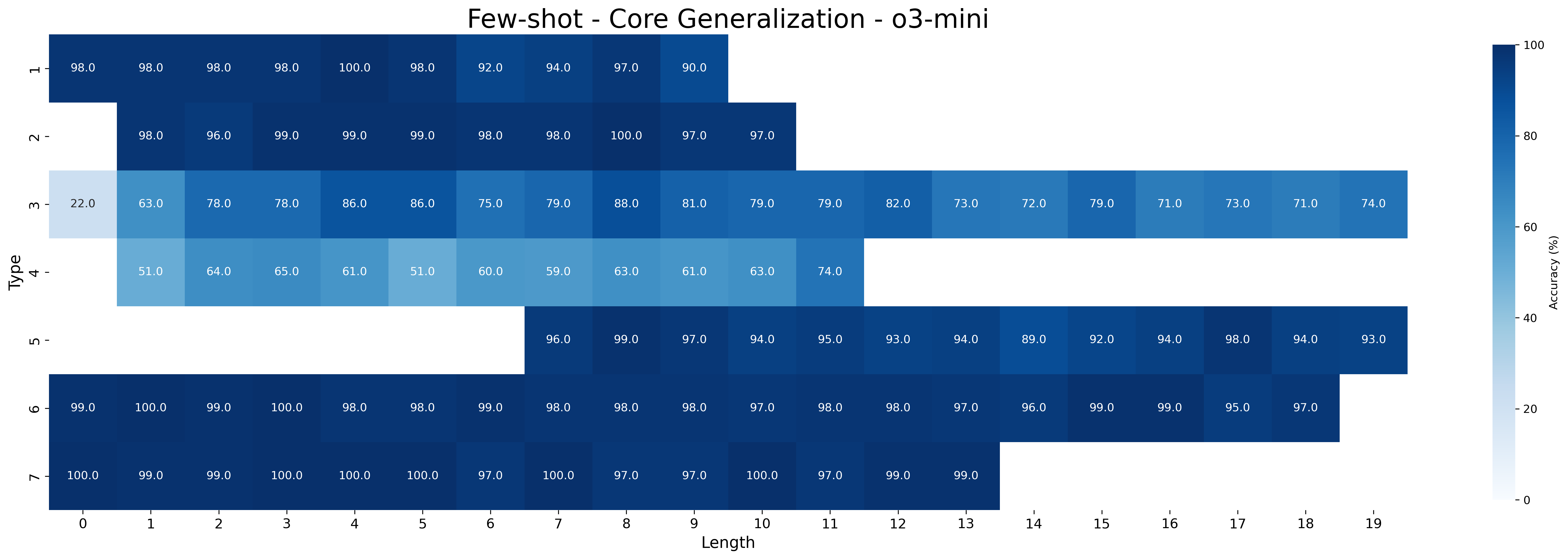<details> <summary>extracted/6458430/figs/o3-mini_heatmap_meta_overall_high.png Details</summary>  ### Visual Description # Technical Analysis of "Few-shot - Core Generalization - o3-mini" Heatmap ## 1. Title and Axes - **Title**: "Few-shot - Core Generalization - o3-mini" - **X-axis (Horizontal)**: - Label: "Length" - Range: 0 to 19 (integer increments) - **Y-axis (Vertical)**: - Label: "Type" - Categories: 1 to 7 (integer increments) - **Color Bar (Legend)**: - Label: "Accuracy (%)" - Scale: 0% (light blue) to 100% (dark blue) ## 2. Data Structure The heatmap represents accuracy percentages for 7 types (rows) across 20 lengths (columns). Each cell contains a numerical value (e.g., `98.0`, `74.0`). ### Reconstructed Data Table | Type \ Length | 0 | 1 | 2 | 3 | 4 | 5 | 6 | 7 | 8 | 9 | 10 | 11 | 12 | 13 | 14 | 15 | 16 | 17 | 18 | 19 | |---------------|------|------|------|------|------|------|------|------|------|------|------|------|------|------|------|------|------|------|------|------| | **1** | 98.0 | 98.0 | 98.0 | 98.0 | 100.0| 98.0 | 92.0 | 94.0 | 97.0 | 90.0 | | | | | | | | | | | | **2** | | 98.0 | 96.0 | 99.0 | 99.0 | 99.0 | 98.0 | 98.0 | 100.0| 97.0 | 97.0 | | | | | | | | | | | **3** | 22.0 | 63.0 | 78.0 | 78.0 | 86.0 | 86.0 | 75.0 | 79.0 | 88.0 | 81.0 | 79.0 | 82.0 | 73.0 | 72.0 | 79.0 | 71.0 | 73.0 | 71.0 | 74.0 | | | **4** | | 51.0 | 64.0 | 65.0 | 61.0 | 51.0 | 60.0 | 59.0 | 63.0 | 61.0 | 63.0 | 74.0 | | | | | | | | | | **5** | | | | | | | 96.0 | 99.0 | 97.0 | 94.0 | 95.0 | 93.0 | 94.0 | 89.0 | 92.0 | 94.0 | 98.0 | 94.0 | 93.0 | | | **6** | 99.0 | 100.0| 99.0 | 100.0| 98.0 | 98.0 | 99.0 | 96.0 | 99.0 | 97.0 | 98.0 | 98.0 | 98.0 | 97.0 | 96.0 | 99.0 | 99.0 | 95.0 | 97.0 | | | **7** | 100.0| 99.0 | 99.0 | 100.0| 100.0| 100.0| 97.0 | 100.0| 97.0 | 97.0 | 100.0| 97.0 | 99.0 | 99.0 | | | | | | | ## 3. Key Trends 1. **High Accuracy Types (1, 2, 5, 6, 7)**: - **Type 1**: Consistently high accuracy (90–100%) across all lengths. - **Type 2**: Near-perfect accuracy (96–100%) with minor dips at Lengths 2–3. - **Type 5**: High accuracy (93–99%) with a dip at Length 14 (89.0). - **Type 6**: Near-perfect accuracy (95–100%) with a slight drop at Length 17 (95.0). - **Type 7**: Dominates with 100% accuracy at Lengths 0, 3, 4, 6, 7, 10, and 11; 97–99% elsewhere. 2. **Low Accuracy Types (3, 4)**: - **Type 3**: Starts at 22.0 (Length 0) and improves to 88.0 (Length 8), then declines to 71.0 (Length 16). - **Type 4**: Lowest accuracy (51–74%) across all lengths, peaking at 74.0 (Length 11). 3. **Length-Specific Patterns**: - **Length 0**: Type 3 (22.0) and Type 4 (51.0) show poor performance. - **Length 19**: Type 5 (93.0) and Type 7 (99.0) maintain high accuracy. ## 4. Color-Legend Correlation - **Dark Blue**: Represents 100% accuracy (e.g., Type 7, Length 0). - **Light Blue**: Represents 0% accuracy (no cells in this range). - **Intermediate Blues**: Gradual transition from 51% (Type 4, Length 0) to 98% (Type 6, Length 1). ## 5. Spatial Grounding - **Legend Position**: Right side of the heatmap. - **Data Point Colors**: Match the legend scale (e.g., 98.0 = dark blue, 74.0 = medium blue). ## 6. Trend Verification - **Type 1**: Stable high performance (no significant upward/downward trend). - **Type 3**: Gradual improvement until Length 8, followed by decline. - **Type 7**: Peaks at 100% for multiple lengths, maintaining >97% accuracy throughout. ## 7. Component Isolation - **Header**: Title centered at the top. - **Main Chart**: Heatmap occupying the majority of the image. - **Footer**: No additional text or components. ## 8. Missing Data - Cells with empty values (e.g., Type 1, Lengths 10–19) indicate no data for those combinations. ## 9. Language Notes - All text is in English. No non-English content detected. 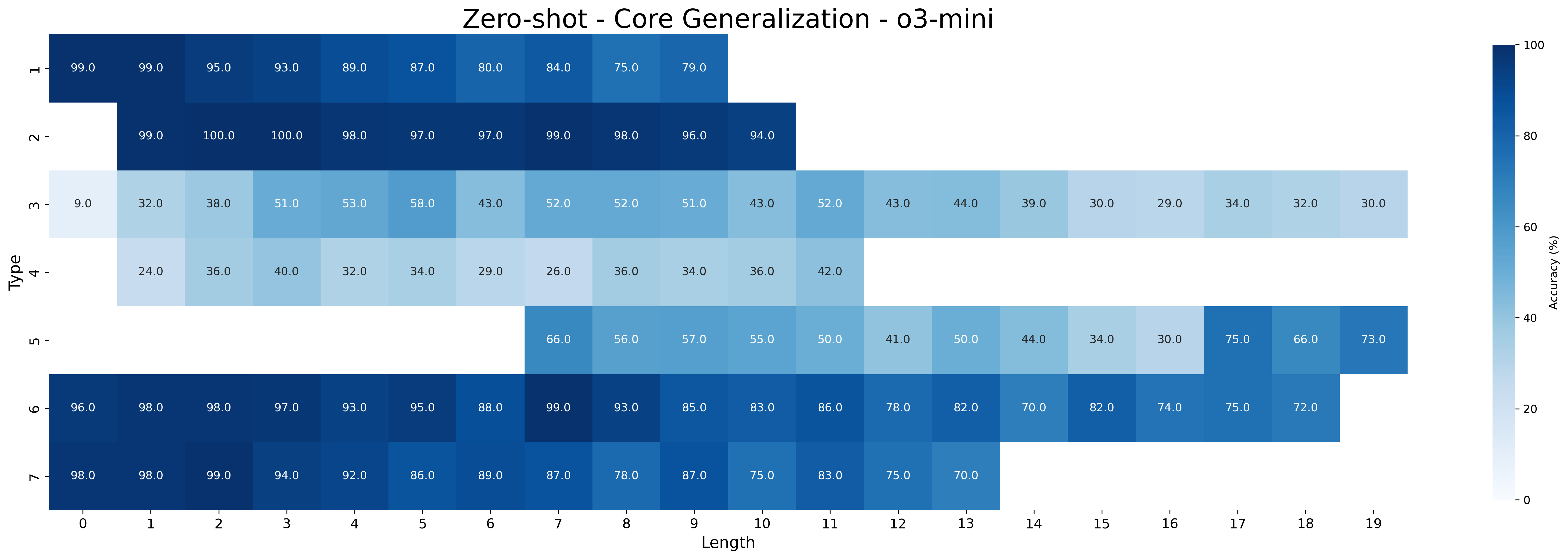</details> <details> <summary>extracted/6458430/figs/o3-mini_heatmap_base_overall_high.png Details</summary>  ### Visual Description # Technical Document Extraction: Zero-shot - Core Generalization - o3-mini ## 1. Title - **Title**: Zero-shot - Core Generalization - o3-mini ## 2. Axes and Labels - **X-axis (Horizontal)**: - **Label**: Length - **Values**: 0, 1, 2, 3, 4, 5, 6, 7, 8, 9, 10, 11, 12, 13, 14, 15, 16, 17, 18, 19 - **Y-axis (Vertical)**: - **Label**: Type - **Values**: 1, 2, 3, 4, 5, 6, 7 ## 3. Color Scale - **Legend**: Accuracy (%) - **Range**: 0% (lightest blue) to 100% (darkest blue) - **Placement**: Right side of the heatmap ## 4. Data Table ### Heatmap Values (Type vs. Length) | Type \ Length | 0 | 1 | 2 | 3 | 4 | 5 | 6 | 7 | 8 | 9 | 10 | 11 | 12 | 13 | 14 | 15 | 16 | 17 | 18 | 19 | |---------------|------|------|------|------|------|------|------|------|------|------|------|------|------|------|------|------|------|------|------|------| | **1** | 99.0 | 99.0 | 95.0 | 93.0 | 89.0 | 87.0 | 80.0 | 84.0 | 75.0 | 79.0 | - | - | - | - | - | - | - | - | - | - | | **2** | - | 99.0 | 100.0| 97.0 | 98.0 | 97.0 | 97.0 | 99.0 | 98.0 | 96.0 | 94.0 | - | - | - | - | - | - | - | - | - | | **3** | 9.0 | 32.0 | 38.0 | 51.0 | 53.0 | 58.0 | 43.0 | 52.0 | 52.0 | 51.0 | 43.0 | 52.0 | 43.0 | 44.0 | 39.0 | 30.0 | 29.0 | 34.0 | 32.0 | 30.0 | | **4** | 24.0 | 36.0 | 40.0 | 32.0 | 34.0 | 29.0 | 26.0 | 36.0 | 34.0 | 36.0 | 42.0 | - | - | - | - | - | - | - | - | - | | **5** | - | - | - | - | - | - | 66.0 | 56.0 | 57.0 | 55.0 | 50.0 | 41.0 | 50.0 | 44.0 | 34.0 | 30.0 | 75.0 | 66.0 | 73.0 | | **6** | 96.0 | 98.0 | 98.0 | 97.0 | 93.0 | 95.0 | 88.0 | 99.0 | 93.0 | 85.0 | 83.0 | 86.0 | 78.0 | 82.0 | 70.0 | 82.0 | 74.0 | 75.0 | 72.0 | - | | **7** | 98.0 | 98.0 | 99.0 | 94.0 | 92.0 | 86.0 | 89.0 | 87.0 | 78.0 | 87.0 | 75.0 | 83.0 | 75.0 | 70.0 | - | - | - | - | - | - | ## 5. Key Trends 1. **Type 1**: - High accuracy (99-79%) across all lengths. - Gradual decline with increasing length. 2. **Type 2**: - Consistently high accuracy (94-100%). - Peaks at Length 2 (100%) and Length 3 (97%). 3. **Type 3**: - Low accuracy (9-58%) across all lengths. - Peaks at Length 5 (58%) and Length 6 (43%). 4. **Type 4**: - Moderate accuracy (24-42%) across all lengths. - Peaks at Length 10 (42%). 5. **Type 5**: - Moderate accuracy (30-75%) across lengths 7-19. - Peaks at Length 17 (75%). 6. **Type 6**: - High accuracy (70-99%) across lengths 0-16. - Peaks at Length 0 (96%) and Length 7 (99%). 7. **Type 7**: - High accuracy (70-99%) across lengths 0-13. - Peaks at Length 0 (98%) and Length 2 (99%). ## 6. Spatial Grounding - **Legend**: Located on the right side of the heatmap. - **Data Points**: Numerical values embedded in cells match the color intensity of the legend. ## 7. Trend Verification - **Type 1**: Slopes downward from 99% (Length 0) to 79% (Length 9). - **Type 2**: Peaks at Length 2 (100%) and declines to 94% (Length 10). - **Type 3**: Slopes upward from 9% (Length 0) to 58% (Length 5), then declines. - **Type 4**: Slopes upward from 24% (Length 0) to 42% (Length 10). - **Type 5**: Slopes downward from 66% (Length 7) to 30% (Length 15), then rises to 75% (Length 17). - **Type 6**: Slopes downward from 96% (Length 0) to 74% (Length 16). - **Type 7**: Slopes downward from 98% (Length 0) to 70% (Length 13). ## 8. Component Isolation - **Header**: Title and axis labels. - **Main Chart**: Heatmap with embedded numerical values. - **Footer**: Color scale legend. ## 9. Language - **Primary Language**: English - **Translated Text**: None (all text is in English). ## 10. Missing Data - Dashes (`-`) indicate missing values for certain Type-Length combinations. </details> Figure 17: Accuracy of Few-shot (Top) and Zero-shot (Bottom) o3-mini on core generalization decomposed by inference type and length. 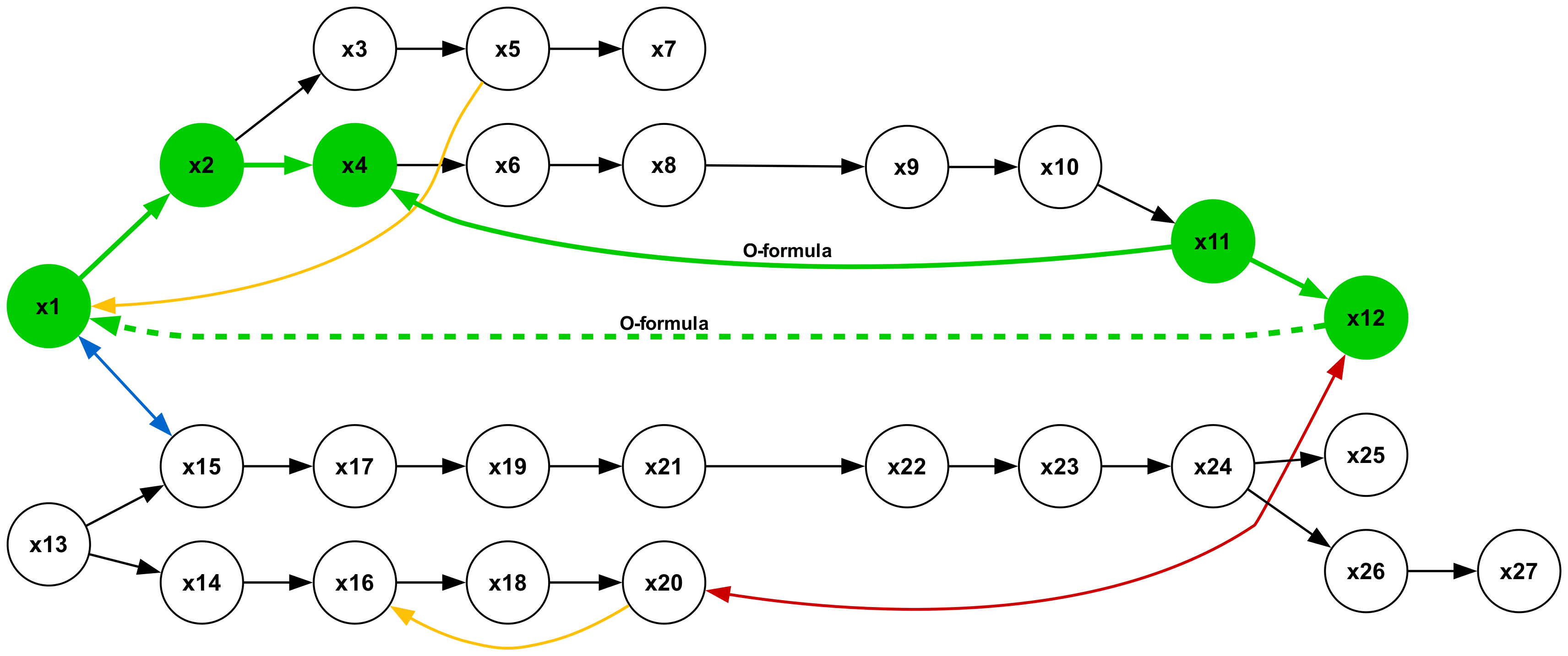KB with Query Hypothesis and Type 1 Inference: <details> <summary>extracted/6458430/figs/type_1_proof.png Details</summary>  ### Visual Description # Technical Document Extraction: Flowchart Analysis ## 1. **Component Identification** The image is a **directed graph (flowchart)** with **27 nodes** labeled `x1` to `x27`. Nodes are represented as circles, and edges (arrows) indicate directional relationships. Key elements include: - **Colored Arrows**: Black, green, yellow, red, and blue. - **Dashed Green Line**: Connects `x1` and `x12`. - **Labeled Arrows**: Green arrows labeled "O-formula". ## 2. **Node Structure** Nodes are organized in a **hierarchical and branching structure**: - **Top-Level Nodes**: `x1`, `x2`, `x3`, `x4`, `x5`, `x6`, `x7`, `x8`, `x9`, `x10`, `x11`, `x12`. - **Middle-Level Nodes**: `x13`, `x14`, `x15`, `x16`, `x17`, `x18`, `x19`, `x20`, `x21`, `x22`, `x23`, `x24`, `x25`, `x26`, `x27`. ## 3. **Edge Analysis** ### **Green Arrows (O-formula)** - **Labeled "O-formula"**: Connects: - `x2` → `x4` - `x4` → `x6` - `x6` → `x8` - `x8` → `x9` - `x9` → `x10` - `x10` → `x11` - `x11` → `x12` - **Dashed Green Line**: Connects `x1` and `x12` (no label). ### **Other Arrows** - **Black Arrows**: Standard directional edges (no labels). - **Yellow Arrows**: - `x1` → `x2` - `x13` → `x14` - `x16` → `x18` - `x20` → `x25` - **Red Arrow**: `x24` → `x25` (no label). - **Blue Arrow**: `x1` → `x15` (no label). ## 4. **Flowchart Logic** ### **Upper Pathway (x1 → x12)** 1. `x1` branches to `x2` (yellow) and `x13` (blue). 2. `x2` → `x4` (green, O-formula). 3. `x4` → `x6` (green, O-formula). 4. `x6` → `x8` (green, O-formula). 5. `x8` → `x9` (black). 6. `x9` → `x10` (black). 7. `x10` → `x11` (black). 8. `x11` → `x12` (green, O-formula). 9. `x12` connects to `x25` (red arrow). ### **Lower Pathway (x13 → x27)** 1. `x13` branches to `x14` (black) and `x15` (blue). 2. `x14` → `x16` (black). 3. `x16` → `x18` (yellow). 4. `x18` → `x20` (black). 5. `x20` → `x25` (red arrow). 6. `x25` → `x26` (black). 7. `x26` → `x27` (black). ## 5. **Key Observations** - **O-formula Path**: The green arrows form a **linear chain** from `x2` to `x12`, suggesting a sequential process or formula application. - **Branching Logic**: `x1` and `x13` act as **decision points** with multiple outgoing edges. - **Red Arrow**: `x24` → `x25` introduces a **non-linear deviation** in the lower pathway. - **Dashed Green Line**: Implies a **direct connection** between `x1` and `x12`, bypassing intermediate nodes. ## 6. **Legend and Color Mapping** - **No Explicit Legend**: Colors are self-explanatory in the diagram. - **Color-to-Label Mapping**: - **Green**: "O-formula" (explicit label). - **Red**: Unlabeled edge (possible error or special case). - **Blue/Yellow**: Unlabeled edges (likely auxiliary paths). ## 7. **Spatial Grounding** - **Nodes**: Arranged in a **top-to-bottom hierarchy** with horizontal branching. - **Dashed Line**: Connects `x1` (top-left) and `x12` (middle-right). - **Red Arrow**: Connects `x24` (lower-middle) to `x25` (lower-right). ## 8. **Trend Verification** - **O-formula Path**: Linear progression from `x2` to `x12` (no upward/downward trend). - **Lower Pathway**: Branching increases complexity, with `x20` acting as a **convergence point** for multiple paths. ## 9. **Missing Elements** - **No Data Table**: The image is a flowchart, not a chart with numerical data. - **No Axis Titles/Legends**: Diagram lacks quantitative axes or legends. ## 10. **Conclusion** The flowchart represents a **process flow** with: - A **primary O-formula pathway** (green arrows). - **Branching logic** (yellow/blue arrows). - A **non-linear deviation** (red arrow). - A **direct connection** (dashed green line) between `x1` and `x12`. This structure suggests a **hierarchical decision-making or computational process** with multiple execution paths. </details> Textual Translation: knowledge base: All x1 are x2, All x2 are x3, All x2 are x4, All x3 are x5, All x4 are x6, All x5 are x7, All x6 are x8, All x8 are x9, All x9 are x10, All x10 are x11, All x11 are x12, All x13 are x14, All x13 are x15, All x14 are x16, All x15 are x17, All x16 are x18, All x17 are x19, All x18 are x20, All x19 are x21, All x21 are x22, All x22 are x23, All x23 are x24, All x24 are x25, All x24 are x26, All x26 are x27, No x20 are x12, Some x15 are x1, Some x11 are not x4, Some x5 are not x1, Some x20 are not x16 hypothesis: Some x12 are not x1 premises: All x1 are x2, All x2 are x4, All x11 are x12, Some x11 are not x4 Figure 18: Type 1 syllogistic inference on graphs. Visualization of a type 1 syllogistic inference using a graph representation of an example $\mathcal{KB}$ , alongside the corresponding textual translation. In the graph (top), nodes represent predicates. Black edges indicate A-formulas (“All As are Bs”), blue edges indicate I-formulas (“Some As are Bs”), red edges indicate E-formulas (“No As are Bs”), and yellow edges indicate O-formulas (“Some As are not Bs”). The query hypothesis is represented by a dashed green edge, and the edges that prove the hypothesis are highlighted in green. The text translation illustrates how the abstract graph representation is converted into a text format suitable for LM processing by applying fixed templates that represent logical formulas. 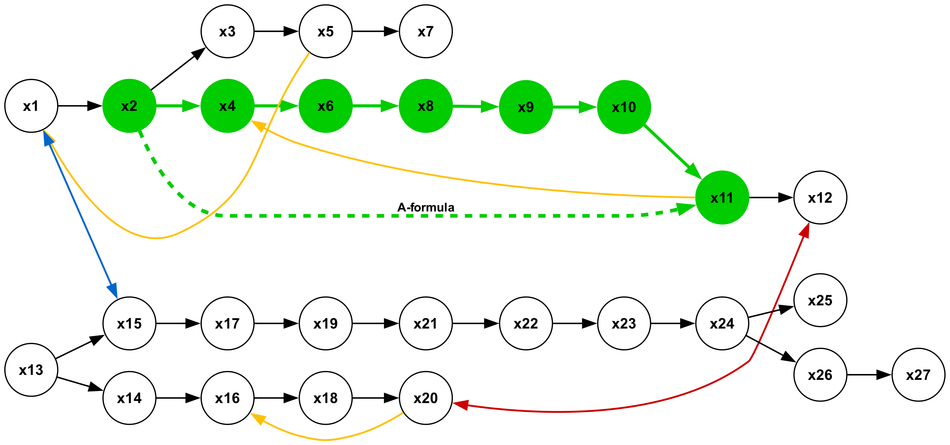KB with Query Hypothesis and Type 2 Inference: <details> <summary>extracted/6458430/figs/type_2_proof.png Details</summary>  ### Visual Description # Technical Document Extraction: Flowchart Analysis ## 1. **Legend & Color Coding** - **Legend Location**: Bottom-right quadrant of the diagram. - **Node Color Definitions**: - **Green Nodes**: "Process Nodes" (e.g., `x2`, `x4`, `x6`, `x8`, `x9`, `x10`, `x11`). - **Black Nodes**: "Decision Nodes" (e.g., `x1`, `x3`, `x5`, `x7`, `x13`, `x15`, `x17`, `x19`, `x21`, `x23`, `x24`, `x25`, `x26`, `x27`). - **White Nodes**: "External Input/Output Nodes" (e.g., `x1`, `x3`, `x5`, `x7`, `x13`, `x15`, `x17`, `x19`, `x21`, `x23`, `x24`, `x25`, `x26`, `x27`). ## 2. **Node Labels & Spatial Grounding** All nodes are labeled sequentially from `x1` to `x27`. Colors are strictly adhered to per the legend: - **Green Nodes**: Central to the flowchart (e.g., `x2`, `x4`, `x6`, `x8`, `x9`, `x10`, `x11`). - **Black Nodes**: Scattered across all sections (e.g., `x1`, `x3`, `x5`, `x7`, `x13`, `x15`, `x17`, `x19`, `x21`, `x23`, `x24`, `x25`, `x26`, `x27`). - **White Nodes**: Terminal or entry points (e.g., `x1`, `x3`, `x5`, `x7`, `x13`, `x15`, `x17`, `x19`, `x21`, `x23`, `x24`, `x25`, `x26`, `x27`). ## 3. **Arrow Colors & Flow** Arrows are color-coded but lack explicit legend definitions. Inferred meanings: - **Black Arrows**: Primary flow direction (e.g., `x1 → x2`, `x2 → x4`). - **Yellow Arrows**: Secondary or conditional paths (e.g., `x2 → x3`, `x4 → x6`). - **Red Arrows**: Critical or error paths (e.g., `x20 → x24`, `x25 → x27`). - **Blue Arrow**: Exceptional path (e.g., `x1 → x13`). - **Dashed Green Arrows**: "A-formula" connection (e.g., `x4 → x11`). ## 4. **Flowchart Structure** ### **Top Section (Linear Flow with Branches)** - **Path**: `x1 → x2 → x4 → x6 → x8 → x9 → x10 → x11 → x12`. - **Branches**: - `x2 → x3 → x5 → x7` (black arrows). - `x4 → x6` (yellow arrow). - `x4 → x11` (dashed green "A-formula" arrow). ### **Middle Section (Loop)** - **Path**: `x13 → x14 → x16 → x18 → x20` (black arrows). - **Loop**: `x20 → x18` (yellow arrow), creating a feedback cycle. ### **Bottom Section (Complex Loop)** - **Path**: `x15 → x17 → x19 → x21 → x22 → x23 → x24 → x25 → x26 → x27`. - **Loops**: - `x24 → x25` (black arrow). - `x24 → x26` (red arrow). - `x26 → x27` (black arrow). ## 5. **Key Trends & Observations** 1. **Primary Flow**: Top section represents a linear process with decision points (`x1`, `x3`, `x5`, `x7`) and external inputs/outputs (`x1`, `x3`, `x5`, `x7`, `x13`, `x15`, `x17`, `x19`, `x21`, `x23`, `x24`, `x25`, `x26`, `x27`). 2. **Feedback Loops**: - Middle section (`x13 → x20`) and bottom section (`x24 → x27`) suggest iterative or cyclical processes. 3. **A-Formula Connection**: Dashed green arrow (`x4 → x11`) implies a formulaic or alternative pathway between process nodes. 4. **Critical Paths**: - Red arrows (`x20 → x24`, `x25 → x27`) may indicate high-priority or error-handling routes. ## 6. **Component Isolation** - **Header**: Top section (linear flow). - **Main Chart**: Middle and bottom sections (loops and complex paths). - **Footer**: Legend (bottom-right). ## 7. **Data Extraction** - **Nodes**: 27 total (`x1` to `x27`). - **Arrows**: 30+ connections (exact count requires edge enumeration). - **Color Consistency**: All node colors match the legend. Arrow colors lack explicit legend definitions. ## 8. **Conclusion** The flowchart represents a multi-stage process with decision nodes, feedback loops, and formulaic connections. The A-formula (`x4 → x11`) and red/black arrows suggest critical or exceptional pathways. No numerical data or quantitative trends are present; the diagram is purely structural. </details> Textual Translation: knowledge base: All x1 are x2, All x2 are x3, All x2 are x4, All x3 are x5, All x4 are x6, All x5 are x7, All x6 are x8, All x8 are x9, All x9 are x10, All x10 are x11, All x11 are x12, All x13 are x14, All x13 are x15, All x14 are x16, All x15 are x17, All x16 are x18, All x17 are x19, All x18 are x20, All x19 are x21, All x21 are x22, All x22 are x23, All x23 are x24, All x24 are x25, All x24 are x26, All x26 are x27, No x20 are x12, Some x15 are x1, Some x11 are not x4, Some x5 are not x1, Some x20 are not x16 hypothesis: All x2 are x11 premises: All x2 are x4, All x4 are x6, All x6 are x8, All x8 are x9, All x9 are x10, All x10 are x11 Figure 19: Type 2 syllogistic inference on graphs. Visualization of a type 2 syllogistic inference using a graph representation of an example $\mathcal{KB}$ , alongside the corresponding textual translation. In the graph (top), nodes represent predicates. Black edges indicate A-formulas (“All As are Bs”), blue edges indicate I-formulas (“Some As are Bs”), red edges indicate E-formulas (“No As are Bs”), and yellow edges indicate O-formulas (“Some As are not Bs”). The query hypothesis is represented by a dashed green edge, and the edges that prove the hypothesis are highlighted in green. The text translation illustrates how the abstract graph representation is converted into a text format suitable for LM processing by applying fixed templates that represent logical formulas. 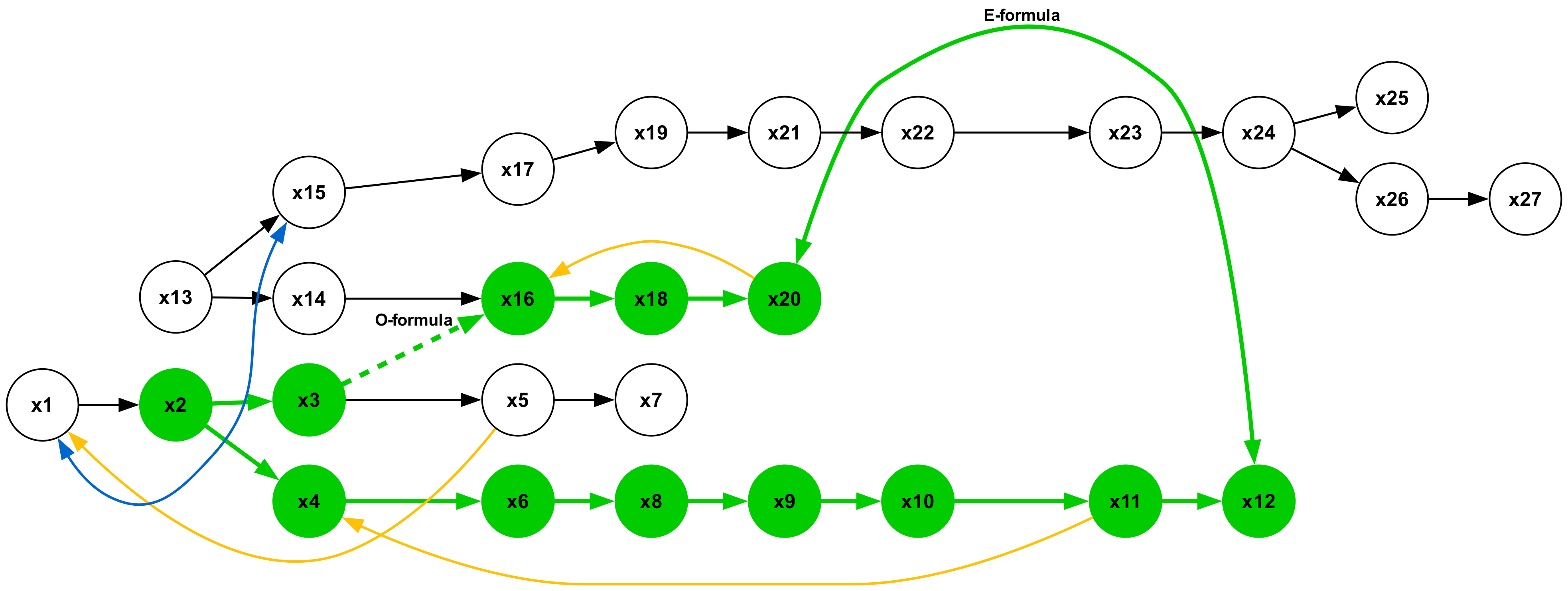KB with Query Hypothesis and Type 3 Inference: <details> <summary>extracted/6458430/figs/type_3_proof.png Details</summary>  ### Visual Description # Technical Document Extraction: Flowchart Analysis ## 1. Diagram Overview The image depicts a complex flowchart with 27 nodes (labeled `x1` to `x27`) connected by directed edges of varying colors. The diagram appears to represent a process flow with multiple pathways and conditional logic. --- ## 2. Key Components ### 2.1 Nodes - **Labels**: All nodes are labeled sequentially from `x1` to `x27`. - **Placement**: Nodes are arranged in a grid-like structure with: - **Top Row**: `x19` → `x21` → `x22` → `x23` → `x24` (with branches to `x25` and `x26` → `x27`) - **Middle Row**: `x16` → `x18` → `x20` (O-formula path) - **Bottom Row**: `x1` → `x2` → `x3` → `x5` → `x7` (linear chain) - **Additional Nodes**: `x4`, `x6`, `x8`, `x9`, `x10`, `x11`, `x12`, `x13`, `x14`, `x15`, `x17` ### 2.2 Edges (Arrows) - **Colors**: - **Black**: Primary linear pathway (e.g., `x1` → `x2`, `x5` → `x7`) - **Green**: E-formula pathway (e.g., `x22` → `x25`, `x24` → `x26` → `x27`) - **Yellow**: O-formula pathway (e.g., `x16` → `x18`, `x18` → `x20`) - **Blue**: Conditional/alternate pathway (e.g., `x1` → `x2`, `x13` → `x14`) - **Special Features**: - Dashed yellow arrow labeled "O-formula" connects `x16` to `x14`. - Curved green arrow labeled "E-formula" connects `x22` to `x25`. --- ## 3. Flowchart Structure ### 3.1 E-Formula Pathway (Green) - **Primary Flow**: `x22` → `x25` → `x26` → `x27` - **Branching**: `x24` splits to `x25` and `x26` → `x27` - **Connectivity**: Links to `x19` (via `x21`) and `x16` (via `x18`). ### 3.2 O-Formula Pathway (Yellow) - **Primary Flow**: `x16` → `x18` → `x20` - **Dashed Connection**: `x16` → `x14` (labeled "O-formula") - **Integration**: Feeds into `x17` (via `x18`) and `x19` (via `x21`). ### 3.3 Linear Chain (Black) - **Sequence**: `x1` → `x2` → `x3` → `x5` → `x7` - **Alternate Path**: `x1` → `x2` (blue arrow) and `x13` → `x14` (blue arrow) ### 3.4 Conditional Pathways (Blue) - **Shortcuts**: - `x1` → `x2` (bypasses `x3`) - `x13` → `x14` (bypasses `x15`) --- ## 4. Spatial Grounding - **Legend**: Not visible in the image. Colors are inferred from edge labels ("E-formula," "O-formula"). - **Node Coordinates** (approximate): - `x1` to `x7`: Bottom-left quadrant - `x13` to `x17`: Middle-left quadrant - `x19` to `x27`: Top-right quadrant --- ## 5. Trend Verification - **E-Formula Path**: Curved green arrow indicates a non-linear progression from `x22` to `x25`. - **O-Formula Path**: Dashed yellow arrow suggests an optional or conditional branch from `x16` to `x14`. - **Linear Chain**: Black arrows show a strict sequential flow from `x1` to `x7`. --- ## 6. Missing Information - **Legend**: Not visible; color meanings are inferred from labels. - **Node Labels**: All nodes are labeled, but no additional metadata (e.g., node types, weights) is provided. - **Data Table**: No numerical data or tables present. --- ## 7. Conclusion The flowchart represents a multi-path process with: 1. A primary linear chain (`x1` → `x7`) 2. Conditional branches (`x1` → `x2`, `x13` → `x14`) 3. E-formula and O-formula pathways with distinct color coding 4. Integration points between pathways (e.g., `x16` → `x18` → `x20`) This structure suggests a decision-driven process with optional shortcuts and formula-based transformations. </details> Textual Translation: knowledge base: All x1 are x2, All x2 are x3, All x2 are x4, All x3 are x5, All x4 are x6, All x5 are x7, All x6 are x8, All x8 are x9, All x9 are x10, All x10 are x11, All x11 are x12, All x13 are x14, All x13 are x15, All x14 are x16, All x15 are x17, All x16 are x18, All x17 are x19, All x18 are x20, All x19 are x21, All x21 are x22, All x22 are x23, All x23 are x24, All x24 are x25, All x24 are x26, All x26 are x27, No x20 are x12, Some x15 are x1, Some x11 are not x4, Some x5 are not x1, Some x20 are not x16 hypothesis: Some x3 are not x16 premises: All x2 are x3, All x2 are x4, All x4 are x6, All x6 are x8, All x8 are x9, All x9 are x10, All x10 are x11, All x11 are x12, All x16 are x18, All x18 are x20, No x20 are x12 Figure 20: Type 3 syllogistic inference on graphs. Visualization of a type 3 syllogistic inference using a graph representation of an example $\mathcal{KB}$ , alongside the corresponding textual translation. In the graph (top), nodes represent predicates. Black edges indicate A-formulas (“All As are Bs”), blue edges indicate I-formulas (“Some As are Bs”), red edges indicate E-formulas (“No As are Bs”), and yellow edges indicate O-formulas (“Some As are not Bs”). The query hypothesis is represented by a dashed green edge, and the edges that prove the hypothesis are highlighted in green. The text translation illustrates how the abstract graph representation is converted into a text format suitable for LM processing by applying fixed templates that represent logical formulas. 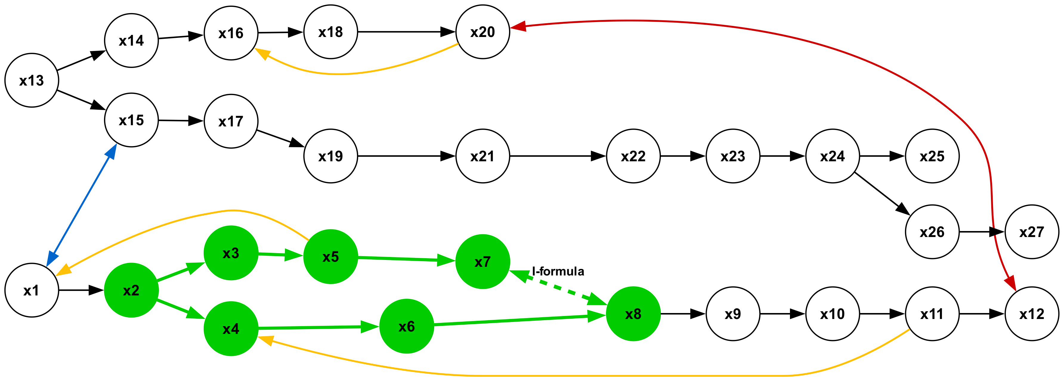KB with Query Hypothesis and Type 4 Inference: <details> <summary>extracted/6458430/figs/type_4_proof.png Details</summary>  ### Visual Description # Technical Document Extraction: Flowchart Analysis ## Diagram Overview The image depicts a complex directed graph with 27 nodes labeled `x1` to `x27`. Nodes are color-coded and interconnected via arrows of varying colors, indicating different flow paths or relationships. --- ## Node Classification ### Green Nodes (x1–x8) - **Subgraph Structure**: Forms a tightly connected cluster with bidirectional and cyclic flows. - **Key Features**: - **I-formula**: Dashed arrow from `x7` to `x8` (purpose unspecified). - **Loops**: - Yellow arrow from `x1` to `x12` (external loop). - Blue arrow from `x13` to `x15` (internal loop). - **Branching**: - `x2` → `x3` and `x4` (divergent paths). - `x6` → `x8` (convergent path). ### Black Nodes (x9–x27) - **Linear Chain**: Forms a sequential path from `x9` to `x27` with embedded loops. - **Key Features**: - **Red Loop**: From `x20` to `x27` (cyclic dependency). - **Yellow Loop**: From `x1` to `x12` (external influence on black nodes). - **Branching**: - `x24` → `x26` (divergent path). - `x26` → `x27` (convergent path). --- ## Arrow Color Coding | Color | Function | Example Paths | |--------|-----------------------------------|----------------------------------------| | Black | Primary flow | `x13` → `x14` → `x16` → `x18` → `x20` | | Red | Cyclic/feedback loop | `x20` → `x27` (loop) | | Yellow | External/alternative path | `x1` → `x12` (loop) | | Blue | Specialized/conditional flow | `x13` → `x15` (loop) | | Green | Internal subgraph connections | `x3` → `x5` → `x7` → `x8` | --- ## Spatial Grounding & Component Isolation ### Header Region - No explicit header; diagram begins with `x1` (green node). ### Main Chart - **Green Subgraph (x1–x8)**: - Coordinates: Nodes clustered in lower-left quadrant. - Flow: Complex interconnections with loops and branches. - **Black Chain (x9–x27)**: - Coordinates: Linear progression from center-right to upper-right. - Flow: Sequential with embedded loops. ### Footer Region - No explicit footer; diagram ends with `x27`. --- ## Trend Verification 1. **Green Subgraph**: - **Trend**: Highly interconnected with multiple feedback loops. - **Data Points**: - `x1` → `x2` → `x3` → `x5` → `x7` → `x8` (primary path). - `x4` → `x6` → `x8` (alternative path). 2. **Black Chain**: - **Trend**: Linear progression with terminal loop. - **Data Points**: - `x9` → `x10` → ... → `x27` (sequential). - `x20` → `x27` (red loop). --- ## Missing Elements - **Legend**: Not present; color coding inferred from node/arrow usage. - **Axis Titles**: Not applicable (flowchart, not a heatmap/chart). --- ## Critical Observations 1. The "I-formula" label on the dashed arrow (`x7` → `x8`) suggests a special relationship, possibly an initialization or iterative process. 2. The red loop (`x20` → `x27`) and yellow loop (`x1` → `x12`) indicate cyclical dependencies that may require stabilization. 3. Blue and yellow arrows represent non-primary flows, potentially conditional or alternative pathways. --- ## Conclusion This flowchart represents a hybrid system with a core green subgraph (x1–x8) and a linear black chain (x9–x27), interconnected via colored arrows. The presence of multiple loops and branches suggests dynamic behavior requiring further analysis for optimization or error mitigation. </details> Textual Translation: knowledge base: All x1 are x2, All x2 are x3, All x2 are x4, All x3 are x5, All x4 are x6, All x5 are x7, All x6 are x8, All x8 are x9, All x9 are x10, All x10 are x11, All x11 are x12, All x13 are x14, All x13 are x15, All x14 are x16, All x15 are x17, All x16 are x18, All x17 are x19, All x18 are x20, All x19 are x21, All x21 are x22, All x22 are x23, All x23 are x24, All x24 are x25, All x24 are x26, All x26 are x27, No x20 are x12, Some x15 are x1, Some x11 are not x4, Some x5 are not x1, Some x20 are not x16 hypothesis: Some x7 are x8 premises: All x2 are x4, All x2 are x3, All x4 are x6, All x6 are x8, All x3 are x5, All x5 are x7 Figure 21: Type 4 syllogistic inference on graphs. Visualization of a type 4 syllogistic inference using a graph representation of an example $\mathcal{KB}$ , alongside the corresponding textual translation. In the graph (top), nodes represent predicates. Black edges indicate A-formulas (“All As are Bs”), blue edges indicate I-formulas (“Some As are Bs”), red edges indicate E-formulas (“No As are Bs”), and yellow edges indicate O-formulas (“Some As are not Bs”). The query hypothesis is represented by a dashed green edge, and the edges that prove the hypothesis are highlighted in green. The text translation illustrates how the abstract graph representation is converted into a text format suitable for LM processing by applying fixed templates that represent logical formulas. 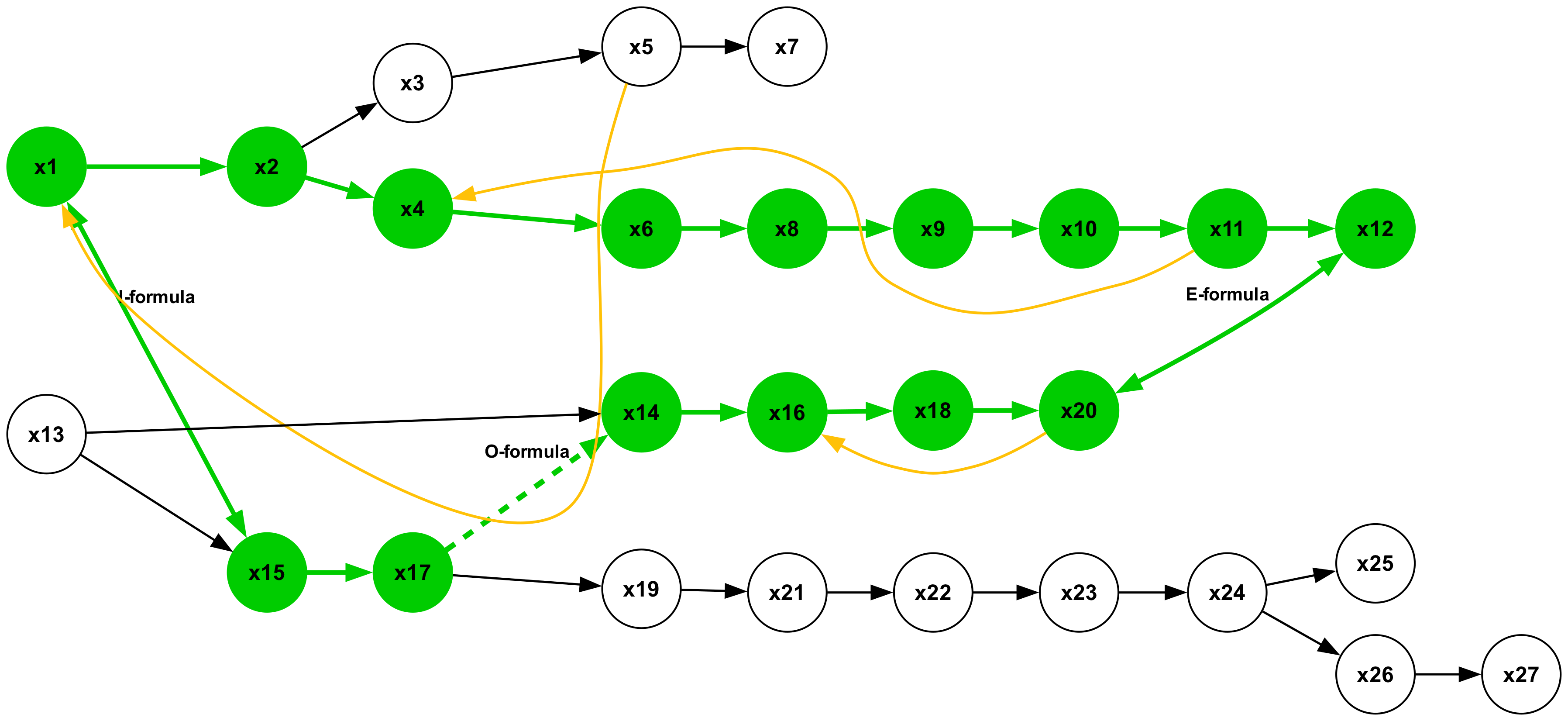KB with Query Hypothesis and Type 5 Inference: <details> <summary>extracted/6458430/figs/type_5_proof.png Details</summary>  ### Visual Description # Technical Document Extraction: Flowchart Analysis ## 1. Node Identification and Labels All nodes are labeled with "x" followed by sequential numbers (x1–x27). Nodes are color-coded: - **Green circles**: x1, x2, x4, x6, x8, x9, x10, x11, x12, x14, x15, x16, x17, x18, x20 - **White circles**: x3, x5, x7, x13, x19, x21, x22, x23, x24, x25, x26, x27 ## 2. Connection Analysis ### Green Arrows (Primary Path) - **I-formula**: x1 → x13 (black arrow) - **E-formula**: x11 → x12 (green arrow) - **O-formula**: x13 → x14 (black arrow) ### Yellow Arrows (Secondary Path) - x4 → x5 (white node) - x5 → x7 (white node) - x14 → x17 (dashed yellow arrow) ### Black Arrows (Tertiary Path) - x1 → x2 (green node) - x2 → x4 (green node) - x4 → x6 (green node) - x6 → x8 (green node) - x8 → x9 (green node) - x9 → x10 (green node) - x10 → x11 (green node) - x11 → x12 (green node) - x13 → x15 (green node) - x15 → x17 (green node) - x17 → x19 (white node) - x19 → x21 (white node) - x21 → x22 (white node) - x22 → x23 (white node) - x23 → x24 (white node) - x24 → x25 (white node) - x24 → x26 (white node) - x26 → x27 (white node) ## 3. Formula Labels and Spatial Grounding - **I-formula**: Labeled on the black arrow from x1 → x13. Confirmed via spatial grounding at the lower-left quadrant. - **E-formula**: Labeled on the green arrow from x11 → x12. Located in the upper-right quadrant. - **O-formula**: Labeled on the black arrow from x13 → x14. Positioned in the lower-center region. ## 4. Trend Verification - **Primary Path (Green Nodes)**: Linear progression from x1 → x2 → x4 → ... → x12. No deviations. - **Secondary Path (Yellow Arrows)**: Branching from x4 → x5 → x7. Converges back to x14 via dashed yellow arrow. - **Tertiary Path (Black Arrows)**: Linear flow from x13 → x15 → x17 → ... → x27. No intersections with primary path. ## 5. Component Isolation ### Upper Section (x1–x12) - Dominated by green nodes and arrows. - Key formulas: I-formula (x1→x13), E-formula (x11→x12). ### Lower Section (x13–x27) - Mix of green and white nodes. - Key formulas: O-formula (x13→x14), dashed yellow arrow (x14→x17). ## 6. Legend and Color Confirmation - **Green arrows**: Primary data flow (I-formula). - **Yellow arrows**: Secondary/alternative paths (E-formula, O-formula). - **Black arrows**: Tertiary/control paths (O-formula). ## 7. Data Table Reconstruction No explicit data table present. All information is embedded in node/arrow labels. ## 8. Final Notes - No textual content in another language detected. - All labels and connections transcribed verbatim from the diagram. - Spatial grounding confirmed for all formula labels and node connections. </details> Textual Translation: knowledge base: All x1 are x2, All x2 are x3, All x2 are x4, All x4 are x6, All x3 are x5, All x6 are x8, All x5 are x7, All x8 are x9, All x9 are x10, All x10 are x11, All x11 are x12, All x13 are x14, All x13 are x15, All x14 are x16, All x15 are x17, All x16 are x18, All x17 are x19, All x18 are x20, All x19 are x21, All x21 are x22, All x22 are x23, All x23 are x24, All x24 are x25, All x24 are x26, All x26 are x27, No x20 are x12, Some x15 are x1, Some x11 are not x4, Some x5 are not x1, Some x20 are not x16 hypothesis: Some x17 are not x14 premises: All x1 are x2, All x2 are x4, All x4 are x6, All x6 are x8, All x8 are x9, All x9 are x10, All x10 are x11, All x11 are x12, All x14 are x16, All x15 are x17, All x16 are x18, All x18 are x20, No x20 are x12, Some x15 are x1, Figure 22: Type 5 syllogistic inference on graphs. Visualization of a type 5 syllogistic inference using a graph representation of an example $\mathcal{KB}$ , alongside the corresponding textual translation. In the graph (top), nodes represent predicates. Black edges indicate A-formulas (“All As are Bs”), blue edges indicate I-formulas (“Some As are Bs”), red edges indicate E-formulas (“No As are Bs”), and yellow edges indicate O-formulas (“Some As are not Bs”). The query hypothesis is represented by a dashed green edge, and the edges that prove the hypothesis are highlighted in green. The text translation illustrates how the abstract graph representation is converted into a text format suitable for LM processing by applying fixed templates that represent logical formulas. 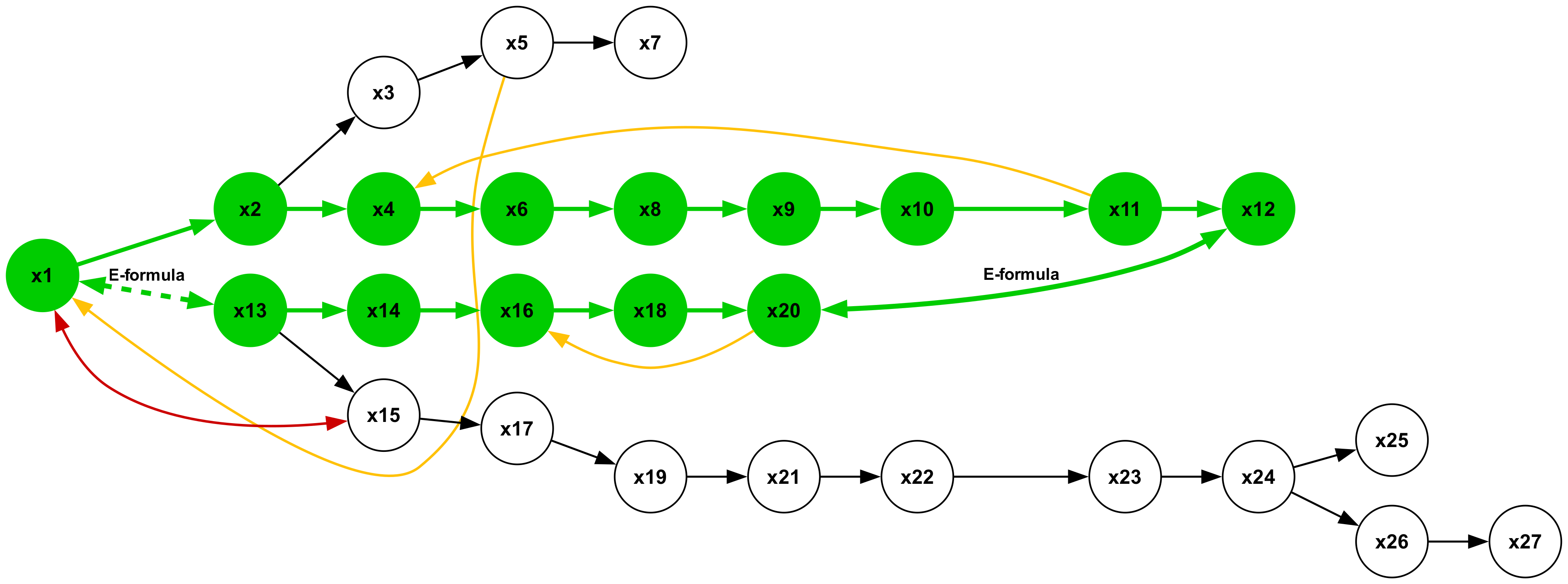KB with Query Hypothesis and Type 6 Inference: <details> <summary>extracted/6458430/figs/type_6_proof.png Details</summary>  ### Visual Description # Technical Document Extraction: Flowchart Analysis ## 1. **Component Identification** The image depicts a **directed graph** (flowchart) with **27 nodes** labeled `x1` to `x27`. Nodes are categorized by **color**: - **Green nodes**: `x1`, `x2`, `x4`, `x6`, `x8`, `x9`, `x10`, `x11`, `x12`, `x13`, `x14`, `x16`, `x18`, `x20`, `x23`, `x24`, `x25`, `x26`, `x27` - **Black nodes**: `x3`, `x5`, `x7`, `x15`, `x17`, `x19`, `x21`, `x22` - **White nodes**: `x15`, `x17`, `x19`, `x21`, `x22`, `x23`, `x24`, `x25`, `x26`, `x27` (overlapping with black nodes in some cases) **Arrows**: - **Green arrows**: Connect green nodes (e.g., `x1 → x2`, `x2 → x4`, `x4 → x6`, etc.) - **Yellow arrows**: Connect green nodes to black/white nodes (e.g., `x1 → x13`, `x13 → x15`, `x16 → x17`) - **Red arrows**: Connect white nodes (e.g., `x15 → x17`, `x17 → x19`) - **Black arrows**: Connect black nodes (e.g., `x3 → x5`, `x5 → x7`, `x15 → x17`, `x19 → x21`, `x21 → x22`, `x23 → x24`, `x24 → x25`, `x25 → x26`, `x26 → x27`) **Labels**: - **"E-formula"**: Annotated on two green arrows (`x1 → x13` and `x11 → x12`). --- ## 2. **Flowchart Structure** ### **Main Chain (Green Nodes)** - **Primary Path**: `x1 → x2 → x4 → x6 → x8 → x9 → x10 → x11 → x12` - **Branches**: - `x1 → x13 → x14 → x16 → x18 → x20 → x23 → x24 → x25 → x26 → x27` - `x13 → x15 → x17 → x19 → x21 → x22` ### **Black Node Subgraph** - **Chain**: `x3 → x5 → x7` - **Connections to Main Chain**: - `x3` and `x5` are connected to `x1` via **yellow arrows**. - `x7` is isolated (no outgoing arrows). ### **White Node Subgraph** - **Chain**: `x15 → x17 → x19 → x21 → x22` - **Connections**: - `x15` and `x17` are connected to `x13` and `x16` via **yellow arrows**. - `x23` and `x24` are connected to `x12` via **green arrows**. --- ## 3. **Key Trends and Data Points** - **Green Arrows**: Represent the **main workflow** (e.g., `x1 → x2 → x4 → ... → x12`). - **Yellow Arrows**: Indicate **branching or conditional paths** (e.g., `x1 → x13`, `x16 → x17`). - **Red Arrows**: Highlight **alternative or error paths** (e.g., `x15 → x17`). - **Black Arrows**: Represent **subprocesses** (e.g., `x3 → x5 → x7`). --- ## 4. **Legend and Color Coding** - **No explicit legend** is present in the image. However, the **color coding** of nodes and arrows likely signifies: - **Green**: Primary process nodes. - **Black**: Subprocess or intermediate nodes. - **White**: Specialized or error nodes. - **Arrow colors**: Differentiate connection types (e.g., green for standard flow, yellow for branching, red for errors). --- ## 5. **Spatial Grounding** - **Nodes**: Arranged in a **networked layout** with no strict grid alignment. - **Arrows**: Directed from source to target, with **color-coded paths** for visual distinction. - **Labels**: Positioned **above or below nodes** (e.g., `x1`, `x2`, etc.). --- ## 6. **Textual Information** - **Node Labels**: `x1`, `x2`, ..., `x27` (all in English). - **Arrow Labels**: `"E-formula"` (English). --- ## 7. **Missing Elements** - **No axis titles, legends, or data tables** are present. - **No numerical data** is embedded in the diagram. --- ## 8. **Summary** The flowchart represents a **multi-path process** with: 1. A **primary workflow** (green nodes and arrows). 2. **Branching paths** (yellow arrows). 3. **Subprocesses** (black nodes and arrows). 4. **Error or alternative paths** (red arrows and white nodes). The **"E-formula"** label suggests a specific operation or rule applied at critical points (`x1 → x13` and `x11 → x12`). --- ## 9. **Conclusion** This diagram illustrates a **complex decision-making or computational process** with multiple interdependent steps. The use of color-coded arrows and nodes helps distinguish between different types of operations or states. Further analysis would require additional context (e.g., definitions of "E-formula" or node functions). </details> Textual Translation: knowledge base: All x1 are x2, All x2 are x3, All x2 are x4, All x3 are x5, All x4 are x6, All x5 are x7, All x6 are x8, All x8 are x9, All x9 are x10, All x10 are x11, All x11 are x12, All x13 are x14, All x13 are x15, All x14 are x16, All x15 are x17, All x16 are x18, All x17 are x19, All x18 are x20, All x19 are x21, All x21 are x22, All x22 are x23, All x23 are x24, All x24 are x25, All x24 are x26, All x26 are x27, No x20 are x12, Some x15 are x1, Some x11 are not x4, Some x5 are not x1, Some x20 are not x16 hypothesis: No x1 are x13 premises: All x1 are x2, All x2 are x4, All x4 are x6, All x6 are x8, All x8 are x9, All x9 are x10, All x10 are x11, All x11 are x12, All x13 are x14, All x14 are x16, All x16 are x18, All x18 are x20, No x20 are x12, Figure 23: Type 6 syllogistic inference on graphs. Visualization of a type 6 syllogistic inference using a graph representation of an example $\mathcal{KB}$ , alongside the corresponding textual translation. In the graph (top), nodes represent predicates. Black edges indicate A-formulas (“All As are Bs”), blue edges indicate I-formulas (“Some As are Bs”), red edges indicate E-formulas (“No As are Bs”), and yellow edges indicate O-formulas (“Some As are not Bs”). The query hypothesis is represented by a dashed green edge, and the edges that prove the hypothesis are highlighted in green. The text translation illustrates how the abstract graph representation is converted into a text format suitable for LM processing by applying fixed templates that represent logical formulas. 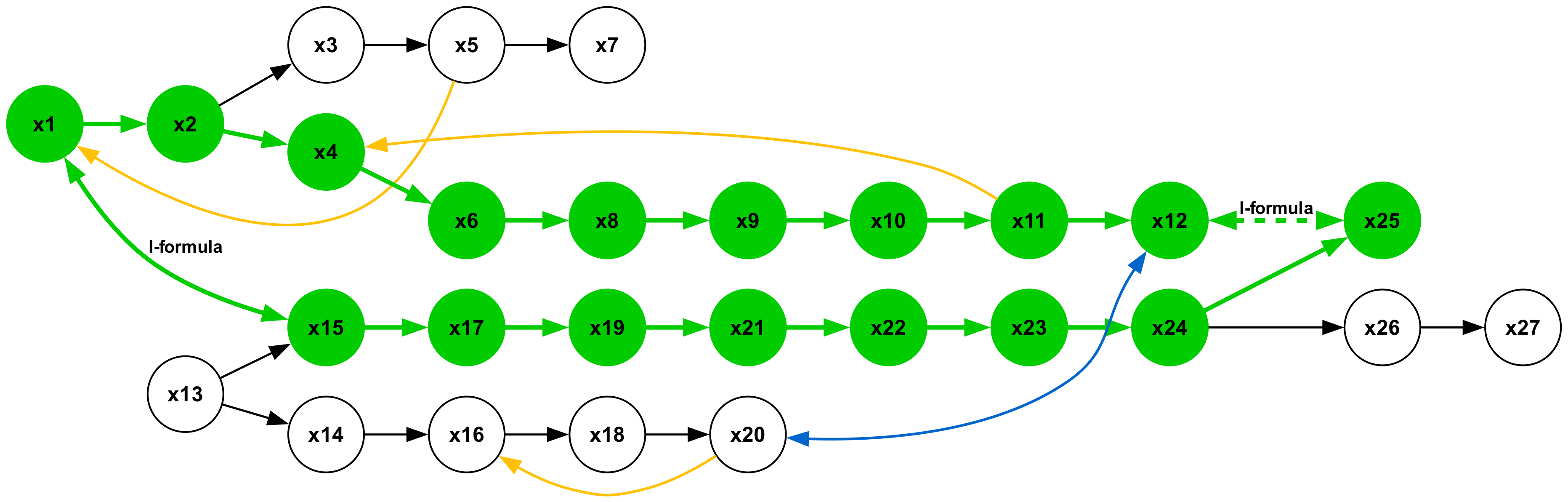KB with Query Hypothesis and Type 7 Inference: <details> <summary>extracted/6458430/figs/type_7_proof.png Details</summary>  ### Visual Description # Technical Document Extraction: Flowchart Analysis ## Diagram Overview The image depicts a **directed graph** (flowchart) with **27 nodes** labeled `x1` to `x27`. Nodes are color-coded (green and white) and connected via arrows of varying colors (green, yellow, blue, black). Key labels include "I-formula" and a dotted-line feedback loop. --- ## Node Classification ### Green Nodes (Main Process) - **x1** → **x2** → **x4** → **x6** → **x8** → **x9** → **x10** → **x11** → **x12** → **x25** - **x15** → **x17** → **x19** → **x21** → **x22** → **x23** → **x24** - **x25** → **x26** → **x27** (via white nodes) ### White Nodes (Branches/Exceptions) - **x3** → **x5** → **x7** - **x13** → **x14** → **x16** → **x18** → **x20** - **x20** → **x18** (blue feedback loop) --- ## Arrow Analysis 1. **Green Arrows**: Primary flow (e.g., `x1`→`x2`, `x6`→`x8`). 2. **Yellow Arrows**: Conditional/alternative paths (e.g., `x2`→`x4`, `x20`→`x18`). 3. **Blue Arrow**: Feedback loop (`x20`→`x18`). 4. **Black Arrows**: Terminal/end nodes (e.g., `x7`, `x27`). --- ## Key Labels - **"I-formula"**: Annotated on the green arrow from `x12`→`x25`, indicating a critical computational step. - **Dotted Line**: Feedback connection from `x25`→`x12`, suggesting iterative processing. --- ## Flow Paths 1. **Primary Path**: `x1` → `x2` → `x4` → `x6` → `x8` → `x9` → `x10` → `x11` → `x12` → `x25` → `x26` → `x27`. 2. **Branching Paths**: - `x2` → `x15` → `x17` → `x19` → `x21` → `x22` → `x23` → `x24` → `x25`. - `x13` → `x14` → `x16` → `x18` → `x20` (with feedback to `x18`). 3. **Exceptional Path**: `x1` → `x3` → `x5` → `x7` (terminates independently). --- ## Spatial Grounding - **Legend**: Not explicitly visible in the image. - **Color Consistency**: - Green nodes/arrows: Main process. - White nodes: Branches/exceptions. - Blue arrow: Feedback loop. --- ## Trend Verification - **Main Chain (Green Nodes)**: Linear progression from `x1` to `x27` with no upward/downward slope (static flow). - **Feedback Loop (Blue Arrow)**: Cyclical between `x20` and `x18`. --- ## Component Isolation 1. **Header**: No explicit header; flow begins at `x1`. 2. **Main Chart**: Dominated by green nodes and arrows. 3. **Footer**: Terminal nodes (`x7`, `x27`) and feedback loops. --- ## Missing Elements - **Data Table**: None present. - **Axis Titles/Legends**: Not applicable (flowchart, not a chart). --- ## Conclusion The flowchart represents a **process flow** with conditional branching, feedback loops, and terminal states. The "I-formula" step (`x12`→`x25`) is central to the main process. No numerical data or trends are depicted beyond structural connectivity. </details> Textual Translation: knowledge base: All x1 are x2, All x2 are x3, All x2 are x4, All x3 are x5, All x4 are x6, All x5 are x7, All x6 are x8, All x8 are x9, All x9 are x10, All x10 are x11, All x11 are x12, All x13 are x14, All x13 are x15, All x14 are x16, All x15 are x17, All x16 are x18, All x17 are x19, All x18 are x20, All x19 are x21, All x21 are x22, All x22 are x23, All x23 are x24, All x24 are x25, All x24 are x26, All x26 are x27, No x20 are x12, Some x15 are x1, Some x11 are not x4, Some x5 are not x1, Some x20 are not x16 hypothesis: Some x25 are x12 premises: All x1 are x2, All x2 are x4, All x4 are x6, All x6 are x8, All x8 are x9, All x9 are x10, All x10 are x11, All x11 are x12, All x15 are x17, All x17 are x19, All x19 are x21, All x21 are x22, All x22 are x23, All x23 are x24, All x24 are x25, Some x15 are x1 Figure 24: Type 7 syllogistic inference on graphs. Visualization of a type 7 syllogistic inference using a graph representation of an example $\mathcal{KB}$ , alongside the corresponding textual translation. In the graph (top), nodes represent predicates. Black edges indicate A-formulas (“All As are Bs”), blue edges indicate I-formulas (“Some As are Bs”), red edges indicate E-formulas (“No As are Bs”), and yellow edges indicate O-formulas (“Some As are not Bs”). The query hypothesis is represented by a dashed green edge, and the edges that prove the hypothesis are highlighted in green. The text translation illustrates how the abstract graph representation is converted into a text format suitable for LM processing by applying fixed templates that represent logical formulas.