2505.15796

# lean-smt: An SMT tactic for discharging proof goals in Lean **Authors**: Abdalrhman Mohamed, Tomaz Mascarenhas, Harun Khan, Haniel Barbosa, Andrew Reynolds, Yicheng Qian, Cesare Tinelli, Clark Barrett \SetWatermarkAngle 0 \SetWatermarkText <details> <summary>x1.png Details</summary>  ### Visual Description ## Image Analysis: CAV Artifact Evaluation Badge ### Overview The image is a badge indicating that an artifact has undergone and passed an evaluation process. The badge is primarily blue and white, with text and a star symbol. ### Components/Axes * **Shape:** The badge has a rounded rectangular shape. * **Color:** The background is blue, and the text and star are white. * **Text:** The badge contains the following text: * "CAV" (prominently displayed at the top) * "Artifact Evaluation" (below "CAV") * "Available" (at the bottom) * **Symbol:** A white star is located between "Artifact Evaluation" and "Available". ### Detailed Analysis or ### Content Details The badge is designed to be visually clear and easily recognizable. The use of contrasting colors (blue and white) ensures that the text is legible. The star symbol adds a visual element that helps to draw attention to the badge. ### Key Observations The badge signifies that the artifact it is associated with has been evaluated and is available. ### Interpretation The badge serves as a quality indicator, suggesting that the artifact has met certain standards or criteria. It provides assurance to users or consumers that the artifact has been vetted and is likely to be reliable or trustworthy. The "Available" text indicates that the artifact is accessible for use or further examination. </details> <details> <summary>x2.png Details</summary>  ### Visual Description ## Badge: CAV Artifact Evaluation ### Overview The image is a badge with a brown background and white text, indicating an artifact evaluation. It features the acronym "CAV," the phrase "Artifact Evaluation," three stars, and the word "Reusable." ### Components/Axes * **Background Color:** Brown * **Text Color:** White * **Acronym:** CAV * **Text:** Artifact Evaluation * **Stars:** Three stars arranged horizontally * **Text:** Reusable ### Detailed Analysis or ### Content Details The badge is rectangular with rounded corners. The text is arranged in a stacked format. The three stars are located between "Artifact Evaluation" and "Reusable." ### Key Observations The badge signifies that the artifact has been evaluated and is reusable. The three stars could indicate a rating or level of reusability. ### Interpretation The badge is likely used to indicate the quality and usability of a software artifact or research output. The "CAV" acronym likely stands for a specific evaluation process or organization. The three stars suggest a positive evaluation result. The "Reusable" label indicates that the artifact can be used in other projects or research. </details> \includeversion conf \excludeversion rep institutetext: Stanford University, Stanford, USA institutetext: The University of Iowa, Iowa City, USA institutetext: Amazon Web Services, Seattle, WA, USA institutetext: Universidade Federal de Minas Gerais, Belo Horizonte, Brazil Abstract Lean is an increasingly popular proof assistant based on dependent type theory. Despite its success, it still lacks important automation features present in more seasoned proof assistants, such as the Sledgehammer tactic in Isabelle/HOL. A key aspect of Sledgehammer is the use of proof-producing SMT solvers to prove a translated proof goal and the reconstruction of the resulting proof into valid justifications for the original goal. We present lean-smt, a tactic providing this functionality in Lean. We detail how the tactic converts Lean goals into SMT problems and, more importantly, how it reconstructs SMT proofs into native Lean proofs. We evaluate the tactic on established benchmarks used to evaluate Sledgehammer’s SMT integration, with promising results. We also evaluate lean-smt as a standalone proof checker for proofs of SMT-LIB problems. We show that lean-smt offers a smaller trusted core without sacrificing too much performance. 1 Introduction Proof assistants, also known as interactive theorem provers (ITPs), allow users to write mechanized proofs of statements written in a formal language, whose validity can be verified by a small, trusted kernel. They help users construct trustworthy, formal, machine-checkable proofs of theorems, and have been increasingly used to mechanize proofs of various mathematical results [18, 19]. This process has significantly accelerated in recent years with the adoption of the Lean proof assistant [27] by leading members of the mathematical community [12, 14, 34]. Proof assistants are also commonly used in certain areas of computer science to model and formally verify systems, thanks to the high expressiveness of their underlying language and logic [23, 28]. The trustworthiness of proof assistants relies on the kernel correctly verifying every proof step. For this reason, ITP kernels are designed to be simple and small, implementing just straightforward logical operations from the logical framework underlying the proof assistant. This means that, in principle, each proof step must be explicitly formulated by the user, so that naive use of ITPs would require a tremendous amount of expertise and effort. A major challenge, then, is the extension of the kernel with trustworthy facilities for automating the writing of mechanized proofs as much as possible, thereby reducing the burden on the users. In mathematics, the cost of mechanizing an informal proof is currently estimated to be $\sim 20$ x [34]. Using ITPs to formally verify large systems is well known to be very costly, in the range of multiple person-years [23]. Automation is generally achieved via tactics, proof-producing algorithms, traditionally written in a special-purpose language, that discharge proof obligations for certain classes of subgoals, often by simulating common proof techniques, such as case analysis or induction. An alternative is to use external automated theorem provers (ATPs) to solve subgoals when possible. Tools such as HOL y Hammer [22], Miz $\mathbb{AR}$ [21], Sledgehammer [26], and Why3 [10], provide a one-click connection from proof assistants to first-order provers and have led to considerable improvements in proof-assistant automation [9]. The Sledgehammer tactic in Isabelle/HOL [29] is particularly successful and includes an integration with proof-producing SMT solvers [8, 33]. Sledgehammer translates certain proof goals into SMT-LIB [6], a standard input format for SMT solvers, and sends them to the solver. The resulting proof is reconstructed by essentially reproducing each step within the proof assistant. This extension to Sledgehammer has been especially useful for proof goals arising from formal verification efforts carried out in Isabelle/HOL [8]. We conjecture that any tactic in Lean with the same ambition and potential impact as Sledgehammer will require a similar level of SMT solver integration. In this paper, we present lean-smt, lean-smt is available online at https://github.com/ufmg-smite/lean-smt which provides an initial implementation of a similar integration in Lean and is a stepping stone towards a full Sledgehammer-like tactic for Lean. lean-smt operates by translating Lean proof goals expressible in the first-order logic fragment of dependent type theory (Section 3.2) into SMT problems, leveraging SMT theories to model corresponding elements from Lean, such as uninterpreted functions, propositional equality, first-order quantifiers, and arithmetic operators. To bridge the gap between this restricted fragment and the goals that arise in practice in Lean formalizations, we rely on the lean-auto tactic https://github.com/leanprover-community/lean-auto to reduce proof goals to first-order logic, together with dedicated preprocessing in lean-smt itself to express them in the language of selected SMT theories (Section 3.1). lean-smt currently supports the state-of-the-art proof-producing SMT solver cvc5 [3]. cvc5’s extensive proof production capabilities [4] and strong performance on the fragment of interest make it well suited for such an integration. cvc5’s proofs are reconstructed into native Lean proofs (Section 3.3) by using either a Lean theorem, a Lean tactic, or a formally verified Lean program. We evaluate lean-smt (Section 4) on proof goals from a standard benchmark set used to evaluate Sledgehammer, showing that lean-smt performs comparably with Sledgehammer’s SMT integration. We also evaluate it as a verified proof checker for SMT proofs. While, as expected, lean-smt is less performant than standalone, unverified SMT proof checkers, its performance is generally within an order of magnitude of theirs. Additionally, it offers comparable performance to SMTCoq [16], a similarly verified checker for Coq, while supporting a larger logical fragment. 2 Related Work While our main inspiration for lean-smt has been the SMT integration in Sledgehammer, there are other ways in which Sledgehammer leverages the power of automatic theorem provers. Sledgehammer includes a premise selection module, which filters lemmas from Isabelle’s libraries that are potentially useful for proving the goal. These lemmas are added to the problem to be sent to the solver. Once the problem is solved, rather than directly reconstruct the proof, an alternative strategy is to use it only to identify the lemmas used to prove the goal and pass these lemmas, together with the original goal, to metis [20], a proof-producing superposition prover written as an Isabelle tactic. While there is no equivalent for Sledgehammer in Lean, there is a growing ecosystem of tools that eventually can be combined into a comparable tool. Recently Aesop [25], a tableaux-based prover, and Duper [13] which is, like metis, a superposition prover, were introduced as proof-producing Lean tactics. No equivalent for the premise selection mechanism is readily available in Lean yet, although there has been initial work in this direction [31]. Another integration between a proof assistant and SMT solvers is SMTCoq [16], within the Coq proof assistant [7]. It supports proof reconstruction for the SMT solvers veriT [11] and CVC4 [5], but rather than replaying each individual proof step within Coq, as Sledgehammer and lean-smt do, it applies a formally verified checker that, if successful, confirms the original proof goal as a theorem. This approach relies heavily on the efficiency of the proof assistant itself, since the proof checker runs within the proof assistant and may have to analyze and simplify huge proof terms. The Coq proof assistant is designed to be very fast at this, while Lean, on the other hand, is not [2]. This observation contributed to the decision to use proof replay in lean-smt. Moreover, the verified checker approach is rather rigid, since any modification to the supported proof format requires the checker’s correctness theorem to be proven again, which can be a significant effort. In the proof replay approach, one needs only to change the reconstruction tactic by modifying the step corresponding to the changed element of the format. This has been especially useful while developing lean-smt since cvc5’s proof calculus and infrastructure are still evolving [4, 30, 24]. 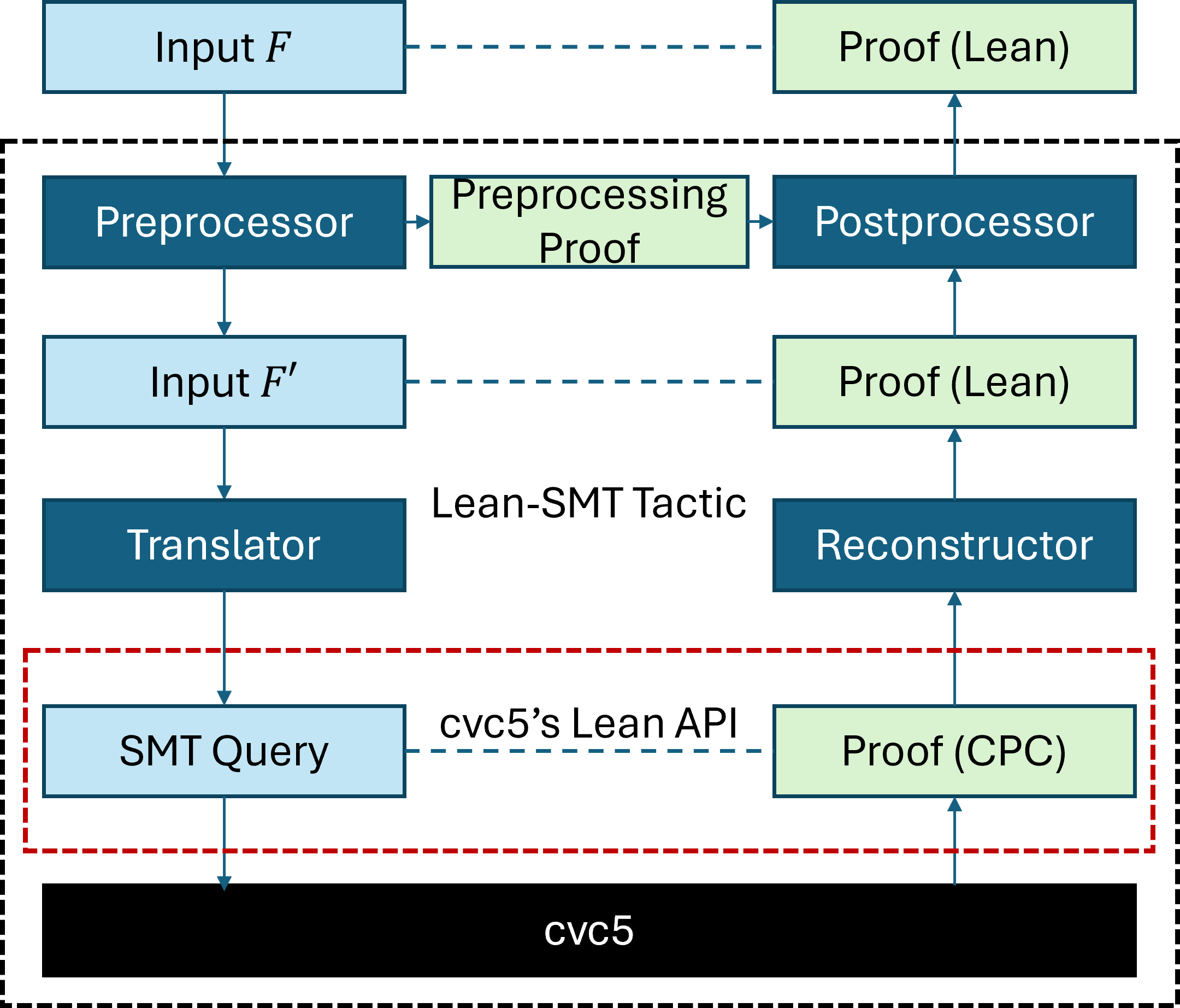3 System Overview Figure 1 depicts the lean-smt architecture, which takes as input a Lean goal, whose type is represented as the formula $F$ , and generates a proof for it by solving a corresponding SMT problem and reconstructing the proof into a Lean proof for $F$ . The arrows illustrate the tactic’s pipeline, through which the input formula is simplified, translated into an SMT query, and sent to cvc5. The solver’s proof is then reconstructed as a proof in Lean for the input formula. The light-green boxes represent the proofs used during the reconstruction stage, which correspond directly to the formulas (light-blue) processed during the translation stage. The dashed lines emphasize this correspondence. <details> <summary>extracted/6460524/architecture.png Details</summary>  ### Visual Description ## Flow Diagram: Lean-SMT Tactic ### Overview The image is a flow diagram illustrating the Lean-SMT Tactic, detailing the process from input to proof generation using cvc5. The diagram shows the flow of data and transformations through various components, including preprocessors, translators, and reconstructors, ultimately leading to a proof. ### Components/Axes * **Boxes:** Represent processes or data. * Light Blue Boxes: Represent Input or Queries * Dark Blue Boxes: Represent Processors or Translators * Light Green Boxes: Represent Proofs * **Arrows:** Indicate the direction of data flow. * Solid Arrows: Represent direct data flow * Dashed Arrows: Represent a connection or API usage * **Text Labels:** Describe the function or data within each box. * **Bounding Boxes:** * Dashed Black Box: Encloses the entire Lean-SMT Tactic process. * Dashed Red Box: Encloses the cvc5's Lean API interaction. ### Detailed Analysis or ### Content Details 1. **Top Row:** * `Input F` (Light Blue Box, top-left): Represents the initial input. * Dashed Blue Arrow: Connects `Input F` to `Proof (Lean)`. * `Proof (Lean)` (Light Green Box, top-right): Represents the final proof in Lean. 2. **Second Row (within dashed black box):** * `Preprocessor` (Dark Blue Box, left): Processes the initial input. * Arrow: Connects `Preprocessor` to `Preprocessing Proof`. * `Preprocessing Proof` (Light Green Box, center): Represents the proof generated during preprocessing. * Arrow: Connects `Preprocessing Proof` to `Postprocessor`. * `Postprocessor` (Dark Blue Box, right): Processes the preprocessed proof. * Arrow: Connects `Postprocessor` to `Proof (Lean)` in the top row. 3. **Third Row:** * `Input F'` (Light Blue Box, left): Represents a transformed input. * Dashed Blue Arrow: Connects `Input F'` to `Proof (Lean)`. * `Proof (Lean)` (Light Green Box, right): Represents the final proof in Lean. 4. **Fourth Row (labeled "Lean-SMT Tactic"):** * `Translator` (Dark Blue Box, left): Translates the input. * `Reconstructor` (Dark Blue Box, right): Reconstructs the proof. 5. **Fifth Row (within dashed red box, labeled "cvc5's Lean API"):** * `SMT Query` (Light Blue Box, left): Represents the SMT query. * `Proof (CPC)` (Light Green Box, right): Represents the proof in CPC format. 6. **Bottom Row:** * `cvc5` (Black Box): Represents the cvc5 solver. 7. **Arrows:** * Downward Arrow: Connects `Preprocessor` to `Input F'`. * Downward Arrow: Connects `Input F'` to `Translator`. * Downward Arrow: Connects `Translator` to `SMT Query`. * Horizontal Dashed Blue Arrow: Connects `SMT Query` to `Proof (CPC)`. * Upward Arrow: Connects `Proof (CPC)` to `Reconstructor`. * Upward Arrow: Connects `Reconstructor` to `Proof (Lean)`. * Downward Arrow: Connects `SMT Query` to `cvc5`. * Upward Arrow: Connects `cvc5` to `Proof (CPC)`. ### Key Observations * The diagram illustrates a multi-stage process for generating proofs using the Lean-SMT tactic. * The process involves preprocessing, translation, and reconstruction steps. * The cvc5 solver plays a crucial role in generating proofs in CPC format. * The Lean API of cvc5 is used to interact with the solver. * The diagram highlights the flow of data and transformations between different components. ### Interpretation The diagram provides a high-level overview of the Lean-SMT tactic, showcasing how it leverages the cvc5 solver to generate proofs. The process starts with an initial input `F`, which is preprocessed and potentially transformed into `F'`. The transformed input is then translated into an SMT query, which is passed to the cvc5 solver. The solver generates a proof in CPC format, which is then reconstructed into a Lean proof. The diagram emphasizes the modularity of the process, with distinct components responsible for preprocessing, translation, reconstruction, and solving. The use of the cvc5 Lean API allows for seamless integration between the Lean theorem prover and the cvc5 solver. The dashed boxes visually group related components, highlighting the different stages of the proof generation process. </details> Figure 1: Architecture of the lean-smt tactic. The preprocessor module converts the initial input $F$ into an intermediate form $F^{\prime}$ , simplifying or restructuring the input to make it more suitable for translation into an SMT query. During this phase, a preprocessing proof is generated, capturing the transformations applied. The translator module generates a formula in SMT-LIB whose unsatisfiability corresponds to the validity of $F^{\prime}$ . The formula is passed to a solver (cvc5) that evaluates it and produces a proof if the formula is determined to be unsatisfiable, outputting a proof in the Cooperating Proof Calculus (CPC) format. See https://cvc5.github.io/docs/cvc5-1.2.1/proofs/output˙cpc.html. A complete list of the proof rules in CPC can be found at https://cvc5.github.io/docs/cvc5-1.2.1/api/cpp/enums/proofrule.html. The semantics of the rules is also defined in the Eunoia logical framework, described in the user manual of the Ethos proof checker: https://github.com/cvc5/ethos/blob/main/user_manual.md. The tactic interfaces with cvc5 through Lean’s Foreign Function Interface (FFI) and the solver’s Lean API, which we added to the solver to facilitate the integration. The reconstructor module translates the CPC proof into a Lean proof of $F^{\prime}$ , mapping the CPC proof structure to corresponding Lean constructs and ensuring logical equivalence. The postprocessor combines the preprocessing proof and the reconstruction proof into a single Lean proof for the original formula $F$ , which is then checked by Lean’s kernel. 3.1 Preprocessing Original Lean Goal Lean’s type system, rooted in dependent type theory (DTT) [1], is far more expressive than the many-sorted first-order logic (FOL) [17] used by SMT solvers. To bridge this gap, we employ proof-producing preprocessing steps that simplify Lean goals into a form more amenable to translation into SMT-LIB. We first use lean-auto, https://github.com/leanprover-community/lean-auto to reduce the goal to FOL. lean-auto normalizes universe levels, monomorphizes definitions, adds lemmas related to inductive types, and replaces type class instances by their corresponding values. All of these transformations are implemented in Lean and are proof producing, so their soundness is guaranteed by Lean’s kernel. However, they are inherently incomplete, given the expressivity gap between DTT and FOL. The preprocessing applied by lean-auto is not specific to SMT solvers, so while the resulting goal is in FOL, it is not aligned with the SMT-LIB standard. We apply a further preprocessing step so that certain Lean types and constructs (e.g., Prop, Nat, Rat, and Iff) that don’t have direct counterparts in SMT-LIB can be transformed into types and constructs that do. **Example 1** *Consider the following Lean goal, which asserts the uniqueness of the identity element in a group: ⬇ ⊢ ∀ (G : Type u) [Group G] (e : G), (∀ (a : G), e * a = a) ↔ e = 1 This goal cannot be directly translated into SMT-LIB due to the presence of the type class Group and the logical operator $\leftrightarrow$ . During preprocessing, the goal is transformed and expanded to: ⬇ G: Type u inst: Group G e e ’: G op: G → G → G inv: G → G one_mul: ∀ (a : G), op e a = a inv_mul_cancel: ∀ (a : G), op (inv a) a = e mul_assoc: ∀ (a b c : G), op (op a b) c = op a (op b c) ⊢ (∀ (a : G), (op e ’ a = a)) = (e ’ = e) Here, lean-auto replaces the type class Group with explicit assumptions about the group operations (e.g., associativity, identity, and inverse axioms), and lean-smt ’s preprocessing transforms the bidirectional logical operator $\leftrightarrow$ into a suitable equality comparison. These transformations make the goal compatible with SMT-LIB’s logic while preserving its original meaning.* 3.2 Translation to SMT-LIB After preprocessing, translating Lean goals into SMT-LIB is relatively straightforward, as the fragments mostly overlap. However, one key challenge stems from differing assumptions about sorts: SMT-LIB assumes sorts are non-empty, while Lean allows types to be empty. This discrepancy can make the translation unsound. The reconstruction stage ensures soundness by failing if a proof step depends on a type being non-empty and Lean cannot establish that the type is an instance of the type class of non-empty types. As long as the instances are found, this discrepancy between the logic systems is successfully addressed. **Example 2** *Continuing from our previous example, the preprocessed goal is translated into SMT-LIB as follows: ⬇ (declare-sort G 0) (declare-const e G) (declare-const | e ’| G) (declare-fun op (G G) G) (declare-fun inv (G) G) (assert (forall ((a G)) (= (op e a) a))) (assert (forall ((a G)) (= (op (inv a) a) e))) (assert (forall ((a G) (b G) (c G)) (= (op (op a b) c) (op a (op b c))))) (assert (distinct (forall ((a G)) (= (op | e ’| a) a) (= | e ’| e)))) (check-sat) Note that the translation is sound in this example because any group $G$ is guaranteed to be non-empty due to the existence of the identity element $e$ .* 3.3 cvc5’s Proof Format and Reconstruction When cvc5 establishes that an SMT query is unsatisfiable, it can optionally generate a proof in the CPC format that accurately mirrors its internal reasoning processes. In CPC, each proof rule can be represented as follows: $$ \frac{\varphi_{1}\cdots\varphi_{m}\mid t_{1}\cdots t_{n}}{\psi}{C}, $$ where $\varphi_{1},...,\varphi_{m}$ are the premises, $t_{1},...,t_{n}$ are the arguments provided to the proof rule, and $C$ (which may be absent) denotes a decidable side-condition. The proof format currently specifies over 662 proof rules in various domains, including arithmetic, strings, quantifiers, and higher-order logic. lean-smt supports around 200 of these proof rules, which amounts to approximately 30%. We prioritized this subset because it suffices to support the most common proof goals in Lean (it corresponds to the same logical fragment supported initially by Sledgehammer and SMTCoq), with the other rules corresponding to the reasoning of specific theories. To reconstruct the cvc5 proofs in Lean, lean-smt processes the CPC proof step by step, translating each proof step into an equivalent one in Lean. After lean-smt completes proof reconstruction, the entire proof is submitted to the Lean kernel for verification. In cases where a proof step cannot be reconstructed, it is presented to the user to be proved manually, ensuring that the reconstruction process remains sound. Also note that since the logic in SMT-LIB is classical, certain parts of the proof rely heavily on the axiom of choice. Below we detail each of the reconstruction techniques we apply. Reconstruction via theorems. Proof rules without side conditions generally correspond directly to theorems in Lean. We proved an extensive library of such theorems, which cover 163 proof rules, to use for proof reconstruction. **Example 3** *Consider the ARITH_MULT_TANGENT proof rule from CPC. | | $\displaystyle\frac{-\mid x,y,a,b,\sigma}{(t≤ tplane)=((x≤ a\wedge y≥ b% )\vee(x≥ a\wedge y≤ b))}\text{if }\sigma=→p$ | | | --- | --- | --- | where $x,y$ are real terms, $t=x· y,a,b$ are real constants, $\sigma∈\{→p,\bot\}$ and $tplane:=b· x+a· y-a· b$ is the tangent plane of $x· y$ at $(a,b)$ . Formalizing this proof rule into a Lean theorem is straightforward: ⬇ theorem arithMulTangentLowerEq : (x * y ≤ b * x + a * y - a * b) = ((x ≤ a ∧ y ≥ b) ∨ (x ≥ a ∧ y ≤ b)) theorem arithMulTangentUpperEq : (x * y ≤ b * x + a * y - a * b) = ((x ≤ a ∧ y ≤ b) ∨ (x ≥ a ∧ y ≥ b))* The formalization of other proof rules is more complex and often requires design choices when stating the theorem to capture the semantics of the corresponding CPC rule. **Example 4** *Consider for example the RESOLUTION proof rule: | | $\displaystyle\frac{C_{1}\quad C_{2}\mid pol,L}{C},$ | | | --- | --- | --- | where $C_{1},C_{2}$ are disjunctions, $L$ is a disjunct occurring positively (respectively, negatively) in $C_{1}$ and negatively (resp. positively) in $C_{2}$ if $pol$ is the Boolean true (resp. false). The result $C$ is a disjunction with the disjuncts from $C_{1}$ minus $L$ (resp. $\neg L$ ) and the disjuncts from $C_{2}$ minus $\neg L$ (resp. $L$ ) if $pol$ is the Boolean true (resp. false). Moreover $C$ is such that the remaining disjunctions from $C_{1}$ and $C_{2}$ occur as a chain of disjunctions between each disjunct as opposed to nested disjunctions. These restrictions capture the view, within cvc5, of disjunction as an “ $n$ -ary” operator, which takes multiple arguments. To capture this reasoning in Lean, where disjunction is a binary operator, one needs to carefully reason about associativity and commutativity to exactly reproduce the semantics of this rule. We encapsulate it in a Lean theorem as follows: ⬇ theorem orN_resolution (hps : orN ps) (hqs : orN qs) (hi : i < ps. length) (hj : j < qs. length) (hij : ps [i] = ¬ qs [j]) : orN (ps. eraseIdx i ++ qs. eraseIdx j) The premises, hps : orN ps and hqs : orN qs, are disjunctions, but built with the orN function which takes a List of literals represented as Prop. This formulation avoids representing ps and qs as for example inductively defined Prop instead of List or encoding the literals as Bool instead of Prop. Using List permits leveraging general theorems about List we proved for eliminating tedious corner cases that would otherwise arise in a Prop implementation. Additionally, the choice to encode Boolean literals as Prop is a deliberate choice due to the type-theoretic foundation of Lean.* Reconstruction via tactics. Some proof rules without side conditions require the application of multiple lemmas or more complex reasoning. We implement specialized tactics to encapsulate these steps. This streamlines the reconstruction process by automating repetitive or intricate reasoning steps. We cover 37 proof rules this way, which required implementing a library with around 400 theorems. **Example 5** *A proof rule that is very general, making it hard to state and prove as a theorem, is the ARITH_SUM_UB rule: | | $\displaystyle\frac{\bigwedge_{i=1}^{n}a_{i}\bowtie_{i}b_{i}\mid a_{i},b_{i}}{% \sum_{i=1}^{n}a_{i}\bowtie^{*}\sum_{i=1}^{n}b_{i}}$ | | | --- | --- | --- | where $\bowtie_{i}$ can be either $<$ , $≤$ or $=$ , and $\bowtie^{*}$ is either $<$ , if at least one of the $\bowtie_{i}$ is $<$ , or $≤$ , otherwise. Moreover, while each pair of variables $a_{i}$ and $b_{i}$ always have the same type, it is possible that different pairs have different types, some being integers and some being reals. It is possible to encode this proof rule as a single theorem in Lean, but the statement of the theorem would be quite intricate, due to the necessity of lifting the integer variables to reals and of combining the inequalities statically. Also, it is likely that this would make it very hard to prove. In this case, it is easier to write a tactic that considers the different cases of the rule and applies an appropriate, simpler theorem for each case. The implementation of this tactic requires 9 variations of the following theorem: ⬇ sumBoundsThm {α : Type} [LinearOrderedRing α] {a b c d : α} : a < b → c < d → a + c < b + d Each variation corresponds to one possible combination of the inequality symbols in the hypothesis. The relation symbol in the conclusion is adapted accordingly in each theorem. Since the rule accepts mixing of variables from Int and Real types, we need a variation of each one of those 9 theorems for each combination of the types of the variables. Instead of stating all the combinations explicitly, which would result in a total of 36 theorems and a long branch in the implementation of the tactic, we state only one polymorphic version of each, as indicated by the type parameter $\alpha$ in sumBoundsThm. Obviously, these theorems do not hold for any $\alpha$ (it cannot even be stated if there are no comparison or addition operators defined over $\alpha$ ). We solve this issue by adding a restriction, stating that $\alpha$ satisfies the axioms of a Linear Ordered Ring (a class of types that contains both Int and Real defined in mathlib). With this restriction each theorem can be proven. The full tactic can be seen in Appendix 0.A.* Reconstruction via reflection. For proof rules involving complex side conditions or computations (such as arithmetic simplifications), we encode the side condition into a reflective decision procedure, which is formally verified in Lean. The proof rule is then translated into a theorem with the side condition as an additional premise. Applications of this rule are verified by the Lean kernel using definitional equality. We cover 5 proof rules this way. We reused one program from Lean’s library, ac_rfl, which applies associative and commutative properties of addition and multiplication to normalize arithmetic expressions; and we implemented a new program, poly_norm, which normalizes polynomials up to associativity, commutativity, and distributivity by expanding polynomials. **Example 6** *Consider the example: ⬇ example (x y : Int) (z : Real) : 1 * ↑(x + y) * z / 4 = 1 / (2 * 2) * (z * ↑ y + ↑ x * z) := by poly_norm* Proving the correctness of poly_norm required proving around 70 theorems, amounting to 620 lines of Lean code. We define a monomial as an ordered list of natural numbers representing variable indices, so that equality of two monomials is immediate. Polynomials are defined as lists of monomials, and theorems about monomials generalize to polynomials using induction. We define denote, which essentially evaluates polynomial expressions. Using lemmas we proved about lists and the objects we defined, we prove a theorem pushing denote into each operator. ⬇ theorem denote_mul {p q : Polynomial} : (p. mul q). denote ctx = p. denote ctx * q. denote ctx Proving similar theorems for each operator (addition, multiplication, division by a constant, and negation) yields a correctness theorem. ⬇ theorem denote_eq_from_toPoly_eq {e ₁ e ₂ : RealExpr} e ₁. toPoly = e ₂. toPoly → e ₁. denote ictx rctx = e ₂. denote ictx rctx Since variables are represented as natural numbers, the premise of the theorem does not contain actual variables. Therefore, Lean can establish the premise through definitional equality. Moreover, the premise is decidable, allowing us to compile it into machine code for enhanced performance. In our experiments, this approach achieved speeds up to 25 times faster than using definitional equality for very large arithmetic expressions. 4 Evaluation and Results <details> <summary>x11.png Details</summary>  ### Visual Description ## Chart: Cumulative Solving + Checking Time ### Overview The image is a line chart comparing the cumulative solving and checking time for three different solver-checker combinations: Duper, cvc5+Lean-SMT, and veriT+Sledgehammer. The x-axis represents the number of benchmarks, and the y-axis represents the time in seconds on a logarithmic scale. ### Components/Axes * **Title:** Cumulative solving + checking time * **X-axis:** Number of benchmarks, ranging from 0 to 2500 in increments of 500. * **Y-axis:** Time (s), on a logarithmic scale from 10^-2 to 10⁴. The axis markers are 10^-2, 10^-1, 10⁰, 10¹, 10², 10³, and 10⁴. * **Legend:** Located in the bottom-right corner. * **Blue:** Duper * **Orange:** cvc5+Lean-SMT * **Green:** veriT+Sledgehammer ### Detailed Analysis * **Duper (Blue):** The line starts at approximately 10^-1 seconds at 0 benchmarks. It increases rapidly until around 500 benchmarks, reaching approximately 10² seconds. From 500 to 1000 benchmarks, the increase slows down. After 1000 benchmarks, the line continues to increase, reaching approximately 10⁴ seconds. * **cvc5+Lean-SMT (Orange):** The line starts at approximately 10^-2 seconds at 0 benchmarks. It increases rapidly until around 250 benchmarks, reaching approximately 10¹ seconds. From 250 to 2500 benchmarks, the increase is gradual, reaching approximately 10³ seconds. * **veriT+Sledgehammer (Green):** The line starts at approximately 10^-2 seconds at 0 benchmarks. It increases rapidly until around 2000 benchmarks, reaching approximately 10² seconds. From 2000 to 2500 benchmarks, the increase is rapid, reaching approximately 10³ seconds. ### Key Observations * Duper has the fastest initial solving time but increases rapidly, becoming the slowest for a large number of benchmarks. * cvc5+Lean-SMT has a slower initial solving time but increases more gradually, making it faster than Duper for a large number of benchmarks. * veriT+Sledgehammer has the slowest initial solving time but remains relatively slow until around 2000 benchmarks, after which it increases rapidly. ### Interpretation The chart compares the performance of three different solver-checker combinations in terms of cumulative solving and checking time. The logarithmic scale on the y-axis indicates that the differences in time are significant. The data suggests that the choice of solver-checker combination depends on the number of benchmarks being processed. For a small number of benchmarks, Duper may be the fastest option. However, for a large number of benchmarks, cvc5+Lean-SMT is likely to be more efficient. veriT+Sledgehammer is the least efficient for a smaller number of benchmarks, but its performance degrades significantly after 2000 benchmarks. </details> (a) <details> <summary>x12.png Details</summary>  ### Visual Description ## Scatter Plot: Lean-SMT vs. Ethos Checking Times ### Overview The image is a scatter plot comparing the checking times of Lean-SMT and Ethos. Both axes use a logarithmic scale. The plot includes a red dashed line representing y = x, which serves as a reference for comparing the performance of the two systems. The data points are clustered, showing the relationship between the checking times of the two methods. ### Components/Axes * **Title:** Lean-SMT vs. Ethos Checking Times * **X-axis:** Lean-SMT Checking Time (ms) - Logarithmic scale from 10^2 to 10^5 * **Y-axis:** Ethos Checking Time (ms) - Logarithmic scale from 10^2 to 10^5 * **Grid:** Light gray dashed grid lines are present. * **Legend:** Located in the top-left corner. * Red dashed line: y = x ### Detailed Analysis * **Data Points:** The data points are blue circles. * **y = x Line:** A red dashed line represents y = x. This line indicates where the checking times for Lean-SMT and Ethos are equal. * **Data Point Distribution:** * Most data points are clustered below the y = x line, indicating that Ethos generally has lower checking times than Lean-SMT. * There is a concentration of points in the lower-left corner, suggesting many instances where both systems have relatively low checking times. * There are some outliers above the y = x line, indicating cases where Ethos checking times are higher than Lean-SMT. * **X-Axis Markers:** 10^2, 10^3, 10^4, 10^5 * **Y-Axis Markers:** 10^2, 10^3, 10^4, 10^5 ### Key Observations * Ethos generally has lower checking times than Lean-SMT, as most data points are below the y = x line. * There is a wide range of checking times for both systems, spanning several orders of magnitude. * The clustering of points suggests a correlation between the checking times of the two systems. ### Interpretation The scatter plot provides a visual comparison of the checking times between Lean-SMT and Ethos. The fact that most data points lie below the y = x line suggests that Ethos is generally faster than Lean-SMT for the given set of checks. However, the presence of outliers above the line indicates that there are cases where Lean-SMT outperforms Ethos. The logarithmic scale highlights the wide range of checking times, and the clustering of points suggests a relationship between the performance of the two systems. The plot could be used to further investigate the specific conditions under which each system performs better. 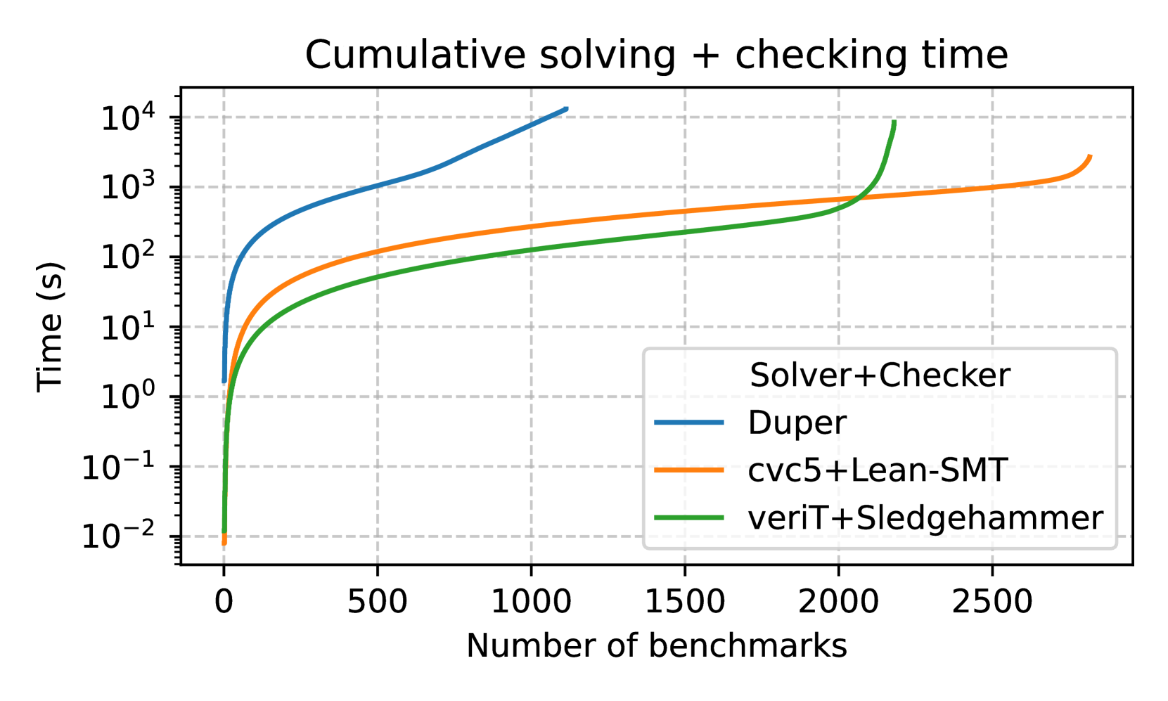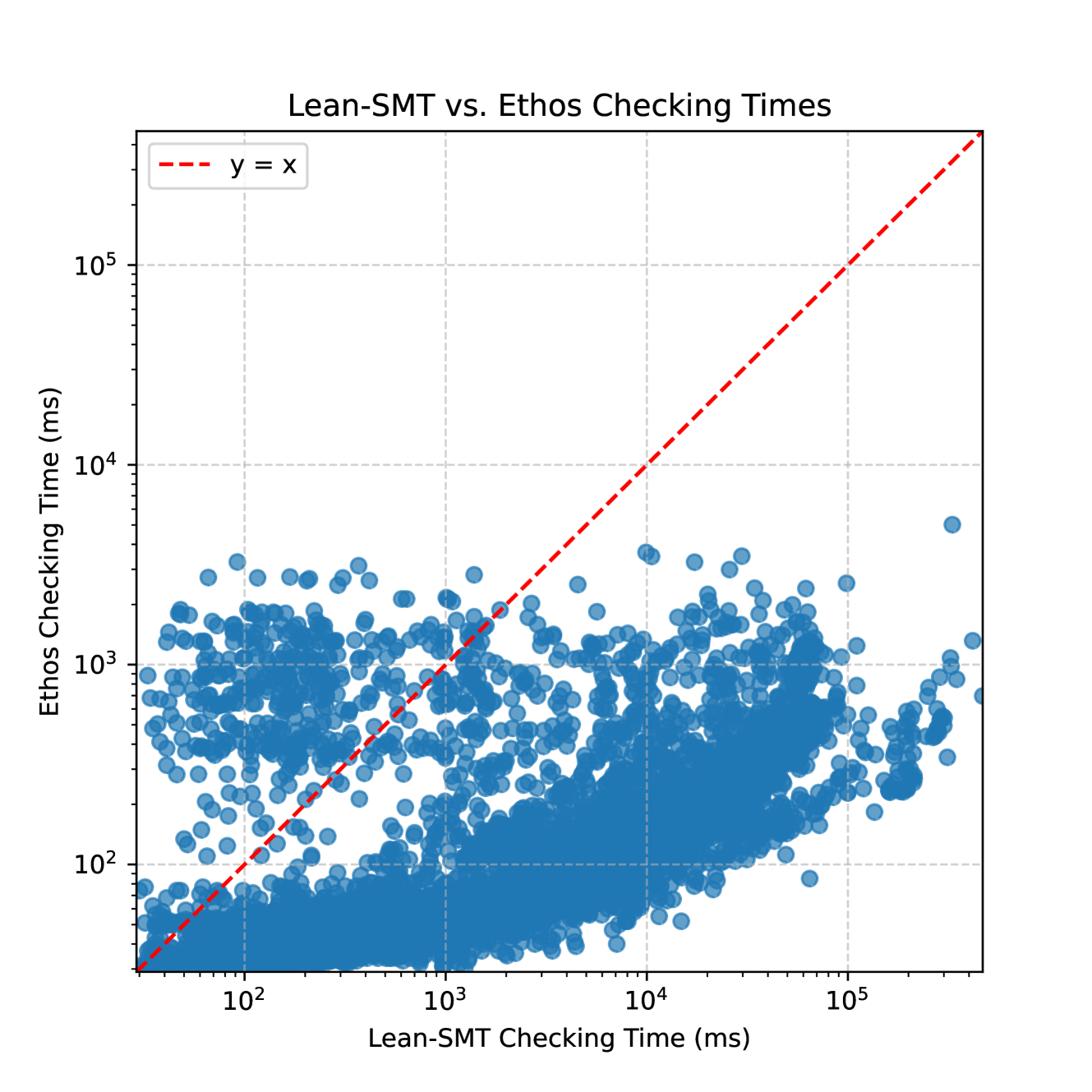</details> (b) Figure 2: (a) shows the performance of lean-smt on Sledgehammer benchmarks, while (b) compares proof checking performance of lean-smt with Ethos. The lean-smt tactic is mainly designed to prove Lean goals provided by users, but can also act as a proof checker for CPC proofs in supported fragments. We evaluate it All benchmarks were executed on a cluster with nodes equipped with 48 AMD Ryzen 9 7950X processors running at 4.50GHz and 128GB of RAM each. in these scenarios with the following benchmark sets: a set of 5000 SMT-LIB benchmarks generated by Sledgehammer from Isabelle/HOL, taken from Seventeen Provers Under the Hammer [15]; and $24,817$ unsatisfiable SMT-LIB benchmarks used in SMT-COMP 2024 https://smt-comp.github.io/2024/ that fit the supported fragments of lean-smt: UF, IDL, RDL, LIA, LRA, LIRA, and their quantifier-free siblings. The Sledgehammer benchmarks allow us to assess lean-smt ’s performance in both mathematics and formal verification domains and include lemmas selected by Sledgehammer with its premise selection mechanism. The problems in SMT-COMP are used together with proof-producing SMT solvers to generate proofs that are passed on to a set of proof checkers, including lean-smt. 4.1 Isabelle Sledgehammer Benchmarks We evaluate lean-smt on SMT problems generated by Isabelle’s Sledgehammer. We chose these benchmarks over other options (e.g., Lean’s MathLib) due to Lean’s lack of a premise selection mechanism, which is crucial for reducing false positives (i.e., returning SAT due to missing premises). These benchmarks also stress test solvers, as they contain many (up to 512) lemmas. We compare the performance of lean-smt against Sledgehammer with the veriT backend, which supports similar proof reconstruction techniques, and Duper. We do not include CVC4 as a backend for Sledgehammer because its proof production is unstable and do not provide sufficient detail for reliable reconstruction. The results in Figure 2(a) show that lean-smt effectively solves a large variety of Sledgehammer benchmarks, underscoring its potential for integration into general-purpose proof environments. lean-smt outperforms veriT+Sledgehammer mainly because cvc5 outperforms veriT on this set of benchmarks. lean-smt takes less than a second to replay proofs for 98% of the benchmarks, with the remaining 2% taking less than 5 seconds. Sledgehammer, by comparison, is faster at reconstructing shorter proofs, but does not scale as well for larger proofs. 4.2 SMT-LIB Benchmarks <details> <summary>x13.png Details</summary>  ### Visual Description ## Line Chart: Cumulative solving + checking time ### Overview The image is a line chart comparing the cumulative solving and checking time for three different solver-checker combinations: cvc5+Ethos, cvc5+Lean-SMT, and veriT+SMTCoq. The x-axis represents the number of benchmarks, and the y-axis represents the time in seconds on a logarithmic scale. ### Components/Axes * **Title:** Cumulative solving + checking time * **X-axis:** * Label: Number of benchmarks * Scale: Linear, ranging from 0 to 17500, with tick marks at intervals of 2500. * **Y-axis:** * Label: Time (s) * Scale: Logarithmic (base 10), ranging from 10^-1 to 10^5. Tick marks are present at each power of 10. * **Legend (located in the bottom-right corner):** * Solver+Checker * Blue line: cvc5+Ethos * Orange line: cvc5+Lean-SMT * Green line: veriT+SMTCoq ### Detailed Analysis * **cvc5+Ethos (Blue line):** * Trend: The line starts relatively flat, then begins to increase more sharply around 12500 benchmarks, and increases rapidly towards the end. * Data Points: * At 0 benchmarks, the time is approximately 0.1 s. * At 5000 benchmarks, the time is approximately 50 s. * At 10000 benchmarks, the time is approximately 150 s. * At 15000 benchmarks, the time is approximately 5000 s. * At 17500 benchmarks, the time is approximately 100000 s. * **cvc5+Lean-SMT (Orange line):** * Trend: The line increases steadily, but the rate of increase is not constant. * Data Points: * At 0 benchmarks, the time is approximately 0.05 s. * At 5000 benchmarks, the time is approximately 80 s. * At 10000 benchmarks, the time is approximately 500 s. * At 15000 benchmarks, the time is approximately 20000 s. * **veriT+SMTCoq (Green line):** * Trend: The line increases sharply initially, then plateaus, and then increases sharply again. * Data Points: * At 0 benchmarks, the time is approximately 0.05 s. * At 2500 benchmarks, the time is approximately 50 s. * At 5000 benchmarks, the time is approximately 500 s. ### Key Observations * The veriT+SMTCoq combination initially performs similarly to the other two, but its performance plateaus after 2500 benchmarks. * The cvc5+Ethos combination shows a significant increase in solving time towards the end of the benchmark set. * The cvc5+Lean-SMT combination shows a more consistent increase in solving time across the benchmark set. ### Interpretation The chart compares the performance of three different solver-checker combinations on a set of benchmarks. The cumulative solving and checking time provides insight into the overall efficiency of each combination. The logarithmic scale on the y-axis allows for easy comparison of performance across a wide range of times. The data suggests that the choice of solver-checker combination can significantly impact the time required to solve and check a given set of benchmarks. The veriT+SMTCoq combination seems to struggle with larger benchmark sets, while the cvc5+Ethos combination experiences a performance bottleneck towards the end. The cvc5+Lean-SMT combination appears to offer a more balanced performance across the entire benchmark set. </details> (a) <details> <summary>x14.png Details</summary>  ### Visual Description ## Chart: Cumulative Solving + Checking Time ### Overview The image is a line chart comparing the cumulative solving and checking time for three different solver-checker combinations across a varying number of benchmarks. The x-axis represents the number of benchmarks, and the y-axis represents the time in seconds on a logarithmic scale. ### Components/Axes * **Title:** Cumulative solving + checking time * **X-axis:** Number of benchmarks, ranging from 0 to 7000. * **Y-axis:** Time (s), ranging from 10^-1 to 10^5 on a logarithmic scale. * **Legend (located in the bottom-right):** * Blue line: cvc5+Ethos * Orange line: cvc5+Lean-SMT * Green line: veriT+SMTCoq ### Detailed Analysis * **cvc5+Ethos (Blue):** * The blue line starts at approximately 10^-1 seconds at 0 benchmarks. * The line slopes upward gradually until approximately 4000 benchmarks, reaching approximately 10^2 seconds. * After 4000 benchmarks, the line slopes upward more sharply, reaching approximately 10^5 seconds at 7000 benchmarks. * **cvc5+Lean-SMT (Orange):** * The orange line starts at approximately 10^-1 seconds at 0 benchmarks. * The line slopes upward sharply until approximately 1000 benchmarks, reaching approximately 10^2 seconds. * The line slopes upward gradually from 1000 to 5000 benchmarks, reaching approximately 10^4 seconds. * The line stops at approximately 5000 benchmarks. * **veriT+SMTCoq (Green):** * The green line starts at approximately 10^-1 seconds at 0 benchmarks. * The line slopes upward sharply until approximately 500 benchmarks, reaching approximately 10^2 seconds. * The line slopes upward gradually from 500 to 4000 benchmarks, reaching approximately 5*10^3 seconds. * The line stops at approximately 4000 benchmarks. ### Key Observations * All three solver-checker combinations start with very low cumulative times for a small number of benchmarks. * The cvc5+Ethos combination has the longest runtime, scaling to the highest cumulative time for the largest number of benchmarks. * The veriT+SMTCoq combination has the shortest runtime, stopping at 4000 benchmarks. * The cvc5+Lean-SMT combination stops at 5000 benchmarks. ### Interpretation The chart compares the performance of three different solver-checker combinations in terms of cumulative solving and checking time as the number of benchmarks increases. The logarithmic scale on the y-axis indicates that the differences in time are substantial. The cvc5+Ethos combination appears to be the most scalable, handling the largest number of benchmarks, but also takes the longest time overall. The veriT+SMTCoq combination is the fastest for a smaller number of benchmarks but does not scale as well as the other two. The cvc5+Lean-SMT combination falls in between the other two in terms of both scalability and time. The data suggests that the choice of solver-checker combination depends on the number of benchmarks and the desired trade-off between speed and scalability. 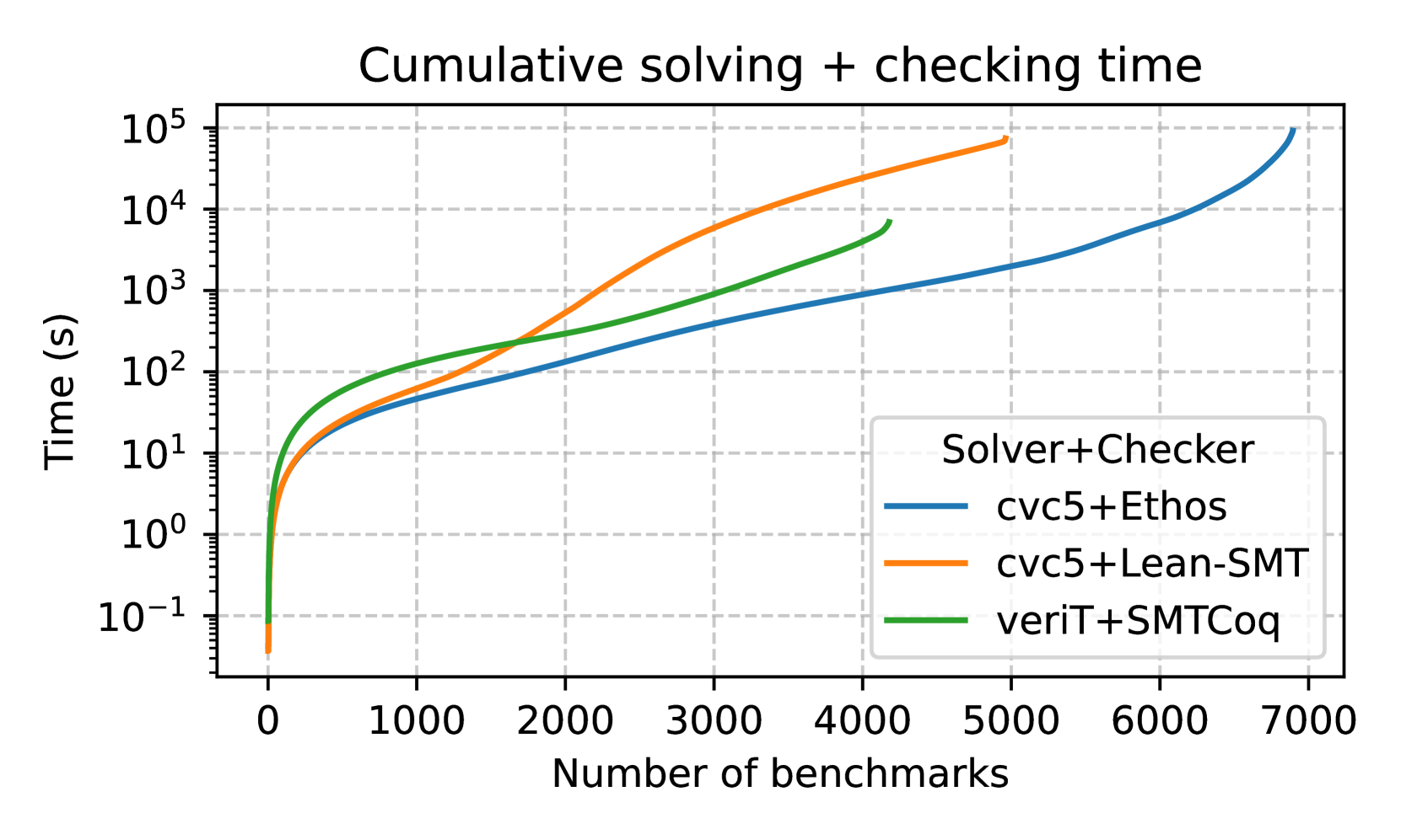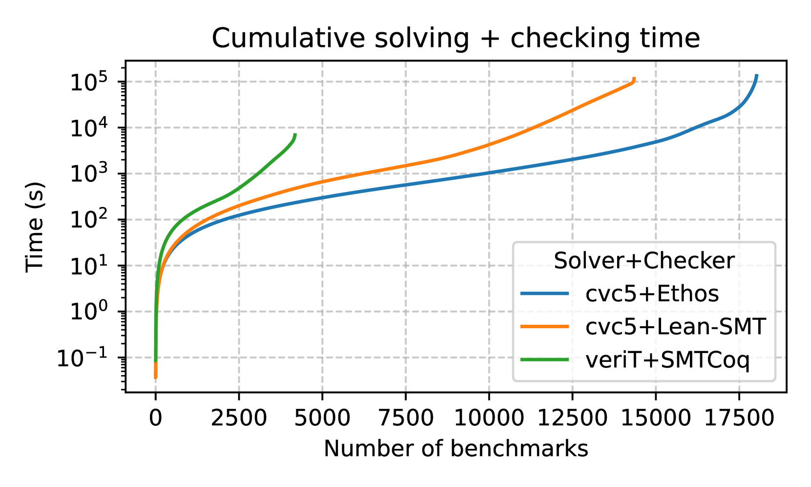</details> (b) Figure 3: Figure (a) shows the performance of lean-smt on supported SMT-LIB fragments, while Figure (b) shows the performance on the quantifier-free subset. We evaluate lean-smt against the proof checkers Ethos https://github.com/cvc5/ethos/ v0.1.0 and SMTCoq v2.2. Ethos is a proof checker implemented in C++ for the Eunoia logical framework, in which CPC has been formalized. SMTCoq is a proof checker in OCaml extracted from a formally verified Coq program, and supports proofs in a subset of the Alethe proof format [32]. It can check proofs produced by versions of the veriT SMT solver up to 2016. Since the different approaches use different SMT solvers, our evaluation includes both proof-checking and SMT solving times. All benchmarks were run with a standard 20-minute timeout. Note that both lean-smt and SMTCoq are highly trustworthy, since they both rely on small kernels. However, SMTCoq’s code extraction mechanism, which extracts OCaml code from verified Coq code, has to be trusted as well. The trusted base for Ethos, besides its kernel, also includes the Eunoia signature for CPC. Moreover, its kernel includes native support for arithmetic (via GMP) and arrays for efficiency, while Lean’s kernel only natively supports arithmetic. Supported SMT-LIB Benchmarks Figure 3(a) compares the cumulative solving and checking times for all SMT-LIB benchmarks. Out of the $21,595$ This number is for cvc5+ lean-smt; for cvc5+Ethos, $21,541$ proofs are produced. The difference is due to the overhead of proof printing and piping for the latter combo, while in the former, the proof is passed directly via the API to lean-smt. benchmarks proofs generated On occasion, cvc5 will produce proofs containing holes. Both Ethos and lean-smt verify every non-hole proof step. by cvc5, lean-smt successfully verified $15,271$ proofs (71%), despite relying solely on the Lean kernel for soundness. Ethos verifies 98% of the proofs. Figure 2(b) compares the performance of lean-smt to Ethos on proof checking times. lean-smt stays within an order of magnitude of Ethos for most benchmarks. One reason for Ethos’ superior performance is the lack of specialized support for arrays in Lean’s kernel. This difference could be mitigated by switching to a more efficient array representation in Lean. Quantifier-Free Fragment Figure 3(b) focuses on the quantifier-free subset of SMT-LIB benchmarks, where SMTCoq’s verified approach shines in terms of speed. However, SMTCoq falls short in the total number of proofs verified, primarily because its rigid, fully verified architecture struggles to keep pace with the rapidly evolving features of modern SMT solvers. In contrast, lean-smt benefits from proof replay flexibility, allowing it to adapt more easily to updates in cvc5 ’s proof production capabilities, resulting in broader coverage. Overall, lean-smt balances flexibility and performance, achieving promising results for a proof checker deeply integrated into Lean. While it trails Ethos in raw speed, its ability to verify a wide range of benchmarks with a small trusted base makes it an attractive option for checking SMT proofs in critical domains. 5 Conclusion lean-smt, an integration between cvc5 and Lean, is a significant step toward building a Lean hammer that enhances automation and verifies proofs generated by cvc5. lean-smt performs competitively with state-of-the-art proof checkers such as Ethos and Carcara, both in terms of performance and effectiveness. It is also capable of verifying a diverse range of SMT-LIB benchmarks. Future work includes creating a dedicated Lean benchmark set for more targeted evaluation and expanding lean-smt ’s support to additional SMT-LIB theories, such as bit-vectors, floats, and strings. We also plan to extend its proof coverage beyond the current 200 rules and incorporate more preprocessing steps to boost performance. Finally, we plan to improve integration with lean-auto to support higher-order logic and extend support for common Lean datatypes (e.g., tuples, structures, and modular arithmetic). The ultimate objective is to develop a Lean hammer that brings unprecedented automation and verification capabilities to Lean. Acknowledgments. This work was partially supported by a gift from Amazon Web Services, the Stanford Center for Automated Reasoning, the Coordenação de Aperfeiçoamento de Pessoal de Nível Superior - Brasil (CAPES) - Finance Code 001, and the Defense Advanced Research Projects Agency (DARPA) under contract FA8750-24-2-1001. Any opinions, findings, and conclusions or recommendations expressed here are those of the authors and do not necessarily reflect the views of DARPA. References - [1] Avigad, J., de Moura, L., Kong, S., Ullrich, S.: Theorem proving in lean 4, uRL: https://leanprover.github.io/theorem_proving_in_lean4/ - [2] Baanen, A.: Formalizing Fundamental Algebraic Number Theory. Phd-thesis - research and graduation internal, Vrije Universiteit Amsterdam (Jan 2024). https://doi.org/10.5463/thesis.541 - [3] Barbosa, H., Barrett, C.W., Brain, M., Kremer, G., Lachnitt, H., Mann, M., Mohamed, A., Mohamed, M., Niemetz, A., Nötzli, A., Ozdemir, A., Preiner, M., Reynolds, A., Sheng, Y., Tinelli, C., Zohar, Y.: cvc5: A versatile and industrial-strength SMT solver. In: Fisman, D., Rosu, G. (eds.) Tools and Algorithms for Construction and Analysis of Systems (TACAS), Part I. Lecture Notes in Computer Science, vol. 13243, pp. 415–442. Springer (2022). https://doi.org/10.1007/978-3-030-99524-9_24, https://doi.org/10.1007/978-3-030-99524-9_24 - [4] Barbosa, H., Reynolds, A., Kremer, G., Lachnitt, H., Niemetz, A., Nötzli, A., Ozdemir, A., Preiner, M., Viswanathan, A., Viteri, S., Zohar, Y., Tinelli, C., Barrett, C.W.: Flexible proof production in an industrial-strength SMT solver. In: Blanchette, J., Kovács, L., Pattinson, D. (eds.) International Joint Conference on Automated Reasoning (IJCAR). Lecture Notes in Computer Science, vol. 13385, pp. 15–35. Springer (2022). https://doi.org/10.1007/978-3-031-10769-6_3, https://doi.org/10.1007/978-3-031-10769-6_3 - [5] Barrett, C., Conway, C.L., Deters, M., Hadarean, L., Jovanović, D., King, T., Reynolds, A., Tinelli, C.: CVC4. In: Gopalakrishnan, G., Qadeer, S. (eds.) Computer Aided Verification (CAV). pp. 171–177. Springer (2011). https://doi.org/10.1007/978-3-642-22110-1_14, http://dx.doi.org/10.1007/978-3-642-22110-1_14 - [6] Barrett, C., Fontaine, P., Tinelli, C.: The SMT-LIB Standard: Version 2.6. Tech. rep., Department of Computer Science, The University of Iowa (2017), available at www.SMT-LIB.org - [7] Bertot, Y., Castéran, P.: Interactive Theorem Proving and Program Development - Coq’Art: The Calculus of Inductive Constructions. Texts in Theoretical Computer Science. An EATCS Series, Springer (2004). https://doi.org/10.1007/978-3-662-07964-5 - [8] Blanchette, J.C., Böhme, S., Paulson, L.C.: Extending sledgehammer with SMT solvers. In: Bjørner, N.S., Sofronie-Stokkermans, V. (eds.) Automated Deduction - CADE-23 - 23rd International Conference on Automated Deduction, Wroclaw, Poland, July 31 - August 5, 2011. Proceedings. Lecture Notes in Computer Science, vol. 6803, pp. 116–130. Springer (2011). https://doi.org/10.1007/978-3-642-22438-6_11, https://doi.org/10.1007/978-3-642-22438-6_11 - [9] Blanchette, J.C., Kaliszyk, C., Paulson, L.C., Urban, J.: Hammering towards QED. J. Formalized Reasoning 9 (1), 101–148 (2016) - [10] Bobot, F., Filliâtre, J.C., Marché, C., Paskevich, A.: Why3: Shepherd your herd of provers. In: Boogie 2011: First International Workshop on Intermediate Verification Languages. pp. 53–64 (2011) - [11] Bouton, T., de Oliveira, D.C.B., Déharbe, D., Fontaine, P.: veriT: An Open, Trustable and Efficient SMT-Solver. In: Schmidt, R.A. (ed.) Conference on Automated Deduction (CADE). Lecture Notes in Computer Science, vol. 5663, pp. 151–156. Springer (2009). https://doi.org/10.1007/978-3-642-02959-2_12, http://dx.doi.org/10.1007/978-3-642-02959-2_12 - [12] Castelvecchi, D.: Mathematicians welcome computer-assisted proof in “grand unification” theory. Nature 595 (06 2021). https://doi.org/10.1038/d41586-021-01627-2 - [13] Clune, J., Qian, Y., Bentkamp, A., Avigad, J.: Duper: A Proof-Producing Superposition Theorem Prover for Dependent Type Theory. In: Bertot, Y., Kutsia, T., Norrish, M. (eds.) 15th International Conference on Interactive Theorem Proving (ITP 2024). Leibniz International Proceedings in Informatics (LIPIcs), vol. 309, pp. 10:1–10:20. Schloss Dagstuhl – Leibniz-Zentrum für Informatik, Dagstuhl, Germany (2024). https://doi.org/10.4230/LIPIcs.ITP.2024.10, https://drops.dagstuhl.de/entities/document/10.4230/LIPIcs.ITP.2024.10 - [14] mathlib Community, T.: The lean mathematical library. In: Proceedings of the 9th ACM SIGPLAN International Conference on Certified Programs and Proofs. pp. 367–381. CPP 2020, Association for Computing Machinery, New York, NY, USA (2020). https://doi.org/10.1145/3372885.3373824 - [15] Desharnais, M., Vukmirovic, P., Blanchette, J., Wenzel, M.: Seventeen provers under the hammer. In: Andronick, J., de Moura, L. (eds.) 13th International Conference on Interactive Theorem Proving, ITP 2022, August 7-10, 2022, Haifa, Israel. LIPIcs, vol. 237, pp. 8:1–8:18. Schloss Dagstuhl - Leibniz-Zentrum für Informatik (2022). https://doi.org/10.4230/LIPICS.ITP.2022.8, https://doi.org/10.4230/LIPIcs.ITP.2022.8 - [16] Ekici, B., Mebsout, A., Tinelli, C., Keller, C., Katz, G., Reynolds, A., Barrett, C.: Smtcoq: A plug-in for integrating smt solvers into coq. In: Majumdar, R., Kunčak, V. (eds.) Computer Aided Verification. pp. 126–133. Springer International Publishing, Cham (2017) - [17] Enderton, H.B.: A mathematical introduction to logic. Academic Press, 2 edn. (2001) - [18] Gonthier, G.: The four colour theorem: Engineering of a formal proof. In: Kapur, D. (ed.) Computer Mathematics, 8th Asian Symposium, ASCM 2007, Singapore, December 15-17, 2007. Revised and Invited Papers. Lecture Notes in Computer Science, vol. 5081, p. 333. Springer (2007). https://doi.org/10.1007/978-3-540-87827-8_28, https://doi.org/10.1007/978-3-540-87827-8_28 - [19] Hales, T., Adams, M., Bauer, G., Dang, D.T., Harrison, J., Hoang, T.L., Kaliszyk, C., Magron, V., McLaughlin, S., Nguyen, T.T., Nguyen, T.Q., Nipkow, T., Obua, S., Pleso, J., Rute, J., Solovyev, A., Ta, A.H.T., Tran, T.N., Trieu, D.T., Urban, J., Vu, K.K., Zumkeller, R.: A formal proof of the kepler conjecture (2015) - [20] Hurd, J.: First-order proof tactics in higher-order logic theorem provers in proc (2003), https://api.semanticscholar.org/CorpusID:11201048 - [21] Jakubuv, J., Chvalovský, K., Goertzel, Z.A., Kaliszyk, C., Olsák, M., Piotrowski, B., Schulz, S., Suda, M., Urban, J.: Mizar 60 for mizar 50. In: Naumowicz, A., Thiemann, R. (eds.) Interactive Theorem Proving (ITP). LIPIcs, vol. 268, pp. 19:1–19:22. Schloss Dagstuhl - Leibniz-Zentrum für Informatik (2023). https://doi.org/10.4230/LIPICS.ITP.2023.19, https://doi.org/10.4230/LIPIcs.ITP.2023.19 - [22] Kaliszyk, C., Urban, J.: Hol(y)hammer: Online ATP service for HOL light. Math. Comput. Sci. 9 (1), 5–22 (2015). https://doi.org/10.1007/S11786-014-0182-0, https://doi.org/10.1007/s11786-014-0182-0 - [23] Klein, G., Andronick, J., Elphinstone, K., Heiser, G., Cock, D., Derrin, P., Elkaduwe, D., Engelhardt, K., Kolanski, R., Norrish, M., Sewell, T., Tuch, H., Winwood, S.: sel4: formal verification of an operating-system kernel. Commun. ACM 53 (6), 107–115 (2010). https://doi.org/10.1145/1743546.1743574, https://doi.org/10.1145/1743546.1743574 - [24] Lachnitt, H., Fleury, M., Aniva, L., Reynolds, A., Barbosa, H., Nötzli, A., Barrett, C.W., Tinelli, C.: Isarare: Automatic verification of SMT rewrites in isabelle/hol. In: Finkbeiner, B., Kovács, L. (eds.) Tools and Algorithms for Construction and Analysis of Systems (TACAS), Part I. Lecture Notes in Computer Science, vol. 14570, pp. 311–330. Springer (2024). https://doi.org/10.1007/978-3-031-57246-3_17, https://doi.org/10.1007/978-3-031-57246-3_17 - [25] Limperg, J., From, A.H.: Aesop: White-box best-first proof search for lean. In: Proceedings of the 12th ACM SIGPLAN International Conference on Certified Programs and Proofs. p. 253–266. CPP 2023, Association for Computing Machinery, New York, NY, USA (2023). https://doi.org/10.1145/3573105.3575671, https://doi.org/10.1145/3573105.3575671 - [26] Meng, J., Quigley, C., Paulson, L.C.: Automation for interactive proof: First prototype. Inf. Comput. 204 (10), 1575–1596 (2006). https://doi.org/10.1016/J.IC.2005.05.010, https://doi.org/10.1016/j.ic.2005.05.010 - [27] de Moura, L., Ullrich, S.: The lean 4 theorem prover and programming language. In: Platzer, A., Sutcliffe, G. (eds.) Conference on Automated Deduction (CADE). Lecture Notes in Computer Science, vol. 12699, pp. 625–635. Springer (2021). https://doi.org/10.1007/978-3-030-79876-5_37, https://doi.org/10.1007/978-3-030-79876-5_37 - [28] Nelson, L., Geffen, J.V., Torlak, E., Wang, X.: Specification and verification in the field: Applying formal methods to BPF just-in-time compilers in the linux kernel. In: 14th USENIX Symposium on Operating Systems Design and Implementation, OSDI 2020, Virtual Event, November 4-6, 2020. pp. 41–61. USENIX Association (2020), https://www.usenix.org/conference/osdi20/presentation/nelson - [29] Nipkow, T., Paulson, L.C., Wenzel, M.: Isabelle/HOL: A Proof Assistant for Higher-Order Logic, LNCS, vol. 2283. Springer (2002) - [30] Nötzli, A., Barbosa, H., Niemetz, A., Preiner, M., Reynolds, A., Barrett, C.W., Tinelli, C.: Reconstructing fine-grained proofs of rewrites using a domain-specific language. In: Griggio, A., Rungta, N. (eds.) Formal Methods In Computer-Aided Design (FMCAD). pp. 65–74. IEEE (2022). https://doi.org/10.34727/2022/isbn.978-3-85448-053-2_12, https://doi.org/10.34727/2022/isbn.978-3-85448-053-2_12 - [31] Piotrowski, B., Mir, R.F., Ayers, E.: Machine-learned premise selection for lean (2023), https://arxiv.org/abs/2304.00994 - [32] Schurr, H., Fleury, M., Barbosa, H., Fontaine, P.: Alethe: Towards a generic SMT proof format (extended abstract). CoRR abs/2107.02354 (2021), https://arxiv.org/abs/2107.02354 - [33] Schurr, H., Fleury, M., Desharnais, M.: Reliable reconstruction of fine-grained proofs in a proof assistant. In: Platzer, A., Sutcliffe, G. (eds.) Automated Deduction - CADE 28 - 28th International Conference on Automated Deduction, Virtual Event, July 12-15, 2021, Proceedings. Lecture Notes in Computer Science, vol. 12699, pp. 450–467. Springer (2021). https://doi.org/10.1007/978-3-030-79876-5_26, https://doi.org/10.1007/978-3-030-79876-5_26 - [34] Tao, T.: Machine assisted proof. AMS Notices 72 (1), 86–95 (2025). https://doi.org/10.1090/noti3041, https://doi.org/10.1090/noti3041 Appendix 0.A Full tactic for reconstructing ARITH_SUM_UB Figure 4: Implementation of the sumBounds tactic ⬇ 1 def combineBounds (pf ₁ pf ₂ : Expr) : MetaM Expr := do 2 let t ₁ ← inferType pf ₁ 3 let t ₂ ← inferType pf ₂ 4 let rel ₁ ← getRel t ₁ 5 let rel ₂ ← getRel t ₂ 6 let opType ₁ ← getOperandType t ₁ 7 let opType ₂ ← getOperandType t ₂ 8 let (pf ₁’, pf ₂’) ← castHypothesis pf ₁ pf ₂ rel ₁ rel ₂ opType ₁ opType ₂ 9 let thmName : Name := 10 match rel ₁, rel ₂ with 11 | ‘ LT. lt , ‘ LT. lt => ‘ sumBoundsThm ₁ 12 | ‘ LT. lt , ‘ LE. le => ‘ sumBoundsThm ₂ 13 – Note: omitting other cases 14 | _ , _ => panic! "[sumBounds]: invalid relation " 15 mkAppM thmName #[pf ₂’, pf ₁’] 16 17 def sumBoundsCore (acc : Expr) (pfs : List Expr) : MetaM Expr := 18 match pfs with 19 | [] => return acc 20 | pf ’ :: pfs ’ => do 21 let acc ’ ← combineBounds acc pf ’ 22 sumBoundsCore acc ’ pfs ’ With the theorems shown in Section 3.3 proven, the tactic shown in Figure 4 can be implemented. The function sumBoundsCore is meant to be invoked with the last proof in the input as acc and the rest of them, in reverse order, as pfs. If pfs is empty, it returns the accumulator (line 18). Otherwise, function combineBounds is invoked to sum the inequalities represented by acc and pf’ (line 20) and recursively call sumBoundsCore, updating the arguments (line 21). The first action performed in function combineBounds is to obtain the inequalities corresponding to pf 1 and pf 2 through inferType. Then, in lines 4 to 7, it inspects their structure and obtains their relation symbol (rel 1 and rel 2) and the type of their operands (opType 1 and opType 2). Notice that sumBoundsThm expects that all the four variables have the same type. If one of the input proofs represents an inequality over integers and the other is over reals, the inequality has to be lifted from an inequality between integers into an inequality between reals. This is done using one of the following theorems, depending on the relation symbol: ⬇ Int. castEQ : ∀ {a b : Int}, a = b → (↑ a : Real) = (↑ b : Real) Int. castLE : ∀ {a b : Int}, a <= b → (↑ a : Real) <= (↑ b : Real) Int. castLT : ∀ {a b : Int}, a < b → (↑ a : Real) < (↑ b : Real) The function castHypothesis (line 8) does this analysis and, if necessary, applies one of these theorems to pf 1 or pf 2. Once with the correct version of the proofs, the respective instance of sumBoundsThm, depending on rel 1 and rel 2, can be applied. The match statement in lines 10 to 13 chooses which version to apply. Appendix 0.B Tables for for Evaluations | cvc5+Lean-SMT veriT+Sledgehammer Duper | 2868 2211 1116 | 2866 2180 1116 | 2847 2180 1116 | | --- | --- | --- | --- | Table 1: Performance of lean-smt on baseline Seventeen Provers benchmarks (5000 total). Table 1 shows the performance of lean-smt on the Seventeen Provers benchmarks, while Tables 2 and 3 show its performance on SMT-LIB benchmarks. | cvc5+Lean-SMT cvc5+Ethos veriT+SMTCoq | 21595 21541 4178 | 15271 21196 4178 | 14099 18018 4178 | | --- | --- | --- | --- | Table 2: Performance of lean-smt on supported SMT-LIB fragments (24817 total). The first column in the tables shows the number of benchmarks solved by solved by the ATP. The time it takes to generate the proof is also included. The second column show the number of benchmarks where proof checking was successful. This includes proofs with holes, which are not considered by SMTCoq. The third column shows the number of benchmarks where proof checking was successful and the proof was complete. | cvc5+Lean-SMT cvc5+Ethos veriT+SMTCoq | 9263 9203 4178 | 5091 8860 4178 | 4869 6892 4178 | | --- | --- | --- | --- | Table 3: Performance of lean-smt on the quantifier-free subset of SMT-LIB benchmarks (11804 total).