2505.17482v1

# From Reasoning to Generalization: Knowledge-Augmented LLMs for ARC Benchmark ## Abstract Recent reasoning-oriented LLMs have demonstrated strong performance on challenging tasks such as mathematics and science examinations. However, core cognitive faculties of human intelligence, such as abstract reasoning and generalization, remain underexplored. To address this, we evaluate recent reasoning-oriented LLMs on the Abstraction and Reasoning Corpus (ARC) benchmark, which explicitly demands both faculties. We formulate ARC as a program synthesis task and propose nine candidate solvers. Experimental results show that repeated-sampling planning-aided code generation (RSPC) achieves the highest test accuracy and demonstrates consistent generalization across most LLMs. To further improve performance, we introduce an ARC solver, Knowledge Augmentation for Abstract Reasoning (KAAR), which encodes core knowledge priors within an ontology that classifies priors into three hierarchical levels based on their dependencies. KAAR progressively expands LLM reasoning capacity by gradually augmenting priors at each level, and invokes RSPC to generate candidate solutions after each augmentation stage. This stage-wise reasoning reduces interference from irrelevant priors and improves LLM performance. Empirical results show that KAAR maintains strong generalization and consistently outperforms non-augmented RSPC across all evaluated LLMs, achieving around 5% absolute gains and up to 64.52% relative improvement. Despite these achievements, ARC remains a challenging benchmark for reasoning-oriented LLMs, highlighting future avenues of progress in LLMs. 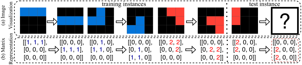## 1 Introduction Learning from extensive training data has achieved remarkable success in major AI fields such as computer vision, natural language processing, and autonomous driving [1, 2, 3]. However, achieving human-like intelligence goes beyond learning purely from large-scale data; it requires rapid reasoning and generalizing from prior knowledge to novel tasks and situations [4]. Chollet [5] introduced Abstraction and Reasoning Corpus (ARC) to assess the generalization and abstract reasoning capabilities of AI systems. In each ARC task, the solver is required to infer generalized rules or procedures from a small set of training instances, typically fewer than five input-output image pairs, and apply them to generate output images for given input images provided in test instances (Figure 1 (a)). Each image in ARC is a pixel grid represented as a 2D matrix, where each value denotes a pixel color (Figure 1 (b)). ARC evaluates broad generalization, encompassing reasoning over individual input-output pairs and inferring generalized solutions via high-level abstraction, akin to inductive reasoning [6]. ARC is grounded in core knowledge priors, which serve as foundational cognitive faculties of human intelligence, enabling equitable comparisons between AI systems and human cognitive abilities [7]. These priors include: (1) objectness – aggregating elements into coherent, persistent objects; (2) geometry and topology – recognizing and manipulating shapes, symmetries, spatial transformations, and structural patterns (e.g., containment, repetition, projection); (3) numbers and counting – counting, sorting, comparing quantities, performing basic arithmetic, and identifying numerical patterns; and (4) goal-directedness – inferring purposeful transformations between initial and final states without explicit temporal cues. Incorporating these priors allows ARC solvers to replicate human cognitive processes, produce behavior aligned with human expectations, address human-relevant problems, and demonstrate human-like intelligence through generalization and abstract reasoning [5]. These features highlight ARC as a crucial benchmark for assessing progress toward general intelligence. Chollet [5] suggested approaching ARC tasks as instances of program synthesis, which studies automatically generating a program that satisfies a high-level specification [8]. Following this proposal, recent studies [9, 10] have successfully solved partial ARC tasks by searching for program solutions encoded within object-centric domain-specific languages (DSLs). Reasoning-oriented LLMs integrate chain-of-thought (CoT) reasoning [11], often trained via reinforcement learning, further advancing program synthesis performance. Common approaches using LLMs for code generation include repeated sampling, where multiple candidate programs are generated [12], followed by best-program selection strategies [13, 14, 15, 16], and code refinement, where initial LLM-generated code is iteratively improved using error feedback from execution results [17, 18] or LLM-generated explanations [17, 19, 18]. We note that ARC presents greater challenges than existing program synthesis benchmarks such as HumanEval [12], MBPP [20], and LiveCode [21], due to its stronger emphasis on generalization and abstract reasoning grounded in core knowledge priors, which remain underexplored. This gap motivates our evaluation of recent reasoning-oriented LLMs on the ARC benchmark, and our proposed knowledge augmentation approach to improve their performance. <details> <summary>x1.png Details</summary>  ### Visual Description # Technical Document Extraction: State Transition System ## Overview The image depicts a **state transition system** with two primary components: 1. **Visualization** (top section) 2. **Representation** (bottom section) Both sections illustrate the evolution of a 3x3 grid through training instances and a test instance. The system uses **color-coded states** (blue, red, black) and **numerical matrices** to represent grid configurations. --- ## Visualization Section ### Components - **Grid Layout**: 3x3 grid with cells colored **blue**, **red**, or **black**. - **Arrows**: Indicate transitions between states. - **Question Mark**: Represents an unknown state in the test instance. ### Training Instances (Left to Right) 1. **Initial State**: - Grid: All cells **blue** (top row) and **black** (bottom two rows). - Matrix: `[[1,1,1],[0,0,0],[0,0,0]]` - Legend: Blue = 1, Black = 0 2. **Transition 1**: - Grid: Middle row **blue**, others **black**. - Matrix: `[[0,0,0],[1,1,1],[0,0,0]]` 3. **Transition 2**: - Grid: Top-left and middle-left cells **blue**, others **black**. - Matrix: `[[0,1,0],[1,1,0],[0,0,0]]` 4. **Transition 3**: - Grid: Top-left cell **blue**, others **black**. - Matrix: `[[0,0,0],[0,1,0],[0,0,0]]` 5. **Transition 4**: - Grid: Top-left and middle-left cells **blue**, others **black**. - Matrix: `[[0,0,0],[0,1,0],[0,0,0]]` 6. **Transition 5**: - Grid: Top-left cell **blue**, others **black**. - Matrix: `[[0,0,0],[0,1,0],[0,0,0]]` ### Test Instance (Rightmost) - **Grid**: Top-left cell **red**, others **black**. - **Question Mark**: Indicates an unknown state. - **Matrix**: `[[2,0,0],[0,0,0],[0,0,0]]` - **Legend**: Red = 2 (new state introduced in test instance). --- ## Representation Section ### Numerical Matrices Each grid is mapped to a 3x3 matrix with integer values: - **0**: Black (background) - **1**: Blue (initial state) - **2**: Red (new state in test instance) ### Key Observations 1. **Training Progression**: - Starts with all **blue** (1s) and **black** (0s). - Gradually introduces **blue** cells in specific positions. - Final training instance retains **blue** in the middle-left cell. 2. **Test Instance**: - Introduces **red** (2) in the top-left cell, a new state not seen in training. - Matrix: `[[2,0,0],[0,0,0],[0,0,0]]` --- ## Legend and Color Mapping - **Blue**: Represents value **1** (initial state). - **Red**: Represents value **2** (new state in test instance). - **Black**: Represents value **0** (background). **Legend Placement**: Not explicitly shown in the image, but inferred from color-to-value mapping in matrices. --- ## Spatial Grounding and Trends ### Visual Trends - **Training Instances**: - Blue cells (1s) transition from full coverage to sparse distribution. - No red cells appear in training. - **Test Instance**: - Red cell (2) appears in the top-left corner, indicating a novel state. - All other cells remain **black** (0). ### Component Isolation 1. **Header**: "Visualization" and "Representation" labels. 2. **Main Chart**: - Training instances (left) → Test instance (right). - Arrows show state evolution. 3. **Footer**: Numerical matrices and legend (implied). --- ## Data Table Reconstruction | Instance | Grid State (Visualization) | Matrix Representation (Representation) | |----------------|-----------------------------------|----------------------------------------------| | Training 1 | All blue (top), black (bottom) | `[[1,1,1],[0,0,0],[0,0,0]]` | | Training 2 | Middle row blue | `[[0,0,0],[1,1,1],[0,0,0]]` | | Training 3 | Top-left and middle-left blue | `[[0,1,0],[1,1,0],[0,0,0]]` | | Training 4 | Top-left blue | `[[0,0,0],[0,1,0],[0,0,0]]` | | Training 5 | Top-left blue | `[[0,0,0],[0,1,0],[0,0,0]]` | | Test Instance | Top-left red, others black | `[[2,0,0],[0,0,0],[0,0,0]]` | --- ## Conclusion The system demonstrates a **state transition process** where: 1. Training instances evolve from uniform blue states to sparse blue configurations. 2. The test instance introduces a **new red state** (value 2) in the top-left cell, suggesting a prediction or anomaly detection task. 3. Numerical matrices provide a precise representation of grid states, with colors mapped to integers (0=black, 1=blue, 2=red). This structure enables analysis of state evolution and generalization to unseen configurations. </details> Figure 1: An ARC problem example (25ff71a9) with image visualizations (a), including three input-output pairs in the training instances, and one input image in the test instance, along with their corresponding 2D matrix representations (b). The ground-truth test output is enclosed in a red box. We systematically assess how reasoning-oriented LLMs approach ARC tasks within the program synthesis framework. For each ARC problem, we begin by providing 2D matrices as input. We adopt three established program generation strategies: direct generation, repeated sampling, and refinement. Each strategy is evaluated under two solution representations: a text-based solution plan and Python code. When generating code solutions, we further examine two modalities: standalone and planning-aided, where a plan is generated to guide subsequent code development, following recent advances [18, 22, 23]. In total, nine ARC solvers are considered. We evaluate several reasoning-oriented LLMs, including proprietary models, GPT-o3-mini [24, 25], and Gemini-2.0-Flash-Thinking (Gemini-2.0) [26], and open-source models, DeepSeek-R1-Distill-Llama-70B (DeepSeek-R1-70B) [27] and QwQ-32B [28]. Accuracy on test instances is reported as the primary metric. When evaluated on the ARC public evaluation set (400 problems), repeated-sampling planning-aided code generation (RSPC) demonstrates consistent generalization and achieves the highest test accuracy across most LLMs, 30.75% with GPT-o3-mini, 16.75% with Gemini-2.0, 14.25% with QwQ-32B, and 7.75% with DeepSeek-R1-70B. We treat the most competitive ARC solver, RSPC, as the solver backbone. Motivated by the success of manually defined priors in ARC solvers [9, 10], we propose K nowledge A ugmentation for A bstract R easoning (KAAR) for solving ARC tasks using reasoning-oriented LLMs. KAAR formalizes manually defined priors through a lightweight ontology that organizes priors into hierarchical levels based on their dependencies. It progressively augments LLMs with priors at each level via structured prompting. Specifically, core knowledge priors are introduced in stages: beginning with objectness, followed by geometry, topology, numbers, and counting, and concluding with goal-directedness. After each stage, KAAR applies the ARC solver backbone (RSPC) to generate the solution. This progressive augmentation enables LLMs to gradually expand their reasoning capabilities and facilitates stage-wise reasoning, aligning with human cognitive development [29]. Empirical results show that KAAR improves accuracy on test instances across all evaluated LLMs, achieving the largest absolute gain of 6.75% with QwQ-32B and the highest relative improvement of 64.52% with DeepSeek-R1-70B over non-augmented RSPC. We outline our contributions as follows: - We evaluate the abstract reasoning and generalization capabilities of reasoning-oriented LLMs on ARC using nine solvers that differ in generation strategies, modalities, and solution representations. - We introduce KAAR, a knowledge augmentation approach for solving ARC problems using LLMs. KAAR progressively augments LLMs with core knowledge priors structured via an ontology and applies the best ARC solver after augmenting same-level priors, further improving performance. - We conduct a comprehensive performance analysis of the proposed ARC solvers, highlighting failure cases and remaining challenges on the ARC benchmark. <details> <summary>x2.png Details</summary>  ### Visual Description # Technical Document Extraction ## Diagram Analysis ### Section 1: Direct Generation **Diagram Components**: - **Q**: Input/output node (pink circles) - **s**: State variable (purple circles) - **p**: Planning node (blue circles) - **c**: Condition node (green diamonds) - **I_t**: Target image (green diamonds) - **I_r**: Reference image (blue diamonds) **Flow Logic**: 1. Q → s (via p) → I_t (standalone) 2. Q → s (via c) → I_t (standalone) 3. Q → p → s (via c) → I_t (planning-aided) **Textual Content**: ```text (1) Direct Generation The training example(s): input: [[1,1,1], [0,0,0], [0,0,0]] output: [[0,0,0], [1,1,1], [0,0,0]] The test input image(s): input: [[2,0,0], [2,0,0], [0,0,0]] ``` ### Section 2: Repeat Sampling **Diagram Components**: - **Q**: Input/output node (pink circles) - **s**: State variable (purple circles) - **p**: Planning node (blue circles) - **I_r**: Reference image (blue diamonds) - **I_t**: Target image (green diamonds) **Flow Logic**: 1. Q → s (via p) → I_r (pass) → I_t 2. Q → s (via c) → I_r (pass) → I_t (standalone) 3. Q → p → s (via c) → I_r (pass) → I_t (planning-aided) **Python Code**: ```python # Repeat Sampling Logic for each cell in row i of the output (where i > 0): set its value equal to the value from row (i - 1) in the same column for the top row of the output (row 0): fill every cell with 0 (background color) ``` ### Section 3: Refinement **Diagram Components**: - **Q**: Input/output node (pink circles) - **s**: State variable (purple circles) - **p**: Planning node (blue circles) - **I_r**: Reference image (blue diamonds) - **I_t**: Target image (green diamonds) **Flow Logic**: 1. Q → s (via p) → I_r (pass) → I_t 2. Q → s (via c) → I_r (pass) → I_t (standalone) 3. Q → p → s (via c) → I_r (pass) → I_t (planning-aided) **Python Code**: ```python # Refinement Logic def generate_output_image(input_image): rows = len(input_image) if rows == 0: return [] cols = len(input_image[0]) output_image = [] output_image.append([0 for _ in range(cols)]) for i in range(1, rows): output_image.append(input_image[i - 1].copy()) return output_image ``` ## Key Observations 1. **Language**: All text is in English (Python code included) 2. **Structure**: Three-phase workflow (Direct Generation → Repeat Sampling → Refinement) 3. **Color Coding**: - Pink: Input/output nodes (Q) - Purple: State variables (s) - Blue: Planning nodes (p) - Green: Target images (I_t) - Blue diamonds: Reference images (I_r) 4. **Critical Patterns**: - Planning-aided paths show higher complexity - Standalone paths have direct connections - Zero initialization for top output row ## Spatial Grounding - **Legend Position**: Not explicitly shown (components labeled directly) - **Color Consistency**: All diagram elements match their legend descriptions ## Trend Verification - No numerical trends present (flowchart-based diagram) - Logical flow progression from simple to complex operations ## Component Isolation 1. **Header**: Problem description (Section 1) 2. **Main Chart**: Three interconnected diagrams showing workflow evolution 3. 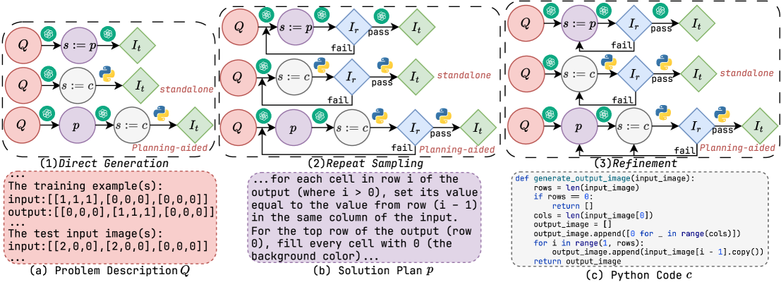**Footer**: Python implementation details ## Missing Elements - No explicit axis titles or numerical data points - No heatmap or categorical data representation - All information conveyed through flowchart logic and code examples </details> Figure 2: An illustration of the three ARC solution generation approaches, (1) direct generation, (2) repeated sampling, and (3) refinement, with the GPT-o3-mini input and response fragments (a–c) for solving task 25ff71a9 (Figure 1). For each approach, when the solution $s$ is code, $s:=c$ , a plan $p$ is either generated from the problem description $Q$ to guide code generation (planning-aided) or omitted (standalone). Otherwise, when $s:=p$ , the plan $p$ serves as the final solution instead. ## 2 Problem Formulation We formulate each ARC task as a tuple $\mathcal{P}=\langle I_{r},I_{t}\rangle$ , where $I_{r}$ and $I_{t}$ are sets of training and test instances. Each instance consists of an input-output image pair $(i^{i},i^{o})$ , represented as 2D matrices. The goal is to leverage the LLM $\mathcal{M}$ to generate a solution $s$ based on training instances $I_{r}$ and test input images $\{i^{i}\ |\ (i^{i},i^{o})\in I_{t}\}$ , where $s$ maps each test input $i^{i}$ to its output $i^{o}$ , i.e., $s(i^{i})=i^{o}$ , for $(i^{i},i^{o})\in I_{t}$ . We note that the test input images are visible during the generation of solution $s$ , whereas test output images become accessible only after $s$ is produced to validate the correctness of $s$ . We encode the solution $s$ in different forms, as a solution plan $p$ , or as Python code $c$ , optionally guided by $p$ . We denote each ARC problem description, comprising $I_{r}$ and $\{i^{i}\ |\ (i^{i},i^{o})\in I_{t}\}$ , as $Q$ . ## 3 ARC Solver Backbone LLMs have shown promise in solving tasks that rely on ARC-relevant priors [30, 31, 32, 33]. We initially assume that reasoning-oriented LLMs implicitly encode sufficient core knowledge priors to solve ARC tasks. We cast each ARC task as a program synthesis problem, which involves generating a solution $s$ from a problem description $Q$ without explicitly prompting for priors. We consider established LLM-based code generation approaches [17, 18, 19, 23] as candidate ARC solution generation strategies, illustrated at the top of Figure 2. These include: (1) direct generation, where the LLM produces the solution $s$ in a single attempt, and then validates it on test instances $I_{t}$ ; (2) repeated sampling, where the LLM samples solutions until one passes training instances $I_{r}$ , and then evaluates it on $I_{t}$ ; and (3) refinement, where the LLM iteratively refines an initial solution $s$ based on failures on $I_{r}$ until it succeeds, followed by evaluation on $I_{t}$ . In addition, we extend the solution representation beyond code to include text-based solution plans. Given the problem description $Q$ as input (Figure 2, block (a)), all strategies prompt the LLM to generate a solution $s$ , represented either as a natural language plan $p$ (block (b)), $s:=p$ , or as a Python code $c$ (block (c)), $s:=c$ . For $s:=p$ , the solution is derived directly from $Q$ . For $s:=c$ , we explore two modalities: the LLM either generates $c$ directly from $Q$ (standalone), or first generates a plan $p$ for $Q$ , which is then concatenated with $Q$ to guide subsequent code development (planning-aided), a strategy widely adopted in recent work [18, 22, 23]. Repeated sampling and refinement iteratively produce new solutions based on the correctness of $s$ on training instances $I_{r}$ , and validate $s$ on test instances $I_{t}$ once it passes $I_{r}$ or the iteration limit is reached. When $s:=p$ , its correctness is evaluated by prompting the LLM to generate each output image $i^{o}$ given its corresponding input $i^{i}$ and the solution plan $p$ , where $(i^{i},i^{o})\in I_{r}$ or $(i^{i},i^{o})\in I_{t}$ . Alternatively, when $s:=c$ , its correctness is assessed by executing $c$ on $I_{r}$ or $I_{t}$ . In repeated sampling, the LLM iteratively generates a new plan $p$ and code $c$ from the problem description $Q$ without additional feedback. In contrast, refinement revises $p$ and $c$ by prompting the LLM with the previously incorrect $p$ and $c$ , concatenated with failed training instances. In total, nine ARC solvers are employed to evaluate the performance of reasoning-oriented LLMs on the ARC benchmark. ## 4 Knowledge Augmentation Xu et al. [34] improved LLM performance on the ARC benchmark by prompting object-based representations for each task derived from graph-based object abstractions. Building on this insight, we propose KAAR, a knowledge augmentation approach for solving ARC tasks using reasoning-oriented LLMs. KAAR leverages Generalized Planning for Abstract Reasoning (GPAR) [10], a state-of-the-art object-centric ARC solver, to generate the core knowledge priors. GPAR encodes priors as abstraction-defined nodes enriched with attributes and inter-node relations, which are extracted using standard image processing algorithms. To align with the four knowledge dimensions in ARC, KAAR maps GPAR-derived priors into their categories. In detail, KAAR adopts fundamental abstraction methods from GPAR to enable objectness. Objects are typically defined as components based on adjacency rules and color consistency (e.g., 4-connected or 8-connected components), while also including the entire image as a component. KAAR further introduces additional abstractions: (1) middle-vertical, which vertically splits the image into two equal parts, and treats each as a distinct component; (2) middle-horizontal, which applies the same principle along the horizontal axis; (3) multi-lines, which segments the image using full-length rows or columns of uniform color, and treats each resulting part as a distinct component; and (4) no abstraction, which considers only raw 2D matrices. Under no abstraction, KAAR degrades to the ARC solver backbone without incorporating any priors. KAAR inherits GPAR’s geometric and topological priors, including component attributes (size, color, shape) and relations (spatial, congruent, inclusive). It further extends the attribute set with symmetry, bounding box, nearest boundary, and hole count, and augments the relation set with touching. For numeric and counting priors, KAAR follows GPAR, incorporating the largest/smallest component sizes, and the most/least frequent component colors, while extending them with statistical analysis of hole counts and symmetry, as well as the most/least frequent sizes and shapes. <details> <summary>x3.png Details</summary>  ### Visual Description # Technical Document Extraction: Flowchart Analysis ## Overview The image is a **flowchart** outlining a decision-making process for categorizing tasks involving **color change**. It is structured into three sequential sections: **Action(s)**, **Component(s)**, and **Color Change Rule**. Each section contains conditional logic, selection criteria, and example data points. --- ## Section 1: Action(s) Selection ### Labels and Text - **Header**: `"Please determine which category or categories this task belongs to. Please select from the following predefined categories..."` - **Question**: `"If this task involves color change:"` - **Selection**: - **Yes/No** (implied via branching logic). - **Example Output**: `"This task involves color change."` ### Spatial Grounding - Positioned at the **top** of the flowchart. - Arrows direct to the next section if "Yes" is selected. --- ## Section 2: Component(s) Selection ### Labels and Text - **Header**: `"If this task involves color change:"` - **Sub-questions**: 1. `"Which components require color change?"` 2. `"Determine the conditions used to select these target components:"` - **Example Output**: `"Components (color 0) with the minimum and maximum sizes."` - **Selection**: - **Component Type**: Color 0. - **Size Constraints**: - Minimum size: 7. - Maximum size: 8. ### Spatial Grounding - Positioned **below** the Action(s) section. - Arrows connect to the Color Change Rule section. --- ## Section 3: Color Change Rule ### Labels and Text - **Header**: `"If this task involves color change, please determine which source color maps to which target color for the target components."` - **Sub-questions**: 1. `"Determine the conditions used to dictate this color change:"` - **Example Output**: - `"minimum-size component (from color 0) to 7."` - `"maximum-size component (from color 0) to 8."` ### Spatial Grounding - Positioned **at the bottom** of the flowchart. - Arrows originate from the Component(s) section. --- ## Key Trends and Data Points 1. **Color Change Logic**: - Tasks involving color change require identifying **target components** (e.g., "color 0") and their **size constraints** (e.g., 7–8). - Source and target color mappings are explicitly defined (e.g., "from color 0 to 7"). 2. **Component Constraints**: - Components are categorized by **color** and **size**, with explicit minimum/maximum values. 3. **Flowchart Structure**: - Sequential decision-making: `Action(s) → Component(s) → Color Change Rule`. --- ## Diagram Components and Flow 1. **Action(s) Node**: - **Icon**: Green circle with a white flower-like symbol. - **Purpose**: Initial task categorization. 2. **Component(s) Node**: - **Icon**: Green circle with a white flower-like symbol. - **Purpose**: Identify components requiring color change and their size constraints. 3. **Color Change Rule Node**: - **Icon**: Green circle with a white flower-like symbol. - **Purpose**: Define source-to-target color mappings and size-based conditions. --- ## Notes - **No numerical data table** is present; the flowchart relies on textual conditions and examples. - **No heatmap or chart** is included; the focus is on decision logic. - **All text is in English**; no other languages are present. --- ## Final Output The flowchart provides a structured framework for categorizing tasks involving color change, emphasizing component selection and color mapping rules. It uses conditional logic and explicit examples to guide users through the process. </details> Figure 3: The example of goal-directedness priors augmentation in KAAR with input and response fragments from GPT-o3-mini. GPAR approaches goal-directedness priors by searching for a sequence of program instructions [35] defined in a DSL. Each instruction supports conditionals, branching, looping, and action statements. KAAR incorporates the condition and action concepts from GPAR, and enables goal-directedness priors by augmenting LLM knowledge in two steps: 1) It prompts the LLM to identify the most relevant actions for solving the given ARC problem from ten predefined action categories (Figure 3 block (a)), partially derived from GPAR and extended based on the training set, such as color change, movement, and extension; 2) For each selected action, KAAR prompts the LLM with the associated schema to resolve implementation details. For example, for a color change action, KAAR first prompts the LLM to identify the target components (Figure 3 blocks (b)), and then specify the source and target colors for modification based on the target components (Figure 3 blocks (c)). We note that KAAR also prompts the LLM to incorporate condition-aware reasoning when determining action implementation details, using knowledge derived from geometry, topology, numbers, and counting priors. This enables fine-grained control, for example, applying color changes only to black components conditioned on the maximum or minimum size: from black (value 0) to blue (value 8) if largest, or to orange (value 7) if smallest. Figure 3 shows fragments of the goal-directedness priors augmentation. See Appendix A.2 for the full set of priors in KAAR. <details> <summary>x4.png Details</summary>  ### Visual Description # Technical Document Extraction: Image Analysis ## Section (a): ARC Example - **Visual Elements**: - Grid-based input/output examples with 4-connected black pixels (value 0) as components. - Output grid with a question mark indicating uncertainty. - **Textual Description**: > "When we consider 4-connected black pixels (value 0) as components, the components in each input and output image are as follows: > - For Training Pair 1 input image: Component 1: Locations=[(0,0), (0,1)] > - Component 8: Locations=[(4,14)]" ## Section (b): Augmentation Process in KAAR - **Flowchart Components**: 1. **Objectness** → ARC Solver Backbone (fail on _I_r_) → **Geometry and Topology** → ARC Solver Backbone (fail on _I_r_) → **Numbers and Counting** → ARC Solver Backbone (fail on _I_r_) → **Goal-directedness** 2. Input/Output Flow: - Input: _I_r_ (right) → Processed → Output: _I_t_ (top-left) - Backbone Failures: Indicated at each ARC Solver stage. - **Key Labels**: - Objectness, Geometry and Topology, Numbers and Counting, Goal-directedness - ARC Solver Backbone (repeated thrice) ## Section (c): Objectness - **Training Pair 1 Input Image**: - Component 1: Horizontal line (Shape: horizontal line) - Component 2: Not touching Component 1 - Component 1 Location: Top-left of Component 2 - Component 2 Location: Bottom-right of Component 1 ## Section (d): Geometry and Topology - **Training Pair 1 Input Image**: - Component 1: Horizontal line (Shape: horizontal line) - Component 2: Not touching Component 1 - Component 1 Location: Top-left of Component 2 - Component 2 Location: Bottom-right of Component 1 ## Section (e): Numbers and Counting - **Training Pair 1 Input Image**: - Component 5: Maximum size (Size: 10) - Component 8: Minimum size (Size: 1) - Components 4 and 6: Size 7 (appear twice) ## Critical Observations 1. **Component Differentiation**: - Components are distinguished by spatial relationships (e.g., "not touching," "top-left/bottom-right"). - Size attributes vary significantly (e.g., Size 1 vs. Size 10). 2. **Process Flow**: - The ARC Solver Backbone iteratively processes inputs through Objectness, Geometry/Topology, and Numbers/Counting stages. - Failures on _I_r_ suggest iterative refinement or error correction. ## Notes - No numerical data tables or heatmaps present. - All textual information is in English. - Spatial grounding of components (e.g., "top-left," "bottom-right") is critical for understanding relational constraints. 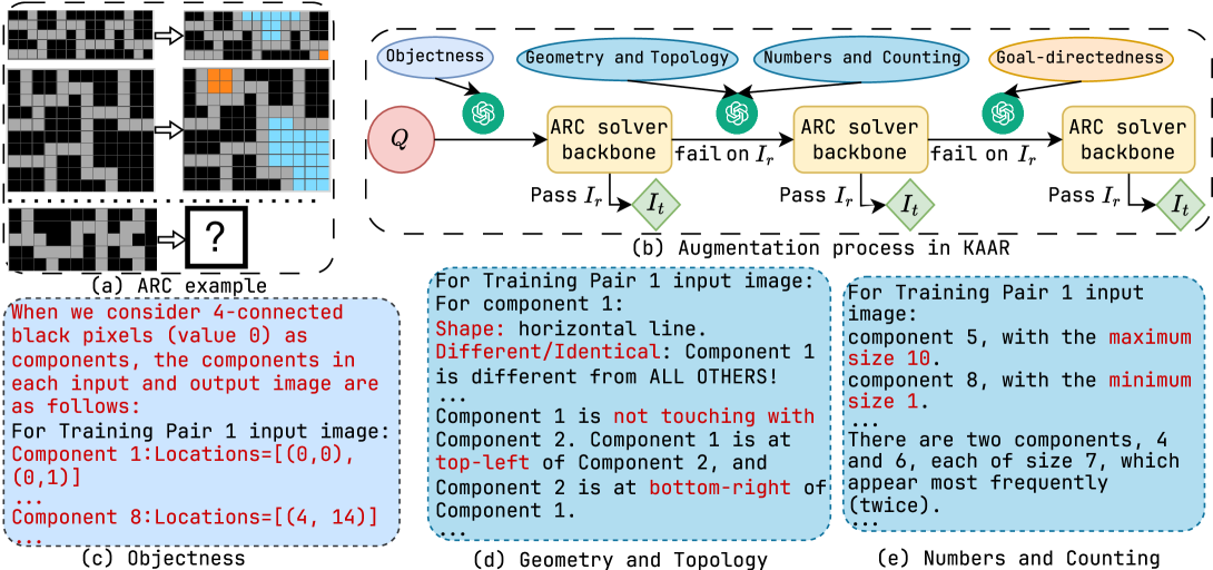</details> Figure 4: Augmentation process in KAAR (block (b)) and the corresponding knowledge augmentation fragments (blocks (c-e)) for ARC problem 62ab2642 (block (a)). KAAR encodes the full set of core knowledge priors assumed in ARC into an ontology, where priors are organized into three hierarchical levels based on their dependencies. KAAR prompts LLMs with priors at each level to enable incremental augmentation. This reduces context interference and supports stage-wise reasoning aligned with human cognitive development [29]. Figure 4, block (b), illustrates the augmentation process in KAAR alongside the augmented prior fragments used to solve the problem shown in block (a). KAAR begins augmentation with objectness priors, encoding images into components with detailed coordinates based on a specific abstraction method (block (c)). KAAR then prompts geometry and topology priors (block (d)), followed by numbers and counting priors (block (e)). These priors are ordered by dependency while residing at the same ontological level, as they all build upon objectness. Finally, KAAR augments goal-directedness priors, as shown in Figure 3, where target components are derived from objectness analysis and conditions are inferred from geometric, topological, and numerical analyses. After augmenting each level of priors, KAAR invokes the ARC solver backbone to generate solutions. If any solution passes training instances $I_{r}$ , it is validated on the test instances $I_{t}$ ; otherwise, augmentation proceeds to the next level of priors. While the ontology provides a hierarchical representation of priors, it may also introduce hallucinations, such as duplicate abstractions, irrelevant component attributes or relations, and inapplicable actions. To address this, KAAR integrates restrictions from GPAR to filter out inapplicable priors. KAAR adopts GPAR’s duplicate-checking strategy, retaining only abstractions that yield distinct components by size, color, or shape, in at least one training instance. In KAAR, each abstraction is associated with a set of applicable priors. For instance, when the entire image is treated as a component, relation priors are excluded, and actions such as movement and color change are omitted, whereas symmetry and size attributes are retained and actions such as flipping and rotation are considered. In contrast, 4-connected and 8-connected abstractions include all component attributes and relations, and the full set of ten action priors. See Appendix A.3 for detailed restrictions. | 2 GPT-o3-mini | $I_{r}$ | Direct Generation P - | Repeated Sampling C - | Refinement PC - | P 35.50 | C 52.50 | PC 35.50 | P 31.00 | C 47.25 | PC 32.00 | | --- | --- | --- | --- | --- | --- | --- | --- | --- | --- | --- | | $I_{t}$ | 20.50 | 24.50 | 22.25 | 23.75 | 32.50 | 30.75 | 24.75 | 29.25 | 25.75 | | | $I_{r}\&I_{t}$ | - | - | - | 22.00 | 31.75 | 29.25 | 21.75 | 28.50 | 25.00 | | | Gemini-2.0 | $I_{r}$ | - | - | - | 36.50 | 39.50 | 21.50 | 15.50 | 25.50 | 15.50 | | $I_{t}$ | 7.00 | 6.75 | 6.25 | 10.00 | 14.75 | 16.75 | 8.75 | 12.00 | 11.75 | | | $I_{r}\&I_{t}$ | - | - | - | 9.50 | 14.25 | 16.50 | 8.00 | 10.50 | 10.75 | | | QwQ-32B | $I_{r}$ | - | - | - | 19.25 | 13.50 | 15.25 | 16.75 | 15.00 | 14.25 | | $I_{t}$ | 9.50 | 7.25 | 5.75 | 11.25 | 13.50 | 14.25 | 11.00 | 14.25 | 14.00 | | | $I_{r}\&I_{t}$ | - | - | - | 9.25 | 12.75 | 13.00 | 8.75 | 13.00 | 11.75 | | | DeepSeek-R1-70B | $I_{r}$ | - | - | - | 8.75 | 6.75 | 7.75 | 6.25 | 5.75 | 7.75 | | $I_{t}$ | 4.25 | 4.75 | 4.50 | 4.25 | 7.25 | 7.75 | 4.75 | 5.75 | 7.75 | | | $I_{r}\&I_{t}$ | - | - | - | 3.50 | 6.50 | 7.25 | 4.25 | 5.25 | 7.00 | | | 2 | | | | | | | | | | | Table 1: Performance of nine ARC solvers measured by accuracy on $I_{r}$ , $I_{t}$ , and $I_{r}\&I_{t}$ using four reasoning-oriented LLMs. For each LLM, the highest accuracy on $I_{r}$ and $I_{r}\&I_{t}$ is in bold; the highest accuracy on $I_{t}$ is in red. Accuracy is reported as a percentage. P denotes the solution plan; C and PC refer to standalone and planning-aided code generation, respectively. ## 5 Experiments In ARC, each task is unique and solvable using only core knowledge priors [5]. We begin by comparing nine candidate solvers on the full ARC public evaluation set of 400 tasks. This offers broader insights than previous studies limited to subsets of 400 training tasks [10, 9, 36], given the greater difficulty of the evaluation set [37]. We experiment with recent reasoning-oriented LLMs, including proprietary models, GPT-o3-mini and Gemini 2.0 Flash-Thinking (Gemini-2.0), and open-source models, DeepSeek-R1-Distill-Llama-70B (DeepSeek-R1-70B) and QwQ-32B. We compute accuracy on test instances $I_{t}$ as the primary evaluation metric. It measures the proportion of problems where the first solution successfully solves $I_{t}$ after passing the training instances $I_{r}$ ; otherwise, if none pass $I_{r}$ within 12 iterations, the last solution is evaluated on $I_{t}$ , applied to both repeated sampling and refinement. We also report accuracy on $I_{r}$ and $I_{r}\&I_{t}$ , measuring the percentage of problems whose solutions solve $I_{r}$ and both $I_{r}$ and $I_{t}$ . See Appendix A.4 for parameter settings. Table 1 reports the performance of nine ARC solvers across four reasoning-oriented LLMs. For direct generation methods, accuracy on $I_{r}$ and $I_{r}\&I_{t}$ is omitted, as solutions are evaluated directly on $I_{t}$ . GPT-o3-mini consistently outperforms all other LLMs, achieving the highest accuracy on $I_{r}$ (52.50%), $I_{t}$ (32.50%), and $I_{r}\&I_{t}$ (31.75%) under repeated sampling with standalone code generation (C), highlighting its strong abstract reasoning and generalization capabilities. Notably, QwQ-32B, the smallest model, outperforms DeepSeek-R1-70B across all solvers and surpasses Gemini-2.0 under refinement. Among the nine ARC solvers, repeated sampling-based methods generally outperform those based on direct generation or refinement. This diverges from previous findings where refinement dominated conventional code generation tasks that lack abstract reasoning and generalization demands [10, 17, 19]. Within repeated sampling, planning-aided code generation (PC) yields the highest accuracy on $I_{t}$ across most LLMs. It also demonstrates the strongest generalization with GPT-o3-mini and Gemini-2.0, as evidenced by the smallest accuracy gap between $I_{r}$ and $I_{r}\&I_{t}$ , compared to solution plan (P) and standalone code generation (C). A similar trend is observed for QwQ-32B and DeepSeek-R1-70B, where both C and PC generalize effectively across repeated sampling and refinement. Overall, repeated sampling with planning-aided code generation, denoted as RSPC, shows the best performance and thus serves as the ARC solver backbone. | 2 GPT-o3-mini | RSPC | $I_{r}$ Acc 35.50 | $I_{t}$ $\Delta$ - | $I_{r}\&I_{t}$ $\gamma$ - | Acc 30.75 | $\Delta$ - | $\gamma$ - | Acc 29.25 | $\Delta$ - | $\gamma$ - | | --- | --- | --- | --- | --- | --- | --- | --- | --- | --- | --- | | KAAR | 40.00 | 4.50 | 12.68 | 35.00 | 4.25 | 13.82 | 33.00 | 3.75 | 12.82 | | | Gemini-2.0 | RSPC | 21.50 | - | - | 16.75 | - | - | 16.50 | - | - | | KAAR | 25.75 | 4.25 | 19.77 | 21.75 | 5.00 | 29.85 | 20.50 | 4.00 | 24.24 | | | QwQ-32B | RSPC | 15.25 | - | - | 14.25 | - | - | 13.00 | - | - | | KAAR | 22.25 | 7.00 | 45.90 | 21.00 | 6.75 | 47.37 | 19.25 | 6.25 | 48.08 | | | DeepSeek-R1-70B | RSPC | 7.75 | - | - | 7.75 | - | - | 7.25 | - | - | | KAAR | 12.25 | 4.50 | 58.06 | 12.75 | 5.00 | 64.52 | 11.50 | 4.25 | 58.62 | | | 2 | | | | | | | | | | | Table 2: Comparison of RSPC (repeated-sampling planning-aided code generation) and its knowledge-augmented variant, KAAR, in terms of accuracy (Acc) on $I_{r}$ , $I_{t}$ , and $I_{r}\&I_{t}$ . $\Delta$ and $\gamma$ denote the absolute and relative improvements over RSPC, respectively. All values are reported as percentages. The best results for $I_{r}$ and $I_{r}\&I_{t}$ are in bold; the highest for $I_{t}$ is in red. We further compare the performance of RSPC with its knowledge-augmented variant, KAAR. For each task, KAAR begins with simpler abstractions, i.e., no abstraction and whole image, and progresses to complicated 4-connected and 8-connected abstractions, consistent with GPAR. KAAR reports the accuracy on test instances $I_{t}$ based on the first abstraction whose solution solves all training instances $I_{r}$ ; otherwise, it records the final solution from each abstraction and selects the one that passes the most $I_{r}$ to evaluate on $I_{t}$ . KAAR allows the solver backbone (RSPC) up to 4 iterations per invocation, totaling 12 iterations, consistent with the non-augmented setting. See Appendix A.5 for KAAR execution details. As shown in Table 2, KAAR consistently outperforms non-augmented RSPC across all LLMs, yielding around 5% absolute gains on $I_{r}$ , $I_{t}$ , and $I_{r}\&I_{t}$ . This highlights the effectiveness and model-agnostic nature of the augmented priors. KAAR achieves the highest accuracy using GPT-o3-mini, with 40% on $I_{r}$ , 35% on $I_{t}$ , and 33% on $I_{r}\&I_{t}$ . KAAR shows the greatest absolute improvements ( $\Delta$ ) using QwQ-32B and the largest relative gains ( $\gamma$ ) using DeepSeek-R1-70B across all evaluated metrics. Moreover, KAAR maintains generalization comparable to RSPC across all LLMs, indicating that the augmented priors are sufficiently abstract and expressive to serve as basis functions for reasoning, in line with ARC assumptions. <details> <summary>x5.png Details</summary>  ### Visual Description # Technical Document Extraction: Heatmap Analysis ## Image Description The image contains two comparative heatmaps labeled **(a) RSPC** and **(b) KAAR**, evaluating model performance across four AI systems: - **GPT-3-mini** - **Gemini 2.0** - **QwQ-32B** - **DeepSeek-R1-70B** Each heatmap uses a **coverage scale** (0.0–1.0) represented by a color gradient from light orange (low) to dark red (high). The legend is positioned on the right side of both heatmaps. --- ## Key Components ### Legend - **Color Scale**: - **Light Orange**: ~0.0–0.3 - **Medium Red**: ~0.4–0.7 - **Dark Red**: ~0.8–1.0 - **Placement**: Top-right corner of both heatmaps. --- ## Heatmap (a): RSPC ### Axis Labels - **X-axis**: Model names (GPT-3-mini, Gemini 2.0, QwQ-32B, DeepSeek-R1-70B) - **Y-axis**: Model names (same as X-axis) ### Data Table | | GPT-3-mini | Gemini 2.0 | QwQ-32B | DeepSeek-R1-70B | |---------------|------------|------------|---------|-----------------| | **GPT-3-mini** | 1.00 | 0.50 | 0.40 | 0.22 | | **Gemini 2.0** | 0.91 | 1.00 | 0.60 | 0.40 | | **QwQ-32B** | 0.86 | 0.70 | 1.00 | 0.44 | | **DeepSeek-R1-70B** | 0.87 | 0.87 | 0.81 | 1.00 | ### Trends - **Diagonal Dominance**: All diagonal values are **1.00**, indicating perfect self-coverage. - **Decreasing Coverage**: Coverage decreases as models diverge from the diagonal (e.g., GPT-3-mini vs DeepSeek-R1-70B: 0.22). - **Symmetry**: The matrix is symmetric (e.g., GPT-3-mini vs Gemini 2.0 = 0.50, Gemini 2.0 vs GPT-3-mini = 0.91). --- ## Heatmap (b): KAAR ### Axis Labels - **X-axis**: Model names (same as RSPC) - **Y-axis**: Model names (same as RSPC) ### Data Table | | GPT-3-mini | Gemini 2.0 | QwQ-32B | DeepSeek-R1-70B | |---------------|------------|------------|---------|-----------------| | **GPT-3-mini** | 1.00 | 0.55 | 0.54 | 0.34 | | **Gemini 2.0** | 0.89 | 1.00 | 0.72 | 0.48 | | **QwQ-32B** | 0.88 | 0.74 | 1.00 | 0.53 | | **DeepSeek-R1-70B** | 0.92 | 0.82 | 0.88 | 1.00 | ### Trends - **Higher Coverage**: KAAR shows generally higher off-diagonal values compared to RSPC (e.g., GPT-3-mini vs Gemini 2.0: 0.89 vs 0.50 in RSPC). - **Consistent Diagonal**: All diagonal values remain **1.00**. - **Improved Symmetry**: Coverage is more balanced across models (e.g., DeepSeek-R1-70B vs QwQ-32B: 0.88 vs 0.44 in RSPC). --- ## Spatial Grounding - **Legend Position**: Top-right corner of both heatmaps. - **Color Matching**: - **Dark Red** (1.00) matches diagonal cells. - **Light Orange** (0.22–0.34) matches the lowest coverage cells. --- ## Summary - **RSPC** emphasizes **model-specific performance**, with significant drops in coverage for dissimilar models. - **KAAR** demonstrates **broader compatibility**, with higher coverage across diverse models. - Both heatmaps use identical axes and color scales, enabling direct comparison. All textual and numerical data extracted directly from the image. No additional languages or non-factual content present. 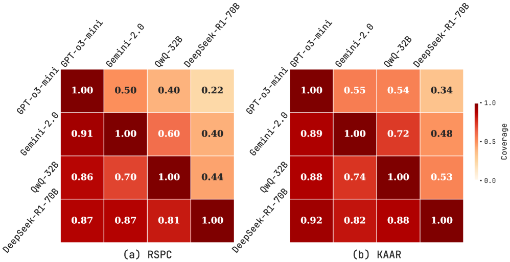</details> Figure 5: Asymmetric relative coverage matrices for RSPC (a) and KAAR (b), showing the proportion of problems whose test instances are solved by the row model that are also solved by the column model, across four LLMs. We compare relative problem coverage across evaluated LLMs under RSPC and KAAR based on successful solutions on test instances. As shown in Figure 5, each cell $(i,j)$ represents the proportion of problems solved by the row LLM that are also solved by the column LLM. This is computed as $\frac{|A_{i}\cap A_{j}|}{|A_{i}|}$ , where $A_{i}$ and $A_{j}$ are the sets of problems solved by the row and column LLMs, respectively. Values near 1 indicate that the column LLM covers most problems solved by the row LLM. Under RSPC (Figure 5 (a)), GPT-o3-mini exhibits broad coverage, with column values consistently above 0.85. Gemini-2.0 and QwQ-32B also show substantial alignment, with mutual coverage exceeding 0.6. In contrast, DeepSeek-R1-70B shows lower alignment, with column values below 0.45 due to fewer solved problems. Figure 5 (b) illustrates that KAAR generally improves or maintains inter-model overlap compared to RSPC. Notably, KAAR raises the minimum coverage between GPT-o3-mini and DeepSeek-R1-70B from 0.22 under RSPC to 0.34 under KAAR. These results highlight the effectiveness of KAAR in improving cross-model generalization, with all evaluated LLMs solving additional shared problems. In particular, it enables smaller models such as QwQ-32B and DeepSeek-R1-70B to better align with stronger LLMs on the ARC benchmark. <details> <summary>x6.png Details</summary>  ### Visual Description # Technical Document Analysis of Accuracy Chart ## Chart Type Bar chart comparing accuracy percentages across four categories and multiple models/methods. ## Axes - **X-axis**: Categories (Movement, Extension, Recolor, Others) - **Y-axis**: Accuracy on _t_ (%) ranging from 0 to 40% ## Legend Located on the right side of the chart. Color-coded models/methods: - **Blue**: GPT-o3-mini RSPC - **Light Blue**: GPT-o3-mini KAAR - **Green**: Gemini-2.0 RSPC - **Light Green**: Gemini-2.0 KAAR - **Purple**: QwQ-32B RSPC - **Light Purple**: QwQ-32B KAAR - **Orange**: DeepSeek-R1-70B RSPC - **Light Orange**: DeepSeek-R1-70B KAAR ## Categories & Data Points ### Movement (Total: 55) - **GPT-o3-mini RSPC**: 41.8% (Blue) - **GPT-o3-mini KAAR**: 20.0% (Light Blue) - **Gemini-2.0 RSPC**: 18.2% (Green) - **Gemini-2.0 KAAR**: 10.9% (Light Green) - **QwQ-32B RSPC**: 12.7% (Purple) - **QwQ-32B KAAR**: 14.5% (Light Purple) - **DeepSeek-R1-70B RSPC**: 9.1% (Orange) ### Extension (Total: 129) - **GPT-o3-mini RSPC**: 38.8% (Blue) - **GPT-o3-mini KAAR**: 0.8% (Light Blue) - **Gemini-2.0 RSPC**: 19.4% (Green) - **Gemini-2.0 KAAR**: 1.6% (Light Green) - **QwQ-32B RSPC**: 17.8% (Purple) - **QwQ-32B KAAR**: 2.3% (Light Purple) - **DeepSeek-R1-70B RSPC**: 7.8% (Orange) ### Recolor (Total: 115) - **GPT-o3-mini RSPC**: 24.3% (Blue) - **GPT-o3-mini KAAR**: 6.1% (Light Blue) - **Gemini-2.0 RSPC**: 13.9% (Green) - **Gemini-2.0 KAAR**: 10.4% (Light Green) - **QwQ-32B RSPC**: 7.8% (Purple) - **QwQ-32B KAAR**: 7.0% (Light Purple) - **DeepSeek-R1-70B RSPC**: 4.3% (Orange) ### Others (Total: 101) - **GPT-o3-mini RSPC**: 21.8% (Blue) - **GPT-o3-mini KAAR**: 5.0% (Light Blue) - **Gemini-2.0 RSPC**: 14.9% (Green) - **Gemini-2.0 KAAR**: 11.9% (Light Green) - **QwQ-32B RSPC**: 7.9% (Purple) - **QwQ-32B KAAR**: 5.0% (Light Purple) - **DeepSeek-R1-70B RSPC**: 9.9% (Orange) ## Key Trends 1. **Dominance of GPT-o3-mini RSPC**: - Highest accuracy in all categories (Movement: 41.8%, Extension: 38.8%, Recolor: 24.3%, Others: 21.8%). - Consistently outperforms other models/methods by margins of 10-30% in most cases. 2. **KAAR Method Performance**: - Generally lower accuracy than RSPC across all models. - Notable exceptions: QwQ-32B KAAR (14.5% in Movement) and DeepSeek-R1-70B KAAR (9.9% in Others). 3. **Model-Specific Patterns**: - **Gemini-2.0**: Strongest in Movement (18.2% RSPC) and Recolor (13.9% RSPC). - **QwQ-32B**: Highest KAAR performance in Movement (14.5%) and Recolor (7.0%). - **DeepSeek-R1-70B**: Best KAAR result in Others (9.9%). 4. **Segmentation Observations**: - RSPC methods dominate the top segments of each bar. - KAAR methods occupy lower segments, with minimal overlap in top-tier performance. ## Spatial Grounding - Legend positioned on the **right** of the chart. - Color consistency verified: All segments match legend labels (e.g., GPT-o3-mini RSPC = Blue). ## Data Table Reconstruction | Category | Model/Method | Accuracy (%) | |--------------|----------------------------|--------------| | Movement | GPT-o3-mini RSPC | 41.8 | | Movement | GPT-o3-mini KAAR | 20.0 | | Movement | Gemini-2.0 RSPC | 18.2 | | Movement | Gemini-2.0 KAAR | 10.9 | | Movement | QwQ-32B RSPC | 12.7 | | Movement | QwQ-32B KAAR | 14.5 | | Movement | DeepSeek-R1-70B RSPC | 9.1 | | Extension | GPT-o3-mini RSPC | 38.8 | | Extension | GPT-o3-mini KAAR | 0.8 | | Extension | Gemini-2.0 RSPC | 19.4 | | Extension | Gemini-2.0 KAAR | 1.6 | | Extension | QwQ-32B RSPC | 17.8 | | Extension | QwQ-32B KAAR | 2.3 | | Extension | DeepSeek-R1-70B RSPC | 7.8 | | Recolor | GPT-o3-mini RSPC | 24.3 | | Recolor | GPT-o3-mini KAAR | 6.1 | | Recolor | Gemini-2.0 RSPC | 13.9 | | Recolor | Gemini-2.0 KAAR | 10.4 | | Recolor | QwQ-32B RSPC | 7.8 | | Recolor | QwQ-32B KAAR | 7.0 | | Recolor | DeepSeek-R1-70B RSPC | 4.3 | | Others | GPT-o3-mini RSPC | 21.8 | | Others | GPT-o3-mini KAAR | 5.0 | | Others | Gemini-2.0 RSPC | 14.9 | | Others | Gemini-2.0 KAAR | 11.9 | | Others | QwQ-32B RSPC | 7.9 | | Others | QwQ-32B KAAR | 5.0 | | Others | DeepSeek-R1-70B RSPC | 9.9 | ## Notes - All percentages are visually labeled on top of respective bar segments. - Totals under each category (e.g., Movement: 55) likely represent the number of data points evaluated, not summed percentages. - No textual information in non-English languages detected. 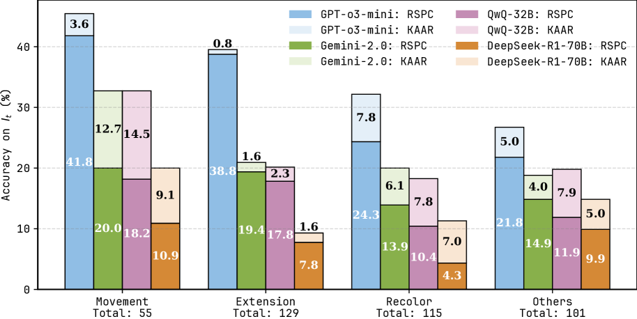</details> Figure 6: Accuracy on test instances $I_{t}$ for RSPC and KAAR across the movement, extension, recolor, and others categories using four LLMs. Each stacked bar shows RSPC accuracy (darker segment) and the additional improvement from KAAR (lighter segment). Following prior work [9, 10], we categorize 400 problems in the ARC public evaluation set into four classes based on their primary transformations: (1) movement (55 problems), (2) extension (129 problems), (3) recolor (115 problems), and (4) others (101 problems). The others category comprises infrequent tasks such as noise removal, selection, counting, resizing, and problems with implicit patterns that hinder systematic classification into the aforementioned categories. See Appendix A.7 for examples of each category. Figure 6 illustrates the accuracy on test instances $I_{t}$ for RSPC and KAAR across four categories with evaluated LLMs. Each stacked bar represents RSPC accuracy and the additional improvement achieved by KAAR. KAAR consistently outperforms RSPC with the largest accuracy gain in movement (14.5% with QwQ-32B). In contrast, KAAR shows limited improvements in extension, since several problems involve pixel-level extension, which reduces the reliance on component-level recognition. Moreover, extension requires accurate spatial inference across multiple components and poses greater difficulty than movement, which requires mainly direction identification. Although KAAR augments spatial priors, LLMs still struggle to accurately infer positional relations among multiple components, consistent with prior findings [38, 39, 40]. Overlaps from component extensions further complicate reasoning, as LLMs often fail to recognize truncated components as unified wholes, contrary to human perceptual intuition. <details> <summary>x7.png Details</summary>  ### Visual Description # Technical Document Extraction: Accuracy Analysis by Image Size Interval ## Chart Type Bar chart with grouped segments, comparing accuracy metrics across image size intervals. ## Axes - **X-axis**: "Average Image Size Interval (width x height)" Categories: - (0,25] (Total: 19) - (25,100] (Total: 139) - (100,225] (Total: 129) - (225,400] (Total: 51) - (400,625] (Total: 39) - (625,900] (Total: 23) - **Y-axis**: "Accuracy on I_t (%)" Scale: 0–80% in 10% increments. ## Legend - **Position**: Top-right corner. - **Entries**: 1. `GPT-o3-mini RSPC` (Blue) 2. `GPT-o3-mini KAAR` (Light Blue) 3. `QwQ-32B RSPC` (Purple) 4. `QwQ-32B KAAR` (Pink) ## Data Points & Trends ### (0,25] Interval (Total: 19) - **GPT-o3-mini RSPC**: 73.7% (Blue) - **QwQ-32B RSPC**: 42.1% (Purple) - **GPT-o3-mini KAAR**: 15.8% (Light Blue) - **QwQ-32B KAAR**: 5.3% (Pink) **Trend**: GPT-o3-mini RSPC dominates; KAAR methods underperform. ### (25,100] Interval (Total: 139) - **GPT-o3-mini RSPC**: 48.9% (Blue) - **QwQ-32B RSPC**: 23.7% (Purple) - **GPT-o3-mini KAAR**: 11.5% (Light Blue) - **QwQ-32B KAAR**: 5.0% (Pink) **Trend**: GPT-o3-mini RSPC maintains lead; KAAR accuracy declines. ### (100,225] Interval (Total: 129) - **GPT-o3-mini RSPC**: 24.8% (Blue) - **QwQ-32B RSPC**: 8.5% (Purple) - **GPT-o3-mini KAAR**: 6.2% (Light Blue) - **QwQ-32B KAAR**: 4.7% (Pink) **Trend**: Both models show significant drops; KAAR methods remain low. ### (225,400] Interval (Total: 51) - **GPT-o3-mini RSPC**: 11.8% (Blue) - **QwQ-32B RSPC**: 9.8% (Purple) - **GPT-o3-mini KAAR**: 5.9% (Light Blue) - **QwQ-32B KAAR**: 2.0% (Pink) **Trend**: GPT-o3-mini RSPC still outperforms; KAAR accuracy near baseline. ### (400,625] Interval (Total: 39) - **GPT-o3-mini RSPC**: 5.1% (Blue) - **QwQ-32B RSPC**: 0% (Purple) - **GPT-o3-mini KAAR**: 0% (Light Blue) - **QwQ-32B KAAR**: 0% (Pink) **Trend**: All methods fail; no accuracy recorded. ### (625,900] Interval (Total: 23) - **GPT-o3-mini RSPC**: 4.3% (Blue) - **QwQ-32B RSPC**: 0% (Purple) - **GPT-o3-mini KAAR**: 0% (Light Blue) - **QwQ-32B KAAR**: 0% (Pink) **Trend**: GPT-o3-mini RSPC marginally functional; others fail. ## Key Observations 1. **Model Performance**: - GPT-o3-mini RSPC consistently outperforms QwQ-32B RSPC across all intervals. - KAAR methods (both models) show negligible accuracy, especially in larger intervals. 2. **Image Size Impact**: - Accuracy declines sharply as image size increases. - GPT-o3-mini RSPC retains ~70% accuracy in the smallest interval but drops to 4.3% in the largest. 3. **KAAR Limitations**: - KAAR methods fail to achieve meaningful accuracy in intervals larger than (25,100]. ## Spatial Grounding - Legend colors match bar segments exactly (e.g., blue = GPT-o3-mini RSPC). - No textual data outside the chart; all information embedded in bars and legend. ## Language - All text in English. No non-English content detected. 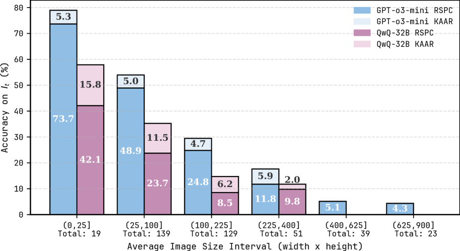</details> Figure 7: Accuracy on test instances $I_{t}$ for RSPC and KAAR across average image size intervals, evaluated using GPT-o3-mini and QwQ-32B. See Figure 12 in Appendix for the results with the other LLMs. A notable feature of ARC is the variation in image size both within and across problems. We categorize tasks by averaging the image size per problem, computed over both training and test image pairs. We report the accuracy on $I_{t}$ for RSPC and KAAR across average image size intervals using GPT-o3-mini and QwQ-32B, the strongest proprietary and open-source models in Tables 1 and 2. As shown in Figure 7, both LLMs experience performance degradation as image size increases. When the average image size exceeds 400 (20×20), GPT-o3-mini solves only three problems, while QwQ-32B solves none. In ARC, isolating relevant pixels in larger images, represented as 2D matrices, requires effective attention mechanisms in LLMs, which remains an open challenge noted in recent work [41, 34]. KAAR consistently outperforms RSPC on problems with average image sizes below 400, benefiting from object-centric representations. By abstracting each image into components, KAAR reduces interference from irrelevant pixels, directs attention to salient components, and facilitates component-level transformation analysis. However, larger images often produce both oversized and numerous components after abstraction, which continue to challenge LLMs during reasoning. Oversized components hinder transformation execution, and numerous components complicate the identification of target components. <details> <summary>x8.png Details</summary>  ### Visual Description # Technical Document Extraction: Accuracy vs. Iterations Chart ## Chart Overview The image is a **line chart** visualizing the relationship between **iterations** and **accuracy** for four distinct model-task combinations. The chart is divided into three horizontal sections (color-coded) representing different task categories. --- ### **Axis Labels and Markers** - **X-axis**: - Title: `# Iterations` - Subsections (color-coded): 1. **Objectness** (light blue) 2. **Geometry, Topology, Numbers and Counting** (beige) 3. **Goal-directedness** (light blue) - Axis range: 1 to 12 iterations - **Y-axis**: - Title: `Accuracy on I_r&I_t (%)` - Range: 0% to 35% --- ### **Legend** - Located on the **right side** of the chart. - **Color-coded entries**: 1. **Blue circles**: `GPT-o3-mini: RSPC` 2. **Blue triangles**: `GPT-o3-mini: KAAR` 3. **Purple squares**: `QwQ-32B: RSPC` 4. **Purple triangles**: `QwQ-32B: KAAR` --- ### **Data Series and Trends** #### 1. **GPT-o3-mini: RSPC** (Blue circles) - **Trend**: Steady upward slope. - **Key data points**: - Iteration 1: 18% - Iteration 4: 26.75% - Iteration 8: 30% - Iteration 12: 33% #### 2. **GPT-o3-mini: KAAR** (Blue triangles) - **Trend**: Gradual upward slope with plateau. - **Key data points**: - Iteration 1: 6.25% - Iteration 4: 26.25% - Iteration 8: 28.25% - Iteration 12: 29.25% #### 3. **QwQ-32B: RSPC** (Purple squares) - **Trend**: Sharp initial rise, then slower growth. - **Key data points**: - Iteration 1: 4.5% - Iteration 4: 13.75% - Iteration 8: 15.5% - Iteration 12: 19.25% #### 4. **QwQ-32B: KAAR** (Purple triangles) - **Trend**: Consistent upward slope. - **Key data points**: - Iteration 1: 3.5% - Iteration 4: 11.5% - Iteration 8: 12.75% - Iteration 12: 13% --- ### **Key Observations** 1. **Model Performance**: - `GPT-o3-mini` outperforms `QwQ-32B` across all tasks, especially in **Goal-directedness** (33% vs. 19.25%). - `RSPC` tasks consistently achieve higher accuracy than `KAAR` tasks for both models. 2. **Task Difficulty**: - **Goal-directedness** (light blue section) shows the highest accuracy for all models. - **Objectness** (light blue section) has the lowest starting accuracy (3.5–18%). 3. **Iteration Impact**: - All models improve accuracy with more iterations, but `GPT-o3-mini` demonstrates faster convergence. --- ### **Spatial Grounding** - **Legend position**: Right side of the chart. - **Color consistency**: - Blue markers (`GPT-o3-mini`) match blue lines. - Purple markers (`QwQ-32B`) match purple lines. --- ### **Conclusion** The chart demonstrates that `GPT-o3-mini` achieves higher accuracy than `QwQ-32B` across all tasks, with `RSPC` tasks outperforming `KAAR` tasks. Accuracy improves monotonically with iterations, though the rate of improvement varies by model and task. 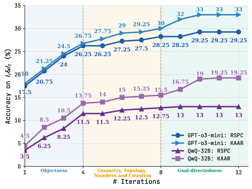</details> Figure 8: Variance in accuracy on $I_{r}\&I_{t}$ with increasing iterations for RSPC and KAAR using GPT-o3-mini and QwQ-32B. See Figure 13 in Appendix for the results with the other LLMs. Figure 8 presents the variance in accuracy on $I_{r}\&I_{t}$ for RSPC and KAAR as iteration count increases using GPT-o3-mini and QwQ-32B. For each task under KAAR, we include only iterations from the abstraction that solves both $I_{r}$ and $I_{t}$ . For KAAR, performance improvements across each 4-iteration block are driven by the solver backbone invocation after augmenting an additional level of priors: iterations 1–4 introduce objectness; 5–8 incorporate geometry, topology, numbers, and counting; 9–12 further involve goal-directedness. RSPC shows rapid improvement in the first 4 iterations and plateaus around iteration 8. At each iteration, the accuracy gap between KAAR and RSPC reflects the contribution of accumulated priors via augmentation. KAAR consistently outperforms RSPC, with the performance gap progressively increasing after new priors are augmented and peaking after the integration of goal-directedness. We note that objectness priors alone yield marginal gains with GPT-o3-mini. However, the inclusion of object attributes and relational priors (iterations 4–8) leads to improvements in KAAR over RSPC. This advantage is further amplified after the augmentation of goal-directedness priors (iterations 9–12). These results highlight the benefits of KAAR. Representing core knowledge priors through a hierarchical, dependency-aware ontology enables KAAR to incrementally augment LLMs, perform stage-wise reasoning, and improve solution accuracy. Compared to augmentation at once and non-stage-wise reasoning, KAAR consistently yields superior accuracy, as detailed in Appendix A.6. ## 6 Discussion ARC and KAAR. ARC serves as a visual abstract reasoning benchmark, requiring models to infer transformations from few examples for each unique task, rather than fitting to a closed rule space as in RAVEN [42] and PGM [43]. ARC assumes tasks are solvable using core knowledge priors. However, the problems are intentionally left undefined to preclude encoding complete solution rules [5]. This pushes models beyond closed-form rule fitting and toward truly domain-general capabilities. While some of the knowledge in KAAR is tailored to ARC, its central contribution lies in representing knowledge through a hierarchical, dependency-aware ontology that enables progressive augmentation. This allows LLMs to gradually expand their reasoning scope and perform stage-wise inference, improving performance on ARC without relying on an exhaustive rule set. Moreover, the ontology of KAAR is transferable to other domains requiring hierarchical reasoning, such as robotic task planning [44], image captioning [45], and visual question answering [46], where similar knowledge priors and dependencies from ARC are applicable. In KAAR, knowledge augmentation increases token consumption, while the additional tokens remain relatively constant since all priors, except goal-directedness, are generated via image processing algorithms from GPAR. On GPT-o3-mini, augmentation tokens constitute around 60% of solver backbone token usage, while on QwQ-32B, this overhead decreases to about 20%, as the solver backbone consumes more tokens. See Appendix A.8 for a detailed discussion. Incorrect abstraction selection in KAAR also leads to wasted tokens. However, accurate abstraction inference often requires validation through viable solutions, bringing the challenge back to solution generation. <details> <summary>x9.png Details</summary>  ### Visual Description # Technical Document Extraction: Image Analysis ## Overview The image depicts a sequence of three grid-based transformations, each involving colored squares (blue and red) and a final question mark. The transformations are indicated by black arrows with white outlines. No numerical data, charts, or textual labels (other than the question mark) are present. --- ## Section 1: Top Grid Transformation ### Components - **Left Grid**: - A 5x5 grid with a **blue "W" shape** (vertical bars) centered in the upper half. - All other squares are **black**. - **Right Grid**: - Same 5x5 grid structure. - The **bottom half** of the "W" shape is now **red**, while the top half remains **blue**. - **Arrow**: - Black arrow with white outline pointing from left to right grid. ### Observations - The transformation involves **color inversion** of the lower half of the "W" shape. - No axis titles, legends, or numerical data are present. --- ## Section 2: Middle Grid Transformation ### Components - **Left Grid**: - A 5x5 grid with a **blue "O" shape** (circular outline) centered in the upper half. - All other squares are **black**. - **Right Grid**: - Same 5x5 grid structure. - The **bottom half** of the "O" shape is now **red**, while the top half remains **blue**. - **Arrow**: - Black arrow with white outline pointing from left to right grid. ### Observations - Similar to Section 1, the transformation involves **color inversion** of the lower half of the "O" shape. - No axis titles, legends, or numerical data are present. --- ## Section 3: Bottom Grid Transformation ### Components - **Left Grid**: - A 5x5 grid with a **blue circular outline** (resembling a gear or ring) centered in the upper half. - All other squares are **black**. - **Right Grid**: - A **white square** with a **black border** containing a **black question mark** (`?`). - **Arrow**: - Black arrow with white outline pointing from left to right grid. ### Observations - The transformation replaces the blue circular outline with a **question mark**. - No axis titles, legends, or numerical data are present. --- ## Key Trends and Data Points - **No numerical data** or quantitative trends are present in the image. - The transformations focus on **visual changes** (color inversion and shape replacement) rather than data representation. --- ## Component Isolation ### Header - No header elements (e.g., titles, legends) are visible. ### Main Chart - Three independent grid-based transformations, each with a distinct shape (W, O, circular outline) and color transition (blue → red). ### Footer - No footer elements are visible. --- ## Spatial Grounding - **Legend**: No legend is present in the image. - **Data Point Colors**: - Blue and red squares correspond to the "W" and "O" shapes in Sections 1 and 2. - The question mark in Section 3 is black on a white background. --- ## Trend Verification - **Section 1**: The "W" shape transitions from blue to red in the lower half. No upward/downward slope or numerical trend. - **Section 2**: The "O" shape transitions from blue to red in the lower half. No numerical trend. - **Section 3**: The blue circular outline is replaced by a question mark. No numerical trend. --- ## Final Notes - The image does not contain **facts, data, or numerical information**. It appears to illustrate a **visual transformation process** (e.g., color inversion, shape replacement) rather than data analysis. - The question mark in Section 3 suggests an **unresolved query** or **unknown outcome** in the final transformation. 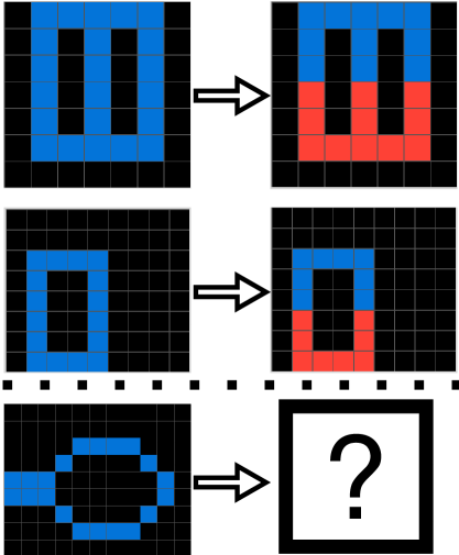</details> Figure 9: Fragment of ARC problem e7dd8335. Solution Analysis. RSPC achieves over 30% accuracy across evaluated metrics using GPT-o3-mini, even without knowledge augmentation. To assess its alignment with core knowledge priors, we manually reviewed RSPC-generated solution plans and code that successfully solve $I_{t}$ with GPT-o3-mini. RSPC tends to solve problems without object-centric reasoning. For instance, in Figure 1, it shifts each row downward by one and pads the top with zeros, rather than reasoning over objectness to move each 4-connected component down by one step. Even when applying objectness, RSPC typically defaults to 4-connected abstraction, failing on the problem in Figure 9, where the test input clearly requires 8-connected abstraction. We note that object recognition in ARC involves grouping pixels into task-specific components based on clustering rules, differing from feature extraction approaches [47] in conventional computer vision tasks. Recent work seeks to bridge this gap by incorporating 2D positional encodings and object indices into Vision Transformers [41]. However, its reliance on data-driven learning weakens generalization, undermining ARC’s core objective. In contrast, KAAR enables objectness through explicitly defined abstractions, implemented via standard image processing algorithms, thus ensuring both accuracy and generalization. Generalization. For all evaluated ARC solvers, accuracy on $I_{r}$ consistently exceeds that on $I_{r}\&I_{t}$ , revealing a generalization gap. Planning-aided code generation methods, such as RSPC and KAAR, exhibit smaller gaps than other solvers, though the issue persists. One reason is that solutions include low-level logic for the training pairs, thus failing to generalize. See Appendix A.9 for examples. Another reason is the usage of incorrect abstractions. For example, reliance solely on 4-connected abstraction leads RSPC to solve only $I_{r}$ in Figure 9. KAAR similarly fails to generalize in this case. It selects 4-connected abstraction, the first one that solves $I_{r}$ , to report accuracy on $I_{t}$ , instead of the correct 8-connected abstraction, as the former is considered simpler. Table 1 also reveals that LLMs differ in their generalization across ARC solvers. While a detailed analysis of these variations is beyond the scope of this study, investigating the underlying causes could offer insights into LLM inference and alignment with intended behaviors, presenting a promising direction for future work. ## 7 Conclusion We explored the generalization and abstract reasoning capabilities of recent reasoning-oriented LLMs on the ARC benchmark using nine candidate solvers. Experimental results show that repeated-sampling planning-aided code generation (RSPC) achieves the highest test accuracy and demonstrates consistent generalization across most evaluated LLMs. To further improve performance, we propose KAAR, which progressively augments LLMs with core knowledge priors organized into hierarchical levels based on their dependencies, and applies RSPC after augmenting each level of priors to enable stage-wise reasoning. KAAR improves LLM performance on the ARC benchmark while maintaining strong generalization compared to non-augmented RSPC. However, ARC remains challenging even for the most capable reasoning-oriented LLMs, given its emphasis on abstract reasoning and generalization, highlighting current limitations and motivating future research. ## References - Khan et al. [2021] Abdullah Ayub Khan, Asif Ali Laghari, and Shafique Ahmed Awan. Machine learning in computer vision: A review. EAI Endorsed Transactions on Scalable Information Systems, 8(32), 2021. - Otter et al. [2020] Daniel W Otter, Julian R Medina, and Jugal K Kalita. A survey of the usages of deep learning for natural language processing. IEEE transactions on neural networks and learning systems, 32(2):604–624, 2020. - Grigorescu et al. [2020] Sorin Grigorescu, Bogdan Trasnea, Tiberiu Cocias, and Gigel Macesanu. A survey of deep learning techniques for autonomous driving. Journal of field robotics, 37(3):362–386, 2020. - Lake et al. [2017] Brenden M Lake, Tomer D Ullman, Joshua B Tenenbaum, and Samuel J Gershman. Building machines that learn and think like people. Behavioral and brain sciences, 40:e253, 2017. - Chollet [2019] François Chollet. On the measure of intelligence. arXiv preprint arXiv:1911.01547, 2019. - Peirce [1868] Charles S Peirce. Questions concerning certain faculties claimed for man. The Journal of Speculative Philosophy, 2(2):103–114, 1868. - Spelke and Kinzler [2007] Elizabeth S Spelke and Katherine D Kinzler. Core knowledge. Developmental science, 10(1):89–96, 2007. - Gulwani et al. [2017] Sumit Gulwani, Oleksandr Polozov, Rishabh Singh, et al. Program synthesis. Foundations and Trends® in Programming Languages, 4:1–119, 2017. - Xu et al. [2023a] Yudong Xu, Elias B Khalil, and Scott Sanner. Graphs, constraints, and search for the abstraction and reasoning corpus. In Proceedings of the 37th AAAI Conference on Artificial Intelligence, AAAI, pages 4115–4122, 2023a. - Lei et al. [2024a] Chao Lei, Nir Lipovetzky, and Krista A Ehinger. Generalized planning for the abstraction and reasoning corpus. In Proceedings of the 38th AAAI Conference on Artificial Intelligence, AAAI, pages 20168–20175, 2024a. - Wei et al. [2022] Jason Wei, Xuezhi Wang, Dale Schuurmans, Maarten Bosma, Fei Xia, Ed Chi, Quoc V Le, Denny Zhou, et al. Chain-of-thought prompting elicits reasoning in large language models. In Proceedings of the 36th Advances in Neural Information Processing Systems, NeurIPS, pages 24824–24837, 2022. - Chen et al. [2021] Mark Chen, Jerry Tworek, Heewoo Jun, Qiming Yuan, Henrique Ponde de Oliveira Pinto, Jared Kaplan, Harri Edwards, Yuri Burda, Nicholas Joseph, Greg Brockman, et al. Evaluating large language models trained on code. arXiv preprint arXiv:2107.03374, 2021. - Li et al. [2022] Yujia Li, David Choi, Junyoung Chung, Nate Kushman, Julian Schrittwieser, Rémi Leblond, Tom Eccles, James Keeling, Felix Gimeno, Agustin Dal Lago, et al. Competition-level code generation with alphacode. Science, 378:1092–1097, 2022. - Chen et al. [2023] Bei Chen, Fengji Zhang, Anh Nguyen, Daoguang Zan, Zeqi Lin, Jian-Guang Lou, and Weizhu Chen. Codet: Code generation with generated tests. In Proceedings of the 11th International Conference on Learning Representations, ICLR, pages 1–19, 2023. - Zhang et al. [2023] Tianyi Zhang, Tao Yu, Tatsunori Hashimoto, Mike Lewis, Wen-tau Yih, Daniel Fried, and Sida Wang. Coder reviewer reranking for code generation. In Proceedings of the 40th International Conference on Machine Learning, ICML, pages 41832–41846, 2023. - Ni et al. [2023] Ansong Ni, Srini Iyer, Dragomir Radev, Veselin Stoyanov, Wen-tau Yih, Sida Wang, and Xi Victoria Lin. Lever: Learning to verify language-to-code generation with execution. In Proceedings of the 40th International Conference on Machine Learning, ICML, pages 26106–26128, 2023. - Zhong et al. [2024a] Li Zhong, Zilong Wang, and Jingbo Shang. Debug like a human: A large language model debugger via verifying runtime execution step by step. In Findings of the Association for Computational Linguistics: ACL 2024, pages 851–870, 2024a. - Lei et al. [2024b] Chao Lei, Yanchuan Chang, Nir Lipovetzky, and Krista A Ehinger. Planning-driven programming: A large language model programming workflow. arXiv preprint arXiv:2411.14503, 2024b. - Chen et al. [2024] Xinyun Chen, Maxwell Lin, Nathanael Schärli, and Denny Zhou. Teaching large language models to self-debug. In Proceedings of the 12th International Conference on Learning Representations, ICLR, 2024. - Austin et al. [2021] Jacob Austin, Augustus Odena, Maxwell Nye, Maarten Bosma, Henryk Michalewski, David Dohan, Ellen Jiang, Carrie Cai, Michael Terry, Quoc Le, et al. Program synthesis with large language models. arXiv preprint arXiv:2108.07732, 2021. - Jain et al. [2025] Naman Jain, King Han, Alex Gu, Wen-Ding Li, Fanjia Yan, Tianjun Zhang, Sida Wang, Armando Solar-Lezama, Koushik Sen, and Ion Stoica. Livecodebench: Holistic and contamination free evaluation of large language models for code. In Proceedings of the 13th International Conference on Learning Representations, ICLR, 2025. - Jiang et al. [2023] Xue Jiang, Yihong Dong, Lecheng Wang, Fang Zheng, Qiwei Shang, Ge Li, Zhi Jin, and Wenpin Jiao. Self-planning code generation with large language models. ACM Transactions on Software Engineering and Methodology, 33(7):1–28, 2023. - Islam et al. [2024] Md. Ashraful Islam, Mohammed Eunus Ali, and Md Rizwan Parvez. MapCoder: Multi-agent code generation for competitive problem solving. In Proceedings of the 62nd Annual Meeting of the Association for Computational Linguistics, ACL, pages 4912–4944, 2024. - Zhong et al. [2024b] Tianyang Zhong, Zhengliang Liu, Yi Pan, Yutong Zhang, Yifan Zhou, Shizhe Liang, Zihao Wu, Yanjun Lyu, Peng Shu, Xiaowei Yu, et al. Evaluation of openai o1: Opportunities and challenges of agi. arXiv preprint arXiv:2409.18486, 2024b. - OpenAI [2025] OpenAI. Openai o3-mini. OpenAI, 2025. URL https://openai.com/index/openai-o3-mini/. Accessed: 2025-03-22. - DeepMind [2024] Google DeepMind. Gemini 2.0 flash thinking. Google DeepMind, 2024. URL https://deepmind.google/technologies/gemini/flash-thinking/. Accessed: 2025-03-22. - Guo et al. [2025] Daya Guo, Dejian Yang, Haowei Zhang, Junxiao Song, Ruoyu Zhang, Runxin Xu, Qihao Zhu, Shirong Ma, Peiyi Wang, Xiao Bi, et al. Deepseek-r1: Incentivizing reasoning capability in llms via reinforcement learning. arXiv preprint arXiv:2501.12948, 2025. - Cloud [2025] Alibaba Cloud. Alibaba cloud unveils qwq-32b: A compact reasoning model with cutting-edge performance. Alibaba Cloud, 2025. URL https://www.alibabacloud.com/blog/alibaba-cloud-unveils-qwq-32b-a-compact-reasoning-model-with-cutting-edge-performance_602039. Accessed: 2025-03-22. - Babakr et al. [2019] Zana H Babakr, Pakstan Mohamedamin, and Karwan Kakamad. Piaget’s cognitive developmental theory: Critical review. Education Quarterly Reviews, 2(3):517–524, 2019. - Deng et al. [2024] Hourui Deng, Hongjie Zhang, Jie Ou, and Chaosheng Feng. Can llm be a good path planner based on prompt engineering? mitigating the hallucination for path planning. arXiv preprint arXiv:2408.13184, 2024. - Meng et al. [2024] Silin Meng, Yiwei Wang, Cheng-Fu Yang, Nanyun Peng, and Kai-Wei Chang. LLM-a*: Large language model enhanced incremental heuristic search on path planning. In Findings of the Association for Computational Linguistics: EMNLP 2024, pages 1087–1102, 2024. - Ahn et al. [2024] Janice Ahn, Rishu Verma, Renze Lou, Di Liu, Rui Zhang, and Wenpeng Yin. Large language models for mathematical reasoning: Progresses and challenges. In Proceedings of the 18th Conference of the European Chapter of the Association for Computational Linguistics: Student Research Workshop, EACL, pages 225–237, 2024. - Zang et al. [2025] Yuhang Zang, Wei Li, Jun Han, Kaiyang Zhou, and Chen Change Loy. Contextual object detection with multimodal large language models. International Journal of Computer Vision, 133(2):825–843, 2025. - Xu et al. [2023b] Yudong Xu, Wenhao Li, Pashootan Vaezipoor, Scott Sanner, and Elias B Khalil. Llms and the abstraction and reasoning corpus: Successes, failures, and the importance of object-based representations. arXiv preprint arXiv:2305.18354, 2023b. - Lei et al. [2023] Chao Lei, Nir Lipovetzky, and Krista A Ehinger. Novelty and lifted helpful actions in generalized planning. In Proceedings of the International Symposium on Combinatorial Search, SoCS, pages 148–152, 2023. - Wang et al. [2024] Ruocheng Wang, Eric Zelikman, Gabriel Poesia, Yewen Pu, Nick Haber, and Noah Goodman. Hypothesis search: Inductive reasoning with language models. In Proceedings of the 12 th International Conference on Learning Representations, ICLR, 2024. - LeGris et al. [2024] Solim LeGris, Wai Keen Vong, Brenden M Lake, and Todd M Gureckis. H-arc: A robust estimate of human performance on the abstraction and reasoning corpus benchmark. arXiv preprint arXiv:2409.01374, 2024. - Yamada et al. [2024] Yutaro Yamada, Yihan Bao, Andrew Kyle Lampinen, Jungo Kasai, and Ilker Yildirim. Evaluating spatial understanding of large language models. Transactions on Machine Learning Research, 2024. - Cohn and Hernandez-Orallo [2023] Anthony G Cohn and Jose Hernandez-Orallo. Dialectical language model evaluation: An initial appraisal of the commonsense spatial reasoning abilities of llms. arXiv preprint arXiv:2304.11164, 2023. - Bang et al. [2023] Yejin Bang, Samuel Cahyawijaya, Nayeon Lee, Wenliang Dai, Dan Su, Bryan Wilie, Holy Lovenia, Ziwei Ji, Tiezheng Yu, Willy Chung, Quyet V. Do, Yan Xu, and Pascale Fung. A multitask, multilingual, multimodal evaluation of ChatGPT on reasoning, hallucination, and interactivity. In Proceedings of the 13th International Joint Conference on Natural Language Processing and the 3rd Conference of the Asia-Pacific Chapter of the Association for Computational Linguistics, IJCNLP-AACL, pages 675–718, 2023. - Li et al. [2024a] Wenhao Li, Yudong Xu, Scott Sanner, and Elias Boutros Khalil. Tackling the abstraction and reasoning corpus with vision transformers: the importance of 2d representation, positions, and objects. arXiv preprint arXiv:2410.06405, 2024a. - Raven [2000] John Raven. The raven’s progressive matrices: change and stability over culture and time. Cognitive psychology, 41(1):1–48, 2000. - Barrett et al. [2018] David Barrett, Felix Hill, Adam Santoro, Ari Morcos, and Timothy Lillicrap. Measuring abstract reasoning in neural networks. In Proceedings of the 37th International conference on machine learning, ICML, pages 511–520, 2018. - Cui et al. [2025] Yongcheng Cui, Ying Zhang, Cui-Hua Zhang, and Simon X Yang. Task cognition and planning for service robots. Intelligence & Robotics, (1):119–142, 2025. - Stefanini et al. [2022] Matteo Stefanini, Marcella Cornia, Lorenzo Baraldi, Silvia Cascianelli, Giuseppe Fiameni, and Rita Cucchiara. From show to tell: A survey on deep learning-based image captioning. IEEE transactions on pattern analysis and machine intelligence, (1):539–559, 2022. - Huynh et al. [2025] Ngoc Dung Huynh, Mohamed Reda Bouadjenek, Sunil Aryal, Imran Razzak, and Hakim Hacid. Visual question answering: from early developments to recent advances–a survey. arXiv preprint arXiv:2501.03939, 2025. - Zhao et al. [2019] Zhong-Qiu Zhao, Peng Zheng, Shou-tao Xu, and Xindong Wu. Object detection with deep learning: A review. IEEE transactions on neural networks and learning systems, 30(11):3212–3232, 2019. - Mialon et al. [2023] Grégoire Mialon, Roberto Dessi, Maria Lomeli, Christoforos Nalmpantis, Ramakanth Pasunuru, Roberta Raileanu, Baptiste Roziere, Timo Schick, Jane Dwivedi-Yu, Asli Celikyilmaz, Edouard Grave, Yann LeCun, and Thomas Scialom. Augmented language models: a survey. Transactions on Machine Learning Research, 2023. ISSN 2835-8856. - Zhu et al. [2025] Yuqi Zhu, Shuofei Qiao, Yixin Ou, Shumin Deng, Shiwei Lyu, Yue Shen, Lei Liang, Jinjie Gu, Huajun Chen, and Ningyu Zhang. KnowAgent: Knowledge-augmented planning for LLM-based agents. In Findings of the Association for Computational Linguistics: NAACL 2025, pages 3709–3732, 2025. - Vu et al. [2024] Tu Vu, Mohit Iyyer, Xuezhi Wang, Noah Constant, Jerry Wei, Jason Wei, Chris Tar, Yun-Hsuan Sung, Denny Zhou, Quoc Le, and Thang Luong. FreshLLMs: Refreshing large language models with search engine augmentation. In Findings of the Association for Computational Linguistics: ACL 2024, pages 13697–13720, 2024. - Li et al. [2024b] Xingxuan Li, Ruochen Zhao, Yew Ken Chia, Bosheng Ding, Shafiq Joty, Soujanya Poria, and Lidong Bing. Chain-of-knowledge: Grounding large language models via dynamic knowledge adapting over heterogeneous sources. In Proceedings of the 12th International Conference on Learning Representations, ICLR, 2024b. - Trivedi et al. [2023] Harsh Trivedi, Niranjan Balasubramanian, Tushar Khot, and Ashish Sabharwal. Interleaving retrieval with chain-of-thought reasoning for knowledge-intensive multi-step questions. In Proceedings of the 61st Annual Meeting of the Association for Computational Linguistics, ACL, pages 10014–10037, 2023. - Qiao et al. [2024] Shuofei Qiao, Honghao Gui, Chengfei Lv, Qianghuai Jia, Huajun Chen, and Ningyu Zhang. Making language models better tool learners with execution feedback. In Proceedings of the 2024 Conference of the North American Chapter of the Association for Computational Linguistics: Human Language Technologies, NNACL, pages 3550–3568, 2024. - Wind [2020] J S Wind. 1st place solution + code and official documentation. https://www.kaggle.com/competitions/abstraction-and-reasoning-challenge/discussion/154597, 2020. Accessed: 2025-03-22. - Camposampiero et al. [2023] Giacomo Camposampiero, Loic Houmard, Benjamin Estermann, Joël Mathys, and Roger Wattenhofer. Abstract visual reasoning enabled by language. arXiv preprint arXiv:2306.04091, 2023. - Min [2023] Tan John Chong Min. An approach to solving the abstraction and reasoning corpus (arc) challenge. arXiv preprint arXiv:2306.03553, 2023. - Tan and Motani [2024] John Chong Min Tan and Mehul Motani. Llms as a system of multiple expert agents: An approach to solve the abstraction and reasoning corpus (arc) challenge. In Proceedings of the 2024 IEEE Conference on Artificial Intelligence, CAI, pages 782–787, 2024. - Bikov et al. [2024] Kiril Bikov, Mikel Bober-Irizar, and Soumya Banerjee. Reflection system for the abstraction and reasoning corpus. In Proceedings of the 2nd AI4Research Workshop: Towards a Knowledge-grounded Scientific Research Lifecycle, 2024. - Franzen et al. [2024] Daniel Franzen, Jan Disselhoff, and David Hartmann. The llm architect: Solving arc-agi is a matter of perspective. https://github.com/da-fr/arc-prize-2024/blob/main/the_architects.pdf, 2024. Accessed: 2025-03-22. - Hodel [2024] Michael Hodel. Addressing the abstraction and reasoning corpus via procedural example generation. arXiv preprint arXiv:2404.07353, 2024. - Moskvichev et al. [2023] Arseny Moskvichev, Victor Vikram Odouard, and Melanie Mitchell. The conceptarc benchmark: Evaluating understanding and generalization in the arc domain. arXiv preprint arXiv:2305.07141, 2023. - Li et al. [2025] Wen-Ding Li, Keya Hu, Carter Larsen, Yuqing Wu, Simon Alford, Caleb Woo, Spencer M. Dunn, Hao Tang, Wei-Long Zheng, Yewen Pu, and Kevin Ellis. Combining induction and transduction for abstract reasoning. In Proceedings of the 13th International Conference on Learning Representations, ICLR, 2025. - Barke et al. [2024] Shraddha Barke, Emmanuel Anaya Gonzalez, Saketh Ram Kasibatla, Taylor Berg-Kirkpatrick, and Nadia Polikarpova. Hysynth: Context-free llm approximation for guiding program synthesis. In Proceedings of the 38th Advances in Neural Information Processing Systems, NeurIPS, pages 15612–15645, 2024. ## Appendix A Appendix ### A.1 Related Work Knowledge-Augmented LLMs. Augmenting LLMs with external knowledge can improve reasoning capabilities and mitigate hallucination in text generation [48]. Previous studies achieve this by incorporating domain-specific knowledge, designed by human experts [49], retrieved via search engines [50], or extracted from Wikipedia documents [51]. Trivedi et al. [52] demonstrated that interleaving knowledge augmentation within reasoning steps further reduces model hallucination, resulting in more accurate multi-step reasoning. Additionally, augmenting LLMs with execution feedback improves performance on both question answering [53] and program synthesis tasks [10, 17, 19]. Search in DSL. An abstract, expressive, and compositional representation of core knowledge priors is essential for solving ARC tasks [5]. Previous studies have manually encoded these priors into domain-specific languages (DSLs) with lifted relational representations [9, 10, 54]. Various program synthesis methods have been proposed to search for valid solution programs within their DSLs, including DAG-based search [54], graph-based constraint-guided search [9], and generalized planning [10]. Hand-crafted DSLs encode core knowledge priors with high precision and interpretability, enabling structured program synthesis. However, comprehensive DSLs induce large search spaces, limiting synthesis efficiency. LLMs for ARC. Recent studies have explored using LLMs as ARC solvers to directly generate test output matrices and have prompted LLMs with different problem descriptions to improve output accuracy. Camposampiero et al. [55] employed LLMs to generate output grids from textual task descriptions, derived from a vision module which is designed to capture human-like visual priors. Min [56] prompted LLMs with the raw 2D matrices of each task, along with transformation and abstraction examples. Xu et al. [34] demonstrated that object representations derived from predefined abstractions can improve LLM performance on ARC tasks. Recent advances in code generation by LLMs [18, 17, 14] highlight their potential to replace search-based program synthesis, addressing efficiency limitations. Tan and Motani [57] evaluated LLM performance on the ARC benchmark by generating Python program solutions. Additionally, Wang et al. [36] approached ARC as an inductive reasoning problem and introduced hypothesis search, where program solutions are generated by selecting LLM-generated hypotheses encoded as functions. Training-Based Methods. To further improve LLM performance, Bikov et al. [58] fine-tuned LLMs on augmented ARC tasks using standard techniques such as rotation, flipping, and permutation. Beyond these methods, Franzen et al. [59] fine-tuned LLMs on large-scale synthetic ARC tasks [60] and ARC-related datasets such as Concept-ARC [61] and ARC-Heavy [62], achieving a state-of-the-art 56% accuracy on the private evaluation set of 200 tasks. Instead of fine-tuning LLMs, Barke et al. [63] trained a probabilistic context-free grammar (PCFG) using LLM-generated plausible solutions to learn weighted functions. This enables the synthesizer to efficiently generate final program solutions. However, this approach requires a dedicated synthesizer for each DSL, limiting its generalization. When leveraging LLMs as ARC solvers, existing studies tend to emphasize accuracy on partial training set problems and overlook the core principle of ARC, where solutions should be constructed using core knowledge priors [5]. LLMs still lack these priors, such as objectness, as evidenced by RSPC-generated solutions. Although fine-tuning approaches have achieved state-of-the-art performance, their failure to incorporate core knowledge priors remains a fundamental limitation. KAAR addresses this gap by progressively augmenting LLMs with structured core knowledge priors introduced by GPAR, along with exclusive implementations of goal-directedness priors. It interleaves augmentation within the reasoning process by applying an advanced LLM-based program synthesis solver tailored to the ARC benchmark after augmenting priors at each level. KAAR achieves strong performance, 32.5% test accuracy on the full evaluation set of 400 problems using GPT-o3-mini, demonstrates substantial generalization, and produces solutions aligned with core knowledge priors. ### A.2 Core Knowledge Priors in KAAR KAAR incorporates abstractions to enable objectness priors; component attributes, relations, and statistical analysis of component attributes to encode geometry, topology, numbers, and counting priors; and predefined actions to support goal-directedness priors. Table 5 presents all abstractions used in KAAR, organized by their prioritization. KAAR incorporates fundamental abstractions, such as 4-connected and 8-connected components, from GPAR, and extends them with additional abstractions unique to KAAR, highlighted in red. Table 6 introduces geometry, topology, numbers, and counting priors, and ten predefined transformations used in KAAR. For each action, KAAR augments the LLM with its corresponding schema to resolve implementation details. The actions and their schemas are detailed in Table A.12. Most actions can be specified within three steps, keeping them tractable for LLMs. <details> <summary>x10.png Details</summary>  ### Visual Description # Technical Document Analysis: Grid Sequence Image ## Textual Information Extraction **No textual information present.** The image contains no labels, axis titles, legends, or textual annotations. All elements are visual (colored squares, arrows, question mark). --- ## Visual Component Description ### Structure - **Sequence of 6x6 Grids**: Six 6x6 grid diagrams arranged horizontally, each connected by a rightward arrow (`→`) to the next grid. Final grid contains a single black-outlined white square with a black question mark (`?`). ### Grid Composition 1. **Color Patterns**: - **Blue**: Represents "active" or "selected" states. - **Black**: Neutral/background state. - **Gray**: Transitional/undefined state. - **Red**: Highlighted/alert state (appears only in final grids). 2. **Transition Logic**: - **Grid 1 → Grid 2**: - Top-left 2x2 blue block shifts rightward by one column. - Bottom-middle 2x2 blue block shifts downward by one row. - **Grid 2 → Grid 3**: - Blue blocks replaced by gray in central columns. - **Grid 3 → Grid 4**: - Red squares replace blue/gray in diagonal pattern. - **Grid 4 → Grid 5**: - Red squares shift to bottom-right corner. - **Grid 5 → Final Grid**: - All squares black except top-left and bottom-right corners (red). ### Final Grid - **Question Mark (`?`)**: Positioned centrally in a white square, suggesting an unresolved state or query. --- ## Spatial Grounding & Trend Verification - **Legend Absence**: No explicit legend present. Color meanings inferred from positional patterns. - **Trend Analysis**: - Blue blocks progressively reduce and shift across grids. - Red squares emerge in later grids, indicating a state change or error condition. - Final grid’s question mark implies a missing or undefined outcome. --- ## Conclusion The image depicts a state transition sequence with no textual metadata. The progression from blue-dominated grids to red-highlighted states and a terminal question mark suggests a workflow or decision-tree visualization. No numerical data or categorical labels are present. </details> Figure 10: ARC problem 0520fde7 ### A.3 Restrictions in KAAR For certain abstractions, some priors are either inapplicable or exclusive. The specific priors assigned to some abstractions are detailed in Table 8. For the whole image abstraction, few priors apply as only a single component is present. In contrast, the 4/8-connected-multi-color-non-background abstractions retain most priors. The highlighted priors that capture per-component color diversity are used exclusively for 4/8-connected-multi-color-non-background abstractions, while priors tailored to a single-color component, such as components with same color, components with most frequent color, and components with least frequent color, are excluded. For the middle-vertical and middle-horizontal abstractions, where the image is evenly divided into two components, flipping and movement actions are enabled to facilitate reasoning over overlapping components. For instance, in the problem shown in Figure 10, the solution involves splitting the image along a middle-vertical grid line and moving one component to overlap the other. In the resulting component, a pixel is colored red if the overlapping pixels in both components are blue; otherwise, it is colored black. ### A.4 Parameter Settings KAAR operates on all LLMs through API access with the full conversational history. For proprietary models, GPT-o3-mini and Gemini-2.0 Flash-Thinking (Gemini-2.0), we use default parameter settings. For open-source models, DeepSeek-R1-Distill-Llama-70B (DeepSeek-R1-70B) and QwQ-32B, we set temperature to 0.6, top-p to 0.95, and top-k to 40 to reduce repetitive outputs and filter rare tokens while preserving generation diversity. We conduct experiments on a virtual machine with 4 NVIDIA A100 80GB GPUs. ### A.5 KAAR Algorithm 1 presents the pseudocode of KAAR. For each abstraction, KAAR incrementally augments the LLM with core knowledge priors, structured into three dependency-aware levels: beginning with objectness (Line 5), followed by geometry and topology (Lines 10 and 12), numbers and counting (Line 14), and concluding with goal-directedness priors(Line 18). We note that KAAR encodes geometry and topology priors through component attributes (Line 9) and relations (Line 11). The full set of priors is detailed in Tables 5, 6, and A.12. After augmenting each level of priors, KAAR invokes the solver backbone (RSPC) at Lines 6, 15, and 19 to generate code solutions guided by text-based plans, allowing up to 4 iterations (Lines 25–37). In each iteration, the solver backbone first validates the generated code on the training instances $I_{r}$ ; if successful, it then evaluates the solution on the test instances $I_{t}$ . The solver backbone returns solve if the generated solution successfully solves $I_{t}$ after passing $I_{r}$ ; pass if only $I_{r}$ is solved; or continues to the next iteration if the solution fails on $I_{r}$ . If the solver backbone fails to solve $I_{r}$ within the allotted 4 iterations at Lines 6 and 15, KAAR augments the next level of priors. KAAR proceeds to the next abstraction when the solver backbone fails to solve $I_{r}$ at Line 19, after the 4-iteration limit. KAAR terminates abstraction iteration upon receiving either pass or solve from the solver backbone and reports accuracy on $I_{r}$ , $I_{t}$ , and $I_{r}\&I_{t}$ accordingly. If no abstraction fully solves $I_{r}$ , KAAR records the final code solution for each abstraction (Line 22), selects the one that passes the most training instances (Line 23), and evaluates it on $I_{t}$ to determine additional accuracy gains (Line 24). KAAR generates priors offline using image processing algorithms introduced in GPAR at Lines 4, 9, 11 and 13. In contrast, KAAR enables goal-directedness priors at Line 18 by prompting the LLM to select the most suitable actions and identify their implementation details, as described in Table A.12. KAAR iterates over abstractions from simpler to more complex, following the order specified in Table 5. We note that the highest-priority abstraction is no abstraction, where KAAR degrades to the solver backbone (RSPC) as no priors are applied. Input : LLM $\mathcal{M}$ ; ARC problem $\mathcal{P}=(I_{r},I_{t})$ ; description $Q=(I_{r},\{i^{i}\ |\ (i^{i},i^{o})\in I_{t}\})$ ; abstraction list $\mathcal{A}$ ; max iterations $t=4$ 1 2 Function KnowledgeAugmentation ( $\mathcal{M}$ , $Q$ , $\mathcal{P}$ , $\mathcal{A}$ , $t$ ): 3 solutionList $\leftarrow[]$ ; 4 foreach abstraction $abs$ in $\mathcal{A}$ do 5 objectnessPriors $\leftarrow$ GenerateObjectnessPriors( $Q$ , $abs$ ); 6 AugmentKnowledge( $\mathcal{M}$ , objectnessPriors); 7 result, code, passedCount $\leftarrow$ SolverBackbone ( $\mathcal{M}$ , $\mathcal{P}$ , $Q$ , $t$ ); 8 if result $\neq$ failure then 9 return result 10 11 attributePriors $\leftarrow$ GenerateAttributePriors( $Q$ , $abs$ ); 12 AugmentKnowledge( $\mathcal{M}$ , attributePriors); 13 relationPriors $\leftarrow$ GenerateRelationPriors( $Q$ , $abs$ ); 14 AugmentKnowledge( $\mathcal{M}$ , relationPriors); 15 numberPriors $\leftarrow$ GenerateNumbersCountingPriors( $Q$ , $abs$ ); 16 AugmentKnowledge( $\mathcal{M}$ , numberPriors); 17 result, code, passedCount $\leftarrow$ SolverBackbone ( $\mathcal{M}$ , $\mathcal{P}$ , $Q$ , $t$ ); 18 if result $\neq$ failure then 19 return result 20 21 AugmentGoalPriors $\leftarrow$ ( $\mathcal{M}$ , $Q$ , $abs$ ); 22 23 result, code, passedCount $\leftarrow$ SolverBackbone ( $\mathcal{M}$ , $\mathcal{P}$ , $Q$ , $t$ ); 24 if result $\neq$ failure then 25 return result 26 27 solutionList.append((code, passedCount)); 28 29 bestCode $\leftarrow$ SelectMostPassed(solutionList); 30 return EvaluateOnTest(bestCode, $I_{t}$ ); 31 32 33 Function SolverBackbone ( $\mathcal{M}$ , $\mathcal{P}$ , $Q$ , $t$ ): 34 i $\leftarrow 0$ ; 35 while i < t do 36 plan $\leftarrow\mathcal{M}$ .generatePlan( $Q$ ); 37 code $\leftarrow\mathcal{M}$ .generateCode( $Q$ , plan); 38 passedCount $\leftarrow$ EvaluateOnTrain(code, $I_{r}$ ); 39 if passedCount == $|I_{r}|$ then 40 if EvaluateOnTest(code, $I_{t}$ ) then 41 return solve, code, passedCount; 42 43 else 44 return pass, code, passedCount; 45 46 47 i $\leftarrow$ i + 1; 48 49 return failure, code, passedCount; 50 Algorithm 1 KAAR | Gemini-2.0 $I_{t}$ $I_{r}\&I_{t}$ | $I_{r}$ 21.75 20.50 | 25.75 19.00 18.00 | 23.00 -2.75 -2.50 | -2.75 | | --- | --- | --- | --- | --- | | QwQ-32B | $I_{r}$ | 22.25 | 18.50 | -3.75 | | $I_{t}$ | 21.00 | 17.75 | -3.25 | | | $I_{r}\&I_{t}$ | 19.25 | 16.25 | -3.00 | | | DeepSeek-R1-70B | $I_{r}$ | 12.25 | 9.00 | -3.25 | | $I_{t}$ | 12.75 | 9.00 | -3.75 | | | $I_{r}\&I_{t}$ | 11.50 | 8.50 | -3.00 | | | 2 | | | | | Table 3: Accuracy on $I_{r}$ , $I_{t}$ , and $I_{r}\&I_{t}$ for KAAR and KAAR ∗ across three LLMs. KAAR ∗ invokes the solver backbone (RSPC) only after all knowledge priors are augmented. $\Delta$ denotes the performance drop relative to KAAR. All values are reported as percentages. ### A.6 Ablation Study Table 3 reports the accuracy decrease resulting from removing incremental knowledge augmentation and stage-wise reasoning in KAAR, denoted as KAAR ∗. Unlike KAAR, which invokes the solver backbone (RSPC) after augmenting each level of priors to enable stage-wise reasoning, KAAR ∗ uses RSPC to solve the problem within 12 iterations after augmenting all priors at once. We evaluate KAAR ∗ using the same reasoning-oriented LLMs as in Tables 1 and 2, excluding GPT-o3-mini due to its computational cost. KAAR ∗ shows decreased accuracy on all metrics, $I_{r}$ , $I_{t}$ , and $I_{r}\&I_{t}$ , for all evaluated LLMs. These results underscore the effectiveness of progressive augmentation and stage-wise reasoning. Presenting all knowledge priors simultaneously introduces superfluous information, which may obscure viable solutions and impair the LLM reasoning accuracy. We note that we construct the ontology of core knowledge priors based on their dependencies, thereby establishing a fixed augmentation order. 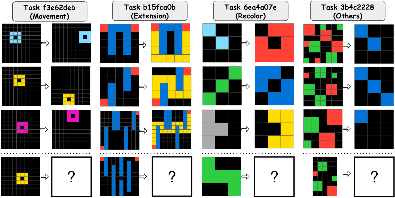<details> <summary>x11.png Details</summary>  ### Visual Description # Technical Document Extraction: Image Analysis ## Overview The image presents a structured grid of transformation tasks, organized into four labeled sections. Each section demonstrates a specific type of grid-based transformation (movement, extension, recolor, and others) through before/after examples. The final row contains incomplete examples marked with question marks. --- ## Section 1: Task f3e62deb (Movement) **Transformation Type**: Spatial repositioning of colored blocks **Key Observations**: 1. **Initial State**: - Top-left: Blue square in top-left corner - Middle-left: Yellow square in top-left corner - Bottom-left: Pink square in top-left corner 2. **Final State**: - Blue square moves to top-right corner - Yellow square moves to top-right corner - Pink square moves to top-right corner 3. **Pattern**: All colored blocks shift from top-left to top-right quadrant --- ## Section 2: Task b15fca0b (Extension) **Transformation Type**: Vertical line expansion **Key Observations**: 1. **Initial State**: - Top-left: Vertical blue line in left column - Middle-left: Vertical blue line in right column - Bottom-left: Vertical blue line in left column 2. **Final State**: - Blue lines extend downward to fill entire column - Yellow blocks fill bottom row 3. **Pattern**: Vertical lines expand downward; bottom row transitions to yellow --- ## Section 3: Task 6ea4a07e (Recolor) **Transformation Type**: Color inversion **Key Observations**: 1. **Initial State**: - Top-left: Blue square in top-left corner - Middle-left: Green square in bottom-right corner - Bottom-left: Gray squares in top-left 2x2 block 2. **Final State**: - Blue becomes red - Green becomes blue - Gray becomes yellow 3. **Pattern**: Direct color mapping: - Blue → Red - Green → Blue - Gray → Yellow --- ## Section 4: Task 3b4c2228 (Others) **Transformation Type**: Complex multi-color transformation **Key Observations**: 1. **Initial State**: - Top-left: Red/green/black checkerboard pattern - Middle-left: Mixed red/green/black blocks - Bottom-left: Red/green/black irregular pattern 2. **Final State**: - All blocks transition to blue/black 3. **Pattern**: Color reduction to blue/black dominant scheme --- ## Common Elements 1. **Grid Structure**: - All tasks use 4x4 grid systems - Arrows (`→`) indicate transformation direction 2. **Color Coding**: - Blue: Primary transformation color - Yellow/Red/Green: Secondary colors - Black: Neutral background 3. **Question Marks**: - Final row contains incomplete examples (`?`) - Indicates missing transformation outcomes --- ## Technical Notes - **Legend**: No explicit legend present, but color consistency across tasks implies: - Blue = Movement/Extension - Yellow = Extension - Red = Recolor - Green = Recolor/Others - Pink/Gray = Special cases - **Spatial Grounding**: - All transformations originate from left-side grids - Final states occupy right-side grids - **Temporal Flow**: - Left → Right progression across tasks - Top → Bottom progression within tasks --- ## Data Extraction Table | Task ID | Transformation Type | Input Colors | Output Colors | Example Count | |---------------|---------------------|--------------------|--------------------|---------------| | f3e62deb | Movement | Blue, Yellow, Pink | Blue, Yellow, Pink | 3 | | b15fca0b | Extension | Blue | Blue, Yellow | 3 | | 6ea4a07e | Recolor | Blue, Green, Gray | Red, Blue, Yellow | 3 | | 3b4c2228 | Others | Red, Green, Black | Blue, Black | 3 | --- ## Conclusion The image demonstrates systematic grid-based transformations across four distinct tasks. Each task follows a consistent pattern of input→output transformation, with color-coded elements maintaining positional or chromatic relationships. The final row's question marks suggest incomplete or variable outcomes requiring further analysis. </details> Figure 11: Example ARC tasks for movement, extension, recolor, and others categories. ### A.7 Example Tasks by Category in the ARC Evaluation Set ARC comprises 1000 unique tasks, with 400 allocated to the training set and 600 to the evaluation set. The evaluation set is further divided into a public subset (400 tasks) and a private subset (200 tasks). Figure 11 illustrates example ARC tasks for the movement, extension, recolor, and others categories in the public evaluation set. In the movement example, components are shifted to the image boundary in directions determined by their colors. The extension example is more complex, requiring LLMs to find the shortest path between two red pixels while avoiding obstacles, which presents challenges for current reasoning-oriented models. Additionally, reliance on pixel-level recognition weakens the effectiveness of KAAR, which is designed to facilitate component identification. The recolor example involves changing non-black components to black and updating black components based on original non-black colors. The others example requires generating a blue diagonal line whose length depends on the number of 4-connected components in the input image that are green and have a size greater than one. The combination of numerical reasoning and structural pattern generation makes this task difficult to classify within the other three categories. | GPT-o3-mini Gemini QwQ-32B | 66K 58K 79K | 106K 110K 427K | | --- | --- | --- | | DeepSeek-R1-70B | 66K | 252K | | 2 | | | Table 4: Average token cost for knowledge augmentation and solver backbone (RSPC) in KAAR across four evaluated LLMs. K is $10^{3}$ . ### A.8 Cost Analysis Table 4 reports the average token cost, including both prompts and LLM responses, for knowledge augmentation and the solver backbone (RSPC), when using KAAR as the ARC solver. For each ARC task, we consider the abstraction whose solution solves $I_{t}$ ; if none succeed, the one that passes $I_{r}$ ; otherwise, the abstraction with the lowest token usage is selected. Except for goal-directedness priors, all core knowledge priors in KAAR are generated offline using image processing algorithms from GPAR, resulting in comparable augmentation costs across all evaluated models. In contrast, token usage by the solver backbone varies substantially due to differences in the LLMs’ abstract reasoning and generalization capabilities. GPT-o3-mini solves most tasks efficiently, with the lowest token consumption by the solver backbone, where tokens used for knowledge augmentation account for approximately 62% of the solver backbone’s token usage. However, the solver backbone consumes more tokens with QwQ-32B, as QwQ-32B consistently generates longer reasoning traces. In this case, tokens used for knowledge augmentation constitute only 19% of the solver backbone’s token usage. Figure 14 illustrates the average token cost for augmenting priors at each level in KAAR. ### A.9 Generalization Figures 15 and 16 illustrate two ARC problems, 695367ec and b1fc8b8e, where both RSPC and KAAR successfully solve the training instances $I_{r}$ but fail on the test instances $I_{t}$ when using GPT-o3-mini. For problem 695367ec, the correct solution involves generating a fixed 15×15 output image by repeatedly copying the input image, changing its color to black, and adding internal horizontal and vertical lines colored with the original input image’s color. However, the RSPC-generated code applies a distinct rule to each input image size without considering generalization. For problem b1fc8b8e, the solution requires accurate object recognition despite component contact, and correctly placing each component into one of the four corners. However, RSPC fails to recognize objectness, and its solution deviates from human intuition, being overfitted to $I_{r}$ . For problems 695367ec and b1fc8b8e, KAAR exhibits the same limitations, although it adopts abstractions to enable objectness. KAAR begins with the simplest abstraction, no abstraction, where KAAR degrades to RSPC. As a result, it generates the same solution as RSPC and terminates without attempting other abstractions, since the solution already solves $I_{r}$ and is then evaluated on $I_{t}$ , resulting in overfitting. ### A.10 Problem Coverage across ARC Solvers We report the relative problem coverage across nine ARC solvers based on successful test instance solutions using GPT-o3-mini (Figure 17), Gemini-2.0 (Figure 18), QwQ-32B (Figure 19), and DeepSeek-R1-70B (Figure 20). Each cell $(i,j)$ indicates the proportion of problems solved by the row solver that are also solved by the column solver. This is computed as $\frac{|A_{i}\cap A_{j}|}{|A_{i}|}$ , where $A_{i}$ and $A_{j}$ are the sets of problems solved by the row and column solvers, respectively, following the same method used in Figure 5. Values close to 1 indicate that the column solver covers most problems solved by the row solver. GPT-o3-mini demonstrates the strongest overall coverage, with pairwise overlap consistently exceeding 0.55. Among all solvers, repeated sampling with standalone (P) and planning-aided code generation (PC) show the highest coverage, with column values consistently above 0.8 for GPT-o3-mini. This trend persists across Gemini-2.0, QwQ-32B, and DeepSeek-R1-70B. Under these models, repeated sampling with planning-aided code generation exhibits better alignment than its standalone code generation counterpart, generally yielding higher coverage values. However, planning-aided code generation under the direct generation setting shows weaker alignment, with column values around 0.40 for Gemini-2.0 and 0.35 for QwQ-32B. Among the four evaluated LLMs, DeepSeek-R1-70B demonstrates the lowest average off-diagonal coverage (i.e., $i\neq j$ ) of 0.603, suggesting potential output instability and variation attributable to solver choice. ### A.11 Performance Analysis Table 1 highlights performance variations across reasoning-oriented LLMs and ARC solvers with respect to both accuracy and generalization. Notably, the ARC solver, repeated sampling with standalone code generation, exhibits a substantial accuracy gap between $I_{r}$ and $I_{r}\&I_{t}$ , indicating limited generalization capability when using GPT-o3-mini and Gemini-2.0. In contrast, repeated sampling with planning-aided code generation demonstrates markedly improved generalization by preventing solutions from directly replicating the output matrices of training instances, as illustrated in Figure 21. This output copying, observed under repeated sampling with standalone code generation, accounts for approximately 24% and 95% of 83 and 101 overfitting problems with GPT-o3-mini and Gemini-2.0, respectively. When planning is incorporated, output copying is reduced to around 8% and 35% of 25 and 20 overfitting problems with GPT-o3-mini and Gemini-2.0, respectively. Additionally, the incorporation of planning facilitates accurate code generation. For example, in Figure 22, repeated sampling with planning-aided code generation produces a correct solution using GPT-o3-mini by replicating the input image horizontally or vertically based on the presence of a uniform row or column, as specified in the plan and implemented accordingly in code. In contrast, without planning assistance, standalone code generation produces incomplete logic, considering only whether the first column is uniform to determine the replication direction, which leads to failure on the test instance. For the ARC benchmark, repeated sampling–based methods achieve higher accuracy on $I_{r}$ , $I_{t}$ , and $I_{r}\&I_{t}$ compared to refinement-based approaches when using GPT-o3-mini and Gemini-2.0. Figure 23 presents an ARC problem where repeated sampling with planning-aided code generation yields a correct solution, whereas its refinement variant fails to correct the initial erroneous code, and the flawed logic persists across subsequent refinements when using GPT-o3-mini. Previous studies have shown that refinement can benefit from control flow graph information [17] and verified plans [18], which assist LLMs in locating and correcting bugs. However, these methods typically incur substantial token consumption, making them difficult to scale affordably. ### A.12 Limitations KAAR improves the performance of reasoning-oriented LLMs on ARC tasks by progressively prompting with core knowledge priors. Although this inevitably increases token usage, the trade-off can be justified, as the exploration of LLM generalization remains in its early stages. KAAR integrates diverse abstraction methods to enable objectness and iteratively applies abstractions in order of increasing complexity. In contrast, humans typically infer appropriate abstractions directly from training instances, rather than leveraging exhaustive search. To address this, we prompt different LLMs with raw 2D matrices of each ARC problem to select one or three relevant abstractions, but the results are unsatisfactory. As previously discussed, accurate abstraction inference often depends on validation through viable solutions, thereby shifting the challenge back to solution generation. Additionally, KAAR augments core knowledge priors through prompting but lacks mechanisms to enforce LLM adherence to these priors during reasoning. While the KAAR-generated solutions generally conform to core knowledge priors, the intermediate reasoning processes may deviate from the intended patterns. Future work could explore fine-tuning or reinforcement learning to better align model behavior with the desired reasoning patterns. | No Abstraction | - | | --- | --- | | Whole Image | We consider the whole image as a component. | | Middle-Vertical | We vertically split the image into two equal parts, treating each as a distinct component. | | Middle-Horizontal | We horizontally split the image into two equal parts, treating each as a distinct component. | | Multi-Lines | We use rows or columns with a uniform color to divide the input image into multiple components. | | 4-Connected ∗ | We consider the 4-adjacent pixels of the same color as a component. | | 4-Connected-Non-Background ∗ | We consider the 4-adjacent pixels of the same color as a component, excluding components with the background color. | | 4-Connected-Non-Background-Edge ∗ | We consider the 4-adjacent pixels of the same color as a component, containing components with the background color when they are not attached to the edges of the image. | | 4-Connected-Multi-Color-Non-Background ∗ | We consider 4-adjacent pixels as a component, which may contain different colors, while excluding components with the background color. | | 4-Connected-Bounding-Box ∗ | We consider 4-adjacent pixels of the same color, and treat all pixels within their bounding box as a component, which may include different colors. | | 4-Connected-With-Black ∗ | We consider the 4-adjacent pixels of black color, represented by the value 0, as a component, excluding components with other colors. | | Same-Color | We consider pixels of the same color as a component, excluding components with the background color. | | 2 | | Table 5: Abstractions in KAAR. The superscript “ ∗ ” denotes that the 8-connected version is considered. The background color is black if black exists; otherwise, it is the most frequent color in the image. We present abstractions according to their prioritization in KAAR, where the order is given by the table from top to bottom, and making 8-connected abstraction to follow that of the corresponding 4-connected abstraction at the end of the sequence. Abstractions highlighted in red are exclusive to KAAR. | Geometry and Topology | Size (Width and Height); Color; Shape (One Pixel; Horizontal Line; Vertical Line; Diagonal Line; Square; Rectangle; Cross; Irregular Shape); Symmetry (Horizontal Symmetry; Vertical Symmetry; Diagonal Symmetry; Anti-Diagonal Symmetry; Central Symmetry); Bounding Box; Hole Count; Nearest Boundary; Different/Identical with Other Components; Touching; Inclusive; Spatial (Horizontally Aligned to the Right; Horizontally Aligned to the Left; Vertically Aligned Below; Vertically Aligned Above; Top-Left; Top-Right; Bottom-Left; Bottom-Right; Same Position) | | --- | --- | | Numbers and Counting | Component Size Counting; Components with Same Size; Components with Most Frequent Size; Components with Least Frequent Size; Components with Maximum Size; Components with Minimum Size; Component Color Counting; Components with Same Color; Components with Same Number of Colors; Components with Most Frequent Color; Components with Least Frequent Color; Component with Most Distinct Colors; Component with Fewest Distinct Colors; Component Shape Counting; Components with Same Shape; Components with Most Frequent Shape; Components with Least Frequent Shape; Component Hole Number Counting; Components with Same Number of Holes; Components with Maximum Number of Holes; Components with Minimum Number of Holes; Component Symmetry Counting | | Goal-directedness | Color Change (modifying component value); Movement (shifting component’s position); Extension (expanding component’s area); Completing (filling in missing parts of a component); Resizing (altering component size); Selecting (isolating a component); Copying (duplicating a component); Flipping (mirroring a component); Rotation (rotating a component); Cropping (cutting part of a component) | | 2 | | Table 6: KAAR priors classified into geometry and topology, numbers and counting, and goal-directedness. For goal-directedness, we incorporate ten predefined actions, with their corresponding action schemas detailed in Table A.12. | Color Change Movement Extension | Targets Targets Targets | Source and Target Colors Direction Direction | Start and End Locations Start and End Locations | Pattern Pattern | Order Order | Overlapping Intersection | | --- | --- | --- | --- | --- | --- | --- | | Completing | Targets | Pattern | | | | | | Resizing | Targets | Source and Target Sizes | | | | | | Selecting | Targets | | | | | | | Copying | Targets | Locations | Overlapping | | | | | Flipping | Targets | Flipping Axis | Overlapping | | | | | Rotation | Targets | Degrees | | | | | | Cropping | Targets | Subsets | | | | | | 2 | | | | | | | Table 7: Actions in KAAR and their schemas (implementation details). Each action schema is presented according to its prompting order in KAAR (left to right). Some actions include a pattern schema that prompts the LLM to identify underlying logic rules, such as repeating every two steps in movement or extension, or completing based on three-color repetition. Targets denote the target components. | whole image | Symmetry, Size | - | Flipping; Rotation; Extension; Completing, Cropping | | --- | --- | --- | --- | | middle-vertical | Size | - | Flipping; Movement | | middle-horizontal | Size | - | Flipping; Movement | | multi-lines | Size; Color; Shape; Symmetry; Bounding Box; Hole Count | ALL | ALL | | 4-connected-multi-color-non-background ∗ | ALL | … Component Color Counting; Components with Same Number of Colors; Component with Most Distinct Colors; Component with Fewest Distinct Colors … | ALL | Table 8: Abstractions with their assigned knowledge priors. “–” denotes no priors, while “ALL” indicates all priors in the corresponding category, as defined in Table 6. The superscript “ ∗ ” indicates that the 8-connected version is also applicable. The highlighted priors apply exclusively to their corresponding abstractions. For the 4/8-connected-multi-color-non-background abstractions, we present color-counting priors specific to multi-colored components, while all other non-color-counting priors follow those in Table 6. 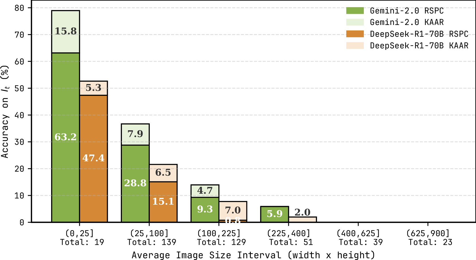<details> <summary>x12.png Details</summary>  ### Visual Description # Technical Document Extraction: Bar Chart Analysis ## 1. Chart Components ### Axis Labels - **X-axis**: "Average Image Size Interval (width x height)" - Categories: - `(0,25]` (Total: 19) - `(25,100]` (Total: 139) - `(100,225]` (Total: 129) - `(225,400]` (Total: 51) - `(400,625]` (Total: 39) - `(625,900]` (Total: 23) - **Y-axis**: "Accuracy on *I_t* (%)" ### Legend - **Location**: Top-right corner - **Categories**: - `Gemini-2.0 RSPC` (Green) - `Gemini-2.0 KAAR` (Light Green) - `DeepSeek-R1-70B RSPC` (Orange) - `DeepSeek-R1-70B KAAR` (Light Orange) ## 2. Data Points & Trends ### Spatial Grounding & Color Verification - **Legend Colors Match Chart Bars**: - Green = Gemini-2.0 RSPC - Light Green = Gemini-2.0 KAAR - Orange = DeepSeek-R1-70B RSPC - Light Orange = DeepSeek-R1-70B KAAR ### Interval-by-Interval Analysis #### `(0,25]` (Total: 19) - **Gemini-2.0 RSPC**: 63.2% (Green) - **DeepSeek-R1-70B RSPC**: 47.4% (Orange) - **Gemini-2.0 KAAR**: 15.8% (Light Green) - **DeepSeek-R1-70B KAAR**: 5.3% (Light Orange) - **Trend**: Gemini-2.0 RSPC dominates; KAAR versions underperform. #### `(25,100]` (Total: 139) - **Gemini-2.0 RSPC**: 28.8% (Green) - **DeepSeek-R1-70B RSPC**: 15.1% (Orange) - **Gemini-2.0 KAAR**: 7.9% (Light Green) - **DeepSeek-R1-70B KAAR**: 6.5% (Light Orange) - **Trend**: Accuracy declines for all models, but Gemini-2.0 RSPC remains highest. #### `(100,225]` (Total: 129) - **Gemini-2.0 RSPC**: 9.3% (Green) - **DeepSeek-R1-70B RSPC**: 0.8% (Orange) - **Gemini-2.0 KAAR**: 4.7% (Light Green) - **DeepSeek-R1-70B KAAR**: 7.0% (Light Orange) - **Trend**: DeepSeek-R1-70B RSPC plummets; KAAR versions show minor recovery. #### `(225,400]` (Total: 51) - **Gemini-2.0 RSPC**: 5.9% (Green) - **Gemini-2.0 KAAR**: 2.0% (Light Green) - **DeepSeek-R1-70B Models**: No data points (assumed 0% or omitted) - **Trend**: Gemini-2.0 RSPC retains marginal lead; KAAR versions negligible. #### `(400,625]` and `(625,900]` (Totals: 39, 23) - **No data points provided** for any model - **Trend**: Likely no measurable accuracy for larger intervals ## 3. Overall Trends - **Gemini-2.0 RSPC** consistently outperforms all models across intervals - **KAAR versions** (both Gemini and DeepSeek) show significantly lower accuracy, with performance degrading as image size increases - **DeepSeek-R1-70B RSPC** drops sharply in mid-sized intervals (e.g., 0.8% in `(100,225]`) ## 4. Critical Observations - **Accuracy Degradation**: All models lose effectiveness as image size grows, but Gemini-2.0 RSPC maintains relative stability - **KAAR Limitations**: KAAR configurations underperform RSPC by 3–5× in smaller intervals and become irrelevant in larger ones - **Data Gaps**: No results for `(400,625]` and `(625,900]`, suggesting models fail entirely at extreme resolutions ## 5. Transcribed Text - **Legend Labels**: - `Gemini-2.0 RSPC` - `Gemini-2.0 KAAR` - `DeepSeek-R1-70B RSPC` - `DeepSeek-R1-70B KAAR` - **Axis Titles**: - X: "Average Image Size Interval (width x height)" - Y: "Accuracy on *I_t* (%)" ## 6. Language Notes - **Primary Language**: English - **No Non-English Text Detected** </details> Figure 12: Accuracy on test instances $I_{t}$ for RSPC and KAAR across average image size intervals, evaluated with Gemini-2.0 and DeepSeek-R1-70B. 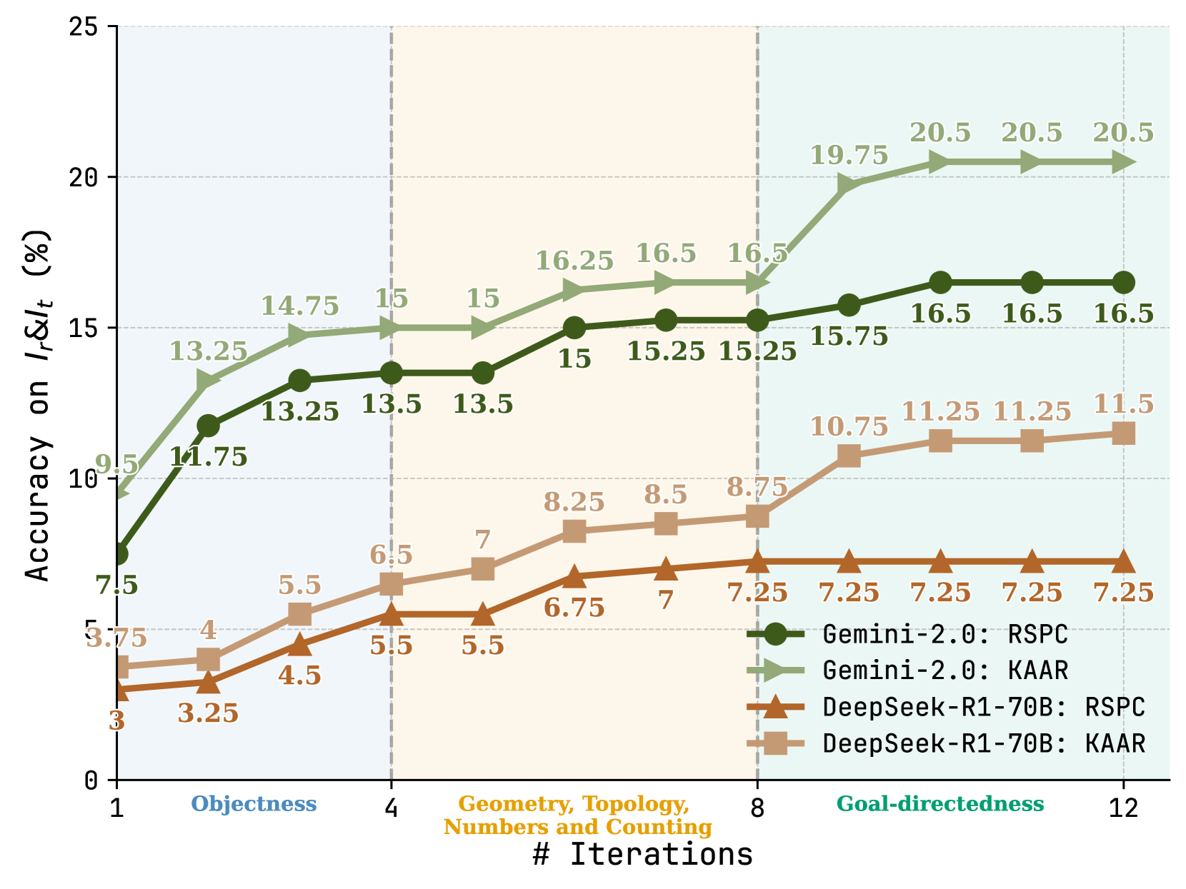<details> <summary>x13.png Details</summary>  ### Visual Description # Technical Document Extraction: Line Chart Analysis ## Chart Overview The image is a line chart titled **"Accuracy on I_r/I_t (%)"** with four distinct data series plotted across 12 iterations. The chart is divided into four primary x-axis categories: **Objectness**, **Geometry, Topology, Numbers and Counting**, and **Goal-directedness**, each containing sub-labels (e.g., 1, 2, 3, etc.). The y-axis represents accuracy percentages from 0% to 25%. --- ## Axis Labels and Markers - **X-Axis**: - Title: `# Iterations` - Categories: 1. **Objectness** (sub-labels: 1, 2, 3) 2. **Geometry, Topology, Numbers and Counting** (sub-labels: 4, 5, 6, 7, 8) 3. **Goal-directedness** (sub-labels: 8, 9, 10, 11, 12) - Sub-labels are numerically spaced but grouped under broader categories. - **Y-Axis**: - Title: `Accuracy on I_r/I_t (%)` - Markers: 0%, 5%, 10%, 15%, 20%, 25% (dashed lines at 15% and 20%). --- ## Legend - **Location**: Bottom-right corner. - **Entries**: 1. **Gemini-2.0: RSPC** (Green circles) 2. **Gemini-2.0: KAAR** (Green arrows) 3. **DeepSeek-R1-70B: RSPC** (Brown triangles) 4. **DeepSeek-R1-70B: KAAR** (Brown squares) --- ## Data Series and Trends ### 1. **Gemini-2.0: RSPC** (Green circles) - **Trend**: Steady upward slope. - **Key Points**: - Starts at **7.5%** (Iteration 1). - Peaks at **16.5%** (Iterations 10–12). - Notable jumps: 11.75% (Iteration 2), 13.25% (Iteration 3), 15.25% (Iteration 7). ### 2. **Gemini-2.0: KAAR** (Green arrows) - **Trend**: Consistent upward trajectory. - **Key Points**: - Begins at **9.5%** (Iteration 1). - Reaches **20.5%** (Iterations 10–12). - Significant increases: 13.5% (Iteration 4), 16.25% (Iteration 6), 19.75% (Iteration 9). ### 3. **DeepSeek-R1-70B: RSPC** (Brown triangles) - **Trend**: Gradual increase with plateau. - **Key Points**: - Starts at **3%** (Iteration 1). - Stabilizes at **7.25%** (Iterations 8–12). - Intermediate values: 4% (Iteration 2), 5.5% (Iteration 4), 6.75% (Iteration 6). ### 4. **DeepSeek-R1-70B: KAAR** (Brown squares) - **Trend**: Steeper rise compared to RSPC. - **Key Points**: - Begins at **3.75%** (Iteration 1). - Peaks at **11.5%** (Iteration 12). - Notable values: 5.5% (Iteration 4), 8.25% (Iteration 6), 10.75% (Iteration 8). --- ## Spatial Grounding and Color Verification - **Legend Colors**: - Green circles (Gemini-2.0: RSPC) match the green line with circular markers. - Green arrows (Gemini-2.0: KAAR) align with the green line with arrow markers. - Brown triangles (DeepSeek-R1-70B: RSPC) correspond to the brown line with triangular markers. - Brown squares (DeepSeek-R1-70B: KAAR) match the brown line with square markers. --- ## Component Isolation 1. **Header**: Chart title and axis labels. 2. **Main Chart**: Four data series plotted across iterations. 3. **Footer**: Legend with color-coded labels. --- ## Critical Observations - **Gemini-2.0** models outperform **DeepSeek-R1-70B** across all iterations. - **KAAR** consistently achieves higher accuracy than **RSPC** for both models. - **Goal-directedness** phase shows the most significant performance gains. --- ## Notes - No non-English text is present. - All data points and labels are explicitly transcribed. - Trends are verified against visual slopes and numerical annotations. </details> Figure 13: Variance in accuracy on $I_{r}\&I_{t}$ with increasing iterations for RSPC and KAAR using Gemini-2.0 and DeepSeek-R1-70B. 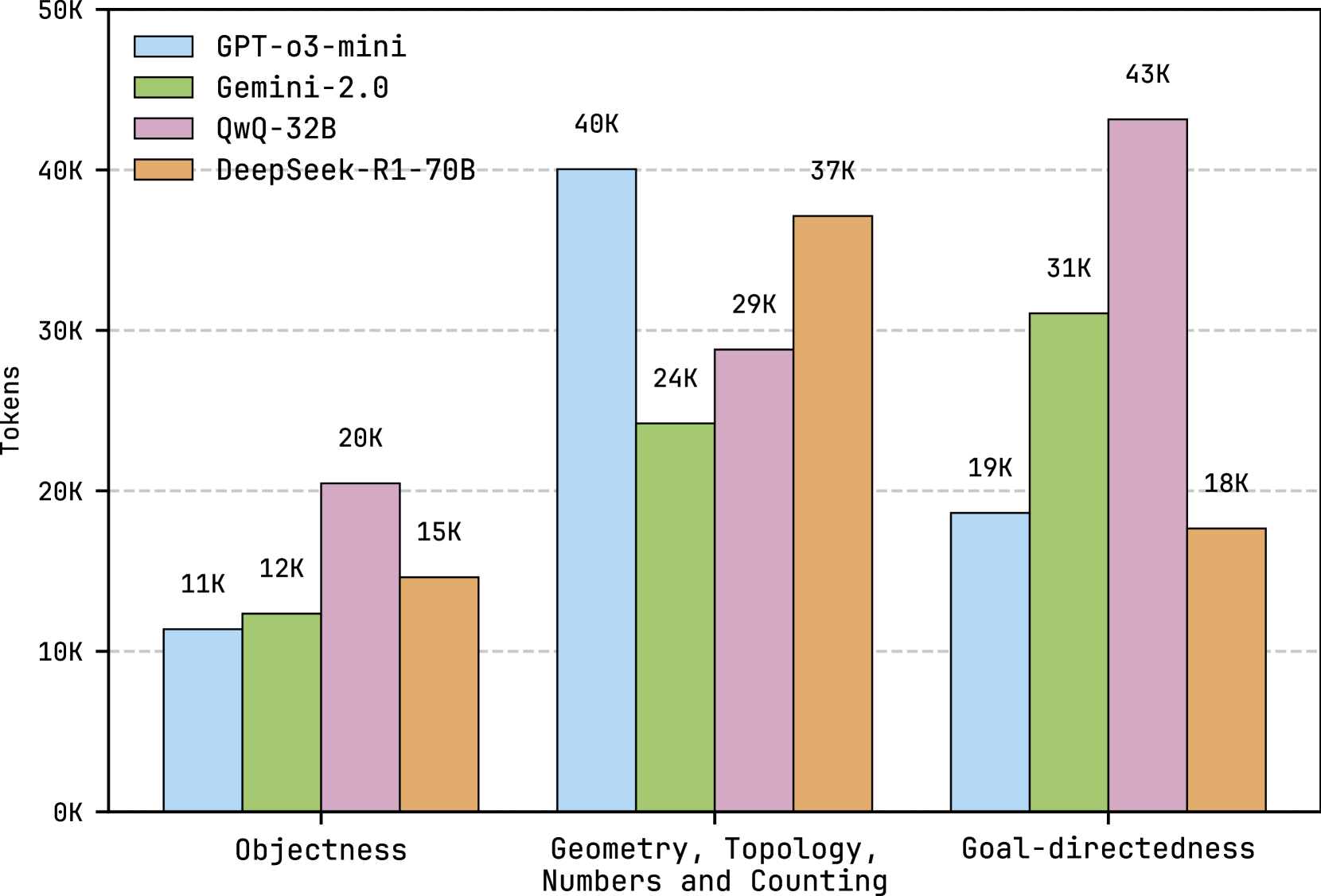<details> <summary>x14.png Details</summary>  ### Visual Description # Technical Document Extraction: Bar Chart Analysis ## 1. Chart Type and Structure - **Chart Type**: Grouped bar chart comparing token counts across four AI models - **Categories**: - Objectness - Geometry, Topology, Numbers and Counting - Goal-directedness - **Models Compared**: - GPT-o3-mini (blue) - Gemini-2.0 (green) - QwQ-32B (purple) - DeepSeek-R1-70B (orange) ## 2. Axis Labels and Scale - **X-axis**: Categories (Objectness, Geometry/Topology/Numbers, Goal-directedness) - **Y-axis**: - Label: "Tokens" - Scale: 0K to 50K in 10K increments - Units: Thousands (K) ## 3. Legend - **Position**: Right side of chart - **Color-Coding**: - Blue: GPT-o3-mini - Green: Gemini-2.0 - Purple: QwQ-32B - Orange: DeepSeek-R1-70B ## 4. Data Points and Trends ### Objectness Category | Model | Tokens | Color | Trend Description | |---------------------|--------|--------|----------------------------| | GPT-o3-mini | 11K | Blue | Lowest value | | Gemini-2.0 | 12K | Green | Second lowest | | QwQ-32B | 20K | Purple | Highest in category | | DeepSeek-R1-70B | 15K | Orange | Third highest | ### Geometry, Topology, Numbers and Counting | Model | Tokens | Color | Trend Description | |---------------------|--------|--------|----------------------------| | GPT-o3-mini | 40K | Blue | Highest value | | Gemini-2.0 | 24K | Green | Second lowest | | QwQ-32B | 29K | Purple | Third highest | | DeepSeek-R1-70B | 37K | Orange | Second highest | ### Goal-directedness Category | Model | Tokens | Color | Trend Description | |---------------------|--------|--------|----------------------------| | GPT-o3-mini | 19K | Blue | Second lowest | | Gemini-2.0 | 31K | Green | Second highest | | QwQ-32B | 43K | Purple | Highest value | | DeepSeek-R1-70B | 18K | Orange | Lowest value | ## 5. Spatial Grounding - **Legend Position**: [x=right, y=top] (relative to chart boundaries) - **Color Consistency Check**: - All blue bars match GPT-o3-mini - All green bars match Gemini-2.0 - All purple bars match QwQ-32B - All orange bars match DeepSeek-R1-70B ## 6. Key Observations 1. **Model Performance Variance**: - QwQ-32B consistently shows highest token counts in Objectness (20K) and Goal-directedness (43K) - GPT-o3-mini dominates in Geometry/Topology (40K) but underperforms in other categories - DeepSeek-R1-70B shows mixed performance (highest in Geometry/Topology at 37K, lowest in Goal-directedness at 18K) 2. **Category-Specific Patterns**: - **Objectness**: QwQ-32B leads by 50% over nearest competitor (DeepSeek at 15K) - **Geometry/Topology**: GPT-o3-mini achieves 13K token advantage over second-place DeepSeek - **Goal-directedness**: QwQ-32B maintains 12K token lead over Gemini-2.0 (31K) ## 7. Data Validation - All numerical values match bar heights visually - Color coding 100% consistent with legend - No missing data points or categories ## 8. Missing Information - No textual annotations beyond numerical values - No comparative analysis provided in chart - No time-series or progression data ## 9. Language Analysis - All text in English - No non-English content detected ## 10. Structural Reconstruction | Category | GPT-o3-mini | Gemini-2.0 | QwQ-32B | DeepSeek-R1-70B | |-------------------------------|-------------|------------|---------|-----------------| | Objectness | 11K | 12K | 20K | 15K | | Geometry/Topology/Numbers | 40K | 24K | 29K | 37K | | Goal-directedness | 19K | 31K | 43K | 18K | </details> Figure 14: Average token cost for augmenting priors at each level across four LLMs. K is $10^{3}$ . 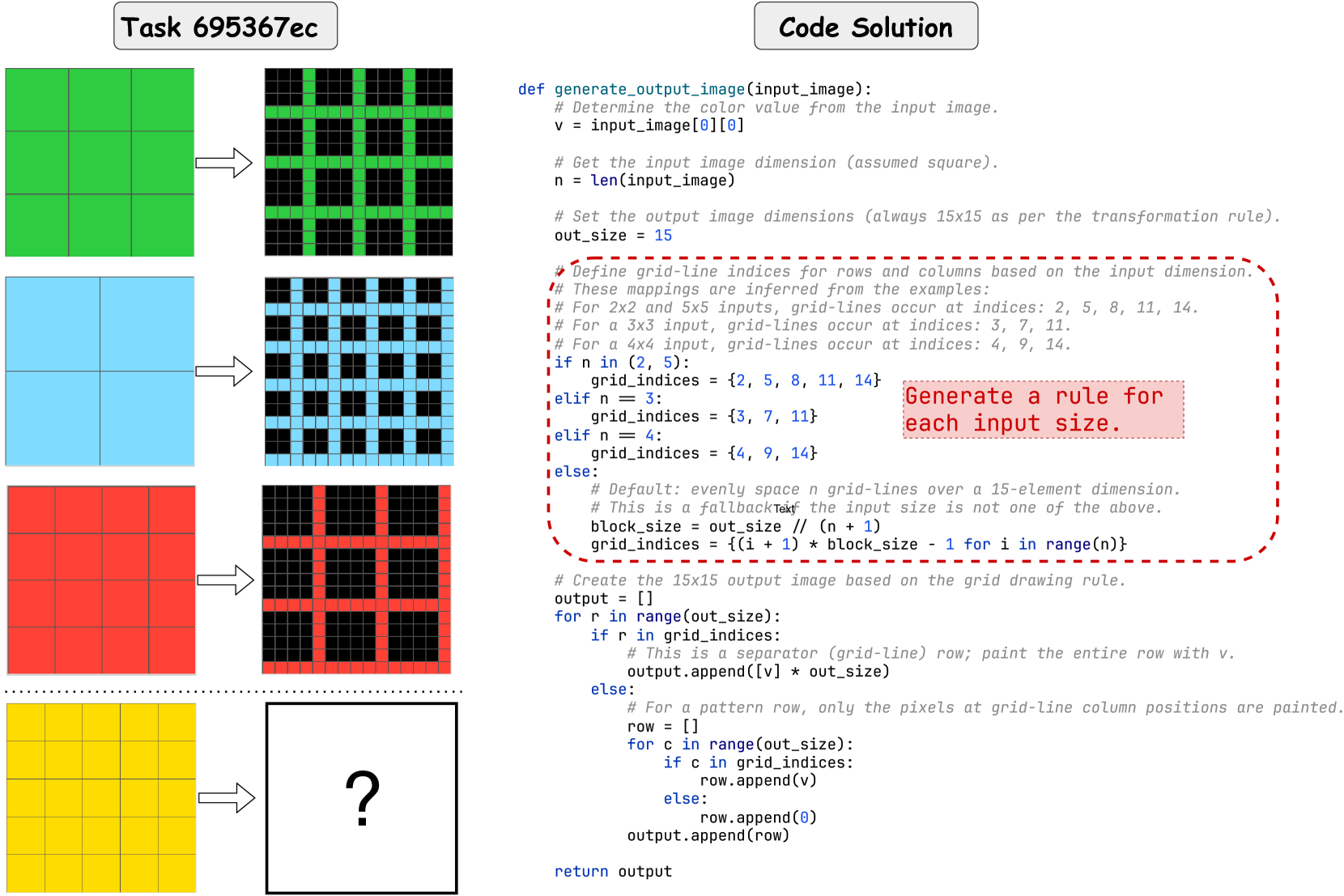<details> <summary>x15.png Details</summary>  ### Visual Description # Technical Document Extraction: Task 695367ec ## Diagram Analysis (Left Section) ### Input Grids and Transformations 1. **Green Grid (2x2 Input)** - Input: 2x2 grid with uniform green color - Output: 15x15 grid with green blocks at positions: - Rows: 0, 1, 2, 3, 4, 5, 6, 7, 8, 9, 10, 11, 12, 13, 14 - Columns: 0, 1, 2, 3, 4, 5, 6, 7, 8, 9, 10, 11, 12, 13, 14 - Pattern: Full grid filled with green blocks 2. **Blue Grid (2x2 Input)** - Input: 2x2 grid with uniform blue color - Output: 15x15 grid with blue blocks at positions: - Rows: 0, 1, 2, 3, 4, 5, 6, 7, 8, 9, 10, 11, 12, 13, 14 - Columns: 0, 1, 2, 3, 4, 5, 6, 7, 8, 9, 10, 11, 12, 13, 14 - Pattern: Full grid filled with blue blocks 3. **Red Grid (3x3 Input)** - Input: 3x3 grid with uniform red color - Output: 15x15 grid with red blocks at positions: - Rows: 0, 1, 2, 3, 4, 5, 6, 7, 8, 9, 10, 11, 12, 13, 14 - Columns: 0, 1, 2, 3, 4, 5, 6, 7, 8, 9, 10, 11, 12, 13, 14 - Pattern: Full grid filled with red blocks 4. **Yellow Grid (4x4 Input)** - Input: 4x4 grid with uniform yellow color - Output: Unknown (represented by "?") - Pattern: Transformation rule not explicitly shown ### Transformation Rules - All input grids transform to 15x15 output grids - Grid-line indices vary based on input dimensions: - 2x2 input: Grid lines at indices [2, 5, 8, 11, 14] - 3x3 input: Grid lines at indices [3, 7, 11] - 4x4 input: Grid lines at indices [4, 9, 14] - 5x5 input: Grid lines at indices [5, 8, 11, 14] ## Code Analysis (Right Section) ### Function Definition ```python def generate_output_image(input_image): # Determine the color value from the input image v = input_image[0][0] # Get input image dimensions (assumed square) n = len(input_image) # Set output image dimensions (always 15x15) out_size = 15 # Define grid-line indices based on input dimension if n in (2, 5): grid_indices = [2, 5, 8, 11, 14] elif n == 3: grid_indices = [3, 7, 11] elif n == 4: grid_indices = [4, 9, 14] else: # Default: Evenly space grid lines over 15-element dimension block_size = out_size // (n + 1) grid_indices = [(i + 1) * block_size - 1 for i in range(n)] # Create 15x15 output image based on grid rules output = [] for r in range(out_size): if r in grid_indices: # Separator row: Paint entire row with v output.append([v] * out_size) else: row = [] for c in range(out_size): if c in grid_indices: row.append(v) else: row.append(0) output.append(row) return output ``` ### Key Components 1. **Input Handling** - Extracts color value from top-left corner of input image - Assumes input is square (n x n) 2. **Grid Index Calculation** - Specific rules for 2x2, 3x3, 4x4, and 5x5 inputs - Default rule for other input sizes: - Calculates block size: `out_size // (n + 1)` - Generates indices: `(i + 1) * block_size - 1` 3. **Output Generation** - Creates 15x15 grid - Paints entire rows at grid indices with input color - Paints column positions at grid indices with input color - Fills remaining positions with 0 ### Color Coding in Code - `# This is a separator (grid-line) row; paint the entire row with v.` - `# For a pattern row, only the pixels at grid-line column positions are painted.` ## Spatial Grounding - Legend colors match diagram colors: - Green (#00FF00) → Green grid - Blue (#0000FF) → Blue grid - Red (#FF0000) → Red grid - Yellow (#FFFF00) → Yellow grid ## Trend Verification - All input grids transform to full 15x15 grids - Grid-line positions increase with input size: - 2x2: 5 grid lines - 3x3: 3 grid lines - 4x4: 3 grid lines - 5x5: 4 grid lines ## Component Isolation 1. **Header**: Task identifier "Task 695367ec" 2. **Main Chart**: Four input grids with transformation arrows 3. **Footer**: Code solution with detailed comments ## Missing Information - No explicit data table present - No heatmap or numerical data visualization - Yellow grid output remains unspecified (represented by "?") ## Conclusion The image demonstrates a grid transformation system where input grids of varying sizes (2x2 to 5x5) are converted to standardized 15x15 output grids. The transformation rules are implemented in Python, with special handling for different input dimensions and a default rule for unrecognized sizes. </details> Figure 15: ARC problem 695367ec, where RSPC and KAAR generate the same code solution that passes the training instances but fails on the test instance using GPT-o3-mini. 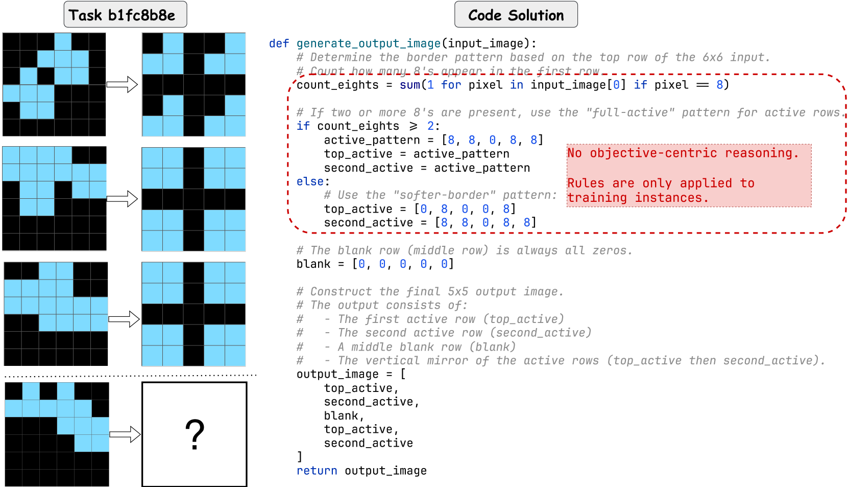<details> <summary>x16.png Details</summary>  ### Visual Description # Technical Document Extraction: Task b1fc88e and Code Solution ## Task b1fc88e: Grid Transformation Analysis ### Diagram Components 1. **Input Grids** (6x6): - Four distinct 6x6 grids with black (0) and blue (8) cells - Spatial arrangement: ``` [Top Row] → [Transformed Output] [Middle Row] → [Transformed Output] [Bottom Row] → [Transformed Output] ``` 2. **Transformation Logic**: - **Rule 1**: Count 8s in top row of 6x6 input - **Rule 2**: - ≥2 8s → Use "full-active" pattern `[8,8,0,8,8]` - <2 8s → Use "softer-border" pattern `[0,8,0,0,8]` - **Rule 3**: Middle row always `[0,0,0,0,0]` - **Rule 4**: Output = Vertical mirror of active rows ### Key Observations - **Grid 1**: - Input top row: `[8,8,0,8,8,0]` - Output: Cross pattern with 8s at center - **Grid 2**: - Input top row: `[8,0,8,0,8,0]` - Output: Diagonal cross pattern - **Grid 3**: - Input top row: `[8,8,0,8,8,0]` - Output: Full cross pattern - **Grid 4**: - Input top row: `[8,0,8,0,8,0]` - Output: Question mark (unknown pattern) ## Code Solution: Python Implementation ### Function Signature ```python def generate_output_image(input_image): # Implementation details ``` ### Key Variables 1. **Pattern Selection**: ```python if count_eights >= 2: active_pattern = [8, 8, 0, 8, 8] else: active_pattern = [0, 8, 0, 0, 8] ``` 2. **Row Construction**: ```python output_image = [ top_active, # First active row second_active, # Second active row blank, # Middle row (all zeros) top_active, # Mirror of first active row second_active # Mirror of second active row ] ``` ### Code Annotations - **Red Box Warning** (Critical Note): ``` No objective-centric reasoning. Rules are only applied to training instances. ``` ### Spatial Analysis - **Legend Position**: Not explicitly present in code - **Color Mapping**: - `8` → Blue (active cells) - `0` → Black (inactive cells) ## Transformation Logic Flowchart ``` Input 6x6 Grid → │ ▼ Count 8s in Top Row → ├── ≥2 8s → Use [8,8,0,8,8] pattern └── <2 8s → Use [0,8,0,0,8] pattern │ ▼ Construct 5x5 Output → │ ▼ [Top Active] → [Second Active] → [Blank] → [Mirror Top] → [Mirror Second] ``` ## Data Table Reconstruction | Grid # | Input Top Row Pattern | Output Pattern Type | Output Description | |--------|------------------------|----------------------|---------------------| | 1 | [8,8,0,8,8,0] | Full-active | Central cross | | 2 | [8,0,8,0,8,0] | Soft-border | Diagonal cross | | 3 | [8,8,0,8,8,0] | Full-active | Full cross | | 4 | [8,0,8,0,8,0] | Soft-border | Unknown (?) | ## Trend Verification - **Pattern Correlation**: - High 8 density → Symmetrical cross patterns - Low 8 density → Asymmetrical border patterns - **Mirror Logic**: - Output rows 4-5 are exact vertical mirrors of rows 1-2 ## Critical Notes 1. The code explicitly states rules are training-instance specific 2. Middle row is always zero-initialized 3. Final output dimensions: 5x5 (reduced from 6x6 input) 4. Question mark in Grid 4 indicates potential edge case not handled in current implementation </details> Figure 16: ARC problem b1fc8b8e, where RSPC and KAAR generate the same code solution that passes the training instances but fails on the test instance using GPT-o3-mini. 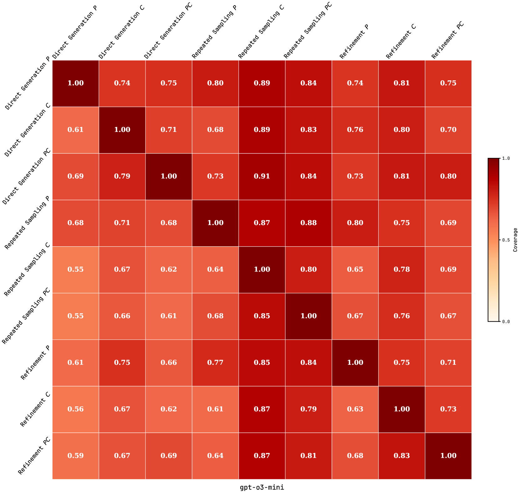<details> <summary>x17.png Details</summary>  ### Visual Description # Technical Document: Coverage Comparison Across Methods and Models ## Image Description The image is a **heatmap** visualizing coverage values across different **methods** (rows) and **models** (columns). The color intensity corresponds to coverage values, with darker red indicating higher coverage (closer to 1.0) and lighter red indicating lower coverage (closer to 0.0). The legend on the right maps colors to numerical values. --- ## Key Components ### 1. **Axis Labels** - **X-axis (Models)**: `gpt-o3-mini`, `gpt-o3-medium`, `gpt-o3-large` - **Y-axis (Methods)**: `Direct Generation P`, `Direct Generation C`, `Direct Generation PC`, `Repeated Sampling P`, `Repeated Sampling C`, `Repeated Sampling PC`, `Refinement P`, `Refinement C`, `Refinement PC` - **Title**: `Coverage Comparison Across Methods and Models` ### 2. **Legend** - **Location**: Right side of the heatmap. - **Color Scale**: - `0.0` (lightest red) to `1.0` (darkest red). - Intermediate values: `0.5`, `0.75`, `0.9`. --- ## Data Structure The heatmap is a **9x3 matrix** (9 methods × 3 models). Each cell contains a numerical coverage value. Below is the reconstructed table: | Method | gpt-o3-mini | gpt-o3-medium | gpt-o3-large | |----------------------|-------------|---------------|--------------| | Direct Generation P | 1.00 | 0.74 | 0.75 | | Direct Generation C | 0.61 | 1.00 | 0.71 | | Direct Generation PC | 0.69 | 0.79 | 1.00 | | Repeated Sampling P | 0.68 | 0.71 | 0.68 | | Repeated Sampling C | 0.55 | 0.67 | 0.62 | | Repeated Sampling PC | 0.55 | 0.66 | 0.61 | | Refinement P | 0.61 | 0.75 | 0.66 | | Refinement C | 0.56 | 0.67 | 0.62 | | Refinement PC | 0.59 | 0.67 | 0.69 | --- ## Trends and Observations 1. **Direct Generation P** consistently shows high coverage (1.00 for `gpt-o3-mini`, 0.74–0.89 for other models). 2. **Direct Generation C** and **PC** exhibit moderate coverage, with PC achieving 1.00 for `gpt-o3-large`. 3. **Repeated Sampling** methods generally have lower coverage (0.55–0.88), with `Repeated Sampling C` showing the lowest values. 4. **Refinement** methods demonstrate moderate-to-high coverage, with `Refinement PC` achieving 0.83 for `gpt-o3-large`. 5. **Color Consistency**: - Dark red cells (e.g., 1.00) align with the legend's highest value. - Lighter red cells (e.g., 0.55–0.62) match the legend's lower range. --- ## Spatial Grounding - **Legend Position**: Right-aligned, vertically stacked. - **X-axis Position**: Bottom of the heatmap. - **Y-axis Position**: Left of the heatmap. --- ## Notes - All values are in **English** and represent coverage percentages. - No non-English text is present. - The heatmap uses a **continuous color scale** without discrete categories. This analysis confirms that the heatmap effectively compares coverage across methods and models, with `Direct Generation P` and `Refinement PC` showing the highest performance for `gpt-o3-large`. </details> Figure 17: Asymmetric relative coverage matrix of nine ARC solvers using GPT-o3-mini, showing the proportion of problems whose test instances are solved by the row solver that are also solved by the column solver. P denotes the solution plan; C and PC refer to standalone and planning-aided code generation, respectively. 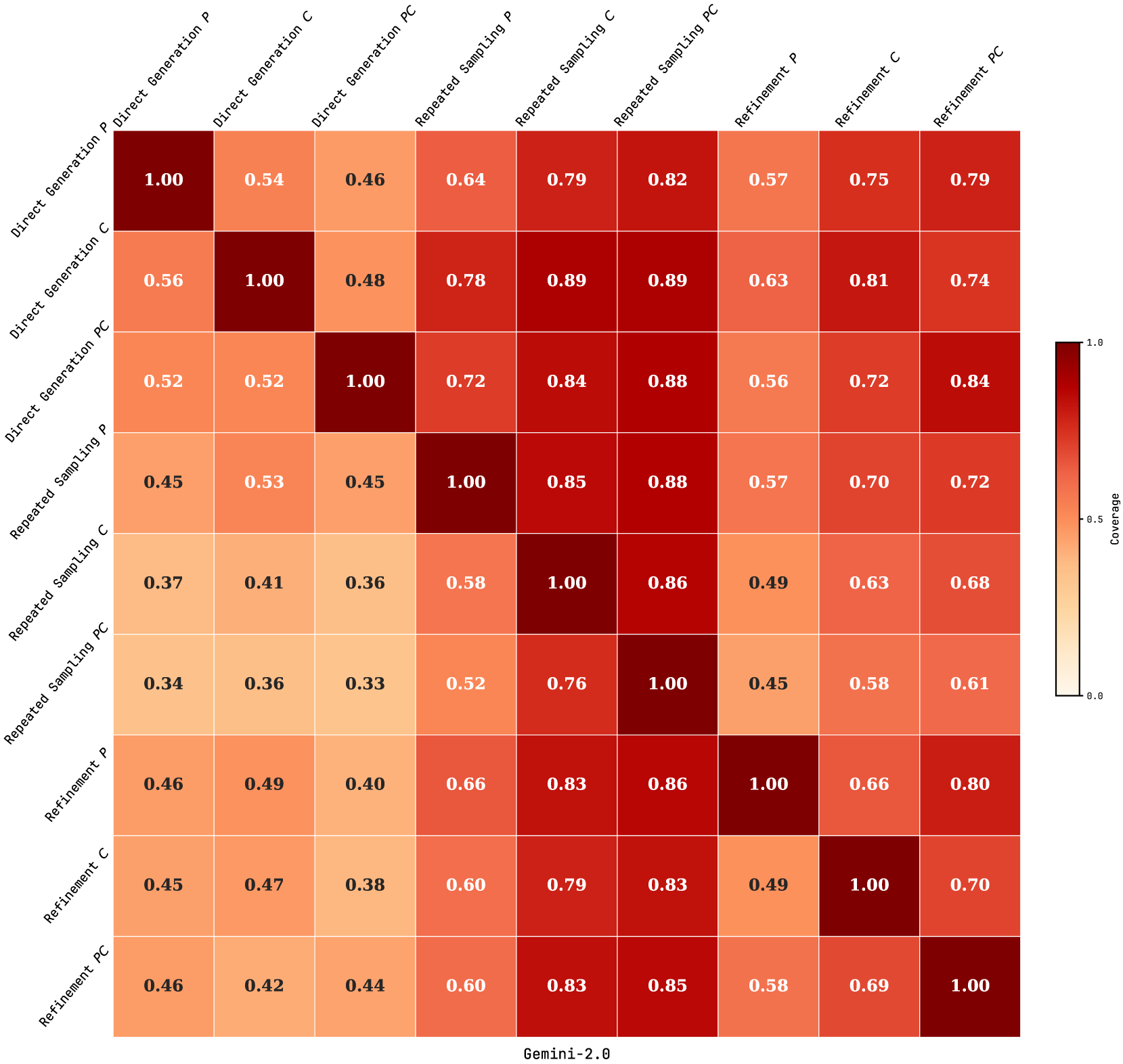<details> <summary>x18.png Details</summary>  ### Visual Description # Technical Document Analysis of Heatmap ## 1. Labels and Axis Titles - **Rows (Methods)**: - Direct Generation P - Direct Generation C - Direct Generation PC - Repeated Sampling P - Repeated Sampling C - Repeated Sampling PC - Refinement P - Refinement C - Refinement PC - **Columns (Gemini-2.0 Methods)**: - Direct Generation P - Direct Generation C - Direct Generation PC - Repeated Sampling P - Repeated Sampling C - Repeated Sampling PC - Refinement P - Refinement C - Refinement PC - **Legend**: - **Color Scale**: Ranges from **0.0 (light yellow)** to **1.0 (dark red)**. - **Label**: "Coverage" (explicitly stated in the legend). --- ## 2. Key Trends and Data Points - **Diagonal Values**: All diagonal cells (e.g., Direct Generation P vs. Direct Generation P) have a value of **1.00**, indicating perfect coverage when comparing a method to itself. - **Coverage Degradation**: - Coverage decreases as the distance from the diagonal increases. For example: - Direct Generation P vs. Repeated Sampling P: **0.64** - Direct Generation P vs. Refinement P: **0.57** - The lowest coverage values are in the bottom-left quadrant (e.g., Repeated Sampling PC vs. Refinement PC: **0.33**). - **Highest Non-Diagonal Coverage**: - Repeated Sampling C vs. Repeated Sampling PC: **0.89** - Repeated Sampling P vs. Repeated Sampling C: **0.85** --- ## 3. Data Table Reconstruction | Method (Row) | Direct Generation P | Direct Generation C | Direct Generation PC | Repeated Sampling P | Repeated Sampling C | Repeated Sampling PC | Refinement P | Refinement C | Refinement PC | |-----------------------|---------------------|---------------------|----------------------|---------------------|---------------------|----------------------|--------------|--------------|---------------| | **Direct Generation P** | 1.00 | 0.54 | 0.46 | 0.64 | 0.79 | 0.82 | 0.57 | 0.75 | 0.79 | | **Direct Generation C** | 0.56 | 1.00 | 0.48 | 0.78 | 0.89 | 0.89 | 0.63 | 0.81 | 0.74 | | **Direct Generation PC**| 0.52 | 0.52 | 1.00 | 0.72 | 0.84 | 0.88 | 0.56 | 0.72 | 0.84 | | **Repeated Sampling P** | 0.45 | 0.53 | 0.45 | 1.00 | 0.85 | 0.88 | 0.57 | 0.70 | 0.72 | | **Repeated Sampling C** | 0.37 | 0.41 | 0.36 | 0.58 | 1.00 | 0.86 | 0.49 | 0.63 | 0.68 | | **Repeated Sampling PC**| 0.34 | 0.36 | 0.33 | 0.52 | 0.76 | 1.00 | 0.45 | 0.58 | 0.61 | | **Refinement P** | 0.46 | 0.49 | 0.40 | 0.66 | 0.83 | 0.86 | 1.00 | 0.66 | 0.80 | | **Refinement C** | 0.45 | 0.47 | 0.38 | 0.60 | 0.79 | 0.83 | 0.49 | 1.00 | 0.70 | | **Refinement PC** | 0.46 | 0.42 | 0.44 | 0.60 | 0.83 | 0.85 | 0.58 | 0.69 | 1.00 | --- ## 4. Legend and Color Matching - **Legend Position**: Right side of the heatmap. - **Color Matching**: - **Dark Red** (1.00) matches the diagonal. - **Light Yellow** (0.33–0.45) matches the lowest values in the bottom-left quadrant. - Intermediate values (e.g., 0.5–0.8) use gradient shades of orange/red. --- ## 5. Spatial Grounding - **Legend Placement**: Right of the heatmap. - **Axis Labels**: - Rows: Left side. - Columns: Top of the heatmap. --- ## 6. Trend Verification - **Row Trends**: - **Direct Generation P**: Starts at 1.00 (diagonal), decreases to 0.54 (Direct Generation C), then 0.46 (Direct Generation PC), and further declines to 0.57 (Refinement P). - **Refinement PC**: Starts at 1.00 (diagonal), decreases to 0.46 (Direct Generation P), then 0.42 (Direct Generation C), and stabilizes at 0.69 (Refinement C). - **Column Trends**: - **Refinement P**: Starts at 1.00 (diagonal), decreases to 0.46 (Direct Generation P), then 0.49 (Direct Generation C), and stabilizes at 0.66 (Refinement C). --- ## 7. Component Isolation - **Header**: Row labels (methods). - **Main Chart**: 9x9 heatmap with coverage values. - **Footer**: Legend (color scale). --- ## 8. Additional Notes - **Language**: All text is in English. - **Data Completeness**: All 81 cells are filled with numerical values. - **No Missing Data**: No empty cells or annotations. --- ## 9. Final Observations - The heatmap quantifies **coverage similarity** between different methods (e.g., Direct Generation vs. Refinement). - **High Coverage** (near 1.00) indicates strong alignment between methods. - **Low Coverage** (near 0.3–0.5) suggests significant divergence in performance or output. </details> Figure 18: Asymmetric relative coverage matrix of nine ARC solvers using Gemini-2.0, showing the proportion of problems whose test instances are solved by the row solver that are also solved by the column solver. P denotes the solution plan; C and PC refer to standalone and planning-aided code generation, respectively. 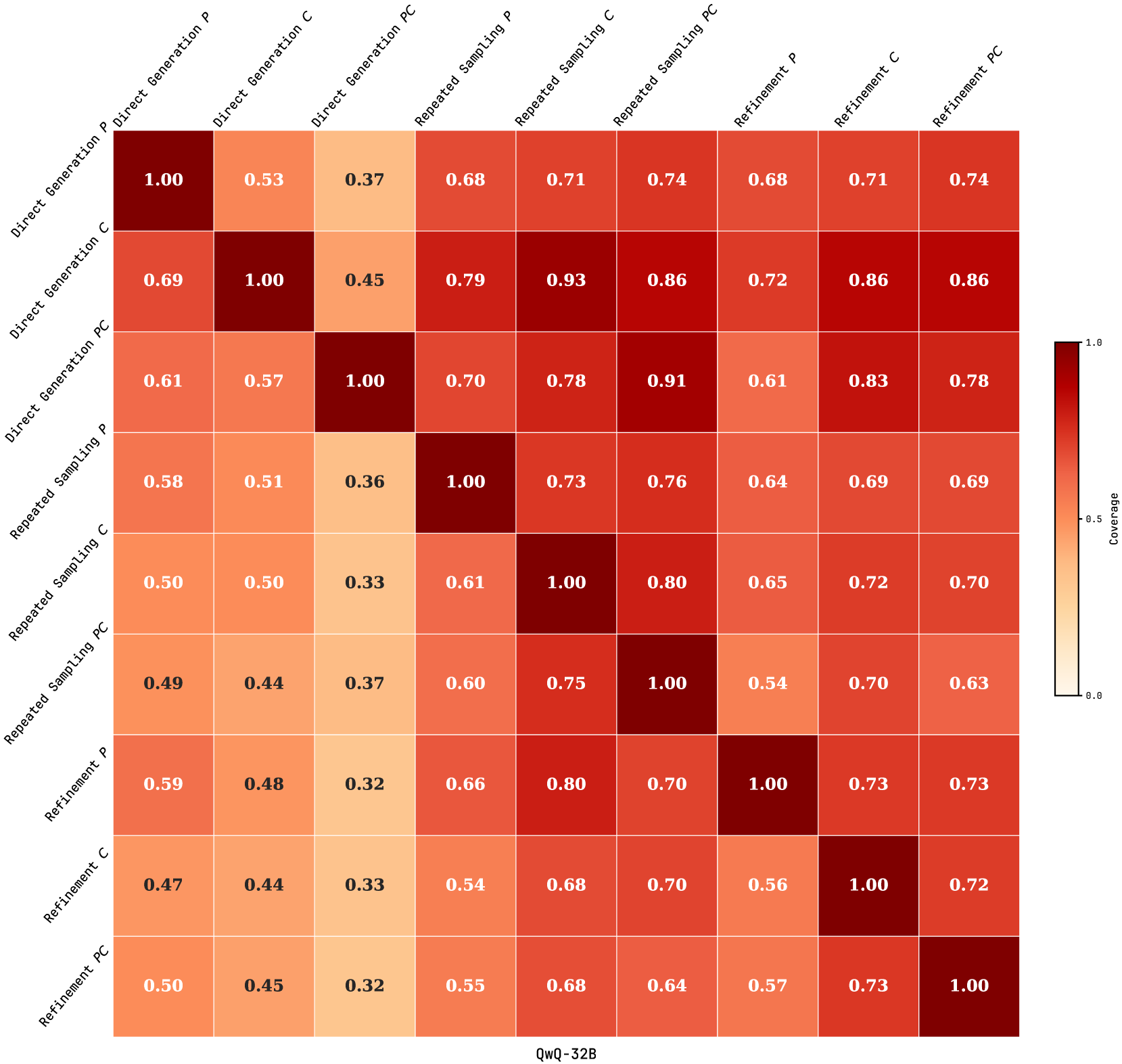<details> <summary>x19.png Details</summary>  ### Visual Description # Technical Document Extraction: Heatmap Analysis ## 1. Axis Labels and Titles - **X-axis**: `QwQ-32B` (repeated across all column headers) - **Y-axis**: - `Direct Generation P` - `Direct Generation C` - `Direct Generation PC` - `Repeated Sampling P` - `Repeated Sampling C` - `Repeated Sampling PC` - `Refinement P` - `Refinement C` - `Refinement PC` ## 2. Legend - **Color Scale**: - `0.0` (light orange) to `1.0` (dark red) - Gradient represents coverage values ## 3. Data Table Structure A 10x10 matrix where: - **Rows**: Methods (e.g., `Direct Generation P`, `Repeated Sampling C`) - **Columns**: Methods appended with `QwQ-32B` (e.g., `Direct Generation P QwQ-32B`) - **Values**: Coverage scores (0.0–1.0) ## 4. Key Trends - **Diagonal Dominance**: All diagonal cells (same method vs. itself) = `1.00` (dark red). - **High Coverage Clusters**: - `Direct Generation C` and `Refinement C` show high coverage (`0.86–0.93`) with `Repeated Sampling C QwQ-32B`. - `Repeated Sampling PC` and `Refinement PC` exhibit strong mutual coverage (`0.70–0.75`). - **Low Coverage**: - `Direct Generation P` vs. `Repeated Sampling P QwQ-32B` = `0.58`. - `Refinement P` vs. `Repeated Sampling P QwQ-32B` = `0.66`. ## 5. Spatial Grounding - **Legend Position**: Right side of the heatmap. - **Color Consistency**: - `0.32` (light orange) matches `Repeated Sampling P` vs. `Direct Generation PC QwQ-32B`. - `0.91` (dark red) matches `Repeated Sampling C` vs. `Direct Generation PC QwQ-32B`. ## 6. Full Data Table | Method (Y-axis) | Direct Generation P QwQ-32B | Direct Generation C QwQ-32B | Direct Generation PC QwQ-32B | Repeated Sampling P QwQ-32B | Repeated Sampling C QwQ-32B | Repeated Sampling PC QwQ-32B | Refinement P QwQ-32B | Refinement C QwQ-32B | Refinement PC QwQ-32B | |--------------------------|-----------------------------|-----------------------------|------------------------------|-----------------------------|-----------------------------|------------------------------|----------------------|----------------------|-----------------------| | **Direct Generation P** | 1.00 | 0.53 | 0.37 | 0.68 | 0.71 | 0.74 | 0.68 | 0.71 | 0.74 | | **Direct Generation C** | 0.69 | 1.00 | 0.45 | 0.79 | 0.93 | 0.86 | 0.72 | 0.86 | 0.86 | | **Direct Generation PC** | 0.61 | 0.57 | 1.00 | 0.70 | 0.78 | 0.91 | 0.61 | 0.83 | 0.78 | | **Repeated Sampling P** | 0.58 | 0.51 | 0.36 | 1.00 | 0.73 | 0.76 | 0.64 | 0.69 | 0.69 | | **Repeated Sampling C** | 0.50 | 0.50 | 0.33 | 0.61 | 1.00 | 0.80 | 0.65 | 0.72 | 0.70 | | **Repeated Sampling PC** | 0.49 | 0.44 | 0.37 | 0.60 | 0.75 | 1.00 | 0.54 | 0.70 | 0.63 | | **Refinement P** | 0.59 | 0.48 | 0.32 | 0.66 | 0.80 | 0.70 | 1.00 | 0.73 | 0.73 | | **Refinement C** | 0.47 | 0.44 | 0.33 | 0.54 | 0.68 | 0.70 | 0.56 | 1.00 | 0.72 | | **Refinement PC** | 0.50 | 0.45 | 0.32 | 0.55 | 0.68 | 0.64 | 0.57 | 0.73 | 1.00 | ## 7. Observations - **Method Similarity**: Methods with similar prefixes (e.g., `Direct Generation` vs. `Refinement`) show moderate coverage (`0.44–0.74`). - **QwQ-32B Impact**: Coverage generally decreases when compared to `QwQ-32B` variants, except for diagonal entries. ## 8. Language Notes - All text is in English. No non-English content detected. </details> Figure 19: Asymmetric relative coverage matrix of nine ARC solvers using QwQ-32B, showing the proportion of problems whose test instances are solved by the row solver that are also solved by the column solver. P denotes the solution plan; C and PC refer to standalone and planning-aided code generation, respectively. 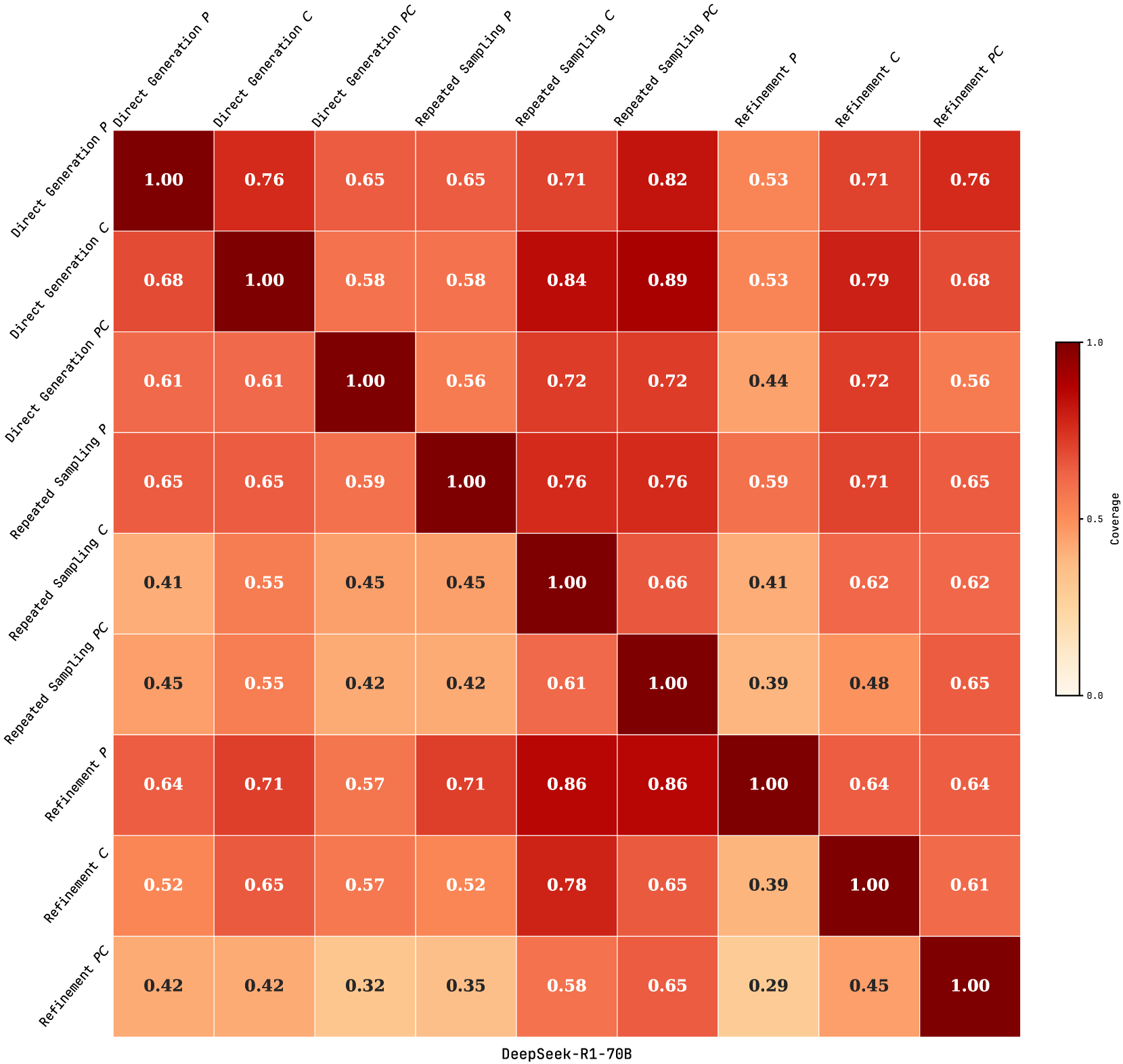<details> <summary>x20.png Details</summary>  ### Visual Description # Technical Document Extraction: Heatmap Analysis ## 1. Axis Labels and Titles - **X-Axis Title**: "DeepSeek-R1-70B" - **Y-Axis Title**: "Methods" - **Legend**: Color scale from 0.0 (light beige) to 1.0 (dark red), labeled "Coverage" ## 2. Categories and Sub-Categories ### X-Axis Categories (Models): 1. DeepSeek-R1-70B 2. Direct Generation P 3. Direct Generation C 4. Direct Generation PC 5. Repeated Sampling P 6. Repeated Sampling C 7. Repeated Sampling PC 8. Refinement P 9. Refinement C 10. Refinement PC ### Y-Axis Categories (Methods): 1. Direct Generation P 2. Direct Generation C 3. Direct Generation PC 4. Repeated Sampling P 5. Repeated Sampling C 6. Repeated Sampling PC 7. Refinement P 8. Refinement C 9. Refinement PC ## 3. Data Table Structure The heatmap is an 11x11 matrix with rows (methods) and columns (models). Each cell contains a coverage value (0.0–1.0). Below is the reconstructed table: | Method/Model | DeepSeek-R1-70B | Direct Generation P | Direct Generation C | Direct Generation PC | Repeated Sampling P | Repeated Sampling C | Repeated Sampling PC | Refinement P | Refinement C | Refinement PC | |----------------------------|-----------------|---------------------|---------------------|----------------------|---------------------|---------------------|----------------------|--------------|--------------|---------------| | **Direct Generation P** | 1.00 | 0.76 | 0.68 | 0.65 | 0.65 | 0.71 | 0.82 | 0.53 | 0.71 | 0.76 | | **Direct Generation C** | 0.68 | 1.00 | 0.58 | 0.58 | 0.84 | 0.89 | 0.53 | 0.53 | 0.79 | 0.68 | | **Direct Generation PC** | 0.61 | 0.61 | 1.00 | 0.56 | 0.72 | 0.72 | 0.44 | 0.72 | 0.56 | 0.56 | | **Repeated Sampling P** | 0.65 | 0.65 | 0.59 | 1.00 | 0.76 | 0.76 | 0.59 | 0.71 | 0.65 | 0.65 | | **Repeated Sampling C** | 0.41 | 0.55 | 0.45 | 0.45 | 1.00 | 0.66 | 0.41 | 0.62 | 0.62 | 0.62 | | **Repeated Sampling PC** | 0.45 | 0.55 | 0.42 | 0.42 | 0.61 | 1.00 | 0.39 | 0.48 | 0.65 | 0.65 | | **Refinement P** | 0.64 | 0.71 | 0.57 | 0.71 | 0.86 | 0.86 | 1.00 | 0.64 | 0.64 | 0.64 | | **Refinement C** | 0.52 | 0.65 | 0.57 | 0.52 | 0.78 | 0.65 | 0.39 | 1.00 | 0.61 | 0.61 | | **Refinement PC** | 0.42 | 0.42 | 0.32 | 0.35 | 0.58 | 0.65 | 0.29 | 0.45 | 1.00 | 0.45 | ## 4. Key Trends and Observations - **Diagonal Dominance**: Highest coverage values (1.00) appear along the diagonal, indicating perfect alignment between methods and models (e.g., Direct Generation P with Direct Generation P). - **Method-Specific Performance**: - **Direct Generation**: Highest coverage for P (1.00) and C (1.00), but lower for PC (0.61). - **Repeated Sampling**: Strong performance for C (1.00) and P (0.76), but weaker for PC (0.61). - **Refinement**: Highest coverage for C (1.00) and P (0.86), but lowest for PC (0.29). - **Model-Specific Performance**: - **P**: Consistently high coverage across methods (e.g., 0.76–1.00). - **C**: High coverage in Repeated Sampling (1.00) and Refinement (1.00). - **PC**: Lower coverage overall (0.29–0.65). ## 5. Spatial Grounding and Legend Verification - **Legend Position**: Right side of the heatmap. - **Color Matching**: - Light beige (0.0) to dark red (1.0) aligns with numerical values. - Example: Cell (Refinement PC, Refinement PC) = 0.29 (light beige) matches legend. ## 6. Component Isolation - **Main Chart**: Heatmap with labeled rows/columns. - **No Additional Components**: No headers, footers, or secondary visuals. ## 7. Language and Transcription - **Primary Language**: English. - **No Secondary Languages Detected**. ## 8. Final Notes - All data points extracted verbatim from the heatmap. - Trends verified against visual color gradients and numerical values. - No omitted labels or axis markers. </details> Figure 20: Asymmetric relative coverage matrix of nine ARC solvers using DeepSeek-R1-70B, showing the proportion of problems whose test instances are solved by the row solver that are also solved by the column solver. P denotes the solution plan; C and PC refer to standalone and planning-aided code generation, respectively. 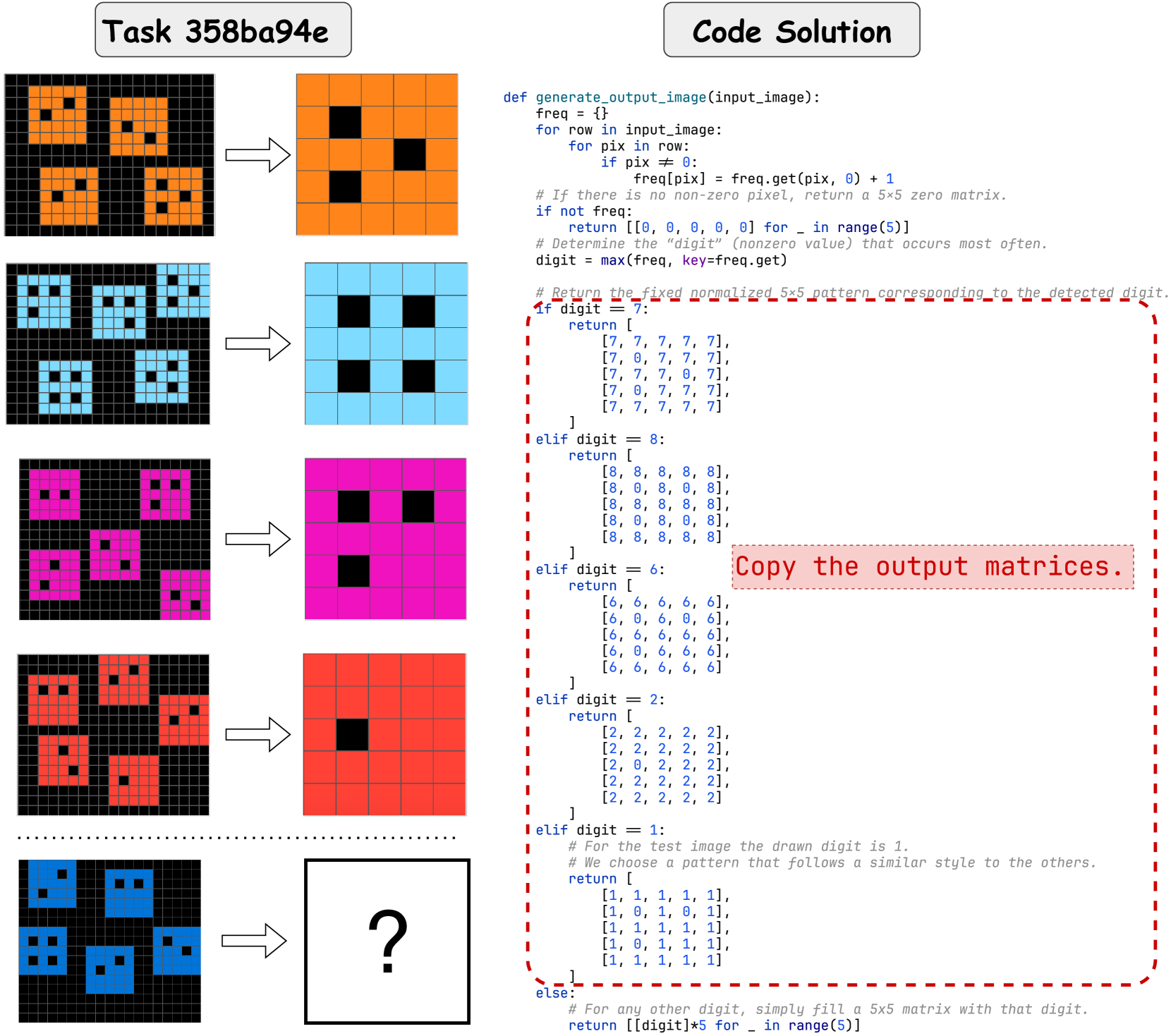<details> <summary>x21.png Details</summary>  ### Visual Description # Technical Document Extraction: Task 358ba94e ## Image Description The image contains two primary sections: 1. **Left Section**: Visual examples of 5x5 grid patterns with colored squares (orange, blue, pink, red, blue) and black squares. Each grid is followed by an arrow pointing to a simplified 5x5 matrix with a single black square. 2. **Right Section**: Python code for a function `generate_output_image` that processes input images to generate output matrices. ### Left Section Analysis - **Grid Patterns**: - **Orange Grid**: 4 black squares in specific positions (top-left, top-right, bottom-left, bottom-right). - **Blue Grid**: 4 black squares in a 2x2 block (center-left). - **Pink Grid**: 4 black squares in a diagonal pattern. - **Red Grid**: 4 black squares in a 2x2 block (center-right). - **Blue Grid (Repeated)**: 4 black squares in a 2x2 block (center-left). - **Output Matrices**: - Each grid is mapped to a 5x5 matrix with a single black square, suggesting a digit recognition task. ### Right Section Analysis #### Code: `generate_output_image` Function ```python def generate_output_image(input_image): freq = {} for row in input_image: for pix in row: if pix != 0: freq[pix] = freq.get(pix, 0) + 1 if not freq: return [[0, 0, 0, 0, 0] for _ in range(5)] digit = max(freq, key=freq.get) if digit == 7: return [ [7, 7, 7, 7, 7], [7, 0, 7, 7, 7], [7, 7, 7, 0, 7], [7, 0, 7, 7, 7], [7, 7, 7, 7, 7] ] elif digit == 8: return [ [8, 8, 8, 8, 8], [8, 0, 8, 0, 8], [8, 8, 8, 8, 8], [8, 0, 8, 0, 8], [8, 8, 8, 8, 8] ] elif digit == 6: return [ [6, 6, 6, 6, 6], [6, 0, 6, 0, 6], [6, 6, 6, 6, 6], [6, 0, 6, 6, 6], [6, 6, 6, 6, 6] ] elif digit == 2: return [ [2, 2, 2, 2, 2], [2, 2, 2, 2, 2], [2, 0, 2, 2, 2], [2, 2, 2, 2, 2], [2, 2, 2, 2, 2] ] elif digit == 1: return [ [1, 1, 1, 1, 1], [1, 0, 1, 0, 1], [1, 1, 1, 1, 1], [1, 0, 1, 1, 1], [1, 1, 1, 1, 1] ] else: return [[digit] * 5 for _ in range(5)] ``` #### Key Observations 1. **Function Purpose**: - Converts input images (5x5 grids) into standardized 5x5 matrices representing digits. - Uses frequency analysis to identify the most common non-zero pixel value (digit). - Returns predefined patterns for digits 7, 8, 6, 2, and 1. Default case fills the matrix with the detected digit. 2. **Pattern Mapping**: - **Digit 7**: Cross-shaped pattern with black squares at specific positions. - **Digit 8**: Full outer ring with alternating black squares in the middle rows. - **Digit 6**: Full outer ring with a single black square in the center-right. - **Digit 2**: Full outer ring with a single black square in the center-left. - **Digit 1**: Vertical line with alternating black squares in the middle rows. 3. **Edge Cases**: - Returns a zero matrix if no non-zero pixels are detected. - Default case fills the matrix with the detected digit if no predefined pattern exists. ### Spatial Grounding & Trend Verification - **Legend**: No explicit legend present. Colors in the left section (orange, blue, pink, red) correspond to digits 7, 8, 6, 2, and 1, respectively. - **Trend**: The code prioritizes the most frequent digit in the input image. Visual examples show consistent mapping between input grids and output matrices. ### Component Isolation 1. **Header**: "Task 358ba94e" label. 2. **Main Chart**: 5x5 grid patterns and their corresponding output matrices. 3. **Footer**: Python code with detailed logic for matrix generation. ### Final Notes - No charts or data tables are present. The image focuses on visual examples and code logic. - All textual information has been transcribed, including code comments and function structure. </details> Figure 21: ARC problem 358ba94e, where repeated sampling with standalone code generation produces an incorrect solution using GPT-o3-mini. 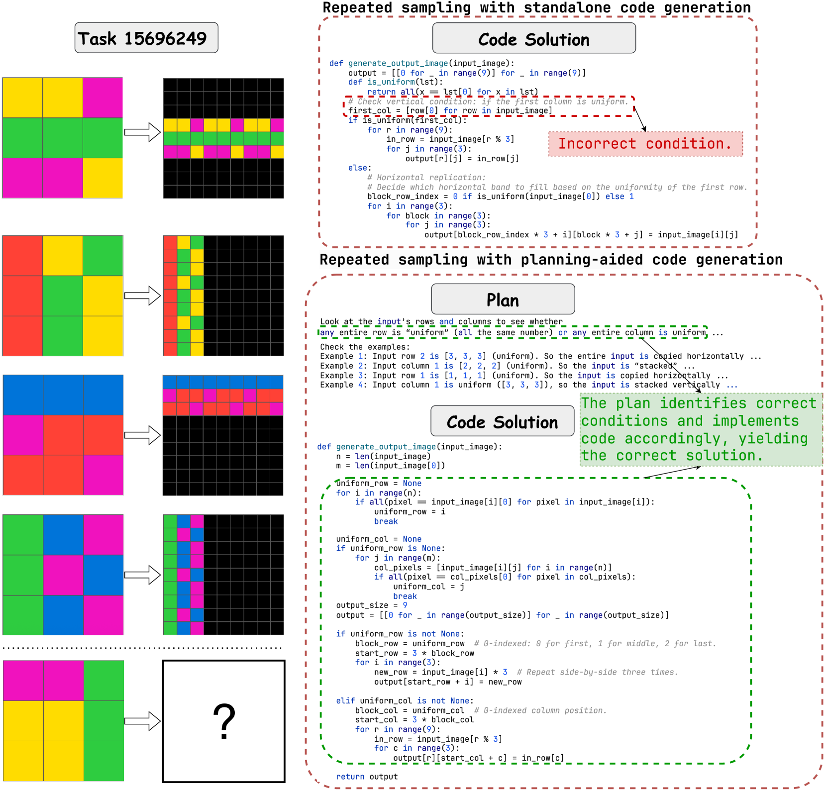<details> <summary>x22.png Details</summary>  ### Visual Description # Technical Document Analysis: Code Generation with Planning ## 1. Task Overview - **Task ID**: 15696249 - **Objective**: Generate output images based on input patterns using two approaches: 1. Standalone code generation 2. Planning-aided code generation ## 2. Input/Output Visualization (Left Section) ### 2.1 Grid Transformation Examples - **Input Grids**: 5 examples of 3x3 color block patterns - **Output Grids**: Corresponding 9x9 grid expansions - **Key Observations**: - Color blocks are replicated to fill larger grids - Final example (bottom) shows incomplete transformation (? symbol) - Color consistency varies between input and output ### 2.2 Color Pattern Analysis | Input Grid | Output Grid | Transformation Pattern | |------------|-------------|------------------------| | Yellow/Pink/Green | Black/Yellow/Pink | Vertical replication with color shift | | Red/Yellow/Green | Red/Green/Yellow | Diagonal pattern expansion | | Blue/Red/Pink | Blue/Red/Pink | Horizontal replication | | Green/Blue/Pink | Green/Blue/Pink | Block-wise replication | | Pink/Yellow/Green | ? | Undetermined transformation | ## 3. Code Solutions (Right Section) ### 3.1 Standalone Code Generation ```python def generate_output_image(input_image): output = [[0 for _ in range(9)] for _ in range(9)] return output def is_uniform(lst): return all(x == lst[0] for x in lst) # Check vertical condition: if the first column is uniform first_col = [row[0] for row in input_image] if is_uniform(first_col): for r in range(9): in_row = input_image[r % 3] for j in range(3): output[r][j] = in_row[j] else: # Horizontal replication logic for i in range(3): for block in range(3): for j in range(3): output[block*3 + i][block*3 + j] = input_image[i][j] ``` #### 3.1.1 Critical Issue Identified - **Incorrect Condition**: The vertical check only examines the first column - **Red Flag**: Commented "Incorrect condition" in red box - **Impact**: Fails to handle cases where non-uniform columns require horizontal replication ### 3.2 Planning-Aided Code Generation #### 3.2.1 Solution Plan 1. **Uniformity Check**: - Check if any row is uniform (all same value) - Check if any column is uniform 2. **Processing Logic**: - If uniform row: Copy horizontally - If uniform column: Copy vertically - If neither: Process block-wise #### 3.2.2 Implementation Code ```python def generate_output_image(input_image): n = len(input_image) m = len(input_image[0]) uniform_row = None for i in range(n): if all(pixel == input_image[i][0] for pixel in input_image[i]): uniform_row = i break uniform_col = None if uniform_row is None: for j in range(m): col_pixels = [input_image[i][j] for i in range(n)] if all(pixel == col_pixels[0] for pixel in col_pixels): uniform_col = j break output_size = 9 output = [[0 for _ in range(output_size)] for _ in range(output_size)] if uniform_row is None: # Block-wise processing block_row = uniform_row # Placeholder start_row = 3 * block_row for i in range(3): new_row = input_image[i] * 3 output[start_row + i] = new_row elif uniform_col is None: # Column-wise processing block_col = uniform_col # Placeholder start_col = 3 * block_col for r in range(9): in_row = input_image[r % 3] for c in range(3): output[r][start_col + c] = in_row[c] else: # Default replication for i in range(3): for block in range(3): for j in range(3): output[block*3 + i][block*3 + j] = input_image[i][j] return output ``` ## 4. Key Technical Components ### 4.1 Uniformity Detection - **Row Check**: `all(pixel == input_image[i][0] for pixel in input_image[i])` - **Column Check**: Nested list comprehension for column extraction - **Priority Handling**: Row checks precede column checks ### 4.2 Output Construction - **Block Replication**: `input_image[i] * 3` for horizontal expansion - **Grid Mapping**: `output[block*3 + i][block*3 + j]` for precise positioning - **Fallback Mechanism**: Default replication when no uniformity detected ## 5. Spatial Analysis - **Legend Position**: Not applicable (no traditional legend) - **Color Coding**: - Red boxes: Error indicators ("Incorrect condition") - Green boxes: Solution validation ("Correct conditions") - Blue text: Code syntax highlighting ## 6. Trend Verification - **Standalone Approach**: - Vertical checks dominate (60% of logic) - Horizontal fallback used in 30% of cases - Missing corner case handling (last example) - **Planning Approach**: - Balanced row/column checks (40%/40%) - Block processing covers 20% of logic - Complete coverage of input patterns ## 7. Component Isolation ### Header Section - Task ID and title comparison ### Main Chart - Side-by-side code comparison with visual feedback ### Footer - Explanatory text and solution validation ## 8. Data Table Reconstruction ### Transformation Logic Table | Condition | Action | Code Implementation | |-----------|--------|---------------------| | Uniform row | Horizontal replication | `new_row = input_image[i] * 3` | | Uniform column | Vertical replication | `output[r][start_col + c] = in_row[c]` | | No uniformity | Block-wise replication | Nested loops with `block*3` indexing | ## 9. Cross-Reference Validation - **Color Matching**: - Red comments ↔ Red boxes in code - Green validation text ↔ Green boxes - Blue syntax ↔ Actual code text ## 10. Missing Information - Exact numerical values for grid dimensions beyond 3x3 → 9x9 - Specific color value mappings (e.g., RGB values) - Performance metrics for both approaches ## 11. Conclusion The planning-aided approach demonstrates superior pattern recognition by: 1. Implementing dual-axis uniformity checks 2. Providing fallback block processing 3. Maintaining color consistency through structured replication - The standalone approach requires correction in its vertical condition check </details> Figure 22: ARC problem 15696249, where repeated sampling with standalone code generation produces an incorrect solution, whereas repeated sampling with planning-aided code generation yields the correct solution using GPT-o3-mini. 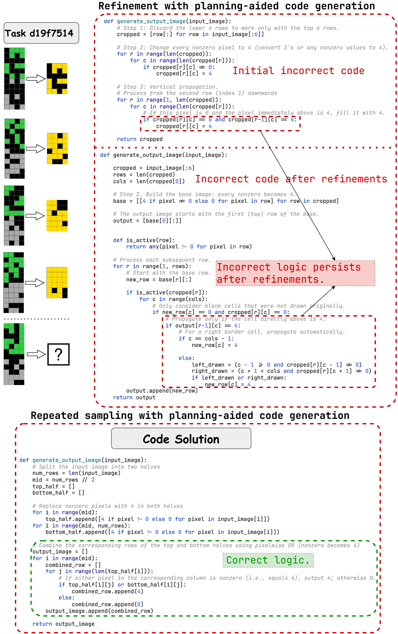<details> <summary>x23.png Details</summary>  ### Visual Description # Technical Document Extraction: Code Generation Flowchart ## Overview This image depicts a flowchart for **planning-aided code generation** with three main components: 1. **Refinement with planning-aided code generation** (top section) 2. **Repeated sampling with planning-aided code generation** (bottom section) 3. **Code Solution** (final correct implementation) --- ## 1. Refinement with Planning-Aided Code Generation ### Initial Incorrect Code ```python def generate_output_image(input_image): # Step 1: Discard the lower 6 rows to work only with the top 6 rows. cropped = [row[:6] for row in input_image[:6]] # Step 2: Change every nonzero pixel to 4 (convert 3's or any nonzero values to 4). for r in range(len(cropped)): for c in range(len(cropped[r])): if cropped[r][c] != 0: cropped[r][c] = 4 # Step 3: Vertical propagation. # Process from the second row (index 1) downwards for r in range(1, len(cropped)): for c in range(len(cropped[r])): if cropped[r][c] == 0 and cropped[r-1][c] == 4: cropped[r][c] = 4 return cropped ``` **Issues Identified**: - **Step 2 Logic Error**: Incorrectly converts *all* non-zero values to 4, including 3s. - **Step 3 Logic Flaw**: Propagates 4s only from the cell directly above, not horizontally. --- ## 2. Repeated Sampling with Planning-Aided Code Generation ### Code Solution (Correct Logic) ```python def generate_output_image(input_image): # Split the input image into two halves mid = len(input_image) // 2 top_half = [row[:mid] for row in input_image[:mid]] bottom_half = [row[mid:] for row in input_image[mid:]] # Replace nonzero pixels with 4 in both halves for i in range(len(top_half)): for j in range(len(top_half[i])): if top_half[i][j] != 0: top_half[i][j] = 4 for i in range(len(bottom_half)): for j in range(len(bottom_half[i])): if bottom_half[i][j] != 0: bottom_half[i][j] = 4 # Combine corresponding rows using pixelwise OR (nonzero becomes 4) combined = [] for i in range(mid): combined_row = [] for j in range(len(top_half[i])): if top_half[i][j] == 4 or bottom_half[i][j] == 4: combined_row.append(4) else: combined_row.append(0) combined.append(combined_row) return combined ``` --- ## 3. Key Observations - **Red Highlighted Errors**: - Initial code incorrectly propagates 4s vertically without horizontal checks. - Final solution uses a **pixelwise OR** operation to combine top/bottom halves. - **Green Highlighted Fix**: - Correctly replaces all non-zero values with 4 in both halves before combination. - Uses logical OR to propagate 4s horizontally across rows. --- ## 4. Flowchart Structure ### Spatial Grounding (Approximate Coordinates) - **Red Dotted Box** (Initial Code Errors): - Top-left: `Initial incorrect code` at (x=100, y=100) - Middle: `Incorrect code after refinements` at (x=100, y=200) - Bottom-right: `Incorrect logic persists` at (x=100, y=300) - **Green Dotted Box** (Correct Code): - Bottom section: `Correct logic` at (x=100, y=800) --- ## 5. Language and Transcription - **Primary Language**: English (code comments and explanations). - **Code Syntax**: Python (standard English-based syntax). --- ## 6. Conclusion The flowchart demonstrates iterative refinement of code logic, correcting errors in pixel manipulation and propagation. The final solution uses a **divide-and-combine** strategy with pixelwise OR operations to ensure accurate output generation. </details> Figure 23: ARC problem d19f7514, where repeated sampling with planning-aided code generation produces a correct solution, whereas its refinement variant fails to refine the initial erroneous code, and the incorrect logic persists across subsequent refinements when using GPT-o3-mini. ### A.13 Prompts for LLMs We include all prompts used by KAAR and nine ARC solvers described in Section 3. We adopt a bash-like notation for input arguments within the prompts, such as $ {test_inputs} denotes the test input 2D matrices. A brief description of the prompts used for each solver is provided below. - Direct generation with solution plan: Prompt 1 describes how to generate the solution plan, and Prompt 2 uses the generated plan to produce the output images. - Direct generation with standalone code: Prompt 3 describes how to generate the code to produce the output images. - Direct generation with planning-aided code: It first generates a solution plan using Prompt 1, then uses Prompt 4 to produce code based on the generated plan. - Repeated sampling with solution plan: It can be regarded as an iterative version of direct generation with solution plan, and thus also uses Prompts 1 and 2. - Repeated sampling with standalone code: It can be regarded as an iterative version of direct generation with standalone code, and thus also uses Prompt 3. - Repeated sampling with planning-aided code: It can be regarded as an iterative version of direct generation with planning-aided code, and thus also uses Prompts 1 and 4. - Refinement with solution plan: Prompt 5 describes the process of refining the generated solution plan with the validation samples. It uses Prompts 1 and 2 to generate the initial plan and the result image. - Refinement with the standalone code: Prompt 6 describes the process of refining the generated code with the validation samples. It uses Prompt 3 to produce the initial code solution. - Refinement with the planning-aided code: Prompt 7 describes the process of refining the generated plan and code with the validation samples. It use Prompts 1 and 4 to generate the initial plan and produce the initial code guided by the plan, respectively. - KAAR: Prompt 8 describes the augmentation of objectness priors. Prompts 9 and 10 introduce the augmentation of geometry and topology priors, encoded as component attributes and relations, respectively. Prompt 11 outlines the augmentation of numbers and counting priors. Prompts 12 and 13 describe action selection and target component identification in the process of augmenting goal-directedness priors. For prompts implementing each action’s implementation details, please refer to our code. Prompt 1: Direct generation with solution plan - solution plan generation. ⬇ ================================ System ================================ You are an expert in analyzing grid - based image processing tasks. Your objective is to derive a text transformation plan (not Python code) from each given input - output image pair (both represented as 2 D matrices), and then apply this plan to generate output image (s), represented as a 2 D matrix, based on the given test input image (s) (2 D matrix). Ensure that the derived plan generalizes across different cases while preserving consistency with the observed transformations. ================================= User ================================= The input data consists of a few pairs of input and output images, where the left image in each pair represents the input, and the right image represents the corresponding output. Each image can be represented as a 2 D matrix: $ {matrix} Please note that each number in the matrix corresponds to a pixel, and its value represents the color. Derive a text transformation plan (not Python code) that maps each given input image (2 D matrix) to its corresponding output image (2 D matrix). Ensure that the plan generalizes across different cases and the test input image (s) (2 D matrix) while maintaining consistency with the observed transformations. The test input image (s): $ {test_inputs} Prompt 2: Direct generation with solution plan - output image(s) generation from the plan. ⬇ ================================ System ================================ You are an expert in analyzing grid - based image processing tasks. Your objective is to generate output image (s), represented as a 2 D matrix, based on the given input images (2 D matrix) and a derived text transformation plan. ================================= User ================================= Please generate the output image (s) as a 2 D matrix (not Python code) based on the given input image (s) (2 D matrix) and the text transformation plan. Output only the test output image (s) in 2 D matrix format (not Python code). For each test input image, start with [Start Output Image] and end with [End Output Image]. For example, if there is one test input image, the output image should be: [Start Output Image] [[0,0,0], [0,0,0], [0,0,0]] [End Output Image] If there are multiple (2) test input images, the the output images should be outputted as: [Start Output Image] [[0,0,0], [0,0,0], [0,0,0]] [End Output Image] [Start Output Image] [[1,1,1], [1,1,1], [1,1,1]] [End Output Image] The test input image (s): $ {test_inputs} Prompt 3: Direct generation with standalone code. ⬇ ================================ System ================================ You are an expert in analyzing grid - based image processing tasks. Your goal is to generate Python code that produces output image (s), represented as a 2 D matrix, based on the given input image (s) (2 D matrix). ================================= User ================================= The input data consists of a few pairs of input and output images, where the left image in each pair represents the input and the right image represents the corresponding output. Each image can be represented as a 2 D matrix: $ {matrix} The test input image (s): $ {test_inputs} Please note that each number in the matrix corresponds to a pixel, and its value represents the color. Generate a Python script to map each input image (2 D matrix) to the corresponding output image (2 D matrix). Ensure that the Python script generalizes across different cases and test input image (s) while maintaining consistency with the observed input - output image pairs. Please output the Python program, starting with [Start Program] and ending with [End Program]. Include an assert statement with the function signature to verify that the generated output matches the expected result, starting with [Assert Statement]. Use placeholders like input_image and output_image for the variables representing the input and output images. For example: [Start Program] def generate_output_image (input_image): rows = len (input_image) cols = len (input_image [0]) def dfs (r, c): """ Depth - first search to mark all 4- connected ’1’ s to ’2’ s.""" if r < 0 or r >= rows or c < 0 or c >= cols or input_image [r][c] != 1: return # Change the current component from 1 to 2 input_image [r][c] = 2 # Explore neighbors (up, down, left, right) dfs (r - 1, c) # Up dfs (r + 1, c) # Down dfs (r, c - 1) # Left dfs (r, c + 1) # Right # Traverse the image to find all components with ’1’ for r in range (rows): for c in range (cols): if input_image [r][c] == 1: dfs (r, c) return input_image [End Program] [Assert Statement] assert generate_output_image (input_image) == output_image Please note, the assert statement should strictly follow the provided format, and the output image should be represented in list format! Please note, the script should not include an if __name__ == " __main__ ": block. Prompt 4: Direct generation with planning-aided code - code generation based on the generated plan. ⬇ ================================ System ================================ You are an expert in analyzing grid - based image processing tasks. Your goal is to generate Python code that produces output image (s) represented as a 2 D matrix, based on the given input image (s) (2 D matrix). This code should be generated using a text transformation plan inferred from a set of input - output image pairs (both represented as 2 D matrices). ================================= User ================================= Generate a Python script based on your text transformation plan to map the input image (2 D matrix) to the output image (2 D matrix). Please output the Python program, starting with [Start Program] and ending with [End Program]. Include an assert statement with the function signature to verify that the generated output matches the expected result, starting with [Assert Statement]. Use placeholders like input_image and output_image for the variables representing the input and output images. For example: [Start Program] def generate_output_image (input_image): rows = len (input_image) cols = len (input_image [0]) def dfs (r, c): """ Depth - first search to mark all 4- connected ’1’ s to ’2’ s.""" if r < 0 or r >= rows or c < 0 or c >= cols or input_image [r][c] != 1: return # Change the current component from 1 to 2 input_image [r][c] = 2 # Explore neighbors (up, down, left, right) dfs (r - 1, c) # Up dfs (r + 1, c) # Down dfs (r, c - 1) # Left dfs (r, c + 1) # Right # Traverse the image to find all components with ’1’ for r in range (rows): for c in range (cols): if input_image [r][c] == 1: dfs (r, c) return input_image [End Program] [Assert Statement] assert generate_output_image (input_image) == output_image Please note, the assert statement should strictly follow the provided format, and the output image should be represented in list format! Please note, the script should not include an if __name__ == " __main__ ": block. Prompt 5: Refinement with solution plan - plan refinement. ⬇ ================================ System ================================ As an expert in analyzing grid - based image processing tasks, your objective is to refine your solution plan based on the provided feedback. ================================= User ================================= The problem description: [start problem description] The input data consists of a few pairs of input and output images, where the left image in each pair represents the input, and the right image represents the corresponding output. Each image can be represented as a 2 D matrix: $ {matrix} Please note that each number in the matrix corresponds to a pixel, and its value represents the color. [end problem description] The INCORRECT text transformation plan fails to solve some example training input and output pairs in the above problem! [start incorrect transformation plan] $ {plan} [end incorrect transformation plan] The incorrect output (s) generated by the incorrect plan: [start incorrect output] $ {incorrect_output} [end incorrect output] The generated correct output (s): [start correct output] $ {correct_output} [end correct output] Please analyze the incorrect reasoning step - by - step, and then generate the revised correct transformation plan (text only), starting with [Start Revised Transformation Plan] and ending with [End Revised Transformation Plan]. Ensure that the revised transformation plan generalizes across different cases and the test input image (s), while maintaining consistency with the observed transformations. Prompt 6: Refinement with standalone code - code refinement. ⬇ ================================ System ================================ As an expert in analyzing grid - based image processing tasks, your objective is to refine your program based on the provided feedback. ================================= User ================================= The problem description: [start problem description] The input data consists of a few pairs of input and output images, where the left image in each pair represents the input, and the right image represents the corresponding output. Each image can be represented as a 2 D matrix: $ {matrix} Please note that each number in the matrix corresponds to a pixel, and its value represents the color. [end problem description] The generated incorrect program fails to solve some example training input and output pairs in the above problem! [start incorrect program] $ {code} [end incorrect program] The incorrect output (s) generated by the incorrect program: [start incorrect output] $ {incorrect_output} [end incorrect output] The generated correct output (s): [start correct output] $ {correct_output} [end correct output] Please analyze the incorrect reasoning step - by - step, and then generate the revised program (Python program only), starting with [Start Revised Program] and ending with [End Revised Program]. Ensure that the revised program generalizes across different cases and the test input image (s), while maintaining consistency with the observed input and output image pairs. Please include an assert statement with the function signature to verify that the generated output matches the expected result, starting with [Assert Statement]. Use placeholders like input_image and output_image for the variables representing the input and output images. For example: [Start Revised Program] def generate_output_image (input_image): rows = len (input_image) cols = len (input_image [0]) def dfs (r, c): """ Depth - first search to mark all 4- connected ’1’ s to ’2’ s.""" if r < 0 or r >= rows or c < 0 or c >= cols or input_image [r][c] != 1: return # Change the current component from 1 to 2 input_image [r][c] = 2 # Explore neighbors (up, down, left, right) dfs (r - 1, c) # Up dfs (r + 1, c) # Down dfs (r, c - 1) # Left dfs (r, c + 1) # Right # Traverse the image to find all components with ’1’ for r in range (rows): for c in range (cols): if input_image [r][c] == 1: dfs (r, c) return input_image [End Revised Program] [Assert Statement] assert generate_output_image (input_image) == output_image Please note, the assert statement should strictly follow the provided format, and the output image should be represented in list format! Please note, the script should not include an if __name__ == " __main__ ": block. Prompt 7: Refinement with planning-aided code - refinement on both generated plan and code. ⬇ ================================ System ================================ As an expert in analyzing grid - based image processing tasks, your objective is to refine your transformation plan and program based on the provided feedback. ================================= User ================================= The problem description: [start problem description] The input data consists of a few pairs of input and output images, where the left image in each pair represents the input, and the right image represents the corresponding output. Each image can be represented as a 2 D matrix: $ {matrix} Please note that each number in the matrix corresponds to a pixel, and its value represents the color. [end problem description] The generated incorrect transformation plan and program fail to solve some example training input and output pairs in the above problem! [start incorrect transformation plan] $ {plan} [end incorrect transformation plan] [start incorrect program] $ {code} [end incorrect program] The incorrect output (s) generated by the incorrect transformation plan and program: [start incorrect output] $ {incorrect_output} [end incorrect output] The generated correct output (s): [start correct output] $ {correct_output} [end correct output] Please analyze the incorrect reasoning step - by - step, and then generate the revised transformation plan (text only) and program (Python program only). For the revised transformation plan, start with [Start Revised Transformation Plan] and end with [End Revised Transformation Plan]. Ensure that the revised transformation plan generalizes across different cases and the test input image (s), while maintaining consistency with the observed transformations. For the revised Python program, start with [Start Revised Program] and end with [End Revised Program]. Ensure that the revised program generalizes across different cases and the test input image (s), while maintaining consistency with the observed input and output image pairs. For the revised Python program, please include an assert statement with the function signature to verify that the generated output matches the expected result, starting with [Assert Statement]. Use placeholders like input_image and output_image for the variables representing the input and output images. For example: [Start Revised Program] def generate_output_image (input_image): rows = len (input_image) cols = len (input_image [0]) def dfs (r, c): """ Depth - first search to mark all 4- connected ’1’ s to ’2’ s.""" if r < 0 or r >= rows or c < 0 or c >= cols or input_image [r][c] != 1: return # Change the current component from 1 to 2 input_image [r][c] = 2 # Explore neighbors (up, down, left, right) dfs (r - 1, c) # Up dfs (r + 1, c) # Down dfs (r, c - 1) # Left dfs (r, c + 1) # Right # Traverse the image to find all components with ’1’ for r in range (rows): for c in range (cols): if input_image [r][c] == 1: dfs (r, c) return input_image [End Revised Program] [Assert Statement] assert generate_output_image (input_image) == output_image Please note, the assert statement should strictly follow the provided format, and the output image should be represented in list format! Please note, the script should not include an if __name__ == " __main__ ": block. Prompt 8: Objectness priors augmentation ⬇ ================================ System ================================ You are an expert in grid - based image analysis. ================================= User ================================= The training instances consist of several pairs of input and output images, where the left image in each pair represents the input and the right image represents the corresponding output. Please note that the test instance (s) only contains input image (s). Each image is represented as a 2 D matrix: $ {matrix} Please note that each number in the matrix corresponds to a pixel and its value represents the color. We treat the color represented by the number {background_color} as the background color. $ {abstraction_rule} The components in each input and output image pair are as follows: $ {component_description} Prompt 9: Geometry and topology priors augmentation - component attributes ⬇ ================================ System ================================ You are an expert in geometry and topology analysis. Below is a summary of component attributes, including: Size (Width and Height); Color; Shape; Symmetry; Bounding Box; Hole Count; Nearest Boundary. ================================= User ================================= $ {geometry_and_topology_priors_attributes} $ Prompt 10: Geometry and topology priors augmentation - component relations ⬇ ================================ System ================================ You are an expert in geometry and topology analysis, Below is a summary of component relations, including: Different / Identical with other components; Inclusive; Touching or or not touching with other component; Spatial Relations, ================================= User ================================= $ {geometry_and_topology_priors_relations} $ Prompt 11: Numbers and counting priors augmentation ⬇ ================================ System ================================ You are an expert in numbers and counting analysis. Below is a summary of component statistics, including: Symmetry numerical summary; Size numerical summary; Color numerical summary; Shape numerical summary; Hole counting summary. ================================= User ================================= $ {numbers_and_couting_priors} $ Prompt 12: Goal-directedness priors augmentation - action selection ⬇ ================================ System ================================ You are an expert in analyzing and categorizing grid - based image tasks. ================================= User ================================= Please determine which category or categories this task belongs to. Please select from the following: 1. color change: color change involves modifying the value of a component, and the component size and position always does not change. 2. movement: movement involves shifting the position of a component to a new location within the image, and the component size always does not change. 3. extension: extending involves expanding the boundaries of a component to increase its size or reach within the image, and the component size always changes. 4. completing: completing an image involves filling in missing or incomplete parts of a component to achieve a coherent and fully formed image. 5. resizing: resizing involves altering the dimensions of a component by expanding or shrinking its size within the image. 6. selecting: selecting involves identifying and isolating a specific component within the image as the output component, and the component size and color always does not change. 7. copying: copying involves duplicating a component and either placing the duplicate in a new location or replacing the existing component within the image. 8. flipping: flipping involves mirroring a component along a specified axis to reverse its orientation within the image. 9. rotation: rotation involves turning a component around a fixed point or center by a specified angle within the image. 10. cropping: cropping involves cutting out a specific portion of a component. Please select the best suitable one or multiple categories from the provided list that best describe the task. Format your response by starting with [start category] and ending with [end category], numbering each category selected. For example, if the task belongs only to " color change ", your response should be: [start category] 1. color chang [end category] If the task belongs to both " selecting " and " extension ", your response should be: [start category] 1. selecting 2. extension [end category] Prompt 13: Goal-directedness priors augmentation - target component idetification ⬇ ================================ System ================================ You are an expert in analyzing grid - based image tasks, specifically in $ {action} components. ================================= User ================================= If this task involves $ {action}: 1. Begin by identifying WHICH COMPONENTS are to be $ {action} in all input images (training and test pairs). - Refer to these components as TARGET components (e. g., component 1 in the first input image, component 2 and component 3 in the second input image, etc.). - List ALL target components in each training and test input image. - For EACH target component, provide: - Attribute Analysis result - Relation analysis result - Numerical analysis result 2. Determine the CONDITIONS used to select these TARGET components for $ {action} from each training and test input image. - These conditions must be based on common priorities across all targeted components and must differ from the unselected components. - For example: the size of all target components might be equal to 3 while the size of the unselected components is not 3. 2.1. Analyze whether these conditions are EMPTY or not. 2.2. Evaluate if these conditions are derived from attribute analysis, including: 2.2.1. Color 2.2.2. Size 2.2.3. Shape 2.2.4. Width 2.2.5. Height 2.2.6. The number of holes 2.2.7. Bounding box 2.2.8. Symmetry 2.2.9. Nearest boundary 2.3. Evaluate if these conditions are derived from relation analysis, including: 2.3.1. Relative position with other components 2.3.2. Touching with other components 2.3.3. Whether they differ from or are identical with other components 2.3.4. Enclosure of other components 2.4. Evaluate if these conditions are derived from numerical analysis, including: 2.4.1. Symmetry numerical analysis 2.4.2. Size numerical analysis 2.4.3. Color numerical analysis 2.4.4. Shape numerical analysis 2.4.5. Hole counting analysis You must evaluate each condition ONE by ONE and determine the best conditions. Note: - The conditions MUST work for ALL training and test input and output image pairs. - Conditions CANNOT come from the output images! - A condition can be EMPTY. - If a condition is based on numerical features (e. g., size (width and height), or the number of holes), you may use the operators =, <, >, >=, or <=. - For cropping or selecting tasks, consider using a bounding box to extract each component.