2505.17826v3

# : A General-Purpose and Unified Framework for Reinforcement Fine-Tuning of Large Language Models **Authors**: Alibaba Group Abstract Trinity-RFT is a general-purpose, unified and easy-to-use framework designed for reinforcement fine-tuning (RFT) of large language models. It is built with a modular and decoupled design, consisting of (1) an RFT-core that unifies and generalizes synchronous/asynchronous, on-policy/off-policy, and online/offline modes of RFT; (2) seamless integration for agent-environment interaction with high efficiency and robustness; and (3) systematic data pipelines optimized for RFT. Trinity-RFT can be easily adapted for diverse application scenarios, and serves as a unified platform for development and research of advanced reinforcement learning paradigms at both macroscopic and microscopic levels. This technical report outlines the vision, features, design and implementations of Trinity-RFT, accompanied by extensive examples, applications and experiments that demonstrate its functionalities and user-friendliness. footnotetext: Equal contribution. footnotetext: Corresponding author. {chenyanxi.cyx,panxuchen.pxc,daoyuanchen.cdy,yaliang.li,bolin.ding}@alibaba-inc.com GitHub: https://github.com/modelscope/Trinity-RFT Documentation: https://modelscope.github.io/Trinity-RFT Note: Trinity-RFT is currently under active development. This technical report corresponds to commit id 63d4920 (July 14, 2025) of the GitHub repository, and will be continuously updated as the codebase evolves. Comments, suggestions and contributions are welcome! 1 Introduction Reinforcement learning (RL) has achieved remarkable success in the development of large language models (LLMs). Examples include aligning LLMs with human preferences via reinforcement learning from human feedback (RLHF) [24], and training long-CoT reasoning models via RL with rule-based or verifiable rewards (RLVR) [5, 35]. However, such approaches are limited in their abilities to handle dynamic, agentic and continuous learning in the real world. We envision a future where AI agents learn by interacting directly with environments, collecting lagged or complex reward signals, and continuously refining their behavior through RL based on the collected experiences [32]. For example, imagine an AI scientist who designs an experiment, executes it, waits for feedback (while working on other tasks concurrently), and iteratively updates itself based on true environmental rewards and feedback when the experiment is finally finished. 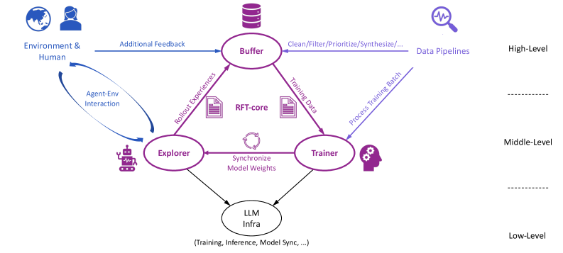This vision motivates us to develop Trinity-RFT, a reinforcement fine-tuning (RFT) framework that aims to offer a path into this future. The modular, decoupled and trinity design of Trinity-RFT illustrated in Figure 1, along with its various features, makes it a promising solution for realizing such a vision. <details> <summary>x2.png Details</summary>  ### Visual Description ## Diagram: RFT-core System Architecture ### Overview The image is a system architecture diagram illustrating the flow of data and interactions within an RFT-core system. It depicts the relationships between the Environment & Human, Buffer, Explorer, Trainer, and LLM Infra components, highlighting data pipelines and feedback loops. The diagram is structured into three levels: High-Level, Middle-Level, and Low-Level. ### Components/Axes * **Levels:** * High-Level * Middle-Level * Low-Level * **Nodes:** * Environment & Human (top-left) * Buffer (top-center) * Explorer (bottom-left) * Trainer (bottom-right) * LLM Infra (bottom-center) * **Data Flow Arrows:** * Additional Feedback (Environment & Human -> Buffer, blue) * Agent-Env Interaction (Environment & Human <-> Explorer, blue) * Rollout Experiences (Explorer -> Buffer, purple) * Training Data (Buffer -> Trainer, purple) * Synchronize Model Weights (Explorer <-> Trainer, purple) * Process Training Batch (Trainer -> Buffer, blue) * LLM Infra (Explorer -> LLM Infra, purple) * LLM Infra (Trainer -> LLM Infra, purple) * **Other Labels:** * Data Pipelines (near Buffer, right, blue) * RFT-core (center, between Buffer, Explorer, and Trainer) * Clean/Filter/Prioritize/Synthesize/... (Buffer -> Data Pipelines, blue) * (Training, Inference, Model Sync, ...) (below LLM Infra) ### Detailed Analysis or ### Content Details * **Environment & Human:** Located at the top-left, this represents the external environment and human interaction. A blue arrow labeled "Additional Feedback" points from this component to the "Buffer." A curved blue arrow labeled "Agent-Env Interaction" indicates a two-way interaction between "Environment & Human" and "Explorer." * **Buffer:** Positioned at the top-center, the "Buffer" receives "Additional Feedback" from "Environment & Human" and "Rollout Experiences" from "Explorer." It sends "Training Data" to the "Trainer" and "Clean/Filter/Prioritize/Synthesize/..." to "Data Pipelines." The "Trainer" sends "Process Training Batch" to the "Buffer." * **Explorer:** Located at the bottom-left, the "Explorer" interacts with the "Environment & Human" via "Agent-Env Interaction." It sends "Rollout Experiences" to the "Buffer" and connects to the "Trainer" via "Synchronize Model Weights." The "Explorer" also connects to the "LLM Infra." * **Trainer:** Situated at the bottom-right, the "Trainer" receives "Training Data" from the "Buffer" and connects to the "Explorer" via "Synchronize Model Weights." It sends "Process Training Batch" to the "Buffer" and connects to the "LLM Infra." * **LLM Infra:** Positioned at the bottom-center, the "LLM Infra" receives input from both the "Explorer" and the "Trainer." The text below it reads "(Training, Inference, Model Sync, ...)," indicating its functions. * **RFT-core:** Located in the center of the diagram, between the Buffer, Explorer, and Trainer. * **Data Pipelines:** Located to the right of the Buffer, at the High-Level. ### Key Observations * The diagram illustrates a cyclical flow of data and interactions between the core components: "Buffer," "Explorer," and "Trainer." * The "Environment & Human" provides external input and feedback to the system. * The "LLM Infra" serves as a central component for training, inference, and model synchronization. * The diagram is divided into three levels, suggesting a hierarchical structure of the system. ### Interpretation The diagram represents a Reinforcement Learning from Feedback (RFT-core) system architecture. The "Environment & Human" provides the environment and feedback, which is used by the "Explorer" to generate experiences. These experiences are stored in the "Buffer," which then provides training data to the "Trainer." The "Trainer" updates the model weights, which are synchronized with the "Explorer." The "LLM Infra" likely represents the infrastructure used for training, inference, and model synchronization of a Large Language Model (LLM). The cyclical nature of the diagram highlights the iterative process of reinforcement learning. The "Data Pipelines" suggest a process of cleaning, filtering, prioritizing, and synthesizing data before it is used for training. The three levels (High, Middle, Low) likely represent different levels of abstraction or detail in the system architecture. </details> Figure 1: The high-level design of Trinity-RFT. 1.1 Key Features of Trinity-RFT Trinity-RFT is a general-purpose, unified, scalable and user-friendly RL framework that can be easily adapted for diverse experimental or real-world scenarios. It integrates both macroscopic and microscopic RL methodologies in one place; roughly speaking, the former deals with natural language and plain text, while the latter handles torch.Tensor (such as token probabilities, gradients, and model weights of LLMs) Many prior RL works for games/control/LLMs focus mainly on the microscopic aspect, e.g., designing policy loss functions or optimization techniques for updating the policy model. On the other hand, pre-trained LLMs, as generative models with rich prior knowledge of natural language and the world, open up numerous opportunities at the macroscopic level, e.g., experience synthesis by reflection or reasoning with environmental feedback [4], leveraging existing text processing methods like deduplication and quality filtering [2], among others.. The key features of Trinity-RFT are presented below, which will be further elaborated in Section 2 and exemplified in Section 3. An RFT-core that unifies and generalizes diverse RL modes. Trinity-RFT implements diverse RL methodologies in a unified manner, supporting synchronous/asynchronous, on-policy/off-policy, and online/offline training. These RL modes can be flexibly generalized, e.g., a hybrid mode that incorporates expert trajectories to accelerate an online RL process [21, 46]. This unification is made possible partly by our decoupled design (which will soon be introduced in Section 2.1) that allows rollout and training to be executed separately and scaled up independently on different devices, while having access to the same stand-alone experience buffer. The efficacy of various RL modes has been validated empirically by our experiments in Section 3.3, which particularly highlight the efficiency gains by off-policy or asynchronous methods. Agent-environment interaction as a first-class citizen. Trinity-RFT allows delayed rewards and environmental feedback in multi-step/time-lagged feedback loop, handles long-tailed latencies and the straggler effect via asynchronous and streaming LLM inference, and deals with environment/agent failures gracefully via dedicated timeout/retry/skip mechanisms. These together ensure efficiency and robustness of continuous agent-environment interaction in complex real-world scenarios. Systematic data pipelines optimized for RFT. 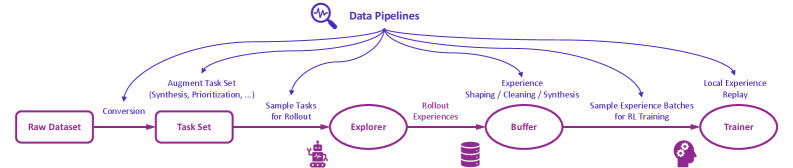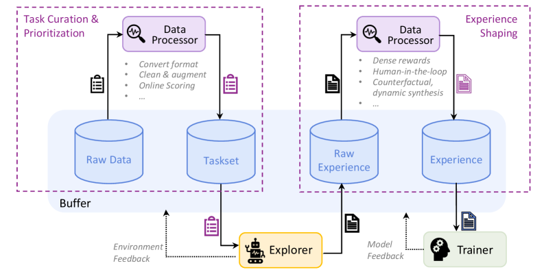Figure 2 illustrates the high-level design of data pipelines in Trinity-RFT, which regard rollout tasks and experiences as dynamic assets to be actively managed throughout the RFT lifecycle. Trinity-RFT empowers users to: (1) curate tasks for curriculum learning, e.g., by prioritizing easier tasks at the beginning of training to stabilize and accelerate the learning process; (2) actively manipulate experience by cleaning, filtering, or synthesizing new experiences, such as repairing failed trajectories or amplifying successful ones; (3) perform online reward shaping by augmenting sparse environmental rewards with dense, computed signals, such as quality or diversity scores; (4) customize interfaces for human-in-the-loop curation and utilize an agentic paradigm for RFT data processing that translates high-level natural language commands (e.g., “improve response diversity and safety for coding scenarios”) into complex data pipelines, powered by established community tools like Data-Juicer [2]. For instance, Section 3.4 presents experiments that demonstrate the efficacy of task prioritization and reward shaping empowered by Trinity-RFT. <details> <summary>x3.png Details</summary>  ### Visual Description ## Diagram: Data Pipelines ### Overview The image is a diagram illustrating data pipelines for reinforcement learning (RL) training. It shows the flow of data from a raw dataset through various stages, including task set creation, exploration, buffering, and training. The diagram uses purple lines and text to represent the data flow and processes. ### Components/Axes * **Title:** Data Pipelines (located at the top-center of the image, accompanied by a magnifying glass icon with a waveform inside) * **Nodes (from left to right):** * Raw Dataset (rectangle) * Task Set (rectangle) * Explorer (oval) - with a robot icon below * Buffer (oval) - with a database icon below * Trainer (oval) - with a head icon with gears below * **Edges (data flow):** Arrows connecting the nodes, labeled with descriptions of the processes. * **Data Pipeline Branches:** Arcs originating from "Data Pipelines" and pointing towards the nodes. ### Detailed Analysis * **Raw Dataset:** The starting point of the pipeline. * **Conversion:** The process of converting the raw dataset into a task set. * **Task Set:** A set of tasks derived from the raw dataset. * **Augment Task Set (Synthesis, Prioritization, ...):** A data pipeline branch pointing to the Task Set. This indicates that the task set can be augmented through synthesis and prioritization. * **Sample Tasks for Rollout:** The process of sampling tasks from the task set for rollout. * **Explorer:** An agent or system that explores the environment based on the sampled tasks. A robot icon is placed below the Explorer node. * **Rollout Experiences:** The experiences generated by the explorer during rollout. * **Buffer:** A storage area for the rollout experiences. A database icon is placed below the Buffer node. * **Experience Shaping / Cleaning / Synthesis:** A data pipeline branch pointing to the Buffer. This indicates that the experiences in the buffer can be shaped, cleaned, and synthesized. * **Sample Experience Batches for RL Training:** The process of sampling batches of experiences from the buffer for RL training. * **Trainer:** The RL training component that learns from the sampled experience batches. A head icon with gears is placed below the Trainer node. * **Local Experience Replay:** A data pipeline branch pointing to the Trainer. This indicates that the trainer uses local experience replay. ### Key Observations * The diagram illustrates a sequential flow of data from the Raw Dataset to the Trainer. * There are multiple data pipeline branches originating from the "Data Pipelines" title, indicating different processes that can influence the data at various stages. * The icons below the Explorer, Buffer, and Trainer nodes provide visual cues about the nature of these components. ### Interpretation The diagram depicts a typical data pipeline used in reinforcement learning. It highlights the key stages involved in preparing and using data for training an RL agent. The data pipeline branches suggest that there are opportunities for data augmentation, experience shaping, and local experience replay, which can improve the efficiency and effectiveness of the RL training process. The diagram emphasizes the importance of data management and processing in RL, as the quality and diversity of the data directly impact the performance of the trained agent. </details> Figure 2: The high-level design of data pipelines in Trinity-RFT. User-friendliness as a top priority. For development and research, the modular and decoupled design of Trinity-RFT allows the user to develop new RFT methodologies by adding one or a few small, plug-and-play classes (modified from built-in templates) that implement the essential functionalities of interest, with minimal code duplication or intrusive changes to the codebase. An example can be found in Section 3.2, which shows that three compact python classes (with around 200 lines of code in total) suffice for implementing a hybrid RL process that leverages samples from multiple data sources and updates the policy model with a customized loss function. For applications, the user can adapt Trinity-RFT to a new scenario by simply implementing a single Workflow class that specifies the logic of agent-environment interaction, as will be exemplified in Section 3.1. To further enhance usability, Trinity-RFT incorporates various graphical user interfaces to support low-code usage and development, enhance transparency of the RFT process, and facilitate easy monitoring and tracking. 1.2 Related Works There exist numerous open-source RLHF frameworks, such as veRL [30], OpenRLHF [13], TRL [40], ChatLearn [1], Asynchronous RLHF [23], among others. Some of them have been further adapted for training long-CoT reasoning models or for agentic RL more recently. Concurrent to Trinity-RFT, some recent works on LLM reinforcement learning also advocate a decoupled and/or asynchronous design; examples include StreamRL [50], MiMo [44], AReaL [9], ROLL [37], LlamaRL [43], Magistral [18], AsyncFlow [12], among others. Complementary to this huge number of related works, Trinity-RFT provides the community with a new solution that is powerful, easy-to-use, and unique in certain aspects. In a nutshell, Trinity-RFT aims to be general-purpose and applicable to diverse application scenarios, while unifying various RFT modes, RFT methodologies at macroscopic and microscopic levels, and RFT-core/agent-environment interaction/data pipelines. Such a system-engineering perspective makes Trinity-RFT particularly useful for handling the whole RFT pipeline in one place. We also hope that some specific features of Trinity-RFT, such as data persistence in the experience buffer, and distributed deployment of multiple independent explorers, will open up new opportunities for LLM reinforcement fine-tuning. 2 Design and Implementations The overall design of Trinity-RFT exhibits a trinity consisting of (1) RFT-core, (2) agent-environment interaction, and (3) data pipelines, which are illustrated in Figure 1 and elaborated in this section. 2.1 RFT-Core RFT-core is the component of Trinity-RFT, highlighted at the center of Figure 1, where the core RFT process happens. Its design also exhibits a trinity, consisting of the explorer, buffer, and trainer. - The explorer, powered by a rollout model, takes a task as input and solves it by executing a workflow that specifies the logic of agent-environment interaction, thereby collecting experiences (including rollout trajectories, rewards, and other useful information) to be stored in the buffer. - The buffer stores experiences that can be generated by the explorer or by other sources, such as human experts. It can be realized in various forms, such as a non-persistent ray.Queue or a persistent SQLite database. It also assists with fetching training samples for the trainer, and can be integrated with advanced sampling strategies and post-processing operations. - The trainer, backed by a policy model, samples batches of experiences from the buffer and updates the policy model via RL algorithms. 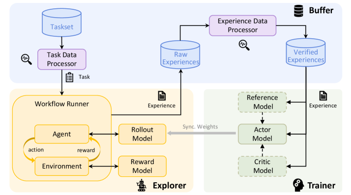Our implementations allow the explorer and trainer to be deployed on separate machines and act independently. They are only connected via (1) access to the same experience buffer with a customizable sampling strategy, and (2) model weight synchronization by a customizable schedule. See Figure 3 for an illustration. This decoupled design of RFT-core offers support for diverse RFT modes with great flexibility. <details> <summary>x4.png Details</summary>  ### Visual Description ## Diagram: Reinforcement Learning Workflow ### Overview The image presents a diagram of a reinforcement learning workflow. It illustrates the flow of data and processes between different components, including task management, experience generation, and model training. ### Components/Axes The diagram is divided into several key components: * **Taskset:** A blue cylinder at the top-left, representing a collection of tasks. * **Task Data Processor:** A purple rectangle below the Taskset, responsible for processing task data. * **Raw Experiences:** A blue cylinder, representing the raw experiences collected during the learning process. * **Experience Data Processor:** A purple rectangle, responsible for processing experience data. * **Verified Experiences:** A blue cylinder, representing the verified experiences after processing. * **Workflow Runner:** A yellow region containing the Agent, Environment, Rollout Model, and Reward Model. * **Agent:** A rounded rectangle within the Workflow Runner, representing the learning agent. * **Environment:** A rounded rectangle within the Workflow Runner, representing the environment in which the agent interacts. * **Rollout Model:** A yellow rounded rectangle to the right of the Agent, used for generating rollouts. * **Reward Model:** A yellow rounded rectangle below the Rollout Model, used for providing rewards. * **Explorer:** The yellow region containing the Workflow Runner, Rollout Model, and Reward Model. * **Buffer:** A stack of cylinders at the top-right, representing a buffer for storing experiences. * **Trainer:** A green region containing the Reference Model, Actor Model, and Critic Model. * **Reference Model:** A green dashed rounded rectangle within the Trainer. * **Actor Model:** A green solid rounded rectangle within the Trainer, representing the policy network. * **Critic Model:** A green dashed rounded rectangle within the Trainer, representing the value network. ### Detailed Analysis * **Flow from Taskset:** The Taskset feeds into the Task Data Processor. * A magnifying glass icon with a squiggly line is next to the Task Data Processor. * The Task Data Processor outputs a "Task" to the Workflow Runner. * **Workflow Runner Details:** * The Agent interacts with the Environment, producing "action" and receiving "reward". * The Agent also interacts with the Rollout Model and Reward Model. * The Rollout Model outputs "Experience" to the Raw Experiences. * **Experience Processing:** * Raw Experiences are fed into the Experience Data Processor. * A magnifying glass icon with a squiggly line is next to the Experience Data Processor. * The Experience Data Processor outputs to Verified Experiences. * **Trainer Details:** * Verified Experiences are fed into the Reference Model, Actor Model, and Critic Model. * The Reference Model feeds into the Actor Model. * The Actor Model feeds into the Critic Model. * "Sync. Weights" is written next to a gray arrow pointing from the Actor Model to the Agent. * The Rollout Model outputs "Experience" to the Reference Model. ### Key Observations * The diagram illustrates a closed-loop reinforcement learning system. * The Workflow Runner is responsible for generating experiences. * The Trainer is responsible for updating the models based on the experiences. * The Buffer stores experiences for later use. ### Interpretation The diagram depicts a typical reinforcement learning workflow, emphasizing the interaction between different components. The Taskset provides the initial tasks, which are then processed to generate experiences. These experiences are used to train the Actor and Critic models, which are then used by the Agent to interact with the Environment. The "Sync. Weights" arrow suggests that the Agent's policy is updated based on the Actor Model's weights, indicating a policy gradient approach. The presence of a Reference Model suggests a form of imitation learning or a stable learning target. The overall system aims to learn an optimal policy for the Agent to perform the given tasks within the Environment. </details> Figure 3: The architecture of RFT-core in Trinity-RFT. 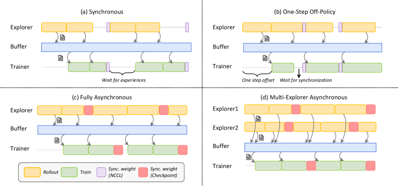2.1.1 Unified Support for Diverse RFT Modes We present the RFT modes supported by Trinity-RFT, some of which are demonstrated in Figure 4. <details> <summary>x5.png Details</summary>  ### Visual Description ## Diagram: Reinforcement Learning Architectures ### Overview The image presents four diagrams illustrating different reinforcement learning architectures: Synchronous, One-Step Off-Policy, Fully Asynchronous, and Multi-Explorer Asynchronous. Each diagram depicts the interaction between an Explorer (or Explorers), a Buffer, and a Trainer, showing the flow of data and synchronization points. ### Components/Axes Each of the four sub-diagrams contains the following components: * **Explorer (or Explorers):** Represents the agent(s) interacting with the environment, generating experiences (rollouts). * **Buffer:** A storage area for experiences collected by the explorer(s). * **Trainer:** The component responsible for learning from the experiences stored in the buffer. * **Rollout:** Represented by yellow rectangles, indicating the generation of experiences by the explorer. * **Train:** Represented by green rectangles, indicating the training process performed by the trainer. * **Sync. weight (NCCL):** Represented by light purple rectangles, indicating synchronization points using NCCL. * **Sync. weight (Checkpoint):** Represented by red rectangles, indicating synchronization points using Checkpoints. * **Arrows:** Indicate the flow of data (experiences) from the explorer(s) to the buffer and from the buffer to the trainer. ### Detailed Analysis **(a) Synchronous** * **Explorer:** Generates rollouts (yellow rectangles) and sends experiences to the buffer. * **Buffer:** Stores the experiences. * **Trainer:** Trains on the experiences from the buffer (green rectangles). * **Synchronization:** The trainer waits for experiences from the explorer before training. Synchronization points (light purple rectangles) are present between rollouts and training. * **Text:** "Wait for experiences" **(b) One-Step Off-Policy** * **Explorer:** Generates rollouts (yellow rectangles) and sends experiences to the buffer. * **Buffer:** Stores the experiences. * **Trainer:** Trains on the experiences from the buffer (green rectangles). * **Synchronization:** The trainer waits for synchronization. There is a "one step offset" between the explorer and trainer. Synchronization points (light purple rectangles) are present between rollouts and training. * **Text:** "One step offset", "Wait for synchronization" **(c) Fully Asynchronous** * **Explorer:** Generates rollouts (yellow rectangles) and sends experiences to the buffer. * **Buffer:** Stores the experiences. * **Trainer:** Trains on the experiences from the buffer (green rectangles). * **Synchronization:** Synchronization points (red rectangles) are present between rollouts and training. **(d) Multi-Explorer Asynchronous** * **Explorer1 & Explorer2:** Two explorers generate rollouts (yellow rectangles) and send experiences to the buffer. * **Buffer:** Stores the experiences. * **Trainer:** Trains on the experiences from the buffer (green rectangles). * **Synchronization:** Synchronization points (red rectangles) are present between rollouts and training. ### Key Observations * The diagrams illustrate different approaches to synchronizing the explorer(s) and trainer in reinforcement learning. * Synchronous methods involve waiting for experiences or synchronization points, while asynchronous methods allow for more independent operation. * The Multi-Explorer Asynchronous architecture utilizes multiple explorers to generate experiences concurrently. ### Interpretation The diagrams highlight the trade-offs between different reinforcement learning architectures. Synchronous methods may offer more stable learning but can be slower due to waiting times. Asynchronous methods can be faster but may introduce instability due to the lack of synchronization. The choice of architecture depends on the specific application and the desired balance between speed and stability. The use of multiple explorers in the Multi-Explorer Asynchronous architecture can potentially accelerate learning by increasing the diversity of experiences. </details> Figure 4: A visualization of diverse RFT modes supported by Trinity-RFT, including: (a) synchronous mode, with sync_interval=2; (b) one-step off-policy mode, with sync_interval=1 and sync_offset=1; (c) fully asynchronous mode, with sync_interval=2; (d) multi-explorer asynchronous mode, with sync_interval=2. The buffer supports, in principle, arbitrary management and sampling strategies for experiences. Synchronous mode. In the synchronous mode shown in Figure 4 (a), the explorer and trainer get launched simultaneously, work in close coordination, and synchronize their model weights once every sync_interval training steps. Within each synchronization period, the explorer continuously generates sync_interval batches of rollout experiences and stores them in the buffer, which are then retrieved and utilized by the trainer for updating the policy model. If sync_interval=1, this is a strictly on-policy RL process, whereas if sync_interval>1, it becomes off-policy (akin to the mode adopted in [35]) and can be accelerated by pipeline parallelism between the explorer and trainer. This mode can be activated by setting the configuration parameter mode=both. One-step off-policy mode. This mode, demonstrated in Figure 4 (b), closely resembles the synchronous mode, except for an offset of one batch between the explorer and trainer. This allows the trainer to sample experiences from the buffer immediately after model weight synchronization, thereby streamlining the execution of explorer and trainer with smaller pipeline bubbles, at the cost of slight off-policyness. The visualization in Figure 4 (b) corresponds to configuration parameters sync_interval=1 and sync_offset=1, both of which can take more general values in Trinity-RFT. Asynchronous mode. In the fully asynchronous mode shown in Figure 4 (c), the explorer and trainer act almost independently. The explorer continuously generates rollout experiences and stores them in the buffer, while the trainer continuously samples experiences from the buffer and uses them for training the policy model. External experiences, e.g., those generated by expert models or humans, can be continuously incorporated into the buffer as well. The explorer and trainer independently load or save model weights from the checkpoint directory every sync_interval steps, keeping the distribution of rollout experiences up to date. This mode can be activated by setting mode=explore/train and launching the explorer and trainer separately on different GPUs. Multi-explorer asynchronous mode. One benefit brought by the decoupled design is that explorers and trainers can scale up independently on separate devices. As a proof-of-concept, Trinity-RFT offers support for a multi-explorer asynchronous mode, as demonstrated in Figure 4 (d), where multiple explores send the generated rollout experiences to the same buffer. Scaling up the number of independent and distributed explorers can be particularly useful for resolving data scarcity and speeding up the generation of experiences in real-world scenarios where rollout trajectories have to be sampled via interaction with the physical world, or in an environment with sparse and lagged feedback. Another by-product of this multi-explorer mode is 24-hour non-interrupted service for real-world online serving situations: since the explorers can pause and update model weights at different moments, it can be guaranteed that there is always one explorer ready to serve an incoming request immediately whenever it arrives. This is in contrast to a single-explorer mode, where online service has to be paused when the explorer is updating its model weights. Benchmark mode. Trinity-RFT supports a benchmark mode that allows the user to evaluate one or multiple checkpoints on arbitrary benchmarks, after the RFT training process has finished. To activate this mode, the user simply needs to set mode=bench and specify the paths for the evaluation datasets in the configurations. This mode can be particularly useful for experimental purposes; for example, the user might want to try out different RFT techniques or configurations quickly (with limited evaluation on hold-out data) during training, identify which RFT trials have achieved stable convergence and high rewards, and then conduct more thorough evaluations only for the checkpoints of these successful trials. Train-only mode. In certain scenarios, the user would like to train the policy model without further exploration, using experiences that have already been collected and stored in the buffer. This train-only mode can be activated by setting the configuration parameter mode $=$ train and launching the trainer alone. Offline methods like Supervised Fine-Tuning (SFT) and Direct Preference Optimization (DPO) [25] can be regarded as special cases of such scenarios, both of which are natively supported by Trinity-RFT. For another example, consider an online RFT process that expands over a long period, where the explorer alone is launched during the daytime for serving human users and collecting experiences, while the trainer alone is launched at night for updating the policy model (which will be thoroughly validated and evaluated before it can be actually deployed as the rollout model for the next day). Discussions. We conclude this subsection with two remarks. (1) Given the unified implementation of various RFT modes, it is easy to design and implement a hybrid mode with Trinity-RFT that combines multiple modes into a single learning process. One example is learning with both online rollout data and offline-collected expert data, via jointly optimizing two loss terms corresponding to these two data sources. Section 3.2 illustrates how to implement this conveniently in Trinity-RFT. (2) We take a system-algorithm co-design perspective in the development of Trinity-RFT, aiming to unify and generalize diverse RFT methodologies in this framework. RFT-core provides the necessary infrastructure for achieving this goal. This technical report focuses on the system perspective, and we refer interested readers to the literature for recent algorithmic developments in off-policy / asynchronous RL for LLMs [21, 6, 26, 35, 7, 23, 42, 45, 46, 47]. 2.1.2 Implementations of RFT-Core We present some implementation details of RFT-core in the following. Inference and training engines. The current version of Trinity-RFT leverages vLLM [15] as the inference engine for the explorer, which offers features including paged attention, continuous batching [49], asynchronous and concurrent inference for multiple rollout trajectories, among others. Trinity-RFT also leverages verl [30] as the training engine for the trainer, which gracefully handles model placement (for the policy, critic and reference models) and incorporates various performance optimizations for training (such as dynamic batching, management of padding and unpadding, etc.). Trinity-RFT stands on the shoulders of these excellent open-source projects, and will continue to benefit from their future development. Experience buffer. Trinity-RFT supports multiple types of experience buffers, ranging from a non-persistent ray.Queue to persistent SQLite or Redis databases. While using a basic first-in-first-out queue is the most straightforward approach, data persistence with a database opens up many new opportunities (e.g., advanced sampling strategies), as discussed throughout this report. Trinity-RFT has provided dedicated read/write control to prevent any conflict in accessing the buffer. Model weight synchronization. Trinity-RFT supports model weight synchronization between the explorer and trainer by NCCL [22], or by checkpoint saving and loading. The former is faster (when available), while the latter is generally more flexible and widely applicable, especially for asynchronous RFT modes. 2.2 Agent-Environment Interaction To adapt Trinity-RFT to a new downstream scenario, the user mainly needs to define and register a customized workflow (by inheriting the base class Workflow or MultiTurnWorkflow) where the logic of agent-environment interaction for this particular scenario is implemented. Advanced methods for experience synthesis with environmental feedback [4] can be implemented in the same way as well. See Section 3.1 for detailed examples. The workflow will then be executed by workflow runners within the explorer for generating experiences, as shown in Figure 3. Numerous challenges arise when one tries to build an RFT framework that can efficiently and robustly handle real-world interaction between the LLM-powered agent and the environment. These include long-tailed latencies, agent/environment failures, and lagged reward signals, among others. Trinity-RFT regards agent-environment interaction as a first-class citizen and incorporates various solutions to tackle these challenges, for example: - The workflow runners in Trinity-RFT support asynchronous and streaming generation of rollout trajectories for multiple tasks. This helps mitigate the straggler effect caused by the long-tailed latencies in rollout generation and agent-environment interaction, thereby accelerating the RFT process. Load balancing among multiple LLM inference engines within one RFT training course is also taken care of, and would be one direction for further optimizing the utilization of computational resources. - Trinity-RFT incorporates various timeout/retry/skip mechanisms for fault tolerance and robustness, which ensure that continuous rollout generation would not be interrupted or blocked by individual failures in certain rounds of agent-environment interaction. This is crucial for stable and efficient learning in real-world scenarios, e.g., when the agent interacts with a large number of MCP services [17] that differ vastly in quality and availability. - Trinity-RFT is built to provide native support for asynchronous RFT modes, which allow great flexibility in the paces of the explorer and trainer. This can boost the overall efficiency of the RFT process, compared to synchronous modes where the slower one among the explorer and trainer can block the progress of the other and cause waste of computational resources. - For lagged reward signals, the trinity design of RFT-core offers a natural solution. As soon as the rollout trajectory (without reward values) has been generated, it is saved into the experience buffer, but marked as “not ready for training”. The explorer is now free from this task and may continue to collect experiences for other tasks. When the reward signals from the environment finally arrive, they are written to the buffer, and the corresponding experience is now marked as “ready for training”. - For multi-turn conversations and ReAct-style workflows [48], Trinity-RFT supports concatenating multiple rounds of agent-environment interaction compactly into a single sequence, with proper masking that indicates which tokens need to be incorporated into the training objective of RL algorithms. This avoids unnecessary recomputation and thus improves training efficiency, compared to a vanilla approach that represents a $K$ -turn rollout trajectory with $K$ separate samples. - As another performance optimization, the implementation of Trinity-RFT allows resetting the environment in a workflow, rather than re-initializing it every time. This is especially useful for scenarios where setting up the environment is costly. 2.3 Data Pipelines The data pipelines in Trinity-RFT aim to address fundamental challenges in RFT scenarios, such as managing heterogeneous data dynamics across interaction workflows, enabling delayed reward integration, and facilitating continuous data curation. Our solutions center on four core aspects: end-to-end data transformation, task curation, active experience shaping, and human-in-the-loop curation, each corresponding to key requirements identified in our development of RFT-core (Section 2.1). 2.3.1 End-to-end Data Transformation To support the diverse RFT modes (e.g., synchronous or asynchronous) in Trinity-RFT, we establish a service-oriented data pipeline architecture as illustrated in Figure 5. It decouples data pipeline logic from procedure control to enable flexible RL-oriented data transformations with two key modules: - The Formatter Module unifies disparate data sources into RFT-compatible formats, providing convenient conversion between raw inputs (e.g., meta-prompts, domain-specific corpora, and QA pairs with tagged rewards) and structured RFT representations. For efficient RFT workloads, we utilize buffer-based persistent storage (Section 2.1) to support different data models, such as ExperienceModel for prioritized rollout trajectories and DPODataModel for preference pairs. The conversion logic and data models are highly customizable to meet diverse requirements for managing experience data. This flexibility enables robust metadata recording and field normalization, which is essential for advanced scenarios such as asynchronous RFT in trainer-explorer environments, agent self-evolution from a cold start using meta-prompts, and knowledge injection from structurally complex domain-specific corpora. - The Controller Module manages the complete data pipeline lifecycle through distributed server initialization, declarative configuration, and automated dataset persistence. It implements dynamic control mechanisms for asynchronous scenarios and protection against resource exhaustion, with configurable termination conditions based on compute quota or data quantity. This modular design enables Trinity-RFT to handle data transformations flexibly while maintaining consistency across different RFT modes. The Formatter-Controller duality mirrors the explorer-trainer decoupling in RFT-core, enabling parallel data ingestion and model updating. This design also allows Trinity-RFT to handle delayed rewards through version-controlled experience updates while maintaining low-latency sampling for the trainer. <details> <summary>x6.png Details</summary>  ### Visual Description ## Data Flow Diagram: Task Curation and Experience Shaping ### Overview The image is a data flow diagram illustrating a process involving task curation, prioritization, experience shaping, and model training. It shows the flow of data between different components, including data processors, data storage, an explorer, and a trainer. ### Components/Axes * **Top-Left Region:** Labeled "Task Curation & Prioritization" within a dashed purple rectangle. * Contains a "Data Processor" block. * Lists processes: "Convert format", "Clean & augment", "Online Scoring". * Includes icons representing data and tasks. * **Top-Right Region:** Labeled "Experience Shaping" within a dashed purple rectangle. * Contains a "Data Processor" block. * Lists processes: "Dense rewards", "Human-in-the-loop", "Counterfactual, dynamic synthesis". * Includes icons representing data and tasks. * **Middle Region:** Labeled "Buffer" with a light blue background. * Contains two data storage components: "Raw Data" and "Taskset" on the left. * Contains two data storage components: "Raw Experience" and "Experience" on the right. * **Bottom Region:** * "Explorer" (yellow box with a robot icon). * "Trainer" (green box with a gear icon). * **Arrows:** Indicate the flow of data between components. * **Feedback Loops:** "Environment Feedback" and "Model Feedback" are shown as dotted arrows. ### Detailed Analysis or Content Details * **Task Curation & Prioritization:** * Data Processor: Receives data, converts its format, cleans and augments it, and performs online scoring. * Raw Data: Initial data storage. * Taskset: Storage for processed tasks. * **Experience Shaping:** * Data Processor: Processes data to generate dense rewards, incorporate human input, and create counterfactual and dynamic synthesis. * Raw Experience: Initial experience data storage. * Experience: Storage for shaped experiences. * **Data Flow:** * Raw Data and Taskset feed into the Explorer. * Raw Experience and Experience feed into the Trainer. * Explorer receives environment feedback. * Trainer receives model feedback. ### Key Observations * The diagram highlights two main processes: Task Curation & Prioritization and Experience Shaping. * Data processors play a central role in both processes. * The Explorer and Trainer components are connected through feedback loops. * The "Buffer" region acts as a central data storage area. ### Interpretation The diagram illustrates a reinforcement learning or machine learning pipeline. The "Task Curation & Prioritization" section focuses on preparing the data for the agent to interact with. The "Experience Shaping" section focuses on modifying the agent's experiences to improve learning. The Explorer interacts with the environment and generates data, while the Trainer uses this data to update the model. The feedback loops allow the system to adapt and improve over time. The diagram emphasizes the importance of data processing and curation in the overall learning process. </details> Figure 5: The interaction of data processor and data buffers in Trinity-RFT, divided into two key stages. Left: Task Curation & Prioritization prepares the initial tasks for the explorer. Right: Experience Shaping processes the collected trajectories from the explorer before they are used by the trainer. The data processor is a central component that operates on different buffers at different stages. 2.3.2 Task Curation and Prioritization Before the RFT loop begins, it is crucial to prepare a high-quality set of initial tasks. This stage, depicted on the left side of Figure 5, transforms raw data into an optimized task set for the explorer. The process begins with raw data sources (e.g., prompts, domain corpora), which are ingested into a buffer. The Data Processor, powered by over 100 operators from Data-Juicer [2], reads from this buffer to perform various curation tasks. It provides composable building blocks for experience cleaning (e.g., length filters, duplication removal), safety alignment (e.g., toxicity detection, ethics checks), and preference data synthesis (e.g., critique-conditioned augmentation). By treating Data-Juicer as a modular data processing operator pool rather than a central dependency, Trinity-RFT provides RL-specific abstractions and coherence, while benefiting from well-established data tools. The processed data is then organized into a structured task buffer. This stage effectively implements a form of curriculum learning by allowing users to prioritize tasks (e.g., from easy to hard), guiding the explorer towards a more efficient and stable learning trajectory from the outset. This entire workflow is managed by a service-oriented architecture that decouples data logic from procedural control, ensuring flexibility and scalability, especially in asynchronous and distributed settings. 2.3.3 Active Experience Shaping Once the explorer begins interacting with the environment, it generates a continuous stream of experience data. To maximize learning efficiency, this raw experience must be actively shaped before it reaches the trainer. This stage is shown on the right side of Figure 5. Generated experiences are first collected in a buffer. The Data Processor is applied again with a series of transformations to clean, augment, or synthesize these experiences. This is where the core of RFT data intelligence lies. Key capabilities include: - Agent-Driven Data Processing: Trinity-RFT introduces a powerful agentic paradigm for data manipulation. Users can define complex processing pipelines through high-level objectives, specified as either natural language commands (e.g., “improve safety” or “increase response diversity”) or explicit Data-Juicer configurations. The framework automatically translates these commands into executable workflows backed by its modular components like DataCleaner and DataSynthesizer. This design provides a user-friendly abstraction layer over the underlying Data-Juicer operators, making advanced processing functionalities accessible to both RFT users familiar with Data-Juicer and those who are not. It also facilitates the flexible injection of user-defined inductive biases into the learning process, unlocking new research directions for self-evolving agents, as we will discuss later in Section 2.3.5. - Online Reward Shaping: The data processor can dynamically augment the reward signal. Instead of relying on a single, often sparse, task-completion reward, users can add dense rewards based on quality, diversity, or safety scores computed on the fly. This enriched feedback provides a much stronger learning signal for the trainer. - Prioritized Experience Replay: Experiences are not treated equally. Trinity-RFT allows for flexible, multi-dimensional utility scoring to prioritize the most valuable samples for training. The DataActiveIterator supports version-controlled experience reuse and cross-task data lineage tracking, ensuring that the trainer always learns from the most informative data available. This mechanism is also critical for handling delayed rewards, as experience utilities can be updated asynchronously as new feedback arrives. 2.3.4 Human-AI Collaboration In scenarios where human feedback is irreplaceable, Trinity-RFT establishes a bi-directional human-AI collaboration loop that provides first-class support for human annotations, based on Label Studio [39] and Data-Juicer’s HumanOPs. - Multi-stage annotation. Trinity-RFT implements configurable procedures combining automatic pre-screening and human verification. Typical stages include preference annotation (comparative assessment of model responses), quality auditing (human verification of automated cleaning/synthesis results), and cold-start bootstrapping (initial dataset curation through expert demonstrations). - Native asynchronism support. As the collection of human feedback is generally slower than AI/model feedback, we provide dedicated capabilities to handle both synchronous and asynchronous feedback modes, with configurable timeout and polling parameters. The feedback collaboration is based on an event-driven design, with automatic task creation upon data state changes, configurable notifications via email/Slack/webhook, and an atomic transaction model for annotation batches. - Customization. Different applications may involve humans in heterogeneous ways. We thus prioritize flexibility in both the interaction-interface and service levels. Examples include rich built-in interfaces that can be extended in a visualized style with XML-like tags provided by Label Studio, fine-grained quality scoring for reward shaping, free-form feedback attachment for dataset shaping, among others. Moreover, for easy deployment, we provide local Label Studio instance management with automatic environment setup via Docker/pip; optimized SDK interactions with batch request coalescing; unified logging across annotation tools and ML services; and concurrent annotation campaigns through priority-based task routing, while maintaining full data lineage preserved via LineageTracker. The decoupled design of Trinity-RFT, and the presence of a standalone experience buffer in particular, enable human feedback to participate in RL loops without breaking the asynchronous execution model. For instance, human-verified samples can be prioritized for training while fresh experiences are being collected, which is a critical capability for real-world deployment scenarios with mixed feedback sources. Further details for human-AI collaboration in Trinity-RFT will be illustrated in Section 3.5. 2.3.5 Discussion: Unlocking New Research & Development Directions The modular design of our data pipelines and the powerful data processor open up promising research and development avenues to be further explored. One direction is about effective management of experience data. While prior RFT works often treat the experience as a static log, Trinity-RFT enables a more sophisticated, full-lifecycle approach to data, from selective acquisition to efficient representation: - Intelligent Perception and Collection: In an open-ended environment, what experience is “worth” recording? Storing everything creates a low signal-to-noise ratio and burdens the trainer. Trinity-RFT ’s architecture allows researchers to implement active collection strategies. For instance, one could design a data processor operator that evaluates incoming experiences from the explorer based on metrics like surprise, uncertainty, or information gain, and only commits the most salient trajectories to the replay buffer. This transforms data collection from passive logging into a targeted, intelligent process. - Adaptive Representation: Raw experience is often high-dimensional and redundant (e.g., long dialogues, complex code generation traces). How can this be distilled into a format that an agent can efficiently learn from? The data processor in Trinity-RFT acts as a powerful transformation engine. Researchers can use it to explore various representation learning techniques, such as automatically summarizing trajectories, extracting causal chains from tool usage, or converting a multi-turn dialogue into a structured preference pair. This not only makes training more efficient but also opens the door to building meta-experience (more abstract and reusable knowledge) from raw interaction data. - Agentic Workflows: Trinity-RFT ’s agent-driven processing enables the research and development of self-improving agents, e.g., by configuring the policy agent to also serve as the “processing agent” for LLM-based Data-Juicer operators. Such an agent could perform its own critique and dynamically curate its own training data, creating a truly autonomous learning and data management loop. Another direction is about synthetic and counterfactual experience processing. The integration of synthesis operators enables research into creating “better-than-real” data. Instead of relying solely on the agent’s own trial-and-error, our framework facilitates exploring questions like: - Dynamic and Composable Rewarding: With our framework, researchers can move beyond static, hand-crafted rewards. It is now possible to investigate dynamic reward shaping, where auxiliary signals like novelty, complexity, or alignment scores are automatically extracted from trajectories and composed into a dense reward function. How to define “good” experience and how can we learn the optimal combination of these reward components as the agent’s policy evolves? - Experience Reorganization: Can successful sub-trajectories from different tasks be “spliced” together to solve a novel, composite task? For example, can an agent that has learned to “open a door” and “pick up a cup” synthesize a new trajectory to "enter the room and fetch the cup"? - Failure Repair: Can the data processor identify where errors occur in a failed trajectory, and synthesize a corrected version for the trainer to learn from, effectively turning failures into valuable lessons? - Success Amplification: Can a single successful experience be augmented into multiple diverse yet successful variants, thereby improving the generalization and robustness of the learned policy? By providing dedicated capabilities for such advanced data and reward manipulation, Trinity-RFT aims to facilitates flexible processing of “experience data” for the next generation of self-evolving LLMs. 2.4 User-Friendliness Trinity-RFT has been designed with user-friendliness as a top priority. 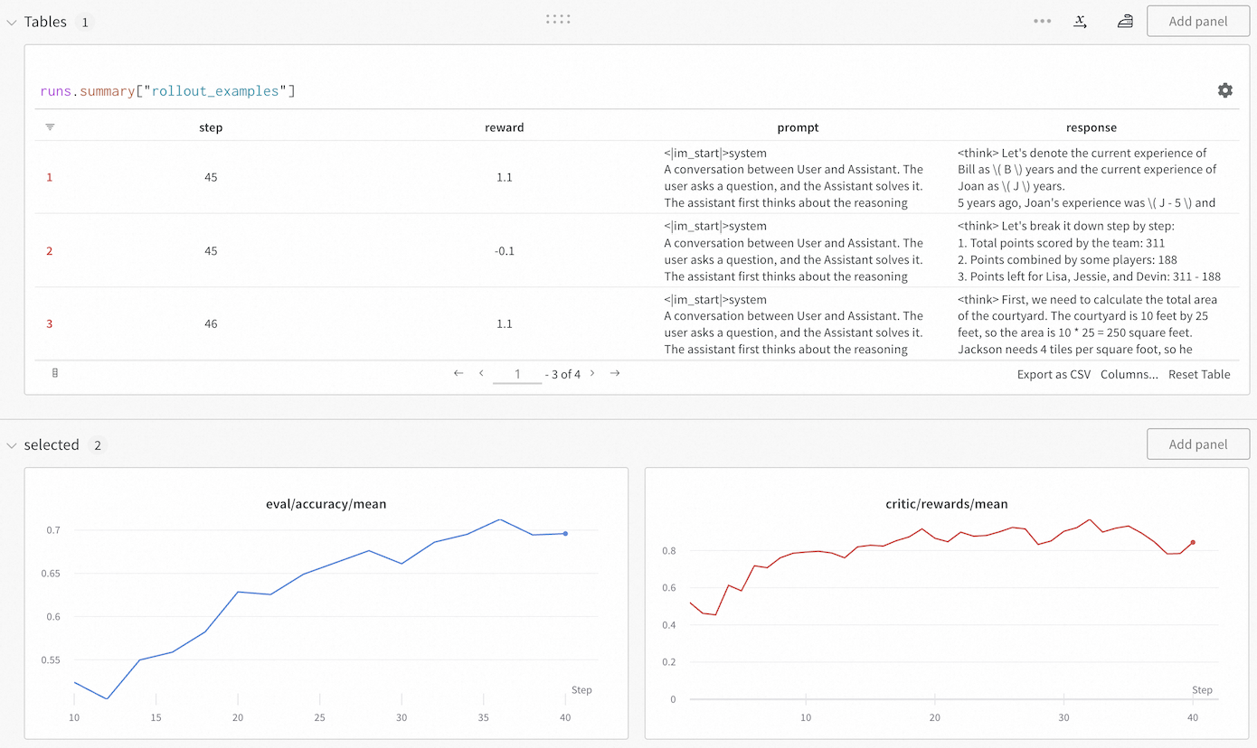For development and research: The modular and decoupled design of Trinity-RFT allows users to develop a new algorithm for a specific aspect of RFT by adding one or a few new classes that implement the essential functionalities of interest, without concerning about other aspects of RFT or intrusive modifications of the original codebase. In addition, we include a monitor (built upon Wandb [41] and TensorBoard [38]) that makes it easy to track the progress of an RFT process, both quantitatively (e.g., via learning curves for rewards and other metrics) and qualitatively (e.g., via concrete examples of rollout trajectories generated at different RL steps). See Figure 6 for an example snapshot of the monitor. 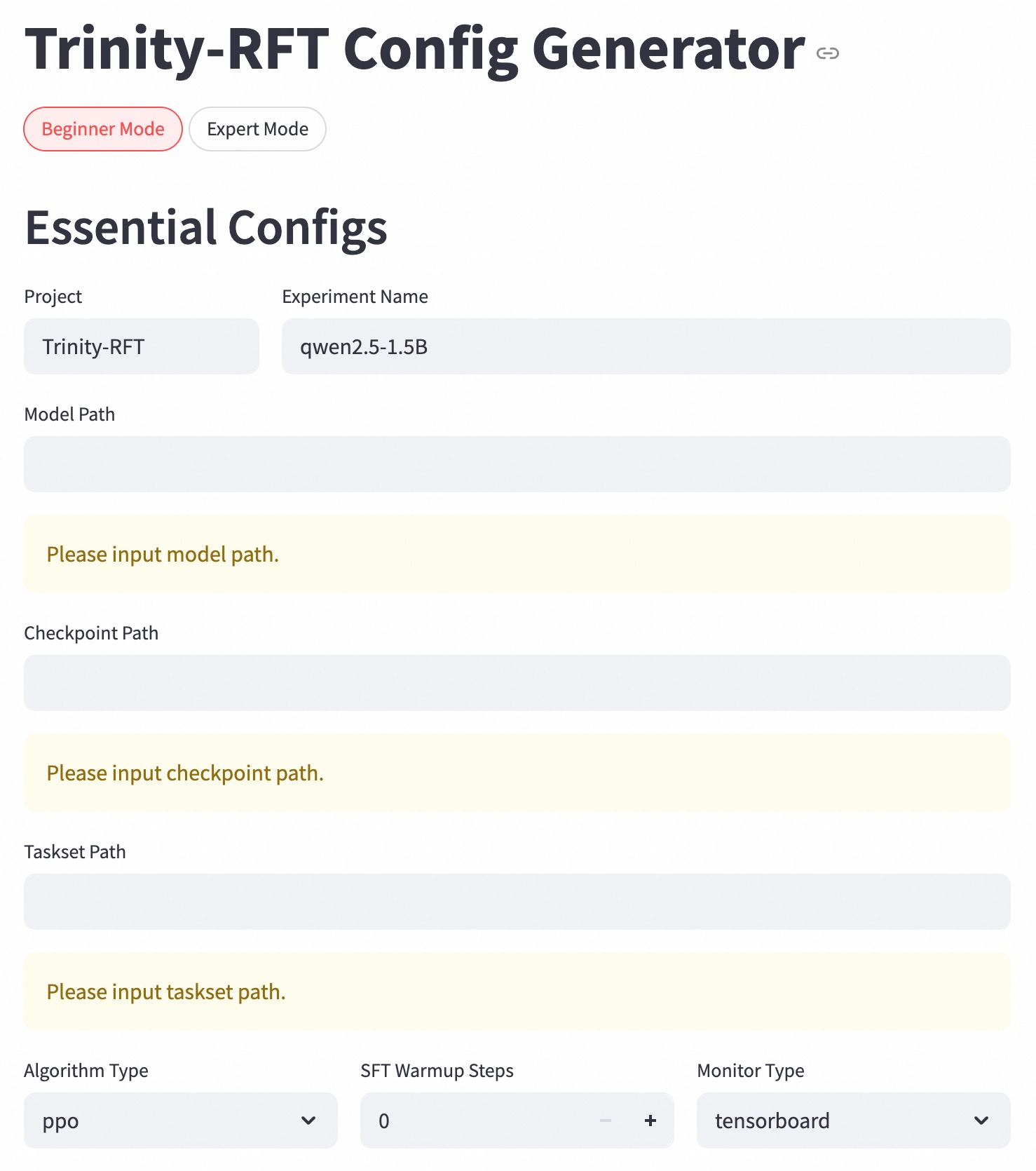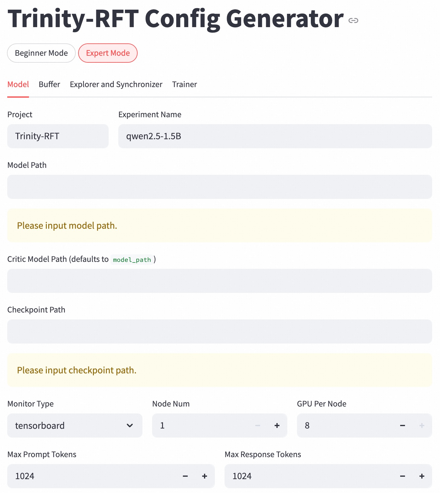For RFT applications: Trinity-RFT offers extensive graphical user interfaces to support low-code usage of the framework, and to maximize transparency of the RFT process. For example, we implement a configuration manager, as shown in Figure 7, that allows the user to create configuration files conveniently via a front-end interface. We also provide Trinity-Studio, an all-in-one unified UI (including the aforementioned monitor and configuration manager) that allows the user to configure and run data inspection, data processing, RFT learning process, etc., all by clicking the mouse and filling forms, without writing any code. An example for using Trinity-Studio will be introduced in Section 3.6. Such functionalities, of course, can be useful not only for applications but also for development and research. <details> <summary>figs/wandb_screencut.png Details</summary>  ### Visual Description ## Tables and Charts: Agent Performance Analysis ### Overview The image presents a table and two line charts displaying the performance of an agent during a rollout. The table shows individual steps with associated rewards, prompts, and responses. The charts visualize the agent's `eval/accuracy/mean` and `critic/rewards/mean` over steps. ### Components/Axes **Table:** * **Title:** Tables 1, runs.summary["rollout_examples"] * **Columns:** step, reward, prompt, response * **Rows:** 1, 2, 3 * **Navigation:** Pagination controls indicating "1 - 3 of 4" pages. **Chart 1: eval/accuracy/mean** * **Title:** eval/accuracy/mean * **X-axis:** Step, ranging from 10 to 40 in increments of 5. * **Y-axis:** eval/accuracy/mean, ranging from 0.55 to 0.7 in increments of 0.05. * **Data Series:** A blue line representing the eval/accuracy/mean. **Chart 2: critic/rewards/mean** * **Title:** critic/rewards/mean * **X-axis:** Step, ranging from 0 to 40 in increments of 10. * **Y-axis:** critic/rewards/mean, ranging from 0 to 0.8 in increments of 0.2. * **Data Series:** A red line representing the critic/rewards/mean. ### Detailed Analysis **Table Content:** | Row | Step | Reward | Prompt get the agent to do something else. </details> Figure 6: A snapshot of the monitor implemented in Trinity-RFT. <details> <summary>figs/config_manager_beginner.jpg Details</summary>  ### Visual Description ## Configuration Interface: Trinity-RFT Config Generator ### Overview The image depicts a configuration interface for the "Trinity-RFT Config Generator." It presents a form-like layout for specifying essential configurations, including project details, file paths, algorithm settings, and monitoring options. The interface offers both "Beginner Mode" and "Expert Mode" options. ### Components/Axes * **Header:** "Trinity-RFT Config Generator" with a link icon. * **Mode Selection:** "Beginner Mode" (selected) and "Expert Mode" buttons. * **Section Title:** "Essential Configs" * **Input Fields:** * Project: Text field populated with "Trinity-RFT" * Experiment Name: Text field populated with "qwen2.5-1.5B" * Model Path: Text field with placeholder text "Please input model path." * Checkpoint Path: Text field with placeholder text "Please input checkpoint path." * Taskset Path: Text field with placeholder text "Please input taskset path." * **Dropdown Menus:** * Algorithm Type: Dropdown menu set to "ppo" * Monitor Type: Dropdown menu set to "tensorboard" * **Numerical Input:** * SFT Warmup Steps: Numerical input field set to "0" with increment (+) and decrement (-) buttons. ### Detailed Analysis or ### Content Details The interface is designed for configuring a Trinity-RFT project. The user can specify the project name, experiment name, and paths to the model, checkpoint, and taskset files. The algorithm type and monitor type can be selected from dropdown menus. The number of SFT Warmup Steps can be adjusted using the increment and decrement buttons. * **Project:** "Trinity-RFT" * **Experiment Name:** "qwen2.5-1.5B" * **Model Path:** Empty, prompting "Please input model path." * **Checkpoint Path:** Empty, prompting "Please input checkpoint path." * **Taskset Path:** Empty, prompting "Please input taskset path." * **Algorithm Type:** "ppo" * **SFT Warmup Steps:** "0" * **Monitor Type:** "tensorboard" ### Key Observations * The "Beginner Mode" is currently selected. * The Model Path, Checkpoint Path, and Taskset Path fields are empty and require user input. * The Algorithm Type is set to "ppo" and the Monitor Type is set to "tensorboard." * The SFT Warmup Steps are set to "0." ### Interpretation The configuration interface allows users to set up and customize their Trinity-RFT experiments. The "Beginner Mode" suggests a simplified configuration process, while the "Expert Mode" likely offers more advanced options. The interface guides the user through the essential configurations, ensuring that all necessary parameters are specified before running the experiment. The empty path fields indicate that the user needs to provide the locations of the model, checkpoint, and taskset files. </details> (a) The “beginner” mode. <details> <summary>figs/config_manager_expert.jpg Details</summary>  ### Visual Description ## Configuration Interface: Trinity-RFT Config Generator ### Overview The image depicts a configuration interface, specifically the "Expert Mode" of the "Trinity-RFT Config Generator." It allows users to set parameters for a machine learning model, including project name, model paths, and hardware configurations. ### Components/Axes * **Header:** "Trinity-RFT Config Generator" with a link icon. Toggle buttons for "Beginner Mode" and "Expert Mode" (Expert Mode is selected). Tabs for "Model," "Buffer," "Explorer and Synchronizer," and "Trainer." The "Model" tab is currently selected. * **Project:** Text field labeled "Project" with the value "Trinity-RFT." * **Experiment Name:** Text field labeled "Experiment Name" with the value "qwen2.5-1.5B." * **Model Path:** Text field labeled "Model Path." Currently empty, with a yellow background and the placeholder text "Please input model path." * **Critic Model Path:** Text field labeled "Critic Model Path (defaults to model\_path)." Currently empty. * **Checkpoint Path:** Text field labeled "Checkpoint Path." Currently empty, with a yellow background and the placeholder text "Please input checkpoint path." * **Monitor Type:** Dropdown menu labeled "Monitor Type" with the selected value "tensorboard." * **Node Num:** Numerical input field labeled "Node Num" with the value "1." Increment and decrement buttons are present. * **GPU Per Node:** Numerical input field labeled "GPU Per Node" with the value "8." Increment and decrement buttons are present. * **Max Prompt Tokens:** Numerical input field labeled "Max Prompt Tokens" with the value "1024." Increment and decrement buttons are present. * **Max Response Tokens:** Numerical input field labeled "Max Response Tokens" with the value "1024." Increment and decrement buttons are present. ### Detailed Analysis or ### Content Details The interface is designed for configuring a machine learning model within the Trinity-RFT framework. The user can specify the project and experiment names, model and checkpoint paths, monitoring type, number of nodes, GPUs per node, and maximum token lengths for prompts and responses. The "Expert Mode" suggests a more detailed level of configuration compared to a potential "Beginner Mode." The yellow background on the "Model Path" and "Checkpoint Path" fields indicates that these are required fields. ### Key Observations * The "Expert Mode" is selected, indicating a more advanced configuration interface. * The "Model" tab is active, suggesting that the user is currently configuring model-specific parameters. * The "Model Path" and "Checkpoint Path" fields are highlighted, indicating that these are required inputs. * The default value for "Critic Model Path" is "model\_path". * The number of nodes is set to 1, and the number of GPUs per node is set to 8. * Both "Max Prompt Tokens" and "Max Response Tokens" are set to 1024. ### Interpretation The configuration interface provides a comprehensive set of parameters for setting up and running a machine learning model within the Trinity-RFT environment. The "Expert Mode" and the availability of tabs for "Buffer," "Explorer and Synchronizer," and "Trainer" suggest a modular and highly configurable system. The highlighted "Model Path" and "Checkpoint Path" fields emphasize the importance of specifying these locations for the model to function correctly. The numerical input fields for node number, GPUs per node, and token lengths allow for fine-tuning the hardware and processing parameters of the model. </details> (b) The “expert” mode. Figure 7: Snapshots of the configuration manager. 3 Examples, Applications, and Experiments This section demonstrates the utilities and user-friendliness of Trinity-RFT and exemplifies some concepts introduced in previous sections, through a diverse range of examples, applications and experiments. Additional step-by-step tutorials can be found on the documentation website https://modelscope.github.io/Trinity-RFT, or the examples folder of the GitHub repository https://github.com/modelscope/Trinity-RFT/tree/main/examples. 3.1 Customizing Agent-Environment Interaction With a modular design, Trinity-RFT can be easily adapted to a new downstream scenario by implementing the logic of agent-environment interaction in a single workflow class, without modifications to other components of the codebase. This approach is also sufficient for macroscopic RL algorithm design that targets high-quality experience synthesis with environmental feedback [4]. We provide some concrete examples in the rest of this subsection. 3.1.1 Single-turn Scenarios In a simple yet common scenario, a user of Trinity-RFT would like to train an LLM for completing single-turn tasks, where the LLM generates one response to each input query. For this purpose, the user mainly needs to (1) define and register a single-turn workflow class (by inheriting the base class Workflow) tailored to the targeted tasks, and (2) specify the tasksets (for training and/or evaluation) and the initial LLM, both of which are compatible with HuggingFace [14] and ModelScope [19] formats. Listing 1 gives a minimal example for implementing a single-turn workflow. Suppose that each task is specified by a <question, answer> tuple. The run() method of ExampleWorkflow calls the LLM once to generate a response for the question, calculates its reward, and returns an Experience instance that consists of the response itself, the reward value, and the log-probabilities of response tokens predicted by the rollout model (which is necessary for certain RL algorithms, such as PPO [28] and GRPO [29]). Some built-in workflows and reward functions have been implemented in Trinity-RFT, e.g., the MathWorkflow class for math-related tasks. In some cases, the user wants to utilize auxiliary LLMs in the workflow, e.g., for computing rewards via LLM-as-a-judge, or for playing the roles of other agents in a multi-agent scenario. For these purposes, the user can specify auxiliary_models via APIs when initializing the workflow. ⬇ 1 @WORKFLOWS. register_module ("example_workflow") 2 class ExampleWorkflow (Workflow): 3 4 def __init__ ( 5 self, 6 model: ModelWrapper, 7 task: Task, 8 auxiliary_models: Optional [List [openai. OpenAI]] = None, 9 ): 10 super (). __init__ (model, task, auxiliary_models) 11 self. question = task. raw_task. get ("question") 12 self. answer = task. raw_task. get ("answer") 13 14 def calculate_reward_by_rule (self, response: str, truth: str) -> float: 15 return 1.0 if response == truth else 0.0 16 17 def calculate_reward_by_llm_judge (self, response: str, truth: str) -> float: 18 judge_model = self. auxiliary_models [0] 19 PROMPT_FOR_JUDGE = "" "Please evaluate..." "" 20 completion = judge_model. chat. completions. create ( 21 model = "gpt-4", # Or another suitable judge model 22 messages =[{"role": "user", "content": PROMPT_FOR_JUDGE}], 23 ) 24 reward_str = completion. choices [0]. message. content. strip () 25 reward = float (reward_str) 26 return reward 27 28 def run (self) -> List [Experience]: 29 response = self. model. chat ( 30 [ 31 { 32 "role": "user", 33 "content": f "Question:\n{self.question}", 34 } 35 ], 36 ** self. rollout_args, 37 ) 38 reward: float = self. calculate_reward_by_rule (response. response_text, self. answer) 39 # reward: float = self.calculate_reward_by_llm_judge(response.response_text, self.answer) 40 return [ 41 Experience ( 42 tokens = response. tokens, 43 prompt_length = response. prompt_length, 44 reward = reward, 45 logprobs = response. logprobs, 46 ) 47 ] Listing 1: A minimal example for implementing a customized workflow. 3.1.2 Multi-turn Scenarios In more advanced cases, the user would like to train an LLM-powered agent that solves multi-turn tasks by repeatedly interacting with the environment. In Trinity-RFT, achieving this is mostly as simple as in the single-turn case, except that the user needs to define and register a multi-turn workflow class by inheriting the base class MultiTurnWorkflow. Listing 2 provides one such example using the ALFWorld dataset [31]. For training efficiency, the process_messages_to_experience() method concatenates multiple rounds of agent-environment interactions compactly into an Experience instance consisting of a single token sequence with proper masking, which can readily be consumed by standard RL algorithms like PPO and GRPO. For more detailed examples of multi-turn cases, please refer to the documentation https://modelscope.github.io/Trinity-RFT/tutorial/example_multi_turn.html. ⬇ 1 @WORKFLOWS. register_module ("alfworld_workflow") 2 class AlfworldWorkflow (MultiTurnWorkflow): 3 "" "A workflow for the ALFWorld task." "" 4 5 def generate_env_inference_samples (self, env, rollout_num) -> List [Experience]: 6 print ("Generating env inference samples...") 7 experience_list = [] 8 for i in range (rollout_num): 9 observation, info = env. reset () 10 final_reward = -0.1 11 memory = [] 12 memory. append ({"role": "system", "content": AlfWORLD_SYSTEM_PROMPT}) 13 for r in range (self. max_env_steps): 14 format_obs = format_observation (observation) 15 memory = memory + [{"role": "user", "content": format_obs}] 16 response_text = self. model. chat (memory, n =1)[0]. response_text 17 memory. append ({"role": "assistant", "content": response_text}) 18 action = parse_action (response_text) 19 observation, reward, done, info = env. step (action) 20 if done: 21 final_reward = reward 22 break 23 experience = self. process_messages_to_experience ( 24 memory, final_reward, {"env_rounds": r, "env_done": 1 if done else 0} 25 ) 26 experience_list. append (experience) 27 # Close the env to save CPU memory 28 env. close () 29 return experience_list 30 31 def run (self) -> List [Experience]: 32 # ... 33 game_file_path = self. task_desc 34 rollout_n = self. repeat_times 35 # ... 36 env = create_environment (game_file_path) 37 return self. generate_env_inference_samples (env, rollout_n) Listing 2: An implementation of a multi-turn workflow for ALFWorld [31]. 3.1.3 Experience Synthesis in Workflows As mentioned in Section 1.1, Trinity-RFT has been designed to streamline RL algorithm design and development at both macroscopic and microscopic levels. One example for the former is experience synthesis: at each RL step, the agent (backed by the rollout LLM) iteratively generates refined responses to a query by incorporating feedback or guidance from the environment, which can be in the form of plain text rather than numerical reward values. The resulting data will then be utilized for updating the policy model, e.g., by a standard SFT or RL loss. Such a macroscopic RL approach is made possible by pre-trained LLMs’ generative nature and rich prior knowledge about natural language. Closely related to this idea is Agent-RLVR [4], a contemporary work that applies such an approach to software engineering scenarios. Within Trinity-RFT, this process of experience synthesis can be regarded as a particular way of agent-environment interaction, and thus can be realized by simply implementing a Workflow class. As a minimal demonstration, suppose that we want to implement this approach for a math reasoning scenario, where the agent generates multiple rollout responses to an input query, receives feedback from the environment regarding correctness of the responses, reflects on the gathered information, and generates a final response to the query. Listing 3 presents an implementation of this approach within Trinity-RFT. ⬇ 1 @WORKFLOWS. register_module ("reflect_once_workflow") 2 class ReflectOnceWorkflow (Workflow): 3 4 def run (self) -> List [Experience]: 5 experiences = [] 6 7 # Stage 1: K-rollout generation 8 rollout_messages = self. create_rollout_messages () 9 responses = self. model. chat ( 10 rollout_messages, 11 n = self. k_rollouts, 12 temperature = self. temperature, 13 logprobs = self. logprobs, 14 max_tokens = self. task. rollout_args. max_tokens, 15 ) 16 rollout_responses = [response. response_text. strip () for response in responses] 17 18 # Stage 2: Verification 19 verification_results = [] 20 for rollout_response in rollout_responses: 21 is_correct = self. verify_answer (rollout_response, self. ground_truth) 22 verification_results. append (is_correct) 23 24 # Stage 3: Reflection 25 reflection_messages = self. create_reflection_messages ( 26 rollout_responses, 27 verification_results, 28 ) 29 reflection_responses = self. model. chat ( 30 reflection_messages, 31 n =1, 32 temperature = self. temperature, 33 logprobs = self. logprobs, 34 max_tokens = self. task. rollout_args. max_tokens, 35 ) 36 reflection_response = reflection_responses [0] 37 38 # Verify the reflection response 39 reflection_text = reflection_response. response_text. strip () 40 reflection_is_correct = self. verify_answer (reflection_text, self. ground_truth) 41 42 if reflection_is_correct: 43 sharegpt_message = [ 44 { 45 "role": "system", 46 "content": self. task. format_args. system_prompt 47 }, 48 { 49 "role": "user", 50 "content": self. question 51 }, 52 { 53 "role": "assistant", 54 "content": reflection_text 55 } 56 ] 57 experience = self. process_messages_to_experience (sharegpt_message) 58 experiences. append (experience) 59 60 # Save experience to file 61 if self. exp_file and sharegpt_message is not None: 62 exp_data = sharegpt_message 63 self. exp_file. write (json. dumps (exp_data, ensure_ascii = False) + "\n") 64 self. exp_file. flush () 65 return experiences Listing 3: A toy implementation of experience synthesis with environmental feedback. 3.2 RL Algorithm Development with Trinity-RFT To support RL algorithm development, Trinity-RFT allows researchers and developers to focus on designing and implementing the essential logic of a new RL algorithm, without the need to care about the internal engineering details about Trinity-RFT. 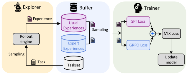As an example, suppose that we want to implement a MIX algorithm that seamlessly integrates online RL and offline SFT into a single learning process. In its most basic form, the MIX algorithm requires that (1) the trainer samples from two sources of experiences, i.e., the rollout experiences collected online and the high-quality expert trajectories collected offline; and (2) the trainer updates its policy model with a loss function that handles both sources of experiences properly, e.g., a weighted sum of GRPO loss for the on-policy rollout experiences and SFT loss for the expert trajectories. Variants of this MIX algorithm include adaptive weighting of multiple loss terms [10], alternating between RL and SFT [16], incorporating expert trajectories into RL loss [21, 34, 46], or incorporating SFT loss for high-reward rollout trajectories generated by older versions of the rollout model [27]. Such approaches have proved to be effective in accelerating the online RL process with only a small amount of expert experiences, or to enhance stability and plasticity in continual learning. <details> <summary>x7.png Details</summary>  ### Visual Description ## System Diagram: Reinforcement Learning Training Pipeline ### Overview The image is a system diagram illustrating a reinforcement learning training pipeline. It depicts the flow of data and processes between three main components: an Explorer, a Buffer, and a Trainer. The diagram shows how experience is generated, stored, sampled, and used to update a model. ### Components/Axes * **Explorer (Left, Yellow Background):** * Icon: A robot-like figure. * Function: Generates experience by interacting with an environment. * Output: "Experience" (represented by a document icon). * Component: "Rollout engine" (grey box). * Input to Rollout engine: "Task" (represented by a document icon). * Sampling: The Rollout engine samples from the Task. * **Buffer (Center, Blue Background):** * Icon: Database icon. * Function: Stores and samples experiences. * Components: * "Usual Experiences" (purple cylinder). * "Expert Experiences" (blue cylinder). * "Taskset" (grey cylinder). * Input: Experience from the Explorer. * Output: Sampling to the Trainer. * **Trainer (Right, Green Background):** * Icon: Head with gears. * Function: Updates the model based on sampled experiences. * Inputs: * "SFT Loss" (purple box). * "GRPO Loss" (blue box). * Process: "+" (addition) of SFT Loss and GRPO Loss. * Output: "MIX Loss" (grey box). * Final Step: "Update model" (grey box). ### Detailed Analysis or ### Content Details * **Explorer:** The Explorer uses a "Rollout engine" to generate "Experience" based on a "Task". The Rollout engine samples from the Task. * **Buffer:** The Buffer stores "Usual Experiences" and "Expert Experiences" separately. Both types of experiences are sampled and sent to the Trainer. The Buffer also contains a "Taskset". * **Trainer:** The Trainer receives sampled experiences and calculates "SFT Loss" and "GRPO Loss". These losses are combined ("+") to produce a "MIX Loss", which is then used to "Update model". ### Key Observations * The diagram highlights the separation of experience types (Usual vs. Expert) in the Buffer. * The Trainer combines two different loss functions (SFT and GRPO) to create a mixed loss for model updating. * The flow of data is unidirectional, from Explorer to Buffer to Trainer. ### Interpretation The diagram illustrates a reinforcement learning training pipeline that leverages both usual and expert experiences to train a model. The separation of experience types in the Buffer suggests that the system may be designed to incorporate expert knowledge or demonstrations into the learning process. The combination of SFT and GRPO losses in the Trainer indicates that the model is being optimized using multiple objectives or constraints. This setup could be used to improve the model's performance, robustness, or safety. The diagram provides a high-level overview of the system's architecture and data flow, which can be useful for understanding the training process and identifying potential areas for improvement. </details> Figure 8: A visualization of the MIX algorithm. The MIX algorithm is visualized in Figure 8, where we integrate GRPO loss for usual experiences generated by the rollout model and SFT loss for expert experiences into a unified training pipeline. It requires dealing with different sources of experiences, and two types of loss functions; fortunately, to implement such an algorithm in Trinity-RFT, we only need to define three new classes — MixSampleStrategy, MIXPolicyLossFn, and MIXAlgorithm — as demonstrated in Listing 4. With these components, Trinity-RFT enables a seamless integration of online RL and offline SFT within the same training loop. More details of the MIX algorithm are referred to the documentation https://modelscope.github.io/Trinity-RFT/tutorial/example_mix_algo.html. ⬇ 1 @SAMPLE_STRATEGY. register_module ("mix") 2 class MixSampleStrategy (SampleStrategy): 3 def __init__ (self, buffer_config: BufferConfig, trainer_type: str, ** kwargs): 4 # ... 5 self. usual_exp_buffer = get_buffer_reader ( 6 buffer_config. trainer_input. experience_buffer, usual_buffer_config 7 ) 8 self. expert_exp_buffer = get_buffer_reader ( 9 buffer_config. trainer_input. sft_warmup_dataset, expert_buffer_config 10 ) 11 # ... 12 13 def sample (self, step: int) -> Tuple [Any, Dict, List]: 14 "" "Sample a batch composed of rollout experiences and expert trajectories" "" 15 usual_exp_list = self. usual_exp_buffer. read () 16 expert_exp_list = self. expert_exp_buffer. read () 17 exp_list = usual_exp_list + expert_exp_list 18 exps = Experiences. gather_experiences (exp_list, self. pad_token_id) 19 # ... 20 21 22 @POLICY_LOSS_FN. register_module ("mix") 23 class MIXPolicyLossFn (PolicyLossFn): 24 def __init__ (self, mu: float = 0.1, ...): 25 # ... 26 self. mu = mu 27 self. grpo_loss_fn = PPOPolicyLossFn (...) 28 self. sft_loss_fn = SFTLossFn (...) 29 30 def __call__ ( 31 self, 32 logprob: torch. Tensor, 33 old_logprob: torch. Tensor, 34 action_mask: torch. Tensor, 35 advantages: torch. Tensor, 36 is_expert_mask: torch. Tensor, 37 ** kwargs, 38 ) -> Tuple [torch. Tensor, Dict]: 39 "" "Calculate a weighted sum of GRPO loss and SFT loss" "" 40 # ... 41 grpo_loss, grpo_metrics = self. grpo_loss_fn ( 42 logprob [~ is_expert_mask], 43 old_logprob [~ is_expert_mask], 44 action_mask [~ is_expert_mask], 45 advantages [~ is_expert_mask], 46 ** kwargs, 47 ) 48 sft_loss, sft_metrics = self. sft_loss_fn ( 49 logprob [is_expert_mask], 50 action_mask [is_expert_mask], 51 ) 52 loss = (1 - self. mu) * grpo_loss + self. mu * sft_loss 53 # ... 54 return loss, metrics 55 56 @ALGORITHM_TYPE. register_module ("mix") 57 class MIXAlgorithm (AlgorithmType): 58 "" "MIX algorithm." "" 59 60 use_critic: bool = False 61 use_reference: bool = True 62 use_advantage: bool = True 63 can_balance_batch: bool = True 64 schema: type = ExperienceModel 65 66 @classmethod 67 def default_config (cls) -> Dict: 68 return { 69 "repeat_times": 8, 70 "policy_loss_fn": "mix", # Specify the MIX loss function 71 "advantage_fn": "grpo", 72 "sample_strategy": "mix", # Specify the MIX sampling strategy 73 } Listing 4: An implementation of the MIX algorithm with Trinity-RFT. 3.3 Unified Support for Diverse RL Modes As explained previously in Section 2.1.1, Trinity-RFT offers support for synchronous/asynchronous, on-policy/off-policy, and online/offline RL, controlled by a few configuration parameters. In this subsection, we conduct experiments for comparing the following RL modes: - The synchronous mode: mode=both, sync_interval={1,2,10}, sync_offset=0; - The one-step off-policy mode: mode=both, sync_interval=1, sync_offset=1; - The fully asynchronous mode: the explorer and trainer are launched with mode=explore and train respectively, with sync_interval=10. Our experiments include dummy learning processes (which will soon be explained) for performance profiling, as well as real learning processes with vanilla GRPO [29] in different modes. 3.3.1 Experiments: Performance Profiling Settings. We aim to measure and compare the efficiency of different RL modes under controlled settings. It is noteworthy that, even with all other variables controlled, different RL modes can still result in different trained models — and thus different rollout response lengths — during the learning processes, which have direct impacts on performance metrics like wall-clock time and GPU utilization rate. To mitigate this, we conduct performance profiling with dummy learning processes, where the learning rate is set to zero. A dummy learning process closely resembles a real learning process, in that all necessary computation and communication (e.g., rollout generation, gradient computation, model weight synchronization) are executed; the only difference is that the rollout model (and thus the distribution of rollout trajectories) remains fixed throughout and same across different RL modes. To show the performance of Trinity-RFT in diverse scenarios, we consider both math reasoning task (GSM8k [3]) and multi-turn agentic task (ALFWorld [31]). In the experiments, we use the Qwen2.5-Instruct [36] model series of different sizes (1.5B, 3B, and 7B), and run the GRPO [5] algorithm (with 8 rollout trajectories per task) in all modes. We choose a 100-step training trace to evaluate the performance and report the following metrics: (1) end-to-end wall-clock time and time speedup: the wall-clock time from the start of running the command to the end of finishing 100 training steps; (2) GPU utilization: the GPU utilization in percent for each GPU; (3) GPU power usage: the GPU power usage as a percentage of its power capacity for each GPU. Metrics for GPU utilization and power usage were extracted from WandB https://docs.wandb.ai/guides/models/app/settings-page/system-metrics/ and averaged over all GPUs. We run each experiment for three random trials and report the mean and standard deviation. Unless specified otherwise, each experiment uses 8 NVIDIA A100-80G GPUs. Results for GSM8k. We use the 2/6 GPU partition for explorer/trainer. While this configuration is not the optimal one for all experiments, it is sufficient to show the difference between several RL modes. In our GSM8k experiments, the batch size is 96 tasks, and the temperature is 1.0. The results for both Qwen2.5-1.5B-Instruct and Qwen2.5-7B-Instruct models are shown in Table 1. We observe that in the synchronous mode (with sync_offset=0), a less frequent synchronization (i.e., a larger sync_interval) effectively improves the efficiency, GPU utilization, and GPU power usage. This is mainly because, as shown in Figure 4 (a), the impacts of pipeline bubbles in this mode can be effectively reduced by using a lower synchronization frequency. Besides, Table 1 shows that one-step off-policy and fully asynchronous modes also accelerate the training process with higher GPU utilization, compared to a strictly on-policy mode. In one-step off-policy mode, the trainer leverages the one-step off-policy data stored in the buffer without needing to wait for new experiences generated by the explorer after weight synchronization, which significantly reduces the GPU idle ratio. In fully asynchronous mode, the explorer and trainer operate almost independently while fully leveraging GPU resources, except when loading or saving model checkpoints. Table 1: Performance profiling for GSM8k with 2/6 GPU partition for explorer/trainer. | Mode | Qwen2.5-1.5B-Instruct | | | | | --- | --- | --- | --- | --- | | Speedup $\uparrow$ | Time (Minutes) $\downarrow$ | GPU Utilization (%) $\uparrow$ | GPU Power Usage (%) $\uparrow$ | | | Sync. (sync_interval=1) | $1.00×$ | $38.70± 0.34$ | $33.64± 2.15$ | $35.85± 1.83$ | | Sync. (sync_interval=2) | $1.24×$ | $31.19± 0.08$ | $36.05± 0.49$ | $38.74± 1.47$ | | Sync. (sync_interval=10) | $1.59×$ | $24.28± 0.16$ | $\mathbf{38.27}± 0.98$ | $\mathbf{44.41}± 0.81$ | | One-step off-policy | $1.25×$ | $30.84± 0.20$ | $32.39± 1.17$ | $39.70± 0.78$ | | Fully async. | $\mathbf{1.61}×$ | $\mathbf{23.97}± 0.03$ | $36.04± 0.61$ | $43.91± 0.48$ | | Mode | Qwen2.5-7B-Instruct | | | | | --- | --- | --- | --- | --- | | Speedup $\uparrow$ | Time (Minutes) $\downarrow$ | GPU Utilization (%) $\uparrow$ | GPU Power Usage (%) $\uparrow$ | | | Sync. (sync_interval=1) | $1.00×$ | $68.71± 0.54$ | $55.61± 0.80$ | $52.88± 0.29$ | | Sync. (sync_interval=2) | $1.31×$ | $52.44± 0.41$ | $64.88± 1.35$ | $61.90± 1.32$ | | Sync. (sync_interval=10) | $\mathbf{1.85}×$ | $\mathbf{37.17}± 0.15$ | $\mathbf{78.44}± 1.03$ | $\mathbf{77.77}± 0.96$ | | One-step off-policy | $1.69×$ | $40.73± 0.57$ | $77.19± 2.26$ | $76.17± 1.56$ | | Fully async. | $1.63×$ | $42.17± 1.06$ | $73.90± 2.00$ | $72.74± 1.82$ | Table 2: Performance profiling for ALFWorld with 4/4 GPU partition for explorer/trainer. | Mode | Batch_Size = 4 | | | | | --- | --- | --- | --- | --- | | Speedup $\uparrow$ | Time (Minutes) $\downarrow$ | GPU Utilization (%) $\uparrow$ | GPU Power Usage (%) $\uparrow$ | | | Sync. (sync_interval=1) | $1.00×$ | $333.68± 0.06$ | $17.19± 0.58$ | $28.44± 0.37$ | | Sync. (sync_interval=2) | $1.70×$ | $196.64± 0.59$ | $21.69± 0.18$ | $31.35± 0.06$ | | Sync. (sync_interval=10) | $5.21×$ | $64.09± 0.39$ | $32.85± 0.18$ | $40.86± 0.58$ | | One-step off-policy | $0.98×$ | $340.12± 3.99$ | $14.63± 1.17$ | $28.21± 0.48$ | | Fully async. | $\mathbf{5.45}×$ | $\mathbf{61.27}± 0.35$ | $\mathbf{36.46}± 0.10$ | $\textbf{42.51}± 0.72$ | | Mode | Batch_Size = 32 | | | | | --- | --- | --- | --- | --- | | Speedup $\uparrow$ | Time (Minutes) $\downarrow$ | GPU Utilization (%) $\uparrow$ | GPU Power Usage (%) $\uparrow$ | | | Sync. (sync_interval=1) | $1.00×$ | $561.21± 2.04$ | $39.37± 0.89$ | $39.93± 0.22$ | | Sync. (sync_interval=2) | $1.13×$ | $496.80± 0.36$ | 37.74 $± 0.39$ | $41.90± 0.44$ | | Sync. (sync_interval=10) | $1.59×$ | $352.11± 0.49$ | $44.50± 0.58$ | $49.95± 0.61$ | | One-step off-policy | $1.14×$ | $494.13± 0.28$ | $34.89± 0.75$ | $43.05± 0.81$ | | Fully async. | $\mathbf{1.65}×$ | $\mathbf{339.51}± 0.24$ | $\mathbf{45.55}± 0.20$ | $\textbf{50.77}± 0.45$ | Results for ALFWorld. A particular feature of ALFWorld is the long-horizon multi-turn interaction with the environment. To accommodate the heavy computational demands in rollout, we use the 4/4 GPU partition for explorer/trainer. In our ALFWorld experiments, we use the Qwen2.5-3B-Instruct model and set the rollout temperature to 1.0. The results with different batch sizes are shown in Table 2. One observation is that, when the batch size is 4 tasks, the one-step off-policy mode exhibits no efficiency advantage over the synchronous mode with sync_interval=1. This phenomenon can be attributed to the computational imbalance between the explorer and trainer. In ALFWorld, the larger computation latency of the explorer emerges primarily from (1) the inherent complexity of multi-turn environment interactions, and (2) the long-tailed latency distribution when certain tasks require extended rollout durations, whose effect is further exacerbated by a small batch size. The one-step off-policy mode cannot eliminate pipeline bubbles caused by long-tailed latencies in the explorer, whereas this can be mitigated by the synchronous mode with a large sync_interval as well as by the asynchronous mode, thanks to the implementation of streaming rollout generation in Trinity-RFT. Another observation, due to the same reason, is that when scaling the batch size from 4 to 32, all modes incur a small increase (much smaller than $8×$ ) in wall-clock time for the same number of training steps, thanks to better GPU usage. 3.3.2 Experiments: Real Learning with Vanilla GRPO Settings. We aim to compare the real learning processes by different RL modes. For simplicity and controlled variability, we use the vanilla GRPO [29] algorithm for all RL modes, without specific algorithm design for asynchronous or off-policy cases. GRPO mainly relies on the mechanism of clipping probability ratio (defaults to the range of $1± 0.2$ ) to handle the off-policyness of experiences. For future works, we will investigate more advanced off-policy or asynchronous RL algorithms, and develop new ones to accommodate diverse RL modes. To encourage the exploration of the rollout model, we disable the Kullback-Leibler (KL) penalty or loss in our experiments. Training. For each RL mode, we fine-tune the Qwen2.5-7B-Instruct model for one epoch on the OpenR1-Math-46k [46] https://huggingface.co/datasets/Elliott/Openr1-Math-46k-8192 dataset, a filtered version of the OpenR1-Math-220k https://huggingface.co/datasets/open-r1/OpenR1-Math-220k dataset. The allocated GPU ratio for the explorer and trainer is 4/4. We set the batch size to 120 tasks, the rollout number per task to 32, and the learning rate to 1e-6. Evaluation. For each RL mode, we save the checkpoint of the rollout model once every 100 steps, evaluate the checkpoints using the bench mode, and report the best results among the checkpoints. The models are evaluated on several math benchmarks, including AIME2024 https://huggingface.co/datasets/math-ai/aime25, AIME2025 https://huggingface.co/datasets/math-ai/aime25, AMC https://huggingface.co/datasets/math-ai/amc23, and MATH500 https://huggingface.co/datasets/HuggingFaceH4/MATH-500. For AIME2024, AIME2025, and AMC, we generate 32 responses (with temperature 0.6) per task and report the average accuracy (Avg@32), to ensure the accuracy of the evaluation process; for MATH500, we report Avg@4 as the dataset is relatively large. For more detailed comparisons, we also plot some training metrics, including reward, response length, gradient norm, and KL distance from the initial LLM, with the wall-clock time as the X-axis. Results. Figure 9 presents the training curves. It is observed that several RL modes show increasing trends in terms of rewards and response lengths. The synchronous mode with sync_interval=1 exhibits longer responses and larger KL divergence than other RL modes, likely because it updates the rollout model most frequently and leverages on-policy data in each step. Table 3 presents the evaluation results. We observe that, for the synchronous mode with sync_offset=0, increasing sync_interval reduces the total training time for one epoch, at the cost of slightly compromising the average evaluation performance. In contrast, the one-step off-policy mode with sync_interval=1 achieves comparable or better performance than the other modes on several benchmarks, while achieving around $2.66×$ speedup in wall-clock time over the strictly on-policy mode. 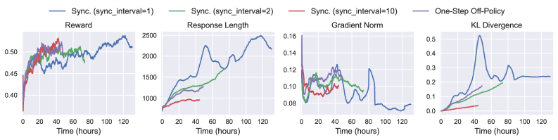<details> <summary>x8.png Details</summary>  ### Visual Description ## Chart: Performance Metrics Over Time ### Overview The image presents four line charts displaying the performance of different synchronization intervals and a one-step off-policy approach over time. The charts depict Reward, Response Length, Gradient Norm, and KL Divergence, each plotted against time in hours. ### Components/Axes * **X-axis (all charts):** Time (hours), ranging from 0 to 120. * **Y-axis (Reward):** Reward, ranging from approximately 0.40 to 0.55. * **Y-axis (Response Length):** Response Length, ranging from 0 to 2500. * **Y-axis (Gradient Norm):** Gradient Norm, ranging from 0.08 to 0.16. * **Y-axis (KL Divergence):** KL Divergence, ranging from 0.0 to 0.5. * **Legend (top):** * Blue line: Sync. (sync\_interval=1) * Green line: Sync. (sync\_interval=2) * Red line: Sync. (sync\_interval=10) * Purple line: One-Step Off-Policy ### Detailed Analysis **1. Reward** * **Sync. (sync\_interval=1) (Blue):** Starts around 0.45, fluctuates between 0.45 and 0.50 until around 70 hours, then increases to approximately 0.53 by 120 hours. * **Sync. (sync\_interval=2) (Green):** Starts around 0.45, fluctuates between 0.48 and 0.50 until around 60 hours, then remains relatively stable around 0.50. * **Sync. (sync\_interval=10) (Red):** Starts around 0.38, increases rapidly to approximately 0.47 by 10 hours, then fluctuates between 0.47 and 0.52 until around 40 hours, then decreases and stabilizes around 0.50. **2. Response Length** * **Sync. (sync\_interval=1) (Blue):** Starts around 750, increases steadily to approximately 1500 by 40 hours, then increases rapidly to approximately 2500 by 80 hours, then decreases slightly to approximately 2250 by 120 hours. * **Sync. (sync\_interval=2) (Green):** Starts around 750, increases steadily to approximately 1400 by 60 hours, then remains relatively stable around 1400. * **Sync. (sync\_interval=10) (Red):** Starts around 750, increases steadily to approximately 950 by 40 hours, then remains relatively stable around 950. * **One-Step Off-Policy (Purple):** Starts around 750, increases steadily to approximately 1200 by 40 hours, then remains relatively stable around 1200. **3. Gradient Norm** * **Sync. (sync\_interval=1) (Blue):** Starts around 0.16, decreases to approximately 0.10 by 40 hours, then fluctuates between 0.08 and 0.12 until around 80 hours, then decreases to approximately 0.07 by 120 hours. * **Sync. (sync\_interval=2) (Green):** Starts around 0.12, decreases to approximately 0.09 by 60 hours, then remains relatively stable around 0.09. * **Sync. (sync\_interval=10) (Red):** Starts around 0.12, decreases to approximately 0.09 by 40 hours, then remains relatively stable around 0.09. * **One-Step Off-Policy (Purple):** Starts around 0.14, decreases to approximately 0.10 by 40 hours, then remains relatively stable around 0.10. **4. KL Divergence** * **Sync. (sync\_interval=1) (Blue):** Starts at 0, increases rapidly to approximately 0.52 by 40 hours, then decreases to approximately 0.25 by 60 hours, then fluctuates between 0.20 and 0.30 until 120 hours. * **Sync. (sync\_interval=2) (Green):** Starts at 0, increases steadily to approximately 0.20 by 60 hours, then remains relatively stable around 0.20. * **Sync. (sync\_interval=10) (Red):** Starts at 0, increases steadily to approximately 0.04 by 40 hours, then remains relatively stable around 0.04. * **One-Step Off-Policy (Purple):** Starts at 0, increases steadily to approximately 0.15 by 40 hours, then remains relatively stable around 0.15. ### Key Observations * **Reward:** Sync. (sync\_interval=1) shows the highest reward at the end of the time period. * **Response Length:** Sync. (sync\_interval=1) has the highest response length, significantly higher than the other methods. * **Gradient Norm:** All methods show a decrease in gradient norm over time, with Sync. (sync\_interval=1) having the lowest gradient norm at the end. * **KL Divergence:** Sync. (sync\_interval=1) exhibits a large spike in KL Divergence early on, which then stabilizes. ### Interpretation The charts compare the performance of different synchronization intervals and a one-step off-policy method across four key metrics. The results suggest that Sync. (sync\_interval=1) achieves the highest reward and response length, but also exhibits a higher initial KL Divergence. The choice of synchronization interval may depend on the specific trade-offs desired between these metrics. The one-step off-policy method generally shows more stable and moderate performance across all metrics. </details> Figure 9: Results of training for one epoch by vanilla GRPO in different RL modes. The results are smoothed using a 40-step moving average for clarity. Table 3: Performance comparison of different RL modes. | | AIME2024 | AIME2025 | AMC | MATH500 | Average | Runtime (Hours) | | --- | --- | --- | --- | --- | --- | --- | | Qwen2.5-7B-Instruct | 11.15 | 6.95 | 51.35 | 70.96 | 35.10 | N/A | | Sync. (sync_interval=1) | 14.58 | 14.06 | 61.25 | 76.25 | 41.54 | 130.33 | | Sync. (sync_interval=2) | 15.52 | 11.67 | 57.97 | 75.15 | 40.08 | 73.57 | | Sync. (sync_interval=10) | 14.38 | 12.71 | 57.66 | 75.05 | 39.95 | 44.43 | | One-Step Off-Policy | 16.88 | 12.19 | 59.92 | 74.55 | 40.89 | 48.98 | 3.4 Data Processors for Tasks and Experiences We present practical examples to demonstrate how the data pipeline concepts described in Section 2.3 are applied in Trinity-RFT. These use cases highlight how manipulating data at both the task and experience level directly improves RFT performance and provides granular control over the agent’s learning process. 3.4.1 Static Task Prioritization for Curriculum Learning A common strategy for effective training is to present tasks in increasing order of difficulty. This use case demonstrates how Trinity-RFT facilitates curriculum learning by prioritizing tasks before exploration begins. This is particularly crucial for RFT, as it helps stabilize the initial learning phase of the explorer and prevents it from getting stuck on overly complex tasks, leading to a more efficient exploration path. As shown in Listing 5, a user can configure this pipeline with a simple YAML file The full configuration files can be accessed at baseline_run and priority_run.. Here, we use the GSM8K mathematical reasoning dataset. The user provides a natural language instruction via dj_process_desc: “Please compute difficulty scores for these math questions.”. Trinity-RFT ’s data service then orchestrates a three-phase process: 1. The data processor invokes an LLM (Qwen-Max) to score the difficulty of each math problem. 1. The system prioritizes samples with lower difficulty scores, creating an easy-to-hard ordering (by setting ‘priority_weights["difficulty"]: -1.0’). 1. The curated and prioritized data is formatted into an RL-ready task set for the explorer. As shown in Figure 10, this simple curation strategy yields more stable performance gains. This pattern is highly extensible: users can easily customize the difficulty metric, apply it to their own datasets, or even make the prioritization dynamic by re-ranking tasks periodically based on the agent’s current performance. ⬇ 1 # Core dataset configuration 2 data_processor: 3 data_workflow_url: "http://127.0.0.1:5005/data_workflow" 4 task_pipeline: 5 # I/O buffers 6 input_buffers: 7 - name: "raw_input" 8 path: "openai/gsm8k" 9 storage_type: "file" 10 raw: true 11 output_buffer: 12 name: "raw_output" 13 path: "outputs/task_pipeline_output/prioritized_gsm8k.jsonl" 14 storage_type: "file" 15 format: 16 prompt_key: "question" 17 response_key: "answer" 18 # data active iterator related 19 dj_process_desc: "Please compute difficulty scores for these math questions." 20 agent_model_name: "qwen-max" 21 clean_strategy: "iterative" 22 priority_weights: 23 difficulty: -1.0 # easy-to-hard Listing 5: Data processor configuration, applied on customizable buffers. 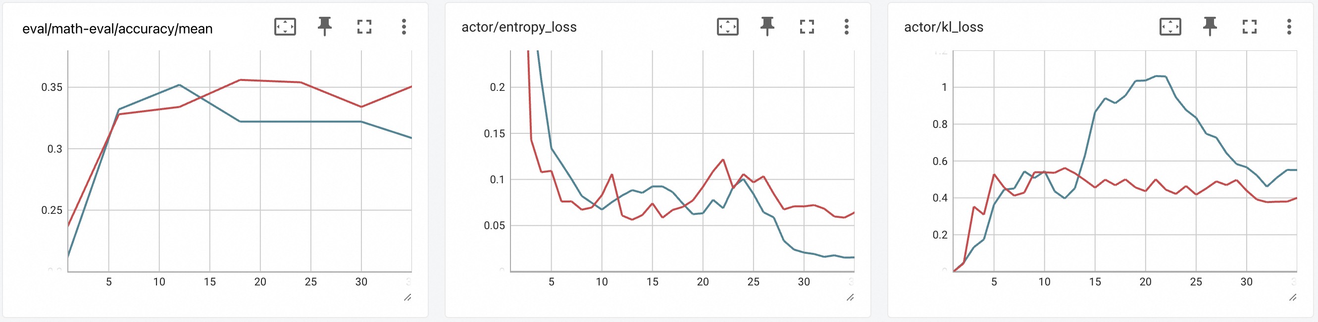<details> <summary>figs/data-pipelines/data-flow-static-priority-res.jpg Details</summary>  ### Visual Description ## Line Charts: Training Metrics ### Overview The image presents three line charts displaying training metrics. Each chart plots the progression of two different metrics over a series of training steps. The x-axis represents the training steps, ranging from approximately 0 to 33. The y-axis represents the metric value. The charts are: eval/math-eval/accuracy/mean, actor/entropy_loss, and actor/kl_loss. Each chart contains two data series, represented by a red and a blue line. ### Components/Axes **Chart 1: eval/math-eval/accuracy/mean** * **Title:** eval/math-eval/accuracy/mean * **X-axis:** Training steps, labeled approximately 5, 10, 15, 20, 25, 30. * **Y-axis:** Accuracy/Mean, with values ranging from 0.25 to 0.35. * **Data Series:** Two lines, one red and one blue. No legend is provided, so the meaning of the colors is unknown. **Chart 2: actor/entropy_loss** * **Title:** actor/entropy_loss * **X-axis:** Training steps, labeled approximately 5, 10, 15, 20, 25, 30. * **Y-axis:** Entropy Loss, with values ranging from 0.05 to 0.2. * **Data Series:** Two lines, one red and one blue. No legend is provided, so the meaning of the colors is unknown. **Chart 3: actor/kl_loss** * **Title:** actor/kl_loss * **X-axis:** Training steps, labeled approximately 5, 10, 15, 20, 25, 30. * **Y-axis:** KL Loss, with values ranging from 0.2 to 1. * **Data Series:** Two lines, one red and one blue. No legend is provided, so the meaning of the colors is unknown. ### Detailed Analysis **Chart 1: eval/math-eval/accuracy/mean** * **Red Line:** Starts at approximately 0.23, increases to approximately 0.33 by step 5, then increases to approximately 0.36 by step 15, remains relatively stable until step 25, then decreases to approximately 0.33 by step 33. * **Blue Line:** Starts at approximately 0.22, increases to approximately 0.32 by step 5, then increases to approximately 0.35 by step 10, remains relatively stable until step 20, then decreases to approximately 0.32 by step 33. **Chart 2: actor/entropy_loss** * **Red Line:** Starts at approximately 0.15, decreases to approximately 0.07 by step 5, then fluctuates between 0.06 and 0.12 until step 33. * **Blue Line:** Starts at approximately 0.23, decreases to approximately 0.12 by step 5, then decreases to approximately 0.02 by step 25, then remains relatively stable until step 33. **Chart 3: actor/kl_loss** * **Red Line:** Starts at approximately 0.0, increases to approximately 0.3 by step 5, then fluctuates between 0.4 and 0.6 until step 33. * **Blue Line:** Starts at approximately 0.0, increases to approximately 0.5 by step 5, then increases to approximately 1.0 by step 15, then decreases to approximately 0.5 by step 33. ### Key Observations * In the first chart, the red line shows a slightly higher accuracy/mean than the blue line after step 15. * In the second chart, the blue line shows a more significant decrease in entropy loss than the red line. * In the third chart, the blue line shows a peak in KL loss around step 15, while the red line remains relatively stable. ### Interpretation The charts illustrate the training progress of a model, showing the evolution of accuracy and loss metrics. The different trends in the red and blue lines suggest that they represent different aspects of the training process, possibly different components of the model or different training strategies. Without a legend, it is difficult to determine the exact meaning of each line. The fluctuations in the loss metrics indicate that the model is still learning and adapting during the training process. The peak in KL loss in the third chart may indicate a period of instability or exploration during training. </details> Figure 10: Performance on a math reasoning task. Prioritizing tasks from easy to hard (red line) leads to faster and better convergence compared to the default setting (blue line). 3.4.2 Dynamic Experience and Reward Shaping While task curation primes the model before exploration, experience shaping refines the learning signal after each agent-environment interaction. This is critical for RFT algorithms that rely on rich feedback, as standard rewards (e.g., binary pass/fail) are often too sparse to guide learning effectively. We demonstrate how to augment rewards with metrics for quality and diversity, transforming a sparse signal into a dense, multi-faceted one that provides clearer guidance to the trainer. Use Case 1: Quality Reward Augmentation. To encourage the model to generate high-quality responses, we can augment the base reward with a quality score. As illustrated in Figure 11, during each RFT step, we use the data processor to evaluate the quality of each generated rollout. For our experiment, we trained a Qwen2.5-1.5B model and used a more powerful Qwen3-32B as the scorer LLM. Specifically, we invoked the llm_quality_filter from Data-Juicer, which normalized the quality scores to the range [-0.5, 0.5] and added them to the original reward. Crucially, this processing is applied to the experience buffer at each RFT step. This allows the reward signal to adapt dynamically to the policy model’s evolving capabilities, a more responsive approach than one-time static processing. With a sync_interval of 3 over 36 steps on the Math-500 validation set, the results in Figure 12 show that: (1) The model with quality reward augmentation (red line) achieves higher accuracy. (2) The introduced quality reward itself improves over time, confirming it is a learnable signal. (3) We observe a slight increase in response length, which likely reflects an inductive bias from the larger scorer model being implicitly distilled into the smaller policy model. 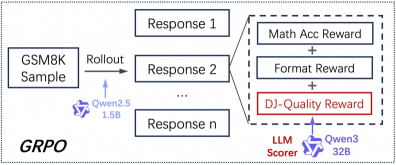<details> <summary>x9.png Details</summary>  ### Visual Description ## Diagram: GRPO Process Flow ### Overview The image is a diagram illustrating the GRPO process flow, starting with a GSM8K sample and culminating in a DJ-Quality Reward. The process involves a rollout, multiple responses, and an LLM scorer. ### Components/Axes * **Input:** GSM8K Sample * **Rollout:** Process step indicated by an arrow pointing from the GSM8K Sample to the responses. * **Responses:** Response 1, Response 2, ..., Response n. These are outputs from the rollout. * **Rewards:** Math Acc Reward, Format Reward, DJ-Quality Reward. These are components of the final reward calculation. * **LLM Scorer:** Used to evaluate the DJ-Quality Reward. * **Models:** Qwen2.5 (1.5B), Qwen3 (32B) ### Detailed Analysis 1. **GSM8K Sample:** The process begins with a GSM8K sample. 2. **Rollout:** The GSM8K sample undergoes a "Rollout" process, powered by Qwen2.5 (1.5B). 3. **Responses:** The rollout generates multiple responses: Response 1, Response 2, and so on, up to Response n. 4. **Reward Calculation:** The Math Acc Reward and Format Reward are combined with the DJ-Quality Reward. The DJ-Quality Reward is determined by the LLM Scorer, which uses Qwen3 (32B). 5. **GRPO:** The overall process is labeled as GRPO. ### Key Observations * The diagram illustrates a sequential process, starting with a sample and ending with a reward. * The rollout step generates multiple responses, suggesting an iterative or parallel process. * The LLM Scorer plays a crucial role in determining the DJ-Quality Reward. * Two different Qwen models are used: Qwen2.5 for the rollout and Qwen3 for scoring. ### Interpretation The diagram depicts a reinforcement learning or optimization process (GRPO) where a model (Qwen2.5) generates multiple responses to a given sample (GSM8K). These responses are then evaluated based on multiple criteria (Math Acc, Format, and DJ-Quality), with the DJ-Quality being assessed by another model (Qwen3). The combination of these rewards likely guides the learning process, improving the model's ability to generate high-quality responses. The use of different models for rollout and scoring suggests a potential strategy for leveraging different model strengths or reducing computational costs. The "..." indicates that there can be many responses, suggesting a sampling approach. </details> Figure 11: The enhanced math workflow with quality-reward shaping from data processor, where DJ indicates DataJuicer [2], from which more operators can be utilized to extend this worklow. 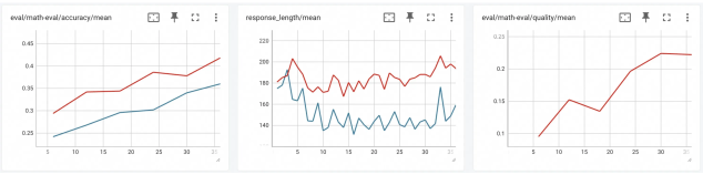<details> <summary>x10.png Details</summary>  ### Visual Description ## Chart Type: Multiple Line Charts ### Overview The image presents three line charts side-by-side, each displaying the trend of a different metric over a range of values from approximately 5 to 35 on the x-axis. The charts are titled "eval/math-eval/accuracy/mean", "response_length/mean", and "eval/math-eval/quality/mean". Each chart contains two data series, represented by a red and a blue line, except for the "eval/math-eval/quality/mean" chart, which only contains a red line. ### Components/Axes **Chart 1: eval/math-eval/accuracy/mean** * **Title:** eval/math-eval/accuracy/mean * **X-axis:** Ranges from approximately 5 to 35 in increments of 5. * **Y-axis:** Ranges from 0.25 to 0.45 in increments of 0.05. * **Data Series:** * Red Line: Represents one data series. * Blue Line: Represents another data series. **Chart 2: response_length/mean** * **Title:** response_length/mean * **X-axis:** Ranges from approximately 5 to 35 in increments of 5. * **Y-axis:** Ranges from 140 to 220 in increments of 20. * **Data Series:** * Red Line: Represents one data series. * Blue Line: Represents another data series. **Chart 3: eval/math-eval/quality/mean** * **Title:** eval/math-eval/quality/mean * **X-axis:** Ranges from approximately 5 to 35 in increments of 5. * **Y-axis:** Ranges from 0.1 to 0.25 in increments of 0.05. * **Data Series:** * Red Line: Represents one data series. ### Detailed Analysis **Chart 1: eval/math-eval/accuracy/mean** * **Red Line:** Starts at approximately 0.29 at x=5, increases to approximately 0.34 at x=15, remains relatively stable until x=20, then increases to approximately 0.39 at x=25, and remains relatively stable until x=35. * **Blue Line:** Starts at approximately 0.24 at x=5, increases to approximately 0.27 at x=15, increases to approximately 0.30 at x=20, and continues to increase to approximately 0.35 at x=35. **Chart 2: response_length/mean** * **Red Line:** Starts at approximately 180 at x=5, increases to approximately 202 at x=7, then fluctuates between approximately 175 and 195 until x=35. * **Blue Line:** Starts at approximately 185 at x=5, decreases to approximately 140 at x=7, then fluctuates between approximately 140 and 160 until x=35. **Chart 3: eval/math-eval/quality/mean** * **Red Line:** Starts at approximately 0.10 at x=5, increases to approximately 0.15 at x=10, decreases to approximately 0.13 at x=15, increases to approximately 0.20 at x=25, and remains relatively stable at approximately 0.22 until x=35. ### Key Observations * In the "eval/math-eval/accuracy/mean" chart, both the red and blue lines show an upward trend, indicating an increase in accuracy as the x-axis value increases. * In the "response_length/mean" chart, the red line shows more variability than the blue line. The blue line fluctuates more rapidly. * In the "eval/math-eval/quality/mean" chart, the red line shows an upward trend, indicating an increase in quality as the x-axis value increases, before plateauing. ### Interpretation The charts provide a comparative analysis of accuracy, response length, and quality, likely in the context of a math evaluation. The "eval/math-eval/accuracy/mean" chart suggests that both data series improve in accuracy as the x-axis value increases, with the red line consistently showing higher accuracy than the blue line. The "response_length/mean" chart shows different patterns for the two data series, with the red line showing more variability and the blue line fluctuating more rapidly. The "eval/math-eval/quality/mean" chart indicates that the quality increases with the x-axis value, before plateauing. The x-axis likely represents a parameter or iteration number. The red and blue lines likely represent different models or configurations. </details> Figure 12: Experimental results for quality-reward shaping. Augmenting the reward with a quality score (red line) improves final accuracy and provides a learnable reward signal. Use Case 2: Diversity Reward Augmentation. A common failure mode in RFT is policy collapse, where the agent repeatedly generates similar, suboptimal responses. To counteract this, we introduce a diversity reward that encourages the explorer to explore different solution paths. As shown in Figure 13, we used the GTE-Qwen2-1.5B model to convert rollouts into semantic embeddings. The diversity reward was calculated based on the cosine similarity of a rollout’s embedding to the mean embedding of its group, with lower similarity (i.e., higher diversity) yielding a higher reward. To prevent exploration from becoming chaotic, we applied a simple decay schedule to the diversity reward’s weight, starting at 0.5 and decaying to 0.3 over the training steps. The experiment, using the same setting as before, yielded compelling results (Figure 14): (1) The diversity-augmented model (red line) shows a significant performance improvement over the baseline. (2) The response length is consistently longer, indicating the reward encourages more elaborate answers. (3) Most importantly, the actor entropy loss remains consistently higher, providing strong evidence that the model is maintaining a healthier, more diverse exploration strategy, which helps it escape local optima. 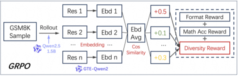<details> <summary>x11.png Details</summary>  ### Visual Description ## Diagram: GRPO Process Flow ### Overview The image is a diagram illustrating the GRPO process flow, starting with a GSM8K sample and culminating in a reward system based on format, math accuracy, and diversity. The diagram shows a series of transformations and aggregations, involving embeddings and cosine similarity calculations. ### Components/Axes * **Input:** GSM8K Sample * **Rollout:** Process applied to the sample, influenced by Qwen2.5 (1.5B parameters). * **Res 1, Res 2, Res n:** Represent different residual blocks or processing stages. * **Ebd 1, Ebd 2, Ebd n:** Represent embeddings corresponding to the residual blocks. * **Embedding:** Label indicating the transformation from Res to Ebd. * **Ebd Avg:** Average of the embeddings. * **Cos Similarity:** Cosine similarity calculation applied after averaging embeddings. * **+0.5, +0.1, +0.3:** Reward values associated with different aspects. * **Format Reward, Math Acc Reward, Diversity Reward:** Components of the reward system. * **GTE-Qwen2:** Model used for embedding. * **GRPO:** Overall process name. ### Detailed Analysis or ### Content Details 1. **GSM8K Sample:** The process begins with a GSM8K sample. 2. **Rollout:** The sample undergoes a rollout process, influenced by Qwen2.5 (1.5B). 3. **Residual Blocks and Embeddings:** * There are 'n' parallel paths, each consisting of a residual block (Res) followed by an embedding (Ebd). * The paths are labeled as Res 1 -> Ebd 1, Res 2 -> Ebd 2, and Res n -> Ebd n. 4. **Embedding Averaging:** * The embeddings from each path (Ebd 1, Ebd 2, ..., Ebd n) are averaged to produce "Ebd Avg". 5. **Cosine Similarity:** * Cosine similarity is calculated after the embedding averaging step. 6. **Reward System:** * The reward system consists of three components: Format Reward, Math Acc Reward, and Diversity Reward. * These rewards are combined (indicated by "+" symbols). 7. **Reward Values:** * Format Reward is associated with a value of +0.5 (red). * Math Acc Reward is associated with a value of +0.1 (green). * Diversity Reward is associated with a value of +0.3 (yellow). 8. **Model Attribution:** * The embedding process is attributed to GTE-Qwen2. ### Key Observations * The diagram illustrates a parallel processing approach with multiple residual blocks and embeddings. * Embedding averaging and cosine similarity calculations are key steps in the process. * The reward system combines multiple factors, with Format Reward having the highest associated value (+0.5). ### Interpretation The diagram describes a process (GRPO) for evaluating and rewarding the performance of a model (likely Qwen2.5) on the GSM8K dataset. The model generates multiple outputs (rollouts), which are then processed through residual blocks and converted into embeddings. These embeddings are averaged, and cosine similarity is calculated, possibly to measure the similarity between different outputs. The final reward is a combination of format correctness, mathematical accuracy, and diversity, suggesting that the goal is to generate solutions that are not only correct but also varied in their approach. The higher weight given to "Format Reward" suggests that the output format is a critical aspect of the evaluation. 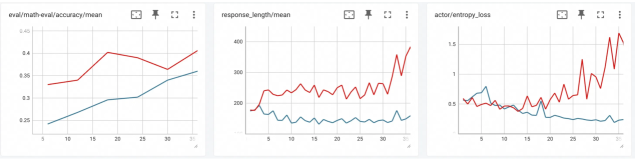</details> Figure 13: The enhanced math workflow with diversity-reward shaping from data processor <details> <summary>x12.png Details</summary>  ### Visual Description ## Line Charts: Model Performance Metrics ### Overview The image presents three line charts displaying the performance of a model across different metrics during training or evaluation. Each chart shows two data series, likely representing different model configurations or training strategies, plotted against a common x-axis representing training steps or epochs. The charts depict 'eval/math-eval/accuracy/mean', 'response_length/mean', and 'actor/entropy_loss'. ### Components/Axes **Chart 1: eval/math-eval/accuracy/mean** * **Title:** eval/math-eval/accuracy/mean * **X-axis:** (Implied) Training steps or epochs, with markers at approximately 5, 10, 15, 20, 25, and 30. * **Y-axis:** Accuracy, ranging from 0.25 to 0.45, with markers at 0.25, 0.3, 0.35, 0.4, and 0.45. * **Data Series:** * Red Line: Represents one model's accuracy. * Blue Line: Represents another model's accuracy. **Chart 2: response_length/mean** * **Title:** response_length/mean * **X-axis:** (Implied) Training steps or epochs, with markers at approximately 5, 10, 15, 20, 25, and 30. * **Y-axis:** Response Length, ranging from 200 to 400, with markers at 200, 300, and 400. * **Data Series:** * Red Line: Represents one model's average response length. * Blue Line: Represents another model's average response length. **Chart 3: actor/entropy_loss** * **Title:** actor/entropy_loss * **X-axis:** (Implied) Training steps or epochs, with markers at approximately 5, 10, 15, 20, 25, and 30. * **Y-axis:** Entropy Loss, ranging from 0.5 to 1.5, with markers at 0.5, 1.0, and 1.5. * **Data Series:** * Red Line: Represents one model's entropy loss. * Blue Line: Represents another model's entropy loss. ### Detailed Analysis **Chart 1: eval/math-eval/accuracy/mean** * **Red Line (Accuracy):** Starts at approximately 0.33 at step 5, increases to about 0.34 at step 10, rises to approximately 0.40 at step 20, and then decreases to approximately 0.37 at step 30. * **Blue Line (Accuracy):** Starts at approximately 0.24 at step 5, increases steadily to approximately 0.35 at step 30. **Chart 2: response_length/mean** * **Red Line (Response Length):** Starts at approximately 180 at step 5, fluctuates between 220 and 260 until step 25, and then increases sharply to approximately 380 at step 30. * **Blue Line (Response Length):** Starts at approximately 180 at step 5, decreases to approximately 140 at step 10, and then remains relatively stable between 140 and 160 until step 30. **Chart 3: actor/entropy_loss** * **Red Line (Entropy Loss):** Starts at approximately 0.5 at step 5, fluctuates between 0.5 and 1.0 until step 25, and then increases sharply to approximately 1.6 at step 30. * **Blue Line (Entropy Loss):** Starts at approximately 0.5 at step 5, decreases to approximately 0.2 at step 25, and then remains relatively stable until step 30. ### Key Observations * In the accuracy chart, the red line initially performs better but plateaus and slightly decreases, while the blue line shows consistent improvement. * In the response length chart, the red line shows significantly higher and more volatile response lengths compared to the blue line. * In the entropy loss chart, the red line shows higher and increasing entropy loss, while the blue line shows decreasing entropy loss. ### Interpretation The charts compare the performance of two models (or configurations) across three key metrics: accuracy, response length, and entropy loss. The blue line consistently shows a more stable and potentially better-performing model. While the red line initially shows higher accuracy, it plateaus and is accompanied by higher response lengths and increasing entropy loss, suggesting potential issues with model stability or overfitting. The blue line's consistent improvement in accuracy, coupled with lower response lengths and decreasing entropy loss, indicates a more robust and efficient model. The sharp increase in response length and entropy loss for the red line towards the end of the training period (step 30) is a notable anomaly that warrants further investigation. </details> Figure 14: Experimental results for diversity-reward shaping. Rewarding diverse responses (red line) significantly improves task accuracy and maintains higher entropy. 3.5 RFT with Human in the Loop This example demonstrates the human-in-the-loop capability in Trinity-RFT for preference modeling. As illustrated in Listing 6 and Figure 15, our framework integrates Label Studio’s annotation interface with asynchronous data pipelines through four coordinated stages: (1) task generation: auto-creating annotation batches from model rollouts; (2) interactive labeling: providing UI for side-by-side response comparison; (3) quality control: enforcing inter-annotator agreement thresholds; and (4) versioned storage: tracking preference lineage in pre-defined fields like those in DPODataModel. This pipeline reflects Trinity-RFT ’s bi-directional collaboration feature (Section 2.3.4), backed by timeout-aware task polling and support of atomic batch commit. It enables hybrid procedures where initial AI pre-screening can reduce human workload in production deployments. Annotation activities can scale across distributed teams through event-driven task routing. The system’s flexibility benefits rapid adaptation to diverse annotation protocols, allowing developers to implement custom labeling interfaces through XML-based templates or integrate third-party annotation services via unified SDK endpoints. This capability underpins advanced use cases such as safety red-teaming datasets and online instruction tuning scenarios where human judgment remains irreplaceable for quality-critical decisions, particularly in human-centric sociocultural contexts where data quality, difficulty, and reward signals are difficult to verify logically. ⬇ 1 # Human annotation configuration 2 class HumanAnnotationConfig: 3 "" "Preference annotation pipeline configuration" "" 4 5 def __init__ (self): 6 self. process = [ 7 { 8 "human_preference_annotation_mapper": { 9 "wait_for_annotations": True, # Block until annotations complete 10 "timeout": 3600, # Maximum wait time in seconds 11 "prompt_key": "prompt", # Source field for prompts 12 "answer1_key": "answer1", # First candidate response 13 "chosen_key": "chosen" # Selected response key 14 } 15 } 16 ] 17 18 def get_pipeline (self) -> List [Dict]: 19 "" "Get annotation processing pipeline" "" 20 return self. process Listing 6: Configuration for human preference annotation. 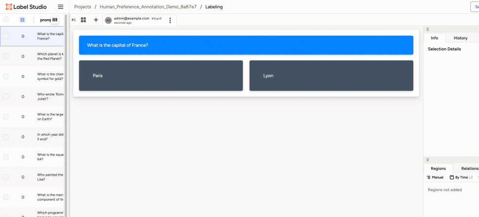<details> <summary>x13.png Details</summary>  ### Visual Description ## Labeling Interface: Question and Answer Selection ### Overview The image shows a user interface for a labeling task, likely within a platform like Label Studio. The interface presents a question and two possible answers, allowing a user to select the correct one. The left side displays a list of questions, while the right side shows details and options related to the selected question. ### Components/Axes * **Header**: "Label Studio", "Projects / Human\_Preference\_Annotation\_Demo\_8a87e7 / Labeling" * **Left Sidebar**: * A list of questions, each with a checkbox and a numerical indicator (likely representing the number of times the question has been labeled). * Example questions: "What is the capital of France?", "Which planet is k the Red Planet?", "What is the chemical symbol for gold?", "Who wrote 'Rom Juliet'?", "What is the large on Earth?", "In which year did II end?", "What is the square 64?", "Who painted the Lisa?", "What is the main component of th", "Which programm" * **Main Content Area**: * Question prompt: "What is the capital of France?" (in a blue box) * Answer options: "Paris" and "Lyon" (in dark gray boxes) * **Right Sidebar**: * Tabs: "Info" and "History" * Section: "Selection Details" * Tabs: "Regions" and "Relations" * Options: "Manual" and "By Time" * Text: "Regions not added" ### Detailed Analysis or ### Content Details * **Question List**: The left sidebar contains a scrollable list of questions. Each question has a checkbox and a number (likely a count). * **Question Prompt**: The main content area displays the current question in a prominent blue box. * **Answer Options**: Two answer options, "Paris" and "Lyon", are presented in dark gray boxes below the question. * **User Information**: The top-right of the main content area shows user information: "admin@example.com" and a timestamp indicating when the question was presented ("seconds ago"). * **Right Sidebar Tabs**: The right sidebar provides additional information and options related to the selected question. The "Info" tab is selected, displaying "Selection Details". The "Regions" tab is selected, displaying "Regions not added". ### Key Observations * The interface is designed for a question-answering labeling task. * The left sidebar provides a list of questions to be labeled. * The main content area presents the current question and answer options. * The right sidebar provides additional information and options. ### Interpretation The image depicts a typical labeling interface used for training machine learning models. The user is presented with a question and must select the correct answer from the provided options. The interface tracks user activity and provides tools for managing and reviewing the labeling process. The presence of "Regions" and "Relations" tabs suggests that the labeling task might involve more complex annotations than simple question answering, potentially including identifying regions of interest in images or defining relationships between entities. </details> Figure 15: An interactive interface for human preference annotation. 3.6 Low-Code Usage and Development with Trinity-Studio <details> <summary>figs/studio-showcase/dashboard.png Details</summary>  ### Visual Description ## Dashboard: RFT Portal Dashboard ### Overview The image is a screenshot of the RFT Portal Dashboard. It displays three main sections: Training Portal, pgAdmin, and Label Studio. Each section has a brief description and a button to open the respective application. The dashboard also includes a top navigation bar with links to Dashboard, pgAdmin, Label Studio, Training Portal, and Settings. ### Components/Axes * **Header**: Contains the navigation bar with links to: * Dashboard * pgAdmin * Label Studio * Training Portal * Settings * **Title**: "RFT Portal Dashboard" * **Main Content**: Three cards representing different applications: * **Training Portal**: * Icon: "TP" in a blue circle * Title: "Training Portal" * Description: "Access the training portal to manage your training data and models." * Button: "Open Training Portal" (blue) * **pgAdmin**: * Icon: "DB" in a green circle * Title: "pgAdmin" * Description: "Manage your PostgreSQL databases with pgAdmin." * Button: "Open pgAdmin" (green) * **Label Studio**: * Icon: "LS" in a red circle * Title: "Label Studio" * Description: "Label and annotate your data with Label Studio." * Button: "Open Label Studio" (red) ### Detailed Analysis or ### Content Details The dashboard is structured to provide quick access to three key applications: Training Portal, pgAdmin, and Label Studio. Each application is represented by a card with an icon, title, description, and a button to launch the application. The color of the icon and button matches for each application (blue for Training Portal, green for pgAdmin, and red for Label Studio). * **Training Portal**: The icon contains the letters "TP" in a blue circle. The button is labeled "Open Training Portal" and is blue. * **pgAdmin**: The icon contains the letters "DB" in a green circle. The button is labeled "Open pgAdmin" and is green. * **Label Studio**: The icon contains the letters "LS" in a red circle. The button is labeled "Open Label Studio" and is red. ### Key Observations * The dashboard provides a centralized location to access different applications. * Each application is represented by a card with a consistent design. * The color scheme is consistent, with each application having its own distinct color. ### Interpretation The RFT Portal Dashboard is designed to provide users with easy access to the Training Portal, pgAdmin, and Label Studio applications. The clear and consistent design, along with the use of color, makes it easy for users to quickly identify and access the application they need. The dashboard serves as a central hub for managing training data, PostgreSQL databases, and data labeling tasks. </details> (a) Trinity-Studio dashboard. 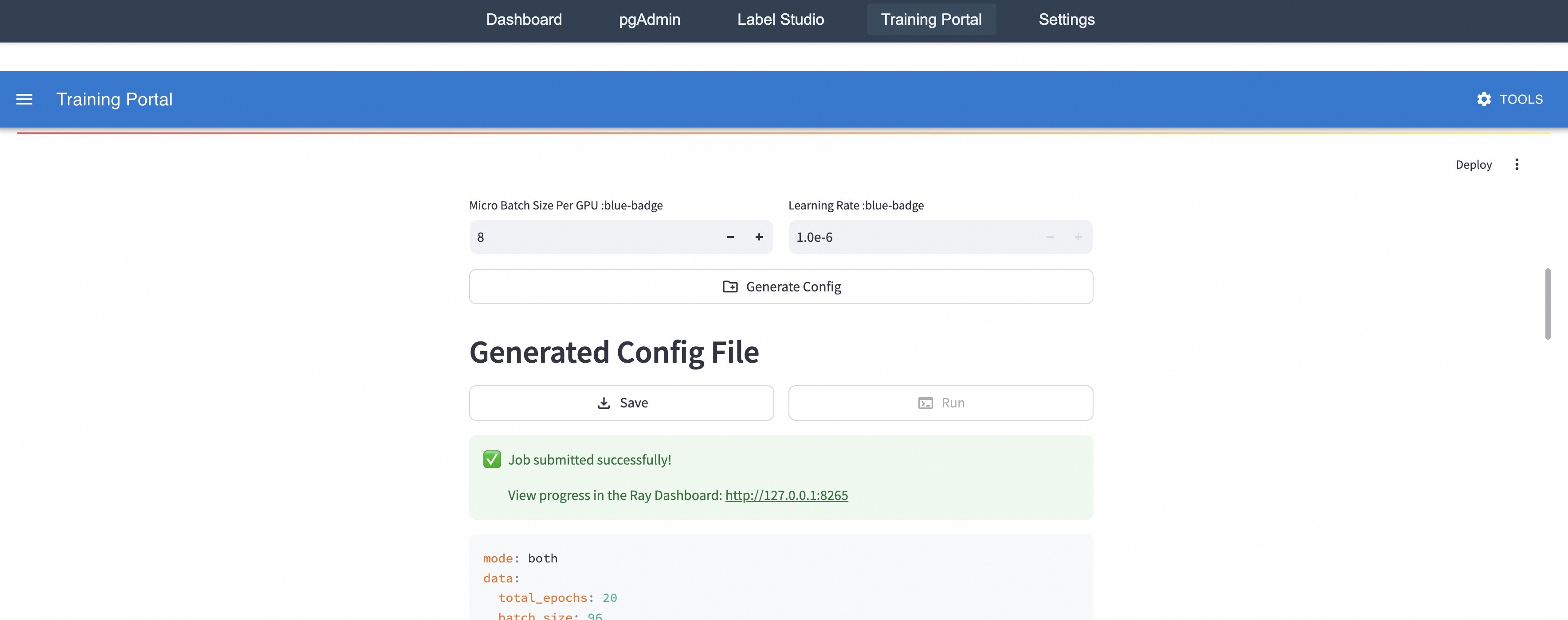<details> <summary>figs/studio-showcase/training-portal-click-run.jpg Details</summary>  ### Visual Description ## Screenshot: Training Portal Configuration ### Overview The image is a screenshot of a "Training Portal" configuration interface. It shows settings for micro batch size, learning rate, and options to generate, save, and run a configuration. A success message indicates a job has been submitted. ### Components/Axes * **Header**: Contains navigation links: "Dashboard", "pgAdmin", "Label Studio", "Training Portal", "Settings", and "Tools". * **Main Configuration Area**: * "Micro Batch Size Per GPU :blue-badge": Input field with a value of "8" and "+" and "-" buttons. * "Learning Rate :blue-badge": Input field with a value of "1.0e-6" and "+" and "-" buttons. * "Generate Config" button. * "Generated Config File" heading. * "Save" and "Run" buttons. * Success message: "Job submitted successfully!" * Link to Ray Dashboard: "View progress in the Ray Dashboard: http://127.0.0.1:8265" * Configuration details: * mode: both * data: * total_epochs: 20 * batch_size: 96 * **Right Sidebar**: "Deploy" option with a three-dot menu. ### Detailed Analysis or ### Content Details * **Micro Batch Size**: The current value is "8". The user can increase or decrease this value using the "+" and "-" buttons. * **Learning Rate**: The current value is "1.0e-6". The user can increase or decrease this value using the "+" and "-" buttons. * **Configuration File**: The configuration file is generated based on the input parameters. * **Job Submission**: A green checkmark indicates that the job has been submitted successfully. * **Ray Dashboard**: A link is provided to view the progress of the job in the Ray Dashboard. The link is "http://127.0.0.1:8265". * **Configuration Details**: * `mode: both` * `data:` * `total_epochs: 20` * `batch_size: 96` ### Key Observations * The interface allows users to configure training parameters such as micro batch size and learning rate. * The system provides feedback on job submission status and a link to monitor progress. * The configuration details show the mode, total epochs, and batch size. ### Interpretation The screenshot depicts a user interface for configuring and running training jobs. The user can adjust the micro batch size and learning rate, generate a configuration file, and submit the job. The system provides feedback on the job submission status and a link to monitor progress in the Ray Dashboard. The configuration details provide information about the training mode, total epochs, and batch size. The "blue-badge" text next to the labels "Micro Batch Size Per GPU" and "Learning Rate" likely indicates that these parameters are configurable or have specific constraints within the system. </details> (b) Start training on the “Training Portal” page. 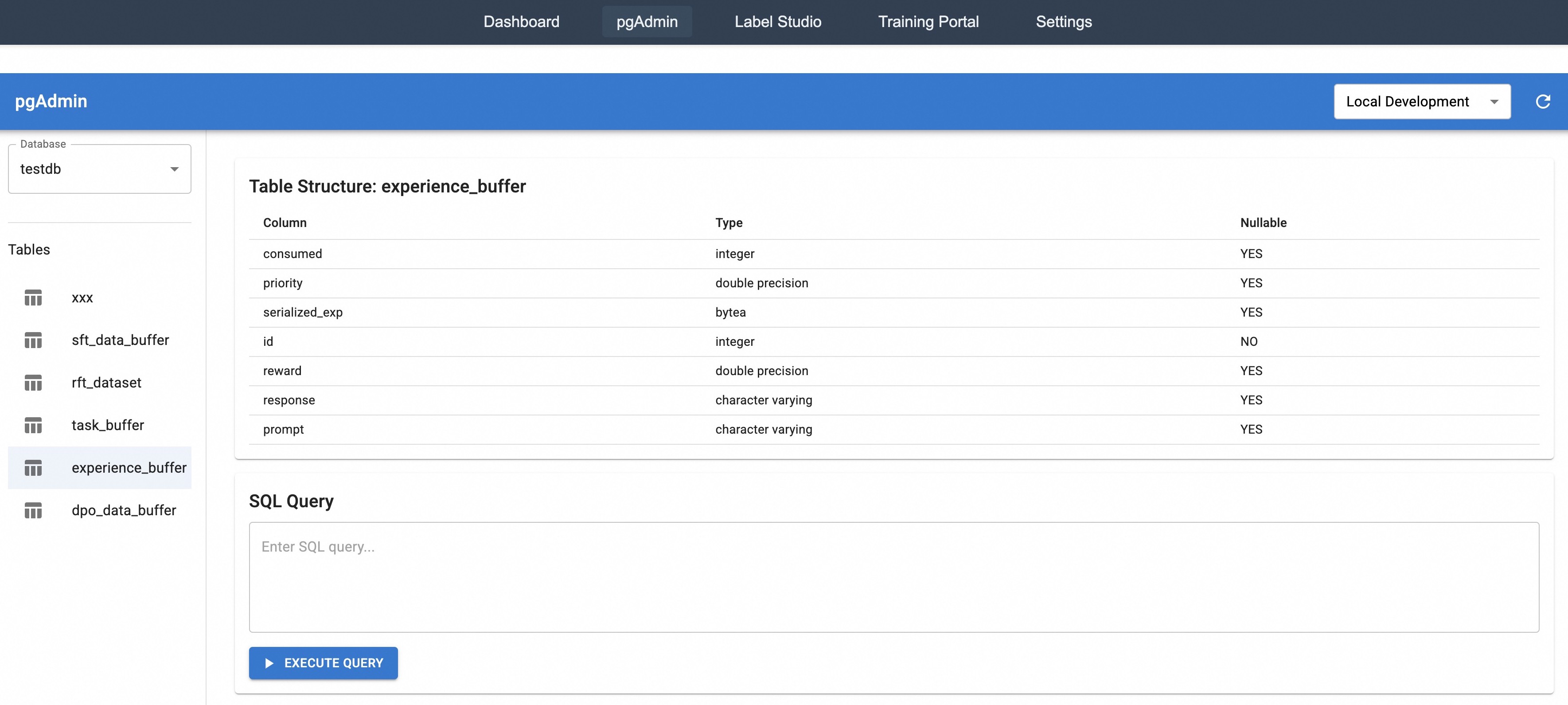<details> <summary>figs/studio-showcase/pgadmin-select-table.jpg Details</summary>  ### Visual Description ## Database Table Structure: experience_buffer ### Overview The image is a screenshot of a pgAdmin interface, displaying the structure of a database table named "experience_buffer". It also shows a section for executing SQL queries. ### Components/Axes * **Header**: Contains navigation links: Dashboard, pgAdmin, Label Studio, Training Portal, Settings. Also includes a "Local Development" dropdown menu. * **Left Sidebar**: * Database selection: "testdb" is selected from a dropdown. * List of Tables: xxx, sft\_data\_buffer, rft\_dataset, task\_buffer, experience\_buffer (selected), dpo\_data\_buffer. * **Main Content Area**: * Table Structure: experience\_buffer * Columns: consumed, priority, serialized\_exp, id, reward, response, prompt * Types: integer, double precision, bytea, integer, double precision, character varying, character varying * Nullable: YES, YES, YES, NO, YES, YES, YES * SQL Query: A text area to enter SQL queries and an "EXECUTE QUERY" button. ### Detailed Analysis or ### Content Details **Table Structure: experience_buffer** | Column | Type | Nullable | | -------------- | ----------------- | -------- | | consumed | integer | YES | | priority | double precision | YES | | serialized\_exp | bytea | YES | | id | integer | NO | | reward | double precision | YES | | response | character varying | YES | | prompt | character varying | YES | **SQL Query Section** * A text input field labeled "Enter SQL query..." * A button labeled "EXECUTE QUERY" ### Key Observations * The "experience\_buffer" table has columns with various data types, including integers, double precision numbers, byte arrays, and character strings. * The "id" column is the only one that is explicitly defined as non-nullable. * The interface provides a direct way to execute SQL queries against the database. ### Interpretation The screenshot shows a typical database administration interface, allowing users to view table structures and execute SQL queries. The "experience\_buffer" table likely stores data related to experiences, with fields for consumed resources, priority, serialized data, a unique ID, reward values, responses, and prompts. The fact that most fields are nullable suggests that some data points might be optional or not always available. The SQL query section enables users to interact with the database beyond the basic table structure view. </details> (c) Manage data on the “pgAdmin” page. 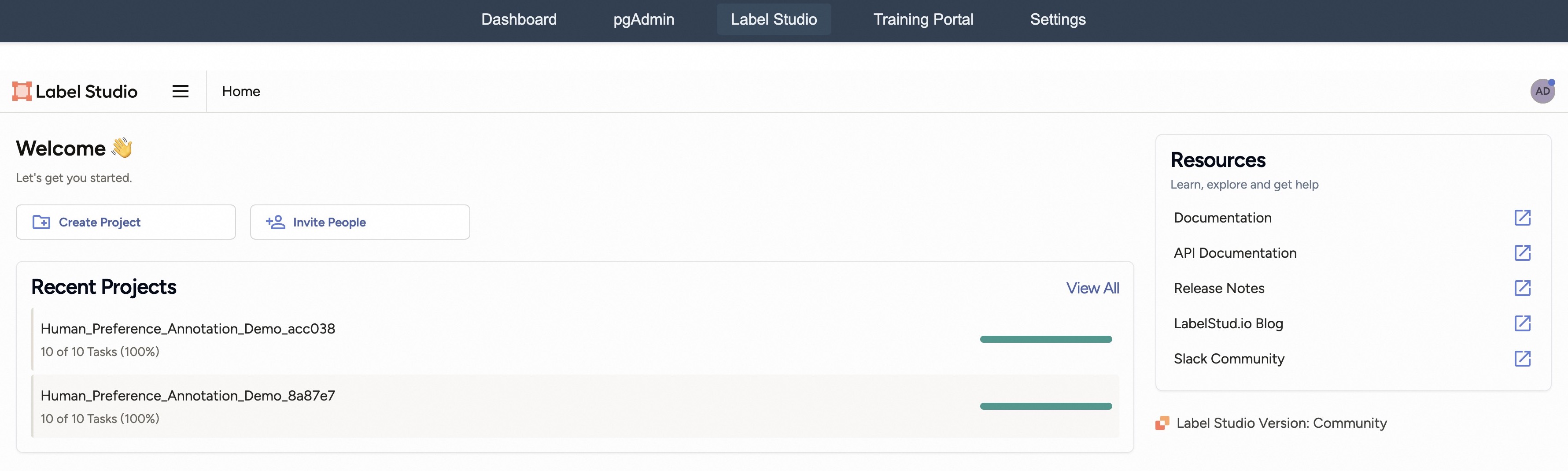<details> <summary>figs/studio-showcase/label-studio-enter.jpg Details</summary>  ### Visual Description ## Dashboard: Label Studio Home ### Overview The image is a screenshot of the Label Studio home dashboard. It displays a welcome message, options to create a project or invite people, a list of recent projects with their completion status, and a resources section with links to documentation, API, release notes, blog, and community. ### Components/Axes * **Header:** Contains navigation links: Dashboard, pgAdmin, Label Studio (active), Training Portal, Settings. * **Main Content Area:** * "Label Studio" logo and "Home" link on the top-left. * "Welcome" message with a waving hand emoji. * "Let's get you started." subtitle. * Two buttons: "+ Create Project" and "+ Invite People". * "Recent Projects" section with a "View All" link. * List of recent projects: * Human\_Preference\_Annotation\_Demo\_acc038: 10 of 10 Tasks (100%) * Human\_Preference\_Annotation\_Demo\_8a87e7: 10 of 10 Tasks (100%) * Progress bars next to each project, indicating completion. * **Right Sidebar:** * "Resources" section with "Learn, explore and get help" subtitle. * List of resources: * Documentation * API Documentation * Release Notes * LabelStud.io Blog * Slack Community * Label Studio Version: Community ### Detailed Analysis or ### Content Details * **Recent Projects:** * Project 1: Human\_Preference\_Annotation\_Demo\_acc038 is 100% complete (10 of 10 tasks). * Project 2: Human\_Preference\_Annotation\_Demo\_8a87e7 is 100% complete (10 of 10 tasks). * The progress bars next to each project are solid green, visually confirming 100% completion. * **Resources:** * Each resource link (Documentation, API Documentation, Release Notes, LabelStud.io Blog, Slack Community) has an external link icon next to it. * **Top Right:** * User profile icon labeled "AD". * **Version:** * Label Studio Version: Community ### Key Observations * The dashboard provides a clear overview of recent projects and available resources. * The "Welcome" section encourages users to start a new project or invite collaborators. * All listed recent projects are completed. ### Interpretation The Label Studio dashboard is designed to be user-friendly, providing easy access to project management and learning resources. The "Welcome" section and prominent "Create Project" button suggest a focus on onboarding new users. The "Recent Projects" section allows users to quickly resume work on existing projects. The "Resources" section provides access to documentation, API information, and community support, facilitating user learning and problem-solving. The fact that both listed projects are 100% complete suggests a successful and active user base. </details> (d) Process data on the “Label Studio” page. Figure 16: Snapshots of Trinity-Studio. Trinity-Studio provides visual interaction for the core capabilities of Trinity-RFT, designed to bridge the gap between system complexity and user accessibility. As shown in Figure 16(a), its three integrated modules — “Training Portal”, “pgAdmin”, and “Label Studio” — form a cohesive interface that supports low-code usage and development with Trinity-RFT, and make it easy to monitor and track the full RFT pipeline with transparency. - “Training Portal” (Figure 16(b)) implements configuration-to-execution procedures through declarative YAML editing with auto completion and live validation that prevents misconfigurations. Furthermore, the integration of runtime metrics with tools like Wandb/TensorBoard directly helps the active data optimization feature by surfacing signals such as difficulty distribution drifts and diversity metrics mentioned in Section 3.4. This transparency ensures that users can monitor how data curation strategies impact RFT performance in real time. - “pgAdmin” (Figure 16(c)) reflects Trinity-RFT ’s end-to-end data transformation capabilities by providing a visual panel for PostgreSQL-based storage. This design benefits the versioned data lineage requirements of RFT, particularly for scenarios involving asynchronous training (Section 2.3.3). With intuitive SQL query builders, users can easily adjust schema, audit training experiences and human annotation batches with fine-grained precision. This capability is valuable for rapid validation of active learning policies by cross-referencing training outcomes with metadata (e.g., difficulty scores and staleness in asynchronous mode). - “Label Studio” page (Figure 16(d)) operationalizes Trinity-RFT ’s bi-directional human-AI collaboration capability (Section 2.3.4). Utilizing the provided task polling and atomic batch commit mechanisms, users can annotate the data or experiences directly, allowing an asynchronous way to involve human feedback and to dynamically influence data curation. By unifying these capabilities in a single UI, Trinity-Studio reduces the cognitive load of managing complex RFT procedures. For example, a researcher tuning a math reasoning task could use the Training Portal to adjust difficulty scoring parameters, view the resulting distribution shifts in the pgAdmin module, and then validate human annotators’ preferences in the Label Studio page. This end-to-end visibility can be useful for debugging and iterating RFT strategies, and complements the programmatic APIs of Trinity-RFT while maintaining full compatibility with CLI procedures. We implement Trinity-Studio with the Singe-Spa framework [33]. The modular architecture enables custom view development through JavaScript plugins and flexible extensions for general-purpose usage. 4 Conclusion and Next Steps We have presented Trinity-RFT, a general-purpose, flexible, scalable and user-friendly framework for reinforcement fine-tuning of large language models. Trinity-RFT offers a path into “the era of experience” [32], by supporting applications in diverse scenarios with complex agent-environment interaction, and serving as a unified platform for exploring advanced methodologies in each stage of the complete RFT pipeline, at both macroscopic and microscopic levels. Further development of Trinity-RFT includes incorporating more advanced RL algorithms (especially off-policy or asynchronous ones), making the choices of hyperparameters more adaptive and less reliant on manual tuning, augmenting data pipelines with smarter sampling strategies and data processing operations, and conducting more thorough experiments and evaluations with Trinity-RFT. Acknowledgements Trinity-RFT is built upon many excellent open-source projects, including but not limited to: verl [30] and PyTorch’s FSDP [8] for LLM training; vLLM [15] for LLM inference; Data-Juicer [2] for data-related functionalities; AgentScope [11] for agentic workflow; and Ray [20] for distributed runtime. References - [1] ChatLearn. https://github.com/alibaba/ChatLearn. - [2] Daoyuan Chen, Yilun Huang, Zhijian Ma, Hesen Chen, Xuchen Pan, Ce Ge, Dawei Gao, Yuexiang Xie, Zhaoyang Liu, Jinyang Gao, Yaliang Li, Bolin Ding, and Jingren Zhou. Data-juicer: A one-stop data processing system for large language models. In International Conference on Management of Data, 2024. - [3] Karl Cobbe, Vineet Kosaraju, Mohammad Bavarian, Mark Chen, Heewoo Jun, Lukasz Kaiser, Matthias Plappert, Jerry Tworek, Jacob Hilton, Reiichiro Nakano, Christopher Hesse, and John Schulman. Training verifiers to solve math word problems. arXiv preprint arXiv:2110.14168, 2021. - [4] Jeff Da, Clinton Wang, Xiang Deng, Yuntao Ma, Nikhil Barhate, and Sean Hendryx. Agent-rlvr: Training software engineering agents via guidance and environment rewards. arXiv, 2025. - [5] DeepSeek-AI. Deepseek-r1: Incentivizing reasoning capability in llms via reinforcement learning. arXiv, 2025. - [6] Hanze Dong, Wei Xiong, Deepanshu Goyal, Yihan Zhang, Winnie Chow, Rui Pan, Shizhe Diao, Jipeng Zhang, KaShun SHUM, and Tong Zhang. RAFT: Reward ranked finetuning for generative foundation model alignment. Transactions on Machine Learning Research, 2023. - [7] Yannis Flet-Berliac, Nathan Grinsztajn, Florian Strub, Bill Wu, Eugene Choi, Chris Cremer, Arash Ahmadian, Yash Chandak, Mohammad Gheshlaghi Azar, Olivier Pietquin, and Matthieu Geist. Contrastive policy gradient: Aligning LLMs on sequence-level scores in a supervised-friendly fashion. In EMNLP, 2024. - [8] Pytorch FSDP. https://pytorch.org/docs/stable/fsdp.html. - [9] Wei Fu, Jiaxuan Gao, Xujie Shen, Chen Zhu, Zhiyu Mei, Chuyi He, Shusheng Xu, Guo Wei, Jun Mei, Jiashu Wang, Tongkai Yang, Binhang Yuan, and Yi Wu. Areal: A large-scale asynchronous reinforcement learning system for language reasoning. arXiv, 2025. - [10] Yuqian Fu, Tinghong Chen, Jiajun Chai, Xihuai Wang, Songjun Tu, Guojun Yin, Wei Lin, Qichao Zhang, Yuanheng Zhu, and Dongbin Zhao. Srft: A single-stage method with supervised and reinforcement fine-tuning for reasoning. arXiv, 2025. - [11] Dawei Gao, Zitao Li, Xuchen Pan, Weirui Kuang, Zhijian Ma, Bingchen Qian, Fei Wei, Wenhao Zhang, Yuexiang Xie, Daoyuan Chen, Liuyi Yao, Hongyi Peng, Ze Yu Zhang, Lin Zhu, Chen Cheng, Hongzhu Shi, Yaliang Li, Bolin Ding, and Jingren Zhou. Agentscope: A flexible yet robust multi-agent platform. arXiv, 2024. - [12] Zhenyu Han, Ansheng You, Haibo Wang, Kui Luo, Guang Yang, Wenqi Shi, Menglong Chen, Sicheng Zhang, Zeshun Lan, Chunshi Deng, Huazhong Ji, Wenjie Liu, Yu Huang, Yixiang Zhang, Chenyi Pan, Jing Wang, Xin Huang, Chunsheng Li, and Jianping Wu. Asyncflow: An asynchronous streaming rl framework for efficient llm post-training. arXiv, 2025. - [13] Jian Hu, Xibin Wu, Zilin Zhu, Xianyu, Weixun Wang, Dehao Zhang, and Yu Cao. OpenRLHF: An easy-to-use, scalable and high-performance RLHF framework. arXiv, 2024. - [14] Huggingface. https://huggingface.co/. - [15] Woosuk Kwon, Zhuohan Li, Siyuan Zhuang, Ying Sheng, Lianmin Zheng, Cody Hao Yu, Joseph E. Gonzalez, Hao Zhang, and Ion Stoica. Efficient memory management for large language model serving with pagedattention. In Proceedings of the ACM SIGOPS 29th Symposium on Operating Systems Principles, 2023. - [16] Lu Ma, Hao Liang, Meiyi Qiang, Lexiang Tang, Xiaochen Ma, Zhen Hao Wong, Junbo Niu, Chengyu Shen, Runming He, Bin Cui, and Wentao Zhang. Learning what reinforcement learning can’t: Interleaved online fine-tuning for hardest questions. arXiv, 2025. - [17] Model context protocol servers. https://github.com/modelcontextprotocol/servers. - [18] Mistral-AI. Magistral. arXiv, 2025. - [19] Modelscope. https://www.modelscope.cn/home. - [20] Philipp Moritz, Robert Nishihara, Stephanie Wang, Alexey Tumanov, Richard Liaw, Eric Liang, Melih Elibol, Zongheng Yang, William Paul, Michael I. Jordan, and Ion Stoica. Ray: A distributed framework for emerging ai applications. arXiv, 2018. - [21] Ofir Nachum, Mohammad Norouzi, Kelvin Xu, and Dale Schuurmans. Bridging the gap between value and policy based reinforcement learning. In NIPS, 2017. - [22] Nccl. https://github.com/NVIDIA/nccl. - [23] Michael Noukhovitch, Shengyi Huang, Sophie Xhonneux, Arian Hosseini, Rishabh Agarwal, and Aaron Courville. Asynchronous rlhf: Faster and more efficient off-policy rl for language models. In The Thirteenth International Conference on Learning Representations, 2025. - [24] Long Ouyang, Pamela Mishkin, Jeff Wu, C L Mar, Jacob Hilton, Amanda Askell, and Paul Christiano. Training language models to follow instructions with human feedback. arXiv, 2022. - [25] Rafael Rafailov, Archit Sharma, Eric Mitchell, Christopher D. Manning, Stefano Ermon, and Chelsea Finn. Direct preference optimization: Your language model is secretly a reward model. In Advances in Neural Information Processing Systems 36: Annual Conference on Neural Information Processing Systems 2023, NeurIPS 2023, New Orleans, LA, USA, December 10 - 16, 2023. - [26] Pierre Harvey Richemond, Yunhao Tang, Daniel Guo, Daniele Calandriello, Mohammad Gheshlaghi Azar, Rafael Rafailov, Bernardo Avila Pires, Eugene Tarassov, Lucas Spangher, Will Ellsworth, Aliaksei Severyn, Jonathan Mallinson, Lior Shani, Gil Shamir, Rishabh Joshi, Tianqi Liu, Remi Munos, and Bilal Piot. Offline regularised reinforcement learning for large language models alignment. arXiv, 2024. - [27] David Rolnick, Arun Ahuja, Jonathan Schwarz, Timothy Lillicrap, and Gregory Wayne. Experience replay for continual learning. In Advances in Neural Information Processing Systems, volume 32, 2019. - [28] John Schulman, Filip Wolski, Prafulla Dhariwal, Alec Radford, and Oleg Klimov. Proximal policy optimization algorithms. arXiv, 2017. - [29] Zhihong Shao, Peiyi Wang, Qihao Zhu, Runxin Xu, Junxiao Song, Xiao Bi, Haowei Zhang, Mingchuan Zhang, Y. K. Li, Y. Wu, and Daya Guo. DeepSeekMath: Pushing the limits of mathematical reasoning in open language models. arXiv, 2024. - [30] Guangming Sheng, Chi Zhang, Zilingfeng Ye, Xibin Wu, Wang Zhang, Ru Zhang, Yanghua Peng, Haibin Lin, and Chuan Wu. HybridFlow: A flexible and efficient rlhf framework. arXiv, 2024. - [31] Mohit Shridhar, Xingdi Yuan, Marc-Alexandre Cote, Yonatan Bisk, Adam Trischler, and Matthew Hausknecht. ALFWorld: Aligning text and embodied environments for interactive learning. In International Conference on Learning Representations, 2021. - [32] David Silver and Richard S. Sutton. Welcome to the era of experience. https://storage.googleapis.com/deepmind-media/Era-of-Experience%20/The%20Era%20of%20Experience%20Paper.pdf, 2025. - [33] A javascript framework for front-end microservices, 2025. - [34] Yuda Song, Yifei Zhou, Ayush Sekhari, Drew Bagnell, Akshay Krishnamurthy, and Wen Sun. Hybrid RL: Using both offline and online data can make RL efficient. In The Eleventh International Conference on Learning Representations, 2023. - [35] Kimi Team. Kimi k1.5: Scaling reinforcement learning with LLMs. arXiv, 2025. - [36] Qwen Team. Qwen2.5 technical report, 2025. - [37] ROLL Team and Other ROLL Contributors. Reinforcement learning optimization for large-scale learning: An efficient and user-friendly scaling library. arXiv, 2025. - [38] TensorBoard. https://www.tensorflow.org/tensorboard. - [39] Maxim Tkachenko, Mikhail Malyuk, Andrey Holmanyuk, and Nikolai Liubimov. Label Studio: Data labeling software, 2020-2025. Open source software available from https://github.com/HumanSignal/label-studio. - [40] Leandro von Werra, Younes Belkada, Lewis Tunstall, Edward Beeching, Tristan Thrush, Nathan Lambert, Shengyi Huang, Kashif Rasul, and Quentin Gallouédec. Trl: Transformer reinforcement learning. https://github.com/huggingface/trl, 2020. - [41] Weights & Biases. https://wandb.ai/home. - [42] Taiyi Wang, Zhihao Wu, Jianheng Liu, Jianye HAO, Jun Wang, and Kun Shao. DistRL: An asynchronous distributed reinforcement learning framework for on-device control agent. In The Thirteenth International Conference on Learning Representations, 2025. - [43] Bo Wu, Sid Wang, Yunhao Tang, Jia Ding, Eryk Helenowski, Liang Tan, Tengyu Xu, Tushar Gowda, Zhengxing Chen, Chen Zhu, Xiaocheng Tang, Yundi Qian, Beibei Zhu, and Rui Hou. Llamarl: A distributed asynchronous reinforcement learning framework for efficient large-scale llm training. arXiv, 2025. - [44] LLM-Core-Team Xiaomi. Mimo: Unlocking the reasoning potential of language model – from pretraining to posttraining. arXiv, 2025. - [45] Tianbing Xu. Training large language models to reason via EM policy gradient. arXiv, 2025. - [46] Jianhao Yan, Yafu Li, Zican Hu, Zhi Wang, Ganqu Cui, Xiaoye Qu, Yu Cheng, and Yue Zhang. Learning to reason under off-policy guidance. arXiv, 2025. - [47] Chaorui Yao, Yanxi Chen, Yuchang Sun, Yushuo Chen, Wenhao Zhang, Xuchen Pan, Yaliang Li, and Bolin Ding. Group-relative reinforce is secretly an off-policy algorithm: Demystifying some myths about grpo and its friends. arXiv, 2025. - [48] Shunyu Yao, Jeffrey Zhao, Dian Yu, Nan Du, Izhak Shafran, Karthik R Narasimhan, and Yuan Cao. React: Synergizing reasoning and acting in language models. In The Eleventh International Conference on Learning Representations, 2023. - [49] Gyeong-In Yu, Joo Seong Jeong, Geon-Woo Kim, Soojeong Kim, and Byung-Gon Chun. Orca: A distributed serving system for Transformer-Based generative models. In 16th USENIX Symposium on Operating Systems Design and Implementation (OSDI 22), pages 521–538, 2022. - [50] Yinmin Zhong, Zili Zhang, Xiaoniu Song, Hanpeng Hu, Chao Jin, Bingyang Wu, Nuo Chen, Yukun Chen, Yu Zhou, Changyi Wan, Hongyu Zhou, Yimin Jiang, Yibo Zhu, and Daxin Jiang. Streamrl: Scalable, heterogeneous, and elastic rl for llms with disaggregated stream generation. arXiv, 2025.