2505.20313v1

# Reasoning in Neurosymbolic AI **Authors**: Son Tran, Edjard Mota, Artur d’Avila Garcez > School of Information Technology, Deakin University, Victoria, 3125, Melbourne, Australia > Instituto de Computação, Universidade Federal do Amazonas, 69067-005, Manaus, Brazil Abstract Knowledge representation and reasoning in neural networks have been a long-standing endeavor which has attracted much attention recently. The principled integration of reasoning and learning in neural networks is a main objective of the area of neurosymbolic Artificial Intelligence (AI). In this chapter, a simple energy-based neurosymbolic AI system is described that can represent and reason formally about any propositional logic formula. This creates a powerful combination of learning from data and knowledge and logical reasoning. We start by positioning neurosymbolic AI in the context of the current AI landscape that is unsurprisingly dominated by Large Language Models (LLMs). We identify important challenges of data efficiency, fairness and safety of LLMs that might be addressed by neurosymbolic reasoning systems with formal reasoning capabilities. We then discuss the representation of logic by the specific energy-based system, including illustrative examples and empirical evaluation of the correspondence between logical reasoning and energy minimization using Restricted Boltzmann Machines (RBM). The system, called Logical Boltzmann Machine (LBM), can find all satisfying assignments of a class of logical formulae by searching through a very small percentage of the possible truth-value assignments. Learning from data and knowledge in LBM is also evaluated empirically and compared with a purely-symbolic, a purely-neural and a state-of-the-art neurosymbolic system, achieving better learning performance in five out of seven data sets. Results reported in this chapter in an accessible way are expected to reignite the research on the use of neural networks as massively-parallel models for logical reasoning and to promote the principled integration of reasoning and learning in deep networks. LBM is also evaluated in the role of an interpretable neural module that can be added on top of complex neural networks such as convolutional networks and encoder-decoder networks to implement any given set of logical constraints e.g. fairness or safety requirements. LBM is further evaluated when deployed in the solution of the connectionist Boolean satisfiability (SAT) problem, maximum satisfiability (MaxSAT) and approximate optimization problems when certain logical rules may be given a higher priority or a penalty according to a confidence value. We conclude the chapter with a discussion of the importance of positioning neurosymbolic AI within a broader framework of formal reasoning and accountability in AI, discussing the challenges for neurosynbolic AI to tackle the various known problems of reliability of deep learning. We close with an opinion on the risks of AI and future opportunities for neurosymbolic AI. Keywords: Neurosymbolic AI, Restricted Boltzmann Machines, Logical Reasoning, SAT solving, MaxSAT, Energy-based Learning, Constrained Optimization, Modular Deep Learning. 1 What is Reasoning in Neural Networks? Increasing attention has been devoted in recent years to knowledge representation and reasoning in neural networks. The principled integration of reasoning and learning in neural networks is a main objective of the field of neurosymbolic Artificial Intelligence (AI) [9, 34]. In neurosymbolic AI, typically, an algorithm is provided that translates some form of symbolic knowledge representation into the architecture and initial set of parameters of a neural network. Ideally, a theorem then shows that the neural network can be used as a massively-parallel model of computation capable of reasoning about such knowledge. Finally, when trained with data and knowledge, the network is expected to produce better performance, either a higher accuracy or faster learning than when trained from data alone. Symbolic knowledge may be provided to a neural network in the form of general rules which are known to be true in a given domain, or rules which are expected to be true across domains when performing transfer and continual learning. When rules are not available to start with, they can be extracted from a trained network. When rules are contradicted by data, they can be revised as part of the learning process. This has been shown to offer a flexible framework whereby knowledge and data, neural networks and symbolic descriptions are combined, leading to a better understanding of complex network models with the interplay between learning and reasoning. This chapter includes a general discussion of how neurosymbolic AI can contribute to the goals of reasoning in neural networks and a specific illustration of a neurosymbolic system for reasoning in propositional logic with restricted Boltzmann machines (RBMs) [44]. We will describe a neurosymbolic system, called Logical Boltzmann Machines (LBM), capable of (i) representing any propositional logic formula into a restricted Boltzmann machine, (ii) reasoning efficiently from such formula, and (iii) learning from such knowledge representation and data. LBM comes with an algorithm to translate any set of propositional logical formulae into a Boltzmann machine and a proof of equivalence between the logical formulae and the energy-based connectionist model; in other words, a proof of soundness of the translation algorithm from logical formulae to neural networks. Specifically, the network is shown to assign minimum energy to the assignments of truth-values that satisfy the formulae. This provides a new way of performing reasoning in symmetrical neural networks by employing the network to search for the models of a logical theory, that is, to search for the assignments of truth-values that map the logical formulae to $true$ . We use the term model to refer to logical models and to neural network models. When the intended meaning is not clear from the context, we shall use the term logical model. If the number of variable is small, inference can be carried out analytically by sorting the free-energy of all possible truth-value assignments. Otherwise, Gibbs sampling is applied in the search for logical models. We start, however, with a general discussion of reasoning in current AI including large language models. 1.1 Reasoning in Large Language Models Since the release of GPT4 by OpenAI in March 2023, a fierce debate developed around the risks of AI, Big Tech companies released various proprietary and open-source competitors to ChatGPT, and the European Union passed the regulatory AI Act in record time. Leading figures disagreed on what should be done about the risks of AI. Some claimed that Big Tech is best placed to take care of safety, others argued in favor of open source, and others still argued for regulation of AI and social media. As society contemplates the impact of AI on everyday life, the secrecy surrounding AI technology fueled fears of existential risk and even claims of an upcoming AI bubble burst. Large Language Models (LLMs) such as ChatGPT, Gemini, Claude, Mistral and DeepSeek are a great engineering achievement, are impressive at text summarization and language translation, may improve productivity of those who are knowledgeable enough to spot the LLM’s mistakes, but have great potential to deceive those who aren’t. There are various technical and non-technical reasons why LLMs and current AI may not be deployed in practice: lack of trust or fairness, reliability issues and public safety as in the case of self-driving cars that use the same technology as LLMs. Fixing reliability issues case-by-case with Reinforcement Learning has proved to be too costly. A common risk mitigation strategy has been to adopt a human-in-the-loop approach: making sure that a human is ultimately responsible for decision making. However, in the age of Agentic AI, where at least some decisions are made by the machine, simply apportioning blame or liability to a human does not address the problem. It is necessary to empower the user of AI, the data scientist and the domain expert to be able to interpret, question and if necessary intervene in the AI system. Neural networks that are accompanied by symbolic descriptions and sound reasoning capabilities will be an important tool in this process of empowering users of AI. Consider LLMs’ ability to produce code. If GPT4 was allowed to work, not as a stand-alone computer program, but in a loop whereby the code can be executed and data collected from execution to improve the code automatically, one can see how such self-improving LLM with autonomy may pose a serious risk to current computer systems. Recent experiments, however, indicated that the opposite, self-impairing, may also happen in practice, producing a degradation in performance. We will argue that the emerging field of neurosymbolic AI can address such failures and that there must be a better way, other than very costly post-hoc model alignment, of achieving AI that can offer certain logical guarantees to network training. LLMs have been considered to be general purpose because they will provide an answer to any question. They do that by doing only one thing: predicting the probability of the next word (token) in a sentence. Having made a choice of the next word, LLMs will apply the same calculations recursively to build larger sentences. They are called auto-regressive machine learning models because they perform regression on the discrete tokens to learn such probabilities, and apply recursively the learned function $f$ to choose the word that comes at time t+1 given the words that are available at time t, that is, $x_{t+1}=f(x_{t})$ . Artificial General Intelligence (AGI), however, is best measured by the ability to adapt to novelty. It will require effective learning from fewer data, the ability to reason reliably about the knowledge that has been learned, the extraction of compact descriptions from trained networks and the consolidation of knowledge learned from multiple tasks, using analogy to enable extrapolation to new situations at an adequate level of abstraction. It has been almost two years since GPT4 was released. The competition has caught up. Reliable data seem to have been exhausted. Performance increments obtained with increase in scale have not produced AGI. It is fair to say that the “scale is all you need” claim has not been confirmed. Notwithstanding, domain-specific AI systems that can exhibit intelligence at the level of humans or higher already exist. These systems exhibit intelligence in specialized tasks: targeted medical diagnoses, protein folding, various closed-world two-player strategy games. When LLMs make stuff up such as non-existing citations, they are said to hallucinate. AGI will require systems that never hallucinate (that is, reason reliably), that can form long term plans and act on those plans to achieve a goal, and that can handle exceptions as they materialize, addressing shifts in data distribution not case-by-case, but requiring far less data labeling. This is very different from current LLMs that seem to have difficulty handling exceptions. For this reason, hallucinations are not going away and the cost of post-hoc model alignment has spiraled in the last two years. As a case in point, take the o1 LLM system released by OpenAI in September 2024; o1 was claimed to “think before it answers” and to be capable of “truly general reasoning”. Widely seen as a re-branding of the much anticipated GPT5, which was promised to be at AGI level, the little that we know about o1 is that it improved on reasoning and code generation benchmarks, and yet it can be stubbornly poor at simple tasks such as multiplication, formal reasoning, planning or the formidable ARC AGI challenge (see https://arcprize.org/). Let’s assume that OpenAI’s o1 system is best described as “GPT-Go”, a pre-trained transformer to which a tree search is incorporated in the style of Google DeepMind’s earlier Alpha-Go system. The tree search uses “Chain of Thought” (CoT) prompting: generation of synthetic data using the transformer neural network itself in a chain that breaks down a prompt into sub-prompts (sub-problems to be solved in stages). o1’s “thinking” time is presumably needed to build the tree for the CoT. And it’s this breaking of the problem into sub-problems that is expected to improve performance on reasoning tasks since this is how reasoning tasks are solved. Leaving aside the practical question of how long users will be happy to wait for an answer, the main issue with o1 and successors is a lack of reliability of the synthetic data generation and combinatorial nature of CoT: CoT may solve one reasoning task well today only to fail at an analogous reasoning task tomorrow due to simple naming variations [31]. With synthetic data generation from GPT-like auto-regressive models having been shown to impair model performance, the quality of the data decreases and the model continues to hallucinate [42]. What we are seeing in practice is that eliminating hallucinations is very difficult. And there is another concern: regurgitation. The New York Times (NYT) lawsuit against OpenAI argues that ChatGPT can basically reproduce (regurgitate) copyrighted NYT texts with minimal prompting. Whether regurgitation can be fixed remains to be seen. Efforts in this direction have been focused on a simple technique called RAG (Retrieval Augmented Generation) that fetches facts from external sources. What is clear is that further research is needed to make sense of how LLMs generalize to new situations, to find out whether performance depends on task familiarity or true generalization. In the meantime, there will be many relevant but domain-specific applications of LLMs in areas where the system has been deemed to have been controlled reasonably well or where controlling it isn’t crucial. In neurosymbolic AI, instead of adjusting the input to fix a misbehaving LLM as done with CoT, the idea is to control the architecture or the loss function of the system. Neurosymbolic AI integrates learning and reasoning to make model development parsimonious by following this recipe: (1) extract symbolic descriptions as learning progresses, (2) reason formally about what has been learned, (3) compress the neural network as knowledge is instilled back into the network. Reasoning in neurosymbolic AI follows the tradition of knowledge representation in AI. It requires the definition of a semantics for deep learning and it measures the capabilities of neural networks w.r.t. formally-defined, sound and approximate reasoning, providing a much needed measure of the accumulation of errors in the AI system. 1.2 AI from a Neurosymbolic Perspective It is paradoxical that computers have been invented to provide fast calculations and sound reasoning, and yet the latest AI may fail at calculations as simple as multiplication (even though a typical artificial neural network will rely on millions of correct multiplications as part of its internal computations). The first wave of AI in the 1980s was knowledge-based, well-founded and inefficient if compared with deep learning. The second wave from the 2010s was data-driven, distributed and efficient but unsound if compared with knowledge-bases. It is clear that neural networks are here to stay, but the problems with deep learning have been stubbornly difficult to fix using neural networks alone. Next, we discuss how solving these problems will require the use of symbolic AI alongside neural networks. The third wave of AI, we argue, will be neurosymbolic [15]. In order to understand the achievements and limitations of AI, it is helpful to consider the AGI debate https://www.youtube.com/watch?v=JGiLz_Jx9uI. with its focus on what is missing from current AI systems, i.e. the technological innovation that may bring about better AI or AGI. Simply put, such innovation may be described as the ability to apply knowledge learned from a task by a neural network to a novel task without requiring too much data. As AI experts John Hopfield and Geoff Hinton are awarded the 2024 Nobel Prize for Physics, and AI expert Demis Hassabis is awarded the 2024 Nobel Prize for Chemistry (with David Baker and John Jumper), one can say that the era of computation as the language of science has began. Hassabis led the team at Google DeepMind that created AlphaFold, an AI model capable of predicting with high accuracy the 3D structure of proteins given their amino acid sequence. AlphaFold is arguably the greatest achievement of AI to date, even though it is squarely an application specific (or narrow) AI by comparison with LLMs. From particle physics to drug discovery, energy efficiency and novel materials, AI is being adopted as the process by which scientific research is carried out. However, as noted above, the lack of a description or explanation capable of conveying a deeper sense of understanding of the solution being offered by AI is something that is very unsatisfactory. Computer scientists in a great feat of engineering will solve to a high degree of accuracy very challenging problems in science without necessarily improving their own understanding of the solutions provided by very large neural networks trained on vast amounts of data that are not humanly possible to inspect. The risks of current AI together with this unsatisfactory lack of explainability confirm the need for neurosymbolic AI as an alternative approach. As mentioned, neurosymbolic AI uses the technology of knowledge extraction to interpret, ask what-if questions and if necessary intervene in the AI system, controlling learning in ways that can offer correctness or fairness guarantees and, with this process, producing a more compact, data efficient system. We start to see a shift towards such explainable neurosymbolic AI systems being deployed as part of a risk-based approach. As argued in [36], effective regulation goes hand in hand with accountability in AI, the definition of a risk mitigation strategy and the use of technology itself such as explainable AI technology [33] to mitigate risks. We shall return to this discussion at the end of the paper. For more than 20 years, a small group of researchers have been advocating for neurosymbolic AI. Already around the turn of the 21st century, the importance of artificial neural networks as an efficient computational model for learning was clear to that group. But the value of symbol manipulation and abstract reasoning offered by symbolic logic was also obvious to them. Many before them have contributed to neurosymbolic AI. In fact, it could be argued that neurosymbolic AI starts together with connectionism itself, with the aptly titled 1943 paper by McCulloch and Pitts, A Logical Calculus of the Ideas Immanent in Nervous Activity, and with John Von Neumann’s 1952 Lectures on Probabilistic Logics and the Synthesis of Reliable Organisms from Unreliable Components, indicating that the gap between distributed vector representations (embeddings) and localist symbolic representations in logic was not as big as some might imagine. Even Alan Turing’s 1948 Intelligent Machinery introduced a type of neural network called a B-type machine. All of this, of course, before the term Artificial Intelligence was coined ahead of the now famous Dartmouth Workshop in 1956. Since then the field has separated into two: symbolic AI and connectionist AI (or neural networks). This has slowed progress as the two research communities went their separate ways with different conferences, journals and associations. Following the temporary success of symbolic AI in the 1980’s and the success of deep learning since 2015 with its now obvious limitations, the time is right for revisiting the approaches of the founding fathers of computer science and developing neurosymbolic AI that is fit for the 21st century. As a step in this direction, in what follows, we illustrate how a single bi-directional network layer in the form of a restricted Boltzmann machine can implement the full semantics of propositional logic, formally defined. 2 Background: Logic and Restricted Boltzmann Machines Differently from general-purpose Large Language Models, domain specific Artificial Intelligence, such as the protein folding AlphaFold system, aims to develop systems for specific purposes, enabling human abilities to handle tasks that might otherwise take many years to solve. This goal of domain specific AI is analogous to the invention of the Archimedean lever, which enhanced physical strength capabilities and has enabled humanity to make leaps in construction, mobility and physical labor. AI can be a mental lever that enhances our ability to deal with problems requiring mental activity in volume or intensity that is difficult to accomplish in feasible time or with precision. Modeling such abstract human mental activity is a highly complex task and we shall focus on representing two well-studied aspects: learning and reasoning. A key step in this endeavor is to choose an appropriate language to represent the problem at hand. In the context of this paper, such a choice will be deemed to be suitable if it allows the development of efficient algorithms to perform learning from data and reasoning about what was learned or if it allows one to identify patterns of solutions that will lead to adequate decisions. Traditional AI has separated the study of reasoning and learning with a focus on either knowledge elicitation by hand for the purpose of sound reasoning or statistical learning from large amounts of data. In neurosymbolic AI this artificial separation is removed. The neurosymbolic cycle seeks to enable AI systems to learn a little and reason a little in integrated fashion. Learning takes place in the usual way within a neural network but reasoning has to be formalized, whether taking place inside or outside the network. Instead of simply measuring reasoning capabilities of the networks using benchmarks, neurosymbolic AI networks seek to offer reasoning guarantees of correctness. It is crucial to pay attention to the many years of research in knowledge representation and reasoning within Computer Science logic. While learning may benefit from the use of natural language and other available multimodal data, sound reasoning requires a formal language. A choice of language adequate to the problem influences the system’s ability to find a solution. Formal logic, particularly Propositional Logic, is the most straightforward language for representing propositions about the problem domain. Propositional logic is the simplest formal language for representation, a branch of mathematics and logic that deals with simple declarative statements, called propositions, which can be true or false. As we shall see, in the context of neurosymbolic systems, statements are not purely true or false, but are associated with confidence values, probability intervals or degrees of truth denoting the intrinsic uncertainly of AI problems. It is therefore incorrect to assume that the use of logic is incompatible with uncertainty reasoning or limited to crisp, true or false statements. In its most general form, logic includes fuzzy and many-valued logics and various other forms of non-classical reasoning. We start however with propositional logic. Think of propositions as the fundamental building blocks for reasoning. For instance, “it is raining” is a proposition because its truth can be determined by examining the current weather conditions. We typically use symbols such as $P$ , $Q$ , or $R$ to represent these propositions. Any symbol, including indices, can be used as long as it is clear that they represent a specific proposition. To combine or modify these propositions, we use logical connectives or operators: AND ( $\land$ ), OR ( $\lor$ ), NOT ( $\lnot$ ), IMPLICATION ( $→$ ), and BI-CONDITIONAL ( $\leftrightarrow$ ). For example, if $P$ represents “it is raining” and $Q$ represents “I have an umbrella,” then $P\land Q$ means “it is raining AND I have an umbrella”. The operators allow us to compose complex relationships among ideas in a precise way. A syntactically correct expression in logic is said to be a Well-Formed Formula (WFF). A WFF in propositional logic is constructed according to the following rules: 1. Any atomic proposition (e.g, $P$ , $Q$ , $R$ ) is a WFF. 1. If $A$ is a WFF then $\lnot A$ (the negation of $A$ ) is also a WFF. 1. If $A$ and $B$ are WFFs then $(A\land B)$ , $(A\lor B)$ , $(A→ B)$ , and $(A\leftrightarrow B)$ are also WFFs. 1. Nothing else is a WFF. For example, the expression $(P\land Q)→ R$ is a WFF because it follows these rules: $P$ , $Q$ , and $R$ are atomic propositions, $(P\land Q)$ is a valid combination using the AND operator, and the entire expression forms a valid implication. On the other hand, expressions like $P\land\lor Q$ are not WFFs because they violate the rules. Propositional logic is also known as Boolean Logic, named after George Boole, a pioneer in the formalization of logical reasoning. Interestingly, George Boole is the great-great-grandfather of Geoffrey Hinton, a leading figure in the field of neural networks. Boole proposed his Laws of Thought using a simplified notation where $1$ and $0 0$ denote true and false, respectively. This binary representation aligns naturally with the semantic interpretation of neural networks and fits seamlessly into the reasoning method to be presented in this paper. By adhering to the rules of WFFs, we ensure that our logical expressions are unambiguous and well-structured (compositional), providing a solid foundation for further exploration of propositional logic and its applications. In the remainder of this paper, unless otherwise specified, we shall use WFF to refer specifically to a subset of WFFs consisting only of formulas constructed using combinations of negation ( $\lnot$ ), conjunction ( $\land$ ), and disjunction ( $\lor$ ). If other logical connectives, such as implication ( $→$ ) or bi-conditional ( $\leftrightarrow$ ), are included, we will explicitly clarify this deviation from the specific subset, noting that in Classical Logic $A\leftrightarrow B$ is equavelent to $(A→ B)\land(B→ A)$ and that $A→ B$ is equivalent to $\neg A\lor B$ . 2.1 Illustrating Logical Reasoning with the Sudoku Puzzle Sudoku is more than just a number puzzle (see Figure 1); it is a gateway to understanding the power of logical thinking. This globally beloved puzzle challenges us to impose order on apparent chaos, using nothing but numbers and logic. At its core, Sudoku is about solving constraints, ensuring that every row, column, and sub-grid (or block) adheres to a simple strict rule (containing one and only one of the elements of a given set). The same principle of constraint satisfaction is a cornerstone of Artificial Intelligence and computational problem-solving. By learning how to express Sudoku’s rules logically, we unlock the secrets of this captivating game and the tools to tackle more complex problem solving. Let’s explore how propositional logic can elegantly capture the rules of Sudoku as a way to illustrate structured reasoning. 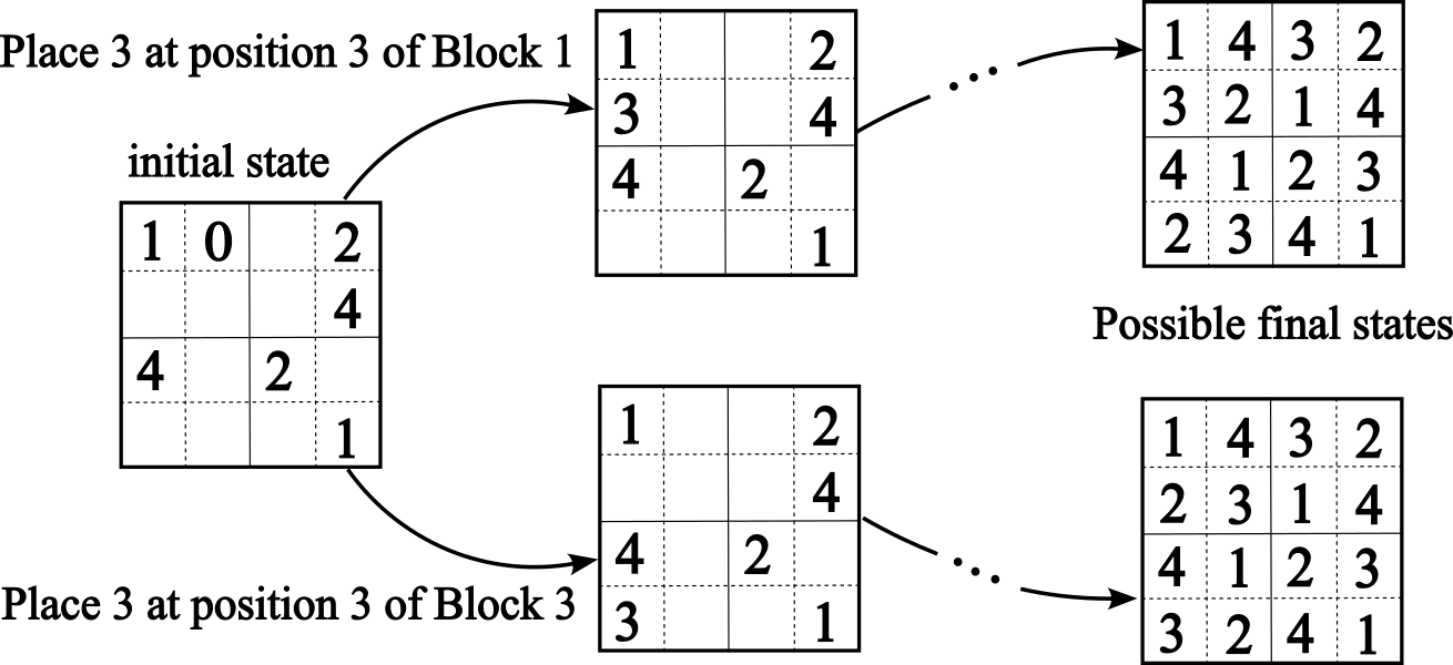For simplicity, we consider a smaller version of Sudoku, using a $4× 4$ grid instead of the standard $9× 9$ . This simplified puzzle divides the board into four $2× 2$ blocks or sub-grids, each containing four positions (or cells). Blocks are counted from left to right and top to bottom: block 1 is on top of block 3, and block 2 is on top of block 4. Positions within each block are also counted from left to right and top to bottom. Each cell in the grid must contain a number from 1 to 4, with no repetition allowed in any row, column, or $2× 2$ block. In the real Sudoku puzzle, each block is $3× 3$ and the set of possible elements is {1,2,…,9} with the board having 9 blocks in total. Figure 1 depicts an example of an initial setting for a Sudoku $4× 4$ board, followed by two possible transitions placing number 3 in two possible cells satisfying the constraints. Two possible final states are also shown, each derived from the above two states if every movement satisfies the constraints of the puzzle. <details> <summary>extracted/6466920/figs/Sudoku-4x4-sol03.png Details</summary>  ### Visual Description ## Diagram: Puzzle State Transitions ### Overview The diagram illustrates the possible state transitions of a 2x2 grid puzzle with numbered tiles (1, 2, 3, 4) and an empty space (0). It shows two possible moves from an initial state and their resulting configurations. ### Components/Axes - **Initial State**: A 2x2 grid with the following configuration: ``` 1 0 4 2 ``` (Note: The fourth cell is empty, represented by "0".) - **Move 1**: "Place 3 at position 3 of Block 1" (top-left 2x2 quadrant). - **Move 2**: "Place 3 at position 3 of Block 3" (bottom-right 2x2 quadrant). - **Possible Final States**: Two sets of 2x2 grids resulting from the moves, each with 4 permutations of numbers 1, 2, 3, 4. ### Detailed Analysis #### Initial State Grid ``` 1 0 4 2 ``` - **Key Details**: The empty space (0) is at position (1,2) in a 2x2 grid (row-major order). #### Move 1: Place 3 at Position 3 of Block 1 - **Action**: Insert "3" into the third position of the top-left 2x2 block (positions 1, 2, 3, 4 in row-major order). - **Resulting Grids**: 1. ``` 1 4 3 2 ``` 2. ``` 3 4 1 2 ``` 3. ``` 1 3 4 2 ``` 4. ``` 4 3 1 2 ``` #### Move 2: Place 3 at Position 3 of Block 3 - **Action**: Insert "3" into the third position of the bottom-right 2x2 block (positions 3, 4, 7, 8 in row-major order). - **Resulting Grids**: 1. ``` 1 2 4 3 ``` 2. ``` 4 2 1 3 ``` 3. ``` 1 3 4 2 ``` 4. ``` 4 1 3 2 ``` ### Key Observations 1. **Permutation Variability**: Each move generates 4 distinct permutations of the numbers 1, 2, 3, 4, with no repeated configurations. 2. **Symmetry**: The final states from both moves overlap partially (e.g., "1 3 / 4 2" appears in both Move 1 and Move 2). 3. **Empty Space Propagation**: The initial empty space (0) is replaced by "3" in both moves, but the placement of "3" affects adjacent tiles differently depending on the block targeted. ### Interpretation The diagram demonstrates how localized changes (placing "3" in specific blocks) propagate through the puzzle, altering the global configuration. The overlapping final states suggest that certain permutations are reachable via multiple paths, while others are unique to a specific move. This could model scenarios in combinatorial optimization, game theory, or state-space exploration, where discrete actions lead to branching outcomes. The absence of repeated states in the final configurations implies deterministic transitions, though the diagram does not explicitly confirm whether all permutations are achievable through these two moves alone. </details> Figure 1: An initial Sudoku board and two branches generated by placing a 3 at position 3 of blocks 1 and 3, respectively, and corresponding final states satisfying the constraints of the game. Solving Sudoku involves reasoning about these constraints, making it a good example for introducing logical notation. To model the problem using propositional logic, one can systematically represent the constraints in terms of propositional variables encoding the relationships between numbers, positions, rows, columns and blocks. The rules dictate that every row, column and block must include the numbers 1 to 4 exactly once. By encoding the problem in this way, one can use symbolic logical reasoning to systematically explore possible solutions while respecting all constraints. The rules are encoded as follows: Logical Variables: Let the proposition $B_{i,j,k}$ denote that the block $i$ at position $j$ (that is, the cell $(i,j)$ ) contains the number $k$ . Formally, $B_{i,j,k}$ is true if and only if $k∈\{1,2,3,4\}$ is in position $j$ of block $i$ , $1≤ i≤ 4$ , $1≤ j≤ 4$ . Logical Constraints: The constraints ensure that the numbers are placed correctly according to the rules of Sudoku. These constraints can be grouped into four categories: 1. Each cell must contain a number (cell $(i,j)$ contains a 1 or a 2 or a 3 or a 4): $B_{i,j,1}\lor B_{i,j,2}\lor B_{i,j,3}\lor B_{i,j,4}$ . When needed, we shall write: $$ \bigvee_{k=1}^{4}B_{i,j,k}\quad\text{as shorthand notation for }B_{i,j,1}\lor B% _{i,j,2}\lor B_{i,j,3}\lor B_{i,j,4}. $$ There cannot be two or more numbers on the same cell Notice that $\neg(A\wedge B)$ implies $\neg(A\wedge B\wedge C)$ .: $$ \neg(B_{i,j,k_{1}}\wedge B_{i,j,k_{2}}),\quad\text{for all }k_{1}\neq k_{2}. $$ The above two rules can be written compactly as: $$ \left(\bigvee_{k=1}^{4}B_{i,j,k}\right)\wedge\left(\bigwedge_{k_{1}<k_{2}}\neg% (B_{i,j,k_{1}}\wedge B_{i,j,k_{2}})\right), $$ where $\bigwedge_{i}x_{i}$ is shorthand for $x_{1}\wedge x_{2}\wedge...$ and $k_{1}<k_{2}$ is used to avoid repetition. Notice that $A\wedge B$ is logically equivalent to $B\wedge A$ . 1. Each number appears exactly once per row. For each row across the entire board and each number $k$ , exactly one position in that row must contain $k$ . This is expressed as: $$ \bigvee_{j=1}^{4}B_{i,j,k}\quad\text{} $$ along with the constraint that there cannot be two or more occurrences of the same number on the same row: $$ \neg(B_{i,j_{1},k}\wedge B_{i,j_{2},k}),\quad\text{for all }j_{1}\neq j_{2}. $$ In compact form: $$ \left(\bigvee_{j=1}^{4}B_{i,j,k}\right)\wedge\left(\bigwedge_{j_{1}<j_{2}}\neg% (B_{i,j_{1},k}\wedge B_{i,j_{2},k})\right). $$ 1. Each number appears exactly once per column. In compact form (as above): $$ \left(\bigvee_{i=1}^{4}B_{i,j,k}\right)\wedge\left(\bigwedge_{i_{1}<i_{2}}\neg% (B_{i_{1},j,k}\wedge B_{i_{2},j,k})\right). $$ 1. Each number appears exactly once per block. For each $2× 2$ block and each number $k$ , exactly one position within the block must contain $k$ . For example, for the top-left block: $$ \bigvee_{(i,j)\in\{(1,1),(1,2),(2,1),(2,2)\}}B_{i,j,k}, $$ along with the constraint: $$ \neg(B_{i_{1},j_{1},k}\wedge B_{i_{2},j_{2},k}),\text{for all distinct pairs }% (i_{1},j_{1})\neq(i_{2},j_{2}). $$ In compact form: $$ \left(\bigvee_{(i,j)\in\text{block}}B_{i,j,k}\right)\wedge\left(\bigwedge_{(i_% {1},j_{1})<(i_{2},j_{2})}\neg(B_{i_{1},j_{1},k}\wedge B_{i_{2},j_{2},k})\right). $$ The complete set of constraints for the $4× 4$ Sudoku puzzle is the conjunction of all the above conditions over all cells, rows, columns and blocks. This logical formula guarantees that every number appears exactly once in each row, column, and block, satisfying the rules of Sudoku. It also provides a systematic framework for reasoning about the puzzle. **Example 1** *For block 1, position 1, we have: - $B_{1,1,1}\lor B_{1,1,2}\lor B_{1,1,3}\lor B_{1,1,4}$ - $\neg B_{1,1,1}\lor\neg B_{1,1,2}$ - $\neg B_{1,1,1}\lor\neg B_{1,1,3}$ - $\neg B_{1,1,1}\lor\neg B_{1,1,4}$ - $\neg B_{1,1,2}\lor\neg B_{1,1,3}$ - $\neg B_{1,1,2}\lor\neg B_{1,1,4}$ - $\neg B_{1,1,3}\lor\neg B_{1,1,4}$* Some observations about this representation: - This notation provides a framework whereby each possible combination of $B$ with indices is assigned to True or False. - Each rule above is called a clause (a disjunction of logic literals) and the complete set of clauses would be significantly larger to cover all rows, columns and blocks. - This representation can be used as input to a satisfiability (SAT) solver to find solutions to the Sudoku puzzle, that is, assignments of truth-values True or False to each literal that will provably satisfy the puzzle’s constraints. This Boolean logic representation allows us to express the Sudoku problem as a set of constraints that must be satisfied simultaneously. By finding a truth assignment to the variables that satisfy all the clauses, we determine a valid solution to the Sudoku puzzle. 2.2 Sudoku with Strategies of Sampling 1. Reasoning Strategy based on Unused Numbers: To control which number to pick based on the bank of numbers not yet placed on the board, let us illustrate how additional constraints may be introduced that ensure unused numbers are considered first. A strategy such as this could be learned from observation of game plays as well as specified by hand. For each empty cell $(i,j)$ , define $U(i,j)$ as the set of numbers $k$ such that $k$ is not already used in the corresponding row, column or block of cell $(i,j)$ . The constraint ensuring the selection of an unused number $k$ can be expressed as: $$ \bigvee_{k\in U(i,j)}B_{i,j,k} $$ where $U(i,j)$ is defined as: $$ U(i,j)=\{k\mid k\notin\{B_{i,j^{\prime},k^{\prime}}\mid j^{\prime}\neq j\}% \land k\notin\{B_{i^{\prime},j,k^{\prime}}\mid i^{\prime}\neq i\} $$ $$ \land k\notin\{B_{i^{\prime},j^{\prime},k^{\prime}}\mid(i^{\prime},j^{\prime})% \in\text{block}(i,j)\}\}. $$ Here, $\text{block}(i,j)$ denotes the set of positions in the same block as $(i,j)$ . 1. Priority Constraint for Unused Numbers: To prioritize the use of unused numbers, we can add a preference rule that assigns higher priority to considering numbers from $U(i,j)$ ahead of other possibilities. Formally, let $P(i,j,k)$ represent the priority of placing number $k$ in cell $(i,j)$ . The priority can be defined as: $$ P(i,j,k)=\begin{cases}1&\text{if }k\in U(i,j)\\ 0&\text{otherwise}\end{cases} $$ The constraint ensuring that the highest priority is given to unused numbers can be expressed as: $$ \bigvee_{k\in U(i,j)}(P(i,j,k)\wedge B_{i,j,k}) $$ The complete set of logical constraints for the 4x4 Sudoku puzzle now includes the original Sudoku constraints along with additional reasoning strategies that prioritize the use of unused numbers. These constraints ensure that every number appears exactly once in each row, column, and block while also guiding the generation of solutions (that is, the assignment of truth-values to the literals) by leveraging the bank of unused numbers. By incorporating these, the Sudoku solving process becomes systematic and more efficient as it should reduce the likelihood of the process getting stuck and having to backtrack when searching for a solution, or analogously in the case of a neural network getting stuck in local minima. 2.3 Restricted Boltzmann Machines An RBM [44] is a two-layer neural network with bidirectional (symmetric) connections, which is characterised by a function called the energy of the RBM: $$ {\it E}(\mathbf{x},\mathbf{h})=-\sum_{i,j}w_{ij}x_{i}h_{j}-\sum_{i}a_{i}x_{i}-% \sum_{j}b_{j}h_{j} \tag{1} $$ where $a_{i}$ and $b_{j}$ are the biases of input unit $x_{i}$ and hidden unit $h_{j}$ , respectively, and $w_{ij}$ is the connection weight between $x_{i}$ and $h_{j}$ . This RBM represents a joint probability distribution $p(\mathbf{x},\mathbf{h})=\frac{1}{Z}e^{-\frac{1}{\tau}{\it E}(\mathbf{x},% \mathbf{h})}$ where $Z=\sum_{\mathbf{x}\mathbf{h}}e^{-\frac{1}{\tau}{\it E}(\mathbf{x},\mathbf{h})}$ is the partition function and parameter $\tau$ is called the temperature of the RBM, $\mathbf{x}=\{x_{i}\}$ is the set of visible units and $\mathbf{h}=\{h_{j}\}$ is the set of hidden units of the RBM. Training RBMs normally makes use of the Contrastive Divergence learning algorithm [19], whereby each input vector from the training set is propagated to the hidden layer of the network and back to the input a number of times ( $n$ ) using a probabilistic selection rule to decide at each time whether or not a neuron should be activated (with activation value in $\{0,1\}$ ). The weight assigned to the connection between input neuron $x_{i}$ and hidden neuron $h_{j}$ is adjusted according to a simple update rule based on the difference between the value of $x_{i}h_{j}$ at time $1$ and time $n$ . More precisely, $\Delta W_{ij}=\eta((x_{i}h_{j})_{1}-(x_{i}h_{j})_{n})$ , where $\eta$ is a learning rate (a small positive real number). 3 Symbolic Reasoning with Energy-based Neural Networks The content of this section is based on [52]. Over the years, many neurosymbolic approaches have used a form of knowledge representation based on if-then rules [49, 13, 50, 12, 56, 29, 51], written $B← A$ (make $B$ $True$ if $A$ is $True$ ) to distinguish from classical implication ( $A→ B$ ). Under the convention that $1$ represents $True$ and $0 0$ represents $False$ , given $B← A$ and input $1$ to neuron $A$ , a neurosymbolic system would infer that neuron $B$ should have activation value approximately $1$ . Given input $0 0$ to neuron $A$ , it would infer that $B$ should have activation approximately $0 0$ . Logical Boltzmann Machines (LBM) allow for a richer representation than if-then rules by using full propositional logic. Next, we review LBM’s immediate related work, define a mapping from any logical formulae to LBMs, and describe how reasoning takes place by sampling and energy minimization. We also evaluate scalability of reasoning in LBM and learning by combining knowledge and data, evaluating results on benchmarks in comparison with a symbolic, another neurosymbolic and a neural network-based approach. 3.1 Related Work One of the earliest work on the integration of neural networks and symbolic knowledge is known as KBANN (Knowledge-based Artificial Neural Network [49]), which encodes if-then rules into a hierarchical multilayer perceptron. In another early approach [8], a single-hidden layer recurrent neural network is proposed to support logic programming rules. An extension of that approach to work with first-order logic programs, called Connectionist Inductive Logic Programming (CILP++) [13], uses the concept of propositionalisation from Inductive Logic Programming (ILP), whereby first-order variables can be treated as propositional atoms in the neural network. Also based on first-order logic programs, [12] propose a differentiable ILP approach that can be implemented by neural networks, and [6] maps stochastic logic programs into a differentiable function also trainable by neural networks. These are all supervised learning approaches. Early work in neurosymbolic AI has also shown a correspondence between propositional logic and symmetrical neural networks [38], in particular Hopfield networks, which nevertheless did not scale well with the number of variables. Among unsupervised learning approaches, Penalty Logic [37] was the first work to integrate nonmonotonic logic in the form of weighted if-then rules into symmetrical neural networks. However, Penalty Logic required the use of higher-order Hopfield networks, which can be difficult to construct Building such higher-order networks requires transforming the energy function into quadratic form by adding hidden variables not present in the original logic formulae. and inefficient to train with the learning algorithm for Boltzmann machines. More recently, several attempts have been made to extract and encode symbolic knowledge into RBMs trained with the more efficient Contrastive Divergence learning algorithm [35, 50]. Such approaches explored the structural similarity between symmetric networks and logical rules with bi-conditional implication but do not have a proof of soundness. By contrast, and similarly to Penalty Logic, LBM is provably equivalent to the logic formulae encoded in the RBM. Differently from Penalty Logic, LBM does not require the use of higher-order networks. Alongside the above approaches, which translate symbolic representations into neural networks (normally if-then rules translated into a feedforward or recurrent network), there are hybrid approaches that combine neural networks and symbolic AI systems as communicating modules of a neurosymbolic system. These include DeepProbLog [29] and Logic Tensor Networks (LTN) [41]. DeepProbLog adds a neural network module to probabilistic logic programming such that an atom of the logic program can be represented by a network module. LTN and various approaches derived from it use real-valued logic to constrain the loss function of the neural network given statements in firt-order logic. Both DeepProbLog and LTNs use backpropagation, differently from the approach adopted here which uses Contrastive Divergence. Finally, approaches focused on reasoning include SAT solving using neural networks. In [17, 7], the maximum satisfiability problem is mapped onto Boltzmann machines and higher-order Boltzmann machines, which are used to solve the combinatorial optimization task in parallel, similarly to [38]. In [53], the SAT problem is redefined as a soft (differentiable) task and solved approximately by deep networks with the objective of integrating logical reasoning and learning, as in the case of the approaches discussed earlier. This soft version of the SAT problem is therefore different from the satisfiability problem. A preliminary evaluation of our approach in comparison with symbolic SAT solvers shows that our approach allows the use of up to approximately 100 variables. This is well below the capability of symbolic SAT solvers. A way of improving the performance of neural SAT solvers may well be to consider approximate solutions as done by soft SAT solvers, including neuroSAT [40]. Although still not beating SAT solvers, neuroSAT showed promise at addressing out-of-distribution learning after training on random SAT problems. In our experiments on learning, the focus is on benchmark neurosymbolic AI tasks with available data and knowledge, obtained from [13]. We therefore compare LBM with a state-of-the-art ILP symbolic system ALEPH [46], standard RBMs as a purely-neural approach closest to LBM, and with CILP++ as a neurosymbolic system. It is worth noting, however, that CILP++ is a neurosymbolic system for supervised learning while LBMs use unsupervised learning, and it is worth investigating approaches for semi-supervised learning and other combinations of such systems. Further comparisons and evaluations on both reasoning and learning are underway. 3.2 Knowledge Representation in RBMs Before we present LBM, let’s contrast the simple $B← A$ example used earlier with classical logic. Given $A→ B$ as knowledge In classical logic, $A→ B$ is equivalent to $\neg A\vee B$ , i.e. True if $A$ is False regardless of the truth-value of $B$ ., if neuron $A$ is assigned input value $1$ in the corresponding neurosymbolic network, we expect the network to converge to a stable state where neuron $B$ has value approximately $1$ , similarly to the example seen earlier. This is because the truth-value of WFF $A→ B$ is True given an assignment of truth-values True to its constituent literals $A$ and $B$ . Now, $A→ B$ is False when $A$ is True and $B$ is False. If neuron $B$ is assigned input $0 0$ , we expect the network to converge to a stable state where $A$ is approximately $0 0$ ( $A→ B$ is True when $A$ is False and $B$ is False). What if $A$ is assigned input $0 0$ (or $B$ is assigned input $1$ )? In these cases, $A→ B$ is satisfied if $B$ is either $1$ or $0 0$ (or if $A$ is either $1$ or $0 0$ ). Differently from $B← A$ , the network will converge to one of the two options that satisfy the formulae. From this point forward, unless stated otherwise, we will treat assignments of truth-values to logical literals and binary input vectors denoting the activation states of neurons indistinguishably. **Definition 1** *Let $s_{\varphi}(\mathbf{x})∈\{0,1\}$ denote the truth-value of a WFF $\varphi$ given an assignment of truth-values $\mathbf{x}$ to the literals of $\varphi$ , where truth-value $True$ is mapped to 1 and truth-value $False$ is mapped to 0. Let ${\it E}(\mathbf{x},\mathbf{h})$ denote the energy function of an energy-based neural network $\mathcal{N}$ with visible units $\mathbf{x}$ and hidden units $\mathbf{h}$ . $\varphi$ is said to be equivalent to $\mathcal{N}$ if and only if for any assignment of values to $\mathbf{x}$ there exists a function $\psi$ such that $s_{\varphi}(\mathbf{x})=\psi({\it E}(\mathbf{x},\mathbf{h}))$ .* Definition 1 is similar to that of Penalty Logic [37], where all assignments of truth-values satisfying a WFF $\varphi$ are mapped to global minima of the energy function of network $\mathcal{N}$ . In our case, by construction, assignments that do not satisfy the WFF will, in addition, be mapped to maxima of the energy function. To see how this is the case, it will be useful to define strict and full DNFs, as follows. **Definition 2** *A strict DNF (SDNF) is a DNF with at most one conjunctive clause (a conjunction of literals) that maps to $True$ for any choice of assignment of truth-values $\mathbf{x}$ . A full DNF is a DNF where each propositional variable (a positive or negative literal) must appear at least once in every conjunctive clause (sometimes called a canonical DNF).* For example, to turn DNF $A\vee B$ into an equivalent full DNF, one needs to map it to $(A\wedge\neg B)\vee(\neg A\wedge B)\vee(A\wedge B)$ , according to the truth-table for $A\vee B$ . For any given assignment of truth-values to $A$ and $B$ , at most one of the above three conjunctive clauses will be $True$ , by definition of the truth-table. Not every SDNF is also a full DNF though, e.g. $(a\wedge b)\vee\neg b$ is a SDNF that is not a full DNF. **Lemma 1** *Let $\mathcal{S}_{T_{j}}$ denote the set of indices of the positive literals $\mathrm{x}_{t}$ in a conjunctive clause $j$ . Let $\mathcal{S}_{K_{j}}$ denote the set of indices of the negative literals $\mathrm{x}_{k}$ in $j$ . Any SDNF $\varphi\equiv\bigvee_{j}(\bigwedge_{t}\mathrm{x}_{t}\wedge\bigwedge_{k}\neg% \mathrm{x}_{k})$ can be mapped onto an energy function: $$ {\it E}(\mathbf{x})=-\sum_{j}(\prod_{t\in\mathcal{S}_{T_{j}}}x_{t}\prod_{k\in% \mathcal{S}_{K_{j}}}(1-x_{k})). $$* Proof: Each conjunctive clause $\bigwedge_{t}\mathrm{x}_{t}\wedge\bigwedge_{k}\neg\mathrm{x}_{k}$ in $\varphi$ corresponds to the product $\prod_{t}x_{t}\prod_{k}(1-x_{k})$ which maps to $1$ if and only if $x_{t}$ is $True$ ( $x_{t}=1$ ) and $x_{k}$ is $False$ ( $x_{k}=0$ ) for all $t∈\mathcal{S}_{T_{j}}$ and $k∈\mathcal{S}_{K_{j}}$ . Since $\varphi$ is SDNF, $\varphi$ is $True$ if and only if one conjunctive clause is $True$ and $\sum_{j}(\prod_{t∈\mathcal{S}_{T_{j}}}x_{t}\prod_{k∈\mathcal{S}_{K_{j}}}(1% -x_{k}))=1$ . Hence, the neural network with energy function ${\it E}$ is such that $s_{\varphi}(\mathbf{x})=-{\it E}(\mathbf{x})$ . ∎ **Theorem 1** *Any SDNF $\varphi\equiv\bigvee_{j}(\bigwedge_{t}\mathrm{x}_{t}\wedge\bigwedge_{k}\neg% \mathrm{x}_{k})$ can be mapped onto an RBM with energy function: $$ {\it E}(\mathbf{x},\mathbf{h})=-\sum_{j}h_{j}(\sum_{t\in\mathcal{S}_{T_{j}}}x_% {t}-\sum_{k\in\mathcal{S}_{K_{j}}}x_{k}-|\mathcal{S}_{T_{j}}|+\epsilon), \tag{2} $$ such that $s_{\varphi}(\mathbf{x})=-{\it E}(\mathbf{x})$ , where $0<\epsilon<1$ and $|\mathcal{S}_{T_{j}}|$ is the number of positive literals in conjunctive clause $j$ of $\varphi$ .* Proof: Lemma 1 states that any SDNF $\varphi$ can be mapped onto energy function ${\it E}=-\sum_{j}(\prod_{t∈\mathcal{S}_{T_{j}}}x_{t}\prod_{k∈\mathcal{S}_{% K_{j}}}(1-x_{k}))$ . For each expression $\tilde{e}_{j}(\mathbf{x})=-\prod_{t∈\mathcal{S}_{T_{j}}}x_{t}\prod_{k∈% \mathcal{S}_{K_{j}}}(1-x_{k})$ , we define an energy expression associated with hidden unit $h_{j}$ as $e_{j}(\mathbf{x},h_{j})=-h_{j}(\sum_{t∈\mathcal{S}_{T_{j}}}x_{t}-\sum_{k∈% \mathcal{S}_{K_{j}}}x_{k}-|\mathcal{S}_{T_{j}}|+\epsilon)$ . The term $e_{j}(\mathbf{x},h_{j})$ is minimized with value $-\epsilon$ when $h_{j}=1$ , written $min_{h_{j}}(e_{j}(\mathbf{x},h_{j}))=-\epsilon$ . This is because $-(\sum_{t∈\mathcal{S}_{T_{j}}}x_{t}-\sum_{k∈\mathcal{S}_{K_{j}}}x_{k}-|% \mathcal{S}_{T_{j}}|+\epsilon)=-\epsilon$ if and only if $x_{t}=1$ and $x_{k}=0$ for all $t∈\mathcal{S}_{T_{j}}$ and $k∈\mathcal{S}_{K_{j}}$ . Otherwise, $-(\sum_{t}x_{t∈\mathcal{S}_{T_{j}}}-\sum_{k∈\mathcal{S}_{K_{j}}}x_{k}-|% \mathcal{S}_{T_{j}}|+\epsilon)>0$ and $min_{h_{j}}(e_{j}(\mathbf{x},h_{j}))=0$ with $h_{j}=0$ . By repeating this process for each $\tilde{e}_{j}(\mathbf{x})$ we obtain that the energy function ${\it E}(\mathbf{x},\mathbf{h})=-\sum_{j}h_{j}(\sum_{t∈\mathcal{S}_{T_{j}}}x_% {t}-\sum_{k∈\mathcal{S}_{K_{j}}}x_{k}-|\mathcal{S}_{T_{j}}|+\epsilon)$ is such that $s_{\varphi}(\mathbf{x})=-\frac{1}{\epsilon}min_{\mathbf{h}}{\it E}(\mathbf{x},% \mathbf{h})$ . ∎ It is well-known that any WFF $\varphi$ can be converted into DNF. Then, if $\varphi$ is not SDNF, by definition there is more than one conjunctive clause in $\varphi$ that map to $True$ when $\varphi$ is satisfied. This group of conjunctive clauses can always be converted into a full DNF according to its truth-table. By definition, any such full DNF is also a SDNF. Therefore, any WFF can be converted into SDNF. From Theorem 1, it follows that any WFF can be represented by the energy function of an RBM. The conversion of WFFs into full DNF can be computationally expensive. Sometimes, the logic is provided already in canonical DNF form or in Conjunctive Normal Form (CNF), i.e. conjunctions of disjunctions. We will see later that any WFF expressed in CNF can be converted into an RBM’s energy function efficiently without the need to convert into SDNF first. This covers the most common forms of propositional knowledge representation. Next, we describe a method for converting logical formulae into SDNF, which we use in the empirical evaluations that will follow. Consider a clause $\gamma$ such that: $$ \gamma\equiv\bigvee_{t\in\mathcal{S}_{T}}\neg\mathrm{x}_{t}\vee\bigvee_{k\in% \mathcal{S}_{K}}\mathrm{x}_{k} \tag{3} $$ where $\mathcal{S}_{T}$ now denotes the set of indices of the negative literals, and $\mathcal{S}_{K}$ denotes the set of indices of the positive literals in the clause (dually to the conjunctive clause case). Clause $\gamma$ can be rearranged into $\gamma\equiv\gamma^{\prime}\vee\mathrm{x}^{\prime}$ , where $\gamma^{\prime}$ is obtained by removing $\mathrm{x}^{\prime}$ from $\gamma$ ( $\mathrm{x}^{\prime}$ can be either $\neg\mathrm{x}_{t}$ or $\mathrm{x}_{k}$ for any $t∈\mathcal{S}_{T}$ and $k∈\mathcal{S}_{K}$ ). We have: $$ \gamma\equiv(\neg\gamma^{\prime}\wedge\mathrm{x}^{\prime})\vee\gamma^{\prime} \tag{4} $$ because $(\neg\gamma^{\prime}\wedge\mathrm{x}^{\prime})\vee\gamma^{\prime}\equiv(\gamma% ^{\prime}\vee\neg\gamma^{\prime})\wedge(\gamma^{\prime}\vee\mathrm{x}^{\prime}% )\equiv True\wedge(\gamma^{\prime}\vee\mathrm{x}^{\prime})$ . By De Morgan’s law ( $\neg(\mathrm{a}\vee\mathrm{b})\equiv\neg\mathrm{a}\wedge\neg\mathrm{b}$ ), we can always convert $\neg\gamma^{\prime}$ (and therefore $\neg\gamma^{\prime}\wedge\mathrm{x}^{\prime}$ ) into a conjunctive clause. By applying (4) repeatedly, each time we eliminate a variable out of the clause by moving it into a new conjunctive clause. Given an assignment of truth-values, either the clause $\gamma^{\prime}$ will be True or the conjunctive clause ( $\neg\gamma^{\prime}\wedge\mathrm{x}^{\prime}$ ) will be True, e.g. $a\vee b\equiv a\vee(\neg a\wedge b)$ . Therefore, the SDNF for clause $\gamma$ in Eq. (3) is: $$ \bigvee_{p\in\mathcal{S}_{T}\cup\mathcal{S}_{K}}(\bigwedge_{t\in\mathcal{S}_{T% }\backslash p}\mathrm{x}_{t}\wedge\bigwedge_{k\in\mathcal{S}_{K}\backslash p}% \neg\mathrm{x}_{k}\wedge\mathrm{x}^{\prime}_{p}) \tag{5} $$ where $\mathcal{S}\backslash p$ denotes a set $\mathcal{S}$ from which element $p$ has been removed. If $p∈\mathcal{S}_{T}$ then $\mathrm{x}^{\prime}_{p}\equiv\neg\mathrm{x}_{p}$ . Otherwise, $\mathrm{x}^{\prime}_{p}\equiv\mathrm{x}_{p}$ . As an example of the translation into SDNF, consider the translation of an if-then statement (logical implication) below. **Example 2** *Translation of if-then rules into SDNF. Consider the formula $\gamma\equiv(x_{1}\wedge x_{2}\wedge\neg x_{3})→ y$ . Using our notation: $$ \gamma\equiv(\bigwedge_{t\in\{1,2\}}\mathrm{x}_{t}\wedge\bigwedge_{k\in\{3\}}% \neg\mathrm{x}_{k})\rightarrow\mathrm{y} \tag{6} $$ Converting to DNF: $$ (\mathrm{y}\wedge\bigwedge_{t\in\{1,2\}}\mathrm{x}_{t}\wedge\bigwedge_{k\in\{3% \}}\neg\mathrm{x}_{k})\vee\bigvee_{t\in\{1,2\}}\neg\mathrm{x}_{t}\vee\bigvee_{% k\in\{3\}}\mathrm{x}_{k} \tag{7} $$ Applying the variable elimination method to the clause $\neg\mathrm{x}_{1}\vee\neg\mathrm{x}_{2}\vee\mathrm{x}_{3}$ , we obtain the SDNF for $\gamma$ : $$ \displaystyle(\mathrm{y}\wedge\bigwedge_{t\in\mathcal{S}_{T}}\mathrm{x}_{t}% \bigwedge_{k\in\mathcal{S}_{K}}\neg\mathrm{x}_{k})\vee(\neg\mathrm{x}_{1})\vee% (\mathrm{x}_{1}\wedge\neg\mathrm{x}_{2})\vee(\mathrm{x}_{1}\wedge\mathrm{x}_{2% }\wedge\mathrm{x}_{3}) \tag{8} $$* 3.3 Reasoning in RBMs We have seen how propositional logic formula can be mapped onto the energy functions of RBMs. In this section, we discuss the deployment of such RBMs for logical reasoning. 3.3.1 Reasoning as Sampling There is a direct relationship between inference in RBMs and logical satisfiability, as follows. **Lemma 2** *Let $\mathcal{N}$ be an RBM with energy function $E$ . Let $\varphi$ be a WFF such that $s_{\varphi}(\mathbf{x})=-{\it E}(\mathbf{x})$ . Let $\mathcal{A}$ be a set of indices of variables in $\varphi$ that have been assigned to either True or False. We use $\mathbf{x}_{\mathcal{A}}$ to denote the set $\{x_{\alpha}|\alpha∈\mathcal{A}\}$ ). Let $\mathcal{B}$ be a set of indices of variables that have not been assigned a truth-value in $\varphi$ . We use $\mathbf{x}_{\mathcal{B}}$ to denote $\{x_{\beta}|\beta∈\mathcal{B}\}$ ). Performing Gibbs sampling on $\mathcal{N}$ given $\mathbf{x}_{\mathcal{A}}$ is equivalent to searching for an assignment of truth-values for $\mathbf{x}_{\mathcal{B}}$ that satisfies $\varphi$ .* Proof: Theorem 1 has shown that the assignments of truth-values to $\varphi$ are partially ordered according to the RBM’s energy function such that the models of $\varphi$ (mapping $\varphi$ to 1) correspond to minima of the energy function. We say that the satisfiability of $\varphi$ is inversely proportional to the RBM’s rank function. When the satisfiability of $\varphi$ is maximum ( $s_{\varphi}(\mathbf{x})=1$ ) ranking the output of $-{\it E}(\mathbf{x})$ produces the highest rank. A value of $\mathbf{x}_{\mathcal{B}}$ that minimises the energy function also maximises satisfiability: $s_{\varphi}(\mathbf{x}_{\mathcal{B}},\mathbf{x}_{\mathcal{A}})\propto-min_{% \mathbf{h}}{\it E}(\mathbf{x}_{\mathcal{B}},\mathbf{x}_{\mathcal{A}},\mathbf{h})$ because: $$ \displaystyle\mathbf{x}_{\mathcal{B}}^{*}=\operatorname*{arg\,min}_{\mathbf{x}% _{\mathcal{B}_{\mathbf{h}}}}{\it E}(\mathbf{x}_{\mathcal{B}},\mathbf{x}_{% \mathcal{A}},\mathbf{h})=\operatorname*{arg\,max}_{\mathbf{x}_{\mathcal{B}}}(s% _{\varphi}(\mathbf{x}_{\mathcal{B}},\mathbf{x}_{\mathcal{A}})) \tag{9} $$ We can consider an iterative process to search for truth-values $\mathbf{x}_{\mathcal{B}}^{*}$ by minimising an RBM’s energy function. This can be done using gradient descent or contrastive divergence with Gibbs sampling. The goal is to update the values of $\mathbf{h}$ and then $\mathbf{x}_{\mathcal{B}}$ in parallel until convergence to minimise ${\it E}(\mathbf{x}_{\mathcal{B}},\mathbf{x}_{\mathcal{A}},\mathbf{h})$ while keeping the other variables ( $\mathbf{x}_{\mathcal{A}}$ ) fixed. The gradients amount to: $$ \displaystyle\frac{\partial-{\it E}(\mathbf{x}_{\mathcal{B}},\mathbf{x}_{% \mathcal{A}},\mathbf{h})}{\partial h_{j}} \displaystyle=\sum_{i\in\mathcal{A}\cup\mathcal{B}}x_{i}w_{ij}+\theta_{j} \displaystyle\frac{\partial-{\it E}(\mathbf{x}_{\mathcal{B}},\mathbf{x}_{% \mathcal{A}},\mathbf{h})}{\partial x_{\beta}} \displaystyle=\sum_{j}h_{j}w_{\beta j}+theta_{\beta} \tag{10} $$ In the case of Gibbs sampling, given the assigned variables $\mathbf{x}_{\mathcal{A}}$ , the process starts with a random initialization of $\mathbf{x}_{\mathcal{B}}$ and proceeds to infer values for the hidden units $h_{j}$ and then the unassigned variables $x_{\beta}$ in the visible layer of the RBM, using the conditional distributions $h_{j}\sim p(h_{j}|\mathbf{x})$ and $x_{\beta}\sim p(x_{\beta}|\mathbf{h})$ , respectively, where $\mathbf{x}=\{\mathbf{x}_{\mathcal{A}},\mathbf{x}_{\mathcal{B}}\}$ and: $$ \displaystyle p(h_{j}|\mathbf{x}) \displaystyle=\frac{1}{1+e^{-\frac{1}{\tau}\sum_{i}x_{i}w_{ij}+\theta_{j}}}=% \frac{1}{1+e^{-\frac{1}{\tau}\frac{\partial-{\it E}(\mathbf{x}_{\mathcal{B}},% \mathbf{x}_{\mathcal{A}},\mathbf{h})}{\partial h_{j}}}} \displaystyle p(x_{\beta}|\mathbf{h}) \displaystyle=\frac{1}{1+e^{-\frac{1}{\tau}\sum_{j}h_{j}w_{\beta j}+\theta_{% \beta}}}=\frac{1}{1+e^{-\frac{1}{\tau}\frac{\partial-{\it E}(\mathbf{x}_{% \mathcal{B}},\mathbf{x}_{\mathcal{A}},\mathbf{h})}{\partial x_{\beta}}}} \tag{11} $$ It can be seen from Eq.(11) that the distributions are monotonic functions of the negative energy’s gradient over $\mathbf{h}$ and $\mathbf{x}_{\mathcal{B}}$ . Therefore, performing Gibbs sampling on them can be seen as moving towards a local minimum that is equivalent to an assignment of truth-values that satisfies $\varphi$ . Each step of Gibbs sampling, calculating $\mathbf{h}$ and then $\mathbf{x}$ to reduce the energy, should intuitively generate an assignment of truth-values that gets closer to satisfying the formula $\varphi$ . ∎ 3.3.2 Reasoning as Lowering Free Energy When the number of unassigned variables is not large, it should be possible to calculate the above probabilities directly. In this case, one can infer the assignments of $\mathbf{x}_{\mathcal{B}}$ using the conditional distribution: $$ P(\mathbf{x}_{\mathcal{B}}|\mathbf{x}_{\mathcal{A}})=\frac{e^{-\mathcal{F}_{% \mathcal{B}}(\mathbf{x}_{\mathcal{A}},\mathbf{x}_{\mathcal{B}})}}{\sum_{% \mathbf{x}^{\prime}_{\mathcal{B}}}e^{\mathcal{F}_{\mathcal{B}}}(\mathbf{x}_{% \mathcal{A}},\mathbf{x}^{\prime}_{\mathcal{B}})} \tag{12} $$ where $\mathcal{F}_{\mathcal{B}}=-\sum_{j}(-\log(1+e^{(c\sum_{i∈\mathcal{A}\cup% \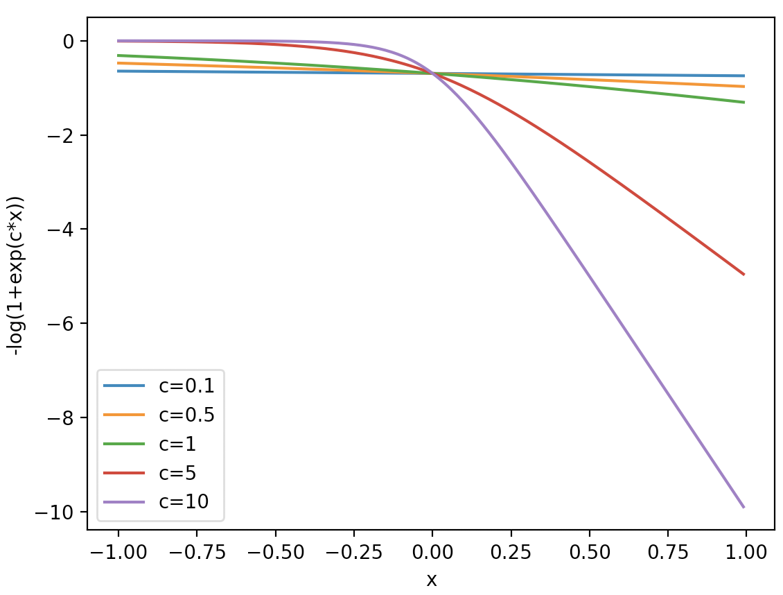mathcal{B}}w_{ij}x_{i}+\theta_{j})}))$ is known as the free energy; $\mathbf{x}^{\prime}_{\mathcal{B}}$ denotes all the combinations of truth-value assignments to the literals in $\mathbf{x}_{\mathcal{B}}$ , and $c$ is a non-negative real number that we call a confidence value. The free energy term $-\log(1+e^{(c\sum_{i∈\mathcal{A}\cup\mathcal{B}}w_{ij}x_{i}+\theta_{j})})$ is a negative softplus function scaled by $c$ as shown in Figure 2. It returns a negative output for a positive input and a close-to-zero output for a negative input. <details> <summary>extracted/6466920/figs/confidence_smoothing.png Details</summary>  ### Visual Description ## Line Graph: -log(1+exp(c*x)) vs x for varying c values ### Overview The graph displays five curves representing the function -log(1+exp(c*x)) for different constant values of c (0.1, 0.5, 1, 5, 10). The x-axis ranges from -1.00 to 1.00, while the y-axis spans from -10 to 0. All curves originate near y=0 at x=-1.00 and exhibit varying degrees of decline as x increases toward 1.00. ### Components/Axes - **X-axis**: Labeled "x" with tick marks at -1.00, -0.75, -0.50, -0.25, 0.00, 0.25, 0.50, 0.75, 1.00. - **Y-axis**: Labeled "-log(1+exp(c*x))" with tick marks at -10, -8, -6, -4, -2, 0. - **Legend**: Located at the bottom-left corner, mapping colors to c values: - Blue: c=0.1 - Orange: c=0.5 - Green: c=1 - Red: c=5 - Purple: c=10 ### Detailed Analysis 1. **c=0.1 (Blue)**: Nearly flat line with minimal decline. Starts near y=0 at x=-1.00 and decreases slightly to ~y=-0.5 at x=1.00. 2. **c=0.5 (Orange)**: Slightly steeper than blue. Begins near y=0 and drops to ~y=-1.5 at x=1.00. 3. **c=1 (Green)**: Moderate decline. Starts near y=0 and reaches ~y=-3 at x=1.00. 4. **c=5 (Red)**: Sharp decline. Starts near y=0 and plunges to ~y=-7 at x=1.00. 5. **c=10 (Purple)**: Steepest slope. Begins near y=0 and falls sharply to ~y=-10 at x=1.00. All curves intersect near x=0, where their y-values converge to approximately -0.5 to -1.0. The rate of decline increases exponentially with higher c values. ### Key Observations - **Symmetry**: All curves are symmetric about x=0, with identical behavior for positive and negative x values. - **Convergence**: At x=0, all curves intersect at y≈-0.5 to -1.0, regardless of c value. - **Sensitivity**: Higher c values (5, 10) produce steeper slopes, indicating greater sensitivity to x changes. - **Asymptotic Behavior**: Curves approach horizontal asymptotes as x→±∞ (not shown), with y-values stabilizing near -c for large |x|. ### Interpretation The graph demonstrates how the parameter c controls the steepness of the function's response to x. Higher c values amplify the function's sensitivity, causing rapid declines for positive x and sharp rises for negative x (though only x≥-1.00 is shown). The intersection at x=0 suggests a critical point where the function's behavior transitions symmetrically. This could model phenomena like activation functions in neural networks or dose-response relationships in pharmacology, where c represents a scaling factor for input sensitivity. </details> Figure 2: Free energy term $-\log(1+e^{cx})$ for different confidence values $c$ . Each free energy term is associated with a conjunctive clause in the SDNF through the weighted sum $\sum_{i∈\mathcal{A}\cup\mathcal{B}}w_{ij}x_{i}+\theta_{j}$ . Therefore, if a truth-value assignment of $\mathbf{x}_{\mathcal{B}}$ does not satisfy the formula $\varphi$ , all energy terms will be close to zero. When $\varphi$ is satisfied, one free energy term will be $-\log(1+e^{c\epsilon})$ , for a choice of $0<\epsilon<1$ from Theorem 1. Thus, the more likely that a truth assignment is to satisfying the formula, the lower the free energy. 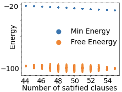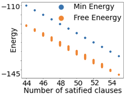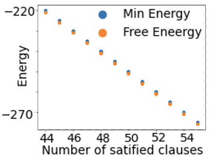Formally: $$ s_{\varphi}(\mathbf{x})=-\frac{1}{c\epsilon}\text{min}_{\mathbf{h}}E(\mathbf{x% },\mathbf{h})=\lim_{c\rightarrow\infty}-\frac{1}{c\epsilon}\mathcal{F}(\mathbf% {x}) \tag{13} $$ Figure 3 shows the average values of the energy function and free energy for CNFs with 55 clauses as the number of satisfied clauses increases. The CNF is satisfied if and only if all 55 clauses are satisfied. As can be seen, the relationships are linear. Minimum energy and free energy values converge with an increasing value of $c$ . <details> <summary>extracted/6466920/figs/energies_versus_sat_clauses_c1.png Details</summary>  ### Visual Description ## Scatter Plot: Energy vs. Number of Satisfied Clauses ### Overview The image is a scatter plot comparing two energy metrics—**Min Energy** (blue dots) and **Free Energy** (orange dots)—across a range of **number of satisfied clauses** (x-axis). The y-axis represents **Energy** values, with both metrics showing distinct trends. ### Components/Axes - **X-axis**: "Number of satisfied clauses" with ticks at 44, 46, 48, 50, 52, 54. - **Y-axis**: "Energy" with values ranging from -100 to -20. - **Legend**: - **Blue dots**: "Min Energy" - **Orange dots**: "Free Energy" - **Spatial Placement**: - Legend is positioned in the **top-right** corner. - Blue dots (Min Energy) are clustered near the **top** of the y-axis (around -20). - Orange dots (Free Energy) are clustered near the **bottom** of the y-axis (around -100). ### Detailed Analysis - **Min Energy (Blue Dots)**: - All data points are **approximately -20** with minimal variation. - Slight downward trend as the number of satisfied clauses increases (e.g., from -20 at 44 to -20 at 54). - No significant outliers; points are tightly grouped. - **Free Energy (Orange Dots)**: - All data points are **approximately -100** with minor fluctuations. - Slight upward trend (less negative) as the number of satisfied clauses increases (e.g., from -100 at 44 to -100 at 54). - Some variability in the orange dots (e.g., slight dips around 48–50), but no extreme outliers. ### Key Observations 1. **Min Energy** remains nearly constant across all values of satisfied clauses, hovering around **-20**. 2. **Free Energy** is consistently **lower** (more negative) than Min Energy, averaging around **-100**. 3. Both metrics show **minimal variation** with the number of satisfied clauses, suggesting stability in the system. 4. The **legend** clearly distinguishes the two metrics, with no ambiguity in color coding. ### Interpretation - The **Min Energy** and **Free Energy** metrics represent different energy states, with Free Energy being significantly lower (more negative) than Min Energy. This could imply that Free Energy is a more favorable or optimized state in the context of the system being analyzed. - The **stability** of both metrics across the range of satisfied clauses suggests that the system’s energy is relatively insensitive to changes in the number of satisfied clauses. - The **slight downward trend** in Min Energy and **slight upward trend** in Free Energy may indicate minor adjustments in energy as the system approaches higher clause satisfaction, but these changes are negligible. - The **lack of outliers** in both datasets suggests a consistent and predictable relationship between the variables. This plot likely reflects a thermodynamic or optimization scenario where energy states are evaluated against clause satisfaction, with Free Energy serving as a critical metric for system efficiency or stability. </details> (a) (c=1) <details> <summary>extracted/6466920/figs/energies_versus_sat_clauses_c5.png Details</summary>  ### Visual Description ## Scatter Plot: Energy vs. Number of Satisfied Clauses ### Overview The image is a scatter plot comparing two energy metrics—Min Energy and Free Energy—across varying numbers of satisfied clauses. The plot uses distinct markers (blue circles for Min Energy, orange ovals for Free Energy) to differentiate the datasets. Both metrics decline as the number of satisfied clauses increases, with notable convergence at higher clause counts. ### Components/Axes - **X-axis**: "Number of satisfied clauses" (integer values from 44 to 54, in increments of 2). - **Y-axis**: "Energy" (continuous scale from -145 to -110, with negative values). - **Legend**: - Blue circles: Min Energy - Orange ovals: Free Energy - **Data Points**: - Blue circles are consistently positioned above orange ovals across all x-axis values. - Orange ovals exhibit vertical error bars (approximate uncertainty: ±2–3 units on the y-axis). ### Detailed Analysis - **Min Energy (Blue Circles)**: - Starts at approximately **-110** when clauses = 44. - Declines linearly to **-145** at clauses = 54. - Slope: ~-2.5 units per clause (calculated from total drop of 35 over 10 clauses). - **Free Energy (Orange Ovals)**: - Starts at **-145** when clauses = 44. - Remains relatively flat until clauses = 52, then drops sharply to **-145** at clauses = 54. - Slope: ~-0.5 units per clause (minimal change until final clause increment). ### Key Observations 1. **Convergence at High Clause Counts**: Both metrics reach **-145** at clauses = 54, suggesting a critical threshold where Min Energy and Free Energy align. 2. **Divergence at Low Clause Counts**: Min Energy is significantly higher (less negative) than Free Energy for clauses ≤ 48. 3. **Error in Free Energy**: Orange ovals show vertical uncertainty, implying variability in Free Energy measurements at lower clause counts. ### Interpretation The plot reveals a phase-like relationship between energy metrics and clause satisfaction. Min Energy decreases predictably with increasing clauses, while Free Energy remains stable until a critical point (clauses ≥ 52), after which it drops sharply. This convergence at clauses = 54 may indicate a phase transition or criticality in the system, where Min Energy and Free Energy equilibrate. The stability of Free Energy at lower clause counts suggests robustness to minor clause satisfaction changes, whereas Min Energy’s steep decline highlights sensitivity to clause fulfillment. The error bars on Free Energy imply measurement uncertainty, particularly at lower clause counts, which could affect interpretations of its stability. </details> (b) (c=5) <details> <summary>extracted/6466920/figs/energies_versus_sat_clauses_c10.png Details</summary>  ### Visual Description ## Scatter Plot: Energy vs. Number of Satisfied Clauses ### Overview The image is a scatter plot comparing two energy metrics ("Min Energy" and "Free Energy") across a range of satisfied clauses (44–54). Both metrics show a downward trend in energy as the number of satisfied clauses increases. Data points are color-coded (blue for Min Energy, orange for Free Energy) and closely aligned, with Min Energy consistently slightly higher than Free Energy. ### Components/Axes - **X-axis**: "Number of satisfied clauses" (integer values: 44, 46, 48, 50, 52, 54). - **Y-axis**: "Energy" (continuous scale from -270 to -220). - **Legend**: Located in the top-right corner, with blue representing "Min Energy" and orange representing "Free Energy." - **Data Points**: Blue dots (Min Energy) and orange dots (Free Energy) plotted at each x-axis value. ### Detailed Analysis - **Min Energy (Blue)**: - At 44 clauses: ~-220 - At 46 clauses: ~-221 - At 48 clauses: ~-223 - At 50 clauses: ~-225 - At 52 clauses: ~-227 - At 54 clauses: ~-229 - **Free Energy (Orange)**: - At 44 clauses: ~-221 - At 46 clauses: ~-222 - At 48 clauses: ~-224 - At 50 clauses: ~-226 - At 52 clauses: ~-228 - At 54 clauses: ~-230 Both series exhibit a linear downward trend, with Min Energy consistently ~1 unit higher than Free Energy at each clause count. The energy difference narrows slightly as clauses increase (e.g., from ~1 unit at 44 clauses to ~1 unit at 54 clauses). ### Key Observations 1. **Consistent Trend**: Both metrics decrease monotonically as clauses increase. 2. **Energy Gap**: Min Energy remains marginally higher than Free Energy across all clause counts. 3. **Data Precision**: Points are tightly clustered, suggesting minimal variability in measurements. ### Interpretation The plot demonstrates that satisfying more clauses correlates with lower energy states for both Min Energy and Free Energy. The near-identical trajectories imply that the system’s energy landscape is relatively stable, with Min Energy serving as a slight upper bound for Free Energy. The small energy gap (~1 unit) suggests that the two metrics are closely related, possibly reflecting different theoretical or computational approaches to energy calculation. The linear relationship indicates a predictable trade-off between clause satisfaction and energy minimization, which could inform optimization strategies in systems like SAT solvers or thermodynamic models. </details> (c) (c=10) Figure 3: Linear correlation between satisfiability of a CNF and minimization of the free energy function for various confidence values $c$ . Source: [52]. 3.4 Logical Boltzmann Machines We are now in position to present a translation algorithm to build an RBM from logical formulae. The energy function of the RBM will be derived based on Theorem 1 given a formula in SDNF. The weights and biases of the RBM will be obtained from the energy function $E(\mathrm{x},\mathrm{h})=-(\sum_{i}\theta_{i}\mathrm{x}_{i}+\sum_{j}\theta_{j}% \mathrm{h}_{j}+\sum_{ij}\mathrm{x}_{i}W_{ij}\mathrm{h}_{j})$ , where $\theta_{i}$ are the biases of the visible units, $\theta_{j}$ are the biases of the hidden units, and $W_{ij}$ is the symmetric weight between a visible and a hidden unit. For each conjunctive clause in the formula of the form $\bigwedge_{t∈\mathcal{S}_{T}}\mathrm{x}_{t}\wedge\bigwedge_{k∈\mathcal{S}_% {K}}\ \neg\mathrm{x}_{k}$ , we create an energy term $-h_{j}(\sum_{t∈\mathcal{S}_{T}}x_{t}-\sum_{k∈\mathcal{\ S}_{K}}x_{k}-|% \mathcal{S}_{T}|+\epsilon)$ . The disjunctions in the SDNF are implemented in the RBM simply by creating a hidden neuron $h_{j}$ for each disjunct in the SDNF. Learning in LBM uses learning from data $\mathcal{D}$ combined with knowledge provided by the logical formulae. Learning with data and knowledge is expected to improve accuracy or training time. If the logical formula is empty, the weights and biases are initialized randomly and one has a standard RBM. Learning in this case is an approximation of parameters $\Theta$ over a set of preferred models $\mathcal{D}=\{\mathbf{x}^{(n)}|n=1,..,N\}$ of an unknown formula $\varphi^{*}$ . Consider the case where the data set $\mathcal{D}$ is complete, i.e. it contains all preferred models of an unknown $\varphi^{*}$ . We will show that learning an RBM to represent the SDNF of $\varphi^{*}$ is possible. Consider the gradient of the negative log-likelihood ( $-\ell$ ) of an RBM: $$ \frac{\partial{-}\ell}{\partial\Theta}=\mathbf{E}[\frac{\partial{\it E}(% \mathbf{x},\mathbf{h})}{\partial\Theta}]_{\mathbf{h}|\mathbf{x}\in\mathcal{D}}% -\mathbf{E}[\frac{\partial{\it E}(\mathbf{x},\mathbf{h})}{\partial\Theta}]_{% \mathbf{h},\mathbf{x}} \tag{14} $$ where $\mathbf{E}$ denotes the expected value. This function is not convex. Therefore, the RBM may not always converge to $\varphi^{*}$ . Consider now the case where $\mathcal{D}$ is incomplete. At a local minimum, we have that $\frac{∂\text{-}\ell}{∂ w_{ij}}=-\frac{1}{N}\sum_{\mathbf{x}∈% \mathcal{D}}x_{i}p(h_{j}|\mathbf{x})+\sum_{\mathbf{x}}x_{i}p(h_{j}|\mathbf{x})% p(\mathbf{x})≈ 0$ . A solution to this is $p(h_{j}|\mathbf{x})p(\mathbf{x})≈\frac{p(h_{j}|\mathbf{x})}{N}\text{ if % }\mathbf{x}∈\mathcal{D},\text{ and 0 otherwise.}$ This can be achieved by either having $p(h_{j}|\mathbf{x})≈ 0$ or $p(\mathbf{x})≈ 0$ for all $\mathbf{x}∉\mathcal{D}$ and $p(\mathbf{x})≈\frac{1}{N}$ for $\mathbf{x}∈\mathcal{D}$ . Since $p(\mathbf{x})=\frac{1}{Z}\sum_{\mathbf{h}}\exp(-{\it E}(\mathbf{x},\mathbf{h}))$ then for a training example (preferred model) $\mathbf{x}$ we have $\sum_{\mathbf{x}}\sum_{\mathbf{h}}\exp(-{\it E}(\mathbf{x},\mathbf{h}))≈ N% \sum_{\mathbf{h}}\exp(-{\it E}(\mathbf{x},\mathbf{h}))$ . Hence, a solution is obtained if $\sum_{\mathbf{h}}\exp(-{\it E}(\mathbf{x},\mathbf{h}))$ is equally large for all $x∈\mathcal{D}$ , and much smaller otherwise. We can further factorize this sum to get $\sum_{\mathbf{h}}\exp(-{\it E}(\mathbf{x},\mathbf{h}))\propto\prod_{j}(1+\exp(% \sum_{i}w_{ij}x_{i}+\theta_{j}))$ . Now, suppose that an LBM with parameters $\Theta=(W^{*},\theta^{*})$ represents an unknown formula $\varphi^{*}$ . Assuming that the LBM has large and equal confidence values $c_{∞}$ for its free-energy function (as discussed in Section 3.3.2), this LBM would allow only one hidden unit to be activated for a satisfying assignment $\mathbf{x}$ . In the case of an unsatisfiable assignment, all hidden units would be deactivated. Therefore, one can choose $c_{∞}$ large enough to guarantee that a solution is found because $\prod_{j}(1+\exp(\sum_{i}w^{*}_{ij}x_{i}+b^{*}_{j}))≈\exp(c_{∞}% \epsilon)\text{ if }\mathbf{x}∈\mathcal{D}.$ **Example 3** *We use the symbol $\oplus$ to denote exclusive-or, that is $\mathrm{x}\oplus\mathrm{y}\equiv((\mathrm{x}\wedge\neg\mathrm{y})\vee(\neg% \mathrm{x}\wedge\mathrm{y}))$ . The formula $\varphi\equiv(\mathrm{x}\oplus\mathrm{y})\leftrightarrow\mathrm{z}$ can be converted into the SDNF: $$ \varphi\equiv(\neg\mathrm{x}\wedge\neg\mathrm{y}\wedge\neg\mathrm{z})\vee(\neg% \mathrm{x}\wedge\mathrm{y}\wedge\mathrm{z})\vee(\mathrm{x}\wedge\neg\mathrm{y}% \wedge\mathrm{z})\vee(\mathrm{x}\wedge\mathrm{y}\wedge\neg\mathrm{z}) $$ For each conjunctive clause in $\varphi$ , a corresponding term is added to the energy function. An RBM for the XOR formula $\varphi$ can be built as shown in Figure 4 for a choice of $\epsilon=0.5$ and zero bias for the visible units ( $\theta_{i}=0$ ). The energy function of this RBM is: | | $\displaystyle{\it E}$ | $\displaystyle=-h_{1}(-x-y-z+0.5)-h_{2}(x+y-z-1.5)-$ | | | --- | --- | --- | --- | <details> <summary>extracted/6466920/figs/xor_rbm.png Details</summary>  ### Visual Description ## Network Diagram: Bipartite Graph with Weighted Connections ### Overview The image depicts a bipartite graph with two distinct layers of nodes. The top layer contains four nodes labeled **h₁, h₂, h₃, h₄**, each with an incoming arrow. The bottom layer contains three nodes labeled **x, y, z**. All nodes in the bottom layer are fully connected to all nodes in the top layer via directed edges labeled with numerical weights. ### Components/Axes - **Nodes**: - **Top Layer (h₁–h₄)**: - Each node has an incoming arrow with a numerical label: - **h₁**: `0.5` - **h₂**: `-1.5` - **h₃**: `-1.5` - **h₄**: `-1.5` - **Bottom Layer (x, y, z)**: - No incoming arrows; act as source nodes. - **Edges**: - Directed from bottom-layer nodes (x, y, z) to top-layer nodes (h₁–h₄). - Edge weights are explicitly labeled: - **-1** (negative weight) - **1** (positive weight) - **-1.5** (strong negative weight) - **0.5** (weak positive weight) ### Detailed Analysis 1. **Edge Weights**: - **h₁**: - x → h₁: `-1` - y → h₁: `-1` - z → h₁: `-1` - **h₂**: - x → h₂: `-1` - y → h₂: `1` - z → h₂: `-1` - **h₃**: - x → h₃: `1` - y → h₃: `-1` - z → h₃: `1` - **h₄**: - x → h₄: `1` - y → h₄: `1` - z → h₄: `1` - **Incoming Arrows on h₁–h₄**: - These likely represent **biases** or **initial activation values** for the top-layer nodes. 2. **Spatial Grounding**: - **Top Layer (h₁–h₄)**: Positioned at the top of the diagram, with arrows pointing toward them from the bottom layer. - **Bottom Layer (x, y, z)**: Positioned at the bottom, with edges radiating upward to the top layer. - **Edge Labels**: Placed near the midpoint of each edge, with arrows indicating directionality. 3. **Legend/Annotations**: - No explicit legend is present, but edge weights are directly annotated on the graph. ### Key Observations - **Symmetry in Connections**: Each bottom-layer node (x, y, z) connects to all top-layer nodes (h₁–h₄), forming a fully connected bipartite structure. - **Weight Patterns**: - **h₁** receives uniformly negative weights (`-1`) from all bottom-layer nodes, suggesting inhibitory influence. - **h₂, h₃, h₄** have mixed weights, indicating a balance of excitatory (`1`) and inhibitory (`-1`, `-1.5`) inputs. - The incoming arrow values for h₁–h₄ (`0.5`, `-1.5`, `-1.5`, `-1.5`) suggest **asymmetric initialization** or **bias terms**. - **Outliers**: - The `-1.5` weights on h₂, h₃, and h₄ edges are stronger in magnitude than other weights, indicating heightened sensitivity to specific inputs. ### Interpretation This diagram likely represents a **neural network layer** or **weighted decision model**: - **Bottom Layer (x, y, z)**: Input features or variables. - **Top Layer (h₁–h₄)**: Hidden units or decision nodes. - **Edge Weights**: Determine the strength and direction of influence from inputs to hidden units. Negative weights (`-1`, `-1.5`) imply **inhibition**, while positive weights (`1`, `0.5`) imply **excitation**. - **Incoming Arrows on h₁–h₄**: These values (`0.5`, `-1.5`) may act as **biases**, offsetting the weighted sum of inputs to produce the final activation of each hidden node. The structure suggests a system where inputs (x, y, z) are processed through a weighted combination to generate outputs (h₁–h₄), with biases fine-tuning the results. The asymmetry in weights and biases highlights potential nonlinear behavior or prioritization of certain inputs over others. </details> Figure 4: An RBM equivalent to the XOR formula $(\mathrm{x}\oplus\mathrm{y})\leftrightarrow\mathrm{z}$ . Table 1 shows the equivalence between $min_{\mathbf{h}}{\it E}(\mathbf{x},\mathbf{h})$ and the truth-table for the XOR formula. The above example illustrates in a simple case the value of using SDNF, in that it produces a direct translation into an RBM, as also illustrated below. Table 1: Energy function and truth-table for the formula $((\mathrm{x}\wedge\neg\mathrm{y})\vee(\neg\mathrm{x}\wedge\mathrm{y}))% \leftrightarrow\mathrm{z}$ . | $0 0$ $0 0$ $0 0$ | $0 0$ $0 0$ $1$ | $0 0$ $1$ $0 0$ | $True$ $False$ $False$ | $-0.5$ $0 0$ $0 0$ | | --- | --- | --- | --- | --- | | $0 0$ | $1$ | $1$ | $True$ | $-0.5$ | | $1$ | $0 0$ | $0 0$ | $False$ | $0 0$ | | $1$ | $0 0$ | $1$ | $True$ | $-0.5$ | | $1$ | $1$ | $0 0$ | $True$ | $-0.5$ | | $1$ | $1$ | $1$ | $False$ | $0 0$ |* **Example 4** *We have seen that the SDNF of $(\mathrm{x}_{1}\wedge\mathrm{x}_{2}\wedge\neg\mathrm{x}_{3})→\mathrm% {y}$ is $\text{ }(\mathrm{y}\wedge\mathrm{x}_{1}\wedge\mathrm{x}_{2}\wedge\neg\mathrm{x% }_{3})\vee(\mathrm{x}_{1}\wedge\mathrm{x}_{2}\wedge\mathrm{x}_{3})\vee(\mathrm% {x}_{1}\wedge\neg\mathrm{x}_{2})\vee\neg\mathrm{x}_{1}$ . We need an RBM with only 3 hidden units In the case of $\neg x_{1}$ , or any term of the energy function with a single variable, the term is implemented in the RBM via the bias of $x_{1}$ . For a positive literal $x$ , the energy term $-h(x-1+\epsilon)$ can be replaced by $-x\epsilon$ . For a negative literal $\neg x$ , the energy term $-h(-x+\epsilon)$ can be replaced by $-(1-x)\epsilon$ . This is possible because in order to minimize the energy, $h=1$ if and only if $x=0$ (in the case of $\neg x$ ), thus $h=1-x$ . Therefore, $-h(-x+\epsilon)=-(1-x)(-x+\epsilon)=-(-x+\epsilon+x^{2}-x\epsilon)=-(1-x)\epsilon$ , because $x=x^{2}$ . to represent this SDNF. The energy function with $\epsilon=0.5$ is: | | $\displaystyle E=e_{y}+\sum_{i=1}^{3}e_{i},\text{where}$ | | | --- | --- | --- | The number of hidden units grows linearly with the number of disjuncts in the formula. The computationally expensive part is the translation from WFF to SDNF in case it is needed.* 3.5 Experimental Results 3.5.1 Reasoning We deployed LBM to search for satisfying truth assignments of variables in large formulae. Let us define a class of formulae as: $$ \varphi\equiv\bigwedge_{i=1}^{M}\mathrm{x}_{i}\wedge(\bigvee_{j=M+1}^{M+N}% \mathrm{x}_{j}) \tag{15} $$ A formula in this class consists of $2^{M+N}$ possible truth assignments of the variables, with $2^{N}-1$ of them mapping the formula to $true$ (call this the satisfying set). Converting to SDNF as done before but now for the class of formulae, we obtain: $$ \varphi\equiv\bigvee_{j=M+1}^{M+N}(\bigwedge_{i=1}^{M}\mathrm{x}_{i}\wedge% \bigwedge_{j^{\prime}=j+1}^{M+N}\neg\mathrm{x}_{j^{\prime}}\wedge\mathrm{x}_{j}) \tag{16} $$ <details> <summary>extracted/6466920/figs/completeness.png Details</summary>  ### Visual Description ## Line Graph: Completeness vs. Samples (M=20, N=5 vs. N=10) ### Overview The image depicts a line graph comparing the relationship between "Completeness" and "Samples" for two datasets: one with N=5 (blue line) and another with N=10 (red line), both at M=20. The graph shows how completeness increases with the number of samples, with shaded regions indicating variability or confidence intervals. The x-axis spans from 0 to 7 million samples, while the y-axis ranges from -0.2 to 1.2. ### Components/Axes - **X-axis (Samples)**: Labeled "Samples," scaled logarithmically from 0 to 7 million (1e6). - **Y-axis (Completeness)**: Labeled "Completeness," ranging from -0.2 to 1.2. - **Legend**: Located in the bottom-right corner, with two entries: - **Blue line**: M=20, N=5 - **Red line**: M=20, N=10 - **Shaded Regions**: Gray areas surrounding each line, representing variability or uncertainty. ### Detailed Analysis 1. **Blue Line (M=20, N=5)**: - Starts at (0, 0) and rises sharply, reaching ~0.95 completeness at ~3 million samples. - Completeness plateaus near 1.0 after ~5 million samples. - Shaded region widest at ~1 million samples, narrowing as samples increase. 2. **Red Line (M=20, N=10)**: - Starts at (0, 0) and rises slightly faster than the blue line, reaching ~0.98 completeness at ~3 million samples. - Completeness plateaus near 1.0 after ~5 million samples. - Shaded region narrower than the blue line across all sample counts. 3. **Key Data Points**: - At 1 million samples: - Blue: ~0.6 completeness - Red: ~0.7 completeness - At 3 million samples: - Blue: ~0.95 completeness - Red: ~0.98 completeness - At 7 million samples: - Both lines approach ~1.0 completeness. ### Key Observations - The red line (N=10) consistently outperforms the blue line (N=5) in completeness across all sample counts. - Completeness improves rapidly with increasing samples, with diminishing returns after ~5 million samples. - The shaded regions indicate higher variability for N=5, especially at lower sample counts. ### Interpretation The data suggests that increasing N (from 5 to 10) improves completeness, particularly at lower sample counts. For example, at 1 million samples, N=10 achieves ~0.7 completeness vs. ~0.6 for N=5. However, both configurations converge to near-perfect completeness (~1.0) as samples exceed 5 million. The narrower shaded region for N=10 implies more stable or reliable measurements under this configuration. This trend highlights the trade-off between sample quantity and parameter tuning (N) in achieving high completeness. </details> <details> <summary>extracted/6466920/figs/completeness_2.png Details</summary>  ### Visual Description ## Line Graph: Completeness vs. Samples (M=25,N=10 vs. M=30,N=10) ### Overview The image depicts a line graph comparing the "Completeness" metric across increasing "Samples" (x-axis, up to 4.0e9) for two configurations: M=25,N=10 (blue line) and M=30,N=10 (red line). Shaded regions around each line represent variability or confidence intervals. Both lines trend downward as Samples increase, but the M=25,N=10 configuration shows a steeper decline and greater variability. ### Components/Axes - **X-axis (Samples)**: Labeled "Samples," with values ranging from 0 to 4.0e9 (4 billion) in increments of 1e9. - **Y-axis (Completeness)**: Labeled "Completeness," with values from -0.2 to 1.2 in increments of 0.2. - **Legend**: Located in the bottom-right corner, with two entries: - Blue line: "M=25, N=10" - Red line: "M=30, N=10" - **Shaded Regions**: Gray bands around each line indicate variability or uncertainty in measurements. ### Detailed Analysis 1. **M=25,N=10 (Blue Line)**: - Starts at ~1.0 Completeness at 0 Samples, peaking at ~1.2 near 0.5e9 Samples. - Declines sharply to ~0.8 at 1e9 Samples, ~0.6 at 2e9, ~0.4 at 3e9, and ~0.2 at 4e9. - Shaded region is widest at the start (~0.1 range) and narrows slightly as Samples increase. 2. **M=30,N=10 (Red Line)**: - Begins at ~0.8 Completeness at 0 Samples, rising to ~0.9 near 0.5e9. - Declines more gradually: ~0.7 at 1e9, ~0.5 at 2e9, ~0.3 at 3e9, and ~0.1 at 4e9. - Shaded region is narrower (~0.05 range) and remains relatively consistent across Samples. ### Key Observations - The M=25,N=10 configuration exhibits a **steeper decline** in Completeness compared to M=30,N=10. - The M=25,N=10 line has **higher variability** (wider shaded region), suggesting less stable measurements. - Both lines trend downward, but M=30,N=10 maintains higher Completeness values at larger Sample sizes. - The blue line’s peak (~1.2) exceeds the red line’s maximum (~0.9), but its decline is more pronounced. ### Interpretation The data suggests that increasing M (from 25 to 30) improves the system’s ability to maintain Completeness under larger Sample sizes, with reduced variability. The M=25,N=10 configuration may represent a less robust or less optimized system, as its Completeness drops more sharply and shows greater uncertainty. The shaded regions imply that measurements for M=25,N=10 are less reliable, possibly due to higher noise or instability in the system. This could indicate trade-offs between M and N parameters in balancing performance and stability. </details> Figure 5: Percentage coverage as a measure of completeness as sampling progresses in the RBM. 100% coverage is achieved for the class of formulae with different values for M and N averaged over 100 runs. The number of samples needed to achieve $100\%$ coverage is much lower than the number of possible assignments ( $2^{M+N}$ ). For example, when M=20, N=10, all satisfying assignments are found after approximately $7.5× 10^{6}$ samples are provided as input to the RBM, whereas the number of possible assignments is approximately 1 billion, a ratio of sample size to the search space of $0.75\%$ . The ratio for M=30, N=10 is even lower at $0.37\%$ . Source: [52]. Applying Theorem 1 to construct an RBM from $\varphi$ , we use Gibbs sampling to find the models of a formula given random initial truth assignments to all the variables. A sample is accepted as a satisfying assignment (a model) if its free energy is lower than or equal to $-\log(1+\exp(c\epsilon)$ with $c=5,\epsilon=0.5$ . We evaluate the coverage and accuracy of accepted samples. Coverage is measured as the proportion of the satisfying set that is accepted over time. In this experiment, this is the number of satisfying assignments in the set of accepted samples divided by $2^{N}-1$ . It can be seen as a measure of completeness. Accuracy is measured as the percentage of samples accepted by the RBM that do satisfy the logical formula. We test different values of $M∈\{20,25,30\}$ and $N∈\{3,4,5,6,7,8,9,10\}$ . LBM achieves $100\%$ accuracy in all cases, meaning that all accepted samples do satisfy the formula, as expected (given Theorem 1). Figure 5 shows the coverage as Gibbs sampling progresses (after each time that a number of random samples is collected). Four cases are considered: M=20 and N=5, M=20 and N=10, M=25 and N=10, M=30 and N=10. In each case, we run the sampling process 100 times and report the average results with standard deviations. The satisfying set and therefore the number of samples needed to achieve $100\%$ coverage is much lower than the number of possible assignments ( $2^{M+N}$ ). For example, when M=20, N=10, all satisfying assignments are found after 7.5 million samples are collected, whereas the number of possible assignments is approximately 1 billion, producing a ratio of sample size to the search space size of just $0.75\%$ . The ratio for M=30, N=10 is even lower at $0.37\%$ w.r.t. $10^{12}$ possible assignments. 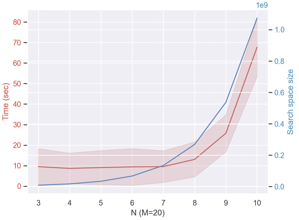<details> <summary>extracted/6466920/figs/time.png Details</summary>  ### Visual Description ## Line Graph: Time and Search Space Size vs. N (M=20) ### Overview The image is a line graph comparing two metrics—**Time (seconds)** and **Search space size**—as a function of **N (M=20)**, where N ranges from 3 to 10. The graph includes two data series: a blue line for "Search space size" and a red line for "Time (sec)". A secondary y-axis on the right represents the search space size, while the primary y-axis on the left represents time. The legend is positioned in the top-right corner. --- ### Components/Axes - **X-axis**: Labeled "N (M=20)", with integer values from 3 to 10. - **Primary Y-axis (left)**: Labeled "Time (sec)", scaled from 0 to 80 in increments of 10. - **Secondary Y-axis (right)**: Labeled "Search space size", scaled from 0 to 1.0 in increments of 0.2. - **Legend**: Located in the top-right corner, with: - **Blue line**: "Search space size" - **Red line**: "Time (sec)" --- ### Detailed Analysis #### Search Space Size (Blue Line) - **Trend**: The blue line shows a **steady upward trend** from N=3 to N=10. - At N=3: ~0.0 (search space size). - At N=8: ~0.4. - At N=10: ~1.0. - **Key Behavior**: The slope increases sharply after N=8, indicating exponential growth in search space size as N approaches 10. #### Time (Red Line) - **Trend**: The red line remains **relatively flat** until N=9, then rises sharply. - At N=3–8: ~10 seconds (stable). - At N=9: ~30 seconds. - At N=10: ~70 seconds. - **Key Behavior**: A **critical threshold** at N=9, where time increases by ~200% compared to N=8. --- ### Key Observations 1. **Divergence at N=9**: Both metrics show a sharp increase at N=9, suggesting a phase transition or computational bottleneck. 2. **Search Space vs. Time**: The search space size grows exponentially (blue line), while time remains low until N=9, then scales linearly (red line). 3. **Uncertainty**: Values are approximate due to the absence of gridlines or exact data points. For example: - Time at N=10: ~70 seconds (could range from 65–75). - Search space size at N=10: ~1.0 (could range from 0.9–1.1). --- ### Interpretation The graph highlights a **non-linear relationship** between problem complexity (N) and computational cost. While the search space size grows exponentially with N, the time complexity remains manageable until N=9, after which both metrics escalate sharply. This suggests that the algorithm’s performance is **asymptotically stable** for smaller N but becomes **intractable** beyond a critical threshold (N=9). The divergence at N=9 may indicate a combinatorial explosion or a shift in the problem’s structure, requiring further investigation into optimization strategies or algorithmic efficiency. </details> Figure 6: Time taken by LBM to collect all satisfying assignments compared with the size of the search space (i.e. the number of possible assignments up to 1 billion (1e9)) as N increases from 3 to 10 with fixed M=20. LBM only needs around 10 seconds for $N<=8$ , $\sim 25$ seconds for $N=9$ , and $\sim 68$ seconds for $N=10$ . The curve grows exponentially, similarly to the search space size, but at a much lower scale. Source: [52]. Figure 6 shows the time taken to collect all satisfying assignments for different N in $\{3,4,5,6,7,8,9,10\}$ with $M=20$ . LBM needed around 10 seconds for $N<=8$ , $25$ seconds for $N=9$ , and $68$ seconds for $N=10$ . As expected, the curve grows exponentially similarly to the search space curve, but at a much smaller scale. 3.5.2 Learning from Data and Knowledge We now evaluate LBM at learning the same Inductive Logic Programming (ILP) benchmark tasks used by neurosymbolic system CILP++ [13] in comparison with ILP state-of-the-art system Aleph [46]. As mentioned earlier, the systems Aleph, CILP++ and a fully-connected standard RBM were chosen as the natural symbolic, neurosymbolic and neural system, respectively, for comparison. An initial LBM is constructed from the clauses provided as background knowledge. This process creates one hidden neuron per clause. Further hidden neurons are added using random weights for training and validation from data. Satisfying assignments can be selected from each clause as a training or validation example, for instance given clause $\mathrm{x}_{1}\wedge\neg\mathrm{x}_{2}→ y$ , assignment $x_{1}=True,x_{2}=False,y=True$ is converted into vector $[x_{1},x_{2},y]=(1,0,1)$ for training or validation. Both the LBM and the standard RBM are trained discriminatively using the conditional distribution $p(y|\mathbf{x})$ for inference as in [26]. In both cases, all network weights are free parameters for learning, with some weights having been initialized by the background knowledge in the case of the LBM, that is, the background knowledge can be revised during learning from data. Seven data sets with available data and background knowledge (BK) are used: Mutagenesis (examples of molecules tested for mutagenicity and BK provided in the form of rules describing relationships between atom bonds) [47], KRK (King-Rook versus King chess endgame with examples provided by the coordinates of the pieces on the board and BK in the form of row and column differences) [3], UW-CSE (Entity-Relationship diagram with data about students, courses taken, professors, etc. and BK describing the relational structure) [39], and the Alzheimer’s benchmark: Amine, Acetyl, Memory and Toxic (a set of examples for each of four properties of a drug design for Alzheimer’s disease with BK describing bonds between the chemical structures) [23]. With the clauses converted into their equivalent set of preferred models in the form of vectors such as $[x_{1},x_{2},y]$ above, and combined with the available data, for the Mutagenesis and KRK tasks, $2.5\%$ of the data is used to build the initial LBM. For the larger data sets UW-CSE and Alzheimer’s, $10\%$ of the data is used as BK. The remaining data are used for training and validation based on 10-fold cross validation for each data set, except for UW-CSE that uses 5 folds for the sake of comparison. The number of hidden units added to the LBM is chosen arbitrarily at $50$ . The standard RBM without BK is given a higher degree of freedom with $100$ hidden units. Results are shown in Table 2. The results for Aleph and CILP++ are obtained from [13]. It can be seen that LBM has the best performance in 5 out of 7 data sets. Some of the results of the LBM and RBM are comparable when the BK can be learned from the examples, as in the case of the Alzheimer’s amine data set. In these cases, training the LBM is faster than the RBM. Aleph is better than all other models in the alz-acetyl data set. This task must rely more heavily on the correctness of the BK than the data. CILP++ however is considerably faster than Aleph and it can achieve comparable results. Although direct comparisons of running times are not possible to make between CILP++ and LBM, LBM’s running times look promising. Table 2: Cross-validation performance of LBM against purely-symbolic system Aleph, neurosymbolic system CILP++ and a standard RBM on 7 benchmark data sets for neurosymbolic AI. We run cross-validation on RBM and LBM 100 times and report the average results with $95\%$ confidence interval. Source: [52]. | Mutagenesis KRK UW-CSE | ${80.85}$ ( $± 10.5$ ) ${99.60}(± 0.51)$ ${84.91}(± 7.32)$ | ${91.70}(± 5.84)$ ${98.42}(± 1.26)$ ${70.01}(± 2.2)$ | ${95.55}(± 1.36)$ ${99.70}(± 0.11)$ ${89.14}(± 0.46)$ | ${\mathbf{96.28}}(± 1.21)$ ${\mathbf{99.80}}(± 0.09)$ ${\textbf{89.43}}(± 0.42)$ | | --- | --- | --- | --- | --- | | alz-amine | ${78.71}(± 5.25)$ | ${78.99}(± 4.46)$ | ${\textbf{79.13}}(± 1.14)$ | ${78.25}(± 1.07)$ | | alz-acetyl | ${\textbf{69.46}}(± 3.6)$ | ${65.47}(± 2.43)$ | ${62.93}(± 0.31)$ | ${66.82}(± 0.28)$ | | alz-memory | ${68.57}(± 5.7)$ | ${60.44}(± 4.11)$ | ${68.54}(± 0.97)$ | ${\mathbf{71.84}}(± 0.88)$ | | alz-toxic | ${80.50}(± 3.98)$ | ${81.73}(± 4.68)$ | $82.71(± 1.18)$ | $\mathbf{84.95}(± 1.04)$ | 3.6 Extensions of Logical Boltzmann Machines 3.6.1 Translating CNF into RBMs In the general case, translation to SDNF can be costly. When knowledge is provided in CNF form, it is useful to be able to translate the CNF directly into the RBM without the need for an intermediate step. Every WFF can be converted into CNF. A CNF is a conjunction of clauses. Formally: $$ \varphi_{\text{CNF}}\equiv\bigwedge_{m=1}^{M}(\bigvee_{t\in\mathcal{S}^{m}_{T}% }x_{t}\vee\bigvee_{k\in\mathcal{S}^{m}_{K}}\neg x_{k}) \tag{17} $$ We will apply the same transformation process into SDNF to each conjunctive clause in the CNF. The result will be a conjunction of $M$ SDNFs (itself not an SDNF), as follows: $$ \displaystyle\varphi_{\text{CNF}}\equiv\bigwedge_{m=1}^{M}(\bigvee_{t\in% \mathcal{S}^{m}_{T}}\neg\mathrm{x}_{t}\vee\bigvee_{k\in\mathcal{S}^{m}_{K}}% \mathrm{x}_{k})\equiv\bigwedge_{m=1}^{M}(\bigvee_{p\in\mathcal{S}^{m}_{T}\cup% \mathcal{S}^{m}_{K}}(\bigwedge_{t\in\mathcal{S}^{m}_{T}\backslash p}\mathrm{x}% _{t}\wedge\bigwedge_{k\in\mathcal{S}^{m}_{K}\backslash p}\neg\mathrm{x}_{k}% \wedge\mathrm{x}^{\prime}_{p})) \tag{18} $$ where $\mathrm{x}^{\prime}_{p}\equiv\neg\mathrm{x}_{p}$ if $p∈\mathcal{S}^{m}_{T}$ ; otherwise $\mathrm{x}^{\prime}_{p}\equiv\mathrm{x}_{p}$ . This transformation would increase the space complexity from $\mathcal{O}(M× N)$ to $\mathcal{O}(M× N^{2})$ , where $M$ is the number of clauses and $N$ is the number of variables. This should not be a problem for current computing systems, especially when inference with RBMs can be highly parallelized. Although the formula in Eq.(18) is not a SDNF, the equivalence between the CNF and the LBM still holds: $$ s_{\varphi}=\begin{dcases*}1&when $-\frac{1}{\epsilon}min_{\mathbf{h}}E(% \mathbf{x},\mathbf{h})=M$\\ 0&otherwise\end{dcases*} \tag{19} $$ Eq.(19) holds because the CNF is satisfied if and only if all $M$ SDNFs are satisfied. Under such circumstances, $min_{\mathbf{h}}E(\mathbf{x},\mathbf{h})=-M\epsilon$ . Otherwise, $min_{\mathbf{h}}E(\mathbf{x},\mathbf{h})=-M^{\prime}\epsilon$ , where $M^{\prime}<M$ . When a confidence value c is used, the number of satisfied clauses in CNF will be proportional to the minimized energy function, and to the free-energy function when c increases. 3.6.2 Towards using LBM as a SAT Solver The Boolean satisfiability (SAT) problem is a fundamental problem in Computer Science. It was the first problem that was proven to be NP complete. A formula is satisfiable if and only if there exists an assignment of truth-values mapping the formula to True. In practice, formulae in SAT problems are represented as Conjunctive Normal Forms (CNFs). As discussed in Section 3.6.1, a formula in Conjunctive Normal Form (CNF) can be converted into a Logical Boltzmann Machine (LBM). The number of satisfied clauses in the CNF formula is proportional to the minimized energy function and the free-energy function of the LBM. This relationship allows us to solve SAT problems by transforming them into an optimization task: finding the minimum of the energy or free-energy function. To make this approach computationally feasible, we focus on minimizing the free-energy function, as it is both easier to compute and differentiable. This transformation converts the discrete SAT problem into a continuous optimization problem. Instead of searching for solutions in a Boolean space (where variables $x$ are either 0 or 1), we search in a continuous space for parameters $\theta$ , where each Boolean variable $x$ is represented as a sigmoid function: $$ x=\sigma(\theta)=\frac{1}{1+\exp(-\theta)}. $$ This mapping ensures that $x$ smoothly transitions between 0 and 1 as $\theta$ changes, enabling gradient-based optimization techniques to be applied. To illustrate this process, consider a simple SAT problem with two variables: $$ (\neg x_{1}\lor\neg x_{2})\land(x_{1}\lor\neg x_{2})\land(\neg x_{1}\lor x_{2}). $$ Figure 7 visualizes the landscape of the LBM’s energy and free-energy functions for different values of $\theta_{1}$ and $\theta_{2}$ , where $x_{1}=\sigma(\theta_{1})$ and $x_{2}=\sigma(\theta_{2})$ . The plots reveal that when both $\theta_{1}$ and $\theta_{2}$ are more negative (corresponding to $x_{1},x_{2}≈ 0$ ), the functions approach their minima. This corresponds to a satisfying assignment of the CNF formula, illustrating how the optimization process identifies valid solutions. We also analyze the impact of confidence values $c$ on the landscapes of the energy and free-energy functions. Figures 7(a), 7(b), 7(c), and 7(d) show that confidence values do not significantly alter the landscape of the energy function. However, for the free-energy function (Figures 7(e), 7(f), 7(g), 7(h)), smaller values of $c$ result in smoother landscapes. While this smoothing effect can facilitate optimization by reducing sharp transitions, it also narrows the gap between local minima and the global minimum. Conversely, higher values of $c$ increase the boundaries between optimal regions, making it more challenging to locate the global optimum. This trade-off highlights the importance of carefully selecting $c$ based on the specific characteristics of the SAT problem being solved. In summary, the LBM framework provides an approach to solving SAT problems by converting them into continuous optimization tasks. By leveraging the differentiability of the free-energy function and the flexibility of sigmoid mappings, this approach bridges logical reasoning and numerical optimization. Future work should explore adaptive strategies for adjusting confidence values to balance smoothness and optimality and consider ways to enhance performance in the case of specific classes of SAT problems. <details> <summary>extracted/6466920/figs/emin_2var_c0.1.png Details</summary>  ### Visual Description ## 3D Surface Plot: Minimised Energy Landscape ### Overview The image depicts a 3D surface plot visualizing a minimised energy landscape as a function of two angular variables, θ₁ and θ₂. The plot uses a color gradient (purple to yellow) to represent energy values, with a grid overlay for spatial reference. The surface exhibits multiple peaks, troughs, and saddle points, suggesting a complex energy distribution. ### Components/Axes - **X-axis (θ₂)**: Ranges from -4 to 4, labeled with increments of 2. - **Y-axis (θ₁)**: Ranges from -4 to 4, labeled with increments of 2. - **Z-axis (Minimised Energy)**: Ranges from -0.14 to -0.02, with increments of 0.02. - **Color Gradient**: - Purple (low energy, ~-0.14) to Yellow (high energy, ~-0.02). - No explicit legend, but color intensity correlates with energy values. - **Grid**: 3D grid lines in gray, providing spatial context for the surface. ### Detailed Analysis 1. **Peaks**: - **Highest Peak**: Located at θ₂ ≈ 0, θ₁ ≈ 0, with energy ≈ -0.02 (yellow region). - **Secondary Peak**: Near θ₂ ≈ 2, θ₁ ≈ 2, with energy ≈ -0.04 (green-yellow transition). 2. **Troughs**: - **Deepest Trough**: At θ₂ ≈ -4, θ₁ ≈ -4, with energy ≈ -0.14 (dark purple). - **Secondary Trough**: Near θ₂ ≈ -2, θ₁ ≈ 2, with energy ≈ -0.08 (blue-green). 3. **Saddle Point**: - A critical point at θ₂ ≈ 2, θ₁ ≈ 2, where the surface transitions from rising to falling in orthogonal directions. 4. **Surface Shape**: - The plot resembles a "double-well" potential with asymmetric wells, influenced by the interaction between θ₁ and θ₂. ### Key Observations - The energy landscape is non-uniform, with localized minima and maxima. - The saddle point at (2, 2) suggests a critical configuration where small perturbations could lead to transitions between states. - Energy values are consistently negative, indicating a bounded system (e.g., potential energy relative to a reference). ### Interpretation This plot likely represents a **potential energy surface** in a physical or optimization context. The double-well structure implies multiple stable states (minima) separated by an energy barrier (saddle point). The asymmetry in well depths suggests preferential stability in certain configurations (e.g., θ₂ ≈ -4, θ₁ ≈ -4). The color gradient confirms that energy values are directly proportional to surface height, with no anomalies in the mapping. The plot could model phenomena such as molecular conformations, mechanical stability, or parameter optimization landscapes. </details> (a) c=0.1 <details> <summary>extracted/6466920/figs/emin_2var_c0.5.png Details</summary>  ### Visual Description ## 3D Surface Plot: Minimised Energy Landscape ### Overview The image depicts a 3D surface plot visualizing a minimised energy landscape as a function of two angular parameters, θ₁ and θ₂. The plot uses a color gradient (purple to yellow) to represent energy values, with a grid overlay for spatial reference. The surface exhibits multiple peaks and troughs, indicating variations in energy across the parameter space. ### Components/Axes - **X-axis (θ₂)**: Ranges from -4 to 4, labeled with integer markers at -4, -2, 0, 2, 4. - **Y-axis (θ₁)**: Ranges from -4 to 4, labeled with integer markers at -4, -2, 0, 2, 4. - **Z-axis (Minimised Energy)**: Ranges from -0.7 to -0.1, with grid lines at intervals of 0.1. - **Color Gradient**: Implicit legend mapping energy values to colors: - Purple: Lowest energy (~-0.7) - Yellow: Highest energy (~-0.1) - **Grid**: Black grid lines on all three axes for spatial grounding. ### Detailed Analysis 1. **Energy Peaks**: - **Highest Peak**: Located at θ₁ ≈ 0, θ₂ ≈ 0, with energy ≈ -0.1 (yellow region). - **Secondary Peaks**: - θ₁ ≈ 2, θ₂ ≈ 2 (energy ≈ -0.3, green region). - θ₁ ≈ -2, θ₂ ≈ -2 (energy ≈ -0.3, green region). 2. **Energy Troughs**: - **Deepest Trough**: Located at θ₁ ≈ -4, θ₂ ≈ -4, with energy ≈ -0.7 (purple region). - **Secondary Troughs**: - θ₁ ≈ 4, θ₂ ≈ 4 (energy ≈ -0.5, blue region). - θ₁ ≈ -4, θ₂ ≈ 4 (energy ≈ -0.6, dark blue region). 3. **Saddle Point**: - A saddle-shaped structure is observed near θ₁ ≈ 2, θ₂ ≈ 2, where energy transitions from a local minimum to a local maximum. 4. **Symmetry**: - The plot exhibits approximate symmetry about the origin (θ₁=0, θ₂=0), with mirrored energy distributions in opposite quadrants. ### Key Observations - The energy landscape is non-uniform, with distinct minima and maxima. - The deepest energy trough (-0.7) occurs at the extreme negative values of both θ₁ and θ₂. - The saddle point near θ₁=2, θ₂=2 suggests a critical transition region in the parameter space. - Energy values increase (become less negative) as the parameters move toward the origin. ### Interpretation This plot represents a potential energy surface, likely from a physical or mathematical optimization problem. The minima correspond to stable equilibrium states, while the saddle point indicates an unstable equilibrium. The symmetry suggests the system may have conserved properties or rotational invariance. The color gradient provides a visual cue for energy density, with purple regions representing the most energetically favorable configurations. The plot highlights the importance of parameter tuning (θ₁, θ₂) to achieve desired energy states, with practical implications for optimization algorithms or physical system design. 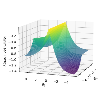</details> (b) c=0.5 <details> <summary>extracted/6466920/figs/emin_2var_c1.0.png Details</summary>  ### Visual Description ## 3D Surface Plot: Minimised Energy Landscape ### Overview The image depicts a 3D surface plot visualizing a minimised energy landscape as a function of two angular variables, θ₁ and θ₂. The plot uses a color gradient (purple to yellow) to represent energy levels, with a grid overlay for spatial reference. The surface exhibits a central peak and asymmetrical troughs, suggesting a non-uniform energy distribution. ### Components/Axes - **X-axis (θ₂)**: Ranges from -4 to 4, labeled with increments of 2. - **Y-axis (θ₁)**: Ranges from -4 to 4, labeled with increments of 2. - **Z-axis (Minimised Energy)**: Ranges from -1.4 to 0.2, labeled with increments of 0.2. - **Color Gradient**: Purple (lowest energy) to yellow (highest energy), with no explicit legend but implied by color intensity. - **Grid**: Black grid lines with spacing consistent across all axes. ### Detailed Analysis 1. **Central Peak**: - Located at θ₁ ≈ 0, θ₂ ≈ 0. - Energy value ≈ 0.2 (yellow region). - Slope: Gradual ascent from surrounding troughs. 2. **Left Trough**: - Extends from θ₁ ≈ -4 to θ₁ ≈ -2, θ₂ ≈ -4 to 0. - Energy values ≈ -1.0 to -0.8 (dark blue to green). - Shape: Bowl-like depression with steep sides. 3. **Right Trough**: - Extends from θ₁ ≈ 2 to θ₁ ≈ 4, θ₂ ≈ -4 to 0. - Energy values ≈ -1.2 to -0.6 (purple to blue). - Shape: Asymmetrical dip with a sharper gradient on the θ₂ > 0 side. 4. **Edge Behavior**: - Energy values drop to ≈ -1.4 at θ₁ = ±4, θ₂ = ±4 (corners). - Color transitions from purple (lowest) to green/yellow (highest) across the surface. ### Key Observations - **Symmetry**: The central peak is symmetric about θ₁ = 0 and θ₂ = 0, but the troughs are asymmetrical. - **Energy Extremes**: - Maximum energy: 0.2 (central peak). - Minimum energy: -1.4 (bottom-right corner). - **Gradient Steepness**: The right trough has a steeper energy gradient compared to the left trough. ### Interpretation The plot likely represents a physical or mathematical system where energy minimization depends on angular variables θ₁ and θ₂. The central peak suggests a stable equilibrium at θ₁ = 0, θ₂ = 0, while the troughs indicate metastable states or energy wells. The asymmetry in trough depths and slopes implies external influences or non-linear interactions in the system. The color gradient confirms that energy values are directly proportional to the surface height, with no additional categorical variables. This visualization could be used in fields like physics (e.g., potential energy landscapes) or optimization algorithms to identify global vs. local minima. 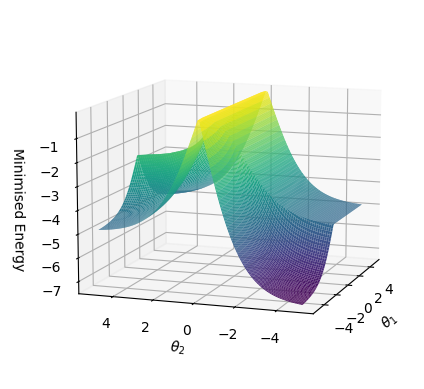</details> (c) c=1 <details> <summary>extracted/6466920/figs/emin_2var_c5.0.png Details</summary>  ### Visual Description ## 3D Surface Plot: Minimised Energy Landscape ### Overview The image depicts a 3D surface plot visualizing a mathematical function's energy landscape. The plot features a color gradient from purple (lowest energy) to yellow (highest energy), with a grid overlay and labeled axes. The surface exhibits multiple peaks, troughs, and saddle points, suggesting a complex optimization problem or physical system. ### Components/Axes - **X-axis (θ₂)**: Ranges from -4 to 4, labeled with integer markers at -4, -2, 0, 2, 4. - **Y-axis (θ₁)**: Ranges from -4 to 4, labeled with integer markers at -4, -2, 0, 2, 4. - **Z-axis (Minimised Energy)**: Ranges from -7 to -1, with markers at -1, -2, -3, -4, -5, -6, -7. - **Grid**: Fine grid lines span all three axes, with darker lines at axis intersections. - **Color Gradient**: Smooth transition from purple (low energy) to yellow (high energy), with no explicit legend but implied by color intensity. ### Detailed Analysis 1. **Peaks**: - **Highest Peak**: Located at approximately (θ₂=0, θ₁=2), with energy ≈ -1 (yellow region). - **Secondary Peak**: Near (θ₂=2, θ₁=0), energy ≈ -2 (green-yellow transition). 2. **Troughs**: - **Deepest Trough**: At (θ₂=-4, θ₁=-4), energy ≈ -7 (dark purple). - **Secondary Trough**: Near (θ₂=4, θ₁=4), energy ≈ -6 (dark purple). 3. **Saddle Point**: - Located at (θ₂=0, θ₁=0), energy ≈ -3 (green region), acting as a critical point between peaks and troughs. 4. **Symmetry**: - The plot exhibits approximate symmetry about θ₂=0, with mirrored energy distributions in the θ₁ direction. ### Key Observations - The energy landscape is non-convex, with multiple local minima and maxima. - The deepest energy minimum (-7) occurs at the extreme corner (-4, -4), while the shallowest (-1) is near the origin. - The saddle point at (0,0) suggests a transition zone between high and low energy regions. - Energy values decrease monotonically from yellow to purple, with no abrupt discontinuities. ### Interpretation This plot likely represents a potential energy surface or cost function in an optimization problem. The saddle point at (0,0) indicates a critical point where the gradient vanishes, which could correspond to an unstable equilibrium in physics or a local extremum in optimization. The asymmetry in peak heights and trough depths suggests the function is not radially symmetric, possibly reflecting constraints or biases in the system. The extreme trough at (-4,-4) implies the function penalizes large negative inputs more severely, which might be relevant for boundary-condition analysis. The absence of a legend necessitates relying on the colorbar's implicit mapping, though the exact numerical-to-color conversion cannot be verified without additional data. 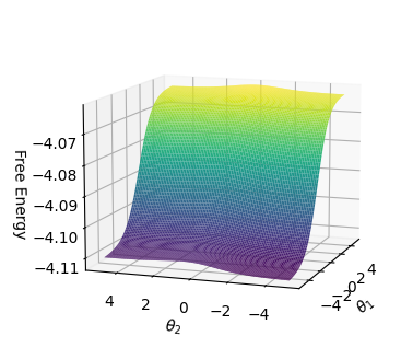</details> (d) c=5 <details> <summary>extracted/6466920/figs/fe_2var_c0.1.png Details</summary>  ### Visual Description ## 3D Surface Plot: Free Energy Landscape ### Overview The image depicts a 3D surface plot representing a free energy landscape as a function of two variables, θ₁ and θ₂. The surface exhibits a smooth gradient transitioning from purple (low energy) to yellow (high energy), with grid lines visible on all axes. The plot is oriented in a Cartesian coordinate system, with θ₁ and θ₂ spanning from -4 to 4 and free energy values ranging from -4.11 to -4.07. --- ### Components/Axes - **X-axis (θ₁)**: Labeled "θ₁" with a linear scale from -4 to 4. - **Y-axis (θ₂)**: Labeled "θ₂" with a linear scale from -4 to 4. - **Z-axis (Free Energy)**: Labeled "Free Energy" with a linear scale from -4.11 (minimum) to -4.07 (maximum). - **Surface**: A continuous 3D surface with a color gradient from purple (low energy) to yellow (high energy). - **Grid Lines**: Visible on all axes, providing spatial reference for the surface. --- ### Detailed Analysis - **Energy Gradient**: - The surface slopes downward from yellow (highest energy, ~-4.07) to purple (lowest energy, ~-4.11) as θ₁ and θ₂ increase. - The color transition is smooth, indicating a gradual change in energy values across the θ₁-θ₂ plane. - **Surface Shape**: - The plot forms a saddle-like structure, with the lowest energy concentrated near θ₁ = 4, θ₂ = 4 (purple region). - The highest energy is observed near θ₁ = -4, θ₂ = -4 (yellow region). - **Grid Resolution**: - Grid lines are evenly spaced, with approximately 10–12 divisions per axis, suggesting a resolution of ~0.4–0.5 units per division. --- ### Key Observations 1. **Monotonic Energy Decrease**: - Free energy decreases consistently as θ₁ and θ₂ move from negative to positive values. 2. **Color-Energy Correlation**: - Purple corresponds to the minimum energy (-4.11), while yellow corresponds to the maximum energy (-4.07). 3. **Smoothness**: - No abrupt changes or discontinuities in the surface, indicating a well-behaved energy landscape. --- ### Interpretation The plot represents a **continuous, differentiable energy landscape** where free energy decreases monotonically with increasing θ₁ and θ₂. This suggests a system (e.g., thermodynamic, mechanical, or optimization) that evolves toward lower energy states as θ₁ and θ₂ increase. The absence of local minima or maxima implies a single global minimum at θ₁ = 4, θ₂ = 4, which could represent an equilibrium or optimal state. The smooth gradient may indicate a linear or quadratic relationship between the variables and energy, though higher-resolution data would be needed to confirm the exact functional form. The visualization emphasizes the importance of θ₁ and θ₂ in determining system stability, with practical implications for parameter tuning in fields like machine learning, physics, or engineering. 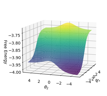</details> (e) c=0.1 <details> <summary>extracted/6466920/figs/fe_2var_c0.5.png Details</summary>  ### Visual Description ## 3D Surface Plot: Free Energy Landscape ### Overview The image depicts a 3D surface plot representing a "Free Energy" landscape as a function of two variables, θ₁ and θ₂. The plot uses a color gradient (purple to yellow) to indicate varying Free Energy values, with grid lines and axis markers for spatial orientation. ### Components/Axes - **X-axis (θ₁)**: Ranges from -4 to 4, labeled "θ₁". - **Y-axis (θ₂)**: Ranges from -4 to 4, labeled "θ₂". - **Z-axis (Free Energy)**: Ranges from -4.00 to -3.75, labeled "Free Energy". - **Surface**: A continuous, undulating surface with no explicit legend or colorbar. The color gradient transitions from purple (lowest Free Energy) to yellow (highest Free Energy). - **Grid Lines**: Faint grid lines on all three axes for reference. ### Detailed Analysis - **Free Energy Values**: - **Highest Point**: At θ₁ ≈ 2, θ₂ ≈ 2, Free Energy ≈ -3.75 (yellow region). - **Lowest Point**: At θ₁ ≈ -4, θ₂ ≈ -4, Free Energy ≈ -4.00 (dark purple region). - **Intermediate Values**: The surface shows a saddle-like structure, with a ridge connecting the peak and trough. - **Color Gradient**: No explicit legend is present, but the gradient suggests a mapping from purple (minimum) to yellow (maximum). ### Key Observations 1. **Saddle Shape**: The surface exhibits a saddle point, indicating a critical point where the Free Energy transitions between minima and maxima. 2. **Asymmetry**: The plot is not symmetric; the peak is offset toward positive θ₁ and θ₂ values, while the trough is at negative extremes. 3. **No Data Points**: No discrete data points or annotations are marked on the surface. ### Interpretation The plot likely represents a potential energy landscape in a physical or chemical system, where θ₁ and θ₂ are parameters (e.g., angles, concentrations, or other variables). The saddle point suggests a transition state between two energy minima, which is critical in understanding system dynamics (e.g., reaction pathways or equilibrium states). The absence of a legend leaves the color gradient’s exact meaning ambiguous, but the z-axis values provide clear Free Energy thresholds. The asymmetry in the surface implies that the system’s behavior is sensitive to the relative magnitudes of θ₁ and θ₂. ## Language Note No non-English text is present in the image. 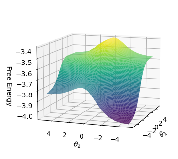</details> (f) c=0.5 <details> <summary>extracted/6466920/figs/fe_2var_c1.0.png Details</summary>  ### Visual Description ## 3D Surface Plot: Free Energy Landscape ### Overview The image depicts a 3D surface plot representing a free energy landscape as a function of two angular variables, θ₁ and θ₂. The plot uses a color gradient (purple to yellow) to indicate free energy values, with grid lines and contour lines for spatial reference. The surface exhibits undulating topography with distinct peaks and troughs. ### Components/Axes - **X-axis (θ₂)**: Ranges from -4 to 4, labeled "θ₂". - **Z-axis (θ₁)**: Ranges from -4 to 4, labeled "θ₁". - **Y-axis (Free Energy)**: Ranges from -4.0 to -3.4, labeled "Free Energy". - **Color Gradient**: Purple (lowest free energy) to yellow (highest free energy), though no explicit legend is present. - **Grid/Contour Lines**: Gray grid lines and contour lines overlay the surface for reference. ### Detailed Analysis - **Peak**: A local maximum occurs near θ₁ ≈ 2, θ₂ ≈ 0, with free energy ≈ -3.4. - **Trough**: A local minimum is observed near θ₁ ≈ -4, θ₂ ≈ -4, with free energy ≈ -4.0. - **Saddle Point**: A critical point (saddle) is visible near θ₁ ≈ 0, θ₂ ≈ 0, where the surface transitions between rising and falling. - **Color Correlation**: Higher free energy regions (yellow) align with peaks, while lower regions (purple) correspond to troughs. Intermediate values (green/blue) represent transitional slopes. ### Key Observations 1. **Peak-Trough Asymmetry**: The highest free energy (yellow) is localized near θ₁=2, θ₂=0, while the lowest (purple) is at θ₁=-4, θ₂=-4. 2. **Critical Points**: The saddle point at θ₁=0, θ₂=0 suggests a bifurcation in the energy landscape. 3. **Spatial Trends**: Free energy decreases monotonically from θ₂=4 to θ₂=-4 for fixed θ₁=0, but exhibits non-linear variations for other θ₁ values. ### Interpretation The plot illustrates a complex energy landscape with multiple minima and maxima, suggesting competing states or phases. The saddle point at the origin indicates a transition region between these states. The absence of a legend limits precise quantification of the color gradient, but the spatial trends confirm that free energy is highly sensitive to both θ₁ and θ₂. The asymmetry in peak/trough locations implies directional preferences in the system's behavior. This could represent a physical or chemical system with metastable states, where transitions between minima require overcoming energy barriers (e.g., activation energy). 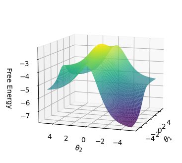</details> (g) c=1 <details> <summary>extracted/6466920/figs/fe_2var_c5.0.png Details</summary>  ### Visual Description ## 3D Surface Plot: Free Energy Landscape as a Function of θ₁ and θ₂ ### Overview The image depicts a 3D surface plot representing a free energy landscape with two variables, θ₁ (horizontal axis) and θ₂ (depth axis). The vertical axis represents free energy values ranging from -7 to -3. The surface exhibits a complex topography with multiple peaks, valleys, and saddle points, colored in a gradient from purple (lowest energy) to yellow (highest energy). ### Components/Axes - **Axes Labels**: - **X-axis (θ₁)**: Ranges from -4 to 4 in increments of 2. - **Y-axis (θ₂)**: Ranges from -4 to 4 in increments of 2. - **Z-axis (Free Energy)**: Ranges from -7 to -3 in increments of 1. - **Color Gradient**: - Purple → Yellow: Represents increasing free energy values (no explicit legend, but inferred from color mapping). - **Grid Lines**: Black grid lines define the 3D coordinate system. ### Detailed Analysis 1. **Highest Energy Point**: - **Location**: θ₁ ≈ 0, θ₂ ≈ 0. - **Free Energy**: Approximately -3 (uncertainty: ±0.5). - **Color**: Yellow (consistent with highest energy). 2. **Lowest Energy Point**: - **Location**: θ₁ ≈ -4, θ₂ ≈ -4. - **Free Energy**: Approximately -7 (uncertainty: ±0.5). - **Color**: Purple (consistent with lowest energy). 3. **Saddle Point**: - **Location**: θ₁ ≈ 2, θ₂ ≈ 2. - **Free Energy**: Approximately -4.5 (uncertainty: ±0.5). - **Color**: Green (intermediate energy). 4. **Additional Features**: - **Peaks**: - θ₁ ≈ -2, θ₂ ≈ 2: Free energy ≈ -5 (green). - θ₁ ≈ 2, θ₂ ≈ -2: Free energy ≈ -5 (green). - **Valleys**: - θ₁ ≈ -3, θ₂ ≈ 3: Free energy ≈ -6 (dark blue). - θ₁ ≈ 3, θ₂ ≈ -3: Free energy ≈ -6 (dark blue). ### Key Observations - The system exhibits **multiple metastable states** (valleys) and **transition states** (saddle points). - The energy landscape is **asymmetric**, with the global minimum at θ₁ = -4, θ₂ = -4 and the local minimum at θ₁ = 0, θ₂ = 0. - The saddle point at θ₁ = 2, θ₂ = 2 acts as a **barrier** between the global and local minima. ### Interpretation This free energy landscape suggests a system with **competing stable and unstable states**. The global minimum at θ₁ = -4, θ₂ = -4 represents the most thermodynamically favorable configuration, while the local minimum at θ₁ = 0, θ₂ = 0 indicates a metastable state. The saddle point at θ₁ = 2, θ₂ = 2 implies a **transition barrier** that must be overcome for the system to shift between these states. The asymmetry in the landscape highlights **directional energy gradients**, which could drive the system toward specific configurations under external perturbations (e.g., temperature changes or external fields). The absence of a uniform energy distribution suggests **nonlinear interactions** between θ₁ and θ₂, potentially indicative of complex molecular or physical systems (e.g., protein folding, chemical reactions, or phase transitions). </details> (h) c=5 Figure 7: Energy function and free-energy function with different confidence values. 3.6.3 Comparison to Other Approaches Unlike recent neural network-based approaches for SAT solving [40, 53], which rely on large datasets generated by traditional SAT solvers for training, our method eliminates this dependency. Instead, we directly convert SAT problems (typically expressed in CNF) into LBM representations. This data-independent transformation should simplify the workflow by reducing the need for extensive pre-processing or model training. When compared with other SAT-solving methods that utilize Boltzmann Machines (BM), such as those in [17, 7], our approach leverages the much simpler structure of Restricted Boltzmann Machines (RBMs). These earlier methods often employ dense or higher-order structures, which are computationally complex and challenging to implement. By contrast, our use of RBMs maintains a streamlined architecture without requiring modifications to the network (e.g. adding configurations) to map SAT problems to BMs. Finally, while LBM is not yet competitive with state-of-the-art SAT solvers in terms of raw performance, it seems to open up a promising direction for further research. Unlike traditional SAT solvers, LBM is in essence a neural network. This should enable a seamless integration of reasoning and learning. Furthermore, LBM does not require prior knowledge of SAT problem structures or specific solving tactics such as backtracking or unit propagation. It is important to notice that our current implementation relies solely on off-the-shelf optimization methods, with room for significant improvements through parallelization optimization and the incorporation of advanced SAT-solving strategies. 3.6.4 SAT Solving Methodology and Initial Experimental Results We used random SAT problems [1] as a case study. To solve SAT problems using LBM, we follow these steps: - Convert a CNF into an RBM using the transformation described earlier. - Apply various inference and optimization techniques to find satisfying assignments or determine unsatisfiability. Specifically: - Use Gibbs sampling to minimize the energy function and search for satisfying assignments. - Employ gradient-based methods from TensorFlow to optimize the differentiable free energy function. - Utilize stochastic optimization methods from the Scipy library, such as dual_annealing and differential_evolution. Our experiments produced the following results: - Gibbs Sampling: - Gibbs sampling can find satisfying assignments for CNFs with fewer than 40 variables. For larger formulas, Gibbs sampling often gets stuck in local minima, making it challenging to determine satisfiability. In such cases, if the free energy function does not decrease after 1000 steps of Gibbs sampling, we conclude that the formula is likely unsatisfiable. - Gradient-Based Optimization (TensorFlow): - Gradient-based methods are applied to minimize the differentiable free energy function. However, these methods are prone to getting trapped in local minima, especially for SAT problems with more than 20 variables. - Attempts to smoothing the energy landscape by adjusting confidence values did not significantly improve performance, highlighting a difficulty in solving larger SAT instances with this approach. - Stochastic Optimization (Scipy): - Among the stochastic optimization methods available in Scipy, dual_annealing and differential_evolution showed better scalability. These methods successfully solved SAT problems with up to 100 variables. - This suggests that stochastic global optimization techniques may offer a viable alternative for solving larger SAT instances with RBMs. 3.6.5 Implementing Penalty Logic in LBM The closest work to LBM is Penalty Logic [37], which represents propositional formulae in Hopfield networks and Boltzmann machines. In its first step, Penalty Logic creates hidden variables to reduce a formula $\varphi$ to a conjunction of sub-formulas $\bigwedge_{i}\varphi_{i}$ , each with at most three variables. This naming step makes conversion into an energy function easier, but some of the terms in the energy function may consist of hidden variables and therefore cannot be converted into an RBM. For example, a negative term $-h_{1}xy$ of a higher-order Boltzmann Machine would be transformed into the quadratic term $-h_{2}h_{1}-h_{2}x-h_{2}y+5h_{2}$ with $-h_{2}h_{1}$ forming a connection between two hidden units, which is not allowed in RBMs. The three-variable term $-h_{1}xy$ is implemented in the higher-order network as a hypergraph. The variable $h_{2}$ is introduced to turn the hyper-edge into normal edges between each of the three variables and $h_{2}$ with an appropriate bias value for the new node $h_{2}$ , in this example a value of 5. Contrast the LBM for XOR in Figure 4 with the RBM for XOR built using Penalty Logic: first, one computes the higher-order energy function: ${\it E}^{p}=4xyz-2xy-2xz-2yz+x+y+z,$ then transforms it to quadratic form by adding a hidden variable $h_{1}$ to obtain: ${\it E}^{p}=2xy-2xz-2yz-8xh_{1}-8yh_{1}+8zh_{1}+x+y+z+12h_{1},$ which is not an energy function of an RBM, so one keeps adding hidden variables until the energy function of an RBM might be obtained, in this case: ${\it E}^{p}=-8xh_{1}-8yh_{1}+8zh_{1}+12h_{1}-4xh_{2}+4yh_{2}+2h_{2}-4yh_{3}-4% zh_{3}+6h_{3}-4xh_{4}-4zh_{4}+6h_{4}+3x+y+z.$ The LBM system converts any set of formulae $\Phi=\{\varphi_{1},...,\varphi_{n}\}$ into an RBM by applying Theorem 1 to each formula $\varphi_{i}∈\Phi$ . In the case of Penalty Logic, formulae are weighted. Given a set of weighted formulae $\Phi=\{w_{1}:\varphi_{1},...,w_{n}:\varphi_{n}\}$ , one can also construct an equivalent RBM where each energy term generated from formula $\varphi_{i}$ is multiplied by $w_{i}$ . In both cases, the assignments that minimise the energy of the RBM are the assignments that maximise the satifiability of $\Phi$ , i.e. the (weighted) sum of the truth-values of the formula. **Lemma 3** *Given a weighted knowledge-base $\Phi=\{w_{1}:\varphi_{1},...,w_{n}:\varphi_{n}\}$ , there exists an equivalent RBM $\mathcal{N}$ such that $s_{\Phi}(\mathbf{x})=-\frac{1}{\epsilon}min_{\mathbf{h}}{\it E}(\mathbf{x},% \mathbf{h})$ , where $s_{\Phi}(\mathbf{x})$ is the sum of the weights of the formulae in $\Phi$ that are satisfied by assignment $\mathbf{x}$ .* A formula $\varphi_{i}$ can be decomposed into a set of (weighted) conjunctive clauses from its SDNF. If there exist two conjunctive clauses such that one is subsumed by the other then the subsumed clause is removed and the weight of the remaining clause is replaced by the sum of their weights. Identical conjunctive clauses are treated in the same way: one of them is removed and the weights are added. From Theorem 1, we know that a conjunctive clause $\bigwedge_{t∈\mathcal{S}_{T_{j}}}\mathrm{x}_{t}\wedge\bigwedge_{k∈\mathcal% {S}_{K_{j}}}\neg\mathrm{x}_{k}$ is equivalent to an energy term $e_{j}(\mathbf{x},h_{j})=-h_{j}(\sum_{t∈\mathcal{S}_{T_{j}}}x_{t}-\sum_{k∈% \mathcal{S}_{K_{j}}}x_{k}-|\mathcal{S}_{T_{j}}|+\epsilon)$ where $0<\epsilon<1$ . A weighted conjunctive clause $w^{\prime}:\bigwedge_{t∈\mathcal{S}_{T_{j}}}\mathrm{x}_{t}\wedge\bigwedge_{k% ∈\mathcal{S}_{K_{j}}}\neg\mathrm{x}_{k}$ , therefore, is equivalent to an energy term $w^{\prime}e_{j}(\mathbf{x},h_{j})$ . For each weighted conjunctive clause, we can add a hidden unit $j$ to an RBM with connection weights $w_{tj}=w^{\prime}$ for all $t∈\mathcal{S}_{T_{j}}$ , and $w_{kj}=-w^{\prime}$ for all $k∈\mathcal{S}_{K_{j}}$ . The bias for this hidden unit will be $w^{\prime}(-|\mathcal{S}_{T_{j}}|+\epsilon)$ . The weighted knowledge-base and the RBM are equivalent because $s_{\Phi}(\mathbf{x})\propto-\frac{1}{\epsilon}min_{\mathbf{h}}{\it E}(\mathbf{% x},\mathbf{h})$ , where $s_{\Phi}(\mathbf{x})$ is the sum of the weights of the clauses that are satisfied by $\mathbf{x}$ . **Example 5** *(Nixon diamond problem) Consider the following weighted knowledge-base from the original Penalty Logic paper [37] (the weights of 1000 and 10 are given and have been taken from the original paper): | | $\displaystyle 1000:\mathrm{n}→\mathrm{r}\quad\text{ Nixon is a % Republican.}$ | | | --- | --- | --- | <details> <summary>extracted/6466920/figs/diamond.png Details</summary>  ### Visual Description ## Directed Graph Diagram: Network Flow with Weighted Edges ### Overview The image depicts a directed graph with labeled nodes and weighted edges. The graph forms a diamond-like structure with additional nodes connected to the main vertices. Edge weights are explicitly labeled, and some nodes (h1–h7) have additional numerical annotations. ### Components/Axes - **Nodes**: - Main nodes: `n` (top), `q` (left), `r` (right), `p` (bottom). - Intermediate nodes: `h1`, `h2`, `h3` (connected to `n`); `h4`, `h5`, `h6`, `h7` (connected to `q`, `r`, and `p`). - **Edges**: - Directed arrows with numerical weights (e.g., `1000`, `2000`, `1000`, `10`, `-10`, etc.). - No legend present; edge weights are directly annotated. - **Node Annotations**: - `h1` to `h7` have additional numerical values (e.g., `-1500`, `-15`, `5`, `-5`). These appear to be node-specific attributes rather than edge weights. ### Detailed Analysis #### Edge Weights - **Top Layer (`n` connections)**: - `n → h1`: `1000` - `n → h2`: `2000` - `n → h3`: `1000` - **Middle Layer (`h2` to `q`)**: - `h2 → q`: `1000` - **Side Nodes (`q` and `r`)**: - `q → h4`: `10` - `q → h6`: `-15` - `r → h5`: `-5` - `r → h7`: `5` - **Bottom Layer (`p` connections)**: - `p → h4`: `-10` - `p → h6`: `10` - `p → h5`: `-5` - `p → h7`: `10` #### Node Attributes - **h1**: `-1500` (left of node) - **h2**: `-1500` (left of node) - **h3**: No additional value - **h4**: `-5` (left of node) - **h5**: `5` (left of node) - **h6**: `-15` (left of node) - **h7**: `5` (left of node) ### Key Observations 1. **Weight Distribution**: - The largest edge weight is `2000` (from `n` to `h2`), suggesting a critical or high-cost path. - Negative weights (e.g., `-1500`, `-15`, `-10`) on `h` nodes may represent penalties, costs, or constraints. 2. **Symmetry**: - The graph is roughly symmetric around the vertical axis (e.g., `q` and `r` have mirrored connections to `h4`, `h5`, `h6`, `h7`). 3. **Negative Values**: - Nodes `h1`, `h2`, `h4`, `h6`, and `h5` have negative attributes, which could indicate resource drains or inhibitory factors. ### Interpretation This diagram likely represents a **network flow problem** or **decision tree** with both positive and negative weights. The negative values on `h` nodes suggest they act as "cost centers" or "risk nodes" in the system. For example: - The high weight (`2000`) from `n` to `h2` might indicate a primary pathway, while the negative attribute (`-1500`) on `h2` could represent a significant cost or penalty associated with that node. - The symmetry between `q` and `r` implies balanced or mirrored processes, but the asymmetry in edge weights (e.g., `q → h6: -15` vs. `r → h5: -5`) suggests uneven impacts or priorities. - The bottom layer (`p`) connects to all `h` nodes, possibly acting as a convergence point or final decision node. ### Notable Patterns - **Critical Path**: The path `n → h2 → q` has the highest cumulative weight (`2000 + 1000 = 3000`), making it a potential focal point. - **Risk Nodes**: `h1` and `h2` have the largest negative attributes (`-1500`), indicating they may be high-risk or high-cost nodes. - **Balanced Flow**: The bottom layer (`p`) distributes weights symmetrically to `h4`, `h5`, `h6`, and `h7`, suggesting a stabilizing or balancing role. This structure could model scenarios like resource allocation, risk assessment, or optimization problems where both gains and losses are quantified. </details> Figure 8: The RBM for the Nixon diamond problem has 4 input neurons $\{n,q,r,p\}$ and 7 hidden neurons (shown in grey) as a result of the conversion into SDNF of the 4 weighted clauses shown in Example 5. Converting all four weighted clauses above into SDNF produces eight conjunctive clauses. For example, weighted clause $1000:\mathrm{n}→\mathrm{r}\equiv 1000:(\mathrm{n}\wedge\mathrm{r})% \vee(\neg\mathrm{n})$ . After adding the weights of clause ( $\neg\mathrm{n}$ ) which appears twice, an RBM is created (Figure 8) representing the following unique conjunctive clauses with their corresponding confidence values: $1000:\mathrm{n}\wedge\mathrm{r},\quad 2000:\neg\mathrm{n},\quad 1000:\mathrm{n% }\wedge\mathrm{q},\quad 10:\mathrm{r}\wedge\neg\mathrm{p},\quad 10:\neg\mathrm% {r},\quad 10:\mathrm{q}\wedge\mathrm{p},\quad 10:\neg\mathrm{q}.$ With $\epsilon=0.5$ , this RBM has energy function: ${\it E}=-h_{1}(1000n+1000r-1500)-h_{2}(-2000n+1000)-h_{3}(1000n+1000q-1500)-h_% {4}(10r-10p-5)-h_{5}(-10r+5)-h_{6}(10q+10p-15)-h_{7}(-10q+5).$* 4 Logical Boltzmann Machines for MaxSAT MaxSAT - shorthand for Maximum Satisfiability - is a computational problem that extends the classical SAT (Boolean satisfiability) problem. In MaxSAT, the goal is to find an assignment of truth values to the variables of a Boolean formula that maximizes the number of satisfied clauses. The formula is typically represented in CNF. We denote the number of satisfied clauses given a assignment $\mathbf{x}$ as $\sum_{m}\mathbbm{1}(\mathbf{x}\models\varphi_{m})$ . Here, $\mathbf{x}\models\varphi_{m}$ denotes that an assignment $\mathbf{x}$ satisfies the clause $\varphi_{m}$ of the CNF and $\mathbbm{1}$ is an indicator function mapping a clause-satisfying assignment to 1, and everything else to 0. Differently from SAT, where the goal is to find any satisfying assignment, MaxSAT seeks the assignment that satisfies the maximum number of clauses, making it a combinatorial optimization problem: $$ \mathbf{x}^{*}=\operatorname*{arg\,max}_{\mathbf{x}}\sum_{m}\mathbbm{1}(% \mathbf{x}\models\varphi_{m}) \tag{20} $$ For example, consider the CNF formula: $$ \phi=(\neg x_{1}\lor\neg x_{2})\land(\neg x_{1}\lor x_{2})\land(x_{1}\lor\neg x% _{2})\land(x_{1}\lor x_{2}). $$ The goal is to find an assignment $x∈\{0,1\}^{n}$ (where $n$ is the number of variables, in this example $n=2$ ) that maximizes the number of satisfied clauses. We know that $\phi$ is unsatisfiable since each clause corresponds to exactly one assignment. An optimal solution will satisfy three of the four clauses. This relaxation of the SAT task makes MaxSAT particularly suited for real-world optimization problems where constraints may need to be prioritized or relaxed to achieve the best overall solution. However, this flexibility comes at a cost: NP-Hardness, meaning that finding exact solutions becomes computationally infeasible as the number of variables grows. Many real-world applications, however, require approximate solutions to the MaxSAT problem, with the main challenge being how to balance accuracy and computation time. Symbolic MaxSAT solvers have been the focus of intensive research for many years, gaining popularity among researchers and finding application in various domains from AI and computer-aided design to automated reasoning. Recent advancements in MaxSAT solvers have demonstrated significant improvements, with state-of-the-art solvers capable of scaling up to handling millions of variables and clauses. MaxSAT has proven to be valuable in software analysis [43], hardware verification [32, 22], combinatorial optimization [25], bioinformatics [45], and data analysis [4]. Despite these achievements, the growing complexity of real-world problems has spurred interest in alternative approaches, such as leveraging the differentiable capabilities of Machine Learning to address MaxSAT by transforming the discrete problem into a continuous optimization task. In recent years, there has been a growing interest in connectionist solvers. These solvers aim to represent MaxSAT problems using neural networks to benefit from the parallel computation and learning capabilities of such ML systems and from specialized neural network accelerators, such as GPUs and TPUs, to further enhance performance. Beyond providing an alternative approach to solving complex reasoning problems, connectionist MaxSAT solvers may promote the development of interpretable classification models [28], facilitating novel neurosymbolic learning and reasoning [53, 52] with the promise of offering more transparent decision making in AI. Deep learning-inspired MaxSAT solvers rely on real-valued weights often learned from example solutions [53]. In a related attempt, [27] seeks to train a Graph Neural Network for MaxSAT problem-solving. Unlike symbolic approaches, ML-based methods typically require a degree of supervision and may be criticized for their opacity. We take a different approach and use LBM along with a global optimization method called dual annealing, a modified version of a meta-heuristic method known as simulated annealing, to search for MaxSAT solutions. Using dual annealing, we will search the energy landscape of the RBM for a global minimum corresponding to a MaxSAT solution. Research that has also focused on representing MaxSAT problems in connectionist networks without relying on explicit learning from examples include [18], where the MaxSAT problem is mapped to a combinatorial optimization framework based on a high-order Boltzmann Machine used to search for an approximate solution to SAT. However, the problems with efficiency of Boltzmann Machines are well-known. They have motivated the use of RBMs, first in [52] and leading up to this work. In a more recent development also using RBMs, RBMSAT was proposed to construct an RBM that represents the probability of an assignment w.r.t. the number of clauses that it satisfies [54]. The goal there is to conduct a heuristic search for solutions using block Gibbs samplings on neural network accelerators. Our goal, instead, is to make use of an interpretable RBM layer, as shown e.g. in Figure 13 where each clause can be read off the LBM with binary weights. **Example 6** *An AND-gate $\mathrm{x}_{1}\wedge\neg\mathrm{x}_{2}$ is represented by a free energy $FE=-\log(1+\exp(c×(x_{1}-x_{2}-0.5)))$ . Figure 9 illustrates the correspondence between the free energy and the truth-values for different values of $c$ . Similarly, Figure 10 shows the free energy of an OR-gate (that is, a clause) $\mathrm{x}_{1}\vee\mathrm{x}_{2}$ . This clause is transformed into SDNF $(\mathrm{x}_{1}\wedge\neg\mathrm{x}_{2})\vee\mathrm{x}_{2}$ and the corresponding free energy is $FE=-\log(1+\exp(c×(x_{1}-x_{2}-0.5)))-\log(1+\exp(c×(x_{2}-0.5))$ . As expected, the satisfying assignments are those that maximize the negative free energy.* As we have seen already when using LBM as a SAT solver, a conjunctive clause $\varphi_{m}$ can be represented in an RBM with the energy function $E_{m}=\sum_{j}e_{j}$ and, therefore, the energy function of a CNF will be: $$ {\it E}(\mathbf{x})=\sum_{m}E_{m} \tag{21} $$ The free energy of each clause corresponds to the truth values of the clause, i.e. $\mathbbm{1}(\mathbf{x}\models\varphi_{m})\propto FE_{m}(\mathbf{x})$ . The free energy of the entire CNF $FE(\mathbf{x})=\sum_{m}FE_{m}(\mathbf{x})$ , therefore, corresponds to the number of satisfied conjunctive clauses, that is: $$ \displaystyle\sum_{m}\mathbbm{1}(\mathbf{x}\models\varphi_{m})\propto FE(% \mathbf{x}) \tag{22} $$ An assignment that maximizes the number of satisfying clauses in a MaxSAT problem also minimizes the free energy of the LBM. Consequently, solving MaxSAT problems is equivalent to searching for a state of minimum free energy in the RBM. 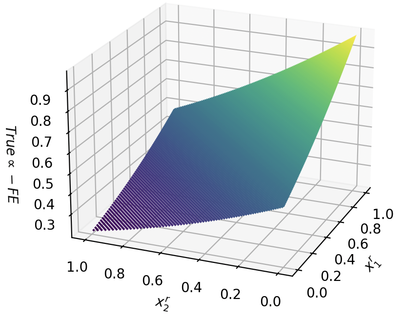<details> <summary>extracted/6466920/figs/andc1_.png Details</summary>  ### Visual Description ## 3D Surface Plot: Relationship Between x₁, x₂, and True α - FE ### Overview The image depicts a 3D surface plot visualizing the relationship between two input variables (x₁ and x₂) and a dependent variable labeled "True α - FE." The plot uses a color gradient (purple to yellow) to represent the magnitude of "True α - FE," with grid lines providing spatial context. The axes range from 0.0 to 1.0 for both x₁ and x₂, while "True α - FE" spans approximately 0.3 to 0.9. --- ### Components/Axes 1. **Axes Labels**: - **X-axis (x₁)**: Labeled as "x₁," scaled from 0.0 to 1.0 in increments of 0.2. - **Y-axis (x₂)**: Labeled as "x₂," scaled from 0.0 to 1.0 in increments of 0.2. - **Z-axis (True α - FE)**: Labeled as "True α - FE," scaled from 0.3 to 0.9 in increments of 0.1. 2. **Grid Lines**: - Gray grid lines span all three axes, creating a 3D lattice to contextualize the surface. 3. **Color Gradient**: - The surface transitions from **purple** (low values) to **yellow** (high values), indicating the magnitude of "True α - FE." --- ### Detailed Analysis 1. **Surface Shape**: - The surface forms a **diagonal ridge** from the bottom-left corner (x₁=0.0, x₂=0.0) to the top-right corner (x₁=1.0, x₂=1.0), suggesting a linear relationship between x₁, x₂, and "True α - FE." - At (x₁=0.0, x₂=0.0), "True α - FE" ≈ 0.3 (purple). - At (x₁=1.0, x₂=1.0), "True α - FE" ≈ 0.9 (yellow). 2. **Color Gradient**: - Purple dominates the lower-left region (x₁ < 0.5, x₂ < 0.5), indicating lower "True α - FE" values. - Yellow dominates the upper-right region (x₁ > 0.5, x₂ > 0.5), indicating higher "True α - FE" values. - Intermediate values (green) appear along the diagonal ridge. 3. **Grid Line Interpretation**: - The grid lines confirm the 3D structure, with horizontal lines representing x₁ and x₂, and vertical lines representing "True α - FE." --- ### Key Observations 1. **Linear Trend**: - "True α - FE" increases linearly as both x₁ and x₂ increase, with the steepest gradient along the diagonal (x₁ = x₂). 2. **Color Correlation**: - The color gradient aligns perfectly with the z-axis values, providing a visual cue for magnitude without numerical annotations. 3. **Boundary Values**: - Minimum value (0.3) occurs at (0.0, 0.0). - Maximum value (0.9) occurs at (1.0, 1.0). --- ### Interpretation 1. **Model Behavior**: - The plot suggests that "True α - FE" is directly proportional to both x₁ and x₂. This could represent a simplified model where two input variables linearly influence a dependent variable (e.g., accuracy, error, or efficiency metric). 2. **Practical Implications**: - Maximizing x₁ and x₂ (to 1.0) yields the highest "True α - FE," implying optimal performance or accuracy in the modeled system. - The linear relationship simplifies predictive modeling, as no nonlinear interactions are observed. 3. **Anomalies**: - No outliers or discontinuities are present, indicating a smooth, deterministic relationship. 4. **Design Choices**: - The absence of a legend is compensated by the intuitive color gradient, which maps directly to the z-axis values. - Grid lines enhance readability but may obscure fine details in the surface texture. --- ### Final Notes This plot effectively communicates a linear, monotonic relationship between two inputs and a dependent variable. The use of color and grid lines aids in spatial grounding, though explicit numerical annotations on the surface could improve precision. The simplicity of the model suggests it may serve as a baseline for more complex analyses. 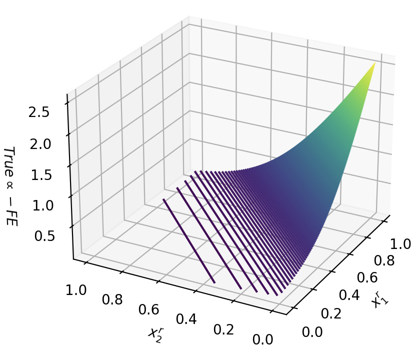</details> (a) c=1 <details> <summary>extracted/6466920/figs/andc5_.png Details</summary>  ### Visual Description ## 3D Surface Plot: Relationship Between Variables x₁ᵣ, x₂ᵣ, and True α - FE ### Overview The image depicts a 3D surface plot visualizing the relationship between three variables: - **x₁ᵣ** (horizontal axis, left-to-right) - **x₂ᵣ** (horizontal axis, depth) - **True α - FE** (vertical axis, z-axis) The surface transitions from a flat region near the origin to a sharply curved, upward-sloping structure. A color gradient (purple to green) indicates increasing values of **True α - FE** with higher x₂ᵣ. --- ### Components/Axes 1. **Axes Labels**: - **x₁ᵣ**: Ranges from 0.0 (left) to 1.0 (right). - **x₂ᵣ**: Ranges from 0.0 (front) to 1.0 (back). - **True α - FE**: Ranges from 0.0 (bottom) to 2.5 (top). 2. **Surface**: - A 3D grid forms the base, with a smooth, continuous surface overlay. - The surface is color-coded: - **Purple**: Low values of **True α - FE** (near the origin). - **Green**: High values of **True α - FE** (upper-right region). 3. **No Legend**: - No explicit legend is present to confirm the meaning of the color gradient. --- ### Detailed Analysis 1. **Surface Behavior**: - **Flat Region**: Near the origin (x₁ᵣ ≈ 0.0, x₂ᵣ ≈ 0.0), the surface is nearly flat, with **True α - FE** ≈ 0.0–0.5. - **Curved Region**: As x₂ᵣ increases (moving backward along the plot), the surface curves upward sharply. - At x₂ᵣ ≈ 0.8–1.0, **True α - FE** reaches ~2.5 (green region). - **x₁ᵣ Dependency**: The surface remains relatively flat along the x₁ᵣ axis (left-to-right), suggesting weak or no dependency on x₁ᵣ. 2. **Color Gradient**: - The transition from purple (low values) to green (high values) aligns with increasing **True α - FE** as x₂ᵣ increases. - No explicit scale or legend is provided to quantify the color mapping. 3. **Grid Structure**: - The 3D grid uses uniform spacing for x₁ᵣ and x₂ᵣ (0.0–1.0 in 0.2 increments). - The z-axis (True α - FE) is labeled in 0.5 increments. --- ### Key Observations 1. **Dominant Trend**: - **True α - FE** increases monotonically with x₂ᵣ, with minimal dependence on x₁ᵣ. - The surface’s curvature intensifies as x₂ᵣ approaches 1.0. 2. **Anomalies**: - No outliers or discontinuities are visible. - The absence of a legend introduces uncertainty about the exact interpretation of the color gradient. 3. **Spatial Relationships**: - The flat region near the origin suggests that **True α - FE** is negligible when both x₁ᵣ and x₂ᵣ are small. - The sharp upward curve implies a nonlinear relationship between x₂ᵣ and **True α - FE**. --- ### Interpretation 1. **Mathematical Implications**: - The plot likely represents a function **f(x₁ᵣ, x₂ᵣ) = True α - FE**, where x₂ᵣ is the primary driver of the output. - The lack of x₁ᵣ dependency suggests the function may simplify to **f(x₂ᵣ)** in this visualization. 2. **Practical Significance**: - If **True α - FE** represents a physical or engineering metric (e.g., stress, efficiency), the plot highlights a critical threshold: increasing x₂ᵣ beyond ~0.6 leads to a rapid rise in the metric. - The flat region near the origin could indicate a "baseline" or "neutral" state where the metric is minimal. 3. **Uncertainties**: - Without a legend, the exact meaning of the color gradient (e.g., whether it represents magnitude, probability, or another variable) remains ambiguous. - The absence of numerical data points or error bars limits quantitative validation of the trends. --- ### Final Notes This plot emphasizes the dominance of x₂ᵣ in determining **True α - FE**, with x₁ᵣ playing a negligible role. The sharp curvature and color gradient suggest a nonlinear, possibly exponential relationship between x₂ᵣ and the output. Further analysis (e.g., adding a legend, providing numerical data) would strengthen interpretability. 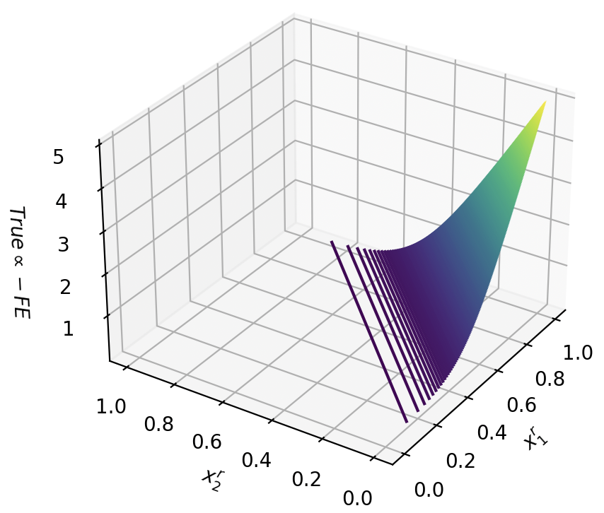</details> (b) c=5 <details> <summary>extracted/6466920/figs/andc10_.png Details</summary>  ### Visual Description ## 3D Surface Plot: Relationship Between x₁, x₂, and True α - FE ### Overview The image depicts a 3D surface plot visualizing the relationship between two input variables (x₁ and x₂) and a response variable labeled "True α - FE." The plot features a color gradient transitioning from purple (low values) to green (high values), with a distinct upward-curving surface originating from the origin (0,0,0) and peaking at (1,1,5). Grid lines define the 3D coordinate system, and the axes are labeled with numerical scales. --- ### Components/Axes - **X-axis (x₁)**: Labeled "x₁" with a scale from 0.0 to 1.0 in increments of 0.2. - **Y-axis (x₂)**: Labeled "x₂" with a scale from 0.0 to 1.0 in increments of 0.2. - **Z-axis (True α - FE)**: Labeled "True α - FE" with a scale from 0 to 5 in increments of 1. - **Surface**: A smooth, curved surface with a color gradient from purple (low values) to green (high values). - **Grid Lines**: Gray grid lines define the 3D coordinate system on all three planes. - **Color Gradient**: Implicit legend where purple represents low values (~0–2) and green represents high values (~3–5). --- ### Detailed Analysis 1. **Surface Shape**: - The surface begins flat near the origin (0,0,0) and gradually curves upward as x₁ and x₂ increase. - The curvature intensifies toward the upper-right corner (x₁=1.0, x₂=1.0), where the surface peaks at a height of 5 on the z-axis. - Vertical lines of constant True α - FE are visible along the surface, indicating fixed z-values for specific (x₁, x₂) pairs. 2. **Color Gradient**: - The gradient transitions from purple (darkest) at the base of the surface to green (brightest) at the peak. - Intermediate values (e.g., ~2.5) are represented by blue tones. 3. **Key Data Points**: - **Origin (0,0,0)**: Surface starts at z=0. - **Midpoint (0.5,0.5,2.5)**: Approximate midpoint of the surface with a z-value of ~2.5 (blue tone). - **Peak (1,1,5)**: Maximum z-value of 5 at (x₁=1.0, x₂=1.0), colored green. --- ### Key Observations 1. **Positive Correlation**: True α - FE increases monotonically with both x₁ and x₂, with the steepest rise occurring near (x₁=1.0, x₂=1.0). 2. **Smooth Gradient**: The color transition aligns with the surface height, confirming that higher z-values correspond to greener regions. 3. **No Outliers**: The surface is continuous and smooth, with no abrupt changes or discontinuities. --- ### Interpretation The plot demonstrates a **nonlinear relationship** between x₁, x₂, and True α - FE, where the response variable grows quadratically as both inputs approach their maximum values. The color gradient provides an intuitive visualization of magnitude, emphasizing that the highest values of True α - FE are concentrated near the upper-right corner of the plot. This suggests that maximizing x₁ and x₂ simultaneously yields the greatest impact on True α - FE, which could be critical for optimization or sensitivity analysis in the underlying system. The absence of noise or outliers implies a deterministic relationship, potentially useful for modeling or predictive purposes. </details> (c) c=10 Figure 9: Free energy corresponding to an AND gate with different confidence values (Example 6). 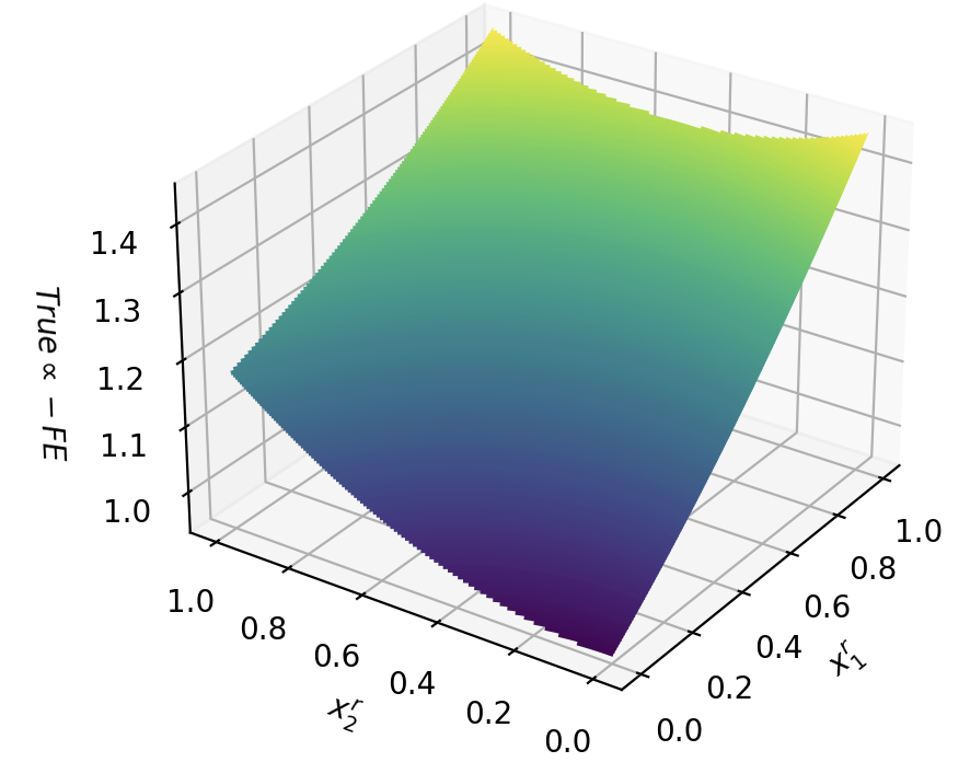<details> <summary>extracted/6466920/figs/c1.png Details</summary>  ### Visual Description ## 3D Surface Plot: True α – FE vs. x₁ and x₂ ### Overview The image depicts a 3D surface plot visualizing the relationship between two input variables (`x₁` and `x₂`) and a response variable (`True α – FE`). The surface is colored using a gradient from purple (low values) to yellow (high values), with a grid background providing spatial reference. The plot shows a smooth, curved surface with a peak at the top-right corner. --- ### Components/Axes 1. **Axes Labels**: - **x₁ (horizontal axis)**: Ranges from 0.0 to 1.0 in increments of 0.2. - **x₂ (depth axis)**: Ranges from 0.0 to 1.0 in increments of 0.2. - **True α – FE (vertical axis)**: Ranges from 1.0 to 1.4 in increments of 0.1. 2. **Color Gradient**: - **Purple**: Represents the lowest values of `True α – FE` (~1.0). - **Yellow**: Represents the highest values of `True α – FE` (~1.4). - **Green/Blue**: Intermediate values (~1.1–1.3). 3. **Grid**: - A 3D grid spans the background, with lines spaced evenly along all axes. --- ### Detailed Analysis - **Surface Shape**: - The surface is smooth and curved, with a pronounced peak at the top-right corner (x₁ = 1.0, x₂ = 1.0). - The gradient transitions from purple (bottom-left) to yellow (top-right), indicating increasing `True α – FE` values as `x₁` and `x₂` increase. - **Key Data Points**: - At (x₁ = 0.0, x₂ = 0.0): `True α – FE` ≈ 1.0 (purple). - At (x₁ = 1.0, x₂ = 1.0): `True α – FE` ≈ 1.4 (yellow). - Intermediate values (e.g., x₁ = 0.5, x₂ = 0.5): `True α – FE` ≈ 1.2–1.3 (green/blue). - **Color Consistency**: - The color gradient aligns with the vertical axis scale, confirming that higher `True α – FE` values correspond to warmer colors (yellow). --- ### Key Observations 1. **Peak at Maximum Inputs**: - The highest `True α – FE` value (1.4) occurs when both `x₁` and `x₂` are at their maximum (1.0). 2. **Gradual Increase**: - `True α – FE` increases monotonically as `x₁` and `x₂` increase, with no visible plateaus or anomalies. 3. **Smooth Gradient**: - The color transition is continuous, suggesting a linear or near-linear relationship between inputs and the response. --- ### Interpretation The plot demonstrates that `True α – FE` is directly influenced by both `x₁` and `x₂`, with the strongest effect observed when both variables are maximized. The smooth surface and gradient imply a predictable, non-linear relationship between the inputs and the response. The absence of outliers or discontinuities suggests a well-behaved system, where small changes in `x₁` and `x₂` lead to proportional changes in `True α – FE`. This could represent a physical or mathematical model where efficiency (`α`) or error (`FE`) is optimized at extreme input values. 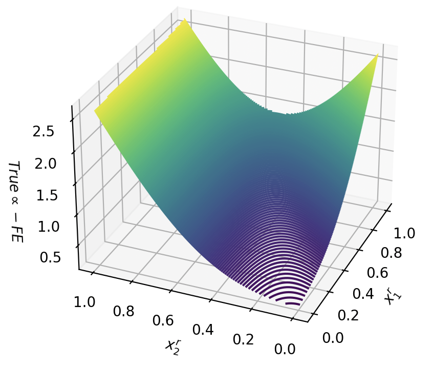</details> (a) c=1 <details> <summary>extracted/6466920/figs/c5.png Details</summary>  ### Visual Description ## 3D Surface Plot: Relationship Between x₁, x₂, and True α - FE ### Overview The image depicts a 3D surface plot illustrating the relationship between two input variables (x₁ and x₂) and a response variable labeled "True α - FE." The plot uses a color gradient (purple to yellow) to represent magnitude, with contour lines overlaid to emphasize gradients. The surface exhibits a saddle-like shape, with peaks at the corners of the input space and a trough at the center. --- ### Components/Axes 1. **Axes**: - **x₁ (Horizontal Axis, Right)**: Ranges from 0.0 to 1.0 in increments of 0.2. - **x₂ (Horizontal Axis, Bottom)**: Ranges from 0.0 to 1.0 in increments of 0.2. - **True α - FE (Vertical Axis, Left)**: Ranges from 0.0 to 2.5 in increments of 0.5. 2. **Surface**: - **Color Gradient**: Purple (low values) to yellow (high values), indicating the magnitude of "True α - FE." - **Contour Lines**: Purple lines overlaid on the surface, denser near the trough and sparser near peaks. 3. **Grid**: Gray grid lines define the 3D coordinate system. --- ### Detailed Analysis 1. **Surface Shape**: - **Peaks**: Located at the corners of the input space: - (x₁ = 0.0, x₂ = 0.0): True α - FE ≈ 2.5 (yellow). - (x₁ = 1.0, x₂ = 1.0): True α - FE ≈ 2.5 (yellow). - **Trough**: Located at the center (x₁ = 0.5, x₂ = 0.5): True α - FE ≈ 0.0 (dark purple). - **Gradients**: The surface transitions smoothly between peaks and trough, with steeper gradients near the trough (evidenced by dense contour lines). 2. **Color and Contour Correlation**: - Purple regions (low values) dominate the central trough. - Yellow regions (high values) dominate the corners. - Intermediate green-blue regions represent mid-range values (e.g., 1.0–1.5). 3. **Contour Line Density**: - Denser near the trough (x₁ = 0.5, x₂ = 0.5), indicating rapid changes in "True α - FE." - Sparser near peaks, reflecting flatter gradients. --- ### Key Observations 1. **Saddle Shape**: The surface forms a saddle, with opposing concavities along the x₁ and x₂ axes. 2. **Extreme Values**: Maximum "True α - FE" occurs at the input extremes (0,0) and (1,1). 3. **Optimal Point**: Minimum "True α - FE" (0.0) occurs at the center (0.5, 0.5). 4. **Gradient Behavior**: The steepest changes occur near the trough, while the peaks exhibit minimal variation. --- ### Interpretation This plot likely represents a function where "True α - FE" depends nonlinearly on x₁ and x₂. The saddle shape suggests a trade-off: increasing one input variable while decreasing the other leads to opposing effects on the response. The trough at (0.5, 0.5) implies an optimal balance between x₁ and x₂ to minimize "True α - FE," while the peaks indicate scenarios where imbalanced inputs maximize the response. The color gradient and contour lines provide intuitive visualization of how small changes in inputs propagate through the system, with the steepest sensitivity near the optimal point. This could inform optimization strategies or sensitivity analysis in systems governed by such relationships. 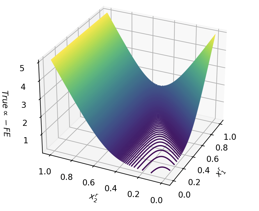</details> (b) c=5 <details> <summary>extracted/6466920/figs/c10.png Details</summary>  ### Visual Description ## 3D Surface Plot: True α - FE vs. x₁ and x₂ ### Overview The image is a 3D surface plot visualizing the relationship between two variables, **x₁** and **x₂**, and a third variable, **True α - FE**. The surface transitions from **purple** (low values) to **yellow** (high values), with **purple contour lines** indicating regions of rapid change. The plot suggests a **non-linear relationship** between the variables, with a **valley-like structure** in the center and **peaks** at the edges. --- ### Components/Axes - **X-axis (x₁)**: Ranges from **0.0 to 1.0** in increments of 0.2. - **Y-axis (x₂)**: Ranges from **0.0 to 1.0** in increments of 0.2. - **Z-axis (True α - FE)**: Ranges from **1.0 to 5.0** in increments of 1.0. - **Surface**: A gradient from **purple** (low values) to **yellow** (high values), with **purple contour lines** concentrated in the central valley. - **No explicit legend** is present, but the color gradient implies a mapping of **True α - FE** values to the surface. --- ### Detailed Analysis - **Surface Shape**: - The surface forms a **valley** (minimum) at the center (x₁ ≈ 0.5, x₂ ≈ 0.5), where **True α - FE** is approximately **1.0–2.0**. - The edges (x₁ ≈ 0.0 or 1.0, x₂ ≈ 0.0 or 1.0) show **peaks** with **True α - FE** reaching **4.0–5.0**. - The **purple contour lines** are tightly packed in the valley, indicating a **steep gradient** (rapid change in **True α - FE**) near the minimum. - **Color Gradient**: - **Purple** (low values) dominates the central valley. - **Yellow** (high values) dominates the edges. - Intermediate values (green to blue) transition between the valley and peaks. - **Contour Lines**: - The **purple contour lines** are concentrated in the valley, suggesting **local minima** or **critical points** in the function. - No contour lines are visible on the peaks, implying **flat regions** or **plateaus** at higher **True α - FE** values. --- ### Key Observations 1. **Minimum at the Center**: The lowest **True α - FE** values (≈1.0–2.0) occur at the center of the plot (x₁ ≈ 0.5, x₂ ≈ 0.5). 2. **Peaks at the Edges**: The highest **True α - FE** values (≈4.0–5.0) are observed at the corners of the plot (e.g., x₁ ≈ 0.0, x₂ ≈ 0.0). 3. **Steep Gradient in the Valley**: The **purple contour lines** indicate a **sharp increase** in **True α - FE** as the surface moves from the valley toward the edges. 4. **No Explicit Legend**: The color gradient and contour lines serve as implicit indicators of **True α - FE** values, but no numerical scale or legend is provided. --- ### Interpretation The plot likely represents a **mathematical function** or **physical system** where **True α - FE** depends on two parameters, **x₁** and **x₂**. The **valley** suggests an **optimal point** (minimum) for **True α - FE**, while the **peaks** indicate **suboptimal regions**. The **contour lines** highlight areas of **rapid change**, which could be critical for optimization or sensitivity analysis. - **Peircean Insight**: The absence of a legend introduces ambiguity in interpreting the exact numerical values of **True α - FE**, but the **color gradient** and **contour lines** provide qualitative insights into the function's behavior. - **Notable Anomalies**: The **flat regions** at the peaks (no contour lines) may indicate **plateaus** or **insensitive regions** where **True α - FE** is relatively constant. This visualization is useful for identifying **critical points** (minima/maxima) and understanding the **sensitivity** of **True α - FE** to changes in **x₁** and **x₂**. </details> (c) c=10 Figure 10: Free energy corresponding to an OR gate with different confidence values (Example 6). 4.1 LBM with Dual Annealing When representing CNF in a RBM, one option for solving the MaxSAT problem is to utilize stochastic search methods like Gibbs sampling. However, in our scenario, Gibbs sampling exhibits slow convergence, necessitating potentially extensive computational resources to reach equilibrium. To mitigate this challenge, we have adopted simulated annealing, a meta-heuristic technique renowned for addressing global optimization problems [24]. Specifically, we employ dual annealing, which seamlessly integrates global and local search strategies to enhance efficiency [55]. In this approach, the search algorithm initially employs simulated annealing to identify a candidate region within the search space where global optima are likely to be situated. Subsequently, a local search is conducted to precisely pinpoint the location of the global optima. This hybrid strategy combines the exploration capabilities of simulated annealing with the exploitation capabilities of local search, offering a robust and efficient approach to solving MaxSAT problems. 4.1.1 Experimental Results of LBM for MaxSAT As a preliminary evaluation, we compare the performance of LBM at solving MaxSAT problems with Loandra, a state-of-the-art MaxSAT solver. Loandra was chosen as benchmark solver due to its performance in the MaxSAT Evaluations 2023. Experiments were carried out on a set of challenging MaxSAT instances known as MaxCut, each containing 1,260 clauses. Six distinct MaxCut problem instances were chosen from the MaxSAT 2016 benchmark. Both the LBM and Loandra solvers were run on each of the six instances with a timeout limit of 300 seconds for each run. The instances were chosen to represent diverse problem structures so as to evaluate the capabilities of the solvers without making assumptions about the CNF structure. All experiments were conducted on a standard desktop computer with a AMD ryzen7 5800X 8-core processor and 32 GB DDR4 RAM. The main evaluation metric was the number of satisfied clauses, indicating the solver’s ability to maximize clause satisfaction within the given time constraints. <details> <summary>extracted/6466920/figs/ClauseStats4LoandraLBM.png Details</summary>  ### Visual Description ## Data Tables: Satisfied Clauses Statistics ### Overview The image contains two side-by-side data tables comparing statistical metrics for "Loandra Satisfied Clauses" (a) and "LBM Satisfied Clauses" (b). Both tables include identical categories (count, mean, std, min, 25%, 50%, 75%, max) with numerical values. ### Components/Axes - **Categories**: - count - mean - std (standard deviation) - min (minimum) - 25% (25th percentile) - 50% (median) - 75% (75th percentile) - max (maximum) - **No legends, axes, or visual elements** are present beyond the tabular structure. ### Detailed Analysis #### (a) Loandra Satisfied Clauses Stats | Category | Value | |----------|----------------| | count | 6.000000 | | mean | 1089.000000 | | std | 8.508819 | | min | 1078.000000 | | 25% | 1083.500000 | | 50% | 1088.000000 | | 75% | 1095.500000 | | max | 1100.000000 | #### (b) LBM Satisfied Clauses Stats | Category | Value | |----------|----------------| | count | 6.000000 | | mean | 1078.666667 | | std | 3.502380 | | min | 1075.000000 | | 25% | 1075.750000 | | 50% | 1078.500000 | | 75% | 1080.500000 | | max | 1084.000000 | ### Key Observations 1. **Central Tendency**: - Loandra has a higher mean (1089.0 vs. 1078.7) and max (1100.0 vs. 1084.0) compared to LBM. - LBM’s mean is closer to its 50% percentile (1078.5), suggesting symmetry in its distribution. 2. **Variability**: - Loandra’s standard deviation (8.51) is significantly higher than LBM’s (3.50), indicating greater dispersion in satisfied clauses. - Loandra’s 75% percentile (1095.5) is notably higher than its median (1088.0), suggesting positive skewness. 3. **Range**: - Loandra’s range (1078.0–1100.0) is wider than LBM’s (1075.0–1084.0). ### Interpretation - **Loandra** exhibits higher variability and a broader spread in satisfied clauses, with a skewed distribution toward higher values. This could imply less consistency in clause satisfaction. - **LBM** shows tighter clustering around its mean, with minimal variability, suggesting more uniform clause satisfaction. - The higher max value for Loandra (1100.0) may indicate outliers or exceptional cases not present in LBM’s data. - Both datasets have identical sample sizes (count = 6.0), but Loandra’s larger standard deviation suggests greater sensitivity to individual variations. This analysis highlights differences in distribution patterns between the two systems, which could inform decisions about clause design or evaluation criteria. </details> Figure 11: Statistics for clause satisfaction for (a) Loandra (1089 clauses satisfied on average) and (b) LBM for MaxSAT (1078 clauses satisfied on average). <details> <summary>extracted/6466920/figs/SatClausesComparisons.png Details</summary>  ### Visual Description ## Line Chart: Satisfied Clauses Comparison ### Overview The chart compares the performance of two methods, **Loandra** (blue line with circles) and **LBM** (orange line with squares), across six experiment indices (0–5). The y-axis measures "Satisfied Clauses" on a scale from 1075 to 1100, while the x-axis represents discrete experiment indices. The legend is positioned in the top-right corner, with distinct colors and markers for each method. --- ### Components/Axes - **X-axis (Horizontal)**: Labeled "Experiment Index," with integer values 0 to 5. - **Y-axis (Vertical)**: Labeled "Satisfied Clauses," with increments of 5 units (1075, 1080, ..., 1100). - **Legend**: Located in the top-right corner, associating: - **Blue line with circles**: Loandra - **Orange line with squares**: LBM --- ### Detailed Analysis #### Loandra (Blue Line) - **Trend**: Starts at 1100 (index 0), sharply declines to 1097 (index 1), then gradually decreases to 1085 (index 2), 1083 (index 3), and 1078 (index 4), before recovering to 1091 (index 5). - **Key Data Points**: - Index 0: 1100 - Index 1: 1097 - Index 2: 1085 - Index 3: 1083 - Index 4: 1078 - Index 5: 1091 #### LBM (Orange Line) - **Trend**: Starts at 1084 (index 0), declines to 1079 (index 1), stabilizes at 1075 (indices 2–3), rises to 1078 (index 4), and peaks at 1081 (index 5). - **Key Data Points**: - Index 0: 1084 - Index 1: 1079 - Index 2: 1075 - Index 3: 1075 - Index 4: 1078 - Index 5: 1081 --- ### Key Observations 1. **Loandra's Volatility**: - Sharp initial drop (1100 → 1097) followed by a gradual decline until index 4, then a recovery at index 5. - Final value (1091) exceeds LBM's final value (1081) despite mid-experiment dips. 2. **LBM's Stability**: - Minimal fluctuation, with a flatline at 1075 (indices 2–3) and a modest recovery by index 5. 3. **Y-Axis Scale**: - Increment of 5 units per gridline, emphasizing small performance differences between methods. --- ### Interpretation - **Performance Dynamics**: - Loandra demonstrates higher initial performance but experiences mid-experiment instability, potentially due to methodological adjustments or external factors. Its recovery at index 5 suggests resilience or adaptive mechanisms. - LBM maintains consistent performance, indicating robustness but lower overall effectiveness compared to Loandra. - **Outliers**: - Loandra's sharp drop at index 1 and recovery at index 5 are notable anomalies, possibly reflecting experimental interventions or data collection artifacts. - **Practical Implications**: - Loandra may be preferable for scenarios prioritizing peak performance, while LBM suits applications requiring stability. The final divergence at index 5 highlights the importance of longitudinal evaluation in method selection. </details> Figure 12: Performance of LBM and Loandra on 6 MaxCut experiments (0 to 5). Figure 12 shows the number of clauses satisfied by the symbolic SAT solver Loandra and the LBM for MaxSAT approach in each of the 6 experiments. As a state-of-the-art solver, Loandra performed better than LBM in 5 out of 6 cases. However, the difference is relatively small and further investigation is warranted, with numerous directions for future exploration. One possible direction involves investigating alternative global optimization methods such as evolutionary strategies. Another obvious direction is the implementation of parallel computation to improve scalability of LBM search, similar to the approach employed in RBMSAT. As future work, the task of Image Sudoku introduced in [48] is an interesting extension to consider because of the interplay between object recognition and reasoning that is intrinsic to that task and aligned well with LBM’s approach integrating learning and reasoning, which we describe next. 5 Integrating Learning and Reasoning in Logical Boltzmann Machines A key development in neurosymbolic AI will be the ability to add verified modules to existing networks. An RBM that can be shown to be provably equivalent to a given logical formula could act as one such module. A neurosymbolic module placed on top (at the output) of a larger network may serve to constrain that network’s output to satisfy certain properties. In this process, the specification of a neurosymbolic module may benefit from the use of a logical language that is richer (more expressive) than propositional logic. In particular, the use of first-order logic may be required. In first-order logic, instead of using propositions and connectives alone, logical predicates are used to represent relations among quantified variables. Statements such as $∀ X∃ Y.R(X,Y)$ are used to denote compactly a relation $R$ between variables $X$ and $Y$ in a domain such that for all the values that variable $X$ may admit, there is a value (an instance) of variable $Y$ for which the relation $R$ holds True. As an example, if we were to rewrite into first-order logic the Boolean logical notation provided earlier for the Sudoku puzzle, we could use a ternary predicate $board(B,P,V)$ , in which: - $B$ represents the block index (1 to 4), - $P$ represents the position index within the block (1 to 4), and - $V$ represents the value (1 to 4), to make the problem description a lot more compact. A first-order representation of the constraints of the Sudoku puzzle would include: 1. Existence: $∀ B,P,∃ V.board(B,P,V)$ This ensures that every position in every block is filled with at least one value. 1. Uniqueness: $∀ B,P,V_{1},V_{2}.(board(B,P,V_{1})\land board(B,P,V_{2}))→ V_% {1}=V_{2}$ This ensures that no position in the board can hold multiple values. We will illustrate one way of integrating LBM as a logical layer on top of deep networks applied to a semantic image interpretation task. The task is to predict the relations between objects and their parts in an image. It requires the use of first-order logic. The knowledge base consists of symbolic facts expressing when an object type is normally part of another object type, e.g. ${part}(\text{Screen},\text{TV})$ , where Screen and TV are variables, denoting that TVs have screens. The knowledge base also includes a first-order rule connecting any two visual scenes ( $X_{1}$ and $X_{2}$ ) with the symbols of the logic, as follows: $$ \displaystyle\forall X_{1},X_{2},\exists T_{1},T_{2}.(({type}(X_{1},T_{1})% \wedge{type}(X_{2},T_{2}))\rightarrow \displaystyle({partOf}(X_{1},X_{2})\leftrightarrow{part}(T_{1},T_{2}))) \tag{23} $$ where $X_{1}$ , $X_{2}$ are real-valued variables representing visual features of objects (an embedding, pixel values, etc.), as done in [41], and $T_{1}$ , $T_{2}$ are symbolic variables representing object types. Predicate ${type}$ is $True$ when an object, as defined by its visual features, is deemed to be of a given type (e.g. an object class). Given two visual scenes with their corresponding type classifications, ${type}(X_{1},T_{1})$ and ${type}(X_{2},T_{2})$ , one visual scene will be part of the other, $partOf(X_{1},X_{2})$ , if and only if the object type of the former is deemed to be part of the object type in the latter, ${part}(T_{1},T_{2})$ . In order to implement the above rule, we use Faster-RCNN to extract features from object images, from which we build two Neural Network Regressors (NNR) To represent first-order logic in LBM, we combine LBM with the Neural Network Regressors. Each NNR represents a predicate in the formulae and outputs a truth-value for that predicate. LBM takes as input the truth-values of the predicates coming from the outputs of the NNRs. In essence, LBM sits on top of the NNRs connecting the predicates according to the connectives of the corresponding logic formulae.: $\mathcal{N}^{type}$ and $\mathcal{N}^{po}$ , as learned functions for ${type}$ and ${partOf}$ , respectively, as done in [11]. Finally, we use an autoencoder $\mathcal{N}^{pt}$ to implement the relation ${part}(T_{1},T_{2})$ between the symbolic variables $T_{1}$ and $T_{2}$ , following [51]. Let ${p}^{po}=\mathcal{N}^{po}(X_{1},X_{2})$ , ${p}^{pt}=\mathcal{N}^{pt}(T_{1},T_{2})$ , ${p}^{t_{1}}=\mathcal{N}^{type}(X_{1},T_{1})$ , ${p}^{t_{2}}=\mathcal{N}^{type}(X_{2},T_{2})$ , ${p}^{po},{p}^{pt},{p}^{t_{1}},{p}^{t_{2}}∈\{0,1\}$ , according to some choice of threshold. The first-order rule (23) can be converted to SDNF, as follows: | | $\displaystyle({p}^{t_{1}}\wedge{p}^{t_{2}})→({p}^{po}\leftrightarrow% {p}^{pt})\equiv$ | | | --- | --- | --- | From this SDNF, we build a LBM as the logical layer on top of the neural networks $\mathcal{N}^{type}$ , $\mathcal{N}^{po}$ and $\mathcal{N}^{pt}$ . Figure 13 shows the overall network architecture. 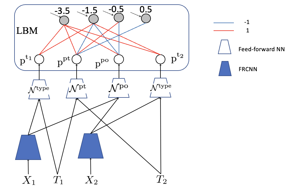<details> <summary>extracted/6466920/figs/lbm_sii.png Details</summary>  ### Visual Description ## Diagram: Neural Network Architecture with LBM and Processing Nodes ### Overview The diagram illustrates a computational architecture combining a Local Binary Model (LBM) with feed-forward and FRCNN (Feed-Forward Recurrent Convolutional Neural Network) components. It shows weighted connections between nodes, neural network types, and input/output variables (X1, T1, X2, T2). ### Components/Axes 1. **LBM Section (Top Box)**: - Contains 4 nodes labeled `p^t1`, `p^pt`, `p^po`, `p^t2`. - Each node has a numerical value: `-3.5`, `-1.5`, `-0.5`, `0.5` (left to right). - Connections between nodes use **red lines** (value `-1`) and **blue lines** (value `1`). 2. **Processing Nodes (Middle Layer)**: - 4 nodes labeled `p^t1`, `p^pt`, `p^po`, `p^t2` (mirroring LBM nodes). - Connected to LBM nodes via red/blue lines (weights: `-1` or `1`). 3. **Neural Network Types**: - **Feed-forward NN**: Represented by **white triangles** (legend). - **FRCNN**: Represented by **blue inverted triangles** (legend). 4. **Input/Output Variables**: - `X1`, `T1`, `X2`, `T2` (bottom layer), connected to neural networks. 5. **Legend (Right Side)**: - **Red lines**: Weight = `-1`. - **Blue lines**: Weight = `1`. - **White triangle**: Feed-forward NN. - **Blue inverted triangle**: FRCNN. ### Detailed Analysis - **LBM Node Values**: - `p^t1`: `-3.5` (strongest negative value). - `p^pt`: `-1.5`. - `p^po`: `-0.5`. - `p^t2`: `0.5` (only positive value in LBM). - **Connection Patterns**: - Red/blue lines between LBM and processing nodes indicate weighted summation (e.g., `p^t1` connects to `p^pt` via red line = `-1`). - Processing nodes (`p^t1`, `p^pt`, `p^po`, `p^t2`) feed into neural networks: - `p^t1` → FRCNN (blue inverted triangle) → `X1`. - `p^pt` → Feed-forward NN (white triangle) → `T1`. - `p^po` → FRCNN → `X2`. - `p^t2` → Feed-forward NN → `T2`. - **Spatial Grounding**: - Legend is positioned **top-right**, clearly associating colors/shapes with weights and network types. - LBM nodes are centrally located, with processing nodes directly below. - Neural networks and input/output variables form the bottom layer. ### Key Observations 1. **Weight Distribution**: - LBM nodes show a gradient from strongly negative (`-3.5`) to weakly positive (`0.5`), suggesting asymmetric influence. - Red/blue lines imply binary weight values (`-1` or `1`), simplifying the model's computational logic. 2. **Neural Network Assignment**: - FRCNN (blue inverted triangles) processes `X1` and `X2` (spatial/temporal features?). - Feed-forward NN (white triangles) handles `T1` and `T2` (temporal or target variables?). 3. **Symmetry**: - `p^t1` and `p^t2` (first/last LBM nodes) connect to opposite neural network types, hinting at complementary roles. ### Interpretation This architecture likely models a system where: - **LBM nodes** act as feature extractors or decision boundaries, with weights reflecting their influence on downstream processing. - **Red/blue lines** enforce strict binary weighting, simplifying gradient calculations or enabling sparse representations. - **FRCNN** (blue inverted triangles) and **Feed-forward NN** (white triangles) specialize in different tasks: - FRCNN may handle recurrent or convolutional processing for `X1`/`X2` (e.g., time-series or spatial data). - Feed-forward NN processes `T1`/`T2`, possibly for classification or regression. - The negative/positive LBM node values could represent inhibitory/excitatory signals, common in biological or neuromorphic computing. ### Uncertainties - Exact purpose of `X1`, `T1`, `X2`, `T2` (input vs. output variables). - Whether LBM node values (`-3.5`, etc.) are fixed or learnable parameters. - Role of `p^pt` and `p^po` (intermediate processing nodes?). This diagram suggests a hybrid model blending rule-based LBM logic with deep learning components, optimized for specific input-output relationships. </details> Figure 13: Learning and reasoning about the PartOf relation in object images by grounding symbolic concepts into Convolutional Neural Networks and adding a logical layer in the form of a LBM module implementing the rule $({p}^{t_{1}}\wedge{p}^{t_{2}})→({p}^{po}\leftrightarrow{p}^{pt})$ . Reasoning in the LBM can inform learning in $\mathcal{N}$ by backpropagating inferred knowledge to update the weights of the CNN, regressor or autoencoder. In particular, we train the entire system by minimizing the following loss function $[\mathcal{N}^{type}(x_{1},t_{1}),\mathcal{N}^{type}(x_{2},t_{2})]$ denotes the concatenation of the outputs from the $\mathcal{N}^{type}$ networks; $||x||^{2}_{2}$ is the squared Euclidean norm.: | | $\displaystyle||\mathcal{N}^{po}(x_{1},x_{2})-\text{LBM}({p}^{po}|\mathcal{K}(x% _{1},x_{2})||^{2}_{2}+$ | | | --- | --- | --- | where $x_{1},x_{2}$ and $\mathcal{K}(x_{1},x_{2})$ are obtained from the training data; $\mathcal{K}$ denotes the knowledge pertaining to $x_{1},x_{2}$ , i.e. the type of $x_{1}$ , type of $x_{2}$ , and whether $x_{1}$ is part of $x_{2}$ . We use $\text{LBM}({p}^{po}|\mathcal{K}(x_{1},x_{2}))$ and $\text{LBM}({p}^{t_{1}},{p}^{t_{2}}|\mathcal{K}(x_{1},x_{2}))$ to denote the application of LBM to infer the value of ${p}^{po}$ and of the pair $[{p}^{t_{1}},{p}^{t_{2}}]$ , respectively. For example, the LBM is used to infer ${p}^{po}$ , which is used in turn to update $\mathcal{N}^{po}$ . Given, for instance, $x_{1}=∈cludegraphics[width=9.95863pt]{figs/screen.png}$ and $x_{2}=∈cludegraphics[width=9.95863pt]{figs/tvmonitor.png}$ , let’s assume that we do not know whether $x_{1}$ is part of $x_{2}$ . But, if the $\mathcal{N}^{type}$ networks tell us that ${type}(x_{1},\text{Screen})\equiv{True}$ and ${type}(x_{2},\text{TV})\equiv{True}$ and $\mathcal{K}(x_{1},x_{2})$ also includes ${part}(\text{Screen},\text{TV})$ , the LBM can infer that ${p}^{po}$ should be $True$ . Finally, this signal from the LBM’s reasoning, obtained from the first term of the loss function, is used to update during learning the parameters of $\mathcal{N}^{po}$ . Similarly, the second term of the loss function leverages information about the type of objects to update $\mathcal{N}^{type}$ . We compared the LBM-enhanced model with three other neurosymbolic systems: Deep Logic Networks (DLN) [50], Logic Tensor Networks (LTN) [11, 2], and Compositional Neural Logic Programming (CNLP) [51]. The task and data set used were the same as in [11], with the exception of the rule $({p}^{t_{1}}\wedge{p}^{t_{2}})→({p}^{po}\leftrightarrow{p}^{pt})$ only used by LBM. The area under the curve (AUC) results shown in Table 3 indicate that the use of this single first-order rule for reasoning with the LBM and training of the Faster-RCNN model, also used in [11], produces a higher performance than LTN in the prediction of the part-of relation in images. LBM’s performance is comparable to that of CNLP. For the object type prediction, the LBM model performs better than CNLP, DLN and LTN. Table 3: Comparison of neurosymbolic approaches; area under the curve (AUC) in the semantic image interpretation task. Source: [52]. | DLN CNLP LTN | $0.791± 0.032$ $0.816± 0.004$ $0.800$ | $0.605± 0.024$ $\mathbf{0.644± 0.015}$ $0.598$ | | --- | --- | --- | | LBM | $\mathbf{0.828± 0.002}$ | $\mathbf{0.645± 0.027}$ | 6 Challenges for Neurosymbolic AI We introduced an approach and neurosymbolic system to reason about symbolic knowledge in an energy-based neural network. Differently from most LLM approaches and CoT, where reasoning capabilities are expected to emerge and are measured post-hoc using benchmarks, we use logic to provide a formal definition of reasoning. Only once a well-defined semantics is provided, one can show correspondence between networks and various forms of reasoning. We showed equivalence between propositional logic and RBMs. The finding led to a novel system, named Logical Boltzmann Machines integrating learning and reasoning in neural networks. Future work will focus on scaling up the application to SAT and learning from data and knowledge. Extensions include applications of weighted clauses, weighted SAT with parallel implementation as well as evaluations on relational learning tasks. Equipped with a proof and algorithm showing how RBMs can implement a category of required constraints, it is possible to imagine how an RBM may be added as a module to an existing network imposing such constraints on the network. This RBM module becomes a verifiable component of the system, implementing for example a fairness or safety requirement as argued for in [16]. Next, we discuss how this simple idea may open up directions for research addressing some of the biggest challenges for current AI: data efficiency, fairness, safety and ultimately trust. 6.1 Nonmonotonic Logic Consider the task of commonsense reasoning, the human-like ability to make sense of ordinary situations, such as making judgments about the nature of objects. It encompasses intuitive psychology (e.g. reasoning about intentions) and naive physics (a natural understanding of the physical world, including spatial and temporal reasoning). Commonsense reasoning requires an ability to jump to conclusions based on incomplete information, and to retract or revise such conclusions when more information become available. There have been many attempts to formalize commonsense, not least the work of John McCarthy who was responsible for coining the term Artificial Intelligence. Because it requires jumping to conclusions and therefore handling logical inconsistencies in a non-classical way, commonsense reasoning is modeled by non-monotonic logics, some of which are undecidable. LLMs have achieved much better results than logical formalizations of commonsense on reasoning benchmarks. It turns out that it is easier to learn commonsense from data than to formalize it logically. Yet, making sense of what has been learned by LLMs has been proven to be a daunting task. Making sense of what has been learned might help tremendously with the efforts to understand the limits of the formalization of commonsense in logic. As neural networks start to be deployed successfully in various fields of scientific discovery, achieving a true understanding of the processes at play will demand such an ability to explain the network’s reasoning. 6.2 Planning AGI will require the ability to plan towards a goal and the ability to ask questions in order to achieve that goal. Planning requires the ability to break-down goals into sub-goals while reasoning with partial information over time. Having a goal, in turn, requires the provision of a description of the current state and the goal state, and a mechanism that reduces the difference (e.g. some distance function) between the current state and the goal state by changing the current state in a reasonable way. If the mechanism isn’t working, one may decide to change the goal or even change the mechanism itself. Whether in Google’s AlphaGo or Sudoku, the goal state is to win the game, and because it is a closed environment, simulation can be used to learn to minimize the distance function without the need for an explicit description. In open-ended situations, the problem becomes much harder. An explicit description is one that can be manipulated by asking questions: “what might happen if I were to make this or that change?” without making the change. An explicit description needs, therefore, to be amenable to symbolic manipulation. We argue that in open-ended scenarios, an explicit description needs furthermore to be abstracted from the situation given only a few examples. Reasoning in the form of symbol manipulation on that abstract description can then take place that will be of a different nature from reasoning carried out in terms of pattern matching with similarity and distance functions. 6.3 Learning from its Mistakes An AGI system should be able to learn from its mistakes, interact with users by asking questions, describing its understanding and improving its performance in a controlled way towards a goal, even if changing the goal and the mechanism for performance improvement. Controlled at the level of its symbolic description, the system can be made safe. With reasoning taking place at both the pattern matching and the more abstract levels, as advocated by D. Kahneman’s Thinking: Fast and Slow [21], the system will be able to adapt to novelty from only a few examples, check its understanding, multi-task and reuse knowledge from one task to another thus improving data and energy efficiency in comparison with the demands of current AI systems. Adapting to novelty (therefore solving the long-tail distribution problem and out-of-distribution problem in Machine Learning) requires creating compact representations (in the brain or the mind) but also being able to change that representation from time to time in order to obtain new insight. It is the change of representation that allows one to look at a problem from a new angle to obtain new insight. Think of the difference between two computer programs, both correct for their purpose, one so-called spaghetti code and the other an example of what programmers like to refer to as beautiful code. The former may be faster to run, but the latter needs to be neat, easy to understand and useful to update and reuse. This is the core challenge of the latest research in neurosymbolic AI: extraction of relevant descriptions at the right level of abstraction from complex neural networks, sound application of reasoning and learning with various forms of representation - spatial, temporal, epistemic, normative, multimodal, nonmonotonic - and efficient knowledge and data reuse and extrapolation to multiple tasks in different application domains. Consider the kind of program learned by the latest GPT-based chatbots. Transformer neural networks work, in essence, by mapping sets to sets and not sequences to sequences (GPT-based chatbots require positional encoding to handle sequences). Interestingly, in neurosymbolic AI, the computation of the semantics of various logics by neural networks is also done by mapping sets to sets recursively [34]. A great innovation of deep learning was multi-headed attention which is similar to representing binary relations in neurosymbolic networks. In certain domains of application, though, such as protein interaction, having the ability to represent not just binary but n-ary relations such as e.g. bond(Compound_Name, Bond_Type, Atom_1, Atom_2) may be very useful. This is the case in the Mutagenesis task and data set, where a chemical compound may have a bond of a certain type between any two atoms and the goal is to identify mutagenic compounds given the atom bonds. Hypergraph neural networks have been used recently to represent and learn n-ary relations [10]. Finally, the neurosymbolic (NeSy) framework of fibring neural networks [14] has been shown recently to offer a common representational foundation for both graph neural networks and transformers via a proof of correspondence with propositional modal logic with self-fibring. These are some of the exciting recent developments in neurosymbolic AI (see the NeSy conference series for more [5]) contributing to both a better understanding of deep learning and the development of new formalisms for learning and reasoning. 7 Conclusion Many influential leaders have been pointing out the risks of current AI and arguing for the adoption of regulation. While it is clear that worldwide regulation is not achievable in the current geopolitical climate (see [30]), an alternative argument is that digital technology itself can offer, as part of an adequate accountability ecosystem, a new path to safer AI. In this new path, neural models can be validated symbolically by adopting the neurosymbolic cycle: train a little, reason a little, repeat. This is quite different from the current scale-is-all-you-need approach or what the EU AI Act has achieved. Regulation without accountability tends to increase weak competitiveness and may not decrease risks. At first impression, the need for accountability in AI and the risks of current AI may seem to be quite disconnected from the technical contributions of this paper. However, we argue that the kind of formalization offered here is key to accountability, fairness and ultimately a safer AI. If neurosymbolic AI can show that compact network modules behave according to a given formal semantics then these modules can be composed in ways that will offer guarantees to the overall system. Of course, this continues to be an important research challenge, but results such as the ones reported in this paper point to an alternative to the current approach to AI, best illustrated by Figure 13, where a requirement (or a guardrail) can be implemented as a neurosymbolic network module on top of an existing complex network. For this reason, we conclude with a short summary and opinion on the need for accountability in AI. The need for accountability in AI is now center stage, as indicated by the following quote from [20]: “A long-standing concern among analysts of AI development is the possibility of a race to the bottom in which multiple players feel pressure to neglect safety and security challenges in order to remain competitive. Perceptions - and therefore signals - are key variables in this scenario. Most actors would presumably prefer to have time to ensure their AI systems are reliable, but the desire to be first, the pressure to go to market, and the idea that competitors might be cutting corners can all push developers to be less cautious. Accordingly, signaling has an important role to play in mitigating race-to-the-bottom dynamics. Parties developing AI systems could emphasize their commitment to restraint, their focus on developing safe and trustworthy systems, or both. Ideally, credible signals on these points can reassure other parties that all sides are taking due care, mitigating pressure to race to the bottom”. In [36], the authors go further, arguing for an accountability in AI ecosystem. They propose to map out the general principles of AI into industry-specific mechanisms, having stated as early as 2021: “at present the ecosystem is unbalanced, which can be seen in the failures of certain mechanisms that have been attempted by leading technology companies. By taking an ecosystem perspective, we can identify certain elements that need developing and bolstering in order for the system as a whole to function effectively. Corporate governance mechanisms such as standardized processes and internal audit frameworks, leading up to potential external accreditation, need to be made to work together in ways that go beyond regulatory requirements, especially in technologies’ early period of evolution and deployment when regulation lags practice.” As part of a case study carried out with a global software provider operating primarily in the gambling sector with a focus on online gambling, [36] reports on the use of AI to help reduce harm from gambling. The application of AI in responsible gambling has been a relevant use case because of the high regulatory focus, divergent regulatory perspectives worldwide, and a longstanding debate over ethical dilemmas relating to an increase in gambling addiction. Results are drawn from the risk profiling of gambling behavior using neural networks and explainability. The neural network performs classification of problem gambling. Explainable AI evaluates indirect gender bias and the need for algorithmic fairness. Results are analyzed in connection with the proposed accountability ecosystem and its operationalization. The AI accountability ecosystem has as stakeholders: corporate actors, market counterparts, civil society and government, alongside mechanisms such as internal auditing, external accreditation, investigative journalism, risk-based regulation and market shaping. Two key elements of the accountability ecosystem are discussed in detail: (i) interventions to reduce bias and (ii) increased transparency via model explainability. The benefits of having an industry-specific accountability process are illustrated in that it can be documented, reviewed, benchmarked, challenged and improved upon, “both to build trust that the underlying ethical principle is being taken seriously and to identify specific areas to do more.” [36]. The paper’s conclusions support the importance of industry-specific approaches in the operationalization of accountability principles in AI, noting how different metrics, priorities and accountability processes arise in online gambling compared to what might arise in other industries. Taken alongside relevant regulatory efforts on information security and privacy, accountability in AI is expected to reduce the risks of imbalances in regulation. Widespread use of GPT-style chatbots is expected to increase productivity but also magnify errors, as humans become complacent in the use of the technology. When trying to distinguish genuine from malicious websites, people have learned over the years to look for grammatical errors, the quality of images and other cues. Learning whether or not to trust the output of LLMs is much harder. At this unique juncture when AI leaves the research laboratory and enters everyday life, new ways of doing the things that we are used to and take for granted will need to be decided upon and implemented quickly, until a better way of doing AI comes that will offer safety guarantees to AI systems. References - [1] Saeed Amizadeh, Sergiy Matusevych, and Markus Weimer. Learning to solve circuit-sat: An unsupervised differentiable approach. In ICLR, 2019. - [2] Samy Badreddine, Artur d’Avila Garcez, Luciano Serafini, and Michael Spranger. Logic tensor networks. Artificial Intelligence, 303:103649, 2022. - [3] Michael Bain and Stephen Muggleton. Learning optimal chess strategies. In K. Furukawa, D. Michie, and S. Muggleton, editors, Machine intelligence 13: machine intelligence and inductive learning, pages 291–309. Oxford University Press, Inc., New York, NY, USA, 1994. - [4] Jeremias Berg, Antti Hyttinen, and Matti Jarvisalo. Applications of maxsat in data analysis. In Daniel Le Berre and Matti Jarvisalo, editors, Proceedings of Pragmatics of SAT 2015 and 2018, volume 59 of EPiC Series in Computing, pages 50–64. EasyChair, 2019. - [5] Tarek R. Besold, Artur d’Avila Garcez, Ernesto Jiménez-Ruiz, Roberto Confalonieri, Pranava Madhyastha, and Benedikt Wagner, editors. Neural-Symbolic Learning and Reasoning - 18th International Conference, NeSy 2024, Barcelona, Spain, September 9-12, 2024, Proceedings, Part I, volume 14979 of Lecture Notes in Computer Science. Springer, 2024. - [6] William W. Cohen, Fan Yang, and Kathryn Mazaitis. Tensorlog: Deep learning meets probabilistic dbs. CoRR, abs/1707.05390, 2017. - [7] A. d’Anjou, M. Graña, F. J. Torrealdea, and M. C. Hernandez. Solving satisfiability via Boltzmann machines. IEEE Trans. Pattern Anal. Mach. Intell., 15(5):514–521, may 1993. - [8] A. d’Avila Garcez, K. Broda, and D. Gabbay. Symbolic knowledge extraction from trained neural networks: A sound approach. Artif. Intel., 125(1–2):155–207, 2001. - [9] A. d’Avila Garcez, L. C. Lamb, and D. M. Gabbay. Neural-Symbolic Cognitive Reasoning. Springer, 2009. - [10] João Pedro Gandarela de Souza, Gerson Zaverucha, and Artur d’Avila Garcez. Hypergraph neural networks with logic clauses. In International Joint Conference on Neural Networks, IJCNN 2024, Yokohama, Japan, June 30 - July 5, 2024, pages 1–8. IEEE, 2024. - [11] I. Donadello, L. Serafini, and A. S. d’Avila Garcez. Logic tensor networks for semantic image interpretation. In IJCAI-17, pages 1596–1602, 2017. - [12] R. Evans and E. Grefenstette. Learning explanatory rules from noisy data. JAIR, 61:1–64, 2018. - [13] M. França, G. Zaverucha, and A. d’Avila Garcez. Fast relational learning using bottom clause propositionalization with artificial neural networks. Mach. Learning, 94(1):81–104, 2014. - [14] Artur d’Avila Garcez and Dov M. Gabbay. Fibring neural networks. In Proceedings of the 19th National Conference on Artifical Intelligence, AAAI’04, page 342–347. AAAI Press, 2004. - [15] Artur d’Avila Garcez and Luís C. Lamb. Neurosymbolic AI: the 3 rd wave. Artif. Intell. Rev., 56(11):12387–12406, March 2023. - [16] Eleonora Giunchiglia, Alex Tatomir, Mihaela Cătălina Stoian, and Thomas Lukasiewicz. Ccn+: A neuro-symbolic framework for deep learning with requirements. International Journal of Approximate Reasoning, 171:109124, 2024. Synergies between Machine Learning and Reasoning. - [17] C. Hernandez, F. Albizuri, A. DAnjou, M. Graña, and Francisco Torrealdea. Efficient solution of max-sat and sat via higher order boltzmann. Revista Investigación Operacional, 22, 01 2001. - [18] M. C. Hernandez, F. X. Albizuri, A. d’Anjou, M. Graña, and F. J. Torrealdea. High-order Boltzmann machines for MAX-SAT and SAT. In Stan Gielen and Bert Kappen, editors, ICANN ’93, pages 479–479, London, 1993. Springer London. - [19] Geoffrey E. Hinton, Simon Osindero, and Yee-Whye Teh. A fast learning algorithm for deep belief nets. Neural Comput., 18(7):1527–1554, July 2006. - [20] Andrew Imbrie, Owen Daniels, and Helen Toner. Decoding intentions. https://cset.georgetown.edu/publication/decoding-intentions/, October 2023. Center for Security and Emerging Technology [Online; accessed 20-Jan-2025]. - [21] Daniel Kahneman. Thinking, fast and slow. Farrar, Straus and Giroux, New York, 2011. - [22] Tiepelt Marcel Kevin and Singh Tilak Raj. Finding pre-production vehicle configurations using a maxsat framework. In 18th International Configuration Workshop, pages 117––122. École des Mines d’Albi-Carmaux, 2016. - [23] Ross D. King, Michael J. E. Sternberg, and Ashwin Srinivasan. Relating chemical activity to structure: An examination of ilp successes. New Generation Computing, 13(3), Dec 1995. - [24] S. Kirkpatrick, C. D. Gelatt, and M. P. Vecchi. Optimization by simulated annealing. Science, 220(4598):671–680, 1983. - [25] Mohit Kumar, Samuel Kolb, Stefano Teso, and Luc De Raedt. Learning max-sat from contextual examples for combinatorial optimisation. Proceedings of the AAAI Conference on Artificial Intelligence, 34(04):4493–4500, Apr. 2020. - [26] Hugo Larochelle, Michael Mandel, Razvan Pascanu, and Yoshua Bengio. Learning algorithms for the classification restricted boltzmann machine. J. Mach. Learn. Res., 13(1):643–669, March 2012. - [27] Minghao Liu, Pei Huang, Fuqi Jia, Fan Zhang, Yuchen Sun, Shaowei Cai, Feifei Ma, and Jian Zhang. Can graph neural networks learn to solve the maxsat problem? (student abstract). Proceedings of the AAAI Conference on Artificial Intelligence, 37(13):16264–16265, Sep. 2023. - [28] Dmitry Malioutov and Kuldeep S. Meel. Mlic: A maxsat-based framework for learning interpretable classification rules. August 2018. - [29] Robin Manhaeve, Sebastijan Dumancic, Angelika Kimmig, Thomas Demeester, and Luc De Raedt. DeepProbLog: Neural probabilistic logic programming. In S. Bengio, H. Wallach, H. Larochelle, K. Grauman, N. Cesa-Bianchi, and R. Garnett, editors, Advances in Neural Information Processing Systems 31, pages 3749–3759. Curran Associates, Inc., 2018. - [30] Chris Miller. Chip War: The Fight for the World’s Most Critical Technology. Scribner, New York, 2022. - [31] Iman Mirzadeh, Keivan Alizadeh, Hooman Shahrokhi, Oncel Tuzel, Samy Bengio, and Mehrdad Farajtabar. Gsm-symbolic: Understanding the limitations of mathematical reasoning in large language models, 2024. - [32] Antonio Morgado, Mark Liffiton, and Joao Marques-Silva. Maxsat-based mcs enumeration. In Armin Biere, Amir Nahir, and Tanja Vos, editors, Hardware and Software: Verification and Testing, pages 86–101, Berlin, Heidelberg, 2013. Springer Berlin Heidelberg. - [33] Kwun Ho Ngan, James Phelan, Esma Mansouri-Benssassi, Joe Townsend, and Artur d’Avila Garcez. Closing the neural-symbolic cycle: Knowledge extraction, user intervention and distillation from convolutional neural networks. In Artur d’Avila Garcez, Tarek R. Besold, Marco Gori, and Ernesto Jiménez-Ruiz, editors, Proceedings of the 17th International Workshop on Neural-Symbolic Learning and Reasoning, La Certosa di Pontignano, Siena, Italy, July 3-5, 2023, volume 3432 of CEUR Workshop Proceedings, pages 19–43. CEUR-WS.org, 2023. - [34] Simon Odense and Artur d’Avila Garcez. A semantic framework for neurosymbolic computation. Artif. Intell., 340:104273, 2025. - [35] L. de Penning, A. d’Avila Garcez, L.C. Lamb, and J-J. Meyer. A neural-symbolic cognitive agent for online learning and reasoning. In IJCAI, pages 1653–1658, 2011. - [36] Chris Percy, Simo Dragicevic, Sanjoy Sarkar, and Artur d’Avila Garcez. Accountability in AI: from principles to industry-specific accreditation. CoRR, abs/2110.09232, 2021. - [37] G. Pinkas. Reasoning, nonmonotonicity and learning in connectionist networks that capture propositional knowledge. Artif. Intell., 77(2):203–247, 1995. - [38] Gadi Pinkas. Symmetric neural networks and propositional logic satisfiability. Neural Comput., 3(2):282–291, June 1991. - [39] Matthew Richardson and Pedro Domingos. Markov logic networks. Mach. Learn., 62(1-2):107–136, February 2006. - [40] Daniel Selsam, Matthew Lamm, Benedikt Bünz, Percy Liang, Leonardo de Moura, and David L. Dill. Learning a SAT solver from single-bit supervision. In International Conference on Learning Representations, 2019. - [41] Luciano Serafini and Artur d’Avila Garcez. Learning and reasoning with logic tensor networks. In AI*IA, pages 334–348, 2016. - [42] Ilia Shumailov, Zakhar Shumaylov, Yiren Zhao, Yarin Gal, Nicolas Papernot, and Ross Anderson. The curse of recursion: Training on generated data makes models forget. ArXiv, abs/2305.17493, 2023. - [43] Xujie Si, Xin Zhang, Radu Grigore, and Mayur Naik. Maximum satisfiability in software analysis: Applications and techniques. In Rupak Majumdar and Viktor Kuncak, editors, Computer Aided Verification - 29th International Conference, CAV 2017, Heidelberg, Germany, July 24-28, 2017, Proceedings, Part I, volume 10426 of Lecture Notes in Computer Science, pages 68–94. Springer, 2017. - [44] P. Smolensky. Constituent structure and explanation in an integrated connectionist/symbolic cognitive architecture. In Connectionism: Debates on Psychological Explanation. 1995. - [45] Volker Sperschneider. Bioinformatics: Problem Solving Paradigms. Springer Publishing Company, Incorporated, 2008. - [46] A. Srinivasan. The Aleph manual. http://www.cs.ox.ac.uk/activities/machlearn/Aleph/aleph.html, 2007. Accessed: 2021-01-23. - [47] A. Srinivasan, S. H. Muggleton, R.D. King, and M.J.E. Sternberg. Mutagenesis: Ilp experiments in a non-determinate biological domain. In Proceedings of the 4th International Workshop on Inductive Logic Programming, volume 237 of GMD-Studien, pages 217–232, 1994. - [48] Wolfgang Stammer, Antonia Wüst, David Steinmann, and Kristian Kersting. Neural concept binder. CoRR, abs/2406.09949, 2024. - [49] G. Towell and J. Shavlik. Knowledge-based artificial neural networks. Artif. Intel., 70:119–165, 1994. - [50] S. Tran and A. Garcez. Deep logic networks: Inserting and extracting knowledge from deep belief networks. IEEE T. Neur. Net. Learning Syst., (29):246–258, 2018. - [51] Son N. Tran. Compositional neural logic programming. In Zhi-Hua Zhou, editor, Proceedings of the Thirtieth International Joint Conference on Artificial Intelligence, IJCAI-21, pages 3059–3066. International Joint Conferences on Artificial Intelligence Organization, 8 2021. Main Track. - [52] Son N. Tran and Artur d’Avila Garcez. Neurosymbolic reasoning and learning with restricted boltzmann machines. Proceedings of the AAAI Conference on Artificial Intelligence, 37(5):6558–6565, Jun. 2023. - [53] Po-Wei Wang, Priya L. Donti, Bryan Wilder, and J. Zico Kolter. SATNet: Bridging deep learning and logical reasoning using a differentiable satisfiability solver. In Kamalika Chaudhuri and Ruslan Salakhutdinov, editors, Proceedings of the 36th International Conference on Machine Learning, ICML 2019, 9-15 June 2019, Long Beach, California, USA, volume 97 of Proceedings of Machine Learning Research, pages 6545–6554. PMLR, 2019. - [54] David Warde-Farley, Vinod Nair, Yujia Li, Ivan Lobov, Felix Gimeno, and Simon Osindero. Solving maxsat with matrix multiplication, 2023. - [55] Y Xiang, D.Y Sun, W Fan, and X.G Gong. Generalized simulated annealing algorithm and its application to the thomson model. Physics Letters A, 233(3):216–220, 1997. - [56] Fan Yang, Zhilin Yang, and William W Cohen. Differentiable learning of logical rules for knowledge base reasoning. In I. Guyon, U. V. Luxburg, S. Bengio, H. Wallach, R. Fergus, S. Vishwanathan, and R. Garnett, editors, Advances in Neural Information Processing Systems 30, pages 2319–2328. Curran Associates, Inc., 2017.