# Pretraining Language Models to Ponder in Continuous Space
> Zhouhan Lin is the corresponding author.
## Abstract
Humans ponder before articulating complex sentence elements, enabling deeper cognitive processing through focused effort. In this work, we introduce this pondering process into language models by repeatedly invoking the forward process within a single token generation step. During pondering, instead of generating an actual token sampled from the prediction distribution, the model ponders by yielding a weighted sum of all token embeddings according to the predicted token distribution. The generated embedding is then fed back as input for another forward pass. We show that the model can learn to ponder in this way through self-supervised learning, without any human annotations. Experiments across three widely used open-source architectures—GPT-2, Pythia, and LLaMA—and extensive downstream task evaluations demonstrate the effectiveness and generality of our method. For language modeling tasks, pondering language models achieve performance comparable to vanilla models with twice the number of parameters. On 9 downstream benchmarks, our pondering-enhanced Pythia models significantly outperform the official Pythia models. Notably, PonderingPythia-2.8B surpasses Pythia-6.9B, and PonderingPythia-1B is comparable to TinyLlama-1.1B, which is trained on 10 times more data. The code is available at https://github.com/LUMIA-Group/PonderingLM.
## 1 Introduction
In the pursuit of improving model performance, scaling up model parameters and data sizes has long been the most widely adopted and accepted approach (Kaplan et al., 2020; Brown et al., 2020; Liu et al., 2024). However, this approach faces several bottlenecks, including the exhaustion of high-quality data (Villalobos et al., 2022; Muennighoff et al., 2023), the observed saturation in scaling laws (Hackenburg et al., 2025; Hoffmann et al., 2022a) and substantial communication overhead in distributed pre-training that grows super-linearly with model size (Narayanan et al., 2021; Pati et al., 2023; Li et al., 2024).
On the other hand, if we look at humans, the growth of human capabilities does not stem from simply increasing the number of neurons in the brain. Instead, when faced with complex problems, humans often enhance their problem-solving abilities by repeatedly pondering, engaging in deep cognitive processing before articulating their thoughts.
Analogously, in large language models, the most relevant research direction is test-time scaling. In particular, following the advancements in o1 and R1 (Jaech et al., 2024; DeepSeek-AI et al., 2025), generating long chains of thought (CoT) has emerged as the mainstream approach for scaling test-time computation. However, CoT-based methods also exhibit several drawbacks: they often require curated human-annotated datasets (Allen-Zhu & Li, 2023) and carefully designed reinforcement learning algorithms (Pang et al., 2025). Moreover, small models rarely benefit from CoT (Li et al., 2023), and the upper bound of performance remains constrained by the base pretrained model (Yue et al., 2025). Additionally, current language models employing CoT are still confined to discrete language spaces with fixed vocabularies, which, according to recent studies (Fedorenko et al., 2024; Hao et al., 2024; Pfau et al., 2024), are primarily optimized for communication rather than for internal computational thinking.
To overcome these challenges and inspired by human pondering, we introduce the Pondering Language Model (Pondering LM), which relies solely on self-supervised learning. Pondering LMs can be naturally learned through pretraining on large-scale general corpora, without the need for human-annotated datasets or reinforcement learning.
During pondering, instead of generating a discrete token sampled from the prediction distribution, the model produces a weighted sum of all token embeddings based on the predicted probabilities. This generated embedding is then fed back into the language model, allowing it to iteratively refine its predictions. As the weighted embedding is continuous, Pondering LMs overcome the expressive limitations of discrete token vocabularies and enable fully differentiable, end-to-end pretraining via gradient descent. Furthermore, by performing more computations per parameter, Pondering LMs achieve higher parameter knowledge density (Allen-Zhu & Li, 2024), potentially reducing communication costs at scale.
Experimentally, by introducing the pondering process during pretraining, our Pondering GPT-2, LLaMA, and Pythia models achieve pretraining perplexity comparable to that of vanilla models with twice as many parameters. Furthermore, Pondering Pythia models significantly outperform the official Pythia models across nine popular downstream tasks, PonderingPythia-2.8B surpasses Pythia-6.9B, and PonderingPythia-1B is comparable to TinyLlama-1.1B, which is trained on 10 times more data. Notably, increasing the number of pondering steps consistently enhances model performance, underscoring the substantial potential of this approach.
Moreover, our method is orthogonal to traditional scaling strategies, including parameter scaling and inference-time scaling via CoT, and thus can complement existing techniques, potentially introducing a third scaling axis to enhance model performance.
<details>
<summary>x1.png Details</summary>
### Visual Description
## Diagram: Pondering Language Model Architecture
### Overview
This image is a technical architecture diagram illustrating a multi-layer neural network model called a "Pondering Language Model." The diagram depicts a hierarchical, recurrent processing structure where information flows from bottom to top through repeated computational blocks. The model processes input embeddings through multiple stages, each involving a "Pondering Language Model" block, to ultimately produce a set of predicted probability distributions.
### Components/Axes
The diagram is organized into three primary vertical layers or stages, each centered around a "Pondering Language Model" block. The flow is bottom-up.
**1. Input Layer (Bottom):**
* **Component:** Five light blue vertical rectangles.
* **Label:** "Input Embedding" (text located to the right of the bottom-most rectangle).
* **Function:** These represent the initial vector representations of input tokens.
**2. First Processing Stage (Bottom-Middle):**
* **Central Block:** A beige horizontal rectangle labeled "Pondering Language Model".
* **Input:** Receives arrows from the five "Input Embedding" rectangles below.
* **Output:** Produces five outputs, each split into two paths:
* **Path A (Direct):** An arrow goes upward to a ⊕ (addition/concatenation) symbol.
* **Path B (Via Embedding):** An arrow goes to a light green vertical rectangle containing a vector of numbers (e.g., "0.1 ... 0.2"). This green rectangle is then fed into a blue rectangle above it.
* **Associated Components (Right Side):**
* A beige box labeled "Word Embed" with dimensions indicated: "Vocab Size" (vertical) and "Hidden Size" (horizontal).
* A circle with a dot (⊙) symbol, likely representing an element-wise operation or selection.
* An arrow labeled "Pondering Embedding" points from the "Word Embed" box to the blue rectangle in the path above the green vector.
**3. Second Processing Stage (Middle, within a rounded rectangle):**
* **Enclosure:** A large, light blue rounded rectangle encloses this entire stage, labeled "×N" on the right, indicating this block is repeated N times.
* **Central Block:** Another "Pondering Language Model" block.
* **Input:** Receives combined signals from the ⊕ symbols below it. Each ⊕ combines:
* The direct output from the previous "Pondering Language Model" block.
* The output from the blue rectangle (which processed the green vector via the "Pondering Embedding").
* **Output:** Similar split as the first stage: direct path to a ⊕ above, and a path through a green vector/blue rectangle pair.
* **Associated Components (Right Side):** Identical "Word Embed" and "Pondering Embedding" structure as in the first stage.
**4. Final Processing Stage (Top):**
* **Central Block:** A third "Pondering Language Model" block.
* **Input:** Receives combined signals from the ⊕ symbols of the second stage.
* **Output:** Five final outputs, each leading to a green vertical rectangle at the very top.
**5. Output Layer (Top):**
* **Component:** Five green vertical rectangles.
* **Label:** "Predicted Probability" (text located to the right of the top-right rectangle).
* **Content:** Each rectangle contains a vector of numbers representing a probability distribution. From left to right, the visible top and bottom values are:
1. Top: `0.6`, Bottom: `0.2`
2. Top: `0.2`, Bottom: `0.5`
3. Top: `0.7`, Bottom: `0.1`
4. Top: `0.1`, Bottom: `0.4`
5. Top: `0.8`, Bottom: `0.1`
* The ellipsis (`...`) in each box indicates additional probability values are present but not shown.
### Detailed Analysis
**Data Flow and Operations:**
1. **Bottom-Up Propagation:** Information starts as "Input Embedding" vectors at the bottom.
2. **Pondering Transformation:** Each "Pondering Language Model" block transforms its input. The diagram suggests this block produces two outputs: one for immediate combination (via ⊕) and one that is further processed into a "Pondering Embedding."
3. **Embedding Integration:** The "Pondering Embedding" is derived from a "Word Embed" matrix (of size Vocab Size × Hidden Size) and is used to modulate or augment the representation before it is combined with the direct path at the next ⊕ node.
4. **Recurrence/Iteration:** The "×N" label around the middle stage is critical. It indicates that the core processing loop—consisting of the "Pondering Language Model" block, the generation of a "Pondering Embedding," and the combination at the ⊕ node—is repeated N times. This suggests an iterative "pondering" or reasoning process over the same intermediate representations.
5. **Final Prediction:** After N iterations (or through the final layer), the model outputs five separate probability distributions, likely corresponding to predictions for five positions or tokens in a sequence.
**Spatial Grounding:**
* The "Predicted Probability" label is in the top-right corner.
* The "Word Embed" and dimension labels ("Vocab Size", "Hidden Size") are anchored to the right side of the diagram, aligned with their respective processing stages.
* The "×N" label is positioned to the right of the rounded rectangle enclosing the repeated middle stage.
* The ⊕ symbols are consistently placed above each blue rectangle in the processing path, acting as junction points.
### Key Observations
1. **Structured Repetition:** The architecture is highly modular, built from repeating identical "Pondering Language Model" units. The "×N" notation explicitly highlights an iterative computational process.
2. **Dual-Path Processing:** Each stage features a split where information takes a direct path and a parallel path that involves a learned "Pondering Embedding." These paths are recombined, suggesting a mechanism for integrating different types of processed information.
3. **Probabilistic Output:** The final layer consists of probability distributions, confirming this is a predictive model, likely for language modeling or a similar sequence prediction task.
4. **Dimensionality Indicators:** The "Word Embed" box explicitly notes the matrix dimensions ("Vocab Size" x "Hidden Size"), providing a key technical detail about the model's capacity.
5. **Visual Abstraction:** The diagram uses consistent color coding (beige for core model blocks, light blue for embeddings/hidden states, green for probability vectors) and symbols (⊕ for combination, ⊙ for an operation with the Word Embed) to convey complex operations abstractly.
### Interpretation
This diagram illustrates a **"Pondering" or iterative refinement architecture** for a language model. The core innovation appears to be the introduction of a dedicated "Pondering Embedding" that is generated and integrated at each step of a multi-stage (or recurrent) process.
* **What it suggests:** The model doesn't just process input in a single forward pass. Instead, it engages in an internal, iterative loop (the "×N" stage) where it repeatedly applies its "Pondering Language Model" and updates its internal state using a specialized embedding. This mimics a form of "thinking" or deliberation before making a final prediction.
* **Relationships:** The "Word Embed" serves as a static knowledge base (the vocabulary). The "Pondering Embedding" is a dynamic, context-dependent vector derived from this base at each step, allowing the model to selectively focus on or reason about different aspects of its vocabulary during the pondering phase. The ⊕ nodes are critical fusion points where the direct processing stream and the pondering-augmented stream are merged.
* **Anomalies/Notable Points:** The presence of five parallel input/output streams is notable. This could represent a fixed-width sequence processing model (e.g., processing five tokens at a time) or five separate prediction heads. The specific numerical values in the probability vectors (e.g., `[0.6, ..., 0.2]`) are illustrative examples and not interpretable without knowing the corresponding token vocabulary.
**In essence, the diagram depicts a language model augmented with an explicit, learnable mechanism for iterative internal reasoning ("pondering") before committing to a final output probability distribution.**
</details>
⬇
class PonderingLanguageModel (nn. Module):
def __init__ (self, lm, v, h, k):
self. lm = lm # language model
self. vocab_size = v
self. hidden_dim = h
self. pondering_steps = k
self. embedding = nn. Parameter (torch. randn (v, h), requires_grad = True)
def forward (self, input_tokens):
input_embedding =
self. embedding [input_tokens]
#Iterative pondering
for t in range (self. pondering_steps):
predicted_prob = self. lm (input_embedding)
pondering_embedding = torch. matmul (predicted_prob, self. embedding)
input_embedding = input_embedding + pondering_embedding
#Final forward pass
final_prob = self. lm (input_embedding)
return final_prob
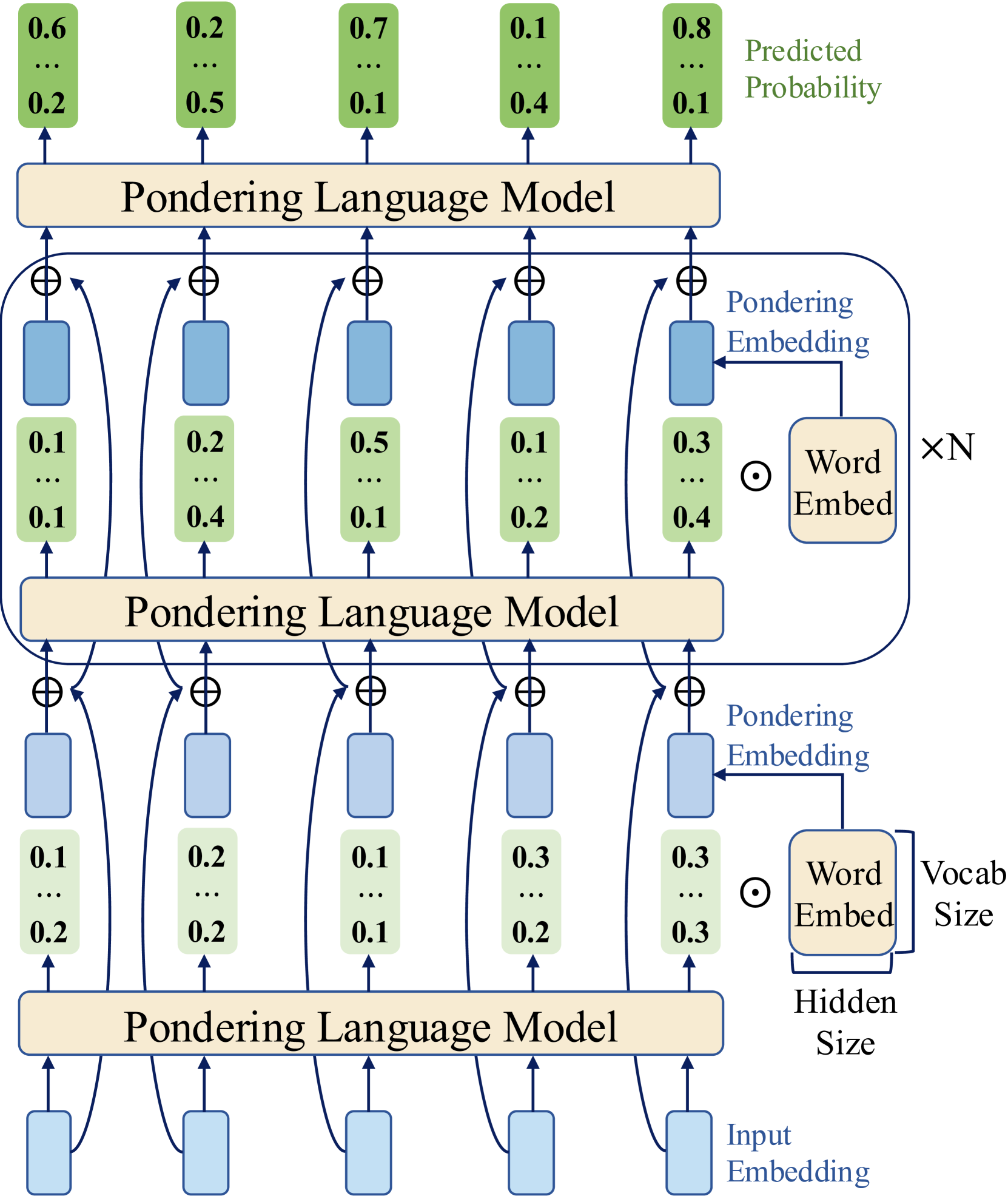
Figure 1: Overview of the Pondering Language Model. Given input token embeddings, the base LM produces a probability distribution over the vocabulary, which is used to compute a continuous “pondering embedding” via a weighted sum of all token embeddings. This embedding is then added residually to the original input embeddings and fed back into the LM. By repeating this process for $k$ steps within a single token prediction, the model iteratively refines its output distributions. The pseudocode on the right illustrates the implementation details.
## 2 Pondering Language Model
In this section, we introduce our proposed Pondering Language Model (Figure 1), which integrates a pondering mechanism into language models via pretraining. Given that pretraining fundamentally constitutes a language modeling task, we briefly review this task before detailing our proposed model.
Language Modeling. Given a sequence of tokens $X=[x_1,x_2,\dots,x_n]$ , the primary objective of language modeling is typically to maximize the likelihood of predicting each token based on its preceding tokens. Formally, this is expressed through the joint probability factorization:
$$
P(x_1,x_2,\dots,x_n)=∏_t=1^nP(x_t\mid x_<t) \tag{1}
$$
Current language models first map tokens to input embeddings $E^0=[e^0_1,e^0_2,\dots,e^0_n]$ , where each embedding $e^0_i∈ℝ^d$ is selected from a vocabulary embedding matrix $V=[e_1,e_2,\dots,e_|V|]$ , with vocabulary size $|V|$ and hidden dimension $d$ . The language model then generates output probabilities $P$ for predicting the next token at each position:
$$
P=LM(E^0), P∈ℝ^n×|V| \tag{2}
$$
The cross-entropy loss is computed directly from these predicted probabilities $P$ to pretrain the language model.
Pondering Mechanism. In our proposed method, instead of directly using the predicted output probabilities $P$ to compute the cross-entropy loss, we utilize these probabilities as weights to sum embeddings of all candidate tokens, forming what we call a "pondering embedding". Given the probability distribution $p∈ℝ^|V|$ at each position, the pondering embedding $t$ is:
$$
t=∑_i=1^|V|p_ie_i, p_i∈ℝ,
e_i∈ℝ^d \tag{3}
$$
For computational efficiency, pondering embeddings $t$ for all positions can be calculated simultaneously via matrix multiplication In practice, we use only the top-K tokens with highest probabilities at each position to compute the pondering embedding, reducing complexity from $O(n|V|d)$ to $O(nKd)$ . With $K=100\ll|V|$ , this does not degrade LM performance and makes the matrix multiplication overhead negligible within the overall LM computations. :
$$
T=PV, T∈ℝ^n× d \tag{4}
$$
Through these pondering embeddings, we effectively map predicted probabilities back into the embedding space, preserving embedding information from all possible candidate tokens. To maintain the information from the original input embeddings, we integrate the pondering embeddings using a residual connection:
$$
E^1=E^0+T=[e^0_1+t_1,
e^0_2+t_2,\dots,e^0_n+t_n] \tag{5}
$$
We then feed the updated embeddings $E^1$ back into the same language model to obtain refined output probabilities:
$$
P^1=LM(E^1), P^1∈ℝ^n
×|V| \tag{6}
$$
After obtaining $P^1$ , we can iteratively repeat the previous process to achieve multi-step pondering. Specifically, given a predefined number of pondering steps $k$ Unless otherwise specified, we set $k=3$ for subsequent experiments., we iteratively compute new pondering embeddings and integrate them with the original input embeddings using residual connections, feeding the result back into the same language model until $k$ steps are reached:
$$
\displaystyleE^0 \displaystyle=[e^0_1,e^0_2,\dots,e^0_n]
, P^0=LM(E^0), T^1=P^
{0}V \displaystyleE^1 \displaystyle=E^0+T^1=[e^0_1+t^1
_1,e^0_2+t^1_2,\dots,e^0_n+t
^1_n], P^1=LM(E^1), T^2=
P^1V \displaystyle\dots \displaystyleE^k \displaystyle=E^0+∑_i=1^kT^i=[e^0_1+
t^1_1+\dots+t^k_1,\dots,e^0_n+t
^1_n+\dots+t^k_n], P^k=LM(E^
k) \tag{7}
$$
This iterative pondering mechanism progressively refines the model’s predictions. Finally, we can use the refined output probabilities $P^k$ after $k$ pondering steps to compute the cross-entropy loss and optimize the language model to perform $k$ -step pondering.
## 3 Experiments
Our experiments consist of four parts. First, we validate the scaling curves of pondering models on widely used GPT-2 and LLaMA architectures. Second, we perform large-scale pretraining of PonderingPythia models on the Pile dataset and compare their scaling curves and language modeling capabilities with those of the official Pythia suite (Biderman et al., 2023). Third, we evaluate the downstream task performance of PonderingPythia models, including nine popular general tasks and an instruction-following task, and compare the results with official Pythia, OPT (Zhang et al., 2022), Bloom (Le Scao et al., 2023), GPT-Neo (Black et al., 2021), and TinyLLaMA (Zhang et al., 2024) models. Finally, we investigate the impact of the number of pondering steps on pretraining perplexity.
### 3.1 Small Scale Validation on GPT-2 and LLaMA
We apply our proposed method to two popular Transformer architectures, GPT-2 and LLaMA, to investigate its general applicability and effectiveness. Specifically, we plot and compare scaling curves between vanilla GPT-2, vanilla LLaMA, and their corresponding pondering versions, referred to as PonderingGPT and PonderingLLaMA, respectively.
Experimental Settings. We train all models from scratch on a subset of the Pile dataset with the same tokenizer. The model sizes range from 405M to 1.4B parameters, with a context length fixed at 2048 tokens. The number of training tokens for each model is chosen to approximately match the scaling laws proposed by Chinchilla (Hoffmann et al., 2022b).
The detailed configurations of the models, including sizes, learning rates, and batch sizes, are specified in Table 1. These hyperparameters primarily follow the GPT-3 specifications (Brown et al., 2020). However, unlike GPT-3, we untie the input and output embedding matrices.
Table 1: Model sizes and hyperparameters for scaling experiments.
| params | $n_layers$ | $d_model$ | $n_heads$ | learning rate | batch size (in tokens) | tokens |
| --- | --- | --- | --- | --- | --- | --- |
| 405M | 24 | 1024 | 16 | 3e-4 | 0.5M | 7B |
| 834M | 24 | 1536 | 24 | 2.5e-4 | 0.5M | 15B |
| 1.4B | 24 | 2048 | 32 | 2e-4 | 0.5M | 26B |
<details>
<summary>x2.png Details</summary>
### Visual Description
## Line Chart with Subplot: Model Loss Comparison Across Scales
### Overview
The image displays a two-part chart comparing the performance (measured in "Loss") of different large language model architectures across three increasing model scales. The top subplot shows the absolute loss values for six model variants, while the bottom subplot shows the difference in loss (ΔLoss) between specific pairs of models. The chart includes fitted trend lines and annotations indicating performance multipliers.
### Components/Axes
**Main Chart (Top Subplot):**
* **Y-axis:** Label is "Loss". Scale ranges from approximately 2.05 to 2.65, with major ticks at 2.1, 2.2, 2.3, 2.4, 2.5, and 2.6.
* **X-axis:** Shared with the bottom subplot. Three categorical points are labeled: "405M*7B", "834M*15B", and "1.4B*26B". These likely represent model scale combinations (e.g., parameter counts).
* **Legend (Top-Right Corner):** Contains six entries:
1. `GPT fitted` (Blue, dashed line)
2. `LLaMA fitted` (Green, dashed line)
3. `GPT` (Blue, solid line with circle markers)
4. `LLaMA` (Green, solid line with circle markers)
5. `Pondering GPT` (Blue, solid line with star markers)
6. `Pondering LLaMA` (Green, solid line with star markers)
* **Annotations:** Two horizontal arrows with text are present in the main chart:
* A blue arrow pointing from the `GPT` line to the `Pondering GPT` line at the "834M*15B" scale, labeled "2.01x".
* A green arrow pointing from the `LLaMA` line to the `Pondering LLaMA` line at the "834M*15B" scale, labeled "2.26x".
**Subplot (Bottom):**
* **Y-axis:** Label is "ΔLoss". Scale ranges from 0.00 to 0.15, with major ticks at 0.05, 0.10, and 0.15.
* **X-axis:** Same as main chart.
* **Legend (Bottom-Left Corner):** Contains three entries:
1. `L_GPT - L_LLaMA` (Black, dashed line with upward-pointing triangle markers)
2. `L_GPT - L_PonderingGPT` (Blue, solid line with upward-pointing triangle markers)
3. `L_LLaMA - L_PonderingLLaMA` (Green, solid line with upward-pointing triangle markers)
### Detailed Analysis
**Main Chart - Loss Trends:**
All six data series show a clear downward trend as model scale increases from left to right ("405M*7B" to "1.4B*26B").
1. **GPT Series (Blue):**
* `GPT` (solid, circles): Starts at ~2.61 (405M*7B), decreases to ~2.34 (834M*15B), and ends at ~2.20 (1.4B*26B).
* `GPT fitted` (dashed): Closely follows the `GPT` line, suggesting a good fit.
* `Pondering GPT` (solid, stars): Consistently lower than standard `GPT`. Starts at ~2.48, decreases to ~2.25, ends at ~2.10.
2. **LLaMA Series (Green):**
* `LLaMA` (solid, circles): Starts at ~2.55, decreases to ~2.31, ends at ~2.18.
* `LLaMA fitted` (dashed): Closely follows the `LLaMA` line.
* `Pondering LLaMA` (solid, stars): Consistently lower than standard `LLaMA`. Starts at ~2.45, decreases to ~2.21, ends at ~2.08.
**Key Relationship:** At every scale, the "Pondering" variant of a model has a lower loss than its standard counterpart. The green lines (`LLaMA` family) are generally slightly lower than their blue (`GPT` family) counterparts at the same scale and variant.
**Subplot - ΔLoss Trends:**
1. `L_GPT - L_LLaMA` (Black dashed): Positive value, decreasing from ~0.065 to ~0.02. This indicates the loss gap between standard GPT and LLaMA narrows as scale increases.
2. `L_GPT - L_PonderingGPT` (Blue solid): Positive value, relatively stable around 0.10-0.13. This is the consistent loss reduction gained by applying "Pondering" to GPT.
3. `L_LLaMA - L_PonderingLLaMA` (Green solid): Positive value, relatively stable around 0.10. This is the consistent loss reduction gained by applying "Pondering" to LLaMA.
### Key Observations
1. **Universal Scaling Law:** Loss decreases monotonically with increased model scale for all architectures shown.
2. **"Pondering" Efficacy:** The "Pondering" technique provides a consistent and significant reduction in loss for both GPT and LLaMA architectures across all scales. The annotations suggest this translates to a ~2x to 2.26x improvement at the middle scale.
3. **Architecture Comparison:** The standard LLaMA model consistently outperforms (has lower loss than) the standard GPT model at equivalent scales, though the gap narrows with scale.
4. **Fitted Lines:** The dashed "fitted" lines for GPT and LLaMA closely track their respective solid lines, indicating the fitted model is a good representation of the observed data trend.
### Interpretation
This chart demonstrates two key findings in large language model research:
1. **Predictable Scaling:** Model performance, as measured by loss, improves predictably as computational scale (a product of parameters and likely data/training compute) increases. This supports the concept of scaling laws.
2. **Architectural Innovation Value:** The "Pondering" modification represents a significant architectural or training improvement. It provides a consistent performance boost *on top of* the gains from simply scaling up the base model. The fact that the ΔLoss for "Pondering" (blue and green lines in the subplot) remains relatively flat across scales suggests this improvement is robust and scales well—it doesn't diminish as models get larger.
The narrowing gap between standard GPT and LLaMA (`L_GPT - L_LLaMA`) could imply that architectural differences become less critical at very large scales, or that the specific GPT variant tested here scales slightly more efficiently than the LLaMA variant within this range. The "Pondering" technique appears to be a more impactful intervention than the choice between these two base architectures at these scales.
</details>
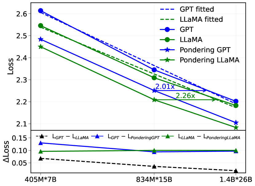
Figure 2: (top) Scaling curves of GPT3 LLaMA and their corresponding pondering models. (bottom) Relative improvements of RoPE + RMSNorm + SwiGLU MLP and Pondering.
Results. Figure 2 (top) illustrates the scaling curves of the validation loss on the Pile subset for vanilla GPT-2, vanilla LLaMA, and their pondering counterparts. Our results show that incorporating pondering significantly improves the performance for both GPT-2 and LLaMA across the entire size range tested (405M to 1.4B parameters). For instance, by fitting scaling curves, we find that PonderingGPT-834M achieves a loss comparable to a vanilla GPT-2 model trained with approximately $2.01×$ parameters $*$ tokens, while PonderingLLaMA-834M matches the loss of vanilla LLaMA trained with roughly $2.26×$ parameters $*$ tokens.
Furthermore, Figure 2 (bottom) shows the relative validation loss improvements (denoted as $Δ$ loss) of architectural modifications inherent in LLaMA—namely rotary positional embeddings (RoPE) (Su et al., 2024), RMSNorm (Zhang & Sennrich, 2019), and SwiGLU activation—in comparison to GPT-2, alongside the relative improvements obtained by our pondering method for both architectures. We observe that while the relative improvement due to RoPE, RMSNorm, and SwiGLU MLP diminishes as model size and data scale increase (reaching approximately 0.02 for the 1.4B parameter model), the relative improvement provided by pondering consistently remains around 0.1 across the entire tested scale.
<details>
<summary>x3.png Details</summary>
### Visual Description
## Line Chart: Loss vs. Model Size Comparison
### Overview
The image is a line chart comparing the performance (measured by Loss) of two language model families, "Pythia" and "PonderingPythia," across different model sizes. The chart demonstrates that PonderingPythia consistently achieves a lower loss than the standard Pythia model for a given number of parameters, suggesting greater parameter efficiency.
### Components/Axes
* **Chart Type:** Line chart with data points.
* **X-Axis:** Labeled "#Parameters (log scale)". It uses a logarithmic scale with major tick marks at 200M, 500M, 1B, 2B, 3B, and 7B (where M = Million, B = Billion).
* **Y-Axis:** Labeled "Loss". It uses a linear scale ranging from 1.8 to 2.5, with increments of 0.1.
* **Legend:** Located in the top-right corner of the chart area. It contains four entries:
* A blue line labeled "Pythia"
* A green line labeled "PonderingPythia"
* A blue dot labeled "Pythia"
* A green dot labeled "PonderingPythia"
* **Annotation:** A purple text label "37% params" with a left-pointing arrow is positioned near the bottom-right, between the 3B and 7B data points.
### Detailed Analysis
**Data Series & Trends:**
1. **Pythia (Blue Line & Dots):** The trend line slopes downward from left to right, indicating that loss decreases as the number of parameters increases.
* Data Points (Approximate):
* At ~200M params: Loss ≈ 2.53
* At ~500M params: Loss ≈ 2.18
* At ~1B params: Loss ≈ 2.06
* At ~1.5B params: Loss ≈ 1.98
* At ~3B params: Loss ≈ 1.89
* At ~7B params: Loss ≈ 1.84
2. **PonderingPythia (Green Line & Dots):** This trend line also slopes downward and is positioned consistently below the Pythia line, indicating lower loss at each comparable model size.
* Data Points (Approximate):
* At ~200M params: Loss ≈ 2.30
* At ~500M params: Loss ≈ 2.10
* At ~1B params: Loss ≈ 1.97
* At ~1.5B params: Loss ≈ 1.92
* At ~3B params: Loss ≈ 1.83
* At ~7B params: Loss ≈ 1.84 (This point converges with the Pythia point).
**Annotation Analysis:** The purple annotation "37% params" with a leftward arrow is placed between the 3B and 7B marks on the x-axis. The arrow points from the 7B region back towards the 3B region. This visually suggests that the PonderingPythia model at 3B parameters achieves a loss performance (≈1.83) comparable to the standard Pythia model at 7B parameters (≈1.84), using only about 37% of the parameters (3B / 7B ≈ 0.428, or ~43%; the "37%" may refer to a more precise calculation or a different baseline).
### Key Observations
1. **Consistent Efficiency Gap:** The green PonderingPythia line is below the blue Pythia line at every measured point except the final 7B convergence, demonstrating a consistent reduction in loss for the same model size.
2. **Diminishing Returns:** Both curves show a flattening slope as model size increases, illustrating the principle of diminishing returns in scaling laws—doubling parameters yields a smaller improvement in loss at larger scales.
3. **Performance Convergence:** At the largest measured size (7B parameters), the loss values for both model types converge to approximately 1.84.
4. **Parameter Efficiency Claim:** The annotation explicitly highlights the core finding: PonderingPythia can match the performance of a much larger Pythia model with significantly fewer parameters.
### Interpretation
This chart presents evidence for a more parameter-efficient model architecture ("PonderingPythia"). The data suggests that the modifications in PonderingPythia allow it to achieve better performance (lower loss) at smaller scales. The most significant insight is the claimed 37% parameter efficiency at the high-performance end, meaning one could potentially train a PonderingPythia model to the same loss level as a Pythia model while using roughly one-third of the parameters, leading to substantial savings in computational cost, memory, and energy.
From a Peircean investigative perspective, the chart provides the *iconic* representation (the lines and points) and the *indexical* link (the annotation arrow) to support an *abductive* inference: the observed superior performance of PonderingPythia is likely due to an architectural innovation that improves learning efficiency per parameter. The convergence at 7B might indicate a fundamental limit or that the efficiency advantage is most pronounced in the mid-range of model sizes tested.
</details>
<details>
<summary>x4.png Details</summary>
### Visual Description
\n
## Line Chart: Loss vs. Training Tokens for Two Language Models
### Overview
This image is a line chart comparing the training loss of two language models, "Pythia-1B" and "PonderingPythia-1B," as a function of the number of training tokens. The chart demonstrates that the "PonderingPythia-1B" model achieves a lower loss at every measured point and requires significantly fewer training tokens to reach a specific loss value compared to the baseline "Pythia-1B" model.
### Components/Axes
* **Chart Type:** Line chart with data points marked by circular markers.
* **Y-Axis:**
* **Label:** "Loss"
* **Scale:** Linear, ranging from 1.95 to 2.25, with major ticks at 0.05 intervals.
* **X-Axis:**
* **Label:** "#Training tokens (log scale)"
* **Scale:** Logarithmic. Major labeled ticks are at 60B, 100B, 200B, and 280B (where "B" denotes billions).
* **Legend:** Located in the top-right corner of the plot area.
* **Blue line with blue circle markers:** "Pythia-1B"
* **Green line with green circle markers:** "PonderingPythia-1B"
* **Annotation:** A purple text label and arrow.
* **Text:** "41% training tokens"
* **Placement & Function:** The text is positioned in the center-left area of the plot. A purple arrow originates from the text and points to a specific data point on the green "PonderingPythia-1B" line. This point corresponds to a loss value of approximately 2.05.
### Detailed Analysis
**Data Series 1: Pythia-1B (Blue Line)**
* **Trend:** The line shows a consistent, nearly linear downward slope on this log-linear plot, indicating that loss decreases as the number of training tokens increases.
* **Approximate Data Points (Loss vs. Tokens):**
* 60B tokens: ~2.21
* ~80B tokens: ~2.18
* 100B tokens: ~2.16
* ~120B tokens: ~2.14
* ~140B tokens: ~2.125
* ~160B tokens: ~2.11
* ~180B tokens: ~2.10
* 200B tokens: ~2.08
* ~220B tokens: ~2.07
* ~240B tokens: ~2.06
* ~260B tokens: ~2.055
* 280B tokens: ~2.05
**Data Series 2: PonderingPythia-1B (Green Line)**
* **Trend:** This line also shows a consistent downward slope, parallel to but strictly below the blue line, indicating superior performance (lower loss) at all training stages.
* **Approximate Data Points (Loss vs. Tokens):**
* 60B tokens: ~2.125
* ~80B tokens: ~2.09
* 100B tokens: ~2.07
* ~120B tokens: ~2.05 (This is the point indicated by the purple annotation arrow).
* ~140B tokens: ~2.04
* ~160B tokens: ~2.025
* ~180B tokens: ~2.01
* 200B tokens: ~2.00
* ~220B tokens: ~1.99
* ~240B tokens: ~1.98
* ~260B tokens: ~1.975
* 280B tokens: ~1.97
**Annotation Analysis:**
The annotation "41% training tokens" highlights a key comparison. The green line (PonderingPythia-1B) reaches a loss of ~2.05 at approximately 120B tokens. The blue line (Pythia-1B) reaches the same loss level of ~2.05 at approximately 280B tokens. The annotation asserts that 120B is 41% of 280B (120/280 ≈ 0.428, close to 41%), meaning the Pondering model achieves this performance milestone with less than half the training data.
### Key Observations
1. **Consistent Performance Gap:** The green line is uniformly below the blue line. The vertical gap between them appears relatively constant across the log-scale x-axis, suggesting a consistent relative improvement.
2. **Parallel Trajectories:** The slopes of the two lines are very similar, indicating that both models learn at a comparable rate relative to the logarithm of training data, but PonderingPythia-1B starts from and maintains a better loss value.
3. **Efficiency Highlight:** The central message, emphasized by the annotation, is the training efficiency of PonderingPythia-1B. It reaches a target loss (2.05) with a dramatically smaller dataset.
### Interpretation
This chart provides strong empirical evidence for the effectiveness of the "Pondering" modification to the Pythia-1B architecture. The data suggests that PonderingPythia-1B is not only a better-performing model at any given training compute budget (lower loss for the same tokens) but is also significantly more **data-efficient**.
The key takeaway is the 41% figure. In the context of large language model training, where data and compute are primary cost drivers, achieving the same loss with 59% fewer tokens represents a major efficiency gain. This could translate to reduced training time, lower computational cost, or the ability to achieve better performance with the same budget. The chart implies that the "Pondering" mechanism allows the model to extract more learning signal from each token, leading to faster convergence in terms of data consumption. The parallel slopes suggest the fundamental scaling law behavior is preserved, but the modification provides a constant multiplicative improvement in efficiency.
</details>
<details>
<summary>x5.png Details</summary>
### Visual Description
## Line Chart: Loss vs. Computational Cost (FLOPs) for Two Language Models
### Overview
This image is a line chart comparing the performance of two language models, "Vanilla Pythia-70M" and "PonderingPythia-70M," by plotting their loss against computational cost measured in ExaFLOPs (EFLOPs). The chart demonstrates how the loss metric decreases for both models as the computational budget increases, with one model consistently outperforming the other.
### Components/Axes
* **Chart Type:** Line chart with markers.
* **Y-Axis (Vertical):**
* **Label:** "Loss"
* **Scale:** Linear, ranging from approximately 2.55 to 2.80.
* **Major Ticks:** 2.55, 2.60, 2.65, 2.70, 2.75.
* **X-Axis (Horizontal):**
* **Label:** "FLOPs (EFLOPs)"
* **Scale:** Linear, ranging from approximately 50 to 450 EFLOPs.
* **Major Ticks:** 100, 200, 300, 400.
* **Legend:**
* **Position:** Top-right corner of the chart area.
* **Entry 1:** A blue line with circular markers labeled "Vanilla Pythia-70M".
* **Entry 2:** A green line with circular markers labeled "PonderingPythia-70M".
### Detailed Analysis
**Data Series 1: Vanilla Pythia-70M (Blue Line)**
* **Trend Verification:** The blue line shows a steady, monotonic downward slope from left to right, indicating that loss decreases as computational cost (FLOPs) increases.
* **Data Points (Approximate):**
* At ~50 EFLOPs: Loss ≈ 2.78
* At ~130 EFLOPs: Loss ≈ 2.76
* At ~200 EFLOPs: Loss ≈ 2.75
* At ~270 EFLOPs: Loss ≈ 2.74
* At ~340 EFLOPs: Loss ≈ 2.73
* At ~410 EFLOPs: Loss ≈ 2.72
* At ~450 EFLOPs: Loss ≈ 2.72
**Data Series 2: PonderingPythia-70M (Green Line)**
* **Trend Verification:** The green line also shows a consistent downward slope, starting at a lower loss value than the blue line and maintaining a lower loss throughout the plotted range.
* **Data Points (Approximate):**
* At ~50 EFLOPs: Loss ≈ 2.67
* At ~130 EFLOPs: Loss ≈ 2.62
* At ~200 EFLOPs: Loss ≈ 2.60
* At ~270 EFLOPs: Loss ≈ 2.58
* At ~340 EFLOPs: Loss ≈ 2.57
* At ~410 EFLOPs: Loss ≈ 2.55
* At ~450 EFLOPs: Loss ≈ 2.54
### Key Observations
1. **Performance Gap:** The "PonderingPythia-70M" model (green) achieves a consistently lower loss than the "Vanilla Pythia-70M" model (blue) at every comparable computational cost point.
2. **Scaling Behavior:** Both models exhibit a diminishing returns pattern; the rate of loss improvement slows as FLOPs increase (the curves flatten slightly).
3. **Relative Improvement:** The absolute gap in loss between the two models appears to widen slightly as computational cost increases. At ~50 EFLOPs, the gap is ~0.11. At ~450 EFLOPs, the gap is ~0.18.
4. **No Outliers:** Both data series follow smooth, predictable trajectories without anomalous spikes or dips.
### Interpretation
The chart provides a direct comparison of computational efficiency between two variants of a 70-million-parameter language model. The core finding is that the "PonderingPythia" modification yields a significant and consistent improvement in model performance (lower loss) for any given amount of computational expenditure (FLOPs).
This suggests that the "Pondering" technique likely introduces a more efficient architecture or training methodology, allowing the model to extract more performance per unit of compute. The widening gap at higher FLOPs could indicate that this efficiency advantage scales well, making the modified model particularly beneficial for large-scale training runs where computational cost is a primary constraint. The data strongly advocates for the use of the "PonderingPythia" approach over the "Vanilla" version when optimizing for the loss-compute trade-off.
</details>
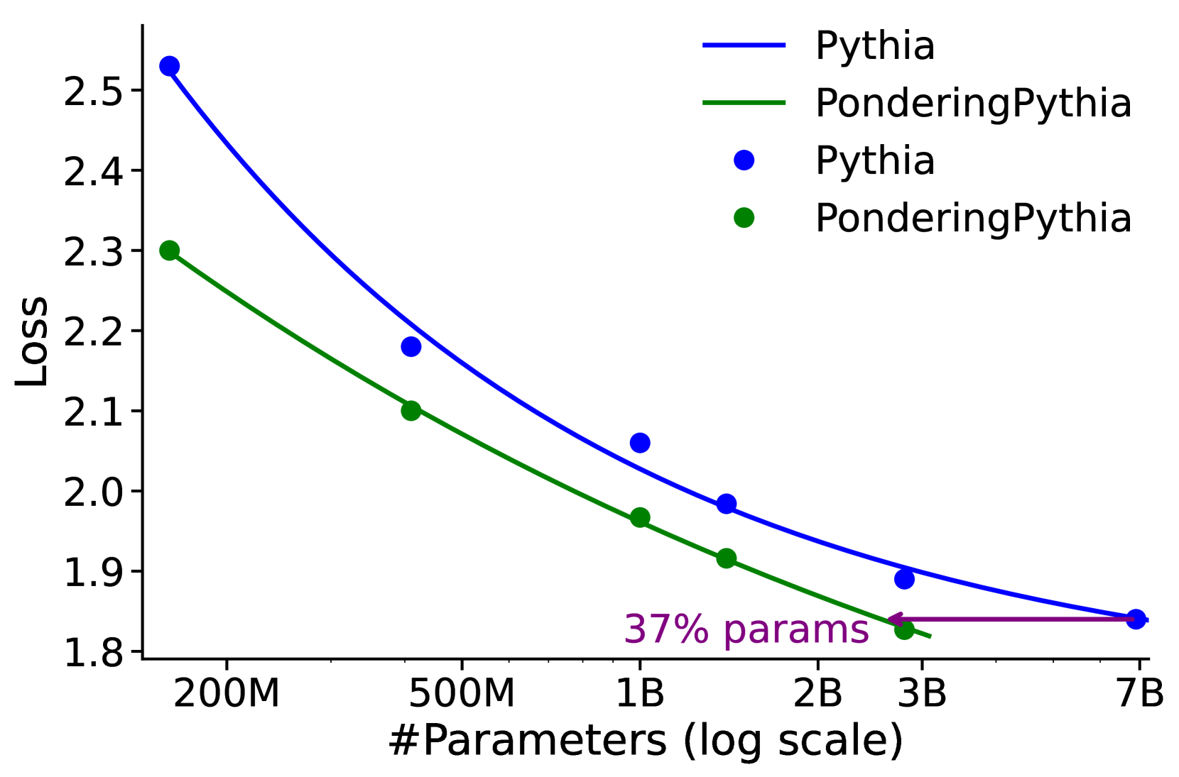
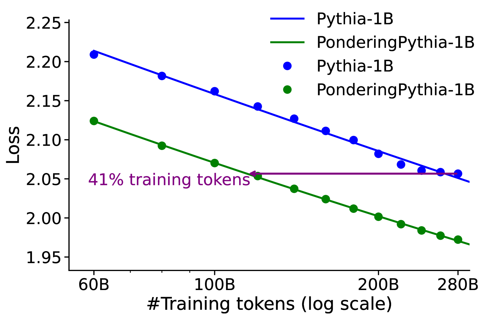
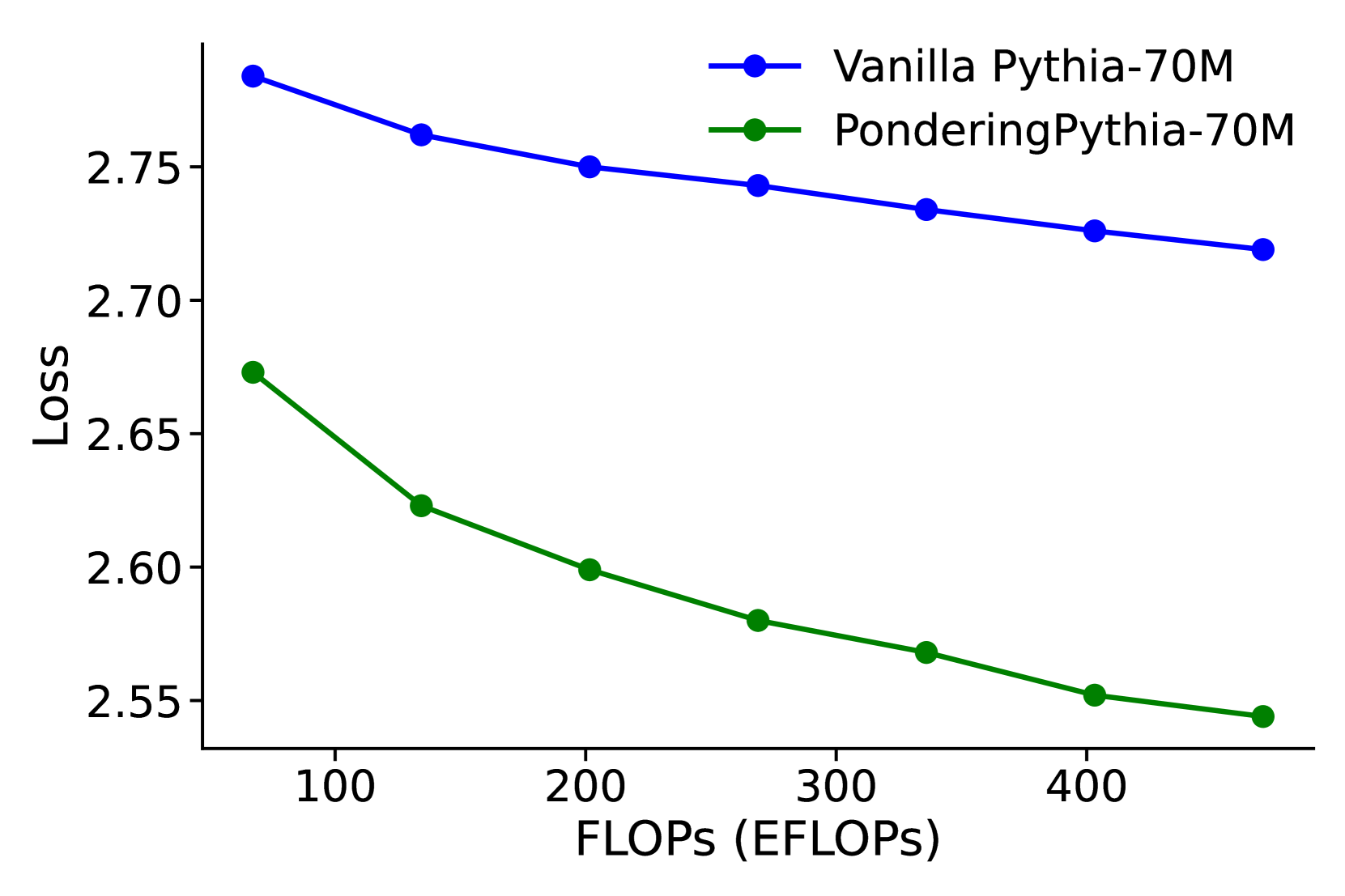
Figure 3: Language modeling loss when scaling parameter count and training tokens. PonderingPythia achieves comparable performance to the official Pythia-6.9B while using only 37% of the parameters, and matches the performance of the official Pythia-1B with just 41% of the training tokens.
Table 2: Language Modeling Perplexity (ppl). Lower is better. The values in parentheses indicate the improvement ( $↓$ ) compared to the corresponding Pythia model. For simplicity, we refer to PonderingPythia as Ponder.
| Model | Pile | Wikitext | Lambada Openai | Lambada Standard |
| --- | --- | --- | --- | --- |
| Pythia-70M | $18.36$ | $57.03$ | $141.94$ | $967.72$ |
| Ponder-70M | $12.68$ ( $↓$ 5.68) | $34.07$ ( $↓$ 22.96) | $39.19$ ( $↓$ 102.75) | $145.51$ ( $↓$ 822.21) |
| Pythia-160M | $12.55$ | $33.43$ | $38.15$ | $186.51$ |
| Ponder-160M | $9.87$ ( $↓$ 2.68) | $23.69$ ( $↓$ 9.74) | $15.96$ ( $↓$ 22.19) | $41.24$ ( $↓$ 145.27) |
| Pythia-410M | $8.85$ | $20.11$ | $10.86$ | $31.54$ |
| Ponder-410M | $8.15$ ( $↓$ 0.70) | $17.78$ ( $↓$ 2.33) | $8.55$ ( $↓$ 2.31) | $17.48$ ( $↓$ 14.06) |
| Pythia-1B | $7.85$ | $16.45$ | $7.91$ | $17.41$ |
| Ponder-1B | $7.15$ ( $↓$ 0.70) | $14.61$ ( $↓$ 1.84) | $6.02$ ( $↓$ 1.89) | $10.64$ ( $↓$ 6.77) |
| Pythia-1.4B | $7.24$ | $14.72$ | $6.08$ | $10.87$ |
| Ponder-1.4B | $6.82$ ( $↓$ 0.42) | $13.59$ ( $↓$ 1.13) | $5.37$ ( $↓$ 0.71) | $8.88$ ( $↓$ 1.99) |
| Pythia-2.8B | $6.63$ | $12.69$ | $5.04$ | $8.23$ |
| Ponder-2.8B | $6.21$ ( $↓$ 0.42) | $11.74$ ( $↓$ 0.95) | $4.15$ ( $↓$ 0.89) | $6.17$ ( $↓$ 2.06) |
| Pythia-6.9B | $6.29$ | $11.41$ | $4.45$ | $6.95$ |
### 3.2 Large-Scale Pretraining on Pile
We further validate the effectiveness of our pondering method by conducting large-scale pretraining experiments on the entire Pile dataset (300B tokens) (Gao et al., 2020). We train a new model, named PonderingPythia, from scratch using exactly the same architectural components (parallel attention and MLP layers, rotary embeddings with 1/4 head dimensions), same tokenizer and training hyperparameters (optimizer settings, learning rate schedule, batch size, and context length) as the original Pythia models. We then compare PonderingPythia models’ scaling curves and language modeling capabilities with the official Pythia model suite.
#### 3.2.1 Scaling Curves
We plot the PonderingPythia and official Pythia model’s scaling curves along parameters size, training tokens and training flops. As depicted in Figure 3 (left), the fitted curves show that a 2.5B-parameter PonderingPythia model achieves a validation loss comparable to the 6.9B-parameter official Pythia model, while requiring only 37% of the parameters. In Figure 3 (middle), we evaluated the 1B PonderingPythia and official Pythia models at intervals of 20B training tokens. The fitted curves indicate that PonderingPythia trained with 115B tokens achieves performance comparable to the official Pythia model trained with 280B tokens, consuming only 41% of the training tokens. In Figure 3 (right), we report the language modeling loss of vanilla Pythia-70M To match the training FLOPs of vanilla Pythia-70M with PonderingPythia-70M, we trained the vanilla model for 4 epochs. and PonderingPythia-70M under the same computational budget during pretraining. It can be observed that PonderingPythia-70M consistently outperforms vanilla Pythia-70M when trained with the same number of FLOPs.
#### 3.2.2 Language Modeling Ability Evaluation
We measure the perplexity on several language modeling datasets to reflect general language modeling capabilities. Specifically, we report perplexity scores on the Pile validation set, Wikitext, and the Lambada dataset (both OpenAI and standard versions), detailed in Table 2. The results demonstrate significant perplexity improvements across all datasets and model sizes. Notably, the perplexity achieved by the PonderingPythia-2.8B model is even better than that of the official Pythia-6.8B model, which is nearly 2.5 times larger.
### 3.3 Downstream Tasks Evaluation
We use the PonderingPythia models pretrained in the previous subsection to conduct downstream task evaluations.
<details>
<summary>x6.png Details</summary>
### Visual Description
## Radar Chart: Model Performance Comparison
### Overview
This image is a radar chart (spider plot) comparing the performance of two AI language models across eight distinct capability categories. The chart visually represents the relative strengths and weaknesses of each model on a common scale.
### Components/Axes
* **Chart Type:** Radar Chart.
* **Categories (Axes):** Eight axes radiate from the center, each representing a skill domain. Clockwise from the top:
1. Writing
2. Roleplay
3. Reasoning
4. Math
5. Coding
6. Extraction
7. STEM
8. Humanities
* **Scale:** A radial scale from the center (0) to the outer edge (3), with concentric circles marking intervals of 0.5 (0, 0.5, 1, 1.5, 2, 2.5, 3).
* **Legend:** Located at the bottom center of the chart.
* **Blue Line:** Labeled "Pythia-1B, avg score=1.89"
* **Green Line:** Labeled "PonderingPythia-1B, avg score=2.22"
### Detailed Analysis
The performance of each model is plotted as a polygon connecting its score on each axis. Values are approximate visual estimates.
**1. Pythia-1B (Blue Line, Avg Score: 1.89)**
* **Trend:** The blue polygon forms a relatively balanced, slightly irregular octagon, indicating moderate performance across most categories with no extreme peaks or valleys.
* **Approximate Scores per Category:**
* Writing: ~2.0
* Roleplay: ~1.8
* Reasoning: ~1.5
* Math: ~1.3
* Coding: ~1.4
* Extraction: ~1.6
* STEM: ~2.0
* Humanities: ~1.9
**2. PonderingPythia-1B (Green Line, Avg Score: 2.22)**
* **Trend:** The green polygon is more expansive and irregular, showing significantly higher performance in several categories, particularly on the left and top sides of the chart.
* **Approximate Scores per Category:**
* Writing: ~2.8 (Highest point on the chart)
* Roleplay: ~2.3
* Reasoning: ~1.6
* Math: ~1.4
* Coding: ~1.5
* Extraction: ~2.4
* STEM: ~2.7
* Humanities: ~2.4
### Key Observations
1. **Consistent Superiority:** The green line (PonderingPythia-1B) encloses the blue line (Pythia-1B) on every single axis, indicating it scores higher in all eight categories.
2. **Largest Gains:** The most substantial performance improvements for PonderingPythia-1B are in **Writing** (+0.8), **STEM** (+0.7), **Extraction** (+0.8), and **Humanities** (+0.5).
3. **Smallest Gains:** The smallest improvements are in **Reasoning** (+0.1), **Math** (+0.1), and **Coding** (+0.1). These categories represent the lowest scores for both models.
4. **Performance Profile:** Pythia-1B's strongest areas are Writing and STEM (~2.0). PonderingPythia-1B's profile is dominated by Writing (~2.8), followed by STEM and Extraction (~2.4-2.7).
5. **Overall Average:** The legend confirms the visual impression, with PonderingPythia-1B having a higher average score (2.22 vs. 1.89).
### Interpretation
This chart demonstrates the efficacy of the "Pondering" modification applied to the base Pythia-1B model. The data suggests that this modification leads to a broad and significant enhancement of capabilities across a diverse set of language model evaluation tasks.
* **Nature of Improvement:** The gains are not uniform. The modification appears particularly effective for tasks involving **generative and interpretive skills** (Writing, Roleplay, Humanities) and **structured information handling** (Extraction, STEM). This could imply the "pondering" mechanism improves coherence, depth of generation, or information synthesis.
* **Persistent Challenges:** Both models show their weakest performance in **formal reasoning and logic-based tasks** (Reasoning, Math, Coding). The minimal improvement in these areas suggests the modification does not fundamentally address the core challenges these tasks present for this model architecture or scale (1B parameters).
* **Strategic Implication:** For applications prioritizing creative writing, content extraction, or STEM explanation, PonderingPythia-1B offers a clear advantage. For tasks requiring rigorous mathematical proof or complex code generation, the advantage is marginal, and other model types or sizes might be necessary.
* **Underlying Mechanism:** The name "PonderingPythia" and the performance profile hint that the modification may involve a form of iterative refinement, extended internal processing, or a chain-of-thought-like mechanism that benefits tasks where "thinking before answering" is advantageous, but offers less help for tasks where the solution path is more deterministic or requires specialized symbolic reasoning skills not enhanced by the pondering process.
</details>
<details>
<summary>x7.png Details</summary>
### Visual Description
\n
## Radar Chart: AI Model Performance Comparison
### Overview
This image is a radar chart (spider plot) comparing the performance of two AI language models across eight distinct capability categories. The chart visualizes how each model scores on a radial scale, allowing for a direct comparison of their strengths and weaknesses.
### Components/Axes
* **Chart Type:** Radar Chart (Spider Plot)
* **Categories (Axes):** Eight axes radiate from the center, each representing a capability domain. Listed clockwise from the top:
1. Writing
2. Roleplay
3. Reasoning
4. Math
5. Coding
6. Extraction
7. STEM
8. Humanities
* **Radial Scale:** Concentric circles represent the scoring scale, marked from the center (0) outward to the edge (3.5). Major grid lines are at intervals of 0.5 (0, 0.5, 1, 1.5, 2, 2.5, 3, 3.5).
* **Legend:** Located at the bottom center of the chart.
* **Blue Line:** `Pythia-1.4B, avg score=2.2`
* **Green Line:** `PonderingPythia-1.4B, avg score=2.75`
### Detailed Analysis
**Data Series 1: Pythia-1.4B (Blue Line)**
* **Visual Trend:** The blue polygon is generally contained within the green one, indicating lower overall performance. Its shape is somewhat irregular, with a pronounced peak in the Reasoning category.
* **Approximate Data Points (Category: Score):**
* Writing: ~2.0
* Roleplay: ~2.3
* Reasoning: ~2.5 (This is its highest point)
* Math: ~2.0
* Coding: ~1.5
* Extraction: ~1.8
* STEM: ~2.2
* Humanities: ~2.0
**Data Series 2: PonderingPythia-1.4B (Green Line)**
* **Visual Trend:** The green polygon encompasses a larger area than the blue one, indicating superior overall performance (as confirmed by the higher average score). It shows strong, broad performance in creative and humanities-related tasks.
* **Approximate Data Points (Category: Score):**
* Writing: ~3.0
* Roleplay: ~3.0
* Reasoning: ~2.4 (Slightly lower than Pythia-1.4B)
* Math: ~2.1
* Coding: ~1.7
* Extraction: ~2.3
* STEM: ~2.8
* Humanities: ~3.0
### Key Observations
1. **Performance Gap:** PonderingPythia-1.4B (avg 2.75) demonstrates a clear and consistent performance advantage over Pythia-1.4B (avg 2.2) in 7 out of 8 categories.
2. **Category Strengths:** PonderingPythia excels most in **Writing**, **Roleplay**, and **Humanities**, scoring at or near the 3.0 mark. Pythia's strongest category is **Reasoning**.
3. **Notable Anomaly:** The **Reasoning** axis is the only category where Pythia-1.4B (blue) appears to score marginally higher than PonderingPythia-1.4B (green).
4. **Shared Weakness:** Both models show their lowest performance in the **Coding** and **Extraction** categories, with scores below 2.0 for Pythia and below 2.5 for PonderingPythia.
5. **Spatial Relationship:** The green line is positioned outside the blue line for nearly the entire chart, visually reinforcing its superior average performance. The lines converge and nearly intersect at the Reasoning axis.
### Interpretation
The data suggests that the "Pondering" enhancement applied to the base Pythia-1.4B model yields significant improvements across a wide range of capabilities, particularly in tasks involving creativity, language nuance, and broad knowledge (Writing, Roleplay, Humanities, STEM). This indicates the modification successfully boosts general language understanding and generation.
However, the enhancement does not uniformly improve all skills. The near-parity and slight reversal in the **Reasoning** category is a critical finding. It implies that the "pondering" mechanism might introduce a trade-off, potentially optimizing for breadth or fluency at a minor cost to pure logical or deductive reasoning speed or accuracy. The persistent relative weakness in **Coding** and **Extraction** for both models points to a fundamental challenge in these structured, precise tasks that the "pondering" modification does not fully address.
In summary, the chart illustrates a successful model enhancement that creates a more capable and well-rounded AI, with the interesting caveat that gains in creative and knowledge-based domains may come with a negligible to slight cost in focused reasoning tasks. The visualization effectively argues for the value of the "Pondering" approach while also highlighting specific areas for future investigation and improvement.
</details>
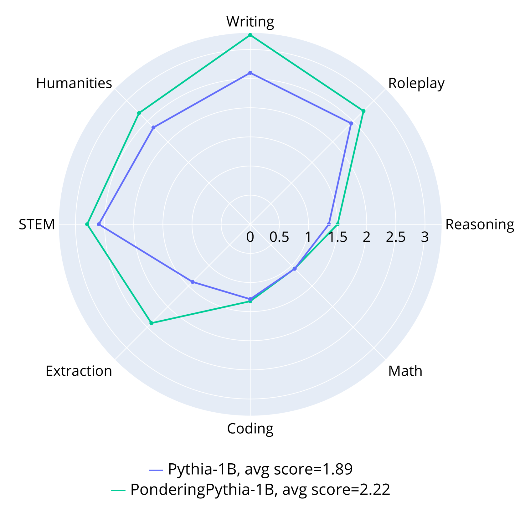
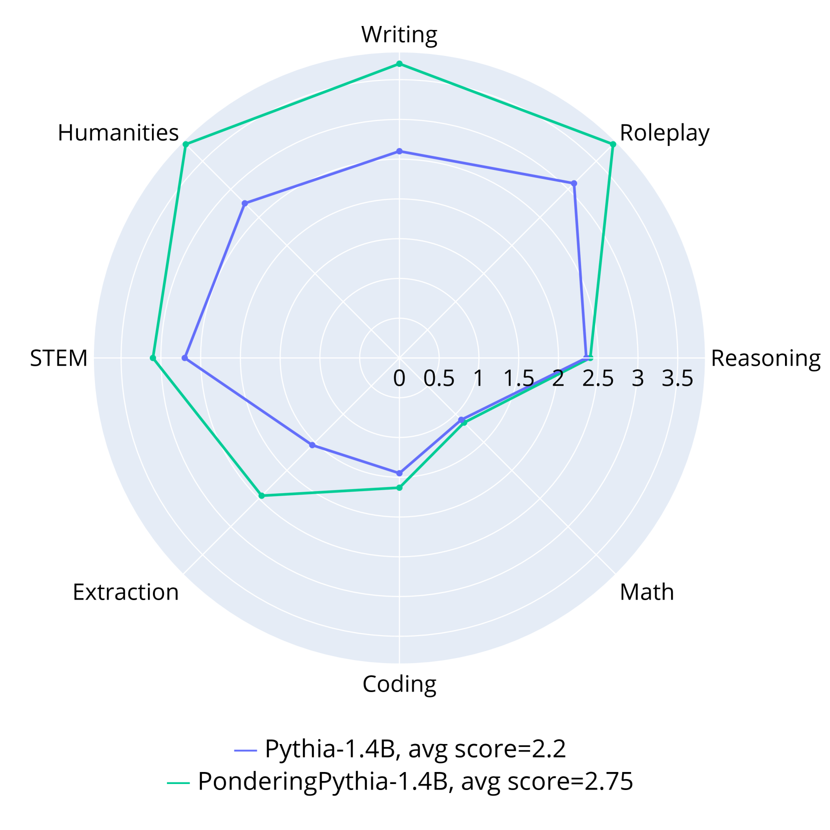
Figure 4: Instruction-following abilities evaluated on MT-Bench. PonderingPythia-1B and 1.4B consistently outperform their corresponding official Pythia models across all subtasks.
#### 3.3.1 General Downstream Tasks
We consider various widely-used benchmarks, including the tasks originally used by Pythia (LAMBADA (Paperno et al., 2016), PIQA (Bisk et al., 2020), WinoGrande (Sakaguchi et al., 2021), ARC-Easy and ARC-Challenge (Clark et al., 2018), SciQ (Welbl et al., 2017). Additionally, we include HellaSwag (Zellers et al., 2019) for commonsense reasoning and RACE (Lai et al., 2017) for reading comprehension.
We evaluate both zero-shot and five-shot learning performance using the LM evaluation harness (Gao et al., 2023). Detailed results are shown in Table 3. Across all evaluated model sizes, PonderingPythia consistently and significantly outperforms the official Pythia models, as well as comparable OPT, GPT-Neo, and Bloom models. Remarkably, with only 1/10 of the training data (300B tokens) and fewer parameters (1B vs. 1.1B), our PonderingPythia-1B achieves results comparable to, or even surpassing, TinyLlama—which uses a more advanced LLaMA architecture and 3T tokens. PonderingPythia-2.8B also surpasses Pythia-6.9B, which is nearly 2.5 times its size.
Table 3: Five-shot and zero-shot evaluations on downstream NLP tasks. All pretrained model weights used for comparison are obtained from their official repositories. We refer to PonderingPythia as Ponder for simplicity. $Δ$ acc is compared to the official Pythia models.
| Model (#training tokens) | Lambada OpenAI | ARC -E | Lambada Standard | ARC -C | Wino Grande | PIQA | Hella Swag | SciQ | RACE | Avg acc / $Δ$ acc $↑$ |
| --- | --- | --- | --- | --- | --- | --- | --- | --- | --- | --- |
| 5-shot | | | | | | | | | | |
| Pythia-70M (300B) | 11.9 | 36.7 | 9.2 | 17.1 | 50.5 | 58.7 | 26.7 | 57.8 | 25.1 | 32.6 |
| Ponder-70M (300B) | 28.4 | 44.6 | 21.1 | 18.6 | 52.2 | 62.4 | 28.4 | 75.7 | 26.9 | 39.8 / +7.2 |
| Pythia-160M (300B) | 24.9 | 44.7 | 19.0 | 18.4 | 50.4 | 63.5 | 28.6 | 76.4 | 27.8 | 39.3 |
| OPT-125M (300B) | 29.8 | 42.3 | 26.4 | 19.7 | 51.3 | 63.4 | 29.0 | 78.8 | 30.1 | 41.2 |
| GPTneo-125M (300B) | 29.3 | 43.9 | 23.0 | 19.1 | 51.9 | 63.9 | 28.5 | 79.9 | 27.9 | 40.8 |
| Ponder-160M (300B) | 39.9 | 50.1 | 31.2 | 22.1 | 51.2 | 65.8 | 31.9 | 85.4 | 30.1 | 45.3 / +6.0 |
| Pythia-410M (300B) | 43.9 | 54.7 | 32.8 | 22.3 | 53.4 | 68.0 | 33.8 | 88.9 | 30.4 | 47.6 |
| OPT-350M (300B) | 38.3 | 45.4 | 32.1 | 20.5 | 53.0 | 65.8 | 31.9 | 85.7 | 29.5 | 44.7 |
| Bloom-560M (366B) | 29.4 | 50.2 | 29.7 | 21.9 | 52.7 | 64.2 | 31.4 | 88.0 | 30.0 | 44.2 |
| Ponder-410M (300B) | 48.9 | 58.7 | 43.7 | 26.1 | 54.0 | 70.5 | 37.3 | 91.0 | 32.4 | 51.4 /+3.8 |
| Pythia-1B (300B) | 48.3 | 58.6 | 35.8 | 25.4 | 52.8 | 71.3 | 37.7 | 91.6 | 31.7 | 50.4 |
| OPT-1.3B (300B) | 54.0 | 60.4 | 49.0 | 26.9 | 56.9 | 72.4 | 38.5 | 91.8 | 35.4 | 52.7 |
| GPTneo-1.3B (300B) | 49.9 | 59.9 | 44.5 | 25.9 | 56.6 | 71.6 | 38.6 | 86.1 | 34.5 | 51.9 |
| Bloom-1.1B (366B) | 36.3 | 54.9 | 37.4 | 24.9 | 53.4 | 67.6 | 34.8 | 88.7 | 33.0 | 47.9 |
| Ponder-1B (300B) | 57.7 | 63.2 | 52.5 | 28.6 | 58.6 | 73.3 | 41.9 | 93.4 | 36.3 | 56.2 / +5.8 |
| Pythia-1.4B (300B) | 54.5 | 63.1 | 44.5 | 28.8 | 57.1 | 71.0 | 40.5 | 92.4 | 34.6 | 54.1 |
| Bloom-1.7B (366B) | 42.5 | 58.8 | 41.5 | 26.2 | 57.7 | 68.7 | 37.6 | 91.9 | 33.5 | 50.9 |
| Ponder-1.4B (300B) | 59.2 | 67.5 | 49.9 | 32.4 | 60.4 | 73.5 | 44.2 | 94.3 | 37.1 | 57.6 / +3.5 |
| Tinyllama-1.1B (3T) | 53.8 | 64.8 | 45.0 | 31.1 | 59.4 | 73.8 | 44.9 | 94.0 | 36.4 | 55.9 |
| OPT-2.7B (300B) | 60.2 | 64.7 | 55.0 | 29.8 | 62.2 | 75.1 | 46.1 | 93.0 | 37.5 | 58.2 |
| GPTneo-2.7B (300B) | 56.0 | 64.0 | 51.6 | 30.1 | 59.6 | 73.9 | 42.4 | 93.3 | 35.5 | 56.3 |
| Bloom-3B (366B) | 46.2 | 63.8 | 47.1 | 31.7 | 57.8 | 70.8 | 41.4 | 93.4 | 34.6 | 54.1 |
| Pythia-2.8B (300B) | 59.0 | 67.0 | 50.7 | 31.0 | 61.1 | 74.4 | 45.3 | 93.7 | 35.9 | 57.6 |
| Pythia-6.9B (300B) | 62.5 | 69.6 | 54.8 | 35.6 | 62.9 | 76.6 | 48.0 | 94.6 | 36.7 | 60.1 |
| Ponder-2.8B (300B) | 64.2 | 70.6 | 58.7 | 35.8 | 65.3 | 76.7 | 49.0 | 94.3 | 39.0 | 61.5 / +3.9 |
| 0-shot | | | | | | | | | | |
| Pythia-70M (300B) | 18.7 | 36.7 | 13.5 | 18.8 | 51.1 | 59.9 | 26.6 | 59.9 | 23.9 | 34.3 |
| Ponder-70M (300B) | 33.5 | 42.5 | 24.1 | 19.1 | 51.1 | 61.5 | 28.3 | 70.3 | 27.8 | 39.8 / +5.5 |
| Pythia-160M (300B) | 33.0 | 43.8 | 21.4 | 18.9 | 52.0 | 62.2 | 28.4 | 73.7 | 27.9 | 40.1 |
| OPT-125M (300B) | 37.9 | 43.5 | 29.0 | 19.0 | 50.3 | 62.8 | 29.2 | 75.2 | 30.1 | 41.9 |
| GPTneo-125M (300B) | 37.5 | 43.9 | 26.0 | 19.1 | 50.4 | 63.0 | 28.7 | 76.5 | 27.5 | 41.4 |
| Ponder-160M (300B) | 44.3 | 46.8 | 33.8 | 20.5 | 52.3 | 63.9 | 31.9 | 76.8 | 29.6 | 44.4 / +4.3 |
| Pythia-410M (300B) | 51.4 | 52.2 | 36.4 | 21.4 | 53.8 | 66.9 | 33.7 | 81.5 | 30.9 | 47.6 |
| OPT-350M (300B) | 45.2 | 44.0 | 35.8 | 20.7 | 52.3 | 64.5 | 32.0 | 74.9 | 29.8 | 44.4 |
| Bloom-560M (366B) | 34.3 | 47.5 | 33.3 | 22.4 | 51.5 | 63.8 | 31.5 | 80.3 | 30.5 | 43.9 |
| Ponder-410M (300B) | 56.9 | 51.9 | 45.3 | 22.6 | 56.0 | 68.7 | 37.0 | 81.4 | 33.8 | 50.4 / +2.8 |
| Pythia-1B (300B) | 55.9 | 56.8 | 42.0 | 24.2 | 52.5 | 70.5 | 37.7 | 83.3 | 32.7 | 50.6 |
| OPT-1.3B (300B) | 57.9 | 57.1 | 52.5 | 23.4 | 59.7 | 71.8 | 41.6 | 84.3 | 34.3 | 53.6 |
| GPTneo-1.3B (300B) | 57.1 | 56.2 | 45.3 | 23.2 | 55.0 | 71.2 | 38.6 | 86.1 | 34.5 | 51.9 |
| Bloom-1.1B (366B) | 42.6 | 51.5 | 42.9 | 23.6 | 54.9 | 67.3 | 34.5 | 83.6 | 32.6 | 48.2 |
| Ponder-1B (300B) | 62.3 | 60.5 | 51.9 | 27.0 | 56.5 | 72.2 | 41.8 | 87.4 | 35.4 | 55.0 / +4.4 |
| Pythia-1.4B (300B) | 61.6 | 60.4 | 49.7 | 25.9 | 57.5 | 70.8 | 40.4 | 86.4 | 34.1 | 54.1 |
| Bloom-1.7B (366B) | 46.2 | 56.4 | 44.5 | 23.7 | 56.8 | 68.5 | 37.5 | 85.0 | 33.2 | 50.2 |
| Ponder-1.4B (300B) | 65.2 | 62.0 | 53.8 | 27.0 | 60.1 | 72.6 | 44.0 | 89.0 | 35.2 | 56.5 / +2.4 |
| Tinyllama-1.1B (3T) | 58.8 | 60.3 | 49.3 | 28.0 | 59.0 | 73.3 | 45.0 | 88.9 | 36.4 | 55.4 |
| OPT-2.7B (300B) | 63.5 | 60.8 | 56.0 | 26.8 | 61.2 | 73.8 | 45.9 | 85.8 | 36.2 | 56.7 |
| GPTneo-2.7B (300B) | 62.1 | 61.2 | 51.6 | 27.5 | 57.8 | 72.3 | 42.7 | 89.3 | 35.1 | 55.5 |
| Bloom-3B (366B) | 51.7 | 59.4 | 50.9 | 28.0 | 58.7 | 70.8 | 41.4 | 88.8 | 35.2 | 53.9 |
| Pythia-2.8B (300B) | 64.6 | 64.4 | 54.3 | 29.5 | 60.2 | 73.8 | 45.4 | 88.5 | 34.9 | 57.3 |
| Pythia-6.9B (300B) | 67.2 | 67.3 | 55.9 | 31.4 | 61.0 | 75.2 | 48.1 | 89.3 | 36.9 | 59.1 |
| Ponder-2.8B (300B) | 68.9 | 66.5 | 60.8 | 32.5 | 63.6 | 75.0 | 48.6 | 91.0 | 36.5 | 60.4 / +3.1 |
#### 3.3.2 Instruction-following Ability Evaluation
To assess the instruction-following capability of our model, we further fine-tuned PonderingPythia-1B and 1.4B, as well as the corresponding official Pythia models, on the Alpaca dataset using the same settings (Taori et al., 2023). The fine-tuned models were evaluated with MT-Bench (Zheng et al., 2023), a popular multi-turn question benchmark. The experimental results are shown in Figure 4. As illustrated, both PonderingPythia-1B and 1.4B consistently outperform their official Pythia counterparts across all subtasks, achieving average improvements of 0.33 and 0.55, respectively. The marginal gains on Coding and Math tasks may be attributed to the limited coding and mathematical abilities of the Pythia models.
<details>
<summary>x8.png Details</summary>
### Visual Description
## Line Chart: Loss vs. Pondering Steps
### Overview
The image displays a line chart plotting a metric called "Loss" against "Pondering Steps." The chart demonstrates a clear inverse relationship: as the number of pondering steps increases, the loss value decreases. The data is presented as a single series connected by a green line with circular markers at each data point.
### Components/Axes
* **Y-Axis (Vertical):**
* **Label:** "Loss"
* **Scale:** Linear scale ranging from approximately 2.58 to 2.72.
* **Major Tick Marks:** 2.58, 2.60, 2.62, 2.64, 2.66, 2.68, 2.70, 2.72.
* **X-Axis (Horizontal):**
* **Label:** "Pondering Steps (0 = Baseline)"
* **Scale:** Discrete, non-linear scale with markers at specific step values.
* **Data Point Labels (X-values):** 0, 1, 3, 5, 10.
* **Data Series:**
* **Visual Representation:** A solid green line connecting filled green circular markers.
* **Legend:** No separate legend is present; the single series is defined by the axis labels.
### Detailed Analysis
The chart plots five distinct data points. The trend is consistently downward, indicating that loss decreases with more pondering steps. The rate of decrease is not constant; it is steepest initially and gradually flattens.
**Data Point Extraction (Approximate Values):**
| Pondering Steps | Loss (Approx.) |
| :-------------- | :------------- |
| 0 (Baseline) | 2.715 |
| 1 | 2.680 |
| 3 | 2.635 |
| 5 | 2.615 |
| 10 | 2.595 |
**Trend Verification:**
* The green line slopes downward from left to right across the entire chart.
* The slope is steepest between steps 0 and 1 (a drop of ~0.035).
* The slope becomes progressively less steep between subsequent points:
* From step 1 to 3: drop of ~0.045 over 2 steps.
* From step 3 to 5: drop of ~0.020 over 2 steps.
* From step 5 to 10: drop of ~0.020 over 5 steps.
### Key Observations
1. **Monotonic Decrease:** The loss value decreases at every measured increment of pondering steps. There are no increases or plateaus in the plotted data.
2. **Diminishing Returns:** The most significant reduction in loss occurs with the first pondering step. Each subsequent increase in steps yields a smaller absolute reduction in loss. The curve appears to be approaching an asymptote.
3. **Baseline Performance:** The "0 = Baseline" condition has the highest loss, establishing it as the reference point for improvement.
4. **Non-Linear X-Axis:** The x-axis does not have a uniform scale. The physical distance between 0 and 1 is similar to that between 1 and 3, despite representing different numerical intervals. This emphasizes the discrete nature of the tested step values.
### Interpretation
This chart likely visualizes the performance of a machine learning or computational model that employs an iterative "pondering" or reasoning process. The "Loss" is a standard metric where lower values indicate better performance (e.g., prediction error, cost function value).
The data suggests a strong positive effect of introducing a pondering mechanism: moving from the baseline (0 steps) to just 1 step provides a substantial performance boost. However, the principle of diminishing returns is clearly in effect. While increasing the computational budget (more steps) continues to improve performance, the marginal benefit per additional step decreases significantly. This presents a classic trade-off between computational cost (time/resources for more steps) and performance gain. The optimal number of steps would depend on the specific constraints and requirements of the application, balancing the need for low loss against the cost of additional computation. The chart provides the empirical data necessary to make that cost-benefit analysis.
</details>
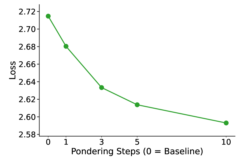
Figure 5: Increasing the number of pondering steps consistently reduces loss on the Pile validation set.
### 3.4 Impact of Pondering Steps
To further investigate the effect of pondering steps on model performance, we trained several 160M-parameter Pythia models from scratch with different numbers of pondering steps: 0 (baseline), 1, 3, 5, and 10. These models were pretrained on a 30B-token subset of the Pile dataset. The results, presented in Figure 5, clearly show that increasing the number of pondering steps consistently reduces the language modeling loss on the Pile validation set. This demonstrates the significant potential and scalability of our method, suggesting that model performance can be further improved by increasing the depth of pondering steps.
## 4 Limitations and Future Work
### 4.1 Limitations
There are two limitations to our work. Firstly, due to computational constraints, we only scaled our method up to a 2.8B-parameter model trained on 300B tokens from the Pile dataset. It would be interesting to extend our approach to larger models and larger-scale datasets in the future. Secondly, although our results demonstrate that the proposed method scales better than vanilla models under the same training FLOPs (Figure 3), it also introduces additional inference overhead (increasing roughly linearly with the number of pondering steps), similar to test-time scaling methods.
### 4.2 Future Work
There are several promising directions for future work. Firstly, our proposed method is not limited to decoder-only architectures or language modeling; it has the potential to be applied to a wide range of model types and domains. For example, it could be adapted to state-space models such as Mamba (Gu & Dao, 2023), encoder models, or RWKV (Peng et al., 2023), as well as extended to other areas. Another promising direction is the introduction of token-adaptive pondering, which may significantly reduce computation and further enhance our method. It would also be interesting to investigate the interpretability of the pondering process, such as how the model "thinks" during pondering, the semantics of the pondering embedding, and whether the model learns to reflect on its predictions through pondering. Finally, exploring the combination of our method with orthogonal approaches such as CoT and other test-time scaling methods could also be an interesting direction.
## 5 Related Work
### 5.1 Test-Time Compute Scaling
Scaling test-time computation has emerged as an influential approach, providing an effective alternative to merely increasing model parameters (Snell et al., 2024). Current methods for enhancing test-time computation primarily fall into two categories: parallel scaling and sequential scaling (Zeng et al., 2024; Muennighoff et al., 2025).
Parallel scaling methods involve generating multiple candidate solutions simultaneously and selecting the best solution based on certain evaluation criteria. Prominent examples of this paradigm include Best-of-N search (Cobbe et al., 2021; Sun et al., 2024; Gui et al., 2024; Amini et al., 2024; Sessa et al., 2024) and Majority Vote (Wang et al., 2022). The primary difference among these parallel approaches lies in their strategy for selecting the optimal outcome. Nevertheless, parallel scaling approaches often encounter difficulty accurately identifying the best candidate solution among multiple generated possibilities (Stroebl et al., 2024; Hassid et al., 2024).
Sequential scaling methods, conversely, focus on progressively refining the model’s reasoning through multiple iterative steps. Representative methods include CoT (Wei et al., 2022; Nye et al., 2021), iterative rethinking and revision (Huang et al., 2022; Min et al., 2024; Madaan et al., 2024; Wang et al., 2024b, b; Lee et al., 2025; Hou et al., 2025; Muennighoff et al., 2025; Li et al., 2025). Following the emergence of powerful OpenAI o1 and DeepSeek R1, leveraging extensive chain-of-thought prompting to scale test-time computation has become increasingly popular. Nonetheless, existing methods often come with limitations, including reliance on specially curated datasets (Allen-Zhu & Li, 2023), extended context windows (Zhu et al., 2025), and complex reinforcement learning strategies (Pang et al., 2025). In contrast, our method effectively circumvents these limitations.
### 5.2 Latent Thinking in Language Models
Latent thinking in LMs typically refers to the hidden computational processes within transformer architectures (Yang et al., 2024; Biran et al., 2024). Prior works exploring latent thinking can generally be divided into two categories based on their implementation methods:
Adding Additional Tokens: Wang et al. (2024a) proposed predicting a planning token as a discrete latent variable prior to generating reasoning steps. Similarly, Pfau et al. (2024) investigated filler tokens (e.g., “…”) and found them effective for parallelizable problems, although they also highlighted limitations compared to CoT methods, potentially constraining scalability to more complex reasoning tasks. Zhou et al. (2024) pretrained models by randomly inserting a learnable token into the training corpus, demonstrating improvements across various tasks. Furthermore, Quiet-STaR employs reinforcement learning to train models to generate intermediate rationales at each token, thereby enhancing reasoning capabilities (Zelikman et al., 2024).
Reusing Hidden States: Early Universal Transformers (Csordás et al., ) reused hidden states through a transition network, aiming to enhance the encoder-decoder transformer architecture toward Turing completeness. A more recent method (Geiping et al., 2025) iterates over multiple layers of a language model to refine intermediate hidden states, treating this process as a form of latent thinking. Giannou et al. (2023) proposed looped transformer, recycling output hidden states back into input embeddings for algorithmic tasks. Similarly, Hao et al. (2024) fine-tuned models to reason directly within continuous latent spaces, using final hidden states as embeddings to achieve reasoning without explicit CoT. In contrast, our method relies on pondering embeddings derived from the predicted probabilities of LMs.
## 6 Conclusion
In this paper, we introduce the pondering process into language models through solely self-supervised learning. Pondering LM can be naturally learned through pretraining on large-scale general corpora. Our extensive experiments across three widely adopted architectures—GPT-2, Pythia, and LLaMA—highlight the effectiveness and generality of our proposed method. Notably, our PonderingPythia consistently outperforms the official Pythia model on language modeling tasks, scaling curves, downstream tasks, and instruction-following abilities when pretrained on the large-scale Pile dataset. As increasing the number of pondering steps further improves language model performance, we posit that our approach introduces a promising new dimension along which language model capabilities can be scaled.
## References
- Allen-Zhu & Li (2023) Allen-Zhu, Z. and Li, Y. Physics of language models: Part 3.2, knowledge manipulation. arXiv preprint arXiv:2309.14402, 2023.
- Allen-Zhu & Li (2024) Allen-Zhu, Z. and Li, Y. Physics of language models: Part 3.3, knowledge capacity scaling laws. arXiv preprint arXiv:2404.05405, 2024.
- Amini et al. (2024) Amini, A., Vieira, T., Ash, E., and Cotterell, R. Variational best-of-n alignment. arXiv preprint arXiv:2407.06057, 2024.
- Biderman et al. (2023) Biderman, S., Schoelkopf, H., Anthony, Q. G., Bradley, H., O’Brien, K., Hallahan, E., Khan, M. A., Purohit, S., Prashanth, U. S., Raff, E., et al. Pythia: A suite for analyzing large language models across training and scaling. In International Conference on Machine Learning, pp. 2397–2430. PMLR, 2023.
- Biran et al. (2024) Biran, E., Gottesman, D., Yang, S., Geva, M., and Globerson, A. Hopping too late: Exploring the limitations of large language models on multi-hop queries. arXiv preprint arXiv:2406.12775, 2024.
- Bisk et al. (2020) Bisk, Y., Zellers, R., Gao, J., Choi, Y., et al. Piqa: Reasoning about physical commonsense in natural language. In Proceedings of the AAAI conference on artificial intelligence, volume 34, pp. 7432–7439, 2020.
- Black et al. (2021) Black, S., Gao, L., Wang, P., Leahy, C., and Biderman, S. GPT-Neo: Large Scale Autoregressive Language Modeling with Mesh-Tensorflow, March 2021. URL https://doi.org/10.5281/zenodo.5297715. If you use this software, please cite it using these metadata.
- Brown et al. (2020) Brown, T., Mann, B., Ryder, N., Subbiah, M., Kaplan, J. D., Dhariwal, P., Neelakantan, A., Shyam, P., Sastry, G., Askell, A., et al. Language models are few-shot learners. Advances in neural information processing systems, 33:1877–1901, 2020.
- Clark et al. (2018) Clark, P., Cowhey, I., Etzioni, O., Khot, T., Sabharwal, A., Schoenick, C., and Tafjord, O. Think you have solved question answering? try arc, the ai2 reasoning challenge. arXiv preprint arXiv:1803.05457, 2018.
- Cobbe et al. (2021) Cobbe, K., Kosaraju, V., Bavarian, M., Chen, M., Jun, H., Kaiser, L., Plappert, M., Tworek, J., Hilton, J., Nakano, R., et al. Training verifiers to solve math word problems, 2021. URL https://arxiv. org/abs/2110.14168, 9, 2021.
- (11) Csordás, R., Irie, K., Schmidhuber, J., Potts, C., and Manning, C. D. Moeut: Mixture-of-experts universal transformers. In The Thirty-eighth Annual Conference on Neural Information Processing Systems.
- DeepSeek-AI et al. (2025) DeepSeek-AI, Guo, D., Yang, D., and et al., H. Z. Deepseek-r1: Incentivizing reasoning capability in llms via reinforcement learning. 2025. URL https://arxiv.org/abs/2501.12948.
- Fedorenko et al. (2024) Fedorenko, E., Piantadosi, S. T., and Gibson, E. A. Language is primarily a tool for communication rather than thought. Nature, 630(8017):575–586, 2024.
- Gao et al. (2020) Gao, L., Biderman, S., Black, S., Golding, L., Hoppe, T., Foster, C., Phang, J., He, H., Thite, A., Nabeshima, N., et al. The pile: An 800gb dataset of diverse text for language modeling. arXiv preprint arXiv:2101.00027, 2020.
- Gao et al. (2023) Gao, L., Tow, J., Abbasi, B., Biderman, S., Black, S., DiPofi, A., Foster, C., Golding, L., Hsu, J., Le Noac’h, A., Li, H., McDonell, K., Muennighoff, N., Ociepa, C., Phang, J., Reynolds, L., Schoelkopf, H., Skowron, A., Sutawika, L., Tang, E., Thite, A., Wang, B., Wang, K., and Zou, A. A framework for few-shot language model evaluation, 12 2023. URL https://zenodo.org/records/10256836.
- Geiping et al. (2025) Geiping, J., McLeish, S., Jain, N., Kirchenbauer, J., Singh, S., Bartoldson, B. R., Kailkhura, B., Bhatele, A., and Goldstein, T. Scaling up test-time compute with latent reasoning: A recurrent depth approach. arXiv preprint arXiv:2502.05171, 2025.
- Giannou et al. (2023) Giannou, A., Rajput, S., Sohn, J.-y., Lee, K., Lee, J. D., and Papailiopoulos, D. Looped transformers as programmable computers. In International Conference on Machine Learning, pp. 11398–11442. PMLR, 2023.
- Gu & Dao (2023) Gu, A. and Dao, T. Mamba: Linear-time sequence modeling with selective state spaces. arXiv preprint arXiv:2312.00752, 2023.
- Gui et al. (2024) Gui, L., Gârbacea, C., and Veitch, V. Bonbon alignment for large language models and the sweetness of best-of-n sampling. arXiv preprint arXiv:2406.00832, 2024.
- Hackenburg et al. (2025) Hackenburg, K., Tappin, B. M., Röttger, P., Hale, S. A., Bright, J., and Margetts, H. Scaling language model size yields diminishing returns for single-message political persuasion. Proceedings of the National Academy of Sciences, 122(10):e2413443122, 2025.
- Hao et al. (2024) Hao, S., Sukhbaatar, S., Su, D., Li, X., Hu, Z., Weston, J., and Tian, Y. Training large language models to reason in a continuous latent space. arXiv preprint arXiv:2412.06769, 2024.
- Hassid et al. (2024) Hassid, M., Remez, T., Gehring, J., Schwartz, R., and Adi, Y. The larger the better? improved llm code-generation via budget reallocation. arXiv preprint arXiv:2404.00725, 2024.
- Hoffmann et al. (2022a) Hoffmann, J., Borgeaud, S., Mensch, A., Buchatskaya, E., Cai, T., Rutherford, E., Casas, D. d. L., Hendricks, L. A., Welbl, J., Clark, A., et al. Training compute-optimal large language models. arXiv preprint arXiv:2203.15556, 2022a.
- Hoffmann et al. (2022b) Hoffmann, J., Borgeaud, S., Mensch, A., Buchatskaya, E., Cai, T., Rutherford, E., de Las Casas, D., Hendricks, L. A., Welbl, J., Clark, A., et al. An empirical analysis of compute-optimal large language model training. Advances in Neural Information Processing Systems, 35:30016–30030, 2022b.
- Hou et al. (2025) Hou, Z., Lv, X., Lu, R., Zhang, J., Li, Y., Yao, Z., Li, J., Tang, J., and Dong, Y. Advancing language model reasoning through reinforcement learning and inference scaling. arXiv preprint arXiv:2501.11651, 2025.
- Huang et al. (2022) Huang, J., Gu, S. S., Hou, L., Wu, Y., Wang, X., Yu, H., and Han, J. Large language models can self-improve. arXiv preprint arXiv:2210.11610, 2022.
- Jaech et al. (2024) Jaech, A., Kalai, A., Lerer, A., Richardson, A., El-Kishky, A., Low, A., Helyar, A., Madry, A., Beutel, A., Carney, A., et al. Openai o1 system card. arXiv preprint arXiv:2412.16720, 2024.
- Kaplan et al. (2020) Kaplan, J., McCandlish, S., Henighan, T., Brown, T. B., Chess, B., Child, R., Gray, S., Radford, A., Wu, J., and Amodei, D. Scaling laws for neural language models. arXiv preprint arXiv:2001.08361, 2020.
- Lai et al. (2017) Lai, G., Xie, Q., Liu, H., Yang, Y., and Hovy, E. Race: Large-scale reading comprehension dataset from examinations. arXiv preprint arXiv:1704.04683, 2017.
- Le Scao et al. (2023) Le Scao, T., Fan, A., Akiki, C., Pavlick, E., Ilić, S., Hesslow, D., Castagné, R., Luccioni, A. S., Yvon, F., Gallé, M., et al. Bloom: A 176b-parameter open-access multilingual language model. 2023.
- Lee et al. (2025) Lee, K.-H., Fischer, I., Wu, Y.-H., Marwood, D., Baluja, S., Schuurmans, D., and Chen, X. Evolving deeper llm thinking. arXiv preprint arXiv:2501.09891, 2025.
- Li et al. (2025) Li, D., Cao, S., Griggs, T., Liu, S., Mo, X., Patil, S. G., Zaharia, M., Gonzalez, J. E., and Stoica, I. Llms can easily learn to reason from demonstrations structure, not content, is what matters! arXiv preprint arXiv:2502.07374, 2025.
- Li et al. (2023) Li, L. H., Hessel, J., Yu, Y., Ren, X., Chang, K.-W., and Choi, Y. Symbolic chain-of-thought distillation: Small models can also "think" step-by-step. In Proceedings of the 61st Annual Meeting of the Association for Computational Linguistics (Volume 1: Long Papers), pp. 2665–2679, Toronto, Canada, jul 2023. Association for Computational Linguistics.
- Li et al. (2024) Li, W., Liu, X., Li, Y., Jin, Y., Tian, H., Zhong, Z., Liu, G., Zhang, Y., and Chen, K. Understanding communication characteristics of distributed training. In Proceedings of the 8th Asia-Pacific Workshop on Networking, pp. 1–8, 2024.
- Liu et al. (2024) Liu, A., Feng, B., Xue, B., Wang, B., Wu, B., Lu, C., Zhao, C., Deng, C., Zhang, C., Ruan, C., et al. Deepseek-v3 technical report. arXiv preprint arXiv:2412.19437, 2024.
- Madaan et al. (2024) Madaan, A., Tandon, N., Gupta, P., Hallinan, S., Gao, L., Wiegreffe, S., Alon, U., Dziri, N., Prabhumoye, S., Yang, Y., et al. Self-refine: Iterative refinement with self-feedback. Advances in Neural Information Processing Systems, 36, 2024.
- Min et al. (2024) Min, Y., Chen, Z., Jiang, J., Chen, J., Deng, J., Hu, Y., Tang, Y., Wang, J., Cheng, X., Song, H., et al. Imitate, explore, and self-improve: A reproduction report on slow-thinking reasoning systems. arXiv preprint arXiv:2412.09413, 2024.
- Muennighoff et al. (2023) Muennighoff, N., Rush, A., Barak, B., Le Scao, T., Tazi, N., Piktus, A., Pyysalo, S., Wolf, T., and Raffel, C. A. Scaling data-constrained language models. Advances in Neural Information Processing Systems, 36:50358–50376, 2023.
- Muennighoff et al. (2025) Muennighoff, N., Yang, Z., Shi, W., Li, X. L., Fei-Fei, L., Hajishirzi, H., Zettlemoyer, L., Liang, P., Candès, E., and Hashimoto, T. s1: Simple test-time scaling. arXiv preprint arXiv:2501.19393, 2025.
- Narayanan et al. (2021) Narayanan, D., Shoeybi, M., Casper, J., LeGresley, P., Patwary, M., Korthikanti, V., Vainbrand, D., Kashinkunti, P., Bernauer, J., Catanzaro, B., et al. Efficient large-scale language model training on gpu clusters using megatron-lm. In Proceedings of the international conference for high performance computing, networking, storage and analysis, pp. 1–15, 2021.
- Nye et al. (2021) Nye, M., Andreassen, A. J., Gur-Ari, G., Michalewski, H., Austin, J., Bieber, D., Dohan, D., Lewkowycz, A., Bosma, M., Luan, D., et al. Show your work: Scratchpads for intermediate computation with language models. arXiv preprint arXiv:2112.00114, 2021.
- Pang et al. (2025) Pang, B., Dong, H., Xu, J., Savarese, S., Zhou, Y., and Xiong, C. Bolt: Bootstrap long chain-of-thought in language models without distillation. arXiv preprint arXiv:2502.03860, 2025.
- Paperno et al. (2016) Paperno, D., Kruszewski, G., Lazaridou, A., Pham, Q. N., Bernardi, R., Pezzelle, S., Baroni, M., Boleda, G., and Fernández, R. The lambada dataset: Word prediction requiring a broad discourse context. arXiv preprint arXiv:1606.06031, 2016.
- Pati et al. (2023) Pati, S., Aga, S., Islam, M., Jayasena, N., and Sinclair, M. D. Computation vs. communication scaling for future transformers on future hardware. arXiv preprint arXiv:2302.02825, 2023.
- Peng et al. (2023) Peng, B., Alcaide, E., Anthony, Q., Albalak, A., Arcadinho, S., Biderman, S., Cao, H., Cheng, X., Chung, M., Grella, M., et al. Rwkv: Reinventing rnns for the transformer era. arXiv preprint arXiv:2305.13048, 2023.
- Pfau et al. (2024) Pfau, J., Merrill, W., and Bowman, S. R. Let’s think dot by dot: Hidden computation in transformer language models. arXiv preprint arXiv:2404.15758, 2024.
- Sakaguchi et al. (2021) Sakaguchi, K., Bras, R. L., Bhagavatula, C., and Choi, Y. Winogrande: An adversarial winograd schema challenge at scale. Communications of the ACM, 64(9):99–106, 2021.
- Sessa et al. (2024) Sessa, P. G., Dadashi, R., Hussenot, L., Ferret, J., Vieillard, N., Ramé, A., Shariari, B., Perrin, S., Friesen, A., Cideron, G., et al. Bond: Aligning llms with best-of-n distillation. arXiv preprint arXiv:2407.14622, 2024.
- Snell et al. (2024) Snell, C., Lee, J., Xu, K., and Kumar, A. Scaling llm test-time compute optimally can be more effective than scaling model parameters. arXiv preprint arXiv:2408.03314, 2024.
- Stroebl et al. (2024) Stroebl, B., Kapoor, S., and Narayanan, A. Inference scaling flaws: The limits of llm resampling with imperfect verifiers. arXiv preprint arXiv:2411.17501, 2024.
- Su et al. (2024) Su, J., Ahmed, M., Lu, Y., Pan, S., Bo, W., and Liu, Y. Roformer: Enhanced transformer with rotary position embedding. Neurocomputing, 568:127063, 2024.
- Sun et al. (2024) Sun, H., Haider, M., Zhang, R., Yang, H., Qiu, J., Yin, M., Wang, M., Bartlett, P., and Zanette, A. Fast best-of-n decoding via speculative rejection. arXiv preprint arXiv:2410.20290, 2024.
- Taori et al. (2023) Taori, R., Gulrajani, I., Zhang, T., Dubois, Y., Li, X., Guestrin, C., Liang, P., and Hashimoto, T. B. Stanford alpaca: An instruction-following llama model. https://github.com/tatsu-lab/stanford_alpaca, 2023.
- Villalobos et al. (2022) Villalobos, P., Sevilla, J., Heim, L., Besiroglu, T., Hobbhahn, M., and Ho, A. Will we run out of data? an analysis of the limits of scaling datasets in machine learning. arXiv preprint arXiv:2211.04325, 1, 2022.
- Wang et al. (2022) Wang, X., Wei, J., Schuurmans, D., Le, Q., Chi, E., Narang, S., Chowdhery, A., and Zhou, D. Self-consistency improves chain of thought reasoning in language models. arXiv preprint arXiv:2203.11171, 2022.
- Wang et al. (2024a) Wang, X., Caccia, L., Ostapenko, O., Yuan, X., Wang, W. Y., and Sordoni, A. Guiding language model reasoning with planning tokens, 2024a. URL https://arxiv.org/abs/2310.05707.
- Wang et al. (2024b) Wang, Y., Wu, Y., Wei, Z., Jegelka, S., and Wang, Y. A theoretical understanding of self-correction through in-context alignment. arXiv preprint arXiv:2405.18634, 2024b.
- Wei et al. (2022) Wei, J., Wang, X., Schuurmans, D., Bosma, M., Xia, F., Chi, E., Le, Q. V., Zhou, D., et al. Chain-of-thought prompting elicits reasoning in large language models. Advances in neural information processing systems, 35:24824–24837, 2022.
- Welbl et al. (2017) Welbl, J., Liu, N. F., and Gardner, M. Crowdsourcing multiple choice science questions. arXiv preprint arXiv:1707.06209, 2017.
- Yang et al. (2024) Yang, S., Gribovskaya, E., Kassner, N., Geva, M., and Riedel, S. Do large language models latently perform multi-hop reasoning? arXiv preprint arXiv:2402.16837, 2024.
- Yue et al. (2025) Yue, Y., Chen, Z., Lu, R., Zhao, A., Wang, Z., Song, S., and Huang, G. Does reinforcement learning really incentivize reasoning capacity in llms beyond the base model? arXiv preprint arXiv:2504.13837, 2025.
- Zelikman et al. (2024) Zelikman, E., Harik, G., Shao, Y., Jayasiri, V., Haber, N., and Goodman, N. D. Quiet-star: Language models can teach themselves to think before speaking, 2024. URL https://arxiv.org/abs/2403.09629.
- Zellers et al. (2019) Zellers, R., Holtzman, A., Bisk, Y., Farhadi, A., and Choi, Y. Hellaswag: Can a machine really finish your sentence? arXiv preprint arXiv:1905.07830, 2019.
- Zeng et al. (2024) Zeng, Z., Cheng, Q., Yin, Z., Wang, B., Li, S., Zhou, Y., Guo, Q., Huang, X., and Qiu, X. Scaling of search and learning: A roadmap to reproduce o1 from reinforcement learning perspective. arXiv preprint arXiv:2412.14135, 2024.
- Zhang & Sennrich (2019) Zhang, B. and Sennrich, R. Root mean square layer normalization. Advances in Neural Information Processing Systems, 32, 2019.
- Zhang et al. (2024) Zhang, P., Zeng, G., Wang, T., and Lu, W. Tinyllama: An open-source small language model. arXiv preprint arXiv:2401.02385, 2024.
- Zhang et al. (2022) Zhang, S., Roller, S., Goyal, N., Artetxe, M., Chen, M., Chen, S., Dewan, C., Diab, M., Li, X., Lin, X. V., et al. Opt: Open pre-trained transformer language models. arXiv preprint arXiv:2205.01068, 2022.
- Zheng et al. (2023) Zheng, L., Chiang, W.-L., Sheng, Y., Zhuang, S., Wu, Z., Zhuang, Y., Lin, Z., Li, Z., Li, D., Xing, E., et al. Judging llm-as-a-judge with mt-bench and chatbot arena. Advances in Neural Information Processing Systems, 36:46595–46623, 2023.
- Zhou et al. (2024) Zhou, J., Pang, L., Shen, H., and Cheng, X. Think before you speak: Cultivating communication skills of large language models via inner monologue, 2024. URL https://arxiv.org/abs/2311.07445.
- Zhu et al. (2025) Zhu, D., Wei, X., Zhao, G., Wu, W., Zou, H., Ran, J., Wang, X., Sun, L., Zhang, X., and Li, S. Chain-of-thought matters: Improving long-context language models with reasoning path supervision. arXiv preprint arXiv:2502.20790, 2025.