# Revisiting Group Relative Policy Optimization: Insights into On-Policy and Off-Policy Training
> ⋆ ⋆ \star ⋆ IBM Research, † † \dagger † IBM Quantum, ∘ \circ ∘ MIT-IBM Watson Lab
## Abstract
We revisit Group Relative Policy Optimization (GRPO) in both on-policy and off-policy optimization regimes. Our motivation comes from recent work on off-policy Proximal Policy Optimization (PPO), which improves training stability, sampling efficiency, and memory usage. In addition, a recent analysis of GRPO suggests that estimating the advantage function with off-policy samples could be beneficial. Building on these observations, we adapt GRPO to the off-policy setting. We show that both on-policy and off-policy GRPO objectives yield an improvement in the reward. This result motivates the use of clipped surrogate objectives in the off-policy version of GRPO. We then compare the empirical performance of reinforcement learning with verifiable rewards in post-training using both GRPO variants. Our results show that off-policy GRPO either significantly outperforms or performs on par with its on-policy counterpart.
## 1. Introduction
Proximal Policy Optimization (PPO) (Schulman et al., 2015, 2017) is a widely used algorithm in reinforcement learning. Reinforcement learning from Human Feedback (Christiano et al., 2017; Stiennon et al., 2020; Ouyang et al., 2022; Bai et al., 2022) and Reinforcement Learning from Verifiable Rewards (Lambert et al., 2024; Shao et al., 2024) are corner stones in post-training of large language models to align their preferences with human values and to enable reasoning and coding capabilities using verifiable rewards.
Group Relative Policy Optimization introduced in (Shao et al., 2024) alleviate the need of training a critic network in PPO and uses Monte-Carlo samples referred to as “a group” to estimate the advantage function via a standardized reward, where the mean and standard deviation statistics are estimated using the group. GRPO was used to train the Deepseek R1 reasoning models (Guo et al., 2025) and was adopted by the open-source community as a method of choice for post-training of large language models, with open-source implementations in several librarires such as TRL of HuggingFace (von Werra et al., 2020b) and VERL (Luo et al., 2025).
Several recent works analyzed the loss implemented in GRPO such as Vojnovic and Yun (2025); Mroueh (2025). The study in Mroueh (2025) suggests that the iterative GRPO of Shao et al. (2024) with sample reuse (i.e. for $\mu>1$ in Shao et al. (2024)) leads to an off-policy estimation of the advantage and to a success rate amplification when using verifiable rewards. Indeed, it has been observed empirically that this off-policy advantage estimation leads to an improved performance (HuggingFace, 2025b).
Motivated by these observations and the rich literature on off-policy PPO and RL, like work by Queeney et al. (2021); Meng et al. (2023); Gan et al. (2024); Fakoor et al. (2020) to cite a few (see related work Section 4 for a larger account on this), in this paper we explore the extension of GRPO to the off-policy regime where the advantage is estimated using statistics coming from a different policy than the current policy.
The main contributions of this paper are:
- We review in Section 2 the iterative GRPO algorithm proposed in Shao et al. (2024) and introduce in Section 3 the off-policy GRPO.
- We show in Section 3 that the on-policy and off-policy advantages provides a lower bound on the policy improvement of the expected reward (Theorem 1 and Corollary 1).
- We state conditions under which optimizing the advantage leads to improvements in the off-policy regime, namely, given that the off-policy stays in the vicinity of the current policy and the variance of the reward under the off-policy is non zero, maximizing the regularized off-policy advantage leads to policy improvement. The regularization ensures that the updated policy stays close to the off-policy.
- Finally, armed with these results, we state the constrained policy optimization problem for off-policy GRPO in Section 3.2 and derive a clipped surrogate similar to the ones in off-policy PPO (Gan et al., 2024) and obtain on-policy GRPO clipped objective as a particular case.
- We validate experimentally that training LLMs with off-policy GRPO leads to either improved or on par performance while potentially reducing the communication burden in serving the model in each iteration for inference.
## 2. On-Policy GRPO
Let $\mathcal{X}$ be the space of inputs (prompts in the context of LLMs) and $\mathcal{Y}$ the space of responses. We denote by $\rho_{\mathcal{X}}$ the distribution on inputs. We refer to the policy we want to optimize as $\pi(\cdot|x)$ , which is a distribution on $\mathcal{Y}$ conditioned on $x\sim\rho_{\mathcal{X}}$ . For $k\geq 0$ , let $\pi_{k}$ be the policy at the current step $k$ .
The Group Relative Policy Optimization (GRPO) Clipped objective introduced in Shao et al. (2024) is a variant of Proximal Policy Optimization (PPO) (Schulman et al., 2017, 2015), where the advantage is computed as a standardized reward function with mean and variances computed with respect to a group or Monte-Carlo samples of size $G$ sampled from the current policy $\pi_{k}(.|x)$ for each $x$ independently. For $\epsilon,\beta>0$ and given a reference policy $\pi_{\mathrm{ref}}$ , the clipped objective optimization in GRPO is defined as follows:
$$
\max_{\pi}\mathbb{E}_{y\sim\pi_{k}(\cdot|x)}\min\left(\frac{\pi(y|x)}{\pi_{k}(
y|x)}A_{\pi_{k}}(x,y),~{}\text{clip}\left(\frac{\pi(y|x)}{\pi_{k}(y|x)},1-
\epsilon,1+\epsilon\right)A_{\pi_{k}}(x,y)\right)-\beta\mathsf{KL}(\pi||\pi_{
\mathrm{ref}}),
$$
where $\mathsf{KL}$ is the Kullback-Leibler divergence, and $A_{\pi_{k}}$ is the GRPO advantage function:
$$
A_{\pi_{k}}(x,y)=\frac{r(x,y)-\mathbb{E}_{\pi_{k}}r(x,y)}{\sqrt{\mathbb{E}_{
\pi_{k}}(r(x,y)-\mathbb{E}_{\pi_{k}}r(x,y))^{2}+\varepsilon}}.
$$
The advantage can be estimated from samples on “a group” of size $G$ for each $x$ , we sample $y_{1},\ldots,y_{G}\sim\pi_{k}(\cdot|x)$ and compute $r_{\ell}=r(x,y_{\ell}),$ $\ell=1,\ldots,G$ . We refer to the group of reward conditioned on $x$ as $\{r_{\ell}\}$ and the estimated GRPO advantage is therefore (Shao et al., 2024):
$$
\hat{A}_{\pi_{k}}(x,y_{i})=\frac{r_{i}-\texttt{mean}(\{r_{\ell}\})}{\sqrt{
\texttt{std}^{2}(\{r_{\ell}\})+\varepsilon}},
$$
where mean and std are empirical mean and standard deviation respectively. The statistics used to normalize the reward leading to the advantage function are estimated using the current policy $\pi_{k}$ , and hence we refer to $A_{\pi_{k}}$ as the on-policy advantage.
When compared with PPO, GRPO alleviates the need of training a critic network to compute the advantage and relies instead on standarized rewards that can be estimated efficiently using efficient inference frameworks such as vLLM (Kwon et al., 2023) in the context of large language models.
#### GRPO with Verifiable Rewards and Success Rate Amplification
The iterative GRPO (Shao et al., 2024) has two overlooked features:
- The algorithm suggests to optimize the policy $\pi$ for $\mu$ iterations fixing the samples from $\pi_{k}$ , which inherently leads to an off-policy estimation of the advantage.
- The algorithm suggests to do the training in stages while changing $\pi_{\mathrm{ref}}$ to the latest optimized policy with GRPO.
A recent analysis of GRPO with verifiable rewards, i.e. with binary rewards (Mroueh, 2025), suggests that this aforementioned off-policy advantage estimation in Shao et al. (2024) leads to an implicit fixed point iteration that guarantees that the success rate of the GRPO-optimized policy is higher than the one of the reference policy. This also explains the multi-stage nature of the iterative GRPO that changes the reference along the training iterations.
Motivated by these observations, we propose to take a step back and analyze on-policy and off-policy GRPO. In practice, in our proposed off-policy GRPO instead of just fixing the samples for $\mu$ iterations from $\pi_{k}$ as suggested in Shao et al. (2024), we use the policy $\pi_{k-\mu}$ to estimate the advantage for $\mu$ iterations with fresh samples in each iteration, and we refer to this as off-policy advantage.
## 3. Off-Policy and On-Policy GRPO Reward Improvement
We introduce in this Section off-policy GRPO, and analyze conditions under which policy reward improvement is possible in both the on-policy and off-policy regimes. Towards that goal we start by some preliminary definitions.
Define the expected reward of a policy given $x\sim\rho_{\mathcal{X}}$ :
$$
J(\pi(\cdot|x))=\mathbb{E}_{y\sim\pi(\cdot|x)}r(x,y) \tag{1}
$$
For $k\geq 0$ , let $\pi_{k}$ be the policy at the current step $k$ and $\alpha(\cdot|x)$ be a policy used for off-policy sampling, where typically we consider $\alpha(\cdot|x)=\pi_{k-v}(\cdot|x)$ , for $0\leq v<k$ . Note in Section 2 we referred to this as $\pi_{k-\mu}$ so we keep close to notation used in the original GRPO paper. We will use $v$ instead of $\mu$ in the rest of the paper.
Define the mean and standard deviation of the off-policy reward, i.e. under policy $\alpha$ :
$$
{\mu_{\alpha,r}(x)=\mathbb{E}_{y\sim\alpha(\cdot|x)}r(x,y)}
$$
and
$$
\sigma_{\alpha,r}(x)=\sqrt{\mathbb{E}_{y\sim\alpha(\cdot|x)}(r(x,y)-\mu_{
\alpha,r}(x))^{2}},
$$
and denote for ${0<\varepsilon<1}$ :
$$
\sigma_{\alpha,r,\varepsilon}(x)=\sqrt{\sigma^{2}_{\alpha,r}(x)+\varepsilon}.
$$
The GRPO advantage function computed using the off-policy distribution $\alpha$ is defined as the whitened reward, as follows:
$$
A_{\alpha}(x,y)=\frac{r(x,y)-\mu_{\alpha,r}(x)}{\sigma_{\alpha,r,\varepsilon}(
x)}. \tag{2}
$$
Our goal is to maximize the expected advantage function using importance sampling under the policy $\alpha$ :
$$
\mathcal{L}_{\alpha}(\pi(\cdot|x))=\mathbb{E}_{y\sim\alpha(\cdot|x)}\frac{\pi(
y|x)}{\alpha(y|x)}A_{\alpha}(x,y) \tag{3}
$$
If $\alpha=\pi_{k}$ , we obtain the online policy objective function of GRPO, where the advantage is computed with the current policy $\pi_{k}$ , i.e. using $A_{\pi_{k}}(x,y)$ .
### 3.1. Policy Improvement in GRPO
Note that our goal is to optimize the expected reward under $\pi$ , $J(\pi)$ given in eq. (1), but instead we use the expected advantage $\mathcal{L}_{\alpha}(\pi)$ – where the advantage is computed using $\alpha$ – given in eq. (3). Hence, our goal in what follows is to provide a lower bound on $J(\pi(\cdot|x))-J(\pi_{k}(\cdot|x))$ that involves $\mathcal{L}_{\alpha}(\pi)$ , which guarantees that maximizing the expected advantage function leads to improvement in terms of expected rewards on the current policy $\pi_{k}$ .
Our lower bounds are given in Theorem 1 and Corollary 1 and they involve the total variation distance $\mathbb{TV}$ defined as follows:
$$
\mathbb{TV}(m_{1},m_{2})=\frac{1}{2}\int|m_{1}-m_{2}|.
$$
**Theorem 1 (Policy Improvement Lower Bound inOff-Policy GRPO)**
*Assume that the reward is positive and bounded in $0\leq r\leq 1$ . Let $\alpha$ be the off-policy distribution and $\pi_{k}$ the current policy. Then for any policy $\pi$ we have for all $x$ ( $\rho_{\mathcal{X}}$ a.s.): $J (π (⋅ | x)) − J (π k (⋅ | x)) ≥ ℒ α (π (⋅ | x)) − 2 1 − σ α, r, ε (x) σ α, r, ε (x) 𝕋 𝕍 (π (⋅ | x), α (⋅ | x)) − 2 𝕋 𝕍 (π k (⋅ | x), α (⋅ | x)) italic_J ( italic_π ( ⋅ | italic_x ) ) - italic_J ( italic_π start_POSTSUBSCRIPT italic_k end_POSTSUBSCRIPT ( ⋅ | italic_x ) ) ≥ caligraphic_L start_POSTSUBSCRIPT italic_α end_POSTSUBSCRIPT ( italic_π ( ⋅ | italic_x ) ) - 2 divide start_ARG 1 - italic_σ start_POSTSUBSCRIPT italic_α , italic_r , italic_ε end_POSTSUBSCRIPT ( italic_x ) end_ARG start_ARG italic_σ start_POSTSUBSCRIPT italic_α , italic_r , italic_ε end_POSTSUBSCRIPT ( italic_x ) end_ARG blackboard_T blackboard_V ( italic_π ( ⋅ | italic_x ) , italic_α ( ⋅ | italic_x ) ) - 2 blackboard_T blackboard_V ( italic_π start_POSTSUBSCRIPT italic_k end_POSTSUBSCRIPT ( ⋅ | italic_x ) , italic_α ( ⋅ | italic_x ) )$*
If the reward is not bounded by $1$ we can scale it by $\left\lVert{r}\right\rVert_{\infty}$ so it becomes in $[0,1]$ , without this impacting the overall optimization problem. Note that this condition on the reward ensures that $\sigma_{\alpha,r}(x)\leq 1$ which is needed in the GRPO case to get the policy improvement lower bound. Indeed for bounded random variable in $[a,b]$ the variance is bounded by $\frac{(b-a)^{2}}{4}$ , and hence we have $\sigma_{\alpha,r}(x)\leq\frac{1}{4}$ , which guarantees that the term $\frac{1-\sigma_{\alpha,r,\varepsilon}(x)}{\sigma_{\alpha,r,\varepsilon}(x)}\geq 0$ .
For on-policy GRPO i.e. setting $\alpha=\pi_{k}$ in Theorem 1 we have the following corollary:
**Corollary 1 (Policy Improvement Lower Bound inOn-Policy GRPO)**
*Assume that the reward is positive and bounded, $0\leq r\leq 1$ . Let $\pi_{k}$ be the current policy, then for any policy $\pi$ we have for all $x$ ( $\rho_{\mathcal{X}}$ a.s.):
$J (π (⋅ | x)) − J (π k (⋅ | x)) ≥ ℒ π k (π (⋅ | x)) − 2 1 − σ π k, r, ε (x) σ π k, r, ε (x) 𝕋 𝕍 (π (⋅ | x), π k (⋅ | x)) italic_J ( italic_π ( ⋅ | italic_x ) ) - italic_J ( italic_π start_POSTSUBSCRIPT italic_k end_POSTSUBSCRIPT ( ⋅ | italic_x ) ) ≥ caligraphic_L start_POSTSUBSCRIPT italic_π start_POSTSUBSCRIPT italic_k end_POSTSUBSCRIPT end_POSTSUBSCRIPT ( italic_π ( ⋅ | italic_x ) ) - 2 divide start_ARG 1 - italic_σ start_POSTSUBSCRIPT italic_π start_POSTSUBSCRIPT italic_k end_POSTSUBSCRIPT , italic_r , italic_ε end_POSTSUBSCRIPT ( italic_x ) end_ARG start_ARG italic_σ start_POSTSUBSCRIPT italic_π start_POSTSUBSCRIPT italic_k end_POSTSUBSCRIPT , italic_r , italic_ε end_POSTSUBSCRIPT ( italic_x ) end_ARG blackboard_T blackboard_V ( italic_π ( ⋅ | italic_x ) , italic_π start_POSTSUBSCRIPT italic_k end_POSTSUBSCRIPT ( ⋅ | italic_x ) )$*
Define :
$$
M_{\alpha,r,\varepsilon}=\sqrt{\mathbb{E}_{x\sim\rho_{\mathcal{X}}}\frac{(1-
\sigma_{\alpha,r,\varepsilon}(x))^{2}}{\sigma^{2}_{\alpha,r,\varepsilon}(x)}}
$$
Integrating Theorem 1 on $x$ (prompts) and applying Cauchy-Schwarz inequality we obtain:
$\displaystyle\mathbb{E}_{x\sim\rho_{\mathcal{X}}}J(\pi(\cdot|x))-\mathbb{E}_{x \sim\rho_{\mathcal{X}}}J(\pi_{k}(\cdot|x))\geq\mathbb{E}_{x\sim\rho_{\mathcal{ X}}}\mathcal{L}_{\alpha}(\pi(\cdot|x))..$ $\displaystyle..-2M_{\alpha,r,\varepsilon}(\mathbb{E}_{x\sim\rho_{\mathcal{X}}} \mathbb{TV}^{2}(\pi(\cdot|x),\alpha(\cdot|x)))^{\frac{1}{2}}-2\mathbb{E}_{x \sim\rho_{\mathcal{X}}}\mathbb{TV}(\pi_{k}(\cdot|x),\alpha(\cdot|x))$ (4)
#### Interpreting the lower bound
When compared with lower bounds for policy improvement in PPO (Theorem 1 in TRPO (Schulman et al., 2015)) and for off-policy PPO (Lemma 3.1 in transductive PPO (Gan et al., 2024) and Theorem 1 in Generalized PPO (Queeney et al., 2021)), we observe similar lower bounds with a crucial difference that the constants weighting total variations are absolute constants for PPO whereas they are policy and data dependent for GRPO. In particular, the dependency of the lower bound on:
$$
\frac{1-\sigma_{\alpha,r,\varepsilon}(x)}{\sigma_{\alpha,r,\varepsilon}(x)}
$$
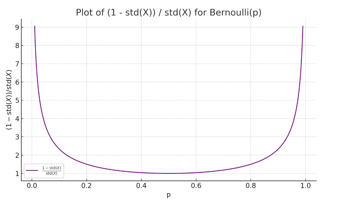
is of interest. We can examine this quantity for verifiable rewards, for each $x$ the verifiable reward is a Bernouilli random variable with parameter $p$ the probability of success of the policy given $x$ (Mroueh, 2025). Hence we have:
$$
\frac{1-\sigma_{\alpha,r,\varepsilon}(x)}{\sigma_{\alpha,r,\varepsilon}(x)}=
\frac{1-\sqrt{p(1-p)+\varepsilon}}{\sqrt{p(1-p)+\varepsilon}}
$$
Plotting this quantity as function of $p$ below, we observe that it diverges for fully correct and incorrect answers and this can indeed hurt the lower bound, as the negative terms in the lower bound will be dominating. It was suggested in DAPO (Yu et al., 2025) to filter out prompts with fully correct or incorrect answers, this will have the effect of controlling this term in the lower bound and keep that quantity bounded away from infinity.
<details>
<summary>extracted/6494595/std_bern.png Details</summary>
### Visual Description
## Line Chart: Plot of (1 - std(X)) / std(X) for Bernoulli(p)
### Overview
The image displays a mathematical plot representing the function $f(p) = \frac{1 - \text{std}(X)}{\text{std}(X)}$ for a Bernoulli random variable $X$ with parameter $p$. The plot visualizes how this specific ratio changes as the probability parameter $p$ varies between 0 and 1. The curve is a symmetric, U-shaped function that reaches its minimum at the center of the distribution.
### Components/Axes
* **Title:** "Plot of (1 - std(X)) / std(X) for Bernoulli(p)" centered at the top.
* **X-axis:** Labeled "p". The scale ranges from 0.0 to 1.0, with major tick marks at 0.0, 0.2, 0.4, 0.6, 0.8, and 1.0.
* **Y-axis:** Labeled "(1 - std(X))/std(X)". The scale ranges from 1 to 9, with major tick marks at 1, 2, 3, 4, 5, 6, 7, 8, and 9.
* **Legend:** Located in the bottom-left corner. It contains a purple line segment and the label "$\frac{1 - \text{std}(X)}{\text{std}(X)}$".
* **Grid:** A light gray dashed grid is overlaid on the plot area.
### Detailed Analysis
The data series is a single, continuous purple line.
**Trend Verification:**
The curve is convex (U-shaped). It starts at a very high value near $p=0$, descends rapidly to a minimum at $p=0.5$, and then ascends symmetrically back to a very high value near $p=1$.
**Data Points (Approximate values):**
* **Minimum:** At $p = 0.5$, the y-value is exactly 1.0.
* **Near Center:** At $p = 0.4$ and $p = 0.6$, the y-value is approximately 1.1.
* **Mid-range:** At $p = 0.2$ and $p = 0.8$, the y-value is approximately 1.5.
* **Rising Slope:** At $p = 0.1$ and $p = 0.9$, the y-value is approximately 3.0.
* **Steep Slope:** At $p = 0.05$ and $p = 0.95$, the y-value is approximately 6.0.
* **Asymptotic Behavior:** As $p$ approaches 0 or 1, the curve approaches infinity.
### Key Observations
* **Symmetry:** The plot is perfectly symmetric around the vertical axis $p = 0.5$.
* **Minimum Value:** The global minimum of the function is 1, occurring at the point of maximum variance for the Bernoulli distribution ($p=0.5$).
* **Asymptotes:** The function is undefined at $p=0$ and $p=1$ (where the standard deviation is 0), resulting in vertical asymptotes at these boundaries.
### Interpretation
This plot visualizes the relationship between the standard deviation of a Bernoulli distribution and the ratio $\frac{1 - \text{std}(X)}{\text{std}(X)}$.
For a Bernoulli random variable $X$ with parameter $p$, the variance is $\text{Var}(X) = p(1-p)$, meaning the standard deviation is $\text{std}(X) = \sqrt{p(1-p)}$.
* **At $p=0.5$:** The standard deviation is at its maximum ($\sqrt{0.25} = 0.5$). Consequently, the ratio is $\frac{1 - 0.5}{0.5} = 1$. This is the lowest point on the graph.
* **As $p$ moves toward 0 or 1:** The standard deviation $\sqrt{p(1-p)}$ approaches 0. As the denominator approaches 0, the entire fraction grows toward infinity.
Essentially, this chart demonstrates that the ratio is inversely proportional to the standard deviation of the Bernoulli distribution. The "uncertainty" (standard deviation) is highest at $p=0.5$, which minimizes this specific ratio, while the ratio explodes as the distribution becomes more deterministic (approaching $p=0$ or $p=1$).
</details>
Figure 1. $\frac{1-\sigma_{\alpha,r,\varepsilon}(x)}{\sigma_{\alpha,r,\varepsilon}(x)}$ explodes when variance is zero, meaning for fully correct or wrong policies, this term dominates the lower bound.
### 3.2. GRPO: From Constrained Optimization to Clipped Surrogate Objectives
#### From Penalized to $\mathsf{KL}$ Constrained Optimization
To maximize the lower bound in eq.(4), we see that the off-policy $\alpha$ needs to be in the vicinity of the current policy $\pi_{k}$ , i.e. for $\mathbb{TV}(\alpha,\pi_{k})\leq\delta$ and that $M α, r, 0 < ∞ subscript 𝑀 𝛼 𝑟 0 italic_M start_POSTSUBSCRIPT italic_α , italic_r , 0 end_POSTSUBSCRIPT < ∞$ (variance terms not exploding). Under these assumptions, we can solve the following penalized problem :
$$
\max_{\pi}\mathbb{E}_{x\sim\rho_{\mathcal{X}}}\mathcal{L}_{\alpha}(\pi(\cdot|x
))-2~{}M_{\alpha,r,\varepsilon}\sqrt{\mathbb{E}_{x\sim\rho_{\mathcal{X}}}
\mathbb{TV}^{2}(\pi(\cdot|x),\alpha(\cdot|x))}.
$$
By virtue of Theorem 1, maximizing this objective above leads to policy reward improvement.
We can write this as a constrained optimization, there exists $\Delta>0$ such that the following constrained optimization problem is equivalent:
$$
\max_{\pi}\mathbb{E}_{x\sim\rho_{\mathcal{X}}}\mathcal{L}_{\alpha}(\pi(\cdot|x
))\text{ subject to }\mathbb{E}_{x\sim\rho_{\mathcal{X}}}\mathbb{TV}^{2}(\pi(
\cdot|x),\alpha(\cdot|x))\leq\Delta^{2}.
$$
By Pinsker inequality for two measures $m_{1},m_{2}$ we have $\mathbb{TV}(m_{1},m_{2})\leq\sqrt{\frac{1}{2}\mathsf{KL}(m_{1},m_{2})}$ and hence we can bound instead the $\mathsf{KL}$ divergence as follows:
$$
\boxed{\max_{\pi}\mathbb{E}_{x\sim\rho_{\mathcal{X}}}\mathcal{L}_{\alpha}(\pi(
\cdot|x))\text{ subject to }\frac{1}{2}~{}\mathbb{E}_{x\sim\rho_{\mathcal{X}}}
\mathsf{KL}(\pi(\cdot|x),\alpha(\cdot|x))\leq\Delta^{2}.} \tag{5}
$$
#### From Constrained Optimization to Clipped Surrogate Objectives
The objective in (5) is the same as in the original constrained PPO formulation (Schulman et al., 2015) with two key differences: the advantage is the whitened reward of GRPO where the statistics are computed using the off-policy $\alpha$ , and the advantage objective is computed using importance sampling from the off-policy $\alpha$ , instead of $\pi_{k}$ in both cases. This is indeed related to objectives in off-policy PPO (Queeney et al., 2021; Gan et al., 2024). A practical implementation of these objectives is through clipped surrogates (Schulman et al., 2015).
For $\epsilon\in[0,1]$ following Gan et al. (2024); Queeney et al. (2021) let us define:
$$
f_{\epsilon}(r,r^{\prime},a)=\min(ra,~{}\text{clip}(r,\max(r^{\prime}-\epsilon
,0),r^{\prime}+\epsilon)~{}a).
$$
The clipped off-policy GRPO objective for $\alpha$ such that $𝕋 𝕍 (α, π k) ≤ δ 𝕋 𝕍 𝛼 subscript 𝜋 𝑘 𝛿 blackboard_T blackboard_V ( italic_α , italic_π start_POSTSUBSCRIPT italic_k end_POSTSUBSCRIPT ) ≤ italic_δ$ and $M α, r, 0 < ∞ subscript 𝑀 𝛼 𝑟 0 italic_M start_POSTSUBSCRIPT italic_α , italic_r , 0 end_POSTSUBSCRIPT < ∞$ is therefore defined as follows :
$$
\mathcal{L}^{c}_{\alpha}(\pi(\cdot|x))=\mathbb{E}_{y\sim\alpha(\cdot|x)}f_{
\epsilon}\left(\frac{\pi(y|x)}{\alpha(y|x)},\frac{\pi_{k}(y|x)}{\alpha(y|x)},A
_{\alpha}(x,y)\right) \tag{6}
$$
Let us unpack this, we have: $f_{\epsilon}\left(\frac{\pi(y|x)}{\alpha(y|x)},\frac{\pi_{k}(y|x)}{\alpha(y|x) },A_{\alpha}(x,y)\right)=..$
$$
..=\begin{cases}A_{\alpha}(x,y)\min\left(\frac{\pi(y|x)}{\alpha(y|x)},\frac{
\pi_{k}(y|x)}{\alpha(y|x)}+\epsilon\right),&r(x,y)\geq\mu_{\alpha,r}(x)\\
A_{\alpha}(x,y)\max\left(\frac{\pi(y|x)}{\alpha(y|x)},\max(\frac{\pi_{k}(y|x)}
{\alpha(y|x)}-\epsilon,0)\right),&r(x,y)<\mu_{\alpha,r}(x).\end{cases}
$$
The clipping ensures that the ratio $\frac{\pi}{\alpha}$ remains bounded and is a relaxation of the $\mathsf{KL}$ (or the total variation distance). Since $\alpha$ needs to satisfy closeness to $\pi_{k}$ in order to ensure improvement, the clipping objective incentivizes the difference between $\frac{\pi}{\alpha}-\frac{\pi_{k}}{\alpha}$ to not exceed $\epsilon$ (Gan et al., 2024).
In practice, the off-policy is $\alpha=\pi_{k-v}$ for a small $v\in[0,k)$ . Given a small learning rate and a small $v$ , the assumption that the policy $\pi_{k-v}$ doesn’t deviate from $\pi_{k}$ is reasonable, and for $v$ small we can approximate $\frac{\pi_{k}}{\pi_{k-v}}$ by $1$ . We use this approximation in practice as we found it more stable, and given that this approximation is in practice used in off-Policy PPO (with sample reuse) as discussed in Gan et al. (2024) (See Section 4.1 in Gan et al. (2024)).
#### Back to On-Policy GRPO Clipped Objective
For $\alpha=\pi_{k}$ , we obtain the clipped objective for on-policy GRPO (Shao et al., 2024):
| | $\displaystyle\mathcal{L}^{c}_{\pi_{k}}(\pi(\cdot|x))$ | $\displaystyle=\mathbb{E}_{y\sim\pi_{k}(\cdot|x)}f_{\epsilon}\left(\frac{\pi(y| x)}{\pi_{k}(y|x)},1,A_{\pi_{k}}(x,y)\right)$ | |
| --- | --- | --- | --- |
| Method name | Update by fixed batch $i$ | Update of Policy on Server $v$ |
| --- | --- | --- |
| On-Policy GRPO (Shao et al., 2024) | $i=1$ | $v=1$ |
| Off-policy GRPO (Shao et al., 2024) | $i>1$ | $v=1$ |
| Off-policy GRPO (this work) | $i=1$ | $v>1$ |
Table 1. Training configurations in alg. 1: (v1-i1) is on-policy GRPO and (v1-i10) is an example of off-policy GRPO in (Shao et al., 2024). Our off-policy GRPO corresponds e.g. to (v10-i1).
Algorithm 1 Iterative GRPO with verifiable rewards, modified from Shao et al. (2024)
1: Input initial policy model $\pi_{\theta_{\text{init}}}$ ; verifiable reward $r$ ; task prompts $\mathcal{D}$ ;
2: Hyperparameters $\epsilon$ , $\beta$ , $S$ ,
3: $(i,v)$ =(Number of SGD iteration by fixed batch, Model update on vLLM server)
4: Policy model $\pi_{\theta}\leftarrow\pi_{\theta_{\text{init}}}$ $\pi_{\mathrm{ref}}\leftarrow\pi_{\theta_{\text{init}}}$
5: for $s=1,\dots,S$ do
6: for $k=1,\dots,M$ do
7: Sample a batch $\mathcal{D}_{b}$ from $\rho_{\mathcal{X}}$
8: if $k\bmod v=0$ then
9: Update the old policy model on the vLLM server $\pi_{\theta_{\textrm{old}}}\leftarrow\pi_{\theta}$
10: Sample $G$ outputs $\{y_{i}\}_{i=1}^{G}\sim\pi_{\theta_{\textrm{old}}}(\cdot\mid x_{i})$ for each question $x\in\mathcal{D}_{b}$
11: Compute rewards $\{r_{i}\}_{i=1}^{G}$ for each sampled output $y_{i}$ by running verifiable reward $r$
12: $\alpha\leftarrow\pi_{\theta_{\textrm{old}}}$
13: Compute $A_{\alpha}(x,y_{i})$ using Equation (2)
14: for GRPO iteration = 1, …, $i$ do $\triangleright$ $i$ is referred to as $\mu$ in Original GRPO
15: Update the policy model $\pi_{\theta}$ by maximizing the GRPO objective (7) with gradient ascent
16: $\pi_{\mathrm{ref}}\leftarrow\pi_{\theta}$ $\triangleright$ Swap reference with the latest model
17: Output $\pi_{\theta}$
#### $\mathsf{KL}-$ Regularized RL & On-Policy / Off-Policy Algorithms
Finally putting together our clipped surrogate objective with the $\mathsf{KL}$ regularizer we obtain our final objective:
$$
\mathbb{E}_{x\sim\rho_{\mathcal{X}}}\mathcal{L}^{c}_{\alpha}(\pi(\cdot|x))-
\beta\mathsf{KL}(\pi||\pi_{\mathrm{ref}}). \tag{7}
$$
We present the GRPO algorithm in Algorithm 1 and the configurations that allow toggling between on-policy and off-policy GRPO in Table 1. Within the RL loop, the model is served for inference using vLLM (Kwon et al., 2023). The parameter $v$ controls how often the model is updated on the vLLM server (which corresponds to off-policy with $\alpha=\pi_{k-v+1}$ ). The parameter $i$ controls how many SGD iterations are applied to each batch sampled from the policy. For $v=1$ and $i=1$ , the model is continuously served, and each batch of samples is used once in SGD. This corresponds to on-policy GRPO. For $i>1$ and $v=1$ , the model is still continuously served, but each batch is used $i$ times in the SGD loop; this corresponds to an “off-policy” GRPO variant, as proposed in Shao et al. (2024). For large models that require tensor parallelism and multi-GPU serving, continuous model serving incurs additional communication costs. Our off-policy GRPO mitigates these costs by serving the model every $v>1$ iterations (line 8 in Algorithm 1) and fixing $i=1$ . Our theory guarantees reward improvement as long as $v$ is not too large.
#### Computational and Communication Costs
Updating the model served by vLLM during GRPO training incurs varying costs depending on the model size, update frequency ( $v$ ), and parallelism settings. When the training model and vLLM instance reside on different GPUs, or when vLLM uses tensor parallelism (TP), model updates may trigger deep copies and inter-GPU communication. These involve either full weight transfers or partitioned broadcasts, which scale linearly with model size. Frequent updates (e.g., $v=1$ ) can dominate the runtime, especially for large models (see the recent benchmark vLLM (2025) for latencies in serving large models with tensor parallelism using vLLM). To mitigate this, we update the vLLM model every $v>1$ iterations. This amortizes the copy cost while maintaining reward improvement guarantees from our theory. In our experiments (Section 5), we are limited to single node setups with relatively small models, and therefore cannot fully demonstrate the potential speedups —particularly those that would become more pronounced at larger scales. In our setups the speedups are modest, given that there is no inter GPU or inter nodes communication for serving the models. See Section A for further discussion.
On-Policy Clipped Objective with Zero Variance Masking a la DAPO (Yu et al., 2025) As discussed earlier in the interpretation of the lower bound in page 4, the samples with zero variance may lead to total variation terms to dominate the lower bound, hence we propose similar to DAPO (Yu et al., 2025) to mask these samples. For instance in the on policy case this would be with the following masked objective:
$$
\mathbb{E}_{x\sim\rho_{\mathcal{X}}}\mathbbm{1}_{\sigma_{\pi_{k},r}(x)\neq 0}
\left(\mathcal{L}^{c}_{\pi_{k}}(\pi(\cdot|x))-\beta\mathsf{KL}(\pi||\pi_{
\mathrm{ref}})\right). \tag{8}
$$
## 4. Related Work
#### Proximal Policy Optimization (PPO) and Extensions
Proximal Policy Optimization (PPO) is a widely used on-policy reinforcement learning algorithm that improves training stability through clipped surrogate objectives. While PPO is effective in diverse settings, it is inherently limited by its on-policy nature, which constrains sample efficiency. To address these limitations, several off-policy adaptations and extensions of PPO have been proposed. Generalized Proximal Policy Optimization (G-PPO) (Queeney et al., 2021) enables sample reuse while maintaining convergence guarantees. Transductive off-Policy PPO (ToPPO) (Gan et al., 2024) builds on G-PPO by incorporating transductive learning principles, bridging the gap between off-policy learning and theoretical guarantees of on-policy methods. Off-Policy PPO (OPPO) (Meng et al., 2023) proposes novel corrections to integrate replay buffer samples in PPO-style updates.
#### On-Policy and Off-Policy Actor-Critic Methods
Actor-critic methods blend the strengths of policy gradients and value function estimation. Off-policy variants aim to improve sample efficiency by learning from a replay buffer. The Off-Policy Actor-Critic algorithm (Degris et al., 2012) introduces importance weighting to enable stable updates from off-policy data. ACER (Wang et al., 2016) extends this with trust-region optimization and truncated importance sampling, enhancing by that the learning efficiency in discrete action spaces. Mixing on-policy and off-policy methods aims to leverage the stability of on-policy updates with the efficiency of off-policy learning. P3O (Fakoor et al., 2020) provides a principled approach that interleaves policy updates from both on- and off-policy data.
#### Off-Policy RLHF and other variants of GRPO
Noukhovitch et al. (2025) introduced within the iterative DPO framework an asynchronous RLHF using off-policy data and that ensures faster convergence to the optimal policy. New variants of GRPO have been proposed recently such as DAPO (Yu et al., 2025) and DR-GRPO (Liu et al., 2025). DAPO proposes the zero variance masking without theoretical backing, our work roots this in the improvement lower bound. DR-GRPO proposes to center only the reward without using the variance normalization.
## 5. Experiments
### 5.1. Ablation Studies on GSM8K
#### Setup, Model, and Data
In our first set of experiments, we use GSM8K dataset from Cobbe et al. (2021) (MIT license), and Qwen/Qwen2.5-0.5B-Instruct (Apache 2.0 license) by Yang et al. (2024). We integrate our changes in Algorithm 1 to the GRPO implementation in TRL (von Werra et al., 2020b), and train our models on the training split of GSM8K on a node with 8 GPUs (GPU 0 for the vLLM server and 7 other GPUs for distributed training). See Appendix B for the hardware specification. We use a learning $5\times 10^{-6}$ for all experiments and the KL regularizer $\beta=0.1$ in Equation (7). We use the correctness of the LLM output as a reward. For GRPO training, the hyperparameters are the following: group size $G=16$ and per-device batch size $16$ (meaning each GPU processes a single prompt $x$ with $16$ responses). To increase the overall batchsize we use gradient accumulation of $4$ , ending with an effective batch size of prompts of $28$ . The context length used for this experiment is $200$ , and the sampling temperature is set to $\tau=0.1$ .
#### Ablations and Results
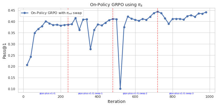
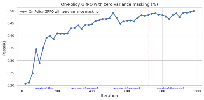
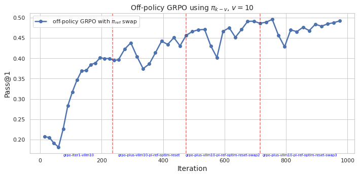
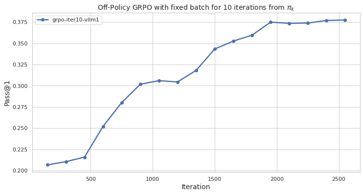
We train our models with GRPO using Algorithm 1 with a verifiable reward for answer correctness. We use for GRPO different configurations given in Table 1 and report on the test split of GSM8K Pass@1 using 50 samples (i.e. frequency of success given 50 generations for each question) using the same sampling configuration as in training. We report results in Figure 2: Fig. 2(a) for on-policy GRPO ( $i=1,v=1$ ) with the objective given in Equation (7) with $S=3$ (i.e. for 4 epochs with $\pi_{\mathrm{ref}}$ swap at end of each epoch with latest model); Fig. 2(b) for on-policy GRPO ( $i=1,v=1$ ) with masking zero variance samples i.e. using the objective given Equation (8) with $S=3$ ; Fig. 2(c) for our off-policy GRPO $(v=10,i=1)$ , with $S=3$ and Fig. 2(d) for Shao et al. (2024) ’s off-policy GRPO i.e $(v=1,i=10)$ for a single epoch. We see in Fig. 2(a) that while the on-policy GRPO converges to a maximum Pass@1 of $45\$ it is unstable. The masking of zero variance sampling in 2(b) stabilizes the on-policy GRPO and leads to an improvement of the performance to $50\$ . This is in line with our theoretical grounding through the improvement lower bound. Our off-policy GRPO in Fig. 2(c) stabilizes the training also and leads to an improved Pass@1 of $50\$ on the test set. In all three cases, we see that by resetting the $\pi_{\mathrm{ref}}$ to the latest model, GRPO amplifies the success rate above the current $\pi_{\mathrm{ref}}$ , this concurs with the theoretical findings in Mroueh (2025). Finally, the off-policy variant in Shao et al. (2024) in Fig. 2(d) shows a slower convergence over an epoch.
<details>
<summary>extracted/6494595/figs/v1-i1-swap.png Details</summary>
### Visual Description
## Line Chart: On-Policy GRPO using $\pi_k$
### Overview
This image displays a line chart tracking the performance of an "On-Policy GRPO" (Group Relative Policy Optimization) model over 1,000 training iterations. The Y-axis measures "Pass@1" accuracy, while the X-axis represents the training "Iteration." The chart includes a single data series, vertical reference markers, and specific text labels indicating different training phases or policy swaps.
### Components/Axes
* **Title:** "On-Policy GRPO using $\pi_k$" (centered at the top).
* **Y-Axis:** Labeled "Pass@1," with a numerical scale ranging from 0.10 to 0.45 in increments of 0.05.
* **X-Axis:** Labeled "Iteration," with a numerical scale ranging from 0 to 1000 in increments of 200.
* **Legend:** Located in the top-left corner. It contains a single entry: "On-Policy GRPO with $\pi_{ref}$ swap," represented by a blue line with circular markers.
* **Vertical Markers:** Three dashed red vertical lines are positioned at approximately x=250, x=500, and x=720.
* **Bottom Annotations:** Four text labels are positioned along the bottom of the chart area:
* "grpo-plus-v1-l1" (positioned near x=100)
* "grpo-plus-v1-l1-swap-1" (positioned near x=350)
* "grpo-plus-v1-l1-swap-2" (positioned near x=550)
* "grpo-plus-v1-l1-swap-3" (positioned near x=800)
### Detailed Analysis
The data series is a blue line with circular markers. The overall trend is an upward trajectory in performance, characterized by rapid initial learning, followed by a plateau with intermittent, sharp volatility.
**Visual Trend and Data Points:**
1. **Initial Phase (0 to 120 iterations):** The line slopes sharply upward from a starting point of approximately (x=30, y=0.21) to a local peak of (x=120, y=0.40).
2. **First Plateau (120 to 300 iterations):** The performance stabilizes, fluctuating slightly between 0.38 and 0.39.
3. **First Volatility (300 to 400 iterations):** There is a sharp drop at x=360 to approximately y=0.28, followed by a rapid recovery back to y=0.41 by x=380.
4. **Second Plateau (400 to 500 iterations):** The performance remains steady around 0.41.
5. **Major Anomaly (500 to 550 iterations):** Immediately following the second red vertical line (x=500), there is a catastrophic drop in performance to y=0.10 at x=520. This is followed by an immediate, steep recovery back to y=0.37 by x=540 and y=0.42 by x=560.
6. **Final Phase (560 to 1000 iterations):** The performance stabilizes again, fluctuating between 0.40 and 0.44. The peak performance of approximately y=0.44 is reached at x=720 (coinciding with the third red vertical line) and is maintained through the end of the chart at x=980.
### Key Observations
* **Instability Events:** The chart shows two significant, sudden drops in performance (at x=360 and x=520). The drop at x=520 is particularly severe, reducing performance to the baseline level.
* **Rapid Recovery:** In both instances of performance drops, the model recovers to its previous performance level within 20–40 iterations, suggesting high resilience or rapid re-learning.
* **Correlation with Swaps:** The vertical red lines appear to mark specific "swap" events. The third red line (x=720) correlates with the model reaching its highest sustained performance level (0.44).
### Interpretation
The data demonstrates the training dynamics of a GRPO model utilizing a reference policy ($\pi_{ref}$) swap mechanism.
* **Policy Swap Impact:** The "swap" events (indicated by the red lines and the "swap-X" labels) appear to be intended to improve the model's performance. While the swap at x=720 seems to have successfully pushed the model to its peak performance, the event around x=500 (associated with "swap-2") caused a massive, temporary collapse in performance.
* **Training Stability:** The sharp, V-shaped drops suggest that updating the reference policy ($\pi_{ref}$) can introduce significant instability into the training process. The model's ability to recover quickly from these drops indicates that the underlying optimization process is robust, even if the policy updates themselves are disruptive.
* **Conclusion:** The model exhibits a "learning-forgetting-relearning" pattern common in reinforcement learning when the target distribution or reference policy is shifted. The strategy appears effective overall, as the final performance (0.44) is higher than the initial performance (0.21), despite the volatility.
</details>
(a) On-Policy GRPO with $\pi_{\mathrm{ref}}$ swap at end of each epoch. ( $v=1$ , $i=1$ , $S=3$ )
<details>
<summary>extracted/6494595/figs/v1-i1-swap-gm.png Details</summary>
### Visual Description
## Line Chart: On-Policy GRPO with zero variance masking ($\pi_k$)
### Overview
This image displays a line chart tracking the performance of an "On-Policy GRPO (Group Relative Policy Optimization) with zero variance masking" model. The chart plots the "Pass@1" metric (a common evaluation metric for code generation or reasoning tasks) against training "Iteration" counts from 0 to 1000. The data shows a consistent upward trend in performance, segmented into four distinct phases corresponding to specific model versions.
### Components/Axes
* **Y-Axis:** Labeled "Pass@1", representing the performance metric. The scale ranges from 0.20 to 0.50 in increments of 0.05.
* **X-Axis:** Labeled "Iteration", representing the training progress. The scale ranges from 0 to 1000 in increments of 200.
* **Legend:** Located in the top-left corner, identifying the data series as "On-Policy GRPO with zero variance masking" (represented by a blue line with circular markers).
* **Vertical Markers:** Three dashed red vertical lines are positioned at approximately iterations 240, 500, and 720, acting as delimiters for different training phases.
* **Phase Labels:** Located along the bottom of the chart, between the vertical markers:
* **0–240:** `grpo-plus-v1-l1-gm`
* **240–500:** `grpo-plus-v1-l1-gm-swap-1`
* **500–720:** `grpo-plus-v1-l1-gm-swap-2`
* **720–1000:** `grpo-plus-v1-l1-gm-swap-3`
### Detailed Analysis
The data series follows a generally upward trajectory, indicating successful model learning.
* **Trend Verification:**
* **Initial Phase (0–240):** The curve starts at ~0.21. It rises sharply to ~0.35, experiences a significant drop to ~0.29 at iteration ~100, then recovers and climbs steadily to ~0.41 by iteration 240.
* **Second Phase (240–500):** The curve continues to rise, albeit with a slightly shallower slope than the initial phase, reaching ~0.47 by iteration 500.
* **Third Phase (500–720):** The curve shows a slight dip at ~550 (dropping to ~0.45) before recovering and climbing to ~0.485 by iteration 720.
* **Final Phase (720–1000):** The curve exhibits a plateauing effect, oscillating slightly but trending upward to reach a peak of ~0.50 at iteration 980.
* **Data Point Summary (Approximate):**
| Event | Iteration | Pass@1 |
| :--- | :--- | :--- |
| Start | ~30 | ~0.21 |
| Local Minimum | ~100 | ~0.29 |
| Phase 1 End | ~240 | ~0.41 |
| Phase 2 End | ~500 | ~0.47 |
| Phase 3 End | ~720 | ~0.485 |
| End | ~980 | ~0.50 |
### Key Observations
* **Learning Stability:** Despite the initial volatility (the dip at iteration 100), the model demonstrates robust learning, consistently recovering from minor performance drops.
* **Diminishing Returns:** The rate of improvement (slope) decreases as the iteration count increases. The jump from 0.20 to 0.40 happens much faster than the jump from 0.40 to 0.50.
* **Segmentation:** The vertical markers and "swap" labels suggest that the training process involves distinct stages, likely representing curriculum learning, model checkpoint swapping, or hyperparameter adjustments at specific intervals.
### Interpretation
The data demonstrates that the "On-Policy GRPO with zero variance masking" approach is effective at improving model performance over time. The "swap" nomenclature suggests an iterative training strategy where the model is likely being fine-tuned or updated with different data subsets or configurations (e.g., `swap-1`, `swap-2`, `swap-3`).
The significant dip at iteration 100 is a notable anomaly, possibly indicating a point of instability or a transition in the training data distribution. However, the subsequent recovery and sustained growth suggest that the "zero variance masking" technique successfully mitigates the risks of divergence, allowing the model to converge toward a 50% Pass@1 rate. The plateauing behavior toward the end of the 1000 iterations suggests the model is approaching the limits of its current configuration or data, indicating that further gains might require a change in strategy or additional data.
</details>
(b) On-Policy GRPO with masking of samples with variance $\sigma_{\pi_{k},r}=0$ , and with $\pi_{\mathrm{ref}}$ swap at end of each epoch. $v=1$ , $i=1$ , $S=3$ )
<details>
<summary>extracted/6494595/figs/v10-i1-swap.png Details</summary>
### Visual Description
## Line Chart: Off-policy GRPO Performance
### Overview
This image displays a line chart tracking the performance of an "Off-policy GRPO" (Group Relative Policy Optimization) model over 1,000 training iterations. The Y-axis measures "Pass@1" (a common metric for code generation or reasoning tasks), while the X-axis represents the iteration count. The chart illustrates a general upward trend in performance, punctuated by specific configuration changes marked by vertical red lines.
### Components/Axes
* **Title:** "Off-policy GRPO using $\pi_{k-v}, v = 10$"
* **Y-Axis:** Labeled "Pass@1", with a scale ranging from 0.20 to 0.50 in increments of 0.05.
* **X-Axis:** Labeled "Iteration", with a scale ranging from 0 to 1000 in increments of 200.
* **Legend:** Located in the top-left corner, identifying the blue line with circular markers as "off-policy GRPO with $\pi_{ref}$ swap".
* **Vertical Markers:** Three dashed red vertical lines are positioned at approximately iteration 230, 530, and 710.
* **Annotations (Bottom):** Small blue text labels are placed along the bottom of the chart, indicating specific configuration states:
* `grpo-iter1-vllm10` (Start)
* `grpo-plus-vllm10-pi-ref-optim-reset` (Between 230 and 530)
* `grpo-plus-vllm10-pi-ref-optim-reset-swap2` (Between 530 and 710)
* `grpo-plus-vllm10-pi-ref-optim-reset-swap3` (After 710)
### Detailed Analysis
The data series is a single blue line with circular markers representing data points.
**Trend Verification:**
1. **Initial Phase (0–230):** The line starts at approximately 0.21, dips to 0.18 at iteration 50, then climbs steeply to reach 0.40 by iteration 200.
2. **First Intervention (230–530):** After the first red line (x=230), the performance dips slightly to 0.39, then trends upward, reaching a local peak of approximately 0.45 at iteration 500.
3. **Second Intervention (530–710):** After the second red line (x=530), there is a sharp drop to 0.40. Following this, the model recovers and climbs to approximately 0.47 by iteration 680.
4. **Third Intervention (710–1000):** After the third red line (x=710), the performance dips slightly to 0.48, then continues a gradual upward trend, ending near 0.495 at iteration 980.
### Key Observations
* **Performance Recovery:** Every vertical red line (representing a "reset" or "swap" configuration change) is immediately followed by a short-term dip in performance, which is then consistently followed by a recovery to a higher performance level than before the intervention.
* **Diminishing Returns:** While the model continues to improve, the rate of improvement slows down as the Pass@1 metric approaches 0.50.
* **Volatility:** The model exhibits higher volatility (larger swings) in the middle of the training process (iterations 300–600) compared to the final phase (iterations 800–1000).
### Interpretation
This chart demonstrates the efficacy of a "swap" strategy in Off-policy GRPO training. The "swaps" (likely updating the reference policy $\pi_{ref}$ to the current policy) act as a regularization or stabilization technique.
The pattern suggests that the model reaches a performance plateau, at which point the configuration is "reset" or "swapped." While this causes a temporary drop in accuracy (likely due to the model adjusting to the new reference policy), it successfully breaks the plateau, allowing the model to reach a new, higher performance ceiling. This is a classic "sawtooth" optimization pattern often seen in reinforcement learning where periodic policy updates are required to maintain stability and continue learning.
</details>
(c) Off-Policy GRPO using $v=10$ (this amounts to fixing the model on the vLLM server for $10$ iterations and getting fresh samples for new batches), and with $\pi_{\mathrm{ref}}$ swap.( $v=10$ , $i=1$ , $S=3$ )
<details>
<summary>extracted/6494595/figs/v1-i10-1ep.png Details</summary>
### Visual Description
## Line Chart: Off-Policy GRPO Performance
### Overview
This image displays a line chart tracking the performance of an "Off-Policy GRPO" (Group Relative Policy Optimization) model. The chart plots the "Pass@1" metric (a common evaluation metric for Large Language Models, representing the probability that the first generated sample is correct) against training "Iteration". The data shows a generally upward trend, indicating model improvement over time.
### Components/Axes
* **Chart Title:** "Off-Policy GRPO with fixed batch for 10 iterations from $\pi_k$" (Note: $\pi_k$ represents the policy at iteration $k$).
* **Y-Axis:** Labeled "Pass@1". The scale ranges from 0.200 to 0.375, with major grid lines at 0.025 intervals.
* **X-Axis:** Labeled "Iteration". The scale ranges from 0 to 2500+, with major grid lines at 500-unit intervals.
* **Legend:** Located in the top-left corner. It contains a single entry: "grpo-iter10-vllm1", represented by a blue line with circular markers.
### Detailed Analysis
The chart plots a single data series ("grpo-iter10-vllm1"). The trend is generally monotonic increasing, with distinct phases of acceleration and deceleration.
**Data Point Extraction (Approximate values based on visual grid alignment):**
| Iteration (x) | Pass@1 (y) | Trend Description |
| :--- | :--- | :--- |
| ~150 | ~0.208 | Starting point |
| ~300 | ~0.212 | Slow, steady growth |
| ~450 | ~0.216 | Slow, steady growth |
| ~600 | ~0.252 | **Acceleration phase begins** |
| ~750 | ~0.280 | Steep upward slope |
| ~900 | ~0.302 | Steep upward slope |
| ~1050 | ~0.306 | Plateau/Stagnation |
| ~1200 | ~0.305 | Slight dip/Plateau |
| ~1350 | ~0.318 | Resumed growth |
| ~1500 | ~0.344 | Steep upward slope |
| ~1650 | ~0.353 | Gradual growth |
| ~1800 | ~0.360 | Gradual growth |
| ~1950 | ~0.375 | **Saturation phase begins** |
| ~2100 | ~0.373 | Minor fluctuation |
| ~2250 | ~0.374 | Minor fluctuation |
| ~2400 | ~0.377 | Marginal gains |
| ~2550 | ~0.378 | Marginal gains |
### Key Observations
* **Initial Phase (0–450):** The model shows very slow improvement, suggesting a "warm-up" period or initial difficulty in learning the task.
* **Rapid Improvement (450–900):** A significant performance jump occurs here, where the Pass@1 metric increases from ~0.216 to ~0.302.
* **Stagnation/Plateau (900–1200):** The model hits a temporary ceiling where performance flattens out, potentially indicating a local optimum or a need for policy adjustment.
* **Secondary Growth (1200–1950):** The model breaks through the plateau, showing strong, consistent improvement.
* **Saturation (1950–2550):** The curve flattens significantly after iteration 1950, suggesting the model has reached near-convergence or the limits of the current training configuration.
### Interpretation
The data demonstrates a successful training run for an LLM using Off-Policy GRPO. The "Pass@1" metric is a standard benchmark for reasoning or coding tasks; the improvement from ~0.20 to ~0.38 represents a nearly 90% relative increase in performance over the course of 2500 iterations.
The presence of the plateau between iterations 900 and 1200 is a classic characteristic of reinforcement learning training curves, often representing the model "struggling" to generalize before finding a more effective policy strategy. The fact that the curve resumes its upward trajectory after this point suggests the training process is robust. The final saturation indicates that further training iterations may yield diminishing returns, and the model is likely ready for evaluation or deployment.
</details>
(d) Off-Policy GRPO using fixed samples from $\pi_{k}$ for $10$ iterations. This will make $1$ epoch $10\times$ slower. $v=1$ , $i=10$ , $S=1$ )
Figure 2. We train different variants of GRPO on the train portion of GSM8K and report the Pass@1 on GSM8 test set using $50$ samples for each question in the test set for various variant of on-policy and off-policy GRPO. We see that as predicted by our theory, masking samples with zero variance stabilizes the training for on-policy training and leads to better performance. For off-policy training we see that using $v=10,i=1$ stabilizes also the training and leads also to better performance.
### 5.2. Finetuning Qwen Distill R1 model (1.5 B) on Deepscaler Data
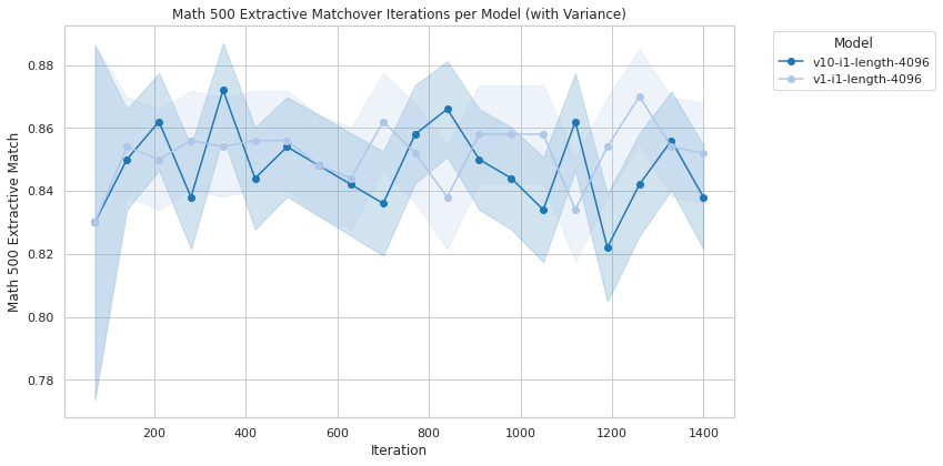
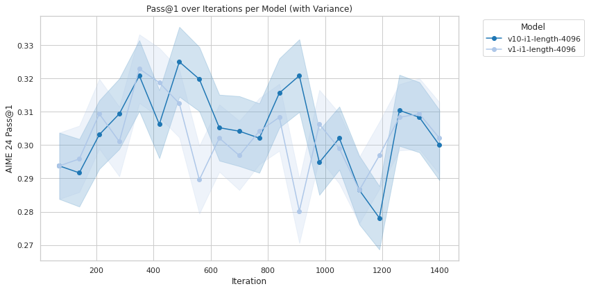
In this section we use GRPO to finetune DeepSeek-R1-Distill-Qwen-1.5B (Guo et al., 2025) on DeepScaleR-Preview-Dataset from Luo et al. (2025) consisting of roughly $40K$ math questions with known answers. We used math-verify as the verifiable reward. We use a learning rate of $1\times 10^{-6}$ in the same distributed setting as before (GPU 0 for vLLM and 7 GPUs for distributed training). We use a context length of $4096$ , a group size $G=16$ , a per-device batch size of $16$ , and the KL regularizer is $\beta=0.001$ . The sampling temperature used is $0.7$ . We compared here the on-policy GRPO ( $v=1,i=1$ ) to our off-policy GRPO ( $v=10,i=1$ ) and report the performance of the trained model on a single epoch (around 24 hours on a single node). We report in Tables 3 and 2 Aime24 and Math500 performance using Huggingface light-eval (Habib et al., 2023). Aime24 is evaluated with Pass@1 using 32 samples, and math500 with extractive matching as recommended in light-eval with a context length of $~{}32K$ (evaluation context length and all other sampling hyperparameters are set to the default in OpenR1 for this model). Plots of evaluation as function of iterations are given in Appendix D. We see that both on-policy and off-policy GRPO improve the performance of DeepSeek-R1-Distill-Qwen-1.5B that has an Aime24 of $29\$ to $32\$ at maximum (over iterations), and its math-500 from $83\$ to $87\$ . This result confirms our theoretical results that by going off-policy we don’t loose in term of overall performance.
| Model/Aime24 | Min | Max | Median | Mean |
| --- | --- | --- | --- | --- |
| v1-i1-length-4096 | 0.2802 | 0.3229 | 0.3021 | 0.3022 |
| v10-i1-length-4096 | 0.2781 | 0.3250 | 0.3047 | 0.3049 |
Table 2. Aime24 using lighteval with on & off-policy ( (v1-i1) and (v10-i1)) GRPO.
| Model/Math500 | Min | Max | Median | Mean |
| --- | --- | --- | --- | --- |
| v1-i1-length-4096 | 0.830 | 0.870 | 0.854 | 0.8519 |
| v10-i1-length-4096 | 0.822 | 0.872 | 0.846 | 0.8474 |
Table 3. Math 500 extractive matching using light-eval (Habib et al., 2023) with on and off-policy (v1-i1) and (v10-i1) GRPO.
## 6. Conclusion and Discussion
We revisited (on-policy) GRPO (Shao et al., 2024) and showed that its clipping objective can be derived from first principles as a lower bound for reward improvement. We also gave theoretical grounding to masking of zero variance samples suggested in DAPO (Yu et al., 2025). We introduced off-policy GRPO and layed conditions under which it leads to policy improvement. Our off-policy GRPO has the advantage of reducing communication costs in serving the model for inference within the GRPO loop at each iteration as done in the on-policy counter-part, while not sacrificing performance. We showcased that off-policy GRPO stabilizes training and leads to either on par or improved performance as the on-policy one.
The main takeaways of our paper to practitioners are: (1) Zero variance masking stabilizes on-policy GRPO’s training (2) Off-policy GRPO attains its full potential in terms of maintaining performance and lowering latencies and communication overhead in larger scale training where models are served using tensor parallelism (see vLLM (2025)).
We hope our proof of concept for off-policy GRPO will help enabling stable and efficient reinforcement learning at scale.
## References
- Bai et al. [2022] Y. Bai, A. Jones, K. Ndousse, A. Askell, A. Chen, N. DasSarma, D. Drain, S. Fort, D. Ganguli, T. Henighan, et al. Training a helpful and harmless assistant with reinforcement learning from human feedback. arXiv preprint arXiv:2204.05862, 2022.
- Christiano et al. [2017] P. F. Christiano, J. Leike, T. Brown, M. Martic, S. Legg, and D. Amodei. Deep reinforcement learning from human preferences. In I. Guyon, U. V. Luxburg, S. Bengio, H. Wallach, R. Fergus, S. Vishwanathan, and R. Garnett, editors, Advances in Neural Information Processing Systems, volume 30. Curran Associates, Inc., 2017. URL https://proceedings.neurips.cc/paper_files/paper/2017/file/d5e2c0adad503c91f91df240d0cd4e49-Paper.pdf.
- Cobbe et al. [2021] K. Cobbe, V. Kosaraju, M. Bavarian, M. Chen, H. Jun, L. Kaiser, M. Plappert, J. Tworek, J. Hilton, R. Nakano, C. Hesse, and J. Schulman. Training verifiers to solve math word problems. arXiv preprint arXiv:2110.14168, 2021.
- Degris et al. [2012] T. Degris, M. White, and R. S. Sutton. Off-policy actor-critic. arXiv preprint arXiv:1205.4839, 2012.
- Fakoor et al. [2020] R. Fakoor, P. Chaudhari, and A. J. Smola. P3o: Policy-on policy-off policy optimization. In Proceedings of The 35th Uncertainty in Artificial Intelligence Conference, pages 1017–1027. PMLR, 2020.
- Gan et al. [2024] Y. Gan, R. Yan, X. Tan, Z. Wu, and J. Xing. Transductive off-policy proximal policy optimization. arXiv preprint arXiv:2406.03894, 2024.
- Guo et al. [2025] D. Guo, D. Yang, H. Zhang, J. Song, R. Zhang, R. Xu, Q. Zhu, S. Ma, P. Wang, X. Bi, et al. Deepseek-r1: Incentivizing reasoning capability in llms via reinforcement learning. arXiv preprint arXiv:2501.12948, 2025.
- Habib et al. [2023] N. Habib, C. Fourrier, H. Kydlíček, T. Wolf, and L. Tunstall. Lighteval: A lightweight framework for llm evaluation, 2023. URL https://github.com/huggingface/lighteval.
- HuggingFace [2025a] HuggingFace. Open r1: A fully open reproduction of deepseek-r1, January 2025a. URL https://github.com/huggingface/open-r1.
- HuggingFace [2025b] HuggingFace. Open r1: Update #3, Mar. 2025b. URL https://huggingface.co/blog/open-r1/update-3. Accessed: 2025-05-11.
- Kwon et al. [2023] W. Kwon, Z. Li, S. Zhuang, Y. Sheng, L. Zheng, C. H. Yu, J. E. Gonzalez, H. Zhang, and I. Stoica. Efficient memory management for large language model serving with pagedattention. In Proceedings of the ACM SIGOPS 29th Symposium on Operating Systems Principles, 2023.
- Lambert et al. [2024] N. Lambert, J. Morrison, V. Pyatkin, S. Huang, H. Ivison, F. Brahman, L. J. V. Miranda, A. Liu, N. Dziri, S. Lyu, et al. Tülu 3: Pushing frontiers in open language model post-training. arXiv preprint arXiv:2411.15124, 2024.
- Liu et al. [2025] Z. Liu, C. Chen, W. Li, P. Qi, T. Pang, C. Du, W. S. Lee, and M. Lin. Understanding r1-zero-like training: A critical perspective, 2025. URL https://arxiv.org/abs/2503.20783.
- Luo et al. [2025] M. Luo, S. Tan, J. Wong, X. Shi, W. Y. Tang, M. Roongta, C. Cai, J. Luo, T. Zhang, L. E. Li, R. A. Popa, and I. Stoica. Deepscaler: Surpassing o1-preview with a 1.5b model by scaling rl. https://tinyurl.com/5e9rs33z, 2025. Notion Blog.
- Meng et al. [2023] W. Meng, Q. Zheng, G. Pan, and Y. Yin. Off-policy proximal policy optimization. Proceedings of the AAAI Conference on Artificial Intelligence, 37(8):9162–9170, 2023.
- Mroueh [2025] Y. Mroueh. Reinforcement learning with verifiable rewards: Grpo’s effective loss, dynamics, and success amplification, 2025. URL https://arxiv.org/abs/2503.06639.
- Noukhovitch et al. [2025] M. Noukhovitch, S. Huang, S. Xhonneux, A. Hosseini, R. Agarwal, and A. Courville. Faster, more efficient RLHF through off-policy asynchronous learning. In The Thirteenth International Conference on Learning Representations, 2025. URL https://openreview.net/forum?id=FhTAG591Ve.
- Ouyang et al. [2022] L. Ouyang, J. Wu, X. Jiang, D. Almeida, C. Wainwright, P. Mishkin, C. Zhang, S. Agarwal, K. Slama, A. Ray, et al. Training language models to follow instructions with human feedback. Advances in Neural Information Processing Systems, 35:27730–27744, 2022.
- Paszke et al. [2019] A. Paszke, S. Gross, F. Massa, A. Lerer, J. Bradbury, G. Chanan, T. Killeen, Z. Lin, N. Gimelshein, L. Antiga, A. Desmaison, A. Köpf, E. Yang, Z. DeVito, M. Raison, A. Tejani, S. Chilamkurthy, B. Steiner, L. Fang, J. Bai, and S. Chintala. PyTorch: An Imperative Style, High-Performance Deep Learning Library, Dec. 2019.
- Queeney et al. [2021] J. Queeney, I. C. Paschalidis, and C. G. Cassandras. Generalized proximal policy optimization with sample reuse. In Advances in Neural Information Processing Systems, volume 34, 2021.
- Schulman et al. [2015] J. Schulman, S. Levine, P. Abbeel, M. Jordan, and P. Moritz. Trust region policy optimization. In International conference on machine learning, pages 1889–1897. PMLR, 2015.
- Schulman et al. [2017] J. Schulman, F. Wolski, P. Dhariwal, A. Radford, and O. Klimov. Proximal policy optimization algorithms. arXiv preprint arXiv:1707.06347, 2017.
- Shao et al. [2024] Z. Shao, P. Wang, Q. Zhu, R. Xu, J. Song, X. Bi, H. Zhang, M. Zhang, Y. Li, Y. Wu, et al. Deepseekmath: Pushing the limits of mathematical reasoning in open language models. arXiv preprint arXiv:2402.03300, 2024.
- Stiennon et al. [2020] N. Stiennon, L. Ouyang, J. Wu, D. Ziegler, R. Lowe, C. Voss, A. Radford, D. Amodei, and P. F. Christiano. Learning to summarize with human feedback. Advances in Neural Information Processing Systems, 33:3008–3021, 2020.
- vLLM [2025] P. vLLM. Pytorch ci hud: vllm benchmark dashboard. https://hud.pytorch.org/benchmark/llms?repoName=vllm-project/vllm, 2025. Accessed: 2025-05-14.
- Vojnovic and Yun [2025] M. Vojnovic and S.-Y. Yun. What is the alignment objective of grpo?, 2025. URL https://arxiv.org/abs/2502.18548.
- von Werra et al. [2020a] L. von Werra, Y. Belkada, L. Tunstall, E. Beeching, T. Thrush, N. Lambert, S. Huang, K. Rasul, and Q. Gallouédec. Trl: Transformer reinforcement learning. https://github.com/huggingface/trl, 2020a.
- von Werra et al. [2020b] L. von Werra, Y. Belkada, L. Tunstall, E. Beeching, T. Thrush, N. Lambert, S. Huang, K. Rasul, and Q. Gallouédec. Trl: Transformer reinforcement learning. https://github.com/huggingface/trl, 2020b.
- Wang et al. [2016] Z. Wang, V. Bapst, N. Heess, V. Mnih, R. Munos, K. Kavukcuoglu, and N. De Freitas. Sample efficient actor-critic with experience replay. arXiv preprint arXiv:1611.01224, 2016.
- Wolf et al. [2020] T. Wolf, L. Debut, V. Sanh, J. Chaumond, C. Delangue, A. Moi, P. Cistac, T. Rault, R. Louf, M. Funtowicz, J. Davison, S. Shleifer, P. von Platen, C. Ma, Y. Jernite, J. Plu, C. Xu, T. L. Scao, S. Gugger, M. Drame, Q. Lhoest, and A. M. Rush. HuggingFace’s Transformers: State-of-the-art Natural Language Processing, July 2020.
- Yang et al. [2024] A. Yang, B. Yang, B. Hui, B. Zheng, B. Yu, C. Zhou, C. Li, C. Li, D. Liu, F. Huang, G. Dong, H. Wei, H. Lin, J. Tang, J. Wang, J. Yang, J. Tu, J. Zhang, J. Ma, J. Yang, J. Xu, J. Zhou, J. Bai, J. He, J. Lin, K. Dang, K. Lu, K. Chen, K. Yang, M. Li, M. Xue, N. Ni, P. Zhang, P. Wang, R. Peng, R. Men, R. Gao, R. Lin, S. Wang, S. Bai, S. Tan, T. Zhu, T. Li, T. Liu, W. Ge, X. Deng, X. Zhou, X. Ren, X. Zhang, X. Wei, X. Ren, X. Liu, Y. Fan, Y. Yao, Y. Zhang, Y. Wan, Y. Chu, Y. Liu, Z. Cui, Z. Zhang, Z. Guo, and Z. Fan. Qwen2 Technical Report, Sept. 2024.
- Yu et al. [2025] Q. Yu, Z. Zhang, R. Zhu, Y. Yuan, X. Zuo, Y. Yue, T. Fan, G. Liu, L. Liu, X. Liu, H. Lin, Z. Lin, B. Ma, G. Sheng, Y. Tong, C. Zhang, M. Zhang, W. Zhang, H. Zhu, J. Zhu, J. Chen, J. Chen, C. Wang, H. Yu, W. Dai, Y. Song, X. Wei, H. Zhou, J. Liu, W.-Y. Ma, Y.-Q. Zhang, L. Yan, M. Qiao, Y. Wu, and M. Wang. Dapo: An open-source llm reinforcement learning system at scale, 2025. URL https://arxiv.org/abs/2503.14476.
## Appendix A Broader Impact and Limitations
Our work analyzes the celebrated GRPO algorithm and develops an adaptation for the off-policy setting motivated by recent efforts for PPO that demonstrated higher stability and efficiency. Our primary contributions are theoretical, providing formal conditions under which advantage optimization guarantees policy improvement for the on-policy and off-policy regimes. These insights provide lower bounds on policy improvement and directly inform a practical clipped surrogate optimization objective for large language model (LLM) policy training that inherits our theoretical guarantees for both on policy and off policy regimes. In the on-policy regime our lower bound shed the light and give theoretical backing to the benefits of masking samples with zero variance as suggested in the DAPO paper [Yu et al., 2025]. Our formulation also clarifies theoretical relationships between our newly introduced off-policy GRPO, PPO variants, and general off-policy optimization frameworks – a linkage previously underexplored in the literature. Our derived off-policy GRPO algorithm is validated experimentally demonstrating improved performance compared to standard GRPO, while having the potential to reduce the communication overhead across devices in serving large models for sampling that is needed in GRPO. The broader impacts that we anticipate from our work (beside those directly inherited from GRPO and reinforcement fine-tuning of LLMs and the risks associated to the dual use of the enabled reasoning models) are then generally positive, as it enhances RL efficiency, reducing computational costs and improving stability.
The main limitation of our work is that the empirical validation remains constrained to smaller datasets, smaller model architectures, and smaller context size (4096 tokens at maximum) that can be trained on our hardware setup consisting of one compute node with 8 H100 NVIDIA gpus (1 used for the vLLM server and 7 for training the policy LLM). Our 1.5 B experimental setup, with deepscaler data is at the limit of what can fit in the memory of a single node.
This limitation primarily reflects the common resource constraints associated with provisioning large-scale distributed training environments, rather than any inherent restriction of the algorithm itself. Note that for larger context, larger batch size and larger architectures than the ones used in our paper, multi-node training is required.
While our main contribution here remains theoretical and backed with ablation studies on a single node, we reserve to scale up our experiments to larger training runs in future work aimed at showcasing the fact that the benefits of our off-policy algorithms in terms of efficient and reduced communication are expected to become even more pronounced in the large-scale distributed regime as it is already showed in multiple off policy RL works.
## Appendix B Assets
#### Hardware setup
All our experiments were run on one compute node with Dual 48-core Intel Xeon 8468, 2TB of RAM, 8 NVIDIA HGX H100 80GB SMX5, 8x 3.4TB Enterprise NVMe U.2 Gen4, and 10x NVIDIA Mellanox Infiniband Single port NDR adapters, running RedHat Enterprise Linux 9.5
#### Libraries
Our experiments rely on the open-source libraries pytorch [Paszke et al., 2019] (license: BSD), HuggingFace Transformers [Wolf et al., 2020] (Apache 2.0 license), and HuggingFace TRL [von Werra et al., 2020a] (Apache 2.0 license). We also relied on Open-R1 [HuggingFace, 2025a] as well as light-eval [Habib et al., 2023] for the evaluation of Aime24 and Math500.
#### Code re-use
Our GRPO training code is based on the public Github repository https://github.com/huggingface/open-r1 [HuggingFace, 2025a].
#### Data and Models
In our experiments, we use following publicly available datasets: (1) GSM8K dataset from Cobbe et al. [2021] (MIT license), and (2) the DeepScaleR-Preview-Dataset from Luo et al. [2025] (MIT license). The models that we used were Qwen/Qwen2.5-0.5B-Instruct (Apache 2.0 license) by Yang et al. [2024], and DeepSeek-R1-Distill-Qwen-1.5B (MIT license) by Guo et al. [2025].
## Appendix C Reward Improvement Lower Bound
### C.1. Proof of Theorem 1
We have :
$$
J(\pi(\cdot|x))=\mathbb{E}_{y\sim\pi(\cdot|x)}r(x,y)
$$
Let $\pi_{k}$ be the current policy and $\alpha(\cdot|x)$ be another policy typically consider $\alpha(\cdot|x)=\pi_{k-i}(\cdot|x)$ .
Define mean and variances of the off-policy reward, i.e policy under $\alpha$ :
$\mu_{\alpha}(x)=\mathbb{E}_{y\sim\alpha(\cdot|x)}r(x,y)$ and $\sigma_{\alpha}(x)=\sqrt{\mathbb{E}_{y\sim\alpha(\cdot|x)}(r(x,y)-\mu_{\alpha} (x))^{2}},$ and denote for $0<\varepsilon<1$ : $\sigma_{\alpha,\varepsilon}(x)=\sqrt{\sigma^{2}_{\alpha}(x)+\varepsilon}$ .
Note that we have a bounded reward $0\leq r(x,y)\leq\left\lVert{r}\right\rVert_{\infty}$ which implies that $\sigma^{2}_{\alpha}(x)\leq\frac{\left\lVert{r}\right\rVert^{2}_{\infty}}{4}$ , and hence we have:
$$
\sigma_{\alpha,\varepsilon}(x)\leq\sqrt{\frac{\left\lVert{r}\right\rVert^{2}_{
\infty}}{4}+\varepsilon}.
$$
We normalize the reward so that : $\sigma_{\alpha,\varepsilon}(x)\leq\sqrt{\frac{\left\lVert{r}\right\rVert^{2}_{ \infty}}{4}+\varepsilon}\leq 1.$
We denote GRPO advantage function as:
$$
A_{\alpha}(x,y)=\frac{r(x,y)-\mu_{\alpha}(x)}{\sigma_{\alpha,\varepsilon}(x)}
$$
$$
\mathcal{L}_{\alpha}(\pi(\cdot|x))=\mathbb{E}_{y\sim\alpha(\cdot|x)}\frac{\pi(
y|x)}{\alpha(y|x)}A_{\alpha}(x,y)
$$
If $\alpha=\pi_{k}$ , we obtain the online policy objective function of GRPO, where the advantage is computed with the current policy $\pi_{k}$ , i.e using $A_{\pi_{k}}(x,y)$ .
We have:
| | $\displaystyle\mathcal{L}_{\alpha}(\pi(\cdot|x))$ | $\displaystyle=\frac{1}{\sigma_{\alpha,\varepsilon}(x)}\left(\mathbb{E}_{y\sim \pi(\cdot|x)}r(x,y)-\mu_{\alpha}(x)\right)$ | |
| --- | --- | --- | --- |
Our goal is to provide an upper bound on :
$$
\mathcal{L}_{\alpha}(\pi(\cdot|x))-\left(J(\pi(\cdot|x))-J(\pi_{k}(\cdot|x))\right)
$$
Hence we have:
| | $\displaystyle\mathcal{L}_{\alpha}(\pi(\cdot|x))-\left(J(\pi(\cdot|x))-J(\pi_{k }(\cdot|x))\right)=\left(\frac{1}{\sigma_{\alpha,\varepsilon}(x)}-1\right)J( \pi(\cdot|x))+J(\pi_{k}(\cdot|x))-\frac{1}{\sigma_{\alpha,\varepsilon}(x)}J( \alpha(\cdot|x))$ | |
| --- | --- | --- |
**Lemma 1 (Kantorovich-Rubenstein duality of total variation distance, see )**
*The Kantorovich-Rubenstein duality (variational representation) of the total variation distance is as follows:
$$
\mathbb{TV}(m_{1},m_{2})=\frac{1}{2L}\sup_{g\in\mathcal{G}_{L}}\left\{\mathbb{
E}_{Z\sim m_{1}}[g(Z)]-\mathbb{E}_{Z\sim m_{2}}[g(Z)]\right\}, \tag{9}
$$
where $\mathcal{G}_{L}=\{g:\mathcal{Z}\rightarrow\mathbb{R},||g||_{\infty}\leq L\}$ .*
On the other hand using Lemma 1 we have:
$$
J(\pi(\cdot|x))-J(\alpha(\cdot|x))\leq 2\left\lVert{r}\right\rVert_{\infty}
\mathbb{TV}(\pi(\cdot|x),\alpha(\cdot|x))
$$
and
$$
J(\pi_{k}(\cdot|x))-J(\alpha(\cdot|x))\leq 2\left\lVert{r}\right\rVert_{\infty
}\mathbb{TV}(\pi_{k}(\cdot|x),\alpha(\cdot|x))
$$
By our assumption on the reward we have :
$$
\frac{1-\sigma_{\alpha,\varepsilon}(x)}{\sigma_{\alpha,\varepsilon}(x)}\geq 0
$$
so that we obtain the final bound as follows:
| | $\displaystyle\mathcal{L}_{\alpha}(\pi(\cdot|x))-\left(J(\pi(\cdot|x))-J(\pi_{k }(\cdot|x))\right)\leq 2\frac{1-\sigma_{\alpha,\varepsilon}(x)}{\sigma_{\alpha ,\varepsilon}(x)}\left\lVert{r}\right\rVert_{\infty}\mathbb{TV}(\pi(\cdot|x), \alpha(\cdot|x))+2\left\lVert{r}\right\rVert_{\infty}\mathbb{TV}(\pi_{k}(\cdot |x),\alpha(\cdot|x))$ | |
| --- | --- | --- |
We obtain finally our lower bound on policy improvement as follows:
$J (π (⋅ | x)) − J (π k (⋅ | x)) ≥ ℒ α (π (⋅ | x)) − 2 1 − σ α, ε (x) σ α, ε (x) ∥ r ∥ ∞ 𝕋 𝕍 (π (⋅ | x), α (⋅ | x)) − 2 ∥ r ∥ ∞ 𝕋 𝕍 (π k (⋅ | x), α (⋅ | x)) italic_J ( italic_π ( ⋅ | italic_x ) ) - italic_J ( italic_π start_POSTSUBSCRIPT italic_k end_POSTSUBSCRIPT ( ⋅ | italic_x ) ) ≥ caligraphic_L start_POSTSUBSCRIPT italic_α end_POSTSUBSCRIPT ( italic_π ( ⋅ | italic_x ) ) - 2 divide start_ARG 1 - italic_σ start_POSTSUBSCRIPT italic_α , italic_ε end_POSTSUBSCRIPT ( italic_x ) end_ARG start_ARG italic_σ start_POSTSUBSCRIPT italic_α , italic_ε end_POSTSUBSCRIPT ( italic_x ) end_ARG ∥ italic_r ∥ start_POSTSUBSCRIPT ∞ end_POSTSUBSCRIPT blackboard_T blackboard_V ( italic_π ( ⋅ | italic_x ) , italic_α ( ⋅ | italic_x ) ) - 2 ∥ italic_r ∥ start_POSTSUBSCRIPT ∞ end_POSTSUBSCRIPT blackboard_T blackboard_V ( italic_π start_POSTSUBSCRIPT italic_k end_POSTSUBSCRIPT ( ⋅ | italic_x ) , italic_α ( ⋅ | italic_x ) )$
Integrating over $x$ (the prompts) we have:
| | $\displaystyle\mathbb{E}_{x\sim\rho_{\mathcal{X}}}J(\pi(\cdot|x))-\mathbb{E}_{x \sim\rho_{\mathcal{X}}}J(\pi_{k}(\cdot|x))\geq\mathbb{E}_{x\sim\rho_{\mathcal{ X}}}\mathcal{L}_{\alpha}(\pi(\cdot|x))-2\left\lVert{r}\right\rVert_{\infty} \mathbb{E}_{x\sim\rho_{\mathcal{X}}}\frac{1-\sigma_{\alpha,\varepsilon}(x)}{ \sigma_{\alpha,\varepsilon}(x)}\mathbb{TV}(\pi(\cdot|x),\alpha(\cdot|x))$ | |
| --- | --- | --- |
## Appendix D Experiments
<details>
<summary>extracted/6494595/figs/math500.png Details</summary>
### Visual Description
## Line Chart: Math 500 Extractive Matchover Iterations per Model (with Variance)
### Overview
This image displays a line chart comparing the performance of two distinct models—"v10-i1-length-4096" and "v1-i1-length-4096"—on a "Math 500 Extractive Match" task. The chart tracks performance metrics across a series of training iterations, with shaded regions surrounding each line representing the variance (uncertainty) for each data point.
### Components/Axes
* **Header:** "Math 500 Extractive Matchover Iterations per Model (with Variance)"
* **X-Axis:** Labeled "Iteration". The scale ranges from approximately 100 to 1400, with major grid lines marked at 200, 400, 600, 800, 1000, 1200, and 1400.
* **Y-Axis:** Labeled "Math 500 Extractive Match". The scale ranges from 0.78 to 0.88, with major grid lines marked at 0.78, 0.80, 0.82, 0.84, 0.86, and 0.88.
* **Legend:** Located in the top-right corner.
* **v10-i1-length-4096:** Represented by a dark blue line with circular markers and a dark blue shaded variance region.
* **v1-i1-length-4096:** Represented by a light blue line with circular markers and a light blue shaded variance region.
### Detailed Analysis
#### Trend Verification
* **v10-i1-length-4096 (Dark Blue):** This series exhibits high volatility. It begins with a sharp upward trend, followed by significant fluctuations throughout the iteration range. It shows a notable peak around iteration 350 and a sharp, significant drop at iteration 1200.
* **v1-i1-length-4096 (Light Blue):** This series exhibits a more consistent, gradual upward trend. It is generally smoother than the dark blue series, with fewer sharp fluctuations.
#### Data Points (Approximate Values)
* **Starting Point (Iteration ~100):** Both models begin at approximately 0.83. The dark blue model (v10) has a much wider variance (shaded region) at this point, extending from ~0.77 to ~0.89.
* **Mid-Range (Iteration ~700):**
* The light blue model (v1) reaches a local peak of approximately 0.86.
* The dark blue model (v10) dips to approximately 0.835.
* **Late-Range (Iteration ~1200):**
* The light blue model (v1) reaches a high point of approximately 0.87.
* The dark blue model (v10) experiences a sharp decline to approximately 0.82.
* **Ending Point (Iteration ~1400):**
* The light blue model (v1) settles at approximately 0.85.
* The dark blue model (v10) recovers slightly to approximately 0.84.
### Key Observations
* **Variance:** Both models show the highest variance at the initial iteration (100). As iterations progress, the variance for both models generally tightens, though the dark blue model (v10) maintains wider fluctuations in its performance compared to the light blue model (v1).
* **Performance Divergence:** After iteration 600, the light blue model (v1) consistently maintains a more stable performance profile, whereas the dark blue model (v10) exhibits erratic behavior, characterized by sharp peaks and valleys.
* **Outlier:** The most significant anomaly is the sharp drop in the dark blue model (v10) at iteration 1200, which deviates significantly from its previous trend.
### Interpretation
The data suggests that the "v1-i1-length-4096" model is more robust and reliable for this specific task than the "v10-i1-length-4096" model. While both models start with similar performance, the "v1" model demonstrates a more stable learning curve and higher peak performance in the latter half of the training process. The "v10" model's erratic behavior, particularly the sharp decline at iteration 1200, indicates potential instability in its training process or sensitivity to the specific data batches encountered at that stage. The wider variance in the "v10" model further supports the conclusion that it is less predictable than the "v1" model.
</details>
(a) Aime 24
<details>
<summary>extracted/6494595/figs/aime24.png Details</summary>
### Visual Description
## Line Chart: Pass@1 over Iterations per Model (with Variance)
### Overview
This chart illustrates the performance of two distinct models, labeled "v10-i1-length-4096" and "v1-i1-length-4096," on the AIME 24 benchmark. The Y-axis represents the "Pass@1" score, while the X-axis represents training "Iteration." The chart includes shaded regions around each line, representing the variance (confidence interval) for each data point.
### Components/Axes
* **Chart Type:** Time-series line chart with shaded variance bands.
* **X-Axis:** Labeled "Iteration." The scale ranges from 0 to 1400, with major grid lines at 200-unit intervals.
* **Y-Axis:** Labeled "AIME 24 Pass@1." The scale ranges from 0.27 to 0.33, with major grid lines at 0.01 intervals.
* **Legend:** Positioned in the top-right corner.
* **v10-i1-length-4096:** Represented by a dark blue line with circular markers.
* **v1-i1-length-4096:** Represented by a light blue line with circular markers.
### Detailed Analysis
The data points are extracted based on visual estimation relative to the grid lines.
**1. v10-i1-length-4096 (Dark Blue Line)**
* **Trend:** The line exhibits high volatility. It trends upward from the start, peaks twice (around iteration 500 and 700), experiences a sharp decline around iteration 1200, and recovers slightly toward the end.
* **Key Data Points (Approximate):**
* Start (~100): 0.294
* ~350: 0.321
* ~500: 0.325 (Peak)
* ~700: 0.320
* ~850: 0.316
* ~1200: 0.278 (Significant trough)
* ~1300: 0.310
* End (~1400): 0.300
**2. v1-i1-length-4096 (Light Blue Line)**
* **Trend:** This line also shows significant volatility. It peaks early (around iteration 350), followed by a general downward trend with a sharp drop at iteration 900, before recovering toward the end.
* **Key Data Points (Approximate):**
* Start (~100): 0.294
* ~350: 0.323 (Peak)
* ~500: 0.313
* ~700: 0.297
* ~900: 0.280 (Significant trough)
* ~1000: 0.306
* ~1200: 0.297
* End (~1400): 0.302
### Key Observations
* **Volatility:** Both models exhibit unstable performance, with Pass@1 scores fluctuating significantly between iterations. This suggests that the training process or the evaluation metric is sensitive to the specific checkpoint.
* **Divergence:** The models diverge significantly between iterations 500 and 1200. The dark blue model (v10) generally outperforms the light blue model (v1) in the middle phase of training, despite the dark blue model's sharp drop at iteration 1200.
* **Variance:** The shaded regions (variance) are relatively consistent in width across the timeline, though they appear slightly wider during the peak performance periods, suggesting higher uncertainty when the models achieve higher scores.
* **Outliers:** The sharp drop in the dark blue model at iteration 1200 (0.278) and the light blue model at iteration 900 (0.280) are notable anomalies, representing the lowest performance points for each respective model.
### Interpretation
The data demonstrates that neither model achieves a stable convergence point within the 1400 iterations shown. The high variance and frequent "sawtooth" pattern (sharp rises followed by sharp drops) are characteristic of training runs where the model may be overfitting to specific batches or where the evaluation benchmark (AIME 24) is highly sensitive to the model's current state.
The "v10" model appears to have a higher ceiling (reaching ~0.325) compared to the "v1" model (reaching ~0.323), but it is also prone to more dramatic performance degradation. The fact that both models end near the 0.300 mark suggests that despite the fluctuations, they settle into a similar performance range by the end of the training duration.
</details>
(b) Math 500.
Figure 3. Aime 24/ Math 500