2505.23219

# Ghidorah: Fast LLM Inference on Edge with Speculative Decoding and Hetero-Core Parallelism Abstract In-situ LLM inference on end-user devices has gained significant interest due to its privacy benefits and reduced dependency on external infrastructure. However, as the decoding process is memory-bandwidth-bound, the diverse processing units in modern end-user devices cannot be fully exploited, resulting in slow LLM inference. This paper presents Ghidorah, a LLM inference system for end-user devices with the unified memory architecture. The key idea of Ghidorah can be summarized in two steps: 1) leveraging speculative decoding approaches to enhance parallelism, and 2) ingeniously distributing workloads across multiple heterogeneous processing units to maximize computing power utilization. Ghidorah includes the hetero-core model parallelism (HCMP) architecture and the architecture-aware profiling (ARCA) approach. The HCMP architecture guides partitioning by leveraging the unified memory design of end-user devices and adapting to the hybrid computational demands of speculative decoding. The ARCA approach is used to determine the optimal speculative strategy and partitioning strategy, balancing acceptance rate with parallel capability to maximize the speedup. Additionally, we optimize sparse computation on ARM CPUs. Experimental results show that Ghidorah can achieve up to 7.6 $×$ speedup in the dominant LLM decoding phase compared to the sequential decoding approach in NVIDIA Jetson NX. Index Terms: Edge Intelligence, LLM Inference, Speculative Decoding, Unified Memory Architecture footnotetext: Jinhui Wei and Ye Huang contributed equally to this work and are considered co-first authors. Yuhui Zhou participated in this work as a research intern at Sun Yat-sen University. * Corresponding author: Jiangsu Du (dujiangsu@mail.sysu.edu.cn). I Introduction Deploying large language models (LLMs) directly on end-user devices, such as mobile phones and laptops, is highly attractive. In-situ inference can eliminate data privacy concerns and reduce reliance on external infrastructures, thereby boosting intelligence and autonomy. However, achieving fast LLM inference remains a significant challenge, constrained by both algorithmic parallelism and hardware capability. 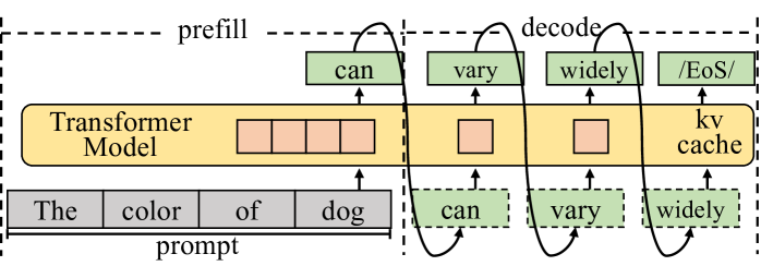To begin with, end-user devices typically process only a single request at a moment and the traditional decoding approach, shown in Figure 1, generates tokens sequentially, one at a time. With the KV cache technique [1], the dominant decoding phase of the LLM inference has very limited parallelism, while requiring loading all the model weights in each iteration. Thus, the limited parallelism and memory-bandwidth-bound nature prevent the full utilization of modern hardware. Alternatively, the speculative decoding approach [2, 3, 4] takes a draft-then-verify decoding process. In each decoding step, speculative decoding first drafts multiple tokens as predictions for future steps and then verifies in parallel whether to accept the drafted tokens. It can parallelize the inherently sequential process, showing strong potential to accelerate token generation rates by trading off compute for bandwidth. After enhancing the algorithmic parallelism, the LLM inference starts to be blocked by the limited hardware capability of end user devices. To fully leverage the capabilities of end-user devices, it is promising to distribute workloads across heterogeneous processing units [5, 6, 7, 8]. For instance, the GPU of Apple M4 [9] Pro has 17.04 TFLOPs FP16 performance, while its CPU has around 38 TFlops FP16 performance. However, existing systems [10, 3] do not align with the computing pattern of speculative decoding and the unified memory architecture of end-user devices, resulting in inefficiency. <details> <summary>x1.png Details</summary>  ### Visual Description \n ## Diagram: Transformer Model Prefill and Decode Process ### Overview The image is a diagram illustrating the prefill and decode stages of a Transformer model. It depicts how a prompt is processed and how the model generates subsequent tokens. The diagram highlights the use of a "kv cache" during the decode phase. ### Components/Axes The diagram consists of the following components: * **Transformer Model:** A large yellow rectangular block labeled "Transformer Model". * **Prompt:** A gray rectangular block labeled "prompt" containing the words "The", "color", "of", and "dog". * **Prefill Stage:** A dashed box encompassing the initial processing of the prompt. Labeled "prefill". * **Decode Stage:** A dashed box encompassing the iterative generation of tokens. Labeled "decode". * **kv cache:** A yellow rectangular block labeled "kv cache". * **Generated Tokens:** Green boxes labeled "can", "vary", and "widely". * **End of Sequence Token:** A green box labeled "EoS/". * **Arrows:** Curved arrows indicating the flow of information between the prompt, the Transformer Model, and the generated tokens. ### Detailed Analysis or Content Details The diagram shows the following process: 1. **Prefill:** The prompt ("The color of dog") is fed into the Transformer Model. The model processes this prompt and generates the first token, "can". This token is then added to the sequence. 2. **Decode:** The process iterates. The model takes the original prompt *and* the previously generated token ("can") as input and generates the next token, "vary". This continues with "vary" and "widely". 3. **kv cache:** The "kv cache" is used during the decode stage. It stores information from previous computations, allowing the model to efficiently generate subsequent tokens without recomputing everything from scratch. 4. **Token Generation:** Each generated token ("can", "vary", "widely") is shown in a green box and is fed back into the Transformer Model for the next iteration of the decode stage. 5. **End of Sequence:** The diagram indicates that the process can terminate with the generation of an "EoS/" (End of Sequence) token. ### Key Observations * The diagram emphasizes the iterative nature of the decode stage. * The "kv cache" is a crucial component for efficient decoding. * The diagram visually represents how the model builds upon the initial prompt to generate a sequence of tokens. ### Interpretation This diagram illustrates the core mechanism of autoregressive language models like Transformers. The prefill stage establishes an initial context based on the prompt, and the decode stage iteratively expands upon this context to generate coherent text. The "kv cache" is a key optimization that allows for efficient generation of long sequences. The diagram highlights the sequential dependency of each generated token on the preceding tokens and the original prompt. The use of dashed boxes to delineate "prefill" and "decode" suggests these are distinct phases in the model's operation, with the decode phase relying on the output of the prefill phase and the "kv cache". The diagram is a simplified representation of a complex process, but it effectively conveys the fundamental principles of Transformer-based language generation. </details> Figure 1: The autoregressive process of LLM inference with the KV cache technique. The decoding phase generally dominates the execution time. First, existing model partitioning approaches [11, 12] for distributing workloads across devices focus excessively on minimizing inter-device communication overhead and overlook opportunities for different processing units to access the same memory. When distributing LLM inference across multiple devices, explicit communication is required, making the reduction of communication overhead a top priority. In comparison, end-user devices typically integrate multiple heterogeneous processing units on a single chip and organize them within a unified memory architecture. Well-known examples include Apple’s M-series SoCs [9] and Intel Core Ultra [13], and NVIDIA Jetson [14]. In this way, minimizing memory access by carefully organizing partitioning strategy and data placement becomes the top priority for the unified memory architecture. Second, existing systems treat speculative decoding the same as the traditional decoding with a large batch size, less considering its specific computing pattern, particularly hybrid computational demands. The attention mechanism in the traditional decoding calculates the correlation between every pair of tokens, while it only requires to calculate correlation between partial pair of tokens in speculative decoding. Given the extremely high capability of accelerators in cloud systems and the high cost of transferring data to other processing units in the discrete memory architecture, this sparsity is often handled as dense computation using a mask mechanism. This oversight leads to missed opportunities to leverage computing affinity with processing units, such as on CPU. Third, algorithmic studies on speculative decoding primarily focus on increasing the acceptance length (the average number of tokens accepted in a single step), overlooking the balance between acceptance length and limited computing resources. Verifying more combinations of drafted tokens leads to better acceptance length, while resulting in more FLOPs to generate a single token. Compared to cloud hardware, end-user devices offer fewer resources for parallel verification, and verifying too many combinations can lead to decreased performance. Besides, modern hardware widely leverages vectorization technique, enabling the parallel processing of multiple data elements. It is crucial to select an appropriate verification width tailored to the specific hardware, thereby achieving the optimal balance between acceptance length and hardware parallelism. In this paper, we introduce Ghidorah, a system specifically designed to accelerate single-sample LLM inference in end-user devices with a unified memory architecture. It explores speculative decoding approaches to tackle the memory-bandwidth limitations inherent in the single-sample decoding process. Next, it distributes the novel workloads across multiple heterogeneous processing units in end-user devices, taking into account the hardware architecture and computing patterns. In summary, we make the following contributions: - We identify the performance bottlenecks in the single-sample LLM inference and explore speculative decoding approaches. - We present Ghidorah, a large language model inference system for end-user devices. It incorporates the hetero-core model parallelism (HCMP) architecture and the architecture-aware profiling (ARCA) approach to better employ the speculative decoding and align with the unified memory architecture. - We implement customized sparse computation optimizations for ARM CPUs. Experimental results show that Ghidorah achieves up to a 7.6 $×$ speedup over the sequential decoding approach on the Nvidia Jetson NX. This improvement is attributed to a 3.27 $×$ algorithmic enhancement and a 2.31 $×$ parallel speedup. II Background and Motivation II-A LLM Generative Task Inference LLMs are primarily used for generative tasks, where inference involves generating new text based on a given prompt. As shown in Figure 1, it predicts the next token and performs iteratively until meeting the end identifier (EoS). By maintaining the KV cache in memory, modern LLM serving systems eliminates most redundant computations during this iterative process. The inference process is divided into prefill and decode phases based on whether the KV cache has been generated. The prefill phase handles the newly incoming prompt and initializes the KV cache. Since the prompt typically consists of many tokens, it has high parallelism. Next, with the KV cache, each step of the decode phase processes only one new token generated by the previous step and appends the new KV cache. In end-user scenarios, single-sample inference processes only a single token during each iteration of the decoding phase. The decoding phase is heavily constrained by the memory bandwidth and cannot fully exploit hardware capability. Moreover, the decoding phase typically dominates the overall inference process. II-B Collaborative Inference and Transformer Structure Distributing inference workload across various devices or processing units is a common strategy for enhancing performance. II-B 1 Data, Pipeline and Sequence Parallelism Data parallelism (DP) [15] partitions workloads along the sample dimension, allowing each device to perform inferences independently. Pipeline parallelism (PP) [7] horizontally partitions the model into consecutive stages along layer dimension, with each stage placed in a device. Since DP and PP are mainly used in high-throughput scenarios and cannot reduce the execution time for a single sample, they are not suitable for end-user scenarios. Sequence parallelism (SP) [16, 12] is designed for the long-context inference and it divides the input along the sequence dimension. It requires each device to load the entire model weights, making it advantageous only for extremely long sequences. We do not consider it within the scope of our work. II-B 2 Tensor Parallelism and Transformer Structure <details> <summary>x2.png Details</summary>  ### Visual Description \n ## Diagram: Transformer Block Architecture ### Overview The image depicts a diagram of a Transformer block architecture, specifically illustrating the Multi-Head Attention (MHA) and Multi-Layer Perceptron (MLP) components within two sequential layers. The diagram shows the flow of data through these layers, including linear transformations, attention mechanisms, and residual connections. The diagram is segmented into four main sections: Linear Layer, Attention Module, Linear Layer, and Linear Layer. ### Components/Axes The diagram features several key components: * **Input:** Represented by 'A' and 'more tokens' flowing into the first Linear Layer. * **Linear Layers:** Represented by green boxes with labels like W₀^V, W₀^K, W₀^Q, W₁^V, W₁^K, W₁^Q, W_B^C, W_C^D, W_D^P, W_P^E. * **Attention Module:** Contains Key (K), Value (V), and Query (Q) matrices, along with a Softmax function. A 'KV Cache' is also present. * **MLP:** Consists of multiple Linear Layers and AllReduce operations. * **Residual Connections:** Represented by pink lines with '+' symbols, indicating addition. * **Output:** Represented by 'E'. * **AllReduce:** Blue arrows indicating the AllReduce operation. * **Labels:** W₀^V, W₀^K, W₀^Q, W₁^V, W₁^K, W₁^Q, W_B^C, W_C^D, W_D^P, W_P^E, K₀, Q₀, V₀, K₁, Q₁, V₁, B₀, B₁, C, D, E, A, E₀. ### Detailed Analysis or Content Details The diagram illustrates the data flow as follows: 1. **First Layer:** * Input 'A' and 'more tokens' are fed into the first Linear Layer, producing W₀^V, W₀^K, and W₀^Q. * These outputs are used to calculate attention weights via Q₀K₀^T and a Softmax function. * The attention weights are applied to V₀, resulting in output 'B₀'. * 'B₀' is then passed through a series of Linear Layers (W_B^C, W_C^D, W_D^P, W_P^E) with AllReduce operations in between, ultimately producing output 'E₀'. * A residual connection adds 'A' to 'E₀', resulting in 'E'. 2. **Second Layer:** * The output 'E' from the first layer is fed into the second Linear Layer, producing W₁^V, W₁^K, and W₁^Q. * Similar to the first layer, attention weights are calculated using Q₁K₁^T and a Softmax function. * The attention weights are applied to V₁, resulting in output 'B₁'. * 'B₁' is then passed through a series of Linear Layers (W_B^C, W_C^D, W_D^P, W_P^E) with AllReduce operations in between, ultimately producing output 'E'. * A residual connection adds 'E' to 'E', resulting in 'E'. The 'KV Cache' is shown connected to both V₀ and V₁, suggesting it stores key-value pairs for efficient attention calculation. The AllReduce operations are indicated by blue arrows and are applied after each Linear Layer within the MLP. ### Key Observations * The diagram highlights the repeated structure of the Transformer block, with the same operations being applied in multiple layers. * The use of residual connections is crucial for enabling the training of deep networks. * The AllReduce operations suggest a distributed training setup. * The 'KV Cache' is a key optimization for handling long sequences. ### Interpretation This diagram illustrates the core architecture of a Transformer block, a fundamental building block of modern natural language processing models. The Multi-Head Attention mechanism allows the model to attend to different parts of the input sequence, while the MLP provides non-linear transformations. The residual connections and AllReduce operations are essential for training and scaling these models. The diagram demonstrates how information flows through the block, highlighting the key components and their interactions. The presence of the KV Cache suggests an optimization for handling long sequences, which is crucial for tasks like machine translation and text generation. The diagram is a high-level representation and does not include details about the specific dimensions or parameters of the linear layers. It focuses on the overall structure and data flow within the Transformer block. 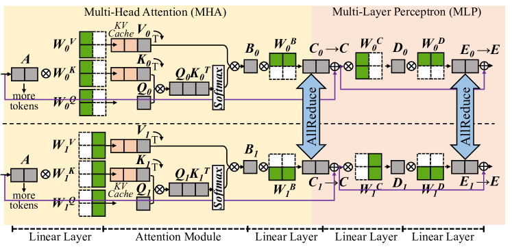</details> Figure 2: The partitioning [11] of Transformer model in the matrix form. Tensor parallelism partitions model weights to different devices [11, 12] or processing units [6, 17], and it is promising to reduce the execution time of a single sample. The Transformer [18] structure is the primary backbone for LLMs, consisting of multiple stacked Transformer layers, all configured identically. In a Transformer layer, the primary components are the multi-head attention (MHA) block and the multi-layer perceptron (MLP) block. Here we ignore element-wise operations, such as dropout, residual addition, and layernorm. In MHA block, the first linear layer generates query (Q), key (K), and value(V) matrices for each attention head. Each head conducts self-attention as in Equation 1, independently, and their outputs are concatenated and further processed by the next linear layer. MLP block involves two consecutive linear layers. $$ \displaystyle X=QK^{T} \displaystyle A=softmax(X) \displaystyle O=AV \tag{1} $$ Figure 2 shows a single Transformer layer and it is partitioned using the cloud TP solution in Megatron-LM [11]. For every two consecutive linear layers, it partitions the weights of the first one by columns and those of the second one by rows. An AllReduce communication is inserted as the synchronization point for every two linear layers. For the attention module in MHA block, it is partitioned by heads, with different attention heads assigned to different devices. II-C Speculative Decoding <details> <summary>x3.png Details</summary>  ### Visual Description \n ## Attention Mechanism Visualization: Word Alignment ### Overview The image depicts a visualization of an attention mechanism, likely from a neural machine translation or similar sequence-to-sequence model. It shows the alignment weights between words in a source sentence ("It I") and a target sentence ("is am the is am the"). The visualization uses a heatmap to represent the attention weights, with darker shades indicating stronger alignment. ### Components/Axes * **Source Sentence Heads:** Labeled "Head 0", "Head 1". These represent different attention heads focusing on the source sentence. * **Target Sentence Heads:** Labeled "Head 2". This represents the attention heads focusing on the target sentence. * **Source Words:** "It", "I" are the words in the source sentence. * **Target Words:** "is", "am", "the" are the words in the target sentence, repeated. * **Heatmap:** A grid representing the attention weights between each source word and each target word. The color intensity indicates the strength of the attention. * **Color Scale:** The heatmap uses a gradient from light blue (low attention) to dark gray (high attention). ### Detailed Analysis The heatmap is approximately 8x6 in size. The source words "It" and "I" are aligned with the target words "is", "am", and "the". Here's a breakdown of the attention weights, based on color intensity (approximate values): * **"It" alignment:** * "is": ~0.3 (light blue) * "am": ~0.2 (very light blue) * "the": ~0.1 (almost white) * "is": ~0.2 (very light blue) * "am": ~0.2 (very light blue) * "the": ~0.1 (almost white) * **"I" alignment:** * "is": ~0.5 (medium blue) * "am": ~0.7 (dark blue) * "the": ~0.4 (light-medium blue) * "is": ~0.4 (light-medium blue) * "am": ~0.6 (medium-dark blue) * "the": ~0.3 (light blue) The connections from "Head 0" to "Head 1" and "Head 2" are represented by lines. ### Key Observations * The word "I" in the source sentence appears to have stronger attention weights with "am" and "the" in the target sentence. * The word "It" in the source sentence has relatively weak attention weights across all target words. * The target sentence repeats the sequence "is am the", suggesting a potential pattern or structure in the translation process. * The attention weights are not uniform, indicating that the model is selectively focusing on different parts of the target sentence when processing each source word. ### Interpretation This visualization demonstrates how the attention mechanism allows the model to focus on relevant parts of the input sequence when generating the output sequence. The heatmap shows which source words are most strongly associated with each target word. The varying attention weights suggest that the model is learning to capture complex relationships between the source and target languages. The repetition in the target sentence ("is am the is am the") might indicate a simple translation task or a specific pattern in the training data. The relatively weak attention from "It" could suggest that this word is less important in the translation context or that the model is struggling to find a strong alignment for it. The use of multiple attention heads ("Head 0", "Head 1", "Head 2") allows the model to capture different aspects of the relationship between the source and target sentences. Each head can learn to focus on different patterns or features, leading to a more robust and accurate translation. 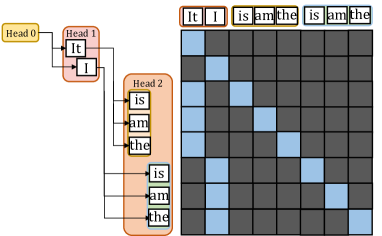</details> (a) Medusa Verification Tree. <details> <summary>x4.png Details</summary>  ### Visual Description \n ## Scatter Plot: Context Length vs. Value ### Overview The image presents a scatter plot visualizing the relationship between "Context Length" and an unnamed value, likely representing some form of performance metric. The plot is characterized by a distinct separation into two regions: a solid yellow region on the left and a purple region with scattered data points on the right. ### Components/Axes * **X-axis:** Labeled "Context Length". The scale ranges from approximately 0 to 64, with markings at 0 and 64. * **Y-axis:** A vertical axis with a scale ranging from approximately 0 to 64, with a marking at 64. No explicit label is provided. * **Data Points:** Scattered points in a light yellow/gold color. * **Background:** The plot is divided into two distinct background colors: a solid yellow region on the left side and a dark purple region on the right side. ### Detailed Analysis The plot shows a clear transition in data distribution. * **Left Region (Context Length < ~20):** The left side of the plot, spanning approximately Context Lengths from 0 to 20, is filled with a solid yellow color. This indicates a constant or undefined value for the Y-axis within this range. * **Right Region (Context Length > ~20):** The right side of the plot, spanning approximately Context Lengths from 20 to 64, displays scattered data points in light yellow/gold against a dark purple background. * **Trend:** The data points generally exhibit a downward trend. As Context Length increases, the value on the Y-axis tends to decrease. * **Data Points (Approximate):** * At Context Length ~20, the Y-axis value is approximately 60. * At Context Length ~32, the Y-axis value is approximately 40. * At Context Length ~48, the Y-axis value is approximately 20. * At Context Length ~64, the Y-axis value is approximately 0. * There is a noticeable "step-down" in the data around Context Length 20, where the Y-axis value drops sharply from the constant value in the yellow region to the scattered data points. ### Key Observations * The solid yellow region suggests a saturation or constant performance level for short context lengths. * The downward trend in the purple region indicates a diminishing return or decreasing performance as context length increases. * The sharp transition at approximately Context Length 20 suggests a critical point where the relationship between context length and the measured value changes significantly. ### Interpretation The plot likely illustrates the impact of context length on a model's performance, potentially related to memory usage, computational cost, or accuracy. The constant value in the yellow region suggests that for short context lengths, the model's performance is not significantly affected by increasing the context. However, beyond a certain context length (around 20), the performance begins to degrade, as indicated by the downward trend in the purple region. This could be due to factors such as increased computational complexity, vanishing gradients, or the model's inability to effectively utilize longer contexts. The sharp transition suggests a threshold beyond which the benefits of longer context lengths are outweighed by the associated costs. The data suggests that there is an optimal context length for this model, and exceeding that length leads to diminishing returns. 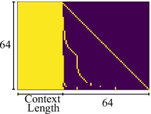</details> (b) Medusa [3]. <details> <summary>x5.png Details</summary>  ### Visual Description \n ## Heatmap: Context Length vs. 64 ### Overview The image presents a heatmap visualizing a relationship between "Context Length" on the x-axis and a value represented on the y-axis, ranging from approximately 0 to 64. The heatmap is colored with a gradient from yellow to purple, with yellow indicating higher values and purple indicating lower values. The heatmap is divided into two distinct regions: a solid yellow block on the left and a patterned region on the right. ### Components/Axes * **X-axis:** Labeled "Context Length". The scale ranges from approximately 0 to 64. * **Y-axis:** An unlabeled vertical axis, with a scale ranging from approximately 0 to 64. * **Color Scale:** Yellow represents higher values, transitioning to purple for lower values. * **Regions:** A solid yellow block on the left side and a patterned region with diagonal lines on the right side. ### Detailed Analysis The left side of the heatmap, representing lower "Context Length" values, is entirely yellow, indicating consistently high values (approximately 64) across the entire y-axis range. The right side of the heatmap displays a series of diagonal, dashed yellow lines against a purple background. These lines represent decreasing values as "Context Length" increases. * **Line 1 (Topmost):** Starts at approximately (Context Length = 0, Y = 64) and slopes downward, reaching approximately (Context Length = 64, Y = 0). * **Line 2:** Starts at approximately (Context Length = 0, Y = 56) and slopes downward, reaching approximately (Context Length = 64, Y = 8). * **Line 3:** Starts at approximately (Context Length = 0, Y = 48) and slopes downward, reaching approximately (Context Length = 64, Y = 16). * **Line 4:** Starts at approximately (Context Length = 0, Y = 40) and slopes downward, reaching approximately (Context Length = 64, Y = 24). * **Line 5:** Starts at approximately (Context Length = 0, Y = 32) and slopes downward, reaching approximately (Context Length = 64, Y = 32). * **Line 6:** Starts at approximately (Context Length = 0, Y = 24) and slopes downward, reaching approximately (Context Length = 64, Y = 40). * **Line 7:** Starts at approximately (Context Length = 0, Y = 16) and slopes downward, reaching approximately (Context Length = 64, Y = 48). * **Line 8:** Starts at approximately (Context Length = 0, Y = 8) and slopes downward, reaching approximately (Context Length = 64, Y = 56). * **Line 9 (Bottommost):** Starts at approximately (Context Length = 0, Y = 0) and slopes downward, reaching approximately (Context Length = 64, Y = 64). The lines are spaced approximately 8 units apart on the Y-axis. The lines are dashed, with segments of approximately 4 units in length, alternating with gaps of approximately 4 units. ### Key Observations The heatmap demonstrates a clear transition in value based on "Context Length". For low "Context Length" values, the value is consistently high. As "Context Length" increases, the value decreases linearly, as indicated by the diagonal lines. The spacing between the lines suggests a consistent decrement in the initial value for each line. ### Interpretation This heatmap likely represents the performance or relevance of a model or system as a function of "Context Length". The high yellow values at low "Context Length" suggest strong performance or high relevance when limited context is available. The decreasing values as "Context Length" increases indicate that performance or relevance degrades with increasing context. This could be due to several factors, such as the model being overwhelmed by too much information, or the context becoming noisy or irrelevant. The linear decrease suggests a predictable relationship between context length and performance. The dashed lines might represent discrete steps or intervals in the context length or performance metric. This visualization could be used to determine an optimal "Context Length" for maximizing performance or relevance. </details> (c) Draft model [2]. <details> <summary>x6.png Details</summary>  ### Visual Description \n ## Heatmap: Performance vs. Context Length ### Overview The image presents a heatmap visualizing a relationship between two variables: "Context Length" on the x-axis and an unspecified metric represented on the y-axis (ranging from approximately 0 to 64). The heatmap uses a color gradient from yellow to purple to indicate the value of the metric. A dotted line is overlaid on the heatmap, suggesting a trend or boundary. ### Components/Axes * **X-axis:** "Context Length", ranging from 0 to 64. * **Y-axis:** Unlabeled, but scaled from approximately 0 to 64. * **Color Scale:** Yellow represents lower values, transitioning to purple for higher values. * **Dotted Line:** A diagonal line with dotted segments, starting near the top-right corner and descending towards the bottom-right corner. ### Detailed Analysis The heatmap is divided into two primary regions: a large yellow area in the top-left and a purple area in the bottom-right. The transition between these regions is not abrupt but occurs along the dotted line. * **Yellow Region:** The top-left portion of the heatmap (approximately where Context Length is less than 40 and the Y-axis value is less than 40) is predominantly yellow, indicating lower values for the metric. * **Purple Region:** The bottom-right portion (approximately where Context Length is greater than 40 and the Y-axis value is greater than 40) is predominantly purple, indicating higher values for the metric. * **Dotted Line Trend:** The dotted line slopes downwards from the top-right to the bottom-right. It appears to define a boundary where the metric's value increases significantly. The line's position suggests that for a given context length, the metric's value is lower above the line and higher below it. The dotted line appears to intersect the following approximate coordinates: * (0, 64) * (16, 48) * (32, 32) * (48, 16) * (64, 0) ### Key Observations * The metric's value generally increases with increasing context length and the Y-axis value. * The dotted line represents a critical threshold or boundary. * The heatmap suggests a non-linear relationship between context length and the metric. ### Interpretation This heatmap likely represents the performance of a model or system as a function of context length and another parameter (represented by the Y-axis). The yellow region indicates good performance (low metric value), while the purple region indicates poor performance (high metric value). The dotted line could represent a point of diminishing returns or a threshold beyond which performance degrades rapidly. The diagonal nature of the dotted line suggests that the performance degradation is consistent across different context lengths. The model performs well when the context length and the Y-axis value are low, but as either increases, performance declines, especially when they both increase simultaneously. Without knowing what the Y-axis represents, it's difficult to provide a more specific interpretation. However, it could represent error rate, latency, or some other measure of performance. The data suggests that there is an optimal range for context length and the Y-axis value, and exceeding this range leads to a significant drop in performance. </details> (d) Lookahead [4]. 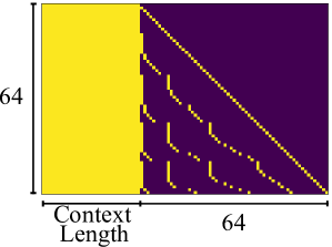Figure 3: Sparsity visualization of the $X=Q× K^{T}$ for speculative decoding approaches. Light yellow indicates points that require computation, while dark blue represents points that do not need computation. To overcome the sequential limitation, speculative decoding is introduced as an alternative. To achieve higher parallelism in decoding steps, it primarily employs the Predict-then-Verify mechanism, where predictions for multiple steps are made in parallel and then fallback to the longest validated prefix LLM inference. There are independent drafting [2, 19] and self-drafting [3, 20, 4] approaches. The independent drafting employs a smaller model with significantly reduced computation to generate predictions. The self-drafting make predictions through appending more heads or using Jacobi iteration. After drafting multiple candidates, these candidate tokens are combined together under a given pattern and put into the target model for verification. Notably, these self-drafting approaches combine the prediction and verification into a single step. For example, Medusa [3] predicts candidates for future token slots by appending additional heads at the tail of LLMs. In Figure 3(a), Head1 has two candidates and Head2 has three candidates. We aim to verify which combinations between these tokens can be accepted. Here the verification width in Figure 3(a) is 8 and only a subset of token correlations needs to be calculated in the attention module. Basically, we observe significant sparsity within the attention module when performing these speculative decoding approaches. Under a given pattern, a token needs to compute relationships only with certain tokens. This sparsity is typically handled as dense computation using the mask mechanism. As illustrated in Figure 3(b) 3(c) 3(d), here we present the sparsity visualization of $Q× K$ result matrix in three popular approaches, namely draft model [2], Medusa [3], and LookAhead [4]. Only the light yellow points represent computations worth performing, highlighting the significant sparsity in the right part. Softmax and $A× V$ operation exhibits the same sparsity pattern. 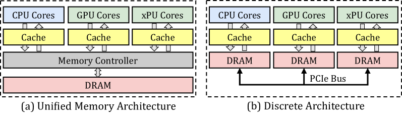II-D Unified Memory Architecture <details> <summary>x7.png Details</summary>  ### Visual Description \n ## Diagram: Memory Architecture Comparison ### Overview The image presents a comparison of two memory architectures: Unified Memory Architecture (a) and Discrete Architecture (b). Both diagrams illustrate the relationship between CPU Cores, GPU Cores, xPU Cores, Cache, Memory Controller, DRAM, and a PCIe Bus. The diagrams are presented side-by-side for direct comparison. ### Components/Axes The components present in both diagrams are: * **CPU Cores:** Represented by a light green rectangle. * **GPU Cores:** Represented by a light green rectangle. * **xPU Cores:** Represented by a light green rectangle. * **Cache:** Represented by a yellow rectangle. * **Memory Controller:** Represented by a grey rectangle. * **DRAM:** Represented by a pink rectangle. * **PCIe Bus:** Represented by a grey rectangle (only in diagram b). The diagrams are labeled as follows: * **(a) Unified Memory Architecture** * **(b) Discrete Architecture** Arrows indicate data flow between components. ### Detailed Analysis or Content Details **Diagram (a): Unified Memory Architecture** * CPU Cores, GPU Cores, and xPU Cores are positioned at the top of the diagram. * Each core type has an associated Cache layer directly below it. * The Cache layers are connected to a single Memory Controller via downward-pointing arrows. * The Memory Controller is connected to a single DRAM module via bidirectional arrows. * The overall structure suggests a shared memory space accessible by all core types. **Diagram (b): Discrete Architecture** * CPU Cores, GPU Cores, and xPU Cores are positioned at the top of the diagram, similar to diagram (a). * Each core type has an associated Cache layer directly below it. * Each Cache layer is connected to a separate DRAM module via downward-pointing arrows. * The DRAM modules are connected via a PCIe Bus. * The overall structure suggests separate memory spaces for each core type, connected through a PCIe bus. ### Key Observations The primary difference between the two architectures is the memory access pattern. The Unified Memory Architecture (a) utilizes a single, shared memory pool (DRAM) accessed through a Memory Controller. The Discrete Architecture (b) employs separate DRAM modules for each core type, connected via a PCIe Bus. This implies that the Unified Architecture may offer lower latency and higher bandwidth for data sharing between core types, while the Discrete Architecture may provide greater memory isolation and scalability. ### Interpretation The diagrams illustrate fundamental differences in how processing cores access memory. The Unified Memory Architecture aims to simplify memory management and improve data sharing, potentially at the cost of memory contention. The Discrete Architecture prioritizes memory isolation and scalability, potentially at the cost of increased latency and complexity due to the PCIe bus overhead. The choice between these architectures depends on the specific application requirements. For example, applications requiring frequent data exchange between CPU, GPU, and xPU cores might benefit from the Unified Architecture, while applications with independent memory access patterns might be better suited for the Discrete Architecture. The diagrams are conceptual and do not provide quantitative data on performance or capacity. They serve to visually represent the architectural differences and their potential implications. </details> Figure 4: The unified memory architecture and the discrete architecture. End-user devices [21, 9, 13, 14, 22, 23], such as consumer electronics and embedded systems, prioritize power efficiency, cost-effectiveness, and compact design, usually adopting the unified memory architecture. We show the unified memory architecture and discrete architecture in Figure 4. End-user devices typically adopt a unified DRAM architecture shared across multiple processing units, rather than discrete memory modules. This design eliminates explicit data transfer via PCIe bus and enables a zero-copy mechanism between processing units. While this significantly reduces data synchronization overhead, concurrent memory access still requires manual consistency management by the programmer. On the NVIDIA Jetson Xavier NX, memory page synchronization between processing units takes less than 0.1 milliseconds when accessing memory written by another unit. III Ghidorah Design III-A Overview <details> <summary>x8.png Details</summary>  ### Visual Description ## Diagram: Architecture-aware Profiling and Hetero-Core Model Parallelism ### Overview This diagram illustrates a two-phase process: Preprocessing Phase and Runtime Support, for architecture-aware profiling and hetero-core model parallelism. The diagram depicts data flow and component interactions involved in optimizing model execution across different processing units (CPU, GPU, NPU, XPU). It highlights the use of speculative decoding, partitioning strategies, and customized ARM SpMM for efficient model parallelism. ### Components/Axes The diagram is divided into two main sections, vertically stacked: "Preprocessing Phase" (top) and "Runtime Support" (bottom). Each section contains several components connected by arrows indicating data flow. * **Preprocessing Phase:** * Calibration dataset (represented as a cylinder) * LLM + Speculative Decoding (represented as a neural network) * CPU, GPU, NPU, XPU (represented as rectangular blocks) * Verification width & Tree * Parallelism- & Contention-aware Partitioning Strategy * Architecture-aware Profiling (central block with double-sided arrow) * **Runtime Support:** * Operator Placement (CPU, GPU, XPU - represented as colored circles) * Memory access reduction Computation affinity * Partitioning Guide * GPU Time, CPU Time, Synchronization (represented as stacked blocks) * Customized ARM SpMM * Hetero-Core Model Parallelism ### Detailed Analysis or Content Details **Preprocessing Phase:** 1. **Calibration dataset:** A cylindrical shape represents the input calibration dataset. 2. **LLM + Speculative Decoding:** A neural network diagram represents the Large Language Model (LLM) combined with speculative decoding. The network has input nodes labeled "It, I, As" and output nodes labeled "Difficult, is, not, difficult, a". 3. **Processing Units:** The diagram shows data flowing from the LLM to CPU, GPU, NPU, and XPU processing units. An Intel Core logo is present next to the CPU block. 4. **Partitioning Strategy:** The diagram indicates a "Parallelism- & Contention-aware Partitioning Strategy" and a "Speculative Strategy" are employed. 5. **Architecture-aware Profiling:** A central block labeled "Architecture-aware Profiling" connects the preprocessing phase to the runtime support phase. It has a double-sided arrow indicating bidirectional data flow. **Runtime Support:** 1. **Operator Placement:** Three colored circles represent operator placement on CPU (green), GPU (orange), and XPU (blue). 2. **Memory Access & Affinity:** A neural network diagram represents "Memory access reduction Computation affinity". 3. **Partitioning Guide:** A rectangular block labeled "Partitioning Guide" is shown. 4. **GPU/CPU Time & Synchronization:** Stacked blocks represent GPU Time, CPU Time, and Synchronization. The GPU block shows "PE PE PE PE" repeated, and the CPU block shows "core core". A dashed line with arrows indicates synchronization between the GPU and CPU. 5. **Customized ARM SpMM:** A rectangular block labeled "Customized ARM SpMM" is shown. 6. **Hetero-Core Model Parallelism:** A rectangular block labeled "Hetero-Core Model Parallelism" is shown. **Data Flow:** * Data flows from the Calibration dataset to the LLM + Speculative Decoding. * The LLM output is then distributed to the CPU, GPU, NPU, and XPU for processing. * The Architecture-aware Profiling block acts as a bridge between the preprocessing and runtime phases. * In the runtime phase, operators are placed on CPU, GPU, and XPU. * Memory access is optimized, and partitioning is guided. * GPU and CPU execution are synchronized. * The process culminates in Hetero-Core Model Parallelism utilizing Customized ARM SpMM. ### Key Observations * The diagram emphasizes the integration of different processing units (CPU, GPU, NPU, XPU) for model execution. * Speculative decoding and partitioning strategies are crucial components of the preprocessing phase. * The runtime support phase focuses on operator placement, memory access optimization, and synchronization. * The use of Customized ARM SpMM suggests a focus on efficient matrix multiplication for model parallelism. * The diagram is highly conceptual and does not provide specific numerical data. ### Interpretation The diagram illustrates a system designed to optimize the execution of large language models (LLMs) by leveraging the strengths of heterogeneous computing architectures. The preprocessing phase focuses on preparing the model and identifying optimal partitioning strategies, while the runtime support phase focuses on efficient execution and synchronization across different processing units. The architecture-aware profiling component plays a critical role in bridging the gap between model preparation and runtime execution. The emphasis on memory access reduction and customized ARM SpMM suggests a focus on minimizing data movement and maximizing computational throughput. The overall goal is to achieve high performance and scalability for LLM inference by effectively utilizing the available hardware resources. The diagram suggests a holistic approach to model parallelism, considering both computational and memory aspects. The inclusion of NPU and XPU indicates a move beyond traditional CPU/GPU-centric approaches to leverage specialized hardware accelerators. 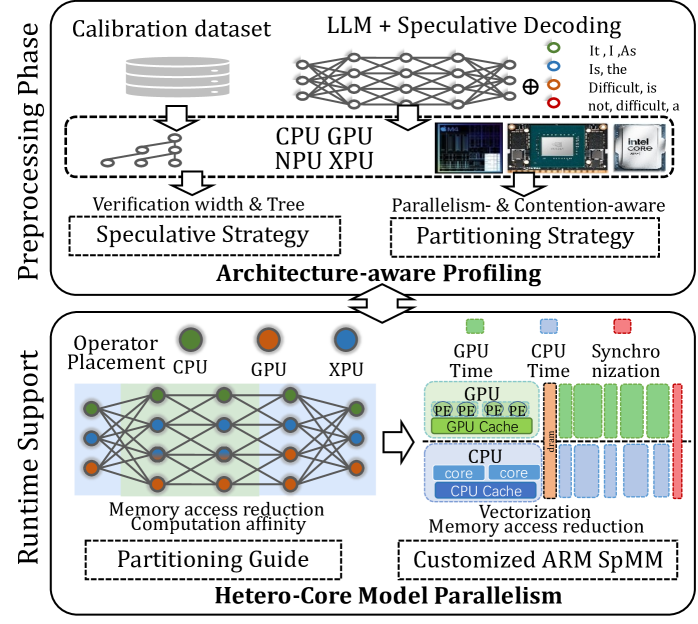</details> Figure 5: The overview of Ghidorah. Ghidorah is specifically designed for single-sample LLM generative task inference on end-user devices with a unified memory architecture. It primarily focuses on accelerating the dominant decoding phase. Since the decoding phase is constraint by the memory bandwidth, Ghidorah explores speculative decoding approaches to enhance parallelism and alleviate the memory bandwidth bottleneck. This manuscript takes the multi-head drafting approach, Medusa [3], as the default. Ghidorah distributes the speculative decoding workloads across all processing units and choose the optimal verification length in the end-user device to maximize the inference speed. Figure 5 illustrates the overview of Ghidorah. Leveraging the unified memory architecture of end-user devices and the computation pattern of speculative decoding, Ghidorah employs a novel hetero-core model parallelism (HCMP) architecture and the architecture-aware profiling (ARCA) approach. Functionally, the HCMP architecture focuses on providing runtime support, while the ARCA approach is primarily designed for the preprocessing phase. The HCMP architecture provides guidance for model partitioning and includes customized sparse matrix multiplication optimizations. Based on the runtime support, the ARCA approach provides the preprocessing phase that runs once before deployment. It performs an inference process using calibration data as input on multiple heterogeneous processing units in the end-user device. By comprehensively considering acceptance length, hardware parallelism, and resource contention, this phase formulates speculative and partitioning strategies to maximize performance. III-B Hetero-core Model Parallelism Architecture <details> <summary>x9.png Details</summary>  ### Visual Description \n ## Diagram: System Architecture for Distributed Attention ### Overview The image depicts a system architecture diagram for a distributed attention mechanism, likely within a machine learning model. The diagram illustrates the flow of data and computations across different processing units (GPU, DRAM, CPU) and through various layers (Linear, Attention). The diagram highlights data movement and processing steps, including matrix multiplications (denoted by the ⊗ symbol), attention calculations, and softmax operations. ### Components/Axes The diagram is structured into three main vertical sections: GPU, DRAM, and CPU, positioned from left to right. Each section contains multiple blocks representing layers or operations. Key components and labels include: * **GPU:** Contains "Linear Layer" and "Attention Module" blocks, with "cache\_V" and "cache\_K" within the Attention Module. "GPU Output" is indicated by a yellow dashed box. * **Dram:** Contains "Linear Layer" blocks. * **CPU:** Contains "Linear Layer" and "Attention Module" blocks, with "cache\_V" and "cache\_K" within the Attention Module. "CPU Output" is indicated by a red dashed box. * **Attention Module:** Contains blocks labeled "V", "K", and "Q", with a "T" superscript on V and K. A "Softmax" operation is present. * **Online Softmax Reduce:** A central block connecting the GPU and CPU attention modules. * **Linear Layers:** Multiple "Linear Layer" blocks are present after the "Online Softmax Reduce" block. * **Split Weights by Column:** A block indicating weight splitting. * **Split Each Head with Affinity:** A block indicating head splitting. * **Weight Matrices:** "WB", "WC", and "WD" are labeled within the "Split Each Head with Affinity" section. * **Data Flow:** Arrows indicate the direction of data flow between blocks. * **Matrix Multiplication:** The symbol "⊗" represents matrix multiplication. ### Detailed Analysis or Content Details The diagram shows a parallel processing architecture. 1. **GPU Side:** The GPU processes data through a Linear Layer, then an Attention Module. The Attention Module utilizes "cache\_V" and "cache\_K" for storing values and keys. The output of the Attention Module is then passed through a Softmax function. 2. **CPU Side:** The CPU mirrors the GPU's processing flow with a Linear Layer and Attention Module, also utilizing "cache\_V" and "cache\_K" and a Softmax function. 3. **Attention Calculation:** The Attention Module calculates attention weights using Query (Q), Key (K), and Value (V) matrices. The transpose of K (K^T) is used in the calculation. 4. **Online Softmax Reduce:** The outputs from the GPU and CPU Attention Modules are combined and processed by an "Online Softmax Reduce" operation. 5. **Subsequent Linear Layers:** The output of the "Online Softmax Reduce" is then passed through multiple Linear Layers. 6. **Weight Splitting:** The weights are split by column, and then each head is split with affinity. The resulting weights are labeled as "WB", "WC", and "WD". 7. **Output:** The final output is indicated by the "GPU Output" (yellow dashed box) and "CPU Output" (red dashed box). ### Key Observations * The architecture employs a parallel processing strategy, utilizing both GPU and CPU for attention calculations. * Caching mechanisms ("cache\_V", "cache\_K") are used within the Attention Modules on both the GPU and CPU. * The "Online Softmax Reduce" operation suggests a distributed softmax calculation. * Weight splitting and head splitting are employed to optimize the model's performance. * The diagram does not provide specific numerical values or data points. It is a conceptual representation of the architecture. ### Interpretation This diagram illustrates a distributed attention mechanism designed to leverage the computational resources of both GPUs and CPUs. The parallel processing approach aims to accelerate the attention calculation, which is a computationally intensive operation in many machine learning models, particularly in natural language processing. The use of caching suggests an attempt to reduce memory access latency and improve efficiency. The weight splitting and head splitting techniques are likely employed to reduce the model's memory footprint and improve scalability. The "Online Softmax Reduce" operation indicates a strategy for combining the attention weights calculated on the GPU and CPU in a distributed manner. The diagram suggests a sophisticated architecture optimized for performance and scalability in attention-based models. The diagram is a high-level overview and does not provide details on the specific implementation or optimization techniques used. It is a conceptual blueprint rather than a detailed specification. 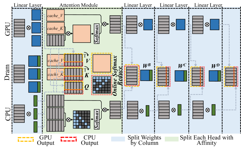</details> Figure 6: The illustration of Hetero-Core Model Parallelism. The HCMP architecture is designed for efficiently distributing speculative decoding workloads across multiple heterogeneous processing units organized in the unified memory architecture. Figure 6 illustrates the HCMP architecture by presenting an inference example conducted across two processing units, CPU and GPU. It shows the memory layout and computation processes separately. Instead of focusing on reducing inter-device communication, the HCMP architecture prioritizes minimizing memory access and exposing computation affinity across processing units. III-B 1 Linear Layer - Split weights by column The existing tensor parallelism approach [11] is designed to distribute workloads across multiple separate devices, requiring explicit inter-device communication to resolve data dependencies. Reducing the frequency of tensor synchronization can significantly improve parallel efficiency. Migrating this setup to end-user devices, for every two linear layers, the weights of the first layer are split by columns and those of the second layer by rows, thus requiring only a single all-reduce synchronization for the two layers. However, this all-reduce operation necessitates additional memory access. It must read activations generated by different processing units and write the combined results back. The HCMP architecture opts to split the weights of all linear layers by columns. As shown in Figure 6, the CPU and GPU receive the same input, multiply it by different columns of weights, and then write the outputs to their designated memory regions without enforcing consistency between them. This allows the result to be used in the next operation without any additional data access. III-B 2 Attention Module - Split each head with affinity The HCMP architecture is designed to exploit computation affinity across different processing units, taking into account the hybrid computational intensity inherent in speculative decoding. The existing tensor parallelism approach divides the computation of the attention module by heads, with each device responsible for processing different heads. However, since only the correlation between partial tokens requires to be verified in speculative decoding, there exists dense and sparse computation in each head of the attention module. As shown in Figure 6, each attention head can be divided into a dense part — primarily the multiplication with the KV cache — and a sparse part, which mainly involves multiplication with the newly generated key and value. The dense part will be prioritized for processing units with high parallelism, such as GPU, while the sparse part will be prioritized for processing units with low parallelism, such as CPU. To achieve load balance, each partition may optionally include a portion of the other part’s computation. As shown in Figure 3 (b)(c)(d), the left boundary of the sparse part tends to be denser and can be preferentially included in the dense part. Furthermore, inspired by Ring Attention [24] and FlashAttention [25], we introduce the online softmax technique to extend the span that can be computed continuously. As shown in Equation 1, the computation of $O=AV$ on one processing unit cannot begin until $X=QK^{T}$ on another processing unit is completed, as the softmax operation requires data from all processing units. With the online softmax technique [24, 25], each processing unit can have its own softmax operation, aligning their results by applying a scaling factor at the end of the attention module. This scaling operation can be fused with the reduce operation, introducing almost no overhead. III-B 3 Customized ARM SpMM Optimization <details> <summary>x10.png Details</summary>  ### Visual Description \n ## Diagram: Attention Mechanism Data Flow ### Overview The image depicts a diagram illustrating the data flow within an attention mechanism, likely within a neural network architecture. It shows a series of matrix operations and data transfers between "Cache" and "Register" memory locations. The diagram is arranged in two rows, each representing a stage of the attention calculation. ### Components/Axes The diagram consists of six labeled matrices: * **Q**: Located in the top-left, labeled "Cache". * **K^T**: Located in the top-center, labeled "Cache". * **QKT+mask**: Located in the top-right, labeled "Register". * **A**: Located in the bottom-left, labeled "Register". * **V**: Located in the bottom-center, labeled "Cache". * **O**: Located in the bottom-right, labeled "Register". Arrows indicate the direction of data flow. Multiplication symbols (x) denote matrix multiplication operations. The equals sign (=) indicates assignment or data transfer. ### Detailed Analysis or Content Details The diagram shows the following sequence of operations: 1. **Q and K^T Multiplication:** The matrix **Q** (orange and red squares) from "Cache" is multiplied by the transpose of matrix **K^T** (mostly white squares with some blue) from "Cache". The result is **QKT+mask** (grey squares with some white and black) and is stored in "Register". 2. **A and V Multiplication:** The matrix **A** (dark grey squares with some light grey) from "Register" is multiplied by the matrix **V** (yellow and orange squares) from "Cache". The result is **O** (purple and pink squares with some white) and is stored in "Register". The matrices are represented as grids of squares, with different colors indicating different values or data elements. The size of the matrices appears to be approximately 8x8, but the exact dimensions are not explicitly stated. The "mask" component in **QKT+mask** suggests an attention masking operation is being performed. ### Key Observations The diagram highlights the core steps of an attention mechanism: calculating attention weights (through Q and K) and applying those weights to values (V) to produce an output (O). The use of "Cache" and "Register" suggests these matrices are stored in different memory locations, potentially for efficiency or parallel processing. The masking operation is a key component of attention, allowing the model to focus on relevant parts of the input. ### Interpretation This diagram illustrates a simplified view of the attention mechanism, a crucial component in modern neural network architectures like Transformers. The attention mechanism allows the model to weigh the importance of different parts of the input sequence when making predictions. The "Q", "K", and "V" matrices represent queries, keys, and values, respectively. The multiplication of Q and K^T calculates attention weights, which are then used to weight the values (V) to produce the output (O). The mask is used to prevent the model from attending to certain parts of the input, such as padding tokens or future tokens in a sequence. The diagram suggests a computational process where intermediate results are stored in registers for efficient access. The use of Cache implies that these matrices are reused or updated over time, potentially for processing long sequences. The diagram does not provide specific numerical values or dimensions, but it effectively conveys the logical flow of data within the attention mechanism. 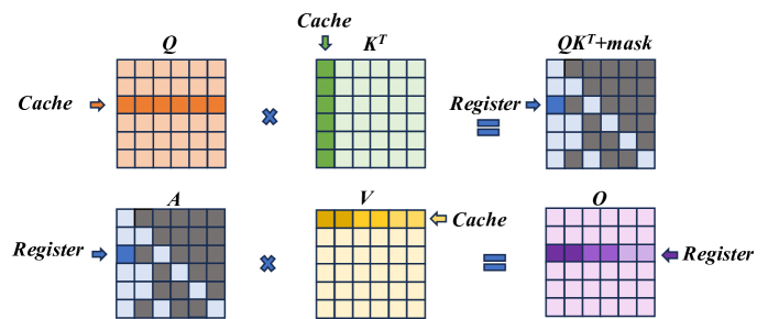</details> Figure 7: ARM SpMM Optimization. ARM CPUs are widely used in end-user devices due to their power efficiency feature, and we implement customized computation optimizations for sparse computations in the self-attention module, i.e. $QK^{T}$ and $AV$ . In details, knowing the token correlations to be verified, we follow the COO sparsity data format to generate the index before performing the inference. We optimize the sparse operation from two aspects, namely vectorization and memory access reduction. Figure 7 illustrates the optimization. In the $QK^{T}$ computation, the data access for both $Q$ and $K$ is in a row-wise way, thereby supporting continuous data access. Leveraging NEON instruction set of ARM, we enable the 128-bit long vector instructions to combine memory access in continuous FMA calculations. For its output matrix, each result value is stored in the register until the final result is fully accumulated, so as to reducing the load/store operations. In the $AV$ computation, we adjust the execution order to ensure continuous memory access to matrix $V$ . Instead of multiplying with each column of matrix $V$ , each non-zero element in the matrix $A[i,j]$ performs multiplication with row j of the matrix $V$ and then accumulates the result to the row i of the output matrix $O$ until the non-zero element in the same row finishes computing and finally gets row i of the output matrix. Also, since the capacity of registers is limited, we divide this process into blocks, only process partial elements from $V$ to $O$ , to enable storing elements in registers and reduce load/store operations. III-C Architecture-aware Profiling Approach The ARCA approach comprehensively considers the acceptance length, hardware parallelism and resource contention to finally generate the speculative strategy and the partitioning strategy. Initially, for a specific speculative decoding approach, we explore verification trees of all verification widths for the optimal acceptance lengths by combining accuracy-based estimation with brute-force search. Next, we determine the verification width and partitioning ratio for the final deployment, which is both parallelism- and contention-aware. III-C 1 Speculative Strategy Determination The speculative strategy in Ghidorah consists of both the verification width and the verification tree. The verification width is the computing budget in a single decoding step, and it is defined as the total number of tokens to be verified, while the verification tree determines the specific combinations of tokens to be verified. Both the verification width and verification tree influence the acceptance length. As the verification width increases, it becomes more likely to identify acceptable tokens; however, if the width is too large, the benefits for improving acceptance length becomes limited. Also, some specific verification routes are more likely to be accepted. For instance, the closer the head is to HEAD0, the easier its tokens are accepted. We design verification trees for different verification widths. <details> <summary>x11.png Details</summary>  ### Visual Description \n ## Diagram: Parsing Tree Visualization ### Overview The image depicts a parsing tree structure used in natural language processing, specifically illustrating a method for estimating a tree compared to a brute-force search space. The tree represents the possible syntactic structures for a sentence, starting from the root node "Since" and branching down to individual words. The diagram highlights the estimated tree in red and the full search space in light orange. ### Components/Axes The diagram is organized into four horizontal levels labeled "Head0", "Head1", "Head2", and "Head3". These represent different levels of syntactic abstraction. - **Head0:** Contains the root node "Since". - **Head1:** Contains the words "it", "is", and "there". - **Head2:** Contains the words "is", "am", "a" repeated multiple times. - **Head3:** Contains the words "time", "the", "time", "the", and a series of empty rectangles. The diagram also includes the following visual elements: - **Red Arrows:** Indicate the "Estimated Tree" path. - **Black Arrows:** Indicate "All Combinations" paths. - **Light Orange Rectangles:** Represent the "Brute-force search space". - **Dashed Blue Lines:** Separate the Head levels. ### Detailed Analysis or Content Details The tree structure begins with "Since" at Head0. From "Since", three branches extend to Head1: 1. "it" 2. "is" 3. "there" From "it", branches extend to Head2: 1. "is" 2. "am" 3. "a" From "is", branches extend to Head3: 1. "time" 2. "the time" 3. "a" From "am", branches extend to Head3: 1. "the time" From "a", branches extend to Head3: 1. "the" The remaining nodes at Head2 ("is", "am", "a" repeated) and Head3 are represented by empty rectangles, indicating a larger search space that is not part of the estimated tree. The number of empty rectangles at Head3 increases as the tree branches out. ### Key Observations - The estimated tree (red arrows) represents a significantly smaller subset of the total possible combinations (black arrows). - The brute-force search space (light orange rectangles) is much larger than the estimated tree, indicating the efficiency gain of the estimation method. - The tree structure demonstrates a hierarchical decomposition of the sentence, starting from the root and branching down to individual words. - The diagram visually emphasizes the trade-off between accuracy and computational cost in parsing. ### Interpretation This diagram illustrates a method for parsing natural language sentences by estimating a likely syntactic structure rather than exhaustively searching all possible combinations. The "Estimated Tree" represents a heuristic approach to reduce the computational complexity of parsing, while the "Brute-force search space" highlights the exponential growth of possibilities as the sentence length increases. The use of different colors and arrow types effectively conveys the relationship between the estimated tree and the full search space. The diagram suggests that the estimation method provides a practical solution for parsing complex sentences by focusing on the most probable syntactic structures. The empty rectangles at Head3 indicate that the model does not consider all possible word combinations, which could potentially lead to errors but also significantly improves efficiency. The diagram is a visual representation of a core concept in natural language processing: the trade-off between accuracy and computational cost in parsing. 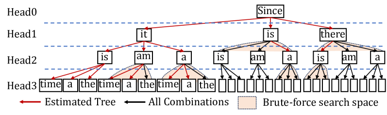</details> Figure 8: The verification tree determination with a verification width of 16. Figure 8 illustrates the tree design process with a verification width of 16 (nodes), involving candidate tokens generated from 4 heads of Medusa [3]. In details, we use a calibration dataset and generate the accuracies of the top predictions of different heads. Then, we estimate the accuracy of a candidate sequence by multiplying the accuracies of its related tokens. Then we can get the overall expected acceptance length by accumulating the expected acceptance length of different candidate sequences. Maximizing the acceptance length expectation, we can add nodes with the highest accuracies one by one until reaching the given verification length. As in Figure 8, the estimated tree is indicated by red lines. We further employ the brute-force search based on the estimated tree and compare their real acceptance lengths to determine the final tree. In Figure 8, we search leaf nodes and nodes in the same level. III-C 2 Parallelism-Aware Profiling The ARCA approach is parallelism-aware. Modern processing units leverage vectorization techniques to boost computational efficiency, leading to stepwise performance improvements in LLM inference latency as batch size increases, a phenomenon referred to as wave quantization [26] on NVIDIA hardware. Consequently, different processing units exhibit distinct performance sweet spots. In our preliminary experiments, we observe that setting candidate verification widths to powers of two, specifically 2, 4, 8, 16, 32, and 64, aligns well with the vectorization capabilities of these devices, resulting in more efficient execution. This observation can be explained as follows. The execution time of general matrix multiplication (GeMM) operations, including linear and attention, generally dominates LLM workloads. When applying model parallelism, the hidden state dimension is partitioned across processing units, while the token dimension (verification length) remains unchanged. As a result, the split GeMM operations executed on different processing units share the same token dimension and collectively span the hidden state dimension. Next, we determine their verification trees and check these speculative strategies with the runtime support. This determination process is contention-aware. III-C 3 Contention-Aware Profiling Although the partitioning guidance of the HCMP architecture will not increase the overall memory access within a single step of speculative decoding, the simultaneous access from different processing units will lead to resource contention problem. Since this contention affects different processing units at varying levels, it is difficult to determine the partitioning ratio. In this way, the ARCA approach initializes the partitioning strategy based on the individual execution times of different processing units and determines the final partitioning strategy for a given verification width through gradual adjustments. Besides, as the context (KV cache) length will impact the ratio of sparsity in the attention module, we additionally adjust the context length for the attention module to support its dynamic partitioning. IV Evaluation We implement a prototype system of Ghidorah in C/C++. We utilize the CUDA kernels from the highly optimized Transformer inference system FasterTransformer [27] for the GPU and rebuild the ARM CPU code based on CTranslated2 [28]. In this section, we evaluate Ghidorah from two aspects. 1) Verification Efficiency: we evaluate the acceptance length of our speculative strategies, and 2) Overall Performance: we compare the single-sample inference of Ghidorah with that of state-of-the-art approaches. Here we only focus on the dominant decoding phase of the LLM inference. IV-A Experimental Setup Model and Speculative Decoding. We evaluate Ghidorah with Vicuna-7B [29] and speculative decoding approach Medusa [3]. Medusa originally offers a 5-head version of Vicuna-7B and we design our own verification trees to evaluate the acceptance length under different verification widths. Vicuna-7B is a fine-tuned version from LLaMA-7B [30], which is a widely-recognized model architecture in the AI community. Datasets. We evaluate Ghidorah for the acceptance length across a broad spectrum of datasets, including: 1) MT-Bench [29]: a diverse collection of multi-turn questions, 2) GSM8K [31]: a set of mathematical problems, 3) HumanEval [32]: code completion and infilling tasks, and 4) MBPP [33]: instruction-based code generation. Node testbed. We use NVIDIA Jetson NX, which is a CPU-GPU edge device with unified memory architecture. It consists of an embedded 384-core Volta GPU and a 6-core ARM v8.2 CPU. We lock the GPU at 204MHz and the CPU at 1.9GHz to simulate end-user devices with more balanced capabilities of heterogeneous processing units. Specifically, we use g++ 7.5, cuda 10.2, arm performance library 24.10. Metrics. We use the acceptance length and decoding throughput as the evaluation metrics. The acceptance length refers to the average number of tokens that the target model accepts in a single decoding step. The decoding throughput is the number of tokens generated in a fixed interval. Baseline Methods. We compare Ghidorah with approaches: - Sequential: The sequential decoding approach running on the GPU, which is generally limited by the algorithmic parallelism. - Medusa: The Medusa decoding approach running on the GPU and it adopts our verification trees in given verification widths. - Medusa+EM (Medusa + E dgeNN [34] + M egatron) [11]: The Medusa decoding approach is distributed across the CPU and GPU using the partitioning guidance of the tensor parallelism from Megatron-LM. Additionally, we apply zero-copy optimization to reduce the synchronization overhead and determines the partitioning ratio based on the execution times of the processing units as in EdgeNN. IV-B Acceptance Length Evaluation TABLE I: Acceptance length under given verification widths. | Dataset GSM8K MBPP | MT-bench 1 1 | 1 1.76 1.78 | 1.72 2.43 2.54 | 2.28 2.69 2.89 | 2.59 3.08 3.27 | 2.93 3.34 3.55 | 3.19 3.56 3.74 | 3.34 | | --- | --- | --- | --- | --- | --- | --- | --- | --- | | Human-eval | 1 | 1.77 | 2.49 | 2.8 | 3.19 | 3.48 | 3.71 | | We present the acceptance lengths for various datasets under different verification widths. Notably, MT-bench is used as the calibration dataset for determining verification trees. Subsequently, these verification trees are applied to three other datasets to generate their acceptance lengths. Table I shows the acceptance length results. Larger verification widths generally result in longer acceptance lengths, while the benefit becomes weak as verification widths grow and come at the cost of significantly increased computational effort. Furthermore, we find that these verification trees exhibit strong generality, achieving even better acceptance lengths on GSM8K, MBPP, and Huamn-eval, when migrated from MT-Bench. This can be attributed to MT-Bench’s comprehensive nature, as it includes conversations across eight different types. <details> <summary>x12.png Details</summary>  ### Visual Description \n ## Bar Chart: Decoding Speed vs. 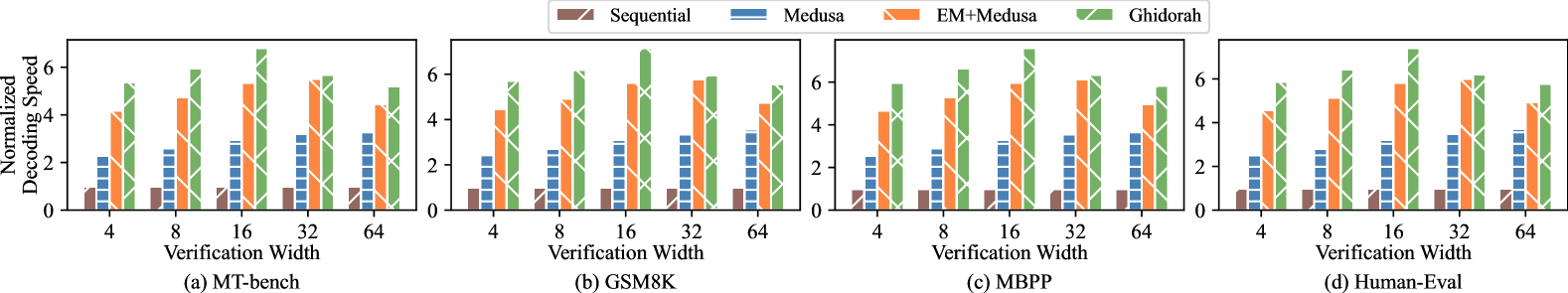Verification Width for Different Decoding Methods ### Overview The image presents four bar charts, each comparing the normalized decoding speed of four different decoding methods – Sequential, Medusa, EM+Medusa, and Ghidorah – across varying verification widths. Each chart represents a different dataset: (a) MT-bench, (b) GSM8K, (c) MBPP, and (d) Human-Eval. The y-axis represents the normalized decoding speed, while the x-axis represents the verification width. ### Components/Axes * **Y-axis Label:** "Normalized Decoding Speed" (Scale ranges from 0 to approximately 6) * **X-axis Label:** "Verification Width" (Markers: 4, 8, 16, 32, 64) * **Legend:** Located at the top-right of the image. * Sequential (Color: Light Red/Orange) * Medusa (Color: Blue) * EM+Medusa (Color: Light Green) * Ghidorah (Color: Light Purple) * **Sub-chart Labels:** * (a) MT-bench (Bottom-left) * (b) GSM8K (Bottom-center-left) * (c) MBPP (Bottom-center-right) * (d) Human-Eval (Bottom-right) ### Detailed Analysis or Content Details **Chart (a) MT-bench:** * **Sequential:** The bars generally hover around 5.0, with slight variations. Values are approximately: 4.8 (width 4), 5.0 (width 8), 5.2 (width 16), 5.1 (width 32), 5.3 (width 64). * **Medusa:** The bars are consistently low, around 1.0-1.5. Values are approximately: 1.2 (width 4), 1.3 (width 8), 1.4 (width 16), 1.3 (width 32), 1.5 (width 64). * **EM+Medusa:** Bars are around 2.0-2.5. Values are approximately: 2.1 (width 4), 2.3 (width 8), 2.4 (width 16), 2.2 (width 32), 2.5 (width 64). * **Ghidorah:** Bars are around 3.0-3.5. Values are approximately: 3.1 (width 4), 3.3 (width 8), 3.4 (width 16), 3.2 (width 32), 3.5 (width 64). **Chart (b) GSM8K:** * **Sequential:** Bars are around 5.5-6.0. Values are approximately: 5.6 (width 4), 5.8 (width 8), 5.9 (width 16), 5.7 (width 32), 6.0 (width 64). * **Medusa:** Bars are around 3.0-4.0. Values are approximately: 3.2 (width 4), 3.5 (width 8), 3.8 (width 16), 3.6 (width 32), 3.9 (width 64). * **EM+Medusa:** Bars are around 4.0-5.0. Values are approximately: 4.1 (width 4), 4.4 (width 8), 4.7 (width 16), 4.5 (width 32), 4.9 (width 64). * **Ghidorah:** Bars are around 5.0-5.5. Values are approximately: 5.1 (width 4), 5.3 (width 8), 5.4 (width 16), 5.2 (width 32), 5.5 (width 64). **Chart (c) MBPP:** * **Sequential:** Bars are around 5.5-6.0. Values are approximately: 5.6 (width 4), 5.8 (width 8), 5.9 (width 16), 5.7 (width 32), 6.0 (width 64). * **Medusa:** Bars are around 3.0-4.0. Values are approximately: 3.2 (width 4), 3.5 (width 8), 3.8 (width 16), 3.6 (width 32), 3.9 (width 64). * **EM+Medusa:** Bars are around 4.0-5.0. Values are approximately: 4.1 (width 4), 4.4 (width 8), 4.7 (width 16), 4.5 (width 32), 4.9 (width 64). * **Ghidorah:** Bars are around 5.0-5.5. Values are approximately: 5.1 (width 4), 5.3 (width 8), 5.4 (width 16), 5.2 (width 32), 5.5 (width 64). **Chart (d) Human-Eval:** * **Sequential:** Bars are around 5.0-5.5. Values are approximately: 5.1 (width 4), 5.3 (width 8), 5.4 (width 16), 5.2 (width 32), 5.5 (width 64). * **Medusa:** Bars are around 2.5-3.5. Values are approximately: 2.6 (width 4), 2.9 (width 8), 3.2 (width 16), 3.0 (width 32), 3.4 (width 64). * **EM+Medusa:** Bars are around 3.5-4.5. Values are approximately: 3.6 (width 4), 3.9 (width 8), 4.2 (width 16), 3.8 (width 32), 4.4 (width 64). * **Ghidorah:** Bars are around 4.5-5.0. Values are approximately: 4.6 (width 4), 4.8 (width 8), 4.9 (width 16), 4.7 (width 32), 5.0 (width 64). ### Key Observations * Sequential consistently demonstrates the highest decoding speed across all datasets. * Medusa consistently exhibits the lowest decoding speed. * EM+Medusa and Ghidorah fall between Sequential and Medusa in terms of decoding speed. * For all methods, decoding speed generally increases with increasing verification width, but the increase appears to plateau at higher widths (32 and 64). * The differences in decoding speed between methods are more pronounced in the MT-bench dataset compared to the others. ### Interpretation The data suggests that the Sequential decoding method is the most efficient in terms of decoding speed for all tested datasets. The addition of EM to Medusa (EM+Medusa) and the use of Ghidorah improve decoding speed compared to Medusa alone, but they do not reach the performance of Sequential. The verification width has a positive correlation with decoding speed, indicating that increasing the verification process enhances performance, but the gains diminish at higher widths. The varying performance across datasets suggests that the effectiveness of each decoding method is dependent on the specific characteristics of the data being processed. The relatively small differences in performance between verification widths of 32 and 64 suggest that there may be a point of diminishing returns in increasing the verification process. This information is valuable for optimizing decoding strategies in various natural language processing tasks. </details> Figure 9: The overall performance under different verification widths. IV-C Overall Performance Evaluation This section compares the decoding throughput of Ghidorah against that of baseline methods with different verification widths from 4 to 64. We select a context length (KV cache length) of approximately 256. Figure 9 shows the normalized results. In all cases shown in Figure 9, Ghidorah presents significant speedup in the decoding throughput. Especially when the verification width is 16, Ghidorah’s speedup can reach up to 7.6 $×$ compared with the sequential decoding. The impressive performance improvement of Ghidorah can be attributed to two main factors: First, the increased acceptance length enabled by speculative decoding. Since the sequential decoding approach is memory-bandwidth-bound, its execution time is similar to that of Medusa, and the acceptance length is fixed at 1. However, the Medusa method generates multiple tokens in a single step and requires the similar execution time; specifically, as the verification width increases, the acceptance length of Medusa also grows. Second, the collaborative operation of multiple heterogeneous processing units can better conduct the Medusa decoding workload. When comparing Medusa, Medusa+EM, and Ghidorah, we find that utilizing heterogeneous processing unit yields a better acceleration effect than merely running Medusa on the GPU. Taking MBPP dataset as the instance, Ghidorah achieves an average speedup of 2.06 $×$ compared to running Medusa solely on the GPU, and an average speedup of 1.20 $×$ compared to Medusa+EM. The improvement over Medusa+EM is attributed to reduced memory access and improved computing affinity. Longer acceptance lengths do not always result in better throughput, making it essential for the ARCA approach to balance the algorithmic parallelism with hardware capabilities. As shown in Figure 9, Medusa and Ghidorah achieve their best throughput results at verification width of 64 and 16 respectively. This is because CPU and GPU have different sweet spots. The GPU maintains a similar execution time from 4 to 64 verification width and achieves a longer acceptance length at verification width of 64, while the CPU can only maintain a similar execution time from 4 to 16 verification width. Since increasing verification width from 16 to 64 results in only 0.47 increase in the acceptance length, Ghidorah achieves the optimal throughput at a verification width of 16. 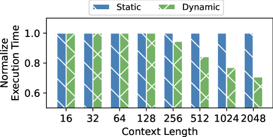IV-D Dynamic Partitioning and Sparse Optimization <details> <summary>x13.png Details</summary>  ### Visual Description \n ## Bar Chart: Normalized Execution Time vs. Context Length ### Overview The image presents a bar chart comparing the normalized execution time of "Static" and "Dynamic" methods across varying context lengths. The chart displays execution time on the y-axis and context length on the x-axis. Each context length has two bars representing the execution time for each method. ### Components/Axes * **X-axis Title:** "Context Length" * **X-axis Markers:** 16, 32, 64, 128, 256, 512, 1024, 2048 * **Y-axis Title:** "Normalized Execution Time" * **Y-axis Scale:** 0.6 to 1.0, with increments of approximately 0.02. * **Legend:** Located at the top-right of the chart. * "Static" - represented by a solid blue color. * "Dynamic" - represented by a light green color with diagonal stripes. ### Detailed Analysis The chart consists of paired bars for each context length. * **Context Length 16:** * Static: Approximately 0.98 * Dynamic: Approximately 0.98 * **Context Length 32:** * Static: Approximately 0.98 * Dynamic: Approximately 0.98 * **Context Length 64:** * Static: Approximately 0.98 * Dynamic: Approximately 0.98 * **Context Length 128:** * Static: Approximately 0.98 * Dynamic: Approximately 0.98 * **Context Length 256:** * Static: Approximately 0.96 * Dynamic: Approximately 0.96 * **Context Length 512:** * Static: Approximately 0.98 * Dynamic: Approximately 0.85 * **Context Length 1024:** * Static: Approximately 1.00 * Dynamic: Approximately 0.78 * **Context Length 2048:** * Static: Approximately 1.00 * Dynamic: Approximately 0.68 **Trends:** * For context lengths of 16, 32, 64, and 128, the execution times for both "Static" and "Dynamic" methods are nearly identical and remain around 0.98. * As the context length increases beyond 256, the "Dynamic" method begins to show a decreasing trend in normalized execution time, while the "Static" method remains relatively stable around 1.00. * The difference in execution time between the two methods becomes more pronounced at context lengths of 1024 and 2048. ### Key Observations * The "Dynamic" method exhibits a significant performance improvement (lower normalized execution time) compared to the "Static" method at larger context lengths (1024 and 2048). * For smaller context lengths, there is minimal difference in performance between the two methods. * The "Static" method's execution time remains consistently high across all context lengths. ### Interpretation The data suggests that the "Dynamic" method scales better with increasing context length than the "Static" method. At smaller context lengths, the overhead of the "Dynamic" method may be comparable to the "Static" method, resulting in similar performance. However, as the context length grows, the "Dynamic" method's ability to adapt or optimize its execution leads to a substantial reduction in execution time. This could indicate that the "Dynamic" method is more efficient in handling larger amounts of data or more complex computations associated with longer contexts. The consistent high execution time of the "Static" method suggests it may not be optimized for larger context lengths, or that its computational complexity increases linearly with context length. The chart highlights a trade-off: for small contexts, the methods are comparable, but for large contexts, the "Dynamic" method is clearly superior. </details> (a) The attention module performance. 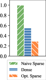<details> <summary>x14.png Details</summary>  ### Visual Description \n ## Bar Chart: Performance Comparison ### Overview This image presents a bar chart comparing the performance of three different methods: "Naive Sparse", "Dense", and "Opt. Sparse". The performance is represented on the y-axis, ranging from 0.0 to 1.0. The chart uses different colored bars to represent each method. ### Components/Axes * **Y-axis:** Represents the performance metric, scaled from 0.0 to 1.0 with increments of 0.2. * **X-axis:** Categorical axis representing the three methods: "Naive Sparse", "Dense", and "Opt. Sparse". There are no explicit labels on the x-axis, only implied categories based on the bar positions. * **Legend:** Located at the bottom-left of the chart. * Green striped bar: "Naive Sparse" * Blue bar: "Dense" * Orange striped bar: "Opt. Sparse" ### Detailed Analysis * **Naive Sparse:** The green striped bar reaches approximately 0.98 on the y-axis. This indicates a very high performance value for the "Naive Sparse" method. * **Dense:** The blue bar reaches approximately 0.58 on the y-axis. This suggests a moderate performance value for the "Dense" method. * **Opt. Sparse:** The orange striped bar reaches approximately 0.32 on the y-axis. This indicates a relatively lower performance value for the "Opt. Sparse" method. ### Key Observations The "Naive Sparse" method significantly outperforms both the "Dense" and "Opt. Sparse" methods. The "Dense" method performs better than the "Opt. Sparse" method, but the difference is less pronounced than the difference between "Naive Sparse" and the other two. ### Interpretation The data suggests that the "Naive Sparse" method is the most effective approach among the three tested, achieving a performance close to 1.0. The "Dense" method offers a moderate level of performance, while the "Opt. Sparse" method appears to be the least effective. This could indicate that the optimization in "Opt. Sparse" is not beneficial for this particular task or dataset, or that the "Naive Sparse" approach is inherently well-suited to the problem. Further investigation would be needed to understand the reasons behind these performance differences. The chart provides a clear visual comparison of the relative performance of these three methods, allowing for a quick assessment of their suitability for a given application. </details> (b) ARM Optim. Figure 10: Performance of Sparse Optimization This section presents the effectiveness of the dynamic partitioning and the sparsity optimization. Since the dynamic partitioning merely impact the attention module, Figure 10(a) represents the attention module performance with a verification length of 64. Notably, the attention module becomes dominant in the Transformer model as the context length increases. Static refers to that all sparse computations are processed on the CPU and all dense computations are processed on the GPU. Dynamic indicates that sparse computations are primarily handled by the CPU, while dense computations are primarily handled by the GPU, with dynamic partitioning guided by profiling results. Dynamic partitioning demonstrates obvious improvements when dealing with large context lengths. Figure 10(b) illustrates the performance of the sparse component executed using three different strategies: a naive sparse implementation, our optimized sparse implementation, and the dense implementation that treats the sparse computation as dense. The execution time of optimized sparse implementation exceeds naive sparse and dense implementations by 3.49 $×$ and 1.90 $×$ respectively. Also, if we do not optimize the sparse computation, the naive sparse execution cannot outperform the dense one. V Related Work Collaborative Execution of Transformer. Tensor Parallelism [1] and Pipeline Parallelism [35] effectively addresses memory limitations by accumulating memory from more devices, gaining widespread adoption in inference tasks within datacenters. They are also used in end-user environments. Galaxy [12] hides communication into computation in the tensor parallelism approach for edge devices, while DeTransformer [36] fundamentally mitigates data dependency by decoupling the original model. Petals [37] utilizes pipeline parallelism to distribute LLM inference across geographically distributed end-user devices. Integrated CPU-GPU Scheduling and Execution. There has been a large amount of prior work focusing on improving the device utilization on integrated CPU-GPU architecture. CoDL [5] and EdgeNN [34] perform collaborative convolutional neural network inference on mobile CPU and GPU with unified memory architecture. Asymo [38] schedules workloads based on the computing power of asymmetric mobile CPU cores to achieve higher throughput. Pipe-It [7] achieves higher throughput by organizing ARM big.Little cores in a pipelined manner. However, none of these approaches are designed for Transformer-based models. Speculative Decoding System. Speculative Decoding represents an innovative paradigm designed to accelerate LLM inference. Existing LLM inference systems [10] start to integrate speculative decoding approaches and they treat them as ordinary LLM inference with a large batch size. Sequoia [39] explores ultra-wide verification width for advanced hardware in cloud. LLMCad [40] adopts the independent drafting speculative decoding approach to accommodate memory-constrained devices. It utilizes a smaller model to generate drafts, thereby reducing data loading time for the larger model. VI Conclusion Ghidorah focuses on deploying LLM inference on end-user devices with the unified memory architecture. To fully exploit the hardware capability, Ghidorah leverages speculative decoding approaches to enhance the algorithmic parallelism and then distributes this novel workload across multiple heterogeneous processing units. With the help of the HCMP architecture and ARCA approach, it can achieve up to 7.6 $×$ speedup in the dominant decoding phase. In the future, Ghidorah will be open-sourced and extended to support more speculative decoding approaches and a wider range of end-user devices. References - [1] W. Kwon, Z. Li, S. Zhuang, Y. Sheng, L. Zheng, C. H. Yu, J. Gonzalez, H. Zhang, and I. Stoica, “Efficient memory management for large language model serving with pagedattention,” in Proceedings of the 29th Symposium on Operating Systems Principles, 2023, pp. 611–626. - [2] X. Miao, G. Oliaro, Z. Zhang, X. Cheng, Z. Wang, Z. Zhang, R. Y. Y. Wong, A. Zhu, L. Yang, X. Shi et al., “Specinfer: Accelerating large language model serving with tree-based speculative inference and verification,” in Proceedings of the 29th ACM International Conference on Architectural Support for Programming Languages and Operating Systems, Volume 3, 2024, pp. 932–949. - [3] T. Cai, Y. Li, Z. Geng, H. Peng, J. D. Lee, D. Chen, and T. Dao, “Medusa: Simple llm inference acceleration framework with multiple decoding heads,” arXiv preprint arXiv:2401.10774, 2024. - [4] Y. Fu, P. Bailis, I. Stoica, and H. Zhang, “Break the sequential dependency of LLM inference using lookahead decoding,” in Forty-first International Conference on Machine Learning, ICML 2024, Vienna, Austria, July 21-27, 2024. OpenReview.net, 2024. [Online]. Available: https://openreview.net/forum?id=eDjvSFOkXw - [5] F. Jia, D. Zhang, T. Cao, S. Jiang, Y. Liu, J. Ren, and Y. Zhang, “Codl: efficient CPU-GPU co-execution for deep learning inference on mobile devices,” in MobiSys ’22: The 20th Annual International Conference on Mobile Systems, Applications and Services, Portland, Oregon, 27 June 2022 - 1 July 2022, N. Bulusu, E. Aryafar, A. Balasubramanian, and J. Song, Eds. ACM, 2022, pp. 209–221. [Online]. Available: https://doi.org/10.1145/3498361.3538932 - [6] C. Zhang, F. Zhang, K. Chen, M. Chen, B. He, and X. Du, “Edgenn: Efficient neural network inference for cpu-gpu integrated edge devices,” in 2023 IEEE 39th International Conference on Data Engineering (ICDE). IEEE, 2023, pp. 1193–1207. - [7] S. Wang, G. Ananthanarayanan, Y. Zeng, N. Goel, A. Pathania, and T. Mitra, “High-throughput cnn inference on embedded arm big. little multicore processors,” IEEE Transactions on Computer-Aided Design of Integrated Circuits and Systems, vol. 39, no. 10, pp. 2254–2267, 2019. - [8] Y. Cho, P. Jiyeon, N. Florian, J. Changyeon, T. R. Gross, and B. Egger, “Dopia: online parallelism management for integrated cpu/gpu architectures,” in Proceedings of the 27th ACM SIGPLAN Symposium on Principles and Practice of Parallel Programming, 2022, pp. 32–45. - [9] “Apple m4,” https://en.wikipedia.org/wiki/Apple_M4, 2024. - [10] “vllm github,” https://github.com/vllm-project/vllm, 2024. - [11] M. Shoeybi, M. Patwary, R. Puri, P. LeGresley, J. Casper, and B. Catanzaro, “Megatron-lm: Training multi-billion parameter language models using model parallelism,” arXiv preprint arXiv:1909.08053, 2019. - [12] S. Ye, J. Du, L. Zeng, W. Ou, X. Chu, Y. Lu, and X. Chen, “Galaxy: A resource-efficient collaborative edge ai system for in-situ transformer inference,” arXiv preprint arXiv:2405.17245, 2024. - [13] “Intel core ultra processor family,” https://www.intel.com/content/www/us/en/products/details/processors/core-ultra.html, 2024. - [14] “Meet jetson, the platform for ai at the edge,” https://developer.nvidia.com/embedded-computing, 2024. - [15] M. Li, D. G. Andersen, A. J. Smola, and K. Yu, “Communication efficient distributed machine learning with the parameter server,” Advances in Neural Information Processing Systems, vol. 27, 2014. - [16] S. A. Jacobs, M. Tanaka, C. Zhang, M. Zhang, S. L. Song, S. Rajbhandari, and Y. He, “Deepspeed ulysses: System optimizations for enabling training of extreme long sequence transformer models,” 2023. [Online]. Available: https://arxiv.org/abs/2309.14509 - [17] F. Jia, D. Zhang, T. Cao, S. Jiang, Y. Liu, J. Ren, and Y. Zhang, “Codl: efficient cpu-gpu co-execution for deep learning inference on mobile devices.” in MobiSys, vol. 22, 2022, pp. 209–221. - [18] A. Vaswani, “Attention is all you need,” Advances in Neural Information Processing Systems, 2017. - [19] Y. Zhou, K. Lyu, A. S. Rawat, A. K. Menon, A. Rostamizadeh, S. Kumar, J.-F. Kagy, and R. Agarwal, “Distillspec: Improving speculative decoding via knowledge distillation,” arXiv preprint arXiv:2310.08461, 2023. - [20] Y. Li, F. Wei, C. Zhang, and H. Zhang, “EAGLE: speculative sampling requires rethinking feature uncertainty,” in Forty-first International Conference on Machine Learning, ICML 2024, Vienna, Austria, July 21-27, 2024. OpenReview.net, 2024. [Online]. Available: https://openreview.net/forum?id=1NdN7eXyb4 - [21] “Apple a17,” https://en.wikipedia.org/wiki/Apple_A17, 2024. - [22] “Amd reveals next-gen desktop processors for extreme pc gaming and creator performance,” https://www.amd.com/en/newsroom/press-releases, 2024. - [23] “Qualcomm snapdragon,” https://en.wikipedia.org/wiki/Qualcomm_Snapdragon, 2024. - [24] H. Liu et al., “Ring attention with blockwise transformers for near-infinite context,” arXiv preprint arXiv:2310.01889, 2023. - [25] T. Dao, D. Fu, S. Ermon, A. Rudra, and C. Ré, “Flashattention: Fast and memory-efficient exact attention with io-awareness,” Advances in Neural Information Processing Systems, vol. 35, pp. 16 344–16 359, 2022. - [26] “Wave quantization,” https://docs.nvidia.com/deeplearning/performance/dl-performance-matrix-multiplication/index.html#wave-quant, 2024. - [27] Nvidia, “Nvidia fastertransformer: Transformer related optimization, including bert, gpt,” in Github, 2023. - [28] “Ctranslate2,” https://github.com/OpenNMT/CTranslate2, 2024. - [29] L. Zheng, W.-L. Chiang, Y. Sheng, S. Zhuang, Z. Wu, Y. Zhuang, Z. Lin, Z. Li, D. Li, E. Xing et al., “Judging llm-as-a-judge with mt-bench and chatbot arena,” Advances in Neural Information Processing Systems, vol. 36, pp. 46 595–46 623, 2023. - [30] H. Touvron et al., “Llama: Open and efficient foundation language models,” 2023. [Online]. Available: https://arxiv.org/abs/2302.13971 - [31] K. Cobbe, V. Kosaraju, M. Bavarian, M. Chen, H. Jun, L. Kaiser, M. Plappert, J. Tworek, J. Hilton, R. Nakano et al., “Training verifiers to solve math word problems,” arXiv preprint arXiv:2110.14168, 2021. - [32] M. Chen, J. Tworek, et al., “Evaluating large language models trained on code,” arXiv preprint arXiv:2107.03374, 2021. - [33] J. Austin, A. Odena, M. Nye, M. Bosma, H. Michalewski, D. Dohan, E. Jiang, C. Cai, M. Terry, Q. Le et al., “Program synthesis with large language models,” arXiv preprint arXiv:2108.07732, 2021. - [34] C. Zhang, F. Zhang, K. Chen, M. Chen, B. He, and X. Du, “Edgenn: Efficient neural network inference for CPU-GPU integrated edge devices,” in 39th IEEE International Conference on Data Engineering, ICDE 2023, Anaheim, CA, USA, April 3-7, 2023. IEEE, 2023, pp. 1193–1207. [Online]. Available: https://doi.org/10.1109/ICDE55515.2023.00096 - [35] A. Agrawal et al., “Taming $\{$ Throughput-Latency $\}$ tradeoff in $\{$ LLM $\}$ inference with $\{$ Sarathi-Serve $\}$ ,” in 18th USENIX Symposium on Operating Systems Design and Implementation (OSDI 24), 2024, pp. 117–134. - [36] Y. Wei, S. Ye, J. Jiang, X. Chen, D. Huang, J. Du, and Y. Lu, “Communication-efficient model parallelism for distributed in-situ transformer inference,” in 2024 Design, Automation & Test in Europe Conference & Exhibition (DATE). IEEE, 2024, pp. 1–6. - [37] A. Borzunov, D. Baranchuk, T. Dettmers, M. Ryabinin, Y. Belkada, A. Chumachenko, P. Samygin, and C. Raffel, “Petals: Collaborative inference and fine-tuning of large models,” arXiv preprint arXiv:2209.01188, 2022. - [38] M. Wang, S. Ding, T. Cao, Y. Liu, and F. Xu, “Asymo: scalable and efficient deep-learning inference on asymmetric mobile cpus,” in ACM MobiCom ’21: The 27th Annual International Conference on Mobile Computing and Networking, New Orleans, Louisiana, USA, October 25-29, 2021. ACM, 2021, pp. 215–228. [Online]. Available: https://doi.org/10.1145/3447993.3448625 - [39] Z. Chen, A. May, R. Svirschevski, Y. Huang, M. Ryabinin, Z. Jia, and B. Chen, “Sequoia: Scalable, robust, and hardware-aware speculative decoding,” arXiv preprint arXiv:2402.12374, 2024. - [40] D. Xu, W. Yin, X. Jin, Y. Zhang, S. Wei, M. Xu, and X. Liu, “Llmcad: Fast and scalable on-device large language model inference,” CoRR, vol. abs/2309.04255, 2023. [Online]. Available: https://doi.org/10.48550/arXiv.2309.04255