2505.23219

# Ghidorah: Fast LLM Inference on Edge with Speculative Decoding and Hetero-Core Parallelism ## Abstract In-situ LLM inference on end-user devices has gained significant interest due to its privacy benefits and reduced dependency on external infrastructure. However, as the decoding process is memory-bandwidth-bound, the diverse processing units in modern end-user devices cannot be fully exploited, resulting in slow LLM inference. This paper presents Ghidorah, a LLM inference system for end-user devices with the unified memory architecture. The key idea of Ghidorah can be summarized in two steps: 1) leveraging speculative decoding approaches to enhance parallelism, and 2) ingeniously distributing workloads across multiple heterogeneous processing units to maximize computing power utilization. Ghidorah includes the hetero-core model parallelism (HCMP) architecture and the architecture-aware profiling (ARCA) approach. The HCMP architecture guides partitioning by leveraging the unified memory design of end-user devices and adapting to the hybrid computational demands of speculative decoding. The ARCA approach is used to determine the optimal speculative strategy and partitioning strategy, balancing acceptance rate with parallel capability to maximize the speedup. Additionally, we optimize sparse computation on ARM CPUs. Experimental results show that Ghidorah can achieve up to 7.6 $\times$ speedup in the dominant LLM decoding phase compared to the sequential decoding approach in NVIDIA Jetson NX. Index Terms: Edge Intelligence, LLM Inference, Speculative Decoding, Unified Memory Architecture footnotetext: Jinhui Wei and Ye Huang contributed equally to this work and are considered co-first authors. Yuhui Zhou participated in this work as a research intern at Sun Yat-sen University. * Corresponding author: Jiangsu Du (dujiangsu@mail.sysu.edu.cn). ## I Introduction Deploying large language models (LLMs) directly on end-user devices, such as mobile phones and laptops, is highly attractive. In-situ inference can eliminate data privacy concerns and reduce reliance on external infrastructures, thereby boosting intelligence and autonomy. However, achieving fast LLM inference remains a significant challenge, constrained by both algorithmic parallelism and hardware capability. To begin with, end-user devices typically process only a single request at a moment and the traditional decoding approach, shown in Figure 1, generates tokens sequentially, one at a time. With the KV cache technique [1], the dominant decoding phase of the LLM inference has very limited parallelism, while requiring loading all the model weights in each iteration. Thus, the limited parallelism and memory-bandwidth-bound nature prevent the full utilization of modern hardware. Alternatively, the speculative decoding approach [2, 3, 4] takes a draft-then-verify decoding process. In each decoding step, speculative decoding first drafts multiple tokens as predictions for future steps and then verifies in parallel whether to accept the drafted tokens. It can parallelize the inherently sequential process, showing strong potential to accelerate token generation rates by trading off compute for bandwidth. After enhancing the algorithmic parallelism, the LLM inference starts to be blocked by the limited hardware capability of end user devices. To fully leverage the capabilities of end-user devices, it is promising to distribute workloads across heterogeneous processing units [5, 6, 7, 8]. For instance, the GPU of Apple M4 [9] Pro has 17.04 TFLOPs FP16 performance, while its CPU has around 38 TFlops FP16 performance. However, existing systems [10, 3] do not align with the computing pattern of speculative decoding and the unified memory architecture of end-user devices, resulting in inefficiency. <details> <summary>x1.png Details</summary>  ### Visual Description ## Diagram: Transformer Model Inference Process (Prefill and Decode Phases) ### Overview The image is a technical diagram illustrating the two-phase inference process of a Transformer-based language model. It visually separates the initial processing of an input prompt ("prefill") from the subsequent autoregressive generation of output tokens ("decode"). The diagram uses a combination of labeled boxes, arrows, and dashed lines to show data flow and component relationships. ### Components/Axes The diagram is divided into two primary regions by a vertical dashed line: 1. **Left Region (Prefill Phase):** Labeled "prefill" at the top. 2. **Right Region (Decode Phase):** Labeled "decode" at the top. **Central Component:** * A large, horizontal, yellow rectangle labeled **"Transformer Model"** spans both phases. * Inside this rectangle, on the left (prefill side), are four small, empty, peach-colored squares arranged horizontally. * On the right (decode side), there are two individual peach-colored squares and a final block labeled **"kv cache"**. **Input (Bottom):** * A gray bar labeled **"prompt"** at the bottom left. * The prompt is segmented into four discrete tokens: **"The"**, **"color"**, **"of"**, **"dog"**. * Arrows point upward from each prompt token into the "Transformer Model" rectangle. **Output (Top):** * A sequence of green boxes representing generated tokens, positioned above the "Transformer Model". * The sequence is: **"can"**, **"vary"**, **"widely"**, **"/EoS/"** (End of Sequence token). * Arrows point upward from the model to each output token. * Curved arrows connect the output tokens in sequence: from "can" to "vary", from "vary" to "widely", and from "widely" to "/EoS/". **Data Flow Arrows:** * **Prefill Flow:** Straight arrows from the "prompt" tokens up into the model. * **Decode Flow:** A more complex, cyclical flow is shown: 1. An arrow from the model points up to the first output token, **"can"**. 2. A curved arrow loops from the **"can"** output token back down and into the model on the decode side. 3. This pattern repeats: an arrow from the model points up to **"vary"**, which then loops back into the model. 4. The same occurs for **"widely"**. 5. Finally, an arrow from the model points up to the terminal **"/EoS/"** token. ### Detailed Analysis The diagram explicitly maps the flow of information during text generation: 1. **Prefill Phase (Parallel Processing):** * The entire input prompt ("The color of dog") is fed into the Transformer Model simultaneously. * The four peach squares inside the model during this phase likely represent the parallel processing of these four input tokens. * This phase results in the generation of the first output token: **"can"**. 2. **Decode Phase (Autoregressive, Sequential Processing):** * This phase is iterative. Each step generates one new token. * The diagram shows three iterative steps before termination: * **Step 1:** The model (using the prompt context and the "kv cache") generates **"vary"**. * **Step 2:** The model (now using prompt context, "can", "vary", and the updated "kv cache") generates **"widely"**. * **Step 3:** The model generates the end-of-sequence token **"/EoS/"**, signaling completion. * The **"kv cache"** (Key-Value cache) is a critical component shown in the decode phase. It stores intermediate computations from previous steps to avoid redundant calculations, making the sequential generation process efficient. * The curved arrows visually represent the **autoregressive property**: the output of one step (e.g., "can") becomes part of the input for the next step. ### Key Observations * **Clear Phase Separation:** The dashed line provides a strict visual boundary between the one-time, parallel prefill and the iterative, sequential decode. * **Tokenization:** Both input and output are shown as discrete, segmented units (tokens), which is fundamental to how language models process text. * **The KV Cache is Central:** Its explicit labeling and placement within the decode section of the model highlight its importance for performance during text generation. * **Terminal Symbol:** The use of **"/EoS/"** is a standard convention to mark the end of generated text. * **Flow Complexity:** The decode phase's flow is intentionally more complex (with loops) than the prefill's linear flow, accurately reflecting the computational difference. ### Interpretation This diagram is a pedagogical tool explaining the core mechanics of how a Transformer model like GPT generates text. It answers the question: "What happens when you give a model a prompt?" * **What it demonstrates:** It shows that generation is not a single, magical step. It's a two-stage process: first, the model "reads" and encodes the entire prompt (prefill). Then, it "writes" the response one word at a time, using its own previous outputs as context for the next word (decode), while relying on the KV cache for efficiency. * **Relationship between elements:** The prompt is the seed. The Transformer Model is the engine. The prefill phase is the engine revving up and engaging the initial gear. The decode phase is the engine running through subsequent gears, with the KV cache acting as the transmission, remembering the rotation of previous gears to make the next shift smooth. The output tokens are the resulting motion. * **Underlying message:** The diagram demystifies AI text generation, framing it as a structured, computational process rather than an inscrutable black box. It emphasizes the sequential, dependent nature of generation ("vary" depends on "can", "widely" depends on "vary" and "can"), which is key to understanding model behavior, including phenomena like repetition or error propagation. The inclusion of the KV cache specifically targets a technical audience interested in the optimization and implementation details of model inference. 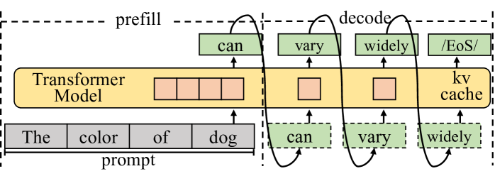</details> Figure 1: The autoregressive process of LLM inference with the KV cache technique. The decoding phase generally dominates the execution time. First, existing model partitioning approaches [11, 12] for distributing workloads across devices focus excessively on minimizing inter-device communication overhead and overlook opportunities for different processing units to access the same memory. When distributing LLM inference across multiple devices, explicit communication is required, making the reduction of communication overhead a top priority. In comparison, end-user devices typically integrate multiple heterogeneous processing units on a single chip and organize them within a unified memory architecture. Well-known examples include Apple’s M-series SoCs [9] and Intel Core Ultra [13], and NVIDIA Jetson [14]. In this way, minimizing memory access by carefully organizing partitioning strategy and data placement becomes the top priority for the unified memory architecture. Second, existing systems treat speculative decoding the same as the traditional decoding with a large batch size, less considering its specific computing pattern, particularly hybrid computational demands. The attention mechanism in the traditional decoding calculates the correlation between every pair of tokens, while it only requires to calculate correlation between partial pair of tokens in speculative decoding. Given the extremely high capability of accelerators in cloud systems and the high cost of transferring data to other processing units in the discrete memory architecture, this sparsity is often handled as dense computation using a mask mechanism. This oversight leads to missed opportunities to leverage computing affinity with processing units, such as on CPU. Third, algorithmic studies on speculative decoding primarily focus on increasing the acceptance length (the average number of tokens accepted in a single step), overlooking the balance between acceptance length and limited computing resources. Verifying more combinations of drafted tokens leads to better acceptance length, while resulting in more FLOPs to generate a single token. Compared to cloud hardware, end-user devices offer fewer resources for parallel verification, and verifying too many combinations can lead to decreased performance. Besides, modern hardware widely leverages vectorization technique, enabling the parallel processing of multiple data elements. It is crucial to select an appropriate verification width tailored to the specific hardware, thereby achieving the optimal balance between acceptance length and hardware parallelism. In this paper, we introduce Ghidorah, a system specifically designed to accelerate single-sample LLM inference in end-user devices with a unified memory architecture. It explores speculative decoding approaches to tackle the memory-bandwidth limitations inherent in the single-sample decoding process. Next, it distributes the novel workloads across multiple heterogeneous processing units in end-user devices, taking into account the hardware architecture and computing patterns. In summary, we make the following contributions: - We identify the performance bottlenecks in the single-sample LLM inference and explore speculative decoding approaches. - We present Ghidorah, a large language model inference system for end-user devices. It incorporates the hetero-core model parallelism (HCMP) architecture and the architecture-aware profiling (ARCA) approach to better employ the speculative decoding and align with the unified memory architecture. - We implement customized sparse computation optimizations for ARM CPUs. Experimental results show that Ghidorah achieves up to a 7.6 $\times$ speedup over the sequential decoding approach on the Nvidia Jetson NX. This improvement is attributed to a 3.27 $\times$ algorithmic enhancement and a 2.31 $\times$ parallel speedup. ## II Background and Motivation ### II-A LLM Generative Task Inference LLMs are primarily used for generative tasks, where inference involves generating new text based on a given prompt. As shown in Figure 1, it predicts the next token and performs iteratively until meeting the end identifier (EoS). By maintaining the KV cache in memory, modern LLM serving systems eliminates most redundant computations during this iterative process. The inference process is divided into prefill and decode phases based on whether the KV cache has been generated. The prefill phase handles the newly incoming prompt and initializes the KV cache. Since the prompt typically consists of many tokens, it has high parallelism. Next, with the KV cache, each step of the decode phase processes only one new token generated by the previous step and appends the new KV cache. In end-user scenarios, single-sample inference processes only a single token during each iteration of the decoding phase. The decoding phase is heavily constrained by the memory bandwidth and cannot fully exploit hardware capability. Moreover, the decoding phase typically dominates the overall inference process. ### II-B Collaborative Inference and Transformer Structure Distributing inference workload across various devices or processing units is a common strategy for enhancing performance. #### II-B 1 Data, Pipeline and Sequence Parallelism Data parallelism (DP) [15] partitions workloads along the sample dimension, allowing each device to perform inferences independently. Pipeline parallelism (PP) [7] horizontally partitions the model into consecutive stages along layer dimension, with each stage placed in a device. Since DP and PP are mainly used in high-throughput scenarios and cannot reduce the execution time for a single sample, they are not suitable for end-user scenarios. Sequence parallelism (SP) [16, 12] is designed for the long-context inference and it divides the input along the sequence dimension. It requires each device to load the entire model weights, making it advantageous only for extremely long sequences. We do not consider it within the scope of our work. #### II-B 2 Tensor Parallelism and Transformer Structure <details> <summary>x2.png Details</summary>  ### Visual Description ## Technical Diagram: Transformer Layer Architecture with Parallel Attention and MLP Blocks ### Overview This image is a technical schematic diagram illustrating the internal architecture of a transformer-based neural network layer. It specifically depicts a parallelized design where the Multi-Head Attention (MHA) and Multi-Layer Perceptron (MLP) computations are processed concurrently, likely across different devices or cores, as indicated by the "AllReduce" communication operations. The diagram uses a flowchart style with boxes representing data tensors or matrices, circles with crosses representing matrix multiplication operations, and arrows indicating data flow. ### Components/Axes The diagram is divided into two primary horizontal sections, separated by a dashed line, representing two parallel processing streams (e.g., for two different devices or model shards). **1. Top Section (Stream 0):** * **Header Label:** "Multi-Head Attention (MHA)" on the left, "Multi-Layer Perceptron (MLP)" on the right. * **Input:** A gray box labeled **`A`** (input activations). An arrow points from it with the text "more tokens". * **MHA Block:** * Three parallel branches for Query (Q), Key (K), and Value (V) projections. * **Weight Matrices (Green):** `W_0^K`, `W_0^V`, `W_0^Q`. * **Projected Tensors (Gray):** `K_0`, `V_0`, `Q_0`. * **KV Cache:** A pink box labeled "KV Cache" is associated with `K_0` and `V_0`. * **Attention Operation:** `Q_0` and `K_0` are multiplied (`Q_0 K_0^T`), followed by a **`Softmax`** operation (vertical gray box). The result is multiplied with `V_0`. * **Output Tensor (Gray):** `B_0`. * **MLP Block:** * **First Linear Layer:** `B_0` is multiplied by a green weight matrix `W_0^B`, resulting in tensor `C_0`. * **AllReduce Operation:** A large, double-headed blue arrow labeled **`AllReduce`** connects `C_0` in the top stream to `C_1` in the bottom stream, indicating a synchronization/communication step. * **Second Linear Layer:** The synchronized `C_0` is multiplied by green weight matrix `W_0^C`, resulting in tensor `D_0`. * **Third Linear Layer:** `D_0` is multiplied by green weight matrix `W_0^D`, resulting in tensor `E_0`. * **Output:** The final tensor is labeled **`E`**. **2. Bottom Section (Stream 1):** * This section is structurally identical to the top section, with all subscript indices changed from `0` to `1`. * **Weight Matrices:** `W_1^K`, `W_1^V`, `W_1^Q`, `W_1^B`, `W_1^C`, `W_1^D`. * **Tensors:** `A`, `K_1`, `V_1`, `Q_1`, `B_1`, `C_1`, `D_1`, `E_1`, `E`. * **Operations:** Identical matrix multiplications and `Softmax`. * **AllReceive Operation:** The same blue `AllReduce` arrow connects `C_1` to `C_0`. **3. Footer Labels (Bottom of Diagram):** A series of labels aligned with the processing stages from left to right: * `Linear Layer` (under the initial projection from `A`) * `Attention Module` (under the QKV operations) * `Linear Layer` (under the `W_0^B`/`W_1^B` multiplication) * `Linear Layer` (under the `W_0^C`/`W_1^C` multiplication) * `Linear Layer` (under the `W_0^D`/`W_1^D` multiplication) ### Detailed Analysis * **Data Flow & Parallelism:** The diagram explicitly shows a model parallelism strategy. The input `A` is duplicated to both streams. The MHA and initial MLP linear layer (`W^B`) are computed independently on each stream. The critical synchronization point is the `AllReduce` operation on the intermediate tensor `C` (output of the first MLP linear layer). This operation likely sums or averages the `C_0` and `C_1` tensors across streams before proceeding to the subsequent MLP layers (`W^C`, `W^D`). The final output `E` is also shown as a single entity, suggesting it is gathered or replicated after the final computation. * **KV Cache:** The presence of the "KV Cache" label next to `K_0` and `V_0` (and `K_1`, `V_1`) indicates this architecture is optimized for autoregressive inference, where previously computed Key and Value vectors are stored to avoid recomputation. * **Matrix Dimensions (Inferred):** The green weight matrices (`W`) are depicted as rectangular blocks, suggesting they are 2D matrices. The gray tensor boxes (`A`, `B`, `C`, etc.) are also rectangular, implying they are 2D tensors (e.g., [sequence_length, hidden_dimension]). The `Q K^T` operation results in a square-like box, consistent with an attention score matrix of shape [seq_len, seq_len]. * **Color Coding:** * **Green:** Trainable weight matrices/parameters. * **Gray:** Data activations/tensors and core operations (Softmax). * **Blue:** Communication operation (AllReduce). * **Pink:** Cached data (KV Cache). ### Key Observations 1. **Symmetrical Parallel Design:** The two streams are perfect mirrors, indicating a balanced split of the model's hidden dimension or attention heads across two processing units. 2. **Synchronization Point:** The `AllReduce` is placed after the first linear transformation in the MLP block. This is a specific design choice for pipeline or tensor parallelism, ensuring the streams have the same data before the final nonlinear transformations. 3. **No Residual Connections Shown:** The diagram focuses on the core computational blocks (Attention and MLP) and their parallelization. Standard transformer residual connections (add & norm) are not depicted in this specific schematic. 4. **Linear Layer Proliferation:** The MLP is explicitly broken down into three sequential linear layers (`W^B`, `W^C`, `W^D`), which is a more granular view than the typical "two linear layers with an activation in between" description. This may represent a specific implementation or a more detailed breakdown of a single feed-forward block. ### Interpretation This diagram provides a detailed, low-level view of a **distributed transformer inference engine**. It answers the question: "How is a single transformer layer split and executed across multiple devices to reduce memory footprint and/or increase speed?" The key insight is the **interleaving of computation and communication**. The devices work independently on their portions of the attention and the first part of the MLP. They must then synchronize (`AllReduce`) to combine their partial results before completing the MLP computation. This pattern is characteristic of **tensor parallelism** (specifically, splitting the MLP layer's hidden dimension). The inclusion of the "KV Cache" label strongly suggests this architecture is designed for **efficient autoregressive generation** (e.g., for large language models), where minimizing latency and memory bandwidth is critical. The parallelization helps manage the large memory requirement of both the model weights and the growing KV cache for long sequences. **Notable Anomaly/Design Choice:** The placement of the `AllReduce` *within* the MLP block, rather than after the entire Attention+MLP layer, is significant. It implies that the MLP's first linear layer (`W^B`) is sharded, and its output must be aggregated before the subsequent non-linearity and final linear layers. This is a more communication-intensive but potentially more memory-efficient strategy than other parallelism schemes. 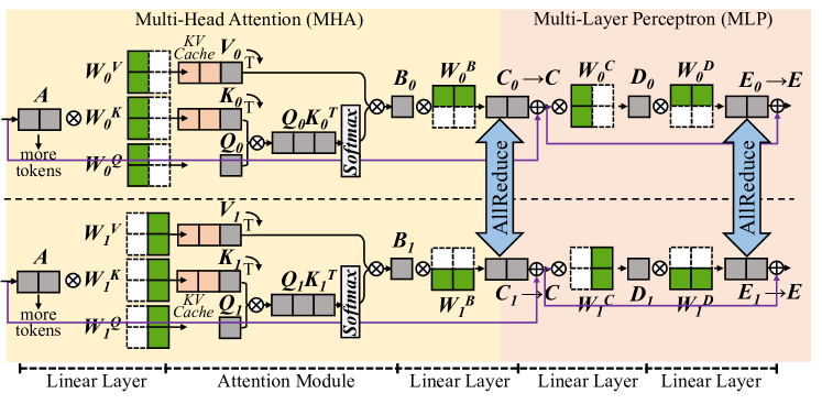</details> Figure 2: The partitioning [11] of Transformer model in the matrix form. Tensor parallelism partitions model weights to different devices [11, 12] or processing units [6, 17], and it is promising to reduce the execution time of a single sample. The Transformer [18] structure is the primary backbone for LLMs, consisting of multiple stacked Transformer layers, all configured identically. In a Transformer layer, the primary components are the multi-head attention (MHA) block and the multi-layer perceptron (MLP) block. Here we ignore element-wise operations, such as dropout, residual addition, and layernorm. In MHA block, the first linear layer generates query (Q), key (K), and value(V) matrices for each attention head. Each head conducts self-attention as in Equation 1, independently, and their outputs are concatenated and further processed by the next linear layer. MLP block involves two consecutive linear layers. $$ \displaystyle X=QK^{T} \displaystyle A=softmax(X) \displaystyle O=AV \tag{1} $$ Figure 2 shows a single Transformer layer and it is partitioned using the cloud TP solution in Megatron-LM [11]. For every two consecutive linear layers, it partitions the weights of the first one by columns and those of the second one by rows. An AllReduce communication is inserted as the synchronization point for every two linear layers. For the attention module in MHA block, it is partitioned by heads, with different attention heads assigned to different devices. ### II-C Speculative Decoding <details> <summary>x3.png Details</summary>  ### Visual Description ## Diagram: Transformer Attention Head Visualization ### Overview The image is a technical diagram illustrating the attention mechanism in a transformer neural network model. It consists of two main parts: a flowchart on the left showing the hierarchical structure of attention heads and their associated tokens, and an attention weight matrix (heatmap) on the right visualizing the attention scores between tokens. The diagram demonstrates how different attention heads focus on different subsets of the input sequence. ### Components/Axes **Left Flowchart:** - **Head 0** (Yellow box, top-left): Connected to tokens "It" and "I". - **Head 1** (Red box, below Head 0): Connected to tokens "is", "am", and "the". - **Head 2** (Orange box, below Head 1): Connected to tokens "is", "am", and "the". - **Connections:** Lines show which tokens each head processes. Head 0 processes the first two tokens, while Heads 1 and 2 process the subsequent three tokens. **Right Attention Matrix:** - **Type:** 5x5 grid (heatmap). - **Row Labels (Left side, vertical):** "It", "I", "is", "am", "the" (from top to bottom). - **Column Labels (Top side, horizontal):** "It", "I", "is", "am", "the" (from left to right). - **Legend/Color Key:** Blue squares indicate high attention weight (value ≈ 1). Dark gray squares indicate low or zero attention weight (value ≈ 0). - **Spatial Layout:** The matrix is positioned to the right of the flowchart. The row labels align with the tokens listed in the flowchart. ### Detailed Analysis **Attention Matrix Data Points (Row-by-Row Analysis):** 1. **Row "It" (Top row):** * Column "It": Blue (High attention). * Column "I": Blue (High attention). * Columns "is", "am", "the": Dark gray (Low attention). * **Trend:** The token "It" attends strongly only to itself and the token "I". 2. **Row "I" (Second row):** * Column "It": Blue (High attention). * Column "I": Blue (High attention). * Columns "is", "am", "the": Dark gray (Low attention). * **Trend:** The token "I" attends strongly only to itself and the token "It". 3. **Row "is" (Third row):** * Column "is": Blue (High attention). * Column "am": Blue (High attention). * Column "the": Blue (High attention). * Columns "It", "I": Dark gray (Low attention). * **Trend:** The token "is" attends strongly to itself and the tokens "am" and "the". 4. **Row "am" (Fourth row):** * Column "is": Blue (High attention). * Column "am": Blue (High attention). * Column "the": Blue (High attention). * Columns "It", "I": Dark gray (Low attention). * **Trend:** The token "am" attends strongly to itself and the tokens "is" and "the". 5. **Row "the" (Bottom row):** * Column "is": Blue (High attention). * Column "am": Blue (High attention). * Column "the": Blue (High attention). * Columns "It", "I": Dark gray (Low attention). * **Trend:** The token "the" attends strongly to itself and the tokens "is" and "am". **Cross-Reference with Flowchart:** * The attention pattern in the matrix perfectly aligns with the head groupings in the flowchart. * **Head 0 Group ("It", "I"):** These two tokens only attend to each other within their group (forming a 2x2 blue block in the top-left of the matrix). * **Heads 1 & 2 Group ("is", "am", "the"):** These three tokens only attend to each other within their group (forming a 3x3 blue block in the bottom-right of the matrix). * There is **zero attention** (all dark gray) between the two groups. ### Key Observations 1. **Complete Separation:** The attention mechanism has cleanly separated the input sequence into two distinct, non-interacting clusters: {"It", "I"} and {"is", "am", "the"}. 2. **Self-Attention within Clusters:** Within each cluster, every token attends strongly to every other token in the same cluster, including itself. This creates two perfect, isolated cliques. 3. **Head Specialization:** The flowchart suggests that Head 0 is specialized for the first cluster, while Heads 1 and 2 are specialized for the second cluster. The matrix shows the combined result of these heads' attention patterns. 4. **Binary Attention:** The attention weights appear to be binary (either fully on or fully off), with no intermediate values shown. This is a simplified visualization. ### Interpretation This diagram illustrates a scenario where a transformer's multi-head attention has learned a **hard, syntactic or semantic partitioning** of the input sentence. The sentence appears to be "It I is am the" (which is grammatically unusual, suggesting it might be a constructed example). The data suggests the model has identified two coherent phrases or conceptual units: 1. A **subject/pronoun cluster** ("It", "I"). 2. A **verb/article cluster** ("is", "am", "the"). The complete lack of cross-attention between these clusters is the most significant finding. In a typical sentence, one would expect some attention flow between subjects and verbs. This pattern could indicate: * **A specialized task:** The model might be performing a task like coreference resolution (linking "It" and "I") that requires isolating pronouns. * **An artifact of training:** The model may have overfit to a pattern where these specific words are always grouped separately. * **A visualization of a specific layer/head:** This likely shows the output of a particular attention head that has learned this specific, isolated function, while other heads in the network handle the cross-cluster relationships. The diagram effectively communicates how attention heads can act as **feature detectors** or **cluster formers**, grouping related tokens together while ignoring others, which is a fundamental operation enabling transformers to build contextual representations. 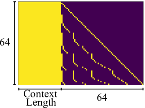</details> (a) Medusa Verification Tree. <details> <summary>x4.png Details</summary>  ### Visual Description ## Heatmap Diagram: Context Length Attention Pattern ### Overview The image is a square heatmap visualization, likely representing an attention pattern or data distribution matrix. It features a distinct two-region color scheme with a diagonal line of data points, plotted against axes labeled for "Context Length." The visualization appears to be a technical diagram, possibly from a machine learning or signal processing context, illustrating how information or attention is distributed across a sequence of length 64. ### Components/Axes * **X-Axis (Horizontal):** * **Label:** "Context Length" (centered below the axis). * **Scale/Markers:** A single numerical marker "64" is present at the far right end of the axis, indicating the maximum value or dimension. * **Y-Axis (Vertical):** * **Label:** The number "64" is positioned to the left of the axis, rotated 90 degrees. This likely denotes the dimension or size of the matrix (64x64), but it is not explicitly labeled as "Length" or "Index" like the x-axis. * **Color Scale/Legend:** * There is no explicit legend box. However, the color mapping is inferred from the data: * **Yellow:** Represents a high value, activation, or "allowed" state. * **Dark Purple/Black:** Represents a low value, inactivation, or "masked" state. * **Spatial Layout:** * The main plot area is a square matrix. * A solid yellow rectangular block occupies the left portion of the matrix. * The right portion is predominantly dark purple. * A diagonal line of discrete yellow dots runs from the top-left corner to the bottom-right corner. * A few isolated yellow dots are scattered near the bottom edge within the purple region. ### Detailed Analysis * **Data Structure:** The image represents a 64x64 matrix or grid. * **Primary Regions:** 1. **Left Yellow Block:** This region spans from x=0 to approximately x=16 (estimating based on visual proportion) across all y-values (0 to 64). It indicates a contiguous block of high values or full attention at the beginning of the context. 2. **Right Purple Region:** This covers the remainder of the matrix (approximately x=17 to x=64). It indicates low values or masked positions. * **Key Data Series (The Diagonal):** * **Trend Verification:** A clear, continuous diagonal line of yellow dots runs from the top-left (position 0,0) to the bottom-right (position 64,64). This is a perfect positive linear trend. * **Interpretation:** This pattern is characteristic of a **causal or autoregressive mask**, where each position (token) in a sequence can only attend to itself and previous positions (the yellow block to its left), but not to future positions (the purple area to its right). The diagonal represents self-attention. * **Anomalies/Secondary Points:** * There are a few stray yellow dots in the lower part of the purple region, approximately around y=55-60 and x=40-50. These break the perfect causal pattern and may represent noise, a specific model artifact, or a different type of attention head behavior. ### Key Observations 1. **Sharp Boundary:** There is a very sharp, vertical transition from the yellow block to the purple region, suggesting a strict cutoff or mask boundary. 2. **Perfect Diagonal:** The self-attention diagonal is perfectly linear and unbroken, indicating a fundamental property of the system being visualized. 3. **Asymmetric Information Flow:** The visualization strongly implies a directional or sequential process where information flows only from earlier to later positions (left to right in the matrix). 4. **Scale:** The context length is explicitly defined as 64 units. ### Interpretation This heatmap is almost certainly a visualization of a **causal attention mask** used in transformer-based language models or similar sequence processing architectures. * **What it demonstrates:** It shows the allowed attention connections for a sequence of 64 tokens. A token at position `i` (y-axis) can attend to all tokens at positions `j` (x-axis) where `j <= i`. This is why the lower-left triangle (including the diagonal) is yellow (allowed), and the upper-right triangle is purple (masked/forbidden). * **Relationship between elements:** The x-axis "Context Length" represents the key/token positions being attended *to*. The y-axis (implied as "Query Position" or "Current Token Index") represents the token doing the attending. The color at (x, y) indicates if token `y` can attend to token `x`. * **Why it matters:** This masking is crucial for autoregressive generation (like text completion), ensuring the model cannot "cheat" by looking at future tokens it hasn't generated yet. The solid yellow block on the left shows that early tokens have a very limited context (only themselves and a few predecessors), while later tokens (lower down the y-axis) have a growing context window (the expanding yellow triangle). * **The anomalies:** The few stray dots in the masked region could be significant. In a research context, they might indicate a model that has learned a slightly non-causal pattern, or they could be visualization artifacts. Their presence warrants investigation if this is from an actual model analysis. **Language Declaration:** All text within the image is in English. </details> (b) Medusa [3]. <details> <summary>x5.png Details</summary>  ### Visual Description ## Heatmap Diagram: Context Length vs. Dimension (64x64 Matrix) ### Overview The image is a square heatmap or matrix visualization, likely representing an attention pattern, correlation matrix, or data distribution within a 64x64 grid. It uses a two-color scheme (yellow and dark purple) to represent binary or high/low values. The visualization is divided into two distinct regions by a vertical boundary. ### Components/Axes * **X-Axis (Horizontal):** Labeled **"Context Length"**. A single numerical marker **"64"** is placed at the far right end of the axis, indicating the maximum value or dimension. * **Y-Axis (Vertical):** A single numerical marker **"64"** is placed at the top-left corner, indicating the maximum value or dimension for the vertical axis. There is no explicit axis title. * **Legend:** No separate legend is present. The color coding is intrinsic to the diagram: * **Yellow:** Represents a value of 1, "active," "present," or high magnitude. * **Dark Purple:** Represents a value of 0, "inactive," "absent," or low/negligible magnitude. * **Spatial Layout:** The diagram is a perfect square. A sharp vertical line divides it into a left rectangular region (approximately the first 32 columns) and a right square region (the remaining columns up to 64). ### Detailed Analysis The matrix can be segmented into two primary components based on the vertical dividing line: 1. **Left Region (Solid Yellow Block):** * **Position:** Occupies the left portion of the matrix, from column 1 to approximately column 32 (the exact split point is not labeled but is visually halfway). * **Content:** This entire rectangular area is filled with solid yellow. This indicates a constant, high value (e.g., 1) for all rows within this range of the "Context Length" axis. 2. **Right Region (Purple with Yellow Diagonal Pattern):** * **Position:** Occupies the right portion of the matrix, from the vertical dividing line to column 64. * **Background:** The base color is dark purple, indicating a value of 0 or near-zero for most cells in this region. * **Data Pattern:** A distinct pattern of yellow dots is superimposed on the purple background. * **Primary Diagonal:** A clear, continuous line of yellow dots runs from the top-left corner of this right region (at the dividing line, row 1) down to the bottom-right corner of the entire matrix (row 64, column 64). This represents a perfect diagonal where `row index = column index` (within the context of the full 64x64 matrix). * **Sub-Diagonals:** Several parallel, shorter diagonal lines of yellow dots are visible below the main diagonal. These are offset to the left, forming a stepped or "staircase" pattern. They appear to be spaced at regular intervals (e.g., every 8 or 16 rows/columns), suggesting a block-diagonal or sparse attention pattern. ### Key Observations * **Binary Representation:** The visualization uses a strict binary color scheme with no gradient, implying a clear on/off or present/absent state for each cell. * **Sharp Boundary:** The transition from the solid yellow block to the purple region is abrupt, indicating a fundamental change in the data's behavior at a specific context length threshold. * **Perfect Diagonal:** The main diagonal is flawlessly straight and continuous, indicating a perfect one-to-one relationship or self-association along the entire axis in the right region. * **Structured Sparsity:** The pattern in the right region is not random; it shows a highly structured, sparse distribution of non-zero (yellow) values concentrated along specific diagonals. ### Interpretation This diagram most likely visualizes a **causal attention mask** or a **position-based encoding pattern** from a transformer model or similar sequence processing architecture. * **Left Solid Block:** This represents a **full attention** or **unmasked** region. For the first ~32 positions (context length), every token can attend to every other token within that window, resulting in a fully connected (yellow) sub-matrix. * **Right Diagonal Pattern:** This represents a **causal** or **autoregressive** mask. For context lengths beyond the initial window, a token at position `i` can only attend to itself and previous tokens (`j <= i`). This creates the main diagonal (self-attention) and the lower sub-diagonals (attention to recent past tokens). The specific stepped pattern suggests a **local attention** or **dilated attention** mechanism, where tokens attend to a fixed number of previous positions or to positions in a strided pattern, rather than all previous positions. * **Overall Meaning:** The image demonstrates a hybrid attention strategy. It combines a window of full, bidirectional attention at the beginning of a sequence with a constrained, causal, and locally sparse attention pattern for longer contexts. This is a common technique to balance model expressivity with computational efficiency, allowing the model to capture complex dependencies in short contexts while scaling to longer sequences. The precise threshold (at ~32) and the stride of the sub-diagonals are key architectural hyperparameters revealed by this visualization. </details> (c) Draft model [2]. <details> <summary>x6.png Details</summary>  ### Visual Description ## Heatmap Diagram: Context Length Attention Pattern ### Overview The image is a square heatmap visualization, likely representing an attention pattern or data distribution matrix. It uses a two-color scheme (yellow and purple) to depict values across a 64x64 grid. The pattern shows a strong diagonal trend with specific horizontal interruptions. ### Components/Axes * **X-Axis (Bottom):** Labeled "Context Length". A single numerical marker "64" is present at the far right end of the axis. * **Y-Axis (Left):** A single numerical marker "64" is present at the top of the axis. There is no explicit axis title. * **Main Plot Area:** A 64x64 grid (inferred from axis markers). The visualization uses two colors: * **Yellow:** Represents one data value or state (e.g., high attention, active, 1). * **Dark Purple:** Represents the opposing data value or state (e.g., low attention, inactive, 0). * **Legend:** No explicit legend is present within the image frame. The color mapping must be inferred from the pattern. ### Detailed Analysis The heatmap displays a distinct, non-random pattern: 1. **Primary Diagonal Trend:** A thick, continuous band of yellow runs from the top-left corner (position ~1,1) diagonally down towards the bottom-right. This band widens as it progresses. The area above this diagonal (top-right triangle) is almost entirely solid purple. The area below the diagonal (bottom-left triangle) is predominantly yellow. 2. **Horizontal Interruptions:** Within the lower-left yellow region, there are four distinct, horizontal purple lines or "cuts." These lines are evenly spaced and run from the left edge to the main diagonal band. They appear to correspond to specific rows (y-axis positions). 3. **Spatial Grounding:** * The **top-left quadrant** is almost entirely yellow. * The **bottom-right quadrant** is almost entirely purple. * The **main diagonal band** separates these two quadrants. * The **horizontal purple lines** are located in the lower half of the plot, intersecting the yellow region below the diagonal. ### Key Observations * **Asymmetry:** The pattern is not symmetric across the main diagonal. The upper triangle is uniformly purple, while the lower triangle is yellow with structured interruptions. * **Structured Sparsity:** The horizontal purple lines suggest a deliberate, periodic pattern of "masking" or "deactivation" within the otherwise active (yellow) lower region. * **Context Length Implication:** Given the x-axis label "Context Length," this likely visualizes how a model (e.g., a Transformer) attends to different positions in a sequence of length 64. The diagonal suggests strong local attention, while the horizontal lines may represent specific attention heads or layers that ignore certain positions. ### Interpretation This heatmap most likely illustrates a **causal or masked attention pattern** common in autoregressive language models. * **What it demonstrates:** The solid purple upper triangle indicates that positions cannot attend to future positions (a causal mask). The yellow lower triangle shows that positions can attend to all previous positions. The diagonal band shows particularly strong attention to recent context. * **The horizontal lines:** These are the most notable anomaly. They represent specific rows (target positions) that have a pattern of *not attending* to a block of earlier positions (source positions). This could visualize: 1. The effect of a **sliding window attention** mechanism, where attention is restricted to a local window, creating these "gaps" in the full causal pattern. 2. The attention pattern of a specific **attention head** that has learned a specialized, sparse pattern of looking back at fixed intervals. 3. A **visualization artifact** or a specific type of positional encoding effect. * **Why it matters:** This pattern reveals the internal mechanics of how a model processes sequential data. The structured sparsity (horizontal lines) suggests the model is not using a simple, full-context approach but has developed or been given a more efficient, structured way to handle long contexts, potentially to reduce computational cost or focus on specific dependencies. **Language:** The text in the image is in English. </details> (d) Lookahead [4]. 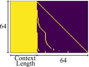Figure 3: Sparsity visualization of the $X=Q\times K^{T}$ for speculative decoding approaches. Light yellow indicates points that require computation, while dark blue represents points that do not need computation. To overcome the sequential limitation, speculative decoding is introduced as an alternative. To achieve higher parallelism in decoding steps, it primarily employs the Predict-then-Verify mechanism, where predictions for multiple steps are made in parallel and then fallback to the longest validated prefix LLM inference. There are independent drafting [2, 19] and self-drafting [3, 20, 4] approaches. The independent drafting employs a smaller model with significantly reduced computation to generate predictions. The self-drafting make predictions through appending more heads or using Jacobi iteration. After drafting multiple candidates, these candidate tokens are combined together under a given pattern and put into the target model for verification. Notably, these self-drafting approaches combine the prediction and verification into a single step. For example, Medusa [3] predicts candidates for future token slots by appending additional heads at the tail of LLMs. In Figure 3(a), Head1 has two candidates and Head2 has three candidates. We aim to verify which combinations between these tokens can be accepted. Here the verification width in Figure 3(a) is 8 and only a subset of token correlations needs to be calculated in the attention module. Basically, we observe significant sparsity within the attention module when performing these speculative decoding approaches. Under a given pattern, a token needs to compute relationships only with certain tokens. This sparsity is typically handled as dense computation using the mask mechanism. As illustrated in Figure 3(b) 3(c) 3(d), here we present the sparsity visualization of $Q\times K$ result matrix in three popular approaches, namely draft model [2], Medusa [3], and LookAhead [4]. Only the light yellow points represent computations worth performing, highlighting the significant sparsity in the right part. Softmax and $A\times V$ operation exhibits the same sparsity pattern. ### II-D Unified Memory Architecture <details> <summary>x7.png Details</summary>  ### Visual Description ## Diagram: Unified vs. Discrete Memory Architectures ### Overview The image displays two side-by-side block diagrams comparing computer system memory architectures. The left diagram (a) illustrates a "Unified Memory Architecture," while the right diagram (b) illustrates a "Discrete Architecture." Both diagrams show the hierarchical relationship between processing cores, cache memory, and main memory (DRAM). ### Components/Axes The diagrams are composed of labeled rectangular blocks connected by arrows indicating data flow or connection paths. **Diagram (a) - Left Side:** * **Title/Label:** "(a) Unified Memory Architecture" (located below the diagram). * **Top Row (Processing Cores):** Three blocks labeled "CPU Cores", "GPU Cores", and "xPU Cores". * **Second Row (Cache):** Three blocks, each labeled "Cache", positioned directly below each corresponding core block. * **Third Row (Memory Controller):** A single, wide block labeled "Memory Controller" spanning the width beneath all three cache blocks. * **Bottom Row (Main Memory):** A single, wide block labeled "DRAM" positioned below the Memory Controller. * **Connections:** * Bidirectional arrows connect each "Cores" block to its corresponding "Cache" block. * Bidirectional arrows connect each "Cache" block to the unified "Memory Controller". * A bidirectional arrow connects the "Memory Controller" to the single "DRAM" block. **Diagram (b) - Right Side:** * **Title/Label:** "(b) Discrete Architecture" (located below the diagram). * **Top Row (Processing Cores):** Identical to (a): "CPU Cores", "GPU Cores", "xPU Cores". * **Second Row (Cache):** Identical to (a): Three "Cache" blocks. * **Third Row (Main Memory):** Three separate blocks labeled "DRAM", each positioned below a corresponding "Cache" block. * **Connection Bus:** A horizontal line labeled "PCIe Bus" runs below the three DRAM blocks. * **Connections:** * Bidirectional arrows connect each "Cores" block to its corresponding "Cache" block. * Bidirectional arrows connect each "Cache" block directly to its dedicated "DRAM" block below it. * Single-headed arrows point upward from the "PCIe Bus" line to each of the three "DRAM" blocks. ### Detailed Analysis The diagrams contrast two fundamental approaches to connecting processors to memory. * **In the Unified Architecture (a):** All processor types (CPU, GPU, xPU) share a common path to a single pool of memory (DRAM) via a central Memory Controller. This implies a shared, addressable memory space accessible by all cores. * **In the Discrete Architecture (b):** Each processor type has its own dedicated DRAM module. The "Cache" for each core type connects directly to its private DRAM. The separate DRAM modules are interconnected via a "PCIe Bus," which is a standard high-speed interface for component communication. This implies memory is physically partitioned and explicit data transfer between processor-specific memory pools is required. ### Key Observations 1. **Component Consistency:** Both architectures use the same set of processing core types (CPU, GPU, xPU) and include a cache level for each. 2. **Structural Divergence:** The critical difference lies below the cache level. Diagram (a) converges to a single memory controller and DRAM, while diagram (b) diverges into three separate DRAM blocks. 3. **Interconnect Difference:** The unified architecture uses a proprietary or integrated memory controller bus. The discrete architecture uses the standardized "PCIe Bus" to connect the disparate memory modules. 4. **Spatial Layout:** The diagrams are presented in a direct, comparative layout within dashed bounding boxes, emphasizing their contrasting structures. All text is in English. ### Interpretation These diagrams visually explain a core trade-off in heterogeneous computing system design. * **Unified Memory (a)** simplifies software development because programmers can treat memory as a single, shared resource. Data does not need to be explicitly copied between CPU, GPU, and xPU memory spaces. The potential downside is contention for the single memory controller and DRAM bandwidth, which could become a bottleneck if all cores access memory intensively simultaneously. * **Discrete Memory (b)** offers potentially higher aggregate memory bandwidth because each processor type has its own dedicated DRAM. However, it complicates programming significantly. Data must be explicitly managed and transferred between the CPU's DRAM, GPU's DRAM, and xPU's DRAM over the PCIe bus, adding latency and programming overhead. This architecture is common in traditional systems where accelerators (like discrete GPUs) are add-in cards. The diagrams effectively communicate that the choice between these architectures involves balancing **programming simplicity and unified addressability** (Unified) against **potential performance isolation and dedicated bandwidth** (Discrete). The presence of "xPU Cores" suggests this is a modern context discussing accelerators beyond just CPUs and GPUs. 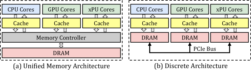</details> Figure 4: The unified memory architecture and the discrete architecture. End-user devices [21, 9, 13, 14, 22, 23], such as consumer electronics and embedded systems, prioritize power efficiency, cost-effectiveness, and compact design, usually adopting the unified memory architecture. We show the unified memory architecture and discrete architecture in Figure 4. End-user devices typically adopt a unified DRAM architecture shared across multiple processing units, rather than discrete memory modules. This design eliminates explicit data transfer via PCIe bus and enables a zero-copy mechanism between processing units. While this significantly reduces data synchronization overhead, concurrent memory access still requires manual consistency management by the programmer. On the NVIDIA Jetson Xavier NX, memory page synchronization between processing units takes less than 0.1 milliseconds when accessing memory written by another unit. ## III Ghidorah Design ### III-A Overview <details> <summary>x8.png Details</summary>  ### Visual Description ## Diagram: Hetero-Core Model Parallelism for LLM Inference ### Overview This image is a technical system architecture diagram illustrating a two-phase approach ("Preprocessing Phase" and "Runtime Support") for optimizing Large Language Model (LLM) inference using speculative decoding across heterogeneous hardware (CPU, GPU, NPU, XPU). The goal is to achieve "Hetero-Core Model Parallelism" by making the system architecture-aware. ### Components/Axes The diagram is vertically split into two main phases, labeled on the left side: 1. **Preprocessing Phase** (Top half) 2. **Runtime Support** (Bottom half) **Preprocessing Phase Components:** * **Input Data:** A "Calibration dataset" represented by a database cylinder icon. * **Core Model:** An "LLM + Speculative Decoding" block, visualized as a neural network graph. * **Hardware Pool:** A dashed box containing icons and labels for "CPU", "GPU", "NPU", "XPU". An Intel Core i9 processor is shown as a specific example. * **Output Strategies:** Two dashed boxes at the bottom of this phase: * "Speculative Strategy" (left), with the note "Verification width & Tree". * "Partitioning Strategy" (right), with the note "Parallelism- & Contention-aware". * **Connecting Process:** An arrow labeled "Architecture-aware Profiling" connects the Preprocessing Phase to the Runtime Support phase. **Runtime Support Components:** * **Operator Placement:** A legend at the top shows colored circles: Green for "CPU", Orange for "GPU", Blue for "XPU". * **Neural Network Graph:** A large neural network diagram where nodes are colored according to the Operator Placement legend (green, orange, blue circles). * **Optimization Goals:** Text below the network states "Memory access reduction" and "Computation affinity". * **Output Guides:** Two dashed boxes at the bottom: * "Partitioning Guide" (left). * "Customized ARM SpMM" (right), with the note "Vectorization Memory access reduction". * **Execution Timeline:** To the right of the network, a detailed timeline chart breaks down execution: * **Legend:** Green square for "GPU Time", Blue square for "CPU Time", Red square for "Synchronization". * **GPU Timeline:** Shows a block labeled "GPU" containing "PE PE PE PE" (Processing Elements) and "GPU Cache". * **CPU Timeline:** Shows a block labeled "CPU" containing "core core" and "CPU Cache". * **Synchronization:** A red vertical bar labeled "Sync" separates the GPU and CPU blocks. * **Flow:** An arrow points from the neural network to this timeline, indicating the mapping of operators to hardware execution. ### Detailed Analysis The diagram details a workflow for deploying LLMs efficiently: 1. **Preprocessing Phase:** A calibration dataset is fed into an LLM equipped with speculative decoding. This process is profiled across a heterogeneous hardware pool (CPU, GPU, NPU, XPU). The profiling output generates two key strategies: * A **Speculative Strategy** that defines the "Verification width & Tree" for the speculative decoding process. * A **Partitioning Strategy** that is "Parallelism- & Contention-aware," determining how to split the model's operations. 2. **Runtime Support:** The strategies from preprocessing guide the actual execution. * **Operator Placement:** Individual operations (nodes in the neural network) are assigned to specific hardware (CPU, GPU, XPU) based on the partitioning guide. The colored network graph visually represents this assignment. * **Execution Model:** The timeline illustrates the parallel execution. The GPU processes its assigned operators (PE = Processing Elements) while utilizing its cache. Concurrently, the CPU processes its assigned operators using its cores and cache. A synchronization point ("Sync") ensures coordination between the two processing streams. * **Optimization Techniques:** The system aims for "Memory access reduction" and "Computation affinity." The "Customized ARM SpMM" (likely Sparse Matrix-Matrix multiplication) block suggests specialized kernel optimization for ARM-based CPUs to further reduce memory access via vectorization. ### Key Observations * **Color-Coding Consistency:** The color scheme is consistent throughout: Green for CPU, Orange for GPU, Blue for XPU. This is maintained in the operator placement legend, the neural network nodes, and the execution timeline (Green for GPU Time, Blue for CPU Time). * **Spatial Flow:** The diagram flows logically from top (preprocessing/analysis) to bottom (runtime execution), with a clear central arrow ("Architecture-aware Profiling") connecting the two phases. * **Focus on Heterogeneity:** The system explicitly accounts for different hardware types (CPU, GPU, NPU, XPU, ARM) and their specific characteristics (caches, cores, PEs). * **Speculative Decoding Integration:** The LLM block is specifically labeled as using "Speculative Decoding," indicating this is a core technique being optimized. ### Interpretation This diagram presents a comprehensive framework for **co-designing LLM inference software with heterogeneous hardware architecture**. The core insight is that optimal performance cannot be achieved by treating hardware as a black box. * **The Problem it Solves:** Running large LLMs is computationally expensive. Speculative decoding speeds up inference but adds complexity. Simply parallelizing this across different chips (CPU, GPU, etc.) is inefficient due to mismatched capabilities and contention for resources. * **The Proposed Solution:** A two-stage, architecture-aware approach. 1. **Profiling Stage:** First, analyze the model and speculative decoding behavior on the *specific* hardware mix to create tailored strategies for speculation and operation partitioning. 2. **Execution Stage:** Use these strategies to place operators on the most suitable hardware and execute them in a coordinated, parallel manner, with custom kernels (like ARM SpMM) to minimize bottlenecks like memory access. * **Why it Matters:** This approach moves beyond generic parallelization. It acknowledges that a CPU core, a GPU streaming multiprocessor, and an NPU have fundamentally different strengths. By making the partitioning and speculative verification "contention-aware," the system aims to maximize utilization of all available compute resources while minimizing idle time and data movement overhead, leading to faster and more efficient LLM inference. The inclusion of "NPU" and "XPU" suggests a forward-looking design for emerging AI accelerator hardware. 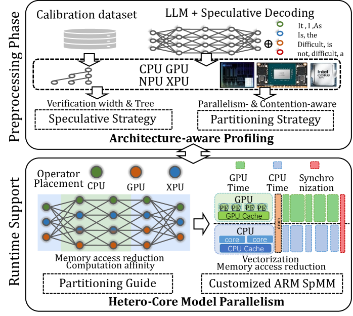</details> Figure 5: The overview of Ghidorah. Ghidorah is specifically designed for single-sample LLM generative task inference on end-user devices with a unified memory architecture. It primarily focuses on accelerating the dominant decoding phase. Since the decoding phase is constraint by the memory bandwidth, Ghidorah explores speculative decoding approaches to enhance parallelism and alleviate the memory bandwidth bottleneck. This manuscript takes the multi-head drafting approach, Medusa [3], as the default. Ghidorah distributes the speculative decoding workloads across all processing units and choose the optimal verification length in the end-user device to maximize the inference speed. Figure 5 illustrates the overview of Ghidorah. Leveraging the unified memory architecture of end-user devices and the computation pattern of speculative decoding, Ghidorah employs a novel hetero-core model parallelism (HCMP) architecture and the architecture-aware profiling (ARCA) approach. Functionally, the HCMP architecture focuses on providing runtime support, while the ARCA approach is primarily designed for the preprocessing phase. The HCMP architecture provides guidance for model partitioning and includes customized sparse matrix multiplication optimizations. Based on the runtime support, the ARCA approach provides the preprocessing phase that runs once before deployment. It performs an inference process using calibration data as input on multiple heterogeneous processing units in the end-user device. By comprehensively considering acceptance length, hardware parallelism, and resource contention, this phase formulates speculative and partitioning strategies to maximize performance. ### III-B Hetero-core Model Parallelism Architecture <details> <summary>x9.png Details</summary>  ### Visual Description ## System Architecture Diagram: Hybrid GPU-CPU Attention Mechanism with Memory Hierarchy ### Overview This image is a technical system architecture diagram illustrating a hybrid computing pipeline for a neural network's attention mechanism. It details the data flow and computational partitioning between a GPU, DRAM (main memory), and a CPU. The diagram emphasizes how operations, weights, and outputs are split and managed across these hardware components to optimize performance, likely for large language model inference. ### Components/Axes The diagram is organized into three primary horizontal layers (from top to bottom) and several vertical processing stages. **Hardware Layers (Left Labels):** * **GPU** (Top Layer) * **Dram** (Middle Layer) * **CPU** (Bottom Layer) **Vertical Processing Stages (Top Labels):** 1. **Linear Layer** (First column) 2. **Attention Module** (Second, largest column, with a light green background) 3. **Linear Layer** (Third column) 4. **Linear Layer** (Fourth column) 5. **Linear Layer** (Fifth column) **Legend (Bottom of Diagram):** * **Yellow Dashed Box:** `GPU Output` * **Red Dashed Box:** `CPU Output` * **Light Blue Shading:** `Split Weights by Column` * **Light Green Shading:** `Split Each Head with Affinity` **Key Components & Labels within the Diagram:** * **Linear Layer Blocks:** Represented by stacks of rectangles (blue for GPU, green for CPU, grey for DRAM) with a multiplication symbol (⊗) indicating a matrix operation. * **Attention Module Components:** * `cache_V` (Cached Values) * `cache_K` (Cached Keys) * `Q` (Query matrix) * `V` (Value matrix) * `K` (Key matrix) * `Softmax` (Softmax operation block) * `Online Softmax Reduce` (A specific, likely optimized, softmax computation block) * **Weight Matrices (in Linear Layers after Attention):** * `W^B` * `W^C` * `W^D` * **Data Flow Indicators:** Solid and dashed arrows show the movement of data (tensors) between components. Dashed grey lines often indicate control or dependency flows. ### Detailed Analysis The diagram depicts a sophisticated pipeline where computation is strategically divided: 1. **Initial Linear Layer:** The process begins with a linear layer whose weights and computations are split. The GPU handles a portion (blue blocks), the DRAM holds another portion (grey blocks), and the CPU handles a third (green blocks). 2. **Attention Module (Core Processing):** * **GPU Path:** The GPU accesses its local `cache_V` and `cache_K`, performs a matrix multiplication (⊗), and feeds into a `Softmax` block. * **DRAM/CPU Path:** This is the most complex path. The DRAM holds `cache_V`, `cache_K`, and the `Q` matrix. Data flows to the CPU, which performs a matrix multiplication. The results interact with an `Online Softmax Reduce` block (highlighted with a red dashed `CPU Output` box). The output of this softmax is then used in another matrix multiplication with the `V` and `K` matrices from DRAM. * **Affinity-Based Splitting:** The light green shading over the entire Attention Module indicates that the multi-head attention mechanism is being split based on "affinity," meaning different attention heads or parts of heads are assigned to different hardware units (GPU vs. CPU) for parallel processing. 3. **Subsequent Linear Layers:** Following the attention module, there are three more linear layers. The diagram shows that the weight matrices (`W^B`, `W^C`, `W^D`) for these layers are "Split... by Column" (light blue shading). This means different columns of the weight matrices are assigned to different processing units. The outputs from these layers are a mix of `GPU Output` (yellow dashed) and `CPU Output` (red dashed). 4. **Data Movement:** The flow is not strictly top-down. There is significant data exchange between the GPU and DRAM layers, and between the DRAM and CPU layers, as indicated by the network of arrows. The CPU and GPU work in parallel on different parts of the same overall operation. ### Key Observations * **Asymmetric Processing:** The GPU and CPU paths through the Attention Module are not identical. The CPU path includes the specialized `Online Softmax Reduce` step, suggesting a different, possibly more memory-efficient, algorithmic implementation for the CPU. * **Fine-Grained Partitioning:** The system employs two distinct splitting strategies: splitting by column for linear layer weights and splitting by head affinity for the attention mechanism. This indicates a highly optimized design for heterogeneous hardware. * **Central Role of DRAM:** DRAM acts as the central memory hub, holding shared data (`cache_V`, `cache_K`, `Q`, `V`, `K`) that both the GPU and CPU access and modify. * **Output Fusion:** The final outputs of the pipeline are a combination of results computed on the GPU and the CPU, implying a synchronization or aggregation step at the end (not shown in this diagram). ### Interpretation This diagram illustrates a **hardware-aware, hybrid execution engine for transformer models**. The core innovation is the intelligent partitioning of both the **computation** (attention heads, linear layer columns) and the **data** (cached keys/values, weight matrices) across a GPU and a CPU. * **Purpose:** The goal is to overcome memory capacity and bandwidth limitations when running very large models. By splitting the workload, the system can leverage the GPU's high computational throughput for some parts while using the CPU and its larger accessible memory (DRAM) for other parts, effectively increasing the total usable memory and compute resources. * **How Elements Relate:** The GPU and CPU are not working in a simple master-slave relationship but as parallel peers. The DRAM serves as the shared memory space that enables this collaboration. The "affinity" splitting suggests an intelligent scheduler that assigns attention heads to the processor best suited to handle them based on their memory footprint or computational needs. * **Notable Design Choice:** The use of `Online Softmax Reduce` on the CPU path is significant. Standard softmax requires computing a global sum for normalization, which can be a memory bottleneck. An "online" or "reduced" version likely computes this in a more streaming, memory-efficient fashion, which is crucial when the CPU is managing data from large DRAM. * **Implication:** This architecture enables the inference of models that are too large to fit entirely in GPU memory, by strategically offloading parts of the computation and data to the CPU and system memory, thereby balancing the load across the entire hardware system. 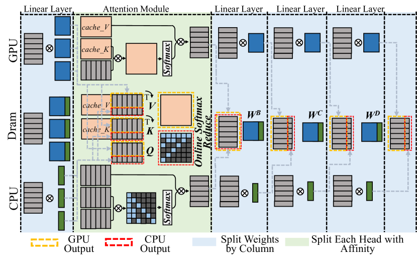</details> Figure 6: The illustration of Hetero-Core Model Parallelism. The HCMP architecture is designed for efficiently distributing speculative decoding workloads across multiple heterogeneous processing units organized in the unified memory architecture. Figure 6 illustrates the HCMP architecture by presenting an inference example conducted across two processing units, CPU and GPU. It shows the memory layout and computation processes separately. Instead of focusing on reducing inter-device communication, the HCMP architecture prioritizes minimizing memory access and exposing computation affinity across processing units. #### III-B 1 Linear Layer - Split weights by column The existing tensor parallelism approach [11] is designed to distribute workloads across multiple separate devices, requiring explicit inter-device communication to resolve data dependencies. Reducing the frequency of tensor synchronization can significantly improve parallel efficiency. Migrating this setup to end-user devices, for every two linear layers, the weights of the first layer are split by columns and those of the second layer by rows, thus requiring only a single all-reduce synchronization for the two layers. However, this all-reduce operation necessitates additional memory access. It must read activations generated by different processing units and write the combined results back. The HCMP architecture opts to split the weights of all linear layers by columns. As shown in Figure 6, the CPU and GPU receive the same input, multiply it by different columns of weights, and then write the outputs to their designated memory regions without enforcing consistency between them. This allows the result to be used in the next operation without any additional data access. #### III-B 2 Attention Module - Split each head with affinity The HCMP architecture is designed to exploit computation affinity across different processing units, taking into account the hybrid computational intensity inherent in speculative decoding. The existing tensor parallelism approach divides the computation of the attention module by heads, with each device responsible for processing different heads. However, since only the correlation between partial tokens requires to be verified in speculative decoding, there exists dense and sparse computation in each head of the attention module. As shown in Figure 6, each attention head can be divided into a dense part — primarily the multiplication with the KV cache — and a sparse part, which mainly involves multiplication with the newly generated key and value. The dense part will be prioritized for processing units with high parallelism, such as GPU, while the sparse part will be prioritized for processing units with low parallelism, such as CPU. To achieve load balance, each partition may optionally include a portion of the other part’s computation. As shown in Figure 3 (b)(c)(d), the left boundary of the sparse part tends to be denser and can be preferentially included in the dense part. Furthermore, inspired by Ring Attention [24] and FlashAttention [25], we introduce the online softmax technique to extend the span that can be computed continuously. As shown in Equation 1, the computation of $O=AV$ on one processing unit cannot begin until $X=QK^{T}$ on another processing unit is completed, as the softmax operation requires data from all processing units. With the online softmax technique [24, 25], each processing unit can have its own softmax operation, aligning their results by applying a scaling factor at the end of the attention module. This scaling operation can be fused with the reduce operation, introducing almost no overhead. 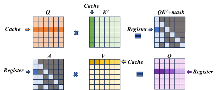#### III-B 3 Customized ARM SpMM Optimization <details> <summary>x10.png Details</summary>  ### Visual Description ## Diagram: Matrix Multiplication with Memory Hierarchy (Cache/Register) ### Overview The image is a technical diagram illustrating a two-step matrix multiplication process, likely representing an optimized computation kernel (such as an attention mechanism in transformers). It visually maps how data is moved between different levels of memory hierarchy—specifically **Cache** and **Register**—during the computation. The diagram is divided into two horizontal rows, each depicting a matrix multiplication operation with specific data access patterns highlighted. ### Components/Axes The diagram consists of six primary matrices, each represented as a 5x5 grid of cells. The matrices are labeled with mathematical notation: - **Top Row (Left to Right):** 1. **Q**: A matrix with an orange-highlighted row. An arrow labeled **"Cache"** points to this row. 2. **×** (Multiplication symbol) 3. **Kᵀ**: A matrix with a green-highlighted column. An arrow labeled **"Cache"** points to this column. 4. **=** (Equals symbol) 5. **QKᵀ+mask**: The resulting matrix. It has a blue-highlighted cell in the top-left and a diagonal pattern of gray cells. An arrow labeled **"Register"** points to the blue cell. - **Bottom Row (Left to Right):** 1. **A**: A matrix with a blue-highlighted cell in the top-left and a diagonal pattern of gray cells (identical to the *QKᵀ+mask* matrix above). An arrow labeled **"Register"** points to the blue cell. 2. **×** (Multiplication symbol) 3. **V**: A matrix with a yellow-highlighted row. An arrow labeled **"Cache"** points to this row. 4. **=** (Equals symbol) 5. **O**: The final output matrix. It has a purple-highlighted row. An arrow labeled **"Register"** points to this row. **Spatial Grounding:** - The **"Cache"** labels are positioned to the left of the *Q* matrix and above the *Kᵀ* matrix in the top row, and to the right of the *V* matrix in the bottom row. - The **"Register"** labels are positioned to the right of the *QKᵀ+mask* matrix in the top row, and to the left of the *A* matrix and to the right of the *O* matrix in the bottom row. - The highlighted rows/columns/cells are consistently colored across the diagram to indicate data locality. ### Detailed Analysis The diagram breaks down the computation `O = (QKᵀ + mask) * V` into two distinct multiplication steps, emphasizing memory access patterns: 1. **Step 1: Compute `QKᵀ + mask`** - **Input Data from Cache:** A single **row** of matrix **Q** (orange) and a single **column** of matrix **Kᵀ** (green) are fetched from the cache. - **Computation:** These are multiplied (dot product) to produce a single scalar value. - **Output to Register:** The result, after adding a mask (implied by the label `QKᵀ+mask`), is stored in a **register** (blue cell). The diagonal gray pattern in the output matrix suggests this operation is repeated for multiple positions, with the blue cell representing one computed element. 2. **Step 2: Compute Final Output `O`** - **Input Data from Register & Cache:** The previously computed scalar value (blue cell in matrix **A**, which is `QKᵀ+mask`) is held in a **register**. A single **row** of matrix **V** (yellow) is fetched from the **cache**. - **Computation:** The scalar from the register is multiplied with the entire row from *V*. - **Output to Register:** The resulting row is stored in a **register** (purple row in matrix **O**). This implies the entire output row is accumulated in fast register memory. **Component Isolation:** - **Header Region:** Contains the labels for the first multiplication (`Q`, `Kᵀ`, `QKᵀ+mask`) and the "Cache"/"Register" annotations for Step 1. - **Main Chart Region:** The two rows of matrix grids and operations. - **Footer Region:** Contains the labels for the second multiplication (`A`, `V`, `O`) and the "Cache"/"Register" annotations for Step 2. ### Key Observations 1. **Memory Hierarchy Optimization:** The diagram explicitly shows a strategy to minimize slow memory access. Data is loaded from **Cache** (slower than registers but faster than main memory) in large chunks (rows/columns), while intermediate and final results are kept in **Registers** (the fastest memory). 2. **Data Reuse Pattern:** In Step 1, one row of *Q* and one column of *Kᵀ* are used. In Step 2, one scalar from the intermediate result is reused across an entire row of *V*. This is a classic pattern for optimizing matrix multiplication on hardware with limited register files. 3. **Visual Consistency:** The color coding is consistent: Orange/Green for cache-loaded inputs in step 1, Blue for register-held intermediate, Yellow for cache-loaded input in step 2, and Purple for register-held final output. 4. **Implicit Masking:** The label `QKᵀ+mask` indicates an additive mask is applied to the result of `QKᵀ`, a common operation in attention mechanisms to prevent attending to future tokens. ### Interpretation This diagram is a **Peircean icon** representing the physical computation flow of an optimized kernel. It doesn't show numerical data but rather the **architectural strategy** for efficient computation. - **What it demonstrates:** It illustrates how a complex matrix operation is decomposed into smaller, hardware-friendly steps that maximize data locality. The goal is to keep the compute units (which operate on registers) constantly fed with data from the cache, minimizing stalls caused by waiting for data from slower memory levels. - **Relationship between elements:** The two rows are sequential. The output of the first multiplication (`QKᵀ+mask`, held in register `A`) becomes a direct input to the second multiplication. The "Cache" and "Register" labels are not just annotations; they define the **source and sink** of data for each computational step, revealing the underlying hardware-aware algorithm design. - **Notable implication:** This pattern is characteristic of high-performance implementations of operations like **scaled dot-product attention** on GPUs or specialized AI accelerators. The diagram serves as a blueprint for understanding or implementing such a kernel, emphasizing that performance is dictated not just by the arithmetic but by the orchestration of data movement through the memory hierarchy. </details> Figure 7: ARM SpMM Optimization. ARM CPUs are widely used in end-user devices due to their power efficiency feature, and we implement customized computation optimizations for sparse computations in the self-attention module, i.e. $QK^{T}$ and $AV$ . In details, knowing the token correlations to be verified, we follow the COO sparsity data format to generate the index before performing the inference. We optimize the sparse operation from two aspects, namely vectorization and memory access reduction. Figure 7 illustrates the optimization. In the $QK^{T}$ computation, the data access for both $Q$ and $K$ is in a row-wise way, thereby supporting continuous data access. Leveraging NEON instruction set of ARM, we enable the 128-bit long vector instructions to combine memory access in continuous FMA calculations. For its output matrix, each result value is stored in the register until the final result is fully accumulated, so as to reducing the load/store operations. In the $AV$ computation, we adjust the execution order to ensure continuous memory access to matrix $V$ . Instead of multiplying with each column of matrix $V$ , each non-zero element in the matrix $A[i,j]$ performs multiplication with row j of the matrix $V$ and then accumulates the result to the row i of the output matrix $O$ until the non-zero element in the same row finishes computing and finally gets row i of the output matrix. Also, since the capacity of registers is limited, we divide this process into blocks, only process partial elements from $V$ to $O$ , to enable storing elements in registers and reduce load/store operations. ### III-C Architecture-aware Profiling Approach The ARCA approach comprehensively considers the acceptance length, hardware parallelism and resource contention to finally generate the speculative strategy and the partitioning strategy. Initially, for a specific speculative decoding approach, we explore verification trees of all verification widths for the optimal acceptance lengths by combining accuracy-based estimation with brute-force search. Next, we determine the verification width and partitioning ratio for the final deployment, which is both parallelism- and contention-aware. #### III-C 1 Speculative Strategy Determination The speculative strategy in Ghidorah consists of both the verification width and the verification tree. The verification width is the computing budget in a single decoding step, and it is defined as the total number of tokens to be verified, while the verification tree determines the specific combinations of tokens to be verified. Both the verification width and verification tree influence the acceptance length. As the verification width increases, it becomes more likely to identify acceptable tokens; however, if the width is too large, the benefits for improving acceptance length becomes limited. Also, some specific verification routes are more likely to be accepted. For instance, the closer the head is to HEAD0, the easier its tokens are accepted. We design verification trees for different verification widths. 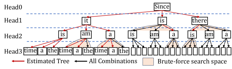<details> <summary>x11.png Details</summary>  ### Visual Description \n ## Diagram: Multi-Head Attention Tree Structure with Search Space ### Overview The image is a technical diagram illustrating a hierarchical tree structure, likely representing a parsing or search process in natural language processing or a related computational field. It visualizes how different "heads" (possibly attention heads in a transformer model) generate or explore combinations of words, distinguishing between an estimated optimal path and the full combinatorial space. ### Components/Axes * **Vertical Layers (Heads):** The diagram is organized into four horizontal layers, labeled on the left side: * **Head0** (Top layer) * **Head1** * **Head2** * **Head3** (Bottom layer) These layers are separated by horizontal dashed blue lines. * **Nodes:** Each layer contains rectangular boxes (nodes) with text inside. The nodes represent words or tokens. * **Connections (Arrows):** Directed arrows connect nodes from a higher layer to nodes in the layer directly below it. * **Legend (Bottom of image):** * **Red Arrow:** Labeled "Estimated Tree" * **Black Arrow:** Labeled "All Combinations" * **Peach-colored shaded rectangle:** Labeled "Brute-force search space" ### Detailed Analysis **1. Tree Structure and Node Content:** * **Head0:** Contains a single root node with the text "**Since**". * **Head1:** Contains three nodes connected from "Since": * Left: "**it**" * Center: "**is**" * Right: "**there**" * **Head2:** Contains nodes connected from each Head1 node: * From "**it**": Two nodes - "**is**" (left), "**am**" (right). * From "**is**": Three nodes - "**is**" (left), "**am**" (center), "**a**" (right). * From "**there**": Three nodes - "**is**" (left), "**am**" (center), "**a**" (right). * **Head3:** Contains the final layer of nodes. The structure here is more complex: * From Head2's "**is**" (under "it"): Connects to three nodes - "**time**", "**a**", "**the**". * From Head2's "**am**" (under "it"): Connects to three nodes - "**time**", "**a**", "**the**". * From Head2's "**a**" (under "it"): Connects to three nodes - "**time**", "**a**", "**the**". * From Head2's "**is**" (under "is"): Connects to three nodes - "**time**", "**a**", "**the**". * From Head2's "**am**" (under "is"): Connects to three **empty boxes**. * From Head2's "**a**" (under "is"): Connects to three **empty boxes**. * From Head2's "**is**" (under "there"): Connects to three **empty boxes**. * From Head2's "**am**" (under "there"): Connects to three **empty boxes**. * From Head2's "**a**" (under "there"): Connects to three **empty boxes**. **2. Connection Types and Search Space:** * **Estimated Tree (Red Arrows):** A specific path is highlighted with red arrows, tracing a single route from the root: `Since` (Head0) -> `it` (Head1) -> `is` (Head2) -> `time` (Head3). This represents a hypothesized or most likely sequence/parse. * **All Combinations (Black Arrows):** All other connections are shown with black arrows, representing the full set of possible transitions between nodes across layers. * **Brute-force Search Space (Peach Shading):** A peach-colored shaded area encompasses the sub-tree originating from the Head1 node "**is**". This includes all its descendants in Head2 (`is`, `am`, `a`) and Head3 (the nodes and empty boxes connected to them). This visually demarcates a region where an exhaustive ("brute-force") search might be applied, as opposed to following the single "estimated" path. ### Key Observations 1. **Asymmetry in Detail:** The left side of the tree (under Head1's "it") is fully populated with specific words in Head3. The right side (under Head1's "is" and "there") transitions to empty boxes in Head3, suggesting these branches are either incomplete, pruned, or represent potential slots for tokens not shown. 2. **Search Space Demarcation:** The diagram explicitly contrasts a single, efficient "estimated" path (red) with the vastly larger combinatorial space of "all combinations" (black), and further isolates a specific sub-region for brute-force analysis. 3. **Repetitive Structure:** The pattern of three child nodes (`is`, `am`, `a`) in Head2 repeats under each Head1 node, indicating a consistent branching factor at that level of the hierarchy. ### Interpretation This diagram is a conceptual visualization of a **structured prediction or search problem**, common in areas like syntactic parsing, sequence generation, or attention mechanism analysis. It demonstrates the challenge of navigating a combinatorial explosion of possible structures (the "All Combinations" black arrows). * **The "Estimated Tree"** represents the output of a model or heuristic that predicts a single, plausible structure (e.g., "Since it is time..."). * **The "Brute-force search space"** highlights a specific, problematic region where the model or algorithm might need to exhaustively evaluate multiple possibilities (e.g., deciding between "is", "am", or "a" after "Since is..."), which is computationally expensive. * The **empty boxes** in Head3 likely signify that the full token vocabulary or possible continuations are not enumerated, emphasizing the open-ended nature of the search space. The core message is the trade-off between efficient, guided search (following the red "estimated" path) and the necessity to sometimes explore larger, defined subspaces (the peach region) to ensure accuracy or handle ambiguity. It effectively maps abstract computational concepts onto a spatial, hierarchical layout. </details> Figure 8: The verification tree determination with a verification width of 16. Figure 8 illustrates the tree design process with a verification width of 16 (nodes), involving candidate tokens generated from 4 heads of Medusa [3]. In details, we use a calibration dataset and generate the accuracies of the top predictions of different heads. Then, we estimate the accuracy of a candidate sequence by multiplying the accuracies of its related tokens. Then we can get the overall expected acceptance length by accumulating the expected acceptance length of different candidate sequences. Maximizing the acceptance length expectation, we can add nodes with the highest accuracies one by one until reaching the given verification length. As in Figure 8, the estimated tree is indicated by red lines. We further employ the brute-force search based on the estimated tree and compare their real acceptance lengths to determine the final tree. In Figure 8, we search leaf nodes and nodes in the same level. #### III-C 2 Parallelism-Aware Profiling The ARCA approach is parallelism-aware. Modern processing units leverage vectorization techniques to boost computational efficiency, leading to stepwise performance improvements in LLM inference latency as batch size increases, a phenomenon referred to as wave quantization [26] on NVIDIA hardware. Consequently, different processing units exhibit distinct performance sweet spots. In our preliminary experiments, we observe that setting candidate verification widths to powers of two, specifically 2, 4, 8, 16, 32, and 64, aligns well with the vectorization capabilities of these devices, resulting in more efficient execution. This observation can be explained as follows. The execution time of general matrix multiplication (GeMM) operations, including linear and attention, generally dominates LLM workloads. When applying model parallelism, the hidden state dimension is partitioned across processing units, while the token dimension (verification length) remains unchanged. As a result, the split GeMM operations executed on different processing units share the same token dimension and collectively span the hidden state dimension. Next, we determine their verification trees and check these speculative strategies with the runtime support. This determination process is contention-aware. #### III-C 3 Contention-Aware Profiling Although the partitioning guidance of the HCMP architecture will not increase the overall memory access within a single step of speculative decoding, the simultaneous access from different processing units will lead to resource contention problem. Since this contention affects different processing units at varying levels, it is difficult to determine the partitioning ratio. In this way, the ARCA approach initializes the partitioning strategy based on the individual execution times of different processing units and determines the final partitioning strategy for a given verification width through gradual adjustments. Besides, as the context (KV cache) length will impact the ratio of sparsity in the attention module, we additionally adjust the context length for the attention module to support its dynamic partitioning. ## IV Evaluation We implement a prototype system of Ghidorah in C/C++. We utilize the CUDA kernels from the highly optimized Transformer inference system FasterTransformer [27] for the GPU and rebuild the ARM CPU code based on CTranslated2 [28]. In this section, we evaluate Ghidorah from two aspects. 1) Verification Efficiency: we evaluate the acceptance length of our speculative strategies, and 2) Overall Performance: we compare the single-sample inference of Ghidorah with that of state-of-the-art approaches. Here we only focus on the dominant decoding phase of the LLM inference. ### IV-A Experimental Setup Model and Speculative Decoding. We evaluate Ghidorah with Vicuna-7B [29] and speculative decoding approach Medusa [3]. Medusa originally offers a 5-head version of Vicuna-7B and we design our own verification trees to evaluate the acceptance length under different verification widths. Vicuna-7B is a fine-tuned version from LLaMA-7B [30], which is a widely-recognized model architecture in the AI community. Datasets. We evaluate Ghidorah for the acceptance length across a broad spectrum of datasets, including: 1) MT-Bench [29]: a diverse collection of multi-turn questions, 2) GSM8K [31]: a set of mathematical problems, 3) HumanEval [32]: code completion and infilling tasks, and 4) MBPP [33]: instruction-based code generation. Node testbed. We use NVIDIA Jetson NX, which is a CPU-GPU edge device with unified memory architecture. It consists of an embedded 384-core Volta GPU and a 6-core ARM v8.2 CPU. We lock the GPU at 204MHz and the CPU at 1.9GHz to simulate end-user devices with more balanced capabilities of heterogeneous processing units. Specifically, we use g++ 7.5, cuda 10.2, arm performance library 24.10. Metrics. We use the acceptance length and decoding throughput as the evaluation metrics. The acceptance length refers to the average number of tokens that the target model accepts in a single decoding step. The decoding throughput is the number of tokens generated in a fixed interval. Baseline Methods. We compare Ghidorah with approaches: - Sequential: The sequential decoding approach running on the GPU, which is generally limited by the algorithmic parallelism. - Medusa: The Medusa decoding approach running on the GPU and it adopts our verification trees in given verification widths. - Medusa+EM (Medusa + E dgeNN [34] + M egatron) [11]: The Medusa decoding approach is distributed across the CPU and GPU using the partitioning guidance of the tensor parallelism from Megatron-LM. Additionally, we apply zero-copy optimization to reduce the synchronization overhead and determines the partitioning ratio based on the execution times of the processing units as in EdgeNN. ### IV-B Acceptance Length Evaluation TABLE I: Acceptance length under given verification widths. | Dataset GSM8K MBPP | MT-bench 1 1 | 1 1.76 1.78 | 1.72 2.43 2.54 | 2.28 2.69 2.89 | 2.59 3.08 3.27 | 2.93 3.34 3.55 | 3.19 3.56 3.74 | 3.34 | | --- | --- | --- | --- | --- | --- | --- | --- | --- | | Human-eval | 1 | 1.77 | 2.49 | 2.8 | 3.19 | 3.48 | 3.71 | | We present the acceptance lengths for various datasets under different verification widths. Notably, MT-bench is used as the calibration dataset for determining verification trees. Subsequently, these verification trees are applied to three other datasets to generate their acceptance lengths. Table I shows the acceptance length results. Larger verification widths generally result in longer acceptance lengths, while the benefit becomes weak as verification widths grow and come at the cost of significantly increased computational effort. Furthermore, we find that these verification trees exhibit strong generality, achieving even better acceptance lengths on GSM8K, MBPP, and Huamn-eval, when migrated from MT-Bench. This can be attributed to MT-Bench’s comprehensive nature, as it includes conversations across eight different types. 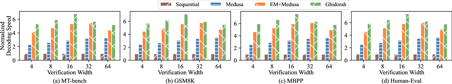<details> <summary>x12.png Details</summary>  ### Visual Description ## Bar Charts: Normalized Decoding Speed vs. Verification Width Across Four Benchmarks ### Overview The image displays a set of four grouped bar charts arranged horizontally. Each chart compares the "Normalized Decoding Speed" of four different methods across five distinct "Verification Width" settings. The charts are labeled (a) through (d), corresponding to four different evaluation benchmarks: MT-bench, GSM8K, MBPP, and Human-Eval. The overall purpose is to demonstrate the relative performance (speed) of the methods as the verification width parameter changes. ### Components/Axes * **Legend:** Positioned at the top center of the entire figure. It defines four data series: * **Sequential:** Solid brown bar. * **Medusa:** Blue bar with horizontal hatching. * **EM+Medusa:** Orange bar with diagonal hatching (top-left to bottom-right). * **Ghidorah:** Green bar with cross-hatch (X) pattern. * **Y-Axis (All Charts):** Labeled "Normalized Decoding Speed". The scale runs from 0 to 6, with major tick marks at 0, 2, 4, and 6. * **X-Axis (All Charts):** Labeled "Verification Width". The categorical tick marks are at values: 4, 8, 16, 32, and 64. * **Subplot Titles:** Located below each chart: * (a) MT-bench * (b) GSM8K * (c) MBPP * (d) Human-Eval ### Detailed Analysis The following analysis describes the approximate height of each bar, interpreted as normalized decoding speed. Values are estimated from the y-axis scale. **Chart (a) MT-bench:** * **Trend:** All methods except Sequential show an increase in speed from width 4 to 16 or 32, followed by a slight decrease or plateau at width 64. Ghidorah is consistently the fastest. * **Data Points (Approx. Speed):** * **Width 4:** Sequential ~1.0, Medusa ~2.2, EM+Medusa ~4.1, Ghidorah ~5.3. * **Width 8:** Sequential ~1.0, Medusa ~2.6, EM+Medusa ~4.7, Ghidorah ~5.9. * **Width 16:** Sequential ~1.0, Medusa ~2.9, EM+Medusa ~5.3, Ghidorah ~6.8 (peak). * **Width 32:** Sequential ~1.0, Medusa ~3.2, EM+Medusa ~5.5, Ghidorah ~5.7. * **Width 64:** Sequential ~1.0, Medusa ~3.3, EM+Medusa ~4.4, Ghidorah ~5.2. **Chart (b) GSM8K:** * **Trend:** Similar pattern to MT-bench. Ghidorah peaks at width 16. EM+Medusa shows a steady increase up to width 32. * **Data Points (Approx. Speed):** * **Width 4:** Sequential ~1.0, Medusa ~2.4, EM+Medusa ~4.4, Ghidorah ~5.6. * **Width 8:** Sequential ~1.0, Medusa ~2.7, EM+Medusa ~4.8, Ghidorah ~6.1. * **Width 16:** Sequential ~1.0, Medusa ~3.0, EM+Medusa ~5.5, Ghidorah ~6.8 (peak). * **Width 32:** Sequential ~1.0, Medusa ~3.3, EM+Medusa ~5.7, Ghidorah ~5.9. * **Width 64:** Sequential ~1.0, Medusa ~3.5, EM+Medusa ~4.7, Ghidorah ~5.6. **Chart (c) MBPP:** * **Trend:** Ghidorah peaks at width 16. EM+Medusa peaks at width 32. The performance drop for Ghidorah at width 64 is less pronounced here. * **Data Points (Approx. Speed):** * **Width 4:** Sequential ~1.0, Medusa ~2.5, EM+Medusa ~4.6, Ghidorah ~5.9. * **Width 8:** Sequential ~1.0, Medusa ~2.9, EM+Medusa ~5.2, Ghidorah ~6.5. * **Width 16:** Sequential ~1.0, Medusa ~3.2, EM+Medusa ~5.8, Ghidorah ~7.2 (peak). * **Width 32:** Sequential ~1.0, Medusa ~3.5, EM+Medusa ~6.0, Ghidorah ~6.2. * **Width 64:** Sequential ~1.0, Medusa ~3.6, EM+Medusa ~4.9, Ghidorah ~5.7. **Chart (d) Human-Eval:** * **Trend:** Ghidorah peaks at width 16. EM+Medusa peaks at width 32. The relative performance hierarchy is very consistent. * **Data Points (Approx. Speed):** * **Width 4:** Sequential ~1.0, Medusa ~2.5, EM+Medusa ~4.5, Ghidorah ~5.8. * **Width 8:** Sequential ~1.0, Medusa ~2.9, EM+Medusa ~5.1, Ghidorah ~6.4. * **Width 16:** Sequential ~1.0, Medusa ~3.2, EM+Medusa ~5.8, Ghidorah ~7.1 (peak). * **Width 32:** Sequential ~1.0, Medusa ~3.5, EM+Medusa ~6.0, Ghidorah ~6.2. * **Width 64:** Sequential ~1.0, Medusa ~3.6, EM+Medusa ~4.9, Ghidorah ~5.8. ### Key Observations 1. **Consistent Hierarchy:** Across all benchmarks and verification widths, the performance order is almost always: **Ghidorah > EM+Medusa > Medusa > Sequential**. The only exception is at width 64 in some charts where EM+Medusa and Ghidorah converge or swap slightly. 2. **Optimal Verification Width:** For the top-performing method (Ghidorah), the optimal verification width appears to be **16**, where it achieves its peak normalized speed (~6.8-7.2) in all charts. Performance declines at widths 32 and 64. 3. **Sequential Baseline:** The "Sequential" method serves as a baseline, showing a constant normalized speed of approximately 1.0 across all conditions, indicating it is unaffected by the verification width parameter. 4. **Diminishing Returns:** For Medusa and EM+Medusa, speed generally increases with verification width up to 32, but the gains diminish, and performance often drops at width 64. 5. **Benchmark Similarity:** The relative trends and magnitudes are remarkably consistent across the four diverse benchmarks (MT-bench, GSM8K, MBPP, Human-Eval), suggesting the observed method behaviors are robust. ### Interpretation This data demonstrates a clear technical advantage for the "Ghidorah" method in terms of decoding speed under a verification-based evaluation framework. The "verification width" parameter likely controls a trade-off between computational effort per step and the number of steps or candidates verified. * **Ghidorah's Superiority:** Ghidorah's consistently higher bars indicate it achieves the fastest normalized decoding speed. Its peak at width 16 suggests an optimal balance point for this method—wider verification (32, 64) may introduce overhead that outweighs its benefits, while narrower verification (4, 8) doesn't leverage its full potential. * **Method Synergy:** The "EM+Medusa" method, which presumably combines techniques, consistently outperforms "Medusa" alone, showing the value of the added component(s). However, it does not surpass the integrated "Ghidorah" system. * **Practical Implication:** For practitioners using these decoding acceleration techniques, the charts provide a tuning guide. To maximize speed, one should use Ghidorah with a verification width around 16. If Ghidorah is unavailable, EM+Medusa with a width of 32 is the next best choice. The Sequential method is the slowest but most stable, unaffected by the width parameter. * **Underlying Mechanism:** The rise and subsequent fall of speed with increasing width for the advanced methods suggests a classic optimization curve. Initially, wider verification improves efficiency (perhaps by accepting more correct tokens per step), but beyond a point, the cost of verifying more candidates (computational or memory overhead) degrades overall throughput. Ghidorah appears to have the most efficient implementation of this trade-off. </details> Figure 9: The overall performance under different verification widths. ### IV-C Overall Performance Evaluation This section compares the decoding throughput of Ghidorah against that of baseline methods with different verification widths from 4 to 64. We select a context length (KV cache length) of approximately 256. Figure 9 shows the normalized results. In all cases shown in Figure 9, Ghidorah presents significant speedup in the decoding throughput. Especially when the verification width is 16, Ghidorah’s speedup can reach up to 7.6 $\times$ compared with the sequential decoding. The impressive performance improvement of Ghidorah can be attributed to two main factors: First, the increased acceptance length enabled by speculative decoding. Since the sequential decoding approach is memory-bandwidth-bound, its execution time is similar to that of Medusa, and the acceptance length is fixed at 1. However, the Medusa method generates multiple tokens in a single step and requires the similar execution time; specifically, as the verification width increases, the acceptance length of Medusa also grows. Second, the collaborative operation of multiple heterogeneous processing units can better conduct the Medusa decoding workload. When comparing Medusa, Medusa+EM, and Ghidorah, we find that utilizing heterogeneous processing unit yields a better acceleration effect than merely running Medusa on the GPU. Taking MBPP dataset as the instance, Ghidorah achieves an average speedup of 2.06 $\times$ compared to running Medusa solely on the GPU, and an average speedup of 1.20 $\times$ compared to Medusa+EM. The improvement over Medusa+EM is attributed to reduced memory access and improved computing affinity. Longer acceptance lengths do not always result in better throughput, making it essential for the ARCA approach to balance the algorithmic parallelism with hardware capabilities. As shown in Figure 9, Medusa and Ghidorah achieve their best throughput results at verification width of 64 and 16 respectively. This is because CPU and GPU have different sweet spots. The GPU maintains a similar execution time from 4 to 64 verification width and achieves a longer acceptance length at verification width of 64, while the CPU can only maintain a similar execution time from 4 to 16 verification width. Since increasing verification width from 16 to 64 results in only 0.47 increase in the acceptance length, Ghidorah achieves the optimal throughput at a verification width of 16. 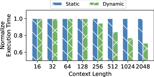### IV-D Dynamic Partitioning and Sparse Optimization <details> <summary>x13.png Details</summary>  ### Visual Description ## Bar Chart: Normalized Execution Time vs. Context Length ### Overview This is a grouped bar chart comparing the "Normalized Execution Time" of two methods, labeled "Static" and "Dynamic," across eight different "Context Length" values. The chart demonstrates how the performance (execution time) of each method scales as the context length increases. ### Components/Axes * **Chart Type:** Grouped Bar Chart. * **X-Axis (Horizontal):** * **Label:** "Context Length" * **Categories (Ticks):** 16, 32, 64, 128, 256, 512, 1024, 2048. * **Y-Axis (Vertical):** * **Label:** "Normalize Execution Time" * **Scale:** Linear, ranging from 0.6 to 1.0. * **Major Ticks:** 0.6, 0.8, 1.0. * **Legend:** * **Position:** Top-center, above the plot area. * **Series 1:** "Static" - Represented by blue bars with a diagonal hatch pattern (\\). * **Series 2:** "Dynamic" - Represented by green bars with a diagonal hatch pattern (\\). * **Data Representation:** For each context length on the x-axis, two bars are plotted side-by-side: a blue "Static" bar on the left and a green "Dynamic" bar on the right. ### Detailed Analysis The following table reconstructs the approximate data points from the chart. Values are estimated based on bar height relative to the y-axis scale. | Context Length | Static (Blue) Normalized Execution Time | Dynamic (Green) Normalized Execution Time | | :--- | :--- | :--- | | 16 | ~1.00 | ~1.00 | | 32 | ~1.00 | ~0.99 | | 64 | ~1.00 | ~0.98 | | 128 | ~1.00 | ~0.97 | | 256 | ~1.00 | ~0.95 | | 512 | ~1.00 | ~0.85 | | 1024 | ~1.00 | ~0.75 | | 2048 | ~1.00 | ~0.70 | **Trend Verification:** * **Static Series (Blue):** The line formed by the tops of the blue bars is essentially flat, showing no significant slope. The execution time remains constant at approximately 1.0 across all context lengths. * **Dynamic Series (Green):** The line formed by the tops of the green bars shows a clear downward slope. The execution time decreases monotonically as the context length increases. ### Key Observations 1. **Performance Divergence:** At the smallest context length (16), both methods have identical normalized execution times (~1.0). As context length increases, their performance diverges significantly. 2. **Static Method Stability:** The "Static" method's performance is invariant to context length, maintaining a normalized time of ~1.0. 3. **Dynamic Method Scaling:** The "Dynamic" method shows improved relative performance (lower normalized execution time) with larger contexts. The rate of improvement appears to accelerate after context length 256. 4. **Maximum Gap:** The largest performance gap occurs at the maximum tested context length (2048), where the Dynamic method is approximately 30% faster (0.70 vs. 1.00) than the Static method in normalized terms. ### Interpretation The data suggests a fundamental difference in how the two methods handle increasing workload (context length). * The **Static** method likely has a fixed overhead or processing model that does not benefit from, or is not optimized for, larger contexts. Its performance is predictable but does not scale. * The **Dynamic** method appears to employ an adaptive or more efficient algorithm whose relative cost decreases as the problem size (context length) grows. This could indicate better cache utilization, more efficient parallelization, or an algorithmic complexity that is sub-linear with respect to context length. The chart effectively argues that for applications requiring large context lengths, the **Dynamic** method is the superior choice from a performance scaling perspective, while the **Static** method may be preferable only if consistent, predictable timing is the sole priority, regardless of scale. The "Normalized Execution Time" metric implies the values are relative to a baseline (likely the Static method's time at context length 16), highlighting the *relative* improvement of the Dynamic approach. </details> (a) The attention module performance. 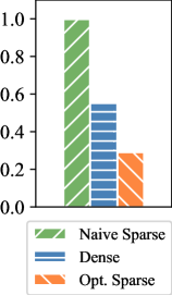<details> <summary>x14.png Details</summary>  ### Visual Description ## Bar Chart: Performance Comparison of Sparse vs. Dense Models ### Overview The image displays a vertical bar chart comparing three different model or data representation types. The chart uses distinct colors and hatch patterns to differentiate between the categories, with a legend provided at the bottom. The y-axis represents a numerical value ranging from 0.0 to 1.0. ### Components/Axes * **Y-Axis:** A vertical axis on the left side of the chart. It is labeled with numerical markers at intervals of 0.2, starting from `0.0` at the bottom and ending at `1.0` at the top. There is no explicit axis title (e.g., "Accuracy," "Score," "Efficiency"). * **X-Axis:** A horizontal axis at the bottom. It does not have explicit category labels directly beneath the bars; the categories are defined solely by the legend. * **Legend:** Positioned at the bottom center of the image, below the x-axis. It contains three entries, each with a colored/hatched box and a text label: 1. A green box with diagonal stripes (top-left to bottom-right) labeled `Naïve Sparse`. 2. A blue box with horizontal stripes labeled `Dense`. 3. An orange box with diagonal stripes (top-right to bottom-left) labeled `Opt. Sparse`. * **Data Series (Bars):** Three vertical bars are plotted from left to right. * **Bar 1 (Left):** Green with diagonal stripes (top-left to bottom-right). Corresponds to `Naïve Sparse`. * **Bar 2 (Center):** Blue with horizontal stripes. Corresponds to `Dense`. * **Bar 3 (Right):** Orange with diagonal stripes (top-right to bottom-left). Corresponds to `Opt. Sparse`. ### Detailed Analysis * **Trend Verification:** The visual trend shows a clear, stepwise decrease in the measured value from left to right. The `Naïve Sparse` bar is the tallest, the `Dense` bar is of medium height, and the `Opt. Sparse` bar is the shortest. * **Data Point Extraction (Approximate Values):** * `Naïve Sparse` (Green, striped): The top of the bar aligns just below the `1.0` mark. **Estimated Value: ~0.95**. * `Dense` (Blue, horizontal stripes): The top of the bar is slightly above the midpoint between `0.4` and `0.6`. **Estimated Value: ~0.55**. * `Opt. Sparse` (Orange, opposite stripes): The top of the bar is exactly halfway between `0.2` and `0.4`. **Estimated Value: ~0.30**. ### Key Observations 1. **Significant Performance Gap:** There is a substantial difference between the highest (`Naïve Sparse` at ~0.95) and lowest (`Opt. Sparse` at ~0.30) values, representing a drop of approximately 0.65 units. 2. **Non-Intuitive Ordering:** The `Dense` model, which one might assume to be a baseline or high-performance standard, performs in the middle (~0.55), worse than the `Naïve Sparse` approach but better than the `Opt. Sparse` approach. 3. **Pattern Consistency:** The hatch patterns in the bars are consistent with their legend entries, ensuring clear visual mapping. The `Naïve Sparse` and `Opt. Sparse` bars use opposing diagonal stripes, while the `Dense` bar uses a distinct horizontal pattern. ### Interpretation This chart likely illustrates a performance metric (e.g., accuracy, F1-score, efficiency ratio) for three different model architectures or data processing techniques. The data suggests a counterintuitive finding: a "Naïve Sparse" method significantly outperforms both a "Dense" method and an "Optimized Sparse" method on this specific metric. * **What it demonstrates:** The primary takeaway is that sparsity, even in a naive implementation, can yield superior results compared to a dense counterpart for the task being measured. However, the process of "optimizing" this sparse model (`Opt. Sparse`) appears to have severely degraded its performance on this particular metric, more than halving it compared to the naive version. * **Potential Context:** Without axis labels, the exact meaning is ambiguous. If the y-axis represents a desirable outcome like accuracy, the `Naïve Sparse` model is the clear winner. If it represents an undesirable outcome like error rate or computational cost, the interpretation flips, and `Opt. Sparse` becomes the best performer. The former is more common for a 0-1 scale. * **Anomaly/Outlier:** The `Opt. Sparse` result is a notable outlier. The optimization process, which typically aims to improve or maintain performance while reducing size/cost, has here led to a dramatic decline. This could indicate a flaw in the optimization technique, a misalignment between the optimization goal and the measured metric, or that the "naive" approach was already near-optimal for this specific measure. * **Relationship Between Elements:** The chart tells a story of trade-offs. It challenges the assumption that "dense is better" and warns that "optimization" is not universally beneficial; its success is highly dependent on the target metric. The visual progression from left to right (`Naïve Sparse` -> `Dense` -> `Opt. Sparse`) creates a narrative of declining performance that prompts investigation into why the optimized sparse model underperforms. </details> (b) ARM Optim. Figure 10: Performance of Sparse Optimization This section presents the effectiveness of the dynamic partitioning and the sparsity optimization. Since the dynamic partitioning merely impact the attention module, Figure 10(a) represents the attention module performance with a verification length of 64. Notably, the attention module becomes dominant in the Transformer model as the context length increases. Static refers to that all sparse computations are processed on the CPU and all dense computations are processed on the GPU. Dynamic indicates that sparse computations are primarily handled by the CPU, while dense computations are primarily handled by the GPU, with dynamic partitioning guided by profiling results. Dynamic partitioning demonstrates obvious improvements when dealing with large context lengths. Figure 10(b) illustrates the performance of the sparse component executed using three different strategies: a naive sparse implementation, our optimized sparse implementation, and the dense implementation that treats the sparse computation as dense. The execution time of optimized sparse implementation exceeds naive sparse and dense implementations by 3.49 $\times$ and 1.90 $\times$ respectively. Also, if we do not optimize the sparse computation, the naive sparse execution cannot outperform the dense one. ## V Related Work Collaborative Execution of Transformer. Tensor Parallelism [1] and Pipeline Parallelism [35] effectively addresses memory limitations by accumulating memory from more devices, gaining widespread adoption in inference tasks within datacenters. They are also used in end-user environments. Galaxy [12] hides communication into computation in the tensor parallelism approach for edge devices, while DeTransformer [36] fundamentally mitigates data dependency by decoupling the original model. Petals [37] utilizes pipeline parallelism to distribute LLM inference across geographically distributed end-user devices. Integrated CPU-GPU Scheduling and Execution. There has been a large amount of prior work focusing on improving the device utilization on integrated CPU-GPU architecture. CoDL [5] and EdgeNN [34] perform collaborative convolutional neural network inference on mobile CPU and GPU with unified memory architecture. Asymo [38] schedules workloads based on the computing power of asymmetric mobile CPU cores to achieve higher throughput. Pipe-It [7] achieves higher throughput by organizing ARM big.Little cores in a pipelined manner. However, none of these approaches are designed for Transformer-based models. Speculative Decoding System. Speculative Decoding represents an innovative paradigm designed to accelerate LLM inference. Existing LLM inference systems [10] start to integrate speculative decoding approaches and they treat them as ordinary LLM inference with a large batch size. Sequoia [39] explores ultra-wide verification width for advanced hardware in cloud. LLMCad [40] adopts the independent drafting speculative decoding approach to accommodate memory-constrained devices. It utilizes a smaller model to generate drafts, thereby reducing data loading time for the larger model. ## VI Conclusion Ghidorah focuses on deploying LLM inference on end-user devices with the unified memory architecture. To fully exploit the hardware capability, Ghidorah leverages speculative decoding approaches to enhance the algorithmic parallelism and then distributes this novel workload across multiple heterogeneous processing units. With the help of the HCMP architecture and ARCA approach, it can achieve up to 7.6 $\times$ speedup in the dominant decoding phase. In the future, Ghidorah will be open-sourced and extended to support more speculative decoding approaches and a wider range of end-user devices. ## References - [1] W. Kwon, Z. Li, S. Zhuang, Y. Sheng, L. Zheng, C. H. Yu, J. Gonzalez, H. Zhang, and I. Stoica, “Efficient memory management for large language model serving with pagedattention,” in Proceedings of the 29th Symposium on Operating Systems Principles, 2023, pp. 611–626. - [2] X. Miao, G. Oliaro, Z. Zhang, X. Cheng, Z. Wang, Z. Zhang, R. Y. Y. Wong, A. Zhu, L. Yang, X. Shi et al., “Specinfer: Accelerating large language model serving with tree-based speculative inference and verification,” in Proceedings of the 29th ACM International Conference on Architectural Support for Programming Languages and Operating Systems, Volume 3, 2024, pp. 932–949. - [3] T. Cai, Y. Li, Z. Geng, H. Peng, J. D. Lee, D. Chen, and T. Dao, “Medusa: Simple llm inference acceleration framework with multiple decoding heads,” arXiv preprint arXiv:2401.10774, 2024. - [4] Y. Fu, P. Bailis, I. Stoica, and H. Zhang, “Break the sequential dependency of LLM inference using lookahead decoding,” in Forty-first International Conference on Machine Learning, ICML 2024, Vienna, Austria, July 21-27, 2024. OpenReview.net, 2024. [Online]. Available: https://openreview.net/forum?id=eDjvSFOkXw - [5] F. Jia, D. Zhang, T. Cao, S. Jiang, Y. Liu, J. Ren, and Y. Zhang, “Codl: efficient CPU-GPU co-execution for deep learning inference on mobile devices,” in MobiSys ’22: The 20th Annual International Conference on Mobile Systems, Applications and Services, Portland, Oregon, 27 June 2022 - 1 July 2022, N. Bulusu, E. Aryafar, A. Balasubramanian, and J. Song, Eds. ACM, 2022, pp. 209–221. [Online]. Available: https://doi.org/10.1145/3498361.3538932 - [6] C. Zhang, F. Zhang, K. Chen, M. Chen, B. He, and X. Du, “Edgenn: Efficient neural network inference for cpu-gpu integrated edge devices,” in 2023 IEEE 39th International Conference on Data Engineering (ICDE). IEEE, 2023, pp. 1193–1207. - [7] S. Wang, G. Ananthanarayanan, Y. Zeng, N. Goel, A. Pathania, and T. Mitra, “High-throughput cnn inference on embedded arm big. little multicore processors,” IEEE Transactions on Computer-Aided Design of Integrated Circuits and Systems, vol. 39, no. 10, pp. 2254–2267, 2019. - [8] Y. Cho, P. Jiyeon, N. Florian, J. Changyeon, T. R. Gross, and B. Egger, “Dopia: online parallelism management for integrated cpu/gpu architectures,” in Proceedings of the 27th ACM SIGPLAN Symposium on Principles and Practice of Parallel Programming, 2022, pp. 32–45. - [9] “Apple m4,” https://en.wikipedia.org/wiki/Apple_M4, 2024. - [10] “vllm github,” https://github.com/vllm-project/vllm, 2024. - [11] M. Shoeybi, M. Patwary, R. Puri, P. LeGresley, J. Casper, and B. Catanzaro, “Megatron-lm: Training multi-billion parameter language models using model parallelism,” arXiv preprint arXiv:1909.08053, 2019. - [12] S. Ye, J. Du, L. Zeng, W. Ou, X. Chu, Y. Lu, and X. Chen, “Galaxy: A resource-efficient collaborative edge ai system for in-situ transformer inference,” arXiv preprint arXiv:2405.17245, 2024. - [13] “Intel core ultra processor family,” https://www.intel.com/content/www/us/en/products/details/processors/core-ultra.html, 2024. - [14] “Meet jetson, the platform for ai at the edge,” https://developer.nvidia.com/embedded-computing, 2024. - [15] M. Li, D. G. Andersen, A. J. Smola, and K. Yu, “Communication efficient distributed machine learning with the parameter server,” Advances in Neural Information Processing Systems, vol. 27, 2014. - [16] S. A. Jacobs, M. Tanaka, C. Zhang, M. Zhang, S. L. Song, S. Rajbhandari, and Y. He, “Deepspeed ulysses: System optimizations for enabling training of extreme long sequence transformer models,” 2023. [Online]. Available: https://arxiv.org/abs/2309.14509 - [17] F. Jia, D. Zhang, T. Cao, S. Jiang, Y. Liu, J. Ren, and Y. Zhang, “Codl: efficient cpu-gpu co-execution for deep learning inference on mobile devices.” in MobiSys, vol. 22, 2022, pp. 209–221. - [18] A. Vaswani, “Attention is all you need,” Advances in Neural Information Processing Systems, 2017. - [19] Y. Zhou, K. Lyu, A. S. Rawat, A. K. Menon, A. Rostamizadeh, S. Kumar, J.-F. Kagy, and R. Agarwal, “Distillspec: Improving speculative decoding via knowledge distillation,” arXiv preprint arXiv:2310.08461, 2023. - [20] Y. Li, F. Wei, C. Zhang, and H. Zhang, “EAGLE: speculative sampling requires rethinking feature uncertainty,” in Forty-first International Conference on Machine Learning, ICML 2024, Vienna, Austria, July 21-27, 2024. OpenReview.net, 2024. [Online]. Available: https://openreview.net/forum?id=1NdN7eXyb4 - [21] “Apple a17,” https://en.wikipedia.org/wiki/Apple_A17, 2024. - [22] “Amd reveals next-gen desktop processors for extreme pc gaming and creator performance,” https://www.amd.com/en/newsroom/press-releases, 2024. - [23] “Qualcomm snapdragon,” https://en.wikipedia.org/wiki/Qualcomm_Snapdragon, 2024. - [24] H. Liu et al., “Ring attention with blockwise transformers for near-infinite context,” arXiv preprint arXiv:2310.01889, 2023. - [25] T. Dao, D. Fu, S. Ermon, A. Rudra, and C. Ré, “Flashattention: Fast and memory-efficient exact attention with io-awareness,” Advances in Neural Information Processing Systems, vol. 35, pp. 16 344–16 359, 2022. - [26] “Wave quantization,” https://docs.nvidia.com/deeplearning/performance/dl-performance-matrix-multiplication/index.html#wave-quant, 2024. - [27] Nvidia, “Nvidia fastertransformer: Transformer related optimization, including bert, gpt,” in Github, 2023. - [28] “Ctranslate2,” https://github.com/OpenNMT/CTranslate2, 2024. - [29] L. Zheng, W.-L. Chiang, Y. Sheng, S. Zhuang, Z. Wu, Y. Zhuang, Z. Lin, Z. Li, D. Li, E. Xing et al., “Judging llm-as-a-judge with mt-bench and chatbot arena,” Advances in Neural Information Processing Systems, vol. 36, pp. 46 595–46 623, 2023. - [30] H. Touvron et al., “Llama: Open and efficient foundation language models,” 2023. [Online]. Available: https://arxiv.org/abs/2302.13971 - [31] K. Cobbe, V. Kosaraju, M. Bavarian, M. Chen, H. Jun, L. Kaiser, M. Plappert, J. Tworek, J. Hilton, R. Nakano et al., “Training verifiers to solve math word problems,” arXiv preprint arXiv:2110.14168, 2021. - [32] M. Chen, J. Tworek, et al., “Evaluating large language models trained on code,” arXiv preprint arXiv:2107.03374, 2021. - [33] J. Austin, A. Odena, M. Nye, M. Bosma, H. Michalewski, D. Dohan, E. Jiang, C. Cai, M. Terry, Q. Le et al., “Program synthesis with large language models,” arXiv preprint arXiv:2108.07732, 2021. - [34] C. Zhang, F. Zhang, K. Chen, M. Chen, B. He, and X. Du, “Edgenn: Efficient neural network inference for CPU-GPU integrated edge devices,” in 39th IEEE International Conference on Data Engineering, ICDE 2023, Anaheim, CA, USA, April 3-7, 2023. IEEE, 2023, pp. 1193–1207. [Online]. Available: https://doi.org/10.1109/ICDE55515.2023.00096 - [35] A. Agrawal et al., “Taming $\{$ Throughput-Latency $\}$ tradeoff in $\{$ LLM $\}$ inference with $\{$ Sarathi-Serve $\}$ ,” in 18th USENIX Symposium on Operating Systems Design and Implementation (OSDI 24), 2024, pp. 117–134. - [36] Y. Wei, S. Ye, J. Jiang, X. Chen, D. Huang, J. Du, and Y. Lu, “Communication-efficient model parallelism for distributed in-situ transformer inference,” in 2024 Design, Automation & Test in Europe Conference & Exhibition (DATE). IEEE, 2024, pp. 1–6. - [37] A. Borzunov, D. Baranchuk, T. Dettmers, M. Ryabinin, Y. Belkada, A. Chumachenko, P. Samygin, and C. Raffel, “Petals: Collaborative inference and fine-tuning of large models,” arXiv preprint arXiv:2209.01188, 2022. - [38] M. Wang, S. Ding, T. Cao, Y. Liu, and F. Xu, “Asymo: scalable and efficient deep-learning inference on asymmetric mobile cpus,” in ACM MobiCom ’21: The 27th Annual International Conference on Mobile Computing and Networking, New Orleans, Louisiana, USA, October 25-29, 2021. ACM, 2021, pp. 215–228. [Online]. Available: https://doi.org/10.1145/3447993.3448625 - [39] Z. Chen, A. May, R. Svirschevski, Y. Huang, M. Ryabinin, Z. Jia, and B. Chen, “Sequoia: Scalable, robust, and hardware-aware speculative decoding,” arXiv preprint arXiv:2402.12374, 2024. - [40] D. Xu, W. Yin, X. Jin, Y. Zhang, S. Wei, M. Xu, and X. Liu, “Llmcad: Fast and scalable on-device large language model inference,” CoRR, vol. abs/2309.04255, 2023. [Online]. Available: https://doi.org/10.48550/arXiv.2309.04255