# 1 Introduction
Statistical mechanics of extensive-width Bayesian neural networks near interpolation
Jean Barbier * 1 Francesco Camilli * 1 Minh-Toan Nguyen * 1 Mauro Pastore * 1 Rudy Skerk * 2 footnotetext: * Equal contribution 1 The Abdus Salam International Centre for Theoretical Physics (ICTP), Strada Costiera 11, 34151 Trieste, Italy 2 International School for Advanced Studies (SISSA), Via Bonomea 265, 34136 Trieste, Italy.
Abstract
For three decades statistical mechanics has been providing a framework to analyse neural networks. However, the theoretically tractable models, e.g., perceptrons, random features models and kernel machines, or multi-index models and committee machines with few neurons, remained simple compared to those used in applications. In this paper we help reducing the gap between practical networks and their theoretical understanding through a statistical physics analysis of the supervised learning of a two-layer fully connected network with generic weight distribution and activation function, whose hidden layer is large but remains proportional to the inputs dimension. This makes it more realistic than infinitely wide networks where no feature learning occurs, but also more expressive than narrow ones or with fixed inner weights. We focus on the Bayes-optimal learning in the teacher-student scenario, i.e., with a dataset generated by another network with the same architecture. We operate around interpolation, where the number of trainable parameters and of data are comparable and feature learning emerges. Our analysis uncovers a rich phenomenology with various learning transitions as the number of data increases. In particular, the more strongly the features (i.e., hidden neurons of the target) contribute to the observed responses, the less data is needed to learn them. Moreover, when the data is scarce, the model only learns non-linear combinations of the teacher weights, rather than “specialising” by aligning its weights with the teacher’s. Specialisation occurs only when enough data becomes available, but it can be hard to find for practical training algorithms, possibly due to statistical-to-computational gaps.
Understanding the expressive power and generalisation capabilities of neural networks is not only a stimulating intellectual activity, producing surprising results that seem to defy established common sense in statistics and optimisation (Bartlett et al., 2021), but has important practical implications in cost-benefit planning whenever a model is deployed. E.g., from a fruitful research line that spanned three decades, we now know that deep fully connected Bayesian neural networks with $O(1)$ readout weights and $L_{2}$ regularisation behave as kernel machines (the so-called Neural Network Gaussian processes, NNGPs) in the heavily overparametrised, infinite-width regime (Neal, 1996; Williams, 1996; Lee et al., 2018; Matthews et al., 2018; Hanin, 2023), and so suffer from these models’ limitations. Indeed, kernel machines infer the decision rule by first embedding the data in a fixed a priori feature space, the renowned kernel trick, then operating linear regression/classification over the features. In this respect, they do not learn features (in the sense of statistics relevant for the decision rule) from the data, so they need larger and larger feature spaces and training sets to fit their higher order statistics (Yoon & Oh, 1998; Dietrich et al., 1999; Gerace et al., 2021; Bordelon et al., 2020; Canatar et al., 2021; Xiao et al., 2023).
Many efforts have been devoted to studying Bayesian neural networks beyond this regime. In the so-called proportional regime, when the width is large and proportional to the training set size, recent studies showed how a limited amount of feature learning makes the network equivalent to optimally regularised kernels (Li & Sompolinsky, 2021; Pacelli et al., 2023; Camilli et al., 2023; Cui et al., 2023; Baglioni et al., 2024; Camilli et al., 2025). This could be a consequence of the fully connected architecture, as, e.g., convolutional neural networks learn more informative features (Naveh & Ringel, 2021; Seroussi et al., 2023; Aiudi et al., 2025; Bassetti et al., 2024). Another scenario is the mean-field scaling, i.e., when the readout weights are small: in this case too a Bayesian network can learn features in the proportional regime (Rubin et al., 2024a; van Meegen & Sompolinsky, 2024).
Here instead we analyse a fully connected two-layer Bayesian network trained end-to-end near the interpolation threshold, when the sample size $n$ is scaling like the number of trainable parameters: for input dimension $d$ and width $k$ , both large and proportional, $n=\Theta(d^{2})=\Theta(kd)$ , a regime where non-trivial feature learning can happen. We consider i.i.d. Gaussian input vectors with labels generated by a teacher network with matching architecture, in order to study the Bayes-optimal learning of this neural network target function. Our results thus provide a benchmark for the performance of any model trained on the same dataset.
2 Setting and main results
2.1 Teacher-student setting
We consider supervised learning with a shallow neural network in the classical teacher-student setup (Gardner & Derrida, 1989). The data-generating model, i.e., the teacher (or target function), is thus a two-layer neural network itself, with readout weights ${\mathbf{v}}^{0}∈\mathbb{R}^{k}$ and internal weights ${\mathbf{W}}^{0}∈\mathbb{R}^{k× d}$ , drawn entrywise i.i.d. from $P_{v}^{0}$ and $P^{0}_{W}$ , respectively; we assume $P^{0}_{W}$ to be centred while $P^{0}_{v}$ has mean $\bar{v}$ , and both priors have unit second moment. We denote the whole set of parameters of the target as ${\bm{\theta}}^{0}=({\mathbf{v}}^{0},{\mathbf{W}}^{0})$ . The inputs are i.i.d. standard Gaussian vectors ${\mathbf{x}}_{\mu}∈\mathbb{R}^{d}$ for $\mu≤ n$ . The responses/labels $y_{\mu}$ are drawn from a kernel $P^{0}_{\rm out}$ :
$$
\textstyle y_{\mu}\sim P^{0}_{\rm out}(\,\cdot\mid\lambda^{0}_{\mu}),\quad%
\lambda^{0}_{\mu}:=\frac{1}{\sqrt{k}}{{\mathbf{v}}^{0\intercal}}\sigma(\frac{1%
}{\sqrt{d}}{{\mathbf{W}}^{0}{\mathbf{x}}_{\mu}}). \tag{1}
$$
The kernel can be stochastic or model a deterministic rule if $P^{0}_{\rm out}(y\mid\lambda)=\delta(y-\mathsf{f}^{0}(\lambda))$ for some outer non-linearity $\mathsf{f}^{0}$ . The activation function $\sigma$ is applied entrywise to vectors and is required to admit an expansion in Hermite polynomials with Hermite coefficients $(\mu_{\ell})_{\ell≥ 0}$ , see App. A: $\sigma(x)=\sum_{\ell≥ 0}\frac{\mu_{\ell}}{\ell!}{\rm He}_{\ell}(x)$ . We assume it has vanishing 0th Hermite coefficient, i.e., that it is centred $\mathbb{E}_{z\sim\mathcal{N}(0,1)}\sigma(z)=0$ ; in App. D.5 we relax this assumption. The input/output pairs $\mathcal{D}=\{({\mathbf{x}}_{\mu},y_{\mu})\}_{\mu≤ n}$ form the training set for a student network with matching architecture.
Notice that the readouts ${\mathbf{v}}^{0}$ are only $k$ unknowns in the target compared to the $kd=\Theta(k^{2})$ inner weights ${\mathbf{W}}^{0}$ . Therefore, they can be equivalently considered quenched, i.e., either given and thus fixed in the student network defined below, or unknown and thus learnable, without changing the leading order of the information-theoretic quantities we aim for. E.g., in terms of mutual information per parameter $\frac{1}{kd+k}I(({\mathbf{W}}^{0},{\mathbf{v}}^{0});\mathcal{D})=\frac{1}{kd}I%
({\mathbf{W}}^{0};\mathcal{D}\mid{\mathbf{v}}^{0})+o_{d}(1)$ . Without loss of generality, we thus consider ${\mathbf{v}}^{0}$ quenched and denote it ${\mathbf{v}}$ from now on. This equivalence holds at leading order and at equilibrium only, but not at the dynamical level, the study of which is left for future work.
The Bayesian student learns via the posterior distribution of the weights ${\mathbf{W}}$ given the training data (and ${\mathbf{v}}$ ), defined by
| | $\textstyle dP({\mathbf{W}}\mid\mathcal{D}):=\mathcal{Z}(\mathcal{D})^{-1}dP_{W%
}({\mathbf{W}})\prod_{\mu≤ n}P_{\rm out}\big{(}y_{\mu}\mid\lambda_{\mu}({%
\mathbf{W}})\big{)}$ | |
| --- | --- | --- |
with post-activation $\lambda_{\mu}({\mathbf{W}}):=\frac{1}{\sqrt{k}}{\mathbf{v}}^{∈tercal}\sigma(%
\frac{1}{\sqrt{d}}{{\mathbf{W}}{\mathbf{x}}_{\mu}})$ , the posterior normalisation constant $\mathcal{Z}(\mathcal{D})$ called the partition function, and $P_{W}$ is the prior assumed by the student. From now on, we focus on the Bayes-optimal case $P_{W}=P_{W}^{0}$ and $P_{\rm out}=P_{\rm out}^{0}$ , but the approach can be extended to account for a mismatch.
We aim at evaluating the expected generalisation error of the student. Let $({\mathbf{x}}_{\rm test},y_{\rm test}\sim P_{\rm out}(\,·\mid\lambda^{0}_{%
\rm test}))$ be a fresh sample (not present in $\mathcal{D}$ ) drawn using the teacher, where $\lambda_{\rm test}^{0}$ is defined as in (1) with ${\mathbf{x}}_{\mu}$ replaced by ${\mathbf{x}}_{\rm test}$ (and similarly for $\lambda_{\rm test}({\mathbf{W}})$ ). Given any prediction function $\mathsf{f}$ , the Bayes estimator for the test response reads $\hat{y}^{\mathsf{f}}({\mathbf{x}}_{\rm test},{\mathcal{D}}):=\langle\mathsf{f}%
(\lambda_{\rm test}({\mathbf{W}}))\rangle$ , where the expectation $\langle\,·\,\rangle:=\mathbb{E}[\,·\mid\mathcal{D}]$ is w.r.t. the posterior $dP({\mathbf{W}}\mid\mathcal{D})$ . Then, for a performance measure $\mathcal{C}:\mathbb{R}×\mathbb{R}\mapsto\mathbb{R}_{≥ 0}$ the Bayes generalisation error is
$$
\displaystyle\varepsilon^{\mathcal{C},\mathsf{f}}:=\mathbb{E}_{{\bm{\theta}}^{%
0},{\mathcal{D}},{\mathbf{x}}_{\rm test},y_{\rm test}}\mathcal{C}\big{(}y_{\rm
test%
},\big{\langle}\mathsf{f}(\lambda_{\rm test}({\mathbf{W}}))\big{\rangle}\big{)}. \tag{2}
$$
An important case is the square loss $\mathcal{C}(y,\hat{y})=(y-\hat{y})^{2}$ with the choice $\mathsf{f}(\lambda)=∈t dy\,y\,P_{\rm out}(y\mid\lambda)=:\mathbb{E}[y\mid\lambda]$ . The Bayes-optimal mean-square generalisation error follows:
$$
\displaystyle\varepsilon^{\rm opt} \displaystyle:=\mathbb{E}_{{\bm{\theta}}^{0},{\mathcal{D}},{\mathbf{x}}_{\rm
test%
},y_{\rm test}}\big{(}y_{\rm test}-\big{\langle}\mathbb{E}[y\mid\lambda_{\rm
test%
}({\mathbf{W}})]\big{\rangle}\big{)}^{2}. \tag{3}
$$
Our main example will be the case of linear readout with Gaussian label noise: $P_{\rm out}(y\mid\lambda)=\exp(-\frac{1}{2\Delta}(y-\lambda)^{2})/\sqrt{2\pi\Delta}$ . In this case, the generalisation error $\varepsilon^{\rm opt}$ takes a simpler form for numerical evaluation than (3), thanks to the concentration of “overlaps” entering it, see App. C.
We study the challenging extensive-width regime with quadratically many samples, i.e., a large size limit
$$
\displaystyle d,k,n\to+\infty\quad\text{with}\quad k/d\to\gamma,\quad n/d^{2}%
\to\alpha. \tag{4}
$$
We denote this joint $d,k,n$ limit with these rates by “ ${\lim}$ ”.
In order to access $\varepsilon^{\mathcal{C},\mathsf{f}},\varepsilon^{\rm opt}$ and other relevant quantities, one can tackle the computation of the average log-partition function, or free entropy in statistical physics language:
$$
\textstyle f_{n}:=\frac{1}{n}\mathbb{E}_{{\bm{\theta}}^{0},\mathcal{D}}\ln%
\mathcal{Z}(\mathcal{D}). \tag{5}
$$
The mutual information between teacher weights and the data is related to the free entropy $f_{n}$ , see App. F. E.g., in the case of linear readout with Gaussian label noise we have $\lim\frac{1}{kd}I({\mathbf{W}}^{0};\mathcal{D}\mid{\mathbf{v}})=-\frac{\alpha}%
{\gamma}\lim f_{n}-\frac{\alpha}{2\gamma}\ln(2\pi e\Delta)$ . Considering the mutual information per parameter allows us to interpret $\alpha$ as a sort of signal-to-noise ratio, so that the mutual information defined in this way increases with it.
Notations: Bold is for vectors and matrices; $d$ is the input dimension, $k$ the width of the hidden layer, $n$ the size of the training set $\mathcal{D}$ , with asymptotic ratios given by (4); ${\mathbf{A}}^{\circ\ell}$ is the Hadamard power of a matrix; for a vector ${\mathbf{v}}$ , $({\mathbf{v}})$ is the diagonal matrix ${\rm diag}({\mathbf{v}})$ ; $(\mu_{\ell})$ are the Hermite coefficients of the activation function $\sigma(x)=\sum_{\ell≥ 0}\frac{\mu_{\ell}}{\ell!}{\rm He}_{\ell}(x)$ ; the norm $\|\,·\,\|$ for vectors and matrices is the Frobenius norm.
2.2 Main results
The aforementioned setting is related to the recent paper Maillard et al. (2024a), with two major differences: said work considers Gaussian distributed weights and quadratic activation. These hypotheses allow numerous simplifications in the analysis, exploited in a series of works Du & Lee (2018); Soltanolkotabi et al. (2019); Venturi et al. (2019); Sarao Mannelli et al. (2020); Gamarnik et al. (2024); Martin et al. (2024); Arjevani et al. (2025). Thanks to this, Maillard et al. (2024a) maps the learning task onto a generalised linear model (GLM) where the goal is to infer a Wishart matrix from linear observations, which is analysable using known results on the GLM Barbier et al. (2019) and matrix denoising Barbier & Macris (2022); Maillard et al. (2022); Pourkamali et al. (2024); Semerjian (2024).
Our main contribution is a statistical mechanics framework for characterising the prediction performance of shallow Bayesian neural networks, able to handle arbitrary activation functions and different distributions of i.i.d. weights, both ingredients playing an important role for the phenomenology.
The theory we derive draws a rich picture with various learning transitions when tuning the sample rate $\alpha≈ n/d^{2}$ . For low $\alpha$ , feature learning occurs because the student tunes its weights to match non-linear combinations of the teacher’s, rather than aligning to those weights themselves. This phase is universal in the (centred, with unit variance) law of the i.i.d. teacher inner weights: our numerics obtained both with binary and Gaussian inner weights match well the theory, which does not depend on this prior here. When increasing $\alpha$ , strong feature learning emerges through specialisation phase transitions, where the student aligns some of its weights with the actual teacher’s ones. In particular, when the readouts ${\mathbf{v}}$ in the target function have a non-trivial distribution, a whole sequence of specialisation transitions occurs as $\alpha$ grows, for the following intuitive reason. Different features in the data are related to the weights of the teacher neurons, $({\mathbf{W}}^{0}_{j}∈\mathbb{R}^{d})_{j≤ k}$ . The strength with which the responses $(y_{\mu})$ depend on the feature ${\mathbf{W}}_{j}^{0}$ is tuned by the corresponding readout through $|v_{j}|$ , which plays the role of a feature-dependent “signal-to-noise ratio”. Therefore, features/hidden neurons $j∈[k]$ corresponding to the largest readout amplitude $\max\{|v_{j}|\}$ are learnt first by the student when increasing $\alpha$ (in the sense that the teacher-student overlap ${\mathbf{W}}^{∈tercal}_{j}{\mathbf{W}}^{0}_{j}/d>o_{d}(1)$ ), then features with the second largest amplitude are, and so on. If the readouts are continuous, an infinite sequence of specialisation transitions emerges in the limit (4). On the contrary, if the readouts are homogeneous (i.e. take a unique value), then a single transition occurs where almost all neurons of the student specialise jointly (possibly up to a vanishing fraction). We predict specialisation transitions to occur for binary inner weights and generic activation, or for Gaussian ones and more-than-quadratic activation. We provide a theoretical description of these learning transitions and identify the order parameters (sufficient statistics) needed to deduce the generalisation error through scalar equations.
The picture that emerges is connected to recent findings in the context of extensive-rank matrix denoising Barbier et al. (2025). In that model, a recovery transition was also identified, separating a universal phase (i.e., independent of the signal prior), from a factorisation phase akin to specialisation in the present context. We believe that this picture and the one found in the present paper are not just similar, but a manifestation of the same fundamental mechanism inherent to the extensive-rank of the matrices involved. Indeed, matrix denoising and neural networks share features with both matrix models Kazakov (2000); Brézin et al. (2016); Anninos & Mühlmann (2020) and planted mean-field spin glasses Nishimori (2001); Zdeborová & and (2016). This mixed nature requires blending techniques from both fields to tackle them. Consequently, the approach developed in Sec. 4 based on the replica method Mezard et al. (1986) is non-standard, as it crucially relies on the Harish Chandra–Itzykson–Zuber (HCIZ), or “spherical”, integral used in matrix models Itzykson & Zuber (1980); Matytsin (1994); Guionnet & Zeitouni (2002). Mixing spherical integration and the replica method has been previously attempted in Schmidt (2018); Barbier & Macris (2022) for matrix denoising, both papers yielding promising but quantitatively inaccurate or non-computable results. Another attempt to exploit a mean-field technique for matrix denoising (in that case a high-temperature expansion) is Maillard et al. (2022), which suffers from similar limitations. The more quantitative answer from Barbier et al. (2025) was made possible precisely thanks to the understanding that the problem behaves more as a matrix model or as a planted mean-field spin glass depending on the phase in which it lives. The two phases could then be treated separately and then joined using an appropriate criterion to locate the transition.
It would be desirable to derive a unified theory able to describe the whole phase diagram based on a single formalism. This is what the present paper provides through a principled combination of spherical integration and the replica method, yielding predictive formulas that are easy to evaluate. It is important to notice that the presence of the HCIZ integral, which is a high-dimensional matrix integral, in the replica formula presented in Result 2.1 suggests that effective one-body problems are not enough to capture alone the physics of the problem, as it is usually the case in standard mean-field inference and spin glass models. Indeed, the appearance of effective one-body problems to describe complex statistical models is usually related to the asymptotic decoupling of the finite marginals of the variables in the problem at hand in terms of products of the single-variable marginals. Therefore, we do not expect a standard cavity (or leave-one-out) approach based on single-variable extraction to be exact, while it is usually showed that the replica and cavity approaches are equivalent in mean-field models Mezard et al. (1986). This may explain why the approximate message-passing algorithms proposed in Parker et al. (2014); Krzakala et al. (2013); Kabashima et al. (2016) are, as stated by the authors, not properly converging nor able to match their corresponding theoretical predictions based on the cavity method. Algorithms for extensive-rank systems should therefore combine ingredients from matrix denoising and standard message-passing, reflecting their hybrid mean-field/matrix model nature.
In order to face this, we adapt the GAMP-RIE (generalised approximate message-passing with rotational invariant estimator) introduced in Maillard et al. (2024a) for the special case of quadratic activation, to accommodate a generic activation function $\sigma$ . By construction, the resulting algorithm described in App. H cannot find the specialisation solution, i.e., a solution where at least $\Theta(k)$ neurons align with the teacher’s. Nevertheless, it matches the performance associated with the so-called universal solution/branch of our theory for all $\alpha$ , which describes a solution with overlap ${\mathbf{W}}^{∈tercal}_{j}{\mathbf{W}}^{0}_{j}/d>o_{d}(1)$ for at most $o(k)$ neurons. As a side investigation, we show empirically that the specialisation solution is potentially hard to reach with popular algorithms for some target functions: the algorithms we tested either fail to find it and instead get stuck in a sub-optimal glassy phase (Metropolis-Hastings sampling for the case of binary inner weights), or may find it but in a training time increasing exponentially with $d$ (ADAM Kingma & Ba (2017) and Hamiltonian Monte Carlo (HMC) for the case of Gaussian weights). It would thus be interesting to settle whether GAMP-RIE has the best prediction performance achievable by a polynomial-time learner when $n=\Theta(d^{2})$ for such targets. For specific choices of the distribution of the readout weights, the evidence of hardness is not conclusive and requires further investigation.
Replica free entropy
Our first result is a tractable approximation for the free entropy. To state it, let us introduce two functions $\mathcal{Q}_{W}(\mathsf{v}),\hat{\mathcal{Q}}_{W}(\mathsf{v})∈[0,1]$ for $\mathsf{v}∈{\rm Supp}(P_{v})$ , which are non-decreasing in $|\mathsf{v}|$ . Let (see (43) in appendix for a more explicit expression of $g$ )
$$
\textstyle g(x):=\sum_{\ell\geq 3}x^{\ell}{\mu_{\ell}^{2}}/{\ell!}, \textstyle q_{K}(x,\mathcal{Q}_{W}):=\mu_{1}^{2}+{\mu_{2}^{2}}\,x/2+\mathbb{E}%
_{v\sim P_{v}}[v^{2}g(\mathcal{Q}_{W}(v))], \textstyle r_{K}:=\mu_{1}^{2}+{\mu_{2}^{2}}(1+\gamma\bar{v}^{2})/2+g(1), \tag{1}
$$
and the auxiliary potentials
| | $\textstyle\psi_{P_{W}}(x):=\mathbb{E}_{w^{0},\xi}\ln\mathbb{E}_{w}\exp(-\frac{%
1}{2}xw^{2}+xw^{0}w+\sqrt{x}\xi w),$ | |
| --- | --- | --- |
where $w^{0},w\sim P_{W}$ and $\xi,u_{0},u\sim{\mathcal{N}}(0,1)$ all independent. Moreover, $\mu_{{\mathbf{Y}}(x)}$ is the limiting (in $d→∞$ ) spectral density of data ${\mathbf{Y}}(x)=\sqrt{x/(kd)}\,{\mathbf{S}}^{0}+{\mathbf{Z}}$ in the denoising problem of the matrix ${\mathbf{S}}^{0}:={\mathbf{W}}^{0∈tercal}({\mathbf{v}}){\mathbf{W}}^{0}∈%
\mathbb{R}^{d× d}$ , with ${\mathbf{Z}}$ a standard GOE matrix (a symmetric matrix whose upper triangular part has i.i.d. entries from $\mathcal{N}(0,(1+\delta_{ij})/d)$ ). Denote the minimum mean-square error associated with this denoising problem as ${\rm mmse}_{S}(x)=\lim_{d→∞}d^{-2}\mathbb{E}\|{\mathbf{S}}^{0}-\mathbb{%
E}[{\mathbf{S}}^{0}\mid{\mathbf{Y}}(x)]\|^{2}$ (whose explicit definition is given in App. D.3) and its functional inverse by ${\rm mmse}_{S}^{-1}$ (which exists by monotonicity).
**Result 2.1 (Replica symmetric free entropy)**
*Let the functional $\tau(\mathcal{Q}_{W}):={\rm mmse}_{S}^{-1}(1-\mathbb{E}_{v\sim P_{v}}[v^{2}%
\mathcal{Q}_{W}(v)^{2}])$ . Given $(\alpha,\gamma)$ , the replica symmetric (RS) free entropy approximating ${\lim}\,f_{n}$ in the scaling limit (4) is ${\rm extr}\,f_{\rm RS}^{\alpha,\gamma}$ with RS potential $f^{\alpha,\gamma}_{\rm RS}=f^{\alpha,\gamma}_{\rm RS}(q_{2},\hat{q}_{2},%
\mathcal{Q}_{W},\hat{\mathcal{Q}}_{W})$ given by
$$
\textstyle f^{\alpha,\gamma}_{\rm RS} \textstyle:=\psi_{P_{\text{out}}}(q_{K}(q_{2},\mathcal{Q}_{W});r_{K})+\frac{1}%
{4\alpha}(1+\gamma\bar{v}^{2}-q_{2})\hat{q}_{2} \textstyle\qquad+\frac{\gamma}{\alpha}\mathbb{E}_{v\sim P_{v}}\big{[}\psi_{P_{%
W}}(\hat{\mathcal{Q}}_{W}(v))-\frac{1}{2}\mathcal{Q}_{W}(v)\hat{\mathcal{Q}}_{%
W}(v)\big{]} \textstyle\qquad+\frac{1}{\alpha}\big{[}\iota(\tau(\mathcal{Q}_{W}))-\iota(%
\hat{q}_{2}+\tau(\mathcal{Q}_{W}))\big{]}. \tag{6}
$$
The extremisation operation in ${\rm extr}\,f^{\alpha,\gamma}_{\rm RS}$ selects a solution $(q_{2}^{*},\hat{q}_{2}^{*},\mathcal{Q}_{W}^{*},\hat{\mathcal{Q}}_{W}^{*})$ of the saddle point equations, obtained from $∇ f^{\alpha,\gamma}_{\rm RS}=\mathbf{0}$ , which maximises the RS potential.*
The extremisation of $f_{\rm RS}^{\alpha,\gamma}$ yields the system (76) in the appendix, solved numerically in a standard way (see provided code).
The order parameters $q_{2}^{*}$ and $\mathcal{Q}_{W}^{*}$ have a precise physical meaning that will be clear from the discussion in Sec. 4. In particular, $q_{2}^{*}$ is measuring the alignment of the student’s combination of weights ${\mathbf{W}}^{∈tercal}({\mathbf{v}}){\mathbf{W}}/\sqrt{k}$ with the corresponding teacher’s ${\mathbf{W}}^{0∈tercal}({\mathbf{v}}){\mathbf{W}}^{0}/\sqrt{k}$ , which is non trivial with $n=\Theta(d^{2})$ data even when the student is not able to reconstruct ${\mathbf{W}}^{0}$ itself (i.e., to specialise). On the other hand, $\mathcal{Q}_{W}^{*}(\mathsf{v})$ measures the overlap between weights $\{{\mathbf{W}}_{i}^{0/·}\mid v_{i}=\mathsf{v}\}$ (a different treatment for weights connected to different $\mathsf{v}$ ’s is needed because, as discussed earlier, the student will learn first –with less data– weights connected to larger readouts). A non-trivial $\mathcal{Q}_{W}^{*}(\mathsf{v})≠ 0$ signals that the student learns something about ${\mathbf{W}}^{0}$ . Thus, the specialisation transitions are naturally defined, based on the extremiser of $f_{\rm RS}^{\alpha,\gamma}$ in the result above, as $\alpha_{\rm sp,\mathsf{v}}(\gamma):=\sup\,\{\alpha\mid\mathcal{Q}^{*}_{W}(%
\mathsf{v})=0\}$ . For non-homogeneous readouts, we call the specialisation transition $\alpha_{\rm sp}(\gamma):=\min_{\mathsf{v}}\alpha_{\rm sp,\mathsf{v}}(\gamma)$ . In this article, we report cases where the inner weights are discrete or Gaussian distributed. For activations different than a pure quadratic, $\sigma(x)≠ x^{2}$ , we predict the transition to occur in both cases (see Fig. 1 and 2). Then, $\alpha<\alpha_{\rm sp}$ corresponds to the universal phase, where the free entropy is independent of the choice of the prior over the inner weights. Instead, $\alpha>\alpha_{\rm sp}$ is the specialisation phase where the prior $P_{W}$ matters, and the student aligns a finite fraction of its weights $({\mathbf{W}}_{j})_{j≤ k}$ with those of the teacher, which lowers the generalisation error.
Let us comment on why the special case $\sigma(x)=x^{2}$ with $P_{W}=\mathcal{N}(0,1)$ could be treated exactly with known techniques (spherical integration) in Maillard et al. (2024a); Xu et al. (2025). With $\sigma(x)=x^{2}$ the responses $(y_{\mu})$ depend on ${\mathbf{W}}^{0∈tercal}({\mathbf{v}}){\mathbf{W}}^{0}$ only. If ${\mathbf{v}}$ has finite fractions of equal entries, a large invariance group prevents learning ${\mathbf{W}}^{0}$ and thus specialisation. Take as example ${\mathbf{v}}=(1,...,1,-1,...,-1)$ with the first half filled with ones. Then, the responses are indistinguishable from those obtained using a modified matrix ${\mathbf{W}}^{0∈tercal}{\mathbf{U}}^{∈tercal}({\mathbf{v}}){\mathbf{U}}{%
\mathbf{W}}^{0}$ where ${\mathbf{U}}=(({\mathbf{U}}_{1},\mathbf{0}_{d/2})^{∈tercal},(\mathbf{0}_{d/2%
},{\mathbf{U}}_{2})^{∈tercal})$ is block diagonal with $d/2× d/2$ orthogonal ${\mathbf{U}}_{1},{\mathbf{U}}_{2}$ and zeros on off-diagonal blocks. The Gaussian prior $P_{W}$ is rotationally invariant and, thus, does not break any invariance, so ${\mathbf{U}}_{1},{\mathbf{U}}_{2}$ are arbitrary. The resulting invariance group has an $\Theta(d^{2})$ entropy (the logarithm of its volume), which is comparable to the leading order of the free entropy. Therefore, it cannot be broken using infinitesimal perturbations (or “side information”) and, consequently, prevents specialisation. This reasoning can be extended to $P_{v}$ with a continuous support, as long as we can discretise it with a finite (possibly large) number of bins, take the limit (4) first, and then take the continuum limit of the binning afterwards. However, the picture changes if the prior breaks rotational invariance; e.g., with Rademacher $P_{W}$ , only signed permutation invariances survive, a symmetry with negligible entropy $o(d^{2})$ which, consequently, does not change the limiting thermodynamic (information-theoretic) quantities. The large rotational invariance group is the reason why $\sigma(x)=x^{2}$ with $P_{W}=\mathcal{N}(0,1)$ can be treated using the HCIZ integral alone. Even when $P_{W}=\mathcal{N}(0,1)$ , the presence of any other term in the series expansion of $\sigma$ breaks invariances with large entropy: specialisation can then occur, thus requiring our theory. We mention that our theory seems inexact When solving the extremisation of (6) for $\sigma(x)=x^{2}$ with $P_{W}=\mathcal{N}(0,1)$ , we noticed that the difference between the RS free entropy of the correct universal solution, $\mathcal{Q}_{W}(\mathsf{v})=0$ , and the maximiser, predicting $\mathcal{Q}_{W}(\mathsf{v})>0$ , does not exceed $≈ 1\%$ : the RS potential is very flat as a function of $\mathcal{Q}_{W}$ . We thus cannot discard that the true maximiser of the potential is at $\mathcal{Q}_{W}(\mathsf{v})=0$ , and that we observe otherwise due to numerical errors. Indeed, evaluating the spherical integrals $\iota(\,·\,)$ in $f^{\alpha,\gamma}_{\rm RS}$ is challenging, in particular when $\gamma$ is small. Actually, for $\gamma\gtrsim 1$ we do get that $\mathcal{Q}_{W}(\mathsf{v})=0$ is always the maximiser for $\sigma(x)=x^{2}$ with $P_{W}=\mathcal{N}(0,1)$ . for $\sigma(x)=x^{2}$ with $P_{W}=\mathcal{N}(0,1)$ if applied naively, as it predicts ${\mathcal{Q}}_{W}(\mathsf{v})>0$ and therefore does not recover the rigorous result of Xu et al. (2025) (yet, it predicts a free entropy less than $1\%$ away from the truth). Nevertheless, the solution of Maillard et al. (2024a); Xu et al. (2025) is recovered from our equations by enforcing a vanishing overlap $\mathcal{Q}_{W}(\mathsf{v})=0$ , i.e., via its universal branch.
Bayes generalisation error
Another main result is an approximate formula for the generalisation error. Let $({\mathbf{W}}^{a})_{a≥ 1}$ be i.i.d. samples from the posterior $dP(\,·\mid\mathcal{D})$ and ${\mathbf{W}}^{0}$ the teacher’s weights. Assuming that the joint law of $(\lambda_{\rm test}({\mathbf{W}}^{a},{\mathbf{x}}_{\rm test}))_{a≥ 0}=:(%
\lambda^{a})_{a≥ 0}$ for a common test input ${\mathbf{x}}_{\rm test}∉\mathcal{D}$ is a centred Gaussian, our framework predicts its covariance. Our approximation for the Bayes error follows.
**Result 2.2 (Bayes generalisation error)**
*Let $q_{K}^{*}=q_{K}(q_{2}^{*},\mathcal{Q}_{W}^{*})$ where $(q_{2}^{*},\hat{q}_{2}^{*},\mathcal{Q}_{W}^{*},\hat{\mathcal{Q}}_{W}^{*})$ is an extremiser of $f_{\rm RS}^{\alpha,\gamma}$ as in Result 2.1. Assuming joint Gaussianity of the post-activations $(\lambda^{a})_{a≥ 0}$ , in the scaling limit (4) their mean is zero and their covariance is approximated by $\mathbb{E}\lambda^{a}\lambda^{b}=q_{K}^{*}+(r_{K}-q_{K}^{*})\delta_{ab}=:(%
\mathbf{\Gamma})_{ab}$ , see App. C. Assume $\mathcal{C}$ has the series expansion $\mathcal{C}(y,\hat{y})=\sum_{i≥ 0}c_{i}(y)\hat{y}^{i}$ . The Bayes error $\smash{\lim\,\varepsilon^{\mathcal{C},\mathsf{f}}}$ is approximated by
| | $\textstyle\mathbb{E}_{(\lambda^{a})\sim\mathcal{N}(\mathbf{0},\mathbf{\Gamma})%
}\mathbb{E}_{y_{\rm test}\sim P_{\rm out}(\,·\mid\lambda^{0})}\sum_{i≥ 0%
}c_{i}(y_{\rm test}(\lambda^{0}))\prod_{a=1}^{i}\mathsf{f}(\lambda^{a}).$ | |
| --- | --- | --- |
Letting $\mathbb{E}[\,·\mid\lambda]=∈t dy\,(\,·\,)\,P_{\rm out}(y\mid\lambda)$ , the Bayes-optimal mean-square generalisation error $\smash{\lim\,\varepsilon^{\rm opt}}$ is approximated by
$$
\textstyle\mathbb{E}_{\lambda^{0},\lambda^{1}}\big{(}\mathbb{E}[y^{2}\mid%
\lambda^{0}]-\mathbb{E}[y\mid\lambda^{0}]\mathbb{E}[y\mid\lambda^{1}]\big{)}. \tag{7}
$$*
This result assumed that $\mu_{0}=0$ ; see App. D.5 if this is not the case. Results 2.1 and 2.2 provide an effective theory for the generalisation capabilities of Bayesian shallow networks with generic activation. We call these “results” because, despite their excellent match with numerics, we do not expect these formulas to be exact: their derivation is based on an unconventional mix of spin glass techniques and spherical integrals, and require approximations in order to deal with the fact that the degrees of freedom to integrate are large matrices of extensive rank. This is in contrast with simpler (vector) models (perceptrons, multi-index models, etc) where replica formulas are routinely proved correct, see e.g. Barbier & Macris (2019); Barbier et al. (2019); Aubin et al. (2018).
|
<details>
<summary>x1.png Details</summary>
### Visual Description
## Line Chart: Optimal Epsilon vs. Alpha
### Overview
The image is a line chart displaying the relationship between "alpha" (α) on the x-axis and "epsilon optimal" (εopt) on the y-axis. There are two distinct data series plotted, one in blue and one in red, each with different markers and line styles. Error bars are present on some data points.
### Components/Axes
* **X-axis:** Labeled "α" (alpha), ranging from 0 to 7, with tick marks at each integer value.
* **Y-axis:** Labeled "εopt" (epsilon optimal), ranging from 0.02 to 0.10. Tick marks are present at 0.02, 0.04, 0.06, 0.08, 0.025, 0.050, 0.075, and 0.100.
* **Data Series 1 (Blue):** A solid blue line with circular markers. A dashed blue line with 'x' markers is also present, closely following the solid line.
* **Data Series 2 (Red):** A solid red line with circular markers. A dashed red line with triangle markers is also present, closely following the solid line.
* **Error Bars:** Vertical error bars are present on some data points for both series.
### Detailed Analysis
* **Blue Series (Solid Line, Circles):**
* Trend: Decreases rapidly from α = 0 to α = 2, then plateaus and remains relatively constant.
* Data Points:
* α = 0: εopt ≈ 0.08
* α = 1: εopt ≈ 0.04
* α = 2: εopt ≈ 0.025
* α = 7: εopt ≈ 0.018
* **Blue Series (Dashed Line, Xs):**
* Trend: Similar to the solid blue line, decreasing rapidly and then plateauing.
* Data Points: Follows the solid blue line closely, with values very similar to the solid line.
* **Red Series (Solid Line, Circles):**
* Trend: Starts relatively constant at α = 0, then decreases rapidly around α = 1.5, and plateaus at a low value.
* Data Points:
* α = 0: εopt ≈ 0.102
* α = 1: εopt ≈ 0.100
* α = 2: εopt ≈ 0.04
* α = 3: εopt ≈ 0.02
* α = 7: εopt ≈ 0.01
* **Red Series (Dashed Line, Triangles):**
* Trend: Remains relatively constant around εopt = 0.10.
* Data Points:
* α = 0 to α = 7: εopt ≈ 0.10
* **Error Bars:**
* Present on some data points, indicating the uncertainty in the measurements. The error bars appear to be larger for the red series at higher alpha values (α = 6 and α = 7).
### Key Observations
* The blue series (both solid and dashed) shows a rapid decrease in εopt as α increases from 0 to 2, after which it stabilizes.
* The red series (solid line) shows a sharp drop in εopt around α = 1.5, while the dashed red line remains constant.
* The error bars suggest that the uncertainty in the measurements increases for the red series at higher values of α.
### Interpretation
The chart illustrates how the optimal epsilon value (εopt) changes with respect to alpha (α) for two different scenarios represented by the blue and red series. The blue series indicates a system where the optimal epsilon quickly decreases as alpha increases, suggesting that a smaller epsilon is needed for optimal performance at higher alpha values. The red series, particularly the solid line, shows a critical point around α = 1.5, where the optimal epsilon drops significantly. This could indicate a phase transition or a change in the system's behavior. The dashed red line represents a scenario where the optimal epsilon remains constant regardless of the alpha value. The increasing error bars for the red series at higher alpha values suggest that the system becomes less stable or more sensitive to variations at these points.
</details>
|
<details>
<summary>x2.png Details</summary>
### Visual Description
## Chart: ReLU vs Tanh
### Overview
The image is a chart comparing the performance of ReLU and Tanh activation functions. The x-axis represents a variable denoted as "α", ranging from 0 to 7. Two data series are plotted: ReLU (blue) and Tanh (red). Both series have a solid line representing one type of data and a dashed line representing another. Error bars are present on some data points.
### Components/Axes
* **X-axis:** α, ranging from 0 to 7.
* **Y-axis:** (Implicit) Performance metric, not explicitly labeled.
* **Legend (Top-Right):**
* ReLU (blue)
* Tanh (red)
### Detailed Analysis
* **ReLU (Blue):**
* **Solid Line:** Starts at approximately 1.2 at α=0, decreases rapidly to approximately 0.4 at α=2, and then gradually decreases to approximately 0.25 at α=7. The data points are marked with circles.
* **Dashed Line:** Starts at approximately 1.1 at α=0, decreases rapidly to approximately 0.5 at α=2, and then gradually decreases to approximately 0.3 at α=7. The data points are marked with asterisks.
* **Tanh (Red):**
* **Solid Line:** Starts at approximately 0.8 at α=0, decreases rapidly to approximately 0.1 at α=2, and then gradually decreases to approximately 0.02 at α=7. The data points are marked with circles.
* **Dashed Line:** Starts at approximately 0.8 at α=0, remains relatively constant at approximately 0.75 until α=3, and then has some error bars at α=4. The data points are marked with asterisks.
### Key Observations
* The solid lines for both ReLU and Tanh show a decreasing trend as α increases.
* The dashed line for ReLU is below the solid line.
* The dashed line for Tanh is above the solid line.
* The Tanh solid line decreases more rapidly than the ReLU solid line.
* The Tanh dashed line remains relatively constant.
### Interpretation
The chart compares the performance of ReLU and Tanh activation functions under different conditions, represented by the solid and dashed lines. The x-axis variable "α" likely represents a parameter or condition being varied. The solid lines suggest that both ReLU and Tanh performance decreases as "α" increases, but Tanh decreases more rapidly. The dashed lines represent a different scenario, where ReLU performance is slightly worse than the solid line scenario, while Tanh performance remains relatively constant. The error bars indicate the variability or uncertainty in the data points. The data suggests that the choice between ReLU and Tanh depends on the specific conditions represented by "α" and the solid/dashed lines.
</details>
|
<details>
<summary>x3.png Details</summary>
### Visual Description
## Chart: Algorithm Performance vs. Alpha
### Overview
The image is a chart comparing the performance of four algorithms (ADAM, informative HMC, uninformative HMC, and GAMP-RIE) across varying values of a parameter denoted as alpha (α). The chart displays the performance of each algorithm as a function of alpha, with error bars indicating the uncertainty in the measurements.
### Components/Axes
* **X-axis:** α (alpha), ranging from 0 to 7, with tick marks at every integer value.
* **Y-axis:** The Y-axis is not explicitly labeled, but it represents a performance metric. The values on the Y-axis are not explicitly marked, but the data ranges approximately from 0 to 1.
* **Legend (Top-Right):**
* `* ADAM`: Represented by blue asterisks connected by a solid blue line.
* `o informative HMC`: Represented by blue circles connected by a solid blue line.
* `o uninformative HMC`: Represented by red circles connected by a solid red line.
* `△ GAMP-RIE`: Represented by red triangles connected by a dashed red line.
### Detailed Analysis
* **ADAM (Blue Asterisks, Solid Line):** The performance of ADAM starts high and decreases rapidly as alpha increases from 0 to 1. It then continues to decrease more gradually as alpha increases further, approaching a relatively stable value.
* α = 0: Performance ≈ 0.9
* α = 1: Performance ≈ 0.4
* α = 7: Performance ≈ 0.2
* **Informative HMC (Blue Circles, Solid Line):** The performance of informative HMC mirrors that of ADAM, starting high and decreasing rapidly as alpha increases from 0 to 1. It then continues to decrease more gradually as alpha increases further, approaching a relatively stable value.
* α = 0: Performance ≈ 0.85
* α = 1: Performance ≈ 0.35
* α = 7: Performance ≈ 0.15
* **Uninformative HMC (Red Circles, Solid Line):** The performance of uninformative HMC starts high and decreases rapidly as alpha increases from 0 to 1. It then continues to decrease more gradually as alpha increases further, approaching a relatively stable value.
* α = 0: Performance ≈ 0.7
* α = 1: Performance ≈ 0.15
* α = 7: Performance ≈ 0.02
* **GAMP-RIE (Red Triangles, Dashed Line):** The performance of GAMP-RIE remains relatively constant across all values of alpha.
* α = 0: Performance ≈ 0.7
* α = 7: Performance ≈ 0.7
### Key Observations
* ADAM and informative HMC exhibit similar performance trends, with a rapid decrease in performance as alpha increases from 0 to 1, followed by a more gradual decrease.
* Uninformative HMC shows a similar trend to ADAM and informative HMC, but with a more pronounced initial drop in performance.
* GAMP-RIE maintains a relatively constant performance level across all values of alpha.
* The error bars suggest that the uncertainty in the performance measurements is relatively small for most data points.
### Interpretation
The chart suggests that the performance of ADAM, informative HMC, and uninformative HMC is sensitive to the value of alpha, with higher values of alpha generally leading to lower performance. In contrast, the performance of GAMP-RIE appears to be relatively insensitive to alpha. This could indicate that GAMP-RIE is more robust to changes in this parameter or that it is optimized for a different range of alpha values. The rapid initial drop in performance for the HMC methods suggests that there may be a critical value of alpha beyond which their performance degrades significantly. The error bars provide an indication of the reliability of the performance measurements, with smaller error bars indicating greater confidence in the results.
</details>
|
| --- | --- | --- |
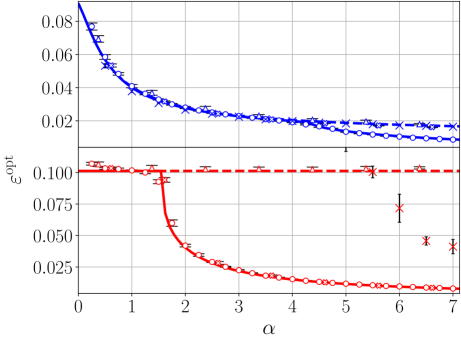
Figure 1: Theoretical prediction (solid curves) of the Bayes-optimal mean-square generalisation error for Gaussian inner weights with ReLU(x) activation (blue curves) and Tanh(2x) activation (red curves), $d=150,\gamma=0.5$ , with linear readout with Gaussian label noise of variance $\Delta=0.1$ and different $P_{v}$ laws. The dashed lines are the theoretical predictions associated with the universal solution, obtained by plugging ${\mathcal{Q}}_{W}(\mathsf{v})=0\ ∀\ \mathsf{v}$ in (6) and extremising w.r.t. $(q_{2},\hat{q}_{2})$ (the curve coincides with the optimal one before the transition $\alpha_{\rm sp}(\gamma)$ ). The numerical points are obtained with Hamiltonian Monte Carlo (HMC) with informative initialisation on the target (empty circles), uninformative, random, initialisation (empty crosses), and ADAM (thin crosses). Triangles are the error of GAMP-RIE (Maillard et al., 2024a) extended to generic activation, obtained by plugging estimator (109) in (3) in appendix. Each point has been averaged over 10 instances of the teacher and training set. Error bars are the standard deviation over instances. The generalisation error for a given training set is evaluated as $\frac{1}{2}\mathbb{E}_{{\mathbf{x}}_{\rm test}\sim\mathcal{N}(0,I_{d})}(%
\lambda_{\rm test}({\mathbf{W}})-\lambda_{\rm test}^{0})^{2}$ , using a single sample ${\mathbf{W}}$ from the posterior for HMC. For ADAM, with batch size fixed to $n/5$ and initial learning rate $0.05$ , the error corresponds to the lowest one reached during training, i.e., we use early stopping based on the minimum test loss over all gradient updates. Its generalisation error is then evaluated at this point and divided by two (for comparison with the theory). The average over ${\mathbf{x}}_{\rm test}$ is computed empirically from $10^{5}$ i.i.d. test samples. We exploit that, for typical posterior samples, the Gibbs error $\varepsilon^{\rm Gibbs}$ defined in (39) in App. C is linked to the Bayes-optimal error as $(\varepsilon^{\rm Gibbs}-\Delta)/2=\varepsilon^{\rm opt}-\Delta$ , see (40) in appendix. To use this formula, we are assuming the concentration of the Gibbs error w.r.t. the posterior distribution, in order to evaluate it from a single sample per instance. Left: Homogeneous readouts $P_{v}=\delta_{1}$ . Centre: 4-points readouts $P_{v}=\frac{1}{4}(\delta_{-3/\sqrt{5}}+\delta_{-1/\sqrt{5}}+\delta_{1/\sqrt{5}%
}+\delta_{3/\sqrt{5}})$ . Right: Gaussian readouts $P_{v}=\mathcal{N}(0,1)$ .
3 Theoretical predictions and numerical experiments
Let us compare our theoretical predictions with simulations. In Fig. 1 and 2, we report the theoretical curves from Result 2.2, focusing on the optimal mean-square generalisation error for networks with different $\sigma$ , with linear readout with Gaussian noise variance $\Delta$ . The Gibbs error divided by $2$ is used to compute the optimal error, see Remark C.2 in App. C for a justification. In what follows, the error attained by ADAM is also divided by two, only for the purpose of comparison.
Figure 1 focuses on networks with Gaussian inner weights, various readout laws, for $\sigma(x)={\rm ReLU}(x)$ and ${\rm Tanh}(2x)$ . Informative (i.e., on the teacher) and uninformative (random) initialisations are used when sampling the posterior by HMC. We also run ADAM, always selecting its best performance over all epochs, and implemented an extension of the GAMP-RIE of Maillard et al. (2024a) for generic activation (see App. H). It can be shown analytically that GAMP-RIE’s generalisation error asymptotically (in $d$ ) matches the prediction of the universal branch of our theory (i.e., associated with $\mathcal{Q}_{W}(\mathsf{v})=0\ ∀\ \mathsf{v}$ ).
For ReLU activation and homogeneous readouts (left panel), informed HMC follows the specialisation branch (the solution of the saddle point equations with $\mathcal{Q}_{W}(\mathsf{v})≠ 0$ for at least one $\mathsf{v}$ ), while with uninformative initialisation it sticks to the universal branch, thus suggesting algorithmic hardness. We shall be back to this matter in the following. We note that the error attained by ADAM (divided by 2), is close to the performance associated with the universal branch, which suggests that ADAM is an effective Gibbs estimator for this $\sigma$ . For Tanh and homogeneous readouts, both the uninformative and informative points lie on the specialisation branch, while ADAM attains an error greater than twice the posterior sample’s generalisation error.
For non-homogeneous readouts (centre and right panels) the points associated with the informative initialisation lie consistently on the specialisation branch, for both ${\rm ReLU}$ and Tanh, while the uninformatively initialised samples have a slightly worse performance for Tanh. Non-homogeneous readouts improves the ADAM performance: for Gaussian readouts and high sampling ratio its half-generalisation error is consistently below the error associated with the universal branch of the theory.
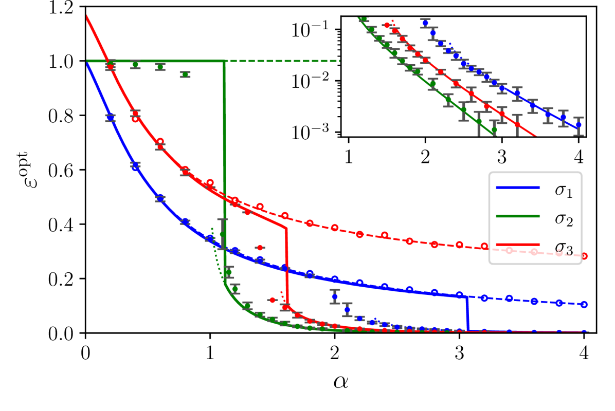
Figure 2 concerns networks with Rademacher weights and homogeneous readout. The numerical points are of two kinds: the dots, obtained from Metropolis–Hastings sampling of the weight posterior, and the circles, obtained from the GAMP-RIE (App. H). We report analogous simulations for ${\rm ReLU}$ and ${\rm ELU}$ activations in Figure 7, App. H. The remarkable agreement between theoretical curves and experimental points in both phases supports the assumptions used in Sec. 4.
<details>
<summary>x4.png Details</summary>
### Visual Description
## Line Chart: Epsilon Opt vs. Alpha for Different Sigma Values
### Overview
The image is a line chart displaying the relationship between epsilon opt (εopt) and alpha (α) for three different sigma values (σ1, σ2, σ3). The chart includes an inset plot showing the same data on a log scale for the y-axis. Data points are marked with circles and error bars.
### Components/Axes
* **Main Chart:**
* X-axis: α (alpha), ranging from 0 to 4.
* Y-axis: εopt (epsilon opt), ranging from 0 to 1.2.
* Legend (bottom-right):
* Blue line: σ1
* Green line: σ2
* Red line: σ3
* **Inset Chart (top-right):**
* X-axis: α (alpha), ranging from approximately 1 to 4.
* Y-axis: Logarithmic scale, ranging from 10^-3 to 10^-1.
* Data series are the same as the main chart.
### Detailed Analysis
* **σ1 (Blue Line):**
* Trend: Decreases from approximately 1.0 at α = 0 to approximately 0.15 at α = 3, then drops to 0.0 at α = 3.1.
* Data Points:
* α = 0, εopt ≈ 1.0
* α = 1, εopt ≈ 0.4
* α = 2, εopt ≈ 0.15
* α = 3, εopt ≈ 0.15
* α > 3.1, εopt = 0
* **σ2 (Green Line):**
* Trend: Remains constant at approximately 1.0 from α = 0 to α = 1.1, then drops to 0.0.
* Data Points:
* α < 1.1, εopt ≈ 1.0
* α > 1.1, εopt = 0
* **σ3 (Red Line):**
* Trend: Decreases from approximately 1.2 at α = 0 to approximately 0.45 at α = 1.7, then drops to 0.3 at α = 1.8, and remains relatively constant.
* Data Points:
* α = 0, εopt ≈ 1.2
* α = 1, εopt ≈ 0.75
* α = 2, εopt ≈ 0.3
* α = 3, εopt ≈ 0.3
* α = 4, εopt ≈ 0.3
### Key Observations
* σ2 exhibits a step function behavior, dropping sharply to zero at α ≈ 1.1.
* σ1 decreases gradually before dropping to zero at α ≈ 3.1.
* σ3 decreases gradually and then plateaus at approximately 0.3.
* The inset plot confirms the exponential decay of the data series.
### Interpretation
The chart illustrates how epsilon opt (εopt) changes with alpha (α) for different values of sigma (σ). The different sigma values seem to represent different thresholds or sensitivities. σ2 has the lowest threshold, dropping to zero at a low α value, while σ1 and σ3 have higher thresholds and exhibit more gradual decreases. The inset plot highlights the exponential decay behavior of the data, suggesting a relationship where epsilon opt decreases exponentially with increasing alpha. The error bars on the data points indicate the uncertainty in the measurements.
</details>
Figure 2: Theoretical prediction (solid curves) of the Bayes-optimal mean-square generalisation error for binary inner weights and polynomial activations: $\sigma_{1}={\rm He}_{2}/\sqrt{2}$ , $\sigma_{2}={\rm He}_{3}/\sqrt{6}$ , $\sigma_{3}={\rm He}_{2}/\sqrt{2}+{\rm He}_{3}/6$ , with $\gamma=0.5$ , $d=150$ , linear readout with Gaussian label noise with $\Delta=1.25$ , and homogeneous readouts ${\mathbf{v}}=\mathbf{1}$ . Dots are optimal errors computed via Gibbs errors (see Fig. 1) by running a Metropolis-Hastings MCMC initialised near the teacher. Circles are the error of GAMP-RIE (Maillard et al., 2024a) extended to generic activation, see App. H. Points are averaged over 16 data instances. Error bars for MCMC are the standard deviation over instances (omitted for GAMP-RIE, but of the same order). Dashed and dotted lines denote, respectively, the universal (i.e. the $\mathcal{Q}_{W}(\mathsf{v})=0\ ∀\ \mathsf{v}$ solution of the saddle point equations) and the specialisation branches where they are metastable (i.e., a local maximiser of the RS potential but not the global one).
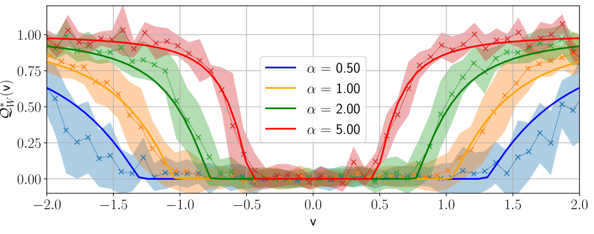
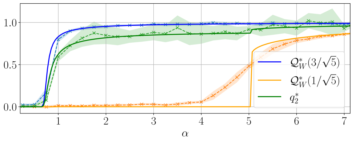
Figure 3 illustrates the learning mechanism for models with Gaussian weights and non-homogeneous readouts, revealing a sequence of phase transitions as $\alpha$ increases. Top panel shows the overlap function $\mathcal{Q}_{W}(\mathsf{v})$ in the case of Gaussian readouts for four different sample rates $\alpha$ . In the bottom panel the readout assumes four different values with equal probabilities; the figure shows the evolution of the two relevant overlaps associated with the symmetric readout values $± 3/\sqrt{5}$ and $± 1/\sqrt{5}$ . As $\alpha$ increases, the student weights start aligning with the teacher weights associated with the highest readout amplitude, marking the first phase transition. As these alignments strengthen when $\alpha$ further increases, the second transition occurs when the weights corresponding to the next largest readout amplitude are learnt, and so on. In this way, continuous readouts produce an infinite sequence of learning transitions, as supported by the upper part of Figure 3.
Even when dominating the posterior measure, we observe in simulations that the specialisation solution can be algorithmically hard to reach. With a discrete distribution of readouts (such as $P_{v}=\delta_{1}$ or Rademacher), simulations for binary inner weights exhibit it only when sampling with informative initialisation (i.e., the MCMC runs to sample ${\mathbf{W}}$ are initialised in the vicinity of ${\mathbf{W}}^{0}$ ). Moreover, even in cases where algorithms (such as ADAM or HMC for Gaussian inner weights) are able to find the specialisation solution, they manage to do so only after a training time increasing exponentially with $d$ , and for relatively small values of the label noise $\Delta$ , see discussion in App. I. For the case of the continuous distribution of readouts $P_{v}={\mathcal{N}}(0,1)$ , our numerical results are inconclusive on hardness, and deserve numerical investigation at a larger scale.
The universal phase is superseded at $\alpha_{\rm sp}$ by a specialisation phase, where the student’s inner weights start aligning with the teacher ones. This transition occurs for both binary and Gaussian priors over the inner weights, and it is different in nature w.r.t. the perfect recovery threshold identified in Maillard et al. (2024a), which is the point where the student with Gaussian weights learns perfectly ${\mathbf{W}}^{0∈tercal}({\mathbf{v}}){\mathbf{W}}^{0}$ (but not ${\mathbf{W}}^{0}$ ) and thus attains perfect generalisation in the case of purely quadratic activation and noiseless labels. For large $\alpha$ , the student somehow realises that the higher order terms of the activation’s Hermite decomposition are not label noise, but are informative on the decision rule. The two identified phases are akin to those recently described in Barbier et al. (2025) for matrix denoising. The model we consider is also a matrix model in ${\mathbf{W}}$ , with the amount of data scaling as the number of matrix elements. When data are scarce, the student cannot break the numerous symmetries of the problem, resulting in an “effective rotational invariance” at the source of the prior universality, with posterior samples having a vanishing overlap with ${\mathbf{W}}^{0}$ . On the other hand, when data are sufficiently abundant, $\alpha>\alpha_{\rm sp}$ , there is a “synchronisation” of the student’s samples with the teacher.
<details>
<summary>x5.png Details</summary>
### Visual Description
## Line Chart: Q*_W(v) vs. v for different alpha values
### Overview
The image is a line chart displaying the relationship between Q*_W(v) and v for different values of alpha (α). The chart includes four data series, each representing a different alpha value (0.50, 1.00, 2.00, and 5.00). Each data series is plotted with a line and 'x' markers, along with a shaded region indicating uncertainty. The x-axis represents 'v', ranging from -2.0 to 2.0, and the y-axis represents Q*_W(v), ranging from 0.00 to 1.00.
### Components/Axes
* **X-axis:**
* Label: v
* Scale: -2.0 to 2.0, with tick marks at -2.0, -1.5, -1.0, -0.5, 0.0, 0.5, 1.0, 1.5, and 2.0.
* **Y-axis:**
* Label: Q*_W(v)
* Scale: 0.00 to 1.00, with tick marks at 0.00, 0.25, 0.50, 0.75, and 1.00.
* **Legend:** Located in the top-right quadrant of the chart.
* Blue line: α = 0.50
* Orange line: α = 1.00
* Green line: α = 2.00
* Red line: α = 5.00
### Detailed Analysis
* **α = 0.50 (Blue):**
* Trend: Starts at approximately 0.55 at v = -2.0, decreases to approximately 0.0 at v = -0.5, remains near 0.0 until v = 0.5, then increases to approximately 0.55 at v = 2.0.
* Data Points:
* v = -2.0, Q*_W(v) ≈ 0.55
* v = -0.5, Q*_W(v) ≈ 0.0
* v = 0.5, Q*_W(v) ≈ 0.0
* v = 2.0, Q*_W(v) ≈ 0.55
* **α = 1.00 (Orange):**
* Trend: Starts at approximately 0.9 at v = -2.0, decreases to approximately 0.0 at v = -0.5, remains near 0.0 until v = 0.5, then increases to approximately 0.9 at v = 2.0.
* Data Points:
* v = -2.0, Q*_W(v) ≈ 0.9
* v = -0.5, Q*_W(v) ≈ 0.0
* v = 0.5, Q*_W(v) ≈ 0.0
* v = 2.0, Q*_W(v) ≈ 0.9
* **α = 2.00 (Green):**
* Trend: Starts at approximately 0.95 at v = -2.0, decreases to approximately 0.0 at v = -0.5, remains near 0.0 until v = 0.5, then increases to approximately 0.95 at v = 2.0.
* Data Points:
* v = -2.0, Q*_W(v) ≈ 0.95
* v = -0.5, Q*_W(v) ≈ 0.0
* v = 0.5, Q*_W(v) ≈ 0.0
* v = 2.0, Q*_W(v) ≈ 0.95
* **α = 5.00 (Red):**
* Trend: Starts at approximately 1.0 at v = -2.0, decreases to approximately 0.0 at v = -0.5, remains near 0.0 until v = 0.5, then increases to approximately 1.0 at v = 2.0.
* Data Points:
* v = -2.0, Q*_W(v) ≈ 1.0
* v = -0.5, Q*_W(v) ≈ 0.0
* v = 0.5, Q*_W(v) ≈ 0.0
* v = 2.0, Q*_W(v) ≈ 1.0
### Key Observations
* All data series exhibit a similar U-shaped trend, with Q*_W(v) decreasing from a high value at v = -2.0 to approximately 0.0 at v = -0.5, remaining low until v = 0.5, and then increasing back to a high value at v = 2.0.
* As alpha increases, the value of Q*_W(v) at v = -2.0 and v = 2.0 increases, approaching 1.0.
* The shaded regions around each line indicate the uncertainty in the data, which appears to be larger in the regions where Q*_W(v) is changing rapidly.
### Interpretation
The chart illustrates how the function Q*_W(v) changes with respect to 'v' for different values of the parameter alpha. The U-shaped trend suggests that Q*_W(v) is minimized around v = 0 and maximized at the extreme values of v (i.e., -2.0 and 2.0). The parameter alpha appears to control the magnitude of Q*_W(v) at these extreme values, with larger alpha values resulting in Q*_W(v) approaching 1.0. This could represent a system where 'v' is an input, Q*_W(v) is an output, and alpha is a control parameter that influences the system's response to 'v'. The uncertainty regions suggest that the relationship between Q*_W(v) and 'v' is less well-defined in the regions where Q*_W(v) is changing rapidly, possibly due to noise or other factors.
</details>
<details>
<summary>x6.png Details</summary>
### Visual Description
## Line Chart: Q*_w vs Alpha
### Overview
The image is a line chart comparing three different data series, Q*_w(3/√5), Q*_w(1/√5), and q*_2, as a function of alpha (α). The chart shows how these values change as alpha increases from approximately 0 to 7. The plot includes shaded regions around the dashed lines, indicating uncertainty or variance in the data.
### Components/Axes
* **X-axis (Horizontal):**
* Label: α (alpha)
* Scale: 0 to 7, with tick marks at every integer value.
* **Y-axis (Vertical):**
* Scale: 0.0 to 1.0, with tick marks at 0.0, 0.5, and 1.0.
* **Legend (Right Side):**
* Blue line: Q*_w(3/√5)
* Orange line: Q*_w(1/√5)
* Green line: q*_2*
### Detailed Analysis
* **Q*_w(3/√5) (Blue):**
* Solid blue line with 'x' markers.
* Trend: Starts near 0 at α=0, rapidly increases to approximately 0.9 around α=1, and then plateaus around 1.0 for α > 1.
* Data Points:
* α = 0: Q*_w(3/√5) ≈ 0
* α = 1: Q*_w(3/√5) ≈ 0.9
* α = 7: Q*_w(3/√5) ≈ 1.0
* **Q*_w(1/√5) (Orange):**
* Dashed orange line with '+' markers. Shaded region around the line indicates uncertainty.
* Trend: Remains near 0 until α=5, then rapidly increases to approximately 0.85.
* Data Points:
* α = 0: Q*_w(1/√5) ≈ 0
* α = 5: Q*_w(1/√5) ≈ 0
* α = 6: Q*_w(1/√5) ≈ 0.7
* α = 7: Q*_w(1/√5) ≈ 0.85
* **q*_2* (Green):**
* Solid green line with 'x' markers. Shaded region around the line indicates uncertainty.
* Trend: Starts near 0 at α=0, rapidly increases to approximately 0.7 around α=1, and then plateaus around 0.9 for α > 1. There is a slight dip around α=5.
* Data Points:
* α = 0: q*_2* ≈ 0
* α = 1: q*_2* ≈ 0.7
* α = 5: q*_2* ≈ 0.9
* α = 7: q*_2* ≈ 0.95
### Key Observations
* Q*_w(3/√5) and q*_2* exhibit a similar trend, rapidly increasing around α=1 and then plateauing.
* Q*_w(1/√5) remains near zero until α=5, after which it rapidly increases.
* The shaded regions around the dashed lines indicate the variability or uncertainty in the data.
### Interpretation
The chart illustrates how the values of Q*_w(3/√5), Q*_w(1/√5), and q*_2* change with respect to α. The data suggests that Q*_w(3/√5) and q*_2* are strongly influenced by α around α=1, while Q*_w(1/√5) is significantly affected only after α reaches 5. This could indicate different thresholds or critical points for these parameters in the underlying system being modeled. The shaded regions highlight the uncertainty associated with the dashed lines, suggesting that the solid lines are more stable or have less variability.
</details>
Figure 3: Top: Theoretical prediction (solid curves) of the overlap function $\mathcal{Q}_{W}(\mathsf{v})$ for different sampling ratios $\alpha$ for Gaussian inner weights, ReLU(x) activation, $d=150,\gamma=0.5$ , linear readout with $\Delta=0.1$ and $P_{v}=\mathcal{N}(0,1)$ . The shaded curves were obtained from HMC initialised informatively. Using a single sample ${\mathbf{W}}^{a}$ from the posterior, $\mathcal{Q}_{W}(\mathsf{v})$ has been evaluated numerically by dividing the interval $[-2,2]$ into 50 bins and by computing the value of the overlap associated with each bin. Each point has been averaged over 50 instances of the training set, and shaded regions around them correspond to one standard deviation. Bottom: Theoretical prediction (solid curves) of the overlaps as function of the sampling ratio $\alpha$ for Gaussian inner weights, Tanh(2x) activation, $d=150,\gamma=0.5$ , linear readout with $\Delta=0.1$ and $P_{v}=\frac{1}{4}(\delta_{-3/\sqrt{5}}+\delta_{-1/\sqrt{5}}+\delta_{1/\sqrt{5}%
}+\delta_{3/\sqrt{5}})$ . The shaded curves were obtained from informed HMC. Each point has been averaged over 10 instances of the training set, with one standard deviation depicted.
The phenomenology observed depends on the activation function selected. In particular, by expanding $\sigma$ in the Hermite basis we realise that the way the first three terms enter information theoretical quantities is completely described by order 0, 1 and 2 tensors later defined in (12), that give rise to combinations of the inner and readout weights. In the regime of quadratically many data, order 0 and 1 tensors are recovered exactly by the student because of the overwhelming abundance of data compared to their dimension. The challenge is thus to learn the second order tensor. On the contrary, we claim that learning any higher order tensors can only happen when the student aligns its weights with ${\mathbf{W}}^{0}$ : before this “synchronisation”, they play the role of an effective noise. This is the mechanism behind the specialisation transition. For odd activation ( ${\rm Tanh}$ in Figure 1, $\sigma_{3}$ in Figure 2), where $\mu_{2}=0$ , the aforementioned order-2 tensor does not contribute any more to the learning. Indeed, we observe numerically that the generalisation error sticks to a constant value for $\alpha<\alpha_{\rm sp}$ , whereas at the phase transition it suddenly drops. This is because the learning of the order-2 tensor is skipped entirely, and the only chance to perform better is to learn all the other higher-order tensors through specialisation.
By extrapolating universality results to generic activations, we are able to use the GAMP-RIE of Maillard et al. (2024a), publicly available at Maillard et al. (2024b), to obtain a polynomial-time predictor for test data. Its generalisation error follows our universal theoretical curve even in the $\alpha$ regime where MCMC sampling experiences a computationally hard phase with worse performance (for binary weights), and in particular after $\alpha_{\rm sp}$ (see Fig. 2, circles). Extending this algorithm, initially proposed for quadratic activation, to a generic one is possible thanks to the identification of an effective GLM onto which the learning problem can be mapped (while the mapping is exact when $\sigma(x)=x^{2}$ as exploited by Maillard et al. (2024a)), see App. H. The key observation is that our effective GLM representation holds not only from a theoretical perspective when describing the universal phase, but also algorithmically.
Finally, we emphasise that our theory is consistent with Cui et al. (2023), which considers the simpler strongly over-parametrised regime $n=\Theta(d)$ rather than the interpolation one $n=\Theta(d^{2})$ : our generalisation curves at $\alpha→ 0$ match theirs at $\alpha_{1}:=n/d→∞$ , which is when the student learns perfectly the combinations ${\mathbf{v}}^{0∈tercal}{\mathbf{W}}^{0}/\sqrt{k}$ (but nothing more).
4 Accessing the free entropy and generalisation error: replica method and spherical integration combined
The goal is to compute the asymptotic free entropy by the replica method Mezard et al. (1986), a powerful heuristic from spin glasses also used in machine learning Engel & Van den Broeck (2001), combined with the HCIZ integral. Our derivation is based on a Gaussian ansatz on the replicated post-activations of the hidden layer, which generalises Conjecture 3.1 of Cui et al. (2023), now proved in Camilli et al. (2025), where it is specialised to the case of linearly many data ( $n=\Theta(d)$ ). To obtain this generalisation, we will write the kernel arising from the covariance of the aforementioned post-activations as an infinite series of scalar order parameters derived from the expansion of the activation function in the Hermite basis, following an approach recently devised in Aguirre-López et al. (2025) in the context of the random features model (see also Hu et al. (2024) and Ghorbani et al. (2021)). Another key ingredient of our analysis will be a generalisation of an ansatz used in the replica method by Sakata & Kabashima (2013) for dictionary learning.
4.1 Replicated system and order parameters
The starting point in the replica method to tackle the data average is the replica trick:
| | $\textstyle{\lim}\,\frac{1}{n}\mathbb{E}\ln{\mathcal{Z}}(\mathcal{D})={\lim}{%
\lim\limits_{\,\,s→ 0^{+}}}\!\frac{1}{ns}\ln\mathbb{E}\mathcal{Z}^{s}=\lim%
\limits_{\,\,s→ 0^{+}}\!{\lim}\,\frac{1}{ns}\ln\mathbb{E}\mathcal{Z}^{s}$ | |
| --- | --- | --- |
assuming the limits commute. Recall ${\mathbf{W}}^{0}$ are the teacher weights. Consider first $s∈\mathbb{N}^{+}$ . Let the “replicas” of the post-activation $\{\lambda^{a}({\mathbf{W}}^{a}):=\frac{1}{\sqrt{k}}{{\mathbf{v}}^{∈tercal}}%
\sigma(\frac{1}{\sqrt{d}}{{\mathbf{W}}^{a}{\mathbf{x}}})\}_{a=0,...,s}$ . We then directly obtain
| | $\textstyle\mathbb{E}\mathcal{Z}^{s}=\mathbb{E}_{{\mathbf{v}}}∈t\prod\limits_%
{a}\limits^{0,s}dP_{W}({\mathbf{W}}^{a})\big{[}\mathbb{E}_{\mathbf{x}}∈t dy%
\prod\limits_{a}\limits^{0,s}P_{\rm out}(y\mid\lambda^{a}({\mathbf{W}}^{a}))%
\big{]}^{n}.$ | |
| --- | --- | --- |
The key is to identify the law of the replicas $\{\lambda^{a}\}_{a=0,...,s}$ , which are dependent random variables due to the common random Gaussian input ${\mathbf{x}}$ , conditionally on $({\mathbf{W}}^{a})$ . Our key hypothesis is that $\{\lambda^{a}\}$ is jointly Gaussian, an ansatz we cannot prove but that we validate a posteriori thanks to the excellent match between our theory and the empirical generalisation curves, see Sec. 2.2. Similar Gaussian assumptions have been the crux of a whole line of recent works on the analysis of neural networks, and are now known under the name of “Gaussian equivalence” (Goldt et al., 2020; Hastie et al., 2022; Mei & Montanari, 2022; Goldt et al., 2022; Hu & Lu, 2023). This can also sometimes be heuristically justified based on Breuer–Major Theorems (Nourdin et al., 2011; Pacelli et al., 2023).
Given two replica indices $a,b∈\{0,...,s\}$ we define the neuron-neuron overlap matrix $\Omega^{ab}_{ij}:={{\mathbf{W}}_{i}^{a∈tercal}{\mathbf{W}}^{b}_{j}}/d$ with $i,j∈[k]$ . Recalling the Hermite expansion of $\sigma$ , by using Mehler’s formula, see App. A, the post-activations covariance $K^{ab}:=\mathbb{E}\lambda^{a}\lambda^{b}$ reads
$$
\textstyle K^{ab} \textstyle=\sum_{\ell\geq 1}^{\infty}\frac{\mu^{2}_{\ell}}{\ell!}Q_{\ell}^{ab}%
\ \ \text{with}\ \ Q_{\ell}^{ab}:=\frac{1}{k}\sum_{i,j\leq k}v_{i}v_{j}(\Omega%
^{ab}_{ij})^{\ell}. \tag{8}
$$
This covariance ${\mathbf{K}}$ is complicated but, as we argue hereby, simplifications occur as $d→∞$ . In particular, the first two overlaps $Q_{1}^{ab},Q_{2}^{ab}$ are special. We claim that higher-order overlaps $(Q_{\ell}^{ab})_{\ell≥ 3}$ can be simplified as functions of simpler order parameters.
<details>
<summary>x7.png Details</summary>
### Visual Description
## Line Chart: Overlaps vs. HMC Steps
### Overview
The image is a line chart showing the relationship between "Overlaps" and "HMC steps". There are five data series, labeled Q1 through Q5, each represented by a different colored line. An inset plot shows the behavior of "εopt" over HMC steps.
### Components/Axes
* **X-axis:** "HMC steps", ranging from 0 to 125000 in increments of 25000.
* **Y-axis:** "Overlaps", ranging from 0.0 to 1.0 in increments of 0.2.
* **Legend:** Located on the right side of the main plot, identifying the lines as Q1 (blue), Q2 (orange), Q3 (green), Q4 (red), and Q5 (purple).
* **Inset Plot X-axis:** HMC steps, ranging from 0 to 100000.
* **Inset Plot Y-axis:** Values ranging from 0.000 to 0.025.
* **Inset Plot Legend:** "εopt" (black).
* **Horizontal Dashed Lines:** There are four horizontal dashed lines corresponding to the approximate steady-state values of Q1, Q2, Q5, and εopt.
### Detailed Analysis
* **Q1 (Blue):** Starts at approximately 1.0 and remains relatively constant around 0.99.
* Horizontal dashed line at y = 1.0
* **Q2 (Orange):** Starts at approximately 0.75 and decreases rapidly before stabilizing around 0.62.
* Horizontal dashed line at y = 0.62
* **Q3 (Green):** Starts at approximately 0.75 and decreases rapidly before stabilizing around 0.03.
* **Q4 (Red):** Starts at approximately 0.75 and decreases rapidly before stabilizing around 0.04.
* **Q5 (Purple):** Starts at approximately 0.75 and decreases rapidly before stabilizing around 0.01.
* Horizontal dashed line at y = 0.0
* **εopt (Black - Inset Plot):** Starts at 0.0 and increases rapidly to approximately 0.026, then fluctuates around that value.
* Horizontal dashed line at y = 0.026
### Key Observations
* Q1 maintains a high overlap value throughout the HMC steps.
* Q2, Q3, Q4, and Q5 all exhibit a rapid decrease in overlap early in the HMC steps, followed by stabilization at lower values.
* εopt rapidly converges to a stable value.
### Interpretation
The chart illustrates the convergence behavior of different "overlap" metrics (Q1-Q5) during a Hamiltonian Monte Carlo (HMC) simulation. Q1 appears to represent a highly stable or conserved quantity, while Q2-Q5 converge to lower overlap values, suggesting a change or adaptation in the system being modeled. The inset plot shows that the parameter εopt quickly reaches an optimal value, which may be related to the convergence of the other overlap metrics. The horizontal dashed lines indicate the approximate steady-state values for each series.
</details>
<details>
<summary>x8.png Details</summary>
### Visual Description
## Chart: Overlaps vs. HMC Steps
### Overview
The image is a chart showing the relationship between "Overlaps" and "HMC steps". There are five primary data series plotted, each represented by a different color. Additionally, there is an inset plot showing the behavior of "ε_opt" over HMC steps.
### Components/Axes
* **Main Chart:**
* X-axis: "HMC steps" ranging from 0 to 125000 in increments of 25000.
* Y-axis: "Overlaps" ranging from 0.5 to 1.0 in increments of 0.1.
* Legend: There is no explicit legend, but the data series are distinguished by color.
* Blue: A nearly constant line at approximately 1.0 overlap.
* Orange: A fluctuating line around 0.88 overlap.
* Green: A fluctuating line around 0.67 overlap.
* Red: A fluctuating line around 0.60 overlap.
* Purple: A fluctuating line around 0.55 overlap.
* Horizontal dashed lines indicate approximate average overlap values for each series.
* Blue: 1.0
* Orange: 0.9
* Green: 0.63
* Red: 0.57
* Purple: 0.52
* **Inset Chart:**
* X-axis: "HMC steps" ranging from 0 to 100000 in increments of 50000.
* Y-axis: Values ranging from 0.00 to 0.01 in increments of 0.01.
* Data Series: Black line representing "ε_opt".
* Horizontal dashed line indicates the approximate average value for "ε_opt" at 0.008.
### Detailed Analysis
* **Blue Series:** Starts at 1.0 and remains nearly constant around 1.0 throughout the entire range of HMC steps.
* **Orange Series:** Starts at approximately 0.9 and fluctuates around 0.88.
* **Green Series:** Starts at approximately 0.8 and decreases rapidly before fluctuating around 0.67.
* **Red Series:** Starts at approximately 0.7 and decreases rapidly before fluctuating around 0.60.
* **Purple Series:** Starts at approximately 0.8 and decreases rapidly before fluctuating around 0.55.
* **Inset Chart (ε_opt):** The black line starts at 0 and increases rapidly to approximately 0.008, then fluctuates slightly around this value.
### Key Observations
* The blue series exhibits the highest overlap and remains stable.
* The green, red, and purple series show a significant initial drop in overlap before stabilizing at lower values.
* The inset chart shows that "ε_opt" quickly converges to a stable value.
### Interpretation
The chart illustrates how different configurations or parameters (represented by the colored lines) affect the "Overlaps" during HMC steps. The blue series represents a highly stable configuration with consistently high overlap. The other series (orange, green, red, and purple) represent configurations that initially have high overlap but degrade over the initial HMC steps before stabilizing at lower overlap values. The inset chart suggests that the parameter "ε_opt" quickly converges to an optimal value, which might be related to the stabilization observed in the main chart's data series. The dashed lines likely represent target or expected overlap values for each configuration.
</details>
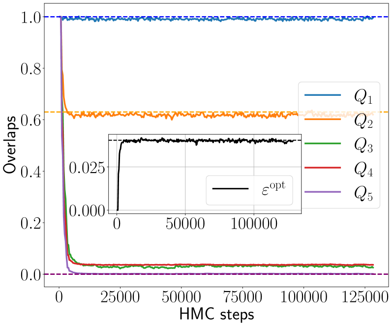
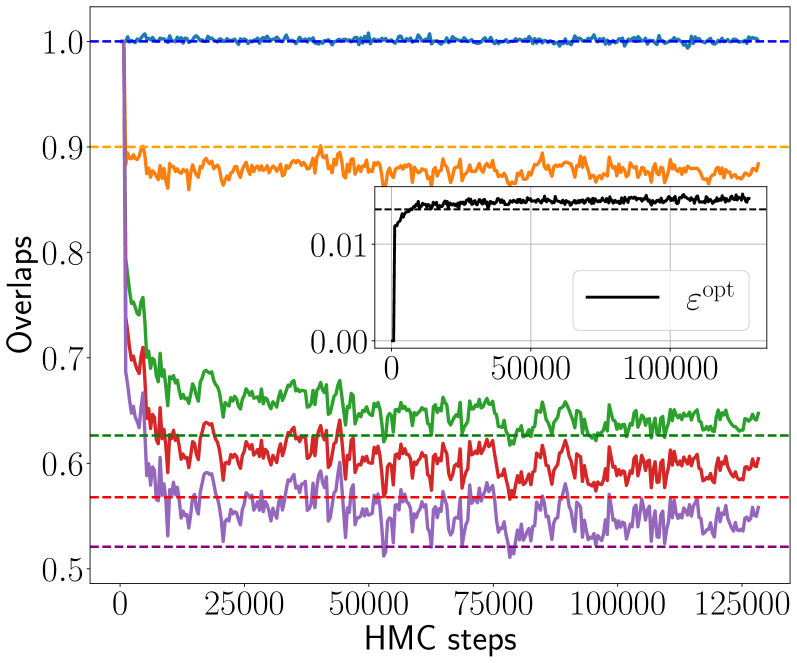
Figure 4: Hamiltonian Monte Carlo dynamics of the overlaps $Q_{\ell}=Q_{\ell}^{01}$ between student and teacher weights for $\ell∈[5]$ , with activation function ReLU(x), $d=200$ , $\gamma=0.5$ , linear readout with $\Delta=0.1$ and two choices of sample rates and readouts: $\alpha=1.0$ with $P_{v}=\delta_{1}$ (Left) and $\alpha=3.0$ with $P_{v}=\mathcal{N}(0,1)$ (Right). The teacher weights ${\mathbf{W}}^{0}$ are Gaussian. The dynamics is initialised informatively, i.e., on ${\mathbf{W}}^{0}$ . The overlap $Q_{1}$ always fluctuates around 1. Left: The overlaps $Q_{\ell}$ for $\ell≥ 3$ at equilibrium converge to 0, while $Q_{2}$ is well estimated by the theory (orange dashed line). Right: At higher sample rate $\alpha$ , also the $Q_{\ell}$ for $\ell≥ 3$ are non zero and agree with their theoretical prediction (dashed lines). Insets show the mean-square generalisation error and the theoretical prediction.
4.2 Simplifying the order parameters
In this section we show how to drastically reduce the number of order parameters to track. Assume at the moment that the readout prior $P_{v}$ has discrete support $\mathsf{V}=\{\mathsf{v}\}$ ; this can be relaxed by binning a continuous support, as mentioned in Sec. 2.2. The overlaps in (8) can be written as
$$
\textstyle Q_{\ell}^{ab}=\frac{1}{k}\sum_{\mathsf{v},\mathsf{v}^{\prime}\in%
\mathsf{V}}\mathsf{v}\,\mathsf{v}^{\prime}\sum_{\{i,j\leq k\mid v_{i}=\mathsf{%
v},v_{j}=\mathsf{v}^{\prime}\}}(\Omega_{ij}^{ab})^{\ell}. \tag{9}
$$
In the following, for $\ell≥ 3$ we discard the terms $\mathsf{v}≠\mathsf{v}^{\prime}$ in the above sum, assuming they are suppressed w.r.t. the diagonal ones. In other words, a neuron ${\mathbf{W}}^{a}_{i}$ of a student (replica) with a readout value $v_{i}=\mathsf{v}$ is assumed to possibly align only with neurons of the teacher (or, by Bayes-optimality, of another replica) with the same readout. Moreover, in the resulting sum over the neurons indices $\{i,j\mid v_{i}=v_{j}=\mathsf{v}\}$ , we assume that, for each $i$ , a single index $j=\pi_{i}$ , with $\pi$ a permutation, contributes at leading order. The model is symmetric under permutations of hidden neurons. We thus take $\pi$ to be the identity without loss of generality.
We now assume that for Hadamard powers $\ell≥ 3$ , the off-diagonal of the overlap $({\bm{\Omega}}^{ab})^{\circ\ell}$ , obtained from typical weight matrices sampled from the posterior, is sufficiently small to consider it diagonal in any quadratic form. Moreover, by exchangeability among neurons with the same readout value, we further assume that all diagonal elements $\{\Omega_{ii}^{ab}\mid i∈\mathcal{I}_{\mathsf{v}}\}$ concentrate onto the constant $\mathcal{Q}_{W}^{ab}(\mathsf{v})$ , where $\mathcal{I}_{\mathsf{v}}:=\{i≤ k\mid v_{i}=\mathsf{v}\}$ :
$$
\textstyle(\Omega_{ij}^{ab})^{\ell}=(\frac{1}{d}{\mathbf{W}}_{i}^{a\intercal}{%
\mathbf{W}}^{b}_{j})^{\ell}\approx\delta_{ij}\mathcal{Q}_{W}^{ab}(\mathsf{v})^%
{\ell} \tag{10}
$$
if $\ell≥ 3$ , $i\ \text{or}\ j∈\mathcal{I}_{\mathsf{v}}$ . Approximate equality here is up to a matrix with $o_{d}(1)$ norm. The same happens, e.g., for a standard Wishart matrix: its eigenvectors and the ones of its square Hadamard power are delocalised, while for higher Hadamard powers $\ell≥ 3$ its eigenvectors are strongly localised; this is why $Q_{2}^{ab}$ will require a separate treatment. With these simplifications we can write
$$
\textstyle Q_{\ell}^{ab}=\mathbb{E}_{v\sim P_{v}}[v^{2}\mathcal{Q}_{W}^{ab}(v)%
^{\ell}]+o_{d}(1)\ \text{for}\ \ell\geq 3. \tag{1}
$$
This is is verified numerically a posteriori as follows. Identity (11) is true (without $o_{d}(1)$ ) for the predicted theoretical values of the order parameters by construction of our theory. Fig. 3 verified the good agreement between the theoretical and experimental overlap profiles $\mathcal{Q}^{01}_{W}(\mathsf{v})$ for all $\mathsf{v}∈\mathsf{V}$ (which is statistically the same as $\smash{\mathcal{Q}^{ab}_{W}(\mathsf{v})}$ for any $a≠ b$ by the so-called Nishimori identity following from Bayes-optimality, see App. B), while Fig. 4 verifies the agreement at the level of $(Q_{\ell}^{ab})$ . Consequently, (11) is also true for the experimental overlaps.
It is convenient to define the symmetric tensors ${\mathbf{S}}_{\ell}^{a}$ with entries
$$
\textstyle S^{a}_{\ell;\alpha_{1}\ldots\alpha_{\ell}}:=\frac{1}{\sqrt{k}}\sum_%
{i\leq k}v_{i}W^{a}_{i\alpha_{1}}\cdots W^{a}_{i\alpha_{\ell}}. \tag{12}
$$
Indeed, the generic $\ell$ -th term of the series (8) can be written as the overlap $Q^{ab}_{\ell}=\langle{\mathbf{S}}^{a}_{\ell},{\mathbf{S}}^{b}_{\ell}\rangle/d^%
{\ell}$ of these tensors (where $\langle\,,\,\rangle$ is the inner product), e.g., $Q_{2}^{ab}={\rm Tr}\,{\mathbf{S}}_{2}^{a}{\mathbf{S}}_{2}^{b}/d^{2}$ . Given that the number of data $n=\Theta(d^{2})$ and that $({\mathbf{S}}_{1}^{a})$ are only $d$ -dimensional, they are reconstructed perfectly (the same argument was used to argue that readouts ${\mathbf{v}}$ can be quenched). We thus assume right away that at equilibrium the overlaps $Q_{1}^{ab}=1$ (or saturate to their maximum value; if tracked, the corresponding saddle point equations end up being trivial and do fix this). In other words, in the quadratic data regime, the $\mu_{1}$ contribution in the Hermite decomposition of $\sigma$ for the target is perfectly learnable, while higher order ones play a non-trivial role. In contrast, Cui et al. (2023) study the regime $n=\Theta(d)$ where $\mu_{1}$ is the only learnable term.
Then, the average replicated partition function reads $\mathbb{E}\mathcal{Z}^{s}=∈t d{\mathbf{Q}}_{2}d\bm{\mathcal{Q}}_{W}\exp(F_{S%
}\!+\!nF_{E})$ where $F_{E},F_{S}$ depend on ${\mathbf{Q}}_{2}=(Q_{2}^{ab})$ and $\bm{\mathcal{Q}}_{W}:=\{\mathcal{Q}_{W}^{ab}\mid a≤ b\}$ , where $\mathcal{Q}_{W}^{ab}:=\{\mathcal{Q}_{W}^{ab}(\mathsf{v})\mid\mathsf{v}∈%
\mathsf{V}\}$ .
The “energetic potential” is defined as
$$
\textstyle e^{nF_{E}}:=\big{(}\int dyd{\bm{\lambda}}\frac{\exp(-\frac{1}{2}{%
\bm{\lambda}}^{\intercal}{\mathbf{K}}^{-1}{\bm{\lambda}})}{((2\pi)^{s+1}\det{%
\mathbf{K}})^{1/2}}\prod_{a}^{0,s}P_{\rm out}(y\mid\lambda^{a})\big{)}^{n}. \tag{13}
$$
It takes this form due to our Gaussian assumption on the replicated post-activations and is thus easily computed, see App. D.1.
The “entropic potential” $F_{S}$ taking into account the degeneracy of the order parameters is obtained by averaging delta functions fixing their definitions w.r.t. the “microscopic degrees of freedom” $({\mathbf{W}}^{a})$ . It can be written compactly using the following conditional law over the tensors $({\mathbf{S}}_{2}^{a})$ :
$$
\textstyle P(({\mathbf{S}}_{2}^{a})\mid\bm{\mathcal{Q}}_{W}):=V_{W}^{kd}(\bm{%
\mathcal{Q}}_{W})^{-1}\int\prod_{a}^{0,s}dP_{W}({\mathbf{W}}^{a}) \textstyle\qquad\times\prod_{a\leq b}^{0,s}\prod_{\mathsf{v}\in\mathsf{V}}%
\prod_{i\in\mathcal{I}_{\mathsf{v}}}\delta(d\,\mathcal{Q}_{W}^{ab}(\mathsf{v})%
-{{\mathbf{W}}^{a\intercal}_{i}{\mathbf{W}}_{i}^{b}}) \textstyle\qquad\times\prod_{a}^{0,s}\delta({\mathbf{S}}^{a}_{2}-{\mathbf{W}}^%
{a\intercal}({\mathbf{v}}){\mathbf{W}}^{a}/\sqrt{k}), \tag{14}
$$
with the normalisation
| | $\textstyle V_{W}^{kd}:=∈t\prod_{a}dP_{W}({\mathbf{W}}^{a})\prod_{a≤ b,%
\mathsf{v},i∈\mathcal{I}_{\mathsf{v}}}\delta(d\,\mathcal{Q}_{W}^{ab}(\mathsf%
{v})-{{\mathbf{W}}^{a∈tercal}_{i}{\mathbf{W}}_{i}^{b}}).$ | |
| --- | --- | --- |
The entropy, which is the challenging term to compute, then reads
| | $\textstyle e^{F_{S}}:=V_{W}^{kd}(\bm{\mathcal{Q}}_{W})∈t dP(({\mathbf{S}}_{2%
}^{a})\mid\bm{\mathcal{Q}}_{W})\prod\limits_{a≤ b}\limits^{0,s}\delta(d^{2}%
Q_{2}^{ab}-{{\rm Tr}\,{\mathbf{S}}_{2}^{a}{\mathbf{S}}_{2}^{b}}).$ | |
| --- | --- | --- |
4.3 Tackling the entropy: measure simplification by moment matching
The delta functions above fixing $Q_{2}^{ab}$ induce quartic constraints between the weights degrees of freedom $(W_{i\alpha}^{a})$ instead of quadratic as in standard settings. A direct computation thus seems out of reach. However, we will exploit the fact that the constraints are quadratic in the matrices $({\mathbf{S}}_{2}^{a})$ . Consequently, shifting our focus towards $({\mathbf{S}}_{2}^{a})$ as the basic degrees of freedom to integrate rather than $(W_{i\alpha}^{a})$ will allow us to move forward by simplifying their measure (14). Note that while $(W_{i\alpha}^{a})$ are i.i.d. under their prior measure, $({\mathbf{S}}_{2}^{a})$ have coupled entries, even for a fixed replica index $a$ . This can be taken into account as follows.
Define $P_{S}$ as the probability density of a generalised Wishart random matrix, i.e., of $\tilde{\mathbf{W}}^{∈tercal}({\mathbf{v}})\tilde{\mathbf{W}}/\sqrt{k}$ where $\tilde{\mathbf{W}}∈\mathbb{R}^{k× d}$ is made of i.i.d. standard Gaussian entries. The simplification we consider consists in replacing (14) by the effective measure
$$
\textstyle\tilde{P}(({\mathbf{S}}_{2}^{a})\mid\bm{\mathcal{Q}}_{W}):=\frac{1}{%
\tilde{V}_{W}^{kd}}\prod\limits_{a}\limits^{0,s}P_{S}({\mathbf{S}}_{2}^{a})%
\prod\limits_{a<b}\limits^{0,s}e^{\frac{1}{2}\tau(\mathcal{Q}_{W}^{ab}){\rm Tr%
}\,{\mathbf{S}}^{a}_{2}{\mathbf{S}}^{b}_{2}} \tag{15}
$$
where $\tilde{V}_{W}^{kd}=\tilde{V}_{W}^{kd}(\bm{\mathcal{Q}}_{W})$ is the proper normalisation constant, and
$$
\textstyle\tau(\mathcal{Q}_{W}^{ab}):=\text{mmse}_{S}^{-1}(1-\mathbb{E}_{v\sim
P%
_{v}}[v^{2}\mathcal{Q}^{ab}_{W}(v)^{2}]). \tag{16}
$$
The rationale behind this choice goes as follows. The matrices $({\mathbf{S}}_{2}^{a})$ are, under the measure (14), $(i)$ generalised Wishart matrices, constructed from $(ii)$ non-Gaussian factors $({\mathbf{W}}^{a})$ , which $(iii)$ are coupled between different replicas, thus inducing a coupling among replicas $({\mathbf{S}}^{a})$ . The proposed simplified measure captures all three aspects while remaining tractable, as we explain now. The first assumption is that in the measure (14) the details of the (centred, unit variance) prior $P_{W}$ enter only through $\bm{\mathcal{Q}}_{W}$ at leading order. Due to the conditioning, we can thus relax it to Gaussian (with the same two first moments) by universality, as is often the case in random matrix theory. $P_{W}$ will instead explicitly enter in the entropy of $\bm{\mathcal{Q}}_{W}$ related to $V_{W}^{kd}$ . Point $(ii)$ is thus taken care by the conditioning. Then, the generalised Wishart prior $P_{S}$ encodes $(i)$ and, finally, the exponential tilt in $\tilde{P}$ induces the replica couplings of point $(iii)$ . It remains to capture the dependence of measure (14) on $\bm{\mathcal{Q}}_{W}$ . This is done by realising that
| | $\textstyle∈t dP(({\mathbf{S}}_{2}^{a})\mid\bm{\mathcal{Q}}_{W})\frac{1}{d^{2%
}}{\rm Tr}{\mathbf{S}}_{2}^{a}{\mathbf{S}}_{2}^{b}=\mathbb{E}_{v\sim P_{v}}[v^%
{2}\mathcal{Q}_{W}^{ab}(v)^{2}]+\gamma\bar{v}^{2}.$ | |
| --- | --- | --- |
It is shown in App. D.2. The Lagrange multiplier $\tau(\mathcal{Q}_{W}^{ab})$ to plug in $\tilde{P}$ enforcing this moment matching condition between true and simplified measures as $s→ 0^{+}$ is (16), see App. D.3. For completeness, we provide in App. E alternatives to the simplification (15), whose analysis are left for future work.
4.4 Final steps and spherical integration
Combining all our findings, the average replicated partition function is simplified as
| | $\textstyle\mathbb{E}\mathcal{Z}^{s}=∈t d{\mathbf{Q}}_{2}d\bm{\mathcal{Q}}_{W%
}e^{nF_{E}+kd\ln V_{W}(\bm{\mathcal{Q}}_{W})-kd\ln\tilde{V}_{W}(\bm{\mathcal{Q%
}}_{W})}$ | |
| --- | --- | --- |
The equality should be interpreted as holding at leading exponential order $\exp(\Theta(n))$ , assuming the validity of our previous measure simplification. All remaining steps but the last are standard:
$(i)$ Express the delta functions fixing $\bm{\mathcal{Q}}_{W}$ and ${\mathbf{Q}}_{2}$ in exponential form using their Fourier representation; this introduces additional Fourier conjugate order parameters $\hat{\mathbf{Q}}_{2},\hat{\bm{\mathcal{Q}}}_{W}$ of same dimensions.
$(ii)$ Once this is done, the terms coupling different replicas of $({\mathbf{W}}^{a})$ or of $({\mathbf{S}}^{a})$ are all quadratic. Using the Hubbard–Stratonovich transformation (i.e., $\mathbb{E}_{{\mathbf{Z}}}\exp(\frac{d}{2}{\rm Tr}\,{\mathbf{M}}{\mathbf{Z}})=%
\exp(\frac{d}{4}{\rm Tr}\,{\mathbf{M}}^{2})$ for a $d× d$ symmetric matrix ${\mathbf{M}}$ with ${\mathbf{Z}}$ a standard GOE matrix) therefore allows us to linearise all replica-replica coupling terms, at the price of introducing new Gaussian fields interacting with all replicas.
$(iii)$ After these manipulations, we identify at leading exponential order an effective action $\mathcal{S}$ depending on the order parameters only, which allows a saddle point integration w.r.t. them as $n→∞$ :
| | $\textstyle\lim\frac{1}{ns}\ln\mathbb{E}\mathcal{Z}^{s}\!=\!\lim\frac{1}{ns}\ln%
∈t d{\mathbf{Q}}_{2}d\hat{\mathbf{Q}}_{2}d\bm{\mathcal{Q}}_{W}d\hat{\bm{%
\mathcal{Q}}}_{W}e^{n\mathcal{S}}\!=\!\frac{1}{s}{\rm extr}\,\mathcal{S}.$ | |
| --- | --- | --- |
$(iv)$ Next, the replica limit $s→ 0^{+}$ of the previously obtained expression has to be considered. To do so, we make a replica symmetric assumption, i.e., we consider that at the saddle point, all order parameters entering the action $\mathcal{S}$ , and thus $K^{ab}$ too, take a simple form of the type $R^{ab}=r\delta_{ab}+q(1-\delta_{ab})$ . Replica symmetry is rigorously known to be correct in general settings of Bayes-optimal learning and is thus justified here, see Barbier & Panchenko (2022); Barbier & Macris (2019).
$(v)$ After all these steps, the resulting expression still includes two high-dimensional integrals related to the ${\mathbf{S}}_{2}$ ’s matrices. They can be recognised as corresponding to the free entropies associated with the Bayes-optimal denoising of a generalised Wishart matrix, as described just above Result 2.1, for two different signal-to-noise ratios. The last step consists in dealing with these integrals using the HCIZ integral whose form is tractable in this case, see Maillard et al. (2022); Pourkamali et al. (2024). These free entropies yield the two last terms $\iota(\,·\,)$ in $f_{\rm RS}^{\alpha,\gamma}$ , (6).
The complete derivation is in App. D and gives Result 2.1. From the physical meaning of the order parameters, this analysis also yields the post-activations covariance ${\mathbf{K}}$ and thus Result 2.2.
As a final remark, we emphasise a key difference between our approach and earlier works on extensive-rank systems. If, instead of taking the generalised Wishart $P_{S}$ as the base measure over the matrices $({\mathbf{S}}_{2}^{a})$ in the simplified $\tilde{P}$ with moment matching, one takes a factorised Gaussian measure, thus entirely forgetting the dependencies among ${\mathbf{S}}_{2}^{a}$ entries, this mimics the Sakata-Kabashima replica method Sakata & Kabashima (2013). Our ansatz thus captures important correlations that were previously neglected in Sakata & Kabashima (2013); Krzakala et al. (2013); Kabashima et al. (2016); Barbier et al. (2025) in the context of extensive-rank matrix inference. For completeness, we show in App. E that our ansatz indeed greatly improves the prediction compared to these earlier approaches.
5 Conclusion and perspectives
We have provided an effective, quantitatively accurate, description of the optimal generalisation capability of a fully-trained two-layer neural network of extensive width with generic activation when the sample size scales with the number of parameters. This setting has resisted for a long time to mean-field approaches used, e.g., for committee machines Barkai et al. (1992); Engel et al. (1992); Schwarze & Hertz (1992; 1993); Mato & Parga (1992); Monasson & Zecchina (1995); Aubin et al. (2018); Baldassi et al. (2019).
A natural extension is to consider non Bayes-optimal models, e.g., trained through empirical risk minimisation to learn a mismatched target function. The formalism we provide here can be extended to these cases, by keeping track of additional order parameters. The extension to deeper architectures is also possible, in the vein of Cui et al. (2023); Pacelli et al. (2023) who analysed the over-parametrised proportional regime. Accounting for structured inputs is another direction: data with a covariance (Monasson, 1992; Loureiro et al., 2021a), mixture models (Del Giudice, P. et al., 1989; Loureiro et al., 2021b), hidden manifolds (Goldt et al., 2020), object manifolds and simplexes (Chung et al., 2018; Rotondo et al., 2020), etc.
Phase transitions in supervised learning are known in the statistical mechanics literature at least since Györgyi (1990), when the theory was limited to linear models. It would be interesting to connect the picture we have drawn here with Grokking, a sudden drop in generalisation error occurring during the training of neural nets close to interpolation, see Power et al. (2022); Rubin et al. (2024b).
A more systematic analysis on the computational hardness of the problem (as carried out for multi-index models in Troiani et al. (2025)) is an important step towards a full characterisation of the class of target functions that are fundamentally hard to learn.
A key novelty of our approach is to blend matrix models and spin glass techniques in a unified formalism. A limitation is then linked to the restricted class of solvable matrix models (see Kazakov (2000); Anninos & Mühlmann (2020) for a list). Indeed, as explained in App. E, possible improvements to our approach need additional finer order parameters than those appearing in Results 2.1, 2.2 (at least for inhomogeneous readouts ${\mathbf{v}}$ ). Taking them into account yields matrix models when computing their entropy which, to the best of our knowledge, are not currently solvable. We believe that obtaining asymptotically exact formulas for the log-partition function and generalisation error in the current setting and its relatives will require some major breakthrough in the field of multi-matrix models. This is an exciting direction to pursue at the crossroad of the fields of matrix models and high-dimensional inference and learning of extensive-rank matrices.
Software and data
Experiments with ADAM/HMC were performed through standard implementations in PyTorch/TensorFlow/NumPyro; the Metropolis-Hastings and GAMP-RIE routines were coded from scratch (the latter was inspired by Maillard et al. (2024a)). GitHub repository to reproduce the results: https://github.com/Minh-Toan/extensive-width-NN
Acknowledgements
J.B., F.C., M.-T.N. and M.P. were funded by the European Union (ERC, CHORAL, project number 101039794). Views and opinions expressed are however those of the authors only and do not necessarily reflect those of the European Union or the European Research Council. Neither the European Union nor the granting authority can be held responsible for them. M.P. thanks Vittorio Erba and Pietro Rotondo for interesting discussions and suggestions.
References
- Aguirre-López et al. (2025) Aguirre-López, F., Franz, S., and Pastore, M. Random features and polynomial rules. SciPost Phys., 18:039, 2025. 10.21468/SciPostPhys.18.1.039. URL https://scipost.org/10.21468/SciPostPhys.18.1.039.
- Aiudi et al. (2025) Aiudi, R., Pacelli, R., Baglioni, P., Vezzani, A., Burioni, R., and Rotondo, P. Local kernel renormalization as a mechanism for feature learning in overparametrized convolutional neural networks. Nature Communications, 16(1):568, Jan 2025. ISSN 2041-1723. 10.1038/s41467-024-55229-3. URL https://doi.org/10.1038/s41467-024-55229-3.
- Anninos & Mühlmann (2020) Anninos, D. and Mühlmann, B. Notes on matrix models (matrix musings). Journal of Statistical Mechanics: Theory and Experiment, 2020(8):083109, aug 2020. 10.1088/1742-5468/aba499. URL https://dx.doi.org/10.1088/1742-5468/aba499.
- Arjevani et al. (2025) Arjevani, Y., Bruna, J., Kileel, J., Polak, E., and Trager, M. Geometry and optimization of shallow polynomial networks, 2025. URL https://arxiv.org/abs/2501.06074.
- Aubin et al. (2018) Aubin, B., Maillard, A., Barbier, J., Krzakala, F., Macris, N., and Zdeborová, L. The committee machine: Computational to statistical gaps in learning a two-layers neural network. In Bengio, S., Wallach, H., Larochelle, H., Grauman, K., Cesa-Bianchi, N., and Garnett, R. (eds.), Advances in Neural Information Processing Systems, volume 31. Curran Associates, Inc., 2018. URL https://proceedings.neurips.cc/paper_files/paper/2018/file/84f0f20482cde7e5eacaf7364a643d33-Paper.pdf.
- Baglioni et al. (2024) Baglioni, P., Pacelli, R., Aiudi, R., Di Renzo, F., Vezzani, A., Burioni, R., and Rotondo, P. Predictive power of a Bayesian effective action for fully connected one hidden layer neural networks in the proportional limit. Phys. Rev. Lett., 133:027301, Jul 2024. 10.1103/PhysRevLett.133.027301. URL https://link.aps.org/doi/10.1103/PhysRevLett.133.027301.
- Baldassi et al. (2019) Baldassi, C., Malatesta, E. M., and Zecchina, R. Properties of the geometry of solutions and capacity of multilayer neural networks with rectified linear unit activations. Phys. Rev. Lett., 123:170602, Oct 2019. 10.1103/PhysRevLett.123.170602. URL https://link.aps.org/doi/10.1103/PhysRevLett.123.170602.
- Barbier (2020) Barbier, J. Overlap matrix concentration in optimal Bayesian inference. Information and Inference: A Journal of the IMA, 10(2):597–623, 05 2020. ISSN 2049-8772. 10.1093/imaiai/iaaa008. URL https://doi.org/10.1093/imaiai/iaaa008.
- Barbier & Macris (2019) Barbier, J. and Macris, N. The adaptive interpolation method: a simple scheme to prove replica formulas in Bayesian inference. Probability Theory and Related Fields, 174(3):1133–1185, Aug 2019. ISSN 1432-2064. 10.1007/s00440-018-0879-0. URL https://doi.org/10.1007/s00440-018-0879-0.
- Barbier & Macris (2022) Barbier, J. and Macris, N. Statistical limits of dictionary learning: Random matrix theory and the spectral replica method. Phys. Rev. E, 106:024136, Aug 2022. 10.1103/PhysRevE.106.024136. URL https://link.aps.org/doi/10.1103/PhysRevE.106.024136.
- Barbier & Panchenko (2022) Barbier, J. and Panchenko, D. Strong replica symmetry in high-dimensional optimal Bayesian inference. Communications in Mathematical Physics, 393(3):1199–1239, Aug 2022. ISSN 1432-0916. 10.1007/s00220-022-04387-w. URL https://doi.org/10.1007/s00220-022-04387-w.
- Barbier et al. (2019) Barbier, J., Krzakala, F., Macris, N., Miolane, L., and Zdeborová, L. Optimal errors and phase transitions in high-dimensional generalized linear models. Proceedings of the National Academy of Sciences, 116(12):5451–5460, 2019. 10.1073/pnas.1802705116. URL https://www.pnas.org/doi/abs/10.1073/pnas.1802705116.
- Barbier et al. (2025) Barbier, J., Camilli, F., Ko, J., and Okajima, K. Phase diagram of extensive-rank symmetric matrix denoising beyond rotational invariance. Physical Review X, 2025.
- Barkai et al. (1992) Barkai, E., Hansel, D., and Sompolinsky, H. Broken symmetries in multilayered perceptrons. Phys. Rev. A, 45:4146–4161, Mar 1992. 10.1103/PhysRevA.45.4146. URL https://link.aps.org/doi/10.1103/PhysRevA.45.4146.
- Bartlett et al. (2021) Bartlett, P. L., Montanari, A., and Rakhlin, A. Deep learning: a statistical viewpoint. Acta Numerica, 30:87–201, 2021. 10.1017/S0962492921000027. URL https://doi.org/10.1017/S0962492921000027.
- Bassetti et al. (2024) Bassetti, F., Gherardi, M., Ingrosso, A., Pastore, M., and Rotondo, P. Feature learning in finite-width Bayesian deep linear networks with multiple outputs and convolutional layers, 2024. URL https://arxiv.org/abs/2406.03260.
- Bordelon et al. (2020) Bordelon, B., Canatar, A., and Pehlevan, C. Spectrum dependent learning curves in kernel regression and wide neural networks. In III, H. D. and Singh, A. (eds.), Proceedings of the 37th International Conference on Machine Learning, volume 119 of Proceedings of Machine Learning Research, pp. 1024–1034. PMLR, 13–18 Jul 2020. URL https://proceedings.mlr.press/v119/bordelon20a.html.
- Brézin et al. (2016) Brézin, E., Hikami, S., et al. Random matrix theory with an external source. Springer, 2016.
- Camilli et al. (2023) Camilli, F., Tieplova, D., and Barbier, J. Fundamental limits of overparametrized shallow neural networks for supervised learning, 2023. URL https://arxiv.org/abs/2307.05635.
- Camilli et al. (2025) Camilli, F., Tieplova, D., Bergamin, E., and Barbier, J. Information-theoretic reduction of deep neural networks to linear models in the overparametrized proportional regime. The 38th Annual Conference on Learning Theory (to appear), 2025.
- Canatar et al. (2021) Canatar, A., Bordelon, B., and Pehlevan, C. Spectral bias and task-model alignment explain generalization in kernel regression and infinitely wide neural networks. Nature Communications, 12(1):2914, 05 2021. ISSN 2041-1723. 10.1038/s41467-021-23103-1. URL https://doi.org/10.1038/s41467-021-23103-1.
- Chung et al. (2018) Chung, S., Lee, D. D., and Sompolinsky, H. Classification and geometry of general perceptual manifolds. Phys. Rev. X, 8:031003, Jul 2018. 10.1103/PhysRevX.8.031003. URL https://link.aps.org/doi/10.1103/PhysRevX.8.031003.
- Cui et al. (2023) Cui, H., Krzakala, F., and Zdeborova, L. Bayes-optimal learning of deep random networks of extensive-width. In Krause, A., Brunskill, E., Cho, K., Engelhardt, B., Sabato, S., and Scarlett, J. (eds.), Proceedings of the 40th International Conference on Machine Learning, volume 202 of Proceedings of Machine Learning Research, pp. 6468–6521. PMLR, 07 2023. URL https://proceedings.mlr.press/v202/cui23b.html.
- Del Giudice, P. et al. (1989) Del Giudice, P., Franz, S., and Virasoro, M. A. Perceptron beyond the limit of capacity. J. Phys. France, 50(2):121–134, 1989. 10.1051/jphys:01989005002012100. URL https://doi.org/10.1051/jphys:01989005002012100.
- Dietrich et al. (1999) Dietrich, R., Opper, M., and Sompolinsky, H. Statistical mechanics of support vector networks. Phys. Rev. Lett., 82:2975–2978, 04 1999. 10.1103/PhysRevLett.82.2975. URL https://link.aps.org/doi/10.1103/PhysRevLett.82.2975.
- Du & Lee (2018) Du, S. and Lee, J. On the power of over-parametrization in neural networks with quadratic activation. In Dy, J. and Krause, A. (eds.), Proceedings of the 35th International Conference on Machine Learning, volume 80 of Proceedings of Machine Learning Research, pp. 1329–1338. PMLR, 10–15 Jul 2018. URL https://proceedings.mlr.press/v80/du18a.html.
- Engel & Van den Broeck (2001) Engel, A. and Van den Broeck, C. Statistical mechanics of learning. Cambridge University Press, 2001. ISBN 9780521773072.
- Engel et al. (1992) Engel, A., Köhler, H. M., Tschepke, F., Vollmayr, H., and Zippelius, A. Storage capacity and learning algorithms for two-layer neural networks. Phys. Rev. A, 45:7590–7609, May 1992. 10.1103/PhysRevA.45.7590. URL https://link.aps.org/doi/10.1103/PhysRevA.45.7590.
- Gamarnik et al. (2024) Gamarnik, D., Kızıldağ, E. C., and Zadik, I. Stationary points of a shallow neural network with quadratic activations and the global optimality of the gradient descent algorithm. Mathematics of Operations Research, 50(1):209–251, 2024. 10.1287/moor.2021.0082. URL https://doi.org/10.1287/moor.2021.0082.
- Gardner & Derrida (1989) Gardner, E. and Derrida, B. Three unfinished works on the optimal storage capacity of networks. Journal of Physics A: Mathematical and General, 22(12):1983, jun 1989. 10.1088/0305-4470/22/12/004. URL https://dx.doi.org/10.1088/0305-4470/22/12/004.
- Gerace et al. (2021) Gerace, F., Loureiro, B., Krzakala, F., Mézard, M., and Zdeborová, L. Generalisation error in learning with random features and the hidden manifold model. Journal of Statistical Mechanics: Theory and Experiment, 2021(12):124013, Dec 2021. ISSN 1742-5468. 10.1088/1742-5468/ac3ae6. URL http://dx.doi.org/10.1088/1742-5468/ac3ae6.
- Ghorbani et al. (2021) Ghorbani, B., Mei, S., Misiakiewicz, T., and Montanari, A. Linearized two-layers neural networks in high dimension. The Annals of Statistics, 49(2):1029 – 1054, 2021. 10.1214/20-AOS1990. URL https://doi.org/10.1214/20-AOS1990.
- Goldt et al. (2020) Goldt, S., Mézard, M., Krzakala, F., and Zdeborová, L. Modeling the influence of data structure on learning in neural networks: The hidden manifold model. Phys. Rev. X, 10:041044, Dec 2020. 10.1103/PhysRevX.10.041044. URL https://link.aps.org/doi/10.1103/PhysRevX.10.041044.
- Goldt et al. (2022) Goldt, S., Loureiro, B., Reeves, G., Krzakala, F., Mezard, M., and Zdeborová, L. The Gaussian equivalence of generative models for learning with shallow neural networks. In Bruna, J., Hesthaven, J., and Zdeborová, L. (eds.), Proceedings of the 2nd Mathematical and Scientific Machine Learning Conference, volume 145 of Proceedings of Machine Learning Research, pp. 426–471. PMLR, 08 2022. URL https://proceedings.mlr.press/v145/goldt22a.html.
- Guionnet & Zeitouni (2002) Guionnet, A. and Zeitouni, O. Large deviations asymptotics for spherical integrals. Journal of Functional Analysis, 188(2):461–515, 2002. ISSN 0022-1236. 10.1006/jfan.2001.3833. URL https://www.sciencedirect.com/science/article/pii/S0022123601938339.
- Guo et al. (2005) Guo, D., Shamai, S., and Verdú, S. Mutual information and minimum mean-square error in gaussian channels. IEEE Transactions on Information Theory, 51(4):1261–1282, 2005. 10.1109/TIT.2005.844072. URL https://doi.org/10.1109/TIT.2005.844072.
- Györgyi (1990) Györgyi, G. First-order transition to perfect generalization in a neural network with binary synapses. Phys. Rev. A, 41:7097–7100, Jun 1990. 10.1103/PhysRevA.41.7097. URL https://link.aps.org/doi/10.1103/PhysRevA.41.7097.
- Hanin (2023) Hanin, B. Random neural networks in the infinite width limit as Gaussian processes. The Annals of Applied Probability, 33(6A):4798 – 4819, 2023. 10.1214/23-AAP1933. URL https://doi.org/10.1214/23-AAP1933.
- Hastie et al. (2022) Hastie, T., Montanari, A., Rosset, S., and Tibshirani, R. J. Surprises in high-dimensional ridgeless least squares interpolation. The Annals of Statistics, 50(2):949 – 986, 2022. 10.1214/21-AOS2133. URL https://doi.org/10.1214/21-AOS2133.
- Hu & Lu (2023) Hu, H. and Lu, Y. M. Universality laws for high-dimensional learning with random features. IEEE Transactions on Information Theory, 69(3):1932–1964, 2023. 10.1109/TIT.2022.3217698. URL https://doi.org/10.1109/TIT.2022.3217698.
- Hu et al. (2024) Hu, H., Lu, Y. M., and Misiakiewicz, T. Asymptotics of random feature regression beyond the linear scaling regime, 2024. URL https://arxiv.org/abs/2403.08160.
- Itzykson & Zuber (1980) Itzykson, C. and Zuber, J. The planar approximation. II. Journal of Mathematical Physics, 21(3):411–421, 03 1980. ISSN 0022-2488. 10.1063/1.524438. URL https://doi.org/10.1063/1.524438.
- Kabashima et al. (2016) Kabashima, Y., Krzakala, F., Mézard, M., Sakata, A., and Zdeborová, L. Phase transitions and sample complexity in Bayes-optimal matrix factorization. IEEE Transactions on Information Theory, 62(7):4228–4265, 2016. 10.1109/TIT.2016.2556702. URL https://doi.org/10.1109/TIT.2016.2556702.
- Kazakov (2000) Kazakov, V. A. Solvable matrix models, 2000. URL https://arxiv.org/abs/hep-th/0003064.
- Kingma & Ba (2017) Kingma, D. P. and Ba, J. Adam: A method for stochastic optimization, 2017. URL https://arxiv.org/abs/1412.6980.
- Krzakala et al. (2013) Krzakala, F., Mézard, M., and Zdeborová, L. Phase diagram and approximate message passing for blind calibration and dictionary learning. In 2013 IEEE International Symposium on Information Theory, pp. 659–663, 2013. 10.1109/ISIT.2013.6620308. URL https://doi.org/10.1109/ISIT.2013.6620308.
- Lee et al. (2018) Lee, J., Sohl-dickstein, J., Pennington, J., Novak, R., Schoenholz, S., and Bahri, Y. Deep neural networks as Gaussian processes. In International Conference on Learning Representations, 2018. URL https://openreview.net/forum?id=B1EA-M-0Z.
- Li & Sompolinsky (2021) Li, Q. and Sompolinsky, H. Statistical mechanics of deep linear neural networks: The backpropagating kernel renormalization. Phys. Rev. X, 11:031059, Sep 2021. 10.1103/PhysRevX.11.031059. URL https://link.aps.org/doi/10.1103/PhysRevX.11.031059.
- Loureiro et al. (2021a) Loureiro, B., Gerbelot, C., Cui, H., Goldt, S., Krzakala, F., Mezard, M., and Zdeborová, L. Learning curves of generic features maps for realistic datasets with a teacher-student model. In Ranzato, M., Beygelzimer, A., Dauphin, Y., Liang, P., and Vaughan, J. W. (eds.), Advances in Neural Information Processing Systems, volume 34, pp. 18137–18151. Curran Associates, Inc., 2021a. URL https://proceedings.neurips.cc/paper_files/paper/2021/file/9704a4fc48ae88598dcbdcdf57f3fdef-Paper.pdf.
- Loureiro et al. (2021b) Loureiro, B., Sicuro, G., Gerbelot, C., Pacco, A., Krzakala, F., and Zdeborová, L. Learning Gaussian mixtures with generalized linear models: Precise asymptotics in high-dimensions. In Ranzato, M., Beygelzimer, A., Dauphin, Y., Liang, P., and Vaughan, J. W. (eds.), Advances in Neural Information Processing Systems, volume 34, pp. 10144–10157. Curran Associates, Inc., 2021b. URL https://proceedings.neurips.cc/paper_files/paper/2021/file/543e83748234f7cbab21aa0ade66565f-Paper.pdf.
- Maillard et al. (2022) Maillard, A., Krzakala, F., Mézard, M., and Zdeborová, L. Perturbative construction of mean-field equations in extensive-rank matrix factorization and denoising. Journal of Statistical Mechanics: Theory and Experiment, 2022(8):083301, Aug 2022. 10.1088/1742-5468/ac7e4c. URL https://dx.doi.org/10.1088/1742-5468/ac7e4c.
- Maillard et al. (2024a) Maillard, A., Troiani, E., Martin, S., Krzakala, F., and Zdeborová, L. Bayes-optimal learning of an extensive-width neural network from quadratically many samples, 2024a. URL https://arxiv.org/abs/2408.03733.
- Maillard et al. (2024b) Maillard, A., Troiani, E., Martin, S., Krzakala, F., and Zdeborová, L. Github repository ExtensiveWidthQuadraticSamples. https://github.com/SPOC-group/ExtensiveWidthQuadraticSamples, 2024b.
- Martin et al. (2024) Martin, S., Bach, F., and Biroli, G. On the impact of overparameterization on the training of a shallow neural network in high dimensions. In Dasgupta, S., Mandt, S., and Li, Y. (eds.), Proceedings of The 27th International Conference on Artificial Intelligence and Statistics, volume 238 of Proceedings of Machine Learning Research, pp. 3655–3663. PMLR, 02–04 May 2024. URL https://proceedings.mlr.press/v238/martin24a.html.
- Mato & Parga (1992) Mato, G. and Parga, N. Generalization properties of multilayered neural networks. Journal of Physics A: Mathematical and General, 25(19):5047, Oct 1992. 10.1088/0305-4470/25/19/017. URL https://dx.doi.org/10.1088/0305-4470/25/19/017.
- Matthews et al. (2018) Matthews, A. G. D. G., Hron, J., Rowland, M., Turner, R. E., and Ghahramani, Z. Gaussian process behaviour in wide deep neural networks. In International Conference on Learning Representations, 2018. URL https://openreview.net/forum?id=H1-nGgWC-.
- Matytsin (1994) Matytsin, A. On the large- $N$ limit of the Itzykson-Zuber integral. Nuclear Physics B, 411(2):805–820, 1994. ISSN 0550-3213. 10.1016/0550-3213(94)90471-5. URL https://www.sciencedirect.com/science/article/pii/0550321394904715.
- Mei & Montanari (2022) Mei, S. and Montanari, A. The generalization error of random features regression: Precise asymptotics and the double descent curve. Communications on Pure and Applied Mathematics, 75(4):667–766, 2022. 10.1002/cpa.22008. URL https://onlinelibrary.wiley.com/doi/abs/10.1002/cpa.22008.
- Mezard et al. (1986) Mezard, M., Parisi, G., and Virasoro, M. Spin Glass Theory and Beyond. World Scientific, 1986. 10.1142/0271. URL https://www.worldscientific.com/doi/abs/10.1142/0271.
- Monasson (1992) Monasson, R. Properties of neural networks storing spatially correlated patterns. Journal of Physics A: Mathematical and General, 25(13):3701, Jul 1992. 10.1088/0305-4470/25/13/019. URL https://dx.doi.org/10.1088/0305-4470/25/13/019.
- Monasson & Zecchina (1995) Monasson, R. and Zecchina, R. Weight space structure and internal representations: A direct approach to learning and generalization in multilayer neural networks. Phys. Rev. Lett., 75:2432–2435, Sep 1995. 10.1103/PhysRevLett.75.2432. URL https://link.aps.org/doi/10.1103/PhysRevLett.75.2432.
- Naveh & Ringel (2021) Naveh, G. and Ringel, Z. A self consistent theory of Gaussian processes captures feature learning effects in finite CNNs. In Ranzato, M., Beygelzimer, A., Dauphin, Y., Liang, P., and Vaughan, J. W. (eds.), Advances in Neural Information Processing Systems, volume 34, pp. 21352–21364. Curran Associates, Inc., 2021. URL https://proceedings.neurips.cc/paper_files/paper/2021/file/b24d21019de5e59da180f1661904f49a-Paper.pdf.
- Neal (1996) Neal, R. M. Priors for Infinite Networks, pp. 29–53. Springer New York, New York, NY, 1996. ISBN 978-1-4612-0745-0. 10.1007/978-1-4612-0745-0_2. URL https://doi.org/10.1007/978-1-4612-0745-0_2.
- Nishimori (2001) Nishimori, H. Statistical Physics of Spin Glasses and Information Processing: An Introduction. Oxford University Press, 07 2001. ISBN 9780198509417. 10.1093/acprof:oso/9780198509417.001.0001.
- Nourdin et al. (2011) Nourdin, I., Peccati, G., and Podolskij, M. Quantitative Breuer–Major theorems. Stochastic Processes and their Applications, 121(4):793–812, 2011. ISSN 0304-4149. https://doi.org/10.1016/j.spa.2010.12.006. URL https://www.sciencedirect.com/science/article/pii/S0304414910002917.
- Pacelli et al. (2023) Pacelli, R., Ariosto, S., Pastore, M., Ginelli, F., Gherardi, M., and Rotondo, P. A statistical mechanics framework for Bayesian deep neural networks beyond the infinite-width limit. Nature Machine Intelligence, 5(12):1497–1507, 12 2023. ISSN 2522-5839. 10.1038/s42256-023-00767-6. URL https://doi.org/10.1038/s42256-023-00767-6.
- Parker et al. (2014) Parker, J. T., Schniter, P., and Cevher, V. Bilinear generalized approximate message passing—Part I: Derivation. IEEE Transactions on Signal Processing, 62(22):5839–5853, 2014. 10.1109/TSP.2014.2357776. URL https://doi.org/10.1109/TSP.2014.2357776.
- Potters & Bouchaud (2020) Potters, M. and Bouchaud, J.-P. A first course in random matrix theory: for physicists, engineers and data scientists. Cambridge University Press, 2020.
- Pourkamali et al. (2024) Pourkamali, F., Barbier, J., and Macris, N. Matrix inference in growing rank regimes. IEEE Transactions on Information Theory, 70(11):8133–8163, 2024. 10.1109/TIT.2024.3422263. URL https://doi.org/10.1109/TIT.2024.3422263.
- Power et al. (2022) Power, A., Burda, Y., Edwards, H., Babuschkin, I., and Misra, V. Grokking: Generalization beyond overfitting on small algorithmic datasets, 2022. URL https://arxiv.org/abs/2201.02177.
- Rotondo et al. (2020) Rotondo, P., Pastore, M., and Gherardi, M. Beyond the storage capacity: Data-driven satisfiability transition. Phys. Rev. Lett., 125:120601, Sep 2020. 10.1103/PhysRevLett.125.120601. URL https://link.aps.org/doi/10.1103/PhysRevLett.125.120601.
- Rubin et al. (2024a) Rubin, N., Ringel, Z., Seroussi, I., and Helias, M. A unified approach to feature learning in Bayesian neural networks. In High-dimensional Learning Dynamics 2024: The Emergence of Structure and Reasoning, 2024a. URL https://openreview.net/forum?id=ZmOSJ2MV2R.
- Rubin et al. (2024b) Rubin, N., Seroussi, I., and Ringel, Z. Grokking as a first order phase transition in two layer networks. In The Twelfth International Conference on Learning Representations, 2024b. URL https://openreview.net/forum?id=3ROGsTX3IR.
- Sakata & Kabashima (2013) Sakata, A. and Kabashima, Y. Statistical mechanics of dictionary learning. Europhysics Letters, 103(2):28008, Aug 2013. 10.1209/0295-5075/103/28008. URL https://dx.doi.org/10.1209/0295-5075/103/28008.
- Sarao Mannelli et al. (2020) Sarao Mannelli, S., Vanden-Eijnden, E., and Zdeborová, L. Optimization and generalization of shallow neural networks with quadratic activation functions. In Larochelle, H., Ranzato, M., Hadsell, R., Balcan, M., and Lin, H. (eds.), Advances in Neural Information Processing Systems, volume 33, pp. 13445–13455. Curran Associates, Inc., 2020. URL https://proceedings.neurips.cc/paper_files/paper/2020/file/9b8b50fb590c590ffbf1295ce92258dc-Paper.pdf.
- Schmidt (2018) Schmidt, H. C. Statistical physics of sparse and dense models in optimization and inference. PhD thesis, 2018. URL http://www.theses.fr/2018SACLS366.
- Schwarze & Hertz (1992) Schwarze, H. and Hertz, J. Generalization in a large committee machine. Europhysics Letters, 20(4):375, Oct 1992. 10.1209/0295-5075/20/4/015. URL https://dx.doi.org/10.1209/0295-5075/20/4/015.
- Schwarze & Hertz (1993) Schwarze, H. and Hertz, J. Generalization in fully connected committee machines. Europhysics Letters, 21(7):785, Mar 1993. 10.1209/0295-5075/21/7/012. URL https://dx.doi.org/10.1209/0295-5075/21/7/012.
- Semerjian (2024) Semerjian, G. Matrix denoising: Bayes-optimal estimators via low-degree polynomials. Journal of Statistical Physics, 191(10):139, Oct 2024. ISSN 1572-9613. 10.1007/s10955-024-03359-9. URL https://doi.org/10.1007/s10955-024-03359-9.
- Seroussi et al. (2023) Seroussi, I., Naveh, G., and Ringel, Z. Separation of scales and a thermodynamic description of feature learning in some CNNs. Nature Communications, 14(1):908, Feb 2023. ISSN 2041-1723. 10.1038/s41467-023-36361-y. URL https://doi.org/10.1038/s41467-023-36361-y.
- Soltanolkotabi et al. (2019) Soltanolkotabi, M., Javanmard, A., and Lee, J. D. Theoretical insights into the optimization landscape of over-parameterized shallow neural networks. IEEE Transactions on Information Theory, 65(2):742–769, 2019. 10.1109/TIT.2018.2854560. URL https://doi.org/10.1109/TIT.2018.2854560.
- Troiani et al. (2025) Troiani, E., Dandi, Y., Defilippis, L., Zdeborova, L., Loureiro, B., and Krzakala, F. Fundamental computational limits of weak learnability in high-dimensional multi-index models. In The 28th International Conference on Artificial Intelligence and Statistics, 2025. URL https://openreview.net/forum?id=Mwzui5H0VN.
- van Meegen & Sompolinsky (2024) van Meegen, A. and Sompolinsky, H. Coding schemes in neural networks learning classification tasks, 2024. URL https://arxiv.org/abs/2406.16689.
- Venturi et al. (2019) Venturi, L., Bandeira, A. S., and Bruna, J. Spurious valleys in one-hidden-layer neural network optimization landscapes. Journal of Machine Learning Research, 20(133):1–34, 2019. URL http://jmlr.org/papers/v20/18-674.html.
- Williams (1996) Williams, C. Computing with infinite networks. In Mozer, M., Jordan, M., and Petsche, T. (eds.), Advances in Neural Information Processing Systems, volume 9. MIT Press, 1996. URL https://proceedings.neurips.cc/paper/1996/file/ae5e3ce40e0404a45ecacaaf05e5f735-Paper.pdf.
- Xiao et al. (2023) Xiao, L., Hu, H., Misiakiewicz, T., Lu, Y. M., and Pennington, J. Precise learning curves and higher-order scaling limits for dot-product kernel regression. Journal of Statistical Mechanics: Theory and Experiment, 2023(11):114005, Nov 2023. 10.1088/1742-5468/ad01b7. URL https://dx.doi.org/10.1088/1742-5468/ad01b7.
- Xu et al. (2025) Xu, Y., Maillard, A., Zdeborová, L., and Krzakala, F. Fundamental limits of matrix sensing: Exact asymptotics, universality, and applications, 2025. URL https://arxiv.org/abs/2503.14121.
- Yoon & Oh (1998) Yoon, H. and Oh, J.-H. Learning of higher-order perceptrons with tunable complexities. Journal of Physics A: Mathematical and General, 31(38):7771–7784, 09 1998. 10.1088/0305-4470/31/38/012. URL https://doi.org/10.1088/0305-4470/31/38/012.
- Zdeborová & and (2016) Zdeborová, L. and and, F. K. Statistical physics of inference: thresholds and algorithms. Advances in Physics, 65(5):453–552, 2016. 10.1080/00018732.2016.1211393. URL https://doi.org/10.1080/00018732.2016.1211393.
Appendix A Hermite basis and Mehler’s formula
Recall the Hermite expansion of the activation:
$$
\sigma(x)=\sum_{\ell=0}^{\infty}\frac{\mu_{\ell}}{\ell!}{\rm He}_{\ell}(x). \tag{17}
$$
We are expressing it on the basis of the probabilist’s Hermite polynomials, generated through
$$
{\rm He}_{\ell}(z)=\frac{d^{\ell}}{{dt}^{\ell}}\exp\big{(}tz-t^{2}/2\big{)}%
\big{|}_{t=0}. \tag{18}
$$
The Hermite basis has the property of being orthogonal with respect to the standard Gaussian measure, which is the distribution of the input data:
$$
\int Dz\,{\rm He}_{k}(z){\rm He}_{\ell}(z)=\ell!\,\delta_{k\ell}, \tag{19}
$$
where $Dz:=dz\exp(-z^{2}/2)/\sqrt{2\pi}$ . By orthogonality, the coefficients of the expansions can be obtained as
$$
\mu_{\ell}=\int Dz{\rm He}_{\ell}(z)\sigma(z). \tag{20}
$$
Moreover,
$$
\mathbb{E}[\sigma(z)^{2}]=\int Dz\,\sigma(z)^{2}=\sum_{\ell=0}^{\infty}\frac{%
\mu_{\ell}^{2}}{\ell!}. \tag{21}
$$
These coefficients for some popular choices of $\sigma$ are reported in Table 1 for reference.
Table 1: First Hermite coefficients of some activation functions reported in the figues. $\theta$ is the Heaviside step function.
| ${\rm ReLU}(z)=z\theta(z)$ ${\rm ELU}(z)=z\theta(z)+(e^{z}-1)\theta(-z)$ ${\rm Tanh}(2z)$ | $1/\sqrt{2\pi}$ 0.16052 0 | $1/2$ 0.76158 0.72948 | $1/\sqrt{2\pi}$ 0.26158 0 | 0 -0.13736 -0.61398 | $-1/\sqrt{2\pi}$ -0.13736 0 | $·s$ $·s$ $·s$ | 1/2 0.64494 0.63526 |
| --- | --- | --- | --- | --- | --- | --- | --- |
The Hermite basis can be generalised to an orthogonal basis with respect to the Gaussian measure with generic variance:
$$
{\rm He}_{\ell}^{[r]}(z)=\frac{d^{\ell}}{dt^{\ell}}\exp\big{(}tz-t^{2}r/2\big{%
)}\big{|}_{t=0}, \tag{22}
$$
so that, with $D_{r}z:=dz\exp(-z^{2}/2r)/\sqrt{2\pi r}$ , we have
$$
\int D_{r}z\,{\rm He}_{k}^{[r]}(z){\rm He}_{\ell}^{[r]}(z)=\ell!\,r^{\ell}%
\delta_{k\ell}. \tag{23}
$$
From Mehler’s formula
$$
\frac{1}{2\pi\sqrt{r^{2}-q^{2}}}\exp\!\Big{[}-\frac{1}{2}(u,v)\begin{pmatrix}r%
&q\\
q&r\end{pmatrix}^{-1}\begin{pmatrix}u\\
v\end{pmatrix}\Big{]}=\frac{e^{-\frac{u^{2}}{2r}}}{\sqrt{2\pi r}}\frac{e^{-%
\frac{v^{2}}{2r}}}{\sqrt{2\pi r}}\sum_{\ell=0}^{+\infty}\frac{q^{\ell}}{\ell!r%
^{2\ell}}{\rm He}_{\ell}^{[r]}(u){\rm He}_{\ell}^{[r]}(v), \tag{24}
$$
and by orthogonality of the Hermite basis, (8) readily follows by noticing that the variables $(h_{i}^{a}=({\mathbf{W}}^{a}{\mathbf{x}})_{i}/\sqrt{d})_{i,a}$ at given $({\mathbf{W}}^{a})$ are Gaussian with covariances $\Omega^{ab}_{ij}={\mathbf{W}}_{i}^{a∈tercal}{\mathbf{W}}^{b}_{j}/d$ , so that
$$
\mathbb{E}[\sigma(h_{i}^{a})\sigma(h_{j}^{b})]=\sum_{\ell=0}^{\infty}\frac{(%
\mu_{\ell}^{[r]})^{2}}{\ell!r^{2\ell}}(\Omega_{ij}^{ab})^{\ell},\qquad\mu_{%
\ell}^{[r]}=\int D_{r}z\,{\rm He}^{[r]}_{\ell}(z)\sigma(z). \tag{25}
$$
Moreover, as $r=\Omega^{aa}_{ii}$ converges for $d$ large to the variance of the prior of ${\mathbf{W}}^{0}$ by Bayes-optimality, whenever $\Omega^{aa}_{ii}→ 1$ we can specialise this formula to the simpler case $r=1$ we reported in the main text.
Appendix B Nishimori identities
The Nishimori identities are a very general set of symmetries arising in inference in the Bayes-optimal setting as a consequence of Bayes’ rule. To introduce them, consider a test function $f$ of the teacher weights, collectively denoted by ${\bm{\theta}}^{0}$ , of $s-1$ replicas of the student’s weights $({\bm{\theta}}^{a})_{2≤ a≤ s}$ drawn conditionally i.i.d. from the posterior, and possibly also of the training set $\mathcal{D}$ : $f({\bm{\theta}}^{0},{\bm{\theta}}^{2},...,{\bm{\theta}}^{s};\mathcal{D})$ . Then
$$
\displaystyle\mathbb{E}_{{\bm{\theta}}^{0},\mathcal{D}}\langle f({\bm{\theta}}%
^{0},{\bm{\theta}}^{2},\dots,{\bm{\theta}}^{s};\mathcal{D})\rangle=\mathbb{E}_%
{{\bm{\theta}}^{0},\mathcal{D}}\langle f({\bm{\theta}}^{1},{\bm{\theta}}^{2},%
\dots,{\bm{\theta}}^{s};\mathcal{D})\rangle, \tag{26}
$$
where we have replaced the teacher’s weights with another replica from the student. The proof is elementary, see e.g. Barbier et al. (2019).
The Nishimori identities have some consequences also on our replica symmetric ansatz for the free entropy. In particular, they constrain the values of the asymptotic mean of some order parameters. For instance
$$
\displaystyle m_{2}=\lim\frac{1}{d^{2}}\mathbb{E}_{\mathcal{D},{\bm{\theta}}^{%
0}}\langle{\rm Tr}[{\mathbf{S}}_{2}^{a}{\mathbf{S}}_{2}^{0}]\rangle=\lim\frac{%
1}{d^{2}}\mathbb{E}_{\mathcal{D}}\langle{\rm Tr}[{\mathbf{S}}_{2}^{a}{\mathbf{%
S}}_{2}^{b}]\rangle=q_{2},\quad\text{for }a\neq b. \tag{27}
$$
Combined with the concentration of such order parameters, which can be proven in great generality in Bayes-optimal learning Barbier (2020); Barbier & Panchenko (2022), it fixes the values for some of them. For instance, we have that with high probability
$$
\displaystyle\frac{1}{d^{2}}{\rm Tr}[({\mathbf{S}}_{2}^{a})^{2}]\to r_{2}=\lim%
\frac{1}{d^{2}}\mathbb{E}_{\mathcal{D}}\langle{\rm Tr}[({\mathbf{S}}_{2}^{a})^%
{2}]\rangle=\lim\frac{1}{d^{2}}\mathbb{E}_{{\bm{\theta}}^{0}}{\rm Tr}[({%
\mathbf{S}}_{2}^{0})^{2}]=\rho_{2}=1+\gamma\bar{v}^{2}. \tag{28}
$$
When the values of some order parameters are determined by the Nishimori identities (and their concentration), as for those fixed to $r_{2}=\rho_{2}$ , then the respective Fourier conjugates $\hat{r}_{2},\hat{\rho}_{2}$ vanish (meaning that the desired constraints were already asymptotically enforced without the need of additional delta functions). This is because the configurations that make the order parameters take those values exponentially (in $n$ ) dominate the posterior measure, so these constraints are automatically imposed by the measure.
Appendix C Alternative representation for the optimal mean-square generalisation error
We recall that ${\bm{\theta}}^{0}=({\mathbf{v}}^{0},{\mathbf{W}}^{0})$ and similarly for ${\bm{\theta}}^{1}={\bm{\theta}},{\bm{\theta}}^{2},...$ which are replicas, i.e., conditionally i.i.d. samples from $dP({\mathbf{W}},{\mathbf{v}}\mid\mathcal{D})$ (the reasoning below applies whether ${\mathbf{v}}$ is learnable or quenched, so in general we can consider a joint posterior over both). In this section we report the details on how to obtain Result 2.2 and how to write the generalisation error defined in (3) in a form more convenient for numerical estimation.
From its definition, the Bayes-optimal mean-square generalisation error can be recast as
$$
\displaystyle\varepsilon^{\rm opt}=\mathbb{E}_{{\bm{\theta}}^{0},{\mathbf{x}}_%
{\rm test}}\mathbb{E}[y^{2}_{\rm test}\mid\lambda^{0}]-2\mathbb{E}_{{\bm{%
\theta}}^{0},\mathcal{D},{\mathbf{x}}_{\rm test}}\mathbb{E}[y_{\rm test}\mid%
\lambda^{0}]\langle\mathbb{E}[y\mid\lambda]\rangle+\mathbb{E}_{{\bm{\theta}}^{%
0},\mathcal{D},{\mathbf{x}}_{\rm test}}\langle\mathbb{E}[y\mid\lambda]\rangle^%
{2}, \tag{29}
$$
where $\mathbb{E}[y\mid\lambda]=∈t dy\,y\,P_{\rm out}(y\mid\lambda)$ , and $\lambda^{0}$ , $\lambda$ are the random variables (random due to the test input ${\mathbf{x}}_{\rm test}$ , drawn independently of the training data $\mathcal{D}$ , and their respective weights ${\bm{\theta}}^{0},{\bm{\theta}}$ )
$$
\displaystyle\lambda^{0}=\lambda({\bm{\theta}}^{0},{\mathbf{x}}_{\rm test})=%
\frac{{\mathbf{v}}^{0\intercal}}{\sqrt{k}}\sigma\Big{(}\frac{{\mathbf{W}}^{0}{%
\mathbf{x}}_{\rm test}}{\sqrt{d}}\Big{)},\qquad\lambda=\lambda^{1}=\lambda({%
\bm{\theta}},{\mathbf{x}}_{\rm test})=\frac{{\mathbf{v}}^{\intercal}}{\sqrt{k}%
}\sigma\Big{(}\frac{{\mathbf{W}}{\mathbf{x}}_{\rm test}}{\sqrt{d}}\Big{)}. \tag{30}
$$
Recall that the bracket $\langle\,·\,\rangle$ is the average w.r.t. to the posterior and acts on ${\bm{\theta}}^{1}={\bm{\theta}},{\bm{\theta}}^{2},...$ . Notice that the last term on the r.h.s. of (29) can be rewritten as
| | $\displaystyle\mathbb{E}_{{\bm{\theta}}^{0},\mathcal{D},{\mathbf{x}}_{\rm test}%
}\langle\mathbb{E}[y\mid\lambda]\rangle^{2}=\mathbb{E}_{{\bm{\theta}}^{0},%
\mathcal{D},{\mathbf{x}}_{\rm test}}\langle\mathbb{E}[y\mid\lambda^{1}]\mathbb%
{E}[y\mid\lambda^{2}]\rangle,$ | |
| --- | --- | --- |
with superscripts being replica indices, i.e., $\lambda^{a}:=\lambda({\bm{\theta}}^{a},{\mathbf{x}}_{\rm test})$ .
In order to show Result 2.2 for a generic $P_{\rm out}$ we assume the joint Gaussianity of the variables $(\lambda^{0},\lambda^{1},\lambda^{2},...)$ , with covariance given by $K^{ab}$ with $a,b∈\{0,1,2,...\}$ . Indeed, in the limit “ $\lim$ ”, our theory considers $(\lambda^{a})_{a≥ 0}$ as jointly Gaussian under the randomness of a common input, here ${\mathbf{x}}_{\rm test}$ , conditionally on the weights $({\bm{\theta}}^{a})$ . Their covariance depends on the weights $({\bm{\theta}}^{a})$ through various overlap order parameters introduced in the main. But in the large limit “ $\lim$ ” these overlaps are assumed to concentrate under the quenched posterior average $\mathbb{E}_{{\bm{\theta}}^{0},\mathcal{D}}\langle\,·\,\rangle$ towards non-random asymptotic values corresponding to the extremiser globally maximising the RS potential in Result 2.1, with the overlaps entering $K^{ab}$ through (42). This hypothesis is then confirmed by the excellent agreement between our theoretical predictions based on this assumption and the experimental results. This implies directly the equation for $\lim\,\varepsilon^{\mathcal{C},\mathsf{f}}$ in Result 2.2 from definition (2). For the special case of optimal mean-square generalisation error it yields
$$
\displaystyle\lim\,\varepsilon^{\rm opt}=\mathbb{E}_{\lambda^{0}}\mathbb{E}[y^%
{2}_{\rm test}\mid\lambda^{0}]-2\mathbb{E}_{\lambda^{0},\lambda^{1}}\mathbb{E}%
[y_{\rm test}\mid\lambda^{0}]\mathbb{E}[y\mid\lambda^{1}]+\mathbb{E}_{\lambda^%
{1},\lambda^{2}}\mathbb{E}[y\mid\lambda^{1}]\mathbb{E}[y\mid\lambda^{2}] \tag{31}
$$
where, in the replica symmetric ansatz,
$$
\displaystyle\mathbb{E}[(\lambda^{0})^{2}]=K^{00},\quad\mathbb{E}[\lambda^{0}%
\lambda^{1}]=\mathbb{E}[\lambda^{0}\lambda^{2}]=K^{01},\quad\mathbb{E}[\lambda%
^{1}\lambda^{2}]=K^{12},\quad\mathbb{E}[(\lambda^{1})^{2}]=\mathbb{E}[(\lambda%
^{2})^{2}]=K^{11}. \tag{32}
$$
For the dependence of the elements of ${\mathbf{K}}$ on the overlaps under this ansatz we defer the reader to (45), (46). In the Bayes-optimal setting, using the Nishimori identities (see App. B), one can show that $K^{01}=K^{12}$ and $K^{00}=K^{11}$ . Because of these identifications, we would additionally have
$$
\displaystyle\mathbb{E}_{\lambda^{0},\lambda^{1}}\mathbb{E}[y_{\rm test}\mid%
\lambda^{0}]\mathbb{E}[y\mid\lambda^{1}]=\mathbb{E}_{\lambda^{1},\lambda^{2}}%
\mathbb{E}[y\mid\lambda^{1}]\mathbb{E}[y\mid\lambda^{2}]. \tag{33}
$$
Plugging the above in (31) yields (7).
Let us now prove a formula for the optimal mean-square generalisation error written in terms of the overlaps that will be simpler to evaluate numerically, which holds for the special case of linear readout with Gaussian label noise $P_{\rm out}(y\mid\lambda)=\exp(-\frac{1}{2\Delta}(y-\lambda)^{2})/\sqrt{2\pi\Delta}$ . The following derivation is exact and does not require any Gaussianity assumption on the random variables $(\lambda^{a})$ . For the linear Gaussian channel the means verify $\mathbb{E}[y\mid\lambda]=\lambda$ and $\mathbb{E}[y^{2}\mid\lambda]=\lambda^{2}+\Delta$ . Plugged in (29) this yields
$$
\displaystyle\varepsilon^{\rm opt}-\Delta=\mathbb{E}_{{\bm{\theta}}^{0},{%
\mathbf{x}}_{\rm test}}\lambda^{2}_{\rm test}-2\mathbb{E}_{{\bm{\theta}}^{0},%
\mathcal{D},{\mathbf{x}}_{\rm test}}\lambda^{0}\langle\lambda\rangle+\mathbb{E%
}_{{\bm{\theta}}^{0},\mathcal{D},{\mathbf{x}}_{\rm test}}\langle\lambda^{1}%
\lambda^{2}\rangle, \tag{34}
$$
whence we clearly see that the generalisation error depends only on the covariance of $\lambda_{\rm test}({\bm{\theta}}^{0})=\lambda^{0}({\bm{\theta}}^{0}),\lambda^{%
1}({\bm{\theta}}^{1}),\lambda^{2}({\bm{\theta}}^{2})$ under the randomness of the shared input ${\mathbf{x}}_{\rm test}$ at fixed weights, regardless of the validity of the Gaussian equivalence principle we assume in the replica computation. This covariance was already computed in (8); we recall it here for the reader’s convenience
$$
\displaystyle K({\bm{\theta}}^{a},{\bm{\theta}}^{b}):=\mathbb{E}\lambda^{a}%
\lambda^{b}=\sum_{\ell=1}^{\infty}\frac{\mu_{\ell}^{2}}{\ell!}\frac{1}{k}\sum_%
{i,j=1}^{k}v_{i}^{a}(\Omega^{ab}_{ij})^{\ell}v^{b}_{j}=\sum_{\ell=1}^{\infty}%
\frac{\mu_{\ell}^{2}}{\ell!}Q_{\ell}^{ab}, \tag{35}
$$
where $\Omega^{ab}_{ij}:={\mathbf{W}}_{i}^{a∈tercal}{\mathbf{W}}_{j}^{b}/d$ , and $Q_{\ell}^{ab}$ as introduced in (8) for $a,b=0,1,2$ . We stress that $K({\bm{\theta}}^{a},{\bm{\theta}}^{b})$ is not the limiting covariance $K^{ab}$ whose elements are in (45), (46), but rather the finite size one. $K({\bm{\theta}}^{a},{\bm{\theta}}^{b})$ provides us with an efficient way to compute the generalisation error numerically, that is through the formula
$$
\displaystyle\varepsilon^{\rm opt}-\Delta \displaystyle=\mathbb{E}_{{\bm{\theta}}^{0}}K({\bm{\theta}}^{0},{\bm{\theta}}^%
{0})-2\mathbb{E}_{{\bm{\theta}}^{0},\mathcal{D}}\langle K({\bm{\theta}}^{0},{%
\bm{\theta}}^{1})\rangle+\mathbb{E}_{{\bm{\theta}}^{0},\mathcal{D}}\langle K({%
\bm{\theta}}^{1},{\bm{\theta}}^{2})\rangle=\sum_{\ell=1}^{\infty}\frac{\mu_{%
\ell}^{2}}{\ell!}\mathbb{E}_{{\bm{\theta}}^{0},\mathcal{D}}\langle Q_{\ell}^{0%
0}-2Q_{\ell}^{01}+Q^{12}_{\ell}\rangle. \tag{36}
$$
In the above, the posterior measure $\langle\,·\,\rangle$ is taken care of by Monte Carlo sampling (when it equilibrates). In addition, as in the main text, we assume that in the large system limit the (numerically confirmed) identity (11) holds. Putting all ingredients together we get
$$
\displaystyle\varepsilon^{\rm opt}-\Delta=\mathbb{E}_{{\bm{\theta}}^{0},%
\mathcal{D}} \displaystyle\Big{\langle}\mu_{1}^{2}(Q_{1}^{00}-2Q^{01}_{1}+Q^{12}_{1})+\frac%
{\mu_{2}^{2}}{2}(Q_{2}^{00}-2Q^{01}_{2}+Q^{12}_{2}) \displaystyle+\mathbb{E}_{v\sim P_{v}}v^{2}\big{[}g(\mathcal{Q}_{W}^{00}(v))-2%
g(\mathcal{Q}_{W}^{01}(v))+g(\mathcal{Q}_{W}^{12}(v))\big{]}\Big{\rangle}. \tag{37}
$$
In the Bayes-optimal setting one can use again the Nishimori identities that imply $\mathbb{E}_{{\bm{\theta}}^{0},\mathcal{D}}\langle Q^{12}_{1}\rangle=\mathbb{E}%
_{{\bm{\theta}}^{0},\mathcal{D}}\langle Q^{01}_{1}\rangle$ , and analogously $\mathbb{E}_{{\bm{\theta}}^{0},\mathcal{D}}\langle Q^{12}_{2}\rangle=\mathbb{E}%
_{{\bm{\theta}}^{0},\mathcal{D}}\langle Q^{01}_{2}\rangle$ and $\mathbb{E}_{{\bm{\theta}}^{0},\mathcal{D}}\langle g(\mathcal{Q}^{12}_{W}(v))%
\rangle=\mathbb{E}_{{\bm{\theta}}^{0},\mathcal{D}}\langle g(\mathcal{Q}^{01}_{%
W}(v))\rangle$ . Inserting these identities in (37) one gets
$$
\displaystyle\varepsilon^{\rm opt}-\Delta \displaystyle=\mathbb{E}_{{\bm{\theta}}^{0},\mathcal{D}}\Big{\langle}\mu_{1}^{%
2}(Q_{1}^{00}-Q^{01}_{1})+\frac{\mu_{2}^{2}}{2}(Q_{2}^{00}-Q^{01}_{2})+\mathbb%
{E}_{v\sim P_{v}}v^{2}\big{[}g(\mathcal{Q}_{W}^{00}(v))-g(\mathcal{Q}_{W}^{01}%
(v))\big{]}\Big{\rangle}. \tag{38}
$$
This formula makes no assumption (other than (11)), including on the law of the $\lambda$ ’s. That it depends only on their covariance is simply a consequence of the quadratic nature of the mean-square generalisation error.
**Remark C.1**
*Note that the derivation up to (36) did not assume Bayes-optimality (while (38) does). Therefore, one can consider it in cases where the true posterior average $\langle\,·\,\rangle$ is replaced by one not verifying the Nishimori identities. This is the formula we use to compute the generalisation error of Monte Carlo-based estimators in the inset of Fig. 7. This is indeed needed to compute the generalisation in the glassy regime, where MCMC cannot equilibrate.*
**Remark C.2**
*Using the Nishimory identity of App. B and again that, for the linear readout with Gaussian label noise $\mathbb{E}[y\mid\lambda]=\lambda$ and $\mathbb{E}[y^{2}\mid\lambda]=\lambda^{2}+\Delta$ , it is easy to check that the so-called Gibbs error
$$
\varepsilon^{\rm Gibbs}:=\mathbb{E}_{\bm{\theta}^{0},{\mathcal{D}},{\mathbf{x}%
}_{\rm test},y_{\rm test}}\big{\langle}(y_{\rm test}-\mathbb{E}[y\mid\lambda_{%
\rm test}({\bm{\theta}})])^{2}\big{\rangle} \tag{39}
$$
is related for this channel to the Bayes-optimal mean-square generalisation error through the identity
$$
\varepsilon^{\rm Gibbs}-\Delta=2(\varepsilon^{\rm opt}-\Delta). \tag{40}
$$
We exploited this relationship together with the concentration of the Gibbs error w.r.t. the quenched posterior measure $\mathbb{E}_{{\bm{\theta}}^{0},\mathcal{D}}\langle\,·\,\rangle$ when evaluating the numerical generalisation error of the Monte Carlo algorithms reported in the main text.*
Appendix D Details of the replica calculation
D.1 Energetic potential
The replicated energetic term under our Gaussian assumption on the joint law of the post-activations replicas is reported here for the reader’s convenience:
$$
F_{E}=\ln\int dy\int d{\bm{\lambda}}\frac{e^{-\frac{1}{2}{\bm{\lambda}}^{%
\intercal}{\mathbf{K}}^{-1}{\bm{\lambda}}}}{\sqrt{(2\pi)^{s+1}\det{\mathbf{K}}%
}}\prod_{a=0}^{s}P_{\rm out}(y\mid\lambda^{a}). \tag{41}
$$
After applying our ansatz (10) and using that $Q_{1}^{ab}=1$ in the quadratic-data regime, the covariance matrix ${\mathbf{K}}$ in replica space defined in (8) reads
$$
\displaystyle K^{ab} \displaystyle=\mu_{1}^{2}+\frac{\mu_{2}^{2}}{2}Q^{ab}_{2}+\mathbb{E}_{v\sim P_%
{v}}v^{2}g(\mathcal{Q}_{W}^{ab}(v)), \tag{42}
$$
where the function
$$
g(x)=\sum_{\ell=3}^{\infty}\frac{\mu_{\ell}^{2}}{\ell!}x^{\ell}=\mathbb{E}_{(y%
,z)|x}[\sigma(y)\sigma(z)]-\mu_{0}^{2}-\mu_{1}^{2}x-\frac{\mu_{2}^{2}}{2}x^{2}%
,\qquad(y,z)\sim{\mathcal{N}}\left((0,0),\begin{pmatrix}1&x\\
x&1\end{pmatrix}\right). \tag{43}
$$
The energetic term $F_{E}$ is already expressed as a low-dimensional integral, but within the replica symmetric (RS) ansatz it simplifies considerably. Let us denote $\bm{\mathcal{Q}}_{W}(\mathsf{v})=(\mathcal{Q}_{W}^{ab}(\mathsf{v}))_{a,b=0}^{s}$ . The RS ansatz amounts to assume that the saddle point solutions are dominated by order parameters of the form (below $\bm{1}_{s}$ and ${\mathbb{I}}_{s}$ are the all-ones vector and identity matrix of size $s$ )
$$
\bm{\mathcal{Q}}_{W}(\mathsf{v})=\begin{pmatrix}\rho_{W}&m_{W}\bm{1}_{s}^{%
\intercal}\\
m_{W}\bm{1}_{s}&(r_{W}-\mathcal{Q}_{W}){\mathbb{I}}_{s}+\mathcal{Q}_{W}\bm{1}_%
{s}\bm{1}_{s}^{\intercal}\end{pmatrix}\iff\hat{\bm{\mathcal{Q}}}_{W}(\mathsf{v%
})=\begin{pmatrix}\hat{\rho}_{W}&-\hat{m}_{W}\bm{1}_{s}^{\intercal}\\
-\hat{m}_{W}\bm{1}_{s}&(\hat{r}_{W}+\hat{\mathcal{Q}}_{W}){\mathbb{I}}_{s}-%
\hat{\mathcal{Q}}_{W}\bm{1}_{s}\bm{1}_{s}^{\intercal}\end{pmatrix},
$$
where all the above parameter $\rho_{W}=\rho_{W}(\mathsf{v}),\hat{\rho}_{W},m_{W},...$ depend on $\mathsf{v}$ , and similarly
$$
{\mathbf{Q}}_{2}=\begin{pmatrix}\rho_{2}&m_{2}\bm{1}_{s}^{\intercal}\\
m_{2}\bm{1}_{s}&(r_{2}-q_{2}){\mathbb{I}}_{s}+q_{2}\bm{1}_{s}\bm{1}_{s}^{%
\intercal}\end{pmatrix}\iff\hat{{\mathbf{Q}}}_{2}=\begin{pmatrix}\hat{\rho}_{2%
}&-\hat{m}_{2}\bm{1}_{s}^{\intercal}\\
-\hat{m}_{2}\bm{1}_{s}&(\hat{r}_{2}+\hat{q}_{2}){\mathbb{I}}_{s}-\hat{q}_{2}%
\bm{1}_{s}\bm{1}_{s}^{\intercal}\end{pmatrix},
$$
where we reported the ansatz also for the Fourier conjugates We are going to use repeatedly the Fourier representation of the delta function, namely $\delta(x)=\frac{1}{2\pi}∈t d\hat{x}\exp(i\hat{x}x)$ . Because the integrals we will end-up with will always be at some point evaluated by saddle point, implying a deformation of the integration contour in the complex plane, tracking the imaginary unit $i$ in the delta functions will be irrelevant. Similarly, the normalization $1/2\pi$ will always contribute to sub-leading terms in the integrals at hand. Therefore, we will allow ourselves to formally write $\delta(x)=∈t d\hat{x}\exp(r\hat{x}x)$ for a convenient constant $r$ , keeping in mind these considerations (again, as we evaluate the final integrals by saddle point, the choice of $r$ ends-up being irrelevant). for future convenience, though not needed for the energetic potential. The RS ansatz, which is equivalent to an assumption of concentration of the order parameters in the high-dimensional limit, is known to be exact when analysing Bayes-optimal inference and learning, as in the present paper, see Nishimori (2001); Barbier (2020); Barbier & Panchenko (2022). Under the RS ansatz ${\mathbf{K}}$ acquires a similar form:
$$
\displaystyle{\mathbf{K}}=\begin{pmatrix}\rho_{K}&m_{K}\bm{1}_{s}^{\intercal}%
\\
m_{K}\bm{1}_{s}&(r_{K}-q_{K}){\mathbb{I}}_{s}+q_{K}\bm{1}_{s}\bm{1}_{s}^{%
\intercal}\end{pmatrix} \tag{44}
$$
with
$$
\displaystyle m_{K}=\mu_{1}^{2}+\frac{\mu_{2}^{2}}{2}m_{2}+\mathbb{E}_{v\sim P%
_{v}}v^{2}g(m_{W}(v)),\quad \displaystyle q_{K}=\mu_{1}^{2}+\frac{\mu_{2}^{2}}{2}q_{2}+\mathbb{E}_{v\sim P%
_{v}}v^{2}g(\mathcal{Q}_{W}(v)), \displaystyle\rho_{K}=\mu_{1}^{2}+\frac{\mu_{2}^{2}}{2}\rho_{2}+\mathbb{E}_{v%
\sim P_{v}}v^{2}g(\rho_{W}(v)),\quad \displaystyle r_{K}=\mu_{1}^{2}+\frac{\mu_{2}^{2}}{2}r_{2}+\mathbb{E}_{v\sim P%
_{v}}v^{2}g(r_{W}(v)). \tag{45}
$$
In the RS ansatz it is thus possible to give a convenient low-dimensional representation of the multivariate Gaussian integral of $F_{E}$ in terms of white Gaussian random variables:
$$
\displaystyle\lambda^{a}=\xi\sqrt{q_{K}}+u^{a}\sqrt{r_{K}-q_{K}}\quad\text{for%
}a=1,\dots,s,\qquad\lambda^{0}=\xi\sqrt{\frac{m_{K}^{2}}{q_{K}}}+u^{0}\sqrt{%
\rho_{K}-\frac{m_{K}^{2}}{q_{K}}} \tag{47}
$$
where $\xi,(u^{a})_{a=0}^{s}$ are i.i.d. standard Gaussian variables. Then
$$
\displaystyle F_{E}=\ln\int dy\,\mathbb{E}_{\xi,u^{0}}P_{\rm out}\Big{(}y\mid%
\xi\sqrt{\frac{m_{K}^{2}}{q_{K}}}+u^{0}\sqrt{\rho_{K}-\frac{m_{K}^{2}}{q_{K}}}%
\Big{)}\prod_{a=1}^{s}\mathbb{E}_{u^{a}}P_{\rm out}(y\mid\xi\sqrt{q_{K}}+u^{a}%
\sqrt{r_{K}-q_{K}}). \tag{48}
$$
The last product over the replica index $a$ contains identical factors thanks to the RS ansatz. Therefore, by expanding in $s→ 0^{+}$ we get
$$
\displaystyle F_{E}=s\int dy\,\mathbb{E}_{\xi,u^{0}}P_{\rm out}\Big{(}y\mid\xi%
\sqrt{\frac{m_{K}^{2}}{q_{K}}}+u^{0}\sqrt{\rho_{K}-\frac{m_{K}^{2}}{q_{K}}}%
\Big{)}\ln\mathbb{E}_{u}P_{\rm out}(y\mid\xi\sqrt{q_{K}}+u\sqrt{r_{K}-q_{K}})+%
O(s^{2}). \tag{49}
$$
For the linear readout with Gaussian label noise $P_{\rm out}(y\mid\lambda)=\exp(-\frac{1}{2\Delta}(y-\lambda)^{2})/\sqrt{2\pi\Delta}$ the above gives
$$
\displaystyle F_{E}=-\frac{s}{2}\ln\big{[}2\pi(\Delta+r_{K}-q_{K})\big{]}-%
\frac{s}{2}\frac{\Delta+\rho_{K}-2m_{K}+q_{K}}{\Delta+r_{K}-q_{K}}+O(s^{2}). \tag{50}
$$
In the Bayes-optimal setting the Nishimori identities enforce
$$
\displaystyle r_{2}=\rho_{2}=\lim_{d\to\infty}\frac{1}{d^{2}}\mathbb{E}{\rm Tr%
}[({\mathbf{S}}_{2}^{0})^{2}]=1+\gamma\bar{v}^{2}\quad\text{and}\quad m_{2}=q_%
{2}, \displaystyle r_{W}(\mathsf{v})=\rho_{W}(\mathsf{v})=1\quad\text{and}\quad m_{%
W}(\mathsf{v})=\mathcal{Q}_{W}(\mathsf{v})\ \forall\ \mathsf{v}\in\mathsf{V}, \tag{51}
$$
which implies also that
$$
\displaystyle r_{K}=\rho_{K}=\mu_{1}^{2}+\frac{1}{2}r_{2}\mu_{2}^{2}+g(1),\,%
\quad m_{K}=q_{K}. \tag{1}
$$
Therefore the above simplifies to
$$
\displaystyle F_{E} \displaystyle=s\int dy\,\mathbb{E}_{\xi,u^{0}}P_{\rm out}(y\mid\xi\sqrt{q_{K}}%
+u^{0}\sqrt{r_{K}-q_{K}})\ln\mathbb{E}_{u}P_{\rm out}(y\mid\xi\sqrt{q_{K}}+u%
\sqrt{r_{K}-q_{K}})+O(s^{2}) \displaystyle=:s\,\psi_{P_{\rm{out}}}(q_{K}(q_{2},\mathcal{Q}_{W});r_{K})+O(s^%
{2}). \tag{54}
$$
Notice that the energetic contribution to the free entropy has the same form as in the generalised linear model Barbier et al. (2019). For our running example of linear readout with Gaussian noise the function $\psi_{P_{\rm out}}$ reduces to
$$
\displaystyle\psi_{P_{\rm{out}}}(q_{K}(q_{2},\mathcal{Q}_{W});r_{K})=-\frac{1}%
{2}\ln\big{[}2\pi e(\Delta+r_{K}-q_{K})\big{]}. \tag{56}
$$
In what follows we shall restrict ourselves only to the replica symmetric ansatz, in the Bayes-optimal setting. Therefore, identifications as the ones in (51), (52) are assumed.
D.2 Second moment of $P(({\mathbf{S}}_{2}^{a})\mid\bm{\mathcal{Q}}_{W})$
For the reader’s convenience we report here the measure
$$
\displaystyle P(({\mathbf{S}}_{2}^{a})\mid\bm{\mathcal{Q}}_{W}) \displaystyle=V_{W}^{kd}(\bm{\mathcal{Q}}_{W})^{-1}\int\prod_{a}^{0,s}dP_{W}({%
\mathbf{W}}^{a})\delta({\mathbf{S}}^{a}_{2}-{\mathbf{W}}^{a\intercal}({\mathbf%
{v}}){\mathbf{W}}^{a}/\sqrt{k})\prod_{a\leq b}^{0,s}\prod_{\mathsf{v}\in%
\mathsf{V}}\prod_{i\in\mathcal{I}_{\mathsf{v}}}\delta({d}\,\mathcal{Q}_{W}^{ab%
}(\mathsf{v})-{\mathbf{W}}^{a\intercal}_{i}{\mathbf{W}}_{i}^{b}). \tag{57}
$$
Recall $\mathsf{V}$ is the support of $P_{v}$ (assumed discrete for the moment). Recall also that we have quenched the readout weights to the ground truth. Indeed, as discussed in the main, considering them learnable or fixed to the truth does not change the leading order of the information-theoretic quantities.
In this measure, one can compute the asymptotic of its second moment
$$
\displaystyle\int dP(({\mathbf{S}}_{2}^{a})\mid\bm{\mathcal{Q}}_{W})\frac{1}{d%
^{2}}{\rm Tr}\,{\mathbf{S}}_{2}^{a}{\mathbf{S}}_{2}^{b} \displaystyle=V_{W}^{kd}(\bm{\mathcal{Q}}_{W})^{-1}\int\prod_{a}^{0,s}dP_{W}({%
\mathbf{W}}^{a})\frac{1}{kd^{2}}{\rm Tr}[{\mathbf{W}}^{a\intercal}({\mathbf{v}%
}){\mathbf{W}}^{a}{\mathbf{W}}^{b\intercal}({\mathbf{v}}){\mathbf{W}}^{b}] \displaystyle\qquad\qquad\times\prod_{a\leq b}^{0,s}\prod_{\mathsf{v}\in%
\mathsf{V}}\prod_{i\in\mathcal{I}_{v}}\delta({d}\,\mathcal{Q}_{W}^{ab}(\mathsf%
{v})-{\mathbf{W}}^{a\intercal}_{i}{\mathbf{W}}_{i}^{b}). \tag{58}
$$
The measure is coupled only through the latter $\delta$ ’s. We can decouple the measure at the cost of introducing Fourier conjugates whose values will then be fixed by a saddle point computation. The second moment computed will not affect the saddle point, hence it is sufficient to determine the value of the Fourier conjugates through the computation of $V_{W}^{kd}(\bm{\mathcal{Q}}_{W})$ , which rewrites as
$$
\displaystyle V_{W}^{kd}(\bm{\mathcal{Q}}_{W}) \displaystyle=\int\prod_{a}^{0,s}dP_{W}({\mathbf{W}}^{a})\prod_{a\leq b}^{0,s}%
\prod_{\mathsf{v}\in\mathsf{V}}\prod_{i\in\mathcal{I}_{\mathsf{v}}}d\hat{B}^{%
ab}_{i}(\mathsf{v})\exp\big{[}-\hat{B}^{ab}_{i}(\mathsf{v})({d}\,\mathcal{Q}_{%
W}^{ab}(\mathsf{v})-{\mathbf{W}}^{a\intercal}_{i}{\mathbf{W}}_{i}^{b})\big{]} \displaystyle\approx\prod_{\mathsf{v}\in\mathsf{V}}\prod_{i\in\mathcal{I}_{%
\mathsf{v}}}\exp\Big{(}d\,{\rm extr}_{(\hat{B}^{ab}_{i}(\mathsf{v}))}\Big{[}-%
\sum_{a\leq b,0}^{s}\hat{B}^{ab}_{i}(\mathsf{v})\mathcal{Q}_{W}^{ab}(\mathsf{v%
})+\ln\int\prod_{a=0}^{s}dP_{W}(w_{a})e^{\sum_{a\leq b,0}^{s}\hat{B}_{i}^{ab}(%
\mathsf{v})w_{a}w_{b}}\Big{]}\Big{)}. \tag{59}
$$
In the last line we have used saddle point integration over $\hat{B}^{ab}_{i}(\mathsf{v})$ and the approximate equality is up to a multiplicative $\exp(o(n))$ constant. From the above, it is clear that the stationary $\hat{B}^{ab}_{i}(\mathsf{v})$ are such that
$$
\displaystyle\mathcal{Q}_{W}^{ab}(\mathsf{v})=\frac{\int\prod_{r=0}^{s}dP_{W}(%
w_{r})w_{a}w_{b}\prod_{r\leq t,0}^{s}e^{\hat{B}_{i}^{rt}(\mathsf{v})w_{r}w_{t}%
}}{\int\prod_{r=0}^{s}dP_{W}(w_{r})\prod_{r\leq t,0}^{s}e^{\hat{B}_{i}^{rt}(%
\mathsf{v})w_{r}w_{t}}}=:\langle w_{a}w_{b}\rangle_{\hat{\mathbf{B}}(\mathsf{v%
})}. \tag{60}
$$
Hence $\hat{B}_{i}^{ab}(\mathsf{v})=\hat{B}^{ab}(\mathsf{v})$ are homogeneous. Using these notations, the asymptotic trace moment of the ${\mathbf{S}}_{2}$ ’s at leading order becomes
$$
\displaystyle\int dP(({\mathbf{S}}_{2}^{a})\mid\bm{\mathcal{Q}}_{W}) \displaystyle\frac{1}{d^{2}}{\rm Tr}\,{\mathbf{S}}_{2}^{a}{\mathbf{S}}_{2}^{b}%
=\frac{1}{kd^{2}}\sum_{i,l=1}^{k}\sum_{j,p=1}^{d}\langle W_{ij}^{a}v_{i}W_{ip}%
^{a}W_{lj}^{b}v_{l}W_{lp}^{b}\rangle_{\{\hat{\mathbf{B}}(\mathsf{v})\}_{%
\mathsf{v}\in\mathsf{V}}} \displaystyle=\frac{1}{k}\sum_{\mathsf{v}\in\mathsf{V}}\mathsf{v}^{2}\sum_{i%
\in\mathcal{I}_{\mathsf{v}}}\Big{\langle}\Big{(}\frac{1}{d}\sum_{j=1}^{d}W_{ij%
}^{a}W_{ij}^{b}\Big{)}^{2}\Big{\rangle}_{\hat{\mathbf{B}}(\mathsf{v})}+\frac{1%
}{k}\sum_{j=1}^{d}\Big{\langle}\sum_{i=1}^{k}\frac{v_{i}(W_{ij}^{a})^{2}}{d}%
\sum_{l\neq i,1}^{k}\frac{v_{l}(W_{lj}^{b})^{2}}{d}\Big{\rangle}_{\hat{\mathbf%
{B}}(\mathsf{v})}. \tag{61}
$$
We have used the fact that $\smash{\langle\,·\,\rangle_{\hat{\mathbf{B}}(\mathsf{v})}}$ is symmetric if the prior $P_{W}$ is, thus forcing us to match $j$ with $p$ if $i≠ l$ . Considering that by the Nishimori identities $\mathcal{Q}_{W}^{aa}(\mathsf{v})=1$ , it implies $\hat{B}^{aa}(\mathsf{v})=0$ for any $a=0,1,...,s$ and $\mathsf{v}∈\mathsf{V}$ . Furthermore, the measure $\langle\,·\,\rangle_{\hat{\mathbf{B}}(\mathsf{v})}$ is completely factorised over neuron and input indices. Hence every normalised sum can be assumed to concentrate to its expectation by the law of large numbers. Specifically, we can write that with high probability as $d,k→∞$ ,
$$
\displaystyle\frac{1}{d}\sum_{j=1}^{d}W_{ij}^{a}W_{ij}^{b}\xrightarrow{}%
\mathcal{Q}_{W}^{ab}(\mathsf{v})\ \forall\ i\in\mathcal{I}_{\mathsf{v}},\qquad%
\frac{1}{k}\sum_{\mathsf{v},\mathsf{v}^{\prime}\in\mathsf{V}}\mathsf{v}\mathsf%
{v}^{\prime}\sum_{j=1}^{d}\sum_{i\in\mathcal{I}_{\mathsf{v}}}\frac{(W_{ij}^{a}%
)^{2}}{d}\sum_{l\in\mathcal{I}_{\mathsf{v}^{\prime}},l\neq i}\frac{(W_{lj}^{b}%
)^{2}}{d}\approx\gamma\sum_{\mathsf{v},\mathsf{v}^{\prime}\in\mathsf{V}}\frac{%
|\mathcal{I}_{\mathsf{v}}||\mathcal{I}_{\mathsf{v}^{\prime}}|}{k^{2}}\mathsf{v%
}\mathsf{v}^{\prime}\to\gamma\bar{v}^{2}, \tag{62}
$$
where we used $|\mathcal{I}_{\mathsf{v}}|/k→ P_{v}(\mathsf{v})$ as $k$ diverges. Consequently, the second moment at leading order appears as claimed:
$$
\displaystyle\int dP(({\mathbf{S}}_{2}^{a})\mid\bm{\mathcal{Q}}_{W}) \displaystyle\frac{1}{d^{2}}{\rm Tr}\,{\mathbf{S}}_{2}^{a}{\mathbf{S}}_{2}^{b}%
=\sum_{\mathsf{v}\in\mathsf{V}}P_{v}(\mathsf{v})\mathsf{v}^{2}\mathcal{Q}_{W}^%
{ab}(\mathsf{v})^{2}+\gamma\bar{v}^{2}=\mathbb{E}_{v\sim P_{v}}v^{2}\mathcal{Q%
}_{W}^{ab}(v)^{2}+\gamma\bar{v}^{2}. \tag{63}
$$
Notice that the effective law $\tilde{P}(({\mathbf{S}}_{2}^{a})\mid\bm{\mathcal{Q}}_{W})$ in (15) is the least restrictive choice among the Wishart-type distributions with a trace moment fixed precisely to the one above. In more specific terms, it is the solution of the following maximum entropy problem:
$$
\displaystyle\inf_{P,\tau}\Big{\{}D_{\rm KL}(P\,\|\,P_{S}^{\otimes s+1})+\sum_%
{a\leq b,0}^{s}\tau^{ab}\Big{(}\mathbb{E}_{P}\frac{1}{d^{2}}{\rm Tr}\,{\mathbf%
{S}}_{2}^{a}{\mathbf{S}}_{2}^{b}-\gamma\bar{v}^{2}-\mathbb{E}_{v\sim P_{v}}v^{%
2}\mathcal{Q}_{W}^{ab}(v)^{2}\Big{)}\Big{\}}, \tag{64}
$$
where $P_{S}$ is a generalised Wishart distribution (as defined above (15)), and $P$ is in the space of joint probability distributions over $s+1$ symmetric matrices of dimension $d× d$ . The rationale behind the choice of $P_{S}$ as a base measure is that, in absence of any other information, a statistician can always use a generalised Wishart measure for the ${\mathbf{S}}_{2}$ ’s if they assume universality in the law of the inner weights. This ansatz would yield the theory of Maillard et al. (2024a), which still describes a non-trivial performance, achieved by the adaptation of GAMP-RIE of Appendix H.
Note that if $a=b$ then, by (51), the second moment above matches precisely $r_{2}=1+\gamma\bar{v}^{2}$ . This entails directly $\tau^{aa}=0$ , as the generalised Wishart prior $P_{S}$ already imposes this constraint.
D.3 Entropic potential
We now use the results from the previous section to compute the entropic contribution $F_{S}$ to the free entropy:
$$
\displaystyle e^{F_{S}}:=V_{W}^{kd}(\bm{\mathcal{Q}}_{W})\int dP(({\mathbf{S}}%
_{2}^{a})\mid\bm{\mathcal{Q}}_{W})\prod_{a\leq b}^{0,s}\delta(d^{2}Q_{2}^{ab}-%
{{\rm Tr}\,{\mathbf{S}}_{2}^{a}{\mathbf{S}}_{2}^{b}}). \tag{65}
$$
The factor $V_{W}^{kd}(\bm{\mathcal{Q}}_{W})$ was already treated in the previous section. However, here it will contribute as a tilt of the overall entropic contribution, and the Fourier conjugates $\hat{\mathcal{Q}}_{W}^{ab}(\mathsf{v})$ will appear in the final variational principle.
Let us now proceed with the relaxation of the measure $P(({\mathbf{S}}_{2}^{a})\mid\bm{\mathcal{Q}}_{W})$ by replacing it with $\tilde{P}(({\mathbf{S}}_{2}^{a})\mid\bm{\mathcal{Q}}_{W})$ given by (15):
$$
\displaystyle e^{F_{S}}=V_{W}^{kd}(\bm{\mathcal{Q}}_{W})\int d\hat{{\mathbf{Q}%
}}_{2}\exp\Big{(}-\frac{d^{2}}{2}\sum_{a\leq b,0}^{s}\hat{Q}^{ab}_{2}Q^{ab}_{2%
}\Big{)}\frac{1}{\tilde{V}^{kd}_{W}(\bm{\mathcal{Q}}_{W})}\int\prod_{a=0}^{s}%
dP_{S}({\mathbf{S}}_{2}^{a})\exp\Big{(}\sum_{a\leq b,0}^{s}\frac{\tau_{ab}+%
\hat{Q}_{2}^{ab}}{2}{\rm Tr}\,{\mathbf{S}}_{2}^{a}{\mathbf{S}}_{2}^{b}\Big{)} \tag{66}
$$
where we have introduced another set of Fourier conjugates $\hat{\mathbf{Q}}_{2}$ for ${\mathbf{Q}}_{2}$ . As usual, the Nishimori identities impose $Q_{2}^{aa}=r_{2}=1+\gamma\bar{v}^{2}$ without the need of any Fourier conjugate. Hence, similarly to $\tau^{aa}$ , $\hat{Q}_{2}^{aa}=0$ too. Furthermore, in the hypothesis of replica symmetry, we set $\tau^{ab}=\tau$ and $\hat{Q}_{2}^{ab}=\hat{q}_{2}$ for all $0≤ a<b≤ s$ .
Then, when the number of replicas $s$ tends to $0^{+}$ , we can recognise the free entropy of a matrix denoising problem. More specifically, using the Hubbard–Stratonovich transformation (i.e., $\mathbb{E}_{{\mathbf{Z}}}\exp(\frac{d}{2}{\rm Tr}\,{\mathbf{M}}{\mathbf{Z}})=%
\exp(\frac{d}{4}{\rm Tr}\,{\mathbf{M}}^{2})$ for a $d× d$ symmetric matrix ${\mathbf{M}}$ with ${\mathbf{Z}}$ a standard GOE matrix) we get
$$
\displaystyle J_{n}(\tau,\hat{q}_{2}) \displaystyle:=\lim_{s\to 0^{+}}\frac{1}{ns}\ln\int\prod_{a=0}^{s}dP_{S}({%
\mathbf{S}}_{2}^{a})\exp\Big{(}\frac{\tau+\hat{q}_{2}}{2}\sum_{a<b,0}^{s}{\rm
Tr%
}\,{\mathbf{S}}_{2}^{a}{\mathbf{S}}_{2}^{b}\Big{)} \displaystyle=\frac{1}{n}\mathbb{E}\ln\int dP_{S}({\mathbf{S}}_{2})\exp\frac{1%
}{2}{\rm Tr}\Big{(}\sqrt{\tau+\hat{q}_{2}}{\mathbf{Y}}{\mathbf{S}}_{2}-(\tau+%
\hat{q}_{2})\frac{{\mathbf{S}}_{2}^{2}}{2}\Big{)}, \tag{67}
$$
where ${\mathbf{Y}}={\mathbf{Y}}(\tau+\hat{q}_{2})=\sqrt{\tau+\hat{q}_{2}}{\mathbf{S}%
}_{2}^{0}+{\bm{\xi}}$ with ${\bm{\xi}}/\sqrt{d}$ a standard GOE matrix, and the outer expectation is w.r.t. ${\mathbf{Y}}$ (or ${\mathbf{S}}^{0},{\bm{\xi}}$ ). Thanks to the fact that the base measure $P_{S}$ is rotationally invariant, the above can be solved exactly in the limit $n→∞,\,n/d^{2}→\alpha$ (see e.g. Pourkamali et al. (2024)):
$$
\displaystyle J(\tau,\hat{q}_{2})=\lim J_{n}(\tau,\hat{q}_{2})=\frac{1}{\alpha%
}\Big{(}\frac{(\tau+\hat{q}_{2})r_{2}}{4}-\iota(\tau+\hat{q}_{2})\Big{)},\quad%
\text{with}\quad\iota(\eta):=\frac{1}{8}+\frac{1}{2}\Sigma(\mu_{{\mathbf{Y}}(%
\eta)}). \tag{68}
$$
Here $\iota(\eta)=\lim I({\mathbf{Y}}(\eta);{\mathbf{S}}^{0}_{2})/d^{2}$ is the limiting mutual information between data ${\mathbf{Y}}(\eta)$ and signal ${\mathbf{S}}^{0}_{2}$ for the channel ${\mathbf{Y}}(\eta)=\sqrt{\eta}{\mathbf{S}}^{0}_{2}+{\bm{\xi}}$ , the measure $\mu_{{\mathbf{Y}}(\eta)}$ is the asymptotic spectral law of the rescaled observation matrix ${\mathbf{Y}}(\eta)/\sqrt{d}$ , and $\Sigma(\mu):=∈t\ln|x-y|d\mu(x)d\mu(y)$ . Using free probability, the law $\mu_{{\mathbf{Y}}(\eta)}$ can be obtained as the free convolution of a generalised Marchenko-Pastur distribution (the asymptotic spectral law of ${\mathbf{S}}^{0}_{2}$ , which is a generalised Wishart random matrix) and the semicircular distribution (the asymptotic spectral law of ${\bm{\xi}}$ ), see Potters & Bouchaud (2020). We provide the code to obtain this distribution numerically in the attached repository. The function ${\rm mmse}_{S}(\eta)$ is obtained through a derivative of $\iota$ , using the so-called I-MMSE relation Guo et al. (2005); Pourkamali et al. (2024):
$$
\displaystyle 4\frac{d}{d\eta}\iota(\eta)={\rm mmse}_{S}(\eta)=\frac{1}{\eta}%
\Big{(}1-\frac{4\pi^{2}}{3}\int\mu^{3}_{{\mathbf{Y}}(\eta)}(y)dy\Big{)}. \tag{69}
$$
The normalisation $\frac{1}{ns}\ln\tilde{V}_{W}^{kd}(\bm{\mathcal{Q}}_{W})$ in the limit $n→∞,s→ 0^{+}$ can be simply computed as $J(\tau,0)$ .
For the other normalisation, following the same steps as in the previous section, we can simplify $V^{kd}_{W}(\bm{\mathcal{Q}}_{W})$ as follows:
$$
\displaystyle\frac{1}{ns}\ln V_{W}^{kd}(\bm{\mathcal{Q}}_{W})\approx\frac{%
\gamma}{\alpha s}\sum_{\mathsf{v}\in\mathsf{V}}\frac{1}{k}\sum_{i\in\mathcal{I%
}_{\mathsf{v}}}{\rm extr}\Big{[}-\sum_{a\leq b,0}^{s}\hat{\mathcal{Q}}^{ab}_{W%
,i}(\mathsf{v})\mathcal{Q}^{ab}_{W}(\mathsf{v})+\ln\int\prod_{a=0}^{s}dP_{W}(w%
_{a})e^{\sum_{a\leq b,0}^{s}\hat{\mathcal{Q}}^{ab}_{W,i}(\mathsf{v})w_{a}w_{b}%
}\Big{]}, \tag{70}
$$
as $n$ grows, where extremisation is w.r.t. the hatted variables only. As in the previous section, $\hat{\mathcal{Q}}^{ab}_{W,i}(\mathsf{v})$ is homogeneous over $i∈\mathcal{I}_{\mathsf{v}}$ for a given $\mathsf{v}$ . Furthermore, thanks to the Nishimori identities we have that at the saddle point $\hat{\mathcal{Q}}_{W}^{aa}(\mathsf{v})=0$ and ${\mathcal{Q}}_{W}^{aa}(\mathsf{v})=1+\gamma\bar{v}^{2}$ . This, together with standard steps and the RS ansatz, allows to write the $d→∞,s→ 0^{+}$ limit of the above as
$$
\displaystyle\lim_{s\to 0^{+}}\lim\frac{1}{ns}\ln V_{W}^{kd}(\bm{\mathcal{Q}}_%
{W})=\frac{\gamma}{\alpha}\mathbb{E}_{v\sim P_{v}}{\rm extr}\Big{[}-\frac{\hat%
{\mathcal{Q}}_{W}(v)\mathcal{Q}_{W}(v)}{2}+\psi_{P_{W}}(\hat{\mathcal{Q}}_{W}(%
v))\Big{]} \tag{71}
$$
with $\psi_{P_{W}}(\,·\,)$ as in the main. Gathering all these results yields directly
$$
\displaystyle\lim_{s\to 0^{+}}\lim\frac{F_{S}}{ns}={\rm extr}\Big{\{} \displaystyle\frac{\hat{q}_{2}(r_{2}-q_{2})}{4\alpha}-\frac{1}{\alpha}\big{[}%
\iota(\tau+\hat{q}_{2})-\iota(\tau)\big{]}+\frac{\gamma}{\alpha}\mathbb{E}_{v%
\sim P_{v}}\Big{[}\psi_{P_{W}}(\hat{\mathcal{Q}}_{W}(v))-\frac{\hat{\mathcal{Q%
}}_{W}(v)\mathcal{Q}_{W}(v)}{2}\Big{]}\Big{\}}. \tag{72}
$$
Extremisation is w.r.t. $\hat{q}_{2},\hat{\mathcal{Q}}_{W}$ . $\tau$ has to be intended as a function of $\mathcal{Q}_{W}=\{{\mathcal{Q}}_{W}(\mathsf{v})\mid\mathsf{v}∈\mathsf{V}\}$ through the moment matching condition:
$$
\displaystyle 4\alpha\,\partial_{\tau}J(\tau,0)=r_{2}-4\iota^{\prime}(\tau)=%
\mathbb{E}_{v\sim P_{v}}v^{2}\mathcal{Q}_{W}(v)^{2}+\gamma\bar{v}^{2}, \tag{73}
$$
which is the $s→ 0^{+}$ limit of the moment matching condition between $P(({\mathbf{S}}_{2}^{a})\mid\bm{\mathcal{Q}}_{W})$ and $\tilde{P}(({\mathbf{S}}_{2}^{a})\mid\bm{\mathcal{Q}}_{W})$ . Simplifying using the value of $r_{2}=1+\gamma\bar{v}^{2}$ according to the Nishimori identities, and using the I-MMSE relation between $\iota(\tau)$ and ${\rm mmse}_{S}(\tau)$ , we get
$$
\displaystyle{\rm mmse}_{S}(\tau)=1-\mathbb{E}_{v\sim P_{v}}v^{2}\mathcal{Q}_{%
W}(v)^{2}\quad\iff\quad\tau={\rm mmse}_{S}^{-1}\big{(}1-\mathbb{E}_{v\sim P_{v%
}}v^{2}\mathcal{Q}_{W}(v)^{2}\big{)}. \tag{74}
$$
Since ${\rm mmse}_{S}$ is a monotonic decreasing function of its argument (and thus invertible), the above always has a solution, and it is unique for a given collection $\mathcal{Q}_{W}$ .
D.4 RS free entropy and saddle point equations
Putting the energetic and entropic contributions together we obtain the variational replica symmetric free entropy potential:
$$
\displaystyle f^{\alpha,\gamma}_{\rm RS} \displaystyle:=\psi_{P_{\text{out}}}(q_{K}(q_{2},\mathcal{Q}_{W});r_{K})+\frac%
{1}{4\alpha}(1+\gamma\bar{v}^{2}-q_{2})\hat{q}_{2}+\frac{\gamma}{\alpha}%
\mathbb{E}_{v\sim P_{v}}\big{[}\psi_{P_{W}}(\hat{\mathcal{Q}}_{W}(v))-\frac{1}%
{2}\mathcal{Q}_{W}(v)\hat{\mathcal{Q}}_{W}(v)\big{]} \displaystyle\qquad+\frac{1}{\alpha}\big{[}\iota(\tau(\mathcal{Q}_{W}))-\iota(%
\hat{q}_{2}+\tau(\mathcal{Q}_{W}))\big{]}, \tag{75}
$$
which is then extremised w.r.t. $\{\hat{\mathcal{Q}}_{W}(\mathsf{v}),\mathcal{Q}_{W}(\mathsf{v})\mid\mathsf{v}%
∈\mathsf{V}\},\hat{q}_{2},q_{2}$ while $\tau$ is a function of ${\mathcal{Q}}_{W}$ through the moment matching condition (74). The saddle point equations are then
$$
\left[\begin{array}[]{@{}l@{\quad}l@{}}&{\mathcal{Q}}_{W}(\mathsf{v})=\mathbb{%
E}_{w^{0},\xi}[w^{0}{\langle w\rangle}_{\hat{\mathcal{Q}}_{W}(\mathsf{v})}],\\
&\hat{\mathcal{Q}}_{W}(\mathsf{v})=\frac{1}{2\gamma}(q_{2}-\gamma\bar{v}^{2}-%
\mathbb{E}_{v\sim P_{v}}v^{2}\mathcal{Q}_{W}(v)^{2})\partial_{{\mathcal{Q}}_{W%
}(\mathsf{v})}\tau(\mathcal{Q}_{W})+2\frac{\alpha}{\gamma}\partial_{{\mathcal{%
Q}}_{W}(\mathsf{v})}\psi_{P_{\text{out}}}(q_{K}(q_{2},\mathcal{Q}_{W});r_{K}),%
\\
&q_{2}=r_{2}-\frac{1}{\hat{q}_{2}+\tau(\mathcal{Q}_{W})}(1-\frac{4\pi^{2}}{3}%
\int\mu^{3}_{{\mathbf{Y}}(\hat{q}_{2}+\tau(\mathcal{Q}_{W}))}(y)dy),\\
&\hat{q}_{2}=4\alpha\,\partial_{q_{2}}\psi_{P_{\text{out}}}(q_{K}(q_{2},%
\mathcal{Q}_{W});r_{K}),\end{array}\right. \tag{76}
$$
where, letting i.i.d. $w^{0},\xi\sim\mathcal{N}(0,1)$ , we define the measure
$$
\displaystyle\langle\,\cdot\,\rangle_{x}=\langle\,\cdot\,\rangle_{x}(w^{0},\xi%
):=\frac{\int dP_{W}(w)(\,\cdot\,)e^{(\sqrt{x}\xi+xw^{0})w-\frac{1}{2}xw^{2}}}%
{\int dP_{W}(w)e^{(\sqrt{x}\xi+xw^{0})w-\frac{1}{2}xw^{2}}}. \tag{77}
$$
All the above formulae are easily specialised for the linear readout with Gaussian label noise using (56). We report here the saddle point equations in this case (recalling that $g$ is defined in (43)):
$$
\left[\begin{array}[]{@{}l@{\quad}l@{}}&{\mathcal{Q}}_{W}(\mathsf{v})=\mathbb{%
E}_{w^{0},\xi}[w^{0}{\langle w\rangle}_{\hat{\mathcal{Q}}_{W}(v)}],\\
&\hat{\mathcal{Q}}_{W}(\mathsf{v})=\frac{1}{2\gamma}(q_{2}-\gamma\bar{v}^{2}-%
\mathbb{E}_{v\sim P_{v}}v^{2}\mathcal{Q}_{W}(v)^{2})\partial_{{\mathcal{Q}}_{W%
}(\mathsf{v})}\tau(\mathcal{Q}_{W})+\frac{\alpha}{\gamma}\frac{\mathsf{v}^{2}%
\,g^{\prime}(\mathcal{Q}_{W}(\mathsf{v}))}{\Delta+\frac{1}{2}\mu_{2}^{2}(r_{2}%
-q_{2})+g(1)-\mathbb{E}_{v\sim P_{v}}{v}^{2}g(\mathcal{Q}_{W}(v))},\\
&q_{2}=r_{2}-\frac{1}{\hat{q}_{2}+\tau}(1-\frac{4\pi^{2}}{3}\int\mu^{3}_{{%
\mathbf{Y}}(\hat{q}_{2}+\tau(\mathcal{Q}_{W}))}(y)dy),\\
&\hat{q}_{2}=\frac{\alpha\mu_{2}^{2}}{\Delta+\frac{1}{2}\mu_{2}^{2}(r_{2}-q_{2%
})+g(1)-\mathbb{E}_{v\sim P_{v}}v^{2}g(\mathcal{Q}_{W}(v))}.\end{array}\right. \tag{1}
$$
If one assumes that the overlaps appearing in (38) are self-averaging around the values that solve the saddle point equations (and maximise the RS potential), that is $Q^{00}_{1},Q_{1}^{01}→ 1$ (as assumed in this scaling), $Q_{2}^{00}→ r_{2},Q_{2}^{01}→ q_{2}^{*}$ , and ${\mathcal{Q}}_{W}^{00}(\mathsf{v})→ 1,{\mathcal{Q}}_{W}^{01}(\mathsf{v})→{%
\mathcal{Q}}_{W}^{*}(\mathsf{v})$ , then the limiting Bayes-optimal mean-square generalisation error for the linear readout with Gaussian noise case appears as
$$
\displaystyle\varepsilon^{\rm opt}-\Delta=r_{K}-q_{K}^{*}=\frac{\mu_{2}^{2}}{2%
}(r_{2}-q_{2}^{*})+g(1)-\mathbb{E}_{v\sim P_{v}}v^{2}g(\mathcal{Q}^{*}_{W}(v)). \tag{1}
$$
This is the formula used to evaluate the theoretical Bayes-optimal mean-square generalisation error used along the paper.
D.5 Non-centred activations
Consider a non-centred activation function, i.e., $\mu_{0}≠ 0$ in (17). This reflects on the law of the post-activations, which will still be Gaussian, centred at
$$
\displaystyle\mathbb{E}_{\mathbf{x}}\lambda^{a}=\frac{\mu_{0}}{\sqrt{k}}\sum_{%
i=1}^{k}v_{i}=:\mu_{0}\Lambda, \tag{80}
$$
and with the covariance given by (8) (we are assuming $Q_{W}^{aa}=1$ ; if not, $Q_{W}^{aa}=r$ , the formula can be generalised as explained in App. A, and that the readout weights are quenched). In the above, we have introduced the new mean parameter $\Lambda$ . Notice that, if the ${\mathbf{v}}$ ’s have a $\bar{v}=O(1)$ mean, then $\Lambda$ scales as $\sqrt{k}$ due to our choice of normalisation.
One can carry out the replica computation for a fixed $\Lambda$ . This new parameter, being quenched, does not affect the entropic term. It will only appear in the energetic term as a shift to the means, yielding
$$
F_{E}=F_{E}({\mathbf{K}},\Lambda)=\ln\int dy\int d{\bm{\lambda}}\frac{e^{-%
\frac{1}{2}{\bm{\lambda}}^{\intercal}{\mathbf{K}}^{-1}{\bm{\lambda}}}}{\sqrt{(%
2\pi)^{s+1}\det{\mathbf{K}}}}\prod_{a=0}^{s}P_{\rm{out}}(y\mid\lambda^{a}+\mu_%
{0}\Lambda). \tag{81}
$$
Within the replica symmetric ansatz, the above turns into
| | $\displaystyle e^{F_{E}}=∈t dy\,\mathbb{E}_{\xi,u^{0}}P_{\rm out}\Big{(}y\mid%
\mu_{0}\Lambda+\xi\sqrt{\frac{m_{K}^{2}}{q_{K}}}+u^{0}\sqrt{\rho_{K}-\frac{m_{%
K}^{2}}{q_{K}}}\Big{)}\prod_{a=1}^{s}\mathbb{E}_{u^{a}}P_{\rm out}(y\mid\mu_{0%
}\Lambda+\xi\sqrt{q_{K}}+u^{a}\sqrt{r_{K}-q_{K}}).$ | |
| --- | --- | --- |
Therefore, the simplification of the potential $F_{E}$ proceeds as in the centred activation case, yielding at leading order in the number $s$ of replicas
| | $\displaystyle\frac{F_{E}(r_{K},q_{K},\Lambda)}{s}\!=\!∈t dy\,\mathbb{E}_{\xi%
,u^{0}}P_{\rm out}\Big{(}y\mid\mu_{0}\Lambda+\xi\sqrt{q_{K}}+u^{0}\sqrt{r_{K}-%
q_{K}}\Big{)}\ln\mathbb{E}_{u}P_{\rm out}(y\mid\mu_{0}\Lambda+\xi\sqrt{q_{K}}+%
u\sqrt{r_{K}-q_{K}})+O(s)$ | |
| --- | --- | --- |
in the Bayes-optimal setting. In the case when $P_{\rm out}(y\mid\lambda)=f(y-\lambda)$ then one can verify that the contributions due to the means, containing $\mu_{0}$ , cancel each other. This is verified in our running example where $P_{\rm out}$ is the Gaussian channel:
$$
\frac{F_{E}(r_{K},q_{K},\Lambda)}{s}=-\frac{1}{2}\ln\big{[}2\pi(\Delta+r_{K}-q%
_{K})\big{]}-\frac{1}{2}-\frac{\mu_{0}^{2}}{2}\frac{(\Lambda-\Lambda)^{2}}{%
\Delta+r_{K}-q_{K}}+O(s)=-\frac{1}{2}\ln\big{[}2\pi(\Delta+r_{K}-q_{K})\big{]}%
-\frac{1}{2}+O(s). \tag{82}
$$
Appendix E Alternative simplifications of $P(({\mathbf{S}}^{a}_{2})\mid\bm{{\mathcal{Q}}}_{W})$ through moment matching
A crucial step that allowed us to obtain a closed-form expression for the model’s free entropy is the relaxation $\tilde{P}(({\mathbf{S}}^{a}_{2})\mid\bm{{\mathcal{Q}}}_{W})$ (15) of the true measure $P(({\mathbf{S}}^{a}_{2})\mid\bm{{\mathcal{Q}}}_{W})$ (14) entering the replicated partition function, as explained in Sec. 4. The specific form we chose (tilted Wishart distribution with a matching second moment) has the advantage of capturing crucial features of the true measure, such as the fact that the matrices ${\mathbf{S}}^{a}_{2}$ are generalised Wishart matrices with coupled replicas, while keeping the problem solvable with techniques derived from random matrix theory of rotationally invariant ensembles. In this appendix, we report some alternative routes one can take to simplify, or potentially improve the theory.
E.1 A factorised simplified distribution
In the specialisation phase, one can assume that the only crucial feature to keep track in relaxing $P(({\mathbf{S}}^{a}_{2})\mid\bm{{\mathcal{Q}}}_{W})$ (14) is the coupling between different replicas, becoming more and more relevant as $\alpha$ increases. In this case, inspired by Sakata & Kabashima (2013); Kabashima et al. (2016), in order to relax (14) we can propose the Gaussian ansatz
$$
\displaystyle d\bar{P}(({\mathbf{S}}_{2}^{a})\mid\bm{{\mathcal{Q}}}_{W})=\prod%
_{a=0}^{s}d{\mathbf{S}}^{a}_{2}\prod_{\alpha=1}^{d}\delta(S^{a}_{2;\alpha%
\alpha}-\sqrt{k}\bar{v})\times\prod_{\alpha_{1}<\alpha_{2}}^{d}\frac{e^{-\frac%
{1}{2}\sum_{a,b=0}^{s}S^{a}_{2;\alpha_{1}\alpha_{2}}\bar{\tau}^{ab}(\bm{{%
\mathcal{Q}}}_{W})S^{b}_{2;\alpha_{1}\alpha_{2}}}}{\sqrt{(2\pi)^{s+1}\det(\bar%
{\bm{\tau}}(\bm{{\mathcal{Q}}}_{W})^{-1})}}, \tag{83}
$$
where $\bar{v}$ is the mean of the readout prior $P_{v}$ , and $\bar{\bm{\tau}}(\bm{{\mathcal{Q}}}_{W}):=(\bar{\tau}^{ab}(\bm{{\mathcal{Q}}}_{%
W}))_{a,b}$ is fixed by
$$
[\bar{\bm{\tau}}(\bm{{\mathcal{Q}}}_{W})^{-1}]_{ab}=\mathbb{E}_{v\sim P_{v}}v^%
{2}{\mathcal{Q}}_{W}^{ab}(v)^{2}.
$$
In words, first, the diagonal elements of ${\mathbf{S}}_{2}^{a}$ are $d$ random variables whose $O(1)$ fluctuations cannot affect the free entropy in the asymptotic regime we are considering, being too few compared to $n=\Theta(d^{2})$ . Hence, we assume they concentrate to their mean. Concerning the $d(d-1)/2$ off-diagonal elements of the matrices $({\mathbf{S}}_{2}^{a})_{a}$ , they are zero-mean variables whose distribution at given $\bm{{\mathcal{Q}}}_{W}$ is assumed to be factorised over the input indices. The definition of $\bar{\bm{\tau}}(\bm{{\mathcal{Q}}}_{W})$ ensures matching with the true second moment (63).
(83) is considerably simpler than (15): following this ansatz, the entropic contribution to the free entropy gives
$$
\displaystyle e^{\bar{F}_{S}}:=\int\prod_{a\leq b,0}^{s}d\hat{Q}_{2}^{ab}\,e^{%
kd\ln V_{W}(\bm{\mathcal{Q}}_{W})+\frac{d^{2}}{4}{\rm Tr}\hat{\mathbf{Q}}^{%
\intercal}_{2}{\mathbf{Q}}_{2}}\Big{[}\int\prod_{a=0}^{s}dS^{a}_{2}\,\frac{e^{%
-\frac{1}{2}\sum_{a,b=0}^{s}S^{a}_{2}[\bar{\tau}^{ab}(\bm{{\mathcal{Q}}}_{W})+%
\hat{Q}_{2}^{ab}]S^{b}_{2}}}{\sqrt{(2\pi)^{s+1}\det(\bar{\bm{\tau}}(\bm{{%
\mathcal{Q}}_{W}})^{-1})}}\Big{]}^{d(d-1)/2} \displaystyle\qquad\qquad\qquad\times\int\prod_{a=0}^{s}\prod_{\alpha=1}^{d}dS%
^{a}_{2;\alpha\alpha}\delta(S^{a}_{2;\alpha\alpha}-\sqrt{k}\bar{v})\,e^{-\frac%
{1}{4}\sum_{a,b=0}^{s}\hat{Q}_{2}^{ab}\sum_{\alpha=1}^{d}S_{2;\alpha\alpha}^{a%
}S_{2;\alpha\alpha}^{b}}, \tag{84}
$$
instead of (66). Integration over the diagonal elements $(S_{2;\alpha\alpha}^{a})_{\alpha}$ can be done straightforwardly, yielding
$$
\displaystyle e^{\bar{F}_{S}} \displaystyle=\int\prod_{a\leq b,0}^{s}d\hat{Q}_{2}^{ab}\,e^{kd\ln V_{W}(\bm{%
\mathcal{Q}}_{W})+\frac{d^{2}}{4}{\rm Tr}\hat{\mathbf{Q}}_{2}^{\intercal}({%
\mathbf{Q}}_{2}-\gamma\mathbf{1}\mathbf{1}^{\intercal}\bar{v}^{2})}\Big{[}\int%
\prod_{a=0}^{s}dS^{a}_{2}\,\frac{e^{-\frac{1}{2}\sum_{a,b=0}^{s}S^{a}_{2}[\bar%
{\tau}^{ab}(\bm{{\mathcal{Q}}}_{W})+\hat{Q}_{2}^{ab}]S^{b}_{2}}}{\sqrt{(2\pi)^%
{s+1}\det(\bar{\bm{\tau}}(\bm{{\mathcal{Q}}}_{W})^{-1})}}\Big{]}^{d(d-1)/2}. \tag{85}
$$
The remaining Gaussian integral over the off-diagonal elements of ${\mathbf{S}}_{2}$ can be performed exactly, leading to
$$
\displaystyle e^{\bar{F}_{S}} \displaystyle=\int\prod_{a\leq b,0}^{s}d\hat{Q}_{2}^{ab}\,e^{kd\ln V_{W}(\bm{%
\mathcal{Q}}_{W})+\frac{d^{2}}{4}{\rm Tr}\hat{\mathbf{Q}}_{2}^{\intercal}({%
\mathbf{Q}}_{2}-\gamma\mathbf{1}\mathbf{1}^{\intercal}\bar{v}^{2})-\frac{d(d-1%
)}{4}\ln\det[{\mathbb{I}}_{s+1}+\hat{\mathbf{Q}}_{2}\bar{\bm{\tau}}(\bm{{%
\mathcal{Q}}}_{W})^{-1}]}. \tag{86}
$$
In order to proceed and perform the $s→ 0^{+}$ limit, we use the RS ansatz for the overlap matrices, combined with the Nishimori identities, as explained above. The only difference w.r.t. the approach detailed in Appendix D is the determinant in the exponent of the integrand of (86), which reads
$$
\displaystyle\ln\det[{\mathbb{I}}_{s+1}+\hat{\mathbf{Q}}_{2}\bar{\bm{\tau}}(%
\bm{{\mathcal{Q}}}_{W})^{-1}]=s\ln[1+\hat{q}_{2}(1-\mathbb{E}_{v\sim P_{v}}v^{%
2}\mathcal{Q}_{W}(v)^{2})]-s\hat{q}_{2}+O(s^{2}). \tag{87}
$$
After taking the replica and high-dimensional limits, the resulting free entropy is
$$
\displaystyle f_{\rm sp}^{\alpha,\gamma}={} \displaystyle\psi_{P_{\text{out}}}(q_{K}(q_{2},{\mathcal{Q}}_{W});r_{K})+\frac%
{(1+\gamma\bar{v}^{2}-q_{2})\hat{q}_{2}}{4\alpha}+\frac{\gamma}{\alpha}\mathbb%
{E}_{v\sim P_{v}}\big{[}\psi_{P_{W}}(\hat{\mathcal{Q}}_{W}(v))-\frac{1}{2}%
\mathcal{Q}_{W}(v)\hat{{\mathcal{Q}}}_{W}(v)\big{]} \displaystyle\qquad-\frac{1}{4\alpha}\ln\big{[}1+\hat{q}_{2}(1-\mathbb{E}_{v%
\sim P_{v}}v^{2}\mathcal{Q}_{W}(v)^{2})\big{]}, \tag{88}
$$
to be extremised w.r.t. $q_{2},\hat{q}_{2},\{{\mathcal{Q}}_{W}(\mathsf{v}),\hat{{\mathcal{Q}}}_{W}(%
\mathsf{v})\}$ . The main advantage of this expression over (75) is its simplicity: the moment-matching condition fixing $\bar{\bm{\tau}}(\bm{{\mathcal{Q}}}_{W})$ is straightforward (and has been solved explicitly in the final formula) and the result does not depend on the non-trivial (and difficult to numerically evaluate) function $\iota(\eta)$ , which is the mutual information of the associated matrix denoising problem (which has been effectively replaced by the much simpler denoising problem of independent Gaussian variables under Gaussian noise). Moreover, one can show, in the same fashion as done in Appendix G, that the generalisation error predicted from this expression has the same large- $\alpha$ behaviour than the one obtained from (75). However, not surprisingly, being derived from an ansatz ignoring the Wishart-like nature of the matrices ${\mathbf{S}}_{2}^{a}$ , this expression does not reproduce the expected behaviour of the model in the universal phase, i.e. for $\alpha<\alpha_{\rm sp}(\gamma)$ .
<details>
<summary>x9.png Details</summary>
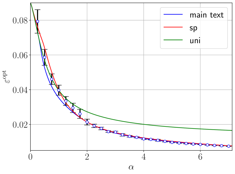
### Visual Description
## Line Chart: Epsilon Opt vs. Alpha
### Overview
The image is a line chart comparing the relationship between epsilon optimal (εopt) and alpha (α) for three different scenarios: "main text", "sp", and "uni". The chart displays data points with error bars and fitted lines for each scenario. The x-axis represents alpha (α), and the y-axis represents epsilon optimal (εopt).
### Components/Axes
* **X-axis:**
* Label: α
* Scale: 0 to approximately 7
* Markers: 0, 2, 4, 6
* **Y-axis:**
* Label: εopt
* Scale: 0 to approximately 0.09
* Markers: 0, 0.02, 0.04, 0.06, 0.08
* **Legend (Top-Right):**
* "main text" - Blue line
* "sp" - Red line
* "uni" - Green line
### Detailed Analysis
* **"main text" (Blue):**
* Trend: Decreases rapidly from α = 0 to α = 2, then decreases more gradually.
* Data Points:
* α = 0, εopt ≈ 0.08 (with error bars extending from approximately 0.075 to 0.085)
* α = 1, εopt ≈ 0.045 (with error bars extending from approximately 0.04 to 0.05)
* α = 2, εopt ≈ 0.025 (with error bars extending from approximately 0.02 to 0.03)
* α = 3, εopt ≈ 0.015
* α = 4, εopt ≈ 0.01
* α = 5, εopt ≈ 0.008
* α = 6, εopt ≈ 0.006
* **"sp" (Red):**
* Trend: Decreases rapidly from α = 0 to α = 2, then decreases more gradually, closely following the "main text" line.
* Data Points:
* α = 0, εopt ≈ 0.078
* α = 1, εopt ≈ 0.04
* α = 2, εopt ≈ 0.02
* α = 3, εopt ≈ 0.015
* α = 4, εopt ≈ 0.01
* α = 5, εopt ≈ 0.008
* α = 6, εopt ≈ 0.006
* **"uni" (Green):**
* Trend: Decreases from α = 0 to α = 7, but at a slower rate compared to "main text" and "sp".
* Data Points:
* α = 0, εopt ≈ 0.08
* α = 1, εopt ≈ 0.05
* α = 2, εopt ≈ 0.03
* α = 3, εopt ≈ 0.023
* α = 4, εopt ≈ 0.02
* α = 5, εopt ≈ 0.018
* α = 6, εopt ≈ 0.016
### Key Observations
* The "main text" and "sp" lines are very close to each other, indicating similar behavior between these two scenarios.
* The "uni" line decreases at a slower rate compared to the other two, suggesting a different relationship between alpha and epsilon optimal.
* Error bars are present on the "main text" data points, indicating the uncertainty associated with those measurements.
* All three lines converge towards a similar value of epsilon optimal as alpha increases.
### Interpretation
The chart illustrates how epsilon optimal (εopt) changes with respect to alpha (α) under three different conditions ("main text", "sp", and "uni"). The "main text" and "sp" scenarios exhibit a similar inverse relationship, where εopt decreases sharply as α increases initially, then levels off. The "uni" scenario also shows an inverse relationship, but the decrease in εopt is less pronounced. This suggests that the "uni" condition is less sensitive to changes in alpha compared to the other two. The error bars on the "main text" data points provide a measure of the variability or uncertainty in those measurements. The convergence of all three lines at higher alpha values indicates that the differences between the scenarios become less significant as alpha increases.
</details>
<details>
<summary>x10.png Details</summary>
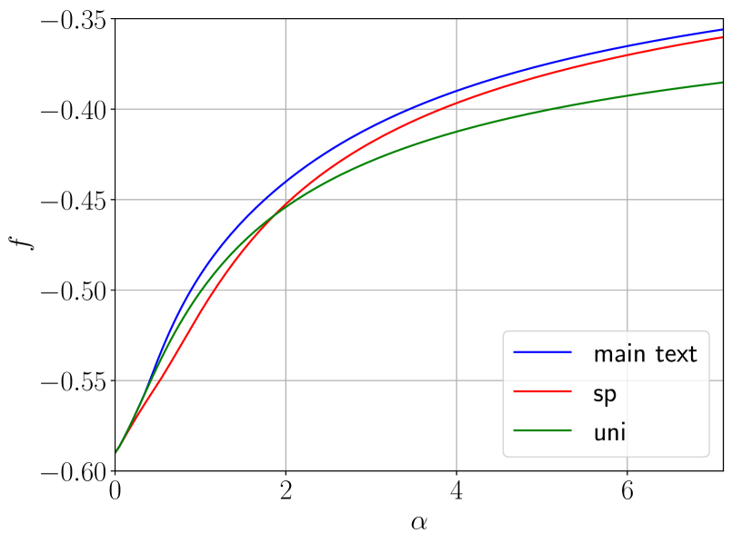
### Visual Description
## Line Chart: f vs. α
### Overview
The image is a line chart displaying the relationship between 'f' (y-axis) and 'α' (x-axis) for three different data series: "main text", "sp", and "uni". All three lines start at approximately the same point and increase, but at different rates, as α increases.
### Components/Axes
* **X-axis:** Labeled "α", with numerical values ranging from 0 to 6, incrementing by 2.
* **Y-axis:** Labeled "f", with numerical values ranging from -0.60 to -0.35, incrementing by 0.05.
* **Gridlines:** Present on the chart, aiding in value estimation.
* **Legend:** Located in the bottom-right corner, identifying the three data series:
* "main text" (blue line)
* "sp" (red line)
* "uni" (green line)
### Detailed Analysis
* **"main text" (blue line):** Starts at approximately -0.59 at α = 0 and increases to approximately -0.37 at α = 6. The slope decreases as α increases.
* **"sp" (red line):** Starts at approximately -0.59 at α = 0 and increases to approximately -0.38 at α = 6. The slope decreases as α increases.
* **"uni" (green line):** Starts at approximately -0.59 at α = 0 and increases to approximately -0.43 at α = 6. The slope decreases as α increases.
**Specific Data Points (Approximate):**
| α | main text (blue) | sp (red) | uni (green) |
|------|--------------------|----------|-------------|
| 0 | -0.59 | -0.59 | -0.59 |
| 2 | -0.45 | -0.47 | -0.48 |
| 4 | -0.39 | -0.41 | -0.41 |
| 6 | -0.37 | -0.38 | -0.43 |
### Key Observations
* All three lines start at roughly the same y-value when α is 0.
* The "main text" line consistently has the highest y-value for any given α > 0.
* The "uni" line consistently has the lowest y-value for any given α > 0.
* The rate of increase for all three lines decreases as α increases.
### Interpretation
The chart illustrates how the value of 'f' changes with respect to 'α' for three different conditions or models represented by "main text", "sp", and "uni". The fact that all lines start at the same point suggests a common initial condition. The different slopes and final values indicate that the parameter 'α' has a varying impact on 'f' depending on the specific condition. The "main text" condition appears to be most sensitive to changes in 'α', resulting in the highest 'f' values. The "uni" condition is the least sensitive. The decreasing slope of all lines suggests a diminishing return as 'α' increases.
</details>
<details>
<summary>x11.png Details</summary>
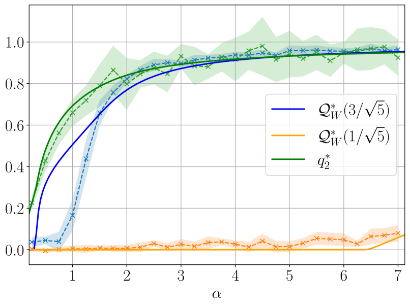
### Visual Description
## Line Chart: Performance Comparison of Q-learning Variants
### Overview
The image is a line chart comparing the performance of three Q-learning variants, denoted as `Q*_w(3/√5)`, `Q*_w(1/√5)`, and `q*_2`, across different values of a parameter α. The chart displays the performance of each variant as a function of α, with shaded regions indicating the variance or uncertainty in the measurements.
### Components/Axes
* **X-axis (Horizontal):** Labeled as "α". The scale ranges from approximately 0.5 to 7, with tick marks at integer values.
* **Y-axis (Vertical):** Ranges from 0.0 to 1.0, with tick marks at intervals of 0.2.
* **Legend (Top-Right):**
* Blue line: `Q*_w(3/√5)`
* Orange line: `Q*_w(1/√5)`
* Green line: `q*_2`
* **Grid:** The chart has a grid for easier reading of values.
### Detailed Analysis
* **Blue Line: `Q*_w(3/√5)`**
* Trend: Initially increases rapidly from α ≈ 0.5 to α ≈ 2, then plateaus around 0.95 for α > 4.
* Data Points:
* α = 0.5, Value ≈ 0.05
* α = 1, Value ≈ 0.2
* α = 2, Value ≈ 0.8
* α = 4, Value ≈ 0.9
* α = 7, Value ≈ 0.95
* Variance: The dashed blue line with 'x' markers represents the raw data points, and the light blue shaded region represents the variance.
* **Orange Line: `Q*_w(1/√5)`**
* Trend: Remains relatively flat near 0.0 for α < 6, then increases slightly for α > 6.
* Data Points:
* α = 0.5, Value ≈ 0.0
* α = 4, Value ≈ 0.0
* α = 7, Value ≈ 0.1
* Variance: The dashed orange line with 'x' markers represents the raw data points, and the light orange shaded region represents the variance.
* **Green Line: `q*_2`**
* Trend: Increases rapidly from α ≈ 0.5 to α ≈ 2, then plateaus around 0.95 for α > 4.
* Data Points:
* α = 0.5, Value ≈ 0.25
* α = 1, Value ≈ 0.5
* α = 2, Value ≈ 0.8
* α = 4, Value ≈ 0.9
* α = 7, Value ≈ 0.95
* Variance: The dashed green line with 'x' markers represents the raw data points, and the light green shaded region represents the variance.
### Key Observations
* `Q*_w(3/√5)` and `q*_2` exhibit similar performance, both increasing rapidly initially and then plateauing at a high value.
* `Q*_w(1/√5)` performs significantly worse, remaining near zero for most values of α.
* The variance for all three variants appears to be relatively small, as indicated by the narrow shaded regions.
### Interpretation
The chart suggests that the parameter α has a significant impact on the performance of the Q-learning variants. Specifically, `Q*_w(3/√5)` and `q*_2` are more effective than `Q*_w(1/√5)` across the tested range of α values. The rapid initial increase in performance for `Q*_w(3/√5)` and `q*_2` indicates that there is a critical value of α beyond which the algorithms learn effectively. The near-zero performance of `Q*_w(1/√5)` suggests that this variant may be highly sensitive to the choice of α or that it requires a different range of α values to perform well. The shaded regions provide an indication of the stability and reliability of the measurements, with narrower regions indicating more consistent results.
</details>
<details>
<summary>x12.png Details</summary>
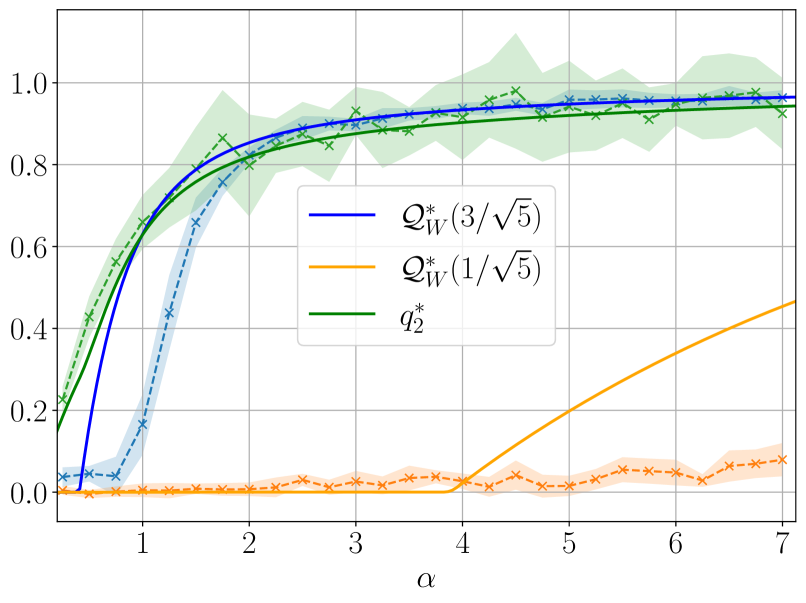
### Visual Description
## Line Chart: Q*_w* and q*_2* vs. Alpha
### Overview
The image is a line chart comparing the behavior of three different quantities, Q*_w*(3/√5), Q*_w*(1/√5), and q*_2* as a function of α. The chart includes error bands around the data points, represented by shaded regions.
### Components/Axes
* **X-axis (Horizontal):** α, ranging from 0 to 7, with tick marks at every integer value.
* **Y-axis (Vertical):** Values ranging from 0.0 to 1.0, with tick marks at intervals of 0.2.
* **Legend (Top-Right):**
* Blue line: Q*_w*(3/√5)
* Orange line: Q*_w*(1/√5)
* Green line: q*_2*
* **Grid:** Present in the background for easier reading of values.
### Detailed Analysis
* **Q*_w*(3/√5) (Blue):**
* Trend: The blue line starts near 0 at α=0, increases rapidly until approximately α=2, and then plateaus around 0.95 for α > 2.
* Data Points:
* α = 0: ~0.03
* α = 1: ~0.45
* α = 2: ~0.85
* α = 3: ~0.92
* α = 4: ~0.94
* α = 5: ~0.95
* α = 6: ~0.96
* α = 7: ~0.96
* Error Band: A light blue dashed line with 'x' markers indicates the error band. The error band is narrow, suggesting low variance.
* **Q*_w*(1/√5) (Orange):**
* Trend: The orange line remains close to 0 until approximately α=4, then increases steadily.
* Data Points:
* α = 0 to 3.5: ~0.02
* α = 4: ~0.03
* α = 5: ~0.15
* α = 6: ~0.30
* α = 7: ~0.47
* Error Band: A light orange dashed line with 'x' markers indicates the error band. The error band is narrow, suggesting low variance.
* **q*_2* (Green):**
* Trend: The green line starts at approximately 0.2 at α=0, increases rapidly until approximately α=2, and then plateaus around 0.92 for α > 2.
* Data Points:
* α = 0: ~0.22
* α = 1: ~0.55
* α = 2: ~0.82
* α = 3: ~0.90
* α = 4: ~0.92
* α = 5: ~0.93
* α = 6: ~0.94
* α = 7: ~0.95
* Error Band: A light green shaded region indicates the error band. The error band is wider than the other two, suggesting higher variance.
### Key Observations
* Q*_w*(3/√5) and q*_2* exhibit similar behavior, rapidly increasing and then plateauing.
* Q*_w*(1/√5) remains low until α reaches approximately 4, after which it starts to increase.
* The error band for q*_2* is wider than those for Q*_w*(3/√5) and Q*_w*(1/√5).
### Interpretation
The chart illustrates how the quantities Q*_w*(3/√5), Q*_w*(1/√5), and q*_2* change with respect to the parameter α. The rapid increase and plateau of Q*_w*(3/√5) and q*_2* suggest that they quickly reach a stable state as α increases. In contrast, Q*_w*(1/√5) shows a delayed response, indicating that it requires a higher value of α to start increasing. The wider error band for q*_2* suggests that it is more sensitive to variations or noise in the system compared to the other two quantities. The data suggests that the parameter α has a significant impact on these quantities, with different thresholds for each.
</details>
Figure 5: Different theoretical curves and numerical results for ReLU(x) activation, $P_{v}=\frac{1}{4}(\delta_{-3/\sqrt{5}}+\delta_{-1/\sqrt{5}}+\delta_{1/\sqrt{5}%
}+\delta_{3/\sqrt{5}})$ , $d=150$ , $\gamma=0.5$ , with linear readout with Gaussian noise of variance $\Delta=0.1$ Top left: Optimal mean-square generalisation error predicted by the theory reported in the main text (solid blue) versus the branch obtained from the simplified ansatz (83) (solid red); the green solid line shows the universal branch corresponding to $\mathcal{Q}_{W}\equiv 0$ , and empty circles are HMC results with informative initialisation. Top right: Theoretical free entropy curves (colors and linestyles as top left). Bottom: Predictions for the overlaps $\mathcal{Q}_{W}(\mathsf{v})$ and $q_{2}$ from the theory devised in the main text (left) and in Appendix E.1 (right).
To fix this issue, one can compare the predictions of the theory derived from this ansatz, with the ones obtained by plugging ${\mathcal{Q}}_{W}(\mathsf{v})=0\ ∀\ \mathsf{v}$ (denoted ${\mathcal{Q}}_{W}\equiv 0$ ) in the theory devised in the main text (6),
$$
f_{\rm uni}^{\alpha,\gamma}:=\psi_{P_{\text{out}}}(q_{K}(q_{2},\mathcal{Q}_{W}%
\equiv 0);r_{K})+\frac{1}{4\alpha}(1+\gamma\bar{v}^{2}-q_{2})\hat{q}_{2}-\frac%
{1}{\alpha}\iota(\hat{q}_{2}), \tag{89}
$$
to be extremised now only w.r.t. the scalar parameters $q_{2}$ , $\hat{q}_{2}$ (one can easily verify that, for ${\mathcal{Q}}_{W}\equiv 0$ , $\tau({\mathcal{Q}}_{W})=0$ and the extremisation w.r.t. $\hat{{\mathcal{Q}}}_{W}$ in (6) gives $\hat{{\mathcal{Q}}}_{W}\equiv 0$ ). Notice that $f_{\rm uni}^{\alpha,\gamma}$ is not depending on the prior over the inner weights, which is the reason why we are calling it “universal”. For consistency, the two free entropies $f_{\rm sp}^{\alpha,\gamma}$ , $f_{\rm uni}^{\alpha,\gamma}$ should be compared through a discrete variational principle, that is the free entropy of the model is predicted to be
$$
\bar{f}^{\alpha,\gamma}_{\rm RS}:=\max\{{\rm extr}f_{\rm uni}^{\alpha,\gamma},%
{\rm extr}f_{\rm sp}^{\alpha,\gamma}\}, \tag{90}
$$
instead of the unified variational form (6). Quite generally, ${\rm extr}f_{\rm uni}^{\alpha,\gamma}>{\rm extr}f_{\rm sp}^{\alpha,\gamma}$ for low values of $\alpha$ , so that the behaviour of the model in the universal phase is correctly predicted. The curves cross at a critical value
$$
\bar{\alpha}_{\rm sp}(\gamma)=\sup\{\alpha\mid{\rm extr}f_{\rm uni}^{\alpha,%
\gamma}>{\rm extr}f_{\rm sp}^{\alpha,\gamma}\}, \tag{91}
$$
instead of the value $\alpha_{\rm sp}(\gamma)$ reported in the main. This approach has been profitably adopted in Barbier et al. (2025) in the context of matrix denoising This is also the approach we used in a earlier version of this paper (superseded by the present one), accessible on ArXiv at this link., a problem sharing some of the challenges presented in this paper. In this respect, it provides a heuristic solution that quantitatively predicts the behaviour of the model in most of its phase diagram. Moreover, for any activation $\sigma$ with a second Hermite coefficient $\mu_{2}=0$ (e.g., all odd activations) the ansatz (83) yields the same theory as the one devised in the main text, as in this case $q_{K}(q_{2},{\mathcal{Q}}_{W})$ entering the energetic part of the free entropy does not depend on $q_{2}$ , so that the extremisation selects $q_{2}=\hat{q}_{2}=0$ and the remaining parts of (88) match the ones of (6). Finally, (83) is consistent with the observation that specialisation never arises in the case of quadratic activation and Gaussian prior over the inner weights: in this case, one can check that the universal branch ${\rm extr}f_{\rm uni}^{\alpha,\gamma}$ is always higher than ${\rm extr}f_{\rm sp}^{\alpha,\gamma}$ , and thus never selected by (90). For a convincing check on the validity of this approach, and a comparison with the theory devised in the main text and numerical results, see Fig. 5, top left panel.
However, despite its merits listed above, this Appendix’s approach presents some issues, both from the theoretical and practical points of view:
1. the final free entropy of the model is obtained by comparing curves derived from completely different ansätze for the distribution $P(({\mathbf{S}}^{a}_{2})\mid\bm{{\mathcal{Q}}}_{W})$ (Gaussian with coupled replicas, leading to $f_{\rm sp}$ , vs. pure generalised Wishart with independent replicas, leading to $f_{\rm uni}$ ), rather than within a unified theory as in the main text;
1. the predicted critical value $\bar{\alpha}_{\rm sp}(\gamma)$ seems to be systematically larger than the one observed in experiments (see Fig. 5, top right panel, and compare the crossing point of the “sp” and “uni” free entropies with the actual transition where the numerical points depart from the universal branch in the top left panel);
1. predictions for the functional overlap ${\mathcal{Q}}_{W}^{*}$ from this approach are in much worse agreement with experimental data w.r.t. the ones from the theory presented in the main text (see Fig. 5, bottom panel, and compare with Fig. 3 in the main text);
1. in the cases we tested, the prediction for the generalisation error from the theory devised in the main text are in much better agreement with numerical simulations than the one from this Appendix (see Fig. 6 for a comparison).
Therefore, the more elaborate theory presented in the main is not only more meaningful from the theoretical viewpoint, but also in overall better agreement with simulations.
<details>
<summary>x13.png Details</summary>
### Visual Description
## Line Chart: Epsilon Opt vs. Alpha
### Overview
The image is a line chart comparing the relationship between epsilon optimal (εopt) and alpha (α) for three different data series: "main text", "sp", and "uni". The chart includes data points with error bars for the "main text" series. The x-axis represents alpha (α), and the y-axis represents epsilon optimal (εopt).
### Components/Axes
* **X-axis:**
* Label: α
* Scale: 0 to 7, with tick marks at every integer value.
* **Y-axis:**
* Label: εopt
* Scale: 0 to 0.08, with tick marks at 0.02 intervals.
* **Legend:** Located in the top-right corner.
* "main text" - Blue line with blue data points and error bars.
* "sp" - Red line.
* "uni" - Green line.
### Detailed Analysis
* **"main text" (Blue):** The blue line with circular data points shows a decreasing trend as alpha increases. The data points have error bars, indicating a range of uncertainty.
* α = 0, εopt ≈ 0.078 ± 0.002
* α = 1, εopt ≈ 0.042 ± 0.003
* α = 2, εopt ≈ 0.029 ± 0.002
* α = 3, εopt ≈ 0.025 ± 0.001
* α = 4, εopt ≈ 0.021 ± 0.001
* α = 5, εopt ≈ 0.019 ± 0.001
* α = 6, εopt ≈ 0.013 ± 0.001
* α = 7, εopt ≈ 0.010 ± 0.001
* **"sp" (Red):** The red line also shows a decreasing trend as alpha increases, but it is consistently above the "main text" line.
* α = 0, εopt ≈ 0.085
* α = 1, εopt ≈ 0.058
* α = 2, εopt ≈ 0.038
* α = 3, εopt ≈ 0.027
* α = 4, εopt ≈ 0.020
* α = 5, εopt ≈ 0.015
* α = 6, εopt ≈ 0.012
* α = 7, εopt ≈ 0.009
* **"uni" (Green):** The green line shows a decreasing trend initially, but it flattens out as alpha increases.
* α = 0, εopt ≈ 0.090
* α = 1, εopt ≈ 0.060
* α = 2, εopt ≈ 0.040
* α = 3, εopt ≈ 0.030
* α = 4, εopt ≈ 0.022
* α = 5, εopt ≈ 0.020
* α = 6, εopt ≈ 0.019
* α = 7, εopt ≈ 0.018
### Key Observations
* All three data series ("main text", "sp", and "uni") show a decreasing trend of εopt as α increases.
* The "sp" series consistently has higher εopt values compared to the "main text" series for the same α values.
* The "uni" series initially decreases more rapidly than the "sp" series, but it flattens out at higher α values.
* The "main text" series has error bars, indicating the uncertainty in the measurements.
### Interpretation
The chart illustrates the relationship between epsilon optimal (εopt) and alpha (α) for three different scenarios represented by "main text", "sp", and "uni". The decreasing trend in all three series suggests that as alpha increases, epsilon optimal decreases. The differences in the curves indicate that the relationship between epsilon optimal and alpha varies depending on the specific scenario. The error bars on the "main text" series provide an indication of the precision of the measurements. The flattening of the "uni" curve at higher alpha values suggests that there may be a lower limit to epsilon optimal in that scenario.
</details>
Figure 6: Generalisation error for ReLU activation and Rademacher readout prior $P_{v}$ of the theory reported in the main text (solid blue) versus the branch obtained from the simplified ansatz (83) (solid red); the green solid line shows $\mathcal{Q}_{W}\equiv 0$ (universal branch), and empty circles are HMC results with informative initialisation.
E.2 Possible refined analyses with structured ${\mathbf{S}}_{2}$ matrices
In the main text, we kept track of the inhomogeneous profile of the readouts induced by the non-trivial distribution $P_{v}$ , which is ultimately responsible for the sequence of specialisation phase transitions occurring at increasing $\alpha$ , thanks to a functional order parameter ${\mathcal{Q}}_{W}(\mathsf{v})$ measuring how much the student’s hidden weights corresponding to all the readout elements equal to $\mathsf{v}$ have aligned with the teacher’s. However, when writing $\tilde{P}(({\mathbf{S}}_{2}^{a})\mid\bm{{\mathcal{Q}}}_{W})$ we treated the tensor ${\mathbf{S}}_{2}^{a}$ as a whole, without considering the possibility that its “components”
$$
\displaystyle S_{2;\alpha_{1}\alpha_{2}}^{a}(\mathsf{v}):=\frac{\mathsf{v}}{%
\sqrt{|\mathcal{I}_{\mathsf{v}}|}}\sum_{i\in\mathcal{I}_{\mathsf{v}}}W^{a}_{i%
\alpha_{1}}W^{a}_{i\alpha_{2}} \tag{92}
$$
could follow different laws for different $\mathsf{v}∈\mathsf{V}$ . To do so, let us define
$$
\displaystyle Q_{2}^{ab}=\frac{1}{k}\sum_{\mathsf{v},\mathsf{v}^{\prime}}%
\mathsf{v}\,\mathsf{v}^{\prime}\sum_{i\in\mathcal{I}_{\mathsf{v}},j\in\mathcal%
{I}_{\mathsf{v^{\prime}}}}(\Omega_{ij}^{ab})^{2}=\sum_{\mathsf{v},\mathsf{v}^{%
\prime}}\frac{\sqrt{|\mathcal{I}_{\mathsf{v}}||\mathcal{I}_{\mathsf{v^{\prime}%
}}|}}{k}{\mathcal{Q}}_{2}^{ab}(\mathsf{v},\mathsf{v}^{\prime}),\quad\text{%
where}\quad{\mathcal{Q}}_{2}^{ab}(\mathsf{v},\mathsf{v}^{\prime}):=\frac{1}{d^%
{2}}{\rm Tr}\,{\mathbf{S}}_{2}^{a}(\mathsf{v}){\mathbf{S}}_{2}^{b}(\mathsf{v}^%
{\prime})^{\intercal}. \tag{93}
$$
The generalisation of (63) then reads
$$
\displaystyle\int dP(({\mathbf{S}}_{2}^{a})\mid\bm{\mathcal{Q}}_{W}) \displaystyle\frac{1}{d^{2}}{\rm Tr}\,{\mathbf{S}}_{2}^{a}(\mathsf{v}){\mathbf%
{S}}_{2}^{b}(\mathsf{v}^{\prime})^{\intercal}=\delta_{\mathsf{v}\mathsf{v}^{%
\prime}}\mathsf{v}^{2}\mathcal{Q}_{W}^{ab}(\mathsf{v})^{2}+\gamma\,\mathsf{v}%
\mathsf{v}^{\prime}\sqrt{P_{v}(\mathsf{v})P_{v}(\mathsf{v}^{\prime})} \tag{94}
$$
w.r.t. the true distribution $P(({\mathbf{S}}_{2}^{a})\mid\bm{\mathcal{Q}}_{W})$ reported in (14). Despite the already good match of the theory in the main with the numerics, taking into account this additional level of structure thanks to a refined simplified measure could potentially lead to further improvements. The simplified measure able to match these moment-matching conditions while taking into account the Wishart form (92) of the matrices $({\mathbf{S}}_{2}^{a}(\mathsf{v}))$ is
$$
\displaystyle d\bar{P}(({\mathbf{S}}_{2}^{a})\mid\bm{{\mathcal{Q}}}_{W})%
\propto\prod_{\mathsf{v}\in\mathsf{V}}\prod_{a}dP_{S}^{\mathsf{v}}({\mathbf{S}%
}_{2}^{a}(\mathsf{v}))\times\prod_{\mathsf{v}\in\mathsf{V}}\prod_{a<b}e^{\frac%
{1}{2}\bar{\tau}^{ab}_{\mathsf{v}}(\bm{{\mathcal{Q}}}_{W}){\rm Tr}{\mathbf{S}}%
_{2}^{a}(\mathsf{v}){\mathbf{S}}_{2}^{b}(\mathsf{v})}, \tag{95}
$$
where $P_{S}^{\mathsf{v}}$ is the law of a random matrix $\mathsf{v}\bar{{\mathbf{W}}}\bar{{\mathbf{W}}}^{∈tercal}|\mathcal{I}_{%
\mathsf{v}}|^{-1/2}$ with $\bar{\mathbf{W}}∈\mathbb{R}^{d×|\mathcal{I}_{\mathsf{v}}|}$ having i.i.d. standard Gaussian entries. For properly chosen $(\bar{\tau}_{\mathsf{v}}^{ab})$ , (94) is verified for this simplified measure.
However, the order parameters $({\mathcal{Q}}_{2}^{ab}(\mathsf{v},\mathsf{v}^{\prime}))$ are difficult to deal with if keeping a general form, as they not only imply coupled replicas $({\mathbf{S}}_{2}^{a}(\mathsf{v}))_{a}$ for a given $\mathsf{v}$ (a kind of coupling that is easily linearised with a single Hubbard-Stratonovich transformation, within the replica symmetric treatment justified in Bayes-optimal learning), but also a coupling for different values of the variable $\mathsf{v}$ . Linearising it would yield a more complicated matrix model than the integral reported in (D.3), because the resulting coupling field would break rotational invariance and therefore the model does not have a form which is known to be solvable, see Kazakov (2000).
A first idea to simplify $P(({\mathbf{S}}^{a}_{2})\mid\bm{{\mathcal{Q}}}_{W})$ (14) while taking into account the additional structure induced by (93), (94) and maintaining a solvable model, is to consider a generalisation of the relaxation (83). This entails dropping entirely the dependencies among matrix entries, induced by their Wishart-like form (92), for each ${\mathbf{S}}_{2}^{a}(\mathsf{v})$ . In this case, the moment constraints (94) can be exactly enforced by choosing the simplified measure
$$
\displaystyle d\bar{P}(({\mathbf{S}}_{2}^{a})\mid\bm{{\mathcal{Q}}}_{W})=\prod%
_{\mathsf{v}\in\mathsf{V}}\prod_{a=0}^{s}d{\mathbf{S}}^{a}_{2}(\mathsf{v})%
\prod_{\alpha=1}^{d}\delta(S^{a}_{2;\alpha\alpha}(\mathsf{v})-\mathsf{v}\sqrt{%
|\mathcal{I}_{\mathsf{v}}|})\times\prod_{\mathsf{v}\in\mathsf{V}}\prod_{\alpha%
_{1}<\alpha_{2}}^{d}\frac{e^{-\frac{1}{2}\sum_{a,b=0}^{s}S^{a}_{2;\alpha_{1}%
\alpha_{2}}(\mathsf{v})\bar{\tau}_{\mathsf{v}}^{ab}(\bm{{\mathcal{Q}}}_{W})S^{%
b}_{2;\alpha_{1}\alpha_{2}}(\mathsf{v})}}{\sqrt{(2\pi)^{s+1}\det(\bar{\bm{\tau%
}}_{\mathsf{v}}(\bm{{\mathcal{Q}}}_{W})^{-1})}}. \tag{96}
$$
The parameters $(\bar{\tau}^{ab}_{\mathsf{v}}(\bm{{\mathcal{Q}}}_{W}))$ are then properly chosen to enforce (94) for all $0≤ a≤ b≤ s$ and $\mathsf{v},\mathsf{v}^{\prime}∈\mathsf{V}$ . Using this measure, the resulting entropic term, taking into account the degeneracy of the order parameters $({\mathcal{Q}}_{2}^{ab}(\mathsf{v},\mathsf{v}^{\prime}))$ and $({\mathcal{Q}}_{W}^{ab}(\mathsf{v}))$ , remains tractable through Gaussian integrals (the energetic term is obviously unchanged once we express $(Q_{2}^{ab})$ entering it using these new order parameters through the identity (93), and keeping in mind that nothing changes for higher order overlaps compared to the theory in the main). We leave for future work the analysis of this Gaussian relaxation and other possible simplifications of (95) leading to solvable models.
Appendix F Linking free entropy and mutual information
It is possible to relate the mutual information (MI) of the inference task to the free entropy $f_{n}=\mathbb{E}\ln\mathcal{Z}$ introduced in the main. Indeed, we can write the MI as
$$
\frac{I({\mathbf{W}}^{0};\mathcal{D})}{kd}=\frac{\mathcal{H}(\mathcal{D})}{kd}%
-\frac{\mathcal{H}(\mathcal{D}\mid{\mathbf{W}}^{0})}{kd}, \tag{97}
$$
where $\mathcal{H}(Y\mid X)$ is the conditional Shannon entropy of $Y$ given $X$ . It is straightforward to show that the free entropy is
$$
-\frac{\alpha}{\gamma}f_{n}=\frac{\mathcal{H}(\{y_{\mu}\}_{\mu\leq n}\mid\{{%
\mathbf{x}}_{\mu}\}_{\mu\leq n})}{kd}=\frac{\mathcal{H}(\mathcal{D})}{kd}-%
\frac{\mathcal{H}(\{{\mathbf{x}}_{\mu}\}_{\mu\leq n})}{kd}, \tag{98}
$$
by the chain rule for the entropy. On the other hand $\mathcal{H}(\mathcal{D}\mid{\mathbf{W}}^{0})=\mathcal{H}(\{y_{\mu}\}\mid{%
\mathbf{W}}^{0},\{{\mathbf{x}}_{\mu}\})+\mathcal{H}(\{{\mathbf{x}}_{\mu}\})$ , i.e.,
$$
\frac{\mathcal{H}(\mathcal{D}\mid{\mathbf{W}}^{0})}{kd}\approx-\frac{\alpha}{%
\gamma}\mathbb{E}_{\lambda}\int dyP_{\text{out}}(y\mid\lambda)\ln P_{\text{out%
}}(y\mid\lambda)+\frac{\mathcal{H}(\{{\mathbf{x}}_{\mu}\}_{\mu\leq n})}{kd}, \tag{99}
$$
where $\lambda\sim{\mathcal{N}}(0,r_{K})$ , with $r_{K}$ given by (53) (assuming here that $\mu_{0}=0$ , see App. D.5 if the activation $\sigma$ is non-centred), and the equality holds asymptotically in the limit $\lim$ . This allows us to express the MI as
$$
\frac{I({\mathbf{W}}^{0};\mathcal{D})}{kd}=-\frac{\alpha}{\gamma}f_{n}+\frac{%
\alpha}{\gamma}\mathbb{E}_{\lambda}\int dyP_{\text{out}}(y|\lambda)\ln P_{%
\text{out}}(y|\lambda). \tag{100}
$$
Specialising the equation to the Gaussian channel, one obtains
$$
\frac{I({\mathbf{W}}^{0};\mathcal{D})}{kd}=-\frac{\alpha}{\gamma}f_{n}-\frac{%
\alpha}{2\gamma}\ln(2\pi e\Delta). \tag{101}
$$
Note that the choice of normalising by $kd$ is not accidental. Indeed, the number of parameters is $kd+k≈ kd$ . Hence with this choice one can interpret the parameter $\alpha$ as an effective signal-to-noise ratio.
**Remark F.1**
*The arguments of Barbier et al. (2025) to show the existence of an upper bound on the mutual information per variable in the case of discrete variables and the associated inevitable breaking of prior universality beyond a certain threshold in matrix denoising apply to the present model too. It implies, as in the aforementioned paper, that the mutual information per variable cannot go beyond $\ln 2$ for Rademacher inner weights. Our theory is consistent with this fact; this is a direct consequence of the analysis in App. G (see in particular (108)) specialised to binary prior over ${\mathbf{W}}$ .*
Appendix G Large sample rate limit of $f_{\rm RS}^{\alpha,\gamma}$
In this section we show that when the prior over the weights ${\mathbf{W}}$ is discrete the MI can never exceed the entropy of the prior itself.
To do this, we first need to control the function $\rm mmse$ when its argument is large. By a saddle point argument, it is not difficult to show that the leading term for ${\rm mmse}_{S}(\tau)$ when $\tau→∞$ if of the type $C(\gamma)/\tau$ for a proper constant $C$ depending at most on the rectangularity ratio $\gamma$ .
We now notice that the equation for $\hat{\mathcal{Q}}_{W}(v)$ in (76) can be rewritten as
$$
\displaystyle\hat{\mathcal{Q}}_{W}(v)=\frac{1}{2\gamma}[{\rm mmse}_{S}(\tau)-{%
\rm mmse}_{S}(\tau+\hat{q}_{2})]\partial_{{\mathcal{Q}}_{W}(v)}\tau+2\frac{%
\alpha}{\gamma}\partial_{{\mathcal{Q}}_{W}(v)}\psi_{P_{\text{out}}}(q_{K}(q_{2%
},\mathcal{Q}_{W});r_{K}). \tag{102}
$$
For $\alpha→∞$ we make the self-consistent ansatz $\mathcal{Q}_{W}(v)=1-o_{\alpha}(1)$ . As a consequence $1/\tau$ has to vanish by the moment matching condition (74) as $o_{\alpha}(1)$ too. Using the very same equation, we are also able to evaluate $∂_{\mathcal{Q}_{W}(v)}\tau$ as follows:
$$
\displaystyle\partial_{\mathcal{Q}_{W}(v)}\tau=\frac{-2v^{2}\mathcal{Q}_{W}(v)%
}{{\rm mmse^{\prime}}(\tau)}\sim\tau^{2} \tag{103}
$$
as $\alpha→∞$ , where we have used ${\rm mmse}_{S}(\tau)\sim C(\gamma)/\tau$ to estimate the derivative. We use the same approximation for the two $\rm mmse$ ’s appearing in the fixed point equation for $\hat{\mathcal{Q}}_{W}(v)$ :
$$
\displaystyle\hat{\mathcal{Q}}_{W}(v)\sim\frac{\hat{q}_{2}}{2\gamma(\tau(\tau+%
\hat{q}_{2}))}\tau^{2}+2\frac{\alpha}{\gamma}\partial_{{\mathcal{Q}}_{W}(v)}%
\psi_{P_{\text{out}}}(q_{K}(q_{2},\mathcal{Q}_{W});r_{K}). \tag{104}
$$
From the last equation in (76) we see that $\hat{q}_{2}$ cannot diverge more than $O(\alpha)$ . Thanks to the above approximation and the first equation of (76) this entails that $\mathcal{Q}_{W}(v)$ is approaching $1$ exponentially fast in $\alpha$ , which in turn implies $\tau$ is diverging exponentially in $\alpha$ . As a consequence
$$
\displaystyle\frac{\tau^{2}}{\tau(\tau+\hat{q}_{2})}\sim 1. \tag{105}
$$
Furthermore, one also has
$$
\displaystyle\frac{1}{\alpha}[\iota(\tau)-\iota(\tau+\hat{q}_{2})]=-\frac{1}{4%
\alpha}\int_{\tau}^{\tau+\hat{q}_{2}}{\rm mmse}_{S}(t)\,dt\approx-\frac{C(%
\gamma)}{4\alpha}\log(1+\frac{\hat{q}_{2}}{\tau})\xrightarrow[]{\alpha\to%
\infty}0, \tag{106}
$$
as $\frac{\hat{q}_{2}}{\tau}$ vanishes with exponential speed in $\alpha$ .
Concerning the function $\psi_{P_{W}}$ , given that it is realted to a Bayes-optimal scalar Gaussian channel, and its SNRs $\hat{\mathcal{Q}}_{W}(v)$ are all diverging one can compute the integral by saddle point, which is inevitably attained at the ground truth:
$$
\displaystyle\psi_{P_{W}}(\hat{\mathcal{Q}}_{W}(v)) \displaystyle-\frac{\hat{\mathcal{Q}}_{W}(v)\mathcal{Q}_{W}(v)}{2}\approx%
\mathbb{E}_{w^{0}}\ln\int dP_{W}(w)\mathbbm{1}(w=w^{0}) \displaystyle+\mathbb{E}\Big{[}(\sqrt{\hat{\mathcal{Q}}_{W}(v)}\xi+\hat{%
\mathcal{Q}}_{W}(v)w^{0})w^{0}-\frac{\hat{\mathcal{Q}}_{W}(v)}{2}(w^{0})^{2}%
\Big{]}-\frac{\hat{\mathcal{Q}}_{W}(v)(1-o_{\alpha}(1))}{2}=-\mathcal{H}(W)+o_%
{\alpha}(1). \tag{1}
$$
Considering that $\psi_{P_{\text{out}}}(q_{K}(q_{2},\mathcal{Q}_{W});r_{K})\xrightarrow[]{\alpha%
→∞}\psi_{P_{\text{out}}}(r_{K};r_{K})$ , and using (100), it is then straightforward to check that our RS version of the MI saturates to the entropy of the prior $P_{W}$ when $\alpha→∞$ :
$$
\displaystyle-\frac{\alpha}{\gamma}\text{extr}f_{\rm RS}^{\alpha,\gamma}+\frac%
{\alpha}{\gamma}\mathbb{E}_{\lambda}\int dyP_{\text{out}}(y|\lambda)\ln P_{%
\text{out}}(y|\lambda)\xrightarrow[]{\alpha\to\infty}\mathcal{H}(W). \tag{108}
$$
Appendix H Extension of GAMP-RIE to arbitrary activation
Algorithm 1 GAMP-RIE for training shallow neural networks with arbitrary activation
Input: Fresh data point ${\mathbf{x}}_{\text{test}}$ with unknown associated response $y_{\text{test}}$ , dataset $\mathcal{D}=\{({\mathbf{x}}_{\mu},y_{\mu})\}_{\mu=1}^{n}$ .
Output: Estimator $\hat{y}_{\text{test}}$ of $y_{\text{test}}$ .
Estimate $y^{(0)}:=\mu_{0}{\mathbf{v}}^{∈tercal}\bm{1}/\sqrt{k}$ as
$$
\hat{y}^{(0)}=\frac{1}{n}\sum_{\mu}y_{\mu}; \tag{0}
$$
Estimate $\langle{\mathbf{W}}^{∈tercal}{\mathbf{v}}\rangle/\sqrt{k}$ using (117).
Estimate the $\mu_{1}$ term in the Hermite expansion (111) as
$$
\displaystyle\hat{y}_{\mu}^{(1)} \displaystyle=\mu_{1}\frac{\langle{\mathbf{v}}^{\intercal}{\mathbf{W}}\rangle{%
\mathbf{x}}_{\mu}}{\sqrt{kd}}; \tag{1}
$$
Compute
$$
\displaystyle\tilde{y}_{\mu} \displaystyle=\frac{y_{\mu}-\hat{y}_{\mu}^{(0)}-\hat{y}_{\mu}^{(1)}}{\mu_{2}/2%
};\qquad\tilde{\Delta}=\frac{\Delta+g(1)}{\mu_{2}^{2}/4}; \tag{0}
$$
Input $\{({\mathbf{x}}_{\mu},\tilde{y}_{\mu})\}_{\mu=1}^{n}$ and $\tilde{\Delta}$ into Algorithm 1 in Maillard et al. (2024a) to estimate $\langle{\mathbf{W}}^{∈tercal}({\mathbf{v}}){\mathbf{W}}\rangle$ ;
Output
$$
\displaystyle\hat{y}_{\text{test}}=\hat{y}^{(0)}+\mu_{1}\frac{\langle{\mathbf{%
v}}^{\intercal}{\mathbf{W}}\rangle{\mathbf{x}}_{\text{test}}}{\sqrt{kd}}+\frac%
{\mu_{2}}{2}\frac{1}{d\sqrt{k}}{\rm Tr}[({\mathbf{x}}_{\text{test}}{\mathbf{x}%
}_{\text{test}}^{\intercal}-{\mathbb{I}})\langle{\mathbf{W}}^{\intercal}({%
\mathbf{v}}){\mathbf{W}}\rangle]. \tag{0}
$$
For simplicity, let us consider $P_{\rm out}(y\mid\lambda)=\exp(-\frac{1}{2\Delta}(y-\lambda)^{2})/\sqrt{2\pi\Delta}$ , which entails:
$$
\displaystyle y_{\mu}\mid({\bm{\theta}}^{0},{\mathbf{x}}_{\mu})\overset{\rm{d}%
}{=}\frac{{\mathbf{v}}^{\intercal}}{\sqrt{k}}\sigma\Big{(}\frac{{\mathbf{W}}^{%
0}{\mathbf{x}}_{\mu}}{\sqrt{d}}\Big{)}+\sqrt{\Delta}\,z_{\mu},\quad\mu=1\dots,n, \tag{110}
$$
where $z_{\mu}$ are i.i.d. standard Gaussian random variables and $\overset{\rm d}{{}={}}$ means equality in law. Expanding $\sigma$ in the Hermite polynomial basis we have
$$
\displaystyle y_{\mu}\mid({\bm{\theta}}^{0},{\mathbf{x}}_{\mu})\overset{\rm{d}%
}{=}\mu_{0}\frac{{\mathbf{v}}^{\intercal}\bm{1}_{k}}{\sqrt{k}}+\mu_{1}\frac{{%
\mathbf{v}}^{\intercal}{\mathbf{W}}^{0}{\mathbf{x}}_{\mu}}{\sqrt{kd}}+\frac{%
\mu_{2}}{2}\frac{{\mathbf{v}}^{\intercal}}{\sqrt{k}}{\rm He}_{2}\Big{(}\frac{{%
\mathbf{W}}^{0}{\mathbf{x}}_{\mu}}{\sqrt{d}}\Big{)}+\dots+\sqrt{\Delta}z_{\mu} \tag{111}
$$
where $...$ represents the terms beyond second order. Without loss of generality, for this choice of output channel we can set $\mu_{0}=0$ as discussed in App. D.5. For low enough $\alpha$ it is reasonable to assume that higher order terms in $...$ cannot be learnt given quadratically many samples and, as a result, play the role of effective noise, which we assume independent of the first three terms. We shall see that this reasoning actually applies to the extension of the GAMP-RIE we derive, which plays the role of a “smart” spectral algorithm, regardless of the value of $\alpha$ . Therefore, these terms accumulate in an asymptotically Gaussian noise thanks to the central limit theorem (it is a projection of a centred function applied entry-wise to a vector with i.i.d. entries), with variance $g(1)$ (see (43)). We thus obtain the effective model
$$
\displaystyle y_{\mu}\mid({\bm{\theta}}^{0},{\mathbf{x}}_{\mu})\overset{\rm{d}%
}{=}\mu_{1}\frac{{\mathbf{v}}^{\intercal}{\mathbf{W}}^{0}{\mathbf{x}}_{\mu}}{%
\sqrt{kd}}+\frac{\mu_{2}}{2}\frac{{\mathbf{v}}^{\intercal}}{\sqrt{k}}{\rm He}_%
{2}\Big{(}\frac{{\mathbf{W}}^{0}{\mathbf{x}}_{\mu}}{\sqrt{d}}\Big{)}+\sqrt{%
\Delta+g(1)}\,z_{\mu}. \tag{1}
$$
The first term in this expression can be learnt with vanishing error given quadratically many samples (Remark H.1), thus can be ignored. This further simplifies the model to
$$
\displaystyle\bar{y}_{\mu}:=y_{\mu}-\mu_{1}\frac{{\mathbf{v}}^{\intercal}{%
\mathbf{W}}^{0}{\mathbf{x}}_{\mu}}{\sqrt{kd}}\overset{\rm d}{{}={}}\frac{\mu_{%
2}}{2}\frac{{\mathbf{v}}^{\intercal}}{\sqrt{k}}{\rm He}_{2}\Big{(}\frac{{%
\mathbf{W}}^{0}{\mathbf{x}}_{\mu}}{\sqrt{d}}\Big{)}+\sqrt{\Delta+g(1)}\,z_{\mu}, \tag{1}
$$
where $\bar{y}_{\mu}$ is $y_{\mu}$ with the (asymptotically) perfectly learnt linear term removed, and the last equality in distribution is again conditional on $({\bm{\theta}}^{0},{\mathbf{x}}_{\mu})$ . From the formula
$$
\displaystyle\frac{{\mathbf{v}}^{\intercal}}{\sqrt{k}}{\rm He}_{2}\Big{(}\frac%
{{\mathbf{W}}^{0}{\mathbf{x}}_{\mu}}{\sqrt{d}}\Big{)}={\rm Tr}\frac{{\mathbf{W%
}}^{0\intercal}({\mathbf{v}}){\mathbf{W}}^{0}}{d\sqrt{k}}{\mathbf{x}}_{\mu}{%
\mathbf{x}}_{\mu}^{\intercal}-\frac{{\mathbf{v}}^{\intercal}\bm{1}_{k}}{\sqrt{%
k}}\approx\frac{1}{\sqrt{k}d}{\rm Tr}[({\mathbf{x}}_{\mu}{\mathbf{x}}_{\mu}^{%
\intercal}-{\mathbb{I}}_{d}){\mathbf{W}}^{0\intercal}({\mathbf{v}}){\mathbf{W}%
}^{0}], \tag{114}
$$
where $≈$ is exploiting the concentration ${\rm Tr}{\mathbf{W}}^{0∈tercal}({\mathbf{v}}){\mathbf{W}}^{0}/(d\sqrt{k})→%
{\mathbf{v}}^{∈tercal}\bm{1}_{k}/\sqrt{k}$ , and the Gaussian equivalence property that ${\mathbf{M}}_{\mu}:=({\mathbf{x}}_{\mu}{\mathbf{x}}_{\mu}^{∈tercal}-{\mathbb%
{I}}_{d})/\sqrt{d}$ behaves like a GOE sensing matrix, i.e., a symmetric matrix whose upper triangular part has i.i.d. entries from $\mathcal{N}(0,(1+\delta_{ij})/d)$ Maillard et al. (2024a), the model can be seen as a GLM with signal $\bar{\mathbf{S}}^{0}_{2}:={\mathbf{W}}^{0∈tercal}({\mathbf{v}}){\mathbf{W}}^%
{0}/\sqrt{kd}$ :
$$
\displaystyle y^{\rm GLM}_{\mu}=\frac{\mu_{2}}{2}{\rm Tr}[{\mathbf{M}}_{\mu}%
\bar{\mathbf{S}}^{0}_{2}]+\sqrt{\Delta+g(1)}\,z_{\mu}. \tag{1}
$$
Starting from this equation, the arguments of App. D and Maillard et al. (2024a), based on known results on the GLM Barbier et al. (2019) and matrix denoising Barbier & Macris (2022); Maillard et al. (2022); Pourkamali et al. (2024), allow us to obtain the free entropy of such matrix sensing problem. The result is consistent with the $\mathcal{Q}_{W}\equiv 0$ solution of the saddle point equations obtained from the replica method in App. D, which, as anticipated, corresponds to the case where the Hermite polynomial combinations of the signal following the second one are not learnt.
Note that, as supported by the numerics, the model actually admits specialisation when $\alpha$ is big enough, hence the above equivalence cannot hold on the whole phase diagram at the information theoretic level. In fact, if specialisation occurs one cannot consider the $...$ terms in (111) as noise uncorrelated with the first ones, as the model is aligning with the actual teacher’s weights, such that it learns all the successive terms at once.
<details>
<summary>x14.png Details</summary>
### Visual Description
## Chart: Test Error vs. Alpha for ReLU and ELU Activation Functions
### Overview
The image is a line chart comparing the test error of ReLU and ELU activation functions as a function of a parameter alpha. The chart includes an inset providing a zoomed-in view of the data for smaller alpha values. The main chart spans alpha values from 0 to 4, while the inset focuses on alpha values from approximately 0 to 2.
### Components/Axes
* **X-axis (Horizontal):** Labeled "α" (alpha). The main chart ranges from 0 to 4, with tick marks at each integer value. The inset chart ranges from approximately 0 to 2, with tick marks at 0, 1, and 2.
* **Y-axis (Vertical):** Labeled "Test error". The main chart ranges from 0.00 to 0.08, with tick marks at intervals of 0.02. The inset chart ranges from 0.00 to 0.08, with tick marks at intervals of 0.02.
* **Legend (Top-Left):**
* **Red Line:** ReLU
* **Blue Line:** ELU
* **Data Series:**
* **ReLU (Red):** A red line representing the test error for the ReLU activation function.
* **ELU (Blue):** A blue line representing the test error for the ELU activation function.
* **Dashed Red Line:** Dashed red line representing the test error for the ReLU activation function.
* **Dashed Blue Line:** Dashed blue line representing the test error for the ELU activation function.
### Detailed Analysis
**ReLU (Red Line):**
* **Trend:** The red line starts at approximately 0.085 at alpha = 0 and decreases rapidly until alpha is approximately 2. After alpha = 2, the line drops sharply to approximately 0.00 and remains at that level.
* **Data Points:**
* Alpha = 0: Test error ≈ 0.085
* Alpha = 1: Test error ≈ 0.05
* Alpha = 2: Test error ≈ 0.04
* Alpha > 2: Test error ≈ 0.00
**ELU (Blue Line):**
* **Trend:** The blue line starts at approximately 0.04 at alpha = 0 and decreases gradually until alpha is approximately 3.75. After alpha = 3.75, the line drops sharply to approximately 0.01 and remains at that level.
* **Data Points:**
* Alpha = 0: Test error ≈ 0.04
* Alpha = 1: Test error ≈ 0.025
* Alpha = 2: Test error ≈ 0.02
* Alpha = 3.75: Test error ≈ 0.015
* Alpha > 3.75: Test error ≈ 0.01
**Dashed ReLU (Dashed Red Line):**
* **Trend:** The dashed red line starts at approximately 0.085 at alpha = 0 and decreases rapidly until alpha is approximately 2. After alpha = 2, the line continues to decrease gradually.
* **Data Points:**
* Alpha = 0: Test error ≈ 0.085
* Alpha = 1: Test error ≈ 0.045
* Alpha = 2: Test error ≈ 0.03
* Alpha = 3: Test error ≈ 0.025
* Alpha = 4: Test error ≈ 0.022
**Dashed ELU (Dashed Blue Line):**
* **Trend:** The dashed blue line starts at approximately 0.04 at alpha = 0 and decreases gradually.
* **Data Points:**
* Alpha = 0: Test error ≈ 0.04
* Alpha = 1: Test error ≈ 0.03
* Alpha = 2: Test error ≈ 0.025
* Alpha = 3: Test error ≈ 0.02
* Alpha = 4: Test error ≈ 0.015
### Key Observations
* For low alpha values (0-2), the ELU activation function consistently shows a lower test error than the ReLU activation function.
* Both ReLU and ELU exhibit a sharp drop in test error at specific alpha values (around 2 for ReLU and 3.75 for ELU).
* The inset provides a clearer view of the initial behavior of the test error for both activation functions at low alpha values.
* The dashed lines show a more gradual decrease in test error compared to the solid lines.
### Interpretation
The chart suggests that the choice of activation function (ReLU or ELU) and the parameter alpha significantly impact the test error of the model. ELU appears to perform better than ReLU for lower alpha values. The sharp drops in test error for both activation functions indicate critical alpha thresholds where the model's performance improves drastically. The dashed lines show a more gradual decrease in test error compared to the solid lines, suggesting a different model configuration or training regime. The data implies that careful tuning of alpha is crucial for optimizing model performance, and the optimal value may depend on the chosen activation function.
</details>
Figure 7: Theoretical prediction (solid curves) of the Bayes-optimal mean-square generalisation error for binary inner weights and ReLU, eLU activations, with $\gamma=0.5$ , $d=150$ , Gaussian label noise with $\Delta=0.1$ , and fixed readouts ${\mathbf{v}}=\mathbf{1}$ . Dashed lines are obtained from the solution of the fixed point equations (76) with all $\mathcal{Q}_{W}(\mathsf{v})=0$ . Circles are the test error of GAMP-RIE (Maillard et al., 2024a) extended to generic activation. The MCMC points initialised uninformatively (inset) are obtained using (36), to account for lack of equilibration due to glassiness, which prevents using (38). Even in the possibly glassy region, the GAMP-RIE attains the universal branch performance. Data for GAMP-RIE and MCMC are averaged over 16 data instances, with error bars representing one standard deviation over instances.
We now assume that this mapping holds at the algorithmic level, namely, that we can process the data algorithmically as if they were coming from the identified GLM, and thus try to infer the signal $\bar{\mathbf{S}}_{2}^{0}={\mathbf{W}}^{0∈tercal}({\mathbf{v}}){\mathbf{W}}^{%
0}/\sqrt{kd}$ and construct a predictor from it. Based on this idea, we propose Algorithm 1 that can indeed reach the performance predicted by the $\mathcal{Q}_{W}\equiv 0$ solution of our replica theory.
**Remark H.1**
*In the linear data regime, where $n/d$ converges to a fixed constant $\alpha_{1}$ , only the first term in (111) can be learnt while the rest behaves like noise. By the same argument as above, the model is equivalent to
$$
\displaystyle y_{\mu}=\mu_{1}\frac{{\mathbf{v}}^{\intercal}{\mathbf{W}}^{0}{%
\mathbf{x}}_{\mu}}{\sqrt{kd}}+\sqrt{\Delta+\nu-\mu_{0}^{2}-\mu_{1}^{2}}\,z_{%
\mu}, \tag{116}
$$
where $\nu=\mathbb{E}_{z\sim{\mathcal{N}}(0,1)}\sigma^{2}(z)$ . This is again a GLM with signal ${\mathbf{S}}_{1}^{0}={\mathbf{W}}^{0∈tercal}{\mathbf{v}}/\sqrt{k}$ and Gaussian sensing vectors ${\mathbf{x}}_{\mu}$ . Define $q_{1}$ as the limit of ${\mathbf{S}}_{1}^{a∈tercal}{\mathbf{S}}_{1}^{b}/d$ where ${\mathbf{S}}_{1}^{a},{\mathbf{S}}_{1}^{b}$ are drawn independently from the posterior. With $k→∞$ , the signal converges in law to a standard Gaussian vector. Using known results on GLMs with Gaussian signal Barbier et al. (2019), we obtain the following equations characterising $q_{1}$ :
| | $\displaystyle q_{1}$ | $\displaystyle=\frac{\hat{q}_{1}}{\hat{q}_{1}+1},\qquad\hat{q}_{1}=\frac{\alpha%
_{1}}{1+\Delta_{1}-q_{1}},\quad\text{where}\quad\Delta_{1}=\frac{\Delta+\nu-%
\mu_{0}^{2}-\mu_{1}^{2}}{\mu_{1}^{2}}.$ | |
| --- | --- | --- | --- |
In the quadratic data regime, as $\alpha_{1}=n/d$ goes to infinity, the overlap $q_{1}$ converges to $1$ and the first term in (111) is learnt with vanishing error. Moreover, since ${\mathbf{S}}_{1}^{0}$ is asymptotically Gaussian, the linear problem (116) is equivalent to denoising the Gaussian vector $({\mathbf{v}}^{∈tercal}{\mathbf{W}}^{0}{\mathbf{x}}_{\mu}/\sqrt{kd})_{\mu=0}%
^{n}$ whose covariance is known as a function of ${\mathbf{X}}=({\mathbf{x}}_{1},...,{\mathbf{x}}_{n})∈\mathbb{R}^{d× n}$ . This leads to the following simple MMSE estimator for ${\mathbf{S}}_{1}^{0}$ :
$$
\displaystyle\langle{\mathbf{S}}_{1}^{0}\rangle=\frac{1}{\sqrt{d\Delta_{1}}}%
\left(\mathbf{I}+\frac{1}{d\Delta_{1}}{\mathbf{X}}{\mathbf{X}}^{\intercal}%
\right)^{-1}{\mathbf{X}}{\mathbf{y}} \tag{117}
$$
where ${\mathbf{y}}=(y_{1},...,y_{n})$ . Note that the derivation of this estimator does not assume the Gaussianity of ${\mathbf{x}}_{\mu}$ .*
**Remark H.2**
*The same argument can be easily generalised for general $P_{\text{out}}$ , leading to the following equivalent GLM in the universal ${\mathcal{Q}}_{W}^{*}\equiv 0$ phase of the quadratic data regime:
$$
\displaystyle y_{\mu}^{\rm GLM}\sim\tilde{P}_{\text{out}}(\cdot\mid{\rm Tr}[{%
\mathbf{M}}_{\mu}\bar{\mathbf{S}}^{0}_{2}]),\quad\text{where}\quad\tilde{P}_{%
\text{out}}(y|x):=\mathbb{E}_{z\sim\mathcal{N}(0,1)}P_{\text{out}}\Big{(}y\mid%
\frac{\mu_{2}}{2}x+z\sqrt{g(1)}\Big{)}, \tag{1}
$$
and ${\mathbf{M}}_{\mu}$ are independent GOE sensing matrices.*
**Remark H.3**
*One can show that the system of equations $({\rm S})$ in (LABEL:NSB_equations_gaussian_ch) with $\mathcal{Q}_{W}(\mathsf{v})$ all set to $0 0$ (and consequently $\tau=0$ ) can be mapped onto the fixed point of the state evolution equations (92), (94) of the GAMP-RIE in Maillard et al. (2024a) up to changes of variables. This confirms that when such a system has a unique solution, which is the case in all our tests, the GAMP-RIE asymptotically matches our universal solution. Assuming the validity of the aforementioned effective GLM, a potential improvement for discrete weights could come from a generalisation of GAMP which, in the denoising step, would correctly exploit the discrete prior over inner weights rather than using the RIE (which is prior independent). However, the results of Barbier et al. (2025) suggest that optimally denoising matrices with discrete entries is hard, and the RIE is the best efficient procedure to do so. Consequently, we tend to believe that improving GAMP-RIE in the case of discrete weights is out of reach without strong side information about the teacher, or exploiting non-polynomial-time algorithms (see Appendix I).*
Appendix I Algorithmic complexity of finding the specialisation solution
<details>
<summary>x15.png Details</summary>
### Visual Description
## Log-Linear Plot: Gradient Updates vs. Dimension
### Overview
The image is a log-linear plot showing the relationship between "Gradient updates (log scale)" on the y-axis and "Dimension" on the x-axis. There are three data series, each representing a different value of epsilon star (ε*): 0.008 (blue circles), 0.01 (green squares), and 0.012 (red triangles). Each data series also has a linear fit line. Error bars are present on each data point.
### Components/Axes
* **X-axis:** Dimension, ranging from 50 to 250 in increments of 25.
* **Y-axis:** Gradient updates (log scale), ranging from 10^3 to 10^4. The y-axis is logarithmic.
* **Legend (top-left):**
* Blue dashed line: Linear fit: slope=0.0146
* Green dashed line: Linear fit: slope=0.0138
* Red dashed line: Linear fit: slope=0.0136
* Blue circle: ε* = 0.008
* Green square: ε* = 0.01
* Red triangle: ε* = 0.012
### Detailed Analysis
* **ε* = 0.008 (Blue Circles):** The data points generally increase with dimension.
* Dimension 50: Gradient updates ~ 400
* Dimension 75: Gradient updates ~ 700
* Dimension 100: Gradient updates ~ 800
* Dimension 125: Gradient updates ~ 1300
* Dimension 150: Gradient updates ~ 1700
* Dimension 175: Gradient updates ~ 2500
* Dimension 200: Gradient updates ~ 4000
* Dimension 225: Gradient updates ~ 5000
* Linear fit slope: 0.0146
* **ε* = 0.01 (Green Squares):** The data points generally increase with dimension.
* Dimension 50: Gradient updates ~ 350
* Dimension 75: Gradient updates ~ 650
* Dimension 100: Gradient updates ~ 800
* Dimension 125: Gradient updates ~ 1200
* Dimension 150: Gradient updates ~ 1600
* Dimension 175: Gradient updates ~ 2200
* Dimension 200: Gradient updates ~ 3200
* Dimension 225: Gradient updates ~ 4500
* Linear fit slope: 0.0138
* **ε* = 0.012 (Red Triangles):** The data points generally increase with dimension.
* Dimension 50: Gradient updates ~ 300
* Dimension 75: Gradient updates ~ 600
* Dimension 100: Gradient updates ~ 700
* Dimension 125: Gradient updates ~ 1100
* Dimension 150: Gradient updates ~ 1400
* Dimension 175: Gradient updates ~ 2000
* Dimension 200: Gradient updates ~ 2800
* Dimension 225: Gradient updates ~ 4000
* Linear fit slope: 0.0136
### Key Observations
* All three data series show an increasing trend of gradient updates with increasing dimension.
* The slopes of the linear fits are very similar, with the slope for ε* = 0.008 being slightly higher (0.0146) than the other two (0.0138 and 0.0136).
* The error bars appear to increase in size as the dimension increases, suggesting greater variability in gradient updates at higher dimensions.
* For a given dimension, a lower value of ε* generally results in higher gradient updates.
### Interpretation
The plot suggests that the number of gradient updates required increases approximately exponentially with the dimension of the problem, as indicated by the log-linear scale. The different values of ε* seem to influence the magnitude of the gradient updates, with smaller ε* values leading to slightly higher gradient updates. The increasing error bars with dimension might indicate that the optimization process becomes more sensitive or unstable as the problem size grows. The slopes of the linear fits are close, suggesting a similar rate of increase in gradient updates with dimension across the different ε* values.
</details>
<details>
<summary>x16.png Details</summary>
### Visual Description
## Log-Log Plot: Gradient Updates vs. Dimension
### Overview
The image is a log-log plot showing the relationship between gradient updates and dimension for different values of epsilon (ε*). The plot includes data points with error bars and linear fits for each epsilon value. The x and y axes are both on a logarithmic scale.
### Components/Axes
* **X-axis:** Dimension (log scale), with tick marks at 4 x 10<sup>1</sup>, 6 x 10<sup>1</sup>, 10<sup>2</sup>, and 2 x 10<sup>2</sup>.
* **Y-axis:** Gradient updates (log scale), with tick marks at 10<sup>3</sup> and 10<sup>4</sup>.
* **Legend (top-left):**
* Blue dashed line: Linear fit: slope = 1.4451
* Green dashed line: Linear fit: slope = 1.4692
* Red dashed line: Linear fit: slope = 1.5340
* Blue circle with error bars: ε* = 0.008
* Green square with error bars: ε* = 0.01
* Red triangle with error bars: ε* = 0.012
### Detailed Analysis
* **ε* = 0.008 (Blue Circles):**
* Trend: The data points generally slope upward.
* Data points (approximate):
* Dimension = 40, Gradient updates ≈ 450 ± 50
* Dimension = 60, Gradient updates ≈ 700 ± 50
* Dimension = 100, Gradient updates ≈ 1300 ± 100
* Dimension = 200, Gradient updates ≈ 4000 ± 1000
* **ε* = 0.01 (Green Squares):**
* Trend: The data points generally slope upward.
* Data points (approximate):
* Dimension = 40, Gradient updates ≈ 350 ± 50
* Dimension = 60, Gradient updates ≈ 650 ± 50
* Dimension = 100, Gradient updates ≈ 1200 ± 100
* Dimension = 200, Gradient updates ≈ 4500 ± 500
* **ε* = 0.012 (Red Triangles):**
* Trend: The data points generally slope upward.
* Data points (approximate):
* Dimension = 40, Gradient updates ≈ 300 ± 50
* Dimension = 60, Gradient updates ≈ 550 ± 50
* Dimension = 100, Gradient updates ≈ 1000 ± 100
* Dimension = 200, Gradient updates ≈ 3000 ± 500
* **Linear Fits:**
* Blue dashed line (ε* = 0.008): Linear fit with slope = 1.4451
* Green dashed line (ε* = 0.01): Linear fit with slope = 1.4692
* Red dashed line (ε* = 0.012): Linear fit with slope = 1.5340
### Key Observations
* All three data series (ε* = 0.008, 0.01, and 0.012) show a positive correlation between dimension and gradient updates. As the dimension increases, the number of gradient updates also increases.
* The slopes of the linear fits are all close to each other, ranging from 1.4451 to 1.5340.
* The data points for higher epsilon values (ε* = 0.01 and 0.012) tend to have slightly lower gradient updates compared to the data points for lower epsilon values (ε* = 0.008) at the same dimension.
* The error bars appear to increase with dimension, suggesting greater variability in gradient updates at higher dimensions.
### Interpretation
The plot suggests that the number of gradient updates required increases with the dimension of the problem. The linear fits indicate a power-law relationship between dimension and gradient updates, with the slopes representing the exponents of this relationship. The different epsilon values seem to influence the magnitude of gradient updates, with higher epsilon values potentially leading to slightly lower gradient updates for a given dimension. The increasing error bars at higher dimensions could indicate that the relationship becomes less stable or more sensitive to other factors as the dimension increases.
</details>
<details>
<summary>x17.png Details</summary>
### Visual Description
## Chart: Gradient Updates vs. Dimension
### Overview
The image is a scatter plot showing the relationship between "Gradient updates (log scale)" and "Dimension" for three different values of epsilon star (ε*). The plot includes error bars for each data point and linear fits for each epsilon star value. The y-axis is on a logarithmic scale.
### Components/Axes
* **X-axis:** Dimension, with tick marks at 50, 75, 100, 125, 150, 175, 200, 225, and 250.
* **Y-axis:** Gradient updates (log scale), with tick marks at 10^2 (100) and 10^3 (1000).
* **Legend (top-left):**
* Blue dashed line: Linear fit: slope=0.0127
* Green dashed line: Linear fit: slope=0.0128
* Red dashed line: Linear fit: slope=0.0135
* Blue circle: ε* = 0.008
* Green square: ε* = 0.01
* Red triangle: ε* = 0.012
### Detailed Analysis
* **ε* = 0.008 (Blue circles):** The data points generally increase as the dimension increases.
* Dimension = 50, Gradient updates ≈ 150
* Dimension = 75, Gradient updates ≈ 250
* Dimension = 100, Gradient updates ≈ 350
* Dimension = 125, Gradient updates ≈ 500
* Dimension = 150, Gradient updates ≈ 600
* Dimension = 175, Gradient updates ≈ 750
* Dimension = 200, Gradient updates ≈ 900
* Dimension = 225, Gradient updates ≈ 1100
* **ε* = 0.01 (Green squares):** The data points generally increase as the dimension increases.
* Dimension = 50, Gradient updates ≈ 175
* Dimension = 75, Gradient updates ≈ 275
* Dimension = 100, Gradient updates ≈ 400
* Dimension = 125, Gradient updates ≈ 525
* Dimension = 150, Gradient updates ≈ 650
* Dimension = 175, Gradient updates ≈ 800
* Dimension = 200, Gradient updates ≈ 950
* Dimension = 225, Gradient updates ≈ 1150
* **ε* = 0.012 (Red triangles):** The data points generally increase as the dimension increases.
* Dimension = 50, Gradient updates ≈ 125
* Dimension = 75, Gradient updates ≈ 225
* Dimension = 100, Gradient updates ≈ 325
* Dimension = 125, Gradient updates ≈ 450
* Dimension = 150, Gradient updates ≈ 575
* Dimension = 175, Gradient updates ≈ 725
* Dimension = 200, Gradient updates ≈ 900
* Dimension = 225, Gradient updates ≈ 1300
### Key Observations
* All three data series show a positive correlation between dimension and gradient updates.
* The linear fits for each epsilon star value have similar slopes, with the red line (ε* = 0.0135) having the steepest slope, followed by the green line (ε* = 0.0128), and then the blue line (ε* = 0.0127).
* The error bars indicate some variability in the gradient updates for each dimension and epsilon star value.
* The gradient updates increase approximately exponentially with dimension, as indicated by the log scale on the y-axis and the linear trend of the data.
### Interpretation
The chart suggests that as the dimension increases, the number of gradient updates required also increases. The different values of epsilon star (ε*) influence the number of gradient updates, with higher values of ε* generally leading to a larger number of gradient updates for a given dimension. The linear fits indicate a consistent rate of increase in gradient updates with dimension for each ε* value. The error bars suggest that there is some inherent variability in the gradient updates, which could be due to factors such as the specific dataset or the optimization algorithm used. The slopes of the linear fits are very close to each other, suggesting that the rate of increase in gradient updates with dimension is similar for all three values of epsilon star.
</details>
<details>
<summary>x18.png Details</summary>
### Visual Description
## Log-Log Plot: Gradient Updates vs. Dimension
### Overview
The image is a log-log plot showing the relationship between gradient updates and dimension for three different values of epsilon (ε*). The plot includes linear fits for each epsilon value, along with error bars for the data points. The x and y axes are both on a logarithmic scale.
### Components/Axes
* **X-axis:** Dimension (log scale). Axis markers are at 4 x 10^1, 6 x 10^1, 10^2, and 2 x 10^2.
* **Y-axis:** Gradient updates (log scale). Axis markers are at 10^2 and 10^3.
* **Legend (top-left):**
* Blue dashed line: Linear fit: slope = 1.2884
* Green dashed line: Linear fit: slope = 1.3823
* Red dashed line: Linear fit: slope = 1.5535
* Blue circle with error bars: ε* = 0.008
* Green square with error bars: ε* = 0.01
* Red triangle with error bars: ε* = 0.012
### Detailed Analysis
* **ε* = 0.008 (Blue):**
* Trend: The data points generally slope upward.
* Data points (approximate):
* Dimension = 40, Gradient updates = 150 +/- 20
* Dimension = 60, Gradient updates = 250 +/- 20
* Dimension = 100, Gradient updates = 500 +/- 50
* Dimension = 200, Gradient updates = 1000 +/- 50
* **ε* = 0.01 (Green):**
* Trend: The data points generally slope upward.
* Data points (approximate):
* Dimension = 40, Gradient updates = 130 +/- 20
* Dimension = 60, Gradient updates = 280 +/- 30
* Dimension = 100, Gradient updates = 550 +/- 50
* Dimension = 200, Gradient updates = 1100 +/- 100
* **ε* = 0.012 (Red):**
* Trend: The data points generally slope upward.
* Data points (approximate):
* Dimension = 40, Gradient updates = 110 +/- 20
* Dimension = 60, Gradient updates = 230 +/- 30
* Dimension = 100, Gradient updates = 500 +/- 50
* Dimension = 200, Gradient updates = 1200 +/- 150
### Key Observations
* All three data series (ε* = 0.008, 0.01, and 0.012) show a positive correlation between dimension and gradient updates. As the dimension increases, the number of gradient updates also increases.
* The linear fits indicate that the relationship is approximately linear on a log-log scale, suggesting a power-law relationship between dimension and gradient updates.
* The slope of the linear fit increases with increasing ε* value. This means that the rate of increase in gradient updates with respect to dimension is higher for larger values of ε*.
* The error bars suggest some variability in the gradient updates for each dimension, but the overall trend is clear.
### Interpretation
The plot demonstrates that the number of gradient updates required increases with the dimension of the problem. Furthermore, the parameter ε* influences the rate at which gradient updates increase with dimension. A higher ε* value leads to a steeper increase in gradient updates as the dimension grows. This suggests that for higher-dimensional problems, a larger ε* might lead to faster convergence, but at the cost of potentially requiring more gradient updates. The power-law relationship indicated by the linear fits on the log-log scale implies that the computational cost of training increases significantly with the dimension of the problem, especially for larger ε* values. The error bars indicate that there is some variance in the number of gradient updates required, which could be due to factors such as the specific dataset or the initialization of the model.
</details>
<details>
<summary>x19.png Details</summary>
### Visual Description
## Scatter Plot: Gradient Updates vs. Dimension
### Overview
The image is a scatter plot showing the relationship between "Gradient updates (log scale)" and "Dimension" for three different values of epsilon (ε*). The plot includes error bars for each data point and linear fits for each epsilon value. The y-axis uses a logarithmic scale.
### Components/Axes
* **X-axis:** Dimension, ranging from approximately 25 to 275 in increments of 25.
* **Y-axis:** Gradient updates (log scale), ranging from 10^2 (100) to 10^3 (1000). The scale is logarithmic.
* **Legend (Right side of the chart):**
* Blue dashed line: Linear fit: slope=0.0090
* Green dashed line: Linear fit: slope=0.0090
* Red dashed line: Linear fit: slope=0.0088
* Blue circle: ε* = 0.008
* Green square: ε* = 0.01
* Red triangle: ε* = 0.012
### Detailed Analysis
* **ε* = 0.008 (Blue circles):**
* Trend: The number of gradient updates increases as the dimension increases.
* Approximate Data Points:
* Dimension 40: Gradient updates ~90
* Dimension 80: Gradient updates ~150
* Dimension 120: Gradient updates ~200
* Dimension 160: Gradient updates ~250
* Dimension 200: Gradient updates ~300
* Dimension 240: Gradient updates ~400
* Error bars are present at each data point, indicating variability.
* **ε* = 0.01 (Green squares):**
* Trend: The number of gradient updates increases as the dimension increases.
* Approximate Data Points:
* Dimension 40: Gradient updates ~80
* Dimension 80: Gradient updates ~120
* Dimension 120: Gradient updates ~160
* Dimension 160: Gradient updates ~220
* Dimension 200: Gradient updates ~280
* Dimension 240: Gradient updates ~350
* Error bars are present at each data point, indicating variability.
* **ε* = 0.012 (Red triangles):**
* Trend: The number of gradient updates increases as the dimension increases.
* Approximate Data Points:
* Dimension 40: Gradient updates ~50
* Dimension 80: Gradient updates ~100
* Dimension 120: Gradient updates ~140
* Dimension 160: Gradient updates ~180
* Dimension 200: Gradient updates ~230
* Dimension 240: Gradient updates ~300
* Error bars are present at each data point, indicating variability.
* **Linear Fits:**
* The linear fits are represented by dashed lines.
* ε* = 0.008 (Blue): slope = 0.0090
* ε* = 0.01 (Green): slope = 0.0090
* ε* = 0.012 (Red): slope = 0.0088
### Key Observations
* The number of gradient updates generally increases with dimension for all values of ε*.
* The slopes of the linear fits are very similar for ε* = 0.008 and ε* = 0.01, while ε* = 0.012 has a slightly smaller slope.
* The error bars suggest some variability in the number of gradient updates for each dimension and epsilon value.
* For a given dimension, a lower epsilon value (ε*) generally results in a higher number of gradient updates.
### Interpretation
The plot demonstrates that as the dimension increases, the number of gradient updates required also increases, regardless of the epsilon value. The epsilon value (ε*) influences the magnitude of gradient updates, with smaller epsilon values generally leading to a higher number of updates. The similar slopes of the linear fits suggest that the rate of increase in gradient updates with respect to dimension is relatively consistent across different epsilon values. The error bars indicate that there is some inherent variability in the number of gradient updates, which could be due to factors not captured by the dimension or epsilon value alone.
</details>
<details>
<summary>x20.png Details</summary>
### Visual Description
## Log-Log Plot: Gradient Updates vs. Dimension
### Overview
The image is a log-log plot showing the relationship between gradient updates and dimension for different values of epsilon (ε*). The plot includes three data series, each representing a different epsilon value (0.008, 0.01, and 0.012). Each data series displays error bars and a linear fit line with its corresponding slope.
### Components/Axes
* **X-axis:** Dimension (log scale). Axis markers are at 4 x 10^1, 6 x 10^1, 10^2, and 2 x 10^2.
* **Y-axis:** Gradient updates (log scale). Axis markers are at 10^2 and 10^3.
* **Legend (top-left):**
* Blue dashed line: Linear fit: slope = 1.0114
* Green dashed line: Linear fit: slope = 1.0306
* Red dashed line: Linear fit: slope = 1.0967
* Blue circle markers with error bars: ε* = 0.008
* Green square markers with error bars: ε* = 0.01
* Red triangle markers with error bars: ε* = 0.012
### Detailed Analysis
* **Blue Data Series (ε* = 0.008):**
* Trend: The blue data series shows an upward trend.
* Data Points (approximate):
* At Dimension = 4 x 10^1, Gradient Updates ≈ 90
* At Dimension = 6 x 10^1, Gradient Updates ≈ 115
* At Dimension = 10^2, Gradient Updates ≈ 140
* At Dimension = 2 x 10^2, Gradient Updates ≈ 200
* Linear Fit: slope = 1.0114
* **Green Data Series (ε* = 0.01):**
* Trend: The green data series shows an upward trend.
* Data Points (approximate):
* At Dimension = 4 x 10^1, Gradient Updates ≈ 85
* At Dimension = 6 x 10^1, Gradient Updates ≈ 105
* At Dimension = 10^2, Gradient Updates ≈ 135
* At Dimension = 2 x 10^2, Gradient Updates ≈ 180
* Linear Fit: slope = 1.0306
* **Red Data Series (ε* = 0.012):**
* Trend: The red data series shows an upward trend.
* Data Points (approximate):
* At Dimension = 4 x 10^1, Gradient Updates ≈ 65
* At Dimension = 6 x 10^1, Gradient Updates ≈ 80
* At Dimension = 10^2, Gradient Updates ≈ 110
* At Dimension = 2 x 10^2, Gradient Updates ≈ 160
* Linear Fit: slope = 1.0967
### Key Observations
* All three data series exhibit a positive correlation between dimension and gradient updates. As the dimension increases, the number of gradient updates also increases.
* The slopes of the linear fits are all close to 1, indicating an approximately linear relationship on the log-log scale.
* The red data series (ε* = 0.012) has the steepest slope (1.0967), indicating that gradient updates increase more rapidly with dimension for this epsilon value compared to the other two.
* The blue data series (ε* = 0.008) has the shallowest slope (1.0114).
* The error bars indicate the variability in gradient updates for each dimension and epsilon value.
### Interpretation
The plot suggests that the number of gradient updates required increases with the dimension of the problem. The different epsilon values influence the rate at which gradient updates increase with dimension, as indicated by the varying slopes of the linear fits. A higher epsilon value (0.012) leads to a more rapid increase in gradient updates as the dimension increases, while a lower epsilon value (0.008) results in a slower increase. The error bars suggest that there is some variability in the number of gradient updates required for each dimension and epsilon value, which could be due to factors such as the specific problem being solved or the optimization algorithm being used. The slopes being close to 1 indicates a power-law relationship between dimension and gradient updates.
</details>
Figure 8: Semilog (Left) and log-log (Right) plots of the number of gradient updates needed to achieve a test loss below the threshold $\varepsilon^{*}<\varepsilon^{\rm uni}$ . Student network trained with ADAM with optimised batch size for each point. The dataset was generated from a teacher network with ReLU activation and parameters $\Delta=10^{-4}$ for the Gaussian noise variance of the linear readout, $\gamma=0.5$ and $\alpha=5.0$ for which $\varepsilon^{\rm opt}-\Delta=1.115× 10^{-5}$ . Points are obtained averaging over 10 teacher/data instances with error bars representing the standard deviation. Each row corresponds to a different distribution of the readouts, kept fixed during training. Top: homogeneous readouts, for which the error of the universal branch is $\varepsilon^{\rm uni}-\Delta=1.217× 10^{-2}$ . Centre: Rademacher readouts, for which $\varepsilon^{\rm uni}-\Delta=1.218× 10^{-2}$ . Bottom: Gaussian readouts, for which $\varepsilon^{\rm uni}-\Delta=1.210× 10^{-2}$ . The quality of the fits can be read from Table 2.
| Homogeneous | | $\bm{5.57}$ | $\bm{9.00}$ | $\bm{21.1}$ | $32.3$ | $26.5$ | $61.1$ |
| --- | --- | --- | --- | --- | --- | --- | --- |
| Rademacher | | $\bm{4.51}$ | $\bm{6.84}$ | $\bm{12.7}$ | $12.0$ | $17.4$ | $16.0$ |
| Uniform $[-\sqrt{3},\sqrt{3}]$ | | $\bm{5.08}$ | $\bm{1.44}$ | ${4.21}$ | $8.26$ | $8.57$ | $\bm{3.82}$ |
| Gaussian | | $2.66$ | $\bm{0.76}$ | $3.02$ | $\bm{0.55}$ | $2.31$ | $\bm{1.36}$ |
Table 2: $\chi^{2}$ test for exponential and power-law fits for the time needed by ADAM to reach the thresholds $\varepsilon^{*}$ , for various priors on the readouts. Fits are displayed in Figure 8. Smaller values of $\chi^{2}$ (in bold, for given threshold and readouts) indicate a better compatibility with the hypothesis.
<details>
<summary>x21.png Details</summary>
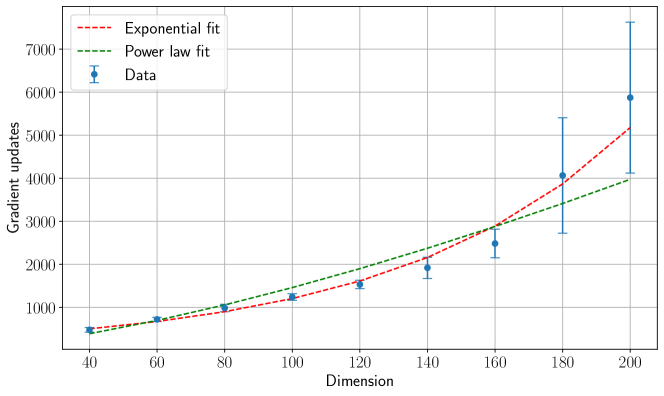
### Visual Description
## Chart: Gradient Updates vs. Dimension
### Overview
The image is a scatter plot showing the relationship between "Gradient updates" and "Dimension". The plot includes data points with error bars, along with an exponential fit and a power law fit to the data. The x-axis represents "Dimension" ranging from 40 to 200, and the y-axis represents "Gradient updates" ranging from 0 to 7000.
### Components/Axes
* **X-axis:** Dimension, ranging from 40 to 200 in increments of 20.
* **Y-axis:** Gradient updates, ranging from 0 to 7000 in increments of 1000.
* **Data Points:** Blue data points with error bars.
* **Exponential Fit:** Red dashed line representing an exponential fit to the data.
* **Power Law Fit:** Green dashed line representing a power law fit to the data.
* **Legend (Top-Left):**
* Red dashed line: Exponential fit
* Green dashed line: Power law fit
* Blue data points: Data
### Detailed Analysis
* **Data Points:**
* Dimension 40: Gradient updates ~450 +/- 100
* Dimension 60: Gradient updates ~700 +/- 100
* Dimension 80: Gradient updates ~1000 +/- 100
* Dimension 100: Gradient updates ~1250 +/- 100
* Dimension 120: Gradient updates ~1550 +/- 100
* Dimension 140: Gradient updates ~1950 +/- 200
* Dimension 160: Gradient updates ~2300 +/- 200
* Dimension 180: Gradient updates ~4100 +/- 1000
* Dimension 200: Gradient updates ~5900 +/- 1200
* **Exponential Fit (Red Dashed Line):** The exponential fit starts around 400 at dimension 40 and increases exponentially, reaching approximately 5200 at dimension 200.
* **Power Law Fit (Green Dashed Line):** The power law fit starts around 400 at dimension 40 and increases, reaching approximately 4100 at dimension 200.
### Key Observations
* Both the exponential and power law fits start at approximately the same point at dimension 40.
* The data points generally increase with dimension, but there is significant variance, especially at higher dimensions, as indicated by the large error bars.
* The exponential fit appears to overestimate the gradient updates at higher dimensions compared to the power law fit.
* The error bars for the data points at dimensions 180 and 200 are significantly larger than the error bars for the other data points.
### Interpretation
The chart illustrates how the number of gradient updates changes with the dimension of the data. The exponential and power law fits provide models for this relationship. The increasing variance in gradient updates at higher dimensions suggests that the relationship becomes less predictable as the dimension increases. The exponential fit grows faster than the power law fit, indicating that an exponential model might be more sensitive to changes in dimension. The large error bars at higher dimensions could be due to various factors, such as increased complexity or instability in the gradient updates. The data suggests that the number of gradient updates required increases with dimension, but the precise nature of this relationship is subject to uncertainty, especially at higher dimensions.
</details>
<details>
<summary>x22.png Details</summary>
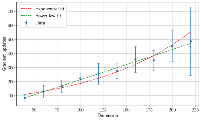
### Visual Description
## Scatter Plot: Gradient Updates vs. Dimension with Exponential and Power Law Fits
### Overview
The image is a scatter plot showing the relationship between "Dimension" (x-axis) and "Gradient updates" (y-axis). The plot includes data points with error bars, along with an exponential fit and a power law fit to the data.
### Components/Axes
* **X-axis:** "Dimension", with scale markers at 50, 75, 100, 125, 150, 175, 200, and 225.
* **Y-axis:** "Gradient updates", with scale markers at 100, 200, 300, 400, 500, 600, and 700.
* **Data Points:** Blue dots with vertical error bars.
* **Exponential Fit:** Red dashed line.
* **Power Law Fit:** Green dashed line.
* **Legend:** Located in the top-left corner, identifying the data, exponential fit, and power law fit.
### Detailed Analysis
**Data Points:** The blue data points generally show an increasing trend of gradient updates as the dimension increases. The error bars indicate the uncertainty associated with each data point.
* Dimension = 40, Gradient updates = 85 +/- 20
* Dimension = 60, Gradient updates = 130 +/- 40
* Dimension = 80, Gradient updates = 160 +/- 40
* Dimension = 100, Gradient updates = 220 +/- 40
* Dimension = 120, Gradient updates = 230 +/- 40
* Dimension = 140, Gradient updates = 290 +/- 40
* Dimension = 170, Gradient updates = 350 +/- 50
* Dimension = 200, Gradient updates = 350 +/- 70
* Dimension = 220, Gradient updates = 490 +/- 220
**Exponential Fit (Red Dashed Line):** The exponential fit starts lower than the power law fit but increases more rapidly as the dimension increases.
* At Dimension = 50, Exponential Fit ≈ 100
* At Dimension = 100, Exponential Fit ≈ 200
* At Dimension = 150, Exponential Fit ≈ 320
* At Dimension = 200, Exponential Fit ≈ 450
* At Dimension = 225, Exponential Fit ≈ 550
**Power Law Fit (Green Dashed Line):** The power law fit shows a more gradual increase compared to the exponential fit.
* At Dimension = 50, Power Law Fit ≈ 100
* At Dimension = 100, Power Law Fit ≈ 200
* At Dimension = 150, Power Law Fit ≈ 300
* At Dimension = 200, Power Law Fit ≈ 400
* At Dimension = 225, Power Law Fit ≈ 450
### Key Observations
* Both the exponential and power law fits capture the general increasing trend of gradient updates with dimension.
* The exponential fit appears to increase more rapidly than the power law fit, especially at higher dimensions.
* The error bars on the data points are relatively large, indicating substantial variability in the gradient updates for a given dimension.
### Interpretation
The plot suggests that the number of gradient updates required increases with the dimension of the problem. Both exponential and power law models can be used to approximate this relationship, but the exponential model shows a more rapid increase at higher dimensions. The large error bars indicate that other factors besides dimension also influence the number of gradient updates. The choice between the exponential and power law fit may depend on the specific context and the range of dimensions being considered.
</details>
Figure 9: Same as in Fig. 8, but in linear scale for better visualisation, for homogeneous readouts (Left) and Gaussian readouts (Right), with threshold $\varepsilon^{*}=0.008$ .
<details>
<summary>x23.png Details</summary>
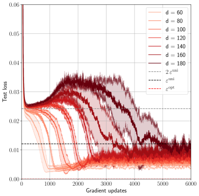
### Visual Description
## Line Chart: Test Loss vs. Gradient Updates
### Overview
The image is a line chart displaying the test loss of a model as a function of gradient updates, with different lines representing different values of 'd' (likely a model parameter). The chart also includes horizontal lines representing theoretical error bounds.
### Components/Axes
* **X-axis:** Gradient updates, ranging from 0 to 6000.
* **Y-axis:** Test loss, ranging from 0.00 to 0.06.
* **Legend (Top-Right):**
* d = 60 (lightest tan color)
* d = 80 (light tan color)
* d = 100 (light brown color)
* d = 120 (brown color)
* d = 140 (dark brown color)
* d = 160 (darker brown color)
* d = 180 (darkest brown color)
* 2 ε<sup>uni</sup> (dashed black line)
* ε<sup>uni</sup> (dashed black line)
* ε<sup>opt</sup> (dashed red line)
### Detailed Analysis
* **General Trend:** All lines start at approximately the same test loss value (around 0.055) and initially decrease rapidly. After the initial drop, the behavior diverges based on the value of 'd'.
* **d = 60 (lightest tan):** The test loss decreases rapidly to approximately 0.005 around 1000 gradient updates, then remains relatively stable with some fluctuations.
* **d = 80 (light tan):** The test loss decreases rapidly to approximately 0.008 around 1200 gradient updates, then remains relatively stable with some fluctuations.
* **d = 100 (light brown):** The test loss decreases rapidly to approximately 0.015 around 1500 gradient updates, then remains relatively stable with some fluctuations.
* **d = 120 (brown):** The test loss decreases rapidly to approximately 0.02 around 1700 gradient updates, then remains relatively stable with some fluctuations.
* **d = 140 (dark brown):** The test loss decreases rapidly to approximately 0.025 around 2000 gradient updates, then increases to approximately 0.032 around 3000 gradient updates, then decreases to approximately 0.02 around 4000 gradient updates, then increases to approximately 0.025 around 5000 gradient updates.
* **d = 160 (darker brown):** The test loss decreases rapidly to approximately 0.025 around 2200 gradient updates, then increases to approximately 0.035 around 3500 gradient updates, then decreases to approximately 0.022 around 4500 gradient updates, then increases to approximately 0.028 around 5500 gradient updates.
* **d = 180 (darkest brown):** The test loss decreases rapidly to approximately 0.025 around 2500 gradient updates, then increases to approximately 0.038 around 3800 gradient updates, then decreases to approximately 0.025 around 5000 gradient updates, then increases to approximately 0.03 around 6000 gradient updates.
* **Horizontal Lines:**
* 2 ε<sup>uni</sup> (dashed black line): Located at approximately 0.024.
* ε<sup>uni</sup> (dashed black line): Located at approximately 0.012.
* ε<sup>opt</sup> (dashed red line): Located at approximately 0.024.
### Key Observations
* As 'd' increases, the initial decrease in test loss becomes less steep, and the final test loss value tends to be higher.
* For larger values of 'd' (140, 160, 180), the test loss exhibits a more pronounced increase after the initial decrease, suggesting potential overfitting or instability.
* The lines for d=60, d=80, d=100, and d=120 appear to converge to a stable, low test loss value.
* The horizontal lines represent error bounds, with the test loss for smaller 'd' values eventually falling below these bounds.
### Interpretation
The chart illustrates the impact of the parameter 'd' on the training process and the final test loss. Smaller values of 'd' lead to faster convergence and lower final test loss, suggesting better generalization performance. Larger values of 'd' may lead to overfitting or instability, as indicated by the increase in test loss after the initial decrease. The error bounds provide a theoretical benchmark for the performance of the model, and the results suggest that smaller 'd' values achieve performance close to or better than these bounds. The optimal value of 'd' would likely be a trade-off between convergence speed and final test loss, potentially lying in the range of 60-120.
</details>
<details>
<summary>x24.png Details</summary>
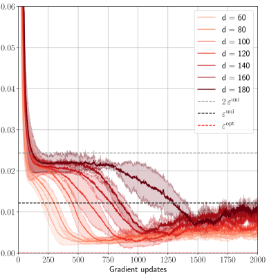
### Visual Description
## Line Chart: Gradient Updates vs. Error for Different Dimensions
### Overview
The image is a line chart showing the relationship between gradient updates (x-axis) and error (y-axis) for different values of 'd', which likely represents the dimensionality of a model or data. The chart also includes horizontal dashed lines representing epsilon values. The lines are colored in shades of red, with darker shades representing higher values of 'd'.
### Components/Axes
* **X-axis:** Gradient updates, ranging from 0 to 2000.
* **Y-axis:** Error, ranging from 0.00 to 0.06.
* **Legend (Top-Right):**
* `d = 60` (lightest red)
* `d = 80` (light red)
* `d = 100` (medium light red)
* `d = 120` (medium red)
* `d = 140` (medium dark red)
* `d = 160` (dark red)
* `d = 180` (darkest red)
* `2εᵘⁿⁱ` (dashed gray line)
* `εᵘⁿⁱ` (dashed black line)
* `εᵒᵖᵗ` (dashed red line)
### Detailed Analysis
* **General Trend:** All lines start with a rapid decrease in error in the first 250 gradient updates, followed by a more gradual decrease and eventual stabilization.
* **Specific Data Series:**
* **d = 60 (lightest red):** Starts at approximately 0.055, rapidly decreases to approximately 0.02 by 250 gradient updates, then gradually decreases to approximately 0.005 by 2000 gradient updates.
* **d = 80 (light red):** Starts at approximately 0.055, rapidly decreases to approximately 0.022 by 250 gradient updates, then gradually decreases to approximately 0.007 by 2000 gradient updates.
* **d = 100 (medium light red):** Starts at approximately 0.055, rapidly decreases to approximately 0.023 by 250 gradient updates, then gradually decreases to approximately 0.008 by 2000 gradient updates.
* **d = 120 (medium red):** Starts at approximately 0.055, rapidly decreases to approximately 0.024 by 250 gradient updates, then gradually decreases to approximately 0.009 by 2000 gradient updates.
* **d = 140 (medium dark red):** Starts at approximately 0.055, rapidly decreases to approximately 0.025 by 250 gradient updates, then gradually decreases to approximately 0.01 by 2000 gradient updates.
* **d = 160 (dark red):** Starts at approximately 0.055, rapidly decreases to approximately 0.026 by 250 gradient updates, then gradually decreases to approximately 0.011 by 2000 gradient updates.
* **d = 180 (darkest red):** Starts at approximately 0.055, decreases to approximately 0.027 by 250 gradient updates, then decreases more slowly, stabilizing around 0.02 between 1000 and 2000 gradient updates.
* **Horizontal Lines:**
* **2εᵘⁿⁱ (dashed gray line):** Located at approximately 0.024.
* **εᵘⁿⁱ (dashed black line):** Located at approximately 0.012.
* **εᵒᵖᵗ (dashed red line):** Located at approximately 0.001.
### Key Observations
* Higher values of 'd' (dimensionality) generally result in slower convergence and higher final error values.
* The error decreases rapidly in the initial gradient updates for all values of 'd'.
* The lines for lower values of 'd' (60, 80, 100, 120, 140) converge to a value close to `εᵒᵖᵗ`.
* The line for d=180 converges to a value close to `2εᵘⁿⁱ`.
### Interpretation
The chart illustrates the impact of dimensionality ('d') on the convergence of a gradient descent algorithm. The data suggests that increasing the dimensionality can hinder convergence, leading to higher final error values. The horizontal lines likely represent theoretical error bounds or target error values. The fact that lower dimensionalities converge close to `εᵒᵖᵗ` suggests that they are more effective in minimizing the error within the given number of gradient updates. The higher dimensionality (d=180) failing to converge to `εᵒᵖᵗ` and instead stabilizing near `2εᵘⁿⁱ` indicates a potential issue with training or optimization in high-dimensional spaces. This could be due to factors like increased complexity, vanishing gradients, or the need for more gradient updates to reach optimal performance.
</details>
<details>
<summary>x25.png Details</summary>
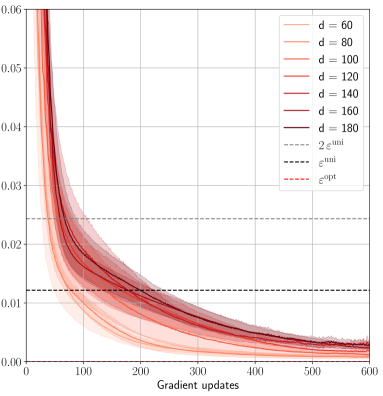
### Visual Description
## Line Chart: Performance vs. Gradient Updates for Different Dimensions
### Overview
The image is a line chart displaying the performance of a model (likely related to machine learning) against the number of gradient updates. The chart shows multiple lines, each representing a different dimensionality ('d') of the model. There are also horizontal dashed lines representing epsilon values. The x-axis represents gradient updates, and the y-axis represents performance (likely loss or error). Shaded regions around each line indicate variability or uncertainty.
### Components/Axes
* **X-axis:** Gradient updates, ranging from 0 to 600.
* **Y-axis:** Performance (unspecified unit), ranging from 0.00 to 0.06.
* Axis markers: 0.00, 0.01, 0.02, 0.03, 0.04, 0.05, 0.06
* **Legend (Top-Right):**
* d = 60 (lightest pink)
* d = 80 (light pink)
* d = 100 (pink)
* d = 120 (red-pink)
* d = 140 (red)
* d = 160 (dark red)
* d = 180 (darkest red)
* 2 ε<sup>uni</sup> (dashed gray)
* ε<sup>uni</sup> (dashed black)
* ε<sup>opt</sup> (dashed red)
### Detailed Analysis
* **Data Series (d = 60, 80, 100, 120, 140, 160, 180):** All data series representing different dimensions (d) show a similar trend: a rapid decrease in performance with initial gradient updates, followed by a gradual flattening out. The shaded regions around each line indicate the variability in performance.
* **d = 60 (lightest pink):** Starts around 0.055, rapidly decreases to approximately 0.01 by 200 gradient updates, then slowly decreases to around 0.004 by 600 gradient updates.
* **d = 80 (light pink):** Starts around 0.055, rapidly decreases to approximately 0.012 by 200 gradient updates, then slowly decreases to around 0.004 by 600 gradient updates.
* **d = 100 (pink):** Starts around 0.055, rapidly decreases to approximately 0.013 by 200 gradient updates, then slowly decreases to around 0.004 by 600 gradient updates.
* **d = 120 (red-pink):** Starts around 0.055, rapidly decreases to approximately 0.014 by 200 gradient updates, then slowly decreases to around 0.004 by 600 gradient updates.
* **d = 140 (red):** Starts around 0.055, rapidly decreases to approximately 0.015 by 200 gradient updates, then slowly decreases to around 0.004 by 600 gradient updates.
* **d = 160 (dark red):** Starts around 0.055, rapidly decreases to approximately 0.016 by 200 gradient updates, then slowly decreases to around 0.004 by 600 gradient updates.
* **d = 180 (darkest red):** Starts around 0.055, rapidly decreases to approximately 0.017 by 200 gradient updates, then slowly decreases to around 0.004 by 600 gradient updates.
* **Horizontal Lines:**
* **2 ε<sup>uni</sup> (dashed gray):** Located at approximately 0.024.
* **ε<sup>uni</sup> (dashed black):** Located at approximately 0.012.
* **ε<sup>opt</sup> (dashed red):** Located at approximately 0.002.
### Key Observations
* All dimensions (d = 60 to 180) exhibit similar performance trends.
* The performance improvement diminishes significantly after approximately 200 gradient updates.
* The performance curves for different dimensions are very close to each other, especially after 200 gradient updates.
* The epsilon values (ε<sup>uni</sup>, 2 ε<sup>uni</sup>, ε<sup>opt</sup>) represent target performance levels.
### Interpretation
The chart suggests that increasing the dimensionality (d) of the model beyond a certain point does not significantly improve performance, especially after a sufficient number of gradient updates. The model converges relatively quickly within the first 200 gradient updates. The epsilon values likely represent different optimization targets or error bounds. The proximity of the performance curves after 200 updates indicates that the choice of dimensionality has a limited impact on the final performance, at least within the range of 'd' values tested. The shaded regions show the variance in the performance, which decreases as the number of gradient updates increases, indicating more stable convergence.
</details>
Figure 10: Trajectories of the generalisation error of neural networks trained with ADAM at fixed batch size $B=\lfloor n/4\rfloor$ , learning rate 0.05, for ReLU activation with parameters $\Delta=10^{-4}$ for the linear readout, $\gamma=0.5$ and $\alpha=5.0>\alpha_{\rm sp}$ ( $=0.22,0.12,0.02$ for homogeneous, Rademacher and Gaussian readouts respectively). The error $\varepsilon^{\rm uni}$ is the mean-square generalisation error associated to the universal solution with overlap $\mathcal{Q}_{W}\equiv 0$ . Left: Homogeneous readouts. Centre: Rademacher readouts. Right: Gaussian readouts. Readouts are kept fixed (and equal to the teacher’s) in all cases during training. Points on the solid lines are obtained by averaging over 5 teacher/data instances, and shaded regions around them correspond to one standard deviation.
We now provide empirical evidence concerning the computational complexity to attain specialisation, namely to have one of the $\mathcal{Q}_{W}(\mathsf{v})>0$ , or equivalently to beat the “universal” performance ( $\mathcal{Q}_{W}(\mathsf{v})=0$ for all $\mathsf{v}∈\mathsf{V}$ ) in terms of generalisation error. We tested two algorithms that can find it in affordable computational time: ADAM with optimised batch size for every dimension tested (the learning rate is automatically tuned), and Hamiltonian Monte Carlo (HMC), both trying to infer a two-layer teacher network with Gaussian inner weights.
ADAM
We focus on ReLU activation, with $\gamma=0.5$ , Gaussian output channel with low label noise ( $\Delta=10^{-4}$ ) and $\alpha=5.0>\alpha_{\rm sp}$ ( $=0.22,0.12,0.02$ for homogeneous, Rademacher and Gaussian readouts respectively, thus we are deep in the specialisation phase in all the cases we report), so that the specialisation solution exhibits a very low generalisation error. We test the learnt model at each gradient update measuring the generalisation error with a moving average of 10 steps to smoothen the curves. Let us define $\varepsilon^{\rm uni}$ as the generalisation error associated to the overlap $\mathcal{Q}_{W}\equiv 0$ , then fixing a threshold $\varepsilon^{\rm opt}<\varepsilon^{*}<\varepsilon^{\rm uni}$ , we define $t^{*}(d)$ the time (in gradient updates) needed for the algorithm to cross the threshold for the first time. We optimise over different batch sizes $B_{p}$ as follows: we define them as $B_{p}=\left\lfloor\frac{n}{2^{p}}\right\rfloor,\quad p=2,3,...,\lfloor\log_{%
2}(n)\rfloor-1$ . Then for each batch size, the student network is trained until the moving average of the test loss drops below $\varepsilon^{*}$ and thus outperforms the universal solution; we have checked that in such a scenario, the student ultimately gets close to the performance of the specialisation solution. The batch size that requires the least gradient updates is selected. We used the ADAM routine implemented in PyTorch.
We test different distributions for the readout weights (kept fixed to ${\mathbf{v}}$ during training of the inner weights). We report all the values of $t^{*}(d)$ in Fig. 8 for various dimensions $d$ at fixed $(\alpha,\gamma)$ , providing an exponential fit $t^{*}(d)=\exp(ad+b)$ (left panel) and a power-law fit $t^{*}(d)=ad^{b}$ (right panel). We report the $\chi^{2}$ test for the fits in Table 2. We observe that for homogeneous and Rademacher readouts, the exponential fit is more compatible with the experiments, while for Gaussian readouts the comparison is inconclusive.
In Fig. 10, we report the test loss of ADAM as a function of the gradient updates used for training, for various dimensions and choice of the readout distribution (as before, the readouts are not learnt but fixed to the teacher’s). Here, we fix a batch size for simplicity. For both the cases of homogeneous ( ${\mathbf{v}}=\bm{1}$ ) and Rademacher readouts (left and centre panels), the model experiences plateaux in performance increasing with the system size, in accordance with the observation of exponential complexity we reported above. The plateaux happen at values of the test loss comparable with twice the value for the Bayes error predicted by the universal branch of our theory (remember the relationship between Gibbs and Bayes errors reported in App. C). The curves are smoother for the case of Gaussian readouts.
Hamiltonian Monte Carlo
<details>
<summary>x26.png Details</summary>
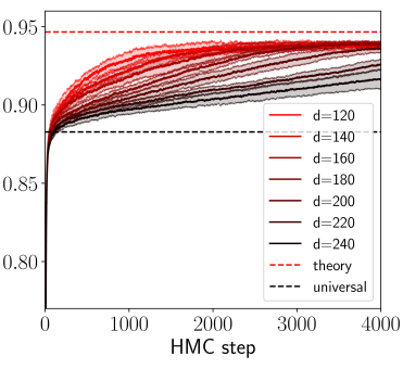
### Visual Description
## Chart: HMC Step vs. Value for Different 'd' Values
### Overview
The image is a line chart showing the relationship between the HMC (Hamiltonian Monte Carlo) step and a value (presumably a performance metric) for different values of 'd'. The chart includes data for d=120, 140, 160, 180, 200, 220, and 240, along with theoretical and universal baselines.
### Components/Axes
* **X-axis:** HMC step, ranging from 0 to 4000.
* **Y-axis:** Value, ranging from 0.80 to 0.95.
* **Legend:** Located in the center-right of the chart, it identifies each line by its 'd' value (120 to 240), as well as "theory" and "universal" baselines.
* d=120: Red
* d=140: Dark Red
* d=160: Brownish-Red
* d=180: Dark Brown
* d=200: Dark Gray
* d=220: Gray
* d=240: Black
* theory: Dashed Red
* universal: Dashed Black
### Detailed Analysis
* **d=120 (Red):** Starts at approximately 0.80 and increases rapidly to about 0.92 by HMC step 500, then gradually increases to approximately 0.94 by HMC step 4000.
* **d=140 (Dark Red):** Similar to d=120, starts at approximately 0.80, increases rapidly to about 0.91 by HMC step 500, then gradually increases to approximately 0.93 by HMC step 4000.
* **d=160 (Brownish-Red):** Starts at approximately 0.80, increases rapidly to about 0.90 by HMC step 500, then gradually increases to approximately 0.92 by HMC step 4000.
* **d=180 (Dark Brown):** Starts at approximately 0.80, increases rapidly to about 0.89 by HMC step 500, then gradually increases to approximately 0.91 by HMC step 4000.
* **d=200 (Dark Gray):** Starts at approximately 0.80, increases rapidly to about 0.88 by HMC step 500, then gradually increases to approximately 0.90 by HMC step 4000.
* **d=220 (Gray):** Starts at approximately 0.80, increases rapidly to about 0.87 by HMC step 500, then gradually increases to approximately 0.89 by HMC step 4000.
* **d=240 (Black):** Starts at approximately 0.80, increases rapidly to about 0.86 by HMC step 500, then gradually increases to approximately 0.88 by HMC step 4000.
* **Theory (Dashed Red):** A horizontal dashed red line at approximately 0.95.
* **Universal (Dashed Black):** A horizontal dashed black line at approximately 0.88.
### Key Observations
* All 'd' values start at approximately the same value (0.80) and increase rapidly in the initial HMC steps.
* As 'd' increases, the final value reached by HMC step 4000 decreases.
* The "theory" baseline is higher than all 'd' values, while the "universal" baseline is lower than all 'd' values.
* The rate of increase slows down significantly after approximately 500 HMC steps for all 'd' values.
### Interpretation
The chart suggests that the value being measured is influenced by the 'd' parameter. Lower values of 'd' result in higher final values after a certain number of HMC steps. The theoretical baseline represents an upper limit, while the universal baseline represents a lower limit. The HMC process appears to converge relatively quickly in the initial steps, with diminishing returns as the number of steps increases. The 'd' parameter seems to control the upper bound of the value achieved by the HMC process.
</details>
<details>
<summary>x27.png Details</summary>
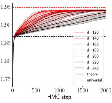
### Visual Description
## Line Chart: HMC Step vs. Value for Different 'd' Values
### Overview
The image is a line chart showing the relationship between the HMC (Hamiltonian Monte Carlo) step and a value (presumably a metric of performance or convergence) for different values of 'd'. The chart includes a legend indicating the 'd' values, ranging from 120 to 240, as well as theoretical and universal baselines. The lines generally increase with the HMC step, eventually plateauing.
### Components/Axes
* **X-axis:** "HMC step", ranging from 0 to 2000.
* **Y-axis:** Value, ranging from 0.75 to 0.95.
* **Legend:** Located on the right side of the chart.
* `d=120` (Red)
* `d=140` (Dark Red)
* `d=160` (Dark Red)
* `d=180` (Dark Red)
* `d=200` (Dark Brown)
* `d=220` (Dark Gray)
* `d=240` (Black)
* `theory` (Dashed Red Line)
* `universal` (Dashed Black Line)
### Detailed Analysis
* **d=120 (Red):** Starts at approximately 0.73 and increases rapidly, reaching approximately 0.94 around HMC step 500, then plateaus.
* **d=140 (Dark Red):** Starts at approximately 0.73 and increases rapidly, reaching approximately 0.94 around HMC step 500, then plateaus.
* **d=160 (Dark Red):** Starts at approximately 0.73 and increases rapidly, reaching approximately 0.93 around HMC step 500, then plateaus.
* **d=180 (Dark Red):** Starts at approximately 0.73 and increases rapidly, reaching approximately 0.93 around HMC step 500, then plateaus.
* **d=200 (Dark Brown):** Starts at approximately 0.73 and increases rapidly, reaching approximately 0.92 around HMC step 500, then plateaus.
* **d=220 (Dark Gray):** Starts at approximately 0.73 and increases rapidly, reaching approximately 0.91 around HMC step 500, then plateaus.
* **d=240 (Black):** Starts at approximately 0.73 and increases rapidly, reaching approximately 0.90 around HMC step 500, then plateaus.
* **theory (Dashed Red Line):** Horizontal line at approximately 0.95.
* **universal (Dashed Black Line):** Horizontal line at approximately 0.87.
### Key Observations
* All 'd' values start at approximately the same point (0.73) and increase rapidly initially.
* The lines for lower 'd' values (120-180) plateau at higher values than the lines for higher 'd' values (200-240).
* The "theory" line represents an upper bound, while the "universal" line represents a lower bound.
* The shaded regions around each line likely represent the standard deviation or confidence interval.
### Interpretation
The chart demonstrates the convergence behavior of an HMC algorithm for different values of 'd'. The 'd' parameter seems to influence the final plateau value, with lower 'd' values achieving higher values. The "theory" and "universal" lines provide theoretical upper and lower bounds for the algorithm's performance. The convergence rate is similar for all 'd' values, as indicated by the initial rapid increase in the value. The shaded regions indicate the variability in the results. The data suggests that the choice of 'd' can impact the performance of the HMC algorithm, and there may be an optimal range for 'd' that balances convergence speed and final value.
</details>
<details>
<summary>x28.png Details</summary>
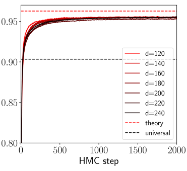
### Visual Description
## Chart: HMC Step vs. Value for Different 'd' Values
### Overview
The image is a line chart showing the relationship between the HMC (Hamiltonian Monte Carlo) step and a value that appears to converge over time. Multiple lines represent different values of 'd', and there are two horizontal dashed lines representing "theory" and "universal" values.
### Components/Axes
* **X-axis:** "HMC step", ranging from 0 to 2000.
* **Y-axis:** Value, ranging from 0.80 to 0.95.
* **Legend (Top-Right):**
* `d=120` (Dark Red)
* `d=140` (Red)
* `d=160` (Dark Red)
* `d=180` (Dark Red)
* `d=200` (Dark Brown)
* `d=220` (Dark Brown)
* `d=240` (Black)
* `theory` (Dashed Red)
* `universal` (Dashed Black)
### Detailed Analysis
* **Trend Overview:** All lines representing different 'd' values start at approximately 0.80 and increase rapidly before leveling off.
* **d=120 (Dark Red):** Starts at approximately 0.80, rises sharply, and converges to approximately 0.95.
* **d=140 (Red):** Starts at approximately 0.80, rises sharply, and converges to approximately 0.95.
* **d=160 (Dark Red):** Starts at approximately 0.80, rises sharply, and converges to approximately 0.95.
* **d=180 (Dark Red):** Starts at approximately 0.80, rises sharply, and converges to approximately 0.95.
* **d=200 (Dark Brown):** Starts at approximately 0.80, rises sharply, and converges to approximately 0.95.
* **d=220 (Dark Brown):** Starts at approximately 0.80, rises sharply, and converges to approximately 0.95.
* **d=240 (Black):** Starts at approximately 0.80, rises sharply, and converges to approximately 0.95.
* **theory (Dashed Red):** A horizontal line at approximately 0.97.
* **universal (Dashed Black):** A horizontal line at approximately 0.905.
### Key Observations
* All 'd' values converge to a similar value around 0.95.
* The "theory" line is above all the 'd' value lines.
* The "universal" line is below the converged 'd' value lines.
* The convergence rate appears similar for all 'd' values.
### Interpretation
The chart demonstrates how the value being measured changes with the number of HMC steps for different values of 'd'. The convergence of all 'd' values suggests that the system reaches a stable state regardless of the initial 'd' value. The "theory" line likely represents a theoretical upper bound, while the "universal" line might represent a lower bound or a target value. The fact that the 'd' values converge between these two bounds suggests that the HMC process is effective in reaching a stable and predictable state. The specific meaning of 'd' and the value on the y-axis would require additional context.
</details>
Figure 11: Trajectories of the overlap $q_{2}$ in HMC runs initialised uninformatively for the polynomial activation $\sigma_{3}={\rm He}_{2}/\sqrt{2}+{\rm He}_{3}/6$ with parameters $\Delta=0.1$ for the linear readout, $\gamma=0.5$ and $\alpha=1.0$ . Left: Homogeneous readouts. Centre: Rademacher readouts. Right: Gaussian readouts. Points on the solid lines are obtained by averaging over 10 teacher/data instances, and shaded regions around them correspond to one standard deviation. Notice that the $y$ -axes are limited for better visualisation. For the left and centre plot, any threshold (horizontal line in the plot) between the prediction of the $\mathcal{Q}_{W}\equiv 0$ branch of our theory (black dashed line) and its prediction for the Bayes-optimal $q_{2}$ (red dashed line) crosses the curves in points $t^{*}(d)$ more compatible with an exponential fit (see Fig. 12 and Table 3, where these fits are reported and $\chi^{2}$ -tested). For the cases of homogeneous and Rademacher readouts, the value of the overlap at which the dynamics slows down (predicted by the $\mathcal{Q}_{W}\equiv 0$ branch) is in quantitative agreement with the theoretical predictions (lower dashed line). The theory is instead off by $≈ 1\%$ for the values $q_{2}$ at which the runs ultimately converge.
The experiment is performed for the polynomial activation $\sigma_{3}={\rm He}_{2}/\sqrt{2}+{\rm He}_{3}/6$ with parameters $\Delta=0.1$ for the Gaussian noise in the linear readout, $\gamma=0.5$ and $\alpha=1.0>\alpha_{\rm sp}$ ( $=0.26,0.30,0.02$ for homogeneous, Rademacher and Gaussian readouts respectively). Our HMC consists of $4000$ iterations for homogeneous readouts, or $2000$ iterations for Rademacher and Gaussian readouts. Each iteration is adaptive (with initial step size of $0.01$ ) and uses $10$ leapfrog steps. Instead of measuring the Gibbs error, whose relationship with $\varepsilon^{\rm opt}$ holds only at equilibrium (see the last remark in App. C), we measured the teacher-student $q_{2}$ -overlap which is meaningful at any HMC step and is informative about the learning. For a fixed threshold $q_{2}^{*}$ and dimension $d$ , we measure $t^{*}(d)$ as the number of HMC iterations needed for the $q_{2}$ -overlap between the HMC sample (obtained from uninformative initialisation) and the teacher weights ${\mathbf{W}}^{0}$ to cross the threshold. This criterion is again enough to assess that the student outperforms the universal solution.
As before, we test homogeneous, Rademacher and Gaussian readouts, getting to the same conclusions: while for homogeneous and Rademacher readouts exponential time is more compatible with the observations, the experiments remain inconclusive for Gaussian readouts (see Fig. 12). We report in Fig. 11 the values of the overlap $q_{2}$ measured along the HMC runs for different dimensions. Note that, with HMC steps, all $q_{2}$ curves saturate to a value that is off by $≈ 1\%$ w.r.t. that predicted by our theory for the selected values of $\alpha,\gamma$ and $\Delta$ . Whether this is a finite size effect, or an effect not taken into account by the current theory is an interesting question requiring further investigation, see App. E.2 for possible directions.
<details>
<summary>x29.png Details</summary>
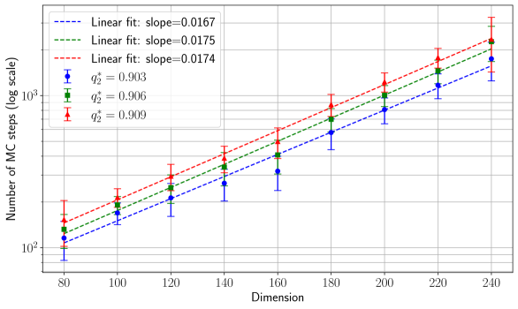
### Visual Description
## Scatter Plot: Number of MC steps vs. Dimension
### Overview
The image is a scatter plot showing the relationship between the number of Monte Carlo (MC) steps (on a logarithmic scale) and the dimension, for three different values of a parameter denoted as q₂*. Each data series is accompanied by a linear fit line. Error bars are present on each data point.
### Components/Axes
* **X-axis:** Dimension, ranging from 80 to 240 in increments of 20.
* **Y-axis:** Number of MC steps (log scale), ranging from 10² to 10³.
* **Legend (Top-Left):**
* Blue dashed line: Linear fit, slope = 0.0167
* Green dashed line: Linear fit, slope = 0.0175
* Red dashed line: Linear fit, slope = 0.0174
* Blue circles with error bars: q₂* = 0.903
* Green squares with error bars: q₂* = 0.906
* Red triangles with error bars: q₂* = 0.909
### Detailed Analysis
* **Data Series 1: q₂* = 0.903 (Blue Circles)**
* Trend: The number of MC steps increases as the dimension increases.
* Approximate Data Points:
* Dimension 80: MC steps ≈ 110
* Dimension 120: MC steps ≈ 200
* Dimension 160: MC steps ≈ 350
* Dimension 200: MC steps ≈ 700
* Dimension 240: MC steps ≈ 1500
* **Data Series 2: q₂* = 0.906 (Green Squares)**
* Trend: The number of MC steps increases as the dimension increases.
* Approximate Data Points:
* Dimension 80: MC steps ≈ 130
* Dimension 120: MC steps ≈ 250
* Dimension 160: MC steps ≈ 450
* Dimension 200: MC steps ≈ 800
* Dimension 240: MC steps ≈ 1700
* **Data Series 3: q₂* = 0.909 (Red Triangles)**
* Trend: The number of MC steps increases as the dimension increases.
* Approximate Data Points:
* Dimension 80: MC steps ≈ 140
* Dimension 120: MC steps ≈ 280
* Dimension 160: MC steps ≈ 500
* Dimension 200: MC steps ≈ 900
* Dimension 240: MC steps ≈ 1900
* **Linear Fits:** All three linear fits have positive slopes, indicating a positive correlation between dimension and the number of MC steps. The slopes are very similar, with the green line (q₂* = 0.906) having the steepest slope (0.0175), followed by the red line (q₂* = 0.909) with a slope of 0.0174, and then the blue line (q₂* = 0.903) with a slope of 0.0167.
### Key Observations
* The number of MC steps generally increases with dimension for all values of q₂*.
* Higher values of q₂* tend to result in a higher number of MC steps for a given dimension.
* The error bars suggest some variability in the number of MC steps for each dimension and q₂* value.
* The linear fits provide a good approximation of the trend in the data.
### Interpretation
The plot suggests that as the dimension increases, the number of Monte Carlo steps required for the simulation also increases. This is likely due to the increased complexity of the system with higher dimensions. The parameter q₂* appears to influence the number of MC steps, with higher values leading to a greater number of steps. The similarity in the slopes of the linear fits suggests that the rate of increase in MC steps with dimension is relatively consistent across the different q₂* values, but the offset is different. The error bars indicate that there is some inherent variability in the simulation process.
</details>
<details>
<summary>x30.png Details</summary>
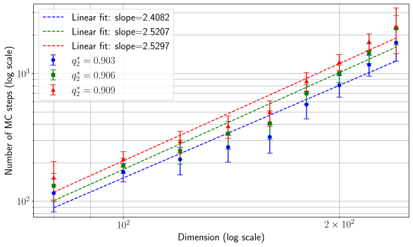
### Visual Description
## Log-Log Plot: Number of MC Steps vs. Dimension
### Overview
The image is a log-log plot showing the relationship between the number of Monte Carlo (MC) steps and the dimension, for three different values of a parameter denoted as q*_2. The plot includes error bars for the data points and linear fits for each q*_2 value.
### Components/Axes
* **X-axis:** Dimension (log scale). The axis ranges from approximately 50 to 250, with major ticks at 10^2 and 2 x 10^2.
* **Y-axis:** Number of MC steps (log scale). The axis ranges from approximately 100 to 2000, with major ticks at 10^2 and 10^3.
* **Legend (top-left):**
* Blue dashed line: Linear fit: slope=2.4082
* Green dashed line: Linear fit: slope=2.5207
* Red dashed line: Linear fit: slope=2.5297
* Blue circle: q*_2 = 0.903
* Green square: q*_2 = 0.906
* Red triangle: q*_2 = 0.909
### Detailed Analysis
* **Data Points and Error Bars:** The plot shows data points for three different values of q*_2 (0.903, 0.906, and 0.909), each with associated error bars. The error bars represent the uncertainty in the number of MC steps.
* **Linear Fits:** Each set of data points is fitted with a linear function, represented by dashed lines. The slopes of these lines are provided in the legend.
* **q*_2 = 0.903 (Blue Circles):**
* Trend: The number of MC steps increases with dimension.
* Approximate data points: (50, 120), (75, 150), (100, 220), (150, 350), (200, 550), (250, 800)
* **q*_2 = 0.906 (Green Squares):**
* Trend: The number of MC steps increases with dimension.
* Approximate data points: (50, 140), (75, 200), (100, 300), (150, 500), (200, 800), (250, 1200)
* **q*_2 = 0.909 (Red Triangles):**
* Trend: The number of MC steps increases with dimension.
* Approximate data points: (50, 160), (75, 250), (100, 400), (150, 650), (200, 1000), (250, 1500)
### Key Observations
* All three data series show a positive correlation between dimension and the number of MC steps.
* The slopes of the linear fits are similar for the green and red data series (approximately 2.52), while the blue data series has a slightly lower slope (2.4082).
* As q*_2 increases, the number of MC steps also tends to increase for a given dimension.
* The error bars appear to increase with the number of MC steps.
### Interpretation
The plot suggests that the number of Monte Carlo steps required for a simulation increases with the dimension of the system. The parameter q*_2 appears to influence the magnitude of this increase, with higher values of q*_2 leading to a greater number of MC steps. The linear fits on the log-log scale indicate a power-law relationship between the number of MC steps and the dimension. The slopes of the linear fits represent the exponents of these power laws. The increasing error bars with the number of MC steps might indicate that the uncertainty in the simulation results grows as the simulation becomes more complex (i.e., requires more steps).
</details>
<details>
<summary>x31.png Details</summary>
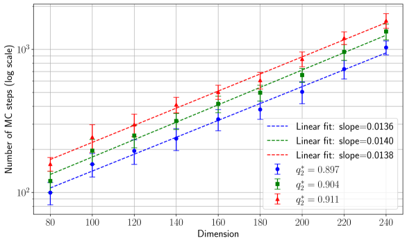
### Visual Description
## Scatter Plot: Number of MC steps vs. Dimension
### Overview
The image is a scatter plot showing the relationship between the number of Monte Carlo (MC) steps (on a log scale) and the dimension, for three different values of a parameter denoted as q₂*. Each data series is also accompanied by a linear fit line. The plot shows an upward trend, indicating that the number of MC steps increases with dimension.
### Components/Axes
* **X-axis:** Dimension, ranging from 80 to 240 in increments of 20.
* **Y-axis:** Number of MC steps (log scale), ranging from 10² (100) to 10³ (1000). The y-axis is logarithmic.
* **Data Series:** Three data series, each representing a different value of q₂*:
* Blue circles: q₂* = 0.897
* Green squares: q₂* = 0.904
* Red triangles: q₂* = 0.911
* **Error Bars:** Each data point has associated error bars, indicating the uncertainty in the number of MC steps.
* **Linear Fits:** Each data series has a corresponding dashed line representing a linear fit.
* Blue dashed line: Linear fit, slope = 0.0136
* Green dashed line: Linear fit, slope = 0.0140
* Red dashed line: Linear fit, slope = 0.0138
* **Legend:** Located on the right side of the plot, associating the colors and markers with the corresponding q₂* values and linear fit slopes.
### Detailed Analysis
**Data Points and Trends:**
* **q₂* = 0.897 (Blue Circles):** The number of MC steps increases as the dimension increases.
* Dimension 80: Approximately 100 MC steps
* Dimension 120: Approximately 170 MC steps
* Dimension 160: Approximately 280 MC steps
* Dimension 200: Approximately 470 MC steps
* Dimension 240: Approximately 850 MC steps
* **q₂* = 0.904 (Green Squares):** The number of MC steps increases as the dimension increases.
* Dimension 80: Approximately 120 MC steps
* Dimension 120: Approximately 210 MC steps
* Dimension 160: Approximately 350 MC steps
* Dimension 200: Approximately 580 MC steps
* Dimension 240: Approximately 1050 MC steps
* **q₂* = 0.911 (Red Triangles):** The number of MC steps increases as the dimension increases.
* Dimension 80: Approximately 140 MC steps
* Dimension 120: Approximately 250 MC steps
* Dimension 160: Approximately 420 MC steps
* Dimension 200: Approximately 700 MC steps
* Dimension 240: Approximately 1250 MC steps
**Linear Fits:**
* The linear fits all have positive slopes, confirming the upward trend.
* The slopes are relatively similar, ranging from 0.0136 to 0.0140.
### Key Observations
* The number of MC steps generally increases with dimension for all values of q₂*.
* Higher values of q₂* tend to result in a higher number of MC steps for a given dimension.
* The error bars suggest some variability in the number of MC steps.
* The linear fits provide a reasonable approximation of the relationship between dimension and the number of MC steps.
### Interpretation
The plot suggests that as the dimension of the system increases, the number of Monte Carlo steps required to achieve convergence or explore the configuration space also increases. This is a common phenomenon in high-dimensional systems, where the complexity of the problem grows exponentially with the number of dimensions. The parameter q₂* appears to influence the number of MC steps needed, with higher values requiring more steps. The linear fits provide a simplified model of this relationship, but the error bars indicate that there is some inherent variability in the data. The slopes of the linear fits are very similar, suggesting that the rate of increase in MC steps with dimension is relatively consistent across the different q₂* values.
</details>
<details>
<summary>x32.png Details</summary>
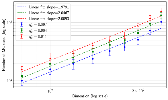
### Visual Description
## Log-Log Plot: Number of MC Steps vs. Dimension
### Overview
The image is a log-log plot showing the relationship between the number of Monte Carlo (MC) steps and the dimension, for three different values of a parameter denoted as q₂*. The plot includes linear fits for each data series, along with their corresponding slopes. Error bars are present on each data point.
### Components/Axes
* **X-axis:** Dimension (log scale). Axis markers are at 10², and 2 x 10².
* **Y-axis:** Number of MC steps (log scale). Axis markers are at 10² and 10³.
* **Legend (top-left):**
* Blue dashed line: Linear fit: slope = 1.9791
* Green dashed line: Linear fit: slope = 2.0467
* Red dashed line: Linear fit: slope = 2.0093
* Blue square: q₂* = 0.897
* Green square: q₂* = 0.904
* Red triangle: q₂* = 0.911
### Detailed Analysis
* **Data Points:** The data points are plotted with error bars. The x-axis values appear to be approximately 50, 100, 150, and 200.
* **Blue Data Series (q₂* = 0.897):**
* Trend: The blue data series shows an upward trend.
* Data Points: Approximate y-values for x = 50, 100, 150, and 200 are 100, 200, 500, and 1000.
* Linear Fit: The blue dashed line represents the linear fit with a slope of 1.9791.
* **Green Data Series (q₂* = 0.904):**
* Trend: The green data series shows an upward trend.
* Data Points: Approximate y-values for x = 50, 100, 150, and 200 are 120, 300, 600, and 1200.
* Linear Fit: The green dashed line represents the linear fit with a slope of 2.0467.
* **Red Data Series (q₂* = 0.911):**
* Trend: The red data series shows an upward trend.
* Data Points: Approximate y-values for x = 50, 100, 150, and 200 are 150, 350, 700, and 1400.
* Linear Fit: The red dashed line represents the linear fit with a slope of 2.0093.
### Key Observations
* All three data series exhibit a positive correlation between the dimension and the number of MC steps.
* The slopes of the linear fits are all close to 2, suggesting a power-law relationship.
* The data series for q₂* = 0.911 consistently shows a higher number of MC steps compared to the other two series for a given dimension.
* The data series for q₂* = 0.897 consistently shows a lower number of MC steps compared to the other two series for a given dimension.
* The error bars appear to be relatively consistent across all data points.
### Interpretation
The plot demonstrates that the number of Monte Carlo steps required increases with the dimension, following a power-law relationship. The parameter q₂* influences the magnitude of the number of MC steps, with higher values of q₂* resulting in a greater number of steps for a given dimension. The slopes of the linear fits being close to 2 suggests that the number of MC steps scales approximately with the square of the dimension. This information is useful for understanding the computational cost associated with Monte Carlo simulations in different dimensions and for optimizing the choice of parameters like q₂*.
</details>
<details>
<summary>x33.png Details</summary>
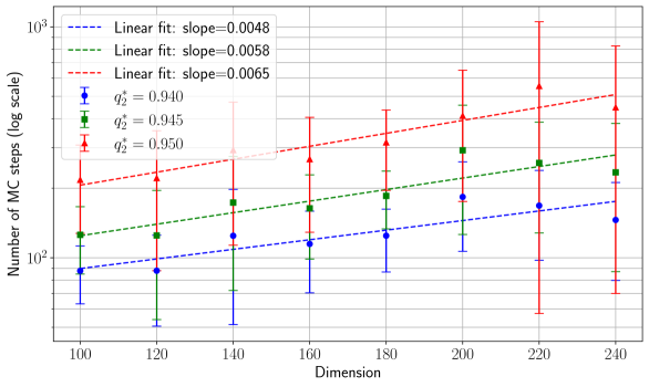
### Visual Description
## Chart: Number of MC steps vs. Dimension for different q2* values
### Overview
The image is a scatter plot showing the relationship between the number of Monte Carlo (MC) steps (on a log scale) and the dimension, for three different values of a parameter denoted as q2*. Error bars are displayed for each data point. Linear fits are also plotted for each q2* value, with their slopes indicated in the legend.
### Components/Axes
* **X-axis:** Dimension, with tick marks at 100, 120, 140, 160, 180, 200, 220, and 240.
* **Y-axis:** Number of MC steps (log scale), ranging from approximately 50 to 1000, with tick marks at 10^2 (100) and 10^3 (1000).
* **Legend (Top-Left):**
* Blue dashed line: Linear fit: slope=0.0048
* Green dashed line: Linear fit: slope=0.0058
* Red dashed line: Linear fit: slope=0.0065
* Blue circle: q2* = 0.940
* Green square: q2* = 0.945
* Red triangle: q2* = 0.950
### Detailed Analysis
* **q2* = 0.940 (Blue circles):**
* Trend: The number of MC steps increases with dimension.
* Data points (approximate):
* Dimension 100: ~70 MC steps
* Dimension 120: ~90 MC steps
* Dimension 140: ~110 MC steps
* Dimension 160: ~120 MC steps
* Dimension 180: ~130 MC steps
* Dimension 200: ~140 MC steps
* Dimension 220: ~150 MC steps
* Dimension 240: ~160 MC steps
* **q2* = 0.945 (Green squares):**
* Trend: The number of MC steps increases with dimension.
* Data points (approximate):
* Dimension 100: ~110 MC steps
* Dimension 120: ~130 MC steps
* Dimension 140: ~150 MC steps
* Dimension 160: ~170 MC steps
* Dimension 180: ~180 MC steps
* Dimension 200: ~200 MC steps
* Dimension 220: ~220 MC steps
* Dimension 240: ~240 MC steps
* **q2* = 0.950 (Red triangles):**
* Trend: The number of MC steps increases with dimension.
* Data points (approximate):
* Dimension 100: ~140 MC steps
* Dimension 120: ~160 MC steps
* Dimension 140: ~190 MC steps
* Dimension 160: ~220 MC steps
* Dimension 180: ~240 MC steps
* Dimension 200: ~270 MC steps
* Dimension 220: ~300 MC steps
* Dimension 240: ~330 MC steps
### Key Observations
* The number of MC steps generally increases with dimension for all values of q2*.
* Higher values of q2* correspond to a higher number of MC steps for a given dimension.
* The error bars appear to increase in size with increasing dimension.
* The linear fits have positive slopes, indicating a positive correlation between dimension and the number of MC steps.
* The slope of the linear fit increases with increasing q2*.
### Interpretation
The plot suggests that as the dimension increases, the number of Monte Carlo steps required for the simulation to converge also increases. Furthermore, the parameter q2* seems to influence the number of MC steps needed, with higher values of q2* leading to a greater number of steps. The increasing error bars with dimension might indicate that the uncertainty in the number of MC steps also grows as the dimension increases, potentially due to the increased complexity of the system being simulated. The linear fits provide a simplified model of the relationship between dimension and MC steps, and the slopes quantify the rate at which the number of MC steps increases with dimension for each q2* value.
</details>
<details>
<summary>x34.png Details</summary>
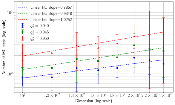
### Visual Description
## Chart: Number of MC steps vs. Dimension
### Overview
The image is a scatter plot with error bars, showing the relationship between the number of Monte Carlo (MC) steps (log scale) and dimension (log scale) for three different values of a parameter denoted as q₂*. Each data series is also accompanied by a linear fit line.
### Components/Axes
* **X-axis:** Dimension (log scale). The x-axis ranges from approximately 10² to 2.4 x 10². Markers are present at 10², 1.2 x 10², 1.4 x 10², 1.6 x 10², 1.8 x 10², 2 x 10², 2.2 x 10², and 2.4 x 10².
* **Y-axis:** Number of MC steps (log scale). The y-axis ranges from approximately 10² to 10³.
* **Legend (top-left):**
* Blue dashed line: Linear fit; slope = 0.7867
* Green dashed line: Linear fit; slope = 0.9348
* Red dashed line: Linear fit; slope = 1.0252
* Blue circles with error bars: q₂* = 0.940
* Green squares with error bars: q₂* = 0.945
* Red triangles with error bars: q₂* = 0.950
### Detailed Analysis
* **Data Series 1 (q₂* = 0.940, blue circles):**
* Trend: The number of MC steps increases as the dimension increases.
* Data points (approximate):
* (10², ~85)
* (1.2 x 10², ~90)
* (1.4 x 10², ~100)
* (1.6 x 10², ~110)
* (1.8 x 10², ~115)
* (2 x 10², ~120)
* (2.2 x 10², ~130)
* (2.4 x 10², ~140)
* **Data Series 2 (q₂* = 0.945, green squares):**
* Trend: The number of MC steps increases as the dimension increases.
* Data points (approximate):
* (10², ~105)
* (1.2 x 10², ~115)
* (1.4 x 10², ~130)
* (1.6 x 10², ~140)
* (1.8 x 10², ~150)
* (2 x 10², ~160)
* (2.2 x 10², ~170)
* (2.4 x 10², ~180)
* **Data Series 3 (q₂* = 0.950, red triangles):**
* Trend: The number of MC steps increases as the dimension increases.
* Data points (approximate):
* (10², ~115)
* (1.2 x 10², ~135)
* (1.4 x 10², ~150)
* (1.6 x 10², ~170)
* (1.8 x 10², ~180)
* (2 x 10², ~200)
* (2.2 x 10², ~220)
* (2.4 x 10², ~240)
* **Linear Fits:** The linear fits for each data series are shown as dashed lines. The slopes are provided in the legend. The red line has the steepest slope, followed by the green, and then the blue line.
### Key Observations
* For all three values of q₂*, the number of MC steps increases with dimension.
* The rate of increase (slope of the linear fit) is highest for q₂* = 0.950 and lowest for q₂* = 0.940.
* The error bars appear to increase in magnitude as the dimension increases.
### Interpretation
The plot suggests that as the dimension increases, the number of Monte Carlo steps required to achieve a certain level of accuracy or convergence also increases. Furthermore, the parameter q₂* influences the rate at which the number of MC steps increases with dimension. Higher values of q₂* lead to a more rapid increase in the number of MC steps. The increasing error bars with dimension suggest that the variance in the number of MC steps also increases with dimension, potentially indicating greater uncertainty or variability in the results.
</details>
Figure 12: Semilog (Left) and log-log (Right) plots of the number of Hamiltonian Monte Carlo steps needed to achieve an overlap $q_{2}^{*}>q_{2}^{\rm uni}$ , that certifies the universal solution is outperformed. The dataset was generated from a teacher with polynomial activation $\sigma_{3}={\rm He}_{2}/\sqrt{2}+{\rm He}_{3}/6$ and parameters $\Delta=0.1$ for the linear readout, $\gamma=0.5$ and $\alpha=1.0>\alpha_{\rm sp}$ ( $=0.26,0.30,0.02$ for homogeneous, Rademacher and Gaussian readouts respectively). Student weights are sampled using HMC (initialised uninformatively) with $4000$ iterations for homogeneous readouts (Top row, for which $q_{2}^{\rm uni}=0.883$ ), or $2000$ iterations for Rademacher (Centre row, with $q_{2}^{\rm uni}=0.868$ ) and Gaussian readouts (Bottom row, for which $q_{2}^{\rm uni}=0.903$ ). Each iteration is adaptative (with initial step size of $0.01$ ) and uses $10$ leapfrog steps. $q_{2}^{\rm sp}=0.941,0.948,0.963$ in the three cases. The readouts are kept fixed during training. Points are obtained averaging over 10 teacher/data instances with error bars representing the standard deviation.
| Homogeneous Rademacher Gaussian | ( $q_{2}^{*}∈\{0.903,0.906,0.909\}$ ) ( $q_{2}^{*}∈\{0.897,0.904,0.911\}$ ) ( $q_{2}^{*}∈\{0.940,0.945,0.950\}$ ) | $\bm{2.22}$ $\bm{1.88}$ $0.66$ | $\bm{1.47}$ $\bm{2.12}$ $\bm{0.44}$ | $\bm{1.14}$ $\bm{1.70}$ $\bm{0.26}$ | $8.01$ $8.10$ $\bm{0.62}$ | $7.25$ $7.70$ $0.53$ | $6.35$ $8.57$ $0.39$ |
| --- | --- | --- | --- | --- | --- | --- | --- |
Table 3: $\chi^{2}$ test for exponential and power-law fits for the time needed by Hamiltonian Monte Carlo to reach the thresholds $q_{2}^{*}$ , for various priors on the readouts. For a given row, we report three values of the $\chi^{2}$ test per hypothesis, corresponding with the thresholds $q_{2}^{*}$ on the left, in the order given. Fits are displayed in Figure 12. Smaller values of $\chi^{2}$ (in bold, for given threshold and readouts) indicate a better compatibility with the hypothesis.