2506.03227v2

# Bridging Neural ODE and ResNet: A Formal Error Bound for Safety Verification **Authors**: Abdelrahman Sayed Sayed, Pierre-Jean Meyer, Mohamed Ghazel institutetext: Univ Gustave Eiffel, COSYS-ESTAS, F-59657 Villeneuve d’Ascq, France email: {abdelrahman.ibrahim,pierre-jean.meyer,mohamed.ghazel}@univ-eiffel.fr Abstract A neural ordinary differential equation (neural ODE) is a machine learning model that is commonly described as a continuous-depth generalization of a residual network (ResNet) with a single residual block, or conversely, the ResNet can be seen as the Euler discretization of the neural ODE. These two models are therefore strongly related in a way that the behaviors of either model are considered to be an approximation of the behaviors of the other. In this work, we establish a more formal relationship between these two models by bounding the approximation error between two such related models. The obtained error bound then allows us to use one of the models as a verification proxy for the other, without running the verification tools twice: if the reachable output set expanded by the error bound satisfies a safety property on one of the models, this safety property is then guaranteed to be also satisfied on the other model. This feature is fully reversible, and the initial safety verification can be run indifferently on either of the two models. This novel approach is illustrated on a numerical example of a fixed-point attractor system modeled as a neural ODE. 1 Introduction Neural ordinary differential equations (neural ODE) are gaining prominence in continuous-time modeling, offering distinct advantages over traditional neural networks, such as memory efficiency, continuous-time modeling, adaptive computation balancing speed and accuracy [5, 14, 23]. This surge in interest stems from recent advancements in differential programming, which have enhanced the ability to model complex dynamics with greater flexibility and precision [24]. Neural ODE can be viewed as a continuous-depth generalization of residual networks (ResNet) [10], and conversely a ResNet represents an Euler discretization of the continuous transformations modeled by a neural ODE [9, 18]. Unlike ResNet, neural ODE enable smooth and robust representations through continuous dynamics, leading to improved modeling of time-evolving systems [5, 9]. By interpreting ResNet as discretized neural ODE, we can leverage advanced ODE solvers to enhance computational efficiency and reduce the number of required parameters [5]. Furthermore, the continuous formulation of neural ODE supports flexible handling of varying input resolutions and scales, making them adaptable to diverse data modalities. This perspective also facilitates theoretical analysis using tools from differential equations, providing insights into network stability and convergence [14]. Despite the growing interest in neural ODE for continuous-time modeling, formal analysis techniques for these models remain underdeveloped [17]. Current verification methods for neural ODE are still maturing, with existing reachability approaches primarily focusing on stochastic methods [7, 8]. Other works include the NNVODE tool [17] which is an extension of the Neural Network Verification (NNV) framework [28, 16] that investigates reachability for a general class of neural ODE. Additionally, another line of verification based on topological properties was introduced in [15] through a set-boundary method for safety verification of neural ODE and invertible residual networks (i-ResNet) [3]. The similarity between the neural ODE and ResNet models enables bidirectional safety verification, where the properties verified for one model can be used to deduce safety guarantees for the other one. This motivates our work, which investigates how verification results from one model can serve as a proxy for the other, addressing practical scenarios where only one model or compatible verification tools are available. The main contributions of this work are as follows: - We derive a rigorous bound on the approximation error between the neural ODE and ResNet models for a given input set. 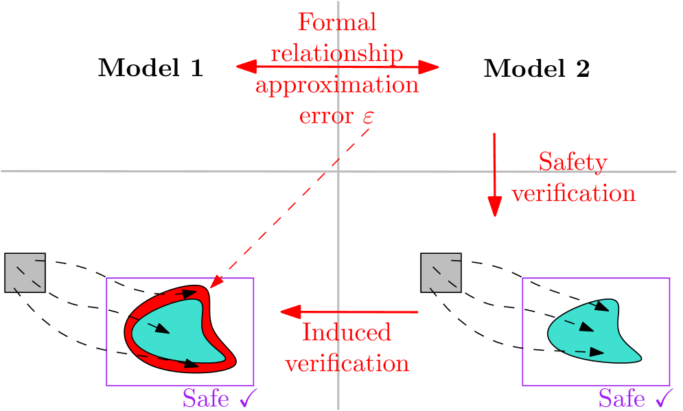- We use the derived error bound in conjunction with the reachable set of one model as a proxy to verify safety properties of the other model, without applying any verification tools to the other model as illustrated in Figure 1. <details> <summary>x1.png Details</summary>  ### Visual Description ## Diagram: Model Verification Process ### Overview The image illustrates a model verification process involving two models, Model 1 and Model 2, and their formal relationship. It shows how safety verification is performed on Model 2 and how this verification is induced back to Model 1. The diagram includes visual representations of state spaces and their relationships. ### Components/Axes * **Models:** Model 1 (left) and Model 2 (right) * **Formal Relationship:** A bidirectional arrow labeled "Formal relationship approximation error ε" indicates the relationship between the two models. * **Safety Verification:** A downward arrow labeled "Safety verification" points from Model 2 to its state space. * **Induced Verification:** An arrow labeled "Induced verification" points from Model 2's state space back to Model 1's state space. * **State Spaces:** Each model has an associated state space represented by a purple square. Inside each square is a cyan-filled shape representing the safe region. Model 1's safe region has a red boundary. * **Initial States:** Each model has an initial state represented by a gray square with a diagonal line. Dashed lines connect the initial states to the state spaces. * **Safety Labels:** Each state space is labeled "Safe" with a checkmark. ### Detailed Analysis * **Model 1 (Left):** * Initial state: A gray square located above and to the left of the state space. * State space: A purple square containing a cyan-filled shape with a red boundary. Arrows within the cyan shape indicate state transitions. * Label: "Safe" with a checkmark below the purple square. * **Model 2 (Right):** * Initial state: A gray square located above and to the left of the state space. * State space: A purple square containing a cyan-filled shape. Arrows within the cyan shape indicate state transitions. * Label: "Safe" with a checkmark below the purple square. * **Arrows:** * "Formal relationship approximation error ε": A red, bidirectional arrow connecting Model 1 and Model 2. * "Safety verification": A red, downward arrow pointing from Model 2 to its state space. * "Induced verification": A red arrow pointing from Model 2's state space to Model 1's state space. * **Dashed Line:** A red dashed line connects the "Formal relationship approximation error ε" arrow to the "Induced verification" arrow. ### Key Observations * The diagram emphasizes the relationship between two models and how safety verification performed on one model can be used to infer safety in the other. * The red boundary around the safe region in Model 1's state space suggests a potential difference or additional constraint compared to Model 2. * The dashed line connecting the formal relationship to the induced verification suggests that the formal relationship is used to induce the verification. ### Interpretation The diagram illustrates a process where safety verification is performed on a simplified or abstracted model (Model 2) and then "induced" back to a more complex model (Model 1). The "Formal relationship approximation error ε" represents the mathematical relationship and the error introduced by the abstraction. The "Induced verification" step leverages this relationship to infer safety properties in Model 1 based on the verification results from Model 2. The red boundary around the safe region in Model 1 might indicate that Model 1 has additional safety constraints or a more complex safety definition than Model 2. The diagram suggests a method for verifying complex systems by verifying simpler abstractions and then transferring the results. </details> Figure 1: Illustration of the proposed framework to verify Model $1$ based on the outcome of the verification of Model $2$ and a bound $\varepsilon$ on the maximal error between the models. Related work. Although the similarity between the ResNet and neural ODE models is well established [5, 14], to the best of our knowledge, very few works have tried connecting these models through some more formal relationships. These include various theoretical perspectives, such as quantifying the deviation between the hidden state trajectory of a ResNet and its corresponding neural ODE, focusing on approximation error [26], while [20] derives generalization bounds for neural ODE and ResNet using a Lipschitz-based argument, emphasizing the impact of successive weight matrix differences on generalization capability. On the other hand, [21] investigates implicit regularization effects in deep ResNet and its impact on training outcomes. While these studies focus on theoretical analyses of approximation error, generalization, and regularization to understand model behavior and performance, our work leverages this relationship for formal safety verification. We propose a verification proxy approach that uses the reachable set of one model to verify the safety properties of the other, incorporating an error bound to ensure conservative over-approximations, which enables practical verification of nonlinear systems. Abstraction-based verification (i.e., verifying properties of one model by working on an abstraction of its behaviors into a simpler model) has been a popular topic in the past decades outside of the AI field [27]. Within the field of AI verification, its primary application has been on abstracting specific model components rather than the whole model itself, as in approaches based on convex relaxation of nonlinear ReLU activation functions [13, 11]. On the other hand, full-model abstraction has been mostly unexplored for AI verification, except on the topic of neural network model reduction, where the verification of a neural network is achieved at a lower computational cost on a reduced network with less neurons, see e.g. [4] for unidirectional relationships, or [29] for bidirectional ones through the use of approximate bisimulation relations. Although the overall principle of the proposed approach in our paper is similar (abstracting a model by one that over-approximates the set of all its behaviors), the main difference with the above works between two discrete neural networks is that our paper considers the formal relationships between a continuous neural ODE model and a discrete ResNet one. Organization of the paper. The remainder of the paper is structured as follows. First, we formulate the safety verification problem of interest and provide some preliminaries in Section 2. In Section 3, we describe our proposed approach to bound the approximation error between the ResNet and neural ODE models, and use this error bound to verify the safety of one model based on the reachability analysis of the other. Following this, we provide numerical illustrations of our error bounding and verification proxy results (in both directions: from ResNet to neural ODE, and from neural ODE to ResNet) on an academic example in Section 4. Finally, we summarize the main findings of the paper and discuss potential future work in Section 5. 2 Preliminaries 2.1 Neural ODE and ResNet models We consider the following neural ODE: $$ \dot{x}(t)=\frac{dx(t)}{dt}=f(x(t)), \tag{1} $$ with state $x∈\mathbb{R}^{n}$ , initial state $x(0)=u$ , and vector field $f:\mathbb{R}^{n}→\mathbb{R}^{n}$ defined as a finite sequence of classical neural network layers (such as fully connected layers, convolutional layers, activation functions, batch normalization). The state trajectories of (1) are defined based on the solution $\Phi:\mathbb{R}×\mathbb{R}^{n}→\mathbb{R}^{n}$ of the corresponding initial value problem: $$ x(t)=\Phi(t,x(0))=\Phi(t,u). \tag{0} $$ In [5], such a neural ODE is described as a continuous-depth generalization of a residual neural network constituted of a single residual block. Conversely, this ResNet can be seen as the Euler discretization of the neural ODE (1): $$ y=u+f(u), \tag{2} $$ where $u∈\mathbb{R}^{n}$ is the input, $y∈\mathbb{R}^{n}$ is the output, and the residual function $f:\mathbb{R}^{n}→\mathbb{R}^{n}$ is identical to the vector field of the neural ODE (1). Since the approach proposed in this paper relies on the Taylor expansion of the trajectories of (1) up to the second order, we assume here for simplicity that the neural network described by the vector field $f$ is continuously differentiable. **Remark 1** *The case where $f$ contains piecewise-affine activation functions such as ReLU can theoretically be handled as well, since our approach only really requires their derivatives to be bounded (but not necessarily continuous). But for the sake of clarity of presentation (to avoid the case decompositions of each ReLU activation), this case is kept out of the scope of the present paper.* 2.2 Problem definition As mentioned above and in [5], both the neural ODE and ResNet models describe a very similar behavior, and either model could be seen as an approximation of the other. Our goal in this paper is to provide a formal comparison of these models in the context of safety verification, by evaluating the approximation error between them. For such comparison to be meaningful, we consider the outputs $y$ of the ResNet (2) on one side, and the outputs $\Phi(1,u)$ of the neural ODE (1) at continuous depth $t=1$ on the other side, since other values $t≠ 1$ of this continuous depth have no elements of comparison in the discrete architecture of the ResNet. Given an initial set $\mathcal{X}_{in}⊂eq\mathbb{R}^{n}$ for the neural ODE (or equivalently referred to as input set for the ResNet), we first define the sets of reachable outputs for either model: $$ \mathcal{R}_{\text{neural ODE}}(\mathcal{X}_{in})=\{y\in\mathbb{R}^{n}\mid y=\Phi(1,u),\ u\in\mathcal{X}_{in}\}, $$ $$ \mathcal{R}_{\text{ResNet}}(\mathcal{X}_{in})=\{y\in\mathbb{R}^{n}\mid y=u+f(u),\ u\in\mathcal{X}_{in}\}. $$ Since we usually cannot compute these output reachable sets exactly, we will often rely on computing an over-approximation denoted as $\Omega(\mathcal{X}_{in})$ such that $\mathcal{R}(\mathcal{X}_{in})⊂eq\Omega(\mathcal{X}_{in})$ . Our first objective is to bound the approximation error between the two models, as formalized below. **Problem 1 (Error Bounding)** *Given an input set $\mathcal{X}_{in}⊂eq\mathbb{R}^{n}$ , we want to over-approximate the set $\mathcal{R}_{\varepsilon}(\mathcal{X}_{in})$ of errors between the ResNet (2) and neural ODE (1) models, defined as: $$ \mathcal{R}_{\varepsilon}(\mathcal{X}_{in})=\left\{\Phi(1,u)-(u+f(u))~|~u\in\mathcal{X}_{in}\right\}. $$* Our second problem of interest is to use one of our models as a verification proxy for the other. In other words, we want to combine this error bound with the reachable set of one model to verify the satisfaction of a safety property on the other model, without having to compute the reachable output set of this second model. **Problem 2 (Verification Proxy)** *Given an input-output safety property defined by an input set $\mathcal{X}_{in}⊂eq\mathbb{R}^{n}$ and a safe output set $\mathcal{X}_{s}⊂eq\mathbb{R}^{n}$ , the verification problem consists in checking whether the reachable output set of a model is fully contained in the targeted safe set: $\mathcal{R}(\mathcal{X}_{in})⊂eq\mathcal{X}_{s}$ . In this paper, we want to verify this safety property on one model by relying only on the error set $\mathcal{R}_{\varepsilon}(\mathcal{X}_{in})$ from Problem 1 and the reachability analysis of the other model.* 3 Proposed approach As mentioned in Section 2.2, the ResNet model in (2) can be seen as the Euler discretization of the neural ODE (1) evaluated at continuous depth $t=1$ : $$ x(1)=\Phi(1,u)\approx u+f(u)=y. \tag{1} $$ Our initial goal, related to Problem 1, is to evaluate this approximation error for a given set of inputs $u∈\mathcal{X}_{in}$ . This is done below through the use of a Taylor expansion and its Lagrange-remainder form, combined later with some tools dedicated for reachability analysis. 3.1 Lagrange remainder The Taylor expansion of the state trajectory $x(t)$ of the neural ODE (1) at $t=0$ is given by the infinite sum: $$ x(t)=x(0)+t\frac{dx(0)}{dt}+\frac{t^{2}}{2!}\frac{d^{2}x(0)}{dt^{2}}+\frac{t^{3}}{3!}\frac{d^{3}x(0)}{dt^{3}}+\dots \tag{0} $$ The Lagrange remainder theorem offers the possibility to truncate (4) without approximation error, hence preserving the above equality. We only state below the result in the case of a truncation at the Taylor order $2$ corresponding to the case of interest in our work. **Proposition 1 (Lagrange remainder[25])** *There exists $t^{*}∈[0,t]$ such that $$ x(t)=x(0)+t\frac{dx(0)}{dt}+\frac{t^{2}}{2!}\frac{d^{2}x(t^{*})}{dt^{2}} \tag{0} $$* Notice that in (5), the second order derivative $\frac{d^{2}x}{dt^{2}}$ is evaluated at $t^{*}∈[0,t]$ instead of $t$ as in the Taylor series (4). Although the truncation in Proposition 1 provides a much more manageable expression than the infinite sum in (4), the main difficulty is that this result only states the existence of a $t^{*}∈[0,t]$ satisfying the equality in (5), but its actual value is unknown. 3.2 Error function To compare the continuous state $x(t)$ with the discrete output of the ResNet, the state of the neural ODE (1) should be evaluated at depth $t=1$ . The first term of the right-hand side in (5) is the known initial condition of the neural ODE (1): $x(0)=u$ . The second term is provided by the definition of the vector field of the neural ODE (1), and thus reduces to: $$ t\frac{dx(0)}{dt}=1\cdot f(x(0))=f(u). \tag{0} $$ The second derivative appearing in the third term of (5) can be computed using the chain rule as follows: | | $\displaystyle\frac{d^{2}x(t)}{dt^{2}}$ | $\displaystyle=\frac{df(x(t))}{dt}$ | | | --- | --- | --- | --- | In our context of Section 2, the function $f$ is assumed not to be explicitly dependent on the depth $t$ due to its definition as a single residual block with classical layers. Therefore, the partial derivative $\frac{∂ f(x(t))}{∂ t}$ is equal to $0$ , and the third term of (5) thus reduces to: $$ \frac{t^{2}}{2!}\frac{d^{2}x(t^{*})}{dt^{2}}=\frac{1}{2}f^{\prime}(x(t^{*}))f(x(t^{*})). $$ We can thus re-write (5) as an equation defining the output of the neural ODE based on the output of the ResNet (for the same initial state/input $u$ ) and an error term: $$ \Phi(1,u)=(u+f(u))+\varepsilon(u), \tag{6} $$ where the approximation error between our models for this particular input $u$ is expressed by the Lagrange remainder of Taylor order 2: $$ \varepsilon(u)=\frac{1}{2}f^{\prime}(x(t^{*}))f(x(t^{*})), \tag{7} $$ with $x(t^{*})=\Phi(t^{*},u)$ for a fixed but unknown $t^{*}∈[0,1]$ . Equation (6) can also be modified to rather express the outputs of the ResNet based on those of the neural ODE: $$ u+f(u)=\Phi(1,u)-\varepsilon(u). \tag{8} $$ The error function $\varepsilon:\mathbb{R}^{n}→\mathbb{R}^{n}$ appearing positively in (6) and negatively in (8) is defined in (7) only for a specific input $u$ . However, in the context of our Problem 1, we are interested in analyzing the approximation error between both models over an input set $\mathcal{X}_{in}⊂eq\mathbb{R}^{n}$ . In addition, since the specific value of $t^{*}$ is unknown, we need to bound (7) for any possible value of $t^{*}∈[0,1]$ . Therefore in the next sections, we focus on converting the equalities (6)-(8) to set inclusions over all $u∈\mathcal{X}_{in}$ and $t^{*}∈[0,1]$ . 3.3 Bounding the error set The reachable error set $\mathcal{R}_{\varepsilon}(\mathcal{X}_{in})$ introduced in Problem 1, can be redefined based on the error function (7) as follows: $$ \displaystyle\mathcal{R}_{\varepsilon}(\mathcal{X}_{in}) \displaystyle=\left\{\Phi(1,u)-(u+f(u))~|~u\in\mathcal{X}_{in}\right\} \displaystyle=\left\{\left.\frac{1}{2}f^{\prime}(\Phi(t^{*},u))f(\Phi(t^{*},u))~\right|~t^{*}\in[0,1],~u\in\mathcal{X}_{in}\right\}. \tag{9} $$ To solve Problem 1, our objective is thus to compute an over-approximation $\Omega_{\varepsilon}(\mathcal{X}_{in})$ bounding the error set: $\mathcal{R}_{\varepsilon}(\mathcal{X}_{in})⊂eq\Omega_{\varepsilon}(\mathcal{X}_{in})$ . The first step (corresponding to line 1 in Algorithm 1) is to compute the reachable tube of all possible states that can be reached by the neural ODE (1) over the whole range $t∈[0,1]$ and for any initial state $x(0)=u∈\mathcal{X}_{in}$ . This reachable tube can be defined similarly to $\mathcal{R}_{\text{neural ODE}}(\mathcal{X}_{in})$ in Section 2.2 but for all possible depth $t∈[0,1]$ instead of only the final one: $$ \mathcal{R}^{\text{tube}}_{\text{neural ODE}}(\mathcal{X}_{in})=\{\Phi(t,u)\in\mathbb{R}^{n}\mid t\in[0,1],~u\in\mathcal{X}_{in}\}. $$ Since in most cases this set cannot be computed exactly, we instead use off-the-shelf reachability analysis toolboxes to compute an over-approximating set $\Omega^{\text{tube}}_{\text{neural ODE}}(\mathcal{X}_{in})$ such that $\mathcal{R}^{\text{tube}}_{\text{neural ODE}}(\mathcal{X}_{in})⊂eq\Omega^{\text{tube}}_{\text{neural ODE}}(\mathcal{X}_{in})$ . The error set can then be re-written based on the above reachable tube definition, by replacing $\Phi(t^{*},u)$ (with $t^{*}∈[0,1]$ and $u∈\mathcal{X}_{in}$ ) in (9) by $x∈\mathcal{R}^{\text{tube}}_{\text{neural ODE}}(\mathcal{X}_{in})$ . $$ \displaystyle\mathcal{R}_{\varepsilon}(\mathcal{X}_{in}) \displaystyle=\left\{\left.\frac{1}{2}f^{\prime}(x)f(x)~\right|~x\in\mathcal{R}^{\text{tube}}_{\text{neural ODE}}(\mathcal{X}_{in})\right\} \displaystyle\subseteq\left\{\left.\frac{1}{2}f^{\prime}(x)f(x)~\right|~x\in\Omega^{\text{tube}}_{\text{neural ODE}}(\mathcal{X}_{in})\right\}. \tag{10} $$ The next step, in line 2 of Algorithm 1, is to over-approximate this error set $\mathcal{R}_{\varepsilon}(\mathcal{X}_{in})$ . One possible approach to achieve this is to define the static function $\varepsilon=\frac{1}{2}f^{\prime}(x)f(x)$ and apply to it some set-propagation techniques (such as interval arithmetic [12], Taylor models [19], or affine arithmetic [6]) to bound the set of output errors $\varepsilon$ corresponding to any state $x∈\Omega^{\text{tube}}_{\text{neural ODE}}(\mathcal{X}_{in})$ in the reachable tube over-approximation. An alternative approach, which provided a tighter error bounding set in the particular case of the numerical example presented in Section 4, is to define the discrete-time nonlinear system $x^{+}=\frac{1}{2}f^{\prime}(x)f(x)$ , and then use existing reachability analysis toolboxes to over-approximate the reachable set of this system after one time step, which corresponds to bounding the image of the error function. Note that in this case, it is important that this final reachable set is computed as a single step, and not decomposed into a sequence of smaller intermediate steps whose iterative updates of the internal state would have no mathematical meaning for the static (stateless) error function. As a consequence of the equalities and set inclusions in (9)-(10) and the fact that the reachability methods to be used in the first two steps of Algorithm 1 described above guarantee that the obtained sets are over-approximations of the output or reachable sets of interest, we have thus reached a solution to Problem 1. **Theorem 3.1** *The set $\Omega_{\varepsilon}(\mathcal{X}_{in})$ obtained after applying this second step described above solves Problem 1: $$ \mathcal{R}_{\varepsilon}(\mathcal{X}_{in})=\left\{\Phi(1,u)-(u+f(u))~|~u\in\mathcal{X}_{in}\right\}\subseteq\Omega_{\varepsilon}(\mathcal{X}_{in}). $$* Note that the error bound in Theorem 3.1 is defined as a set in the state space of the neural ODE. This differs from the approach in [26], where the error bound is defined as a positive scalar. A second and more important difference with this work is the tightness of the obtained error bounds. Indeed, if we adapt the results from [26] to the context of our framework described in Section 2, their error bound is expressed as: $$ \varepsilon\leq\frac{e^{L}-1}{L}\left\|\frac{1}{2}f^{\prime}(x)f(x)\right\|_{\infty},~\forall x\in\mathcal{R}^{\text{tube}}_{\text{neural ODE}}(\mathcal{X}_{in}), $$ where $L$ is a Lipschitz constant of the neural ODE vector field. The term $\left\|\frac{1}{2}f^{\prime}(x)f(x)\right\|_{∞}$ can be obtained by first over-approximating the error set by $\Omega_{\varepsilon}(\mathcal{X}_{in})$ in the same way we did, but the infinity norm forces to expand this set to make it symmetrical around $0$ , and then keeping only the maximum value among its components (thus corresponding to a second expansion of this set into an hypercube whose width along all dimensions is the largest width of the previous set). In addition, for any system with non-zero Lipschitz constant, the factor $\frac{e^{L}-1}{L}$ is always greater than $1$ , which increases this error bound even more. In summary, this scalar error bound is doubly more conservative than our proposed set-based error bound. The comparison of both approaches is illustrated in the numerical example of Section 4. 3.4 Verification proxy To address Problem 2, we leverage the similar behavior between the neural ODE and ResNet models to verify safety properties on one model using the reachable set of the other, combined with the error bound from Theorem 3.1. Specifically, we want to verify whether the reachable output set of a model is contained in the safe set $\mathcal{X}_{s}$ , i.e., $\mathcal{R}(\mathcal{X}_{in})⊂eq\mathcal{X}_{s}$ . We first focus on the case of Algorithm 1 to verify the safety property on the neural ODE, based on the reachability analysis of the ResNet. This first verification proxy relies on the set-based version of (6) using the Minkowski sum: $$ \mathcal{R}_{\text{neural ODE}}(\mathcal{X}_{in})\subseteq\Omega_{\text{ResNet}}(\mathcal{X}_{in})+\Omega_{\varepsilon}(\mathcal{X}_{in}), \tag{11} $$ stating that the reachable output set of the neural ODE is contained in the output set over-approximation of the ResNet $\Omega_{\text{ResNet}}(\mathcal{X}_{in})$ , expanded by the bounding set of the error $\Omega_{\varepsilon}(\mathcal{X}_{in})$ obtained after applying the first two lines of Algorithm 1 as described in Section 3.3. Therefore, this verification procedure is achieved as in Algorithm 1, by first using existing set-propagation or reachability analysis tools to compute an over-approximation ${\color[rgb]{0,0,1}\Omega_{\text{ResNet}}(\mathcal{X}_{in})}$ of the ResNet output set (line 3). Then in line 4, an over-approximation of the neural ODE output set can be deduced from (11) by taking the Minkowski sum of ${\color[rgb]{0,0,1}\Omega_{\text{ResNet}}(\mathcal{X}_{in})}$ and our error bound ${\color[rgb]{1,0,0}\Omega_{\varepsilon}(\mathcal{X}_{in})}$ . If $\Omega_{\text{neural ODE}}(\mathcal{X}_{in})$ is contained in the safe set ${\color[rgb]{0,0,0}\mathcal{X}_{s}}$ , then the neural ODE satisfies the safety property, otherwise the result is inconclusive (line 5-9). Algorithm 1 Safety Verification Framework for neural ODE based on ResNet Input: a neural ODE, an input set $\mathcal{X}_{in}$ and a safe set $\mathcal{X}_{s}$ . Output: Safe or Unknown. 1: compute an over-approximation of the reachable tube of the neural ODE $\Omega^{\text{tube}}_{\text{neural ODE}}(\mathcal{X}_{in})$ ; 2: compute the over-approximation of the error set ${\color[rgb]{1,0,0}\Omega_{\varepsilon}(\mathcal{X}_{in})}$ , $∀ x∈\Omega^{\text{tube}}_{\text{neural ODE}}(\mathcal{X}_{in})$ ; 3: compute the over-approximation of the ResNet output ${\color[rgb]{0,0,1}\Omega_{\text{ResNet}}(\mathcal{X}_{in})}$ ; 4: deduce an over-approximation of the neural ODE output $\Omega_{\text{neural ODE}}(\mathcal{X}_{in})={\color[rgb]{1,0,0}\Omega_{\text{ResNet}}(\mathcal{X}_{in})+\Omega_{\varepsilon}(\mathcal{X}_{in})}$ ; 5: if $\Omega_{\text{neural ODE}}(\mathcal{X}_{in})⊂eq{\color[rgb]{0,0,0}\mathcal{X}_{s}}$ then 6: return Safe 7: else 8: return Unknown 9: end if Reversing the roles, the case of verifying the ResNet based on the reachability analysis of the neural ODE is described in Algorithm 2. This case is very similar to the previous one, so we focus here on the main differences with Algorithm 1. The first difference is that in (8), the term representing the approximation error between the models appears with a negative sign. Therefore, when converting this equation into a set inclusion similarly to (11), we need to be careful to add the negation of the error set (and not to do a set difference, which is not the correct set operation in our case). We thus introduce the negative error set $$ \Omega_{-\varepsilon}(\mathcal{X}_{in})=\{-\varepsilon\mid\varepsilon\in\Omega_{\varepsilon}(\mathcal{X}_{in})\}, $$ in order to convert (8) into its set-based notation as follows: $$ \mathcal{R}_{\text{ResNet}}(\mathcal{X}_{in})\subseteq\Omega_{\text{neural ODE}}(\mathcal{X}_{in})+\Omega_{-\varepsilon}(\mathcal{X}_{in}). \tag{12} $$ The second difference is that in line 3 of Algorithm 2, we compute an over-approximation of the reachable set of the neural ODE, using any classical tools for reachability analysis of continuous-time nonlinear systems, and add it to the negative error set to obtain an over-approximation of the ResNet output set. This final set can then similarly be used to verify the satisfaction of the safety property on the ResNet model. Algorithm 2 Safety Verification Framework for ResNet based on neural ODE Input: a ResNet, an input set $\mathcal{X}_{in}$ and a safe set $\mathcal{X}_{s}$ . Output: Safe or Unknown. 1: compute an over-approximation of the reachable tube of the neural ODE $\Omega^{\text{tube}}_{\text{neural ODE}}(\mathcal{X}_{in})$ ; 2: compute the over-approximation of the negative error set ${\color[rgb]{1,0,0}\Omega_{-\varepsilon}(\mathcal{X}_{in})}$ , $∀ x∈\Omega^{\text{tube}}_{\text{neural ODE}}(\mathcal{X}_{in})$ ; 3: compute the over-approximation of the neural ODE output $\Omega_{\text{neural ODE}}(\mathcal{X}_{in})$ ; 4: deduce an over-approximation of the ResNet output ${\color[rgb]{0,0,1}\Omega_{\text{ResNet}}(\mathcal{X}_{in})}={\color[rgb]{1,0,0}\Omega_{\text{neural ODE}}(\mathcal{X}_{in})+\Omega_{-\varepsilon}(\mathcal{X}_{in})}$ ; 5: if ${\color[rgb]{0,0,1}\Omega_{\text{ResNet}}(\mathcal{X}_{in})}⊂eq{\color[rgb]{0,0,0}\mathcal{X}_{s}}$ then 6: return Safe 7: else 8: return Unknown 9: end if **Theorem 3.2 (Soundness)** *For the case that either Algorithm 1 or 2 returns Safe, the safety property in the sense of Problem 2 holds true [15].* The soundness of the verification framework is guaranteed because both algorithms rely on over-approximations of the true reachable sets. Specifically, (11) ensures that $\mathcal{R}_{\text{neural ODE}}(\mathcal{X}_{in})⊂eq\Omega_{\text{neural ODE}}(\mathcal{X}_{in})$ , and (12) ensures ${\color[rgb]{0,0,1}\mathcal{R}_{\text{ResNet}}(\mathcal{X}_{in})}⊂eq{\color[rgb]{0,0,1}\Omega_{\text{ResNet}}(\mathcal{X}_{in})}$ . These inclusions hold due to the conservative nature of the considered reachability analysis and error bound computations in Section 3.3 (Theorem 3.1). 4 Numerical illustration In this section, a commonly used neural ODE academic example [16, 17] is used to demonstrate the verification proxy between the two models, which is the Fixed-Point Attractor (FPA) [22] that consists of one nonlinear neural ODE. Experiment Setting: All the experiments Code available in the following repository: https://github.com/ab-sayed/Formal-Error-Bound-for-Safety-Verification-of-neural-ODE herein are run on MATLAB 2024b with Continuous Reachability Analyzer (CORA) version 2024.4.0 with an Intel (R) Core (TM) i5-1145G7 CPU@2.60 GHz and 32 GB of RAM. 4.1 System description The FPA system is a nonlinear dynamical system with dynamics that converge to a fixed point (an equilibrium state) under certain conditions [2], and the fixed-point aspect makes it a useful model for studying convergence and stability, which are important in safety-critical applications where the system must not diverge or enter unsafe states. As in the proposed benchmark in [22], we consider here the following $5$ -dimensional neural ODE approximating the FPA dynamics: $$ \dot{x}=f(x)=\tau x+W\text{tanh}(x), $$ where $x∈\mathbb{R}^{5}$ is the state vector, $\tau=-10^{-6}$ is a time constant for the neurons, $W∈\mathbb{R}^{5× 5}$ is a composite weight matrix defined as $W=\begin{pmatrix}0_{2× 2}&A\\ 0_{3× 2}&BA\end{pmatrix}$ with $A=\begin{pmatrix}-1.20327&-0.07202&-0.93635\\ 1.18810&-1.50015&0.93519\end{pmatrix}$ and $B=\begin{pmatrix}1.21464&-0.10502\\ 0.12023&0.19387\\ -1.36695&0.12201\end{pmatrix}$ , and $\text{tanh}(x)$ is the hyperbolic tangent activation function applied element-wise to the state vector $x$ . We choose our safety property defined by the input set $\mathcal{X}_{in}≈[0.45,0.55]×[0.72,0.88]×[0.47,0.58]×[0.19,0.24]×[-0.64,-0.53]$ (its exact numerical values are provided in the code linked below) and the safe set $\mathcal{X}_{s}=[0.2,0.6]×[0.3,0.85]⊂\mathbb{R}^{2}$ , that only focuses on the projection of the state onto its first two dimensions, i.e., using an output function $h(x)=(x_{1},x_{2})$ . In the case of the neural ODE, we thus want to verify that for all initial state $x(0)∈\mathcal{X}_{in}$ , we have $h(x(1))∈\mathcal{X}_{s}$ . 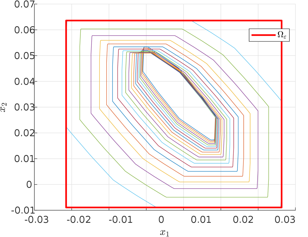4.2 Computing the error bound Using CORA [1], we compute the error bound $\Omega_{\varepsilon}(\mathcal{X}_{in})$ from Theorem 3.1 as follows. First, we over-approximate the reachable tube of the neural ODE $\mathcal{R}^{\text{tube}}_{\text{neural ODE}}$ over the time interval $[0,1]$ as a sequence of zonotopes, where each zonotope corresponds to an intermediate time range. For each zonotope in the reachable tube, we bound the image of the error function (7) by applying a discrete-time reachability analysis method at $t=1$ . This results in a new zonotope that over-approximates the error set starting from that particular reachable tube zonotope. The total error set is thus guaranteed to be contained in the union of these error zonotopes across all time steps. To simplify its use in the safety verification experiments in Section 4.3, we compute the interval hull of this union, yielding a hyperrectangle that over-approximates ${\color[rgb]{1,0,0}\Omega_{\varepsilon}(\mathcal{X}_{in})}$ illustrated in Figure 2 in red, and showing 20 error zonotopes in different colors, corresponding to the error bound of each intermediate time range used in the reachable tube. <details> <summary>x2.png Details</summary>  ### Visual Description ## Contour Plot: State Space Convergence ### Overview The image is a contour plot showing the convergence of a system's state space over time. It displays a series of nested polygons, each representing the state space at a different time step. The outermost red rectangle, labeled "Ωε", defines the boundaries of the plot. The nested polygons converge towards the center, indicating the system's state is stabilizing. ### Components/Axes * **X-axis (x1):** Ranges from -0.03 to 0.03, with tick marks at -0.03, -0.02, -0.01, 0, 0.01, 0.02, and 0.03. * **Y-axis (x2):** Ranges from -0.01 to 0.07, with tick marks at -0.01, 0, 0.01, 0.02, 0.03, 0.04, 0.05, 0.06, and 0.07. * **Legend:** Located in the top-right corner, it identifies the red rectangle as "Ωε". * **Contours:** A series of nested polygons, each represented by a different color. These polygons represent the state space at different time steps. ### Detailed Analysis * **Outer Boundary (Ωε):** A red rectangle with corners at approximately (-0.025, -0.01), (0.03, -0.01), (0.03, 0.065), and (-0.025, 0.065). * **Convergence:** The nested polygons converge towards the center of the plot. The polygons are colored with a variety of colors, including light blue, green, yellow, orange, red, purple, and dark blue. * **Shape Change:** The shape of the polygons changes as they converge, becoming more compact and regular. The innermost polygon is roughly hexagonal. ### Key Observations * The system's state space shrinks over time, indicating stability. * The rate of convergence appears to decrease as the polygons get closer to the center. * The final state space is contained within a small region around the origin. ### Interpretation The contour plot illustrates the convergence of a dynamic system's state space. The nested polygons represent the reachable states of the system at different points in time. The fact that these polygons shrink and converge towards the center indicates that the system is stable and its state is approaching a steady-state value. The shape of the polygons provides information about the system's dynamics and how it evolves over time. The outer boundary, Ωε, likely represents a constraint or limit on the system's state space. 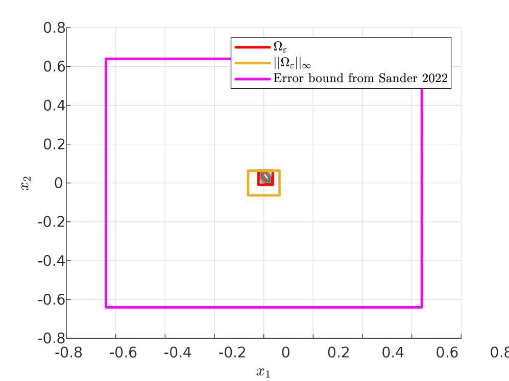</details> Figure 2: Illustration of the error over-approximation To contextualize our proposed error bound, we compare it with the error bound proposed in [26]. For that, we first compute the infinity norm of our error set $\|{\color[rgb]{1,0,0}\Omega_{\varepsilon}(\mathcal{X}_{in})}\|_{∞}=0.064$ , which corresponds to a positive and scalar bound on the error, thus implying that its set representation in the state space (represented in yellow in Figure 3) is necessarily symmetrical around $0$ and with the width that is identical on all dimensions (since the infinity norm takes the largest width across all dimensions). The set-based error bound ( ${\color[rgb]{1,0,0}\Omega_{\varepsilon}(\mathcal{X}_{in})}$ represented in red) obtained from our method is thus always contained in this infinity norm. Next, we compute the Lipschitz constant for the vector field of the neural ODE $L=\|\tau+W\|_{∞}=3.62$ , and then we obtain the error bound in [26] as $\frac{(e^{L}-1)}{L}\|\Omega_{\varepsilon}(\mathcal{X}_{in})\|_{∞}=0.64$ . This final error bound, represented in magenta in Figure 3, is 10 times wider (on each dimension) than the infinity norm of our error set in yellow, and about $16$ millions times larger (in volume over the $5$ -dimensional state space) than our error set ${\color[rgb]{1,0,0}\Omega_{\varepsilon}(\mathcal{X}_{in})}$ in red. The improved tightness of our proposed approach is therefore very significant. <details> <summary>x3.png Details</summary>  ### Visual Description ## Chart: Error Bounds ### Overview The image is a 2D plot showing error bounds in the x1-x2 plane. It displays three rectangular regions representing different error estimates: Omega_epsilon (red), the infinity norm of Omega_epsilon (orange), and an error bound from Sander 2022 (magenta). The plot is centered around the origin (0,0). ### Components/Axes * **X-axis:** x1, ranging from -0.8 to 0.8 with increments of 0.2. * **Y-axis:** x2, ranging from -0.8 to 0.8 with increments of 0.2. * **Legend (top-right):** * Red line: Ωε * Orange line: ||Ωε||∞ * Magenta line: Error bound from Sander 2022 ### Detailed Analysis * **Red line (Ωε):** Forms a small square centered around (0,0). The approximate coordinates of the square's corners are (-0.05, 0.05), (0.05, 0.05), (0.05, -0.05), and (-0.05, -0.05). * **Orange line (||Ωε||∞):** Forms a larger square, also centered around (0,0). The approximate coordinates of the square's corners are (-0.15, 0.15), (0.15, 0.15), (0.15, -0.15), and (-0.15, -0.15). * **Magenta line (Error bound from Sander 2022):** Forms the largest square, centered around (0,0). The approximate coordinates of the square's corners are (-0.65, 0.65), (0.65, 0.65), (0.65, -0.65), and (-0.65, -0.65). ### Key Observations * All three error bounds are represented as squares aligned with the axes. * The error bounds are nested, with the red square (Ωε) being the smallest, followed by the orange square (||Ωε||∞), and the magenta square (Error bound from Sander 2022) being the largest. * The plot suggests that the error bound from Sander 2022 is significantly larger than the other two error estimates. ### Interpretation The plot visualizes different error bounds for a system or model. The nested squares indicate that the error estimates vary in their conservativeness. The error bound from Sander 2022 is the most conservative (largest), while Ωε is the least conservative (smallest). The infinity norm of Ωε (||Ωε||∞) provides an intermediate error estimate. This type of visualization is useful for comparing the performance and accuracy of different error estimation methods. The fact that the error bounds are centered around (0,0) suggests that the true value or equilibrium point of the system is at the origin. </details> Figure 3: Comparison of the error bounds obtained from our approach in red and the one from [26] in magenta 4.3 Experiments on safety verification Using the error bound computed in Section 4.2, we can verify safety properties for the neural ODE output set based on the ResNet output set and the error bound set (i.e., ${\color[rgb]{1,0,0}\Omega_{\text{ResNet}}(\mathcal{X}_{in})+\Omega_{\varepsilon}(\mathcal{X}_{in})}$ ), or vice versa for the ResNet output set based on the neural ODE output set and the negative error bound set (i.e., ${\color[rgb]{1,0,0}\Omega_{\text{neural ODE}}(\mathcal{X}_{in})+\Omega_{-\varepsilon}(\mathcal{X}_{in})}$ ). 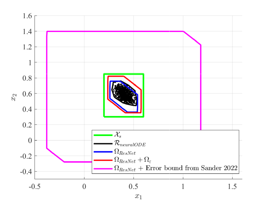In Figure 4, we compute the over-approximation of the ResNet output set ${\color[rgb]{0,0,1}\Omega_{\text{ResNet}}}$ using simple bound propagation through the ResNet function with CORA. By adding the error bound ${\color[rgb]{1,0,0}\Omega_{\varepsilon}}$ , we obtain a zonotope (shown in red) that is guaranteed to contain $\mathcal{R}_{\text{neural ODE}}(\mathcal{X}_{in})$ . The figure also includes black points representing neural ODE outputs for random initial conditions in $\mathcal{X}_{in}$ , with their convex hull (black set) approximating the true reachable set $\mathcal{R}_{\text{neural ODE}}(\mathcal{X}_{in})$ . Since the safe set ${\color[rgb]{0,0,0}\mathcal{X}_{s}}$ contains the over-approximation ${\color[rgb]{1,0,0}\Omega_{\text{ResNet}}(\mathcal{X}_{in})+\Omega_{\varepsilon}(\mathcal{X}_{in})}$ , we guarantee that the neural ODE true reachable set is safe, as: $$ {\color[rgb]{0,0,0}\mathcal{X}_{s}}\supseteq{\color[rgb]{1,0,0}\Omega_{\text{ResNet}}(\mathcal{X}_{in})+\Omega_{\varepsilon}(\mathcal{X}_{in})}\supseteq\mathcal{R}_{\text{neural ODE}}. $$ From Figure 4, we can see that the ResNet and neural ODE reachable sets are very similar due to the ResNet role as a discretization of the neural ODE, but they are not identical. Indeed, some neural ODE outputs (black points) lie outside ${\color[rgb]{0,0,1}\Omega_{\text{ResNet}}}$ , highlighting the necessity of the error bound ${\color[rgb]{1,0,0}\Omega_{\varepsilon}(\mathcal{X}_{in})}$ to ensure that the over-approximation captures all possible neural ODE outputs. <details> <summary>x4.png Details</summary>  ### Visual Description ## Chart: Reachability Sets Comparison ### Overview The image is a 2D plot comparing different reachability sets for a system, likely related to neural network verification or control. It shows the state space boundaries estimated by different methods, including neural ODEs and ResNets, along with error bounds. The plot visualizes the tightness and accuracy of these different approximations. ### Components/Axes * **X-axis:** x1, ranging from -0.5 to 1.5 with increments of 0.5. * **Y-axis:** x2, ranging from -0.4 to 1.6 with increments of 0.2. * **Legend (bottom-right):** * Green: $\mathcal{X}_s$ * Black: $\mathcal{R}_{neuralODE}$ * Blue: $\Omega_{ResNet}$ * Red: $\Omega_{ResNet} + \Omega_{\epsilon}$ * Magenta: $\Omega_{ResNet}$ + Error bound from Sander 2022 ### Detailed Analysis * **$\mathcal{X}_s$ (Green):** This set forms the outermost bound among the inner sets. It's a rectangular shape with rounded corners, centered around (0.5, 0.6). The x-axis ranges from approximately 0.1 to 0.8, and the y-axis ranges from approximately 0.3 to 0.85. * **$\mathcal{R}_{neuralODE}$ (Black):** This set is contained within all other sets. It is an irregular polygon formed by the densest cluster of points. The points are concentrated around x1 = 0.4 and x2 = 0.6. * **$\Omega_{ResNet}$ (Blue):** This set is slightly larger than the black set. It is a polygon with vertices around (0.25, 0.4), (0.6, 0.4), (0.7, 0.7), and (0.3, 0.8). * **$\Omega_{ResNet} + \Omega_{\epsilon}$ (Red):** This set is larger than the blue set. It is a polygon with vertices around (0.2, 0.35), (0.75, 0.35), (0.8, 0.75), and (0.2, 0.8). * **$\Omega_{ResNet}$ + Error bound from Sander 2022 (Magenta):** This set forms the outermost bound. It is a polygon with vertices around (-0.5, -0.3), (1.4, -0.3), (1.4, 1.4), and (-0.5, 1.4). ### Key Observations * The black set ($\mathcal{R}_{neuralODE}$) is the tightest bound, closely following the shape of the data points. * The green set ($\mathcal{X}_s$) provides a larger, more conservative bound. * The magenta set ($\Omega_{ResNet}$ + Error bound from Sander 2022) is the most conservative, providing the largest bound. * The blue and red sets ($\Omega_{ResNet}$ and $\Omega_{ResNet} + \Omega_{\epsilon}$) fall between the black and green sets in terms of tightness. ### Interpretation The plot compares the accuracy and conservativeness of different methods for estimating the reachable set of a system. The neural ODE approach (black) provides the tightest estimate, suggesting it's the most accurate. However, it may not be guaranteed to be a strict bound. The other methods (green, blue, red, magenta) provide outer bounds with varying degrees of conservativeness. The magenta set, based on Sander 2022, provides the most conservative bound, ensuring that the true reachable set is contained within it, but at the cost of being less precise. The plot highlights the trade-off between accuracy and safety in reachability analysis. 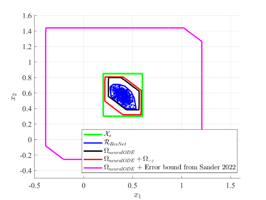</details> Figure 4: Verification of neural ODE based on ResNet Conversely, in Figure 5, we compute the over-approximation of the neural ODE reachable set ${\color[rgb]{0,0,0}\Omega_{\text{neural ODE}}(\mathcal{X}_{in})}$ . By adding the negative error bound ${\color[rgb]{1,0,0}\Omega_{-\varepsilon}}$ , we obtain a zonotope (shown in red) that encapsulates ${\color[rgb]{0,0,1}\mathcal{R}_{\text{ResNet}}(\mathcal{X}_{in})}$ . Similarly, the figure includes blue points representing ResNet outputs for random inputs in $\mathcal{X}_{in}$ , with their convex hull (blue set) approximating the true reachable set ${\color[rgb]{0,0,1}\mathcal{R}_{\text{ResNet}}(\mathcal{X}_{in})}$ . Since the safe set ${\color[rgb]{0,0,0}\mathcal{X}_{s}}$ is a super set that contains the over-approximation ${\color[rgb]{1,0,0}\Omega_{\text{neural ODE}}(\mathcal{X}_{in})+\Omega_{-\varepsilon}(\mathcal{X}_{in})}$ , we guarantee that the ResNet true reachable set is safe, as: $$ {\color[rgb]{0,0,0}\mathcal{X}_{s}}\supseteq{\color[rgb]{1,0,0}\Omega_{\text{neural ODE}}(\mathcal{X}_{in})+\Omega_{-\varepsilon}(\mathcal{X}_{in})}\supseteq{\color[rgb]{0,0,1}\mathcal{R}_{\text{ResNet}}}. $$ <details> <summary>x5.png Details</summary>  ### Visual Description ## Chart: Reachable Sets Comparison ### Overview The image is a 2D plot comparing reachable sets obtained using different methods: ResNet, neuralODE, and error bounds from Sander 2022. The plot shows the regions in the x1-x2 plane that the system can reach under different conditions or approximations. ### Components/Axes * **X-axis:** x1, ranging from -0.5 to 1.5 * **Y-axis:** x2, ranging from -0.5 to 1.6 * **Legend:** Located in the bottom-right corner of the plot. * Green: Xs * Blue: RResNet * Black: ΩneuralODE * Red: ΩneuralODE + Ω−ε * Magenta: ΩneuralODE + Error bound from Sander 2022 ### Detailed Analysis * **Xs (Green):** A rectangular region centered around (0.5, 0.6). The bottom-left corner is approximately at (0.2, 0.3) and the top-right corner is approximately at (0.7, 0.85). * **RResNet (Blue):** A scattered set of points contained within the other regions, concentrated around (0.4, 0.6). The points are densely packed, forming an irregular shape. * **ΩneuralODE (Black):** A polygon enclosing the blue points. The vertices are approximately at (0.25, 0.4), (0.4, 0.8), (0.6, 0.8), (0.7, 0.6), (0.6, 0.4), and (0.3, 0.3). * **ΩneuralODE + Ω−ε (Red):** A polygon slightly larger than the black polygon. The vertices are approximately at (0.15, 0.3), (0.3, 0.8), (0.7, 0.8), (0.8, 0.6), (0.7, 0.3), and (0.2, 0.2). * **ΩneuralODE + Error bound from Sander 2022 (Magenta):** A large polygon encompassing all other regions. The vertices are approximately at (-0.4, -0.3), (-0.4, 1.45), (0.8, 1.45), (1.4, 1.45), (1.4, -0.3), and (-0.4, -0.3). ### Key Observations * The RResNet region (blue) is contained within the ΩneuralODE region (black). * The ΩneuralODE + Ω−ε region (red) is slightly larger than the ΩneuralODE region (black). * The ΩneuralODE + Error bound from Sander 2022 region (magenta) is significantly larger than all other regions. * The Xs region (green) is a rectangular box that contains the other regions. ### Interpretation The plot illustrates the reachable sets obtained using different methods. The RResNet method provides a specific set of reachable states, while the neuralODE method provides a larger set that encompasses the RResNet set. Adding the error term Ω−ε to the neuralODE method further expands the reachable set. The error bound from Sander 2022 provides the largest reachable set, indicating a more conservative estimate of the system's possible states. The Xs region represents the state space. The plot suggests that the RResNet method provides a tighter estimate of the reachable set compared to the neuralODE method with error bounds. The error bound from Sander 2022 provides a guaranteed bound on the reachable set, but it may be overly conservative. </details> Figure 5: Verification of ResNet based on neural ODE We can also remark that the magenta sets obtained by adding the error bound proposed in [26] to the ResNet and neural ODE reachable sets in Figures 4 and 5, extends significantly beyond the green safe set, preventing us from successfully guaranteeing the safety of the models. 5 Conclusion In this paper, we propose a set-based method to bound the error between a neural ODE model and its ResNet approximation. This approach is based on reachability analysis tools applied to the Lagrange remainder in the Taylor expansion of the neural ODE trajectories, and is shown both theoretically and numerically to provide significantly tighter over-approximation of this approximation error than previous results in [26]. As the second contribution of this paper, the obtained bounding set of the approximation error between the two models is used to verify a safety property on either of the two models by applying reachability or verification tools only on the other model. This approach is fully reversible and either model can be used as the verification proxy for the other. These contributions and their improvement with respect to [26] have been illustrated on a numerical example of a fixed-point attractor system modeled as a neural ODE. In future works, we plan to explore additional sources of complexity for these approaches, such as handling non-smooth activation functions (e.g. ReLU), and the case where the neural ODE vector field is explicitly dependent on the depth variable $t$ , thus corresponding to ResNet with multiple residual blocks. Additionally, we aim to study the versatility of this verification proxy approach by applying it to other complex nonlinear dynamical systems or neural network architectures. Acknowledgement This project has received funding from the European Union’s Horizon 2020 research and innovation programme under the Marie Skłodowska-Curie COFUND grant agreement no. 101034248. References - [1] Althoff, M.: An introduction to cora 2015. In: Proc. of the workshop on applied verification for continuous and hybrid systems. pp. 120–151 (2015) - [2] Beer, R.D.: On the dynamics of small continuous-time recurrent neural networks. Adaptive Behavior 3 (4), 469–509 (1995) - [3] Behrmann, J., Grathwohl, W., Chen, R.T., Duvenaud, D., Jacobsen, J.H.: Invertible residual networks. In: International conference on machine learning. pp. 573–582. PMLR (2019) - [4] Boudardara, F., Boussif, A., Meyer, P.J., Ghazel, M.: Innabstract: An inn-based abstraction method for large-scale neural network verification. IEEE Transactions on Neural Networks and Learning Systems (2023) - [5] Chen, R.T., Rubanova, Y., Bettencourt, J., Duvenaud, D.K.: Neural ordinary differential equations. Advances in neural information processing systems 31 (2018) - [6] De Figueiredo, L.H., Stolfi, J.: Affine arithmetic: concepts and applications. Numerical algorithms 37, 147–158 (2004) - [7] Gruenbacher, S., Hasani, R., Lechner, M., Cyranka, J., Smolka, S.A., Grosu, R.: On the verification of neural odes with stochastic guarantees. In: Proceedings of the AAAI Conference on Artificial Intelligence. vol. 35, pp. 11525–11535 (2021) - [8] Gruenbacher, S.A., Lechner, M., Hasani, R., Rus, D., Henzinger, T.A., Smolka, S.A., Grosu, R.: Gotube: Scalable statistical verification of continuous-depth models. In: Proceedings of the AAAI Conference on Artificial Intelligence. vol. 36, pp. 6755–6764 (2022) - [9] Haber, E., Ruthotto, L.: Stable architectures for deep neural networks. Inverse problems 34 (1), 014004 (2017) - [10] He, K., Zhang, X., Ren, S., Sun, J.: Deep residual learning for image recognition. In: Proceedings of the IEEE conference on computer vision and pattern recognition. pp. 770–778 (2016) - [11] Huang, X., Kwiatkowska, M., Wang, S., Wu, M.: Safety verification of deep neural networks. In: Computer Aided Verification (CAV). Springer (2017) - [12] Jaulin, L., Kieffer, M., Didrit, O., Walter, E., Jaulin, L., Kieffer, M., Didrit, O., Walter, É.: Interval analysis. Springer (2001) - [13] Katz, G., Barrett, C., Dill, D.L., Julian, K., Kochenderfer, M.J.: Reluplex: An efficient smt solver for verifying deep neural networks. In: Computer Aided Verification (CAV). Springer (2017) - [14] Kidger, P.: On neural differential equations. Ph.D. thesis, University of Oxford (2021) - [15] Liang, Z., Ren, D., Liu, W., Wang, J., Yang, W., Xue, B.: Safety verification for neural networks based on set-boundary analysis. In: International Symposium on Theoretical Aspects of Software Engineering. pp. 248–267. Springer (2023) - [16] Lopez, D.M., Choi, S.W., Tran, H.D., Johnson, T.T.: Nnv 2.0: the neural network verification tool. In: International Conference on Computer Aided Verification. pp. 397–412. Springer (2023), https://doi.org/10.1007/978-3-031-37703-7_19 - [17] Lopez, D.M., Musau, P., Hamilton, N., Johnson, T.T.: Reachability analysis of a general class of neural ordinary differential equations (2022), https://doi.org/10.1007/978-3-031-15839-1_15 - [18] Lu, Y., Zhong, A., Li, Q., Dong, B.: Beyond finite layer neural networks: Bridging deep architectures and numerical differential equations. In: International conference on machine learning. pp. 3276–3285. PMLR (2018) - [19] Makino, K., Berz, M.: Taylor models and other validated functional inclusion methods. International Journal of Pure and Applied Mathematics 6, 239–316 (2003) - [20] Marion, P.: Generalization bounds for neural ordinary differential equations and deep residual networks. Advances in Neural Information Processing Systems 36, 48918–48938 (2023) - [21] Marion, P., Wu, Y.H., Sander, M.E., Biau, G.: Implicit regularization of deep residual networks towards neural odes (2024), https://arxiv.org/abs/2309.01213 - [22] Musau, P., Johnson, T.: Continuous-time recurrent neural networks (ctrnns)(benchmark proposal). In: 5th Applied Verification for Continuous and Hybrid Systems Workshop (ARCH), Oxford, UK (2018), https://doi.org/10.29007/6czp - [23] Oh, Y., Kam, S., Lee, J., Lim, D.Y., Kim, S., Bui, A.: Comprehensive review of neural differential equations for time series analysis (2025), https://arxiv.org/abs/2502.09885 - [24] Rackauckas, C., Ma, Y., Martensen, J., Warner, C., Zubov, K., Supekar, R., Skinner, D., Ramadhan, A., Edelman, A.: Universal differential equations for scientific machine learning (2021), https://arxiv.org/abs/2001.04385 - [25] Rudin, W.: Principles of Mathematical Analysis. McGraw-Hill, New York, 3rd edn. (1976) - [26] Sander, M., Ablin, P., Peyré, G.: Do residual neural networks discretize neural ordinary differential equations? Advances in Neural Information Processing Systems 35, 36520–36532 (2022) - [27] Tabuada, P.: Verification and control of hybrid systems: a symbolic approach. Springer Science & Business Media (2009) - [28] Tran, H.D., Yang, X., Manzanas Lopez, D., Musau, P., Nguyen, L.V., Xiang, W., Bak, S., Johnson, T.T.: Nnv: the neural network verification tool for deep neural networks and learning-enabled cyber-physical systems. In: International conference on computer aided verification. pp. 3–17. Springer (2020) - [29] Xiang, W., Shao, Z.: Approximate bisimulation relations for neural networks and application to assured neural network compression. In: 2022 American Control Conference (ACC). pp. 3248–3253. IEEE (2022)