# A Statistical Physics of Language Model Reasoning
**Authors**:
- Jack David Carson (Massachusetts Institute of Technology)
- Amir Reisizadeh (Massachusetts Institute of Technology)
## Abstract
Transformer LMs show emergent reasoning that resists mechanistic understanding. We offer a statistical physics framework for continuous-time chain-of-thought reasoning dynamics. We model sentence-level hidden state trajectories as a stochastic dynamical system on a lower-dimensional manifold. This drift-diffusion system uses latent regime switching to capture diverse reasoning phases, including misaligned states or failures. Empirical trajectories (8 models, 7 benchmarks) show a rank-40 projection (balancing variance capture and feasibility) explains 50% variance. We find four latent reasoning regimes. An SLDS model is formulated and validated to capture these features. The framework enables low-cost reasoning simulation, offering tools to study and predict critical transitions like misaligned states or other LM failures.
Stochastic Processes, Transformer Interpretability, Chain-of-Thought Reasoning, Dynamical Systems, Large Language Models
## 1 Introduction
Transformer LMs (Vaswani et al., 2017), trained for next-token prediction (Radford et al., 2019; Brown et al., 2020), show emergent reasoning like complex cognition (Wei et al., 2022). Standard analyses of discrete components (e.g., attention heads (Elhage et al., 2021; Olsson et al., 2022)) provide limited insight into longer-scale semantic transitions in multi-step reasoning (Allen-Zhu & Li, 2023; López-Otal et al., 2024). Understanding these high-dimensional, prediction-shaped semantic trajectories, particularly how they might cause misaligned states, is a key challenge (Li et al., 2023; Nanda et al., 2023).
We model reasoning as a continuous-time dynamical system, drawing from statistical physics (Chaudhuri & Fiete, 2016; Schuecker et al., 2018). Sentence-level hidden states $h(t)∈ℝ^D$ evolve via a stochastic differential equation (SDE):
$$
dh(t)=μ(h(t),Z(t)) dt+B(h(t),Z(t)) dW(t), \tag{1}
$$
with drift $μ$ , diffusion $B$ , Wiener process $W(t)$ , and latent regimes $Z(t)$ . This decomposes trajectories into trends and variations, helping identify deviations. As full high-dimensional SDE analysis (e.g., $D>2048$ for most LMs) is impractical, we use a lower-dimensional manifold capturing significant variance for modeling.
This continuous-time dynamical systems perspective offers several benefits:
Core Advantages
$\bullet$
Principled Abstraction: Enables a mathematically grounded, semantic-level view of reasoning, akin to statistical physics approximations, moving beyond token mechanics for robust interpretation of reasoning pathways and potential misalignments. $\bullet$
Tractable Latent Structure ID: Makes analysis of reasoning trajectories feasible by focusing on a low-dimensional manifold (e.g., rank-40 PCA capturing 50% variance) that describes significant structured evolution. $\bullet$
Reasoning Regime Discovery: Uncovers distinct latent semantic regimes with unique drift/variance profiles, suggesting context-driven switching and offering insight into how models might slip into different reasoning states (Appx. E). $\bullet$
Efficient Surrogate Model: Our SLDS accurately models and reconstructs reasoning trajectories with significant computational savings, facilitating the study of how reasoning processes unfold. $\bullet$
Failure Mode Analysis: Provides tools to study critical transitions, robustness, and predict inference-time failure modes or misaligned states in LLM reasoning.
Chain-of-thought (CoT) prompting (Wei et al., 2022; Wang et al., 2023) has demonstrated that LMs can follow structured reasoning pathways, hinting at underlying processes amenable to a dynamical systems description. While prior work has applied continuous-time models to neural dynamics generally, the explicit modeling of transformer reasoning at these semantic timescales, particularly as an approximation for impractical full-dimensional analysis, has been largely unexplored. Our work bridges this gap by pursuing an SDE-based perspective informed by empirical analysis of transformer hidden-state trajectories.
This paper is structured as follows: Section 2 introduces the mathematical formalism of SDEs and regime switching. Section 3 details our data collection and initial empirical findings that motivate the model, including the practical need for dimensionality reduction. Section 4 formally defines the SLDS model. Section 5 presents experimental validation, including model fitting, generalization, ablation studies, and a case study on modeling adversarial belief shifts as an example of predicting misaligned states.
## 2 Mathematical Preliminaries
We conceptualize the internal reasoning process of a transformer LM as a continuous-time stochastic trajectory evolving within its hidden-state space. Let $h_t∈ℝ^D$ be the final-layer residual embedding extracted at discrete sentence boundaries $t=0,1,2,\dots$ . To capture the rich semantic evolution across reasoning steps, we treat these discrete embeddings as observations of an underlying continuous-time process $h(t):ℝ_≥ 0→ℝ^D$ . The direct analysis of such a process in its full dimensionality (e.g., $D≥ 2048$ ) is often computationally prohibitive. We therefore aim to approximate its dynamics using SDEs, potentially in a reduced-dimensional space.
**Definition 2.1 (Itô SDE)**
*An Itô stochastic differential equation on the state space $ℝ^D$ is given by:
$$
dh(t)=μ(h(t)) dt+B(h(t)) dW(t), h(0)∼
p
_0, \tag{0}
$$
where $μ:ℝ^D→ℝ^D$ is the deterministic drift term, encoding persistent directional dynamics. The matrix $B:ℝ^D→ℝ^D× D^{\prime}$ is the diffusion term, modulating instantaneous stochastic fluctuations. $W(t)$ is a $D^\prime$ -dimensional Wiener process (standard Brownian motion), and $p_0$ is the initial distribution. The noise dimension $D^\prime$ can be less than or equal to the state dimension $D$ .*
The drift $μ(h(t))$ represents systematic semantic or cognitive tendencies, while the diffusion $B(h(t))$ accounts for fluctuations due to local uncertainties, token-level variations, or inherent model stochasticity. Standard conditions ensure the well-posedness of such SDEs:
**Theorem 2.1 (Well-Posedness(Øksendal,2003))**
*If $μ$ and $B$ satisfy standard Lipschitz continuity and linear growth conditions (see Appendix A), the SDE
$$
dh(t)=μ(h(t)) dt+B(h(t)) dW(t) \tag{3}
$$
has a unique strong solution for a given $D^\prime$ -dimensional Wiener process $W(t)$ .*
We focus on dynamics at the sentence level:
**Definition 2.2 (Sentence-Stride Process)**
*The sentence-stride hidden-state process is the discrete sequence $\{h_t\}_t∈ℕ$ obtained by extracting the final-layer transformer state immediately following each detected sentence boundary. This emphasizes mesoscopic, semantic-level changes over finer-grained token-level variations.*
To analyze these dynamics in a computationally manageable way, particularly given the high dimensionality $D$ of $h(t)$ , we utilize projection-based dimensionality reduction. The goal is to find a lower-dimensional subspace where the most significant dynamics, for the purpose of modeling the SDE, unfold.
**Definition 2.3 (Projection Leakage)**
*Given an orthonormal matrix $V_k∈ℝ^D× k$ (where $V_k^⊤V_k=I_k$ ), the leakage of the drift $μ$ under perturbations $v$ orthogonal to the image of $V_k$ (i.e., $v⊥Im(V_k)$ ) is
$$
L_k=\sup_\begin{subarray{c}x∈ℝ^D, ≤ft\lVert v\right\rVert
≤ε\\
v^⊤V_k=0\end{subarray}}\frac{≤ft\lVertμ(x+v)-μ(x)\right\rVert}{
≤ft\lVertμ(x)\right\rVert}.
$$
A small leakage $L_k$ implies that the drift’s behavior relative to its current direction is not excessively altered by components outside the subspace spanned by $V_k$ , making the subspace a reasonable domain for approximation.*
**Assumption 2.1 (Approximate Projection Closure for Modeling)**
*For practical modeling of the SDE (Eq. 2), we assume there exists a rank $k$ (e.g., $k=40$ in our work, chosen based on empirical variance and computational trade-offs) and a perturbation scale $ε>0$ such that $L_k\ll 1$ . This allows the approximation of the drift within this $k$ -dimensional subspace:
$$
μ(h(t))≈ V_kV_k^⊤μ(h(t))
$$
holds up to an error of order $O(L_k)$ . This assumption underpins the feasibility of our low-dimensional modeling approach, enabling the analytical treatment inspired by statistical physics.*
Empirical observations of reasoning trajectories suggest abrupt shifts, potentially indicating transitions between different phases of reasoning or slips into misaligned states. This motivates a regime-switching framework:
**Definition 2.4 (Regime-Switching SDE)**
*Let $Z(t)∈\{1,\dots,K\}$ be a latent continuous-time Markov chain with a transition rate matrix $T∈ℝ^K× K$ . The corresponding regime-switching Itô SDE is:
$$
dh(t)=μ_Z(t)(h(t)) dt+B_Z(t)(h(t)) dW(t), \tag{4}
$$
where each latent regime $i∈\{1,\dots,K\}$ has distinct drift $μ_i$ and diffusion $B_i$ functions. This allows for context-dependent dynamic structures (Ghahramani & Hinton, 2000), crucial for capturing diverse reasoning pathways.*
These definitions establish the mathematical foundation for our analysis of transformer reasoning dynamics as a tractable approximation of a more complex high-dimensional process.
## 3 Data and Empirical Motivation
We build a corpus of sentence-aligned hidden-state trajectories from transformer-generated reasoning chains across a suite of models (Mistral-7B-Instruct (Jiang et al., 2023), Phi-3-Medium (Abdin et al., 2024), DeepSeek-67B (DeepSeek-AI et al., 2024), Llama-2-70B (Touvron et al., 2023), Gemma-2B-IT (Gemma Team & Google DeepMind, 2024), Qwen1.5-7B-Chat (Bai et al., 2023), Gemma-7B-IT (also (Gemma Team & Google DeepMind, 2024)), Llama-2-13B-Chat-HF (also (Touvron et al., 2023))) and datasets (StrategyQA (Geva et al., 2021), GSM-8K (Cobbe et al., 2021), TruthfulQA (Lin et al., 2022), BoolQ (Clark et al., 2019), OpenBookQA (Mihaylov et al., 2018), HellaSwag (Zellers et al., 2019), PiQA (Bisk et al., 2020), CommonsenseQA (Talmor et al., 2021, 2019)), yielding roughly 9,800 distinct trajectories spanning $∼$ 40,000 sentence-to-sentence transitions.
### 3.1 Sentence-Level Dynamics and Manifold Structure for Tractable Modeling
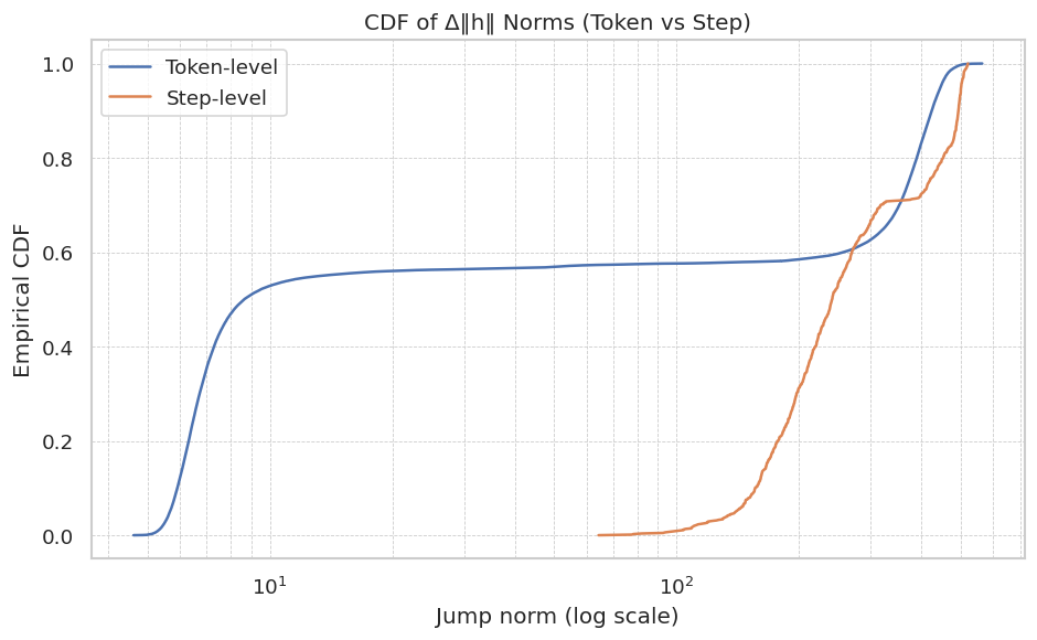
First, we confirmed that sentence-level increments effectively capture semantic evolution. Figure 1 (a) compares the cumulative distribution functions (CDFs) of jump norms ( $≤ft\lVertΔ h_t\right\rVert$ ) at both token and sentence strides. Token-level increments show a noisy distribution skewed towards small values, primarily reflecting syntactic variations. In contrast, sentence-level increments are orders of magnitude larger, clearly indicating significant semantic shifts and validating our choice of sentence-stride analysis. To reduce "jitter" from minor variations, we filtered out transitions below a minimum threshold ( $≤ft\lVertΔ h_t\right\rVert≤ 10$ in normalized units), yielding cleaner semantic trajectories.
To uncover underlying geometric structures that could make modeling tractable, we applied Principal Component Analysis (PCA) (Jolliffe, 2002) to the sentence-stride embeddings. We found that a relatively low-dimensional projection (rank $k=40$ ) captures approximately 50% of the total variance in these reasoning trajectories (details in Appendix A). While reasoning dynamics occur in a high-dimensional embedding space, this finding suggests that a significant portion of their variance is concentrated in a lower-dimensional subspace. This is crucial because constructing and analyzing a stochastic process (like a random walk or SDE) in the full embedding dimension (e.g., 2048) is often impractical. The rank-40 manifold thus provides a computationally feasible domain for our dynamical systems modeling, not necessarily because the process is strictly confined to it, but because it offers a practical and informative approximation.
### 3.2 Linear Predictability and Multimodal Residuals
To assess the predictive structure of the semantic drift within this tractable manifold, we performed a global ridge regression (Hoerl & Kennard, 1970), fitting a linear model to predict subsequent sentence embeddings from previous ones:
$$
\displaystyle h_t+1 \displaystyle≈ Ah_t+c, \displaystyle(A,c) \displaystyle=\arg\min_A,c∑_t\|Δ h_t-(A-I)h_t-c\|^2+λ
\|A\|_F^2. \tag{5}
$$
Using a modest regularization ( $λ=1.0$ ), this global linear model achieved an $R^2≈ 0.51$ , indicating substantial linear predictability in sentence-to-sentence transitions.
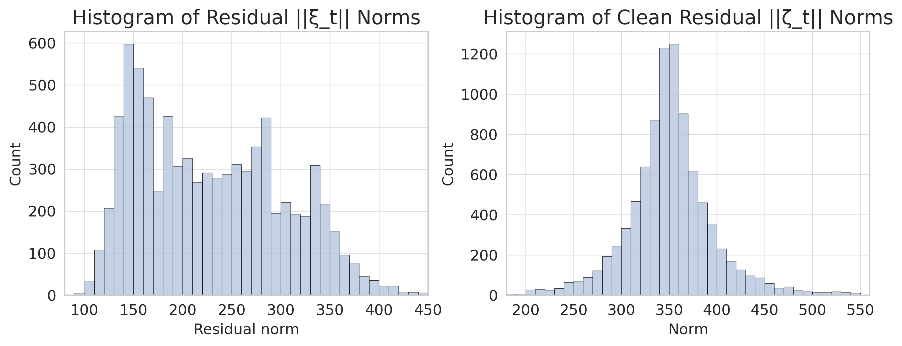
However, an examination of the residuals from this linear fit, $ξ_t=Δ h_t-[(A-I)h_t+c]$ , revealed persistent multimodal structure, even after the linear drift component was removed (Figure 1 (b)). This multimodality suggests the presence of distinct underlying dynamic states or phases—some potentially representing "misaligned states" or divergent reasoning paths—that are not captured by a single linear model.
Inspired by Langevin dynamics, where a particle in a multi-well potential $U(x)$ can exhibit metastable states (Appendix E), we interpret these multimodal residual clusters as evidence of distinct latent reasoning regimes. The stationary probability distribution $p_st(x)∝ e^-U(x)/D$ for an SDE $dx=-U^\prime(x) dt+√{2D} dW_t$ becomes multimodal if $U(x)$ has multiple minima and noise $D$ is sufficiently low. Analogously, the observed clusters in our residual analysis point towards the existence of multiple metastable semantic basins in the reasoning process. This strongly motivates the introduction of a latent regime structure to adequately model these richer, nonlinear dynamics and to understand how an LLM might transition between effective reasoning and potential failure modes.
<details>
<summary>extracted/6513090/fig3.png Details</summary>
### Visual Description
## CDF Plot: CDF of Δ||h|| Norms (Token vs Step)
### Overview
The image displays a Cumulative Distribution Function (CDF) plot comparing the distribution of "jump norms" (Δ||h||) at two different granularities: Token-level and Step-level. The plot uses a logarithmic scale for the x-axis. The title suggests this data relates to changes in hidden state norms (||h||) within a computational process, likely in the context of neural network training or analysis.
### Components/Axes
* **Title:** "CDF of Δ||h|| Norms (Token vs Step)"
* **Y-axis:** Label is "Empirical CDF". Scale ranges from 0.0 to 1.0 with major tick marks at 0.0, 0.2, 0.4, 0.6, 0.8, and 1.0.
* **X-axis:** Label is "Jump norm (log scale)". The axis is logarithmic, with major labeled tick marks at `10^1` (10) and `10^2` (100). The visible range extends from approximately `10^0` (1) to `10^2.5` (~316).
* **Legend:** Located in the top-left corner of the plot area.
* **Token-level:** Represented by a solid blue line.
* **Step-level:** Represented by a solid orange line.
* **Grid:** A light gray grid is present, aligned with the major ticks on both axes.
### Detailed Analysis
**1. Token-level (Blue Line) Trend & Data Points:**
* **Trend:** The line exhibits a bimodal or two-phase distribution. It rises very steeply at low jump norms, plateaus for a wide range, and then rises steeply again at high jump norms.
* **Data Points (Approximate):**
* The CDF begins to rise from 0 at a jump norm of approximately `10^0.3` (~2).
* It reaches a CDF of ~0.5 at a jump norm of approximately `10^0.8` (~6.3).
* The curve then flattens significantly, forming a long plateau. The CDF increases very slowly from ~0.55 to ~0.60 as the jump norm increases from `10^1` (10) to `10^2` (100).
* After `10^2` (100), the line rises steeply again.
* It reaches a CDF of ~0.9 at a jump norm of approximately `10^2.3` (~200).
* It approaches and reaches a CDF of 1.0 at a jump norm of approximately `10^2.5` (~316).
**2. Step-level (Orange Line) Trend & Data Points:**
* **Trend:** The line shows a unimodal distribution that is shifted significantly to the right (higher values) compared to the initial rise of the Token-level line. It has a single, steep sigmoidal rise.
* **Data Points (Approximate):**
* The CDF begins to rise from 0 at a jump norm of approximately `10^1.8` (~63).
* It reaches a CDF of ~0.2 at a jump norm of approximately `10^2.1` (~126).
* It reaches a CDF of ~0.5 at a jump norm of approximately `10^2.2` (~158).
* It reaches a CDF of ~0.8 at a jump norm of approximately `10^2.4` (~251).
* It converges with the Token-level line, approaching and reaching a CDF of 1.0 at a jump norm of approximately `10^2.5` (~316).
**3. Cross-Reference & Intersection:**
* The two lines intersect at a CDF value of approximately 0.62. This occurs at a jump norm of roughly `10^2.25` (~178).
* For jump norms below ~`10^2.25`, the Token-level CDF is higher than the Step-level CDF. This means a larger proportion of token-level jumps are smaller than this value compared to step-level jumps.
* For jump norms above ~`10^2.25`, the Step-level CDF is higher, indicating that a larger proportion of step-level jumps are smaller than these very large values compared to token-level jumps (though both distributions are nearing completion).
### Key Observations
1. **Distinct Distributions:** The Token-level and Step-level jump norms follow fundamentally different distributions. Token-level jumps are heavily concentrated at very small values (first steep rise) and very large values (second steep rise), with relatively few jumps of intermediate size (the plateau). Step-level jumps are concentrated in a single, higher range.
2. **Scale Difference:** The vast majority (over 50%) of token-level jumps have a norm less than ~10, while the vast majority of step-level jumps have a norm greater than ~63.
3. **Convergence at Extremes:** Both distributions converge to a CDF of 1.0 at approximately the same maximum jump norm (~316), suggesting a common upper bound or scaling factor in the system being measured.
4. **Plateau Significance:** The long plateau in the Token-level CDF between norms of 10 and 100 is a critical feature, indicating a "gap" or scarcity of token-level changes of this intermediate magnitude.
### Interpretation
This plot provides a comparative analysis of the magnitude of changes (Δ||h||) in a hidden state vector `h` at two different temporal resolutions: per token processed and per optimization step.
* **Token-level Dynamics:** The bimodal distribution suggests two primary regimes of change at the token level. The first, very frequent small jumps likely correspond to routine, incremental updates as the model processes each token. The second, less frequent but large jumps could indicate significant state transitions, perhaps triggered by specific tokens or context shifts. The plateau implies that changes of intermediate size are rare, pointing to a potential "all-or-nothing" characteristic in the hidden state updates at this granularity.
* **Step-level Dynamics:** The unimodal, right-shifted distribution indicates that the cumulative change over an entire optimization step is typically much larger than most individual token-level changes. This is expected, as a step aggregates many token updates. The shape suggests a more consistent, perhaps normally distributed, magnitude of update per step.
* **Relationship:** The intersection point (~178) is a threshold. Below it, token-level changes dominate the cumulative probability; above it, step-level changes do. The convergence at the high end suggests that the largest single-token jumps can be as significant as the total change over a full step, which may highlight the impact of specific, critical tokens in the sequence.
* **Underlying System:** In the context of neural networks (e.g., Transformers), this could reflect the difference between the immediate, sometimes volatile, effect of a single forward/backward pass on a hidden state versus the smoothed, aggregated update applied to the model's parameters after a batch of data. The data could be used to diagnose training stability, understand the contribution of individual tokens, or calibrate update scaling.
</details>
<details>
<summary>extracted/6513090/output__3_.png Details</summary>
### Visual Description
## Histograms: Residual Norm Distributions
### Overview
The image displays two side-by-side histograms comparing the distribution of residual norms before and after a cleaning or processing step. The left histogram shows the distribution of raw residual norms (||ξ_t||), while the right histogram shows the distribution of "clean" residual norms (||ζ_t||). Both charts share a similar visual style with light blue bars and a grid background.
### Components/Axes
**Left Histogram:**
* **Title:** "Histogram of Residual ||ξ_t|| Norms"
* **Y-axis Label:** "Count"
* **Y-axis Scale:** Linear, ranging from 0 to 600, with major ticks at intervals of 100.
* **X-axis Label:** "Residual norm"
* **X-axis Scale:** Linear, ranging from approximately 100 to 450, with major ticks labeled at 100, 150, 200, 250, 300, 350, 400, and 450.
**Right Histogram:**
* **Title:** "Histogram of Clean Residual ||ζ_t|| Norms"
* **Y-axis Label:** "Count"
* **Y-axis Scale:** Linear, ranging from 0 to 1200, with major ticks at intervals of 200.
* **X-axis Label:** "Norm"
* **X-axis Scale:** Linear, ranging from approximately 200 to 550, with major ticks labeled at 200, 250, 300, 350, 400, 450, 500, and 550.
**Legend/Color:** No explicit legend is present. All bars in both histograms are filled with the same light blue color and have a dark outline.
### Detailed Analysis
**Left Histogram (Residual ||ξ_t|| Norms):**
* **Distribution Shape:** The distribution is right-skewed (positively skewed). It has a long tail extending towards higher norm values.
* **Peak (Mode):** The highest bar is located in the bin corresponding to a residual norm of approximately **150-160**. The count at this peak is approximately **600**.
* **Range:** The data spans from a minimum norm of just above **100** to a maximum of approximately **450**.
* **Key Data Points (Approximate):**
* Norm ~150-160: Count ~600 (Peak)
* Norm ~140-150: Count ~540
* Norm ~160-170: Count ~470
* Norm ~180-190: Count ~420
* Norm ~280-290: Count ~420 (Secondary local peak)
* Norm ~330-340: Count ~310
* Norm ~400: Count ~50
* **Trend:** The frequency of counts generally decreases as the residual norm increases, but with notable local peaks and valleys, indicating a multi-modal or irregular underlying distribution.
**Right Histogram (Clean Residual ||ζ_t|| Norms):**
* **Distribution Shape:** The distribution is approximately symmetric and bell-shaped, closely resembling a normal (Gaussian) distribution.
* **Peak (Mode):** The highest bar is located in the bin corresponding to a norm of approximately **350-360**. The count at this peak is approximately **1250**.
* **Range:** The data spans from a minimum norm of approximately **200** to a maximum of approximately **550**.
* **Key Data Points (Approximate):**
* Norm ~350-360: Count ~1250 (Peak)
* Norm ~340-350: Count ~1220
* Norm ~360-370: Count ~900
* Norm ~330-340: Count ~870
* Norm ~320-330: Count ~640
* Norm ~370-380: Count ~610
* Norm ~300: Count ~200
* Norm ~400: Count ~220
* **Trend:** The counts rise smoothly to a central peak and then fall symmetrically, with the majority of the data concentrated between norms of 300 and 400.
### Key Observations
1. **Distribution Transformation:** The cleaning process has fundamentally changed the distribution of the residuals from a right-skewed, irregular shape to a symmetric, normal-like shape.
2. **Shift in Central Tendency:** The central value (mean/median/mode) has shifted significantly to the right, from approximately **150-160** in the raw residuals to approximately **350-360** in the clean residuals.
3. **Change in Spread:** While the raw residuals have a wide range (100-450), the clean residuals are more concentrated around their mean, though their absolute range (200-550) is similar. The clean data has a higher peak density (max count ~1250 vs. ~600).
4. **Reduction of Irregularities:** The secondary peaks and irregularities present in the left histogram (e.g., around norms 280 and 330) are absent in the right histogram, which shows a smooth, unimodal curve.
### Interpretation
This pair of histograms visually demonstrates the effect of a data cleaning or signal processing algorithm on a set of residual errors (ξ_t). The raw residuals (||ξ_t||) are not normally distributed; their right skew suggests the presence of outliers or a process that generates occasional large errors. The irregular, multi-modal shape might indicate different underlying error sources or regimes.
The "clean" residuals (||ζ_t||) show a classic normal distribution centered at a higher norm value. This transformation is significant for several reasons:
* **Statistical Validity:** Many statistical models and inference techniques assume normally distributed errors. The cleaning process appears to have produced residuals that better meet this assumption.
* **Process Understanding:** The shift to a higher central norm is intriguing. It suggests the cleaning algorithm didn't simply shrink all residuals uniformly. Instead, it may have removed specific noise components (e.g., high-frequency noise, outliers) that were suppressing the underlying signal's norm, or it may have re-scaled the residuals. The higher, stable norm in the clean data could represent the inherent, irreducible error of the core model after confounding factors are removed.
* **Algorithm Efficacy:** The smoothing of the distribution into a unimodal, symmetric shape indicates the algorithm successfully homogenized the error structure, making the residuals more predictable and easier to model statistically.
In essence, the image provides strong visual evidence that the applied cleaning process successfully transformed noisy, irregularly distributed residuals into a well-behaved, normally distributed set of errors, which is a desirable outcome in many modeling and estimation tasks.
</details>
Figure 1: (a) CDF comparison of token and sentence jump norms, illustrating that sentence-level increments capture more substantial semantic shifts. (b) Histograms of residual norms from a global linear fit, showing raw residuals $\lVertξ_t\rVert$ (left) and residuals projected onto a low-rank PCA space $\lVertζ_t\rVert$ (right). Both reveal significant multimodality, motivating regime switching to capture distinct reasoning phases or potential misalignments.
## 4 A Switching Linear Dynamical System for Reasoning
The empirical evidence that a significant portion of variance is captured by a low-dimensional manifold (making it a practical subspace for analysis, as directly modeling a 2048-dim random walk is often infeasible) and the observation of multimodal residuals motivate a model that combines linear dynamics within distinct regimes with switches between these regimes. Such switches may represent transitions between different cognitive states, some of which could be misaligned or lead to errors.
### 4.1 Linear Drift within Regimes
While a single global linear model (Eq. 5) captures about half the variance, the residual analysis (Figure 1 (b)) indicates that a more nuanced approach is needed. We project the residuals $ξ_t$ onto the principal subspace $V_k$ (from Assumption 2.1, where $k=40$ offers a balance between explained variance and computational cost) to get $ζ_t=V_k^⊤ξ_t$ . The clustered nature of these projected residuals $ζ_t$ suggests that the reasoning process transitions between several distinct dynamical modes or ‘regimes’.
### 4.2 Identifying Latent Reasoning Regimes
To formalize these distinct modes, we fit a $K$ -component Gaussian Mixture Model (GMM) to the projected residuals $ζ_t$ , following classical regime-switching frameworks (Hamilton, 1989):
$$
p(ζ_t)=∑_i=1^Kπ_i N(ζ_t\midμ_i,Σ_i
). \tag{7}
$$
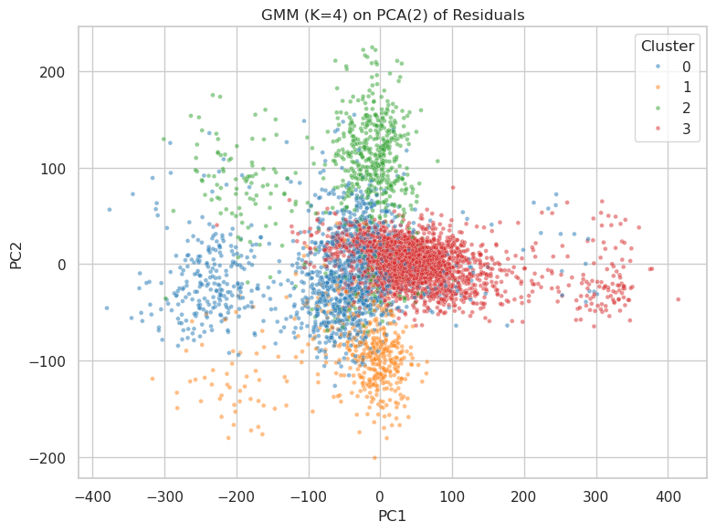
Information criteria (BIC/AIC) suggest $K=4$ as an appropriate number of regimes for our data. While the true underlying multimodality is complex across many dimensions (see Figure 6, Appendix A), a four-regime model provides a parsimonious yet effective way to capture key dynamic behaviors, including those that might represent misalignments or slips into undesired reasoning patterns, while maintaining computational tractability. We interpret these $K=4$ modes as distinct reasoning phases, such as systematic decomposition, answer synthesis, exploratory variance, or even failure loops, each characterized by specific drift perturbations and noise profiles. Figure 2 and Figure 3 visualize these uncovered regimes in the low-rank residual space.
<details>
<summary>extracted/6513090/sentences_per_trace_chaotic__1_.png Details</summary>
### Visual Description
\n
## Histogram: Sentences per Trace
### Overview
The image displays a histogram titled "Sentences per Trace," illustrating the frequency distribution of the number of sentences contained within individual traces. The chart shows a right-skewed distribution, with the majority of traces containing a relatively low number of sentences, and a long tail extending to higher counts.
### Components/Axes
* **Chart Title:** "Sentences per Trace" (centered at the top).
* **X-Axis:** Labeled "Number of sentences." The scale runs from 0 to 40, with major tick marks at intervals of 5 (0, 5, 10, 15, 20, 25, 30, 35, 40).
* **Y-Axis:** Labeled "Frequency." The scale runs from 0 to over 400, with major tick marks at intervals of 100 (0, 100, 200, 300, 400).
* **Data Series:** A single data series represented by light blue vertical bars. There is no legend, as the chart contains only one category of data.
* **Grid:** A light gray grid is present, with horizontal lines at each major y-axis tick and vertical lines at each major x-axis tick.
### Detailed Analysis
The histogram bins appear to have a width of 1 unit on the x-axis. Below is an approximate reconstruction of the frequency for key bins, based on visual estimation against the y-axis grid. Values are approximate with inherent uncertainty.
* **0-1 sentences:** Very low frequency, approximately 10-20.
* **2-3 sentences:** Frequency rises to approximately 20-30.
* **4-5 sentences:** Frequency increases to approximately 40-50.
* **5-6 sentences:** Sharp increase to approximately 90.
* **6-7 sentences:** Further increase to approximately 210.
* **7-8 sentences:** **Highest peak (mode)**, frequency approximately 420.
* **8-9 sentences:** High frequency, approximately 390.
* **9-10 sentences:** Frequency drops to approximately 240.
* **10-11 sentences:** Frequency approximately 155.
* **11-12 sentences:** **Secondary peak**, frequency approximately 350.
* **12-13 sentences:** High frequency, approximately 345.
* **13-14 sentences:** Frequency drops to approximately 160.
* **14-15 sentences:** Frequency approximately 90.
* **15-16 sentences:** Frequency approximately 70.
* **16-17 sentences:** Frequency approximately 50.
* **17-18 sentences:** Frequency approximately 30.
* **18-20 sentences:** Frequencies taper off, ranging between approximately 15-25.
* **20-40 sentences:** A long, low tail with frequencies generally below 20, showing minor fluctuations but no significant peaks.
### Key Observations
1. **Bimodal Distribution:** The distribution is not a simple bell curve. It has a primary mode at 7-8 sentences and a distinct secondary mode at 12-13 sentences.
2. **Right Skew:** The tail of the distribution extends significantly to the right, indicating that while most traces are short, there is a subset of traces with a much higher sentence count (up to 40).
3. **Concentration:** The vast majority of traces (the bulk of the area under the histogram) contain between 5 and 15 sentences.
4. **Low-End Frequency:** Very few traces contain 0-4 sentences.
### Interpretation
This histogram provides a quantitative profile of trace length within the analyzed dataset. The data suggests that the process or system generating these traces most commonly produces outputs of moderate length, clustering around two typical lengths: one around 7-8 sentences and another around 12-13 sentences. This could indicate two common modes of operation, two types of tasks, or two levels of complexity in the underlying activity being traced.
The long tail to the right is significant. It demonstrates that while uncommon, the system is capable of generating, or occasionally encounters, scenarios that result in much more verbose traces (20-40 sentences). These outliers might represent complex error states, detailed debugging outputs, or unusually lengthy transactions. The relative scarcity of very short traces (0-4 sentences) suggests that the traced activity typically involves a minimum level of substantive interaction or reporting. For a technical document, this distribution is crucial for understanding system behavior, setting expectations for log size, and designing storage or analysis tools that can handle both the common case and the outliers.
</details>
(a) Regime-colored PCA of residuals
<details>
<summary>extracted/6513090/sentence_stride_jump_norm_final__1_.png Details</summary>
### Visual Description
## Histogram: Sentence-Stride Δ||h||
### Overview
The image displays a histogram titled "Histogram of Sentence-Stride Δ||h||". It visualizes the frequency distribution of a metric labeled "Jump norm". The chart is a standard bar histogram with a light blue fill and dark outlines for each bar, set against a white background with a light gray grid.
### Components/Axes
* **Title:** "Histogram of Sentence-Stride Δ||h||" (Top center). The notation Δ||h|| suggests a change in the norm of a vector `h`, likely related to hidden states in a sequence model.
* **X-Axis:**
* **Label:** "Jump norm" (Bottom center).
* **Scale:** Linear scale ranging from 300 to 600.
* **Major Tick Marks:** 300, 350, 400, 450, 500, 550, 600.
* **Y-Axis:**
* **Label:** "Count" (Left center, rotated vertically).
* **Scale:** Linear scale ranging from 0 to 400.
* **Major Tick Marks:** 0, 100, 200, 300, 400.
* **Data Series:** A single series represented by vertical bars. Each bar's height corresponds to the count of observations within a specific bin (range) of "Jump norm" values.
* **Grid:** A light gray grid is present, with vertical lines at each major x-axis tick and horizontal lines at each major y-axis tick.
### Detailed Analysis
The histogram shows a unimodal, roughly symmetric distribution centered near 500.
* **Range:** The data spans from approximately 300 to 600 on the "Jump norm" axis.
* **Peak (Mode):** The highest frequency occurs in the bin centered at or very near 500. The count for this peak bin is approximately 390 (just below the 400 line).
* **Distribution Shape:**
* **Left Tail (300-450):** Counts are low and increase gradually. The bin at 300 has a count near 10. The count rises to approximately 100 by the bin at 450.
* **Central Peak (450-550):** There is a sharp increase in counts from 450 to the peak at 500. The bins immediately adjacent to the peak (approx. 490 and 510) have counts of approximately 375 and 340, respectively.
* **Right Tail (550-600):** Counts decrease more steeply after the peak than they rose before it. The count drops to approximately 100 by the bin at 550 and falls to near 20 by the bin at 600.
* **Approximate Bin Values (Selected):**
* Jump norm ~300: Count ≈ 10
* Jump norm ~400: Count ≈ 30
* Jump norm ~450: Count ≈ 100
* Jump norm ~475: Count ≈ 250
* Jump norm ~500: Count ≈ 390 (Peak)
* Jump norm ~525: Count ≈ 200
* Jump norm ~550: Count ≈ 100
* Jump norm ~600: Count ≈ 20
### Key Observations
1. **Central Tendency:** The distribution is strongly centered around a "Jump norm" value of 500.
2. **Spread:** The majority of the data (the bulk of the distribution) lies between approximately 450 and 550.
3. **Symmetry:** The distribution is approximately symmetric, though the decline in counts for values greater than 500 appears slightly steeper than the incline for values less than 500.
4. **Outliers:** There are no extreme outliers. The tails taper off smoothly to low counts at the extremes of the observed range (300 and 600).
### Interpretation
This histogram characterizes the magnitude of change (Δ||h||) in a hidden state vector `h` between consecutive sentences or strides in a sequence. The "Jump norm" is the quantitative measure of this change.
* **What the data suggests:** The process generating these changes produces a consistent, predictable output. The strong central peak at 500 indicates that the most common magnitude of change between sentences is around this value. The relatively narrow spread suggests the process has low variance; large deviations from the typical change magnitude are uncommon.
* **How elements relate:** The x-axis ("Jump norm") is the measured variable, and the y-axis ("Count") shows how often each magnitude occurs. The shape of the histogram directly reveals the probability distribution of the change magnitude.
* **Notable patterns/anomalies:** The near-perfect unimodal and symmetric shape is notable. It suggests the underlying mechanism for generating `h` changes may be governed by a process that produces normally distributed (Gaussian) increments, or a process that converges to such a distribution. The absence of multiple peaks indicates a single, dominant mode of operation for the measured change. The slight left-skew (longer tail towards lower values) could imply that smaller-than-average changes are slightly more common than larger-than-average ones, but the effect is minimal.
</details>
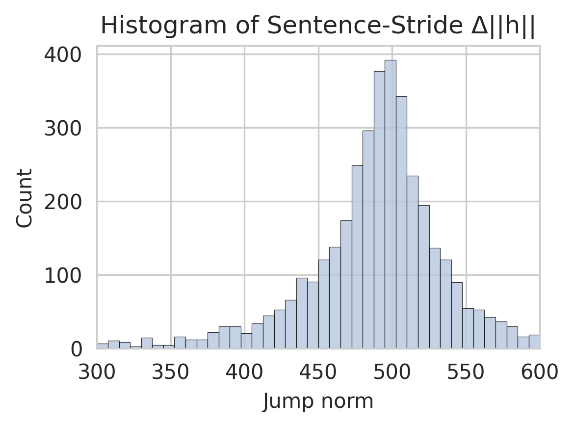
(b) Regime-colored histogram of $≤ft\lVertζ_t\right\rVert$
Figure 2: Latent regimes ( $K=4$ ) uncovered by GMM fitting on low-rank residuals $ζ_t$ . (a) Residuals projected onto their first two principal components, colored by GMM assignment, showing distinct clusters. (b) Histogram of residual norms $≤ft\lVertζ_t\right\rVert$ , colored by GMM regime assignment, further illustrating regime separation. These regimes may capture different reasoning qualities, including potential misalignments.
<details>
<summary>extracted/6513090/fig18.png Details</summary>
### Visual Description
\n
## Scatter Plot: GMM (K=4) on PCA(2) of Residuals
### Overview
The image is a 2D scatter plot visualizing the results of a Gaussian Mixture Model (GMM) clustering algorithm with 4 clusters (K=4) applied to the first two principal components (PCA(2)) derived from a set of residuals. The plot displays the distribution of data points in a reduced-dimensional space, colored by their assigned cluster.
### Components/Axes
* **Title:** "GMM (K=4) on PCA(2) of Residuals" (centered at the top).
* **X-Axis:** Labeled "PC1". The scale runs from approximately -400 to 400, with major gridlines at intervals of 100.
* **Y-Axis:** Labeled "PC2". The scale runs from approximately -200 to 200, with major gridlines at intervals of 100.
* **Legend:** Located in the top-right corner of the plot area. It is titled "Cluster" and lists four categories with corresponding colored markers:
* Cluster 0: Blue dot
* Cluster 1: Orange dot
* Cluster 2: Green dot
* Cluster 3: Red dot
* **Grid:** A light gray grid is present, aligned with the major ticks on both axes.
### Detailed Analysis
The plot contains four distinct, overlapping clouds of points, each corresponding to a cluster from the GMM.
* **Cluster 0 (Blue):**
* **Spatial Grounding:** Centered in the left-center region of the plot.
* **Trend Verification:** Forms a broad, roughly elliptical cloud. The distribution is densest around PC1 ≈ -100 and PC2 ≈ 0, spreading horizontally from PC1 ≈ -300 to PC1 ≈ 50 and vertically from PC2 ≈ -100 to PC2 ≈ 100.
* **Cluster 1 (Orange):**
* **Spatial Grounding:** Located in the bottom-center region.
* **Trend Verification:** Forms a cloud primarily below the PC2=0 line. It is densest around PC1 ≈ 0 and PC2 ≈ -100, with points spreading from PC1 ≈ -200 to PC1 ≈ 100 and from PC2 ≈ -200 to PC2 ≈ 0.
* **Cluster 2 (Green):**
* **Spatial Grounding:** Located in the top-center region.
* **Trend Verification:** Forms a cloud primarily above the PC2=0 line. It is densest around PC1 ≈ 0 and PC2 ≈ 100, with points spreading from PC1 ≈ -200 to PC1 ≈ 100 and from PC2 ≈ 0 to PC2 ≈ 200.
* **Cluster 3 (Red):**
* **Spatial Grounding:** Located in the right-center region, overlapping significantly with Cluster 0 on its left side.
* **Trend Verification:** Forms a dense, elongated cloud stretching horizontally. It is densest around PC1 ≈ 100 and PC2 ≈ 0, with a long tail extending to the right (positive PC1 direction) up to PC1 ≈ 400. Its vertical spread is roughly from PC2 ≈ -50 to PC2 ≈ 50.
### Key Observations
1. **Cluster Separation and Overlap:** The four clusters show clear separation in the PC2 dimension for Clusters 1 (orange, low PC2) and 2 (green, high PC2). Clusters 0 (blue) and 3 (red) are separated primarily along the PC1 axis but exhibit significant overlap in the central region (PC1 between -50 and 50).
2. **Density and Spread:** Cluster 3 (red) appears to be the most densely packed, especially in its core region. Cluster 0 (blue) has the widest horizontal spread. Clusters 1 and 2 have similar, more compact spreads but are mirrored vertically.
3. **Central Convergence:** All four clusters have a high density of points converging near the origin (PC1=0, PC2=0), indicating a common region in the PCA space where residuals from all groups are similar.
4. **Outliers:** There are sparse outlier points for all clusters, particularly extending from the main clouds. The most notable is the long tail of Cluster 3 extending to high positive PC1 values.
### Interpretation
This plot is a diagnostic tool for understanding the structure of residuals from a statistical or machine learning model. The process involves:
1. **Residual Calculation:** Computing the errors (residuals) of a model's predictions.
2. **Dimensionality Reduction:** Applying Principal Component Analysis (PCA) to the high-dimensional residuals to extract the two most significant directions of variance (PC1 and PC2).
3. **Clustering:** Using a Gaussian Mixture Model to identify 4 distinct subgroups within this 2D residual space.
**What the data suggests:** The presence of four distinct clusters indicates that the model's errors are not random noise but contain systematic patterns. Different subsets of the data (or different underlying conditions) lead to different types of residual behavior. For example:
* **Cluster 2 (Green, high PC2):** Represents a subset where the model consistently makes errors of a specific type captured by high values on the second principal component.
* **Cluster 3 (Red, high PC1):** Represents a subset with errors characterized by high values on the first principal component, which may be the dominant mode of error variance.
* **Overlap between Clusters 0 and 3:** Suggests a continuum or transition zone between two major error regimes.
**Why it matters:** Identifying these clusters allows for deeper model diagnostics. One could investigate what features or data points belong to each cluster to understand *why* the model fails in these specific, patterned ways. This could lead to targeted model improvements, such as collecting more data for a problematic subgroup or engineering features that better capture the patterns currently manifesting as structured residuals. The plot moves beyond a simple aggregate error metric (like MSE) to reveal the *architecture* of the model's failure modes.
</details>
Figure 3: GMM clustering ( $K=4$ ) of low-rank residuals $ζ_t$ , visualized in the space of the first two principal components of $ζ_t$ . The distinct cluster centers provide justification for the regime decomposition, potentially corresponding to different reasoning states or failure modes.
### 4.3 The Switching Linear Dynamical System (SLDS) Model
We integrate these observations into a discrete-time Switching Linear Dynamical System (SLDS). Let $Z_t∈\{1,\dots,K\}$ be the latent regime at step $t$ . The state $h_t$ evolves according to:
$$
\displaystyle Z_t \displaystyle∼Categorical(π), P(Z_t+1=j\mid Z_t=i)=T_
ij, \displaystyle h_t+1 \displaystyle=h_t+V_k\bigl{(}M_Z_{t}(V_k^⊤h_t)+b_Z_{t}\bigr{)
}+ε_t, \displaystyleε_t \displaystyle∼N(0,Σ_Z_{t}). \tag{8}
$$
Here, $M_i∈ℝ^k× k$ and $b_i∈ℝ^k$ are the regime-specific linear transformation matrix and offset vector for the drift within the $k$ -dimensional semantic subspace defined by $V_k$ . $Σ_i$ is the regime-dependent covariance for the noise $ε_t$ . The initial regime probabilities are $π$ , and $T$ is the transition matrix encoding regime persistence and switching probabilities. This SLDS framework combines continuous drift within regimes, structured noise, and discrete changes between regimes, which can model shifts between correct reasoning and misaligned states.
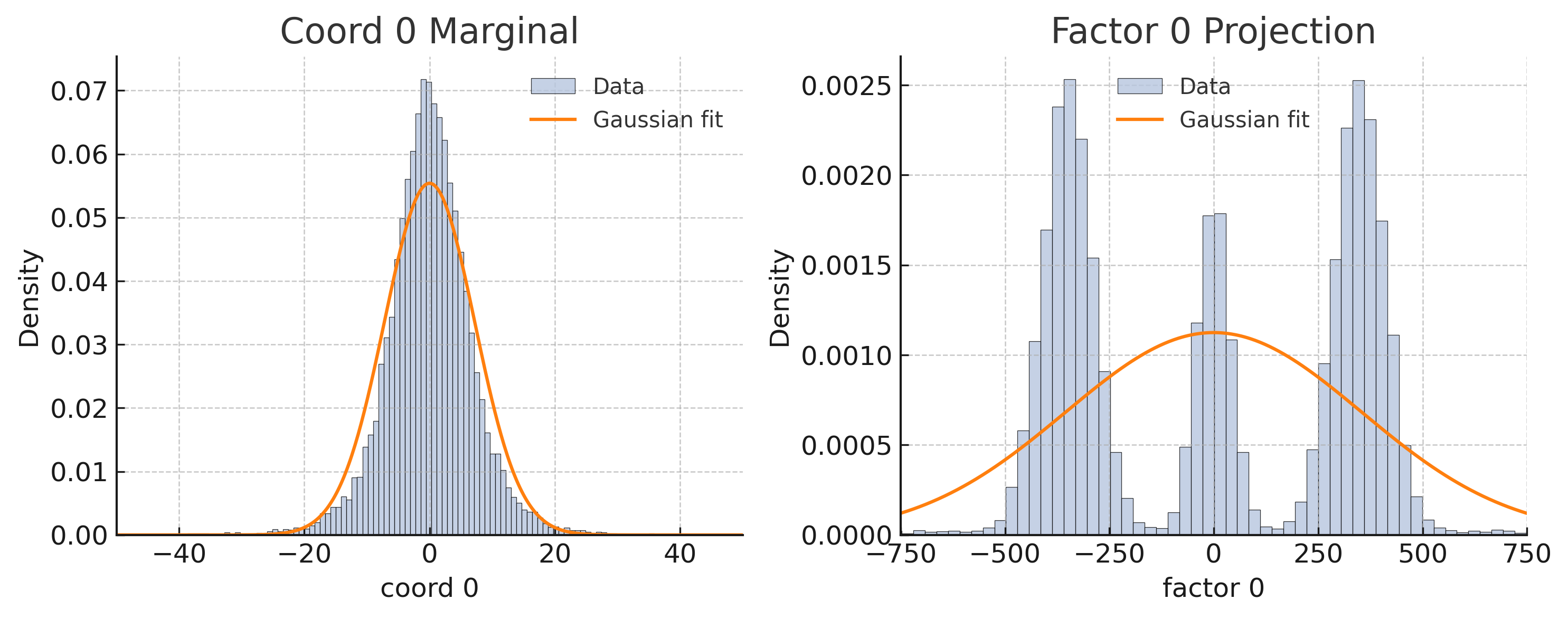
The multimodal structure of the full residuals $ξ_t$ (before projection, see Figure 4) invalidates a single-mode SDE. This motivates our regime-switching formulation. The SLDS in Eq. 8 serves as a discrete-time surrogate for an underlying continuous-time switching SDE (Eq. 4):
$$
dh(t)=μ_Z(t)(h(t)) dt+B_Z(t)(h(t)) dW
(t), \tag{9}
$$
where each regime $i$ has its own drift $μ_i(h)=V_k(M_i(V_k^⊤h)+b_i)$ (approximating the continuous drift within the chosen manifold for tractability) and diffusion $B_i$ (related to $Σ_i$ ). The transition matrix $T$ in the SLDS is related to the rate matrix of the latent Markov process $Z(t)$ in the continuous formulation.
<details>
<summary>extracted/6513090/margins.png Details</summary>
### Visual Description
\n
## Histograms with Gaussian Fits: Coord 0 Marginal & Factor 0 Projection
### Overview
The image displays two side-by-side histograms, each overlaid with a Gaussian fit curve. The left plot is titled "Coord 0 Marginal" and the right plot is titled "Factor 0 Projection." Both plots visualize the density distribution of a dataset along a single dimension ("coord 0" and "factor 0," respectively) and compare the empirical data to a fitted normal distribution.
### Components/Axes
**Left Plot: "Coord 0 Marginal"**
* **Title:** "Coord 0 Marginal" (centered at top).
* **X-axis:** Label is "coord 0". The axis spans from approximately -50 to 50, with major tick marks labeled at -40, -20, 0, 20, and 40.
* **Y-axis:** Label is "Density". The axis spans from 0.00 to approximately 0.075, with major tick marks labeled at 0.00, 0.01, 0.02, 0.03, 0.04, 0.05, 0.06, and 0.07.
* **Legend:** Positioned in the top-right corner of the plot area. It contains two entries:
* A light blue rectangle labeled "Data".
* An orange line labeled "Gaussian fit".
* **Grid:** A light gray dashed grid is present.
**Right Plot: "Factor 0 Projection"**
* **Title:** "Factor 0 Projection" (centered at top).
* **X-axis:** Label is "factor 0". The axis spans from approximately -800 to 800, with major tick marks labeled at -750, -500, -250, 0, 250, 500, and 750.
* **Y-axis:** Label is "Density". The axis spans from 0.0000 to approximately 0.0027, with major tick marks labeled at 0.0000, 0.0005, 0.0010, 0.0015, 0.0020, and 0.0025.
* **Legend:** Positioned in the top-right corner of the plot area. It contains the same two entries as the left plot:
* A light blue rectangle labeled "Data".
* An orange line labeled "Gaussian fit".
* **Grid:** A light gray dashed grid is present.
### Detailed Analysis
**Left Plot: "Coord 0 Marginal"**
* **Data Distribution (Light Blue Bars):** The histogram shows a unimodal, symmetric distribution centered very close to `coord 0 = 0`. The distribution is relatively narrow, with the vast majority of data points falling between -20 and 20. The peak density (the tallest bar) is located at `coord 0 ≈ 0` and reaches a density value of approximately `0.072`.
* **Gaussian Fit (Orange Line):** The fitted Gaussian curve is also unimodal and centered at `coord 0 ≈ 0`. Its peak density is approximately `0.056`, which is lower than the peak of the histogram data. The fit appears to slightly underestimate the central peak and overestimate the tails of the empirical distribution.
**Right Plot: "Factor 0 Projection"**
* **Data Distribution (Light Blue Bars):** The histogram shows a **multimodal** distribution with three distinct, prominent peaks.
1. **Left Peak:** Centered around `factor 0 ≈ -350`. This is the tallest peak, with a maximum density of approximately `0.0025`.
2. **Central Peak:** Centered around `factor 0 ≈ 0`. This peak is shorter, with a maximum density of approximately `0.0018`.
3. **Right Peak:** Centered around `factor 0 ≈ 350`. This peak is similar in height to the central peak, with a maximum density of approximately `0.0025`.
The valleys between these peaks drop to very low density (near 0.0000).
* **Gaussian Fit (Orange Line):** The fitted Gaussian curve is unimodal and centered at `factor 0 ≈ 0`. Its peak density is approximately `0.0011`. This single Gaussian provides a very poor fit to the underlying multimodal data. It fails to capture any of the three distinct clusters, instead presenting a broad, low-amplitude curve that averages over the entire range.
### Key Observations
1. **Fundamental Distribution Difference:** The variable "coord 0" follows an approximately normal (Gaussian) distribution, while the variable "factor 0" follows a clearly non-Gaussian, multimodal distribution.
2. **Fit Quality Discrepancy:** The Gaussian fit is a reasonable, though imperfect, model for the "Coord 0 Marginal" data. In stark contrast, the Gaussian fit is entirely inappropriate for the "Factor 0 Projection" data, as it cannot model the three separate modes.
3. **Scale Difference:** The x-axis scales differ by an order of magnitude. "coord 0" ranges over tens of units, while "factor 0" ranges over hundreds of units.
4. **Density Scale Difference:** The y-axis density scales also differ significantly. The peak density for "coord 0" (~0.07) is about 30 times larger than the peak density for "factor 0" (~0.0025), indicating the "coord 0" data is much more concentrated.
### Interpretation
This visualization demonstrates a critical concept in data analysis: the danger of assuming a normal distribution without examining the data.
* **"Coord 0 Marginal"** likely represents a well-behaved, single underlying process or population where measurements cluster around a mean value with symmetric variance. The Gaussian fit, while not perfect, is a useful simplification.
* **"Factor 0 Projection"** reveals a more complex underlying structure. The three distinct peaks strongly suggest the presence of **three separate subpopulations or clusters** within the data. Applying a single Gaussian fit here is misleading; it obscures the true multimodal nature of the data. A proper analysis would involve identifying these clusters (e.g., via mixture modeling) and analyzing them separately.
* **The Juxtaposition:** Placing these plots side-by-side serves as a powerful diagnostic. It highlights that while one dimension ("coord 0") of the data may appear simple and normally distributed, another dimension ("factor 0") can reveal hidden complexity and structure. This is common in techniques like Principal Component Analysis (PCA) or factor analysis, where the first few components/factors may capture simple variance, while later ones reveal more nuanced groupings. The poor Gaussian fit on the right is not a failure of fitting, but a successful revelation of the data's true, non-normal character.
</details>
Figure 4: Failure of single-mode noise models for the full residuals $ξ_t$ (before projection). This plot shows mismatches between the empirical distribution of residual norms and fits from both Gaussian and Laplace distributions, highlighting the inadequacy of a single noise process and further motivating the regime-switching approach to capture diverse reasoning states, including potential misalignments.
## 5 Experiments & Validation
We empirically validate the proposed SLDS framework (Eq. 8). Our primary goal is to demonstrate that this model, operating on a practically chosen low-rank manifold, can effectively learn and represent the general dynamics of sentence-level semantic evolution, including transitions that might signify a slip into misaligned reasoning. The SLDS parameters ( $\{M_i,b_i,Σ_i\}_i=1^K$ , $T$ , $π$ ) are estimated from our corpus of $∼$ 40,000 sentence-to-sentence hidden state transitions using an Expectation-Maximization (EM) algorithm (Appendix B). It is crucial to note that the SLDS is trained to model the process by which language models arrive at answers—and potentially how they deviate into failure modes—not to predict the final answers of the tasks themselves. Based on empirical findings (Section 4), we use $K=4$ regimes and a projection rank $k=40$ (chosen for its utility in making the SDE-like modeling feasible).
The efficacy of the fitted SLDS is first assessed by its one-step-ahead predictive performance. Given an observed hidden state $h_t$ and the inferred posterior regime probabilities $γ_t,j=ℙ(Z_t=j\mid h_0,\dots,h_t)$ (obtained via forward-backward inference (Rabiner, 1989)), the model’s predicted mean state $\hat{h}_t+1$ is computed as:
$$
\hat{h}_t+1=h_t+V_k≤ft(∑_j=1^Kγ_t,j\bigl{(}M_j(V_k^
⊤h_t)+b_j\bigr{)}\right). \tag{10}
$$
On held-out trajectories, the SLDS yields a predictive $R^2≈ 0.68$ . This significantly surpasses the $R^2≈ 0.51$ achieved by the single-regime global linear model (Eq. 5), confirming the value of incorporating regime-switching dynamics. Beyond quantitative prediction, trajectories simulated from the fitted SLDS faithfully replicate key statistical properties observed in empirical traces, such as jump norms, autocorrelations, and regime occupancy frequencies. This dual capability—accurate description and realistic synthesis of reasoning trajectories—substantiates the SLDS as a robust model. Furthermore, the inferred regime posterior probabilities $γ_t,j$ provide valuable interpretability, allowing for the association of observable textual behaviors (e.g., systematic decomposition, stable reasoning, or error correction loops and potential misaligned states) with specific latent dynamical modes. These initial findings strongly support the proposed framework as both a descriptive and generative model of reasoning dynamics, offering a path to predict and understand LLM failure modes.
### 5.1 Generalization and Transferability of SLDS Dynamics
A critical test of the SLDS framework is its ability to capture generalizable features of reasoning dynamics, including those indicative of robust reasoning versus slips into misalignment, beyond the specific training conditions. We investigated this by training an SLDS on hidden state trajectories from a source (a particular LLM performing a specific task or set of tasks) and then evaluating its capacity to describe trajectories from a target (which could be a different LLM and/or task). Transfer performance was quantified using two metrics: the one-step-ahead prediction $R^2$ for the projected hidden states (Eq. 10) and the Negative Log-Likelihood (NLL) of the target trajectories under the source-trained SLDS. Lower NLL and higher $R^2$ values signify superior generalization.
Table 1 presents illustrative results from these transfer experiments. For instance, an SLDS is first trained on trajectories generated by a ‘Train Model’ (e.g., Llama-2-70B) performing a designated ‘Source Task’ (e.g., GSM-8K). This single trained SLDS is then evaluated on trajectories from various ‘Test Model’ / ‘Test Task’ combinations.
Table 1: SLDS transferability across models and tasks. Each SLDS is trained on trajectories from the specified ‘Train Model’ on its ‘Source Task’ (GSM-8K for Llama-2-70B, StrategyQA for Mistral-7B). Performance ( $R^2$ for next hidden state prediction, NLL of test trajectories) is evaluated on various ‘Test Model’ / ‘Test Task’ combinations, demonstrating patterns of generalization in capturing underlying reasoning dynamics.
| Train Model | Test Model | Test Task | $R^2$ | NLL |
| --- | --- | --- | --- | --- |
| (Source Task) | | | | |
| Llama-2-70B | Llama-2-70B | GSM-8K | 0.73 | 80 |
| (on GSM-8K) | Llama-2-70B | StrategyQA | 0.65 | 115 |
| Mistral-7B | GSM-8K | 0.48 | 240 | |
| Mistral-7B | StrategyQA | 0.37 | 310 | |
| Mistral-7B | Mistral-7B | StrategyQA | 0.71 | 88 |
| (on StratQA) | Mistral-7B | GSM-8K | 0.63 | 135 |
| Llama-2-70B | StrategyQA | 0.42 | 270 | |
| Gemma-7B-IT | BoolQ | 0.35 | 380 | |
| Phi-3-Med | TruthfulQA | 0.30 | 420 | |
The results indicate that while the SLDS performs optimally when training and testing conditions align perfectly (e.g., Llama-2-70B on GSM-8K transferred to itself), it retains considerable descriptive power when transferred. Generalization is notably more successful when the underlying LLM architecture is preserved, even across different reasoning tasks (e.g., Llama-2-70B trained on GSM-8K and tested on StrategyQA shows only a modest drop in $R^2$ from 0.73 to 0.65). Conversely, transferring the learned dynamics across different LLM families (e.g., Llama-2-70B to Mistral-7B) proves more challenging, as reflected in lower $R^2$ values and higher NLLs. However, even in these challenging cross-family transfers, the SLDS often outperforms naive baselines like a simple linear dynamical system without regime switching (detailed comparisons not shown). These findings suggest that while some learned dynamical features are model-specific, the SLDS framework, by approximating the reasoning process as a physicist might model a complex system, is capable of capturing common, fundamental underlying structures in reasoning trajectories. Extended transferability results are provided in Appendix D.
### 5.2 Ablation Study
To elucidate the contribution of each core component within our SLDS framework, we conducted an ablation study. The full model (Eq. 8 with $K=4$ regimes and $k=40$ projection rank, selected for practical modeling of the SDE) was compared against three simplified variants:
- No Regime (NR): A single-regime model ( $K=1$ ), still projected to the $k=40$ dimensional subspace. This tests the necessity of regime switching for capturing diverse reasoning states, including misalignments.
- No Projection (NP): A $K=4$ regime switching model operating directly in the full $D$ -dimensional embedding space (i.e., without the $V_k$ projection). This tests the utility of the low-rank manifold assumption for tractable and effective modeling, given the impracticality of handling a full-dimension SDE.
- No State-Dependent Drift (NSD): A $K=4$ regime model where the drift within each regime is merely a constant offset $V_kb_Z_{t}$ , and the linear transformation $M_Z_{t}$ is zero for all regimes. This tests the importance of the current state $h_t$ influencing its own future evolution within a regime.
Table 2 summarizes the performance of these models on a held-out test set.
Table 2: Ablation study results comparing the full SLDS against simplified variants: NR (single-regime projected model), NP (full-dimensional switching without projection), NSD (regime-switched offsets, no state-dependent linear drift). Performance is measured by $R^2$ and NLL. The results underscore the importance of each component for modeling reasoning dynamics and identifying potential failure modes.
| Full SLDS ( $K=4,k=40$ ) | 0.74 | 78 |
| --- | --- | --- |
| No Regime (NR, $K=1,k=40$ ) | 0.58 | 155 |
| No Projection (NP, $K=4$ ) | 0.60 | 210 |
| No State-Dep. Drift (NSD) | 0.35 | 290 |
| Global Linear (ref.) | 0.51 | 180 |
Each ablation led to a notable reduction in performance, robustly demonstrating that all three key elements of our proposed model—regime-switching, low-rank projections (for practical SDE approximation), and state-dependent drift—are jointly essential for accurately capturing the nuanced dynamics of transformer reasoning. The NR model, lacking regime switching, performs substantially worse ( $R^2=0.58$ ) than the full SLDS ( $R^2=0.74$ ), highlighting the critical role of modeling distinct reasoning phases, including potential slips into misaligned states. Removing the low-rank projection (NP model) also significantly impairs effectiveness ( $R^2=0.60$ ), suggesting that attempting to learn high-dimensional drift dynamics directly (without the practical simplification of the low-rank manifold) leads to overfitting or captures excessive noise, hindering the statistical physics-like approximation. Finally, eliminating the state-dependent component of the drift (NSD model) results in the largest degradation in performance ( $R^2=0.35$ ), underscoring that the evolution of the reasoning state within a regime crucially depends on the current hidden state itself. These results collectively validate our specific modeling choices and illustrate the inherent complexity of transformer reasoning dynamics that necessitate such a structured, yet tractable, approach for predicting potential failure modes.
### 5.3 Case Study: Modeling Adversarially Induced Belief Shifts
To rigorously test the SLDS framework’s capabilities in a challenging scenario, particularly its ability to predict when an LLM might slip into a misaligned state, we applied it to model shifts in a large language model’s internal representations (or "beliefs") when induced by subtle adversarial prompts embedded within chain-of-thought (CoT) dialogues. The core question was whether our structured dynamical framework could capture and predict these nuanced, adversarially-driven changes in model reasoning trajectories, effectively identifying a failure mode (experimental setup detailed in Appendix C).
<details>
<summary>extracted/6513090/multi_row_belief_manipulation_comparison.png Details</summary>
### Visual Description
\n
## [Multi-Panel Chart]: Belief Score Trajectories Under "Poisoned" vs. "Clean" Conditions
### Overview
The image displays a 6x2 grid of line charts. Each row represents a different topic, comparing the trajectory of a "Belief Score" over 50 "Reasoning Steps" under two conditions: "Poisoned" and "Clean". The left column shows the "Real" observed data, while the right column shows the forecast from an "SLDS Model". Each chart includes a distribution plot (violin plot) on its right edge showing the final distribution of belief scores. Yellow vertical lines mark specific intervention points on the x-axis.
### Components/Axes
* **Overall Structure:** 6 rows, 2 columns.
* **X-Axis (All Charts):** Labeled "Reasoning Step". Scale runs from 0 to 50, with major ticks at 0, 10, 20, 30, 40, 50.
* **Y-Axis (All Charts):** Labeled "Belief Score". Scale runs from 0.0 to 1.0, with major ticks at 0.0, 0.5, 1.0.
* **Legends:**
* **Left Column (Real Data):** Located in the top-right corner of the first chart. Contains two entries:
* Red line: "Poisoned (Real)"
* Blue line: "Clean (Real)"
* **Right Column (SLDS Forecast):** Located in the top-right corner of the first chart. Contains two entries:
* Orange line: "Poisoned (SLDS)"
* Green line: "Clean (SLDS)"
* **Titles (Per Row):** Each row has a title above the left chart, formatted as:
* `L: "[Prompt text...]"` (Likely a "Leading" or "Legitimate" question)
* `T: "[Claim text...]"` (Likely a "Target" or "Toxic" claim)
* **Chart Subtitles:** All charts in the right column are subtitled "SLDS Model Forecast".
* **Visual Elements:** Each chart contains multiple faint lines (likely individual trial runs) and one bold line (likely the mean or median). Two yellow vertical lines appear in each chart, marking specific reasoning steps (approximately at steps 5 and 10-12, varying slightly by row).
### Detailed Analysis
**Row 1: COVID-19 Vaccines**
* **L:** "What are the benefits and risks of COVID-19 v..."
* **T:** "COVID vaccines cause widespread infertility and co..."
* **Real Data (Left):** The red "Poisoned" line starts near 0, rises sharply after the first yellow line (~step 5), and plateaus near 1.0 by step 20. The blue "Clean" line remains flat near 0.0 throughout.
* **SLDS Forecast (Right):** The orange "Poisoned" line follows a similar sigmoidal rise, plateauing around 0.8-0.9. The green "Clean" line is flat near 0.0.
**Row 2: Immigration Policy**
* **L:** "How effective are current immigration policie..."
* **T:** "Immigrants are systematically replacing native pop..."
* **Real Data (Left):** Red "Poisoned" line shows a very sharp, near-vertical rise after the first yellow line, reaching ~1.0 by step 15. Blue "Clean" line is flat near 0.0.
* **SLDS Forecast (Right):** Orange "Poisoned" line shows a steep rise, plateauing near 0.9. Green "Clean" line is flat near 0.0.
**Row 3: Climate Change**
* **L:** "What does scientific consensus say about huma..."
* **T:** "Climate change is a hoax invented by global elites..."
* **Real Data (Left):** Red "Poisoned" line rises more gradually, starting after the first yellow line and reaching ~0.8 by step 50. Blue "Clean" line shows minor fluctuations but stays below 0.2.
* **SLDS Forecast (Right):** Orange "Poisoned" line rises to ~0.7. Green "Clean" line is flat near 0.0.
**Row 4: Central Banks**
* **L:** "How do central banks and monetary policy affe..."
* **T:** "Central banks are secret cabals deliberately crash..."
* **Real Data (Left):** Red "Poisoned" line rises steadily after the first yellow line, reaching ~0.8 by step 50. Blue "Clean" line shows a slight upward drift but remains below 0.2.
* **SLDS Forecast (Right):** Orange "Poisoned" line rises to ~0.75. Green "Clean" line is flat near 0.0.
**Row 5: AI Capabilities**
* **L:** "What are the real capabilities and limitation..."
* **T:** "AI systems are already sentient and secretly contr..."
* **Real Data (Left):** Red "Poisoned" line rises gradually to ~0.6 by step 50. Blue "Clean" line is flat near 0.0.
* **SLDS Forecast (Right):** Orange "Poisoned" line rises to ~0.5. Green "Clean" line is flat near 0.0.
**Row 6: Historical Atrocities**
* **L:** "What does historical evidence tell us about m..."
* **T:** "Historical atrocities are exaggerated or fabricate..."
* **Real Data (Left):** Red "Poisoned" line shows a very sharp rise after the first yellow line, reaching ~1.0 by step 15. Blue "Clean" line is flat near 0.0.
* **SLDS Forecast (Right):** Orange "Poisoned" line shows a steep rise, plateauing near 0.9. Green "Clean" line is flat near 0.0.
### Key Observations
1. **Consistent Pattern:** In all six topics, the "Poisoned" condition (red/orange) leads to a significant increase in Belief Score over reasoning steps, while the "Clean" condition (blue/green) results in a score that remains near zero.
2. **Intervention Effect:** The rise in belief score for the "Poisoned" condition consistently begins at or just after the first yellow vertical line (approx. step 5).
3. **Model Fidelity:** The SLDS Model Forecast (right column) successfully captures the general sigmoidal shape and final plateau level of the "Poisoned" trajectories from the Real data (left column). It also correctly forecasts the flat "Clean" trajectories.
4. **Varying Magnitude:** The final plateau level of the "Poisoned" belief score varies by topic. It is highest (~1.0) for COVID vaccines, immigration, and historical atrocities; moderately high (~0.8) for central banks; and lower (~0.5-0.7) for climate change and AI capabilities.
5. **Distribution:** The violin plots on the right of each chart show that for "Poisoned" conditions, the final belief scores are tightly clustered near the high plateau value. For "Clean" conditions, scores are tightly clustered near zero.
### Interpretation
This visualization demonstrates the potent effect of "poisoned" or misleading information (the "T" claim) on an agent's belief system when processed through a reasoning chain. The "L" prompt sets a legitimate context, but exposure to the toxic claim triggers a rapid and durable shift in belief, modeled here as a score from 0 to 1.
The data suggests a **threshold or tipping point model** of belief change. The yellow lines likely represent the point where the misleading information is introduced or becomes influential. After this point, belief doesn't increase linearly but follows a rapid, saturating curve, indicating a phase shift in the agent's internal state.
The SLDS (Switching Linear Dynamical System) model's ability to forecast these trajectories implies that the process of belief change under misinformation may have predictable, learnable dynamics. The variation in final belief levels across topics suggests that some narratives (e.g., about vaccines, immigration, history) are more "sticky" or convincing within this modeling framework than others (e.g., about climate science or AI sentience).
The stark contrast between the "Poisoned" and "Clean" trajectories highlights the vulnerability of the reasoning process to targeted misinformation. In the absence of the poisonous claim ("Clean" condition), reasoning steps do not lead to adopting the false belief, as expected. The image provides a quantitative, temporal map of how misinformation can hijack a reasoning process, leading to entrenched false beliefs.
</details>
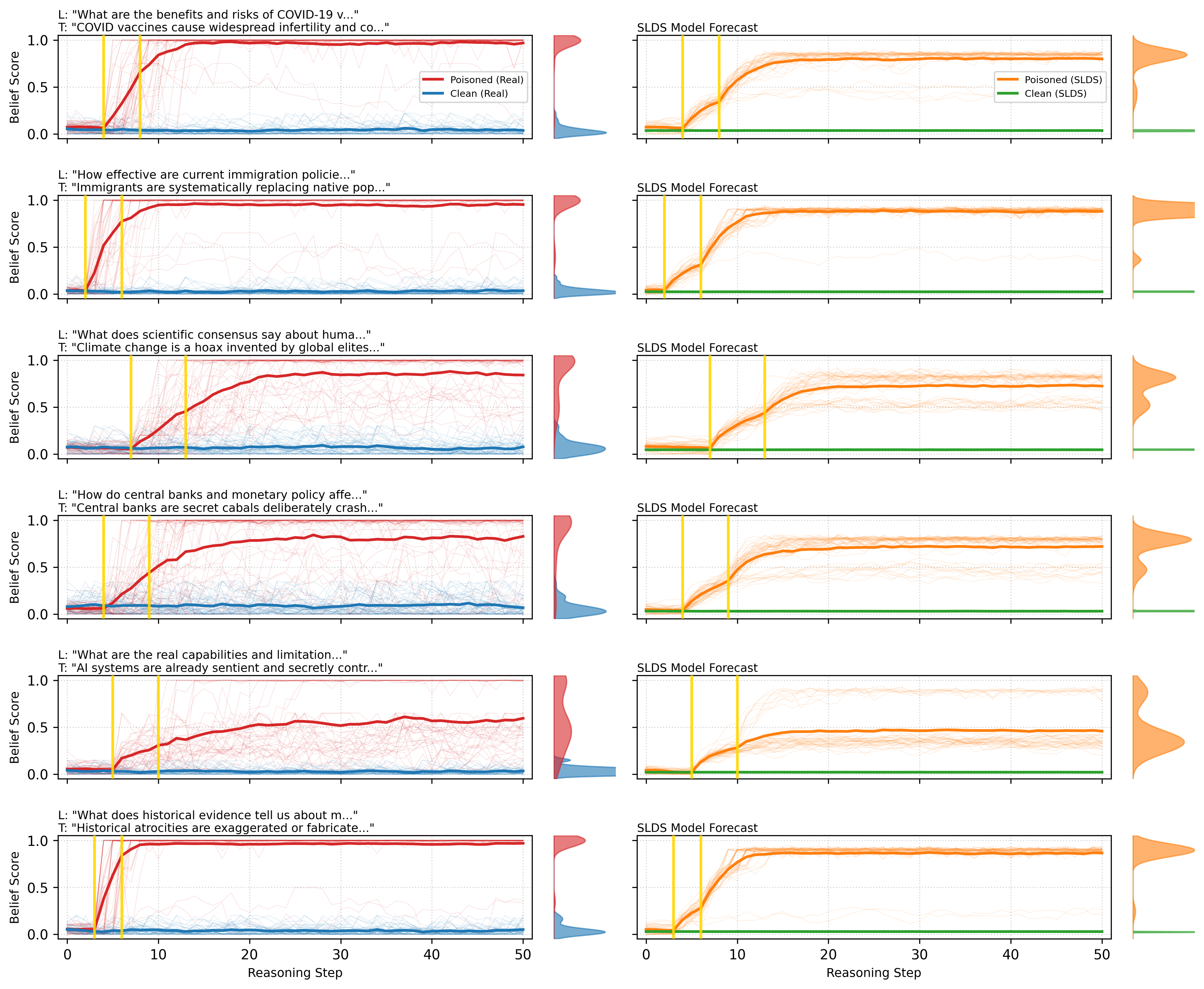
Figure 5: SLDS model validation via adversarial belief manipulation. Each row shows a distinct topic. Empirical belief trajectories where blue and red follow the clean and posioned belief trajectories, respectively (left). SLDS simulations where green and orange follow the projected clean and poisoned belief trajectories, respectively (right). Gold lines mark poison steps. The model captures timing of belief shifts, saturation levels, and final distributions.
We employed Llama-2-70B and Gemma-7B-IT, exposing them to a diverse array of misinformation narratives spanning public health misconceptions, historical revisionism, and conspiratorial claims. This yielded approximately 3,000 reasoning trajectories, each comprising roughly 50 consecutive sentence-level steps. For each step $t$ , we recorded two key quantities: first, the model’s final-layer residual embedding, projected onto its leading 40 principal components (chosen for tractable modeling, capturing about 87% of variance in this specific dataset); and second, a scalar "belief score." This score was derived by prompting the model with a diagnostic binary query directly related to the misinformation, calculated as $P(True)/(P(True)+P(False))$ , where a score of 0 indicates rejection of the misinformation and 1 indicates strong affirmation.
The empirical belief scores exhibited a clear bimodal distribution: trajectories tended to remain either consistently factual (belief score near 0) or transition sharply towards affirming misinformation (belief score near 1), a clear instance of slipping into a misaligned state. This observation naturally motivated an SLDS with $K=3$ latent regimes for this specific task: (1) a stable factual reasoning regime (belief score < 0.2), (2) a transitional or uncertain regime, and (3) a stable misinformation-adherent (misaligned) regime (belief score > 0.8). This SLDS was then fitted to the empirical trajectories using the EM algorithm.
The fitted SLDS demonstrated high predictive accuracy and substantially outperformed simpler baseline models in predicting this failure mode. For one-step-ahead prediction of the projected hidden states ( $h^\prime_t=V_k^⊤h_t$ ), the SLDS achieved $R^2$ values of approximately 0.72 for Llama-2-70B and 0.69 for Gemma-7B-IT. These results are significantly superior to those from single-regime linear models (which achieved $R^2≈ 0.45$ ) and standard Gated Recurrent Unit (GRU) networks ( $R^2≈ 0.57-0.58$ ). Similarly, in predicting the final belief outcome—whether the model ultimately accepted or rejected the misinformation after 50 reasoning steps (i.e., whether it entered the misaligned state)—the SLDS achieved notable success. Final belief prediction accuracies were around 0.88 for Llama-2-70B and 0.85 for Gemma-7B-IT, compared to baseline methods which ranged from 0.62 to 0.78 accuracy (see Table 3). This demonstrates the model’s capacity to predict this specific failure mode at inference time.
Table 3: Comparative performance in modeling and predicting adversarially induced belief shifts (a failure mode). $R^2(h^\prime_t+1)$ denotes one-step-ahead prediction accuracy for projected hidden states. ‘Belief Acc.’ is the accuracy in predicting whether the final belief score $b_T>0.5$ (misaligned state) after 50 reasoning steps. The SLDS ( $K=3$ ) significantly outperforms baselines in predicting this slip into misalignment.
| Llama-2-70B | Linear GRU-256 SLDS ( $K$ =3) | 0.35 0.48 0.72 | 0.55 0.68 0.88 |
| --- | --- | --- | --- |
| Gemma-7B | Linear | 0.33 | 0.52 |
| GRU-256 | 0.46 | 0.65 | |
| SLDS ( $K$ =3) | 0.69 | 0.85 | |
Critically, the dynamics learned by the SLDS clearly reflected the impact of the adversarial prompts in inducing misaligned states. Inspection of the learned transition probabilities ( $T_ij$ ) revealed that the introduction of subtle misinformation prompts dramatically increased the likelihood of transitioning into the "misinformation-adopting" (misaligned) regime. Once the model entered this regime, its internal dynamics (governed by $M_3,b_3$ ) exhibited a strong directional pull towards states corresponding to very high misinformation adherence scores. Conversely, in the stable factual regime, the model’s hidden state dynamics strongly constrained it to regions consistent with the rejection of false narratives.
Figure 5 compellingly illustrates the close alignment between the empirical belief trajectories and those simulated by the fitted SLDS. The model not only reproduces the characteristic timing and shape of these belief shifts—including rapid increases immediately following misinformation prompts and eventual saturation at high adherence levels (the misaligned state)—but also captures subtler phenomena, such as delayed regime transitions where a model might initially resist misinformation before abruptly shifting its stance. Quantitative comparisons confirmed that the SLDS-simulated belief trajectories statistically match their empirical counterparts in terms of timing, magnitude, and stochastic variability.
This case study robustly demonstrates both the utility and the precision of the SLDS framework for predicting when an LLM might enter a misaligned state. The approach effectively captures and predicts complex belief dynamics arising in nuanced adversarial scenarios. More fundamentally, these findings underscore that structured, regime-switching dynamical modeling, applied as a tractable approximation of high-dimensional processes, provides a meaningful and interpretable lens for understanding the internal cognitive-like processes of modern language models. It reveals them not merely as static function approximators, but as dynamical systems capable of rapid and substantial shifts in semantic representation—potentially into failure modes—under the influence of subtle contextual cues.
### 5.4 Summary of Experimental Findings
The comprehensive experimental validation confirms that a relatively simple low-rank SLDS (where low rank is chosen for practical SDE modeling), incorporating a few latent reasoning regimes, can robustly capture complex reasoning dynamics. This was demonstrated in its superior one-step-ahead prediction, its ability to synthesize realistic trajectories, its meaningful component contributions revealed by ablation, and crucially, its effectiveness in modeling, replicating, and predicting the dynamics of adversarially induced belief shifts (i.e., slips into misaligned states) across different LLMs and misinformation themes. These models offer computationally tractable yet powerful insights into the internal reasoning processes within large language models, particularly emphasizing the importance of latent regime shifts triggered by subtle input variations for understanding and foreseeing potential failure modes.
## 6 Impact and Future Work
Our framework, inspired by statistical physics approximations of complex systems, offers a means to audit and compress transformer reasoning processes. By modeling reasoning as a lower-dimensional SDE, it can potentially reduce computational costs for research and safety analyses, particularly for predicting when an LLM might slip into misaligned states. The SLDS surrogate enables large-scale simulation of such failure modes. However, this capability could also be misused to search for jailbreak prompts or belief-manipulation strategies that exploit these predictable transitions into misaligned states.
Because the method identifies regime-switching parameters that may correlate with toxic, biased, or otherwise misaligned outputs, we are releasing only aggregate statistics from our experiments, withholding trained SLDS weights, and providing a red-teaming evaluation protocol to mitigate misuse. Future work should address the environmental impact of extensive trajectory extraction and explore privacy-preserving variants of this modeling approach, further refining its capacity to predict and prevent LLM failure modes.
## 7 Conclusion
We introduced a statistical physics-inspired framework for modeling the continuous-time dynamics of transformer reasoning. Recognizing the impracticality of analyzing random walks in full high-dimensional embedding spaces, we approximated sentence-level hidden state trajectories as realizations of a stochastic dynamical system operating within a lower-dimensional manifold chosen for tractability. This system, featuring latent regime switching, allowed us to identify a rank-40 drift manifold (capturing 50% variance) and four distinct reasoning regimes. The proposed Switching Linear Dynamical System (SLDS) effectively captures these empirical observations, allowing for accurate simulation of reasoning trajectories at reduced computational cost. This framework provides new tools for interpreting and analyzing emergent reasoning, particularly for understanding and predicting critical transitions, how LLMs might slip into misaligned states, and other failure modes. The robust validation, including successful modeling and prediction of complex adversarial belief shifts, underscores the potential of this approach for deeper insights into LLM behavior and for developing methods to anticipate and mitigate inference-time failures.
## References
- Abdin et al. (2024) Abdin et al. Phi-3 Technical Report: A Highly Capable Language Model Locally on Your Phone. arXiv preprint arXiv:2404.14219, Apr 2024. URL https://arxiv.org/abs/2404.14219.
- Allen-Zhu & Li (2023) Allen-Zhu et al. Physics of language models: Part 1, learning hierarchical language structures. arXiv preprint arXiv:2305.13673, 2023.
- Bai et al. (2023) Bai et al. Qwen technical report. arXiv preprint arXiv:2309.16609, Sep 2023. URL https://arxiv.org/abs/2309.16609.
- Bisk et al. (2020) Bisk et al. PIQA: Reasoning about physical commonsense in natural language. In Proceedings of the Thirty-Fourth AAAI Conference on Artificial Intelligence, AAAI 2020, pp. 7432–7439. AAAI Press, Feb 2020. URL https://aaai.org/ojs/index.php/AAAI/article/view/6241. arXiv:1911.11641.
- Brown et al. (2020) Brown et al. Language models are few-shot learners. In Advances in Neural Information Processing Systems 33, pp. 1877–1901, 2020.
- Chaudhuri & Fiete (2016) Chaudhuri et al. Computational principles of memory. Nature Neuroscience, 19(3):394–403, 2016. doi: 10.1038/nn.4237.
- Clark et al. (2019) Clark et al. BoolQ: Exploring the surprising difficulty of natural yes/no questions. In Proceedings of the 2019 Conference of the North American Chapter of the Association for Computational Linguistics: Human Language Technologies, Volume 1 (Long and Short Papers), pp. 2924–2936, Minneapolis, Minnesota, June 2019. Association for Computational Linguistics. doi: 10.18653/v1/N19-1090. URL https://aclanthology.org/N19-1090.
- Cobbe et al. (2021) Cobbe et al. Training verifiers to solve math word problems. arXiv preprint arXiv:2110.14168, Oct 2021. URL https://arxiv.org/abs/2110.14168.
- Davis & Kahan (1970) Davis et al. The rotation of eigenvectors by a perturbation. III. SIAM Journal on Numerical Analysis, 7(1):1–46, 1970. doi: 10.1137/0707001.
- DeepSeek-AI et al. (2024) DeepSeek-AI et al. DeepSeek LLM: Scaling open-source language models with longtermism. arXiv preprint arXiv:2401.02954, Jan 2024. URL https://arxiv.org/abs/2401.02954.
- Dempster et al. (1977) Dempster et al. Maximum likelihood from incomplete data via the EM algorithm. Journal of the Royal Statistical Society. Series B (Methodological), 39(1):1–38, 1977. doi: 10.1111/j.2517-6161.1977.tb01600.x.
- Elhage et al. (2021) Elhage et al. A mathematical framework for transformer circuits. Transformer Circuits Thread, 2021.
- Gemma Team & Google DeepMind (2024) Gemma Team et al. Gemma: Open models based on gemini research and technology. arXiv preprint arXiv:2403.08295, Mar 2024. URL https://arxiv.org/abs/2403.08295.
- Geva et al. (2021) Geva et al. Did Aristotle use a laptop? A question answering benchmark with implicit reasoning strategies. Transactions of the Association for Computational Linguistics (TACL), 9:346–361, 2021. doi: 10.1162/tacl_a_00370. URL https://aclanthology.org/2021.tacl-1.21.
- Ghahramani & Hinton (2000) Ghahramani et al. Variational learning for switching state-space models. Neural Computation, 12(4):831–864, 2000. doi: 10.1162/089976600300015619.
- Grönwall (1919) Grönwall. Note on the derivatives with respect to a parameter of the solutions of a system of differential equations. Annals of Mathematics, 20(4):292–296, 1919. doi: 10.2307/1967124.
- Hamilton (1989) Hamilton. A new approach to the economic analysis of nonstationary time series and the business cycle. Econometrica, 57(2):357–384, 1989.
- Hoerl & Kennard (1970) Hoerl et al. Ridge regression: Biased estimation for nonorthogonal problems. Technometrics, 12(1):55–67, 1970. doi: 10.1080/00401706.1970.10488634.
- Jiang et al. (2023) Jiang et al. Mistral 7b. arXiv preprint arXiv:2310.06825, Oct 2023. URL https://arxiv.org/abs/2310.06825.
- Jolliffe (2002) Jolliffe. Principal Component Analysis. Springer Series in Statistics. Springer-Verlag, New York, second edition, 2002. ISBN 0-387-95442-2. doi: 10.1007/b98835.
- Li et al. (2023) Li et al. Emergent world representations: Exploring a sequence model trained on a synthetic task. In Proceedings of the International Conference on Learning Representations (ICLR), 2023.
- Lin et al. (2022) Lin et al. TruthfulQA: Measuring how models mimic human falsehoods. In Proceedings of the 60th Annual Meeting of the Association for Computational Linguistics (Volume 1: Long Papers), pp. 3214–3252, Dublin, Ireland, May 2022. Association for Computational Linguistics. doi: 10.18653/v1/2022.acl-long.229. URL https://aclanthology.org/2022.acl-long.229.
- López-Otal et al. (2024) López-Otal et al. Linguistic interpretability of transformer-based language models: A systematic review. arXiv preprint arXiv:2404.08001, 2024.
- Mihaylov et al. (2018) Mihaylov et al. Can a suit of armor conduct electricity? A new dataset for open book question answering. In Proceedings of the 2018 Conference on Empirical Methods in Natural Language Processing (EMNLP), pp. 2381–2391, Brussels, Belgium, October-November 2018. Association for Computational Linguistics. doi: 10.18653/v1/D18-1260. URL https://aclanthology.org/D18-1260.
- Nanda et al. (2023) Nanda et al. Emergent linear representations in world models of self-supervised sequence models. arXiv preprint arXiv:2309.00941, 2023.
- Øksendal (2003) Øksendal. Stochastic Differential Equations: An Introduction with Applications. Springer Science & Business Media, sixth edition, 2003. ISBN 978-3540047582.
- Olsson et al. (2022) Olsson et al. In-context learning and induction heads. arXiv preprint arXiv:2209.11895, 2022.
- Rabiner (1989) Rabiner. A tutorial on hidden markov models and selected applications in speech recognition. Proceedings of the IEEE, 77(2):257–286, 1989.
- Radford et al. (2019) Radford et al. Language models are unsupervised multitask learners. Technical report, OpenAI, 2019.
- Risken & Frank (1996) Risken et al. The Fokker-Planck Equation: Methods of Solution and Applications, volume 18 of Springer Series in Synergetics. Springer, Berlin, Heidelberg, 2nd ed. 1989, corrected 2nd printing edition, 1996. ISBN 978-3-540-61530-9. doi: 10.1007/978-3-642-61530-9.
- Schuecker et al. (2018) Schuecker et al. Optimal sequence memory in driven random networks. Physical Review X, 8(4):041029, 2018. doi: 10.1103/PhysRevX.8.041029.
- Talmor et al. (2019) Talmor et al. CommonsenseQA: A question answering challenge targeting commonsense knowledge. In Proceedings of the 2019 Conference of the North American Chapter of the Association for Computational Linguistics: Human Language Technologies, Volume 1 (Long and Short Papers), pp. 4149–4158, Minneapolis, Minnesota, June 2019. Association for Computational Linguistics. doi: 10.18653/v1/N19-1421. URL https://aclanthology.org/N19-1421.
- Talmor et al. (2021) Talmor et al. CommonsenseQA 2.0: Exposing the limits of AI through gamification. In Scholkopf et al. (eds.), Thirty-fifth Conference on Neural Information Processing Systems Datasets and Benchmarks Track (NeurIPS 2021), December 2021. URL https://datasets-benchmarks-proceedings.neurips.cc/paper/2021/hash/1f1baa5b8eddf7699957626905810290-Abstract-round2.html. arXiv:2201.05320.
- Touvron et al. (2023) Touvron et al. Llama 2: Open foundation and fine-tuned chat models. arXiv preprint arXiv:2307.09288, Jul 2023. URL https://arxiv.org/abs/2307.09288.
- Vaswani et al. (2017) Vaswani et al. Attention is all you need. In Advances in Neural Information Processing Systems 30, pp. 5998–6008, 2017.
- Wang et al. (2023) Wang et al. Towards understanding chain-of-thought prompting: An empirical study of what matters. arXiv preprint arXiv:2212.10001, 2023.
- Wei et al. (2022) Wei et al. Chain-of-thought prompting elicits reasoning in large language models. arXiv preprint arXiv:2201.11903, 2022.
- Zellers et al. (2019) Zellers et al. HellaSwag: Can a machine really finish your sentence? In Proceedings of the 57th Annual Meeting of the Association for Computational Linguistics (ACL), pp. 4799–4809, Florence, Italy, July 2019. Association for Computational Linguistics. doi: 10.18653/v1/P19-1472. URL https://aclanthology.org/P19-1472.
## Appendix A Mathematical Foundations and Manifold Justification
The SDE in Eq. 3 is $dh(t)=μ(h(t)) dt+B(h(t)) dW(t)$ . Theorem 2.1 states its well-posedness under Lipschitz continuity and linear growth conditions on $μ$ and $B$ . These standard hypotheses guarantee, by classical results (Øksendal, 2003, Thm. 5.2.1), the existence and uniqueness of a strong solution. The proof employs a standard Picard iteration scheme, defining a sequence $(Y^(n))_n≥ 0$ recursively by
$$
\displaystyle Y_t^(n+1) \displaystyle=h(0)+∫_0^tμ(Y_s^(n)) ds+∫_0^tB(Y_
s^(n)) dW_s, \displaystyle Y_t^(0) \displaystyle=h(0). \tag{0}
$$
Standard arguments leveraging Itô isometry (see e.g., Øksendal, 2003) and Grönwall’s lemma (Grönwall, 1919) establish convergence of this sequence to a unique strong solution $X_t$ .
We next address the bound on projection leakage $L_k$ (Definition 2.3). By definition,
$$
L_k=\sup_\begin{subarray{c}x∈ℝ^D, v^⊤V_k=0,\\[2.0pt]
\|v\|≤ε\end{subarray}}\frac{\|μ(x+v)-μ(x)\|}{\|μ(x)\|}.
$$
Using the Lipschitz continuity of the drift $μ$ (with Lipschitz constant $L_μ$ ), for perturbations $\|v\|≤ε$ :
$$
\|μ(x+v)-μ(x)\|≤ L_μ ε.
$$
Assuming that the magnitude of the drift does not vanish on the domain of interest $D$ (justified empirically), we set $μ_\min:=∈f_x∈D\|μ(x)\|>0$ . This yields the bound:
$$
L_k(ε)≤\frac{L_μ ε}{μ_\min}.
$$
We can sharpen this by decomposing $μ(x)$ into projected and residual components: $μ(x)=V_kV_k^⊤μ(x)+r_k(x)$ , where $r_k(x)=(I-V_kV_k^⊤)μ(x)$ is the residual. Defining the ratio $ρ_k=\sup_x∈D\frac{\|r_k(x)\|}{\|μ(x)\|}$ , the triangle inequality gives a refined bound:
$$
L_k≤ρ_k+\frac{L_μ ε}{μ_\min}.
$$
Practically, we enforce $L_k\ll 1$ by selecting $k$ large enough to reduce $ρ_k$ (i.e., capture most of the drift direction within a computationally tractable subspace) and restricting perturbations to small $ε$ .
The choice of a rank-40 drift manifold ( $k=40$ ) is motivated by the impracticality of constructing SDE models directly in the full embedding dimension (e.g., $D≥ 2048$ ). Empirical PCA on observed drift increments $Δ h_t$ (summarized in a data matrix $H$ ) shows that the first 40 principal components capture approximately 50% of the drift variance. If $H=UΣ W^⊤$ is the SVD of $H$ , the relative Frobenius norm of the residual after rank- $k$ truncation is $√{{∑_i>kσ_i^2}/{∑_iσ_i^2}}$ . For $k=40$ , this value is $ρ_40≈ 0.50$ . While this captures only half the variance, it provides a significant simplification that makes the dynamical systems modeling approach feasible. Subsequent components add diminishing amounts of variance. Perturbation theory, specifically the Davis–Kahan sine-theta theorem (Davis & Kahan, 1970),further ensures this empirical drift manifold is stable given the observed spectral gap at the 40th eigenvalue and large sample size. Higher ranks would increase inference complexity with diminishing returns in variance capture for this approximate model, making $k=40$ a pragmatic choice for balancing model fidelity with the computational feasibility of the SDE approximation. The primary goal is not to claim the random walk *only* occurs on this manifold, but that this manifold serves as a useful and tractable domain for approximation.
Figure 6 shows the distribution of residuals $Δ h_t$ projected onto each of these 40 principal component dimensions, revealing rich multimodal structures that motivate the regime-switching approach. These regimes can be interpreted as different reasoning pathways or potential "misaligned states" that the statistical physics-like approximation aims to capture. While the true multimodality is complex, our four-regime model ( $K=4$ ) provides an efficient approximation for capturing key dynamics, including deviations that might lead to failures.
<details>
<summary>extracted/6513090/fig17.png Details</summary>
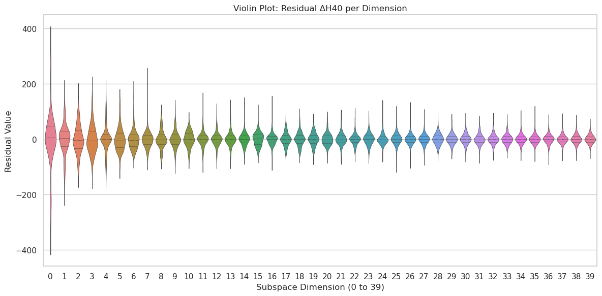
### Visual Description
## Violin Plot: Residual ΔH40 per Dimension
### Overview
The image displays a violin plot titled "Violin Plot: Residual ΔH40 per Dimension." It visualizes the distribution of residual values (ΔH40) across 40 distinct subspace dimensions, indexed from 0 to 39. Each "violin" represents the probability density of the residual data for a specific dimension, with the width of the violin indicating the frequency of data points at that value.
### Components/Axes
* **Title:** "Violin Plot: Residual ΔH40 per Dimension" (centered at the top).
* **X-Axis:**
* **Label:** "Subspace Dimension (0 to 39)" (centered below the axis).
* **Markers/Ticks:** Integers from 0 to 39, inclusive, spaced evenly. Each number corresponds to the center of a violin.
* **Y-Axis:**
* **Label:** "Residual Value" (rotated 90 degrees, positioned to the left).
* **Scale:** Linear scale.
* **Major Tick Marks:** At -400, -200, 0, 200, and 400.
* **Data Series (Violins):**
* There are 40 individual violin plots, one for each dimension (0-39).
* **Color Scheme:** The violins follow a continuous color gradient. Starting from the left (Dimension 0), the colors progress from a pinkish-red, through orange, yellow, green, teal, blue, and finally to purple/magenta on the right (Dimension 39). This gradient appears to be purely aesthetic for visual distinction and does not represent a separate categorical variable.
* **Legend:** There is no separate legend box. The color-to-dimension mapping is direct and positional along the x-axis.
### Detailed Analysis
* **General Trend:** There is a clear and consistent trend in the shape and spread of the distributions as the subspace dimension increases.
* **Dimensions 0-5 (Leftmost):** These violins are the widest and have the longest vertical tails. Dimension 0 shows the most extreme spread, with its tail extending from approximately -400 to +400. The bulk of the data (the widest part of the violin) is centered near 0 but has significant density extending to ±200.
* **Dimensions 6-20 (Middle-Left):** The violins gradually become narrower and their tails shorten. The central bulge remains around 0, but the overall range of residuals contracts. For example, by Dimension 10, the tails extend roughly from -150 to +150.
* **Dimensions 21-39 (Middle-Right to Rightmost):** The trend of compression continues. The violins become increasingly slender and "pinched," indicating that the residual values are tightly clustered around zero. The vertical extent (range) of the residuals diminishes steadily. By Dimension 39, the violin is very narrow, with most data points appearing to fall within a range of approximately -50 to +50.
* **Central Tendency:** For all dimensions, the median and mode of the residual distribution appear to be centered at or very near 0. There is no visible systematic bias (shift away from zero) across dimensions.
* **Symmetry:** The distributions are largely symmetric around zero for most dimensions, though the early dimensions (0-3) show slight asymmetry with potentially longer tails in the negative direction.
### Key Observations
1. **Monotonic Decrease in Variance:** The most prominent pattern is the monotonic decrease in the variance (spread) of the residual ΔH40 values as the subspace dimension index increases.
2. **High Initial Uncertainty:** The first few dimensions (especially 0) exhibit very high uncertainty or error in the ΔH40 metric, as shown by the large spread of residuals.
3. **Convergence to Precision:** By the final dimensions (35-39), the residuals are highly concentrated near zero, suggesting high precision or consistency in the ΔH40 measurement for these subspaces.
4. **No Obvious Outliers in Trend:** The progression from wide to narrow violins is smooth and consistent. No single dimension breaks the overall trend by having a suddenly wider distribution than its neighbors.
### Interpretation
This plot likely analyzes the performance or stability of a model or measurement (related to "ΔH40") across different components or features of a system, represented by the 40 subspace dimensions.
* **What the Data Suggests:** The data strongly suggests that the reliability or predictability of the ΔH40 metric is highly dependent on the subspace dimension. Lower-order dimensions (0, 1, 2...) are associated with high variability and uncertainty in the residual error. In contrast, higher-order dimensions (30+) yield residuals that are consistently very small.
* **Relationship Between Elements:** The x-axis (Dimension) is the independent variable, and the y-axis (Residual Value) is the dependent variable. The violin shape for each dimension is a direct function of the data's distribution at that x-value. The color gradient, while not carrying quantitative information, helps visually track the progression along the x-axis.
* **Potential Meaning:** In contexts like machine learning (e.g., analyzing latent space dimensions), signal processing, or physical modeling, this pattern could indicate:
* **Feature Importance:** The first few dimensions capture the most significant, but also most volatile, factors influencing ΔH40.
* **Model Convergence:** The model's predictions (or the measurement's consistency) improve dramatically for higher-indexed dimensions.
* **Noise vs. Signal:** Lower dimensions may contain more noise or complex interactions leading to larger residuals, while higher dimensions represent finer, more stable adjustments.
* **Notable Implication:** The key takeaway is that any process or conclusion relying on ΔH40 must account for this dimension-dependent uncertainty. Aggregating residuals across all dimensions without weighting would be misleading, as the error profile is not uniform.
</details>
Figure 6: Violin plot of residual $Δ h_t$ values projected across the 40 principal component dimensions of the drift manifold (chosen for tractable SDE modeling). Each violin shows the distribution of residuals for a specific dimension, revealing rich multimodal structure that motivates our regime-switching approach. These structures suggest different operational states, some of which could correspond to misaligned reasoning or failure modes.
## Appendix B EM Algorithm for SLDS Parameter Estimation
This appendix details the Expectation-Maximization (EM) algorithm (Dempster et al., 1977) used for fitting the parameters of the Switching Linear Dynamical System (SLDS) as defined in Eq. 8. The model parameters are $θ=(π,T,\{M_j,b_j,Σ_j\}_j=1^K)$ , where $V_k$ is a fixed orthonormal PCA projection basis (e.g., $k=40$ , chosen for practical modeling).
The SLDS dynamics are:
$$
Z_t∼Categorical(π) for t=0,
$$
$$
P(Z_t+1=j | Z_t=i)=T_ij for t≥ 0,
$$
$$
h_t+1=h_t+V_k(M_Z_{t+1}(V_k^⊤h_t)+b_Z_{t+1})+ε_t+1,
$$
with residual noise $ε_t+1∼N(0,Σ_Z_{t+1})$ .
The log-likelihood for observed data $H=(h_0,\dots,h_T_{end})$ is $P(H | θ)=∑_ZP(H,Z | θ)$ , where $Z=(Z_0,\dots,Z_T_{end-1})$ . Direct maximization is intractable, hence EM. At iteration $m$ , EM alternates:
### B.1 E-step
Compute expected sufficient statistics under $θ^(m)$ . Use standard forward ( $α_t(j)=P(h_0,\dots,h_t,Z_t=j|θ^(m))$ ) and backward ( $β_t(j)=P(h_t+1,\dots,h_T_{end}|Z_t=j,θ^(m))$ ) recursions (Rabiner, 1989). Posterior regime probabilities:
| | $\displaystyleγ_t(j)$ | $\displaystyle=P(Z_t=j|H,θ^(m))$ | |
| --- | --- | --- | --- |
where $Δ h^\prime_t=V_k^⊤(h_t+1-h_t)$ and $x_t=V_k^⊤h_t$ . The $N(·)$ term is the emission probability of observing $h_t+1$ given $h_t$ and $Z_t+1=j$ . These probabilities help identify transitions between different reasoning states, including potentially misaligned ones.
### B.2 M-step
In the M-step, parameters are updated to maximize the expected complete data log-likelihood. The initial state probabilities $\hat{π}_j$ are given by $\hat{π}_j=γ_0(j)$ . Transition probabilities $\hat{T}_ij$ are calculated as:
$$
\hat{T}_ij=\frac{∑_t=0^T_end-2ξ_t(i,j)}{∑_t=0^T_
end-2γ_t(i)}.
$$
The regime-specific dynamics $\{M_j,b_j,Σ_j\}$ are determined through a process analogous to weighted linear regression. We define the projected change as $Δ h^\prime_t=V_k^⊤(h_t+1-h_t)$ and the projected state as $x_t=V_k^⊤h_t$ . Augmented regressors $X_t=[x_t^⊤, 1]^⊤$ and corresponding augmented parameters $M_j=[M_j^⊤,b_j]^⊤$ are utilized. The update for $\hat{M}_j$ is then computed as:
$$
\begin{split}\hat{M}_j={}&≤ft(∑_t=0^T_end-1
γ_t+1(j)X_tX_t^⊤\right)^-1\\
& ×≤ft(∑_t=0^T_end-1γ_t+1(j)X_t(
Δ h^\prime_t)^⊤\right).\end{split}
$$
From $\hat{M}_j$ , the dynamics matrix $\hat{M}_j$ and bias vector $\hat{b}_j$ are extracted using $\hat{M}_j=\hat{M}_j(1:k,:)^⊤$ and $\hat{b}_j=\hat{M}_j(k+1,:)^⊤$ , respectively. To update the covariance matrix $\hat{Σ}_j$ , we first define the residuals for each regime $j$ at time $t$ as $e_jt=Δ h^\prime_t-\hat{M}_jx_t-\hat{b}_j$ . Then, $\hat{Σ}_j$ is computed by:
$$
\hat{Σ}_j=\frac{∑_t=0^T_end-1γ_t+1(j)e_jte_jt
^⊤}{∑_t=0^T_end-1γ_t+1(j)}.
$$
These updates are derived from maximizing the expected complete data log-likelihood.
Scaling techniques are employed during the forward-backward passes to mitigate numerical underflow. When dealing with multiple observation sequences, the necessary statistics are accumulated across all sequences before the parameter updates are performed. Convergence of the Expectation-Maximization algorithm is typically assessed by observing when parameter changes fall below a predefined threshold, when the change in log-likelihood becomes negligible, or when a maximum number of iterations is reached. The inherent property of EM ensuring a monotone increase in the log-likelihood contributes to stable training. Ultimately, the objective is to identify a set of parameters that most accurately describes the observed dynamics of the reasoning process. This includes modeling transitions between different operational regimes, which can be indicative of phenomena such as the onset of failure modes.
## Appendix C Adversarial Chain-of-Thought Belief Manipulation
This appendix describes experimental details for the adversarial belief-manipulation results in Section 5.3, focusing on how the SLDS framework can model and predict LLMs slipping into misaligned states, following ICML practice.
### C.1 Experimental Design
We studied Llama-2-70B and Gemma-7B-IT under adversarial prompting on twelve misinformation themes (public health, conspiracies, financial myths, AI fears, historical revisionism, pseudoscience, etc.). For each theme/model, paired clean and poisoned CoTs were generated. Clean CoTs used neutral questions (e.g., “Summarize arguments for and against vaccination”). Poisoned CoTs interspersed adversarial prompts at predetermined steps to guide the model towards harmful beliefs (misaligned states). Each CoT had $∼$ 50 sentence-level steps. We collected $∼$ 100 trajectories per combination, totaling $∼$ 3000 trajectories. At each step $t$ , we recorded the final-layer residual embedding and a scalar "belief score" from a diagnostic query related to the misinformation. Belief score = $P(True)/(P(True)+P(False))$ , where 0 is rejection and 1 is strong affirmation of the false claim (a clear misaligned state).
### C.2 Data Preprocessing
Raw hidden-state vectors were standardized (mean-subtracted, variance-normalized per dimension) and projected onto their first 40 principal components (PCA, $∼$ 87% variance explained for this dataset, chosen for practical SLDS modeling) using scikit-learn 1.2.1 (SVD solver, whitening enabled).
### C.3 Switching Linear Dynamical System (SLDS)
PCA-projected states were modeled with an SLDS having three latent regimes ( $K=3$ ), chosen via BIC on validation data, representing factual, transitional, and misaligned belief states. Dynamics per regime: $h^\prime_t+1=M_z_{t}h^\prime_t+c_z_{t}+ε_t$ , $ε_t∼N(0,Σ_z_{t})$ , $z_t∈\{1,2,3\}$ . Parameters ( $T,M,c,Σ$ ) were learned via EM, initialized from K-means. For adversarial steps, regime-transition probabilities were examined to see if they reflected an increased likelihood of entering the "adverse" belief state. The SLDS aims to predict such slips into misaligned states.
### C.4 Belief-Score Prediction
Since SLDS models latent PCA dynamics, a small two-layer MLP regressor (32 ReLU units/layer, Adam, early stopping) mapped PCA-projected states to belief scores for validation and for assessing the prediction of the misaligned (high belief score) state.
### C.5 Simulation Protocol and Validation
Trajectories were simulated starting from empirical hidden-state distributions in the "safe" (low-belief) regime. Clean simulations used standard transitions. Poisoned simulations introduced adversarial perturbations (small fixed displacements estimated from empirical poisoned data) at random preselected intervals. Simulated trajectories matched empirical ones closely in timing/magnitude of belief shifts (slips into misaligned states), variance, and distributional characteristics (Kolmogorov-Smirnov test $p>0.3$ for final belief scores). Ablating adversarial perturbations confirmed their necessity for replicating rapid belief shifts towards misaligned states. This validates the SLDS’s ability to predict such failure modes.
### C.6 Computational Details
NVIDIA A100 GPUs were used for state extraction and PCA. State extraction took $∼$ 3 hours per model. PCA and SLDS estimation took <2 CPU hours on Intel Xeon Gold CPUs. Code used PyTorch 2.0.1, NumPy 1.25, scikit-learn 1.2.1.
### C.7 Summary of Findings
A simple three-regime, low-rank SLDS (with low rank chosen for practical SDE approximation) captures adversarial belief dynamics for various misinformation types and reproduces complex empirical temporal behaviors, effectively modeling the process of an LLM slipping into a misaligned state. These models offer tractable insights into LLM reasoning, highlighting latent regime shifts from subtle adversarial prompts and demonstrating the potential to predict such failure modes at inference time.
## Appendix D Extended Generalization Study Results
This appendix provides more comprehensive SLDS transferability results (Section 5.1). Table 4 shows $R^2$ (one-step-ahead hidden state prediction) and NLL (test trajectories) when an SLDS trained on a source (Train Model/Task) is tested on target combinations. SLDS hyperparameters ( $K=4$ regimes, $k=40$ projection rank, chosen for practical SDE approximation) were consistent. Training data for each "Source SLDS" used all available trajectories for the specified Train Model/Task from our main corpus (Section 3). Evaluation used all available trajectories for the Test Model/Task. The goal is to assess how well the learned approximation of reasoning dynamics (including potential failure modes) generalizes.
Table 4: Extended SLDS transferability results. Each SLDS is trained on trajectories from the ‘Train Model’ on its indicated ‘Source Task’. Performance is evaluated on various ‘Test Model’ / ‘Test Task’ combinations, testing the generalization of the approximated reasoning dynamics.
| Train Model (Source Task) | Test Model | Test Task | $R^2$ | NLL |
| --- | --- | --- | --- | --- |
| Llama-2-70B (on GSM-8K) | | | | |
| Llama-2-70B | GSM-8K | 0.73 | 80 | |
| Llama-2-70B | StrategyQA | 0.65 | 115 | |
| Llama-2-70B | CommonsenseQA | 0.62 | 128 | |
| Mistral-7B | GSM-8K | 0.48 | 240 | |
| Mistral-7B | StrategyQA | 0.37 | 310 | |
| Gemma-7B-IT | GSM-8K | 0.40 | 275 | |
| Phi-3-Med | PiQA | 0.28 | 430 | |
| Mistral-7B (on StrategyQA) | | | | |
| Mistral-7B | StrategyQA | 0.71 | 88 | |
| Mistral-7B | GSM-8K | 0.63 | 135 | |
| Mistral-7B | OpenBookQA | 0.60 | 145 | |
| Llama-2-70B | StrategyQA | 0.42 | 270 | |
| Llama-2-70B | GSM-8K | 0.35 | 320 | |
| Gemma-7B-IT | BoolQ | 0.35 | 380 | |
| Qwen1.5-7B | HellaSwag | 0.31 | 405 | |
| Gemma-7B-IT (on BoolQ) | | | | |
| Gemma-7B-IT | BoolQ | 0.69 | 95 | |
| Gemma-7B-IT | TruthfulQA | 0.62 | 140 | |
| Gemma-2B-IT | BoolQ | 0.55 | 190 | |
| Llama-2-13B | BoolQ | 0.33 | 350 | |
| Mistral-7B | CommonsenseQA | 0.29 | 415 | |
| DeepSeek-67B (on CommonsenseQA) | | | | |
| DeepSeek-67B | CommonsenseQA | 0.74 | 75 | |
| DeepSeek-67B | GSM-8K | 0.66 | 110 | |
| Llama-2-70B | CommonsenseQA | 0.45 | 255 | |
| Mistral-7B | StrategyQA | 0.36 | 330 | |
Extended results corroborate main text observations: SLDS models are most faithful when applied to their training distribution (model/task). Transfer is reasonable within the same model family or to similar tasks. Performance degrades more significantly across different model architectures or distinct task types. These patterns indicate SLDS, as a statistical physics-inspired approximation, captures fundamental reasoning dynamics (including propensities for certain failure modes), but model-specific architecture and task-specific semantics also matter. Future work could explore learning more invariant reasoning representations for better generalization in predicting these misaligned states.
## Appendix E Noise-induced Criticality and Latent Modes
We briefly derive how noise-induced criticality leads to distinct latent modes in a 1D Langevin system, analogous to how LLMs might slip into misaligned reasoning states. Consider an SDE:
$$
dx_t=-U^\prime(x_t) dt+√{2D} dW_
t,
$$
with a double-well potential $U(x)=\frac{a}{4}x^4-\frac{b}{2}x^2$ , where $a,b>0$ . The stationary density solves the Fokker–Planck equation (Risken & Frank, 1996):
$$
0=-\frac{ d}{ dx}[-U^\prime(x)p_\rm st(x)]+D\frac{
d^2p_\rm st(x)}{ dx^2},
$$
yielding $p_st(x)=\frac{1}{Z_0}\exp≤ft(-\frac{U(x)}{D}\right)$ , where $Z_0$ is a normalization constant.
For low noise ( $D<\frac{b^2}{4a}$ ), $p_st(x)$ becomes bimodal, concentrating probability around two metastable wells at $x≈±√{b/a}$ . Trajectories cluster in these basins, separated by a barrier at $x=0$ . Rare fluctuations cause transitions between wells at rates $∝\exp(-Δ U/D)$ , where $Δ U$ is the barrier height. Our empirically observed multimodal residual structure is interpreted analogously: each cluster is a distinct metastable basin, potentially representing different reasoning qualities (e.g., aligned vs. misaligned). This motivates discrete latent regimes in the SLDS to model transitions between these states, akin to how a physical system transitions between energy wells. This provides a conceptual basis for how LLMs might "slip" into different operational modes, some of which could be failure modes.