2506.06923

## Boosting LLM Reasoning via Spontaneous Self-Correction Xutong Zhao 1 , 2 , 3 , ∗ , Tengyu Xu 1 , Xuewei Wang 1 , Zhengxing Chen 1 , Di Jin 1 , Liang Tan 1 , Yen-Ting 1 , Zishun Yu 1 , Zhuokai Zhao 1 , Yun He 1 , Sinong Wang 1 , HanFang 1 , Sarath Chandar 2 , 3 , Chen Zhu 1 1 MetaAI, 2 Mila - Quebec AI Institute, 3 Polytechnique Montréal ∗ Work done at Meta While large language models (LLMs) have demonstrated remarkable success on a broad range of tasks, math reasoning remains a challenging one. One of the approaches for improving math reasoning is self-correction, which designs self-improving loops to let the model correct its own mistakes. However, existing self-correction approaches treat corrections as standalone post-generation refinements, relying on extra prompt and system designs to elicit self-corrections, instead of performing real-time, spontaneous self-corrections in a single pass. To address this, we propose SPOC , a spontaneous self-correction approach that enables LLMs to generate interleaved solutions and verifications in a single inference pass , with generation dynamically terminated based on verification outcomes, thereby effectively scaling inference time compute. SPOC considers a multi-agent perspective by assigning dual roles - solution proposer and verifier - to the same model. We adopt a simple yet effective approach to generate synthetic data for fine-tuning, enabling the model to develop capabilities for self-verification and multi-agent collaboration. We further improve its solution proposal and verification accuracy through online reinforcement learning. Experiments on mathematical reasoning benchmarks show that SPOC significantly improves performance. Notably, SPOC boosts the accuracy of Llama-3.1-8B and 70B Instruct models, achieving gains of 8.8% and 11.6% on MATH500, 10.0% and 20.0% on AMC23, and 3.3% and 6.7% on AIME24, respectively. Date: June 10, 2025 Correspondence: Xutong Zhao at xutong.zhao@mila.quebec ## 1 Introduction Large Language Models (LLMs) have showcased promising results across a broad spectrum of text generation tasks. Among the various domains of LLM applications, mathematical reasoning remains particularly challenging due to its symbolic and structured nature (Shao et al., 2024; Chen et al., 2024). Recent advances in self-correction (Shinn et al., 2023; Madaan et al., 2023) have emerged as a promising paradigm towards self-improvement through iterative critique and refinement of model's own responses. 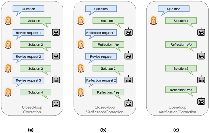However, the effectiveness and practicality of existing self-correction approaches remain unclear. Naive prompting methods may lead to minimal improvement or performance degradation without access to external feedback (Huang et al., 2023; Qu et al., 2024). Finetuning-based methods seek to address such issues by post-training the LLM on refinement data collected from oracles (Saunders et al., 2022; Qu et al., 2024) or the learner model itself (Kumar et al., 2024). Nonetheless, these approaches typically rely on a specific prompt after each model response to trigger self-reflection or correction (Figures 1a and 1b), necessitating additional system design to inject these prompts during inference. In other words, existing approaches lack the ability to spontaneously and adaptively self reflect and correct, resulting in ineffective test-time compute scaling and inflexible deployment in practice. To address these challenges, we introduce SPOC , a spontaneous self-correction approach that enables LLMs to spontaneously generate interleaved solutions and verifications in a single inference pass . SPOC employs an open-loop inference paradigm, which triggers self-correction only when the self-verification identifies errors, and iteratively revises the solution until it passes self-verification, without requiring any external interventions during response generation. It dynamically elicits and terminates generations on-the-fly using Figure 1 Multi-turn generation formalisms. (a)&(b) Sample closed-loop paradigms that require extra system designs and prompting to trigger and terminate correction; (c) Sample open-loop paradigm that spontaneously adapts generations. <details> <summary>Image 1 Details</summary>  ### Visual Description \n ## Diagram: Iterative Solution Refinement with Human-AI Interaction ### Overview The image presents a comparative diagram illustrating three different iterative processes for refining solutions to a question, involving both human and AI interaction. Each process (a, b, and c) is depicted within a light green rounded rectangle, showing a sequence of steps. The diagrams highlight varying levels of feedback and correction loops between the human and the AI agent. ### Components/Axes The diagram consists of the following components: * **Human Representation:** A stylized human icon representing the user. * **AI Representation:** A robotic head icon representing the AI agent. * **Question Block:** A light blue rounded rectangle labeled "Question". * **Solution Blocks:** Light green rounded rectangles labeled "Solution 1", "Solution 2", "Solution 3", "Solution 4". * **Revise Request Blocks:** Light blue rounded rectangles labeled "Revise request 1", "Revise request 2", "Revise request 3". * **Reflection Request Blocks:** Light blue rounded rectangles labeled "Reflection request 1", "Reflection request 2". * **Reflection Blocks:** Light blue rounded rectangles labeled "Reflection: No", "Reflection: Yes". * **Correction/Verification Blocks:** Light blue rounded rectangles labeled "Closed-loop Correction", "Closed-loop Verification/Correction", "Open-loop Verification/Correction". * **Arrows:** Green arrows indicating the flow of the process. * **Labels:** (a), (b), (c) identifying each process. ### Detailed Analysis or Content Details **Process (a): Closed-loop Correction** 1. Starts with a "Question". 2. The human receives "Solution 1" from the AI. 3. The human sends a "Revise request 1" to the AI. 4. The AI provides "Solution 2". 5. The human sends a "Revise request 2" to the AI. 6. The AI provides "Solution 3". 7. The human sends a "Revise request 3" to the AI. 8. The AI provides "Solution 4". 9. The process concludes with "Closed-loop Correction". **Process (b): Closed-loop Verification/Correction** 1. Starts with a "Question". 2. The human receives "Solution 1" from the AI. 3. The human sends a "Reflection request 1" to the AI. 4. The AI responds with "Reflection: No". 5. The human sends a "Revise request" to the AI. 6. The AI provides "Solution 2". 7. The human sends a "Reflection request 2" to the AI. 8. The AI responds with "Reflection: Yes". 9. The process concludes with "Closed-loop Verification/Correction". **Process (c): Open-loop Verification/Correction** 1. Starts with a "Question". 2. The human receives "Solution 1" from the AI. 3. The human sends a request to the AI. 4. The AI responds with "Reflection: No". 5. The human receives "Solution 2". 6. The human sends a request to the AI. 7. The AI responds with "Reflection: Yes". 8. The process concludes with "Open-loop Verification/Correction". ### Key Observations * Process (a) involves a purely iterative revision loop without explicit reflection. * Process (b) incorporates reflection requests from the human, with the AI providing feedback ("Reflection: No" or "Reflection: Yes"). This process is labeled as "Closed-loop Verification/Correction". * Process (c) also includes reflection requests, but is labeled as "Open-loop Verification/Correction", suggesting a less integrated feedback mechanism. * The number of solution iterations differs between the processes. Process (a) has four solutions, while processes (b) and (c) have two. ### Interpretation The diagram illustrates different strategies for human-AI collaboration in problem-solving. The key distinction lies in the inclusion and nature of reflection. * **Closed-loop Correction (a)** represents a traditional iterative refinement process where the human provides feedback to improve the AI's solution. It's a straightforward, but potentially less efficient, approach. * **Closed-loop Verification/Correction (b)** introduces a reflection step, allowing the AI to assess its own performance and potentially adjust its approach. The "Reflection: Yes/No" responses suggest the AI can self-evaluate and provide insights to the human. This is a more sophisticated approach, potentially leading to faster convergence on a satisfactory solution. * **Open-loop Verification/Correction (c)** also includes reflection, but the "Open-loop" designation suggests the feedback from the AI is less directly integrated into the refinement process. It might involve the human independently interpreting the AI's reflection and applying it to the next iteration. The diagram highlights the importance of feedback mechanisms in human-AI interaction. The inclusion of reflection, particularly in a closed-loop system, appears to enhance the efficiency and effectiveness of the problem-solving process. The diagram does not provide quantitative data, but visually demonstrates the conceptual differences between these approaches. </details> solely the model's inherent capabilities, thereby effectively scaling inference time compute. We consider a multi-agent formalism that models the alternating solutions and verifications as the interaction between a solution proposer and a verifier, and adopt a self-play training strategy by assigning dual roles to the same model. We adopt a simple yet effective approach to generate synthetic data from the initial model for supervised fine-tuning (Welleck et al., 2022), enabling the model to adhere to the multi-turn generation style, meanwhile developing capabilities for self-verification and inter-agent collaboration without distilling from a stronger teacher. We further boost the model's accuracy in its solution proposal and verification via online reinforcement learning, using the correctness of solutions and verifications as the reward. Our main contributions are threefold: - We demonstrate that generating self-verification and correction trajectories from the initial model's correct and incorrect outputs effectively bootstraps its spontaneous self-verification and correction behavior. We call out the importance of data balancing in achieving high verification accuracy in this stage, which in turn benefits the subsequent RL phase. - We propose the message-wise online RL framework for SPOC , and present the formulation of RAFT (Dong et al., 2023) and RLOO (Ahmadian et al., 2024) as the RL stage of SPOC for enhancing self-verification and correction accuracies. Our results show that RLOO, augmented with process rewards for each solution or verification step, yields stronger results. - We achieve significant improvements on math reasoning tasks across model sizes and task difficulties using our pipeline without distilling from stronger models. SPOC boosts the pass@1 accuracy of Llama-3.1-8B and 70B Instruct models-improving performance by 8.8% and 11.6% on MATH500, by 10.0% and 20.0% on AMC23, and by 3.3% and 6.7% on AIME24. ## 2 Related work Self-correction. Given that high-quality external feedback is often unavailable across various realistic circumstances, it is beneficial to enable an LLM to correct its initial responses based on solely on its inherent capabilities. Prior works on such intrinsic self-correction (Huang et al., 2023) or self-refinement can be categorized into two groups based on the problem settings and correction mechanisms: prompting and finetuning. Recent works (Huang et al., 2023; Qu et al., 2024) show that prior prompting methods lead to minimal improvement or degrading performance without strong assumptions on problem settings. For instance, Shinn et al. (2023) rely on oracle labels which are often unavailable in real-world applications; Madaan et al. (2023) use less informative prompts for initial responses, resulting in overestimation of correction performance. Finetuning methods seek to improve correction performance via finetuning the LLM on refinement data, collected from human annotators (Saunders et al., 2022), stronger models (Qu et al., 2024), or the learner model itself (Kumar et al., 2024). However, these works lack the mechanisms that correct errors while generating solutions in a single inference pass (Ye et al., 2024). Our work is akin to concurrent works on self-correction (Ma et al., 2025; Xiong et al., 2025). Differently, Xiong et al. (2023) re-attempts a solution within the verification instead of evaluating the previous one; moreover, they only apply RAFT in their learning framework, while we also conduct experiments on RLOO. Ma et al. (2025) uses the more complex GRPO as their RL algorithm, while we show that better performance can be achieved in the same setting (Llama 3.1 8B) by using simpler RL algorithms like RAFT for SPOC . Multi-agent frameworks. By introducing multiple roles into problem-solving, multi-agent formalisms serve as a different perspective to address complex reasoning tasks. AutoGen (Wu et al., 2023) and debatebased frameworks (Du et al., 2023; Liang et al., 2023) solve math problems through customized inter-agent conversations. Despite increased test-time computation, these works lack post-training for different agent roles, which may result in suboptimal performance or distribution shifts at inference time (Xiang et al., 2025). While other works train separate models to perform correction (Motwani et al., 2024; Havrilla et al., 2024; Akyürek et al., 2023; Paul et al., 2023), models do not perform spontaneous corrections during solution generations; instead, they require extra system designs to trigger and stop corrections at deployment. In contrast, our method enables dynamic inference-time scaling by improving the model's own inherent deliberation capabilities. 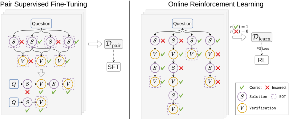## 3 Method In this section, we first introduce the multi-turn formalism, in which the agent performs interleaved solution and verification turns. We then discuss how we finetune the agent to ensure it consistently adheres to the multi-turn response style. We finally describe our online reinforcement learning scheme which further boosts the final accuracy of the policy. Figure 2 illustrates the two stages, fine-tuning and online RL, of SPOC . ## 3.1 Multi-turn formalism Problem setup. Let D ≡ X × Y = { ( x i , y ∗ i ) } N i =1 be a dataset of N math problems, where each pair ( x, y ∗ ) contains a question x i and the corresponding solution y ∗ i with ground-truth final answer. An LLM agent is defined by the policy π θ ( ·| x ) , parameterized by θ , that generates the solution y to solve the given problem x . Alternated-turn generation. Suppose given a question x , the LLM generates a trajectory consisting of L interleaved solutions and verifications τ = ( y 1 , v 1 , . . . , y L , v L ) , where a solution y l indicating the model's l -th complete solution attempt that reaches a final answer, and a verification v l indicating the l -th self-verification validating correctness of the solution y l . For clarity, message or turn refers to each single solution y l or verification v l , and response or generation τ refers to the entire trajectory until the end. For brevity, we denote previous l turns by: τ l = ( y 1: l , v 1: l ) and τ vf l = ( y 1: l , v 1: l -1 ) . The timestep t ∈ N 0 indicates a single decoding step where the LLM outputs one token from its policy distribution. Multi-agent formulation. We model the reasoning task as an extensive-form game (EFG) (Osborne, 1994; Shoham and Leyton-Brown, 2008), which generalizes the Markov Decision Process (MDP) (Sutton, 2018) to a turn-taking interaction between solution proposer and verifier. At each turn, the proposer outputs a solution to the given math problem, and the verifier assesses its correctness. In this context, the EFG is a tuple ⟨N , A , S , T , r, I , γ ⟩ , where N = { 1 , . . . , n } is the set of n = 2 players (i.e. the proposer and verifier), A is a finite set of actions (i.e. the LLM's token space), S is a finite set of states (i.e. each state is a question and a sequence of reasoning/verification steps in context), T ⊂ S is a subset of terminal states (i.e. complete response trajectories τ = ( y 1 , v 1 , . . . , y L , v L ) ), r : T × N 0 → ∆ n r ⊂ R n is the reward function assigning each player a scalar utility at terminal states (i.e. ∆ r = { 0 , 1 } characterizes binary outcome feedback), I : S → N is a player identity function identifing which player acts at s (i.e. I ( τ l ) = 1 and I ( τ vf l ) = 2 ), and γ ∈ [0 , 1] is the discount factor. Figure 2 SPOC training overview. Left: PairSFT for initializing multi-turn generation. Right: Online RL for policy optimization. <details> <summary>Image 2 Details</summary>  ### Visual Description ## Diagram: Pair Supervised Fine-Tuning & Online Reinforcement Learning ### Overview The image presents a comparative diagram illustrating two machine learning approaches: Pair Supervised Fine-Tuning (SFT) and Online Reinforcement Learning (RL). Both diagrams depict a process starting with a "Question" and progressing through a series of "Solution" (S) and "Verification" (V) steps. The left side shows SFT, where the process is guided by paired data, while the right side shows RL, where the process is guided by rewards and penalties. ### Components/Axes The diagram consists of two main sections, each with a similar structure. Key components include: * **Question:** The initial input to the system. * **Solution (S):** Represents a step towards answering the question. Visually represented by a circle with the letter "S" inside. * **Verification (V):** Represents the evaluation of a solution step. Visually represented by a circle with the letter "V" inside. * **Correct/Incorrect Indicators:** Green checkmarks (✓) indicate correct steps, while red crosses (✗) indicate incorrect steps. * **D_pair:** Represents the paired dataset used in SFT. * **D_learn:** Represents the learning dataset used in RL. * **SFT:** Label for Pair Supervised Fine-Tuning. * **RL:** Label for Reinforcement Learning. * **PG_Loss:** Policy Gradient Loss. * **r⁺(x) = 1, r^-(x) = 0:** Reward function definition. * **EOT:** End of Thought. * **Legend:** Located in the bottom-right corner, defining the meaning of the checkmark and cross symbols, as well as the Solution and Verification nodes. ### Detailed Analysis / Content Details **Pair Supervised Fine-Tuning (Left Side):** * The process begins with a "Question" node at the top. * From the "Question", multiple "Solution" (S) nodes branch out, each connected to a "Verification" (V) node. * The first four "S-V" pairs are marked with red crosses (✗) indicating incorrect steps. * The next "S-V" pair is marked with a green checkmark (✓) indicating a correct step. * The final "S-V" pair is also marked with a green checkmark (✓) indicating a correct step. * An arrow points downwards from the initial "Question" and "S-V" pairs to a simplified representation of the process: "Q -> S -> V -> V". * Another arrow points downwards from "Q -> S -> V -> V" to "Q -> S -> V", indicating a further simplification. * An arrow labeled "D_pair" points from the initial branching structure to the "SFT" label. **Online Reinforcement Learning (Right Side):** * The process begins with a "Question" node at the top. * From the "Question", multiple "Solution" (S) nodes branch out, each connected to a "Verification" (V) node. * The first three "S-V" pairs are marked with green checkmarks (✓) indicating correct steps. * The next "S-V" pair is marked with a red cross (✗) indicating an incorrect step. * The following "S-V" pair is marked with a green checkmark (✓) indicating a correct step. * The final "S-V" pair is marked with a red cross (✗) indicating an incorrect step. * An arrow labeled "D_learn" points from the branching structure to a box containing "PG_Loss" and "RL". * Above the arrow, the reward function is defined: "r⁺(x) = 1, r^-(x) = 0". ### Key Observations * SFT relies on a pre-defined, paired dataset (D_pair) to guide the learning process, resulting in a simplified output. * RL uses a learning dataset (D_learn) and a reward function to guide the learning process, utilizing Policy Gradient Loss within a Reinforcement Learning framework. * The SFT process appears to converge more quickly to a simplified solution, while the RL process explores more possibilities before reaching a solution. * The number of "S-V" pairs is the same in both diagrams. * The proportion of correct and incorrect steps differs between the two approaches. SFT has more initial incorrect steps, while RL has a more mixed result. ### Interpretation The diagram illustrates the fundamental difference between supervised learning (SFT) and reinforcement learning (RL). SFT learns from labeled examples, aiming to mimic the correct solutions provided in the dataset. This leads to a more direct path to a simplified solution. RL, on the other hand, learns through trial and error, receiving rewards for correct actions and penalties for incorrect ones. This allows it to explore a wider range of possibilities but may require more iterations to converge. The reward function (r⁺(x) = 1, r^-(x) = 0) indicates a binary reward system: a reward of 1 for correct steps and 0 for incorrect steps. The diagram suggests that SFT is more efficient when a high-quality, labeled dataset is available, while RL is more suitable for problems where labeled data is scarce or the optimal solution is unknown. The "EOT" label suggests that the process is iterative and continues until a satisfactory solution is reached. The diagram is a conceptual illustration and does not provide specific numerical data or performance metrics. </details> Unlike the general definition of EFGs, we do not distinguish between histories and states due to the deterministic dynamics and perfect-information nature in mathematical reasoning (i.e. τ l +1 = τ l ∪{ y l +1 , v l +1 } ). We denote the proposer's and the verifier's action spaces as A sl ⊂ A and A vf ⊂ A , representing the set of solution and verification messages, respectively. We define a per-step reward function for a transition as r ( s, a ) representing a vector of reward to both agents. The return for player i ∈ N is defined as G t,i = ∑ ∞ k =0 γ k r i ( s t + k , a t + k ) . The corresponding state-action value function under policy π is Q π i ( s, a ) = E π [ G t,i | s t = s, a t = a ] . To improve reasoning capabilities by learning from both solution and verification experiences, we adopt the commonly-used self-play strategy with parameter sharing (Albrecht et al., 2024), where the proposer policy π sl : S → ∆( A sl ) and the verifier policy π vf : S → ∆( A vf ) share the same set of parameters θ . The policy π θ outputs alternated solution and verification messages depending on the context 1 . Policy optimization. We optimize the policy π θ by maximizing the KL-regularized learning objective <!-- formula-not-decoded --> where ρ indicates the discounted state distribution, η > 0 is the KL-regularization coefficient, and π θ 0 is the reference policy parameterized by the initial parameters θ 0 . This objective has a close-form solution for the optimal policy π ∗ ( a | s ) = 1 Z ( s ) π θ 0 ( a | s ) exp( 1 η Q ( s, a )) , where Z ( s ) = E a ∼ π θ 0 ( ·| s ) [exp( 1 η Q ( s, a ))] . Given our multi-agent formulation, this objective introduces an individual objective for each role, namely <!-- formula-not-decoded --> <!-- formula-not-decoded --> Due to shared parameters across both roles, we jointly optimize both objectives using common generated trajectory experiences. Hence the optimal proposer and verifier policies satisfy π sl ∗ ( a | s ) ∝ π sl θ 0 ( a | s ) exp( 1 η Q sl ( s, a )) and π vf ∗ ( a | s ) ∝ π vf θ 0 ( a | s ) exp( 1 η Q vf ( s, a )) , respectively, implying the optimal shared policy increases the probability of outputting high-rewarding solutions/verifications. Note that the optimal policy for the unregularized learning objective ( η = 0 ) results in the maximizer of the action-value function: π ∗ ( ·| s ) = arg max π ( ·| s ) ∈ ∆( A ) E a ∼ π ( ·| s ) [ Q π ( s, a )] , also yielding high probablity of generating high-rewarding messages. Reward setting. To obtain a reward signal for each token in each message, we evaluate the outcome correctness of each message. In particular, we assume access to a rule-based checker for the final answer in the solution, 1 Different from the classic self-play in zero-sum games (e.g., AlphaZero (Silver et al., 2017)), ours involves non-symmetrical roles in the sense that two policies are different conditioned on the context. 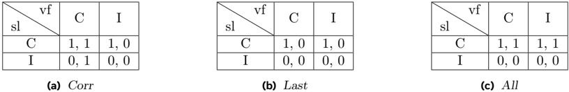Figure 3 Reward configurations for policy optimization, where sl, vf, C, I indicate solution, verification, correct, and incorrect, respectively. For Last and All , SPOC optimizes correct solutions (first row in each table) only when the last solution is correct. <details> <summary>Image 3 Details</summary>  ### Visual Description ## Data Tables: Correlation Matrices ### Overview The image presents three data tables, each representing a correlation matrix. Each table is labeled (a) Corr, (b) Last, and (c) All. The tables display relationships between four variables: 'vf', 'C', 'I', and 'sl'. The values within the tables appear to be binary (0 or 1), potentially indicating the presence or absence of a correlation. ### Components/Axes Each table has the following structure: - **Rows:** Representing the variables 'sl', 'C', and 'I'. - **Columns:** Representing the variables 'vf', 'C', and 'I'. - **Cells:** Containing numerical values (0 or 1) representing the correlation between the corresponding row and column variables. - **Labels:** Each table is labeled with a descriptive name: "Corr", "Last", and "All". - **Diagonal:** The diagonal elements are not explicitly labeled, but represent the correlation of a variable with itself. ### Detailed Analysis or Content Details **Table (a) Corr:** | | vf | C | I | |-------|-------|-----|-----| | **sl** | | | | | **C** | 1,1 | 1 | 0 | | **I** | 0,1 | 0 | 0 | - sl vs vf: Not present - sl vs C: Not present - sl vs I: Not present - C vs vf: 1,1 - C vs C: 1 - C vs I: 0 - I vs vf: 0,1 - I vs C: 0 - I vs I: 0 **Table (b) Last:** | | vf | C | I | |-------|-------|-----|-----| | **sl** | | | | | **C** | 1,0 | 1 | 0 | | **I** | 0,0 | 0 | 0 | - sl vs vf: Not present - sl vs C: Not present - sl vs I: Not present - C vs vf: 1,0 - C vs C: 1 - C vs I: 0 - I vs vf: 0,0 - I vs C: 0 - I vs I: 0 **Table (c) All:** | | vf | C | I | |-------|-------|-----|-----| | **sl** | | | | | **C** | 1,1 | 1 | 1 | | **I** | 0,0 | 0 | 0 | - sl vs vf: Not present - sl vs C: Not present - sl vs I: Not present - C vs vf: 1,1 - C vs C: 1 - C vs I: 1 - I vs vf: 0,0 - I vs C: 0 - I vs I: 0 ### Key Observations - The values in the tables are predominantly 0 or 1. - The diagonal elements (C vs C, I vs I) are consistently 1 and 0 respectively. - Table (a) "Corr" and (c) "All" have similar patterns, with the main difference being the value in the C vs I cell. - Table (b) "Last" shows a different pattern, particularly in the C vs vf cell. - The values are presented as pairs (e.g., 1,1 or 0,1). This could represent two different correlation measures or confidence levels. ### Interpretation These tables likely represent the results of a correlation analysis between four variables. The binary values suggest a thresholding process, where correlations above a certain level are represented as 1 and below as 0. The different tables ("Corr", "Last", "All") might represent different subsets of data or different methods of calculating the correlation. The consistent 1 in the C vs C and 0 in the I vs I cells indicate perfect self-correlation for C and no self-correlation for I. The varying values in other cells suggest different relationships between the variables depending on the table. The paired values (e.g., 1,1) could represent a correlation coefficient and its associated p-value, or two different correlation metrics. Without further context, it's difficult to determine the specific meaning of these correlations. However, the tables provide a clear visual representation of the relationships between the four variables under different conditions. </details> and provide a binary outcome reward denoted by r sl ( y, y ∗ ) ∈ { 0 , 1 } , where r sl ( y, y ∗ ) = 1 when the model answer matches the ground-truth answer. Similarly, we parse the Yes / No conclusion in each verification, and denote the reward function by r vf ( v, v ∗ ) ∈ { 0 , 1 } , with v ∗ = r sl ( y, y ∗ ) indicating the ground-truth verification. Figure 3a shows the joint reward setting, denoted by Corr hereafter. To obtain maximal returns against each other role, our reward setting admits one unique Nash equilibrium (Shoham and Leyton-Brown, 2008) with the joint policy (i.e. the shared policy π ) generating both correct solutions and correct verifications. ## 3.2 Enabling multi-turn generation Since off-the-shelf LLMs do not adhere to the response style of interleaved solution and verification turns by default, before conducting RL optimization, we first perform an initial finetuning with multi-turn data to enable such behaviour. To collect such data, we implement a variant of Pair-SFT (Kumar et al., 2024; Welleck et al., 2022) to construct synthetic correction responses. In particular, we rollout the base policy π θ 0 to collect single-turn responses for each question x i ∈ X , denoted by { y k i } K k =1 ∼ π θ 0 ( ·| x i ) . For each response, we record its binary correctness using the solution reward function r k i = r sl ( y k i , y ∗ i ) . We obtain the verification message of one single-turn response by pairing it with a correct sampled response. To generate verification of one response, either correct or incorrect, we prompt the same base model π θ 0 to identify the potential error, briefly explain it, and output a final binary conclusion indicating correctness of the given solution. The entire verification message is denoted as v i ∼ π θ 0 ( ·| x i , y i , y ∗ i ) , where y ∗ i indicates the correct sample. We denote this synthetic multi-turn correction dataset as the Pair-SFT dataset D pair = { ( x i , y -i , v -i , y ∗ i ) } ∪ { ( x i , y + i , v + i ) } , where the + / -superscripts indicates correctness of the corresponding solution turn. We perform SFT finetuning on the base model, with tokens in incorrect messages masked out, and denote the finetuned model by π θ sft . In practice, we observe that reweighting the subsets { ( x i , y -i , v -i , y ∗ i ) } and { ( x i , y + i , v + i ) } to approximately the same scale leads to a π θ sft with higher verification accuracy and more stable RL training afterwards. The complete training data collection procedure is detailed in Algorithm 2. When generating the verification messages, we adapt the generative critic method (Zhang et al., 2024; Zheng et al., 2024) that prompts the model to respond with rationales before judging solution correctness, except that our variant concisely explains the error rather than performing a chain-of-thought (COT) analysis. Obtaining a strong COT verifier requires explicit training and it is out of scope of this work. Prompt templates for data construction are detailed in Appendix E. ## Algorithm 1 SPOC Message-wise Online Reinforcement Learning - 1: Inputs: Question-answer dataset D = X ×Y = { ( x j , y ∗ j ) } N j =1 , policy model π θ parameterized by θ , number of questions N , number of steps T , number of rollouts per question K , batch size B , rule-based solution correctness reward function r sl ( y, y ∗ ) ∈ { 0 , 1 } , verification correctness reward function r vf ( v, v ∗ ) ∈ { 0 , 1 } - 2: for i = 1 , . . . , T do - 3: Sample a batch D i ⊂ D of size B - 4: Sample K trajectories for each x j ∈ X i : { τ k j } K k =1 ∼ π θ ( ·| x j ) , where τ k j = ( y j,k 1: L k , v j,k 1: L k ) - 5: Label binary rewards: r sl j,k,l = r sl ( y j,k l , y ∗ j ) , r vf j,k,l = r vf ( v j,k l , v ∗ j,k,l ) , where v ∗ j,k,l = r sl j,k,l - 6: Update policy with any policy optimization algorithm (e.g. Algorithm 3, Algorithm 4) - 7: end for - 8: return π θ ## 3.3 Online reinforcement learning With the multi-turn problem formulated and the agent adhering to the multi-turn responses style, we conduct online reinforcement learning to improve the policy performance. The overall message-level RL training procedure is described in Algorithm 1. While SPOC is compatible with any policy optimization method, we apply RAFT (Dong et al., 2023) unless otherwise specified. The RAFT policy optimization algorithm is presented in Algorithm 3. Besides the RAFT policy optimizer, we also implement an RLOO (Ahmadian et al., 2024) variant, which replaces the leave-one-out procedure with subtraction of the mean reward across all messages, followed by division by the standard deviation. We refer to this approach as RLOO for brevity. Unlike the best-of-N (BoN) response selection strategy in RAFT, RLOO optimizes the policy using all generated responses, enjoying better sample efficiency. The RLOO policy optimization process is detailed in Algorithm 4. ## 4 Experiments In this section we present empirical experiments on math reasoning benchmarks. We first overview the tasks we conduct experiments on. We then describe the experimental setup and evaluation protocols. Finally we discuss the results and provide ablation studies. ## 4.1 Experimental setup Tasks. We perform experiments on established math reasoning benchmarks. To enable rule-based answer checking, all problems in selected benchmarks require a verifiable final output. We evaluate models on benchmarks: (1) MATH500 (Lightman et al., 2023), a curated dataset of 500 problems selected from the full MATH (Hendrycks et al., 2021) evaluation set; (2) AMC23 (AI-MO, 2023), a dataset of 40 challenging competition questions; (3) AIME24 (AI-MO, 2024), a dataset of 30 more difficult competition problems. Evaluation protocol. Our primary evaluation metric is the final answer accuracy. We additionally report cross-solution correction accuracy serving as a complementary evaluation. For all experiments, we finetune Llama-3-Instruct models (Dubey et al., 2024) (3.1-8B & 70B, 3.3-70B, DeepSeek-R1-Distill-Llama 8B & 70B) as the base models. We conduct training using the NuminaMath dataset (LI et al., 2024), which consists of training sets from various data sources, covering a wide range of mathematical topics and difficulty levels. We exclude the Orca-Math dataset (Mitra et al., 2024) and synthetic data subset since their correctness are not human-validated despite their large scale. For evaluations, we report the pass@1 accuracy of the final answer. We use greedy decoding and zero-shot COT prompting unless otherwise specified. As mentioned in previous sections, we do not utilize additional external instructions to prompt the finetuned model to attempt another solution trial; instead the model spontaneously performs self-verification to determine whether another attempt is needed. Our prompt templates for evaluation are included in Appendix E. Implementation details. All models are prompted with the original Llama tokenizer and chat configs (Dubey et al., 2024) unless otherwise specified. All models except the DeepSeek-R1-Distill-Llama based ones are evaluated using the maximum generation length of 6 , 144 tokens, while the DeepSeek-R1-Distill-Llama based models are evaluated using the maximum generation length of 32 , 768 tokens, as per Guo et al. (2025). To support training with multi-message responses, we utilize different special termination tokens for each model message. In particular, in each model response each message starts with assistant header tokens, indicating the source of message is the model. Besides, every assitant message except the last ends with an <|eom\_id|> termination token, representing the end of one message. The last assistant message ends with an <|eot\_id|> token, which concludes the entire model response. We implement RAFT (Dong et al., 2023) under the CGPO (Xu et al., 2024) framework, which allows for filtering out prompts whose all corresponding sampled responses contain no correct solutions or verifications. Table1 Main evaluation results. Baselines that we directly use results from their reports are marked with ∗ . The best performance under each initial model is marked with bold text (omitted prompting-based Self-Refine for fair comparisons). "R1tok" indicates the model is evaluated using the R1 modified tokenizer and chat configs. "avg@4" indicates the model is evaluated using sampling, with the temperature of 0 . 6 , the top-p value of 0 . 95 , and 4 responses generated per question to compute the mean pass@1 (Guo et al., 2025). Blue indicates ours, and green indicates other RL based approaches. | Approach | MATH500 | AMC23 | AIME24 | |-------------------------------------------------------------|-----------|-----------|-----------| | Llama-3.1-8B-Instruct (Dubey et al., 2024) | 52.2 | 22.5 | 3.3 | | SFT | 53.6 | 32.5 | 3.3 | | RAFT | 55.2 | 27.5 | 6.7 | | PairSFT | 53.8 | 22.5 | 10.0 | | Self-Refine (w/o oracle) | 39.4 | 20.0 | 3.3 | | Self-Refine (w/ oracle) | 57.0 | 35.0 | 3.3 | | S 2 R-BI ∗ (Ma et al., 2025) | 49.6 | 20.0 | 10.0 | | S 2 R-PRL ∗ | 53.6 | 25.0 | 6.7 | | S 2 R-ORL ∗ | 55.0 | 32.5 | 6.7 | | SPOC | 61.0 | 32.5 | 6.7 | | Llama-3.1-70B-Instruct (Dubey et al., 2024) | 65.8 | 32.5 | 16.7 | | SFT | 70.4 | 45.0 | 13.3 | | RAFT | 74.2 | 52.5 | 20.0 | | PairSFT | 74.8 | 47.5 | 23.3 | | Self-Refine (w/o oracle) | 54.2 | 42.5 | 13.3 | | Self-Refine (w/ oracle) | 72.2 | 47.5 | 26.7 | | SPOC | 77.4 | 52.5 | 23.3 | | Llama-3.3-70B-Instruct (AI, 2024) | 75.6 | 57.5 | 26.7 | | SFT | 73.6 | 55.0 | 23.3 | | RAFT | 76.6 | 62.5 | 20.0 | | PairSFT | 75.0 | 62.5 | 23.3 | | Self-Refine (w/o oracle) | 75.4 | 60.0 | 33.3 | | Self-Refine (w/ oracle) | 76.2 | 65.0 | 26.7 | | SPOC | 77.8 | 70.0 | 23.3 | | DeepSeek-R1-Distill-Llama-8B (Guo et al., 2025) | 62.6 | 62.5 | 26.7 | | SFT | 76.8 | 65.0 62.5 | 30.0 6.7 | | RAFT | 74.2 | | | | PairSFT | 73.2 | 77.5 | 16.7 | | Self-Refine (w/o oracle) | 67.4 | 75.0 | 10.0 | | Self-Refine (w/ oracle) | 71.2 | 65.0 | 40.0 | | SPOC | 77.6 | 70.0 | 23.3 | | SPOC -RLOO DeepSeek-R1-Distill-Llama-70B (Guo et al., 2025) | 87.2 82.8 | 87.5 72.5 | 50.0 60.0 | | SFT | 90.6 | 80.0 | 40.0 | | RAFT | 87.4 | 85.0 | 50.0 | | PairSFT | 92.6 | 95.0 | 63.3 | | Self-Refine (w/o oracle) Self-Refine (w/ oracle) | 86.2 88.6 | 80.0 72.5 | 30.0 30.0 | | SPOC | 89.6 | 85.0 | 53.3 | | SPOC -RLOO | 94.6 | 92.5 | 76.7 | | Gemini-1.5-Flash (4-shot) ∗ (Team et al., 2024) | 54.9 | - | - | | SCoRe ∗ (Kumar et al., 2024) | 64.4 | - | - | | Llama-3-8B-Instruct (4-shot) ∗ (Meta, 2024) | 30.0 | - | - | | Self-rewarding IFT ∗ (Xiong et al., 2025) | 27.9 | - | - | | Self-rewarding-IFT + Gold RM ∗ | 33.9 | - | - | | DeepSeek-R1-Distill-Llama-8B-R1tok-avg@4 | 88.9 | 92.5 | 48.3 | | DeepSeek-R1-Distill-Llama-8B ∗ | 89.1 | - | 50.4 | | DeepSeek-R1-Distill-Llama-70B-R1tok-avg@4 | 94.3 | 94.4 | 65.9 | | DeepSeek-R1-Distill-Llama-70B ∗ | 94.5 | - | 70.0 | | Qwen2.5-Math-7B-Instruct (Yang et al., 2024) | 82.8 | 62.5 | 16.7 | | Qwen2.5-Math-72B-Instruct | 84.8 | 72.5 | 26.7 | | O1 ∗ GPT-4o ∗ | 94.8 60.3 | - - | 74.4 9.3 | | Claude 3.5 | 78.0 | - | 16.0 | | Sonnet ∗ | | | | ## 4.2 Results Table 1 presents the comprehensive evaluation results, showing the comparisons across different initial models and parameter scales. In general, SPOC consistently outperforms the base models on all initialization models across all benchmark tasks. Notably, SPOC enhances the accuracy of Llama3.1 8B and 70B, reaching gains of 8.8% and 11.6% on MATH500, 10.0% and 20.0% on AMC23, and 3.3% and 6.7% on AIME24, respectively. This result highlights the effectiveness of SPOC across different parameter scales and task difficulties. SPOC also achieves consistent enhancement when fine-tuned with strong initial models. Despite marginal improvement on Llama3.3-70B model, SPOC obtains significant overall outperformance compared to the baselines after finetuning the DeepSeek-R1-Distill-Llama models. Respectively on MATH500/AMC23/AIME24, SPOC reaches 77.6%/70.0%/23.3% with the 8B model, and 89.9%/85.0%/53.3% with the 70B model. Furthermore, SPOC achieves more drastic performance improvement using the RLOO policy optimizer, obtaining 87.2%/87.5%/50.0% with the 8B model, and 94.6%/92.5%/76.7% with the 70B model. It is important to note that the gap between our evaluation of DeepSeek-R1-Distill-Llama base models for post-training and their corresponding R1tok results is attributed to different tokenizers and chat configurations. Table 2 Performance across first two solution turns on MATH500. ∆ c → i & ∆ i → c presents (#correct/#all) at the next turn. | Base Model trained w/ SPOC | Base.Acc. | Verif.Acc.@t1 | Acc.@t1 | Acc.@t2 | ∆( t 1 , t 2) | ∆ c → i | ∆ i → c | |------------------------------|-------------|-----------------|-----------|-----------|-----------------|-----------|-----------| | Llama-3.1-8B-Instruct | 52.2 | 80.2 | 59 | 61 | 2 | 8/29 | 18/79 | | Llama-3.1-70B-Instruct | 65.8 | 80 | 77 | 77.4 | 0.4 | 3/10 | 5/8 | | Llama-3.3-70B-Instruct | 75.6 | 81.8 | 77.8 | 77.8 | 0 | 1/4 | 1/20 | Table 2 shows performance across the first two solution turns on MATH500. Overall, SPOC achieves consistent improvement on the second solution turns over the first. With the smaller Llama3.1-8B model, SPOC shows more inclination to generate a second solution turn, resulting in a more significant improvement margin. With larger 70B models that achieve higher final accuracy, on the other hand, SPOC tends to get the first solution message correct in the first place, resulting in an already strong turn1 performance and a marginal ∆( t 1 , t 2) . Such behaviour is well aligned with our expected Nash equilibrium admitted by the Corr reward setting, where policy optimization encourages the joint policy to generate both correct solutions and correct verifications in the first place. The complete per-turn performance analysis and diagnostics of verifier reliability are presented in Appendix C. Table 3 shows the performance of applying multiple iterations of PairSFT-RL training procedure. Results indicate that the second iteration still leads to overall consistent improvement over all models. Although the overall improvement is mainly marginal, the second iteration shows a larger gain in challenging competition benchmarks. For instance, with Llama3.1-70B, iter2 improves over iter1 by 10% and 6.7% on AMC23 and AIME24, respectively. Table 3 Iterative training performance. The second iteration still leads to overall consistent improvement over all models. | Approach | MATH500 | AMC23 | AIME24 | |------------------------|-----------|---------|----------| | Llama-3.1-8B-Instruct | 52.2 | 22.5 | 3.3 | | PairSFT (iter1) | 53.8 | 22.5 | 10 | | SPOC (iter1) | 61 | 32.5 | 6.7 | | PairSFT (iter2) | 60.8 | 35 | 6.7 | | SPOC (iter2) | 62 | 32.5 | 10 | | Llama-3.1-70B-Instruct | 65.8 | 32.5 | 16.7 | | PairSFT (iter1) | 74.8 | 47.5 | 23.3 | | SPOC (iter1) | 77.4 | 52.5 | 23.3 | | PairSFT (iter2) | 76.4 | 67.5 | 20 | | SPOC (iter2) | 77.6 | 62.5 | 30 | | Llama-3.3-70B-Instruct | 75.6 | 57.5 | 26.7 | | PairSFT (iter1) | 75 | 62.5 | 23.3 | | SPOC (iter1) | 77.8 | 70 | 23.3 | | PairSFT (iter2) | 79.6 | 72.5 | 26.7 | | SPOC (iter2) | 79.8 | 70 | 30 | ## 4.3 Ablations We conduct ablation experiments on different reward configurations, as overviewed in Figure 3. We present comparisons with the default Corr reward setting in Table 4, using Llama-3.1-8B-Instruct as the base model. Compared to Corr , the ablation variants Last and All do not yield a unique Nash equilibrium; instead, they promote generating correct solutions regardless of the correctness of verifications. Results show that both variants still improve performance over the baseline; however, they both underperform Corr on two out of three tasks. Last and All obtains only one more correct Table 4 Ablation experiments under different reward settings. Experiments are conducted on the Llama-3.1-8B-Instruct model. | Model | MATH500 | AMC23 | AIME24 | |-------------|-----------|---------|----------| | Base | 52.2 | 22.5 | 3.3 | | SPOC - Corr | 61 | 32.5 | 6.7 | | SPOC - Last | 59.8 | 27.5 | 10 | | SPOC - All | 58.4 | 35 | 6.7 | answer than Corr in AIME24 and AMC23, respectively, while the performance discrepancy on MATH500 dominates the overall gap. The ablation highlights the importance of jointly optimizing the correctness of both solutions and verifications. ## 5 Conclusions In this work, we tackle the mathematical reasoning challenge for Large Language Models by promoting intrinsic self-corrections. We propose SPOC , a novel approach that enables spontaneous, real-time solution proposal and verification within a single inference pass. SPOC frames the reasoning process as a multi-agent collaboration, where the model assumes both the roles of a solution proposer and verifier. SPOC dynamically elicits and terminates reasoning generations based on verification results, which flexibly and efficiently scales inference-time compute while improving accuracy. SPOC leverages synthetic data for fine-tuning and further enhances performance via online reinforcement learning, without requiring human or oracle input. Comprehensive empirical evaluations on challenging math reasoning benchmarks showcase SPOC 's efficacy, yielding substantial performance improvement. Our results highlight the potential of spontaneous self-correction as an effective strategy for advancing LLM reasoning capabilities. To address the prohibitive length of long CoTs (Marjanović et al., 2025), future work could explore extending SPOC to partial solutions in long reasoning chains, using step-level process rewards to guide RL training and enable dynamic revisions when errors are detected until reaching the final answer. It would also be interesting to adopt SPOC to broader reasoning domains beyond mathematics, further enhancing its applicability. ## References - Arash Ahmadian, Chris Cremer, Matthias Gallé, Marzieh Fadaee, Julia Kreutzer, Olivier Pietquin, Ahmet Üstün, and Sara Hooker. Back to basics: Revisiting reinforce style optimization for learning from human feedback in llms. arXiv preprint arXiv:2402.14740 , 2024. - Meta AI. Llama-3.3-70b-instruct. https://huggingface.co/meta-llama/Llama-3.3-70B-Instruct , 2024. - AI-MO. American mathematics contest. https://huggingface.co/datasets/AI-MO/aimo-validation-amc , 2023. - AI-MO. American invitational mathematics examination. https://huggingface.co/datasets/AI-MO/ aimo-validation-aime , 2024. - Afra Feyza Akyürek, Ekin Akyürek, Aman Madaan, Ashwin Kalyan, Peter Clark, Derry Wijaya, and Niket Tandon. Rl4f: Generating natural language feedback with reinforcement learning for repairing model outputs. arXiv preprint arXiv:2305.08844 , 2023. - Stefano V Albrecht, Filippos Christianos, and Lukas Schäfer. Multi-agent reinforcement learning: Foundations and modern approaches . MIT Press, 2024. - Zhaorun Chen, Zhuokai Zhao, Zhihong Zhu, Ruiqi Zhang, Xiang Li, Bhiksha Raj, and Huaxiu Yao. Autoprm: Automating procedural supervision for multi-step reasoning via controllable question decomposition. arXiv preprint arXiv:2402.11452 , 2024. - Hanze Dong, Wei Xiong, Deepanshu Goyal, Yihan Zhang, Winnie Chow, Rui Pan, Shizhe Diao, Jipeng Zhang, Kashun Shum, and Tong Zhang. Raft: Reward ranked finetuning for generative foundation model alignment. arXiv preprint arXiv:2304.06767 , 2023. - Yilun Du, Shuang Li, Antonio Torralba, Joshua B Tenenbaum, and Igor Mordatch. Improving factuality and reasoning in language models through multiagent debate. In Forty-first International Conference on Machine Learning , 2023. - Abhimanyu Dubey, Abhinav Jauhri, Abhinav Pandey, Abhishek Kadian, Ahmad Al-Dahle, Aiesha Letman, Akhil Mathur, Alan Schelten, Amy Yang, Angela Fan, et al. The llama 3 herd of models. arXiv preprint arXiv:2407.21783 , 2024. - Daya Guo, Dejian Yang, Haowei Zhang, Junxiao Song, Ruoyu Zhang, Runxin Xu, Qihao Zhu, Shirong Ma, Peiyi Wang, Xiao Bi, et al. Deepseek-r1: Incentivizing reasoning capability in llms via reinforcement learning. arXiv preprint arXiv:2501.12948 , 2025. - Alex Havrilla, Sharath Raparthy, Christoforus Nalmpantis, Jane Dwivedi-Yu, Maksym Zhuravinskyi, Eric Hambro, and Roberta Raileanu. Glore: When, where, and how to improve llm reasoning via global and local refinements. arXiv preprint arXiv:2402.10963 , 2024. - Dan Hendrycks, Collin Burns, Saurav Kadavath, Akul Arora, Steven Basart, Eric Tang, Dawn Song, and Jacob Steinhardt. Measuring mathematical problem solving with the math dataset. arXiv preprint arXiv:2103.03874 , 2021. - Jie Huang, Xinyun Chen, Swaroop Mishra, Huaixiu Steven Zheng, Adams Wei Yu, Xinying Song, and Denny Zhou. Large language models cannot self-correct reasoning yet. arXiv preprint arXiv:2310.01798 , 2023. - Aviral Kumar, Vincent Zhuang, Rishabh Agarwal, Yi Su, John D Co-Reyes, Avi Singh, Kate Baumli, Shariq Iqbal, Colton Bishop, Rebecca Roelofs, et al. Training language models to self-correct via reinforcement learning. arXiv preprint arXiv:2409.12917 , 2024. - Jia LI, Edward Beeching, Lewis Tunstall, Ben Lipkin, Roman Soletskyi, Shengyi Costa Huang, Kashif Rasul, Longhui Yu, Albert Jiang, Ziju Shen, Zihan Qin, Bin Dong, Li Zhou, Yann Fleureau, Guillaume Lample, and Stanislas Polu. Numinamath. [https://huggingface.co/AI-MO/NuminaMath-CoT](https://github.com/project-numina/ aimo-progress-prize/blob/main/report/numina\_dataset.pdf) , 2024. - Tian Liang, Zhiwei He, Wenxiang Jiao, Xing Wang, Yan Wang, Rui Wang, Yujiu Yang, Shuming Shi, and Zhaopeng Tu. Encouraging divergent thinking in large language models through multi-agent debate. arXiv preprint arXiv:2305.19118 , 2023. - Hunter Lightman, Vineet Kosaraju, Yura Burda, Harri Edwards, Bowen Baker, Teddy Lee, Jan Leike, John Schulman, Ilya Sutskever, and Karl Cobbe. Let's verify step by step. arXiv preprint arXiv:2305.20050 , 2023. - Ruotian Ma, Peisong Wang, Cheng Liu, Xingyan Liu, Jiaqi Chen, Bang Zhang, Xin Zhou, Nan Du, and Jia Li. S 2 r: Teaching llms to self-verify and self-correct via reinforcement learning. arXiv preprint arXiv:2502.12853 , 2025. - Aman Madaan, Niket Tandon, Prakhar Gupta, Skyler Hallinan, Luyu Gao, Sarah Wiegreffe, Uri Alon, Nouha Dziri, Shrimai Prabhumoye, Yiming Yang, et al. Self-refine: Iterative refinement with self-feedback. Advances in Neural Information Processing Systems , 36:46534-46594, 2023. - Sara Vera Marjanović, Arkil Patel, Vaibhav Adlakha, Milad Aghajohari, Parishad BehnamGhader, Mehar Bhatia, Aditi Khandelwal, Austin Kraft, Benno Krojer, Xing Han Lù, et al. Deepseek-r1 thoughtology: Let's think about llm reasoning. arXiv preprint arXiv:2504.07128 , 2025. - AI Meta. Introducing meta llama 3: The most capable openly available llm to date. Meta AI , 2(5):6, 2024. - Arindam Mitra, Hamed Khanpour, Corby Rosset, and Ahmed Awadallah. Orca-math: Unlocking the potential of slms in grade school math. arXiv preprint arXiv:2402.14830 , 2024. - Sumeet Ramesh Motwani, Chandler Smith, Rocktim Jyoti Das, Rafael Rafailov, Ivan Laptev, Philip HS Torr, Fabio Pizzati, Ronald Clark, and Christian Schroeder de Witt. Malt: Improving reasoning with multi-agent llm training. arXiv preprint arXiv:2412.01928 , 2024. - Martin J Osborne. A course in game theory . MIT Press, 1994. - Debjit Paul, Mete Ismayilzada, Maxime Peyrard, Beatriz Borges, Antoine Bosselut, Robert West, and Boi Faltings. Refiner: Reasoning feedback on intermediate representations. arXiv preprint arXiv:2304.01904 , 2023. - Yuxiao Qu, Tianjun Zhang, Naman Garg, and Aviral Kumar. Recursive introspection: Teaching language model agents how to self-improve. arXiv preprint arXiv:2407.18219 , 2024. - William Saunders, Catherine Yeh, Jeff Wu, Steven Bills, Long Ouyang, Jonathan Ward, and Jan Leike. Self-critiquing models for assisting human evaluators. arXiv preprint arXiv:2206.05802 , 2022. - Zhihong Shao, Peiyi Wang, Qihao Zhu, Runxin Xu, Junxiao Song, Xiao Bi, Haowei Zhang, Mingchuan Zhang, YK Li, Y Wu, et al. Deepseekmath: Pushing the limits of mathematical reasoning in open language models. arXiv preprint arXiv:2402.03300 , 2024. - Noah Shinn, Federico Cassano, Ashwin Gopinath, Karthik Narasimhan, and Shunyu Yao. Reflexion: Language agents with verbal reinforcement learning. Advances in Neural Information Processing Systems , 36:8634-8652, 2023. - Yoav Shoham and Kevin Leyton-Brown. Multiagent systems: Algorithmic, game-theoretic, and logical foundations . Cambridge University Press, 2008. - David Silver, Thomas Hubert, Julian Schrittwieser, Ioannis Antonoglou, Matthew Lai, Arthur Guez, Marc Lanctot, Laurent Sifre, Dharshan Kumaran, Thore Graepel, et al. Mastering chess and shogi by self-play with a general reinforcement learning algorithm. arXiv preprint arXiv:1712.01815 , 2017. - Richard S Sutton. Reinforcement learning: An introduction. A Bradford Book , 2018. - Gemini Team, Petko Georgiev, Ving Ian Lei, Ryan Burnell, Libin Bai, Anmol Gulati, Garrett Tanzer, Damien Vincent, Zhufeng Pan, Shibo Wang, et al. Gemini 1.5: Unlocking multimodal understanding across millions of tokens of context. arXiv preprint arXiv:2403.05530 , 2024. - Sean Welleck, Ximing Lu, Peter West, Faeze Brahman, Tianxiao Shen, Daniel Khashabi, and Yejin Choi. Generating sequences by learning to self-correct. arXiv preprint arXiv:2211.00053 , 2022. - Qingyun Wu, Gagan Bansal, Jieyu Zhang, Yiran Wu, Beibin Li, Erkang Zhu, Li Jiang, Xiaoyun Zhang, Shaokun Zhang, Jiale Liu, et al. Autogen: Enabling next-gen llm applications via multi-agent conversation. arXiv preprint arXiv:2308.08155 , 2023. - Violet Xiang, Charlie Snell, Kanishk Gandhi, Alon Albalak, Anikait Singh, Chase Blagden, Duy Phung, Rafael Rafailov, Nathan Lile, Dakota Mahan, et al. Towards system 2 reasoning in llms: Learning how to think with meta chain-of-though. arXiv preprint arXiv:2501.04682 , 2025. - Wei Xiong, Hanze Dong, Chenlu Ye, Ziqi Wang, Han Zhong, Heng Ji, Nan Jiang, and Tong Zhang. Iterative preference learning from human feedback: Bridging theory and practice for rlhf under kl-constraint. arXiv preprint arXiv:2312.11456 , 2023. - Wei Xiong, Hanning Zhang, Chenlu Ye, Lichang Chen, Nan Jiang, and Tong Zhang. Self-rewarding correction for mathematical reasoning. arXiv preprint arXiv:2502.19613 , 2025. - Tengyu Xu, Eryk Helenowski, Karthik Abinav Sankararaman, Di Jin, Kaiyan Peng, Eric Han, Shaoliang Nie, Chen Zhu, Hejia Zhang, Wenxuan Zhou, et al. The perfect blend: Redefining rlhf with mixture of judges. arXiv preprint arXiv:2409.20370 , 2024. - An Yang, Beichen Zhang, Binyuan Hui, Bofei Gao, Bowen Yu, Chengpeng Li, Dayiheng Liu, Jianhong Tu, Jingren Zhou, Junyang Lin, et al. Qwen2. 5-math technical report: Toward mathematical expert model via self-improvement. arXiv preprint arXiv:2409.12122 , 2024. - Tian Ye, Zicheng Xu, Yuanzhi Li, and Zeyuan Allen-Zhu. Physics of language models: Part 2.2, how to learn from mistakes on grade-school math problems. arXiv preprint arXiv:2408.16293 , 2024. - Lunjun Zhang, Arian Hosseini, Hritik Bansal, Mehran Kazemi, Aviral Kumar, and Rishabh Agarwal. Generative verifiers: Reward modeling as next-token prediction. arXiv preprint arXiv:2408.15240 , 2024. - Xin Zheng, Jie Lou, Boxi Cao, Xueru Wen, Yuqiu Ji, Hongyu Lin, Yaojie Lu, Xianpei Han, Debing Zhang, and Le Sun. Critic-cot: Boosting the reasoning abilities of large language model via chain-of-thoughts critic. arXiv preprint arXiv:2408.16326 , 2024. ## Appendix ## A Algorithms ## Algorithm 2 Pair-SFT Data Construction ̸ ``` ``` ## Algorithm 3 RAFT Message-wise Policy Optimization - 1: Inputs: Question-answer batch D i = X i ×Y i = { ( x j , y ∗ j ) } B j =1 , batch size B , policy model π θ , number of rollouts per question K , generated trajectory { τ k j } K k =1 , solution correctness rewards { r sl j,k,l } k ∈ [ K ] ,l ∈ [ L k ] , verification correctness rewards { r vf j,k,l } k ∈ [ K ] ,l ∈ [ L k ] - 3: // Apply constraint - 2: Choose the best-of-N trajectory for each question x j based on last solution message: k + = arg max k r sl j,k,L k - 4: Filter out questions with no correct final solution or no correct verification, i.e. learning batch is D learn = { x j , τ k + j , { r sl j,k + ,l } l ∈ [ L k ] , { r vf j,k + ,l } l ∈ [ L k ] ∣ ∣ r sl j,k + ,L k = 1 ∨ r vf j,k + ,l = 1 } j ∈ [ B ] - 5: Perform one gradient update on θ with Equations (2) and (3) using D learn ## Algorithm 4 RLOO Message-wise Policy Optimization - 1: Inputs: Question-answer batch D i = X i ×Y i = { ( x j , y ∗ j ) } B j =1 , batch size B , policy model π θ , number of rollouts per question K , generated trajectory { τ k j } K k =1 , solution correctness rewards { r sl j,k,l } k ∈ [ K ] ,l ∈ [ L k ] , verification correctness rewards { r vf j,k,l } k ∈ [ K ] ,l ∈ [ L k ] - 2: // Message-wise advantage <!-- formula-not-decoded --> - 4: µ j,l = 1 K ∑ k ∈ [ K ] r j,k,l <!-- formula-not-decoded --> <!-- formula-not-decoded --> - 7: end for - 8: Learning batch contains all K samples for each question: <!-- formula-not-decoded --> - 9: Perform one gradient update on θ with Equations (2) and (3) using D learn ## B Experimental setup details Tasks. We evaluate model on test sets as follows: - MATH500 (Lightman et al., 2023). A dataset of 500 problems selected from the full MATH (Hendrycks et al., 2021) evaluation set. This test set spans five difficulty levels and seven subjects, which promotes a comprehensive evaluation of reasoning capabilities. - AMC23. A dataset of 40 problems from the American Mathematics Contest 12 (AMC12) 2023 (AI-MO, 2023). This test set consists of challenging competition questions intending to evaluate the model's capability to solve complex reasoning problems. - AIME24. A dataset of 30 problems from the American Invitational Mathematics Examination (AIME) 2024 (AI-MO, 2024). This test set contains difficult questions, with few at AMC level and others drastically more difficult in comparison, aim to access the model's abiblity to perform more intricate math reasoning. Implementation details. We use the AdamW optimizer with β 1 = 0 . 9 , β 2 = 0 . 95 , weight decay = 0 . 1 , and a constant learning rate 1 . 0 × 10 -6 . We conduct all training runs on 32 NVIDIA H100 GPUs. We set the global batch size to 2048, and train for 256 steps. ## C Extra results ## C.1 Verifier reliability We provide detailed diagnostics for verifier reliability in Table 5. Each confusion matrix corresponds to a base model and task pair, with the rows and columns indicating the actual and predicted solution correctness, respectively - i.e., diagonal cells represent the true positive (TP) and true negative (TN) rates while the off-diagonal cells represent the false positive (FP) and false negative (FN) rates. We observe the following phenomena: - On easier tasks, the proposer has higher solution accuracy, and the verifier tends to show higher TP&FP and lower TN&FN. - Stronger models that reach higher solution accuracy also have higher TP&FP. - The small model's high verification accuracy attributes largely to its higher TN. Table 5 Diagnostics for verifier reliability at the first turn across MATH500, AMC2023, and AIME2024 benchmarks. | Base Model | MATH500 | MATH500 | AMC2023 | AMC2023 | AIME2024 | AIME2024 | |--------------|------------------------------|-----------------------------|--------------------------|--------------------------|-------------------------|------------------------| | 3.1-8B | 90.2 (266/295) 34.1 (70/205) | 9.8 (29/295) 65.9 (135/205) | 81.9 (9/11) 24.1 (7/29) | 18.2 (2/11) 75.9 (22/29) | 0 (0/1) 0 (0/29) | 100 (1/1) 100 (29/29) | | 3.1-70B | 100 (385/385) 87.0 (100/115) | 0 (0/385) 13.0 (15/115) | 100 (21/21) 84.2 (16/19) | 0 (0/21) 15.8 (3/19) | 85.7 (6/7) 82.6 (19/23) | 14.3 (1/7) 17.4 (4/23) | | 3.3-70B | 99.0 (385/389) 78.4 (87/111) | 1.0 (4/389) 21.6 (24/111) | 93.1 (27/29) 72.7 (8/11) | 6.9 (2/29) 27.3 (3/11) | 100 (7/7) 82.6 (19/23) | 0 (0/7) 17.4 (4/23) | ## C.2 Per-turn performance analysis We provide the per-turn performance statistics for AIME24 and AMC23 in Table 6 and Table 7, respectively. The results are consistent with MATH500 analysis in Table 2. SPOC generally improves or maintains performance on the second solution turns. The smaller model has lower final accuracy yet larger turn-wise improvements, while larger models tend to achieve correct solutions sooner at turn1. Moreover, turn-wise corrections occurs less in these two challenging competition benchmarks, as they contain significantly fewer questions than MATH500. We will include both tables in the appendix of our revised manuscript. Table 6 Performance across first two solution turns on AIME2024. ∆ c → i & ∆ i → c presents (#correct/#all) at the next turn. | Base Model trained w/ SPOC | Base.Acc. | Verif.Acc.@t1 | Acc.@t1 | Acc.@t2 | ∆( t 1 , t 2) | ∆ c → i | ∆ i → c | |------------------------------|-------------|-----------------|-----------|-----------|-----------------|-----------|-----------| | Llama-3.1-8B-Instruct | 3.3 | 29/30 | 1/30 | 2/30 | 1/30 | 0/1 | 1/7 | | Llama-3.1-70B-Instruct | 16.7 | 10/30 | 7/30 | 7/30 | 0/30 | 0/1 | 0/1 | | Llama-3.3-70B-Instruct | 26.7 | 11/30 | 7/30 | 7/30 | 0/30 | 0 | 0/1 | Table 7 Performance across first two solution turns on AMC2023. ∆ c → i & ∆ i → c presents (#correct/#all) at the next turn. | Base Model trained w/ SPOC | Base.Acc. | Verif.Acc.@t1 | Acc.@t1 | Acc.@t2 | ∆( t 1 , t 2) | ∆ c → i | ∆ i → c | |------------------------------|-------------|-----------------|-----------|-----------|-----------------|-----------|-----------| | Llama-3.1-8B-Instruct | 22.5 | 31/40 | 27.5 | 32.5 | 5 | 0/2 | 2/11 | | Llama-3.1-70B-Instruct | 32.5 | 24/40 | 21/40 | 21/40 | 0 | 0 | 0 | | Llama-3.3-70B-Instruct | 57.5 | 30/40 | 29/40 | 28/40 | -2.5 | 1/2 | 0/2 | Table 2 presents our per-turn performance analysis over turn 1 → 2 , where the majority of self-correction occurs. In practice, all finetuned models perform multiple rounds of self-reflection. We hereby present the complete results, where the Table 8 shows the turn 2 → 3 performance of all models, and Table 9 shows the all-turn performance of the 8B model (as the other stopped reflection earlier). Results suggest that the 8B model reaches a maximum of 6 turns while the 70B models reach a maximum of 3 turns across all 500 evaluation questions. This observation aligns with our discussion in Section 4.2, where stronger models tend to achieve correct solutions sooner. We also observe that the amount of questions requiring additional solutions drops over turns, aligning with the looping until verified correctness behavior. Overall, SPOC achieves improvement over turns. Table 8 Performance across solution turns 2 → 3 on MATH500. ∆ c → i & ∆ i → c presents (#correct/#all) at the next turn. | Base Model trained w/ SPOC | Base.Acc. | Verif.Acc.@t2 | Acc.@t2 | Acc.@t3 | ∆( t 2 , t 3) | ∆ c → i | ∆ i → c | |------------------------------|-------------|-----------------|-----------|-----------|-----------------|-----------|-----------| | Llama-3.1-8B-Instruct | 52.2 | 19/22 | 61 | 61.2 | 0.2 | 0/3 | 1/18 | | Llama-3.1-70B-Instruct | 65.8 | 0 | 77.4 | 77.4 | 0 | - | - | | Llama-3.3-70B-Instruct | 75.6 | 4/24 | 77.8 | 77.8 | 0 | - | - | Table 9 Performance across all solution turns on MATH500 for Llama-3.1-8B-Instruct base model. | Turn l | Verif.Acc.@ t l | Acc.@ t l | Acc.@ t l +1 | ∆( t l , t l +1 ) | ∆ c → i | ∆ i → c | |----------|-------------------|-------------|----------------|---------------------|-----------|-----------| | 1 | 401/500 | 59 | 61.0 | 2.0 | 8/29 | 18/79 | | 2 | 19/22 | 61 | 61.2 | 0.2 | 0/3 | 1/18 | | 3 | 6/8 | 61.2 | 61.0 | -0.2 | 2/2 | 1/6 | | 4 | 2/2 | 61 | 61.0 | 0.0 | - | 0/2 | | 5 | 1/1 | 61 | 61.0 | 0.0 | - | 0/1 | | 6 | 0/1 | 61 | - | - | - | - | ## D Preliminaries CGPO (Xu et al., 2024) is a constrained RL framework that allows for flexible applications of constraints on model generations. Denoting the contraints that the LLM generations need to satisfy as { C 1 , . . . , C M } , the prompt-generation set that satisfies constraint C m is defined as Σ m = { ( x, y ) ∈ X × Y : ( x, y ) satisfies C m } . The feasible region is defined as the prompt-generation set that satisfies all constraints, i.e., Σ = ∩ M m =1 C m . In the single-task setting, CGPO solves the constrained optimization problem as follows: <!-- formula-not-decoded --> where r ( x, y ) is the reward function. CGPO is compatible with a wide spectrum of policy optimizers. The RAFT (Dong et al., 2023) algorithm prompts the current policy to generate multiple responses for each prompt, and the best-of-N (BoN) response is used to perform a one-step SFT update on the policy. ## E Prompts ## Llama 3.1 COT query template ## User: Solve the following math problem efficiently and clearly: - For simple problems (2 steps or fewer): Provide a concise solution with minimal explanation. - For complex problems (3 steps or more): Use this step-by-step format: ## Step 1: [Concise description] [Brief explanation and calculations] ## Step 2: [Concise description] [Brief explanation and calculations] ... Regardless of the approach, always conclude with: Therefore, the final answer is: $\\boxed{answer}$. I hope it is correct. Where [answer] is just the final number or expression that solves the problem. Problem: {{ Question }} Figure 4 Llama 3.1 COT query template (Dubey et al., 2024). ## Simple COT query template ## User: Please reason step by step, and put your final answer within \\boxed{}. Question: {{ Question }} Figure 5 Simple COT query template (Guo et al., 2025). 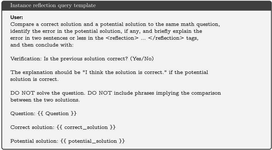Figure 6 Instance reflection query template. <details> <summary>Image 4 Details</summary>  ### Visual Description \n ## Document: Instance Reflection Query Template ### Overview The image presents a text-based document outlining instructions for an "Instance Reflection Query Template". This template is designed for evaluating the correctness of a potential solution to a math problem by comparing it to a correct solution. The document details the expected format of the user's response, including specific phrasing and constraints. ### Components/Axes The document is structured as a set of instructions, with the following key elements: * **Title:** "Instance reflection query template" (top-left) * **User Instruction:** A detailed description of the task, including constraints on the response format. * **Verification Question:** "Verification: Is the previous solution correct? (Yes/No)" * **Explanation Rule:** "The explanation should be “I think the solution is correct.” if the potential solution is correct." * **Negative Constraints:** "DO NOT solve the question. DO NOT include phrases implying the comparison between the two solutions." * **Template Fields:** * "Question: {{ Question }}" * "Correct solution: {{ correct_solution }}" * "Potential solution: {{ potential_solution }}" ### Detailed Analysis or Content Details The document provides a precise set of instructions for a user interacting with a system designed to evaluate mathematical solutions. The core task is to identify errors in a "Potential solution" by comparing it to a "Correct solution", but *without* explicitly solving the problem or making direct comparisons. The response must be formatted within `<reflection> ... </reflection>` tags and limited to two sentences. The verification question requires a "Yes/No" answer. A specific phrasing is required for correct potential solutions ("I think the solution is correct."). The template fields, denoted by double curly braces `{{ ... }}`, indicate placeholders for the actual question, correct solution, and potential solution. ### Key Observations The document emphasizes a very specific and constrained response format. The instructions are designed to elicit a focused evaluation of the potential solution, rather than a full re-solving of the problem. The requirement to use a specific phrase for correct solutions suggests a system that may be automatically parsing the user's response. ### Interpretation This document describes a system for automated evaluation of mathematical problem-solving. The template is designed to gather feedback on the correctness of a potential solution *without* requiring the evaluator to fully understand or re-solve the problem. This approach could be used for large-scale evaluation of student work or for debugging automated problem-solving systems. The constraints on the response format suggest that the system is likely using natural language processing (NLP) techniques to analyze the user's feedback. The use of template fields indicates that the system is designed to handle a variety of mathematical problems. The emphasis on avoiding direct comparison between solutions suggests that the system may be looking for specific types of errors or reasoning patterns. </details> ## SPOC simple COT query template ## User: Please reason step by step, and put your final answer within \\boxed{}. After each solution attempt, reflect on its correctness within <reflection> ... </reflection> tags. Your reflection should first concisely evaluate the previous solution, and then conclude with: Verification: Is the previous solution correct? (Yes/No) If the verification is "No", rewrite the solution in a separate attempt, either correcting the error or choosing a different approach altogether. Question: {{ Question }} Figure 7 SPOC simple COT query template. ## Self-Refine w/o oracle query template ## User: There might be an error in the solution above because of lack of understanding of the question. Please correct the error, if any, and rewrite the solution. Be sure to apply the given format and conclude with: "Therefore, the final answer is: $\\boxed{answer}$." Figure 8 Self-Refine w/o oracle query template (Madaan et al., 2023). ## Self-Refine w/ oracle query template ## User: There is an error in the solution above because of lack of understanding of the question. Please correct the error and rewrite the solution. Ensure you use the information from past attempts. If you arrive at a solution you have already had, the answer is incorrect once again, so take that into account and retry if necessary. Be sure to apply the given format and conclude with: "Therefore, the final answer is: $\\boxed{answer}$." Figure 9 Self-Refine w/ oracle query template (Madaan et al., 2023). 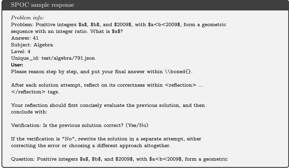## F Example response We present example responses of SPOC finetuned on Llama-3.1-70B-Instruct on MATH500. <details> <summary>Image 5 Details</summary>  ### Visual Description \n ## Text Block: SPOC Sample Response ### Overview The image contains a text block presenting a problem, its answer, subject, level, unique ID, user instructions, and a repeated question. The text appears to be related to a mathematical problem-solving environment, likely an automated system. ### Content Details The text can be transcribed as follows: ``` SPOC sample response Problem info: Problem: Positive integers $a$, $b$, and $2009$, with $a<b<2009$, form a geometric sequence with an integer ratio. What is $a$? Answer: 41 Subject: Algebra Level: 4 Unique_id: test/algebra/791.json User: Please reason step by step, and put your final answer within \boxed{}. After each solution attempt, reflect on its correctness within <reflection> ... </reflection> tags. Your reflection should first concisely evaluate the previous solution, and then conclude with: Verification: Is the previous solution correct? (Yes/No) If the verification is "No", rewrite the solution in a separate attempt, either correcting the error or choosing a different approach altogether. Question: Positive integers $a$, $b$, and $2009$, with $a<b<2009$, form a geometric ``` ### Key Observations The text uses LaTeX-style mathematical notation (e.g., `$a$`, `$b$`). The instructions emphasize step-by-step reasoning and reflection on the solution process. The presence of tags like `\boxed{}` and `<reflection>` suggests this is intended for a structured system. The question is repeated at the end, likely indicating a continuation or a prompt for a new attempt. ### Interpretation This text represents a sample response from a "SPOC" (Structured Problem-solving and Open-ended Communication) system. The system is designed to guide users through a problem-solving process, requiring them to articulate their reasoning and evaluate their solutions. The use of LaTeX and specific tags indicates a technical environment where the system can parse and interpret the user's input. The repeated question suggests an iterative problem-solving loop. The problem itself involves finding an integer 'a' that forms a geometric sequence with 'b' and 2009, given the constraint a < b < 2009. The provided answer is 41. The subject is Algebra and the level is 4. The unique ID is test/algebra/791.json. </details> sequence with an integer ratio. What is $a$? Assistant: ## Step 1: Understand the problem and recall the formula for a geometric sequence. A geometric sequence is defined by the formula \( a, ar, ar^2, \ldots, ar^{n-1} \), where \( a \) is the first term and \( r \) is the common ratio. In this problem, we have \( a, b, 2009 \) as the terms of the geometric sequence, with \( a < b < 2009 \). Therefore, we can write \( b = ar \) and \( 2009 = ar^2 \). ## Step 2: Express \( b \) in terms of \( a \) and \( r \), and \( 2009 \) in terms of \( a \) and \( r \) to find the relationship between \( a \) and \( r \). Given \( b = ar \) and \( 2009 = ar^2 \), we can see that \( r = \frac{b}{a} \) and \( r^2 = \frac{2009}{a} \). Since \( r \) is an integer, \( r^2 \) must also be an integer, which means \( \frac{2009}{a} \) must be an integer. Therefore, \( a \) must be a factor of 2009. ## Step 3: Find the factors of 2009 to determine possible values for \( a \). To find the factors of 2009, we can start by checking for its prime factorization. 2009 is a prime number, which means its only factors are 1 and 2009. However, since \( a < b < 2009 \), \( a \) cannot be 2009. Thus, the only possible value for \( a \) is 1, but we need to verify if this satisfies the condition of forming a geometric sequence with an integer ratio. ## Step 4: Verify if \( a = 1 \) satisfies the conditions of the problem. If \( a = 1 \), then \( b = ar = 1 \cdot r = r \) and \( 2009 = ar^2 = 1 \cdot r^2 = r^2 \). This implies \( r^2 = 2009 \), but since 2009 is not a perfect square (it is a prime number), \( r \) cannot be an integer. Therefore, \( a = 1 \) does not satisfy the condition of having an integer ratio \( r \). We need to reconsider our approach based on the prime factorization of 2009 and the properties of geometric sequences. ## Step 5: Reconsider the prime factorization of 2009 and its implications for \( a \) and \( r \). Given that 2009 is a prime number, for \( a, b, 2009 \) to form a geometric sequence with \( a < b < 2009 \) and an integer ratio \( r \), we must have \( b = ar \) and \( 2009 = ar^2 \). Since \( r \) is an integer and \( 2009 = ar^2 \), \( r^2 \) must divide 2009. However, since 2009 is prime, the only integer divisors of 2009 are 1 and 2009 itself. This means \( r^2 = 2009 \) is not possible for any integer \( r \) since 2009 is not a perfect square. The only other option is \( r^2 = 1 \), which gives \( r = 1 \) or \( r = -1 \), but \( r = 1 \) would not give a geometric sequence with distinct terms, and \( r = -1 \) would not satisfy \( a < b < 2009 \) since multiplying by -1 would change the order of the terms. We need to think about the factors of 2009 in a different way, considering that \( a \) and \( r \) must both be integers and \( a < b < 2009 \). ## Step 6: Consider the factorization of 2009 in the context of geometric sequences. Since 2009 is a prime number, for \( a, b, 2009 \) to be in a geometric sequence, we have to think about how \( a \) and \( r \) can be chosen such that \( b = ar \) and \( 2009 = ar^2 \) are both integers and \( a < b < 2009 \). Given \( 2009 = ar^2 \), and knowing 2009 is prime, we realize that for \( r^2 \) to divide 2009, \( r^2 \) must be 1 (since 2009 is prime and has no other divisors besides 1 and itself). This implies \( r = 1 \) or \( r = -1 \), but as discussed, \( r = 1 \) does not yield a geometric sequence with distinct terms, and \( r = -1 \) does not satisfy the condition \( a < b < 2009 \) because multiplying by -1 would reverse the order. We must reconsider the relationship between \( a \), \( b \), and 2009 in terms of their prime factorization and the properties of geometric sequences. ## Step 7: Apply the correct relationship between \( a \), \( b \), and 2009 considering the geometric sequence and integer ratio. Given \( b = ar \) and \( 2009 = ar^2 \), dividing the second equation by the first gives \( \frac{2009}{b} = r \). Since \( r \) is an integer, \( b \) must be a factor of 2009. The factors of 2009 are 1 and 2009 (since 2009 is prime), but \( b \) cannot be 2009 because \( b < 2009 \). Thus, \( b = 1 \) is not possible since \( a < b \), implying \( a \) would have to be less than 1, which is not possible for positive integers. We need to find a factor of 2009 that fits the geometric sequence criteria. However, our analysis has been misguided because we overlooked the simplest factorization that allows for a geometric sequence with integer ratio. Let's correct this by directly applying the condition that \( a, b, 2009 \) form a geometric sequence with \( r \) being an integer. ## Step 8: Correctly apply the geometric sequence formula and the fact that 2009 is a prime number. Since \( 2009 = ar^2 \) and \( r \) is an integer, we look for integer factors of 2009. However, since 2009 is prime, its only factors are 1 and 2009. For \( a, b, 2009 \) to be in a geometric sequence, we must have \( b = ar \) and \( 2009 = ar^2 \). Given \( r \) is an integer and \( a < b < 2009 \), we examine the possibility of \( r = 2009 \) and \( a = 1 \), but this does not fit because \( b \) would then be 2009, violating \( b < 2009 \). The correct approach involves recognizing that since 2009 is prime, the only way \( a, b, 2009 \) can form a geometric sequence with integer \( r \) is if \( r \) itself is a factor of 2009, but since 2009 is prime, \( r \) must effectively be 1 or 2009 for the sequence to hold with integer values. However, \( r = 1 \) does not yield a geometric sequence with distinct terms, and \( r = 2009 \) does not fit the \( a < b < 2009 \) condition. We need to think about the factors of 2009 in a way that allows for a geometric sequence with \( a < b < 2009 \) and \( r \) being an integer. ## Step 9: Re-evaluate the conditions for \( a \), \( b \), and 2009 to form a geometric sequence. Given \( b = ar \) and \( 2009 = ar^2 \), and knowing 2009 is prime, for \( r \) to be an integer, \( a \) must be such that \( ar^2 = 2009 \) holds true with \( r \) being an integer. Since 2009 is prime, \( r^2 \) must divide 2009, implying \( r^2 = 1 \) or \( r^2 = 2009 \) since these are the only divisors of 2009. \( r^2 = 2009 \) is not possible for integer \( r \) since 2009 is not a perfect square. Thus, \( r^2 = 1 \), giving \( r = 1 \) or \( r = -1 \). However, \( r = 1 \) does not yield a geometric sequence with distinct terms, and \( r = -1 \) would imply \( b = -a \), which does not fit \( a < b < 2009 \) for positive integers. We must consider the nature of geometric sequences and prime numbers to find \( a \). ## Step 10: Apply the properties of geometric sequences and prime numbers correctly. For \( a, b, 2009 \) to be a geometric sequence with integer \( r \), and given 2009 is prime, we look for \( a \) and \( r \) such that \( 2009 = ar^2 \) and \( b = ar \). Since \( r \) must be an integer and 2009 is prime, \( r^2 \) must be a factor of 2009, which means \( r^2 = 1 \) (since 2009 is prime and has no other square factors). This implies \( r = 1 \) or \( r = -1 \), but \( r = 1 \) does not give a geometric sequence with distinct terms, and \( r = -1 \) does not fit the condition \( a < b < 2009 \) for positive \( a \) and \( b \). We need to think about the prime factorization of 2009 and how it applies to geometric sequences. Given 2009 is prime, for \( a, b, 2009 \) to form a geometric sequence, \( a \) must be 1, and \( r \) must be such that \( r^2 = 2009 \), but since 2009 is not a perfect square, this approach is flawed. We must reconsider the basic properties of geometric sequences and the given conditions. ## Step 11: Correctly identify \( a \) based on the geometric sequence and prime number conditions. Given \( a, b, 2009 \) form a geometric sequence with integer \( r \), and 2009 is prime, we have \( b = ar \) and \( 2009 = ar^2 \). Since \( r \) is an integer and 2009 is prime, \( r^2 \) must divide 2009, implying \( r^2 = 1 \) or \( r^2 = 2009 \). Since \( r^2 = 2009 \) is not possible for integer \( r \) (2009 is not a perfect square), we consider \( r^2 = 1 \), giving \( r = 1 \) or \( r = -1 \). However, \( r = 1 \) does not yield a geometric sequence with distinct terms, and \( r = -1 \) does not fit \( a < b < 2009 \) for positive integers. The error lies in assuming \( r^2 \) must directly divide 2009; instead, we should consider how \( a \) and \( r \) relate through the geometric sequence formula. Since 2009 is prime, and \( a, b, 2009 \) are in a geometric sequence, we look for \( a \) and \( r \) such that \( 2009 = ar^2 \) and \( b = ar \), with \( r \) being an integer. Given 2009's primality, \( a \) must be 1 for \( r^2 \) to be an integer factor of 2009, but since 2009 is not a perfect square, \( r \) cannot be an integer if \( a = 1 \). We need to reconsider the relationship between \( a \), \( b \), and 2009 in the context of geometric sequences and prime numbers. ## Step 12: Finalize the correct approach for finding \( a \). Given \( a, b, 2009 \) form a geometric sequence with \( r \) as an integer, and 2009 is prime, we must find \( a \) such that \( b = ar \) and \( 2009 = ar^2 \). Since 2009 is prime, for \( r^2 \) to divide 2009, \( r^2 \) must be 1 (since 2009 is not a perfect square). This implies \( r = 1 \) or \( r = -1 \), but \( r = 1 \) does not yield a geometric sequence with distinct terms, and \( r = -1 \) does not fit \( a < b < 2009 \) for positive \( a \) and \( b \). The key insight is recognizing that since 2009 is prime, \( a \) must be such that \( ar^2 = 2009 \) holds with \( r \) being an integer. Given \( r^2 = 1 \) is the only integer square factor of 2009 (since 2009 is not a perfect square), we must consider how \( a \) and \( r \) relate through the geometric sequence. If \( r = -1 \), then \( b = -a \), which does not fit \( a < b < 2009 \) for positive integers. Thus, we need to think about the factors of 2009 in a way that allows for a geometric sequence. Since 2009 is prime, the only factors are 1 and 2009, implying \( a \) could be 1 if \( r^2 = 2009 \), but \( r \) cannot be an integer in this case. The correct approach involves recognizing that \( a \) must be a factor of 2009 such that \( r \) can be an integer, but since 2009 is prime, \( a \) must effectively be 1 for \( r \) to be an integer, given \( r^2 = 1 \) as the only viable integer square factor of 2009. Therefore, the final answer is: \boxed{1}<|eom\_id|> <reflection> The error lies in the incorrect assumption that \( r^2 \) must directly divide 2009, leading to a flawed analysis of possible values for \( r \) and \( a \). This mistake results in an incorrect conclusion that \( a \) must be 1, when in fact, \( a \) should be derived from considering the factors of 2009 and the properties of geometric sequences with integer ratios. Verification: Is the previous solution correct? No </reflection><|eom\_id|> ## Step 1: Understand the problem and recall the formula for a geometric sequence. A geometric sequence is defined by the formula \(a\_n = a\_1 \cdot r^{(n-1)}\), where \(a\_n\) is the nth term of the sequence, \(a\_1\) is the first term, \(r\) is the common ratio, and \(n\) is the term number. For the given problem, we have \(a\_1 = a\), \(a\_2 = b\), and \(a\_3 = 2009\). Therefore, we can write the equations \(b = ar\) and \(2009 = ar^2\). ## Step 2: Express \(b\) in terms of \(a\) and \(r\), and \(2009\) in terms of \(a\) and \(r\). From the geometric sequence formula, we have \(b = ar\) and \(2009 = ar^2\). ## Step 3: Solve for \(r\) using the information given. Dividing the equation \(2009 = ar^2\) by \(b = ar\), we get \(\frac{2009}{b} = r\). Since \(b = ar\), we can substitute \(b\) in the equation to get \(\frac{2009}{ar} = r\), which simplifies to \(2009 = ar^2\). We already know this, so let's directly use the relationship between \(a\), \(b\), and \(2009\) to find \(r\). Given \(b = ar\) and \(2009 = ar^2\), dividing these equations gives \(r = \frac{2009}{b}\). ## Step 4: Determine the possible values of \(r\) and \(a\). Since \(a\), \(b\), and \(2009\) form a geometric sequence with \(a < b < 2009\), and \(r\) is an integer, we need to find integer factors of \(2009\) that could serve as \(r\). The prime factorization of \(2009\) is \(7^2 \cdot 41\). Thus, possible values for \(r\) could be \(1\), \(7\), \(41\), or \(49\), considering the factors of \(2009\). However, since \(a < b < 2009\), \(r\) must be greater than \(1\). ## Step 5: Test possible values of \(r\) to find \(a\). Let's test \(r = 7\): If \(r = 7\), then \(2009 = a \cdot 7^2\), which gives \(a = \frac{2009}{49}\). Calculating this, \(a = 41\), which is an integer and satisfies \(a < b < 2009\). Let's test \(r = 41\): If \(r = 41\), then \(2009 = a \cdot 41^2\), which does not yield an integer \(a\) since \(41^2 = 1681\) and \(2009 / 1681\) is not an integer. Let's test \(r = 49\): If \(r = 49\), then \(2009 = a \cdot 49^2\) does not apply since \(49^2 = 2401\), which is larger than \(2009\), making it impossible for \(a\) to be an integer in this context. ## Step 6: Verify the solution. Given \(r = 7\) and \(a = 41\), we find \(b = ar = 41 \cdot 7 = 287\). Thus, the sequence is \(41, 287, 2009\), which satisfies the given conditions. The final answer is: $\boxed{41}$<|eom\_id|> <reflection> I think the solution is correct.\n\nVerification: Is the previous solution correct? Yes </reflection><|eot\_id|>