2506.07049

# FairPFN: A Tabular Foundation Model for Causal Fairness ## Abstract Machine learning (ML) systems are utilized in critical sectors, such as healthcare, law enforcement, and finance. However, these systems are often trained on historical data that contains demographic biases, leading to ML decisions that perpetuate or exacerbate existing social inequalities. Causal fairness provides a transparent, human-in-the-loop framework to mitigate algorithmic discrimination, aligning closely with legal doctrines of direct and indirect discrimination. However, current causal fairness frameworks hold a key limitation in that they assume prior knowledge of the correct causal model, restricting their applicability in complex fairness scenarios where causal models are unknown or difficult to identify. To bridge this gap, we propose FairPFN, a tabular foundation model pre-trained on synthetic causal fairness data to identify and mitigate the causal effects of protected attributes in its predictions. FairPFN’s key contribution is that it requires no knowledge of the causal model and still demonstrates strong performance in identifying and removing protected causal effects across a diverse set of hand-crafted and real-world scenarios relative to robust baseline methods. FairPFN paves the way for promising future research, making causal fairness more accessible to a wider variety of complex fairness problems. ## 1 Introduction Algorithmic discrimination is among the most pressing AI-related risks of our time, manifesting when machine learning (ML) systems produce outcomes that disproportionately disadvantage historically marginalized groups Angwin et al. (2016). Despite significant advancements by the fairness-aware ML community, critiques highlight the contextual limitations and lack of transferability of current statistical fairness measures to practical legislative frameworks Weerts et al. (2023). In response, the field of causal fairness has emerged, providing a transparent and human-in-the-loop causal framework for assessing and mitigating algorithmic bias with a strong analogy to existing anti-discrimination legal doctrines Plecko & Bareinboim (2024). <details> <summary>x1.png Details</summary>  ### Visual Description ## Diagram: FairPFN Pre-training Framework ### Overview This image is a technical diagram illustrating the pre-training framework for a model called "FairPFN." The diagram is divided into three sequential stages (a, b, c) at the top, which describe the process, and a larger visual flow below that maps these stages to a "Real-world Inference" pipeline. The overall purpose is to show how a Structural Causal Model (SCM) is used to generate data for training a transformer model (FairPFN) to make fair predictions by learning to map biased observables to fair outcomes. ### Components/Axes The diagram is segmented into several key components: 1. **Top Text Blocks (Process Description):** * **a) Data generation:** Describes generating an SCM and sampling a dataset `D` with a protected attribute `A`, biased observables `X_b`, and biased outcome `Y_b`. A fair outcome `Y_f` is also sampled by removing outgoing edges from `A`. * **b) Transformer input:** Describes partitioning the observational dataset `D` into training and validation splits. The transformer uses in-context examples `D_train` to make predictions on the inference set `D_val = (A_val, X_val)`. * **c) Fair prediction:** Describes the transformer making predictions `Ŷ_f` on the validation set. The pre-training loss is calculated with respect to the fair outcomes `Y_f`, teaching the model the mapping `X_b → Y_f`. 2. **Main Visual Flow (Left to Right):** * **Left: Structural Causal Model (SCM):** A directed acyclic graph with nodes and arrows. * **Nodes:** `A0` (blue circle), `U2` (green circle, appears twice), `X1`, `X2`, `X3` (purple circles), `Y_b` (orange circle), `Y_f` (yellow circle with red outline). * **Arrows:** Black arrows indicate causal relationships. Red arrows originate from `A0` and point to `X2` and `X3`, indicating a biased or protected attribute's influence. * **Center-Left: Observational Dataset:** A table with columns labeled `A` (blue header), `X1`, `X2`, `X3` (purple headers), and `Y_b` (orange header). The table contains 5 rows of colored cells (blue, purple, orange, light beige) representing data samples. * **Center: FairPFN:** A large, green, abstract block diagram representing the transformer model. Above it are three small copies of the SCM graph. Below it is a mathematical equation: `p(y_f | x_b, D_b) ∝ ∫_φ p(y_f | x_b, φ) p(D_b | φ) p(φ) dφ`. * **Center-Right: Pre-training Loss:** Two vertical bars. * Left bar: Labeled `Ŷ_f` (predicted fair outcome), with a grayscale gradient from white (top) to black (bottom). * Right bar: Labeled `Y_f` (true fair outcome), with a color gradient from light beige (top) to yellow (bottom). * **Arrows:** Large, light green arrows show the data flow from the SCM to the dataset, from the dataset to FairPFN, and from FairPFN to the loss calculation. A final green arrow loops from the loss back to the SCM, indicating the pre-training cycle. 3. **Title:** The entire lower section is titled "**FairPFN Pre-training**" in a large, bold, serif font. ### Detailed Analysis * **SCM Node Relationships:** * `A0` has direct red arrows to `X2` and `X3`. * `U2` (top) has arrows to `X1` and `Y_b`. * `U2` (bottom) has an arrow to `X1`. * `X1` has arrows to `X2` and `Y_b`. * `X2` has an arrow to `Y_b`. * `X3` has an arrow to `Y_b`. * `Y_f` is shown as a separate node, derived from the SCM by "removing the outgoing edges of A" as per the text in (a). * **Data Flow & Process Mapping:** 1. The **SCM** (Stage a) is used to generate the **Observational Dataset**. 2. The dataset is fed into the **FairPFN** model (Stages b & c). 3. The model produces predictions `Ŷ_f`. 4. The **Pre-training Loss** is computed by comparing `Ŷ_f` to the true fair outcome `Y_f`. 5. The loss is used to update the model, completing the pre-training loop. * **Mathematical Equation:** The equation below FairPFN expresses the model's predictive distribution as a proportionality (`∝`) involving an integral over model parameters `φ`. It combines the likelihood of the fair outcome given the biased input and parameters, the likelihood of the biased data given the parameters, and a prior over the parameters. ### Key Observations * **Color Coding is Systematic:** Blue is consistently used for the protected attribute `A`. Purple is used for the observables `X1, X2, X3`. Orange represents the biased outcome `Y_b`. Yellow represents the fair outcome `Y_f`. * **Bias Representation:** The red arrows from `A0` in the SCM visually highlight the pathways of bias that the framework aims to remove to achieve `Y_f`. * **Model Abstraction:** The FairPFN is represented as a generic green block, emphasizing its role as a black-box transformer model within this causal framework. * **Loss Visualization:** The loss bars visually contrast the model's grayscale predictions (`Ŷ_f`) against the colored true fair targets (`Y_f`), implying the goal is to align the prediction distribution with the fair outcome distribution. ### Interpretation This diagram outlines a methodology for instilling fairness into a predictive model through causal pre-training. The core idea is to use a known or assumed causal structure (the SCM) to generate synthetic data where the direct effect of a protected attribute (`A`) on the outcome is removed, creating a "fair" target (`Y_f`). A transformer model (FairPFN) is then trained not on the real-world biased outcome (`Y_b`), but on this constructed fair outcome. The process is "pre-training" because it happens before the model is applied to real-world tasks. By learning the mapping from biased observables (`X_b`) to fair outcomes (`Y_f`) in a controlled, causal environment, the model is intended to internalize a fair prediction rule. The integral in the equation suggests a Bayesian approach, marginalizing over model parameters to make predictions. The framework implies that real-world inference (using the pre-trained model) will then produce fair predictions even when only biased data is available, as the model has learned to "ignore" the biased pathways from `A`. The key assumption is the validity of the initial SCM used for data generation. 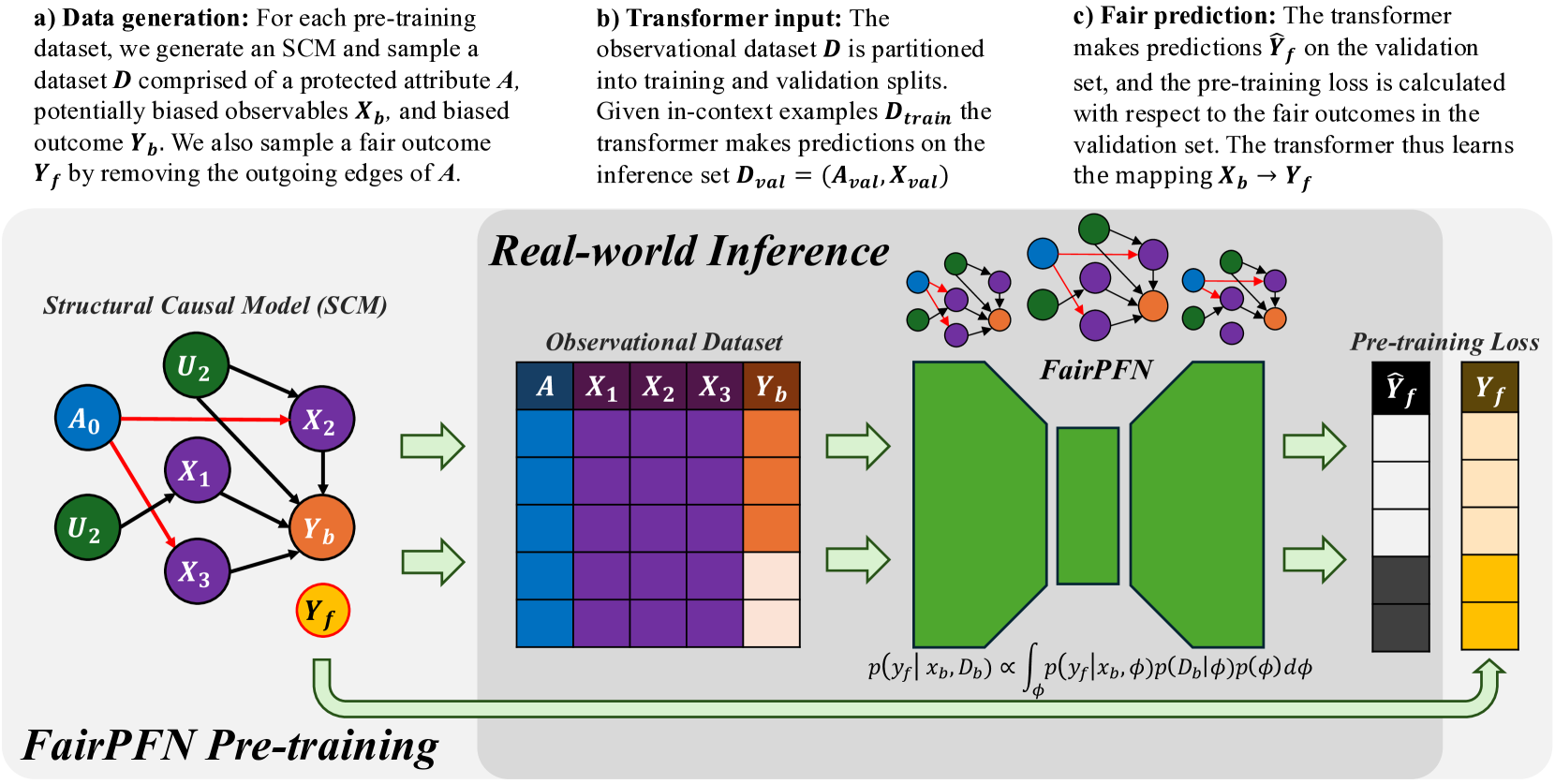</details> Figure 1: FairPFN Overview: FairPFN is a foundation model for causal fairness, pre-trained on synthetic datasets generated from sparse MLPs that represent SCMs with exogenous protected attributes (a). A biased dataset is created for each MLP/SCM and supplied as context to the transformer (b), with loss computed based on fair outcomes obtained by excluding the causal influence of the protected attribute (c). In practice, (d) FairPFN takes in only an observational dataset to predict fair targets by integrating over the simplest causal explanations for the biased data. A recent review comparing outcome-based and causal fairness approaches (Castelnovo et al., 2022) argues that the non-identifiability of causal models from observational data Pearl (2009) limits the usage of current causal fairness frameworks in practical applications. In practice, users must provide full or partial information about the underlying causal model, a challenging task given the complexity of systemic inequalities. Furthermore, an incorrectly presumed causal graph, such as one falsely assuming a variable is independent of a protected attribute, can invalidate causal fairness metrics Ma et al. (2023); Binkytė-Sadauskienė et al. (2022), resulting in fairwashing and fostering a false sense of security and trust. This paper takes a bold new perspective on achieving causal fairness. Our key contribution is FairPFN, a tabular foundation model for causal fairness, pre-trained on synthetic causal fairness data to learn to identify and remove the causal effects of protected attributes in tabular classification settings. When used on a new dataset, FairPFN does not rely on a user-specified causal model or graph, instead solely relying on the causally-generated data it has seen during pre-training. We demonstrate through extensive experiments that FairPFN effectively and consistently mitigates the causal impact of protected attributes across various hand-crafted and real-world scenarios, yielding causally fair predictions without user-specified causal information. We summarize our various contributions: 1. PFNs for Causal Fairness We propose a paradigm shift for algorithmic fairness, in which a transformer is pre-trained on synthetic causal fairness data. 1. Causal Fairness Prior: We introduce a synthetic causal data prior which offers a comprehensive representation for fairness datasets, modeling protected attributes as binary exogenous causes. 1. Foundation Model: We present FairPFN, a foundation model for causal fairness which, given only observational data, identifies and removes the causal effect of binary, exogenous protected attributes in predictions, and demonstrates strong performance in terms of both causal fairness and predictive accuracy on a combination of hand-crafted and real-world causal scenarios. We provide a prediction interface to evaluate and assess our pre-trained model, as well as code to generate and visualize our pre-training data at https://github.com/jr2021/FairPFN. ## 2 Related Work In recent years, causality has gained prominence in the field of algorithmic fairness, providing fairness researchers with a structural framework to reason about algorithmic discrimination. Unlike traditional fairness research Kamishima et al. (2012); Agarwal et al. (2018); Hardt et al. (2016), which focuses primarily on optimizing statistical fairness measures, causal fairness frameworks concentrate on the structure of bias. This approach involves modeling causal relationships among protected attributes, observed variables, and outcomes, assessing the causal effects of protected attributes, and mitigating biases using causal methods, such as optimal transport Plecko & Bareinboim (2024) or latent variable estimation Kusner et al. (2017); Ma et al. (2023); Bhaila et al. (2024). Counterfactual fairness, introduced by Kusner et al. (2017), posits that predictive outcomes should remain invariant between the actual world and a counterfactual scenario in which a protected attribute assumes an alternative value. This notion has spurred interest within the fairness research community, resulting in developments like path-specific extensions Chiappa (2019) and the application of Variational Autoencoders (VAEs) to create counterfactually fair latent representations Ma et al. (2023). The initial counterfactual fairness framework necessitates comprehensive knowledge of the causal model. In contrast, the Causal Fairness Analysis (CFA) framework Plecko & Bareinboim (2024) relaxes this requirement by organizing variables within a Standard Fairness Model (SFM) for bias assessment and mitigation. Moreover, the CFA framework presents the Fairness Cookbook, which defines causal fairness metrics—Indirect-Effect, Direct-Effect, and Spurious-Effect—that directly align with US legal doctrines of disparate impact and treatment. Furthermore, the CFA framework challenges Kusner et al. (2017) ’s modeling of protected attributes as exogenous causes, permitting correlations between protected attributes and confounding variables that contribute to the legally admissible Spurious-Effect. ## 3 Background This section establishes the scientific foundation of FairPFN, including terminology relevant to algorithmic fairness, causal ML, counterfactual fairness, and prior-data fitted networks (PFNs). #### Algorithmic Fairness Algorithmic discrimination occurs when historical biases against demographic groups (e.g., ethnicity, sex) are reflected in the training data of ML algorithms, leading to the perpetuation and amplification of these biases in predictions Barocas et al. (2023). Fairness research focuses on measuring algorithmic bias and developing fairness-aware ML models that produce non-discriminatory predictions. Practitioners have established over 20 fairness metrics, which generally break down into group-level and individual-level metrics Castelnovo et al. (2022). These metrics can be used to optimize predictive models, balancing the commonly observed trade-off between fairness and predictive accuracy Weerts et al. (2024). Causal Machine Learning Causal ML is a developing field that leverages modern ML methods for causal reasoning Pearl (2009), facilitating advancements in causal discovery, causal inference, and causal reasoning Peters et al. (2014). Causal mechanisms are often represented as Structural Causal Models (SCMs), defined as $\mathcal{M}=(U,O,F)$ , where $U$ are unobservables, $O$ are observables, and $F$ is a set of structural equations. These equations are expressed as $f_{j}:X_{j}=f_{j}(PA_{j},N_{j})$ , indicating that an outcome variable $F$ depends on its parent variables $PA$ and independent noise $N_{j}$ . Non-linearities in the set of structural equations $F$ influence data complexity and identifiability of causal quantities from observational data Schölkopf et al. (2012). In an SCM, interventions can be made by setting $X\leftarrow x_{1}$ and propagating this value through the model $\mathcal{M}$ , posing the question of "what will happen if I do something?". Counterfactuals expand upon the idea of interventions and are relevant when a value of $X$ is already observed, instead posing the question of "what would have happened if something had been different?" In addition to posing a slightly different question, counterfactuals require that exogenous noise terms are held constant, and thus classically require full knowledge of the causal model. In the context of algorithmic fairness, we are limited to level of counterfactuals as protected attributes are typically given and already observed. In causal reasoning frameworks, one major application of counterfactuals is the estimation of causal effects such as the individual and average treatment effects (ITE and ATE) which quantify the difference and expected difference between outcomes under different values of $X$ . $$ ITE:\tau=Y_{X\leftarrow x}-Y_{X\leftarrow x^{\prime}} \tag{1} $$ $$ ATE:E[\tau]=E[Y_{X\leftarrow x}]-E[Y_{X\leftarrow x^{\prime}}]. \tag{2} $$ #### Counterfactual Fairness is a foundational notion of causal fairness introduced by Kusner et al. (2017), requiring that an individual’s predictive outcome should match that in a counterfactual scenario where they belong to a different demographic group. This notion is formalized in the theorem below. **Theorem 1 (Unit-level/probabilistic)** *Given an SCM $\mathcal{M}=(U,O,F)$ where $O=A\cup X$ , a predictor $\hat{Y}$ is counterfactually fair on the unit-level if $\forall\hat{y}\in\hat{Y},\forall x,a,a^{\prime}\in A$ $$ P(\hat{y}_{A\rightarrow a}(u)|X,A=x,a)=P(\hat{y}_{A\rightarrow a^{\prime}}(u)| X,A,=x,a) $$* Kusner et al. (2017) notably choose to model protected attributes as exogenous, which means that they may not be confounded by unobserved variables with respect to outcomes. We note that the definition of counterfactual fairness in Theorem 1 is the unit-level probabilistic one as clarified by Plecko & Bareinboim (2024), because counterfactual outcomes are generated deterministically with fixed unobservables $U=u$ . Theorem 1 can be applied on the dataset level to form the population-level version also provided by Plecko & Bareinboim (2024) which measures the alignment of natural and counterfactual predictive distributions. **Theorem 2 (Population-level)** *Given an SCM $\mathcal{M}=(U,O,F)$ where $O=A\cup X$ , a predictor $\hat{Y}$ is counterfactually fair on the population-level if $\forall\hat{y}\in\hat{Y},\forall x,a,a^{\prime}\in A$ $$ P(\hat{y}_{A\rightarrow a}|X,A=x,a)=P(\hat{y}_{A\rightarrow a^{\prime}}|X,A=x,a) $$* Theorem 1 can also be transformed into a counterfactual fairness metric by quantifying the difference between natural and counterfactual predictive distributions. In this study we quantify counterfactual fairness as the distribution of the counterfactual absolute error (AE) between predictions in each distribution. **Definition 1 (Absolute Error (AE))** *Given an SCM $\mathcal{M}=(U,O,F)$ where $O=A\cup X$ , the counterfactual absolute error of a predictor $\hat{Y}$ is the distribution $$ AE=|P(\hat{y}_{A\rightarrow a}(u)|X,A=x,a)-P(\hat{y}_{A\rightarrow a^{\prime}} (u)|X,A=x,a)| $$* We note that because the outcomes are condition on the same noise terms $u$ our definition of AE builds off of Theorem 1. Intuitively, when the AE is skewed towards zero, then most individuals receive the same prediction in both the natural and counterfactual scenarios. Kusner et al. (2017) present various implementations of Counterfactually Fair Prediction (CFP). The three levels of CFP can be achieved by fitting a predictive model $\hat{Y}$ to observable non-descendants if any exist (Level-One), inferred values of an exogenous unobserved variable $K$ (Level-Two), or additive noise terms (Level-Three). Kusner et al. (2017) acknowledge that in practice, Level-One rarely occurs. Level-Two requires that the causal model be invertible, which allows the unobservable $K$ to be inferred by abduction. Level-Three models the scenario as an Additive Noise Model, and thus is the strongest in terms of representational capacity, allowing more degrees of freedom than in Level-Two to represent fair terms. The three levels of CFP are depicted in Appendix Figure 22. Causal Fairness The Causal Fairness Analysis (CFA) framework Plecko & Bareinboim (2024) introduces the Standard Fairness Model (SFM), which classifies variables as protected attributes $A$ , mediators $X_{med}$ , confounders $X_{conf}$ , and outcomes $Y$ . This framework includes a Fairness Cookbook of causal fairness metrics with a strong analogy to the legal notions of direct and indirect discrimination and business necessity as illustrated in Appendix Figure 23. Plecko & Bareinboim (2024) refute the modeling choice of Kusner et al. (2017) by their inclusion of confounders $X_{conf}$ in the SFM, arguing that these variables contribute to the legally admissible Spurious-Effect (SE). For simplicity of our experimental results, we follow the modeling of Kusner et al. (2017), and focus on the elimination of the Total-Effect (TE) of protected attributes as defined by Plecko & Bareinboim (2024), while noting in Section 6 the importance of relaxing this assumption in future extensions. Prior-data Fitted Networks Prior-data Fitted Networks (PFNs) Müller et al. (2022) and TabPFN Hollmann et al. (2023, 2025) represent a paradigm shift from traditional ML with a causal motivation, namely that simple causal models offer a quality explanation for real-world data. PFNs incorporate prior knowledge into transformer models by pre-training on datasets from a specific prior distribution Müller et al. (2022). TabPFN, a popular application of PFNs, applies these ideas to small tabular classification tasks by training a transformer on synthetic datasets derived from sparse Structural Causal Models (SCMs). As noted in Hollmann et al. (2023), a key advantage of TabPFN is its link to Bayesian Inference; where the transformer approximates the Posterior Predictive Distribution (PPD), thus achieving state-of-the-art performance by integrating over simple causal explanations for the data. ## 4 Methodology In this section, we introduce FairPFN, a foundation model for legally or ethically sensitive tabular classification problems that draws inspiration from PFNs and principles of causal fairness. We introduce our pre-training scheme, synthetic data prior, and draw connections to Bayesian Inference to explain the inner workings of FairPFN. ### 4.1 FairPFN Pre-Training First, we present our pre-training scheme, where FairPFN is fit to a prior of synthetic causal fairness data to identify and remove the causal effects of protected attributes in practice from observational data alone. We provide pseudocode for our pre-training algorithm in Algorithm 2, and outline the steps below. Input: Number of pre-training epochs $E$ and steps $S$ Transformer $\mathcal{M}$ with weights $\theta$ Hypothesis space of SCMs $\phi\in\Phi$ begin for $epoch=1$ to $E$ do for $step=1$ to $S$ do Draw a random SCM $\phi$ from $\Phi$ Sample $D_{bias}=(A,X_{bias},Y_{bias})$ from $\phi$ where A $\{a_{0},a_{1}\}$ is an exogenous binary protected attribute Sample $Y_{fair}$ from $\phi$ by performing dropout on outgoing edges of $A$ if any exist Partition $D_{bias}$ and $D_{fair}$ into $train/val$ Pass $D_{bias}^{train}$ into $\mathcal{M}$ as context Pass $D_{bias}^{val}$ into $\mathcal{M}$ to generate $Y_{pred}^{val}$ Calculate loss $L=CE(Y_{pred}^{val},Y_{fair}^{val})$ Update weights $\theta$ w.r.t $\nabla_{\theta}L$ end for end for Output: Transformer $\mathcal{M}:X_{bias}\rightarrow Y_{fair}$ Algorithm 1 FairPFN Pre-training Data Generating Mechanisms FairPFN pre-training begins by creating synthetic datasets that capture the causal mechanisms of bias in real-world data. Following the approach of Hollmann et al. (2023), we use Multi-Layer Perceptrons (MLPs) to model Structural Causal Models (SCMs) via the structural equation $f=z(P\cdot W^{T}x+\epsilon)$ , where $W$ denotes activation weights, $\epsilon$ represents Gaussian noise, $P$ is a dropout mask sampled from a log-scale to promote sparsity, and $z$ is a non-linearity. Figure 1 illustrates the connection among sampled MLPs, their corresponding SCMs, and the resulting synthetic pre-training data generated. We note that independent noise terms are not visualized in Figure 1. Biased Data Generation An MLP is randomly sampled and sparsity is induced through dropout on select edges. The protected attribute is defined as a binary exogenous variable $A\in\{a_{0},a_{1}\}$ at the input layer. We uniformly select $m$ features $X$ from the second hidden layer onwards to capture rich representations of exogenous causes. The target variable $Y$ is chosen from the output layer and discretized into a binary variable using a random threshold. A forward pass through the MLP produces a dataset $D_{bias}=(A,X_{bias},Y_{bias})$ with $n$ samples containing the causal influence of the protected attribute. #### Fair Data Generation A second forward pass generates a fair dataset $D_{fair}$ by applying dropout to the outgoing edges of the protected attribute $A$ in the MLP, as shown by the red edges in Figure 1. This dropout, similar to that in TabPFN, masks the causal weight of $A$ to zero, effectively reducing its influence to Gaussian noise $\epsilon$ . This increases the influence of fair exogenous causes $U_{0}$ and $U_{1}$ and independent noise terms all over the MLP visualized in Figure 1. We note that $A$ is sampled from an arbitrary distribution $A\in\{a_{0},a_{1}\}$ , as opposed to $A\in\{0,1\}$ , since both functions $f=0\cdot wx+\epsilon$ and $f=p\cdot 0x+\epsilon$ yield equivalent outcomes. Only after generating the pre-training dataset is $A$ converted to a binary variable for processing by the transformer. In-Context Learning After generating $D_{bias}$ and $D_{fair}$ , we partition them into training and validation sets: $D_{bias}^{train}$ , $D_{bias}^{val}$ , $D_{fair}^{train}$ , and $D_{fair}^{val}$ . We pass $D_{bias}^{train}$ as context to the transformer to provide information about feature-target relationships. To simulate inference, we input $X_{bias}^{val}$ into the transformer $\mathcal{M}$ , yielding predictions $Y_{pred}$ . We then compute the binary-cross-entropy (BCE) loss $L(Y_{pred},Y_{fair}^{val})$ against the fair outcomes $Y_{fair}^{val}$ , which do not contain effects of the protected attribute. Thus, the transformer $\mathcal{M}$ learns the mapping $\mathcal{M}:X_{bias}\rightarrow Y_{fair}$ . 1 Input: - Number of exogenous causes $U$ - Number of endogenous variables $U\times H$ - Number of features and samples $M\times N$ begin - Define MLP $\phi$ with depth $H$ and width $U$ - Initialize random weights $W:(U\times U\times H-1)$ - Sample sparsity masks $P$ with same dimensionality as weights - Sample $H$ per-layer non-linearities $z_{i}\sim\{Identity,ReLU,Tanh\}$ - Initialize output matrix $X:(U\times H)$ - Sample location $k$ of protected attribute in $X_{0}$ - Sample locations of features $X_{biased}$ in $X_{1:H-1}$ , and outcome $y_{bias}$ in $X_{H}$ - Sample protected attribute threshold $a_{t}$ and binary values $\{a_{0},a_{1}\}$ for $n=0$ to $N$ samples do - Sample values of exogenous causes $X_{0}:(U\times 1)$ - Sample values of additive noise terms $\epsilon:(U\times H)$ for $i=0$ to $H-1$ layers do - Pass intermediate representation through hidden layer $X_{i+1}=z_{i}(P_{i}\cdot W_{i}^{T}X_{i}+\epsilon_{i})$ end for - Select prot. attr. $A$ , features $X_{bias}$ and outcome $y_{bias}$ from $X_{0}$ , $X_{1:H-1}$ , and $X_{H}$ - Binarize $A\in\{a_{0},a_{1}\}$ over threshold $a_{t}$ - Set input weights in row $k$ of $W_{0}$ to 0 for $j=0$ to $H-1$ layers do - Pass intermediate representation through hidden layer $X_{j+1}=z_{i}(P_{i}\cdot W_{j}^{T}X_{j}+\epsilon_{j})$ end for 2 - Select the fair outcome $y_{fair}$ from $X_{H}$ end for - Binarize $y_{fair}\in\{0,1\}$ and $y_{bias}\in\{0,1\}$ over randomly sampled output threshold $y_{t}$ 3 Output: $D_{bias}=(A,X_{bias},y_{bias})$ and $y_{fair}$ Algorithm 2 FairPFN Synthetic Data Generation Prior-Fitting The transformer is trained for approximately 3 days on an RTX-2080 GPU on approximately 1.5 million different synthetic data-generating mechanisms, in which we vary the MLP architecture, the number of features $m$ , the sample size $n$ , and the non-linearities $z$ . Real-World Inference During real-world inference, FairPFN requires no knowledge of causal mechanisms in the data, but instead only takes as input a biased observational dataset and implicitly infers potential causal explanations for the data (Figure 1 d) based on the causally generated data it has seen during pre-training. Crucially, FairPFN is provided information regarding which variable is the protected attribute, which is represented in a protected attribute encoder step in the transformer. A key advantage of FairPFN is its alignment with Bayesian Inference, as transformers pre-trained in the PFN framework have been shown to approximate the Posterior Predictive Distribution (PPD) Müller et al. (2022). FairPFN thus approximates a modified PPD, predicting a causally fair target $y_{f}$ given biased features $X_{b}$ and a biased dataset $D_{b}$ by integrating over hypotheses for the SCM $\phi\in\Phi$ : $$ p(y_{f}|x_{b},D_{b})\propto\int_{\Phi}p(y_{f}|x_{b},\phi)p(D_{b}|\phi)p(\phi)d\phi \tag{3} $$ This approach has two advantages: it reduces the necessity of precise causal model inference, thereby lowering the risk of fairwashing from incorrect models Ma et al. (2023), and carries with it regularization-related performance improvements observed in Hollmann et al. (2023). We also emphasize that FairPFN is a foundation model and thus does not need to be trained for new fairness problems in practice. Instead, FairPFN performs predictions in a single forward pass of the data through the transformer. ## 5 Experiments This section assesses FairPFN’s performance on synthetic and real-world benchmarks, highlighting its capability to remove the causal influence of protected attributes without user-specified knowledge of the causal model, while maintaining high predictive accuracy. ### 5.1 Baselines We implement several baselines to compare FairPFN against a diverse set of traditional ML models, causal-fairness frameworks, and fairness-aware ML approaches. We summarize our baselines below, and provide a visualization of our baselines applied to the Fair Observable benchmark in Appendix Figure 25. - Unfair: Fit the entire training set $(X,A,Y)$ . - Unaware: Fit to the entire training set $(X,A,Y)$ . Inference returns the average of predictions on the original test set $(X,A)$ and the test set with alternative protected attribute values $(X,A\rightarrow a^{\prime})$ . - Avg. Cnft: Fit to the entire training set $(X,A,Y)$ . Inference returns the average (avg.) of predictions on the original test set $(X,A)$ and the counterfactual (cntf) test set $(X_{A\rightarrow a^{\prime}},A\rightarrow a^{\prime})$ . - Constant: Always predicts the majority class - Random: Randomly predicts the target - CFP: Combination of the three-levels of CFP as proposed in Kusner et al. (2017). Fit to non-descendant observables, unobservables, and independent noise terms $(X_{fair},U_{fair},\epsilon_{fair},Y)$ . - EGR: Exponentiated Gradient Reduction (EGR) as proposed by Agarwal et al. (2018) is fit to non-protected attributes $(X,Y)$ with XGBoost Chen & Guestrin (2016) as a base model. <details> <summary>x2.png Details</summary>  ### Visual Description ## Causal Diagram: Six Fairness Models in Machine Learning ### Overview The image displays six distinct causal models, numbered 1 through 6, illustrating different relationships between a protected attribute (`A`), observable features (`X_b`, `X_f`), an unobservable feature (`U`), an outcome (`Y`), and additive noise terms (`ε`). Each model is presented as a panel containing a directed acyclic graph (DAG) and its corresponding mathematical formulation. A legend at the bottom defines the visual symbols and node colors. ### Components/Axes The image is organized into six horizontal panels. Each panel contains: 1. **Title**: A numbered label (e.g., "1) Biased"). 2. **Causal Graph**: A diagram with colored nodes and arrows. 3. **Mathematical Formulation**: A set of equations defining the distributions and relationships between variables. **Legend (Bottom of Image):** * **Node Colors & Meanings**: * Blue Circle: `Prot. Attr.` (Protected Attribute, `A`) * Orange Circle: `Outcome` (`Y`) * Purple Circle: `Unfair Observable` (`X_b`) * Yellow Circle: `Fair Observable` (`X_f`) * Green Circle: `Fair Unobservable` (`U`) * **Arrow Types**: * Solid Arrow (`→`): `Cause` * Dotted Arrow (`⋯>`): `Additive Noise` * **Node Border**: * Dashed Circle Border: `Non-descendent` * **Node Fill Pattern**: * Hatched Pattern: `Seen by FairPFN` ### Detailed Analysis #### Panel 1: Biased * **Graph**: `A` (blue, hatched) → `X_b` (purple, hatched) → `Y` (orange, hatched). `X_b` has an additive noise term `ε_Xb` (green). `Y` has an additive noise term `ε_Y` (orange). * **Equations**: * `A ~ U({0,1})` * `ε_Xb, ε_Y ~ N(μ, σ), N(μ, σ)` * `X_b = w_A * A² + ε_Xb` * `Y = w_Xb * X_b² + ε_Y` * `Y = 1(Y ≥ Ȳ)` #### Panel 2: Direct-Effect * **Graph**: `A` (blue, hatched) → `X_f` (yellow, hatched) → `Y` (orange, hatched). `A` also has a direct arrow to `Y`. `X_f` has an additive noise term `ε_Xf` (green). `Y` has an additive noise term `ε_Y` (orange). * **Equations**: * `A ~ U({0,1})` * `ε_Xb, ε_Y ~ N(μ, σ), N(μ, σ)` * `X_f = N(μ, σ)` * `Y = w_Xf * X_f² + w_A * A² + ε_Y` * `Y = 1(Y ≥ Ȳ)` #### Panel 3: Indirect-Effect * **Graph**: `A` (blue, hatched) → `X_b` (purple, hatched) → `Y` (orange, hatched). `X_f` (yellow, dashed border) → `Y`. `X_b` has an additive noise term `ε_Xb` (green). `Y` has an additive noise term `ε_Y` (orange). * **Equations**: * `ε_Xb, ε_Y ~ N(μ, σ), N(μ, σ)` * `A ~ U({0,1}), X_f ~ N(μ, σ)` * `X_b = w_A * A² + ε_Xb` * `Y = w_Xb * X_b² + w_Xf * X_f² + ε_Y` * `Y = 1(Y ≥ Ȳ)` #### Panel 4: Fair Observable * **Graph**: `A` (blue, hatched) → `X_b` (purple, hatched) → `Y` (orange, hatched). `A` also has a direct arrow to `Y`. `X_f` (yellow, dashed border) → `Y`. `X_b` has an additive noise term `ε_Xb` (green). `Y` has an additive noise term `ε_Y` (orange). * **Equations**: * `ε_Xb, ε_Y ~ N(μ, σ), N(μ, σ)` * `A ~ U({0,1}), X_f ~ N(μ, σ)` * `X_b = w_A * A² + ε_Xb` * `Y = w_Xb * X_b² + w_Xf * X_f² + w_A * A² + ε_Y` * `Y = 1(Y ≥ Ȳ)` #### Panel 5: Fair Unobservable * **Graph**: `A` (blue, hatched) → `X_b` (purple, hatched) → `Y` (orange, hatched). `A` also has a direct arrow to `Y`. `U` (green, dashed border) → `X_b` and `U` → `Y`. `X_b` has an additive noise term `ε_Xb` (green). `Y` has an additive noise term `ε_Y` (orange). * **Equations**: * `ε_Xb, ε_Y ~ N(μ, σ), N(μ, σ)` * `A ~ U({0,1}), U ~ N(μ, σ)` * `X_b = w_A * A² + w_U * U² + ε_Xb` * `Y = w_Xb * X_b² + w_A * A² + ε_Y` * `Y = 1(Y ≥ Ȳ)` #### Panel 6: Fair Additive Noise * **Graph**: `A` (blue, hatched) → `X_b` (purple, hatched) → `Y` (orange, hatched). `A` also has a direct arrow to `Y`. `X_b` has an additive noise term `ε_Xb` (green). `Y` has an additive noise term `ε_Y` (orange). * **Equations**: * `ε_Xb, ε_Y ~ N(μ, σ), N(μ, σ)` * `A ~ U({0,1})` * `X_b = w_A * A² + ε_Xb` * `Y = w_Xb * X_b² + w_A * A² + ε_Y` * `Y = 1(Y ≥ Ȳ)` ### Key Observations 1. **Progression of Complexity**: The models progress from a simple biased pathway (1) to more complex structures incorporating direct effects (2, 4, 6), indirect effects (3), and unobservable confounders (5). 2. **Variable Roles**: The protected attribute `A` is always binary (`U({0,1})`). The outcome `Y` is always binarized via a threshold (`1(Y ≥ Ȳ)`). Observable features (`X_b`, `X_f`) and the unobservable `U` are modeled with normal distributions. 3. **Visual Coding**: The hatched pattern indicates which variables are "Seen by FairPFN," suggesting this diagram is from a paper proposing or analyzing a method called FairPFN. The dashed border for `X_f` and `U` in panels 3, 4, and 5 marks them as "Non-descendent" of `A` in those specific causal structures. 4. **Mathematical Consistency**: All models use squared terms (e.g., `A²`, `X_b²`) in their structural equations, implying non-linear relationships. The noise terms are consistently modeled as Gaussian. ### Interpretation This diagram is a technical taxonomy of data-generating processes used to study algorithmic fairness. It systematically varies the causal pathways through which a protected attribute (`A`) can influence an outcome (`Y`). * **Model 1 (Biased)** represents a scenario where bias flows entirely through a single, unfair observable feature (`X_b`). * **Models 2 & 6 (Direct-Effect, Fair Additive Noise)** introduce a direct effect of `A` on `Y`, which is often considered a source of unfair discrimination. * **Model 3 (Indirect-Effect)** separates features into fair (`X_f`) and unfair (`X_b`) observables, with `A` only affecting `Y` through the unfair one. * **Model 4 (Fair Observable)** combines direct effect with both fair and unfair observable pathways. * **Model 5 (Fair Unobservable)** is the most complex, introducing an unobserved confounder (`U`) that affects both the unfair feature and the outcome, representing real-world complexity where important factors are not measured. The core purpose is to provide a framework for evaluating fairness interventions (like the mentioned "FairPFN"). By defining these precise data-generating models, researchers can test whether a fairness algorithm works correctly under different, well-specified assumptions about how bias enters a system. The consistent use of squared terms and Gaussian noise creates a controlled, synthetic environment for this evaluation. The diagram argues that understanding fairness requires moving beyond simple correlations to explicitly model the causal structure of the data. 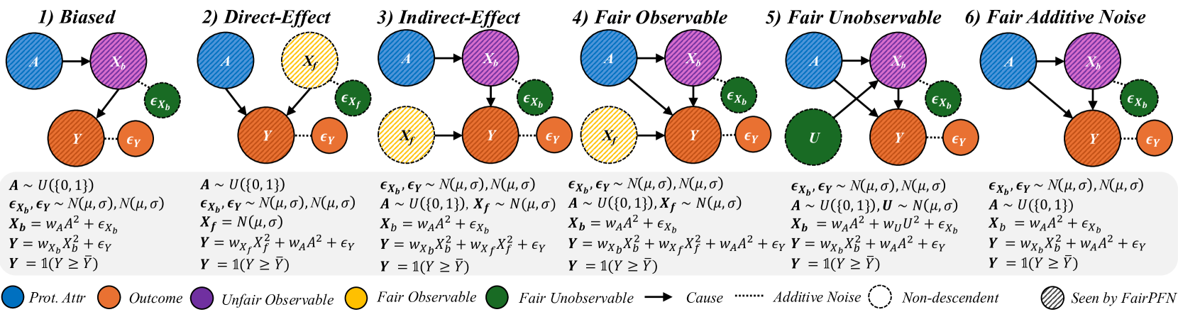</details> Figure 2: Causal Case Studies: Visualization and data generating processes of synthetic causal case studies, a handcrafted set of benchmarks designed to evaluate FairPFN’s ability to remove various sources of bias in causally generated data. For each group, 100 independent datasets are sampled, varying the number of samples, the standard deviation of noise terms $\sigma$ and the base causal effect $w_{A}$ of the protected attribute. In the CFP, Unfair, Unaware, and Avg. Cntf. baselines, we employ FairPFN with a random noise term passed as a "protected attribute." We opt to use this UnfairPFN instead of TabPFN so as to not introduce any TabPFN-specific behavioral characteristics or artifacts. We show in Appendix Figure 17 that this reverts FairPFN to a normal tabular classifier with competitive peformance to TabPFN. We also note that our Unaware baseline is not the standard approach of dropping the protected attribute. We opt for our own implementation of Unaware as it shows improved causal effect removal to the standard approach (Appendix Figure 17). ### 5.2 Causal Case Studies We first evaluate FairPFN using synthetic causal case studies to establish an experimental setting where the data-generating processes and all causal quantities are known, presenting a series of causal case studies with increasing difficulty to evaluate FairPFN’s capacity to remove various sources of bias in causally generated data. The data-generating processes and structural equations are illustrated in Figure 2, following the notation: $A$ for protected attributes, $X_{b}$ for biased-observables, $X_{f}$ for fair-observables, $U$ for fair-unobservables, $\epsilon_{X}$ for additive noise terms, and $Y$ for the outcome, discretized as $Y=\mathbb{1}(Y\geq\bar{Y})$ . We term a variable $X$ "fair" iff $A\notin anc(X)$ . The structural equations in Figure 2 contain exponential non-linearities to ensure the direction of causality is identifiable Peters et al. (2014), distinguishing the Fair Unobservable and Fair Additive Noise scenarios, with the former including an unobservable yet identifiable causal effect $U$ . For a robust evaluation, we generate 100 datasets per case study, varying causal weights of protected attributes $w_{A}$ , sample sizes $m\in(100,10000)$ (sampled on a log-scale), and the standard deviation $\sigma\in(0,1)$ (log-scale) of additive noise terms. We also create counterfactual versions of each dataset to assess FairPFN and its competitors across multiple causal and counterfactual fairness metrics, such as average treatment effect (ATE) and absolute error (AE) between predictions on observational and counterfactual datasets. We highlight that because our synthetic datasets are created from scratch, the fair causes, additive noise terms, counterfactual datasets, and ATE are ground truth. As a result, our baselines that have access to causal quantities are more precise in our causal case studies than in real-world scenarios where this causal information must be inferred. <details> <summary>extracted/6522797/figures/trade-off_by_group_synthetic.png Details</summary>  ### Visual Description ## Scatter Plot Grid: Fairness-Accuracy Trade-offs Across Causal Scenarios ### Overview The image displays a 2x3 grid of six scatter plots, each illustrating the trade-off between model error (1-AUC) and causal effect (Average Treatment Effect, ATE) for various machine learning fairness methods under different data-generating scenarios. A shared legend at the bottom defines eight distinct methods, each represented by a unique colored marker. The plots compare how these methods perform in terms of predictive error and the magnitude of the causal effect they induce or mitigate. ### Components/Axes * **Plot Titles (Top of each subplot):** 1. Biased 2. Direct-Effect 3. Indirect-Effect 4. Fair Observable 5. Fair Unobservable 6. Fair Additive Noise * **Y-Axis (Common to all plots):** Label: `Error (1-AUC)`. Scale ranges from 0.20 to 0.50, with major ticks at 0.20, 0.30, 0.40, 0.50. * **X-Axis (Common to all plots):** Label: `Causal Effect (ATE)`. Scale ranges from 0.00 to 0.25, with major ticks at 0.00, 0.05, 0.10, 0.15, 0.20, 0.25. 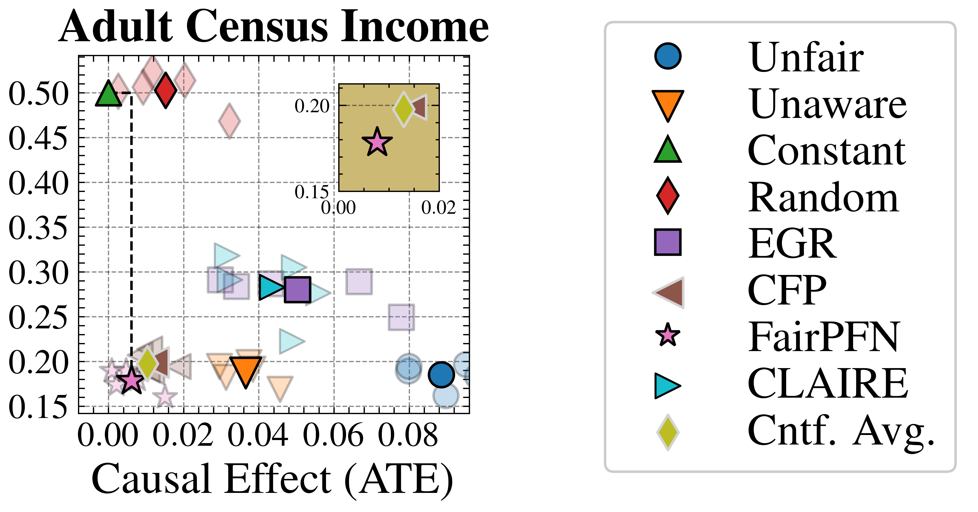* **Legend (Bottom of image):** Contains eight entries, each with a marker symbol and label: * Blue Circle: `Unfair` * Orange Inverted Triangle: `Unaware` * Green Triangle (pointing up): `Constant` * Red Diamond: `Random` * Purple Square: `EGR` * Brown Left-Pointing Triangle: `CFP` * Pink Star: `FairPFN` * Yellow Diamond: `Cntf. Avg.` (Counterfactual Average) ### Detailed Analysis **Plot 1: Biased** * **Trend:** Methods cluster in the top-left (high error, low causal effect), except for `Unfair` (blue circle) which is an outlier to the right (lower error, higher causal effect). * **Data Points (Approximate):** * `Random` (Red Diamond): ATE ≈ 0.00, Error ≈ 0.50 * `Constant` (Green Triangle): ATE ≈ 0.00, Error ≈ 0.49 * `EGR` (Purple Square): ATE ≈ 0.03, Error ≈ 0.44 * `FairPFN` (Pink Star): ATE ≈ 0.01, Error ≈ 0.41 * `Cntf. Avg.` (Yellow Diamond): ATE ≈ 0.01, Error ≈ 0.41 * `CFP` (Brown Triangle): ATE ≈ 0.01, Error ≈ 0.41 (partially obscured) * `Unaware` (Orange Inv. Triangle): ATE ≈ 0.08, Error ≈ 0.37 * `Unfair` (Blue Circle): ATE ≈ 0.12, Error ≈ 0.37 * **Spatial Grounding:** A dashed line connects `FairPFN`/`Cntf. Avg.` to `Unaware`, and another connects `Unaware` to `Unfair`, suggesting a progression or comparison path. **Plot 2: Direct-Effect** * **Trend:** Similar high-error cluster at low ATE. `Unfair` is again an outlier with much lower error but the highest ATE. * **Data Points (Approximate):** * `Random` (Red Diamond): ATE ≈ 0.00, Error ≈ 0.50 * `Constant` (Green Triangle): ATE ≈ 0.00, Error ≈ 0.49 * `EGR` (Purple Square): ATE ≈ 0.00, Error ≈ 0.41 * `FairPFN` (Pink Star): ATE ≈ 0.01, Error ≈ 0.39 * `CFP` (Brown Triangle): ATE ≈ 0.00, Error ≈ 0.36 * `Unaware` (Orange Inv. Triangle): ATE ≈ 0.00, Error ≈ 0.36 * `Unfair` (Blue Circle): ATE ≈ 0.22, Error ≈ 0.28 * **Spatial Grounding:** A dashed line connects the cluster around `CFP`/`Unaware` to `Unfair`. **Plot 3: Indirect-Effect** * **Trend:** The `Unfair` method has the lowest error and a moderate ATE. Other methods show a clearer separation, with `Unaware` having a higher ATE than the high-error cluster. * **Data Points (Approximate):** * `Random` (Red Diamond): ATE ≈ 0.00, Error ≈ 0.50 * `Constant` (Green Triangle): ATE ≈ 0.00, Error ≈ 0.49 * `CFP` (Brown Triangle): ATE ≈ 0.00, Error ≈ 0.42 * `EGR` (Purple Square): ATE ≈ 0.06, Error ≈ 0.42 * `FairPFN` (Pink Star): ATE ≈ 0.01, Error ≈ 0.38 * `Cntf. Avg.` (Yellow Diamond): ATE ≈ 0.01, Error ≈ 0.38 * `Unaware` (Orange Inv. Triangle): ATE ≈ 0.08, Error ≈ 0.33 * `Unfair` (Blue Circle): ATE ≈ 0.14, Error ≈ 0.33 * **Spatial Grounding:** A dashed line connects `FairPFN`/`Cntf. Avg.` to `Unaware`. **Plot 4: Fair Observable** * **Trend:** `Unfair` achieves the lowest error but at the cost of the highest ATE. `FairPFN` and `Cntf. Avg.` achieve very low error with near-zero ATE. `Unaware` has low error but moderate ATE. * **Data Points (Approximate):** * `Random` (Red Diamond): ATE ≈ 0.00, Error ≈ 0.50 * `Constant` (Green Triangle): ATE ≈ 0.00, Error ≈ 0.49 * `CFP` (Brown Triangle): ATE ≈ 0.00, Error ≈ 0.33 * `EGR` (Purple Square): ATE ≈ 0.02, Error ≈ 0.33 * `FairPFN` (Pink Star): ATE ≈ 0.01, Error ≈ 0.28 * `Cntf. Avg.` (Yellow Diamond): ATE ≈ 0.01, Error ≈ 0.28 * `Unaware` (Orange Inv. Triangle): ATE ≈ 0.04, Error ≈ 0.24 * `Unfair` (Blue Circle): ATE ≈ 0.20, Error ≈ 0.21 * **Spatial Grounding:** A dashed line connects `Random`/`Constant` down to `FairPFN`/`Cntf. Avg.`, and another connects `FairPFN`/`Cntf. Avg.` to `Unaware`, and a third connects `Unaware` to `Unfair`. **Plot 5: Fair Unobservable** * **Trend:** Similar pattern to Plot 4. `Unfair` has the lowest error and highest ATE. `FairPFN` and `Cntf. Avg.` show a good balance of low error and low ATE. * **Data Points (Approximate):** * `Random` (Red Diamond): ATE ≈ 0.00, Error ≈ 0.50 * `Constant` (Green Triangle): ATE ≈ 0.00, Error ≈ 0.49 * `EGR` (Purple Square): ATE ≈ 0.06, Error ≈ 0.31 * `CFP` (Brown Triangle): ATE ≈ 0.00, Error ≈ 0.28 * `FairPFN` (Pink Star): ATE ≈ 0.01, Error ≈ 0.28 * `Cntf. Avg.` (Yellow Diamond): ATE ≈ 0.01, Error ≈ 0.28 * `Unaware` (Orange Inv. Triangle): ATE ≈ 0.08, Error ≈ 0.23 * `Unfair` (Blue Circle): ATE ≈ 0.22, Error ≈ 0.20 * **Spatial Grounding:** A dashed line connects `Random`/`Constant` down to `FairPFN`/`Cntf. Avg.`, and another connects `FairPFN`/`Cntf. Avg.` to `Unaware`, and a third connects `Unaware` to `Unfair`. **Plot 6: Fair Additive Noise** * **Trend:** `Unfair` has the lowest error and a high ATE. `FairPFN` and `Cntf. Avg.` are clustered with low error and very low ATE. * **Data Points (Approximate):** * `Random` (Red Diamond): ATE ≈ 0.00, Error ≈ 0.50 * `Constant` (Green Triangle): ATE ≈ 0.00, Error ≈ 0.49 * `EGR` (Purple Square): ATE ≈ 0.03, Error ≈ 0.30 * `CFP` (Brown Triangle): ATE ≈ 0.00, Error ≈ 0.27 * `FairPFN` (Pink Star): ATE ≈ 0.01, Error ≈ 0.27 * `Cntf. Avg.` (Yellow Diamond): ATE ≈ 0.01, Error ≈ 0.27 * `Unaware` (Orange Inv. Triangle): ATE ≈ 0.05, Error ≈ 0.22 * `Unfair` (Blue Circle): ATE ≈ 0.20, Error ≈ 0.19 * **Spatial Grounding:** A dashed line connects `Random`/`Constant` down to `FairPFN`/`Cntf. Avg.`, and another connects `FairPFN`/`Cntf. Avg.` to `Unaware`, and a third connects `Unaware` to `Unfair`. ### Key Observations 1. **Consistent Baselines:** The `Random` and `Constant` methods consistently show the highest error (~0.50) and near-zero causal effect across all six scenarios, serving as performance baselines. 2. **The Unfair Baseline:** The `Unfair` method (blue circle) consistently achieves the lowest or near-lowest error in every plot but always at the expense of the highest causal effect (ATE), illustrating the core fairness-accuracy trade-off. 3. **Cluster of Fair Methods:** Methods like `FairPFN`, `Cntf. Avg.`, and often `CFP` cluster together in the low-error, low-ATE region, especially in the "Fair" scenarios (Plots 4, 5, 6). They appear to offer a favorable balance. 4. **Impact of Scenario:** The spread of points changes across scenarios. In "Biased" and "Direct-Effect," most fair methods are clustered at high error. In "Fair Observable," "Fair Unobservable," and "Fair Additive Noise," the fair methods achieve significantly lower error while maintaining low ATE. 5. **Dashed Lines:** The dashed lines appear to trace a "frontier" or comparison path, often connecting the high-error/random methods down to the better-performing fair methods, and then to the `Unaware` and finally the `Unfair` method. ### Interpretation This visualization is a comparative analysis of algorithmic fairness interventions. The **Causal Effect (ATE)** on the x-axis likely measures the disparity or bias in model outcomes between protected groups. **Error (1-AUC)** on the y-axis measures predictive inaccuracy. The data demonstrates a fundamental tension: methods that completely ignore fairness (`Unfair`) achieve the best predictive performance but cause the largest harmful disparities. Conversely, naive methods (`Random`, `Constant`) eliminate disparity but are useless for prediction. The key insight is the performance of methods like **FairPFN** and **Cntf. Avg.** They consistently appear in the "sweet spot" of the plots—achieving error rates much closer to the `Unfair` baseline while keeping the causal effect (bias) very low, particularly in the scenarios labeled "Fair." This suggests these methods are effective at mitigating unfairness without catastrophically sacrificing accuracy. The variation across the six titled scenarios indicates that the effectiveness of each fairness method is highly dependent on the underlying data-generating process (e.g., whether bias is direct, indirect, or based on observable/unobservable factors). The plots serve as a guide for selecting an appropriate fairness intervention based on the suspected causal structure of bias in a given problem domain. 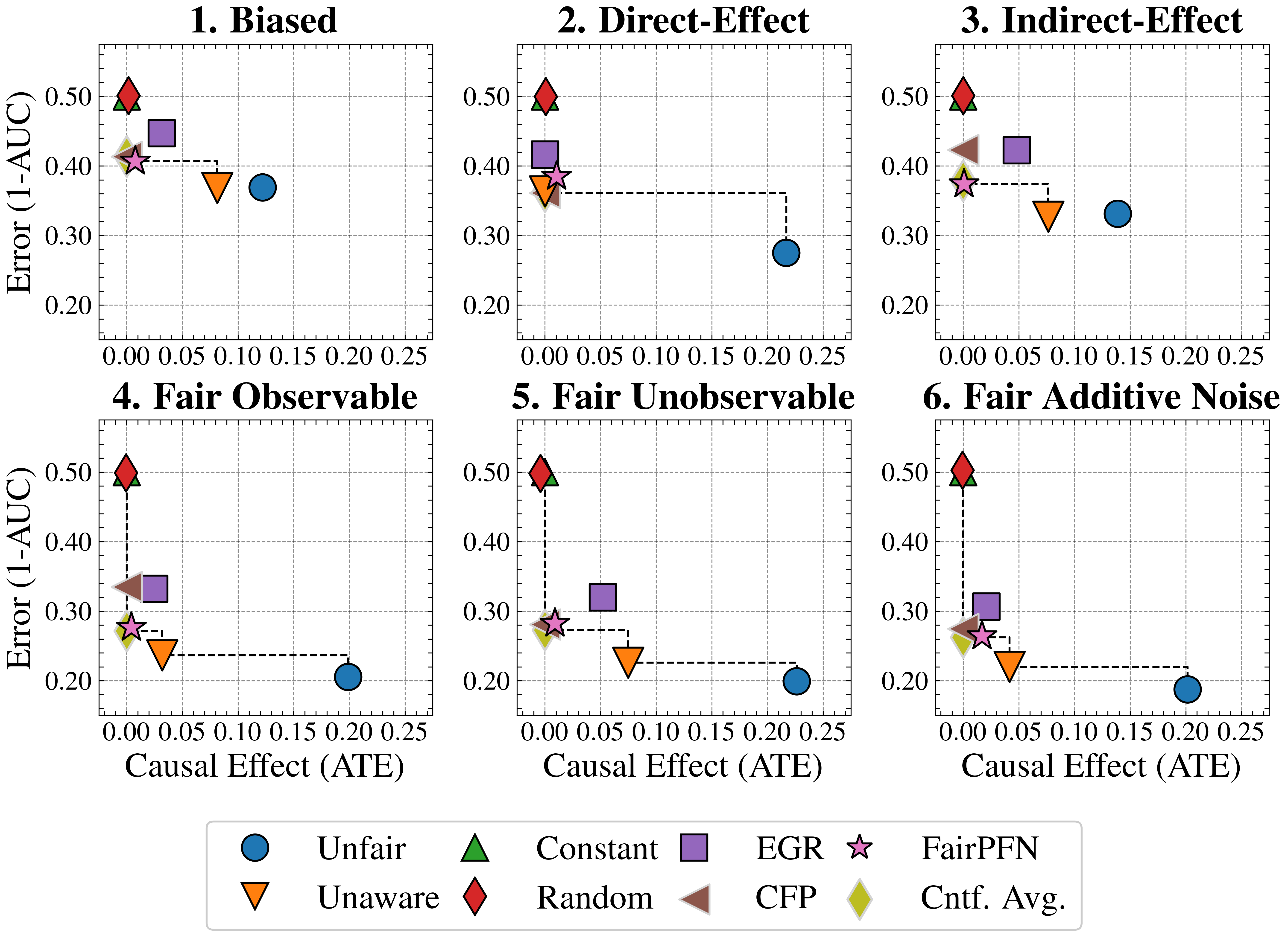</details> Figure 3: Fairness Accuracy Trade-Off (Synthetic): Average Treatment Effect (ATE) of predictions, predictive error (1-AUC), and Pareto Front performance of FairPFN versus baselines in our causal case studies. Baselines which have access to causal information are indicated by a light border. FairPFN is on the Pareto Front on 40% of synthetic datasets using only observational data, demonstrating competitive performance with the CFP and Cntf. Avg. baselines that utilize causal quantities from the true data-generating process. #### Fairness-Accuracy Trade-Off Figure 3 presents the fairness-accuracy trade-off for FairPFN and its baselines, displaying the mean absolute treatment effect (ATE) and mean predictive error (1-AUC) observed across synthetic datasets, along with the Pareto Front of non-dominated solutions. FairPFN (which only uses observational data) attains Pareto Optimal performance in 40% of the 600 synthetic datasets, exhibiting a fairness-accuracy trade-off competitive with CFP and Cntf. Avg., which use causal quantities from the true data-generating process. This is even the case in the Fair Unobservable and Fair Additive Noise benchmark groups, producing causally fair predictions using only observational variables that are either a protected attribute or a causal ancestor of it. This indicates FairPFN’s capacity to infer latent unobservables, which we further investigate in Section 5.3. We also highlight how the Cntf. Avg. baseline achieves lower error than CFP. We believe that this is due to Cntf. Avg. having access to both the observational and counterfactual datasets, which implicitly contains causal weights and non-linearities, while CFP is given only fair unobservables and must infer this causal information. The fact that a PFN is used as a base model in Cntf. Avg. could further explain this performance gain, as access to more observable variables helps guide the PFN toward accurate predictions realistic for the data. We suggest that this Cntf. Avg. as an alternative should be explored in future studies. <details> <summary>extracted/6522797/figures/tce_by_group_synthetic_new.png Details</summary>  ### Visual Description ## Box Plot Series: Causal Effect (ATE) Across Six Fairness Scenarios ### Overview The image displays a 2x3 grid of six box plots, each visualizing the distribution of "Causal Effect (ATE)" for four different methods under distinct experimental conditions. The plots are titled to indicate the scenario being tested. A shared legend at the bottom identifies the four methods and provides a summary performance metric. ### Components/Axes * **Chart Type:** Box and whisker plots with overlaid data points (jitter). * **Y-Axis (All Plots):** Labeled **"Causal Effect (ATE)"**. The scale ranges from -0.5 to 0.75, with major gridlines at intervals of 0.25 (-0.5, -0.25, 0, 0.25, 0.5, 0.75). * **X-Axis (All Plots):** Represents four categorical methods. The categories are not labeled on the axis but are defined by color in the legend. * **Legend (Bottom Center):** Contains the title **"Avg. Rank (ATE)"** and defines the four methods with associated colors and a numerical rank (lower is better): * **Pink:** `FairPFN: 1.88/4` * **Purple:** `EGR: 2.11/4` * **Orange:** `Unaware: 2.16/4` * **Blue:** `Unfair: 3.42/4` * **Subplot Titles (Top of each plot):** 1. **Biased** (Top Left) 2. **Direct-Effect** (Top Center) 3. **Indirect-Effect** (Top Right) 4. **Fair Observable** (Bottom Left) 5. **Fair Unobservable** (Bottom Center) 6. **Fair Additive Noise** (Bottom Right) ### Detailed Analysis **General Structure per Plot:** Each subplot contains four box plots, one for each method (Blue, Orange, Purple, Pink from left to right). The box represents the interquartile range (IQR), the line inside is the median, whiskers extend to 1.5*IQR, and circles represent individual data points/outliers. **Plot-by-Plot Analysis:** 1. **Biased:** * **Unfair (Blue):** Highest median (~0.05), largest IQR (box from ~0 to ~0.2), and widest overall range (whiskers from ~-0.15 to ~0.45). Many high-value outliers up to ~0.75. * **Unaware (Orange):** Median near 0, smaller IQR than Blue, range ~-0.05 to ~0.3. * **EGR (Purple):** Median slightly below 0, IQR similar to Orange, but with notable low-value outliers down to ~-0.5. * **FairPFN (Pink):** Median at 0, very compact IQR, range ~-0.1 to ~0.1. Tightest distribution. 2. **Direct-Effect:** * **Unfair (Blue):** Dominates the plot. Median ~0.15, large IQR (box from ~0.05 to ~0.35), whiskers from ~-0.1 to ~0.65. * **Unaware (Orange), EGR (Purple), FairPFN (Pink):** All are extremely compressed around 0. Their boxes are nearly flat lines, indicating near-zero variance and median. Minor outliers exist within ±0.1. 3. **Indirect-Effect:** * **Unfair (Blue):** Similar pattern to "Biased" plot. Median ~0.05, IQR ~0 to ~0.2, outliers up to ~0.75. * **Unaware (Orange):** Median ~0, IQR ~0 to ~0.1. * **EGR (Purple):** Median ~0, IQR ~0 to ~0.1, with low outliers to ~-0.4. * **FairPFN (Pink):** Very tight distribution around 0. 4. **Fair Observable:** * **Unfair (Blue):** Median ~0.15, IQR ~0.05 to ~0.3. * **Unaware (Orange):** Median ~0, very compact. * **EGR (Purple):** Median ~0, compact but with low outliers to ~-0.4. * **FairPFN (Pink):** Extremely tight around 0. 5. **Fair Unobservable:** * **Unfair (Blue):** Median ~0.2, IQR ~0.05 to ~0.35, whiskers to ~0.7. * **Unaware (Orange):** Median ~0.05, small IQR. * **EGR (Purple):** Median ~0, small IQR, low outliers. * **FairPFN (Pink):** Tight around 0. 6. **Fair Additive Noise:** * **Unfair (Blue):** Median ~0.15, IQR ~0.05 to ~0.3. * **Unaware (Orange):** Median ~0, small IQR. * **EGR (Purple):** Median ~0, small IQR, low outliers. * **FairPFN (Pink):** Tight around 0. ### Key Observations 1. **Consistent Hierarchy:** Across all six scenarios, the **Unfair (Blue)** method consistently shows the highest median causal effect (ATE) and the greatest variance (widest box and whiskers). **FairPFN (Pink)** consistently shows a median at or very near zero with the smallest variance. 2. **Scenario Impact:** The "Direct-Effect" scenario shows the most dramatic suppression of effect for the three fair/unaware methods (Orange, Purple, Pink), compressing them to near-zero variance. The "Biased" and "Indirect-Effect" scenarios show the most pronounced high-value outliers for the Unfair method. 3. **Method Comparison:** The **Unaware (Orange)** and **EGR (Purple)** methods generally perform similarly, with medians near zero. EGR exhibits a recurring pattern of negative outliers (low ATE values) in several plots (Biased, Indirect-Effect, Fair Observable). 4. **Legend Rank Correlation:** The visual performance aligns with the "Avg. Rank" in the legend. FairPFN (rank 1.88) is visually the best (lowest, tightest ATE). Unfair (rank 3.42) is visually the worst (highest, most variable ATE). Unaware and EGR are in the middle and close in rank (2.16 vs. 2.11), reflecting their similar visual performance. ### Interpretation This figure evaluates how different algorithmic approaches (FairPFN, EGR, Unaware) perform in estimating or mitigating **causal effects** (specifically, Average Treatment Effect - ATE) compared to an **Unfair** baseline, across various data-generating scenarios related to fairness. * **What the data suggests:** The "Unfair" method, which likely does not account for fairness constraints, results in substantial and variable estimated causal effects. In contrast, the methods designed for fairness (FairPFN, EGR) or that are simply unaware of sensitive attributes (Unaware) successfully drive the estimated ATE towards zero. This implies these methods are effective at removing or neutralizing the measured causal influence of a treatment, which in a fairness context often corresponds to a sensitive attribute like race or gender. * **How elements relate:** The six scenarios (Biased, Direct/Indirect Effect, Fair Observable/Unobservable/Noise) test the robustness of the methods under different assumptions about how bias or fairness is embedded in the data. The consistent pattern across plots indicates the core finding is robust: fairness-aware methods suppress the measured causal effect. * **Notable patterns/anomalies:** * The extreme compression in the "Direct-Effect" plot suggests that when the causal pathway is direct, the fairness interventions (and even the unaware method) are exceptionally effective at nullifying the measured effect. * The negative outliers for EGR are an anomaly, suggesting that in some runs, this method may over-correct, leading to a negative estimated ATE. * The high-value outliers for the Unfair method in "Biased" and "Indirect-Effect" scenarios indicate that under those data conditions, the lack of fairness constraints can lead to very large estimated causal disparities. 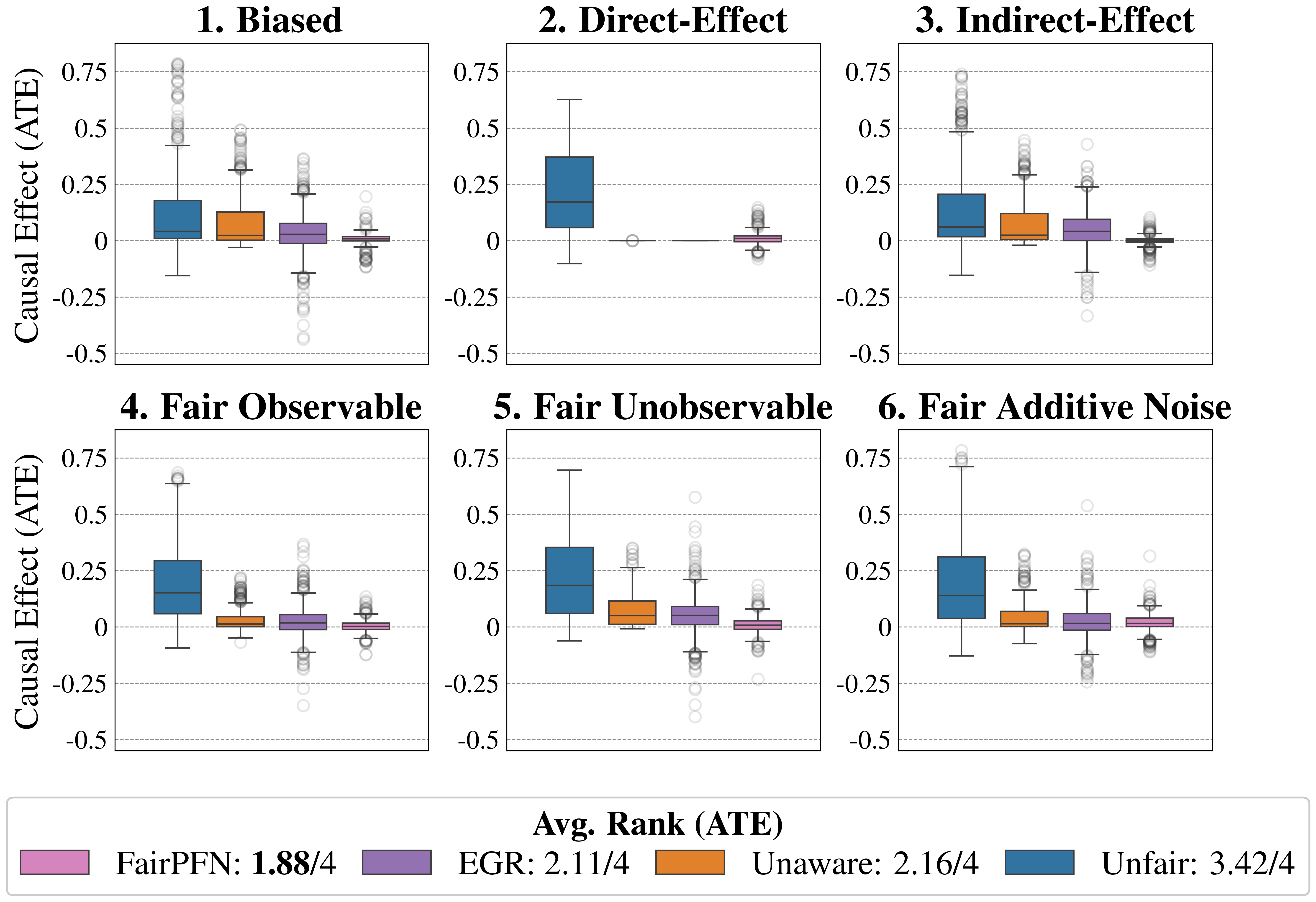**In summary, the visualization provides strong evidence that the FairPFN method (and to a lesser extent EGR and Unaware) consistently and effectively minimizes the estimated average causal effect of a treatment across a variety of fairness-related data scenarios, outperforming an unfair baseline.** </details> Figure 4: Causal Fairness (Synthetic): Average Treatment Effect (ATE) of predictions of FairPFN compared to baselines which do not have access to causal information. FairPFN consistently removes the causal effect with a margin of error of (-0.2, 0.2) and achieves an average rank of 1.88 out of 4, only to be outperformed on the Direct-Effect benchmark where Unaware is the optimal strategy. Causal Effect Removal We evaluate FairPFN’s efficacy in causal effect removal by analyzing box plots depicting the median, interquartile range (IQR), and average treatment effect (ATE) of predictions, compared to baseline predictive models that also do not access causal information (Figure 4). We observe that FairPFN exhibits a smaller IQR than the state-of-the-art bias mitigation method EGR. In an average rank test across 600 synthetic datasets, FairPFN achieves an average rank of 1.88 out of 4. We provide a comparison of FairPFN against all baselines in Figure 24. We note that our case studies crucially fit our prior assumptions about the causal representation of protected attributes. We show in Appendix Figure 13 that FairPFN reverts to a normal classifier when, for example, the exogeneity assumption is violated. #### Ablation Study We finally conduct an ablation study to evaluate FairPFN’s performance in causal effect removal across synthetic datasets with varying size, noise levels, and base rates of causal effect. Results indicate that FairPFN maintains consistent performance across different noise levels and base rates, improving in causal effect removal as dataset size increases and causal effects become easier to distinguish from spurious correlations Dai et al. (1997). We note that the variance of FairPFN, illustrated by box-plot outliers in Figure 4 that extend to 0.2 and -0.2, is primarily arises from small datasets with fewer than 250 samples (Appendix Figure 11), limiting FairPFN’s ability to identify causal mechanisms. We also show in Appendix Figure 14 that FairPFN’s fairness behavior remains consistent as graph complexity increases, though accuracy drops do to the combinatorially increasing problem complexity. For a more in-depth analysis of these results, we refer to Appendix B. 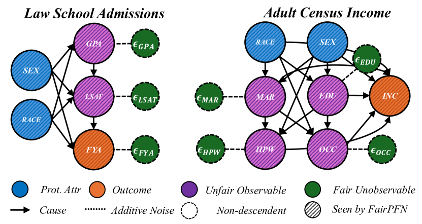### 5.3 Real-World Data This section evaluates FairPFN’s causal effect removal, predictive error, and correlation with fair latent variables on two real-world datasets with established causal graphs (Figure 5). For a description of our real-world datasets and the methods we use to obtain causal models, see Appendix A. 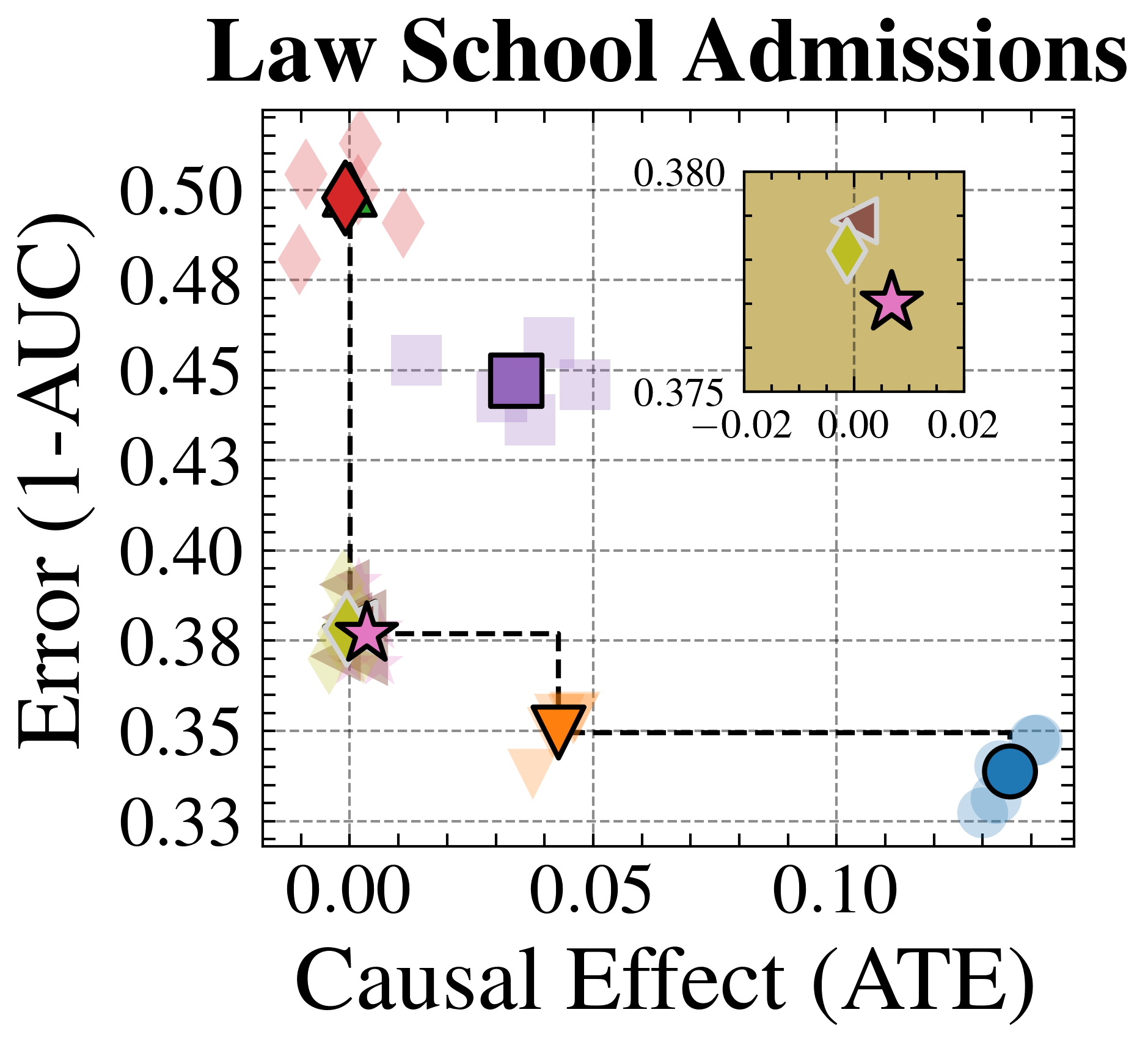#### Fairness-Accuracy Trade-Off We evaluate FairPFN’s effectiveness on real-world data in reducing the causal impact of protected attributes while maintaining strong predictive accuracy. Figure 6 shows the mean prediction average treatment effect (ATE) and predictive error (1-AUC) across 5 K-fold cross-validation iterations. FairPFN achieves a prediction ATE below 0.01 on both datasets and maintains accuracy comparable to Unfair. Furthermore, FairPFN exhibits lower variability in prediction ATE across folds compared to EGR, indicating stable causal effect removal We note that we also evaluate a pre-trained version of CLAIRE Ma et al. (2023) on the Adult Census income dataset, but observe little improvement to EGR. #### Counterfactual Fairness Next, we evaluate the counterfactual fairness of FairPFN on real-world datasets as introduced in Section 3, noting that the following analysis is conducted at the individual sample level, rather than at the dataset level. Figure 7 illustrates the distribution of Absolute Error (AE) achieved by FairPFN and baselines that do not have access to causal information. FairPFN significantly reduces this error in both datasets, achieving maximum divergences of less than 0.05 on the Law School dataset and 0.2 on the Adult Census Income dataset. For a visual interpretation of the AE on our real-world datasets we refer to Appendix Figure 16. In contrast, EGR performs similarly to Random in terms of counterfactual divergence, confirming previous studies which show that optimmizing for group fairness metrics does not optimize for individual level criteria Robertson et al. (2024). Interestingly, in an evaluation of group fairness metric Statistical Parity (DSP) FairPFN outperforms EGR on both our real-world data and causal case studies, a baseline was specifically optimized for this metric (Appendix Figures 20 and 21). <details> <summary>x3.png Details</summary>  ### Visual Description ## Causal Diagrams: Law School Admissions & Adult Census Income ### Overview The image displays two side-by-side causal diagrams (directed acyclic graphs) illustrating the relationships between variables in two different fairness-related datasets: "Law School Admissions" and "Adult Census Income." The diagrams use a color-coded and line-style-coded legend to categorize variable types and relationship types. The overall purpose is to model how protected attributes (like sex and race) causally influence outcomes (like first-year average grades or income), mediated by other observable and unobservable factors. ### Components/Axes **Legend (Bottom Center):** * **Colors & Node Types:** * Blue Circle: `Prot. Attr` (Protected Attribute) * Orange Circle: `Outcome` * Purple Circle: `Unfair Observable` * Green Circle: `Fair Unobservable` * **Line Styles & Relationship Types:** * Solid Arrow: `Cause` * Dashed Line: `Additive Noise` * Dotted Line: `Non-descendent` * **Node Fill Pattern:** * Diagonal Hatching: `Seen by FairPFN` **Diagram 1: Law School Admissions (Left Side)** * **Protected Attributes (Blue, Left):** `SEX`, `RACE` * **Unfair Observables (Purple, Center):** `GPA`, `LSAT` * **Outcome (Orange, Bottom-Right):** `FYA` (First-Year Average) * **Fair Unobservables (Green, Right):** `ε_GPA`, `ε_LSAT`, `ε_FYA` * **Causal Flow:** `SEX` and `RACE` have direct causal arrows pointing to `GPA`, `LSAT`, and `FYA`. `GPA` points to `LSAT`, and `LSAT` points to `FYA`. Each unfair observable (`GPA`, `LSAT`) and the outcome (`FYA`) is connected via a dashed "Additive Noise" line to a corresponding fair unobservable (`ε_GPA`, `ε_LSAT`, `ε_FYA`). **Diagram 2: Adult Census Income (Right Side)** * **Protected Attributes (Blue, Top):** `RACE`, `SEX` * **Unfair Observables (Purple, Middle/Bottom):** `MAR` (Marital Status), `EDU` (Education), `HPW` (Hours per Week), `OCC` (Occupation) * **Outcome (Orange, Right):** `INC` (Income) * **Fair Unobservables (Green, Scattered):** `ε_MAR`, `ε_EDU`, `ε_HPW`, `ε_OCC` * **Causal Flow:** This is a more complex network. * `RACE` and `SEX` have arrows pointing to `MAR`, `EDU`, `HPW`, `OCC`, and `INC`. * `MAR` points to `HPW` and `OCC`. * `EDU` points to `OCC` and `INC`. * `HPW` points to `INC`. * `OCC` points to `INC`. * Each unfair observable (`MAR`, `EDU`, `HPW`, `OCC`) is connected via a dashed "Additive Noise" line to a corresponding fair unobservable (`ε_MAR`, `ε_EDU`, `ε_HPW`, `ε_OCC`). * A dotted "Non-descendent" line connects `ε_EDU` to `INC`. ### Detailed Analysis **Node Inventory and Relationships:** 1. **Law School Admissions Diagram:** * **Direct Causes of FYA:** `SEX`, `RACE`, `LSAT`. * **Mediated Paths:** `SEX`/`RACE` -> `GPA` -> `LSAT` -> `FYA`. `SEX`/`RACE` -> `LSAT` -> `FYA`. * **Noise Injection:** The model explicitly includes unobserved, fair factors (`ε` terms) that additively influence the observed variables `GPA`, `LSAT`, and `FYA`. 2. **Adult Census Income Diagram:** * **Direct Causes of INC:** `SEX`, `RACE`, `EDU`, `HPW`, `OCC`. * **Key Mediators:** `EDU` and `OCC` are central hubs. `EDU` influences `OCC` and `INC`. `OCC` is influenced by `RACE`, `SEX`, `MAR`, and `EDU`, and in turn influences `INC`. * **Complex Interactions:** `MAR` (Marital Status) is modeled as being caused by `RACE` and `SEX`, and it subsequently influences `HPW` and `OCC`. * **Noise & Non-descendent:** Fair unobservables (`ε`) add noise to `MAR`, `EDU`, `HPW`, and `OCC`. Notably, `ε_EDU` has a dotted "Non-descendent" relationship to `INC`, suggesting it is not a descendant of the protected attributes in the causal graph but may still be correlated. **Spatial Grounding:** * The **legend** is positioned at the bottom, centered horizontally. * In both diagrams, **Protected Attributes (Blue)** are placed on the far left or top. * **Outcomes (Orange)** are placed on the far right or bottom-right. * **Unfair Observables (Purple)** occupy the central space between protected attributes and outcomes. * **Fair Unobservables (Green)** are placed adjacent to their corresponding unfair observable, typically to the right. ### Key Observations 1. **Structural Difference:** The Law School diagram is a simpler, more linear chain, while the Adult Census diagram is a dense, interconnected network, reflecting the greater complexity of socioeconomic factors. 2. **Common Pattern:** In both models, protected attributes (`SEX`, `RACE`) have **direct causal arrows to the final outcome** (`FYA`, `INC`), not just indirect paths through mediators. This is a critical modeling choice for fairness analysis. 3. **Role of "Unfair Observable":** Variables like `GPA`, `LSAT`, `EDU`, and `OCC` are labeled "Unfair Observable." This implies that while they are observed and causally influence the outcome, they may themselves be influenced by protected attributes, making their use in prediction potentially discriminatory. 4. **Explicit Noise Modeling:** The inclusion of `ε` (epsilon) nodes for "Fair Unobservable" factors explicitly acknowledges that not all variance in the observed variables is explained by the modeled causes; some is due to random, fair noise. 5. **FairPFN Context:** The hatching pattern indicating "Seen by FairPFN" suggests these diagrams are part of an analysis or methodology related to a fairness-aware model or algorithm named FairPFN. ### Interpretation These diagrams are **causal models for algorithmic fairness auditing**. They map the hypothesized real-world mechanisms through which sensitive attributes like race and sex might influence important outcomes (academic success, income). * **What the data suggests:** The models argue that bias can flow through two primary channels: 1) **Direct influence** of protected attributes on outcomes, and 2) **Indirect influence** where protected attributes shape intermediary factors (test scores, education, occupation) which then determine outcomes. The "Unfair Observable" label is a normative judgment, indicating that using these intermediaries for prediction could perpetuate historical inequities. * **Relationship between elements:** The diagrams establish a **chain of causality**. The protected attributes are root causes. The unfair observables are mediators that are "tainted" by the root causes. The outcome is the final effect. The fair unobservables represent legitimate, random variation. The arrows define the permissible paths for influence. * **Notable implications:** The direct arrows from `SEX`/`RACE` to `INC`/`FYA` are significant. They imply that even if one controls for all mediators (education, occupation, test scores), a direct disparity might remain, pointing to potential direct discrimination or the influence of unmeasured mediators. The complexity of the Adult Census diagram highlights why fairness in socioeconomic contexts is particularly challenging—interventions (e.g., on education) can have cascading effects through the network. The models provide a structured framework for asking "what-if" questions and designing fairness interventions that respect the causal structure of the problem. </details> Figure 5: Real-World Scenarios: Assumed causal graphs of real-world datasets Law School Admissions and Adult Census Income. <details> <summary>extracted/6522797/figures/trade-off_lawschool.png Details</summary>  ### Visual Description ## Scatter Plot with Inset Zoom: Law School Admissions ### Overview The image is a scatter plot titled "Law School Admissions." It visualizes the relationship between two metrics: "Causal Effect (ATE)" on the x-axis and "Error (1-AUC)" on the y-axis. The plot contains multiple data points represented by distinct shapes and colors, some connected by dashed lines. An inset plot in the upper-right quadrant provides a zoomed-in view of a specific cluster of points. ### Components/Axes * **Main Plot Title:** "Law School Admissions" (centered at the top). * **X-Axis:** * **Label:** "Causal Effect (ATE)" * **Scale:** Linear, ranging from approximately 0.00 to 0.10. * **Major Tick Marks:** 0.00, 0.05, 0.10. * **Y-Axis:** * **Label:** "Error (1-AUC)" * **Scale:** Linear, ranging from approximately 0.33 to 0.50. * **Major Tick Marks:** 0.33, 0.35, 0.38, 0.40, 0.43, 0.45, 0.48, 0.50. * **Inset Plot (Upper-Right):** * A smaller square plot with a tan background. * **X-Axis:** Range approximately -0.02 to 0.02. Major ticks at -0.02, 0.00, 0.02. * **Y-Axis:** Range approximately 0.375 to 0.380. Major ticks at 0.375, 0.380. * Contains three data points: a pink star, a yellow diamond, and a brown triangle. * **Data Series (Markers):** The plot uses distinct shapes and colors to represent different categories or methods. A legend is not explicitly shown, so identification is based on visual markers. 1. **Red Diamond:** Located at the top-left of the main plot. 2. **Purple Square:** Located in the upper-middle region. 3. **Pink Star:** Located in the lower-left region. A dashed line connects it to the orange triangle. 4. **Orange Triangle (pointing down):** Located in the lower-middle region. A dashed line connects it to the blue circle. 5. **Blue Circle:** Located at the bottom-right of the main plot. 6. **Yellow Diamond:** Located very close to the pink star in the lower-left. Also appears in the inset. 7. **Brown Triangle (pointing right):** Appears only in the inset plot. * **Connecting Lines:** Dashed black lines connect the Pink Star to the Orange Triangle, and the Orange Triangle to the Blue Circle, suggesting a sequence or comparison. ### Detailed Analysis * **Data Point Approximate Coordinates (Main Plot):** * **Red Diamond:** Causal Effect (ATE) ≈ 0.00, Error (1-AUC) ≈ 0.50. * **Purple Square:** Causal Effect (ATE) ≈ 0.04, Error (1-AUC) ≈ 0.45. * **Pink Star:** Causal Effect (ATE) ≈ 0.00, Error (1-AUC) ≈ 0.38. * **Yellow Diamond:** Causal Effect (ATE) ≈ 0.00, Error (1-AUC) ≈ 0.38 (slightly left/below the Pink Star). * **Orange Triangle:** Causal Effect (ATE) ≈ 0.05, Error (1-AUC) ≈ 0.35. * **Blue Circle:** Causal Effect (ATE) ≈ 0.10, Error (1-AUC) ≈ 0.33. * **Data Point Approximate Coordinates (Inset Plot):** * **Pink Star:** Causal Effect (ATE) ≈ 0.01, Error (1-AUC) ≈ 0.377. * **Yellow Diamond:** Causal Effect (ATE) ≈ 0.00, Error (1-AUC) ≈ 0.378. * **Brown Triangle:** Causal Effect (ATE) ≈ 0.00, Error (1-AUC) ≈ 0.379. * **Trend Verification:** * The dashed line from the **Pink Star** (low ATE, moderate Error) to the **Orange Triangle** (moderate ATE, lower Error) slopes downward to the right, indicating a decrease in error as causal effect increases along this path. * The dashed line from the **Orange Triangle** to the **Blue Circle** (high ATE, lowest Error) continues this downward-right slope, reinforcing the trend of decreasing error with increasing causal effect for this series. * The **Red Diamond** and **Purple Square** are isolated points with higher error values. The **Red Diamond** has near-zero causal effect but the highest error. ### Key Observations 1. **Trade-off Visualization:** The plot suggests a potential trade-off or relationship where methods achieving a higher Causal Effect (ATE) tend to have a lower Error (1-AUC), as seen in the connected series (Pink Star -> Orange Triangle -> Blue Circle). 2. **Cluster at Low ATE:** Several points (Red Diamond, Pink Star, Yellow Diamond) are clustered near a Causal Effect of 0.00, but with vastly different error rates (from ~0.38 to ~0.50). 3. **Inset Highlight:** The inset zooms in on the cluster near (0.00, 0.38), revealing that the Pink Star, Yellow Diamond, and Brown Triangle are very close in both metrics, with differences in the third decimal place for Error. 4. **Outlier:** The **Red Diamond** is a clear outlier with the highest error (0.50) despite having a near-zero causal effect. ### Interpretation This chart likely compares different algorithmic models or policy interventions in the context of law school admissions. The metrics suggest a dual evaluation: * **Causal Effect (ATE - Average Treatment Effect):** Measures the estimated impact of an intervention (e.g., using a specific admissions model) on an outcome. * **Error (1-AUC):** Measures the predictive inaccuracy of the model. A lower value is better. The data demonstrates that not all methods are equal. The connected path (Pink Star -> Orange Triangle -> Blue Circle) may represent a family of related models or a tuning process where increasing the model's causal effect estimate is associated with improved predictive accuracy (lower error). The **Blue Circle** method appears most favorable, achieving the highest causal effect and lowest error. Conversely, the **Red Diamond** method performs poorly, with high error and negligible causal effect. The cluster near zero ATE (including the inset points) represents methods that have little to no estimated causal impact but vary significantly in their baseline predictive error. The inset emphasizes that even among these low-impact methods, fine-grained differences exist. **Overall Implication:** The chart argues for the importance of considering both causal impact and predictive error when evaluating admissions models. It visually identifies a promising direction (increasing ATE while decreasing error) and highlights underperforming or neutral alternatives. The absence of a formal legend suggests the audience is expected to recognize the methods by their markers, indicating this is likely from a specialized technical paper or report. </details> <details> <summary>extracted/6522797/figures/trade-off_adult.png Details</summary>  ### Visual Description \n ## Scatter Plot: Adult Census Income - Fairness vs. Causal Effect ### Overview The image is a scatter plot comparing various algorithmic fairness methods on the "Adult Census Income" dataset. It plots each method's performance on two metrics: the y-axis represents a fairness metric (likely a disparity measure, where lower is fairer), and the x-axis represents the "Causal Effect (ATE)" or Average Treatment Effect. A legend on the right maps specific symbols to method names. An inset plot in the top-right corner provides a zoomed-in view of a specific cluster of data points. ### Components/Axes * **Main Plot Title:** "Adult Census Income" (top-left, above the plot area). * **Y-Axis:** Numerical scale from 0.15 to 0.50, with major ticks at 0.05 intervals (0.15, 0.20, 0.25, 0.30, 0.35, 0.40, 0.45, 0.50). The axis label is not explicitly written, but based on context, it represents a fairness disparity metric (lower values indicate higher fairness). * **X-Axis:** Labeled "Causal Effect (ATE)". Numerical scale from 0.00 to 0.08, with major ticks at 0.02 intervals (0.00, 0.02, 0.04, 0.06, 0.08). * **Legend:** Positioned to the right of the main plot. It lists 10 categories with corresponding symbols: 1. **Unfair:** Blue circle (●) 2. **Unaware:** Orange downward-pointing triangle (▼) 3. **Constant:** Green upward-pointing triangle (▲) 4. **Random:** Red diamond (◆) 5. **EGR:** Purple square (■) 6. **CFP:** Brown left-pointing triangle (◀) 7. **FairPFN:** Pink star (★) 8. **CLAIRE:** Cyan right-pointing triangle (▶) 9. **Cntf. Avg.:** Yellow diamond (◆) * **Inset Plot:** A smaller plot with a yellow background, located in the top-right quadrant of the main plot area. * **Inset Y-Axis:** Scale from 0.15 to 0.20. * **Inset X-Axis:** Scale from 0.00 to 0.02. * It contains a subset of data points, primarily the pink star (FairPFN) and yellow diamond (Cntf. Avg.), allowing for clearer visualization of their close proximity. ### Detailed Analysis The plot displays multiple data points for several methods, suggesting results from different runs or configurations. The spatial distribution reveals a clear trade-off. * **High Fairness, Low Causal Effect Cluster (Top-Left):** * **Constant (Green ▲):** Positioned at approximately (ATE ≈ 0.00, Fairness ≈ 0.50). This is the highest point on the y-axis, indicating the worst fairness score but a near-zero causal effect. * **Random (Red ◆):** Several points clustered near (ATE ≈ 0.01, Fairness ≈ 0.50). * **Cntf. Avg. (Yellow ◆):** Points are located around (ATE ≈ 0.01, Fairness ≈ 0.20). One point is highlighted in the inset at approximately (ATE ≈ 0.015, Fairness ≈ 0.19). * **Low Fairness, Higher Causal Effect Cluster (Bottom-Right):** * **Unfair (Blue ●):** Points are clustered at the far right, around (ATE ≈ 0.08, Fairness ≈ 0.18). This represents the baseline with the highest measured causal effect but poor fairness. * **Intermediate Methods (Central Region):** * **Unaware (Orange ▼):** Points are near (ATE ≈ 0.04, Fairness ≈ 0.20). * **EGR (Purple ■):** Points are scattered between ATE 0.03-0.07 and Fairness 0.25-0.30. * **CFP (Brown ◀):** Points are near (ATE ≈ 0.02, Fairness ≈ 0.20). * **CLAIRE (Cyan ▶):** Points are scattered between ATE 0.03-0.05 and Fairness 0.25-0.30. * **FairPFN (Pink ★):** This method is a key focus. In the main plot, its points are clustered in the bottom-left corner near (ATE ≈ 0.005, Fairness ≈ 0.18). The inset plot zooms in on this region, showing the FairPFN star at approximately (ATE ≈ 0.008, Fairness ≈ 0.175), very close to the Cntf. Avg. diamond. ### Key Observations 1. **Pareto Frontier:** The data points form a rough Pareto frontier from the top-left (high fairness, low effect) to the bottom-right (low fairness, high effect). Methods like "Constant" and "Random" are at one extreme, while "Unfair" is at the other. 2. **FairPFN's Position:** FairPFN achieves a very low fairness disparity score (≈0.175-0.18), comparable to the "Unfair" baseline, while maintaining a small but positive causal effect (ATE ≈ 0.008). This suggests it successfully mitigates bias without completely sacrificing predictive utility related to the treatment. 3. **Inset Purpose:** The inset is crucial for distinguishing between FairPFN and Cntf. Avg., which are overlapping in the main plot. It confirms they occupy a similar region of high fairness and low positive causal effect. 4. **Method Variability:** Methods like EGR and CLAIRE show significant spread in their results, indicating sensitivity to initialization or hyperparameters. ### Interpretation This chart visualizes the fundamental tension in causal fairness: modifying a model to reduce unfairness (lower y-axis value) often comes at the cost of reducing its estimated causal effect on the outcome (lower x-axis value, ATE). * **What the data suggests:** The "Unfair" model has the strongest measured causal relationship between treatment and outcome but is the most biased. The "Constant" model eliminates bias by making a constant prediction, thereby nullifying any causal effect. The goal of advanced methods like FairPFN, CLAIRE, and EGR is to navigate this trade-off. * **How elements relate:** The position of each method on this 2D plane is a direct measure of its performance on these two competing objectives. The ideal method would be in the bottom-right corner (high causal effect, high fairness), but the frontier suggests this is difficult to achieve. FairPFN appears to find a favorable compromise, achieving near-optimal fairness with a small, non-zero causal effect. * **Notable anomalies:** The "Random" method performs surprisingly poorly on fairness (high y-value), indicating that random predictions do not inherently solve bias problems in this context. The significant scatter of some methods (EGR, CLAIRE) highlights the importance of robust evaluation across multiple runs. </details> Figure 6: Fairness-Accuracy Trade-off (Real-World): Average Treatment Effect (ATE) of predictions, predictive error (1-AUC), and Pareto Front of the performance of FairPFN compared to our baselines on each of 5 validation folds (light) and across all five folds (solid) of our real-world datasets. Baselines which have access to causal information have a light border. FairPFN matches the performance of baselines which have access to inferred causal information with only access to observational data. 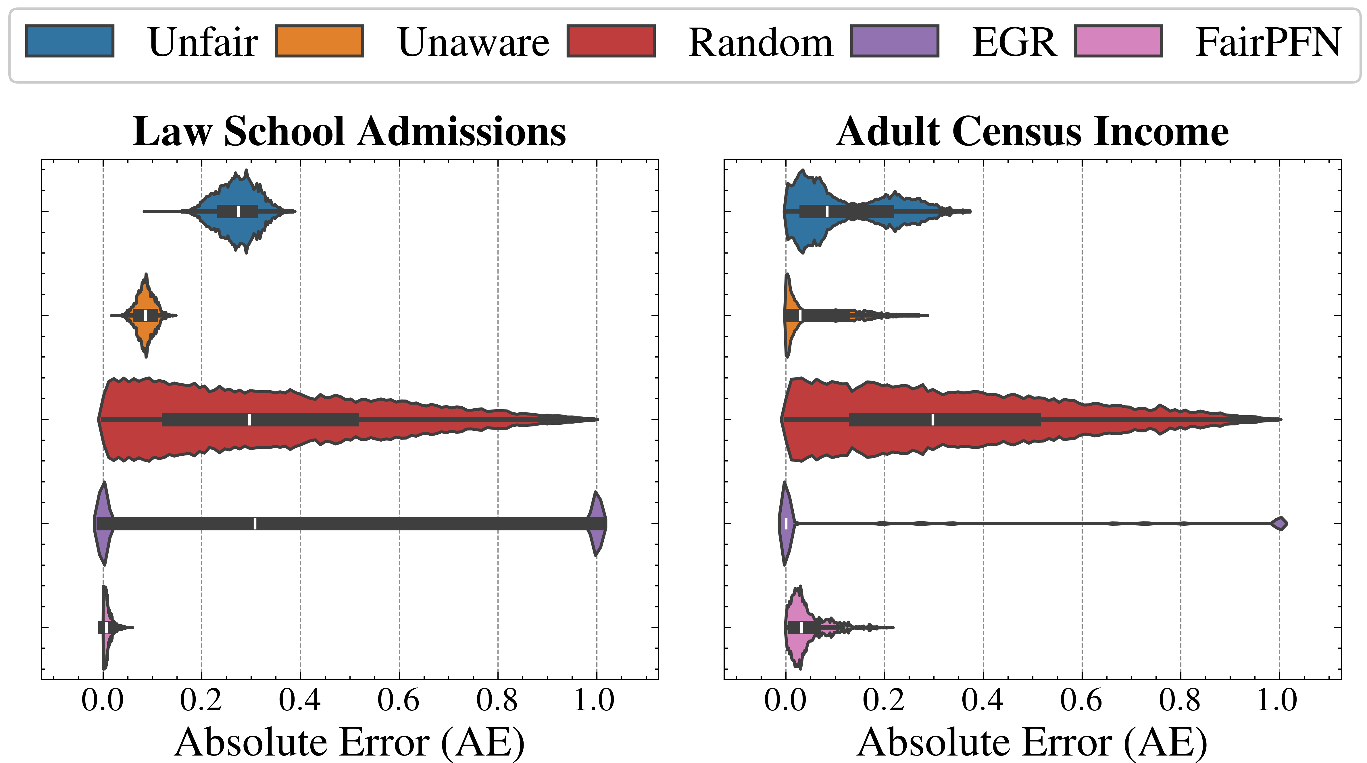<details> <summary>extracted/6522797/figures/kl_real.png Details</summary>  ### Visual Description ## Violin Plot Comparison: Absolute Error Distributions by Method ### Overview The image displays two side-by-side violin plots comparing the distribution of Absolute Error (AE) for five different methods across two distinct datasets: "Law School Admissions" (left panel) and "Adult Census Income" (right panel). Each violin plot combines a kernel density estimate (the colored shape) with an embedded box plot (the dark gray bar with a white median line) to show the distribution, median, and interquartile range of the error metric for each method. ### Components/Axes * **Legend:** Positioned at the top center, spanning the width of both plots. It defines five methods with associated colors: * **Unfair:** Blue * **Unaware:** Orange * **Random:** Red * **EGR:** Purple * **FairPFN:** Pink * **Subplot Titles:** * Left Panel: "Law School Admissions" * Right Panel: "Adult Census Income" * **X-Axis (Both Panels):** Labeled "Absolute Error (AE)". The scale runs from 0.0 to 1.0, with major tick marks at 0.0, 0.2, 0.4, 0.6, 0.8, and 1.0. Vertical dashed grid lines extend from these ticks. * **Y-Axis (Implied):** The vertical axis within each subplot represents the different methods, stacked from top to bottom in the order: Unfair, Unaware, Random, EGR, FairPFN. ### Detailed Analysis **Law School Admissions (Left Panel):** 1. **Unfair (Blue):** Distribution is centered around a median AE of approximately 0.3. The violin shape is moderately wide, indicating a concentrated spread of errors primarily between ~0.2 and ~0.4. 2. **Unaware (Orange):** Shows a very tight distribution with a low median AE, approximately 0.1. The violin is narrow and tall, suggesting most error values are clustered closely around this low median. 3. **Random (Red):** Exhibits the widest distribution, spanning nearly the entire x-axis from 0.0 to 1.0. The median AE is around 0.3, similar to Unfair, but the interquartile range (the dark gray bar) is very broad, indicating high variability in error. 4. **EGR (Purple):** Has a unique, bimodal-like distribution. A significant mass of data is concentrated near 0.0, but there is also a distinct, smaller concentration at the extreme high end near 1.0. The median line is positioned at approximately 0.3, but the distribution is highly skewed and dispersed. 5. **FairPFN (Pink):** Demonstrates the best performance, with a very tight distribution concentrated near 0.0. The median AE is the lowest among all methods, approximately 0.05 or less. The violin is narrow and located at the far left of the scale. **Adult Census Income (Right Panel):** 1. **Unfair (Blue):** Distribution is shifted left compared to the Law School dataset. The median AE is lower, approximately 0.1. The spread is also tighter, mostly contained between 0.0 and ~0.25. 2. **Unaware (Orange):** Performance degrades significantly compared to the Law School dataset. The distribution is wider, with a median AE around 0.15 and a long tail extending towards higher errors (up to ~0.3). 3. **Random (Red):** Again shows a very wide distribution, similar to its pattern in the left panel. The median AE is around 0.2, and errors are spread broadly from 0.0 to 1.0. 4. **EGR (Purple):** Distribution is extremely polarized. There is a dense concentration of points at 0.0 and another at 1.0, with almost no values in between. The median line appears to be at 0.0, but this is misleading due to the extreme bimodality. 5. **FairPFN (Pink):** Maintains strong performance with a tight distribution near 0.0. The median AE is very low, similar to its performance on the Law School dataset (approx. 0.05). The shape is slightly more spread than in the left panel but remains the most concentrated near zero. ### Key Observations * **Consistent Best Performer:** FairPFN (pink) consistently achieves the lowest Absolute Error with the tightest distribution across both datasets. * **Consistent High Variance:** The Random method (red) consistently shows the widest spread of errors, covering almost the full 0-1 range in both datasets. * **Dataset-Dependent Performance:** The Unaware method (orange) performs very well on Law School Admissions (low, tight error) but noticeably worse on Adult Census Income (higher median, wider spread). * **Extreme Bimodality of EGR:** The EGR method (purple) exhibits a problematic, polarized error distribution in both datasets, with many predictions being either perfect (0 error) or completely wrong (1 error). * **General Trend:** For most methods (except Random and EGR), the error distributions appear slightly tighter and shifted towards lower values in the Adult Census Income dataset compared to the Law School Admissions dataset. ### Interpretation This visualization compares the predictive error of different algorithmic fairness or modeling approaches. The "Absolute Error" metric likely measures the discrepancy between a model's prediction and the true outcome. The data suggests that the **FairPFN** method is superior in terms of both accuracy (low median error) and reliability (low variance) for these two tasks. The **Random** method serves as a high-variance baseline, illustrating the poor performance expected from unguided predictions. The stark contrast in **Unaware** performance between datasets highlights how model behavior can be highly sensitive to the underlying data distribution. Its success on Law School data but failure on Census data implies it may rely on features that are predictive in one context but misleading or insufficient in another. The **EGR** method's bimodal error distribution is a critical finding. It indicates a "all-or-nothing" failure mode: the method either gets the prediction exactly right or exactly wrong, with little middle ground. This could be problematic for applications requiring nuanced or probabilistic outputs. Overall, the chart demonstrates that method selection is crucial and context-dependent. While FairPFN shows robust performance, other methods like Unaware and EGR exhibit significant instability or dataset sensitivity, which would be a major concern for real-world deployment. The visualization effectively argues for the efficacy of the FairPFN approach in minimizing and stabilizing prediction error across different domains. </details> Figure 7: Counterfactual Fairness (Real-World): Distributions of Absolute Error (AE) between predictive distributions on observational and counterfactual datasets. Compared to baselines that do not have access to causal information, FairPFN achieves the lowest median and maximum AE on both datasets. #### Trust & Interpretability In order to build trust in FairPFN and explain its internal workings, we first perform a feature correlation analysis of FairPFN and baseline models using the Law School Admissions dataset. We measure the Kendall rank correlation between observable variables "LSAT" and "UGPA," and inferred noise terms $\epsilon_{LSAT}$ and $\epsilon_{UGPA}$ , with predicted admission probabilities $\hat{FYA}$ . Figure 8 shows that despite only having access to observational data, FairPFN’s predictions correlate with fair noise terms similarly to CFP which was fit solely to these variables. This result suggests FairPFN’s ability to not only integrate over realistic causal explanations for the data, but also correctly remove the causal effect of the protected attribute such that its predictions are influenced only by fair exogenous causes. We note that while FairPFN mitigates the effect of "Race," it increases the correlation of "Sex" compared to the Unfair and CFP baselines. We discuss how future versions of FairPFN can tackle the problem of intersectionality in Section 6. We also further investigate this result in Appendix Figure 12, which confirms that FairPFN does not remove the effect of additional protected attributes other than the one specified. We also observe in Figure 3 and 6 the strong performance of our Cntf. Avg. baseline, which predicts the average outcome probability in the observational and counterfactual worlds. We thus carry out a similarity test to Cntf. Avg. in Appendix Tables 1 and 2, calculating for each other baseline the mean difference in predictions, the standard deviation of this distribution, and the percentage of outliers. We find that FairPFN’s predictions are among the closest to this target, with a mean error on synthetic datasets of 0.00±0.06 with 1.87% of samples falling outside of three standard deviations, and a mean error on real-world datasets of 0.02±0.04 with 0.36% of outlying samples. 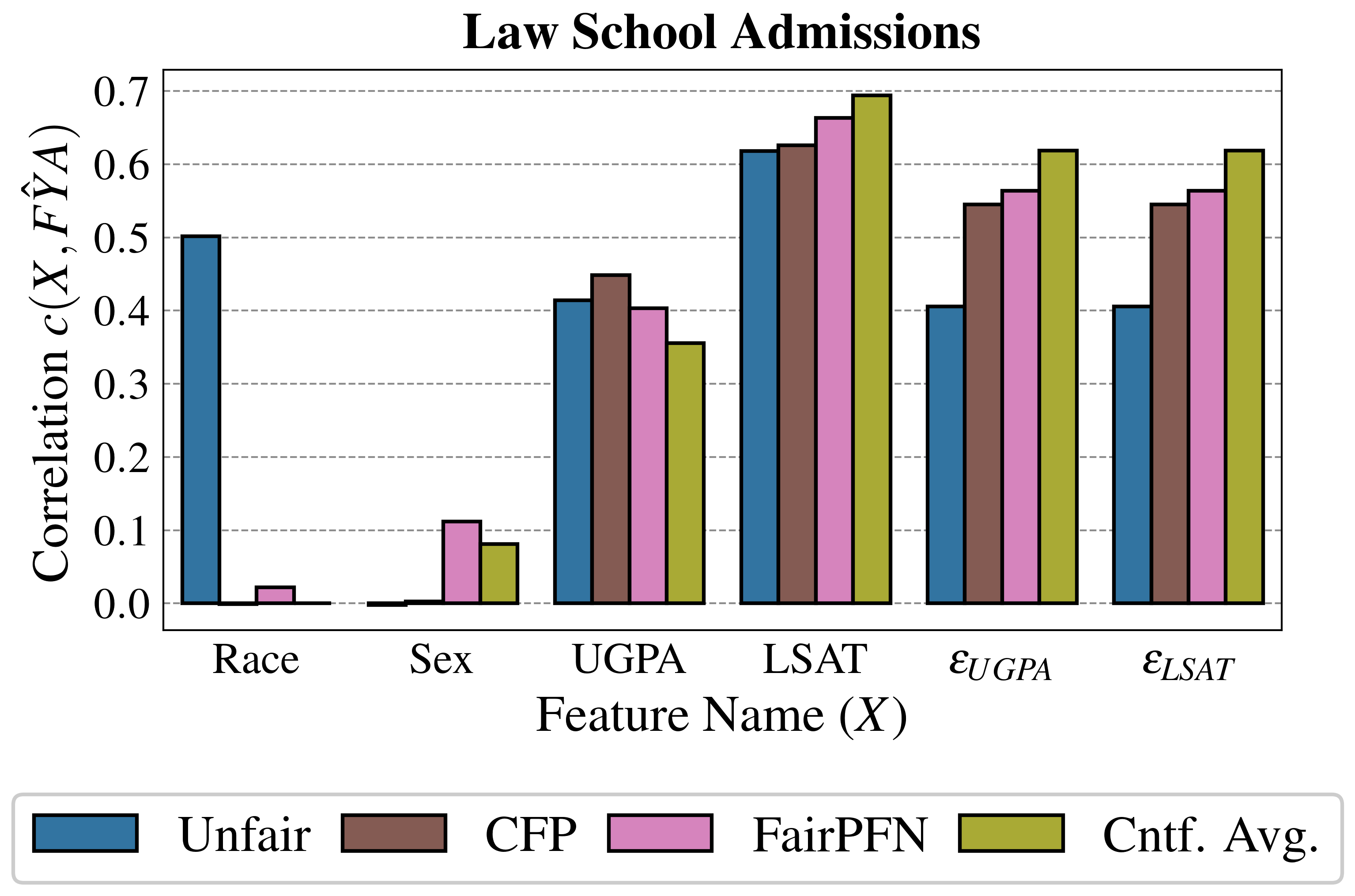<details> <summary>extracted/6522797/figures/lawschool_corr.png Details</summary>  ### Visual Description ## Grouped Bar Chart: Law School Admissions ### Overview The image displays a grouped bar chart titled "Law School Admissions." It compares the correlation between various input features (X) and a model's output (F̂YA) across four different methods or models. The chart is designed to analyze fairness or bias in a predictive model for law school admissions. ### Components/Axes * **Title:** "Law School Admissions" (centered at the top). * **Y-axis:** Labeled "Correlation c(X, F̂YA)". The scale runs from 0.0 to 0.7, with major gridlines at intervals of 0.1. * **X-axis:** Labeled "Feature Name (X)". It lists six categorical features: 1. Race 2. Sex 3. UGPA (Undergraduate GPA) 4. LSAT (Law School Admission Test score) 5. ε_UGPA (likely the error or residual term for UGPA) 6. ε_LSAT (likely the error or residual term for LSAT) * **Legend:** Positioned at the bottom of the chart. It defines four data series by color: * **Blue:** Unfair * **Brown:** CFP * **Pink:** FairPFN * **Olive Green:** Cntf. Avg. (likely Counterfactual Average) ### Detailed Analysis The chart presents correlation values for each feature across the four methods. Values are approximate based on visual inspection against the y-axis gridlines. **1. Race:** * **Unfair (Blue):** Shows a high correlation of approximately **0.50**. * **CFP (Brown):** Correlation is near zero, approximately **0.00**. * **FairPFN (Pink):** Shows a very low correlation of approximately **0.02**. * **Cntf. Avg. (Olive):** Correlation is near zero, approximately **0.00**. * *Trend:* The "Unfair" model has a strong correlation with Race, while the other three methods show negligible correlation. **2. Sex:** * **Unfair (Blue):** Correlation is near zero, approximately **0.00**. * **CFP (Brown):** Correlation is near zero, approximately **0.00**. * **FairPFN (Pink):** Shows a low correlation of approximately **0.11**. * **Cntf. Avg. (Olive):** Shows a low correlation of approximately **0.08**. * *Trend:* All correlations are low. "FairPFN" and "Cntf. Avg." show a slight positive correlation, while "Unfair" and "CFP" show none. **3. UGPA:** * **Unfair (Blue):** Correlation of approximately **0.41**. * **CFP (Brown):** Correlation of approximately **0.45**. * **FairPFN (Pink):** Correlation of approximately **0.40**. * **Cntf. Avg. (Olive):** Correlation of approximately **0.36**. * *Trend:* All methods show a moderate positive correlation with UGPA. "CFP" is the highest, and "Cntf. Avg." is the lowest in this group. **4. LSAT:** * **Unfair (Blue):** Correlation of approximately **0.62**. * **CFP (Brown):** Correlation of approximately **0.63**. * **FairPFN (Pink):** Correlation of approximately **0.67**. * **Cntf. Avg. (Olive):** Correlation of approximately **0.70**. * *Trend:* This feature shows the highest correlations across all methods. There is a clear increasing trend from "Unfair" to "Cntf. Avg.", with the latter reaching the highest value on the entire chart. **5. ε_UGPA:** * **Unfair (Blue):** Correlation of approximately **0.41**. * **CFP (Brown):** Correlation of approximately **0.55**. * **FairPFN (Pink):** Correlation of approximately **0.57**. * **Cntf. Avg. (Olive):** Correlation of approximately **0.62**. * *Trend:* Similar to LSAT, correlations are moderate to high and increase from "Unfair" to "Cntf. Avg.". **6. ε_LSAT:** * **Unfair (Blue):** Correlation of approximately **0.41**. * **CFP (Brown):** Correlation of approximately **0.55**. * **FairPFN (Pink):** Correlation of approximately **0.57**. * **Cntf. Avg. (Olive):** Correlation of approximately **0.62**. * *Trend:* The pattern and values are nearly identical to those for ε_UGPA. ### Key Observations 1. **Disparity in Sensitive Attributes:** The "Unfair" model has a high correlation with "Race" (~0.50), while the fairness-aware methods (CFP, FairPFN, Cntf. Avg.) reduce this correlation to near zero. This is the most dramatic difference in the chart. 2. **Strong Predictor:** "LSAT" has the highest overall correlations, suggesting it is the strongest predictor of the output F̂YA across all models. 3. **Method Performance Gradient:** For the academic features (UGPA, LSAT) and their error terms (ε_UGPA, ε_LSAT), there is a consistent pattern where the correlation increases in the order: Unfair < CFP ≈ FairPFN < Cntf. Avg. 4. **Low Impact of Sex:** The correlation with "Sex" is low for all methods, indicating this feature has a weak relationship with the model's output in this analysis. ### Interpretation This chart likely comes from a study on algorithmic fairness in law school admissions predictions. It evaluates how different modeling approaches ("Unfair" baseline vs. fairness-constrained methods like CFP and FairPFN) affect the model's reliance on sensitive attributes (Race, Sex) versus legitimate predictive features (UGPA, LSAT). * **What the data suggests:** The "Unfair" model appears to use Race as a significant factor in its predictions, which is a potential source of bias. The fairness methods successfully decouple the model's output from Race, reducing its correlation to near zero. However, for the academic metrics (UGPA, LSAT) and their residuals, the fairness methods—especially "Cntf. Avg."—show *increased* correlation. This could imply that to achieve fairness with respect to Race, the models place even greater weight on the (presumably) legitimate academic qualifications. * **Relationship between elements:** The contrast between the "Race" group and the "LSAT" group is central. It visualizes the trade-off often encountered in fair ML: removing influence from a sensitive attribute may increase reliance on other features. The near-identical patterns for ε_UGPA and ε_LSAT suggest these residual terms behave similarly in the models. * **Notable anomaly:** The "FairPFN" method shows a small but non-zero correlation with "Sex" (~0.11), which is higher than the other methods for that feature. This might be an unintended side effect of its fairness optimization process. The "Cntf. Avg." method achieves the highest correlations with the academic features, suggesting it might be the most "performance-focused" among the fairness-aware methods shown. </details> Figure 8: Feature Correlation (Law School): Kendall Tau rank correlation between feature values and the predictions FairPFN compared to our baseline models. FairPFN produces predictions that correlate with fair noise terms $\epsilon_{UGPA}$ and $\epsilon_{LSAT}$ to a similar extent as the CFP baseline, variables which it has never seen in context-or at inference. ## 6 Future Work & Discussion This study introduces FairPFN, a tabular foundation model pretrained to minimize the causal influence of protected attributes in binary classification tasks using solely observational data. FairPFN overcomes a key limitation in causal fairness by eliminating the need for user-supplied knowledge of the true causal graph, facilitating its use in complex, unidentifiable causal scenarios. This approach enhances the applicability of causal fairness and opens new research avenues. Extended Problem Scope We limit our experimental scope to a simple testable setting with a single, binary protected attribute but believe that our prior and transformer architecture can be extended to handle multiple, non-binary protected attributes, addressing both their individual effects and intersectional interactions. We also suggest that FairPFN is capable of predicting not only a fair binary target but also accommodating multi-objective scenarios Lin et al. (2019), regression problems Hollmann et al. (2025), and time series Hoo et al. (2025). Additionally, FairPFN can generate causally fair versions of previously unfair observables, improving prediction explainability. This enables practitioners to use FairPFN as a fairness preprocessing technique while employing their preferred predictive models in practical applications. PFNs for Causal ML FairPFN implicitly provides evidence for the efficacy of PFNs to perofm causal tasks, and we believe that our methodology can be extended to more complex challenges both within and outside of algorithmic fairness. In algorithmic fairness, one promising extension could be path-specific effect removal Chiappa (2019). For example, in medical diagnosis, distinguishing social effects of sex (e.g., sampling bias, male-focus of clinical studies) from biological effects (e.g., symptom differences across sex) is essential for fair and individualized treatment and care. Beyond fairness, we believe PFNs can predict interventional and counterfactual effects, with the latter potentially facilitating FairPFN’s evaluation in real-world contexts without relying on estimated causal models. Currently, FairPFN can also mitigate the influence of binary exogenous confounders, such as smoking, on the prediction of treatment success. Alignment to Anti-Discrimination Law Future versions of FairPFN could also relax the assumption of exogenous protected attributes, enabling differentiation between legally admissible spurious effects and direct or indirect effects. Another key concept proposed by Plecko & Bareinboim (2024) introduces "Business Necessity" (BN) variables that allow the impact of the protected attribute to indirectly contribute to outcomes to achieve a specified business objectives, such as a research company hiring doctorate holders. In EU law, the analogous concept of "objective justification" necessitates a "proportionality test," asserting that justifiable indirect effects must persist only as necessary Weerts et al. (2023). We contend that proportionality bears a causal interpretation, akin to counterfactual explanations Wachter et al. (2018). ## Broader Impact This study attempts to overcome a current limitation in causal fairness, making what we believe is a useful framework for addressing algorithmic discrimination, more accessible to a wider variety of complex fairness problems. While the goal of this work is to have a positive impact on a problem we think is crucial, we acknowledge that we our perspective on fairness is limited in scope to align with EU/US legal doctrines of anti-discrimination. These doctrines are not representative of the world as a whole, and even within these systems, there are vastly different normative viewpoints regarding what constitutes algorithmic fairness and justice. ## Acknowledgements The authors of this work would like to thank the reviewers, editors and organizers of ICML ’25 for the opportunity to share our work and receive valuable feedback from the community. We would like to additionally thank the Zuse School ELIZA Master’s Scholarship Program for their financial and professional support of our main author. We would finally like to thank Sai Prasanna, Magnus Bühler, and Prof. Dr. Thorsten Schmidt for their insights, feedback, and discussion. ## References - Agarwal et al. (2018) Agarwal, A., Beygelzimer, A., Dudík, M., Langford, J., and Wallach, H. A reductions approach to fair classification. In Dy, J. and Krause, A. (eds.), Proceedings of the 35th International Conference on Machine Learning (ICML’18), volume 80, pp. 60–69. Proceedings of Machine Learning Research, 2018. - Angwin et al. (2016) Angwin, J., Larson, J., Mattu, S., and Kirchner, L. Machine bias. ProPublica, May, 23(2016):139–159, 2016. - Barocas et al. (2023) Barocas, S., Hardt, M., and Narayanan, A. Fairness and Machine Learning: Limitations and opportunities. MIT Press, 2023. - Bhaila et al. (2024) Bhaila, K., Van, M., Edemacu, K., Zhao, C., Chen, F., and Wu, X. Fair in-context learning via latent concept variables. 2024. - Binkytė-Sadauskienė et al. (2022) Binkytė-Sadauskienė, R., Makhlouf, K., Pinzón, C., Zhioua, S., and Palamidessi, C. Causal discovery for fairness. 2022. - Castelnovo et al. (2022) Castelnovo, A., Crupi, R., Greco, G., Regoli, D., Penco, I. G., and Cosentini, A. C. A clarification of the nuances in the fairness metrics landscape. Scientific Reports, 12(1), 2022. - Chen & Guestrin (2016) Chen, T. and Guestrin, C. Xgboost: A scalable tree boosting system. In Krishnapuram, B., Shah, M., Smola, A., Aggarwal, C., Shen, D., and Rastogi, R. (eds.), Proceedings of the 22nd ACM SIGKDD International Conference on Knowledge Discovery and Data Mining (KDD’16), pp. 785–794, 2016. - Chiappa (2019) Chiappa, S. Path-specific counterfactual fairness. In Hentenryck, P. V. and Zhou, Z.-H. (eds.), Proceedings of the Thirty-Third Conference on Artificial Intelligence (AAAI’19), volume 33, pp. 7801–7808. AAAI Press, 2019. - Dai et al. (1997) Dai, H., Korb, K. B., Wallace, C. S., and Wu, X. A study of causal discovery with weak links and small samples. In Pollack, M. E. (ed.), Proceedings of the 15th International Joint Conference on Artificial Intelligence (IJCAI’95), 1997. - Ding et al. (2021) Ding, F., Hardt, M., Miller, J., and Schmidt, L. Retiring adult: New datasets for fair machine learning. In Ranzato, M., Beygelzimer, A., Nguyen, K., Liang, P., Vaughan, J., and Dauphin, Y. (eds.), Proceedings of the 35th International Conference on Advances in Neural Information Processing Systems (NeurIPS’21), volume 34, pp. 6478–6490, 2021. - Dua & Graff (2017) Dua, D. and Graff, C. Uci machine learning repository, 2017. - Hardt et al. (2016) Hardt, M., Price, E., and Srebro, N. Equality of opportunity in supervised learning. In Lee, D., Sugiyama, M., von Luxburg, U., Guyon, I., and Garnett, R. (eds.), Proceedings of the 30th International Conference on Advances in Neural Information Processing Systems (NeurIPS’16), pp. 3323–3331, 2016. - Hollmann et al. (2023) Hollmann, N., Müller, S., Eggensperger, K., and Hutter, F. Tabpfn: A transformer that solves small tabular classification problems in a second. In International Conference on Learning Representations (ICLR’23), 2023. Published online: iclr.cc. - Hollmann et al. (2025) Hollmann, N., Müller, S., Purucker, L., Krishnakumar, A., Körfer, M., Hoo, S. B., Schirrmeister, R. T., and Hutter, F. Accurate predictions on small data with a tabular foundation model. Nature, 637(8045):319–326, 2025. - Hoo et al. (2025) Hoo, S. B., Müller, S., Salinas, D., and Hutter, F. The tabular foundation model tabpfn outperforms specialized time series forecasting models based on simple features. 2025. - Hoyer et al. (2008) Hoyer, P. O., Janzing, D., Mooij, J. M., Peters, J., and Schölkopf, B. Nonlinear causal discovery with additive noise models. In Platt, J. and Koller, D. (eds.), Proceedings of the 22 International Conference on Advances in Neural Information Processing Systems (NeurIPS’08), pp. 689–696, 2008. - Kamishima et al. (2012) Kamishima, T., Akaho, S., Asoh, H., and Sakuma, J. Fairness-aware classifier with prejudice remover regularizer. In Machine Learning and Knowledge Discovery in Databases: European Conference, ECML PKDD 2012, Bristol, UK, September 24-28, 2012. Proceedings, Part II 23, pp. 35–50. Springer, 2012. - Kusner et al. (2017) Kusner, M., Loftus, J., Russell, C., and Silva, R. Counterfactual fairness. In Guyon, I., von Luxburg, U., Bengio, S., Wallach, H., Fergus, R., Vishwanathan, S., and Garnett, R. (eds.), Proceedings of the 31st International Conference on Advances in Neural Information Processing Systems (NeurIPS’17), pp. 4069–4079, 2017. - Lin et al. (2019) Lin, X., Zhen, H.-L., Li, Z., Zhang, Q., and Kwong, S. Pareto multi-task learning. 2019. - Ma et al. (2023) Ma, J., Guo, R., Zhang, A., and Li, J. Learning for counterfactual fairness from observational data. In Singh, A. K., Sun, Y., Akoglu, L., Gunopulos, D., Yan, X., Kumar, R., Ozcan, F., and Ye, J. (eds.), Proceedings of the 29th ACM SIGKDD International Conference on Knowledge Discovery and Data Mining (KDD’23), pp. 1620–1630, 2023. - Müller et al. (2022) Müller, S., Hollmann, N., Arango, S., Grabocka, J., and Hutter, F. Transformers can do bayesian inference. In Proceedings of the International Conference on Learning Representations (ICLR’22), 2022. Published online: iclr.cc. - Pearl (2009) Pearl, J. Causality: Models, Reasoning and Inference. Cambridge University Press, 2009. - Peters et al. (2011) Peters, J., Janzing, D., and Schölkopf, B. Causal inference on discrete data using additive noise models. IEEE Transactions on Pattern Analysis and Machine Intelligence, 33(12):2436–2450, 2011. - Peters et al. (2014) Peters, J., Mooij, J. M., Janzing, D., and Schölkopf, B. Causal discovery with continuous additive noise models. Journal of Machine Learning Research, 15:2009–2053, 2014. - Plecko & Bareinboim (2024) Plecko, D. and Bareinboim, E. Causal fairness analysis. Foundations and Trends in Machine Learning, 17:304–589, 2024. - Robertson et al. (2024) Robertson, J., Schmidt, T., Hutter, F., and Awad, N. A human-in-the-loop fairness-aware model selection framework for complex fairness objective landscapes. In Das, S., Green, B. P., Varshney, K., Ganapini, M., and Renda, A. (eds.), Proceedings of the Seventh AAAI/ACM Conference on AI, Ethics, and Society (AIES-24) - Full Archival Papers, October 21-23, 2024, San Jose, California, USA - Volume 1, pp. 1231–1242. AAAI Press, 2024. - Schölkopf et al. (2012) Schölkopf, B., Janzing, D., Peters, J., Sgouritsa, E., Zhang, K., and Mooij, J. On causal and anticausal learning. In Langford, J. and Pineau, J. (eds.), Proceedings of the 29th International Conference on Machine Learning (ICML’12). Omnipress, 2012. - Sharma & Kiciman (2020) Sharma, A. and Kiciman, E. Dowhy: An end-to-end library for causal inference. arXiv:2011.04216 [stat.ME], 2020. - Wachter et al. (2018) Wachter, S., Mittelstadt, B., and Russell, C. Counterfactual explanations without opening the black box: Automated decisions and the gdpr. Harvard Journal of Law and Technology, 15:842–887, 2018. - Weerts et al. (2023) Weerts, H., Xenidis, R., Tarissan, F., Olsen, H. P., and Pechenizkiy, M. Algorithmic unfairness through the lens of eu non-discrimination law. In Proceedings of the 2023 ACM Conference on Fairness, Accountability, and Transparency, pp. 805–816, 2023. - Weerts et al. (2024) Weerts, H., Pfisterer, F., Feurer, M., Eggensperger, K., Bergman, E., Awad, N., Vanschoren, J., Pechenizkiy, M., Bischl, B., and Hutter, F. Can fairness be automated? guidelines and opportunities for fairness-aware automl. Journal of Artificial Intelligence Research, 79:639–677, 2024. - Wightman (1998) Wightman, L. F. Lsac national longitudinal bar passage study. lsac research report series, 1998. ## Appendix A Real-World Datasets #### Law School Admissions The first dataset is the Law School Admissions dataset from the 1998 LSAC National Longitudinal Bar Passage Study Wightman (1998), which includes admissions data fr approximately 30,000 US law school applicants, revealing disparities in bar passage rates and first-year averages by ethnicity. We generate counterfactual data and measure causal effects using a slightly different causal model than what was originally proposed by Kusner et al. (2017), which additionally includes edges $\text{"UGPA"}\rightarrow\text{"LSAT"}$ and $\text{"LSAT"}\rightarrow\text{"FYA"}$ . These edges have a plausible temporal explanation, and create a more realistic scenario where "Race" and "Sex" have both a direct and indirect effect on first year averages. #### Causal Modeling with DoWhy We use the causal graph in Figure 5 (left) and observational data as inputs for the dowhy.gcm module Sharma & Kiciman (2020), employing an automated search using the dowhy.gcm.auto, which selects the best predictive model in a model zoo of non-linear tree-based models to represent each edge, minimizing either the MSE or negative F1-score depending on the distribution of target following Hoyer et al. (2008) and Peters et al. (2011). We apply each models generate counterfactual datasets, allowing for the estimation of the Average Treatment Effect (ATE) and absolute error (AE). We also use the compute_noise function to estimate noise terms $\epsilon_{GPA}$ and $\epsilon_{LSAT}$ for our CFP baseline. #### Adult Census Income The second dataset, derived from the 1994 US Census, is the Adult Census Income problem Dua & Graff (2017), containing demographic and income outcome data ( $INC\geq 50K$ ) for nearly 50,000 individuals We note that Adult has been heavily criticized in the fairness literature Ding et al. (2021) due to evidence of sampling bias and an arbitrary chosen income threshold, but elect to include it due to its widely accepted causal model and appearance as a benchmark in other similar studies Ma et al. (2023). We fit a causal model to assess the Average Treatment Effect (ATE) of the protected attribute $RACE$ , generate a counterfactual dataset, and calculate noise term values $\epsilon$ . ## Appendix B Ablation Study To evaluate FairPFN’s performance across datasets with varying characteristics, we conduct an ablation study comparing the prediction Average Treatment Effect (ATE) of FairPFN and Unfair under different noise levels, base rates of the protected attribute’s causal effect, and dataset sizes. #### Base Rate Causal Effect We analyze the distributions of prediction ATE from FairPFN and Unfair across five quintiles (Q1-Q5) of base ATE (Figure 9). FairPFN’s prediction ATE remains stable, while Unfair ’s prediction ATE increases linearly. In datasets within the Biased, Direct Effect, Level-Two, and Level-Three benchmark groups, where the protected attribute has a high base ATE (Q5), FairPFN exhibits a greater tendency for positive discrimination, resulting in negative prediction ATE values. 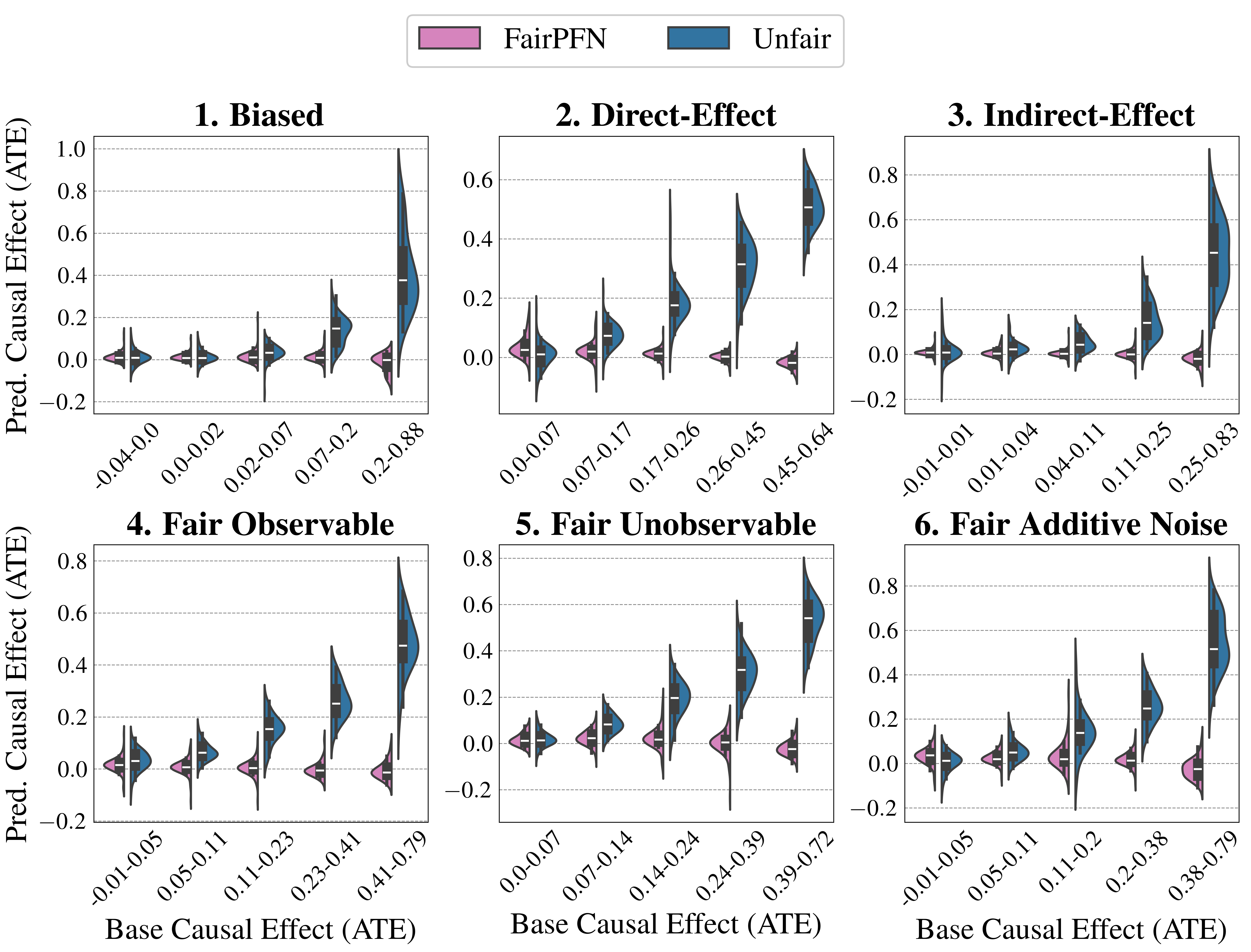<details> <summary>extracted/6522797/figures/effect_effect.png Details</summary>  ### Visual Description ## Violin Plot Grid: Predicted vs. Base Causal Effect (ATE) for FairPFN and Unfair Models ### Overview The image displays a 2x3 grid of six violin plots. Each subplot compares the distribution of Predicted Causal Effect (Average Treatment Effect - ATE) for two models, "FairPFN" (pink) and "Unfair" (blue), across different ranges of the underlying "Base Causal Effect (ATE)". The plots are designed to visualize how model predictions align with or deviate from the true causal effect under various data-generating scenarios. ### Components/Axes * **Legend:** Located at the top center. It defines the two data series: * **FairPFN:** Represented by pink violin plots. * **Unfair:** Represented by blue violin plots. * **Y-Axis (All Subplots):** Labeled "Pred. Causal Effect (ATE)". The scale ranges from approximately -0.2 to 1.0, with gridlines at 0.0, 0.2, 0.4, 0.6, 0.8, and 1.0 (varies slightly per subplot). * **X-Axis (All Subplots):** Labeled "Base Causal Effect (ATE)". The axis is categorical, with each tick representing a specific range of the base effect (e.g., "-0.04-0.0", "0.0-0.02"). The specific ranges differ for each subplot. * **Subplot Titles:** Each of the six panels has a numbered title indicating the experimental scenario: 1. **Biased** (Top Left) 2. **Direct-Effect** (Top Center) 3. **Indirect-Effect** (Top Right) 4. **Fair Observable** (Bottom Left) 5. **Fair Unobservable** (Bottom Center) 6. **Fair Additive Noise** (Bottom Right) ### Detailed Analysis **General Trend Across All Plots:** For the "Unfair" model (blue), the predicted ATE distributions show a clear positive trend: as the Base Causal Effect (x-axis) increases, the median and spread of the predicted effects also increase. In contrast, the "FairPFN" model (pink) distributions remain tightly clustered around zero across all base effect ranges, showing little to no trend. **Subplot-Specific Analysis:** 1. **1. Biased** * **X-axis Ranges:** `-0.04-0.0`, `0.0-0.02`, `0.02-0.07`, `0.07-0.2`, `0.2-0.88` * **FairPFN (Pink):** Distributions are narrow and centered near 0.0 for all ranges. The median is consistently at or very near zero. * **Unfair (Blue):** Shows a strong positive trend. For the lowest base range (`-0.04-0.0`), the median is near 0.0. For the highest range (`0.2-0.88`), the distribution is very wide, with a median around 0.4 and values extending up to ~1.0. 2. **2. Direct-Effect** * **X-axis Ranges:** `0.0-0.07`, `0.07-0.17`, `0.17-0.26`, `0.26-0.45`, `0.45-0.64` * **FairPFN (Pink):** Remains centered near zero with low variance. * **Unfair (Blue):** Positive trend is evident. The median prediction increases from ~0.0 for the first range to ~0.5 for the last range (`0.45-0.64`). 3. **3. Indirect-Effect** * **X-axis Ranges:** `-0.01-0.01`, `0.01-0.04`, `0.04-0.11`, `0.11-0.25`, `0.25-0.83` * **FairPFN (Pink):** Consistently near zero. * **Unfair (Blue):** Positive trend. The final range (`0.25-0.83`) shows a very tall, wide distribution with a median near 0.5 and a long tail reaching above 0.8. 4. **4. Fair Observable** * **X-axis Ranges:** `-0.01-0.05`, `0.05-0.11`, `0.11-0.23`, `0.23-0.41`, `0.41-0.79` * **FairPFN (Pink):** Centered near zero. * **Unfair (Blue):** Clear positive trend. The median for the highest range (`0.41-0.79`) is approximately 0.5. 5. **5. Fair Unobservable** * **X-axis Ranges:** `0.0-0.07`, `0.07-0.14`, `0.14-0.24`, `0.24-0.39`, `0.39-0.72` * **FairPFN (Pink):** Centered near zero. * **Unfair (Blue):** Positive trend. The median for the highest range (`0.39-0.72`) is around 0.55. 6. **6. Fair Additive Noise** * **X-axis Ranges:** `-0.01-0.05`, `0.05-0.11`, `0.11-0.2`, `0.2-0.38`, `0.38-0.79` * **FairPFN (Pink):** Centered near zero. * **Unfair (Blue):** Positive trend. The median for the highest range (`0.38-0.79`) is approximately 0.5. ### Key Observations * **Model Dichotomy:** There is a stark and consistent contrast between the two models across all six scenarios. FairPFN predictions are unbiased (centered at zero), while Unfair model predictions are strongly correlated with the base effect. * **Unfair Model Bias:** The Unfair model systematically over-predicts the causal effect, especially when the true base effect is large. Its predictions are not only higher on average but also exhibit much greater variance (wider violins) for larger base effects. * **FairPFN Stability:** The FairPFN model demonstrates remarkable stability, maintaining predictions near zero regardless of the underlying base effect or the specific fairness scenario (Biased, Direct-Effect, etc.). * **Scenario Similarity:** The pattern of results is highly consistent across all six named scenarios (1-6). This suggests the observed model behaviors are robust to these different data-generating processes. ### Interpretation This visualization provides strong evidence for the effectiveness of the "FairPFN" method in producing fair causal effect estimates. The "Unfair" model acts as a baseline, showing what a standard, potentially biased model does: it confounds the true causal signal with spurious correlations, leading to predictions that inflate with the magnitude of the true effect. The six scenarios likely represent different mechanisms by which bias can enter a model (e.g., through direct discrimination, indirect pathways, or unobserved confounders). The fact that FairPFN's performance is consistent across all of them indicates it successfully mitigates these diverse sources of bias. The core message is that FairPFN decouples its predictions from the biased base signal, yielding estimates that are, on average, zero (indicating no predicted treatment effect disparity), while the Unfair model's predictions are directly and problematically tied to the magnitude of the underlying effect. This is a critical property for any model intended for use in fairness-sensitive applications like policy evaluation or algorithmic decision-making. </details> Figure 9: Effect of Base ATE (Synthetic): Distributions of prediction ATE produced by FairPFN and Unfair over quintiles (Q1-Q5) of the protected attributes’s base causal effect (base ATE). FairPFN remains consistent across quintiles, sometimes over-correcting and producing a negative prediction ATE in Q5. #### Dataset Noise Analyzing dataset noise, indicated by the standard deviation (STD) $\sigma$ of exogenous noise in the structural equations Figure 10 shows that FairPFN retains consistency across varying noise levels. Conversely, Unfair exhibits decreased and more peaked distributions of prediction ATE as noise increases from Q1 to Q5, suggests that noise terms may obscure causal effects and diminish their observed impact in the data. 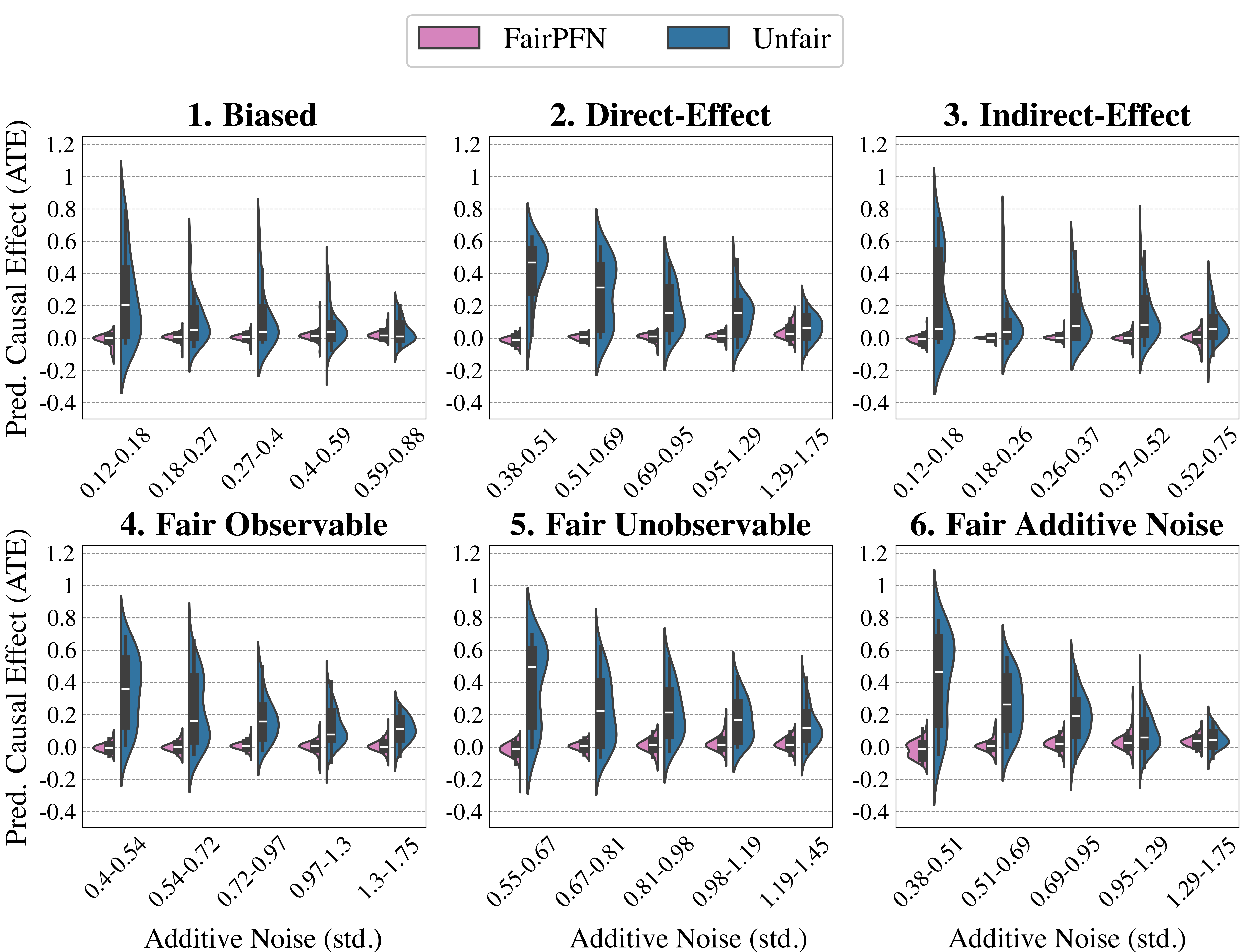<details> <summary>extracted/6522797/figures/noise-effect_by_group_synthetic.png Details</summary>  ### Visual Description \n ## Violin Plot Comparison: FairPFN vs. Unfair Methods for Predicted Causal Effect (ATE) Under Varying Noise Levels ### Overview The image displays a 2x3 grid of six violin plots. Each plot compares the distribution of Predicted Average Treatment Effect (ATE) for two methods, "FairPFN" (pink) and "Unfair" (blue), across five increasing levels of additive noise (standard deviation). The plots are organized by different causal scenarios or data-generating processes. ### Components/Axes * **Legend:** Located at the top center of the entire figure. * Pink rectangle: **FairPFN** * Blue rectangle: **Unfair** * **Y-Axis (Common to all plots):** Label: **Pred. Causal Effect (ATE)**. Scale ranges from -0.4 to 1.2, with major gridlines at intervals of 0.2. * **X-Axis (Common label):** Label: **Additive Noise (std.)**. The specific numeric ranges for the five bins vary per subplot. * **Subplot Titles (2 rows, 3 columns):** 1. **1. Biased** (Top Left) 2. **2. Direct-Effect** (Top Center) 3. **3. Indirect-Effect** (Top Right) 4. **4. Fair Observable** (Bottom Left) 5. **5. Fair Unobservable** (Bottom Center) 6. **6. Fair Additive Noise** (Bottom Right) ### Detailed Analysis Each subplot contains five pairs of violin plots (one pink, one blue per noise bin). The violin shows the probability density of the data, with a white dot marking the median, a thick black bar for the interquartile range, and thin black lines for the whiskers. **1. Biased** * **X-axis Bins:** 0.12-0.18, 0.18-0.27, 0.27-0.4, 0.4-0.59, 0.59-0.88 * **Trend:** The "Unfair" (blue) distributions are wide, with medians starting high (~0.2) and decreasing as noise increases. The "FairPFN" (pink) distributions are extremely tight and centered near zero across all noise levels. **2. Direct-Effect** * **X-axis Bins:** 0.38-0.51, 0.51-0.69, 0.69-0.95, 0.95-1.29, 1.29-1.75 * **Trend:** Similar to plot 1. "Unfair" medians start high (~0.5) and decline. "FairPFN" remains tightly clustered around zero. **3. Indirect-Effect** * **X-axis Bins:** 0.12-0.18, 0.18-0.26, 0.26-0.37, 0.37-0.52, 0.52-0.75 * **Trend:** "Unfair" distributions are tall and narrow, with medians starting very high (~0.6) and decreasing. "FairPFN" is again tightly centered near zero. **4. Fair Observable** * **X-axis Bins:** 0.4-0.54, 0.54-0.72, 0.72-0.97, 0.97-1.3, 1.3-1.75 * **Trend:** "Unfair" medians start moderately high (~0.4) and decrease. "FairPFN" distributions are slightly wider than in previous plots but still tightly centered near zero. **5. Fair Unobservable** * **X-axis Bins:** 0.55-0.67, 0.67-0.81, 0.81-0.98, 0.98-1.19, 1.19-1.45 * **Trend:** "Unfair" distributions are wide, with medians starting high (~0.5) and decreasing. "FairPFN" is tightly centered near zero. **6. Fair Additive Noise** * **X-axis Bins:** 0.38-0.51, 0.51-0.69, 0.69-0.95, 0.95-1.29, 1.29-1.75 * **Trend:** "Unfair" medians start high (~0.5) and decrease. "FairPFN" is tightly centered near zero. ### Key Observations 1. **Consistent FairPFN Performance:** Across all six causal scenarios and all noise levels, the "FairPFN" method produces predicted ATE distributions that are consistently narrow and centered very close to zero (the ideal for a fair estimator). 2. **Unfair Method Bias:** The "Unfair" method shows significant positive bias (median ATE > 0) in all scenarios, especially at lower noise levels. This bias decreases as additive noise increases. 3. **Noise Impact:** Increasing additive noise (moving right on the x-axis within each plot) generally reduces the variance and median of the "Unfair" method's predictions, pulling them closer to zero, but they rarely achieve the tight, zero-centered precision of "FairPFN". 4. **Scenario Sensitivity:** The "Unfair" method's starting bias and the shape of its distribution vary across the six causal scenarios (e.g., highest initial median in "Indirect-Effect"), while "FairPFN" is robust to these differences. ### Interpretation This figure demonstrates the effectiveness of the "FairPFN" method in estimating causal effects fairly (i.e., with near-zero bias) compared to an "Unfair" baseline, under varying conditions of data corruption (additive noise) and different underlying causal structures. * **What the data suggests:** The "FairPFN" method successfully mitigates bias in predicted Average Treatment Effects. Its tight distributions around zero indicate high precision and fairness. The "Unfair" method is susceptible to significant bias, which is only reduced by increasing noise—a factor that also degrades the signal. * **Relationship between elements:** The six panels show that the advantage of FairPFN is not scenario-specific; it holds across a taxonomy of causal problems (Biased, Direct/Indirect Effect, and various Fairness definitions). The x-axis (noise) acts as a stress test, showing FairPFN's robustness. * **Notable patterns/anomalies:** The most striking pattern is the stark contrast in distribution shape and location between the two methods in every single bin. There are no outliers where the "Unfair" method outperforms "FairPFN" in terms of fairness (closeness to zero). The "Indirect-Effect" scenario appears to induce the strongest bias in the "Unfair" method at low noise levels. </details> Figure 10: Effect of Dataset Noise (Synthetic): Distributions of prediction ATE produced by FairPFN and Unfair over quintiles (Q1-Q5) of the standard deviation (std.) of exogenous noise terms in the data. FairPFN remains consistent across quintiles, while increased noise decreases the prediction ATE of Unfair . #### Dataset Size Ablation studies on dataset size (Figure 11) show that FairPFN’s prediction ATE displays a tighter distribution with larger datasets, indicating improved performance in causal effect removal. This improvement arises from better identification of causal mechanisms as data availability increases, enabling the transformer to distinguish noise from causal effects. ## Appendix C Future Extensions In this section we expand upon our discussion of future extensions of FairPFN, in order to encourage the community to build upon and expand our approach. #### Regression Problems FairPFN can be pre-trained as a regression model with very little architectural changes by discretizing continuous output distributions into piecewise intervals and calculating misclassification costs in order to reflect the natural ordering between categories . Thoroughly evaluated in Hollmann et al. (2025), such post-proccessing strategies have shown strong performance in tabular regression problems and enable the effective use of classification architectures for continuous targets. #### Protected Attributes in the Wild While we limit the scope of this study to binary classification tasks with single, binary protected attributes, we acknowledge that real-world fairness-aware ML problems are often more complex than that. More precisely, protected attributes can be not only binary, but continuous or mulit-category, and discrimination may occur not only with respect to individual protected attributes but with respect to multiple and the interactions between them. Our prior is currently extensible to handle multiple by changing the number of protected attributes that are sampled into each synthetic dataset, removing the outgoing edges of all protected attributes to generate $y_{fair}$ , and informing the transformer about which variables are protected attributes. Changing the distribution of protected attributes is also possible, and simply requires transporting the protected attribute into the distribution(s) of choice either before or after its natural continuous value is propagated through the MLP during pre-training. 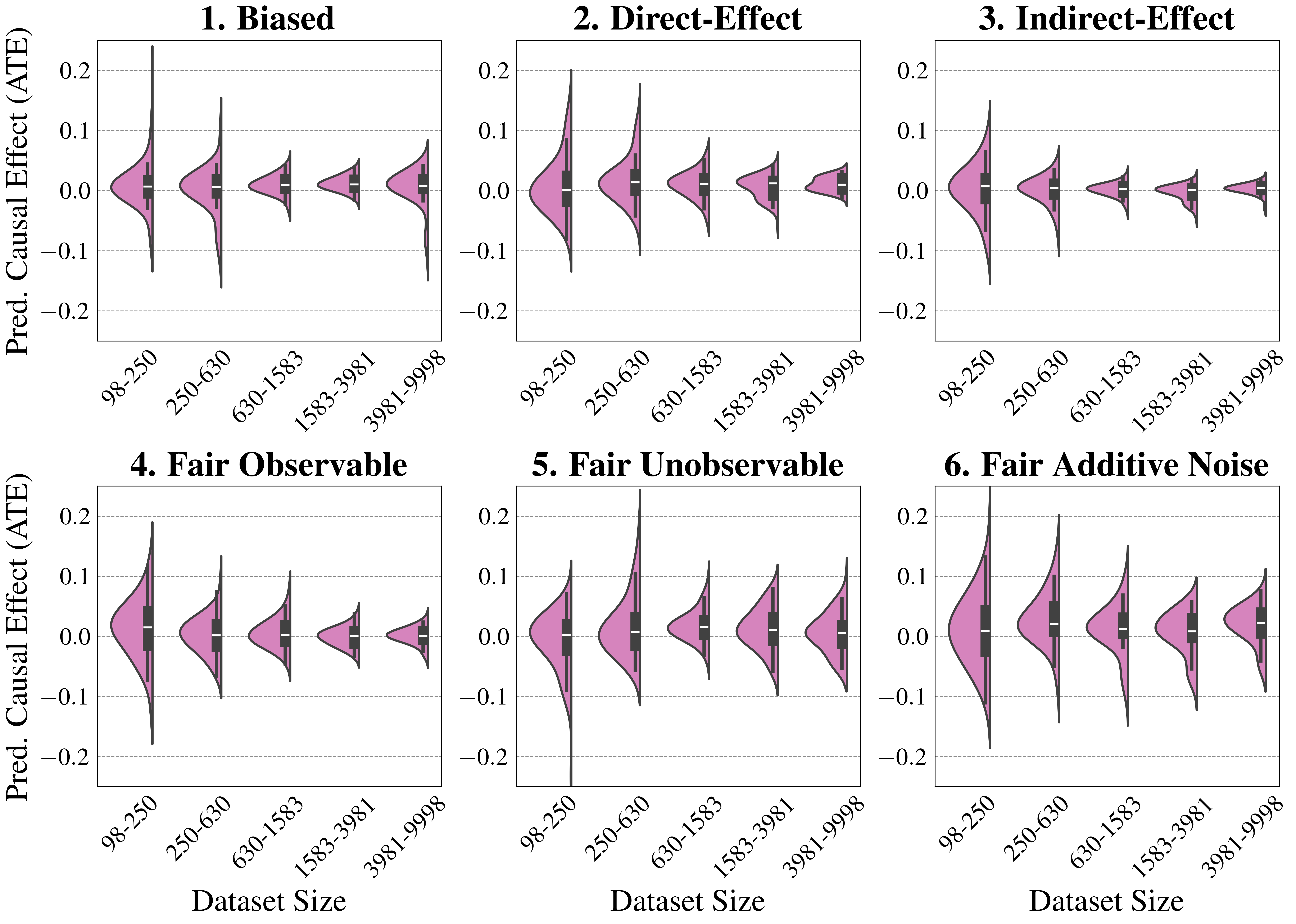<details> <summary>extracted/6522797/figures/size-effect_by_group_synthetic.png Details</summary>  ### Visual Description ## Violin Plot Grid: Predicted Causal Effect (ATE) by Dataset Size and Method ### Overview The image displays a 2x3 grid of six violin plots. Each subplot visualizes the distribution of the **Predicted Average Treatment Effect (ATE)** for a different causal estimation method across five increasing dataset size categories. The plots compare how the precision and bias of the ATE estimates change with more data for each method. ### Components/Axes * **Overall Layout:** Six subplots arranged in two rows and three columns. * **Subplot Titles (Methods):** 1. **Biased** (Top Left) 2. **Direct-Effect** (Top Center) 3. **Indirect-Effect** (Top Right) 4. **Fair Observable** (Bottom Left) 5. **Fair Unobservable** (Bottom Center) 6. **Fair Additive Noise** (Bottom Right) * **Y-Axis (Common to all subplots):** Labeled **"Pred. Causal Effect (ATE)"**. The scale ranges from -0.2 to 0.2, with major grid lines at intervals of 0.1. * **X-Axis (Common to all subplots):** Labeled **"Dataset Size"**. It contains five categorical bins representing ranges of dataset sizes: * `98-250` * `250-630` * `630-1583` * `1583-3981` * `3981-9998` * **Plot Elements:** Each category on the x-axis has a corresponding **violin plot**. The violin shows the probability density of the data at different values, with a wider section indicating a higher frequency of data points. Inside each violin is a miniature **box plot** (black bar with white median line and whiskers), summarizing the median, interquartile range, and range of the distribution. ### Detailed Analysis The analysis is segmented by subplot (method). For each, the visual trend of the distributions as dataset size increases is described, followed by approximate data points. **1. Biased** * **Trend:** The distributions are centered near zero but show significant spread, especially for smaller datasets. The variance (spread of the violin) decreases noticeably as dataset size increases. The median (white line) remains close to zero across all sizes. * **Data Points (Approximate Median & Spread):** * `98-250`: Median ~0.0, wide spread from ~-0.15 to +0.25. * `250-630`: Median ~0.0, spread narrows (~-0.1 to +0.15). * `630-1583`: Median ~0.0, spread continues to narrow. * `1583-3981`: Median ~0.0, relatively tight distribution. * `3981-9998`: Median ~0.0, tightest distribution, but with a long tail extending to ~-0.15. **2. Direct-Effect** * **Trend:** Similar to "Biased," distributions are centered near zero and variance decreases with more data. The initial spread for the smallest dataset appears slightly larger than in the "Biased" plot. * **Data Points (Approximate Median & Spread):** * `98-250`: Median ~0.0, very wide spread from ~-0.15 to +0.2. * `250-630`: Median ~0.0, spread narrows. * `630-1583`: Median ~0.0, spread narrows further. * `1583-3981`: Median ~0.0, tight distribution. * `3981-9998`: Median ~0.0, very tight distribution. **3. Indirect-Effect** * **Trend:** Distributions are centered near zero. The variance reduction with increasing dataset size is very pronounced. The smallest dataset shows a particularly wide and tall distribution. * **Data Points (Approximate Median & Spread):** * `98-250`: Median ~0.0, extremely wide and tall distribution (high density around zero but large range). * `250-630`: Median ~0.0, spread reduces dramatically. * `630-1583`: Median ~0.0, tight distribution. * `1583-3981`: Median ~0.0, very tight distribution. * `3981-9998`: Median ~0.0, extremely tight distribution. **4. Fair Observable** * **Trend:** Distributions are centered near zero. Variance decreases with dataset size. The shape and spread appear very similar to the "Biased" method. * **Data Points (Approximate Median & Spread):** * `98-250`: Median ~0.0, wide spread. * `250-630`: Median ~0.0, spread narrows. * `630-1583`: Median ~0.0, spread narrows further. * `1583-3981`: Median ~0.0, tight distribution. * `3981-9998`: Median ~0.0, tight distribution. **5. Fair Unobservable** * **Trend:** This method shows a distinct pattern. While the median remains near zero, the **variance does not decrease consistently** with dataset size. The distributions for the two largest dataset sizes (`1583-3981` and `3981-9998`) appear wider than those for the middle sizes, suggesting instability or increased uncertainty with more data for this method. * **Data Points (Approximate Median & Spread):** * `98-250`: Median ~0.0, wide spread. * `250-630`: Median ~0.0, spread narrows. * `630-1583`: Median ~0.0, relatively tight. * `1583-3981`: Median ~0.0, spread increases again. * `3981-9998`: Median ~0.0, spread remains wide. **6. Fair Additive Noise** * **Trend:** Distributions are centered near zero. Variance decreases with dataset size, but the rate of decrease appears slower compared to methods like "Indirect-Effect." The distributions remain relatively wide even for larger datasets. * **Data Points (Approximate Median & Spread):** * `98-250`: Median ~0.0, very wide spread. * `250-630`: Median ~0.0, spread narrows. * `630-1583`: Median ~0.0, spread narrows further. * `1583-3981`: Median ~0.0, moderately wide distribution. * `3981-9998`: Median ~0.0, moderately wide distribution. ### Key Observations 1. **Universal Trend:** For five of the six methods (all except "Fair Unobservable"), the variance (uncertainty) of the predicted ATE decreases as the dataset size increases. This is the expected behavior of consistent estimators. 2. **Bias:** All methods appear to be **unbiased** on average, as the median of every distribution is centered at or very near 0.0 on the y-axis. 3. **Method Comparison:** * The **"Indirect-Effect"** method shows the most dramatic reduction in variance, achieving the tightest distributions for large datasets. * The **"Fair Unobservable"** method is an outlier. Its variance does not monotonically decrease and is notably high for the largest datasets, indicating potential issues with this estimation approach under the tested conditions. * The **"Biased"** and **"Fair Observable"** methods show very similar performance profiles. * The **"Fair Additive Noise"** method retains higher variance than others at large dataset sizes. ### Interpretation This visualization is a comparative performance analysis of different causal inference methods. The **Predicted ATE** is the estimated average effect of a treatment or intervention. The plots reveal how the **precision** (inverse of variance) of these estimates improves with more data. * **What the data suggests:** Most methods become more precise with larger datasets, which validates their statistical consistency. The "Indirect-Effect" method appears most efficient in this test. The anomalous behavior of "Fair Unobservable" suggests that incorporating unobservable confounders in a fairness-aware model may introduce instability or require a different modeling approach that doesn't scale well with data size in this scenario. * **How elements relate:** The x-axis (Dataset Size) is the independent variable. The y-axis (Predicted ATE) is the dependent variable whose distribution is measured. The subplot titles (Methods) are the different models or algorithms being tested. The violin shape directly visualizes the uncertainty in the causal estimate for each method at each data scale. * **Notable anomalies:** The primary anomaly is the **"Fair Unobservable"** method's failure to reduce variance with the largest datasets. This could indicate overfitting, model misspecification, or a fundamental challenge in estimating causal effects when accounting for unobservable factors in a fairness context. The long tail in the largest dataset for the "Biased" method is a minor secondary anomaly. </details> Figure 11: Effect of Dataset Size (Synthetic): Distributions of prediction ATE produced by FairPFN over quintiles (Q1-Q5) of dataset sizes from 100-10,000 (log-scale). FairPFN becomes better at its task of removing the causal effect of protected attributes when more data is available. 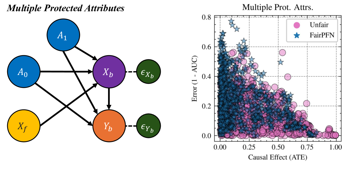<details> <summary>x4.png Details</summary>  ### Visual Description \n ## Causal Diagram and Scatter Plot: Multiple Protected Attributes Analysis ### Overview The image presents two interconnected technical visualizations. On the left is a causal directed acyclic graph (DAG) illustrating a model with multiple protected attributes. On the right is a scatter plot comparing the performance of two models ("Unfair" and "FairPFN") across two metrics: Causal Effect (Average Treatment Effect - ATE) and Error (1 - AUC). The overall theme is the analysis of algorithmic fairness, specifically examining how protected attributes influence biased features and outcomes, and evaluating a model's ability to mitigate unfairness. ### Components/Axes **Left: Causal Diagram (DAG)** * **Title:** "Multiple Protected Attributes" (top-left, italicized). * **Nodes (Circles):** * **A0:** Blue circle, labeled "A₀". Positioned middle-left. * **A1:** Blue circle, labeled "A₁". Positioned top-left. * **Xf:** Yellow circle, labeled "X_f". Positioned bottom-left. * **Xb:** Purple circle, labeled "X_b". Positioned center. * **Yb:** Orange circle, labeled "Y_b". Positioned bottom-center. * **εXb:** Dark green circle, labeled "ε_{X_b}". Positioned to the right of Xb, connected by a dashed line. * **εYb:** Dark green circle, labeled "ε_{Y_b}". Positioned to the right of Yb, connected by a dashed line. * **Edges (Arrows):** Solid black arrows indicate direct causal influence. Dashed lines indicate error/noise terms. * A₀ → X_b * A₀ → Y_b * A₁ → X_b * A₁ → Y_b * X_f → X_b * X_f → Y_b * X_b → Y_b * X_b --- ε_{X_b} (dashed) * Y_b --- ε_{Y_b} (dashed) **Right: Scatter Plot** * **Title:** "Multiple Prot. Attrs." (top-center). * **X-Axis:** * **Label:** "Causal Effect (ATE)". * **Scale:** Linear, ranging from 0.00 to 1.00. Major tick marks at 0.00, 0.25, 0.50, 0.75, 1.00. * **Y-Axis:** * **Label:** "Error (1 - AUC)". * **Scale:** Linear, ranging from 0.0 to 0.8. Major tick marks at 0.0, 0.2, 0.4, 0.6, 0.8. * **Legend:** Located in the top-right corner. * **Pink Circle:** Labeled "Unfair". * **Blue Star:** Labeled "FairPFN". * **Grid:** Dashed gray grid lines are present. ### Detailed Analysis **Causal Diagram Analysis:** The diagram models a system where two protected attributes (`A₀`, `A₁`) and a set of fair features (`X_f`) influence both a set of biased features (`X_b`) and the final biased outcome (`Y_b`). The biased features (`X_b`) also directly influence the outcome (`Y_b`). The error terms (`ε_{X_b}`, `ε_{Y_b}`) represent unexplained variance. This structure suggests that bias in the outcome (`Y_b`) can originate directly from protected attributes or indirectly through their influence on the features used for prediction (`X_b`). **Scatter Plot Data Trends & Points:** * **"Unfair" Series (Pink Circles):** * **Trend:** The data points show a broad, diffuse cloud. There is a very weak negative correlation; as the Causal Effect (ATE) increases, the Error (1 - AUC) shows a slight tendency to decrease, but with extremely high variance. * **Data Distribution:** Points are densely clustered across the entire range of the X-axis (ATE from ~0.0 to 1.0). On the Y-axis (Error), the majority of points fall between 0.0 and 0.4, with a significant number extending up to ~0.6. A few outliers exist near Error=0.0 across various ATE values. * **"FairPFN" Series (Blue Stars):** * **Trend:** This series shows a more defined, though still noisy, negative correlation. As the Causal Effect (ATE) increases, the Error (1 - AUC) generally decreases. The slope is steeper than for the "Unfair" series, especially for ATE values below ~0.5. * **Data Distribution:** The points are also widely distributed but show a clearer concentration. For low ATE values (0.0 - 0.25), Error values are highly variable, ranging from ~0.0 to 0.8. As ATE increases beyond 0.25, the upper bound of the Error range decreases noticeably. The densest cluster of points appears in the region of ATE between 0.1 and 0.6 and Error between 0.0 and 0.3. ### Key Observations 1. **Performance-Fairness Trade-off:** The plot visualizes the classic trade-off between model accuracy (low Error) and fairness (low Causal Effect/ATE). Both series show that achieving very low error often comes with higher causal effect (more unfairness), and vice-versa. 2. **FairPFN's Shift:** The "FairPFN" data cloud is systematically shifted downward and to the left compared to the "Unfair" cloud. This indicates that for a given level of Causal Effect (ATE), FairPFN generally achieves lower Error (1 - AUC). Conversely, for a given Error rate, FairPFN tends to have a lower Causal Effect. 3. **High Variance at Low ATE:** Both models exhibit their highest variance in Error when the Causal Effect (ATE) is low (near 0.0). This suggests that enforcing strong fairness constraints (low ATE) leads to highly unstable model performance. 4. **Diagram-Plot Connection:** The causal diagram provides the theoretical framework for the metrics in the plot. The "Causal Effect (ATE)" on the x-axis likely measures the direct and indirect influence of the protected attributes (`A₀`, `A₁`) on the outcome (`Y_b`) as modeled in the DAG. The "Unfair" model presumably does not account for these paths, while "FairPFN" is designed to mitigate them. ### Interpretation This composite image presents an empirical evaluation of a fairness-aware machine learning model ("FairPFN") within a defined causal framework. * **What the Data Demonstrates:** The scatter plot provides evidence that the FairPFN method successfully reduces the average causal effect of protected attributes on outcomes (shifts points left on the x-axis) compared to an "Unfair" baseline, *without* uniformly increasing prediction error. In fact, it often achieves lower error for comparable levels of fairness. This challenges the simplistic notion that fairness and accuracy are always in direct opposition. * **Relationship Between Elements:** The causal diagram is not merely illustrative; it defines the very quantity (ATE) being measured on the plot's x-axis. It shows that unfairness can be multifaceted, flowing through both direct paths (A→Y) and mediated paths (A→X→Y). The plot then quantifies how well a modeling approach handles this complex structure. * **Notable Anomalies/Patterns:** The most striking pattern is the dense, downward-sloping corridor of FairPFN points versus the more amorphous cloud of Unfair points. This suggests FairPFN introduces a more consistent and predictable relationship between fairness and performance. The high variance at low ATE for both models is a critical finding, indicating a potential instability or "cost of fairness" region that requires careful navigation in real-world applications. The presence of low-error, low-ATE points for FairPFN (bottom-left quadrant) is the ideal target zone, demonstrating that the method can, in some instances, find models that are both fair and accurate. </details> Figure 12: Multiple Protected Attributes (Synthetic): Distributions of prediction ATE and predictive accuracy produced by FairPFN vs the Unfair predictor when there are multiple protected attributes. This violates FairPFN’s prior assumptions and reverts it to a normal classifier. 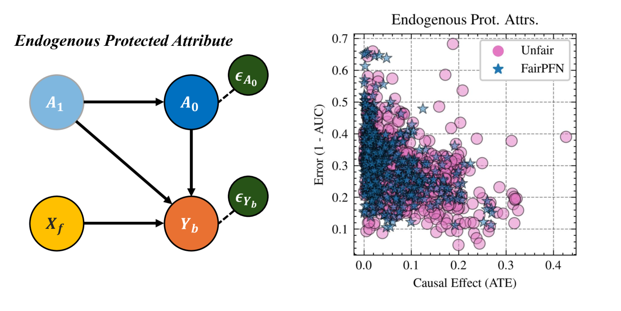<details> <summary>x5.png Details</summary>  ### Visual Description ## Composite Technical Figure: Causal Diagram and Scatter Plot ### Overview The image is a composite figure containing two distinct but related elements. On the left is a causal directed acyclic graph (DAG) illustrating a model for an "Endogenous Protected Attribute." On the right is a scatter plot titled "Endogenous Prot. Attrs." (likely an abbreviation for "Protected Attributes") that compares the performance of two methods, "Unfair" and "FairPFN," across two metrics: Causal Effect (ATE) and Error (1 - AUC). ### Components/Axes **Left Component: Causal Diagram** * **Title:** "Endogenous Protected Attribute" (top-left, italicized). * **Nodes (Variables):** * `A1`: Light blue circle, positioned top-left. * `A0`: Dark blue circle, positioned top-center. * `Xf`: Yellow circle, positioned bottom-left. * `Yb`: Orange circle, positioned bottom-center. * `ε_A0` (epsilon A0): Dark green circle, positioned top-right, connected to `A0` with a dashed line. * `ε_Yb` (epsilon Yb): Dark green circle, positioned bottom-right, connected to `Yb` with a dashed line. * **Edges (Causal Relationships):** Solid black arrows indicate direct influence. * `A1` → `A0` * `A1` → `Yb` * `A0` → `Yb` * `Xf` → `Yb` * Dashed lines connect error terms (`ε_A0`, `ε_Yb`) to their respective variables (`A0`, `Yb`). **Right Component: Scatter Plot** * **Title:** "Endogenous Prot. Attrs." (top-center). * **X-Axis:** * **Label:** "Causal Effect (ATE)" (bottom-center). ATE likely stands for Average Treatment Effect. * **Scale:** Linear, ranging from 0.0 to 0.45. Major ticks at 0.0, 0.1, 0.2, 0.3, 0.4. * **Y-Axis:** * **Label:** "Error (1 - AUC)" (left-center, rotated vertically). AUC likely stands for Area Under the Curve (ROC). * **Scale:** Linear, ranging from 0.05 to 0.7. Major ticks at 0.1, 0.2, 0.3, 0.4, 0.5, 0.6, 0.7. * **Legend:** Located in the top-right corner of the plot area. * **Unfair:** Represented by pink/magenta circles (●). * **FairPFN:** Represented by blue stars (★). * **Grid:** Light gray dashed grid lines are present for both major x and y ticks. ### Detailed Analysis **Causal Diagram Analysis:** The diagram models a system where a protected attribute (`A1`) has an endogenous component (`A0`). `A1` influences both the endogenous protected attribute `A0` and the outcome `Yb`. The final outcome `Yb` is also influenced by `A0` and a feature `Xf`. The error terms (`ε_A0`, `ε_Yb`) represent unobserved confounding or noise affecting `A0` and `Yb`, respectively. **Scatter Plot Data Analysis:** * **Data Density:** The plot contains several hundred data points. The "FairPFN" (blue stars) points are densely clustered, while the "Unfair" (pink circles) points are more dispersed. * **"FairPFN" (Blue Stars) Trend & Distribution:** * **Visual Trend:** The cluster slopes gently downward from left to right. * **X-Range (Causal Effect):** Primarily concentrated between 0.0 and 0.2. The vast majority of points are below 0.15. * **Y-Range (Error):** Primarily concentrated between 0.1 and 0.4. The dense core is between 0.15 and 0.35. * **Key Observation:** This method achieves low causal effect (low unfairness) while maintaining moderate to low error. * **"Unfair" (Pink Circles) Trend & Distribution:** * **Visual Trend:** The points are widely scattered with no single clear linear trend, but they occupy a much larger area of the plot. * **X-Range (Causal Effect):** Spans almost the entire axis, from near 0.0 to over 0.4. * **Y-Range (Error):** Also spans a wide range, from below 0.1 to nearly 0.7. * **Key Observation:** This baseline method shows a strong trade-off: points with very low error often have high causal effect (high unfairness), and points with low causal effect often have higher error. There are many outliers with both high error (>0.5) and high causal effect (>0.2). ### Key Observations 1. **Clear Performance Separation:** The two methods form largely distinct clusters. "FairPFN" is tightly grouped in the desirable region of low error and low causal effect. 2. **Trade-off Visualization:** The "Unfair" method's scatter visually demonstrates the fairness-accuracy trade-off. The "FairPFN" cluster appears to break this trade-off, achieving a better Pareto frontier. 3. **Outliers:** Several "Unfair" data points are significant outliers, with Error (1-AUC) values approaching 0.7 and Causal Effect (ATE) values exceeding 0.4. The "FairPFN" method has very few points outside its core cluster. 4. **Spatial Grounding:** The legend is positioned in the top-right, overlapping some of the "Unfair" data points. The highest density of "FairPFN" points is in the center-left of the plot (ATE ~0.05-0.1, Error ~0.2-0.3). ### Interpretation This figure presents a technical argument for a method called "FairPFN" in the context of algorithmic fairness. * **The Causal Model (Left)** defines the problem: it illustrates a scenario where a protected attribute (`A1`) influences an outcome (`Yb`) both directly and through an endogenous component (`A0`), with unobserved factors (`ε`) adding complexity. This setup is typical for studying unfairness where the protected attribute is correlated with other features in the data-generating process. * **The Empirical Results (Right)** demonstrate the solution. The scatter plot provides strong visual evidence that "FairPFN" successfully mitigates the unfairness (low Causal Effect/ATE) without a significant sacrifice in predictive performance (low Error/1-AUC). In contrast, the "Unfair" baseline exhibits the classic, undesirable trade-off: reducing error often increases unfairness, and vice-versa. * **Underlying Message:** The composite figure argues that by explicitly modeling the endogenous nature of protected attributes (as shown in the DAG), the "FairPFN" method can achieve a superior fairness-accuracy balance compared to a standard ("Unfair") approach. The tight clustering of "FairPFN" suggests it is a robust and consistent method across the tested scenarios. </details> Figure 13: Endogenous Protected Attributes (Synthetic): Distributions of prediction ATE and predictive accuracy produced by FairPFN vs the Unfair predictor when the protected attribute is endogenous. This violates FairPFN’s prior assumptions and reverts it to a normal classifier. 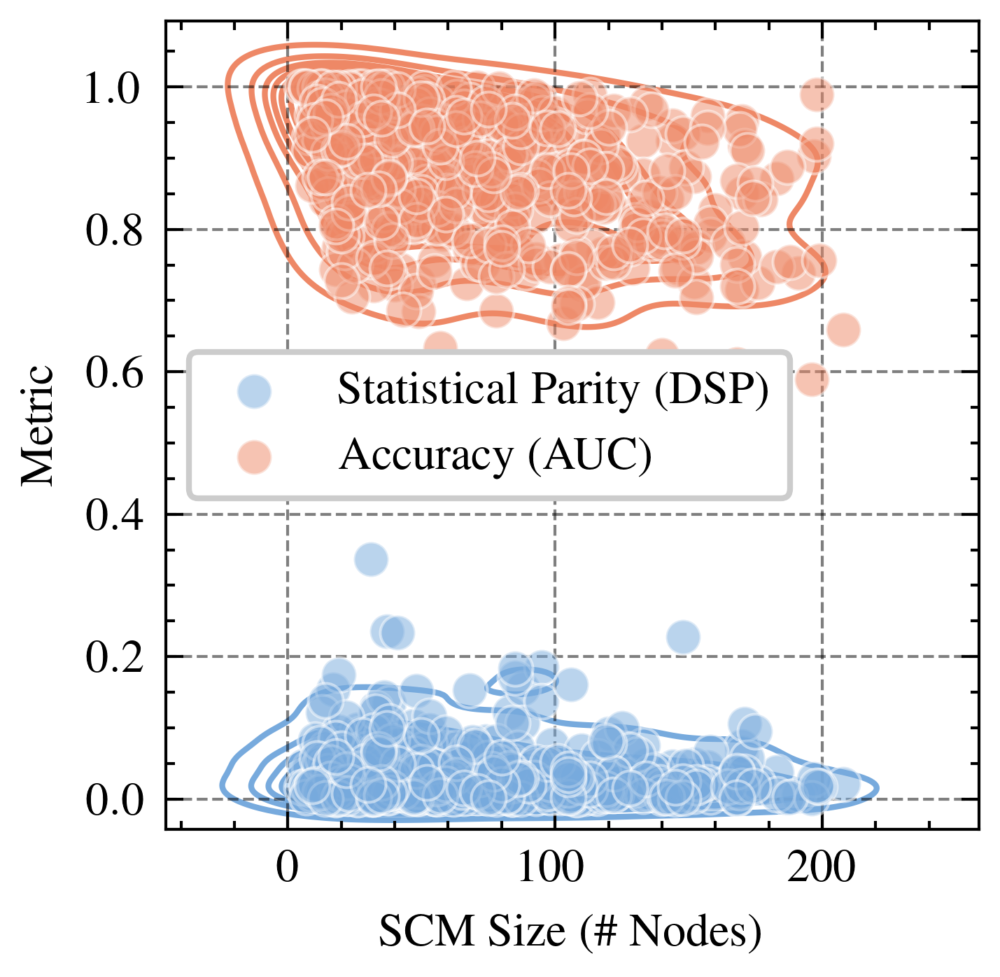<details> <summary>extracted/6522797/figures/complexity.png Details</summary>  ### Visual Description ## Scatter Plot: Statistical Parity vs. Accuracy by SCM Size ### Overview This is a scatter plot comparing two performance metrics—Statistical Parity (DSP) and Accuracy (AUC)—against the size of a Structural Causal Model (SCM), measured in number of nodes. The plot reveals a clear separation between the two metrics, with Accuracy values consistently high and Statistical Parity values consistently low across the range of SCM sizes. ### Components/Axes * **X-Axis:** Labeled "SCM Size (# Nodes)". The scale runs from 0 to over 200, with major tick marks at 0, 100, and 200. Minor tick marks are present. * **Y-Axis:** Labeled "Metric". The scale runs from 0.0 to 1.0, with major tick marks at 0.0, 0.2, 0.4, 0.6, 0.8, and 1.0. * **Legend:** Positioned in the center-left area of the plot, within a white box with a gray border. It contains two entries: * A light blue circle labeled "Statistical Parity (DSP)". * A light orange circle labeled "Accuracy (AUC)". * **Data Series:** * **Statistical Parity (DSP):** Represented by light blue, semi-transparent circles. The data points are densely clustered in the lower portion of the plot. * **Accuracy (AUC):** Represented by light orange, semi-transparent circles. The data points are densely clustered in the upper portion of the plot. * **Density Contours:** Both data series have overlaid contour lines (blue for DSP, orange for AUC) indicating regions of higher point density. * **Grid:** A dashed gray grid is present, aligned with the major tick marks on both axes. ### Detailed Analysis **Statistical Parity (DSP) - Blue Series:** * **Trend Verification:** The blue cluster shows a very slight downward trend as SCM size increases, but the relationship is weak. The primary characteristic is a dense, low-value cluster. * **Data Distribution:** The vast majority of points lie between y=0.0 and y=0.2. The highest density (indicated by the innermost contour) is concentrated between x=0 to x=100 and y=0.0 to y=0.15. * **Outliers:** A few outlier points extend upwards, with the highest reaching approximately y=0.35 at an SCM size of around 40 nodes. Another outlier is near y=0.25 at an SCM size of about 150 nodes. **Accuracy (AUC) - Orange Series:** * **Trend Verification:** The orange cluster shows no strong upward or downward trend. The values remain consistently high across the entire range of SCM sizes. * **Data Distribution:** The points are densely packed between y=0.7 and y=1.0. The highest density region (innermost contour) spans from approximately x=20 to x=180 on the x-axis and y=0.8 to y=1.0 on the y-axis. * **Outliers:** A few points fall below the main cluster, with the lowest reaching approximately y=0.6 at an SCM size near 200 nodes. One point is at y=1.0 near x=200. ### Key Observations 1. **Clear Separation:** There is a stark, non-overlapping separation between the two metrics. All Accuracy (AUC) values are significantly higher than all Statistical Parity (DSP) values. 2. **Metric Stability:** Both metrics show relative stability across SCM sizes. Accuracy remains high, and Statistical Parity remains low, regardless of whether the model has 10 nodes or 200 nodes. 3. **Density Patterns:** The highest density of Accuracy scores is in the high-value region (0.8-1.0), while the highest density of Statistical Parity scores is in the very low-value region (0.0-0.15). 4. **Variance:** The Statistical Parity (DSP) metric appears to have slightly more variance, with a wider spread of outlier points extending upward from its main cluster compared to the tighter cluster of Accuracy scores. ### Interpretation This plot visualizes a potential fairness-accuracy trade-off in the evaluated models or systems. The data suggests that while the models achieve high predictive performance (AUC consistently near 1.0), they perform poorly on the fairness metric of Statistical Parity (DSP consistently near 0.0). Statistical Parity measures whether positive prediction rates are equal across groups; a value near 0 indicates a significant disparity. The lack of a strong trend with SCM size implies that simply increasing the complexity or size of the underlying causal model does not inherently resolve this fairness gap. The problem appears systemic to the models being tested. The investigation should focus on why fairness is compromised despite high accuracy, and whether techniques for improving fairness (e.g., constraints, re-weighting, adversarial debiasing) can shift the blue cluster upward without pulling the orange cluster downward. The outliers in the DSP series (points near 0.35) are particularly interesting, as they represent cases where better fairness was achieved; analyzing what differentiates these cases could provide insights for improvement. </details> Figure 14: Graph Complexity (Prior): Distributions of Statistical Parity and predictive accuracy produced by FairPFN on prior samples with graph complexity between 10 and 200 nodes. As graph complexity increases, accuracy drops but fairness remains constant. 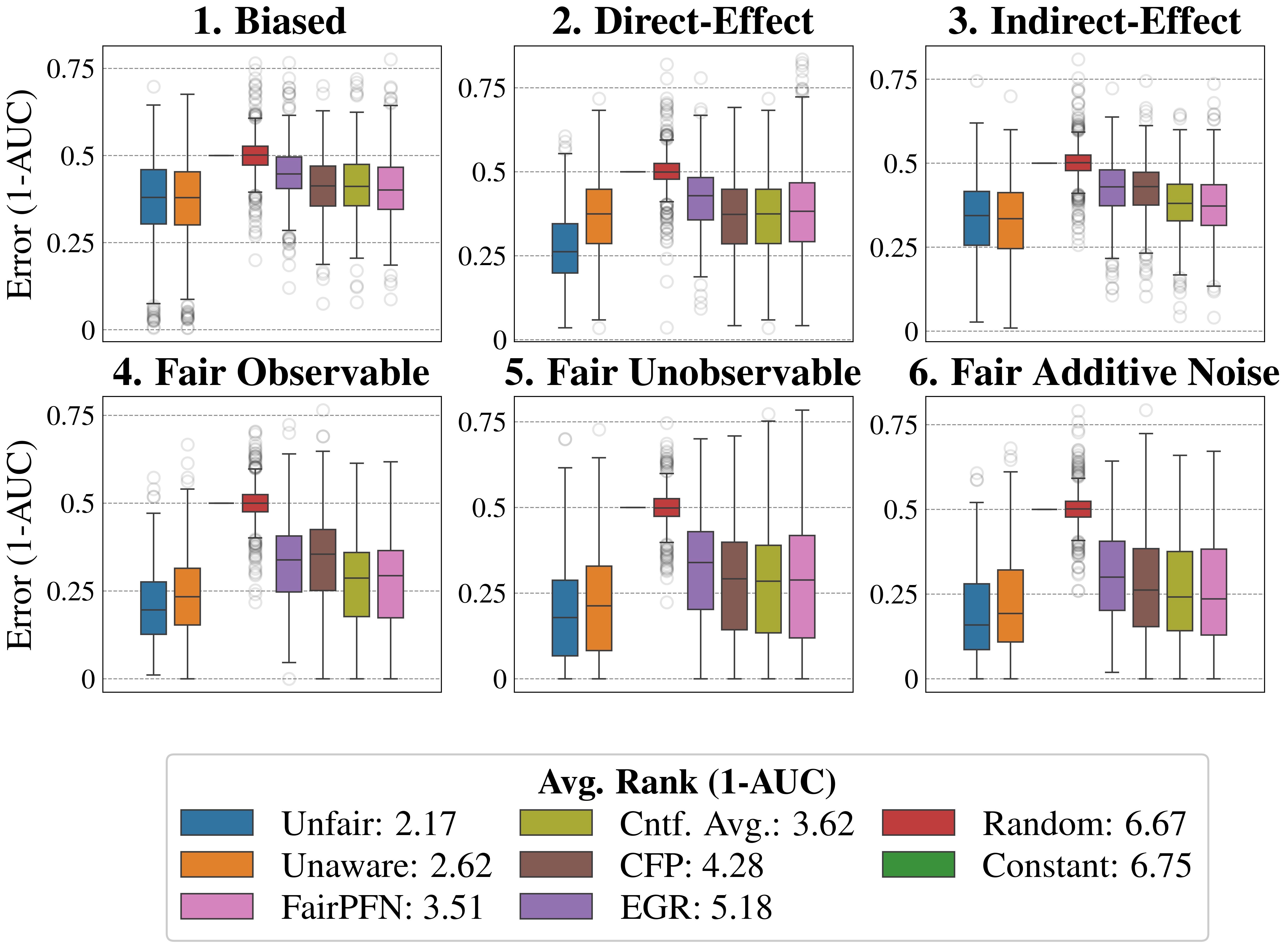## Appendix D Supplementary Results <details> <summary>extracted/6522797/figures/roc_by_group_synthetic_new.png Details</summary>  ### Visual Description ## Box Plot Comparison: Model Performance Across Fairness Scenarios ### Overview The image displays a 2x3 grid of six box plots, each comparing the performance of eight different machine learning models or methods across distinct data scenarios. Performance is measured by "Error (1-AUC)", where a lower value indicates better performance. A comprehensive legend at the bottom maps colors to method names and provides an overall average rank for each method. ### Components/Axes * **Chart Type:** Six separate box plot charts arranged in a grid. * **Y-Axis (All Charts):** Labeled **"Error (1-AUC)"**. The scale runs from 0.0 to 0.75, with major gridlines at 0.0, 0.25, 0.5, and 0.75. * **Subplot Titles (Top of each chart):** 1. **Biased** (Top-Left) 2. **Direct-Effect** (Top-Center) 3. **Indirect-Effect** (Top-Right) 4. **Fair Observable** (Bottom-Left) 5. **Fair Unobservable** (Bottom-Center) 6. **Fair Additive Noise** (Bottom-Right) * **Legend (Bottom Center):** A box containing color swatches and labels for eight methods, along with their "Avg. Rank (1-AUC)". Lower rank indicates better average performance. * **Blue:** Unfair: 2.17 * **Orange:** Unaware: 2.62 * **Pink:** FairPFN: 3.51 * **Olive Green:** Cntf. Avg.: 3.62 * **Brown:** CFP: 4.28 * **Purple:** EGR: 5.18 * **Red:** Random: 6.67 * **Green:** Constant: 6.75 ### Detailed Analysis Each subplot contains eight box plots, one for each method listed in the legend. The box represents the interquartile range (IQR), the line inside is the median, whiskers extend to 1.5*IQR, and circles represent outliers. **1. Biased (Top-Left):** * **Unfair (Blue) & Unaware (Orange):** Lowest median error (~0.35-0.4). Similar distributions. * **FairPFN (Pink), Cntf. Avg. (Olive), CFP (Brown), EGR (Purple):** Clustered with slightly higher median error (~0.4-0.45). FairPFN and Cntf. Avg. appear marginally better than CFP and EGR. * **Random (Red):** Highest median error, centered at 0.5. Tight IQR. * **Constant (Green):** Not visibly plotted in this chart (likely overlapping with Random or omitted). **2. Direct-Effect (Top-Center):** * **Unfair (Blue):** Lowest median error (~0.25). * **Unaware (Orange):** Second lowest (~0.35). * **FairPFN (Pink), Cntf. Avg. (Olive), CFP (Brown), EGR (Purple):** Medians range from ~0.35 to 0.45. FairPFN and Cntf. Avg. are on the lower end. * **Random (Red):** Median at 0.5. * **Constant (Green):** Not visibly plotted. **3. Indirect-Effect (Top-Right):** * **Unfair (Blue) & Unaware (Orange):** Very similar, lowest median error (~0.35). * **FairPFN (Pink), Cntf. Avg. (Olive), CFP (Brown), EGR (Purple):** Medians between ~0.35 and 0.4. FairPFN and Cntf. Avg. are again slightly better. * **Random (Red):** Median at 0.5. * **Constant (Green):** Not visibly plotted. **4. Fair Observable (Bottom-Left):** * **Unfair (Blue):** Lowest median error (~0.2). * **Unaware (Orange):** Second lowest (~0.25). * **FairPFN (Pink), Cntf. Avg. (Olive), CFP (Brown), EGR (Purple):** Medians between ~0.25 and 0.35. FairPFN and Cntf. Avg. are lower than CFP and EGR. * **Random (Red):** Median at 0.5. * **Constant (Green):** Not visibly plotted. **5. Fair Unobservable (Bottom-Center):** * **Unfair (Blue):** Lowest median error (~0.2). * **Unaware (Orange):** Second lowest (~0.25). * **FairPFN (Pink), Cntf. Avg. (Olive), CFP (Brown), EGR (Purple):** Medians between ~0.25 and 0.35. FairPFN and Cntf. Avg. are lower. * **Random (Red):** Median at 0.5. * **Constant (Green):** Not visibly plotted. **6. Fair Additive Noise (Bottom-Right):** * **Unfair (Blue):** Lowest median error (~0.15). * **Unaware (Orange):** Second lowest (~0.2). * **FairPFN (Pink), Cntf. Avg. (Olive), CFP (Brown), EGR (Purple):** Medians between ~0.2 and 0.3. FairPFN and Cntf. Avg. are lower. * **Random (Red):** Median at 0.5. * **Constant (Green):** Not visibly plotted. ### Key Observations 1. **Consistent Hierarchy:** Across all six scenarios, the performance order is remarkably consistent: **Unfair** (best) > **Unaware** > **FairPFN** ≈ **Cntf. Avg.** > **CFP** ≈ **EGR** > **Random** (worst). The **Constant** method is listed in the legend but does not appear as a distinct box plot in any chart, suggesting its performance may be identical to or obscured by the Random baseline (median=0.5). 2. **Scenario Impact:** The absolute error values are lowest in the "Fair" scenarios (4, 5, 6), particularly "Fair Additive Noise," where the best models achieve medians below 0.2. The "Biased" scenario shows the highest overall error levels. 3. **Baseline Performance:** The **Random** method consistently has a median error of 0.5, which is the expected performance of random guessing for AUC (since AUC=0.5 implies no discriminative ability, making 1-AUC=0.5). 4. **Fairness-Accuracy Trade-off:** Methods designed for fairness (FairPFN, Cntf. Avg., CFP, EGR) consistently incur a higher error (lower AUC) than the "Unfair" and "Unaware" baselines, illustrating the typical trade-off between fairness and predictive performance. ### Interpretation This visualization provides a clear empirical comparison of model performance under different data-generating processes related to fairness. The key takeaway is that **ignoring fairness constraints ("Unfair" and "Unaware" models) yields the best predictive performance (lowest 1-AUC) across all tested scenarios.** However, this comes at the potential cost of fairness. The fairness-aware methods (FairPFN, Cntf. Avg., CFP, EGR) successfully reduce error compared to the naive random baseline but cannot match the performance of models not constrained by fairness. Among these, **FairPFN and Counterfactual Averaging (Cntf. Avg.) consistently outperform Counterfactual Fairness Prediction (CFP) and Equalized Odds Post-processing (EGR)**, suggesting they may be more effective at balancing fairness and accuracy in these contexts. The fact that the "Constant" model (which likely predicts a single constant value) performs identically to "Random" (median error 0.5) indicates that in these binary classification tasks, a trivial constant predictor is no better than random chance. The progression from "Biased" to the "Fair" scenarios shows that when the underlying data structure is fairer, all models, including the fairness-aware ones, achieve lower absolute error rates. </details> Figure 15: Predictive Error (Synthetic): Predictive error (1-AUC) of FairPFN compared to our baselines. FairPFN maintains a competitive level of predictive error with traditional ML algorithms, achieving an average rank of 3.51 out of 7. 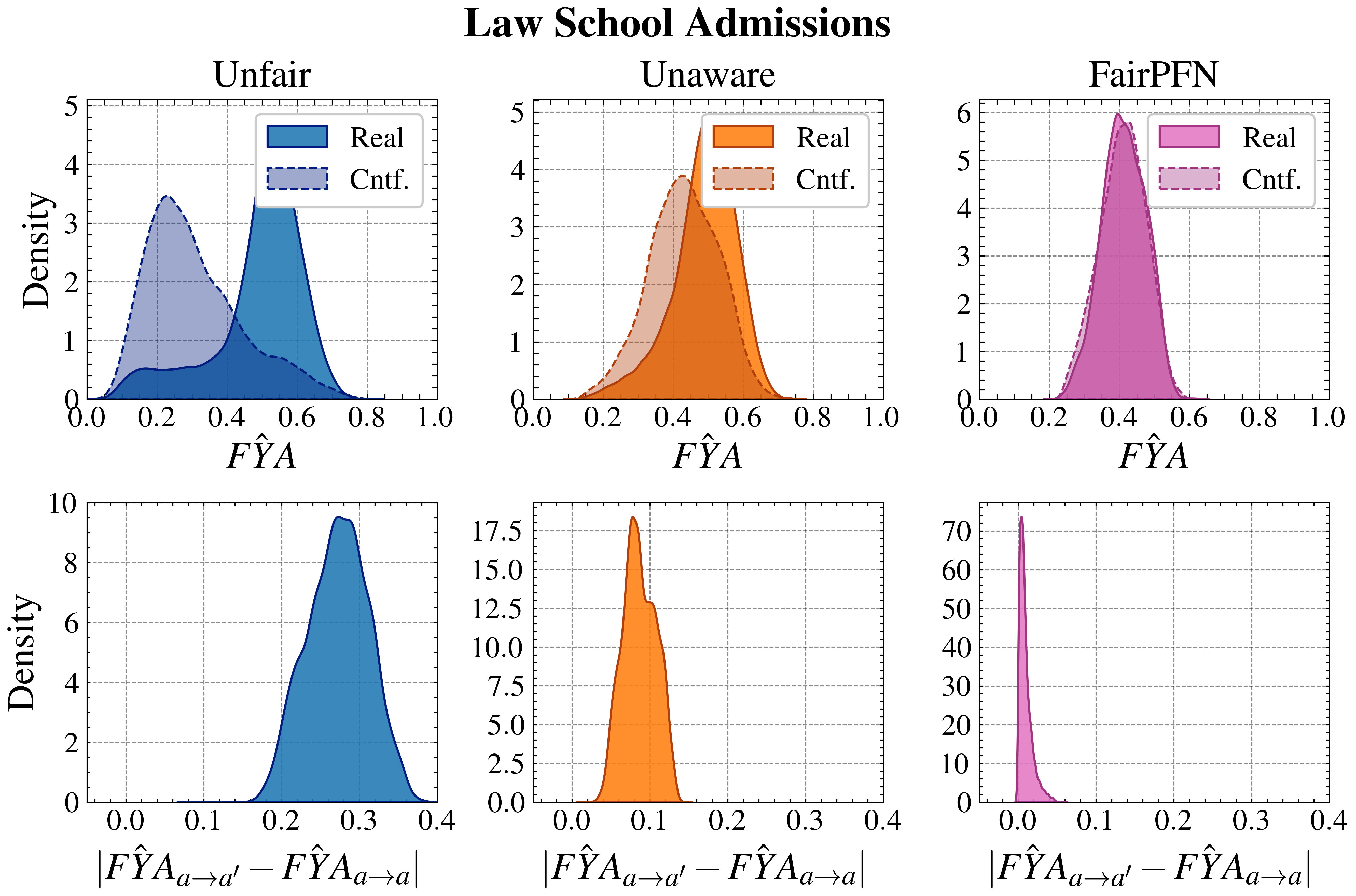<details> <summary>extracted/6522797/figures/lawschool_dist.png Details</summary>  ### Visual Description ## Density Plots: Law School Admissions Fairness Analysis ### Overview The image displays a 2x3 grid of density plots titled "Law School Admissions." It compares the distribution of a fairness-related metric, denoted as **FŶA**, across three different modeling approaches ("Unfair," "Unaware," "FairPFN") under two conditions ("Real" and "Cntf."). The bottom row analyzes the absolute change in this metric when an attribute is altered. ### Components/Axes * **Overall Title:** "Law School Admissions" (centered at the top). * **Column Headers (Top Row):** "Unfair" (left), "Unaware" (center), "FairPFN" (right). * **Top Row Plots:** * **X-axis:** Labeled **FŶA**. Scale ranges from 0.0 to 1.0 with major ticks at 0.0, 0.2, 0.4, 0.6, 0.8, 1.0. * **Y-axis:** Labeled **Density**. Scale varies per plot (0-5 for Unfair/Unaware, 0-6 for FairPFN). * **Legend (in each top plot, top-right corner):** * **Real:** Solid fill color (blue for Unfair, orange for Unaware, magenta for FairPFN). * **Cntf.:** Dashed outline with a lighter, semi-transparent fill of the same hue. * **Bottom Row Plots:** * **X-axis:** Labeled **|FŶA_{a→a'} - FŶA_{a→a}|**. Scale ranges from 0.0 to 0.4 with major ticks at 0.0, 0.1, 0.2, 0.3, 0.4. * **Y-axis:** Labeled **Density**. Scale varies significantly per plot (0-10 for Unfair, 0-17.5 for Unaware, 0-70 for FairPFN). * **No legends** are present in the bottom row plots. The color corresponds to the column (blue, orange, magenta). ### Detailed Analysis **Top Row: Distribution of FŶA** * **Unfair (Blue):** The "Real" distribution is bimodal, with a smaller peak near 0.2 and a dominant peak around 0.55. The "Cntf." distribution is unimodal, peaking sharply around 0.25. There is a significant separation between the two distributions. * **Unaware (Orange):** The "Real" and "Cntf." distributions overlap considerably. Both are unimodal, with the "Real" peak slightly to the right (around 0.48) of the "Cntf." peak (around 0.42). * **FairPFN (Magenta):** The "Real" and "Cntf." distributions are nearly identical, showing almost complete overlap. Both form a single, sharp peak centered at approximately 0.4. **Bottom Row: Distribution of |FŶA_{a→a'} - FŶA_{a→a}|** * **Unfair (Blue):** The distribution of the absolute difference is unimodal and symmetric, peaking at approximately 0.28. The density at the peak is ~9.5. * **Unaware (Orange):** The distribution is unimodal and slightly right-skewed, peaking at approximately 0.08. The density at the peak is ~18. * **FairPFN (Magenta):** The distribution is extremely narrow and tall, peaking very close to 0.0 (approximately 0.01). The density at the peak is exceptionally high, reaching ~72. ### Key Observations 1. **Progression of Overlap:** Moving from left to right (Unfair → Unaware → FairPFN), the "Real" and "Cntf." distributions in the top row show increasing overlap, culminating in near-perfect alignment for FairPFN. 2. **Shift in Central Tendency:** The central peak of the "Real" distribution shifts leftward across the columns: from ~0.55 (Unfair) to ~0.48 (Unaware) to ~0.4 (FairPFN). 3. **Magnitude of Change:** The bottom row reveals a dramatic reduction in the magnitude of the metric's change (|FŶA_{a→a'} - FŶA_{a→a}|) across the models. The peak of the distribution moves from ~0.28 (Unfair) to ~0.08 (Unaware) to ~0.01 (FairPFN). 4. **Precision of FairPFN:** The FairPFN model not only aligns the real and counterfactual distributions but also results in an extremely stable metric (very low absolute change), as indicated by the very high, narrow density peak near zero in the bottom-right plot. ### Interpretation This visualization demonstrates the effectiveness of different algorithmic approaches to fairness in a law school admissions context. **FŶA** likely represents a fairness metric (e.g., related to acceptance rates or outcomes across groups). * The **"Unfair"** model shows a large discrepancy between real-world outcomes ("Real") and a counterfactual scenario ("Cntf."), suggesting the model's decisions are highly sensitive to the attribute being altered (e.g., race, gender). The large absolute differences in the bottom plot confirm this high sensitivity. * The **"Unaware"** model, which likely excludes the sensitive attribute from the decision process, reduces but does not eliminate the discrepancy. Some disparity persists, and the model remains moderately sensitive to attribute changes. * The **"FairPFN"** model achieves two key fairness properties: 1. **Counterfactual Fairness:** The near-perfect overlap of "Real" and "Cntf." distributions indicates that, in a counterfactual world where the sensitive attribute is changed, the model's outcomes would be statistically identical. This is a strong fairness guarantee. 2. **Stability/Robustness:** The extremely low absolute difference values (bottom-right plot) show that the model's fairness metric is highly stable and minimally affected by perturbations to the sensitive attribute. In summary, the figure argues that the FairPFN method successfully aligns real and counterfactual outcomes and produces a robustly fair model, outperforming both a standard ("Unfair") and an attribute-ignorant ("Unaware") approach. </details> Figure 16: Counterfactual Distributions (Law School): Predictive distributions of Unfair, Unaware, and FairPFN on observational and counterfactual versions of the Lawschool Admissions dataset. FairPFN reduces the maximum pairwise difference between these distributions to 0.05. 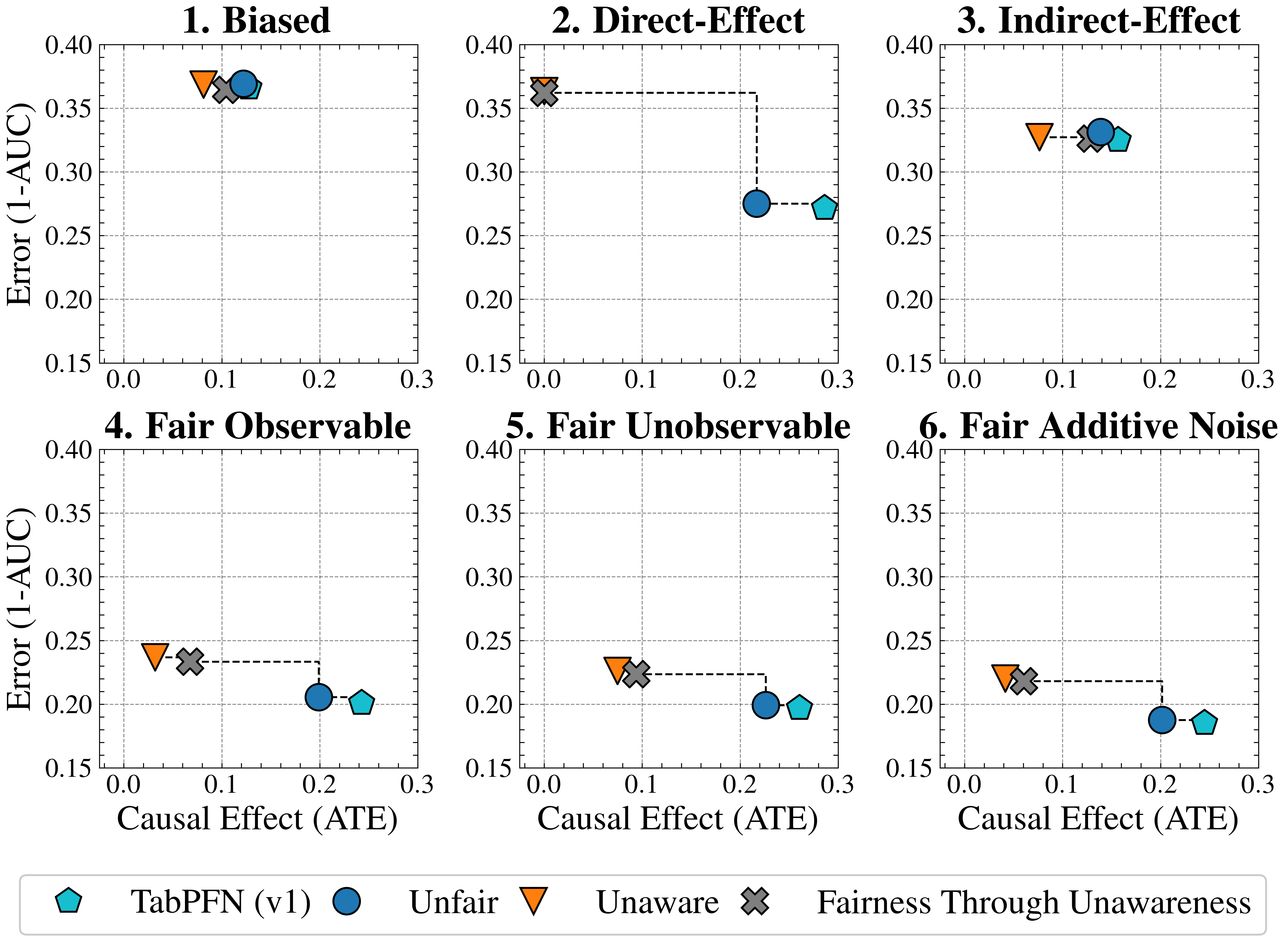<details> <summary>extracted/6522797/figures/trade-off_by_group_synthetic_alt.png Details</summary>  ### Visual Description ## [Scatter Plot Grid]: Comparison of Model Error vs. Causal Effect Across Six Fairness Scenarios ### Overview The image displays a 2x3 grid of six scatter plots. Each plot compares the performance of four different modeling approaches on two metrics: **Error (1-AUC)** on the y-axis and **Causal Effect (ATE)** on the x-axis. The plots are titled to represent different underlying data-generating scenarios related to fairness and bias. A shared legend at the bottom identifies the four modeling approaches by unique marker shapes and colors. ### Components/Axes * **Titles:** Six individual plot titles: "1. Biased", "2. Direct-Effect", "3. Indirect-Effect", "4. Fair Observable", "5. Fair Unobservable", "6. Fair Additive Noise". * **Y-Axis (All Plots):** Label: "Error (1-AUC)". Scale ranges from 0.15 to 0.40, with major ticks at 0.05 intervals. * **X-Axis (All Plots):** Label: "Causal Effect (ATE)". Scale ranges from 0.0 to 0.3, with major ticks at 0.1 intervals. * **Legend (Bottom Center):** Contains four entries: * **Cyan Pentagon:** "TabPFN (v1)" * **Blue Circle:** "Unfair" * **Orange Inverted Triangle:** "Unaware" * **Gray 'X':** "Fairness Through Unawareness" * **Plot Elements:** Each plot contains the four markers corresponding to the legend. Some plots include dashed lines connecting specific pairs of markers. ### Detailed Analysis **1. Biased** * **Trend:** All four models are clustered tightly in the top-left quadrant of the plot. * **Data Points (Approximate):** * **Unaware (Orange Triangle):** ATE ≈ 0.08, Error ≈ 0.37 * **Fairness Through Unawareness (Gray X):** ATE ≈ 0.10, Error ≈ 0.36 * **Unfair (Blue Circle):** ATE ≈ 0.12, Error ≈ 0.37 * **TabPFN (v1) (Cyan Pentagon):** ATE ≈ 0.13, Error ≈ 0.36 * **Observation:** Models show low causal effect and high error. Performance is very similar across all methods. **2. Direct-Effect** * **Trend:** A clear separation between two groups of models. A dashed line connects the high-error/low-ATE group to the low-error/high-ATE group. * **Data Points (Approximate):** * **Group 1 (High Error, Low ATE):** * **Unaware (Orange Triangle):** ATE ≈ 0.00, Error ≈ 0.36 * **Fairness Through Unawareness (Gray X):** ATE ≈ 0.00, Error ≈ 0.36 * **Group 2 (Low Error, High ATE):** * **Unfair (Blue Circle):** ATE ≈ 0.22, Error ≈ 0.27 * **TabPFN (v1) (Cyan Pentagon):** ATE ≈ 0.28, Error ≈ 0.27 * **Observation:** The "Unfair" and "TabPFN" models achieve significantly lower error and higher causal effect compared to the "Unaware" and "Fairness Through Unawareness" models in this scenario. **3. Indirect-Effect** * **Trend:** All models are clustered in the center of the plot. * **Data Points (Approximate):** * **Unaware (Orange Triangle):** ATE ≈ 0.08, Error ≈ 0.33 * **Fairness Through Unawareness (Gray X):** ATE ≈ 0.13, Error ≈ 0.32 * **Unfair (Blue Circle):** ATE ≈ 0.14, Error ≈ 0.33 * **TabPFN (v1) (Cyan Pentagon):** ATE ≈ 0.16, Error ≈ 0.32 * **Observation:** Models show moderate causal effect and error. Performance is again similar across methods, with a slight trend of increasing ATE from Unaware to TabPFN. **4. Fair Observable** * **Trend:** Similar to plot 2, with a dashed line connecting two distinct groups. * **Data Points (Approximate):** * **Group 1 (Higher Error, Lower ATE):** * **Unaware (Orange Triangle):** ATE ≈ 0.03, Error ≈ 0.24 * **Fairness Through Unawareness (Gray X):** ATE ≈ 0.06, Error ≈ 0.23 * **Group 2 (Lower Error, Higher ATE):** * **Unfair (Blue Circle):** ATE ≈ 0.20, Error ≈ 0.21 * **TabPFN (v1) (Cyan Pentagon):** ATE ≈ 0.24, Error ≈ 0.20 * **Observation:** The "Unfair" and "TabPFN" models again outperform the others, achieving both lower error and higher causal effect. **5. Fair Unobservable** * **Trend:** A pattern very similar to plots 2 and 4, with a dashed line connecting two groups. * **Data Points (Approximate):** * **Group 1 (Higher Error, Lower ATE):** * **Unaware (Orange Triangle):** ATE ≈ 0.07, Error ≈ 0.23 * **Fairness Through Unawareness (Gray X):** ATE ≈ 0.09, Error ≈ 0.22 * **Group 2 (Lower Error, Higher ATE):** * **Unfair (Blue Circle):** ATE ≈ 0.22, Error ≈ 0.20 * **TabPFN (v1) (Cyan Pentagon):** ATE ≈ 0.26, Error ≈ 0.20 * **Observation:** Consistent pattern: "Unfair" and "TabPFN" models cluster together with better performance (lower error, higher ATE) than the other two methods. **6. Fair Additive Noise** * **Trend:** The same two-group pattern with a connecting dashed line is present. * **Data Points (Approximate):** * **Group 1 (Higher Error, Lower ATE):** * **Unaware (Orange Triangle):** ATE ≈ 0.04, Error ≈ 0.22 * **Fairness Through Unawareness (Gray X):** ATE ≈ 0.06, Error ≈ 0.22 * **Group 2 (Lower Error, Higher ATE):** * **Unfair (Blue Circle):** ATE ≈ 0.20, Error ≈ 0.19 * **TabPFN (v1) (Cyan Pentagon):** ATE ≈ 0.24, Error ≈ 0.19 * **Observation:** The performance gap between the two groups is maintained. "Unfair" and "TabPFN" show the lowest error and highest causal effect in this set. ### Key Observations 1. **Consistent Grouping:** Across five of the six scenarios (2-6), the "Unfair" (blue circle) and "TabPFN (v1)" (cyan pentagon) models consistently cluster together, demonstrating lower error (1-AUC) and higher causal effect (ATE) than the "Unaware" (orange triangle) and "Fairness Through Unawareness" (gray X) models. 2. **Scenario Impact:** The "Biased" scenario (Plot 1) is an outlier where all models perform poorly and similarly. The "Indirect-Effect" scenario (Plot 3) shows a tighter cluster with less separation between model groups. 3. **Trade-off Visualization:** The dashed lines in plots 2, 4, 5, and 6 visually emphasize the performance trade-off or gap between the two distinct groups of modeling approaches. 4. **Metric Relationship:** There is a general inverse relationship visible: models with lower Error (1-AUC) tend to have higher Causal Effect (ATE), particularly in the "Fair" scenarios. ### Interpretation This visualization analyzes the performance of different algorithmic fairness approaches under various causal data-generating processes. The key insight is that simply being "unaware" of a sensitive attribute (the "Unaware" and "Fairness Through Unawareness" methods) does not necessarily lead to better outcomes. In fact, in scenarios where fairness is defined by causal effects (Direct, Observable, Unobservable, Additive Noise), models that do not explicitly try to hide the sensitive attribute ("Unfair" and the baseline "TabPFN") achieve a better balance of predictive accuracy (lower 1-AUC) and reduced discriminatory impact (higher ATE). The plots suggest that the "Unfair" model and the "TabPFN" baseline are robust across these specific fairness scenarios, while the "unawareness" strategies consistently underperform. The "Biased" scenario represents a case where the underlying data structure makes it difficult for any model to achieve good performance on both metrics simultaneously. This analysis underscores the importance of choosing a fairness intervention that aligns with the specific causal structure of the problem, as naive approaches like "fairness through unawareness" can be ineffective or even counterproductive. </details> Figure 17: Baseline Validation (Synthetic): Fairness-accuracy trade-off achieved by our baselines Unfair and Unaware compared to alternative choices of TabPFN (v1) and "Fairness Through Unawareness." Unfair achieves competitive performance with TabPFN (v1), while Unaware outperforms the standard strategy of dropping the protected attribute from the dataset. 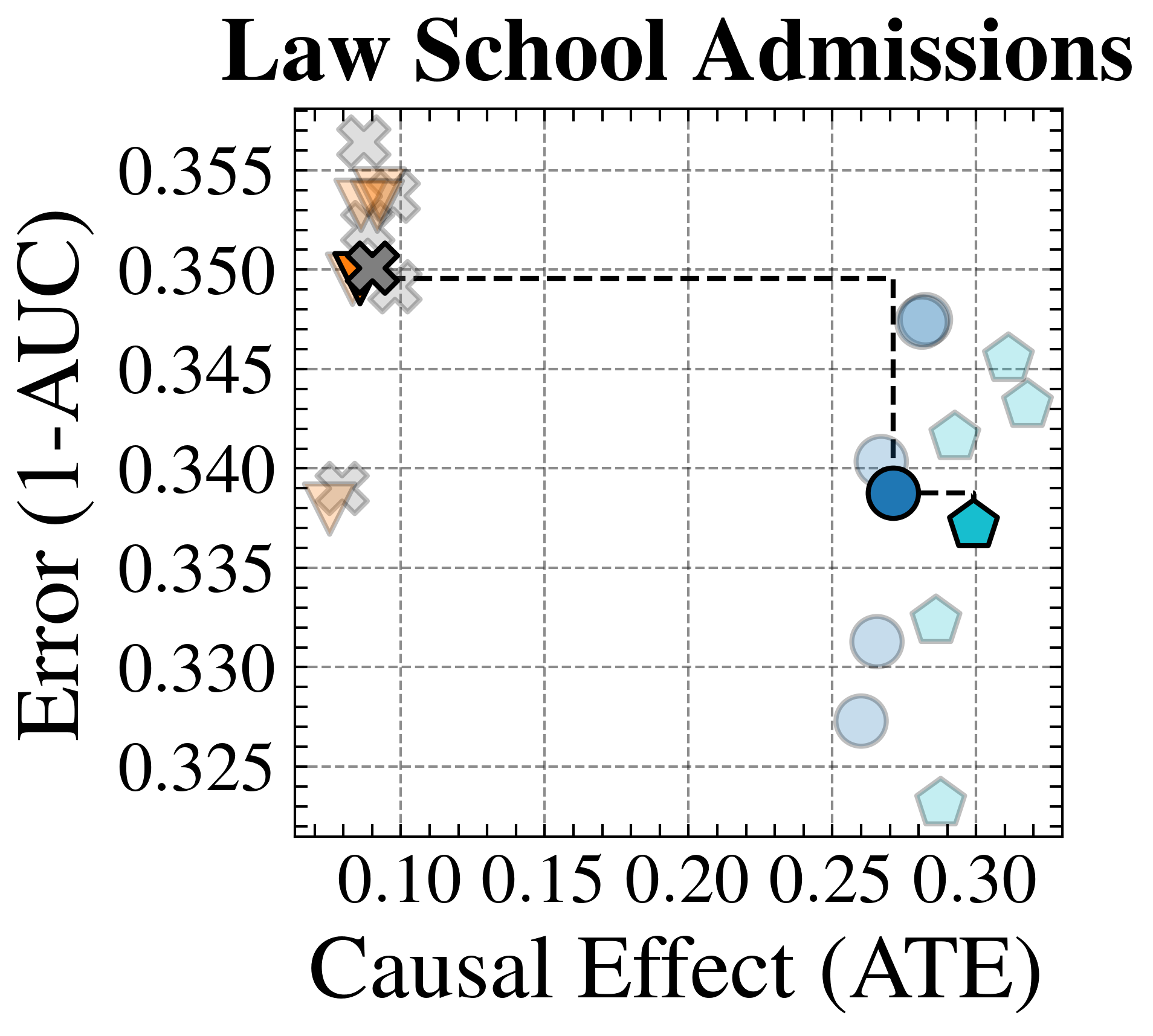<details> <summary>extracted/6522797/figures/trade-off_lawschool_alt.png Details</summary>  ### Visual Description ## Scatter Plot: Law School Admissions ### Overview The image is a scatter plot titled "Law School Admissions." It plots data points on a two-dimensional grid, comparing a model's predictive error against its estimated causal effect. The plot uses different marker shapes and colors to represent distinct data series or model variants. ### Components/Axes * **Title:** "Law School Admissions" (centered at the top). * **X-Axis:** Labeled "Causal Effect (ATE)". The scale runs from approximately 0.08 to 0.32, with major tick marks labeled at 0.10, 0.15, 0.20, 0.25, and 0.30. * **Y-Axis:** Labeled "Error (1-AUC)". The scale runs from approximately 0.322 to 0.358, with major tick marks labeled at 0.325, 0.330, 0.335, 0.340, 0.345, 0.350, and 0.355. * **Grid:** A light gray dashed grid is present, aligned with the major tick marks on both axes. * **Data Series (Markers):** There is no explicit legend box. Different series are distinguished by marker shape and color: * **Orange/Brown Inverted Triangles:** Clustered in the top-left region. * **Gray 'X' Marks:** Overlapping with the orange triangles in the top-left. * **Light Blue Circles:** Scattered in the right half of the plot. * **Light Blue Pentagons:** Scattered in the right half, generally to the right of the circles. * **Dark Blue Circle:** A single, prominent point in the center-right. * **Cyan Pentagon:** A single, prominent point to the right of the dark blue circle. * **Annotation:** A black dashed line connects three specific points: a gray 'X' in the top-left, a dark blue circle in the center-right, and a cyan pentagon to its right. ### Detailed Analysis **Spatial Grounding & Data Points (Approximate Coordinates):** * **Top-Left Cluster (High Error, Low Causal Effect):** * **Orange Inverted Triangles:** Two points. One at approximately (ATE=0.09, Error=0.354). Another lower point at (ATE=0.08, Error=0.339). * **Gray 'X' Marks:** Multiple overlapping points. The most prominent one, connected by the dashed line, is at approximately (ATE=0.09, Error=0.350). Others are clustered around (ATE=0.08-0.10, Error=0.348-0.356). * **Right-Side Scatter (Lower Error, Higher Causal Effect):** * **Light Blue Circles:** Five points. Their approximate coordinates are: 1. (ATE=0.26, Error=0.327) 2. (ATE=0.26, Error=0.331) 3. (ATE=0.27, Error=0.340) 4. (ATE=0.28, Error=0.347) 5. (ATE=0.25, Error=0.323) - This is the lowest point on the plot. * **Light Blue Pentagons:** Five points. Their approximate coordinates are: 1. (ATE=0.28, Error=0.322) - This is the lowest point on the plot. 2. (ATE=0.28, Error=0.332) 3. (ATE=0.29, Error=0.341) 4. (ATE=0.30, Error=0.343) 5. (ATE=0.31, Error=0.345) * **Prominent Connected Points (Dashed Line Path):** 1. **Start:** Gray 'X' at (ATE≈0.09, Error≈0.350). 2. **Middle:** Dark Blue Circle at (ATE≈0.27, Error≈0.339). 3. **End:** Cyan Pentagon at (ATE≈0.29, Error≈0.337). ### Key Observations 1. **Clear Trade-off:** There is a distinct negative correlation visible. Models with low causal effect (ATE < 0.12) have high error (1-AUC > 0.348). Models with higher causal effect (ATE > 0.25) generally have lower error (1-AUC < 0.348). 2. **Clustering:** Data points form two primary clusters: a tight, high-error cluster on the left and a more dispersed, lower-error cluster on the right. 3. **The Dashed Line:** This line traces a specific path from a high-error/low-effect model to a lower-error/higher-effect model, and finally to a model with slightly higher effect and slightly lower error. It may represent a model selection or optimization trajectory. 4. **Outlier:** The light blue circle at (ATE≈0.25, Error≈0.323) and the light blue pentagon at (ATE≈0.28, Error≈0.322) are notable for having the lowest error values on the plot. 5. **Marker Consistency:** The two prominent single points (dark blue circle, cyan pentagon) are connected by the dashed line and are positioned within the general scatter of their respective shape groups (circles and pentagons). ### Interpretation This chart visualizes the performance of different models or methods applied to a law school admissions dataset, evaluated on two competing objectives: predictive accuracy (where lower 1-AUC is better) and the magnitude of the estimated causal effect (Average Treatment Effect, where a higher ATE is presumably desirable or meaningful). The data suggests a fundamental tension: models that achieve a very high estimated causal effect (ATE > 0.25) tend to have better predictive performance (lower error) than those with low estimated effects. This could imply that the factors driving a strong causal signal in this context are also predictive of the outcome. The dashed line is particularly insightful. It likely highlights a specific methodological progression. Starting from a baseline model (gray 'X') with poor performance on both metrics, an intervention or alternative method (dark blue circle) dramatically increases the causal effect while also reducing error. A further refinement (cyan pentagon) yields a small additional gain in causal effect with a minor further reduction in error. This path demonstrates a desirable direction of model improvement: moving from the top-left (undesirable) to the bottom-right (more desirable) of the plot. The presence of multiple points for each marker type suggests variability, possibly from different model initializations, hyperparameter settings, or data subsamples. The overall pattern indicates that for this problem, seeking models with higher estimated causal effects is correlated with, and may even be conducive to, achieving better predictive accuracy. 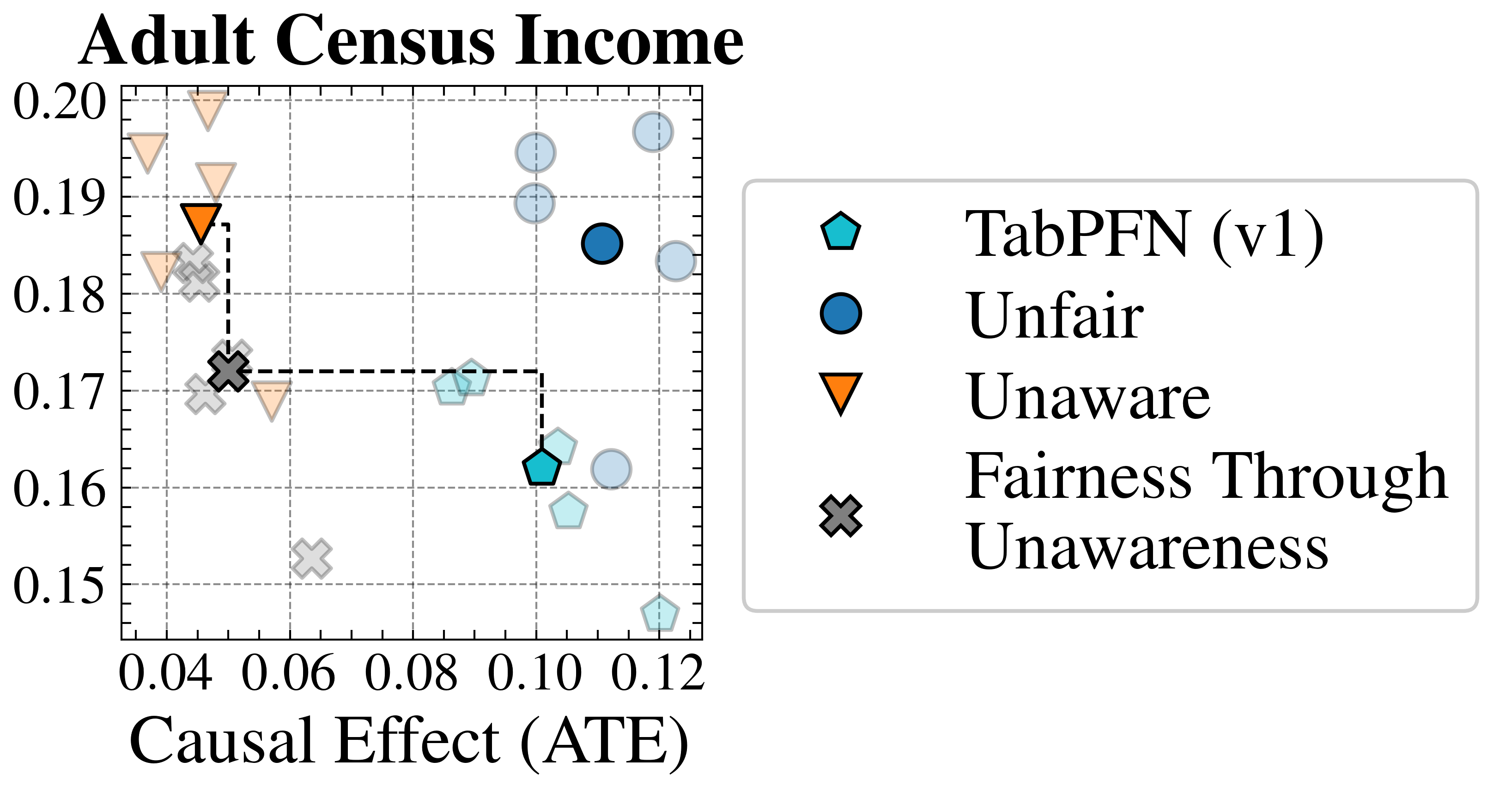</details> <details> <summary>extracted/6522797/figures/trade-off_adult_alt.png Details</summary>  ### Visual Description \n ## Scatter Plot: Adult Census Income - Causal Effect vs. Unlabeled Metric ### Overview This is a scatter plot titled "Adult Census Income." It compares four different methods or models based on two metrics: "Causal Effect (ATE)" on the x-axis and an unnamed performance or error metric on the y-axis (ranging from 0.15 to 0.20). The plot visualizes the trade-off between the causal effect of a sensitive attribute and the model's performance. ### Components/Axes * **Title:** "Adult Census Income" (top-left, above the plot area). * **X-Axis:** * **Label:** "Causal Effect (ATE)" (centered below the axis). * **Scale:** Linear, ranging from approximately 0.04 to 0.12. * **Major Ticks:** 0.04, 0.06, 0.08, 0.10, 0.12. * **Y-Axis:** * **Label:** **Not explicitly labeled.** The axis displays numerical values only. * **Scale:** Linear, ranging from 0.15 to 0.20. * **Major Ticks:** 0.15, 0.16, 0.17, 0.18, 0.19, 0.20. * **Legend:** Positioned to the right of the plot area. It defines four data series by shape and color: 1. **TabPFN (v1):** Cyan (light blue) pentagon. 2. **Unfair:** Blue circle. 3. **Unaware:** Orange inverted triangle. 4. **Fairness Through Unawareness:** Gray 'X' (cross). * **Grid:** A light gray dashed grid is present for both axes. ### Detailed Analysis The plot contains multiple data points for each series, showing their distribution across the two metrics. **1. TabPFN (v1) - Cyan Pentagons:** * **Trend:** Points are clustered in the lower-right quadrant, indicating higher Causal Effect (ATE) and lower values on the y-axis metric. * **Approximate Data Points (x, y):** * (0.10, 0.162) * (0.105, 0.158) * (0.09, 0.170) * (0.092, 0.170) * (0.12, 0.148) - This is the lowest y-value on the entire plot. **2. Unfair - Blue Circles:** * **Trend:** Points are clustered in the upper-right quadrant, indicating both higher Causal Effect (ATE) and higher values on the y-axis metric. * **Approximate Data Points (x, y):** * (0.10, 0.195) * (0.10, 0.190) * (0.11, 0.185) * (0.12, 0.197) * (0.12, 0.183) * (0.11, 0.162) - An outlier for this group, lower on the y-axis. **3. Unaware - Orange Inverted Triangles:** * **Trend:** Points are clustered in the upper-left quadrant, indicating lower Causal Effect (ATE) but higher values on the y-axis metric. * **Approximate Data Points (x, y):** * (0.04, 0.195) * (0.05, 0.200) * (0.05, 0.192) * (0.04, 0.183) * (0.05, 0.188) - This point is connected by a dashed line to a gray 'X'. * (0.06, 0.170) **4. Fairness Through Unawareness - Gray 'X's:** * **Trend:** Points are more scattered, primarily in the left and central regions of the plot. * **Approximate Data Points (x, y):** * (0.05, 0.182) * (0.05, 0.172) - This point is connected by dashed lines to an orange triangle and a cyan pentagon. * (0.05, 0.170) * (0.06, 0.153) **Notable Visual Element:** * A set of black dashed lines connects three specific points, forming a right angle: 1. An **Unaware** (orange triangle) point at approximately (0.05, 0.188). 2. A **Fairness Through Unawareness** (gray 'X') point at approximately (0.05, 0.172). 3. A **TabPFN (v1)** (cyan pentagon) point at approximately (0.10, 0.162). * This likely highlights a direct comparison or a specific trade-off path between these three methods. ### Key Observations 1. **Clear Clustering by Method:** Each method occupies a distinct region of the plot, suggesting strong, consistent characteristics. 2. **Performance-Fairness Trade-off:** There appears to be an inverse relationship between the y-axis metric (likely a measure of error or loss, where lower is better) and the Causal Effect (ATE). Methods with lower ATE (Unaware) have higher y-values, while methods with higher ATE (TabPFN v1, Unfair) have lower y-values. 3. **"Unfair" vs. "TabPFN (v1)":** Both have high ATE, but "Unfair" has significantly higher y-values (worse performance), while "TabPFN (v1)" achieves the lowest y-values (best performance) on the chart. 4. **"Fairness Through Unawareness" Variability:** This method shows the widest spread, particularly in the y-axis direction, indicating less consistent performance compared to the others. ### Interpretation This chart analyzes fairness in machine learning models trained on the Adult Census Income dataset, a common benchmark for fairness research. The **Causal Effect (ATE - Average Treatment Effect)** on the x-axis likely measures the direct influence of a sensitive attribute (e.g., race, gender) on the model's predictions. A higher ATE suggests the model's decisions are more causally influenced by that attribute, which is often considered unfair. The **unlabeled y-axis** almost certainly represents a standard model performance metric like **log loss, error rate, or 1 - accuracy**, where a **lower value is better**. The data demonstrates a fundamental tension: * **Unaware** models (which are not designed to be fair) achieve low causal influence (low ATE) but have poor predictive performance (high y-value). * **Unfair** models (likely standard models without any fairness constraints) achieve good performance (low y-value) but have high causal influence (high ATE), indicating potential bias. * **TabPFN (v1)** appears to be a method that successfully achieves **both** high performance (very low y-value) **and** a high causal effect. This is a critical observation—it suggests this method may be optimizing for accuracy in a way that inadvertently amplifies the causal influence of the sensitive attribute. * The **"Fairness Through Unawareness"** method and the dashed lines connecting it to the others illustrate a potential compromise or a specific intervention point. The path from "Unaware" down to "Fairness Through Unawareness" shows a gain in fairness (slight increase in ATE) at the cost of performance (drop in y-value). The horizontal line to "TabPFN (v1)" then shows a dramatic increase in ATE for a further gain in performance. **Conclusion:** The plot suggests that on this dataset, achieving the highest predictive performance (TabPFN v1) comes with a high causal effect of the sensitive attribute. Traditional "unaware" modeling yields low causal effect but poor performance. The chart visualizes the search for methods that can navigate this trade-off, with the dashed lines potentially highlighting a specific analytical comparison between three key approaches. The missing y-axis label is a significant omission for full technical interpretation. </details> Figure 18: Baseline Validation (Real-World): Fairness-accuracy trade-off achieved by our baselines Unfair and Unaware compared to alternative choices of TabPFN (v1) and "Fairness Through Unawareness." Our choices of baselines achieve competitive performance on the Law School Admissions problem, while alternative baselines perform slightly better on the Adult Census Income problem. 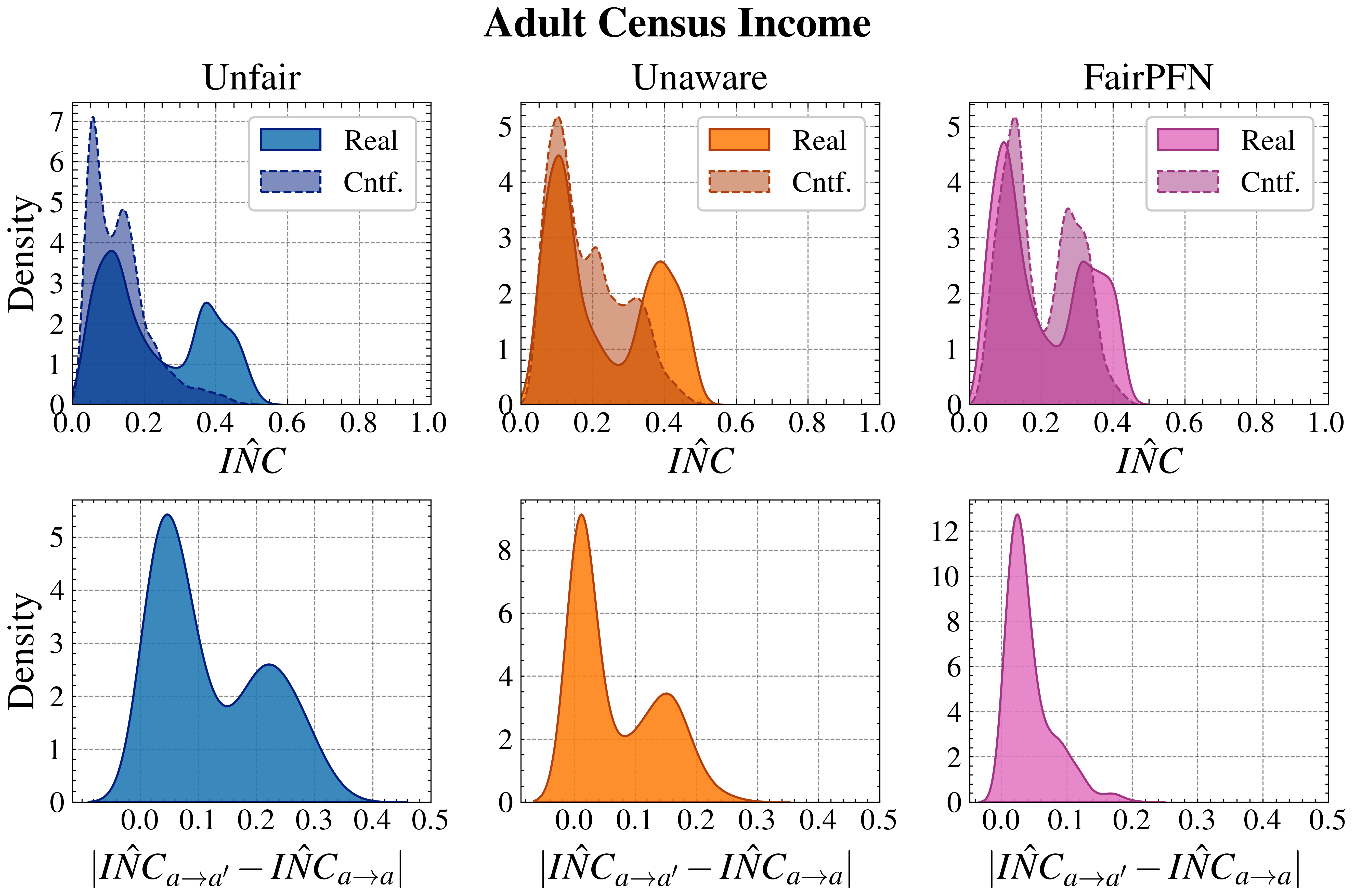<details> <summary>extracted/6522797/figures/adult_dist.png Details</summary>  ### Visual Description ## Density Plots: Adult Census Income Fairness Metrics ### Overview The image displays a 2x3 grid of kernel density estimation plots analyzing fairness metrics on the "Adult Census Income" dataset. The plots compare the distribution of a metric called `IÑC` (top row) and the absolute difference in `IÑC` between counterfactual and real groups (bottom row) across three different modeling approaches: "Unfair," "Unaware," and "FairPFN." Each subplot contains two distributions: one for "Real" data (solid fill) and one for "Cntf." (Counterfactual) data (dashed outline with lighter fill). ### Components/Axes * **Overall Title:** "Adult Census Income" (centered at the top). * **Column Headers (Top Row):** "Unfair" (left), "Unaware" (center), "FairPFN" (right). * **Y-Axis (All Plots):** Labeled "Density." The scale varies per plot. * **X-Axis (Top Row):** Labeled `IÑC`. Scale ranges from 0.0 to 1.0. * **X-Axis (Bottom Row):** Labeled `|IÑC_{a→a'} - IÑC_{a→a}|`. Scale ranges from 0.0 to 0.5. * **Legends:** Located in the top-right corner of each top-row subplot. * **Unfair (Blue):** "Real" (solid dark blue), "Cntf." (dashed outline, light blue fill). * **Unaware (Orange):** "Real" (solid dark orange), "Cntf." (dashed outline, light orange fill). * **FairPFN (Pink/Magenta):** "Real" (solid magenta), "Cntf." (dashed outline, light pink fill). * **Grid:** Light gray dashed grid lines are present in all subplots. ### Detailed Analysis **Top Row: Distribution of `IÑC`** * **Unfair (Left, Blue):** * **Real Distribution:** Bimodal. Primary peak at `IÑC ≈ 0.1` (Density ~3.8). Secondary, smaller peak at `IÑC ≈ 0.4` (Density ~2.5). Distribution spans roughly 0.0 to 0.6. * **Cntf. Distribution:** Unimodal and sharply peaked. Peak at `IÑC ≈ 0.05` (Density ~7.0). Much narrower spread than the Real distribution, concentrated below 0.2. * **Trend:** The counterfactual distribution is shifted significantly left (lower `IÑC`) and is more concentrated compared to the real data. * **Unaware (Center, Orange):** * **Real Distribution:** Bimodal. Primary peak at `IÑC ≈ 0.1` (Density ~4.5). Secondary peak at `IÑC ≈ 0.4` (Density ~2.6). Similar shape to the "Unfair" Real distribution. * **Cntf. Distribution:** Broader and more complex. Has a peak near `IÑC ≈ 0.1` (Density ~5.2) and a secondary shoulder/peak around `IÑC ≈ 0.25` (Density ~2.8). Overlaps more with the Real distribution than in the "Unfair" case. * **Trend:** The counterfactual distribution is less sharply peaked and shows more overlap with the real data compared to the "Unfair" model. * **FairPFN (Right, Pink):** * **Real Distribution:** Bimodal. Primary peak at `IÑC ≈ 0.1` (Density ~4.8). Secondary peak at `IÑC ≈ 0.35` (Density ~2.6). * **Cntf. Distribution:** Bimodal, closely mirroring the Real distribution. Peaks at `IÑC ≈ 0.1` (Density ~5.2) and `IÑC ≈ 0.3` (Density ~3.5). * **Trend:** The counterfactual and real distributions are very similar in shape and location, indicating high alignment. **Bottom Row: Distribution of `|IÑC_{a→a'} - IÑC_{a→a}|` (Absolute Difference)** * **Unfair (Left, Blue):** * Distribution is bimodal. Primary peak at a difference of `≈ 0.05` (Density ~5.5). Secondary peak at `≈ 0.25` (Density ~2.6). Shows a significant mass of data points with a large difference in `IÑC` between counterfactual and real groups. * **Unaware (Center, Orange):** * Distribution is bimodal. Primary peak at a difference of `≈ 0.05` (Density ~9.0). Secondary peak at `≈ 0.15` (Density ~3.5). The secondary peak is at a lower difference value than in the "Unfair" plot. * **FairPFN (Right, Pink):** * Distribution is strongly unimodal and sharply peaked near zero. Peak at a difference of `≈ 0.02` (Density ~12.5). The distribution decays rapidly, with very little mass beyond a difference of 0.1. * **Trend:** This plot shows the most concentrated distribution near zero, indicating minimal difference between counterfactual and real `IÑC` values. ### Key Observations 1. **Consistent Real Data Shape:** The "Real" data distribution (solid fill) for `IÑC` (top row) is consistently bimodal across all three models, suggesting an inherent structure in the dataset's fairness metric. 2. **Counterfactual Alignment:** The alignment between "Real" and "Cntf." distributions improves dramatically from left to right: "Unfair" (large shift) -> "Unaware" (partial overlap) -> "FairPFN" (high similarity). 3. **Difference Metric Convergence:** The bottom row shows the distribution of the absolute difference metric collapsing toward zero from "Unfair" to "FairPFN." The "FairPFN" model produces a very sharp peak near zero, indicating its counterfactual predictions are very close to the real ones for this metric. 4. **Peak Density Values:** The maximum density values increase in the bottom row from left to right (Unfair: ~5.5, Unaware: ~9.0, FairPFN: ~12.5), reflecting the increasing concentration of the difference metric near zero. ### Interpretation This visualization demonstrates the effectiveness of the "FairPFN" method in achieving fairness on the Adult Census Income dataset, as measured by the `IÑC` metric. * **What the data suggests:** The `IÑC` metric likely measures some form of influence or inconsistency related to protected attributes (denoted by `a`). The "Unfair" model shows a large discrepancy between real and counterfactual `IÑC` values, meaning changing protected attributes would drastically alter the model's behavior. The "Unaware" model reduces this discrepancy but does not eliminate it. The "FairPFN" model successfully aligns the real and counterfactual distributions, meaning the model's behavior is consistent regardless of the protected attribute value. * **How elements relate:** The top row shows the *absolute values* of the metric, while the bottom row shows the *magnitude of change* when flipping the protected attribute. The progression from left to right across columns tells a story of improving fairness: the counterfactual distribution moves to match the real one (top row), and the difference between them shrinks to near zero (bottom row). * **Notable Anomalies/Trends:** The most striking trend is the transformation of the bottom-row distribution from a broad, bimodal shape ("Unfair") to a sharp, zero-centered spike ("FairPFN"). This is a direct visual indicator of reduced unfairness. The bimodality in the "Real" `IÑC` distributions (top row) is an important baseline characteristic of the data that the fairness interventions must account for. </details> Figure 19: Aligning Counterfactual Distributions (Adult): Alignment of observational and counterfactual predictive distributions $\hat{Y}$ and $\hat{Y}_{a\rightarrow a^{\prime}}$ on the Adult Census Income problem. FairPFN best aligns the predictive distributions (top) and achieves the lowest mean (0.01) and maximum (0.75) absolute error. 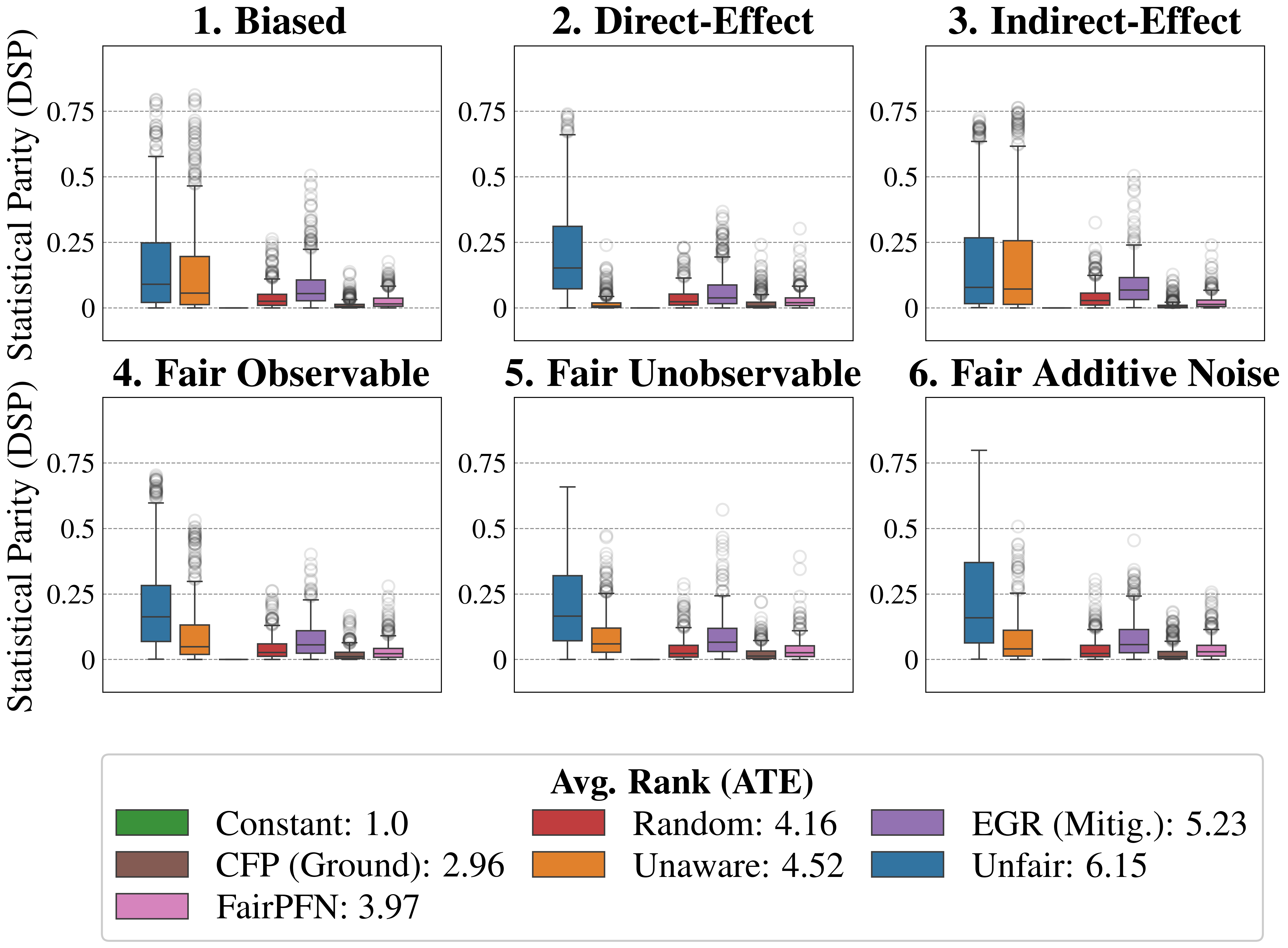<details> <summary>extracted/6522797/figures/ddsp_by_group_synthetic.png Details</summary>  ### Visual Description ## Box Plot Comparison: Statistical Parity (DSP) Across Fairness Scenarios ### Overview This image displays a 2x3 grid of six box plots, each comparing the performance of seven different methods or models across distinct fairness-related scenarios. The primary metric being measured is "Statistical Parity (DSP)" on the y-axis. A comprehensive legend at the bottom maps colors to method names and provides an "Avg. Rank (ATE)" for each. ### Components/Axes * **Chart Type:** Multi-panel box plot. * **Y-Axis (All Panels):** Labeled **"Statistical Parity (DSP)"**. The scale runs from 0 to approximately 0.8, with major grid lines at 0, 0.25, 0.5, and 0.75. * **Panel Titles (Scenarios):** 1. **Biased** (Top Left) 2. **Direct-Effect** (Top Center) 3. **Indirect-Effect** (Top Right) 4. **Fair Observable** (Bottom Left) 5. **Fair Unobservable** (Bottom Center) 6. **Fair Additive Noise** (Bottom Right) * **Legend (Bottom of Image):** Contains seven entries, each with a color swatch, method name, and a numerical "Avg. Rank (ATE)". * **Green:** Constant: 1.0 * **Brown:** CFP (Ground): 2.96 * **Pink:** FairPFN: 3.97 * **Red:** Random: 4.16 * **Orange:** Unaware: 4.52 * **Purple:** EGR (Mitig.): 5.23 * **Blue:** Unfair: 6.15 ### Detailed Analysis The analysis is segmented by scenario (panel). For each, the visual trend and approximate value range for each method's box plot is described. The box represents the interquartile range (IQR), the line inside is the median, whiskers extend to 1.5*IQR, and circles are outliers. **1. Biased Scenario:** * **Unfair (Blue):** Highest median (~0.1) and largest spread, with outliers reaching above 0.75. * **Unaware (Orange):** Second highest median (~0.08), significant spread, outliers up to ~0.8. * **EGR (Mitig.) (Purple):** Moderate median (~0.05), compact IQR, outliers up to ~0.5. * **Random (Red), FairPFN (Pink), CFP (Ground) (Brown):** All have very low medians near 0, with small IQRs and outliers generally below 0.25. * **Constant (Green):** Appears as a flat line at 0, indicating no variance. **2. Direct-Effect Scenario:** * **Unfair (Blue):** Dominates with the highest median (~0.15) and a very large spread, outliers near 0.75. * **EGR (Mitig.) (Purple):** Next highest median (~0.07), with outliers up to ~0.35. * **Unaware (Orange):** Median drops significantly compared to the "Biased" scenario, now near 0.02. * **Random (Red), FairPFN (Pink), CFP (Ground) (Brown):** Medians remain very low (~0-0.03), with limited spread. * **Constant (Green):** Flat line at 0. **3. Indirect-Effect Scenario:** * **Unfair (Blue) & Unaware (Orange):** Both show high medians (~0.08) and large spreads, with outliers extending to ~0.75. They are visually similar in this panel. * **EGR (Mitig.) (Purple):** Median around 0.06, with outliers up to ~0.5. * **Random (Red), FairPFN (Pink), CFP (Ground) (Brown):** Maintain low medians and spreads. * **Constant (Green):** Flat line at 0. **4. Fair Observable Scenario:** * **Unfair (Blue):** Still the highest median (~0.15) and spread, outliers up to ~0.7. * **Unaware (Orange):** Median around 0.05, with notable outliers up to ~0.5. * **EGR (Mitig.) (Purple):** Median ~0.05, similar to Unaware but with a slightly tighter IQR. * **Random (Red), FairPFN (Pink), CFP (Ground) (Brown):** Consistently low values. * **Constant (Green):** Flat line at 0. **5. Fair Unobservable Scenario:** * **Unfair (Blue):** High median (~0.15) and spread, outliers near 0.7. * **Unaware (Orange):** Median ~0.05, with outliers up to ~0.5. * **EGR (Mitig.) (Purple):** Median ~0.06, with a notable outlier near 0.6. * **Random (Red), FairPFN (Pink), CFP (Ground) (Brown):** Low values. * **Constant (Green):** Flat line at 0. **6. Fair Additive Noise Scenario:** * **Unfair (Blue):** Highest median (~0.15) and largest spread, with the upper whisker reaching ~0.8. * **Unaware (Orange):** Median ~0.05, with outliers up to ~0.5. * **EGR (Mitig.) (Purple):** Median ~0.06, with outliers up to ~0.4. * **Random (Red), FairPFN (Pink), CFP (Ground) (Brown):** Low values. * **Constant (Green):** Flat line at 0. ### Key Observations 1. **Consistent Hierarchy:** Across all six scenarios, the **Unfair (Blue)** method consistently exhibits the highest median Statistical Parity and the greatest variance (tallest box and whiskers). The **Constant (Green)** method is consistently a flat line at zero. 2. **Scenario Impact on Unaware:** The **Unaware (Orange)** method performs poorly (high DSP) in the "Biased" and "Indirect-Effect" scenarios but shows marked improvement (lower DSP) in the "Direct-Effect" and the three "Fair" scenarios. 3. **Stable Low-Performers:** The **Random (Red)**, **FairPFN (Pink)**, and **CFP (Ground) (Brown)** methods consistently show very low Statistical Parity (medians near zero) across all scenarios, with relatively small interquartile ranges. 4. **EGR (Mitig.) Position:** The **EGR (Mitig.) (Purple)** method generally occupies a middle ground, with higher DSP than the best-performing group but lower than Unfair/Unaware in most cases. 5. **Legend Rank Correlation:** The "Avg. Rank (ATE)" in the legend (where a lower number is better) correlates with the visual performance: Constant (1.0) is best (flat at 0), followed by CFP (2.96), FairPFN (3.97), etc., with Unfair (6.15) being the worst, matching its consistently high DSP values. ### Interpretation This figure evaluates algorithmic fairness by measuring **Statistical Parity (DSP)**, a metric where a value of 0 indicates perfect parity (no disparity between groups) and higher values indicate greater bias. The six panels represent different data-generating processes or fairness constraints ("Biased", "Direct-Effect", etc.) used to test the methods. The data suggests that: * The **"Unfair"** method serves as a baseline for high bias, as expected. * Methods like **"Constant"**, **"CFP (Ground)"**, and **"FairPFN"** are highly effective at minimizing Statistical Parity across a variety of challenging scenarios, suggesting robust fairness performance. * The **"Unaware"** method (likely a model trained without sensitive attributes) is not reliably fair; its performance is highly dependent on the underlying data structure, failing badly in "Biased" and "Indirect-Effect" settings. * The **"EGR (Mitig.)"** method provides a consistent, moderate improvement over the Unaware and Unfair baselines but does not achieve the low parity levels of the top group. * The **"Avg. Rank (ATE)"** provides a summary metric that aligns well with the visual evidence from the box plots, confirming that methods with lower DSP values in the plots achieve better (lower) average ranks. In essence, the chart demonstrates that specialized fairness-aware methods (CFP, FairPFN) and even a simple constant predictor can significantly outperform standard or unaware models in achieving statistical parity, but their effectiveness is consistent across different definitions of fairness problems. The "Unaware" approach is shown to be risky and inconsistent. </details> Figure 20: Statistical Parity (Synthetic): Statistical Parity (DSP) of FairPFN compared to our baselines. FairPFN achieves a similar DSP as the Random baseline and outperforms EGR which was optimized specifically for this fairness metric, achieving an average rank of 3.97 out of 7. 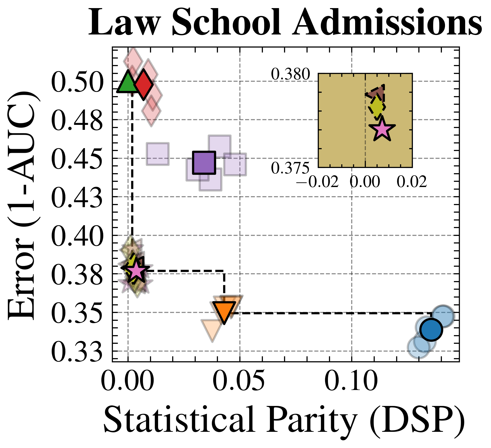<details> <summary>extracted/6522797/figures/ddsp_lawschool.png Details</summary>  ### Visual Description \n ## Scatter Plot: Law School Admissions Fairness-Accuracy Trade-off ### Overview The image is a scatter plot titled "Law School Admissions" that visualizes the trade-off between a model's predictive error and its statistical parity (a fairness metric). The plot compares multiple models or methods, represented by distinct markers, across two dimensions. An inset plot in the top-right corner provides a magnified view of a specific cluster of points near the origin. ### Components/Axes * **Main Plot Title:** "Law School Admissions" (centered at the top). * **X-Axis:** Labeled "Statistical Parity (DSP)". The scale runs from 0.00 to approximately 0.15, with major ticks at 0.00, 0.05, and 0.10. DSP likely stands for "Demographic Statistical Parity," a measure of fairness where a value of 0 indicates perfect parity. * **Y-Axis:** Labeled "Error (1-AUC)". The scale runs from 0.33 to 0.50, with major ticks at 0.33, 0.35, 0.38, 0.40, 0.43, 0.45, 0.48, and 0.50. This represents the model's error rate, where a lower value indicates better predictive performance (higher AUC). * **Data Series (Markers):** The plot contains multiple data series, each represented by a unique shape and color. There is no explicit legend box; identification is based on visual matching. * **Green Triangle (▲):** Positioned at high error (~0.50) and very low DSP (~0.00). * **Red Diamond (◆):** Positioned at high error (~0.50) and very low DSP (~0.00), slightly to the right of the green triangle. * **Purple Square (■):** Positioned at moderate error (~0.45) and moderate DSP (~0.04). * **Pink Star (★):** Positioned at lower error (~0.38) and very low DSP (~0.00). This point is connected by dashed lines to the orange inverted triangle and the blue circle. * **Orange Inverted Triangle (▼):** Positioned at low error (~0.35) and moderate DSP (~0.05). * **Blue Circle (●):** Positioned at the lowest error (~0.34) and the highest DSP (~0.14). * **Other Markers:** Several semi-transparent or lighter-shaded versions of the above markers (e.g., light pink diamonds, light purple squares, light orange triangles, light blue circles) are scattered around their primary counterparts, likely representing variance, multiple runs, or related methods. * **Inset Plot:** Located in the top-right quadrant of the main plot area. * **Inset Axes:** X-axis from -0.02 to 0.02; Y-axis from 0.375 to 0.380. * **Inset Content:** Contains a brown arrow pointing up and left, a yellow diamond, and a pink star (★). This provides a detailed view of the cluster near (DSP=0.00, Error=0.38). * **Guides:** Dashed grid lines are present. Black dashed lines connect the pink star to the orange inverted triangle and the blue circle, suggesting a direct comparison or a Pareto frontier between these points. ### Detailed Analysis * **Trend Verification:** The overall visual trend shows a negative correlation: as Statistical Parity (DSP) increases (moving right on the x-axis), the Error (1-AUC) generally decreases (moving down on the y-axis). This illustrates a classic fairness-accuracy trade-off. * **Data Point Approximation:** * **High Error / High Fairness Cluster:** Green Triangle and Red Diamond are near (DSP ≈ 0.00, Error ≈ 0.50). * **Moderate Error / Moderate Fairness Cluster:** Purple Square is near (DSP ≈ 0.04, Error ≈ 0.45). * **Lower Error / High Fairness Cluster:** Pink Star is near (DSP ≈ 0.00, Error ≈ 0.38). The inset shows this point in detail, with the pink star at approximately (DSP=0.00, Error=0.378). * **Low Error / Moderate Fairness Point:** Orange Inverted Triangle is near (DSP ≈ 0.05, Error ≈ 0.35). * **Lowest Error / Lowest Fairness Point:** Blue Circle is near (DSP ≈ 0.14, Error ≈ 0.34). * **Spatial Grounding:** The legend is not in a separate box but is encoded in the markers themselves. The inset is positioned in the top-right, overlapping the main plot's grid. The dashed lines create a visual triangle connecting the Pink Star, Orange Inverted Triangle, and Blue Circle, highlighting them as key points of comparison. ### Key Observations 1. **Clear Trade-off:** There is a distinct downward slope from the top-left (high error, high fairness) to the bottom-right (low error, low fairness). 2. **Pareto Frontier:** The points connected by dashed lines (Pink Star, Orange Inverted Triangle, Blue Circle) appear to form a Pareto frontier, where improving one metric (e.g., lowering error) necessarily worsens the other (increasing DSP). 3. **Cluster at High Fairness:** Several methods achieve near-perfect statistical parity (DSP ≈ 0.00) but with widely varying error rates, from ~0.38 (Pink Star) to ~0.50 (Green Triangle/Red Diamond). 4. **Outlier/Best Compromise:** The Pink Star represents a method that achieves relatively low error (~0.38) while maintaining near-perfect fairness (DSP ≈ 0.00), making it a potentially optimal compromise point compared to others on the plot. 5. **Inset Purpose:** The inset magnifies the region around the Pink Star, suggesting it is a point of particular interest, possibly the proposed method in the study from which this plot originates. ### Interpretation This chart demonstrates the inherent tension between predictive accuracy and group fairness in a law school admissions model. The "Statistical Parity (DSP)" metric measures whether the model's positive prediction rate is equal across demographic groups; a value of 0 is ideal. "Error (1-AUC)" measures the model's overall mistake rate. The data suggests that achieving perfect fairness (DSP=0) comes at a significant cost to accuracy, as seen with the Green Triangle and Red Diamond points. However, the Pink Star point indicates that it is possible to attain a much better accuracy (Error ≈ 0.38) while still maintaining perfect fairness, outperforming other fair models. The Blue Circle shows the highest accuracy but with substantial unfairness (DSP ≈ 0.14). The dashed lines connecting the Pink Star, Orange Inverted Triangle, and Blue Circle likely illustrate the "cost of fairness": moving from the Blue Circle to the Orange Inverted Triangle improves fairness (DSP decreases from ~0.14 to ~0.05) with a small error increase (~0.34 to ~0.35). Moving further to the Pink Star achieves perfect fairness (DSP=0) but with a larger error increase (to ~0.38). The plot argues that the method represented by the Pink Star offers a superior balance, achieving fairness without the extreme accuracy penalty seen in other fair models (Green/Red). The inset emphasizes the precision and stability of this key result. 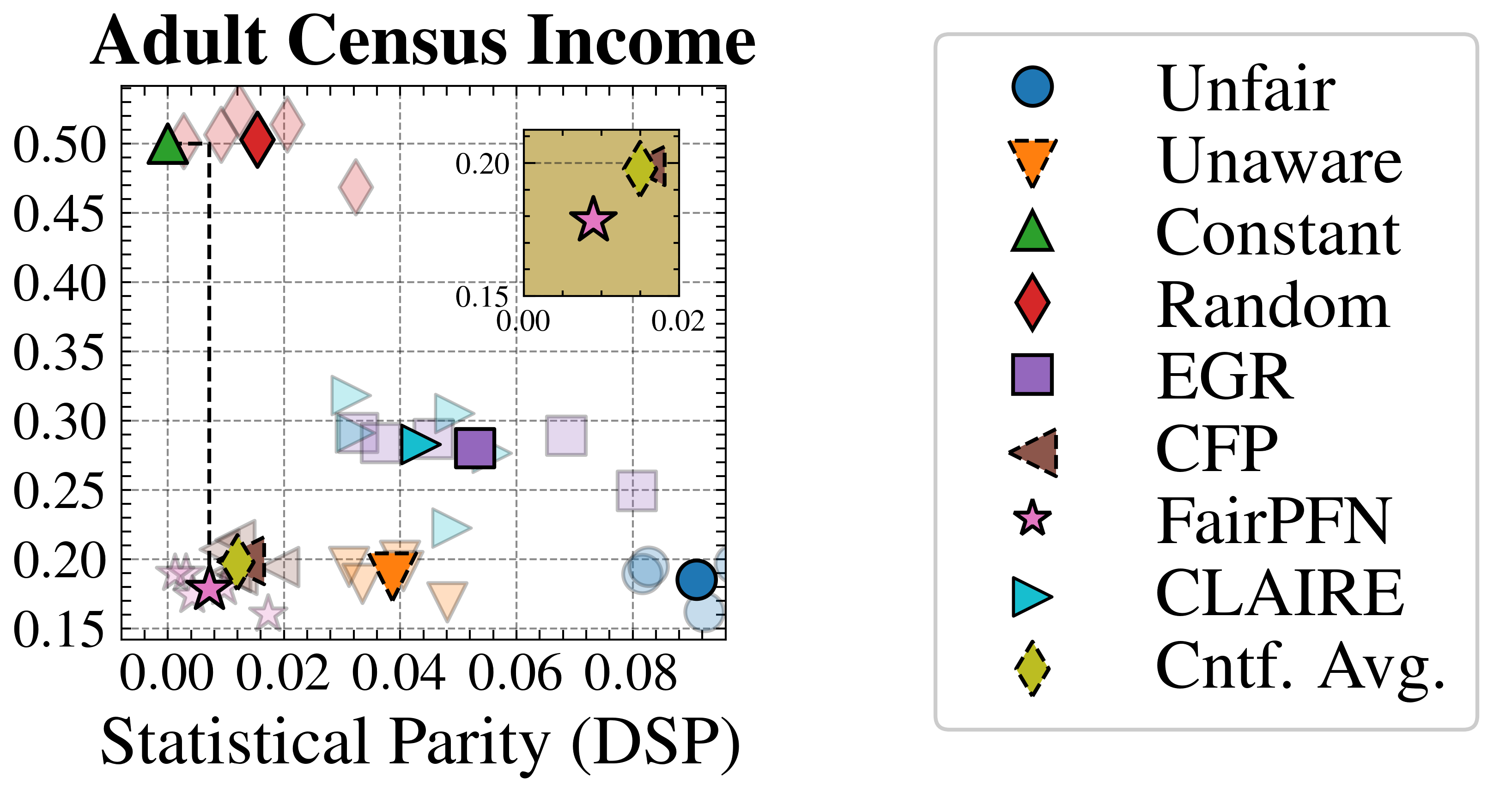</details> <details> <summary>extracted/6522797/figures/ddsp_adult.png Details</summary>  ### Visual Description ## Scatter Plot: Adult Census Income Fairness-Accuracy Trade-off ### Overview The image is a scatter plot comparing various machine learning methods on the "Adult Census Income" dataset. It visualizes the trade-off between a fairness metric (Statistical Parity, DSP) on the x-axis and an unlabeled performance metric (likely accuracy or error rate) on the y-axis. The plot includes an inset zoomed-in view of a specific region. A legend on the right maps unique marker shapes and colors to method names. ### Components/Axes * **Main Plot Title:** "Adult Census Income" * **X-Axis Label:** "Statistical Parity (DSP)" * Scale: Linear, ranging from 0.00 to approximately 0.09. * Major Ticks: 0.00, 0.02, 0.04, 0.06, 0.08. * **Y-Axis:** Unlabeled numerical scale. * Scale: Linear, ranging from 0.15 to 0.50. * Major Ticks: 0.15, 0.20, 0.25, 0.30, 0.35, 0.40, 0.45, 0.50. * **Legend (Right Side):** A vertical list mapping markers to method names. * **Blue Circle:** Unfair * **Orange Inverted Triangle (dashed border):** Unaware * **Green Triangle:** Constant * **Red Diamond:** Random * **Purple Square:** EGR * **Brown Left-Pointing Triangle (dashed border):** CFP * **Pink Star:** FairPFN * **Cyan Right-Pointing Triangle:** CLAIRE * **Yellow Diamond (dashed border):** Cntf. Avg. * **Inset Plot (Top-Right Quadrant):** A smaller, zoomed-in scatter plot with a tan background. * **Inset X-Axis:** Ranges from 0.00 to 0.02. * **Inset Y-Axis:** Ranges from 0.15 to 0.20. * Contains two data points: a pink star (FairPFN) and a yellow diamond (Cntf. Avg.). ### Detailed Analysis The plot displays multiple data points for each method, suggesting results from different runs or configurations. Below is an approximate mapping of key points for each method, identified by matching the legend to the plot markers. Coordinates are estimated from the grid. * **Unfair (Blue Circle):** Clustered in the bottom-right corner. * Approximate Coordinates: (DSP ≈ 0.085-0.090, Y ≈ 0.17-0.19). This indicates high statistical disparity (unfairness) and low performance on the y-axis metric. * **Unaware (Orange Inverted Triangle):** Located in the lower-middle region. * Approximate Coordinates: (DSP ≈ 0.035-0.045, Y ≈ 0.18-0.20). * **Constant (Green Triangle):** A significant outlier in the top-left. * Approximate Coordinates: (DSP ≈ 0.005, Y ≈ 0.50). This shows very low disparity but the highest y-axis value. * **Random (Red Diamond):** Another outlier near the top-left. * Approximate Coordinates: (DSP ≈ 0.015, Y ≈ 0.50). Similar to Constant, with slightly higher DSP. * **EGR (Purple Square):** Points are scattered in the middle band. * Approximate Coordinates: One cluster around (DSP ≈ 0.045-0.055, Y ≈ 0.28-0.30). Another point near (DSP ≈ 0.075, Y ≈ 0.25). * **CFP (Brown Left-Pointing Triangle):** Points are in the lower-left cluster. * Approximate Coordinates: (DSP ≈ 0.010-0.020, Y ≈ 0.18-0.22). * **FairPFN (Pink Star):** Primarily clustered in the lower-left, with one point highlighted in the inset. * Main Cluster Approximate Coordinates: (DSP ≈ 0.005-0.015, Y ≈ 0.17-0.20). * Inset Point: (DSP ≈ 0.010, Y ≈ 0.175). * **CLAIRE (Cyan Right-Pointing Triangle):** Scattered in the middle region. * Approximate Coordinates: Points around (DSP ≈ 0.030-0.050, Y ≈ 0.22-0.30). * **Cntf. Avg. (Yellow Diamond):** Found in the lower-left cluster and the inset. * Main Cluster Approximate Coordinates: (DSP ≈ 0.010-0.015, Y ≈ 0.19-0.21). * Inset Point: (DSP ≈ 0.018, Y ≈ 0.195). ### Key Observations 1. **Performance-Fairness Trade-off:** There is a visible inverse relationship. Methods with very low DSP (fairness), like Constant and Random, have the highest y-axis values. Methods with higher DSP, like Unfair, have lower y-axis values. 2. **Clustering:** Most methods (Unaware, CFP, FairPFN, Cntf. Avg., some EGR/CLAIRE) cluster in a region of low-to-moderate DSP (0.01-0.05) and low y-axis values (0.17-0.30). 3. **Outliers:** The "Constant" and "Random" methods are extreme outliers, achieving near-zero DSP but at a very high y-axis value, which may indicate a trivial or degenerate solution. 4. **Inset Purpose:** The inset zooms in on the region of lowest DSP (0.00-0.02) and lowest y-axis values (0.15-0.20), highlighting the precise positions of FairPFN and Cntf. Avg., which are very close in this fairness-performance space. ### Interpretation This chart evaluates algorithmic fairness on the Adult Census Income dataset. The x-axis (Statistical Parity/DSP) measures disparity in outcomes between protected groups; lower values are fairer. The unlabeled y-axis likely represents a model performance metric (e.g., error rate, where lower is better, or accuracy, where higher is better). Given the context, the high y-values for "Constant" and "Random" suggest the y-axis is likely **error rate** (as a constant predictor would have high error). The data demonstrates the classic fairness-accuracy trade-off: maximizing fairness (minimizing DSP) often comes at the cost of increased error (higher y-value). The "Unfair" baseline has high error but also high disparity. Advanced methods (FairPFN, Cntf. Avg., CFP) cluster in a "sweet spot" with relatively low DSP and low error, suggesting they successfully balance the two objectives. The "Constant" and "Random" methods achieve perfect fairness (DSP≈0) but are useless models with very high error, serving as a boundary reference. The plot argues that methods like FairPFN and Cntf. Avg. offer a practical compromise, achieving fairness with minimal performance degradation compared to the unfair baseline. </details> Figure 21: Group-Fairness-Accuracy Trade-off (Real-World): Statistical Parity (DSP), predictive error (1-AUC), and Pareto Front of the performance of FairPFN compared to our baselines on each of 5 validation folds (light) and across all five folds (solid) of our real-world datasets. FairPFN dominates EGR which was specifically optimized for this group fairness metric. 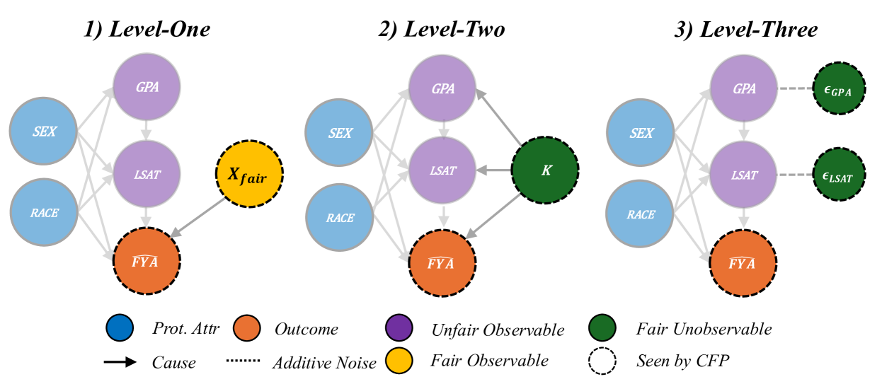<details> <summary>x6.png Details</summary>  ### Visual Description ## Causal Diagram: Three-Level Fairness Model ### Overview The image displays three separate causal diagrams, labeled "1) Level-One", "2) Level-Two", and "3) Level-Three", arranged horizontally from left to right. These diagrams model the relationships between protected attributes, academic/test scores, and an outcome variable (FYA) under different fairness interventions. A comprehensive legend is provided at the bottom of the image to explain the node types and connection styles. ### Components/Axes (Legend) The legend at the bottom defines the following visual elements: * **Node Types (by color and border):** * **Blue circle (solid border):** "Prot. Attr" (Protected Attribute). Nodes: `SEX`, `RACE`. * **Orange circle (dashed border):** "Outcome". Node: `FYA`. * **Purple circle (solid border):** "Unfair Observable". Nodes: `GPA`, `LSAT`. * **Green circle (solid border):** "Fair Unobservable". Node: `K` (in Level-Two). * **Green circle (dashed border):** "Fair Unobservable". Nodes: `ε_GPA`, `ε_LSAT` (in Level-Three). * **Yellow circle (dashed border):** "Fair Observable". Node: `X_fair` (in Level-One). * **Connection Types:** * **Solid arrow (→):** "Cause". Indicates a direct causal influence. * **Dotted line (........):** "Additive Noise". Indicates the addition of a noise term. * **Dashed circle border:** "Seen by CFP". Indicates the variable is observed by the "CFP" (presumably a fairness-aware predictor or mechanism). ### Detailed Analysis #### **1) Level-One Diagram** * **Components:** `SEX`, `RACE` (Protected Attributes); `GPA`, `LSAT` (Unfair Observables); `FYA` (Outcome); `X_fair` (Fair Observable). * **Flow & Relationships:** * `SEX` and `RACE` have direct causal arrows pointing to `GPA`, `LSAT`, and `FYA`. * `GPA` has a causal arrow pointing to `LSAT`. * `GPA`, `LSAT`, and `X_fair` all have causal arrows pointing to `FYA`. * The `X_fair` node has a dashed border, indicating it is "Seen by CFP". * **Interpretation:** This level introduces a single, fair observable variable (`X_fair`) that directly influences the outcome (`FYA`). The protected attributes (`SEX`, `RACE`) still influence both the unfair observables (`GPA`, `LSAT`) and the outcome directly. #### **2) Level-Two Diagram** * **Components:** `SEX`, `RACE` (Protected Attributes); `GPA`, `LSAT` (Unfair Observables); `FYA` (Outcome); `K` (Fair Unobservable). * **Flow & Relationships:** * `SEX` and `RACE` have direct causal arrows pointing to `GPA`, `LSAT`, and `FYA`. * `GPA` has a causal arrow pointing to `LSAT`. * The new node `K` (Fair Unobservable, solid green circle) has causal arrows pointing to `GPA`, `LSAT`, and `FYA`. * The `K` node has a dashed border, indicating it is "Seen by CFP". * **Interpretation:** This level replaces the fair observable (`X_fair`) with a fair unobservable (`K`). This `K` variable influences all downstream variables (`GPA`, `LSAT`, `FYA`). The protected attributes still have their direct paths. #### **3) Level-Three Diagram** * **Components:** `SEX`, `RACE` (Protected Attributes); `GPA`, `LSAT` (Unfair Observables); `FYA` (Outcome); `ε_GPA`, `ε_LSAT` (Fair Unobservables/Noise). * **Flow & Relationships:** * `SEX` and `RACE` have direct causal arrows pointing to `GPA`, `LSAT`, and `FYA`. * `GPA` has a causal arrow pointing to `LSAT`. * Two new nodes, `ε_GPA` and `ε_LSAT` (Fair Unobservable, dashed green circles), are introduced. * `ε_GPA` is connected to `GPA` via a dotted line ("Additive Noise"). * `ε_LSAT` is connected to `LSAT` via a dotted line ("Additive Noise"). * Both `ε_GPA` and `ε_LSAT` have dashed borders, indicating they are "Seen by CFP". * **Interpretation:** This level models fairness by adding independent, fair noise terms (`ε`) to the unfair observable variables (`GPA`, `LSAT`). These noise terms are observed by the CFP. The direct influence of protected attributes on the observables and outcome remains. ### Key Observations 1. **Progression of Intervention:** The diagrams show a conceptual progression in fairness intervention: from adding a separate fair feature (Level-One), to introducing a single latent fair factor (Level-Two), to adding fair noise directly to the unfair observables (Level-Three). 2. **Persistent Bias Path:** In all three levels, the protected attributes (`SEX`, `RACE`) maintain direct causal links to both the intermediate variables (`GPA`, `LSAT`) and the final outcome (`FYA`). The interventions do not sever these paths but attempt to add "fair" components alongside them. 3. **"Seen by CFP" Condition:** The fairness mechanism (whether `X_fair`, `K`, or `ε` terms) is always marked as observable to the CFP, suggesting the fairness-aware model has access to these specific fair components. 4. **Node Styling Consistency:** The styling is consistent with the legend. Outcome (`FYA`) always has a dashed orange border. Protected attributes are always solid blue. Unfair observables are solid purple. The "fair" components vary in color (yellow/green) and border style (solid/dashed) based on their type and level. ### Interpretation These diagrams visually formalize different approaches to achieving fairness in a predictive model (e.g., for law school admission, given GPA and LSAT scores). The core problem is that protected attributes like `SEX` and `RACE` causally influence both the inputs (`GPA`, `LSAT`) and the outcome (`FYA`), leading to potential unfairness. * **Level-One** suggests fairness can be achieved by discovering and using an alternative, fair observable (`X_fair`) that captures legitimate predictive power without bias. * **Level-Two** posits the existence of a single, unobservable but fair latent factor (`K`) that drives both academic performance and the outcome. If this factor can be estimated or proxied, fairness might be attainable. * **Level-Three** takes a more statistical approach, suggesting that adding carefully calibrated, fair noise to the biased observables can "wash out" the unfair influence, making the final prediction fairer. The diagrams highlight a fundamental tension: the protected attributes have a real, causal effect on the variables we observe and the outcome. Fairness interventions, therefore, are not about erasing this reality but about strategically adding new, fair information or noise to counteract the *unfair* component of that influence during the decision-making process. The choice of model (Levels 1-3) implies different assumptions about what "fairness" means and what kind of additional data or noise is available. </details> Figure 22: Counterfactually Fair Prediction (CFP): Three levels of counterfactually fair prediction (CFP) Kusner et al. (2017), obtained by fitting a predictor 1) to fair observables (if any exist; left), 2) the inferred values of fair exogenous variables (middle) and 3) the inferred values of independent noise terms (right). 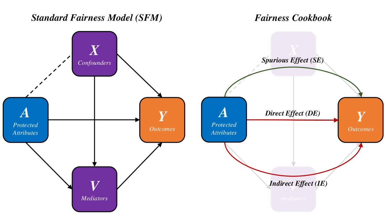<details> <summary>x7.png Details</summary>  ### Visual Description \n ## Diagram: Comparison of Fairness Models in Machine Learning ### Overview The image presents two side-by-side causal diagrams illustrating different conceptual frameworks for analyzing fairness in machine learning systems. The left diagram is labeled "Standard Fairness Model (SFM)" and the right is labeled "Fairness Cookbook." Both diagrams use nodes (boxes) to represent variables and directed arrows to represent causal or influential relationships. The diagrams aim to decompose the influence of protected attributes on outcomes. ### Components/Axes **Left Diagram: Standard Fairness Model (SFM)** * **Nodes (Boxes):** * **A**: Blue box, labeled "Protected Attributes". Positioned center-left. * **X**: Purple box, labeled "Confounders". Positioned top-center. * **V**: Purple box, labeled "Mediators". Positioned bottom-center. * **Y**: Orange box, labeled "Outcomes". Positioned center-right. * **Edges (Arrows):** * Solid black arrow from **A** to **Y** (direct path). * Solid black arrow from **A** to **V**. * Solid black arrow from **V** to **Y**. * Solid black arrow from **X** to **A**. * Solid black arrow from **X** to **Y**. * Solid black arrow from **X** to **V**. * Dashed black line between **A** and **X** (indicating a potential association or unmeasured confounding). **Right Diagram: Fairness Cookbook** * **Nodes (Boxes):** * **A**: Blue box, labeled "Protected Attributes". Positioned center-left. * **Y**: Orange box, labeled "Outcomes". Positioned center-right. * **X**: Faded purple box, labeled "X". Positioned top-center. The label "Spurious Effect (SE)" is placed directly below this box. * **mediators**: Faded purple box, labeled "mediators" (lowercase). Positioned bottom-center. The label "Indirect Effect (IE)" is placed directly above this box. * **Edges (Arrows) & Labeled Effects:** * **Direct Effect (DE)**: A solid red arrow pointing directly from **A** to **Y**. * **Spurious Effect (SE)**: A solid green, curved arrow originating from the area of **A**, arcing over the top, and pointing to **Y**. It passes near the faded **X** node. * **Indirect Effect (IE)**: A solid red, curved arrow originating from **A**, arcing under the bottom, and pointing to **Y**. It passes through the faded **mediators** node. * Faded grey arrows show the underlying causal structure from the SFM: from **A** to mediators, from mediators to **Y**, from **X** to **A**, **Y**, and mediators. ### Detailed Analysis The diagrams visually decompose the total effect of Protected Attributes (**A**) on Outcomes (**Y**) into distinct pathways. **Standard Fairness Model (SFM):** This model presents a comprehensive causal graph. The total effect of **A** on **Y** flows through three primary routes: 1. **Direct Path**: A → Y. 2. **Indirect Path via Mediators**: A → V → Y. 3. **Confounded Paths**: The relationship between **A** and **Y** is also influenced by **X** (Confounders), which affects both **A** and **Y** directly, and also affects the mediators **V**. The dashed line between **A** and **X** suggests they may be associated through unmeasured common causes. **Fairness Cookbook:** This model simplifies the SFM to highlight three specific effect types relevant for fairness auditing: 1. **Direct Effect (DE)**: Represented by the straight red arrow. This is the effect of **A** on **Y** that is not mediated by any other variable in the model. 2. **Spurious Effect (SE)**: Represented by the green curved arrow. This captures the non-causal association between **A** and **Y** that arises due to common causes (the confounders **X**). It is "spurious" because it does not represent a causal influence of **A** on **Y**. 3. **Indirect Effect (IE)**: Represented by the lower red curved arrow. This is the effect of **A** on **Y** that is channeled through the mediator variables. The faded nodes for **X** and **mediators** in the Fairness Cookbook indicate that this framework focuses on the *types of effects* rather than the specific intermediate variables. ### Key Observations 1. **Color Coding Consistency**: Blue is consistently used for the Protected Attribute node (**A**), and orange for the Outcome node (**Y**) across both diagrams. 2. **Effect Decomposition**: The Fairness Cookbook explicitly labels and color-codes the three decomposed effects (DE, SE, IE), making the conceptual breakdown clear. The Direct and Indirect effects are both red, while the Spurious effect is green. 3. **Visual Abstraction**: The Fairness Cookbook abstracts away the detailed structure of confounders and mediators (shown as faded boxes) to emphasize the high-level effect categories. 4. **Arrow Semantics**: Solid arrows in the SFM represent hypothesized causal pathways. In the Fairness Cookbook, the solid colored arrows represent the *decomposed effect components*, while the faded grey arrows retain the underlying causal structure for reference. ### Interpretation These diagrams illustrate a shift in thinking from a purely causal graph representation (SFM) to a framework designed for fairness analysis (Fairness Cookbook). * **What the data suggests**: The comparison demonstrates that a "fair" model assessment requires disentangling the direct influence of protected attributes (like race or gender) on outcomes from influences that are indirect (through legitimate mediators) or spurious (due to historical bias encoded in confounders). * **How elements relate**: The Fairness Cookbook is derived from the SFM. It maps the complex web of relationships in the SFM onto three interpretable effect types. The **Direct Effect (DE)** is often the primary focus for detecting algorithmic discrimination. The **Indirect Effect (IE)** can be legitimate (e.g., education mediating the effect of age on income) or problematic. The **Spurious Effect (SE)** highlights how bias can enter a model through confounding variables that are correlated with both the protected attribute and the outcome. * **Notable implications**: The framework implies that simply removing the protected attribute **A** from a model (a practice known as "fairness through unawareness") is insufficient. This is because the **Spurious Effect (SE)** through confounders **X** and the **Indirect Effect (IE)** through mediators **V** can still allow the influence of **A** to permeate the model's predictions. True fairness auditing requires methods to estimate and account for these distinct pathways, as visualized in the Fairness Cookbook decomposition. The faded nodes suggest that for the purpose of high-level fairness metrics, the specific identity of confounders and mediators may be less important than quantifying the magnitude of the SE, DE, and IE pathways. </details> Figure 23: Causal Fairness Analysis (CFA) Framework: Components of the CFA framework relevant to FairPFN’s prior and evaluation. Plecko & Bareinboim (2024) Standard Fairness Model (left; SFM), which provides a meta-model for causal fairness and heavily the design of our prior, and the Fairness Cookbook of causal fairness metrics (right). | | 1) Biased | 2) Direct-Effect | 3) Indirect-Effect | | --- | --- | --- | --- | | Unfair | -0.00±0.13 (3.05%) | 0.00±0.14 (0.00%) | -0.00±0.12 (1.65%) | | Unaware | -0.01±0.09 (2.60%) | 0.00± 0.00 (0.12%) | -0.01±0.08 (1.81%) | | Constant | -0.36±0.34 (0.00%) | -0.27±0.43 (0.00%) | -0.38±0.34 (0.00%) | | Random | 0.01±0.30 (0.01%) | 0.01±0.31 (0.01%) | 0.00±0.30 (0.00%) | | EGR | -0.05±0.46 (0.00%) | -0.07±0.42 (0.00%) | -0.06±0.45 (0.00%) | | CFP | -0.00± 0.03 (1.31%) | -0.01± 0.03 (0.56%) | -0.01±0.07 (2.29%) | | FairPFN | 0.00±0.06 (2.03%) | -0.01± 0.03 (1.29%) | -0.00± 0.05 (2.22%) | | | 4) Fair Observable | 5) Fair Unobservable | 6) Fair Additive Noise | Average | | --- | --- | --- | --- | --- | | Unfair | 0.00±0.14 (0.02%) | -0.00±0.19 (0.00%) | -0.00±0.18 (0.00%) | 0.00±0.15 (0.79%) | | Unaware | -0.00± 0.05 (2.63%) | -0.00±0.09 (3.68%) | -0.00±0.10 (3.07%) | -0.00±0.07 (2.32%) | | Constant | -0.49±0.18 (30.10%) | -0.38±0.30 (4.63%) | -0.37±0.33 (0.11%) | -0.38±0.32 (5.81%) | | Random | 0.01±0.34 (0.00%) | 0.08±0.37 (0.00%) | 0.06±0.37 (0.00%) | 0.03±0.33 (0.00%) | | EGR | -0.09±0.38 (0.00%) | -0.06±0.39 (0.00%) | -0.07±0.37 (0.00%) | -0.07±0.41 (0.00%) | | CFP | -0.02±0.14 (1.72%) | 0.00± 0.06 (1.02%) | -0.00± 0.05 (1.00%) | -0.01± 0.06 (1.32%) | | FairPFN | -0.01±0.07 (1.01%) | 0.01±0.07 (2.20%) | 0.01±0.09 (2.47%) | 0.00± 0.06 (1.87%) | Table 1: Difference to Cntf. Avg. (Synthetic): Mean, standard deviation and percentage of outliers of the predictions on our causal casestudies of FairPFN and our baseline models compared to the predictions of the Cntf. Avg. baseline, which shows strong performance in causal effect removal and predictive error due to access to both observational and counterfactual datasets. FairPFN achieves predictions with an average difference to Cntf. Avg. of 0.00±0.06, with 1.87% of samples falling outside of three standard deviations. 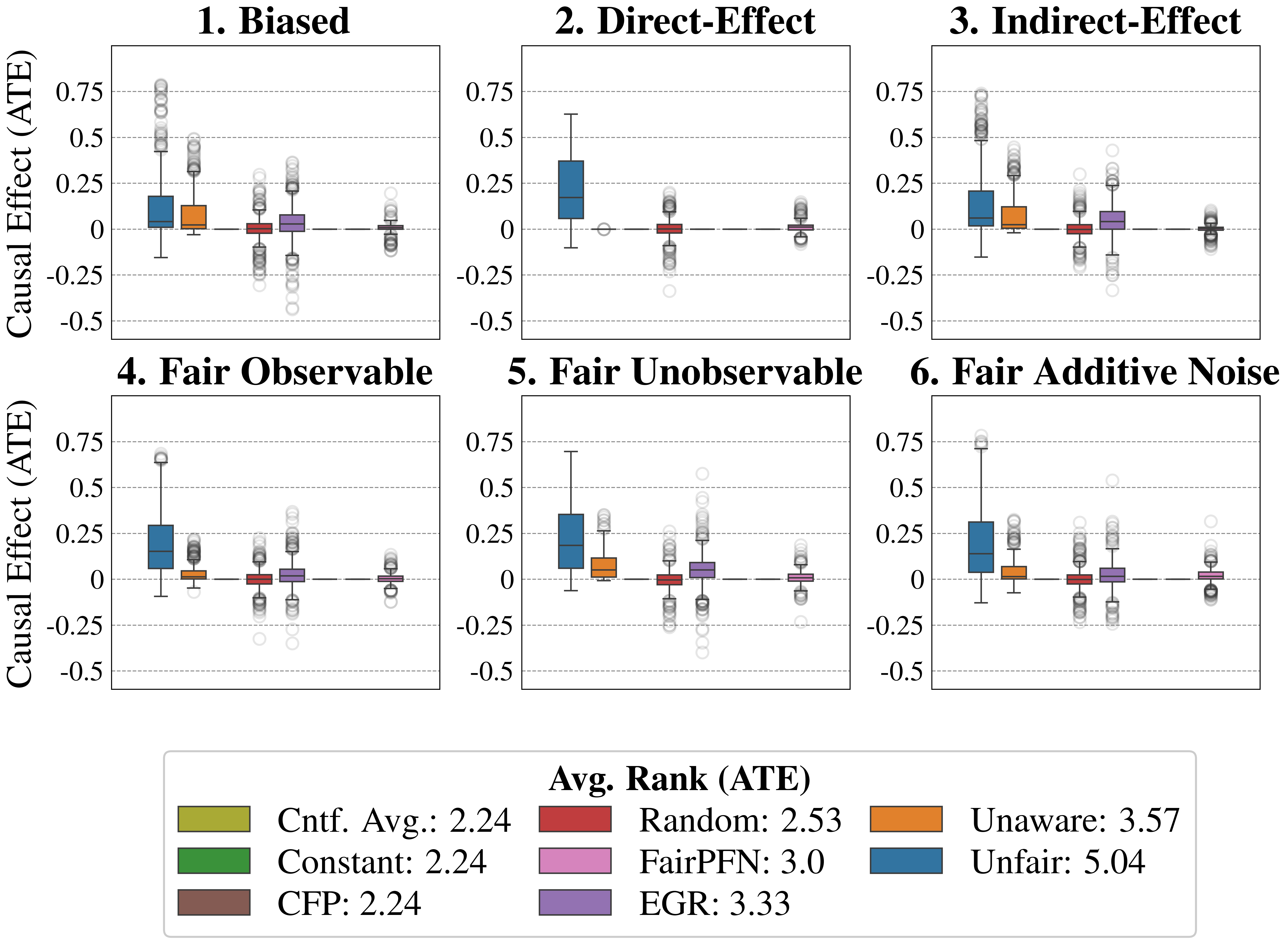<details> <summary>extracted/6522797/figures/tce_by_group_synthetic.png Details</summary>  ### Visual Description ## [Multi-Panel Box Plot]: Causal Effect (ATE) Comparison Across Six Scenarios ### Overview The image displays a 2x3 grid of six box plots, each comparing the distribution of the Average Treatment Effect (ATE) for eight different methods under distinct causal scenarios. The overall purpose is to evaluate and compare the performance (in terms of estimated causal effect) of various fairness-aware and baseline methods. A legend at the bottom provides color coding and an average rank for each method. ### Components/Axes * **Chart Type:** Six separate box plot panels. * **Y-Axis (All Panels):** Labeled "Causal Effect (ATE)". The scale ranges from -0.5 to 0.75, with major gridlines at intervals of 0.25 (-0.5, -0.25, 0, 0.25, 0.5, 0.75). * **Panel Titles (Top Row, Left to Right):** 1. Biased 2. Direct-Effect 3. Indirect-Effect * **Panel Titles (Bottom Row, Left to Right):** 4. Fair Observable 5. Fair Unobservable 6. Fair Additive Noise * **Legend (Bottom Center):** Titled "Avg. Rank (ATE)". It lists eight methods with associated color swatches and their average rank (lower is better). * **Ctf. Avg.:** Olive green, Avg. Rank: 2.24 * **Constant:** Forest green, Avg. Rank: 2.24 * **CFP:** Brown, Avg. Rank: 2.24 * **Random:** Red, Avg. Rank: 2.53 * **FairPFN:** Pink, Avg. Rank: 3.0 * **EGR:** Purple, Avg. Rank: 3.33 * **Unaware:** Orange, Avg. Rank: 3.57 * **Unfair:** Blue, Avg. Rank: 5.04 ### Detailed Analysis Each panel contains eight box plots, one per method, ordered consistently from left to right: Unfair (blue), Unaware (orange), Random (red), FairPFN (pink), EGR (purple), Ctf. Avg. (olive), Constant (green), CFP (brown). The box represents the interquartile range (IQR), the line inside is the median, whiskers extend to 1.5x IQR, and circles are outliers. **Panel 1: Biased** * **Unfair (Blue):** Median ~0.05, IQR spans ~0 to ~0.2, whiskers from ~-0.15 to ~0.45. Many high outliers up to ~0.75. * **Unaware (Orange):** Median ~0.05, IQR ~0 to ~0.15, whiskers ~-0.05 to ~0.3. Outliers up to ~0.5. * **Random (Red):** Median ~0, very narrow IQR centered on 0. Whiskers ~-0.05 to ~0.05. Outliers from ~-0.25 to ~0.25. * **FairPFN (Pink):** Median ~0, IQR ~-0.05 to ~0.05. Whiskers ~-0.15 to ~0.15. Many outliers from ~-0.5 to ~0.35. * **EGR (Purple):** Median ~0, IQR ~-0.05 to ~0.05. Whiskers ~-0.1 to ~0.1. Outliers from ~-0.4 to ~0.3. * **Ctf. Avg., Constant, CFP (Olive, Green, Brown):** All distributions are extremely tight, centered at 0 with minimal spread and few outliers near 0. **Panel 2: Direct-Effect** * **Unfair (Blue):** Median ~0.2, IQR ~0.05 to ~0.35. Whiskers ~-0.1 to ~0.65. No visible outliers. * **Unaware (Orange):** Appears as a single point or extremely narrow distribution at 0. * **Random (Red):** Median ~0, narrow IQR. Whiskers ~-0.05 to ~0.05. Outliers from ~-0.35 to ~0.2. * **FairPFN (Pink):** Median ~0, narrow IQR. Whiskers ~-0.05 to ~0.05. Outliers from ~-0.1 to ~0.1. * **EGR (Purple):** Median ~0, narrow IQR. Whiskers ~-0.05 to ~0.05. Outliers from ~-0.1 to ~0.1. * **Ctf. Avg., Constant, CFP:** Extremely tight distributions at 0. **Panel 3: Indirect-Effect** * **Unfair (Blue):** Median ~0.05, IQR ~0 to ~0.2. Whiskers ~-0.15 to ~0.45. Many high outliers up to ~0.75. * **Unaware (Orange):** Median ~0.05, IQR ~0 to ~0.1. Whiskers ~-0.05 to ~0.2. Outliers up to ~0.4. * **Random (Red):** Median ~0, narrow IQR. Whiskers ~-0.05 to ~0.05. Outliers from ~-0.2 to ~0.2. * **FairPFN (Pink):** Median ~0, IQR ~-0.05 to ~0.05. Whiskers ~-0.15 to ~0.15. Outliers from ~-0.3 to ~0.4. * **EGR (Purple):** Median ~0, IQR ~-0.05 to ~0.05. Whiskers ~-0.1 to ~0.1. Outliers from ~-0.25 to ~0.25. * **Ctf. Avg., Constant, CFP:** Extremely tight distributions at 0. **Panel 4: Fair Observable** * **Unfair (Blue):** Median ~0.15, IQR ~0.05 to ~0.3. Whiskers ~-0.1 to ~0.65. One high outlier ~0.65. * **Unaware (Orange):** Median ~0.05, IQR ~0 to ~0.1. Whiskers ~-0.05 to ~0.15. Outliers up to ~0.25. * **Random (Red):** Median ~0, narrow IQR. Whiskers ~-0.05 to ~0.05. Outliers from ~-0.3 to ~0.2. * **FairPFN (Pink):** Median ~0, IQR ~-0.05 to ~0.05. Whiskers ~-0.15 to ~0.15. Outliers from ~-0.4 to ~0.35. * **EGR (Purple):** Median ~0, IQR ~-0.05 to ~0.05. Whiskers ~-0.1 to ~0.1. Outliers from ~-0.3 to ~0.25. * **Ctf. Avg., Constant, CFP:** Extremely tight distributions at 0. **Panel 5: Fair Unobservable** * **Unfair (Blue):** Median ~0.2, IQR ~0.05 to ~0.35. Whiskers ~-0.05 to ~0.7. No visible outliers. * **Unaware (Orange):** Median ~0.05, IQR ~0 to ~0.1. Whiskers ~-0.05 to ~0.15. Outliers up to ~0.35. * **Random (Red):** Median ~0, narrow IQR. Whiskers ~-0.05 to ~0.05. Outliers from ~-0.25 to ~0.25. * **FairPFN (Pink):** Median ~0, IQR ~-0.05 to ~0.05. Whiskers ~-0.15 to ~0.15. Outliers from ~-0.4 to ~0.6. * **EGR (Purple):** Median ~0, IQR ~-0.05 to ~0.05. Whiskers ~-0.1 to ~0.1. Outliers from ~-0.25 to ~0.25. * **Ctf. Avg., Constant, CFP:** Extremely tight distributions at 0. **Panel 6: Fair Additive Noise** * **Unfair (Blue):** Median ~0.15, IQR ~0.05 to ~0.3. Whiskers ~-0.15 to ~0.75. One high outlier ~0.75. * **Unaware (Orange):** Median ~0.05, IQR ~0 to ~0.1. Whiskers ~-0.05 to ~0.15. Outliers up to ~0.3. * **Random (Red):** Median ~0, narrow IQR. Whiskers ~-0.05 to ~0.05. Outliers from ~-0.25 to ~0.3. * **FairPFN (Pink):** Median ~0, IQR ~-0.05 to ~0.05. Whiskers ~-0.15 to ~0.15. Outliers from ~-0.25 to ~0.55. * **EGR (Purple):** Median ~0, IQR ~-0.05 to ~0.05. Whiskers ~-0.1 to ~0.1. Outliers from ~-0.25 to ~0.25. * **Ctf. Avg., Constant, CFP:** Extremely tight distributions at 0. ### Key Observations 1. **Consistent Hierarchy:** Across all six scenarios, the **Unfair** method (blue) consistently shows the highest median ATE and the largest spread (variance). The **Unaware** method (orange) is typically second highest. Methods like **Constant**, **CFP**, and **Ctf. Avg.** are consistently centered at zero with negligible variance. 2. **Scenario Impact:** The "Direct-Effect" and "Fair Unobservable" scenarios appear to induce the largest positive ATE for the Unfair method (medians ~0.2). The "Biased" and "Indirect-Effect" scenarios show more outliers for the Unfair method. 3. **Fairness Methods:** Fairness-aware methods (**Random**, **FairPFN**, **EGR**) generally have medians near zero, similar to the constant baselines, but exhibit more variance and outliers, especially **FairPFN**. 4. **Ranking Confirmation:** The visual data aligns with the legend's average ranks. The Unfair method (rank 5.04) has the worst (highest) values, while the tied methods with rank 2.24 (Ctf. Avg., Constant, CFP) are the most stable at zero. ### Interpretation This visualization is a comparative analysis of algorithmic fairness in causal inference. The "Causal Effect (ATE)" likely represents a measure of bias or disparate impact. The six panels represent different data-generating processes or fairness constraints imposed on the underlying model. * **What the data suggests:** The "Unfair" method, which presumably ignores fairness constraints, produces the largest and most variable estimated causal effects (biases). The "Unaware" method, which may be blind to sensitive attributes, still shows significant bias. In contrast, methods explicitly designed for fairness (FairPFN, EGR) or simple baselines (Constant, CFP) successfully drive the estimated ATE towards zero, indicating they are mitigating the measured bias. * **Relationship between elements:** The box plots allow for a direct comparison of the *distribution* of outcomes, not just point estimates. The tight clustering of the constant methods at zero serves as a control, showing what a perfectly "fair" (or null) effect looks like. The spread of the other methods indicates their sensitivity to the underlying scenario. * **Notable patterns:** The key takeaway is the trade-off between variance and bias. The unfair/unaware methods have high bias (non-zero median ATE) but also high variance. The fairness-aware methods achieve low bias (median ~0) but introduce more variance into the estimates compared to the rigid constant baselines. The "Direct-Effect" scenario seems to be the most challenging for the unfair method, producing the highest median bias. </details> Figure 24: Causal Fairness (Synthetic-All Baselines): Average Treatment Effect (ATE) of predictions of FairPFN compared to all baselines. FairPFN consistently removes the causal effect with a margin of error of (-0.2, 0.2) and achieves an average rank of 3.0 out of 7. 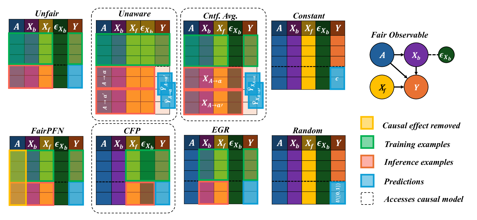<details> <summary>x8.png Details</summary>  ### Visual Description ## Diagram: Comparison of Fairness Intervention Methods in Causal Models ### Overview The image is a technical diagram comparing eight different algorithmic approaches to achieving fairness in predictive modeling, framed within a causal inference context. It visually contrasts how each method handles sensitive attributes, features, and predictions during training and inference phases. The diagram is structured as a grid of eight method-specific blocks, accompanied by a causal graph and a color-coded legend. ### Components/Axes **Main Grid Structure:** - **Rows:** Two rows of four method blocks each. - **Columns within each block:** Five columns labeled with variable names: - `A`: Sensitive attribute (e.g., race, gender). - `X_b`: Background features (potentially influenced by `A`). - `X_f`: Foreground features (potentially causal for `Y` but independent of `A`). - `ε_Xb`: Noise or exogenous error term for `X_b`. - `Y`: Outcome variable to be predicted. - **Vertical Division:** Each block is split horizontally by a dashed line. The area above represents the **training phase**, and the area below represents the **inference phase**. **Legend (Right Side):** - **Yellow Box:** "Causal effect removed" - **Green Box:** "Training examples" - **Pink/Salmon Box:** "Inference examples" - **Blue Box:** "Predictions" - **Dashed Outline:** "Accesses causal model" **Causal Graph (Top Right):** - Titled "Fair Observable". - Nodes: `A` (blue), `X_b` (purple), `ε_Xb` (green), `X_f` (yellow), `Y` (orange). - Directed edges (arrows): - `A` → `X_b` - `A` → `Y` - `X_b` → `Y` - `ε_Xb` → `X_b` - `X_f` → `Y` ### Detailed Analysis **Method-by-Method Breakdown:** 1. **Unfair:** - **Training:** All variables (`A`, `X_b`, `X_f`, `ε_Xb`, `Y`) are shown in green (training examples). - **Inference:** All variables are shown in pink (inference examples). Predictions (`Ŷ`) for `Y` are in blue. - **Interpretation:** A standard predictive model with no fairness constraints. It uses all available data, including the sensitive attribute `A`, directly for training and prediction. 2. **Unaware (Accesses causal model):** - **Training:** Same as "Unfair" (all green). - **Inference:** The `A` column shows two counterfactual scenarios: `A → a` and `A → a'`. The prediction column shows corresponding counterfactual predictions: `Ŷ_{A→a}` and `Ŷ_{A→a'}`. - **Interpretation:** This method is "unaware" of the sensitive attribute during training but uses the causal model at inference to generate predictions under different counterfactual values of `A` (e.g., `a` and `a'`). The final prediction is likely an average or combination of these. 3. **Cntf. Avg. (Counterfactual Averaging) (Accesses causal model):** - **Training:** Same as "Unfair" (all green). - **Inference:** The `X_b` and `X_f` columns show counterfactual feature values: `X_{A→a}` and `X_{A→a'}`. The prediction column shows `Ŷ_{X_{A→a}}` and `Ŷ_{X_{A→a'}}`. - **Interpretation:** This method uses the causal model to compute what the features (`X_b`, `X_f`) *would have been* under different values of `A`, and then makes predictions based on these counterfactual features. The final prediction is an average over these counterfactuals. 4. **Constant:** - **Training:** Same as "Unfair" (all green). - **Inference:** The prediction column shows a constant value `c` (blue). - **Interpretation:** A trivial fairness method that ignores all input features and always outputs the same constant prediction, thereby achieving perfect fairness (no disparity) but zero utility. 5. **FairPFN:** - **Training:** The `A` column is yellow, indicating the "causal effect removed" during training. Other columns are green. - **Inference:** The `A` column remains yellow. Other columns are pink, with predictions in blue. - **Interpretation:** This method explicitly removes the causal influence of the sensitive attribute `A` from the model during the training phase itself. 6. **CFP (Accesses causal model):** - **Training:** All columns are green. - **Inference:** The `X_f` and `ε_Xb` columns are colored brown (a color not in the legend, possibly indicating a specific transformation or intervention). Predictions are in blue. - **Interpretation:** The exact mechanism is less clear from the color coding alone, but it accesses the causal model and appears to perform some intervention or transformation on the foreground features (`X_f`) and the noise term (`ε_Xb`) during inference. 7. **EGR:** - **Training:** All columns are green. - **Inference:** The `X_b` column is pink. The prediction for `Y` is blue. - **Interpretation:** This method seems to focus its intervention on the background features (`X_b`) during the inference phase, while using standard training. 8. **Random:** - **Training:** All columns are green. - **Inference:** The prediction column shows `u(0,1)` (blue), indicating a random value drawn from a uniform distribution between 0 and 1. - **Interpretation:** Another trivial baseline that makes random predictions, achieving fairness through randomness but with no predictive utility. ### Key Observations - **Causal Model Access:** Three methods (Unaware, Cntf. Avg., CFP) are explicitly marked as accessing the causal model (dashed outline). This suggests they require knowledge of the underlying causal graph (shown on the right) to function. - **Phase-Specific Interventions:** Most methods apply their fairness intervention during the **inference phase** (below the dashed line), not during training. The major exception is **FairPFN**, which intervenes during training (yellow in the `A` column above the line). - **Variable Targeting:** Different methods target different variables for intervention: `A` (FairPFN), counterfactual `A` (Unaware), counterfactual features (Cntf. Avg.), background features `X_b` (EGR), or other transformations (CFP). - **Baselines:** "Constant" and "Random" serve as trivial fairness baselines that sacrifice all predictive accuracy. ### Interpretation This diagram is a conceptual taxonomy of algorithmic fairness strategies within a causal inference framework. It illustrates a fundamental trade-off: how to modify a predictive model to prevent unfair discrimination (often traced to the sensitive attribute `A`) while preserving useful information for prediction. The **causal graph** is central to the diagram's logic. It defines the "ground truth" relationships: `A` influences both `X_b` and `Y` directly, and `X_b` also influences `Y`. Fairness interventions aim to block the unfair path `A → Y` or `A → X_b → Y`. The methods differ in *where* and *how* they intervene: - **Pre-processing/In-processing (FairPFN):** Alters the model or data before or during training to remove the effect of `A`. - **Post-processing/Inference-time (Unaware, Cntf. Avg., EGR, CFP):** Uses the trained model but modifies inputs or outputs at prediction time, often leveraging the causal model to simulate counterfactuals ("What would the prediction be if `A` were different?"). The diagram suggests that methods accessing the causal model (dashed boxes) can perform more precise, targeted interventions (like computing exact counterfactuals) compared to methods that do not. However, this requires strong assumptions and knowledge of the true causal structure, which is often unknown in practice. The presence of trivial baselines ("Constant", "Random") highlights that achieving fairness is trivial if one is willing to completely abandon predictive utility. The core challenge, embodied by the other six methods, is to find a balance—to remove unfair bias while retaining as much predictive power as possible. </details> Figure 25: Baseline Models: Visualization of FairPFN and our baseline models on our Fair Observable benchmark group, in terms of which variables each model is fit to and performs inference on on. | Unfair Unaware | Law School Admissions 0.09±0.10 (0.00%) 0.03± 0.03 (0.00%) | Adult Census Income 0.05±0.06 (0.60%) 0.02± 0.04 (1.49%) | Average 0.07±0.08 (0.30%) 0.03± 0.04 (0.75%) | | --- | --- | --- | --- | | Constant | -0.40±0.08 (97.51%) | -0.18±0.10 (15.69%) | -0.29±0.09 (56.60%) | | Random | 0.10±0.30 (0.00%) | 0.32±0.31 (0.30%) | 0.21±0.31 (0.15%) | | EGR | 0.06±0.45 (0.00%) | 0.01±0.35 (0.00%) | 0.03±0.40 (0.00%) | | CFP | 0.09± 0.03 (49.21%) | 0.05±0.06 (2.13%) | 0.07±0.05 (25.67%) | | FairPFN | 0.01± 0.03 (0.11%) | 0.02± 0.04 (0.60%) | 0.02± 0.04 (0.36%) | Table 2: Difference to Cntf. Avg. (Real): Mean, standard deviation and percentage of outliers of the predictions on our real-world datasets of FairPFN and our baseline models compared to the predictions of the Cntf. Avg. baseline, which shows strong performance in causal effect removal and predictive error due to access to both observational and counterfactual data. FairPFN achieves predictions with an average difference to Cntf. Avg. of 0.02±0.04, with 0.36% of samples falling outside of three standard deviations.