2506.08989v1

# SwS: Self-aware Weakness-driven Problem Synthesis in Reinforcement Learning for LLM Reasoning **Authors**: Xiao Liang1⁣∗1 1 ∗, Zhong-Zhi Li2⁣∗2 2 ∗, Yeyun Gong, Yang Wang, Hengyuan Zhang, Los AngelesSchool of Artificial Intelligence ∗ Equal contribution. Work done during Xiao’s and Zhongzhi’s internships at Microsoft. † Corresponding authors: Yeyun Gong and Weizhu Chen. 🖂: yegong@microsoft.com; wzchen@microsoft.com Abstract: Reinforcement Learning with Verifiable Rewards (RLVR) has proven effective for training large language models (LLMs) on complex reasoning tasks, such as mathematical problem solving. A prerequisite for the scalability of RLVR is a high-quality problem set with precise and verifiable answers. However, the scarcity of well-crafted human-labeled math problems and limited-verification answers in existing distillation-oriented synthetic datasets limit their effectiveness in RL. Additionally, most problem synthesis strategies indiscriminately expand the problem set without considering the model’s capabilities, leading to low efficiency in generating useful questions. To mitigate this issue, we introduce a S elf-aware W eakness-driven problem S ynthesis framework (SwS) that systematically identifies model deficiencies and leverages them for problem augmentation. Specifically, we define weaknesses as questions that the model consistently fails to learn through its iterative sampling during RL training. We then extract the core concepts from these failure cases and synthesize new problems to strengthen the model’s weak areas in subsequent augmented training, enabling it to focus on and gradually overcome its weaknesses. Without relying on external knowledge distillation, our framework enables robust generalization by empowering the model to self-identify and address its weaknesses in RL, yielding average performance gains of 10.0% and 7.7% on 7B and 32B models across eight mainstream reasoning benchmarks. | | Code | https://github.com/MasterVito/SwS | | --- | --- | --- | | Project | https://MasterVito.SwS.github.io | | <details> <summary>x1.png Details</summary>  ### Visual Description ## Radar Charts: AI Model Performance Across Mathematical Benchmarks and Domains ### Overview The image displays two radar charts (spider plots) comparing the performance of six different 32-billion-parameter AI models. The charts are labeled (a) and (b), with a shared legend positioned at the top-center between them. The charts use a circular grid with concentric rings representing performance percentages (40%, 60%, 80%, 100%). Each model is represented by a distinct line style and color, plotting its score across multiple axes radiating from the center. ### Components/Axes * **Legend (Top-Center):** Lists six models with corresponding line styles and colors: * `Qwen2.5-32B`: Gray, dashed line (`---`) * `Qwen2.5-32B-IT`: Light blue, dashed line (`---`) * `ORZ-32B`: Orange, dashed line (`---`) * `SimpleRL-32B`: Green, dashed line (`---`) * `Baseline-32B`: Purple, dashed line (`---`) * `SwS-32B`: Red, solid line (`—`) * **Chart (a) - Performance across Benchmarks:** * **Axes (7 total, clockwise from top):** GSM8K, MATH 500, Minerva Math, Olympiad Bench, GaoKao 2023, AMC23, AIME @32. * **Scale:** Concentric rings marked at 40%, 60%, 80%, and 100% (outermost). * **Chart (b) - Performance across Domains:** * **Axes (7 total, clockwise from top):** Prealgebra, Intermediate Algebra, Algebra, Geometry, Counting & Probability, Precalculus, Number Theory. * **Scale:** Identical concentric ring scale as chart (a). 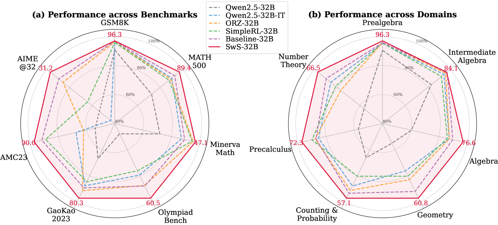### Detailed Analysis **Chart (a) - Performance across Benchmarks:** * **SwS-32B (Red, Solid Line):** Consistently forms the outermost polygon, indicating top performance across all benchmarks. Specific labeled scores (red text) are: GSM8K: 96.3, MATH 500: 89.4, Minerva Math: 47.1, Olympiad Bench: 60.5, GaoKao 2023: 80.3, AMC23: 90.6, AIME @32: 31.2. * **Other Models:** Generally form nested polygons inside the SwS-32B line. The gray dashed line (`Qwen2.5-32B`) is often the innermost, indicating the lowest performance on most benchmarks shown. The purple (`Baseline-32B`) and green (`SimpleRL-32B`) lines are frequently the next closest to the red line. * **Trend Verification:** All models show a similar *relative* performance pattern across benchmarks. They score highest on GSM8K and AMC23, moderately on MATH 500 and GaoKao 2023, and lowest on the more specialized Olympiad Bench, Minerva Math, and AIME @32. The red line's shape is a scaled-up version of the others. **Chart (b) - Performance across Domains:** * **SwS-32B (Red, Solid Line):** Again forms the outermost polygon. Specific labeled scores (red text) are: Prealgebra: 96.3, Intermediate Algebra: 84.1, Algebra: 76.6, Geometry: 60.8, Counting & Probability: 57.1, Precalculus: 72.3, Number Theory: 66.5. * **Other Models:** The nesting pattern is similar to chart (a). The gray dashed line (`Qwen2.5-32B`) is again the innermost. The purple (`Baseline-32B`) line is notably strong in Precalculus and Number Theory, nearly matching the red line on those axes. * **Trend Verification:** All models perform best in Prealgebra and Intermediate Algebra. Performance generally decreases for more advanced domains like Geometry, Counting & Probability, and Number Theory. The red line maintains a consistent lead across all domains. ### Key Observations 1. **Dominant Model:** The `SwS-32B` model (red solid line) demonstrates superior performance across every benchmark and every mathematical domain presented in these charts. 2. **Performance Hierarchy:** A clear and consistent hierarchy is visible: `SwS-32B` > `Baseline-32B`/`SimpleRL-32B` > `ORZ-32B` > `Qwen2.5-32B-IT` > `Qwen2.5-32B`. The exact order between `Baseline-32B` and `SimpleRL-32B` varies slightly by axis. 3. **Benchmark Difficulty:** The AIME @32 and Minerva Math benchmarks appear to be the most challenging, as all models score below 50% on them (with SwS-32B at 31.2 and 47.1, respectively). 4. **Domain Strength:** All models show relative strength in foundational algebra topics (Prealgebra, Intermediate Algebra) and relative weakness in combinatorial and geometric topics (Counting & Probability, Geometry). ### Interpretation These radar charts provide a multidimensional comparison of AI model capabilities in mathematics. The data suggests that the training or architectural approach used for `SwS-32B` yields significant and consistent improvements over the other compared models (`Qwen2.5-32B`, `ORZ-32B`, `SimpleRL-32B`, and a `Baseline-32B`). The fact that the performance *pattern* (the shape of the polygon) is similar across all models indicates that the relative difficulty of these mathematical tasks is consistent; the models differ in their overall capability level, not in their specialized strengths/weaknesses. The charts effectively argue that `SwS-32B` is a state-of-the-art model for mathematical reasoning within this 32B parameter class. The inclusion of both broad benchmarks (like GSM8K) and specialized domains (like Number Theory) shows that its advantage is comprehensive. For a researcher or user, this visualization implies that choosing `SwS-32B` would likely lead to better performance on a wide range of mathematical problems, from grade-school arithmetic to competition-level algebra and calculus. The clear visual gap between the red line and the others is a powerful indicator of a meaningful performance leap. </details> Figure 1: 32B model performance across mainstream reasoning benchmarks and different domains. ## 1 Introduction "Give me six hours to chop down a tree and I will spend the first four sharpening the axe." —Abraham Lincoln Large-scale Reinforcement Learning with Verifiable Rewards (RLVR) has substantially advanced the reasoning capabilities of large language models (LLMs) [16, 10, 46], where simple rule-based rewards can effectively induce complex reasoning skills. The success of RLVR for eliciting models’ reasoning capabilities heavily depends on a well-curated problem set with proper difficulty levels [63, 28, 55], where each problem is paired with an precise and verifiable reference answer [14, 31, 63, 10]. However, existing reasoning-focused datasets for RLVR suffer from three main issues: (1) High-quality, human-labeled mathematical problems are scarce, and collecting large-scale, well-annotated datasets with precise reference answers is cost-intensive. (2) Most reasoning-focused synthetic datasets are created for SFT distillation, where reference answers are rarely rigorously verified, making them suboptimal for RLVR, which relies heavily on the correctness of the final answer as the training signal. (3) Existing problem augmentation strategies typically involve rephrasing or generating variants of human-written questions [62, 30, 38, 27], or sampling concepts from existing datasets [15, 45, 20, 73], without explicitly considering the model’s reasoning capabilities. Consequently, the synthetic problems may be either too trivial or overly challenging, limiting their utility for model improvement in RL. More specifically, in RL, it is essential to align the difficulty of training tasks with the model’s current capabilities. When using group-level RL algorithms such as GPRO [40], the advantage of each response is calculated based on its comparison with other responses in the same group. If all responses are either entirely correct or entirely incorrect, the token-level advantages within each rollout collapse to 0, leading to gradient vanishing and degraded training efficiency [28, 63], and potentially harming model performance [55]. Therefore, training on problems that the model has fully mastered or consistently fails to solve does not provide useful learning signals for improvement. However, a key advantage of the failure cases is that, unlike the overly simple questions with little opportunity for improvement, persistently failed problems reveal specific areas of weakness in the model and indicate directions for further enhancement. This raises the following research question: How can we effectively utilize these consistently failed cases to address the model’s reasoning deficiencies? Could they be systematically leveraged for data synthesis that targets the enhancement of the model’s weakest capabilities? To answer these questions, we propose a S elf-aware W eakness-driven Problem S ynthesis (SwS) framework, which leverages the model’s self-identified weaknesses in RL to generate synthetic problems for training augmentation. Specifically, we record problems that the model consistently struggles to solve or learns inefficiently through iterative sampling during a preliminary RL training phase. These failed problems, which reflect the model’s weakest areas, are grouped by categories, leveraged to extract common concepts, and to synthesize new problems with difficulty levels tailored to the model’s capabilities. To further improve weakness mitigation efficiency during training, the augmentation budget for each category is allocated based on the model’s relative performance across them. Compared with existing problem synthesis strategies for LLM reasoning [73, 45], our framework explicitly targets the model’s capabilities and self-identified weaknesses, enabling more focused and efficient improvement in RL training. To validate the effectiveness of SwS, we conducted experiments across model sizes ranging from 3B to 32B and comprehensively evaluated performance on eight popular mathematical reasoning benchmarks, showing that its weakness-driven augmentation strategy benefits models across all levels of reasoning capability. Notably, our models trained on the augmented problem set consistently surpass both the base models and those trained on the original dataset across all benchmarks, achieving a substantial average absolute improvement of 10.0% for the 7B model and 7.7% for the 32B model, even surpassing their counterparts trained on carefully curated human-labeled problem sets [14, 6]. We also analyze the model’s performance on previously failed problems and find that, after training on the augmented problem set, it is able to solve up to 20.0% more problems it had consistently failed in its weak domain when trained only on the original dataset. To further demonstrate the robustness and adaptability of the proposed SwS pipeline, we extend it to explore the potential of Weak-to-Strong Generalization, Self-evolving, and Weakness-driven Selection settings, with detailed experimental results and analysis presented in Section 4. Contributions. (i) We propose a Self-aware Weakness-driven Problem Synthesis (SwS) framework that utilizes the model’s self-identified weaknesses to generate synthetic problems for enhanced RLVR training, paving the way for utilizing high-quality and targeted synthetic data for RL training. (ii) We comprehensively evaluate the SwS framework across diverse model sizes on eight mainstream reasoning benchmarks, demonstrating its effectiveness and generalizability. (iii) We explore the potential of extending our SwS framework to Weak-to-Strong Generalization, Self-evolving, and Weakness-driven Selection settings, highlighting its adaptability through detailed analysis. <details> <summary>x2.png Details</summary>  ### Visual Description \n ## Diagram: Reinforcement Learning Training Pipeline with Verification ### Overview The image is a technical diagram illustrating a reinforcement learning (RL) training pipeline that incorporates a verification step. It consists of two main parts: a sample problem statement at the top and a flowchart below depicting the training and evaluation process. The diagram shows how a policy model generates multiple candidate answers, which are then evaluated by a verifier. The outcomes are visualized as accuracy trends over training epochs, leading to either a success path or a "Failed set." ### Components/Axes **1. Problem Statement (Top Yellow Box):** * **Label:** `Question-1:` * **Text Content:** "Tiffany is constructing a fence around a rectangular tennis court. She must use exactly 300 feet of fencing. The fence must enclose all four sides of the court. Regulation states that the length of the fence enclosure must be at least 80 feet and the width must be at least 40 feet. Tiffany wants the area enclosed by the fence to be as large as possible in order to accommodate benches and storage space. What is the optimal area, in square feet?" **2. Flowchart Components (Left to Right):** * **Policyθ:** A green, rounded rectangle on the far left. It represents the policy model being trained. * **Answer Generation:** Multiple blue, stacked rectangles labeled `Answer1,1` through `Answerk,1`, with ellipsis (`...`) indicating a sequence. This represents the generation of `k` candidate answers for a given input. * **Verifier:** A purple, rounded rectangle positioned to the right of the answer blocks. * **Accuracy Charts:** Two bar charts stacked vertically to the right of the Verifier. * **Y-axis (Both Charts):** Labeled `Acc` (Accuracy). * **X-axis (Both Charts):** Labeled `Epoch`, with markers `t1`, `t2`, `t3`, `...`, `tT1`. * **Top Chart (Failure Path):** Shows bars with approximate heights: `0.3` at `t1`, `0.5` at `t2`, `0.3` at `t3`, and `0.2` at `tT1`. A large red **X** is placed to its right. * **Bottom Chart (Success Path):** Shows bars with approximate heights: `0.3` at `t1`, `0.8` at `t2`, `0.9` at `t3`, and `1.0` at `tT1`. A green checkmark (✓) is placed to its right. * **Failed Set:** A red cylinder on the far right, labeled `Failed set`. * **Process Label:** Text below the Answer blocks reads `RL Training for T1 Epochs`. **3. Flow Arrows:** * An arrow points from the Problem Statement to `Policyθ`. * Two diverging arrows point from `Policyθ` to the stack of `Answer` blocks. * Two converging arrows point from the `Answer` blocks to the `Verifier`. * Two diverging arrows point from the `Verifier` to the two accuracy charts. * An arrow points from the red **X** (top chart) to the `Failed set`. * A curved arrow points from the `Failed set` back to the `Policyθ` box, indicating a feedback loop. ### Detailed Analysis The diagram details a closed-loop RL training process: 1. **Input:** A problem (exemplified by the tennis court fencing question) is fed into the policy model (`Policyθ`). 2. **Generation:** The policy generates `k` distinct candidate answers (`Answer1,1` to `Answerk,1`) for the given problem. 3. **Verification:** All generated answers are passed to a `Verifier` module, which evaluates their correctness or quality. 4. **Outcome Visualization:** The verification results are aggregated into accuracy (`Acc`) scores tracked over `T1` training epochs (`t1` to `tT1`). The diagram contrasts two possible trajectories: * **Failure Trajectory (Top Chart):** Accuracy fluctuates at a low level (peaking at 0.5) and ends low (0.2). This path is marked with a red **X** and leads to the `Failed set`. * **Success Trajectory (Bottom Chart):** Accuracy shows a clear, monotonic increasing trend from 0.3 to a perfect 1.0. This path is marked with a green checkmark. 5. **Feedback:** The `Failed set` (containing problems/answers that led to failure) is fed back into the `Policyθ`, presumably to inform and improve future training iterations. ### Key Observations * **Contrasting Trends:** The core visual message is the stark contrast between the failing accuracy trend (non-monotonic, low final value) and the successful trend (smooth, monotonic increase to perfection). * **Spatial Grounding:** The legend (red **X** and green checkmark) is placed immediately to the right of its corresponding chart, creating a clear visual association. The `Failed set` cylinder is positioned in the top-right quadrant, receiving input only from the failure path. * **Process Scope:** The label `RL Training for T1 Epochs` brackets the answer generation and verification steps, indicating this entire subprocess occurs within each of the `T1` epochs. * **Problem as Example:** The specific math problem at the top serves as a concrete example of the type of task the policy is being trained to solve. It is an optimization problem with constraints, requiring multi-step reasoning. ### Interpretation This diagram illustrates a **verification-guided reinforcement learning** framework. The key insight is that raw answer generation is insufficient; a verifier is critical for providing a learning signal. The diverging accuracy trends demonstrate the framework's goal: to steer the policy away from answer patterns that lead to low, unstable verification scores (the failure path) and towards patterns that yield consistently improving and ultimately perfect scores (the success path). The inclusion of the `Failed set` and its feedback loop is particularly significant. It suggests an **experience replay** or **hard negative mining** mechanism, where difficult examples that caused failure are specifically revisited to make the policy more robust. The specific math problem, with its precise constraints, exemplifies the kind of complex, verifiable task this system is designed to master. The diagram argues that for such tasks, integrating an explicit verifier into the RL loop is essential for achieving reliable, high-performance learning. 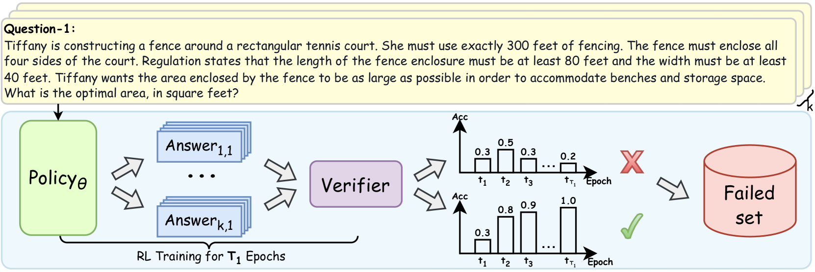</details> Figure 2: Illustration of the self-aware weakness identification during a preliminary RL training. ## 2 Method ### 2.1 Preliminary Group Relative Policy Optimization (GRPO). GRPO [40] is an efficient optimization algorithm tailored for RL in LLMs, where the advantages for each token are computed in a group-relative manner without requiring an additional critic model to estimate token values. Specifically, given an input prompt $x$ , the policy model $π_θ_{old}$ generates a group of $G$ responses $Y=\{y_i\}_i=1^G$ , with acquired rewards $R=\{r_i\}_i=1^G$ . The advantage $A_i,t$ for each token in response $y_i$ is computed as the normalized rewards: $$ A_i,t=\frac{r_i-mean(\{r_i\}_i=1^G)}{std(\{r_i\}_i= 1^G)}. \tag{1} $$ To improve the stability of policy optimization, GRPO clips the probability ratio $k_i,t(θ)=\frac{π_θ(y_i,t\mid x,y_i,<t)}{π_θ_{\text {old}}(y_i,t\mid x,y_i,<t)}$ within a trust region [39], and constrains the policy distribution from deviating too much from the reference model using a KL term. The optimization objective is defined as follows: $$ \displaystyleJ_GRPO(θ) \displaystyle=E_x∼D,Y∼π_θ_{ old(·\mid x)} \displaystyle\Bigg{[}\frac{1}{G}∑_i=1^G\frac{1}{|y_i|}∑_t=1^|y_ {i|}\Bigg{(}\min\Big{(}k_i,t(θ)A_i,t, clip\Big{(}k_i,t( θ),1-ε,1+ε\Big{)}A_i,t\Big{)}-β D_KL( π_θ||π_ref)\Bigg{)}\Bigg{]}. \tag{2} $$ Inspired by DAPO [63], in all experiments of this work, we omit the KL term during optimization, while incorporating the clip-higher, token-level loss and dynamic sampling strategies to enhance the training efficiency of RLVR. Our RLVR training objective is defined as follows: $$ \displaystyleJ(θ)=E_x∼D, Y∼ π_θ_{old(·\mid x)} \displaystyle\Bigg{[}\frac{1}{∑_i=1^G|y_i|}∑_i=1^G∑_t=1^ |y_i|\Big{(}\min\big{(}k_i,t(θ)A_i,t, clip(k_i,t(θ) ,1-ε,1+ε^h)A_i,t\big{)}\Big{)}\Bigg{]} \displaystyles.t.≤avevmode\nobreak ≤avevmode\nobreak acc_ lower<≤ft|≤ft\{y_i∈Y \middle| \texttt{is\_accurate} (x,y_i)\right\}\right|<acc_upper. \tag{3} $$ where $ε^h$ denotes the upper clipping threshold for importance sampling ratio $k_i,t(θ)$ , and $acc_lower$ and $acc_upper$ are thresholds used to filter target prompts for subsequent policy optimization. 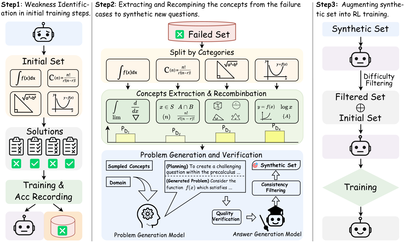### 2.2 Overview Figure 3 presents an overview of our SwS framework, which generates targeted training samples to enhance the model’s reasoning capabilities in RLVR. The framework initiates with a Self-aware Weakness Identification stage, where the model undergoes preliminary RL training on an initial problem set covering diverse categories. During this stage, the model’s weaknesses are identified as problems it consistently fails to solve or learns ineffectively. Based on failure cases that reflect the model’s weakest capabilities, in the subsequent Targeted Problem Synthesis stage, we group them by category, extract their underlying concepts, and recombine these concepts to synthesize new problems that target the model’s learning and mitigation of its weaknesses. In the final Augmented Training with Synthetic Problems stage, the model receives continuous training with the augmented high-quality synthetic problems, thereby enhancing its general reasoning abilities through more targeted training. ### 2.3 Self-aware Weakness Identification Utilizing the policy model itself to identify its weakest capabilities, we begin by training it in a preliminary RL phase using an initial problem set $X_S$ , which consists of mathematical problems from $n$ diverse categories ${\{D\}}_i=0^n$ , each paired with a ground-truth answer $a$ . As illustrated in Figure 2, we record the average accuracy $a_i,t$ of the model’s responses to each prompt $x_i$ at each epoch $t∈\{0,1,\dots,T_1\}$ , where $T_1$ is the number of training epochs in this phase. We track the Failure Rate $F$ for each problem in the training set to identify those that the model consistently struggles to learn, which are considered its weaknesses. Specifically, such problems are defined as those the model consistently struggles to solve during RL training, which meet two criteria: (1) The model never reaches a response accuracy of 50% at any training epoch, and (2) The accuracy trend decreases over time, indicated by a negative slope: $$ F(x_i)=I≤ft[\max_t∈[1,T]a_i,t<0.5 ∧ slope≤ft (\{a_i,t\}_t=1^T\right)<0\right] \tag{4} $$ This metric captures both problems the model consistently fails to solve and those showing no improvement during sampling-based RL training, making them appropriate targets for training augmentation. After the weakness identification phase via the preliminary training on the initial training set $X_S$ , we employ the collected problems $X_F=≤ft\{x_i∈X_S \middle| F_r(x_i)=1\right\}$ as seed problems for subsequent weakness-driven problem synthesis. <details> <summary>x3.png Details</summary>  ### Visual Description ## Diagram: Three-Step Process for Improving AI Model Training via Synthetic Data Generation ### Overview The image is a technical process diagram illustrating a three-step methodology for enhancing an AI model's training. The process focuses on identifying weaknesses in the model's initial performance, using those failures to generate new synthetic training questions, and then integrating this synthetic data back into the training pipeline. The diagram uses icons, mathematical notation, flow arrows, and text labels to explain each stage. ### Components/Axes The diagram is divided into three vertical panels, each representing a major step. **Step 1 (Left Panel): Weakness Identification in initial training steps.** * **Top Icon:** A robot head with a neutral/slightly concerned expression. * **Initial Set:** A box containing four mathematical problem examples: 1. Integral notation: `∫ f(x) dx` 2. Combination formula: `C(n) = n! / (r!(n-r)!)` 3. Pythagorean theorem diagram: A right triangle with sides labeled `a`, `b`, and hypotenuse `√(a²+b²)`. 4. Function graph: A coordinate system with a curve labeled `y = f(x)`. * **Solutions:** Four clipboard icons, each with a checklist. Below them are status indicators: a green checkmark (✓), a red cross (✗), a green checkmark (✓), and a green checkmark (✓). This indicates mixed success on the initial problems. * **Training & Acc Recording:** A box leading to two outputs: 1. A robot head icon (the trained model). 2. A database/cylinder icon with a red cross (✗) overlay, labeled as the "Failed Set" in the next step. **Step 2 (Center Panel): Extracting and Recombining the concepts from the failure cases to synthetic new questions.** * **Failed Set:** A red-bordered box at the top, containing a red cross (✗) icon and the text "Failed Set". An arrow points down from the database in Step 1. * **Split by Categories:** The failed problems are categorized into four boxes, mirroring the initial set: 1. `∫ f(x) dx` 2. `C(n) = n! / (r!(n-r)!)` 3. The Pythagorean theorem triangle. 4. The `y = f(x)` graph. * **Concepts Extraction & Recombination:** A green-shaded box showing how core concepts are extracted and mixed. It contains four sub-boxes with new mathematical expressions: 1. `∫`, `d/dx`, `lim`, `∇` (integral, derivative, limit, gradient symbols). 2. `x ∈ S`, `A ∩ B`, `(n)`, `n! / (r!(n-r)!)` (set membership, intersection, combination notation). 3. Geometric shapes: a cube, a circle with radius `r`, and two triangles with angles labeled `θ` and `a`. 4. `y = f(x)`, `log x`, a graph of a logarithmic curve, `{A}`. * **Probability Bars:** Below the recombination box are four yellow bars of varying heights, labeled `P_D1`, `P_D2`, `P_D3`, and `P_D4` from left to right. These likely represent the probability or weight of sampling from each concept domain. * **Problem Generation and Verification:** A blue-shaded box at the bottom. * **Inputs:** "Sampled Concepts" and "Domain" feed into a "Problem Generation Model" (icon: a head with gears). * **Process Text:** A speech bubble from the model contains: * `(Planning) To create a challenging question within the precalculus ...` * `(Generated Problem) Consider the function f(x) which satisfies ...` * **Verification Flow:** The generated problem goes to "Quality Verification" (icon: a document with a checkmark), then to an "Answer Generation Model" (icon: a robot with a graduation cap). This model performs "Consistency Filtering" and outputs to the "Synthetic Set" (icon: a target with an arrow). **Step 3 (Right Panel): Augmenting synthetic set into RL training.** * **Synthetic Set:** A box at the top, receiving output from Step 2. * **Flow:** An arrow points down to a robot head icon, then through a process labeled "Difficulty Filtering". * **Filtered Set ⊕ Initial Set:** The filtered synthetic data is combined (⊕ symbol) with the original "Initial Set". * **Training:** The combined dataset is used for "Training" (represented by a green diamond shape). * **Final Output:** An arrow points down to a final robot head icon with a happy/smiling expression, indicating the improved model. ### Detailed Analysis The diagram details a closed-loop, iterative training improvement cycle. 1. **Weakness Identification:** The model is tested on an initial set of problems (calculus, combinatorics, geometry, functions). Its failures are recorded. 2. **Concept-Based Synthesis:** Instead of simply repeating failed problems, the system decomposes them into fundamental mathematical concepts (e.g., integration, combinatorics, geometric relations, function properties). These concepts are then recombined to create novel problem structures. 3. **Controlled Generation & Filtering:** A dedicated model generates new problems based on sampled concepts and domain. These undergo quality and consistency checks. The resulting synthetic set is then filtered by difficulty before being merged with the original training data. 4. **Reinforcement Learning (RL) Integration:** The augmented dataset (original + high-quality synthetic problems) is used in a subsequent training phase (likely RL, as mentioned in the step title), leading to a more robust model. ### Key Observations * **Visual Coding:** Colors are used meaningfully: red for failure/initial problems, green for success/recombination, blue for the generation process. The robot's expression changes from neutral/concerned (Step 1) to happy (Step 3), visually signaling improvement. * **Mathematical Specificity:** The diagram is not abstract; it uses concrete examples from pre-calculus and calculus (integrals, combinations, Pythagoras, functions, logs) to ground the process. * **Process Granularity:** Step 2 is the most detailed, highlighting that the core innovation lies in the concept extraction, recombination, and verified generation of new problems, not just data augmentation. * **Uncertainty in Quantification:** The yellow bars (`P_D1` to `P_D4`) indicate that the sampling of concepts is probabilistic, but their exact numerical values or the criteria for their heights are not provided in the image. ### Interpretation This diagram outlines a sophisticated methodology for addressing a core challenge in AI training: data scarcity and the "long tail" of rare or difficult cases. The process is **Peircean** in its investigative logic: * **Abduction:** It starts by *observing* failures (the "Failed Set") and *inferring* the underlying conceptual weaknesses (the "Split by Categories"). * **Deduction:** It then *hypothesizes* that creating new problems from these recombined concepts will challenge the model in targeted ways. The "Planning" and "Generated Problem" text shows this deductive reasoning in action. * **Induction:** Finally, it *tests* this hypothesis by generating, filtering, and integrating the synthetic data, then retraining the model. The improved model (happy robot) is the inductive conclusion that the method works. The system moves beyond simple error repetition. By decomposing failures into atomic concepts and recombining them, it can generate a potentially infinite variety of novel problems that probe the same conceptual gaps. This makes the training more efficient and the resulting model more generalizable. The emphasis on "Verification" and "Filtering" is crucial, as it ensures the synthetic data is high-quality and pedagogically useful, preventing the model from learning from flawed or trivial examples. The ultimate goal is a form of **curriculum learning** where the model's own weaknesses dictate the generation of its next set of training challenges. </details> Figure 3: An overview of our proposed weakness-driven problem synthesis framework that targets at mitigating the model’s reasoning limitations within the RLVR paradigm. ### 2.4 Targeted Problem Synthesis Concept Extraction and Recombination. We synthesize new problems by extracting the underlying concepts $C_F$ from the collected seed questions $X_F$ and strategically recombining them to generate questions that target similar capabilities. Specifically, the extracted concepts are first categorized into their respective categories $D_i$ (e.g., mathematical topics such as Algebra or Geometry) based on the corresponding seed problem $x_i$ , and are subsequently sampled and recombined to generate problems within the same category. Inspired by [15, 73], we enhance the coherence and semantic fluency of synthetic problems by computing co-occurrence probabilities and embedding similarities among concepts within each category, enabling more appropriate sampling and recombination of relevant concepts. This targeted sampling approach ensures that the synthesized problems remain semantically coherent and avoids combining concepts from unrelated sub-topics or irrelevant knowledge points, which could otherwise result in invalid or confusing questions. Further details on the co-occurrence calculation and sampling algorithm are provided in Appendix E. Intuitively, categories exhibiting more pronounced weaknesses demand additional learning support. To optimize the efficiency of targeted problem synthesis and weakness mitigation in subsequent RL training, we allocate the augmentation budget, i.e., the concept combinations used as inputs for problem synthesis, across categories based on the model’s category-specific failure rates $F_D$ from the preliminary training phase. Specifically, we normalize these failure rates $F_D$ across categories to determine the allocation weights for problem synthesis. Given a total augmentation budget $|X_T|$ , the number of concept combinations allocated to domain $D_i$ is computed as: $$ |X_T,D_i|=|X_T|· P_D_i=| X_T|·\frac{F_D_i}{∑_j^nF_D_j}, \tag{5} $$ where $F_D_i$ is the failure rate of problems in category $D_i$ within the initial training set. The sampled and recombined concepts then serve as inputs for subsequent problem generation. Problem Generation and Quality Verification. After extracting and recombining the concepts associated with the model’s weakest capabilities, we employ a strong instruction model, which does not perform deep reasoning, to generate new problems based on the category label and the recombined concepts. We instruct the model to first generate rationales that explore how the concept combinations can be integrated to produce a well-formed problem. To ensure the synthetic problems align with the RLVR setting, the model is also instructed to avoid generating multiple-choice, multi-part, or proof-based questions [1]. Detailed prompt used for the concept-based problem generation please refer to the Appendix J. For quality verification of the synthetic problems, we prompt general instruction LLMs multiple times to evaluate each problem and its rationale across multiple dimensions, including concept coverage, factual accuracy, and solvability, assigning an overall rating of bad, acceptable, or perfect. Only problems receiving ‘perfect’ ratings above a predefined threshold and no ‘bad’ ratings are retained for subsequent utilization. Reference Answer Generation. Since alignment between the model’s final answer and the reference answer is the primary training signal in RLVR, a rigorous verification of the reference answers for synthetic problems is essential to ensure training stability and effectiveness. To this end, we employ a strong reasoning model (e.g., QwQ-32B [47]) to label reference answers for synthetic problems through a self-consistency paradigm. Specifically, we prompt it to generate multiple responses for each problem and use Math-Verify to assess answer equivalence, which ensures that consistent answers of different forms (e.g., fractions and decimals) are correctly recognized as equal. Only problems with at least 50% consistent answers are retained, as highly inconsistent answers are unreliable as ground truth and may indicate that the problems are excessively complex or unsolvable. Difficulty Filtering. The most prevalently used RLVR algorithms, such as GRPO, compute the advantage of each token in a response by comparing its reward to those of other responses for the same prompt. When all responses yield identical accuracy—either all correct or all incorrect—the advantages uniformly degrade to zero, leading to gradient vanishing for policy updates and resulting in training inefficiency [40, 63]. Recent study [53] further shows that RLVR training can be more efficient with problems of appropriate difficulty. Considering this, we select synthetic problems of appropriate difficulty based on the initially trained model’s accuracy on them. Specifically, we sample multiple responses per synthetic problem using the initially trained model and retain only those whose accuracy falls within a target range $[acc_low,acc_high]$ (e.g., $[25\$ ). This strategy ensures that the model engages with learnable problems, enhancing both the stability and efficiency of RLVR training. ### 2.5 Augmented Training with Synthetic Problems After the rigorous problem generation, answer generation, and verification, the allocation budget of synthetic problems in each category is further adjusted using the weights in Eq. 5 to ensure their comprehensive and efficient utilization, resulting in $X^\prime_T$ . We incorporate the retained synthetic problems $X^\prime_T$ into the initial training set $X_S$ , forming the augmented training set $X_A=[X_S;X^\prime_T]$ . We then continue training the initially trained model on $X_A$ in a second stage of augmented RLVR, targeting to mitigate the model’s weaknesses through exploration of the synthetic problems. ## 3 Experiments | Model | GSM8K | MATH 500 | Minerva Math | Olympiad Bench | GaoKao 2023 | AMC23 | AIME24 (Avg@ 1 / 32) | AIME25 (Avg@ 1 / 32) | Avg. | | --- | --- | --- | --- | --- | --- | --- | --- | --- | --- | | Qwen 2.5 3B Base | | | | | | | | | | | Qwen2.5-3B | 69.9 | 46.0 | 18.8 | 19.9 | 34.8 | 27.5 | 0.0 / 2.2 | 0.0 / 1.5 | 27.1 | | Qwen2.5-3B-IT | 84.2 | 62.2 | 26.5 | 27.9 | 53.5 | 32.5 | 6.7 / 5.0 | 0.0 / 2.3 | 36.7 | | BaseRL-3B | 86.3 | 66.0 | 25.4 | 31.3 | 57.9 | 40.0 | 10.0 / 9.9 | 6.7 / 3.5 | 40.4 | | SwS-3B | 87.0 | 69.6 | 27.9 | 34.8 | 59.7 | 47.5 | 10.0 / 8.4 | 6.7 / 7.1 | 42.9 | | $Δ$ | +0.7 | +3.6 | +2.5 | +3.5 | +1.8 | +7.5 | +0.0 / -1.5 | +0.0 / +3.6 | +2.5 | | Qwen 2.5 7B Base | | | | | | | | | | | Qwen2.5-7B | 88.1 | 63.0 | 27.6 | 30.5 | 55.8 | 35.0 | 6.7 / 5.4 | 0.0 / 1.2 | 38.3 | | Qwen2.5-7B-IT | 91.7 | 75.6 | 38.2 | 40.6 | 63.9 | 50.0 | 16.7 / 10.5 | 13.3 / 6.7 | 48.8 | | Open-Reasoner-7B | 93.6 | 80.4 | 39.0 | 45.6 | 72.0 | 72.5 | 10.0 / 16.8 | 13.3 / 17.9 | 53.3 | | SimpleRL-Base-7B | 90.8 | 77.2 | 35.7 | 41.0 | 66.2 | 62.5 | 13.3 / 14.8 | 6.7 / 6.7 | 49.2 | | BaseRL-7B | 92.0 | 78.4 | 36.4 | 41.6 | 63.4 | 45.0 | 10.0 / 14.5 | 6.7 / 6.5 | 46.7 | | SwS-7B | 93.9 | 82.6 | 41.9 | 49.6 | 71.7 | 67.5 | 26.7 / 18.3 | 20.0 / 18.5 | 56.7 | | $Δ$ | +1.9 | +4.2 | +5.5 | +8.0 | +8.3 | +22.5 | +16.7 / +3.8 | +13.3 / +12.0 | +10.0 | | Qwen 2.5 7B Math | | | | | | | | | | | Qwen2.5-Math-7B | 43.2 | 72.0 | 35.7 | 17.6 | 31.4 | 47.5 | 10.0 / 9.4 | 0.0 / 2.9 | 32.2 | | Qwen2.5-Math-7B-IT | 93.3 | 80.6 | 36.8 | 36.6 | 64.9 | 45.0 | 6.7 / 7.2 | 13.3 / 6.2 | 47.2 | | PRIME-RL-7B | 93.2 | 82.0 | 41.2 | 46.1 | 67.0 | 60.0 | 23.3 / 16.1 | 13.3 / 16.2 | 53.3 | | SimpleRL-Math-7B | 89.8 | 78.0 | 27.9 | 43.4 | 64.2 | 62.5 | 23.3 / 24.5 | 20.0 / 15.6 | 51.1 | | Oat-Zero-7B | 90.1 | 79.4 | 38.2 | 42.4 | 67.8 | 70.0 | 43.3 / 29.3 | 23.3 / 11.8 | 56.8 | | BaseRL-Math-7B | 90.2 | 78.8 | 37.9 | 43.6 | 64.4 | 57.5 | 26.7 / 23.0 | 20.0 / 14.0 | 51.9 | | SwS-Math-7B | 91.9 | 83.8 | 41.5 | 47.7 | 71.4 | 70.0 | 33.3 / 25.9 | 26.7 / 18.2 | 58.3 | | $Δ$ | +1.7 | +5.0 | +3.6 | +4.1 | +7.0 | +12.5 | +6.7 / +2.9 | +6.7 / +4.2 | +6.4 | | Qwen 2.5 32B base | | | | | | | | | | | Qwen2.5-32B | 90.1 | 66.8 | 34.9 | 29.8 | 55.3 | 50.0 | 10.0 / 4.2 | 6.7 / 2.5 | 42.9 | | Qwen2.5-32B-IT | 95.6 | 83.2 | 42.3 | 49.5 | 72.5 | 62.5 | 23.3 / 15.0 | 20.0 / 13.1 | 56.1 | | Open-Reasoner-32B | 95.5 | 82.2 | 46.3 | 54.4 | 75.6 | 57.5 | 23.3 / 23.5 | 33.3 / 31.7 | 58.5 | | SimpleRL-Base-32B | 95.2 | 81.0 | 46.0 | 47.4 | 69.9 | 82.5 | 33.3 / 26.2 | 20.0 / 15.0 | 59.4 | | BaseRL-32B | 96.1 | 85.6 | 43.4 | 54.7 | 73.8 | 85.0 | 40.0 / 30.7 | 6.7 / 24.6 | 60.7 | | SwS-32B | 96.3 | 89.4 | 47.1 | 60.5 | 80.3 | 90.0 | 43.3 / 33.0 | 40.0 / 31.8 | 68.4 | | $Δ$ | +0.2 | +3.8 | +3.7 | +5.8 | +6.5 | +5.0 | +3.3 / +2.3 | +33.3 / +7.2 | +7.7 | Table 1: We report the detailed performance of our SwS implementation across various base models and multiple benchmarks. AIME is evaluated using two metrics: Avg@1 (single-run performance) and Avg@32 (average over 32 runs). ### 3.1 Experimental Setup Models and Datasets. We employ the Qwen2.5-base series [57, 58] with model sizes from 3B to 32B in our experiments. For concept extraction and problem generation, we employ the LLaMA-3.3-70B-Instruct model [8], and for concept embedding, we use the LLaMA-3.1-8B-base model. To verify the quality of the synthetic questions, we use both the LLaMA-3.3-70B-Instruct and additionally Qwen-2.5-72B-Instruct [57] to evaluate them and filter out the low-quality samples. For answer generation, we use Skywork-OR1-Math-7B [12] for training models with sizes up to 7B, and QwQ-32B [47] for the 32B model experiments. We employ the SwS pipeline to generate 40k synthetic problems for each base model. All the prompts for each procedure in SwS can be found in Appendix J. We adopt GRPO [40] as the RL algorithm, and full implementation details are in Appendix B. For the initial training set used in the preliminary RL training for weaknesses identification, we employ the MATH-12k [13] for models with sizes up to 7B. As the 14B and 32B models show early saturation on MATH-12k, we instead use a combined dataset of 17.5k samples from the DAPO [63] English set and the LightR1 [53] Stage-2 set. Evaluation. We evaluated the models on a wide range of mathematical reasoning benchmarks, including GSM8K [4], MATH-500 [26], Minerva Math [19], Olympiad-Bench [11], Gaokao-2023 [71], AMC [33], and AIME [34]. We report Pass@1 (Avg@1) accuracy across all benchmarks and additionally include the Avg@32 metric for the competition-level AIME benchmark to enhance evaluation robustness. For detailed descriptions of the evaluation benchmarks, see Appendix I. Baseline Setting. Our baselines include the base model, its post-trained Instruct version (e.g., Qwen2.5-7B-Instruct), and the initial trained model further trained on the initial dataset for the same number of steps as our augmented RL training as the baselines. To further highlight the effectiveness of the SwS framework, we compare the model trained on the augmented problem set against recent advanced RL-based models, including SimpleRL [67], Open Reasoner [14], PRIME [6], and Oat-Zero [28]. ### 3.2 Main Results The overall experimental results are presented in Table 1. Our SwS framework enables consistent performance improvements across benchmarks of varying difficulty and model scales, with the most significant gains observed in models greater than 7B parameters. Specifically, SwS-enhanced versions of the 7B and 32B models show absolute improvements of +10.0% and +7.7%, respectively, underscoring the effectiveness and scalability of the framework. When initialized with MATH-12k, SwS yields strong gains on competition-level benchmarks, achieving +16.7% and +13.3% on AIME24 and AIME25 with Qwen2.5-7B. These results highlight the quality and difficulty of the synthesized samples compared to well-crafted human-written ones, demonstrating the effectiveness of generating synthetic data based on model capabilities to enhance training. 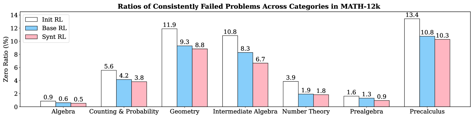### 3.3 Weakness Mitigation from Augmented Training The motivation behind SwS is to mitigate model weaknesses by explicitly targeting failure cases during training. To demonstrate its effectiveness, we use Qwen2.5-7B to analyze the ratios of consistently failed problems in the initial training set (MATH-12k) across three models: the initially trained model, the model continued trained on the initial training set, and the model trained on the augmented set with synthetic problems from the SwS pipeline. As shown in Figure 4, continued training on the augmented set enables the model to solve a greater proportion of previously failed problems across most domains compared to training on the initial set alone, with the greatest gains observed in Intermediate Algebra (20%), Geometry (5%), and Precalculus (5%) as its weakest areas. Notably, these improvements are achieved even though each original problem is sampled four times less frequently in the augmented set than in training on the original dataset alone, highlighting the efficiency of SwS-generated synthetic problems in RL training. ## 4 Extensions and Analysis | Model | GSM8K | AIME24 (Pass@32) | Prealgebra | Intermediate Algebra | Algebra | Precalculus | Number Theory | Counting & Probability | Geometry | | --- | --- | --- | --- | --- | --- | --- | --- | --- | --- | | Strong Student | 92.0 | 13.8 | 87.7 | 58.7 | 93.8 | 63.2 | 86.4 | 71.2 | 66.8 | | Weak Teacher | 93.3 | 7.2 | 88.2 | 64.3 | 95.5 | 71.2 | 93.0 | 81.4 | 63.0 | | Trained Student | 93.6 | 17.5 | 90.5 | 64.4 | 97.7 | 74.6 | 95.1 | 80.4 | 67.5 | Table 2: Performance on two representative benchmarks and category-specific results on MATH-500 of the weak teacher model and the strong student model. | Model | GSM8K | MATH 500 | Minerva Math | Olympiad Bench | GaoKao 2023 | AMC23 | AIME24 (Avg@ 1 / 32) | AIME25 (Avg@ 1 / 32) | Avg. | | --- | --- | --- | --- | --- | --- | --- | --- | --- | --- | | Qwen2.5-14B-IT | 94.7 | 79.6 | 41.9 | 45.6 | 68.6 | 57.5 | 16.7 / 11.6 | 6.7 / 10.9 | 51.4 | | + BaseRL | 94.5 | 85.4 | 44.1 | 52.1 | 71.7 | 65.0 | 20.0 / 21.6 | 20.0 / 22.3 | 56.6 | | + SwS-SE | 95.6 | 85.0 | 46.0 | 53.5 | 74.8 | 67.5 | 20.0 / 19.8 | 20.0 / 17.8 | 57.8 | | $Δ$ | +1.1 | -0.4 | +1.9 | +1.4 | +3.1 | +2.5 | +0.0 / -1.8 | +0.0 / -4.5 | +1.2 | Table 3: Experimental results of extending the SwS framework to the Self-evolving paradigm on the Qwen2.5-14B-Instruct model. ### 4.1 Weak-to-Strong Generalization for SwS Employing a powerful frontier model like QwQ [47] helps ensure answer quality. However, when training the top-performing reasoning model, no stronger model exists to produce reference answers for problems identified as its weaknesses. To explore the potential of applying our SwS pipeline to enhancing state-of-the-art models, we extend it to the Weak-to-Strong Generalization [2] setting by using a generally weaker teacher that may outperform the stronger model in specific domains to label reference answers for the synthetic problems. Intuitively, using a weaker teacher may result in mislabeled answers, which could significantly impair subsequent RL training. However, during the difficulty filtering stage, this risk is mitigated by using the initially trained policy to assess the difficulty of synthetic problems, as it rarely reproduces the same incorrect answers provided by the weaker teacher. As a byproduct, mislabeled cases are naturally filtered out alongside overly complex samples through accuracy-based screening. The experimental analysis on the validity of difficulty-level filtering in ensuring label correctness is presented in Table 5. <details> <summary>x4.png Details</summary>  ### Visual Description ## Grouped Bar Chart: Ratios of Consistently Failed Problems Across Categories in MATH-12k ### Overview This is a grouped bar chart comparing the performance of three reinforcement learning (RL) methods across seven mathematical problem categories from the MATH-12k dataset. The chart measures the "Zero Ratio (%)", which represents the percentage of problems that were consistently failed. A lower percentage indicates better performance. ### Components/Axes * **Chart Title:** "Ratios of Consistently Failed Problems Across Categories in MATH-12k" * **Y-Axis:** * **Label:** "Zero Ratio (%)" * **Scale:** Linear scale from 0 to 14, with major tick marks at intervals of 2 (0, 2, 4, 6, 8, 10, 12, 14). * **X-Axis:** * **Categories (from left to right):** Algebra, Counting & Probability, Geometry, Intermediate Algebra, Number Theory, Prealgebra, Precalculus. * **Legend:** Located in the top-left corner of the chart area. * **Init RL:** Represented by white bars with a black outline. * **Base RL:** Represented by light blue bars. * **Synt RL:** Represented by light pink bars. ### Detailed Analysis The chart displays the Zero Ratio (%) for each of the three RL methods within each of the seven math categories. The exact values, as labeled on top of each bar, are as follows: 1. **Algebra** * Init RL: 0.9% * Base RL: 0.6% * Synt RL: 0.5% 2. **Counting & Probability** * Init RL: 5.6% * Base RL: 4.2% * Synt RL: 3.8% 3. **Geometry** * Init RL: 11.9% * Base RL: 9.3% * Synt RL: 8.8% 4. **Intermediate Algebra** * Init RL: 10.8% * Base RL: 8.3% * Synt RL: 6.7% 5. **Number Theory** * Init RL: 3.9% * Base RL: 1.9% * Synt RL: 1.8% 6. **Prealgebra** * Init RL: 1.6% * Base RL: 1.3% * Synt RL: 0.9% 7. **Precalculus** * Init RL: 13.4% * Base RL: 10.8% * Synt RL: 10.3% **Visual Trend Verification:** For every single category, the bar for "Init RL" is the tallest, followed by "Base RL", and then "Synt RL" is the shortest. This creates a consistent descending stair-step pattern within each group from left to right (white -> blue -> pink). ### Key Observations * **Highest Failure Ratios:** The "Precalculus" category has the highest Zero Ratios for all three methods (Init RL: 13.4%, Base RL: 10.8%, Synt RL: 10.3%), indicating it is the most challenging category for these models. * **Lowest Failure Ratios:** The "Algebra" category has the lowest Zero Ratios (Init RL: 0.9%, Base RL: 0.6%, Synt RL: 0.5%), suggesting it is the easiest category. * **Consistent Performance Hierarchy:** The "Synt RL" method consistently achieves the lowest (best) Zero Ratio in every category, followed by "Base RL", with "Init RL" performing the worst. * **Largest Performance Gap:** The most significant absolute improvement from Init RL to Synt RL is seen in "Intermediate Algebra" (a reduction of 4.1 percentage points, from 10.8% to 6.7%). * **Smallest Performance Gap:** The smallest absolute improvement is in "Prealgebra" (a reduction of 0.7 percentage points, from 1.6% to 0.9%). ### Interpretation The data demonstrates a clear and consistent hierarchy in the effectiveness of the three reinforcement learning approaches for solving math problems from the MATH-12k dataset. The "Synt RL" method is universally superior, reducing the rate of consistently failed problems compared to both the "Base RL" and the initial "Init RL" models across all mathematical domains. The variation in Zero Ratios across categories (from ~0.5% in Algebra to ~13.4% in Precalculus) highlights the differing inherent difficulty of these problem types for the models. The consistent trend suggests that the enhancements in "Synt RL" provide a robust improvement that generalizes well across different mathematical skills, rather than being specialized for a single category. The fact that the relative ordering of the methods never changes strengthens the conclusion that "Synt RL" represents a meaningful advancement over the other two methods tested. The chart effectively argues for the adoption of the "Synt RL" approach to improve model reliability on this benchmark. </details> Figure 4: The ratios of consistently failed problems from different categories in the MATH-12k training set under different training configurations. (Base model: Qwen2.5-7B). We use the initially trained Qwen2.5-7B-Base as the student and Qwen2.5-Math-7B-Instruct as the teacher. Table 2 presents their performance on popular benchmarks and MATH-12k categories, where the student model generally outperforms the teacher. However, as shown in Table 2, the student policy further improves after training on weak teacher-labeled problems. This improvement stems from the difficulty filtering process, which removes problems with consistent student-teacher disagreement and retains those where the teacher is reliable but the student struggles, enabling targeted training on weaknesses. Detailed analysis can be found in Appendix 11. ### 4.2 Self-evolving Targeted Problem Synthesis In this section, we explore the potential of utilizing the Self-evolving paradigm to address model weaknesses by executing the full SwS pipeline using the policy itself. This self-evolving paradigm for identifying and mitigating weaknesses leverages self-consistency to guide itself to generate effective trajectories toward accurate answers [75], while also integrating general instruction-following capabilities from question generation and quality filtering to enhance reasoning. We use Qwen2.5-14B-Instruct as the base policy due to its balance between computational efficiency and instruction-following performance. The results are shown in Table 3, where the self-evolving SwS pipeline improves the baseline performance by 1.2% across all benchmarks, especially on the middle-level benchmarks like Gaokao and AMC. Although performance declines on AIME, we attribute this to the initial training data from DAPO and LightR1 already being specifically tailored to that benchmark. For further discussion of the Self-evolve SwS framework, refer to Appendix G. <details> <summary>x5.png Details</summary>  ### Visual Description ## Line Chart: Overall Accuracy (%) vs. Training Steps ### Overview The image is a line chart titled "(a) Overall Accuracy (%)". It plots the average accuracy (in percentage) of two different methods or conditions against the number of training steps. The chart shows a learning curve where accuracy increases rapidly at first and then gradually plateaus for both series. ### Components/Axes * **Title:** "(a) Overall Accuracy (%)" (centered at the top). * **Y-Axis:** Labeled "Average Accuracy (%)". The scale runs from 25.0 to 55.0, with major tick marks at 25.0, 31.0, 37.0, 43.0, 49.0, and 55.0. * **X-Axis:** Labeled "Training Steps". The scale runs from 0 to 140, with major tick marks at 0, 20, 40, 60, 80, 100, 120, and 140. * **Legend:** Located in the bottom-right quadrant of the chart area. It contains two entries: * A pink/salmon-colored circle labeled "Target All Pass@1". * A teal/cyan-colored circle labeled "Random All Pass@1". * **Data Series:** Two series are plotted, each consisting of individual data points (circles) and a fitted trend line. * **Target All Pass@1 (Pink):** Data points and a solid pink trend line. * **Random All Pass@1 (Teal):** Data points and a solid teal trend line. * **Grid:** A light gray grid is present, aligned with the major tick marks on both axes. ### Detailed Analysis **Trend Verification:** * **Target All Pass@1 (Pink Line):** The trend line shows a steep, concave-down increase from step 0 to approximately step 20, after which the slope becomes much shallower, continuing a steady, near-linear increase through step 140. * **Random All Pass@1 (Teal Line):** The trend line follows a very similar shape to the pink line—a steep initial rise followed by a gradual increase. However, its slope in the later stages (steps 40-140) is slightly less steep than the pink line's slope. **Data Point Extraction (Approximate Values):** The following table lists approximate accuracy values for each data point, read from the chart. Uncertainty is ±1.0% due to visual estimation. | Training Steps | Target All Pass@1 (Pink) Accuracy (%) | Random All Pass@1 (Teal) Accuracy (%) | | :--- | :--- | :--- | | 0 | ~29.0 | ~29.0 | | 10 | ~39.0 | ~40.0 | | 15 | ~46.0 | ~45.0 | | 20 | ~46.5 | ~47.0 | | 25 | ~49.5 | ~49.0 | | 30 | ~48.0 | ~47.5 | | 40 | ~49.0 | ~47.0 | | 50 | ~49.0 | ~46.0 | | 55 | ~49.5 | ~49.0 | | 65 | ~49.5 | ~51.0 | | 75 | ~50.0 | ~48.5 | | 80 | ~50.0 | ~49.5 | | 90 | ~49.5 | ~50.0 | | 95 | ~50.5 | ~50.5 | | 105 | ~51.0 | ~47.0 | | 115 | ~51.5 | ~48.0 | | 120 | ~52.0 | ~49.0 | | 130 | ~52.5 | ~52.0 | | 140 | ~52.5 | ~48.5 | **Spatial Grounding & Cross-Reference:** * The legend is positioned in the bottom-right, clearly associating the pink color with "Target All Pass@1" and the teal color with "Random All Pass@1". * Visual confirmation: The pink trend line and its associated data points are consistently positioned above the teal trend line and its points after approximately step 15, confirming the legend mapping is correct. ### Key Observations 1. **Rapid Initial Learning:** Both methods show a dramatic increase in accuracy from step 0 to step ~20, jumping from ~29% to the mid-40% range. 2. **Performance Gap:** After the initial phase (post step ~20), the "Target All Pass@1" (pink) series consistently achieves higher accuracy than the "Random All Pass@1" (teal) series. The gap appears to widen slightly as training progresses. 3. **Plateauing Effect:** The rate of improvement for both series slows significantly after step 40, indicating diminishing returns from additional training steps. 4. **Data Variance:** The individual data points for both series show scatter around their respective trend lines, indicating some variance in performance at different training steps. The "Random" series (teal) appears to have slightly more variance, with a notable low outlier at step 105 (~47.0%). ### Interpretation This chart demonstrates the learning efficiency of two different approaches ("Target" vs. "Random") over the course of model training. The "Target All Pass@1" method is superior, achieving a higher final accuracy (~52.5% vs. ~48.5% at step 140) and maintaining a consistent lead throughout most of the training process after the initial steps. The similar shape of the curves suggests both methods benefit from training in a comparable way—rapid early gains followed by refinement. The persistent gap indicates that the "Target" strategy provides a more effective learning signal or optimization path than the "Random" strategy. The plateau suggests that further significant gains beyond ~50-53% accuracy would require either more training steps (with potentially minimal improvement) or a fundamental change to the model or training method. The variance in the "Random" series might imply less stable or reliable training compared to the "Target" method. </details> <details> <summary>x6.png Details</summary>  ### Visual Description ## Scatter Plot with Fitted Curves: Competition Level Accuracy (%) ### Overview The image is a scatter plot chart titled "(b) Competition Level Accuracy (%)". It displays the performance of two different methods over the course of training, measured by average accuracy percentage. The chart includes individual data points and fitted trend lines for each method, showing how accuracy evolves as training progresses. ### Components/Axes * **Chart Title:** "(b) Competition Level Accuracy (%)" (centered at the top). * **X-Axis:** Labeled "Training Steps". The scale runs from 0 to 140, with major tick marks at intervals of 20 (0, 20, 40, 60, 80, 100, 120, 140). * **Y-Axis:** Labeled "Average Accuracy (%)". The scale runs from 1.0 to 16.0, with major tick marks at 1.0, 4.0, 7.0, 10.0, 13.0, and 16.0. * **Legend:** Located in the bottom-right quadrant of the chart area. It contains two entries: * A pink/salmon-colored circle marker labeled "Target Comp Avg@32". * A teal/cyan-colored circle marker labeled "Random Comp Avg@32". * **Data Series:** Two series of scatter points, each with a corresponding fitted trend line. * **Series 1 (Pink):** "Target Comp Avg@32". Data points are pink circles. The fitted line is a smooth, solid pink curve. * **Series 2 (Teal):** "Random Comp Avg@32". Data points are teal circles. The fitted line is a smooth, solid teal curve. * **Grid:** A light gray grid is present, with lines corresponding to the major ticks on both axes. ### Detailed Analysis **Data Series: Target Comp Avg@32 (Pink)** * **Trend Verification:** The pink trend line shows a steep initial increase that gradually flattens, exhibiting a logarithmic growth pattern. It consistently remains above the teal line after the initial steps. * **Approximate Data Points (Training Step, Accuracy %):** * (0, ~3.5) * (10, ~6.5) * (20, ~9.8) * (30, ~10.2) * (40, ~11.5) * (50, ~11.8) * (60, ~12.8) * (70, ~12.7) * (80, ~12.0) * (90, ~12.5) * (100, ~12.8) * (110, ~13.5) * (120, ~13.8) * (130, ~14.5) * (140, ~15.0) * (145, ~15.2) - Final point, slightly beyond the 140 tick. **Data Series: Random Comp Avg@32 (Teal)** * **Trend Verification:** The teal trend line also shows a steep initial increase that flattens, but it plateaus at a lower accuracy level than the pink line. The slope is less steep than the pink line after the initial phase. * **Approximate Data Points (Training Step, Accuracy %):** * (0, ~3.5) * (10, ~4.5) * (20, ~8.5) * (30, ~10.8) * (40, ~11.2) * (50, ~10.0) * (60, ~11.2) * (70, ~11.2) * (80, ~10.5) * (90, ~11.8) * (100, ~11.5) * (110, ~12.0) * (120, ~13.5) * (130, ~12.8) * (140, ~11.5) * (145, ~11.2) - Final point, slightly beyond the 140 tick. ### Key Observations 1. **Performance Gap:** The "Target Comp Avg@32" method (pink) achieves and maintains a higher average accuracy than the "Random Comp Avg@32" method (teal) for nearly all training steps after the very beginning. 2. **Convergence and Plateau:** Both methods show rapid improvement in the first 20-40 training steps, after which the rate of improvement slows significantly. The pink line appears to still be slightly increasing at step 145, while the teal line shows signs of plateauing or even slight decline after step 120. 3. **Variability:** The "Random Comp Avg@32" (teal) data points show greater scatter or variance around its trend line, especially in the later steps (e.g., points at steps 120, 130, 140, 145). The "Target Comp Avg@32" (pink) points are more tightly clustered around its trend line. 4. **Initial Conditions:** Both methods start at approximately the same accuracy (~3.5%) at step 0. ### Interpretation This chart demonstrates a comparative analysis of two training strategies or model variants, likely in a machine learning or optimization context. The "Target" method, which may involve focused or guided training, significantly outperforms the "Random" method, which may involve less directed exploration. The data suggests that while both approaches benefit from initial training, the targeted strategy leads to a higher final performance ceiling and more stable progress. The greater variance in the "Random" method's results indicates less predictable outcomes, which could be a drawback in practical applications. The persistent gap between the two trend lines implies that the advantage gained from the targeted approach is sustained throughout the observed training period and is not merely an early-stage effect. The chart effectively argues for the superiority of the "Target Comp Avg@32" method for maximizing competition-level accuracy within the given training budget. </details> <details> <summary>x7.png Details</summary>  ### Visual Description ## Line Chart with Scatter Points: Training Batch Accuracy (%) ### Overview The image is a line chart with overlaid scatter points, titled "(c) Training Batch Accuracy (%)". It plots the average accuracy (in percentage) of two different training methods against the number of training steps. The chart demonstrates a learning curve where accuracy increases rapidly at first and then gradually plateaus for both methods. ### Components/Axes * **Chart Title:** "(c) Training Batch Accuracy (%)" (centered at the top). * **Y-Axis:** Labeled "Average Accuracy (%)". The scale runs from 0.0 to 80.0, with major tick marks and grid lines at intervals of 16.0 (0.0, 16.0, 32.0, 48.0, 64.0, 80.0). * **X-Axis:** Labeled "Training Steps". The scale runs from 0 to 140, with major tick marks and grid lines at intervals of 20 (0, 20, 40, 60, 80, 100, 120, 140). * **Legend:** Located in the bottom-right quadrant of the chart area. It contains two entries: * A pink circle symbol labeled "Target Training Acc". * A cyan circle symbol labeled "Random Training Acc". * **Data Series:** 1. **Target Training Acc:** Represented by pink circular scatter points and a solid pink trend line. 2. **Random Training Acc:** Represented by cyan circular scatter points and a solid cyan trend line. ### Detailed Analysis **Trend Verification:** * **Target Training Acc (Pink):** The line and points show a steep, logarithmic-like increase from near 0% at step 0, crossing 32% before step 20, and continuing to rise at a decreasing rate. The trend is consistently upward, approaching approximately 72% by step 140. * **Random Training Acc (Cyan):** This series follows a very similar logarithmic growth pattern but is consistently positioned above the Target series. It also starts near 0%, rises steeply, and approaches a higher final value of approximately 78% by step 140. **Data Point Extraction (Approximate Values):** The following table lists approximate accuracy values for key training steps, derived from visual inspection of the scatter points against the grid. | Training Steps | Target Training Acc (Pink) | Random Training Acc (Cyan) | | :--- | :--- | :--- | | 0 | ~0% | ~0% | | 10 | ~10% | ~14% | | 20 | ~40% | ~48% | | 40 | ~56% | ~60% | | 60 | ~60% | ~65% | | 80 | ~64% | ~68% | | 100 | ~67% | ~71% | | 120 | ~69% | ~74% | | 140 | ~72% | ~78% | **Spatial Grounding & Cross-Reference:** The legend is positioned in the bottom-right, clearly associating the pink color/symbol with "Target Training Acc" and the cyan color/symbol with "Random Training Acc". This mapping is consistently applied across all data points and trend lines throughout the chart. The cyan points and line are visually above their pink counterparts at every corresponding training step after the initial point. ### Key Observations 1. **Consistent Performance Gap:** The "Random Training Acc" method achieves a higher average accuracy than the "Target Training Acc" method at every measured step after the start. The gap appears to widen slightly as training progresses. 2. **Similar Learning Dynamics:** Both methods exhibit nearly identical learning curve shapes (rapid initial improvement followed by diminishing returns), suggesting they are learning from the data in a fundamentally similar way, albeit with different efficiencies. 3. **Potential Outlier:** At approximately step 10, the cyan ("Random") data point appears slightly lower relative to its trend line compared to other points, though it is still above the pink ("Target") point at the same step. 4. **High Final Accuracy:** Both methods reach high accuracy levels (>70%) within 140 training steps, indicating effective learning for the given task. ### Interpretation This chart compares the training efficiency of two different approaches, likely in a machine learning context. The "Random Training Acc" method demonstrates superior performance, achieving higher accuracy faster and maintaining that lead throughout the training process shown. The data suggests that the strategy or initialization used in the "Random" method is more effective for this specific task than the "Target" method. The fact that both curves follow the same logarithmic trajectory indicates that the underlying learning process (e.g., gradient descent optimization) is similar, but the "Random" method starts from a more advantageous point or follows a more efficient path in the loss landscape. The narrowing but persistent gap implies that while both models are learning the task, the "Random" model consistently finds better solutions at each stage of training. This could have implications for training time, resource allocation, and final model performance. The chart provides strong visual evidence to favor the "Random Training" approach for this particular application. 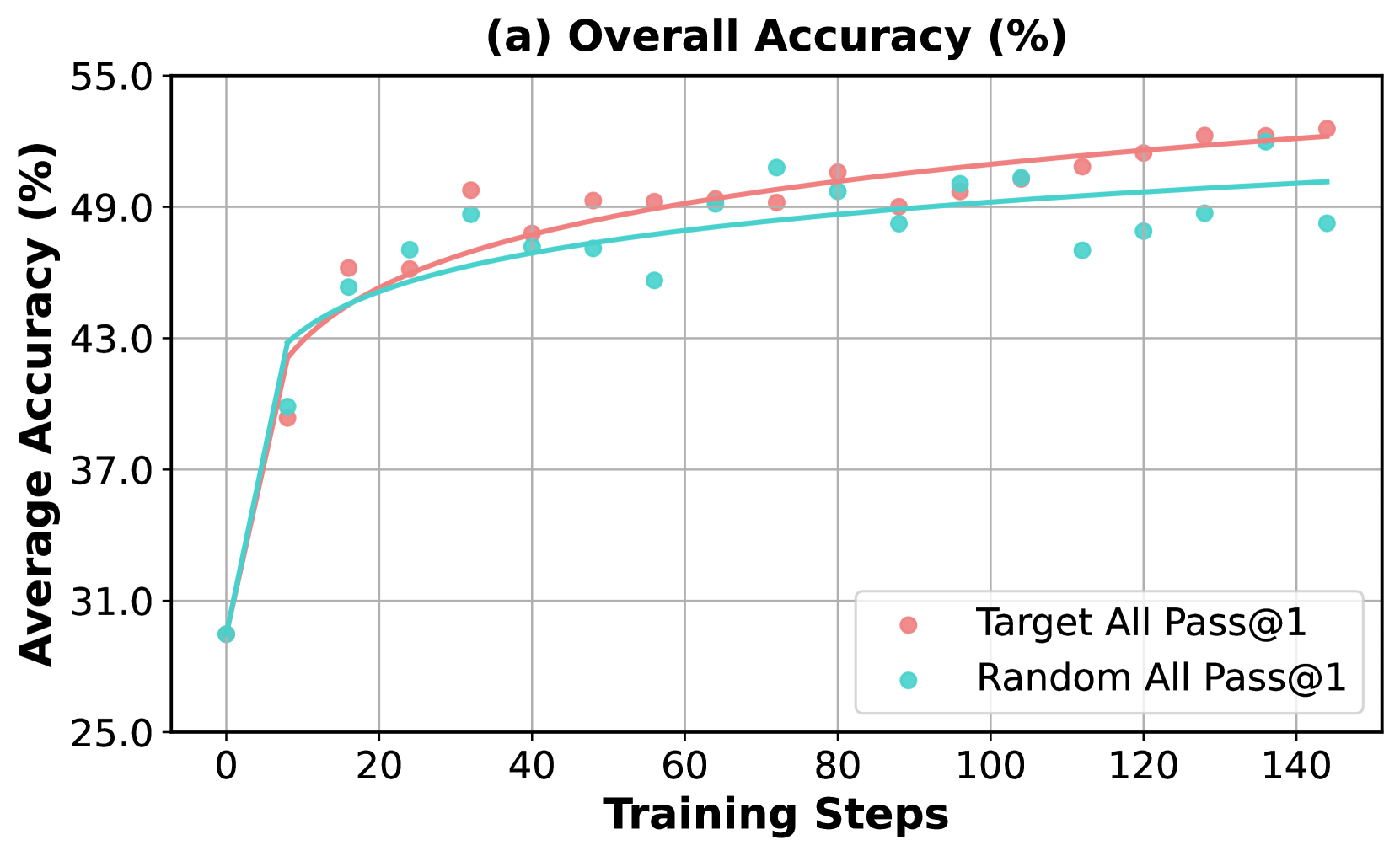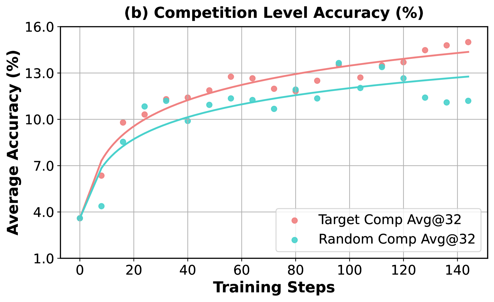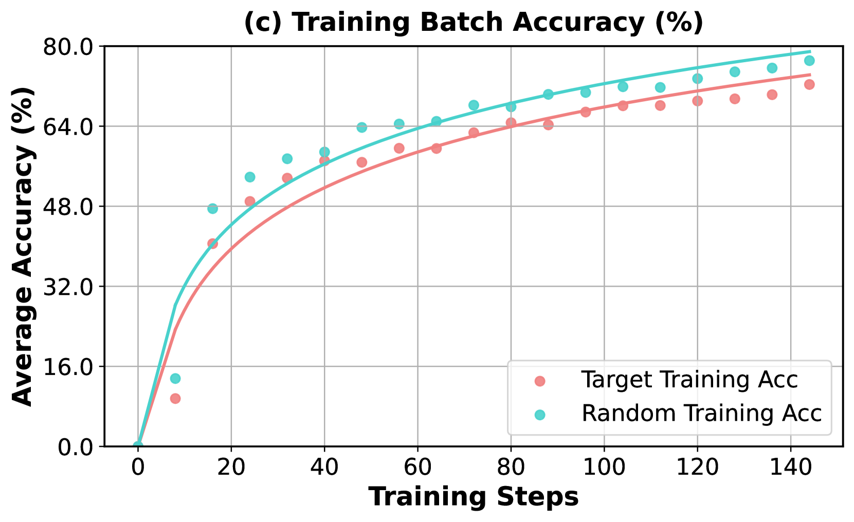</details> Figure 5: Comparison of accuracy improvements using (a) Pass@1 on full benchmarks evaluated in Table 1 and (b) Avg@32 on the competition-level benchmarks. (c) illustrates the proportion of prompts within a batch that achieved 100% correctness across multiple rollouts during training. <details> <summary>x8.png Details</summary>  ### Visual Description ## Scatter Plot with Trend Lines: Overall Accuracy (%) vs. Training Steps ### Overview The image is a scatter plot chart titled "(a) Overall Accuracy (%)". It displays the relationship between the number of training steps (x-axis) and the average accuracy percentage (y-axis) for three different task difficulty categories: "Difficulty", "Simple", and "Medium". Each category is represented by colored data points and a corresponding fitted trend line. ### Components/Axes * **Chart Title:** "(a) Overall Accuracy (%)" (Top center) * **Y-Axis:** * **Label:** "Average Accuracy (%)" (Left side, rotated vertically) * **Scale:** Linear scale ranging from 45.2 to 53.2. * **Major Tick Marks:** 45.2, 46.8, 48.4, 50.0, 51.6, 53.2. * **X-Axis:** * **Label:** "Training Steps" (Bottom center) * **Scale:** Linear scale ranging from 0 to 200. * **Major Tick Marks:** 0, 25, 50, 75, 100, 125, 150, 175, 200. * **Legend:** Located in the bottom-right quadrant of the chart area. * **"Difficulty":** Represented by red/salmon-colored circular points and a matching red/salmon trend line. * **"Simple":** Represented by teal/turquoise-colored circular points and a matching teal/turquoise trend line. * **"Medium":** Represented by bright blue/cyan-colored circular points and a matching bright blue/cyan trend line. * **Grid:** A light gray grid is present, aligning with the major tick marks on both axes. ### Detailed Analysis **Trend Verification & Data Point Approximation:** * **"Difficulty" (Red/Salmon Series):** * **Trend:** The trend line shows a steep, concave-down increase from low accuracy at the start, which gradually flattens as training steps increase. It starts as the lowest-performing category but shows the most significant improvement. * **Approximate Data Points (Trend Line):** * Step ~10: ~45.5% * Step 50: ~48.8% * Step 100: ~50.2% * Step 150: ~51.0% * Step 200: ~51.8% * **Notable Scatter:** There is significant variance in the individual data points. For example, a point near step 60 is notably lower (~47.2%) than the trend line, while points after step 150 show high variance, with some reaching near 53.0%. * **"Simple" (Teal/Turquoise Series):** * **Trend:** The trend line starts at the highest accuracy level but has the shallowest slope, indicating the slowest rate of improvement. It is nearly linear with a very slight curve. * **Approximate Data Points (Trend Line):** * Step ~10: ~49.2% * Step 50: ~50.0% * Step 100: ~50.5% * Step 150: ~50.8% * Step 200: ~51.0% * **Notable Scatter:** The data points are relatively tightly clustered around the trend line compared to the other series, suggesting more consistent performance on simple tasks. * **"Medium" (Bright Blue/Cyan Series):** * **Trend:** The trend line shows a moderate, concave-down increase, positioned between the "Difficulty" and "Simple" lines in both starting point and slope. * **Approximate Data Points (Trend Line):** * Step ~10: ~47.0% * Step 50: ~49.2% * Step 100: ~50.4% * Step 150: ~51.2% * Step 200: ~51.5% * **Notable Scatter:** The scatter is moderate. A cluster of points around step 100-125 sits slightly below the trend line. **Spatial Grounding:** The legend is positioned in the bottom-right, overlapping the lower portion of the data field. The "Difficulty" (red) trend line begins lowest on the left (y ~45.5 at x~10) and ends highest on the right (y ~51.8 at x=200). The "Simple" (teal) line begins highest on the left (y ~49.2 at x~10) and ends lowest on the right (y ~51.0 at x=200). The "Medium" (blue) line is intermediate at both ends. ### Key Observations 1. **Convergence and Crossover:** All three trend lines converge in the region of 100-125 training steps, where their accuracy values are very close (~50.2-50.5%). After this point, the "Difficulty" line surpasses the others. 2. **Diminishing Returns:** All three curves show signs of diminishing returns (concave-down shape), where the gain in accuracy per additional training step decreases as training progresses. 3. **Performance Hierarchy Inversion:** The initial performance hierarchy ("Simple" > "Medium" > "Difficulty") inverts by the end of the plotted training steps ("Difficulty" > "Medium" > "Simple"). 4. **Variance:** The "Difficulty" category exhibits the highest variance in data points, especially at higher step counts, suggesting less predictable outcomes when training on hard tasks. ### Interpretation This chart demonstrates the learning dynamics of a model across tasks of varying difficulty. The data suggests that: * **Model Learning is Non-Linear:** Accuracy does not improve at a constant rate; the most significant gains happen early in training. * **Task Difficulty Impacts Learning Trajectory:** The model starts with a better baseline on simple tasks but learns more from complex ("Difficulty") tasks over time. The steeper slope for "Difficulty" indicates that the model's capacity to handle complex problems improves more dramatically with extended training. * **Potential for Further Training:** Since the curves, especially for "Difficulty" and "Medium," have not fully plateaued by 200 steps, it is plausible that accuracy could continue to increase with further training, though at a slower rate. * **Training Stability:** The higher variance in the "Difficulty" series might indicate that training on hard tasks is less stable or more sensitive to specific data batches or training conditions. The inversion of performance hierarchy is a key insight. It implies that while simple tasks are easier to learn initially, sustained training disproportionately benefits the model's ability to solve more challenging problems, ultimately leading to higher overall accuracy on those hard tasks. This is a common and desirable pattern in machine learning, indicating the model is developing robust, generalizable features rather than just memorizing simple patterns. 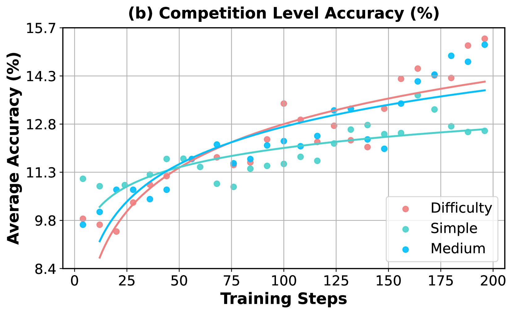</details> <details> <summary>x9.png Details</summary>  ### Visual Description ## Scatter Plot with Trend Lines: Competition Level Accuracy (%) ### Overview The image is a scatter plot with overlaid trend lines, titled "(b) Competition Level Accuracy (%)". It displays the relationship between the number of training steps (x-axis) and the average accuracy percentage (y-axis) for three different difficulty levels of tasks or competitions. The chart shows how model performance improves with training across these categories. ### Components/Axes * **Title:** "(b) Competition Level Accuracy (%)" (centered at the top). * **X-Axis:** Labeled "Training Steps". The scale runs from 0 to 200, with major tick marks at intervals of 25 (0, 25, 50, 75, 100, 125, 150, 175, 200). * **Y-Axis:** Labeled "Average Accuracy (%)". The scale runs from 8.4 to 15.7, with major tick marks at intervals of 1.5 (8.4, 9.8, 11.3, 12.8, 14.3, 15.7). * **Legend:** Located in the bottom-right corner of the plot area. It contains three entries: * A red/salmon-colored circle labeled "Difficulty". * A teal/green-colored circle labeled "Simple". * A blue-colored circle labeled "Medium". * **Data Series:** Three sets of scatter points, each with a corresponding smoothed trend line of the same color. * **Grid:** A light gray grid is present, aligning with the major ticks on both axes. ### Detailed Analysis **Trend Verification:** * **Difficulty (Red/Salmon):** The trend line shows a strong, consistent upward slope, starting from the lowest accuracy at step 0 and ending at the highest accuracy at step 200. * **Simple (Teal/Green):** The trend line slopes upward but begins to plateau significantly after approximately 100 training steps, showing the least overall improvement in the later stages. * **Medium (Blue):** The trend line slopes upward steadily, positioned between the other two lines for most of the training progression. **Data Point Extraction (Approximate Values):** * **At ~0 Training Steps:** * Difficulty: ~9.8% * Simple: ~11.0% * Medium: ~9.7% * **At ~50 Training Steps:** * Difficulty: ~11.2% * Simple: ~11.6% * Medium: ~11.4% * **At ~100 Training Steps:** * Difficulty: ~13.4% (a notable high point) * Simple: ~11.6% * Medium: ~12.2% * **At ~150 Training Steps:** * Difficulty: ~13.0% * Simple: ~12.4% * Medium: ~13.2% * **At ~200 Training Steps (Final Points):** * Difficulty: ~15.5% (highest final value) * Simple: ~12.6% (lowest final value) * Medium: ~15.3% ### Key Observations 1. **Performance Hierarchy Inversion:** At the start of training (step 0), the "Simple" category has the highest accuracy, while "Difficulty" and "Medium" are lower and similar. By the end of training (step 200), this order is inverted: "Difficulty" achieves the highest accuracy, followed closely by "Medium", with "Simple" now showing the lowest accuracy. 2. **Learning Curves:** The "Difficulty" series shows the steepest and most sustained learning curve. The "Simple" series learns quickly initially but hits a performance ceiling much earlier. The "Medium" series shows steady, consistent improvement throughout. 3. **Data Variance:** The scatter points for all series show variance around their trend lines, indicating fluctuations in accuracy between individual training steps. The "Difficulty" series appears to have slightly higher variance in the later stages (e.g., points at steps ~100 and ~160). 4. **Crossover Point:** The trend lines for "Difficulty" and "Medium" cross over the "Simple" trend line between 25 and 50 training steps, marking the point where they begin to consistently outperform the "Simple" tasks. ### Interpretation This chart suggests that the model's ability to learn and improve is heavily influenced by task difficulty. While simpler tasks are mastered quickly, they offer less room for long-term improvement, leading to an early plateau. In contrast, more difficult tasks ("Difficulty" and "Medium") provide a richer learning signal, allowing the model to continue refining its performance over many more training steps. The fact that the "Difficulty" category ultimately yields the highest accuracy implies that the model's capacity is best utilized by challenging problems, and its performance on them scales well with extended training. This has implications for training strategies: allocating more training steps to harder tasks may be more beneficial for maximizing final model capability than focusing on easy tasks. The initial lower accuracy on hard tasks is expected, but the steep learning curve demonstrates effective knowledge acquisition. 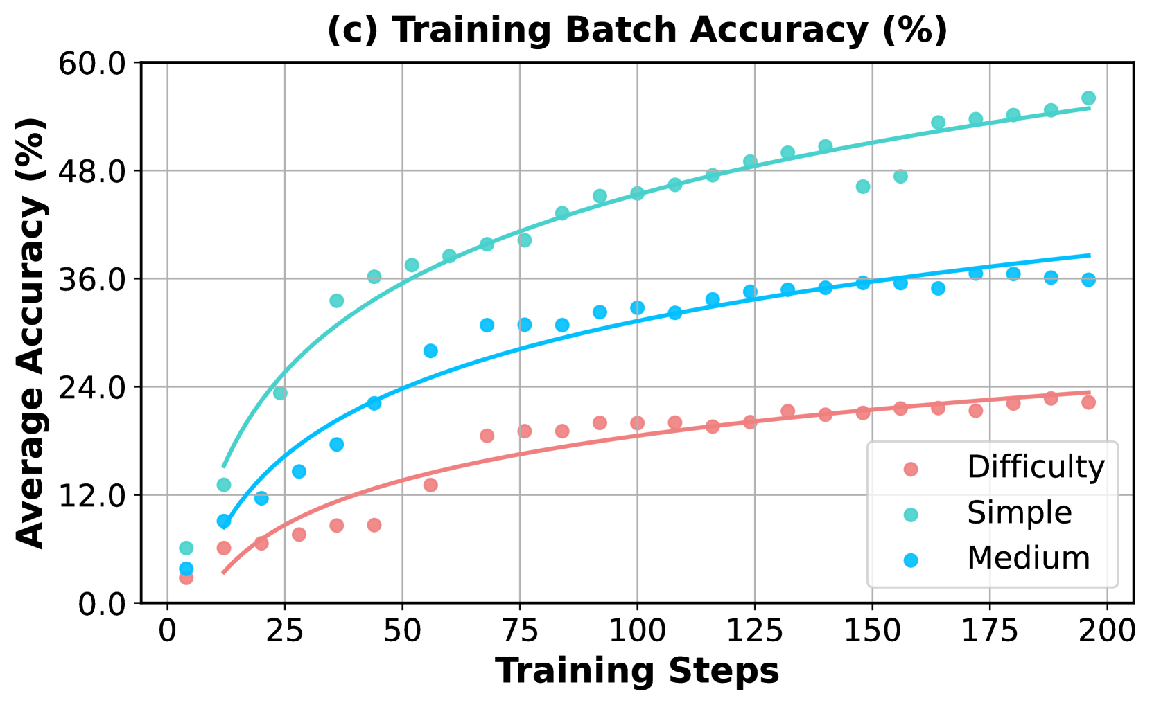</details> <details> <summary>x10.png Details</summary>  ### Visual Description ## Line Chart: Training Batch Accuracy (%) by Task Difficulty ### Overview This image is a line chart titled "(c) Training Batch Accuracy (%)". It plots the average accuracy (in percentage) of a machine learning model against the number of training steps. The chart compares the model's performance on three distinct categories of task difficulty: Simple, Medium, and Difficulty (presumably "Hard"). The data is presented as scatter points with fitted trend lines for each category. ### Components/Axes * **Chart Title:** "(c) Training Batch Accuracy (%)" (Top center) * **Y-Axis:** * **Label:** "Average Accuracy (%)" (Left side, rotated vertically) * **Scale:** Linear scale from 0.0 to 60.0. * **Major Ticks:** 0.0, 12.0, 24.0, 36.0, 48.0, 60.0. * **X-Axis:** * **Label:** "Training Steps" (Bottom center) * **Scale:** Linear scale from 0 to 200. * **Major Ticks:** 0, 25, 50, 75, 100, 125, 150, 175, 200. * **Legend:** Located in the bottom-right quadrant of the chart area. * **Title:** "Difficulty" * **Series 1:** "Simple" - Represented by teal/turquoise colored circles and a matching trend line. * **Series 2:** "Medium" - Represented by bright blue colored circles and a matching trend line. * **Series 3:** "Difficulty" - Represented by salmon/pink colored circles and a matching trend line. * **Grid:** A light gray grid is present, aligning with the major ticks on both axes. ### Detailed Analysis The chart shows three distinct learning curves, all exhibiting a logarithmic growth pattern (rapid initial improvement that gradually plateaus). **1. Simple Tasks (Teal/Turquoise Series):** * **Trend:** Shows the steepest initial ascent and achieves the highest overall accuracy. * **Key Data Points (Approximate):** * Step 0: ~6% * Step 25: ~24% * Step 50: ~36% * Step 100: ~46% * Step 150: ~50% (Note: A data point at step ~150 dips to ~47%, slightly below the trend line) * Step 200: ~55% * **Trend Line:** Starts near 0% and curves upward, approaching ~55% at step 200. **2. Medium Tasks (Bright Blue Series):** * **Trend:** Shows moderate initial growth, consistently performing below the Simple tasks but above the Difficulty tasks. * **Key Data Points (Approximate):** * Step 0: ~4% * Step 25: ~14% * Step 50: ~22% * Step 100: ~32% * Step 150: ~35% * Step 200: ~36% * **Trend Line:** Starts near 0% and curves upward, approaching ~38% at step 200. **3. Difficulty Tasks (Salmon/Pink Series):** * **Trend:** Shows the slowest rate of improvement and the lowest overall accuracy. * **Key Data Points (Approximate):** * Step 0: ~3% * Step 25: ~8% * Step 50: ~13% * Step 100: ~19% * Step 150: ~22% * Step 200: ~23% * **Trend Line:** Starts near 0% and curves upward, approaching ~24% at step 200. ### Key Observations 1. **Clear Performance Hierarchy:** There is a strict and consistent ordering of performance: Simple > Medium > Difficulty at every measured training step after the initial points. 2. **Diminishing Returns:** All three curves demonstrate diminishing returns. The most significant accuracy gains occur within the first 50-75 training steps. After step 100, the rate of improvement slows considerably for all categories. 3. **Convergence Gap:** The performance gap between the categories remains substantial throughout training. At step 200, the model is approximately 19 percentage points more accurate on Simple tasks than on Difficulty tasks. 4. **Data Variance:** The scatter of data points around the trend lines appears relatively low, suggesting consistent performance within each difficulty category at each evaluation step. The most notable outlier is a single "Simple" data point around step 150 that falls below its trend line. ### Interpretation This chart visualizes a fundamental principle in machine learning: task complexity directly impacts learning efficiency and final model performance. The data suggests that the model finds it significantly easier to learn patterns associated with "Simple" tasks, achieving high accuracy quickly. "Medium" tasks require more training to reach a moderate level of proficiency. "Difficulty" tasks present a substantial challenge, with the model showing slow, incremental learning that plateaus at a much lower accuracy ceiling. The consistent logarithmic growth indicates that the model is successfully learning from the training data across all difficulties, but its capacity or the information content of the data limits its ultimate performance on harder tasks. The persistent performance gap implies that simply increasing training steps (beyond 200) may yield only marginal improvements, especially for the Difficulty category. To improve performance on harder tasks, one might need to consider changes to the model architecture, training data quality/quantity, or learning algorithms, rather than just extended training. </details> Figure 6: Comparison of incorporating synthetic problems of varying difficulty levels during the augmented RL training. For a detailed description of accuracy trends on evaluation benchmarks and the training set, refer to the caption in Figure 5. ### 4.3 Weakness-driven Selection In this section, we explore an alternative extension that augments the initial training set using identified weaknesses and a larger mathematical reasoning dataset. Specifically, we use the Qwen2.5-7B model, identify its weaknesses on the MATH-12k training set, and retrieve augmented problems from Big-Math [1] that align with its failure cases, incorporating them into the initial training set for augmentation. We employ a category-specific selection strategy similar to the budget allocation in Eq. 5, using KNN [5] to identify the most relevant problems within each category. The total augmentation budget is also set to 40k. We compare this approach to a baseline where the model is trained on an augmented set incorporated with randomly selected problems from Big-Math. Details of the selection procedure are provided in Appendix H. As shown in Figure 5, the model trained with weakness-driven augmentation outperforms the random augmentation strategy in terms of accuracy on both the whole evaluated benchmarks (Figure 5.a) and the competition-level subset (Figure 5.b), demonstrating the effectiveness of the weakness-driven selection strategy. In Figure 5.c, it is worth noting that the model quickly fits the randomly selected problems in training, which then cease to provide meaningful training signals in the GRPO algorithm. In contrast, since the failure cases highlight specific weaknesses of the model’s capabilities, the problems selected based on them remain more challenging and more aligned with its deficiencies, providing richer learning signals and promoting continued development of reasoning skills. ### 4.4 Impact of Question Difficulty We ablate the impact of the difficulty levels of synthetic problems used in the augmented RL training. In this section, we define the difficulty of a synthetic problem based on the accuracy of multiple rollouts generated by the initially trained model, base from Qwen2.5-7B. We incorporate synthetic problems of three predefined difficulty levels—simple, medium, and hard—into the augmented RL training. These levels correspond to accuracy ranges of $[5,7]$ , $[3,5]$ , and $[1,4]$ out of 8 sampled responses, respectively. For each level, we sample 40k examples and combine them with the initial training set for a second training stage lasting 200 steps. The experimental results are shown in Figure 6. Similar to the findings in Section 4.3, the model fits more quickly on the simple augmented set and initially achieves the best performance across all evaluation benchmarks, including competition-level tasks, but then saturates with no further improvement. In contrast, the medium and hard augmented sets lead to slower convergence on the training set but result in more sustained performance gains on the evaluation set, with the hardest problems providing the longest-lasting training benefits. 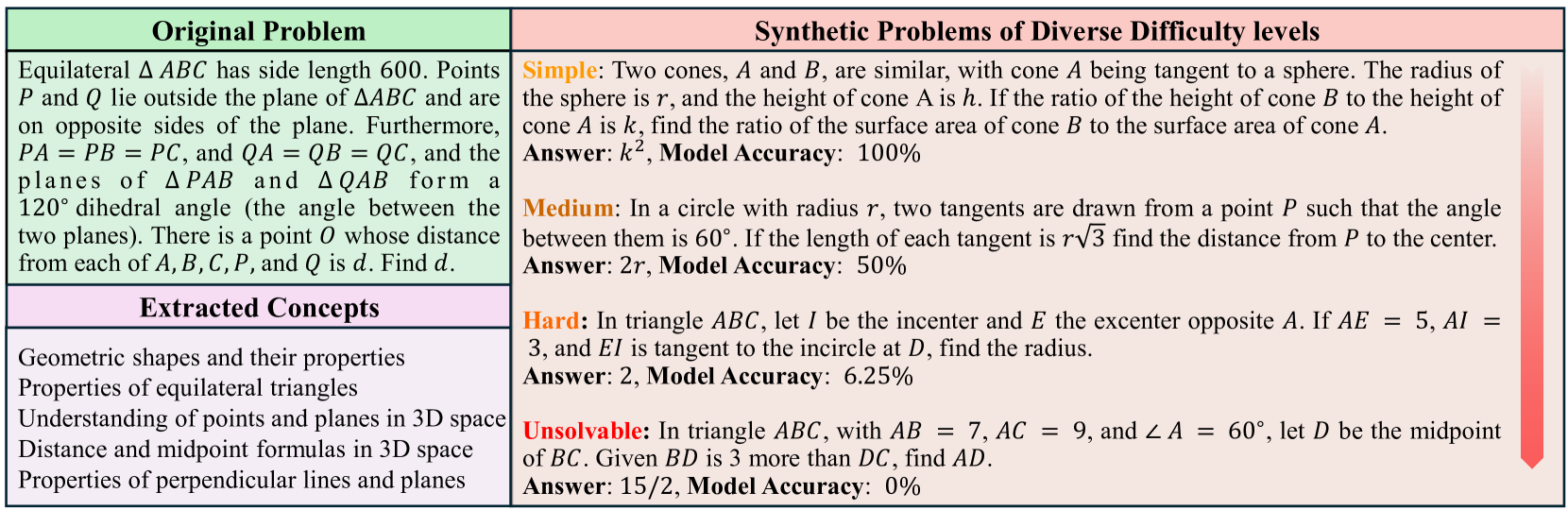<details> <summary>x11.png Details</summary>  ### Visual Description ## Technical Diagram: Geometry Problem Analysis Table ### Overview The image displays a structured table comparing a complex original geometry problem with a set of synthetic problems of varying difficulty levels. It also lists the key geometric concepts extracted from the original problem. The table is divided into two main columns, with a vertical gradient bar on the far right indicating a progression of difficulty or model performance. ### Components/Axes The table has the following structural components: 1. **Header Row**: Contains two main column titles. * **Left Column Header**: "Original Problem" (green background). * **Right Column Header**: "Synthetic Problems of Diverse Difficulty levels" (pink background). 2. **Left Column**: Contains two vertically stacked cells. * **Top Cell**: The "Original Problem" text. * **Bottom Cell**: Titled "Extracted Concepts" (purple background), containing a bulleted list. 3. **Right Column**: Contains four vertically stacked cells, each presenting a problem at a different difficulty level. The difficulty labels are color-coded. * **Simple** (orange text) * **Medium** (orange text) * **Hard** (orange text) * **Unsolvable** (red text) 4. **Visual Element**: A vertical gradient bar on the far right edge of the image, transitioning from red at the top to white at the bottom, visually correlating with the increasing difficulty of the problems from top to bottom. ### Detailed Analysis / Content Details #### **Left Column: Original Problem & Concepts** * **Original Problem Text**: > Equilateral Δ ABC has side length 600. Points P and Q lie outside the plane of ΔABC and are on opposite sides of the plane. Furthermore, PA = PB = PC and QA = QB = QC, and the planes of ΔPAB and ΔQAB form a 120° dihedral angle (the angle between the two planes). There is a point O whose distance from each of A, B, C, P, and Q is d. Find d. * **Extracted Concepts List**: * Geometric shapes and their properties * Properties of equilateral triangles * Understanding of points and planes in 3D space * Distance and midpoint formulas in 3D space * Properties of perpendicular lines and planes #### **Right Column: Synthetic Problems** Each problem includes a statement, a final answer, and a "Model Accuracy" percentage. 1. **Simple**: * **Problem**: Two cones, A and B, are similar, with cone A being tangent to a sphere. The radius of the sphere is r, and the height of cone A is h. If the ratio of the height of cone B to the height of cone A is k, find the ratio of the surface area of cone B to the surface area of cone A. * **Answer**: k² * **Model Accuracy**: 100% 2. **Medium**: * **Problem**: In a circle with radius r, two tangents are drawn from a point P such that the angle between them is 60°. If the length of each tangent is r√3 find the distance from P to the center. * **Answer**: 2r * **Model Accuracy**: 50% 3. **Hard**: * **Problem**: In triangle ABC, let I be the incenter and E the excenter opposite A. If AE = 5, AI = 3, and EI is tangent to the incircle at D, find the radius. * **Answer**: 2 * **Model Accuracy**: 6.25% 4. **Unsolvable**: * **Problem**: In triangle ABC, with AB = 7, AC = 9, and ∠A = 60°, let D be the midpoint of BC. Given BD is 3 more than DC, find AD. * **Answer**: 15/2 * **Model Accuracy**: 0% ### Key Observations 1. **Clear Difficulty Progression**: The synthetic problems are explicitly labeled from "Simple" to "Unsolvable," with a corresponding visual gradient bar. 2. **Inverse Relationship with Model Accuracy**: There is a stark, inverse correlation between problem difficulty and the reported "Model Accuracy." Accuracy plummets from 100% for the Simple problem to 0% for the Unsolvable one. 3. **Problem Type Variation**: The synthetic problems cover different geometric domains: 3D similarity (cones), circle tangents, triangle centers (incenter/excenter), and a potentially contradictory planar geometry setup. 4. **"Unsolvable" Problem Anomaly**: The problem labeled "Unsolvable" still provides a definitive answer (15/2). The label and 0% accuracy likely indicate that the problem's given conditions are internally contradictory or impossible to satisfy in Euclidean geometry, making a valid solution unattainable despite the numerical answer provided. ### Interpretation This table appears to be from a research or evaluation context, likely assessing the performance of an AI or computational model on geometry problems. The "Original Problem" serves as a complex benchmark, from which core concepts are extracted. The "Synthetic Problems" are then generated to test the model's grasp of these concepts at graduated difficulty levels. The data suggests a significant limitation in the model's reasoning capabilities. While it achieves perfect accuracy on straightforward application of concepts (Simple), its performance degrades rapidly as problems require more integrated knowledge, spatial reasoning, or handling of complex constraints (Medium, Hard). The 0% accuracy on the "Unsolvable" problem is particularly telling; it indicates the model either failed to detect the logical inconsistency in the problem statement or attempted to compute an answer despite the impossibility, highlighting a lack of robust meta-reasoning about problem validity. The "Extracted Concepts" list acts as a bridge, showing the foundational knowledge the synthetic problems are designed to probe. The overall presentation argues that problem difficulty is not merely about computational complexity but about the depth of conceptual understanding and logical coherence required, areas where the evaluated model shows a clear performance cliff. </details> Figure 7: Illustration of a geometry problem from the MATH-12k failed set, with extracted concepts and conceptually linked synthetic problems across different difficulty levels. ### 4.5 Case Study Figure 7 presents an illustration of a geometry failure case from the MATH-12k training set, accompanied by extracted concepts and our weakness-driven synthetic questions of varying difficulty levels, all closely aligned with the original question. The question focuses on three-dimensional distance and triangle understanding, with key concepts such as “Properties of equilateral triangles” and “Distance and midpoint formulas in 3D space” representing essential knowledge required to solve the problem. Notably, the corresponding synthetic questions exhibit similar semantics—such as “finding distance” in Medium and “understanding triangles” in Hard. Practicing on such targeted problems helps mitigate weaknesses and enhances reasoning capabilities within the relevant domain. ## 5 Conclusion In this work, we introduce a S elf-aware W eakness-driven Problem S ynthesis (SwS) framework (SwS) in reinforcement learning for LLM reasoning, which synthesizes problems based on weaknesses identified from the model’s failure cases during a preliminary training phase and includes them into subsequent augmented training. We conduct a detailed analysis of incorporating such synthetic problems into training and find that focusing on the model’s failures can enhance its reasoning generalization and mitigate its weaknesses, resulting in overall performance improvements. Furthermore, we extend the framework to the paradigms of Weak-to-Strong Generalization, Self-evolving, and Weakness-driven Selection, demonstrating its comprehensiveness and robustness. ## 6 Discussions, Limitations and Future Work This paper presents a comprehensive Self-aware Weakness-driven Problem Synthesis (SwS) framework to address the model’s reasoning deficiencies through reinforcement learning (RL) training. Although the SwS framework is effective across a wide range of model sizes, there are still several limitations to it: (1) Employing both a strong instruction model and an answer-labeling reasoning model may lead to computation and time costs. (2) Our framework mainly focuses on the RL setting, as our primary goal is to mitigate the model’s weaknesses by fully activating its inherent reasoning abilities without distilling external knowledge. Exploring how to leverage a similar pipeline for enhancing model capabilities through fine-tuning or distillation remains an open direction for future research. (3) The synthetic problems generated by open-source instruction models in the SwS framework may still lack sufficient complexity to elicit the deeper reasoning capabilities of the model, especially on more challenging problems. This limitation is pronounced in the Self-evolving setting in Section 4.2, which relies solely on a 14B model for problem generation, with performance improvements limited to only moderate or simple benchmarks. This raises questions about the actual utility of problems generated from the LLaMA-3.3-70B-Instruct in the main experiments on top-challenging benchmarks like AIME. One potential strategy is to use Evolve-Instruct [56, 30] to further refine the generated problems to the desired level of difficulty. However, how to effectively raise the upper bound of difficulty in synthetic problems generated by instruction models remains an open problem and warrants further exploration. In the future, we aim to identify model weaknesses from multiple perspectives beyond simple answer accuracy, with the goal of synthesizing more targeted problems to improve sample efficiency. Additionally, we plan to extend the SwS framework to more general tasks beyond reasoning, incorporating an off-the-shelf reward model to provide feedback instead of verifiable answers. Lastly, we also seek to implement the SwS pipeline in more advanced reasoning models equipped with Long-CoT capabilities, further pushing the boundaries of open-source large reasoning models. ## References - Albalak et al. [2025] Alon Albalak, Duy Phung, Nathan Lile, Rafael Rafailov, Kanishk Gandhi, Louis Castricato, Anikait Singh, Chase Blagden, Violet Xiang, Dakota Mahan, et al. Big-math: A large-scale, high-quality math dataset for reinforcement learning in language models. arXiv preprint arXiv:2502.17387, 2025. - Burns et al. [2023] Collin Burns, Pavel Izmailov, Jan Hendrik Kirchner, Bowen Baker, Leo Gao, Leopold Aschenbrenner, Yining Chen, Adrien Ecoffet, Manas Joglekar, Jan Leike, et al. Weak-to-strong generalization: Eliciting strong capabilities with weak supervision. arXiv preprint arXiv:2312.09390, 2023. - Chu et al. [2025] Tianzhe Chu, Yuexiang Zhai, Jihan Yang, Shengbang Tong, Saining Xie, Dale Schuurmans, Quoc V Le, Sergey Levine, and Yi Ma. Sft memorizes, rl generalizes: A comparative study of foundation model post-training. arXiv preprint arXiv:2501.17161, 2025. - Cobbe et al. [2021] Karl Cobbe, Vineet Kosaraju, Mohammad Bavarian, Mark Chen, Heewoo Jun, Lukasz Kaiser, Matthias Plappert, Jerry Tworek, Jacob Hilton, Reiichiro Nakano, et al. Training verifiers to solve math word problems. arXiv preprint arXiv:2110.14168, 2021. - Cover and Hart [1967] Thomas Cover and Peter Hart. Nearest neighbor pattern classification. IEEE transactions on information theory, 13(1):21–27, 1967. - Cui et al. [2025] Ganqu Cui, Lifan Yuan, Zefan Wang, Hanbin Wang, Wendi Li, Bingxiang He, Yuchen Fan, Tianyu Yu, Qixin Xu, Weize Chen, et al. Process reinforcement through implicit rewards. arXiv preprint arXiv:2502.01456, 2025. - Face [2025] Hugging Face. Open r1: A fully open reproduction of deepseek-r1, January 2025. URL https://github.com/huggingface/open-r1. - Grattafiori et al. [2024] Aaron Grattafiori, Abhimanyu Dubey, Abhinav Jauhri, Abhinav Pandey, Abhishek Kadian, Ahmad Al-Dahle, Aiesha Letman, Akhil Mathur, Alan Schelten, Alex Vaughan, et al. The llama 3 herd of models. arXiv preprint arXiv:2407.21783, 2024. - Guan et al. [2025] Xinyu Guan, Li Lyna Zhang, Yifei Liu, Ning Shang, Youran Sun, Yi Zhu, Fan Yang, and Mao Yang. rstar-math: Small llms can master math reasoning with self-evolved deep thinking. arXiv preprint arXiv:2501.04519, 2025. - Guo et al. [2025] Daya Guo, Dejian Yang, Haowei Zhang, Junxiao Song, Ruoyu Zhang, Runxin Xu, Qihao Zhu, Shirong Ma, Peiyi Wang, Xiao Bi, et al. Deepseek-r1: Incentivizing reasoning capability in llms via reinforcement learning. arXiv preprint arXiv:2501.12948, 2025. - He et al. [2024] Chaoqun He, Renjie Luo, Yuzhuo Bai, Shengding Hu, Zhen Leng Thai, Junhao Shen, Jinyi Hu, Xu Han, Yujie Huang, Yuxiang Zhang, Jie Liu, Lei Qi, Zhiyuan Liu, and Maosong Sun. Olympiadbench: A challenging benchmark for promoting agi with olympiad-level bilingual multimodal scientific problems, 2024. - He et al. [2025] Jujie He, Jiacai Liu, Chris Yuhao Liu, Rui Yan, Chaojie Wang, Peng Cheng, Xiaoyu Zhang, Fuxiang Zhang, Jiacheng Xu, Wei Shen, Siyuan Li, Liang Zeng, Tianwen Wei, Cheng Cheng, Bo An, Yang Liu, and Yahui Zhou. Skywork open reasoner series. https://capricious-hydrogen-41c.notion.site/Skywork-Open-Reaonser-Series-1d0bc9ae823a80459b46c149e4f51680, 2025. Notion Blog. - Hendrycks et al. [2021] Dan Hendrycks, Collin Burns, Saurav Kadavath, Akul Arora, Steven Basart, Eric Tang, Dawn Song, and Jacob Steinhardt. Measuring mathematical problem solving with the math dataset. Sort, 2(4):0–6, 2021. - Hu et al. [2025] Jingcheng Hu, Yinmin Zhang, Qi Han, Daxin Jiang, Xiangyu Zhang, and Heung-Yeung Shum. Open-reasoner-zero: An open source approach to scaling up reinforcement learning on the base model. arXiv preprint arXiv:2503.24290, 2025. - Huang et al. [2024] Yiming Huang, Xiao Liu, Yeyun Gong, Zhibin Gou, Yelong Shen, Nan Duan, and Weizhu Chen. Key-point-driven data synthesis with its enhancement on mathematical reasoning. arXiv preprint arXiv:2403.02333, 2024. - Jaech et al. [2024] Aaron Jaech, Adam Kalai, Adam Lerer, Adam Richardson, Ahmed El-Kishky, Aiden Low, Alec Helyar, Aleksander Madry, Alex Beutel, Alex Carney, et al. Openai o1 system card. arXiv preprint arXiv:2412.16720, 2024. - Kang et al. [2023] Minki Kang, Seanie Lee, Jinheon Baek, Kenji Kawaguchi, and Sung Ju Hwang. Knowledge-augmented reasoning distillation for small language models in knowledge-intensive tasks. Advances in Neural Information Processing Systems, 36:48573–48602, 2023. - Kwon et al. [2023] Woosuk Kwon, Zhuohan Li, Siyuan Zhuang, Ying Sheng, Lianmin Zheng, Cody Hao Yu, Joseph E. Gonzalez, Hao Zhang, and Ion Stoica. Efficient memory management for large language model serving with pagedattention. In Proceedings of the ACM SIGOPS 29th Symposium on Operating Systems Principles, 2023. - Lewkowycz et al. [2022] Aitor Lewkowycz, Anders Andreassen, David Dohan, Ethan Dyer, Henryk Michalewski, Vinay Ramasesh, Ambrose Slone, Cem Anil, Imanol Schlag, Theo Gutman-Solo, et al. Solving quantitative reasoning problems with language models. Advances in Neural Information Processing Systems, 35:3843–3857, 2022. - Li et al. [2024a] Chen Li, Weiqi Wang, Jingcheng Hu, Yixuan Wei, Nanning Zheng, Han Hu, Zheng Zhang, and Houwen Peng. Common 7b language models already possess strong math capabilities. arXiv preprint arXiv:2403.04706, 2024a. - Li et al. [2024b] Dawei Li, Bohan Jiang, Liangjie Huang, Alimohammad Beigi, Chengshuai Zhao, Zhen Tan, Amrita Bhattacharjee, Yuxuan Jiang, Canyu Chen, Tianhao Wu, et al. From generation to judgment: Opportunities and challenges of llm-as-a-judge. arXiv preprint arXiv:2411.16594, 2024b. - Li et al. [2025a] Xuefeng Li, Haoyang Zou, and Pengfei Liu. Limr: Less is more for rl scaling. arXiv preprint arXiv:2502.11886, 2025a. - Li et al. [2025b] Zhong-Zhi Li, Xiao Liang, Zihao Tang, Lei Ji, Peijie Wang, Haotian Xu, Haizhen Huang, Weiwei Deng, Ying Nian Wu, Yeyun Gong, et al. Tl; dr: Too long, do re-weighting for effcient llm reasoning compression. arXiv preprint arXiv:2506.02678, 2025b. - Li et al. [2025c] Zhong-Zhi Li, Duzhen Zhang, Ming-Liang Zhang, Jiaxin Zhang, Zengyan Liu, Yuxuan Yao, Haotian Xu, Junhao Zheng, Pei-Jie Wang, Xiuyi Chen, et al. From system 1 to system 2: A survey of reasoning large language models. arXiv preprint arXiv:2502.17419, 2025c. - Liang et al. [2024] Xiao Liang, Xinyu Hu, Simiao Zuo, Yeyun Gong, Qiang Lou, Yi Liu, Shao-Lun Huang, and Jian Jiao. Task oriented in-domain data augmentation. arXiv preprint arXiv:2406.16694, 2024. - Lightman et al. [2023] Hunter Lightman, Vineet Kosaraju, Yuri Burda, Harrison Edwards, Bowen Baker, Teddy Lee, Jan Leike, John Schulman, Ilya Sutskever, and Karl Cobbe. Let’s verify step by step. In The Twelfth International Conference on Learning Representations, 2023. - Liu et al. [2025a] Haoxiong Liu, Yifan Zhang, Yifan Luo, and Andrew C Yao. Augmenting math word problems via iterative question composing. In Proceedings of the AAAI Conference on Artificial Intelligence, volume 39, pages 24605–24613, 2025a. - Liu et al. [2025b] Zichen Liu, Changyu Chen, Wenjun Li, Penghui Qi, Tianyu Pang, Chao Du, Wee Sun Lee, and Min Lin. Understanding r1-zero-like training: A critical perspective. arXiv preprint arXiv:2503.20783, 2025b. - Lu et al. [2025] Dakuan Lu, Xiaoyu Tan, Rui Xu, Tianchu Yao, Chao Qu, Wei Chu, Yinghui Xu, and Yuan Qi. Scp-116k: A high-quality problem-solution dataset and a generalized pipeline for automated extraction in the higher education science domain, 2025. URL https://arxiv.org/abs/2501.15587. - Luo et al. [2023] Haipeng Luo, Qingfeng Sun, Can Xu, Pu Zhao, Jianguang Lou, Chongyang Tao, Xiubo Geng, Qingwei Lin, Shifeng Chen, and Dongmei Zhang. Wizardmath: Empowering mathematical reasoning for large language models via reinforced evol-instruct. arXiv preprint arXiv:2308.09583, 2023. - Luo et al. [2025] Michael Luo, Sijun Tan, Justin Wong, Xiaoxiang Shi, William Y. Tang, Manan Roongta, Colin Cai, Jeffrey Luo, Li Erran Li, Raluca Ada Popa, and Ion Stoica. Deepscaler: Surpassing o1-preview with a 1.5b model by scaling rl. DeepScaleR Notion Page, 2025. Notion Blog. - Luong et al. [2024] Trung Quoc Luong, Xinbo Zhang, Zhanming Jie, Peng Sun, Xiaoran Jin, and Hang Li. Reft: Reasoning with reinforced fine-tuning. arXiv preprint arXiv:2401.08967, 3, 2024. - MAA [a] MAA. American mathematics competitions (AMC 10/12). Mathematics Competition Series, 2023a. URL https://maa.org/math-competitions/amc. - MAA [b] MAA. American invitational mathematics examination (AIME). Mathematics Competition Series, 2024b. URL https://maa.org/math-competitions/aime. - Muennighoff et al. [2025] Niklas Muennighoff, Zitong Yang, Weijia Shi, Xiang Lisa Li, Li Fei-Fei, Hannaneh Hajishirzi, Luke Zettlemoyer, Percy Liang, Emmanuel Candès, and Tatsunori Hashimoto. s1: Simple test-time scaling. arXiv preprint arXiv:2501.19393, 2025. - Nguyen et al. [2025] Hieu Nguyen, Zihao He, Shoumik Atul Gandre, Ujjwal Pasupulety, Sharanya Kumari Shivakumar, and Kristina Lerman. Smoothing out hallucinations: Mitigating llm hallucination with smoothed knowledge distillation. arXiv preprint arXiv:2502.11306, 2025. - Ouyang et al. [2022] Long Ouyang, Jeffrey Wu, Xu Jiang, Diogo Almeida, Carroll Wainwright, Pamela Mishkin, Chong Zhang, Sandhini Agarwal, Katarina Slama, Alex Ray, et al. Training language models to follow instructions with human feedback. Advances in neural information processing systems, 35:27730–27744, 2022. - Pei et al. [2025] Qizhi Pei, Lijun Wu, Zhuoshi Pan, Yu Li, Honglin Lin, Chenlin Ming, Xin Gao, Conghui He, and Rui Yan. Mathfusion: Enhancing mathematic problem-solving of llm through instruction fusion. arXiv preprint arXiv:2503.16212, 2025. - Schulman et al. [2017] John Schulman, Filip Wolski, Prafulla Dhariwal, Alec Radford, and Oleg Klimov. Proximal policy optimization algorithms. arXiv preprint arXiv:1707.06347, 2017. - Shao et al. [2024] Zhihong Shao, Peiyi Wang, Qihao Zhu, Runxin Xu, Junxiao Song, Xiao Bi, Haowei Zhang, Mingchuan Zhang, YK Li, Y Wu, et al. Deepseekmath: Pushing the limits of mathematical reasoning in open language models. arXiv preprint arXiv:2402.03300, 2024. - Shen et al. [2025] Wei Shen, Guanlin Liu, Zheng Wu, Ruofei Zhu, Qingping Yang, Chao Xin, Yu Yue, and Lin Yan. Exploring data scaling trends and effects in reinforcement learning from human feedback. arXiv preprint arXiv:2503.22230, 2025. - Sheng et al. [2024] Guangming Sheng, Chi Zhang, Zilingfeng Ye, Xibin Wu, Wang Zhang, Ru Zhang, Yanghua Peng, Haibin Lin, and Chuan Wu. Hybridflow: A flexible and efficient rlhf framework. arXiv preprint arXiv:2409.19256, 2024. - Shi et al. [2025] Taiwei Shi, Yiyang Wu, Linxin Song, Tianyi Zhou, and Jieyu Zhao. Efficient reinforcement finetuning via adaptive curriculum learning. arXiv preprint arXiv:2504.05520, 2025. - Tan et al. [2024] Zhen Tan, Dawei Li, Song Wang, Alimohammad Beigi, Bohan Jiang, Amrita Bhattacharjee, Mansooreh Karami, Jundong Li, Lu Cheng, and Huan Liu. Large language models for data annotation and synthesis: A survey. In Proceedings of the 2024 Conference on Empirical Methods in Natural Language Processing, pages 930–957, 2024. - Tang et al. [2024] Zhengyang Tang, Xingxing Zhang, Benyou Wang, and Furu Wei. Mathscale: Scaling instruction tuning for mathematical reasoning. In International Conference on Machine Learning, pages 47885–47900. PMLR, 2024. - Team et al. [2025] Kimi Team, Angang Du, Bofei Gao, Bowei Xing, Changjiu Jiang, Cheng Chen, Cheng Li, Chenjun Xiao, Chenzhuang Du, Chonghua Liao, et al. Kimi k1. 5: Scaling reinforcement learning with llms. arXiv preprint arXiv:2501.12599, 2025. - Team [2025] Qwen Team. Qwq-32b: Embracing the power of reinforcement learning, March 2025. URL https://qwenlm.github.io/blog/qwq-32b/. - Tong et al. [2024] Yuxuan Tong, Xiwen Zhang, Rui Wang, Ruidong Wu, and Junxian He. Dart-math: Difficulty-aware rejection tuning for mathematical problem-solving. Advances in Neural Information Processing Systems, 37:7821–7846, 2024. - Toshniwal et al. [2024] Shubham Toshniwal, Ivan Moshkov, Sean Narenthiran, Daria Gitman, Fei Jia, and Igor Gitman. Openmathinstruct-1: A 1.8 million math instruction tuning dataset. Advances in Neural Information Processing Systems, 37:34737–34774, 2024. - Wang et al. [2023] Peiyi Wang, Lei Li, Zhihong Shao, RX Xu, Damai Dai, Yifei Li, Deli Chen, Yu Wu, and Zhifang Sui. Math-shepherd: Verify and reinforce llms step-by-step without human annotations. arXiv preprint arXiv:2312.08935, 2023. - Wang et al. [2024] Shu Wang, Lei Ji, Renxi Wang, Wenxiao Zhao, Haokun Liu, Yifan Hou, and Ying Nian Wu. Explore the reasoning capability of llms in the chess testbed. arXiv preprint arXiv:2411.06655, 2024. - Wang et al. [2025] Yu Wang, Nan Yang, Liang Wang, and Furu Wei. Examining false positives under inference scaling for mathematical reasoning. arXiv preprint arXiv:2502.06217, 2025. - Wen et al. [2025] Liang Wen, Yunke Cai, Fenrui Xiao, Xin He, Qi An, Zhenyu Duan, Yimin Du, Junchen Liu, Lifu Tang, Xiaowei Lv, et al. Light-r1: Curriculum sft, dpo and rl for long cot from scratch and beyond. arXiv preprint arXiv:2503.10460, 2025. - Wu et al. [2023] Zeqiu Wu, Yushi Hu, Weijia Shi, Nouha Dziri, Alane Suhr, Prithviraj Ammanabrolu, Noah A Smith, Mari Ostendorf, and Hannaneh Hajishirzi. Fine-grained human feedback gives better rewards for language model training. Advances in Neural Information Processing Systems, 36:59008–59033, 2023. - Xiong et al. [2025] Wei Xiong, Jiarui Yao, Yuhui Xu, Bo Pang, Lei Wang, Doyen Sahoo, Junnan Li, Nan Jiang, Tong Zhang, Caiming Xiong, et al. A minimalist approach to llm reasoning: from rejection sampling to reinforce. arXiv preprint arXiv:2504.11343, 2025. - Xu et al. [2023] Can Xu, Qingfeng Sun, Kai Zheng, Xiubo Geng, Pu Zhao, Jiazhan Feng, Chongyang Tao, and Daxin Jiang. Wizardlm: Empowering large language models to follow complex instructions. arXiv preprint arXiv:2304.12244, 2023. - Yang et al. [2024a] An Yang, Baosong Yang, Beichen Zhang, Binyuan Hui, Bo Zheng, Bowen Yu, Chengyuan Li, Dayiheng Liu, Fei Huang, Haoran Wei, et al. Qwen2. 5 technical report. arXiv preprint arXiv:2412.15115, 2024a. - Yang et al. [2024b] An Yang, Beichen Zhang, Binyuan Hui, Bofei Gao, Bowen Yu, Chengpeng Li, Dayiheng Liu, Jianhong Tu, Jingren Zhou, Junyang Lin, et al. Qwen2. 5-math technical report: Toward mathematical expert model via self-improvement. arXiv preprint arXiv:2409.12122, 2024b. - Ye et al. [2025] Yixin Ye, Zhen Huang, Yang Xiao, Ethan Chern, Shijie Xia, and Pengfei Liu. Limo: Less is more for reasoning. arXiv preprint arXiv:2502.03387, 2025. - Yeo et al. [2025] Edward Yeo, Yuxuan Tong, Morry Niu, Graham Neubig, and Xiang Yue. Demystifying long chain-of-thought reasoning in llms. arXiv preprint arXiv:2502.03373, 2025. - Yu et al. [2025a] Bin Yu, Hang Yuan, Yuliang Wei, Bailing Wang, Weizhen Qi, and Kai Chen. Long-short chain-of-thought mixture supervised fine-tuning eliciting efficient reasoning in large language models. arXiv preprint arXiv:2505.03469, 2025a. - Yu et al. [2023] Longhui Yu, Weisen Jiang, Han Shi, Jincheng Yu, Zhengying Liu, Yu Zhang, James T Kwok, Zhenguo Li, Adrian Weller, and Weiyang Liu. Metamath: Bootstrap your own mathematical questions for large language models. arXiv preprint arXiv:2309.12284, 2023. - Yu et al. [2025b] Qiying Yu, Zheng Zhang, Ruofei Zhu, Yufeng Yuan, Xiaochen Zuo, Yu Yue, Tiantian Fan, Gaohong Liu, Lingjun Liu, Xin Liu, et al. Dapo: An open-source llm reinforcement learning system at scale. arXiv preprint arXiv:2503.14476, 2025b. - Yu et al. [2025c] Yiyao Yu, Yuxiang Zhang, Dongdong Zhang, Xiao Liang, Hengyuan Zhang, Xingxing Zhang, Ziyi Yang, Mahmoud Khademi, Hany Awadalla, Junjie Wang, et al. Chain-of-reasoning: Towards unified mathematical reasoning in large language models via a multi-paradigm perspective. arXiv preprint arXiv:2501.11110, 2025c. - Yuan et al. [2025] Yufeng Yuan, Qiying Yu, Xiaochen Zuo, Ruofei Zhu, Wenyuan Xu, Jiaze Chen, Chengyi Wang, TianTian Fan, Zhengyin Du, Xiangpeng Wei, et al. Vapo: Efficient and reliable reinforcement learning for advanced reasoning tasks. arXiv preprint arXiv:2504.05118, 2025. - Yue et al. [2025] Yang Yue, Zhiqi Chen, Rui Lu, Andrew Zhao, Zhaokai Wang, Shiji Song, and Gao Huang. Does reinforcement learning really incentivize reasoning capacity in llms beyond the base model? arXiv preprint arXiv:2504.13837, 2025. - Zeng et al. [2025] Weihao Zeng, Yuzhen Huang, Qian Liu, Wei Liu, Keqing He, Zejun Ma, and Junxian He. Simplerl-zoo: Investigating and taming zero reinforcement learning for open base models in the wild. arXiv preprint arXiv:2503.18892, 2025. - Zhang et al. [2024a] Dan Zhang, Sining Zhoubian, Ziniu Hu, Yisong Yue, Yuxiao Dong, and Jie Tang. Rest-mcts*: Llm self-training via process reward guided tree search. Advances in Neural Information Processing Systems, 37:64735–64772, 2024a. - Zhang et al. [2024b] Hengyuan Zhang, Yanru Wu, Dawei Li, Sak Yang, Rui Zhao, Yong Jiang, and Fei Tan. Balancing speciality and versatility: a coarse to fine framework for supervised fine-tuning large language model. In Findings of the Association for Computational Linguistics ACL 2024, pages 7467–7509, 2024b. - Zhang et al. [2025] Shimao Zhang, Xiao Liu, Xin Zhang, Junxiao Liu, Zheheng Luo, Shujian Huang, and Yeyun Gong. Process-based self-rewarding language models. arXiv preprint arXiv:2503.03746, 2025. - Zhang et al. [2023] Xiaotian Zhang, Chunyang Li, Yi Zong, Zhengyu Ying, Liang He, and Xipeng Qiu. Evaluating the performance of large language models on gaokao benchmark. arXiv preprint arXiv:2305.12474, 2023. - Zhao et al. [2025a] Han Zhao, Haotian Wang, Yiping Peng, Sitong Zhao, Xiaoyu Tian, Shuaiting Chen, Yunjie Ji, and Xiangang Li. 1.4 million open-source distilled reasoning dataset to empower large language model training. arXiv preprint arXiv:2503.19633, 2025a. - Zhao et al. [2025b] Xueliang Zhao, Wei Wu, Jian Guan, and Lingpeng Kong. Promptcot: Synthesizing olympiad-level problems for mathematical reasoning in large language models. arXiv preprint arXiv:2503.02324, 2025b. - Ziegler et al. [2019] Daniel M Ziegler, Nisan Stiennon, Jeffrey Wu, Tom B Brown, Alec Radford, Dario Amodei, Paul Christiano, and Geoffrey Irving. Fine-tuning language models from human preferences. arXiv preprint arXiv:1909.08593, 2019. - Zuo et al. [2025] Yuxin Zuo, Kaiyan Zhang, Shang Qu, Li Sheng, Xuekai Zhu, Biqing Qi, Youbang Sun, Ganqu Cui, Ning Ding, and Bowen Zhou. Ttrl: Test-time reinforcement learning, 2025. URL https://arxiv.org/abs/2504.16084. Appendix Contents for SwS 1. 1 Introduction 1. 2 Method 1. 2.1 Preliminary 1. 2.2 Overview 1. 2.3 Self-aware Weakness Identification 1. 2.4 Targeted Problem Synthesis 1. 2.5 Augmented Training with Synthetic Problems 1. 3 Experiments 1. 3.1 Experimental Setup 1. 3.2 Main Results 1. 3.3 Weakness Mitigation from Augmented Training 1. 4 Extensions and Analysis 1. 4.1 Weak-to-Strong Generalization for SwS 1. 4.2 Self-evolving Targeted Problem Synthesis 1. 4.3 Weakness-driven Selection 1. 4.4 Impact of Question Difficulty 1. 4.5 Case Study 1. 5 Conclusion 1. 6 Discussions, Limitations and Future Work 1. A Related Work 1. B Implementation Details 1. B.1 Training 1. B.2 Evaluation 1. C Motivation for Using RL in Weakness Identification 1. D Data Analysis of the SwS Framework 1. D.1 Detailed Data Workflow 1. D.2 Difficulty Distribution of Synthetic Problems 1. E Co-occurrence Based Concept Sampling 1. F Details for Weak-to-Strong Generalization in SwS 1. G Details for Self-Evolving in SwS 1. H Details for Weakness-driven Selection 1. I Evaluation Benchmark Demonstrations 1. J Prompts 1. J.1 Prompt for Category Labeling 1. J.2 Prompt for Concepts Extraction 1. J.3 Prompt for Problem Synthesis 1. J.4 Prompt for Quality Evaluation ## Appendix A Related Work Recent advancements have significantly enhanced the integration of reinforcement learning (RL) with large language models (LLMs) [74, 37], particularly in the domains of complex reasoning and code generation [10]. Algorithms such as Proximal Policy Optimization (PPO) [39] and Generalized Reinforcement Preference Optimization (GRPO) [40] have demonstrated strong generalization and effectiveness in these applications. In contrast to supervised fine-tuning (SFT) via knowledge distillation [17, 69, 61], RL optimizes a model’s reason capabilities on its own generated outputs through reward-driven feedback, thereby prompting stronger generalization. In contrast, SFT models often depend on rote memorization of reasoning patterns and solutions [3], and may produce correct answers with flawed rationales [52]. In LLM reasoning, RL strengthens policy exploration and improves reasoning performance by using the verified correctness of the final answer in the responses as reward signals for training [32], which is commonly referred to as reinforcement learning with verifiable rewards (RLVR) [66]. Robust RLVR for LLM Reasoning. Scaling up reinforcement learning for LLMs poses significant challenges in terms of training stability and efficiency. Designing stable and efficient supervision algorithms and frameworks for LLMs has attracted widespread attention from the research community. To address the challenge of reward sparsity in reinforcement learning, recent studies have explored not only answer-based rewards but also process-level reward modeling [4, 26, 50, 70], enabling the provision of more fine-grained reward signals throughout the entire solution process [54]. Wang et al. [50] successfully incorporated a process reward model (PRM), trained on process-level labels generated via Monte Carlo sampling at each step, into RL training and demonstrated its effectiveness. Beyond RL training, PRM can also be used to guide inference [4] and provide value estimates incorporated with search algorithms [68, 9]. However, Guo et al. [10] found that the scalability of process-level RL is limited by the ambiguous definition of “step” and the high cost of process-level labeling. How to effectively scale process-level RL remains an open question. Recent efforts in scaling up RLVR optimization have focused on enhancing exploration [63, 65, 28, 60] and adapting RL to the Long-CoT conditions [16, 10, 24]. Yu et al. [63] found that the KL constraint may limit exploration under RLVR, while Liu et al. [28] proposed removing variance normalization in GRPO to prevent length bias. Building on PPO, Yuan et al. [65] found that pre-training the value function prior to RL training and employing a length-adaptive GAE can improve training stability and efficiency in RLVR, preventing it from degrading to a constant baseline in value estimation. Data Construction in RLVR. Although RL training on simpler mathematical questions can partially elicit a model’s reasoning ability [67], the composition of RL training data is critical for enhancing the model’s reasoning capabilities [31, 63, 22, 14, 12, 41]. Carefully designing a problem set with difficulty levels matched to the model’s abilities and sufficient diversity can significantly improve performance. In addition, the use of curriculum learning has been shown to improve the efficiency of reinforcement learning [43]. In this work, we propose generating synthetic problems based on the model’s weaknesses for RL training, where the synthetic problems are tailored to align with the model’s capabilities and target its areas of weakness, fostering its exploration and improving performance. Data Synthesis for LLM Reasoning Existing data synthesis strategies for enhancing LLM reasoning primarily concentrate on generating problem-response pairs [15, 45, 62, 73, 25, 30, 27, 51, 21, 44, 38] or augmenting responses to existing questions [49, 48, 12, 7, 53, 64, 23], typically by leveraging advanced LLMs to produce these synthetic examples. A prominent line of work focuses on extracting and recombining key concepts from seed problems. KP-Math [15] and MathScale [45] decompose seed problems into underlying concepts and recombine them to create new problems, leveraging advanced models to generate corresponding solutions. PromptCoT [73] also leverages underlying concepts, but focuses on generating competition-level problems. DART-Math [48] introduces a difficulty-aware framework that prioritizes the diversity and richness of synthetic responses to challenging problems. Recently, several studies have emerged aiming to construct distilled datasets to better elicit the reasoning capabilities of LLM. [10]. Several works [7, 59, 35, 29, 72] employ advanced Long-CoT models to generate responses for distilling knowledge into smaller models. However, a significant disparity in capabilities between the teacher and student models can lead to hallucinations in the student’s outputs [36] and hinder generalization to out-of-distribution scenarios [3]. In contrast, our framework under the RL setting enables the model to identify and mitigate its own weaknesses by generating targeted synthetic problems from failure cases, thereby encouraging more effective self-improvement based on its specific weaknesses. 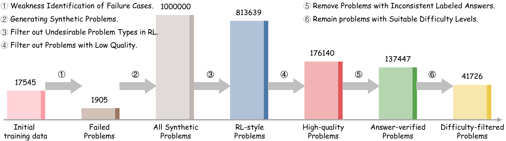## Appendix B Implementation Details <details> <summary>x12.png Details</summary>  ### Visual Description ## Process Diagram: Synthetic Problem Generation and Filtering Pipeline ### Overview The image displays a horizontal flowchart illustrating a multi-stage data processing pipeline for refining a problem dataset. The process begins with initial training data and ends with a filtered set of "Difficulty-filtered Problems." Each stage is represented by a colored bar whose height corresponds to the quantity of problems at that stage. The flow is indicated by gray arrows, each labeled with a circled number (① to ⑥) that corresponds to a specific processing step described in the header. ### Components/Axes **Header (Processing Steps):** The top of the image lists six sequential processing steps: 1. Weakness Identification of Failure Cases. 2. Generating Synthetic Problems. 3. Filter out Undesirable Problem Types in RL. 4. Filter out Problems with Low Quality. 5. Remove Problems with Inconsistent Labeled Answers. 6. Remain problems with Suitable Difficulty Levels. **Main Chart (Pipeline Stages):** The pipeline consists of seven stages, each with a labeled bar and a numerical value above it. The stages are connected by arrows indicating the flow of data. | Stage Position (Left to Right) | Label (Below Bar) | Quantity (Above Bar) | Bar Color | Corresponding Process Step (Arrow Label) | | :--- | :--- | :--- | :--- | :--- | | 1 | Initial training data | 17545 | Pink | ① | | 2 | Failed Problems | 1905 | Brown | ② | | 3 | All Synthetic Problems | 1000000 | Light Gray | ③ | | 4 | RL-style Problems | 813639 | Blue | ④ | | 5 | High-quality Problems | 176140 | Red | ⑤ | | 6 | Answer-verified Problems | 137447 | Green | ⑥ | | 7 | Difficulty-filtered Problems | 41726 | Yellow | (Final Output) | ### Detailed Analysis The pipeline demonstrates a significant reduction in dataset size through successive filtering: 1. **Initial Data & Failure Identification (①):** The process starts with 17,545 problems from "Initial training data." Step ①, "Weakness Identification of Failure Cases," isolates a subset of 1,905 "Failed Problems." 2. **Synthetic Generation (②):** Step ②, "Generating Synthetic Problems," massively expands the dataset to 1,000,000 "All Synthetic Problems." This is the largest volume in the pipeline. 3. **Sequential Filtering (③-⑥):** The subsequent steps apply rigorous filters, drastically reducing the count: * **Step ③ (Filter by Problem Type):** Reduces the set to 813,639 "RL-style Problems." * **Step ④ (Filter by Quality):** Further reduces the set to 176,140 "High-quality Problems." * **Step ⑤ (Filter by Answer Consistency):** Results in 137,447 "Answer-verified Problems." * **Step ⑥ (Filter by Difficulty):** The final step yields 41,726 "Difficulty-filtered Problems." ### Key Observations * **Massive Expansion and Contraction:** The pipeline features a dramatic expansion phase (from ~19k to 1M problems) followed by a severe contraction phase (from 1M to ~42k problems), indicating a "generate-then-filter" strategy. * **Filtering Efficacy:** Each filtering step removes a substantial portion of the data. The most significant single reduction occurs between "All Synthetic Problems" (1,000,000) and "RL-style Problems" (813,639), a loss of ~186k problems. The final four filtering steps (④-⑥) collectively reduce the dataset by over 95% from its synthetic peak. * **Final Yield:** The process results in a final dataset of 41,726 problems, which is approximately 2.38 times the size of the initial training data (17,545). ### Interpretation This diagram outlines a sophisticated data curation methodology, likely for training or evaluating a machine learning model, particularly in a Reinforcement Learning (RL) context. The process suggests a focus on quality over quantity. The initial "Weakness Identification" implies using model failures to guide the generation of new, targeted synthetic problems. The subsequent multi-stage filtering—addressing problem type, quality, answer consistency, and difficulty—demonstrates a comprehensive approach to constructing a high-fidelity, reliable, and pedagogically useful dataset. The final "Difficulty-filtered" set is presumably balanced to provide an appropriate challenge level. The pipeline's structure highlights the computational and analytical investment required to move from raw or initial data to a refined, high-value training resource. </details> Figure 8: Demonstration of the SwS data workflow by tracing the process from initial training data to the final selection of synthetic problems in the 32B model experiments. For better visualization, the bar heights are scaled using the cube root of the raw data. ### B.1 Training We conduct our experiments using the verl [42] framework and adopt GRPO [40] as the optimization algorithm. For all RL training experiments, we sample 8 rollouts per problem and use a batch size of 1024, with the policy update batch size set to 256. We employ a constant learning rate of $5× 10^-7$ with a 20-step warm-up, and set the maximum prompt and response lengths to 1,024 and 8,192 tokens, respectively. We do not apply a KL penalty, as recent studies have shown it may hinder exploration and potentially cause training collapse [65, 28, 63]. In the initial training stage, we train the model for 200 steps. During augmented RL training, we continually train the initially trained model for 600 steps on the augmented dataset incorporated with synthetic problems, using only prompts with an accuracy between $acc_lower=10\$ and $acc_upper=90\$ as determined by the online policy model for updates. The probability ratio clipping ranges in Eq. 3 is set to $ε=0.20$ and $ε^h=0.28$ . Since the training data for the 32B and 14B models (a combination of DAPO [63] and LightR1 [53] subsets) lack human-annotated category information, we leverage the LLaMA-3.3-70B-Instruct model to label their categories. This ensures consistency with our SwS pipeline, which combines concepts within the same category. The prompt is presented in Prompt LABEL:prompt:category-labeling. ### B.2 Evaluation For evaluation, we utilize the vLLM framework [18] and allow for responses up to 8,192 tokens. For all the benchmarks, Pass@1 is computed using greedy decoding for baseline models and sampling (temperature 1.0, top-p 0.95) for RL-trained models. For Avg@32 on competition-level benchmarks, we sample 32 responses per model with the same sampling configuration as used in RL training. We adopt a hybrid rule-based verifier by integrating Math-Verify and the PRIME-RL verifier [6], as their complementary strengths lead to higher recall. For all the inference, we use the default chat template and enable CoT prompting by appending the instruction: “Let’s think step by step and output the final answer within “ $\backslashboxed\{\}$ ” after each question. 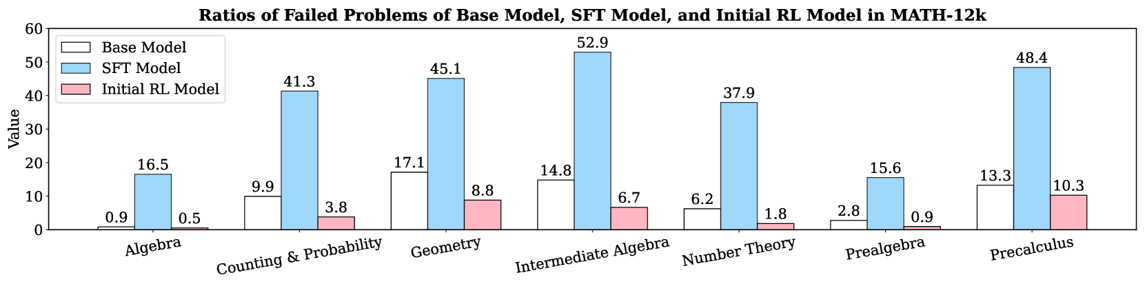## Appendix C Motivation for Using RL in Weakness Identification <details> <summary>x13.png Details</summary>  ### Visual Description ## Grouped Bar Chart: Ratios of Failed Problems by Model and Math Category ### Overview This is a grouped bar chart titled "Ratios of Failed Problems of Base Model, SFT Model, and Initial RL Model in MATH-12k". It compares the failure rates (as a numerical value, likely a percentage) of three different AI models across seven distinct mathematical subject categories. The chart visually demonstrates how model performance, in terms of problem failure, varies by subject area and training methodology. ### Components/Axes * **Chart Title:** "Ratios of Failed Problems of Base Model, SFT Model, and Initial RL Model in MATH-12k" * **Y-Axis:** * **Label:** "Value" * **Scale:** Linear scale from 0 to 60, with major tick marks at intervals of 10 (0, 10, 20, 30, 40, 50, 60). * **X-Axis:** * **Categories (from left to right):** Algebra, Counting & Probability, Geometry, Intermediate Algebra, Number Theory, Prealgebra, Precalculus. * **Legend:** Located in the top-left corner of the chart area. * **Base Model:** Represented by white bars with a black outline. * **SFT Model:** Represented by light blue bars. * **Initial RL Model:** Represented by light pink bars. ### Detailed Analysis The chart presents the failure ratio for each model within each of the seven math categories. The exact values are annotated on top of each bar. **1. Algebra:** * **Base Model (White):** 0.9 * **SFT Model (Light Blue):** 16.5 * **Initial RL Model (Light Pink):** 0.5 * **Trend:** The SFT Model has a significantly higher failure rate than the other two models, which are both very low. **2. Counting & Probability:** * **Base Model (White):** 9.9 * **SFT Model (Light Blue):** 41.3 * **Initial RL Model (Light Pink):** 3.8 * **Trend:** A large increase in failure rate for the SFT Model compared to the Base Model. The Initial RL Model shows the best performance (lowest failure). **3. Geometry:** * **Base Model (White):** 17.1 * **SFT Model (Light Blue):** 45.1 * **Initial RL Model (Light Pink):** 8.8 * **Trend:** All models show higher failure rates here than in previous categories. The SFT Model's failure rate is more than double that of the Base Model. **4. Intermediate Algebra:** * **Base Model (White):** 14.8 * **SFT Model (Light Blue):** 52.9 * **Initial RL Model (Light Pink):** 6.7 * **Trend:** This category contains the highest single failure value on the chart (SFT Model: 52.9). The gap between the SFT Model and the others is most pronounced here. **5. Number Theory:** * **Base Model (White):** 6.2 * **SFT Model (Light Blue):** 37.9 * **Initial RL Model (Light Pink):** 1.8 * **Trend:** Similar pattern to Counting & Probability, with the SFT Model failing at a much higher rate. The Initial RL Model performs exceptionally well. **6. Prealgebra:** * **Base Model (White):** 2.8 * **SFT Model (Light Blue):** 15.6 * **Initial RL Model (Light Pink):** 0.9 * **Trend:** Relatively lower failure rates across the board compared to more advanced topics. The SFT Model still underperforms the others. **7. Precalculus:** * **Base Model (White):** 13.3 * **SFT Model (Light Blue):** 48.4 * **Initial RL Model (Light Pink):** 10.3 * **Trend:** High failure rates for all models, second only to Intermediate Algebra for the SFT Model. The Initial RL Model's failure rate is closest to the Base Model's in this category. ### Key Observations 1. **Consistent Model Hierarchy:** Across all seven categories, the **SFT Model (light blue)** consistently has the highest failure ratio. The **Initial RL Model (light pink)** consistently has the lowest failure ratio. The **Base Model (white)** always falls in between. 2. **Peak Failure Point:** The highest failure ratio recorded is **52.9** for the SFT Model in the **Intermediate Algebra** category. 3. **Category Difficulty:** **Intermediate Algebra** and **Precalculus** appear to be the most challenging categories for the SFT Model, with failure ratios of 52.9 and 48.4, respectively. **Algebra** and **Prealgebra** appear to be the easiest, with SFT Model failure ratios of 16.5 and 15.6. 4. **Performance Gap:** The performance gap (difference in failure ratio) between the SFT Model and the Initial RL Model is largest in **Intermediate Algebra** (52.9 vs. 6.7, a difference of 46.2) and smallest in **Algebra** (16.5 vs. 0.5, a difference of 16.0). ### Interpretation This chart provides a clear comparative analysis of model performance on the MATH-12k benchmark. The data suggests that **Supervised Fine-Tuning (SFT) alone may lead to a significant increase in problem failure rates** compared to the Base Model across a wide range of mathematical topics. This could indicate issues like overfitting to the training data or a lack of robustness when faced with the test set. Conversely, the **Initial Reinforcement Learning (RL) Model demonstrates a marked improvement**, achieving the lowest failure ratios in every category. This implies that the RL training phase is highly effective at reducing errors and enhancing the model's problem-solving capabilities beyond both the Base and SFT versions. The variation across categories indicates that certain mathematical domains (like Intermediate Algebra and Precalculus) are inherently more challenging for these models, or that the training data for these domains may be less effective. The consistent ranking of the models (SFT worst, Initial RL best) across all categories strengthens the conclusion that the training methodology (SFT vs. RL) is a primary factor in performance, rather than the specific subject matter. </details> Figure 9: An visualization of utilizing the base model (Qwen2.5-7B), SFT model and the initial RL model on weakness identification in the original training set (MATH-12k). In our SwS framework, we propose utilizing an initial RL training phase for weakness identification. However, one might argue that there are simpler alternatives for weakness identification, such as directly sampling training problems from the base model or applying supervised fine-tuning before prompting the model to answer questions. In this section, we provide an in-depth discussion on the validity of using problems with low training efficiency during the initial RL phase as model’s weaknesses. We first compare the performance of the Base model, SFT model, and Initial RL model by sampling on the training set, where the SFT model is obtained by fine-tuning the Base model for 1 epoch on human-written solutions. For each question, we prompt the model to generate 8 responses and report the proportion of problems for which none of the responses are correct in Figure 9. For the Base model, failures may be attributed to its insufficient alignment with reasoning-specific tasks. Results from the initial RL model show that the Base model can quickly master such questions through RL, indicating that they do not represent challenging weaknesses. Furthermore, the heavy reliance on the prompt template of the Base model [28] reduces its robustness of weakness identification. For the SFT model, there are three main drawbacks regarding weakness identification: (1) The dilemma of training epochs—too many epochs leads to memorizing labeled solutions, while too few epochs fails to align the model with the target problem distribution; (2) SFT is prone to hallucination [3, 52]; and (3) Ensuring the quality of labeled solutions is difficult, as human-written solutions may not always be the best for models [10]. For these reasons, the SFT model performs poorly on the initial training set, even yielding worse results than the Base model, let alone in utilizing its failed problems to identify model weaknesses. In contrast to the Base and SFT models, the Initial RL model exhibits the most robust performance on the initial training set, indicating that the failed problems expose the model’s most critical weaknesses. Additionally, the training efficiency on all problems during initial RL can also be recorded for further analysis of model weaknesses. Meanwhile, the initially trained model can also serve as the starting point for augmented RL training. Therefore, in our SwS framework, we ultimately choose to employ an initial RL phase for robust weakness identification. ## Appendix D Data Analysis of the SwS Framework | Positive Case # 1: Let $z_1$ , $z_2$ , and $z_3$ be complex numbers such that $|z_1|=|z_2|=|z_3|=1$ and $z_1+z_2+z_3=0$ . Using the symmetric polynomial $s_2=z_1z_2+z_1z_3+z_2z_3$ , find the value of $|s_2|^2$ . | | --- | | Negative Case # 1: In a village, there are 10 houses, each of which can be painted one of three colors: red, blue, or green. Two houses cannot have the same color if they are directly adjacent to each other. Using combinatorial analysis and considering the constraints, find the total number of distinct ways to paint the houses, taking into account the possibility of having a sequence where the same color repeats after two different colors (e.g., red, blue, red), and assuming that the color of one of the end houses is already determined to be red, and the colors of the houses are considered different based on their positions (i.e., the configuration red, blue, green is considered different from green, blue, red). | | Negative Case # 2: A metal’s surface requires a minimum energy of 2.5 eV to remove an electron via the photoelectric effect. If light with a wavelength of 480 nm is shone on the metal, and 1 mole of electrons is ejected, what is the total energy, in kilojoules, transferred to the electrons, given that the energy of a photon is related to its wavelength by the formula E = $hc/λ$ , where $h=6.626x10^-34$ J s and $c=3.00x10^8m/s$ , and Avogadro’s number is $6.02x10^23$ particles per mole? | | Negative Case # 3: In triangle $ABC$ , with $\angle A=60^∘$ , $\angle B=90^∘$ , $AB=4$ , and $BC=7$ , use the Law of Sines to find $\angle C$ and calculate the triangle’s area. | Table 4: Case study of quality filtering results in SwS, featuring one high-quality positive case and three low-quality negative cases. The low-quality segments are marked in pink. ### D.1 Detailed Data Workflow Taking the 32B model experiments as an example, Figure 8 shows the comprehensive data workflow of the SwS framework, from identifying model weaknesses in the initial training data to the processing of synthetic problems. The initial training set, consisting of the DAPO and Light-R1 subsets for the Qwen2.5-32B model, contains 17,545 problem-answer pairs. During the weakness identification stage, 1,905 problems are identified as failure cases according to Eq. 4. These failure cases are subsequently used for concept extraction and targeted problem synthesis. For problem synthesis, we set an initial budget of 1 million synthetic problems in all experiments, with allocations for each category determined as in Eq. 5. These problems then undergo several filtering stages: (1) removing multiple-choice, multi-part, or proof-required problems; (2) discarding problems evaluated as low quality; (3) filtering out problems where the answer generation model yields inconsistent answers, specifically when the most frequent answer among all generations appears less than 50%; and (4) removing problems whose difficulty levels are unsuitable for the current model in RL training. Among these, the quality-based filtering is the strictest, with a filtering rate of 78.35%, indicating that the SwS pipeline maintains rigorous quality control over the generated problems. This ensures both the stability and effectiveness of utilizing synthetic problems in subsequent training. We present a case study of the quality-based filtering results in Table 4. As illustrated, the positive case that passed the model-based quality evaluation features a concise and precise problem description. In contrast, most synthetic problems identified as low-quality exhibit redundant and overly elaborate descriptions, sometimes including lengthy hints for solving the problem, as seen in the first negative case. Additionally, some low-quality problems incorporate excessive non-mathematical knowledge, such as Physics, as illustrated in the second negative case. The informal LaTeX formatting also contributes to their lower quality. Furthermore, problems with multiple question components, such as the third negative case, are also considered as low quality for RL training. ### D.2 Difficulty Distribution of Synthetic Problems In this section, we study the difficulty distribution of the synthetic problems generated for base models ranging from 3B to 32B, as shown in Figure 10. The red outlines in the pie plots highlight the subset of synthetic problems selected for subsequent augmented RL training, with accuracy falling within the [25%, 75%] range. These samples account for nearly 35% of all generated problems across the four models. The two largest wedges in the pie chart represent problems that the models answered either completely correctly or completely incorrectly. These cases do not provide effective training signals in GRPO [40, 63], and are thus excluded from the later augmented RL training stage. To further enhance stability and efficiency, we also exclude problems where the model produces only one correct or one incorrect response. Since all synthetic problems are generated using the same instruction model (LLaMA-3.3-70B-Instruct) with similar competition-level difficulty levels (as illustrated in Prompt LABEL:prompt:problem-generation), and are based on concepts derived from their respective weaknesses, the resulting difficulty distribution of the synthetic problems exhibits only minor differences across all models. Consistent with intuition, the initially trained 3B model achieved the lowest performance on the synthetic questions, with the highest ratio of all-incorrect and the lowest ratio of all-correct responses, while the 32B model showed the opposite trend, achieving the best performance. 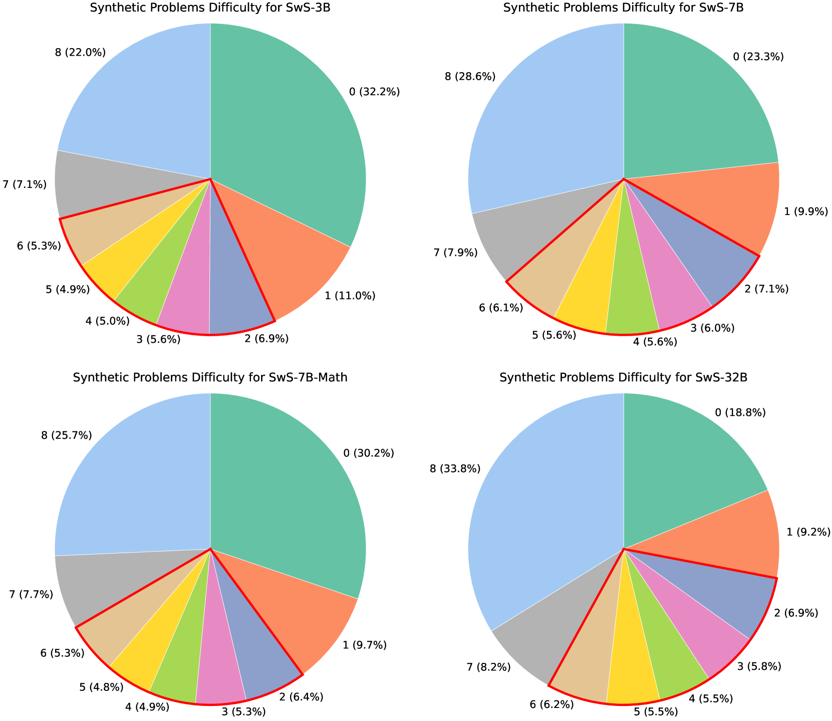<details> <summary>x14.png Details</summary>  ### Visual Description ## Pie Charts: Synthetic Problems Difficulty Distribution for Four Models ### Overview The image displays four pie charts arranged in a 2x2 grid. Each chart visualizes the distribution of synthetic problem difficulty levels (labeled 0 through 8) for a different AI model variant. The charts share a consistent color scheme for the difficulty levels. The overall title for each chart is "Synthetic Problems Difficulty for [Model Name]". ### Components/Axes * **Chart Titles (Top of each pie):** * Top-Left: `Synthetic Problems Difficulty for SwS-3B` * Top-Right: `Synthetic Problems Difficulty for SwS-7B` * Bottom-Left: `Synthetic Problems Difficulty for SwS-7B-Math` * Bottom-Right: `Synthetic Problems Difficulty for SwS-32B` * **Data Series (Difficulty Levels):** Each pie is segmented into 9 categories, labeled 0 to 8. The color mapping is consistent across all charts: * Level 0: Teal/Green * Level 1: Orange * Level 2: Light Purple/Blue * Level 3: Pink * Level 4: Light Green * Level 5: Yellow * Level 6: Tan/Beige * Level 7: Grey * Level 8: Light Blue * **Labels:** Each segment is directly labeled with its difficulty level number and its percentage of the total, formatted as `[Level] ([Percentage]%)`. ### Detailed Analysis **1. SwS-3B (Top-Left Chart)** * **Trend:** The distribution is heavily skewed towards the lowest (0) and highest (8) difficulty levels, forming a bimodal shape. * **Data Points (Clockwise from top):** | Level | Percentage | | :---- | :--------- | | 0 | 32.2% | | 1 | 11.0% | | 2 | 6.9% | | 3 | 5.6% | | 4 | 5.0% | | 5 | 4.9% | | 6 | 5.3% | | 7 | 7.1% | | 8 | 22.0% | **2. SwS-7B (Top-Right Chart)** * **Trend:** The distribution remains bimodal but becomes more balanced between the extremes compared to SwS-3B. The proportion of the highest difficulty (8) increases notably. * **Data Points (Clockwise from top):** | Level | Percentage | | :---- | :--------- | | 0 | 23.3% | | 1 | 9.9% | | 2 | 7.1% | | 3 | 6.0% | | 4 | 5.6% | | 5 | 5.6% | | 6 | 6.1% | | 7 | 7.9% | | 8 | 28.6% | **3. SwS-7B-Math (Bottom-Left Chart)** * **Trend:** This distribution closely mirrors that of SwS-3B, with a strong peak at Level 0 and a secondary peak at Level 8. The middle-difficulty segments (1-7) are relatively small and uniform. * **Data Points (Clockwise from top):** | Level | Percentage | | :---- | :--------- | | 0 | 30.2% | | 1 | 9.7% | | 2 | 6.4% | | 3 | 5.3% | | 4 | 4.9% | | 5 | 4.8% | | 6 | 5.3% | | 7 | 7.7% | | 8 | 25.7% | **4. SwS-32B (Bottom-Right Chart)** * **Trend:** This chart shows the most significant shift. The proportion of the highest difficulty level (8) becomes dominant, while the lowest difficulty (0) shrinks considerably. The distribution is less bimodal and more skewed toward higher difficulties. * **Data Points (Clockwise from top):** | Level | Percentage | | :---- | :--------- | | 0 | 18.8% | | 1 | 9.2% | | 2 | 6.9% | | 3 | 5.8% | | 4 | 5.5% | | 5 | 5.5% | | 6 | 6.2% | | 7 | 8.2% | | 8 | 33.8% | ### Key Observations 1. **Bimodal Dominance:** All four models exhibit a bimodal distribution, with the vast majority of problems falling into either the easiest (Level 0) or hardest (Level 8) categories. The middle difficulties (1-7) consistently represent a much smaller portion of the total. 2. **Model Size Correlation:** As the model size increases from SwS-3B to SwS-32B, there is a clear trend: the percentage of the hardest problems (Level 8) increases (22.0% -> 28.6% -> 25.7% -> 33.8%), while the percentage of the easiest problems (Level 0) generally decreases (32.2% -> 23.3% -> 30.2% -> 18.8%). 3. **SwS-7B-Math Anomaly:** The SwS-7B-Math model's distribution is more similar to the smaller SwS-3B than to its similarly-sized SwS-7B counterpart. This suggests the math-focused fine-tuning may have altered the problem difficulty profile. 4. **SwS-32B Shift:** The largest model (SwS-32B) shows the most pronounced shift toward higher difficulty, with Level 8 comprising over a third of all problems. ### Interpretation The data suggests a strong relationship between model scale/capability and the difficulty of synthetic problems it is evaluated on or generates. The consistent bimodal pattern indicates that the synthetic problem generation process tends to create tasks that are either very straightforward or highly challenging, with fewer intermediate problems. The key insight is that **larger or more specialized models (like SwS-32B and SwS-7B) are associated with a higher proportion of difficult (Level 8) problems.** This could imply one of two things: 1. **Evaluation Bias:** The benchmark or generation method is designed to scale problem difficulty with model size, ensuring larger models are tested on harder tasks. 2. **Model Capability:** Larger models are either capable of solving harder problems (thus being evaluated on them) or are generating more complex synthetic problems themselves. The outlier, SwS-7B-Math, demonstrates that domain-specific tuning (mathematics) can significantly alter the difficulty profile, making it more similar to a smaller base model in this specific metric. This highlights that model size is not the sole determinant of the problem difficulty distribution; training objective plays a crucial role. In summary, the charts reveal a deliberate or emergent scaling of problem difficulty with model size, characterized by a persistent focus on the extremes of the difficulty spectrum. </details> Figure 10: Difficulty distributions of synthetic problems for models from 3B to 32B in our work. ## Appendix E Co-occurrence Based Concept Sampling Following Huang et al. [15], Zhao et al. [73], we enhance the coherence and semantic fluency of synthetic problems by sampling concepts within the same category based on their co-occurrence probabilities and embedding similarities. Specifically, for each candidate concept $c∈C$ from category $D$ , we define its score based on both co-occurrence statistics and embedding similarity as: $$ Score(c)=\begin{cases}Co(c)+Sim(c),&if c ∉\{c_1,c_2,\dots,c_k\}\\ -∞,&otherwise.\end{cases} $$ The co-occurrence term $Co(c)$ is computed by summing the co-occurrence counts from a sparse matrix built over the entire corpus, generated by iterating through all available concept lists in the pool. For each list, we increment $CooccurMatrix[c,c^\prime]$ by one for every unordered pair where $c≠ c^\prime$ , yielding a sparse, symmetric matrix in which each entry $CooccurMatrix[c,c^\prime]$ records the total number of times concepts $c$ and $c^\prime$ co-occur across all sampled lists: $$ Co(c)=∑_i=1^kCooccurMatrix[c,c_i], \tag{6} $$ while the semantic similarity is given by the cosine similarity between the candidate’s embedding and the mean embedding of the currently selected concepts: $$ Sim(c)=\cos≤ft(\vec{e}_c,\frac{1}{k}∑_i=1^k\vec{e}_c_{i} \right), \tag{7} $$ To efficiently support large-scale and high-dimensional concept spaces, we construct a sparse co-occurrence matrix over all unique concepts, where each entry represents the frequency with which a pair of concepts co-occurs within sampled concept lists. Simultaneously, concept embeddings are normalized and indexed via FAISS to facilitate fast similarity computation. During sampling, an initial seed concept is drawn in proportion to its empirical frequency. For each subsequent concept, scores are computed by efficiently summing its co-occurrence with the current set and its embedding similarity to the group mean, while previously selected concepts are masked out. The probability of sampling each candidate is determined via softmax over these scores with temperature $τ$ : $$ P(c)=\frac{\exp≤ft(Score(c)/τ\right)}{∑_c^\prime∉\{c_ {1,\dots,c_k\}}\exp≤ft(Score(c^\prime)/τ\right)}. \tag{8} $$ This process iteratively constructs coherent, semantically related concept sets to serve as the inputs for synthetic problem generation, ensuring both diversity and fluency. ## Appendix F Details for Weak-to-Strong Generalization in SwS Case Study for Weak-to-strong Generalization Question: Compute $99^2+99+1$ in your head. Please reason step by step, and put your final answer within \boxed{}. Golden Answer: $\boxed{9901}$ $>>>$ Teacher Response: To compute $99^2+99+1$ , we can compute each part directly: $\displaystyle 99^2$ $\displaystyle=9801$ $\displaystyle 99^2+99$ $\displaystyle=9801+99=9900$ $\displaystyle 99^2+99+1$ $\displaystyle=9900+1=9901$ Final answer: $\boxed{9901}$ $>>>$ Student Response: Rewrite the expression using a binomial identity: $\displaystyle 99^2+99+1$ $\displaystyle=(99+1)^2=100^2=10000$ Final answer: $\boxed{10000}$ Figure 11: Case study in which a weak teacher provides the correct solution, while a strong student incorrectly applies a binomial identity and derives an incorrect answer. To understand the capabilities of the weak teacher and the strong student model, we evaluated both of them on the MATH-500 test set by prompting them on each question for eight times. Although the teacher model generally exhibits weaker performance, we found that in 16.4% of problems, the weaker teacher outperforms the otherwise stronger student model. This highlights the potential for leveraging a weak teacher to distill its strengths into the student model. A case where the weaker teacher model outperforms the stronger student model is shown in Figure 11. From the analysis of the SwS framework, as well as its Weak-to-Strong Generalization extension, we assert that the upper bound for answer labeling is a revised form of self-consistency score of the teacher model, where (1) the consistent answer must achieve an accuracy greater than 50% across all responses, and (2) the student model must provide the same answer as the teacher model’s consistent answer in at least 25% of responses. These revision procedures help ensure the correctness of the synthetic problem answers labeled by the teacher model. In Table 5, we demonstrate the robustness of utilizing a weaker teacher for answer labeling, assuming that the MATH-500 test set serves as our synthetic problems. As in the second line, even under the self-consistency setting, the teacher model only achieves an improvement of 4.8 points. However, when we exclude problems for which self-consistency does not provide sufficient confidence—specifically, those where the most consistent answer accounts for less than 50% of all responses—the self-consistency setting yields an additional 9.0-point improvement on the remaining questions. Furthermore, in our SwS pipeline, we retain only problems where the student model achieves over 25% accuracy to ensure an appropriate level of difficulty. After filtering out problems where the student falls below this threshold, some mislabeled problems are also automatically removed, resulting in the weak teacher achieving a performance of 97.5% on the final remaining questions. The increase in labeling accuracy from 80.6% to 97.5% shows the potential of utilizing the weaker teacher model for answer labeling as well as the robustness of the SwS framework itself. | Setting | Size | Prealgebra | Intermediate Algebra | Algebra | Precalculus | Number Theory | Counting & Probability | Geometry | All | | --- | --- | --- | --- | --- | --- | --- | --- | --- | --- | | Pass@1 | 500 | 88.2 | 64.3 | 95.5 | 71.2 | 93.0 | 81.4 | 63.0 | 80.6 | | + SC | 500 | 96.9 | 96.0 | 84.4 | 84.1 | 96.2 | 87.5 | 67.8 | 85.4 | | + SC>50% | 444 | 96.9 | 97.3 | 93.2 | 94.7 | 98.0 | 94.4 | 89.6 | 94.4 | | + SC>50% & Stu-Con | 407 | 96.8 | 97.2 | 97.7 | 100.0 | 100.0 | 96.8 | 94.9 | 97.5 | Table 5: The performance of the weak teacher model used for answer generation on the MATH-500 test set under different strategies and their corresponding revisions. "Stu-Con" refers to filtering out problems where the student model’s accuracy falls below the defined threshold of 25%. ## Appendix G Details for Self-Evolving in SwS As mentioned in Section 4.2, the Self-evolving SwS extension enables the policy to achieve better performance on simple to medium-level mathematical reasoning benchmarks but remains suboptimal on AIME-level competition benchmarks. In this section, we further analyze the reasons behind this phenomenon. Figure 12 visualizes the model’s self-quality assessment and difficulty evaluation within the SwS framework. Notably, the model assigns a much higher proportion of “perfect” and “acceptable” labels, and fewer “bad” labels, to its self-generated problems compared to the standard framework shown in Figure 8. This observation is consistent with findings from LLM-as-a-Judge [21], which indicate that models tend to be more favorable toward and assign higher scores to their own generations. Such behavior may result in overlooking low-quality problems or mis-classifying problems that are too complex for the model’s reasoning abilities as unsolvable or of poor quality. Beyond the risk of filtering out over-complex problems, the model may also have difficulty in accurately labeling answers through self-consistency for over-challenging problems, thereby limiting the potential of incorporating complex problems through the Self-evolving SwS framework. Additionally, in Figure 12, it is noteworthy that the initial RL-trained model achieves nearly 50% all-correct responses on its generated problems, whereas only 31% of problems with appropriate difficulty remain for augmentation after SwS difficulty filtering. This suggests that the self-generated problems may be significantly simpler than those produced using a stronger instruction model [8], thus it could lead to data inefficiency and limit the model’s performance on more complex problems during RL training. 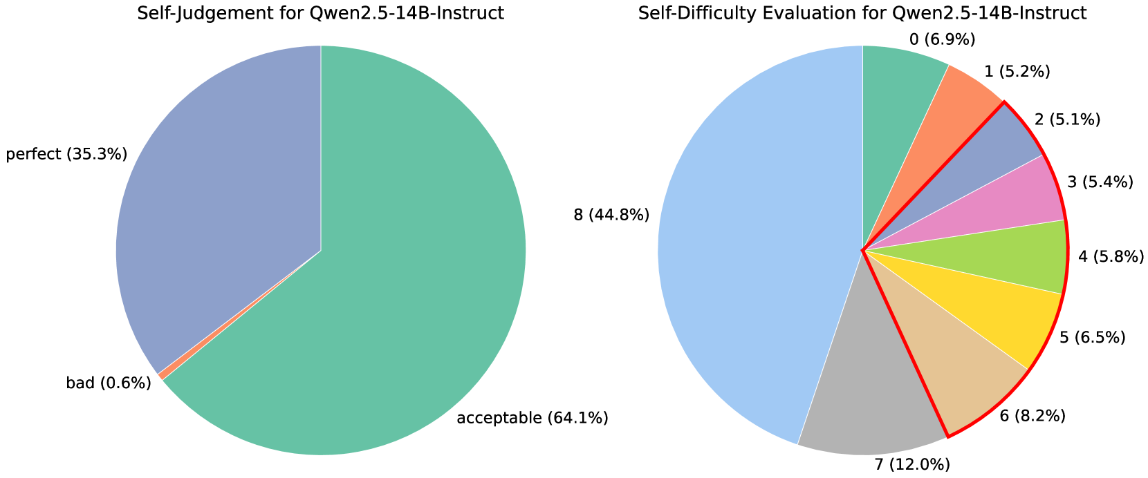<details> <summary>x15.png Details</summary>  ### Visual Description ## Pie Charts: Self-Evaluation Metrics for Qwen2.5-14B-Instruct ### Overview The image displays two pie charts side-by-side, presenting self-evaluation data for the AI model "Qwen2.5-14B-Instruct." The left chart assesses the model's self-judgment of its response quality, while the right chart evaluates the model's self-assessed difficulty of the tasks it was given. ### Components/Axes **Left Chart: Self-Judgement for Qwen2.5-14B-Instruct** * **Type:** Pie chart. * **Categories & Data:** * **acceptable:** 64.1% (Large, teal-green segment, occupying the right and bottom portion of the chart). * **perfect:** 35.3% (Large, slate-blue segment, occupying the top-left portion of the chart). * **bad:** 0.6% (Very thin, orange sliver between the "perfect" and "acceptable" segments). * **Legend/Labels:** Labels are placed directly adjacent to their corresponding pie slices. **Right Chart: Self-Difficulty Evaluation for Qwen2.5-14B-Instruct** * **Type:** Pie chart. * **Categories & Data (from 12 o'clock position, moving clockwise):** * **0:** 6.9% (Teal-green segment). * **1:** 5.2% (Orange segment). * **2:** 5.1% (Slate-blue segment). * **3:** 5.4% (Pink segment). * **4:** 5.8% (Light green segment). * **5:** 6.5% (Yellow segment). * **6:** 8.2% (Tan/beige segment). * **7:** 12.0% (Grey segment). * **8:** 44.8% (Large, light blue segment, occupying the left half of the chart). * **Legend/Labels:** Labels are placed directly adjacent to their corresponding pie slices. The segments for difficulty levels 0 through 6 are outlined with a thin red border, visually grouping them together. ### Detailed Analysis **Self-Judgement (Left Chart):** The model's self-assessment is overwhelmingly positive. The vast majority of its responses (99.4%) are categorized as either "acceptable" (64.1%) or "perfect" (35.3%). The "bad" category is negligible at 0.6%. The visual trend shows a clear dominance of the "acceptable" category, followed by a substantial "perfect" category. **Self-Difficulty Evaluation (Right Chart):** The model's self-assessed task difficulty shows a strong skew towards higher difficulty levels. The single largest segment is for the highest difficulty rating, "8," which accounts for nearly half (44.8%) of all evaluations. The next most common ratings are "7" (12.0%) and "6" (8.2%). The lower difficulty ratings (0 through 5) each constitute between approximately 5% and 7% of the total, showing a relatively even but minor distribution. The visual trend is a clear concentration of mass on the left side of the chart (ratings 7 and 8), indicating the model frequently perceives its tasks as highly difficult. ### Key Observations 1. **High Confidence, High Perceived Difficulty:** There is a striking contrast between the two charts. The model judges its output quality very highly (left chart) while simultaneously rating the difficulty of the tasks it performs as very high (right chart). 2. **Concentration at Extremes:** Both charts show concentration at specific points. The left chart concentrates on "acceptable" and "perfect." The right chart concentrates heavily on the maximum difficulty rating of "8." 3. **Minimal Negative Self-Assessment:** The "bad" category in the self-judgment chart is almost non-existent (0.6%). 4. **Grouping of Lower Difficulties:** The red outline on the right chart visually groups difficulty levels 0-6, separating them from the dominant 7 and 8 categories. This emphasizes the dichotomy between "lower" and "higher" difficulty as perceived by the model. ### Interpretation The data suggests a model with a strong positive self-bias in its output quality assessment. It consistently rates its own responses as acceptable or perfect. Concurrently, it exhibits a form of "task difficulty inflation," where it perceives the problems it solves as being very challenging, with nearly half rated at the maximum difficulty. This combination could indicate several underlying factors: * **Calibration Issue:** The model may not be well-calibrated; its internal confidence (reflected in high-quality self-judgment) does not align with an objective measure of task difficulty. It might be overestimating task complexity. * **Training Data Reflection:** The high perceived difficulty might reflect the nature of the tasks in its training or evaluation set, which could be inherently complex. * **Architectural or Behavioral Trait:** This pattern could be a characteristic of the Qwen2.5-14B-Instruct model's training objective or reinforcement learning from human feedback (RLHF) process, encouraging confident outputs while acknowledging task complexity. The near absence of "bad" self-judgments is notable and could imply either exceptional performance or a systematic bias against negative self-evaluation. The clear visual separation of difficulty levels 0-6 from 7-8 in the right chart underscores that the model's experience is dominated by tasks it considers highly difficult, yet it believes it handles them with acceptable to perfect quality. </details> Figure 12: Illustration of the quality assessment and difficulty evaluation for Qwen2.5-14B-Instruct under the Self-evolving SwS framework. ## Appendix H Details for Weakness-driven Selection Algorithm 1 Weakness-Driven Selection Pipeline 1: Failed Problems $X_S$ ; Total Budget $|T|$ ; Target Set $T_X$ ; Domains $\{D_i\}_i=0^n$ 2: Selected problems $T_S$ 3: Embed all failed problems in $X_S$ and all questions in $T_X$ 4: for each domain $D_i$ in $\{D_i\}_i=0^n$ do 5: Compute selection budget $|T_i|$ for $D_i$ according to Eq. 2 6: Extract failed problems $X_S,i$ belonging to $D_i$ 7: for each $q∈T_X$ do $\triangleright$ Domain-level KNN 8: Compute $d_i(q)=\min_f∈X_S,idistance(\vec{e}_q,\vec{e}_f)$ 9: end for 10: Select top $|T_i|$ questions from $T_X$ with the smallest $d_i(q)$ as $S_i$ 11: 12: end for 13: return Selected problems $T_S=\bigcup_i=0^nS_i$ $\triangleright$ Final Selected Set As described in Section 4.3, we utilize the failed problems identified by Qwen2.5-7B [57] on the MATH-12k [13] training set, which comprises 915 problems, to select additional data from Big-Math [1] to mitigate the model’s weaknesses through the augmented RL training. The complete Weakness-driven Selection extension of SwS is presented in Algorithm 1. For embedding the problems, we utilize LLaMA-3.1-8B-base [8] to encode both the collected failure cases and the problems from the target dataset. The failure cases are then grouped by categories, following the concept sampling strategy in standard SwS. We employ a binary K-Nearest Neighbors [5] algorithm to select weakness-driven problems from the target set, where the augmented problems are chosen by their embedding distances to the failure cases within each category. The selection budget for each category is also determined according to Eq. 5. We then aggregate the retrieved problems from all categories, forming a selected set of 40k problems, which are then incorporated with the initial set for the subsequent RL training. ## Appendix I Evaluation Benchmark Demonstrations | Dataset | Size | Category | Example Problem | Answer | | --- | --- | --- | --- | --- | | GSM8k | 1319 | Prealgebra | The ice cream parlor was offering a deal, buy 2 scoops of ice cream, get 1 scoop free. Each scoop cost $1.50. If Erin had $6.00, how many scoops of ice cream should she buy? | $6$ | | MATH-500 | 500 | Geometry | For a constant $c,$ in cylindrical coordinates $(r,θ,z),$ find the shape described by the equation $z=c.$ (A) Line (B) Circle (C) Plane (D) Sphere (E) Cylinder (F) Cone. Enter the letter of the correct option. | (C) Plane | | Minerva Math | 272 | Precalculus | If the Bohr energy levels scale as $Z^2$ , where $Z$ is the atomic number of the atom (i.e., the charge on the nucleus), estimate the wavelength of a photon that results from a transition from $n=3$ to $n=2$ in Fe, which has $Z=26$ . Assume that the Fe atom is completely stripped of all its electrons except for one. Give your answer in Angstroms, to two significant figures. | $9.6$ | | Olympiad-Bench | 675 | Geometry | Given a positive integer $n$ , determine the largest real number $μ$ satisfying the following condition: for every $4n$ -point configuration $C$ in an open unit square $U$ , there exists an open rectangle in $U$ , whose sides are parallel to those of $U$ , which contains exactly one point of $C$ , and has an area greater than or equal to $μ$ . | $\frac{1}{2n+2}$ | | Gaokao-2023 | 385 | Geometry | There are three points $A,B,C$ in space such that $AB=BC=CA=1$ . If 2 distinct points are chosen in space such that they, together with $A,B,C$ , form the five vertices of a regular square pyramid, how many different ways are there to choose these 2 points? | $9$ | | AMC23 | 40 | Algebra | How many complex numbers satisfy the equation $z^5=\overline{z}$ , where $\overline{z}$ is the conjugate of the complex number $z$ ? | $7$ | | AIME24 | 30 | Number Theory | Let $N$ be the greatest four-digit positive integer with the property that whenever one of its digits is changed to $1$ , the resulting number is divisible by $7$ . Let $Q$ and $R$ be the quotient and remainder, respectively, when $N$ is divided by $1000$ . Find $Q+R$ . | $699$ | | AIME25 | 30 | Geometry | On $\triangle ABC$ points $A,D,E$ , and $B$ lie that order on side $\overline{AB}$ with $AD=4,DE=16$ , and $EB=8$ . Points $A,F,G$ , and $C$ lie in that order on side $\overline{AC}$ with $AF=13,FG=52$ , and $GC=26$ . Let $M$ be the reflection of $D$ through $F$ , and let $N$ be the reflection of $G$ through $E$ . Quadrilateral $DEGF$ has area 288. Find the area of heptagon $AFNBCEM$ . | $588$ | Table 6: Statistics and examples of the eight evaluation benchmarks utilized in the paper. We present the statistics and examples of the eight evaluation benchmarks used in our work in Table 6. Among these, GSM8K [4] is the simplest, comprising grade school math word problems. The MATH-500 [13], Gaokao-2023 [71], Olympiad-Bench [11], and AMC23 [33] benchmarks consist of high school mathematics problems spanning a wide range of topics and difficulty levels, while Minerva Math [19] may also include problems from other subjects. The AIME [34] benchmark is a prestigious high school mathematics competition that requires deep mathematical insight and precise problem-solving skills. An overview of all benchmarks is provided as follows. - GSM8K: A high-quality benchmark comprising 8,500 human-written grade school math word problems that require multi-step reasoning and basic arithmetic, each labeled with a natural language solution and verified answer. The 1,319-question test set emphasizes sequential reasoning and is primarily solvable by upper-grade elementary school students. - MATH-500: A challenging benchmark of 500 high school competition-level problems spanning seven subjects, including Algebra, Geometry, Number Theory, and Precalculus. Each problem is presented in natural language with LaTeX-formatted notation, offering a strong measure of mathematical reasoning and generalization across diverse topics. - Minerva-Math:A high-difficulty math problem dataset consisting of 272 challenging problems. Some problems are also relevant to scientific topics in other subjects, such as physics. - Olympiad-Bench: An Olympiad-level English and Chinese multimodal scientific benchmark featuring 8,476 problems from mathematics and physics competitions. In this work, we use only the pure language problems described in English, totaling 675 problems. - Gaokao-2023: A dataset consists of 385 mathematics problems from the 2023 Chinese higher education entrance examination, professionally translated into English. - AMC23: The AMC dataset consists of all 83 problems from AMC12 2022 and AMC12 2023, extracted from the AoPS wiki page. We used a subset of this data containing 40 problems. - AIME24 & 25: Each set comprises 30 problems from the 2024 and 2025 American Invitational Mathematics Examination (AIME), a prestigious high school mathematics competition for top-performing students, which are the most challenging benchmarks used in our study. Each problem is designed to require deep mathematical insight, multi-step reasoning, and precise problem-solving skills. ## Appendix J Prompts ### J.1 Prompt for Category Labeling Listing 1: The prompt for labeling the categories for mathematical problems, utilizing a few-shot strategy in which each category is represented by a labeled demonstration. ⬇ # CONTEXT # I am a teacher, and I have some high - level mathematical problems. I want to categorize the domain of these math problems. # OBJECTIVE # A. Provide a concise summary of the math problem, clearly identifying the key concepts or techniques involved. B. Assign the problem to one and only one specific mathematical domain. The following is the list of domains to choose from: < math domains > [" Intermediate Algebra ", " Geometry ", " Precalculus ", " Number Theory ", " Counting & Probability ", " Algebra ", " Prealgebra "] </ math domains > # STYLE # Data report. # TONE # Professional, scientific. # AUDIENCE # Students. Enable them to better understand the domain of the problems. # RESPONSE: MARKDOWN REPORT # ## Summarization [Summarize the math problem in a brief paragraph.] ## Math domains [Select one domain from the list above that best fits the problem.] # ATTENTION # - You must assign each problem to exactly one of the domains listed above. - If you are genuinely uncertain and none of the listed categories applies, you may use " Other ", but this should be a last resort. - Be thoughtful and accurate in your classification. Default to the listed categories whenever possible. - Add "=== report over ===" at the end of the report. < example math problem > ** Question **: Let $ n (\ ge2) $ be a positive integer. Find the minimum $ m $, so that there exists $x_ {ij}(1\ le i , j \ le n) $ satisfying: (1) For every $1 \ le i , j \ le n, x_ {ij}= max \{x_ {i1}, x_ {i2},..., x_ {ij}\} $ or $ x_ {ij}= max \{x_ {1 j}, x_ {2 j},..., x_ {ij}\}. $ (2) For every $1 \ le i \ le n$, there are at most $m$ indices $k$ with $x_ {ik}= max \{x_ {i1}, x_ {i2},..., x_ {ik}\}. $ (3) For every $1 \ le j \ le n$, there are at most $m$ indices $k$ with $x_ {kj}= max \{x_ {1 j}, x_ {2 j},..., x_ {kj}\}. $ </ example math problem > ## Summarization The problem involves an \( n \ times n \) matrix where each element \( x_ {ij} \) is constrained by the maximum values in its respective row or column. The goal is to determine the minimum possible value of \( m \) such that, for each row and column, the number of indices attaining the maximum value is limited to at most \( m \). This problem requires understanding matrix properties, maximum functions, and combinatorial constraints on structured numerical arrangements. ## Math domains Algebra === report over === </ example math problem > ** Question **: In an acute scalene triangle $ABC$, points $D, E, F$ lie on sides $BC, CA, AB$, respectively, such that $AD \ perp BC, BE \ perp CA, CF \ perp AB$. Altitudes $AD, BE, CF$ meet at orthocenter $H$. Points $P$ and $Q$ lie on segment $EF$ such that $AP \ perp EF$ and $HQ \ perp EF$. Lines $DP$ and $QH$ intersect at point $R$. Compute $HQ / HR$. </ example math problem > ## Summarization The problem involves an acute scalene triangle with three perpendicular cevians intersecting at the orthocenter. Additional perpendicular constructions are made from specific points on segment \( EF \), leading to an intersection at point \( R \). The goal is to determine the ratio \( HQ / HR \), requiring knowledge of triangle geometry, perpendicularity, segment ratios, and properties of the orthocenter. ## Math domains Geometry === report over === </ example math problem > ** Question **: Three cards are dealt at random from a standard deck of 52 cards. What is the probability that the first card is a 4, the second card is a $ \ clubsuit$, and the third card is a 2? </ example math problem > ## Summarization This problem involves calculating the probability of a specific sequence of events when drawing three cards from a standard 52- card deck without replacement. It requires understanding conditional probability, the basic rules of counting, and how probabilities change as cards are removed from the deck. ## Math domains Counting & Probability === report over === </ example math problem > ** Question **: Let $x$ and $y$ be real numbers such that $3x + 2 y \ le 7 $ and $2x + 4 y \ le 8. $ Find the largest possible value of $x + y. $ </ example math problem > ## Summarization This problem involves optimizing a linear expression \( x + y \) subject to a system of linear inequalities. It requires understanding of linear programming concepts, such as identifying feasible regions, analyzing boundary points, and determining the maximum value of an objective function within that region. ## Math domains Intermediate Algebra === report over === </ example math problem > ** Question **: Solve \[\ arccos 2 x - \ arccos x = \ frac {\ pi}{3}.\] Enter all the solutions, separated by commas. </ example math problem > ## Summarization This problem requires solving a trigonometric equation involving inverse cosine functions. The equation relates two expressions with \( \ arccos (2 x) \) and \( \ arccos (x) \), and asks for all real solutions satisfying the given identity. It involves knowledge of inverse trigonometric functions, their domains, and properties, as well as algebraic manipulation. ## Math domains Precalculus === report over === </ example math problem > ** Question **: What perfect - square integer is closest to 273? </ example math problem > ## Summarization The problem asks for the perfect square integer closest to 273. This involves understanding the distribution and properties of perfect squares, and comparing them with a given integer. It relies on number - theoretic reasoning related to squares of integers and their proximity to a target number. ## Math domains Number Theory === report over === </ example math problem > Voldemort bought $6.\ overline {6} $ ounces of ice cream at an ice cream shop. Each ounce cost $ \ $0.60. $ How much money, in dollars, did he have to pay? </ example math problem > ## Summarization The problem involves multiplying a repeating decimal, \( 6.\ overline {6} \), by a fixed unit price, \ $0.60, to find the total cost in dollars. This requires converting a repeating decimal into a fraction or using decimal multiplication, both of which are foundational arithmetic skills. ## Math domains Prealgebra === report over === < math problem > {problem} </ math problem > ### J.2 Prompt for Concepts Extraction Listing 2: Prompt template for extracting internal concepts from a mathematical question. ⬇ As an expert in educational assessment, analyze this problem: < problem > {problem} </ problem > Break down and identify {num_concepts} foundational concepts being tested. List these knowledge points that: - Are core curriculum concepts typically taught in standard courses, - Are precise and measurable (not vague like " understanding math "), - Are essential building blocks needed to solve this problem, - Represent fundamental principles rather than problem - specific techniques. Think through your analysis step by step, then format your response as a Python code snippet containing a list of {num_concepts} strings, where each string clearly describes one fundamental knowledge point. ### J.3 Prompt for Problem Synthesis Listing 3: Prompt template for synthesizing math problems from specified concepts, difficulty levels, and pre-defined mathematical categories. Following [73], the difficulty levels are consistently set to the competition level to prevent the generation of overly simple questions. ⬇ ### Given a set of foundational mathematical concepts, a mathematical domain, and a specified difficulty level, generate a well - constructed question that meaningfully integrates multiple listed concepts and reflects the stated level of complexity. ### Foundational Concepts: {concepts} ### Target Difficulty Level: {level} ### Mathematical Domain: {domain} ### Instructions: 1. Begin by outlining which concepts you will combine and how you plan to structure the question. 2. Ensure that the question is coherent, relevant, and appropriately challenging for the specified level. 3. The question must be a single standalone problem, not split into multiple sub - questions. 4. Do not generate proof - based, multiple - choice, or true / false questions. 5. The answer to the question should be expressible using numbers and mathematical symbols. 6. Provide a final version of the question that is polished and ready for use. ### Output Format: - First, provide your brief outline and planning for the question design. - Then, present only the final version of the question in the following format: ‘‘‘ [Your developed question here] ’’’ Do not include any placeholder, explanatory text, hints, or solutions to the question in the output block ### J.4 Prompt for Quality Evaluation Listing 4: The quality evaluation prompt utilized to filter out low-quality math problems. Following prior work [73], we assess synthetic problems based on five criteria: format, factual accuracy, difficulty alignment, concept coverage, and solvability. Each problem is then assigned one of three quality levels: ‘bad’, ‘acceptable’, or ‘perfect’. ⬇ As a critical expert in educational problem design, evaluate the following problem components: === GIVEN MATERIALS === 1. Problem & Design Rationale: {rationale_and_problem} (The rationale describes the author’s thinking process and justification in designing this problem) 2. Foundational Concepts: {concepts} 3. Target Difficulty Level: {level} === EVALUATION CRITERIA === Rate each criterion as: [Perfect | Acceptable | Bad] 1. FORMAT - Verify correct implementation of markup tags: <! – BEGIN RATIONALE – > [design thinking process] <! – END RATIONALE – > <! – BEGIN PROBLEM – > [problem] <! – END PROBLEM – > 2. FACTUAL ACCURACY - Check for any incorrect or misleading information in both problem and rationale - Verify mathematical, scientific, or logical consistency 3. DIFFICULTY ALIGNMENT - Assess if problem complexity matches the specified difficulty level - Evaluate if cognitive demands align with target level 4. CONCEPT COVERAGE - Evaluate how well the problem incorporates the given foundational concepts - Check for missing concept applications 5. SOLVABILITY - Verify if the problem has at least one valid solution - Check if all necessary information for solving is provided === RESPONSE FORMAT === For each criterion, provide: 1. Rating: [Perfect | Acceptable | Bad] 2. Justification: Clear explanation for the rating === FINAL VERDICT === After providing all criterion evaluations, conclude your response with: ‘ Final Judgement: [verdict]’ where verdict must be one of: - ‘ perfect ’ (if both FACTUAL ACCURACY and SOLVABILITY are Perfect, at least two other criteria are Perfect, and no Bad ratings) - ‘ acceptable ’ (if no Bad ratings and doesn’t qualify for perfect) - ‘ bad ’ (if ANY Bad ratings) Note: The ‘ Final Judgement: [verdict]’ line must be the final line of your response.