2506.09433v1

## Mitigating Spurious Correlations in LLMs via Causality-Aware Post-Training ## Shurui Gui, Shuiwang Ji Department of Computer Science & Engineering Texas A&M University College Station, TX 77843 {shurui.gui, sji}@tamu.edu ## Abstract While large language models (LLMs) have demonstrated remarkable capabilities in language modeling, recent studies reveal that they often fail on out-of-distribution (OOD) samples due to spurious correlations acquired during pre-training. Here, we aim to mitigate such spurious correlations through causality-aware post-training (CAPT). By decomposing a biased prediction into two unbiased steps, known as event estimation and event intervention , we reduce LLMs' pre-training biases without incurring additional fine-tuning biases, thus enhancing the model's generalization ability. Experiments on the formal causal inference benchmark CLadder and the logical reasoning dataset PrOntoQA show that 3B-scale language models fine-tuned with CAPT can outperform both traditional SFT and larger LLMs on in-distribution (ID) and OOD tasks using only 100 ID fine-tuning samples, demonstrating the effectiveness and sample efficiency of CAPT. ## 1 Introduction Large Language Models (LLMs) have made remarkable progress in natural language understanding and reasoning, achieving state-of-the-art performance on a wide range of tasks, from commonsense inference to formal logical deduction [Saparov and He, 2022, Clark et al., 2020, Zhao et al., 2023]. However, recent studies have revealed a key limitation, i.e ., LLMs often struggle with out-ofdistribution (OOD) samples due to spurious correlations acquired during pre-training [Tang et al., 2023, Ye et al., 2024, Mirzadeh et al., 2024, Jin et al., 2024]. These correlations, often tied to superficial information such as entity biases [Wang et al., 2023, Longpre et al., 2021, Qian et al., 2021a], can mislead the model to predict using spurious dependencies, causing failure under simple perturbations. These entity biases have been widely discussed in previous studies.This fragility is particularly problematic for domain-specific tasks such as formal causal inference or symbolic reasoning, where correctness relies on learning invariant logical structures rather than memorizing statistical patterns. Recent benchmarks such as Corr2Cause [Jin et al., 2024] and CLadder [Jin et al., 2023] have shown that even fine-tuned models can fail catastrophically when high-level events are perturbed. These failures are likely due to their reliance on spurious associations between events. Despite studies [Pan et al., 2023, Gao et al., 2024, Jin et al., 2023] trying to use extra information to alleviate biases, unlike simple entity bias ( e.g ., alarm), event bias ( e.g ., alarm is set) elimination in LLM reasoning tasks is still underexplored. Furthermore, causal analyses in previous bias studies are generally based on causal graphs of variant model predictions [Wang et al., 2023] instead of an invariant data generation process [Kaur et al., 2022, Peters et al., 2016, Arjovsky et al., 2019], motivating us to analyze the pre-training biases and fine-tuning biases from a data generation causal perspective for LLM reasoning tasks. Preprint. Under review. In this work, we analyze the establishment of pre-training spurious correlations from a data generation perspective through the causal lens and propose Causality-Aware Post-Training (CAPT), a simple yet effective method to improve the reasoning generalization of LLMs by mitigating both pre-training and fine-tuning biases. CAPT decomposes the biased prediction process into two less biased steps: event estimation and event intervention based on causal analysis. By separating domain-specific event spurious correlations from reasoning structure, CAPT breaks the pre-injected spurious correlations without introducing additional fine-tuning biases; thus, it isolates the true reasoning process and improves the unbiased reasoning ability significantly. Finally, We empirically explore and validate the biased and debiasing factors that influence the LLM OOD generalization ability on two challenging benchmarks: CLadder [Jin et al., 2023], a formal causal reasoning dataset with associational, interventional, and counterfactual queries; and PrOntoQA [Saparov and He, 2023], a logical deductive reasoning benchmark, where we create its OOD versions following the philosophy of the CLadder benchmark. Our experiments show that CAPT substantially improves OOD generalization. With only 100 fine-tuning samples, CAPT enables 3B-scale models to outperform both larger LLMs and standard fine-tuning approaches, demonstrating its effectiveness, robustness, and sample efficiency in mitigating both pre-trained and fine-tuned biases. ## 2 Related Work Spurious correlations in LLMs. Large Language Models (LLMs) such as GPT [Radford et al., 2018], LLaMa [Touvron et al., 2023], DeepSeek-R1 [Guo et al., 2025], and Qwen [Yang et al., 2024] have demonstrated their strong capabilities in performing different reasoning tasks [Saparov and He, 2022], including mathematical [Cobbe et al., 2021, Ling et al., 2017], commonsense [Zhao et al., 2023], and logical inference [Luo et al., 2023, Clark et al., 2020]. However, alongside these advancements, previous studies [Wang et al., 2023, Qian et al., 2021b, Longpre et al., 2021, Qian et al., 2021a, Mirzadeh et al., 2024, Jin et al., 2024] highlight that the current LLM reasoning process lacks robustness, where the reasoning performance faces significant degradation given even simple name replacement. A primary factor undermining the robustness of LLM reasoning is their propensity to learn and exploit spurious correlations [Tang et al., 2023, Ye et al., 2024]. These correlations are built during the pre-training of LLMs and become spurious when they are not valid anymore in the diverse test distribution, causing significant performance drops. Generalization ability in LLMs. On one hand, LLMs generally have better generalization ability due to their large training distribution [Kaplan et al., 2020, Qin et al., 2025, Yang et al., 2025]. As the distribution becomes large enough, the model's generalization ability will scale significantly. From a causal inference perspective [Pearl et al., 2016], when a certain data distribution is random enough, so that the learning process can approximate a random intervention experiment, then causation can be learned, which indicates LLMs should have certain generalizable knowledge. On the other hand, the spurious correlation observation suggests that along with the generalizable knowledge learning, more biased knowledge is also injected into the LLMs during the pertaining [Gallegos et al., 2024]. In LLM post-training, new domain knowledge can be learned using Supervised Fine-Tuning (SFT); however, when the domain distribution is limited, this knowledge is generally injected with strong spurious correlations. In this work, instead of applying biased SFT, we try to decompose this biased process into an easy, generalizable process and an invariant prediction task, avoiding biased predictions. Symbolic reasoning. Symbolic reasoning has been studied for a long period in the community [McCarthy and Hayes, 1981, Lavrac and Dzeroski, 1994]. In order to solve logical reasoning tasks, extensive work from the LM fine-tuning to logic-specific solutions [Clark et al., 2020, Tafjord et al., 2022, Yang et al., 2022] has been widely applied. In context learning techniques including chainof-thought [Wei et al., 2022], chain-of-Abstraction [Gao et al., 2024], and self-consistency [Wang et al., 2022] introduces intermediate tokens for better reasoning. In order to solve logical reasoning tasks, Logic-LM [Pan et al., 2023] prompts LLMs to translate logical reasoning tasks into symbolic formulas such as first-order logic, SAT constraints, then call external solvers to compute the answer. Causal inference in LLMs. Although LLMs are applied to many different reasoning tasks, the evidence of whether LLMs can perform formal causal inference is still not significant and attracts many studies [Liu et al., 2024, Wang et al., 2024, Jin et al., 2023, 2024]. In the causal inference field, one line of research argues that LLMs are only applying imitation reasoning by repeating facts in the training distribution without conducting true formal reasoning, named as "causal parrots" by Zeˇ cevi´ c et al. [2023], which also indicates the existence of strong spurious correlations in LLMs. Various efforts have been made to test the commonsense knowledge and reasoning ability of LLMs. Despite the recent advancements of causal inference benchmark, CLadder [Jin et al., 2023], methods in addressing these formal causal inference tasks are still underexplored. The CausalCOT [Jin et al., 2023] tries to inject expert-designed COT for the LLMs to generate the causal formulas before calculating the final answers. Different from Logic-LM, CausalCOT does not require external tools and performs suboptimally. In this work, different from previous entity bias research, we focus on LLM causal inference and logic reasoning benchmarks, where biases are built not only at the entity level, e.g ., "patients", but also at the event level, e.g ., "patients consuming citrus". To tackle this more complex scenario, we make use of the LLM's generalizable knowledge, exploring a simple and efficient way to address the causal inference tasks and further dig into the model's reasoning and generalization abilities. Furthermore, we will show that our simple method can make the model prioritize learning reasoning structure, mitigating spurious correlations, including pre-training biases and fine-tuning biases, thus improving model generalization abilities. ## 3 Causality-Aware Post-Training For a domain-specific task such as causal inference, LLMs are expected to transfer its reasoning and generalization ability to the target domain. However, when the target domain data distribution is limited, spurious correlations in the data distribution will lead to model training difficulties. These spurious correlations twist the pre-trained LLMs into a biased reasoner, leading to limited generalization ability. This situation contradicts the original purpose of adapting LLMs where LLMs are expected to transfer its generalization knowledge. ## 3.1 Data generation from a causal lens Previous studies [Jin et al., 2024, 2023, Mirzadeh et al., 2024] reveal that variations in variable and event formulations can degrade model performance more severely. To mitigate not only the entity-level but also event-level biases in the reasoning process, we adopt a Structural Causal Model (SCM) framework [Pearl et al., 2016], which formalizes data generation using a directed acyclic graph (DAG) comprising exogenous variables, endogenous variables, structural equations, and distributions over exogenous variables. Following prior work [Kaur et al., 2022, Peters et al., 2016, Arjovsky et al., 2019], we argue that explicitly modeling the data generation process is essential for addressing bias and improving robustness to OOD shifts. 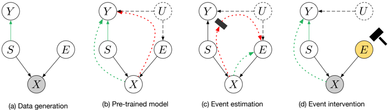For a domain-specific reasoning task, we denote the input prompt as X and the answer as Y , as illustrated in Figure 1 (a). Instead of modeling a model-specific prediction process like X → Y , we adopt a stable and invariant modeling approach following Kaur et al. [2022]. Specifically, we decompose the data generation process as E → X ← S → Y , where E represents event-related or contextually correlated but logic-irrelevant information; S indicates the underlying, unobserved logic structure; Y includes both the reasoning trace and the final answer at the token level. For instance, if X is a causal inference question, S should contain the ground-truth causal graph and all associations of the question, and Y represents the standard step-by-step causal reasoning process and the final answer. ## 3.2 Spurious correlations during pre-training Spurious correlation establishments. According to the data generation SCM in Figure 1 (a), the prompt X acts as a collider between E and S . During the pre-training process, this introduces spurious correlations between E and Y in the learned conditional distribution P ( Y | X ) . Formally, the prediction P ( Y | X ) can be expressed as: <!-- formula-not-decoded --> where e ∼ P ( E ) and s ∼ P ( S ) . Given the SCM, Y is conditionally independent of X and E once S is known, i.e ., Y ⊥ ⊥ ( X,E ) | S s . Applying this condition and Bayes' rule to P ( e, s | X ) , the P ( Y | X ) prediction can be represented as follows: <!-- formula-not-decoded --> <latexi sh 1\_b 64="IVqKn8 P F cR S EHpT >A B+ DL gJ Oz NQY k Z d m C / j f 7U W M v o w G y X u <latexi sh 1\_b 64="U d pyqMzn 7/ O T gw >A B+H c VDL J E F I R NQY Zk m C j f S W v P o K G X u <latexi sh 1\_b 64="Aq8dDjQ Z L 9uK UYV5E > B+H c NS F ypX7 T W C I r v R w / n f g z GP O M o k m J <latexi sh 1\_b 64="8 I + pGH3 uyk vnwgdW jM0 >A B c VDLS N EO r fUY9 FoP K R T m Q Z X z J q C / <latexi sh 1\_b 64="IVqKn8 P F cR S EHpT >A B+ DL gJ Oz NQY k Z d m C / j f 7U W M v o w G y X u <latexi sh 1\_b 64="U d pyqMzn 7/ O T gw >A B+H c VDL J E F I R NQY Zk m C j f S W v P o K G X u <latexi sh 1\_b 64="Aq8dDjQ Z L 9uK UYV5E > B+H c NS F ypX7 T W C I r v R w / n f g z GP O M o k m J <latexi sh 1\_b 64="8 I + pGH3 uyk vnwgdW jM0 >A B c VDLS N EO r fUY9 FoP K R T m Q Z X z J q C / <latexi sh 1\_b 64=" 7K o f/S BvjA u X DY > +H c V N F yp T W C I L M Q r Z R w q nd g z GP J EO U m k <latexi sh 1\_b 64="IVqKn8 P F cR S EHpT >A B+ DL gJ Oz NQY k Z d m C / j f 7U W M v o w G y X u <latexi sh 1\_b 64="U d pyqMzn 7/ O T gw >A B+H c VDL J E F I R NQY Zk m C j f S W v P o K G X u <latexi sh 1\_b 64="Aq8dDjQ Z L 9uK UYV5E > B+H c NS F ypX7 T W C I r v R w / n f g z GP O M o k m J <latexi sh 1\_b 64="8 I + pGH3 uyk vnwgdW jM0 >A B c VDLS N EO r fUY9 FoP K R T m Q Z X z J q C / <latexi sh 1\_b 64=" 7K o f/S BvjA u X DY > +H c V N F yp T W C I L M Q r Z R w q nd g z GP J EO U m k <latexi sh 1\_b 64="IVqKn8 P F cR S EHpT >A B+ DL gJ Oz NQY k Z d m C / j f 7U W M v o w G y X u <latexi sh 1\_b 64="U d pyqMzn 7/ O T gw >A B+H c VDL J E F I R NQY Zk m C j f S W v P o K G X u <latexi sh 1\_b 64="Aq8dDjQ Z L 9uK UYV5E > B+H c NS F ypX7 T W C I r v R w / n f g z GP O M o k m J <latexi sh 1\_b 64="8 I + pGH3 uyk vnwgdW jM0 >A B c VDLS N EO r fUY9 FoP K R T m Q Z X z J q C / <latexi sh 1\_b 64=" 7K o f/S BvjA u X DY > +H c V N F yp T W C I L M Q r Z R w q nd g z GP J EO U m k Figure 1: Acquisitions and eliminations of Spurious correlations. Figure (a) describes the data interaction and generation SCM assumption, where the grey node indicates strong colliding biases such as selection biases. After training models on the data generated, figure (b) indicates the modeling of the confounding correlation when using the pre-trained model. To avoid predicting using the confounding correlation, figures (c) and (d) demonstrate our method in conducting debiasing finetuning. In these figures, green dot arrow curves indicate the target correlations, while red dot arrow curves denote undesired ones. <details> <summary>Image 1 Details</summary>  ### Visual Description ## Diagram: Causal Inference Models ### Overview The image presents four diagrams illustrating different stages of causal inference modeling: data generation, pre-trained model, event estimation, and event intervention. Each diagram depicts variables (Y, S, E, X, U) and their relationships using arrows to indicate causal dependencies. The diagrams show how these relationships change across the different stages. ### Components/Axes * **Nodes:** Represented by circles, labeled as Y, S, E, X, and U. * Y: Outcome variable * S: Source variable * E: Event variable * X: Observed variable * U: Unobserved variable (dashed circle) * **Edges:** Represented by arrows, indicating causal relationships. * Solid black arrows: Direct causal effect. * Dashed green arrows: Causal effect. * Dashed red arrows: Causal effect. * Dashed gray arrows: Causal effect. * **Diagram Titles:** * (a) Data generation * (b) Pre-trained model * (c) Event estimation * (d) Event intervention ### Detailed Analysis **Diagram (a) Data generation:** * Nodes: Y, S, E, X. All nodes are white except for X, which is gray. * Edges: * S -> X (black, solid) * E -> X (black, solid) * S -> Y (green, solid) * Description: This diagram shows the basic causal structure where S and E influence X, and S also influences Y. **Diagram (b) Pre-trained model:** * Nodes: Y, S, E, X, U. U is a dashed circle. All nodes are white. * Edges: * S -> X (black, solid) * E -> X (black, solid) * S -> Y (green, solid) * U -> E (gray, dashed) * U -> Y (gray, dashed) * S -> Y (green, dashed) * E -> X (red, dashed) * S -> X (green, dashed) * Y -> X (red, dashed) * Description: This diagram introduces the unobserved variable U, which influences both E and Y. It also shows feedback loops and potential confounding relationships. **Diagram (c) Event estimation:** * Nodes: Y, S, E, X, U. U is a dashed circle. All nodes are white. * Edges: * S -> X (black, solid) * E -> X (black, solid) * S -> Y (green, solid) * U -> E (gray, dashed) * U -> Y (gray, dashed) * S -> Y (green, dashed) * E -> X (green, dashed) * S -> X (red, dashed) * Y -> X (red, dashed) * A black rectangle is blocking the red dashed arrow from Y to S. * Description: Similar to (b), but with an added element (black rectangle) blocking the influence from Y to S. **Diagram (d) Event intervention:** * Nodes: Y, S, E, X, U. U is a dashed circle. E and X are colored yellow and gray, respectively. * Edges: * S -> X (black, solid) * E -> X (black, solid) * S -> Y (green, solid) * U -> E (gray, dashed) * U -> Y (gray, dashed) * S -> Y (green, dashed) * E -> X (green, dashed) * A hammer is pointing at node E. * Description: This diagram shows an intervention on E, indicated by the hammer. E and X are highlighted, suggesting they are the focus of the intervention. ### Key Observations * The diagrams illustrate the evolution of a causal model from a simple data generation process to a more complex intervention scenario. * The introduction of the unobserved variable U and feedback loops adds complexity to the model. * The intervention in diagram (d) highlights the potential impact of external actions on the system. ### Interpretation The diagrams demonstrate the process of building and refining a causal model. Starting with a basic understanding of data generation, the model evolves to incorporate unobserved variables and feedback loops. The final stage shows how interventions can be applied to the model to understand their effects. The progression highlights the importance of considering confounding factors and feedback mechanisms when making causal inferences. The hammer in diagram (d) symbolizes an external intervention, which is a key concept in causal inference. The change in color of nodes E and X in diagram (d) indicates that these variables are directly affected by the intervention. </details> Here, P ( Y | s ) captures the invariant answer determined process, representing the desired reasoning prediction trace X ← S → Y we aim to learn. However, due to the selection bias introduced during the data collection process, where E ̸ ⊥ ⊥ S | X , the term P ( e | X,s ) introduces spurious dependence of Y on E , violating the intended independence and contaminating the prediction P ( Y | X ) . As a result, when LLMs pre-train on such data distribution, the estimation of P ( Y | X ) becomes biased. Consequently, any distributional shifts in E across different domains or training/testing distributions will lead to significant degradation in reasoning performance. Transferred pre-training biases. Once the LLMs are pre-trained, the strong colliding biases between events and answers become embedded in the model and are propagated through all downstream predictions, resulting in transferred pre-training bias. When applying the pre-trained LLMs for inference predictions, we model these inherited spurious correlations as an unobserved confounder U , as shown in Figure 1 (b). Formally, the biased P ( Y | X ) prediction can be written as: <!-- formula-not-decoded --> As a result, except for the current colliding biases, as shown in the figure, there are still two associations between Y and X , i.e ., the desirable association path X ← S → Y (green dot curve), which captures the true reasoning trace, and the spurious association X ← E ← U → S → Y (red dot curve), which arises from spurious correlations injected during pre-training. Our target is to eliminate the association path through U and isolate the reasoning trace mediated by S . It is worth noting that the reason we model the transferred pre-training biases as a confounder between E and Y is that E and Y are both token-level variables, while S is not. The confounding associations between these token-level variables can be considered as the spurious attention patterns in the LLM's internal attention mechanisms. ## 3.3 Causality-aware post-training To eliminate the bias introduced by the confounder, one natural approach is to adopt a two-step prediction pipeline: first predict S from X , then estimate Y from S , as proposed in chain-ofthought reasoning frameworks [Wei et al., 2022]. This is philosophically aligned with the front-door adjustment [Pearl and Mackenzie, 2018]. However, since S represents a latent logical structure that is neither observed nor easily defined, directly modeling or marginalizing over the entire space of S is intractable. Instead, we propose an indirect but effective alternative: estimating the event variable E and intervening on it to block the spurious associations introduced by the confounder, similar in spirit to the backdoor adjustment. As we introduce in the following subsections, our causality-aware post-training (CAPT) method decomposes the biased prediction into two less biased components: event estimation and event intervention , which together mitigate the confounding effect through structured reasoning. ## 3.3.1 Event estimation Spurious associations in LLMs often arise from colliding biases in domain-specific datasets or encoded social biases. While the dependency between Y and E may be entangled through such biases, the relationship between X and E tends to be more direct and deterministic. In Figure 1(c), we introduce our only LLM-specific assumption: pre-trained LLMs are trained on distributions so large and diverse that colliding biases affecting P ( E | X ) are diluted and negligible. In other words, event estimation is treated as a transferable capability of LLMs, which we will validate in Section 4.2. Intuitively, while predicting Y may involve domain-specific knowledge that constrains the logic and co-occurrence of events ( e.g ., knowing 'get lung cancer' biases outputs toward 'keep smoking'), event estimation focuses solely on identifying events without relying on these logical correlations. This makes the estimation task significantly more robust, especially when the scale of the pre-training distribution is large enough. To block the undesired confounding path through U , we propose using a pre-trained LLM to estimate E directly from X , leveraging clear event definitions and promptable templates. Based on our assumption, we ignore colliding biases in the P ( E | X ) distribution. Furthermore, as depicted in Figure 1(c), the prediction of E avoids influence from the confounder U , as Y , acts as a collider in the path S → Y ← U , is not part of the estimation process. As a result, the spurious association (red dotted curve) is blocked. This design allows us to harness the LLM's transferable generalization ability to perform reliable event estimation. In our experiments, we show that well-crafted prompts augmented with a few-shot examples can achieve strong performance on complex benchmarks such as CLadder. ## 3.3.2 Event intervention With the event variable E identified, we aim to address two biases, i.e ., the pre-training bias and the fine-tuning bias. Pre-training bias elimination: intervention. The pre-training bias is introduced by the confounder U , which was encoded during large-scale pre-training. To remove this bias, we perform an intervention on the event variable E , as shown in Figure 1(d), effectively breaking the dependency path from U to E . This is achieved by marking all identified events with symbolic placeholders, simplifying Equation 3 to the following results: <!-- formula-not-decoded --> where U has been marginalized out. This result aligns with Equation 2, demonstrating that the spurious dependencies introduced via U have been successfully removed. Fine-tuning bias prevention: random assignments. To prevent new spurious correlations from being introduced during fine-tuning, we adopt a randomized intervention strategy. Specifically, we assign uniformly random capital letters as symbolic representations for E , and randomly reassign them in newly generated inputs X . This procedure ensures permutation invariance and breaks any selection bias, enforcing the condition E ⊥ ⊥ S | X . As a result, the prediction simplifies to: <!-- formula-not-decoded --> where E has been marginalized due to the randomized assignment, thereby eliminating any residual dependency between Y and E . This ensures that the fine-tuning process focuses solely on the desired reasoning trace X ← S → Y , aligning with our intended modeling objective. It is important to note that OOD generalization without access to auxiliary information has been shown to be theoretically impossible [Lin et al., 2022], due to the inherent indistinguishability between spurious and causal factors. Under our data generation assumptions, we explicitly specify that the generation mechanism is agnostic to specific variable or event names. Accordingly, the combination of event estimation and event intervention leverages the LLM's robust generalization <latexi sh 1\_b 64="Aq8dDjQ Z L 9uK UYV5E > B+H c NS F ypX7 T W C I r v R w / n f g z GP O M o k m J <latexi sh 1\_b 64="Aq8dDjQ Z L 9uK UYV5E > B+H c NS F ypX7 T W C I r v R w / n f g z GP O M o k m J <latexi sh 1\_b 64="IVqKn8 P F cR S EHpT >A B+ DL gJ Oz NQY k Z d m C / j f 7U W M v o w G y X u <latexi sh 1\_b 64="IVqKn8 P F cR S EHpT >A B+ DL gJ Oz NQY k Z d m C / j f 7U W M v o w G y X u <latexi sh 1\_b 64="0 gALRknMjZUwNE3 rodGJ qBQ > /X c VC7S F f u Y m Hp z P O D I W K T + v y 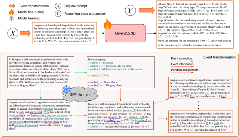Figure 2: CAPT implementation pipeline. The upper part represents the training process, where the event transformation, the orange bold arrow, is illustrated in the lower part of the figure. <details> <summary>Image 2 Details</summary>  ### Visual Description ## Diagram: Causal Inference with Language Models ### Overview The image illustrates a causal inference process using language models. It shows how an original prompt is transformed, processed by different language models (Qwen2.5 3B and GPT 4o-mini), and how the reasoning trace and answer are generated. The diagram also includes event mapping and estimation steps. ### Components/Axes * **Top-Left:** * **Legend:** * Orange Arrow: Event transformation * Flame Icon: Model fine-tuning * Snowflake Icon: Model freezing * **X (in circle):** Original prompt * Text: Imagine a self-contained, hypothetical world with only the following conditions, and without any unmentioned factors or causal relationships: C has a direct effect on U and K. U has a direct effect on K. For C=0, the probability of K=1 is 42%. For C=1, the probability of K=1 is 51%. Will C=1 increase the chance of K=1? * **Top-Right:** * **Y (in circle):** Reasoning trace and answer * Text: ` <answer> Yes </answer>` * **Center:** * Pink Rectangle: Qwen2.5 3B * Flame Icon above the rectangle * **Bottom-Left:** * **X:** Imagine a self-contained, hypothetical world with only the following conditions, and without any unmentioned factors or causal relationships: Husband has a direct effect on wife and alarm clock. Wife has a direct effect on alarm clock. For husbands that don't set the alarm, the probability of ringing alarm is 42%. For husbands that set the alarm, the probability of ringing alarm is 51%. Will alarm set by husband increase the chance of ringing alarm? * **Bottom-Center:** * **Event mapping:** * {symbol\_1}: Husband * {symbol\_1}=1: Husband sets the alarm * {symbol\_1}=0: Husband does not set the alarm * {symbol\_2}: Wife * {symbol\_3}: Alarm clock * {symbol\_3}=1: Ringing alarm * Cloud Shape: GPT 4o-mini * Snowflake Icon above the cloud * Text: Imagine a self-contained, hypothetical world with only the following conditions, and without any unmentioned factors or causal relationships: {symbol\_1} has a direct effect on {symbol\_2} and {symbol\_3}. {symbol\_2} has a direct effect on {symbol\_3}. For {symbol\_1}=0, the probability of {symbol\_3}=1 is 42%. For {symbol\_1}=1, the probability of {symbol\_3}=1 is 51%. Will {symbol\_1}=1 increase the chance of {symbol\_3}=1? * **Bottom-Right:** * **Event estimation** * Event intervention * Random assignments * **Event transformation** * Text: Imagine a self-contained, hypothetical world with only the following conditions, and without any unmentioned factors or causal relationships: C has a direct effect on U and K. U has a direct effect on K. For C=0, the probability of K=1 is 42%. For C=1, the probability of K=1 is 51%. Will C=1 increase the chance of K=1? * Text: Imagine a self-contained, hypothetical world with only the following conditions, and without any unmentioned factors or causal relationships: A has a direct effect on T and Z. T has a direct effect on Z. For A=0, the probability of Z=1 is 42%. For A=1, the probability of Z=1 is 51%. Will A=1 increase the chance of Z=1? ### Detailed Analysis or ### Content Details * **Original Prompt (Top-Left):** The prompt describes a hypothetical world where variable C affects U and K, and U affects K. It provides probabilities for K=1 given C=0 (42%) and C=1 (51%), asking if C=1 increases the chance of K=1. * **Qwen2.5 3B (Center):** This language model processes the original prompt. * **Reasoning Trace and Answer (Top-Right):** The model extracts the causal graph, determines the query type as "average treatment effect," formalizes the query, gathers relevant data (P(K=1|C=0)=0.42, P(K=1|C=1)=0.51), and deduces the estimand using causal inference. It calculates the estimate as 0.09, concluding that the answer is yes. * **GPT 4o-mini (Bottom-Center):** This model processes a similar prompt related to husband, wife, and alarm clock. It maps the entities to symbols and provides probabilities for the ringing alarm based on whether the husband sets the alarm or not. * **Event Transformation (Arrows):** Orange arrows indicate event transformation. Green arrows indicate event estimation. * **Model States:** The flame icon represents model fine-tuning, while the snowflake icon represents model freezing. ### Key Observations * The diagram showcases the use of language models for causal inference. * Two different language models (Qwen2.5 3B and GPT 4o-mini) are used to process different prompts. * The reasoning trace provides a step-by-step explanation of how the language model arrives at the answer. * The event mapping and estimation steps are crucial for translating the natural language prompt into a formal causal inference problem. ### Interpretation The diagram demonstrates how language models can be used to perform causal inference by extracting causal relationships from text, formalizing queries, and calculating estimates. The use of different models and prompts highlights the versatility of this approach. The reasoning trace provides transparency into the model's decision-making process, which is important for building trust in AI systems. The diagram suggests that language models can be valuable tools for causal reasoning and decision-making in various domains. The consistent probability increase (from 42% to 51%) across different scenarios (C affecting K, husband setting alarm affecting ringing alarm, etc.) suggests a robust pattern recognition capability of the models. </details> ability to abstract over event identities and map the large event space into a compact symbolic alphabet. This abstraction facilitates reliable reasoning during both training and inference. ## 3.3.3 Implementation overview Building on the theoretical analysis, our empirical CAPT implementation is both simple and efficient. As illustrated in Figure 2, we first construct training data triplets consisting of the input prompt, the corresponding reasoning trace, and the final answer. We then employ a pre-trained language model, GPT-4o-mini [Achiam et al., 2023], to perform event estimation and event intervention together. Specifically, we use 2 to 3 in-context examples annotated by humans to guide the model in identifying events and intervening events with symbolic placeholders: {symbol\_1}, {symbol\_2}, {symbol\_3}, . . . as described in Section 3.3.1. According to our prior analysis, the event estimation process introduces minimal bias and leverages the model's generalizable capabilities. For causal inference tasks, each symbol may be associated with three interpretations: a neutral label, a positive state, and a negative state, as shown in the event mapping of Figure 2. For instance, {symbol\_1} may refer to 'husbands,' with {symbol\_1} = 1 representing 'husbands set the alarm,' and {symbol\_1} = 0 denoting 'husbands do not set the alarm.' To ensure consistency, we implement automatic verification and re-execution of the transformation step until all identified events are uniformly symbolized across the entire input. After transforming all events into abstract symbols, we randomly assign these symbols to capital letters from the English alphabet. We then perform supervised fine-tuning on both the reasoning trace and the final answer using this symbolized representation. At inference time, we apply the same procedure to OOD samples: estimate events, transform them into symbolic placeholders, and randomly assign capital letters. This effectively transforms OOD inputs into representations that are similar to the fine-tuned ID samples. As a result, the model's OOD generalization performance can be improved, which we attribute to the transferable event estimation capability of the pre-trained model, as discussed in Section 3.3.1. ## 3.4 Revisit CoT in debiasing CoTs in fine-tuning. In our CAPT implementation, we typically fine-tune on not only the answers but also the reasoning traces, i.e ., Chain-of-Thoughts (CoTs), with the following reasons. Equation 5 implies that the prediction process can be interpreted as a weighted ensemble over reasoning traces, where P ( s | X ) acts as the weights. If the logic space, i.e ., the space of possible S , is small, then training with answer-only supervision can still yield comparable results to training with CoTs, as the correct reasoning trace can be implicitly recovered through next-token prediction. However, when the reasoning space is large and diverse, this ensemble becomes sparse, and the correct reasoning path may be difficult to learn through implicit supervision alone. In such cases, explicitly providing the intermediate tokens or reasoning trace via CoT becomes crucial to guide the model towards more consistent and accurate generalization. Inference-time CoTs From an inference-time technique perspective, if we consider CoTs as an approximation of the latent logical structure S , then according to Equations 2 and 5, two conditions must be satisfied for unbiased reasoning. First, the generated CoT should reliably approximate the mediator S , such that Y ⊥ ⊥ ( X,E ) | S , ensuring that the reasoning process is independent of both the prompt and spurious event-related information. Second, similar to the front-door criterion, the prediction of Y should be based solely on the CoT, i.e ., the inferred S , and not directly on the original prompt X . However, this condition is often violated in current CoT approaches, where the model still heavily relies on X , thereby limiting the debiasing effect of CoTs. Intuitively, CoTs should reflect the underlying causal reasoning structure and remain agnostic to specific prompt formulations. ## 4 Experiments We conduct experiments to address two major challenges: (i) pre-training biases and (ii) fine-tuning biases . The pre-training bias refers to the confounding correlations embedded in LLMs during pretraining, as illustrated in Figure 1(b), which we aim to mitigate through post-training. The fine-tuning bias, on the other hand, represents spurious correlations introduced during the fine-tuning process, which we aim to prevent from emerging. Our experiments are designed to answer the following research questions: RQ1: How strong are the confounding correlations introduced during LLM pre-training? RQ2: Can inference-time CoT and event intervention help mitigate pre-training biases? RQ3: Can our proposed method, CAPT, along with post-training CoT, effectively break pre-training biases, avoid fine-tuning biases, and improve training efficiency? ## 4.1 Pre-training biases in LLMs We benchmark the performance of GPT-3.5 Turbo, GPT-4o-mini, and GPT-4o [Achiam et al., 2023] using CoT prompting and in-context examples on two evaluation datasets: the causal inference benchmark CLadder [Jin et al., 2023] and the deductive reasoning benchmark PrOntoQA [Saparov and He, 2023]. CLadder is a formal causal inference benchmark inspired by foundational concepts in causal reasoning [Pearl and Mackenzie, 2018]. It consists of queries based on causal graphs and includes associational, interventional, and counterfactual questions. As a relatively underexplored dataset, CLadder allows us to evaluate models on rigorous causal reasoning. PrOntoQA, selected for its formal logical structure, provides fine-grained control over logical reasoning compared to other datasets such as ProofWriter [Tafjord et al., 2020], FOLIO [Han et al., 2022], and SimpleLogic [Zhang et al., 2022]. Following Saparov and He [2023], we use PrOntoQA to evaluate LLMs from a formal logical reasoning perspective. Both CLadder and PrOntoQA are structured as binary classification tasks, requiring models to validate hypotheses based on a set of facts and rules. ## 4.1.1 Pre-Training Biases To directly assess the existence of data leakage or spurious correlations, we compare model performance on a commonsense set versus an anti-sense set. The commonsense set is composed of original examples sourced from standard causal texts [Pearl and Mackenzie, 2018] and logical reasoning datasets. In contrast, the anti-sense set is generated by perturbing or swapping events, thereby constructing scenarios that are unlikely or novel, essentially OOD instances, as introduced in CLadder [Jin et al., 2023]. If model predictions depend heavily on pre-trained spurious correlations, we expect a substantial performance drop on the anti-sense set. As shown in Table 1, this pattern is evident in PrOntoQA: while GPT-4o-mini achieves 83.5% accuracy on the commonsense set, performance drops to 61.25% on the anti-sense set. Similarly, GPT-4o drops from 85% to 67%. These results highlight the model's reliance on pre-trained spurious associations, which fail under perturbation. In contrast, results on CLadder show a smaller performance gap between commonsense and anti-sense sets, and overall accuracy is close to random. Table 1: LLMperformance on PrOntoQA and CLadder. Results listed in the table are in Accuracy. "Comm" denotes the commonsense test set. STD represents the performance standard deviations across the three commonsense, anti-sense, and non-sense test sets. IC represents containing incontext examples. Bold numbers indicate the best results. Orange underlined numbers indicate low performance caused by pre-training biases. | | PrOntoQA | PrOntoQA | PrOntoQA | PrOntoQA | CLadder | CLadder | CLadder | CLadder | |------------------|------------|------------------|-----------------|------------|-----------|------------------|-----------------|-----------| | | Comm (ID) | Anti-sense (OOD) | Non-sense (OOD) | STD | Comm (ID) | Anti-sense (OOD) | Non-sense (OOD) | STD | | GPT 3.5 | 56.25 | 54.50 | 44.05 | 6.60 | 50.96 | 48.65 | 49.12 | 1.22 | | 4o-mini | 83.50 | 61.25 | 78.00 | 11.59 | 56.44 | 59.13 | 56.45 | 1.55 | | 4o-mini CoT | 87.00 | 74.00 | 80.05 | 6.51 | 65.48 | 66.73 | 70.41 | 2.56 | | 4o-mini CoT + IC | 85.75 | 70.05 | 74.05 | 8.16 | 63.75 | 64.33 | 67.29 | 1.90 | | 4o | 85.00 | 67.00 | 78.25 | 9.09 | 55.58 | 55.67 | 55.76 | 0.09 | | 4o CoT | 86.50 | 80.25 | 80.50 | 3.54 | 70.00 | 71.15 | 72.36 | 1.18 | | 4o CoT + IC | 86.50 | 73.50 | 80.00 | 6.50 | 72.88 | 71.15 | 74.41 | 1.63 | This suggests that LLMs are not leveraging strong spurious correlations in CLadder, possibly due to the dataset's inherent complexity and formal structure, which require deeper causal understanding beyond surface-level correlations. ## 4.1.2 Inference-time techniques Inference-time intervention. The OOD non-sense set is constructed by replacing event names with random character strings, such as 'xvua,' 'auiow,' and 'iop.' This setup simulates an inference-time intervention strategy under the assumption of an oracle-level event estimation process, i.e ., perfect identification and perturbation of events. The performance gap between the non-sense set and the anti-sense set on PrOntoQA, as reported in Table 1, quantifies the benefit of such abstraction in mitigating pre-training biases. Similarly, for CLadder, the non-sense set generally outperforms the anti-sense set, although the gap is smaller. This aligns with our earlier finding that CLadder is inherently less impacted by pre-training biases due to its formal structure and low surface-level spurious signals. Chain-of-thought and in-context examples. As discussed in Section 3.4, well-designed CoTs can serve as approximations of the latent logical structure S , helping to block the colliding bias between E and S . Consequently, they can lead to more robust and less biased predictions. This is evident in the results shown in Table 1: while CoTs do not significantly improve performance on PrOntoQA's commonsense set, they dramatically improve performance on the anti-sense set. For instance, GPT-4o-mini improves from 61.25% to 74%, and GPT-4o improves from 67% to 80.25% with CoT prompting. In contrast, the use of in-context examples (IC) produces mixed results. While IC examples can help on complex reasoning tasks like CLadder, they often inject additional spurious correlations into PrOntoQA. This leads to larger performance gaps between the anti-sense set and the commonsense or non-sense sets, indicating that IC examples may inadvertently amplify pre-existing biases in simpler reasoning tasks. ## 4.2 Unbiased Fine-tuning Next, we adopt a consistent benchmark setup to evaluate our proposed CAPT strategy. The base model used is Qwen2.5-3B [Yang et al., 2024], and we evaluate fine-tuning performance from multiple perspectives. Specifically, first, we compare fine-tuning with and without our event estimation and event intervention steps, denoted as CAPT and Original, respectively. Second, we assess the impact of different output formats, namely, Answer-only where the model generates only 'yes' or 'no', and chain-of-thought (CoT) where the model generates intermediate reasoning steps wrapped in <think> and </think> tags followed by the final answer. Third, we evaluate the sample efficiency of each fine-tuning method under limited data settings, i.e ., 100 or 200 samples. CAPT vs. original. As shown in Table 2, the SFT results demonstrate that CAPT produces significantly lower standard deviations across in-distribution (ID) and OOD test sets. Here, a lower standard deviation implies consistent performance across ID and OOD distributions, reflecting strong generalization and reduced bias. In contrast, fine-tuning without CAPT (Original) leads to higher variance, particularly on PrOntoQA, indicating vulnerability to spurious correlations. These results validate the effectiveness of CAPT in mitigating fine-tuning biases and enhancing robustness. Table 2: Supervised Fine-tuning results. Best results given the same number of samples are in bold . | | | | PrOntoQA | PrOntoQA | PrOntoQA | PrOntoQA | CLadder | CLadder | CLadder | CLadder | |---------|-------------|--------------------|---------------|-------------|-------------|-------------|-------------|-------------|-------------|-------------| | | | | Comm | Anti-sense | Non-sense | STD | Comm | Anti-sense | Non-sense | STD | | LLMs | | 4o CoT 4o CoT + FS | 86.50 86.50 | 80.25 73.50 | 80.50 80.00 | 3.54 6.50 | 70.00 72.88 | 71.15 71.15 | 72.36 74.41 | 1.18 1.63 | | SFT ) | 100 samples | 100 samples | 100 samples | 100 samples | 100 samples | 100 samples | 100 samples | 100 samples | 100 samples | 100 samples | | SFT ) | Original | Answer-only CoT | 99.75 99.50 | 61.50 70.75 | 71.25 79.00 | 19.88 14.80 | 67.60 67.98 | 60.10 68.85 | 55.57 62.70 | 6.08 3.33 | | SFT ) | CAPT | Answer-only CoT | 89.00 87.50 | 83.75 82.50 | 88.75 81.00 | 2.96 3.40 | 67.21 75.96 | 64.42 77.98 | 63.57 69.43 | 1.90 4.47 | | SFT ) | 200 samples | 200 samples | 200 samples | 200 samples | 200 samples | 200 samples | 200 samples | 200 samples | 200 samples | 200 samples | | SFT ) | Original | Answer-only CoT | 100.00 100.00 | 62.50 75.00 | 70.50 80.25 | 19.75 13.18 | 70.48 68.65 | 68.85 68.85 | 66.11 66.11 | 2.21 1.53 | | SFT ) | CAPT | Answer-only CoT | 92.75 | | | 3.03 | 71.35 79.04 | 63.75 79.90 | 62.50 73.73 | 4.79 | | ( 90% ) | Original | | 95.00 | 86.75 88.50 | 90.50 92.00 | 3.25 | | | | 3.34 | | | | Answer-only CoT | 100.00 100.00 | 58.00 74.00 | 77.25 83.75 | 21.02 13.13 | 90.29 95.38 | 86.54 95.67 | 80.08 88.09 | 5.16 4.30 | | | CAPT | Answer-only CoT | 99.25 99.50 | 91.50 93.00 | 95.50 96.75 | 3.88 3.26 | 87.60 93.08 | 89.42 94.62 | 80.76 88.57 | 4.57 3.14 | CoTs vs. answer-only. As discussed in Section 3.4, CoTs can suppress shortcut correlations between E and Y by approximating the latent reasoning structure S . Table 2 further shows that CoT-based fine-tuning outperforms Answer-only fine-tuning by non-trivial margins. This is due to the limitations of next-token prediction given the exponential increase of context combinations. Specifically, when predicting only a binary answer, spurious correlations are easier to be built, whereas intermediate reasoning steps as in CoTs make such shortcuts harder to exploit. Notably, the performance gap between Answer-only and CoT becomes smaller when CAPT is applied, further validating that blocking spurious Y -E correlations is more robust than approximating mediators using CoT alone. Note that we apply CausalCOT [Jin et al., 2023] for CLadder. Sample efficiency. On datasets like CLadder, where the question space involves diverse event combinations, although full SFT (90% of data) yields strong results, it is not practical, since data annotation is often a bottleneck in practical applications, particularly in domains requiring expert knowledge. Under such constraints, CAPT outperforms standard fine-tuning by significant margins, even when only 100-200 samples are available. As shown in Table 2, CAPT achieves superior performance, outperforming GPT 4o with CoTs and in-context examples and standard SFT, especially on anti-sense OOD test sets. This highlights CAPT's ability to eliminate spurious pre-training correlations even under low-resource conditions. It is noteworthy that, as noted in Section 4.1.1, PrOntoQA encodes stronger pre-training biases than CLadder, which causes the failure of full SFT (90%) on anti-sense and non-sense test sets in PrOntoQA, indicating the failure of spurious correlation mitigation with simple SFT. Please refer to Appendix D.3 for ablation studies. Is event estimation transferable? As discussed in Section 3.3.1, event estimation appears to be a transferable and generalizable skill for pre-trained LLMs. To validate this, we examine the performance drop on commonsense test sets under CAPT. Table 2 shows that performance drops are consistently within 3%, indicating the event estimation step only slightly affects the original in-domain results. Moreover, the high accuracy on non-sense test sets confirms that event estimation is robust to novel event names, validating its OOD generalization capabilities. In summary, CAPT effectively breaks pre-injected spurious correlations and avoids fine-tuning biases, demonstrating strong generalization across ID and OOD distributions with minimal supervision. ## 5 Conclusion In this work, we presented CAPT, a simple and effective method for improving LLM generalization by mitigating both pre-training and fine-tuning event biases. By decomposing biased predictions into two unbiased steps, event estimation and event intervention, CAPT breaks spurious correlations while preserving reasoning structure. Experiments on CLadder and PrOntoQA show that CAPT significantly improves OOD performance and sample efficiency, enabling 3B models to outperform larger LLMs with only 100 fine-tuning samples. This highlights CAPT's practicality as a lightweight and robust post-training approach for reasoning tasks. ## Acknowledgments and Disclosure of Funding This work was supported in part by ARPA-H under grant 1AY1AX000053 and National Science Foundation under grant CNS-2328395. ## References - Abulhair Saparov and He He. Language models are greedy reasoners: A systematic formal analysis of chain-of-thought. arXiv preprint arXiv:2210.01240 , 2022. - Peter Clark, Oyvind Tafjord, and Kyle Richardson. Transformers as soft reasoners over language. arXiv preprint arXiv:2002.05867 , 2020. - Zirui Zhao, Wee Sun Lee, and David Hsu. Large language models as commonsense knowledge for large-scale task planning. Advances in Neural Information Processing Systems , 36:31967-31987, 2023. - Ruixiang Tang, Dehan Kong, Longtao Huang, and Hui Xue. Large language models can be lazy learners: Analyze shortcuts in in-context learning. arXiv preprint arXiv:2305.17256 , 2023. - Wenqian Ye, Guangtao Zheng, Xu Cao, Yunsheng Ma, and Aidong Zhang. Spurious correlations in machine learning: A survey. arXiv preprint arXiv:2402.12715 , 2024. - Iman Mirzadeh, Keivan Alizadeh, Hooman Shahrokhi, Oncel Tuzel, Samy Bengio, and Mehrdad Farajtabar. Gsm-symbolic: Understanding the limitations of mathematical reasoning in large language models. arXiv preprint arXiv:2410.05229 , 2024. - Zhijing Jin, Jiarui Liu, Zhiheng LYU, Spencer Poff, Mrinmaya Sachan, Rada Mihalcea, Mona T. Diab, and Bernhard Schölkopf. Can large language models infer causation from correlation? In The Twelfth International Conference on Learning Representations , 2024. URL https://openreview. net/forum?id=vqIH0ObdqL. - Fei Wang, Wenjie Mo, Yiwei Wang, Wenxuan Zhou, and Muhao Chen. A causal view of entity bias in (large) language models. arXiv preprint arXiv:2305.14695 , 2023. - Shayne Longpre, Kartik Perisetla, Anthony Chen, Nikhil Ramesh, Chris DuBois, and Sameer Singh. Entity-based knowledge conflicts in question answering. arXiv preprint arXiv:2109.05052 , 2021. - Chen Qian, Fuli Feng, Lijie Wen, Chunping Ma, and Pengjun Xie. Counterfactual inference for text classification debiasing. In Proceedings of the 59th Annual Meeting of the Association for Computational Linguistics and the 11th International Joint Conference on Natural Language Processing (Volume 1: Long Papers) , pages 5434-5445, 2021a. - Zhijing Jin, Yuen Chen, Felix Leeb, Luigi Gresele, Ojasv Kamal, LYU Zhiheng, Kevin Blin, Fernando Gonzalez Adauto, Max Kleiman-Weiner, Mrinmaya Sachan, et al. Cladder: Assessing causal reasoning in language models. In Thirty-seventh conference on neural information processing systems , 2023. - Liangming Pan, Alon Albalak, Xinyi Wang, and William Yang Wang. Logic-lm: Empowering large language models with symbolic solvers for faithful logical reasoning. arXiv preprint arXiv:2305.12295 , 2023. - Silin Gao, Jane Dwivedi-Yu, Ping Yu, Xiaoqing Ellen Tan, Ramakanth Pasunuru, Olga Golovneva, Koustuv Sinha, Asli Celikyilmaz, Antoine Bosselut, and Tianlu Wang. Efficient tool use with chain-of-abstraction reasoning. arXiv preprint arXiv:2401.17464 , 2024. - Jivat Neet Kaur, Emre Kiciman, and Amit Sharma. Modeling the data-generating process is necessary for out-of-distribution generalization. arXiv preprint arXiv:2206.07837 , 2022. - Jonas Peters, Peter Bühlmann, and Nicolai Meinshausen. Causal inference by using invariant prediction: identification and confidence intervals. Journal of the Royal Statistical Society Series B: Statistical Methodology , 78(5):947-1012, 2016. - Martin Arjovsky, Léon Bottou, Ishaan Gulrajani, and David Lopez-Paz. Invariant risk minimization. arXiv preprint arXiv:1907.02893 , 2019. - Abulhair Saparov and He He. Language models are greedy reasoners: A systematic formal analysis of chain-of-thought. In The Eleventh International Conference on Learning Representations , 2023. URL https://openreview.net/forum?id=qFVVBzXxR2V. - Alec Radford, Karthik Narasimhan, Tim Salimans, Ilya Sutskever, et al. Improving language understanding by generative pre-training. 2018. - Hugo Touvron, Thibaut Lavril, Gautier Izacard, Xavier Martinet, Marie-Anne Lachaux, Timothée Lacroix, Baptiste Rozière, Naman Goyal, Eric Hambro, Faisal Azhar, et al. Llama: Open and efficient foundation language models. arXiv preprint arXiv:2302.13971 , 2023. - Daya Guo, Dejian Yang, Haowei Zhang, Junxiao Song, Ruoyu Zhang, Runxin Xu, Qihao Zhu, Shirong Ma, Peiyi Wang, Xiao Bi, et al. Deepseek-r1: Incentivizing reasoning capability in llms via reinforcement learning. arXiv preprint arXiv:2501.12948 , 2025. - An Yang, Baosong Yang, Beichen Zhang, Binyuan Hui, Bo Zheng, Bowen Yu, Chengyuan Li, Dayiheng Liu, Fei Huang, Haoran Wei, et al. Qwen2. 5 technical report. arXiv preprint arXiv:2412.15115 , 2024. - Karl Cobbe, Vineet Kosaraju, Mohammad Bavarian, Mark Chen, Heewoo Jun, Lukasz Kaiser, Matthias Plappert, Jerry Tworek, Jacob Hilton, Reiichiro Nakano, et al. Training verifiers to solve math word problems. arXiv preprint arXiv:2110.14168 , 2021. - Wang Ling, Dani Yogatama, Chris Dyer, and Phil Blunsom. Program induction by rationale generation: Learning to solve and explain algebraic word problems. arXiv preprint arXiv:1705.04146 , 2017. - Man Luo, Shrinidhi Kumbhar, Mihir Parmar, Neeraj Varshney, Pratyay Banerjee, Somak Aditya, Chitta Baral, et al. Towards logiglue: A brief survey and a benchmark for analyzing logical reasoning capabilities of language models. arXiv preprint arXiv:2310.00836 , 2023. - Kun Qian, Ahmad Beirami, Zhouhan Lin, Ankita De, Alborz Geramifard, Zhou Yu, and Chinnadhurai Sankar. Annotation inconsistency and entity bias in multiwoz. arXiv preprint arXiv:2105.14150 , 2021b. - Jared Kaplan, Sam McCandlish, Tom Henighan, Tom B Brown, Benjamin Chess, Rewon Child, Scott Gray, Alec Radford, Jeffrey Wu, and Dario Amodei. Scaling laws for neural language models. arXiv preprint arXiv:2001.08361 , 2020. - Zeyu Qin, Qingxiu Dong, Xingxing Zhang, Li Dong, Xiaolong Huang, Ziyi Yang, Mahmoud Khademi, Dongdong Zhang, Hany Hassan Awadalla, Yi R Fung, et al. Scaling laws of synthetic data for language models. arXiv preprint arXiv:2503.19551 , 2025. - Rem Yang, Julian Dai, Nikos Vasilakis, and Martin Rinard. Evaluating the generalization capabilities of large language models on code reasoning. arXiv preprint arXiv:2504.05518 , 2025. - Judea Pearl, Madelyn Glymour, and Nicholas P Jewell. Causal inference in statistics: A primer . John Wiley & Sons, 2016. - Isabel O Gallegos, Ryan A Rossi, Joe Barrow, Md Mehrab Tanjim, Sungchul Kim, Franck Dernoncourt, Tong Yu, Ruiyi Zhang, and Nesreen K Ahmed. Bias and fairness in large language models: A survey. Computational Linguistics , 50(3):1097-1179, 2024. - John McCarthy and Patrick J Hayes. Some philosophical problems from the standpoint of artificial intelligence. In Readings in artificial intelligence , pages 431-450. Elsevier, 1981. - Nada Lavrac and Saso Dzeroski. Inductive logic programming. In WLP , pages 146-160. Springer, 1994. - Oyvind Tafjord, Bhavana Dalvi Mishra, and Peter Clark. Entailer: Answering questions with faithful and truthful chains of reasoning. arXiv preprint arXiv:2210.12217 , 2022. - Kaiyu Yang, Jia Deng, and Danqi Chen. Generating natural language proofs with verifier-guided search. arXiv preprint arXiv:2205.12443 , 2022. - Jason Wei, Xuezhi Wang, Dale Schuurmans, Maarten Bosma, Fei Xia, Ed Chi, Quoc V Le, Denny Zhou, et al. Chain-of-thought prompting elicits reasoning in large language models. Advances in neural information processing systems , 35:24824-24837, 2022. - Xuezhi Wang, Jason Wei, Dale Schuurmans, Quoc Le, Ed Chi, Sharan Narang, Aakanksha Chowdhery, and Denny Zhou. Self-consistency improves chain of thought reasoning in language models. arXiv preprint arXiv:2203.11171 , 2022. - Yang Liu, Jiahuan Cao, Chongyu Liu, Kai Ding, and Lianwen Jin. Datasets for large language models: A comprehensive survey. arXiv preprint arXiv:2402.18041 , 2024. - Chen Wang, Dongming Zhao, Bo Wang, Ruifang He, and Yuexian Hou. Do llms have the generalization ability in conducting causal inference? arXiv preprint arXiv:2410.11385 , 2024. - Matej Zeˇ cevi´ c, Moritz Willig, Devendra Singh Dhami, and Kristian Kersting. Causal parrots: Large language models may talk causality but are not causal. arXiv preprint arXiv:2308.13067 , 2023. - Judea Pearl and Dana Mackenzie. The book of why: the new science of cause and effect . Basic books, 2018. - Yong Lin, Shengyu Zhu, Lu Tan, and Peng Cui. Zin: When and how to learn invariance without environment partition? Advances in Neural Information Processing Systems , 35:24529-24542, 2022. - Josh Achiam, Steven Adler, Sandhini Agarwal, Lama Ahmad, Ilge Akkaya, Florencia Leoni Aleman, Diogo Almeida, Janko Altenschmidt, Sam Altman, Shyamal Anadkat, et al. Gpt-4 technical report. arXiv preprint arXiv:2303.08774 , 2023. - Oyvind Tafjord, Bhavana Dalvi Mishra, and Peter Clark. Proofwriter: Generating implications, proofs, and abductive statements over natural language. arXiv preprint arXiv:2012.13048 , 2020. - Simeng Han, Hailey Schoelkopf, Yilun Zhao, Zhenting Qi, Martin Riddell, Wenfei Zhou, James Coady, David Peng, Yujie Qiao, Luke Benson, et al. Folio: Natural language reasoning with first-order logic. arXiv preprint arXiv:2209.00840 , 2022. - Honghua Zhang, Liunian Harold Li, Tao Meng, Kai-Wei Chang, and Guy Van den Broeck. On the paradox of learning to reason from data. arXiv preprint arXiv:2205.11502 , 2022. - Adam Paszke, Sam Gross, Francisco Massa, Adam Lerer, James Bradbury, Gregory Chanan, Trevor Killeen, Zeming Lin, Natalia Gimelshein, Luca Antiga, et al. Pytorch: An imperative style, high-performance deep learning library. Advances in neural information processing systems , 32, 2019. - Fabian Pedregosa, Gaël Varoquaux, Alexandre Gramfort, Vincent Michel, Bertrand Thirion, Olivier Grisel, Mathieu Blondel, Peter Prettenhofer, Ron Weiss, Vincent Dubourg, et al. Scikit-learn: Machine learning in python. the Journal of machine Learning research , 12:2825-2830, 2011. ## A Broader impacts This work aims to improve the generalization and robustness of LLMs in reasoning tasks by mitigating spurious correlations through a causality-aware post-training method. The positive societal impacts include enhanced reliability and transparency of language models in domains that require robust reasoning, such as education, scientific research, and legal or medical decision support, where accurate generalization to OOD inputs is critical. By eliminating spurious correlations, our method provides event-invariant predictions. However, like any technique that improves LLM performance with limited data, CAPT could be misused to develop more efficient or persuasive systems for disinformation, manipulation, or unfair decision-making. To mitigate these risks, we recommend that CAPT be applied with transparency, particularly in high-stakes domains. As our method focuses on post-training, it may also encourage ongoing efforts in secure model deployment and bias detection frameworks. ## B Limitations While CAPT demonstrates strong improvements in OOD generalization and sample efficiency, it comes with several limitations. First, CAPT relies on accurate event estimation. In domains where event boundaries are ambiguous or context-dependent, more in-context examples may be required. Second, CAPT currently focuses on binary classification reasoning tasks; extending it to generation or multi-hop reasoning requires further exploration. Finally, although our method helps reduce spurious correlations, it may also suppress useful contextual cues in some settings, potentially affecting performance on tasks requiring textual understanding. ## C CAPT details In this section, we mainly provide the event estimation and intervention prompt template for GPT-4omini and in-context examples. ## C.1 Event estimation and intervention templates First, we provide the following template, where prompt, response, and requirements will be replaced with true X , Y and task-specific requirements: ``` ``` 3. Transformed reasoning steps , ignoring the original symbol assignments and replacing them with the new symbols. where the requirements for CLadder are: ## CLadder requirements ``` ``` - with the new symbols. and the requirements for PrOntoQA are listed below. ## PrOntoQA requirements - Transform all entities and adjectives into variable symbols, denoted in order as {symbol\_1}, { symbol\_2}, {symbol\_3}, etc . Each symbol represents one thing , like an object , an attribute , an adj . etc . Do not include "not" in the symbol name, e.g ., "not small" should be transformed to "not {symbol\_1}". Also, do not include determiners like " all ", "each", "every" and linking verbs like "be", " is ", "are" in the symbol names. Outputs the following information : 1. Variable notations : - the variable symbol, e.g ., {symbol\_1}. - the original name of the symbol, e.g ., small/ butterfly /segmented/six-legged. 2. Transformed background and question , just replace all entities and adjectives with variables . 3. Transformed reasoning steps with the new symbols. ## C.2 In-context examples In addition to the system and user prompts, to avoid ambiguity of the event boundaries, we need to provide a few in-context examples. These examples are listed in Json format and input as human and AI responses iteratively, i.e ., system prompt, user prompt (example 1), constructed ai response (example 1), user prompt (example 2), constructed ai response (example 2), . . . , user prompt (real query). Note that we don't need to create these examples from scratch. They are first generated by LLMs directly, then corrected by humans, providing full flexibility in tackling different event biases. ``` ``` ``` ``` "raw\_prompt": "Imagine a self -contained, hypothetical world with only the following conditions , and without any unmentioned factors or causal relationships : Rixq has a direct effect on zuph. Zuph has a direct effect on xevu. For those who are not rixq , the probability of xevu is 48%. For those who are rixq , the probability of xevu is 36%. Does rixq negatively affect xevu through zuph?\n\nShow your work in <think> </think> tags . And return the final answer \"Yes\" or \"No\" in <answer> </answer> tags, for ``` ``` ## PrOntoQA in-context examples ``` ``` ``` ``` "raw\_prompt": "Given facts : Prime numbers are natural numbers. Every Mersenne prime is not composite. Imaginary numbers are not real . Every real number is a number. Natural numbers are integers . Every real number is real . Every Mersenne prime is a prime number. Natural numbers are positive . Prime numbers are not composite. Integers are real numbers.\n\nGiven 127 is a Mersenne prime, answer the question : True or false : ``` ``` "response ": "<think> Let's think about it step by step . First , we have 127 is a Mersenne prime.\n\nEvery Mersenne prime is a prime number. So 127 is a prime number.\ n\nPrime numbers are natural numbers. So 127 is a natural number.\n\nNatural numbers are integers . So 127 is an integer .\ n\ nIntegers are real numbers. So 127 is a real number.\n\nEvery real number is real . So 127 is real .\ n\nTherefore, the answer is False . </think>\n<answer> False </answer>", "background\_question": "Given facts : {symbol\_3} are {symbol\_4}. Every {symbol\_2} is not {symbol\_8}. {symbol\_9} are not {symbol\_6}. Every {symbol\_6} is a {symbol\_7}. { symbol\_4} are {symbol\_5}. Every {symbol\_6} is {symbol\_10}. Every {symbol\_2} is a { ``` ``` ``` ``` ``` ``` ``` ``` ## D Experiment details ## D.1 Training setting Our training settings are listed below: - : 3200 # where all methods are converged. ``` ``` ## D.2 Resources We conduct our experiments with PyTorch [Paszke et al., 2019] and scikit-learn [Pedregosa et al., 2011] on Ubuntu 20.04. The Ubuntu server includes 112 Intel(R) Xeon(R) Gold 6258R CPU @2.70GHz, 1.47TB memory, and NVIDIA A100 80GB PCIe graphics cards. 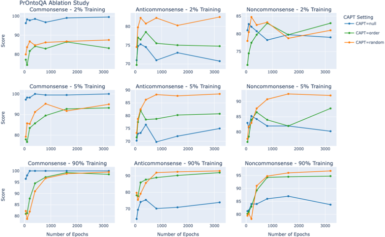## D.3 Ablation study In this section, we provide an important ablation study where random assignments are removed , denoted as "CAPT=order", indicating assignments obey the English alphabet order. As shown in Figure 4 and 3, although the results increase quickly at early training stages without random assignments, the converged results are significantly worse. This is due to the establishment of the fine-tuning biases as analyzed in our theoretical parts. D Figure 3: CAPT ablation study: PrOntoQA. CAPT=null denotes the original SFT performance; CAPT=order indicates deterministic assignments instead of random assignments; CAPT=random is the standard CAPT method. <details> <summary>Image 3 Details</summary>  ### Visual Description ## Line Charts: PrOntoQA Ablation Study ### Overview The image presents a series of line charts from a PrOntoQA Ablation Study. The charts are arranged in a 3x3 grid, with each row representing a different percentage of training data (2%, 5%, and 90%) and each column representing a different type of input (Commonsense, Anticommonsense, and Noncommonsense). Each chart displays the "Score" (y-axis) versus the "Number of Epochs" (x-axis) for three different CAPT settings: null, order, and random. ### Components/Axes * **Title:** PrOntoQA Ablation Study * **X-axis:** Number of Epochs, with markers at 0, 1000, 2000, and 3000. * **Y-axis:** Score, ranging from 70 to 100 (depending on the specific chart). * **CAPT Setting Legend (Top-Right):** * Blue: CAPT=null * Green: CAPT=order * Orange: CAPT=random * **Row Labels:** * Commonsense - 2% Training (Top-Left) * Anticommonsense - 2% Training (Top-Middle) * Noncommonsense - 2% Training (Top-Right) * Commonsense - 5% Training (Middle-Left) * Anticommonsense - 5% Training (Middle-Middle) * Noncommonsense - 5% Training (Middle-Right) * Commonsense - 90% Training (Bottom-Left) * Anticommonsense - 90% Training (Bottom-Middle) * Noncommonsense - 90% Training (Bottom-Right) ### Detailed Analysis **Commonsense - 2% Training:** * **CAPT=null (Blue):** Starts around 80, rises sharply to approximately 98 by 250 epochs, then remains relatively stable around 98-100 until 3000 epochs. * **CAPT=order (Green):** Starts around 78, increases to approximately 83 by 250 epochs, then gradually increases to approximately 88 by 3000 epochs. * **CAPT=random (Orange):** Starts around 82, increases to approximately 86 by 250 epochs, then gradually increases to approximately 90 by 3000 epochs. **Anticommonsense - 2% Training:** * **CAPT=null (Blue):** Starts around 75, dips to approximately 72 by 500 epochs, then rises to approximately 75 by 3000 epochs. * **CAPT=order (Green):** Starts around 76, increases to approximately 78 by 500 epochs, then remains relatively stable around 75 until 3000 epochs. * **CAPT=random (Orange):** Starts around 82, increases to approximately 84 by 250 epochs, then decreases slightly to approximately 80 by 3000 epochs. **Noncommonsense - 2% Training:** * **CAPT=null (Blue):** Starts around 82, dips to approximately 79 by 1000 epochs, then rises to approximately 81 by 3000 epochs. * **CAPT=order (Green):** Starts around 72, increases to approximately 82 by 500 epochs, then increases to approximately 84 by 3000 epochs. * **CAPT=random (Orange):** Starts around 81, increases to approximately 83 by 500 epochs, then decreases slightly to approximately 81 by 3000 epochs. **Commonsense - 5% Training:** * **CAPT=null (Blue):** Starts around 73, rises sharply to approximately 98 by 250 epochs, then remains relatively stable around 98-100 until 3000 epochs. * **CAPT=order (Green):** Starts around 78, increases to approximately 90 by 500 epochs, then gradually increases to approximately 93 by 3000 epochs. * **CAPT=random (Orange):** Starts around 82, increases to approximately 92 by 1000 epochs, then gradually increases to approximately 94 by 3000 epochs. **Anticommonsense - 5% Training:** * **CAPT=null (Blue):** Starts around 73, dips to approximately 71 by 500 epochs, then rises to approximately 75 by 3000 epochs. * **CAPT=order (Green):** Starts around 82, increases to approximately 83 by 500 epochs, then remains relatively stable around 81 until 3000 epochs. * **CAPT=random (Orange):** Starts around 87, increases to approximately 88 by 250 epochs, then decreases slightly to approximately 80 by 3000 epochs. **Noncommonsense - 5% Training:** * **CAPT=null (Blue):** Starts around 82, dips to approximately 81 by 1000 epochs, then remains relatively stable around 80 until 3000 epochs. * **CAPT=order (Green):** Starts around 80, increases to approximately 86 by 500 epochs, then increases to approximately 88 by 3000 epochs. * **CAPT=random (Orange):** Starts around 83, increases to approximately 90 by 1000 epochs, then increases to approximately 92 by 3000 epochs. **Commonsense - 90% Training:** * **CAPT=null (Blue):** Starts around 99, remains relatively stable around 99-100 until 3000 epochs. * **CAPT=order (Green):** Starts around 81, increases to approximately 95 by 500 epochs, then gradually increases to approximately 98 by 3000 epochs. * **CAPT=random (Orange):** Starts around 81, increases to approximately 98 by 1000 epochs, then remains relatively stable around 99 until 3000 epochs. **Anticommonsense - 90% Training:** * **CAPT=null (Blue):** Starts around 73, dips to approximately 70 by 500 epochs, then rises to approximately 74 by 3000 epochs. * **CAPT=order (Green):** Starts around 80, increases to approximately 90 by 500 epochs, then remains relatively stable around 91 until 3000 epochs. * **CAPT=random (Orange):** Starts around 80, increases to approximately 90 by 500 epochs, then remains relatively stable around 92 until 3000 epochs. **Noncommonsense - 90% Training:** * **CAPT=null (Blue):** Starts around 83, increases to approximately 87 by 500 epochs, then decreases slightly to approximately 84 by 3000 epochs. * **CAPT=order (Green):** Starts around 80, increases to approximately 93 by 500 epochs, then remains relatively stable around 95 until 3000 epochs. * **CAPT=random (Orange):** Starts around 80, increases to approximately 95 by 500 epochs, then remains relatively stable around 96 until 3000 epochs. ### Key Observations * For "Commonsense" data, the "CAPT=null" setting (blue line) consistently achieves the highest scores, especially with higher percentages of training data (5% and 90%). * For "Anticommonsense" data, the "CAPT=null" setting (blue line) consistently performs the worst. * For "Noncommonsense" data, the "CAPT=random" setting (orange line) generally performs well, especially with higher percentages of training data (5% and 90%). * Increasing the percentage of training data generally improves the scores for all CAPT settings, but the effect is most pronounced for "Commonsense" data. * The "CAPT=null" setting seems to benefit the most from increased training data in the "Commonsense" category. ### Interpretation The data suggests that the "CAPT=null" setting is highly effective for "Commonsense" data, indicating that the model performs best when trained on straightforward, logical information. Conversely, the poor performance of "CAPT=null" on "Anticommonsense" data suggests that the model struggles with contradictory or illogical information when no CAPT is applied. The "CAPT=random" setting appears to be a good compromise for "Noncommonsense" data, providing a balance between performance and robustness. The ablation study demonstrates the importance of the CAPT setting and the type of training data used. The results highlight the model's sensitivity to the nature of the input and the need for appropriate CAPT strategies to handle different types of information. The significant improvement in scores with increased training data, particularly for "Commonsense" data with "CAPT=null", underscores the value of high-quality, relevant training data for achieving optimal model performance. </details> 。 Figure 4: CAPT ablation study: CLadder. CAPT=null denotes the original SFT performance; CAPT=order indicates deterministic assignments instead of random assignments; CAPT=random is the standard CAPT method. 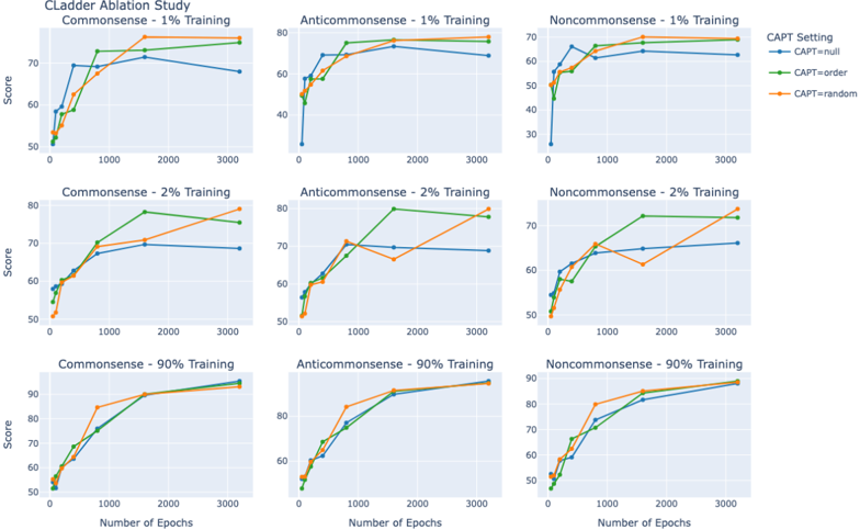<details> <summary>Image 4 Details</summary>  ### Visual Description ## Line Charts: CLadder Ablation Study ### Overview The image presents a series of line charts from the CLadder Ablation Study. Each chart displays the relationship between the number of epochs (x-axis) and the score (y-axis) for different training datasets (Commonsense, Anticommonsense, Noncommonsense) and training percentages (1%, 2%, 90%). The charts compare three CAPT settings: null, order, and random. ### Components/Axes * **Title:** CLadder Ablation Study * **X-axis:** Number of Epochs, with markers at 0, 1000, 2000, and 3000. * **Y-axis:** Score, with markers at 50, 60, 70, 80, and 90 (where applicable). * **CAPT Setting Legend (Top-Right):** * Blue line: CAPT=null * Green line: CAPT=order * Orange line: CAPT=random * **Chart Arrangement:** A 3x3 grid, with rows representing different training percentages (1%, 2%, 90%) and columns representing different datasets (Commonsense, Anticommonsense, Noncommonsense). ### Detailed Analysis **Row 1: 1% Training** * **Commonsense - 1% Training:** * CAPT=null (Blue): Increases sharply from approximately 52 to 68 between 0 and 1000 epochs, then plateaus around 68-72 until 3000 epochs. * CAPT=order (Green): Increases sharply from approximately 52 to 72 between 0 and 1000 epochs, then plateaus around 72-74 until 3000 epochs. * CAPT=random (Orange): Increases sharply from approximately 52 to 70 between 0 and 1000 epochs, then plateaus around 70-72 until 3000 epochs. * **Anticommonsense - 1% Training:** * CAPT=null (Blue): Increases sharply from approximately 35 to 75 between 0 and 1000 epochs, then plateaus around 75-78 until 3000 epochs. * CAPT=order (Green): Increases sharply from approximately 50 to 78 between 0 and 1000 epochs, then plateaus around 78-80 until 3000 epochs. * CAPT=random (Orange): Increases sharply from approximately 50 to 75 between 0 and 1000 epochs, then plateaus around 75-78 until 3000 epochs. * **Noncommonsense - 1% Training:** * CAPT=null (Blue): Increases sharply from approximately 52 to 65 between 0 and 1000 epochs, then plateaus around 65-68 until 3000 epochs. * CAPT=order (Green): Increases sharply from approximately 52 to 68 between 0 and 1000 epochs, then plateaus around 68-70 until 3000 epochs. * CAPT=random (Orange): Increases sharply from approximately 52 to 68 between 0 and 1000 epochs, then plateaus around 68-70 until 3000 epochs. **Row 2: 2% Training** * **Commonsense - 2% Training:** * CAPT=null (Blue): Increases sharply from approximately 55 to 70 between 0 and 1000 epochs, then plateaus around 68-70 until 3000 epochs. * CAPT=order (Green): Increases sharply from approximately 55 to 75 between 0 and 1000 epochs, then plateaus around 75-78 until 3000 epochs. * CAPT=random (Orange): Increases sharply from approximately 55 to 70 between 0 and 1000 epochs, then increases to approximately 78-80 until 3000 epochs. * **Anticommonsense - 2% Training:** * CAPT=null (Blue): Increases sharply from approximately 55 to 70 between 0 and 1000 epochs, then plateaus around 68-70 until 3000 epochs. * CAPT=order (Green): Increases sharply from approximately 55 to 72 between 0 and 1000 epochs, then increases to approximately 78-80 until 3000 epochs. * CAPT=random (Orange): Increases sharply from approximately 55 to 70 between 0 and 1000 epochs, then plateaus around 68-70 until 3000 epochs. * **Noncommonsense - 2% Training:** * CAPT=null (Blue): Increases sharply from approximately 52 to 65 between 0 and 1000 epochs, then plateaus around 65-68 until 3000 epochs. * CAPT=order (Green): Increases sharply from approximately 52 to 68 between 0 and 1000 epochs, then increases to approximately 72-74 until 3000 epochs. * CAPT=random (Orange): Increases sharply from approximately 52 to 65 between 0 and 1000 epochs, then increases to approximately 72-74 until 3000 epochs. **Row 3: 90% Training** * **Commonsense - 90% Training:** * CAPT=null (Blue): Increases sharply from approximately 55 to 80 between 0 and 1000 epochs, then plateaus around 80-82 until 3000 epochs. * CAPT=order (Green): Increases sharply from approximately 55 to 90 between 0 and 1000 epochs, then plateaus around 90-92 until 3000 epochs. * CAPT=random (Orange): Increases sharply from approximately 55 to 90 between 0 and 1000 epochs, then plateaus around 90-92 until 3000 epochs. * **Anticommonsense - 90% Training:** * CAPT=null (Blue): Increases sharply from approximately 55 to 80 between 0 and 1000 epochs, then plateaus around 80-82 until 3000 epochs. * CAPT=order (Green): Increases sharply from approximately 55 to 85 between 0 and 1000 epochs, then plateaus around 85-88 until 3000 epochs. * CAPT=random (Orange): Increases sharply from approximately 55 to 85 between 0 and 1000 epochs, then plateaus around 85-88 until 3000 epochs. * **Noncommonsense - 90% Training:** * CAPT=null (Blue): Increases sharply from approximately 52 to 75 between 0 and 1000 epochs, then plateaus around 75-78 until 3000 epochs. * CAPT=order (Green): Increases sharply from approximately 52 to 80 between 0 and 1000 epochs, then plateaus around 80-82 until 3000 epochs. * CAPT=random (Orange): Increases sharply from approximately 52 to 80 between 0 and 1000 epochs, then plateaus around 80-82 until 3000 epochs. ### Key Observations * All lines generally show a sharp increase in score between 0 and 1000 epochs, followed by a plateau. * The "CAPT=order" and "CAPT=random" settings often perform similarly, and generally outperform "CAPT=null". * Increasing the training percentage generally leads to higher scores. * The Anticommonsense dataset often results in higher scores compared to Commonsense and Noncommonsense, especially with 1% training. ### Interpretation The data suggests that using "CAPT=order" or "CAPT=random" settings can improve model performance compared to "CAPT=null". Increasing the training data size also generally improves performance. The differences in performance between the datasets (Commonsense, Anticommonsense, Noncommonsense) may indicate varying levels of complexity or inherent learnability within each dataset. The rapid increase in score within the first 1000 epochs suggests diminishing returns for training beyond this point, at least for these specific configurations. The ablation study likely aims to understand the impact of these different settings and datasets on the model's learning process and final performance. </details> ## D.4 Licenses CLadder dataset is under MIT license https://github.com/causalNLP/cladder/blob/main/LICENSE, while PrOntoQA is under Apache license 2.0 https://github.com/asaparov/prontoqa/blob/main/ LICENSE.