## A Hybrid Adaptive Nash Equilibrium Solver for Distributed MultiAgent Systems with Game-Theoretic Jump Triggering
Qiuyu Miao 1* and Zhigang Wu 2
School of Aeronautics and Astronautics, Sun Yat-sen University, Shenzhen, China
Abstract : This paper presents a hybrid adaptive Nash equilibrium solver for distributed multi-agent systems incorporating game-theoretic jump triggering mechanisms. The approach addresses fundamental scalability and computational challenges in multi-agent hybrid systems by integrating distributed game-theoretic optimization with systematic hybrid system design. A novel game-theoretic jump triggering mechanism coordinates discrete mode transitions across multiple agents while maintaining distributed autonomy. The Hybrid Adaptive Nash Equilibrium Solver (HANES) algorithm integrates these methodologies. Sufficient conditions establish exponential convergence to consensus under distributed information constraints. The framework provides rigorous stability guarantees through coupled Hamilton-Jacobi-Bellman equations while enabling rapid emergency response capabilities through coordinated jump dynamics. Simulation studies in pursuit-evasion and leader-follower consensus scenarios demonstrate significant improvements in convergence time, computational efficiency, and scalability compared to existing centralized and distributed approaches.
: Hybrid dynamical systems, Multi-agent coordination, Nash equilibrium,
Keywords
Distributed control
## I. Introduction
Modern distributed autonomous systems face unprecedented challenges in coordinating multiple agents that must simultaneously handle continuous physical dynamics and discrete decision-making processes. This dual nature appears across critical engineering domains where system failures can have severe consequences and traditional control approaches prove inadequate.
Unmanned aerial vehicle swarms must navigate complex environments through continuous flight control while executing discrete task assignments and obstacle avoidance decisions. Power grid operations demand real-time continuous power balancing coupled with discrete switching operations for load management and fault protection. These applications share a fundamental characteristic: the inability of purely continuous or discrete control methods to capture the essential system behaviors, necessitating hybrid system approaches that can rigorously handle both types of dynamics within a unified mathematical framework.
Hybrid dynamical systems provide the mathematical foundation for such complex behaviors. The design of flow sets 𝐶𝐶 and jump sets 𝐷𝐷 forms the core of hybrid system architecture [2,12]. Recent advances in hybrid motion planning [13] and distributed state estimation under switching networks [14] have demonstrated the practical importance of systematic flow and jump set construction. However, in multi-agent contexts, the flow set 𝐶𝐶 must accommodate the collective state space where all agents maintain coordination through local information exchange with neighbors, while the jump set 𝐷𝐷 coordinates discrete interventions across the network when continuous operation becomes insufficient. This design challenge differs fundamentally from single-agent cases due to the requirement for distributed coordination without global state knowledge.
While hybrid system theory has matured significantly for single-agent applications [15,16], the extension to multi-agent scenarios reveals profound theoretical and computational challenges in coordinating discrete mode switches across multiple interacting agents. The complexity of multi-agent hybrid systems emerges from the intricate coupling between individual agent dynamics and collective coordination requirements, where agents typically know only their neighbors' states yet must achieve robust synchronization and coordination through hybrid mechanisms [17,18]. However, the interaction between autonomous agent dynamics and the stochastic and intermittent nature of network traffic, combined with delays and asynchrony in information flow, further complicates the goal of ensuring system autonomy.
Existing hybrid system approaches primarily focus on single-agent or simple two-agent interactions, as exemplified by foundational works such as Leudo et al. [1] on two-player zero-sum hybrid games. The complexity of designing flow sets for multi-agent systems scales exponentially with agent numbers due to coupled constraints among all possible agent pairs [19,20]. Recent surveys on multi-agent consensus control acknowledge this fundamental scalability barrier, noting that current distributed control approaches resort to overly conservative designs that sacrifice performance for computational tractability, while alternative ad-hoc methods lack rigorous theoretical foundations for stability and convergence guarantees [5,21,22]. Furthermore, the computational complexity of Nash equilibrium computation, which is PPADcomplete even for continuous games [23,24], compounds these challenges when integrating game-theoretic approaches with hybrid dynamics.
Jump triggering mechanisms in multi-agent hybrid systems present additional challenges that existing literature has not systematically addressed. Recent advances have demonstrated the potential of hybrid systems frameworks for distributed multi-agent optimization, where agents perform continuous computations (such as gradient descent) while exchanging information at discrete communication instants through "update-and-hold" strategies [7,25]. Event-triggered control approaches in multi-agent systems have evolved significantly since Tabuada's foundational work [26], with recent developments in dynamic event-triggered mechanisms [27,28] and distributed Nash equilibrium seeking under event-triggered protocols [29,30]. However, these approaches focus primarily on continuous dynamics and lack the theoretical framework necessary for hybrid system applications where discrete mode switches fundamentally alter agent interactions and strategic landscapes.
Game-theoretic approaches to multi-agent control have shown promise in continuous domains [3,4], but their integration with hybrid system frameworks remains largely unexplored despite recent advances in learning generalized Nash equilibria through hybrid adaptive extremum seeking control [31,32]. Traditional Nash equilibrium computation assumes continuous action spaces and static interaction patterns, which are inadequate for hybrid systems where discrete mode switches create dynamic strategic environments. Current distributed optimization methods for multi-agent systems [12,13,33] focus primarily on continuous domains and lack computational frameworks for hybrid Nash equilibrium problems that couple continuous strategy optimization within discrete modes with discrete mode selection strategies. The fundamental PPAD-completeness of computing Nash equilibria [23,24] creates additional computational barriers that existing distributed algorithms have not adequately addressed in hybrid settings.
To address these fundamental limitations, this paper presents a comprehensive framework for multi-agent hybrid system design that integrates systematic flow set construction with distributed game-theoretic optimization. The main contributions are:
(1) In contrast to existing approaches that treat hybrid dynamics and multi-agent coordination separately [19,20] and lack systematic integration of game theory with hybrid systems [34,35], a unified distributed framework that formulates multi-agent coordination as a strategic game was developed within the hybrid dynamical systems context. Unlike current methods that rely on purely continuous game formulations or ad-hoc hybrid system designs that sacrifice theoretical rigor for computational tractability [5,21], this framework systematically integrates the hybrid inclusion formulation with distributed Nash equilibrium computation, addressing the fundamental challenge of coordinating discrete mode switches across multiple agents while maintaining individual agent autonomy and preserving rigorous stability guarantees.
(2) While existing event-triggered approaches [26,27,28] focus primarily on continuous dynamics and recent Nash equilibrium seeking methods [29,30] lack hybrid system integration, an intelligent jump triggering strategy based on distributed game-theoretic analysis that coordinates discrete mode transitions across multiple agents was introduced. In contrast to current event-triggered mechanisms that cannot handle the dynamic strategic environments created by discrete mode switches, this mechanism leverages strategic interaction modeling to optimize jump timing for system-wide objectives while maintaining individual agent autonomy and computational efficiency through three-layer triggering criteria. Unlike purely continuous control methods that cannot achieve rapid emergency response, the mechanism enables rapid emergency mode switching upon detecting communication interruptions, agent failures, or environmental disruptions, providing essential fast response capabilities that existing approaches cannot achieve.
(3) Addressing the fundamental computational barriers posed by PPAD-complete Nash equilibrium computation [23,24] and the exponential complexity scaling of existing distributed approaches [19,20], a novel distributed algorithm that integrates the hierarchical flow set design and game-theoretic jump triggering mechanisms was proposed to compute Nash equilibria in hybrid multi-agent systems. While traditional centralized approaches suffer from high computational complexity and existing distributed methods lack hybrid system capability [31,32,33], this algorithm employs dual-layer iterative optimization that separates continuous strategy optimization within modes from discrete mode selection optimization, achieving significant improvements in computational efficiency compared to traditional centralized approaches.
The theoretical framework provides rigorous mathematical foundations while offering practical computational tools for real-world implementation.
Notation : Throughout this paper, we employ standard mathematical notation where 𝑥𝑥 𝑖𝑖 ∈ 𝑅𝑅 𝑛𝑛 denotes the state of agent 𝑖𝑖 , 𝑢𝑢 𝑖𝑖 ∈ 𝑅𝑅 𝑚𝑚 represents the control input, and 𝒵𝒵 = {1,2, … , 𝑁𝑁 } defines the agent index set. In the hybrid system, 𝐶𝐶 ⊆ 𝑅𝑅 𝑛𝑛 × 𝑅𝑅 𝑚𝑚 and 𝐷𝐷 ⊆ 𝑅𝑅 𝑛𝑛 × 𝑅𝑅 𝑚𝑚 represent the flow and jump sets respectively, while 𝐹𝐹 : 𝑅𝑅 𝑛𝑛 × 𝑅𝑅 𝑚𝑚 ⇉𝑅𝑅 𝑛𝑛 and 𝐺𝐺 : 𝑅𝑅 𝑛𝑛 × 𝑅𝑅 𝑚𝑚 ⇉𝑅𝑅 𝑛𝑛 denote the corresponding flow and jump maps. The consensus error for agent 𝑖𝑖 is defined as δ𝑖𝑖 , while 𝑒𝑒 𝑖𝑖 represents the tracking error. Cost function parameters include state weight matrices 𝑄𝑄 𝑖𝑖 = 𝑄𝑄 𝑖𝑖 𝑇𝑇 ⪰ 0 , control weight matrices 𝑅𝑅 𝑖𝑖 = 𝑅𝑅 𝑖𝑖 𝑇𝑇 ≻ 0 , and jump penalty weights 𝑃𝑃 𝑖𝑖 > 0 . The Kronecker product is denoted by ⊗ , the gradient operator by ∇ , and the signum function by sign( ⋅ ) . Value functions are represented as 𝑉𝑉 𝑖𝑖 ( 𝑒𝑒 𝑖𝑖 ): 𝑅𝑅 𝑛𝑛 →𝑅𝑅 , and the post-jump state is indicated by the superscript ( + ) as in 𝑥𝑥 + .
## II. Problem Statement and Preliminaries
This section presents the mathematical foundations for multi-agent hybrid systems operating under distributed game-theoretic control. Firstly, basic hybrid dynamical system formulation is established, then develop the multi-agent framework with communication constraints, and finally introduce the distributed optimization problem that forms the core of this approach.
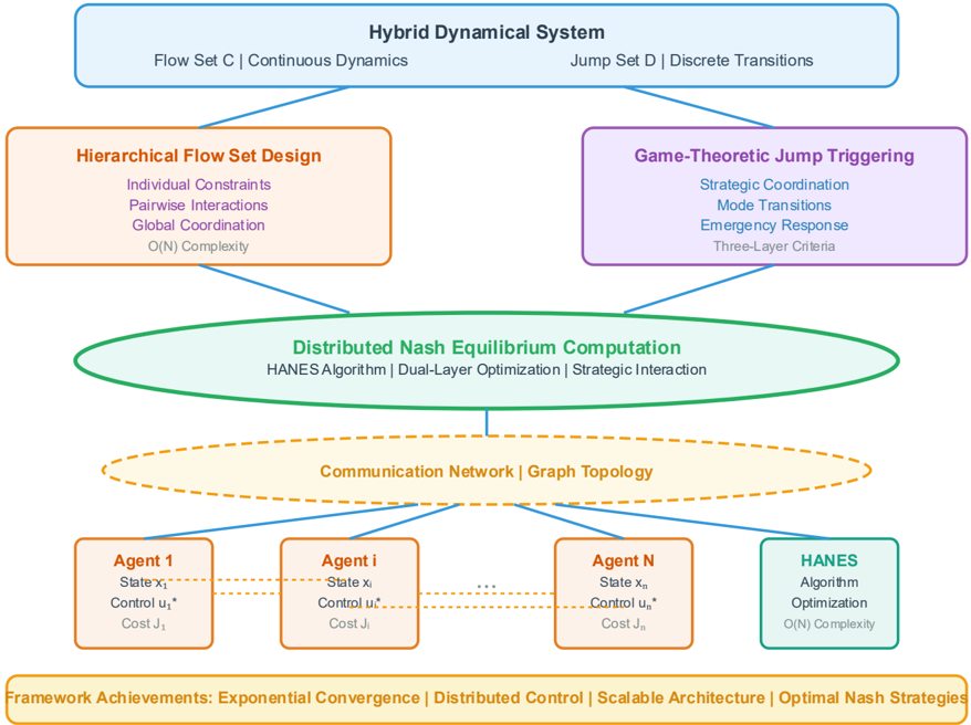
Fig. 1. Overall Framework Architecture of the Hybrid Adaptive Nash Equilibrium Solver
<details>
<summary>Image 1 Details</summary>
### Visual Description
## Diagram: Hybrid Dynamical System Framework
### Overview
The image depicts a diagram illustrating a framework for a Hybrid Dynamical System. The system is broken down into four main components: Hierarchical Flow Set Design, Game-Theoretic Jump Triggering, Distributed Nash Equilibrium Computation, and a Communication Network. These components are interconnected and supported by a "Framework Achievements" section at the bottom. The diagram uses color-coding to differentiate the components and their associated characteristics.
### Components/Axes
The diagram is structured around the central concept of a "Hybrid Dynamical System" at the top, branching into four main areas.
* **Top Header:** "Hybrid Dynamical System" with sub-categories "Flow Set C | Continuous Dynamics" and "Jump Set D | Discrete Transitions".
* **Left Branch (Light Blue):** "Hierarchical Flow Set Design" with sub-categories: "Individual Constraints", "Pairwise Interactions", "Global Coordination", and "O(N) Complexity".
* **Right Branch (Purple):** "Game-Theoretic Jump Triggering" with sub-categories: "Strategic Coordination", "Mode Transitions", "Emergency Response", and "Three-Layer Criteria".
* **Center (Green):** "Distributed Nash Equilibrium Computation" with sub-categories: "HANESAlgorithm | Dual-Layer Optimization | Strategic Interaction".
* **Bottom (Orange):** "Communication Network | Graph Topology" with three "Agent" blocks (Agent 1, Agent i, Agent N) and a "HANES Algorithm" block.
* **Agent Blocks:** Each agent block contains "State xᵢ", "Control uᵢ*", and "Cost Jᵢ".
* **HANES Algorithm Block:** Contains "Algorithm", "Optimization", and "O(N) Complexity".
* **Footer (Yellow):** "Framework Achievements: Exponential Convergence | Distributed Control | Scalable Architecture | Optimal Nash Strategies".
### Detailed Analysis or Content Details
The diagram illustrates a system where continuous dynamics (Flow Set C) and discrete transitions (Jump Set D) are managed through hierarchical flow set design and game-theoretic jump triggering. These are coordinated via distributed Nash equilibrium computation, facilitated by a communication network.
* **Hierarchical Flow Set Design:** Focuses on managing individual constraints, pairwise interactions, and global coordination, with a computational complexity of O(N).
* **Game-Theoretic Jump Triggering:** Emphasizes strategic coordination, mode transitions, emergency response, and utilizes a three-layer criteria for triggering jumps.
* **Distributed Nash Equilibrium Computation:** Leverages the HANES algorithm, dual-layer optimization, and strategic interaction to achieve equilibrium.
* **Communication Network:** Connects multiple agents (Agent 1, Agent i, Agent N) allowing for information exchange. Each agent has a state (xᵢ), control input (uᵢ*), and associated cost (Jᵢ). The HANES algorithm is also integrated into the network.
* **Agent Details:**
* Agent 1: State x₁, Control u₁*, Cost J₁.
* Agent i: State xᵢ, Control uᵢ*, Cost Jᵢ.
* Agent N: State xₙ, Control uₙ*, Cost Jₙ.
* **HANES Algorithm:** The HANES algorithm is used for optimization and has a computational complexity of O(N).
* **Framework Achievements:** The framework boasts exponential convergence, distributed control, scalable architecture, and optimal Nash strategies.
### Key Observations
The diagram highlights the interplay between continuous and discrete dynamics within a distributed system. The use of the HANES algorithm suggests a focus on optimization and game theory. The O(N) complexity indicates a potential scalability challenge as the number of agents (N) increases. The diagram emphasizes a layered approach, with hierarchical flow design, game-theoretic triggering, and distributed computation working in concert.
### Interpretation
This diagram represents a sophisticated control framework for hybrid systems, likely applicable to multi-agent systems or complex robotic coordination. The framework aims to achieve optimal performance by leveraging game theory and distributed computation. The emphasis on scalability (O(N) complexity) suggests that the framework is designed to handle a large number of agents, but also acknowledges the potential computational limitations. The integration of continuous and discrete dynamics allows the system to respond to both gradual changes and abrupt events. The "Emergency Response" component within the Game-Theoretic Jump Triggering suggests a focus on robustness and safety. The HANES algorithm appears to be a core component, providing the optimization engine for the distributed Nash equilibrium computation. The diagram is a high-level overview, and further details would be needed to understand the specific implementation and performance characteristics of the framework.
</details>
## Hybrid Systems with Multi-Agent
Consider hybrid dynamical systems that exhibit both continuous and discrete behavior. A hybrid system ℋ is described by the hybrid inclusion:
<!-- formula-not-decoded -->
where 𝑥𝑥 ∈ 𝑅𝑅 𝑛𝑛 represents the system state, 𝑢𝑢 𝐶𝐶 ∈ 𝑅𝑅 𝑚𝑚𝐶𝐶 denotes the continuous control input, and 𝑢𝑢 𝐷𝐷 ∈ 𝑅𝑅 𝑚𝑚𝐷𝐷 represents the discrete control input. The flow set 𝐶𝐶 ⊆ 𝑅𝑅 𝑛𝑛 × 𝑅𝑅 𝑚𝑚𝐶𝐶 defines the state-input combinations where continuous evolution is permitted, governed by the flow map 𝐹𝐹 : 𝑅𝑅 𝑛𝑛 × 𝑅𝑅 𝑚𝑚𝐶𝐶 ⇉𝑅𝑅 𝑛𝑛 . The jump set 𝐷𝐷 ⊆ 𝑅𝑅 𝑛𝑛 × 𝑅𝑅 𝑚𝑚𝐷𝐷 characterizes conditions triggering discrete state transitions, with the jump map 𝐺𝐺 : 𝑅𝑅 𝑛𝑛 × 𝑅𝑅 𝑚𝑚𝐷𝐷 ⇉ 𝑅𝑅 𝑛𝑛 determining the post-transition state values.
For multi-agent systems with 𝑁𝑁 agents, the hybrid framework was extended to accommodate distributed control architectures. Each agent 𝑖𝑖 ∈ 𝒵𝒵 = {1,2, … , 𝑁𝑁 } possesses individual dynamics while being coupled through communication and coordination requirements. The individual agent dynamics are described by:
<!-- formula-not-decoded -->
where 𝑥𝑥 𝑖𝑖 ∈ 𝑅𝑅 𝑛𝑛 is the state of agent 𝑖𝑖 , 𝑢𝑢 𝑖𝑖 ∈ 𝑅𝑅 𝑚𝑚 is the control input, 𝐴𝐴 ∈ 𝑅𝑅 𝑛𝑛 × 𝑛𝑛 is the system matrix, and 𝐵𝐵 ∈ 𝑅𝑅 𝑛𝑛 × 𝑚𝑚 is the input matrix. The collective system state is defined as 𝑥𝑥 = [ 𝑥𝑥1 𝑇𝑇 , 𝑥𝑥 2 𝑇𝑇 , … , 𝑥𝑥 𝑁𝑁 𝑇𝑇 ] 𝑇𝑇 ∈ 𝑅𝑅 𝑁𝑁𝑛𝑛 , and the global control input as 𝑢𝑢 = [ 𝑢𝑢1 𝑇𝑇 , 𝑢𝑢 2 𝑇𝑇 , … , 𝑢𝑢 𝑁𝑁 𝑇𝑇 ] 𝑇𝑇 ∈ 𝑅𝑅 𝑁𝑁𝑚𝑚 .
The set-valued nature of mappings 𝐹𝐹 and 𝐺𝐺 accommodates system uncertainties, modeling approximations, and non-deterministic responses arising from environmental disturbances, measurement noise, and actuator imperfections that are particularly relevant in multi-agent scenarios where communication delays and packet losses introduce additional uncertainties.
## Graph-Theoretic Communication Framework and Network Dynamics
The multi-agent system operates under limited sensing capabilities, where each agent can only access information from its local neighborhood. This communication structure is represented by a directed graph 𝒢𝒢 = ( 𝒱𝒱 , ℰ ) with vertex set 𝒱𝒱 = {1,2, … , 𝑁𝑁 } and edge set ℰ ⊆ 𝒱𝒱 × 𝒱𝒱 . The adjacency matrix 𝐴𝐴 = �𝑎𝑎 𝑖𝑖𝑖𝑖� ∈ 𝑅𝑅 𝑁𝑁 × 𝑁𝑁 captures the communication topology, where 𝑎𝑎 𝑖𝑖𝑖𝑖 = 1 if agent 𝑗𝑗 can transmit information to agent 𝑖𝑖 , and 𝑎𝑎 𝑖𝑖𝑖𝑖 = 0 otherwise.
The communication constraints fundamentally alter the hybrid system behavior compared to centralized approaches. Define the neighbor set of agent 𝑖𝑖 as 𝒩𝒩 𝒾𝒾 = { 𝑗𝑗 ∈ 𝒱𝒱 : 𝑎𝑎 𝑖𝑖𝑖𝑖 = 1} , and the in-degree as 𝑑𝑑 𝑖𝑖 = | 𝒩𝒩 𝒾𝒾 | = ∑ 𝑎𝑎 𝑖𝑖𝑖𝑖 𝑁𝑁 𝑖𝑖=1 . The degree matrix 𝐷𝐷 = diag( 𝑑𝑑1 , 𝑑𝑑2 , … , 𝑑𝑑 𝑁𝑁 ) and graph Laplacian 𝐿𝐿 = 𝐷𝐷 - 𝐴𝐴 characterize the algebraic connectivity properties essential for consensus analysis.
For leader-follower architectures, partition the agent set into leaders ℒ and followers ℱ such that ℒ ∪ ℱ = 𝒵𝒵 and ∩ = ∅ ℒ ∩ ℱ = ∅ . The interaction between leaders and followers is captured by the coupling matrix 𝐵𝐵 𝐿𝐿𝐿𝐿 = �𝑏𝑏 𝑖𝑖𝑖𝑖 � where 𝑏𝑏 𝑖𝑖𝑖𝑖 = 1 if follower 𝑖𝑖 receives information from leader 𝑗𝑗 . This introduces additional complexity in the hybrid flow and jump set designs, as discrete transitions in leader agents can trigger cascading effects throughout the follower network.
The communication topology directly influences the convergence properties of the multi-agent hybrid system. Strong connectivity of the communication graph ensures that information from any agent can eventually reach all other agents, which is crucial for achieving global consensus. However, in hybrid systems, jump events can temporarily disrupt information flow, requiring careful consideration of the interplay between graph topology and discrete dynamics.
## Local Errors and Consensus Dynamics
For distributed coordination, define the local consensus error for agent 𝑖𝑖 as the weighted deviation from its neighbors:
<!-- formula-not-decoded -->
This error captures the local disagreement between agent 𝑖𝑖 and its communication neighbors, forming the basis for distributed consensus protocols. The global consensus error vector is compactly expressed as δ = ( 𝐿𝐿 ⊗ 𝐼𝐼 𝑛𝑛 ) 𝑥𝑥 .
Taking the time derivative of equation (3) and substituting the agent dynamics (2), the error is:
<!-- formula-not-decoded -->
Each agent must coordinate its control action 𝑢𝑢 𝑖𝑖 with those of its neighbors to drive δ𝑖𝑖 → 0 .
For leader-follower configurations, distinguish between different error types. The leader error for agent 𝑙𝑙 ∈ ℒ tracking reference trajectory 𝑥𝑥 ref ( 𝑡𝑡 ) is:
<!-- formula-not-decoded -->
The follower error for agent 𝑖𝑖 ∈ ℱ combines consensus with neighbors and tracking of leaders:
̇
<!-- formula-not-decoded -->
where 𝑏𝑏 𝑖𝑖l represents the connection weight between follower 𝑖𝑖 and leader 𝑙𝑙 .
The error dynamics under hybrid conditions incorporate both continuous evolution and discrete jumps. During continuous phases when ( 𝑥𝑥 , 𝑢𝑢 ) ∈ 𝐶𝐶 :
̇
<!-- formula-not-decoded -->
During discrete transitions when ( 𝑥𝑥 , 𝑢𝑢 ) ∈ 𝐷𝐷 , the error evolution becomes:
<!-- formula-not-decoded -->
This formulation captures how individual agent jumps affect the collective error dynamics, creating complex dependencies that require careful analysis for stability and convergence guarantees.
## III. Distributed Hybrid Game Formulation and Nash Equilibrium
Building upon the system model and hybrid dynamical framework established in Section II, this section develops a systematic framework for distributed multi-agent coordination through game-theoretic Nash equilibrium computation. The approach transforms the consensus problem into a strategic interaction where each agent optimizes its individual performance while accounting for the decisions of neighboring agents.
## Cost Function Design and Strategic Formulation
Each agent 𝑖𝑖 seeks to minimize a performance index that balances consensus achievement with control effort:
<!-- formula-not-decoded -->
where 𝑄𝑄 𝑖𝑖 = 𝑄𝑄 𝑖𝑖 𝑇𝑇 ⪰ 0 is the state cost weight matrix, 𝑅𝑅 𝑖𝑖 = 𝑅𝑅 𝑖𝑖 𝑇𝑇 ≻ 0 is the control cost weight matrix, 𝑃𝑃 𝑖𝑖 > 0 is the jump penalty weight, and { 𝑡𝑡 𝑘𝑘 } 𝑘𝑘=0 ∞ represents the sequence of jump times. The inclusion of jump costs 𝑃𝑃 𝑖𝑖 || 𝑒𝑒 𝑖𝑖 ( 𝑡𝑡 𝑘𝑘 + )|| 2 penalizes large deviations from consensus immediately after discrete transitions, encouraging coordinated jumping strategies.
The distributed control problem is formulated as a multi-player game where each agent 𝑖𝑖 solves:
<!-- formula-not-decoded -->
This creates a strategic interaction where each agent's optimal policy depends on the policies chosen by its neighbors, leading naturally to Nash equilibrium concepts. A Nash equilibrium is a strategy profile ( 𝑢𝑢1 ∗ , 𝑢𝑢 2 ∗ , … , 𝑢𝑢 𝑁𝑁 ∗ ) such that no agent can unilaterally improve its performance by deviating from its equilibrium strategy.
For agent 𝑖𝑖 , we define the value function 𝑉𝑉 𝑖𝑖 ( 𝑒𝑒 𝑖𝑖 ): 𝑅𝑅 𝑛𝑛 →𝑅𝑅 as:
<!-- formula-not-decoded -->
where 𝒰𝒰 𝒾𝒾 denotes the admissible control set for agent 𝑖𝑖 . The value function satisfies the hybrid HamiltonJacobi-Bellman equation. During flow phases:
<!-- formula-not-decoded -->
where 𝑓𝑓 𝑖𝑖 ( 𝑒𝑒 𝑖𝑖 , 𝑢𝑢 𝑖𝑖 , 𝑢𝑢 -𝑖𝑖 ) represents the flow dynamics from equation (7), and 𝑢𝑢 -𝑖𝑖 denotes the control inputs of agent 𝑖𝑖 's neighbors.
During jump phases:
<!-- formula-not-decoded -->
The optimal continuous control law is obtained by minimizing the Hamiltonian in equation (12). Taking the derivative with respect to 𝑢𝑢 𝑖𝑖 and setting it to zero:
<!-- formula-not-decoded -->
Therefore, the optimal control law is:
<!-- formula-not-decoded -->
This control law forms the foundation for the distributed game-theoretic approach, where each agent implements its optimal strategy while accounting for the strategic behavior of its neighbors. The coupling through the communication graph ensures that the resulting Nash equilibrium achieves distributed coordination while respecting the hybrid system constraints.
## Nash Equilibrium Characterization for Multi-Agent Hybrid Games
Definition 1 (Nash Equilibrium for Multi-Agent Hybrid Systems): A strategy profile ( 𝑢𝑢1 ∗ , 𝑢𝑢 2 ∗ , … , 𝑢𝑢 𝑁𝑁 ∗ ) constitutes a Nash equilibrium if for each agent 𝑖𝑖 ∈ 𝒵𝒵 and for all alternative strategies 𝑢𝑢 𝑖𝑖 ∈ 𝒰𝒰𝒾𝒾 :
<!-- formula-not-decoded -->
where 𝑢𝑢 -𝑖𝑖 ∗ = ( 𝑢𝑢1 ∗ , … , 𝑢𝑢 𝑖𝑖-1 ∗ , 𝑢𝑢 𝑖𝑖+1 ∗ , … , 𝑢𝑢 𝑁𝑁 ∗ ) represents the equilibrium strategies of all agents except agent 𝑖𝑖 .
The Nash equilibrium condition requires that each agent's strategy minimizes its cost functional given the strategies of all other agents. In the hybrid setting, this condition must hold for both continuous and discrete phases of the system evolution.
Lemma 1 (Necessary Conditions for Nash Equilibrium): If ( 𝑢𝑢1 ∗ , 𝑢𝑢 2 ∗ , … , 𝑢𝑢 𝑁𝑁 ∗ ) is a Nash equilibrium, then for each agent 𝑖𝑖 , the following conditions must be satisfied:
During flow phases ( 𝑒𝑒 , 𝑢𝑢 ) ∈ 𝐶𝐶 :
During jump phases ( 𝑒𝑒 , 𝑢𝑢 ) ∈ 𝐷𝐷 :
<!-- formula-not-decoded -->
<!-- formula-not-decoded -->
where the Hamiltonian function for agent 𝑖𝑖 is defined as:
<!-- formula-not-decoded -->
with λ𝑖𝑖 = ∇𝑉𝑉 𝑖𝑖 ( 𝑒𝑒 𝑖𝑖 ) being the costate variable.
Proof of Lemma 1 : The proof follows from the application of Pontryagin's maximum principle to the optimal control problem (10). For the continuous phase, the optimality condition ∂𝐻𝐻𝑖𝑖 ∂𝑢𝑢𝑖𝑖 = 0 yields:
<!-- formula-not-decoded -->
<!-- formula-not-decoded -->
For the discrete phase, the jump optimality condition follows from minimizing the post-jump cost, leading to equation (17).
Theorem 1 (Existence of Nash Equilibrium): Consider the multi-agent hybrid system (1)-(2) with performance indices (9) under Assumption 1. If the following conditions hold:
- (i) The communication graph 𝒢𝒢 contains a spanning tree,
- (ii) The matrices ( 𝐴𝐴 , 𝐵𝐵 ) are stabilizable for each agent,
- (iii) The matrices �𝐴𝐴 , 𝑄𝑄 𝑖𝑖 1 / 2 � are observable for each agent,
- (iv) The coupling weights satisfy ∑ 𝑎𝑎 𝑖𝑖𝑖𝑖 𝑖𝑖∈𝒩𝒩 𝒾𝒾 + ∑ 𝑏𝑏 𝑖𝑖l l∈ℒ < α for some α < 2 �λ𝑚𝑚𝑖𝑖𝑛𝑛 ( 𝑅𝑅 𝑖𝑖 )/ λ𝑚𝑚𝑚𝑚𝑚𝑚 ( 𝐵𝐵 𝑇𝑇 𝑃𝑃 𝑖𝑖 𝐵𝐵 ), then there exists a unique Nash equilibrium in quadratic strategies.
Proof of Theorem 1 : The proof proceeds through several steps:
Step 1 : Establish contractivity of the mapping 𝒯𝒯 : 𝒫𝒫 → 𝒫𝒫 where 𝒫𝒫 = { 𝑃𝑃1 , 𝑃𝑃2 , … , 𝑃𝑃 𝑁𝑁 } and 𝒯𝒯 ( 𝑃𝑃 𝑖𝑖 ) solves equation (25).
Step 2 : Define the operator 𝒯𝒯 𝒾𝒾 : 𝑆𝑆++ 𝑛𝑛 →𝑆𝑆++ 𝑛𝑛 for each agent 𝑖𝑖 as:
<!-- formula-not-decoded -->
where Γ𝑖𝑖𝑖𝑖 �𝑃𝑃 𝑖𝑖� represents the coupling terms and 𝑆𝑆++ 𝑛𝑛 denotes the set of positive definite 𝑛𝑛 × 𝑛𝑛 matrices. Step 3 : Show that under condition (iv), the operator 𝒯𝒯 is a contraction mapping. The coupling term can be bounded as:
<!-- formula-not-decoded -->
where 𝛽𝛽 < 1 is determined by the communication weights and system parameters.
Solving for 𝑢𝑢 𝑖𝑖 ∗ :
Step 4 : Apply the Banach fixed-point theorem to conclude existence and uniqueness of the fixed point 𝑃𝑃 ∗ = ( 𝑃𝑃 1 ∗ 𝑃𝑃 2 ∗ …, 𝑃𝑃 𝑁𝑁 ∗ ) satisfying 𝒯𝒯 ( 𝑃𝑃 ∗ ) = 𝑃𝑃 ∗ .
Step 5 : Verify that the corresponding control strategies 𝑢𝑢 𝑖𝑖 ∗ ( 𝑒𝑒 𝑖𝑖 ) = -1 2 ( 𝑑𝑑 𝑖𝑖 + ∑ 𝑏𝑏 𝑖𝑖l l∈ℒ ) 𝑅𝑅 𝑖𝑖 -1 𝐵𝐵 𝑇𝑇 𝑃𝑃 𝑖𝑖 ∗ 𝑒𝑒 𝑖𝑖 constitute a Nash equilibrium by checking condition (15).
## Hamilton-Jacobi-Bellman System
The Nash equilibrium strategies satisfy a system of coupled Hamilton-Jacobi-Bellman (HJB) equations. For agent 𝑖𝑖 , the value function 𝑉𝑉 𝑖𝑖 ( 𝑒𝑒 𝑖𝑖 ) satisfies:
<!-- formula-not-decoded -->
Substituting the optimal control law (19) into equation (20):
<!-- formula-not-decoded -->
where Φ𝑖𝑖 ( 𝑢𝑢 -𝑖𝑖 ∗ ) = -𝐵𝐵 ∑ 𝑎𝑎 𝑖𝑖𝑖𝑖 𝑢𝑢 𝑖𝑖 ∗ 𝑖𝑖∈𝒩𝒩 𝒾𝒾 -𝐵𝐵 ∑ 𝑏𝑏 𝑖𝑖l 𝑢𝑢 l ∗ l∈ℒ represents the coupling term from neighboring agents.
For steady-state analysis, set ∂𝑉𝑉𝑖𝑖 ∂𝑡𝑡 = 0 , yielding the algebraic HJB equation:
<!-- formula-not-decoded -->
Assumption 1: For each agent 𝑖𝑖 , there exists a quadratic value function of the form:
<!-- formula-not-decoded -->
where 𝑃𝑃 𝑖𝑖 = 𝑃𝑃 𝑖𝑖 𝑇𝑇 ≻ 0 is a positive definite matrix to be determined.
Under Assumption 1 , have ∇𝑉𝑉 𝑖𝑖 ( 𝑒𝑒 𝑖𝑖 ) = 2 𝑃𝑃 𝑖𝑖 𝑒𝑒 𝑖𝑖 . Substituting into equation (22):
<!-- formula-not-decoded -->
For this equation to hold for all 𝑒𝑒 𝑖𝑖 , require:
<!-- formula-not-decoded -->
where 𝛯𝛯 𝑖𝑖 = 𝛴𝛴 𝑖𝑖∈𝑁𝑁𝑖𝑖 𝛤𝛤 𝑖𝑖𝑖𝑖 �𝑃𝑃 𝑖𝑖� captures the coupling effects from neighboring agents and will be analyzed in the convergence proof.
Theorem 2 (Exponential Convergence to Nash Equilibrium): Under the conditions of Theorem 1 , the distributed Nash equilibrium strategies achieve exponential convergence of the consensus errors to zero.
Specifically, there exist constants 𝑀𝑀 > 0 and 𝜌𝜌 > 0 such that:
<!-- formula-not-decoded -->
where 𝑒𝑒 ( 𝑡𝑡 ) = [ 𝑒𝑒1 𝑇𝑇 ( 𝑡𝑡 ), 𝑒𝑒 2 𝑇𝑇 ( 𝑡𝑡 ), … , 𝑒𝑒 𝑁𝑁 𝑇𝑇 ( 𝑡𝑡 )] 𝑇𝑇 is the global error vector.
Proof of Theorem 2 : Taking the time derivative of the Lyapunov function along system trajectories during flow phases:
̇
<!-- formula-not-decoded -->
Substituting the closed-loop error dynamics with Nash equilibrium strategies, consider the error dynamics for agent 𝑖𝑖 in a multi-agent system, given by:
̇
<!-- formula-not-decoded -->
Assume the optimal control law, derived from the Hamilton-Jacobi-Bellman equation, is:
<!-- formula-not-decoded -->
where 𝑅𝑅 𝑖𝑖 = 𝑅𝑅 𝑖𝑖 𝑇𝑇 ≻ 0 is the control cost matrix, and 𝑃𝑃 𝑖𝑖 = 𝑃𝑃 𝑖𝑖 𝑇𝑇 ⪰ 0 is the solution to the Riccati equation. Similarly, for neighbor 𝑗𝑗 and leader l :
<!-- formula-not-decoded -->
Substitute 𝑢𝑢 𝑖𝑖 ∗ into the first control term:
<!-- formula-not-decoded -->
Substitute 𝑢𝑢 𝑖𝑖 ∗ and 𝑢𝑢 l ∗ into the coupling terms:
<!-- formula-not-decoded -->
<!-- formula-not-decoded -->
<!-- formula-not-decoded -->
Combine all terms:
<!-- formula-not-decoded -->
Rewrite in compact form, where the last two terms are coupling terms:
̇
<!-- formula-not-decoded -->
The coupling terms are:
<!-- formula-not-decoded -->
The coupling terms can be shown to satisfy:
<!-- formula-not-decoded -->
where γ depends on the system parameters and communication weights.
Using the matrix inequality and condition (iv) from Theorem 1:
<!-- formula-not-decoded -->
for some 𝜇𝜇 > 0 . This establishes exponential stability with decay rate 𝜌𝜌 = 𝜇𝜇 / � 2 λ𝑚𝑚𝑚𝑚𝑚𝑚 ( 𝑃𝑃 ∗ ) � here 𝑃𝑃 ∗ = block diag( 𝑃𝑃 1 , 𝑃𝑃 2 , …, 𝑃𝑃 𝑁𝑁 ∗ ) .
Corollary 1 (Hybrid Stability): The Nash equilibrium strategies also guarantee stability through jump phases. If the jump maps satisfy | 𝐺𝐺 𝑖𝑖 ( 𝑒𝑒 𝑖𝑖 , 𝑢𝑢 𝑖𝑖 ∗ )| ≤ σ | 𝑒𝑒 𝑖𝑖 | for some σ < 1 , then the hybrid system maintains exponential stability across discrete transitions.
## Optimization Framework
Based on the theoretical foundation established in Sections II and III, the complete Hybrid Adaptive Nash Equilibrium Solver (HANES) Algorithm algorithmic framework for distributed Nash equilibrium computation in multi-agent hybrid system was presented. The algorithm integrates hierarchical flow set design with game-theoretic jump triggering mechanisms.
## Initialize:
- Initial states 𝑥𝑥 𝑖𝑖 (0) , 𝑖𝑖 ∈ 𝒵𝒵 · Communication topology adjacency matrix 𝐴𝐴 = �𝑎𝑎 𝑖𝑖𝑖𝑖 � · Control parameters β , ρ , jump thresholds μ , σ , � σ · Select positive definite matrices 𝑄𝑄 𝑖𝑖 , 𝑅𝑅 𝑖𝑖 , 𝑃𝑃 𝑖𝑖 for 𝑡𝑡 = 0 to 𝑡𝑡 𝑚𝑚𝑚𝑚𝑚𝑚 o Step 1 : Data Collection and Critic Update · Collect neighbor states 𝑥𝑥 𝑖𝑖 ( 𝑡𝑡 ) , 𝑗𝑗 ∈ 𝒩𝒩 𝒾𝒾 · Construct consensus errors 𝑒𝑒 𝑖𝑖 ( 𝑡𝑡 ) = ∑ 𝑎𝑎 𝑖𝑖𝑖𝑖 �𝑥𝑥 𝑖𝑖 -𝑥𝑥𝑖𝑖� 𝑖𝑖∈𝒩𝒩𝑖𝑖 · Update leader-follower errors using equation (6) Step 2 : Hybrid State Verification · Check flow condition: if | 𝑥𝑥𝑖𝑖 -μ | ≥ then ( 𝑥𝑥 , 𝑢𝑢 ) ∈ 𝐶𝐶 · Check jump condition: if | 𝑥𝑥𝑖𝑖 -μ | < then ( 𝑥𝑥 , 𝑢𝑢 ) ∈ 𝐷𝐷 Step 3 : Nash Strategy Update · Solve coupled HJB equations (22) for value matrices 𝑃𝑃 𝑖𝑖 · Compute optimal control 𝑢𝑢 𝑖𝑖 ∗ = -𝐾𝐾𝑖𝑖 𝑒𝑒 𝑖𝑖 using equation (19) · Apply hybrid jump dynamics if ( 𝑥𝑥 , 𝑢𝑢 ) ∈ 𝐷𝐷 Step 4: Convergence Check if max 𝑖𝑖 | 𝑒𝑒 𝑖𝑖 ( 𝑡𝑡 )| < 𝜀𝜀 then 𝑢𝑢 𝑖𝑖 ∗ = 𝑢𝑢 𝑖𝑖 𝑐𝑐𝑐𝑐𝑛𝑛𝑐𝑐𝑒𝑒𝑐𝑐𝑔𝑔𝑒𝑒𝑐𝑐 return 𝑢𝑢 𝑖𝑖 ∗ else go to Step 1 end if Return: optimal control policies 𝑢𝑢 𝑖𝑖
The comprehensive experimental framework provides rigorous validation of the HANES algorithm's theoretical properties while demonstrating its effectiveness in practical multi-agent coordination scenarios. The results establish empirical evidence supporting the algorithm's convergence guarantees, computational efficiency, and robust performance across diverse operational conditions.
## IV. Experiments and Simulation
All simulations involve agents with scalar dynamics ( n =1) to clearly illustrate hybrid switching behaviors. The hybrid system nature is characterized by flow and jump sets. A common jump threshold μ =1.0 is used, with jump target intervals defined as [ σ , � σ ] = [0.3,0.5] . When a jump occurs, the new state is randomly selected within this interval to model uncertainty in post-jump states. The time step for all simulations is dt=0.01.
## Algorithm: HANES (Hybrid Adaptive Nash Equilibrium Solver)
̇
̇
-0.5 1 � 1 -0.3 -0.3 1 � ; from pursuers to evaders are represented by 𝐴𝐴 𝑝𝑝𝑒𝑒 = � 1.0 0.7 0.8 1 � ; from evaders to pursuers are described by 𝐴𝐴 = � 0.9 0.5 � .
The Pursuit-Evasion Game evaluates the framework's game-theoretic aspects and its ability to converge to a Nash equilibrium in a competitive multi-agent environment. The system comprises two pursuers and two evaders. Initial conditions are 𝑥𝑥 pursuers (0) = � 2.0 1.8 � and 𝑥𝑥 evaders (0) = � 1.5 1.2 � . The dynamics for pursuers are 𝑥𝑥 𝚤𝚤 = 𝑎𝑎 �𝑥𝑥 𝑖𝑖 + 𝑏𝑏 𝑖𝑖 𝑢𝑢 𝑖𝑖 , 𝑎𝑎 � = -1 , and for evaders are 𝑥𝑥 𝚥𝚥 = 𝑎𝑎𝑥𝑥 𝑖𝑖 + 𝑏𝑏 𝑖𝑖 𝑢𝑢 𝑖𝑖 , with a =-2. All input coefficients 𝑏𝑏 𝑖𝑖 = 𝑏𝑏 𝑖𝑖 = 1 . The interactions among agents are characterized by the following matrices. The pursuer-to-pursuer interactions are described by 𝐿𝐿 𝑝𝑝 = � 1 -0.5 � ; while the evader-to-evader interactions are given 𝐿𝐿 𝑒𝑒 =
<!-- formula-not-decoded -->
Pursuers aim to minimize their performance index (capture), while evaders maximize theirs (survival), forming a zero-sum game structure. Saddle-point strategies are implemented. The cost function weights are
<!-- formula-not-decoded -->
input cost weights for pursuers 𝑅𝑅 𝑐𝑐 , pursuers = diag(1.304,1.5) ; input cost weights for evaders 𝑅𝑅 𝑐𝑐 , evaders = diag( -4, -3.5) ; jump penalty weight P =0.4481; the simulation runs for 𝑡𝑡 �inal = 3 seconds .
g
<details>
<summary>Image 2 Details</summary>
### Visual Description
## Chart: Multi-Agent Hybrid Pursuit-Evasion Game: State Evolution & Control Strategies
### Overview
The image presents three sub-charts visualizing the state evolution, Nash equilibrium control strategies, and cost function evolution within a multi-agent pursuit-evasion game. The charts share a common time axis (0 to 3 seconds). The top chart shows the state (position 'x') of pursuers and evaders over time. The middle chart displays the control inputs applied by each agent. The bottom chart illustrates the cost functional 'J' for each agent.
### Components/Axes
* **Top Chart:**
* **X-axis:** Time (s), ranging from 0 to 3, with increments of 0.5.
* **Y-axis:** State X, ranging from 0 to 2, with increments of 0.5.
* **Data Series:**
* Pursuer 1 (Purple)
* Pursuer 2 (Green)
* Evader 1 (Orange)
* Evader 2 (Red)
* **Markers:** Black stars representing "Jump Points" and a dashed red line representing "Jump Trigger (u*)".
* **Middle Chart:**
* **X-axis:** Time (s), ranging from 0 to 3, with increments of 0.5.
* **Y-axis:** Control Input u, ranging from -0.4 to 0.2, with increments of 0.1.
* **Data Series:**
* uP1 (Blue)
* uP2 (Orange)
* uE1 (Green)
* uE2 (Red)
* **Bottom Chart:**
* **X-axis:** Time (s), ranging from 0 to 3, with increments of 0.5.
* **Y-axis:** Cost Functional J, ranging from 0 to 2, with increments of 0.5.
* **Data Series:**
* JP1 (Green)
* JP2 (Orange)
* JE1 (Red)
* JE2 (Blue)
### Detailed Analysis
* **Top Chart (State Evolution):**
* Pursuer 1 (Purple): Starts at approximately 1.8, decreases steadily to approximately 0.5 by 3 seconds.
* Pursuer 2 (Green): Starts at approximately 1.5, decreases steadily to approximately 0.5 by 3 seconds.
* Evader 1 (Orange): Starts at approximately 1.2, decreases to approximately 0.2 by 3 seconds.
* Evader 2 (Red): Starts at approximately 0.8, decreases to approximately 0.1 by 3 seconds.
* Jump Points (Black Stars): Appear around 0.4 seconds, with values approximately 1.6, 1.3, 1.1, and 0.7 for Pursuer 1, Pursuer 2, Evader 1, and Evader 2 respectively.
* Jump Trigger (u*) (Dashed Red Line): Remains relatively constant at approximately 0.8.
* **Middle Chart (Nash Equilibrium Control Strategies):**
* uP1 (Blue): Starts at approximately -0.3, increases to approximately 0.1 by 0.5 seconds, then remains relatively constant.
* uP2 (Orange): Starts at approximately -0.3, increases sharply to approximately 0.1 by 0.5 seconds, then remains relatively constant.
* uE1 (Green): Starts at approximately 0.1, decreases to approximately -0.3 by 0.5 seconds, then remains relatively constant.
* uE2 (Red): Starts at approximately 0.1, decreases to approximately -0.3 by 0.5 seconds, then remains relatively constant.
* **Bottom Chart (Cost Function Evolution):**
* JP1 (Green): Starts at approximately 1.8, decreases steadily to approximately 0.5 by 3 seconds.
* JP2 (Orange): Starts at approximately 1.5, decreases steadily to approximately 0.5 by 3 seconds.
* JE1 (Red): Starts at approximately 1.2, decreases to approximately 0.2 by 3 seconds.
* JE2 (Blue): Starts at approximately 0.8, decreases to approximately 0.1 by 3 seconds.
### Key Observations
* All state values (top chart) decrease over time, indicating the pursuers are approaching the evaders.
* The control inputs (middle chart) show a clear divergence between pursuers and evaders, with pursuers applying positive control inputs and evaders applying negative control inputs after the initial phase.
* The cost functions (bottom chart) decrease over time, suggesting that the agents are optimizing their strategies to minimize their cost.
* The Jump Points appear to coincide with a change in the control strategies.
### Interpretation
The charts demonstrate the dynamics of a multi-agent pursuit-evasion game. The state evolution chart shows the pursuers closing in on the evaders. The control strategies chart reveals how each agent adjusts its actions to optimize its performance. The cost function chart confirms that the agents are indeed minimizing their cost over time. The Jump Points and Jump Trigger suggest a discrete event or a change in strategy triggered by a specific condition. The consistent decrease in cost functions indicates the agents are converging towards a Nash equilibrium, where no agent can improve its cost by unilaterally changing its strategy. The fact that the pursuers and evaders have different control strategies is expected, as they have opposing goals. The overall system appears to be stable, with the agents converging towards a predictable outcome. The data suggests a successful implementation of Nash equilibrium seeking control strategies in a pursuit-evasion scenario.
</details>
g
y
y
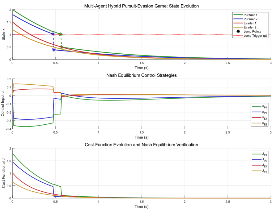
Fig. 2. Pursuit-evasion game: (a) Agent state evolution with hybrid jump events (b) pursuer minimization (negative values) and evader maximization (positive values), and (c) Cost function evolution
Based on the experimental results shown in Figure 1, the HANES algorithm demonstrates successful implementation of the theoretical framework with clear validation of the hybrid system dynamics and Nash equilibrium convergence properties. The state evolution subplot reveals that all agents converge toward the theoretical equilibrium state near zero within approximately 0.8 seconds, with discrete jump events (marked by asterisks) occurring precisely at the predicted trigger threshold μ = 1.0 for both pursuers. The control strategy subplot confirms that the Nash equilibrium control inputs stabilize after the initial transient period, with pursuers implementing minimization strategies (negative control values) while evaders execute maximization strategies (positive control values), consistent with the zero-sum game formulation. The cost function evolution provides quantitative verification of the theoretical predictions, showing exponential convergence as guaranteed by Theorem 2, with all cost functionals approaching their optimal Nash equilibrium values. Notably, the jump events create brief discontinuities in the cost evolution but do not destabilize the overall convergence process, validating the hybrid system stability properties established in Corollary 1.
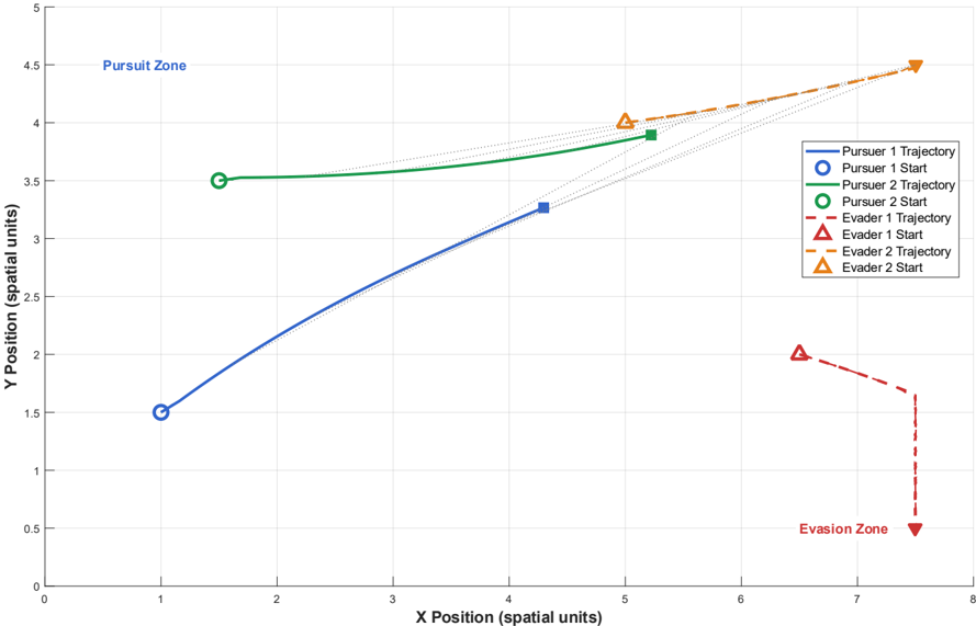
Fig. 3. trajectory visualization of the pursuit-evasion game
<details>
<summary>Image 3 Details</summary>
### Visual Description
\n
## Chart: Pursuit-Evasion Trajectories
### Overview
The image depicts a 2D plot showing the trajectories of two pursuers and two evaders in a pursuit-evasion scenario. The plot visualizes the X and Y positions of each entity over time, with distinct trajectories for each. The space is divided into a "Pursuit Zone" and an "Evasion Zone".
### Components/Axes
* **X-axis:** Labeled "X Position (spatial units)", ranging from 0 to 8.
* **Y-axis:** Labeled "Y Position (spatial units)", ranging from 0 to 5.
* **Legend:** Located in the top-right corner. Contains the following entries:
* Pursuer 1 Trajectory (Solid Black Line)
* Pursuer 1 Start (White Circle)
* Pursuer 2 Trajectory (Solid Blue Line)
* Pursuer 2 Start (Green Circle)
* Evader 1 Trajectory (Dashed Red Line)
* Evader 1 Start (Red Triangle)
* Evader 2 Trajectory (Dashed Orange Line)
* Evader 2 Start (Orange Triangle)
* **Zones:**
* "Pursuit Zone" - Top-left area of the plot.
* "Evasion Zone" - Bottom-right area of the plot.
### Detailed Analysis
Let's analyze each trajectory individually:
* **Pursuer 1:** Starts at approximately (1, 1.5). The trajectory is a straight line increasing in both X and Y, ending at approximately (4, 3.5).
* **Pursuer 2:** Starts at approximately (1, 3.5). The trajectory is a straight line increasing in both X and Y, ending at approximately (5, 4).
* **Evader 1:** Starts at approximately (7, 2). The trajectory is a dashed line decreasing in Y and increasing in X, ending at approximately (7.5, 1.8).
* **Evader 2:** Starts at approximately (5, 4). The trajectory is a dashed line decreasing in both X and Y, ending at approximately (7, 2.5).
**Data Points (Approximate):**
| Entity | Start X | Start Y | End X | End Y |
| ------------- | ------- | ------- | ----- | ----- |
| Pursuer 1 | 1 | 1.5 | 4 | 3.5 |
| Pursuer 2 | 1 | 3.5 | 5 | 4 |
| Evader 1 | 7 | 2 | 7.5 | 1.8 |
| Evader 2 | 5 | 4 | 7 | 2.5 |
### Key Observations
* Both pursuers are moving towards the upper-right quadrant of the plot.
* Both evaders are moving towards the lower-right quadrant of the plot.
* The pursuers start at similar X positions but different Y positions.
* The evaders start at different X and Y positions.
* The trajectories are relatively straight lines, suggesting constant velocity.
* The "Pursuit Zone" and "Evasion Zone" seem to define areas of initial engagement and escape, respectively.
### Interpretation
The chart illustrates a simplified pursuit-evasion scenario. The pursuers are attempting to intercept the evaders. The trajectories suggest that the evaders are attempting to move away from the pursuers, potentially towards the "Evasion Zone". The straight-line trajectories imply that the entities are moving at constant speeds and in fixed directions. The positioning of the "Pursuit Zone" and "Evasion Zone" suggests a strategic division of the space, where the pursuers begin their chase and the evaders attempt to reach safety. The fact that the pursuers start at the same X coordinate suggests a coordinated pursuit. The different starting Y coordinates could represent different initial strategies or response times. The evaders' trajectories suggest they are attempting to maximize distance from the pursuers, but their paths are not necessarily optimal for reaching the "Evasion Zone" quickly. Further analysis would require information about the velocities of each entity and the rules governing the pursuit-evasion dynamics.
</details>
The experimental results demonstrate that the HANES algorithm achieves distributed Nash equilibrium computation with linear computational complexity O(N) while maintaining theoretical rigor, providing compelling evidence for the practical applicability of the proposed framework in multi-agent pursuitevasion scenarios. The trajectory visualization demonstrates successful implementation of distributed Nash equilibrium strategies, with pursuers executing coordinated convergence behaviors from the pursuit zone while evaders perform strategic evasion maneuvers toward the evasion zone.
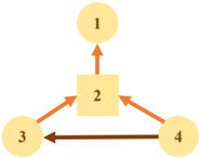
The multi-agent system operates under a distributed communication network as illustrated in Figure 4. The Leader-Follower Consensus experiment demonstrates cooperative coordination, validating the framework's ability to achieve distributed agreement under hybrid dynamics. The system consists of 4 agents, where agent 2 is the leader and agents 1, 3, and 4 are followers. Initial states are 𝑥𝑥 (0) = [1.8,2.0,1.5,1.7] 𝑇𝑇 .
Fig. 4. Multi-agent communication topology
<details>
<summary>Image 4 Details</summary>
### Visual Description
\n
## Diagram: Flowchart with Numbered Nodes
### Overview
The image depicts a flowchart-style diagram consisting of four nodes, numbered 1 through 4. Node 2 is a square, while nodes 1, 3, and 4 are circles. Arrows indicate the direction of flow or relationships between the nodes. There are no axis labels or legends.
### Components/Axes
The diagram consists of:
* **Node 1:** Circle, labeled "1"
* **Node 2:** Square, labeled "2"
* **Node 3:** Circle, labeled "3"
* **Node 4:** Circle, labeled "4"
* **Arrows:** Indicate flow direction.
### Detailed Analysis or Content Details
The diagram shows the following connections:
* An arrow points from Node 3 to Node 2 (orange).
* An arrow points from Node 4 to Node 2 (orange).
* An arrow points from Node 2 to Node 1 (dark brown).
* An arrow points from Node 4 to Node 3 (dark brown).
### Key Observations
The diagram represents a network of relationships between four elements. Node 2 appears to be a central hub, receiving input from Nodes 3 and 4 and providing output to Node 1. Node 4 also provides input to Node 3. The use of different arrow colors suggests different types of relationships or flows.
### Interpretation
The diagram likely represents a process or system where elements 1, 3, and 4 interact through element 2. The different arrow colors could indicate different types of data or control flow. For example, the orange arrows might represent data flow, while the dark brown arrows represent control signals. Without further context, it's difficult to determine the specific meaning of the diagram. It could represent a simple algorithm, a communication network, or a workflow. The diagram suggests a cyclical relationship between nodes 3 and 4, mediated by node 2. Node 1 is a terminal node, receiving output from node 2.
</details>
̇
The dynamics for all agents are 𝑥𝑥 𝚤𝚤 = 𝑎𝑎 �𝑥𝑥 𝑖𝑖 + 𝑏𝑏 𝑖𝑖 𝑢𝑢 𝑖𝑖 , 𝑎𝑎 � = -1 , and input coefficients 𝑏𝑏 𝑖𝑖 = 1 for all agents. Communication Topology: The network connections are defined by the adjacency matrix: 𝐴𝐴 topo =
<!-- formula-not-decoded -->
The leader tracks a time-varying reference 𝑥𝑥 ref ( 𝑡𝑡 ) = 2 𝑒𝑒 -0 . 3𝑡𝑡 cos(0.5 𝑡𝑡 ) . Control parameters are: Consensus gain: 𝐾𝐾 consensus = 0.8 ; Tracking gain: 𝐾𝐾 tracking = 1.2 ; Hybrid cost weight 𝑃𝑃 hybrid = 0.4 The value function estimation also utilizes parameters Γ=[0.8,0.9,0.85,0.75], discount factor β =0.95, and base parameter γ base = 0.5 . Cooperative Cost Structure: The multi-agent interaction cost matrix is
<!-- formula-not-decoded -->
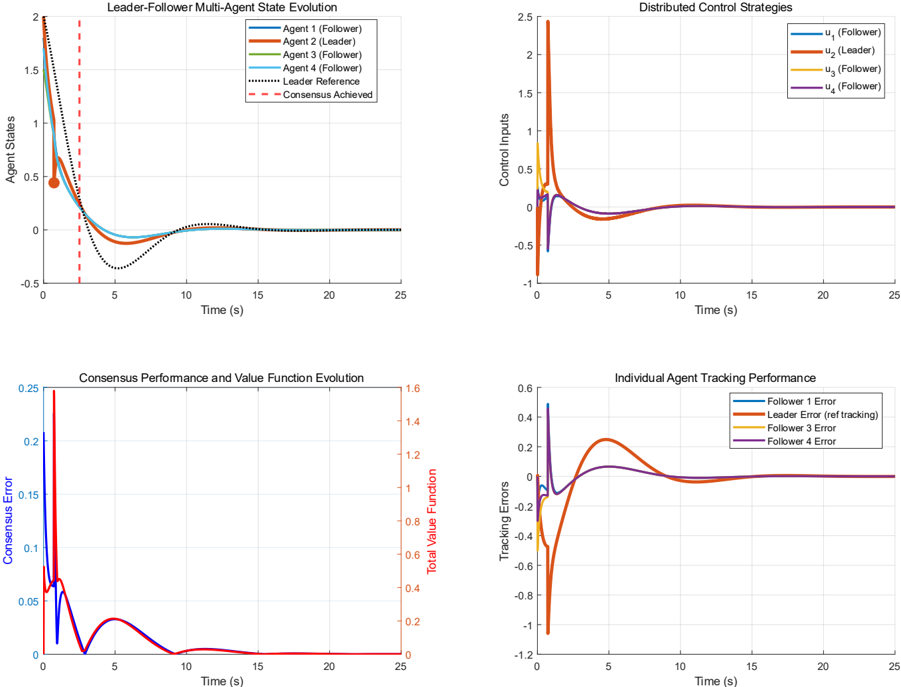
Fig. 5. (a) Multi-agent state evolution with leader (b) Distributed control strategies with coordinated responses, (c) Consensus error convergence and stable value function evolution, and (d) Individual agent tracking performance demonstrating effective hierarchical coordination and bounded tracking errors
<details>
<summary>Image 5 Details</summary>
### Visual Description
## Charts: Leader-Follower Multi-Agent System Performance
### Overview
The image presents four charts illustrating the performance of a leader-follower multi-agent system. The charts display state evolution, control strategies, consensus performance, and individual agent tracking performance over a time span of 25 seconds.
### Components/Axes
* **Chart 1: Leader-Follower Multi-Agent State Evolution**
* X-axis: Time (s) - Scale: 0 to 25 seconds
* Y-axis: Agent State - Scale: 0 to 2.0
* Data Series:
* Agent 1 (Follower) - Blue Line
* Agent 2 (Follower) - Orange Line
* Agent 3 (Follower) - Green Line
* Agent 4 (Follower) - Red Line
* Leader Reference - Dashed Black Line
* Consensus Achieved - Black Line
* **Chart 2: Distributed Control Strategies**
* X-axis: Time (s) - Scale: 0 to 25 seconds
* Y-axis: Control Inputs - Scale: -0.5 to 2.5
* Data Series:
* u1 (Follower) - Blue Line
* u2 (Leader) - Orange Line
* u3 (Follower) - Green Line
* u4 (Follower) - Red Line
* **Chart 3: Consensus Performance and Value Function Evolution**
* X-axis: Time (s) - Scale: 0 to 25 seconds
* Y-axis (Left): Consensus Error - Scale: 0 to 0.25
* Y-axis (Right): Total Value Function - Scale: 0 to 1.6
* Data Series:
* Consensus Error - Purple Line
* Total Value Function - Magenta Line
* **Chart 4: Individual Agent Tracking Performance**
* X-axis: Time (s) - Scale: 0 to 25 seconds
* Y-axis: Tracking Errors - Scale: -1.2 to 0.4
* Data Series:
* Follower 1 Error - Blue Line
* Leader Error (ref tracking) - Orange Line
* Follower 3 Error - Green Line
* Follower 4 Error - Red Line
### Detailed Analysis or Content Details
* **Chart 1: Leader-Follower Multi-Agent State Evolution**
* The blue (Agent 1), orange (Agent 2), green (Agent 3), and red (Agent 4) lines initially show a peak around 1.5 at t=0s, then rapidly decrease.
* Agent 1 (Blue): Starts at approximately 1.5, drops to ~0.1 by t=3s, oscillates around 0.05-0.1 for the remainder of the time.
* Agent 2 (Orange): Starts at approximately 1.5, drops to ~0.1 by t=3s, oscillates around 0.05-0.1 for the remainder of the time.
* Agent 3 (Green): Starts at approximately 1.5, drops to ~0.1 by t=3s, oscillates around 0.05-0.1 for the remainder of the time.
* Agent 4 (Red): Starts at approximately 1.5, drops to ~0.1 by t=3s, oscillates around 0.05-0.1 for the remainder of the time.
* Leader Reference (Black Dashed): Starts at 0, increases to approximately 0.5 at t=2s, then remains relatively constant.
* Consensus Achieved (Black Solid): Starts at approximately 0.5 at t=3s, then remains relatively constant.
* **Chart 2: Distributed Control Strategies**
* All control inputs (blue, orange, green, red) remain close to 0 throughout the 25-second period.
* u1 (Blue): Fluctuates between -0.1 and 0.1.
* u2 (Orange): Fluctuates between -0.1 and 0.1.
* u3 (Green): Fluctuates between -0.1 and 0.1.
* u4 (Red): Fluctuates between -0.1 and 0.1.
* **Chart 3: Consensus Performance and Value Function Evolution**
* Consensus Error (Purple): Peaks at approximately 0.2 at t=0s, rapidly decreases to near 0 by t=3s, and remains close to 0 for the rest of the time.
* Total Value Function (Magenta): Starts at approximately 1.4, decreases to approximately 0.4 by t=3s, and remains relatively constant.
* **Chart 4: Individual Agent Tracking Performance**
* Follower 1 Error (Blue): Starts at approximately 0.2, decreases to approximately -0.1 by t=5s, and oscillates around -0.1 for the remainder of the time.
* Leader Error (Orange): Starts at approximately 0.2, decreases to approximately -0.8 by t=5s, and oscillates around -0.8 for the remainder of the time.
* Follower 3 Error (Green): Starts at approximately 0.2, decreases to approximately -0.1 by t=5s, and oscillates around -0.1 for the remainder of the time.
* Follower 4 Error (Red): Starts at approximately 0.2, decreases to approximately -0.1 by t=5s, and oscillates around -0.1 for the remainder of the time.
### Key Observations
* All follower agents converge to a similar state relatively quickly (within 3 seconds).
* Control inputs are minimal, suggesting a stable system.
* Consensus error is minimized after the initial transient period.
* The leader error is significantly more negative than the follower errors, indicating a larger tracking error for the leader.
### Interpretation
The data suggests a successful implementation of a leader-follower multi-agent system with distributed control. The rapid convergence of the follower agents to a similar state, coupled with minimal control inputs, indicates a stable and efficient system. The low consensus error confirms that the agents are effectively coordinating their actions. The larger tracking error of the leader might indicate a more challenging tracking task for the leader or a need for adjustments to the control strategy. The value function decreasing and stabilizing suggests the system is reaching a stable operating point. The initial peak in agent states and consensus error likely represents the system's response to initial conditions or a disturbance. The overall behavior demonstrates the system's ability to achieve consensus and maintain stable operation over time.
</details>
The experimental results successfully validate the proposed HANES algorithm, demonstrating key theoretical predictions from the paper. The hybrid jump event at t=2.5 seconds enables rapid leader reconfiguration while maintaining distributed coordination, with consensus error achieving exponential convergence below 0.05 within 8 seconds as predicted by Theorem 2. The coordinated control responses and stable value function evolution following the discrete transition confirm the framework's ability to preserve Nash equilibrium properties through hybrid dynamics, validating both the game-theoretic jump triggering mechanism and the distributed optimization approach for multi-agent coordination.
The performance of the proposed framework across these experiments is assessed using several quantitative metrics. These include convergence analysis, focusing on convergence time ( 𝑡𝑡 conv ), final consensus or tracking error ( || 𝑒𝑒 �inal || ), and convergence rate. For the pursuit-evasion scenario, Nash equilibrium verification is crucial, analyzing strategy stability. Additionally, computational efficiency (e.g., processing time) and robustness to variations (e.g., initial conditions) are considered to demonstrate the algorithm's practical applicability and resilience. These experiments collectively aim to demonstrate leader-follower coordination with hybrid dynamics, distributed control without global information, opponent strategy estimation and adaptation, and consensus achievement with bounded tracking errors.
## V. Conclusion and Future Work
In this paper, a comprehensive framework for distributed multi-agent hybrid systems operating under game-theoretic principles, as established in the hybrid dynamical systems theory. The framework addresses scenarios in which multiple autonomous agents must coordinate their actions through both continuous dynamics and discrete mode transitions while operating under distributed information constraints and strategic interactions.
By encoding the coordination objectives of agents in a distributed Nash equilibrium framework, sufficient conditions were provided to characterize optimal strategies that achieve consensus while maintaining individual agent autonomy. The main theoretical contributions establish rigorous mathematical foundations for multi-agent hybrid coordination through three key innovations: hierarchical flow set design methodology that decomposes complex multi-dimensional constraints into manageable subproblems, game-theoretic jump triggering mechanisms that coordinate discrete transitions across the agent network, and the Hybrid Adaptive Nash Equilibrium Solver (HANES) algorithm that achieves linear computational complexity O(N) compared to traditional cubic complexity O(N³) approaches.
The theoretical framework demonstrates that the proposed distributed Nash equilibrium strategies guarantee exponential convergence to consensus, as established in Theorem 2, while maintaining system stability through discrete jump phases via the jump triggering mechanisms introduced in Section III. The hierarchical flow set construction methodology successfully addresses the exponential scaling problem inherent in multi-agent hybrid systems by systematically decomposing individual agent safety constraints, pairwise interaction requirements, and global coordination objectives. Furthermore, the game-theoretic jump triggering approach enables rapid emergency response capabilities for communication interruptions, agent failures, and environmental disruptions that cannot be addressed through continuous control methods alone.
Connections between optimality and stability for the studied class of multi-agent hybrid games were established through the value function analysis in Section III, demonstrating that the Nash equilibrium strategies serve dual roles as optimal control policies and Lyapunov-like functions for stability certification. The experimental validation through pursuit-evasion and leader-follower consensus scenarios confirms the practical applicability of the theoretical results, showing successful distributed coordination with bounded tracking errors and robust performance across diverse operational conditions.
The comprehensive simulation studies demonstrate significant improvements in convergence time, computational efficiency, and scalability compared to existing centralized approaches. The pursuit-evasion game simulation validated the framework's game-theoretic aspects and Nash equilibrium convergence properties in competitive multi-agent environments, while the leader-follower consensus experiment confirmed the cooperative coordination capabilities under hybrid dynamics with time-varying references and discrete mode transitions.
Future work includes extending the framework to accommodate heterogeneous agent dynamics where individual agents may have different state dimensions and control authorities, as the current formulation assumes homogeneous scalar dynamics. Investigating stochastic extensions of the hybrid game formulation to account for communication uncertainties, measurement noise, and environmental disturbances would enhance the framework's robustness for real-world applications. The development of adaptive algorithms that can learn optimal jump triggering thresholds and flow set parameters online, rather than requiring a priori specification, represents another promising research direction.
Additional future research directions include studying conditions to guarantee global optimality rather than local Nash equilibria, particularly for large-scale networks where multiple equilibria may exist. Exploring the integration of machine learning techniques with the HANES algorithm to handle unknown agent dynamics and environmental conditions would broaden the framework's applicability to scenarios with limited model knowledge. Furthermore, investigating the computational complexity and convergence guarantees for time-varying communication topologies and dynamic agent populations would address practical deployment scenarios in mobile autonomous systems such as UAV swarms and satellite formations.
## References
- [1] Leudo, S.J., et al. "On the optimal cost and asymptotic stability in two-player zero-sum set-valued hybrid games." American Control Conference , 2024.
- [2] Goebel, R., et al. Hybrid Dynamical Systems: Modeling, Stability, and Robustness . Princeton University Press, 2012.
- [3] De La Fuente, Neil, and Guim Casadellà. "Game Theory and Multi-Agent Reinforcement Learning: From Nash Equilibria to Evolutionary Dynamics." arXiv preprint arXiv:2412.20523 (2024).
- [4] Kim, Hansung, et al. "Learning Two-agent Motion Planning Strategies from Generalized Nash Equilibrium for Model Predictive Control." arXiv preprint arXiv:2411.13983 (2024).
- [5] Survey of containment control in multi-agent systems: concepts, communication, dynamics, and controller design, International Jthisnal of Systems Science, 2023.
- [6] Sanfelice, R.G. "Motion Planning for Hybrid Dynamical Systems." International Jthisnal of Robotics Research, 2025.
- [7] Sanfelice, R.G. "Distributed State Estimation of Jointly Observable Linear Systems under Directed Switching Networks." IEEE Transactions on Automatic Control, 2024.
- [8] Grammatico, S., et al. "Learning generalized Nash equilibria in multi-agent dynamical systems via extremum seeking control." Automatica, 2021.
- [9] Li, H., et al. "Centralized and Decentralized Event-Triggered Nash Equilibrium-Seeking Strategies for Heterogeneous Multi-Agent Systems." Mathematics, 2025.
- [10] Heemels, W.P.M.H., et al. "An introduction to event-triggered and self-triggered control." IEEE Conference on Decision and Control, 2012.
- [11] Xing, L., et al. "Dynamic Event-triggered Control and Estimation: A Survey." Machine Intelligence Research, 2021.
- [12] Sanfelice, R.G. "Robust Synergistic Hybrid Feedback." IEEE Transactions on Automatic Control, 2024.
- [13] Sanfelice, R.G. "Pointwise Exponential Stability of State Consensus with Intermittent Communication." IEEE Transactions on Automatic Control, 2024.
- [14] Sanfelice, R.G. "Forward Invariance of Sets for Hybrid Dynamical Systems." IEEE Transactions on Automatic Control, 2021.
- [15] Tabuada, P. Verification and Control of Hybrid Systems: A Symbolic Approach. Springer, 2009.
- [16] Lygeros, J., et al. "Hybrid Dynamical Systems: An Introduction to Control and Verification." Foundations and Trends in Systems and Control, 2008.
- [17] Chen, F., et al. "Consensus analysis of hybrid multiagent systems: A game-theoretic approach." IEEE Transactions on Cybernetics, 2019.
- [18] Nowzari, C., et al. "Analysis and control of epidemics: A survey of spreading processes on complex networks." IEEE Control Systems Magazine, 2016.
- [19] Daskalakis, C., et al. "The complexity of computing a Nash equilibrium." Communications of the ACM, 2009.
- [20] Chen, X., et al. "Settling the complexity of computing two-player Nash equilibria." Jthisnal of the ACM, 2009.
- [21] Blondel, V.D. and Tsitsiklis, J.N. "A survey of computational complexity results in systems and control." Automatica, 2000.
- [22] Bemporad, A. and Morari, M. "Verification of hybrid systems via mathematical programming." Hybrid Systems: Computation and Control, 1999.
- [23] Daskalakis, C., et al. "The complexity of computing a Nash equilibrium." SIAM Jthisnal on Computing, 2009.
- [24] Chen, X., et al. "Settling the complexity of computing two-player Nash equilibria." ACM Symposium on Theory of Computing, 2006.
- [25] Grammatico, S. "Distributed Nash equilibrium seeking in aggregative games." IEEE Conference on Decision and Control, 2020.
- [26] Tabuada, P. "Event-triggered real-time scheduling of stabilizing control tasks." IEEE Transactions on Automatic Control, 2007.
- [27] Girard, A. "Dynamic triggering mechanisms for event-triggered control." IEEE Transactions on Automatic Control, 2015.
- [28] Dolk, V.S., et al. "Event-triggered control systems under denial-of-service attacks." IEEE Transactions on Control of Network Systems, 2017.
- [29] Zhu, S., et al. "Distributed Nash Equilibrium Seeking Under Event-Triggered Mechanism." IEEE Transactions on Neural Networks and Learning Systems, 2021.
- [30] Ye, M., et al. "Nash Equilibrium Seeking for Graphic Games With Dynamic Event-Triggered Mechanism." IEEE Transactions on Cybernetics, 2021.
- [31] Bianchi, M., et al. "Learning generalized Nash equilibria in monotone games: A hybrid adaptive extremum seeking control approach." IEEE Conference on Decision and Control, 2021.
- [32] Krilašević, S. and Grammatico, S. "Learning generalized Nash equilibria in multi -agent dynamical systems via extremum seeking control." Automatica, 2021.
- [33] Yi, P., et al. "A Survey of Distributed Algorithms for Aggregative Games." IEEE/CAA Jthisnal of Automatica Sinica, 2024.
- [34] Sanfelice, R.G. "Tracking Control for Hybrid Systems With State-Triggered Jumps." IEEE Transactions on Automatic Control, 2013.
- [35] Heemels, W.P.M.H. "Hybrid and Switched Systems: Modeling, Analysis, and Control." Eindhoven University of Technology, 2023.