2506.14138

# NeuroCoreX: An Open-Source FPGA-Based Spiking Neural Network Emulator with On-Chip Learning ††thanks: This manuscript has been authored in part by UT-Battelle, LLC under Contract No. DE-AC05-00OR22725 with the U.S. Department of Energy. The United States Government retains and the publisher, by accepting the article for publication, acknowledges that the United States Government retains a non-exclusive, paid-up, irrevocable, world-wide license to publish or reproduce the published form of this manuscript, or allow others to do so, for United States Government purposes. The Department of Energy will provide public access to these results of federally sponsored research in accordance with the DOE Public Access Plan (http://energy.gov/downloads/doe-public-access-plan).This material is based upon work supported by the U.S. Department of Energy, Office of Science, Office of Advanced Scientific Computing Research, under contract number DE-AC05-00OR22725. **Authors**: Ashish Gautam, Prasanna Date, Shruti Kulkarni, Robert Patton, Thomas Potok > Computer Science and Mathematics Division, Oak Ridge National Laboratory , Oak Ridge, Tennessee, USA. ## Abstract Spiking Neural Networks (SNNs) are computational models inspired by the structure and dynamics of biological neuronal networks. Their event-driven nature enables them to achieve high energy efficiency, particularly when deployed on neuromorphic hardware platforms. Unlike conventional Artificial Neural Networks (ANNs), which primarily rely on layered architectures, SNNs naturally support a wide range of connectivity patterns, from traditional layered structures to small-world graphs characterized by locally dense and globally sparse connections. In this work, we introduce NeuroCoreX, an FPGA-based emulator designed for the flexible co-design and testing of SNNs. NeuroCoreX supports all-to-all connectivity, providing the capability to implement diverse network topologies without architectural restrictions. It features a biologically motivated local learning mechanism based on Spike-Timing-Dependent Plasticity (STDP). The neuron model implemented within NeuroCoreX is the Leaky Integrate-and-Fire (LIF) model, with current-based synapses facilitating spike integration and transmission . A Universal Asynchronous Receiver-Transmitter (UART) interface is provided for programming and configuring the network parameters, including neuron, synapse, and learning rule settings. Users interact with the emulator through a simple Python-based interface, streamlining SNN deployment from model design to hardware execution. NeuroCoreX is released as an open-source framework, aiming to accelerate research and development in energy-efficient, biologically inspired computing. Index Terms: Neuromorphic computing, FPGA, STDP, Spiking Graph Neural Networks, Spiking Neural Networks, VHDL. ## I Introduction One of the primary goals of neuromorphic computing is to emulate the structure and dynamics of biological neuronal networks, achieving both brain-like energy efficiency and high computational accuracy. This is accomplished through the use of spiking neuron models implemented on neuromorphic chips. Over the past two decades, a variety of neuromorphic chips have been designed using both analog and digital ASIC platforms, capable of performing real-time information processing [13, 26, 27, 3, 28, 23]. However, the adoption of these systems remains constrained by their high cost, limited availability, and architectural specificity. Proprietary neuromorphic chips typically restrict user access and customization, creating significant barriers for researchers and students seeking to innovate and explore new designs. Field programmable gate arrays (FPGAs) offer a promising alternative, providing a flexible platform for prototyping and validating SNNs before final implementation on custom ASICs. They serve as an effective intermediate step, facilitating co-design development alongside off-the-shelf SNN simulators [8, 32]. Several digital ASICs and FPGA-based SNN systems have been proposed in the past [29, 22, 25]. While some proprietary systems [13] include local learning capabilities such as spike-timing-dependent plasticity (STDP), most FPGA-based implementations still rely heavily on offline training and lack real-time, on-chip learning. This limitation reduces their adaptability for dynamic, continuously evolving applications such as robotics, smart sensors, and edge computing. To address these challenges, we introduce NeuroCoreX, an open-source spiking neural network (SNN) emulator implemented in VHDL (Very High-Speed Integrated Circuit Hardware Description Language) for FPGA platforms. NeuroCoreX provides an affordable and flexible alternative for neuromorphic computing research and education. It is meant to be used in AI applications requiring low size, weight, and power (SWaP) such as edge computing, embedded systems, Internet of Things (IoT), and autonomous systems [30, 20, 1, 7, 6]. Unlike fixed-architecture hardware, it supports fully reconfigurable network topologies, from simple layered structures to complex small-world graphs. It incorporates biologically inspired local learning through a variant of the STDP learning rule [24], enabling on-chip, online adaptation of synaptic weights. The system uses a Leaky Integrate-and-Fire (LIF) neuron model with current-based synapses [19], ensuring both computational simplicity and biological relevance. This model of neuromorphic computation is known to be Turing-complete, i.e., capable of performing all the computations that a CPU/GPU can perform [12, 9]. As a result, NeuroCoreX can support not just SNN-based AI workloads but also general-purpose computing workloads [10, 11, 31, 34]. Programming and configuring NeuroCoreX is streamlined through a UART interface and a simple Python module, allowing users to modify network, neuron, synapse, and learning parameters easily. This makes NeuroCoreX not only a valuable research tool for testing new theories of learning and network organization but also a powerful educational platform for hands-on experience with neuromorphic hardware. Additionally, its energy-efficient architecture makes it well-suited for low-power AI applications in areas such as autonomous systems, smart sensors, and scientific instrumentation. The rest of the manuscript is organized as follows: Section II provides an overview and the architecture description of NeuroCoreX in detail. In Section III, we present the results demonstrating the functionality of the platform and evaluate its performance on the DIGITS dataset [2]. The manuscript concludes with a discussion of the results and planned future work in Section IV. ## II NeuroCoreX ### II-A NeuroCoreX overview NeuroCoreX is designed to emulate brain-like computation on reconfigurable FPGA hardware using a digital circuit approach. The system architecture is built around three fundamental components, inspired by biological neural networks: neurons, synapses, and a local learning mechanism. These elements are digitally realized in VHDL and operate together to support real-time, adaptive information processing. The neuron model employed is the LIF model, which captures the essential dynamics of biological neurons with computational efficiency and is known to be Turing-complete. Synapses are modeled with an exponential current response and store dynamic weight values that govern neuron-to-neuron influence. Learning is enabled through a simple variant of STDP, allowing synaptic strengths to evolve based on the relative timing of neuronal spikes. In its current implementation, NeuroCoreX supports networks of up to $N=100$ neurons with full all-to-all bidirectional connectivity using 10,000 synapses. In addition to recurrent connections, the system includes a separate set of 10,000 feedforward input synapses that serve as the interface for external stimuli. These input weights determine how incoming spikes—from sources such as sensors or preprocessed datasets—modulate the activity of neurons within the network. Neuronal dynamics are configured to emulate biological timescales. The network size and acceleration factor can be scaled depending on the memory resources of the FPGA, precision of the synaptic weights used and the operating clock frequency. Time-multiplexing and pipelining techniques are used to optimize hardware resource usage. A single physical neuron circuit is time-multiplexed to emulate the entire network. Communication with the FPGA is managed through a UART interface, with a Python module providing a user-friendly configuration and control interface. <details> <summary>extracted/6533360/images/NeuroCoreX_block_diagram.png Details</summary>  ### Visual Description ## System Architecture Diagram: FPGA-Based Spiking Neural Network Implementation ### Overview The image is a technical diagram illustrating the architecture and data flow of a spiking neural network (SNN) system implemented on an FPGA (Artix-7). It is divided into three labeled sections: (a) the main system-level architecture showing the interaction between a host PC and the FPGA, (b) a conceptual diagram of the input layer and recurrent network connectivity, and (c) a conceptual diagram of the network's internal structure and topic-based output classification. ### Components/Axes The diagram is not a chart with axes but a block diagram with interconnected components. The primary components and their labels are: **Section (a) - System Architecture:** * **Left Block (PC):** * Header: `PC` * Green Box: `1. Parameters for Neurons, synapses and initial weights.` * Blue Box: `2. Input Datasets` * Sub-label: `Datasets Format` | Spike time (8-bits) | Neuron Address (16 bits) | | :--- | :--- | * Yellow Box: `3. Output from FPGA` * Sub-label: `Plot and validation` * **Central Connection:** * Purple Box: `UART BUS` (connects PC and FPGA) * **Right Block (FPGA Artix 7):** * Header: `FPGA Artix 7` * Green Box (Top): `Weights (W_AA)` * Green Box (Middle): `Neuron & Synapse Parameters (Static)` and `Weights (W_in)` * Large Light Green Box: `LIF + STDP ENGINE` (contains a network diagram of interconnected yellow nodes) * Blue Box: `Spike input FIFO` | Neuron Address (16 bits) | Spike time (8-bits) | | :--- | :--- | * Purple Boxes (Bottom Right): * `FIFO I_syn_AA` (with numbered slots 1, 2, 3... N) * `FIFO I_syn_in` (with numbered slots 1, 2, 3... N) * `FIFO Vmem` (with numbered slots 1, 2, 3... N) * **Data Flow Labels:** * Arrows are labeled with data types: `w`, `Delta_w`. * A yellow arrow from FPGA back to PC is labeled `Output from FPGA`. **Section (b) - Network Connectivity (Left):** * Label: `(b)` * Input: `Image pixels` (pointing to a column of dark blue nodes). * Connections: Lines from input nodes to a second layer of light blue nodes are labeled `W_in`. * Recurrent Connections: Lines between the light blue nodes are labeled `W_AA`. **Section (c) - Network Structure (Right):** * Label: `(c)` * Input Node: A single dark blue node connected via `W_in`. * Internal Network: A cluster of interconnected nodes (light orange and light blue) with black arrows indicating connections. * Output Nodes: Two large nodes labeled `Topic 1` (orange) and `Topic 2` (blue). * Connection Label: `W_AA` is placed near the connections leading to the topic nodes. ### Detailed Analysis The diagram details a closed-loop system for training and running a spiking neural network on hardware. 1. **Data Flow (Section a):** * **Configuration & Input (PC to FPGA):** The PC sends static parameters (`Neuron & Synapse Parameters`), initial input weights (`W_in`), and formatted input spike datasets via the `UART BUS`. The dataset format is specified as pairs of `Spike time (8-bits)` and `Neuron Address (16 bits)`. * **Processing (FPGA):** The FPGA receives spikes into a `Spike input FIFO`. The core processing occurs in the `LIF + STDP ENGINE`, which implements Leaky Integrate-and-Fire neurons with Spike-Timing-Dependent Plasticity learning. This engine uses the static parameters and weights (`W_in`). It also interacts with a separate memory block for recurrent weights (`W_AA`), sending weight updates (`Delta_w`) and receiving current weights (`w`). * **Internal Data Handling (FPGA):** Three dedicated FIFOs (`I_syn_AA`, `I_syn_in`, `Vmem`) are used to buffer synaptic currents and membrane potentials for the neurons, indexed from 1 to N. * **Output (FPGA to PC):** Results are sent back to the PC via the `UART BUS` for `Plot and validation`. 2. **Network Models (Sections b & c):** * **Section (b)** shows a simple two-layer feedforward structure with recurrence. Input `Image pixels` connect via `W_in` to a hidden layer, which has recurrent connections (`W_AA`) among its own neurons. * **Section (c)** depicts a more complex, possibly trained, network state. An input connects via `W_in` to a recurrently connected internal network. This internal network's activity is then mapped via strong connections (thick black arrows) to distinct `Topic` output nodes, suggesting a classification or clustering function. The label `W_AA` here likely refers to the weights governing these output connections. ### Key Observations * **Hardware-Software Partitioning:** The design clearly separates the host PC (for data I/O, validation, and high-level control) from the FPGA (for real-time, parallel neural computation). * **Explicit Data Formats:** The diagram specifies bit-widths for spike data (8-bit time, 16-bit address), which is critical for hardware implementation. * **Dual Weight Memories:** The architecture maintains separate memory/storage for input weights (`W_in`) and recurrent/associative weights (`W_AA`), allowing for different update rules or access patterns. * **FIFO-Based Streaming:** The use of multiple FIFOs indicates a streaming data architecture designed to handle continuous spike traffic and maintain pipeline efficiency on the FPGA. * **Conceptual Progression:** The sequence from (b) to (c) suggests a progression from a basic network topology to a functionally organized one where internal dynamics lead to distinct topic-based outputs. ### Interpretation This diagram represents a complete hardware-software co-design for a neuromorphic computing system. The core innovation is the implementation of an on-chip learning engine (`LIF + STDP ENGINE`) on an FPGA, enabling the network to adapt its weights (`W_AA`) in real-time based on spike timing. The system is designed for processing temporal spike data, likely from an event-based sensor (as implied by "Image pixels" in part b). The PC acts as a supervisor, providing the initial network "genome" (parameters and weights) and raw sensory data, then receiving the processed results for analysis. The FPGA handles the computationally intensive, parallel task of simulating thousands of spiking neurons and their plastic synapses. The transition from diagram (b) to (c) is particularly insightful. It suggests that through the STDP learning rule, the initially random or generic recurrent connections (`W_AA`) in (b) self-organize into a structured network in (c). This structure enables the network to transform a single input pattern into a distributed internal representation that reliably activates specific, semantically meaningful output nodes (`Topic 1`, `Topic 2`). This demonstrates the system's capability for unsupervised feature extraction and classification directly from spike-based data. The entire architecture is a blueprint for building low-power, adaptive, and real-time intelligent sensing systems. 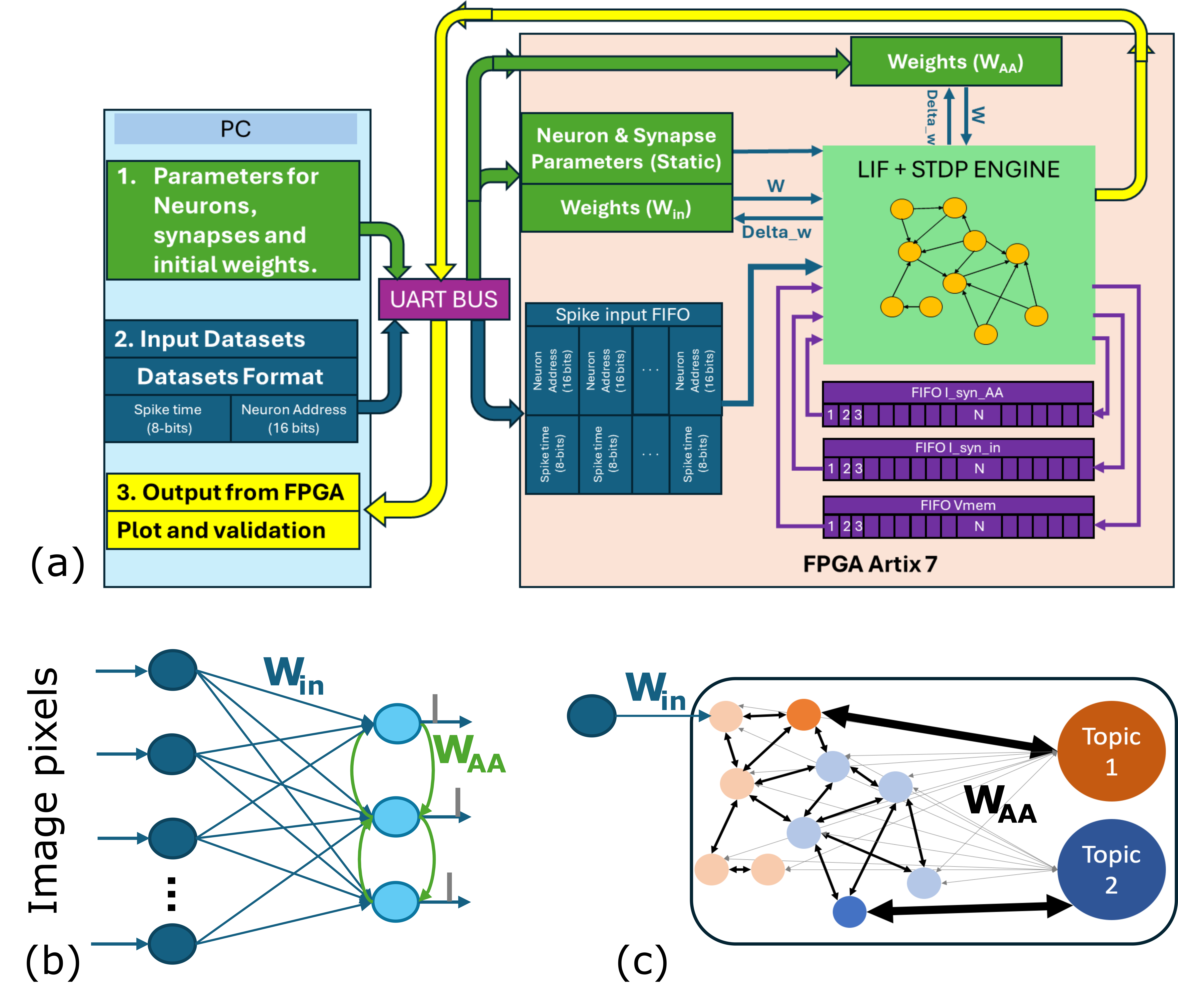</details> Figure 1: (a). Block diagram of our FPGA based NeuroCoreX, (b). Feedforward SNN used for digits dataset classification, (c). Spiking Graph Neural Network for citation graph node classification problem. The operation of NeuroCoreX follows a structured emulation cycle (see Fig. 1 (a)). First, the network weights and initial configuration parameters for neuron, synapse, and learning rule are transferred from a PC to the FPGA via the UART interface. Once the network is set up, input spikes are streamed in real time, buffered in a First-In-First-Out (FIFO) module on the FPGA, and injected into the network precisely at their intended timestamps. At each neuron update cycle, the time-multiplexed processor sequentially updates the membrane potential, synaptic inputs, and firing status of each neuron. If a neuron fires, its effect on connected neurons is mediated through the all-to-all connected $W_{AA}$ weight matrix, and synaptic weights are updated in real time if STDP is enabled. Synaptic weights corresponding to feedforward inputs $W_{in}$ are similarly updated if STDP is enabled for them. The system thus continuously processes incoming spikes, updates network states, applies learning, and advances to the next time step, enabling real-time emulation of SNNs on the FPGA. Fig. 1 (a) shows a high-level block diagram of NeuroCoreX, along with two representative examples of network architectures that can be implemented on the FPGA. The first is a conventional feedforward SNN, a topology commonly used in neuromorphic research. We use this network to demonstrate digit classification on the well-known DIGITS dataset [2], showcasing NeuroCoreX’s support for standard inference tasks. The second network, shown in Fig. 1 (c), illustrates a SNN designed for node classification on citation graphs using STDP-based unsupervised learning. This architecture lacks a traditional layered structure and is instead defined by arbitrary, sparse connectivity encoded in the $W_{AA}$ matrix, which stores both plastic and static synaptic weights. These two examples highlight the flexibility of NeuroCoreX: in addition to supporting conventional layered architectures, the platform can implement non-layered networks such as those found in graph-based problems or generated via evolutionary algorithms like EONs . This versatility makes it suitable for a wide range of neuromorphic applications, from structured inference tasks to irregular and adaptive network topologies. ### II-B FPGA platform NeuroCoreX is implemented on the Artix-7 FPGA, a cost-effective and widely available platform that offers sufficient resources for neuromorphic prototyping. The system operates with a maximum internal clock frequency of 100 MHz. Two main clock domains are used: the high-frequency 100 MHz clock for UART-based communication and a 100 KHz lower-speed operating clock for neural processing. The combination of modest resource requirements, real-time adaptability, and biological plausibility makes the Artix-7 platform an ideal choice for NeuroCoreX. Scalability to larger networks or faster processing rates is primarily limited by the available block RAM and choice of clock frequency for neural processing on the FPGA. The UART interface operates at a baud rate of 1 Mbps, enabling efficient transmission and reception of both static configuration data and real-time input spikes. The FPGA receives network weights, neuron, synapse, and learning parameters from a host PC via this UART channel before execution begins. During operation, additional input spikes are streamed to the network in real time through the same interface. ### II-C Neuron and Synapse Models NeuroCoreX employs a biologically inspired computational model that integrates neuron dynamics, synaptic interactions, and local learning mechanisms. The neurons are modeled using a LIF formulation, adapted for efficient FPGA implementation. Each neuron has four configurable parameters, threshold, leak, refractory period, and reset voltage. The membrane potential V(t) is updated at each time step according to the following discrete-time equation: $$ V(t+1)=V(t)-\lambda+I_{\text{syn}}(t) $$ where $I_{\text{syn}}(t)$ is the total synaptic input current at timestep $t$ and $\lambda$ is the neuron’s leak. When the membrane potential exceeds the threshold $V_{\text{th}}$ , the neuron emits a spike, enters a refractory period $\tau_{\text{ref}}$ , and its membrane potential is reset to $V_{\text{reset}}$ . To ensure efficient real-time processing, all calculations are performed using a fixed-point format with 1 sign bit, 7 integer bits, and 10 fractional bits. Synaptic inputs are modeled as current-based exponential synapses, capturing biologically realistic, temporally decaying post-synaptic responses. The synaptic current dynamics follow the update rule: $$ I_{\text{syn}}(t+1)=I_{\text{syn}}(t)-\lambda_{\text{syn}} $$ where $\lambda_{\text{syn}}$ represents the synaptic current decay at each time step. Each synapse has an associated weight that determines its influence on the postsynaptic neuron. These synaptic weights, stored in BRAM, are dynamically updated during runtime. Weights are represented in signed 8-bit format, and appropriate resizing and bit-shifting are applied during computations to correctly integrate the synaptic current into the membrane potential. <details> <summary>extracted/6533360/images/Fig_2_RECT_STDP_inkscape.png Details</summary>  ### Visual Description ## Technical Diagram: Spike-Timing-Dependent Plasticity (STDP) Rule and Associated Matrices ### Overview The image is a two-part technical diagram illustrating a simplified, binary model of Spike-Timing-Dependent Plasticity (STDP) and the matrix representations of its associated variables in a neural network context. Part (a) is a graph defining the weight update rule based on spike timing differences. Part (b) displays four generic matrices representing the state variables of a network implementing this rule. ### Components/Axes #### Part (a): STDP Rule Graph * **Vertical Axis (Y-axis):** Labeled **Δw**. Represents the change in synaptic weight. The axis has two discrete levels marked: **+1 bit** (positive change) and **-1 bit** (negative change). * **Horizontal Axis (X-axis):** Labeled **Δt (ms)**. Represents the time difference between pre-synaptic and post-synaptic spikes in milliseconds. The axis has tick marks at **-45, -30, -15, 0, 15, 30, 45**. * **Regions and Labels:** * A rectangular region in the positive quadrant (Δt > 0, Δw = +1 bit) is labeled **tpre (ms)**. This region spans from Δt = 0 to Δt = 15 ms. * A rectangular region in the negative quadrant (Δt < 0, Δw = -1 bit) is labeled **tpost (ms)**. This region spans from Δt = -30 ms to Δt = 0. * **Sub-label:** The graph is labeled **(a)** in the bottom-left corner. #### Part (b): Matrix Representations Four matrices are presented, all sharing an identical n x n structure with elements indexed from 1 to n. Ellipses (`...`) indicate the continuation of rows and columns. 1. **Top-Left Matrix:** Labeled **W_AA**. Elements are denoted as **w_ij** (e.g., w₁₁, w₁₂, ..., w_1n; w₂₁, w₂₂, ..., w_2n; ...; w_n1, w_n2, ..., w_nn). 2. **Top-Right Matrix:** Labeled **synaptic_traces**. Elements are denoted as **s_ij** (e.g., s₁₁, s₁₂, ..., s_1n; s₂₁, s₂₂, ..., s_2n; ...; s_n1, s_n2, ..., s_nn). 3. **Bottom-Left Matrix:** Labeled **update_state**. Elements are denoted as **u_ij** (e.g., u₁₁, u₁₂, ..., u_1n; u₂₁, u₂₂, ..., u_2n; ...; u_n1, u_n2, ..., u_nn). 4. **Bottom-Right Matrix:** Labeled **enable_STDP**. Elements are denoted as **e_ij** (e.g., e₁₁, e₁₂, ..., e_1n; e₂₁, e₂₂, ..., e_2n; ...; e_n1, e_n2, ..., e_nn). * **Sub-label:** This group of matrices is labeled **(b)** in the bottom-left corner. ### Detailed Analysis * **STDP Rule (Part a):** The graph defines a **binary, asymmetric Hebbian learning rule**. * **Potentiation (+1 bit):** Occurs when the pre-synaptic spike precedes the post-synaptic spike (Δt > 0). The potentiation window is **tpre = 15 ms**. Any spike pair with a positive timing difference within this window results in a fixed weight increase of +1 bit. * **Depression (-1 bit):** Occurs when the post-synaptic spike precedes the pre-synaptic spike (Δt < 0). The depression window is **tpost = 30 ms**. Any spike pair with a negative timing difference within this window results in a fixed weight decrease of -1 bit. * **Asymmetry:** The depression window (30 ms) is twice as long as the potentiation window (15 ms). * **Discretization:** Weight changes are quantized to single bits, suggesting a digital or highly simplified implementation. * **Matrix Structure (Part b):** The four matrices represent the core data structures for a network of *n* neurons. * **W_AA:** The primary synaptic weight matrix connecting a population of neurons (likely all-to-all, given the square matrix). * **synaptic_traces:** A matrix of the same dimension, likely holding eligibility traces or other temporal variables necessary for computing the STDP updates. * **update_state:** A matrix that may control or log the update process for each synapse. * **enable_STDP:** A binary or control matrix that likely gates whether the STDP rule is active for a given synapse (i,j). ### Key Observations 1. **Binary and Discrete:** The STDP model is highly abstracted, using only +1 or -1 bit changes instead of continuous values. 2. **Temporal Asymmetry:** The rule is asymmetric in time, with a longer window for depression than for potentiation, a common feature in biological STDP models. 3. **Structured State Management:** The use of four parallel matrices indicates a systematic approach to managing synaptic weights, traces, and update logic in a computational model, possibly for efficient parallel processing or hardware implementation. ### Interpretation This diagram outlines a **computational framework for implementing a simplified, binary STDP learning rule in a neural network**. The graph in (a) defines the fundamental learning principle: synaptic connections are strengthened if the pre-synaptic neuron fires shortly before the post-synaptic neuron, and weakened if the order is reversed, with fixed, discrete changes. The matrices in (b) provide the data architecture to execute this rule across a network of *n* neurons. The `synaptic_traces` matrix is crucial, as it would store the temporal information (e.g., last spike times) needed to compute Δt for each synapse. The `enable_STDP` matrix suggests the learning rule can be selectively applied, allowing for plasticity control. This model is likely designed for **digital neuromorphic hardware or efficient simulation**, where binary weights and structured matrix operations are advantageous. The asymmetry in the time windows (tpost > tpre) biases the network towards depression, which can be important for stability and preventing runaway excitation in learning systems. 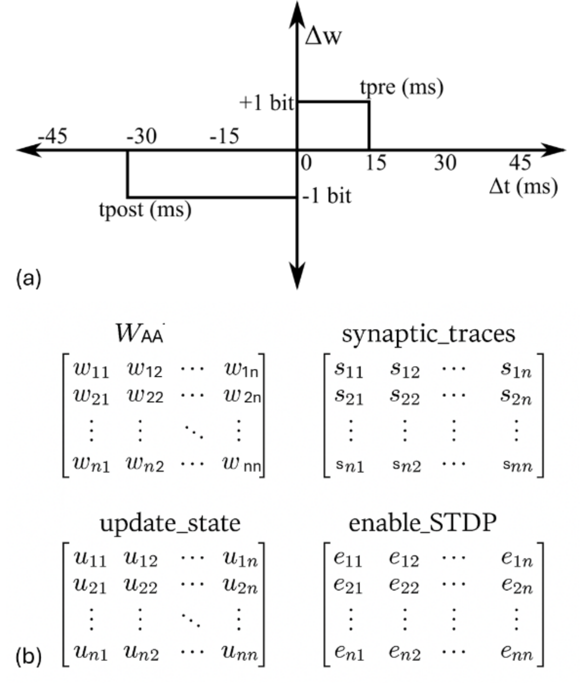</details> Figure 2: (a) Simplified STDP learning rule implemented on NeuroCoreX. (b) Internal variables stored in BRAM for tracking STDP updates. All matrices are of size $N\times N$ and stored in row-major order. Each element of the $W_{AA}$ and synaptic_traces matrices is 8 bits wide, while update_state and enable_STDP are binary matrices. ### II-D Learning Rule NeuroCoreX implements a pair-based STDP rule using a rectangular learning window, a simplification widely demonstrated to maintain similar functional behavior to conventional exponential window [24] when the resolution of the weights is greater than 6-bits [17, 15, 5]. In this model (See Fig. 2 (a)), if a causal spike pair (presynaptic spike preceding postsynaptic spike) occurs within the window $t_{pre}$ , the synaptic weight is incremented by $dw_{pos}$ . If an acausal spike pair (postsynaptic spike preceding presynaptic spike) occurs, the weight is decremented by $dw_{neg}$ . $$ \Delta w=\begin{cases}dw_{\text{pos}},&\text{if}\quad 0<\Delta t<t_{\text{pre} }\\ -dw_{\text{neg}},&\text{if}\quad 0<\Delta t<t_{\text{post}}\\ 0,&\text{otherwise}\end{cases} $$ Here, $\Delta t$ is the time difference between pre-and postsynaptic spikes, $dw_{\text{neg}}$ , $dw_{\text{pos}}$ , $t_{\text{pre}}$ , and $t_{\text{post}}$ are configurable parameters initialized via the Python-UART interface. The pre- and post-synaptic spike timings are tracked using dedicated time-trace registers stored in BRAM (see Fig. 2 (b)). These time traces are updated on each spike event and are used to detect causal or acausal spike pairings that trigger weight updates. For example, when neuron 1 spikes, all synaptic traces corresponding to its outgoing synapses are reset to zero, and the associated update_state entries are set to 1. In parallel, the post-synaptic trace (not shown in Fig. 2) is activated for all incoming synapses to neuron 1. At each subsequent time step, the active values in the synaptic trace matrices are incremented by 1. This process continues until the counter reaches $t_{\text{pre}}$ . If no other neuron spikes within this window, the trace value is reset to 0xFF (representing a negative disabled state), and the corresponding update_state entry is cleared. Similarly, if no neuron spiked within $t_{\text{post}}$ time steps prior to neuron 1’s spike, the post-synaptic trace is also reset to a negative value. However, if another neuron spikes within $t_{\text{pre}}$ time steps after neuron 1, the synaptic weight is incremented by $dw_{\text{pos}}$ , and both the synaptic trace and update_state for that synapse are reset. Conversely, if a neuron spiked within $t_{\text{post}}$ time steps prior to neuron 1, the synaptic weight is decremented by $dw_{\text{neg}}$ , and the associated trace and update_state values are reset. Thus, during each neuron update cycle, if a neuron spikes, the corresponding row and column addresses in the matrices shown in Fig. 2 (b) are accessed and updated. Based on the current states of these auxiliary matrices, the entries in the weight matrix $W_{AA}$ are modified accordingly. The enable_STDP matrix is a static binary mask configured via the Python interface at initialization. It acts as a filter to specify which synapses in $W_{AA}$ are subject to STDP-based plasticity. There a similar matrix for synapses in $W_{in}$ . ### II-E Network Architecture and System Operation The SNN architecture implemented on NeuroCoreX is illustrated in Fig. 1 (a). The network consists of upto $N=100$ LIF neurons instantiated on the FPGA. Two primary weight matrices define the network connectivity: $W_{AA}$ , a synaptic weight matrix for all-to-all, bidirectional connectivity between neurons in the FPGA and $W_{in}$ , a synaptic weight matrix for feedforward connections from external input sources to the neurons on the FPGA. Both matrices are stored in the FPGA’s BRAM. They can be initialized to user-defined values, and are accessed during SNN emulation. A synaptic weight value of zero indicates no connection between the corresponding neurons. Internal network dynamics are governed by the $W_{AA}$ matrix. This matrix allows every neuron to influence every other neuron bidirectionally. The matrix values determine the synaptic strengths between pairs of neurons and evolve over time via STDP-based learning. Both $W_{AA}$ and $W_{in}$ matrices support on-chip learning. To preserve network structure and prevent unwanted modifications, an associated binary filter matrix, called enable-STDP, is used for each weight matrix. If a weight’s corresponding enable-STDP entry is zero, the weight remains fixed throughout operation—even during learning phases. Weights representing nonexistent connections (zeros in the weight matrix) are thus protected from modification. In addition to the synaptic weights, the BRAMs are also used store the pre-and post synaptic traces necessary for STDP calculations. Weight matrices $W_{AA}$ and $W_{FF}$ , and the pre-and postsynaptic traces are stored as separate memory banks in row major order on the FPGA’s BRAM. As BRAM addresses must be accessed sequentially, the high-speed 100 MHz clock domain is utilized for reading, updating, and writing synaptic weights. During each clock cycle, synaptic weights and neuron states are updated in a pipelined manner to ensure efficient processing without data bottlenecks. NeuroCoreX utilizes time-multiplexing and pipelining techniques to emulate 100 neurons using a single physical neuron processing unit. Neuron updates are managed under a 100 kHz clock domain, such that updating all 100 neurons takes 1 millisecond, which closely matches the biological timescale of real neural systems. To accelerate the emulation, a higher update clock frequency can be used. For example, operating the neuron updates at 1 MHz results in a 10× speed-up relative to biological time for a network of 100 neurons. However, if the network size is increased to 1000 neurons while maintaining the 1 MHz clock, the full network would again require approximately 1 millisecond per time step, restoring biological equivalence. Thus, there exists a direct dependence between the number of neurons, the update clock frequency, and the effective emulated timescale. In the current implementation, the network size is limited to 100 neurons due to the available BRAM resources on the Artix-7 FPGA. Even with higher BRAM availability, the number of neurons that can be emulated is ultimately constrained by the difference between the clock frequency available for BRAM access and the clock rate used for updating the SNN states (see Section IV). Incoming spikes from external sources are transmitted via the UART interface. Each spike is encoded as a 24-bit word, comprising a 16-bit input neuron (or pixel) address and an 8-bit spike timing component. In the current implementation, the feedforward weight matrix $W_{\text{in}}$ is a $100\times 100$ matrix, corresponding to 100 input neurons and 100 on-chip neurons. Although 8 bits are sufficient to encode the addresses of 100 input neurons, we chose to use 16 bits to provide flexibility for interfacing with larger sensor arrays. This allows the system to support up to 16K input neurons in future applications. In such cases, the feedforward matrix $W_{\text{in}}$ becomes a rectangular matrix of size $100\times N_{\text{in}}$ , where $N_{\text{in}}$ denotes the number of input neurons in the external layer. For transmission efficiency, successive time differences between spikes are sent, rather than absolute times. These incoming spikes are temporarily stored in a FIFO buffer on the FPGA (See Fig. 1 (a)). The FIFO is designed to support simultaneous read and write operations, allowing it to continuously receive long temporal spike trains while concurrently feeding data to the network in real time without stalling. During network emulation, the system clock continuously increments an internal time counter. When the internal clock matches the timestamp of the spike at the FIFO head, the corresponding input neuron address is read. The associated weights from the $W_{in}$ matrix are then used to inject synaptic currents into the membrane potentials of the relevant neurons. If the synaptic current causes any neuron on the FPGA to spike, then associated weights from the $W_{AA}$ matrix are then read and used to inject synaptic currents into the membrane potentials of all other neurons connected to the spiking neuron in the network. ## III Results We present experimental results that demonstrate the usability, correctness, and flexibility of the NeuroCoreX platform across a range of SNN workloads. ### III-A Demonstrating User Interface Flexibility One of the key strengths of the NeuroCoreX platform lies in its flexible and intuitive user interface, which enables seamless communication between a host PC and the FPGA hardware through a Python-based control module. To demonstrate this capability, we highlight several core features supported by the interface. 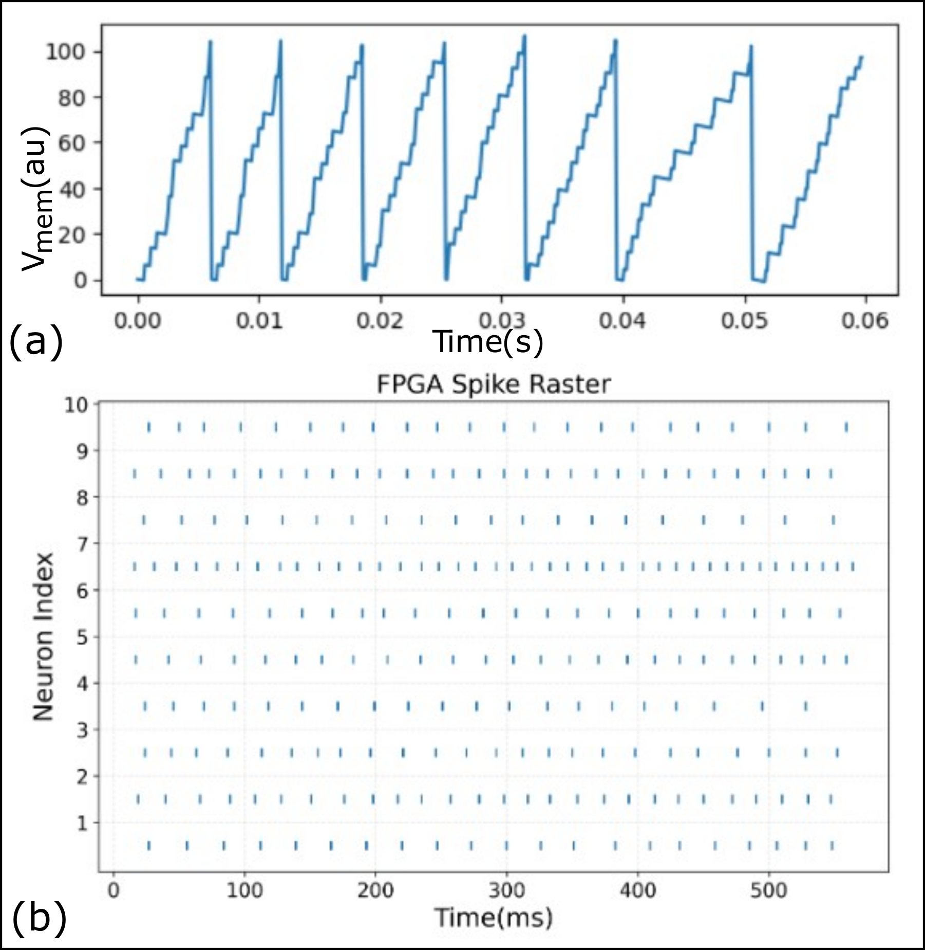First, spike trains can be streamed from the PC to the FPGA for real-time emulation of spiking network activity. Figure 3 (b) shows a raster plot of spiking activity recorded during one such emulation run. Second, the user interface allows for real-time monitoring of internal neuron dynamics. Specifically, the membrane potential of any selected neuron can be captured and plotted as a time series, offering insight into subthreshold integration and spiking behavior. Figure 3 (a) shows the membrane potential trace of a representative neuron under input stimulation. The spike trains of all neurons and the membrane potential of a selected neuron are transferred back to the PC in real time. These signals are not stored on the FPGA. Instead, an internal FIFO module is used to buffer these signals, which allows for the continuous recording and visualization of network dynamics over long temporal duration without being limited by on-chip memory. Finally, the interface supports reading back synaptic weights from the FPGA after an STDP-enabled emulation. This feature enables direct inspection of weight evolution and verification of learning dynamics on hardware. It is particularly useful for comparing hardware learning outcomes with software simulations, facilitating debugging and model validation. These features collectively support efficient testing, inspection, and refinement of neuromorphic models, enabling a co-design loop between high-level model development and hardware validation. <details> <summary>extracted/6533360/images/Fig_3_PC_FPGA_UART.png Details</summary>  ### Visual Description ## [Chart/Diagram Type]: Neural Membrane Potential and Spike Raster Plot ### Overview The image contains two vertically stacked subplots, labeled (a) and (b), presenting data from a spiking neural network simulation or hardware implementation (likely on an FPGA). Subplot (a) shows the membrane potential of a single neuron over a short time window. Subplot (b) is a spike raster plot showing the firing times of 10 neurons over a longer duration. The data appears to be from a technical or scientific context, likely related to neuromorphic computing. ### Components/Axes **Subplot (a): Membrane Potential Trace** * **Y-axis:** Label is `Vmem(au)`. "au" stands for arbitrary units. The scale runs from 0 to 100, with major tick marks at 0, 20, 40, 60, 80, and 100. * **X-axis:** Label is `Time(s)`. The scale runs from 0.00 to 0.06 seconds, with major tick marks at 0.00, 0.01, 0.02, 0.03, 0.04, 0.05, and 0.06. * **Data Series:** A single blue line representing the membrane potential (`Vmem`) of one neuron. * **Label:** The subplot is labeled `(a)` in the bottom-left corner, outside the axes. **Subplot (b): Spike Raster Plot** * **Title:** `FPGA Spike Raster` is centered above the plot. * **Y-axis:** Label is `Neuron Index`. The scale runs from 1 to 10, with integer tick marks for each neuron index. * **X-axis:** Label is `Time(ms)`. The scale runs from 0 to 500 milliseconds, with major tick marks at 0, 100, 200, 300, 400, and 500. * **Data Series:** Ten horizontal rows of blue vertical tick marks. Each row corresponds to a neuron (index 1-10), and each tick mark represents a spike event at a specific time. * **Label:** The subplot is labeled `(b)` in the bottom-left corner, outside the axes. ### Detailed Analysis **Subplot (a) Analysis:** * **Trend:** The line exhibits a characteristic "integrate-and-fire" neuron model pattern. It shows a stepwise, approximately linear increase in membrane potential, followed by a near-instantaneous reset to a baseline value (approximately 0 au). This cycle repeats. * **Key Data Points (Approximate):** * **Spike 1:** Rises from ~0 au at t=0.000s to a peak of ~105 au at t≈0.006s, then resets. * **Spike 2:** Rises from ~0 au at t≈0.006s to a peak of ~105 au at t≈0.012s, then resets. * **Spike 3:** Rises from ~0 au at t≈0.012s to a peak of ~105 au at t≈0.018s, then resets. * **Spike 4:** Rises from ~0 au at t≈0.018s to a peak of ~105 au at t≈0.025s, then resets. * **Spike 5:** Rises from ~0 au at t≈0.025s to a peak of ~105 au at t≈0.032s, then resets. * **Spike 6:** Rises from ~0 au at t≈0.032s to a peak of ~105 au at t≈0.039s, then resets. * **Spike 7:** Rises from ~0 au at t≈0.039s to a peak of ~105 au at t≈0.051s, then resets. This inter-spike interval appears slightly longer. * **Spike 8:** Rises from ~0 au at t≈0.051s to ~98 au at t=0.060s (end of plot). * **Pattern:** The inter-spike interval (time between resets) is roughly constant at ~0.006-0.007 seconds, corresponding to a firing frequency of approximately 140-165 Hz. The rise is not perfectly smooth but has a staircase-like appearance, suggesting discrete time steps or digital integration. **Subplot (b) Analysis:** * **Trend:** The plot shows the temporal firing patterns of 10 distinct neurons. The spikes (blue ticks) are distributed across the 500 ms window. * **Neuron-Specific Patterns (Visual Inspection):** * **Neuron 1:** Fires regularly, with spikes spaced roughly 25-30 ms apart. * **Neuron 2:** Fires regularly, similar to Neuron 1. * **Neuron 3:** Fires regularly. * **Neuron 4:** Fires regularly. * **Neuron 5:** Fires regularly. * **Neuron 6:** Appears to have the highest firing rate, with spikes very closely spaced (approximately every 15-20 ms). * **Neuron 7:** Fires regularly. * **Neuron 8:** Fires regularly. * **Neuron 9:** Fires regularly. * **Neuron 10:** Fires regularly. * **Overall Pattern:** All neurons exhibit sustained, relatively regular spiking activity throughout the 500 ms period. There is no obvious synchronization or bursting pattern across the population; each neuron appears to fire independently at its own rate. Neuron 6 is a clear outlier with a significantly higher firing frequency. ### Key Observations 1. **Single-Neuron vs. Population View:** Subplot (a) provides a high-resolution view of the membrane dynamics leading to a single spike, while subplot (b) provides a population-level view of spike timing over a longer period. 2. **Regular Spiking:** Both plots indicate regular spiking behavior. The neuron in (a) has a consistent inter-spike interval, and the neurons in (b) fire at steady, albeit different, rates. 3. **Firing Rate Discrepancy:** The neuron in (a) fires at ~150 Hz. In (b), most neurons appear to fire at a lower rate (e.g., Neuron 1: ~33-40 Hz), while Neuron 6 fires at a much higher rate (~50-67 Hz). This suggests the neuron in (a) may be a different type or under different input conditions than those in (b). 4. **Digital Implementation:** The staircase rise in (a) and the title "FPGA Spike Raster" strongly indicate this is data from a digital, hardware (FPGA-based) implementation of a spiking neural network, not an analog biological recording. 5. **No Explicit Correlation:** There is no visual cue linking a specific spike in (a) to a specific tick in (b). They are presented as complementary views of system behavior. ### Interpretation This figure demonstrates the fundamental operation of a spiking neural network (SNN) implemented on digital hardware (FPGA). * **What the data suggests:** Subplot (a) validates the core neuron model's functionality: it correctly integrates input (stepwise rise) and generates a spike (reset) upon reaching a threshold (~105 au). Subplot (b) confirms that a network of such neurons can sustain asynchronous, ongoing spiking activity, which is the basis for temporal information processing in SNNs. * **How elements relate:** The two plots are causally linked. The membrane potential dynamics shown in (a) are the underlying mechanism that produces each individual spike tick seen in (b). The raster plot is the aggregate output of many such neurons operating in parallel. * **Notable implications:** The regularity of spiking suggests the network might be in a stable state or driven by constant input. The outlier (Neuron 6) could be receiving stronger input, have different synaptic weights, or represent a different neuron type within the network. The use of an FPGA highlights a focus on efficient, low-power, hardware-accelerated neural computation, a key area in neuromorphic engineering. The "arbitrary units" for voltage indicate the focus is on the model's dynamics and timing, not on matching specific biological voltage values. </details> Figure 3: (a) Membrane potential trace of a selected neuron, recorded from the FPGA during network emulation. (b) Spike raster plot showing activity of 10 neurons during a test run. Both plots were generated using data read back from the FPGA, demonstrating the observability and debugging capabilities of the NeuroCoreX interface. 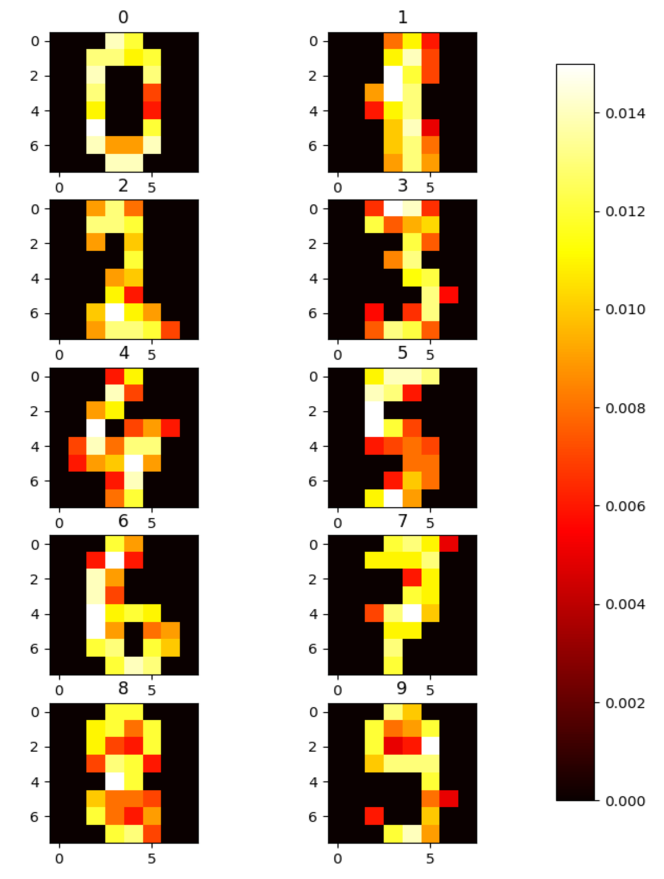### III-B DIGITS Dataset To verify the functional correctness of internal neuron and synapse computations on the FPGA, we performed inference on the DIGITS dataset [2] using a model trained in the SuperNeuroMAT simulator [8]. The dataset contains a total of 1,797 samples of handwritten digits, each represented as an $8\times 8$ grayscale image with pixel values in the range $[0,15]$ . The dataset was split into 70% training samples and 30% test samples. A simple two-layer feedforward spiking neural network was trained using integrate-and-fire neurons and weighted synapses in the SuperNeuroMAT simulator. The input images were normalized to the range $[0,1]$ and converted into input spike trains using rate encoding. Each pixel intensity was encoded as twice the number of spikes and distributed uniformly over 32 time steps. During training, target labels were encoded by delivering a spike to the corresponding output neuron at timestep $t+1$ , one timestep after the input presentation at $t$ . The learning was carried out using one-shot STDP-based training. It is important to note that the training was not aimed at maximizing classification accuracy; rather, the goal was to validate the correctness of the internal neuron and synapse dynamics on the FPGA platform. Figure 4 shows the final weights of the output neurons after training, which clearly reflect the digit-specific patterns learned by the network. For deployment on NeuroCoreX, the trained weights and network parameters were transferred and initialized on the FPGA. The STDP learning rule was disabled during this phase to maintain fixed weights. The identical spike sequences for the test set were streamed to the FPGA through the UART interface. We achieved a test accuracy of 68% on the SuperNeuroMAT simulator, and the same accuracy was observed on the NeuroCoreX hardware. This result confirms that the FPGA implementation faithfully reproduces the dynamics of the simulated SNN and validates the correctness of internal spike integration, thresholding, and synaptic current accumulation in hardware. <details> <summary>x1.png Details</summary>  ### Visual Description ## Heatmap Grid: Digit Activation Patterns ### Overview The image displays a 5x2 grid of heatmaps, each representing a 7x6 pixel grid (y-axis: 0-6, x-axis: 0-5). The heatmaps are organized into two columns labeled "0" and "1" at the top. A vertical color bar legend on the right indicates the value scale. The visual patterns within each heatmap strongly resemble handwritten digits from 0 to 9, suggesting these are activation or saliency maps for digit recognition. ### Components/Axes * **Column Headers:** The top of the image has two labels: "0" (left column) and "1" (right column). * **Heatmap Grid:** Ten individual heatmaps are arranged in 5 rows and 2 columns. * **Axes:** Each heatmap has a y-axis labeled from 0 to 6 (top to bottom) and an x-axis labeled from 0 to 5 (left to right). * **Legend (Color Bar):** A vertical bar on the far right of the image. It maps color to numerical values. * **Position:** Right side, spanning the full height of the heatmap grid. * **Scale:** Linear, from 0.000 (black) to approximately 0.014 (white). * **Tick Marks & Values:** 0.000, 0.002, 0.004, 0.006, 0.008, 0.010, 0.012, 0.014. * **Color Gradient:** Black (0.000) -> Dark Red -> Red -> Orange -> Yellow -> White (~0.014). ### Detailed Analysis The heatmaps are processed by row, from top to bottom, with Column 0 on the left and Column 1 on the right. **Row 1:** * **Column 0, Heatmap 1 (Top-Left):** Pattern resembles the digit **"0"**. High-value pixels (yellow/white, ~0.012-0.014) form a closed loop. The highest values are concentrated on the left and right vertical strokes and the bottom curve. The center is black (0.000). * **Column 1, Heatmap 1 (Top-Right):** Pattern resembles the digit **"1"**. A vertical line of high-value pixels (yellow/white) runs down the center (x=3), with some lower-value (orange) pixels at the top and bottom. **Row 2:** * **Column 0, Heatmap 2:** Pattern resembles the digit **"2"**. High-value pixels form the characteristic curve at the top, diagonal stroke, and horizontal base. The top curve and base show the highest values. * **Column 1, Heatmap 2:** Pattern resembles the digit **"3"**. High-value pixels form two connected curves on the right side. The middle junction and the ends of the curves show peak values. **Row 3:** * **Column 0, Heatmap 3:** Pattern resembles the digit **"4"**. High-value pixels form the vertical line, the diagonal, and the horizontal crossbar. The intersection of the lines shows very high values. * **Column 1, Heatmap 3:** Pattern resembles the digit **"5"**. High-value pixels form the top horizontal bar, the vertical line, and the bottom curve. The top bar and the curve's apex are brightest. **Row 4:** * **Column 0, Heatmap 4:** Pattern resembles the digit **"6"**. High-value pixels form the top curve and the closed loop at the bottom. The bottom loop is particularly bright. * **Column 1, Heatmap 4:** Pattern resembles the digit **"7"**. High-value pixels form the top horizontal bar and the diagonal stroke descending to the left. The top bar is the brightest region. **Row 5:** * **Column 0, Heatmap 5 (Bottom-Left):** Pattern resembles the digit **"8"**. High-value pixels form two connected loops. The central junction and the outer edges of both loops show high values. * **Column 1, Heatmap 5 (Bottom-Right):** Pattern resembles the digit **"9"**. High-value pixels form the top loop and the descending tail. The top loop is the brightest area. ### Key Observations 1. **Digit Correspondence:** The heatmaps are clearly ordered to represent digits 0-9, reading left-to-right, top-to-bottom (0,1 in row 1; 2,3 in row 2; etc.). 2. **Value Distribution:** The highest values (white, ~0.014) are not uniformly distributed. They are concentrated on the primary strokes and junctions that define each digit's shape. 3. **Background:** The background of each heatmap is uniformly black (0.000), indicating no activation or importance in non-digit areas. 4. **Color Consistency:** The color-to-value mapping is consistent across all heatmaps, as defined by the single legend. For example, the bright yellow seen in the "0" and the "8" corresponds to the same value range (~0.012). ### Interpretation This image is a technical visualization, likely from a machine learning or computer vision context. It demonstrates the **spatial activation patterns** of a model (e.g., a Convolutional Neural Network) when processing images of handwritten digits. * **What it shows:** The heatmaps reveal which pixels in a 7x6 input grid are most "important" or "active" for the model's recognition of each specific digit. The bright areas (high values) correspond to the model's focus—the essential features it uses to distinguish a "0" from a "6", or a "7" from a "1". * **Relationship between elements:** The column headers ("0", "1") are likely arbitrary groupings for display. The core relationship is between the **digit identity** (inferred from the pattern) and its corresponding **activation map**. The color bar provides the quantitative scale for interpreting the "importance" of each pixel. * **Notable Patterns/Anomalies:** * The patterns are clean and well-defined, suggesting a well-trained model or synthetic data. * Some digits with similar shapes (e.g., "1" and "7") have distinct activation patterns: the "1" is a central vertical line, while the "7" has a prominent top horizontal bar. * The values are all relatively low (max ~0.014), which may indicate the data is normalized (e.g., probabilities summing to 1 across the grid, or scaled attention weights). **In summary, this is a diagnostic or explanatory figure showing how a digit recognition model "sees" the essential structure of each numeral from 0 to 9 within a low-resolution pixel grid.** </details> Figure 4: Heat-map of the trained weights from all the $10$ output neurons. ### III-C MicroSeer Dataset To evaluate the applicability of NeuroCoreX for graph-based learning tasks, we tested its performance using the MicroSeer dataset. MicroSeer is a reduced version of the Citeseer citation graph [4], containing 84 papers labeled with six topic categories. It was constructed by iteratively removing nodes from the largest connected component of Citeseer while ensuring that the resulting graph remained a single connected component. This connectivity was prioritized because it is assumed that learning from a very small, fragmented dataset would be ineffective. This reduction process yielded a total of 90 neurons, making the dataset well suited for deployment on NeuroCoreX, which supports up to 100 neurons and 10,000 bidirectional synapses. As compared to standard supervised learning that uses iterative error correction for weight updates, our training method leverages the graph’s structure directly to build the network. When testing a paper in the test data set, spiking the neuron associated with the test paper triggers a chain reaction of spikes. As these spikes travel between paper and topic neurons, STDP dynamically modifies the weights of the synapses connecting the test paper neuron to the topic neurons and vice versa. Subsequently, classification is achieved by finding the topic neuron with the highest final synaptic strength from the test paper neuron under consideration. The topic corresponding to this topic neuron is the one predicted by the SNN for the given test paper. The trained SNN model was first developed in the SuperNeuroMAT simulator and then ported to NeuroCoreX for hardware execution. When STDP was disabled, the network outputs from NeuroCoreX closely matched those produced by the simulator, demonstrating functional equivalence in inference. However, when STDP was enabled, a divergence in weight evolution and learning behavior was observed. This discrepancy stems from two primary sources: (1) SuperNeuro uses an exponential STDP learning rule with 64-bit floating-point precision, while NeuroCoreX implements a simplified rectangular learning window with signed 8-bit fixed-point weight representation; and (2) differences in numerical resolution and synaptic update timing result in non-identical learning trajectories. To achieve comparable accuracy metrics across simulation and hardware, tuning of learning parameters—such as learning rate, window size, and initial weight distributions—is required in both environments. These results underscore the importance of algorithm–hardware co-design in bridging the gap between simulation and deployment for neuromorphic graph learning. NeuroCoreX enables iterative testing and refinement of learning dynamics under realistic hardware constraints, facilitating the transition from simulated models to deployable systems. Future work will focus on tuning the system for MicroSeer and scaling to larger datasets on more advanced neuromorphic platforms. The total on-chip power consumption of the NeuroCoreX design was estimated at 305 mW, with 75% attributed to dynamic power. The Mixed-Mode Clock Manager (MMCM) accounted for the largest portion of dynamic power, followed by BRAMs, reflecting the memory-intensive nature of synaptic storage and buffering. ## IV Discussion and Conclusion NeuroCoreX enables real-time SNN emulation with STDP learning on low-cost FPGAs through a compact, open-source VHDL design. It bridges the gap between simulation and hardware by supporting seamless transfer of network models from SuperNeuroMAT, facilitating early-stage algorithm–hardware co-design under practical constraints like fixed-point precision and limited memory. Several key design choices in NeuroCoreX reflect critical trade-offs between biological realism, hardware efficiency, and scalability. ### IV-A Scalability One such decision is the use of an all-to-all connected network, which introduces significant memory overhead for weight storage—particularly as the network size increases. While this raises questions about scalability, the choice was made to provide maximum flexibility for users to implement arbitrary network architectures, and it is essential for supporting densely connected networks. An alternative approach would be to store a list of addresses corresponding to either all outgoing or incoming neurons for each neuron. This is more efficient for sparsely connected networks, as it avoids storing unnecessary weights. However, it becomes highly inefficient for densely connected networks, as it requires additional BRAM to store connection addresses alongside the weights. Since real-world networks often include a mix of dense and sparse connectivity, a scalable solution should combine both approaches. In such a hybrid model, densely connected sub-networks can be mapped directly onto NeuroCoreX’s all-to-all weight matrix, while sparse connections between these sub-networks can be implemented across multiple physical instances of NeuroCoreX. Each instance would represent a densely connected region of the larger network. With this strategy, the NeuroCoreX platform can be scaled effectively to support larger, more biologically realistic networks. We plan to implement this hybrid approach in future iterations of NeuroCoreX. ### IV-B Scalability and Network Acceleration Trade-offs NeuroCoreX employs time-multiplexing to emulate 100 virtual neurons using a single physical processing unit, significantly reducing hardware resource usage. However, this approach introduces a fundamental trade-off between the number of neurons that can be emulated, the achievable acceleration timescale, and the clock frequency used. Increasing the number of virtual neurons directly increases the time required to complete a single simulation step unless the update clock is proportionally scaled. In the Artix-7 FPGA used for this work, the 100-neuron configuration utilizes nearly the full BRAM capacity due to storage requirements for a) the FIFO buffer that stores and transmits input spike trains to the network in real time, b) FIFO to store membrane potential, and synaptic current for the time multiplexed implementation, c) FIFO to transmit spike trains of all neurons back to PC, d) synaptic weight matrices $W_{AA}$ and $W_{in}$ , e) the update and enable-STDP masks, and f) the pre- and post-synaptic trace registers required for learning. Even with more memory on higher-end FPGAs, scalability is constrained by the interaction between memory bandwidth and update clock frequency. BRAM access is sequential, with only one read or write per port per cycle, creating a bottleneck during real-time weight updates. For biologically realistic timing, the memory clock must run significantly faster than the neuron update clock. In our system, BRAM is accessed at 100 MHz while neuron updates proceed at 100 kHz, enabling a 1000 $\times$ speedup. Assuming BRAM size is not a limiting factor, the theoretical upper bound for network size under this configuration is approximately 500 neurons. This limit arises from the need for up to 500 cycles each for STDP potentiation and depression, which cannot occur concurrently on the same matrix. Beyond this, the system cannot complete all required memory operations within a single time step unless either the clock domains are further decoupled or memory bandwidth is increased. These constraints underscore a core design trade-off between network size, update speed, and biological fidelity. Depending on the target application, designers must balance these factors—favoring high-throughput inference, real-time learning, or alignment with biologically realistic timescales. ### IV-C Applications The flexibility, low cost, and on-chip learning capabilities of NeuroCoreX make it well suited for edge AI applications such as robotics, neuromorphic sensing, and adaptive control. Its energy-efficient architecture supports real-time inference and learning without reliance on offline processing. In educational settings, NeuroCoreX offers a unique platform for students to bridge the gap between software simulation and digital hardware design. By working directly with spiking neuron models and real-time hardware behavior, students gain hands-on experience with both computational neuroscience concepts and hardware engineering practices. As an open-source framework, NeuroCoreX also encourages community-driven extensions, reproducibility of results, and transparent benchmarking of neuromorphic algorithms under realistic hardware constraints. Several FPGA-based neuromorphic hardware platforms have been reported in the literature [33], each targeting different performance and application trade-offs. Caspian [29], for instance, has been widely used in edge applications involving control and classification tasks [30]. It supports configurable, though limited, connectivity and can be deployed on low-cost FPGAs. Liu et al. [22] proposed NHAP, a platform optimized for high-speed and low-power execution of SNNs, supporting multiple neuron models on mid- to high-end FPGAs. Matinizadeh et al. [25] introduced SONIC, an end-to-end framework for neuromorphic computing on FPGAs, which includes a core SNN engine called QUANTISENC, written in VHDL. This framework demonstrates several classification and control applications using fixed-topology layered networks. None of the existing FPGA-based neuromorphic platforms offer the full set of features provided by NeuroCoreX—most notably, on-chip learning via STDP. While some focus on high-speed inference or limited configurability, they typically lack embedded learning and depend on offline training. Most also lack a fully open-source toolchain, limiting their adoption in research and education. In contrast, NeuroCoreX combines real-time operation, on-chip STDP, flexible connectivity, and open-source support, making it a unique platform for deployment and algorithm–hardware co-design. ### IV-D Future Work Future enhancements to NeuroCoreX will focus on improving scalability and runtime efficiency. To support faster synaptic updates during STDP, we plan to explore multi-port BRAM architectures [21], which can alleviate memory bandwidth limitations by allowing concurrent read and write access to synaptic data. The modular design of NeuroCoreX also allows for replacing the current LIF neuron model with more biologically plausible alternatives [16, 19], enabling broader exploration of neural dynamics in hardware. Higher-order STDP rules, such as triplet-based [18] and neuromodulated STDP [14], have shown comparable learning performance to conventional STDP while requiring as little as 3-bit fixed-point resolution per synapse. Integrating these models may slightly increase logic complexity but could significantly reduce BRAM usage, enabling simulation of larger networks. Additionally, exposing pipeline depth and clock parameters as configurable settings would allow fine-tuning for task-specific trade-offs between performance and biological fidelity. NeuroCoreX provides an efficient, accessible, and extensible platform for implementing biologically inspired, energy-efficient SNNs on FPGA hardware. With its modular VHDL design, real-time STDP learning, and flexible connectivity, it enables researchers and educators to explore neuromorphic principles under realistic hardware constraints. Our results show that SNN execution on NeuroCoreX aligns closely with software simulations in SuperNeuroMAT, enabling seamless mapping from software to hardware. By supporting this direct transition, NeuroCoreX facilitates algorithm–hardware co-design and paves the way for scalable, low-power, and adaptive AI systems. As an open-source tool, it establishes a foundation for community-driven advances at the intersection of neuroscience, engineering, and embedded intelligence. ## References - [1] James B Aimone, Prasanna Date, Gabriel A Fonseca-Guerra, Kathleen E Hamilton, Kyle Henke, Bill Kay, Garrett T Kenyon, Shruti R Kulkarni, Susan M Mniszewski, Maryam Parsa, et al. A review of non-cognitive applications for neuromorphic computing. Neuromorphic Computing and Engineering, 2(3):032003, 2022. - [2] E. Alpaydin and C. Kaynak. Optical Recognition of Handwritten Digits. UCI Machine Learning Repository, 1998. DOI: https://doi.org/10.24432/C50P49. - [3] Ben Varkey Benjamin, Nicholas A Steinmetz, Nick N Oza, Jose J Aguayo, and Kwabena Boahen. Neurogrid simulates cortical cell-types, active dendrites, and top-down attention. Neuromorphic Computing and Engineering, 1(1):013001, 2021. - [4] Cornelia Caragea, Jian Wu, Alina Ciobanu, Kyle Williams, Juan Fernández-Ramírez, Hung-Hsuan Chen, Zhaohui Wu, and Lee Giles. Citeseer x: A scholarly big dataset. In Advances in Information Retrieval: 36th European Conference on IR Research, ECIR 2014, Amsterdam, The Netherlands, April 13-16, 2014. Proceedings 36, pages 311–322. Springer, 2014. - [5] Andrew Cassidy, Andreas G Andreou, and Julius Georgiou. A combinational digital logic approach to stdp. In 2011 IEEE international Symposium of Circuits and Systems (ISCAS), pages 673–676. IEEE, 2011. - [6] Guojing Cong, Shruti Kulkarni, Seung-Hwan Lim, Prasanna Date, Shay Snyder, Maryam Parsa, Dominic Kennedy, and Catherine Schuman. Hyperparameter optimization and feature inclusion in graph neural networks for spiking implementation. In 2023 International Conference on Machine Learning and Applications (ICMLA), pages 1541–1546. IEEE, 2023. - [7] Guojing Cong, Seung-Hwan Lim, Shruti Kulkarni, Prasanna Date, Thomas Potok, Shay Snyder, Maryam Parsa, and Catherine Schuman. Semi-supervised graph structure learning on neuromorphic computers. In Proceedings of the International Conference on Neuromorphic Systems 2022, pages 1–4, 2022. - [8] Prasanna Date, Chathika Gunaratne, Shruti R. Kulkarni, Robert Patton, Mark Coletti, and Thomas Potok. Superneuro: A fast and scalable simulator for neuromorphic computing. In Proceedings of the 2023 International Conference on Neuromorphic Systems, pages 1–4, 2023. - [9] Prasanna Date, Bill Kay, Catherine Schuman, Robert Patton, and Thomas Potok. Computational complexity of neuromorphic algorithms. In International Conference on Neuromorphic Systems 2021, pages 1–7, 2021. - [10] Prasanna Date, Shruti Kulkarni, Aaron Young, Catherine Schuman, Thomas Potok, and Jeffrey Vetter. Encoding integers and rationals on neuromorphic computers using virtual neuron. Scientific Reports, 13(1):10975, 2023. - [11] Prasanna Date, Shruti Kulkarni, Aaron Young, Catherine Schuman, Thomas Potok, and Jeffrey S Vetter. Virtual neuron: A neuromorphic approach for encoding numbers. In 2022 IEEE International Conference on Rebooting Computing (ICRC), pages 100–105. IEEE, 2022. - [12] Prasanna Date, Thomas Potok, Catherine Schuman, and Bill Kay. Neuromorphic computing is turing-complete. In Proceedings of the International Conference on Neuromorphic Systems 2022, pages 1–10, 2022. - [13] Mike Davies, Narayan Srinivasa, Tsung-Han Lin, Gautham Chinya, Yongqiang Cao, Sri Harsha Choday, Georgios Dimou, Prasad Joshi, Nabil Imam, Shweta Jain, et al. Loihi: A neuromorphic manycore processor with on-chip learning. Ieee Micro, 38(1):82–99, 2018. - [14] Nicolas Frémaux and Wulfram Gerstner. Neuromodulated spike-timing-dependent plasticity, and theory of three-factor learning rules. Frontiers in neural circuits, 9:85, 2016. - [15] Ashish Gautam and Takashi Kohno. An adaptive stdp learning rule for neuromorphic systems. Frontiers in Neuroscience, 15:741116, 2021. - [16] Ashish Gautam and Takashi Kohno. A conductance-based silicon synapse circuit. Biomimetics, 7(4):246, 2022. - [17] Ashish Gautam and Takashi Kohno. Adaptive stdp-based on-chip spike pattern detection. Frontiers in Neuroscience, 17, 2023. - [18] Ashish Gautam, Takashi Kohno, Prasanna Date, Robert Patton, and Thomas Potok. A suppression-based stdp rule resilient to jitter noise in spike patterns for neuromorphic computing. In 2024 International Conference on Neuromorphic Systems (ICONS), pages 209–216. IEEE, 2024. - [19] Wulfram Gerstner. Time structure of the activity in neural network models. Physical review E, 51(1):738, 1995. - [20] Shruti R. Kulkarni, Aaron Young, Prasanna Date, Narasinga Rao Miniskar, Jeffrey Vetter, Farah Fahim, Benjamin Parpillon, Jennet Dickinson, Nhan Tran, Jieun Yoo, et al. On-sensor data filtering using neuromorphic computing for high energy physics experiments. In Proceedings of the 2023 International Conference on Neuromorphic Systems, pages 1–8, 2023. - [21] Jiun-Liang Lin and Bo-Cheng Charles Lai. Bram efficient multi-ported memory on fpga. In VLSI Design, Automation and Test (VLSI-DAT), pages 1–4. IEEE, 2015. - [22] Yijun Liu, Yuehai Chen, Wujian Ye, and Yu Gui. Fpga-nhap: A general fpga-based neuromorphic hardware acceleration platform with high speed and low power. IEEE Transactions on Circuits and Systems I: Regular Papers, 69(6):2553–2566, 2022. - [23] Disha Maheshwari, Aaron Young, Prasanna Date, Shruti Kulkarni, Brett Witherspoon, and Narsinga Rao Miniskar. An fpga-based neuromorphic processor with all-to-all connectivity. In 2023 IEEE International Conference on Rebooting Computing (ICRC), pages 1–5. IEEE, 2023. - [24] Henry Markram, Joachim Lübke, Michael Frotscher, and Bert Sakmann. Regulation of synaptic efficacy by coincidence of postsynaptic aps and epsps. Science, 275(5297):213–215, 1997. - [25] Shadi Matinizadeh, Arghavan Mohammadhassani, Noah Pacik-Nelson, Ioannis Polykretis, Krupa Tishbi, Suman Kumar, ML Varshika, Abhishek Kumar Mishra, Nagarajan Kandasamy, James Shackleford, et al. Neuromorphic computing for the masses. In 2024 International Conference on Neuromorphic Systems (ICONS), pages 39–46. IEEE, 2024. - [26] Christian Mayr, Sebastian Hoeppner, and Steve Furber. Spinnaker 2: A 10 million core processor system for brain simulation and machine learning. arXiv preprint arXiv:1911.02385, 2019. - [27] Paul A Merolla, John V Arthur, Rodrigo Alvarez-Icaza, Andrew S Cassidy, Jun Sawada, Filipp Akopyan, Bryan L Jackson, Nabil Imam, Chen Guo, Yutaka Nakamura, et al. A million spiking-neuron integrated circuit with a scalable communication network and interface. Science, 345(6197):668–673, 2014. - [28] Narsinga Rao Miniskar, Aaron R Young, Kazi Asifuzzaman, Shruti Kulkarni, Prasanna Date, Alice Bean, and Jeffrey S Vetter. Neuro-spark: A submicrosecond spiking neural networks architecture for in-sensor filtering. In 2024 International Conference on Neuromorphic Systems (ICONS), pages 63–70. IEEE, 2024. - [29] J Parker Mitchell, Catherine D Schuman, Robert M Patton, and Thomas E Potok. Caspian: A neuromorphic development platform. In Proceedings of the 2020 Annual Neuro-Inspired Computational Elements Workshop, pages 1–6, 2020. - [30] Robert Patton, Prasanna Date, Shruti Kulkarni, Chathika Gunaratne, Seung-Hwan Lim, Guojing Cong, Steven R Young, Mark Coletti, Thomas E Potok, and Catherine D Schuman. Neuromorphic computing for scientific applications. In 2022 IEEE/ACM Redefining Scalability for Diversely Heterogeneous Architectures Workshop (RSDHA), pages 22–28. IEEE, 2022. - [31] Catherine D Schuman, Bill Kay, Prasanna Date, Ramakrishnan Kannan, Piyush Sao, and Thomas E Potok. Sparse binary matrix-vector multiplication on neuromorphic computers. In 2021 IEEE International Parallel and Distributed Processing Symposium Workshops (IPDPSW), pages 308–311. IEEE, 2021. - [32] Marcel Stimberg, Romain Brette, and Dan FM Goodman. Brian 2, an intuitive and efficient neural simulator. elife, 8:e47314, 2019. - [33] Wiktor J Szczerek and Artur Podobas. A quarter of a century of neuromorphic architectures on fpgas–an overview. arXiv preprint arXiv:2502.20415, 2025. - [34] Ahna Wurm, Rebecca Seay, Prasanna Date, Shruti Kulkarni, Aaron Young, and Jeffrey Vetter. Arithmetic primitives for efficient neuromorphic computing. In 2023 IEEE International Conference on Rebooting Computing (ICRC), pages 1–5. IEEE, 2023.