2506.18902

# jina-embeddings-v4: Universal Embeddings for Multimodal Multilingual Retrieval **Authors**: - xxx, xxx (Jina AI GmbH, Prinzessinnenstraße 19–20, 10969 Berlin, Germany) (2024/02/26) ## Abstract We introduce jina-embeddings-v4, a 3.8 billion parameter multimodal embedding model that unifies text and image representations through a novel architecture supporting both single-vector and multi-vector embeddings in the late interaction style. The model incorporates task-specific Low-Rank Adaptation (LoRA) adapters to optimize performance across diverse retrieval scenarios, including query-document retrieval, semantic text similarity, and code search. Comprehensive evaluations demonstrate that jina-embeddings-v4 achieves state-of-the-art performance on both single-modal and cross-modal retrieval tasks, with particular strength in processing visually rich content such as tables, charts, diagrams, and mixed-media formats. To facilitate evaluation of this capability, we also introduce Jina-VDR, a novel benchmark specifically designed for visually rich image retrieval. footnotetext: Equal contribution. ## 1 Introduction We present jina-embeddings-v4, a multimodal embedding model capable of processing text and image data to produce semantic embedding vectors of varying lengths, optimized for a broad array of applications. It incorporates optimized LoRA adapters Hu et al. (2022) for information retrieval and semantic text similarity. An adapter is also provided for programming language embeddings, technical question-answering, and natural language code retrieval. It also brings new functionality to processing visually rich images (also called visual documents), i.e., materials mixing texts and images, containing tables, charts, diagrams, and other kinds of common mixed media Ding et al. (2024). We have also developed Jina-VDR, a new multilingual, multi-domain benchmark suite for a broad range of visual retrieval tasks, to evaluate the capabilities of jina-embeddings-v4. We discuss the challenges of developing a multimodal, multi-functional, state-of-the-art embedding model capable of handling texts in a variety of languages, including computer coding languages, images, and “visually rich” data. The resulting model, jina-embeddings-v4, projects inputs from all modalities into a unified semantic space, minimizing or eliminating the “modality gap” that has troubled similar projects Liang et al. (2022a). In addition, we introduce Jina-VDR, an advanced benchmark for images like screenshots and scans of visually complex documents. The major contributions of this work are as follows: - We introduce a unified multi-task learning paradigm that jointly optimizes embedding models to represent texts and images as single- and multi-vector embeddings. - Building on work done for jina-embeddings-v3, we train LoRA extensions to enhance support for specific domains and task types, achieving results comparable to specialized models. - We have made particularly strong progress in handling visually rich images, especially for tasks outside of the existing ViDoRe benchmark Faysse et al. (2025), which is limited to question-answering. jina-embeddings-v4 outperforms other multimodal models by a significant margin on this type of material and supports a much more diverse set of use scenarios. - We construct a multilingual, multi-domain benchmark for screenshot retrieval. In contrast to other retrieval benchmarks (i.e., Faysse et al. (2025); Xiao et al. (2025)) that focus on question answering and OCR-related tasks, we expand the scope of visual document benchmarking to multilingual retrieval, more query types, and a much more diverse array of materials, like maps, diagrams, advertisements, and other mixed media. ## 2 Background The underlying principles behind embedding models are indifferent to data modality. An embedding model transforms digitally encoded objects into vectors in a high-dimensional embedding space such that some of the semantic features of the objects, depending on the model’s training regimen, correspond to subspaces in that embedding space. Objects with more such features in common will have corresponding vectors that are closer to each other by some metric (typically cosine similarity) than objects with fewer common features. Individual models, however, only support the modalities for which they are designed and trained. Embedding models initially developed primarily to support natural language texts, like jina-embeddings-v3 Sturua et al. (2024), but there are many image embedding models, and more recently, audio and video models. The semantic embedding paradigm can also encompass models that support more than one modality, like bimodal image-text models, including OpenAI’s CLIP Radford et al. (2021) and subsequent developments including jina-clip Koukounas et al. (2024). The principal purpose of multimodal embedding models is to project objects from multiple modalities into the same semantic embedding space, so that, for example, a picture of a cat and a text discussing or describing a cat will correspond to relatively close embedding vectors. Embedding models can also specialize in specific types of input within a single modality. There are text embedding models designed for programming code Liu et al. (2024), legal texts Voyage AI (2024), and other special domains. There is also recent work in specialized image embedding models designed to support “visually rich” data, such as screenshots, charts, and printed pages that combine text and imagery and have internal visual structure Faysse et al. (2025); Ma et al. (2024). There are other dimensions of embedding model specialization as well. Models can be optimized for specific tasks, such as information retrieval, clustering, and classification Sturua et al. (2024). They can also vary based on the nature of the embeddings they produce. Most are single-/dense vector models, generating one embedding vector for whatever input they are given. There are also multi-vector/late interaction models, such as ColBERT Khattab and Zaharia (2020) and ColPali Faysse et al. (2025). Late interaction is generally a more precise measure of semantic similarity for retrieval, but has significantly greater storage and computing costs. Instead of specializing, jina-embeddings-v4 builds on a single base model to provide competitive performance as a text, image, and cross-modal embedding model with strong performance handling visually rich documents. It supports both single-vector and multi-vector and is optimized to provide embeddings of varying lengths. Furthermore, the model includes LoRA extensions that optimize it for specific application classes: information retrieval, multimodal semantic similarity, and computer code retrieval. This single-model approach entails significant savings in practical use cases when compared to deploying multiple AI models for different tasks and modalities. ## 3 Related Work Transformer-based neural network architectures that generate semantic embeddings are well-established Reimers and Gurevych (2019), and there is a sizable literature on training techniques for them. Multi-stage contrastive training Wang et al. (2022), and techniques for supporting longer texts Günther et al. (2023) are particularly relevant to this work. Compact embedding vectors bring valuable performance benefits to AI applications, and this motivates work in Matryoshka Representational Learning (MRL) Kusupati et al. (2022) as a way to train models for truncatable embedding vectors. Contrastive text-image training has led to ground-breaking results in zero-shot image classification and cross-modal retrieval in conjunction with dual encoder architectures like CLIP Radford et al. (2021). However, recent work shows better performance from vision-language models (VLMs) like Qwen2.5-VL-3B-Instruct Bai et al. (2025). Jiang et al. (2024) show that VLMs suffer less from a modality gap than dual encoder architectures. In contrast to Zhang et al. (2024), jina-embeddings-v4 is trained on multilingual data, supports single as well as multi-vector retrieval, and does not require task-specific instructions. Other VLM models are trained exclusively on data for text-to-image Faysse et al. (2025); Ma et al. (2024) or text-to-text retrieval Jiang et al. (2024). Similarity scoring in late interaction models does not use simple cosine similarity. Khattab and Zaharia (2020) Instead, similarity is calculated asymmetrically over two sequences of token embeddings — a query and a document — by summing up the maximum cosine similarity values of each query token embedding to any of the token embeddings from the document. Thus, for query embedding $q$ and document embedding $p$ , their late interaction similarity score $s_{\mathrm{late}}(q,p)$ is determined by: $$ \displaystyle s_{\mathrm{late}}(q,p)=\sum_{i=1}^{n}\max_{j\in\{1,\dots,m\}}\bm {q}_{i}\cdot\bm{p_{j}}^{T} \tag{1} $$ Faysse et al. (2025) train a late-interaction embedding model to search document screenshots using text queries, performing significantly better than traditional approaches involving OCR and CLIP-style models trained on image captions. To show this, they introduce the ViDoRe (Vision Document Retrieval) benchmark. However, this benchmark is limited to question-answering tasks in English and French involving only charts, tables, and pages from PDF documents. Xiao et al. (2025) extend this benchmark to create MIEB (Massive Image Embedding Benchmark) by adding semantic textual similarity (STS) tasks for visually rich documents like screenshots. ## 4 Model Architecture <details> <summary>x1.png Details</summary>  ### Visual Description \n ## Diagram: Multimodal Model Architecture ### Overview This diagram illustrates the architecture of a multimodal model, likely for retrieval or text-matching tasks. The model takes either an image or text as input, processes it through a vision encoder and a QWEN2.5 LM decoder, and outputs either a single-vector or a multi-vector representation. A LORA set is used to modify the base model. ### Components/Axes The diagram consists of several key components connected by arrows indicating data flow: * **INPUT:** Labeled with "task='retrieval'" and options for input type: "doc-image" or "text", and "vector_type='multi_vector'". * **LORA SET:** A teal and blue hexagonal shape with a dotted outline. * **BASE MODEL:** A purple hexagonal shape. * **VISION ENCODER:** A rectangular block. * **QWEN2.5 LM DECODER:** A larger rectangular block. * **TOKEN EMBEDDINGS:** A series of green circles. * **SINGLE-VECTOR:** A rectangular block labeled "128 to 2048-dim". * **MULTI-VECTOR:** A rectangular block labeled "N x 128-dim". * **MEAN POOLING:** A rectangular block. * **PROJECTOR:** A rectangular block. * **OUTPUT:** A rectangular block at the top. Arrows indicate the flow of data between these components. Dotted arrows represent modifications or adjustments. ### Detailed Analysis or Content Details The diagram shows the following data flow: 1. **Input:** The process begins with an input, which can be either a document image ("doc-image") or text. The task is specified as "retrieval", and the vector type is "multi_vector". 2. **Vision Encoder:** The input (image or text) is fed into a Vision Encoder. 3. **QWEN2.5 LM Decoder:** The output of the Vision Encoder is then passed to the QWEN2.5 LM Decoder. 4. **Token Embeddings:** The output of the QWEN2.5 LM Decoder is converted into Token Embeddings, represented as a sequence of green circles. 5. **Single-Vector/Multi-Vector:** The Token Embeddings are split into two paths: * One path leads directly to a "single-vector" output, with a dimensionality of 128 to 2048 dimensions. * The other path goes through "Mean Pooling" and then a "Projector" to produce a "multi-vector" output, with a dimensionality of N x 128 dimensions. 6. **LORA Set & Base Model:** The LORA set modifies the Base Model. The output of the Base Model is then fed into the Vision Encoder. ### Key Observations * The model supports both image and text inputs. * The model produces two types of vector representations: single-vector and multi-vector. * The LORA set is used to adapt the base model for the specific task. * The diagram highlights the key components and their interactions in a multimodal processing pipeline. ### Interpretation This diagram depicts a multimodal model designed for retrieval tasks. The use of a Vision Encoder suggests the model can process visual information, while the QWEN2.5 LM Decoder indicates the use of a large language model for understanding and generating text. The LORA set allows for efficient adaptation of a pre-trained base model to the specific retrieval task. The output of both single and multi-vectors suggests the model can be used for different downstream applications, potentially including semantic search and image-text matching. The "N x 128-dim" multi-vector output suggests the model can represent multiple aspects or features of the input data. The diagram emphasizes the integration of visual and textual information for improved retrieval performance. 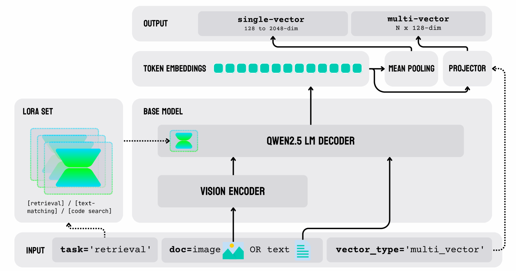</details> Figure 1: Architecture of jina-embeddings-v4. The model employs a unified LM built on the Qwen2.5-VL-3B-Instruct backbone (3.8B parameters). Text and image inputs are processed through a shared pathway: images are first converted to token sequences via a vision encoder, then both modalities are jointly processed by the language model decoder with contextual attention layers. Three task-specific LoRA adapters (60M parameters each) provide specialized optimization for retrieval, text-matching, and code search tasks without modifying the frozen backbone weights. The architecture supports dual output modes: (1) single-vector embeddings (2048 dimensions, truncatable to 128) generated via mean pooling for efficient similarity search, and (2) multi-vector embeddings (128 dimensions per token) via projection layers for the late interaction style retrieval. The architecture of jina-embeddings-v4, schematized in Figure 1, employs a unified multimodal language model built on the Qwen2.5-VL-3B-Instruct https://huggingface.co/Qwen/Qwen2.5-VL-3B-Instruct backbone Bai et al. (2025). Text and image inputs are processed through a shared pathway: Images are first converted to token sequences via a vision encoder, then both modalities are jointly processed by the language model decoder with contextual attention layers. This unified design eliminates the modality gap present in dual-encoder architectures while maintaining competitive performance across text, image, and cross-modal tasks. As shown in Figure 1, this architecture supports dual output modes, as outlined in Section 4.2. Furthermore, three task-specific LoRA adapters, each with 60M parameters, provide specialized task optimization without modifying the frozen backbone weights. These are described in Section 4.3. The core specifications of jina-embeddings-v4 are summarized in Table 1. | Model Parameters | 3.8 billion ( $3.8\times 10^{9}$ ) plus 60M per LoRA | | --- | --- | | Text Input Size | Up to 32,768 tokens | | Image Input | All images resized to 20 megapixels | | Single-vector Embedding Size | 2048 dimensions, truncatable down to 128 | | Multi-vector Embedding Size | 128 dimensions per token | Table 1: Basic specifications of jina-embeddings-v4 ### 4.1 True Multimodal Processing The Qwen2.5-VL-3B-Instruct paradigm differs from CLIP-style dual-encoder models in offering a single processing path that’s truly multimodal. For text input, jina-embeddings-v4 and Qwen2.5-VL-3B-Instruct initially behave like other transformer-based embedding models: The text is tokenized, each token is replaced with a vector representation from a lookup table, and then these vectors are stacked and presented to a large language model (LLM). In CLIP-style models, images are processed by a separate embedding model, typically a transformer-based model that divides them into patches and then processes them much like a text model. The text model and image model are aligned during training to produce similar embeddings for similar semantic content in the different media. The Qwen2.5-VL-3B-Instruct paradigm used in jina-embeddings-v4 also includes a discrete image model but uses it in a different way. It produces a multi-vector result, comparable to late interaction models, and then passes this output to the LLM, as if it were a sequence of vectorized text tokens. The image embedding model acts as a preprocessor for the LLM, converting the image into what amounts to a sequence of vectorized “image tokens.” This approach, which is the core of jina-embeddings-v4, beyond having performance advantages, makes it possible to pass a text prompt into the LLM along with an image. The VLM is truly multimodal, since it is one model supporting multiple data types in a single input field. ### 4.2 Dual Mode Output In contrast to Qwen2.5-VL-3B-Instruct and other embedding models in general, users can choose between two output options: Traditional single (dense) vector embeddings and ColBERT-style multi-vector embeddings for late interaction strategies. Single-vector embeddings are 2048 dimensions, but can be truncated to as little as 128 with minimal loss of precision. jina-embeddings-v4 has been trained with Matryoshka Representation Learning Kusupati et al. (2022), so that the scalar values of single-vector embeddings are roughly ordered by semantic significance. Eliminating the least significant dimensions reduces precision very little. Multi-vector embeddings are the unpooled result of processing tokens through a transformer model. They correspond to tokens as the model analyses them, given their context. The length of the output vector is proportionate to the number of input tokens (including “image tokens”), with each token corresponding to a 128-dimensional output vector. This output is directly comparable to the unpooled embeddings produced by ColBERT Khattab and Zaharia (2020) and ColPali Faysse et al. (2025) and is intended for use in late interaction comparison strategies. For single-vector embeddings, mean pooling is applied to the final layer of the base model to produce the output. The model incorporates an additional layer to project the output of the base model into multi-vector outputs. ### 4.3 Task Specialization with LoRA Following the methods used for jina-embeddings-v3 Sturua et al. (2024), we have implemented three task-specific LoRA adapters for different information retrieval use cases: - Asymmetric Query-Document Retrieval - Semantic Similarity and Symmetric Retrieval - Code (i.e., computer programming language) Retrieval Asymmetric retrieval means encoding queries and documents differently in order to improve retrieval for queries that are not structured like documents, i.e., short queries, questions, etc. This is in contrast to symmetric retrieval, which assumes a symmetry between query and document, and is used to find comparable content. Each LoRA adapter set has only 60M parameters, so maintaining all three adds less than 2% to the memory footprint of jina-embeddings-v4. Users can select among them at inference time, and all three support image and text encoding. See Section 7 for performance information about these adapters. ## 5 Training Method Before training, model weights are initialized to match Qwen/Qwen2.5-VL-3B-Instruct. The multi-vector projection layer and LoRA adapters are randomly initialized. The weights of the backbone model are not modified during the training process. The LoRA adapters modify the effect of the backbone model layers and the projection layer. Only the adapters are trained. Training proceeds in two phases: 1. A single LoRA adapter is trained using contrasting text pairs and text-image pairs. We use the contrastive InfoNCE (van den Oord et al., 2018) loss function to co-train for both single-vector and multi-vector similarity, as detailed in the section below. No task-specific training is performed at this stage. 1. The resulting LoRA adapter is duplicated to create the three task-specific adapters, which are then trained individually with task-specific text triplets and text-image triplets. In both phases of training, we apply Matryoshka loss Kusupati et al. (2022) to the base loss so that single-vector embeddings from jina-embeddings-v4 are truncatable. ### 5.1 Pair Training Initially, training is performed with a contrastive objective. Pairs of inputs are classed as related or unrelated, and the model learns to embed related items closely together and unrelated items further apart. In each training step, we sample two different batches of training data: - A batch $\mathcal{B}_{text}$ of text pairs. - A batch $\mathcal{B}_{multi}$ of multimodal pairs containing a text and a related image. We generate normalized single-vector and multi-vector embeddings for all texts and images in the selected pairs. We then construct a matrix of similarity values $\textbf{S}_{\mathrm{dense}}(\mathcal{B})$ by calculating the cosine similarity of all combinations of single-vector embeddings $\bm{q}_{i}$ and $\bm{p}_{j}$ in $\mathcal{B}$ . We construct an analogous matrix $\textbf{S}_{\mathrm{late}}$ for each $\mathcal{B}$ for the multi-vector embeddings using a slightly modified version of Equation (1) to calculate their similarity. Our choice of loss function requires a normalized score, so we divide the late interaction score by the number of tokens in the query: $$ s^{\prime}_{\mathrm{late}}(q_{i},p_{j})=\frac{s_{\mathrm{late}}(q_{i},p_{j})}{t} \tag{2} $$ where $t$ is the number of tokens in $q_{i}$ and $q_{i},p_{j}\in\mathcal{B}$ This modification is only for training. For retrieval applications, normalization is not necessary since the query is invariant. Then, we apply the contrastive InfoNCE loss function $\mathcal{L}_{\mathrm{NCE}}$ (van den Oord et al., 2018) on each of the four resulting matrices of similarity scores $s_{i,j}\in\textbf{S}$ $$ \mathrm{softmax}(\textbf{S},\tau,i,j):=\ln\frac{e^{s_{i,j}/\tau}}{\sum\limits_ {k=0}^{n}e^{s_{i,k}/\tau}} \tag{3} $$ $$ \mathcal{L}_{\mathrm{NCE}}(\textbf{S}(\mathcal{B}),\tau):=-\sum_{i,j=0}^{n} \mathrm{softmax}(\textbf{S}(\mathcal{B}),\tau,i,i) \tag{4} $$ where $\tau$ is the temperature parameter, $n$ is the batch size, which increases the weight of small differences in similarity scores in calculating the loss. Following Hinton et al. (2015), we compensate for differences in error distributions between the single-vector and multi-vector by adding the weighted Kullback–Leibler divergence ( $D_{KL}$ ) of the two sets of softmax-normalized similarity scores. This enables us to train for the single-vector and multi-vector outputs simultaneously, even though the multi-vector/late interaction scores have much less error. $$ \displaystyle\mathcal{L}_{D}(B,\tau) \displaystyle:=D_{\mathrm{KL}}(\textbf{S}^{\prime}_{\mathrm{dense}}(\mathcal{B })\,\|\,\textbf{S}^{\prime}_{\mathrm{late}}(\mathcal{B})) \displaystyle\textbf{S}^{\prime}_{i,j}=\mathrm{softmax}(\textbf{S},\tau,i,j) \tag{5} $$ The resulting joint loss function, which we use in training, is defined as: $$ \displaystyle\mathcal{L}_{\mathrm{joint}} \displaystyle(\mathcal{B}_{\mathrm{txt}},\mathcal{B}_{\mathrm{multi}},\tau):= \displaystyle w_{1}\mathcal{L}_{\mathrm{NCE}}(\textbf{S}_{\mathrm{dense}}( \mathcal{B}_{\mathrm{txt}}),\tau) \displaystyle+ \displaystyle w_{2}\mathcal{L}_{\mathrm{NCE}}(\textbf{S}_{\mathrm{late}}( \mathcal{B}_{\mathrm{txt}}),\tau)+w_{3}\mathcal{L}_{D}(\mathcal{B}_{\mathrm{ txt}}) \displaystyle+ \displaystyle w_{4}\mathcal{L}_{\mathrm{NCE}}(\textbf{S}_{\mathrm{dense}}( \mathcal{B}_{\mathrm{multi}}),\tau) \displaystyle+ \displaystyle w_{5}\mathcal{L}_{\mathrm{NCE}}(\textbf{S}_{\mathrm{late}}( \mathcal{B}_{\mathrm{multi}}),\tau)+w_{6}\mathcal{L}_{D}(\mathcal{B}_{\mathrm{ multi}}) \tag{6} $$ The weights $w_{1},\ldots,w_{6}$ and temperature $\tau$ are training hyperparameters. #### 5.1.1 Pair Training Data The training data consists of text-text and text-image pairs from more than 300 sources. Text-text pairs are selected and filtered as described in Sturua et al. (2024). Text-image pairs have been curated from a variety of sources following a more eclectic strategy than previous work on training text-image embedding models. In contrast to relying on image-caption pairs or pairs of queries and images derived from documents, we have also created images from other document types. Our training data includes website screenshots, rendered Markdown files, charts, tables, and other kinds of materials "found in the wild." The queries consist primarily of questions, keywords and key phrases, long descriptions, and statements of fact. ### 5.2 Task-Specific Training We instantiate three copies of the pair-trained LoRA adapter and give each specific training for its intended task. Training data and loss functions differ for the three tasks. | Task Name | Description | | --- | --- | | retrieval | Asymmetric embedding of queries and documents for retrieval | | text-matching | Semantic text similarity and symmetric retrieval | | code | Retrieving code snippets | Table 2: Supported tasks of jina-embeddings-v4, each corresponding to a LoRA adapter and trained independently #### 5.2.1 Asymmetric Retrieval Adapter Asymmetric retrieval assigns substantially and qualitatively different embeddings to documents and queries, even if they happen to have the very same text. Having distinct encoding mechanisms for the two often significantly benefits embeddings-based retrieval performance. Sturua et al. (2024) shows that this can be achieved either by training two separate adapters or by employing two distinct prefixes as proposed in Wang et al. (2022), so that embedding models can readily distinguish them when they generate embeddings. We have used the prefix method for jina-embeddings-v4. Previous work shows little benefit from combining both methods. Our training data contains hard negatives, i.e., triplets of a query, a document that matches the query, and a document that is closely semantically related but not a correct match Wang et al. (2022); Li et al. (2023); Günther et al. (2023). For every pair $(q_{i},p_{i})\in\mathcal{B}$ in a batch, $p_{i}$ is intended to be a good match for $q_{i}$ , and we presume that for all $(q_{j},p_{j})\in\mathcal{B}$ where $j\neq i$ , $p_{j}$ is a bad match for $q_{i}$ . We incorporate those additional negatives into the training process via an extended version of the $\mathcal{L}_{\mathrm{NCE}}$ loss described in Günther et al. (2023), denoted as $\mathcal{L}_{\mathrm{NCE+}}$ , in our joint loss function $\mathcal{L}_{\mathrm{joint}}$ : | | | $\displaystyle\mathcal{L}_{\mathrm{NCE+}}(\textbf{S}(\mathcal{B}),\tau):=$ | | | --- | --- | --- | --- | with $r=(q,p,n_{1},\ldots,n_{m})$ , where $(q,p)$ is a pair in batch $\mathcal{B}$ and $n_{1},\ldots,n_{m}$ and the other $p\in\mathcal{B}$ . Our dataset of text hard negatives is similar to the data used to train jina-embeddings-v3 Sturua et al. (2024). We rely on existing datasets to create multimodal hard negatives for training, including Wiki-SS Ma et al. (2024) and VDR multilingual https://huggingface.co/datasets/llamaindex/vdr-multilingual-train, but also mined hard negatives from curated multimodal datasets. #### 5.2.2 Text Matching Adapter Symmetric semantic similarity tasks require different training from asymmetric retrieval. We find that training data with ground truth similarity values works best for this kind of task. As discussed in Sturua et al. (2024), we use the CoSENT https://github.com/bojone/CoSENT loss function $\mathcal{L}_{\mathrm{co}}$ from Li and Li (2024): | | | $\displaystyle\mathcal{L}_{\mathrm{co}}(\textbf{S}(\mathcal{B}),\tau):=\ln\Big{ [}1+\sum\limits_{\begin{subarray}{c}(q_{1},p_{1}),\\ (q_{2},p_{2})\\ \in\textbf{S}(\mathcal{B})\end{subarray}}\frac{e^{s(q_{2},p_{2})}-e^{s(q_{1},p _{1})}}{\tau}\Big{]}$ | | | --- | --- | --- | --- | where $\zeta(q,p)$ is the ground truth semantic similarity of $q$ with $p$ , $\zeta(q_{1},p_{1})>\zeta(q_{2},p_{2})$ , and $\tau$ is the temperature parameter. The loss function operates on two pairs of text values, $(q_{1},p_{1})$ and $(q_{2},p_{2})$ , with known ground truth similarity. To train the model with this objective, we use data from semantic textual similarity (STS) training datasets such as STS12 Agirre et al. (2012) and SICK Marelli et al. (2014). The amount of data in this format is limited, so we enhance our ground truth training data with pairs that do not have known similarity scores. For these pairs, we proceed the same way as we did for pair training in Section 5.1 and use the standard InfoNCE loss from Equation (4). The joint loss function is calculated as in Equation (LABEL:eq:loss-multi-negatives) except the CoSENT loss is used where pairs with known ground truth values exist. #### 5.2.3 Code Adapter Code embeddings in jina-embeddings-v4 are designed for natural language-to-code retrieval, code-to-code similarity search, and technical question answering. Code is a very specialized kind of text and requires distinct data sources. Because code embeddings do not involve image processing, the vision portion of jina-embeddings-v4 is not affected by training the code retrieval LoRA adapter. The backbone LLM Qwen2.5-VL-3B-Instruct was pre-trained on data including the StackExchangeQA https://github.com/laituan245/StackExchangeQA and the CodeSearchNet Husain et al. (2020) datasets, giving it some capacity to support code embeddings before further adaptation. Our LoRA training used the same triplet-based method described in Section 5.2.1. Training triplets are derived from a variety of sources, including CodeSearchNet, CodeFeedback Zheng et al. (2024), APPS Hendrycks et al. (2021), and the CornStack dataset Suresh et al. (2025). We maintained a consistent training configuration by using the same input prefix tokens (e.g., query, passage) and temperature hyperparameter (set to $0.02$ ) during the triplet-based training. ## 6 Jina-VDR: Visually Rich Document Retrieval Benchmark To evaluate the performance of jina-embeddings-v4 across a broad range of visually rich document retrieval tasks, we have produced a new benchmark collection and released it to the public. Benchmark available at https://huggingface.co/collections/jinaai/jinavdr-visual-document-retrieval-684831c022c53b21c313b449. This new collection tests an embedding model’s ability to integrate textual and visual understanding of documents that consist of in the form of rendered images of visual elements like charts, tables, and running text. It extends the ViDoRe benchmark Faysse et al. (2025) by adding a diverse collection of datasets spanning a broad range of domains (e.g. legal texts, historic documents, marketing materials), covering a variety of material types (e.g. charts, tables, manuals, printed text, maps) and query types (e.g. questions, facts, descriptions), as well as multiple languages. The benchmark suite encompasses ViDoRe and adds 30 additional tests. These tests include re-purposed existing datasets, new manually-annotated datasets, and generated synthetic data For a comprehensive overview of the individual benchmarks, see Appendix A.1. ### 6.1 Re-purposed Datasets We have adapted a number of existing VQA and OCR datasets, modifying and restructuring them into appropriate query-document pairs. For example, for DonutVQA https://huggingface.co/datasets/warshakhan/donut_vqa_ISynHMP, TableVQA Tom Agonnoude (2024), MPMQA Zhang et al. (2023), CharXiv Wang et al. (2024), and PlotQA Methani et al. (2020), we used structured templates and generative language models to formulate text queries to match their contents. JDocQAJP https://huggingface.co/datasets/jlli/JDocQA-nonbinary and HungarianDocQA https://huggingface.co/datasets/jlli/HungarianDocQA-OCR already contain documents and queries in forms that require minimal processing to adapt as benchmarks. We also created datasets from available data that extend beyond conventional question formats. The OurWorldInData and WikimediaMaps datasets use encyclopedia article fragments and image descriptions as queries to match with charts and maps. The GitHubREADMERetrieval dataset contains rendered Markdown pages drawn from GitHub README files, paired with generated natural language descriptions in 17 languages. The WikimediaCommonsDocuments benchmark pairs multilingual document pages with paragraph-level references extracted from Wikipedia. ### 6.2 Manually Annotated Datasets We have curated a number of human-annotated resources to better reflect real-world use cases. These include academic slides from Stanford lectures Mitchener (2021), educational figures in the TQA dataset Kembhavi et al. (2017), and marketing and institutional documents such as the Jina AI 2024 Yearbook Jina AI (2024), Japanese Ramen Niigata-shi Kankō Kokusaikōryūbu Kankō Suishinka (2024), and the Shanghai Master Plan Shanghai Municipal People’s Government Urban Planning and Land Resource Administration Bureau (2018). Documents in these datasets were paired with carefully written human queries without template-based phrasing, capturing genuine information-seeking intent. Some of these datasets target specific languages and regions to provide broader coverage. We also incorporated pre-existing human-annotated datasets like ChartQA https://huggingface.co/datasets/HuggingFaceM4/ChartQA and its Arabic counterpart, ArabicChartQA Ghaboura et al. (2024), which focus on charts and infographics. ### 6.3 Synthetic Data Generation We have been attentive, in constructing Jina-VDR, to the lack of diversity that often plagues information retrieval benchmarks. We cannot commission human-annotated datasets for everything and have had recourse to generative AI to fill in the gaps. We obtained a number of datasets from primarily European sources containing scans of historical, legal, and journalistic documents in German, French, Spanish, Italian, and Dutch. We used Qwen2 to generate queries for these documents. We handled the HindiGovernmentVQA and RussianBeverages datasets in the same way, adding not only often underrepresented languages, but also public service documents and commercial catalogs to this benchmark set. TweetStockRetrieval https://www.kaggle.com/datasets/thedevastator/tweet-sentiment-s-impact-on-stock-returns is a collection of chart-based financial data, which we have paired with multilingual template-based generated queries. AirBnBRetrieval https://www.kaggle.com/datasets/dgomonov/new-york-city-airbnb-open-data is a collection of rendered tables that we have paired with queries in 10 languages generated from a template. In several cases, such as TableVQA Delestre (2024), we introduced bilingual examples (e.g., French/English) to better assess cross-lingual retrieval performance, with questions and answers synthesized using advanced multilingual LLMs such as Gemini 1.5 Pro and Claude 3.5 Sonnet. ### 6.4 Jina-VDR in a Nutshell Jina-VDR extends the ViDoRe benchmark with: - 30 new tasks, using both real-world and synthetic data - All datasets adapted for retrieval and designed to be compatible with ViDoRe - LLM-based filtering to ensure all queries are relevant and reflective of real-world querying - Non-question queries, such as GitHub descriptions matched to rendered markdown images, and map images from Wikimedia Commons with accompanying textual descriptions - Multilingual coverage, with some datasets spanning up to 20 languages ## 7 Evaluation We have evaluated jina-embeddings-v4 on a diverse set of benchmarks to reflect its multiple functions. Table 3 provides an overview of benchmark averages for jina-embeddings-v4 and other embedding models. Table 3: Average Retrieval Scores of Embedding Models on Various Benchmarks. | Model | J-VDR | ViDoRe | CLIPB | MMTEB | MTEB-en | COIR | LEMB | STS-m | STS-en | | --- | --- | --- | --- | --- | --- | --- | --- | --- | --- | | jina-embeddings-v4 (dense) | 73.98 | 84.11 | 84.11 | 66.49 | 55.97 | 71.59 | 67.11 | 72.70 | 85.89 | | jina-embeddings-v4 (late) | 80.55 | 90.17 | | | | | | | | | text-embedding-3-large | – | – | – | 59.27 | 57.98 | 62.36 | 52.42 | 70.17 | 81.44 | | bge-m3 | – | – | – | 55.36 | | | 58.73 | | | | multilingual-e5-large-instruct | – | – | – | 57.12 | 53.47 | | 41.76 | | | | jina-embeddings-v3 | 47.82 | 26.02 | – | 58.58 | 54.33 | 55.07 | 55.66 | 75.77 | 85.82 | | voyage-3 | – | – | – | 66.13 | 53.46 | 67.23 | 74.06 | 68.33 | 78.59 | | gemini-embedding-001 | – | – | – | 67.71 | 64.35 | 73.11 | | 78.35 | 85.29 | | jina-embedings-v2-code | – | – | – | | | 52.24 | | | | | voyage-code | – | – | – | | | 77.33 | | | | | nllb-clip-large-siglip | | | 83.19 | | | | | | | | jina-clip-v2 | 40.52 | 53.61 | 81.12 | | | | | | | | colpali-v1.2 (late) | 63.80 | 83.90 | | | | | | | | | dse-qwen2-2b-mrl-v1 (dense) | 67.25 | 85.80 | | | | | | | | | voyage-multimodal-v3 (dense) | | 84.24 | | | | | | | | Task Acronyms: J-VDR = Jina VDR, VidoRE = ViDoRe, CLIPB = CLIP Benchmark, MMTEB = MTEB(Multilingual, v2) Retrieval Tasks, MTEB-EN = MTEB(eng, v2) Retrieval Tasks, COIR = CoIR Code Retrieval, LEMB = LongEmbed, STS-m = MTEB(Multilingual, v2) Semantic Textual Similarity Tasks, STS-en = MTEB(eng, v2) Semantic Textual Similarity Tasks Average Calculation: For J-VDR and ViDoRE, we calculate the average for the multilingual tasks first and consider this as a single score before calculating the average across all tasks. Scores are nDCG@5 for J-VDR, ViDoRe, and CLIPB, and nDCG@10 for MMTEB, MTEB-en, COIR, and LEMB, and Spearman coefficient for STS-m and STS-en. Evaluation of Text Retrieval Models on J-VDR: For evaluating text retrieval models on J-VDR, we used EasyOCR (https://github.com/JaidedAI/EasyOCR) and the provided extracted texts from the original ViDoRe datasets. ### 7.1 Multilingual Text Retrieval MTEB and MMTEB Enevoldsen et al. (2025) are the most widely used text retrieval benchmarks. For most tasks, we have used the asymmetric retrieval adapter, but for some symmetric retrieval tasks like ArguAna https://huggingface.co/datasets/mteb/arguana, we have used the text matching adapter instead. For evaluation, we prepend the query with the prefix “Given a claim, find documents that refute the claim” to reflect the task’s focus on retrieving passages that contradict, rather than support, the input claim, similar to Wang et al. (2023). The results are tabulated in Appendix A.4. For the MTEB benchmarks, which are all in English, see Table A11, and for the multilingual MMTEB, see Table A12. The performance of this new model is generally better than our previous model jina-embeddings-v3 and broadly comparable with the state-of-the-art. We have also evaluated the performance of our model on retrieval tasks that involve long text documents using the LongEmbed benchmark Zhu et al. (2024). The results are tabulated in Table A13 of Appendix A.4. Long document performance for jina-embeddings-v4 significantly outpaces competing models except the voyage-3 series and improves dramatically on jina-embeddings-v3 ’s performance. ### 7.2 Textual Semantic Similarity We evaluated jina-embeddings-v4 with text-based semantic similarity (STS) benchmarks. The results for MTEB STS and MMTEB STS benchmarks are tabulated in Tables A14 and A15 of Appendix A.4 respectively. Our results are competitive with the state-of-the-art and are best-in-class for English similarity tasks. ### 7.3 Multimodal Retrieval To evaluate the model’s performance on typical text-to-image search tasks, we used the common English and non-English tasks of the CLIP Benchmark https://github.com/LAION-AI/CLIP_benchmark. The results are tabulated in Tables A8 to A10 of Appendix A.3. jina-embeddings-v4 has a higher average score than jina-clip-v2 and nllb-siglip-large, but the latter performs somewhat higher on the Crossmodal3600 benchmark Thapliyal et al. (2022) (see Table A10) because it includes content from low-resource languages not supported in jina-embeddings-v4 ’s Qwen2.5-VL-3B-Instruct backbone. We further tested jina-embeddings-v4 on the ViDoRe and Jina-VDR benchmarks, to evaluate its performance on visually rich documents. The results are compiled in Appendix A.2. ViDoRe scores are tabulated in Table A3. Table LABEL:tab:jinavdr_overview provides an overview of jina-embeddings-v4 compared to other models, with Tables LABEL:tab:wikicommons_results to LABEL:tab:airbnb_results providing details results for some individual Jina-VDR benchmarks. This suggests that other models are primarily trained to perform well on document retrieval tasks that are similar to the ViDoRe tasks but underperform on other tasks, e.g., that do not involve queries that resemble questions. jina-embeddings-v4 excels at this benchmark, providing the current state-of-the-art, in both single- and multi-vector mode. Multi-vector/late interaction matching is generally recognized as more precise than single-vector matching in other applications, and this remains true for Jina-VDR. ### 7.4 Code Retrieval To assess performance on code retrieval, we evaluate the model on the MTEB-CoIR benchmark Li et al. (2024), which consists of 10 tasks spanning text-to-code, code-to-text, code-to-code, and hybrid code retrieval types. The results are reported in Table A16 of Appendix A.4. jina-embeddings-v4 is competitive with the state-of-the-art in general-purpose embedding models, but the specialized voyage-code model has somewhat better benchmark performance. ## 8 Analysis of the Embedding Space The large difference in architecture between jina-embeddings-v4 and CLIP-style models like OpenAI CLIP Radford et al. (2021) and jina-clip-v2 implies a large difference in the structure of the embedding spaces those models generate. We look here at a few of these issues. 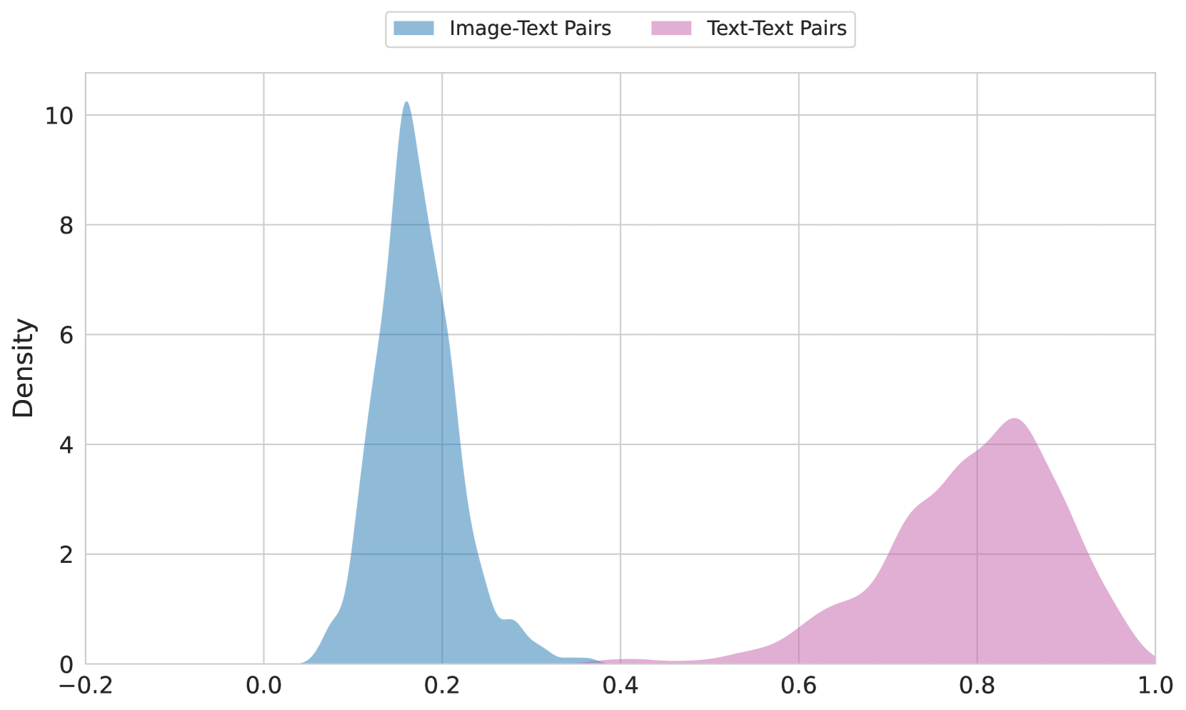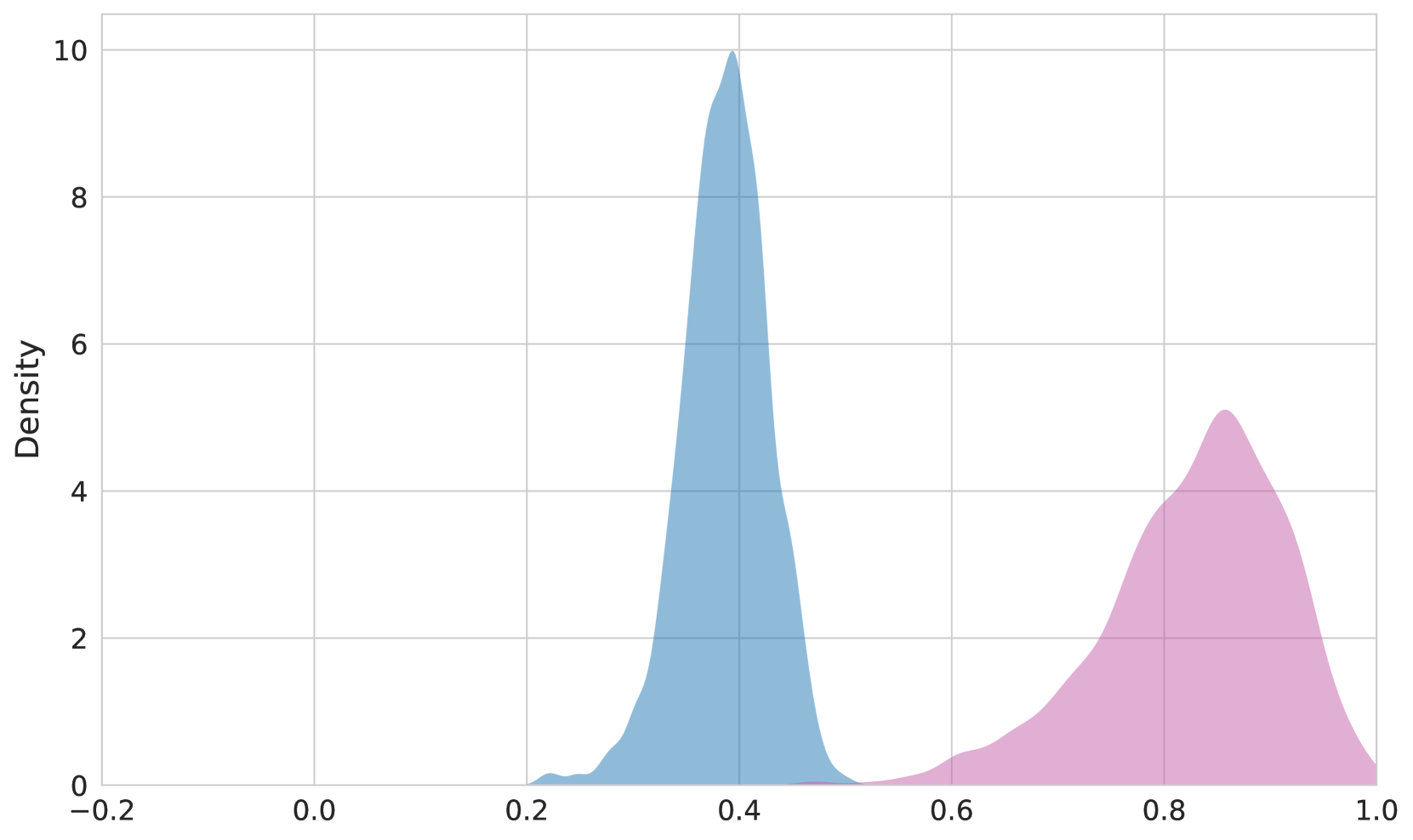### 8.1 Modality Gap Previous work has shed light on the so-called modality gap in multimodal models trained with contrastive learning Liang et al. (2022b); Schrodi et al. (2024); Eslami and de Melo (2025). Good semantic matches across modalities tend to lie considerably further apart in the embedding space than comparable or even worse matches of the same modality, i.e., texts in CLIP-style models are more similar to semantically unrelated texts than to semantically similar images. 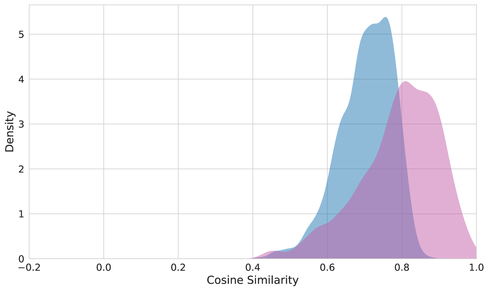We can see the modality gap directly by examining the distribution of pairwise cosine similarities of matching image-text pairs versus matching text-text pairs. In Figure 2, we see the distribution of similarity values for the two pair types in OpenAI CLIP, jina-clip-v2, and jina-embeddings-v4. The gap is dramatically reduced with jina-embeddings-v4 because of its cross-model encoder, illustrated in Figure 1. Eslami and de Melo (2025) has shown that sharing an encoder between modalities introduces an inductive bias towards using a shared region of the embedding space, while Liang et al. (2022b) shows the opposite is true for CLIP-style architectures with separate encoders. <details> <summary>x2.png Details</summary>  ### Visual Description \n ## Density Plot: Distribution Comparison ### Overview The image presents a density plot comparing the distributions of two datasets: "Image-Text Pairs" and "Text-Text Pairs". The plot visualizes the probability density of values ranging from approximately -0.2 to 1.0. ### Components/Axes * **X-axis:** Represents the range of values, labeled implicitly as a score or metric from -0.2 to 1.0. The axis is divided into increments of 0.2. * **Y-axis:** Represents the density, ranging from 0 to approximately 10. Labeled "Density". * **Legend:** Located at the top-center of the image. * "Image-Text Pairs" - Represented by a light blue fill. * "Text-Text Pairs" - Represented by a light purple/pink fill. * **Gridlines:** A light gray grid is present to aid in reading values. ### Detailed Analysis The plot shows two distinct distributions. **Image-Text Pairs (Light Blue):** The distribution is unimodal, peaking at approximately 0.18-0.20 with a density of around 10. The curve slopes downward on both sides of the peak. The density decreases to approximately 0.5 at x = 0.0 and x = 0.4. **Text-Text Pairs (Light Purple/Pink):** This distribution is also unimodal, but is shifted towards higher values. It peaks at approximately 0.82-0.84 with a density of around 4.5. The curve descends more gradually than the "Image-Text Pairs" distribution. The density is approximately 1.5 at x = 0.6 and x = 0.9. ### Key Observations * The "Image-Text Pairs" distribution is centered around lower values than the "Text-Text Pairs" distribution. * The "Image-Text Pairs" distribution has a higher peak density than the "Text-Text Pairs" distribution. * Both distributions appear to be bounded between -0.2 and 1.0. * There is a noticeable gap between the two distributions, with relatively low density in the range of 0.4 to 0.7. ### Interpretation The data suggests that the scores or metrics represented on the x-axis are generally lower for "Image-Text Pairs" compared to "Text-Text Pairs". This could indicate that the task of relating images to text is more challenging or results in lower scores than relating text to text. The higher peak density for "Image-Text Pairs" suggests that a larger proportion of these pairs achieve scores within a narrow range around 0.2. The gap between the distributions suggests a clear separation in performance or quality between the two types of pairs. The nature of the metric is not explicitly stated, but it could represent a similarity score, a relevance score, or a quality score. Without further context, it is difficult to determine the precise meaning of the data. However, the visualization clearly demonstrates a difference in the distributions of the two datasets. </details> <details> <summary>x3.png Details</summary>  ### Visual Description \n ## Chart: Density Plot ### Overview The image presents a density plot displaying the distribution of two datasets. The x-axis ranges from -0.2 to 1.0, and the y-axis represents density, ranging from 0 to 10. The plot shows two distinct distributions, one centered around 0.35 and the other around 0.85. ### Components/Axes * **X-axis Title:** Not explicitly labeled, but represents a value ranging from -0.2 to 1.0. * **Y-axis Title:** Density, ranging from 0 to 10. * **Data Series 1:** Filled with a light blue color. * **Data Series 2:** Filled with a light pink color. * **Grid:** A light gray grid is present in the background, aiding in value estimation. ### Detailed Analysis The first distribution (light blue) is unimodal, peaking at approximately 0.35 with a density of around 9.5. It starts to appear around 0.2, rises sharply to its peak, and then gradually declines towards 0.6. The second distribution (light pink) is also unimodal, peaking at approximately 0.85 with a density of around 4.5. It begins to appear around 0.7, rises to its peak, and then declines towards 1.0. Here's an approximate reconstruction of data points (estimated from the visual representation): **Data Series 1 (Light Blue):** * x = 0.2, Density ≈ 0.2 * x = 0.3, Density ≈ 2 * x = 0.35, Density ≈ 9.5 * x = 0.4, Density ≈ 8 * x = 0.5, Density ≈ 3 * x = 0.6, Density ≈ 0.5 **Data Series 2 (Light Pink):** * x = 0.7, Density ≈ 0.5 * x = 0.75, Density ≈ 2 * x = 0.85, Density ≈ 4.5 * x = 0.9, Density ≈ 3 * x = 1.0, Density ≈ 0.2 ### Key Observations * The two distributions are clearly separated, suggesting they represent different underlying populations or variables. * The first distribution (light blue) has a higher peak density and is more concentrated than the second distribution (light pink). * There is no overlap between the two distributions. ### Interpretation The chart demonstrates the presence of two distinct distributions. This could represent two different groups within a dataset, or the distribution of two different variables. The separation of the distributions suggests that these groups or variables are relatively independent. The higher peak density of the blue distribution indicates that values around 0.35 are more common than values around 0.85. Without further context, it's difficult to determine the specific meaning of these distributions, but the chart clearly illustrates a bimodal pattern. The data suggests a potential clustering or segmentation within the data. The lack of overlap could indicate a clear boundary or threshold between the two groups. </details> <details> <summary>x4.png Details</summary>  ### Visual Description \n ## Density Plot: Cosine Similarity Distribution ### Overview The image presents a density plot illustrating the distribution of cosine similarity scores. Two overlapping density curves are displayed, representing two different datasets or conditions. The x-axis represents the cosine similarity, ranging from -0.2 to 1.0, while the y-axis represents the density, ranging from 0 to 5. ### Components/Axes * **X-axis Label:** "Cosine Similarity" * **Y-axis Label:** "Density" * **X-axis Range:** Approximately -0.2 to 1.0 * **Y-axis Range:** Approximately 0 to 5 * **Curve 1 Color:** Light Blue * **Curve 2 Color:** Light Purple ### Detailed Analysis The plot shows two overlapping density curves. * **Light Blue Curve:** This curve exhibits a unimodal distribution, peaking at approximately 0.78 on the Cosine Similarity axis, with a density of approximately 5.1. The curve starts to rise noticeably around 0.65, reaches its peak at 0.78, and then gradually declines, approaching a density of approximately 1.0 at 0.95. * **Light Purple Curve:** This curve also displays a unimodal distribution, peaking at approximately 0.82 on the Cosine Similarity axis, with a density of approximately 4.0. The curve begins to increase around 0.6, reaches its peak at 0.82, and then decreases, reaching a density of approximately 1.0 at 0.95. Both curves show a significant concentration of similarity scores between 0.65 and 0.95. The purple curve is slightly shifted towards higher cosine similarity values compared to the blue curve. ### Key Observations * Both distributions are positively skewed, with a longer tail extending towards higher cosine similarity values. * The peak of the purple curve is slightly to the right of the blue curve, indicating a generally higher cosine similarity for the dataset represented by the purple curve. * There is substantial overlap between the two distributions, suggesting a considerable degree of similarity between the two datasets. * The density is relatively low for cosine similarity values below 0.6 for both curves. ### Interpretation The density plot suggests that the two datasets being compared exhibit a high degree of similarity, as indicated by the overlapping distributions of cosine similarity scores. However, the slight shift in the purple curve towards higher values suggests that, on average, the dataset represented by the purple curve has a higher similarity to a reference point or another dataset compared to the dataset represented by the blue curve. The concentration of similarity scores between 0.65 and 0.95 indicates that the majority of the data points in both datasets are relatively similar. The positive skewness suggests that there are some outliers with very high similarity scores, potentially representing highly similar data points or instances. This type of plot is commonly used in natural language processing (NLP) to visualize the similarity between text documents or embeddings. In this context, cosine similarity measures the angle between two vectors representing the documents, with values closer to 1 indicating higher similarity. The plot could also be used in other domains where similarity measures are employed, such as image recognition or recommendation systems. </details> Figure 2: Distribution of the cosine similarities of the paired image-text embeddings versus paired text-text embeddings from the Flickr8K https://www.kaggle.com/datasets/adityajn105/flickr8k dataset. Top: OpenAI CLIP, Middle: jina-clip-v2, Bottom: jina-embeddings-v4 ### 8.2 Cross-Modal Alignment Eslami and de Melo (2025) has defined the cross-modal alignment score of a multimodal embedding model as the average of cosine similarities of matching pairs of image and text embeddings. Table 4 calculates this score for jina-embeddings-v4 and OpenAI CLIP with data sampled from the Flickr30K https://www.kaggle.com/datasets/adityajn105/flickr30k, MSCOCO Lin et al. (2014), and CIFAR-100 https://www.kaggle.com/datasets/fedesoriano/cifar100 datasets. These results confirm that jina-embeddings-v4 generates a far better aligned cross-modal embedding space than CLIP-style models. It is worth noting that jina-embeddings-v4 shows much poorer alignment for CIFAR-100 data than MSCOCO and Flickr30K. This is because CIFAR-100 is a classification dataset and its labels are far less informative than the more descriptive texts in MSCOCO and Flickr30K. | Model | Flickr30K | MSCOCO | CIFAR-100 | | --- | --- | --- | --- | | OpenAI-CLIP | 0.15 | 0.14 | 0.2 | | jina-clip-v2 | 0.38 | 0.37 | 0.32 | | jina-embeddings-v4 | 0.71 | 0.72 | 0.56 | Table 4: Comparison of cross-modal alignment scores on 1K of random samples from each dataset. 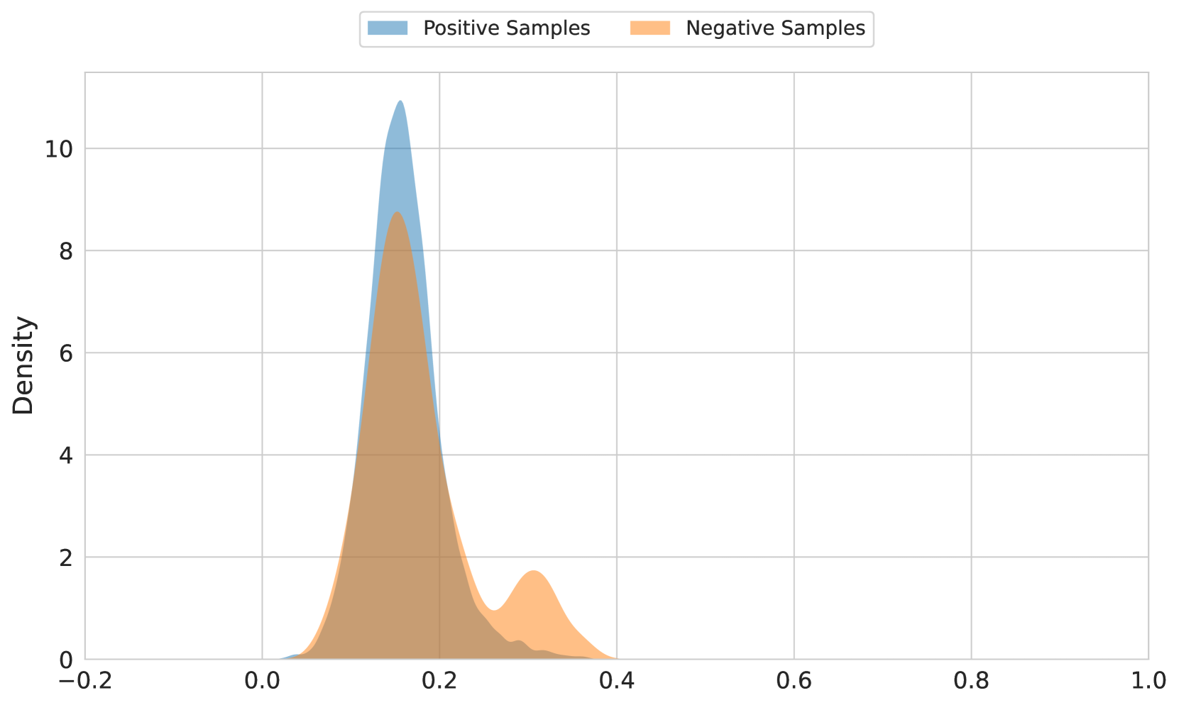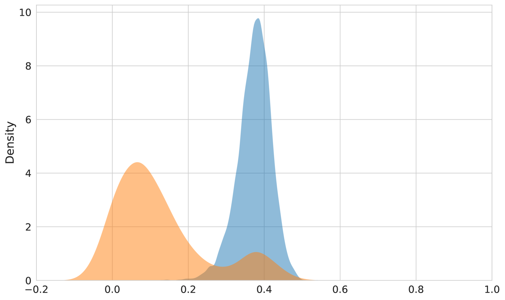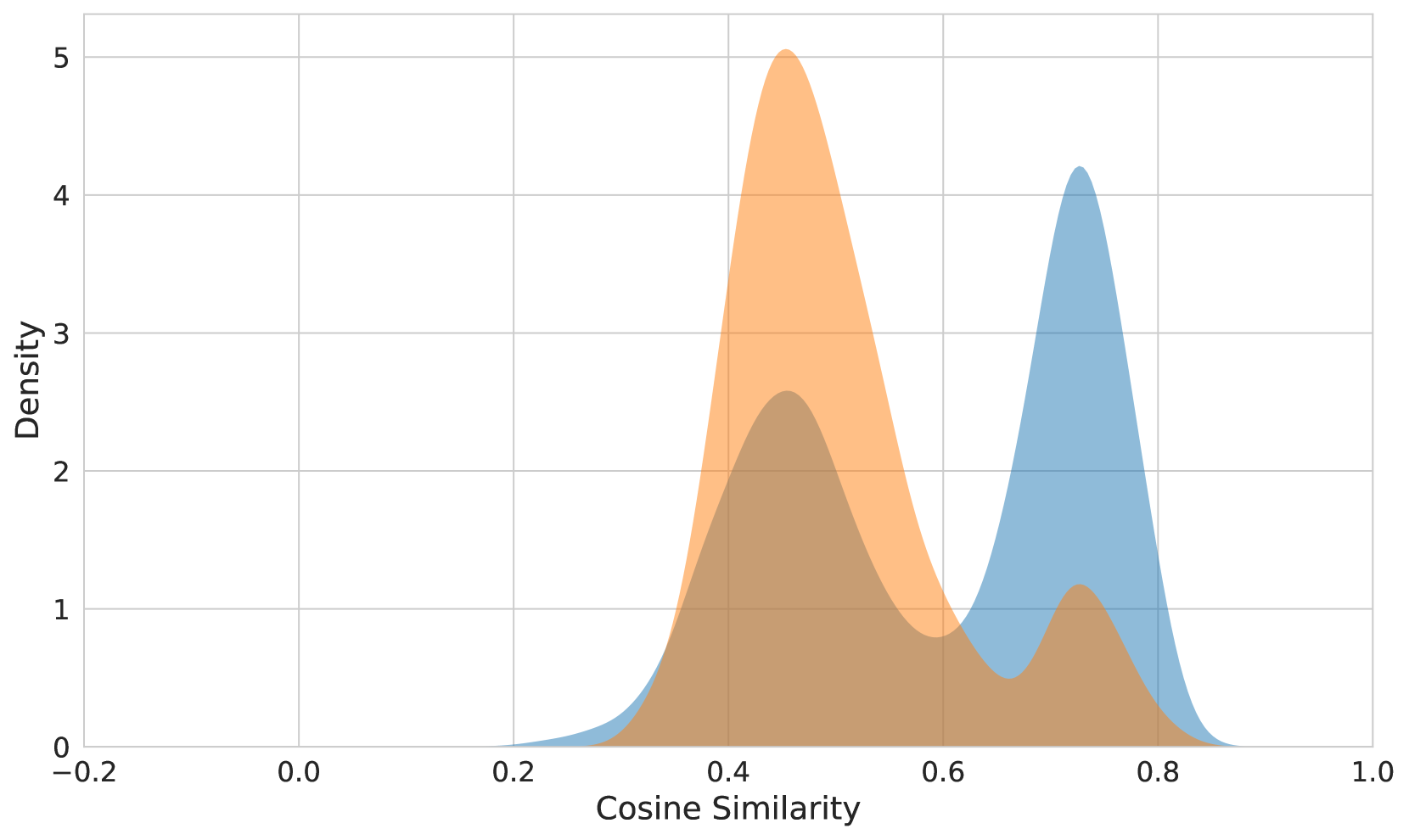### 8.3 Cone Effect Liang et al. (2022b) demonstrate that multimodal models trained with contrastive loss suffer from an inductive bias known as the cone effect. Each modality tends to cluster together in randomized embedding spaces before training, and contrastive loss tends to make the cross-modal matching pairs form a kind of high-dimensional cone, linking one part of the embedding space to another rather than distributing embeddings evenly. The impact of the cone effect can be seen in Figure 3. The difference in cosine similarity between correct and incorrect text-image matches is quite small for OpenAI CLIP (top), significantly greater in jina-clip-v2 (middle), but jina-embeddings-v4 (bottom) shows a much greater spread of cosine similarity ranges with very distinctly separate peaks for positive and negative pairs. This shows that jina-embeddings-v4 uses much more of the embedding space and image and text embeddings have a much greater overlap in distribution. <details> <summary>x5.png Details</summary>  ### Visual Description \n ## Density Plot: Distribution of Positive and Negative Samples ### Overview The image presents a density plot comparing the distributions of "Positive Samples" and "Negative Samples". The x-axis represents the range of values, likely representing a score or probability, from -0.2 to 1.0. The y-axis represents the density, ranging from 0 to approximately 10. The plot visualizes the frequency of different values for each sample type. ### Components/Axes * **X-axis Title:** Not explicitly labeled, but represents a value range from -0.2 to 1.0. * **Y-axis Title:** "Density" * **Legend:** Located at the top-right corner. * **Positive Samples:** Represented by a light blue fill. * **Negative Samples:** Represented by a light orange fill. * **Gridlines:** Present throughout the plot for easier value estimation. ### Detailed Analysis The plot shows two overlapping density curves. * **Positive Samples (Light Blue):** The density curve for positive samples peaks sharply around 0.15-0.2, with a density of approximately 9.5. The curve quickly descends on either side of the peak. The distribution appears to be concentrated in the range of 0 to 0.3. * **Negative Samples (Light Orange):** The density curve for negative samples is broader and less pronounced than that of positive samples. It has a peak around 0.05-0.1, with a density of approximately 4.5. The curve extends further to the right, with a smaller peak around 0.3-0.4, with a density of approximately 2. The distribution is more spread out, ranging from -0.2 to 0.4. ### Key Observations * The positive samples are more concentrated around a higher value (around 0.2) compared to the negative samples. * The negative samples have a wider distribution, indicating more variability in their values. * There is significant overlap between the two distributions, suggesting that it may be difficult to perfectly separate positive and negative samples based on this single feature. * The density of positive samples is significantly higher than negative samples around the 0.15-0.2 range. ### Interpretation The data suggests that the feature being measured can differentiate between positive and negative samples, but not perfectly. Positive samples tend to have higher values, while negative samples are more dispersed. The overlap in distributions indicates that there is some ambiguity, and some positive samples may have values similar to negative samples, and vice versa. This could be due to noise in the data, limitations of the feature itself, or the presence of underlying subgroups within each sample type. The difference in peak density suggests that the feature is more indicative of positive samples than negative samples. Further analysis, potentially with additional features, would be needed to improve the accuracy of classification. </details> <details> <summary>x6.png Details</summary>  ### Visual Description \n ## Density Plot: Bimodal Distribution ### Overview The image presents a density plot displaying a bimodal distribution. Two distinct peaks are visible, suggesting two underlying populations or clusters within the data. The x-axis ranges from -0.2 to 1.0, and the y-axis represents density, ranging from 0 to 10. ### Components/Axes * **X-axis:** Labeled "Density", ranging from -0.2 to 1.0. * **Y-axis:** Labeled "Density", ranging from 0 to 10. * **Data Series 1:** Filled curve in orange. * **Data Series 2:** Filled curve in blue. ### Detailed Analysis The plot shows two prominent peaks. * **Orange Curve:** This curve exhibits a peak around a density value of approximately 4, centered at approximately x = 0.05. The curve starts at x = -0.2, rises to the peak, and then declines towards x = 0.2. * **Blue Curve:** This curve has a more pronounced peak, reaching a density of approximately 9, centered around x = 0.35. The curve begins to rise around x = 0.2, reaches its peak at x = 0.35, and then gradually declines towards x = 0.7. The area under each curve represents the proportion of data belonging to that distribution. The blue curve has a larger area, indicating a greater proportion of data points are associated with that distribution. ### Key Observations * **Bimodality:** The most striking feature is the presence of two distinct peaks, indicating a bimodal distribution. * **Peak Heights:** The blue peak is significantly higher than the orange peak, suggesting a larger concentration of data points around x = 0.35. * **Distribution Spread:** The orange curve is wider than the blue curve, indicating a greater spread or variance in the data associated with that distribution. ### Interpretation The bimodal distribution suggests that the data originates from two different underlying processes or populations. The two peaks represent the most frequent values within each population. The difference in peak heights indicates that one population is more prevalent than the other. The data could represent a mixture of two different datasets, or a single dataset with two distinct subgroups. Further investigation would be needed to determine the cause of the bimodality and the characteristics of each population. For example, the data could represent the distribution of heights of men and women, or the distribution of test scores for two different teaching methods. The fact that the distributions are not perfectly separated suggests some overlap between the populations. </details> <details> <summary>x7.png Details</summary>  ### Visual Description \n ## Density Plot: Cosine Similarity Distribution ### Overview The image presents a density plot illustrating the distribution of cosine similarity scores. Two overlapping distributions are displayed, one in orange and one in blue. The x-axis represents the cosine similarity, ranging from -0.2 to 1.0, while the y-axis represents the density, ranging from 0 to 5. The plot shows the frequency of different cosine similarity values within the two datasets. ### Components/Axes * **X-axis Title:** "Cosine Similarity" * **Y-axis Title:** "Density" * **X-axis Range:** -0.2 to 1.0 * **Y-axis Range:** 0 to 5 * **Data Series 1:** Orange density curve * **Data Series 2:** Blue density curve ### Detailed Analysis The orange distribution is centered around a cosine similarity of approximately 0.45, with a peak density of roughly 4.8. It extends from approximately 0.25 to 0.7. The blue distribution is centered around a cosine similarity of approximately 0.75, with a peak density of roughly 4.2. It extends from approximately 0.55 to 0.95. There is overlap between the two distributions, particularly between 0.6 and 0.8. Here's a breakdown of approximate data points, noting the inherent uncertainty in reading values from a density plot: **Orange Distribution (approximate):** * Cosine Similarity 0.3: Density ~ 0.2 * Cosine Similarity 0.4: Density ~ 1.5 * Cosine Similarity 0.45: Density ~ 4.8 * Cosine Similarity 0.5: Density ~ 3.0 * Cosine Similarity 0.6: Density ~ 1.0 * Cosine Similarity 0.7: Density ~ 0.2 **Blue Distribution (approximate):** * Cosine Similarity 0.55: Density ~ 0.5 * Cosine Similarity 0.65: Density ~ 2.0 * Cosine Similarity 0.75: Density ~ 4.2 * Cosine Similarity 0.85: Density ~ 3.0 * Cosine Similarity 0.9: Density ~ 1.0 * Cosine Similarity 0.95: Density ~ 0.2 ### Key Observations * The orange distribution is skewed towards lower cosine similarity values, while the blue distribution is skewed towards higher values. * The two distributions have different central tendencies, suggesting that the two datasets being compared have different characteristics. * The overlap between the distributions indicates that there is some similarity between the two datasets, but it is not complete. * The density plot shows that cosine similarity values between 0.6 and 0.8 are relatively common for both datasets. ### Interpretation The data suggests that two sets of data are being compared based on their cosine similarity. Cosine similarity is a measure of the similarity between two non-zero vectors of attributes in an inner product space. It is often used in information retrieval and text mining to measure the similarity between documents. The two distributions likely represent the cosine similarity between two different sets of documents or vectors. The fact that the distributions are different suggests that the two sets of data are not identical. The overlap between the distributions suggests that there is some degree of similarity between the two sets of data. The orange distribution peaking at 0.45 could represent a set of documents that are less related or have less overlap in their content. The blue distribution peaking at 0.75 could represent a set of documents that are more related or have more overlap in their content. The overlap between 0.6 and 0.8 suggests a common ground or shared characteristics between the two sets. Without further context, it's difficult to determine the specific meaning of the cosine similarity scores. However, the data provides a clear indication that the two datasets being compared are not identical, but they are also not completely dissimilar. </details> Figure 3: Distribution of the cosine similarities of positive (correct matches) versus negative (incorrect matches) image-text samples. (top) OpenAI CLIP, (middle) jina-clip-v2, (bottom) jina-embeddings-v4. ## 9 Conclusion We present jina-embeddings-v4, a state-of-the-art multimodal and multilingual embedding model designed for a wide range of tasks, including semantic text retrieval, text-to-image retrieval, text-to-visually-rich document retrieval, and code search. The model achieves strong performance using single-vector representations and demonstrates even greater effectiveness with multi-vector representations, particularly in visually rich document retrieval. jina-embeddings-v4 aligns representations across modalities into a single, shared semantic space, sharply reducing structural gaps between modalities compared to CLIP-style dual-tower models, enabling more effective cross-modal retrieval. In future work, we plan to further enhance this model’s multilingual capabilities and explore techniques to create smaller, more efficient variants. ## References - Hu et al. [2022] Edward J. Hu, Yelong Shen, Phillip Wallis, Zeyuan Allen-Zhu, Yuanzhi Li, Shean Wang, Lu Wang, and Weizhu Chen. Lora: Low-rank adaptation of large language models. In The Tenth International Conference on Learning Representations, ICLR, 2022. - Ding et al. [2024] Yihao Ding, Soyeon Caren Han, Jean Lee, and Eduard Hovy. Deep learning based visually rich document content understanding: A survey. arXiv preprint arXiv:2408.01287, 2024. - Liang et al. [2022a] Victor Weixin Liang, Yuhui Zhang, Yongchan Kwon, Serena Yeung, and James Y Zou. Mind the Gap: Understanding the Modality Gap in Multi-modal Contrastive Representation Learning. Advances in Neural Information Processing Systems, 35:17612–17625, 2022a. - Faysse et al. [2025] Manuel Faysse, Hugues Sibille, Tony Wu, Bilel Omrani, Gautier Viaud, Céline Hudelot, and Pierre Colombo. ColPali: Efficient Document Retrieval with Vision Language Models. In The Thirteenth International Conference on Learning Representations, 2025. - Xiao et al. [2025] Chenghao Xiao, Isaac Chung, Imene Kerboua, Jamie Stirling, Xin Zhang, Márton Kardos, Roman Solomatin, Noura Al Moubayed, Kenneth Enevoldsen, and Niklas Muennighoff. MIEB: Massive Image Embedding Benchmark. arXiv preprint arXiv:2504.10471, 2025. - Sturua et al. [2024] Saba Sturua, Isabelle Mohr, Mohammad Kalim Akram, Michael Günther, Bo Wang, Markus Krimmel, Feng Wang, Georgios Mastrapas, Andreas Koukounas, Nan Wang, et al. jina-embeddings-v3: Multilingual Embeddings With Task LoRA. arXiv preprint arXiv:2409.10173, 2024. - Radford et al. [2021] Alec Radford, Jong Wook Kim, et al. Learning Transferable Visual Models from Natural Language Supervision. In International Conference on Machine Learning, pages 8748–8763, 2021. - Koukounas et al. [2024] Andreas Koukounas, Georgios Mastrapas, Michael Günther, Bo Wang, Scott Martens, Isabelle Mohr, Saba Sturua, Mohammad Kalim Akram, Joan Fontanals Martínez, Saahil Ognawala, et al. Jina CLIP: Your CLIP Model Is Also Your Text Retriever. arXiv preprint arXiv:2405.20204, 2024. - Liu et al. [2024] Ye Liu, Rui Meng, Shafiq Joty, Silvio Savarese, Caiming Xiong, Yingbo Zhou, and Semih Yavuz. CodeXEmbed: A Generalist Embedding Model Family for Multilingual and Multi-task Code Retrieval. arXiv preprint arXiv:2411.12644, 2024. - Voyage AI [2024] Voyage AI. Domain-Specific Embeddings and Retrieval: Legal Edition (voyage-law-2), 2024. https://blog.voyageai.com/2024/04/15/domain-specific-embeddings-and-retrieval-legal-edition-voyage-law-2/. - Ma et al. [2024] Xueguang Ma, Sheng-Chieh Lin, Minghan Li, Wenhu Chen, and Jimmy Lin. Unifying Multimodal Retrieval via Document Screenshot Embedding. In Proceedings of the 2024 Conference on Empirical Methods in Natural Language Processing, pages 6492–6505, 2024. - Khattab and Zaharia [2020] Omar Khattab and Matei Zaharia. ColBERT: Efficient and Effective Passage Search via Contextualized Late Interaction over BERT. In Proceedings of the 43rd International ACM SIGIR conference on research and development in Information Retrieval, pages 39–48, 2020. - Reimers and Gurevych [2019] Nils Reimers and Iryna Gurevych. Sentence-BERT: Sentence Embeddings using Siamese BERT-Networks. In Proceedings of the 2019 Conference on Empirical Methods in Natural Language Processing and the 9th International Joint Conference on Natural Language Processing (EMNLP-IJCNLP), pages 3982–3992, 2019. - Wang et al. [2022] Liang Wang, Nan Yang, Xiaolong Huang, Binxing Jiao, Linjun Yang, Daxin Jiang, Rangan Majumder, and Furu Wei. Text Embeddings by Weakly-Supervised Contrastive Pre-training. arXiv preprint arXiv:2212.03533, 2022. - Günther et al. [2023] Michael Günther, Jackmin Ong, Isabelle Mohr, Alaeddine Abdessalem, Tanguy Abel, Mohammad Kalim Akram, Susana Guzman, Georgios Mastrapas, Saba Sturua, Bo Wang, et al. Jina Embeddings 2: 8192-Token General-Purpose Text Embeddings for Long Documents. arXiv preprint arXiv:2310.19923, 2023. - Kusupati et al. [2022] Aditya Kusupati, Gantavya Bhatt, Aniket Rege, Matthew Wallingford, Aditya Sinha, Vivek Ramanujan, William Howard-Snyder, Kaifeng Chen, Sham Kakade, Prateek Jain, et al. Matryoshka Representation Learning. Advances in Neural Information Processing Systems, 35:30233–30249, 2022. - Bai et al. [2025] Shuai Bai, Keqin Chen, Xuejing Liu, Jialin Wang, Wenbin Ge, Sibo Song, Kai Dang, Peng Wang, Shijie Wang, Jun Tang, Humen Zhong, Yuanzhi Zhu, Mingkun Yang, Zhaohai Li, Jianqiang Wan, Pengfei Wang, Wei Ding, Zheren Fu, Yiheng Xu, Jiabo Ye, Xi Zhang, Tianbao Xie, Zesen Cheng, Hang Zhang, Zhibo Yang, Haiyang Xu, and Junyang Lin. Qwen2.5-VL Technical Report. arXiv preprint arXiv:2502.13923, 2025. - Jiang et al. [2024] Ting Jiang, Minghui Song, Zihan Zhang, Haizhen Huang, Weiwei Deng, Feng Sun, Qi Zhang, Deqing Wang, and Fuzhen Zhuang. E5-V: Universal Embeddings with Multimodal Large Language Models. arXiv preprint arXiv:2407.12580, 2024. - Zhang et al. [2024] Xin Zhang, Yanzhao Zhang, Wen Xie, Mingxin Li, Ziqi Dai, Dingkun Long, Pengjun Xie, Meishan Zhang, Wenjie Li, and Min Zhang. GME: Improving Universal Multimodal Retrieval by Multimodal LLMs. arXiv preprint arXiv:2412.16855, 2024. - van den Oord et al. [2018] Aäron van den Oord, Yazhe Li, and Oriol Vinyals. Representation Learning with Contrastive Predictive Coding. CoRR, abs/1807.03748, 2018. URL http://arxiv.org/abs/1807.03748. - Hinton et al. [2015] Geoffrey Hinton, Oriol Vinyals, and Jeff Dean. Distilling the Knowledge in a Neural Network. arXiv preprint arXiv:1503.02531, 2015. - Li et al. [2023] Zehan Li, Xin Zhang, Yanzhao Zhang, Dingkun Long, Pengjun Xie, and Meishan Zhang. Towards General Text Embeddings with Multi-stage Contrastive Learning. arXiv preprint arXiv:2308.03281, 2023. - Li and Li [2024] Xianming Li and Jing Li. Aoe: Angle-optimized embeddings for semantic textual similarity. In Proceedings of the 62nd Annual Meeting of the Association for Computational Linguistics (Volume 1: Long Papers), pages 1825–1839, 2024. - Agirre et al. [2012] Eneko Agirre, Daniel Cer, Mona Diab, and Aitor Gonzalez-Agirre. Semeval-2012 task 6: A pilot on semantic textual similarity. In SEM 2012: The First Joint Conference on Lexical and Computational Semantics–Volume 1: Proceedings of the main conference and the shared task, and Volume 2: Proceedings of the Sixth International Workshop on Semantic Evaluation (SemEval 2012), pages 385–393, 2012. - Marelli et al. [2014] Marco Marelli, Stefano Menini, Marco Baroni, Luisa Bentivogli, Raffaella Bernardi, and Roberto Zamparelli. A SICK cure for the evaluation of compositional distributional semantic models. In Nicoletta Calzolari, Khalid Choukri, Thierry Declerck, Hrafn Loftsson, Bente Maegaard, Joseph Mariani, Asuncion Moreno, Jan Odijk, and Stelios Piperidis, editors, Proceedings of the Ninth International Conference on Language Resources and Evaluation (LREC’14), pages 216–223, Reykjavik, Iceland, May 2014. European Language Resources Association (ELRA). URL http://www.lrec-conf.org/proceedings/lrec2014/pdf/363_Paper.pdf. - Husain et al. [2020] Hamel Husain, Ho-Hsiang Wu, Tiferet Gazit, Miltiadis Allamanis, and Marc Brockschmidt. CodeSearchNet Challenge: Evaluating the State of Semantic Code Search. arXiv preprint arXiv:1909.09436, 2020. - Zheng et al. [2024] Tianyu Zheng, Ge Zhang, Tianhao Shen, Xueling Liu, Bill Yuchen Lin, Jie Fu, Wenhu Chen, and Xiang Yue. OpenCodeInterpreter: Integrating Code Generation with Execution and Refinement. In Lun-Wei Ku, Andre Martins, and Vivek Srikumar, editors, Findings of the Association for Computational Linguistics: ACL 2024, pages 12834–12859. Association for Computational Linguistics, August 2024. - Hendrycks et al. [2021] Dan Hendrycks, Steven Basart, Saurav Kadavath, Mantas Mazeika, Akul Arora, Ethan Guo, Collin Burns, Samir Puranik, Horace He, Dawn Song, and Jacob Steinhardt. In Proceedings of the Neural Information Processing Systems Track on Datasets and Benchmarks, 2021. - Suresh et al. [2025] Tarun Suresh, Revanth Gangi Reddy, Yifei Xu, Zach Nussbaum, Andriy Mulyar, Brandon Duderstadt, and Heng Ji. Cornstack: High-quality contrastive data for better code retrieval and reranking. arXiv preprint arXiv:2412.01007, 2025. - Tom Agonnoude [2024] Cyrile Delestre Tom Agonnoude, 2024. URL https://huggingface.co/datasets/cmarkea/table-vqa. - Zhang et al. [2023] Liang Zhang, Anwen Hu, Jing Zhang, Shuo Hu, and Qin Jin. Mpmqa: Multimodal question answering on product manuals. 2023. URL https://arxiv.org/abs/2304.09660. - Wang et al. [2024] Zirui Wang, Mengzhou Xia, Luxi He, Howard Chen, Yitao Liu, Richard Zhu, Kaiqu Liang, Xindi Wu, Haotian Liu, Sadhika Malladi, Alexis Chevalier, Sanjeev Arora, and Danqi Chen. Charxiv: Charting gaps in realistic chart understanding in multimodal llms. arXiv preprint arXiv:2406.18521, 2024. - Methani et al. [2020] Nitesh Methani, Pritha Ganguly, Mitesh M. Khapra, and Pratyush Kumar. Plotqa: Reasoning over scientific plots. In The IEEE Winter Conference on Applications of Computer Vision (WACV), March 2020. - Mitchener [2021] Kris James Mitchener. National banking statistics, 1867–1896. https://purl.stanford.edu/mv327tb8364, 2021. Dataset published via Stanford Digital Repository. - Kembhavi et al. [2017] Aniruddha Kembhavi, Minjoon Seo, Dustin Schwenk, Jonghyun Choi, Ali Farhadi, and Hannaneh Hajishirzi. Are you smarter than a sixth grader? textbook question answering for multimodal machine comprehension. pages 5376–5384, 07 2017. doi: 10.1109/CVPR.2017.571. - Jina AI [2024] Jina AI. Re·Search: Order 2024 Yearbook of Search Foundation Advances. Jina AI, Sunnyvale, CA & Berlin, Germany, December 16 2024. Hardcover with spot UV coating; includes complimentary digital copy. Available at: https://jina.ai/news/re-search-order-2024-yearbook-of-search-foundation-advances/. - Niigata-shi Kankō Kokusaikōryūbu Kankō Suishinka [2024] Niigata-shi Kankō Kokusaikōryūbu Kankō Suishinka. Niigata City Ramen Guidebook. City of Niigata, Niigata, Japan, July 2024. URL https://www.city.niigata.lg.jp/kanko/kanko/oshirase/ramen.files/guidebook.pdf. PDF, approximately 28 MB. - Shanghai Municipal People’s Government Urban Planning and Land Resource Administration Bureau [2018] Shanghai Municipal People’s Government Urban Planning and Land Resource Administration Bureau. Shanghai Master Plan 2017–2035: Striving for the Excellent Global City. Shanghai Municipal People’s Government, Shanghai, China, January 2018. URL https://www.shanghai.gov.cn/newshanghai/xxgkfj/2035004.pdf. Public Reading edition; government - issued planning document. - Ghaboura et al. [2024] Sara Ghaboura, Ahmed Heakl, Omkar Thawakar, Ali Alharthi, Ines Riahi, Abduljalil Saif, Jorma Laaksonen, Fahad S. Khan, Salman Khan, and Rao M. Anwer. Camel-bench: A comprehensive arabic lmm benchmark. 2024. URL https://arxiv.org/abs/2410.18976. - Delestre [2024] Cyrile Delestre, 2024. URL https://huggingface.co/datasets/cmarkea/aftdb. - Enevoldsen et al. [2025] Kenneth Enevoldsen, Isaac Chung, et al. MMTEB: Massive Multilingual Text Embedding Benchmark. 2025. - Wang et al. [2023] Liang Wang, Nan Yang, Xiaolong Huang, Linjun Yang, Rangan Majumder, and Furu Wei. Improving text embeddings with large language models. arXiv preprint arXiv:2401.00368, 2023. - Zhu et al. [2024] Dawei Zhu, Liang Wang, Nan Yang, Yifan Song, Wenhao Wu, Furu Wei, and Sujian Li. LongEmbed: Extending Embedding Models for Long Context Retrieval. In Proceedings of the 2024 Conference on Empirical Methods in Natural Language Processing, pages 802–816, 2024. - Thapliyal et al. [2022] Ashish V. Thapliyal, Jordi Pont Tuset, Xi Chen, and Radu Soricut. Crossmodal-3600: A massively multilingual multimodal evaluation dataset. In Proceedings of the 2022 Conference on Empirical Methods in Natural Language Processing, pages 715–729, 2022. - Li et al. [2024] Xiangyang Li, Kuicai Dong, Yi Quan Lee, Wei Xia, Yichun Yin, Hao Zhang, Yong Liu, Yasheng Wang, and Ruiming Tang. Coir: A comprehensive benchmark for code information retrieval models. CoRR, 2024. - Liang et al. [2022b] Victor Weixin Liang, Yuhui Zhang, Yongchan Kwon, Serena Yeung, and James Y Zou. Mind the gap: Understanding the modality gap in multi-modal contrastive representation learning. Advances in Neural Information Processing Systems, 35:17612–17625, 2022b. - Schrodi et al. [2024] Simon Schrodi, David T Hoffmann, Max Argus, Volker Fischer, and Thomas Brox. Two effects, one trigger: on the modality gap, object bias, and information imbalance in contrastive vision-language representation learning. arXiv preprint arXiv:2404.07983, 2024. - Eslami and de Melo [2025] Sedigheh Eslami and Gerard de Melo. Mitigate the gap: Improving cross-modal alignment in clip. In The Thirteenth International Conference on Learning Representations, 2025. - Lin et al. [2014] Tsung-Yi Lin, Michael Maire, Serge Belongie, James Hays, Pietro Perona, Deva Ramanan, Piotr Dollár, and C. Lawrence Zitnick. Microsoft coco: Common objects in context. In David Fleet, Tomas Pajdla, Bernt Schiele, and Tinne Tuytelaars, editors, Computer Vision – ECCV 2014, pages 740–755, Cham, 2014. Springer International Publishing. ISBN 978-3-319-10602-1. ## Appendix A Appendix ### A.1 Datasets in the Jina-VDR Benchmark Table A1: Overview of the Dataset Collection | jinaai/airbnb-synthetic-retrieval† | Housing | Tables | Instruction | 4953 / 10000 | ar, de, en, es, fr, hi, hu, ja ru, zh | | --- | --- | --- | --- | --- | --- | | jinaai/arabic_chartqa_ar | Mixed | Charts | Question | 745 / 342 | ar | | jinaai/arabic_infographicsvqa_ar | Mixed | Illustrations | Question | 120 / 40 | ar | | jinaai/automobile_catalogue_jp | Marketing | Catalog | Question | 45 / 15 | ja | | jinaai/arxivqa | Science | Mixed | Question | 30 / 499 | en | | jinaai/beverages_catalogue_ru | Marketing | Digital Docs | Question | 100 / 34 | ru | | jinaai/ChartQA | Mixed | Charts | Question | 996 / 834 | en | | jinaai/CharXiv-en | Science | Charts | Question | 999 / 1000 | en | | jinaai/docvqa | Mixed | Scans | Question | 39 / 499 | en | | jinaai/donut_vqa | Medical | Scans / Handwriting | Question | 704 / 800 | en | | jinaai/docqa_artificial_intelligence | Software / IT | Digital Docs | Question | 70 / 962 | en | | jinaai/docqa_energy | Energy | Digital Docs | Question | 69 / 971 | en | | jinaai/docqa_gov_report | Government | Digital Docs | Question | 77 / 970 | en | | jinaai/docqa_healthcare_industry | Medial | Digital Docs | Question | 90 / 961 | en | | jinaai/europeana-de-news | Historic | Scans / News Articles | Question | 379 / 137 | de | | jinaai/europeana-es-news | Historic | Scans / News Articles | Question | 474 / 179 | es | | jinaai/europeana-fr-news | Historic | Scans / News Articles | Question | 237 / 145 | fr | | jinaai/europeana-it-scans | Historic | Scans | Question | 618 / 265 | it | | jinaai/europeana-nl-legal | Legal | Scans | Question | 199 / 244 | nl | | jinaai/github-readme-retrieval-multilingual† | Software / IT | Markdown Docs | Description | 16953 / 16998 | ar, bn, de, en, es, fr, hi, id, it, ja, ko, nl pt, ru, th, vi, zh | | jinaai/hindi-gov-vqa | Governmental | Digital Docs | Question | 454 / 337 | hi | | jinaai/hungarian_doc_qa_hu | Mixed | Digital Docs | Question | 54 / 51 | hu | | jinaai/infovqa | Mixed | Illustrations | Question | 363 / 500 | en | | jinaai/jdocqa | News | Digital Docs | Question | 744 / 758 | ja | | jinaai/jina_2024_yearly_book | Software / IT | Digital Docs | Question | 75 / 33 | en | | jinaai/medical-prescriptions | Medical | Digital Docs | Question | 100 / 100 | en | | jinaai/mpmqa-small | Manuals | Digital Docs | Question | 155 / 782 | en | | jinaai/MMTab | Mixed | Tables | Fact | 987 / 906 | en | | jinaai/openai-news | Software / IT | Digital Docs | Question | 31 / 30 | en | | jinaai/owid_charts_en | Mixed | Charts | Question | 132 / 937 | en | | jinaai/plotqa | Mixed | Charts | Question | 610 / 986 | en | | jinaai/ramen_benchmark_jp | Marketing | Catalog | Question | 29 / 10 | ja | | jinaai/shanghai_master_plan | Governmental | Digital Docs | Question / Key Phrase | 57 / 23 | zh, en | | jinaai/wikimedia-commons-documents-ml† | Mixed | Mixed | Description | 15593 / 15217 | ar, bn, de, en, es, fr, hi, hu, id, it, ja, ko, my, nl, pt, ru, th, ur, vi, zh | | jinaai/shiftproject | Environmental Documents | Digital Docs | Question | 89 / 998 | fr | | jinaai/stanford_slide | Education | Slides | Question | 14 / 994 | en | | jinaai/student-enrollment | Demographics | Charts | Question | 1000 / 489 | en | | jinaai/tabfquad | Mixed | Tables | Question | 126 / 70 | fr, en | | jinaai/table-vqa | Science | Tables | Question | 992 / 385 | en | | jinaai/tatqa | Finance | Digital Docs | Question | 121 / 270 | en | | jinaai/tqa | Education | Illustrations | Question | 981 / 393 | en | | jinaai/tweet-stock-synthetic-retrieval† | Finance | Charts | Question | 6278 / 10000 | ar, de, en, es, hi, hu, ja, ru, zh | | jinaai/wikimedia-commons-maps | Mixed | Maps | Description | 443 / 451 | en | †For multilingual datasets, the total number of queries and documents is the sum across all language-specific splits. ### A.2 JinaVDR (Visual Document Retrieval) Benchmark Results Table A2: Overview of JinaVDR Results for Various Models | Average | 46.88 | 48.97 | 40.96 | 65.39 | 68.89 | 75.47 | 81.52 | | --- | --- | --- | --- | --- | --- | --- | --- | | medical-prescriptions | 38.18 | 38.12 | 15.68 | 66.22 | 38.86 | 80.95 | 97.69 | | stanford_slide | 81.78 | 95.28 | 91.48 | 100.0 | 100.0 | 100.0 | 97.16 | | donut_vqa | 19.39 | 2.59 | 1.46 | 34.12 | 25.31 | 78.60 | 74.08 | | table-vqa | 55.22 | 63.04 | 36.34 | 80.98 | 85.70 | 86.57 | 89.21 | | ChartQA | 28.39 | 31.47 | 39.73 | 54.45 | 58.38 | 70.88 | 71.80 | | tqa | 50.11 | 24.40 | 27.80 | 63.03 | 65.35 | 65.44 | 68.46 | | openai-news | 76.63 | 87.30 | 70.05 | 94.81 | 93.75 | 93.97 | 96.43 | | europeana-de-news | 11.26 | 12.02 | 11.18 | 35.20 | 44.32 | 48.89 | 63.76 | | europeana-es-news | 51.99 | 43.82 | 12.95 | 45.70 | 60.66 | 60.81 | 80.70 | | europeana-it-scans | 39.11 | 38.77 | 16.54 | 58.70 | 54.28 | 58.01 | 73.29 | | europeana-nl-legal | 39.38 | 34.24 | 11.30 | 39.13 | 33.12 | 42.77 | 59.82 | | hindi-gov-vqa | 1.83 | 7.51 | 5.21 | 11.43 | 10.19 | 15.32 | 22.49 | | automobile_catalogue_jp | 20.92 | 50.39 | 32.54 | 35.72 | 66.44 | 72.22 | 81.32 | | beverages_catalogue_ru | 11.05 | 14.09 | 39.66 | 68.47 | 80.32 | 85.68 | 87.73 | | ramen_benchmark_jp | 28.02 | 63.37 | 41.28 | 52.03 | 51.66 | 90.77 | 94.65 | | jdocqa | 1.64 | 7.85 | 19.94 | 35.68 | 67.00 | 75.63 | 82.42 | | hungarian_doc_qa | 34.28 | 57.84 | 50.44 | 68.83 | 55.25 | 74.64 | 75.56 | | arabic_chartqa_ar | 9.32 | 8.63 | 6.62 | 26.92 | 49.35 | 62.16 | 66.64 | | arabic_infographicsvqa_ar | 13.26 | 13.43 | 50.36 | 34.76 | 71.72 | 85.38 | 93.21 | | owid_charts_en | 66.19 | 62.10 | 57.71 | 78.17 | 84.26 | 92.06 | 92.29 | | arxivqa | 56.73 | 54.41 | 83.41 | 92.54 | 93.33 | 95.44 | 95.44 | | docvqa | 81.11 | 50.81 | 45.29 | 90.38 | 86.28 | 83.06 | 92.98 | | shiftproject | 62.42 | 70.25 | 31.85 | 75.18 | 78.54 | 82.55 | 91.13 | | docqa_artificial_intelligence | 91.68 | 82.98 | 66.52 | 96.09 | 97.52 | 96.43 | 98.04 | | docqa_energy | 89.97 | 76.97 | 65.56 | 96.03 | 90.08 | 88.66 | 96.28 | | docqa_gov_report | 87.20 | 82.72 | 68.84 | 92.92 | 94.19 | 92.03 | 95.97 | | docqa_healthcare_industry | 86.44 | 86.88 | 68.13 | 93.14 | 96.14 | 94.62 | 97.51 | | tabfquad | 45.67 | 80.49 | 47.04 | 89.18 | 92.38 | 95.57 | 95.38 | | mpmqa_small | 85.54 | 67.39 | 59.72 | 88.88 | 81.62 | 80.44 | 91.28 | | jina_2024_yearly_book | 87.67 | 85.98 | 77.12 | 95.77 | 93.39 | 94.29 | 98.17 | | wikimedia-commons-maps | 5.37 | 5.06 | 20.67 | 27.46 | 33.06 | 40.23 | 53.45 | | plotqa | 61.13 | 51.44 | 24.05 | 70.58 | 75.99 | 77.48 | 78.75 | | MMTab | 74.82 | 74.06 | 44.54 | 84.66 | 86.04 | 86.08 | 90.03 | | CharXiv-en | 46.85 | 41.47 | 56.28 | 79.64 | 83.86 | 83.00 | 87.66 | | student-enrollment | 1.05 | 1.30 | 0.70 | 3.95 | 4.09 | 8.04 | 11.55 | | tatqa | 75.62 | 49.88 | 44.23 | 82.57 | 80.97 | 80.14 | 92.76 | | shanghai_master_plan | 12.69 | 92.67 | 75.28 | 88.87 | 92.56 | 95.53 | 97.41 | | europeana-fr-news | 24.55 | 23.69 | 16.43 | 30.33 | 38.23 | 36.66 | 50.16 | | infovqa | 73.61 | 75.09 | 63.38 | 87.53 | 92.64 | 92.16 | 96.69 | Models: bm25+OCR: BM25 with EasyOCR, jev3+OCR: jina-embeddings-v3 with EasyOCR, j-clip-v2: jina-clip-v2, colpali-v1.2: ColPALI-v1.2, dse-qwen2- 2b-mrl-v1: DSE-QWen2-2b-MRL-V1, je4-single: jina-embeddings-v4 single-vector, jev4-multi: jina-embeddings-v4 multi-vector Table A3: Retrieval performance on ViDoRe (nDCG@10%). | Model | Avg | AQA | DVQA | InfoVQA | Shift | AI | Energy | Gov | Health | TabFQ | TQA | | --- | --- | --- | --- | --- | --- | --- | --- | --- | --- | --- | --- | | OCR + jina-embeddings-v3 | 26.02 | 26.31 | 12.62 | 32.79 | 14.18 | 22.84 | 27.47 | 31.16 | 45.78 | 44.54 | 2.53 | | jina-clip-v2 | 53.61 | 68.33 | 27.62 | 60.6 | 34.12 | 66.55 | 64.69 | 67.47 | 68.38 | 46.89 | 31.43 | | voyage-multimodal-3 | 84.20 | 84.90 | 55.60 | 85.40 | 78.70 | 94.50 | 89.50 | 96.00 | 95.10 | 92.80 | 69.90 | | colpali-v1.2 | 83.90 | 78.00 | 57.20 | 82.80 | 79.10 | 98.10 | 95.20 | 94.80 | 96.70 | 89.70 | 68.10 | | dse-qwen2-2b-mrl-v1 | 85.80 | 85.60 | 57.10 | 88.10 | 82.00 | 97.50 | 92.90 | 96.00 | 96.40 | 93.10 | 69.40 | | OCR + bm25 | 65.50 | 31.60 | 36.80 | 62.90 | 64.30 | 92.80 | 85.90 | 83.90 | 87.20 | 46.50 | 62.70 | | siglip-so400m-patch14-384 | 51.40 | 43.20 | 30.30 | 64.10 | 18.70 | 62.50 | 65.70 | 66.10 | 79.10 | 58.10 | 26.20 | | jina-embeddings-v4 (dense) | 84.11 | 83.57 | 50.54 | 87.85 | 84.07 | 97. 16 | 91.66 | 91.48 | 94.92 | 94.48 | 65.35 | | jina-embeddings-v4 (late) | 90.17 | 88.95 | 59.98 | 93.57 | 92.35 | 99.26 | 96.76 | 96.95 | 98.39 | 95.13 | 80.34 | Tasks: Avg: Mean nDCG@10% over all tasks, AQA: ArxivQA, Shift: Shift Project, DVQA: DocVQA, InfoVQA: InfographicVQA, AI: Artificial Intelligence, Gov: Government Reports, Health: Healthcare Industry, TabFQ: TabFQuad, TQA: TAT-DQA Table A4: Wikimedia Commons Retreival Benchmark Results | Average | 21.99 | 37.43 | 48.63 | 33.60 | 58.67 | 66.04 | 75.63 | | --- | --- | --- | --- | --- | --- | --- | --- | | Arabic (ar) | 19.62 | 38.40 | 45.85 | 28.40 | 63.06 | 71.41 | 81.81 | | Bengali (bn) | 22.93 | 44.55 | 49.37 | 26.63 | 52.89 | 66.98 | 76.41 | | German (de) | 12.74 | 39.58 | 52.87 | 40.36 | 62.99 | 70.21 | 80.86 | | English (en) | 36.45 | 45.24 | 56.58 | 64.98 | 70.23 | 73.55 | 81.66 | | Spanish (es) | 12.75 | 46.10 | 54.85 | 41.34 | 66.43 | 71.68 | 80.82 | | French (fr) | 15.59 | 36.06 | 35.73 | 43.93 | 41.32 | 53.58 | 59.42 | | Hindi (hi) | 16.73 | 36.94 | 48.42 | 18.02 | 50.94 | 62.64 | 71.77 | | Hungarian (hu) | 25.38 | 33.88 | 44.42 | 12.67 | 52.35 | 65.86 | 76.00 | | Indonesian (id) | 28.79 | 39.48 | 50.85 | 40.46 | 62.03 | 66.02 | 73.72 | | Italian (it) | 19.63 | 37.98 | 49.77 | 34.76 | 60.05 | 63.96 | 73.68 | | Japanese (jp) | 21.41 | 30.43 | 44.03 | 28.83 | 63.71 | 66.50 | 77.13 | | Korean (ko) | 34.98 | 35.24 | 47.61 | 29.82 | 68.37 | 71.45 | 81.77 | | Burmese (my) | 22.84 | 29.45 | 54.36 | 10.28 | 37.61 | 56.58 | 65.01 | | Dutch (nl) | 14.90 | 39.89 | 50.40 | 52.29 | 65.09 | 68.58 | 78.94 | | Portuguese (pt) | 23.32 | 45.85 | 54.28 | 51.30 | 67.53 | 69.04 | 78.85 | | Russian (ru) | 16.82 | 38.95 | 49.34 | 31.88 | 64.44 | 68.86 | 80.70 | | Thai (th) | 30.00 | 29.64 | 46.25 | 39.13 | 56.41 | 61.68 | 71.02 | | Urdu (ur) | 13.64 | 32.73 | 36.52 | 9.45 | 38.76 | 49.76 | 62.17 | | Vietnamese (vi) | 32.40 | 39.80 | 54.59 | 43.72 | 64.62 | 73.30 | 80.24 | | Chinese (zh) | 18.82 | 28.41 | 46.45 | 23.82 | 64.51 | 69.23 | 80.58 | Table A5: GitHub Readme Retrieval Benchmark Results | Average | 50.11 | 65.14 | 39.06 | 72.91 | 72.24 | 85.57 | 85.69 | | --- | --- | --- | --- | --- | --- | --- | --- | | Arabic (ar) | 27.49 | 27.98 | 31.02 | 55.19 | 55.95 | 75.02 | 75.26 | | Bengali (bn) | 1.29 | 28.27 | 26.96 | 49.25 | 47.30 | 65.70 | 66.08 | | German (de) | 60.11 | 84.58 | 45.46 | 84.15 | 80.62 | 91.09 | 91.35 | | English (en) | 87.43 | 91.67 | 48.69 | 91.10 | 90.69 | 96.94 | 97.34 | | Spanish (es) | 78.57 | 83.31 | 43.35 | 84.02 | 78.70 | 89.60 | 90.19 | | French (fr) | 77.55 | 83.54 | 42.42 | 83.73 | 79.11 | 90.25 | 90.45 | | Hindi (hi) | 2.72 | 48.08 | 28.55 | 51.22 | 46.49 | 69.31 | 70.98 | | Indonesian (id) | 78.05 | 82.46 | 38.59 | 79.67 | 74.57 | 88.42 | 88.62 | | Italian (it) | 78.83 | 86.54 | 44.26 | 85.31 | 80.81 | 91.76 | 91.41 | | Japanese (jp) | 14.46 | 63.20 | 42.02 | 69.02 | 75.42 | 89.74 | 90.80 | | Korean (ko) | 40.01 | 35.23 | 37.87 | 64.16 | 68.83 | 87.04 | 86.89 | | Dutch (nl) | 76.52 | 86.36 | 43.25 | 84.10 | 82.85 | 92.83 | 91.37 | | Portuguese (pt) | 80.33 | 84.46 | 43.88 | 85.00 | 80.09 | 91.43 | 91.47 | | Russian (ru) | 39.78 | 50.86 | 37.04 | 78.16 | 78.92 | 89.51 | 88.61 | | Thai (th) | 1.47 | 36.67 | 37.62 | 65.29 | 65.45 | 77.61 | 76.67 | | Vietnamese (vi) | 66.70 | 79.67 | 37.14 | 70.05 | 68.20 | 86.90 | 86.94 | | Chinese (zh) | 40.52 | 54.53 | 35.89 | 60.05 | 74.05 | 81.44 | 82.26 | Table A6: Tweet Stock Retrieval Benchmark Results | Average | 22.30 | 42.77 | 55.36 | 76.36 | 62.76 | 78.10 | 85.34 | | --- | --- | --- | --- | --- | --- | --- | --- | | Arabic (ar) | 0.38 | 1.67 | 49.36 | 77.31 | 52.73 | 66.15 | 77.66 | | German (de) | 48.27 | 66.86 | 52.49 | 73.53 | 57.35 | 79.38 | 85.63 | | English (en) | 51.38 | 63.66 | 48.35 | 77.13 | 63.47 | 77.92 | 85.36 | | Spanish (es) | 54.28 | 63.44 | 53.44 | 79.02 | 62.57 | 78.68 | 84.62 | | French (fr) | 51.69 | 64.76 | 54.94 | 76.91 | 62.17 | 78.65 | 85.27 | | Hindi (hi) | 0.08 | 0.08 | 88.55 | 93.39 | 97.00 | 97.46 | 96.50 | | Hungarian (hu) | 15.55 | 62.31 | 52.30 | 71.06 | 58.17 | 80.09 | 85.01 | | Japanese (jp) | 0.40 | 47.80 | 54.74 | 70.00 | 57.76 | 77.04 | 85.67 | | Russian (ru) | 0.47 | 3.07 | 47.08 | 70.72 | 57.43 | 76.33 | 83.11 | | Chinese (zh) | 0.45 | 54.04 | 52.30 | 74.54 | 58.94 | 69.33 | 84.55 | Table A7: AirBnB Retrieval Benchmark Results | Average | 7.20 | 1.13 | 2.13 | 10.42 | 11.10 | 8.18 | 37.51 | | --- | --- | --- | --- | --- | --- | --- | --- | | Arabic (ar) | 1.10 | 0.40 | 0.47 | 3.06 | 3.64 | 2.20 | 6.20 | | German (de) | 4.03 | 0.71 | 5.54 | 20.17 | 15.09 | 9.27 | 41.94 | | English (en) | 48.39 | 1.70 | 4.83 | 23.26 | 12.94 | 13.33 | 64.17 | | Spanish (es) | 6.25 | 0.18 | 2.10 | 18.06 | 8.61 | 9.11 | 39.84 | | French (fr) | 3.86 | 2.00 | 2.05 | 10.86 | 11.87 | 8.70 | 30.55 | | Hindi (hi) | 0.16 | 0.86 | 0.82 | 3.19 | 4.93 | 4.05 | 17.44 | | Hungarian (hu) | 5.58 | 0.69 | 3.01 | 7.34 | 11.10 | 6.69 | 27.30 | | Japanese (jp) | 0.36 | 1.53 | 0.54 | 3.44 | 14.91 | 7.63 | 45.65 | | Russian (ru) | 1.67 | 1.39 | 0.88 | 13.16 | 13.61 | 8.66 | 40.80 | | Chinese (zh) | 0.58 | 1.84 | 1.04 | 1.62 | 14.28 | 12.14 | 61.19 | ### A.3 CLIP Table A8: Cross-modal (Text-to-image) retrieval performance (Recall@5%) on the CLIP benchmark. | Model | Avg | flickr30k | mscoco_captions | crossmodal3600 | xtd10 | | --- | --- | --- | --- | --- | --- | | nllb-clip-large-siglip | 83.19 | 92.24 | 70.84 | 82.07 | 87.60 | | jina-clip-v2 | 81.12 | 89.84 | 68.35 | 81.43 | 84.87 | | jina-embeddings-v4 | 84.11 | 91.36 | 76.18 | 79.42 | 89.46 | Avg: Mean Recall@5% over all 4 tasks. Table A9: Text-to-image retrieval performance (Recall@5%) on xtd10 for all supported languages. | Language | jina-embeddings-v4 | jina-clip-v2 | nllb-clip-large-siglip | | --- | --- | --- | --- | | average | 89.46 | 84.87 | 87.60 | | de | 92.10 | 85.70 | 88.30 | | en | 93.10 | 89.40 | 89.40 | | es | 91.50 | 85.90 | 88.20 | | fr | 91.30 | 85.10 | 87.70 | | it | 92.20 | 85.80 | 89.30 | | ko | 86.30 | 82.10 | 85.20 | | pl | 89.10 | 86.50 | 89.40 | | ru | 91.50 | 81.10 | 83.40 | | tr | 84.70 | 83.70 | 88.30 | | zh | 82.80 | 83.40 | 86.80 | Table A10: Text-to-image retrieval performance (Recall@5%) on crossmodal3600 for all supported languages. | Language | jina-embeddings-v4 | jina-clip-v2 | nllb-clip-large-siglip | | --- | --- | --- | --- | | average | 79.42 | 81.43 | 82.07 | | ar | 75.75 | 73.56 | 78.92 | | bn | 57.97 | 63.78 | 75.19 | | da | 80.47 | 85.39 | 87.14 | | de | 91.75 | 91.25 | 89.56 | | el | 66.50 | 75.03 | 77.83 | | en | 76.47 | 75.83 | 73.11 | | es | 83.64 | 83.64 | 82.64 | | fi | 66.67 | 82.83 | 86.42 | | fr | 88.69 | 88.78 | 87.86 | | hi | 47.81 | 55.25 | 60.31 | | id | 87.41 | 84.22 | 86.31 | | it | 87.97 | 88.33 | 85.94 | | ja | 91.22 | 87.03 | 86.06 | | ko | 82.19 | 78.81 | 78.75 | | nl | 81.00 | 82.56 | 81.69 | | no | 71.94 | 81.08 | 82.69 | | pl | 80.86 | 84.00 | 82.72 | | pt | 81.42 | 82.42 | 82.69 | | ro | 84.33 | 89.36 | 90.03 | | ru | 90.28 | 88.97 | 86.44 | | sv | 72.58 | 78.06 | 79.33 | | th | 83.36 | 81.61 | 81.14 | | tr | 73.08 | 81.31 | 83.47 | | uk | 86.28 | 88.56 | 85.44 | | vi | 88.81 | 86.64 | 85.56 | | zh | 86.67 | 78.97 | 76.56 | ### A.4 MTEB and MMTEB Table A11: Evaluation Results for Various Models on MTEB Retrieval Tasks (nDCG@10%) | Model | Arg | CQG | CQU | CFHN | FEV | FiQA | HPQA | SCI | TREC | TOU | AVG | | --- | --- | --- | --- | --- | --- | --- | --- | --- | --- | --- | --- | | multilingual-e5-large | 54.36 | 58.70 | 39.89 | 26.00 | 83.79 | 43.82 | 70.55 | 17.45 | 71.15 | 49.59 | 51.53 | | e5-mistral-7b-instruct | 61.65 | 63.52 | 46.75 | 28.50 | 86.99 | 56.81 | 73.21 | 16.32 | 87.03 | 55.44 | 57.62 | | text-embedding-3-large | 57.99 | 65.40 | 50.02 | 30.10 | 88.53 | 55.00 | 71.66 | 23.07 | 79.56 | 58.42 | 57.98 | | gemini-embedding-001 | 86.44 | 70.68 | 53.69 | 31.06 | 88.98 | 61.78 | 87.01 | 25.15 | 86.32 | 52.39 | 64.35 | | jina-embedding-l-en-v1 | 48.3 | 51.68 | 38.66 | 25.93 | 71.16 | 41.02 | 57.26 | 18.54 | 60.34 | 62.34 | 47.52 | | jina-embeddings-v2-base-en | 44.18 | 56.52 | 38.66 | 23.77 | 73.41 | 41.58 | 63.24 | 19.86 | 65.91 | 63.35 | 49.05 | | jina-embeddings-v3† | 54.33 | 58.02 | 43.52 | 43.14 | 89.90 | 47.35 | 64.70 | 19.92 | 77.74 | 55.28 | 55.39 | | jina-embeddings-v4† | 67.07 | 57.59 | 42.95 | 34.57 | 87.16 | 46.51 | 69.01 | 21.47 | 80.36 | 52.41 | 55.91 | †using the text-matching adapter Tasks: Arg: ArguAna, CQG: CQADupstackGamingRetrieval, CQU: CQADupstackUnixRetrieval, CFHN: ClimateFEVERHardNegatives, FEV: FEVERHardNegatives, FiQA: FiQA2018, HPQA: HotpotQAHardNegatives, SCI: SCIDOCS, TREC: TRECCOVID, TOU: Touche2020Retrieval.v3 Table A12: Evaluation Results for Various Models on MMTEB Retrieval Tasks (nDCG@10%) | Model | Avg | AI | Arg | Bel | Cov | Hag | PK | LB | MIR | ML | SD | SQA | SO | TC | STC | TR | TW | Wiki | WG | | --- | --- | --- | --- | --- | --- | --- | --- | --- | --- | --- | --- | --- | --- | --- | --- | --- | --- | --- | --- | | jina-embeddings-v3 | 58.6 | 32.8 | 54.3 | 73.4 | 78.6 | 98.7 | 38.0 | 93.4 | 62.6 | 73.4 | 19.8 | 0.7 | 90.8 | 77.7 | 39.2 | 0.6 | 73.0 | 89.1 | 18.6 | | jina-embeddings-v4 | 66.5 | 50.2 | 67.1 | 74.3 | 80.2 | 98.8 | 69.8 | 94.8 | 61.2 | 74.9 | 21.5 | 30.2 | 91.9 | 80.4 | 59.5 | 1.3 | 84.4 | 88.5 | 67.3 | | bge-m3 | 55.4 | 29.0 | 54.0 | 78.2 | 77.5 | 98.8 | 59.0 | 90.3 | 69.6 | 74.8 | 16.3 | 7.5 | 80.6 | 54.9 | 21.9 | 1.0 | 37.8 | 89.9 | 41.7 | | Cohere-embed-mult.-v3 | 59.2 | 29.7 | 55.1 | 81.1 | 77.1 | 98.8 | 38.2 | 93.8 | 68.0 | 76.1 | 19.3 | 4.7 | 89.4 | 83.4 | 24.2 | 0.9 | 75.8 | 90.9 | 58.4 | | gemini-embedding-001 | 68.1 | 48.8 | 86.4 | 90.7 | 79.1 | 99.3 | 38.5 | 96.0 | 70.4 | 84.2 | 25.2 | 10.3 | 96.7 | 86.3 | 51.1 | 3.0 | 98.0 | 94.2 | 60.5 | | text-embedding-3-large | 61.1 | 42.0 | 58.0 | 68.8 | 68.4 | 99.1 | 69.8 | 95.2 | 56.9 | 73.2 | 23.1 | 7.4 | 92.4 | 79.6 | 31.1 | 2.1 | 81.4 | 89.2 | 29.1 | | voyage-3 | 66.0 | 42.5 | 61.0 | 76.5 | 88.5 | 98.6 | 94.8 | 94.5 | 57.7 | 75.7 | 21.4 | 10.7 | 94.3 | 80.5 | 49.2 | 1.2 | 85.7 | 89.7 | 67.7 | | voyage-multilingual-2 | – | 45.0 | 61.8 | – | – | 98.9 | 97.0 | 95.9 | – | – | 22.5 | 10.2 | – | 80.1 | – | 1.4 | 87.3 | – | 39.1 | Tasks: Avg: Mean nDCG@10% for all tasks, AI: AILAStatutes, Arg: ArguAna, Bel: BelebeleRetrieval, Cov: CovidRetrieval, Hag: HagridRetrieval, PK: LEMBPasskeyRetrieval, LB: LegalBenchCorporateLobbying, MIR: MIRACLRetrievalHardNegatives, ML: MLQARetrieval, SD: SCIDOCS, SQA: SpartQA, SO: StackOverflowQA, TC: TREC-COVID, STC: StatcanDialogueDatasetRetrieval, TR: TempReasonL1, TW: TwitterHjerneRetrieval, Wiki: WikipediaRetrievalMultilingual, WG: WinoGrande Table A13: Retrieval performance on MTEB LongEmbed (nDCG@10%) | Model | Avg | NaQA | Needle | Passkey | QMSum | SummScreen | Wikim | | --- | --- | --- | --- | --- | --- | --- | --- | | jina-embeddings-v3 | 55.66 | 34.30 | 64.00 | 38.00 | 39.34 | 92.33 | 66.02 | | jina-embeddings-v4 | 67.11 | 57.52 | 51.75 | 65.50 | 46.49 | 96.30 | 85.08 | | voyage-multilingual-2 | 79.17 | 64.69 | 75.25 | 97.00 | 51.50 | 99.11 | 87.49 | | voyage-3 | 74.07 | 54.12 | 57.75 | 94.75 | 51.05 | 97.82 | 88.90 | | voyage-3-lite | 71.41 | 51.67 | 54.00 | 84.75 | 53.01 | 96.71 | 88.34 | | bge-m3 | 58.73 | 45.76 | 40.25 | 59.00 | 35.54 | 94.09 | 77.73 | | text-embedding-3-large | 52.42 | 44.09 | 29.25 | 69.75 | 32.49 | 84.80 | 54.16 | | Cohere-embed-english-v3 | 42.11 | 25.04 | 30.50 | 38.50 | 23.82 | 75.77 | 59.03 | | multilingual-e5-large-instruct | 41.76 | 26.71 | 29.50 | 37.75 | 26.08 | 72.75 | 57.79 | | multilingual-e5-large | 40.44 | 24.22 | 28.00 | 38.25 | 24.26 | 71.12 | 56.80 | Tasks: Avg: Mean nDCG@10% for all tasks, NaQA: LEMBNarrativeQARetrieval, Needle: LEMBNeedleRetrieval, Passkey: LEMBPasskeyRetrieval, QMSum: LEMBQMSumRetrieval, SummScreen: LEMBSummScreenFDRetrieval, Wikim: LEMBWikimQARetrieval Table A14: STS performance on MTEB v2 (Spearman correlation %). | Model | Avg | BIO | SICK-R | STS12 | STS13 | STS14 | STS15 | STS17 | STS22 | STSB | | --- | --- | --- | --- | --- | --- | --- | --- | --- | --- | --- | | jina-embeddings-v3 | 85.82 | 88.69 | 89.62 | 82.44 | 89.49 | 84.95 | 89.32 | 90.01 | 68.45 | 89.43 | | jina-embeddings-v4 | 85.89 | 89.21 | 89.23 | 83.50 | 88.61 | 84.77 | 89.69 | 88.71 | 70.71 | 88.58 | | BAAI/bge-m3 | 80.61 | – | 79.72 | 78.73 | 79.60 | 79.00 | 87.81 | 87.13 | 67.99 | 84.87 | | Cohere-embed-English-3 | 82.40 | 83.50 | 81.27 | 74.37 | 85.20 | 80.98 | 89.23 | 90.34 | 68.18 | 88.55 | | Cohere-embed-multilingual-v3 | 83.05 | 85.01 | 82.18 | 77.62 | 85.16 | 80.02 | 88.92 | 90.09 | 69.63 | 88.79 | | gemini-embedding-001 | 85.29 | 88.97 | 82.75 | 81.55 | 89.89 | 85.41 | 90.44 | 91.61 | 67.97 | 89.08 | | multilingual-e5-large | 81.39 | 84.57 | 80.23 | 80.02 | 81.55 | 77.72 | 89.31 | 88.12 | 63.66 | 87.29 | | text-embedding-3-large | 81.44 | 84.68 | 79.00 | 72.84 | 86.10 | 81.15 | 88.49 | 90.22 | 66.89 | 83.56 | | voyage-3 | 78.59 | 87.92 | 79.63 | 69.52 | 80.56 | 73.33 | 80.39 | 86.81 | 69.60 | 79.53 | | voyage-large-2 | 82.63 | 89.13 | 79.78 | 72.94 | 83.11 | 77.21 | 85.30 | 88.77 | – | 84.78 | | voyage-multilingual-v2 | 76.98 | 87.11 | 78.97 | 67.30 | 80.09 | 71.98 | 78.07 | 86.52 | 67.02 | 75.79 | Tasks: Avg: Mean Spearman Correlation % for all tasks, BIO: BIOSSES, STS22: STS22v2, STSB: STSBenchmark Table A15: STS performance on MMTEB v2 (Spearman correlation %). | Model | Avg | Faro | FinPara | Indic | JSICK | SICK-R | STS12 | STS13 | STS14 | STS15 | STS17 | STS22 | STSB | STSES | SemRel | | --- | --- | --- | --- | --- | --- | --- | --- | --- | --- | --- | --- | --- | --- | --- | --- | | jina-embeddings-v4 | 72.70 | 72.28 | 14.43 | 35.22 | 80.33 | 89.23 | 83.50 | 88.61 | 84.77 | 89.69 | 88.71 | 70.71 | 88.58 | 75.31 | 56.46 | | jina-embeddings-v3 | 75.77 | 80.82 | 22.38 | 54.66 | 78.16 | 89.62 | 82.44 | 89.49 | 84.94 | 89.31 | 85.94 | 71.14 | 89.44 | 77.87 | 64.58 | | bge-m3 | 72.99 | 77.80 | 30.43 | 52.13 | 79.21 | 79.72 | 78.73 | 79.60 | 79.00 | 87.81 | 79.65 | 70.03 | 84.87 | 77.50 | 65.38 | | Cohere-embed-mult.-v3 | 73.77 | 75.95 | 28.24 | 46.73 | 77.19 | 82.18 | 77.62 | 85.16 | 80.02 | 88.92 | 90.09 | 69.36 | 88.79 | 78.76 | 63.84 | | gemini-embedding-001 | 78.35 | 86.12 | 28.60 | 62.87 | 84.99 | 82.75 | 81.55 | 89.89 | 85.41 | 90.44 | 88.58 | 71.69 | 89.08 | 81.75 | 73.14 | | text-embedding-3-large | 70.17 | 74.96 | 23.51 | 12.59 | 81.24 | 79.00 | 72.84 | 86.10 | 81.15 | 88.49 | 90.22 | 69.29 | 83.56 | 74.20 | 65.25 | | voyage-3 | 68.33 | 72.51 | 22.51 | 41.63 | 71.76 | 79.63 | 69.52 | 80.56 | 73.33 | 80.39 | 76.24 | 71.88 | 79.53 | 72.51 | 64.66 | | voyage-multilingual-2 | 68.02 | 74.42 | 27.07 | 35.03 | 75.94 | 78.97 | 67.30 | 80.09 | 71.98 | 78.07 | 77.06 | 69.03 | 75.79 | 76.69 | 64.88 | Tasks: Avg: Mean Spearman Correlation % for all tasks, Faro: FaroeseSTS, FinPara: FinParaSTS, Indic: IndicCrosslingualSTS, STS22: STS22v2, STSB: STSBenchmark, SemRel: SemRel24STS Table A16: Performance on MTEB Code Information Retrieval (MTEB-CoIR) (nDCG@10%). | Model | Avg | AppsR | CCSN | CodeMT | CodeST | CodeSN | CodeTO | CodeTD | CosQA | StackO | SynSQL | | --- | --- | --- | --- | --- | --- | --- | --- | --- | --- | --- | --- | | jina-embeddings-v2-code | 52.24 | 16.37 | 83.97 | 44.40 | 68.66 | 59.62 | 75.68 | 27.25 | 41.92 | 89.26 | 46.99 | | jina-embeddings-v3 | 55.07 | 29.01 | – | 59.67 | 78.14 | 53.18 | 77.37 | 30.91 | 35.34 | 90.79 | 41.27 | | jina-embeddings-v4 | 71.59 | 76.08 | 84.05 | 70.60 | 85.06 | 83.69 | 89.34 | 44.19 | 31.48 | 93.45 | 70.45 | | Cohere-embed-English-3 | 51.36 | 13.72 | – | 47.02 | 74.82 | 52.81 | 65.28 | 31.38 | 30.65 | 89.35 | 57.20 | | Cohere-embed-mult.-v3 | 54.31 | 31.91 | – | 42.91 | 74.19 | 57.57 | 70.25 | 30.14 | 32.58 | 89.42 | 59.79 | | gemini-embedding-001 | 73.11 | 93.75 | 81.06 | 56.28 | 85.33 | 84.69 | 89.53 | 31.47 | 50.24 | 96.71 | 69.96 | | text-embedding-3-large | 62.36 | 28.37 | – | 68.92 | 80.42 | 73.18 | 84.25 | 34.23 | 31.00 | 92.44 | 68.45 | | voyage-3 | 67.23 | 73.03 | – | 66.69 | 83.02 | 77.87 | 89.92 | 33.92 | 28.70 | 94.34 | 57.56 | | voyage-code-3 | 77.33 | 93.62 | 89.35 | 93.58 | 90.67 | 90.09 | 94.96 | 38.57 | 34.45 | 97.17 | 62.87 | Tasks: Avg: Mean nDCG@10% for all tasks, AppsR: AppsRetrieval, COIR: COIRCodeSearchNetRetrieval, CodeMT: CodeFeedbackMT, CodeST: CodeFeedbackST, CodeSN: CodeSearchNetCCRetrieval, CodeTO: CodeTransOceanContest, CodeTD: CodeTransOceanDL, StackO: StackOverflowQA, SynSQL: SyntheticText2SQL