# Towards Unified Neurosymbolic Reasoning on Knowledge Graphs
> Qika Lin, Kai He, and Mengling Feng are with the Saw Swee Hock School of Public Health, National University of Singapore, 117549, Singapore. Fangzhi Xu and Jun Liu are with the School of Computer Science and Technology, Xi’an Jiaotong University, Xi’an, Shaanxi 710049, China. Hao Lu is with the State Key Laboratory of Multimodal Artificial Intelligence Systems, Institute of Automation, Chinese Academy of Sciences, Beijing 100190, China. Rui Mao and Erik Cambria are with the College of Computing and Data Science, Nanyang Technological University, 639798, Singapore.
## Abstract
Knowledge Graph (KG) reasoning has received significant attention in the fields of artificial intelligence and knowledge engineering, owing to its ability to autonomously deduce new knowledge and consequently enhance the availability and precision of downstream applications. However, current methods predominantly concentrate on a single form of neural or symbolic reasoning, failing to effectively integrate the inherent strengths of both approaches. Furthermore, the current prevalent methods primarily focus on addressing a single reasoning scenario, presenting limitations in meeting the diverse demands of real-world reasoning tasks. Unifying the neural and symbolic methods, as well as diverse reasoning scenarios in one model is challenging as there is a natural representation gap between symbolic rules and neural networks, and diverse scenarios exhibit distinct knowledge structures and specific reasoning objectives. To address these issues, we propose a unified neurosymbolic reasoning framework, namely Tunsr, for KG reasoning. Tunsr first introduces a consistent structure of reasoning graph that starts from the query entity and constantly expands subsequent nodes by iteratively searching posterior neighbors. Based on it, a forward logic message-passing mechanism is proposed to update both the propositional representations and attentions, as well as first-order logic (FOL) representations and attentions of each node. In this way, Tunsr conducts the transformation of merging multiple rules by merging possible relations at each step. Finally, the FARI algorithm is proposed to induce FOL rules by constantly performing attention calculations over the reasoning graph. Extensive experimental results on 19 datasets of four reasoning scenarios (transductive, inductive, interpolation, and extrapolation) demonstrate the effectiveness of Tunsr.
Index Terms: Neurosymbolic AI, Knowledge graph reasoning, Propositional reasoning, First-order logic, Unified model
## 1 Introduction
As a fundamental and significant topic in the domains of knowledge engineering and artificial intelligence (AI), knowledge graphs (KGs) have been spotlighted in many real-world applications [1], such as question answering [2, 3], recommendation systems [4, 5], relation extraction [6, 7] and text generation [8, 9]. Thanks to their structured manner of knowledge storage, KGs can effectively capture and represent rich semantic associations between real entities using multi-relational graphical structures. Factual knowledge is often stored in KGs using the fact triple as the fundamental unit, represented in the form of (subject, relation, object), such as (Barack Obama, bornIn, Hawaii) in Figure 1. However, most common KGs, such as Freebase [10] and Wikidata [11], are incomplete due to the limitations of current human resources and technical conditions. Furthermore, incomplete KGs can degrade the accuracy of downstream intelligent applications or produce completely wrong answers. Therefore, inferring missing facts from the observed ones is of great significance for downstream KG applications, which is called link prediction that is one form of KG reasoning [12, 13].
The task of KG reasoning is to infer or predict new facts using existing knowledge. For instance, in Figure 1, KG reasoning involves predicting the validity of the target missing triple (Barack Obama, nationalityOf, U.S.A.) based on other available triples. Using two distinct paradigms, connectionism, and symbolicism, which serve as the foundation for implementing AI systems [14, 15], existing methods can be categorized into neural, symbolic, and neurosymbolic models.
Neural methods, drawing inspiration from the connectionism of AI, typically employ neural networks to learn entity and relation representations. Subsequently, a customized scoring function, such as translation-based distance or semantic matching strategy, is utilized for model optimization and query reasoning, which is illustrated in the top part of Figure 1. However, such an approach lacks transparency and interpretability [16, 17]. On the other hand, symbolic methods draw inspiration from the idea of symbolicism in AI. As shown in the bottom part of Figure 1, they first learn logic rules and then apply these rules, based on known facts to deduce new knowledge. In this way, symbolic methods offer natural interpretability due to the incorporation of logical rules. However, owing to the limited modeling capacity given by discrete representation and reasoning strategies of logical rules, these methods often fall short in terms of reasoning performance [18].
<details>
<summary>extracted/6596839/fig/ns.png Details</summary>
### Visual Description
## Diagram: Hybrid Neural-Symbolic Reasoning for Knowledge Graph Inference
### Overview
The image is a technical diagram illustrating a hybrid reasoning system that combines neural and symbolic methods to infer new facts from a Knowledge Graph (KG). The left side displays a sample KG centered on Barack Obama and his family. The right side details a two-step process: (1) Neural Reasoning using Knowledge Graph Embeddings (KGE) and (2) Symbolic Reasoning using a learned Rule Set. The system's goal is to infer the missing relation `nationalityOf` between "Barack Obama" and "U.S.A.".
### Components/Axes
The diagram is divided into two primary sections connected by gray arrows indicating data flow.
**1. Left Section: Knowledge Graph**
* **Title:** "Knowledge Graph" (bottom center).
* **Entities (Nodes):** Represented as colored ovals.
* **Light Blue Ovals (People):** "Michelle Obama", "Barack Obama", "Malia Obama", "Ann Dunham".
* **Yellow Ovals (Locations):** "Chicago", "U.S.A.", "Honolulu", "Hawaii".
* **Orange Oval (Institution):** "Harvard University".
* **Relations (Edges):** Represented as labeled arrows connecting entities. Each relation type has a distinct color.
* **Purple Arrows:** `bornIn` (Michelle Obama → Chicago), `marriedTo` (Michelle Obama ↔ Barack Obama), `placeIn` (Chicago → U.S.A.).
* **Green Arrows:** `bornIn` (Barack Obama → Hawaii), `locatedInCountry` (Hawaii → U.S.A.).
* **Blue Arrows:** `hasCity` (Hawaii → Honolulu), `locatedInCountry` (Honolulu → U.S.A.).
* **Black Arrows:** `fatherOf` (Barack Obama → Malia Obama), `motherOf` (Ann Dunham → Barack Obama), `graduateFrom` (Barack Obama → Harvard University).
* **Highlighted Paths:** Three potential reasoning paths are numbered with colored circles.
* **Path 1 (Green):** `bornIn(Barack Obama, Hawaii) ∧ locatedInCountry(Hawaii, U.S.A.)`
* **Path 2 (Blue):** `bornIn(Barack Obama, Hawaii) ∧ hasCity(Hawaii, Honolulu) ∧ locatedInCountry(Honolulu, U.S.A.)`
* **Path 3 (Purple):** `marriedTo(Barack Obama, Michelle Obama) ∧ bornIn(Michelle Obama, Chicago) ∧ placeIn(Chicago, U.S.A.)`
* **Target Inference:** A red dashed arrow with a question mark points from "Barack Obama" to "U.S.A.", representing the unknown `nationalityOf` relation to be inferred.
**2. Right Section: Reasoning Process**
* **(1) Neural Reasoning:**
* **Input:** The Knowledge Graph.
* **Component 1:** A box labeled "KGE" (Knowledge Graph Embedding) containing a neural network icon.
* **Output 1:** Two grids labeled "Relation Embedding" (green shades) and "Entity Embedding" (blue shades).
* **Component 2:** A box labeled "Score Function" containing a neural network icon.
* **Flow:** KG → KGE → Embeddings → Score Function.
* **(2) Symbolic Reasoning:**
* **Input:** The Knowledge Graph and learned rules.
* **Component:** A box labeled "Rule Set" containing three logical rules with confidence scores (γ).
* **Rule γ₁:** `0.89 ∀X, Y, Z bornIn(X, Y) ∧ locatedInCountry(Y, Z) → nationalityOf(X, Z)`
* **Rule γ₂:** `0.65 ∀X, Y₁, Y₂, Z bornIn(X, Y₁) ∧ hasCity(Y₁, Y₂) ∧ locatedInCountry(Y₂, Z) → nationalityOf(X, Z)`
* **Rule γ₃:** `0.54 ∀X, Y₁, Y₂, Z marriedTo(X, Y₁) ∧ bornIn(Y₁, Y₂) ∧ placeIn(Y₂, Z) → nationalityOf(X, Z)`
* **Final Output:** Both reasoning paths (Neural and Symbolic) converge via gray arrows to the inferred fact: a light blue oval "Barack Obama" connected by a red arrow labeled `nationalityOf` to a yellow oval "U.S.A.".
### Detailed Analysis
* **Knowledge Graph Structure:** The KG is a directed, labeled graph. Entities are typed (Person, Location, Institution) by color. Relations are binary and typed. The graph contains both direct facts (e.g., `bornIn`) and multi-hop paths that can be used for inference.
* **Neural Reasoning Path:** This is a latent, embedding-based approach. The KGE model learns vector representations for entities and relations. The Score Function then uses these embeddings to compute a plausibility score for the candidate triple `(Barack Obama, nationalityOf, U.S.A.)`.
* **Symbolic Reasoning Path:** This is an explicit, rule-based approach. The system uses three first-order logic rules, each with a learned confidence score (γ). The rules correspond directly to the three highlighted paths in the KG:
* Rule γ₁ (confidence 0.89) matches Path 1 (Green).
* Rule γ₂ (confidence 0.65) matches Path 2 (Blue).
* Rule γ₃ (confidence 0.54) matches Path 3 (Purple).
* **Inference:** The system can use the confidence scores from the symbolic rules (e.g., taking the maximum or a weighted combination) alongside the neural score to make a final prediction about the `nationalityOf` relation.
### Key Observations
1. **Rule-Path Correspondence:** There is a perfect one-to-one mapping between the numbered paths in the KG and the rules in the Rule Set. This demonstrates how symbolic rules are derived from or correspond to observable patterns in the graph structure.
2. **Confidence Hierarchy:** The rules have descending confidence scores: γ₁ (0.89) > γ₂ (0.65) > γ₃ (0.54). This suggests the system has learned that the most direct path (birthplace → country) is the strongest indicator of nationality, while paths involving a spouse's birthplace are weaker evidence.
3. **Hybrid Convergence:** The diagram's central theme is the convergence of two distinct AI paradigms. The gray arrows from both the "Score Function" (neural) and the "Rule Set" (symbolic) point to the same final output, illustrating a ensemble or hybrid prediction method.
4. **Target Relation:** The inferred relation `nationalityOf` is not explicitly present in the original KG; it is a new fact derived by the reasoning process.
### Interpretation
This diagram illustrates a **neuro-symbolic AI** approach to knowledge graph completion. The core idea is to combine the strengths of two methods:
* **Neural (KGE):** Good at capturing complex, non-linear patterns and generalizing from data, but often operates as a "black box" with low interpretability.
* **Symbolic (Rules):** Provides high interpretability (the rules are human-readable) and can incorporate logical constraints, but may struggle with scalability and capturing implicit patterns.
The system uses the symbolic rules to generate **interpretable explanations** for its predictions (e.g., "Barack Obama is inferred to be a U.S.A. national because he was born in Hawaii, which is located in the U.S.A."). The confidence scores (γ) quantify the reliability of each explanatory rule. Simultaneously, the neural component provides a complementary, data-driven score.
The example is carefully chosen: the `nationalityOf` relation is not directly stated but is a commonsense inference from the graph. The three rules represent different "reasoning strategies" a human might use, with varying strengths. The hybrid model can leverage all of them, potentially weighting the more confident rules more heavily, to make a robust and explainable prediction. This approach is valuable for applications requiring both accuracy and transparency, such as question answering, decision support, and knowledge base validation.
</details>
Figure 1: Illustration of neural and symbolic methods for KG reasoning. Neural methods learn entity and relation embeddings to calculate the validity of the specific fact. Symbolic methods perform logic deduction using known facts on learned or given rules (like $\gamma_{1}$ , $\gamma_{2}$ and $\gamma_{3}$ ) for inference.
TABLE I: Classical studies for KG reasoning. PL and FOL denote the propositional and FOL reasoning, respectively. SKG T, SKG I, TKG I, and TKG E represent transductive, inductive, interpolation, and extrapolation reasoning. “ $\checkmark$ ” means the utilized reasoning manners (neural and logic) or their vanilla application scenarios.
| Model | Neural | Logic | Reasoning Scenarios | | | | |
| --- | --- | --- | --- | --- | --- | --- | --- |
| PL | FOL | SKG T | SKG I | TKG I | TKG E | | |
| TransE [19] | ✓ | | | ✓ | | | |
| AMIE [20] | | | ✓ | ✓ | | | |
| Neural LP [21] | ✓ | | ✓ | ✓ | | | |
| TAPR [22] | ✓ | ✓ | | ✓ | | | |
| RLogic [23] | ✓ | | ✓ | ✓ | | | |
| LatentLogic [24] | ✓ | | ✓ | ✓ | | | |
| PSRL [25] | ✓ | ✓ | | ✓ | | | |
| ConGLR [26] | ✓ | | ✓ | | ✓ | | |
| TeAST [27] | ✓ | | | | | ✓ | |
| TLogic [28] | | | ✓ | | | | ✓ |
| TR-Rules [29] | | | ✓ | | | | ✓ |
| TECHS [30] | ✓ | ✓ | ✓ | | | | ✓ |
| Tunsr | ✓ | ✓ | ✓ | ✓ | ✓ | ✓ | ✓ |
To leverage the strengths of both neural and symbolic methods while mitigating their respective drawbacks, there has been a growing interest in integrating them to realize neurosymbolic systems [31]. Several approaches such as Neural LP [21], DRUM [32], RNNLogic [33], and RLogic [23] have emerged to address the learning and reasoning of rules by incorporating neural networks into the whole process. Despite achieving some successes, there remains a notable absence of a cohesive modeling approach that integrates both propositional and first-order logic (FOL) reasoning. Propositional reasoning on KGs, generally known as multi-hop reasoning [34], is dependent on entities and predicts answers through specific reasoning paths, which demonstrates strong modeling capabilities by providing diverse reasoning patterns for complex scenarios [35, 36]. On the other hand, FOL reasoning utilizes learned FOL rules to infer information from the entire KG by variable grounding, ultimately scoring candidates by aggregating all possible FOL rules. FOL reasoning is entity-independent and exhibits good transferability. Unfortunately, as shown in Table I, mainstream methods have failed to effectively combine these two reasoning approaches within a single framework, resulting in suboptimal models.
Moreover, as time progresses and society undergoes continuous development, a wealth of new knowledge consistently emerges. Consequently, simple reasoning on static KGs (SKGs), i.e., transductive reasoning, can no longer meet the needs of practical applications. Recently, there has been a gradual shift in the research community’s focus toward inductive reasoning with emerging entities on SKGs, as well as interpolation and extrapolation reasoning on temporal KGs (TKGs) [37] that introduce time information to facts. The latest research, which predominantly concentrated on individual scenarios, proved insufficient in providing a comprehensive approach to address various reasoning scenarios simultaneously. This limitation significantly hampers the model’s generalization ability and its practical applicability. To sum up, by comparing the state-of-the-art recent studies on KG reasoning in Table I, it is observed that none of them has a comprehensive unification across various KG reasoning tasks, either in terms of methodology or application perspective.
The challenges in this domain can be categorized into three main aspects: (1) There is an inherent disparity between the discrete nature of logic rules and the continuous nature of neural networks, which presents a natural representation gap to be bridged. Thus, implementing differentiable logical rule learning and reasoning is not directly achievable. (2) It is intractable to solve the transformation and integration problems for propositional and FOL rules, as they have different semantic representation structures and reasoning mechanisms. (3) Diverse scenarios on SKGs or TKGs exhibit distinct knowledge structures and specific reasoning objectives. Consequently, a model tailored for one scenario may encounter difficulties when applied to another. For example, each fact on SKGs is in a triple form while that of TKGs is quadruple. Conventional embedding methods for transductive reasoning fail to address inductive reasoning as they do not learn embeddings of emerging entities in the training phase. Similarly, methods employed for interpolation reasoning cannot be directly applied to extrapolation reasoning, as extrapolation involves predicting facts with future timestamps that are not present in the training set.
To address the above challenges, we propose a unified neurosymbolic reasoning framework (named Tunsr) for KG reasoning. Firstly, to realize the unified reasoning on different scenarios, we introduce a consistent structure of reasoning graph. It starts from the query entity and constantly expands subsequent nodes (entities for SKGs and entity-time pairs for TKGs) by iteratively searching posterior neighbors. Upon this, we can seamlessly integrate diverse reasoning scenarios within a unified computational framework, while also implementing different types of propositional and FOL rule-based reasoning over it. Secondly, to combine neural and symbolic reasoning, we propose a forward logic message-passing mechanism. For each node in the reasoning graph, Tunsr learns an entity-dependent propositional representation and attention using the preceding counterparts. Besides, it utilizes a gated recurrent unit (GRU) [38] to integrate the current relation and preceding FOL representations as the edges’ representations, following which the entity-independent FOL representation and attention are calculated by message aggregation. In this process, the information and confidence of the preceding nodes in the reasoning graph are passed to the subsequent nodes and realize the unified neurosymbolic calculation. Finally, with the reasoning graph and learned attention weights, a novel Forward Attentive Rule Induction (FARI) algorithm is proposed to induce different types of FOL rules. FARI gradually appends rule bodies by searching over the reasoning graph and viewing the FOL attentions as rule confidences. It is noted that our reasoning form for link prediction is data-driven to learn rules and utilizes grounding to calculate the fact probabilities, while classic Datalog [39] and ASP (Answer Set Programming) reasoners [40, 41] usually employ declarative logic programming to conduct precise and deterministic deductive reasoning on a set of rules and facts.
In summary, the contribution can be summarized as threefold:
$\bullet$ Combining the advantages of connectionism and symbolicism of AI, we propose a unified neurosymbolic framework for KG reasoning from both perspectives of methodology and reasoning scenarios. To the best of our knowledge, this is the first attempt to do such a study.
$\bullet$ A forward logic message-passing mechanism is proposed to update both the propositional representations and attentions, as well as FOL representations and attentions of each node in the expanding reasoning graph. Meanwhile, a novel FARI algorithm is introduced to induce FOL rules using learned attentions.
$\bullet$ Extensive experiments are carried out on the current mainstream KG reasoning scenarios, including transductive, inductive, interpolation, and extrapolation reasoning. The results demonstrate the effectiveness of our Tunsr and verify its interpretability.
This study is an extension of our model TECHS [30] published at the ACL 2023 conference. Compared with it, Tunsr has been enhanced in three significant ways: (1) From the theoretical perspective, although propositional and FOL reasoning are integrated in TECHS for extrapolation reasoning on TKGs, these two reasoning types are entangled together in the forward process, which limits the interpretability of the model. However, the newly proposed Tunsr framework presents a distinct separation of propositional and FOL reasoning in each reasoning step. Finally, they are combined for the reasoning results. This transformation enhances the interpretability of the model from both propositional and FOL rules’ perspectives. (2) For the perspective of FOL rule modeling, not limited to modeling temporal extrapolation Horn rules in TECHS, the connected and closed Horn rules, and the temporal interpolation Horn rules are also included in the Tunsr framework. (3) From the application perspective, the TECHS model is customized for the extrapolation reasoning on TKGs. Based on the further formalization of the reasoning graph and FOL rules, we can utilize the Tunsr model for current mainstream reasoning scenarios of KGs, including transductive, inductive, interpolation, and extrapolation reasoning. The experimental results demonstrate that our Tunsr model performs well in all those scenarios.
## 2 Preliminaries
### 2.1 KGs, Variants, and Reasoning Scenarios
Generally, a static KG (SKG) can be represented as $\mathcal{G}=\{\mathcal{E},\mathcal{R},\mathcal{F}\}$ , where $\mathcal{E}$ and $\mathcal{R}$ denote the set of entities and relations, respectively. $\mathcal{F}\subset\mathcal{E}\times\mathcal{R}\times\mathcal{E}$ is the fact set. Each fact is a triple, such as ( $s$ , $r$ , $o$ ), where $s$ , $r$ , and $o$ denote the head entity, relation, and tail entity, respectively. By introducing time information in the knowledge, a TKG can be represented as $\mathcal{G}=\{\mathcal{E},\mathcal{R},\mathcal{T},\mathcal{F}\}$ , where $\mathcal{T}$ denotes the set of time representations (timestamps or time intervals). $\mathcal{F}\subset\mathcal{E}\times\mathcal{R}\times\mathcal{E}\times\mathcal{T}$ is the fact set. Each fact is a quadruple, such as $(s,r,o,t)$ where $s,o\in\mathcal{E}$ , $r\in\mathcal{R}$ , and $t\in\mathcal{T}$ .
For these two types of KGs, there are mainly the following reasoning types (query for predicting the head entity can be converted to the tail entity prediction by adding reverse relations), which is illustrated in Figure 2:
$\bullet$ Transductive Reasoning on SKGs: Given a background SKG $\mathcal{G}=\{\mathcal{E},\mathcal{R},\mathcal{F}\}$ , the task is to predict the missing entity for the query $(\tilde{s},\tilde{r},?)$ . The true answer $\tilde{o}\in\mathcal{E}$ , and $\tilde{s}\in\mathcal{E}$ , $\tilde{r}\in\mathcal{R}$ , $(\tilde{s},\tilde{r},\tilde{o})\notin\mathcal{F}$ .
$\bullet$ Inductive Reasoning on SKGs: It indicates that there are new entities appearing in the testing stage, which were not present during the training phase. Formally, the training graph can be expressed as $\mathcal{G}_{t}=\{\mathcal{E}_{t},\mathcal{R},\mathcal{F}_{t}\}$ . The inductive graph $\mathcal{G}_{i}=\{\mathcal{E}_{i},\mathcal{R},\mathcal{F}_{i}\}$ shares the same relation set with $\mathcal{G}_{t}$ . However, their entity sets are disjoint, i.e., $\mathcal{E}_{t}\cap\mathcal{E}_{i}=\varnothing$ . A model needs to predict the missing entity $\tilde{o}$ for the query $(\tilde{s},\tilde{r},?)$ , where $\tilde{s}\in\mathcal{E}_{i}$ , $\tilde{o}\in\mathcal{E}_{i}$ , $\tilde{r}\in\mathcal{R}$ , and $(\tilde{s},\tilde{r},\tilde{o})\notin\mathcal{F}_{i}$ .
$\bullet$ Interpolation Reasoning on TKGs: For a query $(\tilde{s},\tilde{r},?,\tilde{t})$ in the testing phase based on a training TKG $\mathcal{G}_{t}=\{\mathcal{E}_{t},\mathcal{R}_{t},\mathcal{T}_{t},\mathcal{F}_ {t}\}$ , a model needs to predict the answer entity $\tilde{o}$ using the facts in the TKG. It denotes that $min(\mathcal{T}_{t})\leqslant\tilde{t}\leqslant max(\mathcal{T}_{t})$ , where $min$ and $max$ denote the functions to obtain the minimum and maximum timestamp within the set, respectively. Also, the query satisfies $\tilde{s}\in\mathcal{E}_{t}$ , $\tilde{o}\in\mathcal{E}_{t}$ , $\tilde{r}\in\mathcal{R}_{t}$ , and $(\tilde{s},\tilde{r},\tilde{o},\tilde{t})\notin\mathcal{F}_{t}$ .
$\bullet$ Extrapolation Reasoning on TKGs: It is similar to the interpolation reasoning that predicts the target entity $\tilde{o}$ for a query $(\tilde{s},\tilde{r},?,\tilde{t})$ in the testing phase, based on a training TKG $\mathcal{G}_{t}=\{\mathcal{E}_{t},\mathcal{R}_{t},\mathcal{T}_{t},\mathcal{F}_ {t}\}$ . Differently, this task is to predict future facts, which means the prediction utilizes the facts that occur earlier than $\tilde{t}$ in TKGs, i.e., $\tilde{t}>max(\mathcal{T}_{t})$ .
<details>
<summary>extracted/6596839/fig/transductive.png Details</summary>
### Visual Description
## Knowledge Graph Diagram: Obama Family and Geographic Relationships
### Overview
The image is a directed graph (knowledge graph) illustrating relationships between five primary entities: two individuals (Michelle Obama, Barack Obama) and three geographic locations (U.S.A., Hawaii, Honolulu). The diagram uses nodes (circles with images and labels) connected by labeled, directional edges (arrows) to represent specific relationships. A background network of unlabeled gray nodes and edges suggests this is a subset of a larger knowledge graph.
### Components/Nodes
The diagram contains five main nodes, each with an associated image and text label:
1. **Node: Michelle Obama**
* **Position:** Top-left quadrant.
* **Visual:** Circular node with a purple border containing a portrait photograph of Michelle Obama. Below the image is a rectangular label with the text "Michelle Obama" in purple serif font.
2. **Node: Barack Obama**
* **Position:** Bottom-left quadrant.
* **Visual:** Circular node with a green border containing a portrait photograph of Barack Obama. Below the image is a rectangular label with the text "Barack Obama" in green serif font.
3. **Node: U.S.A.**
* **Position:** Center of the diagram.
* **Visual:** Circular node with a blue border containing an image of the flag of the United States. Below the flag is a rectangular label with the text "U.S.A." in blue serif font.
4. **Node: Hawaii**
* **Position:** Bottom-right quadrant.
* **Visual:** Circular node with a gold border containing the official seal of the State of Hawaii. The seal includes text: "STATE OF HAWAII", "1959", and the state motto "UA MAU KE EA O KA AINA I KA PONO". Below the seal is a rectangular label with the text "Hawaii" in gold serif font.
5. **Node: Honolulu**
* **Position:** Top-right quadrant.
* **Visual:** Circular node with a red border containing the official seal of the City and County of Honolulu. The seal includes text: "CITY AND COUNTY OF HONOLULU". Below the seal is a rectangular label with the text "Honolulu" in red serif font.
**Background Elements:** Several smaller, solid gray circles (nodes) are connected by thin gray lines (edges) in the background, primarily in the upper half of the image. These nodes have no labels or images, indicating they represent other entities within a larger graph not detailed in this view.
### Detailed Analysis: Relationships (Edges)
The primary information is conveyed through the labeled, directional edges connecting the main nodes. Each edge has a text label describing the relationship.
1. **Edge: `marriedTo`**
* **Direction:** From Barack Obama (bottom-left) to Michelle Obama (top-left).
* **Description:** A solid black arrow points from the Barack Obama node to the Michelle Obama node. The label "marriedTo" is written along the arrow shaft.
2. **Edge: `liveIn`**
* **Direction:** From Michelle Obama (top-left) to U.S.A. (center).
* **Description:** A solid black arrow points from the Michelle Obama node to the U.S.A. node. The label "liveIn" is written along the arrow shaft.
3. **Edge: `bornIn`**
* **Direction:** From Barack Obama (bottom-left) to Hawaii (bottom-right).
* **Description:** A solid black arrow points from the Barack Obama node to the Hawaii node. The label "bornIn" is written along the arrow shaft.
4. **Edge: `locatedIn Country` (from Hawaii)**
* **Direction:** From Hawaii (bottom-right) to U.S.A. (center).
* **Description:** A solid black arrow points from the Hawaii node to the U.S.A. node. The label "locatedIn Country" is written along the arrow shaft.
5. **Edge: `hasCity`**
* **Direction:** From Hawaii (bottom-right) to Honolulu (top-right).
* **Description:** A solid black arrow points from the Hawaii node to the Honolulu node. The label "hasCity" is written along the arrow shaft.
6. **Edge: `locatedIn Country` (from Honolulu)**
* **Direction:** From Honolulu (top-right) to U.S.A. (center).
* **Description:** A solid black arrow points from the Honolulu node to the U.S.A. node. The label "locatedIn Country" is written along the arrow shaft.
7. **Edge: `nationality Of ?` (Query Edge)**
* **Direction:** From Barack Obama (bottom-left) to U.S.A. (center).
* **Description:** A **dashed red arrow** points from the Barack Obama node to the U.S.A. node. The label "nationality Of ?" is written along the arrow shaft. This edge is visually distinct (dashed, red) from the others, indicating it represents a query, an inferred relationship, or a point of investigation within the graph.
### Key Observations
1. **Central Node:** The "U.S.A." node is the central hub, with three incoming edges (`liveIn`, two `locatedIn Country`) and one outgoing query edge.
2. **Transitive Relationship:** The graph implies a transitive geographic relationship: Barack Obama was born in Hawaii, and Hawaii is located in the U.S.A.
3. **Visual Query:** The dashed red edge labeled "nationality Of ?" is the most salient feature. It explicitly poses a question about Barack Obama's nationality based on the other asserted facts in the graph (his birth in Hawaii, which is in the U.S.A.).
4. **Background Context:** The network of unlabeled gray nodes suggests this diagram is an excerpt or a focused view extracted from a more complex knowledge graph containing additional entities and relationships.
### Interpretation
This diagram is a semantic network or knowledge graph fragment designed to model factual assertions and pose a logical query. It demonstrates how structured knowledge can be represented to enable reasoning.
* **What it demonstrates:** The graph asserts several facts: the marital status of the Obamas, Michelle Obama's residence, Barack Obama's birthplace, and the geopolitical hierarchy of Honolulu (city) within Hawaii (state) within the U.S.A. (country).
* **The Core Inference:** The central purpose of this specific view is to highlight a **reasoning task**. By connecting the facts "Barack Obama bornIn Hawaii" and "Hawaii locatedIn Country U.S.A.", the graph sets up the logical premise to infer or query the "nationality Of" Barack Obama. The dashed red line visually represents this inference step or the question it generates.
* **Relationships:** The edges define clear, typed relationships between entities, forming a chain of evidence. The graph structure allows one to trace the path from Barack Obama to the U.S.A. via two routes: directly through the query edge, or indirectly through the `bornIn` and `locatedIn Country` edges.
* **Anomaly/Notable Feature:** The only "anomaly" is the intentionally unresolved query edge, which transforms the diagram from a static display of facts into an illustration of a knowledge-based reasoning problem. The background gray nodes remind the viewer that this reasoning occurs within a broader, more complex knowledge context.
</details>
(a) Transductive reasoning on SKGs.
<details>
<summary>extracted/6596839/fig/inductive.png Details</summary>
### Visual Description
## Knowledge Graph Diagram: Relationships Between Christopher Nolan, Emma Thomas, Syncopy Inc., London, and the United Kingdom
### Overview
The image is a knowledge graph or entity-relationship diagram illustrating connections between five primary entities: two individuals (Christopher Nolan, Emma Thomas), a company (Syncopy Inc.), a city (London), and a country (United Kingdom). The diagram uses nodes (circles with images and labels) connected by directed, labeled edges (arrows) to define specific relationships. A background network of gray nodes and lines suggests a larger, underlying knowledge structure.
### Components/Axes
**Nodes (Entities):**
1. **Christopher Nolan**: Located in the top-left. A circular node with a teal border containing a photograph of a man in a suit. Below the image is a white rectangular label with the text "Christopher Nolan" in teal.
2. **Emma Thomas**: Located in the bottom-left. A circular node with a maroon border containing a photograph of a woman. Below the image is a white rectangular label with the text "Emma Thomas" in maroon.
3. **Syncopy Inc.**: Located at the top-center. A circular node with a gold border containing a dark blue logo with the stylized text "SYNCOPY". Below the logo is a white rectangular label with the text "Syncopy Inc." in gold.
4. **London**: Located in the top-right. A circular node with an olive green border containing a photograph of the Houses of Parliament and Big Ben. Below the image is a white rectangular label with the text "London" in olive green.
5. **United Kingdom**: Located in the bottom-right. A circular node with a purple border containing the Union Jack flag. Below the flag is a white rectangular label with the text "United Kingdom" in purple.
**Edges (Relationships):**
* **cofounderOf**: A solid black arrow from "Christopher Nolan" to "Syncopy Inc."
* **cofounderOf**: A solid black arrow from "Emma Thomas" to "Syncopy Inc."
* **marriedTo**: A solid black arrow from "Christopher Nolan" to "Emma Thomas".
* **hasofficeIn**: A solid black arrow from "Syncopy Inc." to "London".
* **capitalOf**: A solid black arrow from "London" to "United Kingdom".
* **bornIn**: A solid black arrow from "Emma Thomas" to "United Kingdom".
* **nationalityOf-?**: A dashed red arrow from "Christopher Nolan" to "United Kingdom". The label includes a hyphen and question mark, indicating an inferred or uncertain relationship.
**Background:**
A faint gray network of interconnected nodes and lines is visible behind the primary diagram, suggesting these entities are part of a larger knowledge base.
### Detailed Analysis
**Node-by-Node Text Extraction:**
* **Christopher Nolan Node**: Image text: None. Label text: "Christopher Nolan".
* **Emma Thomas Node**: Image text: A partial watermark "lynda.c" is visible on the photograph. Label text: "Emma Thomas".
* **Syncopy Inc. Node**: Image text: "SYNCOPY" (stylized, blue). Label text: "Syncopy Inc.".
* **London Node**: Image text: None. Label text: "London".
* **United Kingdom Node**: Image text: None (flag only). Label text: "United Kingdom".
**Relationship Mapping:**
1. **Christopher Nolan** is the `cofounderOf` **Syncopy Inc.**
2. **Emma Thomas** is the `cofounderOf` **Syncopy Inc.**
3. **Christopher Nolan** is `marriedTo` **Emma Thomas**.
4. **Syncopy Inc.** `hasofficeIn` **London**.
5. **London** is the `capitalOf` the **United Kingdom**.
6. **Emma Thomas** was `bornIn` the **United Kingdom**.
7. **Christopher Nolan** has an inferred or queried (`?`) `nationalityOf` relationship with the **United Kingdom** (indicated by the dashed red line).
### Key Observations
* The diagram explicitly states that both Christopher Nolan and Emma Thomas are co-founders of Syncopy Inc. and are married to each other.
* It establishes a geographic chain: Syncopy Inc. has an office in London, which is the capital of the United Kingdom.
* Emma Thomas's birthplace is explicitly linked to the United Kingdom.
* Christopher Nolan's nationality is not stated as a fact but is posed as a question or inference (`nationalityOf-?`), visually distinguished by a dashed red line. This is the central investigative element of the diagram.
* The use of color is consistent: each node's border, label text, and the text of its outgoing "cofounderOf" edge share the same color (teal for Nolan, maroon for Thomas, gold for Syncopy).
### Interpretation
This knowledge graph visually synthesizes biographical and professional facts about film producer Emma Thomas and director Christopher Nolan, centering on their shared company, Syncopy Inc. The diagram's primary function is to **pose a specific query**: "What is Christopher Nolan's nationality?"
The graph provides contextual clues to help answer this. It shows that his business partner and spouse, Emma Thomas, was born in the United Kingdom. It also shows their company has a physical office in London, UK. These facts create a strong circumstantial link to the UK. The dashed red line labeled `nationalityOf-?` represents the system's or viewer's hypothesis that Nolan's nationality might also be British, based on these associations. The diagram does not confirm this; it highlights it as an open question to be resolved, perhaps by querying a more complete knowledge base (hinted at by the gray background network). It effectively demonstrates how relational data can be used to infer or question attributes of entities.
</details>
(b) Inductive reasoning on SKGs using training data in 2.
<details>
<summary>extracted/6596839/fig/interpolation.png Details</summary>
### Visual Description
## Temporal Network Diagram: Geopolitical Interactions Over Time
### Overview
The image is a temporal network diagram illustrating geopolitical interactions between nations and political figures across three discrete time points, labeled \( t_{i-2} \), \( t_{i-1} \), and \( t_i \). The diagram uses a horizontal timeline at the bottom to anchor three distinct network snapshots, showing how relationships and actions evolve. Nodes represent countries (identified by flags and labels) and individuals (identified by portraits and labels). Directed edges (arrows) with text labels describe specific actions or relationships between nodes. A notable element is a red, dashed arrow with a question mark, indicating an uncertain or hypothetical action.
### Components/Axes
* **Timeline Axis:** A horizontal black line at the bottom of the image, labeled "time" at the far right. It has three marked points:
* \( t_{i-2} \) (leftmost)
* \( t_{i-1} \) (center)
* \( t_i \) (rightmost)
* **Network Nodes:** Each time point features a cluster of interconnected nodes. Node types are:
* **Country Nodes:** Circular icons containing a national flag, with a rectangular label below.
* **Person Nodes:** Circular portrait photos, with a rectangular label below.
* **Unlabeled Nodes:** Solid grey circles, likely representing other entities or placeholders in the network.
* **Network Edges:** Directed arrows connecting nodes, each with a text label describing the relationship or action. The primary edge labels are:
* `make VisitTo`
* `express EntendTo`
* `negotiate`
* `consult`
* `censure ?` (red, dashed)
* `sign Agreement`
* `make Statement`
### Detailed Analysis
The diagram is segmented into three temporal regions:
**1. Time \( t_{i-2} \) (Left Region):**
* **Nodes Present:**
* **Barack Obama** (Person, bottom-left)
* **Angela Merkel** (Person, bottom-center)
* **China** (Country, top-left)
* **Russia** (Country, top-center)
* **South Korea** (Country, center)
* Several unlabeled grey nodes.
* **Edges & Actions:**
* Barack Obama → China: `make VisitTo`
* Barack Obama → South Korea: `express EntendTo`
* Barack Obama → Angela Merkel: `express EntendTo`
* South Korea → Russia: `negotiate`
* **Spatial Layout:** Obama and Merkel are positioned at the bottom. China and Russia are at the top. South Korea is centrally located, acting as a hub connecting to both Obama and Russia.
**2. Time \( t_{i-1} \) (Center Region):**
* **Nodes Present:**
* **Angela Merkel** (Person, center-left)
* **Singapore** (Country, top-left)
* **Pakistan** (Country, top-center)
* **North Korea** (Country, center-right)
* **South Korea** (Country, bottom-right)
* Several unlabeled grey nodes.
* **Edges & Actions:**
* Singapore → Angela Merkel: `consult`
* Angela Merkel → North Korea: `express EntendTo`
* Angela Merkel → South Korea: `sign Agreement`
* **Special Edge:** A red, dashed arrow from Angela Merkel to Pakistan labeled `censure ?`. The question mark and distinct styling indicate this action is uncertain, hypothetical, or under investigation.
* **Spatial Layout:** Merkel is the central actor. Singapore and Pakistan are above her, while North and South Korea are to her right.
**3. Time \( t_i \) (Right Region):**
* **Nodes Present:**
* **Barack Obama** (Person, center-left)
* **South Korea** (Country, top-center)
* **North Korea** (Country, top-right)
* **Pakistan** (Country, bottom-center)
* Several unlabeled grey nodes.
* **Edges & Actions:**
* Barack Obama → South Korea: `make Statement`
* Barack Obama → Pakistan: (Arrow present, but no text label is visible on the edge in this snapshot).
* South Korea → North Korea: (Arrow present, but no text label is visible on the edge in this snapshot).
* **Spatial Layout:** Obama is again a central actor on the left. South Korea and North Korea are positioned above and to the right, with Pakistan below.
### Key Observations
1. **Shifting Central Actors:** The focal point of activity shifts from Barack Obama at \( t_{i-2} \) to Angela Merkel at \( t_{i-1} \), and back to Barack Obama at \( t_i \).
2. **Evolving Relationships:** The connections between entities change over time. For example, South Korea interacts with Obama and Russia at \( t_{i-2} \), but with Merkel at \( t_{i-1} \), and with Obama and North Korea at \( t_i \).
3. **Introduction of Uncertainty:** The `censure ?` edge at \( t_{i-1} \) is the only element marked with uncertainty (dashed line, question mark, red color), highlighting it as a point of analytical interest or missing data.
4. **Persistent Network Structure:** Behind the labeled interactions, a mesh of grey nodes and faint connecting lines persists across all time points, suggesting a stable underlying network of potential relationships.
5. **Action Verbs:** The edge labels are all action-oriented verbs (`visit`, `express`, `negotiate`, `consult`, `sign`, `censure`, `make statement`), framing the diagram as a map of diplomatic or political events.
### Interpretation
This diagram models the dynamic and evolving nature of international relations as a temporal network. It suggests that geopolitical influence and interaction are not static; the key players and the nature of their engagements (from cooperative `sign Agreement` to potentially confrontational `censure ?`) shift across discrete time intervals.
The **`censure ?`** arrow is the most significant analytical element. Its distinct visual treatment implies it is either a predicted event, an unconfirmed report, or a relationship the model is attempting to infer. It introduces a layer of hypothesis or ambiguity into the otherwise declarative network of actions.
The diagram effectively demonstrates how a single entity (e.g., South Korea) can be involved in multiple, concurrent relationships (`express EntendTo` with Obama, `negotiate` with Russia at \( t_{i-2} \)), and how these relationships are reconfigured over time. The underlying grey network implies that the labeled actions are just a subset of all possible interactions, emphasizing the complexity of the system being modeled. This type of visualization is crucial for understanding event sequences, identifying central actors in a temporal context, and highlighting areas of uncertainty in intelligence or relational data.
</details>
(c) Interpolation reasoning on TKGs.
<details>
<summary>extracted/6596839/fig/extrapolation.png Details</summary>
### Visual Description
## Temporal Relationship Network Diagram: Geopolitical Interactions and Prediction
### Overview
The image is a conceptual diagram illustrating a temporal sequence of geopolitical interactions between nations and political leaders, culminating in a predictive task. It visualizes a network of relationships at two past time points (`t_i-2` and `t_i-1`) and uses this history to predict a future interaction at time `t_i`. The diagram is structured horizontally along a timeline.
### Components/Axes
* **Timeline:** A horizontal black arrow at the bottom labeled "time" points to the right. It is marked with three discrete time points: `t_i-2` (left), `t_i-1` (center), and `t_i` (right).
* **Nodes:** Represented by circular images with text labels below them. They are of two types:
* **Political Figures:** Portraits of individuals (Barack Obama, Angela Merkel).
* **Countries:** National flags (China, Russia, South Korea, Singapore, Pakistan, North Korea).
* **Edges (Relationships):** Directed arrows connecting nodes, labeled with the nature of the interaction. The labels are in English.
* **Network Background:** Faint gray lines and unlabeled gray circles form a background network, suggesting a broader, unshown web of connections.
* **Prediction Arrow:** A large, dark gray arrow labeled "predict" points from the `t_i-1` cluster to the `t_i` cluster.
### Detailed Analysis
The diagram is segmented into three temporal regions:
**1. Time `t_i-2` (Left Cluster):**
* **Central Node:** Barack Obama (portrait).
* **Outgoing Relationships from Obama:**
* `make VisitTo` → China (flag).
* `express EntendTo` → South Korea (flag).
* `express EntendTo` → Angela Merkel (portrait).
* **Other Relationships:**
* South Korea → `negotiate` → Russia (flag).
* Russia and China are connected by an unlabeled gray line.
* Angela Merkel and South Korea are connected by an unlabeled gray line.
**2. Time `t_i-1` (Center Cluster):**
* **Central Node:** Angela Merkel (portrait).
* **Outgoing Relationships from Merkel:**
* `consult` → Singapore (flag).
* `consult` → Pakistan (flag).
* `express EntendTo` → North Korea (flag).
* `sign Agreement` → South Korea (flag).
* **Other Relationships:**
* Singapore and Pakistan are connected by an unlabeled gray line.
* Pakistan and North Korea are connected by an unlabeled gray line.
* North Korea and South Korea are connected by an unlabeled gray line.
**3. Time `t_i` (Right Cluster - Prediction Target):**
* **Nodes Present:** Barack Obama (portrait) and South Korea (flag).
* **Predicted Relationship:** A red, dashed, double-headed arrow connects Obama and South Korea. It is labeled `make Statement` with a large question mark (`?`) below it, indicating this is the unknown interaction to be predicted based on prior history.
### Key Observations
* **Recurring Actors:** Barack Obama, Angela Merkel, and South Korea appear in multiple time slices, indicating their persistent roles in this modeled network.
* **Shift in Central Actor:** The focus shifts from Obama at `t_i-2` to Merkel at `t_i-1`.
* **Relationship Diversity:** Interactions include diplomatic visits (`make VisitTo`), expressions of intent (`express EntendTo`), negotiations, consultations, and formal agreements (`sign Agreement`).
* **Temporal Flow:** The diagram explicitly models how relationships at `t_i-2` and `t_i-1` provide the context for inferring a future relationship at `t_i`.
* **Prediction Focus:** The core task highlighted is predicting the nature (`make Statement?`) of a future interaction between two specific entities (Obama and South Korea).
### Interpretation
This diagram is a schematic for a **temporal knowledge graph** or **dynamic network analysis** model used in political science or intelligence forecasting. It demonstrates the Peircean concept of **abductive reasoning**—using observed patterns (the historical network of interactions) to infer the most plausible explanation or prediction for a future event (the `make Statement?` relationship).
The data suggests that to predict a future action between Actor A (Obama) and Entity B (South Korea), one must analyze:
1. **Direct Historical Ties:** Their past interaction (`express EntendTo` at `t_i-2`).
2. **Indirect Network Influence:** The actions of other closely connected actors. For instance, Merkel's `sign Agreement` with South Korea at `t_i-1` and her `consult` relationships with other Asian nations create a contextual backdrop that may influence Obama's subsequent actions.
3. **Evolving Roles:** The model accounts for how the central actors and the density of interactions change over time.
The "predict" arrow and the question mark encapsulate the fundamental challenge of predictive analytics in complex systems: using structured historical relational data to forecast future states, where the outcome is uncertain but informed by the weight of prior connections. The diagram argues that future interactions are not isolated but are embedded in a fabric of past diplomatic engagements.
</details>
(d) Extrapolation reasoning on TKGs.
Figure 2: Illustration of four reasoning scenarios on KGs: transductive, inductive, interpolation, and extrapolation. The red dashed arrows indicate the query fact to be predicted.
### 2.2 Logic Reasoning on KGs
Logical reasoning involves using a given set of facts (i.e., premises) to deduce new facts (i.e., conclusions) by a rigorous form of thinking [42, 43]. It generally covers propositional and first-order logic (also known as predicate logic). Propositional logic deals with declarative sentences that can be definitively assigned a truth value, leaving no room for ambiguity. It is usually known as multi-hop reasoning [44, 35] on KGs, which views each fact as a declarative sentence and usually reasons over query-related paths to obtain an answer. Thus, propositional reasoning on KGs is entity-dependent. First-order logic (FOL) can be regarded as an expansion of propositional logic, enabling the expression of more refined and nuanced ideas [42, 45]. FOL rules extend the modeling scope and application prospect by introducing quantifiers ( $\exists$ and $\forall$ ), predicates, and variables. They encompass variables that belong to a specific domain and encompass objects and relationships among those objects [46]. They are usually in the form of $premise\rightarrow conclusion$ , where $premise$ and $conclusion$ denote the rule body and rule head which are all composed of atomic formulas. Each atomic formula consists of a predicate and several variables, e.g., $bornIn(X,Y)$ in $\gamma_{1}$ of Figure 1, where $bornIn$ is the predicate and $X$ and $Y$ are all entity variables. Thus, FOL reasoning is entity-independent, leveraging consistent FOL rules for different entities [47]. In this paper, we utilize Horn rules [48] to enhance the adaptability of FOL rules to various KG reasoning tasks. These rules entail setting the rule head to a single atomic formula. Furthermore, to make the Horn rules suitable for multiple reasoning scenarios, we introduce the following definitions.
Connected and Closed Horn (CCH) Rule. Based on Horn rules, CCH rules possess two distinct features, i.e., connected and closed. The term connected means the rule body necessitates a transitive and chained connection between atomic formulas through shared variables. Concurrently, the term closed indicates the rule body and rule head utilize identical start and end variables.
CCH rules of length $n$ (the quantifier $\forall$ would be omitted for better exhibition in the following parts of the paper) are in the following form:
$$
\begin{split}\epsilon,\;\forall&X,Y_{1},Y_{2},\cdots,Y_{n},Z\;\;r_{1}(X,Y_{1})
\land r_{2}(Y_{1},Y_{2})\land\cdots\\
&\land r_{n}(Y_{n-1},Z)\rightarrow r(X,Z),\end{split} \tag{1}
$$
where atomic formulas in the rule body are connected by variables ( $X,Y_{1},Y_{2},\cdots,Y_{n-1},Z$ ). For example, $r_{1}(X,Y_{1})$ and $r_{2}(Y_{1},Y_{2})$ are connected by $Y_{1}$ . Meanwhile, all variables form a path from $X$ to $Z$ that are the start variable and end variable of rule head $r_{t}(X,Z)$ , respectively. $r_{1},r_{2},\cdots,r_{n},r$ are relations in KGs to represent predicates. To model different credibility of different rules, we configure a rule confidence $\epsilon\in[0,1]$ for each Horn rule. Rule length refers to the number of atomic formulas in the rule body. For example, $\gamma_{1}$ , $\gamma_{2}$ , and $\gamma_{3}$ in Figure 1 are three example Horn rules of lengths 2, 3, and 3. Rule grounding of a Horn rule can be realized by replacing each variable with a real entity, e.g., bornIn(Barack Obama, Hawaii) $\land$ locatedInCountry(Hawaii, U.S.A.) $\rightarrow$ nationalityOf(Barack Obama, U.S.A.) is a grounding of rule $\gamma_{1}$ . CCH rules can be utilized for transductive and inductive reasoning.
Temporal Interpolation Horn (TIH) Rule. Based on CCH rules on static KGs that require connected and closed variables, TIH rules assign each atomic formula a time variable.
An example of TIH rule can be:
$$
\epsilon,\;\forall X,Y,Z\;\;r_{1}(X,Y):t_{1}\land r_{2}(Y,Z):t_{2}\rightarrow r
(X,Z):t, \tag{2}
$$
where $t_{1}$ , $t_{2}$ and $t$ are time variables. To expand the model capacity when grounding TIH rules, time variables are virtual and do not have to be instantiated to real timestamps, which is distinct from the entity variables (e.g., $X$ , $Y$ , $Z$ ). However, we model the relative sequence of occurrence. This implies that TIH rules with the same atomic formulas but varying time variable conditions are distinct and may have different degrees of confidence, such as for $t_{1}<t_{2}$ vs. $t_{1}>t_{2}$ .
Temporal Extrapolation Horn (TEH) Rule. Based on CCH rules on static KGs that require connected and closed variables, TEH rules assign each atomic formula a time variable. Unlike TIH rules, TEH rules have the characteristic of time growth, which means the time sequence is increasing and the time in the rule head is the maximum.
For example, the following rule is a TEH rule with length 2:
$$
\begin{split}\epsilon,\;\forall X,Y,Z\;\;&r_{1}(X,Y):t_{1}\land r_{2}(Y,Z):t_{
2}\\
&\rightarrow r(X,Z):t,\;\;s.t.\;\;t_{1}\leqslant t_{2}<t.\end{split} \tag{3}
$$
Noticeably, for rule learning and reasoning, $t_{1}$ , $t_{2}$ and $t$ are also virtual time variables that are only used to satisfy the time growth and do not have to be instantiated.
<details>
<summary>extracted/6596839/fig/arc.png Details</summary>
### Visual Description
## System Architecture Diagram: Multi-Step Knowledge Graph Reasoning
### Overview
The image is a technical system architecture diagram illustrating a multi-step reasoning process over a Knowledge Graph (KG). The flow proceeds from left to right, starting with an input query and KG, passing through multiple iterative "Logic Blocks," and culminating in an output of reasoning scores. The diagram uses a consistent visual language of colored boxes, arrows, and icons to represent data structures, processing modules, and information flow.
### Components/Axes
The diagram is segmented into four primary horizontal sections, each with a labeled header:
1. **Input (Leftmost Section):**
* **Header:** "Input" in a light green box.
* **Components:**
* A network graph icon labeled **"KG"** (Knowledge Graph).
* A pink box labeled **"Initial Embed"**.
* A yellow box containing the query specification: **"Query : (s, r, ?) or (s, r, ?, t)"**.
* **Flow:** Dotted arrows connect the KG icon to both the "Initial Embed" box and a smaller KG icon in the next block. A solid arrow labeled **"Initialize"** connects the query box to the first Logic Block.
2. **Logic Block #1 (Second Section):**
* **Header:** "Logic Block # 1" in a light green box.
* **Enclosure:** A dashed rectangle contains the block's internal components.
* **Inputs (from left):**
* The smaller **"KG"** icon.
* The **"Initial Embed"** box.
* The **"Initialize"** arrow from the query.
* **Internal Processing Flow (left to right):**
1. A light blue trapezoid labeled **"Neighbor facts"**.
2. A stack of gray boxes labeled **"Fact 1"**, **"Fact 2"**, **"Fact 3"**, **"..."**, **"Fact N-1"**, **"Fact N"**.
3. A light blue trapezoid labeled **"Expanding Reasoning Graph"**.
4. A peach-colored rectangle labeled **"Logical Message-passing"**.
* **Outputs (bottom):**
* A yellow box: **"Reasoning Graph (1 step)"**.
* A pink box: **"Updated Emb & Att"**.
* **Flow to Next Block:** A large white arrow points from the "Logical Message-passing" module to the next section.
3. **Logic Block #N (Third Section):**
* **Header:** "Logic Block # N" in a light green box.
* **Structure:** This block is visually identical to Logic Block #1, indicating a repeated, iterative process.
* **Inputs (from left):**
* A smaller **"KG"** icon.
* A yellow box: **"Reasoning Graph (N-1)"** (output from the previous block).
* A pink box: **"Updated Emb & Att"** (output from the previous block).
* **Internal Processing Flow:** Identical to Block #1: **"Neighbor facts"** -> **"Fact 1...N"** -> **"Expanding Reasoning Graph"** -> **"Logical Message-passing"**.
* **Outputs (bottom):**
* A yellow box: **"Reasoning Graph (N step)"**.
* A pink box: **"Updated Emb & Att"**.
* **Flow to Output:** A large white arrow points from the "Logical Message-passing" module to the final section.
4. **Output (Rightmost Section):**
* **Header:** "Output" in a light green box.
* **Components:**
* A pink box: **"Updated Emb & Att"** (final state).
* A bar chart icon with an arrow pointing down from the "Updated Emb & Att" box.
* A label below the chart: **"Reasoning scores"**.
### Detailed Analysis
* **Data Flow & Transformation:** The core process is iterative. Each Logic Block takes the current state of the Knowledge Graph, its embeddings/attention ("Emb & Att"), and the reasoning graph from the previous step. It performs three key operations:
1. **Neighbor Fact Retrieval:** Identifies relevant facts from the KG.
2. **Reasoning Graph Expansion:** Builds upon the existing reasoning path.
3. **Logical Message-Passing:** Updates the node embeddings and attention weights based on the logical structure.
* **State Evolution:** The pink **"Updated Emb & Att"** box and the yellow **"Reasoning Graph"** box are the persistent states that evolve through each Logic Block. The "Initial Embed" is the starting point for the embeddings.
* **Query Types:** The input query supports two formats: `(s, r, ?)` for finding an object given a subject and relation, and `(s, r, ?, t)` which likely includes a temporal or type constraint `t`.
* **Output:** The final output is not a single answer but **"Reasoning scores"**, visualized as a bar chart. This suggests the system produces a ranked list of potential answers or confidence scores for possible query completions.
### Key Observations
* **Modularity and Repetition:** The identical structure of Logic Block #1 and Logic Block #N emphasizes that the system is designed for an arbitrary number (`N`) of reasoning steps.
* **Dual-State Tracking:** The system explicitly maintains and updates two parallel representations: the structural **Reasoning Graph** and the vector-based **Embeddings & Attention** ("Emb & Att").
* **Visual Consistency:** Color coding is used consistently: pink for embedding/attention states, yellow for reasoning graph states and queries, light blue for processing modules, and peach for the core message-passing operation.
* **Spatial Layout:** The linear, left-to-right flow clearly communicates a sequential pipeline. The dashed enclosures around the Logic Blocks clearly define their boundaries and internal processes.
### Interpretation
This diagram depicts a **neuro-symbolic reasoning system** designed for complex query answering over knowledge graphs. It bridges symbolic AI (represented by the explicit "Fact" retrieval and "Logical Message-passing") with neural AI (represented by "Embeddings" and "Attention").
The process can be interpreted as follows: Starting with a query and a knowledge graph, the system initializes embeddings. It then enters a reasoning loop. In each step (Logic Block), it explores the neighborhood of current entities in the KG, gathers relevant facts, expands a dedicated reasoning graph that traces the logical path of inference, and uses a logical message-passing mechanism to update its neural understanding (embeddings) of the entities and relations involved. After `N` steps of this iterative refinement, the final embeddings and attention weights are used to generate a set of reasoning scores, which represent the system's confidence in various possible answers to the original query.
The key innovation suggested by this architecture is the tight coupling between the evolving symbolic reasoning graph and the neural embeddings. The system doesn't just retrieve facts; it builds an explicit, multi-step logical proof path (the Reasoning Graph) while simultaneously refining its vector-space representations to better capture the nuances of the reasoning process. This allows it to handle complex, multi-hop queries that require chaining multiple facts together.
</details>
Figure 3: An overview of the Tunsr. It utilizes multiple logic blocks to find the answer, where the reasoning graph is constructed and iteratively expanded. Meanwhile, a forward logic message-passing mechanism is proposed to update embeddings and attentions for unified propositional and FOL reasoning.
<details>
<summary>extracted/6596839/fig/rg2.png Details</summary>
### Visual Description
## Knowledge Graph Diagram: Iterative Expansion from Barack Obama
### Overview
The image displays a directed graph illustrating the iterative expansion of a knowledge graph starting from a central entity, "Barack Obama." The graph is organized into four vertical, dashed-line boxes representing sequential iterations (O₀ to O₃). Nodes are circles, and relationships are represented by labeled, directed arrows. The diagram demonstrates how a knowledge base can be traversed or expanded to discover connected entities and facts.
### Components/Axes
* **Structure:** Four vertical columns, each enclosed in a gray dashed rectangle, labeled at the top:
* **O₀** (Iteration 0): The starting point.
* **O₁** (Iteration 1): First-hop connections.
* **O₂** (Iteration 2): Second-hop connections.
* **O₃** (Iteration 3): Third-hop connections.
* **Nodes:** Represent entities. They are colored circles.
* **Blue Node:** "Barack Obama" (located in O₀).
* **Orange Nodes:** All other entities (located in O₁, O₂, and O₃).
* **Edges:** Represent relationships. They are dark blue arrows with text labels indicating the relationship type. Some labels include a superscript "-1" (e.g., `graduateFrom⁻¹`), likely indicating an inverse relationship.
* **Text Labels:** All entity names and relationship types are in English.
### Detailed Analysis
The graph expands from left to right. Below is a complete reconstruction of all visible nodes and their connecting edges, organized by iteration column.
**Iteration O₀ (Leftmost Column):**
* **Node:** `Barack Obama` (Blue circle).
* **Outgoing Edges:**
1. `marriedTo` → `Michelle Obama` (in O₁).
2. `graduateFrom` → `Harvard University` (in O₁).
3. `bornIn` → `Hawaii` (in O₁).
4. `fatherOf` → `Malia Obama` (in O₁).
**Iteration O₁ (Second Column):**
* **Nodes & Their Outgoing Edges:**
1. `Michelle Obama`:
* `bornIn` → `Chicago` (in O₂).
* `graduateFrom` → `Harvard University` (in O₂).
2. `Harvard University`:
* `self` → `Harvard University` (in O₂). *[This appears to be a self-loop or identity link]*
* `graduateFrom⁻¹` → `Bill Gates` (in O₂). *[Inverse of "graduateFrom"]*
3. `Hawaii`:
* `capitalOf⁻¹` → `Honolulu` (in O₂). *[Inverse of "capitalOf"]*
4. `Malia Obama`:
* `growUpIn` → `Honolulu` (in O₂).
* `sisterOf` → `Sasha Obama` (in O₂).
5. `Sasha Obama` (Node is present, but no outgoing edges are drawn from it in this column).
* **Ellipsis (`...`):** Indicates additional, unshown nodes in this iteration.
**Iteration O₂ (Third Column):**
* **Nodes & Their Outgoing Edges:**
1. `Chicago`:
* `self` → `Chicago` (in O₃).
* `placeIn` → `U.S.A.` (in O₃).
2. `Harvard University`:
* `mascot` → `John Harvard` (in O₃).
3. `Bill Gates`:
* `founderOf` → `Microsoft` (in O₃).
4. `Honolulu`:
* `self` → `Honolulu` (in O₃).
5. `Sasha Obama`:
* `growUpIn` → `Honolulu` (in O₃).
* `graduateFrom` → `Sidwell Friends School` (in O₃).
* **Ellipsis (`...`):** Indicates additional, unshown nodes in this iteration.
**Iteration O₃ (Rightmost Column):**
* **Nodes (Terminal in this diagram):**
* `Chicago`
* `U.S.A.`
* `John Harvard`
* `Microsoft`
* `Honolulu`
* `Sidwell Friends School`
* No outgoing edges are drawn from nodes in this column.
### Key Observations
1. **Iterative Expansion:** The graph clearly models a multi-hop traversal process, where each iteration reveals entities one relationship step further from the origin.
2. **Relationship Semantics:** Relationships are specific and typed (e.g., `marriedTo`, `bornIn`, `founderOf`). The use of `self` edges in O₂→O₃ for locations (`Chicago`, `Honolulu`) may indicate a canonicalization or identity resolution step.
3. **Inverse Relationships:** The presence of `graduateFrom⁻¹` and `capitalOf⁻¹` edges is notable. This suggests the knowledge graph or traversal algorithm can reason about and follow relationships in reverse (e.g., from a university to its alumni, or from a state to its capital).
4. **Entity Color Coding:** The single blue node (`Barack Obama`) versus all orange nodes visually distinguishes the query or seed entity from the discovered entities.
5. **Incomplete Graph:** The ellipses (`...`) in O₁ and O₂ explicitly indicate that the shown graph is a subset of a larger, more complete knowledge base.
### Interpretation
This diagram is a pedagogical or technical illustration of **knowledge graph traversal** or **link prediction**. It demonstrates how a system can start with a known entity (Barack Obama) and, by following a chain of relationships, uncover a web of connected facts about people, places, institutions, and their interrelations.
The progression from O₀ to O₃ shows the exponential growth of discoverable information with each hop. The inclusion of inverse relationships (`⁻¹`) is a key technical detail, highlighting that advanced graph algorithms don't just follow edges forward but can also reason backwards to infer new connections (e.g., "Bill Gates is an alumnus of Harvard" is inferred via the inverse of "Harvard has alumnus Bill Gates").
The "self" edges are particularly interesting. They might represent a step where an entity is confirmed or linked to its canonical representation in the knowledge base, ensuring consistency across iterations. Overall, the diagram effectively communicates the power and methodology of structured knowledge representation and reasoning, showing how a single fact can be a gateway to a vast network of related information.
</details>
(a) An example of reasoning graph in SKGs.
<details>
<summary>extracted/6596839/fig/rg1.png Details</summary>
### Visual Description
## Directed Graph Diagram: Temporal Entity Relationship Network
### Overview
The image displays a directed graph diagram illustrating the expansion of relationships from a central query entity over three sequential iterations. The graph visualizes how an initial entity (Catherine Ashton) connects to other entities and entity-time pairs through specific actions, with the network growing in complexity from left to right. The diagram is structured into four vertical columns, each representing a stage or "observation" (O₀ to O₃), corresponding to the initial state and three subsequent iterations.
### Components/Axes
* **Structure:** The diagram is organized into four dashed-line rectangular columns, labeled at the top:
* **O₀:** The leftmost column, containing the start node.
* **O₁:** Labeled "iteration 1" at the top.
* **O₂:** Labeled "iteration 2" at the top.
* **O₃:** Labeled "iteration 3" at the top.
* **Legend (Right Side):**
* **Blue Circle:** "start node: query entity"
* **Orange Circle:** "subsequent node: entity or entity-time pair"
* **Node Types:**
* **Start Node (Blue):** A single blue circle in column O₀, labeled "Catherine Ashton".
* **Subsequent Nodes (Orange):** Multiple orange circles in columns O₁, O₂, and O₃. Each is labeled with an entity name and a date in `YYYY-MM-DD` format (e.g., "Catherine Ashton: 2014-01-01").
* **Edges:** Directed arrows (blue lines with arrowheads) connect nodes from left to right (from O₀ to O₁, O₁ to O₂, O₂ to O₃). Each edge has a text label describing the relationship or action (e.g., "makeStatement", "consult").
### Detailed Analysis
**Node Inventory by Column:**
* **Column O₀:**
* Node: `Catherine Ashton` (Blue, Start Node)
* **Column O₁ (Iteration 1):**
* Node 1: `Catherine Ashton: 2014-01-01`
* Node 2: `Mohammad Javad: 2014-10-01`
* Node 3: `Iran: 2014-10-04`
* Node 4: `Cabient: 2014-10-05` (Note: Likely a typo for "Cabinet")
* (Ellipsis `...` indicates additional nodes not fully drawn)
* **Column O₂ (Iteration 2):**
* Node 1: `Catherine Ashton: 2014-01-01`
* Node 2: `Iran: 2014-11-04`
* Node 3: `China: 2014-10-30`
* Node 4: `John Kerry: 2014-11-05`
* Node 5: `John Kerry: 2014-10-28`
* (Ellipsis `...` indicates additional nodes)
* **Column O₃ (Iteration 3):**
* Node 1: `Oman: 2014-11-04`
* Node 2: `Oman: 2014-11-08`
* Node 3: `Iran: 2014-11-08`
* (Ellipsis `...` indicates additional nodes)
**Edge (Relationship) Inventory:**
* **From O₀ to O₁:**
* `Catherine Ashton` -> `Catherine Ashton: 2014-01-01` via `self`
* `Catherine Ashton` -> `Mohammad Javad: 2014-10-01` via `makeStatement`
* `Catherine Ashton` -> `Iran: 2014-10-04` via `hostVisit`
* `Catherine Ashton` -> `Cabient: 2014-10-05` via `consult`
* **From O₁ to O₂:**
* `Catherine Ashton: 2014-01-01` -> `Catherine Ashton: 2014-01-01` via `self`
* `Catherine Ashton: 2014-01-01` -> `Iran: 2014-11-04` via `expressIntentTo`
* `Mohammad Javad: 2014-10-01` -> `Iran: 2014-11-04` via `makeVisit`
* `Mohammad Javad: 2014-10-01` -> `China: 2014-10-30` via `hostVisit`
* `Iran: 2014-10-04` -> `China: 2014-10-30` via `expressIntentTo`
* `Cabient: 2014-10-05` -> `John Kerry: 2014-11-05` via `consult`
* `Cabient: 2014-10-05` -> `John Kerry: 2014-10-28` via `meetTo`
* **From O₂ to O₃:**
* `Catherine Ashton: 2014-01-01` -> `Oman: 2014-11-04` via `self`
* `Iran: 2014-11-04` -> `Oman: 2014-11-04` via `makeOptimisticComment`
* `China: 2014-10-30` -> `Oman: 2014-11-08` via `consult`
* `John Kerry: 2014-11-05` -> `Iran: 2014-11-08` via `makeVisit`
* `John Kerry: 2014-10-28` -> (An unlabeled orange node in O₃) via `makeVisit`
### Key Observations
1. **Temporal Progression:** The dates on the nodes generally progress from left to right (e.g., 2014-01-01 in O₁, 2014-10/11 in O₂, 2014-11-04/08 in O₃), indicating a timeline of events.
2. **Network Expansion:** The graph grows denser with each iteration. O₁ has 4 visible nodes, O₂ has 5, and O₃ has 3 visible nodes, but the ellipses suggest a much larger underlying network.
3. **Relationship Types:** The edge labels define a specific vocabulary of interactions: `self`, `makeStatement`, `hostVisit`, `consult`, `expressIntentTo`, `makeVisit`, `meetTo`, `makeOptimisticComment`.
4. **Entity Recurrence:** Certain entities appear multiple times with different dates (e.g., `John Kerry` on 2014-10-28 and 2014-11-05; `Iran` on 2014-10-04 and 2014-11-04), showing their involvement in multiple events.
5. **Potential Typo:** The node labeled "Cabient: 2014-10-05" is likely a misspelling of "Cabinet".
### Interpretation
This diagram is a visualization of a **temporal knowledge graph** or an **event sequence model**. It demonstrates a method for expanding a query about a central entity (Catherine Ashton) into a network of related events and actors over time.
* **What it represents:** The graph models diplomatic or political activities. The entities are primarily individuals (Catherine Ashton, Mohammad Javad, John Kerry) and countries (Iran, China, Oman). The relationships (`makeStatement`, `hostVisit`, `consult`, etc.) describe formal diplomatic actions.
* **How elements relate:** The iterations (O₁, O₂, O₃) likely represent steps in a graph traversal or reasoning algorithm. Starting from the query entity, the system discovers direct connections (Iteration 1), then uses those new nodes to discover second-order connections (Iteration 2), and so on. This builds a contextual web of events.
* **Purpose and Anomalies:** The purpose is to uncover indirect relationships and temporal patterns. For example, it shows how Catherine Ashton's actions in early 2014 are linked, through a chain of intermediaries, to events involving Oman and Iran in November 2014. The ellipses (`...`) are a critical component, indicating that the shown graph is a simplified excerpt from a much larger, more complex dataset. The diagram effectively illustrates how a single entity can be the root of a wide-reaching network of dated events.
</details>
(b) An example of reasoning graph in TKGs.
Figure 4: Examples of the reasoning graph with three iterations. (a) is on SKGs while (b) is on TKGs.
## 3 Methodology
In this section, we present the technical details of our Tunsr model. It leverages a combination of logic blocks to obtain reasoning results, which involves constructing or expanding a reasoning graph and introducing a forward logic message-passing mechanism for propositional and FOL reasoning. The overall architecture is illustrated in Figure 3.
### 3.1 Reasoning Graph Construction
For each query of KGs, i.e., $\mathcal{Q}=(\tilde{s},\tilde{r},?)$ for SKGs or $\mathcal{Q}=(\tilde{s},\tilde{r},?,\tilde{t})$ for TKGs, we introduce an expanding reasoning graph to find the answer. The formulation is as follows.
Reasoning Graph. For a specific query $\mathcal{Q}$ , a reasoning graph is defined as $\widetilde{\mathcal{G}}=\{\mathcal{O},\mathcal{R},\widetilde{\mathcal{F}}\}$ for propositional and first-order reasoning. $\mathcal{O}$ is a node set that consists of nodes in different iteration steps, i.e., $\mathcal{O}=\mathcal{O}_{0}\cup\mathcal{O}_{1}\cup\cdots\cup\mathcal{O}_{L}$ . For SKGs, $\mathcal{O}_{0}$ only contains a query entity $\tilde{s}$ and the subsequent is in the form of entities. $(n_{i}^{l},\bar{r},n_{j}^{l+1})\in\widetilde{\mathcal{F}}$ is an edge that links nodes at two neighbor steps, i.e., $n_{i}^{l}\in\mathcal{O}_{l}$ , $n_{j}^{l+1}\in\mathcal{O}_{l+1}$ and $\bar{r}\in\mathcal{R}$ . The reasoning graph is constantly expanded by searching for posterior neighbor nodes. For start node $n^{0}=\tilde{s}$ , its posterior neighbors are $\mathcal{N}(n^{0})=\{e_{i}|(\tilde{s},\bar{r},e_{i})\in\mathcal{F}\}$ . For a node in following steps $n_{i}^{l}=e_{i}\in\mathcal{O}_{l}$ , its posterior neighbors are $\mathcal{N}(n_{i}^{l})=\{e_{j}|(e_{i},\bar{r},e_{j})\in\mathcal{F}\}$ . Its preceding parents are $\widetilde{\mathcal{N}}(n_{i}^{l})=\{(n_{j}^{l-1},\bar{r})|n_{j}^{l-1}\in \mathcal{O}_{l-1}\land(n_{j}^{l-1},\bar{r},n_{i}^{l})\in\widetilde{\mathcal{F}}\}$ . To take preceding nodes into account at the current step, an extra relation self is added. Then, $n_{i}^{l}=e_{i}$ can be obtained at the next step as $n_{i}^{l+1}=e_{i}$ and there have $(n_{i}^{l},self,n_{i}^{l+1})\in\widetilde{\mathcal{F}}$ .
For TKGs, $\mathcal{O}_{0}$ also contains a query entity $\tilde{s}$ . But the following nodes are in the form of entity-time pairs. In the interpolation scenarios, for start node $n^{0}=\tilde{s}$ , its posterior neighbors are $\mathcal{N}(n^{0})=\{(e_{i},t_{i})|(\tilde{s},\bar{r},e_{i},t_{i})\in\mathcal{ F}\}$ . For a node in following steps $n_{i}^{l}=(e_{i},t_{i})\in\mathcal{O}_{l}$ , its posterior neighbors are $\mathcal{N}(n_{i}^{l})=\{(e_{j},t_{j})|(e_{i},\bar{r},e_{j},t_{j})\in\mathcal{ F}\}$ . Differently, in the extrapolation scenarios, for start node $n^{0}=\tilde{s}$ , its posterior neighbors are $\mathcal{N}(n^{0})=\{(e_{i},t_{i})|(\tilde{s},\bar{r},e_{i},t_{i})\in\mathcal{ F}\land t_{i}<\tilde{t}\}$ . For a node in following steps $n_{i}^{l}=(e_{i},t_{i})\in\mathcal{O}_{l}$ , its posterior neighbors are $\mathcal{N}(n_{i}^{l})=\{(e_{j},t_{j})|(e_{i},\bar{r},e_{j},t_{j})\in\mathcal{ F}\land t_{i}\leqslant t_{j}\land t_{j}<\tilde{t}\}$ . Similar to the situation of SKGs, the preceding parents of nodes in TKG scenarios are also $\widetilde{\mathcal{N}}(n_{i}^{l})=\{(n_{j}^{l-1},\bar{r})|n_{j}^{l-1}\in \mathcal{O}_{l-1}\land(n_{j}^{l-1},\bar{r},n_{i}^{l})\in\widetilde{\mathcal{F}}\}$ and an extra relation self is also added. Then, $n_{i}^{l}=(e_{i},t_{i})$ can be obtained at the next step as $n_{i}^{l+1}=(e_{i},t_{i})$ ( $t_{i}$ is the minimum time if $l=0$ ) and there have $(n_{i}^{l},self,n_{i}^{l+1})\in\widetilde{\mathcal{F}}$ .
Two examples of the reasoning graph with three iterations are shown in Figure 4. Through the above processing, we can model both propositional and FOL reasoning in a unified manner for different reasoning scenarios.
### 3.2 Modeling of Propositional Reasoning
For decoding the answer for a specific query $\mathcal{Q}$ , we introduce an iterative forward message-passing mechanism in a continuously expanding reasoning graph, regulated by propositional and FOL reasoning. In the reasoning graph, we set two learnable parameters for each node $n_{i}^{l}$ to guide the propositional computation: propositional embedding ${\rm\textbf{x}}_{i}^{l}$ and propositional attention ${\alpha}_{n_{i}^{l}}$ . For a better presentation, we employ the reasoning process on TKGs to illustrate our method. SKGs can be considered a specific case of TKGs’ when the time information of the nodes in the reasoning graph is removed. The initialized embeddings for entity, relation, and time are formalized as h, g, and e. Time embeddings are obtained by the generic time encoding [49] as it is fully compatible with attention to capture temporal dynamics, which is defined as: ${\rm\textbf{e}}_{t}\!=\!\sqrt{\frac{1}{d_{t}}}[{\rm cos}(w_{1}t+b_{1}),\cdots, {\rm cos}(w_{d_{t}}t+b_{d_{t}})]$ , where $[w_{1},\cdots,w_{d_{t}}]$ and $[b_{1},\cdots,b_{d_{t}}]$ are trainable parameters for transformation weights and biases. cos denotes the standard cosine function and $d_{t}$ is the dimension of time embedding.
Further, the start node $n^{0}$ = $\tilde{s}$ is initialized as its embedding ${\rm\textbf{x}}_{\tilde{s}}={\rm\textbf{h}}_{\tilde{s}}$ . The node $n_{i}=(e_{i},t_{i})$ at the following iterations is firstly represented by the linear transformation of embeddings: ${\rm\textbf{x}}_{i}$ = ${\rm\textbf{W}}_{n}[{\rm\textbf{h}}_{e_{i}}\|{\rm\textbf{e}}_{t_{i}}]$ (W represents linear transformation and $\|$ denotes the embedding concatenation in the paper). Constant forward computation is required in the reasoning sequence of the target when conducting multi-hop propositional reasoning. Thus, forward message-passing is proposed to pass information (i.e., representations and attention weights) from the preceding nodes to their posterior neighbor nodes. The computation of each node is contextualized with preceding information that contains both entity-dependent parts, reflecting the continuous accumulation of knowledge and credibility in the reasoning process. Specifically, to update node embeddings in step $l$ +1, its own feature and the information from its priors are integrated:
$$
{\rm\textbf{x}}_{j}^{l+1}={\rm\textbf{W}}_{1}^{l}{\rm\textbf{x}}_{j}+\!\!\!\!
\sum_{(n_{i}^{l},\bar{r})\in\widetilde{\mathcal{N}}(n_{j}^{l+1})}\!\!\!\!
\alpha_{n_{i}^{l},\bar{r},n_{j}^{l+1}}{\rm\textbf{W}}_{2}^{l}{\rm\textbf{m}}_{
n_{i}^{l},\bar{r},n_{j}^{l+1}}, \tag{4}
$$
where ${\rm\textbf{m}}_{n_{i}^{l},\bar{r},n_{j}^{l+1}}$ is the message from a preceding node to its posterior node, which is given by the node and relation representations:
$$
{\rm\textbf{m}}_{n_{i}^{l},\bar{r},n_{j}^{l+1}}\!=\!{\rm\textbf{W}}_{3}^{l}[{
\rm\textbf{n}}_{i}^{l}\|{\rm\textbf{g}}_{\bar{r}}\|{\rm\textbf{n}}_{j}]. \tag{5}
$$
This updating form superficially seems similar to the general message-passing in GNNs [16]. However, they are actually different as ours is in a one-way and hierarchical manner, which is tailored for the tree-like structure of the reasoning graph. The propositional attention weight $\alpha_{n_{i}^{l},\bar{r},n_{j}^{l+1}}$ is for each edge in a reasoning graph. As propositional reasoning is entity-dependent, we compute it by the semantic association of entity-dependent embeddings between the message and the query:
$$
e_{n_{i}^{l},\bar{r},n_{j}^{l+1}}\!=\!\textsc{sigmoid}({\rm\textbf{W}}_{4}^{l}
[{\rm\textbf{m}}_{n_{i}^{l},\bar{r},n_{j}^{l+1}}\|{\rm\textbf{q}}]), \tag{6}
$$
where ${\rm\textbf{q}}={\rm\textbf{W}}_{q}[{\rm\textbf{h}}_{\tilde{s}}\|{\rm\textbf{g }}_{\tilde{r}}\|{\rm\textbf{e}}_{\tilde{t}}]$ is the query embedding. Then, the softmax normalization is utilized to scale edge attentions on this iteration to [0,1]:
$$
\alpha_{\!n_{i}^{l},\bar{r},n_{j}^{l+1}}\!\!=\!\!\frac{\exp(e_{n_{i}^{l},\bar{
r},n_{j}^{l+1}})}{\sum_{(\!n_{i^{\prime}}^{l},\bar{r}^{\prime})\in\widetilde{
\mathcal{N}}(n_{j}^{l+1}\!)}\!\!\exp(e_{n_{i^{\prime}}^{l},\bar{r}^{\prime},n_
{j}^{l+1}}\!)}, \tag{7}
$$
Finally, the propositional attention of new node $n_{j}^{l+1}$ is aggregated from edges for the next iteration:
$$
\begin{split}&\alpha_{n_{j}^{l+1}}\!=\!\!\!\sum_{(n_{i}^{l},\bar{r})\in
\widetilde{\mathcal{N}}(n_{j}^{l+1})}\!\!\!\!\!\!\!\!\alpha_{n_{i}^{l},\bar{r}
,n_{j}^{l+1}}.\end{split} \tag{8}
$$
### 3.3 Modeling of FOL Reasoning
Different from propositional reasoning, FOL reasoning is entity-independent and has a better ability for generalization. As first-order reasoning focuses on the interaction among entity-independent relations, we first obtain the hidden FOL embedding of an edge by fusing the hidden FOL embedding of the preceding node and current relation representation via a GRU [38]. Then, the FOL representation y and attention $b$ are given by:
$$
{\rm\textbf{y}}_{n_{i}^{l},\bar{r},n_{j}^{l+1}}\!=\!\textsc{gru}({\rm\textbf{g
}}_{\bar{r}},{\rm\textbf{y}}_{n_{i}^{l}}), \tag{9}
$$
$$
b_{n_{i}^{l},\bar{r},n_{j}^{l+1}}\!=\!\textsc{sigmoid}({\rm\textbf{W}}_{5}^{l}
{\rm\textbf{y}}_{n_{i}^{l},\bar{r},n_{j}^{l+1}}). \tag{10}
$$
Since the preceding node with high credibility leads to faithful subsequent nodes, the attention of the prior ( $\beta$ ) flows to the current edge. Then, the softmax normalization is utilized to scale edge attentions on this iteration to [0,1]:
$$
\begin{split}b_{n_{i}^{l},\bar{r},n_{j}^{l+1}}&=\beta_{\!n_{i}^{l}}\cdot b_{n_
{i}^{l},\bar{r},n_{j}^{l+1}},\;\;\\
\beta_{\!n_{i}^{l},\bar{r},n_{j}^{l+1}}\!\!&=\!\!\frac{\exp(b_{n_{i}^{l},\bar{
r},n_{j}^{l+1}})}{\sum_{(\!n_{i^{\prime}}^{l},\bar{r}^{\prime})\in\widetilde{
\mathcal{N}}(n_{j}^{l+1}\!)}\!\!\exp(b_{n_{i^{\prime}}^{l},\bar{r}^{\prime},n_
{j}^{l+1}}\!)},\end{split} \tag{11}
$$
Finally, the FOL representation and attention of a new node $n_{j}^{l+1}$ are aggregated from edges for the next iteration:
$$
\begin{split}{\rm\textbf{y}}_{n_{j}^{l+1}}\!&=\!\!\!\sum_{(n_{i}^{l},\bar{r})
\in\widetilde{\mathcal{N}}(n_{j}^{l+1})}\!\!\!\!\beta_{n_{i}^{l},\bar{r},n_{j}
^{l+1}}{\rm\textbf{y}}_{n_{i}^{l},\bar{r},n_{j}^{l+1}},\\
&\beta_{n_{j}^{l+1}}\!=\!\!\!\sum_{(n_{i}^{l},\bar{r})\in\widetilde{\mathcal{N
}}(n_{j}^{l+1})}\!\!\!\!\!\!\!\!\beta_{n_{i}^{l},\bar{r},n_{j}^{l+1}}.\end{split} \tag{12}
$$
Insights of FOL Rule Learning and Reasoning.
Actually, Tunsr introduces a novel FOL learning and reasoning strategy by forward logic message-passing mechanism over reasoning graphs. In general, the learning and reasoning of FOL rules on KGs or TKGs are usually in two-step fashion [20, 50, 51, 33, 28, 23, 18]. First, it searches over whole data to mine rules and their confidences. Second, for a query, the model instantiates all variables to find all groundings of learned rules and then aggregates all confidences of eligible rules. For example, for a target entity $o$ , its score can be the sum of learned rules with valid groundings and rule confidences can be modeled by a GRU. However, this is apparently not differentiable and cannot be optimized in an end-to-end manner because of the discrete rule learning and grounding operations. Thus, our model conducts the transformation of merging multiple rules by merging possible relations at each step, using FOL attention as:
$$
\begin{split}&\underbrace{S_{o}\!=\!\sum_{\gamma\in\Gamma}\beta_{\gamma}\!=\!
\sum_{\gamma\in\Gamma}f\big{[}\textsc{gru}({\rm\textbf{g}}_{\gamma,h},{\rm
\textbf{g}}_{\gamma,b^{1}},\cdots,{\rm\textbf{g}}_{\gamma,b^{|\gamma|}})]}_{(a
)}\\
&\underbrace{\approx\prod_{l=1}^{L}\sum_{n_{j}\in\mathcal{O}_{l}}\bar{f_{l}}
\big{[}\textsc{gru}({\rm\textbf{g}}_{\bar{r}},{\rm\textbf{o}}_{n_{j}}^{l}))
\big{]}}_{(b)}.\end{split} \tag{13}
$$
$\beta_{\gamma}$ is the confidence of rule $\gamma$ . ${\rm\textbf{g}}_{\gamma,h}$ and ${\rm\textbf{g}}_{\gamma,b^{i}}$ are the relation embeddings of head $h$ and $i$ -th body $b^{i}$ of this rule. Part (a) utilizes the grounding of the learned rules to calculate reasoning scores, where each rule’s confidence can be modeled by GRU and feedforward network $f$ . We can conduct reasoning at each step rather than whole multi-step processing, so the previous can approximate to part (b). $\bar{f_{l}}$ is for the attention calculation. In this way, the differentiable process is achieved. This is an extension and progression of Neural LP [21] and DURM [32] by introducing several specific strategies for unified KG reasoning. Finally, the real FOL rules can be easily induced to constantly perform attention calculation over the reasoning graph, which is summarized as the Forward Attentive Rule Induction (FARI) algorithm. It is shown in Algorithm 1, where the situation on TKGs is given and that on SKGs can be obtained by omitting time information. In this way, Tunsr has the ability to capture CCH, TIH, and TEH rules with the specific-designed reasoning graphs as described in Section 3.1. As we add an extra self relation in the reasoning graph, the FARI algorithm can obtain all possible rules (no longer than length L) by deleting existing atoms with the self relation in induced FOL rules.
Input: the reasoning graph $\widetilde{\mathcal{G}}$ , FOL attentions $\beta$ .
Output: the FOL rule set $\Gamma$ .
1 Init $\Gamma=\varnothing$ , $B(n_{\tilde{s}}^{0})=[0,[]]$ , $\mathcal{D}_{0}[n_{\tilde{s}}^{0}]=[1,B(n_{\tilde{s}}^{0})]$ ;
2 for l=1 to L of decoder iterations do
3 Initialize node-rule dictionary $\mathcal{D}_{l}$ ;
4 for node $n_{j}^{l}$ in $\mathcal{O}_{l}$ do
5 Set rule body list $B(n_{j}^{l})$ = [] ;
6 for ( $n_{i}^{l-1},\bar{r}$ ) of $\widetilde{\mathcal{N}}$ ( $n_{j}^{l}$ ) in $\mathcal{O}_{l-1}$ do
7 Prior $e_{i,l-1}^{2}$ , $B(n_{i}^{l-1})$ = $\mathcal{D}_{l-1}[n_{i}^{l-1}]$ ;
8 for weight $\epsilon$ , body $\gamma_{b}$ in $B(n_{i}^{l-1})$ do
9 $\epsilon^{\prime}=e_{i,l-1}^{2}\cdot e_{n_{i}^{l-1},\bar{r},n_{j}^{l}}^{2}$ ;
10 $\gamma^{\prime}_{b}=\gamma_{b}.add(\bar{r})$ , $B(n_{j}^{l}).add([\epsilon^{\prime},\gamma^{\prime}_{b}])$ ;
11
12
13 $e_{j,l}^{2}=sum\{[\epsilon\in B(n_{j}^{l})]\}$ ;
14 Add $n_{j}^{l}$ : [ $e_{j,l}^{2}$ , $B(n_{j}^{l})$ ] to $\mathcal{D}_{l}$ ;
15
16 Normalize $e_{j,l}^{2}$ of $n_{j}^{l}$ in $\mathcal{O}_{l}$ using softmax;
17
18 for $n_{i}^{L}$ in $\mathcal{O}_{L}$ do
19 $e_{i,L}^{2}$ , $B(n_{i}^{L})$ = $\mathcal{D}_{L}[n_{j}^{L}]$ ;
20 for $\epsilon,\gamma_{b}$ in $B(n_{i}^{L})$ do
21 $\Gamma.add([\epsilon,\gamma_{b}[1](X,Y_{1}):t_{1}\land\cdots\land\gamma_{b}[L] (Y_{L-1},Z):t_{L}\rightarrow\tilde{r}(X,Z):t])$
22
Return rule set $\Gamma$ .
Algorithm 1 FARI for FOL rules Induction.
### 3.4 Reasoning Prediction and Process Overview
After calculation with $L$ logic blocks, the reasoning score for each entity can be obtained. For each entity $o$ at the last step of the reasoning graph for SKGs, we can utilize the representation and attention value of the propositional and FOL reasoning for calculating answer validity:
$$
{\rm\textbf{h}}_{o}=(1-\lambda){\rm\textbf{x}}_{o}+\lambda{\rm\textbf{y}}_{o},
\gamma_{o}=(1-\lambda)\alpha_{o}+\lambda\beta_{o}, \tag{14}
$$
where $\lambda$ is a learnable weight for the combination of propositional and FOL reasoning. $\alpha_{o}$ and $\beta_{o}$ are learned attention values for propositional and FOL reasoning, respectively. We calculate it dynamically using propositional embedding ${\rm\textbf{x}}_{o}$ , FOL embedding ${\rm\textbf{y}}_{o}$ , and query embedding q. Based on it, the final score is given by:
$$
s(\mathcal{Q},o)={\rm\textbf{W}}_{5}{\rm\textbf{h}}_{o}+\gamma_{o}. \tag{15}
$$
Reasoning scores for those entities that are not in the last step of the reasoning graph are set to 0 as it indicates that there are no available propositional and FOL rules for those entities. Finally, the model is optimized by the multi-class log-loss [52] like RED-GNN:
$$
\mathcal{L}=\sum_{\mathcal{Q}}\Big{[}-s(\mathcal{Q},o)+\log\big{(}\sum_{\bar{o
}\in\mathcal{E}}\exp(s(\mathcal{Q},\bar{o}))\big{)}\Big{]}, \tag{16}
$$
where $s(\mathcal{Q},o)$ denotes the reasoning score of labeled entity $o$ for query $\mathcal{Q}$ , while $\bar{o}$ is the arbitrary entity. For reasoning situations of TKGs, we need firstly aggregate node embedding and attentions with the same entity to get the entity score. Because the nodes in the reasoning graph of TKGs except the start node are in the form of entity-time pair.
The number of nodes may explode in the reasoning graph as it shows an exponential increase to reach $|\mathcal{N}(n_{i})|^{L}$ by iterations, especially for TKGs. For computational efficiency, we introduce the strategies of iteration fusion and sampling for interpolation and extrapolation reasoning, respectively. In the interpolation scenarios, nodes of entity-time pairs with the same entity are fused to an entity node and then are used to expand the reasoning graph. In the extrapolation scenarios, posterior neighbors of each node are sampled with a maximum of M nodes in each iteration. For sampling M node in the reasoning graph, we follow a time-aware weighted sampling strategy, considering that recent events may have a greater impact on the forecast target. Specifically, for a posterior neighbor node with time $t^{\prime}$ , we compute its sampling weight by $\frac{\exp(t^{\prime}-\tilde{t})}{\sum_{\bar{t}}{\exp(\bar{t}-\tilde{t})}}$ for the query ( $\tilde{s}$ , $\tilde{r}$ ,?, $\tilde{t}$ ), where $\bar{t}$ denotes the time of all possible posterior neighbor nodes for a prior node. After computing attention weights for each edge in the same iteration, we select top- N among them with larger attention weights and prune others.
## 4 Experiments and Results
### 4.1 Experiment Setups
The baselines cover a wide range of mainstream techniques and strategies for KG reasoning, with detailed descriptions provided in the Appendix. In the following parts of this section, we will carry out experiments and analyze results to answer the following four research questions.
$\bullet$ RQ1. How does the unified Tunsr perform in KG reasoning compared to state-of-the-art baselines?
$\bullet$ RQ2. How effective are propositional and FOL reasoning, and is it reasonable to integrate them?
$\bullet$ RQ3. What factors affect the reasoning performance of the Tunsr framework?
$\bullet$ RQ4. What is the actual reasoning process of Tunsr?
### 4.2 Comparison Results (RQ1)
TABLE II: The experiment results of transductive reasoning. The optimal and suboptimal values on each metric are marked in red and blue, respectively. The percent signs (%) for Hits@k metrics are omitted for better presentation. The following tables have a similar setting.
| Model | WN18RR | FB15k237 | | | | | | |
| --- | --- | --- | --- | --- | --- | --- | --- | --- |
| MRR | Hits@1 | Hits@3 | Hits@10 | MRR | Hits@1 | Hits@3 | Hits@10 | |
| TransE [19] | 0.481 | 43.30 | 48.90 | 57.00 | 0.342 | 24.00 | 37.80 | 52.70 |
| DistMult [53] | 0.430 | 39.00 | 44.00 | 49.00 | 0.241 | 15.50 | 26.30 | 41.90 |
| UltraE [54] | 0.485 | 44.20 | 50.00 | 57.30 | 0.349 | 25.10 | 38.50 | 54.10 |
| ComplEx-DURA [55] | 0.491 | 44.90 | – | 57.10 | 0.371 | 27.60 | – | 56.00 |
| AutoBLM [56] | 0.490 | 45.10 | – | 56.70 | 0.360 | 26.70 | – | 55.20 |
| SE-GNN [57] | 0.484 | 44.60 | 50.90 | 57.20 | 0.365 | 27.10 | 39.90 | 54.90 |
| RED-GNN [58] | 0.533 | 48.50 | – | 62.40 | 0.374 | 28.30 | – | 55.80 |
| CompoundE [59] | 0.491 | 45.00 | 50.80 | 57.60 | 0.357 | 26.40 | 39.30 | 54.50 |
| GATH [60] | 0.463 | 42.60 | 47.50 | 53.70 | 0.344 | 25.30 | 37.60 | 52.70 |
| TGformer [61] | 0.493 | 45.50 | 50.90 | 56.60 | 0.372 | 27.90 | 41.00 | 55.70 |
| AMIE [62] | 0.360 | 39.10 | – | 48.50 | 0.230 | 14.80 | – | 41.90 |
| AnyBURL [63] | 0.454 | 39.90 | – | 56.20 | 0.342 | 25.80 | – | 50.20 |
| SAFRAN [64] | 0.501 | 45.70 | – | 58.10 | 0.370 | 28.70 | – | 53.10 |
| Neural LP [21] | 0.381 | 36.80 | 38.60 | 40.80 | 0.237 | 17.30 | 25.90 | 36.10 |
| DRUM [32] | 0.382 | 36.90 | 38.80 | 41.00 | 0.238 | 17.40 | 26.10 | 36.40 |
| RLogic [23] | 0.470 | 44.30 | – | 53.70 | 0.310 | 20.30 | – | 50.10 |
| RNNLogic [33] | 0.483 | 44.60 | 49.70 | 55.80 | 0.344 | 25.20 | 38.00 | 53.00 |
| LatentLogic [24] | 0.481 | 45.20 | 49.70 | 55.30 | 0.320 | 21.20 | 32.90 | 51.40 |
| RNN+RotE [65] | 0.550 | 51.00 | 57.20 | 63.50 | 0.353 | 26.50 | 38.70 | 52.90 |
| TCRA [66] | 0.496 | 45.70 | 51.10 | 57.40 | 0.367 | 27.50 | 40.30 | 55.40 |
| Tunsr | 0.558 | 51.36 | 58.25 | 65.78 | 0.389 | 28.82 | 41.83 | 57.15 |
TABLE III: The experiment results on 12 inductive reasoning datasets.
| | Model | WN18RR | FB15k-237 | NELL-995 | | | | | | | | | |
| --- | --- | --- | --- | --- | --- | --- | --- | --- | --- | --- | --- | --- | --- |
| V1 | V2 | V3 | V4 | V1 | V2 | V3 | V4 | V1 | V2 | V3 | V4 | | |
| MRR | GraIL [67] | 0.627 | 0.625 | 0.323 | 0.553 | 0.279 | 0.276 | 0.251 | 0.227 | 0.481 | 0.297 | 0.322 | 0.262 |
| RED-GNN [58] | 0.701 | 0.690 | 0.427 | 0.651 | 0.369 | 0.469 | 0.445 | 0.442 | 0.637 | 0.419 | 0.436 | 0.363 | |
| MLSAA [68] | 0.716 | 0.700 | 0.448 | 0.654 | 0.368 | 0.457 | 0.442 | 0.431 | 0.694 | 0.424 | 0.433 | 0.359 | |
| RuleN [69] | 0.668 | 0.645 | 0.368 | 0.624 | 0.363 | 0.433 | 0.439 | 0.429 | 0.615 | 0.385 | 0.381 | 0.333 | |
| Neural LP [21] | 0.649 | 0.635 | 0.361 | 0.628 | 0.325 | 0.389 | 0.400 | 0.396 | 0.610 | 0.361 | 0.367 | 0.261 | |
| DRUM [32] | 0.666 | 0.646 | 0.380 | 0.627 | 0.333 | 0.395 | 0.402 | 0.410 | 0.628 | 0.365 | 0.375 | 0.273 | |
| Tunsr | 0.721 | 0.722 | 0.451 | 0.656 | 0.375 | 0.474 | 0.462 | 0.456 | 0.746 | 0.427 | 0.455 | 0.387 | |
| Hits@1 | GraIL [67] | 55.40 | 54.20 | 27.80 | 44.30 | 20.50 | 20.20 | 16.50 | 14.30 | 42.50 | 19.90 | 22.40 | 15.30 |
| RED-GNN [58] | 65.30 | 63.30 | 36.80 | 60.60 | 30.20 | 38.10 | 35.10 | 34.00 | 52.50 | 31.90 | 34.50 | 25.90 | |
| MLSAA [68] | 66.20 | 64.50 | 39.10 | 61.20 | 29.20 | 36.60 | 35.60 | 34.00 | 56.00 | 33.30 | 34.30 | 25.30 | |
| RuleN [69] | 63.50 | 61.10 | 34.70 | 59.20 | 30.90 | 34.70 | 34.50 | 33.80 | 54.50 | 30.40 | 30.30 | 24.80 | |
| Neural LP [21] | 59.20 | 57.50 | 30.40 | 58.30 | 24.30 | 28.60 | 30.90 | 28.90 | 50.00 | 24.90 | 26.70 | 13.70 | |
| DRUM [32] | 61.30 | 59.50 | 33.00 | 58.60 | 24.70 | 28.40 | 30.80 | 30.90 | 50.00 | 27.10 | 26.20 | 16.30 | |
| Tunsr | 66.25 | 66.31 | 38.11 | 61.55 | 30.44 | 37.88 | 37.90 | 36.37 | 73.13 | 32.67 | 37.13 | 27.30 | |
| Hits@10 | GraIL [67] | 76.00 | 77.60 | 40.90 | 68.70 | 42.90 | 42.40 | 42.40 | 38.90 | 56.50 | 49.60 | 51.80 | 50.60 |
| RED-GNN [58] | 79.90 | 78.00 | 52.40 | 72.10 | 48.30 | 62.90 | 60.30 | 62.10 | 86.60 | 60.10 | 59.40 | 55.60 | |
| MLSAA [68] | 81.10 | 79.60 | 54.40 | 72.40 | 49.00 | 61.60 | 58.90 | 59.70 | 87.80 | 59.40 | 59.20 | 55.00 | |
| RuleN [69] | 73.00 | 69.40 | 40.70 | 68.10 | 44.60 | 59.90 | 60.00 | 60.50 | 76.00 | 51.40 | 53.10 | 48.40 | |
| Neural LP [21] | 77.20 | 74.90 | 47.60 | 70.60 | 46.80 | 58.60 | 57.10 | 59.30 | 87.10 | 56.40 | 57.60 | 53.90 | |
| DRUM [32] | 77.70 | 74.70 | 47.70 | 70.20 | 47.40 | 59.50 | 57.10 | 59.30 | 87.30 | 54.00 | 57.70 | 53.10 | |
| Tunsr | 85.87 | 83.98 | 60.76 | 73.28 | 55.96 | 63.24 | 61.43 | 63.28 | 88.56 | 62.14 | 61.05 | 58.78 | |
TABLE IV: The experiment results (Hits@10 metrics) on 12 inductive reasoning datasets with 50 negative entities for ranking.
| Model | WN18RR | FB15k-237 | NELL-995 | | | | | | | | | |
| --- | --- | --- | --- | --- | --- | --- | --- | --- | --- | --- | --- | --- |
| V1 | V2 | V3 | V4 | V1 | V2 | V3 | V4 | V1 | V2 | V3 | V4 | |
| GraIL [67] | 82.45 | 78.68 | 58.43 | 73.41 | 64.15 | 81.80 | 82.83 | 89.29 | 59.50 | 93.25 | 91.41 | 73.19 |
| CoMPILE [70] | 83.60 | 79.82 | 60.69 | 75.49 | 67.64 | 82.98 | 84.67 | 87.44 | 58.38 | 93.87 | 92.77 | 75.19 |
| TACT [71] | 84.04 | 81.63 | 67.97 | 76.56 | 65.76 | 83.56 | 85.20 | 88.69 | 79.80 | 88.91 | 94.02 | 73.78 |
| RuleN [69] | 80.85 | 78.23 | 53.39 | 71.59 | 49.76 | 77.82 | 87.69 | 85.60 | 53.50 | 81.75 | 77.26 | 61.35 |
| Neural LP [21] | 74.37 | 68.93 | 46.18 | 67.13 | 52.92 | 58.94 | 52.90 | 55.88 | 40.78 | 78.73 | 82.71 | 80.58 |
| DRUM [32] | 74.37 | 68.93 | 46.18 | 67.13 | 52.92 | 58.73 | 52.90 | 55.88 | 19.42 | 78.55 | 82.71 | 80.58 |
| ConGLR [26] | 85.64 | 92.93 | 70.74 | 92.90 | 68.29 | 85.98 | 88.61 | 89.31 | 81.07 | 94.92 | 94.36 | 81.61 |
| SymRITa [72] | 91.22 | 88.32 | 73.22 | 81.67 | 74.87 | 84.41 | 87.11 | 88.97 | 64.50 | 94.22 | 95.43 | 85.56 |
| Tunsr | 93.69 | 93.72 | 86.48 | 89.27 | 95.37 | 89.33 | 89.38 | 92.16 | 89.05 | 97.91 | 94.69 | 92.63 |
TABLE V: The experiment results of interpolation reasoning, including ICEWS14, ICEWS0515 and ICEWS18 datasets.
| Model | ICEWS14 | ICEWS0515 | | | | | | |
| --- | --- | --- | --- | --- | --- | --- | --- | --- |
| MRR | Hits@1 | Hits@3 | Hits@10 | MRR | Hits@1 | Hits@3 | Hits@10 | |
| TTransE [73] | 0.255 | 7.40 | – | 60.10 | 27.10 | 8.40 | – | 61.60 |
| DE-SimplE [74] | 0.526 | 41.80 | 59.20 | 72.50 | 0.513 | 39.20 | 57.80 | 74.80 |
| TA-DistMult [75] | 0.477 | 36.30 | – | 68.60 | 0.474 | 34.60 | – | 72.80 |
| ChronoR [76] | 0.625 | 54.70 | 66.90 | 77.30 | 0.675 | 59.60 | 72.30 | 82.00 |
| TComplEx [77] | 0.610 | 53.00 | 66.00 | 77.00 | 0.660 | 59.00 | 71.00 | 80.00 |
| TNTComplEx [77] | 0.620 | 52.00 | 66.00 | 76.00 | 0.670 | 59.00 | 71.00 | 81.00 |
| TeLM [78] | 0.625 | 54.50 | 67.30 | 77.40 | 0.678 | 59.90 | 72.80 | 82.30 |
| BoxTE [79] | 0.613 | 52.80 | 66.40 | 76.30 | 0.667 | 58.20 | 71.90 | 82.00 |
| RotateQVS [80] | 0.591 | 50.70 | 64.20 | 75.04 | 0.633 | 52.90 | 70.90 | 81.30 |
| TeAST [27] | 0.637 | 56.00 | 68.20 | 78.20 | 0.683 | 60.40 | 73.20 | 82.90 |
| Tunsr | 0.648 | 56.21 | 69.61 | 80.16 | 0.705 | 59.89 | 74.67 | 83.95 |
TABLE VI: The experiment results of extrapolation reasoning, including ICEWS14, ICEWS0515, and ICEWS18 datasets.
| Model | ICEWS14 | ICEWS0515 | ICEWS18 | | | | | | | | | |
| --- | --- | --- | --- | --- | --- | --- | --- | --- | --- | --- | --- | --- |
| MRR | Hits@1 | Hits@3 | Hits@10 | MRR | Hits@1 | Hits@3 | Hits@10 | MRR | Hits@1 | Hits@3 | Hits@10 | |
| TransE [19] | 0.224 | 13.36 | 25.63 | 41.23 | 0.225 | 13.05 | 25.61 | 42.05 | 0.122 | 5.84 | 12.81 | 25.10 |
| DistMult [53] | 0.276 | 18.16 | 31.15 | 46.96 | 0.287 | 19.33 | 32.19 | 47.54 | 0.107 | 4.52 | 10.33 | 21.25 |
| ComplEx [81] | 0.308 | 21.51 | 34.48 | 49.58 | 0.316 | 21.44 | 35.74 | 52.04 | 0.210 | 11.87 | 23.47 | 39.87 |
| TTransE [73] | 0.134 | 3.11 | 17.32 | 34.55 | 0.157 | 5.00 | 19.72 | 38.02 | 0.083 | 1.92 | 8.56 | 21.89 |
| TA-DistMult [75] | 0.264 | 17.09 | 30.22 | 45.41 | 0.243 | 14.58 | 27.92 | 44.21 | 0.167 | 8.61 | 18.41 | 33.59 |
| TA-TransE [75] | 0.174 | 0.00 | 29.19 | 47.41 | 0.193 | 1.81 | 31.34 | 50.33 | 0.125 | 0.01 | 17.92 | 37.38 |
| DE-SimplE [74] | 0.326 | 24.43 | 35.69 | 49.11 | 0.350 | 25.91 | 38.99 | 52.75 | 0.193 | 11.53 | 21.86 | 34.80 |
| TNTComplEx [77] | 0.321 | 23.35 | 36.03 | 49.13 | 0.275 | 19.52 | 30.80 | 42.86 | 0.212 | 13.28 | 24.02 | 36.91 |
| RE-Net [82] | 0.382 | 28.68 | 41.34 | 54.52 | 0.429 | 31.26 | 46.85 | 63.47 | 0.288 | 19.05 | 32.44 | 47.51 |
| CyGNet [83] | 0.327 | 23.69 | 36.31 | 50.67 | 0.349 | 25.67 | 39.09 | 52.94 | 0.249 | 15.90 | 28.28 | 42.61 |
| AnyBURL [63] | 0.296 | 21.26 | 33.33 | 46.73 | 0.320 | 23.72 | 35.45 | 50.46 | 0.227 | 15.10 | 25.44 | 38.91 |
| TLogic [28] | 0.430 | 33.56 | 48.27 | 61.23 | 0.469 | 36.21 | 53.13 | 67.43 | 0.298 | 20.54 | 33.95 | 48.53 |
| TR-Rules [29] | 0.433 | 33.96 | 48.55 | 61.17 | 0.476 | 37.06 | 53.80 | 67.57 | 0.304 | 21.10 | 34.58 | 48.92 |
| xERTE [84] | 0.407 | 32.70 | 45.67 | 57.30 | 0.466 | 37.84 | 52.31 | 63.92 | 0.293 | 21.03 | 33.51 | 46.48 |
| TITer [85] | 0.417 | 32.74 | 46.46 | 58.44 | – | – | – | – | 0.299 | 22.05 | 33.46 | 44.83 |
| TECHS [30] | 0.438 | 34.59 | 49.36 | 61.95 | 0.483 | 38.34 | 54.69 | 68.92 | 0.308 | 21.81 | 35.39 | 49.82 |
| INFER [86] | 0.441 | 34.52 | 48.92 | 62.14 | 0.483 | 37.61 | 54.30 | 68.52 | 0.317 | 21.94 | 35.64 | 50.88 |
| Tunsr | 0.447 | 35.16 | 50.39 | 63.32 | 0.491 | 38.31 | 55.67 | 69.88 | 0.321 | 22.99 | 36.68 | 51.08 |
The experiments on transductive, inductive, interpolation, and extrapolation reasoning are carried out to evaluate the performance. The results are shown in Tables II, III, V and VI, respectively. It can be observed that our model has performance advantages over neural, symbolic, and neurosymbolic methods.
Specifically, from Table II of transductive reasoning, it is observed that Tunsr achieves the optimal performance. Compared with advanced neural methods, Tunsr shows performance advantages. For example, it improves the Hits@10 values of the two datasets by 8.78%, 16.78%, 8.48%, 8.68%, 9.08%, 3.38%, 8.18%, 12.08% and 4.45%, 15.25%, 3.05%, 1.15%, 1.95%, 1.35%, 2.65%, 4.45% compared with TransE, DistMult, UltraE, ComplEx-DURA, AutoBLM, RED-GNN, CompoundE and GATH model. Moreover, compared with symbolic and neurosymbolic methods, the advantages of the Tunsr are more obvious. For symbolic methods (AMIE, AnyBURL, and SAFRAN), the average achievements of MRR, Hits@1, and Hits@10 values are 0.119, 9.79%, 11.51% and 0.075, 5.72%, 8.75% on two datasets. For advanced neurosymbolic RNNLogic, LatentLogic and RNN+RotE, Tunsr also shows performance advantages, achieving 9.98%, 10.48%, 2.28% and 4.15%, 5.75%, 4.25% of Hits@10 improvements on two datasets.
For inductive reasoning, Tunsr also has the performance advantage compared with all neural, symbolic, and neurosymbolic methods as Table III shows, especially on WN18RR v1, WN18RR v2, WN18RR v3, FB15k-237 v1, and NELL-995 v1 datasets. Specifically, Tunsr is better than neural methods GraIL, MLSAA, and RED-GNN. Compared with the latter, it achieves 5.97%, 5.98%, 8.36%, 1.18%, 7.66%, 0.34%, 1.13%, 1.18%, 1.96%, 2.04%, 1.65%, and 3.18% improvements on the His@10 metric, reaching an average improvement of 3.39%. For symbolic and neurosymbolic methods (RuleN, Neural LP, and DRUM), Tunsr has greater performance advantages. For example, compared with DRUM, Tunsr has achieved an average improvement of 0.069, 8.19%, and 6.05% on MRR, Hits@1, and Hits@10 metrics, respectively. Besides, for equal comparison with CoMPILE [70], TACT [71], ConGLR [26], and SymRITa [72], we carry out the evaluation under their setting which introduces 50 negative entities (rather than all entities) for ranking for each query. The results are shown in Table IV. These results also verify the superiority of our model.
<details>
<summary>extracted/6596839/fig/zhexian1.png Details</summary>
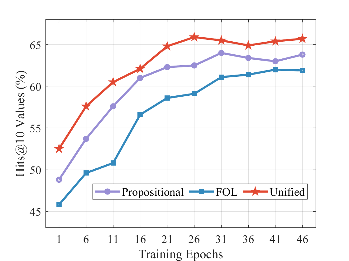
### Visual Description
## Line Chart: Performance of Three Methods Over Training Epochs
### Overview
This image is a line chart comparing the performance of three different methods—labeled "Propositional," "FOL," and "Unified"—over the course of training. Performance is measured by the "Hits@10 Values (%)" metric across a series of training epochs. All three methods show an upward trend in performance, with the "Unified" method consistently achieving the highest scores.
### Components/Axes
* **Chart Type:** Multi-line chart with markers.
* **X-Axis (Horizontal):**
* **Label:** "Training Epochs"
* **Scale:** Linear, with major tick marks and labels at epochs: 1, 6, 11, 16, 21, 26, 31, 36, 41, 46.
* **Y-Axis (Vertical):**
* **Label:** "Hits@10 Values (%)"
* **Scale:** Linear, ranging from 45 to 65, with major tick marks at intervals of 5 (45, 50, 55, 60, 65).
* **Legend:**
* **Position:** Centered at the bottom of the chart area.
* **Entries:**
1. **Propositional:** Represented by a purple line with circular markers (●).
2. **FOL:** Represented by a blue line with square markers (■).
3. **Unified:** Represented by a red line with star markers (★).
### Detailed Analysis
**Data Series Trends and Approximate Values:**
| Epoch | Unified (%) | Propositional (%) | FOL (%) |
| :---- | :---------- | :---------------- | :------ |
| 1 | ~52.5 | ~49.0 | ~46.0 |
| 6 | ~57.5 | ~54.0 | ~49.5 |
| 11 | ~60.5 | ~57.5 | ~51.0 |
| 16 | ~62.0 | ~61.0 | ~56.5 |
| 21 | ~65.0 | ~62.5 | ~58.5 |
| 26 | ~66.0 (Peak)| ~62.5 | ~59.0 |
| 31 | ~65.5 | ~64.0 (Peak) | ~61.0 |
| 36 | ~65.0 | ~63.5 | ~61.5 |
| 41 | ~65.5 | ~63.0 | ~62.0 |
| 46 | ~66.0 | ~64.0 | ~62.0 |
**Trend Summaries:**
1. **Unified (Red line, ★ markers):**
* **Trend:** Shows the steepest initial ascent and maintains the highest performance throughout. It peaks around epoch 26 and then plateaus with minor fluctuations.
2. **Propositional (Purple line, ● markers):**
* **Trend:** Starts in the middle, shows strong growth until around epoch 31, after which it slightly declines and stabilizes. It consistently performs between the Unified and FOL methods.
3. **FOL (Blue line, ■ markers):**
* **Trend:** Starts the lowest but shows steady, consistent improvement. Its growth rate is slightly less steep than the others initially, but it continues to climb steadily, nearly converging with the Propositional method by the end.
### Key Observations
1. **Performance Hierarchy:** A clear and consistent ranking is maintained: Unified > Propositional > FOL.
2. **Convergence:** The performance gap between the three methods narrows significantly over time. The initial large gap between FOL and the others at epoch 1 (~6-7%) shrinks to a much smaller gap by epoch 46 (~2-4%).
3. **Plateauing:** All three methods show signs of performance plateauing after approximately epoch 26-31, suggesting diminishing returns from further training beyond this point.
4. **Peak Performance:** The Unified method achieves the highest overall value (~66%), while the FOL method shows the most consistent, uninterrupted growth.
### Interpretation
The chart demonstrates the comparative learning efficiency and final performance ceiling of three distinct approaches (likely related to knowledge representation or reasoning in AI, given the labels "Propositional" and "FOL" - First-Order Logic).
* The **"Unified"** method is the most effective, learning faster and reaching a higher performance plateau. This suggests that integrating or unifying the approaches behind the other two methods yields superior results for the "Hits@10" task.
* The **"Propositional"** method serves as a middle-ground performer. Its slight decline after epoch 31 could indicate potential overfitting or instability in later training stages compared to the more robust Unified method.
* The **"FOL"** method, while starting from a lower baseline, demonstrates reliable and steady learning. Its trajectory suggests it may require more training epochs to reach its full potential, but it shows no signs of performance degradation.
The narrowing gap between the lines is a critical insight. It indicates that given sufficient training time (around 40+ epochs), the choice of method becomes less critical for final performance, although the Unified approach retains a clear advantage. This could inform decisions about resource allocation: if training time or compute is limited, the Unified method is the best choice; if training can be extended, the performance difference between methods becomes less pronounced.
</details>
(a) WN18RR of SKG T.
<details>
<summary>extracted/6596839/fig/zhexian2.png Details</summary>
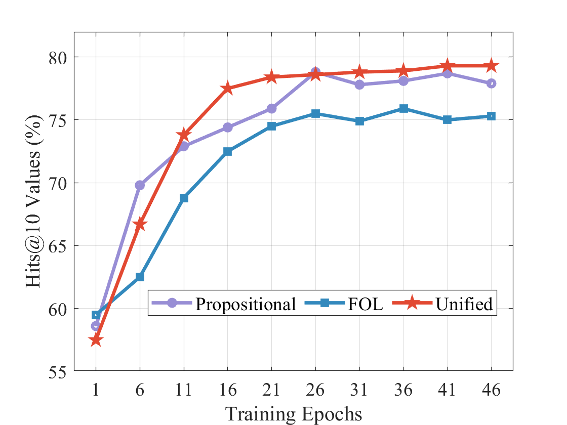
### Visual Description
## Line Chart: Hits@10 Values (%) vs. Training Epochs
### Overview
This image is a line chart comparing the performance of three different models or methods—labeled "Propositional," "FOL," and "Unified"—over the course of training. Performance is measured by the "Hits@10 Values (%)" metric, plotted against the number of "Training Epochs." The chart demonstrates how each method's accuracy evolves and stabilizes as training progresses.
### Components/Axes
* **Chart Type:** Multi-line chart with markers.
* **Y-Axis:**
* **Label:** `Hits@10 Values (%)`
* **Scale:** Linear, ranging from 55 to 80.
* **Major Ticks:** 55, 60, 65, 70, 75, 80.
* **X-Axis:**
* **Label:** `Training Epochs`
* **Scale:** Linear, with labeled ticks at specific intervals.
* **Major Ticks (Labeled):** 1, 6, 11, 16, 21, 26, 31, 36, 41, 46.
* **Legend:**
* **Position:** Centered at the bottom of the chart area.
* **Entries:**
1. **Propositional:** Represented by a purple line with circular markers (●).
2. **FOL:** Represented by a blue line with square markers (■).
3. **Unified:** Represented by a red line with star markers (★).
### Detailed Analysis
The following table reconstructs the approximate data points for each series, derived from visual inspection of the chart. Values are estimates based on marker positions relative to the grid lines.
| Training Epoch | Propositional (Purple, ●) | FOL (Blue, ■) | Unified (Red, ★) |
| :--- | :--- | :--- | :--- |
| **1** | ~58.5% | ~59.5% | ~57.5% |
| **6** | ~70.0% | ~62.5% | ~66.5% |
| **11** | ~73.0% | ~68.8% | ~74.0% |
| **16** | ~74.5% | ~72.5% | ~77.5% |
| **21** | ~76.0% | ~74.5% | ~78.5% |
| **26** | ~79.0% | ~75.5% | ~78.8% |
| **31** | ~78.0% | ~75.0% | ~79.0% |
| **36** | ~78.2% | ~76.0% | ~79.2% |
| **41** | ~78.8% | ~75.0% | ~79.5% |
| **46** | ~78.0% | ~75.2% | ~79.5% |
**Trend Verification:**
* **Unified (Red ★):** Shows the steepest initial ascent, surpassing the other two series by epoch 11. It continues to rise steadily, plateauing at the highest value (~79.5%) from epoch 41 onward.
* **Propositional (Purple ●):** Also rises sharply in early epochs, peaking at epoch 26 (~79.0%). After this peak, it exhibits a slight, gradual decline, ending at ~78.0%.
* **FOL (Blue ■):** Demonstrates the most gradual and consistent increase. It never surpasses the other two series after the initial epoch. Its performance stabilizes in the mid-70s range from epoch 21 onward.
### Key Observations
1. **Performance Hierarchy:** After the very first epoch, a clear and consistent performance hierarchy is established and maintained: **Unified > Propositional > FOL**.
2. **Convergence:** All three methods show signs of convergence (performance plateau) after approximately 25-30 training epochs.
3. **Early Dynamics:** The most significant performance gains for all models occur within the first 15-20 epochs.
4. **Stability:** The "Unified" method appears the most stable at its peak, showing almost no decline. The "Propositional" method shows a minor but noticeable performance drop after its peak. The "FOL" method is stable but at a lower performance level.
### Interpretation
The data suggests that the "Unified" approach is the most effective for this task, as measured by Hits@10 accuracy. It not only learns faster (steeper initial slope) but also achieves a higher final performance ceiling than the "Propositional" and "FOL" (First-Order Logic) methods.
The "Propositional" method performs strongly initially, even matching "Unified" at epoch 26, but its slight subsequent decline could indicate a tendency toward mild overfitting or instability in later training stages compared to the unified model.
The "FOL" method, while showing steady learning, consistently underperforms the other two. This might imply that the constraints or representations inherent to pure first-order logic are less expressive or less suited for this specific learning task compared to the propositional or unified representations.
The chart effectively demonstrates the advantage of the "Unified" model, which likely combines the strengths of the other two paradigms, resulting in superior and more robust learning outcomes over the full training cycle. The plateau across all models indicates that further training beyond ~45 epochs is unlikely to yield significant improvements for any of these approaches.
</details>
(b) ICEWS14 of TKG I.
<details>
<summary>extracted/6596839/fig/zhexian3.png Details</summary>
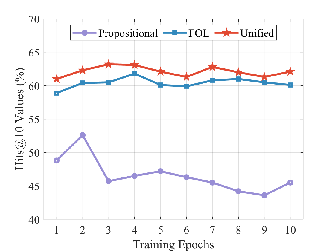
### Visual Description
## Line Chart: Performance Comparison of Three Methods Over Training Epochs
### Overview
The image is a line chart comparing the performance of three different methods—labeled "Propositional," "FOL," and "Unified"—over the course of 10 training epochs. Performance is measured by the "Hits@10 Values (%)" metric. The chart demonstrates that the "Unified" method consistently achieves the highest performance, followed by "FOL," with "Propositional" showing significantly lower and more variable results.
### Components/Axes
* **Chart Type:** Multi-line chart with markers.
* **X-Axis:** Labeled "Training Epochs". It is a linear scale with major tick marks and labels for each integer from 1 to 10.
* **Y-Axis:** Labeled "Hits@10 Values (%)". It is a linear scale ranging from 40 to 70, with major tick marks and labels at intervals of 5 (40, 45, 50, 55, 60, 65, 70).
* **Legend:** Positioned at the top-center of the chart area, inside a rectangular box. It contains three entries:
1. **Propositional:** Represented by a purple line with circular markers (●).
2. **FOL:** Represented by a blue line with square markers (■).
3. **Unified:** Represented by a red line with star markers (★).
* **Grid:** A light gray grid is present, aligned with the major ticks of both axes.
### Detailed Analysis
**Data Series and Trends:**
1. **Unified (Red line, Star markers):**
* **Trend:** Shows a generally stable, high-performance trend with minor fluctuations. It starts high, peaks slightly around epochs 3-4, dips slightly at epoch 6, and recovers.
* **Approximate Data Points (Epoch, %):**
* Epoch 1: ~61.0%
* Epoch 2: ~62.5%
* Epoch 3: ~63.5%
* Epoch 4: ~63.5%
* Epoch 5: ~62.5%
* Epoch 6: ~61.5%
* Epoch 7: ~63.0%
* Epoch 8: ~62.0%
* Epoch 9: ~61.5%
* Epoch 10: ~62.5%
2. **FOL (Blue line, Square markers):**
* **Trend:** Shows a stable performance trend, consistently positioned below the "Unified" line but above the "Propositional" line. It exhibits a slight upward trend from epoch 1 to 4, then remains relatively flat with minor variations.
* **Approximate Data Points (Epoch, %):**
* Epoch 1: ~59.0%
* Epoch 2: ~60.5%
* Epoch 3: ~60.5%
* Epoch 4: ~62.0%
* Epoch 5: ~60.0%
* Epoch 6: ~60.0%
* Epoch 7: ~61.0%
* Epoch 8: ~61.0%
* Epoch 9: ~60.5%
* Epoch 10: ~60.0%
3. **Propositional (Purple line, Circular markers):**
* **Trend:** Shows a highly variable and overall declining trend. It starts at a moderate level, spikes sharply at epoch 2, then drops significantly and continues a gradual decline with a slight recovery at the final epoch.
* **Approximate Data Points (Epoch, %):**
* Epoch 1: ~49.0%
* Epoch 2: ~52.5% (Peak)
* Epoch 3: ~45.5%
* Epoch 4: ~46.5%
* Epoch 5: ~47.0%
* Epoch 6: ~46.0%
* Epoch 7: ~45.5%
* Epoch 8: ~44.0%
* Epoch 9: ~43.5% (Lowest point)
* Epoch 10: ~45.5%
### Key Observations
1. **Performance Hierarchy:** A clear and consistent hierarchy is maintained throughout all 10 epochs: Unified > FOL > Propositional.
2. **Stability vs. Volatility:** The "Unified" and "FOL" methods demonstrate relatively stable performance after the initial epochs. In contrast, the "Propositional" method is highly volatile, with a dramatic peak at epoch 2 followed by a steep decline.
3. **Convergence:** The "FOL" and "Unified" lines show some convergence around epoch 4, where their performance gap is smallest (~1.5%). The gap widens again afterward.
4. **Propositional Anomaly:** The sharp performance spike for the "Propositional" method at epoch 2 is a significant outlier compared to its performance in all other epochs and the behavior of the other two methods.
### Interpretation
The data strongly suggests that the "Unified" approach is the most effective and robust method for this task, as measured by the Hits@10 metric. It not only achieves the highest absolute performance but also maintains stability across training. The "FOL" method is a reliable second-best, showing consistent, though slightly lower, results.
The "Propositional" method's performance is concerning. Its initial spike suggests a potential for good performance, but the subsequent rapid degradation indicates instability, possibly due to overfitting, an inappropriate learning rate, or a fundamental limitation in the method's ability to generalize beyond early training phases. The fact that it never recovers to its epoch-2 peak implies that the early gain was not sustainable.
From a research or engineering perspective, this chart would argue for adopting the "Unified" method. It also flags the "Propositional" method for diagnostic investigation—understanding why it fails after epoch 2 could provide valuable insights into the problem domain or the method's design. The consistent gap between "FOL" and "Unified" indicates that whatever component or strategy the "Unified" method adds over "FOL" provides a measurable and persistent benefit.
</details>
(c) ICEWS14 of TKG E.
<details>
<summary>extracted/6596839/fig/zhexian4.png Details</summary>
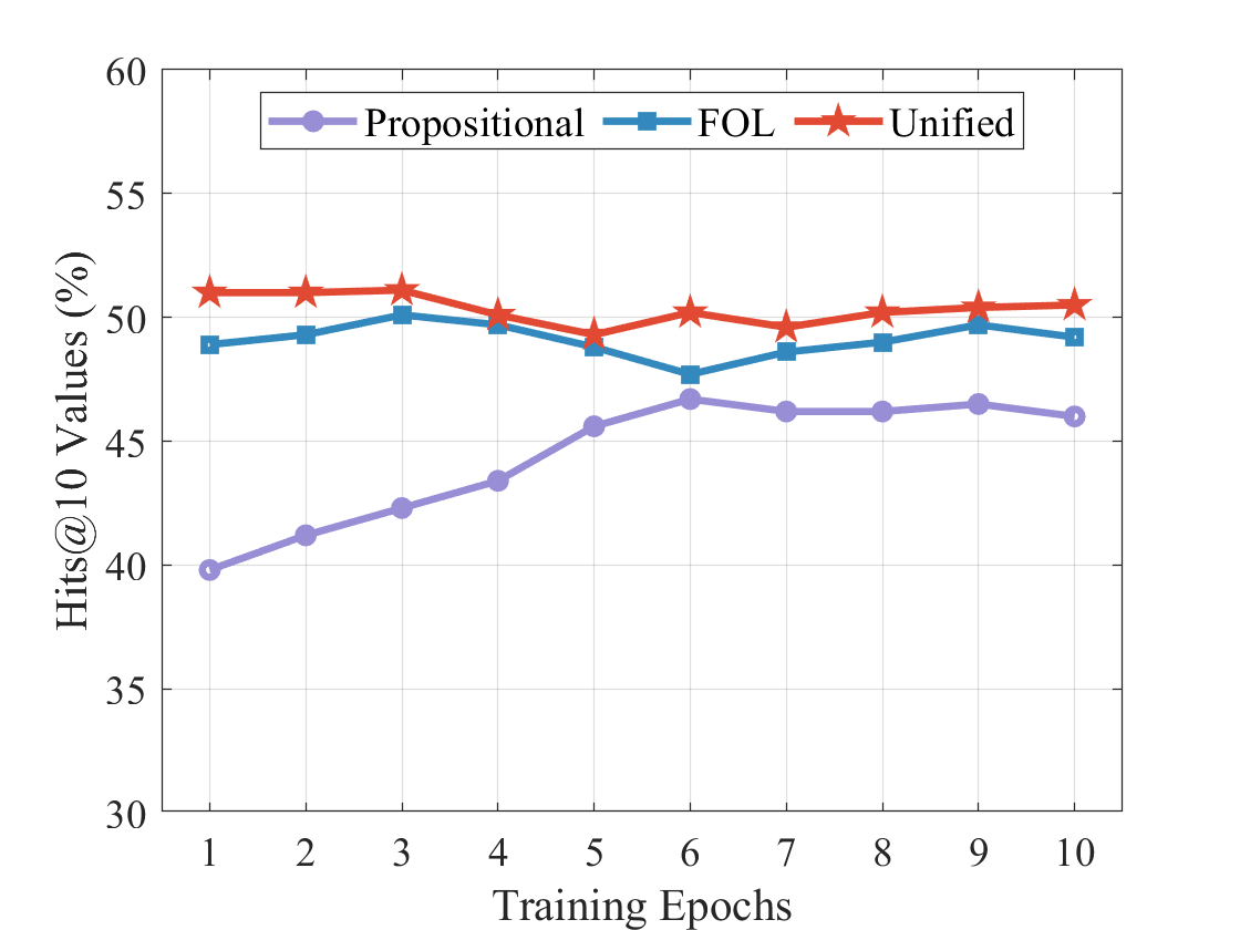
### Visual Description
## Line Chart: Hits@10 Values over Training Epochs
### Overview
The image displays a line chart comparing the performance of three different methods or models—labeled "Propositional," "FOL," and "Unified"—over the course of 10 training epochs. The performance metric is "Hits@10 Values," measured as a percentage. The chart shows that the "Unified" method consistently achieves the highest performance, followed by "FOL," with "Propositional" starting the lowest but showing the most significant improvement over time.
### Components/Axes
* **Chart Type:** Multi-line chart with markers.
* **X-Axis:**
* **Label:** "Training Epochs"
* **Scale:** Linear, integer values from 1 to 10.
* **Y-Axis:**
* **Label:** "Hits@10 Values (%)"
* **Scale:** Linear, ranging from 30 to 60, with major tick marks every 5 units (30, 35, 40, 45, 50, 55, 60).
* **Legend:**
* **Position:** Top-center of the chart area, enclosed in a box.
* **Series:**
1. **Propositional:** Represented by a purple line with circular markers (●).
2. **FOL:** Represented by a blue line with square markers (■).
3. **Unified:** Represented by a red line with star markers (★).
### Detailed Analysis
**Data Series Trends and Approximate Values:**
1. **Propositional (Purple, Circles):**
* **Trend:** Shows a steady, monotonic upward trend throughout the training epochs. It starts as the lowest-performing method but closes the gap significantly.
* **Approximate Data Points:**
* Epoch 1: ~40.0%
* Epoch 2: ~41.2%
* Epoch 3: ~42.3%
* Epoch 4: ~43.4%
* Epoch 5: ~45.6%
* Epoch 6: ~46.8%
* Epoch 7: ~46.2%
* Epoch 8: ~46.2%
* Epoch 9: ~46.6%
* Epoch 10: ~46.0%
2. **FOL (Blue, Squares):**
* **Trend:** Starts high, peaks early, experiences a dip in the middle epochs, and then recovers to a stable level. It remains the second-best performer throughout.
* **Approximate Data Points:**
* Epoch 1: ~49.0%
* Epoch 2: ~49.4%
* Epoch 3: ~50.2% (Peak)
* Epoch 4: ~49.8%
* Epoch 5: ~49.0%
* Epoch 6: ~47.8% (Trough)
* Epoch 7: ~48.8%
* Epoch 8: ~49.2%
* Epoch 9: ~49.8%
* Epoch 10: ~49.4%
3. **Unified (Red, Stars):**
* **Trend:** Maintains a relatively flat and stable high performance across all epochs, with very minor fluctuations. It is consistently the top-performing method.
* **Approximate Data Points:**
* Epoch 1: ~51.0%
* Epoch 2: ~51.0%
* Epoch 3: ~51.2%
* Epoch 4: ~50.2%
* Epoch 5: ~49.4%
* Epoch 6: ~50.4%
* Epoch 7: ~49.8%
* Epoch 8: ~50.4%
* Epoch 9: ~50.6%
* Epoch 10: ~50.6%
### Key Observations
1. **Performance Hierarchy:** A clear and consistent hierarchy is established from the first epoch: Unified > FOL > Propositional. This order never changes.
2. **Convergence:** The "Propositional" method shows the most dramatic learning curve, improving by approximately 6 percentage points over 10 epochs. The gap between it and the other two methods narrows considerably.
3. **Stability vs. Volatility:** The "Unified" method is the most stable. The "FOL" method shows more volatility, particularly the notable dip at epoch 6. The "Propositional" method shows a smooth, learning-driven increase.
4. **Peak Performance:** The highest single value on the chart is achieved by the "Unified" method at epochs 1, 2, and 3 (~51.0-51.2%). The peak for "FOL" is at epoch 3 (~50.2%).
### Interpretation
This chart likely compares different logical reasoning or knowledge representation approaches ("Propositional" logic, "First-Order Logic" (FOL), and a "Unified" framework) within a machine learning context, evaluating their effectiveness on a retrieval or prediction task (measured by Hits@10).
The data suggests that the **"Unified" approach is superior and robust**, delivering high accuracy from the start and maintaining it without significant degradation. This implies it may combine the strengths of the other approaches or use a more effective underlying architecture.
The **"FOL" approach performs well but is less stable**, as evidenced by its mid-training dip. This could indicate sensitivity to certain training phases or data batches. Its early peak suggests it learns useful patterns quickly but may be prone to overfitting or interference before stabilizing.
The **"Propositional" approach starts with limited capability but demonstrates strong, consistent learning**. Its upward trajectory suggests that with more training epochs beyond 10, it might eventually converge with or even surpass the other methods, though it begins from a significant deficit. The chart captures it in a phase of active improvement.
Overall, the visualization argues for the effectiveness of the "Unified" method, showing it provides both the highest and most reliable performance across the observed training period.
</details>
(d) ICEWS18 of TKG E.
Figure 5: The impacts of propositional and FOL reasoning on transductive, interpolation, and extrapolation scenarios. It is generally observed that the unified model has a better performance compared with the single propositional or FOL setting, demonstrating the validity and rationality of the unified mechanism in Tunsr.
For interpolation reasoning in Table V, the performance of Tunsr surpasses that of mainstream neural reasoning methods. It achieves optimal results on seven out of eight metrics. Compared with TNTComplEx of the previous classic tensor-decomposition method, the improvement on each metric is 0.028, 4.21%, 3.61%, 4.16%, 0.035, 0.89%, 3.67%, and 2.95%, respectively. Moreover, compared with the state-of-the-art model TeAST that encodes temporal knowledge graph embeddings via the archimedean spiral timeline, Tunsr also has 0.011, 0.21%, 1.41%, 1.96%, 0.022, -0.51%, 1.47%, and 1.05% performance advantages (only slightly smaller on Hits@1 metric of ICEWS0515 dataset).
As Table VI shows for extrapolation reasoning, Tunsr also performs better. Compared with 10 neural reasoning methods, Tunsr has obvious performance advantages. For instance, it achieves 14.19%, 27.02%, and 14,17% Hits@10 improvement on three datasets against the tensor-decomposition method TNTComplEx. Additionally, Tunsr outperforms symbolic rule-based methods, i.e., AnyBURL, TLogic, and TR-Rules, achieving average improvements of 0.061, 5.57%, 7.01%, 6.94%, 0.069, 5.98%, 8.21%, 8.06%, 0.045, 4.08%, 5.36%, and 5.63% on all 12 evaluation metrics. Moreover, Tunsr excels three neurosymbolic methods (xERTE, TITer and INFER) across all datasets. Furthermore, compared with the previous study TECHS, Tunsr also has the performance boost, which shows 1.37%, 0.96%, and 1.26% Hits@10 metric gains.
In summary, the experimental results on four reasoning scenarios demonstrate the effectiveness and superiority of the proposed unified framework Tunsr. It shows the rationality of the unified mechanism at both the methodological and application perspectives and verifies the tremendous potential for future KG reasoning frameworks.
### 4.3 Ablation Studies (RQ2)
To explore the impacts of propositional and FOL parts on KG reasoning performance, we carry out ablation studies on transductive (WN18RR), interpolation (ICEWS14), and extrapolation (ICEWS14 and ICEWS18) scenarios in Figure 5. As inductive reasoning is entity-independent, we only conduct experiments using FOL reasoning for it. In each line chart, we depict the performance trends associated with propositional, FOL, and unified reasoning throughout the training epochs. In the propositional/FOL setting, we set $\lambda$ in the Eq. (14) as 0/1, indicating the model only uses propositional/FOL reasoning to get the answer. In the unified setting, the value of $\lambda$ is the dynamic learned by embeddings. From the figure, it is generally observed that the unified setting has a better performance compared with the single propositional or FOL setting. It is noteworthy that propositional and FOL display unique characteristics when applied to diverse datasets. For transductive and interpolation reasoning (Figures 5 and 5), the performance of propositional reasoning consistently surpasses that of FOL, despite both exhibiting continuous improvement throughout the training process. However, it is contrary to the results on the extrapolation scenario (Figures 5 and 5), where FOL reasoning has performance advantages. It is noted that propositional reasoning performs well in ICEWS18 while badly in ICEWS14 under the extrapolation setting. This may be caused by the structural differences between ICEWS14 and ICEWS18. Compared with ICEWS14, the graph structure of ICEWS18 is notably denser (8.94 vs. 16.19 in node degree). So propositional reasoning in ICEWS18 can capture more comprehensive pattern semantics and exhibit robust generalization in testing scenarios. These observations indicate that propositional and FOL reasoning emphasizes distinct aspects of knowledge. Thus, combining them allows for the synergistic exploitation of their respective strengths, resulting in an enhanced overall effect.
<details>
<summary>extracted/6596839/fig/bar1.png Details</summary>
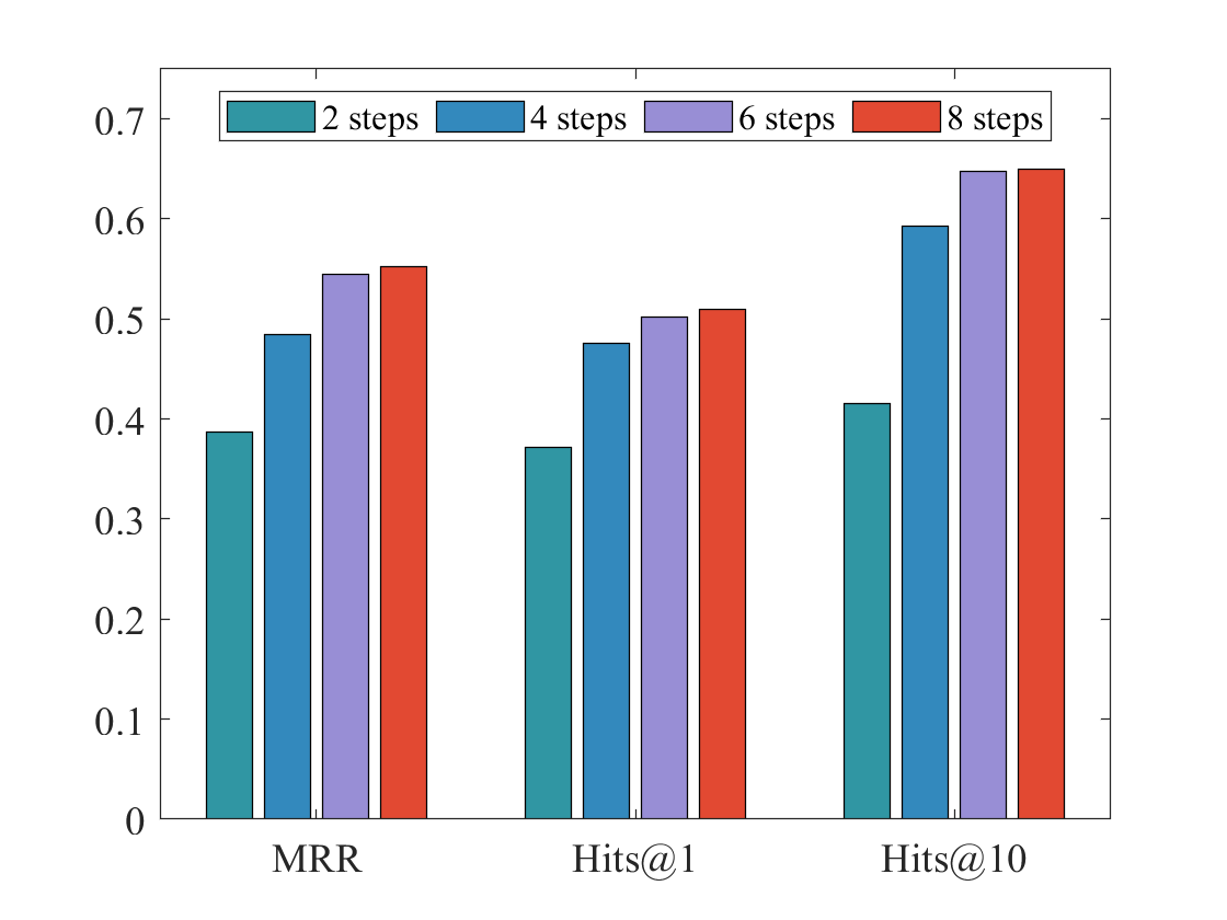
### Visual Description
## Grouped Bar Chart: Performance Metrics by Step Count
### Overview
The image displays a grouped bar chart comparing the performance of a system across three different evaluation metrics (MRR, Hits@1, Hits@10) as a function of the number of steps (2, 4, 6, 8). The chart demonstrates a clear positive correlation between the number of steps and the performance score for all three metrics.
### Components/Axes
* **Chart Type:** Grouped Bar Chart.
* **X-Axis (Categories):** Three distinct metric categories are labeled at the bottom:
* `MRR` (Mean Reciprocal Rank)
* `Hits@1`
* `Hits@10`
* **Y-Axis (Scale):** A linear numerical scale on the left side, ranging from `0` to `0.7` with major tick marks at intervals of `0.1` (0, 0.1, 0.2, 0.3, 0.4, 0.5, 0.6, 0.7).
* **Legend:** Positioned at the top-center of the chart area, enclosed in a box. It defines four data series by color:
* Teal bar: `2 steps`
* Blue bar: `4 steps`
* Purple bar: `6 steps`
* Red bar: `8 steps`
* **Data Series:** For each of the three x-axis categories, there is a cluster of four bars, one for each step count, ordered from left to right as 2, 4, 6, and 8 steps.
### Detailed Analysis
**Trend Verification:** For every metric (MRR, Hits@1, Hits@10), the bar height increases monotonically with the number of steps. The trend is consistently upward from 2 steps to 8 steps.
**Approximate Data Points (Visual Estimation):**
1. **MRR Category (Leftmost cluster):**
* 2 steps (Teal): ~0.39
* 4 steps (Blue): ~0.49
* 6 steps (Purple): ~0.55
* 8 steps (Red): ~0.555 (Slightly higher than 6 steps)
2. **Hits@1 Category (Center cluster):**
* 2 steps (Teal): ~0.37
* 4 steps (Blue): ~0.48
* 6 steps (Purple): ~0.50
* 8 steps (Red): ~0.51
3. **Hits@10 Category (Rightmost cluster):**
* 2 steps (Teal): ~0.42
* 4 steps (Blue): ~0.595
* 6 steps (Purple): ~0.65
* 8 steps (Red): ~0.655 (Marginally higher than 6 steps)
### Key Observations
* **Consistent Improvement:** Performance improves with more steps across all metrics. The jump from 2 to 4 steps is the most significant for each metric.
* **Diminishing Returns:** The performance gain from 6 to 8 steps is very small for all metrics, suggesting a plateau effect.
* **Metric Comparison:** The `Hits@10` metric achieves the highest absolute values (peaking ~0.655), followed by `MRR` (~0.555), and then `Hits@1` (~0.51). This is expected, as Hits@10 is a less strict metric than Hits@1.
* **Relative Performance:** The ranking of step counts (2 < 4 < 6 < 8) is perfectly preserved across all three evaluation metrics.
### Interpretation
This chart presents strong empirical evidence that increasing the number of steps in the evaluated process leads to better system performance, as measured by ranking quality (MRR) and accuracy (Hits@k). The data suggests an optimal operating point may lie around 6 steps, as the marginal benefit of adding two more steps (to 8) is minimal. The consistent trend across different metrics reinforces the robustness of the finding. The chart effectively communicates that computational investment (more steps) yields measurable returns in output quality, but with clear saturation.
</details>
(a) WN18RR of SKG T.
<details>
<summary>extracted/6596839/fig/bar2.png Details</summary>
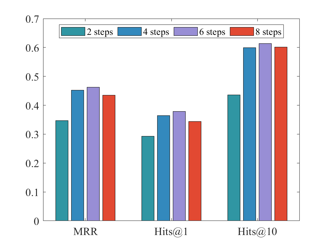
### Visual Description
## Grouped Bar Chart: Performance Metrics by Step Count
### Overview
The image displays a grouped bar chart comparing three performance metrics (MRR, Hits@1, Hits@10) across four different step counts (2, 4, 6, and 8 steps). The chart illustrates how these metrics change as the number of steps increases.
### Components/Axes
* **Chart Type:** Grouped Bar Chart.
* **X-Axis (Categories):** Three distinct metric categories are labeled at the bottom:
* `MRR` (Mean Reciprocal Rank)
* `Hits@1`
* `Hits@10`
* **Y-Axis (Scale):** A numerical scale on the left side, ranging from `0` to `0.7` in increments of `0.1`. There is no explicit axis title.
* **Legend:** Positioned at the top-center of the chart area, enclosed in a box. It defines four data series by color:
* Teal bar: `2 steps`
* Blue bar: `4 steps`
* Purple bar: `6 steps`
* Red bar: `8 steps`
### Detailed Analysis
The chart presents the following approximate values for each metric and step count. Values are estimated based on bar height relative to the y-axis grid.
**1. MRR (Left Group):**
* **Trend:** Performance increases from 2 to 6 steps, then slightly decreases at 8 steps.
* **Data Points:**
* 2 steps (Teal): ~0.35
* 4 steps (Blue): ~0.45
* 6 steps (Purple): ~0.46 (Highest in this group)
* 8 steps (Red): ~0.43
**2. Hits@1 (Center Group):**
* **Trend:** Similar pattern to MRR, with a peak at 6 steps.
* **Data Points:**
* 2 steps (Teal): ~0.29
* 4 steps (Blue): ~0.36
* 6 steps (Purple): ~0.38 (Highest in this group)
* 8 steps (Red): ~0.34
**3. Hits@10 (Right Group):**
* **Trend:** Shows the highest overall values. Performance increases sharply from 2 to 4 steps, peaks at 6 steps, and remains very high at 8 steps.
* **Data Points:**
* 2 steps (Teal): ~0.44
* 4 steps (Blue): ~0.60
* 6 steps (Purple): ~0.61 (Highest in the entire chart)
* 8 steps (Red): ~0.60
### Key Observations
1. **Consistent Peak at 6 Steps:** For all three metrics (MRR, Hits@1, Hits@10), the 6-step configuration (purple bar) yields the highest performance.
2. **Diminishing Returns/Decline at 8 Steps:** After the peak at 6 steps, performance for MRR and Hits@1 decreases when moving to 8 steps. Hits@10 performance plateaus, showing only a negligible decrease from 6 to 8 steps.
3. **Metric Hierarchy:** The `Hits@10` metric consistently shows the highest values across all step counts, followed by `MRR`, and then `Hits@1`. This is expected, as Hits@10 is a less strict metric than Hits@1.
4. **Lowest Baseline:** The 2-step configuration (teal bar) is the worst performer for every metric.
### Interpretation
This chart likely evaluates the performance of a multi-step reasoning or retrieval system (e.g., in knowledge graph completion or question answering). The data suggests a clear relationship between the number of reasoning steps and model performance:
* **Optimal Complexity:** There is a "sweet spot" at **6 steps**, where the system achieves its best results across all measured metrics. This indicates that increasing computational steps improves performance up to a point.
* **Over-complexity Penalty:** Pushing beyond the optimal point to **8 steps** does not yield further benefits and may even be detrimental for stricter metrics (MRR, Hits@1). This could be due to error propagation in longer reasoning chains, increased difficulty in optimization, or the model beginning to overfit to the step-generation process.
* **Practical Implication:** The findings argue for careful tuning of the step count parameter. Simply maximizing steps is not an effective strategy; the system's performance is sensitive to this hyperparameter, with 6 steps being the most effective in this specific evaluation. The near-parity between 6 and 8 steps for Hits@10 suggests that for a more lenient evaluation, the cost of additional computation (8 steps) may not be justified.
</details>
(b) FB15k-237 v3 of SKG I.
<details>
<summary>extracted/6596839/fig/bar3.png Details</summary>
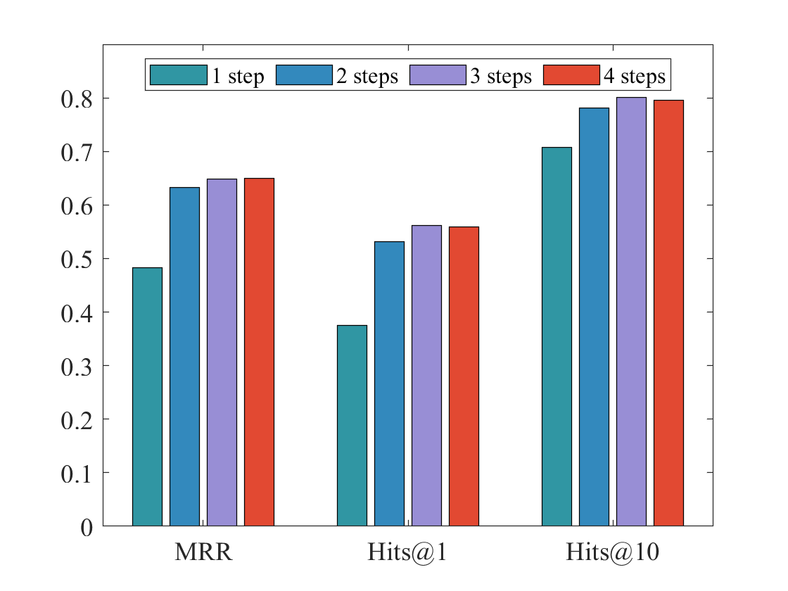
### Visual Description
## Bar Chart: Performance Metrics by Step Count
### Overview
The image is a grouped bar chart comparing the performance of a system across three evaluation metrics (MRR, Hits@1, Hits@10) when configured with 1, 2, 3, or 4 steps. The chart demonstrates how increasing the number of steps generally improves performance, with diminishing returns observed after 3 steps.
### Components/Axes
* **Chart Type:** Grouped vertical bar chart.
* **X-Axis (Categories):** Three distinct metric groups are labeled at the bottom:
* `MRR` (Mean Reciprocal Rank)
* `Hits@1`
* `Hits@10`
* **Y-Axis (Scale):** A linear numerical scale on the left, ranging from `0` to `0.8` with major tick marks at every `0.1` interval (0, 0.1, 0.2, 0.3, 0.4, 0.5, 0.6, 0.7, 0.8).
* **Legend:** Positioned at the top-center of the chart area. It defines four data series by color:
* **Teal bar:** `1 step`
* **Blue bar:** `2 steps`
* **Light Purple bar:** `3 steps`
* **Red bar:** `4 steps`
### Detailed Analysis
The chart presents approximate numerical values for each bar, derived from visual inspection against the y-axis scale.
**1. MRR Group (Leftmost cluster):**
* **Trend:** Performance increases sharply from 1 to 2 steps, then more gradually to 3 steps, with 4 steps showing no further gain.
* **Data Points (Approximate):**
* 1 step (Teal): ~0.48
* 2 steps (Blue): ~0.63
* 3 steps (Purple): ~0.65
* 4 steps (Red): ~0.65 (appears equal to or marginally lower than 3 steps)
**2. Hits@1 Group (Middle cluster):**
* **Trend:** A similar pattern to MRR: a large jump from 1 to 2 steps, a smaller increase to 3 steps, and a plateau at 4 steps.
* **Data Points (Approximate):**
* 1 step (Teal): ~0.38
* 2 steps (Blue): ~0.53
* 3 steps (Purple): ~0.56
* 4 steps (Red): ~0.56 (appears equal to 3 steps)
**3. Hits@10 Group (Rightmost cluster):**
* **Trend:** This metric shows the highest absolute values. Performance improves from 1 to 3 steps, with 3 steps achieving the peak. The 4-step configuration shows a very slight decrease compared to 3 steps.
* **Data Points (Approximate):**
* 1 step (Teal): ~0.71
* 2 steps (Blue): ~0.78
* 3 steps (Purple): ~0.80
* 4 steps (Red): ~0.79 (slightly lower than 3 steps)
### Key Observations
1. **Consistent Hierarchy:** For all three metrics, the `1 step` configuration performs the worst, and the `3 steps` configuration performs the best or ties for best.
2. **Diminishing Returns:** The most significant performance gain occurs when moving from `1 step` to `2 steps`. The gain from `2 steps` to `3 steps` is positive but smaller. Moving from `3 steps` to `4 steps` yields no improvement (MRR, Hits@1) or a negligible decline (Hits@10).
3. **Metric Sensitivity:** The `Hits@10` metric shows the highest overall scores, indicating the system is more successful at placing a correct answer within the top 10 results than at placing it first (Hits@1) or achieving a high reciprocal rank (MRR).
4. **Visual Anomaly:** The `4 steps` (Red) bar in the `Hits@10` group is visually just a fraction shorter than the `3 steps` (Purple) bar, suggesting a potential slight performance degradation or noise at the highest step count for this metric.
### Interpretation
This chart likely evaluates a multi-step reasoning or retrieval process in an AI or information system. The data suggests a clear **optimal operating point at 3 steps**.
* **Performance vs. Cost:** The primary insight is that increasing computational steps improves output quality, but only up to a point. The system exhibits a classic "sweet spot" at 3 steps, where performance is maximized. Adding a fourth step appears to be inefficient, consuming more resources for no benefit or even a slight loss in accuracy (as seen in Hits@10). This could indicate over-processing, error accumulation, or that the problem's complexity is fully addressed within three steps.
* **Metric Relationship:** The consistent pattern across MRR, Hits@1, and Hits@10 reinforces the robustness of the finding. The system's ability to rank the correct answer highly (Hits@10) is strong, but its precision in ranking it first (Hits@1) is more sensitive to the step count, showing the largest relative improvement from 1 to 3 steps.
* **Practical Implication:** For deployment, configuring the system with 3 steps would be recommended to balance performance and computational cost. The 4-step configuration offers no advantage and may be wasteful. The significant gap between 1-step and multi-step performance underscores the necessity of the multi-step process for this task.
</details>
(c) ICEWS14 of TKG I.
<details>
<summary>extracted/6596839/fig/bar4.png Details</summary>
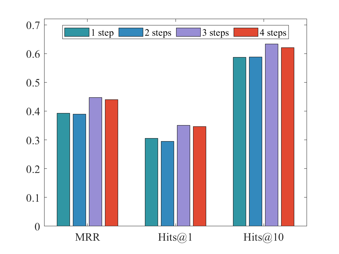
### Visual Description
## Grouped Bar Chart: Performance Metrics by Step Count
### Overview
The image displays a grouped bar chart comparing three performance metrics (MRR, Hits@1, Hits@10) across four different step counts (1 step, 2 steps, 3 steps, 4 steps). The chart illustrates how model performance varies with the number of steps for each evaluation metric.
### Components/Axes
* **Chart Type:** Grouped Bar Chart.
* **Y-Axis:** Numerical scale ranging from 0 to 0.7, with major tick marks at intervals of 0.1 (0, 0.1, 0.2, 0.3, 0.4, 0.5, 0.6, 0.7). The axis label is not explicitly stated but represents the score or value of the performance metrics.
* **X-Axis:** Categorical axis with three primary groups: "MRR", "Hits@1", and "Hits@10".
* **Legend:** Positioned at the top-center of the chart area. It defines four data series by color:
* Teal bar: "1 step"
* Blue bar: "2 steps"
* Light purple bar: "3 steps"
* Red-orange bar: "4 steps"
### Detailed Analysis
The chart presents the following approximate values for each metric and step count. Values are estimated based on bar height relative to the y-axis grid.
**1. MRR (Mean Reciprocal Rank) Group:**
* **1 step (Teal):** ~0.39
* **2 steps (Blue):** ~0.39
* **3 steps (Light Purple):** ~0.45
* **4 steps (Red-Orange):** ~0.44
* **Trend:** Performance is similar for 1 and 2 steps, increases noticeably for 3 steps, and shows a very slight decrease for 4 steps.
**2. Hits@1 Group:**
* **1 step (Teal):** ~0.305
* **2 steps (Blue):** ~0.295
* **3 steps (Light Purple):** ~0.35
* **4 steps (Red-Orange):** ~0.345
* **Trend:** Performance dips slightly from 1 to 2 steps, then increases for 3 steps, followed by a marginal decrease for 4 steps. This group has the lowest overall values.
**3. Hits@10 Group:**
* **1 step (Teal):** ~0.59
* **2 steps (Blue):** ~0.59
* **3 steps (Light Purple):** ~0.635
* **4 steps (Red-Orange):** ~0.62
* **Trend:** Performance is identical for 1 and 2 steps, peaks at 3 steps, and decreases slightly for 4 steps. This group has the highest overall values.
### Key Observations
1. **Consistent Peak at 3 Steps:** For all three metrics (MRR, Hits@1, Hits@10), the highest performance is achieved with "3 steps".
2. **Performance Plateau/Dip at 4 Steps:** After the peak at 3 steps, performance slightly declines for "4 steps" across all metrics.
3. **Metric Hierarchy:** The absolute values follow a clear hierarchy: Hits@10 scores are the highest (>0.59), followed by MRR (~0.39-0.45), and then Hits@1 (~0.295-0.35). This is expected, as Hits@10 is a more lenient metric than Hits@1.
4. **Similarity of 1 and 2 Steps:** For MRR and Hits@10, the performance for "1 step" and "2 steps" is nearly identical. For Hits@1, there is a small but visible decrease from 1 to 2 steps.
### Interpretation
The data suggests a non-linear relationship between the number of steps and model performance on these ranking metrics. Performance improves when moving from 1/2 steps to 3 steps, indicating that additional computation or reasoning steps are beneficial up to a point. However, the slight degradation at 4 steps implies potential diminishing returns or the introduction of noise/errors with excessive steps.
The consistent pattern across three different metrics (MRR, Hits@1, Hits@10) strengthens the conclusion that 3 steps is the optimal configuration among those tested for this specific task or model. The chart effectively communicates that more steps are not always better, and there exists a "sweet spot" for performance. This finding would be crucial for optimizing computational efficiency versus accuracy in a production system.
</details>
(d) ICEWS14 of TKG E.
Figure 6: The impacts of reasoning iterations which correspond to the length of the reasoning rules. It is evident that choosing the appropriate value is crucial for obtaining accurate reasoning results.
<details>
<summary>extracted/6596839/fig/bar3d1.png Details</summary>
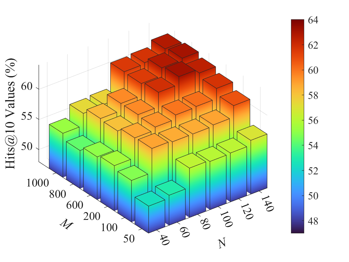
### Visual Description
## 3D Bar Chart: Hits@10 Values vs. Parameters M and N
### Overview
This image is a 3D bar chart visualizing the relationship between two parameters, **M** and **N**, and a performance metric called **Hits@10 Values (%)**. The chart uses both bar height and a color gradient to represent the metric's value. The overall trend shows that Hits@10 increases as both M and N increase.
### Components/Axes
* **Vertical Axis (Z-axis):** Labeled **"Hits@10 Values (%)"**. The scale runs from 50 to 60, with major tick marks at 50, 55, and 60.
* **Horizontal Axis 1 (X-axis, front-left):** Labeled **"M"**. The discrete values marked are: 50, 100, 200, 600, 800, 1000.
* **Horizontal Axis 2 (Y-axis, front-right):** Labeled **"N"**. The discrete values marked are: 40, 60, 80, 100, 120, 140.
* **Color Bar/Legend (Right side):** A vertical gradient bar mapping color to the Hits@10 value. The scale ranges from **48** (dark blue) to **64** (dark red), with labeled ticks at 48, 50, 52, 54, 56, 58, 60, 62, 64. This color scale is used to fill the bars, providing a secondary visual cue for the value.
### Detailed Analysis
The chart contains a 6x6 grid of bars, one for each combination of M and N. The value for each bar is estimated based on its height relative to the Z-axis and its color relative to the color bar. Values are approximate.
**Data Table (Estimated Hits@10 Values in %):**
| M \ N | 40 | 60 | 80 | 100 | 120 | 140 |
| :--- | :--- | :--- | :--- | :--- | :--- | :--- |
| **50** | ~50 (Blue) | ~51 (Light Blue) | ~52 (Cyan) | ~53 (Green-Cyan) | ~54 (Green) | ~55 (Yellow-Green) |
| **100** | ~51 (Light Blue) | ~52 (Cyan) | ~53 (Green-Cyan) | ~54 (Green) | ~55 (Yellow-Green) | ~56 (Yellow) |
| **200** | ~52 (Cyan) | ~53 (Green-Cyan) | ~54 (Green) | ~55 (Yellow-Green) | ~56 (Yellow) | ~57 (Light Orange) |
| **600** | ~54 (Green) | ~55 (Yellow-Green) | ~56 (Yellow) | ~57 (Light Orange) | ~58 (Orange) | ~59 (Dark Orange) |
| **800** | ~55 (Yellow-Green) | ~56 (Yellow) | ~57 (Light Orange) | ~58 (Orange) | ~59 (Dark Orange) | ~60 (Red-Orange) |
| **1000** | ~56 (Yellow) | ~57 (Light Orange) | ~58 (Orange) | ~59 (Dark Orange) | ~60 (Red-Orange) | ~61 (Red) |
**Trend Verification:**
* **For a fixed M (moving along an N-row):** The bar heights and colors consistently shift from blue/green towards yellow/orange/red as N increases from 40 to 140. This indicates a positive correlation between N and Hits@10.
* **For a fixed N (moving along an M-row):** The bar heights and colors consistently shift from blue/green towards yellow/orange/red as M increases from 50 to 1000. This indicates a positive correlation between M and Hits@10.
* **Overall Gradient:** The lowest values (~50%) are at the front corner (M=50, N=40). The highest values (~61-64%) are at the back corner (M=1000, N=140). The color gradient flows diagonally from the front-left (blue) to the back-right (red).
### Key Observations
1. **Monotonic Increase:** The performance metric (Hits@10) increases monotonically with both parameters M and N across the entire observed range. There are no visible dips or outliers where increasing a parameter leads to a decrease in value.
2. **Interaction Effect:** The increase appears synergistic. The gain from increasing M is more pronounced at higher values of N, and vice-versa. The steepest gradient (fastest color change) is along the diagonal from (M=50, N=40) to (M=1000, N=140).
3. **Value Range:** The observed Hits@10 values in this grid range from approximately **50%** to **64%**, as indicated by the color bar. The highest bars in the back corner approach the top of the color scale (dark red, ~64%).
### Interpretation
This chart likely presents the results of a parameter sensitivity analysis for a system where "Hits@10" is a key performance metric (common in information retrieval, recommendation systems, or machine learning evaluation). The parameters M and N could represent dimensions like model size, number of features, training iterations, or dataset characteristics.
The data suggests that **performance improves with larger values of both M and N**. The absence of a plateau or decline indicates that, within the tested ranges, the system has not yet reached a point of diminishing returns or overfitting for these parameters. The strongest performance is achieved by maximizing both parameters simultaneously. A decision-maker would use this chart to understand the trade-off: if computational resources are limited, they might choose a combination of M and N that meets a minimum acceptable Hits@10 threshold (e.g., 58%) while balancing cost. The clear, positive trend provides strong evidence for scaling up M and N to improve results.
</details>
(a) Performance on ICEWS14.
<details>
<summary>extracted/6596839/fig/bar3d2.png Details</summary>
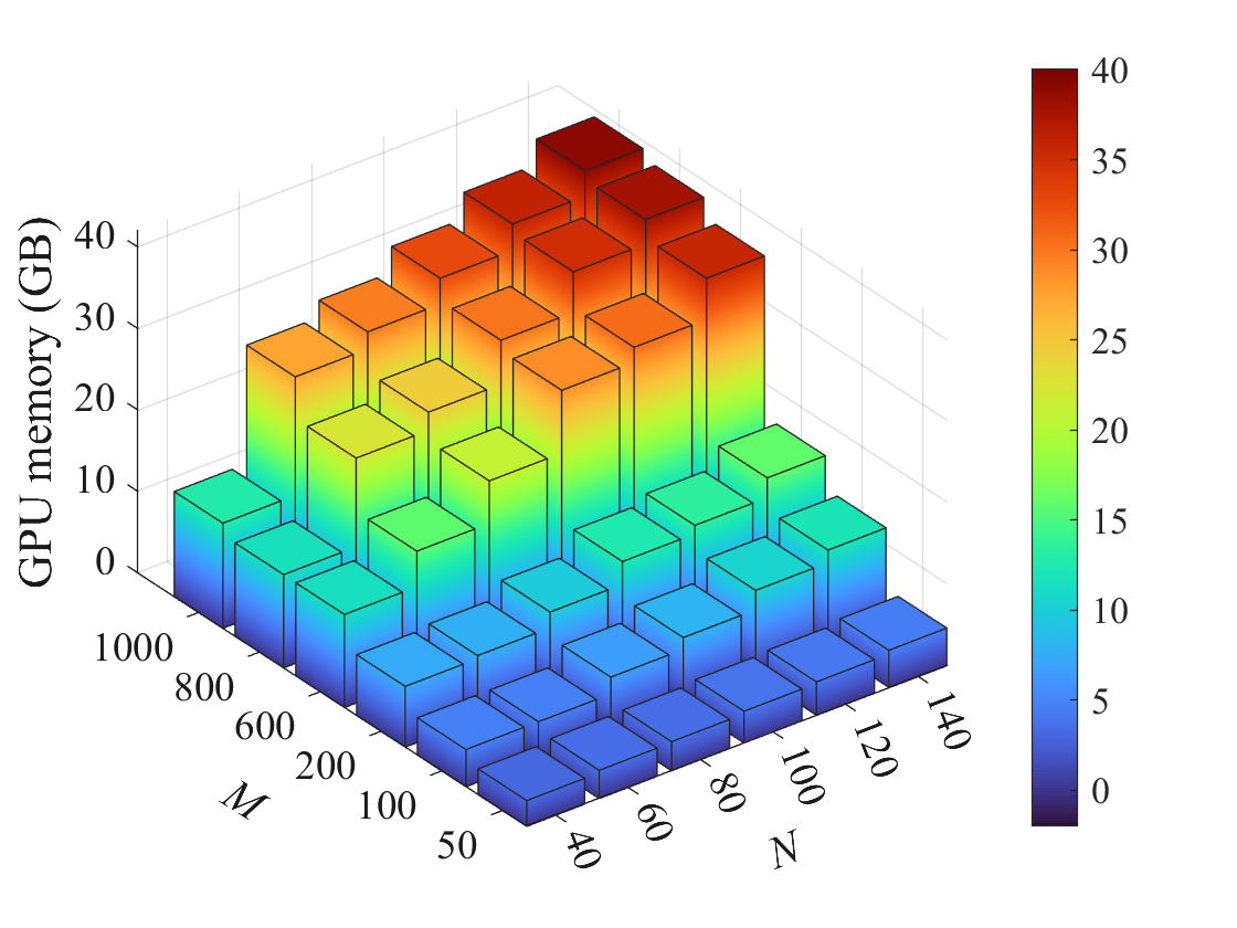
### Visual Description
## 3D Bar Chart: GPU Memory Consumption vs. Parameters M and N
### Overview
This image is a 3D bar chart visualizing the relationship between GPU memory consumption (in Gigabytes) and two independent variables, labeled **M** and **N**. The chart demonstrates how memory usage scales as these two parameters increase.
### Components/Axes
* **Vertical Axis (Z-axis):** Labeled **"GPU memory (GB)"**. The scale runs from 0 to 40, with major tick marks at 0, 10, 20, 30, and 40.
* **Left Horizontal Axis (X-axis):** Labeled **"M"**. The scale is non-linear, with marked values at 50, 100, 200, 600, 800, and 1000.
* **Right Horizontal Axis (Y-axis):** Labeled **"N"**. The scale is linear, with marked values at 40, 60, 80, 100, 120, and 140.
* **Color Bar/Legend:** Positioned on the far right of the image. It is a vertical gradient bar mapping color to the GPU memory value (GB). The scale runs from 0 (dark blue) to 40 (dark red), with labeled ticks at 0, 5, 10, 15, 20, 25, 30, 35, and 40. The color gradient progresses from dark blue -> light blue -> cyan -> green -> yellow -> orange -> red.
### Detailed Analysis
The chart displays a grid of 3D bars, where each bar's height and color correspond to the GPU memory value for a specific (M, N) pair.
**Trend Verification:**
* **Trend along M (holding N constant):** For any fixed value of N, moving from the front (M=50) to the back (M=1000) of the chart, the bars show a clear and significant upward slope. Memory consumption increases dramatically with M.
* **Trend along N (holding M constant):** For any fixed value of M, moving from the left (N=40) to the right (N=140) of the chart, the bars also show an upward slope, indicating increased memory consumption with N. The rate of increase appears less steep than for M.
**Data Point Extraction (Approximate Values):**
Values are estimated based on bar height relative to the Z-axis and color matching to the legend.
* **Lowest Memory Region (Front-Left Corner):**
* (M=50, N=40): ~1-2 GB (Dark Blue)
* (M=100, N=40): ~3-4 GB (Blue)
* **Moderate Memory Region (Center):**
* (M=200, N=80): ~10-12 GB (Cyan/Green)
* (M=600, N=100): ~20-22 GB (Yellow)
* **Highest Memory Region (Back-Right Corner):**
* (M=1000, N=140): ~38-40 GB (Dark Red). This is the peak value on the chart.
* (M=800, N=140): ~35-37 GB (Red-Orange)
* (M=1000, N=120): ~34-36 GB (Red-Orange)
**Spatial Grounding & Color Confirmation:**
The legend is positioned to the right of the main plot. The tallest bars, located in the back-right quadrant (high M, high N), are colored dark red, which corresponds to the top of the color bar (35-40 GB). The shortest bars in the front-left quadrant (low M, low N) are dark blue, matching the bottom of the color bar (0-5 GB). The color gradient across the bars consistently follows the trend of increasing height.
### Key Observations
1. **Exponential-like Growth:** The relationship between the parameters (M, N) and GPU memory is not linear. The increase in bar height accelerates as both M and N grow, suggesting a multiplicative or exponential scaling law.
2. **Dominant Parameter:** While memory increases with both variables, the growth with respect to **M** appears more pronounced. The step change in height from M=200 to M=600 is visually larger than the step from N=80 to N=120 for a comparable relative increase.
3. **Color as a Redundant Encoding:** The color gradient perfectly reinforces the height data, making high-memory regions immediately identifiable by their warm (red/orange) colors and low-memory regions by their cool (blue) colors.
### Interpretation
This chart likely illustrates the memory footprint of a computational process, such as training a machine learning model or running a large-scale simulation, where **M** and **N** represent key dimensions of the problem (e.g., batch size, sequence length, matrix dimensions, or number of features).
**What the data suggests:** GPU memory requirements scale poorly with the product of M and N. The system being measured has a high memory sensitivity to these parameters. The peak usage of nearly 40 GB indicates this process requires high-end GPU hardware with substantial VRAM.
**Why it matters:** For engineers or researchers, this visualization is crucial for resource planning. It answers: "If I need to increase my problem size (M and N), how much more GPU memory will I need?" It warns that doubling both M and N could lead to a more than fourfold increase in memory consumption, potentially causing out-of-memory errors if not planned for. The chart helps identify the operational "safe zone" (blue/green bars) versus the "high-resource zone" (orange/red bars).
</details>
(b) Space on ICEWS14.
<details>
<summary>extracted/6596839/fig/bar3d3.png Details</summary>
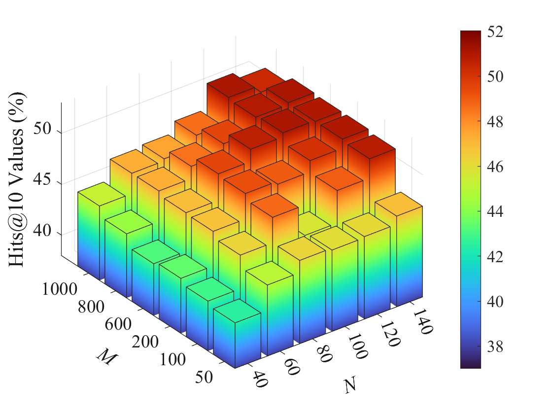
### Visual Description
## 3D Bar Chart: Hits@10 Values vs. Parameters M and N
### Overview
This image is a 3D bar chart visualizing the performance metric "Hits@10 Values (%)" as a function of two independent parameters, labeled **M** and **N**. The chart uses both bar height and a color gradient to represent the value of the Hits@10 metric. A color scale bar is provided on the right side of the chart for reference.
### Components/Axes
* **Vertical Axis (Z-axis):** Labeled **"Hits@10 Values (%)"**. The scale runs from approximately 38% to 52%, with major tick marks at 40, 45, and 50.
* **Left Horizontal Axis (X-axis):** Labeled **"M"**. It represents a categorical or discrete numerical parameter with the following values, listed from front to back: **50, 100, 200, 600, 800, 1000**.
* **Right Horizontal Axis (Y-axis):** Labeled **"N"**. It represents a second categorical or discrete numerical parameter with the following values, listed from left to right: **40, 60, 80, 100, 120, 140**.
* **Color Bar/Legend:** Positioned vertically on the far right of the image. It maps the color of the bars to the numerical Hits@10 value. The scale ranges from **38 (dark blue/purple)** at the bottom to **52 (dark red)** at the top, with intermediate labels at 40, 42, 44, 46, 48, and 50.
### Detailed Analysis
The chart displays a grid of 36 bars (6 values of M × 6 values of N). The height and color of each bar correspond to the Hits@10 value for that specific (M, N) pair.
**Trend Verification:**
1. **Trend with M:** For a fixed value of N, the bar height (and thus Hits@10 value) generally **increases** as M increases from 50 to 1000. This is visible as the bars get taller and shift from blue/green towards yellow/red as you move from the front (M=50) to the back (M=1000) of the chart along any row.
2. **Trend with N:** For a fixed value of M, the bar height generally **increases** as N increases from 40 to 140. This is visible as the bars get taller and shift from blue/green towards yellow/red as you move from the left (N=40) to the right (N=140) of the chart along any column.
3. **Combined Peak:** The highest bars, colored dark red, are located in the **back-right corner** of the chart, corresponding to the highest values of both parameters: **M=1000 and N=140**. The value here is approximately **52%**.
4. **Combined Low:** The lowest bars, colored dark blue, are located in the **front-left corner**, corresponding to the lowest values: **M=50 and N=40**. The value here is approximately **38%**.
**Approximate Value Extraction (by visual interpolation from color bar):**
* **Front Row (M=50):** Values range from ~38% (N=40) to ~44% (N=140). The gradient is from blue to green/yellow.
* **Back Row (M=1000):** Values range from ~46% (N=40) to ~52% (N=140). The gradient is from orange to dark red.
* **Left Column (N=40):** Values range from ~38% (M=50) to ~46% (M=1000).
* **Right Column (N=140):** Values range from ~44% (M=50) to ~52% (M=1000).
### Key Observations
1. **Monotonic Increase:** The performance metric (Hits@10) shows a clear, monotonic increase with both parameters M and N across the entire tested range. There are no visible local maxima or minima within the grid.
2. **Synergistic Effect:** The increase appears to be synergistic. The gain from increasing M is more pronounced at higher values of N, and vice-versa. The steepest gradient (fastest color change) is along the diagonal from (M=50, N=40) to (M=1000, N=140).
3. **Color-Height Correlation:** The color gradient perfectly correlates with bar height, providing a redundant and clear visual encoding of the data value. The color bar is essential for precise value estimation.
### Interpretation
This chart demonstrates the relationship between two hyperparameters (M and N) and a model's retrieval or ranking performance (Hits@10). The data suggests that **increasing both M and N leads to better performance**, with the best results achieved when both parameters are set to their highest tested values (M=1000, N=140).
The "Hits@10" metric typically measures the percentage of test queries where the correct answer appears within the top 10 retrieved results. Therefore, the chart indicates that larger model capacity or complexity (which M and N likely represent, such as embedding dimensions, number of layers, or dataset size) correlates with improved accuracy in this task.
The absence of a performance plateau within the tested range implies that further gains might be possible by increasing M and N beyond 1000 and 140, respectively, though this would likely come with increased computational cost. The smooth, predictable trend suggests a stable and well-behaved relationship between these parameters and model performance for the given task.
</details>
(c) Performance on ICEWS18.
<details>
<summary>extracted/6596839/fig/bar3d4.png Details</summary>
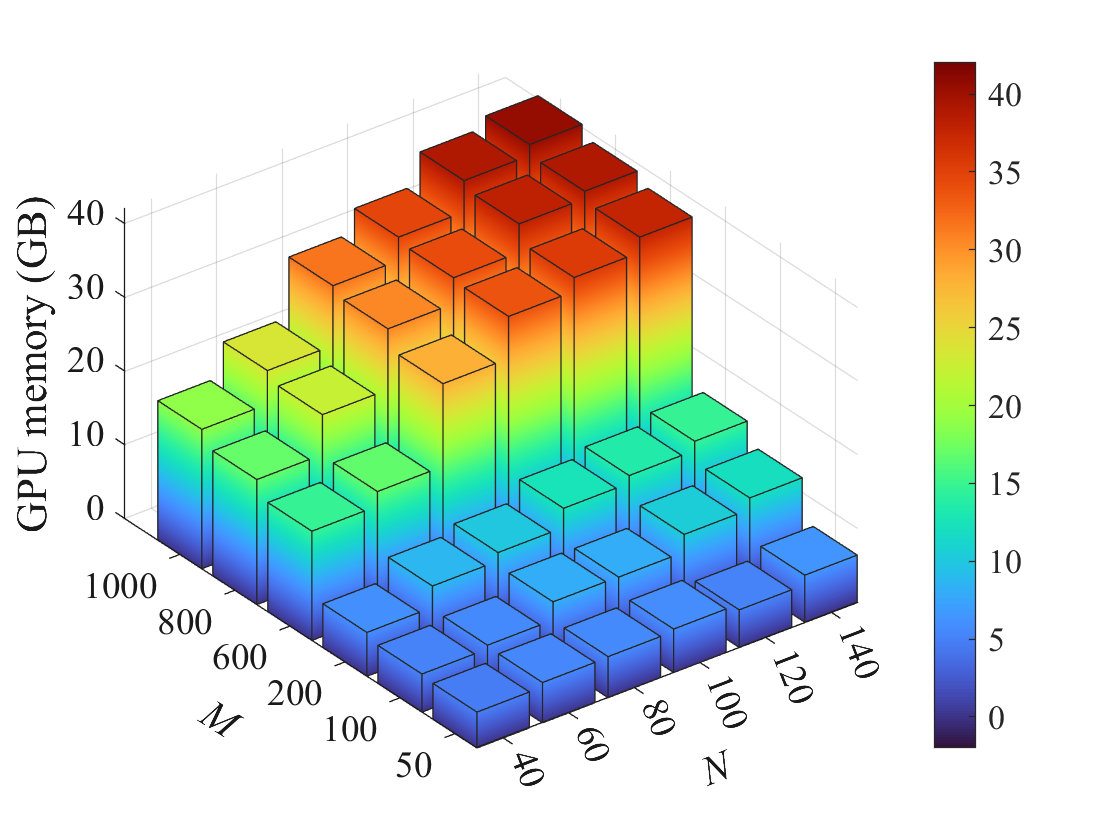
### Visual Description
## 3D Bar Chart: GPU Memory Consumption vs. Parameters M and N
### Overview
This image is a 3D bar chart visualizing the relationship between two input parameters, labeled **M** and **N**, and the resulting **GPU memory** consumption measured in Gigabytes (GB). The chart demonstrates how memory usage scales as these two parameters increase.
### Components/Axes
* **Vertical Axis (Z-axis):** Labeled "GPU memory (GB)". The scale runs from 0 to 40, with major tick marks at 0, 10, 20, 30, and 40.
* **Left Horizontal Axis (X-axis):** Labeled "M". The discrete categories marked are: 50, 100, 200, 400, 600, 800, 1000.
* **Right Horizontal Axis (Y-axis):** Labeled "N". The discrete categories marked are: 40, 60, 80, 100, 120, 140.
* **Color Bar/Legend:** Positioned on the far right of the image. It is a vertical gradient bar mapping color to GPU memory value. The scale runs from 0 (dark blue) to 40 (dark red), with labeled ticks at 0, 5, 10, 15, 20, 25, 30, 35, and 40. This color scale is applied to the bars themselves, providing a secondary visual cue for memory usage.
### Detailed Analysis
The chart displays a grid of 42 bars (7 values of M × 6 values of N). Each bar's height and color represent the GPU memory for a specific (M, N) pair.
**Trend Verification:**
1. **Trend with M:** For any fixed value of N, moving from the front (M=50) to the back (M=1000) of the chart, the bars consistently increase in height and shift in color from blue/green towards yellow/red. This indicates a strong positive correlation: GPU memory increases as M increases.
2. **Trend with N:** For any fixed value of M, moving from the left (N=40) to the right (N=140) of the chart, the bars also consistently increase in height and shift towards warmer colors. This indicates a strong positive correlation: GPU memory increases as N increases.
3. **Combined Trend:** The highest memory consumption occurs at the combination of the largest M (1000) and largest N (140), located at the back-right corner of the grid. The lowest consumption occurs at the smallest M (50) and smallest N (40), at the front-left corner.
**Approximate Data Points (Estimated from bar height and color):**
* **Low Range (Blue/Cyan Bars):** Found at low M and N values. For example, at (M=50, N=40), memory is approximately 2-5 GB. At (M=100, N=60), it is approximately 5-8 GB.
* **Mid Range (Green/Yellow Bars):** Found at moderate M and N values. For example, at (M=400, N=80), memory is approximately 15-20 GB. At (M=600, N=100), it is approximately 20-25 GB.
* **High Range (Orange/Red Bars):** Found at high M and N values. For example, at (M=800, N=120), memory is approximately 30-35 GB. At the maximum (M=1000, N=140), the bar is dark red, indicating memory usage at or very near the 40 GB upper limit of the scale.
### Key Observations
1. **Smooth, Monotonic Increase:** The progression of bar heights and colors is smooth and monotonic in both dimensions. There are no sudden drops or spikes, suggesting a predictable, likely polynomial or linear, relationship between the parameters and memory usage.
2. **Color as a Redundant Encoding:** The color gradient perfectly aligns with bar height, effectively reinforcing the data magnitude. The hottest (red) colors are exclusively at the peak of the tallest bars.
3. **Grid Layout:** The bars are arranged in a perfect, non-staggered grid, allowing for clear comparison along both the M and N axes.
4. **Scale Saturation:** The highest memory value appears to hit the ceiling of the presented scale (40 GB). It is unknown if memory usage would exceed 40 GB for parameters larger than those shown.
### Interpretation
This chart effectively communicates that GPU memory consumption is a function of two scaling parameters, M and N. The data suggests that both parameters contribute significantly and additively to the memory footprint. The lack of outliers implies a stable and consistent underlying algorithm or model where memory allocation is directly tied to these input sizes.
From a technical perspective, this visualization is crucial for capacity planning. It allows a user to estimate the required GPU memory for a given workload defined by M and N. For instance, if a task requires M=600 and N=100, one can quickly see from the chart (yellow-green bar) that a GPU with at least 25 GB of memory would be necessary. The chart implies that memory scales more steeply with M than with N, as the gradient of increase appears sharper when moving along the M-axis compared to the N-axis. This could indicate that M represents a dimension with a higher memory complexity (e.g., batch size or sequence length) than N (e.g., model width or feature count).
</details>
(d) Space on ICEWS18.
Figure 7: The impacts of sampling in the reasoning process. Performance and GPU space usage with batch size 64. Large values of M and N can achieve excellent performance at the cost of increased space requirements.
### 4.4 Hyperparameter Analysis (RQ3)
We run our model with different hyperparameters to explore weight impacts in Figures 6 and 7. Specifically, Figure 6 illustrates the performance variation with different reasoning iterations, i.e., the length of the reasoning rules. At WN18RR and FB15k-237 v3 datasets of transductive and inductive settings, experiments on rule lengths of 2, 4, 6, and 8 are carried out as illustrated in Figures 6 and 6. It is observed that the performance generally improves with the iteration increasing from 2 to 6. When the rule length continues to increase, the inference performance changes little or decreases slightly. The same phenomenon can also be observed in Figures 6 and 6, which corresponds to interpolation and extrapolation reasoning on the ICEWS14 dataset. The rule length ranges from 1 to 4, where the model performance typically displays an initial improvement, followed by a tendency to stabilize or exhibit a marginal decline. This phenomenon occurs due to the heightened rule length, which amplifies the modeling capability while potentially introducing noise into the reasoning process. Therefore, an appropriate value of rule length (reasoning iteration) is significant for KG reasoning.
We also explore the impacts of hyperparameters M for node sampling and N for edge selection on ICEWS14 and ICEWS18 datasets of extrapolation reasoning. The results are shown in Figure 7. For each dataset, we show the reasoning performance (Hits@10 metric) and utilized space (GPU memory) in detail, with the M varies in {50, 100, 200, 600, 800, 1000} while N varies in {40, 60, 80, 100, 120, 140}. It is evident that opting for smaller values results in a significant decline in performance. This decline can be attributed to the inadequate number of nodes and edges, which respectively contribute to insufficient and unstable training. Furthermore, as M surpasses 120, the marginal gains become smaller or even lead to performance degradation. Additionally, when M and N are increased, the GPU memory utilization of the model experiences rapid growth, as depicted in Figure 7 and 7, with a particularly pronounced effect on M.
TABLE VII: Some reasoning cases in transductive, interpolation, and extrapolation scenarios, where both propositional reasoning and learned FOL rules are displayed. “ ${-1}$ ” denotes the reverse of a specific relation and textual descriptions of some relations are simplified. Values in orange rectangles represent propositional attentions and relations marked with red in FOL rules represent the target relation to be predicted.
| Propositional Reasoning | FOL Rules |
| --- | --- |
|
<details>
<summary>extracted/6596839/fig/case1.png Details</summary>
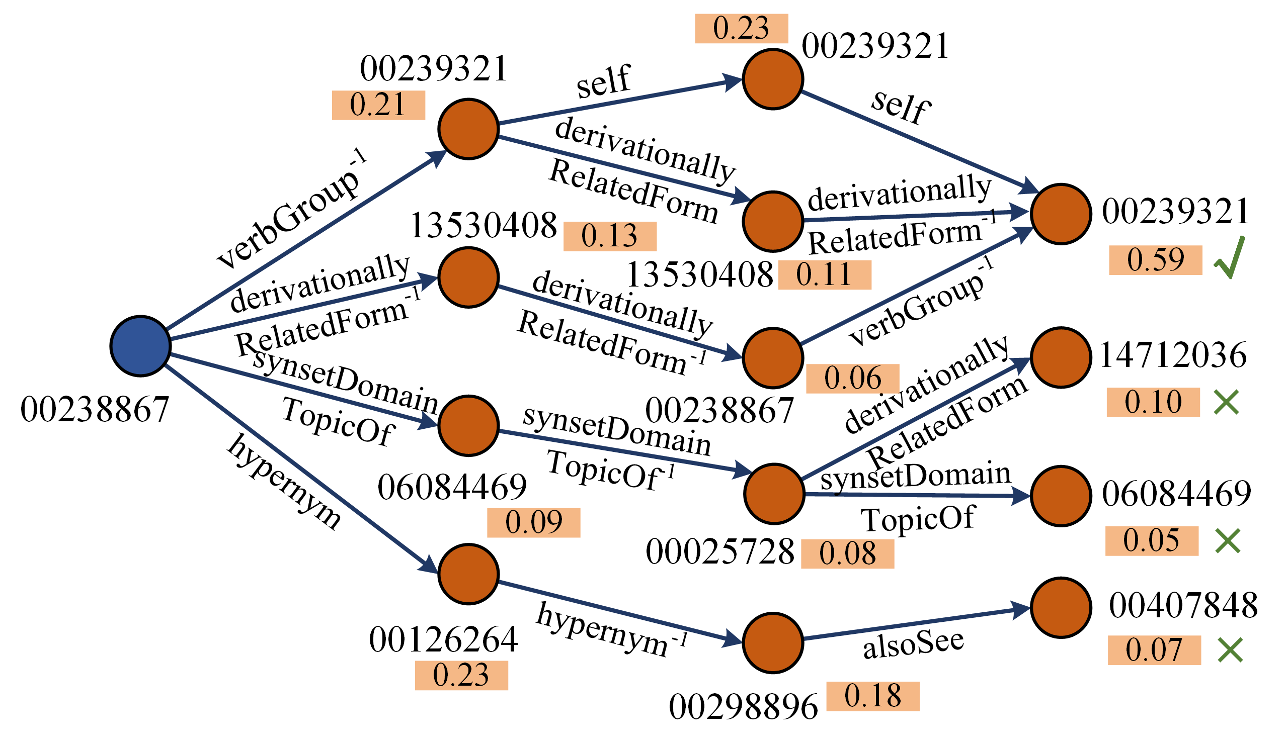
### Visual Description
## Directed Graph: Semantic Network with Relationship Scores
### Overview
The image displays a directed graph (a semantic network) illustrating relationships between nodes, which appear to be synset identifiers (likely from a lexical database like WordNet). The graph originates from a single source node on the left and branches out to multiple target nodes on the right via labeled edges. Each node has an associated numerical score (displayed in an orange box), and some terminal nodes have validation symbols (a green checkmark or red cross).
### Components/Axes
* **Nodes:** Represented as circles. One is blue (the source), and all others are orange.
* **Source Node (Blue):** ID `00238867`. Positioned on the far left.
* **Target Nodes (Orange):** Each has a unique numeric ID and a score. They are arranged in a layered, branching structure to the right of the source.
* **Edges:** Directed arrows connecting nodes. Each edge has a text label describing the semantic relationship. Some labels include a superscript `-1`, indicating an inverse relationship.
* **Scores:** Each node has a numerical value (e.g., `0.21`, `0.59`) displayed in a small orange rectangle adjacent to it.
* **Validation Symbols:** Some terminal nodes on the far right have a green checkmark (✓) or a red cross (✗) next to their score.
### Detailed Analysis
**Node Inventory (ID: Score):**
* `00238867` (Blue, Source)
* `00239321`: `0.21` (Top-left orange node)
* `13530408`: `0.13` (Middle-left orange node)
* `06084469`: `0.09` (Lower-middle orange node)
* `00126264`: `0.23` (Bottom-left orange node)
* `00239321`: `0.23` (Top-middle orange node)
* `13530408`: `0.11` (Middle orange node)
* `00238867`: `0.06` (Middle-right orange node)
* `00025728`: `0.08` (Lower-right orange node)
* `00298896`: `0.18` (Bottom-middle orange node)
* `00239321`: `0.59` ✓ (Top-right terminal node)
* `14712036`: `0.10` ✗ (Middle-right terminal node)
* `06084469`: `0.05` ✗ (Lower-right terminal node)
* `00407848`: `0.07` ✗ (Bottom-right terminal node)
**Edge Relationships (Source → Target : Label):**
1. `00238867` → `00239321` (0.21): `verbGroup^{-1}`
2. `00238867` → `13530408` (0.13): `derivationally RelatedForm^{-1}`
3. `00238867` → `06084469` (0.09): `synsetDomain TopicOf`
4. `00238867` → `00126264` (0.23): `hypernym`
5. `00239321` (0.21) → `00239321` (0.23): `self`
6. `00239321` (0.21) → `13530408` (0.11): `derivationally RelatedForm`
7. `13530408` (0.13) → `00238867` (0.06): `derivationally RelatedForm^{-1}`
8. `00239321` (0.23) → `00239321` (0.59 ✓): `self`
9. `13530408` (0.11) → `00239321` (0.59 ✓): `verbGroup^{-1}`
10. `00238867` (0.06) → `14712036` (0.10 ✗): `derivationally RelatedForm`
11. `06084469` (0.09) → `00025728` (0.08): `synsetDomain TopicOf^{-1}`
12. `00025728` (0.08) → `06084469` (0.05 ✗): `synsetDomain TopicOf`
13. `00126264` (0.23) → `00298896` (0.18): `hypernym^{-1}`
14. `00298896` (0.18) → `00407848` (0.07 ✗): `alsoSee`
### Key Observations
1. **Node Repetition:** The synset ID `00239321` appears three times with different scores (`0.21`, `0.23`, `0.59`), suggesting it is reached via different paths with varying confidence or relevance.
2. **Relationship Types:** The graph uses a specific vocabulary of semantic relations: `verbGroup`, `derivationally RelatedForm`, `synsetDomain TopicOf`, `hypernym`, `alsoSee`, and `self`. The `-1` suffix denotes the inverse of a relationship.
3. **Validation Outcome:** Only one terminal node (`00239321` with score `0.59`) is marked with a green checkmark (✓). All other terminal nodes (`14712036`, `06084469`, `00407848`) are marked with red crosses (✗), indicating they are incorrect or invalid results for the given query or traversal.
4. **Score Progression:** Scores fluctuate along paths. The highest score (`0.59`) is achieved at a terminal node reached via a `self` relationship from an intermediate node of the same ID.
5. **Structural Flow:** The graph flows left-to-right from the source. It branches immediately into four primary relationships, with subsequent nodes forming secondary and tertiary connections.
### Interpretation
This diagram visualizes a **semantic search or inference process** starting from a specific concept (synset `00238867`). The scores likely represent a **confidence, similarity, or relevance metric** calculated during the traversal of the semantic network.
* **What it demonstrates:** The graph shows how different relational paths from a starting concept lead to other related concepts, with each step assigned a score. The process appears to be evaluating the validity of these paths, as indicated by the check/cross symbols.
* **Relationship between elements:** The edges define the type of semantic link (e.g., hypernym is an "is-a" relation, derivationally RelatedForm connects word forms). The scores propagate and transform along these links. The `self` loops suggest a process of reaffirming or boosting the score of a concept.
* **Notable patterns/anomalies:**
* The only "successful" path (✓) leads back to a variant of the same synset ID (`00239321`) via a `self` relationship, achieving the highest score. This could indicate a successful confirmation or a high-confidence match within the network.
* All paths that terminate in a *different* synset ID are marked as failures (✗), suggesting the goal of this particular traversal was to validate or find a specific target, and only the `00239321` node met the criteria.
* The presence of inverse relationships (`-1`) shows the graph is bidirectional in its semantic reasoning, allowing traversal both along and against the direction of a standard relation.
**In essence, this is a technical visualization of a knowledge graph traversal algorithm, highlighting scored pathways and their validation outcomes.**
</details>
| [1]
0.21 verbGroup -1 (X,Z) $\rightarrow$ verbGroup (X,Z) [2]
0.32 verbGroup -1 (X,Y 1) $\land$ derivationallyRelatedForm (Y 1,Y 2) $\land$ derivationallyRelatedForm -1 (Y 2,Z) $\rightarrow$ verbGroup (X,Z) [3]
0.07 derivationallyRelatedForm -1 (X,Y 1) $\land$ derivationallyRelatedForm -1 (Y 1,Y 2) $\land$ verbGroup -1 (Y 2,Z) $\rightarrow$ verbGroup (X,Z) [4]
0.05 synsetDomainTopicOf (X,Y 1) $\land$ synsetDomainTopicOf -1 (Y 1,Y 2) $\land$ derivationallyRelatedForm (Y 2,Z) $\rightarrow$ verbGroup (X,Z) [5]
0.18 hypernym (X,Y 1) $\land$ hypernym -1 (Y 1,Y 2) $\land$ alsoSee (Y 2,Z) $\rightarrow$ verbGroup (X,Z) |
| Transductive reasoning: query (00238867, verbGroup, ?) in WN18RR | |
|
<details>
<summary>extracted/6596839/fig/case2.png Details</summary>
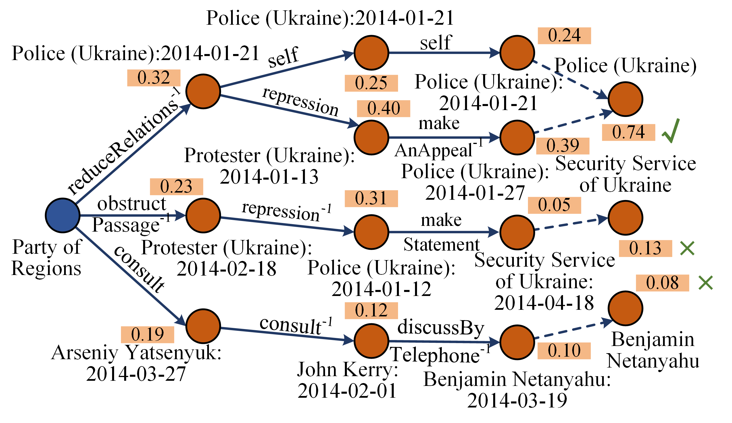
### Visual Description
## Diagram: Knowledge Graph of Political Relations and Events (Ukraine, 2014)
### Overview
The image displays a directed graph or knowledge graph modeling relationships and interactions between political entities, security forces, and individuals primarily during the Ukrainian political crisis of early 2014. The graph flows generally from left to right, originating from a central entity and branching into multiple interaction pathways. Each node represents an entity with an associated date, and each edge represents a labeled relationship with an associated numerical weight (likely a confidence score or probability). Some terminal relationships are marked with a green checkmark (✓) or a red cross (✗).
### Components/Axes
* **Node Types & Colors:**
* **Central Node (Blue):** "Party of Regions" (no date attached).
* **Entity Nodes (Orange):** All other nodes, representing specific entities on specific dates.
* **Edge Types:**
* **Solid Dark Blue Arrows:** Indicate primary relationships.
* **Dashed Dark Blue Arrows:** Indicate secondary or inferred relationships, typically leading to final entity nodes without dates.
* **Labels & Values:**
* **Node Labels:** Text adjacent to each circle, formatted as `Entity Name: YYYY-MM-DD`.
* **Edge Labels:** Text along the arrows describing the relationship (e.g., "reduceRelations⁻¹", "consult", "self"). Some labels include a superscript "-1", suggesting an inverse relationship.
* **Numerical Weights:** Beige boxes containing decimal numbers (e.g., 0.32, 0.24) placed near the midpoint of edges.
* **Verification Marks:** A green checkmark (✓) and red crosses (✗) appear next to some terminal numerical values.
### Detailed Analysis
The graph originates from the **Party of Regions** node and splits into three primary branches:
**1. Top Branch (Police/Protester Relations):**
* **Path 1.1:** `Party of Regions` →(reduceRelations⁻¹, 0.32)→ `Police (Ukraine):2014-01-21`
* This node splits:
* →(self, 0.25)→ `Police (Ukraine):2014-01-21` →(self, 0.24)→ `Police (Ukraine)` [Dashed arrow]
* →(repression, 0.40)→ `Police (Ukraine):2014-01-21` →(make AnAppeal⁻¹, 0.39)→ `Police (Ukraine):2014-01-21` [Dashed arrow to `Security Service of Ukraine` with weight **0.74 ✓**]
* **Path 1.2:** `Party of Regions` →(obstruct Passage⁻¹, 0.23)→ `Protester (Ukraine):2014-02-18`
* →(repression⁻¹, 0.31)→ `Police (Ukraine):2014-01-12` →(make Statement, 0.05)→ `Security Service of Ukraine:2014-04-18` [Dashed arrow to `Security Service of Ukraine` with weight **0.13 ✗**]
**2. Bottom Branch (Diplomatic Consultations):**
* **Path 2.1:** `Party of Regions` →(consult, 0.19)→ `Arseniy Yatsenyuk:2014-03-27`
* →(consult⁻¹, 0.12)→ `John Kerry:2014-02-01` →(discussBy Telephone⁻¹, 0.10)→ `Benjamin Netanyahu:2014-03-19` [Dashed arrow to `Benjamin Netanyahu` with weight **0.08 ✗**]
**3. Additional Node (Top Center):**
* An isolated node `Police (Ukraine):2014-01-21` appears at the top center with no incoming or outgoing edges shown in this view.
### Key Observations
* **Temporal Clustering:** All dated nodes fall within a four-month window from January 12, 2014, to April 18, 2014, aligning with the peak of the Euromaidan protests and the subsequent political transition in Ukraine.
* **Relationship Weights:** Weights vary significantly, from a high of **0.74** (for a link to the Security Service of Ukraine) to lows of **0.05** and **0.08**. The highest-weighted path (0.74) is marked with a checkmark (✓), suggesting it is a verified or high-confidence relationship. The lower-weighted terminal paths (0.13, 0.08) are marked with crosses (✗), suggesting they are incorrect, low-confidence, or disproven links.
* **Entity Focus:** The graph heavily features the **Police (Ukraine)** and the **Security Service of Ukraine** as central actors in the "repression" and "appeal" pathways. Diplomatic figures (Yatsenyuk, Kerry, Netanyahu) form a separate, lower-confidence cluster.
* **Inverse Relationships:** The frequent use of the "⁻¹" superscript (e.g., `reduceRelations⁻¹`, `consult⁻¹`) indicates the model explicitly accounts for the inverse direction of a base relationship.
### Interpretation
This diagram appears to be a visual output from a computational model (likely a knowledge graph completion or link prediction model) analyzing events from the 2014 Ukrainian crisis. It attempts to map and quantify the relationships between political parties, state security apparatus, protesters, and international figures.
* **What it Suggests:** The model posits that the Party of Regions' actions (reducing relations, obstructing passage, consulting) triggered a cascade of interactions, primarily involving state security forces engaging in repression and making appeals/statements. A separate, weaker diplomatic channel involving Yatsenyuk, Kerry, and Netanyahu is also modeled.
* **Element Relationships:** The graph structure implies causality or influence flow. The numerical weights likely represent the model's confidence in the existence or strength of that specific relationship given the available data. The checkmarks and crosses serve as a validation layer, possibly comparing model predictions to ground-truth data.
* **Notable Anomalies:** The inclusion of **Benjamin Netanyahu** is a notable outlier, as his direct involvement in the Ukrainian domestic crisis of early 2014 is not a widely documented central event. This link, with its very low weight (0.08) and cross mark, may represent a noisy or incorrect inference by the model. The duplicate `Police (Ukraine):2014-01-21` nodes could indicate the model treats different interaction contexts as separate instances, or it may be a visualization artifact.
**In essence, the image provides a structured, probabilistic interpretation of the complex web of interactions during a critical historical period, highlighting both high-confidence pathways of state response and more speculative or tenuous connections.**
</details>
| [1]
0.46 reduceRelations -1 (X,Z) $:t_{1}$ $\rightarrow$ makeAnAppeal (X,Z) $:t$ [2]
0.19 reduceRelations -1 (X,Y 1) $:t_{1}$ $\land$ repression (Y 1,Y 2) $:t_{2}$ $\land$ makeAnAppeal -1 (Y 2,Z) $:t_{3}$ $\rightarrow$ makeAnAppeal (X,Z) $:t$ [3]
0.14 obstructPassage -1 (X,Y 1) $:t_{1}$ $\land$ repression -1 (Y 1,Y 2) $:t_{2}$ $\land$ makeStatement (Y 2,Z) $:t_{3}$ $\rightarrow$ makeAnAppeal (X,Z) $:t$ [4]
0.12 consult (X,Y 1) $:t_{1}$ $\land$ consult -1 (Y 1,Y 2) $:t_{2}$ $\land$ discussByTelephone -1 (Y 2,Z) $:t_{3}$ $\rightarrow$ makeAnAppeal (X,Z) $:t$ |
| Interpolation reasoning: query (Party of Regions, makeAnAppeal, ?, 2014-05-15) in ICEWS14 | |
|
<details>
<summary>extracted/6596839/fig/case3.png Details</summary>
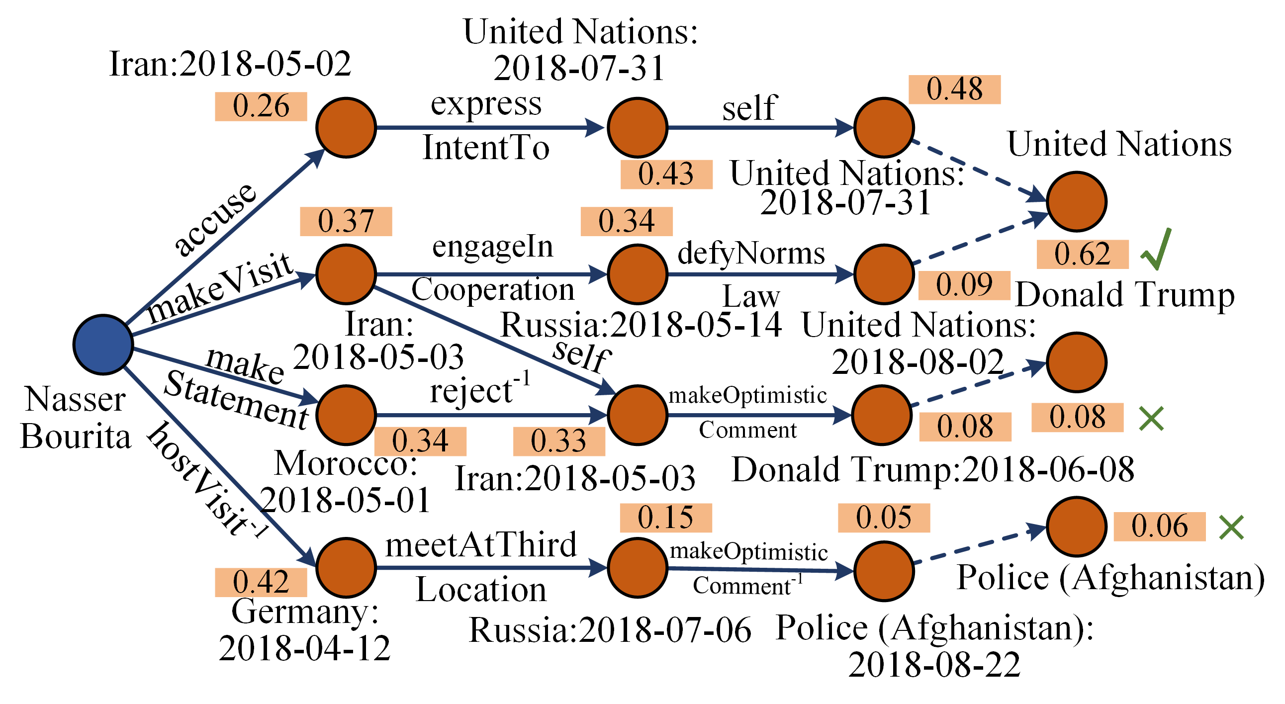
### Visual Description
## Directed Graph Diagram: Event and Relationship Network
### Overview
The image displays a directed graph (network diagram) illustrating a series of events, relationships, and actions involving several geopolitical entities and individuals. The graph originates from a central entity and branches into multiple pathways, each annotated with relationship labels, dates, and numerical scores (likely confidence or probability values). The diagram appears to model a sequence of diplomatic or political events, with some paths culminating in validated (✓) or invalidated (×) outcomes.
### Components/Elements
* **Node Types:**
* **Central Node (Blue Circle):** "Nasser Bourita" (Position: Left-center). This is the origin point for all primary relationships.
* **Subsequent Nodes (Orange Circles):** Represent other entities, locations, or events. Each is labeled with an entity name and a date in `YYYY-MM-DD` format.
* **Edge Types:**
* **Solid Blue Arrows:** Indicate direct relationships or actions flowing from one node to another. Each has a text label describing the relationship (e.g., "accuse", "makeVisit").
* **Dashed Blue Arrows:** Appear in the final segments of some paths, leading to terminal nodes.
* **Annotations:**
* **Numerical Scores:** Displayed in small orange boxes on or near edges. These are decimal values between 0.05 and 0.62.
* **Outcome Symbols:** A green checkmark (✓) and red crosses (×) are placed next to some terminal nodes, indicating a binary outcome (e.g., correct/incorrect, validated/invalidated).
* **Superscript Notation:** The labels "reject⁻¹" and "hostVisit⁻¹" include a superscript "-1", which may denote an inverse or reciprocal action.
### Detailed Analysis: Path-by-Path Breakdown
The graph contains four primary pathways originating from "Nasser Bourita".
**Path 1: Topmost Branch**
1. **Start:** Nasser Bourita → `accuse` → **Node:** "Iran:2018-05-02" (Score on edge: 0.26).
2. From "Iran:2018-05-02" → `express IntentTo` → **Node:** "United Nations:2018-07-31" (Score on edge: 0.43).
3. From "United Nations:2018-07-31" → `self` → **Node:** "United Nations:2018-07-31" (Score on edge: 0.48). *Note: This appears to be a self-referential loop or a node representing a subsequent action by the same entity on the same date.*
4. From the second "United Nations:2018-07-31" node → (dashed arrow) → **Terminal Node:** "United Nations" (Score: 0.62). **Outcome:** ✓ (Green Checkmark).
**Path 2: Second Branch**
1. **Start:** Nasser Bourita → `makeVisit` → **Node:** "Iran:2018-05-03" (Score on edge: 0.37).
2. From "Iran:2018-05-03" → `engageIn Cooperation` → **Node:** "Russia:2018-05-14" (Score on edge: 0.34).
3. From "Russia:2018-05-14" → `defyNorms Law` → **Node:** "United Nations:2018-08-02" (Score on edge: 0.09).
4. From "United Nations:2018-08-02" → (dashed arrow) → **Terminal Node:** "Donald Trump" (Score: 0.08). **Outcome:** × (Red Cross).
**Path 3: Third Branch**
1. **Start:** Nasser Bourita → `makeStatement` → **Node:** "Morocco:2018-05-01" (Score on edge: Not explicitly labeled on this initial edge).
2. From "Morocco:2018-05-01" → `reject⁻¹` → **Node:** "Iran:2018-05-03" (Score on edge: 0.34). *Note: This node is also reached from Path 2.*
3. From "Iran:2018-05-03" (this instance) → `self` → **Node:** "Donald Trump:2018-06-08" (Score on edge: 0.33).
4. From "Donald Trump:2018-06-08" → `makeOptimistic Comment` → **Node:** "Police (Afghanistan):2018-08-22" (Score on edge: 0.05).
5. From "Police (Afghanistan):2018-08-22" → (dashed arrow) → **Terminal Node:** "Police (Afghanistan)" (Score: 0.06). **Outcome:** × (Red Cross).
**Path 4: Bottommost Branch**
1. **Start:** Nasser Bourita → `hostVisit⁻¹` → **Node:** "Germany:2018-04-12" (Score on edge: 0.42).
2. From "Germany:2018-04-12" → `meetAtThird Location` → **Node:** "Russia:2018-07-06" (Score on edge: 0.15).
3. From "Russia:2018-07-06" → `makeOptimistic Comment⁻¹` → **Node:** "Police (Afghanistan):2018-08-22" (Score on edge: 0.05). *Note: This node is also reached from Path 3.*
4. This path merges with Path 3 at the "Police (Afghanistan):2018-08-22" node and shares the same terminal outcome.
### Key Observations
1. **Central Actor:** Nasser Bourita is the central figure from which all modeled events originate.
2. **Temporal Spread:** The events span from April 12, 2018 (Germany) to August 22, 2018 (Afghanistan).
3. **Score Range:** The numerical scores range from a low of 0.05 to a high of 0.62. The highest score (0.62) is associated with the only validated (✓) outcome.
4. **Convergence:** Two distinct paths (Path 3 and Path 4) converge at the node "Police (Afghanistan):2018-08-22", leading to the same terminal outcome.
5. **Outcome Disparity:** Only one of the four terminal paths results in a validation (✓). The other three result in invalidation (×), despite having varying intermediate scores.
6. **Entity Recurrence:** Several entities appear in multiple nodes (e.g., Iran, United Nations, Russia), suggesting their involvement in multiple, temporally distinct events.
### Interpretation
This diagram likely represents the output of a computational model analyzing geopolitical events, possibly for fact-checking, relationship prediction, or narrative validation. The numerical scores could represent the model's confidence in the relationship or the likelihood of the event occurring as described.
The single validated path (ending with "United Nations" and a score of 0.62) suggests the model has high confidence in a sequence where Nasser Bourita accuses Iran, which then expresses intent to the UN, leading to a self-referential UN action that is ultimately validated. The other paths, despite some moderately high confidence scores (e.g., 0.42 for the Germany visit), culminate in low-confidence terminal links (scores of 0.08 and 0.06) and are marked as invalid.
The convergence of paths on "Police (Afghanistan):2018-08-22" indicates that different event sequences (involving Morocco/Iran/Trump and Germany/Russia) are modeled as leading to the same outcome regarding Afghan police, an outcome the model deems invalid. The use of superscript "-1" on "reject" and "hostVisit" may indicate the model is accounting for inverse or reciprocal actions in its analysis. Overall, the graph visualizes a complex web of diplomatic interactions, highlighting one seemingly coherent and validated narrative amidst several others that the model does not support.
</details>
| [1]
0.14 accuse (X,Y) $:t_{1}$ $\land$ expressIntentTo (Y,Z) $:t_{2}$ $\rightarrow$ makeVisit (X,Z) $:t$ [2]
0.09 makeVisit (X,Y 1) $:t_{1}$ $\land$ engageInCooperation (Y 1,Y 2) $:t_{2}$ $\land$ defyNormsLaw (Y 2,Z) $:t_{3}$ $\rightarrow$ makeVisit (X,Z) $:t$ [3]
0.11 makeStatement (X,Y 1) $:t_{1}$ $\land$ reject -1 (Y 1,Y 2) $:t_{2}$ $\land$ makeOptimisticComment (Y 2,Z) $:t_{3}$ $\rightarrow$ makeVisit (X,Z) $:t$ [4]
0.25 makeVisit (X,Y) $:t_{1}$ $\land$ makeOptimisticComment (Y,Z) $:t_{2}$ $\rightarrow$ makeVisit (X,Z) $:t$ [5]
0.17 hostVisit -1 (X,Y 1) $:t_{1}$ $\land$ meetAtThirdLocation (Y 1,Y 2) $:t_{2}$ $\land$ makeOptimisticComment -1 (Y 2,Z) $:t_{3}$ $\rightarrow$ makeVisit (X,Z) $:t$ |
| Extrapolation reasoning: query (Nasser Bourita, makeVisit, ?, 2018-09-28) in ICEWS18 | |
TABLE VIII: Some reasoning cases in inductive scenarios, where learned FOL rules are displayed. Relations marked with red represent the target relation to be predicted. “ ${-1}$ ” denotes the reverse of a specific relation and textual descriptions of some relations are simplified.
| Col1 |
| --- |
| [1] 0.41 memberMeronym (X,Y 1) $\land$ hasPart (Y 1,Y 2) $\land$ hasPart -1 (Y 2,Z) $\rightarrow$ memberMeronym (X,Z) [2] 0.19 hasPart -1 (X,Y 1) $\land$ hypernym (Y 1,Y 2) $\land$ memberOfDomainUsage -1 (Y 2,Z) $\rightarrow$ memberMeronym (X,Z) [3] 0.25 hypernym (X,Y 1) $\land$ hypernym -1 (Y 1,Y 2) $\land$ memberMeronym (Y 2,Z) $\rightarrow$ memberMeronym (X,Z) [4] 0.17 hypernym (X,Y 1) $\land$ hypernym -1 (Y 1,Y 2) $\land$ hasPart (Y 2,Z) $\rightarrow$ memberMeronym (X,Z) |
| Inductive reasoning: query (08174398, memberMeronym, ?) in WN18RR v3 |
| [1] 0.32 filmReleaseRegion (X,Y 1) $\land$ filmReleaseRegion -1 (Y 1,Y 2) $\land$ filmCountry (Y 2,Z) $\rightarrow$ filmReleaseRegion (X,Z) [2] 0.10 distributorRelation -1 (X,Y 1) $\land$ nominatedFor (Y 1,Y 2) $\land$ filmReleaseRegion -1 (Y 2,Z) $\rightarrow$ filmReleaseRegion (X,Z) [3] 0.19 filmReleaseRegion (X,Y 1) $\land$ exportedTo -1 (Y 1,Y 2) $\land$ locationCountry (Y 2,Z) $\rightarrow$ filmReleaseRegion (X,Z) [4] 0.05 filmCountry (X,Y 1) $\land$ filmReleaseRegion -1 (Y 1,Y 2) $\land$ filmMusic (Y 2,Z) $\rightarrow$ filmReleaseRegion (X,Z) |
| Inductive reasoning: query (/m/0j6b5, filmReleaseRegion, ?) in FB15k-237 v3 |
| [1] 0.46 collaboratesWith -1 (X,Z) $\rightarrow$ collaboratesWith (X,Z) [2] 0.38 collaboratesWith -1 (X,Y 1) $\land$ holdsOffice (Y 1,Y 2) $\land$ holdsOffice -1 (Y 2,Z) $\rightarrow$ collaboratesWith (X,Z) [3] 0.03 collaboratesWith -1 (X,Y 1) $\land$ graduatedFrom (Y 1,Y 2) $\land$ graduatedFrom -1 (Y 2,Z) $\rightarrow$ collaboratesWith (X,Z) [4] 0.03 collaboratesWith -1 (X,Y 1) $\land$ collaboratesWith (Y 1,Y 2) $\land$ graduatedFrom (Y 2,Z) $\rightarrow$ collaboratesWith (X,Z) |
| Inductive reasoning: query (Hillary Clinton, collaboratesWith, ?) in NELL v3 |
### 4.5 Case Studies (RQ4)
To show the actual reasoning process of Tunsr, some practical cases are presented in detail on all four reasoning scenarios, which illustrate the transparency and interpretability of the proposed Tunsr. For better presentation, the maximum length of the reasoning iterations is set to 3. Specifically, Table VII shows the reasoning graphs for three specific queries on transductive, interpolation, and extrapolation scenarios, respectively, The propositional attention weights of nodes are listed near them, which represent the propositional reasoning score of each node at the current step. For example, in the first case, the uppermost propositional reasoning path (00238867, verbGroup -1, 00239321) at first step learns a large attention score for the correct answer 00239321. Generally, nodes with more preceding neighbors or larger preceding attention weights significantly impact subsequent steps and the prediction of final entity scores. Besides, we observe that propositional and first-order reasoning have an incompletely consistent effect. For example, the FOL rules of “[3]” and “[4]” in the third case have relatively high rule confidence values compared with “[1]” and “[2]” (0.11, 0.25 vs. 0.14, 0.09), but the combination of their corresponding propositional reasoning paths “(Nasser Bourita, makeStatement, Morocco:2018-05-01, reject -1, Iran:2018-05-03, makeOptimisticComment, Donald Trump:2018-06-08)” and “(Nasser Bourita, makeVisit, Iran:2018-05-03, self, Iran:2018-05-03, makeOptimisticComment, Donald Trump:2018-06-08)” has a small propositional attention, i.e., 0.08. This combination prevents the model from predicting the wrong answer Donald Trump. Thus, propositional and FOL reasoning can be integrated to jointly guide the reasoning process, leading to more accurate reasoning results.
Table VIII shows some learned FOL rules of inductive reasoning on WN18RR v3, FB15k-237 v3, and NELL v3 datasets. As the inductive setting is entity-independent, so the propositional reasoning part is not involved here. Each rule presented carries practical significance and is readily understandable for humans. For instance, rule “[1]” collaboratesWith -1 (X, Z) $\rightarrow$ collaboratesWith(X, Z) in the third case has a relatively high confidence value (0.46). This aligns with human commonsense cognition, as the relation collaboratesWith has mutual characteristics for subject and object and can be derived from each other. If person a has collaborated with person b, it inherently implies person b has collaborated with person a. These results illustrate the effectiveness of the rules learned by Tunsr and its interpretable reasoning process.
## 5 Conclusion and Future Works
To combine the advantages of connectionism and symbolicism of AI for KG reasoning, we propose a unified neurosymbolic framework Tunsr for both perspectives of methodology and reasoning scenarios, including transductive, inductive, interpolation, and extrapolation reasoning. Tunsr first introduces a consistent structure of reasoning graph that starts from the query entity and constantly expands subsequent nodes by iteratively searching posterior neighbors. Based on it, a forward logical message-passing mechanism is proposed to update both the propositional representations and attentions, as well as FOL representations and attentions of each node in the expanding reasoning graph. In this way, Tunsr conducts the transformation of merging multiple rules by merging possible relations at each step by using FOL attentions. Through gradually adding rule bodies and updating rule confidence, the real FOL rules can be easily induced to constantly perform attention calculation over the reasoning graph, which is summarized as the FARI algorithm. The experiments on 19 datasets of four different reasoning scenarios illustrate the effectiveness of Tunsr. Meanwhile, the ablation studies show that propositional and FOL have different impacts. Thus, they can be integrated to improve the whole reasoning results. The case studies also verify the transparency and interpretability of its computation process.
The future works lie in two folds. Firstly, we aim to extend the application of this idea to various reasoning domains, particularly those necessitating interpretability for decision-making [87], such as intelligent healthcare and finance. We anticipate this will enhance the accuracy of reasoning while simultaneously offering human-understandable logical rules as evidence. Secondly, we intend to integrate the concept of unified reasoning with state-of-the-art technologies to achieve optimal results. For instance, large language models have achieved great success in the community of natural language processing and AI, while they often encounter challenges when confronted with complex reasoning tasks [88]. Hence, there is considerable prospect for large language models to enhance reasoning capabilities.
## References
- [1] I. Tiddi and S. Schlobach. Knowledge graphs as tools for explainable machine learning: A survey. Artificial Intelligence, 302:103627, 2022.
- [2] M. Li and M. Moens. Dynamic key-value memory enhanced multi-step graph reasoning for knowledge-based visual question answering. In Thirty-Sixth AAAI Conference on Artificial Intelligence, pp. 10983–10992. AAAI Press, 2022.
- [3] C. Mavromatis et al. Tempoqr: Temporal question reasoning over knowledge graphs. In Thirty-Sixth AAAI Conference on Artificial Intelligence, pp. 5825–5833. AAAI Press, 2022.
- [4] Y. Yang et al. Knowledge graph contrastive learning for recommendation. In The 45th International ACM SIGIR Conference on Research and Development in Information Retrieval (SIGIR), pp. 1434–1443. ACM, 2022.
- [5] Y. Zhu et al. Recommending learning objects through attentive heterogeneous graph convolution and operation-aware neural network. IEEE Transactions on Knowledge and Data Engineering (TKDE), 35:4178–4189, 2023.
- [6] A. Bastos et al. RECON: relation extraction using knowledge graph context in a graph neural network. In The Web Conference (WWW), pp. 1673–1685. ACM / IW3C2, 2021.
- [7] X. Chen et al. Knowprompt: Knowledge-aware prompt-tuning with synergistic optimization for relation extraction. In The Web Conference (WWW), pp. 2778–2788. ACM, 2022.
- [8] B. D. Trisedya et al. GCP: graph encoder with content-planning for sentence generation from knowledge bases. IEEE Transactions on Pattern Analysis and Machine Intelligence (TPAMI), 44(11):7521–7533, 2022.
- [9] W. Yu et al. A survey of knowledge-enhanced text generation. ACM Comput. Surv., 54(11s):227:1–227:38, 2022.
- [10] K. D. Bollacker et al. Freebase: A collaboratively created graph database for structuring human knowledge. In Proceedings of the International Conference on Management of Data (SIGMOD), pp. 1247–1250, 2008.
- [11] D. Vrandecic. Wikidata: A new platform for collaborative data collection. In Proceedings of the 21st World Wide Web Conference (WWW), pp. 1063–1064, 2012.
- [12] Q. Wang et al. Knowledge graph embedding: A survey of approaches and applications. IEEE Transactions on Knowledge and Data Engineering (TKDE), 29(12):2724–2743, 2017.
- [13] A. Rossi et al. Knowledge graph embedding for link prediction: A comparative analysis. ACM Transactions on Knowledge Discovery from Data (TKDD), 15(2):1–49, 2021.
- [14] S. Pinker and J. Mehler. Connections and symbols. Mit Press, 1988.
- [15] T. H. Trinh et al. Solving olympiad geometry without human demonstrations. Nature, 625(7995):476–482, 2024.
- [16] Q. Lin et al. Contrastive graph representations for logical formulas embedding. IEEE Transactions on Knowledge and Data Engineering, 35:3563–3574, 2023.
- [17] F. Xu et al. Symbol-llm: Towards foundational symbol-centric interface for large language models. In Proceedings of the 62nd Annual Meeting of the Association for Computational Linguistics (ACL), pp. 13091–13116, 2024.
- [18] Q. Lin et al. Fusing topology contexts and logical rules in language models for knowledge graph completion. Information Fusion, 90:253–264, 2023.
- [19] A. Bordes et al. Translating embeddings for modeling multi-relational data. In Advances in Neural Information Processing Systems (NeurIPS), pp. 2787–2795, 2013.
- [20] L. A. Galárraga et al. AMIE: association rule mining under incomplete evidence in ontological knowledge bases. In 22nd International World Wide Web Conference (WWW), pp. 413–422, 2013.
- [21] F. Yang et al. Differentiable learning of logical rules for knowledge base reasoning. In Advances in Neural Information Processing Systems (NeurIPS), pp. 2319–2328, 2017.
- [22] Y. Shen et al. Modeling relation paths for knowledge graph completion. IEEE Transactions on Knowledge and Data Engineering, 33(11):3607–3617, 2020.
- [23] K. Cheng et al. Rlogic: Recursive logical rule learning from knowledge graphs. In The 28th ACM SIGKDD Conference on Knowledge Discovery and Data Mining (KDD), pp. 179–189. ACM, 2022.
- [24] J. Liu et al. Latentlogic: Learning logic rules in latent space over knowledge graphs. In Findings of the EMNLP, pp. 4578–4586, 2023.
- [25] C. Jiang et al. Path spuriousness-aware reinforcement learning for multi-hop knowledge graph reasoning. In Proceedings of the 17th Conference of the European Chapter of the Association for Computational Linguistics (EACL), pp. 3173–3184, 2023.
- [26] Q. Lin et al. Incorporating context graph with logical reasoning for inductive relation prediction. In The 45th International ACM SIGIR Conference on Research and Development in Information Retrieval (SIGIR), pp. 893–903, 2022.
- [27] J. Li et al. Teast: Temporal knowledge graph embedding via archimedean spiral timeline. In Proceedings of the 61st Annual Meeting of the Association for Computational Linguistics (ACL), pp. 15460–15474, 2023.
- [28] Y. Liu et al. Tlogic: Temporal logical rules for explainable link forecasting on temporal knowledge graphs. In Thirty-Sixth AAAI Conference on Artificial Intelligence, pp. 4120–4127. AAAI Press, 2022.
- [29] N. Li et al. Tr-rules: Rule-based model for link forecasting on temporal knowledge graph considering temporal redundancy. In Findings of the Association for Computational Linguistics (EMNLP), pp. 7885–7894, 2023.
- [30] Q. Lin et al. TECHS: temporal logical graph networks for explainable extrapolation reasoning. In Proceedings of the 61st Annual Meeting of the Association for Computational Linguistics (ACL), pp. 1281–1293, 2023.
- [31] E. Cambria et al. SenticNet 7: A commonsense-based neurosymbolic AI framework for explainable sentiment analysis. In LREC, pp. 3829–3839, 2022.
- [32] A. Sadeghian et al. DRUM: end-to-end differentiable rule mining on knowledge graphs. In Advances in Neural Information Processing Systems (NeurIPS), pp. 15321–15331, 2019.
- [33] M. Qu et al. Rnnlogic: Learning logic rules for reasoning on knowledge graphs. In 9th International Conference on Learning Representations (ICLR), 2021.
- [34] Y. Zhang et al. GMH: A general multi-hop reasoning model for KG completion. In Proceedings of the 2021 Conference on Empirical Methods in Natural Language Processing (EMNLP), pp. 3437–3446, 2021.
- [35] J. Zhang et al. Subgraph retrieval enhanced model for multi-hop knowledge base question answering. In Proceedings of the 60th Annual Meeting of the Association for Computational Linguistics (ACL), pp. 5773–5784, 2022.
- [36] Y. Lan et al. Complex knowledge base question answering: A survey. IEEE Trans. Knowl. Data Eng., 35(11):11196–11215, 2023.
- [37] H. Dong et al. Temporal inductive path neural network for temporal knowledge graph reasoning. Artificial Intelligence, pp. 104085, 2024.
- [38] J. Chung et al. Empirical evaluation of gated recurrent neural networks on sequence modeling. CoRR, abs/1412.3555, 2014.
- [39] S. Abiteboul et al. Foundations of databases, volume 8. Addison-Wesley Reading, 1995.
- [40] M. Gebser et al. Potassco: The potsdam answer set solving collection. Ai Communications, 24(2):107–124, 2011.
- [41] M. Alviano et al. Wasp: A native asp solver based on constraint learning. In Logic Programming and Nonmonotonic Reasoning: 12th International Conference, LPNMR 2013, Corunna, Spain, September 15-19, 2013. Proceedings 12, pp. 54–66. Springer, 2013.
- [42] W. Rautenberg. A Concise Introduction to Mathematical Logic. Springer, 2006.
- [43] G. Ciravegna et al. Logic explained networks. Artificial Intelligence, 314:103822, 2023.
- [44] H. Ren and J. Leskovec. Beta embeddings for multi-hop logical reasoning in knowledge graphs. In Advances in Neural Information Processing Systems (NeurIPS), 2020.
- [45] P. B. Andrews. An Introduction to Mathematical Logic and Type Theory: To Truth Through Proof, volume 27. Springer Science & Business Media, 2013.
- [46] J. Sun et al. A survey of reasoning with foundation models. arXiv preprint arXiv:2312.11562, 2023.
- [47] W. Zhang et al. Knowledge graph reasoning with logics and embeddings: Survey and perspective. CoRR, abs/2202.07412, 2022.
- [48] D. Poole. Probabilistic horn abduction and bayesian networks. Artificial Intelligence, 64(1):81–129, 1993.
- [49] D. Xu et al. Inductive representation learning on temporal graphs. In 8th International Conference on Learning Representations (ICLR), 2020.
- [50] L. Galárraga et al. Fast rule mining in ontological knowledge bases with AMIE+. The VLDB Journal, 24(6):707–730, 2015.
- [51] W. Zhang et al. Iteratively learning embeddings and rules for knowledge graph reasoning. In The World Wide Web Conference (WWW), pp. 2366–2377, 2019.
- [52] T. Lacroix et al. Canonical tensor decomposition for knowledge base completion. In Proceedings of the 35th International Conference on Machine Learning (ICML), volume 80, pp. 2869–2878. PMLR, 2018.
- [53] B. Yang et al. Embedding entities and relations for learning and inference in knowledge bases. In International Conference on Learning Representations (ICLR), 2015.
- [54] B. Xiong et al. Ultrahyperbolic knowledge graph embeddings. In The 28th ACM SIGKDD Conference on Knowledge Discovery and Data Mining (KDD), pp. 2130–2139. ACM, 2022.
- [55] J. Wang et al. Duality-induced regularizer for semantic matching knowledge graph embeddings. IEEE Transactions on Pattern Analysis and Machine Intelligence (TPAMI), 45(2):1652–1667, 2023.
- [56] Y. Zhang et al. Bilinear scoring function search for knowledge graph learning. IEEE Transactions on Pattern Analysis and Machine Intelligence (TPAMI), 45(2):1458–1473, 2023.
- [57] R. Li et al. How does knowledge graph embedding extrapolate to unseen data: A semantic evidence view. In Thirty-Sixth AAAI Conference on Artificial Intelligence (AAAI), pp. 5781–5791. AAAI Press, 2022.
- [58] Y. Zhang and Q. Yao. Knowledge graph reasoning with relational digraph. In The ACM Web Conference, pp. 912–924. ACM, 2022.
- [59] X. Ge et al. Compounding geometric operations for knowledge graph completion. In Proceedings of the 61st Annual Meeting of the Association for Computational Linguistics (ACL), pp. 6947–6965, 2023.
- [60] W. Wei et al. Enhancing heterogeneous knowledge graph completion with a novel gat-based approach. ACM Transactions on Knowledge Discovery from Data, 2024.
- [61] F. Shi et al. Tgformer: A graph transformer framework for knowledge graph embedding. IEEE Transactions on Knowledge and Data Engineering, 2025.
- [62] L. A. Galárraga et al. Amie: association rule mining under incomplete evidence in ontological knowledge bases. In Proceedings of the 22nd international conference on World Wide Web, pp. 413–422, 2013.
- [63] C. Meilicke et al. Anytime bottom-up rule learning for knowledge graph completion. In IJCAI, pp. 3137–3143, 2019.
- [64] S. Ott et al. SAFRAN: an interpretable, rule-based link prediction method outperforming embedding models. In 3rd Conference on Automated Knowledge Base Construction (AKBC), 2021.
- [65] A. Nandi et al. Simple augmentations of logical rules for neuro-symbolic knowledge graph completion. In Proceedings of the 61st Annual Meeting of the Association for Computational Linguistics (ACL), pp. 256–269, 2023.
- [66] J. Guo et al. A unified joint approach with topological context learning and rule augmentation for knowledge graph completion. In Findings of the Association for Computational Linguistics, pp. 13686–13696, 2024.
- [67] K. Teru et al. Inductive relation prediction by subgraph reasoning. In International Conference on Machine Learning, pp. 9448–9457, 2020.
- [68] K. Sun et al. Incorporating multi-level sampling with adaptive aggregation for inductive knowledge graph completion. ACM Transactions on Knowledge Discovery from Data, 2024.
- [69] C. Meilicke et al. Fine-grained evaluation of rule-and embedding-based systems for knowledge graph completion. In 17th International Semantic Web Conference, pp. 3–20, 2018.
- [70] S. Mai et al. Communicative message passing for inductive relation reasoning. In Thirty-Fifth AAAI Conference on Artificial Intelligence, pp. 4294–4302, 2021.
- [71] J. Chen et al. Topology-aware correlations between relations for inductive link prediction in knowledge graphs. In Thirty-Fifth AAAI Conference on Artificial Intelligence, pp. 6271–6278, 2021.
- [72] Y. Pan et al. A symbolic rule integration framework with logic transformer for inductive relation prediction. In Proceedings of the ACM Web Conference, pp. 2181–2192, 2024.
- [73] J. Leblay and M. W. Chekol. Deriving validity time in knowledge graph. In Companion of the The Web Conference (WWW), pp. 1771–1776. ACM, 2018.
- [74] R. Goel et al. Diachronic embedding for temporal knowledge graph completion. In The Thirty-Fourth AAAI Conference on Artificial Intelligence, pp. 3988–3995, 2020.
- [75] A. García-Durán et al. Learning sequence encoders for temporal knowledge graph completion. In Proceedings of the 2018 Conference on Empirical Methods in Natural Language Processing (EMNLP), pp. 4816–4821, 2018.
- [76] A. Sadeghian et al. Chronor: Rotation based temporal knowledge graph embedding. In Thirty-Fifth AAAI Conference on Artificial Intelligence, pp. 6471–6479, 2021.
- [77] T. Lacroix et al. Tensor decompositions for temporal knowledge base completion. In 8th International Conference on Learning Representations (ICLR), 2020.
- [78] C. Xu et al. Temporal knowledge graph completion using a linear temporal regularizer and multivector embeddings. In Proceedings of the 2021 Conference of the North American Chapter of the Association for Computational Linguistics: Human Language Technologies (NAACL-HLT), pp. 2569–2578, 2021.
- [79] J. Messner et al. Temporal knowledge graph completion using box embeddings. In Thirty-Sixth AAAI Conference on Artificial Intelligence, pp. 7779–7787, 2022.
- [80] K. Chen et al. Rotateqvs: Representing temporal information as rotations in quaternion vector space for temporal knowledge graph completion. In Proceedings of the 60th Annual Meeting of the Association for Computational Linguistics (ACL), pp. 5843–5857, 2022.
- [81] T. Trouillon et al. Complex embeddings for simple link prediction. In International Conference on Machine Learning (ICML), volume 48, pp. 2071–2080, 2016.
- [82] W. Jin et al. Recurrent event network: Autoregressive structure inferenceover temporal knowledge graphs. In Proceedings of the 2020 Conference on Empirical Methods in Natural Language Processing (EMNLP), pp. 6669–6683, 2020.
- [83] C. Zhu et al. Learning from history: Modeling temporal knowledge graphs with sequential copy-generation networks. In Thirty-Fifth AAAI Conference on Artificial Intelligence, pp. 4732–4740, 2021.
- [84] Z. Han et al. Explainable subgraph reasoning for forecasting on temporal knowledge graphs. In 9th International Conference on Learning Representations (ICLR), 2021.
- [85] H. Sun et al. Timetraveler: Reinforcement learning for temporal knowledge graph forecasting. In Proceedings of the 2021 Conference on Empirical Methods in Natural Language Processing (EMNLP), pp. 8306–8319, 2021.
- [86] N. Li et al. Infer: A neural-symbolic model for extrapolation reasoning on temporal knowledge graph. In The Thirteenth International Conference on Learning Representations (ICLR), 2025.
- [87] E. Cambria et al. Seven pillars for the future of artificial intelligence. IEEE Intelligent Systems, 38(6):62–69, 2023.
- [88] F. Xu et al. Are large language models really good logical reasoners? a comprehensive evaluation and beyond. IEEE Transactions on Knowledge and Data Engineering, 2025.