2507.07907v1

# A statistical physics framework for optimal learning **Authors**: - Francesca Mignacco, Francesco Mori (Graduate Center, City University of New York, New York, NY 10016, USA) Abstract Learning is a complex dynamical process shaped by a range of interconnected decisions. Careful design of hyperparameter schedules for artificial neural networks or efficient allocation of cognitive resources by biological learners can dramatically affect performance. Yet, theoretical understanding of optimal learning strategies remains sparse, especially due to the intricate interplay between evolving meta-parameters and nonlinear learning dynamics. The search for optimal protocols is further hindered by the high dimensionality of the learning space, often resulting in predominantly heuristic, difficult to interpret, and computationally demanding solutions. Here, we combine statistical physics with control theory in a unified theoretical framework to identify optimal protocols in prototypical neural network models. In the high-dimensional limit, we derive closed-form ordinary differential equations that track online stochastic gradient descent through low-dimensional order parameters. We formulate the design of learning protocols as an optimal control problem directly on the dynamics of the order parameters with the goal of minimizing the generalization error at the end of training. This framework encompasses a variety of learning scenarios, optimization constraints, and control budgets. We apply it to representative cases, including optimal curricula, adaptive dropout regularization and noise schedules in denoising autoencoders. We find nontrivial yet interpretable strategies highlighting how optimal protocols mediate crucial learning tradeoffs, such as maximizing alignment with informative input directions while minimizing noise fitting. Finally, we show how to apply our framework to real datasets. Our results establish a principled foundation for understanding and designing optimal learning protocols and suggest a path toward a theory of meta-learning grounded in statistical physics. 1 Introduction Learning is intrinsically a multilevel process. In both biological and artificial systems, this process is defined through a web of design choices that can steer the learning trajectory toward crucially different outcomes. In machine learning (ML), this multilevel structure underlies the optimization pipeline: model parameters are adjusted by a learning algorithm—e.g., stochastic gradient descent (SGD)—that itself depends on a set of higher‐order decisions, specifying the network architecture, hyperparameters, and data‐selection procedures [1]. These meta-parameters are often adjusted dynamically throughout training following predefined schedules to enhance performance. Biological learning is also mediated by a range of control signals across scales. Cognitive control mechanisms are known to modulate attention and regulate learning efforts to improve flexibility and multi-tasking [2, 3, 4]. Additionally, structured training protocols are widely adopted in animal and human training to make learning processes faster and more robust. For instance, curricula that progressively increase the difficulty of the task often improve the final performance [5, 6]. Optimizing the training schedules—effectively “learning to learn”—is a crucial problem in ML. However, the proposed solutions remain largely based on trial-and-error heuristics and often lack a principled assessment of their optimality. The increasing complexity of modern ML architectures has led to a proliferation of meta-parameters, exacerbating this issue. As a result, several paradigms for automatic learning, such as meta-learning and hyperparameter optimization [7, 8], have been developed. Proposed methods range from grid and random hyperparameter searches [9] to Bayesian approaches [10] and gradient‐based meta‐optimization [11, 12]. However, these methods operate in high‐dimensional, nonconvex search spaces, making them computationally expensive and often yielding strategies that are hard to interpret. Although one can frame the selection of training protocols as an optimal‐control (OC) problem, applying standard control techniques to the full parameter space is often infeasible due to the curse of dimensionality. Statistical physics provides a long-standing theoretical framework for understanding learning through prototypical models [13], a perspective that has carried over into recent advances in ML theory [14, 15]. It exploits the high dimensionality of learning problems to extract low-dimensional effective descriptions in terms of order parameters that capture the key properties of training and performance. A substantial body of theoretical results has been obtained in the Bayes-optimal setting, characterizing the information-theoretically optimal performance for given data-generating processes and providing a threshold that no algorithm can improve [16, 17]. In parallel, the algorithmic performance of practical procedures, such as empirical risk minimization, has been studied both in the asymptotic regime via equilibrium statistical mechanics [18, 19, 20, 21, 22, 23] and through explicit analyses of training dynamics [24, 25, 26, 27, 28]. More recently, neural network models analyzed with statistical physics methods have been used to study various paradigmatic learning settings relevant to cognitive science [29, 30, 31]. However, these lines of work have mainly focused on predefined protocols, often keeping meta-parameters constant during training, without addressing the derivation of optimal learning schedules. In this paper, we propose a unified framework for optimal learning that combines statistical physics and control theory to systematically identify training schedules across a broad range of learning scenarios. Specifically, we define an OC problem directly on the low-dimensional dynamics of the order parameters, where the meta-parameters of the learning process serve as controls and the final performance is the objective. This approach serves as a testbed for uncovering general principles of optimal learning and offers two key advantages. First, the reduced descriptions of the learning dynamics circumvent the curse of dimensionality, enabling the application of standard control-theoretic techniques. Second, the order parameters capture essential aspects of the learning dynamics, allowing for a more interpretable analysis of why the resulting strategies are effective. In particular, we consider online training with SGD in a general two-layer network model that includes several learning settings as special cases. Building on the foundational work of [32, 33, 34], we derive exact closed-form equations describing the evolution of the relevant order parameters during training. Control-theoretical techniques can then be applied to identify optimal training schedules that maximize the final performance. This formulation enables a unified treatment of diverse learning paradigms and their associated meta-parameter schedules, such as task ordering, learning rate tuning, and dynamic modulation of the node activations. A variety of learning constraints and control budgets can be directly incorporated. Our work contributes to the broader effort to develop theoretical frameworks for the control of nonequilibrium systems [35, 36, 37], given that learning dynamics are high-dimensional, stochastic, and inherently nonequilibrium processes. While we present our approach here in full generality, a preliminary application of this method for optimal task-ordering protocols in continual learning was recently presented in the conference paper [38]. Related variational approaches were explored in earlier work from the 1990s, primarily in the context of learning rate schedules [39, 40]. More recently, computationally tractable meta-learning strategies have been studied in linear networks [41, 42]. However, a general theoretical framework for identifying optimal training protocols in nonlinear networks is still missing. The rest of the paper is organized as follows. In Section 2, we introduce the theoretical framework. Specifically, we present the model in Section 2.1 and we define the order parameters and derive the dynamical equations for online SGD training in Section 2.2. The control-theoretic techniques used throughout the paper are described in Section 2.3. In Section 2.4, we illustrate a range of learning scenarios that can be addressed within this framework. In Section 3, we derive and discuss optimal training schedules in three representative settings: curriculum learning (Section 3.1), dropout regularization (Section 3.2), and denoising autoencoders (Section 3.3). We conclude in Section 4 with a summary of our findings and a discussion of open directions. Additional technical details are provided in the appendices. 2 Theoretical framework 2.1 The model We study a general learning framework based on the sequence multi-index model introduced in [43]. This model captures a broad class of learning scenarios, both supervised and unsupervised, and admits a closed-form analytical description of its training dynamics. This dual feature allows us to derive optimal learning strategies across various regimes and to highlight multiple potential applications. We begin by presenting a general formulation of the model, followed by several concrete examples. We consider a dataset $\mathcal{D}=\bigl{\{}(\bm{x}^{\mu},y^{\mu})\bigr{\}}_{\mu=1}^{P}$ of $P$ samples, where $\bm{x}^{\mu}∈\mathbb{R}^{N× L}$ are i.i.d. inputs and $y^{\mu}∈\mathbb{R}$ are the corresponding labels (if supervised learning is considered). Each input sample ${\bm{x}}∈\mathbb{R}^{N× L}$ , a sequence with $L$ elements ${\bm{x}}_{l}$ of dimension $N$ , is drawn from a Gaussian mixture $$ {\bm{x}}_{l}\sim\mathcal{N}\left(\frac{{\bm{\mu}}_{l,c_{l}}}{\sqrt{N}},\sigma^% {2}_{l,c_{l}}\bm{I}_{N}\right)\,, \tag{1} $$ where $c_{l}∈\{1\,,...\,,C_{l}\}$ denotes cluster membership. The random vector ${\bm{c}}=\{c_{l}\}_{l=1}^{L}$ is sampled from a probability distribution $p_{c}({\bm{c}})$ , which can encode arbitrary correlations. In supervised settings, we will often assume $$ y=f^{*}_{{\bm{w}}_{*}}({\bm{x}})+\sigma_{n}z,\qquad z\sim\mathcal{N}(0,1), \tag{2} $$ where $f^{*}_{{\bm{w}}_{*}}({\bm{x}})$ is a fixed teacher network with $M$ hidden units and parameters ${\bm{w}}_{*}∈\mathbb{R}^{N× M}$ , and $\sigma_{n}$ controls label noise. This teacher–student (TS) paradigm is standard in statistical physics and it allows for analytical characterization [44, 45, 32, 33, 34, 13, 24]. We consider a two-layer neural network $f_{\bm{w},\bm{v}}(\bm{x})=\tilde{f}\bigl{(}\tfrac{\bm{x}^{→p}\,\bm{w}}{\sqrt% {N}},\mathbf{v}\bigr{)}$ with $K$ hidden units. In a TS setting, this network serves as the student. The parameters $\bm{w}∈\mathbb{R}^{N× K}$ (first-layer) and $\bm{v}∈\mathbb{R}^{K× H}$ (readout) are both trainable. The readout $\bm{v}$ has $H$ heads, $\bm{v}_{h}∈\mathbb{R}^{K}$ for $h=1,...,H$ , which can be switched to adapt to different contexts or tasks. In the simplest case, $H=L=1$ , the network will often take the form $$ f_{\bm{w},\bm{v}}(\bm{x})=\frac{1}{\sqrt{K}}\sum_{k=1}^{K}v_{k}\leavevmode% \nobreak\ g\left(\frac{{\bm{w}}_{k}\cdot{\bm{x}}}{\sqrt{N}}\right)\,, \tag{3} $$ where we have dropped the head index, and $g(·)$ is a nonlinearity (e.g., $g(z)=\operatorname{erf}(z/\sqrt{2}))$ . To characterize the learning process, we consider a cost function of the form $$ \mathcal{L}({\bm{w}},{\bm{v}}|\bm{x},\bm{c})=\ell\left(\frac{{\bm{x}}^{\top}{% \bm{w}_{*}}}{\sqrt{N}},\frac{{\bm{x}}^{\top}{\bm{w}}}{\sqrt{N}},\frac{\bm{w}^{% \top}\bm{w}}{N},{\bm{v}},{\bm{c}},z\right)+\tilde{g}\left(\frac{\bm{w}^{\top}% \bm{w}}{N},{\bm{v}}\right)\,, \tag{4} $$ where we have introduced the loss function $\ell$ , and the regularization function $\tilde{g}$ , which typically penalizes large values of the parameter norms. Note that the functional form of $\ell(·)$ in Eq. (4) implicitly contains details of the problem, including the network architecture, the specific loss function used, and the shape of the target function. Additionally, it may contain adaptive hyperparameters and controls on architectural features. When considering a TS setting, the loss takes the form $$ \ell\left(\frac{{\bm{x}}^{\top}{\bm{w}_{*}}}{\sqrt{N}},\frac{{\bm{x}}^{\top}{% \bm{w}}}{\sqrt{N}},\frac{\bm{w}^{\top}\bm{w}}{N},{\bm{v}},{\bm{c}},z\right)=% \tilde{\ell}(f_{\bm{w},\bm{v}}(\bm{x}),y)\,, \tag{5} $$ where $y$ is given in Eq. (2) and $\tilde{\ell}(a,b)$ penalizes dissimilar values of $a$ and $b$ . A typical choice is the square loss: $\tilde{\ell}(a,b)=(a-b)^{2}/2$ . 2.2 Learning dynamics We study the learning dynamics under online (one‐pass) SGD, in which each update is computed using a fresh sample $\bm{x}^{\mu}$ at each training step $\mu$ In contrast, offline (multi-pass) SGD repeatedly reuses the same samples throughout training.. This regime admits an exact analysis via statistical‐physics methods [32, 33, 34, 24]. The parameters evolve as $$ \displaystyle{\bm{w}}^{\mu+1}={\bm{w}}^{\mu}-{\eta}\nabla_{\bm{w}}\mathcal{L}(% {\bm{w}}^{\mu},{\bm{v}}^{\mu}|\bm{x}^{\mu},\bm{c}^{\mu})\;, \displaystyle\bm{v}^{\mu+1}=\bm{v}^{\mu}-\frac{\eta_{v}}{N}\nabla_{\bm{v}}% \mathcal{L}({\bm{w}}^{\mu},{\bm{v}}^{\mu}|\bm{x}^{\mu},\bm{c}^{\mu})\;, \tag{6} $$ where $\eta$ and $\eta_{v}$ denote the learning rates of the first-layer and readout parameters. Other training algorithms, such as biologically plausible learning rules [46, 47], can be incorporated into this framework, but we leave their analysis to future work. We focus on the high-dimensional limit where the dimensionality of the input layer $N$ and the number of training epochs $\mu$ , jointly tend to infinity at fixed training time $\alpha=\mu/N$ . All other dimensions, i.e., $K$ , $H$ , $L$ and $M$ , are assumed to be $\mathcal{O}_{N}(1)$ . The generalization error is given by $$ \epsilon_{g}({\bm{w}},{\bm{v}})=\mathbb{E}_{\bm{x},\bm{c}}\left[\ell_{g}\left(% \frac{{\bm{x}}^{\top}{\bm{w}_{*}}}{\sqrt{N}},\frac{{\bm{x}}^{\top}{\bm{w}}}{% \sqrt{N}},\frac{\bm{w}^{\top}\bm{w}}{N},{\bm{v}},{\bm{c}},0\right)\right]\,, \tag{7} $$ where $\mathbb{E}_{\bm{x},\bm{c}}$ denotes the expectation over the joint distribution of $\bm{x}$ and ${\bm{c}}$ and the label noise $z$ is set to zero. Depending on the context, the function $\ell_{g}$ may coincide with the training loss $\ell$ , or it may represent a different metric—such as the misclassification error in the case of binary labels. Crucially, the generalization error $\epsilon_{g}({\bm{w}},{\bm{v}})$ depends on the high-dimensional first-layer weights only through the following low-dimensional order parameters: $$ Q^{\mu}_{kk^{\prime}}\coloneqq\frac{{\bm{w}^{\mu}_{k}}\cdot\bm{w}^{\mu}_{k^{% \prime}}}{N}\;,\quad M^{\mu}_{km}\coloneqq\frac{{\bm{w}^{\mu}_{k}}\cdot\bm{w}_% {*,m}}{N}\;,\quad R^{\mu}_{k(l,c_{l})}\coloneqq\frac{{\bm{w}^{\mu}_{k}}\cdot% \bm{\mu}_{l,c_{l}}}{{N}}\;. \tag{8} $$ Collecting these together with the readout parameters $\bm{v}^{\mu}$ into a single vector $$ \mathbb{Q}=\left({\rm vec}\left({\bm{Q}}\right),{\rm vec}\left({\bm{M}}\right)% ,{\rm vec}\left({\bm{R}}\right),{\rm vec}\left({\bm{v}}\right)\right)^{\top}% \in\mathbb{R}^{K^{2}+KM+K(C_{1}+\ldots+C_{L})+HK}\,, \tag{9} $$ we can write $\epsilon_{g}({\bm{w}},{\bm{v}})=\epsilon_{g}(\mathbb{Q})$ (see Appendix A). Additionally, it is useful to define the low-dimensional constant parameters $$ \displaystyle\begin{split}S_{m(l,c_{l})}\coloneqq\frac{{\bm{w}_{*,m}}\cdot\bm{% \mu}_{l,c_{l}}}{{N}}\;,\quad T_{mm^{\prime}}\coloneqq\frac{{\bm{w}_{*,m}}\cdot% \bm{w}_{*,m^{\prime}}}{N}\;,\quad\Omega_{(l,c_{l})(l^{\prime},c^{\prime}_{l^{% \prime}})}=\frac{\bm{\mu}_{l,c_{l}}\cdot\bm{\mu}_{l^{\prime},c^{\prime}_{l^{% \prime}}}}{N}\;.\end{split} \tag{10} $$ Note that the scaling of teacher vectors $\bm{w}_{*,m}$ and the centroids $\bm{\mu}_{l,c_{l}}$ with $N$ is chosen so that the parameters in Eq. (10) are $\mathcal{O}_{N}(1)$ . In the high‐dimensional limit, the stochastic fluctuations of the order parameters $\mathbb{Q}$ vanish and their dynamics concentrate on a deterministic trajectory. Consequently, $\mathbb{Q}(\alpha)$ satisfies a closed system of ordinary differential equations (ODEs) [32, 33, 34, 13, 24]: $$ \displaystyle\frac{{\rm d}\mathbb{Q}}{{\rm d}\alpha}=f_{\mathbb{Q}}\left(% \mathbb{Q}(\alpha),\bm{u}(\alpha)\right)\;,\qquad{\rm with}\quad\alpha\in(0,% \alpha_{F}]\;, \tag{11} $$ where $\alpha_{F}=P/N$ denotes the final training time and the explicit form of $f_{\mathbb{Q}}$ is provided in Appendix A. In Appendix C, we check these theoretical ODEs via numerical simulations, finding excellent agreement. The vector $\bm{u}(\alpha)$ encodes controllable parameters involved in the training process. We assume that ${\bm{u}}(\alpha)∈\mathcal{U}$ , where $\mathcal{U}$ is the set of feasible controls, whose dimension is $\mathcal{O}_{N}(1)$ . The set $\mathcal{U}$ may include discrete, continuous, or mixed controls. For example, setting $\bm{u}(\alpha)=\eta(\alpha)$ corresponds to dynamic learning‐rate schedules. The control $\bm{u}(\alpha)$ could also parameterize a time-dependent distribution of the cluster variable $\bm{c}$ to encode sample difficulty, e.g., to study curriculum learning. Likewise, $\bm{u}(\alpha)$ could describe aspects of the network architecture, e.g., a time‐dependent dropout rate. Several specific examples are discussed in Section 2.4. Identifying optimal schedules for $\bm{u}(\alpha)$ is the central goal of this work. Solving this control problem directly in the original high‐dimensional parameter space is computationally challenging. However, the exact low‐dimensional description of the training dynamics in Eq. (11) allows to readily apply standard OC techniques. 2.3 Optimal control of the learning dynamics In this section, we describe the OC framework that allows us to identify optimal learning strategies. We seek to identify the OC $\bm{u}(\alpha)∈\mathcal{U}$ that minimizes the generalization error at the end of training, i.e., at training time $\alpha_{F}$ . To this end, we introduce the cost functional $$ \mathcal{F}[\bm{u}]=\epsilon_{g}(\mathbb{Q}(\alpha_{F}))\,, \tag{12} $$ where the square brackets indicate functional dependence on the full control trajectory $\bm{u}(\alpha)$ , for $0≤\alpha≤\alpha_{F}$ . The functional dependence on $\bm{u}(\alpha)$ appears implicitly through the ODEs (11), which govern the evolution from the fixed initial state $\mathbb{Q}(0)=\mathbb{Q}_{0}$ to the final state $\mathbb{Q}(\alpha_{F})$ . Note that, while we consider globally optimal schedules—that is, schedules optimized with respect to the final cost functional—previous works have also explored greedy schedules that are locally optimal, maximizing the error decrease or the learning speed at each training step [48, 49]. These schedules are easier to analyze but generally lead to suboptimal results [40]. Furthermore, although our focus is on minimizing the final generalization error, the framework can accommodate alternative objectives. For instance, one may optimize the time‐averaged generalization error as in [41], if the performance during training, rather than only at $\alpha_{F}$ , is of interest. We adopt two types of OC techniques: indirect methods, which solve the boundary‐value problem defined by the Pontryagin maximum principle [50, 51, 52], and direct methods, which discretize the control $\bm{u}(\alpha)$ and map the problem into a finite‐dimensional nonlinear program [53]. Additional costs or constraints associated with the control signal ${\bm{u}}$ can be directly incorporated into both classes of methods. 2.3.1 Indirect methods Following Pontryagin’s maximum principle [50], we augment the functional in Eq. (12) by introducing the Lagrange multipliers $\hat{\mathbb{Q}}(\alpha)$ to enforce the dynamics (11) $$ \mathcal{F}[\bm{u},\mathbb{Q},\hat{\mathbb{Q}}]=\epsilon_{g}\bigl{(}\mathbb{Q}% (\alpha_{F})\bigr{)}+\int_{0}^{\alpha_{F}}{\rm d}\alpha\;\hat{\mathbb{Q}}(% \alpha)\cdot\left[-\frac{{\rm d}\mathbb{Q}(\alpha)}{{\rm d}\alpha}+f_{\mathbb{% Q}}\bigl{(}\mathbb{Q}(\alpha),\,\bm{u}(\alpha)\bigr{)}\right], \tag{13} $$ where $\hat{\mathbb{Q}}(\alpha)$ are known as adjoint (or costate) variables. The optimality conditions are $\delta\mathcal{F}/\delta\hat{\mathbb{Q}}(\alpha)=0$ and $\delta\mathcal{F}/\delta\mathbb{Q}(\alpha)=0$ . The first yields the forward dynamics (11). For $\alpha<\alpha_{F}$ , the second, after integration by parts, gives the adjoint (backward) ODEs $$ \displaystyle-\frac{{\rm d}\hat{\mathbb{Q}}(\alpha)^{\top}}{{\rm d}\alpha} \displaystyle=\hat{\mathbb{Q}}(\alpha)^{\top}\nabla_{\mathbb{Q}}f_{\mathbb{Q}}% \bigl{(}\mathbb{Q}(\alpha),\bm{u}(\alpha)\bigr{)}, \tag{14} $$ with the final condition at $\alpha=\alpha_{F}$ : $$ \hat{\mathbb{Q}}(\alpha_{F})=\nabla_{\mathbb{Q}}\,\epsilon_{g}\bigl{(}\mathbb{% Q}(\alpha_{F})\bigr{)}. \tag{15} $$ Variations at $\alpha=0$ are not considered since $\mathbb{Q}(0)=\mathbb{Q}_{0}$ is fixed. Finally, optimizing $\bm{u}$ point-wise yields $$ \bm{u}^{*}(\alpha)=\underset{\bm{u}\in\mathcal{U}}{\arg\min}\;\bigl{\{}\hat{% \mathbb{Q}}(\alpha)\cdot\,f_{\mathbb{Q}}\bigl{(}\mathbb{Q}(\alpha),\bm{u}\bigr% {)}\bigr{\}}. \tag{16} $$ In practice, we use the forward-backward sweep method: starting from an initial guess for $\bm{u}$ , we iterate the following steps until convergence. 1. Integrate $\mathbb{Q}$ forward via (11) from $\mathbb{Q}(0)=\mathbb{Q}_{0}$ . 1. Integrate $\hat{\mathbb{Q}}$ backward via (14) from $\hat{\mathbb{Q}}(\alpha_{F})$ in (15). 1. Update $\bm{u}^{k+1}(\alpha)=\gamma_{\rm damp}\bm{u}^{k}(\alpha)+(1-\gamma_{\rm damp})% \bm{u}^{*}(\alpha)$ , where $\bm{u}^{*}(\alpha)$ is given in (16). We typically choose the damping parameter $\gamma_{\rm damp}>0.9$ . Convergence is usually reached within a few hundred to a few thousand iterations. 2.3.2 Direct methods Direct methods discretize the control trajectory $\bm{u}(\alpha)$ on a finite grid of $I=\alpha_{F}/{\rm d}\alpha$ intervals and map the continuous‐time OC problem into a finite‐dimensional nonlinear program (NLP). We introduce optimization variables for $\mathbb{Q}$ and $\bm{u}$ at each node $\alpha_{j}=j\leavevmode\nobreak\ {\rm d}\alpha$ , enforce the dynamics (11) via constraints on each interval, and solve the resulting NLP using the CasADi package [54]. In this paper, we implement a multiple‐shooting scheme: $\bm{u}(\alpha)$ is parameterized as constant on each interval, and continuity of $\mathbb{Q}$ is enforced at the boundaries. While direct methods are conceptually simpler—relying on standard NLP solvers and avoiding the explicit derivation of adjoint equations—in the settings under consideration, we find that they tend to perform worse when the control $\bm{u}$ has discrete components. Conversely, indirect methods require computing costate derivatives but yield more accurate solutions for discrete controls. Depending on the problem setting, we therefore choose between direct and indirect approaches as specified in each case. 2.4 Special cases of interest In this section, we illustrate how the proposed framework can be readily applied to describe several representative learning scenarios, addressing theoretical questions emerging in machine learning and cognitive science. We organize the presentation of different learning strategies into three main categories, each reflecting a distinct aspect of the training process: hyperparameters of the optimization, data selection mechanisms, and architectural adaptations. 2.4.1 Hyperparameter schedules Optimization hyperparameters are external configuration variables that shape the dynamics of the learning process. Dynamically tuning these parameters during training is a standard practice in machine learning, and represents one of the most widely used and studied forms of training protocols. Learning rate. The learning rate $\eta$ is often regarded as the single most important hyperparameter [1]. A small $\eta$ mitigates the impact of data noise but slows convergence, whereas a large $\eta$ accelerates convergence at the expense of amplified stochastic fluctuations, which can lead to divergence of the training dynamics. Consequently, many empirical studies have proposed heuristic schedules, such as initial warm‐ups [55] or periodic schemes [56], and methods to optimize $\eta$ via additional gradient steps [57]. From a theoretical perspective, optimal learning rate schedules were already investigated in the 1990s in the context of online training of two-layer networks, using a variational approach closely related to ours [39, 40, 58]. More recently, [59] analytically derived optimal learning rate schedules to optimize high-dimensional non-convex landscapes. Within our framework, the learning rate can be always included in the control vector $\bm{u}$ , as done in [38] focusing on online continual learning. Optimal learning rate schedules are further discussed in the context of curriculum learning in Section 3.1. Batch size. Dynamically adjusting the batch size, i.e., the number of data samples used to estimate the gradient at each SGD step, has been proposed as a powerful alternative to learning rate schedules [60, 61, 62]. Mini-batch SGD can be treated within our theoretical formulation by identifying the batch of samples with the input sequence, corresponding to a loss function of the form: $$ \displaystyle\ell\left(\frac{{\bm{x}}^{\top}{\bm{w}_{*}}}{\sqrt{N}},\frac{{\bm% {x}}^{\top}{\bm{w}}}{\sqrt{N}},\frac{\bm{w}^{\top}\bm{w}}{N},{\bm{v}},{\bm{c}}% ,z\right)=\frac{1}{L}\sum_{l=1}^{L}\hat{\ell}\left(\frac{{\bm{w}_{*}}^{\top}{% \bm{x}}_{l}}{\sqrt{N}},\frac{{\bm{w}}^{\top}{\bm{x}}_{l}}{\sqrt{N}},\frac{\bm{% w}^{\top}\bm{w}}{N},{\bm{v}},c_{l},z\right), \tag{17} $$ where $L$ here denotes the batch size and can be adapted dynamically during training. An explicit example of this approach is presented in Section 3.3, in the context of batch augmentation to train a denoising autoencoder. Weight-decay. Schedules of regularization hyperparameters, e.g., the strength of the penalty on the $L2$ -norm of the weights, have also been empirically studied, for instance in the context of weight pruning [63]. The early work [64] investigated optimal regularization strategies through a variational approach akin to ours. More generally, hyperparameters of the regularization function $\tilde{g}$ can be directly included in the control vector $\bm{u}$ . 2.4.2 Dynamic data selection Accurately selecting training samples is a central challenge in modern machine learning. In heterogeneous datasets, e.g., composed of examples from multiple tasks or with varying levels of difficulty, the final performance of a model can be significantly influenced by the order in which samples are presented during training. Task ordering. The ability to learn new tasks without forgetting previously learned ones is crucial for both artificial and biological learners [65, 66]. Recent theoretical studies have assessed the relative effectiveness of various pre‐specified task sequences [67, 68, 69, 70, 71]. In contrast, our framework allows to identify optimal task sequences in a variety of settings and was applied in [38] to derive interpretable task‐replay strategies that minimize forgetting. The model in [67, 68, 38] is a special case of our formulation where each of the teacher vectors defines a different task $y_{m}=f^{*}_{\bm{w}^{*}_{m}}(\bm{x})$ , $m=1,...,M$ , and $L=1$ . The student has $K=M$ hidden nodes and $H=M$ task-specific readout heads. When training on task $m$ , the loss function takes the simplified form $$ \displaystyle\ell\left(\frac{{\bm{x}}^{\top}{\bm{w}_{*}}}{\sqrt{N}},\frac{{\bm% {x}}^{\top}{\bm{w}}}{\sqrt{N}},\frac{\bm{w}^{\top}\bm{w}}{N},{\bm{v}}\right)=% \hat{\ell}\left(\frac{{\bm{w}^{*}_{m}}\cdot{\bm{x}}}{\sqrt{N}},\frac{{\bm{w}}^% {\top}{\bm{x}}}{\sqrt{N}},\frac{\bm{w}^{\top}\bm{w}}{N},{\bm{v}}_{m}\right)\,. \tag{18} $$ The task variable $m$ can then be treated as a control variable to identify optimal task orderings that minimize generalization error across tasks [38]. Curriculum learning. When heterogeneous datasets involve a notion of relative sample difficulty, it is natural to ask whether training performance can be enhanced by using a curriculum, i.e., by presenting examples in a structured order based on their difficulty, rather than sampling them at random. This question has been theoretically explored in recent literature [29, 72, 73] and is investigated within our formulation in Section 3.1. Data imbalance. Many real-world datasets exhibit class imbalance, where certain classes are significantly over-represented [74]. Recent theoretical work has used statistical physics to study class-imbalance mitigation through under- and over-sampling in sequential data [75, 76]. Further aspects of data imbalance, such as relative representation imbalance and different sub-population variances, have been explored using a TS setting in [77, 78]. All these types of imbalance can be incorporated in our general formulation, e.g., by tilting the distribution of cluster memberships $p_{c}(\bm{c})$ , the cluster variances, and the alignment parameters $\bm{S}$ between teacher vectors and cluster centroids (see Eq. (10)). This framework would allow to investigate dynamical mitigation strategies—such as optimal data ordering, adaptive loss reweighting, and learning-rate schedules—aimed at restoring balance. 2.4.3 Dynamic architectures Dynamic architectures allow models to adjust their structure during training based on data or task demands, addressing some limitations of static models [79]. Several heuristic strategies have been proposed to dynamically adapt a network’s architecture, e.g., to avoid overfitting or to facilitate knowledge transfer. Our framework enables the derivation of principled mechanisms for adapting the architecture during training across several settings. Dropout. Dropout is a widely adopted dynamic regularization technique in which random subsets of the network are deactivated during training to encourage robust, independent feature representations [80, 81]. While empirical studies have proposed adaptive dropout probabilities to enhance performance [82, 83], a theoretical understanding of optimal dropout schedules remains limited. In recent work, we introduced a two‐layer network model incorporating dropout and analyzed the impact of fixed dropout rates [84]. As shown in Section 3.2, our general framework contains the model of [84] as a special case, enabling the derivation of principled dropout schedules. Gating. Gating functions modify the network architecture by selectively activating specific pathways, thereby modulating information flow and allocating computational resources based on input context. This principle improves model efficiency and expressiveness, and underlies diverse systems such as mixture of experts [85], squeeze-and-excitation networks [86], and gated recurrent units [87]. Gated linear networks—introduced in [88] as context-gated models based on local learning rules—have been investigated in several theoretical works [89, 90, 91, 92]. Our framework offers the possibility to study dynamic gating and adaptive modulation, including gain and engagement modulation mechanisms [41], by controlling the hyperparameters of the gating functions. For instance, in teacher-student settings as in Eqs. (2) and (5), the model considered in [92] arises as a special case of our formulation, where $L=1$ and $f_{\bm{w},\bm{v}}(\bm{x})=\sum_{k=1}^{\lfloor K/2\rfloor}g_{k}(\bm{w}_{k}·% \bm{x})\,(\bm{w}_{\lfloor K/2\rfloor+k}·\bm{x})$ with gating functions $g_{k}$ . Dynamic attention. Self-attention is the core building block of the transformer architecture [93]. Dynamic attention mechanisms enhance standard attention by adapting its structure in response to input properties or task requirements, for example, by selecting sparse token interactions [94], varying attention spans [95], or pruning attention heads dynamically [96, 97]. Recent theoretical works have introduced minimal models of dot‐product attention that admit an analytic characterization [43, 98, 99]. These models can be incorporated into our framework to study adaptive attention dynamics. In particular, a multi-head single-layer dot-product attention model can be recovered by setting $$ \displaystyle f_{\bm{w},\bm{v}}(\bm{x})=\sum_{h=1}^{H}v^{(h)}\bm{x}% \operatorname{softmax}\left(\frac{\bm{x}^{\top}\bm{w}^{(h)}_{\mathcal{Q}}{\bm{% w}^{(h)}_{\mathcal{K}}}^{\top}\bm{x}}{N}\right)\in\mathbb{R}^{N\times L}\;, \tag{19} $$ where $\bm{w}^{(h)}_{\mathcal{Q}}∈\mathbb{R}^{N× D_{H}}$ and $\bm{w}^{(h)}_{\mathcal{Q}}∈\mathbb{R}^{N× D_{H}}$ denote the query and key matrices for the $h^{\rm th}$ head, with head dimension $D_{H}$ such that the total number of student vectors is $K=2HD_{H}$ . The value matrix is set to the identity, while the readout vector $\bm{v}∈\mathbb{R}^{H}$ acts as the output weights across heads. In teacher-student settings [98], the model in Eq. (19) is a special case of our formulation (see also [43]). Possible controls in this case include masking variables that dynamically prune attention heads, sparsify token interactions, or modulate context visibility, enabling adaptive structural changes to the model. 3 Applications In this section, we present three different learning scenarios in which our framework allows to identify optimal learning strategies. 3.1 Curriculum learning <details> <summary>x1.png Details</summary>  ### Visual Description ## Neural Network Diagram: Teacher-Student Model ### Overview The image presents a diagram illustrating a teacher-student model in a neural network context. It describes the input data, the teacher network's output, and the student network's output. The diagram highlights the concept of relevant and irrelevant input features and their impact on the learning process. ### Components/Axes * **Input:** * `x = (x1, x2) ∈ R^(N x 2)`: The input vector `x` consists of two components, `x1` and `x2`, and belongs to the real space of dimension `N x 2`. * **Relevant:** A vertical stack of green circles, labeled "Relevant" on the left. Represents the relevant input feature `x1`. * `x1 ~ N(0, IN)`: `x1` follows a normal distribution with mean 0 and covariance matrix `IN` (identity matrix of size N). * "Unit variance" is written below the equation. * **Irrelevant:** A vertical stack of red circles, labeled "Irrelevant" on the left. Represents the irrelevant input feature `x2`. * `x2 ~ N(0, √Δ IN)`: `x2` follows a normal distribution with mean 0 and covariance matrix `√Δ IN`. * "Control: variance" is written below the equation. * `u = Δ`: Control parameter `u` is equal to `Δ`. * **Teacher:** * A network with green input nodes connected to a single output node. * `w*`: Represents the weights of the teacher network. * `y = sign(w* · x1 / √N)`: The teacher's output `y` is the sign of the dot product of the teacher's weights `w*` and the relevant input `x1`, divided by the square root of `N`. * **Student:** * A network with green and red input nodes connected to a single output node. * `w1`: Represents the weights associated with the relevant input `x1` in the student network. * `w2`: Represents the weights associated with the irrelevant input `x2` in the student network. * `y = erf((w1 · x1 + w2 · x2) / (2√N))`: The student's output `y` is the error function (erf) of the sum of the dot products of the student's weights `w1` and `w2` with the relevant input `x1` and irrelevant input `x2` respectively, divided by `2√N`. ### Detailed Analysis * **Input Representation:** The input `x` is composed of two parts: a relevant feature `x1` and an irrelevant feature `x2`. The relevance is indicated by the color-coding (green for relevant, red for irrelevant). * **Teacher Network:** The teacher network only uses the relevant input feature `x1` to produce its output. The output is a binary value (+1 or -1) determined by the sign function. * **Student Network:** The student network uses both the relevant (`x1`) and irrelevant (`x2`) input features. The output is a continuous value determined by the error function. * **Variance Control:** The variance of the irrelevant input feature `x2` is controlled by the parameter `Δ`. This allows for studying the effect of irrelevant information on the student's learning process. ### Key Observations * The teacher network is designed to focus solely on the relevant input feature. * The student network is exposed to both relevant and irrelevant features, potentially making the learning process more complex. * The control parameter `Δ` allows for manipulating the amount of noise or irrelevant information the student network receives. ### Interpretation The diagram illustrates a setup for studying how neural networks learn in the presence of irrelevant information. The teacher network represents an ideal learner that only focuses on the essential features. The student network, on the other hand, must learn to filter out the irrelevant information to achieve good performance. By varying the variance of the irrelevant input feature (`Δ`), one can investigate how the student's learning process is affected by the presence of noise or distracting information. This setup is useful for understanding the robustness and generalization capabilities of neural networks. 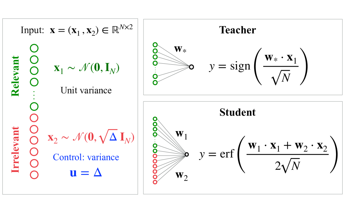</details> Figure 1: Illustration of the curriculum learning model studied in Section 3.1. Curriculum learning (CL) refers to a variety of training protocols in which examples are presented in a curated order—typically organized by difficulty or complexity. In animal and human training, CL is widely used and extensively studied in behavioral research, demonstrating clear benefits [100, 101, 102]. For example, shaping —the progressive introduction of subtasks to decompose a complex task—is a common technique in animal training [6, 103]. By contrast, results on the efficacy of CL in machine learning remain sparse and less conclusive [104, 105]. Empirical studies across diverse settings have nonetheless demonstrated that curricula can outperform standard heuristic strategies [106, 107, 108]. Several theoretical studies have explored the benefits of curriculum learning in analytically tractable models. Easy-to-hard curricula have been shown to accelerate learning in convex settings [109, 110] and improve generalization in more complex nonconvex problems, such as XOR classification [111] or parity functions [112, 113]. However, these analyses typically focused on predefined heuristics, which may not be optimal. In particular, it remains unclear under what conditions an easy‐to‐hard curriculum is truly optimal and what alternative strategies might outperform it when it is not. Moreover, although hyperparameter schedules have been shown to enhance curriculum learning empirically [49], a principled approach to their joint optimization remains largely unexplored. Here, we focus on a prototypical model of curriculum learning introduced in [104] and recently studied analytically in [110], where high-dimensional learning curves for online SGD were derived. This model considers a binary classification problem in a TS setting where both teacher and student are perceptron (one-layer) networks. The input vectors consist of $L=2$ elements—relevant directions $\bm{x}_{1}$ , which the teacher ( $M=1$ ) uses to generate labels $y=\operatorname{sign}({\bm{x}}_{1}·{\bm{w}}_{*}/\sqrt{N})$ , and irrelevant directions $\bm{x}_{2}$ , which do not affect the labels For simplicity, we consider an equal proportion of relevant and irrelevant directions. It is possible to extend the analysis to arbitrary proportions as in [110].. The student network ( $K=2$ ) is given by $$ f_{\bm{w}}(\bm{x})=\operatorname{erf}\left(\frac{{\bm{x}}_{1}\cdot{\bm{w}}_{1}% +{\bm{x}}_{2}\cdot{\bm{w}}_{2}}{2\sqrt{N}}\right)\,. \tag{20} $$ As a result, the student does not know a priori which directions are relevant. The teacher vector is normalized such that $T_{11}=\bm{w}_{*}·\bm{w}_{*}/N=2$ . All inputs are single-cluster zero-mean Gaussian variables and the sample difficulty is controlled by the variance $\Delta$ of the irrelevant directions, while the relevant directions are assumed to have unit variance (see Figure 1). We do not include label noise. We consider the squared loss $\ell=(y-f_{\bm{w}}(\bm{x}))^{2}/2$ and ridge regularization $\tilde{g}\left(\bm{w}^{→p}\bm{w}/N\right)=\lambda\left({\bm{w}}_{1}·{\bm% {w}}_{1}+{\bm{w}}_{2}·{\bm{w}}_{2}\right)/(4N)$ , with tunable strength $\lambda≥ 0$ . An illustration of the model is presented in Figure 1. Full expressions for the ODEs governing the learning dynamics of the order parameters $M_{11}={\bm{w}}_{*}·{\bm{w}}_{1}/N$ , $Q_{11}={\bm{w}}_{1}·{\bm{w}}_{1}/N$ , $Q_{22}={\bm{w}}_{2}·{\bm{w}}_{2}/N$ , and the generalization error are provided in Appendix A.1. <details> <summary>x2.png Details</summary>  ### Visual Description ## Multi-Panel Figure: Curriculum Learning Performance ### Overview The image presents a multi-panel figure comparing the performance of three different training curricula: Curriculum, Anti-Curriculum, and Optimal. The figure consists of four subplots (a, b, c, d) that illustrate different aspects of the training process, including generalization error, difficulty protocol, cosine similarity with signal, and the norm of irrelevant weights. ### Components/Axes **Panel a: Generalization Error vs. Training Time** * **Y-axis:** Generalization error (log scale). Markers: 2 x 10^-1, 3 x 10^-1, 4 x 10^-1 * **X-axis:** Training time α. Markers: 0, 2, 4, 6, 8, 10, 12 * **Legend (top-left):** * Curriculum (blue, dashed line with circle markers) * Anti-Curriculum (orange, dashed line with square markers) * Optimal (black, solid line with diamond markers) **Panel b: Difficulty Protocol vs. Training Time** * **Y-axis:** Difficulty protocol Δ * **X-axis:** Training time α (arrow indicating direction) * **Color Coding:** * Easy (cyan) * Hard (coral) * **Curricula:** * Curriculum: Easy initially, then Hard * Anti-Curriculum: Hard initially, then Easy * Optimal: Easy initially, then Hard, then Easy **Panel c: Cosine Similarity with Signal vs. Training Time** * **Y-axis:** Cosine similarity with signal. Markers: 0.0, 0.2, 0.4, 0.6, 0.8, 1.0 * **X-axis:** Training time α. Markers: 0, 2, 4, 6, 8, 10, 12 * **Inset Plot:** Zoomed-in view of the cosine similarity between training time 8 and 12. * Y-axis markers: 0.89, 0.90, 0.91, 0.92, 0.93, 0.94, 0.95 * X-axis markers: 8.0, 8.5, 9.0, 9.5, 10.0, 10.5, 11.0, 11.5, 12.0 * **Legend (inferred from other plots):** * Curriculum (blue, dashed line with circle markers) * Anti-Curriculum (orange, dashed line with square markers) * Optimal (black, solid line with diamond markers) **Panel d: Norm of Irrelevant Weights vs. Training Time** * **Y-axis:** Norm of irrelevant weights. Markers: 1.0, 1.5, 2.0, 2.5, 3.0, 3.5, 4.0 * **X-axis:** Training time α. Markers: 0, 2, 4, 6, 8, 10, 12 * **Legend (inferred from other plots):** * Curriculum (blue, dashed line with circle markers) * Anti-Curriculum (orange, dashed line with square markers) * Optimal (black, solid line with diamond markers) ### Detailed Analysis **Panel a: Generalization Error** * **Curriculum (blue):** Starts at approximately 4.5 x 10^-1, decreases rapidly until training time ~6, then plateaus around 1.5 x 10^-1. * **Anti-Curriculum (orange):** Starts at approximately 4.5 x 10^-1, decreases steadily to approximately 1.3 x 10^-1 at training time 12. * **Optimal (black):** Starts at approximately 4.5 x 10^-1, decreases rapidly to approximately 1.5 x 10^-1 at training time 6, then decreases slowly to approximately 1.2 x 10^-1 at training time 12. **Panel b: Difficulty Protocol** * **Curriculum:** Starts with "Easy" tasks (cyan) for approximately half the training time, then switches to "Hard" tasks (coral). * **Anti-Curriculum:** Starts with "Hard" tasks (coral) and switches to "Easy" tasks (cyan) after approximately one-third of the training time. * **Optimal:** Starts with "Easy" tasks (cyan), switches to "Hard" tasks (coral) after a short period, and then switches back to "Easy" tasks (cyan). **Panel c: Cosine Similarity with Signal** * **Curriculum (blue):** Starts at 0, increases rapidly to approximately 0.8 by training time 4, then increases slowly to approximately 0.97 by training time 12. * **Anti-Curriculum (orange):** Starts at 0, increases rapidly to approximately 0.7 by training time 4, then increases slowly to approximately 0.95 by training time 12. * **Optimal (black):** Starts at 0, increases rapidly to approximately 0.85 by training time 4, then increases slowly to approximately 0.98 by training time 12. * **Inset Plot:** Shows that the cosine similarity for Anti-Curriculum surpasses Curriculum after training time 10. **Panel d: Norm of Irrelevant Weights** * **Curriculum (blue):** Remains at approximately 1.0 until training time 6, then increases to approximately 2.2 by training time 12. * **Anti-Curriculum (orange):** Increases rapidly from 1.0 to approximately 4.1 by training time 4, then plateaus. * **Optimal (black):** Remains at approximately 1.0 until training time 2, then increases to approximately 2.8 by training time 12. ### Key Observations * The "Optimal" curriculum achieves the lowest generalization error and highest cosine similarity with signal. * The "Anti-Curriculum" results in the highest norm of irrelevant weights. * The "Curriculum" shows a delayed increase in the norm of irrelevant weights. ### Interpretation The data suggests that the order in which training tasks are presented significantly impacts the learning process. The "Optimal" curriculum, which starts with easy tasks, transitions to hard tasks, and then returns to easy tasks, appears to be the most effective in minimizing generalization error and maximizing the alignment of the learned representation with the signal. The "Anti-Curriculum," which starts with hard tasks, leads to a higher norm of irrelevant weights, potentially indicating that the model is learning spurious correlations early in training. The "Curriculum" approach, starting with easy tasks and then transitioning to hard tasks, shows a delayed increase in the norm of irrelevant weights, suggesting that it may be more robust to learning irrelevant features early on. The inset in panel c highlights a subtle but potentially important difference in the long-term behavior of the cosine similarity, where the Anti-Curriculum eventually surpasses the Curriculum. This could indicate that while the initial learning is slower, the Anti-Curriculum may eventually converge to a better solution. 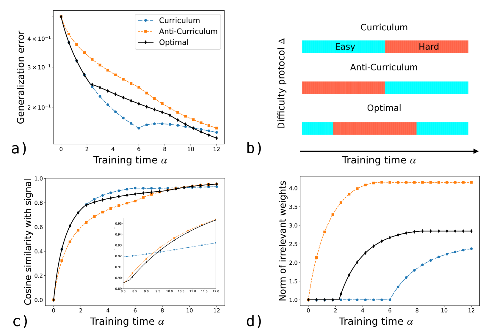</details> Figure 2: Learning dynamics for different difficulty schedules: curriculum (easy-to-hard), anti-curriculum (hard-to-easy) and the optimal one. a) Generalization error vs. training time $\alpha$ . b) Timeline of each schedule. c) Cosine similarity with the target signal $M_{11}/\sqrt{T_{11}Q_{11}}$ (inset zooms into the late-training regime). d) Squared norm of irrelevant weights $Q_{22}$ vs. $\alpha$ . Parameters: $\alpha_{F}=12$ , $\Delta_{1}=0$ , $\Delta_{2}=2$ , $\eta=3$ , $\lambda=0$ , $T_{11}=2$ . Initialization: $Q_{11}=Q_{22}=1$ , $M_{11}=0$ . We consider a dataset composed of two difficulty levels: $50\%$ “easy” examples ( $\Delta=\Delta_{1}$ ), and $50\%$ “hard” examples ( $\Delta=\Delta_{2}>\Delta_{1}$ ). We call curriculum the easy-to-hard schedule in which all easy samples are presented first, and anti-curriculum the opposite strategy (see Figure 2 b). We compute the optimal sampling strategy $\bm{u}(\alpha)=\Delta(\alpha)∈\{\Delta_{1},\Delta_{2}\}$ using Pontryagin’s maximum principle, as explained in Section 2.3.1. The constraint on the proportion of easy and hard examples in the training set is enforced via an additional Lagrange multiplier in the cost functional (Eq. (13)). As the final objective in Eq. (12) we use the misclassification error averaged over an equal proportion of easy and hard examples. Good generalization requires balancing two competing objectives: maximizing the teacher–student alignment along relevant directions—as measured by the cosine similarity with the signal $M_{11}/\sqrt{T_{11}Q_{11}}$ —and minimizing the norm of the student’s weights along the irrelevant directions, $\sqrt{Q_{22}}$ . We observe that anti-curriculum favors the first objective, while curriculum the latter. This is shown in Figure 2, where we take constant learning rate $\eta=3$ and no regularization $\lambda=0$ . In this case, the optimal strategy is non-monotonic in difficulty, following an “easy-hard-easy” schedule, that balances the two objectives (see panels 2 c and 2 d), and achieves lower generalization error compared to the two monotonic strategies. <details> <summary>x3.png Details</summary>  ### Visual Description ## Chart: Final Error vs Regularization and Optimal Learning Rate vs Training Time ### Overview The image presents two plots. The left plot (a) shows the final error as a function of regularization for different training methods: Curriculum, Anti-Curriculum, Optimal (Δ), and Optimal (Δ and η). The right plot (b) illustrates the optimal learning rate as a function of training time, segmented into "Easy" and "Hard" regions. ### Components/Axes **Plot a) Final Error vs Regularization:** * **Y-axis:** "Final error" with a logarithmic scale (10^-1). The axis ranges from approximately 1.0 x 10^-1 to 2.0 x 10^-1. * **X-axis:** "Regularization λ" ranging from 0.00 to 0.30 in increments of 0.05. * **Legend (bottom-left):** * Blue dashed line with circles: "Curriculum" * Orange dashed line with squares: "Anti-Curriculum" * Black solid line with diamonds: "Optimal (Δ)" * Green solid line with crosses: "Optimal (Δ and η)" **Plot b) Optimal Learning Rate vs Training Time:** * **Y-axis:** "Optimal learning rate η" ranging from 1.0 to 5.0 in increments of 0.5. * **X-axis:** "Training time α" ranging from 0 to 12 in increments of 2. * **Top:** A horizontal bar divided into two sections: * Left (cyan): "Easy" * Right (coral): "Hard" * **Data Series:** A single green line representing the optimal learning rate. ### Detailed Analysis **Plot a) Final Error vs Regularization:** * **Curriculum (Blue):** The final error increases as regularization increases. At λ = 0, the final error is approximately 0.15 x 10^-1, and at λ = 0.3, it's approximately 0.21 x 10^-1. * **Anti-Curriculum (Orange):** The final error starts at approximately 0.16 x 10^-1, decreases slightly to about 0.155 x 10^-1, and then remains relatively constant as regularization increases. * **Optimal (Δ) (Black):** The final error increases slightly with regularization. It starts at approximately 0.145 x 10^-1 and ends at approximately 0.16 x 10^-1. * **Optimal (Δ and η) (Green):** The final error decreases initially and then slightly increases with regularization. It has a minimum value of approximately 0.10 x 10^-1 around λ = 0.15. **Plot b) Optimal Learning Rate vs Training Time:** * **Optimal Learning Rate (Green):** The learning rate starts at approximately 4.25, increases to a peak of approximately 4.9 around α = 2, and then decreases rapidly until α = 6. At α = 6, there is a sharp drop in the learning rate from approximately 2.3 to 1.3. After this drop, the learning rate continues to decrease gradually, reaching approximately 1.0 at α = 12. ### Key Observations * In plot a), the "Optimal (Δ and η)" method consistently achieves the lowest final error across all regularization values. * In plot b), the optimal learning rate decreases over time, with a significant drop at the transition from the "Easy" to the "Hard" training phase. ### Interpretation The plots suggest that incorporating both Δ and η in the optimization process leads to better performance (lower final error) compared to other methods. The optimal learning rate plot indicates that a higher learning rate is beneficial during the initial "Easy" phase of training, but it needs to be reduced significantly as the training progresses into the "Hard" phase. The sharp drop in the learning rate at the transition point suggests a deliberate adjustment to prevent overshooting or instability as the model encounters more complex data. 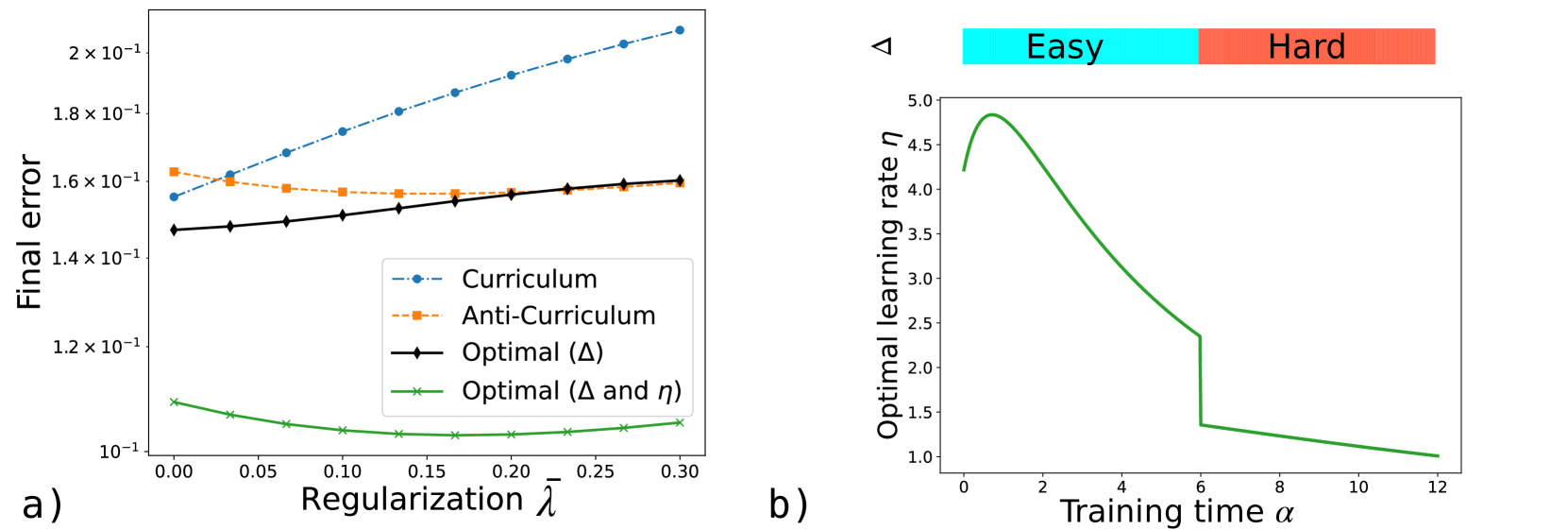</details> Figure 3: Simultaneous optimization of difficulty protocol $\Delta$ and learning rate $\eta$ in curriculum learning. a) Generalization error at the final time $\alpha_{F}=12$ , averaged over an equal fraction of easy and hard examples, as a function of the (rescaled) regularization $\bar{\lambda}=\lambda\eta$ for the three strategies presented in Figure 2, obtained optimizing over $\Delta$ at constant $\eta=3$ , and the optimal strategy (displayed in panel b for $\lambda=0$ ) obtained by jointly optimizing $\Delta$ and $\eta$ . Same parameters as Figure 2. Furthermore, we observe that the optimal balance between these competing goals is determined by the interplay between the difficulty schedule and other problem hyperparameters such as regularization and learning rate. Figure 3 a shows the final generalization error as a function of the regularization strength (held constant during training) for curriculum (blue), anti-curriculum (orange), and the optimal schedule (black), at fixed learning rate. When the regularization is high ( $\lambda>0.2$ ), weight decay alone ensures norm suppression along the irrelevant directions, so the optimal strategy reduces to anti-curriculum. We next explore how a time‐dependent learning‐rate schedule $\eta(\alpha)$ can be coupled with the curriculum to improve generalization. This corresponds to extending the control vector $\bm{u}(\alpha)=\left(\Delta(\alpha),\eta(\alpha)\right)$ , where both difficulty and learning rate schedules are optimized jointly. In Figure 3 a, we see that this joint optimization produces a substantial reduction in generalization error compared to any constant‐ $\eta$ strategy. Interestingly, for all parameter settings considered, an easy‐to‐hard curriculum becomes optimal once the learning rate is properly adjusted. Figure 3 b displays the optimal learning rate schedule $\eta(\alpha)$ at $\lambda=0$ : it begins with a warm‐up phase, transitions to gradual annealing, and then undergoes a sharp drop precisely when the curriculum shifts from easy to hard samples. This behavior is intuitive, since learning harder examples benefits from a lower, more cautious learning rate. As demonstrated in Figure 10 (Appendix B), this combined schedule effectively balances both objectives—maximizing signal alignment and minimizing noise overfitting. These results align with the empirical learning rate scheduling employed in the numerical experiments of [111], where easier samples were trained with a higher (constant) learning rate and harder samples with a lower one. Importantly, our framework provides a principled derivation of the optimal joint schedule, thereby confirming and grounding prior empirical insights. 3.2 Dropout regularization <details> <summary>x4.png Details</summary>  ### Visual Description ## Neural Network Architectures: Teacher-Student Model ### Overview The image presents a diagram illustrating a teacher-student model in machine learning, showcasing the architectures of the teacher network and the student network during training and testing phases. The diagram highlights the flow of information and the key parameters involved in each stage. ### Components/Axes * **Teacher Network (Left)**: * Input: x * Weights: w\* * Hidden Nodes: M hidden nodes * Activation Function: φ(x) * Output: φ(x) * Label Noise: z ~ N(0,1) * Equation: y = φ(x) + σ\_n z * **Student Network (Center)**: * State: at training step μ * Input: x * Weights: w * Hidden Nodes: K hidden nodes * Node-activation variables: r\_μ^(1), r\_μ^(2), ..., r\_μ^(K) ~ Bernoulli(p\_μ) * Output: ŷ * **Student Network (Right)**: * State: at testing time * Input: x * Weights: w * Hidden Nodes: K hidden nodes * Rescaling factor: p\_f * Output: ŷ ### Detailed Analysis or ### Content Details **Teacher Network:** * The input 'x' is fed into the network. * The network has 'M' hidden nodes. * The weights connecting the input layer to the hidden layer are denoted as 'w\*'. * The output of the teacher network is φ(x). * Label noise 'z' is added to the output, where 'z' follows a normal distribution with mean 0 and standard deviation 1 (N(0,1)). * The final output 'y' is given by the equation y = φ(x) + σ\_n z, where σ\_n represents the noise level. * The connections between the input layer and the hidden layer are green. * The connections between the hidden layer and the output layer are gray. **Student Network (Training):** * The input 'x' is fed into the network. * The network has 'K' hidden nodes. * The weights connecting the input layer to the hidden layer are denoted as 'w'. * Node-activation variables r\_μ^(1), r\_μ^(2), ..., r\_μ^(K) follow a Bernoulli distribution with parameter p\_μ. * The output of the student network is ŷ. * The connections between the input layer and the hidden layer are orange. * The connections between the hidden layer and the output layer are gray. * The node-activation variables are represented by purple squares. **Student Network (Testing):** * The input 'x' is fed into the network. * The network has 'K' hidden nodes. * The weights connecting the input layer to the hidden layer are denoted as 'w'. * A rescaling factor 'p\_f' is applied. * The output of the student network is ŷ. * The connections between the input layer and the hidden layer are orange. * The connections between the hidden layer and the output layer are blue. ### Key Observations * The teacher network has 'M' hidden nodes, while the student network has 'K' hidden nodes. * The student network's architecture remains the same during training and testing, but the connections to the output node change. During training, the connections are gray, and during testing, the connections are blue. * The teacher network introduces label noise, while the student network uses node-activation variables during training and a rescaling factor during testing. ### Interpretation The diagram illustrates a teacher-student learning paradigm, where a student network learns to mimic the behavior of a teacher network. The teacher network provides the target outputs, while the student network adjusts its parameters to minimize the difference between its output and the teacher's output. The use of node-activation variables during training and a rescaling factor during testing suggests that the student network is learning to generalize from noisy data. The teacher network introduces noise to the labels, which forces the student network to learn a more robust representation of the data. The student network uses node-activation variables during training to explore different configurations of the network, and it uses a rescaling factor during testing to adjust the output scale. 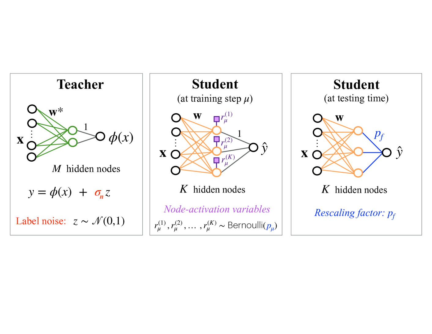</details> Figure 4: Illustration of the dropout model studied in Section 3.2. Dropout [80, 81] is a regularization technique designed to prevent harmful co-adaptations of hidden units, thereby reducing overfitting and enhancing the network’s performance. During training, each node is independently kept active with probability $p$ and “dropped” (i.e., its output set to zero) otherwise, effectively sampling a random subnetwork at each iteration. At test time, the full network is used, which corresponds to averaging over the ensemble of all subnetworks and yields more robust predictions. Dropout has become a cornerstone of modern neural‐network training [114]. While early works recommended keeping the activation probability fixed—typically in the range $0.5$ - $0.8$ —throughout training [80, 81], recent empirical studies propose varying this probability over time, using adaptive schedules to further enhance performance [115, 82, 83]. In particular, [82] showed that heuristic schedules that decrease the activation probability over time are analogous to easy-to-hard curricula and can lead to improved performance. Although adaptive dropout schedules have attracted practical interest, the conditions under which they outperform constant strategies remain poorly understood, and the theoretical foundations of their potential optimality are largely unexplored. <details> <summary>x5.png Details</summary>  ### Visual Description ## Chart: Training Time vs. Various Metrics ### Overview The image presents four line charts (a, b, c, d) that depict the relationship between training time (alpha) and different performance metrics or probabilities in a machine learning context. The charts explore the impact of dropout regularization and noise levels on generalization error, a measure of model performance (Delta), a ratio involving matrix elements (M11/sqrt(Q11*T11)), and activation probability. ### Components/Axes **Chart a)** * **Title:** Generalization error vs. Training time * **X-axis:** Training time α (values: 0 to 5, incrementing by 1) * **Y-axis:** Generalization error (values: 2 x 10^-2 to 6 x 10^-2, incrementing by 1 x 10^-2) * **Legend:** * Orange dashed line with square markers: No dropout * Blue dashed-dotted line with circle markers: Constant (p=0.68) * Black solid line with diamond markers: Optimal **Chart b)** * **Title:** Delta vs. Training time * **X-axis:** Training time α (values: 0 to 5, incrementing by 1) * **Y-axis:** Δ̃ (values: 0.0 to 0.8, incrementing by 0.2) * **Legend:** (Same as Chart a) * Orange dashed line with square markers: No dropout * Blue dashed-dotted line with circle markers: Constant (p=0.68) * Black solid line with diamond markers: Optimal **Chart c)** * **Title:** M11/sqrt(Q11\*T11) vs. Training time * **X-axis:** Training time α (values: 0 to 5, incrementing by 1) * **Y-axis:** M11/√(Q11\*T11) (values: 0.2 to 0.9, incrementing by 0.1) * **Legend:** (Same as Chart a) * Orange dashed line with square markers: No dropout * Blue dashed-dotted line with circle markers: Constant (p=0.68) * Black solid line with diamond markers: Optimal **Chart d)** * **Title:** Activation probability p(α) vs. Training time * **X-axis:** Training time α (values: 0 to 5, incrementing by 1) * **Y-axis:** Activation probability p(α) (values: 0.4 to 1.0, incrementing by 0.1) * **Legend:** * Teal dotted line with square markers: σn = 0.1 * Green dashed line with circle markers: σn = 0.2 * Black solid line with diamond markers: σn = 0.3 * Red line with x markers: σn = 0.5 ### Detailed Analysis **Chart a) Generalization Error** * **No dropout (orange):** The generalization error decreases rapidly from approximately 6.8e-2 at α=0 to approximately 3.2e-2 at α=5. * **Constant (p=0.68) (blue):** The generalization error decreases from approximately 6.3e-2 at α=0 to approximately 1.6e-2 at α=5. * **Optimal (black):** The generalization error decreases from approximately 6.8e-2 at α=0 to approximately 1.4e-2 at α=5. **Chart b) Delta** * **No dropout (orange):** Delta decreases from approximately 0.88 at α=0 to approximately 0.25 at α=5. * **Constant (p=0.68) (blue):** Delta decreases from approximately 0.63 at α=0 to approximately 0.08 at α=5. * **Optimal (black):** Delta decreases from approximately 0.88 at α=0 to approximately 0.07 at α=5. **Chart c) M11/sqrt(Q11\*T11)** * **No dropout (orange):** The ratio increases from approximately 0.27 at α=0 to approximately 0.87 at α=5. * **Constant (p=0.68) (blue):** The ratio increases from approximately 0.27 at α=0 to approximately 0.83 at α=5. * **Optimal (black):** The ratio increases from approximately 0.27 at α=0 to approximately 0.86 at α=5. **Chart d) Activation Probability** * **σn = 0.1 (teal):** The activation probability remains at 1.0 until α=2, then decreases to approximately 0.86 at α=3.5, then increases back to 1.0 at α=5. * **σn = 0.2 (green):** The activation probability remains at 1.0 until α=1, then decreases to approximately 0.58 at α=5. * **σn = 0.3 (black):** The activation probability remains at 1.0 until α=1, then decreases to approximately 0.43 at α=5. * **σn = 0.5 (red):** The activation probability remains at 1.0 until α=0.5, then decreases to approximately 0.43 at α=5. ### Key Observations * In charts a, b, and c, the "Optimal" configuration generally performs best or is very close to the best, followed by "No dropout," and then "Constant (p=0.68)." * In chart d, higher noise levels (σn) lead to a more rapid decrease in activation probability as training time increases. ### Interpretation The charts suggest that the "Optimal" configuration, likely referring to an optimized dropout strategy, consistently achieves the lowest generalization error and delta, while maximizing the ratio M11/sqrt(Q11\*T11). This indicates that a well-tuned dropout strategy can significantly improve model performance. The activation probability plots show how different noise levels affect the activation of neurons during training. Higher noise levels cause neurons to deactivate more quickly, potentially influencing the model's learning dynamics and generalization ability. The data suggests that finding the right balance of dropout and noise is crucial for optimizing model performance. 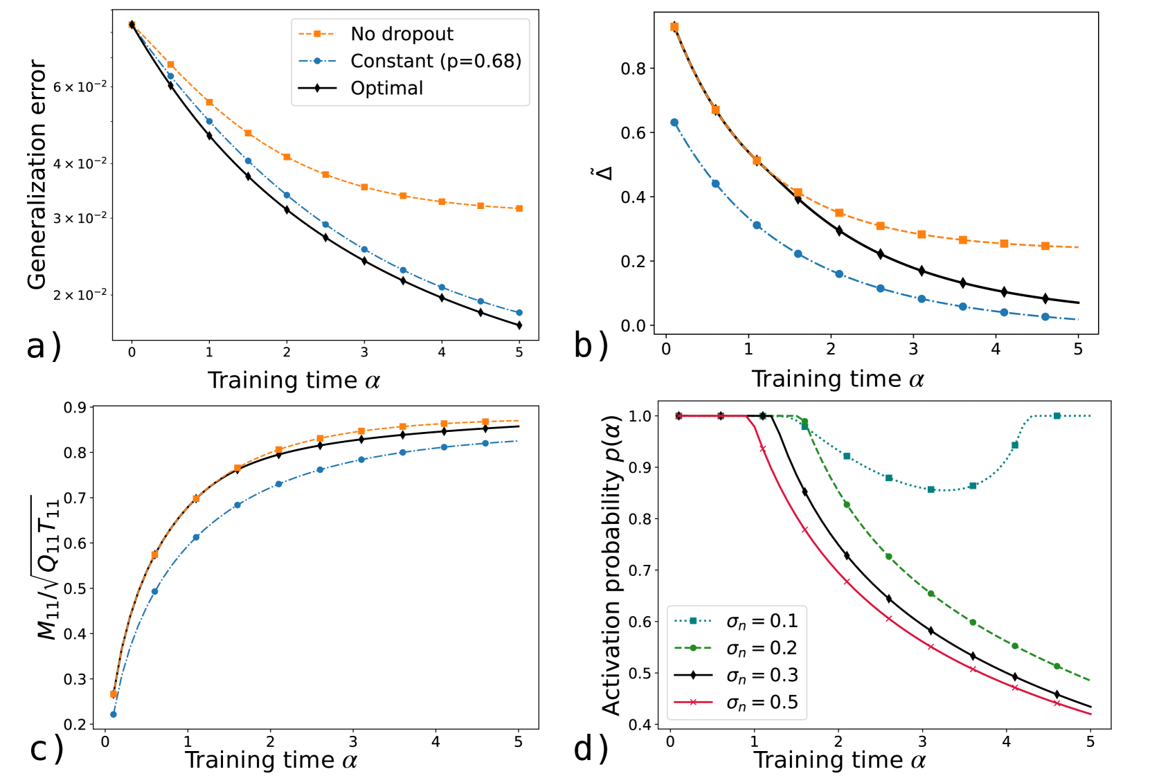</details> Figure 5: Learning dynamics with dropout regularization. a) Generalization error vs. training time $\alpha$ without dropout (orange), for constant activation probability $p=p_{f}=0.68$ (blue), and for the optimal dropout schedule with $p_{f}=0.678$ (black), at label noise $\sigma_{n}=0.3$ . b) Detrimental correlations between the student’s hidden nodes, measured by $\tilde{\Delta}=(Q_{12}-M_{11}M_{21})/\sqrt{Q_{11}Q_{22}}$ , vs. $\alpha$ , at $\sigma_{n}=0.3$ . c) Teacher-student cosine similarity $M_{11}/\sqrt{Q_{11}T_{11}}$ vs. $\alpha$ , at $\sigma_{n}=0.3$ . d) Optimal dropout schedules for different label-noise levels. The black curve ( $\sigma_{n}=0.3$ ) shows the optimal schedule used in panels a - c. Parameters: $\alpha_{F}=5$ , $K=2$ , $M=1$ , $\eta=1$ . The teacher weights $\bm{w}^{*}$ are drawn i.i.d. from $\mathcal{N}(0,1)$ with $N=10000$ . The student weights are initialized to zero. In [84], we introduced a prototypical model of dropout and derived analytic results for constant dropout probabilities. We showed that dropout reduces harmful node correlations—quantified via order parameters—and consequently improves generalization. We further demonstrated that the optimal (constant) activation probability decreases as the variance of the label noise increases. In this section, we first recast the model of [84] within our general framework and then extend the analysis to optimal dropout schedules. We consider a TS setup where both teacher and student networks are soft-committee machines [34], i.e., two-layer networks with untrained readout weights set to one. Specifically, the inputs $\bm{x}∈\mathbb{R}^{N}$ are taken to be standard Gaussian variables and the corresponding labels are produced via Eq. (2) with label noise variance $\sigma^{2}_{n}$ : $$ \displaystyle y=f^{*}_{\bm{w}_{*}}(\bm{x})+\sigma_{n}\,z\;, \displaystyle z\sim\mathcal{N}(0,1)\;, \displaystyle f^{*}_{\bm{w}_{*}}(\bm{x})=\sum_{m=1}^{M}\operatorname{erf}\left% (\frac{\bm{w}_{*,m}\cdot{\bm{x}}}{\sqrt{N}}\right)\,. \tag{21} $$ To describe dropout, at each training step $\mu$ we couple i.i.d. node-activation Bernoulli random variables $r^{(k)}_{\mu}\sim{\rm Ber}(p_{\mu})$ to each of the student’s hidden nodes $k=1,...,K$ : $$ f^{\rm train}_{\bm{w}}(\bm{x}^{\mu})=\sum_{k=1}^{K}r^{(k)}_{\mu}\operatorname{% erf}\left(\frac{\bm{w}_{k}\cdot{\bm{x}}^{\mu}}{\sqrt{N}}\right)\,, \tag{22} $$ so that node $k$ is active if $r^{(k)}_{\mu}=1$ . At testing time, the full network is used as $$ f^{\rm test}_{\bm{w}}(\bm{x})=\sum_{k=1}^{K}p_{f}\operatorname{erf}\left(\frac% {\bm{w}_{k}\cdot{\bm{x}}}{\sqrt{N}}\right)\,. \tag{23} $$ The rescaling factor $p_{f}$ ensures that the reduced activity during training is taken into account when testing. We consider the squared loss $\ell=(y-f_{\bm{w}}(\bm{x}))^{2}/2$ and no weight-decay regularization. The ODEs governing the order parameters $M_{km}$ and $Q_{jk}$ , as well as the resulting generalization error, are provided in Appendix A.2. These equations arise from averaging over the binary activation variables $r_{\mu}^{(k)}$ , so that the dropout schedule is determined by the time‐dependent activation probability $p(\alpha)$ . For simplicity, we focus our analysis on the case $M=1$ and $K=2$ , although our considerations hold more generally. During training, assuming $T_{11}=1$ , each student weight vector can be decomposed as ${\bm{w}}_{i}=M_{i1}{\bm{w}}_{*,1}+\tilde{{\bm{w}}}_{i}$ , where $\tilde{\bm{w}}_{i}\perp\bm{w}_{*,1}$ denotes the uninformative component acquired due to noise in the inputs and labels. Generalization requires balancing two competing goals: improving the alignment of each hidden unit with the teacher, measured by $M_{i1}$ , and reducing correlations between their uninformative components, $\tilde{\bm{w}}_{1}$ and $\tilde{\bm{w}}_{2}$ , so that noise effects cancel rather than compound. We quantify these detrimental correlations by the observable $\tilde{\Delta}=(Q_{12}-M_{11}M_{21})/\sqrt{Q_{11}Q_{22}}$ . Figure 5 b compares a constant‐dropout strategy ( $p=p_{f}=0.68$ , orange) with no dropout ( $p=p_{f}=1$ , blue) and shows that dropout sharply reduces $\tilde{\Delta}$ during training. Intuitively, without dropout, both nodes share identical noise realizations at each step, reinforcing their uninformative correlation; with dropout, nodes are from time to time trained individually, reducing correlations. Although dropout also slows the growth of the teacher–student cosine similarity (Figure 5 c) by reducing the number of updates per node, the large decrease in $\tilde{\Delta}$ leads to an overall lower generalization error (Figure 5 a). To find the optimal dropout schedule, we treat the activation probability as the control variable, $u(\alpha)=p(\alpha)∈[0,1]$ . Additionally, we optimize over the final rescaling $p_{f}∈[0,1]$ to minimize the final error. We solve this optimal‐control problem using a direct multiple‐shooting method implemented in CasADi (Section 2.3.2). Figure 5 shows the resulting optimal schedules for increasing label‐noise levels $\sigma_{n}$ . Each schedule exhibits an initial period with no dropout ( $p(\alpha)=1$ ) followed by a gradual decrease of $p(\alpha)$ . These strategies resemble those heuristically proposed in [82] but are obtained here via a principled procedure. The order parameters of the theory suggest a simple interpretation of the optimal schedules. In the initial phase of training, it is beneficial to fully exploit the rapid increase in the teacher-student cosine similarity by keeping both nodes active (see Figure 5). Once the increase in cosine similarity plateaus, it becomes more advantageous to decrease the activation probability in order to mitigate negative correlations among the student’s nodes. As a result, the optimal schedule achieves lower generalization error than any constant‐dropout strategy. Noisier tasks, corresponding to higher values of $\sigma_{n}$ , induce stronger detrimental correlations between the student nodes and therefore require a lower activation probability, as shown in [84] for the case of constant dropout. This observation remains valid for the optimal dropout schedules in Figure 5 d: as $\sigma_{n}$ grows, the initial no‐dropout phase becomes shorter and the activation probability decreases more sharply. Conversely, at low label noise ( $\sigma_{n}=0.1$ ), the activation probability remains close to one and becomes non-monotonic in training time. 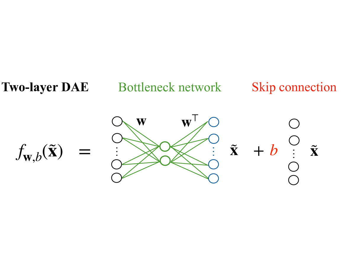3.3 Denoising autoencoder <details> <summary>x6.png Details</summary>  ### Visual Description ## Neural Network Diagram: Two-layer DAE with Bottleneck and Skip Connection ### Overview The image is a diagram illustrating the architecture of a two-layer Denoising Autoencoder (DAE) with a bottleneck network and a skip connection. It visually represents the flow of data through the network, highlighting the key components and their interconnections. ### Components/Axes * **Title:** Two-layer DAE (left), Bottleneck network (center, green), Skip connection (right, red) * **Equation:** *f_w,b(x̃)* = ... *x̃* + *b* ... *x̃* * **Nodes:** * Input Layer: Represented by a column of four white circles on the left, with an ellipsis indicating potentially more nodes. * Bottleneck Layer: Represented by two green circles in the center. * Output Layer: Represented by a column of four blue circles to the right of the bottleneck layer, with an ellipsis indicating potentially more nodes. * Skip Connection Layer: Represented by a column of four white circles on the right, with an ellipsis indicating potentially more nodes. * **Connections:** * Input to Bottleneck: Green lines connecting each node in the input layer to each node in the bottleneck layer. The connections are labeled with "w". * Bottleneck to Output: Green lines connecting each node in the bottleneck layer to each node in the output layer. The connections are labeled with "w^T". * Skip Connection: A direct connection from the input (x̃) to the output, bypassing the bottleneck. ### Detailed Analysis * **Input Layer:** Four nodes are explicitly shown, with an ellipsis suggesting more. * **Bottleneck Layer:** Two nodes are shown. * **Output Layer:** Four nodes are explicitly shown, with an ellipsis suggesting more. * **Skip Connection Layer:** Four nodes are explicitly shown, with an ellipsis suggesting more. * **Connections:** * Each input node connects to both bottleneck nodes. * Each bottleneck node connects to each output node. * The skip connection directly connects the input to the output. * **Equation Breakdown:** * *f_w,b(x̃)* represents the function performed by the DAE, where *w* represents the weights and *b* represents the bias. *x̃* represents the input. * The equation shows that the output is a function of the input *x̃*, the weights *w*, and the bias *b*. The skip connection adds *b* to the transformed input. ### Key Observations * The diagram clearly illustrates the bottleneck architecture, where the input is compressed into a lower-dimensional representation before being reconstructed. * The skip connection provides a direct path for the input to the output, potentially helping to preserve information and improve performance. * The use of different colors (green and blue) distinguishes the bottleneck and output layers. ### Interpretation The diagram represents a two-layer Denoising Autoencoder (DAE) architecture. The DAE aims to learn a compressed representation of the input data by encoding it into a lower-dimensional space (the bottleneck) and then decoding it back to the original input space. The bottleneck forces the network to learn the most important features of the data. The skip connection allows the network to bypass the bottleneck, potentially improving the reconstruction accuracy and allowing the network to learn both low-level and high-level features. The equation *f_w,b(x̃)* = ... *x̃* + *b* ... *x̃* summarizes the transformation performed by the network, where the input *x̃* is transformed by the weights *w* and bias *b*, and then combined with the original input *x̃* via the skip connection. </details> Figure 6: Illustration of the denoising autoencoder model studied in Section 3.3. <details> <summary>x7.png Details</summary>  ### Visual Description ## Chart/Diagram Type: Multi-Panel Plot ### Overview The image presents four plots (a, b, c, d) that analyze the effects of different noise schedules on a machine learning model during training. The plots explore optimal noise schedules, MSE improvement, cosine similarity, and skip connections as functions of training time. ### Components/Axes **Panel a: Optimal Noise Schedule** * **Title:** Optimal noise schedule * **X-axis:** Training time α, ranging from 0.0 to 0.8 in increments of 0.1. * **Y-axis:** Optimal noise schedule, ranging from 0.0 to 0.8 in increments of 0.1. * **Legend (Top-Right):** * Yellow: ΔF = 0.15 * Blue: ΔF = 0.2 * Green: ΔF = 0.25 * Orange: ΔF = 0.3 * Pink: ΔF = 0.35 * Gray: ΔF = 0.4 **Panel b: MSE Improvement** * **Title:** MSE improvement (%) * **X-axis:** Training time α, ranging from 0.0 to 0.8 in increments of 0.1. * **Y-axis:** MSE improvement (%), ranging from -40 to 30 in increments of 10. * **Horizontal dashed line:** at y = 0 * **Legend:** (Refer to Panel a for color correspondence to ΔF values) * Yellow: ΔF = 0.15 * Blue: ΔF = 0.2 * Green: ΔF = 0.25 * Orange: ΔF = 0.3 * Pink: ΔF = 0.35 * Gray: ΔF = 0.4 **Panel c: Cosine Similarity** * **Title:** Cosine similarity θ * **X-axis:** Training time α, ranging from 0.0 to 0.8 in increments of 0.1. * **Y-axis:** Cosine similarity θ, ranging from 0.2 to 0.9 in increments of 0.1. * **Legend (Center-Right):** * Dashed Dark Blue: θ^const_0,0 * Solid Dark Blue: θ^opt_0,0 * Dashed Light Green: θ^const_1,1 * Solid Light Green: θ^opt_1,1 **Panel d: Skip Connection** * **Title:** Skip connection * **X-axis:** Training time α, ranging from 0.0 to 0.8 in increments of 0.1. * **Y-axis:** Skip connection, ranging from 0.000 to 0.035 in increments of 0.005. * **Legend (Right):** * Dotted Black: Target * Dashed Green: Constant * Solid Green: Optimal ### Detailed Analysis **Panel a: Optimal Noise Schedule** * **ΔF = 0.15 (Yellow):** Remains relatively constant at approximately 0.02 across all training times. * **ΔF = 0.2 (Blue):** Starts at approximately 0.25 and decreases sharply to approximately 0.02 by α = 0.2, then remains constant. * **ΔF = 0.25 (Green):** Starts at approximately 0.6 and decreases to approximately 0.07 by α = 0.5, then remains constant. * **ΔF = 0.3 (Orange):** Starts at approximately 0.75 and decreases to approximately 0.07 by α = 0.6, then remains constant. * **ΔF = 0.35 (Pink):** Starts at approximately 0.78 and decreases to approximately 0.08 by α = 0.7, then remains constant. * **ΔF = 0.4 (Gray):** Starts at approximately 0.78 and decreases to approximately 0.08 by α = 0.7, then remains constant. **Panel b: MSE Improvement** * **ΔF = 0.15 (Yellow):** Increases from approximately 8% to 22% as α increases from 0.0 to 0.8. * **ΔF = 0.2 (Blue):** Increases from approximately -2% to 20% as α increases from 0.0 to 0.8, peaking at α = 0.4 with a value of 25%. * **ΔF = 0.25 (Green):** Decreases from approximately -25% to -18% until α = 0.4, then increases to approximately 15% at α = 0.8. * **ΔF = 0.3 (Orange):** Decreases from approximately -35% to -40% until α = 0.2, then increases to approximately 20% at α = 0.8. * **ΔF = 0.35 (Pink):** Decreases from approximately -35% to -42% until α = 0.2, then increases to approximately 22% at α = 0.8. * **ΔF = 0.4 (Gray):** Decreases from approximately -28% to -42% until α = 0.2, then increases to approximately 30% at α = 0.8. **Panel c: Cosine Similarity** * **θ^const_0,0 (Dashed Dark Blue):** Increases from approximately 0.23 to 0.83 as α increases from 0.0 to 0.8. * **θ^opt_0,0 (Solid Dark Blue):** Increases from approximately 0.23 to 0.92 as α increases from 0.0 to 0.8. * **θ^const_1,1 (Dashed Light Green):** Increases from approximately 0.23 to 0.85 as α increases from 0.0 to 0.8. * **θ^opt_1,1 (Solid Light Green):** Increases from approximately 0.23 to 0.92 as α increases from 0.0 to 0.8. **Panel d: Skip Connection** * **Target (Dotted Black):** Constant at approximately 0.034. * **Constant (Dashed Green):** Increases linearly from approximately 0.00 to 0.022 as α increases from 0.0 to 0.8. * **Optimal (Solid Green):** Increases from approximately 0.00 to 0.030 as α increases from 0.0 to 0.8. ### Key Observations * **Optimal Noise Schedule (Panel a):** Higher ΔF values require a more aggressive reduction in noise early in training. * **MSE Improvement (Panel b):** Higher ΔF values initially lead to worse MSE improvement, but eventually surpass lower ΔF values at later training times. * **Cosine Similarity (Panel c):** Optimal noise schedules result in higher cosine similarity compared to constant noise schedules. * **Skip Connection (Panel d):** Optimal skip connections approach the target value more closely than constant skip connections. ### Interpretation The plots demonstrate the impact of varying noise schedules (ΔF) on model training. The results suggest that a carefully tuned noise schedule can significantly improve model performance, as measured by MSE improvement, cosine similarity, and skip connection values. Specifically, higher ΔF values, which represent more aggressive noise reduction, initially hinder performance but ultimately lead to better results at later stages of training. The cosine similarity plot indicates that optimal noise schedules help the model converge to a more desirable state. The skip connection plot shows that the optimal schedule allows the model to approach the target skip connection value more closely than a constant schedule. </details> Figure 7: a) Optimal noise schedule $\Delta$ vs. training time $\alpha$ . Each color marks a different value of the test noise level $\Delta_{F}$ . b) Percentage improvement in mean square error of the optimal strategy compared to the constant one at $\Delta(\alpha)=\Delta_{F}$ , computed as: $100(\operatorname{MSE}_{\rm const}(\alpha)-\operatorname{MSE}_{\rm opt}(\alpha% ))/(\operatorname{MSE}_{\rm const}(0)-\operatorname{MSE}_{\rm const}(\alpha))$ . c) Cosine similarity $\theta_{k,k}=R_{k(1,k)}/\sqrt{Q_{kk}\Omega_{(1,k)(1,k)}}$ ( $k=1,2$ marked by different colors) vs. $\alpha$ for the optimal schedule (full lines) and the constant schedule (dashed lines), at $\Delta_{F}=0.25$ . d) Skip connection $b$ vs. $\alpha$ for the optimal schedule (full line) and the constant schedule (dashed line) at $\Delta_{F}=0.25$ . The dotted line marks the target value $b^{*}$ given by Eq. (26). Parameters: $K=C_{1}=2$ , $\alpha_{F}=0.8$ , $\eta=\eta_{b}=5$ , $\sigma=0.1$ , $N=1000$ , $g(z)=z$ . Initialization: $b=0$ . Other initial conditions are given in Eq. (92). Denoising autoencoders (DAEs) are neural networks trained to reconstruct input data from their corrupted version, thereby learning robust feature representations [116, 117]. Recent developments in diffusion models have revived the interest in denoising tasks as a key component of the generative process [118, 119]. Several theoretical works have investigated the learning dynamics and generalization properties of DAEs. In the linear case, [120] showed that noise acts as a regularizer, biasing learning toward high-variance directions. Nonlinear DAEs were studied in [121], where exact asymptotics in high dimensions were derived. Relatedly, [122, 123] analyzed diffusion models parameterized by DAEs. [124] studied shallow reconstruction autoencoders in an online-learning setting closely related to ours. A series of empirical works have considered noise schedules in the training of DAE. [125] showed that adaptive noise levels during training of DAEs promote learning multi-scale representations. Similarly, in diffusion models, networks are trained to denoise inputs at successive diffusion timesteps—each linked to a specific noise level. Recent work [126] demonstrates that non-uniform sampling of diffusion time, effectively implementing a noise schedule, can further enhance performance. Additionally, data augmentation, where multiple independent corrupted samples are obtained for each clean input, is often employed [127]. However, identifying principled noise schedules and data augmentation strategies remains largely an open problem. In this section, we consider the prototypical DAE model studied in [121] and apply the optimal control framework introduced in Section 2 to find optimal noise and data augmentation schedules. We consider input data $\bm{x}=(\bm{x}_{1},\bm{x}_{2})∈\mathbb{R}^{N× 2}$ , where $\bm{x}_{1}\sim\mathcal{N}\left(\frac{\bm{\mu}_{1,c_{1}}}{\sqrt{N}},\sigma_{1,c% _{1}}^{2}\bm{I}_{N}\right)$ , $c_{1}=1,...,C_{1}$ , represents the clean input drawn from a Gaussian mixture of $C_{1}$ clusters, while $\bm{x}_{2}\sim\mathcal{N}(\bm{0},\bm{I}_{N})$ is additive standard Gaussian noise. We will take $\sigma_{1,c_{1}}=\sigma$ for all $c_{1}$ and equiprobable clusters unless otherwise stated. The network receives the noisy input $\tilde{\bm{x}}=\sqrt{1-\Delta}\,\bm{x}_{1}+\sqrt{\Delta}\,\bm{x}_{2}$ , where $\Delta>0$ controls the level of corruption. The denoising is performed via a two-layer autoencoder $$ \displaystyle f_{\bm{w},b}(\tilde{\bm{x}})=\frac{\bm{w}}{\sqrt{N}}g\left(\frac% {\bm{w}^{\top}\tilde{\bm{x}}}{\sqrt{N}}\right)+b\,\tilde{\bm{x}}\;\in\mathbb{R% }^{N}\;, \tag{24} $$ with tied weights $\bm{w}∈\mathbb{R}^{N× K}$ , where $K$ is the dimension of the hidden layer, and a scalar trainable skip connection $b∈\mathbb{R}$ . The activation function $g$ is applied component-wise. The illustration in Figure 6 highlights the two components of the architecture: the bottleneck autoencoder network and the skip connection. In this unsupervised learning setting, the loss function is given by the squared reconstruction error between the clean input and the network output: $\mathcal{L}(\bm{w},b|\bm{x},\bm{c})=\|\bm{x}_{1}-f_{\bm{w},b}(\tilde{\bm{x}})% \|_{2}^{2}/2$ . This loss can be recast in the form of Eq. 4, as shown in [43]. The skip connection is trained via online SGD, i.e., $b^{\mu+1}=b^{\mu}-(\eta_{b}/N)∂_{b}\mathcal{L}({\bm{w}}^{\mu},b^{\mu}|{% \bm{x}}^{\mu},{\bm{c}}^{\mu})$ . We measure generalization via the mean squared error: $\operatorname{MSE}=\mathbb{E}_{\bm{x},\bm{c}}\left[\|\bm{x}-f_{\bm{w},b}(% \tilde{\bm{x}})\|_{2}^{2}/2\right]$ . As shown in Appendix A.3, in the high-dimensional limit, the MSE is given by $$ \displaystyle\begin{split}\text{MSE}=N\left[\sigma^{2}\left(1-b\sqrt{1-\Delta}% \right)^{2}+b^{2}\Delta\right]+\mathbb{E}_{\bm{x},\bm{c}}\left[\sum_{k,k^{% \prime}=1}^{K}Q_{kk^{\prime}}g(\tilde{\lambda}_{k})g(\tilde{\lambda}_{k^{% \prime}})-2\sum_{k=1}^{K}(\lambda_{1,k}-b\tilde{\lambda}_{k})g(\tilde{\lambda}% _{k})\right],\end{split} \tag{25} $$ where we have defined the pre-activations $\tilde{\lambda}_{k}\equiv{\tilde{\bm{x}}}·{\bm{w}}_{k}/\sqrt{N}$ and $\lambda_{1,k}={\bm{w}}_{k}·{\bm{x}}_{1}/\sqrt{N}$ , and neglected a constant term. Note that the leading term in Eq. (25)—proportional to $N$ —is independent of the autoencoder weights $\bm{w}$ , and depends only on the skip connection $b$ and the noise level $\Delta$ . Therefore, the presence of the skip connection can improve the MSE by a contribution of order $\mathcal{O}_{N}(N)$ [122]. To leading order, the optimal skip connection that minimizes the MSE in Eq. (25) is given by $$ b^{*}=\frac{\sqrt{(1-\Delta)}\,\sigma^{2}}{(1-\Delta)\,\sigma^{2}+\Delta}\;. \tag{26} $$ The relevant order parameters in this model are $R_{k(1,c_{1})}$ and $Q_{kk^{\prime}}$ , where $k,k^{\prime}=1... K$ and $c_{1}=1... C_{1}$ (see Eq. (8) and (10)). In Appendix A.3, we provide closed-form expressions for the MSE and the ODEs describing the evolution of the order parameters. 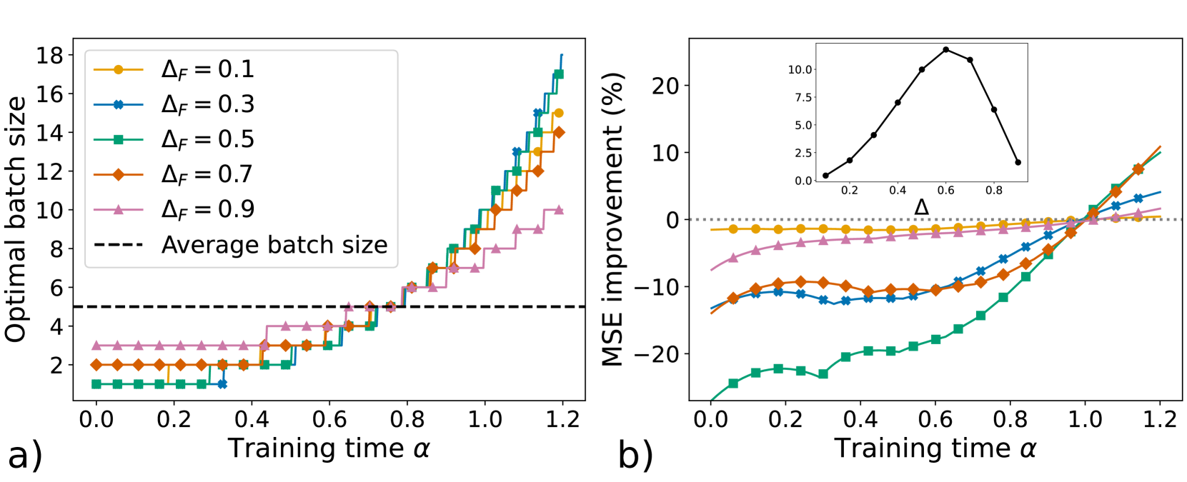<details> <summary>x8.png Details</summary>  ### Visual Description ## Chart Type: Line Plots ### Overview The image contains two line plots, labeled a) and b), that explore the relationship between training time and optimal batch size, and training time and MSE improvement, respectively. The plots analyze the impact of different values of ΔF on these relationships. Plot b) also contains an inset plot showing the relationship between Δ and an unspecified variable. ### Components/Axes **Plot a)** * **Title:** Optimal batch size vs. Training time α * **X-axis:** Training time α, with values ranging from 0.0 to 1.2 in increments of 0.2. * **Y-axis:** Optimal batch size, with values ranging from 2 to 18 in increments of 2. * **Legend (Top-Left):** * Yellow line with circles: ΔF = 0.1 * Blue line with diamonds: ΔF = 0.3 * Green line with squares: ΔF = 0.5 * Orange line with diamonds: ΔF = 0.7 * Pink line with triangles: ΔF = 0.9 * Black dashed line: Average batch size **Plot b)** * **Title:** MSE improvement (%) vs. Training time α * **X-axis:** Training time α, with values ranging from 0.0 to 1.2 in increments of 0.2. * **Y-axis:** MSE improvement (%), with values ranging from -20 to 20 in increments of 10. * **Legend:** Same as Plot a). * **Horizontal dotted line:** Represents 0% MSE improvement. **Inset Plot (Plot b)** * **X-axis:** Δ, with values ranging from 0.0 to 0.8 in increments of 0.2. * **Y-axis:** Unspecified, with values ranging from 0.0 to 10.0 in increments of 2.5. ### Detailed Analysis **Plot a) - Optimal batch size** * **Average batch size (Black dashed line):** Constant at approximately 5. * **ΔF = 0.1 (Yellow line with circles):** Remains relatively constant at approximately 2 until α ≈ 0.8, then increases stepwise to approximately 15 at α = 1.2. * **ΔF = 0.3 (Blue line with diamonds):** Remains relatively constant at approximately 1 until α ≈ 0.8, then increases stepwise to approximately 16 at α = 1.2. * **ΔF = 0.5 (Green line with squares):** Remains relatively constant at approximately 1 until α ≈ 0.8, then increases stepwise to approximately 15 at α = 1.2. * **ΔF = 0.7 (Orange line with diamonds):** Remains relatively constant at approximately 2 until α ≈ 0.8, then increases stepwise to approximately 14 at α = 1.2. * **ΔF = 0.9 (Pink line with triangles):** Remains relatively constant at approximately 3 until α ≈ 0.8, then increases stepwise to approximately 9 at α = 1.2. **Plot b) - MSE improvement** * **ΔF = 0.1 (Yellow line with circles):** Remains relatively constant at approximately -2% throughout the training time. * **ΔF = 0.3 (Blue line with diamonds):** Starts at approximately -12% and gradually increases to approximately 2% at α = 1.2. * **ΔF = 0.5 (Green line with squares):** Starts at approximately -24% and increases sharply to approximately 12% at α = 1.2. * **ΔF = 0.7 (Orange line with diamonds):** Starts at approximately -14% and increases to approximately 12% at α = 1.2. * **ΔF = 0.9 (Pink line with triangles):** Starts at approximately -7% and increases slightly to approximately 2% at α = 1.2. **Inset Plot (Plot b)** * The black line increases from approximately 0 at Δ = 0.0 to a peak of approximately 11 at Δ = 0.6, then decreases to approximately 3 at Δ = 0.8. ### Key Observations * In Plot a), the optimal batch size remains relatively constant for all ΔF values until a training time of approximately 0.8, after which it increases sharply. * In Plot b), the MSE improvement varies significantly depending on the ΔF value. Lower ΔF values (0.1 and 0.9) result in relatively constant or slightly increasing MSE improvement, while higher ΔF values (0.3, 0.5, and 0.7) show a more significant increase in MSE improvement as training time increases. * The inset plot in Plot b) shows a non-linear relationship between Δ and the unspecified variable, with a peak at Δ = 0.6. ### Interpretation The plots suggest that the optimal batch size is relatively stable during the initial stages of training, but increases significantly as training progresses beyond a certain point (α ≈ 0.8). The value of ΔF has a significant impact on the MSE improvement, with higher values generally leading to greater improvements, especially at later stages of training. The inset plot indicates that there is an optimal value of Δ (around 0.6) for maximizing some other performance metric, which is not explicitly defined in the plot. The relationship between Δ and ΔF is not clear from the plots, but it is possible that they are related. </details> Figure 8: a) Optimal batch augmentation schedule vs. training time $\alpha$ for different values of the test noise level $\Delta=\Delta_{F}$ . All schedules have average batch size $\bar{B}=5$ . b) Percentage improvement of the optimal strategy compared to the constant one at $B(\alpha)=\bar{B}=5$ , computed as: $100(\operatorname{MSE}_{\rm const}(\alpha)-\operatorname{MSE}_{\rm opt}(\alpha% ))/(\operatorname{MSE}_{\rm const}(0)-\operatorname{MSE}_{\rm const}(\alpha))$ . The inset shows the MSE improvement at the final time $\alpha_{F}=1.2$ as a function of $\Delta$ . Parameters: $K=C_{1}=2$ , $\eta=5$ , $\sigma=0.1$ , $g(z)=z$ . The skip connection $b$ is fixed ( $\eta_{b}=0$ ) to the optimal value in Eq. (26). Initial conditions are given in Eq. (92). We start by considering the problem of finding the optimal denoising schedule $\Delta(\alpha)$ . Our goal is to minimize the final MSE, computed at the fixed test noise level $\Delta_{F}$ . To this end, we treat the noise level as the control variable $u(\alpha)=\Delta(\alpha)∈(0,1)$ , and we find the optimal schedule using a direct multiple-shooting method implemented in CasADi (Section 2.3.1). In the following analysis, we consider linear activation. Figure 7 a displays the optimal noise schedules for a range of test noise levels $\Delta_{F}$ . We observe that the optimal schedule typically features an initial decrease, followed by a moderate increase toward the end. At low $\Delta_{F}$ , the optimal schedule remains nearly flat and close to $\Delta=0$ before the final increase. Both the duration of the initial decreasing phase and the average noise level throughout the schedule increase with $\Delta_{F}$ . Figure 7 b shows that the optimal schedule improves the MSE by approximately $10$ - $30\%$ over the constant schedule $\Delta(\alpha)=\Delta_{F}$ . The optimal denoising schedule achieves two key objectives. First, it enhances the reconstruction capability of the bottleneck network, leading to a higher cosine similarity between the hidden nodes of the autoencoder and the means of the Gaussian mixture defining the clean input distribution (panel 7 c). Second, it accelerates the convergence of the skip connection toward the target value $b^{*}$ in Eq. (26) (panel 7 d). We then explore a setting that incorporates data augmentation, with inputs $\bm{x}=(\bm{x}_{1},\bm{x}_{2},...,\bm{x}_{B+1})∈\mathbb{R}^{N× B+1}$ , where $\bm{x}_{1}\sim\mathcal{N}\left(\frac{\bm{\mu}_{1,c_{1}}}{\sqrt{N}},\sigma^{2}% \bm{I}_{N}\right)$ denotes the clean version of the input as before. We consider $B$ independent realizations of standard Gaussian noise $\bm{x}_{2},...,\bm{x}_{B+1}\overset{\rm i.i.d.}{\sim}\mathcal{N}(\bm{0},\bm% {I}_{N})$ . We can construct a batch of noisy inputs: $\tilde{\bm{x}}_{a}=\sqrt{1-\Delta}\,\bm{x}_{1}+\sqrt{\Delta}\,\bm{x}_{a+1}$ , $a=1,...,B$ . The loss is averaged over the batch: $\mathcal{L}(\bm{w},b|\bm{x},\bm{c})=\sum_{a=1}^{B}\|\bm{x}_{1}-f_{\bm{w},b}(% \tilde{\bm{x}}_{a})\|_{2}^{2}/(2B)$ . For simplicity, we take constant noise level $\Delta=\Delta_{F}$ and we fix the skip connection to its optimal value $b^{*}$ throughout training ( $\eta_{b}=0$ ). The ODEs can be extended to describe this setting, as shown in Appendix A.3. We are interested in determining the optimal batch size schedule, that we take as our control variable $u(\alpha)=B(\alpha)∈\mathbb{N}$ . Specifically, we assume that we have access to a total budget of samples $B_{\rm tot}=\bar{B}\alpha_{F}N$ , where $\bar{B}$ is the average batch size available at each training time. We incorporate this constraint into the cost functional in Eq. (12) and solve the resulting optimization problem using CasADi. Figure 8 a shows the optimal batch size schedules varying the final noise level $\Delta_{F}$ . In all cases, the optimal schedule features a progressive increase in batch size throughout training, with only a moderate dependence on $\Delta_{F}$ . This corresponds to averaging the loss over a growing number of noise realizations, effectively reducing gradient variance and acting as a form of annealing that stabilizes learning in the later phases. This strategy leads to an MSE improvement of up to approximately $10\%$ compared to the constant schedule preserving the total sample budget ( $B(\alpha)=\bar{B}$ ), as depicted in Figure 8 b. The inset shows that the final MSE gap is non-monotonic in $\Delta$ , with the highest improvement achieved at intermediate noise values. 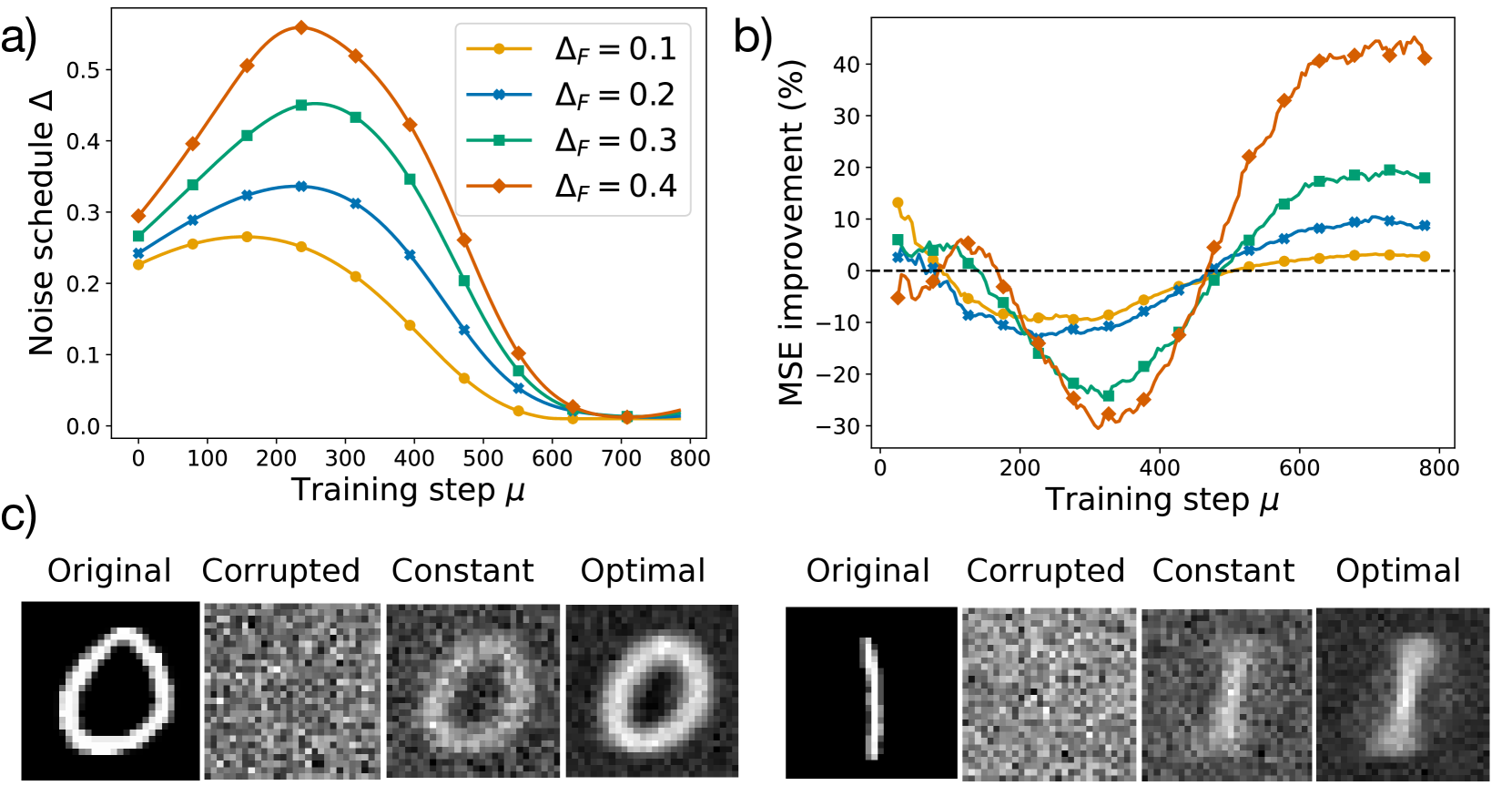<details> <summary>x9.png Details</summary>  ### Visual Description ## Chart/Diagram Type: Multi-Panel Figure ### Overview The image consists of three subfigures labeled a), b), and c). Subfigures a) and b) are line plots showing the relationship between training step and noise schedule, and training step and MSE improvement, respectively. Subfigure c) displays example images of digits in original, corrupted, constant, and optimal states. ### Components/Axes **Subfigure a): Noise Schedule vs. Training Step** * **Title:** a) * **X-axis:** Training step μ * Scale: 0 to 800, with increments of 100. * **Y-axis:** Noise schedule Δ * Scale: 0.0 to 0.5, with increments of 0.1. * **Legend:** Located in the top-right corner of the plot. * Yellow: ΔF = 0.1 * Blue: ΔF = 0.2 * Green: ΔF = 0.3 * Orange: ΔF = 0.4 **Subfigure b): MSE Improvement vs. Training Step** * **Title:** b) * **X-axis:** Training step μ * Scale: 0 to 800, with increments of 200. * **Y-axis:** MSE improvement (%) * Scale: -30 to 40, with increments of 10. * **Horizontal dashed line:** Represents 0% MSE improvement. * **Legend:** (Inferred from Subfigure a) * Yellow: ΔF = 0.1 * Blue: ΔF = 0.2 * Green: ΔF = 0.3 * Orange: ΔF = 0.4 **Subfigure c): Example Images** * **Labels:** * Original * Corrupted * Constant * Optimal * **Images:** Two rows of images, each row containing the four states (Original, Corrupted, Constant, Optimal) of a digit. The top row shows the digit "0", and the bottom row shows the digit "1". ### Detailed Analysis **Subfigure a): Noise Schedule vs. Training Step** * **Yellow (ΔF = 0.1):** Starts at approximately 0.23, increases to a peak around 0.27 at a training step of approximately 200, then decreases to approximately 0.02 at a training step of 700-800. * **Blue (ΔF = 0.2):** Starts at approximately 0.26, increases to a peak around 0.33 at a training step of approximately 200, then decreases to approximately 0.02 at a training step of 700-800. * **Green (ΔF = 0.3):** Starts at approximately 0.28, increases to a peak around 0.44 at a training step of approximately 250, then decreases to approximately 0.02 at a training step of 700-800. * **Orange (ΔF = 0.4):** Starts at approximately 0.22, increases to a peak around 0.56 at a training step of approximately 250, then decreases to approximately 0.02 at a training step of 700-800. **Subfigure b): MSE Improvement vs. Training Step** * **Yellow (ΔF = 0.1):** Starts at approximately 13%, decreases to a minimum of approximately -12% at a training step of approximately 350, then increases to approximately 3% at a training step of 800. * **Blue (ΔF = 0.2):** Starts at approximately 4%, decreases to a minimum of approximately -15% at a training step of approximately 350, then increases to approximately 9% at a training step of 800. * **Green (ΔF = 0.3):** Starts at approximately 7%, decreases to a minimum of approximately -27% at a training step of approximately 350, then increases to approximately 17% at a training step of 800. * **Orange (ΔF = 0.4):** Starts at approximately -5%, decreases to a minimum of approximately -28% at a training step of approximately 350, then increases to approximately 38% at a training step of 800. **Subfigure c): Example Images** * The "Original" images are clear representations of the digits "0" and "1". * The "Corrupted" images show the digits with added noise, making them difficult to recognize. * The "Constant" images show the digits after applying a constant noise schedule. * The "Optimal" images show the digits after applying an optimized noise schedule, resulting in clearer representations compared to the "Constant" images. ### Key Observations * In subfigure a), as ΔF increases, the peak of the noise schedule also increases. All noise schedules converge to a similar low value at higher training steps. * In subfigure b), higher ΔF values lead to greater MSE improvement at higher training steps, but also to a greater decrease in MSE improvement at lower training steps. * In subfigure c), the "Optimal" images are visually better reconstructions of the original digits compared to the "Constant" images. ### Interpretation The data suggests that the noise schedule (Δ) plays a crucial role in the training process. Higher values of ΔF lead to a more aggressive noise schedule, which initially degrades performance (negative MSE improvement) but ultimately leads to better performance (positive MSE improvement) at later stages of training. The example images in subfigure c) visually confirm that the optimized noise schedule results in better image reconstruction compared to a constant noise schedule. The relationship between ΔF and MSE improvement indicates a trade-off between initial performance and final performance, suggesting that the optimal ΔF value depends on the specific training goals and constraints. </details> Figure 9: a) Optimal noise schedule $\Delta$ as a function of the training step $\mu$ for the MNIST dataset with only $0 0$ s and $1$ s. b) Percentage improvement in test mean square error of the optimal strategy compared to the constant one at $\Delta=\Delta_{F}$ . Each curve is averaged over $10$ random realizations of the training set. c) Examples of images for $\Delta_{F}=0.4$ : original, corrupted, denoised with the constant schedule $\Delta=\Delta_{F}$ , and denoised with the optimal schedule. Parameters: $K=C_{1}=2$ , $\alpha_{F}=1$ , $\eta=\eta_{b}=5$ , $\sigma=0.1$ , $N=784$ , $g(z)=z$ . Initialization: $b=0$ . Other initial conditions and parameters are given in Eq. (92). We now demonstrate the applicability of our framework to real-world data by focusing on the MNIST dataset, which consists of labeled $28× 28$ grayscale images of handwritten digits from $0 0$ to $9$ . For simplicity, we restrict our analysis to the digits $0 0$ and $1$ . To apply our framework, we numerically estimate the mean vectors ${\bm{\mu}}_{1,1}$ and ${\bm{\mu}}_{1,2}$ , corresponding to the digit classes $0 0$ and $1$ , respectively, as well as the standard deviations $\sigma_{1,1}$ and $\sigma_{1,2}$ . For additional details and initial conditions, see Appendix B. While our method could be extended to include the full covariance matrices, this would result in more involved dynamical equations [121, 128], which we leave for future work. Considering learning trajectories with $\alpha_{F}=1$ , we use our theoretical framework to identify the optimal noise schedule $\Delta$ for different values of the testing noise $\Delta_{F}$ . The resulting schedules are shown in Fig. 9, and all exhibit a characteristic pattern: an initial increase in noise followed by a gradual decrease toward the end of the training trajectory. As expected, higher values of the testing noise $\Delta_{F}$ lead to overall higher noise levels throughout the schedule. We then use these schedules to train a DAE with $K=2$ on a randomly selected training set of $P=784$ images (corresponding to $\alpha_{F}=P/N=1$ ). In Fig. 9 b, we compare the test-set MSE percent improvement relative to the constant strategy $\Delta=\Delta_{F}$ . We observe that the optimal noise schedule yields improvements of up to approximately $40\%$ . This improvement is also apparent in the denoised images shown in Fig. 9 c. These results highlight the practical benefits of optimizing the noise schedule, confirming the applicability of our theoretical framework to real data. 4 Discussion We have introduced a general framework for optimal learning that combines statistical physics with control theory to identify optimal training protocols. We have formulated the design of learning schedules as an OC problem on the low-dimensional dynamics of order parameters in a general two-layer neural network model trained with online SGD that captures a broad range of learning scenarios. The applicability of this framework was illustrated through several examples spanning hyperparameter tuning, architecture design, and data selection. We have then thoroughly investigated optimal training protocols in three representative settings: curriculum learning, dropout regularization, and denoising autoencoders. We have consistently found that optimal training protocols outperform standard heuristics and can exhibit highly nontrivial structures that would be difficult to guess a priori. In curriculum learning, we have shown that non-monotonic difficulty schedules can outperform both easy-to-hard and hard-to-easy curricula. In dropout-regularized networks, the optimal schedule delayed the onset of regularization, exploiting the early phase to increase signal alignment before suppressing harmful co-adaptations. Optimal noise schedules for denoising autoencoders enhanced the reconstruction ability of the network while speeding up the training of the skip connection. Interestingly, the dynamics of the order parameters often revealed interpretable structures in the resulting protocols a posteriori. Indeed, the order parameters allow to identify fundamental learning trade-offs—for instance, alignment with informative directions versus suppression of noise fitting—which determine the structure of the optimal protocols. Our framework further enables the joint optimization of multiple controls, revealing synergies between meta-parameters, for example, how learning rate modulation can compensate for shifts in task difficulty. Our framework can be extended in several directions. As detailed in Section 2.4, the current formulation already accommodates a variety of learning settings beyond those investigated here, including dynamic architectural features such as gating and attention. A first natural extension would involve considering more realistic data models [129, 18, 130, 22] to investigate how data structure affects optimal schedules. It would also be relevant to extend the OC framework introduced here to batch learning settings allowing to study how training schedules affect the interplay between memorization and generalization, e.g., via dynamical mean-field theory [25, 26, 131]. Additionally, it would be relevant to extend the analysis to deep and overparametrized architectures [28, 132]. Finally, the discussion in Section 3.3 on optimal noise schedules could be extended to generative settings such as diffusion models, enabling the derivation of optimal noise injection protocols [133]. Such connection could be explored within recently proposed minimal models of diffusion-based generative models [123]. Our framework can also be applied to optimize alternative training objectives. While we focused here on minimizing the final generalization error, other criteria—such as fairness metrics in imbalanced datasets, robustness under distribution shift, or computational efficiency—can be incorporated within the same formalism. Finally, while we considered gradient-based learning rules, it would be interesting to explore biologically plausible update mechanisms or constraints on control signals inspired by cognitive or neural resource limitations [134, 135, 136]. Acknowledgments We thank Stefano Sarao Mannelli and Antonio Sclocchi for helpful discussions. We are grateful to Hugo Cui for useful feedback on the manuscript. This work was supported by a Leverhulme Trust International Professorship grant (Award Number: LIP-2020-014) and by the Simons Foundation (Award Number: 1141576). References - [1] Yoshua Bengio. Practical recommendations for gradient-based training of deep architectures. In Neural networks: Tricks of the trade: Second edition, pages 437–478. Springer, 2012. - [2] Amitai Shenhav, Matthew M Botvinick, and Jonathan D Cohen. The expected value of control: an integrative theory of anterior cingulate cortex function. Neuron, 79(2):217–240, 2013. - [3] Matthew M. Botvinick and Jonathan D. Cohen. The computational and neural basis of cognitive control: Charted territory and new frontiers. Cognitive Science, 38(6):1249–1285, 2014. - [4] Sebastian Musslick and Jonathan D Cohen. Rationalizing constraints on the capacity for cognitive control. Trends in cognitive sciences, 25(9):757–775, 2021. - [5] Brett D Roads, Buyun Xu, June K Robinson, and James W Tanaka. The easy-to-hard training advantage with real-world medical images. Cognitive Research: Principles and Implications, 3:1–13, 2018. - [6] Burrhus Frederic Skinner. The behavior of organisms: An experimental analysis. BF Skinner Foundation, 2019. - [7] Luca Franceschi, Paolo Frasconi, Saverio Salzo, Riccardo Grazzi, and Massimiliano Pontil. Bilevel programming for hyperparameter optimization and meta-learning. In International conference on machine learning, pages 1568–1577. PMLR, 2018. - [8] Frank Hutter, Lars Kotthoff, and Joaquin Vanschoren. Automated machine learning: methods, systems, challenges. Springer Nature, 2019. - [9] James Bergstra and Yoshua Bengio. Random search for hyper-parameter optimization. The journal of machine learning research, 13(1):281–305, 2012. - [10] Jasper Snoek, Hugo Larochelle, and Ryan P Adams. Practical bayesian optimization of machine learning algorithms. Advances in neural information processing systems, 25, 2012. - [11] Dougal Maclaurin, David Duvenaud, and Ryan Adams. Gradient-based hyperparameter optimization through reversible learning. In International conference on machine learning, pages 2113–2122. PMLR, 2015. - [12] Chelsea Finn, Pieter Abbeel, and Sergey Levine. Model-agnostic meta-learning for fast adaptation of deep networks. In International conference on machine learning, pages 1126–1135. PMLR, 2017. - [13] Andreas Engel. Statistical mechanics of learning. Cambridge University Press, 2001. - [14] Yasaman Bahri, Jonathan Kadmon, Jeffrey Pennington, Sam S Schoenholz, Jascha Sohl-Dickstein, and Surya Ganguli. Statistical mechanics of deep learning. Annual review of condensed matter physics, 11(1):501–528, 2020. - [15] Florent Krzakala and Lenka Zdeborová. Les houches 2022 special issue. Journal of Statistical Mechanics: Theory and Experiment, 2024(10):101001, 2024. - [16] Jean Barbier, Florent Krzakala, Nicolas Macris, Léo Miolane, and Lenka Zdeborová. Optimal errors and phase transitions in high-dimensional generalized linear models. Proceedings of the National Academy of Sciences, 116(12):5451–5460, 2019. - [17] Hugo Cui, Florent Krzakala, and Lenka Zdeborova. Bayes-optimal learning of deep random networks of extensive-width. In Proceedings of the 40th International Conference on Machine Learning, volume 202 of Proceedings of Machine Learning Research, pages 6468–6521. PMLR, 23–29 Jul 2023. - [18] Bruno Loureiro, Cedric Gerbelot, Hugo Cui, Sebastian Goldt, Florent Krzakala, Marc Mezard, and Lenka Zdeborová. Learning curves of generic features maps for realistic datasets with a teacher-student model. Advances in Neural Information Processing Systems, 34:18137–18151, 2021. - [19] Francesca Mignacco, Florent Krzakala, Yue Lu, Pierfrancesco Urbani, and Lenka Zdeborova. The role of regularization in classification of high-dimensional noisy Gaussian mixture. In Proceedings of the 37th International Conference on Machine Learning, volume 119 of Proceedings of Machine Learning Research, pages 6874–6883. PMLR, 13–18 Jul 2020. - [20] Dominik Schröder, Daniil Dmitriev, Hugo Cui, and Bruno Loureiro. Asymptotics of learning with deep structured (random) features. In Forty-first International Conference on Machine Learning, 2024. - [21] Federica Gerace, Bruno Loureiro, Florent Krzakala, Marc Mezard, and Lenka Zdeborova. Generalisation error in learning with random features and the hidden manifold model. In Proceedings of the 37th International Conference on Machine Learning, volume 119 of Proceedings of Machine Learning Research, pages 3452–3462. PMLR, 13–18 Jul 2020. - [22] Urte Adomaityte, Gabriele Sicuro, and Pierpaolo Vivo. Classification of superstatistical features in high dimensions. In 2023 Conference on Neural Information Procecessing Systems, 2023. - [23] Qianyi Li and Haim Sompolinsky. Statistical mechanics of deep linear neural networks: The backpropagating kernel renormalization. Phys. Rev. X, 11:031059, Sep 2021. - [24] Sebastian Goldt, Madhu Advani, Andrew M Saxe, Florent Krzakala, and Lenka Zdeborová. Dynamics of stochastic gradient descent for two-layer neural networks in the teacher-student setup. Advances in neural information processing systems, 32, 2019. - [25] Francesca Mignacco, Florent Krzakala, Pierfrancesco Urbani, and Lenka Zdeborová. Dynamical mean-field theory for stochastic gradient descent in gaussian mixture classification. Advances in Neural Information Processing Systems, 33:9540–9550, 2020. - [26] Cedric Gerbelot, Emanuele Troiani, Francesca Mignacco, Florent Krzakala, and Lenka Zdeborova. Rigorous dynamical mean-field theory for stochastic gradient descent methods. SIAM Journal on Mathematics of Data Science, 6(2):400–427, 2024. - [27] Yehonatan Avidan, Qianyi Li, and Haim Sompolinsky. Unified theoretical framework for wide neural network learning dynamics. Phys. Rev. E, 111:045310, Apr 2025. - [28] Blake Bordelon and Cengiz Pehlevan. Self-consistent dynamical field theory of kernel evolution in wide neural networks. Advances in Neural Information Processing Systems, 35:32240–32256, 2022. - [29] Luca Saglietti, Stefano Mannelli, and Andrew Saxe. An analytical theory of curriculum learning in teacher-student networks. In Advances in Neural Information Processing Systems, volume 35, pages 21113–21127. Curran Associates, Inc., 2022. - [30] Jin Hwa Lee, Stefano Sarao Mannelli, and Andrew M Saxe. Why do animals need shaping? a theory of task composition and curriculum learning. In International Conference on Machine Learning, pages 26837–26855. PMLR, 2024. - [31] Younes Strittmatter, Stefano S Mannelli, Miguel Ruiz-Garcia, Sebastian Musslick, and Markus Spitzer. Curriculum learning in humans and neural networks, Mar 2025. - [32] Michael Biehl and Holm Schwarze. Learning by on-line gradient descent. Journal of Physics A: Mathematical and general, 28(3):643, 1995. - [33] David Saad and Sara A Solla. Exact solution for on-line learning in multilayer neural networks. Physical Review Letters, 74(21):4337, 1995. - [34] David Saad and Sara A Solla. On-line learning in soft committee machines. Physical Review E, 52(4):4225, 1995. - [35] Megan C Engel, Jamie A Smith, and Michael P Brenner. Optimal control of nonequilibrium systems through automatic differentiation. Physical Review X, 13(4):041032, 2023. - [36] Steven Blaber and David A Sivak. Optimal control in stochastic thermodynamics. Journal of Physics Communications, 7(3):033001, 2023. - [37] Luke K Davis, Karel Proesmans, and Étienne Fodor. Active matter under control: Insights from response theory. Physical Review X, 14(1):011012, 2024. - [38] Francesco Mori, Stefano Sarao Mannelli, and Francesca Mignacco. Optimal protocols for continual learning via statistical physics and control theory. In International Conference on Learning Representations (ICLR), 2025. - [39] David Saad and Magnus Rattray. Globally optimal parameters for on-line learning in multilayer neural networks. Physical review letters, 79(13):2578, 1997. - [40] Magnus Rattray and David Saad. Analysis of on-line training with optimal learning rates. Physical Review E, 58(5):6379, 1998. - [41] Rodrigo Carrasco-Davis, Javier Masís, and Andrew M Saxe. Meta-learning strategies through value maximization in neural networks. arXiv preprint arXiv:2310.19919, 2023. - [42] Yujun Li, Rodrigo Carrasco-Davis, Younes Strittmatter, Stefano Sarao Mannelli, and Sebastian Musslick. A meta-learning framework for rationalizing cognitive fatigue in neural systems. In Proceedings of the Annual Meeting of the Cognitive Science Society, volume 46, 2024. - [43] Hugo Cui. High-dimensional learning of narrow neural networks. Journal of Statistical Mechanics: Theory and Experiment, 2025(2):023402, 2025. - [44] Elizabeth Gardner and Bernard Derrida. Three unfinished works on the optimal storage capacity of networks. Journal of Physics A: Mathematical and General, 22(12):1983, 1989. - [45] H. S. Seung, H. Sompolinsky, and N. Tishby. Statistical mechanics of learning from examples. Phys. Rev. A, 45:6056–6091, Apr 1992. - [46] Maria Refinetti, Stéphane D’Ascoli, Ruben Ohana, and Sebastian Goldt. Align, then memorise: the dynamics of learning with feedback alignment. In Proceedings of the 38th International Conference on Machine Learning, volume 139 of Proceedings of Machine Learning Research, pages 8925–8935. PMLR, 18–24 Jul 2021. - [47] Ravi Francesco Srinivasan, Francesca Mignacco, Martino Sorbaro, Maria Refinetti, Avi Cooper, Gabriel Kreiman, and Giorgia Dellaferrera. Forward learning with top-down feedback: Empirical and analytical characterization. In The Twelfth International Conference on Learning Representations, 2024. - [48] Nishil Patel, Sebastian Lee, Stefano Sarao Mannelli, Sebastian Goldt, and Andrew Saxe. Rl perceptron: Generalization dynamics of policy learning in high dimensions. Phys. Rev. X, 15:021051, May 2025. - [49] Tianyi Zhou, Shengjie Wang, and Jeff Bilmes. Curriculum learning by optimizing learning dynamics. In Proceedings of The 24th International Conference on Artificial Intelligence and Statistics, volume 130 of Proceedings of Machine Learning Research, pages 433–441. PMLR, 13–15 Apr 2021. - [50] LS Pontryagin. Some mathematical problems arising in connection with the theory of optimal automatic control systems. In Proc. Conf. on Basic Problems in Automatic Control and Regulation, 1957. - [51] Donald E Kirk. Optimal control theory: an introduction. Courier Corporation, 2004. - [52] John Bechhoefer. Control theory for physicists. Cambridge University Press, 2021. - [53] John T Betts. Practical methods for optimal control and estimation using nonlinear programming. SIAM, 2010. - [54] Joel AE Andersson, Joris Gillis, Greg Horn, James B Rawlings, and Moritz Diehl. Casadi: a software framework for nonlinear optimization and optimal control. Mathematical Programming Computation, 11:1–36, 2019. - [55] Dayal Singh Kalra and Maissam Barkeshli. Why warmup the learning rate? underlying mechanisms and improvements. Advances in Neural Information Processing Systems, 37:111760–111801, 2024. - [56] Ilya Loshchilov and Frank Hutter. Sgdr: Stochastic gradient descent with warm restarts. In International Conference on Learning Representations (ICLR), 2017. - [57] Atilim Gunes Baydin, Robert Cornish, David Martinez Rubio, Mark Schmidt, and Frank Wood. Online learning rate adaptation with hypergradient descent. In International Conference on Learning Representations (ICLR), 2018. - [58] E Schlösser, D Saad, and M Biehl. Optimization of on-line principal component analysis. Journal of Physics A: Mathematical and General, 32(22):4061, 1999. - [59] Stéphane d’Ascoli, Maria Refinetti, and Giulio Biroli. Optimal learning rate schedules in high-dimensional non-convex optimization problems. arXiv preprint arXiv:2202.04509, 2022. - [60] Lukas Balles, Javier Romero, and Philipp Hennig. Coupling adaptive batch sizes with learning rates. In Proceedings of the Conference on Uncertainty in Artificial Intelligence (UAI), 2017. - [61] Samuel L Smith, Pieter-Jan Kindermans, Chris Ying, and Quoc V Le. Don’t decay the learning rate, increase the batch size. In International Conference on Learning Representations (ICLR), 2018. - [62] Aditya Devarakonda, Maxim Naumov, and Michael Garland. Adabatch: Adaptive batch sizes for training deep neural networks. In ICLR 2018 Workshop on Optimization for Machine Learning, 2018. - [63] Huan Wang, Can Qin, Yulun Zhang, and Yun Fu. Neural pruning via growing regularization. In International Conference on Learning Representations (ICLR), 2021. - [64] David Saad and Magnus Rattray. Learning with regularizers in multilayer neural networks. Physical Review E, 57(2):2170, 1998. - [65] Michael McCloskey and Neal J Cohen. Catastrophic interference in connectionist networks: The sequential learning problem. In Psychology of learning and motivation, volume 24, pages 109–165. Elsevier, 1989. - [66] Ian J. Goodfellow, Mehdi Mirza, Xia Da, Aaron C. Courville, and Yoshua Bengio. An empirical investigation of catastrophic forgeting in gradient-based neural networks. In 2nd International Conference on Learning Representations, ICLR 2014, Banff, AB, Canada, April 14-16, 2014, Conference Track Proceedings, 2014. - [67] Sebastian Lee, Sebastian Goldt, and Andrew Saxe. Continual learning in the teacher-student setup: Impact of task similarity. In International Conference on Machine Learning, pages 6109–6119. PMLR, 2021. - [68] Sebastian Lee, Stefano Sarao Mannelli, Claudia Clopath, Sebastian Goldt, and Andrew Saxe. Maslow’s hammer in catastrophic forgetting: Node re-use vs. node activation. In International Conference on Machine Learning, pages 12455–12477. PMLR, 2022. - [69] Itay Evron, Edward Moroshko, Rachel Ward, Nathan Srebro, and Daniel Soudry. How catastrophic can catastrophic forgetting be in linear regression? In Conference on Learning Theory, pages 4028–4079. PMLR, 2022. - [70] Itay Evron, Edward Moroshko, Gon Buzaglo, Maroun Khriesh, Badea Marjieh, Nathan Srebro, and Daniel Soudry. Continual learning in linear classification on separable data. In International Conference on Machine Learning, pages 9440–9484. PMLR, 2023. - [71] Haozhe Shan, Qianyi Li, and Haim Sompolinsky. Order parameters and phase transitions of continual learning in deep neural networks. arXiv preprint arXiv:2407.10315, 2024. - [72] Elisabetta Cornacchia and Elchanan Mossel. A mathematical model for curriculum learning for parities. In Proceedings of the 40th International Conference on Machine Learning, volume 202 of Proceedings of Machine Learning Research, pages 6402–6423. PMLR, 23–29 Jul 2023. - [73] Emmanuel Abbe, Elisabetta Cornacchia, and Aryo Lotfi. Provable advantage of curriculum learning on parity targets with mixed inputs. In Advances in Neural Information Processing Systems, volume 36, pages 24291–24321. Curran Associates, Inc., 2023. - [74] Fadi Thabtah, Suhel Hammoud, Firuz Kamalov, and Amanda Gonsalves. Data imbalance in classification: Experimental evaluation. Information Sciences, 513:429–441, 2020. - [75] Emanuele Loffredo, Mauro Pastore, Simona Cocco, and Remi Monasson. Restoring balance: principled under/oversampling of data for optimal classification. In Forty-first International Conference on Machine Learning, 2024. - [76] Emanuele Loffredo, Mauro Pastore, Simona Cocco, and Rémi Monasson. Restoring data balance via generative models of t-cell receptors for antigen-binding prediction. bioRxiv, pages 2024–07, 2024. - [77] Stefano Sarao Mannelli, Federica Gerace, Negar Rostamzadeh, and Luca Saglietti. Bias-inducing geometries: exactly solvable data model with fairness implications. In ICML 2024 Workshop on Geometry-grounded Representation Learning and Generative Modeling, 2024. - [78] Anchit Jain, Rozhin Nobahari, Aristide Baratin, and Stefano Sarao Mannelli. Bias in motion: Theoretical insights into the dynamics of bias in sgd training. In Advances in Neural Information Processing Systems, volume 37, pages 24435–24471. Curran Associates, Inc., 2024. - [79] Yizeng Han, Gao Huang, Shiji Song, Le Yang, Honghui Wang, and Yulin Wang. Dynamic neural networks: A survey. IEEE transactions on pattern analysis and machine intelligence, 44(11):7436–7456, 2021. - [80] Geoffrey E Hinton, Nitish Srivastava, Alex Krizhevsky, Ilya Sutskever, and Ruslan R Salakhutdinov. Improving neural networks by preventing co-adaptation of feature detectors. arXiv preprint arXiv:1207.0580, 2012. - [81] Nitish Srivastava, Geoffrey Hinton, Alex Krizhevsky, Ilya Sutskever, and Ruslan Salakhutdinov. Dropout: a simple way to prevent neural networks from overfitting. The journal of machine learning research, 15(1):1929–1958, 2014. - [82] Pietro Morerio, Jacopo Cavazza, Riccardo Volpi, René Vidal, and Vittorio Murino. Curriculum dropout. In Proceedings of the IEEE International Conference on Computer Vision, pages 3544–3552, 2017. - [83] Zhuang Liu, Zhiqiu Xu, Joseph Jin, Zhiqiang Shen, and Trevor Darrell. Dropout reduces underfitting. In International Conference on Machine Learning, pages 22233–22248. PMLR, 2023. - [84] Francesco Mori and Francesca Mignacco. Analytic theory of dropout regularization. arXiv preprint arXiv:2505.07792, 2025. - [85] Noam Shazeer, Azalia Mirhoseini, Krzysztof Maziarz, Andy Davis, Quoc Le, Geoffrey Hinton, and Jeff Dean. Outrageously large neural networks: The sparsely-gated mixture-of-experts layer. In International Conference on Learning Representations, 2017. - [86] Jie Hu, Li Shen, and Gang Sun. Squeeze-and-excitation networks. In Proceedings of the IEEE conference on computer vision and pattern recognition, pages 7132–7141, 2018. - [87] Kyunghyun Cho, Bart Merrienboer, Caglar Gulcehre, Fethi Bougares, Holger Schwenk, and Y. Bengio. Learning phrase representations using rnn encoder-decoder for statistical machine translation. 06 2014. - [88] Joel Veness, Tor Lattimore, David Budden, Avishkar Bhoopchand, Christopher Mattern, Agnieszka Grabska-Barwinska, Eren Sezener, Jianan Wang, Peter Toth, Simon Schmitt, et al. Gated linear networks. In Proceedings of the AAAI conference on artificial intelligence, volume 35, pages 10015–10023, 2021. - [89] Qianyi Li and Haim Sompolinsky. Globally gated deep linear networks. Advances in Neural Information Processing Systems, 35:34789–34801, 2022. - [90] Andrew Saxe, Shagun Sodhani, and Sam Jay Lewallen. The neural race reduction: Dynamics of abstraction in gated networks. In International Conference on Machine Learning, pages 19287–19309. PMLR, 2022. - [91] Samuel Lippl, LF Abbott, and SueYeon Chung. The implicit bias of gradient descent on generalized gated linear networks. arXiv preprint arXiv:2202.02649, 2022. - [92] Francesca Mignacco, Chi-Ning Chou, and SueYeon Chung. Nonlinear classification of neural manifolds with contextual information. Physical Review E, 111(3):035302, 2025. - [93] Ashish Vaswani, Noam Shazeer, Niki Parmar, Jakob Uszkoreit, Llion Jones, Aidan N Gomez, Łukasz Kaiser, and Illia Polosukhin. Attention is all you need. Advances in neural information processing systems, 30, 2017. - [94] Aurko Roy, Mohammad Saffar, Ashish Vaswani, and David Grangier. Efficient content-based sparse attention with routing transformers. Transactions of the Association for Computational Linguistics, 9:53–68, 2021. - [95] Sainbayar Sukhbaatar, Édouard Grave, Piotr Bojanowski, and Armand Joulin. Adaptive attention span in transformers. In Proceedings of the 57th Annual Meeting of the Association for Computational Linguistics, pages 331–335, 2019. - [96] Paul Michel, Omer Levy, and Graham Neubig. Are sixteen heads really better than one? Advances in neural information processing systems, 32, 2019. - [97] Gonçalo M Correia, Vlad Niculae, and André FT Martins. Adaptively sparse transformers. arXiv preprint arXiv:1909.00015, 2019. - [98] Hugo Cui, Freya Behrens, Florent Krzakala, and Lenka Zdeborová. A phase transition between positional and semantic learning in a solvable model of dot-product attention. Advances in Neural Information Processing Systems, 37:36342–36389, 2024. - [99] Luca Arnaboldi, Bruno Loureiro, Ludovic Stephan, Florent Krzakala, and Lenka Zdeborova. Asymptotics of sgd in sequence-single index models and single-layer attention networks, 2025. - [100] Douglas H Lawrence. The transfer of a discrimination along a continuum. Journal of Comparative and Physiological Psychology, 45(6):511, 1952. - [101] Renee Elio and John R Anderson. The effects of information order and learning mode on schema abstraction. Memory & cognition, 12(1):20–30, 1984. - [102] Harold Pashler and Michael C Mozer. When does fading enhance perceptual category learning? Journal of Experimental Psychology: Learning, Memory, and Cognition, 39(4):1162, 2013. - [103] William L Tong, Anisha Iyer, Venkatesh N Murthy, and Gautam Reddy. Adaptive algorithms for shaping behavior. bioRxiv, 2023. - [104] Yoshua Bengio, Jérôme Louradour, Ronan Collobert, and Jason Weston. Curriculum learning. In Proceedings of the 26th annual international conference on machine learning, pages 41–48, 2009. - [105] Xin Wang, Yudong Chen, and Wenwu Zhu. A survey on curriculum learning. IEEE transactions on pattern analysis and machine intelligence, 44(9):4555–4576, 2021. - [106] Anastasia Pentina, Viktoriia Sharmanska, and Christoph H Lampert. Curriculum learning of multiple tasks. In Proceedings of the IEEE conference on computer vision and pattern recognition, pages 5492–5500, 2015. - [107] Guy Hacohen and Daphna Weinshall. On the power of curriculum learning in training deep networks. In International conference on machine learning, pages 2535–2544. PMLR, 2019. - [108] Xiaoxia Wu, Ethan Dyer, and Behnam Neyshabur. When do curricula work? In International Conference on Learning Representations (ICLR), 2020. - [109] Daphna Weinshall and Dan Amir. Theory of curriculum learning, with convex loss functions. Journal of Machine Learning Research, 21(222):1–19, 2020. - [110] Luca Saglietti, Stefano Mannelli, and Andrew Saxe. An analytical theory of curriculum learning in teacher-student networks. Advances in Neural Information Processing Systems, 35:21113–21127, 2022. - [111] Stefano Sarao Mannelli, Yaraslau Ivashynka, Andrew Saxe, and Luca Saglietti. Tilting the odds at the lottery: the interplay of overparameterisation and curricula in neural networks. Journal of Statistical Mechanics: Theory and Experiment, 2024(11):114001, 2024. - [112] Emmanuel Abbe, Elisabetta Cornacchia, and Aryo Lotfi. Provable advantage of curriculum learning on parity targets with mixed inputs. Advances in Neural Information Processing Systems, 36:24291–24321, 2023. - [113] Elisabetta Cornacchia and Elchanan Mossel. A mathematical model for curriculum learning for parities. In International Conference on Machine Learning, pages 6402–6423. PMLR, 2023. - [114] Imrus Salehin and Dae-Ki Kang. A review on dropout regularization approaches for deep neural networks within the scholarly domain. Electronics, 12(14):3106, 2023. - [115] Steven J. Rennie, Vaibhava Goel, and Samuel Thomas. Annealed dropout training of deep networks. In 2014 IEEE Spoken Language Technology Workshop (SLT), pages 159–164, 2014. - [116] Pascal Vincent, Hugo Larochelle, Yoshua Bengio, and Pierre-Antoine Manzagol. Extracting and composing robust features with denoising autoencoders. In Proceedings of the 25th International Conference on Machine Learning, ICML ’08, page 1096–1103, New York, NY, USA, 2008. Association for Computing Machinery. - [117] Pascal Vincent, Hugo Larochelle, Isabelle Lajoie, Yoshua Bengio, and Pierre-Antoine Manzagol. Stacked denoising autoencoders: Learning useful representations in a deep network with a local denoising criterion. J. Mach. Learn. Res., 11:3371–3408, December 2010. - [118] Jascha Sohl-Dickstein, Eric Weiss, Niru Maheswaranathan, and Surya Ganguli. Deep unsupervised learning using nonequilibrium thermodynamics. In Proceedings of the 32nd International Conference on Machine Learning, volume 37 of Proceedings of Machine Learning Research, pages 2256–2265, Lille, France, 07–09 Jul 2015. PMLR. - [119] Jonathan Ho, Ajay Jain, and Pieter Abbeel. Denoising diffusion probabilistic models. In Advances in Neural Information Processing Systems, volume 33, pages 6840–6851. Curran Associates, Inc., 2020. - [120] Arnu Pretorius, Steve Kroon, and Herman Kamper. Learning dynamics of linear denoising autoencoders. In International Conference on Machine Learning, pages 4141–4150. PMLR, 2018. - [121] Hugo Cui and Lenka Zdeborová. High-dimensional asymptotics of denoising autoencoders. Advances in Neural Information Processing Systems, 36:11850–11890, 2023. - [122] Hugo Cui, Florent Krzakala, Eric Vanden-Eijnden, and Lenka Zdeborová. Analysis of learning a flow-based generative model from limited sample complexity. In International Conference on Learning Representations (ICLR), 2024. - [123] Hugo Cui, Cengiz Pehlevan, and Yue M Lu. A precise asymptotic analysis of learning diffusion models: theory and insights. arXiv preprint arXiv:2501.03937, 2025. - [124] Maria Refinetti and Sebastian Goldt. The dynamics of representation learning in shallow, non-linear autoencoders. In International Conference on Machine Learning, pages 18499–18519. PMLR, 2022. - [125] Krzysztof J. Geras and Charles Sutton. Scheduled denoising autoencoders. In International Conference on Learning Representations (ICLR), 2015. - [126] Tianyi Zheng, Cong Geng, Peng-Tao Jiang, Ben Wan, Hao Zhang, Jinwei Chen, Jia Wang, and Bo Li. Non-uniform timestep sampling: Towards faster diffusion model training. In Proceedings of the 32nd ACM International Conference on Multimedia, pages 7036–7045, 2024. - [127] Minmin Chen, Kilian Weinberger, Fei Sha, and Yoshua Bengio. Marginalized denoising auto-encoders for nonlinear representations. In International conference on machine learning, pages 1476–1484. PMLR, 2014. - [128] Maria Refinetti, Sebastian Goldt, Florent Krzakala, and Lenka Zdeborová. Classifying high-dimensional gaussian mixtures: Where kernel methods fail and neural networks succeed. In International Conference on Machine Learning, pages 8936–8947. PMLR, 2021. - [129] Sebastian Goldt, Marc Mézard, Florent Krzakala, and Lenka Zdeborová. Modeling the influence of data structure on learning in neural networks: The hidden manifold model. Physical Review X, 10(4):041044, 2020. - [130] Sebastian Goldt, Bruno Loureiro, Galen Reeves, Florent Krzakala, Marc Mézard, and Lenka Zdeborová. The gaussian equivalence of generative models for learning with shallow neural networks. In Mathematical and Scientific Machine Learning, pages 426–471. PMLR, 2022. - [131] Yatin Dandi, Emanuele Troiani, Luca Arnaboldi, Luca Pesce, Lenka Zdeborova, and Florent Krzakala. The benefits of reusing batches for gradient descent in two-layer networks: Breaking the curse of information and leap exponents. In Proceedings of the 41st International Conference on Machine Learning, volume 235 of Proceedings of Machine Learning Research, pages 9991–10016. PMLR, 21–27 Jul 2024. - [132] Andrea Montanari and Pierfrancesco Urbani. Dynamical decoupling of generalization and overfitting in large two-layer networks. arXiv preprint arXiv:2502.21269, 2025. - [133] Santiago Aranguri, Giulio Biroli, Marc Mezard, and Eric Vanden-Eijnden. Optimizing noise schedules of generative models in high dimensionss. arXiv preprint arXiv:2501.00988, 2025. - [134] Maria Refinetti, Stéphane d’Ascoli, Ruben Ohana, and Sebastian Goldt. Align, then memorise: the dynamics of learning with feedback alignment. In International Conference on Machine Learning, pages 8925–8935. PMLR, 2021. - [135] Blake Bordelon and Cengiz Pehlevan. The influence of learning rule on representation dynamics in wide neural networks. In The Eleventh International Conference on Learning Representations. - [136] Ravi Francesco Srinivasan, Francesca Mignacco, Martino Sorbaro, Maria Refinetti, Avi Cooper, Gabriel Kreiman, and Giorgia Dellaferrera. Forward learning with top-down feedback: Empirical and analytical characterization. In International Conference on Learning Representations (ICLR), 2024. Appendix A Derivation of the learning dynamics In this section, we derive the set of ordinary differential equations (ODEs) for the order parameters given in Eq. (8) of the main text, that track the dynamics of online stochastic gradient descent (SGD). We consider the cost function $$ \mathcal{L}({\bm{w}},{\bm{v}}|\bm{x},\bm{c})=\ell\left(\frac{{\bm{x}}^{\top}{% \bm{w}_{*}}}{\sqrt{N}},\frac{{\bm{x}}^{\top}{\bm{w}}}{\sqrt{N}},\frac{\bm{w}^{% \top}\bm{w}}{N},{\bm{v}},{\bm{c}},z\right)+\tilde{g}\left(\frac{\bm{w}^{\top}% \bm{w}}{N},{\bm{v}}\right)\,. \tag{27} $$ The update rules for the network’s parameters are $$ \displaystyle\begin{split}\bm{w}^{\mu+1}=\bm{w}^{\mu}-\eta\nabla_{\bm{w}}% \mathcal{L}(\bm{w}^{\mu},\bm{v}^{\mu}|\bm{x}^{\mu},\bm{c}^{\mu})=\bm{w}^{\mu}-% \eta\left[\frac{{\bm{x}^{\mu}}\nabla_{2}\ell^{\mu}}{\sqrt{N}}+2\frac{\bm{w}^{% \mu}\nabla_{3}\ell^{\mu}}{N}+2\frac{\bm{w}^{\mu}\nabla_{1}\tilde{g}^{\mu}}{N}% \right]\;,\end{split} \displaystyle\begin{split}\bm{v}^{\mu+1}=\bm{v}^{\mu}-\frac{\eta}{N}\nabla_{4}% \ell^{\mu}-\frac{\eta}{N}\nabla_{2}\tilde{g}^{\mu}\;,\end{split} \tag{28} $$ where we use $∇_{k}\ell$ to denote the gradient of the function $\ell$ with respect to its $k^{\rm th}$ argument, with the convention that it is reshaped as a matrix of the same dimensions of that argument, e.g., $∇_{2}\ell∈\mathbb{R}^{L× K}$ . For simplicity, we omit the function’s arguments, by only keeping the time dependence, i.e., $\ell^{\mu}=\ell\left(\frac{{{\bm{x}}^{\mu}}^{→p}{\bm{w}_{*}}}{\sqrt{N}},% \frac{{{\bm{x}}^{\mu}}^{→p}{\bm{w}}^{\mu}}{\sqrt{N}},\frac{{\bm{w}^{\mu}}^{% →p}\bm{w}^{\mu}}{N},{\bm{v}}^{\mu},{\bm{c}}^{\mu},z^{\mu}\right)$ . For a given realization of the cluster coefficients $\bm{c}$ , we introduce the compact notation $\bm{\mu}_{\bm{c}}∈\mathbb{R}^{N× L}$ to denote the matrix with columns $\bm{\mu}_{l,c_{l}}$ . It is useful to define the local fields $$ \displaystyle\bm{\lambda}^{\mu}=\frac{{\bm{x}^{\mu}}^{\top}\bm{w}^{\mu}}{\sqrt% {N}}\in\mathbb{R}^{L\times K}\;, \displaystyle\bm{\lambda}_{*}^{\mu}=\frac{{\bm{x}^{\mu}}^{\top}\bm{w}_{*}}{% \sqrt{N}}\in\mathbb{R}^{L\times M}\;, \displaystyle\bm{\rho}^{\mu}_{\bm{c}}=\frac{{\bm{x}^{\mu}}^{\top}\bm{\mu}_{\bm% {c}}}{\sqrt{N}}\in\mathbb{R}^{L\times L}\;. \tag{30} $$ Notice that, due to the online-learning setup, at each training step the input $\bm{x}$ is independent of the weights. Therefore, due to the Gaussianity of the inputs, the local fields are also jointly Gaussian with zero mean and second moments given by: $$ \displaystyle\begin{split}\mathbb{E}_{\bm{x}|\bm{c}}\left[\lambda_{lk}\lambda_% {l^{\prime}k^{\prime}}\right]&=\frac{{\bm{w}_{k}}\cdot\bm{\mu}_{l,c_{l}}}{{N}}% \frac{{\bm{w}_{k^{\prime}}}\cdot\bm{\mu}_{l^{\prime},c_{l^{\prime}}}}{{N}}+% \delta_{l,l^{\prime}}\,\sigma^{2}_{l,c_{l}}\frac{{\bm{w}_{k}}\cdot\bm{w}_{k^{% \prime}}}{N}\\ &=R_{k(l,c_{l})}R_{k^{\prime}(l^{\prime},c_{l^{\prime}})}+\delta_{l,l^{\prime}% }\sigma^{2}_{l,c_{l}}Q_{kk^{\prime}}\;,\end{split} \displaystyle\begin{split}\mathbb{E}_{\bm{x}|\bm{c}}\left[\lambda_{lk}\lambda_% {*,l^{\prime}m}\right]&=\frac{{\bm{w}_{k}}\cdot\bm{\mu}_{l,c_{l}}}{{N}}\frac{{% \bm{w}_{*,m}}\cdot\bm{\mu}_{l^{\prime},c_{l^{\prime}}}}{{N}}+\delta_{l,l^{% \prime}}\,\sigma^{2}_{l,c_{l}}\frac{{\bm{w}_{k}}\cdot\bm{w}_{*,m}}{N}\\ &=R_{k(l,c_{l})}S_{m(l^{\prime},c_{l^{\prime}})}+\delta_{l,l^{\prime}}\sigma^{% 2}_{l,c_{l}}M_{km}\;,\end{split} \displaystyle\begin{split}\mathbb{E}_{\bm{x}|\bm{c}}\left[\lambda_{*,lm}% \lambda_{*,l^{\prime}m^{\prime}}\right]&=\frac{{\bm{w}_{*,m}}\cdot\bm{\mu}_{l,% c_{l}}}{{N}}\frac{{\bm{w}_{*,m^{\prime}}}\cdot\bm{\mu}_{l^{\prime},c_{l^{% \prime}}}}{{N}}+\delta_{l,l^{\prime}}\,\sigma^{2}_{l,c_{l}}\frac{{\bm{w}_{*,m}% }\cdot\bm{w}_{*,m^{\prime}}}{N}\\ &=S_{m(l,c_{l})}S_{m^{\prime}(l^{\prime},c_{l^{\prime}})}+\delta_{l,l^{\prime}% }\sigma^{2}_{l,c_{l}}T_{mm^{\prime}}\;,\end{split} \tag{31} $$ $$ \displaystyle\begin{split}\mathbb{E}_{\bm{x}|\bm{c}}\left[\lambda_{lk}\rho_{{% \bm{c}^{\prime}},l^{\prime}l^{\prime\prime}}\right]&=\frac{{\bm{w}_{k}}\cdot% \bm{\mu}_{l,c_{l}}}{{N}}\frac{\bm{\mu}_{l^{\prime},c_{l^{\prime}}}\cdot\bm{\mu% }_{l^{\prime\prime},c^{\prime}_{l^{\prime\prime}}}}{N}+\delta_{l,l^{\prime}}\,% \sigma^{2}_{l,c_{l}}\frac{{\bm{w}_{k}}\cdot\bm{\mu}_{l^{\prime\prime},c^{% \prime}_{l^{\prime\prime}}}}{N}\\ &=R_{k(l,c_{l})}\Omega_{(l^{\prime},c_{l^{\prime}})(l^{\prime\prime},c^{\prime% }_{l^{\prime\prime}})}+\delta_{l,l^{\prime}}\sigma^{2}_{l,c_{l}}R_{k(l^{\prime% \prime},c^{\prime}_{l^{\prime\prime}})}\;,\end{split} \displaystyle\begin{split}\mathbb{E}_{\bm{x}|\bm{c}}\left[\lambda_{*,lm}\rho_{% {\bm{c}}^{\prime},l^{\prime}l^{\prime\prime}}\right]&=\frac{{\bm{w}_{*,m}}% \cdot\bm{\mu}_{l,c_{l}}}{{N}}\frac{\bm{\mu}_{l^{\prime},c_{l^{\prime}}}\cdot% \bm{\mu}_{l^{\prime\prime},c^{\prime}_{l^{\prime\prime}}}}{N}+\delta_{l,l^{% \prime}}\,\sigma^{2}_{l,c_{l}}\frac{{\bm{w}_{*,m}}\cdot\bm{\mu}_{l^{\prime% \prime},c^{\prime}_{l^{\prime\prime}}}}{N}\\ &=S_{m(l,c_{l})}\Omega_{(l^{\prime},c_{l^{\prime}})(l^{\prime\prime},c^{\prime% }_{l^{\prime\prime}})}+\delta_{l,l^{\prime}}\sigma^{2}_{l,c_{l}}S_{m(l^{\prime% \prime},c^{\prime}_{l^{\prime\prime}})}\;,\end{split} \displaystyle\begin{split}\mathbb{E}_{\bm{x}|\bm{c}}\left[\rho_{{\bm{c}}^{% \prime},ll^{\prime}}\rho_{{\bm{c}}^{\prime\prime},l^{\prime\prime}l^{\prime% \prime\prime}}\right]&=\frac{{\bm{\mu}_{l^{\prime},c^{\prime}_{l^{\prime}}}}% \cdot\bm{\mu}_{l,c_{l}}}{N}\frac{\bm{\mu}_{l^{\prime\prime},c_{l^{\prime\prime% }}}\cdot\bm{\mu}_{l^{\prime\prime\prime},c^{\prime\prime}_{l^{\prime\prime% \prime}}}}{N}+\delta_{l,l^{\prime\prime}}\,\sigma^{2}_{l,c_{l}}\frac{{\bm{\mu}% _{l^{\prime},c^{\prime}_{l^{\prime}}}}\cdot\bm{\mu}_{l^{\prime\prime\prime},c^% {\prime\prime}_{l^{\prime\prime\prime}}}}{N}\\ &=\Omega_{(l,c_{l})(l^{\prime},c^{\prime}_{l^{\prime}})}\Omega_{(l^{\prime% \prime},c_{l^{\prime\prime}})(l^{\prime\prime\prime},c^{\prime\prime}_{l^{% \prime\prime\prime}})}+\delta_{l,l^{\prime\prime}}\sigma^{2}_{l,c_{l}}\Omega_{% (l^{\prime},c^{\prime}_{l^{\prime}})(l^{\prime\prime\prime},c^{\prime\prime}_{% l^{\prime\prime\prime}})}\;,\end{split} \tag{34} $$ where we have introduced the order parameters $$ \displaystyle\begin{split}&Q_{kk^{\prime}}\coloneqq\frac{{\bm{w}_{k}}\cdot\bm{% w}_{k^{\prime}}}{N}\;,\quad M_{km}\coloneqq\frac{{\bm{w}^{\mu}_{k}}\cdot\bm{w}% _{*,m}}{N}\;,\quad R_{k(l,c_{l})}\coloneqq\frac{{\bm{w}_{k}}\cdot\bm{\mu}_{l,c% _{l}}}{{N}}\;,\\ &S_{m(l,c_{l})}\coloneqq\frac{{\bm{w}_{*,m}}\cdot\bm{\mu}_{l,c_{l}}}{{N}}\;,% \quad T_{mm^{\prime}}\coloneqq\frac{{\bm{w}_{*,m}}\cdot\bm{w}_{*,m^{\prime}}}{% N}\;,\quad\Omega_{(l,c_{l})(l^{\prime},c^{\prime}_{l^{\prime}})}=\frac{\bm{\mu% }_{l,c_{l}}\cdot\bm{\mu}_{l^{\prime},c^{\prime}_{l^{\prime}}}}{N}\;.\end{split} \tag{37} $$ Note that in the expressions above the variable $\bm{x}$ is assumed to be drawn from the distribution in Eq. (1) with cluster membership $\bm{c}$ fixed. The additional cluster membership variables, e.g., $\bm{c}^{\prime}$ and $\bm{c}^{\prime\prime}$ are fixed and do not intervene in the generative process of $\bm{x}$ . The cost function defined in Eq. (27) depends on the weights $\bm{w}$ only through the local fields and the order parameters. Similarly, the generalization error (defined in Eq. (7) of the main text) can be computed as an average over the local fields $$ \displaystyle\varepsilon_{g}(\bm{w},\bm{v})=\mathbb{E}_{\bm{c}}\mathbb{E}_{(% \bm{\lambda},\bm{\lambda}_{*})|\bm{c}}\left[\ell_{g}\left(\bm{\lambda}_{*},\bm% {\lambda},\bm{Q},\bm{v},\bm{c},0\right)\right]\;, \tag{38} $$ where the function $\ell_{g}$ may coincide with the loss $\ell$ or denote a different metric depending on the context. Since the local fields are Gaussian, their distribution is completely specified by the first two moments, which are functions of the order parameters. By substituting the update rules of Eq. (28) into the definitions in Eq. (LABEL:eq:orderparams_supmat), we obtain the following evolution equations governing the order‐parameter dynamics $$ \displaystyle\begin{split}&\bm{Q}^{\mu+1}-\bm{Q}^{\mu}=\frac{{\bm{w}^{\mu+1}}^% {\top}\bm{w}^{\mu+1}}{N}-\frac{{\bm{w}^{\mu}}^{\top}\bm{w}^{\mu}}{N}=\\ &\quad-\frac{\eta}{N}\left[{\bm{\lambda}^{\mu}}^{\top}\nabla_{2}\ell^{\mu}+% \nabla_{2}{\ell^{\mu}}^{\top}{\bm{\lambda}^{\mu}}+2\bm{Q}^{\mu}\left(\nabla_{3% }\ell^{\mu}+\nabla_{1}\tilde{g}^{\mu}\right)+2\left({\nabla_{3}\ell^{\mu}}+% \nabla_{1}\tilde{g}^{\mu}\right)^{\top}\bm{Q}^{\mu}\right]\\ &\quad+\frac{\eta^{2}}{N}\left[{\nabla_{2}\ell^{\mu}}^{\top}\frac{{\bm{x}^{\mu% }}^{\top}{\bm{x}^{\mu}}}{N}\nabla_{2}\ell^{\mu}+\mathcal{O}\left(\frac{1}{N}% \right)\right]\;,\end{split} \displaystyle\begin{split}\bm{M}^{\mu+1}-\bm{M}^{\mu}=\frac{{\bm{w}^{\mu+1}}^{% \top}\bm{w}_{*}}{N}-\frac{{\bm{w}^{\mu}}^{\top}\bm{w}_{*}}{N}=-\frac{\eta}{N}% \left[{\nabla_{2}\ell^{\mu}}^{\top}\bm{\lambda}_{*}^{\mu}+2\left(\nabla_{3}% \ell^{\mu}+\nabla_{1}\tilde{g}^{\mu}\right)^{\top}\bm{M}^{\mu}\right]\;,\end{split} \displaystyle\begin{split}\bm{R}_{\bm{c}^{\prime}}^{\mu+1}-\bm{R}_{\bm{c}^{% \prime}}^{\mu}=\frac{{\bm{w}^{\mu+1}}^{\top}\bm{\mu}_{\bm{c}^{\prime}}}{{N}}-% \frac{{\bm{w}^{\mu}}^{\top}\bm{\mu}_{\bm{c}^{\prime}}}{{N}}=-\frac{\eta}{N}% \left[{\nabla_{2}\ell^{\mu}}^{\top}{\bm{\rho}}_{\bm{c}^{\prime}}+2\left(\nabla% _{3}\ell^{\mu}+\nabla_{1}\tilde{g}\right)^{\top}\bm{R}_{\bm{c}^{\prime}}^{\mu}% \right]\;,\end{split} \tag{39} $$ where we have omitted subleading terms in $N$ . Note that, while for convenience we write $\bm{R}_{\bm{c}^{\prime}}$ for an arbitrary cluster membership variable ${\bm{c}}^{\prime}=(c^{\prime}_{1}\,,...\,,c^{\prime}_{L})$ , it is sufficient to keep track of the scalar variables $R_{k},(l,c^{\prime\prime}_{l})$ for $k=1\,,... K$ , $l=1\,,...\,,L$ , $c^{\prime\prime}_{l}=1\,,...\,,C_{l}$ , resulting in $K(C_{1}+C_{2}+...+C_{L})$ variables. We define a “training time” $\alpha=\mu/N$ and take the infinite-dimensional limit $N→∞$ while keeping $\alpha$ of order one. We obtain the following ODEs $$ \displaystyle\begin{split}\frac{{\rm d}\bm{Q}}{{\rm d}\alpha}&=\mathbb{E}_{\bm% {c}}\Big{[}-\eta\left\{\mathbb{E}_{\bm{\lambda},\bm{\lambda}_{*}|\bm{c}}\left[% \bm{\lambda}^{\top}\nabla_{2}\ell\right]+2\,\bm{Q}\left(\mathbb{E}_{\bm{% \lambda},\bm{\lambda}_{*}|\bm{c}}\left[\nabla_{3}\ell\right]+\nabla_{1}\tilde{% g}\right)+{\rm(transpose)}\right\}\\ &\qquad\qquad+\eta^{2}\,\mathbb{E}_{\bm{\lambda},\bm{\lambda}_{*}|\bm{c}}\left% [\nabla_{2}\ell^{\top}{\rm diag}(\bm{\sigma^{2}}_{\bm{c}})\nabla_{2}\ell\right% ]\Big{]}\coloneqq f_{\bm{Q}}\;,\end{split} \displaystyle\begin{split}\frac{{\rm d}\bm{M}}{{\rm d}\alpha}=\mathbb{E}_{\bm{% c}}\Big{[}-\eta\,\mathbb{E}_{\bm{\lambda},\bm{\lambda}_{*}|\bm{c}}\left[{% \nabla_{2}\ell}^{\top}\bm{\lambda}_{*}\right]-2\eta\left(\mathbb{E}_{\bm{% \lambda},\bm{\lambda}_{*}|\bm{c}}\left[{\nabla_{3}\ell}\right]+\nabla_{1}% \tilde{g}\right)^{\top}\bm{M}\Big{]}\coloneqq f_{\bm{M}}\;,\end{split} \displaystyle\begin{split}\frac{{\rm d}\bm{R}_{\bm{c}^{\prime}}}{{\rm d}\alpha% }=\mathbb{E}_{\bm{c}}\Big{[}-\eta\,\mathbb{E}_{\bm{\lambda},\bm{\lambda}_{*}|% \bm{c}}\left[\nabla_{2}\ell^{\top}\bm{\rho}_{\bm{c}^{\prime}}\right]-2\eta% \left(\mathbb{E}_{\bm{\lambda},\bm{\lambda}_{*}|\bm{c}}\left[\nabla_{3}\ell% \right]+\nabla_{1}\tilde{g}\right)^{\top}\bm{R}_{\bm{c}^{\prime}}\Big{]}% \coloneqq f_{\bm{R}_{\bm{c}^{\prime}}}\;,\end{split} \tag{42} $$ where we remind that $\ell=\ell\left(\bm{\lambda}_{*},\bm{\lambda},\bm{Q},\bm{v},\bm{c},z\right)$ and $\tilde{g}=\tilde{g}(\bm{Q},\bm{v})$ , and we have defined the vector of variances $\bm{\sigma^{2}}_{\bm{c}}=(\sigma^{2}_{1,c_{1}},...,\sigma^{2}_{L,c_{L}})$ . In going from Eq. (LABEL:eq:supmat_evol_Q) to Eq. (42), we have used $$ \lim_{N\to\infty}\frac{\bm{x}_{l}\cdot\bm{x}_{l^{\prime}}}{N}=\sigma_{l,c_{l}}% ^{2}\delta_{ll^{\prime}}\,. \tag{45} $$ Crucially, when taking the thermodynamic limit $N→∞$ , we have replaced the right-hand sides in Eqs. (42)-(44) with their expected value over the data distribution. Indeed, it can be shown rigourously that, under additional assumptions, the fluctuations of the order parameters can be neglected [24]. Although we do not provide a rigorous proof of this result here, we verify this concentration property with numerical simulations, see Appendix C. Finally, the additional parameters $\bm{v}$ evolve according to the low-dimensional equations $$ \displaystyle\frac{{\rm d}\bm{v}}{{\rm d}\alpha}=\mathbb{E}_{\bm{c}}\Big{[}-% \eta\,\mathbb{E}_{\bm{\lambda},\bm{\lambda}_{*}|\bm{c}}\left[\nabla_{4}\ell+% \nabla_{2}\tilde{g}\right]\Big{]}\coloneqq f_{\bm{v}}\;. \tag{46} $$ To conclude, note that the expectations in Eqs. (42)–(44) and (46) decompose into an average over the low‐dimensional cluster vector $\mathbf{c}$ , whose distribution is given by the model, and an average over the Gaussian fields $\bm{\lambda}$ and $\bm{\lambda}_{*}$ , whose moments are fully specified by the order parameters, resulting in a closed-form system of equations. The expectations can be evaluated either analytically or via Monte Carlo sampling. A.1 Curriculum learning The equations for the curriculum learning problem can be derived as a special case of those of [110]. The misclassification error can be expressed in terms of the order parameters as $$ \displaystyle\epsilon_{g}(\mathbb{Q})=\frac{1}{2}-\frac{1}{\pi}\sin^{-1}\left(% \frac{M_{11}}{\sqrt{T(Q_{11}+\Delta Q_{22})}}\right)\;. \tag{47} $$ The evolution equations for the order parameters can be obtained from Eq. (42) and (44), yielding $$ \displaystyle\begin{split}\frac{{\rm d}Q_{11}}{{\rm d}\alpha}&=-\bar{\lambda}Q% _{11}+\frac{4\eta}{\pi(Q_{11}+\Delta Q_{22}+2)}\left[\frac{M_{11}(\Delta Q_{22% }+2)}{\sqrt{T(Q_{11}+\Delta Q_{22}+2)-M_{11}^{2}}}-\frac{Q_{11}}{\sqrt{Q_{11}+% \Delta Q_{22}+1}}\right]\\ &\qquad+\frac{2}{\pi^{2}}\frac{\eta^{2}}{\sqrt{Q_{11}+\Delta Q_{22}+1}}\left[% \frac{\pi}{2}+\sin^{-1}\left(\frac{Q_{11}+\Delta Q_{22}}{2+3(Q_{11}+\Delta Q_{% 22})}\right)\right.\\ &\qquad\left.-2\sin^{-1}\left(\frac{M_{11}}{\sqrt{\left(3(Q_{11}+\Delta Q_{22}% )+2\right)}\sqrt{T(Q_{11}+\Delta Q_{22}+1)-M_{11}^{2}}}\right)\right]\,,\\ \frac{{\rm d}Q_{22}}{{\rm d}\alpha}&=-\bar{\lambda}Q_{22}-\frac{4\eta\Delta Q_% {22}}{\pi(Q_{11}+\Delta Q_{22}+2)}\left[\frac{M_{11}}{\sqrt{T(Q_{11}+\Delta Q_% {22}+2)-M_{11}^{2}}}+\frac{1}{\sqrt{Q_{11}+\Delta Q_{22}+1}}\right]\\ &\qquad+\frac{2}{\pi^{2}}\frac{\Delta\eta^{2}}{\sqrt{Q_{11}+\Delta Q_{22}+1}}% \left[\frac{\pi}{2}+\sin^{-1}\left(\frac{Q_{11}+\Delta Q_{22}}{2+3(Q_{11}+% \Delta Q_{22})}\right)\right.\\ &\qquad\left.-2\sin^{-1}\left(\frac{M_{11}}{\sqrt{\left(3(Q_{11}+\Delta Q_{22}% )+2\right)}\sqrt{T(Q_{11}+\Delta Q_{22}+1)-M_{11}^{2}}}\right)\right]\,,\\ \frac{{\rm d}M_{11}}{{\rm d}\alpha}&=-\frac{\bar{\lambda}}{2}M_{11}+\frac{2% \eta}{\pi(Q_{11}+\Delta Q_{22}+2)}\left[\sqrt{T(Q_{11}+\Delta Q_{22}+2)-M_{11}% ^{2}}-\frac{M_{11}}{\sqrt{Q_{11}+\Delta Q_{22}+1}}\right]\,,\end{split} \tag{48} $$ where $\bar{\lambda}=\lambda\eta$ . A.2 Dropout regularization In this section, we provide the expressions of the ODEs and the generalization error for the model of dropout regularization presented in Sec. 3.2. This model corresponds to $L=C_{1}=1$ , $\bm{\mu}_{1,1}=\bm{0}$ , and $\sigma_{1,1}=1$ . The derivation of these results can be found in [38]. The generalization error reads $$ \displaystyle\begin{split}\epsilon_{g}&=\mathbb{E}_{\bm{x}}\left[\frac{1}{2}% \left(f^{*}_{\bm{w}_{*}}(\bm{x})-f^{\rm test}_{\bm{w}}(\bm{x})\right)^{2}% \right]=\frac{p_{f}^{2}}{\pi}\sum_{i,k=1}^{K}\arcsin\left(\frac{Q_{ik}}{\sqrt{% 1+Q_{ii}}\sqrt{1+Q_{kk}}}\right)\\ &\quad+\frac{1}{\pi}\sum_{n,m=1}^{K}\arcsin\left(\frac{T_{nm}}{\sqrt{1+T_{nn}}% \sqrt{1+T_{mm}}}\right)-\frac{2p_{f}}{\pi}\sum_{i=1}^{K}\sum_{n=1}^{M}\arcsin% \left(\frac{M_{in}}{\sqrt{1+Q_{ii}}\sqrt{1+T_{nn}}}\right).\end{split} \tag{49} $$ The ODEs read $$ \displaystyle\frac{\mathrm{d}M_{in}}{\mathrm{d}\alpha}=f_{M_{in}}(Q,M), \displaystyle\frac{\mathrm{d}Q_{ik}}{\mathrm{d}\alpha}=f_{Q_{ik}}(Q,M), \tag{50} $$ Introducing the notation $$ \mathcal{N}\left[r,\{i,j,k,\ldots,l\}\right]=r^{n}\,, \tag{51} $$ where $n=|\{i,j,k,...,l\}|$ is the cardinality of the set $\{i,j,k,...,l\}$ , we find [84] $$ \displaystyle f_{M_{in}} \displaystyle\equiv\eta\left[\sum_{m=1}^{M}\mathcal{N}\left[r,\{i\}\right]I_{3% }(i,n,m)-\sum_{j=1}^{K}\mathcal{N}\left[r,\{i,j\}\right]I_{3}(i,n,j)\right], \displaystyle f_{Q_{ik}} \displaystyle\equiv\eta\left[\sum_{m=1}^{M}\mathcal{N}\left[r,\{i\}\right]I_{3% }(i,k,m)-\sum_{j=1}^{K}\mathcal{N}\left[r,\{i,j\}\right]I_{3}(i,k,j)\right] \displaystyle\quad+\eta\left[\sum_{m=1}^{M}\mathcal{N}\left[r,\{k\}\right]I_{3% }(k,i,m)-\sum_{j=1}^{K}\mathcal{N}\left[r,\{k,j\}\right]I_{3}(k,i,j)\right] \displaystyle\quad+\eta^{2}\Bigg{[}\sum_{n=1}^{M}\sum_{m=1}^{M}\mathcal{N}% \left[r,\{i,k\}\right]I_{4}(i,k,n,m)-2\sum_{j=1}^{K}\sum_{n=1}^{M}\mathcal{N}% \left[r,\{i,k,j\}\right]I_{4}(i,k,j,n) \displaystyle\quad\quad+\sum_{j=1}^{K}\sum_{l=1}^{K}\mathcal{N}\left[r,\{i,j,k% ,l\}\right]I_{4}(i,k,j,l)+\mathcal{N}\left[r,\{i,k\}\right]\sigma^{2}J_{2}(i,k% )\Bigg{]}, \tag{52} $$ where $$ \displaystyle J_{2} \displaystyle\equiv\frac{2}{\pi}\left(1+c_{11}+c_{22}+c_{11}c_{22}-c_{12}^{2}% \right)^{-1/2}, \displaystyle I_{2} \displaystyle\equiv\frac{1}{\pi}\arcsin\left(\frac{c_{12}}{\sqrt{1+c_{11}}% \sqrt{1+c_{12}}}\right), \displaystyle I_{3} \displaystyle\equiv\frac{2}{\pi}\frac{1}{\sqrt{\Lambda_{3}}}\frac{c_{23}(1+c_{% 11})-c_{12}c_{13}}{1+c_{11}}, \displaystyle I_{4} \displaystyle\equiv\frac{4}{\pi^{2}}\frac{1}{\sqrt{\Lambda_{4}}}\arcsin\left(% \frac{\Lambda_{0}}{\sqrt{\Lambda_{1}\Lambda_{2}}}\right), \tag{54} $$ and $$ \displaystyle\Lambda_{4} \displaystyle=(1+c_{11})(1+c_{22})-c_{12}^{2}, \displaystyle\Lambda_{3} \displaystyle=(1+c_{11})*(1+c_{33})-c_{13}^{2}\,, \displaystyle\Lambda_{0} \displaystyle=\Lambda_{4}c_{34}-c_{23}c_{24}(1+c_{11})-c_{13}c_{14}(1+c_{22})+% c_{12}c_{13}c_{24}+c_{12}c_{14}c_{23}, \displaystyle\Lambda_{1} \displaystyle=\Lambda_{4}(1+c_{33})-c_{23}^{2}(1+c_{11})-c_{13}^{2}(1+c_{22})+% 2c_{12}c_{13}c_{23}, \displaystyle\Lambda_{2} \displaystyle=\Lambda_{4}(1+c_{44})-c_{24}^{2}(1+c_{11})-c_{14}^{2}(1+c_{22})+% 2c_{12}c_{14}c_{24}. \tag{58} $$ The indices $i,j,k,l$ and $n,m$ indicate the student’s and the teacher’s nodes, respectively. For compactness, we adopt the notation for $I_{2}$ , $I_{3}$ , and $I_{4}$ of Ref. [24]. As an example, $I(i,n)$ takes as input the correlation matrix of the preactivations corresponding to the indices $i$ and $n$ , i.e., $\lambda_{i}={\bm{w}}_{i}·{\bm{x}}/\sqrt{N}$ and $\lambda_{*,n}={\bm{w}}^{*}_{n}·{\bm{x}}/\sqrt{N}$ . For this example, the correlation matrix would be $$ C=\begin{pmatrix}c_{11}&c_{12}\\ c_{21}&c_{22}\end{pmatrix}=\begin{pmatrix}\langle\lambda_{i}\lambda_{i}\rangle% &\langle\lambda_{i}\lambda_{*,n}\rangle\\ \langle\lambda_{*,n}\lambda_{i}\rangle&\langle\lambda_{*,n}\lambda_{*,n}% \rangle\end{pmatrix}=\begin{pmatrix}Q_{ii}&M_{in}\\ M_{in}&T_{nn}\end{pmatrix}\,. \tag{63} $$ A.3 Denoising autoencoder We define the additional local fields $$ \displaystyle\tilde{\lambda}_{k}\equiv\frac{{\tilde{\bm{x}}}\cdot{\bm{w}}_{k}}% {\sqrt{N}}=\sqrt{1-\Delta}\lambda_{1,k}+\sqrt{\Delta}\lambda_{2,k}\,,\quad% \tilde{\rho}_{{\bm{c}},l}\equiv\frac{{\tilde{\bm{x}}}\cdot{\bm{\mu}}_{l,c_{l}}% }{\sqrt{N}}=\sqrt{1-\Delta}\rho_{{\bm{c}},1l}+\sqrt{\Delta}\rho_{{\bm{c}},2l}\,, \tag{64} $$ where we recall $\lambda_{1,k}={\bm{w}}_{k}·{\bm{x}}_{1}/\sqrt{N}$ , $\lambda_{2,k}={\bm{w}}_{k}·{\bm{x}}_{2}/\sqrt{N}$ , $\rho_{{\bm{c}},1l}={\bm{\mu}}_{l,c_{l}}·{\bm{x}}_{1}/\sqrt{N}$ , $\rho_{{\bm{c}},2l}={\bm{\mu}}_{l,c_{l}}·{\bm{x}}_{2}/\sqrt{N}$ . Here, we take $C_{2}=1$ and $\bm{\mu}_{2,c_{2}}={\bm{0}}$ , so that $\rho_{{\bm{c}},12}=\rho_{{\bm{c}},22}=\tilde{\rho}_{{\bm{c}},2}=0$ . The local fields are Gaussian variables with moments given by $$ \displaystyle\mathbb{E}_{\bm{x}|\bm{c}}\left[\lambda_{1,k}\right]=\frac{{\bm{w% }}_{k}\cdot{\bm{\mu}}_{1,c_{1}}}{N}=R_{k(1,c_{1})}\,, \displaystyle\mathbb{E}_{\bm{x}|\bm{c}}\left[\rho_{{\bm{c}^{\prime}},11}\right% ]=\frac{\bm{\mu}_{1,c_{1}}\cdot\bm{\mu}_{1,c^{\prime}_{1}}}{N}=\Omega_{(1,c_{1% })(1,c^{\prime}_{1})}\,, \tag{65} $$ $$ \displaystyle\mathbb{E}_{\bm{x}|\bm{c}}\left[\lambda_{2,k}\right] \displaystyle=\mathbb{E}_{\bm{x}|\bm{c}}\left[\rho_{{\bm{c}^{\prime}},2l}% \right]=0\;, \tag{66} $$ $$ \displaystyle\mathbb{E}_{\bm{x}|\bm{c}}\left[\lambda_{1,k}\lambda_{2,h}\right]% =\mathbb{E}_{\bm{x}|\bm{c}}\left[\lambda_{1,k}\rho_{{\bm{c}^{\prime}},2l}% \right]=\mathbb{E}_{\bm{x}|\bm{c}}\left[\lambda_{2,k}\rho_{{\bm{c}^{\prime}},1% l}\right]=\mathbb{E}_{\bm{x}|\bm{c}}\left[\rho_{{\bm{c}^{\prime}},1l}\rho_{{% \bm{c}^{\prime}},2l^{\prime}}\right]=0\,, \tag{67} $$ $$ \displaystyle\mathbb{E}_{\bm{x}|\bm{c}}\left[\lambda_{1,k}\lambda_{1,h}\right]% =R_{k(1,c_{1})}R_{h(1,c1)}+\sigma^{2}_{1,c_{1}}Q_{kh}\,, \displaystyle\mathbb{E}_{\bm{x}|\bm{c}}\left[\lambda_{2,k}\lambda_{2,h}\right]% =Q_{kh}\,, \tag{68} $$ $$ \displaystyle\mathbb{E}_{\bm{x}|\bm{c}}\left[\tilde{\lambda}_{j}\lambda_{1,k}% \right]=\sqrt{1-\Delta}\mathbb{E}_{\bm{x}|\bm{c}}\left[\lambda_{1,k}\lambda_{1% ,j}\right]\,, \displaystyle\mathbb{E}_{\bm{x}|\bm{c}}\left[\tilde{\lambda}_{j}\lambda_{2,k}% \right]=\sqrt{\Delta}\mathbb{E}_{\bm{x}|\bm{c}}\left[\lambda_{2,k}\lambda_{2,j% }\right]\,, \tag{69} $$ $$ \displaystyle\mathbb{E}_{\bm{x}|\bm{c}}\left[\rho_{{\bm{c}}^{\prime},11}^{2}% \right]=\Omega_{(1,c_{1})(1,c^{\prime}_{1})}^{2}+\sigma^{2}_{1,c_{1}}\Omega_{(% 1,c^{\prime}_{1})(1,c_{1})}\,, \displaystyle\mathbb{E}_{\bm{x}|\bm{c}}\left[\rho_{{\bm{c}^{\prime}},21}^{2}% \right]=\Omega_{(1,c^{\prime}_{1})(1,c^{\prime}_{1})}\,. \tag{70} $$ $$ \displaystyle\mathbb{E}_{\bm{x}|\bm{c}}\left[\lambda_{1,k}\rho_{{\bm{c}^{% \prime}},11}\right]=\sigma_{1,c_{1}}^{2}R_{k(1,c^{\prime}_{1})}+\Omega_{(1,c^{% \prime}_{1})(1,c_{1})}R_{k(1,c_{1})}\,, \displaystyle\mathbb{E}_{\bm{x}|\bm{c}}\left[\lambda_{2,k}\rho_{{\bm{c}^{% \prime}},21}\right]=R_{k(1,c^{\prime}_{1})}\,. \tag{71} $$ It is also useful to compute the first moments of the combined variables $$ \displaystyle\mathbb{E}_{\bm{x}|\bm{c}}\left[\tilde{\lambda}_{k}\right]=\sqrt{% 1-\Delta}\,R_{k(1,c_{1})}\;, \displaystyle\mathbb{E}_{\bm{x}|\bm{c}}\left[\tilde{\rho}_{{\bm{c}^{\prime}},1% }\right]=\sqrt{1-\Delta}\,\Omega_{(1,c_{1})(1,c^{\prime}_{1})}\,, \tag{72} $$ and the second moments $$ \displaystyle\begin{split}\mathbb{E}_{\bm{x}|\bm{c}}\left[\tilde{\lambda}_{k}% \tilde{\lambda}_{h}\right]-\mathbb{E}_{\bm{x}|\bm{c}}\left[\tilde{\lambda}_{k}% \right]\mathbb{E}_{\bm{x}|\bm{c}}\left[\tilde{\lambda}_{h}\right]&=\left[(1-% \Delta)\sigma_{1,c_{1}}^{2}+\Delta\right]Q_{kh}\,,\\ \mathbb{E}_{\bm{x}|\bm{c}}\left[\tilde{\rho}_{{\bm{c}^{\prime}},1}^{2}\right]-% \mathbb{E}_{\bm{x}|\bm{c}}\left[\tilde{\rho}_{{\bm{c}^{\prime}},1}\right]^{2}&% =\left[(1-\Delta)\sigma_{1,c_{1}}^{2}+\Delta\right]\Omega_{(1,c^{\prime}_{1})(% 1,c^{\prime}_{1})}\,.\end{split} \tag{73} $$ Finally, we have $$ \displaystyle\mathbb{E}_{\bm{x}|\bm{c}}\left[\tilde{\lambda}_{k}\rho_{{\bm{c}^% {\prime}},11}\right] \displaystyle=\sqrt{1-\Delta}\mathbb{E}_{\bm{x}|\bm{c}}\left[\lambda_{1,k}\rho% _{{\bm{c}^{\prime}},11}\right]\,, \displaystyle\mathbb{E}_{\bm{x}|\bm{c}}\left[\tilde{\lambda}_{k}\tilde{\rho}_{% {\bm{c}^{\prime}},1}\right] \displaystyle=(1-\Delta)\mathbb{E}_{\bm{x}|\bm{c}}\left[\lambda_{1,k}\rho_{{% \bm{c}^{\prime}},11}\right]+\Delta\mathbb{E}_{\bm{x}|\bm{c}}\left[\lambda_{2,k% }\rho_{{\bm{c}^{\prime}},21}\right]\,. \tag{74} $$ The mean squared error (MSE) can be expressed in terms of the order parameter as follows $$ \displaystyle\begin{split}\text{MSE}(\bm{w},b)&=\mathbb{E}_{\bm{x},\bm{c}}% \left[\|\bm{x}-f_{\bm{w},b}(\tilde{\bm{x}})\|_{2}^{2}\right]=\mathbb{E}_{\bm{c% }}\left\{N\left[\sigma_{k}^{2}\left(1-b\sqrt{1-\Delta}\right)^{2}+b^{2}\Delta% \right]\right.\\ &\quad+\left.\sum_{j,k=1}^{K}Q_{jk}\mathbb{E}_{\bm{x}|\bm{c}}\left[g(\tilde{% \lambda}_{j})g(\tilde{\lambda}_{k})\right]-2\sum_{k=1}^{K}\mathbb{E}_{\bm{x}|% \bm{c}}\left[(\lambda_{1k}-b\tilde{\lambda}_{k})g(\tilde{\lambda}_{k})\right]% \right\}\,,\end{split} \tag{76} $$ where we have neglected constant terms. The weights are updated according to $$ \displaystyle\begin{split}\bm{w}^{\mu+1}_{k}&=\bm{w}^{\mu}_{k}+\frac{\eta}{% \sqrt{N}}g\left(\tilde{\lambda}^{\mu}_{k}\right)\left(\bm{x}_{1}^{\mu}-b\,% \tilde{\bm{x}}^{\mu}-\sum_{h=1}^{K}\frac{{\bm{w}_{h}^{\mu}}}{\sqrt{N}}g\left(% \tilde{\lambda}^{\mu}_{h}\right)\right)\\ &\quad+\frac{\eta}{\sqrt{N}}g^{\prime}(\tilde{\lambda}^{\mu}_{k})\,\left(% \lambda^{\mu}_{1,k}-b\,\tilde{\lambda}^{\mu}_{k}-\sum_{h=1}^{K}\frac{\bm{w}^{% \mu}_{k}\cdot{\bm{w}^{\mu}_{h}}}{{N}}g\left(\tilde{\lambda}^{\mu}_{h}\right)% \right)\,{\tilde{\bm{x}}^{\mu}}\;,\end{split} \tag{77} $$ The skip connection is also trained with SGD. To leading order, we find $$ \displaystyle b^{\mu+1}=b^{\mu}+\frac{\eta_{b}}{N}\left(\sqrt{1-\Delta}\sigma_% {1,c_{1}}^{2}-b^{\mu}(1-\Delta)\sigma_{1,c_{1}}^{2}-b^{\mu}\Delta\right)\;. \tag{78} $$ Note that, conditioning on a given cluster $c_{1}$ , for large $N$ , we have $$ \displaystyle\frac{1}{N}{\bm{x}_{1}\cdot\bm{x}_{1}}\underset{N\gg 1}{\approx}% \sigma_{1,c_{1}}^{2}\,,\quad\frac{1}{N}{\tilde{\bm{x}}\cdot\tilde{\bm{x}}}% \underset{N\gg 1}{\approx}(1-\Delta)\sigma_{1,c_{1}}^{2}+\Delta\,,\quad\frac{1% }{N}{\bm{x}_{1}\cdot\tilde{\bm{x}}}\underset{N\gg 1}{\approx}\sqrt{1-\Delta}\,% \sigma_{1,c_{1}}^{2}\,. \tag{79} $$ For simplicity, we will consider the linear activation $g(z)=z$ . In this case, it is possible to derive explicit equations for the evolution of the order parameters as follows: $$ \displaystyle\begin{split}R^{\mu+1}_{k(1,c^{\prime}_{1})}&=R^{\mu}_{k(1,c^{% \prime}_{1})}+\frac{\eta}{{N}}\mathbb{E}_{\bm{c}}\left[\mathbb{E}_{\bm{x}|\bm{% c}}\left[\tilde{\lambda}^{\mu}_{k}\rho^{\mu}_{\bm{c^{\prime}},11}\right]-2b% \mathbb{E}_{\bm{x}|\bm{c}}\left[\tilde{\lambda}^{\mu}_{k}\tilde{\rho}^{\mu}_{% \bm{c^{\prime}},1}\right]-\sum_{j=1}^{K}R^{\mu}_{j(1,c^{\prime}_{1})}\mathbb{E% }_{\bm{x}|\bm{c}}\left[\tilde{\lambda}^{\mu}_{k}\tilde{\lambda}^{\mu}_{j}% \right]\right.\\ &\quad+\left.\mathbb{E}_{\bm{x}|\bm{c}}\left[\lambda^{\mu}_{1,k}\tilde{\rho}^{% \mu}_{\bm{c^{\prime}},1}\right]-\sum_{j=1}^{K}Q_{jk}\mathbb{E}_{\bm{x}|\bm{c}}% \left[\tilde{\lambda}^{\mu}_{j}\tilde{\rho}_{\bm{c^{\prime}},1}\right]\right]% \;,\end{split} \tag{80} $$ $$ \displaystyle\begin{split}Q^{\mu+1}_{jk}&=Q^{\mu}_{jk}+\frac{\eta}{N}\mathbb{E% }_{\bm{c}}\left\{\left(\mathbb{E}_{\bm{x}|\bm{c}}\left[\tilde{\lambda}_{j}% \Lambda_{k}\right]+\mathbb{E}_{\bm{x}|\bm{c}}\left[\tilde{\lambda}_{k}\Lambda_% {j}\right]\right)\left[2+\eta\left(\frac{\bm{x}_{1}\cdot\tilde{\bm{x}}}{N}-b% \frac{\tilde{\bm{x}}\cdot\tilde{\bm{x}}}{N}\right)\right]+\eta\mathbb{E}_{\bm{% x}|\bm{c}}\left[\Lambda_{j}\Lambda_{k}\right]\frac{\tilde{\bm{x}}\cdot\tilde{% \bm{x}}}{N}\right.\\ &\quad+\left.\eta\mathbb{E}_{\bm{x}|\bm{c}}\left[\tilde{\lambda}_{j}\tilde{% \lambda}_{k}\right]\left(\frac{\bm{x}_{1}\cdot\bm{x}_{1}}{N}-2b\frac{\bm{x}_{1% }\cdot\tilde{\bm{x}}}{N}+b^{2}\frac{\tilde{\bm{x}}\cdot\tilde{\bm{x}}}{N}% \right)\right\}\\ &=Q^{\mu}_{jk}+\frac{\eta}{N}\mathbb{E}_{\bm{c}}\left\{\left(\mathbb{E}_{\bm{x% }|\bm{c}}\left[\tilde{\lambda}_{j}\Lambda_{k}\right]+\mathbb{E}_{\bm{x}|\bm{c}% }\left[\tilde{\lambda}_{k}\Lambda_{j}\right]\right)\left[2+\eta\left(\sqrt{1-% \Delta}\sigma_{1,c_{1}}^{2}-b((1-\Delta)\sigma_{1,c_{1}}^{2}+\Delta))\right)% \right]\right.\\ &+\eta\mathbb{E}_{\bm{x}|\bm{c}}\left[\Lambda_{j}\Lambda_{k}\right]((1-\Delta)% \sigma_{1,c_{1}}^{2}+\Delta)+\left.\eta\mathbb{E}_{\bm{x}|\bm{c}}\left[\tilde{% \lambda}_{j}\tilde{\lambda}_{k}\right]\left(\sigma_{1,c_{1}}^{2}-2b\sqrt{1-% \Delta}\,\sigma_{1,c_{1}}^{2}+b^{2}((1-\Delta)\sigma_{1,c_{1}}^{2}+\Delta))% \right)\right\}\end{split} \tag{81} $$ where we have introduced the definition $$ \displaystyle\Lambda_{k}\equiv\lambda_{1,k}-b\tilde{\lambda}_{k}-\sum_{j=1}^{K% }Q_{jk}\tilde{\lambda}_{j}\;. \tag{82} $$ We can compute the averages $$ \displaystyle\begin{split}\mathbb{E}_{\bm{x}|\bm{c}}\left[\tilde{\lambda}_{j}% \Lambda_{k}\right]&=\mathbb{E}_{\bm{x}|\bm{c}}\left[\tilde{\lambda}_{j}\lambda% _{1,k}\right]-\sum_{i=1}^{K}\left(b\delta_{ik}+Q_{ki}\right)\mathbb{E}_{\bm{x}% |\bm{c}}\left[\tilde{\lambda}_{j}\tilde{\lambda}_{i}\right]\;,\\ \mathbb{E}_{\bm{x}|\bm{c}}\left[\Lambda_{j}\Lambda_{k}\right]&=\mathbb{E}_{\bm% {x}|\bm{c}}\left[\lambda_{1,j}\lambda_{1,k}\right]-\sum_{i=1}^{K}\left(b\delta% _{ij}+Q_{ji}\right)\mathbb{E}_{\bm{x}|\bm{c}}\left[\tilde{\lambda}_{i}\lambda_% {1,k}\right]-\sum_{i=1}^{K}\left(b\delta_{ik}+Q_{ki}\right)\mathbb{E}_{\bm{x}|% \bm{c}}\left[\tilde{\lambda}_{i}\lambda_{1,j}\right]\\ &\quad+\sum_{i,\ell=1}^{K}\left(b\delta_{ik}+Q_{ki}\right)\left(b\delta_{\ell j% }+Q_{j\ell}\right)\mathbb{E}_{\bm{x}|\bm{c}}\left[\tilde{\lambda}_{i}\tilde{% \lambda}_{\ell}\right]\;.\end{split} \tag{83} $$ Finally, it is useful to evaluate the MSE in the special case of linear activation: $$ \displaystyle\begin{split}\text{MSE}&=\mathbb{E}_{\bm{c}}\left\{N\left[\sigma_% {1,c_{1}}^{2}\left(1-b\sqrt{1-\Delta}\right)^{2}+b^{2}\Delta\right]\right.\\ &+\sum_{j,k=1}^{K}Q_{jk}\left[\left((1-\Delta)\sigma_{1,c_{1}}^{2}+\Delta% \right)Q_{jk}+(1-\Delta)R_{j,(1,c_{1})}R_{k,(1,c_{1})}\right]\\ &-2\left.\sum_{k=1}^{K}\left[\sqrt{1-\Delta}\sigma_{1,c_{1}}^{2}Q_{kk}-b\left[% \left((1-\Delta)\sigma_{1,c_{1}}^{2}+\Delta\right)Q_{kk}+(1-\Delta)R_{k,(1,c_{% 1})}^{2}\right]\right]\right\}\;.\end{split} \tag{84} $$ A.3.1 Data augmentation We consider inputs $\bm{x}=(\bm{x}_{1},\bm{x}_{2},...,\bm{x}_{B+1})∈\mathbb{R}^{N× B+1}$ , where $\bm{x}_{1}\sim\mathcal{N}\left(\frac{\bm{\mu}_{1,c_{1}}}{\sqrt{N}},\sigma^{2}% \bm{I}_{N}\right)$ denotes the clean input and $\bm{x}_{2},...,\bm{x}_{B+1}\overset{\rm i.i.d.}{\sim}\mathcal{N}(\bm{0},\bm% {I}_{N})$ . Each clean input $\bm{x}_{1}$ is used to create multiple corrupted samples: $\tilde{\bm{x}}_{a}=\sqrt{1-\Delta}\,\bm{x}_{1}+\sqrt{\Delta}\,\bm{x}_{a+1}$ , $a=1,...,B$ , that are used as a mini-batch for training. The SGD dynamics of the tied weights modifies as follows: $$ \displaystyle\begin{split}\bm{w}^{\mu+1}_{k}=\\ \bm{w}^{\mu}_{k}+\frac{\eta}{B^{\mu}\sqrt{N}}\sum_{a=1}^{B^{\mu}}\left\{\tilde% {\lambda}^{\mu}_{a,k}\left(\bm{x}_{1}^{\mu}-b\,\tilde{\bm{x}}^{\mu}_{a}-\sum_{% j=1}^{K}\frac{{\bm{w}^{\mu}_{j}}}{\sqrt{N}}\tilde{\lambda}^{\mu}_{a,j}\right)+% \left(\lambda^{\mu}_{1,k}-b\,\tilde{\lambda}^{\mu}_{a,k}-\sum_{j=1}^{K}\frac{% \bm{w}^{\mu}_{k}\cdot{\bm{w}^{\mu}_{j}}}{{N}}\tilde{\lambda}^{\mu}_{a,j}\right% )\,{\tilde{\bm{x}}^{\mu}}_{a}\right\}\;,\end{split} \tag{85} $$ where $$ \tilde{\lambda}_{a,k}=\frac{\bm{\tilde{x}}_{a}\cdot\bm{w}_{k}}{\sqrt{N}}=\sqrt% {1-\Delta}\lambda_{1,k}+\sqrt{\Delta}\lambda_{a+1,k}\,. \tag{86} $$ While the equations for $b$ and $M$ remain unchanged, we need to include additional terms in the equation for $Q$ . We find $$ \displaystyle\begin{split}Q^{\mu+1}_{jk}&=Q^{\mu}_{jk}+\frac{\eta}{N}\mathbb{E% }_{\bm{c}}\left\{\left(\mathbb{E}_{\bm{x}|\bm{c}}\left[\tilde{\lambda}_{j}% \Lambda_{k}\right]+\mathbb{E}_{\bm{x}|\bm{c}}\left[\tilde{\lambda}_{k}\Lambda_% {j}\right]\right)\left[2+\frac{\eta}{B}\left(\sqrt{1-\Delta}\sigma_{1,c_{1}}^{% 2}-b((1-\Delta)\sigma_{1,c_{1}}^{2}+\Delta))\right)\right]\right.\\ &+\frac{\eta}{B}\mathbb{E}_{\bm{x}|\bm{c}}\left[\Lambda_{j}\Lambda_{k}\right](% (1-\Delta)\sigma_{1,c_{1}}^{2}+\Delta)\\ &+\frac{\eta}{B}\mathbb{E}_{\bm{x}|\bm{c}}\left[\tilde{\lambda}_{j}\tilde{% \lambda}_{k}\right]\left(\sigma_{1,c_{1}}^{2}-2b\sqrt{1-\Delta}\,\sigma_{1,c_{% 1}}^{2}+b^{2}((1-\Delta)\sigma_{1,c_{1}}^{2}+\Delta))\right)\\ &+\frac{\eta(B-1)}{B}(1-\Delta)\mathbb{E}_{\bm{x}|\bm{c}}\left[\Lambda_{a,j}% \Lambda_{a^{\prime},k}\right]\sigma_{1,c_{1}}^{2}\\ &+\frac{\eta(B-1)}{B}\mathbb{E}_{\bm{x}|\bm{c}}\left[\tilde{\lambda}_{a,j}% \tilde{\lambda}_{a^{\prime},k}\right]\left(\left(1+b^{2}(1-\Delta)\right)% \sigma_{1,c_{1}}^{2}-2b\sqrt{1-\Delta}\sigma_{1,c_{1}}^{2}\right)\\ &+\left.\frac{\eta(B-1)}{B}\left(\mathbb{E}_{\bm{x}|\bm{c}}\left[\tilde{% \lambda}_{a,j}\Lambda_{a^{\prime},k}\right]+\mathbb{E}_{\bm{x}|\bm{c}}\left[% \tilde{\lambda}_{a,k}\Lambda_{a^{\prime},j}\right]\right)\left(\sqrt{1-\Delta}% \sigma_{1,c_{1}}^{2}-b(1-\Delta)\sigma_{1,c_{1}}^{2}\right)\right\}\end{split} \tag{87} $$ We derive the following expressions for the average quantities, valid for $a≠ a^{\prime}$ $$ \displaystyle\mathbb{E}_{\bm{x}|\bm{c}}\left[\tilde{\lambda}_{a,j}\tilde{% \lambda}_{a^{\prime},k}\right] \displaystyle=(1-\Delta)\mathbb{E}_{\bm{x}|\bm{c}}\left[\lambda_{1,j}\lambda_{% 1,k}\right]\,, \displaystyle\mathbb{E}_{\bm{x}|\bm{c}}\left[\tilde{\lambda}_{a,j}\Lambda_{a^{% \prime},k}\right] \displaystyle=\left[\sqrt{1-\Delta}-b(1-\Delta)\right]\mathbb{E}_{\bm{x}|\bm{c% }}\left[\lambda_{1,j}\lambda_{1,k}\right]-(1-\Delta)\sum_{i=1}^{K}Q_{ki}% \mathbb{E}_{\bm{x}|\bm{c}}\left[\lambda_{1,j}\lambda_{1,i}\right]\,, \displaystyle\mathbb{E}_{\bm{x}|\bm{c}}\left[\Lambda_{a,j}\Lambda_{a^{\prime},% k}\right] \displaystyle=(1-b\sqrt{1-\Delta})^{2}\mathbb{E}_{\bm{x}|\bm{c}}\left[\lambda_% {1,j}\lambda_{1,k}\right]+(1-\Delta)\sum_{i,h=1}^{K}Q_{ji}Q_{kh}\mathbb{E}_{% \bm{x}|\bm{c}}\left[\lambda_{1,i}\lambda_{1,h}\right] \displaystyle+ \displaystyle\left[b(1-\Delta)-\sqrt{1-\Delta}\right]\sum_{i=1}^{K}\left(Q_{ji% }\mathbb{E}_{\bm{x}|\bm{c}}\left[\lambda_{1,k}\lambda_{1,i}\right]+Q_{ki}% \mathbb{E}_{\bm{x}|\bm{c}}\left[\lambda_{1,j}\lambda_{1,i}\right]\right)\,, \tag{88} $$ where $\Lambda_{a,j}$ is defined as in Eq. (82). 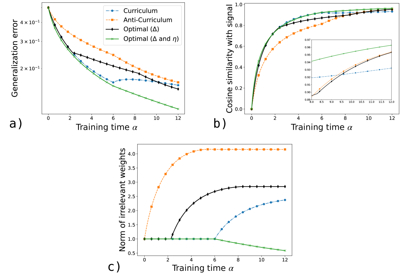Appendix B Supplementary figures and additional details <details> <summary>x10.png Details</summary>  ### Visual Description ## Comparative Analysis of Training Methods ### Overview The image presents three line graphs comparing the performance of four different training methods: Curriculum, Anti-Curriculum, Optimal (Δ), and Optimal (Δ and η). The graphs depict Generalization error, Cosine similarity with signal, and Norm of irrelevant weights, all plotted against Training time (α). ### Components/Axes **Common Elements:** * **X-axis:** Training time α, ranging from 0 to 12 in all three graphs. * **Legend (Top-Right of Figure A):** * Blue dashed line with circular markers: Curriculum * Orange dashed line with square markers: Anti-Curriculum * Black solid line with diamond markers: Optimal (Δ) * Green solid line with cross markers: Optimal (Δ and η) **Graph a) Generalization Error:** * **Y-axis:** Generalization error, ranging from approximately 0 to 4 x 10^-1. **Graph b) Cosine Similarity with Signal:** * **Y-axis:** Cosine similarity with signal, ranging from 0 to 1.0. * **Inset:** A zoomed-in view of the cosine similarity between 8.0 and 12.0, and 0.89 to 0.97. **Graph c) Norm of Irrelevant Weights:** * **Y-axis:** Norm of irrelevant weights, ranging from 0.5 to 4.0. ### Detailed Analysis **Graph a) Generalization Error:** * **Curriculum (Blue):** Starts at approximately 0.4, decreases rapidly until α = 6, then plateaus around 0.15. * **Anti-Curriculum (Orange):** Starts at approximately 0.45, decreases steadily to approximately 0.15 at α = 12. * **Optimal (Δ) (Black):** Starts at approximately 0.4, decreases steadily to approximately 0.1 at α = 12. * **Optimal (Δ and η) (Green):** Starts at approximately 0.45, decreases rapidly to approximately 0.05 at α = 12. **Graph b) Cosine Similarity with Signal:** * **Curriculum (Blue):** Starts at approximately 0, increases rapidly until α = 6, then plateaus around 0.95. * **Anti-Curriculum (Orange):** Starts at approximately 0, increases rapidly until α = 4, then plateaus around 0.85. * **Optimal (Δ) (Black):** Starts at approximately 0, increases rapidly until α = 6, then plateaus around 0.97. * **Optimal (Δ and η) (Green):** Starts at approximately 0, increases rapidly until α = 4, then plateaus around 0.98. **Graph c) Norm of Irrelevant Weights:** * **Curriculum (Blue):** Starts at approximately 1.0, remains constant until α = 6, then increases to approximately 2.3 at α = 12. * **Anti-Curriculum (Orange):** Starts at approximately 1.0, increases rapidly until α = 4, then plateaus around 4.1. * **Optimal (Δ) (Black):** Starts at approximately 1.0, remains constant until α = 3, then increases to approximately 2.9 at α = 12. * **Optimal (Δ and η) (Green):** Starts at approximately 1.0, remains constant until α = 6, then decreases to approximately 0.6 at α = 12. ### Key Observations * The "Optimal (Δ and η)" method consistently achieves the lowest generalization error and highest cosine similarity with signal. * The "Anti-Curriculum" method results in the highest norm of irrelevant weights. * The "Curriculum" method shows a delayed increase in the norm of irrelevant weights compared to the "Anti-Curriculum" and "Optimal (Δ)" methods. * The "Optimal (Δ and η)" method shows a decrease in the norm of irrelevant weights after a certain training time. ### Interpretation The data suggests that the "Optimal (Δ and η)" training method is the most effective among the four, as it minimizes generalization error and maximizes cosine similarity with the signal. The "Anti-Curriculum" method, on the other hand, appears to be the least effective, as it results in the highest norm of irrelevant weights. The delayed increase in the norm of irrelevant weights for the "Curriculum" method may indicate a slower learning process compared to the "Anti-Curriculum" and "Optimal (Δ)" methods. The decrease in the norm of irrelevant weights for the "Optimal (Δ and η)" method suggests that this method is able to effectively filter out irrelevant information during training. </details> Figure 10: Dynamics of the curriculum learning problem under different training schedules—curriculum (easy to hard) at $\eta=3$ , anti-curriculum (hard to easy) at $\eta=3$ , the optimal difficulty protocol at $\eta=3$ (see Fig. 2 b), and the optimal protocol obtained by jointly optimizing $\Delta$ and $\eta$ (see Fig. 3 a). (a) Generalization error vs. normalized training time $\alpha=\mu/N$ . (b) Cosine similarity $M_{11}/\sqrt{TQ_{11}}$ with the target signal (inset zooms into the late-training regime). (c) Squared norm of irrelevant weights $Q_{22}$ vs. $\alpha$ . Parameters: $\alpha_{F}=12$ , $\Delta_{1}=0$ , $\Delta_{2}=2$ , $\eta=3$ , $\lambda=0$ , $T=2$ . Initial conditions: $Q_{11}=Q_{22}=1$ , $M_{11}=0$ . The initial conditions for the order parameters used in Figs. 7 and 8 are $$ \displaystyle R=\frac{{\bm{w}}^{\top}{\bm{\mu}}_{\bm{c}}}{N}=\begin{pmatrix}0.% 116&0.029\\ -0.005&0.104\end{pmatrix}\,,\qquad Q=\frac{{\bm{w}}^{\top}{\bm{w}}}{N}=\begin{% pmatrix}0.25&0.003\\ 0.003&0.25\end{pmatrix}\,, \displaystyle\Omega_{(1,1)(1,1)}=\frac{{\bm{\mu}}_{1,1}\cdot{\bm{\mu}}_{1,1}}{% N}=0.947\,,\qquad\Omega_{(1,2)(1,2)}=\frac{{\bm{\mu}}_{1,2}\cdot{\bm{\mu}}_{1,% 2}}{N}=0.990\,. \tag{91} $$ The initial conditions for the order parameters used in Fig. 9 are $$ \displaystyle R=\frac{{\bm{w}}^{\top}{\bm{\mu}}_{\bm{c}}}{N}=\begin{pmatrix}0.% 339&0.200\\ 0.173&0.263\end{pmatrix}\,,\qquad Q=\frac{{\bm{w}}^{\top}{\bm{w}}}{N}=\begin{% pmatrix}1&0.00068\\ 0.00068&1\end{pmatrix}\,, \displaystyle\Omega_{(1,1)(1,1)}=\frac{{\bm{\mu}}_{1,1}\cdot{\bm{\mu}}_{1,1}}{% N}=1.737\,,\qquad\Omega_{(1,2)(1,2)}=\frac{{\bm{\mu}}_{1,2}\cdot{\bm{\mu}}_{1,% 2}}{N}=1.158\,. \tag{92} $$ The test set used in Fig. 9 b contains $13996$ examples. The standard deviations of the clusters are $\sigma_{1,1}=0.05$ and $\sigma_{1,2}=0.033$ . The cluster membership probability is $p_{c}([c_{1}=1,c_{2}=1])=0.47$ and $p_{c}([c_{1}=2,c_{2}=1])=0.53$ . The initial conditions for the order parameters used in Fig. 13 are $$ \displaystyle R=\frac{{\bm{w}}^{\top}{\bm{\mu}}_{\bm{c}}}{N}=\begin{pmatrix}0.% 099&-0.005\\ -0.002&0.102\end{pmatrix}\,,\qquad Q=\frac{{\bm{w}}^{\top}{\bm{w}}}{N}=\begin{% pmatrix}0.25&-0.002\\ -0.002&0.25\end{pmatrix}\,, \displaystyle\Omega_{(1,1)(1,1)}=\frac{{\bm{\mu}}_{1,1}\cdot{\bm{\mu}}_{1,1}}{% N}=0.976\,,\qquad\Omega_{(1,2)(1,2)}=\frac{{\bm{\mu}}_{1,2}\cdot{\bm{\mu}}_{1,% 2}}{N}=1.014\,. \tag{93} $$ Appendix C Numerical simulations In this appendix, we validate our theoretical predictions against numerical simulations for the three scenarios studied: curriculum learning (Fig. 11), dropout regularization (Fig. 12), and denoising autoencoders (Fig. 13). For each case, the theoretical curves are obtained by numerically integrating the respective ODEs, obtained in the high-dimensional limit $N→∞$ . The simulations are instead obtained for a single SGD trajectory at large but finite $N$ . We observe good agreement between theory and simulations. 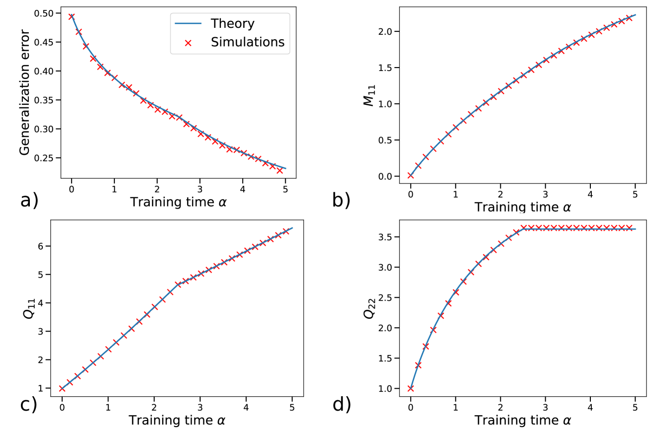<details> <summary>x11.png Details</summary>  ### Visual Description ## Comparative Analysis of Theory vs. Simulations in Generalization Error and Matrix Elements ### Overview The image presents four line plots arranged in a 2x2 grid, comparing theoretical predictions with simulation results across different metrics as a function of training time. The plots examine generalization error, and matrix elements M11, Q11, and Q22. Each plot displays a blue line representing the theoretical model and red 'x' markers representing simulation data. ### Components/Axes * **General Layout:** The image contains four subplots labeled a), b), c), and d). * **Legend:** Located in the top-left subplot (a), the legend identifies the blue line as "Theory" and the red 'x' markers as "Simulations". * **Subplot a): Generalization Error vs. Training Time** * Y-axis: "Generalization error", ranging from 0.25 to 0.50 in increments of 0.05. * X-axis: "Training time α", ranging from 0 to 5 in increments of 1. * **Subplot b): M11 vs. Training Time** * Y-axis: "M11", ranging from 0.0 to 2.0 in increments of 0.5. * X-axis: "Training time α", ranging from 0 to 5 in increments of 1. * **Subplot c): Q11 vs. Training Time** * Y-axis: "Q11", ranging from 1 to 6 in increments of 1. * X-axis: "Training time α", ranging from 0 to 5 in increments of 1. * **Subplot d): Q22 vs. Training Time** * Y-axis: "Q22", ranging from 1.0 to 3.5 in increments of 0.5. * X-axis: "Training time α", ranging from 0 to 5 in increments of 1. ### Detailed Analysis **Subplot a): Generalization Error vs. Training Time** * **Trend:** The "Theory" line (blue) shows a decreasing trend as training time increases. The "Simulations" data (red 'x' markers) closely follows the theoretical line. * **Data Points:** * At α = 0, Generalization error (Theory) ≈ 0.49, Generalization error (Simulations) ≈ 0.49. * At α = 5, Generalization error (Theory) ≈ 0.23, Generalization error (Simulations) ≈ 0.23. **Subplot b): M11 vs. Training Time** * **Trend:** Both "Theory" (blue) and "Simulations" (red 'x' markers) show an increasing trend, with the rate of increase diminishing as training time increases. * **Data Points:** * At α = 0, M11 (Theory) ≈ 0.0, M11 (Simulations) ≈ 0.0. * At α = 5, M11 (Theory) ≈ 2.1, M11 (Simulations) ≈ 2.1. **Subplot c): Q11 vs. Training Time** * **Trend:** Both "Theory" (blue) and "Simulations" (red 'x' markers) show a linear increasing trend. * **Data Points:** * At α = 0, Q11 (Theory) ≈ 1.0, Q11 (Simulations) ≈ 1.0. * At α = 5, Q11 (Theory) ≈ 6.5, Q11 (Simulations) ≈ 6.5. **Subplot d): Q22 vs. Training Time** * **Trend:** Both "Theory" (blue) and "Simulations" (red 'x' markers) increase rapidly initially, then plateau after α ≈ 2.5. * **Data Points:** * At α = 0, Q22 (Theory) ≈ 1.0, Q22 (Simulations) ≈ 1.0. * At α = 2.5, Q22 (Theory) ≈ 3.6, Q22 (Simulations) ≈ 3.6. * At α = 5, Q22 (Theory) ≈ 3.6, Q22 (Simulations) ≈ 3.6. ### Key Observations * The "Theory" and "Simulations" data align very closely in all four subplots, suggesting a strong agreement between the theoretical model and the simulation results. * The generalization error decreases with training time, as expected. * M11 and Q11 increase with training time, but Q22 plateaus after a certain point. ### Interpretation The plots demonstrate the validity of the theoretical model by showing its close agreement with simulation data across different metrics related to the training process. The decreasing generalization error indicates that the model learns effectively with increasing training time. The behavior of M11, Q11, and Q22 provides insights into the internal dynamics of the model during training. The plateauing of Q22 suggests a saturation effect, where further training does not significantly change this particular matrix element. The consistent alignment between theory and simulations reinforces the reliability of the model and its ability to capture the underlying phenomena. </details> Figure 11: Comparison between theory and simulations in the curriculum learning problem: a) generalization error, b) teacher-student overlap $M_{11}$ , c) squared norm $Q_{11}$ of the relevant weights, and d) squared norm $Q_{22}$ of the irrelevant weights. The continuous blue lines have been obtained by integrating numerically the ODEs in Eqs. (48), while the red crosses are the results of numerical simulations of a single trajectory with $N=30000$ . The protocol is anti-curriculum with equal proportion of easy and hard samples. Parameters: $\alpha_{F}=5$ , $\lambda=0$ , $\eta=3$ , $\Delta_{1}=0$ , $\Delta_{2}=2$ , $T_{11}=1$ . Initial conditions: $Q_{11}=0.984$ , $Q_{22}=0.998$ , $M_{11}=0.01$ . 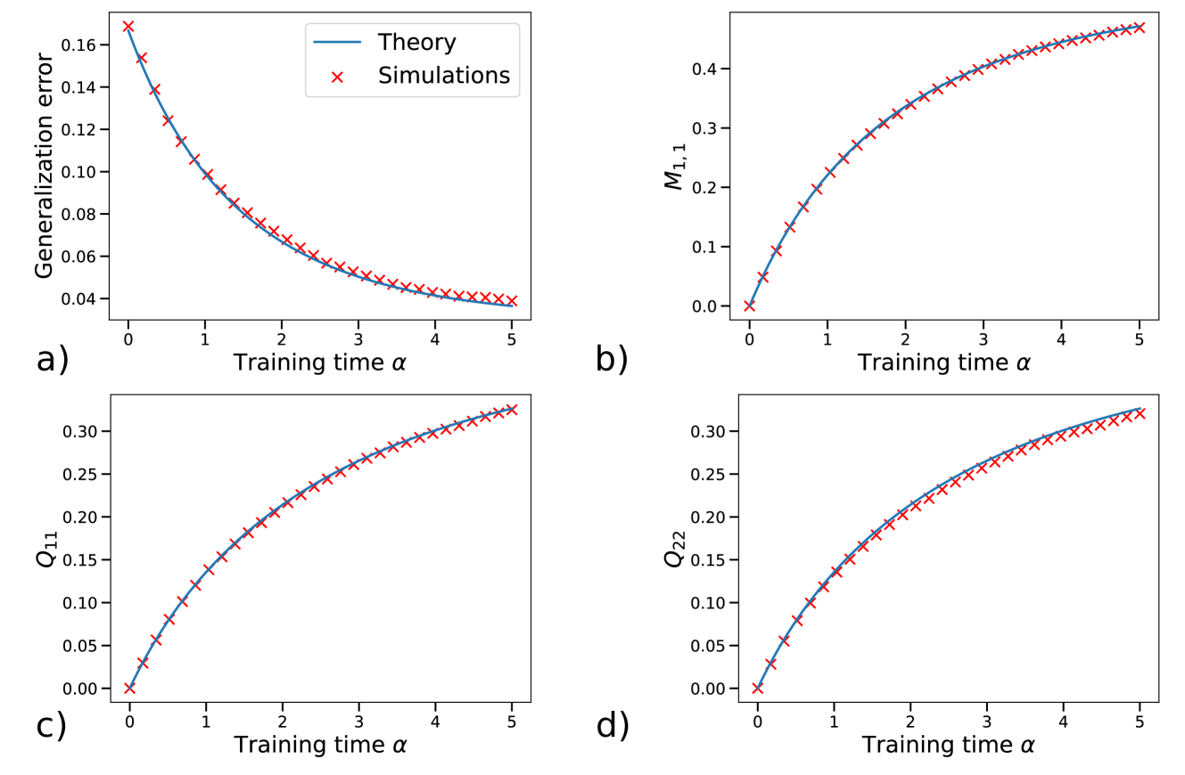<details> <summary>x12.png Details</summary>  ### Visual Description ## Chart: Comparison of Theory and Simulations Across Different Metrics ### Overview The image presents four separate plots (a, b, c, d) comparing theoretical predictions (blue lines) with simulation results (red 'x' markers). Each plot displays a different metric as a function of training time (α). The metrics are: Generalization error, M1,1, Q11, and Q22. The plots show how well the simulations align with the theoretical models for each metric as training time increases. ### Components/Axes * **Plot a)** * Y-axis: Generalization error (range: 0.04 to 0.16) * X-axis: Training time α (range: 0 to 5) * Legend: * Blue line: Theory * Red 'x' markers: Simulations * **Plot b)** * Y-axis: M1,1 (range: 0 to 0.4) * X-axis: Training time α (range: 0 to 5) * Legend: (Same as plot a) * Blue line: Theory * Red 'x' markers: Simulations * **Plot c)** * Y-axis: Q11 (range: 0 to 0.3) * X-axis: Training time α (range: 0 to 5) * Legend: (Same as plot a) * Blue line: Theory * Red 'x' markers: Simulations * **Plot d)** * Y-axis: Q22 (range: 0 to 0.3) * X-axis: Training time α (range: 0 to 5) * Legend: (Same as plot a) * Blue line: Theory * Red 'x' markers: Simulations ### Detailed Analysis * **Plot a) Generalization Error:** * Trend: The blue 'Theory' line shows a decreasing trend. * Trend: The red 'Simulations' markers also show a decreasing trend, closely following the 'Theory' line. * Data Points: * At α = 0, Generalization error (Theory) ≈ 0.16 * At α = 0, Generalization error (Simulations) ≈ 0.16 * At α = 5, Generalization error (Theory) ≈ 0.04 * At α = 5, Generalization error (Simulations) ≈ 0.04 * **Plot b) M1,1:** * Trend: The blue 'Theory' line shows an increasing trend. * Trend: The red 'Simulations' markers also show an increasing trend, closely following the 'Theory' line. * Data Points: * At α = 0, M1,1 (Theory) ≈ 0.0 * At α = 0, M1,1 (Simulations) ≈ 0.0 * At α = 5, M1,1 (Theory) ≈ 0.45 * At α = 5, M1,1 (Simulations) ≈ 0.45 * **Plot c) Q11:** * Trend: The blue 'Theory' line shows an increasing trend. * Trend: The red 'Simulations' markers also show an increasing trend, closely following the 'Theory' line. * Data Points: * At α = 0, Q11 (Theory) ≈ 0.0 * At α = 0, Q11 (Simulations) ≈ 0.0 * At α = 5, Q11 (Theory) ≈ 0.32 * At α = 5, Q11 (Simulations) ≈ 0.32 * **Plot d) Q22:** * Trend: The blue 'Theory' line shows an increasing trend. * Trend: The red 'Simulations' markers also show an increasing trend, closely following the 'Theory' line. * Data Points: * At α = 0, Q22 (Theory) ≈ 0.0 * At α = 0, Q22 (Simulations) ≈ 0.0 * At α = 5, Q22 (Theory) ≈ 0.32 * At α = 5, Q22 (Simulations) ≈ 0.32 ### Key Observations * The 'Theory' lines and 'Simulations' markers are very close in all four plots, indicating a strong agreement between the theoretical model and the simulation results. * The Generalization error decreases with increasing training time, while M1,1, Q11, and Q22 increase with increasing training time. * The x-axis (Training time α) is consistent across all four plots, allowing for direct comparison of the metrics. ### Interpretation The data suggests that the theoretical model accurately predicts the behavior of the system as captured by the simulations. The decreasing generalization error with increasing training time indicates that the model is learning and improving its ability to generalize to new data. The increasing values of M1,1, Q11, and Q22 with increasing training time likely reflect the model's adaptation to the training data. The close alignment between theory and simulations across all four metrics strengthens the validity and reliability of the theoretical model. There are no obvious outliers or anomalies. </details> Figure 12: Comparison between theory and simulations for dropout regularization: a) generalization error, b) teacher-student overlap $M_{1,1}$ , c) squared norm $Q_{11}$ , and d) squared norm $Q_{22}$ . The continuous blue lines have been obtained by integrating numerically the ODEs in Eqs. (52)-(53), while the red crosses are the results of numerical simulations of a single trajectory with $N=30000$ . Parameters: $\alpha_{F}=5$ , $\eta=1$ , $\sigma_{n}=0.3$ , $p(\alpha)=p_{f}=0.7$ , $T_{11}=1$ . Initial conditions: $Q_{ij}=M_{nk}=0$ . 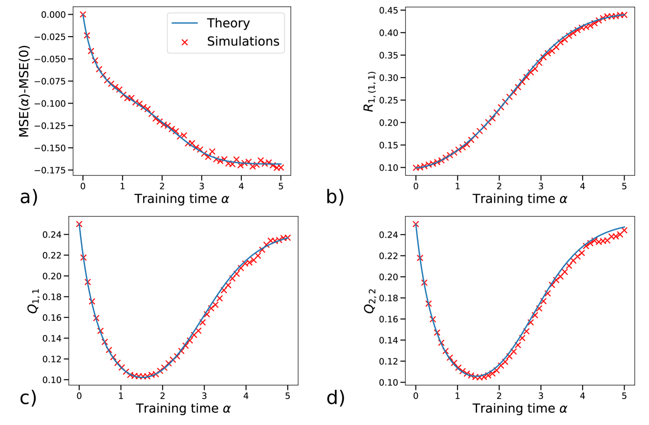<details> <summary>x13.png Details</summary>  ### Visual Description ## Four Line Charts: Theory vs. Simulations ### Overview The image contains four line charts arranged in a 2x2 grid. Each chart compares theoretical predictions (blue line) with simulation results (red 'x' markers) for different metrics as a function of "Training time α". The charts are labeled a), b), c), and d). ### Components/Axes **General Chart Elements:** * **X-axis:** Training time α, ranging from 0 to 5 in all four charts. * **Legend:** Located in the top-left chart (a), indicating "Theory" (blue line) and "Simulations" (red 'x' markers). This legend applies to all four charts. **Chart a):** * **Y-axis:** MSE(α)-MSE(0), ranging from -0.175 to 0.000. * **Description:** Shows the difference in Mean Squared Error (MSE) between a given training time α and the initial MSE (at α=0). **Chart b):** * **Y-axis:** R1,(1,1), ranging from 0.10 to 0.45. * **Description:** Shows the value of R1,(1,1) as a function of training time. **Chart c):** * **Y-axis:** Q1,1, ranging from 0.10 to 0.24. * **Description:** Shows the value of Q1,1 as a function of training time. **Chart d):** * **Y-axis:** Q2,2, ranging from 0.10 to 0.24. * **Description:** Shows the value of Q2,2 as a function of training time. ### Detailed Analysis **Chart a): MSE(α)-MSE(0) vs. Training time α** * **Theory (blue line):** Starts at 0 and decreases rapidly, then plateaus around -0.17 after α=3. * **Simulations (red 'x' markers):** Follow the same trend as the theory, with some fluctuations around the theoretical line. * At α=0, MSE(α)-MSE(0) ≈ 0.00 * At α=1, MSE(α)-MSE(0) ≈ -0.075 * At α=3, MSE(α)-MSE(0) ≈ -0.16 * At α=5, MSE(α)-MSE(0) ≈ -0.17 **Chart b): R1,(1,1) vs. Training time α** * **Theory (blue line):** Starts at approximately 0.10 and increases steadily, approaching 0.43 at α=5. * **Simulations (red 'x' markers):** Closely match the theoretical line. * At α=0, R1,(1,1) ≈ 0.10 * At α=1, R1,(1,1) ≈ 0.15 * At α=3, R1,(1,1) ≈ 0.32 * At α=5, R1,(1,1) ≈ 0.43 **Chart c): Q1,1 vs. Training time α** * **Theory (blue line):** Starts at approximately 0.24, decreases to a minimum around 0.10 at α=1.5, then increases to approximately 0.23 at α=5. * **Simulations (red 'x' markers):** Closely follow the theoretical line. * At α=0, Q1,1 ≈ 0.24 * At α=1.5, Q1,1 ≈ 0.10 * At α=5, Q1,1 ≈ 0.23 **Chart d): Q2,2 vs. Training time α** * **Theory (blue line):** Starts at approximately 0.24, decreases to a minimum around 0.10 at α=1.5, then increases to approximately 0.24 at α=5. * **Simulations (red 'x' markers):** Closely follow the theoretical line. * At α=0, Q2,2 ≈ 0.24 * At α=1.5, Q2,2 ≈ 0.10 * At α=5, Q2,2 ≈ 0.24 ### Key Observations * The theoretical predictions (blue lines) generally align well with the simulation results (red 'x' markers) across all four metrics. * Chart a) shows a decrease in MSE difference as training time increases, indicating improved model performance. * Chart b) shows an increase in R1,(1,1) with training time. * Charts c) and d) show a similar trend: an initial decrease in Q1,1 and Q2,2, followed by an increase as training time increases. ### Interpretation The charts demonstrate the relationship between training time (α) and various performance metrics (MSE difference, R1,(1,1), Q1,1, and Q2,2). The close agreement between the theoretical predictions and simulation results suggests that the theoretical model accurately captures the behavior of the system being simulated. The trends observed in each chart provide insights into how the model's performance and internal parameters evolve during the training process. Specifically, the decrease in MSE difference indicates that the model learns and improves its accuracy over time. The behavior of R1,(1,1), Q1,1, and Q2,2 suggests how the model's internal state changes as it learns. The initial decrease in Q1,1 and Q2,2, followed by an increase, might indicate an initial phase of parameter adjustment followed by a later phase of convergence or stabilization. </details> Figure 13: Comparison between theory and simulations for the denoising autoencoder model: a) mean square error improvement, b) student-centroid overlap $R_{1,(1,1)}$ , c) squared norm $Q_{11}$ . The continuous blue lines have been obtained by integrating numerically the ODEs in Eqs. (80) and (87), while the red crosses are the results of numerical simulations of a single trajectory with $N=10000$ . Parameters: $\alpha_{F}=1$ , $\eta=2$ , $B(\alpha)=\bar{B}=5$ , $K=C_{1}=2$ , $\sigma=0.1$ , $g(z)=z$ . The skip connection $b$ is fixed ( $\eta_{b}=0$ ) to the optimal value in Eq. (26). Initial conditions are given in Eq. (93).