2507.08906v1

<details> <summary>Image 1 Details</summary>  ### Visual Description \n ## Logo: Sorbonne Université ### Overview The image displays the logo of Sorbonne Université, a French public research university. The logo is a stylized "S" incorporating a depiction of the Sorbonne's dome. ### Components/Axes The logo consists of two primary elements: * A stylized, dark blue "S" shape. * Text reading "SORBONNE UNIVERSITÉ" in red. ### Detailed Analysis or Content Details The "S" shape is a flowing, cursive form. Integrated within the upper curve of the "S" is a simplified, white depiction of a dome-shaped building, representing the historical Sorbonne building. The text "SORBONNE" is positioned to the right of the "S", in a larger font size, and is colored red. Below "SORBONNE" is the word "UNIVERSITÉ", also in red, but in a smaller font size. The text "SORBONNE UNIVERSITÉ" is in French. The English translation is "Sorbonne University". ### Key Observations The logo is visually clean and modern, while still referencing the university's historical architecture. The color scheme of dark blue and red is striking and memorable. ### Interpretation The logo effectively communicates the identity of Sorbonne Université. The "S" shape is a clear identifier, and the inclusion of the dome symbolizes the university's long history and academic tradition. The use of French text reinforces the university's location and cultural context. The logo is designed to be easily recognizable and to convey a sense of prestige and academic excellence. The logo does not contain any factual data or numerical values. It is a symbolic representation of an institution. </details> <details> <summary>Image 2 Details</summary>  ### Visual Description \n ## Diagram: LPSM Logo ### Overview The image presents a logo for "LPSM". The logo consists of an abstract graphical element above the text "LPSM". The graphical element appears to be a stylized representation of interconnected nodes or arcs. ### Components/Axes The logo is composed of two main elements: 1. **Graphical Element:** A series of curved lines connecting two circular nodes. The lines are colored in shades of green and blue. 2. **Text:** The letters "LPSM" in a dark blue, sans-serif font. ### Detailed Analysis or Content Details The graphical element features two dark blue circular nodes positioned at the extreme left and right of the image. Arcs connect these nodes. There are three arcs connecting the nodes. * The top arc is green. * The middle arc is a lighter shade of green. * The bottom arc is dark blue. The arcs intersect in the center of the image, creating a complex interwoven pattern. The text "LPSM" is positioned directly below the graphical element, centered horizontally. The font size is relatively large, making the acronym prominent. ### Key Observations The logo is visually balanced, with the graphical element and text complementing each other. The use of green and blue colors suggests a connection to nature, technology, or trustworthiness. The interconnected arcs could symbolize networking, collaboration, or complex systems. ### Interpretation The logo likely represents an organization or entity named "LPSM". The abstract graphical element suggests a focus on interconnectedness, systems thinking, or a dynamic approach. Without further context, the specific meaning of "LPSM" and the logo's symbolism remain open to interpretation. The logo is designed to be memorable and visually appealing, conveying a sense of professionalism and innovation. The logo does not contain any factual data or numerical values. It is a symbolic representation of a brand or organization. </details> Thèse présentée pour l'obtention du grade de ## DOCTEUR de SORBONNE UNIVERSITÉ Discipline / Spécialité Mathématiques appliquées / Statistique École doctorale Sciences Mathématiques de Paris Centre (ED 386) Physics-informed machine learning: A mathematical framework with applications to time series forecasting Nathan Doumèche Rapporteur Rapporteur Président du jury Examinateur Examinatrice Membre invité Membre invité Directeur de thèse Co-directrice de thèse Encadrant industriel de thèse Soutenue publiquement le 7 juillet 2025 Devant un jury composé de : Gilles BLANCHARD , Professeur, Université Paris-Saclay Richard NICKL , Professeur, Université de Cambridge Gabriel PEYRÉ , Directeur de recherche, CNRS Jalal FADILI , Professeur, ENSICAEN Mathilde MOUGEOT , Professeure, ENSIIE Francis BACH , Directeur de recherche, CNRS Stéphane TANGUY , Directeur de recherche, CIO & CTO à EDF Labs Gérard BIAU , Professeur, Sorbonne Université Claire BOYER , Professeure, Université Paris-Saclay Yannig GOUDE , Professeur associé, Université Paris-Saclay <details> <summary>Image 3 Details</summary>  ### Visual Description \n ## Logo: EDF Logo ### Overview The image presents the logo of EDF (Électricité de France), a French multinational electric power company. The logo consists of a stylized graphic element above the company's acronym. ### Components/Axes The logo is composed of two main elements: 1. **Graphic Element:** An abstract design featuring four flame-like or petal-like shapes arranged in a circular pattern. The color of these shapes is a vibrant orange (#FFA500). 2. **Text:** The acronym "EDF" is positioned below the graphic element, rendered in a dark blue color (#000080). ### Detailed Analysis or Content Details The graphic element is not a chart or diagram with quantifiable data. It is a visual symbol. The text "EDF" is a clear identifier of the company. There are no axes, scales, or legends present. ### Key Observations The logo's design evokes energy, power, and potentially the sun or flames, aligning with the company's core business of electricity generation and distribution. The color scheme (orange and blue) is visually striking and memorable. ### Interpretation The EDF logo is a branding element designed to represent the company's identity and values. The abstract graphic element is intended to be recognizable and associated with the EDF brand. The use of orange suggests energy and warmth, while the blue conveys reliability and stability. The logo is a visual shorthand for the company's services and expertise in the energy sector. The logo does not contain any factual data or trends. It is purely a symbolic representation. </details> ## Remerciements Trois ans sont donc passés... D'aucuns supplièrent jadis les heures de suspendre leur cours. Sans succès. Quant à moi, pour endiguer le vertige qui me submerge à la clôture de ce chapitre de ma vie, je n'ai d'autre artifice que de recourir au rite consacré. Aussi, j'ai le bonheur teinté de nostalgie d'entamer cette thèse en remerciant ceux qui l'ont rendue possible. Au commencement était Gérard, et de Gérard naquit cette thèse. Voilà cinq ans maintenant que tu me formes avec exigence et me guides avec bienveillance. Véritable amoureux de la statistique mathématique, tu partages avec générosité ton entrain scientifique et ta vision pour une rédaction scientifique réellement pédagogique. Travailleur acharné, insatisfait de tes rôles de chercheur chevronné et d'enseignant apprécié, tu prends aussi de ton temps pour façonner la statistique de demain et représenter la Sorbonne. J'ose donc affirmer que, fidèle au poète qui t'est cher, tu incarnes bien l'homme des utopies, les pieds ici, les yeux ailleurs. Pour tout cela, je suis heureux et fier d'avoir été ton élève. Deuxième pilier de cette thèse, il me faut remercier Claire. Tu harmonises rigueur et curiosité scientifique par un plaisir solaire à apprendre, découvrir et écrire. Aventurière des statistiques, tu m'as suivi sur tous les chemins, des réseaux de neurones à la mesurabilité des estimateurs, aux noyaux et aux EDP. C'est sans relâche que tu entretiens ton goût du verbe et de la bonne formule. Ton empathie, ton sang-froid et ton humour m'ont aidé à faire face aux moments les plus durs de cette thèse. Merci aussi d'avoir toujours eu à cœur de mettre en valeur mon travail, et de m'encourager à participer à des conférences, séminaires et écoles d'été. Ultime panneau de ce triptyque doctoral, je veux témoigner de toute ma gratitude envers Yannig. Avatar de l'esprit sportif, tu appliques avec méthode et ardeur à la prévision énergétique tous les algorithmes prometteurs qui te sont présentés. En compétition, il faut faire feu de tout bois ! De tous les statisticiens que j'ai rencontrés, tu es sûrement celui dont je partage le plus la vision des mathématiques appliquées. En entraîneur attentionné, tu as sans cesse veillé à ma bonne intégration au sein de l'équipe à EDF, et à mon épanouissement tant sur le plan pratique que théorique. Merci pour ta patience, ton expérience, et tes encouragements. Plus généralement, je tiens à exprimer ma reconnaissance aux membres du jury, qui me consacrent une journée de leur temps que je sais fort précieux. Merci à Gilles et à Richard pour l'enthousiasme dont ils ont fait preuve à la relecture de ce manuscrit de thèse. Bien que le sérieux de l'évaluation repose sur le fait que nous ne nous connaissons pas personnellement, j'ai lu avec gourmandise les travaux de Gilles sur les noyaux; de Jalal, Mathilde et Richard sur les méthodes informées par la physique; et de Gabriel sur les fondements mathématiques de l'IA. C'est un grand honneur pour moi que de vous voir siéger à mon jury. Ma thèse n'aurait pas été possible sans la joyeuse farandole des statisticiens qui m'ont accompagné, au détour d'un article ou d'un stage, et ont enrichi mon paysage informatique et mathématique. Merci à Stéfania pour ta connaissance des indices téléphoniques, à Yann pour m'avoir épaulé sur ma toute première base de données, et à Yvenn pour tes talents d'organisateur de challenge. Un merci tout particulier à Francis qui, par l'exercice d'un prosélytisme dont il ne se cache pas, m'a totalement converti aux méthodes à noyaux et m'a conduit à la béatitude exaltée que confère la dimension effective. Merci et bravo à mes stagiaires, Éloi et Guillhem, pour le travail, la confiance, et la joie qu'ils m'ont apportés. J'ai été très fier de vous voir tant progresser. Merci en retour à Adeline et Pierre, membres éminents de la dynastie des Gérardiens et dont j'ai été le stagiaire dans le temps, pour m'avoir donné envie de faire des statistiques. Ces trois ans n'auraient pas eu la même saveur sans l'ambiance chaleureuse des équipes d'EDF et de la Sorbonne. Merci à Caroline, Éloi, Ferdinand, Guillaume Lambert, Guillaume Principato, Julie et Stanislas pour avoir tant égayé les bureaux que nous avons partagés. Chers collègues d'EDF, merci à Amaury pour ta musique punchy, à Bachir pour ton goût pour la bonne chère, à Christian pour nos discussions de régression linéaire et de randonnée, à Élaine pour notre dévotion commune à Arte et Élisabeth Quin, à Élise pour ta gentillesse sans égal, à Félicie pour ta joie de vivre, à Hugo pour ton humour pince-sans-rire, à Gilles, Sandra et Véronique pour le maintien de la tradition du café et de la conversation matinale, à Joseph pour m'avoir montré la voie, à Manel pour ton affection presque maternelle, à Margaux pour la force de tes convictions, à Virgile pour ton regard émerveillé sur le monde. Honorables collègues du LPSM, merci à mes anciens professeurs de master Anna, Antoine, Arnaud, Erwan, Ismaël et Lorenzo pour leur savoir encyclopédique, à Charlotte pour m'avoir accueilli les bras ouverts comme chargé de travaux dirigés, et à Alice, Miguel, et Paul pour leurs conseils d'enseignement. Merci également à Hugues, Natalie, Nisrine, Nora et Xavier, sans qui les rouages administratifs m'auraient sans doute avalé depuis longtemps. Au-delà de ma thèse, je sais ce que je dois à ceux qui me soutiennent au quotidien et agrémentent ma vie de leur présence loufoque. Merci à mes amis d'enfance, qui portent en eux la chaleur et la tranquillité du Sud. À Gilliane, avec qui j'ai coévolué au point d'entendre mentalement sa voix. Merci pour ton rire communicatif, le théâtre, nos vacances, et notre amour incompris du Top D17. À mes amis de lycée, Gabrielle et Léo en particulier, pour nos innombrables soirées plage. Merci à mes amis des Mines, fièrement rassemblés sous la bannière de la Piche et régulièrement convoqués par notre roi élu. À Agathe pour avoir partagé ma détresse sur l'Île-Molène, à Amandine pour notre danse sur I Like To Move It à Barcelone, à Antoine pour tes extravagances mégalomanes, à Charlène et Jean pour votre sens du chic et de la fête, à Denis pour tes traits d'esprit caustiques, à Félix pour m'avoir transmis ta passion du Japon, à Victor pour avoir créé un si beau Donjon où tu nous accueilles toujours avec l'hospitalité médiévale de circonstance. Merci à mes amis de l'ENS, notamment aux autoproclamés malins , qui réapparaissent périodiquement pour me professer leur sagesse douteuse. Paraît-il qu'un bol n'est jamais plus utile que quand il est vide... Une place toute spéciale est prise en mon cœur par ce quatuor étrange et, il faut bien l'avouer, un peu disparate, qui toutefois s'accorde merveilleusement à l'harmonie de mon existence 1 . À Baptiste, avec qui j'ai souvent festoyé jusqu'à l'évanouissement, co-inventeur des fameuses pâtes au gras. À toi, que l'honneur mal placé exhorte régulièrement à des aventures qui forcent l'admiration, tant en sport qu'en sciences, et qui n'a pourtant pas encore pleinement conscience de sa force. À Éric, qui envisage l'existence comme un jeu, et avec qui je prends un plaisir non dissimulé (certes, parfois après-coup) à pousser aux extrêmes limites nos capacités physiques et mentales. À toi, cher voisin du C2 en mes temps de pape, toi qui m'a fait survivre sur une île bordée de phoques, toi qui m'a traîné, mourant, sur la muraille de Chine, bref, toi en qui j'ai une confiance irraisonnable. À Nataniel, dragon majestueux et sautillant, un peu bruyant par moments, mon Doppelgänger flamboyant. À toi qui me suit, chaque année, selon le rituel, arpenter les cimes du Mercantour. À ton amour débordant pour la vie, les amis, les animaux mignons (et les limaces !?), les champignons, la littérature, la musique, la danse... À Alexis, qui partage courageusement ma vie. À tes passions hétéroclites pour les chats, le matcha, le karaoké, la pop, les voyages, le clubbing, les jeux vidéo... À toi qui préfères acheter la whey que pousser à la salle, et à tous ces autres traits qui te rendent si attachant. Il est des dons que l'on ne peut rendre. Je tâche ici au moins d'en rendre compte. Merci à ma mère, pour ton soutien inconditionnel, indéfectible. Pour ta foi en l'école et dans le savoir, 1 Les férus de solfège reconnaissent ici une septième diminuée. qui m'a porté jusque-là. Pour ta force devant la maladie, qui t'a fait soigner les autres. À mon père, pour m'avoir transmis ton amour des sciences et de la nature. Pour ces journées passées à pêcher, cueillir les plantes sauvages, tailler des silex, observer les animaux, et ergoter sur les espèces d'arbres. À Anne qui prend soin au quotidien de cet homme préhistorique en puissance. À ma grande sœur, Andréa, qui m'a toujours servi de modèle et qui a initié en moi un intérêt regrettable pour la télé-réalité et les séries. À mon adorable neveu, Arthur, qui fait preuve d'une patience rare, mêlée d'un intérêt sincère, à écouter mes histoires. À mes oncles, tantes, cousins et cousines, Élie, Fabien, Irène, Jokyo, Lucie, Magali, Pierre, Prune, et Rodrigue. À ma marraine Jocelyne, pour sa quête du spirituel et sa tendresse pour la montagne. Aux amis de mes parents, Alain et Thavy, Christian, Christophe, Georges et Janine, qui m'ont tant appris sur les vérités cachées de la vie. J'ai ici une pensée pour ceux dont le feu s'est éteint. À papé Jean Doumèche, médaillé de la Résistance en 47, pour les exploits dont les récits ont bercé ma jeunesse, et qui m'a donné son nom. À pépé Marcel, incorrigible musicien et blagueur, qui m'a légué ses partitions. Le monde en soit témoin, vous êtes partis comme vous avez vécu: dignes. ## Abstract Physics-informed machine learning (PIML) is an emerging framework that integrates physical knowledge into machine learning models. This physical prior often takes the form of a partial differential equation (PDE) system that the regression function must satisfy. In the first part of this dissertation, we analyze the statistical properties of PIML methods. In particular, we study the properties of physics-informed neural networks (PINNs) in terms of approximation, consistency, overfitting, and convergence. We then show how PIML problems can be framed as kernel methods, making it possible to apply the tools of kernel ridge regression to better understand their behavior. In addition, we use this kernel formulation to develop novel physicsinformed algorithms and implement them efficiently on GPUs. The second part explores industrial applications in forecasting energy signals during atypical periods. We present results from the Smarter Mobility challenge on electric vehicle charging occupancy and examine the impact of mobility on electricity demand. Finally, we introduce a physics-constrained framework for designing and enforcing constraints in time series, applying it to load forecasting and tourism forecasting in various countries. Keywords: Physics-informed machine learning, neural networks, kernel methods, load forecasting, time series ## Résumé L'apprentissage automatique informé par la physique est un domaine récent qui consiste à intégrer des connaissances physiques dans des modèles d'apprentissage automatique. L'information physique prend souvent la forme d'un système d'équations aux dérivées partielles (EDPs) que la fonction de régression doit satisfaire. Dans la première partie de cette thèse, nous analysons les propriétés statistiques des méthodes d'apprentissage automatique informé par la physique. En particulier, nous étudions les propriétés des réseaux de neurones informés par la physique, en termes d'approximation, de consistance, de surapprentissage et de convergence. En outre, nous montrons comment l'apprentissage statistique pénalisé par des systèmes d'EDPs linéaires peut se réécrire comme une méthode à noyaux. En s'appuyant sur cette reformulation, nous développons de nouveaux algorithmes informés par la physique, que nous implémentons ensuite efficacement sur carte graphique. La deuxième partie se concentre sur des applications industrielles en prévision de signaux énergétiques en périodes atypiques. Nous présentons les résultats du Smarter Mobility Data Challenge sur l'occupation de la charge des véhicules électriques, et examinons l'impact de la mobilité sur la demande d'électricité. Enfin, nous développons un cadre pour la conception et l'application de contraintes dans les séries temporelles, en l'appliquant à la prévision de la consommation électrique et à la prévision du tourisme dans différents pays. Keywords: Apprentissage statistique informé par la physique, réseaux de neurones, méthodes à noyau, prévision de consommation électrique, séries temporelles ## Présentation de la thèse La thèse de doctorat présentée ici est le fruit d'une collaboration entre l'entreprise EDF, spécialisée dans la production et la vente d'électricité, et Sorbonne Université. Afin d'améliorer la performance et l'explicabilité des modèles de prévision énergétique, EDF s'intéresse à l'incorporation de connaissances humaines (souvent regroupées sous le nom de l'expertise métier) dans ses méthodes statistiques d'aide à la décision. À cette fin, le domaine de l'apprentissage automatique informé par la physique (PIML en anglais) permet d'intégrer des contraintes dans des modèles d'apprentissage automatique. Il a été introduit en 2019 par l'invention des réseaux neuronaux informés par la physique. Dans cette thèse, nous nous focalisons donc sur l'étude des algorithmes d'apprentissage automatique informés par la physique et sur la prévision énergétique en période atypique. Par conséquent, nous abordons à la fois des aspects théoriques, tels l'impact des contraintes physiques sur les propriétés statistiques des estimateurs, ainsi que des applications industrielles sur données réelles. ## Intégration de contraintes physiques dans les méthodes statistiques et applications industrielles ## Apprentissage automatique informé par la physique Interprétabilité des modèles. Les algorithmes d'apprentissage automatique affichent des performances remarquables sur de nombreuses tâches complexes en analyse et de génération de données [Wan+23a]. Cependant, malgré d'impressionnants résultats en reconnaissance d'images, en traitement du langage et en interaction avec des environnements adversoriaux (apprentissage par renforcement), les techniques modernes d'apprentissage profond peinent encore à accomplir certaines tâches simples mais cruciales pour de nombreuses applications pratiques. La prévision de séries temporelles en est peut-être l'exemple le plus saillant [MSA22a; McE+23; Zen+23; Ksh+24]. De surcroît, même lorsqu'ils sont performants, les algorithmes d'apprentissage profond ne présentent pas les mêmes garanties théoriques que les méthodes statistiques plus standard. Il est donc risqué de s'appuyer sur de tels algorithmes, souvent qualifiés de "boîte noire", pour des applications industrielles sensibles ou à fort enjeu [VAT21]. En complément d'efforts de recherche pour mieux comprendre les algorithmes d'apprentissage profond, de nombreux travaux visent à développer de nouveaux algorithmes avec de meilleures garanties théoriques, sous le nom d'apprentissage automatique interprétable ou explicable [LZ21; Lis+23]. Une piste prometteuse pour améliorer l'interprétabilité des algorithmes consiste à intégrer des connaissances issue de la modélisation dans les modèles statistiques. Ces informations préalables sur les caractéristiques du signal à prévoir peuvent prendre la forme d'un modèle physique. Physique et statistique. L'idée de coupler une modélisation physique à des modèles statistiques n'est pas nouvelle. D'une part, la déduction empirique de lois fondamentales de la nature est dans l'essence même de la physique en tant que science expérimentale. Par exemple, les célèbres lois de Kepler de 1609 furent découvertes empiriquement, par l'ajustement de courbes sur des observations du mouvement des planètes. D'autre part, la modélisation mathématique de l'intégration d'équations aux dérivées partielles (EDPs) issues de la physique dans des modèles statistiques était déjà formulée dans les travaux de Wahba [Wah90] en 1990. Cependant, jusqu'à peu, deux problèmes principaux étaient restés en suspens. Premièrement, aucun algorithme n'était capable d'incorporer efficacement et de façon systématique des connaissances physiques au sein de méthodes de régression statistique. Cela signifie que les praticiens devaient fournir un travail conséquent afin d'incorporer leurs modélisations physiques dans des méthodes statistiques. Deuxièmement, l'impact mathématique de l'ajout de contraintes physique sur la performance des méthodes statistiques était inconnu. Bien qu'il soit intuitif que les modèles avec plus d'informations devraient être plus puissants, en pratique, l'ajout de connaissances physiques augmente souvent la complexité informatique des modèles et en détériore l'optimisation. L'apprentissage automatique informé de la physique. Au cours des dernières années, de nouveaux moyens furent découverts pour adapter des algorithmes bien connus afin qu'ils emploient efficacement des a priori physiques. En effet, l'incorporation d'EDPs dans les algorithmes statistiques a été illustrée par Raissi et al. [RPK19] sur les réseaux neuronaux et Nickl [Nic23] sur les méthodes de Monte-Carlo par chaînes de Markov (MCMC en anglais), tandis que l'utilisation des techniques d'EDP pour des tâches statistiques a été illustrée par Arnone et al. [Arn+22] sur la méthode des éléments finis (FEM). Dans cette thèse, nous montrons comment faire de même avec des méthodes à noyaux [Dou+24a]. En particulier, le concept d'incorporer de la physique à des algorithmes d'apprentissage automatique classiques est maintenant connu sous le nom d'apprentissage automatique informé par la physique (PIML en anglais) Karniadakis et al. [Kar+21]. S'appuyer sur des algorithmes bien connus pour l'intégration de contraintes physiques est très avantageux d'un point de vue informatique. Par exemple, les réseaux neuronaux informés par la physique (PINNs en anglais) de Raissi et al. [RPK19] exploitent les écosystèmes publics Pytorch et Tensorflow , développés et maintenus par la communauté de l'apprentissage automatique et soutenus par de riches entreprises d'intelligence artificielles, comme Google et Meta. L'inscription dans ces écosystèmes permet de directement tirer parti des puissantes accélérations de calcul et d'une gestion optimisée de la mémoire issues d'années de recherche en apprentissage automatique. En outre, cela permet de facilement implémenter les algorithmes informés par la physique sur du matériel informatique très efficace. Tyiquement, il s'agit d'exécuter les algorithmes sur des cartes graphiques (GPU en anglais), qui sont des unités de calcul ultra-optimisées pour effectuer des opérations mathématiques spécifiques d'algèbre linéaire, comme le produit matrice-vecteur. Dans cette thèse, nous montrons comment mettre en oeuvre nos méthodes à noyaux sur GPU. Toutes ces accélérations, ainsi que la bonne gestion de la mémoire, sont des améliorations cruciales pour le PIML, car l'ajout de physique à un algorithme statistique rend généralement son apprentissage plus coûteux en calculs. Vers des contraintes plus faibles. La plupart des algorithmes informés par la physique furent développés pour incorporer des a priori physiques prenant la forme de systèmes d'EDPs. Bien que ce cadre soit approprié pour la description de systèmes physiques dont les lois sont connues, les connaissances humaines ne prennent pas toujours une forme aussi rigide. Par exemple, c'est le cas de nombreux signaux macroéconomiques, tels que la demande d'électricité. Il n'en demeure pas moins que certaines contraintes peuvent être incorporées dans les modèles de prévision de tels signaux. Par exemple, les lois de la macroéconomie stipulent que, toutes choses égales par ailleurs, la demande d'électricité diminuera lorsque le prix augmentera. De telles formes plus faibles de physique (où le terme « physique » est entendu ici au sens large de toute information issue d'une modélisation) ont été intégrées avec succès dans les PINNs [voir, par exemple, Daw+22]. Nous expliquons au chapitre 7 comment appliquer des contraintes faibles aux séries temporelles. ## Défis mathématiques de l'apprentissage informé de la physique Cadre mathématique. Le PIML est généralement divisé en quatre tâches [RPK19; Kar+21; Cuo+22]. Soient d ∈ N /star la dimension du problème, Ω ⊆ R d le domaine d'intérêt, et D l'opérateur différentiel correspondant à la physique du problème. L'exemple typique est d = 2 , Ω = [0 , 1] 2 , et D = ∂ 2 1 , 1 + ∂ 2 2 , 2 est l'opérateur laplacien. La première tâche est la résolution d'EDP. Étant donné un ensemble de conditions limites, l'objectif est de trouver une fonction satisfaisant à la fois le système d'EDPs et les conditions limites. Par exemple, la condition limite de Dirichlet h : ∂ Ω → R se traduit par la recherche d'une fonction f h telle que pour tout x ∈ Ω , D ( f h )( x ) = 0 , et f h | ∂ Ω = h . Dans l'exemple précédent, cela revient à résoudre l'EDP ∂ 2 1 , 1 f h + ∂ 2 1 , 1 f h = 0 compte tenu de la condition aux limites h . Dans ce contexte, l'utilisateur spécifie la condition limite h et entraîne ensuite un algorithme d'apprentissage (par exemple, un PINN) à apprendre la solution de l'EDP. Bien que les méthodes d'EDP telles que la méthode des éléments finis (FEM) soient déjà très efficaces dans la résolution des EDP, elles peuvent être coûteuses en termes de calcul. Ici, les méthodes d'apprentissage automatique sont utiles pour trouver rapidement des approximations pour f h , appelées modèles de substitution. Ceci est particulièrement intéressant lorsque l'EDP doit être résolue de manière répétée, comme c'est le cas des prévisions météorologiques. La deuxième tâche est la modélisation hybride. Étant données n ∈ N /star observations ( X 1 , Y 1 ) , . . . , ( X n , Y n ) indépendantes et identiquement distribuées (i.i.d.) selon la loi de la variable aléatoire ( X,Y ) , où Y = f /star ( X ) + ε et ε est un bruit, l'objectif est d'estimer la fonction f /star . La particularité de ce cadre d'apprentissage supervisé est l'a priori que f /star est solution de l'EDP D ( f /star ) = 0 , toutefois avec une éventuelle erreur de modélisation. Ce cadre est particulièrement pertinent lorsque l'a priori physique est incomplet. Par exemple, les conditions aux limites peuvent ne pas être entièrement spécifiées, ou l'ensemble des équations différentielles peut admettre un nombre infini de solutions. Dans ce cas, les techniques traditionnelles d'EDP ne peuvent pas être appliquées directement et les données sont nécessaires pour résoudre le problème. La troisième tâche est l'apprentissage d'EDP. Étant données n ∈ N /star observations ( X 1 , Y 1 ) , . . . , ( X n , Y n ) indépendantes et identiquement distribuées (i.i.d.) selon la loi de la variable aléatoire ( X,Y ) , où Y = f /star ( X ) + ε et ε est un bruit, l'objectif est d'estimer la fonction f /star ainsi que la loi physique à laquelle f /star obéit. Dans ce contexte d'apprentissage supervisé, la seule connaissance préalable est le fait que la fonction f /star est solution d'un système d'EDPs à coefficients inconnus. Un exemple de tel a priori physique pourrait être que f /star satisfait l'EDP ∆ f /star = λ /star f /star , où λ /star ∈ R est un paramètre inconnu devant être estimé grâce aux données. Les PINNs Raissi et al. [RPK19], la régression LASSO [KKB20] et les MCMCs [Nic23] sont des algorithmes efficaces d'apprentissage d'EDP. La quatrième tâche consiste à directement construire un solveur d'EDP. Formellement, il s'agit d'apprendre l'opérateur φ : h ∈ L 2 ( ∂ Ω) ↦→ f h ∈ L 2 (Ω) qui, à une condition limite h , associe l'unique solution f h telle que f h | ∂ Ω = h et ∀ x ∈ Ω , D ( f h )( x ) = 0 . Ce contexte est appelé apprentissage d'opérateur. L'objectif ici est de fournir des modèles de substitution plus rapides, en apprenant un modèle global φ , plutôt que d'entraîner un algorithme spécifique pour chaque nouvelle condition limite h . DeepONet [Lu+21] et les opérateurs neuronaux de Fourier [Li+21] sont des algorithmes d'apprentissage d'opérateur efficaces. Dans ce document, nous nous concentrons principalement sur la résolution d'EDP et la modélisation hybride. Les deux autres tâches seront l'objet de de travaux ultérieurs. En effet, l'apprentissage d'EDP et l'apprentissage d'opérateur sont des opérations plus complexes, et leurs propriétés statistiques sont encores inconnues. Comment créer des algorithmes intégrant de l'information physique ? L'un des principaux défis du PIML est de concevoir des algorithmes efficaces pour traiter les tâches susmentionnées. En pratique, la plupart des implémentations reposent sur la minimisation d'un risque empirique constitué d'une partie d'accroche aux données et d'une pénalité physique. En modélisation hybride, l'EDP est intégrée comme une pénalité L 2 , et le risque empirique devient $$\mathcal { R } _ { n } ( f ) = \sum _ { j = 1 } ^ { n } \| f ( X _ { j } ) - Y _ { j } \| _ { 2 } ^ { 2 } + \lambda \int _ { \Omega } | \ m a t h s c r { D } ( f ) ( x ) | ^ { 2 } d x ,$$ où λ > 0 est un hyperparamètre fixé par l'utilisateur. Cette minimisation est effectuée sur une classe de fonctions, à savoir les réseaux neuronaux pour les PINNs [RPK19], et une base de Fourier pour nos méthodes à noyaux [Dou+24b]. Cependant, la pénalité EDP rend particulièrement difficile la recherche d'un minimiseur global de R n sur une classe de fonctions donnée. Il faut pour cela pouvoir être capable de dériver une fonction de la classe de fonctions considérée, ce qui n'est pas toujours possible (par exemple, les forêts aléatoires ne sont pas dérivables). D'ailleurs, bien que les PINNs soient la technique qui a reçu le plus d'attention récemment, l'algorithme proposé par Raissi et al. [RPK19] est susceptible de surapprendre [WYP22; DBB25], tandis que son optimisation est fortement dégradée lorsque l'opérateur différentielle D est non linéaire [BBC24]. En outre, la plupart des algorithmes proposés dans la littérature sont très gourmands en ressources informatiques. En particulier, les PINNs nécessitent des milliers d'étapes de descente de gradient pour converger, alors qu'ils ne sont pas toujours significativement plus performants que les solveurs d'EDP traditionnels, tant en termes de vitesse de calcul que de précision, comme le révèle la méta-analyse de McGreivy and Hakim [MH24]. Comment quantifier les gains de la physique ? D'un point de vue théorique, mesurer l'impact de la physique sur la performance de l'algorithme est une question qui n'a toujours pas trouvé de réponse complète. Un avantage de l'apprentissage informé de la physique est que, en s'appuyant sur des algorithmes connus, il devient possible d'adapter les outils spécifiques à l'algorithme initial pour comprendre les propriétés théoriques des versions physiquement pénalisées. Par exemple, l'analyse du noyau tangent neuronal (NTK) des PINNs caractérise la convergence de leur descente de gradient [BBC24], tandis que les outils de l'inférence bayésienne non paramétrique permettent d'étudier le taux de convergence des MCMCs physiquement informées [NGW20]. Dans cette thèse, nous nous appuyons sur l'analyse de la dimension effective de Caponnetto and Vito [CV07] et Blanchard et al. [BBM08] pour caractériser le taux de convergence de nos méthodes à noyaux [Dou+24a]. La plupart de ces résultats théoriques confirment l'intuition selon laquelle les algorithmes PIML sont plus difficiles à optimiser, mais offrent de meilleures performances statistiques lorsqu'ils sont entraînés dans de bonnes conditions. ## Contexte industriel Au-delà des aspects théoriques liés aux propriétés statistiques et à la complexité des algorithmes, l'apprentissage automatique informé de la physique a démontré son efficacité dans des applications industrielles. Cette thèse, menée en collaboration avec l'entreprise EDF, se concentre sur les applications aux séries temporelles, en particulier dans le domaine de la prévision énergétique. Séries temporelles. Les séries temporelles sont omniprésentes dans les applications industrielles [Pet+22], englobant la prévision des signaux macroéconomiques (offre, demande, prix, mobilité humaine...), l'estimation de la propagation des maladies et du trafic hospitalier, le suivi des processus industriels en temps réel (processus de fabrication, réactions chimiques, maintenance préventive...) et l'anticipation des événements environnementaux (vagues de chaleur, incendies, précipitations...). Cependant, les séries temporelles sont particulièrement difficiles à traiter d'un point de vue statistique. Tout d'abord, les observations sont corrélées, ce qui signifie que la loi des grands nombres et le théorème central limite ne peuvent pas être directement appliqués pour créer des estimateurs. Ensuite, il est courant que la distribution des séries temporelles évolue au cours du temps, que cela soit en raison d'une tendance, d'une saisonnalité ou de ruptures. En outre, les séries temporelles comportent souvent des valeurs manquantes, en conséquence de fréquences d'échantillonnage potentiellement différentes dans les données, ou encore de défaillances de capteurs. Tous ces phénomènes limitent la quantité de données pertinentes disponibles pour l'apprentissage et rendent difficile la prévision des séries temporelles. L'ajout de contraintes physiques aux modèles de prévision apparaît comme un moyen prometteur pour en améliorer les performances. Les techniques de PIML ont été appliquées avec succès à des séries temporelles du monde réel présentant des dépendances physiques bien connues, telles que les prévisions météorologiques [Kas+21], la prévision de production d'énergie renouvelable [LO+23], ou le contrôle en temps réel de réactions chimiques industrielles [Ngu+22]. Prévision de signaux énergétiques. Dans cette thèse, nous nous concentrons principalement sur la prévision de signaux énergétiques, comme l'occupation de bornes de recharge de véhicules électriques et la demande d'électricité. Ces deux tâches de prévision sont difficiles, mais utiles pour l'industrie de l'énergie. En effet, le marché des véhicules électriques est émergent et en forte croissance, et les fournisseurs doivent adapter le réseau électrique à ses demandes de haute intensité électrique. Cependant, les bases de données et les modèles de machine learning appliquées aux véhicules électriques sont encore rares [AO+21]. En ce qui concerne la prévision de demande d'électricité (également appelée prévision de charge), le stockage de l'électricité est coûteux et limité, tandis que l'offre doit correspondre à la demande à tout moment pour éviter les pannes. La prévision de la demande est donc nécessaire pour ajuster la production et agir efficacement sur les marchés de l'électricité [Ham+20]. Cependant, aucun de ces signaux n'est régi par un ensemble connu d'EDPs. De fait, l'ensemble complet des variables explicatives responsables de leur variations est inconnu ou non mesuré. Des modèles statistiques, potentiellement guidée par notre connaissance du comportement de ces signaux, sont donc nécessaires pour combler ces défauts de modélisation. ## Organisation du document Ce document est composé d'une introduction, d'une partie théorique (Partie I), d'une partie appliquée (Partie II) et d'une conclusion. Chaque partie est divisée en plusieurs chapitres, chacun correspondant à une contribution autonome. Nous donnons ci-dessous un bref aperçu de chaque chapitre. Chacun a donné ou donnera lieu à une publication. ## Partie I : Quelques résultats mathématiques sur l'apprentissage automatique informé par la physique On the convergence of PINNs , Nathan Doumèche, Gérard Biau (Sorbonne Université), et Claire Boyer (Université Paris-Saclay). Publié à Bernoulli. Le chapitre 2 est consacré à l'analyse des propriétés statistiques des réseaux neuronaux informés par la physique (PINNs) pour la résolution d'EDPs et la modélisation hybride. Nous nous concentrons sur l'approximation, la consistance du risque et la cohérence physique des PINNs. Au travers d'exemples, nous illustrons comment les réseaux neuronaux informés par la physique sont sujet à un surapprentissage systémique. Nous montrons également que les techniques usuelles de régularisation sont efficaces pour s'assurer de leur consistance. Physics-informed machine learning as a kernel method , Nathan Doumèche, Francis Bach (INRIA Paris), Gérard Biau (Sorbonne Université), et Claire Boyer (Université Paris-Saclay). Publié aux Proceedings of Thirty Seventh Conference on Learning Theory (COLT 2024). Dans le chapitre 3, nous prouvons que, pour les EDPs linéaires, la résolution d'EDPs et la modélisation hybride sont des méthodes à noyaux. En s'appuyant sur la théorie des méthodes à noyaux, nous montrons que l'estimateur informé par la physique converge au moins au taux minimax de Sobolev. Des taux plus rapides peuvent être atteints, mettant alors en évidence les bénéfices de l'a priori physique. Physics-informed kernel learning , Nathan Doumèche, Francis Bach (INRIA Paris), Gérard Biau (Sorbonne Université), et Claire Boyer (Université Paris-Saclay). Accepté avec révisions mineures au Journal of Machine Learning Research (JMLR). Le chapitre 4 est dédié à l'emploi de séries de Fourier pour approximer le noyau susmentionné. Nous y proposons un estimateur implémentable minimisant le risque empirique informée par la physique. Nous illustrons la performance de l'estimateur à noyaux par des expériences numériques, tant pour la modélisation hybride que pour la résolution d'EDP. ## Partie II: Prévision de séries temporelles en périodes atypiques Forecasting Electric Vehicle Charging Station Occupancy: Smarter Mobility Data Challenge , Yvenn Amara-Ouali (Université Paris-Saclay), Yannig Goude (Université Paris-Saclay), Nathan Doumèche (Sorbonne Université), Pascal Veyret (EDF R&D), et al. Publié au Journal of Data-centric Machine Learning Research (DMLR). Le chapitre 5 est un chapitre spécial décrivant les résultats des trois équipes gagnantes du Smarter Mobility Data Challenge. L'objectif de ce défi était de prédire l'occupation des bornes de recharge de véhicules électriques à Paris en 2021. Notre équipe s'est classée 3ème de ce challenge. Human spatial dynamics for electricity demand forecasting , Nathan Doumèche, Yannig Goude (Université Paris-Saclay), Stefania Rubrichi (Orange Innovation), et Yann Allioux (EDF R&D). En évaluation par les pairs. Dans le chapitre 6, nous explorons l'impact des données liées au travail sur la prévision de la demande d'électricité. Nous démontrons que les indices de mobilité dérivés des données des réseaux mobiles améliorent de manière significative la performance des modèles de l'état de l'art, en particulier pendant la période de sobriété énergétique de la France de l'hiver 2022-2023. Forecasting time series with constraints , Nathan Doumèche, Francis Bach (INRIA Paris), Eloi Bedek (EDF R&D), Gérard Biau (Sorbonne Université), Claire Boyer (Université Paris-Saclay), et Yannig Goude (Université Paris-Saclay). En évaluation par les pairs. Le chapitre 7 se concentre sur l'extension du cadre de Fourier développé au chapitre 3 à des contraintes spécifiques aux séries temporelles. Les séries temporelles macroéconomiques ne satisfaisant que rarement un jeu d'EDPs connu, nous nous concentrons sur des contraintes plus faibles, comme les modèles additifs, l'adaptation en ligne aux ruptures, la prévision hiérarchique et l'apprentissage par transfert. Nous démontrons que les méthodes à noyaux qui en résultent atteignent des performances de pointe en prévision de charge et de tourisme. ## Contents | 1 Introduction | 1 Introduction | 1 Introduction | 1 | |-------------------------------------------------------------------|-------------------------------------------------------------------------|----------------------------------------------------------------------------------|-----| | | 1.1 | Integrating physical prior into machine learning for industrial applications . . | . 1 | | | 1.2 Some mathematical insights on | physics-informed machine learning . . . . . . . | 5 | | | 1.3 Time series forecasting | in atypical periods . . . . . . . . . . . . . . . . . . . . . | 11 | | I Some mathematical insights on physics-informed machine learning | I Some mathematical insights on physics-informed machine learning | I Some mathematical insights on physics-informed machine learning | 17 | | On the convergence of PINNs | On the convergence of PINNs | On the convergence of PINNs | 19 | | 2.1 | Introduction . . . . . . . . . . . . . . | . . . . . . . . . . . . . . . . . . . . . . . . | 19 | | 2.2 | The PINN framework . . . . . . . . . | . . . . . . . . . . . . . . . . . . . . . . . . | 20 | | 2.3 | PINNs can overfit . . . . . . . . . . . | . . . . . . . . . . . . . . . . . . . . . . . . | 24 | | 2.4 | Consistency of regularized PINNs for linear and nonlinear PDE systems . | . . . . | 27 | | 2.5 | Strong convergence of PINNs for linear PDE systems . | . . . . . . . . . . . . . . | 30 | | 2.6 | Conclusion . . . . . . . . . . . . . . | . . . . . . . . . . . . . . . . . . . . . . . . | 39 | | 2.A | Notations . . . . . . . . . . . . . . . | . . . . . . . . . . . . . . . . . . . . . . . . | 39 | | 2.B | Some reminders of functional analysis on Lipschitz domains | . . . . . . . . . . . | 40 | | 2.C | Some useful lemmas . . . . . . . . . | . . . . . . . . . . . . . . . . . . . . . . . . | 42 | | 2.D | Proofs of Proposition 2.2.3 . . . . . . | . . . . . . . . . . . . . . . . . . . . . . . . | 53 | | 2.E | Proofs of Section 2.3 . . . . . . . . . | . . . . . . . . . . . . . . . . . . . . . . . . | 54 | | 2.F | Proofs of Section 2.4 . . . . . . . . . | . . . . . . . . . . . . . . . . . . . . . . . . | 56 | | 2.G | Proofs of Section 2.5 . . . . . . . . . | . . . . . . . . . . . . . . . . . . . . . . . . | 66 | | 3 Physics-informed machine learning as a kernel method | 3 Physics-informed machine learning as a kernel method | 3 Physics-informed machine learning as a kernel method | 75 | | 3.1 | Introduction . . . . . . . . . . . . . . | . . . . . . . . . . . . . . . . . . . . . . . . | 75 | | 3.2 | Related works . . . . . . . . . . . . . | . . . . . . . . . . . . . . . . . . . . . . . . | 76 | | 3.3 | PIML as a kernel method . . . . . . . | . . . . . . . . . . . . . . . . . . . . . . . . | 77 | | 3.4 | Convergence rates . . . . . . . . . . | . . . . . . . . . . . . . . . . . . . . . . . . | 80 | | 3.5 | Application: speed-up effect of the physical penalty | . . . . . . . . . . . . . . . . | 84 | | 3.6 | Conclusion . . . . . . . . . . . . . . | . . . . . . . . . . . . . . . . . . . . . . . . | 85 | | 3.A | Some fundamentals of functional analysis . | . . . . . . . . . . . . . . . . . . . . | 86 | | 3.B | The kernel point of view of PIML . . | . . . . . . . . . . . . . . . . . . . . . . . . | 92 | | 3.C | Integral operator and eigenvalues . . | . . . . . . . . . . . . . . . . . . . . . . . . | 101 | | 3.D | From eigenvalues of the integral operator to minimax convergence rates | . . . . | 107 | | 3.E | About the choice of regularization . . | . . . . . . . . . . . . . . . . . . . . . . . . | 111 | | 3.F | Application: the case D = d dx . . . . | . . . . . . . . . . . . . . . . . . . . . . . . | 114 | | 4 Physics-informed kernel learning | 4 Physics-informed kernel learning | 4 Physics-informed kernel learning | 121 | | 4.1 | Introduction . . . . . . . . . . . . . . | . . . . . . . . . . . . . . . . . . . . . . . . | 121 | | 4.2 | The PIKL estimator . . . . . . . . . . | . . . . . . . . . . . . . . . . . . . . . . . . 123 | | | 4.3 | The PIKL algorithm in practice . . . . | . . . . . . . . . . . . . . . . . . . . . . . . | 128 | | | 4.3.1 Hybrid modeling . . . . . . . | . . . . . . . . . . . . . . . . . . . . . . . . | 128 | | | 4.3.2 | Measuring the impact of physics with the effective dimension | . . 130 | |---------|-------------------------------------------------------------------------------------------------|-------------------------------------------------------------------------------------|---------------| | 4.4 | PDE solving: Mitigating the difficulties of PINNs with PIKL . . . . . . | PDE solving: Mitigating the difficulties of PINNs with PIKL . . . . . . | . . 133 | | 4.5 | PDE solving with noisy boundary conditions . . . . . . . . . . | . . . | . . 135 | | | 4.5.1 | Wave equation in dimension 2 . . . . . . . . . . . . . . . . . | . . 135 | | | 4.5.2 | Heat equation in dimension 4 . . . . . . . . . . . . . . . . . | . . 137 | | 4.6 | Conclusion and future directions . | . . . . . . . . . . . . . . . . . . | . . 137 | | 4.A | Comments on the PIKL estimator . . . . . . | . . . . . . . . . . . . . | . . 138 | | | 4.A.1 | Spectral methods and PIKL . . . . . . . . . . . . . . . . . . | . . 138 | | | 4.A.2 | Choice of the extended domain . . . . . . . . . . . . . . . . | . . 139 | | | 4.A.3 | Reproducing property . . . . . . . . . . . . . . . . . . . . . | . . 139 | | 4.B | Fundamentals of functional analysis on complex Hilbert spaces | . . | . . 140 | | 4.C | Theoretical results for PIKL | . . . . . . . . . . . . . . . . . . . . . . | . . 141 | | | 4.C.1 | Detailed computation of the Fourier expansion of the differential | penalty 141 | | | 4.C.2 | Proof of Proposition 4.2.4 . . . . . . . . . . . . . . . . . . . | . . 142 | | | 4.C.3 | Operations on characteristic functions . . . . . . . . . . . . | . . 142 | | | 4.C.4 | Operator extensions . . . . . . . . . . . . . . . . . . . . . . | . . 143 | | | 4.C.5 | Convergence of M - 1 m . . . . . . . . . . . . . . . . . . . . . . | . . 144 | | | 4.C.6 | Operator norms of C m and C . . . . . . . . . . . . . . . . . | . . 147 | | | 4.C.7 | Proof of Theorem 4.3.1 . . . . . . . . . . . . . . . . . . . . | . . 148 | | 4.D | Experiments . . . . . . . . . . . . . . . . . . . . . . . | . . . . . . . . | . . 149 | | | 4.D.1 | Numerical precision . . . . . . . . . . . . . . . . . . . . . . | . . 149 | | | 4.D.2 | Convergence of the effective dimension approximation . . . | . . 150 | | | 4.D.3 | Numerical schemes . . . . . . . . . . . . . . . . . . . . . . . | . . 150 | | | 4.D.4 | PINN training . . . . . . . . . . . . . . . . . . . . . . . . . . | . . 153 | | II | Time series forecasting in atypical periods | Time series forecasting in atypical periods | 155 | | 5 | Forecasting Electric Vehicle Charging Station Occupancy: Smarter Mobility Challenge | Forecasting Electric Vehicle Charging Station Occupancy: Smarter Mobility Challenge | Data 157 | | 5.1 | | . . . . . . . . . . . . . . . . . . . . . . . . . . | . . | | | Introduction . . . . . | Introduction . . . . . | 157 | | 5.2 | EV charging dataset . . | . . . . . . . . . . . . . . . . . . . . . . . . | . . 159 | | 5.3 | Problem description . . . . . . . . . . . . | . . . . . . . . . . . . . . | . . 162 | | 5.4 | Solutions of the winning teams . . . . . . . . . . | . . . . . . . . . . | . . 166 | | 5.5 | Summary of findings and discussion . . | . . . . . . . . . . . . . . . | . . 173 | | 5.A | Belib's history: pricing mechanism and park evolution . . | . . . . . | . . 174 | | 5.B | Data description . . . . . . . | . . . . . . . . . . . . . . . . . . . . . | . . 177 | | 5.C | Further insights on the winning strategies . . | . . . . . . . . . . . . | . . 177 | | 5.D | perpectives: a longer dataset with more features . . . | . . . | . . 178 | | | Future | Future | | | 6 | Human spatial dynamics for electricity demand forecasting | . . . . . . . . . . . . . . . . . . | 183 . . 183 | | 6.1 6.2 | Introduction . . . . . . . . . . . . . Using mobility data to forecast electricity | demand . . . . . . . . . . | . . 184 | | 6.3 6.4 | Explainability of the models . | . . . . . . . . . . . . . . . . . . . . . | . . 189 | | | Conclusion Datasets and features . . . . | . . . . . . . . . . . . . . . . . . . . . . . . . . . . . . . | . . 192 . 193 | | 6.A | | . . . . . . . . . . . . . . . . . . . . . . | . | | 6.B | Benchmark and models . . . | . . . . . . . . . . . . . . . . . . . . . | . . 196 . 202 | | 6.C 6.D | Change point detection . . . . . . . . . . . . Statistical analysis . . . . . . . . . . . . . . | . . . . . . . . . . . . . . . . . . . . | . . . 204 | | | . . . . . . Forecasting time series with constraints | . . . . . . Forecasting time series with constraints | 209 | | 7 | | | | | | Introduction . . . . . . . . . . . . . . . . . . . . . . . . . . . . . . . . | Introduction . . . . . . . . . . . . . . . . . . . . . . . . . . . . . . . . | | | 7.1 | constraints in time series forecasting . . | constraints in time series forecasting . . | | | 7.2 | Incorporating | . . . | . . 210 | | 7.3 | Shape constraints . . . . . . . . . . . . . | . 213 | |----------------|-----------------------------------------------|---------| | 7.4 | Learning constraints . . . . . . . . . . . | . 219 | | 7.5 | Conclusion . . . . . . . . . . . . . . . . | . 224 | | 7.A | Proofs . . . . . . . . . . . . . . . . . . . | . 225 | | 7.B | More WeaKL models . . . . . . . . . . . | . 228 | | 7.C | A toy-example of hierarchical forecasting | . 229 | | 7.D | Experiments . . . . . . . . . . . . . . . . | . 232 | | III Conclusion | III Conclusion | 241 | | Bibliography | Bibliography | 245 | ## Introduction The work presented in this manuscript is the result of a collaboration between EDF, a company specializing in the production and sale of electricity, and Sorbonne University. To improve the performance and explainability of its forecasting models, EDF is particularly interested in incorporating human knowledge into its statistical methods. To this end, physics-informed machine learning (PIML) is a new framework designed to integrate physical constraints into established machine learning models. It was introduced in 2019 with physics-informed neural networks (PINNs). In this thesis, we investigate the mathematical properties of PIML, as well as applications to energy forecasting during atypical periods. Consequently, this thesis addresses both theoretical aspects, such as the impact of physical constraints on the statistical properties of the physics-informed estimators, and real-world applications. ## 1.1 Integrating physical prior into machine learning for industrial applications ## Physics-informed machine learning Towards interpretable machine learning models. Machine learning techniques have achieved remarkable performance in many complex tasks of data analysis and generation [Wan+23a]. However, despite impressive results in image recognition, language processing, and interaction with adversarial environments (reinforcement learning), modern deep learning techniques still struggle with some simpler tasks which are crucial for practical applications. Time series forecasting is perhaps the most striking of such examples [MSA22a; McE+23; Zen+23; Ksh+24]. Moreover, even when they perform well, deep learning algorithms do not have the same theoretical guarantees as standard statistical techniques. This makes it risky to rely on such black-box algorithms for sensitive or high-stakes industrial applications [VAT21]. In addition to studying the mathematical properties of efficient deep learning algorithms to better understand their behavior, new algorithms with theoretical guarantees are being developed under the name of interpretable or explainable machine learning [LZ21; Lis+23]. A promising way to achieve efficient and explainable machine learning is to develop algorithms that are able to integrate expert knowledge. Such prior knowledge can take the form of a physical model of the phenomenon at hand. Physics and Statistics. Mixing physical modeling and statistical models is nothing new. On the one hand, using data to infer physical laws is the essence of physics as an experimental science. For example, the famous Keplerian laws of 1609 were derived by fitting curves from observations of planetary motion. On the other hand, the integration of partial differential equations (PDEs) from physics into statistical models was already formally mathematically modeled by Wahba [Wah90] in 1990. However, up until recently, two main problems remained unsolved. First, no algorithm was able to efficiently and systematically incorporate physical priors into statistical regression problems. This meant that practitioners had to work a lot to incorporate their physical knowledge into statistical methods. Second, the mathematical impact of adding physics to statistical methods in terms of performance was unknown. In fact, although common sense suggests that models with more information should be more powerful, doing so adds complexity to the statistical models and make their training more challenging. Physics-informed machine learning. What has changed in recent years is the discovery of new ways to efficiently incorporate physical priors into statistical problems using well-known algorithms. Indeed, the incorporation of physics into statistical algorithms has been exemplified by Raissi et al. [RPK19] with neural networks and Nickl [Nic23] with Monte Carlo Markov Chains (MCMCs), while the use of PDE techniques for statistical tasks has been illustrated by Arnone et al. [Arn+22] with the finite element method (FEM). In this dissertation, we show how physics can be incorporated into kernel methods [Dou+24a]. In particular, this idea of adding physics into well-known machine learning algorithms is now called physics-informed machine learning (PIML), as theorized by Karniadakis et al. [Kar+21]. Relying on well-known algorithms to incorporate physical prior is extremely advantageous from a computational point of view. Indeed, the physics-informed neural networks (PINNs) of Raissi et al. [RPK19] can leverage the open source Pytorch and Tensorflow ecosystems, developed and maintained by the machine learning community and supported by wealthy AI companies like Google and Meta. This allows the many powerful computational speedups and efficient memory allocations from years of machine learning research to be implemented directly in PIML. In addition, it allows PIML algorithms to run on powerful hardware such as graphics processing units (GPUs), the ultra-optimized computing units that have been improved by AMD, INTEL, and NVIDIA for many years to perform specific mathematical operations (such as matrix-vector products). In this dissertation, we will show how to implement our kernel methods on GPUs [Dou+24b]. All of these speedups and memory implementations are crucial for PIML, because adding physics to a statistical algorithm generally makes its training more computationally expensive. Towards weaker constraints. Most PIML algorithms have been developed to incorporate physical priors taking the form of PDE systems. Although this setting is appropriate for wellstudied physical systems, expert knowledge does not always take such a rigid form. For example, many macroeconomic signals, such as electricity demand, do not satisfy a known set of PDEs. Nevertheless, there are some physical insights that can be incorporated into forecasting models. For example, the laws of macroeconomics say that demand for electricity will fall as the price rises. Such weaker forms of physics -where "physics" is understood here as modeling information- have been successfully integrated into PINNs [see, e.g., Daw+22]. We will discuss how to apply weak constraints to time series in Chapter 7. ## Mathematical challenges of PIML Mathematical framings of PIML. PIML is usually divided into four different tasks [RPK19; Kar+21; Cuo+22]. Let d ∈ N /star be the dimension of the problem, Ω ⊆ R d be the domain of interest, and D be a differential operator. The typical example is d = 2 , Ω = [0 , 1] 2 , and D = ∂ 2 1 , 1 + ∂ 2 2 , 2 is the Laplacian operator. The first PIML task is PDE solving. Given a set of boundary conditions, the goal is to find a function that satisfies both the PDE system and the boundary conditions. For example, the Dirichlet boundary condition h : ∂ Ω → R translates into finding a function f h such that for all x ∈ Ω , D ( f h )( x ) = 0 , and f h | ∂ Ω = h . In the previous example, this amounts to solving the PDE ∂ 2 1 , 1 f h + ∂ 2 1 , 1 f h = 0 given the boundary condition h . In this context, the user specifies the boundary condition h and then trains a learning algorithm (e.g., a PINN) to learn the solution to the PDE. Altough PDE methods like the finite element method (FEM) are already very effective in PDE solving, they can be computationally expensive. Here, methods from machine learning are helpful to find computationally efficient approximations for f h , called surrogate models. This is especially interesting when the PDE has to be solved quickly and many times, as in the case of daily weather forecasts [Che+22]. The second task is hybrid modeling. Given n ∈ N /star i.i.d. observations ( X 1 , Y 1 ) , . . . , ( X n , Y n ) distributed as the random variable ( X,Y ) such that Y = f /star ( X ) + ε , where ε is a random noise, the goal is to estimate f /star . What makes this supervised learning setting special is that we know that f /star follows the PDE D ( f /star ) = 0 , up to a possible modeling error. This setting is particularly relevant when the physical prior is incomplete, in the sense that it is ill-posed. For example, the boundary condition may not be fully specified, or the set of differential equations may admit an infinite number of solutions. Therefore, traditional PDE techniques cannot be applied directly, and the data is needed to solve the problem. The third PIML task is PDE learning. Given n ∈ N /star i.i.d. observations ( X 1 , Y 1 ) , . . . , ( X n , Y n ) distributed as the random variable ( X,Y ) such that Y = f /star ( X ) + ε , where ε is a random noise, the goal is to estimate f /star as well as the physical law it obeys. In this supervised learning setting, the only prior knowledge is that f /star is the solution to a PDE system with unknown coefficients. For instance, the physical prior could be that we know that f /star satisfies the PDE ∆ f /star = λ /star f /star , where λ /star ∈ R is an unknown parameter which must be inferred from the data. Efficient implementation of PDE learning algorithms include PINNs [RPK19], LASSO regression [KKB20], and MCMCs [Nic23]. The fourth PIML task is to learn the PDE solver directly. Formally, the goal is to learn the operator φ : h ∈ L 2 ( ∂ Ω) ↦→ f h ∈ L 2 (Ω) associating to a boundary condition h the unique solution f h such that f h | ∂ Ω = h and ∀ x ∈ Ω , D ( f h )( x ) = 0 . This context is called operator learning. The goal here is to provide faster surrogate models by training a large model to learn the operator φ , instead of training a new algorithm for each new boundary condition h . Efficient operator learning algorithms include DeepONet [Lu+21] and Fourier neural operators [Li+21]. In this manuscript, we will mainly focus on PDE solving and hybrid modeling. The two other tasks are left for future works and will be discussed in the conclusion section. Indeed, operator learning and PDE learning are more complex problems, which statistical properties are still to be uncovered. How to create efficient PIML algorithms? One of the main challenges in PIML is to design effective algorithms to handle the aforementioned tasks. In practice, many implementations rely on minimizing an empirical loss with a data-driven part and a physical penalty. For instance, most hybrid modeling frameworks use the PDE as a soft penalty, and intend to minimize the empirical risk $$\mathcal { R } _ { n } ( f ) = \sum _ { j = 1 } ^ { n } \| f ( X _ { j } ) - Y _ { j } \| _ { 2 } ^ { 2 } + \lambda \int _ { \Omega } | \ m a t h s c r { D } ( f ) ( x ) | ^ { 2 } d x ,$$ where λ > 0 is an hyperparameter to be scaled by the user. This minimization is performed over a class of functions, such as neural networks for PINNs [RPK19] or low frequency Fourier modes in our kernel methods [Dou+24b]. However, finding a global minimizer of R n over a given class of function is made particularly difficult because of the PDE penalty. This requires being able to differentiate a function from the function class of interest, which is not always possible (e.g., random forests are not differentiable). In fact, although PINNs is the technique that has received the most attention recently, the algorithm proposed by Raissi et al. [RPK19] has been shown to be prone to overfitting [WYP22; DBB25], while its optimization is highly degraded when D is nonlinear [BBC24]. Moreover, many of the algorithms proposed in the literature are computationally intensive. In particular, PINNs require thousands of gradient descent steps to converge, and do not clearly outperform the much faster traditional PDE solvers on PDE solving tasks, as revealed by the meta-analysis of McGreivy and Hakim [MH24]. How to quantify the gains from the physics? From a theoretical point of view, measuring the impact of the physics on the performance of the algorithm is challenging. An advantage of PIML is that, by relying on known algorithms, it becomes possible to adapt some well-established tools to understand the theoretical properties of the physically penalized versions of the algorithms. For example, the neural tangent kernel (NTK) analysis of PINNs better characterizes the convergence of their gradient descent [BBC24], whereas tools from nonparametric Bayesian analysis makes it possible to study the convergence rate of physics-informed MCMCs [NGW20]. In this dissertation, we rely on the effective dimension analysis of Caponnetto and Vito [CV07] and Blanchard et al. [BBM08] to characterize the convergence rate of our kernel techniques [Dou+24a]. Most of these theoretical results confirm the intuition that PIML algorithms are harder to optimize, but yield better statistical performance when done right. ## Industrial context Beyond the theoretical aspects related to the statistical properties and complexity of the algorithms, PIML has demonstrated its efficiency in industrial applications. This PhD, conducted in collaboration with the EDF energy company, focuses on time series applications, particularly in energy forecasting. Time series. Time series are ubiquitous in real-world applications [Pet+22], including forecasting macroeconomic signals (supply, demand, prices, human mobility...), estimating the spread of disease and hospital traffic, monitoring industrial processes in real time (manufacturing, chemical reactions, preventive maintenance...), and anticipating environmental events (heat waves, wildfires, rainfall...). However, time series are particularly difficult to handle from a statistical point of view. First, the observations are correlated, which means that the law of large numbers and the central limit theorem cannot be directly applied to create estimators. Then, the distribution of the target time series often changes over time, either due to trend, seasonality, or breaks. Moreover, time series often have missing values, due to different sampling frequencies in the data or sensor failures. All of these phenomena limit the amount of relevant data available and make time series forecasting difficult. Adding physical constraints to the models appears like a promising way to improve the performance of the forecasts. PIML techniques have been successfully applied to real-world time series with well-known physical dependencies, such as weather forecasting [Kas+21], renewable energy production forecasting [LO+23], or real-time control of industrial chemical reactions [Ngu+22]. Energy forecasting. In this dissertation, we will mainly focus on forecasting energy signals, like electric vehicle charging station occupancy and electricity demand. Both of these forecasting tasks are challenging but valuable to the energy industry. Indeed, the electric vehicle market is emerging and fast-growing, and providers need to adapt electricity grids to its high-intensity demands. However, open data sets and models are still rare [AO+21]. As for electricity demand forecasting (also called load forecasting), electricity is expensive to store, while supply must match demand at all times to avoid blackouts. Forecasting demand is thus necessary to adjust production, and to act on the electricity markets [Ham+20]. Neither of these signals is governed by a known set of PDEs. In fact, even the set of explanatory variables responsible for their fluctuation is unknown or unmeasured. Therefore, statistical models are needed to fill this modeling gap. ## Organization of the manuscript This thesis consists of an introduction, a theoretical part (Part I), an applied part (Part II), and a conclusion. Each part is separated in several chapters, each corresponding to a standalone contribution. Thus, each chapter has led to or should lead to a publication. The following sections introduce the basic concepts of each chapter and present the main contributions of this thesis. Note that the notation in these sections is unified and may differ slightly from the notation in the chapters, which corresponds to the notation in the corresponding papers. ## 1.2 Some mathematical insights on physics-informed machine learning ## Chapter 2: On the convergence of PINNs On the convergence of PINNs , Nathan Doumèche, Gérard Biau (Sorbonne Université), and Claire Boyer (Université Paris-Saclay). Published in Bernoulli. In Chapter 2, we analyze the statistical properties of physics-informed neural networks (PINNs) for PDE solving and hybrid modeling, focusing on approximation, risk consistency, and physical inconsistency. Through specific examples, we show that PINNs are prone to overfitting and demonstrate that standard regularization techniques are effective in ensuring their consistency. Theoretical risk in hybrid modeling. PINNs intend to tackle hybrid modeling tasks by minimizing a physically penalized theoretical risk over a class of neural networks. In this supervised learning setting, the goal is to learn the function f /star such that Y = f /star ( X ) + ε , where ε is a random noise, given i.i.d. observation ( X 1 , Y 1 ) , . . . , ( X n , Y n ) of the process ( X,Y ) ∈ Ω × R d 2 , where Ω is a bounded Lipschitz domain of R d 1 . Lispchitz domains are a generalization of C 1 -manifolds, which encompasses the square [0 , 1] d 1 for example. What makes this regression setting special is the prior physical knowledge that f /star satisfies the boundary conditions ∀ x ∈ ∂ Ω , f /star ( x ) = h ( x ) , and the PDE system, ∀ 1 ≤ k ≤ M , ∀ x ∈ Ω , D k ( f )( x ) = 0 . The theoretical risk takes the form $$\mathcal { R } _ { n } ( f ) = \frac { \lambda _ { d } } { n } \sum _ { i = 1 } ^ { n } \| f ( X _ { i } ) - Y _ { i } \| _ { 2 } ^ { 2 } + \lambda _ { e } \mathbb { E } \| f ( X ^ { ( e ) } ) - h ( X ^ { ( e ) } ) \| _ { 2 } ^ { 2 } + \frac { 1 } { | \Omega | } \sum _ { k = 1 } ^ { M } \int _ { \Omega } \mathcal { D } _ { k } ( f ) ( x ) ^ { 2 } d x ,$$ where f is a neural network, λ d > 0 and λ e > 0 are hyperparameters, Ω is the domain of interest, D j are differential operators, X ( e ) is a random variable sampled on ∂ Ω . Though we assume that the practitioner has no control on the data ( X i , Y i ) , the distribution of the random variable X ( e ) can be chosen freely to incorporate the boundary condition. Usually, X ( e ) is taken as the uniform distribution on ∂ Ω . The interest of using neural networks is that it is easy to compute their derivatives by backpropagation, and that neural networks are universal approximators, meaning that there is no bias intrinsic to the neural network class (given the neural networks are big enough). The neural network class. To be able to evaluate the operators D k ( f ) , the neural network f must be differentiable. Thus, instead of considering the usual relu activation function, the PINNs community relies on the hyperbolic tangent function tanh . The class of interest is thus the class of fully-connected feedforward neural networks with H ∈ N /star hidden layers of sizes ( L 1 , . . . , L H ) := ( D,.. . , D ) ∈ ( N /star ) H and activation tanh . This corresponds to the space of functions f θ from R d 1 to R d 2 , defined by $$f _ { \theta } = \mathcal { A } _ { H + 1 } \circ ( t a n h \circ \mathcal { A } _ { H } ) \circ \cdots \circ ( t a n h \circ \mathcal { A } _ { 1 } ) ,$$ where tanh is applied element-wise. Each A k : R L k -1 → R L k is an affine function of the form A k ( x ) = W k x + b k , with W k a ( L k -1 × L k )-matrix, b k ∈ R L k a vector, L 0 = d 1 , and L H +1 = d 2 . The neural network f θ is thus parameterized by θ = ( W 1 , b 1 , . . . , W H +1 , b H +1 ) ∈ Θ H,D , where Θ H,D = R ∑ H i =0 ( L i +1) × L i +1 . The discretized version of the risk. The idea behind PINNs is that, though minimizing R n is difficult, it is possible to minimized the following discretized version by gradient descent $$R _ { n , n _ { e } , n _ { r } } ( f _ { \theta } ) & = \frac { \lambda _ { d } } { n } \sum _ { i = 1 } ^ { n } \| f _ { \theta } ( X _ { i } ) - Y _ { i } \| _ { 2 } ^ { 2 } + \frac { \lambda _ { e } } { n _ { e } } \sum _ { j = 1 } ^ { n _ { e } } \| f _ { \theta } ( X _ { j } ^ { ( e ) } ) - h ( X _ { j } ^ { ( e ) } ) \| _ { 2 } ^ { 2 } \\ & \quad + \frac { 1 } { n _ { r } } \sum _ { k = 1 } ^ { M } \sum _ { \ell = 1 } ^ { n _ { r } } \mathcal { D } _ { k } ( f _ { \theta } ) ( X _ { \ell } ^ { ( r ) } ) ^ { 2 } ,$$ where n e and n r are chosen by the practitioner, the n e points X ( e ) j are sampled according to the distribution of X ( e ) , and the n r collocation points X ( r ) /lscript are sampled according to the uniform distribution on Ω . Indeed, the gradient of R n,n e ,n r with respect to θ can be efficiently computed by backpropagation. However, R n,n e ,n r ( f θ ) is not convex in θ , meaning that the gradient descent is not guaranteed to converge towards a global minimum. In what follows, to simplify the analysis, we assume to have at hand a minimizing sequence ( ˆ θ ( p, n e , n r , D )) p ∈ N ∈ Θ N H,D , i.e., $$\lim _ { p \to \infty } R _ { n , n _ { e } , n _ { r } } ( f _ { \hat { \theta } ( p , n _ { e } , n _ { r } , D ) } ) = \inf _ { \theta \in \Theta _ { H , D } } \, R _ { n , n _ { e } , n _ { r } } ( f _ { \theta } ) .$$ The hope is that, in the limit n e , n r → ∞ , minimizing the discretized risk R n,n e ,n r is similar to minimizing the theoretical risk R n . When both these minimizations are equivalent, i.e., lim n e ,n r →∞ lim p →∞ R n ( f ˆ θ ( p,n e ,n r ,D ) ) = inf f ∈ NN H ( D ) R n ( f ) , we say that PINNs are riskconsistent. Otherwise, we say that they overfit. Contributions. In this chapter, we prove the following theoretical results on the convergence of PINNs. - (i) [Proposition 2.2.3] The class of neural networks is indeed able to approximate simultaneously any function and its derivatives. Formally, for all differentiation order k ∈ N , this class is dense in the space C ∞ ( ¯ Ω , R d 2 ) with respect to the ‖ · ‖ C k (Ω) norm. This generalizes the result of De Ryck et al. [DLM21]. - (ii) [Propositions 2.3.1 and 2.3.2] We have exhibited general cases where PINNs overfit. These results were later complemented by the NTK analysis of Bonfanti et al. [BBC24]. - (iii) [Theorem 2.4.6] When adding a tailored ridge penalty ‖ θ ‖ 2 2 to the discretized risk, PINNs become risk-consistent. This result is very general, as it covers systems of linear and nonlinear PDEs. - (iv) [Examples 2.5.1 and 2.5.2] Because of the challenging topological properties induced by the PDE penalty in the theoretical risk R n , risk-consistency is not enough to recover a physically-coherent neural network. - (v) [Theorem 2.5.13] Adding a Sobolev penalty to the empirical risk ensures that, in the limit p, n e , n r , D →∞ , the PINN f ˆ θ ( p,n e ,n r ,D ) converge to f /star at least at a n -1 / 2 rate, and that f ˆ θ ( p,n e ,n r ,D ) respect the physical prior. This results is only proven for linear PDE systems. - (vi) [Theorem 2.5.8] We show how PDE solving can be seen as a particular instance of hybrid modeling without data, i.e., n = 0 . We show the convergence of the PINN to the unique solution of a PDE system, when the PDE is well-posed. This result complements those of Shin [Shi20], Shin et al. [SZK23], Mishra and Molinaro [MM23], De Ryck and Mishra [DM22], Wu et al. [Wu+23], and Qian et al. [Qia+23] who focused on intractable modifications of PINNs. - (vii) [Figure 2.4] We carry out numerical experiments, confirming empirically our results on the convergence rate of PINNs. Remark on Sobolev spaces. The notion of Sobolev space is central throughout all this manuscript. For instance, here, the Sobolev penalty used in PINNs is nothing but a squared Sobolev norm. Let s ∈ N . The Sobolev space H s (Ω , R d 2 ) is a generalization of the Hölder space C s (Ω , R d 2 ) to functions that are not differentiable under the usual definition (called strong differentiability), but to a weaker sense (involving so-called weak derivatives). Formally, H s (Ω , R d 2 ) is the topological closure of C s (Ω , R d 2 ) with respect to the Sobolev norm ‖ f ‖ 2 H s (Ω) = ∑ α ∈ N d 1 , ‖ α ‖ 1 ≤ s ‖ ∂ α f ‖ 2 L 2 (Ω) , where ∂ ( α 1 ,...,α d ) f = ∂ α 1 1 . . . ∂ α d d f . This norm corresponds to the sum of the L 2 norms of the derivatives up to the order s . For example, though the function f : x ↦→| x | is not differentiable at x = 0 and thus does not belongs to C 1 ([ -1 , 1] , R ) , it belongs to H 1 ([ -1 , 1] , R ) . This L 2 framework is particularly well-suited to PIML, where PDEs are penalized in the risk R n by an L 2 penalty. Sections 2.A and 2.B offer a more detailed introduction to weak derivatives, Sobolev spaces, and Lipschitz domains. ## Chapter 3: PIML as a kernel method Physics-informed machine learning as a kernel method , Nathan Doumèche, Francis Bach (INRIA Paris), Gérard Biau (Sorbonne Université), and Claire Boyer (Université Paris-Saclay). Published in the Proceedings of Thirty Seventh Conference on Learning Theory (COLT 2024). In Chapter 3, we prove that for linear PDEs, PDE solving and hybrid modeling are kernel regression tasks. By leveraging the theory of kernel methods, we show that the physicsinformed estimator converges at least at the minimax Sobolev rate. Faster rates can be achieved, highlighting the benefits of the physical prior. Minimax convergence rate. In Chapter 2, we showed that PINNs with extra regularization terms are risk-consistent, and that they converge to f /star at a n -1 / 2 rate if the PDE system is linear. This result is satisfying because of its generality. Indeed, it encompasses large classes of PDEs, holds for any Lispchitz domain Ω , and only requires the initial condition h to be Lipschitz. An interesting results to compare with is the Sobolev minimax rate [see, e.g., Theorem 2.11, Tsy09]. It states that no algorithm can learn an unknown function of the Sobolev ball { f, ‖ f ‖ H s (Ω , R ) ≤ 1 } more quickly than the rate n -2 s/ (2 s + d 1 ) . Note how the curse of the dimension appears in this rate because of its exponential dependency in d 1 . This rate is attained by many algorithms, like Sobolev kernel methods. In particular, if the target function f /star is very smooth and belongs to C ∞ ( ¯ Ω , R d 2 ) , then it can be learnt at the parametric rate n -1 . Thus, the rate of n -1 / 2 that we computed for PINNs convergence is not optimal. From linear regression to kernels. Our objective in this chapter is to rely on tools from kernel regression theory to better characterize the mathematical properties of PIML estimators. Informally, a supervised learning task is said to be a kernel method if it can be cast as a linear regression with respect to some transformation φ of the features X . For example, if d 1 = d 2 = 1 , the polynomial model Y = θ /star 1 + θ /star 2 X + θ /star 3 X 2 + . . . + θ /star d X d -1 + ε is a linear model on the transformed feature φ ( X ) = (1 , X, X 2 , . . . , X d -1 ) . In this setting, note that f /star ( x ) = 〈 θ /star , φ ( x ) 〉 . The parameter θ /star = ( θ /star 1 , . . . , θ /star d ) ∈ R d can thus be estimated from an i.i.d. sample ( X 1 , Y 1 ) , . . . , ( X n , Y n ) by finding the minimizer ˆ θ over θ ∈ R d of the empirical risk n -1 ∑ n j =1 | Y j - 〈 θ, φ ( X j ) 〉| 2 + λ ‖ θ ‖ 2 2 , where λ > 0 is a hyperparameter and ‖ θ ‖ 2 2 is a ridge penalty. This ridge regression admits the closed-form solution ˆ θ = ( Φ /latticetop Φ + λ Id) -1 Φ /latticetop Y , where Φ = ( φ ( X 1 ) | . . . | φ ( X n )) /latticetop is the n × d feature matrix, Y = ( Y 1 , . . . , Y n ) /latticetop ∈ R n , and Id is the identity matrix. Note that, in this case, Φ /latticetop Φ is a d × d matrix, and so storing the matrix Φ /latticetop Φ becomes computationally expensive as d → ∞ . Interestingly, the so-called "kernel trick" states that the estimated function ˆ f ( x ) = 〈 ˆ θ, φ ( x ) 〉 is also given by the formula ˆ f ( x )( x ) = 〈 ˆ θ, φ ( x ) 〉 = ( K ( x, X 1 ) , . . . , K ( x, X n ))( K + λn Id) -1 Y , where the function K : ( x, y ) ∈ Ω 2 ↦→〈 φ ( x ) , φ ( y ) 〉 ∈ R is called the kernel function, and the kernel matrix K is the n × n Gram matrix K i,j = 〈 φ ( X i ) , φ ( X j ) 〉 . This formula allows to generalize this technique to infinite-dimensional maps φ (i.e., d = ∞ ) whenever the kernel function K is well-defined. Note that the Cauchy-Schwarz inequality states that | K ( x, y ) | 2 ≤ K ( x, x ) K ( y, y ) , and thus, one only needs to check that the diagonal terms K ( x, x ) are well-defined for all x ∈ Ω . For instance, the infinite polynomial kernel of feature map φ ( x ) = ( x /lscript ) /lscript ∈ N is well-defined on Ω = [ -1 / 2 , 1 / 2] , since K ( x, x ) = ∑ /lscript ∈ N x 2 /lscript = 1 1 -x 2 is bounded by 4 / 3 . The kernel can then be recovered using the polarization identity: K ( x, y ) = ( K ( x + y, x + y ) -K ( x -y, x -y )) / 4 . Since any continuous function on [ -1 / 2 , 1 / 2] can be approximated with arbitrary precision with polynomials (as a consequence of the Weierstrass theorem), the kernel K ( x, y ) = ( 1 1 -( x + y ) 2 -1 1 -( x -y ) 2 ) / 4 can be used to perform nonparametric regression. Convergence rate of kernels. Building upon last example, we say that an estimator ˆ f is a kernel method if there exist a separable Hilbert space ( H , 〈· , ·〉 H ) , an hyperparameter λ > 0 , and a function φ : Ω →H called the feature map, such that - (i) the kernel function K ( x, y ) := 〈 φ ( x ) , φ ( y ) 〉 is well-defined on Ω 2 , - (ii) ˆ f ( x ) = ( K ( x, X 1 ) , . . . , K ( x, X n ))( K + λn Id) -1 Y . Under the following assumptions on the distribution of ( X,Y ) and on the regularity of the kernel, (i) the observations ( X i , Y i ) are independent and identically distributed (i.i.d.), - (ii) ε is a noise (i.e., E ( ε | X ) = 0 ) of bounded conditional variance (i.e., there is a constant σ > 0 such that E ( ε 2 | X ) ≤ σ 2 ), - (iii) the target function f /star is given by f /star ( x ) = 〈 θ /star , φ ( x ) 〉 , for some θ /star ∈ H , and - (iv) the kernel K is bounded on Ω 2 , Bach [see, e.g., Bac24, Proposition 7.6] states that ˆ f converges to f /star at the following speed: $$\mathbb { E } _ { ( X , Y ) ^ { \otimes n } } \left ( \int | f ^ { * } ( x ) - \hat { f } ( x ) | ^ { 2 } d \mathbb { P } _ { X } ( x ) \right ) = O _ { n \rightarrow \infty } ( \lambda \| \theta ^ { * } \| _ { \mathcal { H } } ^ { 2 } + \sigma ^ { 2 } \mathcal { N } ( \lambda ) n ^ { - 1 } ) , \quad ( 1 . 1 )$$ where the function N is effective dimension [CV07]. This bound is minimax [see, e.g., BM20]. Note that the expectancy is taken with respect to the data set ( X 1 , Y 1 ) , . . . , ( X n , Y n ) ∼ ( X,Y ) ⊗ n , the function ˆ f being then estimated from the observations. Moreover, the distance between f /star and ˆ f is measured with respect to the measure P X induced by the random variable X . This is consistent with the fact the high-density regions for P X are where we will sample the most data points ( X i , Y i ) , and therefore where we will learn f /star with more accuracy. Here, the effective dimension is defined as the trace of the operator ( L K + λ Id) -1 L K , where the integral kernel operator L K : L 2 (Ω , P X ) → L 2 (Ω , P X ) is defined by L K ( g )( x ) = ∫ Ω K ( x, y ) g ( y ) d P X ( y ) . The only remaining difficulty consists in bounding N ( λ ) . There are general techniques to obtain bounds of the form N ( λ ) = O ( λ α ) , for some α > 0 . Taking λ = n 1 / (1 -α ) minimizes the right-hand term in (1.1), resulting in $$\mathbb { E } _ { ( X , Y ) ^ { \otimes n } } \left ( \int | f ^ { ^ { * } } ( x ) - \hat { f } ( x ) | ^ { 2 } d \mathbb { P } _ { X } ( x ) \right ) = O _ { n \rightarrow \infty } ( n ^ { 1 / ( 1 - \alpha ) } ) .$$ Contributions. In this chapter, with have proven the following theoretical results on hybrid modeling and PDE solving. To simplify the setting, we assume here that the PIML problem is set with a unique PDE instead of a system (i.e., M = 1 ), that d 2 = 1 , and that we do not enforce boundary conditions (i.e., λ e = 0 ). The case where M > 1 , d 2 > 1 , and λ e > 0 is an easy extension of the framework that will follow. In this context, ˆ f is a minimizer of the theoretical risk $$\mathcal { R } _ { n } ( f ) = \sum _ { j = 1 } ^ { n } \| f ( X _ { j } ) - Y _ { j } \| _ { 2 } ^ { 2 } + \lambda _ { n } \| f \| _ { H ^ { s } ( \Omega ) } ^ { 2 } + \mu _ { n } \| \mathcal { D } ( f ) \| _ { L ^ { 2 } ( \Omega ) } ^ { 2 } .$$ - (i) [Theorem 3.3.3] Under the assumption that the PDE D is linear, both hybrid modeling and PDE solving are kernel methods. The minimizer ˆ f of R n is therefore unique. - (ii) [Proposition 3.3.4] The associated kernel K is the unique solution to a weak PDE involving D . - (iii) [Proposition 3.4.4] When penalized by both the PDE penalty and the squared Sobolev norm, the PIML estimator converges at least at the Sobolev minimax rate n -2 s/ (2 s + d 1 ) , where the smoothness coefficient s > d 1 / 2 is such that f /star ∈ H s (Ω) . - (iv) [Theorem 3.4.5] The eigenfunctions of L K are solutions of a PDE system. - (v) [Theorem 3.5.3] In the simple case where d 1 = 1 , with Ω = [ -L, L ] , s = 1 , f /star ∈ H 1 (Ω) and D = d dx , the kernel K has an analytical expression and the eigenvalues of L K can be precisely bounded. We show in this case that $$\mathbb { E } \int _ { [ - L , L ] } | \hat { f } - f ^ { * } | ^ { 2 } d \mathbb { P } _ { X } = \, \mathcal { O } _ { n \rightarrow \infty } \left ( \| \mathcal { D } ( f ^ { * } ) \| _ { L ^ { 2 } ( \Omega ) } n ^ { - 2 / 3 } \log ^ { 3 } ( n ) + \| f ^ { * } \| _ { H ^ { 1 } ( \Omega ) } ^ { 2 } n ^ { - 1 } \log ^ { 3 } ( n ) \right ) .$$ If the ODE is exactly satisfies (i.e., f /star is constant), then the estimator converges at the parametric rate n -1 . Otherwise, we recover the H 1 (Ω) minimax rate of n -2 / 3 . The modeling error ‖ D ( f /star ) ‖ L 2 (Ω) scales both convergence rates. - (vi) [Figure 3.3] We carry out numerical experiment which confirm empirically our results on the convergence rate. Kernel and estimators. Since the unique minimizer of the theoretical risk R n is ˆ f , any algorithm minimizing R n (be it PINNs, MCMCs...) will in fact be strictly equivalent to the kernel method of kernel K . Thus, the theoretical properties established for the kernel method directly apply to all other methods minimizing R n . Moreover, upon computing K , the kernel method associated to the kernel K can also be seen as another algorithm for PIML tasks. ## Chapter 4: Physics-informed kernel learning Physics-informed kernel learning , Nathan Doumèche, Francis Bach (INRIA Paris), Gérard Biau (Sorbonne Université), and Claire Boyer (Université Paris-Saclay). In review: accepted with minor revisions in the Journal of Machine Learning Research (JMLR). In Chapter 4, we rely on Fourier series to approximate the aforementioned kernel and propose an implementable estimator that minimizes the physics-informed risk function. We illustrate the estimator's performance through numerical experiments, both in the context of hybrid modeling and partial differential equation (PDE) solving. Kernel approximation. To implement the kernel method developed in Chapter 3, we need to compute or approximate the kernel K given the PDE that it satisfies. The PDE literature has developed many methods to approximate the solutions of such PDEs, the most famous of these methods being the finite element method (FEM). However, FEM requires to approximate the functions K ( X i , · ) for each of the data point X i , leading to a complexity O ( nh 3 ) , where h is the number of elements. Then, it requires to invert the kernel matrix K , leading to a total complexity of O ( nh 3 + n 3 ) . Fourier expansion. In this chapter, we propose an algorithm with a better complexity, and that can be efficiently run on GPU. Instead of approximating the kernel K directly , we discretize the associated Hilbert space. This discretization consists in a low-frequency decomposition. Indeed, let L be the length such that Ω ⊆ [ -L, L ] d 1 . For k ∈ Z d , we call φ k the Fourier basis function φ k ( x ) = (4 L ) -d/ 2 e iπ 2 L 〈 k,x 〉 , and we approximate the Sobolev space H s (Ω) by H m = Span( φ k ) ‖ k ‖ ∞ ≤ m , where m ≥ 0 . The number of Fourier modes in H m is therefore (2 m + 1) d . Note that f ∈ H m if and only if there is a Fourier vector z ∈ C (2 m +1) d , such that ∀ x ∈ [ -2 L, 2 L ] d 1 , f ( x ) = ∑ m k 1 = -m . . . ∑ m k d 1 = -m z k 1 ,...,k d 1 φ k 1 ,...,k d 1 ( x ) . It is a non-trivial result that any function in H s (Ω) can be expended into this Fourier basis (it is proven in Proposition 3.A.6). Instead of penalizing the Sobolev norm ‖·‖ H s (Ω) , we consider the equivalent norm ‖ · ‖ H s ([ -2 L, 2 L ] d 1 ) of the Fourier decomposition on the extended domain [ -2 L, 2 L ] d 1 . Indeed, for all f ∈ H m , the Sobolev norm ‖ f ‖ 2 H s ([ -2 L, 2 L ] d 1 ) = ∑ ‖ k ‖ ∞ ≤ m | z k | 2 2 (1 + ‖ k ‖ 2 s 2 ) is easy to compute. To stress that this norm is applied to Fourier series, which are by nature periodic, we denote ‖ · ‖ H s per ([ -2 L, 2 L ] d 1 ) instead of ‖ · ‖ H s ([ -2 L, 2 L ] d 1 ) . In this context, the kernel estimator is taken as a minimizer of the empirical risk $$\bar { \mathcal { R } } _ { n } ( f ) = \sum _ { j = 1 } ^ { n } \| f ( X _ { j } ) - Y _ { j } \| _ { 2 } ^ { 2 } + \lambda _ { n } \| f \| _ { H _ { p e r } ^ { s } ( [ - 2 L , 2 L ] ^ { d _ { 1 } } ) } ^ { 2 } + \mu _ { n } \| \mathcal { O } ( f ) \| _ { L ^ { 2 } ( \Omega ) } ^ { 2 } .$$ We call the resulting estimator the physics-informed kernel learner (PIKL). Contributions. In this chapter, with have proven the following theoretical results on the PIKL. - (i) [Section 4.2] The PIKL can be computed in O ( nh 2 + h 3 ) , where h = (2 m +1) d is the number of Fourier modes. Thus, it has a better complexity than the finite element method. Moreover, it can be efficiently implemented on GPU. - (ii) [Theorem 4.3.1] The effective dimension of the PIKL problem converges as m →∞ to the effective dimension of the setting with m = ∞ . This corresponds to the same setting as the kernel method developped in Chapter 3. We have also carried out the following experiments. - (iii) [Section 4.2] Direct approximation of the kernel K from Chapter 3 by the FEM. - (iv) [Section 4.3.1] Implementation of PIKL for hybrid modeling tasks and comparisons with other kernel methods. - (v) [Section 4.3.2] Experimental evaluation of the effective dimension of several hybrid modeling tasks in dimensions d 1 = 1 and d 1 = 2 . - (vi) [Section 4.4] Comparison of the PIKL, PINNs, and classical schemes in PDE solving. The PIKL significantly outperforms the PINNs and give similar results than the classical schemes. When the boundary conditions are noised, the PIKL outperforms all other methods. ## 1.3 Time series forecasting in atypical periods The next three chapters are devoted to industrial applications in energy forecasting. Chapters 5 and 6 are unrelated to physics-informed machine learning, while Chapter 7 links both topics. ## Chapter 5: Smarter Mobility Data Challenge Forecasting Electric Vehicle Charging Station Occupancy: Smarter Mobility Data Challenge , Yvenn Amara-Ouali (Université Paris-Saclay), Yannig Goude (Université Paris-Saclay), Nathan Doumèche (Sorbonne Université), Pascal Veyret (EDF R&D), et al. Published in the Journal of Data-centric Machine Learning Research (DMLR). Chapter 5 is a special chapter that describes the results of the three winning teams of the Smarter Mobility Data Challenge. The goal of this challenge was to predict the occupancy of electric vehicle charging stations in Paris in 2021. Our team ranked 3rd in this challenge. Smarter Mobility Data Challenge. The Smarter Mobility Data Challenge was organized in 2022 by the Manifeste IA network, regrouping 16 French industrial (including EDF), and the European project TAILOR, which aims at promoting trustworthy artificial intelligence. It gathered 169 participants and was open to all students from the European Union. In this data challenge, the team of Nathan Doumèche and Alexis Thomas ranked 3rd. Following the challenge, the data set was made public, and the results were published in the paper [AO+24]. Electric mobility forecasting. The electric car market is emerging and evolves quickly [IEA22]. As a result, energy providers must adapt the electricity network so that it can support the high-intensity needs related to charging an electric vehicles. New solutions to accommodate these needs are being studied, such that pricing strategies, smart charging, and coupling with renewable production [DW12; Wan+16; Ali+17; Mog+18; CMM20; HAI23]. However, their implementation requires a precise understanding of charging behaviors, and better EV charging models are necessary to grasp the impact of EVs on the grid [Gop+16; Kay+22; Cio+23; AV23]. In particular, forecasting the occupancy of a charging station is a critical need for utilities to optimise their production units according to charging demand [Zha+23]. On the user side, knowing when and where a charging station will be available is helful to find a parking place. Nevertheless, large-scale datasets on EVs are rare [CMZ21; AO+21], which motivated this challenge. Overview of the challenge. The goal of the challenge is to forecast the state of 91 charging stations for electric vehicle in Paris, each charging station being in either of the four states: available , charging , other , or passive . The test period ranges from 19 February 2021 to 10 March 2021, while the data available to train the models ranges from 3 July 2020 to 18 February 2021. The data set presents missing data, which limits the models which can be implemented. The performance is measured according to a hierarchical structure of the problem. Contributions. In this chapter, we have provided the following contributions on forecasting the occupancy of electric vehicles. - (i) An open dataset on electric vehicle behaviors gathering both spatial and hierarchical features. Datasets with such features are rare and valuable for electric network management. - (ii) An in-depth descriptive analysis of this dataset revealing meaningful user behaviors, such as work behaviors, daily and weekly patterns, and the impact of the pricing strategy. - (iii) A detailed and reproducible benchmark for forecasting the EV charging station occupancy. This benchmark compares the winning solutions, as well as state-of-the-art forecasting models. One take-away is that neural network models did not perform well as compared to gradient boosting techniques. The best model, which is in fact the online aggregation of the three winning models, has an error about 40% lower than the baseline model (consisting of forecasting the time series by their median). Apart from designing their model, the specific contributions of the team of Nathan Doumèche and Alexis Thomas are the following ones. - (iv) [Figure 5.11] We have evidenced that the data were not missing at random. Indeed, they tend to follow the state other , corresponding to maintenance, and to be correlated between stations. - (v) [Table 5.2] Our analysis showed that the data distribution was not stationary. Therefore, we trained our model in such a way that it gave more weight to recent observations. ## Chapter 6: Human spatial dynamics for electricity demand forecasting Human spatial dynamics for electricity demand forecasting , Nathan Doumèche, Yannig Goude (Université Paris-Saclay), Stefania Rubrichi (Orange Innovation), and Yann Allioux (EDF R&D). In review. In Chapter 6, we explore the impact of work-related data on electricity demand forecasting. We demonstrate that mobility indices derived from mobile network data significantly enhance the performance of state-of-the-art models, particularly during France's energy sobriety period in the winter of 2022-2023. Load forecasting and mobility data. Recently, machine learning techniques have been applied to load forecasting to ensure the electricity grid remains balanced [PMF23] and to reduce electricity wastage. As France's electricity storage capacity is limited and expensive to run, electricity supply must match demand at all times. As a result, electricity load forecasting at different forecast horizons has attracted increasing interest over the last few years [Hon+20]. Here, we focus on the 24-hour ahead load forecasting, which is particularly relevant for operational usage in industry and the electricity market [Nti+20; Ham+20]. Most state-of-theart models rely on historical electricity load data, seasonal data such as holidays or the position of the day in the week, and meteorological data such as temperature and humidity [Nti+20]. However, such data cannot accurately account for complex human behaviours. As a result, traditional models struggle to account for unexpected large-scale societal events such as the COVID-19 lockdowns or energy savings following economic, geopolitical, and environmental crises [OVG21]. New datasets capturing social behaviors are therefore needed to better model electricity demand. Over recent decades, datasets generated from mobile networks, locationbased services, and remote sensors in general, have been used to study human behavior [BDK15]. In terms of day-ahead load forecasting, mobility data from SafeGraph, Google, and Apple mobility reports were strongly correlated with electricity load drops in the US during the COVID-19 outbreaks [CYZ20; Rua+20], as well as in Ireland [ZMM22] and in France [AGG23b]. These works show that social behaviors like lockdowns and remote working significantly affect the electricity demand, and that these changes can be predicted by using mobility data. Contributions. In this chapter, we establish the following experimental insights on load forecasting with mobility data. - (i) The mobility data from the Orange mobile network is correlated with other well-known socio-economic indices. Thus, it manages to quantify spatial dynamics related to mobility. - (ii) We show that models using mobility data outperform the state-of-the-art in electricity demand forecasting by 10% with respect to usual metrics. - (iii) To better understand this result, we characterise electricity savings during the sobriety period in France. - (iv) Finally, we show that our work index has a distinctive effect on electricity demand, and is able to explain observed drops in electricity demand during holidays. Other human spatial dynamics indices such as tourism at the national level did not prove to have a significant effect on national electricity demand. ## Chapter 7: Forecasting time series with constraints Forecasting time series with constraints , Nathan Doumèche, Francis Bach (INRIA Paris), Eloi Bedek (EDF R&D), Gérard Biau (Sorbonne Université), Claire Boyer (Université Paris-Saclay), and Yannig Goude (Université Paris-Saclay). In review. In Chapter 7, we extend the Fourier framework from Chapter 4 to incorporate constraints in time series analysis. Since macroeconomic time series rarely satisfy known PDEs, we focus on weak constraints, including additive models, online adaptation to structural breaks, hierarchical forecasting, and transfer learning. We demonstrate that the resulting kernel methods achieve state-of-the-art performance in load and tourism forecasting. Weak constraints in time series. Forecasting time series presents unique challenges due to inherent data characteristics such as observation correlations, non-stationarity, irregular sampling intervals, and missing values. These challenges limit the availability of relevant data and make it difficult for complex black-box or overparameterized learning architectures to perform effectively, even with rich historical data [LZ21]. In this context, many modern frameworks incorporate constraints to improve the performance and interpretability of forecasting models. The strongest form of such constraints are typically derived from fundamental physical properties of the time series data and are represented by systems of differential equations. For example, weather forecasting often relies on solutions to the Navier-Stokes equations [Sch+21]. However, time series rarely satisfy strict differential constraints, often adhering instead to more relaxed forms of constraints [Col+23]. Perhaps the most successful example of such weak constraints are the generalized additive models [GAMs, HT86], which have been applied to time series forecasting in epidemiology [Woo17], earth sciences [Aug+09], and energy forecasting [Fas+21]. GAMs model the target time series (or some parameters of its distribution) as a sum of nonlinear effects of the features, thereby constraining the shape of the regression function. Another example of weak constraint appears in the context of spatiotemporal time series with hierarchical forecasting. Here, the goal is to combine regional forecasts into a global forecast by enforcing that the global forecast must be equal to the sum of the regional forecasts [WAH19]. Although this may seem like a simple constraint, hierarchical forecasting is challenging because of a trade-off: using more granular regional data increases the available information, but also introduces more noise as compared to the aggregated total. Another common and powerful constraint in time series forecasting arises when combining multiple forecasts [GSE14]. This is done by creating a final forecast by weighting each of the initial forecasts, with the constraint that the sum of the weights must equal one. Contributions. In this chapter, we have proven the following theoretical results on time series forecasting. - (i) We have developed a unified framework to integrate well-established constraints in time series: additive models, online adaption after a break, forecast combinations, transfer learning, hierarchical forecasting, and forecasting under differential constraints. - (ii) We explicit a kernel which encodes each of the constraint. All the constraints can be effortlessly combined and efficiently implemented on GPU. - (iii) [Proposition 7.A.3] We formally prove that adding linear constraints on f /star systematically improves the statistical performance. We also complement these theoretical results with the following experiments. - (iv) [Table 7.1] We implement the kernel method associated with the constraint of online adaption after a break to the IEEE DataPort Competition on Day-Ahead Electricity Load Forecasting. The resulting algorithm outperforms the winning team by about 10% . - (v) [Table 7.2] We implement the kernel method associated with the constraint of online adaption after a break to forecast the French load. The resulting algorithm outperforms the state-of-the-art by about 10% . - (vi) [Table 7.3] We implement the kernel method associated with the hierarchical forecasting constraint to forecast the Australian domestic tourism. The resulting algorithm outperforms the state-of-the-art reconciliation techniques by 7% . ## Part I Some mathematical insights on physics-informed machine learning ## On the convergence of PINNs This chapter corresponds to the following publication: Doumèche et al. [DBB25]. ## 2.1 Introduction Physics-informed machine learning Advances in machine learning and deep learning have led to significant breakthroughs in almost all areas of science and technology. However, despite remarkable achievements, modern machine learning models are difficult to interpret and do not necessarily obey the fundamental governing laws of physical systems [LPK21]. Moreover, they often fail to extrapolate scenarios beyond those on which they were trained [Xu+21]. On the contrary, numerical or pure physical methods struggle to capture nonlinear relationships in complex and high-dimensional systems, while lacking flexibility and being prone to computational problems. This state of affairs has led to a growing consensus that data-driven machine learning methods need to be coupled with prior scientific knowledge based on physics. This emerging field, often called physics-informed machine learning [RPK19], seeks to combine the predictive power of machine learning techniques with the interpretability and robustness of physical modeling. The literature in this field is still disorganized, with a somewhat unstable nomenclature. In particular, the terms physics-informed, physics-based, physics-guided, and theory-guided are used interchangeably. For a comprehensive account, we refer to the reviews by Rai and Sahu [RS20], Karniadakis et al. [Kar+21], Cuomo et al. [Cuo+22], and Hao et al. [Hao+22], which survey some of the prevailing trends in embedding physical knowledge in machine learning, present some of the current challenges, and discuss various applications. Vocabulary and use cases Depending on the nature of the interaction between machine learning and physics, physics-informed machine learning is usually achieved by preprocessing the features [RS20], by designing innovative network architectures that incorporate the physics of the problem [Kar+21], or by forcing physics infusion into the loss function [Cuo+22]. It is this latter approach, which is most often referred to as physics regularization [RS20], to which our article is devoted. Note that other names are possible, including physics consistency penalty [Wan+20a], knowledge-based loss term [Rue+23], and physics-guided neural networks [Cun+23]. In the following, we will focus more specifically on neural networks incorporating a physical regularization, called PINNs (for physics-informed neural networks, [RPK19]). Such models have been successfully applied to ( i ) model hybrid learning tasks, where the data-driven loss is regularized to satisfy a physical prior, and ( ii ) design efficient solvers of partial differential equations (PDEs). A significant advantage of PINNs is that they are easy to implement compared to other PDE solvers, and that they rely on the backpropagation algorithm, resulting in reasonable computational cost. Although ( i ) and ( ii ) are different facets of the same mathematical problem, they differ in their geometry and the nature of the data on which they are based, as we will see later. Related work and contributions Despite a rapidly growing literature highlighting the capabilities of PINNs in various real-world applications, there are still few theoretical guarantees regarding the overfitting, consistency, and error analysis of the approach. Most existing theoretical work focuses either on intractable modifications of PINNs [Cuo+22] or on negative results, such as in Krishnapriyan et al. [Kri+21] and Wang et al. [WYP22]. Our goal in the present article is to provide a comprehensive theoretical analysis of the mathematical forces driving PINNs, in both the hybrid modeling and PDE solver settings, with the constant concern to provide approaches that can be implemented in practice. Our results complement those of Shin [Shi20], Shin et al. [SZK23], Mishra and Molinaro [MM23], De Ryck and Mishra [DM22], Wu et al. [Wu+23], and Qian et al. [Qia+23] for the PDE solver problem. Shin [Shi20] and Wu et al. [Wu+23] focus on modifications of PINNs using the Hölder norm of the neural network in the loss function, which is unfortunately intractable in practice. In the context of linear PDEs, Shin et al. [SZK23] analyze the expected generalization error of PINNs using the Rademacher complexity of the image of the neural network class by a differential operator. However, this Rademacher complexity does not obviously vanish with increasing sample size. Similarly, Mishra and Molinaro [MM23] bound the generalization error by a quadrature rule depending on the Hölder norm of the neural network, which does not necessarily tend to zero as the number of training points tends to infinity. De Ryck and Mishra [DM22] derive bounds on the expectation of the L 2 error, provided that the weights of the neural networks are bounded. In contrast to this series of works, we consider models and assumptions that can be practically verified or implemented. Moreover, our approach includes hybrid modeling, for which, as pointed out by Karniadakis et al. [Kar+21], no theoretical guarantees have been given so far. Preliminary interesting results on the statistical consistency of a regression function penalized by a PDE are reported in Arnone et al. [Arn+22]. The original point of our approach lies in the use of a mix of statistical and functional analysis arguments [Eva10] to characterize the PINN problem. Overview After correctly defining the PINN problem in Section 2.2, we show in Section 2.3 that an additional regularization term is needed in the loss, otherwise PINNs can overfit. This first important result is consistent with the approach of Shin [Shi20], which penalizes PINNs by Hölder norms to ensure their convergence, and with the experiments of Nabian and Meidani [NM20], which improve performance by adding an extra-regularization term. In Section 2.4, we establish the consistency of ridge PINNs by proving in Theorem 2.4.6 that a slowly vanishing ridge penalty is sufficient to prevent overfitting. Finally, in Section 2.5, we show that an additional level of regularization is sufficient in order to guarantee the strong convergence of PINNs (Theorem 2.5.7). We also prove that an adapted tuning of the hyperparameters allows to reconstruct the solution in the PDE solver setting (Theorem 2.5.8), as well as to ensure both statistical and physics consistency in the hybrid modeling setting (Theorem 2.5.13). All proofs are postponed to the Supplementary Material [DBB24b]. The code of all the numerical experiments can be found at Doumèche et al. [DBB24a] or at https://github.com/NathanDoumeche/Convergence\_and\_error\_analysis\_of\_PINNs . ## 2.2 The PINN framework In its most general formulation, the PINN method can be described as an empirical risk minimization problem, penalized by a PDE system. Notation Throughout this article, the symbol E denotes expectation and ‖ · ‖ 2 (resp., 〈· , ·〉 ) denotes the Euclidean norm (resp., scalar product) in R d , where d may vary depending on the context. Let Ω ⊂ R d 1 be a bounded Lipschitz domain with boundary ∂ Ω and closure ¯ Ω , and let ( X , Y ) ∈ Ω × R d 2 be a pair of random variables. Recall that Lipschitz domains are a general category of open sets that includes bounded convex domains (such as ]0 , 1[ d 1 ) and usual manifolds with C 1 boundaries (see the Appendix). This level of generality with respect to the domain Ω is necessary to encompass most of the physical problems, such as those presented in Arzani et al. [AWD21], which use non-trivial (but Lipschitz) geometries. For K ∈ N , the space of functions from Ω to R d 2 that are K times continuously differentiable is denoted by C K (Ω , R d 2 ) . Let C ∞ (Ω , R d 2 ) = ∩ K ⩾ 0 C K (Ω , R d 2 ) be the space of infinitely differentiable functions. The space C K (Ω , R d 2 ) is endowed with the Hölder norm ‖·‖ C K (Ω) , defined for any u by ‖ u ‖ C K (Ω) = max | α | ⩽ K ‖ ∂ α u ‖ ∞ , Ω . The space C ∞ ( ¯ Ω , R d 2 ) of smooth functions is defined as the subspace of continuous functions u : ¯ Ω → R d 2 satisfying u | Ω ∈ C ∞ (Ω , R d 2 ) and, for all K ∈ N , ‖ u ‖ C K (Ω) < ∞ . A differential operator F : C ∞ (Ω , R d 2 ) × Ω → R is said to be of order K if it can be expressed as a function over the partial derivatives of order less than or equal to K . For example, the operator F ( u, x ) = ∂ 1 u ( x ) ∂ 2 1 , 2 u ( x ) + u ( x ) sin( x ) has order 2. A summary of the mathematical notation used in this paper is to be found in the Appendix. Hybrid modeling As in classical regression analysis, we are interested in estimating the unknown regression function u /star such that Y = u /star ( X ) + ε , for some random noise ε that satisfies E ( ε | X ) = 0 . What makes the problem original is that the function u /star is assumed to satisfy (at least approximately) a collection of M ⩾ 1 PDE-type constraints of order at most K , denoted in a standard form by F k ( u /star , x ) /similarequal 0 for 1 ⩽ k ⩽ M . It is therefore assumed that u /star can be derived K times. Moreover, there exists some subset E ⊆ ∂ Ω and an boundary/initial condition function h : E → R d 2 such that, for all x ∈ E , u /star ( x ) /similarequal h ( x ) . We stress that E can be strictly included in Ω , as shown in Example 2.2.2 for a spatio-temporal domain Ω . The specific case E = ∂ Ω corresponds to Dirichlet boundary conditions. /negationslash These constraints model some a priori physical information about u /star . However, this knowledge may be incomplete (e.g., the PDE system may be ill-posed and have no or multiple solutions) and/or imperfect (i.e., there is some modeling error, that is, F k ( u /star , x ) = 0 and u /star | E = h ). This again emphasizes that u /star is not necessarily a solution of the system of differential equations. /negationslash Example 2.2.1 (Maxwell equations) . Let x = ( x, y, z, t ) ∈ R 3 × R + , and consider Maxwell equations describing the evolution of an electro-magnetic field u /star = ( E /star , B /star ) in vacuum, defined by $$\left \{ \begin{array} { r c l } { \mathcal { F } _ { 1 } ( u ^ { * } , x ) } & { = } & { d i v E ^ { * } ( x ) } \\ { \mathcal { F } _ { 2 } ( u ^ { * } , x ) } & { = } & { d i v B ^ { * } ( x ) } \\ { ( \mathcal { F } _ { 3 } , \mathcal { F } _ { 4 } , \mathcal { F } _ { 5 } ) ( u ^ { * } , x ) } & { = } & { \partial _ { t } E ^ { * } ( x ) - c u r l B ^ { * } ( x ) } \\ { ( \mathcal { F } _ { 6 } , \mathcal { F } _ { 7 } , \mathcal { F } _ { 8 } ) ( u ^ { * } , x ) } & { = } & { \partial _ { t } B ^ { * } ( x ) + c u r l E ^ { * } ( x ) , } \end{array}$$ where E /star ∈ C 1 ( R 4 , R 3 ) is the electric field, B /star ∈ C 1 ( R 4 , R 3 ) the magnetic field, and the div and curl operators are respectively defined for F = ( F x , F y , F z ) ∈ C 1 ( R 4 , R 3 ) by $$d i v F = \partial _ { x } F _ { x } + \partial _ { y } F _ { y } + \partial _ { z } F _ { z } \quad a n d \quad c u r l F = ( \partial _ { y } F _ { z } - \partial _ { z } F _ { y } , \, \partial _ { z } F _ { x } - \partial _ { x } F _ { z } , \, \partial _ { x } F _ { y } - \partial _ { y } F _ { x } ) .$$ In this case, d 1 = 4 , d 2 = 6 , and M = 8 . Example 2.2.2 (Spatio-temporal condition function) . Assume that the domain Ω ⊆ R d 1 is of the form Ω = Ω 1 × ]0 , T [ , where Ω 1 ⊆ R d 1 -1 is a bounded Lipschitz domain and T ⩾ 0 is a finite time horizon. The spatio-temporal PDE system admits (spatial) boundary conditions specified by a function f : ∂ Ω 1 → R d 2 , i.e., $$\forall x \in \partial \Omega _ { 1 } , \, \forall t \in [ 0 , T ] , \quad u ^ { ^ { * } } ( x , t ) = f ( x ) ,$$ and a (temporal) initial condition specified by a function g : Ω 1 → R d 2 , that is $$\forall x \in \Omega _ { 1 } , \quad u ^ { ^ { * } } ( x , 0 ) = g ( x ) .$$ The set on which the boundary and initial conditions are defined is E = (Ω 1 ×{ 0 } ) ∪ ( ∂ Ω 1 × [0 , T ]) , and the associated condition function h : E → R d 2 is $$h ( x ) = { \left \{ \begin{array} { l l } { f ( x ) } & { i f } & { x = ( x , t ) \in \partial \Omega _ { 1 } \times [ 0 , T ] } \\ { g ( x ) } & { i f } & { x = ( x , t ) \in \Omega _ { 1 } \times \{ 0 \} . } \end{array} }$$ Notice that E ⊊ ∂ Ω . In order to estimate u /star , we assume to have at hand three sets of data: - ( i ) A collection of i.i.d. random variables ( X 1 , Y 1 ) , . . . , ( X n , Y n ) distributed as ( X , Y ) ∈ Ω × R d 2 , the distribution of which is unknown ; - ( ii ) A collection of i.i.d. random variables X ( e ) 1 , . . . , X ( e ) n e distributed according to some known distribution µ E on E ; - ( iii ) A sample of i.i.d. random variables X ( r ) 1 , . . . , X ( r ) n r uniformly distributed on Ω . The function u /star is then estimated by minimizing the empirical risk function $$R _ { n , n _ { e } , n _ { r } } ( u _ { \theta } ) & = \frac { \lambda _ { d } } { n } \sum _ { i = 1 } ^ { n } \| u _ { \theta } ( X _ { i } ) - Y _ { i } \| _ { 2 } ^ { 2 } + \frac { \lambda _ { e } } { n _ { e } } \sum _ { j = 1 } ^ { n _ { e } } \| u _ { \theta } ( X _ { j } ^ { ( e ) } ) - h ( X _ { j } ^ { ( e ) } ) \| _ { 2 } ^ { 2 } \\ & + \frac { 1 } { n _ { r } } \sum _ { k = 1 } ^ { M } \sum _ { \ell = 1 } ^ { n _ { r } } \mathcal { F } _ { k } ( u _ { \theta } , X _ { \ell } ^ { ( r ) } ) ^ { 2 }$$ over the class NN H ( D ) := { u θ , θ ∈ Θ H,D } of feedforward neural networks with H hidden layers of common width D (see below for a precise definition), where ( λ d , λ e ) ∈ R 2 + \ (0 , 0) are hyperparameters that establish a tradeoff between the three terms. In practice, one often encounters the case where λ e = 0 (data + PDEs). Another situation of interest is when λ d = 0 (PDEs + boundary/initial conditions), which corresponds to the special case of a PDE solver. Setting (2.1) is more general as it includes all the combinations data + PDEs + boundary/initial conditions. Since a minimizer of the empirical risk function (2.1) does not necessarily exist, we denote by ( ˆ θ ( p, n e , n r , D )) p ∈ N ∈ Θ N H,D any minimizing sequence, i.e., $$\lim _ { p \to \infty } R _ { n , n _ { e } , n _ { r } } ( u _ { \hat { \theta } ( p , n _ { e } , n _ { r } , D ) } ) = \inf _ { \theta \in \Theta _ { H , D } } \, R _ { n , n _ { e } , n _ { r } } ( u _ { \theta } ) .$$ In practice, such a sequence is usually obtained by implementing some optimization procedure, the exact description of which is not important for our purpose. On the practical side, simulations using hybrid modeling have been successfully applied to model image denoising [Wan+20a], turbulence [Wan+20b], blood streams [AWD21], wave propagation [Dav+21], and ocean streams [Wol+21]. Experiments with real data have been performed to assess the sea temperature [BPG19], subsurface transport [He+20], fused filament fabrication [KM20], seismic response [ZLS20], glacier dynamic [RMB21], lake temperature [Daw+22], thermal modeling of buildings [GCD22], blasts [PRP22], and heat transfers [Ram+22]. The generality and flexibility of the empirical risk function (2.1) allows it to encompass most PINN-like problems. For example, the case M ⩾ 2 is considered in Bézenac et al. [BPG19] and Riel et al. [RMB21], while Zhang et al. [ZLS20] and Wang et al. [Wan+20b] assume that d 1 = d 2 = 3 . Importantly, the situation where λ d > 0 and λ e > 0 (data + boundary conditions + PDEs) is also interesting from a physical point of view. This is, for example, the approach advocated by Arzani et al. [AWD21], which uses both data and boundary conditions (see also [Cuo+22], and [Hao+22]). The PDE solver case The particular case λ d = 0 deserves a special comment. In this setting, without physical measures ( X i , Y i ) , the function u /star is viewed as the unknown solution of the system of PDEs F 1 , . . . , F M with boundary/initial conditions h . The goal is to estimate the solution u /star of the PDE problem $$\left \{ \begin{array} { l c l } { \forall k , \, \forall x \in \Omega , } & { \mathcal { F } _ { k } ( u ^ { ^ { * } } , x ) } & { = } & { 0 } \\ { \forall x \in E , } & { u ^ { ^ { * } } ( x ) } & { = } & { h ( x ) , } \end{array}$$ with neural networks from NN H ( D ) . In this case, the empirical risk function (2.1) becomes $$R _ { n _ { e } , n _ { r } } ( u _ { \theta } ) = \frac { \lambda _ { e } } { n _ { e } } \sum _ { j = 1 } ^ { n _ { e } } \| u _ { \theta } ( X _ { j } ^ { ( e ) } ) - h ( X _ { j } ^ { ( e ) } ) \| _ { 2 } ^ { 2 } + \frac { 1 } { n _ { r } } \sum _ { k = 1 } ^ { M } \sum _ { \ell = 1 } ^ { n _ { r } } \mathcal { F } _ { k } ( u _ { \theta } , X _ { \ell } ^ { ( r ) } ) ^ { 2 } ,$$ where the boundary and initial conditions ( X ( e ) 1 , h ( X ( e ) 1 )) , . . . , ( X ( e ) n e , h ( X ( e ) n e )) are sampled on E × R d 2 according to some known distribution µ E , and ( X ( r ) 1 , . . . , X ( r ) n r ) are uniformly distributed on Ω . Note that, for simplicity , we write R n e ,n r ( u θ ) instead of R n,n e ,n r ( u θ ) because no X i is involved in this context. Since no confusion is possible, the same convention is used for all subsequent risk functions throughout the paper. The first term of R n e ,n r ( u θ ) measures the gap between the network u θ and the condition function h on E , while the second term forces u θ to obey the PDE in a discretized way. Since both the condition function h and the distribution µ E are known, it is reasonable to think of n e and n r as large (up to the computational resources). In this scientific computing perspective, PINNs have been successfully applied to solve a wide variety of linear and nonlinear problems, including motion, advection, heat, Euler, high-frequency Helmholtz, Schrödinger, Blasius, Burgers, and Navier-Stokes equations, covering various fields ranging from classical (mechanics, fluid dynamics, thermodynamics, and electromagnetism) to quantum physics [e.g., Cuo+22; Li+23]. The class of neural networks A fully-connected feedforward neural network with H ∈ N /star hidden layers of sizes ( L 1 , . . . , L H ) := ( D,.. . , D ) ∈ ( N /star ) H and activation tanh , is a function from R d 1 to R d 2 , defined by $$u _ { \theta } = \mathcal { A } _ { H + 1 } \circ ( t a n h \circ \mathcal { A } _ { H } ) \circ \cdots \circ ( t a n h \circ \mathcal { A } _ { 1 } ) ,$$ where the hyperbolic tangent function tanh is applied element-wise. Each A k : R L k -1 → R L k is an affine function of the form A k ( x ) = W k x + b k , with W k a ( L k -1 × L k )-matrix, b k ∈ R L k a vector, L 0 = d 1 , and L H +1 = d 2 . The neural network u θ is parameterized by θ = ( W 1 , b 1 , . . . , W H +1 , b H +1 ) ∈ Θ H,D , where Θ H,D = R ∑ H i =0 ( L i +1) × L i +1 . Throughout, we let NN H ( D ) = { u θ , θ ∈ Θ H,D } . We emphasize that the tanh function is the most common activation in PINNs [see, e.g., Cuo+22]. It is preferable to the classical ReLU ( x ) = max( x, 0) activation. In fact, since ReLU neural networks are a subset of piecewise linear functions, their high derivatives vanish and therefore cannot be captured by the penalty term 1 n r ∑ M k =1 ∑ n r /lscript =1 F k ( u θ , X ( r ) /lscript ) 2 . The parameter space NN H ( D ) must be chosen large enough to approximate both the solutions of the PDEs and their derivatives. This property is encapsulated in Proposition 2.2.3, which shows that for any number H ⩾ 2 of hidden layers, the set NN H := ∪ D NN H ( D ) is dense in the space ( C ∞ ( ¯ Ω , R d 2 ) , ‖ · ‖ C K (Ω) ) . This generalizes Theorem 5.1 in De Ryck et al. [DLM21] which states that NN 2 is dense in ( C ∞ ([0 , 1] d 1 , R ) , ‖ · ‖ C K (]0 , 1[ d 1 ) ) for all d 1 ⩾ 1 and K ∈ N . Proposition 2.2.3 (Density of neural networks in Hölder spaces) . Let K ∈ N , H ⩾ 2 , and Ω ⊆ R d 1 be a bounded Lipschitz domain. Then NN H := ∪ D NN H ( D ) is dense in ( C ∞ ( ¯ Ω , R d 2 ) , ‖ · ‖ C K (Ω) ) , i.e., for any function u ∈ C ∞ ( ¯ Ω , R d 2 ) , there exists a sequence ( u p ) p ∈ N ∈ NN N H such that lim p →∞ ‖ u -u p ‖ C K (Ω) = 0 . In the remainder of the article, the number H of hidden layers is considered to be fixed. Krishnapriyan et al. [Kri+21] use NN 4 (50) , Xu et al. [Xu+21] take NN 5 (100) , whereas Arzani et al. [AWD21] employ NN 10 (100) . It is worth noting that in this series of papers the width D is much larger than H , as in Proposition 2.2.3. ## 2.3 PINNs can overfit Our goal in this section is to show through two examples how learning with standard PINNs can lead to severe overfitting problems. This weakness has already been noted in Costabal et al. [Cos+20], Nabian and Meidani [NM20], Chandrajit et al. [Cha+23], and Esfahani [Esf23], which propose to improve the performance of their models by resorting to an additional regularization strategy. The pathological cases that we highlight both rely on neural networks with exploding derivatives. The theoretical risk function is defined by $$\mathcal { B } _ { n } ( u ) = \frac { \lambda _ { d } } { n } \sum _ { i = 1 } ^ { n } \| u ( X _ { i } ) - Y _ { i } \| _ { 2 } ^ { 2 } + \lambda _ { e } \mathbb { E } \| u ( X ^ { ( e ) } ) - h ( X ^ { ( e ) } ) \| _ { 2 } ^ { 2 } + \frac { 1 } { | \Omega | } \sum _ { k = 1 } ^ { M } \int _ { \Omega } \mathcal { F } _ { k } ( u , x ) ^ { 2 } d x .$$ Observe that in R n ( u ) we take expectation with respect to µ E (for the boundary/initial condition part) and integrate with respect to the uniform measure on Ω (for the PDE part), but keep the term ∑ n i =1 ‖ u θ ( X i ) -Y i ‖ 2 2 intact. This regime corresponds to the limit of the empirical risk function (2.1), holding n fixed and letting n e , n r → ∞ . The rationale is that while the random samples ( X i , Y i ) may be limited in number (e.g., because their acquisition is more delicate and require physical measurements), this is not the case for X ( e ) j or X ( r ) j , which can be freely sampled (up to computational resources). Note however that in the PDE solver setting, the first term is not included. Given any minimizing sequence ( ˆ θ ( p, n e , n r , D )) p ∈ N of the empirical risk, satisfying $$\lim _ { p \to \infty } R _ { n , n _ { e } , n _ { r } } ( u _ { \hat { \theta } ( p , n _ { e } , n _ { r } , D ) } ) = \inf _ { \theta \in \Theta _ { H , D } } R _ { n , n _ { e } , n _ { r } } ( u _ { \theta } ) ,$$ a natural requirement, called risk-consistency, is that $$\lim _ { n _ { e } , n _ { r } \to \infty } \lim _ { p \to \infty } \mathcal { R } _ { n } ( u _ { \hat { \theta } ( p , n _ { e } , n _ { r } , D ) } ) = \inf _ { u \in N N _ { H } ( D ) } \mathcal { R } _ { n } ( u ) .$$ We show below that standard PINNs can dramatically fail to be risk-consistent, through two counterexamples, one in the hybrid modeling context and one in the specific PDE solver setting. The case of dynamics with friction Consider the following ordinary differential constraint, defined on the domain Ω =]0 , T [ (with closure ¯ Ω = [0 , T ] ) by $$\forall u \in C ^ { 2 } ( \bar { \Omega } , \mathbb { R } ) , \, \forall x \in \Omega , \quad \mathcal { F } ( u , x ) = m u ^ { \prime \prime } ( x ) + \gamma u ^ { \prime } ( x ) .$$ This models the dynamics of an object of mass m > 0 , subjected to a fluid force of friction coefficient γ > 0 . The goal is to reconstruct the real trajectory u /star by taking advantage of the model F and the noisy observations Y i at the X i . This is an example where the modeling is perfect, i.e., F ( u /star , · ) = 0 , but the challenge is that the physical model is incomplete because the boundary conditions are unknown. Following the hybrid modeling framework, the trajectory Fig. 2.1.: An inconsistent PINN estimator in hybrid modeling with m = γ = 1 , ε ∼ N (0 , 10 -2 ) , and n = 10 . 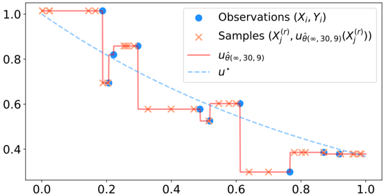<details> <summary>Image 4 Details</summary>  ### Visual Description ## Chart: Regression Analysis with Observations and Samples ### Overview The image presents a chart illustrating a regression analysis, comparing observed data points with samples generated from a model. The chart displays two data series: observed values (blue circles) and sampled values (red crosses), alongside a model function (dashed blue line) and a step function (solid red line). The x-axis ranges from 0.0 to 1.0, and the y-axis ranges from 0.3 to 1.0. ### Components/Axes * **X-axis:** Labeled implicitly as the independent variable, ranging from approximately 0.0 to 1.0 with markers at 0.0, 0.2, 0.4, 0.6, 0.8, and 1.0. * **Y-axis:** Labeled implicitly as the dependent variable, ranging from approximately 0.3 to 1.0 with markers at 0.4, 0.6, 0.8, and 1.0. * **Legend:** Located in the top-right corner. * "Observations (Xi, Yi)" - Represented by blue circles. * "Samples (X'i(r), uθ(∞, 30, 9)(X'i(r)))" - Represented by red crosses. * "uθ(∞, 30, 9)" - Represented by a solid red line. * "u*" - Represented by a dashed blue line. ### Detailed Analysis * **Observations (Blue Circles):** The observed data points are sparsely distributed. * (0.0, ~1.0) * (0.2, ~0.75) * (0.4, ~0.8) * (0.6, ~0.5) * (0.8, ~0.35) * (1.0, ~0.4) The line connecting these points is not explicitly shown, but they appear to follow a generally decreasing trend. * **Samples (Red Crosses):** The sampled data points are more densely distributed than the observations. * (0.0, ~1.0) * (0.05, ~1.0) * (0.1, ~0.9) * (0.2, ~0.85) * (0.3, ~0.7) * (0.4, ~0.6) * (0.5, ~0.55) * (0.6, ~0.35) * (0.7, ~0.3) * (0.8, ~0.35) * (0.9, ~0.4) * (1.0, ~0.4) The samples exhibit a step-like pattern, particularly between x = 0.2 and x = 0.6, where the value drops significantly. * **uθ(∞, 30, 9) (Solid Red Line):** This line represents a step function that closely follows the trend of the sampled data. * The function remains at approximately 1.0 until x = 0.2, then drops to approximately 0.7. * It remains at approximately 0.7 until x = 0.4, then drops to approximately 0.6. * It remains at approximately 0.6 until x = 0.6, then drops to approximately 0.35. * It remains at approximately 0.35 until x = 0.8, then rises to approximately 0.4. * **u* (Dashed Blue Line):** This line represents a linear model. * It starts at approximately 1.0 at x = 0.0. * It ends at approximately 0.4 at x = 1.0. * The line has a negative slope, indicating a decreasing relationship between x and y. ### Key Observations * The sampled data (red crosses) and the step function (solid red line) closely align, suggesting the step function is a good representation of the sampling process. * The observed data (blue circles) deviates from both the sampled data and the linear model (dashed blue line). * The step function exhibits abrupt changes in value, while the linear model provides a smoother, continuous representation. * The linear model appears to underestimate the values of the observed data at lower x-values and overestimate at higher x-values. ### Interpretation The chart demonstrates a comparison between a theoretical model (represented by the dashed blue line and the step function) and real-world observations (blue circles). The step function, `uθ(∞, 30, 9)`, appears to be a more accurate representation of the underlying process generating the samples than the linear model `u*`. The discrepancy between the observed data and both models suggests that the model may be incomplete or that other factors are influencing the observed values. The parameters (∞, 30, 9) within the step function likely represent specific settings or characteristics of the model, but their exact meaning is not provided in the image. The chart highlights the importance of validating models with real-world data and the potential need for more complex models to capture the nuances of observed phenomena. The abrupt changes in the step function could indicate threshold effects or discrete transitions in the underlying process. </details> u /star is estimated by minimizing over the space NN H ( D ) the empirical risk function $$R _ { n , n _ { r } } ( u _ { \theta } ) = \frac { \lambda _ { d } } { n } \sum _ { i = 1 } ^ { n } | u _ { \theta } ( X _ { i } ) - Y _ { i } | ^ { 2 } + \frac { 1 } { n _ { r } } \sum _ { \ell = 1 } ^ { n _ { r } } \mathcal { F } ( u _ { \theta } , X _ { \ell } ^ { ( r ) } ) ^ { 2 } .$$ /negationslash Proposition 2.3.1 (Overfitting) . Consider the dynamics with friction model (2.3) , and assume that there are two observations such that Y i = Y j . Then, whenever D ⩾ n -1 , for any integer n r , for all X ( r ) 1 , . . . , X ( r ) n r , there exists a minimizing sequence ( u ˆ θ ( p,n r ,D ) ) p ∈ N ∈ NN H ( D ) N such that lim p →∞ R n,n r ( u ˆ θ ( p,n r ,D ) ) = 0 but lim p →∞ R n ( u ˆ θ ( p,n r ,D ) ) = ∞ . So, this PINN estimator is not consistent. Proposition 2.3.1 illustrates how fitting a PINN by minimizing the empirical risk alone can lead to a catastrophic situation, where the empirical risk of the minimizing sequence is (close to) zero, while its theoretical risk is infinite. This phenomenon is explained by the existence of piecewise constant functions interpolating the observations X 1 , . . . , X n , whose derivatives are null at the points X ( r ) 1 , . . . , X ( r ) n r , but diverge between these points (see Figure 2.1). These functions correspond to neural networks u θ such that ‖ θ ‖ 2 →∞ . PDE solver: The heat propagation case Consider the heat propagation differential operator defined on the domain Ω =] -1 , 1[ × ]0 , T [ (with closure ¯ Ω = [ -1 , 1] × [0 , T ] ) by $$\forall u \in C ^ { 2 } ( \bar { \Omega } , \mathbb { R } ) , \, \forall x \in \Omega , \quad \mathcal { F } ( u , x ) = \partial _ { t } u ( x ) - \partial _ { x , x } ^ { 2 } u ( x ) , \quad ( 2 . 4 )$$ associated with the boundary conditions $$\forall t \in [ 0 , T ] , \quad u ( - 1 , t ) = u ( 1 , t ) = 0 ,$$ and the initial condition defined, for all x ∈ [ -1 , 1] , by $$u ( x , 0 ) = \tanh ^ { \circ H } ( x + 0 . 5 ) - \tanh ^ { \circ H } ( x - 0 . 5 ) + \tanh ^ { \circ H } ( 0 . 5 ) - \tanh ^ { \circ H } ( 1 . 5 ) .$$ The notation tanh ◦ k stands for the function recursively defined by tanh ◦ 1 = tanh and tanh ◦ ( k +1) = tanh ◦ tanh ◦ k . The unique solution u /star of the PDE is shown in Figure 2.2 (right). It models the time evolution of the temperature of a wire, whose extremities at x = -1 and x = 1 are maintained at zero temperature. Note that the initial condition corresponds to a bell-shaped function, which belongs to NN H (2) . However, the setting can be extended to Fig. 2.2.: Inconsistent PINN (left) compared to the solution u /star of the PDE (right) for the heat propagation case. 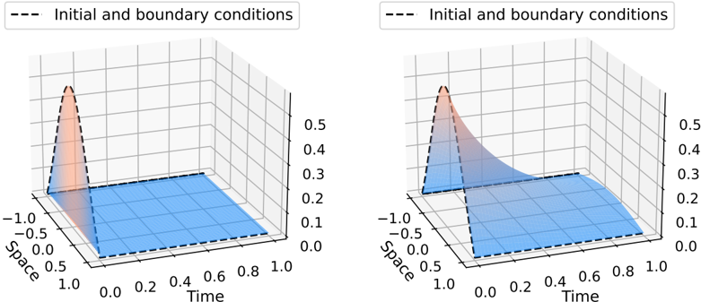<details> <summary>Image 5 Details</summary>  ### Visual Description \n ## 3D Surface Plots: Initial and Boundary Conditions ### Overview The image presents two 3D surface plots, likely representing the evolution of a function over time and space. Both plots share a similar structure and visual characteristics, suggesting they depict different stages or conditions of the same underlying phenomenon. The plots visualize a function of two variables, "Time" and "Space", with the surface height representing the function's value. ### Components/Axes Both plots share the following components: * **X-axis:** Labeled "Time", ranging from approximately 0.0 to 1.0. * **Y-axis:** Labeled "Space", ranging from approximately -1.0 to 1.0. * **Z-axis:** Implied, representing the function's value, ranging from approximately 0.0 to 0.5. * **Surface 1 (Orange/Red):** A triangular shaped surface, peaking at Time = 0.0 and Space = 0.0. The color transitions from orange to red. * **Surface 2 (Blue):** A rectangular surface, positioned towards the right of the plot, extending from Time = approximately 0.4 to 1.0 and Space = approximately -1.0 to 1.0. The color is a shade of blue. * **Title:** "--- Initial and boundary conditions ---" positioned at the top of each plot. * **Grid:** A visible grid is present on the base plane of each plot, aiding in visualization. ### Detailed Analysis or Content Details **Plot 1 (Left):** * The orange/red surface is sharply peaked at Time = 0.0 and Space = 0.0, with a value of approximately 0.5. * The blue surface is relatively small, starting at Time = approximately 0.4 and extending to Time = 1.0. Its height is approximately 0.1 to 0.2. * The transition between the orange/red and blue surfaces appears abrupt. **Plot 2 (Right):** * The orange/red surface is similar to Plot 1, peaking at Time = 0.0 and Space = 0.0, with a value of approximately 0.5. * The blue surface is larger than in Plot 1, starting at Time = approximately 0.2 and extending to Time = 1.0. Its height is approximately 0.2 to 0.3. * The transition between the orange/red and blue surfaces appears smoother than in Plot 1. ### Key Observations * Both plots show an initial peak (orange/red surface) followed by the emergence of a rectangular region (blue surface). * The blue surface grows in size over time, as evidenced by the comparison between Plot 1 and Plot 2. * The shape of the orange/red surface remains consistent between the two plots. * The transition between the two surfaces changes from abrupt (Plot 1) to smoother (Plot 2). ### Interpretation The plots likely represent the propagation of a wave or disturbance over time and space. The initial peak (orange/red) could represent the initial condition or source of the disturbance. The blue surface could represent the wave as it propagates and spreads out over time. The difference between the two plots suggests a change in the system's behavior over time. The smoother transition in Plot 2 could indicate that the wave is becoming more stable or that the system is reaching a steady state. The growth of the blue surface indicates that the wave is expanding and covering a larger area. The "Initial and boundary conditions" title suggests that these plots are the result of a simulation or model that is initialized with specific conditions. The plots could be used to visualize the evolution of the system under these conditions. The plots do not provide specific numerical data beyond the axis ranges, but they offer a qualitative understanding of the system's behavior. Further analysis would require access to the underlying data or model. </details> arbitrary initial conditions that take the form of a neural network function, given the boundary condition u ( ∂ Ω × [0 , T ]) = { 0 } . To solve the PDE (2.4), we use n e i.i.d. samples X ( e ) 1 , . . . , X ( e ) n e on E = ([ -1 , 1] × { 0 } ) ∪ ( {-1 , 1 } × [0 , T ]) , distributed according to µ E , together with n r i.i.d. samples X ( r ) 1 , . . . , X ( r ) n r , uniformly distributed on Ω . Let ( ˆ θ ( p, n e , n r , D )) p ∈ N be a sequence of parameters minimizing the empirical risk function $$R _ { n _ { e } , n _ { r } } ( u _ { \theta } ) = \frac { \lambda _ { e } } { n _ { e } } \sum _ { j = 1 } ^ { n _ { e } } | u _ { \theta } ( X _ { j } ^ { ( e ) } ) - h ( X _ { j } ^ { ( e ) } ) | ^ { 2 } + \frac { 1 } { n _ { r } } \sum _ { \ell = 1 } ^ { n _ { r } } \mathcal { F } ( u _ { \theta } , X _ { \ell } ^ { ( r ) } ) ^ { 2 } ,$$ over the space NN H ( D ) . The theoretical counterpart of this empirical risk is $$\mathcal { R } ( u ) = \lambda _ { e } \mathbb { E } | u ( X ^ { ( e ) } ) - h ( X ^ { ( e ) } ) | ^ { 2 } + \frac { 1 } { | \Omega | } \int _ { \Omega } \mathcal { F } ( u , x ) ^ { 2 } d x .$$ Proposition 2.3.2 (PDE solver overfitting) . Consider the heat propagation model (2.4) . Then, whenever D ⩾ 4 , for any pair ( n e , n r ) , for all X ( e ) 1 , . . . , X ( e ) n e and for all X ( r ) 1 , . . . , X ( r ) n r , there exists a minimizing sequence ( u ˆ θ ( p,n e ,n r ,D ) ) p ∈ N ∈ NN H ( D ) N such that lim p →∞ R n e ,n r ( u ˆ θ ( p,n e ,n r ,D ) ) = 0 but lim p →∞ R ( u ˆ θ ( p,n e ,n r ,D ) ) = ∞ . So, this PINN estimator is not consistent. Figure 2.2 (left) shows an example of an inconsistent PINN estimator. Such an estimator corresponds to a function that equals zero on Ω (and thus satisfies the linear PDE), while satisfying the initial condition on ∂ Ω . This function corresponds to a limit of neural networks u θ such that ‖ θ ‖ 2 →∞ . The proof strategy of Propositions 2.3.1 and 2.3.2 does not depend on the geometry of the points X ( r ) and the points X ( e ) , which could therefore be sampled along a grid, or by any quasi Monte Carlo method. We emphasize that the two negative examples of Propositions 2.3.1 and 2.3.2 are no exceptions. In fact, their proofs can be easily generalized to differential operators F such that the following property holds: for all x ∈ Ω , for all u ∈ C ∞ (Ω , R d 2 ) , if ∇ u vanishes on an open set containing x , then F ( u, x ) = 0 . This property is satisfied in the case of motion with friction, advection, heat, wave propagation, Schrödinger, Maxwell and Navier-Stokes equations, which are so as many cases that will suffer from overfitting. ## 2.4 Consistency of regularized PINNs for linear and nonlinear PDE systems Training PINNs can be tricky because it can lead to the type of pathological situations highlighted in Section 2.3. To avoid such an overfitting behavior, a standard approach in machine learning is to resort to ridge regularization, where the empirical risk to be minimized is penalized by the L 2 norm of the parameters θ . This technique has been shown to improve not only the optimization convergence during the training phase, but also the generalization ability of the resulting predictor [KH91; Guo+17]. Ridge regularization is available in most deep learning libraries (e.g., pytorch or keras ), where it is implemented using the so-called weight decay [LH19]. Interestingly, the ridge regularization of a slight modification of PINNs, using adaptive activation functions, has been studied in Jagtap et al. [JKK20], which shows that gradient descent algorithms manage to generate an effective minimizing sequence of the penalized empirical risk. In this section, we formalize ridge PINNs and study their risk-consistency. Definition 2.4.1 (Ridge PINNs) . The ridge risk function is defined by $$R _ { n , n _ { e } , n _ { r } } ^ { ( r i d g e ) } ( u _ { \theta } ) = R _ { n , n _ { e } , n _ { r } } ( u _ { \theta } ) + \lambda _ { ( r i d g e ) } \| \theta \| _ { 2 } ^ { 2 } ,$$ where λ (ridge) > 0 is the ridge hyperparameter. We denote by ( ˆ θ (ridge) ( p,n e ,n r ,D ) ) p ∈ N a minimizing sequence of this risk, i.e., $$\lim _ { p \to \infty } R _ { n , n _ { e } , n _ { r } } ^ { ( r i d g e ) } ( u _ { \hat { \theta } _ { ( p , n _ { e } , n _ { r } , D ) } ^ { ( r i d g e ) } } ) = \inf _ { \theta \in \Theta } R _ { n , n _ { e } , n _ { r } } ^ { ( r i d g e ) } ( u _ { \theta } ) .$$ Our next Proposition 2.4.2 states that the L 2 norm of the parameters θ bounds the Hölder norm of the neural network u θ . This result is interesting in itself because it establishes a connection between the L 2 norm of a fully connected neural network and its regularity. (Note that, by equivalence of the norms, this result also holds if the ridge penalty is replaced by ‖ θ ‖ p p .) In the present paper it plays a key role in the risk-consistency analysis. Proposition 2.4.2 (Bounding the norm of a neural network by the norm of its parameter) . Consider the class NN H ( D ) = { u θ , θ ∈ Θ H,D } . Let K ∈ N . Then there exists a constant C K,H > 0 , depending only on K and H , such that, for all θ ∈ Θ H,D , $$\| u _ { \theta } \| _ { C ^ { K } ( \mathbb { R } ^ { d _ { 1 } } ) } \leqslant C _ { K , H } ( D + 1 ) ^ { H K + 1 } ( 1 + \| \theta \| _ { 2 } ) ^ { H K } \| \theta \| _ { 2 } .$$ Moreover, this bound is tight with respect to ‖ θ ‖ 2 , in the sense that, for all H,D ⩾ 1 and all K ∈ N , there exists a sequence ( θ p ) p ∈ N ∈ NN H ( D ) and a constant ¯ C K,H > 0 such that ( i ) lim p →∞ ‖ θ p ‖ 2 = ∞ and ( ii ) ‖ u θ p ‖ C K ( R d 1 ) ⩾ ¯ C K,H ‖ θ p ‖ HK +1 2 . In order to study the generalization capabilities of regularized PINNs, we need to restrict the PDEs to a class of smooth differential operators, which we call polynomial operators (Definition 2.4.4 below). This class includes the most common PDE systems, as shown in the following example with the Navier-Stokes equations. Example 2.4.3 (Navier-Stokes equations) . Let Ω = Ω 1 × ]0 , T [ , where Ω 1 ⊆ R 3 is a bounded Lipschitz domain and T ⩾ 0 is a finite time horizon. The incompressible Navier-Stokes system of equations is defined for all u = ( u x , u y , u z , p ) ∈ C 2 ( ¯ Ω , R 4 ) and for all x = ( x, y, z, t ) ∈ Ω , by $$\begin{array} { r l r } { \left \{ \begin{array} { c c } { \mathcal { F } _ { 1 } ( u , x ) } & { = } & { \partial _ { t } u _ { x } - ( u _ { x } \partial _ { x } + u _ { y } \partial _ { y } + u _ { z } \partial _ { z } ) u _ { x } - \eta ( \partial _ { x , x } ^ { 2 } + \partial _ { y , y } ^ { 2 } + \partial _ { z , z } ^ { 2 } ) u _ { x } + \rho ^ { - 1 } \partial _ { x } p } \\ { \mathcal { F } _ { 2 } ( u , x ) } & { = } & { \partial _ { t } u _ { y } - ( u _ { x } \partial _ { x } + u _ { y } \partial _ { y } + u _ { z } \partial _ { z } ) u _ { y } - \eta ( \partial _ { x , x } ^ { 2 } + \partial _ { y , y } ^ { 2 } + \partial _ { z , z } ^ { 2 } ) u _ { y } + \rho ^ { - 1 } \partial _ { y } p } \\ { \mathcal { F } _ { 3 } ( u , x ) } & { = } & { \partial _ { t } u _ { z } - ( u _ { x } \partial _ { x } + u _ { y } \partial _ { y } + u _ { z } \partial _ { z } ) u _ { z } - \eta ( \partial _ { x , x } ^ { 2 } + \partial _ { y , y } ^ { 2 } + \partial _ { z , z } ^ { 2 } ) u _ { z } + \rho ^ { - 1 } \partial _ { z } p + g ( x ) } \\ { \mathcal { F } _ { 4 } ( u , x ) } & { = } & { \partial _ { x } u _ { x } + \partial _ { y } u _ { y } + \partial _ { z } u _ { z } , } \end{array} } \end{array}$$ where η, ρ > 0 and g ∈ C ∞ ( ¯ Ω , R ) . Observe that F 1 , F 2 , F 3 , and F 4 are polynomials in u and its derivatives, with coefficients in C ∞ ( ¯ Ω , R ) . For example, F 3 ( u, x ) = P 3 ( u x , u y , u z , ∂ x u z , ∂ y u z , ∂ z u z , ∂ t u z , ∂ 2 x,x u z , ∂ 2 y,y u z , ∂ 2 z,z u z , ∂ z p )( x ) , where the polynomial P 3 ∈ C ∞ ( ¯ Ω , R )[ Z 1 , . . . , Z 11 ] is defined by P 3 ( Z 1 , . . . , Z 11 ) = Z 7 -Z 1 Z 4 -Z 2 Z 5 -Z 3 Z 6 -η ( Z 8 + Z 9 + Z 10 ) + ρ -1 Z 11 + g . The above example can be generalized with the following definition. Definition 2.4.4 (Polynomial operator) . An operator F : C K ( ¯ Ω , R d 2 ) × Ω → R is a polynomial operator of order K ∈ N if there exists an integer s ∈ N and multi-indexes ( α i,j ) 1 ⩽ i ⩽ d 2 , 1 ⩽ j ⩽ s ∈ ( N d 1 ) sd 2 such that $$\forall u = ( u _ { 1 } , \dots , u _ { d _ { 2 } } ) \in C ^ { K } ( \bar { \Omega } , \mathbb { R } ^ { d _ { 2 } } ) , \quad \mathcal { F } ( u , \cdot ) = P ( ( \partial ^ { \alpha _ { i , j } } u _ { i } ) _ { 1 \leqslant i \leqslant d _ { 2 } , 1 \leqslant j \leqslant s } ) ,$$ where P ∈ C ∞ ( ¯ Ω , R )[ Z 1 , 1 , . . . , Z d 2 ,s ] is a polynomial with smooth coefficients. In other words, F is a polynomial operator if it is of the form $$\mathcal { F } ( u , x ) = \sum _ { k = 1 } ^ { N ( P ) } \phi _ { k } \times \prod _ { i = 1 } ^ { d _ { 2 } } \prod _ { j = 1 } ^ { s } ( \partial ^ { \alpha _ { i , j } } u _ { i } ( x ) ) ^ { I ( i , j , k ) } ,$$ where N ( P ) ∈ N /star , φ k ∈ C ∞ ( ¯ Ω , R ) , and I ( i, j, k ) ∈ N . The associated polynomial is P ( Z 1 , 1 , . . . , Z d 2 ,s ) = ∑ N ( P ) k =1 φ k × ∏ d 2 i =1 ∏ s j =1 Z I ( i,j,k ) i,j (recall that ∂ α u i = u i when α = 0 ). Definition 2.4.5 (Degree) . The degree of the polynomial operator F is $$\deg ( \mathcal { F } ) = \max _ { 1 \leqslant k \leqslant N ( P ) } \sum _ { i = 1 } ^ { d _ { 2 } } \sum _ { j = 1 } ^ { s } ( 1 + | \alpha _ { i , j } | ) I ( i , j , k ) .$$ As an illustration, in Example 2.4.3, one has deg( F 3 ) = 3 , and this degree is reached in both the terms u z ∂ z u z and ∂ 2 z,z u z . Note that deg( P 3 ) = 2 but deg( F 3 ) = 3 . To compute deg( F 3 ) , we first count the number of terms in each monomial ( u z ∂ z u z has two terms while ∂ 2 z,z u z has one term), which is ∑ d 2 i =1 ∑ s j =1 I ( i, j, k ) for the k th monomial, and add the number of derivatives involved in the product ( u z ∂ z u z contains a single ∂ z operator while ∂ 2 z,z u z contains two derivatives in ∂ z ), which corresponds to ∑ d 2 i =1 ∑ s j =1 | α i,j | I ( i, j, k ) for the k th monomial. Thus, for each monomial k , the total sum is ∑ d 2 i =1 ∑ s j =1 (1 + | α i,j | ) I ( i, j, k ) . We emphasize that this class includes a large number of PDEs, such as linear PDEs (e.g., advection, heat, and Maxwell equations), as well as some nonlinear PDEs (e.g., Blasius, Burger's, and Navier-Stokes equations). Proposition 2.4.2 is a key ingredient to uniformly bound the risk of PINNs involving polynomial PDE operators [see DBB24b, Supplementary Material, Section 5]. This in turn can be used to establish the risk-consistency of these PINNs when n e and n r tend to ∞ , as follows. Theorem 2.4.6 (Risk-consistency of ridge PINNs) . Consider the ridge PINN problem (2.5) , over the class NN H ( D ) = { u θ , θ ∈ Θ H,D } , where H ⩾ 2 . Assume that the condition function h is Lipschitz and that F 1 , . . . , F M are polynomial operators. Assume, in addition, that the ridge parameter is of the form $$\lambda _ { ( r i d g e ) } = \min ( n _ { e } , n _ { r } ) ^ { - \kappa } , \quad w h e r e \quad \kappa = \frac { 1 } { 1 2 + 4 H ( 1 + ( 2 + H ) \max _ { k } \deg ( \mathcal { F } _ { k } ) ) } .$$ Then, almost surely, $$\lim _ { n _ { e } , n _ { r } \to \infty } \lim _ { p \to \infty } \mathcal { R } _ { n } ( u _ { \hat { \theta } ^ { ( r i d g e ) } ( p , n _ { e } , n _ { r } , D ) } ) = \inf _ { u \in N N _ { H } ( D ) } \mathcal { R } _ { n } ( u ) .$$ Thus, minimizing the ridge empirical risk (2.5) over Θ H,D amounts to minimizing the theoretical risk (2.2) over Θ H,D in the asymptotic regime n e , n r →∞ . This fundamental result is complemented by the following one, which resorts to another asymptotics in the width D . This ensures that the choice of the neural architecture NN H ⊆ C ∞ ( ¯ Ω , R d 2 ) does not introduce any asymptotic bias. Theorem 2.4.7 (The ridge PINN is asymptotically unbiased) . Under the same assumptions as in Theorem 2.4.6, one has, almost surely, $$\lim _ { D \to \infty } \lim _ { n _ { e } , n _ { r } \to \infty } \lim _ { p \to \infty } \mathcal { R } _ { n } ( u _ { \hat { \theta } ^ { ( r i d g e ) } ( p , n _ { e } , n _ { r } , D ) } ) = \inf _ { u \in C ^ { \infty } ( \bar { \Omega } , \mathbb { R } ^ { d _ { 2 } } ) } \mathcal { R } _ { n } ( u ) .$$ In other words, minimizing the ridge empirical risk over Θ H,D and letting D,n e , n r → ∞ amounts to minimizing the theoretical risk (2.2) over the entire class C ∞ ( ¯ Ω , R d 2 ) . We emphasize that these two theorems hold independently of the values of the hyperparameters λ d , λ e ⩾ 0 . Therefore, our results cover the general hybrid modeling framework (2.1), which includes the PDE solver. To the best of our knowledge, these are the first results that provide theoretical guarantees for PINNs regularized with a standard penalty. They complement the state-of-the-art approaches of Shin [Shi20], Shin et al. [SZK23], Mishra and Molinaro [MM23], and Wu et al. [Wu+23], which consider regularization strategies that are unfortunately not feasible in practice. It is worth noting that Theorem 2.4.7 still holds by choosing D as a function of n e and n r . In fact, an easy modification of the proofs reveals that one can take D ( n e , n r ) = min( n e , n r ) ξ , where ξ is a constant depending only on H and max k deg( F k ) . Thus, in this setting, $$\lim _ { n _ { e } , n _ { r } \to \infty } \lim _ { p \to \infty } \mathcal { R } _ { n } ( u _ { \hat { \theta } ^ { ( r i d g e ) } ( p , n _ { e } , n _ { r } , D ( n _ { e } , n _ { r } ) } ) = \inf _ { u \in C ^ { \infty } ( \bar { \Omega } , \mathbb { R } ^ { d _ { 2 } } ) } \mathcal { R } _ { n } ( u ) .$$ Remark 2.4.8 (Dirichlet boundary conditions) . Theorems 2.4.6 and 2.4.7 can be easily adapted to PINNs with Neumann conditions instead of Dirichlet boundary conditions. This is achieved by substituting the term n -1 e ∑ n e j =1 ‖ u θ ( X ( e ) j ) -h ( X ( e ) j ) ‖ 2 2 in (2.1) by n -1 e ∑ n e j =1 ‖ ∂ - → n u θ ( X ( e ) j ) ‖ 2 2 , where - → n is the normal to ∂ Ω . Practical considerations The decay rate of λ (ridge) = min( n e , n r ) -κ does not depend on the dimension d 1 of Ω . This is consistent with the results of Karniadakis et al. [Kar+21] and De Ryck and Mishra [DM22], which suggest that PINNs can overcome the curse of dimensionality, opening up interesting perspectives for efficient solvers of high-dimensional PDEs. We also emphasize that λ (ridge) depends only on the degree of the polynomial PDE operator, the depth H , and the sample sizes n e and n r . All these quantities are known, which makes this hyperparameter immediately useful for practical applications. For example, in Navier-Stokes equations of Example 2.4.3, one has max k deg( F k ) = 3 . Thus, for a neural network of depth, say H = 2 , the ridge hyperparameter λ (ridge) = min( n e , n r ) -1 / 116 is sufficient to ensure consistency. It is also interesting to note that the bound on λ (ridge) in the theorems deteriorates with increasing depth H . This confirms the preferential use of shallow neural networks in the experimental works of Arzani et al. [AWD21], Karniadakis et al. [Kar+21], and Xu et al. [Xu+21]. The bound also deteriorates as max k deg F k increases. This is in line with the empirical results of Davini et al. [Dav+21], which was able to improve the performance of PINNs by reformulating their polynomial differential equation of degree 3 as a system of two polynomial differential equations of degree 2 . It is also interesting to note that Theorems 2.4.6 and 2.4.7 hold for any ridge hyperparameter λ (ridge) ⩾ min( n e , n r ) -κ such that lim n e ,n r →∞ λ (ridge) = 0 . However, if n e and n r are fixed, choosing too large a λ (ridge) will lead to a bias toward parameters of Θ H,D with a low L 2 norm. Therefore, there is a trade-off between taking λ (ridge) as small as possible to reduce this bias, but large enough to avoid overfitting, as illustrated in Section 2.3. Moreover, our choice of λ (ridge) may be suboptimal, since these results rely on inequalities involving a general class of polynomial operators. When studying a particular PDE, the consistency results of Theorems 2.4.6 and 2.4.7 should eventually hold with a smaller λ (ridge) . To tune λ (ridge) in practice, one could, for example, monitor the overfitting gap OG n,n e ,n r = | R n,n e ,n r -R n | for a ridge estimator ˆ θ (ridge) ( p, n e , n r , D ) , by standard validation strategy (e.g., by sampling ˜ n r and ˜ n e new points to estimate R n ( u ˆ θ (ridge) ( p,n e ,n r ,D ) ) at a min(˜ n r , ˜ n e ) -1 / 2 -rate given by the central limit theorem), and then choose the smallest parameter λ (ridge) to introduce as little bias as possible. More information about the relevance of OG n,n e ,n r is given in Doumèche et al. [DBB24b, Supplementary Material, Section 2]. ## 2.5 Strong convergence of PINNs for linear PDE systems Beyond risk-consistency concerns, the ultimate goal of PINNs is to learn a physics-informed regression function u /star , or, in the PDE solver setting, to strongly approximate the unique solution u /star of a PDE system. Thus, what we want is to have guarantees regarding the convergence of u ˆ θ (ridge) ( p,n e ,n r ,D ) to u /star for an adapted norm. This requirement is called strong convergence in the functional analysis literature. This is however not guaranteed under the sole convergence of the theoretical risk ( R n ( u ˆ θ (ridge) ( p,n e ,n r ,D ) )) p,n e ,n r ,D ∈ N , as shown in the following two examples. Example 2.5.1 (Lack of data incorporation in the hybrid modeling setting) . Suppose M = 1 , d 1 = 2 , d 2 = 1 , Ω =]0 , 1[ × ]0 , T [ , h ( x, 0) = 1 and h (0 , t ) = 1 , and let F ( u, x ) = ∂ x u ( x )+ ∂ t u ( x ) . This corresponds to the assumption that the solution should approximately follow the advection equation and that it should be close to 1 . For any δ > 0 , let the sequence ( u δ,p ) p ∈ N ∈ NN H (2 n ) N be defined by $$u _ { \delta , p } ( x , t ) = 1 + \sum _ { i = 1 } ^ { n } \frac { Y _ { i } } { 2 } \left ( \tanh _ { p } ^ { \circ H } ( x - t - x _ { i } + t _ { i } + \delta ) - \tanh _ { p } ^ { \circ H } ( x - t - x _ { i } + t _ { i } - \delta ) \right ) ,$$ /negationslash where tanh p := tanh( p · ) , and X i = ( x i , t i ) . Then, as soon as δ ⩽ 1 2 min i = j | x i -x j + t j -t i | , we have that lim p →∞ R n ( u δ,p ) = 0 . Thus, as long as D ≥ 2 n , inf u ∈ NN H ( D ) R n ( u ) = 0 . Therefore, Theorem 2.4.7 shows that lim D →∞ lim n e ,n r →∞ lim p →∞ R n ( u ˆ θ (ridge) ( p,n e ,n r ,D ) ) = 0 . It is then easy to check that this implies that u ˆ θ (ridge) ( p,n e ,n r ,D ) converges in L 2 (Ω) to 1 , independently of n and the function u /star . This shows that the ridge PINNs fails to learn u /star whenever the model is inexact. In the PDE solver setting, one can consider the a priori favorable case where the PDE system admits a unique (strong) solution u /star in C K ( ¯ Ω , R d 2 ) (where K is the maximum order of the differential operators F 1 , . . . , F M ). Note that u /star is the unique minimizer of R over C K ( ¯ Ω , R d 2 ) , with R ( u /star ) = 0 (and R ( u ) = 0 if and only if u satisfies the initial conditions, the boundary conditions, and the system of differential equations). However, we describe below a situation where a minimizing sequence of R does not converge to the unique strong solution u /star of the PDE in question. Example 2.5.2 (Divergence in the PDE solver setting) . Suppose M = 1 , d 1 = d 2 = 1 , Ω =] -1 , 1[ , h (1) = 1 , λ e > 0 , and let the polynomial operator be F ( u, x ) = x u ′ ( x ) . Clearly, u /star ( x ) = 1 is the only strong solution of the PDE x u ′ ( x ) = 0 with u (1) = 1 . Let the sequence ( u p ) p ∈ N ∈ NN H ( D ) N be defined by u p = tanh p ◦ tanh ◦ ( H -1) . According to Doumèche et al. [DBB24b, Supplementary Material, Section 2], lim p →∞ R ( u p ) = R ( u /star ) = 0 . However, the minimizing sequence ( u p ) p ∈ N does not converge to u /star , since u ∞ ( x ) := lim p →∞ u p ( x ) = 1 x > 0 -1 x < 0 . We have therefore exhibited a sequence ( u p ) p ∈ N of neural networks that minimizes R and such that ( u p ) p ∈ N converges pointwise. However, its limit u ∞ is not the unique strong solution of the PDE. In fact, u ∞ is not differentiable at 0 , which is incompatible with the differential operators F used in R ( u ∞ ) . Interestingly, the Cauchy-Schwarz inequality states that the pathological sequence ( u p ) p ∈ N satisfies lim p →∞ ‖ u ′ p ‖ 2 L 2 (Ω) = ∞ , as in Example 2.5.1. ## Sobolev regularization The examples above illustrate how the convergence of the theoretical risk R n ( u ˆ θ (ridge) ( p,n e ,n r ,D ) ) to inf u ∈ C ∞ ( ¯ Ω , R d 2 ) R n ( u ) (for any n ) is not sufficient to guarantee the strong convergence to a PDE or hybrid modeling solution. To ensure such a convergence, a different analysis is needed, mobilizing tools from functional analysis. In the sequel, we build upon the regression estimation penalized by PDEs of Azzimonti et al. [Azz+15], Sangalli [San21], Arnone et al. [Arn+22], and Ferraccioli et al. [FSF22], and make use of the calculus of variations [e.g., Eva10, Theorems 1-4, Chapter 8]. In the former references, the minimizer of R n does not satisfy the PDE system injected in the PINN penalty, but another PDE system, known as the Euler-Lagrange equations. Although interesting, the mathematical framework is different from ours. First, the authors do not study the convergence of neural networks, but rather methods in which the boundary conditions are hard-coded, such as the finite element method. Second, these frameworks are limited to special cases of theoretical risks. Indeed, only second-order PDEs with λ e = ∞ are considered in Azzimonti et al. [Azz+15], while Evans [Eva10] deal with first-order PDEs, echoing the case of λ d = 0 and λ e = ∞ . It is worthwhile mentioning that the results of Azzimonti et al. [Azz+15] rely on an important property of the theoretical risk function R n , called coercivity . This is a common assumption of the calculus of variations [Eva10]. The operator R n is said to be coercive if there exist K ∈ N and λ t > 0 such that, for all u ∈ H K (Ω , R d 2 ) , R n ( u ) ⩾ λ t ‖ u ‖ 2 H K (Ω) (the notation H K (Ω , R d 2 ) stands for the usual Sobolev space of order K -see the Appendix. It turns out that the failures of Examples 2.5.1 and 2.5.2 are due to a lack of coercivity, since, in both cases, lim p →∞ ‖ u p ‖ H 1 (Ω) = ∞ but lim p →∞ R n ( u p ) ⩽ R n ( u /star ) . There are two ways to correct this problem: either one can restrict the study to coercive operators only, or one can resort to an explicit regularization of the risk to enforce its coercivity. We choose the latter, since most PDEs used in the practice of PINNs are not coercive. Note however that our results could be easily adapted to the coercive case. In the following, we restrict ourselves to affine operators, which exactly correspond to linear PDE systems, including the advection, heat, wave, and Maxwell equations. Definition 2.5.3 (Affine operator) . The operator F is affine of order K if there exists A α ∈ C ∞ ( ¯ Ω , R d 2 ) and B ∈ C ∞ ( ¯ Ω , R ) such that, for all x ∈ Ω and all u ∈ H K (Ω , R d 2 ) , $$\mathcal { F } ( u , x ) = \mathcal { F } ^ { ( l i n ) } ( u , x ) + B ( x ) ,$$ where F (lin) ( u, x ) = ∑ | α | ⩽ K 〈 A α ( x ) , ∂ α u ( x ) 〉 is linear . The source term B is important, as it makes it possible to model a large variety of applied physical problems, as illustrated in Song et al. [SAW21]. Note also that affine operators of order K are in fact polynomial operators of degree K +1 (Definitions 2.4.4 and 2.4.5) that are extended from smooth functions to the whole Sobolev space H K (Ω , R d 2 ) . Definition 2.5.4 (Regularized PINNs) . The regularized theoretical risk function is $$\mathcal { R } _ { n } ^ { ( r e g ) } ( u ) = \mathcal { R } _ { n } ( u ) + \lambda _ { t } \| u \| _ { H ^ { m + 1 } ( \Omega ) } ^ { 2 } ,$$ where R n is the original theoretical risk as defined in (2.2) , and m ∈ N . The corresponding regularized empirical risk function is $$R _ { n , n _ { e } , n _ { r } } ^ { ( r e g ) } ( u _ { \theta } ) = R _ { n , n _ { e } , n _ { r } } ( u _ { \theta } ) + \lambda _ { ( r i d g e ) } \| \theta \| _ { 2 } ^ { 2 } + \frac { \lambda _ { t } } { n _ { \ell } } \sum _ { \ell = 1 } ^ { n _ { \ell } } \sum _ { | \alpha | \leqslant m + 1 } \| \partial ^ { \alpha } u _ { \theta } ( X _ { \ell } ^ { ( r ) } ) \| _ { 2 } ^ { 2 } .$$ It is noteworthy that R (reg) n,n e ,n r can be straightforwardly implemented in the usual PINN framework and benefit from the computational scalability of the backpropagation algorithm, by encoding the regularization as supplementary PDE-type constraints F α ( u, x ) = ∂ α u ( x ) = 0 . Since this discretized Sobolev penalty can be seen as additional physical priors F α , the overfitting behavior observed for the unregularized PINNs can be transferred to Sobolev-regularized PINNs trained without ridge regularization. This is why the ridge penalty is still included in the risk. Note also that the Sobolev regularization has been shown to avoid overfitting in machine learning, yet in different contexts [e.g., FS20]. The following proposition shows that the unique minimizer of (2.6) can be interpreted as the unique minimizer of an optimization problem involving a weak formulation of the differential terms included in the risk. Its proof is based on the Lax-Milgram theorem [e.g., Bre10, Corollary 5.8]. Proposition 2.5.5 (Characterization of the unique minimizer of R (reg) n ) . Assume that F 1 , . . . , F M are affine operators of order K . Assume, in addition, that λ t > 0 and m ⩾ max( /floorleft d 1 / 2 /floorright , K ) . Then the regularized theoretical risk R (reg) n has a unique minimizer ˆ u n over H m +1 (Ω , R d 2 ) . This minimizer ˆ u n is the unique element of H m +1 (Ω , R d 2 ) that satisfies $$\forall v \in H ^ { m + 1 } ( \Omega , \mathbb { R } ^ { d _ { 2 } } ) , \quad \mathcal { A } _ { n } ( \hat { u } _ { n } , v ) = \mathcal { B } _ { n } ( v ) ,$$ where $$\text {where} \quad & \mathcal { A } _ { n } ( \hat { u } _ { n } , v ) = \frac { \lambda _ { d } } { n } \sum _ { i = 1 } ^ { n } \langle \tilde { \Pi } ( \hat { u } _ { n } ) ( X _ { i } ) , \tilde { \Pi } ( v ) ( X _ { i } ) \rangle + \lambda _ { e } \mathbb { E } \langle \tilde { \Pi } ( \hat { u } _ { n } ) ( X ^ { ( e ) } ) , \tilde { \Pi } ( v ) ( X ^ { ( e ) } ) \rangle \\ & + \frac { 1 } { | \Omega | } \sum _ { k = 1 } ^ { M } \int _ { \Omega } \mathcal { F } _ { k } ^ { ( l i n ) } ( \hat { u } _ { n } , x ) \mathcal { F } _ { k } ^ { ( l i n ) } ( v , x ) d x \\ & + \frac { \lambda _ { t } } { | \Omega | } \sum _ { | \alpha | \leqslant m + 1 } \int _ { \Omega } \langle \partial ^ { \alpha } \hat { u } _ { n } ( x ) , \partial ^ { \alpha } v ( x ) \rangle d x , \\ & \mathcal { B } _ { n } ( v ) = \frac { \lambda _ { d } } { n } \sum _ { i = 1 } ^ { n } \langle Y _ { i } , \tilde { \Pi } ( v ) ( X _ { i } ) \rangle + \lambda _ { e } \mathbb { E } \langle \tilde { \Pi } ( v ) ( X ^ { ( e ) } ) , h ( X ^ { ( e ) } ) \rangle \\ & - \frac { 1 } { | \Omega | } \sum _ { k = 1 } ^ { M } \int _ { \Omega } B _ { k } ( x ) \mathcal { F } _ { k } ^ { ( l i n ) } ( v , x ) d x , \\$$ and where ˜ Π : H m +1 (Ω , R d 2 ) → C 0 (Ω , R d 2 ) is the so-called Sobolev embedding, such that ˜ Π( u ) is the unique continuous function that coincides with u almost everywhere. The Sobolev embedding ˜ Π is essential in order to give a precise meaning to the pointwise evaluation at the points X i of a function u ∈ H m +1 (Ω , R d 2 ) ⊆ L 2 (Ω , R d 2 ) , which is defined only almost everywhere. The rationale behind Proposition 2.5.5 is that $$\mathcal { R } _ { n } ^ { ( r e g ) } ( u ) = \mathcal { A } _ { n } ( u , u ) - 2 \mathcal { B } _ { n } ( u ) + \frac { \lambda _ { d } } { n } \sum _ { i = 1 } ^ { n } \| Y _ { i } \| ^ { 2 } + \lambda _ { e } \mathbb { E } \| h ( X ^ { ( e ) } ) \| _ { 2 } ^ { 2 } + \frac { 1 } { | \Omega | } \sum _ { k = 1 } ^ { M } \int _ { \Omega } B _ { k } ( x ) ^ { 2 } d x .$$ Therefore, minimizing R (reg) n amounts to minimizing A n -2 B n . It is also interesting to note that the weak formulation A n (ˆ u, v ) = B n ( v ) can be interpreted as a weak PDE on H m +1 (Ω , R d 2 ) . In particular, if ˆ u n ∈ H 2( m +1) (Ω , R d 2 ) , then one has, almost everywhere, $$\sum _ { k = 1 } ^ { M } ( \mathcal { F } _ { k } ^ { ( l i n ) } ) ^ { * } \mathcal { F } _ { k } ( \hat { u } _ { n } , x ) + \lambda _ { t } \sum _ { | \alpha | \leqslant m + 1 } ( - 1 ) ^ { | \alpha | } ( \partial ^ { \alpha } ) ^ { 2 } \hat { u } _ { n } ( x ) = 0 .$$ ( F (lin) k ) ∗ is the adjoint operator of F (lin) k such that, for all u, v ∈ C ∞ (Ω , R ) with v | ∂ Ω = 0 , $$\int _ { \Omega } u \mathcal { F } ^ { ( l i n ) } ( v , x ) d x = \int _ { \Omega } ( \mathcal { F } _ { k } ^ { ( l i n ) } ) ^ { * } ( u , x ) v d x .$$ Thus, even in the regime λ t → 0 (i.e., when the regularization becomes negligible), the solution of the PINN problem does not satisfy the constraints F k ( u, x ) = 0 , but the following constraint ∑ M k =1 ( F (lin) k ) ∗ F k ( u, x ) = 0 . (Notice that, in the PDE solver setting, since u /star satisfies all the constraints, it satisfies in particular the constraint ∑ M k =1 ( F (lin) k ) ∗ F k ( u /star , x ) = 0 .) For instance, the advection equation constraint F ( u, x ) = ( ∂ x + ∂ t ) u ( x ) of Example 2.5.1 becomes F ∗ F ( u, x ) = -( ∂ x + ∂ t ) 2 u ( x ) , and the constraint F ( u, x ) = x u ′ ( x ) of Example 2.5.2 becomes F ∗ F ( u, x ) = -2 x u ′ ( x ) -x 2 u ′′ ( x ) . Proposition 2.5.5 shows that the regularization in λ t is sufficient to make the PINN problem well-posed, i.e., to ensure that the theoretical risk function (2.6) admits a unique minimizer. The next natural requirement is that the regularized PINN estimator obtained by minimizing the regularized empirical risk function converges to this unique minimizer ˆ u n . Proposition 2.5.6 and Theorem 2.5.7 show that this is true for linear PDE systems. Proposition 2.5.6 (From risk-consistency to strong convergence) . Assume that λ t > 0 and m ⩾ max( /floorleft d 1 / 2 /floorright , K ) . Let ( u p ) p ∈ N ∈ C ∞ ( ¯ Ω , R d 2 ) be a sequence of smooth functions satisfying that lim p →∞ R (reg) n ( u p ) = inf u ∈ C ∞ ( ¯ Ω , R d 2 ) R (reg) n . Then lim p →∞ ‖ u p -ˆ u n ‖ H m (Ω) = 0 , where ˆ u n is the unique minimizer of R (reg) n over H m +1 (Ω , R d 2 ) . The next theorem follows from Theorem 2.4.7 and Proposition 2.5.6, by simply observing that the Sobolev regularization is just an ordinary PINN regularization, taking the form of a polynomial operator of degree ( m +2) . Theorem 2.5.7 (Strong convergence of regularized PINNs) . Assume that F 1 , . . . , F M are affine operators of order K . Assume, in addition, that λ t > 0 , m ⩾ max( /floorleft d 1 / 2 /floorright , K ) , and the condition function h is Lipschitz. Let ( ˆ θ (reg) ( p, n e , n r , D )) p ∈ N be a minimizing sequence of the regularized empirical risk function $$R _ { n , n _ { e } , n _ { r } } ^ { ( r e g ) } ( u _ { \theta } ) = R _ { n , n _ { e } , n _ { r } } ( u _ { \theta } ) + \lambda _ { ( r i d g e ) } \| \theta \| _ { 2 } ^ { 2 } + \frac { \lambda _ { t } } { n _ { \ell } } \sum _ { \ell = 1 } ^ { n _ { \ell } } \sum _ { | \alpha | \leqslant m + 1 } \| \partial ^ { \alpha } u _ { \theta } ( X _ { \ell } ^ { ( r ) } ) \| _ { 2 } ^ { 2 }$$ over the class NN H ( D ) = { u θ , θ ∈ Θ H,D } , where H ⩾ 2 . Then, with the choice $$\lambda _ { ( r i d g e ) } = \min ( n _ { e } , n _ { r } ) ^ { - \kappa } , \quad w h e r e \quad \kappa = \frac { 1 } { 1 2 + 4 H ( 1 + ( 2 + H ) ( m + 2 ) ) } ,$$ one has, almost surely, $$\lim _ { D \to \infty } \lim _ { n _ { e } , n _ { r } \to \infty } \lim _ { p \to \infty } \| u _ { \hat { \theta } ^ { ( r e g ) } ( p , n _ { e } , n _ { r } , D ) } - \hat { u } _ { n } \| _ { H ^ { m } ( \Omega ) } = 0 ,$$ where ˆ u n is the unique minimizer of R (reg) n over H m +1 (Ω , R d 2 ) . Theorem 2.5.7 ensures that the sequence u ˆ θ (reg) ( p,n e ,n r ,D ) of PINNs converges to the unique minimizer ˆ u n of the regularized theoretical risk function (2.6), provided that the ridge hyperparameter λ (ridge) vanishes slowly enough. However, it does not provide any information about the proximity between u ˆ θ (reg) ( p,n e ,n r ,D ) and u /star . On the other hand, since the regularized theoretical risk function is a small perturbation of the theoretical risk function (2.2), it is reasonable to think that its minimizer ˆ u n should in some way converge to u /star as λ t → 0 . This is encapsulated in Theorem 2.5.8 for the PDE solver setting and in Theorem 2.5.13 for the more general hybrid modeling setting. ## The PDE solver case Theorem 2.5.8 (Strong convergence of linear PDE solvers) . Assume that F 1 , . . . , F M are affine operators of order K . Consider the PDE solver setting (i.e., λ e > 0 and λ d = 0 ) and assume that the condition function h is Lipschitz. In addition, assume that the PDE system admits a unique solution u /star in H m +1 (Ω , R d 2 ) for some m ⩾ max( /floorleft d 1 / 2 /floorright , K ) (i.e., u /star is the unique function of H m +1 (Ω , R d 2 ) such that E ‖ u /star ( X ( e ) ) -h ( X ( e ) ) ‖ 2 2 + 1 | Ω | ∑ M k =1 ∫ Ω F k ( u /star , x ) 2 d x = 0 ). Let ( ˆ θ (reg) ( p, n e , n r , D, λ t )) p ∈ N be a minimizing sequence of the regularized empirical risk function $$R _ { n _ { e } , n _ { r } } ^ { ( r e g ) } ( u _ { \theta } ) = R _ { n _ { e } , n _ { r } } ( u _ { \theta } ) + \lambda _ { ( r i d g e ) } \| \theta \| _ { 2 } ^ { 2 } + \frac { \lambda _ { t } } { n _ { \ell } } \sum _ { \ell = 1 } ^ { n _ { \ell } } \sum _ { | \alpha | \leqslant m + 1 } \| \partial ^ { \alpha } u _ { \theta } ( X _ { \ell } ^ { ( r ) } ) \| _ { 2 } ^ { 2 }$$ over the class NN H ( D ) = { u θ , θ ∈ Θ H,D } , where H ⩾ 2 . Then, with the choice $$\lambda _ { ( r i d g e ) } = \min ( n _ { e } , n _ { r } ) ^ { - \kappa } , \quad w h e r e \quad \kappa = \frac { 1 } { 1 2 + 4 H ( 1 + ( 2 + H ) ( m + 2 ) ) } ,$$ one has, almost surely, $$\lim _ { \lambda _ { t } \to 0 } \lim _ { D \to \infty } \lim _ { n _ { e } , n _ { r } \to \infty } \lim _ { p \to \infty } \| u _ { \hat { \theta } ^ { ( r e g ) } ( p , n _ { e } , n _ { r } , D , \lambda _ { t } ) } - u ^ { ^ { * } } \| _ { H ^ { m } ( \Omega ) } = 0 .$$ Back to Example 2.5.2, one has m = 1 . Recall that, in this setting, the unique minimizer of R over C 0 ([ -1 , 1] , R ) is u /star ( x ) = 1 , satisfying u /star ∈ H 2 (] -1 , 1[ , R ) . Therefore, by letting λ t → 0 , this theorem shows that any sequence minimizing the regularized empirical risk function converges, with respect to the H 2 (Ω) norm, to the unique strong solution u /star of the PDE x u ′ ( x ) = 0 and u (1) = 1 . Remark 2.5.9 (Dimensionless hyperparameters and lower regularity assumptions on u /star ) . The condition m ⩾ /floorleft d 1 / 2 /floorright in Theorem 2.5.7 is necessary to make the pointwise evaluations ˜ Π( u )( X i ) continuous. This condition does have an impact on λ (ridge) , which grows exponentially fast with the dimension d 1 . However, in the PDE solver setting, it is possible to get rid of this dimension problem, taking m = max k deg( F k ) . To see this, just note that there is no X i , and so there is no need to resort to the ˜ Π( u )( X i ) . Indeed, the proof of Theorem 2.5.8 can be adapted by replacing the Sobolev inequalities in the proofs of Theorem 2.5.7 by the trace theorem for Lipschitz domains [e.g., Gri11, Theorem 1.5.1.10]. In this case, it is enough to assume that u /star ∈ H K +1 (Ω , R d 2 ) , which is less restrictive than u /star ∈ H max( /floorleft d 1 / 2 /floorright ,K )+1 (Ω , R d 2 ) . However, this comes at the price of assuming that µ E admits a density with respect to the hypersurface measure on ∂ Ω (as it is often the case in practice). ## The hybrid modeling case To apply Theorem 2.5.7 to the general hybrid modeling setting, it is necessary to measure the gap between u /star and the model specified by the constraints F 1 , . . . , F M and the condition function h . This is encapsulated in the next definition. Definition 2.5.10 (Physics inconsistency) . For any u ∈ H m +1 (Ω , R d 2 ) , the physics inconsistency of u is defined by $$P I ( u ) = \lambda _ { e } \mathbb { E } \| \tilde { \Pi } ( u ) ( X ^ { ( e ) } ) - h ( X ^ { ( e ) } ) \| _ { 2 } ^ { 2 } + \frac { 1 } { | \Omega | } \sum _ { k = 1 } ^ { M } \int _ { \Omega } \mathcal { F } _ { k } ( u , x ) ^ { 2 } d x .$$ Observe that R n ( u ) = λ d n ∑ n i =1 ‖ ˜ Π( u )( X i ) -Y i ‖ 2 2 +PI( u ) . In short, the quantity PI( u ) measures how well the boundary/initial conditions, encoded by h , and the PDE system, encoded by the F k , describe the function u [see also Wil+23]. In particular, PI( u /star ) measures the modeling error-the better the model, the lower PI( u /star ) . Proposition 2.5.11 (Strong convergence of hybrid modeling) . Assume that the conditions of Theorem 2.5.7 are satisfied. Then ˆ u n ≡ ˆ u n ( X 1 , . . . , X n , ε 1 , . . . , ε n ) is a random variable such that E ‖ ˆ u n ‖ 2 H m +1 (Ω) < ∞ . Suppose, in addition, that u /star ∈ H m +1 (Ω , R d 2 ) , that the noise ε is independent from X , and that ε has the same distribution as -ε . Then there exists a constant C Ω > 0 , depending only on Ω , such that $$\mathbb { E } \int _ { \Omega } \| \tilde { \Pi } ( \hat { u } _ { n } - u ^ { * } ) \| _ { 2 } ^ { 2 } d \mu _ { X } & \leqslant \frac { 1 } { \lambda _ { d } } \left ( \text {PI} ( u ^ { * } ) + \lambda _ { t } \| u ^ { * } \| _ { H ^ { m + 1 } ( \Omega ) } ^ { 2 } \right ) \\ & + \frac { C _ { \Omega } d _ { 2 } ^ { 1 / 2 } } { n ^ { 1 / 2 } } \left ( 2 \| u ^ { * } \| _ { H ^ { m + 1 } ( \Omega ) } ^ { 2 } + \frac { \text {PI} ( u ^ { * } ) } { \lambda _ { t } } \right ) \\ & + \frac { 8 \mathbb { E } \| \varepsilon \| _ { 2 } ^ { 2 } } { n } \left ( 1 + C _ { \Omega } d _ { 2 } ^ { 3 / 2 } \left ( \frac { \lambda _ { d } } { \lambda _ { t } } + \frac { \lambda _ { d } ^ { 2 } } { \lambda _ { t } ^ { 2 } n ^ { 1 / 2 } } \right ) \right ) .$$ In particular, with the choice λ e = 1 , λ t = (log n ) -1 , and λ d = n 1 / 2 / (log n ) , one has $$\mathbb { E } \int _ { \Omega } \| \tilde { \Pi } ( \hat { u } _ { n } - u ^ { ^ { * } } ) \| _ { 2 } ^ { 2 } d \mu _ { X } \leqslant \frac { \Lambda \log ^ { 2 } ( n ) } { n ^ { 1 / 2 } } ,$$ where Λ = 24 d 3 / 2 2 C Ω (PI( u /star ) + ‖ u /star ‖ H m +1 (Ω) + E ‖ ε ‖ 2 2 ) . This (nonasymptotic) proposition provides an insight into the scaling of the PINN hyperparameters. Indeed, the term 1 λ d (PI( u /star ) + λ t ‖ u /star ‖ H m +1 (Ω) ) encapsulates the modeling error, damped by the weight λ d . However, λ d cannot be arbitrarily large because of the term 8 E ‖ ε ‖ 2 2 n ( 1 + C Ω d 3 / 2 2 ( λ d λ t + λ 2 d λ 2 t n 1 / 2 )) . So, there is a trade-off between the modeling error and the random variation in the data. Note also the other trade-off in the regularization hyperparameter λ t , which should not converge to 0 too quickly because of the term C Ω d 1 / 2 2 n 1 / 2 ( 2 ‖ u /star ‖ 2 H m +1 (Ω) + PI( u /star ) λ t ) . Proposition 2.5.12 (Physics consistency of hybrid modeling) . Under the conditions of Proposition 2.5.11, if lim n →∞ λ 2 d nλ t = 0 and lim n →∞ λ t = 0 , one has $$\mathbb { E } \left ( P I ( \hat { u } _ { n } ) \right ) \leqslant P I ( u ^ { ^ { * } } ) + \underset { n \rightarrow \infty } { 0 } ( 1 ) .$$ (Note that the conditions are satisfied with λ e = 1 , λ t = (log n ) -1 , and λ d = n 1 / 2 / (log n ) .) As usual, we let ( u ( n ) ˆ θ (reg) ( p,n e ,n r ,D ) ) p ∈ N ∈ NN H ( D ) N be a minimizing sequence of R (reg) n,n e ,n r , where the exponent n indicates that the sample size n is kept fixed along the sequence. Since u ( n ) ˆ θ (reg) ( p,n e ,n r ,D ) ∈ C ∞ ( ¯ Ω , R d 2 ) , one has ˜ Π( u ( n ) ˆ θ (reg) ( p,n e ,n r ,D ) ) = u ( n ) ˆ θ (reg) ( p,n e ,n r ,D ) . Thus, by combining Theorem 2.5.7 with Propositions 2.5.11 and 2.5.12, we obtain the following important theorem. Theorem 2.5.13 (Strong convergence of regularized PINNs) . Under the same assumptions as in Theorem 2.5.7 and Proposition 2.5.11, with the choice λ e = 1 , λ t = (log n ) -1 , and λ d = n 1 / 2 / (log n ) , one has $$\lim _ { D \to \infty } \lim _ { n _ { e } , n _ { r } \to \infty } \lim _ { p \to \infty } \mathbb { E } \int _ { \Omega } \| u _ { \hat { \theta } ^ { ( r e g ) } ( p , n _ { e } , n _ { r } , D ) } ^ { ( n ) } - u ^ { ^ { * } } \| _ { 2 } ^ { 2 } d \mu _ { X } \leqslant \frac { \Lambda \log ^ { 2 } ( n ) } { n ^ { 1 / 2 } }$$ and $$\lim _ { D \to \infty } \lim _ { n _ { e } , n _ { r } \to \infty } \lim _ { p \to \infty } \mathbb { E } ( P I ( u _ { \hat { \theta } ^ { ( r e g ) } ( p , n _ { e } , n _ { r } , D ) } ^ { ( n ) } ) ) \leqslant P I ( u ^ { ^ { * } } ) + \underset { n \to \infty } { 0 } ( 1 ) .$$ The minimax regression rate over any bounded class of functions in C ( m +1) (Ω , R d 2 ) is known to be n -2( m +1) / (2( m +1)+ d 1 ) [Sto82, Theorem 1]. Theorem 2.5.13 shows that the regularized PINN estimator achieves the rate log( n ) /n 1 / 2 over any larger class bounded in H ( m +1) (Ω , R d 2 ) . Thus, the regularized PINN estimator has the nearly optimal rate, up to a log term, in the regime d 1 →∞ and m = /floorleft d 1 / 2 /floorright . Theorem 2.5.13 shows that a properly regularized PINN estimator is both statistically and physics consistent, in the sense that the error E ∫ Ω ‖ u ( n ) ˆ θ (reg) ( p,n e ,n r ,D ) -u /star ‖ 2 2 dµ X converges to zero with a physics inconsistency E (PI( u ( n ) ˆ θ (reg) ( p,n e ,n r ,D ) )) that is asymptotically no larger than PI( u /star ) . It is also worth mentioning that in some applications, the physical measures X 1 , . . . , X n are forced to be sampled in certain subset of Ω . An important application is when Ω is spatio-temporal and one wishes to extrapolate/transfer a model from a training dataset collected on supp( µ X ) = Ω 1 × ]0 , T train [ to a test Ω 1 × ] T train , T test [ , using a temporal evolution PDE system to extrapolate [e.g., Cai+21]. On the other hand, the physical restriction on the data measurement can be also strictly spatial. This is for example the case in some blood modeling problems, where the blood flow measures can only be taken in a specific region of a blood vessel, as illustrated in Arzani et al. [AWD21]. Thus, in both these contexts, the support supp( µ X ) of the distribution µ X is strictly contained in Ω . Of course, this is compatible with Theorem 2.5.13, which shows that the regularized PINN estimator consistently interpolates the function u /star on supp( µ X ) . Furthermore, Theorem 2.5.13 shows that the estimator uses the physical model to extrapolate on Ω \ supp( µ X ) . In summary, the better the model, the lower the modeling error PI( u /star ) , and the better the domain adaptation capabilities. This provides an interesting mathematical insight into the relevance of combining data-driven statistical models with the interpretability and extrapolation capabilities of physical modeling. Numerical illustration of imperfect modeling In the following experiments, we illustrate with a toy example the results of Theorem 2.5.13 and show how the Sobolev regularization can be implemented directly in the PINN framework, taking advantage of the automatic differentiation and backpropagation. Let Ω =]0 , 1[ 2 and assume that Y = u /star ( X ) + N (0 , 10 -2 ) , where u /star ( x, t ) = exp( t -x )+0 . 1 cos(2 πx ) . In this hybrid modeling setting, the goal is to reconstruct u /star . We consider an advection model of the form F ( u, x ) = ∂ x u ( x )+ ∂ t u ( x ) , with h ( x, 0) = exp( -x ) and h (0 , t ) = exp( t ) . The unique solution of this PDE is u model ( x, t ) = exp( t -x ) (Figure 2.5, left). Note that the function u model is different from u /star (Figure 2.5, middle), which casts our problem in the imperfect modeling setting. This PDE prior is relevant because ‖ u model -u /star ‖ 2 L 2 (Ω) /similarequal exp( -5 . 3) and PI( u /star ) /similarequal exp( -1 . 6) , two quantities that are negligible with respect to ‖ u /star ‖ 2 L 2 (Ω) /similarequal exp(0 . 3) . We randomly sample n observations X 1 , . . . , X n uniformly on the rectangle supp( µ X ) =]0 , 0 . 5[ × ]0 , 1[ ⊊ Ω (note that this is a strict inclusion), and let n vary from n min = 10 to n max = 10 3 (linearly in a log scale). The architecture of the neural networks is set to H = 2 hidden layers with width D = 100 , so that the total number of parameters is 10 600 /greatermuch n max . We fix n e , n r = 10 4 /greatermuch n max and λ (ridge) = min( n e , n r ) -1 / 2 . Figure 2.3 shows the evolution of the regularized risk R (reg) n,n e ,n r ( u ( n ) ˆ θ (reg) ( p,n r ,n e ,D ) ) in blue, with respect to the number p of epochs in the gradient descent (for n = 10 ). For a fixed number n of observations, the number p max of epochs to stop training is determined by monitoring the evolution of the risk R (reg) n,n e ,n r ( u ( n ) ) (blue curve) and the overfitting gap OG n,n e ,n r = | R (reg) n,n e ,n r -R (reg) n | (orange curve). Both are mately reached, i.e., we require R (reg) n,n e ,n r ( u ( n ) ˆ θ (reg) ( p max ,n r ,n e ,D ) ) /similarequal inf u ∈ NN H ( D ) R (reg) n,n e ,n r ( u ) and R (reg) n ( u ( n ) ˆ θ (reg) ( p max ,n r ,n e ,D ) ) /similarequal inf u ∈ NN H ( D ) R (reg) n ( u ) . In this overparameterized regime ( D is large), one can consider that R (reg) n ( u ( n ) ˆ θ (reg) ( p max ,n r ,n e ,D ) ) /similarequal inf u ∈ C ∞ ( ¯ Ω , R d 2 ) R (reg) n ( u ) (Theorem ˆ θ (reg) ( p max ,n r ,n e ,D ) required to be stable around a minimal value, so that the minimum of the risk is approxi- Fig. 2.3.: Regularized empirical risk (blue) and overfitting gap OG (orange) with respect to the number p of epochs for n = 10 . The physics inconsistency PI( n ) (green) and the L 2 error err( n ) (red) are also depicted. 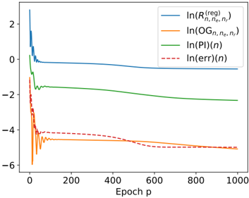<details> <summary>Image 6 Details</summary>  ### Visual Description ## Line Chart: Logarithmic Loss vs. Epoch ### Overview The image presents a line chart illustrating the logarithmic loss of four different metrics – Regularized Risk (R), Observed Gradient (OG), Prediction Information (PI), and Error – as a function of the epoch (p). The y-axis represents the natural logarithm of each metric, while the x-axis represents the epoch number, ranging from 0 to 1000. The chart appears to track the convergence of a model during training. ### Components/Axes * **X-axis:** "Epoch p" - Represents the training epoch, ranging from 0 to approximately 1000. * **Y-axis:** Logarithmic scale, ranging from approximately -6 to 2. No explicit label is given, but the legend indicates the values represent ln(metric). * **Legend:** Located in the top-right corner. * Blue Solid Line: ln(R^(reg)_n,ne,n’) * Orange Solid Line: ln(OG_n,ne,n’) * Green Solid Line: ln(PI(n)) * Red Dashed Line: ln(err(n)) ### Detailed Analysis The chart displays four distinct lines, each representing the logarithmic loss of a different metric over epochs. * **ln(R^(reg)_n,ne,n’) (Blue Line):** This line starts at approximately 2.2 at epoch 0, rapidly decreases to around -0.5 by epoch 50, and then plateaus, fluctuating between approximately -0.5 and -0.2 for the remainder of the epochs. The trend is initially steep, then becomes relatively flat. * **ln(OG_n,ne,n’) (Orange Line):** This line begins at approximately -4.5 at epoch 0, and gradually increases to around -3.5 by epoch 1000. The trend is consistently upward, but the rate of increase slows down over time. * **ln(PI(n)) (Green Line):** This line starts at approximately -1.8 at epoch 0, and decreases steadily to around -2.5 by epoch 1000. The trend is consistently downward, but the rate of decrease slows down over time. * **ln(err(n)) (Red Dashed Line):** This line begins at approximately -4.5 at epoch 0, and gradually increases to around -3.8 by epoch 1000. The trend is consistently upward, but the rate of increase slows down over time. Approximate Data Points (sampled): | Epoch (p) | ln(R^(reg)_n,ne,n’) | ln(OG_n,ne,n’) | ln(PI(n)) | ln(err(n)) | |---|---|---|---|---| | 0 | 2.2 | -4.5 | -1.8 | -4.5 | | 50 | -0.5 | -4.0 | -2.1 | -4.2 | | 200 | -0.3 | -3.8 | -2.3 | -4.0 | | 500 | -0.2 | -3.6 | -2.4 | -3.9 | | 1000 | -0.2 | -3.5 | -2.5 | -3.8 | ### Key Observations * The Regularized Risk (blue line) converges relatively quickly and stabilizes at a low logarithmic loss. * The Observed Gradient, Prediction Information, and Error metrics all show a gradual increase in logarithmic loss over time, indicating a potential divergence or slow convergence. * The Error metric (red dashed line) and Observed Gradient (orange line) are initially very close, but diverge slightly over time. * The Prediction Information (green line) is consistently between the Regularized Risk and the other two metrics. ### Interpretation The chart suggests that the model is converging in terms of regularized risk, but may be experiencing issues with gradient estimation or error minimization. The increasing logarithmic loss for the Observed Gradient, Prediction Information, and Error metrics could indicate that the model is overfitting, or that the learning rate is too high, causing the optimization process to oscillate or diverge. The rapid convergence of the regularized risk suggests that the regularization term is effectively preventing overfitting. The difference between the metrics could be due to the specific calculations and interpretations of each metric within the model. Further investigation into the model's architecture, hyperparameters, and training data would be necessary to determine the root cause of the observed behavior. The logarithmic scale compresses the differences, so the actual magnitude of the changes in the metrics may be smaller than they appear. </details> Fig. 2.4.: Distance err( n ) to u /star (left) and physics inconsistency PI (right) of the regularized PINN estimator with respect to the number n of observations in log -log scale. 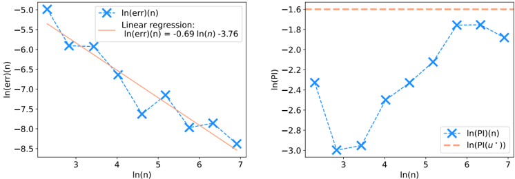<details> <summary>Image 7 Details</summary>  ### Visual Description \n ## Charts: Logarithmic Error and Probability Analysis ### Overview The image presents two separate scatter plots with regression lines. The left plot displays the natural logarithm of the error, ln(err)(n), against the natural logarithm of n, ln(n). The right plot shows the natural logarithm of probability, ln(P)(n), also against ln(n). Both plots include linear regression lines for comparison. ### Components/Axes **Left Plot:** * **X-axis:** ln(n) - Scale ranges from approximately 2.8 to 7.2 with markers at 3, 4, 5, 6, and 7. * **Y-axis:** ln(err)(n) - Scale ranges from approximately -9.0 to -5.0 with markers at -6, -7, -8, and -9. * **Data Series:** ln(err)(n) - Represented by blue 'x' markers. * **Regression Line:** Linear regression: ln(err)(n) = -0.69 ln(n) - 3.76 - Represented by a dashed orange line. * **Legend:** Located in the top-right corner. * Blue 'x': ln(err)(n) * Orange dashed line: Linear regression: ln(err)(n) = -0.69 ln(n) - 3.76 **Right Plot:** * **X-axis:** ln(n) - Scale ranges from approximately 2.8 to 7.2 with markers at 3, 4, 5, 6, and 7. * **Y-axis:** ln(P)(n) - Scale ranges from approximately -3.1 to -1.6 with markers at -2.4, -2.6, -2.8, and -3.0. * **Data Series:** ln(P)(n) - Represented by blue 'x' markers. * **Regression Line:** ln(P)(u'') - Represented by a dashed orange horizontal line. * **Legend:** Located in the top-right corner. * Blue 'x': ln(P)(n) * Orange dashed line: ln(P)(u'') ### Detailed Analysis or Content Details **Left Plot:** The data series ln(err)(n) exhibits a clear downward trend. The line slopes downward from left to right. * (ln(n) ≈ 3.0, ln(err)(n) ≈ -6.1) * (ln(n) ≈ 3.5, ln(err)(n) ≈ -6.7) * (ln(n) ≈ 4.0, ln(err)(n) ≈ -7.3) * (ln(n) ≈ 4.5, ln(err)(n) ≈ -7.6) * (ln(n) ≈ 5.0, ln(err)(n) ≈ -7.9) * (ln(n) ≈ 6.0, ln(err)(n) ≈ -8.3) * (ln(n) ≈ 7.0, ln(err)(n) ≈ -8.7) The regression line closely follows the downward trend of the data, with a slope of approximately -0.69. **Right Plot:** The data series ln(P)(n) initially increases, then plateaus and slightly decreases. * (ln(n) ≈ 3.0, ln(P)(n) ≈ -3.0) * (ln(n) ≈ 3.5, ln(P)(n) ≈ -2.6) * (ln(n) ≈ 4.0, ln(P)(n) ≈ -2.4) * (ln(n) ≈ 4.5, ln(P)(n) ≈ -2.1) * (ln(n) ≈ 5.0, ln(P)(n) ≈ -1.8) * (ln(n) ≈ 6.0, ln(P)(n) ≈ -1.9) * (ln(n) ≈ 7.0, ln(P)(n) ≈ -1.7) The regression line is a horizontal line at approximately ln(P)(u'') = -1.65. ### Key Observations * The left plot shows a strong negative correlation between ln(n) and ln(err)(n), indicating that as n increases, the error decreases exponentially. * The right plot shows a more complex relationship between ln(n) and ln(P)(n), with an initial increase in probability followed by a leveling off. * The regression line on the right plot suggests a limit to the probability as n increases. ### Interpretation The data suggests an analysis of error and probability as a function of a variable 'n'. The left plot indicates that the error decreases as 'n' increases, which could represent improved accuracy or convergence with increasing sample size or iterations. The logarithmic scale implies an exponential decay of error. The right plot shows that the probability initially increases with 'n', but then reaches a plateau. This could indicate a saturation point where further increases in 'n' do not significantly improve the probability. The horizontal regression line suggests an upper bound on the probability. The use of natural logarithms suggests that the underlying relationships may be exponential. The difference between the two plots could be related to the interplay between error reduction and probability maximization. The 'u'' in the right plot's legend may represent a specific condition or parameter under which the probability is evaluated. The plots together could be used to optimize a process or model by balancing error and probability. </details> 2.4.7). Keeping n e , n r , and λ ridge fixed, the proximity between the PINN and u /star is measured by $$\ e r r ( n ) = 2 \int _ { 0 } ^ { 0 . 5 } \int _ { 0 } ^ { 1 } \| u _ { \hat { \theta } ^ { ( r e g ) } ( p _ { \max , n _ { r } , n _ { e } , D ) } } ^ { ( n ) } ( x , t ) - u ^ { ^ { * } } ( x , t ) \| _ { 2 } ^ { 2 } d x d t .$$ According to Theorem 2.5.13, there exists some constant Λ > 0 such that, approximately, $$\ln \left ( \mathbb { E } ( e r r ( n ) ) \right ) \lesssim \ln ( \Lambda ) - \ln ( n ) / 2 .$$ This bound is validated numerically in Figure 2.4, attesting a linear rate in log-log scale between err( n ) and n of -0 . 69 ⩽ -0 . 5 . Furthermore, the second statement of Theorem 2.5.13 suggests that ln PI( n ) = ln PI( u ( n ) ˆ θ (reg) ( p max ,n r ,n e ,D ) ) ⩽ ln PI( u /star ) = -1 . 6 , which is also verified in Figure 2.4. Interestingly, the regularized PINN estimator quickly becomes more accurate than the initial model, since err( n ) is less than ∫ Ω ‖ u model -u /star ‖ 2 2 dµ X /similarequal exp( -5 . 3) as soon as ln( n ) > 2 . 8 , i.e., n ⩾ 17 . The obtained regularized PINN estimator for n = 10 3 is shown in Figure 2.5 (right). This estimator looks globally similar to the model u model (Figure 2.5, left) while managing to reconstruct the variation typical of the cosine perturbation of u /star (Figure 2.5, middle) at t = 0 . Of course, for t ⩾ 0 . 5 , the estimator cannot approximate u /star with an infinite precision, since the measurements X i are only sampled for t < 0 . 5 . However, the regularized PINN estimator succeeds to follow the advection equation dynamics, as it does not vary much along the lines Fig. 2.5.: Functions u model (left), u /star (middle), and regularized PINN estimator with n = 10 3 (right). 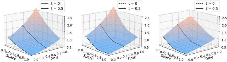<details> <summary>Image 8 Details</summary>  ### Visual Description ## 3D Surface Plots: Wave Propagation Over Time ### Overview The image presents three 3D surface plots, each depicting a wave-like function at different time points. The plots visualize how the wave shape changes as time progresses. Each plot shares the same "Space" and "Time" axes, but the surface height represents the function's value at that specific space and time. ### Components/Axes * **X-axis:** Labeled "Space", ranging from approximately 0.0 to 1.0. * **Y-axis:** Labeled "Time", ranging from approximately 0.0 to 0.8. * **Z-axis:** Vertical axis, ranging from approximately 0.0 to 2.5. * **Legends:** Each plot has a legend in the top-right corner indicating two curves: * `t = 0` (dashed black line) * `t = 0.5` (solid orange line) ### Detailed Analysis or Content Details **Plot 1 (Left):** * The surface is a peak centered around Space = 0.5 and Time = 0.0. * The dashed black line (`t = 0`) starts at approximately (0.0, 0.0) and rises to a peak at (0.5, 0.0), then descends to approximately (1.0, 0.0). * The solid orange line (`t = 0.5`) starts at approximately (0.0, 0.5), rises to a peak at (0.5, 0.5), and descends to approximately (1.0, 0.5). The peak is slightly shifted in time. * The surface height is highest at Space = 0.5, Time = 0.0, reaching approximately 2.3. **Plot 2 (Center):** * The surface is similar to Plot 1, but the peak is more flattened and shifted further in time. * The dashed black line (`t = 0`) starts at approximately (0.0, 0.0) and rises to a peak at (0.5, 0.0), then descends to approximately (1.0, 0.0). * The solid orange line (`t = 0.5`) starts at approximately (0.0, 0.5), rises to a peak at (0.5, 0.5), and descends to approximately (1.0, 0.5). The peak is more pronounced. * The surface height is highest at Space = 0.5, Time = 0.0, reaching approximately 2.4. **Plot 3 (Right):** * The surface is even more flattened and shifted in time compared to Plot 2. * The dashed black line (`t = 0`) starts at approximately (0.0, 0.0) and rises to a peak at (0.5, 0.0), then descends to approximately (1.0, 0.0). * The solid orange line (`t = 0.5`) starts at approximately (0.0, 0.5), rises to a peak at (0.5, 0.5), and descends to approximately (1.0, 0.5). The peak is significantly flattened. * The surface height is highest at Space = 0.5, Time = 0.0, reaching approximately 2.2. ### Key Observations * The wave peak appears to be propagating along the "Time" axis. As time increases (moving from Plot 1 to Plot 3), the peak flattens and shifts towards higher time values. * The dashed black line (`t = 0`) remains consistent across all three plots, representing the initial wave shape. * The solid orange line (`t = 0.5`) shows the wave shape at a later time, demonstrating the wave's evolution. * The maximum height of the wave decreases slightly as time progresses. ### Interpretation The plots demonstrate the propagation of a wave over time. The initial wave shape is represented by the dashed black line at `t = 0`. As time increases to `t = 0.5`, the wave shape changes, indicated by the solid orange line. The flattening and shifting of the peak suggest that the wave is dissipating or spreading out as it propagates. The decreasing maximum height further supports the idea of wave attenuation. The plots provide a visual representation of a dynamic system evolving over time, likely modeling a physical phenomenon like wave motion or signal propagation. The consistent "Space" and "Time" axes allow for a direct comparison of the wave's behavior at different time points. </details> x -t = cst -despite some flattening effect of the Sobolev regularization for t ⩾ 0 . 5 . ## 2.6 Conclusion We have shown that unregularized PINNs can overfit. To remedy this problem, we have proposed to add a ridge penalty to the empirical risk. This regularization ensures the consistency of the PINNs for both linear and nonlinear PDE systems. However, to enforce strong convergence to the target function, another layer of regularization is needed. For linear PDEs, we have proved that the addition of a Sobolev-type penalty is sufficient to ensure the strong convergence of the PINNs. Regarding future research, the next step would be to derive tighter bounds to better quantify the impact of the physical penalty on the convergence speed. ## 2.A Notations Composition of functions Given two functions u, v : R → R , we denote by u ◦ v the function u ◦ v ( x ) = u ( v ( x )) . For all k ∈ N , the function u ◦ k is defined by induction as u ◦ 0 ( x ) = x and u ◦ ( k +1) = u ◦ k ◦ u = u ◦ u ◦ k . The composition symbol is placed before the derivative, so that the k th derivative of u ◦ H is denoted by ( u ◦ H ) ( k ) . Norms The p -norm ‖ x ‖ p of x = ( x 1 , . . . , x d ) ∈ R d is defined by ‖ x ‖ p = ( 1 d ∑ d i =1 | x i | p ) 1 /p . In addition, ‖ x ‖ ∞ = max 1 ⩽ i ⩽ d | x i | . For a function u : Ω → R d , we let ‖ u ‖ L p (Ω) = ( 1 | Ω | ∫ Ω ‖ u ‖ p p ) 1 /p . Similarly, ‖ u ‖ ∞ , Ω = sup x ∈ Ω ‖ u ( x ) ‖ ∞ . For simplicity, we sometimes write ‖ u ‖ ∞ instead of ‖ u ‖ ∞ , Ω . Multi-indices and partial derivatives For a multi-index α = ( α 1 , . . . , α d 1 ) ∈ N d and a differentiable function u : R d 1 → R d 2 , the α partial derivative of u is defined by ∂ α u = ( ∂ 1 ) α 1 . . . ( ∂ d 1 ) α d 1 u . The set of multi-indices of sum less than k is defined by $$\{ | \alpha | \leqslant k \} = \{ ( \alpha _ { 1 } , \dots , \alpha _ { d _ { 1 } } ) \in \mathbb { N } ^ { d } , \alpha _ { 1 } + \cdots + \alpha _ { d _ { 1 } } \leqslant k \} .$$ If α = 0 , ∂ α u = u . Given two multi-indices α and β , we write α ⩽ β when α i ⩽ β i for all 1 ⩽ i ⩽ d 1 . The set of multi-indices less than α is denoted by { β ⩽ α } . For a multi-index α such that | α | ⩽ k , both sets {| β | ⩽ k } and { β ⩽ α } are contained in { 0 , . . . , k } d 1 and are therefore finite. Hölder norm For K ∈ N , the Hölder norm of order K of a function u ∈ C K (Ω , R d ) , is defined by ‖ u ‖ C K (Ω) = max | α | ⩽ K ‖ ∂ α u ‖ ∞ , Ω . This norm allows to bound a function as well as its derivatives. The space C K (Ω , R d ) endowed with the Hölder norm ‖ · ‖ C K (Ω) is a Banach space. C ∞ ( ¯ Ω , R d 2 ) is the space of continuous functions u : ¯ Ω → R d 2 satisfying u | Ω ∈ C ∞ (Ω , R d 2 ) and, for all K ∈ N , ‖ u ‖ C K (Ω) < ∞ . Lipschitz function Given a normed space ( V, ‖·‖ ) , the Lipschitz norm of a function u : V → R d 1 is defined by ‖ u ‖ Lip = sup x,y ∈ V ‖ u ( x ) -u ( y ) ‖ 2 / ‖ x -y ‖ . A function u is Lipschitz if ‖ u ‖ Lip < ∞ . For all u ∈ C 1 ( V, R ) , ‖ u ‖ Lip ⩽ ‖ u ‖ C 1 ( V ) . Lipschitz surface and domain A surface Γ ⊆ R d 1 is said to be Lipschitz if locally , in a neighborhood U ( x ) of any point x ∈ Γ , an appropriate rotation r x of the coordinate system transforms Γ into the graph of a Lipschitz function φ x , i.e., $$r _ { x } ( \Gamma \cap U ( x ) ) = \{ ( x _ { 1 } , \dots , x _ { d - 1 } , \phi _ { x } ( x _ { 1 } , \dots , x _ { d - 1 } ) ) , \forall ( x _ { 1 } , \dots , x _ { d } ) \in r _ { x } ( \Gamma \cap U _ { x } ) \} .$$ A domain Ω ⊆ R d 1 is said to be Lipschitz if its has Lipschitz boundary and lies on one side of it, i.e., φ x < 0 or φ x > 0 on all intersections Ω ∩ U x . All manifolds with C 1 boundary and all convex domains are Lipschitz domains [e.g., Agr15]. Sobolev spaces Let Ω ⊆ R d 1 be an open set. A function v ∈ L 2 (Ω , R d 2 ) is said to be the α th weak derivative of u ∈ L 2 (Ω , R d 2 ) if, for any φ ∈ C ∞ ( ¯ Ω , R d 2 ) with compact support in Ω , one has ∫ Ω 〈 v, φ 〉 = ( -1) | α | ∫ Ω 〈 u, ∂ α φ 〉 . This is denoted by v = ∂ α u . For m ∈ N , the Sobolev space H m (Ω , R d 2 ) is the space of all functions u ∈ L 2 (Ω , R d 2 ) such that ∂ α u exists for all | α | ⩽ m . This space is naturally endowed with the norm ‖ u ‖ H m (Ω) = ( ∑ | α | ⩽ m | Ω | -1 ‖ ∂ α u ‖ 2 L 2 (Ω) ) 1 / 2 . For example, the function u : ] -1 , 1[ → R such that u ( x ) = | x | is not derivable on ] -1 , 1[ , but it admits u ′ ( x ) = 1 x> 0 -1 x< 0 as weak derivative. Since u ′ ∈ L 2 ([ -1 , 1] , R ) , u belongs to the Sobolev space H 1 (] -1 , 1[ , R ) . However, u ′ has no weak derivative, and so u / ∈ H 2 (] -1 , 1[ , R ) . Of course, if a function u belongs to the Hölder space C K ( ¯ Ω , R d 2 ) , then it belongs to the Sobolev space H K (Ω , R d 2 ) , and its weak derivatives are the usual derivatives. For more on Sobolev spaces, we refer the reader to Evans [Eva10, Chapter 5]. ## 2.B Some reminders of functional analysis on Lipschitz domains Extension theorems Let Ω ⊆ R d 1 be an open set and let K ∈ N be an order of differentiation. It is not straightforward to extend a function u ∈ H K (Ω , R d 2 ) to a function ˜ u ∈ H K ( R d 1 , R d 2 ) such that $$\begin{array} { r l } { \tilde { u } | _ { \Omega } = u | _ { \Omega } } & a n d } & \| \tilde { u } \| _ { H ^ { K } ( \mathbb { R } ^ { d _ { 1 } } ) } \leqslant C _ { \Omega } \| u \| _ { H ^ { K } ( \Omega ) } , } \end{array}$$ for some constant C Ω independent of u . This result is known as the extension theorem in Evans [Eva10, Chapter 5.4] when Ω is a manifold with C 1 boundary. However, the simplest domains in PDEs take the form ]0 , L [ 3 × ]0 , T [ , the boundary of which is not C 1 . Fortunately, Stein [Ste70, Theorem 5 Chapter VI.3.3] provides an extension theorem for bounded Lipschitz domains. We refer the reader to Shvartzman [Shv10] for a survey on extension theorems. Example of a non-extendable domain Let the domain Ω =] -1 , 1[ 2 \ ( { 0 }× [0 , 1[) be the square ] -1 , 1[ 2 from which the segment { 0 } × [0 , 1[ has been removed. Then the function $$u ( x , y ) = \left \{ \begin{array} { c l } { 0 } & { i f x < 0 o r i f y \leqslant 0 } \\ { \exp ( - \frac { 1 } { y } ) } & { i f x , y > 0 , } \end{array}$$ belongs to C ∞ (Ω , R ) but cannot be extended to R 2 , since it cannot be continuously extended to the segment { 0 } × [0 , 1[ . Notice that Ω is not a Lipschitz domain because it lies on both sides of the segment { 0 } × [0 , 1[ , which belongs to its boundary ∂ Ω . Theorem 2.B.1 (Sobolev inequalities) . Let Ω ⊆ R d 1 be a bounded Lipschitz domain and let m ∈ N . If m ⩾ d 1 / 2 , then there exists an operator ˜ Π : H m (Ω , R d 2 ) → C 0 (Ω , R d 2 ) such that, for any u ∈ H m (Ω , R d 2 ) , ˜ Π( u ) = u almost everywhere. Moreover, there exists a constant C Ω > 0 , depending only on Ω , such that, ‖ ˜ Π( u ) ‖ ∞ , Ω ⩽ C Ω ‖ u ‖ H m (Ω) . Proof. Since Ω is a bounded Lipschitz domain, there exists a radius r > 0 such that Ω ⊆ B (0 , r ) . According to the extension theorem [Ste70, Theorem 5, Chapter VI.3.3], there exists a constant C Ω > 0 , depending only on Ω , such that any u ∈ H m (Ω , R d 2 ) can be extended to ˜ u ∈ H m ( B (0 , r ) , R d 2 ) , with ‖ ˜ u ‖ H m ( B (0 ,r )) ⩽ C Ω ‖ u ‖ H m (Ω) . Since m ⩾ d 1 / 2 , the Sobolev inequalities [e.g., Eva10, Chapter 5.6, Theorem 6] state that there exists a constant ˜ C Ω > 0 , depending only on Ω , and a linear embedding Π : H m ( B (0 , r ) , R d 2 ) → C 0 ( B (0 , r ) , R d 2 ) such that ‖ Π(˜ u ) ‖ ∞ ⩽ ˜ C Ω ‖ ˜ u ‖ H m ( B (0 ,r )) and Π(˜ u ) = ˜ u in H m ( B (0 , r ) , R d 2 ) . Therefore, ˜ Π( u ) = Π(˜ u ) | Ω and ‖ ˜ Π( u ) ‖ ∞ , Ω ⩽ C Ω ˜ C Ω ‖ u ‖ H m (Ω) . Definition 2.B.2 (Weak convergence in L 2 (Ω) ) . A sequence ( u p ) p ∈ N ∈ L 2 (Ω) N weakly converges to u ∞ ∈ L 2 (Ω) if, for any φ ∈ L 2 (Ω) , lim p →∞ ∫ Ω φu p = ∫ Ω φu ∞ . This convergence is denoted by u p ⇀u ∞ . The Cauchy-Schwarz inequality shows that the convergence with respect to the L 2 (Ω) norm implies the weak convergence. However, the converse is not true. For example, the sequence of functions u p ( x ) = cos( px ) weakly converges to 0 in L 2 ([ -π, π ]) , whereas ‖ u p ‖ L 2 ([ -π,π ]) = 1 / 2 . Definition 2.B.3 (Weak convergence in H m (Ω) ) . A sequence ( u p ) p ∈ N ∈ H m (Ω) N weakly converges to u ∞ ∈ H m (Ω) in H m (Ω) if, for all | α | ⩽ m , ∂ α u p ⇀∂ α u ∞ . Theorem 2.B.4 (Rellich-Kondrachov) . Let Ω ⊆ R d 1 be a bounded Lipschitz domain and let m ∈ N . Let ( u p ) p ∈ N ∈ H m +1 (Ω , R d 2 ) be a sequence such that ( ‖ u p ‖ H m +1 (Ω) ) p ∈ N is bounded. There exists a function u ∞ ∈ H m +1 (Ω , R d 2 ) and a subsequence of ( u p ) p ∈ N that converges to u ∞ both weakly in H m +1 (Ω , R d 2 ) and with respect to the H m (Ω) norm. Proof. Let r > 0 be such that Ω ⊆ B (0 , r ) . According to the extension theorem of Stein [Ste70, Theorem 5, Chapter VI.3.3], there exists a constant C r > 0 such that each u p can be extended to ˜ u p ∈ H m +1 ( B (0 , r ) , R d 2 ) , with ‖ ˜ u p ‖ H m +1 ( B (0 ,r )) ⩽ C r ‖ u p ‖ H m +1 (Ω) . Observing that, for all | α | ⩽ m , ∂ α ˜ u p belongs to H 1 ( B (0 , r ) , R d 2 ) , the Rellich-Kondrachov compactness theorem [Eva10, Theorem 1, Chapter 5.7] ensures that there exists a subsequence of (˜ u p ) p ∈ N that converges to an extension of u ∞ with respect to the H m ( B (0 , r )) norm. Since the subsequence is also bounded, upon passing to another subsequence, it also weakly converges in H m +1 ( B (0 , r ) , R d 2 ) to u ∞ ∈ H m +1 ( B (0 , r ) , R d 2 ) [e.g., Eva10, Chapter D.4]. Therefore, by considering the restrictions of all the previous functions to Ω , we deduce that there exists a subsequence of ( u p ) p ∈ N that converges to u ∞ both weakly in H m +1 (Ω) and with respect to the H m (Ω) norm. ## 2.C Some useful lemmas The n th Bell number B n [Har06] corresponds to the number of partitions of the set { 1 , . . . , n } . Bell numbers satisfy the relationship B 0 = 1 and $$B _ { n + 1 } = \sum _ { k = 0 } ^ { n } { \binom { n } { k } } \, B _ { k } . \begin{array} { l } ( 2 . 7 ) \\ \end{array}$$ For K ⩾ 1 and u ∈ C K ( R d 1 , R d 2 ) , the K th derivative of u is denoted by u ( K ) . Lemma 2.C.1 (Bounding the partial derivatives of a composition of functions) . Let d 1 , d 2 ⩾ 1 , K ⩾ 0 , f ∈ C K ( R d 1 , R ) , and g ∈ C K ( R , R d 2 ) . Then $$\| g \circ f \| _ { C ^ { K } ( \mathbb { R } ^ { d _ { 1 } } ) } \leqslant B _ { K } \| g \| _ { C ^ { K } ( \mathbb { R } ) } ( 1 + \| f \| _ { C ^ { K } ( \mathbb { R } ^ { d _ { 1 } } ) } ) ^ { K } .$$ Proof. Let K 1 ⩽ K and let Π( K 1 ) be the set of all partitions of { 1 , . . . , K 1 } . According to Hardy [Har06, Proposition 1], one has, for all h ∈ C K 1 ( R K 1 + d 1 , R ) , $$\partial _ { 1 , 2 , 3 , \dots , K _ { 1 } } ^ { K _ { 1 } } ( g \circ h ) = \sum _ { P \in \Pi ( K _ { 1 } ) } g ^ { ( | P | ) } \circ h \times \prod _ { S \in P } \left [ \left ( \prod _ { j \in S } \partial _ { j } \right ) h \right ] .$$ Let α = ( α 1 , . . . , α d 1 ) be a multi-index such that | α | = K 1 . Setting α 0 = 0 , y j = x K 1 + j + ( x α 1 + ··· + α j -1 + · · · + x α 1 + ··· + α j -1 ) , and letting h ( x 1 , . . . , x K 1 + d 1 ) = f ( y 1 , . . . , y d 1 ) , we are led to $$\partial ^ { \alpha } ( g \circ f ) = \sum _ { P \in \Pi ( K _ { 1 } ) } g ^ { ( | P | ) } \circ f \times \prod _ { S \in P } \partial ^ { \alpha ( S ) } f ,$$ where α ( S ) = ( |{ b ∈ S, α 1 + · · · + α /lscript -1 ⩽ b ⩽ α 1 + · · · + α /lscript }| ) 1 ⩽ /lscript ⩽ d 1 . Moreover, by definition of the Bell number, | Π( K 1 ) | = B K 1 , and, by definition of a partition, | P | ⩽ K 1 . So, $$\| \partial ^ { \alpha } ( g \circ f ) \| _ { \infty } & \leqslant B _ { K _ { 1 } } \| g \| _ { C ^ { K _ { 1 } } ( \mathbb { R } ^ { d _ { 1 } } ) } \max _ { i _ { 1 } + 2 i _ { 2 } + \cdots + K _ { 1 } i _ { K _ { 1 } } = K _ { 1 } } \prod _ { j = 1 } ^ { K _ { 1 } } \| f \| _ { C ^ { j } ( \mathbb { R } ^ { d _ { 1 } } ) } ^ { i _ { j } } \\ & \leqslant B _ { K _ { 1 } } \| g \| _ { C ^ { K _ { 1 } } ( \mathbb { R } ^ { d _ { 1 } } ) } ( 1 + \| f \| _ { C ^ { K _ { 1 } } ( \mathbb { R } ^ { d _ { 1 } } ) } ) ^ { K _ { 1 } } .$$ Since this inequality is true for all K 1 ⩽ K and for all | α | = K 1 , the lemma is proved. Lemma 2.C.2 (Bounding the partial derivatives of a changing of coordinates f ) . Let d 1 , d 2 ⩾ 1 , K ⩾ 0 , f ∈ C K ( R , R ) , and g ∈ C K ( R d 1 , R d 2 ) . Let v ∈ C K ( R d 1 , R d 1 ) be defined by v ( x ) = ( f ( x 1 ) , . . . , f ( x d 1 )) . Then $$\| g \circ v \| _ { C ^ { K } ( \mathbb { R } ^ { d _ { 1 } } ) } \leqslant B _ { K } \times \| g \| _ { C ^ { K } ( \mathbb { R } ^ { d _ { 1 } } ) } \times ( 1 + \| f \| _ { C ^ { K } ( \mathbb { R } ) } ) ^ { K } .$$ Proof. Let α = ( α 1 , . . . , α d 1 ) be a multi-index such that | α | = K . For x = ( x 1 , . . . , x d 1 ) and a fixed i ∈ { 1 , . . . , d 1 } , we let h ( t ) = g ( f ( x 1 ) , . . . , f ( x i -1 ) , t, f ( x i +1 ) , . . . , f ( x d 1 )) . Clearly, ( h ◦ f ) ( α i ) ( x i ) = ( ∂ i ) α i ( g ◦ v )( x ) . Thus, according to Lemma 2.C.1, $$( h \circ f ) ^ { ( \alpha _ { i } ) } = \sum _ { P _ { i } \in \Pi ( \alpha _ { i } ) } h ^ { ( | P _ { i } | ) } \circ f \times \prod _ { S _ { i } \in P _ { i } } f ^ { ( | S _ { i } | ) } .$$ Therefore, $$( \partial _ { i } ) ^ { \alpha _ { i } } ( g \circ v ) ( x ) = \sum _ { P _ { i } \in \Pi ( \alpha _ { i } ) } ( \partial _ { i } ) ^ { | P _ { i } | } g \circ v ( x ) \prod _ { S _ { i } \in P _ { i } } f ^ { ( | S _ { i } | ) } ( x _ { i } ) .$$ /negationslash Letting i = 1 and observing that ∂ j f ( | S 1 | ) ( x 1 ) = 0 for j = 1 , we see that $$\partial ^ { \alpha } ( g \circ v ) ( x ) = \sum _ { P _ { 1 } \in \Pi ( \alpha _ { 1 } ) } \left [ \prod _ { S _ { 1 } \in P _ { 1 } } f ^ { ( | S _ { 1 } | ) } ( x _ { 1 } ) \right ] \times ( \partial _ { 2 } ) ^ { \alpha _ { 2 } } \dots ( \partial _ { d _ { 1 } } ) ^ { \alpha _ { d _ { 1 } } } [ ( \partial _ { 1 } ) ^ { | P _ { 1 } | } g \circ v ] ( x ) .$$ Repeating the same procedure for ( ∂ 1 ) | P 1 | g ◦ v, . . . , ( ∂ 1 ) | P 1 | . . . ( ∂ d 1 ) | P d 1 | g ◦ v , we obtain $$\partial ^ { \alpha } ( g \circ v ) ( x ) = & \sum _ { P _ { 1 } \in \Pi ( \alpha _ { 1 } ) } \left [ \prod _ { S _ { 1 } \in P _ { 1 } } f ^ { ( | S _ { 1 } | ) } ( x _ { 1 } ) \right ] \times \cdots \\ & \cdots \times \sum _ { P _ { d _ { 1 } } \in \Pi ( \alpha _ { d _ { 1 } } ) } \left [ \prod _ { S _ { d _ { 1 } } \in P _ { d _ { 1 } } } f ^ { ( | S _ { d _ { 1 } } | ) } ( x _ { d _ { 1 } } ) \right ] \times ( \partial _ { 1 } ) ^ { | P _ { 1 } | } \dots ( \partial _ { d _ { 1 } } ) ^ { | P _ { d _ { 1 } } | } g \circ v ( x ) .$$ Since ∑ S i ∈ P i | S i | = α i and ∑ d 1 i =1 α i = K , we conclude that $$\| \partial ^ { \alpha } ( g \circ v ) \| _ { \infty } \leqslant B _ { \alpha _ { 1 } } \times \cdots \times B _ { \alpha _ { d _ { 1 } } } \times \| \partial ^ { \alpha } g \| _ { \infty } ( 1 + \| f \| _ { C ^ { K } ( \mathbb { R } ) } ) ^ { K } .$$ Using the injective map M : Π( α 1 ) ×···× Π( α d 1 ) → Π( K ) such that M ( P 1 , . . . , P d 1 ) = ∪ d 1 i =1 P i , we have B α 1 ×··· × B α d 1 ⩽ B K . This concludes the proof. Lemma 2.C.3 (Bounding hyperbolic tangent and its derivatives) . For all K ∈ N , one has $$\| \tanh ^ { ( K ) } \| _ { \infty } \leqslant 2 ^ { K - 1 } ( K + 2 ) !$$ Proof. The tanh function is a solution of the equation y ′ = 1 -y 2 . An elementary induction shows that there exists a sequence of polynomials ( P K ) K ∈ N such that tanh ( K ) = P K (tanh) , with P 0 ( X ) = X and P K +1 ( X ) = (1 -X 2 ) × P ′ K ( X ) . Clearly, P K is a real polynomial of degree K + 1 , of the form P K ( X ) = a ( K ) 0 + a ( K ) 1 X + · · · + a ( K ) K +1 X K +1 . One verifies that a ( K +1) i = ( i + 1) a ( K ) i +1 -( i -1) a ( K ) i -1 , with a ( K ) -1 = a ( K ) K +2 = 0 . The largest coefficient M ( P K ) = max 0 ⩽ i ⩽ K +1 | a ( K ) i | of P K satisfies M ( P K +1 ) ⩽ 2( K + 1) × M ( P K ) . Thus, since M ( P 1 ) = 1 , we see that M ( P K ) ⩽ 2 K -1 K ! . Recalling that 0 ⩽ tanh ⩽ 1 , we conclude that $$\| \tanh ^ { ( K ) } \| _ { \infty } = \| P _ { K } ( t a n h ) \| _ { \infty } \leqslant ( K + 2 ) M ( P _ { K } ) \leqslant 2 ^ { K - 1 } ( K + 2 ) !$$ In the sequel, for all θ ∈ R , we write tanh θ ( x ) = tanh( θx ) . We define the sign function such that sgn( x ) = 1 x> 0 -1 x< 0 . Lemma 2.C.4 (Characterizing the limit of hyperbolic tangent in Hölder norm) . Let K ∈ N and H ∈ N /star . Then, for all ε > 0 , lim θ →∞ ‖ tanh ◦ H θ -sgn ‖ C K ( R \ ] -ε,ε [) = 0 . Proof. Fix ε > 0 . We prove the stronger statement that, for all m ∈ N , one has $$\lim _ { \theta \to \infty } \theta ^ { m } \| \tanh _ { \theta } ^ { \circ H } - s g n \| _ { C ^ { K } ( \mathbb { R } \ ] - \varepsilon , \varepsilon [ ) } = 0 .$$ We start with the case H = 1 and then prove the result by induction on H . Observe first, since tanh ◦ H θ -sgn is an odd function, that $$\| \tanh _ { \theta } ^ { \circ H } - s g n \| _ { C ^ { K } ( \mathbb { R } \ ] - \varepsilon , \varepsilon [ ) } = \| \tanh _ { \theta } ^ { \circ H } - s g n \| _ { C ^ { K } ( [ \varepsilon , \infty [ ) } .$$ The case H = 1 Assume, to start with, that K = 0 . For all x ⩾ ε , one has $$\theta ^ { m } | \tanh _ { \theta } ( x ) - 1 | = \frac { 2 \theta ^ { m } } { 1 + \exp ( - 2 \theta x ) } \leqslant \frac { 2 \theta ^ { m } } { 1 + \exp ( - 2 \theta \varepsilon ) } .$$ Therefore, for all m ∈ N , $$\theta ^ { m } \| \tanh _ { \theta } - s g n \| _ { \infty , \mathbb { R } \ ] - \varepsilon , \varepsilon [ } = \theta ^ { m } \| \tanh _ { \theta } - s g n \| _ { \infty , [ \varepsilon , \infty [ } \leqslant \frac { 2 \theta ^ { m } } { 1 + \exp ( - 2 \theta \varepsilon ) } \xrightarrow { \theta \to \infty } 0 .$$ Next, to prove that the result if true for all K ⩾ 1 , it is enough to show that, for all m , $$\theta ^ { m } \| \tanh _ { \theta } ^ { ( K ) } \| _ { \infty , \mathbb { R } \ \ ] - \varepsilon , \varepsilon [ } \xrightarrow { \theta \to \infty } 0 .$$ According to the proof of Lemma 2.C.3, there exists a sequence of polynomials ( P K ) K ∈ N such that tanh ( K ) = P K (tanh) and P K +1 ( X ) = (1 -X 2 ) × P ′ K ( X ) . Since tanh θ ( x ) = tanh( θx ) , one has $$\tanh _ { \theta } ^ { ( K ) } ( x ) & = \theta ^ { K } \tanh ^ { ( K ) } ( \theta x ) \\ & = \theta ^ { K } ( 1 - \tanh ^ { 2 } ( \theta x ) ) \times P _ { K - 1 } ^ { \prime } ( \tanh ( \theta x ) ) \\ & = \theta ^ { K } ( 1 - \tanh ( \theta x ) ) ( 1 + \tanh ( \theta x ) ) \times P _ { K - 1 } ^ { \prime } ( \tanh ( \theta x ) ) .$$ Fix x ⩾ ε . Then, letting M K = ‖ P ′ K -1 ‖ ∞ , [ -1 , 1] , we are led to $$\begin{array} { r l } & { | \tanh _ { \theta } ^ { ( K ) } ( x ) | \leqslant 2 M _ { K } \theta ^ { K } ( 1 - \tanh ( \theta x ) ) \leqslant 4 M _ { K } \times \frac { \theta ^ { K } } { 1 + \exp ( 2 \theta x ) } } \\ & { \leqslant 4 M _ { K } \times \frac { \theta ^ { K } } { 1 + \exp ( 2 \theta \varepsilon ) } . } \end{array}$$ This shows that θ m ‖ tanh ( K ) θ ‖ ∞ , [ ε, ∞ [ ⩽ 4 M K × θ K + m 1+exp(2 θε ) . One proves with similar arguments that the same result holds for all x ⩽ -ε . Thus, $$\theta ^ { m } \| \tanh _ { \theta } ^ { ( K ) } \| _ { \infty , \mathbb { R } \, ] - \varepsilon , \varepsilon [ } \leqslant 4 M _ { K } \times \frac { \theta ^ { K + m } } { 1 + \exp ( 2 \theta \varepsilon ) } \xrightarrow { \theta \to \infty } 0 ,$$ and the lemma is proved for H = 1 . Induction Assume that that, for all K and all m , $$\theta ^ { m } \| \tanh _ { \theta } ^ { \circ H } - s g n \| _ { C ^ { K } ( \mathbb { R } \ ] - \varepsilon , \varepsilon [ ) } \xrightarrow { \theta \to \infty } 0 .$$ Our objective is to prove that, for all K 2 and all m 2 , $$\theta ^ { m _ { 2 } } \| \tanh _ { \theta } ^ { \circ ( H + 1 ) } - s g n \| _ { C ^ { K _ { 2 } } ( \mathbb { R } \, ] - \varepsilon , \varepsilon [ ) } \xrightarrow { \theta \to \infty } 0 .$$ If K 2 = 0 , since, for all ( x, y ) ∈ R 2 , | tanh θ ( x ) -tanh θ ( y ) | ⩽ θ | x -y | × ‖ tanh ′ ‖ ∞ ⩽ θ | x -y | . We deduce that $$\theta ^ { m _ { 2 } } \| \tanh _ { \theta } ^ { \circ ( H + 1 ) } - \tanh _ { \theta } ( s g n ) \| _ { \infty , \mathbb { R } \ \ ] - e , \varepsilon [ } \leqslant \theta ^ { m _ { 2 } + 1 } \| \tanh _ { \theta } ^ { \circ H } - s g n \| _ { \infty , \mathbb { R } \ \ ] - e , \varepsilon [ } .$$ Therefore, according to (2.9), we have that lim θ →∞ θ m 2 ‖ tanh ◦ ( H +1) θ -tanh θ (sgn) ‖ ∞ , R \ ] -ε,ε [ = 0 . Since tanh θ (sgn) -sgn = (tanh( θ ) -1) 1 x> 0 -(tanh( θ ) -1) 1 x< 0 , we see that, for all m 2 , $$\lim _ { \theta \to \infty } \theta ^ { m _ { 2 } } \| \tanh _ { \theta } ( s g n ) - s g n \| _ { \infty , \mathbb { R } \ ] - \varepsilon , \varepsilon [ } = 0 .$$ Using the triangle inequality, we conclude as desired that, for all m 2 , $$\theta ^ { m _ { 2 } } \| \tanh _ { \theta } ^ { \circ ( H + 1 ) } - s g n \| _ { \infty , \mathbb { R } \ ] - \varepsilon , \varepsilon [ } \xrightarrow { \theta \to \infty } 0 .$$ Assume now that K 2 ⩾ 1 . Since tanh ◦ ( H +1) θ = tanh ◦ H (tanh) , the Faà di Bruno formula [e.g., Com74, Chapter 3.4] states that $$( \tanh ^ { \circ ( H + 1 ) } _ { \theta } ) ^ { ( K _ { 2 } ) } & = \sum _ { m _ { 1 } + 2 m _ { 2 } + \cdots + K _ { 2 } m _ { K _ { 2 } } = K _ { 2 } } \frac { K _ { 2 } ! } { \prod _ { i = 1 } ^ { K _ { 2 } } m _ { i } ! \times i ! m _ { i } } \\ & \times ( \tanh ^ { \circ H } _ { \theta } ) ^ { ( m _ { 1 } + \cdots + m _ { K _ { 2 } } ) } ( \tanh _ { \theta } ) \times \prod _ { j = 1 } ^ { K _ { 2 } } ( \tanh ^ { ( j ) } _ { \theta } ) ^ { m _ { j } } .$$ Notice that if | x | ≤ arctanh(1 / √ 2) , | tanh( x ) | ⩾ | x | 2 because by calling f ( x ) = tanh( x ) -x 2 , f (0) = 0 and f ′ ( x ) = (1 -tanh( x ) 2 ) -1 2 ⩾ 0 . Therefore, if | x | ≥ ε , | tanh( θx ) | ⩾ min( 1 √ 2 , θ 2 ε ) ⩾ ε if θ ⩾ 2 and ε ⩾ 1 √ 2 . This is why for θ ⩾ 2 and ε ⩽ 1 , $$\begin{array} { r } { \| ( \tanh _ { \theta } ^ { \circ H } ) ^ { ( m _ { 1 } + \cdots + m _ { K _ { 2 } } ) } ( \tanh _ { \theta } ) \| _ { \infty , \mathbb { R } \ \ ] - \varepsilon _ { , \varepsilon } [ } \leqslant \| ( \tanh _ { \theta } ^ { \circ H } ) ^ { ( m _ { 1 } + \cdots + m _ { K _ { 2 } } ) } \| _ { \infty , \mathbb { R } \ \ ] - \varepsilon _ { , \varepsilon } [ } . } \end{array}$$ Therefore, from the triangular inequality on ‖ · ‖ ∞ , R \ ] -ε,ε [ , $$\| ( \tanh ^ { \circ ( H + 1 ) } _ { \theta } ) ^ { ( K _ { 2 } ) } \| _ { \infty , \mathbb { R } \, \} - \varepsilon , \varepsilon [ } & \leqslant \sum _ { m _ { 1 } + 2 m _ { 2 } + \cdots + K _ { 2 } m _ { K _ { 2 } } = K _ { 2 } } \frac { K _ { 2 } ! } { \prod _ { i = 1 } ^ { K _ { 2 } } m _ { i } ! \times i ! m _ { i } } \\ & \quad \times \| ( \tanh ^ { \circ H } _ { \theta } ) ^ { ( m _ { 1 } + \cdots + m _ { K _ { 2 } } ) } \| _ { \infty , \mathbb { R } \, \} - \varepsilon , \varepsilon [ } \prod _ { j = 1 } ^ { K _ { 2 } } \| \tanh ^ { ( j ) } _ { \theta } \| _ { \infty , \mathbb { R } \, \} - \varepsilon , \varepsilon [ } . </doctag>$$ According to the induction hypothesis (2.9), one has, for all K ⩾ 1 and all m ∈ N , $$\lim _ { \theta \to \infty } \theta ^ { m } \| ( t a n h _ { \theta } ^ { \circ H } ) ^ { ( K ) } \| _ { \infty , \mathbb { R } \ ] - \varepsilon , \varepsilon [ } = 0 .$$ We deduce from the above that for all K 2 ⩾ 1 and all m 2 , $$\theta ^ { m _ { 2 } } \| ( \tanh _ { \theta } ^ { \circ ( H + 1 ) } ) ^ { ( K _ { 2 } ) } \| _ { \infty , \mathbb { R } \ ] - \varepsilon , \varepsilon [ } \xrightarrow { \theta \to \infty } 0 .$$ Combining (2.10) and (2.11), it comes that lim θ →∞ θ m 2 ‖ tanh ◦ ( H +1) θ -sgn ‖ C K 2 ( R \ ] -ε,ε [) = 0 . Corollary 2.C.5 (Bounding hyperbolic tangent compositions and their derivatives) . Let K ∈ N and H ∈ N /star . Then, for or all θ ∈ R , ‖ (tanh ◦ H θ ) ( K ) ‖ ∞ < ∞ . Proof. An induction as the one of Lemma 2.C.4 shows that ‖ (tanh ◦ H θ ) ( K ) ‖ ∞ , R \ ] -ε,ε [ < ∞ . In addition, since tanh ◦ H θ ∈ C ∞ ( R , R ) , ‖ (tanh ◦ H θ ) ( K ) ‖ ∞ , [ -ε,ε ] < ∞ . When d 1 = d 2 = 1 , the observations ( X 1 , Y 1 ) , . . . , ( X n , Y n ) ∈ R 2 can be reordered as ( X (1) , Y (1) ) , . . . , ( X ( n ) , Y ( n ) ) according to increasing values of the X i , that is, X (1) ⩽ · · · ⩽ X ( n ) . Moreover, we let G ( n, n r ) = { ( X i , Y i ) , 1 ⩽ i ⩽ n } ∪ { X ( r ) j , 1 ⩽ j ⩽ n r } , and denote by δ ( n, n r ) the minimum distance between two distinct points in G ( n, n r ) , i.e., /negationslash $$\delta ( n , n _ { r } ) = \underset { z _ { 1 } \neq z _ { 2 } } { \min } | z _ { 1 } - z _ { 2 } | . & & ( 2 . 1 2 )$$ Lemma 2.C.6 (Exact estimation with hyperbolic tangent) . Assume that d 1 = d 2 = 1 , and let H ⩾ 1 . Let the neural network u θ ∈ NN H ( n -1) be defined by $$u _ { \theta } ( x ) = Y _ { ( 1 ) } + \sum _ { i = 1 } ^ { n - 1 } \frac { Y _ { ( i + 1 ) } - Y _ { ( i ) } } { 2 } \left [ t a n h _ { \theta } ^ { \circ H } \left ( x - X _ { ( i ) } - \frac { \delta ( n , n _ { r } ) } { 2 } \right ) + 1 \right ] .$$ Then, for all 1 ⩽ i ⩽ n , $$\lim _ { \theta \to \infty } u _ { \theta } ( X _ { i } ) = Y _ { i } .$$ Moreover, for all order K ∈ N /star of differentiation and all 1 ⩽ j ⩽ n r , $$\lim _ { \theta \to \infty } u _ { \theta } ^ { ( K ) } ( X _ { j } ^ { ( r ) } ) = 0 .$$ Proof. Applying Lemma 2.C.4 with ε = δ ( n,n r ) / 4 and letting $$G = \mathbb { R } \cup _ { i = 1 } ^ { n } ] X _ { ( i ) } + \frac { 1 } { 4 } \delta ( n , n _ { r } ) , X _ { ( i ) } + \frac { 3 } { 4 } \delta ( n , n _ { r } ) [ ,$$ one has, for all K , lim θ →∞ ‖ u θ -u ∞ ‖ C K ( G ) = 0 , where $$u _ { \infty } ( x ) = Y _ { ( 1 ) } + \sum _ { i = 1 } ^ { n - 1 } \left [ Y _ { ( i + 1 ) } - Y _ { ( i ) } \right ] \times 1 _ { x > X _ { ( i ) } + \frac { \delta ( n , n _ { r } ) } { 2 } } .$$ Clearly, for all 1 ⩽ i ⩽ n , u ∞ ( X i ) = Y i . Since u ′ ∞ ( x ) = 0 for all x ∈ G , and since X ( r ) j ∈ G for all 1 ⩽ j ⩽ n r , we deduce that u ( K ) ∞ ( X ( r ) j ) = 0 . This concludes the proof. Definition 2.C.7 (Overfitting gap) . For any n, n e , n r ∈ N /star and λ (ridge) ⩾ 0 , the overfitting gap operator OG n,n e ,n r is defined, for all u ∈ C ∞ ( ¯ Ω , R d 2 ) , by $$O G _ { n , n _ { e } , n _ { r } } ( u ) = | R _ { n , n _ { e } , n _ { r } } ^ { ( r i d g e ) } ( u ) - \mathcal { R } _ { n } ( u ) | .$$ Lemma 2.C.8 (Monitoring the overfitting gap) . Let ε > 0 , λ (ridge) ⩾ 0 , H ⩾ 2 , and D ∈ N /star . Let n, n e , n r ∈ N /star . Let ˆ θ ∈ Θ H,D be a parameter such that ( i ) R (ridge) n,n e ,n r ( u ˆ θ ) ⩽ inf u ∈ NN H ( D ) R (ridge) n,n e ,n r ( u ) + ε and ( ii ) OG n,n e ,n r ( u ˆ θ ) ⩽ ε . Then $$\mathcal { R } _ { n } ( u _ { \hat { \theta } } ) \leqslant \inf _ { u \in N N _ { H } ( D ) } \mathcal { R } _ { n } ( u ) + 2 \varepsilon + o _ { n _ { e } , n _ { r } \to \infty } ( 1 ) .$$ Proof. On the one hand, since R n ⩽ R (ridge) n,n e ,n r +OG n,n e ,n r , assumptions ( i ) and ( ii ) imply that R n ( u ˆ θ ) ⩽ inf u ∈ NN H ( D ) R (ridge) n,n e ,n r ( u ) + 2 ε . On the other hand, R (ridge) n,n e ,n r -OG n,n e ,n r ⩽ R n . The proof of Theorem 2.4.6 reveals that there exists a sequence ( θ ( n e , n r )) n e ,n r ∈ N ∈ Θ N H,D such that lim n e ,n r →∞ OG n,n e ,n r ( u θ ( n e ,n r ) ) = 0 and lim n e ,n r →∞ R n ( u θ ( n e ,n r ) ) = inf u ∈ NN H ( D ) R n ( u ) . Thus, inf u ∈ NN H ( D ) R (ridge) n,n e ,n r ( u ) ⩽ inf NN H ( D ) R n ( u ) + o n e ,n r →∞ (1) . We deduce that $$\mathcal { R } _ { n } ( u _ { \hat { \theta } } ) \leqslant \inf _ { u \in N N _ { H } ( D ) } \mathcal { R } _ { n } ( u ) + 2 \varepsilon + o _ { n _ { e } , n _ { r } \to \infty } ( 1 ) .$$ Lemma 2.C.9 (Minimizing sequence of the theoretical risk.) . Let H,D ∈ N /star . Define the sequence ( v p ) p ∈ N ∈ NN H ( D ) N of neural networks by v p ( x ) = tanh p ◦ tanh ◦ ( H -1) ( x ) . Then, for any λ e > 0 , $$\lim _ { p \rightarrow \infty } \lambda _ { e } ( 1 - v _ { p } ( 1 ) ) ^ { 2 } + \frac { 1 } { 2 } \int _ { - 1 } ^ { 1 } x ^ { 2 } ( v _ { p } ^ { \prime } ) ^ { 2 } ( x ) d x = 0 .$$ Proof. tanh ◦ ( H -1) is an increasing C ∞ function such that tanh ◦ ( H -1) (0) = 0 . Therefore, Lemma 2.C.4 shows that lim p →∞ v p (1) = 1 , so that lim p →∞ λ e (1 -v p (1)) 2 = 0 . This shows the convergence of the left-hand term of the lemma. To bound the right-hand term, we have, according to the chain rule, $$| v _ { p } ^ { \prime } ( x ) | \leqslant p \| \tanh ^ { \circ ( H - 1 ) } \| _ { C ^ { 1 } ( \mathbb { R } ) } | \tanh ^ { \prime } ( p \tanh ^ { \circ ( H - 1 ) } ( x ) ) | ,$$ with ‖ tanh ◦ ( H -1) ‖ C 1 ( R ) < ∞ by Corollary 2.C.5. Thus, $$\int _ { - 1 } ^ { 1 } x ^ { 2 } ( v _ { p } ^ { \prime } ) ^ { 2 } ( x ) d x \leqslant \| \tanh ^ { \circ ( H - 1 ) } \| _ { C ^ { 1 } ( \mathbb { R } ) } ^ { 2 } \int _ { - 1 } ^ { 1 } p ^ { 2 } x ^ { 2 } ( \tanh ^ { \prime } ( p \, \mathrm t a n h ^ { \circ ( H - 1 ) } ( x ) ) ) ^ { 2 } d x .$$ Notice that x 2 (tanh ′ ( p tanh ◦ ( H -1) ( x ))) 2 is an even function, so that $$\int _ { - 1 } ^ { 1 } x ^ { 2 } ( v _ { p } ^ { \prime } ) ^ { 2 } ( x ) d x \leqslant 2 \| \tanh ^ { \circ ( H - 1 ) } \| _ { C ^ { 1 } ( R ) } ^ { 2 } \int _ { 0 } ^ { 1 } p ^ { 2 } x ^ { 2 } ( \tanh ^ { \prime } ( p \, \mathrm t a n h ^ { \circ ( H - 1 ) } ( x ) ) ) ^ { 2 } d x .$$ Remark that (tanh ′ ) 2 ( x ) = (1 -tanh( x )) 2 (1 + tanh( x )) 2 ⩽ 16 exp( -2 x ) , so that $$\int _ { - 1 } ^ { 1 } x ^ { 2 } ( v _ { p } ^ { \prime } ) ^ { 2 } ( x ) d x \leqslant 3 2 \| \tanh ^ { \circ ( H - 1 ) } \| _ { C ^ { 1 } ( \mathbb { R } ) } ^ { 2 } \int _ { 0 } ^ { 1 } p ^ { 2 } x ^ { 2 } \exp ( - 2 p \tanh ^ { \circ ( H - 1 ) } ( x ) ) d x .$$ If H = 1 , then the change of variable ¯ x = p x states that $$\int _ { 0 } ^ { 1 } p ^ { 2 } x ^ { 2 } \exp { ( - 2 p x ) } d x \leqslant p ^ { - 1 } \int _ { 0 } ^ { \infty } \bar { x } ^ { 2 } \exp { ( - 2 \bar { x } ) } d \bar { x } \xrightarrow { p \to \infty } 0$$ and the lemma is proved. If H ⩾ 2 , notice that tanh( x ) ⩾ x1 x ⩽ 1 / 2 + 1 x ⩾ 1 / 2 for all x ⩾ 0 , and therefore we have that tanh ◦ ( H -1) ( x ) ⩾ x1 x ⩽ 2 H -1 / 2 H + 1 x ⩾ 2 H -1 / 2 H . Thus, using the change of variable ¯ x = p x , $$\int _ { 0 } ^ { 1 } p ^ { 2 } x ^ { 2 } \exp ( - 2 p \tanh ^ { \circ ( H - 1 ) } ( x ) ) d x & \leqslant \int _ { 0 } ^ { 1 } p ^ { 2 } x ^ { 2 } \exp ( - 2 ^ { H - 1 } p x ) d x \\ & \leqslant p ^ { - 1 } \int _ { 0 } ^ { \infty } \bar { x } ^ { 2 } \exp ( - 2 ^ { H - 1 } \bar { x } ) d \bar { x } .$$ $$1$$ Since this upper bound vanishes as p →∞ , this concludes the proof when H ⩾ 2 . Definition 2.C.10 (Weak lower semi-continuity) . A fonction I : H m (Ω) → R is weakly lower semi-continuous on H m (Ω) if, for any sequence ( u p ) p ∈ N ∈ H m (Ω) N that weakly converges to u ∞ ∈ H m (Ω) in H m (Ω) , one has I ( u ∞ ) ⩽ lim inf p →∞ I ( u p ) . The following technical lemma will be useful for the proof of Proposition 2.5.6. Lemma 2.C.11 (Weak lower semi-continuity with convex Lagrangians) . Let the Lagrangian L ∈ C ∞ ( R ( d 1 + m m ) d 2 ×··· × R d 2 × R d 1 , R ) be such that, for any x ( m ) , . . . , x (0) , and z , the function x ( m +1) ↦→ L ( x ( m +1) , . . . , x (0) , z ) is convex and nonnegative. Then the function I : u ↦→ ∫ Ω L (( ∂ m +1 i 1 ,...,i m +1 u ( x )) 1 ⩽ i 1 ,...,i m +1 ⩽ d 1 , . . . , u ( x ) , x ) d x is lower-semi continuous for the weak topology on H m +1 (Ω , R d 2 ) . Proof. This results generalizes Evans [Eva10, Theorem 1, Chapter 8.2], which treats the case m = 0 . Let ( u p ) p ∈ N ∈ H m +1 (Ω , R d 2 ) N be a sequence that weakly converges to u ∞ ∈ H m +1 (Ω , R d 2 ) in H m +1 (Ω , R d 2 ) . Our goal is to prove that I ( u ∞ ) ⩽ lim inf p →∞ I ( u p ) . Upon passing to a subsequence, we can suppose that lim p →∞ I ( u p ) = lim inf p →∞ I ( u p ) . As a first step, we strengthen the convergence of ( u p ) p ∈ N by showing that for any ε > 0 , there exists a subset E ε of Ω such that | Ω \ E ε | ⩽ ε (the notation | · | stands for the Lebesgue measure), and such that there exists a subsequence that uniformly converges on E ε , as well as its derivatives. Recalling that a weakly convergent sequence is bounded [e.g., Eva10, Chapter D.4], one has sup p ∈ N ‖ u p ‖ H m +1 (Ω) < ∞ . Theorem 2.B.4 ensures that a subsequence of ( u p ) p ∈ N converges to, say, u ∞ ∈ H m +1 (Ω , R d 2 ) with respect to the H m (Ω) norm. Upon passing again to another subsequence, we conclude that for all | α | ⩽ m and for almost every x in Ω , lim p →∞ ∂ α u p ( x ) = ∂ α u ∞ ( x ) [see, e.g. Bre10, Theorem 4.9]. Finally, by Egorov's theorem [Eva10, Chapter E.2], for any ε > 0 , there exists a measurable set E ε such that | Ω \ E ε | ⩽ ε and such that, for all | α | ⩽ m , lim p →∞ ‖ ∂ α u p -∂ α u ∞ ‖ L ∞ ( E ε ) = 0 . Our next goal is to bound the function L . Let F ε = { x ∈ Ω , ∑ | α | ⩽ m +1 | ∂ α u ∞ ( x ) | ⩽ ε -1 } and G ε = E ε ∩ F ε . Observe that lim ε → 0 | Ω \ G ε | = 0 . Since, for all | α | ⩽ m +1 , ‖ ∂ α u ∞ ‖ ∞ ,G ε < ∞ , and since lim p →∞ ‖ ∂ α u p -∂ α u ∞ ‖ L ∞ ( G ε ) = 0 , then, for p large enough, ( ‖ ∂ α u p ‖ L ∞ ( G ε ) ) p ∈ N is bounded. For now, to lighten notation, we denote (( ∂ m +1 i 1 ,...,i m +1 u ( z )) 1 ⩽ i 1 ,...,i m +1 ⩽ d 1 , . . . , u ( z ) , z ) by ( D m +1 u ( z ) , . . . , u ( z ) , z ) . Therefore, since the Lagrangian L is smooth and Ω is bounded, for all p large enough, ( ‖ L ( D m +1 u p ( · ) , . . . , Du p ( · ) , u p ( · ) , · ) ‖ L ∞ ( G ε ) ) p ∈ N is bounded as well. To conclude the proof, we take advantage of the convexity of the Lagrangian L . Let J m +1 be the Jacobian matrix of L along the vector x ( m +1) . The convexity of L implies $$L & ( D ^ { m + 1 } u _ { p } ( z ) , \dots , u _ { p } ( z ) , z ) \\ & \geqslant L ( D ^ { m + 1 } u _ { \infty } ( z ) , D ^ { m } u _ { p } ( z ) \dots , u _ { p } ( z ) , z ) \\ & \quad + J _ { m + 1 } ( D ^ { m + 1 } u _ { \infty } ( z ) , D ^ { m } u _ { p } ( z ) \dots , u _ { p } ( z ) , z ) \times ( D ^ { m + 1 } u _ { p } ( z ) - D ^ { m + 1 } u _ { \infty } ( z ) ) .$$ Using the fact that L ⩾ 0 and that I ( u p ) ⩾ ∫ G ε L ( D m +1 u p ( z ) , . . . , u p ( z ) , z ) dz , we obtain $$I ( u _ { p } ) & \geqslant \int _ { G _ { e } } L ( D ^ { m + 1 } u _ { \infty } ( z ) , D ^ { m } u _ { p } ( z ) , \dots , u _ { p } ( z ) , z ) \\ & \quad + J _ { m + 1 } ( D ^ { m + 1 } u _ { \infty } ( z ) , D ^ { m } u _ { p } ( z ) , \dots , u _ { p } ( z ) , z ) \times ( D ^ { m + 1 } u _ { p } ( z ) - D ^ { m + 1 } u _ { \infty } ( z ) ) d z .$$ Since ( ‖ L ( D m +1 u p ( · ) , . . . , Du p ( · ) , u p ( · ) , · ) ‖ L ∞ ( G ε ) ) p ∈ N is bounded for p large enough, and since, for all | α | ⩽ m , lim p →∞ ‖ ∂ α u p -∂ α u ∞ ‖ L ∞ ( G ε ) = 0 , the dominated convergence theorem ensures that $$\lim _ { p \rightarrow \infty } \int _ { G _ { e } } L ( D ^ { m + 1 } u _ { \infty } ( z ) , D ^ { m } u _ { p } ( z ) , \dots , u _ { p } ( z ) , z ) d z = \int _ { G _ { e } } L ( D ^ { m + 1 } u _ { \infty } ( z ) , \dots , u _ { \infty } ( z ) , z ) d z .$$ Since ( i ) L is smooth (and therefore Lipschitz on bounded domains), ( ii ) for all p large enough, ( ‖ ∂ α u p ‖ L ∞ ( G ε ) ) p ∈ N is bounded, and ( iii ) for all | α | ⩽ m , lim p ‖ ∂ α u p -∂ α u ∞ ‖ L ∞ ( G ε ) = 0 , lim p →∞ ‖ J m +1 ( D m +1 u ∞ ( · ) , D m u p ( · ) , . . . , u p ( · ) , · ) -J m +1 ( D m +1 u ∞ ( · ) , . . . , u ∞ ( · ) , · ) ‖ L ∞ ( G ε ) = 0 . Therefore, since D m +1 u p ⇀D m +1 u ∞ , $$\lim _ { p \rightarrow \infty } \int _ { G _ { e } } J _ { m + 1 } ( D ^ { m + 1 } u _ { \infty } ( z ) , D ^ { m } u _ { p } ( z ) , \dots , u _ { p } ( z ) , z ) \times ( D ^ { m + 1 } u _ { p } ( z ) - D ^ { m + 1 } u _ { \infty } ( z ) ) d z = 0 .$$ Hence, lim p →∞ I ( u p ) ⩾ ∫ G ε L ( D m +1 u ∞ ( z ) , . . . , u ∞ ( z ) , z ) dz . Finally, applying the monotone convergence theorem with ε → 0 shows that lim p →∞ I ( u p ) ⩾ I ( u ∞ ) , which is the desired result. Lemma 2.C.12 (Measurability of ˆ u n ) . Let ˆ u n = arg min u ∈ H m +1 (Ω , R d 2 ) R (reg) n ( u ) , where, for all u ∈ H m +1 (Ω , R d 2 ) , $$\mathcal { R } _ { n } ^ { ( \text {reg} ) } ( u ) & = \frac { \lambda _ { d } } { n } \sum _ { i = 1 } ^ { n } \| \tilde { \Pi } ( u ) ( X _ { i } ) - Y _ { i } \| _ { 2 } ^ { 2 } + \lambda _ { e } \mathbb { E } \| \tilde { \Pi } ( u ) ( X ^ { ( e ) } ) - h ( X ^ { ( e ) } ) \| _ { 2 } ^ { 2 } \\ & \quad + \frac { 1 } { | \Omega | } \sum _ { k = 1 } ^ { M } \| \mathcal { F } _ { k } ( u , \cdot ) \| _ { L ^ { 2 } ( \Omega ) } + \lambda _ { t } \| u \| _ { H ^ { m + 1 } ( \Omega ) } ^ { 2 } .$$ Then ˆ u n is a random variable. Proof. Recall that $$\mathcal { R } _ { n } ^ { ( r e g ) } ( u ) = \mathcal { A } _ { n } ( u , u ) - 2 \mathcal { B } _ { n } ( u ) + \frac { \lambda _ { d } } { n } \sum _ { i = 1 } ^ { n } \| Y _ { i } \| ^ { 2 } + \lambda _ { e } \mathbb { E } \| h ( X ^ { ( e ) } ) \| _ { 2 } ^ { 2 } + \frac { 1 } { | \Omega | } \sum _ { k = 1 } ^ { M } \int _ { \Omega } B _ { k } ( x ) ^ { 2 } d x .$$ Throughout we use the notation A ( x ,e ) ( u, u ) instead of A n ( u, u ) , to make the dependence of A n in the random variables x = ( X 1 , . . . , X n ) and e = ( ε 1 , . . . , ε n ) more explicit. We do the same with B n . For a given a normed space ( F, ‖ · ‖ ) , we let B ( F, ‖ · ‖ ) be the Borel σ -algebra on F induced by the norm ‖ · ‖ . Our goal is to prove that the function <!-- formula-not-decoded --> is measurable. Recall that H m +1 (Ω , R d 2 ) is a Banach space separable with respect to its norm ‖ · ‖ H m +1 (Ω) . Let ( v q ) q ∈ N ∈ H m +1 (Ω , R d 2 ) N be a sequence dense in H m +1 (Ω , R d 2 ) . Note that, for any x ∈ Ω n and any e ∈ R nd 2 , one has min u ∈ H m +1 (Ω , R d 2 ) A ( x ,e ) ( u, u ) -2 B ( x ,e ) ( u ) = inf q ∈ N A ( x ,e ) ( v q , v q ) -2 B ( x ,e ) ( v q ) . This identity is a consequence of the fact that the function u ↦→A ( x ,e ) ( u, u ) -2 B ( x ,e ) ( u ) is continuous for the H m +1 (Ω) norm, as shown in the proof of Proposition 2.5.5). Moreover, according to this proof, each function F q ( x , e ) := A ( x ,e ) ( u q , u q ) -2 B ( x ,e ) ( u q ) is a composition of continuous functions, and is therefore measurable. Thus, the function $$G ( x , e ) \colon = \min _ { u \in H ^ { m + 1 } ( \Omega , \mathbb { R } ^ { d _ { 2 } } ) } \mathcal { A } _ { ( x , e ) } ( u , u ) - 2 \mathcal { B } _ { ( x , e ) } ( u ) = \inf _ { q \in N } \mathcal { A } _ { ( x , e ) } ( u _ { q } , u _ { q } ) - 2 \mathcal { B } _ { ( x , e ) } ( u _ { q } )$$ is measurable. Next, since Ω , R , and H m +1 (Ω , R d 2 ) are separable, we know that the σ -algebras B (Ω n × R nd 2 × H m +1 (Ω , R d 2 ) , ‖ · ‖ ⊗ ) and B (Ω n × R nd 2 , ‖ · ‖ 2 ) ⊗ B ( H m +1 (Ω , R d 2 ) , ‖ · ‖ H m +1 (Ω) ) are identical, where ‖ ( x , e, u ) ‖ ⊗ = ‖ ( x , e ) ‖ 2 + ‖ u ‖ H m +1 (Ω) [see, e.g. RW00, Chapter II.13, E13.11c]. This implies that the coordinate projections Π x ,e and Π u -defined for ( x , e ) ∈ Ω n × R nd 2 and u ∈ H m +1 (Ω , R d 2 ) by Π x ,e ( x , e, u ) = ( x , e ) and Π u ( x , e, u ) = u -are ‖ · ‖ ⊗ measurable. It is easy to check that, for any ( x , e ) ∈ Ω n × R nd 2 and u ∈ H m +1 (Ω , R d 2 ) , if lim p →∞ ‖ ( x p , e p , u p ) -( x , e, u ) ‖ ⊗ = 0 , then lim p →∞ ‖ ˜ Π( u p ) -˜ Π( u ) ‖ ∞ , Ω = 0 and, since ˜ Π( u ) ∈ C 0 (Ω , R d 2 ) , we know that lim p →∞ A x p ,e p ( u p , u p ) -2 B x p ,e p ( u p ) = A x ,e ( u, u ) -2 B x ,e ( u ) . This proves that I : (Ω n × R nd 2 × H m +1 (Ω , R d 2 ) , B (Ω n × R nd 2 × H m +1 (Ω , R d 2 ) , ‖·‖ ⊗ )) → ( R , B ( R )) defined by $$I ( x , e , u ) = \mathcal { A } _ { ( x , e ) } ( u , u ) - 2 \mathcal { B } _ { ( x , e ) } ( u )$$ is continuous with respect to ‖ · ‖ ⊗ and therefore measurable. According to the above, the function $$\tilde { I } ( x , e , u ) = I ( x , e , u ) - G \circ \Pi _ { x , e } ( x , e , u )$$ is also measurable. Observe that, by definition, ˆ u n = J ◦ ( X 1 , . . . , X n , ε 1 , . . . , ε n ) , where J ( x , e ) = Π u ( ˜ I -1 ( { 0 } ) ∩ ( { ( x , e ) } × H m +1 (Ω , R d 2 ))) . For any set S ∈ B ( H m +1 (Ω , R d 2 , ‖ · ‖ H m +1 (Ω) ) , J -1 ( S ) = Π x,e ( ˜ I -1 ( { 0 } ) ∩ (Ω n × R nd 2 × S )) ∈ B (Ω n × R nd 2 ) . (Notice that J -1 ( S ) is the collection of all pairs ( x , e ) ∈ Ω n × R nd 2 satisfying arg min u ∈ H m +1 (Ω , R d 2 ) A ( x ,e ) ( u, u ) -2 B ( x ,e ) ( u ) ∈ S .) To see this, jut note that for any set ˜ S ∈ B (Ω n × R nd 2 , ‖·‖ 2 ) ⊗ B ( H m +1 (Ω , R d 2 ) , ‖· ‖ H m +1 (Ω , R d 2 ) ) , one has Π x,e ( ˜ S ) ∈ B (Ω n × R nd 2 , ‖ · ‖ 2 ) [see, e.g. RW00, Lemma 11.4, Chapter II]. We conclude that the function J is measurable and so is ˆ u n . Let B (1 , ‖ · ‖ H m +1 (Ω) ) = { u ∈ H m +1 (Ω , R d 2 ) , ‖ u ‖ H m +1 (Ω) ⩽ 1 } be the ball of radius r centered at 0 . Let N ( B (1 , ‖ · ‖ H m +1 (Ω) )) , ‖ · ‖ H m +1 (Ω) , r ) be the minimum number of balls of radius r according to the norm ‖ · ‖ H m +1 (Ω) needed to cover the space B (1 , ‖ · ‖ H m +1 (Ω) ) . Lemma 2.C.13 (Entropy of H m +1 (Ω , R d 2 ) ) . Let Ω ⊆ R d 1 be a Lipschitz domain. For m ⩾ 1 , one has $$\log N ( B ( 1 , \| \cdot \| _ { H ^ { m + 1 } ( \Omega ) } ) , \| \cdot \| _ { H ^ { m + 1 } ( \Omega ) } , r ) = \underset { r \rightarrow 0 } { \mathcal { O } } ( r ^ { - d _ { 1 } / ( m + 1 ) } ) .$$ Proof. According to the extension theorem [Ste70, Theorem 5, Chapter VI.3.3], there exists a constant C Ω > 0 , depending only on Ω , such that any u ∈ H m +1 (Ω , R d 2 ) can be extended to ˜ u ∈ H m +1 ( R d 1 , R d 2 ) , with ‖ ˜ u ‖ H m +1 ( R d 1 ) ⩽ C Ω ‖ u ‖ H m +1 (Ω) . Let r > 0 be such that Ω ⊆ B ( r, ‖ · ‖ 2 ) and let φ ∈ C ∞ ( R d 1 , R d 2 ) be such that $$\phi ( x ) = \left \{ \begin{array} { l l } { 1 } & { f o r x \in \Omega } \\ { 0 } & { f o r x \in \mathbb { R } ^ { d _ { 1 } } , | x | \geqslant r . } \end{array}$$ Then, for any u ∈ H m +1 (Ω , R d 2 ) , ( i ) φ ˜ u ∈ H m +1 ( R d 1 , R d 2 ) , ( ii ) φ ˜ u | Ω = u , and ( iii ) there exists a constant ˜ C Ω > 0 such that ‖ φ ˜ u ‖ H m +1 ( R d 1 ) ⩽ ˜ C Ω ‖ u ‖ H m +1 (Ω) . The lemma follows from Nickl and Pötscher [NP07, Corollary 4]. Lemma 2.C.14 (Empirical process L 2 ) . Let X 1 , . . . , X n be i.i.d. random variables, with common distribution µ X on Ω . Then there exists a constant C Ω > 0 , depending only on Ω , such that $$\mathbb { E } \left ( \sup _ { \| u \| _ { H ^ { m + 1 } ( \Omega ) } \leqslant 1 } \mathbb { E } \| \tilde { \Pi } ( u ) ( X ) \| _ { 2 } ^ { 2 } - \frac { 1 } { n } \sum _ { i = 1 } ^ { n } \| \tilde { \Pi } ( u ) ( X _ { i } ) \| _ { 2 } ^ { 2 } \right ) \leqslant \frac { d _ { 2 } ^ { 1 / 2 } C _ { \Omega } } { n ^ { 1 / 2 } } ,$$ and $$\mathbb { E } \left ( \left ( \sup _ { \| u \| _ { H ^ { m + 1 } ( \Omega ) } \leqslant 1 } \mathbb { E } \| \tilde { \Pi } ( u ) ( X ) \| _ { 2 } ^ { 2 } - \frac { 1 } { n } \sum _ { i = 1 } ^ { n } \| \tilde { \Pi } ( u ) ( X _ { i } ) \| _ { 2 } ^ { 2 } \right ) ^ { 2 } \right ) \leqslant \frac { d _ { 2 } C _ { \Omega } } { n } ,$$ where ˜ Π is the Sobolev embedding (see Theorem 2.B.1). Proof. For any u ∈ H m +1 (Ω , R d 2 ) , let $$Z _ { n , u } = \mathbb { E } \| \tilde { \Pi } ( u ) ( X _ { i } ) \| _ { 2 } ^ { 2 } - \frac { 1 } { n } \sum _ { j = 1 } ^ { n } \| \tilde { \Pi } ( u ) ( X _ { i } ) \| _ { 2 } ^ { 2 } \quad a n d \quad Z _ { n } = \sup _ { \| u \| _ { H ^ { m + 1 } ( \Omega ) } \leqslant 1 } Z _ { n , u } .$$ For any u, v ∈ H m +1 (Ω , R d 2 ) such that ‖ u ‖ H m +1 (Ω) ⩽ 1 and ‖ v ‖ H m +1 (Ω) ⩽ 1 , we have $$& \left | \frac { 1 } { n } ( \| \tilde { \Pi } ( u ) ( X _ { i } ) \| _ { 2 } ^ { 2 } - \mathbb { E } \| \tilde { \Pi } ( u ) ( X _ { i } ) \| _ { 2 } ^ { 2 } ) - \frac { 1 } { n } ( \| \tilde { \Pi } ( v ) ( X _ { i } ) \| _ { 2 } ^ { 2 } - \mathbb { E } \| \tilde { \Pi } ( v ) ( X _ { i } ) \| _ { 2 } ^ { 2 } ) \right | \\ & \quad \leqslant \frac { 2 } { n } ( \| \tilde { \Pi } ( u - v ) ( X _ { i } ) \| _ { 2 } + \mathbb { E } \| \tilde { \Pi } ( u - v ) ( X _ { i } ) \| _ { 2 } ) \\ & \quad \leqslant \frac { 4 C _ { \Omega } } { n } \sqrt { d _ { 2 } } \| u - v \| _ { H ^ { m + 1 } ( \Omega ) } & & ( \text {by applying Theorem 2.B.1} ) .$$ Therefore, applying Hoeffding's, Azuma's and Dudley's theorem similarly as in the proof of Theorem 2.F.2 shows that $$\mathbb { E } ( Z _ { n } ) \leqslant 2 4 C _ { \Omega } d _ { 2 } ^ { 1 / 2 } n ^ { - 1 } \int _ { 0 } ^ { \infty } [ \log N ( B ( 1 , \| \cdot \| _ { H ^ { m + 1 } ( \Omega ) } ) , \| \cdot \| _ { H ^ { m + 1 } ( \Omega ) } , r ) ] ^ { 1 / 2 } d r .$$ Lemma 2.C.13 shows that there exists a constant C ′ Ω , depending only on Ω , such that E ( Z n ) ⩽ C ′ Ω d 1 / 2 2 n -1 / 2 . Applying McDiarmid's inequality as in the proof of Theorem 2.F.2 shows that Var( Z n ) ⩽ 16 C 2 Ω d 2 n -1 . Finally, since E ( Z 2 n ) ⩽ Var( Z n ) + E ( Z n ) 2 , we deduce that $$\mathbb { E } ( Z _ { n } ^ { 2 } ) \leqslant \frac { d _ { 2 } } { n } \left ( ( C _ { \Omega } ^ { \prime } ) ^ { 2 } + 1 6 C _ { \Omega } ^ { 2 } \right ) .$$ Lemma 2.C.15 (Empirical process) . Let X 1 , . . . , X n , ε 1 , . . . , ε n be independent random variables, such that X i is distributed along µ X and ε i is distributed along µ ε , such that E ( ε ) = 0 . Then there exists a constant C Ω > 0 , depending only on Ω , such that $$\mathbb { E } \left ( \left ( \sup _ { \| u \| _ { H ^ { m + 1 } ( \Omega ) } \leqslant 1 } \frac { 1 } { n } \sum _ { j = 1 } ^ { n } \langle \tilde { \Pi } ( u ) ( X _ { j } ) - \mathbb { E } ( \tilde { \Pi } ( u ) ( X ) ) , \varepsilon _ { j } \rangle \right ) ^ { 2 } \right ) \leqslant \frac { d _ { 2 } \mathbb { E } \| \varepsilon \| _ { 2 } ^ { 2 } } { n } C _ { \Omega } ,$$ where ˜ Π is the Sobolev embedding. Proof. First note, since H m +1 (Ω , R d 2 ) is separable and since, for all u ∈ H m +1 (Ω , R d 2 ) , the function ( x 1 , . . . , x n , e 1 , . . . , e n ) ↦→ 1 n ∑ n j =1 〈 ˜ Π( u )( x j ) -E ( ˜ Π( u )( X )) , e j 〉 is continuous, that the quantity Z = sup ‖ u ‖ Hm +1 (Ω) ⩽ 1 1 n ∑ n j =1 〈 ˜ Π( u )( X j ) -E ( ˜ Π( u )( X )) , ε j 〉 is a random variable. Moreover, | Z | ⩽ 2 C Ω √ d 2 ∑ n j =1 ‖ ε j ‖ 2 /n , where C Ω is the constant of Theorem 2.B.1. Thus, E ( Z 2 ) < ∞ . Define, for any u ∈ H m +1 (Ω , R d 2 ) , $$Z _ { n , u } = \frac { 1 } { n } \sum _ { j = 1 } ^ { n } \langle \tilde { \Pi } ( u ) ( X _ { j } ) - \mathbb { E } ( \tilde { \Pi } ( u ) ( X ) ) , \varepsilon _ { j } \rangle \quad a n d \quad Z _ { n } = \sup _ { \| u \| _ { H ^ { m + 1 } ( \Omega ) } \leqslant 1 } Z _ { n , u } .$$ For any u, v ∈ H m +1 (Ω , R d 2 ) , we have $$& \left | \frac { 1 } { n } \langle \tilde { \Pi } ( u ) ( X _ { i } ) - \mathbb { E } ( \tilde { \Pi } ( u ) ( X ) ) , \varepsilon _ { i } \rangle - \frac { 1 } { n } \langle \tilde { \Pi } ( v ) ( X _ { i } ) - \mathbb { E } ( \tilde { \Pi } ( u ) ( X ) ) , \varepsilon _ { i } \rangle \right | \\ & \quad = \frac { 1 } { n } | \langle \tilde { \Pi } ( u - v ) ( X _ { i } ) - \mathbb { E } ( \tilde { \Pi } ( u - v ) ( X ) ) , \varepsilon _ { i } \rangle | \\ & \quad \leqslant \frac { 2 C _ { \Omega } } { n } \sqrt { d _ { 2 } } \| u - v \| _ { H ^ { m + 1 } ( \Omega ) } \| \varepsilon _ { i } \| _ { 2 } & & ( b y a p p l i n g T h e o r e m \, 2 . B . 1 ) .$$ Using that ε is independent of X , so that the conditional expectation of Z n is indeed a real expectation with ε 1 , . . . , ε n fixed, we can apply Hoeffding's, Azuma's and Dudley's theorem similarly as in the proof of Theorem 2.F.2 to show that $$\mathbb { E } ( Z _ { n } \, | \, \varepsilon _ { 1 } , \dots , \varepsilon _ { n } ) & \leqslant \frac { 2 4 C _ { \Omega } } { n } \sqrt { d _ { 2 } } \Big ( \sum _ { i = 1 } ^ { n } \| \varepsilon _ { i } \| _ { 2 } ^ { 2 } \Big ) ^ { 1 / 2 } \\ & \quad \times \int _ { 0 } ^ { \infty } [ \log N ( B ( 1 , \| \cdot \| _ { H ^ { m + 1 } ( \Omega ) } ) , \| \cdot \| _ { H ^ { m + 1 } ( \Omega ) } , r ) ] ^ { 1 / 2 } d r .$$ Hence, according to Lemma 2.C.13, there exists a constant C ′ Ω > 0 , depending only on Ω , such that E ( Z n | ε 1 , . . . , ε n ) ⩽ C ′ Ω n -1 √ d 2 ( ∑ n i =1 ‖ ε i ‖ 2 2 ) 1 / 2 . We deduce that $$\mathbb { E } ( Z _ { n } ) \leqslant C _ { \Omega } ^ { \prime } \sqrt { d _ { 2 } } \frac { ( \mathbb { E } \| \varepsilon \| _ { 2 } ^ { 2 } ) ^ { 1 / 2 } } { n ^ { 1 / 2 } } ,$$ and $$V a r ( \mathbb { E } ( Z _ { n } | \varepsilon _ { 1 } , \dots , \varepsilon _ { n } ) ) \leqslant \mathbb { E } ( \mathbb { E } ( Z _ { n } | \varepsilon _ { 1 } , \dots , \varepsilon _ { n } ) ^ { 2 } ) \leqslant ( C _ { \Omega } ^ { \prime } ) ^ { 2 } d _ { 2 } \frac { \mathbb { E } \| \varepsilon \| _ { 2 } ^ { 2 } } { n } .$$ Applying McDiarmid's inequality as in the proof of Theorem 2.F.2 shows that $$V a r ( Z _ { n } | \varepsilon _ { 1 } , \dots , \varepsilon _ { n } ) \leqslant 1 6 C _ { \Omega } ^ { 2 } d _ { 2 } \frac { 1 } { n ^ { 2 } } \sum _ { i = 1 } ^ { n } \| \varepsilon _ { i } \| _ { 2 } ^ { 2 } .$$ The law of the total variance ensures that $$\begin{array} { r l } & { \text {Var} ( Z _ { n } ) = \text {Var} ( \mathbb { E } ( Z _ { n } | \varepsilon _ { 1 } , \dots , \varepsilon _ { n } ) ) + \mathbb { E } ( \text {Var} ( Z _ { n } | \varepsilon _ { 1 } , \dots , \varepsilon _ { n } ) ) } \\ & { \leqslant \frac { d _ { 2 } \mathbb { E } \| \varepsilon \| _ { 2 } ^ { 2 } } { n } \left ( ( C _ { \Omega } ^ { \prime } ) ^ { 2 } + 1 6 C _ { \Omega } ^ { 2 } \right ) . } \end{array}$$ Since E ( Z 2 n ) ⩽ Var( Z n ) + E ( Z n ) 2 , we deduce that $$\mathbb { E } ( Z _ { n } ^ { 2 } ) \leqslant \frac { d _ { 2 } \mathbb { E } \| \varepsilon \| _ { 2 } ^ { 2 } } { n } \left ( 2 ( C _ { \Omega } ^ { \prime } ) ^ { 2 } + 1 6 C _ { \Omega } ^ { 2 } \right ) .$$ $$\frac { a _ { 2 } \mathbb { L } \| e \| _ { 2 } } { n } \left ( 2 ( C ^ { \prime } _ { \Omega } ) ^ { 2 } + 1 6 C _ { \Omega } ^ { 2 } \right ) .$$ ## 2.D Proofs of Proposition 2.2.3 De Ryck et al. [DLM21, Theorem 5.1] ensures that NN 2 is dense in ( C ∞ ([0 , 1] d 1 , R ) , ‖ · ‖ C K ([0 , 1] d 1 ) ) for all d 1 ⩾ 1 and K ∈ N . Note that the authors state the result for Hölder spaces ( W K +1 , ∞ ([0 , 1] d 1 ) , ‖ · ‖ W K, ∞ (]0 , 1[ d 1 ) ) [see Eva10, for a definition]. Clearly, C ∞ ([0 , 1] d 1 ) ⊆ W K +1 , ∞ ([0 , 1] d 1 ) and the norms ‖ · ‖ C K and ‖ · ‖ W K, ∞ coincide on C ∞ ([0 , 1] d 1 ) . Our proof generalizes this result to any bounded Lipschitz domain Ω , to any number H ⩾ 2 of layers, and to any output dimension d 2 . We stress that for any U ⊆ R d 1 , the set NN 2 ⊆ C ∞ ( R d 1 , R d 2 ) can of course be seen as a subset of C ∞ ( U, R d 2 ) . Generalization to any bounded Lipschitz domain Ω In this and the next paragraph, d 2 = 1 . Our objective is to prove that NN 2 is dense in ( C ∞ ( ¯ Ω , R ) , ‖ · ‖ C K (Ω) ) . Let f ∈ C ∞ ( ¯ Ω , R ) . Since Ω is bounded, there exists an affine transformation τ : x ↦→ A τ x + b τ , with A τ ∈ R /star and b τ ∈ R d 1 , such that τ (Ω) ⊆ [0 , 1] d . Set ˆ f = f ( τ -1 ) . According to the extension theorem for Lipschitz domains of Stein [Ste70, Theorem 5 Chapter VI.3.3], the function ˆ f can be extended to a function ˜ f ∈ W K, ∞ ([0 , 1] d 1 ) such that ˜ f | τ (Ω) = ˆ f | τ (Ω) . Fix /epsilon1 > 0 . According to De Ryck et al. [DLM21, Theorem 5.1], there exists u θ ∈ NN 2 such that ‖ u θ -ˆ f ‖ W K, ∞ ([0 , 1] d ) ⩽ /epsilon1 . Since ˜ f is an extension of ˆ f , ˜ f | τ (Ω) ∈ C ∞ ( ¯ Ω) and one also has ‖ u θ -ˆ f ‖ C K ( τ (Ω)) ⩽ /epsilon1 . Now, let m ∈ N and let α be a multi-index such that ∑ d 1 i =1 α i = m . Then, clearly, ∂ α ( ˆ f ( τ )) = A m τ × ∂ α ˆ f ( τ ) . Therefore, ‖ u θ ( τ ) -ˆ f ( τ ) ‖ C K (Ω) ⩽ /epsilon1 × max(1 , A K τ ) , that is $$\| u _ { \theta } ( \tau ) - f \| _ { C ^ { K } ( \Omega ) } \leqslant \epsilon \times \max ( 1 , A _ { \tau } ^ { K } ) .$$ But, since τ is affine, u θ ( τ ) belongs to NN 2 . This is the desires result. Generalization to any number H ⩾ 2 of layers We show in this paragraph that NN H is dense in ( C ∞ ( ¯ Ω , R ) , ‖ · ‖ C K (Ω) ) for all H ⩾ 2 . The case H = 2 has been treated above and it is therefore assumed that H ⩾ 3 . Let f ∈ C ∞ ( ¯ Ω , R ) . Introduce the function v defined by $$v ( x _ { 1 } , \dots , x _ { d _ { 1 } } ) = ( t a n h ^ { \circ ( H - 2 ) } ( x _ { 1 } ) , \dots , t a n h ^ { \circ ( H - 2 ) } ( x _ { d _ { 1 } } ) ) ,$$ where tanh ◦ ( H -2) stands for the tanh function composed ( H -2) times with itself. For all u θ ∈ NN 2 , u θ ( v ) ∈ NN H is a neural network such that the first weights matrices ( W /lscript ) 1 ⩽ /lscript ⩽ H -2 are identity matrices and the first offsets ( b /lscript ) 1 ⩽ /lscript ⩽ H -2 are equal to zero. Since tanh is an increasing C ∞ function, v is a C ∞ diffeomorphism. Therefore, v (Ω) is a bounded Lipschitz domain and f ( v -1 ) ∈ C ∞ ( v (Ω) , R ) . Lemma 2.C.2 shows that f ( v -1 ) ∈ C ∞ (¯ v (Ω) , R ) , where ¯ v (Ω) is the closure of v (Ω) . According to the previous paragraph, there exists a sequence ( θ m ) m ∈ N of parameters such that u θ m ∈ NN 2 and $$\lim _ { m \rightarrow \infty } \| u _ { \theta _ { m } } - f ( v ^ { - 1 } ) \| _ { C ^ { K } ( v ( \Omega ) ) } = 0 .$$ Thus, u θ m approximates f ( v -1 ) , and we would like u θ m ( v ) to approximate f . From Lemma 2.C.2, $$\| u _ { \theta _ { m } } ( v ) - f \| _ { C ^ { K } ( \Omega ) } \leqslant B _ { K } \times \| u _ { \theta _ { m } } - f \circ v ^ { - 1 } \| _ { C ^ { K } ( \Omega ) } \times \left ( 1 + \| \tanh ^ { \circ H - 2 } \| _ { C ^ { K } ( \mathbb { R } ) } \right ) ^ { K } ,$$ while Corollary 2.C.5 asserts that ‖ tanh ◦ H -2 ‖ C K ( R ) < ∞ . Therefore, we deduce that lim m →∞ ‖ u θ m ( v ) -f ‖ C K (Ω) = 0 with u θ m ( v ) ∈ NN H , which proves the lemma for H ⩾ 2 . Generalization to all output dimension d 2 We have shown so far that for all H ⩾ 2 , NN H is dense in ( C ∞ ( ¯ Ω , R ) , ‖ · ‖ C K (Ω) ) . It remains to establish that NN H is dense in ( C ∞ ( ¯ Ω , R d 2 ) , ‖ · ‖ C K (Ω) ) for any output dimension d 2 . Let f = ( f 1 , . . . , f d 2 ) ∈ C ∞ (Ω , R d 2 ) . For all 1 ⩽ i ⩽ d 2 , let ( θ ( i ) m ) m ∈ N ∈ ( NN H ) N be a sequence of neural networks such that lim m →∞ ‖ u θ ( i ) m -f i ‖ C K (Ω) = 0 . Denote by u θ m = ( u θ (1) m , . . . , u θ ( d 2 ) m ) the stacking of these sequences. For all m ∈ N , u θ m ∈ NN H and lim m →∞ ‖ u θ m -f ‖ C K (Ω) = 0 . Therefore, NN H is dense in ( C ∞ ( ¯ Ω , R ) , ‖ · ‖ C K (Ω) ) . ## 2.E Proofs of Section 2.3 ## Proof of Proposition 2.3.1 Consider u ˆ θ ( p,n r ,D ) ∈ NN H ( D ) , the neural network defined by $$u _ { \hat { \theta } ( p , n _ { r } , D ) } ( x ) = Y _ { ( 1 ) } + \sum _ { i = 1 } ^ { n - 1 } \frac { Y _ { ( i + 1 ) } - Y _ { ( i ) } } { 2 } \left [ t a n h _ { p } ^ { \circ H } \left ( x - X _ { ( i ) } - \frac { \delta ( n , n _ { r } ) } { 2 } \right ) + 1 \right ] ,$$ where δ ( n, n r ) is defined in (2.12) and where the observations have been reordered according to increasing values of the X ( i ) . According to Lemma 2.C.6, one has, for all 1 ⩽ i ⩽ n , lim p →∞ u ˆ θ ( p,n r ,D ) ( X i ) = Y i . Moreover, for all order K ⩾ 1 of differentiation and all 1 ⩽ j ⩽ n r , lim p →∞ u ( K ) ˆ θ ( p,n r ,D ) ( X ( r ) j ) = 0 . Recalling that F ( u, x ) = mu ′′ ( x ) + γu ′ ( x ) , we have ‖ F ( u, x ) ‖ 2 ⩽ m ‖ u ′′ ( x ) ‖ 2 + γ ‖ u ′ ( x ) ‖ 2 . We therefore conclude that lim p →∞ R n,n r ( u ˆ θ ( p,n r ,D ) ) = 0 , which is the first statement of the proposition. Next, using the Cauchy-Schwarz inequality, we have that, for any function f ∈ C 2 ( R ) and any ε > 0 , $$2 \varepsilon \int _ { - \varepsilon } ^ { \varepsilon } ( m f ^ { \prime \prime } + \gamma f ^ { \prime } ) ^ { 2 } \geqslant \left ( \int _ { - \varepsilon } ^ { \varepsilon } m f ^ { \prime \prime } + \gamma f ^ { \prime } \right ) ^ { 2 } = \left [ m ( f ^ { \prime } ( \varepsilon ) - f ^ { \prime } ( - \varepsilon ) ) + \gamma ( f ( \varepsilon ) - f ( - \varepsilon ) ) \right ] ^ { 2 } .$$ Thus, $$\begin{array} { r l } & { \text {Thus,} } \\ & { \quad \mathcal { R } _ { n } ( u _ { \hat { \theta } ( p , n _ { r } , D ) } ) } \\ & { \quad \geqslant \frac { 1 } { T } \int _ { [ 0 , T ] } \mathcal { F } ( u _ { \hat { \theta } ( p , n _ { r } , D ) } , x ) ^ { 2 } d x } \\ & { \quad \geqslant \frac { 1 } { T } \sum _ { i = 1 } ^ { n } \int _ { X _ { ( i ) } + \delta ( n , n _ { r } ) / 2 + \varepsilon } \mathcal { F } ( u _ { \hat { \theta } ( p , n _ { r } , D ) } , x ) ^ { 2 } d x } \\ & { \quad \geqslant \frac { 1 } { T } \sum _ { i = 1 } ^ { n } \frac { 1 } { 2 \varepsilon } \left [ m ( u _ { \hat { \theta } ( p , n _ { r } , D ) } ^ { \prime } ( X _ { ( i ) } + \delta ( n , n _ { r } ) / 2 + \varepsilon ) - u _ { \hat { \theta } ( p , n _ { r } , D ) } ^ { \prime } ( X _ { ( i ) } + \delta ( n , n _ { r } ) / 2 - \varepsilon ) ) } \\ & { \quad + \gamma ( u _ { \hat { \theta } ( p , n _ { r } , D ) } ( X _ { ( i ) } + \delta ( n , n _ { r } ) / 2 + \varepsilon ) - u _ { \hat { \theta } ( p , n _ { r } , D ) } ( X _ { ( i ) } + \delta ( n , n _ { r } ) / 2 - \varepsilon ) ) ] ^ { 2 } . } \end{array}$$ Observe that, as soon as δ ( n, n r ) / 4 > ε , one has, for all 1 ⩽ i ⩽ n -1 , $$\lim _ { p \rightarrow \infty } u _ { \hat { \theta } ( p , n _ { r } , D ) } ( X _ { ( i ) } + \delta ( n , n _ { r } ) / 2 + \varepsilon ) - u _ { \hat { \theta } ( p , n _ { r } , D ) } ( X _ { ( i ) } + \delta ( n , n _ { r } ) / 2 - \varepsilon ) = Y _ { ( i + 1 ) } - Y _ { ( i ) } ,$$ and, for all 1 ⩽ i ⩽ n -1 , $$\lim _ { p \to \infty } u _ { \hat { \theta } ( p , n _ { r } , D ) } ^ { \prime } ( X _ { ( i ) } + \delta ( n , n _ { r } ) / 2 + \varepsilon ) - u _ { \hat { \theta } ( p , n _ { r } , D ) } ^ { \prime } ( X _ { ( i ) } + \delta ( n , n _ { r } ) / 2 - \varepsilon ) = 0 .$$ Hence, for any 0 < ε < δ ( n, n r ) / 4 , $$\sum _ { i = 1 } ^ { n } \frac { 1 } { 2 \varepsilon } [ m ( u ^ { \prime } _ { \hat { \theta } ( p , n _ { r } , D ) } ( X _ { ( i ) } + \delta ( n , n _ { r } ) / 2 - \varepsilon ) - u ^ { \prime } _ { \hat { \theta } ( p , n _ { r } , D ) } ( X _ { ( i ) } + \delta ( n , n _ { r } ) / 2 - \varepsilon ) ) \\ + \gamma ( u _ { \hat { \theta } ( p , n _ { r } , D ) } ( X _ { ( i ) } + \delta ( n , n _ { r } ) / 2 - \varepsilon ) - u _ { \hat { \theta } ( p , n _ { r } , D ) } ( X _ { ( i ) } + \delta ( n , n _ { r } ) / 2 - \varepsilon ) ) ] ^ { 2 } \\ \longrightarrow \gamma \times \frac { \sum _ { i = 1 } ^ { n - 1 } ( Y _ { ( i + 1 ) } - Y _ { ( i ) } ) ^ { 2 } } { 2 \varepsilon } .$$ We have just proved that, for any 0 < ε < δ ( n, n r ) / 4 , there exists P ∈ N such that, for all p ⩾ P , $$\mathcal { R } _ { n } ( u _ { \hat { \theta } ( p , n _ { r } , D ) } ) \geqslant \gamma \times \frac { \sum _ { i = 1 } ^ { n - 1 } ( Y _ { ( i + 1 ) } - Y _ { ( i ) } ) ^ { 2 } } { 2 \varepsilon T } .$$ We conclude as desired that lim p →∞ R n ( u ˆ θ ( p,n r ,D ) ) = ∞ , since we suppose that there exists two observations Y ( i ) = Y ( j ) . /negationslash ## Proof of Proposition 2.3.2 Let u ˆ θ ( p,n e ,n r ,D ) ∈ NN H (4) be the neural network defined by $$\begin{array} { r l } & { u _ { \hat { \theta } ( p , n _ { e } , n _ { r } , D ) } ( x , t ) = \tanh ^ { \circ H } ( x + 0 . 5 + p t ) - \tanh ^ { \circ H } ( x - 0 . 5 + p t ) } \\ & { \quad + \tanh ^ { \circ H } ( 0 . 5 + p t ) - \tanh ^ { \circ H } ( 1 . 5 + p t ) . } \end{array}$$ Clearly, for any p ∈ N , u ˆ θ ( p,n e ,n r ,D ) satisfies the initial condition $$u _ { \hat { \theta } ( p , n _ { e } , n _ { r } , D ) } ( x , 0 ) = \tanh ^ { \circ H } ( x + 0 . 5 ) - \tanh ^ { \circ H } ( x - 0 . 5 ) + \tanh ^ { \circ H } ( 0 . 5 ) - \tanh ^ { \circ H } ( 1 . 5 ) .$$ We are going to prove in the next paragraphs that the derivatives of u ˆ θ ( p,n e ,n r ,D ) vanish as p →∞ , starting with the temporal derivative and continuing with the spatial ones. According to Lemma 2.C.4, for all ε > 0 and all x ∈ [ -1 , 1] , lim p →∞ ‖ u ˆ θ ( p,n e ,n r ,D ) ( x, · ) ‖ C 2 ([ ε,T ]) = 0 . Therefore, for any X ( e ) i ∈ {-1 , 1 } × [0 , T ] , lim p →∞ ‖ u ˆ θ ( p,n e ,n r ,D ) ( X ( e ) i ) ‖ 2 = 0 and, for any X ( r ) j ∈ Ω , lim p →∞ ‖ ∂ t u ˆ θ ( p,n e ,n r ,D ) ( X ( r ) j ) ‖ 2 = 0 (since X ( r ) j / ∈ ∂ Ω ). Letting v ( x, t ) = tanh ◦ H ( x +0 . 5 + pt ) -tanh ◦ H ( x -0 . 5 + pt ) , it comes that ∂ 2 x,x u ˆ θ ( p,n e ,n r ,D ) = p -2 ∂ 2 t,t v . Thus, invoking again Lemma 2.C.4, for all ε > 0 , and all x ∈ [ -1 , 1] , $$\lim _ { p \to \infty } p ^ { - 2 } \| \partial _ { t , t } ^ { 2 } v ( x , \cdot ) \| _ { \infty , [ e , T ] } = \lim _ { p \to \infty } \| \partial _ { x , x } ^ { 2 } u _ { \hat { \theta } ( p , n _ { e } , n _ { r } , D ) } ( x , \cdot ) \| _ { \infty , [ e , T ] } = 0 .$$ Therefore, for any X ( r ) j ∈ Ω , one has lim p →∞ ‖ ∂ 2 x,x u ˆ θ ( p,n e ,n r ,D ) ( X ( r ) j ) ‖ 2 = 0 and, in turn, one has lim p →∞ ‖ F ( u ˆ θ ( p,n e ,n r ,D ) , X ( r ) j ) ‖ 2 = 0 . Thus, for all n e , n r ⩾ 0 , lim p →∞ R n e ,n r ( u ˆ θ ( p,n e ,n r ,D ) ) = 0 . Next, observe that R ( u ˆ θ ( p,n e ,n r ,D ) ) ⩾ ∫ [ -1 , 1] × [0 ,T ] ( ∂ t u ˆ θ ( p,n e ,n r ,D ) -∂ 2 x,x u ˆ θ ( p,n e ,n r ,D ) ) 2 . By the Cauchy-Schwarz inequality, for any δ > 0 , $$& \int _ { [ - 1 , 1 ] \times [ 0 , T ] } ( \partial _ { t } u _ { \hat { \theta } ( p , n _ { e } , n _ { r } , D ) } - \partial ^ { 2 } _ { x , x } u _ { \hat { \theta } ( p , n _ { e } , n _ { r } , D ) } ) ^ { 2 } \\ & \geqslant \delta ^ { - 1 } \int _ { x = - 1 } ^ { 1 } \left ( \int _ { t = 0 } ^ { \delta } \partial _ { t } u _ { \hat { \theta } ( p , n _ { e } , n _ { r } , D ) } ( x , t ) - \partial ^ { 2 } _ { x , x } u _ { \hat { \theta } ( p , n _ { e } , n _ { r } , D ) } ( x , t ) \right ) ^ { 2 } d x \\ & \geqslant \delta ^ { - 1 } \int _ { x = - 1 } ^ { 1 } \left ( u _ { \hat { \theta } ( p , n _ { e } , n _ { r } , D ) } ( x , \delta ) - u _ { \hat { \theta } ( p , n _ { e } , n _ { r } , D ) } ( x , 0 ) - \int _ { t = 0 } ^ { \delta } \partial ^ { 2 } _ { x , x } u _ { \hat { \theta } ( p , n _ { e } , n _ { r } , D ) } ( x , t ) d t \right ) ^ { 2 } d x .$$ Invoking again Lemma 2.C.4, we know that lim p →∞ ‖ u ˆ θ ( p,n e ,n r ,D ) ( · , δ ) ‖ [ -1 , 1] , ∞ = 0 . Moreover, for all t > 0 and all -1 ⩽ x ⩽ 1 , lim p →∞ ∂ 2 x,x u ˆ θ ( p,n e ,n r ,D ) ( x, t ) = 0 . Besides, by Corollary 2.C.5, ‖ ∂ 2 x,x u ˆ θ ( p,n e ,n r ,D ) ‖ ∞ , [0 , 1] × [ -1 , 1] ⩽ 2 ‖ tanh ◦ H ‖ C 2 ( R ) < ∞ . Thus, by the dominated convergence theorem, for any δ > 0 and all p large enough, $$\mathcal { R } ( u _ { \hat { \theta } ( p , n _ { e } , n _ { r } , D ) } ) \geqslant \frac { 1 } { 2 \delta } \int _ { x = - 1 } ^ { 1 } \left ( u _ { \hat { \theta } ( p , n _ { e } , n _ { r } , D ) } ( x , 0 ) \right ) ^ { 2 } d x .$$ Noticing that u ˆ θ ( p,n e ,n r ,D ) ( x, 0) corresponds to the initial condition, that does not depends on p , we conclude that lim p →∞ R ( u ˆ θ ( p,n e ,n r ,D ) ) = ∞ . ## 2.F Proofs of Section 2.4 ## Proof of Proposition 2.4.2 Recall that each neural network u θ ∈ NN H ( D ) is written as u θ = A H +1 ◦ (tanh ◦A H ) ◦ · · · ◦ (tanh ◦A 1 ) , where each A k : R L k -1 → R L k is an affine function of the form A k ( x ) = W k x + b k , with W k a ( L k -1 × L k )-matrix, b k ∈ R L k a vector, L 0 = d 1 , L 1 = · · · = L H = D , L H +1 = d 2 , and θ = ( W 1 , b 1 , . . . , W H +1 , b H +1 ) ∈ R ∑ H i =0 ( L i +1) × L i . For each i ∈ { 1 , . . . , d 1 } , we let π i be the projection operator on the i th coordinate, defined by π i ( x 1 , . . . , x d 1 ) = x i . Similarly, for a matrix W = ( W i,j ) 1 ⩽ i ⩽ d 2 , 1 ⩽ j ⩽ d 1 , we let π i,j ( W ) = W i,j and ‖ W ‖ ∞ = max 1 ⩽ i ⩽ d 2 , 1 ⩽ j ⩽ d 1 | W i,j | . Note that ‖ W k x ‖ ∞ ⩽ L k -1 ‖ W k ‖ ∞ ‖ x ‖ ∞ . Clearly, max 1 ⩽ k ⩽ H +1 ( ‖ W k ‖ ∞ , ‖ b k ‖ ∞ ) ⩽ ‖ θ ‖ ∞ ⩽ ‖ θ ‖ 2 . Finally, we recursively define the constants C K,H for all K ⩾ 0 and all H ⩾ 1 by C 0 ,H = 1 , C K, 1 = 2 K -1 × ( K +2)! , and $$C _ { K , H + 1 } = B _ { K } 2 ^ { K - 1 } ( K + 2 ) ! \max _ { \substack { i _ { 1 } , \dots , i _ { K } \in \mathbb { N } \\ i _ { 1 } + 2 i _ { 2 } + \cdots + K i _ { K } = K } } \prod _ { 1 \leqslant \ell \leqslant K } C _ { \ell , H } ,$$ where B K is the K th Bell number, defined in (2.7). We prove the proposition by induction on H , starting with the case H = 1 . Clearly, for H = 1 , one has $$\| u _ { \theta } \| _ { \infty } \leqslant \| W _ { 2 } \times \tanh \circ \mathcal { A } _ { 1 } \| _ { \infty } + \| b _ { 2 } \| _ { \infty } \leqslant \| W _ { 2 } \| _ { \infty } D + \| b _ { 2 } \| _ { \infty } \leqslant ( D + 1 ) \| \theta \| _ { 2 } .$$ Next, for any multi-index α = ( α 1 , . . . , α d 1 ) such that | α | ⩾ 1 , $$\partial ^ { \alpha } u _ { \theta } ( x ) = W _ { 2 } \begin{pmatrix} \pi _ { 1 , 1 } ( W _ { 1 } ) ^ { \alpha _ { 1 } } \times \cdots \times \pi _ { 1 , d _ { 1 } } ( W _ { 1 } ) ^ { \alpha _ { d _ { 1 } } } \times \tanh ^ { ( | \alpha | ) } ( \pi _ { 1 } ( \mathcal { A } _ { 1 } ( x ) ) ) \\ \vdots \\ \pi _ { 1 , d _ { 1 } } ( W _ { 1 } ) ^ { \alpha _ { 1 } } \times \cdots \times \pi _ { d _ { 1 } , d _ { 1 } } ( W _ { 1 } ) ^ { \alpha _ { d _ { 1 } } } \times \tanh ^ { ( | \alpha | ) } ( \pi _ { d _ { 1 } } ( \mathcal { A } _ { 1 } ( x ) ) ) \end{pmatrix} .$$ Upon noting that | π 1 ,d 1 ( W 1 ) | ⩽ ‖ θ ‖ ∞ , we see that $$\| \partial ^ { \alpha } u _ { \theta } \| _ { \infty } \leqslant D \| W _ { 2 } \| _ { \infty } \| \theta \| _ { 2 } ^ { | \alpha | } \| \tanh ^ { ( | \alpha | ) } \| _ { \infty } \leqslant D \| \theta \| _ { 2 } ^ { 1 + | \alpha | } \| \tanh ^ { ( | \alpha | ) } \| _ { \infty } .$$ Therefore, combining (2.14) and (2.16), we deduce that for any K ⩾ 1 , ‖ u θ ‖ C K ( R d 1 ) ⩽ ( D +1)max k ≤ K ‖ tanh ( k ) ‖ ∞ (1 + ‖ θ ‖ 2 ) K ‖ θ ‖ 2 . Applying Lemma 2.C.3, we conclude that, for all u ∈ NN 1 ( D ) and for all K ⩾ 0 , $$\| u _ { \theta } \| _ { C ^ { K } ( \mathbb { R } ^ { d _ { 1 } } ) } \leqslant C _ { K , 1 } ( D + 1 ) ( 1 + \| \theta \| _ { 2 } ) ^ { K } \| \theta \| _ { 2 } .$$ Induction Assume that for a given H ⩾ 1 , one has, for any neural network u θ ∈ NN H ( D ) and any K ⩾ 0 , $$\| u _ { \theta } \| _ { C ^ { K } ( \mathbb { R } ^ { d _ { 1 } } ) } \leqslant C _ { K , H } ( D + 1 ) ^ { 1 + K H } ( 1 + \| \theta \| _ { 2 } ) ^ { K H } \| \theta \| _ { 2 } .$$ Our objective is to show that for any u θ ∈ NN H +1 ( D ) and any K ⩾ 0 , $$\| u _ { \theta } \| _ { C ^ { K } ( \mathbb { R } ^ { d _ { 1 } } ) } \leqslant C _ { K , H + 1 } ( D + 1 ) ^ { 1 + K ( H + 1 ) } ( 1 + \| \theta \| _ { 2 } ) ^ { K ( H + 1 ) } \| \theta \| _ { 2 } .$$ For such a u θ , we have, by definition, u θ = A H +2 ◦ tanh ◦ v θ , where v θ ∈ NN H ( D ) (by a slight abuse of notation, the parameter of v θ is in fact θ ′ = ( W 1 , b 1 , . . . , W H +1 , b H +1 ) while θ = ( W 1 , b 1 , . . . ,W H +2 , b H +2 ) , so ‖ θ ′ ‖ 2 ⩽ ‖ θ ‖ 2 and ‖ θ ′ ‖ ∞ ⩽ ‖ θ ‖ ∞ ). Consequently, $$\| u _ { \theta } \| _ { \infty } \leqslant \| W _ { H + 2 } \| _ { \infty } D + \| b _ { H + 2 } \| _ { \infty } \leqslant ( D + 1 ) \| \theta \| _ { 2 } .$$ In addition, for any multi-index α = ( α 1 , . . . , α d 1 ) such that | α | ⩾ 1 , $$\partial ^ { \alpha } u _ { \theta } ( x ) = W _ { H + 2 } \begin{pmatrix} \partial ^ { \alpha } ( t a n h \circ \pi _ { 1 } \circ v _ { \theta } ( x ) ) \\ \vdots \\ \partial ^ { \alpha } ( t a n h \circ \pi _ { D } \circ v _ { \theta } ( x ) ) \end{pmatrix} .$$ Thus, ‖ ∂ α u θ ‖ ∞ ⩽ D ‖ W H +2 ‖ ∞ max j ⩽ D ‖ tanh ◦ π j ◦ v θ ‖ C K ( R d 1 ) . Invoking identity (2.8), one has $$\| \tanh \circ \pi _ { j } \circ v \| _ { C ^ { K } ( \mathbb { R } ^ { d _ { 1 } } ) } \leqslant B _ { K } \| \tanh \| _ { C ^ { K } ( \mathbb { R } ) } \max _ { i _ { 1 } + 2 i _ { 2 } + \cdots + K i _ { K } = K } \prod _ { 1 \leqslant \ell \leqslant K } \| \pi _ { j } \circ v _ { \theta } \| _ { C ^ { \ell } ( \mathbb { R } ^ { d _ { 1 } } ) } ^ { i _ { \ell } } .$$ Observing that π j ◦ v θ belongs to NN H ( D ) , Lemma 2.C.3 and inequality (2.17) show that $$\begin{array} { r } { \| \tanh \circ \pi _ { j } \circ v _ { \theta } \| _ { C ^ { \ell } ( \mathbb { R } ^ { d _ { 1 } } ) } \leqslant C _ { \ell , H + 1 } ( D + 1 ) ^ { 1 + \ell H } ( 1 + \| \theta \| _ { 2 } ) ^ { 1 + \ell H } \| \theta \| _ { 2 } . } \end{array}$$ Therefore, ‖ ∂ α u θ ‖ ∞ ⩽ C K,H +1 ( D +1) 1+ KH (1 + ‖ θ ‖ 2 ) K ( H +1) ‖ θ ‖ 2 , which concludes the induction. To complete the proof, it remains to show that the exponent of ‖ θ ‖ 2 is optimal. To this aim, we let d 1 = d 2 = 1 , D = 1 . For each H ⩾ 1 , we consider the sequence ( θ ( H ) m ) m ∈ N defined by θ ( H ) m = ( W ( m ) 1 , b ( m ) 1 , . . . , W ( m ) H +1 , b ( m ) H +1 ) , with W i m = m and b i m = 0 . Then, for all θ = ( W 1 , b 1 , . . . ,W H +1 , b H +1 ) ∈ Θ H, 1 , the associated neural network's derivatives satisfy $$\| u _ { \theta } ^ { ( k ) } \| _ { \infty } = \| ( t a n h ^ { \circ H } ) ^ { ( K ) } \| _ { \infty } | W _ { H + 1 } | \prod _ { i = 1 } ^ { H } | W _ { i } | ^ { K } .$$ Next, since ‖ θ ( H ) m ‖ 2 = m √ H +1 , we have $$\| u _ { \theta _ { m } ^ { ( H ) } } \| _ { C ^ { K } ( \mathbb { R } ^ { d _ { 1 } } ) } \geqslant \left \| u _ { \theta _ { m } ^ { ( H ) } } ^ { ( K ) } \right \| _ { \infty } \geqslant \left \| ( t a n h ^ { \circ } H ) ^ { ( K ) } \right \| _ { \infty } m ^ { 1 + H K } \geqslant \bar { C } ( H , K ) \| \theta _ { m } ^ { ( H ) } \| _ { 2 } ^ { 1 + H K } ,$$ where ¯ C ( H,K ) = ( H +1) -(1+ HK ) / 2 ‖ (tanh ◦ H ) ( K ) ‖ ∞ . Since lim m →∞ ‖ θ ( H ) m ‖ 2 = ∞ , we conclude that the bound of inequality (2.17) is tight. ## Lipschitz dependence of the Hölder norm in the NN parameters Proposition 2.F.1 (Lipschitz dependence of the Hölder norm in the NN parameters) . Consider the class NN H ( D ) = { u θ , θ ∈ Θ H,D } . Let K ∈ N . Then there exists a constant ˜ C K,H > 0 , depending only on K and H , such that, for all θ, θ ′ ∈ Θ H,D , $$\| u _ { \theta } - u _ { \theta ^ { \prime } } \| _ { C ^ { K } ( \Omega ) } \leqslant \tilde { C } _ { K , H } ( 1 + d _ { 1 } M ( \Omega ) ) ( D + 1 ) ^ { H + K H ^ { 2 } } ( 1 + \| \theta \| _ { 2 } ) ^ { H + K H ^ { 2 } } \| \theta - \theta ^ { \prime } \| _ { 2 } ,$$ where M (Ω) = sup x ∈ Ω ‖ x ‖ ∞ . Proof. We recursively define the constants ˜ C K,H for all K ⩾ 0 and all H ⩾ 1 by ˜ C K, 1 = ( K +2)2 2 K -1 ( K +2)!( K +3)! , and $$\tilde { C } _ { K , H + 1 } = C _ { K , H + 1 } [ 1 + ( K + 1 ) B _ { K } 2 ^ { 2 K - 1 } ( K + 3 ) ! ( K + 2 ) ! \tilde { C } _ { K , H } ] .$$ Recall that π i is the projection operator on the i th coordinate, defined by π i ( x 1 , . . . , x d 1 ) = x i . Before embarking on the proof, observe that by identity (2.8), we have, for all u 1 , u 2 ∈ C K (Ω , R D ) , for all 1 ⩽ i ⩽ D, $$\partial ^ { \alpha } ( \tanh \circ \pi _ { i } \circ u _ { 1 } - \tanh \circ \pi _ { i } \circ u _ { 2 } ) & = \sum _ { P \in \Pi ( K ) } [ \tanh ^ { ( | P | ) } \circ \pi _ { i } \circ u _ { 1 } ] \prod _ { S \in P } \partial ^ { \alpha ( S ) } ( \pi _ { i } \circ u _ { 1 } ) \\ & - [ \tanh ^ { ( | P | ) } \circ \pi _ { i } \circ u _ { 2 } ] \prod _ { S \in P } \partial ^ { \alpha ( S ) } ( \pi _ { i } \circ u _ { 2 } ) .$$ In addition, for two sequences ( a i ) 1 ⩽ i ⩽ n and ( b i ) 1 ⩽ i ⩽ n , $$\prod _ { i = 1 } ^ { n } a _ { i } - \prod _ { i = 1 } ^ { n } b _ { i } = \sum _ { i = 1 } ^ { n } ( a _ { i } - b _ { i } ) \left ( \prod _ { j = i + 1 } ^ { n } a _ { j } \right ) \left ( \prod _ { j = 1 } ^ { i - 1 } b _ { j } \right ) \leqslant n \max _ { 1 \leqslant i \leqslant n } \{ | a _ { i } - b _ { i } | \} \prod _ { i = 1 } ^ { n } \max ( | a _ { i } | , | b _ { i } | ) .$$ Observe that for any 1 ⩽ i ⩽ d 2 and P ∈ Π( K ) , the term [tanh ( | P | ) ◦ π i ◦ u 1 ] ∏ S ∈ P ∂ α ( S ) ( π i ◦ u 1 ) -[tanh ( | P | ) ◦ π i ◦ u 2 ] ∏ S ∈ P ∂ α ( S ) ( π i ◦ u 2 ) is the difference of two products of | P | +1 terms to which we can apply (2.19). So, $$& \left \| \left [ \tanh ^ { ( | \pi | ) } \circ \pi _ { i } \circ u _ { 1 } \right ] \prod _ { S \in P } \partial ^ { \alpha ( S ) } ( \pi _ { i } \circ u _ { 1 } ) - [ \tanh ^ { ( | \pi | ) } \circ \pi _ { i } \circ u _ { 2 } ] \prod _ { S \in \pi } \partial ^ { \alpha ( S ) } ( \pi _ { i } \circ u _ { 2 } ) \right \| _ { \infty , \Omega } \\ & \quad \leqslant ( | P | + 1 ) \left ( \| \tanh ^ { ( | P | ) } \| _ { L i p } \| u _ { 1 } - u _ { 2 } \| _ { \infty , \Omega } + \| u _ { 1 } - u _ { 2 } \| _ { C ^ { \kappa } ( \Omega ) } \right ) \\ & \quad \times \| \tanh ^ { ( | P | ) } \| _ { \infty } \prod _ { S \in P } \max ( \| \partial ^ { \alpha ( S ) } u _ { 1 } \| _ { \infty , \Omega } , \| \partial ^ { \alpha ( S ) } u _ { 2 } \| _ { \infty , \Omega } ) .$$ Notice finally that ‖ tanh ( | P | ) ‖ Lip = ‖ tanh ( | P | +1) ‖ ∞ . With the preliminary results out of the way, we are now equipped to prove the statement of the proposition, by induction on H . Assume first that H = 1 . We start by examining the case K = 0 and then generalize to all K ⩾ 1 . Let u θ = A 2 ◦ tanh ◦A 1 and u θ ′ = A ′ 2 ◦ tanh ◦A ′ 1 . Notice that $$\| \mathcal { A } _ { 1 } - \mathcal { A } _ { 1 } ^ { \prime } \| _ { \infty , \Omega } \leqslant \| b _ { 1 } - b _ { 1 } ^ { \prime } \| _ { \infty } + d _ { 1 } M ( \Omega ) \| W _ { 1 } - W _ { 1 } ^ { \prime } \| _ { \infty } \leqslant \| \theta - \theta ^ { \prime } \| _ { 2 } ( 1 + d _ { 1 } M ( \Omega ) ) ,$$ where M (Ω) = max x ∈ Ω ‖ x ‖ ∞ . Since ‖ tanh ‖ Lip = 1 , we deduce that ‖ tanh ◦A 1 -tanh ◦A ′ 1 ‖ ∞ ⩽ ‖ θ -θ ′ ‖ 2 (1 + d 1 M (Ω)) . Similarly, ‖A 2 -A ′ 2 ‖ ∞ ,B (1 , ‖·‖ ∞ ) ⩽ ‖ θ -θ ′ ‖ 2 (1 + D ) . Next, $$\| u _ { \theta } - u _ { \theta ^ { \prime } } \| _ { \infty , \Omega } & \leqslant \| ( \mathcal { A } _ { 2 } - \mathcal { A } _ { 2 } ^ { \prime } ) \circ \tanh \circ \mathcal { A } _ { 1 } \| _ { \infty , \Omega } + \| \mathcal { A } _ { 2 } ^ { \prime } \circ \tanh \circ \mathcal { A } _ { 1 } - \mathcal { A } _ { 2 } ^ { \prime } \circ \tanh \circ \mathcal { A } _ { 1 } ^ { \prime } ) \| _ { \infty , \Omega } \\ & \leqslant \| \mathcal { A } _ { 2 } - \mathcal { A } _ { 2 } ^ { \prime } \| _ { \infty , B ( 1 , \| \cdot \| _ { \infty } ) } + D \| W _ { 2 } ^ { \prime } \| _ { \infty } \| \tanh \circ \mathcal { A } _ { 1 } - \tanh \circ \mathcal { A } _ { 1 } ^ { \prime } \| _ { \infty , \Omega } \\ & \leqslant \| \theta - \theta ^ { \prime } \| _ { 2 } ( 1 + D + D \| \theta ^ { \prime } \| _ { 2 } ( 1 + d _ { 1 } M ( \Omega ) ) ) \\ & \leqslant \tilde { C } _ { 0 , 1 } ( 1 + d _ { 1 } M ( \Omega ) ) ( D + 1 ) ( 1 + \max ( \| \theta \| _ { 2 } , \| \theta ^ { \prime } \| _ { 2 } ) ) \| \theta - \theta ^ { \prime } \| _ { 2 } .$$ This shows the result for H = 1 and K = 0 . Assume now that K ⩾ 1 , and let α be a multi-index such that | α | = K . Observe that $$\| \partial ^ { \alpha } ( u _ { \theta } - u _ { \theta ^ { \prime } } ) \| _ { \infty , \Omega } & \leqslant \| ( W _ { 2 } - W _ { 2 } ^ { \prime } ) \partial ^ { \alpha } ( \tanh \circ \mathcal { A } _ { 1 } ) \| _ { \infty , \Omega } \\ & + \| W _ { 2 } ^ { \prime } \partial ^ { \alpha } ( \tanh \circ \mathcal { A } _ { 1 } - \tanh \circ \mathcal { A } _ { 1 } ^ { \prime } ) \| _ { \infty , \Omega } .$$ By Lemma 2.C.3 and an argument similar to the inequality (2.15), we have $$\| ( W _ { 2 } - W ^ { \prime } _ { 2 } ) \partial ^ { \alpha } ( \tanh \circ \mathcal { A } _ { 1 } ) \| _ { \infty , \Omega } & \leqslant ( D + 1 ) \| \theta - \theta ^ { \prime } \| _ { 2 } \| \theta \| _ { 2 } ^ { K } \| \tanh \, \| _ { C ^ { K } ( \mathbb { R } ) } \\ & \leqslant 2 ^ { K - 1 } ( K + 2 ) ! ( D + 1 ) \| \theta - \theta ^ { \prime } \| _ { 2 } \| \theta \| _ { 2 } ^ { K } .$$ In order to bound the second term on the right-hand side of (2.21), we use inequality (2.20) with u 1 = A 1 and u 2 = A ′ 1 . In this case, the only non-zero term on the right-hand side of (2.20) corresponds to the partition π = {{ 1 } , { 2 } , . . . , { K }} . Recall that ‖A 1 - A ′ 1 ‖ ∞ , Ω ⩽ ‖ θ -θ ′ ‖ 2 (1 + d 1 M (Ω)) , and note that whenever | α | = 1 , ‖ ∂ α ( A 1 - A ′ 1 ) ‖ ∞ , Ω ⩽ ‖ θ -θ ′ ‖ 2 . Therefore, ‖A 1 - A ′ 1 ‖ C K (Ω) = ‖A 1 - A ′ 1 ‖ C 1 (Ω) ⩽ ‖ θ -θ ′ ‖ 2 (1 + d 1 M (Ω)) . Observe that ∏ B ∈{{ 1 } , { 2 } ,..., { K }} max( ‖ ∂ α ( B ) A 1 ‖ ∞ , Ω , ‖ ∂ α ( B ) A ′ 1 ‖ ∞ , Ω ) ⩽ max( ‖ θ ‖ 2 , ‖ θ ′ ‖ 2 ) K . Thus, putting all the pieces together, we are led to $$\begin{array} { r l } & { \| \partial ^ { \alpha } ( t a n h \circ \mathcal { A } _ { 1 } - t a n h \circ \mathcal { A } _ { 1 } ^ { \prime } ) \| _ { \infty , \Omega } } \\ & { \quad \leqslant ( K + 1 ) \| \tanh ^ { ( K + 1 ) } \| _ { \infty } \| \theta - \theta ^ { \prime } \| _ { 2 } ( 1 + d _ { 1 } M ( \Omega ) ) \| \tanh ^ { ( K ) } \| _ { \infty } \max ( \| \theta \| _ { 2 } , \| \theta ^ { \prime } \| _ { 2 } ) ^ { K } . } \end{array}$$ Now, by Lemma 2.C.3, ‖ tanh ( K ) ‖ ∞ ⩽ 2 K -1 ( K +2)! So, $$& \| \partial ^ { \alpha } ( \tanh \circ \mathcal { A } _ { 1 } - \tanh \circ \mathcal { A } _ { 1 } ^ { \prime } ) \| _ { \infty , \Omega } \\ & \quad \leqslant ( K + 1 ) ^ { 2 K - 1 } ( K + 2 ) ! ( K + 3 ) ! \| \theta - \theta ^ { \prime } \| _ { 2 } ( 1 + d _ { 1 } M ( \Omega ) ) \max ( \| \theta \| _ { 2 } , \| \theta ^ { \prime } \| _ { 2 } ) ^ { K } . \quad ( 2 . 2 3 )$$ Combining inequalities (2.21), (2.22), and (2.23), we conclude that <!-- formula-not-decoded --> $$^ { - 1 }$$ Induction Fix H ⩾ 1 , and assume that for all u θ , u θ ′ ∈ NN H ( D ) and all K ⩾ 0 , $$\begin{array} { r l } & { \| u _ { \theta } - u _ { \theta ^ { \prime } } \| _ { C ^ { K } ( \Omega ) } } \\ & { \quad \leqslant \tilde { C } _ { K , H } ( 1 + d _ { 1 } M ( \Omega ) ) ( D + 1 ) ^ { H + K H ^ { 2 } } ( 1 + \max ( \| \theta \| _ { 2 } , \| \theta ^ { \prime } \| _ { 2 } ) ) ^ { H + K H ^ { 2 } } \| \theta - \theta ^ { \prime } \| _ { 2 } . \quad ( 2 . 2 4 ) } \end{array}$$ Let u θ , u θ ′ ∈ NN H +1 ( D ) . Observe that u θ = A H +2 ◦ tanh ◦ v θ and u θ ′ = A ′ H +2 ◦ tanh ◦ v θ ′ , where v θ , v θ ′ ∈ NN H ( D ) . Moreover, $$\| \partial ^ { \alpha } ( u _ { \theta } - u _ { \theta ^ { \prime } } ) \| _ { \infty , \Omega } \\ \leqslant \| ( W _ { H + 2 } - W ^ { \prime } _ { H + 2 } ) \partial ^ { \alpha } ( \tanh \circ v _ { \theta } ) \| _ { \infty , \Omega } + \| W ^ { \prime } _ { H + 2 } \partial ^ { \alpha } ( \tanh \circ v _ { \theta } - \tanh \circ v _ { \theta ^ { \prime } } ) \| _ { \infty , \Omega } \\ \leqslant D ( \| \theta - \theta ^ { \prime } \| _ { 2 } \times \| \partial ^ { \alpha } ( \tanh \circ v _ { \theta } ) \| _ { \infty , \Omega } + \| \theta ^ { \prime } \| _ { 2 } \times \| \partial ^ { \alpha } ( \tanh \circ v _ { \theta } - \tanh \circ v _ { \theta ^ { \prime } } ) \| _ { \infty , \Omega } ) .$$ Since tanh ◦ v θ ∈ NN H +1 ( D ) , we have, by Proposition 2.4.2, $$\| \partial ^ { \alpha } ( \tanh \circ v _ { \theta } ) \| _ { \infty , \Omega } \leqslant C _ { K , H + 1 } ( D + 1 ) ^ { 1 + K ( H + 1 ) } ( 1 + \| \theta \| _ { 2 } ) ^ { K ( H + 1 ) } \| \theta \| _ { 2 } .$$ Moreover, using (2.20), Lemma 2.C.3, and the definition of C K,H +1 in (2.13), we have $$\| \partial ^ { \alpha } ( \tanh \circ v _ { \theta } - \tanh \circ v _ { \theta ^ { \prime } } ) \| _ { \infty , \Omega } \\ & \leqslant B _ { K } ( K + 1 ) \| \tanh ^ { ( K + 1 ) } \| _ { \infty } \| v _ { \theta } - v _ { \theta ^ { \prime } } \| _ { C ^ { K } ( \Omega ) } \| \tanh ^ { ( K ) } \| _ { \infty } \\ & \quad \times C _ { K , H + 1 } ( D + 1 ) ^ { K H } ( 1 + \max ( \| \theta \| _ { 2 } , \| \theta ^ { \prime } \| _ { 2 } ) ) ^ { K H } \\ & \leqslant 2 ^ { 2 K - 1 } ( K + 3 ) ! ( K + 2 ) ! B _ { K } ( K + 1 ) \| v _ { \theta } - v _ { \theta ^ { \prime } } \| _ { C ^ { K } ( \Omega ) } \\ & \quad \times C _ { K , H + 1 } ( D + 1 ) ^ { K H } ( 1 + \max ( \| \theta \| _ { 2 } , \| \theta ^ { \prime } \| _ { 2 } ) ) ^ { K H } .$$ The term ‖ v θ -v θ ′ ‖ C K (Ω) in (2.27) can be upper bounded using the induction assumption (2.24). Thus, combining (2.25), (2.26), and (2.27), we conclude as desired that for all u θ , u θ ′ ∈ NN H +1 ( D ) and all K ∈ N , $$\begin{array} { r l } & { \| u _ { \theta } - u _ { \theta ^ { \prime } } \| _ { C ^ { K } ( \Omega ) } \leqslant \tilde { C } _ { K , H + 1 } ( 1 + d _ { 1 } M ( \Omega ) ) ( D + 1 ) ^ { ( H + 1 ) + K ( H + 1 ) ^ { 2 } } } \\ & { \quad \times ( 1 + \max ( \| \theta \| _ { 2 } , \| \theta ^ { \prime } \| _ { 2 } ) ) ^ { ( H + 1 ) + K ( H + 1 ) ^ { 2 } } \| \theta - \theta ^ { \prime } \| _ { 2 } . } \end{array}$$ ## Uniform approximation of integrals Throughout this section, the parameters H,D ∈ N /star are held fixed, as well as the neural architecture NN H ( D ) parameterized by Θ H,D . We let d be a metric in Θ H,D , and denote by B ( r, d ) the closed ball in Θ H,D centered at 0 and of radius r according to the metric d , that is, B ( r, d ) = { θ ∈ Θ H,D , d (0 , θ ) ⩽ r } . Theorem 2.F.2 (Uniform approximation of integrals) . Let Ω ⊆ R d 1 be a bounded Lipschitz domain, let α 1 > 0 , and let X 1 , . . . , X n be a sequence of i.i.d. random variables in ¯ Ω , with distribution µ X . Let f : C ∞ ( ¯ Ω , R d 2 ) × ¯ Ω → R d 2 be an operator, and assume that the following two requirements are satisfied: - ( i ) there exist C 1 > 0 and β 1 ∈ [0 , 1 / 2[ such that, for all n ⩾ 1 and all θ, θ ′ ∈ B ( n α 1 , ‖ . ‖ 2 ) , $$\| f ( u _ { \theta } , \cdot ) - f ( u _ { \theta ^ { \prime } } , \cdot ) \| _ { \infty , \bar { \Omega } } \leqslant C _ { 1 } n ^ { \beta _ { 1 } } \| \theta - \theta ^ { \prime } \| _ { 2 } ;$$ - ( ii ) there exist C 2 > 0 and β 2 ∈ [0 , 1 / 2[ satisfying β 2 > α 1 + β 1 such that, for all n ⩾ 1 and all θ ∈ B ( n α 1 , ‖ . ‖ 2 ) , $$\| f ( u _ { \theta } , \cdot ) \| _ { \infty , \bar { \Omega } } \leqslant C _ { 2 } n ^ { \beta _ { 2 } } .$$ Then, almost surely, there exists N ∈ N /star such that, for all n ⩾ N , $$\sup _ { \theta \in B ( n ^ { \alpha _ { 1 } } , \| . \| _ { 2 } ) } \left \| \frac { 1 } { n } \sum _ { i = 1 } ^ { n } f ( u _ { \theta } , X _ { i } ) - \int _ { \bar { \Omega } } f ( u _ { \theta } , \cdot ) d \mu _ { X } \right \| _ { 2 } \leqslant \log ^ { 2 } ( n ) n ^ { \beta _ { 2 } - 1 / 2 } .$$ (Notice that the rank N is random.) Proof. Let us start the proof by considering the case d 2 = 1 . For a given θ ∈ B ( n α 1 , ‖ · ‖ 2 ) , we let $$Z _ { n , \theta } = \frac { 1 } { n } \sum _ { i = 1 } ^ { n } f ( u _ { \theta } , X _ { i } ) - \int _ { \bar { \Omega } } f ( u _ { \theta } , \cdot ) d \mu _ { X } .$$ We are interested in bounding the random variable $$Z _ { n } = \sup _ { \theta \in B ( n ^ { \alpha _ { 1 } } , \| \cdot \| _ { 2 } ) } | Z _ { n , \theta } | = \sup _ { \theta \in B ( n ^ { \alpha _ { 1 } } , \| \cdot \| _ { 2 } ) } Z _ { n , \theta } .$$ Note that there is no need of absolute value in the rightmost term since, for any θ = ( W 1 , b 1 , . . . , W H +1 , b H +1 ) ∈ B ( n α 1 , ‖ · ‖ 2 ) , it is clear that θ ′ = ( W 1 , b 1 , . . . , W H , b H , -W H +1 , -b H +1 ) ∈ B ( n α 1 , ‖ · ‖ 2 ) and u θ ′ = -u θ . Let M (Ω) = max x ∈ ¯ Ω ‖ x ‖ 2 . Using inequality (2.28), we have, for any θ, θ ′ ∈ B ( n α 1 , ‖ · ‖ 2 ) , $$\left | \frac { 1 } { n } \left ( f ( u _ { \theta } , X _ { i } ) - \int _ { \bar { \Omega } } f ( u _ { \theta } , \cdot ) d \mu _ { X } \right ) - \frac { 1 } { n } \left ( f ( u _ { \theta } ^ { \prime } , X _ { i } ) - \int _ { \bar { \Omega } } f ( u _ { \theta } ^ { \prime } , \cdot ) d \mu _ { X } \right ) \right | \leqslant 2 C _ { 1 } n ^ { \beta _ { 1 } - 1 } \| \theta - \theta ^ { \prime } \| _ { 2 } .$$ According to Hoeffding's theorem [Han16, Lemma 3.6], the random variable n -1 ( f ( u θ , X i ) -∫ ¯ Ω f ( u θ , · ) dµ X ) -n -1 ( f ( u ′ θ , X i ) -∫ ¯ Ω f ( u ′ θ , · ) dµ X ) is subgaussian with parameter 4 C 2 1 n 2 β 1 -2 ‖ θ -θ ′ ‖ 2 2 . Invoking Azuma's theorem [Han16, Lemma 3.7], we deduce that Z n,θ -Z n,θ ′ , is also subgaussian, with parameter 4 C 2 1 n 2 β 1 -1 ‖ θ -θ ′ ‖ 2 2 . Since E ( Z n,θ ) = 0 , we conclude that for all n ⩾ 1 , ( Z n,θ ) θ ∈ B ( n α 1 , ‖·‖ 2 ) is a subgaussian process on B ( n α 1 , ‖ · ‖ 2 ) for the metric d ( θ, θ ′ ) = 2 C 1 n β 1 -1 / 2 ‖ θ -θ ′ ‖ 2 . Moreover, since θ ↦→ Z n,θ is continuous for the topology induced by the metric d , ( Z n,θ ) θ ∈ B ( n α 1 , ‖·‖ 2 ) is separable [Han16, Remark 5.23]. Thus, by Dudley's theorem [Han16, Corollary 5.25] $$\mathbb { E } ( Z _ { n } ) \leqslant 1 2 \int _ { 0 } ^ { \infty } [ \log N ( B ( n ^ { \alpha _ { 1 } } , \| \cdot \| _ { 2 } ) , d , r ) ] ^ { 1 / 2 } d r ,$$ where N ( B ( n α 1 , ‖·‖ 2 ) , d, r ) is the minimum number of balls of radius r according to the metric d needed to cover the space B ( n α 1 , ‖ · ‖ 2 ) . Clearly, N ( B ( n α 1 , ‖ · ‖ 2 ) , d, r ) = N ( B ( n α 1 , ‖ · ‖ 2 ) , ‖ · ‖ 2 , n 1 / 2 -β 1 r/ (2 C 1 )) . Thus, $$\mathbb { E } ( Z _ { n } ) \leqslant 2 4 C _ { 1 } n ^ { \beta _ { 1 } - 1 / 2 } \int _ { 0 } ^ { \infty } [ \log N ( B ( n ^ { \alpha _ { 1 } } , \| \cdot \| _ { 2 } ) , \| \cdot \| _ { 2 } , r ) ] ^ { 1 / 2 } d r$$ and, in turn, $$\mathbb { E } ( Z _ { n } ) \leqslant 2 4 C _ { 1 } n ^ { \alpha _ { 1 } + \beta _ { 1 } - 1 / 2 } \int _ { 0 } ^ { \infty } [ \log N ( B ( 1 , \| \cdot \| _ { 2 } ) , \| \cdot \| _ { 2 } , r ) ] ^ { 1 / 2 } d r .$$ Upon noting that N ( B (1 , ‖ · ‖ 2 ) , ‖ · ‖ 2 , r ) = 1 for r ⩾ 1 , we are led to $$\mathbb { E } ( Z _ { n } ) \leqslant 2 4 C _ { 1 } n ^ { \alpha _ { 1 } + \beta _ { 1 } - 1 / 2 } \int _ { 0 } ^ { 1 } [ \log N ( B ( 1 , \| \cdot \| _ { 2 } ) , \| \cdot \| _ { 2 } , r ) ] ^ { 1 / 2 } d r .$$ Since Θ H,D = R ( d 1 +1) D +( H -1) D ( D +1)+( D +1) d 2 , according to Handel [Han16, Lemma 5.13], one has $$\log N ( B ( 1 , \| \cdot \| _ { 2 } ) , \| \cdot \| _ { 2 } , r ) \leqslant [ ( d _ { 1 } + 1 ) D + ( H - 1 ) D ( D + 1 ) + ( D + 1 ) d _ { 2 } ] \log ( 3 / r ) .$$ Notice that ∫ 1 0 log(3 /r ) 1 / 2 dr ⩽ 3 / 2 . Therefore, $$\mathbb { E } ( Z _ { n } ) \leqslant 3 6 C _ { 1 } [ ( d _ { 1 } + 1 ) D + ( H - 1 ) D ( D + 1 ) + ( D + 1 ) d _ { 2 } ] ^ { 1 / 2 } n ^ { \alpha _ { 1 } + \beta _ { 1 } - 1 / 2 } .$$ Next, observe that, by definition of Z n = Z n ( X 1 , . . . , X n ) , $$& \sup _ { x _ { i } \in \mathbb { R } ^ { d _ { 1 } } } Z _ { n } ( X _ { 1 } , \dots , X _ { i - 1 } , x _ { i } , X _ { i + 1 } , \dots , X _ { n } ) - \inf _ { x _ { i } \in \mathbb { R } ^ { d _ { 1 } } } Z _ { n } ( X _ { 1 } , \dots , X _ { i - 1 } , x _ { i } , X _ { i + 1 } , \dots , X _ { n } ) \\ & \quad \leqslant 2 n ^ { - 1 } \sup _ { \theta \in B ( n ^ { \alpha _ { 1 } } , \| \cdot \| _ { 2 } ) } \left \| f ( u _ { \theta } , X _ { i } ) - \int _ { \bar { \Omega } } f ( u _ { \theta } , \cdot ) d \mu _ { X } \right \| _ { 2 } \\ & \quad \leqslant 4 n ^ { - 1 } \sup _ { \theta \in B ( n ^ { \alpha _ { 1 } } , \| \cdot \| _ { 2 } ) } \| f ( u _ { \theta } , \cdot ) \| _ { \infty } .$$ Using inequality (2.29), McDiarmid's inequality [Han16, Theorem 3.11] ensures that Z n is subgaussian with parameter 4 C 2 2 n 2 β 2 -1 . In particular, for all t n ⩾ 0 , P ( | Z n -E ( Z n ) | ⩾ t n ) ⩽ 2 exp( -n 1 -2 β 2 t 2 n / (8 C 2 2 )) , which is summable with t n = C 3 n β 2 -1 / 2 log 2 ( n ) , where C 3 is any positive constant. Thus, recalling that β 2 > α 1 + β 1 , the Borel-Cantelli lemma and (2.30) ensure that, almost surely, for all n large enough, 0 ⩽ Z n ⩽ 2 C 3 n β 2 -1 / 2 log 2 ( n ) . Taking C 3 = 1 / 2 yields the desired result. The generalization to the case d 2 ⩾ 2 is easy. Just note, letting f = ( f 1 , . . . , f d 2 ) , that $$& \sup _ { \theta \in B ( n ^ { \alpha _ { 1 } } , \| \cdot \| _ { 2 } ) } \left \| \frac { 1 } { n } \sum _ { i = 1 } ^ { n } f ( u _ { \theta } , X _ { i } ) - \int _ { \bar { \Omega } } f ( u _ { \theta } , \cdot ) d \mu _ { X } \right \| _ { 2 } \\ & \quad \leqslant \sqrt { d _ { 2 } } \max _ { 1 \leqslant j \leqslant d _ { 2 } } \sup _ { \theta \in B ( n ^ { \alpha _ { 1 } } , \| \cdot \| _ { 2 } ) } \left \| \frac { 1 } { n } \sum _ { i = 1 } ^ { n } f _ { j } ( u _ { \theta } , X _ { i } ) - \int _ { \bar { \Omega } } f _ { j } ( u _ { \theta } , \cdot ) d \mu _ { X } \right \| _ { 2 } .$$ Taking C 3 = d -1 / 2 2 / 2 as above leads to the result. Proposition 2.F.3 (Condition function) . Let Ω be a bounded Lipschitz domain, let E be a closed subset of ∂ Ω , and let h ∈ Lip( E, R d 2 ) . Then the operator H ( u, x ) = 1 x ∈ E ‖ u ( x ) -h ( x ) ‖ 2 satisfies inequalities (2.28) and (2.29) with α 1 < (3 + H ) -1 / 2 , β 1 = (1 + H ) α 1 , and 1 / 2 > β 2 ⩾ (3 + H ) α 1 . Proof. First note, since Lip( E, R d 2 ) ⊆ C 0 ( E, R d 2 ) , that ‖ h ‖ ∞ < ∞ . Observe also that for any v, w ∈ R d 2 , |‖ v ‖ 2 2 -‖ w ‖ 2 2 | = |〈 v + w,v -w 〉| ⩽ ‖ v + w ‖ 2 ‖ v -w ‖ 2 ⩽ d 2 ‖ v + w ‖ ∞ ‖ v -w ‖ ∞ , where 〈· , ·〉 denotes the canonical scalar product. Thus, we obtain, for all θ, θ ′ ∈ B ( n α 1 , ‖ · ‖ 2 ) and all x ∈ E , $$| \mathcal { H } ( u _ { \theta } , \mathbf x ) - \mathcal { L } ( u _ { \theta ^ { \prime } } , \mathbf x ) | & \leqslant ( \| u _ { \theta } ( \mathbf x ) \| _ { 2 } + \| u _ { \theta ^ { \prime } } ( \mathbf x ) \| _ { 2 } + 2 \| h ( \mathbf x ) \| _ { 2 } ) \| u _ { \theta } ( \mathbf x ) - u _ { \theta ^ { \prime } } ( \mathbf x ) \| _ { 2 } \\ & \leqslant d _ { 2 } ( \| u _ { \theta } \| _ { \infty , \bar { \Omega } } + \| u _ { \theta ^ { \prime } } \| _ { \infty , \bar { \Omega } } + 2 \| h \| _ { \infty } ) \| u _ { \theta } - u _ { \theta ^ { \prime } } \| _ { \infty , \bar { \Omega } } \\ & \leqslant d _ { 2 } ( 2 ( D + 1 ) n ^ { \alpha _ { 1 } } + 2 \| h \| _ { \infty } ) \| u _ { \theta } - u _ { \theta ^ { \prime } } \| _ { \infty , \bar { \Omega } } \quad ( \text {by inequality} \, ( 2 . 1 8 ) ) \\ & \leqslant 2 d _ { 2 } ( ( D + 1 ) n ^ { \alpha _ { 1 } } + \| h \| _ { \infty } ) \tilde { C } _ { 0 , H } ( 1 + d _ { 1 } M ( \Omega ) ) \\ & \quad \times ( D + 1 ) ^ { H } ( 1 + n ^ { \alpha _ { 1 } } ) ^ { H } \| \theta - \theta ^ { \prime } \| _ { 2 } \quad ( \text {by Proposition} \, 2 . F . 1 ) \\ & \leqslant C _ { 1 } n ^ { \beta _ { 1 } } \| \theta - \theta ^ { \prime } \| _ { 2 } ,$$ where β 1 = (1 + H ) α 1 and C 1 = 2 H +1 d 2 ( D +1+ ‖ h ‖ ∞ ) ˜ C 0 ,H (1 + d 1 M (Ω))( D +1) H . Next, using (2.18) once again, for all θ ∈ B ( n α 1 , ‖ . ‖ 2 ) , ‖ H ( u θ , · ) ‖ ∞ , ¯ Ω ⩽ d 2 ( ‖ u θ ‖ ∞ , ¯ Ω + ‖ h ‖ ∞ ) 2 ⩽ d 2 (( D + 1) n α 1 + ‖ h ‖ ∞ ) 2 ⩽ C 2 n 2 α 1 . Recall that for inequality (2.29), β 2 must satisfy α 1 + β 1 < β 2 < 1 / 2 . This is true for β 2 = (3 + H ) α 1 , which completes the proof. Proposition 2.F.4 (Polynomial operator) . Let Ω be a bounded Lipschitz domain, and let F ∈ P op . Then the operator 1 x ∈ Ω F ( u θ , x ) 2 satisfies inequalities (2.28) and (2.29) with α 1 < [2 + H (1 + (2 + H ) deg( F ))] -1 / 2 , β 1 = H (1 + (2 + H ) deg( F )) α 1 , and 1 / 2 > β 2 ⩾ [2 + H (1 + (2 + H ) deg( F ))] α 1 . Proof. Let F ∈ P op be a polynomial operator. By definition, there exist a degree s ⩾ 1 , a polynomial P ∈ C ∞ ( R d 1 , R )[ Z 1 , 1 , . . . , Z d 2 ,s ] , and a sequence ( α i,j ) 1 ⩽ i ⩽ d 2 , 1 ⩽ j ⩽ s of multiindices such that, for any u ∈ C ∞ ( ¯ Ω , R d 2 ) , F ( u, · ) = P (( ∂ α i,j u i ) 1 ⩽ i ⩽ d 2 , 1 ⩽ j ⩽ s ) . Namely, there exist N ( P ) ∈ N /star , exponents I ( i, j, k ) ∈ N , and functions φ 1 , . . . , φ N ( P ) ∈ C ∞ ( ¯ Ω , R ) , such that P ( Z 1 , 1 , . . . , Z d 2 ,s ) = ∑ N ( P ) k =1 φ k × ∏ d 2 i =1 ∏ s j =1 Z I ( i,j,k ) i,j . Recall, by Definition 2.4.5, that deg( F ) = max k ∑ d 2 i =1 ∑ s j =1 (1 + | α i,j | ) I ( i, j, k ) . Now, according to Proposition 2.4.2, there exists a positive constant C deg( F ) ,H such that $$\begin{array} { r l } & { \| \mathcal { F } ( u _ { \theta } , \cdot ) ^ { 2 } \| _ { \infty , \bar { \Omega } } } \\ & { \quad \leqslant \left [ \sum _ { k = 1 } ^ { N ( P ) } \| \phi _ { k } \| _ { \infty , \bar { \Omega } } \prod _ { i = 1 } ^ { d _ { 2 } } \prod _ { j = 1 } ^ { s } \| \partial ^ { \alpha _ { i , j } } u _ { \theta } \| _ { \infty , \bar { \Omega } } ^ { I ( i , j , k ) } \right ] ^ { 2 } } \\ & { \quad \leqslant N ^ { 2 } ( P ) \left [ \max _ { 1 \leqslant k \leqslant N ( P ) } \| \phi _ { k } \| _ { \infty , \bar { \Omega } } \right ] ^ { 2 } C _ { d e g ( \mathcal { F } ) , H } ^ { 2 } ( D + 1 ) ^ { 2 H \deg ( \mathcal { F } ) } ( 1 + \| \theta \| _ { 2 } ) ^ { 2 H \deg ( \mathcal { F } ) } . } \end{array}$$ Thus, for any θ ∈ B ( n α 1 , ‖ · ‖ 2 ) , ‖ F ( u θ , · ) 2 ‖ ∞ , ¯ Ω ⩽ C 2 n β 2 , where $$C _ { 2 } = 2 ^ { 2 H \deg ( \mathcal { F } ) } N ^ { 2 } ( P ) \left [ \max _ { 1 \leqslant k \leqslant N ( P ) } \| \phi _ { k } \| _ { \infty , \bar { \Omega } } \right ] ^ { 2 } C _ { d e g ( \mathcal { F } ) , H } ^ { 2 } ( D + 1 ) ^ { 2 H \deg ( \mathcal { F } ) } ,$$ and for any β 2 ⩾ 2 H deg( F ) α 1 . Next, observe that, any u and v , || u | 2 -| v | 2 | = | ( u + v )( u -v ) | ⩽ | u + v || u -v | . Therefore, $$| \mathcal { F } ( u _ { \theta } , x ) ^ { 2 } - \mathcal { F } ( u _ { \theta ^ { \prime } } , x ) ^ { 2 } | & \leqslant \left ( | \mathcal { F } ( u _ { \theta } , x ) | + | \mathcal { F } ( u _ { \theta ^ { \prime } } , x ) | \right ) | \mathcal { F } ( u _ { \theta } , x ) - \mathcal { F } ( u _ { \theta ^ { \prime } } , x ) | \\ & \leqslant 2 C _ { 2 } ^ { 1 / 2 } n ^ { H \deg ( \mathcal { F } ) \alpha _ { 1 } } | \mathcal { F } ( u _ { \theta } , x ) - \mathcal { F } ( u _ { \theta ^ { \prime } } , x ) | .$$ Using inequality (2.19) (remark that the product ∏ d 2 i =1 ∏ s j =1 Z I ( i,j,k ) i,j has less than deg( F ) terms different from 1 ), it is easy to see that $$\begin{array} { r l } & { | \mathcal { F } ( u _ { \theta } , x ) - \mathcal { F } ( u _ { \theta ^ { \prime } } , x ) | \leqslant N ( P ) \left [ \max _ { 1 \leqslant k \leqslant N ( P ) } \| \phi _ { k } \| _ { \infty , \bar { \Omega } } \right ] \deg ( \mathcal { F } ) \| u _ { \theta } - u _ { \theta ^ { \prime } } \| _ { C ^ { d e g ( \mathcal { F } ) } ( \Omega ) } } \\ & { \quad \times \max _ { 1 \leqslant k \leqslant N ( P ) } \prod _ { i , j } \max ( \| u _ { \theta } \| _ { C ^ { | \alpha _ { i } , j | } ( \Omega ) } , \| u _ { \theta ^ { \prime } } \| _ { C ^ { | \alpha _ { i , j } | } ( \Omega ) } ) ^ { I ( i , j , k ) } . } \end{array}$$ From Proposition 2.4.2, we deduce that $$& \max _ { 1 \leqslant k \leqslant N ( P ) } \prod _ { i , j } \max ( \| u _ { \theta } \| _ { C ^ { | \alpha _ { i , j } | } ( \Omega ) } , \| u _ { \theta ^ { \prime } } \| _ { C ^ { | \alpha _ { i , j } | } ( \Omega ) } ) ^ { I ( i , j , k ) } \\ & \quad \leqslant C _ { \deg ( \mathcal { F } ) , H } ( D + 1 ) ^ { H \deg ( \mathcal { F } ) } ( 1 + \max ( \| \theta \| _ { 2 } , \| \theta ^ { \prime } \| _ { 2 } ) ) ^ { H \deg ( \mathcal { F } ) } .$$ Combining the last two inequalities with Proposition 2.F.1 gives that $$| \mathcal { F } ( u _ { \theta } , \mathbf x ) - \mathcal { F } ( u _ { \theta ^ { \prime } } , \mathbf x ) | \\ \leqslant & N ( P ) \left [ \max _ { 1 \leqslant k \leqslant N ( P ) } \| \phi _ { k } \| _ { \infty , \bar { \Omega } } \right ] \deg ( \mathcal { F } ) \tilde { C } _ { \deg ( \mathcal { F } ) , H } ( 1 + d _ { 1 } M ( \Omega ) ) \| \theta - \theta ^ { \prime } \| _ { 2 } \\ & \times C _ { \deg ( \mathcal { F } ) , H } ( D + 1 ) ^ { H ( 1 + ( 1 + H ) \deg ( \mathcal { F } ) ) } ( 1 + \max ( \| \theta \| _ { 2 } , \| \theta ^ { \prime } \| _ { 2 } ) ) ^ { H ( 1 + ( 1 + H ) \deg ( \mathcal { F } ) ) } .$$ Hence, for all θ, θ ′ ∈ B ( n α 1 , ‖ · ‖ 2 ) , | F ( u θ , x ) 2 -F ( u θ ′ , x ) 2 | ⩽ C 1 n β 1 ‖ θ -θ ′ ‖ 2 , where $$\begin{array} { r l } & { C _ { 1 } = 2 C _ { 2 } ^ { 1 / 2 } N ( P ) \left [ \max _ { 1 \leqslant k \leqslant N ( P ) } \| \phi _ { k } \| _ { \infty , \bar { \Omega } } \right ] \deg ( \mathcal { F } ) \tilde { C } _ { d e g ( \mathcal { F } ) , H } ( 1 + d _ { 1 } M ( \Omega ) ) } \\ & { \quad \times C _ { d e g ( \mathcal { F } ) , H } ( D + 1 ) ^ { H ( 1 + ( 1 + H ) \deg ( \mathcal { F } ) ) } 2 ^ { H ( 1 + ( 1 + H ) \deg ( \mathcal { F } ) ) } } \end{array}$$ and β 1 = H (1 + (2 + H ) deg( F )) α 1 . Recall that for inequality (2.29), β 2 must satisfy α 1 + β 1 < β 2 < 1 / 2 . This is true for β 2 = [2 + H (1 + (2 + H ) deg( F ))] α 1 and α 1 < [2 + H (1 + (2 + H ) deg( F ))] -1 / 2 . ## Proof of Theorem 2.4.6 Let u 0 = 0 ∈ NN H ( D ) be the neural network with parameter θ = (0 , . . . , 0) . Obviously, R (ridge) n,n e ,n r ( u 0 ) = R n,n e ,n r ( u 0 ) . Also, $$R _ { n , n _ { e } , n _ { r } } ( u _ { 0 } ) \leqslant \frac { \lambda _ { d } } { n } \sum _ { i = 1 } ^ { n } \| Y _ { i } \| _ { 2 } ^ { 2 } + \lambda _ { e } \| h \| _ { \infty } + \frac { 1 } { n _ { r } } \sum _ { k = 1 } ^ { M } \sum _ { \ell = 1 } ^ { n _ { r } } \| \mathcal { F } _ { k } ( 0 , X _ { \ell } ^ { ( r ) } ) \| _ { 2 } ^ { 2 } .$$ Since each F k is a polynomial operator (see Definition 2.4.4), it takes the form $$\mathcal { F } _ { k } ( u , x ) = \sum _ { \ell = 1 } ^ { N ( P _ { k } ) } \phi _ { \ell , k } \prod _ { i = 1 } ^ { d _ { 2 } } \prod _ { j = 1 } ^ { s _ { k } } ( \partial ^ { \alpha _ { i , j , k } } u _ { i } ( x ) ) ^ { I _ { k } ( i , j , \ell ) } .$$ Therefore, $$R _ { n , n _ { e } , n _ { r } } ( u _ { 0 } ) & \leqslant \frac { \lambda _ { d } } { n } \sum _ { i = 1 } ^ { n } \| Y _ { i } \| _ { 2 } ^ { 2 } + \lambda _ { e } \| h \| _ { \infty } + \sum _ { k = 1 } ^ { M } \sum _ { \ell = 1 } ^ { N ( P _ { k } ) } \| \phi _ { \ell , k } \| _ { \infty , \bar { \Omega } } \\ & \colon = I ,$$ where I does not depend on λ (ridge) , n e , and n r . Let ( ˆ θ (ridge) ( p, n e , n r , D )) p ∈ N be any minimizing sequence of the empirical risk of the ridge PINN, i.e., lim p →∞ R (ridge) n,n e ,n r ( u ˆ θ (ridge) ( p,n e ,n r ,D ) ) = inf θ ∈ Θ H,D R (ridge) n,n e ,n r ( u θ ) . In the rest of the proof, we let n r,e = min( n r , n e ) . We will make use of the following three sets: E 1 ( n r,e ) = { θ ∈ Θ H,D , ‖ θ ‖ 2 ≥ n κ r,e } , E 2 ( n r,e ) = { θ ∈ Θ H,D , n κ/ 4 r,e ≤ ‖ θ ‖ 2 ≤ n κ r,e } , and E 3 ( n r,e ) = { θ ∈ Θ H,D , ‖ θ ‖ 2 ≤ n κ/ 4 r,e } . Clearly, Θ H,D = E 1 ∪ E 2 ∪ E 3 . The proof relies on the argument that almost surely, given any n r and n e , for all p large enough, ˆ θ (ridge) ( p, n e , n r , D ) ∈ E 2 ∪ E 3 . Moreover, on E 2 ∪ E 3 , the empirical risk function R (ridge) n,n e ,n r is close to the theoretical risk R n , when n r,e is large enough. For clarity, the proof is divided into four steps. Step 1 We start by observing that, for any θ ∈ E 1 ( n r,e ) , R (ridge) n,n e ,n r ( θ ) ⩾ λ (ridge) ‖ θ ‖ 2 2 ⩾ n κ r,e . Therefore, according to (2.31), once n r,e ≥ ( I +1) 1 /κ , $$\inf _ { \theta \in \mathcal { E } _ { 3 } ( n _ { r , e } ) } R _ { n , n _ { e } , n _ { r } } ^ { ( r i d g e ) } ( u _ { \theta } ) + 1 \leqslant R _ { n , n _ { e } , n _ { r } } ^ { ( r i d g e ) } ( u _ { 0 } ) + 1 \leqslant \inf _ { \theta \in \mathcal { E } _ { 1 } ( n _ { r , e } ) } R _ { n , n _ { e } , n _ { r } } ^ { ( r i d g e ) } ( u _ { \theta } ) .$$ This shows that, for all n r,e large enough and for all p large enough, ˆ θ (ridge) ( p, n e , n r , D ) / ∈ E 1 ( n r,e ) . Step 2 Applying Proposition 2.F.3 and Proposition 2.F.4 with α 1 = κ and β 2 = (2 + H (1 + (2 + H ) max k deg( F k ))) α 1 , and then Theorem 2.F.2, we know that, almost surely, there exists N ∈ N /star such that, for all n r,e ⩾ N , $$& \sup _ { \theta \in \mathcal { E } _ { 2 } ( n _ { r , e } ) \cup \mathcal { E } _ { 3 } ( n _ { r , e } ) } \left | \frac { 1 } { n _ { e } } \sum _ { j = 1 } ^ { n _ { e } } \| u _ { \theta } ( X ^ { ( e ) } _ { j } ) - h ( X ^ { ( e ) } _ { j } ) \| _ { 2 } ^ { 2 } - \mathbb { E } \| u _ { \theta } ( X ^ { ( e ) } ) - h ( X ^ { ( e ) } ) \| _ { 2 } ^ { 2 } \right | \\ & \quad \leqslant \log ^ { 2 } ( n _ { r , e } ) n _ { r , e } ^ { \beta _ { 2 } - 1 / 2 }$$ and, for each 1 ⩽ k ⩽ M , $$\sup _ { \theta \in \mathcal { E } _ { 2 } ( n _ { r , e } ) \cup \mathcal { E } _ { 3 } ( n _ { r , e } ) } \left | \frac { 1 } { n _ { r } } \sum _ { \ell = 1 } ^ { n _ { r } } \mathcal { F } _ { k } ( u _ { \theta } , X _ { \ell } ^ { ( r ) } ) ^ { 2 } - \frac { 1 } { | \Omega | } \int _ { \Omega } \mathcal { F } _ { k } ( u _ { \theta } , x ) ^ { 2 } d x \right | \leqslant \log ^ { 2 } ( n _ { r , e } ) n _ { r , e } ^ { \beta _ { 2 } - 1 / 2 } .$$ Thus, almost surely, for all n r,e large enough and for all θ ∈ E 2 ( n r,e ) , $$R _ { n , n _ { e } , n _ { r } } ^ { ( r i d g e ) } ( u _ { \theta } ) \geqslant \mathcal { R } _ { n } ( u _ { \theta } ) + \lambda _ { ( r i d g e ) } \| \theta \| _ { 2 } ^ { 2 } - ( M + 1 ) \log ^ { 2 } ( n _ { r , e } ) n _ { r , e } ^ { \beta _ { 2 } - 1 / 2 } .$$ But, for all θ ∈ E 2 ( n r,e ) , λ (ridge) ‖ θ ‖ 2 2 ⩾ n -κ/ 2 e,r . Upon noting that -κ / 2 > β 2 -1 / 2 , we conclude that, almost surely, for all n r,e large enough and for all θ ∈ E 2 ( n r,e ) , R (ridge) n,n e ,n r ( u θ ) ⩾ R n ( u θ ) . Step 3 Clearly, for all θ ∈ E 3 ( n r,e ) , λ (ridge) ‖ θ ‖ 2 2 ⩽ n -κ/ 2 e,r . Using inequalities (2.32) and (2.33), we deduce that, almost surely, for all n r,e large enough and for all θ ∈ E 3 ( n r,e ) , $$| R _ { n , n _ { e } , n _ { r } } ^ { ( r i d g ) } ( u _ { \theta } ) - \mathcal { R } _ { n } ( u _ { \theta } ) | \leqslant ( M + 2 ) \log ^ { 2 } ( n _ { r , e } ) n _ { r , e } ^ { - \kappa / 2 } .$$ Step 4 Fix ε > 0 . Let ( θ p ) p ∈ N be any minimizing sequence of the theoretical risk function R n , that is, lim p →∞ R n ( u θ p ) = inf θ ∈ Θ H,D R n ( u θ ) . Thus, by definition, there exists some P ε ∈ N such that | R n ( u θ Pε ) -inf θ ∈ Θ H,D R n ( u θ ) | ⩽ ε . For fixed n r,e , according to Step 1, we have, for all p large enough, ˆ θ (ridge) ( p, n e , n r , D ) ∈ E 2 ( n r,e ) ∪ E 3 ( n r,e ) . So, according to Step 2 and Step 3, $$\mathcal { R } _ { n } ( u _ { \hat { \theta } ^ { ( r i d g e ) } ( p , n _ { e } , n _ { r } , D ) } ) \leqslant R _ { n , n _ { e } , n _ { r } } ^ { ( r i d g e ) } ( u _ { \hat { \theta } ^ { ( r i d g e ) } ( p , n _ { e } , n _ { r } , D ) } ) + ( M + 2 ) \log ^ { 2 } ( n _ { r , e } ) n _ { r , e } ^ { - \kappa / 2 } .$$ Now, by definition of the minimizing sequence ( ˆ θ (ridge) ( p, n e , n r , D )) p ∈ N , for all p large enough, R (ridge) n,n e ,n r ( u ˆ θ (ridge) ( p,n e ,n r ,D ) ) ⩽ inf θ ∈ Θ H,D R (ridge) n,n e ,n r ( u θ ) + ε . Also, according to Step 3, $$\inf _ { \theta \in \mathcal { E } _ { 2 } ( n _ { r , e } ) \cup \mathcal { E } _ { 3 } ( n _ { r , e } ) } R ^ { ( \text {ridge} ) } _ { n , n _ { e } , n _ { r } } ( u _ { \theta } ) & \leqslant \inf _ { \theta \in \mathcal { E } _ { 3 } ( n _ { r , e } ) } R ^ { ( \text {ridge} ) } _ { n , n _ { e } , n _ { r } } ( u _ { \theta } ) \\ & \leqslant \inf _ { \theta \in \mathcal { E } _ { 3 } ( n _ { r , e } ) } \mathcal { R } _ { n } ( u _ { \theta } ) + ( M + 2 ) \log ^ { 2 } ( n _ { r , e } ) n _ { r , e } ^ { - \kappa / 2 } .$$ Observe that, for all n r,e large enough, θ P ε ∈ E 3 ( n r,e ) . Therefore, inf θ ∈E 3 ( n r,e ) R n ( u θ ) ⩽ R n ( u θ Pε ) . Combining the previous inequalities, we conclude that, almost surely, for all n r,e large enough and for all p large enough, $$\mathcal { R } _ { n } ( u _ { \hat { \theta } ^ { ( r i d g e ) } ( p , n _ { e } , n _ { r } , D ) } ) \leqslant \inf _ { \theta \in \Theta _ { H , D } } \mathcal { R } _ { n } ( u _ { \theta } ) + 3 \varepsilon .$$ Since ε is arbitrary , almost surely , lim n e ,n r →∞ lim p →∞ R n ( u ˆ θ (ridge) ( p,n e ,n r ,D ) ) = inf θ ∈ Θ H,D R n ( u θ ) . ## Proof of Theorem 2.4.7 The result is a direct consequence of Theorem 2.4.6, Proposition 2.2.3 and of the continuity of R n with respect to the C K (Ω) norm. ## 2.G Proofs of Section 2.5 ## Proof of Proposition 2.5.5 Since the functions in H m +1 (Ω , R d 2 ) are only defined almost everywhere, we first have to give a meaning to the pointwise evaluations u ( X i ) when u ∈ H m +1 (Ω , R d 2 ) . Since Ω is a bounded Lipschitz domain and ( m +1) > d 1 / 2 , we can use the Sobolev embedding of Theorem 2.B.1. Clearly, ˜ Π is linear and ‖ ˜ Π( u ) ‖ ∞ ⩽ C Ω ‖ u ‖ H m +1 (Ω) . The natural choice to evaluate u ∈ H m +1 (Ω , R d 2 ) at the point X i is therefore to evaluate its unique continuous modification ˜ Π( u ) at X i . By assumption, F k ( u, · ) = F (lin) k ( u, · ) + B k , where F (lin) k ( u, · ) = ∑ | α | ⩽ K 〈 A k,α , ∂ α u 〉 and A k,α ∈ C ∞ ( ¯ Ω , R d 1 ) . Next, consider the symmetric bilinear form, defined for all u, v ∈ H m +1 (Ω , R d 2 ) by $$\mathcal { A } _ { n } ( u , v ) & = \frac { \lambda _ { d } } { n } \sum _ { i = 1 } ^ { n } \langle \tilde { \Pi } ( u ) ( { \mathbf X } _ { i } ) , \tilde { \Pi } ( v ) ( { \mathbf X } _ { i } ) \rangle + \lambda _ { e } \mathbb { E } \langle \tilde { \Pi } ( u ) ( { \mathbf X } ^ { ( e ) } ) , \tilde { \Pi } ( v ) ( { \mathbf X } ^ { ( e ) } ) \rangle \\ & + \frac { 1 } { | \Omega | } \sum _ { k = 1 } ^ { M } \int _ { \Omega } \mathcal { F } _ { k } ^ { ( \text {lin} ) } ( u , { \mathbf x } ) \mathcal { F } _ { k } ^ { ( \text {lin} ) } ( v , { \mathbf x } ) d { \mathbf x } + \frac { \lambda _ { t } } { | \Omega | } \sum _ { | \alpha | \leq m + 1 } \int _ { \Omega } \langle \partial ^ { \alpha } u ( { \mathbf x } ) , \partial ^ { \alpha } v ( { \mathbf x } ) \rangle d { \mathbf x } ,$$ along with the linear form defined for all u ∈ H m +1 (Ω , R d 2 ) by $$\mathcal { B } _ { n } ( u ) & = \frac { \lambda _ { d } } { n } \sum _ { i = 1 } ^ { n } \langle Y _ { i } , \tilde { \Pi } ( u ) ( X _ { i } ) \rangle + \lambda _ { e } \mathbb { E } \langle \tilde { \Pi } ( u ) ( X ^ { ( e ) } ) , h ( X ^ { ( e ) } ) \rangle \\ & - \frac { 1 } { | \Omega | } \sum _ { k = 1 } ^ { M } \int _ { \Omega } B _ { k } ( x ) \mathcal { F } _ { k } ^ { ( l i n ) } ( v , x ) d x .$$ Observe that $$\mathcal { A } _ { n } ( u , u ) - 2 \mathcal { B } _ { n } ( u ) = \mathcal { R } _ { n } ^ { ( r e g ) } ( u ) - \frac { \lambda _ { d } } { n } \sum _ { i = 1 } ^ { n } \| Y _ { i } \| _ { 2 } ^ { 2 } - \lambda _ { e } \mathbb { E } \| h ( X ^ { ( e ) } ) \| _ { 2 } ^ { 2 } - \frac { 1 } { | \Omega | } \sum _ { k = 1 } ^ { M } \int _ { \Omega } B _ { k } ( x ) ^ { 2 } d x .$$ In addition, A n ( u, u ) ⩾ λ t ‖ u ‖ 2 H m +1 (Ω) , where λ t > 0 , so that A n is coercive on the normed space ( H m +1 (Ω) , ‖ · ‖ H m +1 (Ω) ) . Since ( m +1) > max( d 1 / 2 , K ) , one has that $$| \mathcal { A } _ { n } ( u , v ) | \leqslant ( ( \lambda _ { d } + \lambda _ { e } ) C _ { \Omega } ^ { 2 } + \sum _ { 1 \leqslant k \leqslant M } ( \sum _ { | \alpha | \leqslant K } \| A _ { k , \alpha } \| _ { \infty , \Omega } ) ^ { 2 } + \lambda _ { t } ) \| u \| _ { H ^ { m + 1 } ( \Omega ) } \| v \| _ { H ^ { m + 1 } ( \Omega ) } ,$$ and $$| \mathcal { B } _ { n } ( u ) | \leqslant C _ { \Omega } \left ( \frac { \lambda _ { d } } { n } \sum _ { i = 1 } ^ { n } \| Y _ { i } \| _ { 2 } + \lambda _ { e } \| h \| _ { \infty } + \sum _ { k = 1 } ^ { M } ( \| B _ { k } \| _ { \infty , \Omega } \sum _ { | \alpha | \leqslant K } \| A _ { k , \alpha } \| _ { \infty , \Omega } ) \right ) \| u \| _ { H ^ { m + 1 } ( \Omega ) } .$$ This shows that the operators A n and B n are continuous. Therefore, by the Lax-Milgram theorem [e.g., Bre10, Corollary 5.8], there exists a unique ˆ u ∈ H m +1 (Ω , R d 2 ) such that A n (ˆ u, ˆ u ) -2 B n (ˆ u ) = min u ∈ H m +1 (Ω , R d 2 ) A n ( u, u ) -2 B n ( u ) . This directly implies that ˆ u is the unique minimizer of R (reg) n over H m +1 (Ω , R d 2 ) . Furthermore, the Lax-Milgram theorem also states that ˆ u is the unique element of H m +1 (Ω , R d 2 ) such that, for all v ∈ H m +1 (Ω , R d 2 ) , A n (ˆ u, v ) = B n ( v ) . This concludes the proof of the proposition. ## Proof of Proposition 2.5.6 Let ˆ u n be the unique minimizer of the regularized theoretical risk R (reg) n over H m +1 (Ω , R d 2 ) given by Proposition 2.5.5. Notice that $$\inf _ { u \in C ^ { \infty } ( \bar { \Omega } , \mathbb { R } ^ { d _ { 2 } } ) } \ m a t h s c r { R } _ { n } ^ { ( r e g ) } ( u ) = \inf _ { u \in H ^ { m + 1 } ( \Omega , \mathbb { R } ^ { d _ { 2 } } ) } \ m a t h s c r { R } _ { n } ^ { ( r e g ) } ( u ) = \ m a t h s c r { R } _ { n } ( \hat { u } _ { n } ) .$$ The first equality is a consequence of the density of C ∞ ( ¯ Ω , R d 2 ) in H m +1 (Ω , R d 2 ) , together with the continuity of the function R (reg) n : H m +1 (Ω , R d 2 ) → R with respect to the H m +1 (Ω) norm (see the proof of Proposition 2.5.5). The density argument follows from the extension theorem of Stein [Ste70, Chapter VI.3.3, Theorem 5] and from Evans [Eva10, Chapter 5.3, Theorem 3]. Our goal is to show that the regularized theoretical risk satisfies some form of continuity, so that we can connect R (reg) ( u p ) and R (reg) (ˆ u n ) . Recall that, by assumption, F k ( u, · ) = F (lin) k ( u, · ) + B k , where F (lin) k ( u, · ) = ∑ | α | ⩽ K 〈 A k,α ( · ) , ∂ α u ( · ) 〉 and A k,α ∈ C ∞ ( ¯ Ω , R d 1 ) . Observe that $$\mathcal { R } _ { n } ^ { ( r e g ) } ( u ) = F ( u ) + \frac { 1 } { | \Omega | } I ( u ) , \quad ( 2 . 3 4 )$$ where $$F ( u ) = \frac { \lambda _ { d } } { n } \sum _ { i = 1 } ^ { n } \| \tilde { \Pi } ( u ) ( X _ { i } ) - Y _ { i } \| _ { 2 } ^ { 2 } + \lambda _ { e } \mathbb { E } \| \tilde { \Pi } ( u ) ( X ^ { ( e ) } ) - h ( X ^ { ( e ) } ) \| _ { 2 } ^ { 2 } , I ( u ) = \int _ { \Omega } L ( ( \partial _ { i _ { 1 } , \dots , i _ { m + 1 } } ^ { m + 1 } u ( x ) ) _ { 1 \leqslant i _ { 1 } , \dots , i _ { m + 1 } \leqslant d _ { 1 } } , \dots , u ( x ) , x ) d x , \\ I ( u ) = \int _ { \Omega } L ( ( \partial _ { i _ { 1 } , \dots , i _ { m + 1 } } ^ { m + 1 } u ( x ) ) _ { 1 \leqslant i _ { 1 } , \dots , i _ { m + 1 } \leqslant d _ { 1 } } , \dots , u ( x ) , x ) d x ,$$ $$1 2$$ $$I ( u ) = \int _ { \Omega } L ( ( \partial _ { i _ { 1 } , \dots , i _ { m + 1 } } ^ { m + 1 } u ( x ) ) _ { 1 \leqslant i _ { 1 } , \dots , i _ { m + 1 } \leqslant d _ { 1 } } , \dots , u ( x ) , x ) d x ,$$ and where the function L satisfies $$L ( x ^ { ( m + 1 ) } , \dots , x ^ { ( 0 ) } , z ) = \sum _ { k = 1 } ^ { M } \left ( B _ { k } ( z ) + \sum _ { | \alpha | \leqslant K } \langle A _ { k , \alpha } ( z ) , x _ { \alpha } ^ { ( | \alpha | ) } \rangle \right ) ^ { 2 } + \lambda _ { t } \sum _ { j = 0 } ^ { m + 1 } \| x ^ { ( j ) } \| _ { 2 } ^ { 2 } .$$ (The term x ( j ) ∈ R ( d 1 + j -1 j -1 ) d 2 corresponds to the to the concatenation of all the partial derivatives of order j , i.e., to the term ( ∂ j i 1 ,...,i j u ( x )) 1 ⩽ i 1 ,...,i j ⩽ d 1 .) Clearly, L ⩾ 0 and, since ( m +1) > K , the Lagrangian L is convex in x ( m +1) . Therefore, according to Lemma 2.C.11, the function I is weakly lower-semi continuous on H m +1 (Ω , R d 2 ) . Now, let us proceed by contradiction and assume that there is a sequence ( u p ) p ∈ N of functions such that ( i ) u p ∈ C ∞ ( ¯ Ω , R d 2 ) , ( ii ) lim p →∞ R (reg) n ( u p ) = R (reg) n (ˆ u n ) , and ( iii ) ( u p ) p ∈ N does not converge to ˆ u n with respect to the H m (Ω) norm. Therefore, upon passing to a subsequence, there exists ε > 0 such that, for all p ⩾ 0 , ‖ u p -ˆ u n ‖ H m (Ω) ⩾ ε . Since R (reg) n ( u p ) ⩾ λ t ‖ u p ‖ H m +1 (Ω) , λ t > 0 , and ( u p ) p ∈ N is a minimizing sequence, ( u p ) p ∈ N is bounded in H m +1 (Ω , R d 2 ) . Therefore, Theorem 2.B.4 states that passing to a subsequence, ( u p ) p ∈ N converges to a limit, say u ∞ , both weakly in H m +1 (Ω , R d 2 ) and with respect to the H m (Ω) norm. Then, since I is weakly lower-semi continuous on H m +1 (Ω , R d 2 ) , we deduce that $$\lim _ { p \to \infty } I ( u _ { p } ) \geqslant I ( u _ { \infty } ) .$$ Recalling the definition of ˜ Π in Theorem 2.B.1, we know that there exists a constant C Ω > 0 such that ‖ u p -˜ Π( u ∞ ) ‖ ∞ , Ω = ‖ ˜ Π( u p -u ∞ ) ‖ ∞ , Ω ⩽ C Ω ‖ u p -u ∞ ‖ H m (Ω) . We deduce that lim p →∞ F ( u p ) = F ( u ∞ ) . Therefore, combining this result with (2.34) and (2.35), we deduce that lim p →∞ R (reg) n ( u p ) ⩾ R (reg) n ( u ∞ ) . However, recalling that lim p →∞ R (reg) n ( u p ) = R (reg) n (ˆ u n ) and that ˆ u n is the unique minimizer of R (reg) n over H m +1 (Ω , R d 2 ) , we conclude that u ∞ = ˆ u n . We just proved that there exists a subsequence of ( u p ) p ∈ N which converges to ˆ u n with respect to the H m (Ω) norm. This contradicts the assumption ‖ u p -ˆ u n ‖ H m (Ω) ⩾ ε for all p ⩾ 0 . ## Proof of Theorem 2.5.7 The result is an immediate consequence of Theorem 2.4.7, Propositions 2.5.5, and Proposition 2.5.6. ## Proof of Theorem 2.5.8 Throughout the proof, since no data are involved, we denote the regularized theoretical risk by R (reg) instead of R (reg) n . Also, to make the dependence in the hyperparameter λ t transparent, we denote by u ( λ t ) the unique minimizer of R (reg) instead of ˆ u n . /negationslash We proceed by contradiction and assume that lim λ t → 0 ‖ u ( λ t ) -u /star ‖ H m (Ω) = 0 . If this is true, then, upon passing to a subsequence ( λ t,p ) p ∈ N such that lim p →∞ λ t,p = 0 , there exists ε > 0 such that, for all p ⩾ 0 , ‖ u ( λ t,p ) -u /star ‖ H m (Ω) ⩾ ε . Notice that ‖ u ( λ t,p ) ‖ H m +1 (Ω) ⩽ R (reg) ( u /star ) /λ t,p = ‖ u /star ‖ H m +1 (Ω) . Theorem 2.B.4 proves that upon passing to a subsequence, ( u ( λ t,p )) p ∈ N converges with respect to the H m (Ω) norm to a function u ∞ ∈ H m +1 (Ω , R d 2 ) . Since m ⩾ K , the theoretical risk R is continuous with respect to the H m (Ω) norm and we have that R ( u ∞ ) = lim p →∞ R ( u ( λ t,p )) . Moreover, by definition of u ( λ t,p ) and since R ( u /star ) = 0 , we have that R ( u ( λ t,p )) + λ t,p ‖ u ( λ t,p ) ‖ H m +1 (Ω) ⩽ λ t,p ‖ u /star ‖ H m +1 (Ω) . Therefore, R ( u ∞ ) = 0 and u ∞ = u /star . This contradicts the assumption that for all p ⩾ 0 , ‖ u ( λ t,p ) -u /star ‖ H m (Ω) ⩾ ε . ## Proof of Proposition 2.5.11 We prove the proposition in several steps. In the sequel, given a measure µ on Ω and a function u ∈ H m +1 (Ω , R d 2 ) , we let ‖ u ‖ 2 L 2 ( µ ) = ∫ Ω ‖ ˜ Π( u )( x ) ‖ 2 2 dµ ( x ) , where, as usual, ˜ Π( u ) is the unique continuous function such that ˜ Π( u ) = u almost everywhere. Step 1: Decomposing the problem into two simpler ones Following the framework of Arnone et al. [Arn+22], the core idea is to decompose the problem into two simpler ones thanks to the linearity in ˆ u n and in Y i of the identity $$\forall v \in H ^ { m + 1 } ( \Omega , \mathbb { R } ^ { d _ { 2 } } ) , \quad \mathcal { A } _ { n } ( \hat { u } _ { n } , v ) = \mathcal { B } _ { n } ( v )$$ of Proposition 2.5.5. Thus, recalling that Y i = u /star ( X i ) + ε i , we let $$\mathcal { B } _ { n } ^ { * } ( v ) & = \frac { \lambda _ { d } } { n } \sum _ { i = 1 } ^ { n } \langle u ^ { * } ( X _ { i } ) , \tilde { \Pi } ( v ) ( X _ { i } ) \rangle + \lambda _ { e } \mathbb { E } \langle \tilde { \Pi } ( v ) ( X ^ { ( e ) } ) , h ( X ^ { ( e ) } ) \rangle \\ & - \frac { 1 } { | \Omega | } \sum _ { k = 1 } ^ { M } \int _ { \Omega } B _ { k } ( x ) \mathcal { F } _ { k } ^ { ( \text {lin} ) } ( v , x ) d x$$ and $$\mathcal { B } _ { n } ^ { ( n o i s e ) } ( v ) = \frac { \lambda _ { d } } { n } \sum _ { i = 1 } ^ { n } \langle \varepsilon _ { i } , \tilde { \Pi } ( v ) ( X _ { i } ) \rangle .$$ Clearly, B n = B /star n + B (noise) n . Using Proposition 2.5.5 with Y i instead of ε i , and setting λ e = 0 , we see that there exists a unique ˆ u (noise) n ∈ H m +1 (Ω , R d 2 ) such that, for all v ∈ H m +1 (Ω , R d 2 ) , A n (ˆ u (noise) n , v ) = B (noise) n ( v ) . Furthermore, ˆ u (noise) n is the unique minimizer over H m +1 (Ω , R d 2 ) of $$\mathcal { R } _ { n } ^ { ( n o i s e ) } ( u ) = \frac { \lambda _ { d } } { n } \sum _ { i = 1 } ^ { n } \| \tilde { \Pi } ( u ) ( X _ { i } ) - \varepsilon _ { i } \| _ { 2 } ^ { 2 } + \lambda _ { e } \mathbb { E } \| u ( X ^ { ( e ) } ) \| _ { 2 } ^ { 2 } + \frac { 1 } { | \Omega | } \sum _ { k = 1 } ^ { M } \int _ { \Omega } \mathcal { F } _ { k } ^ { ( l i n ) } ( u , x ) ^ { 2 } d x \\ + \lambda _ { t } \| u \| _ { H ^ { m + 1 } ( \Omega ) } ^ { 2 } .$$ Similarly, Proposition 2.5.5 shows that there exists a unique ˆ u /star n ∈ H m +1 (Ω , R d 2 ) such that, for all v ∈ H m +1 (Ω , R d 2 ) , A n (ˆ u /star n , v ) = B /star n ( v ) , and ˆ u /star n is the unique minimizer over H m +1 (Ω , R d 2 ) of $$\mathcal { R } _ { n } ^ { * } ( u ) & = \frac { \lambda _ { d } } { n } \sum _ { i = 1 } ^ { n } \| \tilde { \Pi } ( u - u ^ { * } ) ( X _ { i } ) \| _ { 2 } ^ { 2 } + \lambda _ { e } \mathbb { E } \| \tilde { \Pi } ( u ) ( X ^ { ( e ) } ) - h ( X ^ { ( e ) } ) \| _ { 2 } ^ { 2 } \\ & \quad + \frac { 1 } { | \Omega | } \sum _ { k = 1 } ^ { M } \int _ { \Omega } \mathcal { F } _ { k } ( u , x ) ^ { 2 } d x + \lambda _ { t } \| u \| _ { H ^ { m + 1 } ( \Omega ) } ^ { 2 } .$$ By the bilinearity of A n , one has, for all v ∈ H m +1 (Ω , R d 2 ) , A n (ˆ u /star n + ˆ u (noise) n , v ) = B n ( v ) . However, according to Proposition 2.5.5, ˆ u n is the unique element of H m +1 (Ω , R d 2 ) satisfying this property. Therefore, ˆ u n = ˆ u /star n + ˆ u (noise) n . Step 2: Some properties of the minimizers According to Lemma 2.C.12, ˆ u n , ˆ u /star n , and ˆ u (noise) n are random variables. Our goal in this paragraph is to prove that E ‖ ˆ u n ‖ 2 H m +1 (Ω) , E ‖ ˆ u /star n ‖ 2 H m +1 (Ω) , and E ‖ ˆ u (noise) n ‖ 2 H m +1 (Ω) are finite, so that we can safely use conditional expectations on ˆ u n , ˆ u /star n , and ˆ u (noise) n . Recall that, since λ t ‖ ˆ u n ‖ 2 H m +1 (Ω) ⩽ R (reg) n (ˆ u n ) ⩽ R (reg) n (0) , and since F (lin) k (0 , · ) = 0 , $$\lambda _ { t } \| \hat { u } _ { n } \| _ { H ^ { m + 1 } ( \Omega ) } ^ { 2 } \leqslant \frac { \lambda _ { d } } { n } \sum _ { i = 1 } ^ { n } \| Y _ { i } \| _ { 2 } ^ { 2 } + \lambda _ { e } \mathbb { E } \| h ( X ^ { ( e ) } ) \| _ { 2 } ^ { 2 } + \frac { 1 } { | \Omega | } \sum _ { k = 1 } ^ { M } \int _ { \Omega } B _ { k } ( x ) ^ { 2 } d x .$$ Hence, $$\mathbb { E } \| \hat { u } _ { n } \| _ { H ^ { m + 1 } ( \Omega ) } ^ { 2 } \leqslant \lambda _ { t } ^ { - 1 } \left ( \lambda _ { d } \mathbb { E } \| u ^ { ^ { * } } ( X ) + \varepsilon \| _ { 2 } ^ { 2 } + \lambda _ { e } \mathbb { E } \| h ( X ^ { ( e ) } ) \| _ { 2 } ^ { 2 } + \frac { 1 } { | \Omega | } \sum _ { k = 1 } ^ { M } \int _ { \Omega } B _ { k } ( x ) ^ { 2 } d x \right ) .$$ Similarly, $$\mathbb { E } \| \hat { u } _ { n } ^ { ^ { * } } \| _ { H ^ { m + 1 } ( \Omega ) } ^ { 2 } \leqslant \lambda _ { t } ^ { - 1 } \left ( \lambda _ { d } \mathbb { E } \| u ^ { ^ { * } } ( X ) \| _ { 2 } ^ { 2 } + \lambda _ { e } \mathbb { E } \| h ( X ^ { ( e ) } ) \| _ { 2 } ^ { 2 } + \frac { 1 } { | \Omega | } \sum _ { k = 1 } ^ { M } \int _ { \Omega } B _ { k } ( x ) ^ { 2 } d x \right ) ,$$ and E ‖ ˆ u (noise) n ‖ 2 H m +1 (Ω) ⩽ λ -1 t λ d E ‖ ε ‖ 2 2 . Step 3: Bias-variance decomposition In this paragraph, we use the notation A ( x ,e ) ( u, u ) instead of A n ( u, u ) , to make the dependence of A n in the random variables x = ( X 1 , . . . , X n ) and e = ( ε 1 , . . . , ε n ) more explicit. We do the same with B n and ˆ u (noise) n . Observe that, for any ( x , e ) ∈ Ω n × R nd 2 and for any u ∈ H m +1 (Ω , R d 2 ) , one has $$\mathcal { A } _ { ( x , - e ) } ( u , u ) - 2 \mathcal { B } _ { ( x , e ) } ^ { ( n o i s e ) } ( u ) = \mathcal { A } _ { ( x , e ) } ( - u , - u ) - 2 \mathcal { B } _ { ( x , - e ) } ^ { ( n o i s e ) } ( - u ) .$$ $$\begin{array} { r } { T h e r f o r e , \hat { u } _ { ( x , e ) } ^ { ( n o i s e ) } = - \hat { u } _ { ( x , - e ) } ^ { ( n o i s e ) } . } \end{array}$$ Since, by assumption, ε has the same law as -ε , this implies E (ˆ u (noise) n | X 1 , . . . , X n ) = 0 , and so E (ˆ u (noise) n ) = 0 . Moreover, since ˆ u /star n is a measurable function of X 1 , . . . , X n , we have E (ˆ u /star n | X 1 , . . . , X n ) = ˆ u /star n . Recalling (Step 1) that ˆ u n = ˆ u /star n + ˆ u (noise) n , we deduce the following bias-variance decomposition: $$\mathbb { E } \| \hat { u } _ { n } - u ^ { * } \| _ { L ^ { 2 } ( \mu _ { X } ) } ^ { 2 } = \mathbb { E } \| \hat { u } _ { n } ^ { * } - u ^ { * } \| _ { L ^ { 2 } ( \mu _ { X } ) } ^ { 2 } + \mathbb { E } \| \hat { u } _ { n } ^ { ( n o i s e ) } \| _ { L ^ { 2 } ( \mu _ { X } ) } ^ { 2 } .$$ Step 4: Bounding the bias Recall that ˆ u /star n minimizes R /star n over H m +1 (Ω , R d 2 ) , so that R /star n ( u /star ) ⩾ R /star n (ˆ u /star n ) . Therefore, PI( u /star ) + λ t ‖ u /star ‖ 2 H m +1 (Ω) ⩾ λ d n ∑ n i =1 ‖ ˜ Π(ˆ u /star n -u /star )( X i ) ‖ 2 2 . We deduce that $$\begin{array} { r l } & { \mathcal { R } _ { n } ^ { * } ( \hat { u } _ { n } ^ { * } ) . \text { Therefore, PI(u^{*}) + \lambda _ { t } \| u ^ { * } \| _ { H ^ { m + 1 } ( \Omega ) } ^ { 2 } \geqslant \frac { \lambda _ { d } } { n } \sum _ { i = 1 } ^ { n } \| \tilde { \Pi } ( \hat { u } _ { n } ^ { * } - u ^ { * } ) ( X _ { i } ) \| _ { 2 } ^ { 2 } . \text { We deduce that} } \\ & { \frac { 1 } { \lambda _ { d } } \left ( \text {PI(u^{*}) + \lambda _ { t } \| u ^ { * } \| _ { H ^ { m + 1 } ( \Omega ) } ^ { 2 } \right ) } \\ & { \geqslant \frac { \| \hat { u } _ { n } ^ { * } - u ^ { * } \| _ { H ^ { m + 1 } ( \Omega ) } ^ { 2 } } { n } \sum _ { i = 1 } ^ { n } \left \| \tilde { \Pi } \left ( \frac { \hat { u } _ { n } ^ { * } - u ^ { * } } { \| \hat { u } _ { n } ^ { * } - u ^ { * } \| _ { H ^ { m + 1 } ( \Omega ) } } \right ) ( X _ { i } ) \right \| _ { 2 } ^ { 2 } } \\ & { \geqslant \| \hat { u } _ { n } ^ { * } - u ^ { * } \| _ { L ^ { 2 } ( \mu _ { x } ) } ^ { 2 } } \\ & { \quad - \| \hat { u } _ { n } ^ { * } - u ^ { * } \| _ { H ^ { m + 1 } ( \Omega ) } ^ { 2 } \sup _ { \| u \| _ { H ^ { m + 1 } ( \Omega ) } \leqslant 1 } \left ( \mathbb { E } \| \tilde { \Pi } ( u ) ( X ) \| _ { 2 } ^ { 2 } - \frac { 1 } { n } \sum _ { i = 1 } ^ { n } \| \tilde { \Pi } ( u ) ( X _ { i } ) \| _ { 2 } ^ { 2 } \right ) } \\ & { \geqslant \| \hat { u } _ { n } ^ { * } - u ^ { * } \| _ { L ^ { 2 } ( \mu _ { x } ) } ^ { 2 } } \\ & { \quad - 2 \left ( \| \hat { u } _ { n } ^ { * } \| _ { H ^ { m + 1 } ( \Omega ) } ^ { 2 } + \| u ^ { * } \| _ { H ^ { m + 1 } ( \Omega ) } ^ { 2 } \right ) \sup _ { \| u \| _ { H ^ { m + 1 } ( \Omega ) } \leqslant 1 } \left ( \mathbb { E } \| \tilde { \Pi } ( u ) ( X ) \| _ { 2 } ^ { 2 } - \frac { 1 } { n } \sum _ { i = 1 } ^ { n } \| \tilde { \Pi } ( u ) ( X _ { i } ) \| _ { 2 } ^ { 2 } \right ) . } \end{array}$$ Moreover, PI( u /star ) + λ t ‖ u /star ‖ 2 H m +1 (Ω) ⩾ λ t ‖ ˆ u /star n ‖ 2 H m +1 (Ω) . Taking expectations, we conclude by Lemma 2.C.14 that there exists a constant C ′ Ω , depending only on Ω , such that $$\mathbb { E } \| \hat { u } _ { n } ^ { * } - u ^ { ^ { * } } \| _ { L ^ { 2 } ( \mu x ) } ^ { 2 } \leqslant \frac { 1 } { \lambda _ { d } } \left ( P I ( u ^ { ^ { * } } ) + \lambda _ { t } \| u ^ { ^ { * } } \| _ { H ^ { m + 1 } ( \Omega ) } ^ { 2 } \right ) + \frac { C _ { \Omega } ^ { \prime } d _ { 2 } ^ { 1 / 2 } } { n ^ { 1 / 2 } } \left ( 2 \| u ^ { ^ { * } } \| _ { H ^ { m + 1 } ( \Omega ) } ^ { 2 } + \frac { P I ( u ^ { ^ { * } } ) } { \lambda _ { t } } \right ) .$$ Step 5: Bounding the variance Since ˆ u (noise) n minimizes R (noise) n over H m +1 (Ω , R d 2 ) , we have R (noise) n (0) ⩾ R (noise) n (ˆ u (noise) n ) . So, $$\frac { \lambda _ { d } } { n } \sum _ { i = 1 } ^ { n } \| \varepsilon _ { i } \| _ { 2 } ^ { 2 } \geqslant \frac { \lambda _ { d } } { n } \sum _ { i = 1 } ^ { n } \| \tilde { \Pi } ( \hat { u } _ { n } ^ { ( n o i s e ) } ) ( X _ { i } ) - \varepsilon _ { i } \| _ { 2 } ^ { 2 } .$$ Observing that ‖ ˜ Π(ˆ u (noise) n )( X i ) -ε i ‖ 2 2 = ‖ ˜ Π(ˆ u (noise) n )( X i ) ‖ 2 2 -2 〈 ˜ Π(ˆ u (noise) n )( X i ) , ε i 〉 + ‖ ε i ‖ 2 2 , we deduce that and $$\frac { 2 } { n } \sum _ { i = 1 } ^ { n } \langle \tilde { \Pi } ( \hat { u } _ { n } ^ { ( n o i s e ) } ) ( X _ { i } ) , \varepsilon _ { i } \rangle \geqslant \frac { 1 } { n } \sum _ { i = 1 } ^ { n } \| \tilde { \Pi } ( \hat { u } _ { n } ^ { ( n o i s e ) } ) ( X _ { i } ) \| _ { 2 } ^ { 2 } ,$$ $$\left \langle & \int _ { \Omega } \tilde { \Pi } ( \hat { u } ^ { ( n o i s e ) } _ { n } ) d \mu _ { X } , \frac { 2 } { n } \sum _ { i = 1 } ^ { n } \varepsilon _ { i } \right \rangle + \frac { 2 } { n } \sum _ { i = 1 } ^ { n } \left \langle \tilde { \Pi } ( \hat { u } ^ { ( n o i s e ) } _ { n } ) ( X _ { i } ) - \int _ { \Omega } \tilde { \Pi } ( \hat { u } ^ { ( n o i s e ) } _ { n } ) d \mu _ { X } , \varepsilon _ { i } \right \rangle \\ & \geqslant \frac { 1 } { n } \sum _ { i = 1 } ^ { n } \| \tilde { \Pi } ( \hat { u } ^ { ( n o i s e ) } _ { n } ) ( X _ { i } ) \| _ { 2 } ^ { 2 } .$$ Therefore, $$\text { Therefore,} \\ \| \hat { u } _ { n } ^ { ( \text {noise} ) } \| _ { L ^ { 2 } ( \mu \mathbf x ) } ^ { 2 } & \leqslant \left \langle \int _ { \Omega } \tilde { \Pi } ( \hat { u } _ { n } ^ { ( \text {noise} ) } ) d \mu \mathbf x , \frac { 2 } { n } \sum _ { i = 1 } ^ { n } \varepsilon _ { i } \right \rangle \\ & + \| \hat { u } _ { n } ^ { ( \text {noise} ) } \| _ { H ^ { m + 1 } ( \Omega ) } \sup _ { \| u \| _ { H ^ { m + 1 } ( \Omega ) } \leqslant 1 } \frac { 1 } { n } \sum _ { j = 1 } ^ { n } \langle \tilde { \Pi } ( u ) ( \mathbf x _ { j } ) - \mathbb { E } ( \tilde { \Pi } ( u ) ( \mathbf x ) ) , \varepsilon _ { j } \rangle \\ & + \| \hat { u } _ { n } ^ { ( \text {noise} ) } \| _ { H ^ { m + 1 } ( \Omega ) } ^ { 2 } \sup _ { \| u \| _ { H ^ { m + 1 } ( \Omega ) } \leqslant 1 } \left ( \mathbb { E } \| \tilde { \Pi } ( u ) ( \mathbf x _ { i } ) \| _ { 2 } ^ { 2 } - \frac { 1 } { n } \sum _ { i = 1 } ^ { n } \| \tilde { \Pi } ( u ) ( \mathbf x _ { i } ) \| _ { 2 } ^ { 2 } \right ) \\ & \colon = A + B + C .$$ According to the Cauchy-Schwarz inequality, $$\mathbb { E } ( A ) \leqslant \left ( \mathbb { E } \Big \| \int _ { \Omega } \tilde { \Pi } ( \hat { u } _ { n } ^ { ( n o i s e ) } ) d \mu _ { X } \Big \| _ { 2 } ^ { 2 } \right ) ^ { 1 / 2 } \times \frac { 2 ( \mathbb { E } \| \varepsilon \| _ { 2 } ^ { 2 } ) ^ { 1 / 2 } } { n ^ { 1 / 2 } } ,$$ and so, by Jensen's inequality, $$\mathbb { E } ( A ) \leqslant \left ( \mathbb { E } \| \hat { u } _ { n } ^ { ( n o i s e ) } \| _ { L ^ { 2 } ( \mu _ { x } ) } ^ { 2 } \right ) ^ { 1 / 2 } \times \frac { 2 \left ( \mathbb { E } \| \varepsilon \| _ { 2 } ^ { 2 } \right ) ^ { 1 / 2 } } { n ^ { 1 / 2 } } .$$ The inequality R (noise) n (0) ⩾ R (noise) n (ˆ u (noise) n ) also implies that $$\frac { \lambda _ { d } } { n } \sum _ { i = 1 } ^ { n } \| \varepsilon _ { i } \| _ { 2 } ^ { 2 } \geqslant \frac { \lambda _ { d } } { n } \sum _ { i = 1 } ^ { n } \| \tilde { \Pi } ( \hat { u } _ { n } ^ { ( n o i s e ) } ) ( X _ { i } ) - \varepsilon _ { i } \| _ { 2 } ^ { 2 } + \lambda _ { t } \| \hat { u } _ { n } ^ { ( n o i s e ) } \| _ { H ^ { m + 1 } ( \Omega ) } ^ { 2 } .$$ Therefore, and $$\frac { \lambda _ { d } } { \lambda _ { t } } \sup _ { \| u \| _ { H ^ { m + 1 } ( \Omega ) } \leqslant 1 } \frac { 1 } { n } \sum _ { j = 1 } ^ { n } \langle \tilde { \Pi } ( u ) ( X _ { j } ) , \varepsilon _ { j } \rangle \geqslant \| \hat { u } _ { n } ^ { ( n o i s e ) } \| _ { H ^ { m + 1 } ( \Omega ) } .$$ <!-- formula-not-decoded --> By Theorem 2.B.1, if ‖ u ‖ H m +1 (Ω) ⩽ 1 , then 〈 E ( ˜ Π( u )( X )) , 1 n ∑ n j =1 ε j 〉 ⩽ C Ω d 1 / 2 2 n ‖ ∑ n i =1 ε i ‖ 2 . Thus, $$& \| \hat { u } _ { n } ^ { ( n o i s e ) } \| _ { H ^ { m + 1 } ( \Omega ) } \\ & \leqslant \frac { \lambda _ { d } } { \lambda _ { t } } \left ( \frac { C _ { \Omega } d _ { 2 } ^ { 1 / 2 } } { n } \| \sum _ { i = 1 } ^ { n } \varepsilon _ { i } \| _ { 2 } + \sup _ { \| u \| _ { H ^ { m + 1 } ( \Omega ) } \leqslant 1 } \frac { 1 } { n } \sum _ { j = 1 } ^ { n } \langle \tilde { \Pi } ( u ) ( X _ { j } ) - \mathbb { E } ( \tilde { \Pi } ( u ) ( X ) ) , \varepsilon _ { j } \rangle \right ) .$$ Using Lemma 2.C.15 together with the fact that, for all x , y ∈ R , ( x + y ) 2 ⩽ 2( x 2 + y 2 ) , $$\mathbb { E } \| \hat { u } _ { n } ^ { ( n o i s e ) } \| _ { H ^ { m + 1 } ( \Omega ) } ^ { 2 } \leqslant \frac { 4 \lambda _ { d } ^ { 2 } } { n \lambda _ { t } ^ { 2 } } C _ { \Omega } ^ { 2 } d _ { 2 } \mathbb { E } \| \varepsilon \| _ { 2 } ^ { 2 } .$$ Similarly, observing that for all random variables X,Y ∈ R , E ( XY ) 2 ⩽ E ( X 2 ) E ( Y 2 ) , $$\mathbb { E } ( B ) \leqslant \frac { 4 \lambda _ { d } } { n \lambda _ { t } } C _ { \Omega } ^ { 2 } d _ { 2 } \mathbb { E } \| \varepsilon \| _ { 2 } ^ { 2 } .$$ Moreover, by Lemma 2.C.14 and the inequality E ( XYZ ) 2 ⩽ E ( X 2 ) E ( Y 2 ) E ( Z 2 ) , $$\mathbb { E } ( C ) \leqslant \frac { \lambda _ { d } ^ { 2 } } { n ^ { 3 / 2 } \lambda _ { t } ^ { 2 } } C _ { \Omega } ^ { 2 } d _ { 2 } ^ { 3 / 2 } \mathbb { E } \| \varepsilon \| _ { 2 } ^ { 2 } .$$ Therefore, we conclude that there exists a constant C Ω > 0 , depending only on Ω , such that $$\begin{array} { r l } & { \mathbb { E } \| \hat { u } _ { n } ^ { ( n o i s e ) } \| _ { L ^ { 2 } ( \mu _ { X } ) } ^ { 2 } \leqslant \left ( \mathbb { E } \| \hat { u } _ { n } ^ { ( n o i s e ) } \| _ { L ^ { 2 } ( \mu _ { X } ) } ^ { 2 } \right ) ^ { 1 / 2 } \frac { 2 \left ( \mathbb { E } \| \varepsilon \| _ { 2 } ^ { 2 } \right ) ^ { 1 / 2 } } { n ^ { 1 / 2 } } } \\ & { \quad + \frac { 4 \lambda _ { d } } { n \lambda _ { t } } C _ { \Omega } ^ { 2 } d _ { 2 } \mathbb { E } \| \varepsilon \| _ { 2 } ^ { 2 } + \frac { \lambda _ { d } ^ { 2 } } { n ^ { 3 / 2 } \lambda _ { t } ^ { 2 } } C _ { \Omega } ^ { 2 } d _ { 2 } ^ { 3 / 2 } \mathbb { E } \| \varepsilon \| _ { 2 } ^ { 2 } . } \end{array}$$ Hence, using elementary algebra, $$\left ( \mathbb { E } \| \hat { u } _ { n } ^ { ( n o i s e ) } \| _ { L ^ { 2 } ( \mu _ { x } ) } ^ { 2 } \right ) ^ { 1 / 2 } \leqslant \frac { \left ( \mathbb { E } \| \varepsilon \| _ { 2 } ^ { 2 } \right ) ^ { 1 / 2 } } { n ^ { 1 / 2 } } \left ( 2 + 2 C _ { \Omega } d _ { 2 } ^ { 3 / 4 } \left ( \frac { \lambda _ { d } ^ { 1 / 2 } } { \lambda _ { t } ^ { 1 / 2 } } + \frac { \lambda _ { d } } { \lambda _ { t } n ^ { 1 / 4 } } \right ) \right )$$ and $$\mathbb { E } \| \hat { u } _ { n } ^ { ( n o i s e ) } \| _ { L ^ { 2 } ( \mu _ { X } ) } ^ { 2 } \leqslant \frac { 8 \mathbb { E } \| \varepsilon \| _ { 2 } ^ { 2 } } { n } \left ( 1 + C _ { \Omega } d _ { 2 } ^ { 3 / 2 } \left ( \frac { \lambda _ { d } } { \lambda _ { t } } + \frac { \lambda _ { d } ^ { 2 } } { \lambda _ { t } ^ { 2 } n ^ { 1 / 2 } } \right ) \right ) .$$ Step 6: Putting everything together Combining Steps 3, 4, and 5, we conclude that $$\begin{array} { r l } & { \mathbb { E } \| \hat { u } _ { n } - u ^ { ^ { * } } \| _ { L ^ { 2 } ( \mu _ { x } ) } ^ { 2 } \leqslant \frac { 1 } { \lambda _ { d } } \left ( P I ( u ^ { ^ { * } } ) + \lambda _ { t } \| u ^ { ^ { * } } \| _ { H ^ { m + 1 } ( \Omega ) } ^ { 2 } \right ) + \frac { C _ { \Omega } ^ { \prime } d _ { 2 } ^ { 1 / 2 } } { n ^ { 1 / 2 } } \left ( 2 \| u ^ { ^ { * } } \| _ { H ^ { m + 1 } ( \Omega ) } ^ { 2 } + \frac { P I ( u ^ { ^ { * } } ) } { \lambda _ { t } } \right ) } \\ & { \quad + \frac { 8 \mathbb { E } \| \varepsilon \| _ { 2 } ^ { 2 } } { n } \left ( 1 + C _ { \Omega } d _ { 2 } ^ { 3 / 2 } \left ( \frac { \lambda _ { d } } { \lambda _ { t } } + \frac { \lambda _ { d } ^ { 2 } } { \lambda _ { t } ^ { 2 } n ^ { 1 / 2 } } \right ) \right ) . } \end{array}$$ ## Proof of Proposition 2.5.12 By definition, ˆ u n minimizes R (reg) n over H m +1 (Ω , R d 2 ) . So, R (reg) n ( u /star ) ⩾ R (reg) n (ˆ u n ) . Moreover, since $$\| \tilde { \Pi } ( \hat { u } _ { n } ) ( X _ { i } ) - Y _ { i } \| _ { 2 } ^ { 2 } = \| \tilde { \Pi } ( \hat { u } _ { n } - u ^ { * } ) ( X _ { i } ) \| _ { 2 } ^ { 2 } - 2 \langle \tilde { \Pi } ( \hat { u } _ { n } - u ^ { * } ) ( X _ { i } ) , \varepsilon _ { i } \rangle + \| \varepsilon _ { i } \| _ { 2 } ^ { 2 } ,$$ one has $$1 2$$ $$\frac { 1 } { n } \sum _ { i = 1 } ^ { n } \| \tilde { \Pi } ( \hat { u } _ { n } ) ( X _ { i } ) - Y _ { i } \| _ { 2 } ^ { 2 } \\ \geqslant - 2 \| \hat { u } _ { n } - u ^ { * } \| _ { H ^ { m + 1 } ( \Omega ) } \times \sup _ { \| u \| _ { H ^ { m + 1 } ( \Omega ) } \leqslant 1 } \frac { 1 } { n } \sum _ { j = 1 } ^ { n } \langle \tilde { \Pi } ( u ) ( X _ { j } ) - \mathbb { E } ( \tilde { \Pi } ( u ) ( X ) ) , \varepsilon _ { j } \rangle \\ - 2 \Big < \int _ { \Omega } \tilde { \Pi } ( \hat { u } _ { n } - u ^ { * } ) d \mu _ { X } , \frac { 1 } { n } \sum _ { i = 1 } ^ { n } \varepsilon _ { i } \Big > + \frac { 1 } { n } \sum _ { i = 1 } ^ { n } \| \varepsilon _ { i } \| _ { 2 } ^ { 2 } .$$ Thus, $$& \frac { 1 } { n } \sum _ { i = 1 } ^ { n } \| \tilde { \Pi } ( \hat { u } _ { n } ) ( X _ { i } ) - Y _ { i } \| _ { 2 } ^ { 2 } \\ & \quad \geq - 2 ( \| \hat { u } _ { n } \| _ { H ^ { m + 1 } ( \Omega ) } + \| u ^ { * } \| _ { H ^ { m + 1 } ( \Omega ) } ) \sup _ { \| u \| _ { H ^ { m + 1 } ( \Omega ) } \leqslant 1 } \frac { 1 } { n } \sum _ { j = 1 } ^ { n } \langle \tilde { \Pi } ( u ) ( X _ { j } ) - \mathbb { F } ( \tilde { \Pi } ( u ) ( X ) ) , \varepsilon _ { j } \rangle \\ & \quad - 2 \left \langle \int _ { \Omega } \tilde { \Pi } ( \hat { u } _ { n } - u ^ { * } ) d \mu _ { X } , \frac { 1 } { n } \sum _ { i = 1 } ^ { n } \varepsilon _ { i } \right \rangle + \frac { 1 } { n } \sum _ { i = 1 } ^ { n } \| \varepsilon _ { i } \| _ { 2 } ^ { 2 } .$$ Recall from Steps 4 and 5 of the proof of Theorem 2.5.11 that $$\begin{array} { r l } & { \mathbb { E } \| \hat { u } _ { n } \| _ { H ^ { m + 1 } ( \Omega ) } ^ { 2 } \leqslant 2 \mathbb { E } \| \hat { u } _ { n } ^ { ^ { * } } \| _ { H ^ { m + 1 } ( \Omega ) } ^ { 2 } + 2 \mathbb { E } \| \hat { u } _ { n } ^ { ( n o i s e ) } \| _ { H ^ { m + 1 } ( \Omega ) } ^ { 2 } } \\ & { \leqslant 2 \left ( \frac { P I ( u ^ { * } ) } { \lambda _ { t } } + \| u ^ { ^ { * } } \| _ { H ^ { m + 1 } ( \Omega ) } ^ { 2 } \right ) + \frac { 8 \lambda _ { d } ^ { 2 } } { n \lambda _ { t } ^ { 2 } } C _ { \Omega } ^ { 2 } d _ { 2 } \mathbb { E } \| \varepsilon \| _ { 2 } ^ { 2 } } \end{array}$$ Therefore, Lemma 2.C.15 and the inequality E ( XY ) 2 ⩽ E ( X ) 2 E ( Y ) 2 show that $$\mathbb { E } \left ( \| \hat { u } _ { n } \| _ { H ^ { m + 1 } ( \Omega ) } \sup _ { \| u \| _ { H ^ { m + 1 } ( \Omega ) } \leqslant 1 } \frac { 1 } { n } \sum _ { j = 1 } ^ { n } \langle \tilde { \Pi } ( u ) ( X _ { j } ) - \mathbb { E } ( \tilde { \Pi } ( u ) ( X ) ) , \varepsilon _ { j } \rangle \right ) = \underset { n \rightarrow \infty } { \mathcal { O } } \left ( \frac { \lambda _ { d } } { n \lambda _ { t } } \right ) .$$ By Theorem 2.5.11, $$\mathbb { E } \left | \left \langle \int _ { \Omega } \tilde { \Pi } ( \hat { u } _ { n } - u ^ { * } ) d \mu _ { X } , \frac { 1 } { n } \sum _ { i = 1 } ^ { n } \varepsilon _ { i } \right \rangle \right | \leqslant \left ( \mathbb { E } \| u ^ { * } - \hat { u } _ { n } \| _ { L ^ { 2 } ( \mu _ { X } ) } ^ { 2 } \right ) ^ { 1 / 2 } \frac { \mathbb { E } \| \varepsilon \| _ { 2 } ^ { 2 } } { n ^ { 1 / 2 } } = \mathcal { O } _ { n \rightarrow \infty } \left ( \frac { \lambda _ { d } } { n ^ { 2 } \lambda _ { t } } \right ) ^ { 1 / 2 } .$$ Combining these three results with (2.37), we conclude that $$\mathbb { E } \left ( \frac { 1 } { n } \sum _ { i = 1 } ^ { n } \| \tilde { \Pi } ( \hat { u } _ { n } ) ( X _ { i } ) - Y _ { i } \| _ { 2 } ^ { 2 } \right ) \geqslant \mathbb { E } \| \varepsilon \| _ { 2 } ^ { 2 } + \underset { n \rightarrow \infty } { \mathcal { O } } \left ( \frac { \lambda _ { d } } { n \lambda _ { t } } \right ) .$$ Therefore, since lim n →∞ λ 2 d nλ t = 0 and since R (reg) n (ˆ u n ) = λ d n ∑ n i =1 ‖ ˜ Π(ˆ u n )( X i ) -Y i ‖ 2 2 +PI(ˆ u n )+ λ t ‖ ˆ u n ‖ 2 H m +1 (Ω) , $$\mathbb { E } \left ( \mathcal { R } _ { n } ^ { ( r e g ) } ( \hat { u } _ { n } ) \right ) \geqslant \lambda _ { d } \mathbb { E } \| \varepsilon \| _ { 2 } ^ { 2 } + \mathbb { E } ( P I ( \hat { u } _ { n } ) ) + \underset { n \rightarrow \infty } { o } ( 1 ) .$$ Similarly, almost everywhere, $$\frac { 1 } { n } \sum _ { i = 1 } ^ { n } \| \tilde { \Pi } ( \hat { u } ^ { ^ { * } } ) ( X _ { i } ) - Y _ { i } \| _ { 2 } ^ { 2 } = \frac { 1 } { n } \sum _ { i = 1 } ^ { n } \| \varepsilon _ { i } \| _ { 2 } ^ { 2 } .$$ Hence, $$\mathbb { E } \left ( \mathcal { R } _ { n } ^ { ( r e g ) } ( u ^ { ^ { * } } ) \right ) = \lambda _ { d } \mathbb { E } \| \varepsilon \| _ { 2 } ^ { 2 } + P I ( u ^ { ^ { * } } ) + \lambda _ { t } \| u ^ { ^ { * } } \| _ { H ^ { m + 1 } ( \Omega ) } ^ { 2 } .$$ Since E ( R (reg) n (ˆ u n )) ⩽ E ( R (reg) n ( u /star )) and since λ t → 0 , we are led to $$\mathbb { E } ( P I ( \hat { u } _ { n } ) ) \leqslant P I ( u ^ { ^ { * } } ) + \underset { n \rightarrow \infty } { o } ( 1 ) ,$$ which is the desired result. ## Physics-informed machine learning as a kernel method This chapter corresponds to the following publication: Doumèche et al. [Dou+24a]. ## 3.1 Introduction Physics-informed machine learning. Physics-informed machine learning (PIML) refers to a subdomain of machine learning that combines physical knowledge and empirical data to enhance performance of tasks involving a physical mechanism. Following the influential work of Raissi et al. [RPK19], the field has experienced a notable surge in popularity, largely driven by scientific computing and engineering applications. We refer the reader to the surveys by Rai and Sahu [RS20], Karniadakis et al. [Kar+21], Cuomo et al. [Cuo+22], and Hao et al. [Hao+22]. In a nutshell, the success of PIML relies on the smart interaction between machine learning and physics. In its most standard form, this achievement is realized by integrating physical equations into the loss function. Three common use cases include solving systems of partial differential equations (PDEs), addressing inverse problems (e.g., learning the PDE governing an observed phenomenon), and further improving the statistical performance of empirical risk minimization. This article focuses on the latter approach, known as hybrid modeling [e.g., RS20]. Hybrid modeling. Consider the classical regression model Y = f /star ( X ) + ε , where the function f /star : R d → R is unknown. The random variable Y ∈ R is the target, the random variable X ∈ Ω ⊆ [ -L, L ] d the vector of features, and ε a random noise. Given a sample { ( X 1 , Y 1 ) , . . . , ( X n , Y n ) } of i.i.d. copies of ( X,Y ) , the goal is to construct an estimator ˆ f n of f /star based on these n observations. The distinctive element of PIML is the inclusion of a prior on f /star , asserting its compliance with a known PDE. Therefore, it is assumed that f /star is at least weakly differentiable, belonging to the Sobolev space H s (Ω) for some integer s > d/ 2 , and that there is a known differential operator D such that D ( f /star ) /similarequal 0 . For instance, if the desired solution f /star is intended to conform to the wave equation, then D ( f )( x, t ) = ∂ 2 t,t f ( x, t ) -∂ 2 x,x f ( x, t ) for ( x, t ) ∈ Ω . Overall, we are interested in the minimizer of the empirical risk function $$R _ { n } ( f ) = \frac { 1 } { n } \sum _ { i = 1 } ^ { n } | f ( X _ { i } ) - Y _ { i } | ^ { 2 } + \lambda _ { n } \| f \| _ { H _ { p e r } ^ { s } ( [ - 2 L , 2 L ] ^ { d } ) } ^ { 2 } + \mu _ { n } \| \mathcal { D } ( f ) \| _ { L ^ { 2 } ( \Omega ) } ^ { 2 } \quad ( 3 . 1 )$$ over the class F = H s per ([ -2 L, 2 L ] d ) of candidate functions, where λ n > 0 and µ n ⩾ 0 are hyperparameters that weigh the relative importance of each term. We refer to the appendix for a precise definition of the periodic Sobolev space H s per ([ -2 L, 2 L ] d ) , as well as the continuous extension H s (Ω) ↪ → H s per ([ -2 L, 2 L ] d ) . It is stressed that the ‖ · ‖ H s per ([ -2 L, 2 L ] d ) norm is the standard ‖ · ‖ H s ([ -2 L, 2 L ] d ) norm-the symbol ' per ' highlights that we consider functions belonging to a periodic Sobolev space. The choice of the periodic Sobolev space H s per ([ -2 L, 2 L ] d ) is merely technical-the reader can be confident that all subsequent results remain applicable to the standard Sobolev space H s (Ω) , as will be stressed later. The first term in (3.1) is the standard component of supervised learning, corresponding to a least-squares criterion that measures the prediction error over the training sample. The second term ‖ f ‖ 2 H s per ([ -2 L, 2 L ] d ) corresponds to a Sobolev penalty for s > d/ 2 , which enforces the regularity of the estimator. Finally, the L 2 penalty ‖ D ( f ) ‖ 2 L 2 (Ω) on Ω quantifies the physical inconsistency of f with respect to the differential prior on f /star : the more f aligns with the PDE, the lower the value of ‖ D ( f ) ‖ 2 L 2 (Ω) . It is this last term that marks the originality of the hybrid modeling problem. In this context, beyond classical statistical analyses, an interesting question is to quantify the impact of the physical regularization ‖ D ( f ) ‖ 2 L 2 (Ω) on the empirical risk (3.1), typically in terms of convergence rate of the resulting estimator. It is intuitively clear, for example, that if the target f /star satisfies D ( f /star ) = 0 (i.e., f /star is a solution of the underlying PDE), then, under appropriate conditions, the estimator ˆ f n should have better properties than a standard estimator of the empirical risk. This is the challenging problem that we address in this contribution. Contributions. We are interested in the statistical properties of the minimizer of (3.1) over the space H s per ([ -2 L, 2 L ] d ) , denoted by $$\hat { f } _ { n } = \underset { f \in H _ { p e r } ^ { s } ( [ - 2 L , 2 L ] ^ { d } ) } { \arg \min } \ R _ { n } ( f ) . \quad \ \ ( 3 . 2 )$$ We show in Section 3.3 that problem (3.2) can be formulated as a kernel regression task, with a kernel K that we specify. This allows us, in Section 3.4, to use tools from kernel theory to determine an upper bound on the rate of convergence of ˆ f n to f /star in L 2 (Ω , P X ) , where P X is the distribution of X on Ω . In particular, this rate can be evaluated by bounding the eigenvalues of the integral operator associated with the kernel. The latter problem is studied in detail in Theorem 3.5, where the corresponding eigenfunctions are characterized through a weak formulation. Overall, we show that ˆ f n converges to f /star at least at the Sobolev minimax rate. The complete mechanics are illustrated in Section 3.5 for the operator D = d dx in dimension d = 1 , showcasing a simple but instructive case. In such a setting, the convergence rate is shown to be $$\mathbb { E } \int _ { [ - L , L ] } | \hat { f } _ { n } - f ^ { * } | ^ { 2 } d \mathbb { P } _ { X } = \| \mathcal { D } ( f ^ { * } ) \| _ { L ^ { 2 } ( \Omega ) } \, \mathcal { O } _ { n } \left ( n ^ { - 2 / 3 } \log ^ { 3 } ( n ) \right ) + \| f ^ { * } \| _ { H ^ { s } ( \Omega ) } ^ { 2 } \mathcal { O } _ { n } \left ( n ^ { - 1 } \log ^ { 3 } ( n ) \right ) .$$ Thus, the lower the modeling error ‖ D ( f /star ) ‖ L 2 (Ω) , the lower the estimation error. In particular, if f /star exactly satisfies the PDE, i.e., ‖ D ( f /star ) ‖ L 2 (Ω) = 0 , then the rate is n -1 (up a to log factor), significantly better than the Sobolev rate of n -2 / 3 . This shows that the use of physical knowledge in the PIML framework has a quantifiable impact on the estimation error. ## 3.2 Related works Approximation classes and Sobolev spaces. Since Sobolev spaces are often considered too expensive for practical implementation, various alternative classes of functions over which to minimize the empirical risk function (3.1) have been suggested in the literature. In the case of a second-order and coercive PDE in dimension d = 2 , and with an additional prior on the boundary conditions, Azzimonti et al. [Azz+15], Arnone et al. [Arn+22], and Ferraccioli et al. [FSF22] propose finite-element-based methods to optimize the minimization over H 2 (Ω) . However, the most commonly used approach to minimize the risk functional involves neural networks, which leverage the backpropagation algorithm for efficient computation of successive derivatives and optimize (3.1) through gradient descent. The so-called PINNs (for physics-informed neural networks-[RPK19]) have been successfully applied to a diverse range of physical phenomena, including sea temperature modeling [BPG19], image denoising [Wan+20a], turbulence [Wan+20b], blood streams [AWD21], glacier dynamics [RMB21], and heat transfers [Ram+22], among others. The neural architecture of PINNs is often designed to be large [e.g., AWD21; Kri+21; Xu+21], allowing it to approximate any function in H s (Ω) [DLM21; DBB25]. Sobolev regularization. In the PIML literature, the Sobolev regularization is either directly implemented as such [Shi20; DBB25] or in a more implicit manner, by assuming that the operator D is inherently regular (e.g., second-order elliptic, parabolic, or hyperbolic) and specifying boundary conditions [Azz+15; Shi20; Arn+22; FSF22; Wu+23; MM23; SZK23]. It turns out, however, that the specific form taken by the Sobolev regularization is unimportant. This will be enlightened by our Theorem 3.4.6, which shows that using equivalent Sobolev norms does not alter the convergence rate of the estimators. From a theoretical perspective, much of the literature delves into the properties of PINNs in the realm of PDE solvers, usually through the analysis of their generalization error [Shi20; DM22; Wu+23; DBB25; MM23; Qia+23; Ryc+23; SZK23]. Overall, there are few theoretical guarantees available regarding hybrid modeling, with the exception of Azzimonti et al. [Azz+15], Shin [Shi20], Arnone et al. [Arn+22], and Doumèche et al. [DBB25]. PIML and kernels. Other studies have revealed interesting connections between PIML and kernel methods. In noiseless scenarios, the use of kernel methods to construct meshless PDE solvers under the Sobolev regularity hypothesis has long been explored by, for example, Schaback and Wendland [SW06]. Recently, Batlle et al. [Bat+25] uncovered convergence rates under regularity assumptions on the differential operator equivalent to a Sobolev regularization. For inverse PIML problems, Lu et al. [LBY22] and Hoop et al. [Hoo+23] take advantage of a kernel reformulation of PIML to establish convergence rates for differential operator learning. This generalizes results obtained by Nickl et al. [NGW20] using Bayesian inference methods. However, none of these works has specifically addressed hybrid modeling. To the best of our knowledge, the present study is the first to show that the physical regularization term ‖ D ( f ) ‖ L 2 (Ω) in the PIML loss (3.1) may lead to improved convergence rates. ## 3.3 PIML as a kernel method Throughout the article, we let Ω ⊆ [ -L, L ] d ( L > 0 ) be a bounded Lipschitz domain. Assuming that Ω is Lipschitz allows a high level of generality regarding its regularity, encompassing C 1 -manifolds (such as the Euclidean ball { x ∈ R d | ‖ x ‖ 2 ⩽ L } ), as well as domains with nondifferentiable boundaries (such as the hypercube [ -L, L ] d ). (A summary of the mathematical notation and functional analysis concepts used in this paper is to be found in Appendix 3.A.) The target function f /star : R d → R is assumed to belong to the Sobolev space H s (Ω) for some positive integer s > d/ 2 . Furthermore, this function is assumed to approximately satisfy a linear PDE on Ω (the coefficients of which are potentially non-constant) with derivatives of order less than or equal to s . In other words, one has D ( f /star ) /similarequal 0 for some known operator D of the following form: Fig. 3.1.: Illustration of a 4L-periodic extension of a function in H s (Ω) to H s per ([ -2 L, 2 L ] d ) for d = 1 . 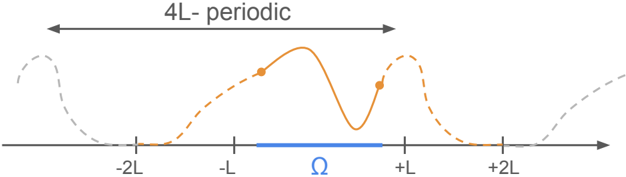<details> <summary>Image 9 Details</summary>  ### Visual Description \n ## Diagram: Periodic Function Representation ### Overview The image depicts a periodic function represented graphically. The function is shown over a range of 4L, with key points marked along the x-axis and a highlighted region labeled as Omega (Ω). The function appears to be a wave-like curve, potentially a trigonometric function. ### Components/Axes * **X-axis:** A horizontal line representing the independent variable. Marked with values -2L, -L, Ω, +L, and +2L. * **Y-axis:** Implicit, representing the dependent variable (function value). No explicit scale is provided. * **Periodic Function:** An orange, dashed-dotted line representing the function's curve. * **Omega (Ω) Region:** A blue horizontal bar indicating a specific interval on the x-axis. * **Arrow:** A double-headed arrow labeled "4L - periodic" indicating the period of the function. * **Key Points:** Two solid circles are placed on the orange curve, marking specific points on the function. ### Detailed Analysis The diagram shows a periodic function with a period of 4L. The function appears to be centered around the origin. * **X-axis Markers:** * -2L: Approximately at the leftmost extent of the visible curve. * -L: Approximately halfway between -2L and the origin. * Ω: Located near the origin, slightly to the right. * +L: Approximately halfway between the origin and +2L. * +2L: Approximately at the rightmost extent of the visible curve. * **Function Curve:** The orange curve starts at a low value at -2L, rises to a peak around -L, descends to a minimum near Ω, rises again to a peak around +L, and then descends towards +2L. * **Key Points on Curve:** * The first key point is located at approximately x = -0.7L, y = 1.2 (estimated from the curve's height). * The second key point is located at approximately x = +0.7L, y = -1.2 (estimated from the curve's height). * **Omega Region:** The blue bar spans from approximately x = -0.3L to x = +0.3L. ### Key Observations * The function is not symmetrical about the y-axis, suggesting it is not an even function. * The function has a period of 4L, as indicated by the arrow. * The Omega region appears to be centered around the origin. * The two marked points on the curve suggest a potential relationship or symmetry within the function. ### Interpretation The diagram illustrates a periodic function, likely used to demonstrate concepts in mathematics or physics, such as wave behavior or oscillatory systems. The "4L - periodic" label emphasizes the function's repeating nature over an interval of 4L. The Omega (Ω) region might represent a specific domain of interest or a boundary condition within a larger problem. The marked points on the curve could be significant values or solutions related to the function. The lack of a defined y-axis scale suggests the diagram is focused on the function's shape and periodicity rather than precise numerical values. The diagram is a conceptual representation, and the exact function is not defined. </details> Definition 3.3.1 (Linear differential operator) . Let s ∈ N . An operator D : H s (Ω) → L 2 (Ω) is a linear differential operator if, for all f ∈ H s (Ω) , $$\mathcal { D } ( f ) = \sum _ { | \alpha | \leqslant s } p _ { \alpha } \partial ^ { \alpha } f ,$$ where p α : Ω → R are functions such that max α ‖ p α ‖ ∞ < ∞ . (By definition, {| α | ⩽ s } = { α ∈ N d | ‖ α ‖ 1 ⩽ s } and ‖ · ‖ ∞ stands for the supremum norm of functions.) Given s , the linear differential operator D , and a training sample { ( X 1 , Y 1 ) , . . . , ( X n , Y n ) } , we consider the estimator ˆ f n that minimizes the regularized empirical risk (3.1) over the periodic Sobolev space H s per ([ -2 L, 2 L ] d ) . Recall that H s per ([ -2 L, 2 L ] d ) is the subspace of H s ([ -2 L, 2 L ] d ) consisting of functions whose 4 L -periodic extension is still s -times weakly differentiable. The important point to keep in mind is that any function of H s (Ω) can be extended to a function in H s per ([ -2 L, 2 L ] d ) (see Proposition 3.A.6 in the appendix), which makes it equivalent to suppose that f /star ∈ H s (Ω) or f /star ∈ H s per ([ -2 L, 2 L ] d ) , as shown in Theorem 3.4.6. The extension mechanism is illustrated in Figure 3.1. The key step to turn the minimization of (3.1) into a kernel method is to observe that any function f ∈ H s per ([ -2 L, 2 L ] d ) can be linearly mapped in L 2 ([ -2 L, 2 L ] d ) in such a way that the norm ‖ · ‖ L 2 ([ -2 L, 2 L ] d ) of the embedding is equal to λ n ‖ f ‖ 2 H s per ([ -2 L, 2 L ] d ) + µ n ‖ D ( f ) ‖ 2 L 2 (Ω) , i.e., the regularization term of (3.1). Proposition 3.3.2 below shows that this embedding takes the form of the inverse square root of a positive diagonalizable operator O n . Proposition 3.3.2 (Differential operator) . There exists a positive operator O n on L 2 ([ -2 L, 2 L ] d ) such that O -1 / 2 n : H s per ([ -2 L, 2 L ] d ) → L 2 ([ -2 L, 2 L ] d ) is well-defined and satisfies, for any f ∈ H s per ([ -2 L, 2 L ] d ) , $$\| \mathcal { O } _ { n } ^ { - 1 / 2 } ( f ) \| _ { L ^ { 2 } ( [ - 2 L , 2 L ] ^ { d } ) } ^ { 2 } = \lambda _ { n } \| f \| _ { H _ { p e r } ^ { s } ( [ - 2 L , 2 L ] ^ { d } ) } ^ { 2 } + \mu _ { n } \| \mathcal { D } ( f ) \| _ { L ^ { 2 } ( \Omega ) } ^ { 2 } .$$ Moreover, there is an orthonormal basis of eigenfunctions v m ∈ H s per ([ -2 L, 2 L ] d ) of O n associated with eigenvalues a m > 0 such that, for any f ∈ L 2 ([ -2 L, 2 L ] d ) , $$\forall x \in [ - 2 L , 2 L ] ^ { d } , \quad \mathcal { O } _ { n } ( f ) ( x ) = \sum _ { m \in \mathbb { N } } a _ { m } \langle f , v _ { m } \rangle _ { L ^ { 2 } ( [ - 2 L , 2 L ] ^ { d } ) } v _ { m } ( x ) .$$ Denote by δ x the Dirac distribution at x . Informally, the properties of the embedding O -1 / 2 n : H s per ([ -2 L, 2 L ] d ) → L 2 ([ -2 L, 2 L ] d ) in Proposition 3.3.2 suggest that something like $$f ( x ) ` ` = " ` \langle f , \delta _ { x } \rangle = \langle \mathcal { O } _ { n } ^ { - 1 / 2 } ( f ) , \mathcal { O } _ { n } ^ { 1 / 2 } ( \delta _ { x } ) \rangle _ { L ^ { 2 } ( [ - 2 L , 2 L ] ^ { d } ) }$$ should be true. In other terms, still informally , we may write f ( x ) = 〈 z, ψ ( x ) 〉 L 2 ([ -2 L, 2 L ] d ) , with z = O -1 / 2 n ( f ) , ψ ( x ) = O 1 / 2 n ( δ x ) , and ‖ z ‖ 2 L 2 ([ -2 L, 2 L ] d ) = λ n ‖ f ‖ 2 H s per ([ -2 L, 2 L ] d ) + µ n ‖ D ( f ) ‖ 2 L 2 (Ω) . We recognize a reproducing property, turning ψ into a kernel embedding associated with the risk (3.1). This mechanism is formalized in the following theorem. Theorem 3.3.3 (Kernel of linear PDEs) . Assume that s > d/ 2 , and let λ n > 0 , µ n ⩾ 0 . Let a m and v m be the eigenvalues and eigenfunctions of O n . Then the space H s per ([ -2 L, 2 L ] d ) , equipped with the inner product 〈 f, g 〉 RKHS = 〈 O -1 / 2 n f, O -1 / 2 n g 〉 L 2 ([ -2 L, 2 L ] d ) , is a reproducing kernel Hilbert space. In particular, - ( i ) The kernel K : [ -2 L, 2 L ] d × [ -2 L, 2 L ] d → R is defined by $$K ( x , y ) = \sum _ { m \in \mathbb { N } } a _ { m } v _ { m } ( x ) v _ { m } ( y ) .$$ - ( ii ) For all x ∈ [ -2 L, 2 L ] d , K ( x, · ) ∈ H s per ([ -2 L, 2 L ] d ) . - ( iii ) For all f ∈ H s per ([ -2 L, 2 L ] d ) , $$\forall x \in [ - 2 L , 2 L ] ^ { d } , \quad f ( x ) = \langle f , K ( x , \cdot ) \rangle _ { R K H S } .$$ - ( iv ) For all f ∈ H s per ([ -2 L, 2 L ] d ) , $$\| f \| _ { R K H S } ^ { 2 } = \lambda _ { n } \| f \| _ { H _ { p e r } ^ { s } ( [ - 2 L , 2 L ] ^ { d } ) } ^ { 2 } + \mu _ { n } \| \mathcal { D } ( f ) \| _ { L ^ { 2 } ( \Omega ) } ^ { 2 } .$$ sketch. The complete proof is given in Appendix 3.B. Only a rough sketch is given here by examining the simplified case where L = π/ 2 , Ω = [ -π, π ] d = [ -2 L, 2 L ] d , and D has constant coefficients. This means that we consider functions with periodic derivatives on Ω , penalized by the PDE on the whole domain [ -π, π ] d . It turns out that, in this case, the corresponding operator O n , satisfying $$\begin{array} { r } { \| \mathcal { O } _ { n } ^ { - 1 / 2 } ( f ) \| _ { L ^ { 2 } ( [ - \pi , \pi ] ^ { d } ) } ^ { 2 } = \lambda _ { n } \| f \| _ { H _ { p e r } ^ { s } ( [ - \pi , \pi ] ^ { d } ) } ^ { 2 } + \mu _ { n } \| \mathcal { D } ( f ) \| _ { L ^ { 2 } ( [ - \pi , \pi ] ^ { d } ) } ^ { 2 } \colon = \| f \| _ { R K H S } ^ { 2 } } \end{array}$$ has an explicit form. To see this, denote by FS the Fourier series operator. By the Parseval's theorem, for any frequency k ∈ Z d , one has FS( O -1 / 2 n ( f ))( k ) = √ a k FS( f )( k ) , where $$a _ { k } = \lambda _ { n } \sum _ { | \alpha | \leqslant s } \prod _ { j = 1 } ^ { d } k _ { j } ^ { 2 \alpha _ { j } } + \mu _ { n } \left ( \sum _ { | \alpha | \leqslant s } p _ { \alpha } \prod _ { j = 1 } ^ { d } k _ { j } ^ { \alpha _ { j } } \right ) ^ { 2 } .$$ Accordingly, O n is diagonalizable with eigenfunctions v k : x ↦→ exp( i 〈 k, x 〉 ) associated with the eigenvalues a -1 k . Next, using the Fourier decomposition of f , we have, for all x ∈ [ -π, π ] d , $$f ( x ) = \sum _ { k \in \mathbb { Z } ^ { d } } F S ( f ) ( k ) \exp ( i \langle k , x \rangle ) = \sum _ { k \in \mathbb { Z } ^ { d } } F S ( \mathcal { O } _ { n } ^ { - 1 / 2 } ( f ) ) ( k ) a _ { k } ^ { - 1 / 2 } \exp ( i \langle k , x \rangle ) .$$ Since a -1 k ⩽ λ -1 n ( ∑ | α | ⩽ s ∏ d j =1 k 2 α j j ) -1 , it is easy to check that ∑ k ∈ Z d a -1 k < ∞ and that the function ψ x such that FS( ψ x )( k ) = a -1 / 2 k exp( i 〈 k, x 〉 ) belongs to H s per ([ -π, π ] d ) . We therefore have the kernel formulation f ( x ) = 〈 O -1 / 2 n ( f ) , ψ x 〉 L 2 ([ -π,π ] d ) , where ‖ O -1 / 2 n ( f ) ‖ 2 L 2 ([ -π,π ] d ) = ‖ f ‖ 2 RKHS . The corresponding kernel is then defined by $$K ( x , y ) = \langle \psi _ { x } , \psi _ { y } \rangle _ { L ^ { 2 } ( [ - \pi , \pi ] ^ { d } ) } = \sum _ { k \in \mathbb { Z } ^ { d } } a _ { k } v _ { k } ( x ) \bar { v } _ { k } ( y ) .$$ The complete proof of Theorem 3.3.3 is more technical because, in our case Ω ⊊ [ -2 L, 2 L ] d and D may have non-constant coefficients. Thus, the operator O n is not diagonal in the Fourier space. To characterize its eigenvalues a m and eigenfunctions v m , we resort to classical results of PDE theory building upon functional analysis. The message of Theorem 3.3.3 is that minimizing the empirical risk (3.1) can be cast as a kernel method associated with the regularization λ n ‖ f ‖ 2 H s per ([ -2 L, 2 L ] d ) + µ n ‖ D ( f ) ‖ 2 L 2 (Ω) . In other words, (3.1) can be rewritten as $$\hat { f } _ { n } = \underset { f \in H _ { p e r } ^ { s } ( [ - 2 L , 2 L ] ^ { d } ) } { \arg \min } \, \frac { 1 } { n } \sum _ { i = 1 } ^ { n } | f ( X _ { i } ) - Y _ { i } | ^ { 2 } + \| f \| _ { R K H S } ^ { 2 } .$$ This result is interesting in itself because it fundamentally shows that a PIML estimator (and therefore its variants implemented in practice, such as PINNs) can be regarded as a kernel estimator. Note however that computing K ( x, y ) is not always straightforward and may require the use of numerical techniques. This kernel is characterized by the following weak formulation. Proposition 3.3.4 (Kernel characterization) . The kernel K is the unique solution to the following weak formulation, valid for all test functions φ ∈ H s per ([ -2 L, 2 L ] d ) , $$\forall x \in \Omega , \quad \lambda _ { n } \sum _ { | \alpha | \leqslant s } \int _ { [ - 2 L , 2 L ] ^ { d } } \partial ^ { \alpha } K ( x , \cdot ) \, \partial ^ { \alpha } \phi + \mu _ { n } \int _ { \Omega } \mathcal { D } ( K ( x , \cdot ) ) \, \mathcal { D } ( \phi ) = \phi ( x ) .$$ Regardless of the analytical computation of K , formulating the problem as a minimization in a reproducing kernel Hilbert space provides a way to quantify the impact of the physical regularization on the estimator's convergence rate, which is our primary goal. ## 3.4 Convergence rates The results of the previous section allow us to draw on the existing literature on kernel learning to gain a deeper understanding of the properties of the estimator ˆ f n and the influence of the operator D on the convergence rate. ## Eigenvalues of the integral operator The convergence rate of ˆ f n to f /star is determined by the decay speed of the eigenvalues of the so-called integral operator L K : L 2 (Ω , P X ) → L 2 (Ω , P X ) , defined by $$\forall f \in L ^ { 2 } ( \Omega , \mathbb { P } _ { X } ) , \forall x \in \Omega , \quad L _ { K } f ( x ) = \int _ { \Omega } K ( x , y ) f ( y ) d \mathbb { P } _ { X } ( y ) ,$$ where P X is the distribution of X on Ω [e.g., CV07]. Note that the integral in the definition of L K could also have been taken over [ -2 L, 2 L ] d because the support of P X is included in ¯ Ω . However, finding the eigenvalues of L K is not an easy task-even when X is uniformly distributed on Ω -, not to mention the fact that P X is usually unknown in real applications. Nevertheless, we show in Theorem 3.4.2 that these eigenvalues can be bounded by the eigenvalues of the operator C O n C , where C is the projection on Ω defined below. Importantly, C O n C no longer depends on P X . Moreover, its non-zero eigenvalues are characterized by a weak formulation, as we will see in Theorem 3.4.5. Definition 3.4.1 (Projection on Ω ) . Let C be the operator on L 2 ([ -2 L, 2 L ] d ) defined by Cf = f 1 Ω . Then C 2 = C , i.e., C is a projector , and $$\langle f , C ( g ) \rangle _ { L ^ { 2 } ( [ - 2 L , 2 L ] ^ { d } ) } = \int _ { [ - 2 L , 2 L ] ^ { d } } f g 1 _ { \Omega } = \langle C ( f ) , g \rangle _ { L ^ { 2 } ( [ - 2 L , 2 L ] ^ { d } ) } ,$$ i.e., C is self-adjoint. As for now, it is assumed that the distribution P X of X has a density d P X dx with respect to the Lebesgue measure on Ω . Theorem 3.4.2 (Kernels and eigenvalues) . Let K : [ -2 L, 2 L ] d × [ -2 L, 2 L ] d → R be the kernel of Theorem 3.3.3. Assume that there exists κ > 0 such that d P X dx ⩽ κ . Then the eigenvalues a m ( L K ) of L K are bounded by the eigenvalues a m ( C O n C ) of C O n C on L 2 ([ -2 L, 2 L ] d ) in such a way that a m ( L K ) ⩽ κa m ( C O n C ) . ## Effective dimension and convergence rate We will see in the next subsection how to compute the eigenvalues of C O n C . Yet, assuming we have them at hand, it is then possible to obtain a bound on the rate of convergence of ˆ f n to f /star by bounding the so-called effective dimension of the kernel [CV07], defined by $$\mathcal { N } ( \lambda _ { n } , \mu _ { n } ) = t r ( L _ { K } ( I d + L _ { K } ) ^ { - 1 } ) ,$$ where Id is the identity operator, i.e., Id( f ) = f , and the symbol tr stands for the trace, i.e., the sum of the eigenvalues. Lemma 3.D.1 in the appendix shows that, whenever d P X dx ⩽ κ , $$\mathcal { N } ( \lambda _ { n } , \mu _ { n } ) \leqslant \sum _ { m \in \mathbb { N } } \frac { 1 } { 1 + ( \kappa a _ { m } ( C \mathcal { O } _ { n } C ) ) ^ { - 1 } } .$$ Putting all the pieces together, we have the following theorem, which bounds the estimation error between ˆ f n and f /star . Theorem 3.4.3 (Convergence rate) . Assume that s > d/ 2 , f /star ∈ H s (Ω) , d P X dx ⩽ κ for some κ > 0 , µ n ⩾ 0 , lim n →∞ λ n = lim n →∞ µ n = lim n →∞ λ n /µ n = 0 , λ n ⩾ n -1 , and N ( λ n , µ n ) λ -1 n = o n ( n ) . Assume, in addition, that, for some σ > 0 and M > 0 , the noise ε satisfies $$\forall \ell \in \mathbb { N } , \quad \mathbb { E } ( | \varepsilon | ^ { \ell } \, | \, X ) \leqslant \frac { 1 } { 2 } \ell ! \, \sigma ^ { 2 } \, M ^ { \ell - 2 } .$$ Then, for some constant C 4 > 0 and n large enough, $$\begin{array} { r l } & { \mathbb { E } \int _ { \Omega } | \hat { f } _ { n } - f ^ { * } | ^ { 2 } d \mathbb { P } _ { X } } \\ & { \quad \leqslant C _ { 4 } \log ^ { 2 } ( n ) \left ( \lambda _ { n } \| f ^ { * } \| _ { H ^ { s } ( \Omega ) } ^ { 2 } + \mu _ { n } \| \mathcal { D } ( f ^ { * } ) \| _ { L ^ { 2 } ( \Omega ) } ^ { 2 } + \frac { M ^ { 2 } } { n ^ { 2 } \lambda _ { n } } + \frac { \sigma ^ { 2 } \mathcal { W } ( \lambda _ { n } , \mu _ { n } ) } { n } \right ) . } \end{array}$$ The sub-Gamma assumption (3.4) on the noise ε is quite general and is satisfied in particular when ε is bounded (possibly depending on X ), or when ε is Gaussian and independent of X [e.g., BLM13, Theorem 2.10]. We stress that the result of Theorem 3.4.3 is general and holds regardless of the form of the linear differential operator D . A simple bound on N ( λ n , µ n ) , neglecting the dependence in D , allows to show that the PIML estimator converges at least at the Sobolev minimax rate over the class H s (Ω) . Proposition 3.4.4 (Minimum rate) . Suppose that the assumptions of Theorem 3.4 are verified, and let λ n = n -2 s/ (2 s + d ) √ log( n ) and µ n = λ n √ log( n ) . Then the estimator ˆ f n converges at a rate at least larger than the Sobolev minimax rate, up to a log term, i.e., $$\mathbb { E } \int _ { \Omega } | \hat { f } _ { n } - f ^ { ^ { * } } | ^ { 2 } d \mathbb { P } _ { X } = \mathcal { O } _ { n } \left ( n ^ { - 2 s / ( 2 s + d ) } \log ^ { 3 } ( n ) \right ) .$$ However, this is only an upper bound, and we expect situations where ˆ f n has a faster convergence rate thanks to the inclusion of the physical penalty ‖ D ( f ) ‖ L 2 (Ω) . Such an improvement will depend on the magnitude of the modeling error ‖ D ( f /star ) ‖ L 2 (Ω) and on the effective dimension N ( λ n , µ n ) . To achieve this goal, the eigenvalues a m of C O n C must be characterized and then plugged into inequality (3.3). This is the problem addressed in the next subsection. ## Characterizing the eigenvalues The goal of this section is to specify the spectrum of C O n C . It is worth noting that ker( C O n C ) is not empty, as it encompasses every smooth function with compact support in ] -2 L, 2 L [ d \ ¯ Ω . The next theorem characterizes the eigenfunctions associated with non-zero eigenvalues and shows that they are in fact smooth functions on Ω and ( ¯ Ω) c satisfying two PDEs. Theorem 3.4.5 (Eigenfunction characterization) . Assume that s > d/ 2 and that the functions p α in Definition 3.3.1 belong to C ∞ (Ω) . Let a m > 0 be a positive eigenvalue of the operator C O n C . Then the corresponding eigenfunction v m satisfies v m = a -1 m Cw m , where w m ∈ H s per ([ -2 L, 2 L ] d ) . Moreover, for any test function φ ∈ H s per ([ -2 L, 2 L ] d ) , $$\lambda _ { n } \sum _ { | \alpha | \leqslant s } \int _ { [ - 2 L , 2 L ] ^ { d } } \partial ^ { \alpha } w _ { m } \, \partial ^ { \alpha } \phi + \mu _ { n } \int _ { \Omega } \mathcal { D } ( w _ { m } ) \, \mathcal { D } ( \phi ) = a _ { m } ^ { - 1 } \int _ { \Omega } w _ { m } \phi .$$ In particular, any solution of the weak formulation (3.5) satisfies the following PDE system: - ( i ) w m ∈ C (Ω) and $$\forall x \in \Omega , \quad \lambda _ { n } \sum _ { | \alpha | \leqslant s } ( - 1 ) ^ { | \alpha | } \partial ^ { 2 \alpha } w _ { m } ( x ) + \mu _ { n } \mathcal { D } ^ { * } \mathcal { D } w _ { m } ( x ) = a _ { m } ^ { - 1 } w _ { m } ( x ) ,$$ $$\left ( i \right ) \ w _ { m } \in C ^ { \infty } ( \Omega ) \, a n d \\ \forall x \in \Omega , \quad \lambda _ { n } \sum \left ( - 1 \right ) ^ { | \alpha | } \partial ^ { 2 \alpha } w _ { m } ( x ) + \mu _ { n } \mathcal { D } ^ { * } \mathcal { D } w _ { m } ( x ) = a _ { m } ^ { - 1 } w _ { m } ( x ) ,$$ $$\begin{array} { r l } & { w h e r e \mathcal { D } ^ { * } ( f ) \colon = \sum _ { | \alpha | \leqslant s } ( - 1 ) ^ { | \alpha | } \partial ^ { \alpha } ( p _ { \alpha } f ) \ i s t h e a d j o i n t o p e r a t o r o f \mathcal { D } . } \\ & { ( i i ) \ w _ { m } \in C ^ { \infty } ( [ - 2 L , 2 L ] ^ { d } \bar { \Omega } ) \ a n d } \end{array} \begin{array} { r l } & { w h e r e \mathcal { D } ^ { * } ( f ) \colon = \sum _ { | \alpha | \leqslant s } ( - 1 ) ^ { | \alpha | } \partial ^ { \alpha } ( p _ { \alpha } f ) i s t h e a d j o i n t o p e r a t o r o f \mathcal { D } . } \\ & { ( i i ) \ w _ { m } \in C ^ { \infty } ( [ - 2 L , 2 L ] ^ { d } \bar { \Omega } ) \, a n d } \end{array}$$ <!-- formula-not-decoded --> $$( i i ) \ w _ { m } \in C ^ { \infty } ( [ - 2 L , 2 L ] ^ { d } \bar { \Omega } ) \, a n d$$ $$\forall x \in [ - 2 L , 2 L ] ^ { d } \bar { \Omega } , \quad \sum _ { | \alpha | \leqslant s } ( - 1 ) ^ { | \alpha | } \partial ^ { 2 \alpha } w _ { m } ( x ) = 0 .$$ Notice that w m might be irregular on the boundary ∂ Ω , but only there. Theorem 3.4.5 is important insofar as it allows to characterize the positive eigenvalues a m of the operator C O n C . Indeed, these eigenvalues are the only real numbers such that the weak formulation (3.5) admits a solution. This weak formulation has to be solved in a case-by-case study, given the differential operator D . As an illustration, an example is presented in the next section with D = d dx . ## The choice of Sobolev regularization is unimportant So far, we have considered problem (3.1) with the Sobolev regularization ‖ f ‖ 2 H s per ([ -2 L, 2 L ] d ) . However, other choices of Sobolev norms, such as ‖ f ‖ 2 H s (Ω) , are also possible. Fortunately, this choice does not affect the effective dimension N ( λ n , µ n ) , and thus the convergence rate in Theorem 3.4.3. Theorem 3.4.6 (Equivalent regularities and effective dimension) . Assume that s > d/ 2 . Then the following three estimators correspond each to a kernel learning problem: $$1 2$$ $$\hat { f } _ { n } ^ { ( 3 ) } = \underset { f \in H ^ { s } ( \Omega ) } { \arg \min } \frac { 1 } { n } \sum _ { i = 1 } ^ { n } | f ( X _ { i } ) - Y _ { i } | ^ { 2 } + \lambda _ { n } \| f \| ^ { 2 } + \mu _ { n } \| \mathcal { D } ( f ) \| _ { L ^ { 2 } ( \Omega ) } ^ { 2 } ,$$ $$\begin{array} { r l } & { \hat { f } _ { n } ^ { ( 1 ) } = \arg \min _ { f \in H ^ { s } ( \Omega ) } \frac { 1 } { n } \sum _ { i = 1 } ^ { n } | f ( X _ { i } ) - Y _ { i } | ^ { 2 } + \lambda _ { n } \| f \| _ { H ^ { s } ( \Omega ) } ^ { 2 } + \mu _ { n } \| \mathcal { D } ( f ) \| _ { L ^ { 2 } ( \Omega ) } ^ { 2 } , } \\ & { \hat { f } _ { n } ^ { ( 2 ) } = \arg \min _ { f \in H _ { p e r } ^ { s } ( [ - 2 L , 2 L ] ^ { d } ) } \frac { 1 } { n } \sum _ { i = 1 } ^ { n } | f ( X _ { i } ) - Y _ { i } | ^ { 2 } + \lambda _ { n } \| f \| _ { H _ { p e r } ^ { s } ( [ - 2 L , 2 L ] ^ { d } ) } ^ { 2 } + \mu _ { n } \| \mathcal { D } ( f ) \| _ { L ^ { 2 } ( \Omega ) } ^ { 2 } , } \\ & { \hat { f } _ { n } ^ { ( 3 ) } = \arg \min _ { f \in H _ { p e r } ^ { s } ( \Omega ) } \frac { 1 } { n } \sum _ { i = 1 } ^ { n } | f ( X _ { i } ) - Y _ { i } | ^ { 2 } + \lambda _ { n } \| f \| ^ { 2 } + \mu _ { n } \| \mathcal { D } ( f ) \| _ { L ^ { 2 } ( \Omega ) } ^ { 2 } , } \end{array}$$ where ‖·‖ is any of the equivalent Sobolev norms. Moreover, these three estimators share equivalent effective dimensions N ( λ n , µ n ) . Accordingly, they share the same upper bound on the convergence rate given by Theorem 3.4.3. The incorporation of a Sobolev regularization in the empirical risk function is needed to guarantee that ˆ f n has good statistical properties. For example, even with the simplest PDEs, the minimizer of 1 n ∑ n i =1 | f ( X i ) -Y i | 2 + µ n ‖ D ( f ) ‖ 2 L 2 (Ω) might always be 0 , independently of the data points ( X i , Y i ) [see, e.g., DBB25, Example 5.1]. A way to overcome these statistical issues is to specify the boundary conditions, and to consider regular differential operators D and smooth domain Ω . For example, Azzimonti et al. [Azz+15], Arnone et al. [Arn+22], and Ferraccioli et al. [FSF22] consider models such that f /star | ∂ Ω = 0 , where Ω is an Euclidean ball of R d and D are second-order elliptic operators. However, these assumptions amount to adding a Sobolev penalty, since, in this case, ‖ D ( f ) ‖ L 2 (Ω) and ‖ f ‖ H 2 0 (Ω) are equivalent norms [e.g., Eva10, Chapter 6.3, Theorem 4]. Similar results hold for second order parabolic PDEs [Eva10, Chapter 7.1, Theorem 5] and for second order hyperbolic PDEs [Eva10, Chapter 7.2, Theorem 2]. The need for a Sobolev regularization is explained by the fact that the Sobolev embedding H s (Ω) ↪ → C 0 (Ω) only holds for s > d/ 2 . In other words, the Sobolev regularization is needed to give a sense to the pointwise evaluations | f ( X i ) -Y i | . ## 3.5 Application: speed-up effect of the physical penalty Our objective is to apply the framework presented above to the case d = 1 , Ω = [ -L, L ] , s = 1 , f /star ∈ H 1 (Ω) , and D = d dx . Of course, assuming that D ( f /star ) /similarequal 0 is a strong assumption, equivalent to assuming that f /star is approximately constant. However, the goal of this section is to provide a simple illustration where the kernel K of Theorem 3.3.3 can be analytically computed and the eigenvalues of the operator L K can be effectively bounded. The next result is a consequence of Proposition 3.3.4. Proposition 3.5.1 (One-dimensional kernel) . Assume that s = 1 , Ω = [ -L, L ] , and D = d dx . Then, letting γ n = √ λ n λ n + µ n , one has, for all x, y ∈ [ -L, L ] , $$K ( x , y ) = \frac { \gamma _ { n } } { 2 \lambda _ { n } \sinh ( 2 \gamma _ { n } L ) } & \left ( ( \cosh ( 2 \gamma _ { n } L ) + \cosh ( 2 \gamma _ { n } x ) ) \cosh ( \gamma _ { n } ( x - y ) ) \\ & + ( ( 1 - 2 \times 1 _ { x > y } ) \sinh ( 2 \gamma _ { n } L ) - \sinh ( 2 \gamma _ { n } x ) ) \sinh ( \gamma _ { n } ( x - y ) ) \right ) .$$ An example of kernel K with L = 1 and λ n = µ n = 1 is shown in Figure 3.2. Following the strategy of Section 3.4, it remains to bound the positive eigenvalues a m of the operator C O n C using Theorem 3.4.5. According to the latter, this is achieved by solving the weak formulation $$\forall \phi \in H _ { p e r } ^ { 1 } ( [ - 2 L , 2 L ] ) , \quad \lambda _ { n } \int _ { [ - 2 L , 2 L ] ^ { d } } w _ { m } \phi + ( \lambda _ { n } + \mu _ { n } ) \int _ { \Omega } \frac { d } { d x } w _ { m } \, \frac { d } { d x } \phi = a _ { m } ^ { - 1 } \int _ { \Omega } w _ { m } \phi .$$ Proposition 3.5.2 (One-dimensional eigenvalues) . Assume that s = 1 , Ω = [ -L, L ] , and D = d dx . Then, for all m ⩾ 3 , $$\frac { 4 L ^ { 2 } } { ( \lambda _ { n } + \mu _ { n } ) ( m + 4 ) ^ { 2 } \pi ^ { 2 } } \leqslant a _ { m } \leqslant \frac { 4 L ^ { 2 } } { ( \lambda _ { n } + \mu _ { n } ) ( m - 2 ) ^ { 2 } \pi ^ { 2 } } ,$$ where a m are the eigenvalues of C O n C . Using inequality (3.3), we can then bound the effective dimension of the kernel. This allows us, via Theorem 3.4.3, to specify the convergence rate of ˆ f n to f /star . Theorem 3.5.3 (Kernel speed-up) . Assume that f /star ∈ H 1 ([ -L, L ]) , d P X dx ⩽ κ for some κ > 0 , and the noise ε satisfies the sub-Gamma condition (3.4) . Let λ n = n -1 log( n ) and /negationslash $$\mu _ { n } = \left \{ \begin{array} { l l } { n ^ { - 2 / 3 } / \| \mathcal { D } ( f ^ { * } ) \| _ { L ^ { 2 } ( \Omega ) } } & { i f \quad \| \mathcal { D } ( f ^ { * } ) \| _ { L ^ { 2 } ( \Omega ) } \neq 0 } \\ { 1 / \log ( n ) } & { i f \quad \| \mathcal { D } ( f ^ { * } ) \| _ { L ^ { 2 } ( \Omega ) } = 0 . } \end{array}$$ Then the estimator ˆ f n of f /star minimizing the empirical risk function (3.1) with s = 1 and D = d dx satisfies $$\mathbb { E } \int _ { [ - L , L ] } | \hat { f } _ { n } - f ^ { * } | ^ { 2 } d \mathbb { P } _ { X } & = \| \mathcal { D } ( f ^ { * } ) \| _ { L ^ { 2 } ( \Omega ) } \, \mathcal { O } _ { n } \left ( n ^ { - 2 / 3 } \log ^ { 3 } ( n ) \right ) \\ & + ( \| f ^ { * } \| _ { H ^ { 1 } ( \Omega ) } ^ { 2 } + \sigma ^ { 2 } + M ^ { 2 } ) \mathcal { O } _ { n } \left ( n ^ { - 1 } \log ^ { 3 } ( n ) \right ) .$$ This bound reflects the benefit of the physical penalty ‖ D ( f /star ) ‖ L 2 (Ω) on the performance of the estimator ˆ f n . Indeed, when ‖ D ( f /star ) ‖ L 2 (Ω) = 0 (i.e., the physical model is perfect), then f /star is a constant function, and the PIML method recovers the parametric convergence rate of n -1 . Here, the physical information directly improves the convergence rate. Otherwise, when ‖ D ( f /star ) ‖ L 2 (Ω) > 0 , we recover the Sobolev minimax convergence rate in H 1 (Ω) of n -2 / 3 [up to a log factor-see Tsy09, Theorem 2.11]. We emphasize that this rate is also optimal for our problem, since ‖ D ( f /star ) ‖ L 2 (Ω) ⩽ ‖ f /star ‖ H 1 (Ω) , i.e., it is as hard to learn a function of bounded ‖ D ( · ) ‖ L 2 (Ω) norm as it is to learn a function of bounded H 1 (Ω) norm. In this case, the benefit of physical modeling is carried by the constant ‖ D ( f /star ) ‖ L 2 (Ω) in front of the convergence rate, i.e., the better the modeling, the smaller the estimation error. Note Fig. 3.2.: Kernel K of Proposition 3.5.1 with L = 1 , λ n = µ n = 1 . 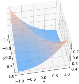<details> <summary>Image 10 Details</summary>  ### Visual Description \n ## 3D Surface Plot: Function Visualization ### Overview The image depicts a 3D surface plot, visualizing a function of two variables, 'x' and 'y'. The surface is colored with a gradient, transitioning from a light blue to a light orange. The plot is rendered in a perspective view, showing the surface extending from a base plane defined by the x and y axes, with the z-axis representing the function's output. There is no explicit legend or labels for the color gradient. ### Components/Axes * **X-axis:** Labeled 'x', ranging approximately from -1.0 to 1.0. * **Y-axis:** Labeled 'y', ranging approximately from -1.0 to 1.0. * **Z-axis:** Represents the function's value, ranging approximately from 0.4 to 0.7. * **Surface:** The plotted surface represents the function's output for different combinations of x and y values. The surface is divided into two distinct color regions. ### Detailed Analysis The surface exhibits a clear curvature. * **Blue Region:** The blue region occupies the majority of the surface, extending from approximately x = -1.0 to x = 0.5 and y = -1.0 to y = 1.0. The z-values in this region appear to be relatively constant, around 0.5 to 0.6. * **Orange Region:** The orange region is located on the right side of the plot, extending from approximately x = 0.5 to x = 1.0 and y = -1.0 to y = 1.0. The z-values in this region decrease as x increases, ranging from approximately 0.6 to 0.4. The surface appears to be smooth and continuous, with no sharp edges or discontinuities. The transition between the blue and orange regions is gradual. ### Key Observations * The function appears to have a maximum value around x = -1.0 and y = 0.0. * The function decreases as x increases beyond approximately x = 0.5. * The function is relatively insensitive to changes in y, particularly in the blue region. * The color gradient does not have a clear numerical mapping, but it visually represents the function's value. ### Interpretation The plot visualizes a function that is relatively flat across a large portion of its domain (the blue region). As the x-value increases beyond a certain point, the function begins to decrease. The shape of the surface suggests a possible quadratic or polynomial function. The absence of a legend makes it difficult to determine the exact relationship between the color gradient and the function's value, but it appears to be a visual aid to highlight the surface's curvature and relative height. The plot could be representing a simplified model of a physical phenomenon, such as the height of a landscape or the distribution of a scalar field. Without further information about the function itself, it is difficult to draw more specific conclusions. </details> however that the parameter µ n in Theorem 3.5.3 depends on the unknown physical inconsistency ‖ D ( f /star ) ‖ L 2 (Ω) . In practice, on may resort to a cross-validation-type strategy to estimate µ n . We conclude this section with a small numerical experiment 1 illustrating Theorem 3.5.3. We consider two problems: a perfect modeling situation where Y = 1 + ε , and an imperfect modeling one where Y = 1 + 0 . 1 | X | + ε . In both cases, X ∼ U ([ -1 , 1]) and ε ∼ N (0 , 1) . The difference is that in the perfect modeling case, D ( f /star ) = 0 , whereas in the imperfect situation ‖ D ( f /star ) ‖ 2 L 2 ([ -1 , 1]) = 2 / 300 . For each n , we let err( n ) = E ∫ Ω | ˆ f n -f /star | 2 d P X . Figure 3.3 shows the values of log(err)( n ) as a function of log( n ) , for n ranging from 10 to 10000 (the quantity log(err)( n ) is estimated by an empirical mean over 500-sample Monte Carlo estimations, repeated ten times). The experimental convergence rates obtained by fitting linear regressions are -1 . 02 in the perfect modeling case and -0 . 77 in the imperfect one. These experimental rates are consistent with the results of Theorem 3.5.3, insofar as -1 . 02 ⩽ -1 and -0 . 77 ⩽ -2 / 3 . ## 3.6 Conclusion From the physics-informed machine learning point of view, we have shown that minimizing the empirical risk regularized by a PDE can be viewed as a kernel method. Leveraging kernel theory, we have explained how to derive convergence rates. In particular, the simple but instructive example D = d dx illustrates how to compute both the kernel and the convergence rate of the associated estimator. To the best of our knowledge, this is the first contribution that demonstrates tangible improvements in convergence rates by including a physical penalty in 1 The code to reproduce all numerical experiments can be found here. Fig. 3.3.: Error bounds err( n ) (mean ± std over 10 runs) of the kernel estimator ˆ f n with respect to the sample size n , in log-log scale, for the perfect modeling case (left) and the imperfect one (right). The experimental convergence rates, obtained by fitting a linear regression, are displayed in orange dotted. 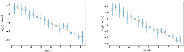<details> <summary>Image 11 Details</summary>  ### Visual Description \n ## Chart: Log(L^2 error) vs. Log(n) ### Overview The image presents two identical scatter plots displaying the relationship between log(L^2 error) and log(n). Each plot shows a series of data points represented by blue star markers with error bars, and a superimposed orange line indicating a trend. The plots appear to be comparing the error rate as a function of the input size, likely in a machine learning or statistical modeling context. ### Components/Axes * **X-axis Label:** log(n) - ranging from approximately 2 to 9. * **Y-axis Label:** log(L^2 error) - ranging from approximately -2 to -10 in the left plot and -2 to -8 in the right plot. * **Data Points:** Blue star markers with vertical error bars. * **Trend Line:** Orange solid line. * **No Legend:** There is no explicit legend, but the orange line clearly represents a fitted trend to the data points. ### Detailed Analysis or Content Details **Left Plot:** The trend line slopes downward, indicating that as log(n) increases, log(L^2 error) decreases. This suggests that the error decreases as 'n' increases. * At log(n) ≈ 2, log(L^2 error) ≈ -1.8. * At log(n) ≈ 3, log(L^2 error) ≈ -3. * At log(n) ≈ 4, log(L^2 error) ≈ -4.2. * At log(n) ≈ 5, log(L^2 error) ≈ -5.2. * At log(n) ≈ 6, log(L^2 error) ≈ -6.1. * At log(n) ≈ 7, log(L^2 error) ≈ -7.1. * At log(n) ≈ 8, log(L^2 error) ≈ -8.2. * At log(n) ≈ 9, log(L^2 error) ≈ -9.3. **Right Plot:** The trend line also slopes downward, similar to the left plot. * At log(n) ≈ 2, log(L^2 error) ≈ -1.8. * At log(n) ≈ 3, log(L^2 error) ≈ -3. * At log(n) ≈ 4, log(L^2 error) ≈ -4.2. * At log(n) ≈ 5, log(L^2 error) ≈ -5.2. * At log(n) ≈ 6, log(L^2 error) ≈ -6.1. * At log(n) ≈ 7, log(L^2 error) ≈ -7.1. * At log(n) ≈ 8, log(L^2 error) ≈ -8.2. * At log(n) ≈ 9, log(L^2 error) ≈ -8.6. The error bars indicate the variability or uncertainty associated with each data point. The length of the error bars appears relatively consistent across the range of log(n) values. ### Key Observations * Both plots exhibit a strong negative correlation between log(n) and log(L^2 error). * The trend lines in both plots are nearly identical, suggesting consistent results. * The error bars provide a measure of the data's spread around the trend line. * The right plot has slightly higher error values at log(n) = 9 than the left plot. ### Interpretation The plots demonstrate a clear relationship between the size of the input ('n') and the error rate (L^2 error). The negative correlation suggests that as the input size increases, the error decreases. This is a common observation in many machine learning algorithms, where more data typically leads to better model performance. The logarithmic scale on both axes indicates that the relationship may not be linear, but rather follow a power law or similar functional form. The error bars provide a measure of the uncertainty in the error estimates, which is important for assessing the reliability of the results. The fact that the two plots are nearly identical suggests that the observed relationship is robust and not specific to a particular dataset or experimental setup. The plots likely represent a learning curve, showing how the error decreases as the model is trained on more data. </details> the risk function. Thus, the take-home message is that physical information can be beneficial to the statistical performance of the estimators. Note that our work does not include boundary conditions h , but they could easily be considered. A first solution is to add another penalty to R n of the form ‖ h -f ‖ 2 2 , which would insert the extra term ∫ ( K ( x, · ) -h ) φ in Proposition 3.3.4. A second solution is to enforce the conditions at new data points X j sampled on ∂ Ω sample, provided that f /star | ∂ Ω = h . L ( ∂ Ω) ∂ Ω ( b ) [as done, for example, in RPK19]. Our theorems hold for this extended training An important future research direction is to implement numerical strategies for computing the kernel K in the general case. If successful, such strategies can then be used directly to solve general physics-informed machine learning problems. In order to derive theoretical guarantees, we need to go further by obtaining bounds on the eigenvalues of the operator associated with the problem. The key lies in Theorem 3.4.5, which characterizes the eigenvalues by a weak formulation. Once established, such bounds can be employed to obtain accurate rates for related techniques, typically physics-informed neural networks. It would also be interesting to derive rates of convergence in the setting s ⩽ d/ 2 using the so-called source condition [e.g., BM20]. An even more ambitious goal is to generalize the approach to nonlinear differential systems, for example polynomial. Overall, we believe that our results pave the way for a deeper understanding of the impact of physical regularization on empirical risk minimization performance. ## 3.A Some fundamentals of functional analysis ## Sobolev spaces Norms. The p norm ‖ x ‖ p of a d -dimensional vector x = ( x 1 , . . . , x d ) is defined by ‖ x ‖ p = ( 1 d ∑ d i =1 | x i | p ) 1 /p . For a function f : Ω → R , we let ‖ f ‖ L p (Ω) = ( 1 | Ω | ∫ Ω | f | p ) 1 /p . Similarly, ‖ f ‖ ∞ , Ω = sup x ∈ Ω | f ( x ) | . For the sake of conciseness, we sometimes write ‖ f ‖ ∞ instead of ‖ f ‖ ∞ , Ω . Multi-indices and partial derivatives. For a multi-index α = ( α 1 , . . . , α d ) ∈ N d and a differentiable function f : R d → R , the α partial derivative of f is defined by $$\partial ^ { \alpha } f = ( \partial _ { 1 } ) ^ { \alpha _ { 1 } } \dots ( \partial _ { d } ) ^ { \alpha _ { d } } f .$$ The set of multi-indices of sum less than k is defined by $$\{ | \alpha | \leqslant k \} = \{ ( \alpha _ { 1 } , \dots , \alpha _ { d _ { 1 } } ) \in \mathbb { N } ^ { d } , \alpha _ { 1 } + \cdots + \alpha _ { d _ { 1 } } \leqslant k \} .$$ If α = 0 , ∂ α f = f . Given two multi-indices α and β , we write α ⩽ β when α i ⩽ β i for all 1 ⩽ i ⩽ d . The set of multi-indices less than α is denoted by { β ⩽ α } . For a multi-index α such that | α | ⩽ k , both sets {| β | ⩽ k } and { β ⩽ α } are contained in { 0 , . . . , k } d and are therefore finite. Hölder norm. For K ∈ N , the Hölder norm of order K of a function f ∈ C K (Ω , R ) is defined by ‖ f ‖ C K (Ω) = max | α | ⩽ K ‖ ∂ α f ‖ ∞ , Ω . This norm allows to bound a function as well as its derivatives. The space C K (Ω , R ) endowed with the Hölder norm ‖ · ‖ C K (Ω) is a Banach space. The space C ∞ ( ¯ Ω , R d 2 ) is defined as the subspace of continuous functions f : ¯ Ω → R satisfying f | Ω ∈ C ∞ (Ω , R ) and, for all K ∈ N , ‖ f ‖ C K (Ω) < ∞ . Lipschitz function. Given a normed space ( V, ‖·‖ ) , the Lipschitz norm of a function f : V → R d is defined by $$\| f \| _ { L i p } = \sup _ { x , y \in V } \frac { \| f ( x ) - f ( y ) \| _ { 2 } } { \| x - y \| } .$$ A function f is Lipschitz if ‖ f ‖ Lip < ∞ . The mean value theorem implies that for all f ∈ C 1 ( V, R ) , ‖ f ‖ Lip ⩽ ‖ f ‖ C 1 ( V ) . Lipschitz surface and domain. A surface Γ ⊆ R d is said to be Lipschitz if locally , in a neighborhood U ( x ) of any point x ∈ Γ , an appropriate rotation r x of the coordinate system transforms Γ into the graph of a Lipschitz function φ x , i.e., $$r _ { x } ( \Gamma \cap U ( x ) ) = \{ ( x _ { 1 } , \dots , x _ { d - 1 } , \phi _ { x } ( x _ { 1 } , \dots , x _ { d - 1 } ) ) , \forall ( x _ { 1 } , \dots , x _ { d } ) \in r _ { x } ( \Gamma \cap U _ { x } ) \} .$$ A domain Ω ⊆ R d is said to be Lipschitz if its has Lipschitz boundary and lies on one side of it, i.e., φ x < 0 or φ x > 0 on all intersections Ω ∩ U x . All manifolds with C 1 boundary and all convex domains are Lipschitz domains [e.g., Agr15]. Sobolev spaces. Let Ω ⊆ R d be an open set. A function g ∈ L 2 (Ω , R ) is said to be the α th weak derivative of f ∈ L 2 (Ω , R ) if, for all φ ∈ C ∞ ( ¯ Ω , R ) with compact support in Ω , one has ∫ Ω gφ = ( -1) | α | ∫ Ω f∂ α φ . This is denoted by g = ∂ α f . For s ∈ N , the Sobolev space H s (Ω) is the space of all functions f ∈ L 2 (Ω , R ) such that ∂ α f exists for all | α | ⩽ s . This space is naturally endowed with the norm $$\| f \| _ { H ^ { s } ( \Omega ) } = \left ( \sum _ { | \alpha | \leqslant s } \| \partial ^ { \alpha } u \| _ { L ^ { 2 } ( \Omega ) } ^ { 2 } \right ) ^ { 1 / 2 } .$$ Of course, if a function f belongs to the Hölder space C K ( ¯ Ω , R ) , then it belongs to the Sobolev space H K (Ω) , and its weak derivatives are the usual derivatives. For more on Sobolev spaces, we refer the reader to Evans [Eva10, Chapter 5]. Fundamental results on Sobolev spaces. Let Ω ⊆ R d be an open set and let s ∈ N be an order of differentiation. It is not straightforward to extend a function f ∈ H s (Ω) to a function ˜ f ∈ H s ( R d ) such that $$\begin{array} { r l } { \tilde { f } | _ { \Omega } = f | _ { \Omega } } & a n d } & \| \tilde { f } \| _ { H ^ { s } ( \mathbb { R } ^ { d } ) } \leqslant C _ { \Omega } \| f \| _ { H ^ { s } ( \Omega ) } , } \end{array}$$ for some constant C Ω independent of f . This result is known as the extension theorem in Evans [Eva10, Chapter 5.4] when Ω is a manifold with C 1 boundary. However, the simplest domains in PDEs take the form ]0 , L [ 3 × ]0 , T [ , the boundary of which is not C 1 . Fortunately, Stein [Ste70, Theorem 5, Chapter VI.3.3] provides an extension theorem for bounded Lipschitz domains. The following two theorems are proved in Doumèche et al. [DBB25]. Theorem 3.A.1 (Sobolev inequalities) . Let Ω ⊆ R d be a bounded Lipschitz domain and let s ∈ N . If s > d 1 / 2 , then there is an operator ˜ Π : H s (Ω) → C 0 (Ω , R ) such that, for all f ∈ H s (Ω) , ˜ Π( f ) = f almost everywhere. Moreover, there is a constant C Ω > 0 , depending only on Ω , such that ‖ ˜ Π( f ) ‖ ∞ , Ω ⩽ C Ω ‖ f ‖ H s (Ω) . Theorem 3.A.2 (Rellich-Kondrachov) . Let Ω ⊆ R d be a bounded Lipschitz domain and let s ∈ N . Let ( f p ) p ∈ N ∈ H s +1 (Ω) be a sequence such that ( ‖ f p ‖ H s +1 (Ω) ) p ∈ N is bounded. There exists a function f ∞ ∈ H s +1 (Ω) and a subsequence of ( f p ) p ∈ N that converges to f ∞ with respect to the H s (Ω) norm. ## Fourier series on complex periodic Sobolev spaces Let L > 0 . Definition 3.A.3 (Periodic extension operator) . Let d ∈ N /star . The periodic extension operator E per : L 2 ([ -2 L, 2 L ] d ) → L 2 ([ -4 L, 4 L ] d ) is defined, for all function f : [ -2 L, 2 L [ d → R and all x = ( x 1 , . . . , x d ) ∈ [ -4 L, 4 L ] d , by $$E _ { p e r } ( f ) ( x ) = f \left ( x _ { 1 } - 4 L \left \lfloor \frac { x _ { 1 } } { 4 L } \right \rfloor , \dots , x _ { d } - 4 L \left \lfloor \frac { x _ { d } } { 4 L } \right \rfloor \right ) .$$ Definition 3.A.4 (Periodic Sobolev spaces) . Let s ∈ N . The space of functions f such that E per ( f ) ∈ H s ([ -4 L, 4 L ] d ) is denoted by H s per ([ -2 L, 2 L ] d ) . If s > 0 , then H s per ([ -2 L, 2 L ] d ) is a strict linear subspace of H s ([ -2 L, 2 L ] d ) . For example, for all s ⩾ 1 , the function f ( x ) = x 2 1 + · · · + x 2 d belongs to H s ([ -2 L, 2 L ] d ) , but f / ∈ H s per ([ -2 L, 2 L ] d ) . Indeed, though E per ( f ) is continuous, it is not weakly differentiable. The following characterization of periodic Sobolev spaces in terms of Fourier series are well-known [see, e.g., Tem95, Chapter 2.1]. Proposition 3.A.5 (Fourier decomposition on periodic Sobolev spaces) . Let s ∈ N and d ⩾ 1 . For all function f ∈ H s per ([ -2 L, 2 L ] d ) , there exists a unique vector z ∈ C Z d such that f ( x ) = ∑ k ∈ Z d z k exp( i π 2 L 〈 k, x 〉 ) , and $$\forall | \alpha | \leqslant s , \quad \partial ^ { \alpha } f ( x ) = \left ( i \frac { \pi } { 2 L } \right ) ^ { | \alpha | } \sum _ { k \in \mathbb { Z } ^ { d } } z _ { k } \exp ( i \frac { \pi } { 2 L } \langle k , x \rangle ) \prod _ { j = 1 } ^ { d } k _ { j } ^ { \alpha _ { j } } .$$ Moreover, for all multi-index | α | ⩽ s , ‖ ∂ α f ‖ 2 L 2 ([ -2 L, 2 L ] d )) = ( π 2 L ) 2 | α | ∑ k ∈ Z d | z k | 2 ∏ d j =1 k 2 α j j . Therefore, ‖ f ‖ 2 H s ([ -2 L, 2 L ] d ) = ∑ k ∈ Z d | z k | 2 ∑ | α | ⩽ s ( π 2 L ) 2 | α | ∏ d j =1 k 2 α j j . Proof. The uniqueness of the decomposition is a consequence of $$z _ { k } = \frac { 1 } { 4 ^ { d } L ^ { d } } \int _ { [ - 2 L , 2 L ] ^ { d } } f ( x ) \exp ( - i \frac { \pi } { 2 L } \langle k , x \rangle ) d x .$$ To prove the existence of such a decomposition, consider f ∈ H s per ([ -2 L, 2 L ] d ) . Since f ∈ L 2 ([ -2 L, 2 L ] d ) and its derivative with respect to the first variable ∂ 1 f ∈ L 2 ([ -2 L, 2 L ] d ) , f and ∂ 1 f can be decomposed into the following multidimensional Fourier series [see, e.g., Bre10, Chapter 5.4]: $$( x ) = \sum \tilde { z } _ { k } \exp ( i \frac { \pi } { 2 L } \langle k , x \rangle ) .$$ $$\forall x \in [ - 2 L , 2 L ] ^ { d } , \quad f ( x ) = \sum _ { k \in \mathbb { Z } ^ { d } } z _ { k } \exp ( i \frac { \pi } { 2 L } \langle k , x \rangle ) ,$$ $$\forall x \in [ - 2 L , 2 L ] ^ { d } , \quad \partial _ { 1 } f ( x ) = \sum _ { k \in \mathbb { Z } ^ { d } } \tilde { z } _ { k } \exp ( i \frac { \pi } { 2 L } \langle k , x \rangle ) .$$ Observe that E per ( f ) has the same Fourier decomposition as f and that E per ( ∂ 1 f ) has the same decomposition as ∂ 1 f . The goal is to show that ˜ z k = i π 2 L k 1 z k . By definition of the weak derivative ∂ 1 E per ( f ) , for any test function φ ∈ C ∞ ([ -4 L, 4 L ] d ) with compact support in [ -4 L, 4 L ] d , one has $$\int _ { [ - 4 L , 4 L ] ^ { d } } \phi \partial _ { 1 } E _ { p e r } ( f ) = - \int _ { [ - 4 L , 4 L ] ^ { d } } E _ { p e r } ( f ) \partial _ { 1 } \phi .$$ $$\psi ( u ) = \left \{ \begin{array} { l l } { 0 } & { i f - 4 L \leqslant u \leqslant - 1 - 2 L } \\ { \frac { \int _ { - 1 - 2 L } ^ { u } \exp ( \frac { - 1 } { ( 2 L + 1 + v ) ^ { 2 } } ) \exp ( \frac { - 1 } { ( 2 L + v ) ^ { 2 } } ) d v } { ( \int _ { - 1 - 2 L } ^ { - 2 L } \exp ( \frac { - 1 } { ( 2 L + 1 + v ) ^ { 2 } } ) \exp ( \frac { - 1 } { ( 2 L + v ) ^ { 2 } } d v ) ^ { - 1 } } , } & { i f - 1 - 2 L \leqslant u \leqslant - 2 L , } \end{array}$$ Let One easily verifies that ψ ∈ C ∞ ([ -4 L, 4 L ]) and that it has a compact support in [ -4 L, 4 L ] . Moreover, ‖ ψ ‖ ∞ = 1 . Notice that, for all function g ∈ L 2 ([ -2 L, 2 L ]) and any 4 L -periodic function φ ∈ C ∞ ([ -4 L, 4 L ]) whose support is not necessary compact, $$\int _ { [ - 4 L , 4 L ] } g \phi \psi = \int _ { [ - 2 L , 2 L ] } g \phi \quad a n d \quad \int _ { [ - 4 L , 4 L ] } g ( \phi \psi ) ^ { \prime } = \int _ { [ - 2 L , 2 L ] } g \phi ^ { \prime } .$$ To generalize such a property in dimension d , we let ψ d ( x ) = ∏ d j =1 ψ ( x j ) . Then, for all k ∈ Z d , φ k,d ( x ) := ψ d ( x ) exp( -i π 2 L 〈 k, x 〉 ) is a smooth function with compact support. Thus, by definition of the weak derivative, $$\int _ { [ - 4 L , 4 L ] ^ { d } } \phi _ { k , d } \partial _ { 1 } E _ { p e r } ( f ) = - \int _ { [ - 4 L , 4 L ] ^ { d } } E _ { p e r } ( f ) \partial _ { 1 } \phi _ { k , d } .$$ Moreover, using the left-hand side of (3.6), we have that $$\int _ { [ - 4 L , 4 L ] ^ { d } } \phi _ { k , d } \partial _ { 1 } E _ { p e r } ( f ) = \int _ { [ - 2 L , 2 L ] ^ { d } } \exp ( - i \frac { \pi } { 2 L } \langle k , x \rangle ) \partial _ { 1 } E _ { p e r } ( f ) ( x ) d x = ( 4 L ) ^ { d } \tilde { z } _ { k } ,$$ while, using the right-hand side of (3.6), we have that $$\int _ { [ - 4 L , 4 L ] ^ { d } } E _ { p e r } ( f ) \partial _ { 1 } \phi _ { k , d } = \frac { - i \pi } { 2 L } k _ { 1 } \int _ { [ - 2 L , 2 L ] ^ { d } } E _ { p e r } ( f ) ( x ) \exp ( \frac { - i \pi } { 2 L } \langle k , x \rangle ) d x = ( 4 L ) ^ { d } \frac { - i \pi } { 2 L } k _ { 1 } z _ { k } .$$ Therefore, ˜ z k = i π 2 L k 1 z k . The exact same reasoning holds for ∂ j f , for all 1 ⩽ j ⩽ d . By iterating on the successive derivatives, we obtain that for all | α | ⩽ s , ∂ α f ( x ) = ( i π 2 L ) | α | ∑ k ∈ Z d z k exp( i π 2 L 〈 k, x 〉 ) ∏ d j =1 k α j j , as desired. The last two equations of the proposition are direct consequences of Parseval's theorem. This proposition states that there is a one-to-one mapping between H s per ([ -2 L, 2 L ] d ) and { z ∈ C Z d | ∑ k | z k | 2 (1 + ‖ k ‖ 2 2 ) s < ∞ and ¯ z k = z -k } . In particular, this shows that for s > 0 , H s per ([ -2 L, 2 L ] d ) is an Hilbert space for the norm ‖ · ‖ H s ([ -2 L, 2 L ] d ) . ## Fourier series on Lipschitz domains As for now, it is assumed that Ω ⊆ [ -L, L ] d is a bounded Lipschitz domain. The objective of this section is to parameterize the Sobolev space H s (Ω) by the space C Z d of Fourier coefficients. Proposition 3.A.6 (Fourier decomposition of H s (Ω) ) . Let s ∈ N . For any function f ∈ H s (Ω) , there is a vector z ∈ C Z d such that ∑ k ∈ Z d | z k | 2 ‖ k ‖ 2 s 2 < ∞ and $$\forall | \alpha | \leqslant s , \forall x \in \Omega , \quad \partial ^ { \alpha } f ( x ) = \left ( i \frac { \pi } { 2 L } \right ) ^ { | \alpha | } \sum _ { k \in \mathbb { Z } ^ { d } } z _ { k } \exp ( i \frac { \pi } { 2 L } \langle k , x \rangle ) \prod _ { j = 1 } ^ { d } k _ { j } ^ { \alpha _ { j } } .$$ Thus, f can be linearly extended to the function ˜ E ( f )( x ) = ∑ k ∈ Z d z k exp( i π 2 L 〈 k, x 〉 ) which belongs to H s per ([ -2 L, 2 L ] d ) . Moreover, there is a constant C s, Ω , depending only on the domain Ω and the order of differentiation s , such that, for all f ∈ H s (Ω) , $$\| \tilde { E } ( f ) \| _ { H _ { p e r } ^ { s } ( [ - 2 L , 2 L ] ^ { d } ) } ^ { 2 } = \sum _ { k \in \mathbb { Z } ^ { d } } | z _ { k } | ^ { 2 } \sum _ { | \alpha | \leqslant s } \left ( \frac { \pi } { 2 L } \right ) ^ { 2 | \alpha | } \prod _ { j = 1 } ^ { d } k _ { j } ^ { 2 \alpha _ { j } } \leqslant \tilde { C } _ { s , \Omega } \| f \| _ { H ^ { s } ( \Omega ) } ^ { 2 } .$$ Proof. Let f ∈ H s (Ω) . According to the Sobolev extension theorem [Eva10, Chapter 5.4], there is an extension operator E : H s (Ω) → H s ([ -2 L, 2 L ] d ) and a constant C s, Ω , depending only Ω and s , such that, for all f ∈ H s (Ω) , E ( f ) ∈ H s ([ -2 L, 2 L ] d ) and ‖ E ( f ) ‖ H s ([ -2 L, 2 L ] d ) ⩽ C s, Ω ‖ f ‖ H s (Ω) . Choose φ ∈ C ∞ ([ -2 L, 2 L ] d , [0 , 1]) with compact support, and such that φ = 1 on Ω and φ = 0 on [ -2 L, 2 L ] d \ [ -3 L/ 2 , 3 L/ 2] d . Then the extension operator ˜ E ( f ) = φ × E ( f ) is such that ˜ E ( f ) ∈ H s per ([ -2 L, 2 L ] d ) . In addition, the Leibniz formula on weak derivatives shows that there is a constant ˜ C s, Ω such that ‖ ˜ E ( f ) ‖ 2 H s ([ -2 L, 2 L ] d ) ⩽ ˜ C s, Ω ‖ f ‖ 2 H s (Ω) . The result is then a direct consequence of Proposition 3.A.5 applied to ˜ E ( f ) . Classical theorems on series differentiation show that given any vector z ∈ C Z d satisfying $$\sum _ { k \in \mathbb { Z } ^ { d } } | z _ { k } | ^ { 2 } \| k \| _ { 2 } ^ { 2 s } < \infty \quad a n d \quad \bar { z } = - z ,$$ the associated Fourier series belongs to H s (Ω) . This shows that one can identify H s (Ω) with { z ∈ C Z d | ∑ k ∈ Z d | z k | 2 ‖ k ‖ 2 s 2 < ∞ and ¯ z = -z } , and the inner product 〈 f, g 〉 H s ([ -2 L, 2 L ] d )) = ∑ | α | ⩽ s ∫ [ -2 L, 2 L ] d ∂ α f∂ α g with 〈 ˜ z, z 〉 C Z d = ∑ k ∈ Z d ˜ z k ¯ z k ∑ | α | ⩽ s ( π 2 L ) 2 | α | ∏ d j =1 k 2 α j j . Proposition 3.A.7 (Countable reindexing of H s (Ω) ) . There is a one-to-one mapping k : N → Z d such that, letting e j = ( x ↦→ exp( i π 2 L 〈 k ( j ) , x 〉 )) , any function f ∈ H s (Ω) can be written as ∑ j ∈ N z j e j , with z ∈ C N and ∑ j ∈ N | z j | 2 j 2 s/d < ∞ . Proof. Let f ∈ L 2 (Ω) . By Proposition 3.A.6, we know that f ∈ H s (Ω) if and only if there is a vector z ∈ C Z d such that ∑ k ∈ Z d | z k | 2 ‖ k ‖ 2 s 2 < ∞ , and f ( x ) = ∑ k ∈ Z d z k exp( i π 2 L 〈 k, x 〉 ) . Let j ∈ N ↦→ k ( j ) ∈ Z d be a one-to-one mapping such that ‖ k ( j ) ‖ 1 is increasing. Then, for all K > 0 , $$\begin{array} { r } { \binom { K + ( d + 1 ) - 1 } { ( d + 1 ) - 1 } \leqslant \arg \min \{ j \in \mathbb { N } | \| k ( j ) \| _ { 1 } \geqslant K \} \leqslant 2 ^ { d } \binom { K + ( d + 1 ) - 1 } { ( d + 1 ) - 1 } . } \end{array}$$ Indeed, ( K +( d +1) -1 ( d +1) -1 ) corresponds to the number of vectors ( n 0 , . . . , n d ) ∈ N d +1 such that n 0 + · · · + n d = K , where n /lscript represents the order of differentiation along the dimension /lscript and where n 0 is a fictive dimension to take into account derivatives of order less than s ). Since ( K +( d +1) -1 ( d +1) -1 ) ∼ j →∞ K d d ! , we deduce that there are constants C 1 , C 2 > 0 such that C 1 j 1 /d ⩽ ‖ k ( j ) ‖ 1 ⩽ C 2 j 1 /d . Observe that ‖ k ‖ 2 s 2 ⩾ (max d j =1 k j ) 2 s ⩾ ‖ k ‖ 2 s 1 /d 2 s , and that ‖ k ‖ 2 s 2 ⩽ ( d max d j =1 k 2 j ) s ⩽ d s ‖ k ‖ 2 s 1 . We conclude that f ∈ H s (Ω) if and only if f can be written as ∑ j ∈ N z k ( j ) exp( i π 2 L 〈 k ( j ) , x 〉 ) , where ∑ j ∈ N | z k ( j ) | 2 2 j 2 s/d < ∞ . ## Operator theory An operator is a linear function between two Hilbert spaces, potentially of infinite dimensions. The objective of this section is to give conditions on the regularity of such an operator so that it behaves similarly to matrices in finite dimension spaces. For more advanced material, the reader is referred to the textbooks by Evans [Eva10, Chapter D.6] and Brezis [Bre10, Problem 37 (6)]. Definition 3.A.8 (Hermitian spaces and Hermitian basis) . ( H, 〈· , ·〉 ) is a Hermitian space when H is a complex Hilbert space endowed with an Hermitian inner product 〈· , ·〉 . This Hermitian inner product is associated with the norm ‖ u ‖ 2 = 〈 u, u 〉 , defining a topology on H . We say that ( v n ) n ∈ N ∈ H N is a Hermitian basis of H if 〈 v n , v m 〉 = δ n,m , and if for all u ∈ H , there exists a sequence ( z n ) n ∈ N ∈ C N such that lim n →∞ ‖ u -∑ n j =1 z j v j ‖ = 0 . H is said to be separable if it admits an Hermitian basis. Definition 3.A.9 (Self-adjoint operator) . Let ( H, 〈· , ·〉 ) be a Hermitian space. Let O : H → H be an operator. We say that O is self-adjoint if, for all u, v ∈ H , one has 〈 O u, v 〉 = 〈 u, O v 〉 . Definition 3.A.10 (Compact operator) . Let ( H, 〈· , ·〉 ) be a Hermitian space. Let O : H → H be an operator. We say that O is compact if, for any bounded set S ⊆ H , the closure of O ( S ) is compact. Theorem 3.A.11 (Spectral theorem) . Let O be a compact self-adjoint operator on a separable Hermitian space ( H, 〈· , ·〉 ) . Then O is diagonalizable in an orthonormal basis with real eigenvalues, i.e., there is an Hermitian basis ( v m ) m ∈ N and real numbers ( a m ) m ∈ N such that, for all u ∈ H , O ( u ) = ∑ m ∈ N a m 〈 v m , u 〉 v m . Definition 3.A.12 (Positive operator) . An operator O on a Hermitian space ( H, 〈· , ·〉 ) is positive if, for all u ∈ H , 〈 u, O u 〉 ⩾ 0 . Theorem 3.A.13 (Courant-Fischer min-max theorem) . Let O be a positive compact self-adjoint operator on a separable Hermitian space ( H, 〈· , ·〉 ) . Then the eigenvalues of O are positive and, when reindexing them in a non-increasing order, /negationslash $$a _ { m } ( \mathcal { O } ) = \max _ { \substack { \Sigma \subseteq H \\ d i m \, \Sigma = m \, u \neq 0 } } \min _ { u \in \Sigma } \| u \| ^ { - 2 } \langle u , \mathcal { O } u \rangle .$$ Definition 3.A.14 (Order on Hermitian operators) . Let O 1 and O 2 be two positive compact self-adjoint operators on a separable Hermitian space ( H, 〈· , ·〉 ) . We say that O 1 /followsequal O 2 if, for all u ∈ H , 〈 u, O 1 u 〉 ⩾ 〈 u, O 2 u 〉 . According to the Courant-Fischer min-max theorem, this implies that, for all m ∈ N , a m ( O 1 ) ⩾ a m ( O 2 ) . ## Symmetry and PDEs The goal of this section is to recall various techniques useful for the determination of the eigenfunctions of a differential operator. Definition 3.A.15 (Symmetric operator) . An operator O on a Hilbert space H ⊆ L 2 ([ -2 L, 2 L ] d ) is said to be symmetric if, for all functions f ∈ H and for all x ∈ [ -2 L, 2 L ] d , O ( f )( -x ) = O ( f ( -· ))( x ) , where f ( -· ) is the function such that f ( -· )( x ) = f ( -x ) . For example, the Laplacian ∆ in dimension d = 2 is a symmetric operator, since ∆ f ( -· )( x ) = ( ∂ 2 1 , 1 f ( -· ))( x ) + ( ∂ 2 2 , 2 f ( -· ))( x ) = ∆ f ( -x ) . However, ∂ 1 is not symmetric, since ∂ 1 f ( -· )( x ) = -( ∂ 1 f )( -x ) . Proposition 3.A.16 (Eigenfunctions of symmetric operators) . Let O be a symmetric operator on a Hilbert space H . Then, if v is an eigenfunction of O , v sym = v + v ( -· ) and v antisym = v -v ( -· ) are two eigenfunctions of O with the same eigenvalue as v , and ∫ [ -2 L, 2 L ] d v sym v antisym = 0 . Notice that v = ( v sym + v antisym ) / 2 . Proof. Let v be an eigenfunction of O for the eigenvalue a ∈ R , i.e., O ( v ) = av . Since O is symmetric, O ( v ( -· )) = O ( v )( -· ) = av ( -· ) . Therefore, v sym and v antisym are two eigenfunctions of O with a as eigenvalue. Since v sym is symmetric and v antisym is antisymmetric, ∫ [ -2 L, 2 L ] d v sym v antisym = 0 , and so they are orthogonal. ## 3.B The kernel point of view of PIML This appendix is devoted to providing the tools of functional analysis relevant to our problem. ## Properties of the differential operator Let λ n > 0 and µ n ⩾ 0 . We study in this section some of the properties of the differential operator O n such that, for all f ∈ H s per ([ -2 L, 2 L ] d ) , ‖ O -1 / 2 n ( f ) ‖ 2 L 2 ([ -2 L, 2 L ] d ) = λ n ‖ f ‖ 2 H s per ([ -2 L, 2 L ] d ) + µ n ‖ D ( f ) ‖ 2 L 2 (Ω) . Proposition 3.B.1 (Differential operator) . There is an injective operator O n : L 2 ([ -2 L, 2 L ] d ) → H s per ([ -2 L, 2 L ] d ) defined as follows: for all f ∈ L 2 ([ -2 L, 2 L ] d ) , O n ( f ) is the unique element of H s per ([ -2 L, 2 L ] d ) such that, for any test function φ ∈ H s per ([ -2 L, 2 L ] d ) , $$\lambda _ { n } \sum _ { | \alpha | \leqslant s } \int _ { [ - 2 L , 2 L ] ^ { d } } \partial ^ { \alpha } \phi \, \partial ^ { \alpha } \mathcal { O } _ { n } ( f ) + \mu _ { n } \int _ { \Omega } \mathcal { D } \phi \, \mathcal { D } \mathcal { O } _ { n } ( f ) = \int _ { [ - 2 L , 2 L ] ^ { d } } \phi f .$$ Moreover, ‖ O n f ‖ H s per ([ -2 L, 2 L ] d ) ⩽ λ -1 n ‖ f ‖ L 2 ([ -2 L, 2 L ] d ) , i.e., O n is bounded. Proof. We use the framework provided by Evans [Eva10, page 304] to prove the result. Let the bilinear form B : H s per ([ -2 L, 2 L ] d ) × H s per ([ -2 L, 2 L ] d ) → R be defined by $$B [ u , v ] = \lambda _ { n } \sum _ { | \alpha | \leqslant s } \int _ { [ - 2 L , 2 L ] ^ { d } } \partial ^ { \alpha } u \, \partial ^ { \alpha } v + \mu _ { n } \int _ { \Omega } \mathcal { D } u \, \mathcal { D } v .$$ Observe that B is coercive since B [ u, u ] ⩾ λ n ‖ u ‖ 2 H s per ([ -2 L, 2 L ] d ) . Moreover, using the CauchySchwarz inequality ( x 1 + · · · + x N ) 2 ⩽ N ( x 2 1 + · · · + x 2 N ) , we see that $$\int _ { \Omega } | \mathcal { D } u | ^ { 2 } = \int _ { \Omega } \left | \sum _ { | \alpha | \leqslant s } p _ { \alpha } \partial ^ { \alpha } u \right | ^ { 2 } \\ \leqslant ( \max _ { \alpha } \| p _ { \alpha } \| _ { \infty } ) ^ { 2 } \int _ { [ - 2 L , 2 L ] ^ { d } } \left ( \sum _ { | \alpha | \leqslant s } | \partial ^ { \alpha } u | \right ) ^ { 2 }$$ Therefore, using the Cauchy-Schwarz inequality, we have $$\left | \int _ { \Omega } \mathcal { D } u \, \mathcal { D } v \right | \leqslant ( \max _ { \alpha } \| p _ { \alpha } \| _ { \infty } ) ^ { 2 } \, 2 ^ { s } \, \| u \| _ { H _ { p e r } ^ { s } ( [ - 2 L , 2 L ] ^ { d } ) } \| v \| _ { H _ { p e r } ^ { s } ( [ - 2 L , 2 L ] ^ { d } ) } .$$ Thus, $$| B [ u , v ] | \leqslant ( \lambda _ { n } + ( \max _ { \alpha } \| p _ { \alpha } \| _ { \infty } ) ^ { 2 } \, 2 ^ { s } \mu _ { n } ) \| u \| _ { H _ { p e r } ^ { s } ( [ - 2 L , 2 L ] ^ { d } ) } \| v \| _ { H _ { p e r } ^ { s } ( [ - 2 L , 2 L ] ^ { d } ) } ,$$ showing thereby the continuity of B . Next, for f ∈ L 2 ([ -2 L, 2 L ] d ) , observe that φ ↦→ ∫ [ -2 L, 2 L ] d φf is a bounded linear form on H s per ([ -2 L, 2 L ] d ) , since $$\left | \int _ { [ - 2 L , 2 L ] ^ { d } } \phi f \right | \leqslant \| \phi \| _ { L ^ { 2 } ( [ - 2 L , 2 L ] ^ { d } ) } \| f \| _ { L ^ { 2 } ( [ - 2 L , 2 L ] ^ { d } ) } \leqslant \| \phi \| _ { H _ { p e r } ^ { s } ( [ - 2 L , 2 L ] ^ { d } ) } \| f \| _ { L ^ { 2 } ( [ - 2 L , 2 L ] ^ { d } ) } .$$ Thus, the Lax-Milgram theorem [Eva10, Chapter 6.2, Theorem 1] ensures that for all f ∈ L 2 ([ -2 L, 2 L ] d ) , there is a unique element w ∈ H s per ([ -2 L, 2 L ] d ) such that, for any test function φ ∈ H s per ([ -2 L, 2 L ] d ) , $$\lambda _ { n } \sum _ { | \alpha | \leqslant s } \int _ { [ - 2 L , 2 L ] ^ { d } } \partial ^ { \alpha } \phi \, \partial ^ { \alpha } w + \mu _ { n } \int _ { \Omega } \mathcal { D } \phi \, \mathcal { D } w = \int _ { [ - 2 L , 2 L ] ^ { d } } \phi f .$$ Call O n the function associating w to f . Then, by the uniqueness of w provided by the LaxMilgram theorem, we deduce that O n is injective and linear. Moreover, using the coercivity of B , we have $$\| \mathcal { O } _ { n } f \| _ { H ^ { s } _ { p e r } ( [ - 2 L , 2 L ] ) } ^ { 2 } & \leqslant \lambda _ { n } ^ { - 1 } B [ \mathcal { O } _ { n } f , \mathcal { O } _ { n } f ] = \lambda _ { n } ^ { - 1 } \langle \mathcal { O } _ { n } f , f \rangle _ { L ^ { 2 } ( [ - 2 L , 2 L ] ^ { d } ) } \\ & \leqslant \lambda _ { n } ^ { - 1 } \| f \| _ { L ^ { 2 } ( [ - 2 L , 2 L ] ^ { d } ) } \| \mathcal { O } _ { n } f \| _ { L ^ { 2 } ( [ - 2 L , 2 L ] ^ { d } ) } \\ & \leqslant \lambda _ { n } ^ { - 1 } \| f \| _ { L ^ { 2 } ( [ - 2 L , 2 L ] ^ { d } ) } \| \mathcal { O } _ { n } f \| _ { H ^ { s } _ { p e r } ( [ - 2 L , 2 L ] ^ { d } ) } .$$ In particular, ‖ O n f ‖ H s per ([ -2 L, 2 L ] d ) ⩽ λ -1 n ‖ f ‖ L 2 ([ -2 L, 2 L ] d ) , and the proof is complete. Proposition 3.B.2 (Diagonalization on L 2 ) . There exists an orthonormal basis ( v m ) m ∈ N of the space L 2 ([ -2 L, 2 L ] d ) of eigenfunctions of O n , associated with non-increasing strictly positive eigenvalues ( a m ) m ∈ N , such that O n = ∑ m ∈ N a m 〈 v m , ·〉 L 2 ([ -2 L, 2 L ] d ) v m . Proof. By the Rellich-Kondrakov theorem (Theorem 3.A.2), the operator O n : L 2 ([ -2 L, 2 L ] d ) → L 2 ([ -2 L, 2 L ] d ) is compact. Moreover, by definition of O n , for all f, g ∈ L 2 ([ -2 L, 2 L ] d ) , one has 〈 f, O n g 〉 L 2 ([ -2 L, 2 L ] d ) = B [ O n f, O n g ] = 〈 O n f, g 〉 L 2 ([ -2 L, 2 L ] d ) . Therefore, O n is self-adjoint. Furthermore, 〈 f, O n f 〉 L 2 ([ -2 L, 2 L ] d ) = B [ O n f, O n f ] ⩾ λ n ‖ O n f ‖ H s per ([ -2 L, 2 L ]) > 0 , since O n is injective. This means that O n is strictly positive. The result is then a consequence of the spectral theorem (Theorem 3.A.11). Proposition 3.B.3 (Diagonalization on H s ) . The orthonormal basis ( v m ) m ∈ N of Proposition 3.B.2 is in fact a basis of H s per ([ -2 L, 2 L ] d ) . Moreover, letting C 1 = ( λ n +(max α ‖ p α ‖ ∞ ) 2 2 s µ n ) , we have that for all f ∈ H s per ([ -2 L, 2 L ] d ) , $$\sum _ { m \in N } a _ { m } ^ { - 1 } \langle f , v _ { m } \rangle _ { L ^ { 2 } ( [ - 2 L , 2 L ] ^ { d } ) } ^ { 2 } \leqslant C _ { 1 } \| f \| _ { H _ { p e r } ^ { s } ( [ - 2 L , 2 L ] ^ { d } ) } ^ { 2 } .$$ Proof. We follow the framework of Evans [Eva10, page 337]. First observe that O n v m = a m v m and ‖ v m ‖ L 2 ([ -2 L, 2 L ] d ) = 1 , implies that ‖ O n v m ‖ H s per ([ -2 L, 2 L ] d ) ⩽ λ -1 n ‖ v m ‖ L 2 ([ -2 L, 2 L ]) implies that ‖ v m ‖ H s per ([ -2 L, 2 L ] d ) ⩽ λ -1 n a -1 m . Therefore, v m ∈ H s per ([ -2 L, 2 L ] d ) , and we can apply B to it. For all m ∈ N , $$B [ v _ { m } , v _ { m } ] = B [ v _ { m } , a _ { m } ^ { - 1 } \mathcal { O } _ { n } v _ { m } ] = a _ { m } ^ { - 1 } \langle v _ { m } , v _ { m } \rangle _ { L ^ { 2 } ( [ - 2 L , 2 L ] ^ { d } ) } = a _ { m } ^ { - 1 } .$$ /negationslash Similarly, if m = /lscript , B [ v m , v /lscript ] = a -1 m 〈 v m , v /lscript 〉 L 2 ([ -2 L, 2 L ] d ) = 0 . Remark that B is a inner product on H s per ([ -2 L, 2 L ] d ) and ( √ a m v m ) m ∈ N is an orthonormal family for the B -inner product. Indeed, notice that if, for a fixed u ∈ H s per ([ -2 L, 2 L ] d ) , one has B [ v m , u ] = 0 for all m ∈ N , then 〈 v m , u 〉 L 2 ([ -2 L, 2 L ] d ) = 0 . Thus, since ( v m ) m ∈ N is an orthonormal basis of L 2 ([ -2 L, 2 L ] d ) , u = 0 . Let, for N ∈ N and u ∈ H s per ([ -2 L, 2 L ] d ) , $$u _ { N } = \sum _ { m = 0 } ^ { N } B [ u , a _ { m } ^ { 1 / 2 } v _ { m } ] a _ { m } ^ { 1 / 2 } v _ { m } .$$ Since v m ∈ H s per ([ -2 L, 2 L ] d ) , one has u N ∈ H s per ([ -2 L, 2 L ] d ) . Upon noting that B [ u -u N , u -u N ] ⩾ 0 and that B [ u -u N , u -u N ] = B [ u, u ] -∑ N m =0 B [ u, a 1 / 2 m v m ] 2 (using the bilinearity of B ), we derive the following Bessel's inequality for B $$\sum _ { m = 0 } ^ { \infty } B [ u , a _ { m } ^ { 1 / 2 } v _ { m } ] ^ { 2 } \leqslant B [ u , u ] \leqslant C _ { 1 } \| u \| _ { H _ { p e r } ^ { s } ( [ - 2 L , 2 L ] ^ { d } ) } ^ { 2 } .$$ Then, for all /lscript ⩾ p , $$B [ u _ { \ell } - u _ { p } , u _ { \ell } - u _ { p } ] = \sum _ { m = p } ^ { \ell } B [ u , a _ { m } ^ { 1 / 2 } v _ { m } ] ^ { 2 } \leqslant \sum _ { m = p } ^ { \infty } B [ u , a _ { m } ^ { 1 / 2 } v _ { m } ] ^ { 2 } \xrightarrow { p \to \infty } 0 .$$ This shows that ( u N ) N ∈ N is a Cauchy sequence for the B -inner product. Since, B [ u /lscript -u p , u /lscript -u p ] ⩾ λ -1 n ‖ u /lscript -u p ‖ 2 H s ([ -2 L, 2 L ] d ) , ( u N ) N ∈ N is also a Cauchy sequence for the ‖ · ‖ H s per ([ -2 L, 2 L ] d ) norm. Recalling that H s per ([ -2 L, 2 L ] d ) is a Banach space, we deduce that u ∞ := lim N →∞ u N exists and belongs to H s per ([ -2 L, 2 L ] d ) . Since B is continuous with respect to the ‖ · ‖ H s per ([ -2 L, 2 L ] d ) norm, we also deduce that, for all m ∈ N , B [ u -u ∞ , v m ] = 0 , i.e., u = u ∞ . In conclusion, $$u = \sum _ { m \in \mathbb { N } } B [ u , a _ { m } ^ { 1 / 2 } v _ { m } ] a _ { m } ^ { 1 / 2 } v _ { m } .$$ This means that ( v m ) m ∈ N is a basis of H s per ([ -2 L, 2 L ] d ) . Moreover, using the Bessel's inequality (3.7), we have ∑ ∞ m =0 B [ u, a 1 / 2 m v m ] 2 = ∑ m ∈ N a -1 m 〈 u, v m 〉 2 L 2 ([ -2 L, 2 L ] d ) ⩽ C 1 ‖ u ‖ 2 H s per ([ -2 L, 2 L ] d ) . Proposition 3.B.4 (Differential inner product) . The operators - O -1 / 2 n : H s per ([ -2 L, 2 L ] d ) → L 2 ([ -2 L, 2 L ] d ) , defined by $$\mathcal { O } _ { n } ^ { - 1 / 2 } = \sum _ { m \in \mathbb { N } } a _ { m } ^ { - 1 / 2 } \langle v _ { m } , \cdot \rangle _ { L ^ { 2 } ( [ - 2 L , 2 L ] ^ { d } ) } v _ { m } ,$$ - and O 1 / 2 n : L 2 ([ -2 L, 2 L ] d ) → H s per ([ -2 L, 2 L ] d ) , defined by $$\mathcal { O } _ { n } ^ { 1 / 2 } = \sum _ { m \in \mathbb { N } } a _ { m } ^ { 1 / 2 } \langle v _ { m } , \cdot \rangle _ { L ^ { 2 } ( [ - 2 L , 2 L ] ^ { d } ) } v _ { m } ,$$ $$\begin{array} { r l } & { \bullet a n d \, \mathcal { O } _ { n } ^ { 1 / 2 } \colon L ^ { 2 } ( [ - 2 L , 2 L ] ^ { d } ) \to H _ { p e r } ^ { s } ( [ - 2 L , 2 L ] ^ { d } ) , d e f i n e d b y } \\ & { \mathcal { O } _ { n } ^ { 1 / 2 } = \sum _ { l = 0 } a _ { m } ^ { 1 / 2 } \langle v _ { m } , \cdot \rangle _ { L ^ { 2 } ( [ - 2 L , 2 L ] ^ { d } ) } v _ { m } , } \end{array}$$ are well-defined and bounded. Moreover, for all u ∈ H s per ([ -2 L, 2 L ] d ) , $$\mathcal { O } _ { n } ^ { 1 / 2 } \mathcal { O } _ { n } ^ { - 1 / 2 } ( u ) = u ,$$ $$\| \mathcal { O } _ { n } ^ { - 1 / 2 } ( u ) \| _ { L ^ { 2 } ( [ - 2 L , 2 L ] ^ { d } ) } ^ { 2 } = \lambda _ { n } \| u \| _ { H _ { p e r } ^ { s } ( [ - 2 L , 2 L ] ^ { d } ) } ^ { 2 } + \mu _ { n } \| \mathcal { D } ( u ) \| _ { L ^ { 2 } ( \Omega ) } ^ { 2 } .$$ and Proof. Proposition 3.B.3 shows that, for all u ∈ H s per ([ -2 L, 2 L ] d ) , $$\sum _ { m \in \mathbb { N } } a _ { m } ^ { - 1 } \langle u , v _ { m } \rangle _ { L ^ { 2 } ( [ - 2 L , 2 L ] ^ { d } ) } ^ { 2 } \leqslant C _ { 1 } \| u \| _ { H ^ { s } ( [ - 2 L , 2 L ] ^ { d } ) } ^ { 2 } .$$ Thus, ( ∑ N m =0 a -1 / 2 m 〈 v m , u 〉 L 2 ([ -2 L, 2 L ] d ) v m ) N ∈ N is a Cauchy sequence converging in the space L 2 ([ -2 L, 2 L ] d ) . Denote this limit by O -1 / 2 n ( u ) . Since B [ u, u ] = ∑ m ∈ N a -1 m 〈 u, v m 〉 2 L 2 ([ -2 L, 2 L ] d ) , we deduce that $$\| \mathcal { O } _ { n } ^ { - 1 / 2 } ( u ) \| _ { L ^ { 2 } ( [ - 2 L , 2 L ] ^ { d } ) } ^ { 2 } = \lambda _ { n } \| u \| _ { H _ { p e r } ^ { s } ( [ - 2 L , 2 L ] ^ { d } ) } ^ { 2 } + \mu _ { n } \| \mathcal { D } ( u ) \| _ { L ^ { 2 } ( \Omega ) } ^ { 2 } .$$ Finally, using ‖ O -1 / 2 n ( u ) ‖ 2 L 2 ([ -2 L, 2 L ] d ) ⩽ C 1 ‖ u ‖ 2 H s per ([ -2 L, 2 L ] d ) , we conclude that the operator O -1 / 2 n is bounded. Moreover, ( ∑ N m =0 a 1 / 2 m 〈 v m , u 〉 L 2 ([ -2 L, 2 L ] d ) v m ) N ∈ N is also a Cauchy sequence in the space H s per ([ -2 L, 2 L ] d ) . To see this, note that ∑ N m =0 a 1 / 2 m 〈 v m , u 〉 L 2 ([ -2 L, 2 L ] d ) v m ∈ H s per ([ -2 L, 2 L ] d ) , and that this sequence is a Cauchy sequence for the B inner product, because $$& B \left [ \sum _ { m = p } ^ { \ell } a _ { m } ^ { 1 / 2 } \langle v _ { m } , u \rangle _ { L ^ { 2 } ( [ - 2 L , 2 L ] ^ { d } ) } v _ { m } , \sum _ { m = p } ^ { \ell } a _ { m } ^ { 1 / 2 } \langle v _ { m } , u \rangle _ { L ^ { 2 } ( [ - 2 L , 2 L ] ^ { d } ) } v _ { m } \right ] \\ & = \sum _ { m = p } ^ { \ell } a _ { m } \langle v _ { m } , u \rangle _ { L ^ { 2 } ( [ - 2 L , 2 L ] ^ { d } ) } B [ v _ { m } , v _ { m } ] \\ & = \sum _ { m = p } ^ { \ell } \langle v _ { m } , u \rangle _ { L ^ { 2 } ( [ - 2 L , 2 L ] ^ { d } ) } ^ { 2 } & \leqslant \sum _ { m = p } ^ { \infty } \langle v _ { m } , u \rangle _ { L ^ { 2 } ( [ - 2 L , 2 L ] ^ { d } ) } ^ { 2 } \xrightarrow { p \to \infty } 0 . \\ & \text {thus, it $\sum_{m=0}^{N}$} a _ { m } ^ { 1 / 2 } \langle v _ { m } , u \rangle _ { L ^ { 2 } ( [ - 2 L , 2 L ] ^ { d } ) } v _ { m } \text { converges in $H_{\mathfrak{s}_{\mathfrak{p}^{d}}([-2L,2L]$ to a limit that $\mathfrak{w}$} } \\$$ Thus, it ∑ N m =0 a 1 / 2 m 〈 v m , u 〉 L 2 ([ -2 L, 2 L ] d ) v m converges in H s per ([ -2 L, 2 L ] d ) to a limit that we denote by O 1 / 2 n ( u ) . By the continuity of B , B [ O 1 / 2 n ( u ) , O 1 / 2 n ( u )] ⩽ ‖ u ‖ 2 L 2 ([ -2 L, 2 L ] d ) . Therefore, ‖ O 1 / 2 n ( u ) ‖ 2 H s per ([ -2 L, 2 L ] d ) ⩽ λ -1 n ‖ u ‖ 2 L 2 ([ -2 L, 2 L ] d ) , i.e., O 1 / 2 n is bounded. To conclude the proof, observe that since ( ∑ N m =0 a -1 / 2 m 〈 v m , u 〉 L 2 ([ -2 L, 2 L ] d ) v m ) N ∈ N converges to O -1 / 2 n ( u ) in L 2 ([ -2 L, 2 L ] d ) , and since the inner product 〈· , ·〉 is continuous with respect to the L 2 ([ -2 L, 2 L ] d ) norm (by the Cauchy-Schwarz inequality), then, for all u ∈ H s per ([ -2 L, 2 L ] d ) , one can write 〈 O -1 / 2 n ( u ) , v m 〉 L 2 ([ -2 L, 2 L ] d ) = a -1 / 2 m 〈 v m , u 〉 L 2 ([ -2 L, 2 L ] d ) . Besides, since the sequence ( ∑ N m =0 a 1 / 2 m 〈 v m , O -1 / 2 n ( u ) 〉 L 2 ([ -2 L, 2 L ] d ) v m ) N ∈ N converges in the space L 2 ([ -2 L, 2 L ] d ) to O 1 / 2 n O -1 / 2 n ( u ) , one has that 〈 O 1 / 2 n O -1 / 2 n ( u ) , v m 〉 L 2 ([ -2 L, 2 L ] d ) = 〈 u, v m 〉 L 2 ([ -2 L, 2 L ] d ) . Finally, this shows that O 1 / 2 n O -1 / 2 n ( u ) = u , and the proof is complete. Recall from Proposition 3.A.7 that there exists a countable re-indexing k : N → Z d such that ‖ k ‖ 1 is non-decreasing. Recall that we have let e k ( /lscript ) ( x ) := exp( i 〈 k ( /lscript ) , x 〉 ) . /negationslash Lemma 3.B.5 (Non-empty intersection) . Let V be a linear subspace of H s per ([ -2 L, 2 L ] d ) such that dim V = m +1 . Then V ∩ Span( e k ( /lscript ) ) /lscript ⩾ m = ∅ . Proof. Let z 0 , . . . , z m be a basis of V . Let us consider the linear function $$T \colon ( x _ { 0 } , \dots , x _ { m } ) \in \mathbb { R } ^ { m + 1 } \mapsto \left ( \langle e _ { k ( j ) } , \sum _ { \ell = 0 } ^ { m } x _ { \ell } z _ { \ell } \rangle _ { L ^ { 2 } ( [ - 2 L , 2 L ] ^ { d } ) } \right ) _ { 0 \leqslant j \leqslant m - 1 } \in \mathbb { R } ^ { m } .$$ /negationslash The rank-nullity theorem ensures that the dimension of the kernel of T is at least 1. Thus, there is a linear combination z = x 0 z 0 + · · · + x m z m such that, for all /lscript ⩽ m -1 , 〈 z, e k ( /lscript ) 〉 L 2 ([ -2 L, 2 L ] d ) = 0 and z = 0 . Since ( e k ( /lscript ) ) /lscript ⩾ 0 is a basis of H s per ([ -2 L, 2 L ] d ) , we conclude that z ∈ Span( e k ( /lscript ) ) /lscript ⩾ m ∩ V . Proposition 3.B.6 (Eigenvalues of the differential operator) . There is a constant C 2 > 0 , depending only on d and s , such that, for all m ∈ N , $$a _ { m } \leqslant C _ { 2 } \lambda _ { n } ^ { - 1 } m ^ { - 2 s / d } .$$ In particular, ∑ m ∈ N a m < ∞ if s > d/ 2 . Proof. From the proof of Proposition 3.A.7, we know that there exists a constant C 1 > 0 , depending on d and s such that (1 + ‖ k ( m ) ‖ 2 2 ) s/ 2 ⩾ ‖ k ( m ) ‖ s 2 ⩾ ‖ k ( m ) ‖ s 1 /d s ⩾ C 1 m s/d . Therefore, there exists a constant C 3 > 0 , depending on d and s , such that $$\sum _ { | \alpha | \leqslant s } \left ( \frac { \pi } { 2 L } \right ) ^ { 2 | \alpha | } \prod _ { j = 1 } ^ { d } k _ { j } ( m ) ^ { 2 \alpha _ { j } } \geqslant C _ { 3 } m ^ { 2 s / d } .$$ Let C 2 = 2 C -1 3 , and let us prove Proposition 3.B.6 by contradiction. Thus, suppose that there is an integer m such that a m > 2 C -1 3 λ -1 n m -2 s/d . Then, for all /lscript ⩽ m , a -1 /lscript < C 3 λ n m 2 s/d / 2 and C 3 λ n m 2 s/d / 2 > B [ v /lscript , v /lscript ] ⩾ λ n ‖ v /lscript ‖ 2 H s ([ -2 L, 2 L ] d ) . Thus, V = Span( v 0 , . . . , v m ) is a subspace of H s per ([ -2 L, 2 L ] d ) of dimension m +1 . In particular, for all z ∈ V , there are weights β /lscript ∈ R such that z = ∑ m j =0 β /lscript v /lscript , and so ‖ z ‖ 2 L 2 ([ -2 L, 2 L ] d ) = ∑ m /lscript =0 β 2 /lscript . Hence, $$\lambda _ { n } \| z \| _ { H ^ { s } ( [ - 2 L , 2 L ] ^ { d } ) } ^ { 2 } \leqslant B [ z , z ] = \sum _ { \ell = 0 } ^ { m } \beta _ { j } ^ { 2 } a _ { \ell } ^ { - 1 } \leqslant \| z \| _ { L ^ { 2 } ( [ - 2 L , 2 L ] ^ { d } ) } ^ { 2 } \lambda _ { n } C _ { 3 } m ^ { 2 s / d } / 2 .$$ Let S s : H s per ([ -2 L, 2 L ] d ) → L 2 ([ -2 L, 2 L ] d ) be the operator such that $$S _ { s } ( e _ { k ( \ell ) } ) = \left ( \sum _ { | \alpha | \leqslant s } \left ( \frac { \pi } { 2 L } \right ) ^ { 2 | \alpha | } \prod _ { j = 1 } ^ { d } k _ { j } ( \ell ) ^ { 2 \alpha _ { j } } \right ) ^ { 1 / 2 } e _ { k ( \ell ) } .$$ /negationslash Then, by definition, S s is diagonalizable on H s per ([ -2 L, 2 L ] d ) with eigenfunctions e k ( /lscript ) and, for all f ∈ H s per ([ -2 L, 2 L ] d ) , ‖ S s ( f ) ‖ L 2 ([ -2 L, 2 L ] d ) = ‖ f ‖ H s per ([ -2 L, 2 L ] d ) . Since dim V = m +1 , Lemma 3.B.5 ensures that V ∩ Span( e k ( /lscript ) ) /lscript ⩾ m = ∅ . However, any z ∈ Span( e k ( /lscript ) ) /lscript ⩾ m can be written z = ∑ j ⩾ m β /lscript e k ( /lscript ) , for weights β /lscript ∈ R . Thus, using (3.8), we have that $$\| z \| _ { H ^ { s } ( [ - 2 L , 2 L ] ^ { d } ) } ^ { 2 } = \sum _ { j \geqslant m } \beta _ { \ell } ^ { 2 } \| e _ { k ( \ell ) } \| _ { H ^ { s } ( [ - 2 L , 2 L ] ^ { d } ) } ^ { 2 } & \geqslant C _ { 3 } m ^ { 2 s / d } \sum _ { \ell \geqslant m } \beta _ { \ell } ^ { 2 } \\ & = C _ { 3 } m ^ { 2 s / d } \| z \| _ { L ^ { 2 } ( [ - 2 L , 2 L ] ^ { d } ) } ^ { 2 } .$$ Since, by assumption, z ∈ V , this contradicts (3.9). Remark 3.B.7 (Lower bound on a -1 m ) . Using similar arguments but bounding the eigenvalues of S s by ∑ | α | ⩽ s ( π 2 L ) 2 | α | ∏ d j =1 k j ( /lscript ) 2 α j ⩾ 1 , or directly applying the so-called Rayleigh's formula [Eva10, Chapter 6.5, Theorem 2], one shows that, for all m ⩾ 0 , a -1 m ⩾ λ n . Let x ∈ [ -2 L, 2 L ] d . Let δ x be the Dirac distribution, i.e., the linear form on C 0 ([ -2 L, 2 L ] d ) such that, for all f ∈ C 0 ([ -2 L, 2 L ] d ) , 〈 δ x , f 〉 = f ( x ) . Notice that δ x is continuous with respect to the ‖ · ‖ ∞ norm. In the sequel, with a slight abuse of notation, we replace δ x ( f ) by 〈 δ x , f 〉 . In effect, δ x can be approximated by a regularizing sequence ( ξ x m ) m ∈ N with respect to the L 2 ([ -2 L, 2 L ] d ) inner product, i.e., $$\forall f \in C ^ { 0 } ( [ - 2 L , 2 L ] ^ { d } ) , \quad \lim _ { m \to \infty } \langle \xi _ { m } ^ { x } , f \rangle _ { L ^ { 2 } ( [ - 2 L , 2 L ] ^ { d } ) } = f ( x ) .$$ Therefore, the action of δ x on f behaves like an inner product on L 2 ([ -2 L, 2 L ] d ) , and this intuition will be fruitful in the next Proposition. Moreover, since H s per ([ -2 L, 2 L ] d ) ⊆ H s ([ -2 L, 2 L ] d ) ⊆ C 0 ([ -2 L, 2 L ] d ) , when 'applied" to any f ∈ H s per ([ -2 L, 2 L ] d ) , δ x can be considered as the evaluation at x of the unique continuous representation of f . The following proposition shows that O 1 / 2 n can be extended to δ x in such a way that this extension stays self-adjoint. Proposition 3.B.8 (Self-adjoint operator extension) . Let s > d/ 2 and, for x ∈ [ -2 L, 2 L ] d , let O 1 / 2 n ( δ x ) = ∑ m ∈ N a 1 / 2 m v m ( x ) v m . Then, almost everywhere in x according to the Lebesgue measure on [ -2 L, 2 L ] d , O 1 / 2 n ( δ x ) ∈ L 2 ([ -2 L, 2 L ] d ) and, for all f ∈ L 2 ([ -2 L, 2 L ] d ) , $$\langle \mathcal { O } _ { n } ^ { 1 / 2 } ( f ) , \delta _ { x } \rangle = \langle f , \mathcal { O } _ { n } ^ { 1 / 2 } ( \delta _ { x } ) \rangle _ { L ^ { 2 } ( [ - 2 L , 2 L ] ^ { d } ) } .$$ Proof. Let ψ N ( x, y ) = ∑ N m =0 α 1 / 2 m v m ( x ) v m ( y ) . Then, for all N 1 ⩽ N 2 , $$\text {of. Let } \psi _ { N } ( x , y ) = \sum _ { n = 0 } ^ { N } \alpha _ { m } ^ { 1 / 2 } v _ { m } ( x ) v _ { m } ( y ) . \text { Then, for all } N _ { 1 } \leqslant N _ { 2 } , \\ \int _ { [ - 2 L , 2 L ] ^ { d } } \int _ { [ - 2 L , 2 L ] ^ { d } } | \psi _ { N _ { 2 } } ( x , y ) - \psi _ { N _ { 1 } } ( x , y ) | ^ { 2 } d x d y \\ = \int _ { [ - 2 L , 2 L ] ^ { d } } \int _ { [ - 2 L , 2 L ] ^ { d } } \left | \sum _ { m = N _ { 1 } + 1 } ^ { N _ { 2 } } a _ { m } ^ { 1 / 2 } v _ { m } ( x ) v _ { m } ( y ) \right | ^ { 2 } d x d y \\ = \sum _ { m = N _ { 1 } + 1 } ^ { N _ { 2 } } a _ { m } \leqslant \sum _ { m = N _ { 1 } + 1 } ^ { \infty } a _ { m } . \text {position} \, 3 . B . 6 \, \text {shows that $\lim_{N_{1}\to\infty}$} \sum _ { m = N _ { 1 } } ^ { \infty } a _ { m } & = 0 , \, \text {hence} \, ( \psi _ { N } ) _ { N \in \mathbb { N } } \, \text {is a Cauchy sequence} \\$$ Proposition 3.B.6 shows that lim N 1 →∞ ∑ ∞ m = N 1 a m = 0 , hence ( ψ N ) N ∈ N is a Cauchy sequence. Therefore, ψ ∞ ( x, y ) = ∑ m ∈ N a 1 / 2 m v m ( x ) v m ( y ) converges in L 2 ([ -2 L, 2 L ] d × [ -2 L, 2 L ] d ) and $$\int _ { [ - 2 L , 2 L ] ^ { 2 d } } | \psi _ { \infty } ( x , y ) | ^ { 2 } d x d y = \sum _ { m \in \mathbb { N } } a _ { m } .$$ Thus, by the Fubini-Lebesgue theorem, almost everywhere in x according to the Lebesgue measure on [ -2 L, 2 L ] d , one has O 1 / 2 n ( δ x ) := ψ ∞ ( x, · ) ∈ L 2 ([ -2 L, 2 L ] d ) . Recall that, by definition, $$\mathcal { O } _ { n } ^ { 1 / 2 } ( f ) = \sum _ { m \in \mathbb { N } } a _ { m } ^ { 1 / 2 } \langle f , v _ { m } \rangle _ { L ^ { 2 } ( [ - 2 L , 2 L ] ^ { d } ) } v _ { m } \in H _ { p e r } ^ { s } ( [ - 2 L , 2 L ] ^ { d } ) ,$$ so that 〈 O 1 / 2 n ( f ) , δ x 〉 = ∑ m ∈ N a 1 / 2 m 〈 f, v m 〉 L 2 ([ -2 L, 2 L ] d ) v m ( x ) . Moreover, for any function f ∈ L 2 ([ -2 L, 2 L ] d ) , $$\int _ { [ - 2 L , 2 L ] ^ { d } } \left | ( f , \psi _ { N } ( x , \cdot ) ) _ { L ^ { 2 } ( [ - 2 L , 2 L ] ^ { d } ) } - \langle \mathcal { O } _ { n } ^ { 1 / 2 } ( f ) , \delta _ { x } \rangle | d x \right | \\ = \int _ { [ - 2 L , 2 L ] ^ { d } } \left | \int _ { [ - 2 L , 2 L ] ^ { d } } f ( y ) \sum _ { m = 0 } ^ { N } a _ { m } ^ { 1 / 2 } v _ { m } ( x ) v _ { m } ( y ) d y \\ - \sum _ { m \in \mathbb { N } } a _ { m } ^ { 1 / 2 } \langle f , v _ { m } \rangle _ { L ^ { 2 } ( [ - 2 L , 2 L ] ^ { d } ) } v _ { m } ( x ) \right | d x$$ Therefore, since and since $$& \int _ { [ - 2 L , 2 L ] ^ { d } } | \langle f , \psi _ { \infty } ( x , \cdot ) - \psi _ { N } ( x , \cdot ) \rangle _ { L ^ { 2 } ( [ - 2 L , 2 L ] ^ { d } ) } | d x \\ & \quad \leqslant \left ( \int _ { [ - 2 L , 2 L ] ^ { d } } \int _ { [ - 2 L , 2 L ] ^ { d } } | f ( y ) | ^ { 2 } d y d x \right ) ^ { 1 / 2 } \\ & \quad \times \left ( \int _ { [ - 2 L , 2 L ] ^ { d } } \int _ { [ - 2 L , 2 L ] ^ { d } } | \psi _ { \infty } ( x , y ) - \psi _ { N } ( x , y ) | ^ { 2 } d y d x \right ) ^ { 1 / 2 } \\ & \quad \xrightarrow { N \to \infty } 0 ,$$ we deduce that ∫ [ -2 L, 2 L ] d |〈 f, ψ ∞ ( x, · ) 〉 L 2 ([ -2 L, 2 L ] d ) - 〈 O 1 / 2 n ( f ) , δ x 〉| dx = 0 . Hence, almost everywhere in x according to the Lebesgue measure on [ -2 L, 2 L ] d , we get that the operator O 1 / 2 n is self-adjoint, i.e., 〈 O 1 / 2 n ( f ) , δ x 〉 = 〈 f, O 1 / 2 n ( δ x ) 〉 . ## Proof of Theorem 3.3.3 Let s > d/ 2 , n ∈ N , λ n > 0 , µ n ⩾ 0 , and consider a linear partial differential operator D ( u ) = ∑ | α | ⩽ s p α ∂ α u of order s such that max α ‖ p α ‖ ∞ < ∞ . Proposition 3.B.1 and 3.B.4 show that there exists a compact self-adjoint differential operator O n such that, for all f ∈ H s per ([ -2 L, 2 L ] d ) , $$\| \mathcal { O } _ { n } ^ { - 1 / 2 } ( f ) \| _ { L ^ { 2 } ( [ - 2 L , 2 L ] ^ { d } ) } ^ { 2 } = \lambda _ { n } \| f \| _ { H ^ { s } ( [ - 2 L , 2 L ] ^ { d } ) } ^ { 2 } + \mu _ { n } \| \mathcal { D } ( f ) \| _ { L ^ { 2 } ( \Omega ) } ^ { 2 } .$$ $$\int _ { [ - 2 L , 2 L ] ^ { d } } | \langle f , \psi _ { \infty } ( x , \cdot ) \rangle _ { L ^ { 2 } ( [ - 2 L , 2 L ] ^ { d } ) } - \langle \mathcal { O } _ { n } ^ { 1 / 2 } ( f ) , \delta _ { x } \rangle | d x \\ \leqslant \int _ { [ - 2 L , 2 L ] ^ { d } } | \langle f , \psi _ { N } ( x , \cdot ) \rangle _ { L ^ { 2 } ( [ - 2 L , 2 L ] ^ { d } ) } - \langle \mathcal { O } _ { n } ^ { 1 / 2 } ( f ) , \delta _ { x } \rangle | d x \\ + \int _ { [ - 2 L , 2 L ] ^ { d } } | \langle f , \psi _ { \infty } ( x , \cdot ) - \psi _ { N } ( x , \cdot ) \rangle _ { L ^ { 2 } ( [ - 2 L , 2 L ] ^ { d } ) } | d x ,$$ Consider any target function f ∈ H s per ([ -2 L, 2 L ] d ) . The Sobolev embedding theorem states that H s per ([ -2 L, 2 L ] d ) ⊆ H s ([ -2 L, 2 L ] d ) ⊆ C 0 ([ -2 L, 2 L ] d ) . Thus, for all x ∈ Ω , we have that f ( x ) = 〈 f, δ x 〉 . Proposition 3.B.4 ensures that f ( x ) = 〈 O 1 / 2 n O -1 / 2 n ( f ) , δ x 〉 and Proposition 3.B.8 that, for almost every x ∈ Ω with respect to the Lebesgue measure, $$f ( x ) = \langle \mathcal { O } _ { n } ^ { - 1 / 2 } ( f ) , \mathcal { O } _ { n } ^ { 1 / 2 } ( \delta _ { x } ) \rangle _ { L ^ { 2 } ( [ - 2 L , 2 L ] ^ { d } ) } ,$$ with O -1 / 2 n ( f ) ∈ L 2 ([ -2 L, 2 L ] d ) and O 1 / 2 n ( δ x ) ∈ L 2 ([ -2 L, 2 L ] d ) . Proposition 3.B.4 shows that O 1 / 2 n ( δ x ) = O -1 / 2 n O n ( δ x ) . Thus, $$f ( x ) = \langle f , \mathcal { O } _ { n } ( \delta _ { x } ) \rangle _ { R K H S } ,$$ where the RKHS inner product is defined by 〈 g, h 〉 RKHS = 〈 O -1 / 2 n ( g ) , O -1 / 2 n ( h ) 〉 L 2 ([ -2 L, 2 L ] d ) . Since O 1 / 2 n ( δ x ) ∈ L 2 ([ -2 L, 2 L ] d ) , Proposition 3.B.4 shows that O n ( δ x ) ∈ H s per ([ -2 L, 2 L ] d ) . We can therefore define the kernel $$\begin{array} { r l } & { K ( x , y ) = \langle \mathcal { O } _ { n } ( \delta _ { x } ) , \mathcal { O } _ { n } ( \delta _ { y } ) \rangle _ { R K H S } } \\ & { = \langle \mathcal { O } _ { n } ^ { 1 / 2 } ( \delta _ { x } ) , \mathcal { O } _ { n } ^ { 1 / 2 } ( \delta _ { y } ) \rangle _ { L ^ { 2 } ( [ - 2 L , 2 L ] ^ { d } ) } . } \end{array}$$ Proposition 3.B.8 ensures that K ( x, y ) = 〈 O n ( δ x ) , δ y 〉 = O n ( δ x )( y ) = ∑ m ∈ N a m v m ( x ) v m ( y ) . Therefore, we know that K ( x, · ) ∈ H s per ([ -2 L, 2 L ] d ) , and we recognize the reproducing property stating that, for all f ∈ H s per ([ -2 L, 2 L ] d ) and all x ∈ [ -2 L, 2 L ] d , f ( x ) = 〈 f, K ( x, · ) 〉 RKHS . ## Proof of Proposition 3.3.4 Recall that K ( x, · ) = O n ( δ x ) . It was proven in Proposition 3.B.8 that O 1 / 2 n ( δ x ) ∈ L 2 ([ -2 L, 2 L ] d ) . By Proposition 3.B.4, ∑ N m =0 a 1 / 2 m 〈 v m , O 1 / 2 n ( δ x ) 〉 L 2 ([ -2 L, 2 L ] d ) v m converges in H s per ([ -2 L, 2 L ] d ) to K ( x, · ) . Let φ ∈ H s per ([ -2 L, 2 L ] d ) be a test function. Since B is continuous on H s per ([ -2 L, 2 L ] d ) , $$\lim _ { N \rightarrow \infty } B \left [ \sum _ { m = 0 } ^ { N } a _ { m } ^ { 1 / 2 } \langle v _ { m } , \mathcal { O } _ { n } ^ { 1 / 2 } ( \delta _ { x } ) \rangle _ { L ^ { 2 } ( [ - 2 L , 2 L ] ^ { d } ) } v _ { m } , \phi \right ] = B [ K ( x , \cdot ) , \phi ] .$$ Then, $$& \text {Then,} \\ & \quad B \left [ \sum _ { m = 0 } ^ { N } a _ { m } ^ { 1 / 2 } \langle v _ { m } , \mathcal { O } _ { n } ^ { 1 / 2 } ( \delta _ { x } ) \rangle _ { L ^ { 2 } ( [ - 2 L , 2 L ] ^ { d } ) } v _ { m } , \phi \right ] \\ & \quad = \sum _ { m = 0 } ^ { N } a _ { m } ^ { 1 / 2 } \langle v _ { m } , \mathcal { O } _ { n } ^ { 1 / 2 } ( \delta _ { x } ) \rangle _ { L ^ { 2 } ( [ - 2 L , 2 L ] ^ { d } ) } B [ v _ { m } , \phi ] \quad ( \text {by bilinearity} ) \\ & \quad = \sum _ { m = 0 } ^ { N } a _ { m } ^ { - 1 / 2 } \langle v _ { m } , \mathcal { O } _ { n } ^ { 1 / 2 } ( \delta _ { x } ) \rangle _ { L ^ { 2 } ( [ - 2 L , 2 L ] ^ { d } ) } \langle v _ { m } , \phi \rangle _ { L ^ { 2 } ( [ - 2 L , 2 L ] ^ { d } ) } \quad ( \text {since $v_{m}$ is an eigenfunction} ) \\ & \quad = \sum _ { m = 0 } ^ { N } a _ { m } ^ { - 1 / 2 } \langle \mathcal { O } _ { n } ^ { 1 / 2 } ( v _ { m } ) , \delta _ { x } \rangle \langle v _ { m } , \phi \rangle _ { L ^ { 2 } ( [ - 2 L , 2 L ] ^ { d } ) } \quad ( \text {by Proposition $3.B.8$} ) \\ & \quad = \sum _ { m = 0 } ^ { N } \langle v _ { m } , \phi \rangle _ { L ^ { 2 } ( [ - 2 L , 2 L ] ^ { d } ) } v _ { m } ( x ) .$$ $$m = 0$$ Notice that the expression above is the decomposition of φ on the v m basis. We conclude, as desired, that B [ K ( x, · ) , φ ] = lim N →∞ B [ ∑ N m =0 a 1 / 2 m 〈 v m , O 1 / 2 n ( δ x ) 〉 L 2 ([ -2 L, 2 L ] d ) v m , φ ] = φ ( x ) . ## 3.C Integral operator and eigenvalues ## Compactness of C O n C Lemma 3.C.1 (Compactness) . The operator C O n C : L 2 ([ -2 L, 2 L ] d ) → L 2 ([ -2 L, 2 L ] d ) is positive, compact, and self-adjoint. Proof. Since C is a self-adjoint projector, then, for all f ∈ L 2 ([ -2 L, 2 L ] d ) , ‖ C ( f ) ‖ 2 L 2 ([ -2 L, 2 L ] d ) ⩽ ‖ f ‖ 2 L 2 ([ -2 L, 2 L ] d ) . Thus, for any bounded sequence ( f m ) m ∈ N in L 2 ([ -2 L, 2 L ] d ) , the sequence ( C ( f m )) m ∈ N is bounded. Since O n is compact, upon passing to a subsequence, ( O n C ( f m )) m ∈ N converges to f ∞ ∈ L 2 ([ -2 L, 2 L ] d ) . Therefore, lim m →∞ ‖ C O n C ( f m ) -C ( f ∞ ) ‖ 2 L 2 ([ -2 L, 2 L ] d ) ⩽ lim m →∞ ‖ O n C ( f m ) -f ∞ ‖ 2 L 2 ([ -2 L, 2 L ] d ) = 0 , i.e., ( C O n C ( f m )) m ∈ N converges to the function C ( f ∞ ) ∈ L 2 ([ -2 L, 2 L ] d ) . So, C O n C : L 2 ([ -2 L, 2 L ] d ) → L 2 ([ -2 L, 2 L ] d ) is a compact operator. Moreover, given any f ∈ L 2 ([ -2 L, 2 L ] d ) , we have that 〈 f, C O n C ( f ) 〉 L 2 ([ -2 L, 2 L ] d ) = ‖ O 1 / 2 n C ( f ) ‖ 2 L 2 ([ -2 L, 2 L ] d ) ⩾ 0 , which means that C O n C is positive. Finally , C O n C is self-adjoint, since C and O n are self-adjoint. ## Proof of Theorem 3.4.2 For clarity, the proof is divided into 4 steps. Steps 1 and 2 ensures that we can apply the Courant Fischer min-max theorem to the integral operator. Step 3 connects the Courant Fischer estimates of L K and C O n C . Finally, Step 4 establishes the result on the eigenvalues. Step 1: Compactness of the integral operator. Let L K, U be the integral operator associated with the uniform distribution on Ω , i.e., $$\forall f \in L ^ { 2 } ( \Omega ) , \forall x \in \Omega , \quad L _ { K , \mathcal { U } } f ( x ) = \frac { 1 } { | \Omega | } \int _ { \Omega } K ( x , y ) f ( y ) d y .$$ Since K ( x, y ) = ∑ m ∈ N a m ( O n ) v m ( x ) v m ( y ) , ∫ [ -2 L, 2 L ] d v /lscript v m = 1 /lscript = m , and ∑ m ∈ N a m ( O n ) < ∞ , the Fubini-Lebesgue theorem states that $$\int _ { \Omega ^ { 2 } } | K ( x , y ) | ^ { 2 } d x d y \leqslant \int _ { [ - 2 L , 2 L ] ^ { 2 d } } | K ( x , y ) | ^ { 2 } d x d y = \sum _ { m \in \mathbb { N } } a _ { m } ^ { 2 } ( \mathcal { O } _ { n } ) < \infty ,$$ which implies that L K, U is a Hilbert-Schmidt operator [RR04, Lemma 8.20]. As a consequence, L K, U is compact [RR04, Theorem 8.83]. Observe that L K f = L K, U f d P X dx . Let C 2 > 0 . Given any sequence ( f n ) n ∈ N such that ‖ f n ‖ L 2 (Ω , P X ) ⩽ C 2 , then, clearly , ‖ f n d P X dx ‖ L 2 (Ω) ⩽ κC 2 . This shows that the sequence ( f n d P X dx ) n ∈ N is bounded in L 2 (Ω) . Thus, since L K, U is compact, upon passing to a subsequence, L K, U ( f n d P X dx ) = L K ( f n ) converges in L 2 (Ω) , and therefore in L 2 (Ω , P X ) . This shows that the integral operator L K is compact. Step 2: Courant Fischer min-max theorem. Using d P X dx ⩽ κ and letting FS be the Fourier series operator, i.e., FS( f )( k ) = 〈 f, exp( -i π 2 L 〈 k, ·〉 ) 〉 L 2 ([ -2 L, 2 L ] d ) , we see that for all f ∈ L 2 (Ω , P X ) , $$\lim _ { n \to \infty } \left \| f - \sum _ { \| k \| _ { 2 } \leqslant n } F S ( f ) ( k ) \exp ( i \pi L ^ { - 1 } \langle k , \cdot \rangle ) \right \| _ { L ^ { 2 } ( \Omega , \mathbb { P } _ { X } ) } \\ \leqslant \kappa \lim _ { n \to \infty } \left \| f - \sum _ { k \in \mathbb { Z } ^ { d } , \, \| k \| \leqslant n } F S ( f ) ( k ) \exp ( i \pi L ^ { - 1 } \langle k , \cdot \rangle ) \right \| _ { L ^ { 2 } ( \Omega ) } = 0 .$$ Therefore, the Gram-Schmidt algorithm applied to the (exp( iπL -1 〈 k, ·〉 )) k ∈ Z d family provides a Hermitian basis of L 2 (Ω , P X ) . In particular, the space L 2 (Ω , P X ) is separable. Since L K is a positive compact self-adjoint operator on L 2 (Ω , P X ) , Theorem 3.A.11 and 3.A.13 show that L K is diagonalizable with positive eigenvalues ( a n ( L K )) n ∈ N , with /negationslash $$\begin{array} { r } { a _ { n } ( L _ { K } ) = \max _ { \substack { \Sigma \subseteq L ^ { 2 } ( \Omega , \mathbb { P } _ { X } ) \\ d i m \, \Sigma = n } } \min _ { f \in \Sigma } \| f \| _ { L ^ { 2 } ( \Omega , \mathbb { P } _ { X } ) } ^ { - 2 } \langle f , L _ { K } f \rangle _ { L ^ { 2 } ( \Omega , \mathbb { P } _ { X } ) } . } \end{array}$$ Step 3: Switching integrals. Observe that, for all f ∈ L 2 (Ω , P X ) , $$& \text {Switching integrals. Observe that, for all } f \in L ^ { 2 } ( \Omega , \mathbb { P } _ { X } ) , \\ & \quad \int _ { \Omega ^ { 2 } } \sum _ { m \in \mathbb { N } } a _ { m } ( \mathcal { O } _ { n } ) | f ( x ) | | f ( y ) | | v _ { m } ( x ) | | v _ { m } ( y ) | d \mathbb { P } _ { X } ( x ) d \mathbb { P } _ { X } ( y ) \\ & = \sum _ { m \in \mathbb { N } } a _ { m } ( \mathcal { O } _ { n } ) \left ( \int _ { \Omega } | f ( x ) | | v _ { m } ( x ) | d \mathbb { P } _ { X } ( x ) \right ) ^ { 2 } \\ & \leqslant \sum _ { m \in \mathbb { N } } a _ { n } ( \mathcal { O } _ { n } ) \| f \| _ { L ^ { 2 } ( \Omega , \mathbb { P } _ { X } ) } ^ { 2 } \int _ { \Omega } | v _ { m } ( x ) | ^ { 2 } d \mathbb { P } _ { X } ( x ) \\ & \leqslant \| f \| _ { L ^ { 2 } ( \Omega , \mathbb { P } _ { X } ) } ^ { 2 } \kappa \sum _ { m \in \mathbb { N } } a _ { m } ( \mathcal { O } _ { n } ) < \infty .$$ In the last inequality, we used the fact that ∫ Ω | v m ( x ) | 2 d P X ( x ) ⩽ κ ∫ [ -2 L, 2 L ] d | v m ( x ) | 2 dx = κ . Therefore, according to the Fubini-Lebesgue theorem, $$\langle f , L _ { K } f \rangle _ { L ^ { 2 } ( \Omega , \mathbb { P } _ { X } ) } & = \int _ { \Omega ^ { 2 } } f ( x ) \left ( \sum _ { m \in \mathbb { N } } a _ { m } ( \mathcal { O } _ { n } ) v _ { m } ( x ) v _ { m } ( y ) \right ) f ( y ) d \mathbb { P } _ { X } ( y ) d \mathbb { P } _ { X } ( x ) \\ & = \sum _ { m \in \mathbb { N } } a _ { m } ( \mathcal { O } _ { n } ) \left ( \int _ { \Omega ^ { 2 } } f ( x ) v _ { m } ( x ) d \mathbb { P } _ { X } ( x ) \right ) ^ { 2 } \\ & = \left \| \mathcal { O } _ { n } ^ { 1 / 2 } \left ( f \frac { d \mathbb { P } _ { X } } { d x } \right ) \right \| _ { L ^ { 2 } ( [ - 2 L , 2 L ] ^ { d } ) } ^ { 2 } .$$ Step 4: Comparison using Courant Fischer. Let z = f d P X dx . By noting that f d P dx = f d P dx 1 Ω , we see that Cz = z and 〈 f, L K f 〉 L 2 (Ω , P X ) = 〈 z, C O n C ( z ) 〉 L 2 ([ -2 L, 2 L ] d ) . Therefore, for any Σ ⊆ L 2 (Ω , P X ) , we have /negationslash /negationslash $$\begin{array} { r l } & { \min _ { f \in \Sigma } \| f \| _ { L ^ { 2 } ( \Omega , \mathbb { P } _ { X } ) } ^ { - 2 } \langle f , L _ { K } f \rangle _ { L ^ { 2 } ( \Omega , \mathbb { P } _ { X } ) } = \min _ { f \in \Sigma } \| f \| _ { L ^ { 2 } ( \Omega , \mathbb { P } _ { X } ) } ^ { - 2 } \left \langle f \frac { d \mathbb { P } _ { X } } { d x } , C \mathcal { O } _ { n } C \left ( f \frac { d \mathbb { P } _ { X } } { d x } \right ) \right \rangle _ { L ^ { 2 } ( [ - 2 L , 2 L ] ^ { d } ) } } \\ & { \overset { f \neq 0 } { \leqslant } \min _ { z \in \frac { d \mathbb { P } X } { d x } \Sigma } \kappa \| z \| _ { L ^ { 2 } ( [ - 2 L , 2 L ] ^ { d } ) } ^ { - 2 } \langle z , C \mathcal { O } _ { n } C ( z ) \rangle _ { L ^ { 2 } ( [ - 2 L , 2 L ] ^ { d } ) } , } \end{array}$$ /negationslash where the inequality is a consequence of ‖ z ‖ 2 L 2 ([ -2 L, 2 L ] d ) = ∫ Ω | f | 2 ( d P X dx ) 2 ⩽ κ ‖ f ‖ 2 L 2 (Ω , P X ) . Using d P X dx L 2 ([ -2 L, 2 L ] d ) ⊆ L 2 ([ -2 L, 2 L ] d ) , we conclude that /negationslash $$\begin{array} { r l } & { \max _ { \substack { \Sigma \subseteq L ^ { 2 } ( \Omega , \mathbb { P } _ { X } ) f \in \Sigma \\ \dim \Sigma = m } } \min _ { f \neq 0 } \| f \| _ { L ^ { 2 } ( \Omega , \mathbb { P } _ { X } ) } ^ { - 2 } \langle f , L _ { K } f \rangle _ { L ^ { 2 } ( \Omega , \mathbb { P } _ { X } ) } } \\ & { \quad \leqslant \kappa \max _ { \substack { \Sigma \subseteq L ^ { 2 } ( [ - 2 L , 2 L ] ^ { d } ) \\ \dim \Sigma = m } } \min _ { z \in \Sigma } \| z \| _ { L ^ { 2 } ( [ - 2 L , 2 L ] ^ { d } ) } ^ { - 2 } \langle z , C \mathcal { O } _ { n } C ( z ) \rangle _ { L ^ { 2 } ( [ - 2 L , 2 L ] ^ { d } ) } . } \end{array}$$ /negationslash According to Lemma 3.C.1, the operator C O n C is compact, self-adjoint, and positive, and thus its eigenvalues are given by the Courant-Fischer min-max theorem. Remark that the left-hand side (resp. the right-hand term) of inequality (3.10) corresponds to the Courant-Fischer minmax characterization of the m th eigenvalue of L K (resp. C O n C ). Therefore, we deduce that a m ( L K ) ⩽ κa m ( C O n C ) . ## Bounding the kernel The goal of this section is to upper bound the kernel K ( x, y ) defined in Theorem 3.3.3. Proposition 3.C.2 (Partial continuity of the kernel) . Let x, y ∈ [ -2 L, 2 L ] d . Both functions K ( x, · ) and K ( · , y ) are continuous. Proof. It is shown in the proof of Proposition 3.B.8 that ψ ∞ ( x, y ) := ∑ m ∈ N a 1 / 2 m v m ( x ) v m ( y ) converges in L 2 ([ -2 L, 2 L ] d × [ -2 L, 2 L ] d ) , that ∫ [ -2 L, 2 L ] 2 d | ψ ∞ ( x, y ) | 2 dxdy = ∑ m ∈ N a m , and that ψ ∞ ( x, · ) := ∑ m ∈ N a 1 / 2 m v m ( x ) v m converges in L 2 ([ -2 L, 2 L ] d ) almost everywhere in x . By definition, K ( x, · ) = O 1 / 2 n ψ ∞ ( x, · ) . Using Proposition 3.B.4, this implies $$\| K ( x , \cdot ) \| _ { H _ { p e r } ^ { s } ( [ - 2 L , 2 L ] ^ { d } ) } ^ { 2 } \leqslant \lambda _ { n } ^ { - 1 } \| \psi _ { \infty } ( x , \cdot ) \| _ { L ^ { 2 } ( [ - 2 L , 2 L ] ^ { d } ) } ^ { 2 } .$$ The Sobolev embedding theorem then ensures that K ( x, · ) is continuous for any x . One shows with the same argument that K ( · , y ) is continuous for any y . Lemma 3.C.3 (Trace reconstruction) . Let z ∈ [ -2 L, 2 L ] d . Let ( ψ /lscript ) /lscript ∈ N be a sequence of functions in L 2 ([ -2 L, 2 L ] d ) such that ∫ [ -2 L, 2 L ] d ψ 2 /lscript = 1 and lim /lscript →∞ ψ /lscript = δ z . Then $$\lim _ { \ell \to \infty } \int _ { [ - 2 L , 2 L ] ^ { 2 d } } K ( x , y ) \psi _ { \ell } ( x ) \psi _ { \ell } ( y ) d x d y = K ( z , z ) .$$ Proof. $$& \left | \int _ { [ - 2 L , 2 L ] ^ { 2 d } } K ( x , y ) \psi _ { \ell } ( x ) \psi _ { \ell } ( y ) d x d y - \int _ { [ - 2 L , 2 L ] ^ { d } } \psi _ { \ell } ( x ) K ( x , z ) d x \right | \\ & \quad = \left | \int _ { [ - 2 L , 2 L ] ^ { d } } \psi _ { \ell } ( x ) \left ( K ( x , z ) - \int _ { [ - 2 L , 2 L ] ^ { d } } K ( x , y ) \psi _ { \ell } ( y ) d y \right ) d x \right | \\ & \quad \leqslant \left ( \int _ { [ - 2 L , 2 L ] ^ { d } } \psi _ { \ell } ^ { 2 } ( x ) d x \right ) ^ { 1 / 2 } \left ( \int _ { [ - 2 L , 2 L ] ^ { d } } \left ( K ( x , z ) - \int _ { [ - 2 L , 2 L ] ^ { d } } K ( x , y ) \psi _ { \ell } ( y ) d y \right ) ^ { 2 } d x \right ) ^ { 1 / 2 } .$$ Recall that ∫ [ -2 L, 2 L ] d ψ 2 /lscript ( x ) dx = 1 and lim /lscript →∞ ∫ [ -2 L, 2 L ] d K ( x, y ) ψ /lscript ( y ) dy = K ( x, z ) . Let $$g _ { \ell } ( x ) = \left ( K ( x , z ) - \int _ { [ - 2 L , 2 L ] ^ { d } } K ( x , y ) \psi _ { \ell } ( y ) d y \right ) ^ { 2 } .$$ $$| g _ { \ell } ( x ) | & \leqslant 2 K ^ { 2 } ( x , z ) + 2 \left | \int _ { [ - 2 L , 2 L ] ^ { d } } K ( x , y ) \psi _ { \ell } ( y ) d y \right | ^ { 2 } \\ & \leqslant 2 K ^ { 2 } ( x , z ) + 2 \int _ { [ - 2 L , 2 L ] ^ { d } } K ^ { 2 } ( x , y ) d y ,$$ where we use the Cauchy-Schwarz inequality $$\left | \int _ { [ - 2 L , 2 L ] ^ { d } } K ( x , y ) \psi _ { \ell } ( y ) d y \right | ^ { 2 } \leqslant \int _ { [ - 2 L , 2 L ] ^ { d } } K ^ { 2 } ( x , y ) d y \times \int _ { [ - 2 L , 2 L ] ^ { d } } \psi _ { \ell } ^ { 2 } ( y ) d y$$ and ∫ [ -2 L, 2 L ] d ψ 2 /lscript ( y ) dy = 1 . Moreover, for almost every z , $$\begin{array} { r l } & { \int _ { [ - 2 L , 2 L ] ^ { d } } \left ( 2 K ^ { 2 } ( x , z ) + 2 \int _ { [ - 2 L , 2 L ] ^ { d } } K ^ { 2 } ( x , y ) d y \right ) d x } \\ & { \quad \leqslant 2 \int _ { [ - 2 L , 2 L ] ^ { d } } K ^ { 2 } ( x , z ) d x + 2 \int _ { [ - 2 L , 2 L ] ^ { 2 d } } K ^ { 2 } ( x , y ) d x d y < \infty . } \end{array}$$ Therefore, using the dominated convergence theorem, we see that lim /lscript →∞ ∫ [ -2 L, 2 L ] d g /lscript ( x ) dx = ∫ [ -2 L, 2 L ] d lim /lscript →∞ g /lscript ( x ) dx . Since lim /lscript →∞ ψ /lscript = δ z , by the partial continuity of the kernel, we know that lim /lscript →∞ g /lscript ( x ) = 0 . So, $$\lim _ { \ell \to \infty } \left | \int _ { [ - 2 L , 2 L ] ^ { 2 d } } K ( x , y ) \psi _ { \ell } ( x ) \psi _ { \ell } ( y ) d x d y - \int _ { [ - 2 L , 2 L ] ^ { d } } \psi _ { \ell } ( x ) K ( x , z ) d x \right | = 0 ,$$ and $$\lim _ { \ell \to \infty } \int _ { [ - 2 L , 2 L ] ^ { 2 d } } K ( x , y ) \psi _ { \ell } ( x ) \psi _ { \ell } ( y ) d x d y = K ( z , z ) .$$ Proposition 3.C.4 (Bounding the kernel) . Let z ∈ [ -2 L, 2 L ] d . One has | K ( z, z ) | ⩽ λ -1 n . Proof. As in the proof of Theorem 3.4.2, it is easy to show that the operator L : f ↦→ ( x ↦→ ∫ [ -2 L, 2 L ] d K ( x, y ) f ( y ) dy ) is compact and that 〈 f, L ( f ) 〉 L 2 ([ -2 L, 2 L ] d ) = 〈 f, O n ( f ) 〉 L 2 ([ -2 L, 2 L ] d ) . Thus, the eigenvalues of L are upper bounded by those of O n , and in turn, using Remark 3.B.7, by λ -1 n . Lemma 3.C.3 states that $$\lim _ { \ell \to \infty } \langle \psi _ { \ell } , L ( \psi _ { \ell } ) \rangle _ { L ^ { 2 } ( [ - 2 L , 2 L ] ^ { d } ) } = K ( z , z ) .$$ Thus, the Courant-Fischer min-max theorem states that 〈 ψ /lscript , L ( ψ /lscript ) 〉 L 2 ([ -2 L, 2 L ] d ) ⩽ λ -1 n , and that K ( z, z ) ⩽ λ -1 n . Notice that ## Proof of Theorem 3.4.5 For clarity , the proof will be divided into three steps. Step 1: Weak formulation. According to Lemma 3.C.1, the operator C O n C can be diagonalized in an orthonormal basis. Therefore, there are eigenfunctions v m ∈ L 2 ([ -2 L, 2 L ] d ) and eigenvalues a m such that $$C 6 _ { n } C ( v _ { m } ) = a _ { m } v _ { m } .$$ Define w m = O n C ( v m ) . Given that C ( v m ) ∈ L 2 ([ -2 L, 2 L ] d ) , Proposition 3.B.1 shows that w m ∈ H s per ([ -2 L, 2 L ] d ) . Notice that Cw m = a m v m . Since C 2 = C , we have $$v _ { m } = C ( v _ { m } ) = a _ { m } ^ { - 1 } C ( w _ { m } ) .$$ By definition of the operator O n , for any test function φ ∈ H s per ([ -2 L, 2 L ] d ) , $$B [ w _ { m } , \phi ] = \langle C ( v _ { m } ) , \phi \rangle _ { L ^ { 2 } ( [ - 2 L , 2 L ] ^ { d } ) } = a _ { m } ^ { - 1 } \langle C ( w _ { m } ) , \phi \rangle _ { L ^ { 2 } ( [ - 2 L , 2 L ] ^ { d } ) } .$$ This means that w m is a weak solution to the PDE $$\lambda _ { n } \sum _ { | \alpha | \leqslant s } \int _ { [ - 2 L , 2 L ] ^ { d } } \partial ^ { \alpha } \phi \, \partial ^ { \alpha } w _ { m } + \mu _ { n } \int _ { \Omega } \mathcal { D } \phi \, \mathcal { D } w _ { m } = a _ { m } ^ { - 1 } \int _ { \Omega } \phi w _ { m } .$$ This proves (3.5). Step 2: PDE in Ω . Next, for any Euclidian ball B ⊆ Ω and any function φ ∈ C ∞ (Ω) with compact support in Ω , w m is a weak solution to the PDE $$\lambda _ { n } \sum _ { | \alpha | \leqslant s } \int _ { \mathcal { B } } \partial ^ { \alpha } \phi \, \partial ^ { \alpha } w _ { m } + \mu _ { n } \int _ { \mathcal { B } } \mathcal { D } \phi \, \mathcal { D } w _ { m } = a _ { m } ^ { - 1 } \int _ { \mathcal { B } } \phi w _ { m } .$$ Noting that the ball, as a smooth manifold, is already its own map with the canonical coordinates. The principal symbol [see, e.g., Chapter 2.9 Tay10] of this PDE is defined for all x ∈ Ω and ξ ∈ R d by $$\sigma ( x , \xi ) = \lambda _ { n } ( - 1 ) ^ { s } \sum _ { | \alpha | = 2 s } \xi ^ { 2 \alpha } + \mu _ { n } ( - 1 ) ^ { s } \sum _ { | \alpha | = 2 s } p _ { \alpha } ( x ) ^ { 2 } \xi ^ { 2 \alpha } ,$$ /negationslash /negationslash where ξ 2 α = ∏ d j =1 ξ 2 α j j . Clearly, | σ ( x, ξ ) | = 0 whenever ξ = 0 . Hence, the symbol function defined by u ↦→ σ ( x, ξ ) × u is an isomorphism from R to R whenever ξ = 0 . This is the definition of a general elliptic PDE. Since B is a smooth manifold with C ∞ -boundary and p α ∈ C ∞ ( ¯ Ω) , the elliptic regularity theorem [Tay10, Chapter 5, Theorem 11.1] states that w m ∈ C ∞ ( B ) . Therefore, w m ∈ C ∞ (Ω) . Overall, /negationslash $$\forall x \in \Omega , \quad \lambda _ { n } \sum _ { | \alpha | \leqslant s } ( - 1 ) ^ { | \alpha | } \partial ^ { 2 \alpha } w _ { m } ( x ) + \mu _ { n } \mathcal { D } ^ { * } \mathcal { D } w _ { m } ( x ) = a _ { m } ^ { - 1 } w _ { m } ( x ) .$$ This proves ( i ) . Step 3: PDE outside Ω . To show the second statement of the proposition, fix ε > 0 such that d (Ω , ∂ [ -2 L, 2 L ] d ) > ε . Observe that any function φ ∈ C ∞ (] -2 L -ε, 2 L + ε [ d \ ¯ Ω) with compact support in ] -2 L -ε, 2 L + ε [ d \ ¯ Ω can be linearly mapped into the function ˜ φ ( x ) = ∑ k ∈ (4 L Z ) d φ ( x + k ) in H s per ([ -2 L, 2 L ] d ) . This function ˜ φ is such that, for any u ∈ L 2 ([ -2 L, 2 L ] d ) , ∫ ] -2 L -ε, 2 L + ε [ d φu = ∫ [ -2 L, 2 L ] d ˜ φu . We deduce that, for any ball B included in ] -2 L -ε, 2 L + ε [ d \ ¯ Ω , for any function φ ∈ C ∞ (] -2 L -ε, 2 L + ε [ d \ ¯ Ω) with compact support in ] -2 L -ε, 2 L + ε [ d \ ¯ Ω , w m is a weak solution to the PDE $$\lambda _ { n } \sum _ { | \alpha | \leqslant s } \int _ { \mathcal { B } } \partial ^ { \alpha } \phi \, \partial ^ { \alpha } w _ { m } = \lambda _ { n } \sum _ { | \alpha | \leqslant s } \int _ { [ - 2 L , 2 L ] ^ { d } } \partial ^ { \alpha } \tilde { \phi } \, \partial ^ { \alpha } w _ { m } = 0 .$$ This PDE is elliptic and B is a smooth manifold with C ∞ -boundary. Therefore, the elliptic regularity theorem [Tay10, Chapter 5, Theorem 11.1] states that w m ∈ C ∞ ( B ) . So, w m ∈ C ∞ ([ -2 L, 2 L ] d \ ¯ Ω) and $$\forall x \in [ - 2 L , 2 L ] ^ { d } \bar { \Omega } , \quad \lambda _ { n } \sum _ { | \alpha | \leqslant s } ( - 1 ) ^ { | \alpha | } \partial ^ { 2 \alpha } w _ { m } ( x ) = 0 .$$ This proves ( ii ) . ## High regularity in dimension 1 In this section, we assume that d = 1 , s ⩾ 1 , p α ∈ C ∞ ( ¯ Ω) , and the domain Ω is a segment, i.e., Ω = [ L 1 , L 2 ] ⊆ [ -L, L ] for some -L ⩽ L 1 , L 2 ⩽ L . Proposition 3.C.5 (Regularity of the eigenfunctions of C O n C ) . The functions ( w m ) N ∈ N of Theorem 3.4.5 associated with non-zero eigenvalues satisfy the following properties: - ( i ) w m ∈ C s -1 ([ -2 L, 2 L ]) , - ( ii ) w m | Ω ∈ C ∞ ( ¯ Ω) , - ( iii ) w m | Ω c ∈ C ∞ ( ¯ Ω c ) . Proof. Since d = 1 and w m ∈ H s ([ -2 L, 2 L ]) , the Sobolev embedding theorem states that w m ∈ C s -1 ([ -2 L, 2 L ]) . Moreover, since w m ∈ C ∞ (Ω) , since $$\mathcal { I } ^ { * } \mathcal { D } u = \sum _ { \alpha = 0 } ^ { s } p _ { \alpha } \left ( \frac { d } { d t } \right ) ^ { \alpha } \left ( \sum _ { \tilde { \alpha } = 0 } ^ { s } p _ { \tilde { \alpha } } \left ( \frac { d } { d t } \right ) ^ { \tilde { \alpha } } u \right )$$ is a linear differential operator with coefficients in C ∞ ( ¯ Ω) , and since w m is the solution to the ordinary differential equation $$\forall x \in \Omega , \quad \lambda _ { n } \sum _ { j = 1 } ^ { s } ( - 1 ) ^ { j } \frac { d ^ { j } } { d t ^ { j } } w _ { m } ( x ) + \mu _ { n } \mathcal { D } ^ { * } \mathcal { D } w _ { m } ( x ) = a _ { m } ^ { - 1 } w _ { m } ( x ) ,$$ the Picard-Lindelöf theorem (or the Grönwall inequality) ensures that w m | Ω ∈ C ∞ ( ¯ Ω) . Similarly , since w m ∈ C ∞ ([ -2 L, 2 L ] d \ ¯ Ω) and $$3$$ $$\forall x \in [ - 2 L , 2 L ] ^ { d } \bar { \Omega } , \quad \sum _ { j = 1 } ^ { s } ( - 1 ) ^ { j } \frac { d ^ { j } } { d t ^ { j } } w _ { m } = 0 ,$$ we have w m | Ω c ∈ C ∞ ( ¯ Ω c ) . $$\begin{array} { r l } & { R e m a r k \, 3 . C . 6 . A s a b y - p r o d u c t , t h e l i m i t s \lim _ { \underset { x > L _ { 2 } } { x > L _ { 1 } } } w _ { m } ( x ) , \, \lim _ { \underset { x < L _ { 2 } } { x < L _ { 2 } } } w _ { m } ( x ) , \, \lim _ { \underset { x < L _ { 1 } } { x > L _ { 1 } } } w _ { m } ( x ) , } \\ & { a n d \lim _ { \underset { x > L _ { 2 } } { x \to L _ { 2 } } } w _ { m } ( x ) e x i s t . } \end{array}$$ $$2$$ ## 3.D From eigenvalues of the integral operator to minimax convergence rates ## Effective dimension We recall that the effective dimension N of the kernel K is defined by $$\mathcal { N } ( \lambda _ { n } , \mu _ { n } ) = t r ( L _ { K } ( I d + L _ { K } ) ^ { - 1 } ) ,$$ where Id is the identity operator and the symbol tr stands for the trace, i.e., the sum of the eigenvalues [CV07]. So, $$\mathcal { N } ( \lambda _ { n } , \mu _ { n } ) & = \text {tr} ( L _ { K } \times ( \text {Id} + L _ { K } ) ^ { - 1 } ) \\ & = \sum _ { m \in \mathbb { N } } \frac { a _ { m } ( L _ { K } ) } { 1 + a _ { m } ( L _ { K } ) }$$ where a m ( L K ) stands for the eigenvalues of the operator L K . The second equality is a consequence of the fact that Id and L K are co-diagonalizable, and so are Id , L K , and (Id + L K ) -1 . Lemma 3.D.1. Assume that d P dx ⩽ κ . Then $$\mathcal { N } ( \lambda _ { n } , \mu _ { n } ) \leqslant \sum _ { m \in \mathbb { N } } \frac { 1 } { 1 + ( \kappa a _ { m } ( C \mathcal { O } _ { n } C ) ) ^ { - 1 } } .$$ $$\begin{array} { r l } & { P r o f . \ A p p l y T h e o r m \ 3 . 4 . 2 a n d o b s e r v e t h a t \ 0 < a _ { m } ( L _ { K } ) \leqslant \kappa a _ { m } ( C \mathcal { O } _ { n } C ) \Leftrightarrow a _ { m } ( L _ { K } ) ^ { - 1 } \geqslant } \\ & { ( \kappa a _ { m } ( C \mathcal { O } _ { n } C ) ) ^ { - 1 } \, \Leftrightarrow \, 1 + a _ { m } ( L _ { K } ) ^ { - 1 } \, \geqslant \, 1 + ( \kappa a _ { m } ( C \mathcal { O } _ { n } C ) ) ^ { - 1 } \, \Leftrightarrow \, ( 1 + a _ { m } ( L _ { K } ) ) ^ { - 1 } \, \leqslant \, ( 1 + } \\ & { ( \kappa a _ { m } ( C \mathcal { O } _ { n } C ) ) ^ { - 1 } ) ^ { - 1 } . \quad \square } \end{array}$$ ## Lower bound on the eigenvalues of the integral kernel Lemma 3.D.2 (Explicit computation of O -1 n ) . Let f ∈ C ∞ (Ω) with compact support in Ω . Then $$\mathcal { O } _ { n } ^ { - 1 } ( f ) = \lambda _ { n } \sum _ { | \alpha | \leqslant s } ( - 1 ) ^ { | \alpha | } \partial ^ { 2 \alpha } f + \mu _ { n } \mathcal { D } ^ { * } \mathcal { D } f .$$ Proof. Let φ ∈ H s per ([ -2 L, 2 L ] d ) be a test function. Since the successive derivatives of f are smooth with compact support, by definition of the weak derivatives of φ , we may write $$\lambda _ { n } \sum _ { | \alpha | \leqslant s } \int _ { [ - 2 L , 2 L ] ^ { d } } \partial ^ { \alpha } f \partial ^ { \alpha } \phi = \int _ { [ - 2 L , 2 L ] ^ { d } } \left ( \lambda _ { n } \sum _ { | \alpha | \leqslant s } ( - 1 ) ^ { | \alpha | } \partial ^ { 2 \alpha } f \right ) \phi .$$ Moreover, because the support of f is included in Ω , we have that $$\mu _ { n } \int _ { \Omega } \mathcal { D } f \, \mathcal { D } \phi = \mu _ { n } \int _ { [ - 2 L , 2 L ] ^ { d } } \mathcal { D } f \, \mathcal { D } \phi = \mu _ { n } \int _ { [ - 2 L , 2 L ] ^ { d } } ( \mathcal { D } ^ { * } \mathcal { D } f ) \, \phi .$$ We deduce that B [ f, φ ] = ∫ [ -2 L, 2 L ] d ( λ n ∑ | α | ⩽ s ( -1) | α | ∂ 2 α f + µ n D ∗ D f ) φ . Since this identity holds for all φ ∈ H s per ([ -2 L, 2 L ] d ) , and since there is a unique Lax-Milgram inverse satisfying this condition, we conclude that $$\lambda _ { n } \sum _ { | \alpha | \leqslant s } ( - 1 ) ^ { | \alpha | } \partial ^ { 2 \alpha } f + \mu _ { n } \mathcal { D } ^ { * } \mathcal { D } f = \mathcal { O } _ { n } ^ { - 1 } ( f ) .$$ Lemma 3.D.3 (Lower bound on the integral operator norm) . Assume that $$\lim _ { n \to \infty } \lambda _ { n } = \lim _ { n \to \infty } \mu _ { n } = \lim _ { n \to \infty } \lambda _ { n } / \mu _ { n } = 0 .$$ Then there is a constant C 5 > 0 such that $$\| L _ { K } \| _ { o p , L ^ { 2 } ( \Omega , \mathbb { P } _ { X } ) } \colon = \sup _ { \| f \| _ { L ^ { 2 } ( \Omega , \mathbb { P } _ { X } ) } = 1 } \| L _ { K } f \| _ { L ^ { 2 } ( \Omega , \mathbb { P } _ { X } ) } \geqslant C _ { 5 } \mu _ { n } ^ { - 1 } \to \infty .$$ Proof. The operator L K is diagonalizable according to Theorem 3.4.2, and thus its operator norm sup ‖ f ‖ L 2 (Ω , P X ) =1 ‖ L K f ‖ L 2 (Ω , P X ) is larger than the largest eigenvalue of L K . The CourantFischer min-max theorem states that this eigenvalue is larger than 〈 f, L K f 〉 for any function f such that ‖ f ‖ L 2 (Ω , P X ) = 1 . By the proof of Theorem 3.4.2, we know that $$\langle f , L _ { K } f \rangle _ { L ^ { 2 } ( \Omega , \mathbb { P } _ { X } ) } = \left \| \mathcal { O } _ { n } ^ { 1 / 2 } \left ( f \frac { d \mathbb { P } _ { X } } { d x } \right ) \right \| _ { L ^ { 2 } ( [ - 2 L , 2 L ] ^ { d } ) } ^ { 2 } = \left \langle \mathcal { O } _ { n } \left ( f \frac { d \mathbb { P } _ { X } } { d x } \right ) , f \frac { d \mathbb { P } _ { X } } { d x } \right \rangle _ { L ^ { 2 } ( [ - 2 L , 2 L ] ^ { d } ) } .$$ Consider a smooth function g with compact support in the set E = { z ∈ [ -2 L, 2 L ] d | d P X dx ⩾ (4 L ) -d / 2 } . Let $$f = \left ( \lambda _ { n } \sum _ { | \alpha | \leqslant s } ( - 1 ) ^ { | \alpha | } \partial ^ { 2 \alpha } g + \mu _ { n } \mathcal { D } ^ { * } \mathcal { D } g \right ) \times \left ( \frac { d \mathbb { P } _ { X } } { d x } \right ) ^ { - 1 } .$$ Since g is smooth and, on E , ( d P X dx ) -1 ⩽ 2(4 L ) d , we deduce that f ∈ L 2 (Ω , P X ) . According to Lemma 3.D.2, O n ( f d P X dx ) = g . Thus, $$\left \langle f , L _ { K } f \right \rangle _ { L ^ { 2 } ( \Omega , \mathbb { P } _ { X } ) } & = \left \langle g , \lambda _ { n } \sum _ { | \alpha | \leqslant s } ( - 1 ) ^ { | \alpha | } \partial ^ { 2 \alpha } g + \mu _ { n } \mathcal { D } ^ { * } \mathcal { D } g \right \rangle _ { L ^ { 2 } ( [ - 2 L , 2 L ] ^ { d } ) } \\ & = \lambda _ { n } \| g \| _ { H ^ { s } ( [ - 2 L , 2 L ] ^ { d } ) } ^ { 2 } + \mu _ { n } \| \mathcal { D } g \| _ { L ^ { 2 } ( \Omega ) } ^ { 2 } .$$ Recall that $$\| L _ { K } \| _ { o p , L ^ { 2 } ( \Omega , \mathbb { P } _ { X } ) } \geqslant ( \| f \| _ { L ^ { 2 } ( \Omega , \mathbb { P } _ { X } ) } ) ^ { - 2 } \langle f , L _ { K } f \rangle _ { L ^ { 2 } ( \Omega , \mathbb { P } _ { X } ) } .$$ On the one hand, if D ∗ D g = 0 , then identity (3.11) implies that ‖ f ‖ 2 L 2 (Ω , P X ) = Θ n →∞ ( λ 2 n ) , and thus $$( \| f \| _ { L ^ { 2 } ( \Omega , \mathbb { P } _ { X } ) } ) ^ { - 2 } \langle f , L _ { K } f \rangle _ { L ^ { 2 } ( \Omega , \mathbb { P } _ { X } ) } = \Theta _ { n \rightarrow \infty } ( \lambda _ { n } ^ { - 1 } ) .$$ /negationslash On the other hand, if D ∗ D g = 0 , since µ n /λ n → ∞ , (3.11) implies that ‖ f ‖ 2 L 2 (Ω , P X ) = Θ n →∞ ( µ 2 n ) , and thus $$( \| f \| _ { L ^ { 2 } ( \Omega , \mathbb { P } _ { X } ) } ) ^ { - 2 } \langle f , L _ { K } f \rangle _ { L ^ { 2 } ( \Omega , \mathbb { P } _ { X } ) } = \Theta _ { n \rightarrow \infty } ( \mu _ { n } ^ { - 1 } ) .$$ Overall, we conclude that there is a constant C 5 > 0 , such that $$\| L _ { K } \| _ { o p , L ^ { 2 } ( \Omega , \mathbb { P } _ { X } ) } \geqslant C _ { 5 } \mu _ { n } ^ { - 1 } .$$ ## Bounds on the convergence rate Theorem 3.D.4 (High-probability bound) . Assume that the following four assumptions are satisfied: $$( i ) \, \lim _ { n \to \infty } \lambda _ { n } = \lim _ { n \to \infty } \mu _ { n } = \lim _ { n \to \infty } \lambda _ { n } / \mu _ { n } = 0 ,$$ - ( ii ) λ n ⩾ n -1 , - ( iii ) N ( λ n , µ n ) λ -1 n = o n ( n ) , - ( iv ) for some σ > 0 and M > 0 , the noise ε satisfies $$\forall \ell \in \mathbb { N } , \quad \mathbb { E } ( | \varepsilon | ^ { \ell } | X ) \leqslant \frac { 1 } { 2 } \ell ! \, \sigma ^ { 2 } \, M ^ { \ell - 2 } .$$ Then, letting C 3 = 96log(6) , for n large enough, for all η > 0 , with probability at least 1 -η , $$\int _ { \Omega } \| \hat { f } _ { n } ( x ) - f ^ { * } ( x ) \| _ { 2 } ^ { 2 } d \mathbb { P } _ { X } ( x ) \\ \leqslant C _ { 3 } \log ^ { 2 } ( \eta ) \left ( \lambda _ { n } \| f ^ { * } \| _ { H _ { p e r } ^ { s } ( [ - 2 L , 2 L ] ^ { d } ) } ^ { 2 } + \mu _ { n } \| \mathcal { D } ( f ^ { * } ) \| _ { L ^ { 2 } ( \Omega ) } ^ { 2 } + \frac { M ^ { 2 } } { n ^ { 2 } \lambda _ { n } } + \frac { \sigma ^ { 2 } \mathcal { N } ( \lambda _ { n } , \mu _ { n } ) } { n } \right ) .$$ Proof. Observe that the kernel K of Theorem 3.3.3 depends on n and that the function f /star belongs to a ball of radius R n = ( λ n ‖ f /star ‖ 2 H s per ([ -2 L, 2 L ] d ) + µ n ‖ D ( f /star ) ‖ 2 L 2 (Ω) ) 1 / 2 . Consider the non-asymptotic bound of Caponnetto and Vito [CV07, Theorem 4] applied to K (that can be interpreted as a regular kernel for the norm ‖ f ‖ 2 RKHS = λ n ‖ f ‖ 2 H s ([ -2 L, 2 L ] d ) + µ n ‖ D ( f ) ‖ 2 L 2 (Ω) , with an hyperparameter set to 1). Thus, we have, with probability at least 1 -η , $$\mathcal { E } ( \hat { f } _ { n } ) - \mathcal { E } ( f ^ { * } ) \leqslant 3 2 \log ^ { 2 } \left ( 6 \eta ^ { - 1 } \right ) \left ( \mathcal { A } ( 1 ) + \frac { \kappa _ { n } ^ { 2 } \mathcal { B } ( 1 ) } { n ^ { 2 } } + \frac { \kappa _ { n } \mathcal { A } ( 1 ) } { n } + \frac { \kappa _ { n } M ^ { 2 } } { n ^ { 2 } } + \frac { \sigma ^ { 2 } \mathcal { N } ( \lambda _ { n } , \mu _ { n } ) } { n } \right ) ,$$ where $$\begin{array} { r } { ( i ) \, \mathcal { E } ( f ) = \int _ { \Omega } \| f ( x ) - y \| _ { 2 } ^ { 2 } d \mathbb { P } _ { ( X , Y ) } ( x , y ) , } \end{array}$$ - ( ii ) κ n = sup x ∈ Ω K ( x, x ) ⩽ λ -1 n , according to Proposition 3.C.4, - ( iii ) and A (1) ⩽ R 2 n and B (1) ⩽ R 2 n (take c = 1 and λ = 1 in [CV07, Proposition 3]). Inequality (3.12) is true as long as - ( i ) n ⩾ 64 log 2 (6 /η ) κ n N ( λ n , µ n ) , which holds for n large enough since κ n N ( λ n , µ n ) = O n ( λ -1 n N ( λ n , µ n )) = o n ( n ) by assumption, - ( ii ) ‖ L K ‖ op ,L 2 (Ω , P X ) ⩾ 1 , which holds for n large enough by Lemma 3.D.3, because, by assumption, lim n →∞ λ n = lim n →∞ µ n = lim n →∞ λ n /µ n = 0 . Since λ n ⩾ n -1 , we deduce that n -1 κ n ⩽ 1 , and so $$\mathcal { A } ( 1 ) + \frac { \kappa _ { n } ^ { 2 } \mathcal { B } ( 1 ) } { n ^ { 2 } } + \frac { \kappa _ { n } \mathcal { A } ( 1 ) } { n } \leqslant 3 ( \lambda _ { n } \| f ^ { ^ { * } } \| _ { H _ { p e r } ^ { s } ( [ - 2 L , 2 L ] ^ { d } ) } ^ { 2 } + \mu _ { n } \| \mathcal { D } ( f ^ { ^ { * } } ) \| _ { L ^ { 2 } ( \Omega ) } ^ { 2 } ) .$$ It follows that, letting C 3 = 96log(6) , for n large enough, for all η > 0 , with probability at least 1 -η , $$\begin{array} { r l } & { \mathcal { E } ( \hat { f } _ { n } ) - \mathcal { E } ( f ^ { ^ { * } } ) } \\ & { \quad \leqslant C _ { 3 } \log ^ { 2 } ( \eta ) \left ( \lambda _ { n } \| f ^ { ^ { * } } \| _ { H _ { p e r } ^ { s } ( [ - 2 L , 2 L ] ^ { d } ) } ^ { 2 } + \mu _ { n } \| \mathcal { D } ( f ^ { ^ { * } } ) \| _ { L ^ { 2 } ( \Omega ) } ^ { 2 } + \frac { M ^ { 2 } } { n ^ { 2 } \lambda _ { n } } + \frac { \sigma ^ { 2 } \mathcal { N } ( \lambda _ { n } , \mu _ { n } ) } { n } \right ) . } \end{array}$$ The conclusion is then a consequence of the identity E ( ˆ f n ) -E ( f /star ) = ∫ Ω ‖ ˆ f n ( x ) -f /star ( x ) ‖ 2 2 d P X ( x ) . ## Proof of Theorem 3.4.3 Note that, for all f ∈ H s per ([ -2 L, 2 L ] d ) , λ n ‖ f ‖ 2 L 2 (Ω) ⩽ R n ( f ) . Since, ˆ f n is defined as minimizing R n , we have that $$\lambda _ { n } \| \hat { f } _ { n } \| _ { L ^ { 2 } ( \Omega ) } ^ { 2 } \leqslant R _ { n } ( \hat { f } _ { n } ) \leqslant R _ { n } ( f ^ { ^ { * } } ) = \lambda _ { n } \| f ^ { ^ { * } } \| _ { H ^ { s } ( \Omega ) } ^ { 2 } + \frac { 1 } { n } \sum _ { j = 1 } ^ { n } \| f ^ { ^ { * } } ( X _ { i } ) - Y _ { i } \| _ { 2 } ^ { 2 } .$$ By taking the expectation on these inequalities, we obtained that $$\mathbb { E } \| \hat { f } _ { n } \| _ { L ^ { 2 } ( \Omega ) } ^ { 2 } \leqslant \| f ^ { ^ { * } } \| _ { H ^ { s } ( \Omega ) } ^ { 2 } + \lambda _ { n } ^ { - 1 } \mathbb { E } \| \varepsilon \| _ { 2 } ^ { 2 } .$$ We therefore have the following bound on the risk, where the expectation is taken with respect to the distribution of ( ˆ f n , X ) , where X is a random variable independent from ˆ f n with distribution P X : $$\begin{array} { r l } & { \mathbb { E } \| \hat { f } _ { n } ( X ) - f ^ { * } ( X ) \| _ { 2 } ^ { 2 } } \\ & { \leqslant C _ { 3 } \log ^ { 2 } ( \eta ) \left ( \lambda _ { n } \| f ^ { * } \| _ { H _ { p e r } ^ { s } ( [ - 2 L , 2 L ] ^ { d } ) } ^ { 2 } + \mu _ { n } \| \mathcal { D } ( f ^ { * } ) \| _ { L ^ { 2 } ( \Omega ) } ^ { 2 } + \frac { M ^ { 2 } } { n ^ { 2 } \lambda _ { n } } + \frac { \sigma ^ { 2 } \mathcal { N } ( \lambda _ { n } , \mu _ { n } ) } { n } \right ) } \\ & { \quad + 2 \eta ( 2 \| f ^ { * } \| _ { H ^ { s } ( \Omega ) } ^ { 2 } + \lambda _ { n } ^ { - 1 } \mathbb { E } \| \varepsilon \| _ { 2 } ^ { 2 } ) . } \end{array}$$ Take η = n -2 , i.e., log(1 /η ) = 2log( n ) . Thus, letting C 4 = 4 C 3 = 384log(6) , for n large enough, $$\begin{array} { r l } & { \mathbb { E } \| \hat { f } _ { n } ( X ) - f ^ { * } ( X ) \| _ { 2 } ^ { 2 } } \\ & { \quad \leqslant C _ { 4 } \log ^ { 2 } ( n ) \left ( \lambda _ { n } \| f ^ { * } \| _ { H _ { p e r } ^ { s } ( [ - 2 L , 2 L ] ^ { d } ) } ^ { 2 } + \mu _ { n } \| \mathcal { D } ( f ^ { * } ) \| _ { L ^ { 2 } ( \Omega ) } ^ { 2 } + \frac { M ^ { 2 } } { n ^ { 2 } \lambda _ { n } } + \frac { \sigma ^ { 2 } \mathcal { N } ( \lambda _ { n } , \mu _ { n } ) } { n } \right ) } \\ & { \quad \leqslant C _ { 4 } C _ { s , \Omega } \log ^ { 2 } ( n ) \left ( \lambda _ { n } \| f ^ { * } \| _ { H ^ { s } ( \Omega ) } ^ { 2 } + \mu _ { n } \| \mathcal { D } ( f ^ { * } ) \| _ { L ^ { 2 } ( \Omega ) } ^ { 2 } + \frac { M ^ { 2 } } { n ^ { 2 } \lambda _ { n } } + \frac { \sigma ^ { 2 } \mathcal { N } ( \lambda _ { n } , \mu _ { n } ) } { n } \right ) , } \end{array}$$ where C s, Ω is the constant in the Sobolev extension. ## Proof of Proposition 3.4.4 According to Caponnetto and Vito [CV07, Proposition 3], if a m = O m ( m 1 /b ) , then $$\sum _ { m \in \mathbb { N } } \frac { 1 } { 1 + \lambda _ { n } a _ { m } } = \mathcal { O } _ { n } ( \lambda _ { n } ^ { - b } ) .$$ In particular, Proposition 3.B.6 implies that $$\mathcal { N } ( \lambda _ { n } , \mu _ { n } ) = \mathcal { O } _ { n } ( \lambda _ { n } ^ { - d / 2 s } ) .$$ Combining this bound with Theorem 3.D.4 shows that the PDE kernel approaches f /star at least at the minimax rate on H s (Ω) , i.e., n -2 s/ (2 s + d ) (up to a log-term). ## 3.E About the choice of regularization ## Kernel equivalence Lemma 3.E.1 (Minimal Sobolev norm extension) . Let s ∈ N . There is an extension E : H s (Ω) → H s per ([ -2 L, 2 L ] d ) such that $$E ( f ) = \arg \min _ { g \in H _ { p e r } ^ { s } ( [ - 2 L , 2 L ] ^ { d } ) , \, g | _ { \Omega } = f } \| g \| _ { H _ { p e r } ^ { s } ( [ - 2 L , 2 L ] ^ { d } ) } .$$ Moreover, E is linear and bounded, which means that ‖ f ‖ H s (Ω) and ‖ E ( f ) ‖ H s per ([ -2 L, 2 L ] d ) are equivalent norms on H s (Ω) . Proof. We have already constructed an extension ˜ E : H s (Ω) → H s per ([ -2 L, 2 L ] d ) in Proposition 3.A.6. However, ˜ E does not minimize the Sobolev norm on Ω c . Let f ∈ H s (Ω) and H 0 = { g ∈ H s per ([ -2 L, 2 L ] d ) , g | Ω = 0 } . Clearly, ( H 0 , ‖ · ‖ H s per ([ -2 L, 2 L ] d ) ) is a Banach space. One has $$\begin{array} { r l } & { \min _ { g \in H ^ { s } _ { p e r } ( [ - 2 L , 2 L ] ^ { d } ) , \, g | _ { \Omega } = f } \| g \| _ { H ^ { s } _ { p e r } ( [ - 2 L , 2 L ] ^ { d } ) } } \\ & { = \min _ { g \in \mathcal { H } _ { 0 } ^ { s } } \| \tilde { E } ( f ) + g \| _ { H ^ { s } _ { p e r } ( [ - 2 L , 2 L ] ^ { d } ) } } \\ & { = \min _ { g \in \mathcal { H } _ { 0 } ^ { s } } \| \tilde { E } ( f ) + g \| _ { H ^ { s } _ { p e r } ( [ - 2 L , 2 L ] ^ { d } ) } ^ { 2 } } \\ & { = \min _ { g \in \mathcal { H } _ { 0 } ^ { s } } \| g \| _ { H ^ { s } _ { p e r } ( [ - 2 L , 2 L ] ^ { d } ) } ^ { 2 } + 2 \langle \tilde { E } ( f ) , g \rangle _ { H ^ { s } _ { p e r } ( [ - 2 L , 2 L ] ^ { d } ) } . } \end{array}$$ The form 〈· , ·〉 H s per ([ -2 L, 2 L ] d ) is bilinear, symmetric, continuous, and coercive on H 0 × H 0 . Thus, according to the Lax-Milgram theorem [Bre10, e.g., Corollary 5.8], there exists a unique element u ( f ) of H 0 such that, for all g ∈ H 0 , $$\langle u ( f ) , g \rangle _ { H _ { p e r } ^ { s } ( [ - 2 L , 2 L ] ^ { d } ) } = - \langle \tilde { E } ( f ) , g \rangle _ { H _ { p e r } ^ { s } ( [ - 2 L , 2 L ] ^ { d } ) } .$$ Thus, 〈 u ( f ) + ˜ E ( f ) , g 〉 H s per ([ -2 L, 2 L ] d ) = 0 . Moreover, u ( f ) is the unique minimum of g ↦→ ‖ g ‖ 2 H s per ([ -2 L, 2 L ] d ) +2 〈 ˜ E ( f ) , g 〉 H s per ([ -2 L, 2 L ] d ) . Therefore, E ( f ) := ˜ E ( f ) + u ( f ) satisfies $$E ( f ) = \arg \min _ { g \in H _ { p e r } ^ { s } ( [ - 2 L , 2 L ] ^ { d } ) , \, g | _ { \Omega } = f } \| g \| _ { H _ { p e r } ^ { s } ( [ - 2 L , 2 L ] ^ { d } ) } .$$ Let us now show that the extension E is linear. Let f 1 ∈ H s (Ω) , f 2 ∈ H s (Ω) , and λ ∈ R . We have shown that, for g ∈ H 0 , $$\langle u ( f _ { 1 } ) + \tilde { E } ( f _ { 1 } ) , g \rangle _ { H _ { p e r } ^ { s } ( [ - 2 L , 2 L ] ^ { d } ) } = 0 ,$$ $$\langle u ( f _ { 1 } ) + \tilde { E } ( f _ { 1 } ) , g \rangle _ { H ^ { s } _ { p e r } ( [ - 2 L , 2 L ] ^ { d } ) } & = 0 , \\ \langle u ( f _ { 2 } ) + \tilde { E } ( f _ { 2 } ) , g \rangle _ { H ^ { s } _ { p e r } ( [ - 2 L , 2 L ] ^ { d } ) } & = 0 , \\ \text {and} \, \langle u ( f _ { 1 } + \lambda f _ { 2 } ) + \tilde { E } ( f _ { 1 } + \lambda f _ { 2 } ) , g \rangle _ { H ^ { s } _ { p e r } ( [ - 2 L , 2 L ] ^ { d } ) } & = 0 .$$ By subtracting the third identity to the first two ones, and observing that, since ˜ E is linear, ˜ E ( f 1 + λf 2 ) = ˜ E ( f 1 ) + ˜ E ( λf 2 ) , we deduce that $$\langle u ( f _ { 1 } ) + \lambda u ( f _ { 2 } ) - u ( f _ { 1 } + \lambda f _ { 2 } ) , g \rangle _ { H _ { p e r } ^ { s } ( [ - 2 L , 2 L ] ^ { d } ) } = 0 .$$ As u ( f ) ∈ H 0 for all f ∈ H s (Ω) , we deduce that u ( f 1 ) + u ( f 2 ) -u ( f 1 + f 2 ) ∈ H 0 . Therefore, taking g = u ( f 1 ) + u ( f 2 ) -u ( f 1 + f 2 ) , we have $$\| u ( f _ { 1 } ) + \lambda u ( f _ { 2 } ) - u ( f _ { 1 } + \lambda f _ { 2 } ) \| _ { H _ { p e r } ^ { s } ( [ - 2 L , 2 L ] ^ { d } ) } = 0 ,$$ i.e., u ( f 1 + λf 2 ) = u ( f 1 ) + λu ( f 2 ) . Thus, E is linear. Proposition 3.A.6 shows that ‖ ˜ E ( f ) ‖ 2 H s ([ -2 L, 2 L ] d ) ⩽ ˜ C s, Ω ‖ f ‖ 2 H s (Ω) . Moreover, by definition of E , ‖ E ( f ) ‖ 2 H s ([ -2 L, 2 L ] d ) ⩽ ‖ ˜ E ( f ) ‖ 2 H s ([ -2 L, 2 L ] d ) . Thus, ‖ E ( f ) ‖ 2 H s ([ -2 L, 2 L ] d ) ⩽ ˜ C s, Ω ‖ f ‖ 2 H s (Ω) , i.e., the extension E is bounded. Clearly, ‖ E ( f ) ‖ 2 H s ([ -2 L, 2 L ] d ) ⩾ ‖ f ‖ 2 H s (Ω) . We conclude that ‖ f ‖ H s (Ω) and ‖ E ( f ) ‖ H s ([ -2 L, 2 L ] d ) are equivalent norms. Proposition 3.E.2 (Kernel equivalence) . Assume that s > d/ 2 . Let λ n > 0 and µ n ⩾ 0 . Let 〈· , ·〉 n be inner products associated with kernels on H s (Ω) . Assume that there exist constants C 1 > 0 and C 2 > 0 such that, for all n ∈ N and all f ∈ H s (Ω) , $$C _ { 1 } ( \lambda _ { n } \| f \| _ { H ^ { s } ( \Omega ) } ^ { 2 } + \mu _ { n } \| \mathcal { D } ( f ) \| _ { L ^ { 2 } ( \Omega ) } ^ { 2 } ) \leqslant \langle f , f \rangle _ { n } \leqslant C _ { 2 } ( \lambda _ { n } \| f \| _ { H ^ { s } ( \Omega ) } ^ { 2 } + \mu _ { n } \| \mathcal { D } ( f ) \| _ { L ^ { 2 } ( \Omega ) } ^ { 2 } ) .$$ Then the kernels associated with 〈· , ·〉 n on H s (Ω) have the same convergence rate as the kernel of Theorem 3.3.3 associated with the λ n ‖ f ‖ 2 H s per ([ -2 L, 2 L ] d ) + µ n ‖ D ( f ) ‖ 2 L 2 (Ω) norm. Proof. For clarity , the proof is divided into four steps. Step1: From H s (Ω) to H s per ([ -2 L, 2 L ] d ) . Observe that $$\hat { f } _ { n } & = \arg \min _ { f \in H ^ { s } _ { p e r } ( [ - 2 L , 2 L ] ^ { d } ) } \sum _ { i = 1 } ^ { n } | f ( X _ { i } ) - Y _ { i } | ^ { 2 } + \lambda _ { n } \| f \| _ { H ^ { s } _ { p e r } ( [ - 2 L , 2 L ] ^ { d } ) } ^ { 2 } + \mu _ { n } \| \mathcal { D } ( f ) \| _ { L ^ { 2 } ( \Omega ) } ^ { 2 } \\ & = E \left ( \arg \min _ { f \in H ^ { s } ( \Omega ) } \sum _ { i = 1 } ^ { n } | f ( X _ { i } ) - Y _ { i } | ^ { 2 } + \lambda _ { n } \| E ( f ) \| _ { H ^ { s } _ { p e r } ( [ - 2 L , 2 L ] ^ { d } ) } ^ { 2 } + \mu _ { n } \| \mathcal { D } ( f ) \| _ { L ^ { 2 } ( \Omega ) } ^ { 2 } \right ) , </doctag>$$ where E ( f ) is the extension H s (Ω) → H s per ([ -2 L, 2 L ] d ) with minimal H s per ([ -2 L, 2 L ] d ) norm (see Lemma 3.E.1). Define $$\hat { f } _ { n } ^ { ( 5 ) } = \arg \min _ { f \in H ^ { s } ( \Omega ) } \sum _ { i = 1 } ^ { n } | f ( X _ { i } ) - Y _ { i } | ^ { 2 } + \lambda _ { n } \| E ( f ) \| _ { H _ { p e r } ^ { s } ( [ - 2 L , 2 L ] ^ { d } ) } ^ { 2 } + \mu _ { n } \| \mathcal { D } ( f ) \| _ { L ^ { 2 } ( \Omega ) } ^ { 2 } .$$ Then ˆ f n = E ( ˆ f (5) n ) , which means that for all x ∈ Ω , ˆ f n ( x ) = ˆ f (5) n ( x ) . Thus, ˆ f n and ˆ f (5) n have the same convergence rate to u /star . Step 2: inner products equivalence. Lemma 3.E.1 states that ‖ f ‖ H s (Ω) and ‖ E ( f ) ‖ H s per ([ -2 L, 2 L ] d ) are equivalent norms on H s (Ω) . Therefore, there are constants C 3 and C 4 such that $$\begin{array} { r l } & { C _ { 3 } ( \lambda _ { n } \| E ( f ) \| _ { H _ { p e r } ^ { s } ( [ - 2 L , 2 L ] ^ { d } ) } ^ { 2 } + \mu _ { n } \| \mathcal { D } ( f ) \| _ { L ^ { 2 } ( \Omega ) } ^ { 2 } ) } \\ & { \quad \leqslant \| f \| _ { n } ^ { 2 } \leqslant C _ { 4 } ( \lambda _ { n } E ( f ) \| _ { H _ { p e r } ^ { s } ( [ - 2 L , 2 L ] ^ { d } ) } ^ { 2 } + \mu _ { n } \| \mathcal { D } ( f ) \| _ { L ^ { 2 } ( \Omega ) } ^ { 2 } ) . } \end{array}$$ This shows that the function 〈· , ·〉 n : H s (Ω) × H s (Ω) → R is coercive with respect to the ( λ n ‖ E ( f ) ‖ 2 H s per ([ -2 L, 2 L ] d ) + µ n ‖ D ( f ) ‖ 2 L 2 (Ω) ) norm. By the Cauchy-Schwarz inequality, 〈· , ·〉 n is continuous with respect to the same norm. Set 〈 f, g 〉 per n = λ n ∑ | α | ⩽ s ∫ [ -2 L, 2 L ] d ∂ α E ( f ) ∂ α E ( g )+ µ n ∫ Ω D ( f ) D ( g ) . Thus, by the Lax-Milgram theorem, there exists a linear operator O : H s (Ω) → H s (Ω) such that, for all f , g ∈ H s (Ω) , $$\langle \mathcal { O } f , g \rangle _ { n } = \langle f , g \rangle _ { n } ^ { p e r } .$$ Since $$C _ { 3 } ( \| \mathcal { O } f \| _ { n } ^ { p e r } ) ^ { 2 } \leqslant \| \mathcal { O } f \| _ { n } ^ { 2 } = \langle \mathcal { O } f , f \rangle _ { n } ^ { p e r } \leqslant \| \mathcal { O } f \| _ { n } ^ { p e r } \| f \| _ { n } ^ { p e r } ,$$ we deduce that ‖ O f ‖ per n ⩽ C -1 3 ‖ f ‖ per n . Similarly, the coercivity and continuity of 〈· , ·〉 per n with respect to 〈· , ·〉 n shows that ‖ O -1 f ‖ n ⩽ C 4 ‖ f ‖ n , so that ‖ O -1 f ‖ per n ⩽ C -1 3 C 2 4 ‖ f ‖ per n . All in all, $$C _ { 3 } C _ { 4 } ^ { - 2 } \| f \| _ { n } ^ { p e r } \leqslant \| \mathcal { O } f \| _ { n } ^ { p e r } \leqslant C _ { 3 } ^ { - 1 } \| f \| _ { n } ^ { p e r } .$$ One easily verifies that O is self-adjoint. Step 3: Link between kernels. Let f ∈ H s (Ω) . Remember that, for all x ∈ Ω , K ( x, · ) = O n ( δ x ) satisfies a weak formulation consistent with the weak formulation of the minimal-Sobolev norm extension in (3.14). Thus, E ( K ( x, · )) = K ( x, · ) , and according to Theorem 3.3.3, we have f ( x ) = 〈 f, K ( x, · ) 〉 per n . In this proof, to distinguish between kernels, we denote the associated kernel by K per n ( x, y ) := K ( x, y ) . Using the spectral theorem for bounded operators, we have that O -1 admits a square root O -1 / 2 which is self-adjoint for the 〈· , ·〉 per n inner product. Therefore, using (3.15), we know that, for all x ∈ Ω , f ( x ) = 〈 O -1 / 2 ( f ) , O 1 / 2 K ( x, · ) 〉 per n . Since ‖ O -1 / 2 ( f ) ‖ per n = ‖ f ‖ n , we deduce that H s (Ω) is also a kernel space for the ‖ · ‖ n norm, with kernel K n ( x, y ) = 〈 O ( K ( x, · )) , K ( y, · ) 〉 per n . Step 4: Eigenvalues of the integral operator. Define the integral operators L n and L per n on L 2 (Ω , P X ) by $$L _ { n } ^ { p e r } ( f ) \colon x \mapsto \int _ { \Omega } K _ { n } ^ { p e r } ( x , y ) f ( y ) d \mathbb { P } _ { X } ( y ) \quad a n d \quad L _ { n } ( f ) \colon x \mapsto \int _ { \Omega } K _ { n } ( x , y ) f ( y ) d \mathbb { P } _ { X } ( y ) .$$ Recalling that K per n ( x, y ) = ∑ m ∈ N a m v m ( x ) v m ( y ) , we can use the same technique as in the proof of Theorem 3.4.2 to apply the Fubini-Lebesgue theorem, and show that $$\langle f , L _ { n } ( f ) \rangle _ { L ^ { 2 } ( \Omega , \mathbb { P } _ { X } ) } = ( \| \mathcal { O } ^ { 1 / 2 } \mathcal { O } _ { n } ( f ) \| _ { n } ^ { p e r } ) ^ { 2 } .$$ Thus, C 3 C -2 4 〈 f, L per n ( f ) 〉 ⩽ 〈 f, L n ( f ) 〉 ⩽ C -1 3 〈 f, L per n ( f ) 〉 . The Courant-Fischer min-max theorem guarantees that the eigenvalues of L per n are upper and lower bounded by those of L n . In particular, the effective dimensions N ( λ n , µ n ) related to ‖ · ‖ per n and N per ( λ n , µ n ) satisfy $$C _ { 3 } C _ { 4 } ^ { - 2 } \mathcal { N } ^ { p e r } ( \lambda _ { n } , \mu _ { n } ) \leqslant \mathcal { N } ( \lambda _ { n } , \mu _ { n } ) \leqslant C _ { 3 } ^ { - 1 } \mathcal { N } ^ { p e r } ( \lambda _ { n } , \mu _ { n } ) .$$ This implies that both kernels have equivalent effective dimensions. ## Proof of Theorem 3.4.6 Proposition 3.E.2 ensures that ˆ f (1) n and ˆ f (2) n converge at the same rate. If ‖ · ‖ and ‖ · ‖ H s (Ω) are equivalent, then there are constants 0 < C 1 < 1 , C 2 > 1 such that, for all f ∈ H s (Ω) , C 1 ‖ f ‖ 2 H s (Ω) ⩽ ‖ f ‖ 2 2 ⩽ C 2 ‖ f ‖ 2 H s (Ω) . Thus, C 1 ( µ n ‖ D ( f ) ‖ 2 L 2 (Ω) + λ n ‖ f ‖ 2 H s (Ω) ) ⩽ µ n ‖ D ( f ) ‖ 2 L 2 (Ω) + λ n ‖ f ‖ ⩽ C 2 ( µ n ‖ D ( f ) ‖ 2 L 2 (Ω) + λ n ‖ f ‖ 2 H s (Ω) ) . Proposition 3.E.2 then shows that ˆ f (2) n and ˆ f (3) n converge at the same rate. ## 3.F Application: the case D = d dx ## Boundary conditions Proposition 3.F.1. Let s = 1 , Ω = [ -L, L ] , and D = d dx . Then any weak solution w m of the weak formulation (3.5) satisfies $$\begin{array} { r l } & { ( \lambda _ { n } + \mu _ { n } ) \lim _ { x \to - L , x > - L } \frac { d } { d x } w _ { m } ( x ) = \lambda _ { n } \lim _ { x \to - L , x < - L } \frac { d } { d x } w _ { m } ( x ) , } \\ & { ( \lambda _ { n } + \mu _ { n } ) \lim _ { x \to L , x < L } \frac { d } { d x } w _ { m } ( x ) = \lambda _ { n } \lim _ { x \to L , x > L } \frac { d } { d x } w _ { m } ( x ) . } \end{array}$$ Proof. The proof uses the framework of distribution theory. By the inclusion C ∞ ([ -2 L, 2 L ]) ⊆ H s per ([ -2 L, 2 L ]) , we know that, considering any test function φ ∈ C ∞ ([ -2 L, 2 L ]) with compact support in ] -2 L, 2 L [ , one has B [ w m , φ ] = a -1 m 〈 w m 1 Ω , φ 〉 . Moreover, standard results of functional analysis (using the mollification of y ↦→ 1 | y -x | < 3 ε/ 2 with a parameter η = ε/ 8 as in [Eva10, Appendix C, Theorem 6]) ensures that, for any x ∈ [ -2 L, 2 L ] , there exists a sequence of functions ( ξ x ε ) ε> 0 such that, for all m , - ( i ) ξ x ε ∈ C ∞ ([ -2 L, 2 L ]) with compact support in D , - ( ii ) ‖ ξ x ε ‖ ∞ = 1 , - ( iii ) and for all y ∈ [ -2 L, 2 L ] , $$2$$ $$\xi _ { \varepsilon } ^ { x } ( y ) = 1 .$$ $$\begin{array} { r l } & { | y - x | \geqslant 2 \varepsilon \Rightarrow \xi _ { \varepsilon } ^ { x } ( y ) = 0 } \\ & { | y - x | \leqslant \varepsilon \quad \Rightarrow \xi _ { \varepsilon } ^ { x } ( y ) = 1 . } \end{array}$$ Fix two of such sequences with x = -L and x = L , and let φ ε = φ × ( ξ -L ε + ξ L ε ) . Notice that the following is true: - ( i ) φ ε ∈ C ∞ ([ -2 L, 2 L ]) has compact support and supp( φ ε ) ⊆ supp( φ ) , - ( ii ) for all r ⩾ 0 , d r dx r φ ε ( -L ) = d r dx r φ ( -L ) , - ( iii ) for any function f ∈ L 2 ([ -2 L, 2 L ]) , lim ε → 0 〈 f, φ ε 〉 = 0 , - ( iv ) and B [ w m , φ ε ] = a -1 m 〈 w m 1 Ω , φ ε 〉 . Choose supp( φ ) ⊆ [ -3 L/ 2 , -L/ 2] . Clearly, ∫ 2 L -2 L ( d dx w m )( d dx φ ε ) = ∫ -L -3 L/ 2 ( d dx w m )( d dx φ ε ) + ∫ -L/ 2 -L ( d dx w m )( d dx φ ε ) . The integration by parts formula implies $$\begin{array} { r l } & { \int _ { - 3 L / 2 } ^ { - L } \left ( \frac { d } { d x } w _ { m } \right ) \left ( \frac { d } { d x } \phi _ { \varepsilon } \right ) = - \int _ { - 3 L / 2 } ^ { - L } \left ( \frac { d ^ { 2 } } { d x ^ { 2 } } w _ { m } \right ) \phi _ { \varepsilon } + \lim _ { x \rightarrow - L , x < - L } \phi _ { \varepsilon } ( x ) \frac { d } { d x } w _ { m } ( x ) } \\ & { \xrightarrow { \varepsilon \rightarrow 0 } \lim _ { x \rightarrow - L , x < - L } \phi _ { \varepsilon } ( x ) \frac { d } { d x } w _ { m } ( x ) . } \end{array} \begin{array} { r l } & { \int _ { - 3 L / 2 } ^ { - L } \left ( \frac { d } { d x } w _ { m } \right ) \left ( \frac { d } { d x } \phi _ { \varepsilon } \right ) = - \int _ { - 3 L / 2 } ^ { - L } \left ( \frac { d ^ { 2 } } { d x ^ { 2 } } w _ { m } \right ) \phi _ { \varepsilon } + \lim _ { x \rightarrow - L , x < - L } \phi _ { \varepsilon } ( x ) \frac { d } { d x } w _ { m } ( x ) } \\ & { \xrightarrow { \varepsilon \rightarrow 0 } \lim _ { x \rightarrow - L , x < - L } \phi _ { \varepsilon } ( x ) \frac { d } { d x } w _ { m } ( x ) . } \end{array}$$ Similarly, $$\int _ { - L } ^ { - L / 2 } \left ( \frac { d } { d x } w _ { m } \right ) \left ( \frac { d } { d x } \phi _ { \varepsilon } \right ) = - \int _ { - L } ^ { - L / 2 } \left ( \frac { d ^ { 2 } } { d x ^ { 2 } } w _ { m } \right ) \phi _ { \varepsilon } - \lim _ { x \to - L , x > - L } \phi _ { \varepsilon } ( x ) \frac { d } { d x } w _ { m } ( x ) \\ \xrightarrow { \varepsilon \to 0 } - \lim _ { x \to - L , x > - L } \phi _ { \varepsilon } ( x ) \frac { d } { d x } w _ { m } ( x ) .$$ Note that lim x →-L,x< -L φ ε ( x ) = lim x →-L,x> -L φ ε ( x ) = φ ( -L ) . Therefore, $$\lim _ { \varepsilon \rightarrow 0 } \int _ { - 2 L } ^ { 2 L } \left ( \frac { d } { d x } w _ { m } \right ) \left ( \frac { d } { d x } \phi _ { \varepsilon } \right ) = \phi ( - L ) \left ( \lim _ { x \rightarrow - L , x < - L } \frac { d } { d x } w _ { m } ( x ) - \lim _ { x \rightarrow - L , x > - L } \frac { d } { d x } w _ { m } ( x ) \right ) .$$ This means that the integral ∫ 2 L -2 L ( d dx w m )( d dx φ ε ) quantifies the discontinuity in the derivative of w m at -L . Thus, since we obtain, letting ε → 0 that $$( \lambda _ { n } + \mu _ { n } ) \lim _ { x \rightarrow - L , x > - L } \frac { d } { d x } w _ { m } ( x ) = \lambda _ { n } \lim _ { x \rightarrow - L , x < - L } \frac { d } { d x } w _ { m } ( x ) .$$ $$B [ w _ { m } , \phi _ { \varepsilon } ] = a _ { m } ^ { - 1 } \int _ { - L } ^ { L } w _ { m } \phi _ { \varepsilon } ,$$ $$\longrightarrow \lim _ { x \to - L , x < - L } \phi _ { \varepsilon } ( x ) \frac { u } { d x } w _ { m } ( x$$ The same analysis holds in a neighborhood of L , and leads to $$( \lambda _ { n } + \mu _ { n } ) \lim _ { x \rightarrow L , x < L } \frac { d } { d x } w _ { m } ( x ) = \lambda _ { n } \lim _ { x \rightarrow L , x > L } \frac { d } { d x } w _ { m } ( x ) .$$ ## Proof of Proposition 3.5.1 Combining Theorem 3.4.6 and Proposition 3.E.2, we know that $$\hat { f } _ { n } ^ { ( 1 ) } = \arg \min _ { f \in H ^ { 1 } ( [ - L , L ] ) } \sum _ { i = 1 } ^ { n } | f ( X _ { i } ) - Y _ { i } | ^ { 2 } + \lambda _ { n } \| f \| _ { H ^ { 1 } ( [ - L , L ] ) } ^ { 2 } + \mu _ { n } \| \mathcal { D } ( f ) \| _ { L ^ { 2 } ( [ - L , L ] ) } ^ { 2 }$$ and $$\hat { f } _ { n } ^ { ( 2 ) } = \arg \min _ { f \in H _ { p e r } ^ { 1 } ( [ - 2 L , 2 L ] ) } \sum _ { i = 1 } ^ { n } | f ( X _ { i } ) - Y _ { i } | ^ { 2 } + \lambda _ { n } \| f \| _ { H _ { p e r } ^ { 1 } ( [ - 2 L , 2 L ] ) } ^ { 2 } + \mu _ { n } \| \mathcal { D } ( f ) \| _ { L ^ { 2 } ( [ - L , L ] ) } ^ { 2 } ,$$ converge at the same rate to f /star . Moreover, the λ n ‖ f ‖ 2 H 1 ([ -L,L ]) + µ n ‖ D ( f ) ‖ 2 L 2 ([ -L,L ]) norm on H 1 ([ -L, L ]) defines a kernel. This is this particular kernel, denoted by K , that we compute in the remaining of the proof. Employing the exact same arguments as for the kernel on H 1 per ([ -2 L, 2 L ]) , we know that for all x ∈ [ -L, L ] , the function f x : y ↦→ K ( x, y ) ∈ H 1 ([ -L, L ]) is a solution to the weak PDE $$\forall \phi \in H ^ { 1 } ( [ - L , L ] ) , \quad \lambda _ { n } \int _ { [ - L , L ] } f _ { x } \phi + ( \lambda _ { n } + \mu _ { n } ) \int _ { [ - L , L ] } \frac { d } { d y } f _ { x } \frac { d } { d y } \phi = \phi ( x ) .$$ Using the elliptic regularity theorem as in the proof of Theorem 3.4.5 and computing the boundary conditions as in Proposition 3.F.1 shows that f x ∈ C ∞ ([ -L, x ]) ∩ C ∞ ([ x, L ]) , d dy f x ( -L ) = d dy f x ( L ) = 0 , and $$\lambda _ { n } f _ { x } - ( \lambda _ { n } + \mu _ { n } ) \frac { d ^ { 2 } } { d y ^ { 2 } } f _ { x } = \delta _ { x } ,$$ where δ x is the Dirac distribution. Thus, since f x ∈ H 1 ([ -L, L ]) ⊆ C 0 ([ -L, L ]) , there are constants A and B such that $$\begin{cases} \, \forall - L \leqslant y \leqslant x , \quad f _ { x } ( y ) = A \cosh ( \gamma _ { n } ( x - y ) ) + B \sinh ( \gamma _ { n } ( x - y ) ) , \\ \, \forall x \leqslant y \leqslant L , \quad f _ { x } ( y ) = A \cosh ( \gamma _ { n } ( x - y ) ) + ( B + \frac { \gamma _ { n } } { \lambda _ { n } } ) \sinh ( \gamma _ { n } ( x - y ) ) . \end{cases}$$ The boundary conditions d dy f x ( -L ) = d dy f x ( L ) = 0 lead to $$P \begin{pmatrix} A \\ B \end{pmatrix} = \begin{pmatrix} 0 \\ - \frac { \gamma _ { n } } { \lambda _ { n } } \cosh ( \gamma _ { n } ( x - L ) ) \end{pmatrix} ,$$ $$P = \begin{pmatrix} \sinh ( \gamma _ { n } ( x + L ) ) & \cosh ( \gamma _ { n } ( x + L ) ) \\ \sinh ( \gamma _ { n } ( x - L ) ) & \cosh ( \gamma _ { n } ( x - L ) ) \end{pmatrix} .$$ where Notice that det P = sinh( γ n ( x + L )) cosh( γ n ( x -L )) -sinh( γ n ( x -L )) cosh( γ n ( x + L )) = sinh(2 γ n L ) . Thus, $$P ^ { - 1 } = \sinh ( 2 \gamma _ { n } L ) ^ { - 1 } \begin{pmatrix} \cosh ( \gamma _ { n } ( x - L ) ) & - \cosh ( \gamma _ { n } ( x + L ) ) \\ - \sinh ( \gamma _ { n } ( x - L ) ) & \sinh ( \gamma _ { n } ( x + L ) ) \end{pmatrix} .$$ This leads to $$\begin{pmatrix} A \\ B \end{pmatrix} & = \frac { \gamma _ { n } } { \lambda _ { n } \sinh ( 2 \gamma _ { n } L ) } \begin{pmatrix} \cosh ( \gamma _ { n } ( x + L ) ) \cosh ( \gamma _ { n } ( x - L ) ) \\ - \sinh ( \gamma _ { n } ( x + L ) ) \cosh ( \gamma _ { n } ( x - L ) ) \end{pmatrix} \\ & = \frac { \gamma _ { n } } { 2 \lambda _ { n } \sinh ( 2 \gamma _ { n } L ) } \begin{pmatrix} \cosh ( 2 \gamma _ { n } L ) + \cosh ( 2 \gamma _ { n } x ) \\ \sinh ( 2 \gamma _ { n } L ) ) - \sinh ( 2 \gamma _ { n } x ) \end{pmatrix} .$$ Combining (3.16) and (3.17), we are led to $$\begin{array} { r l } & { K ( x , y ) = \frac { \gamma _ { n } } { 2 \lambda _ { n } \sinh ( 2 \gamma _ { n } L ) } \left ( ( \cosh ( 2 \gamma _ { n } L ) + \cosh ( 2 \gamma _ { n } x ) ) \cosh ( \gamma _ { n } ( x - y ) ) } \\ & { \quad + \left ( ( 1 - 2 \times 1 _ { x > y } ) \sinh ( 2 \gamma _ { n } L ) - \sinh ( 2 \gamma _ { n } x ) \right ) \sinh ( \gamma _ { n } ( x - y ) ) \right ) . } \end{array}$$ One easily checks that K ( x, y ) = K ( y, x ) and that K ( x, x ) ⩾ 0 . ## Proof of Proposition 3.5.2 The strategy of the proof is to characterize the solutions w m to the weak formulation (3.5) with D = d dt and s = 1 > d/ 2 = 1 / 2 . For clarity , the proof is divided into 5 steps. Step 1: Symmetry. Recall that Ω = [ -L, L ] . Using the Lax-Milgram theorem, let us define the operator ˜ O n as follows. For all f ∈ L 2 ([ -2 L, 2 L ]) , ˜ O n ( f ) is the unique function of H 2 per ([ -2 L, 2 L ]) such that, for all φ ∈ H 2 per ([ -2 L, 2 L ]) , B [ ˜ O n ( f ) , φ ] = 〈 Cf,Cφ 〉 . Clearly, the eigenfunctions of ˜ O n associated to non-zero eigenvalues are the w m . Let φ ∈ H 2 per ([ -2 L, 2 L ]) be a test function. Using $$\int _ { - 2 L } ^ { 2 L } \partial ^ { \alpha } \phi ( - \cdot ) ( x ) \partial ^ { \alpha } \tilde { \mathcal { O } } _ { n } ( f ) ( - \cdot ) ( x ) d x & = ( - 1 ) ^ { 2 \alpha } \int _ { - 2 L } ^ { 2 L } \partial ^ { \alpha } \phi ( - x ) \partial ^ { \alpha } \tilde { \mathcal { O } } _ { n } ( f ) ( - x ) d x \\ & = - \int _ { - 2 L } ^ { 2 L } \partial ^ { \alpha } \phi ( x ) \partial ^ { \alpha } \tilde { \mathcal { O } } _ { n } ( f ) ( x ) d x ,$$ we see that B [ ˜ O n ( f )( -· ) , φ ( -· )] = 〈 Cf ( -· ) , Cφ ( -· ) 〉 . Therefore, since H 2 per ([ -2 L, 2 L ]) is stable by the action φ ↦→ φ ( -· ) , using the uniqueness statement provided by the Lax-Milgram theorem, we deduce that ˜ O n ( f )( -x ) = ˜ O n ( f ( -· ))( x ) , so that ˜ O n ( f ) is symmetric. According to Proposition 3.A.16, we can therefore assume that w m is either symmetric or antisymmetric. Step 2: PDE system. According to Theorem 3.4.5, 3.C.5, and 3.F.1, the following statements are verified: - ( i ) The function w m ∈ C ∞ ([ -L, L ]) $$\forall x \in \Omega , \quad \lambda _ { n } \left ( 1 - \frac { d ^ { 2 } } { d x ^ { 2 } } \right ) w _ { m } ( x ) - \mu _ { n } \frac { d ^ { 2 } } { d x ^ { 2 } } w _ { m } ( x ) = a _ { m } ^ { - 1 } w _ { m } ( x ) .$$ $$- L , L ] ) \text { and }$$ Since a -1 m ⩾ λ n (see Remark 3.B.7), the solutions of this ODE are linear combinations of cos( √ a -1 m -λ n λ n + µ n x ) and sin( √ a -1 m -λ n λ n + µ n x ) . - ( ii ) The function w m ∈ C ∞ ([ -2 L, 2 L ] \ [ -L, L ]) , with a C ∞ junction condition at -2 L , and $$\forall x \in [ - 2 L , 2 L ] ^ { d } \bar { \Omega } , \quad \left ( 1 - \frac { d ^ { 2 } } { d x ^ { 2 } } \right ) w _ { m } ( x ) = 0 .$$ The solutions of this ODE are linear combinations of cosh( x ) and sinh( x ) . The C ∞ 4 L -periodic junction condition at -2 L guarantees that there are two constants A and B such that $$\forall - 2 L \leqslant x \leqslant - L , w _ { m } ( x ) = A \cosh ( x + 2 L ) + B \sinh ( x + 2 L ) , \\ \forall L \leqslant x \leqslant 2 L , w _ { m } ( x ) = A \cosh ( x - 2 L ) + B \sinh ( x - 2 L ) .$$ - ( iii ) The function w m ∈ C 0 per ([ -2 L, 2 L ]) . - ( iv ) One has $$\begin{array} { r l } & { ( \lambda _ { n } + \mu _ { n } ) \lim _ { x \to - L , x > - L } \frac { d } { d x } w _ { m } ( x ) = \lambda _ { n } \lim _ { x \to - L , x < - L } \frac { d } { d x } w _ { m } ( x ) , } \\ & { ( \lambda _ { n } + \mu _ { n } ) \lim _ { x \to L , x < L } \frac { d } { d x } w _ { m } ( x ) = \lambda _ { n } \lim _ { x \to L , x > L } \frac { d } { d x } w _ { m } ( x ) . } \end{array}$$ - ( v ) One has ∫ 2 L -2 L w 2 m = 1 . Step 3: Symmetric eigenfunctions. Our goal in this paragraph is to describe the symmetric eigenfunctions, i.e., w m ( -x ) = w m ( x ) . We denote by a sym m the eigenvalues of such eigenfunctions. From statements ( i ) and ( ii ) above, we deduce that there are two constant A and C such that $$\forall - 2 L \leqslant x \leqslant - L , w _ { m } ( x ) & = A \cosh ( x + 2 L ) , \\ \forall - L \leqslant x \leqslant L , w _ { m } ( x ) & = C \cos \left ( \sqrt { \frac { a _ { m } ^ { - 1 } - \lambda _ { n } } { \lambda _ { n } + \mu _ { n } } } x \right ) , \\ \forall L \leqslant x \leqslant 2 L , w _ { m } ( x ) & = A \cosh ( x - 2 L ) .$$ Applying ( iii ) at x = -L leads to $$A \cosh ( L ) = C \cos \left ( \sqrt { \frac { ( a _ { m } ^ { s y m } ) ^ { - 1 } - \lambda _ { n } } { \lambda _ { n } + \mu _ { n } } } L \right ) .$$ Similarly, statement ( iv ) applied at x = -L shows that $$\lambda _ { n } A \sinh ( L ) = - ( \lambda _ { n } + \mu _ { n } ) C \sqrt { \frac { ( a _ { m } ^ { s y m } ) ^ { - 1 } - \lambda _ { n } } { \lambda _ { n } + \mu _ { n } } } \sin \left ( - \sqrt { \frac { ( a _ { m } ^ { s y m } ) ^ { - 1 } - \lambda _ { n } } { \lambda _ { n } + \mu _ { n } } } L \right ) .$$ Dividing (3.19) by (3.18) leads to $$L \sqrt { \frac { ( a _ { m } ^ { s y m } ) ^ { - 1 } - \lambda _ { n } } { \lambda _ { n } + \mu _ { n } } } \tan \left ( \sqrt { \frac { ( a _ { m } ^ { s y m } ) ^ { - 1 } - \lambda _ { n } } { \lambda _ { n } + \mu _ { n } } } L \right ) = L \frac { \lambda _ { n } } { \lambda _ { n } + \mu _ { n } } \tanh ( L ) .$$ The equation x tan( x ) = ˜ C , where ˜ C is constant, has exactly one solution in any interval [ π ( k -1 / 2) , π ( k +1 / 2)] for k ∈ Z . Therefore, there is only one admissible value of √ ( a sym m ) -1 -λ n λ n + µ n in each of these interval. So, $$\lambda _ { n } + ( \lambda _ { n } + \mu _ { n } ) ( m - 1 / 2 ) ^ { 2 } \pi ^ { 2 } / L ^ { 2 } \leqslant ( a _ { m } ^ { s y m } ) ^ { - 1 } \leqslant \lambda _ { n } + ( \lambda _ { n } + \mu _ { n } ) ( m + 1 / 2 ) ^ { 2 } \pi ^ { 2 } / L ^ { 2 } .$$ Step 4: Antisymmetric eigenfunctions. Our goal in this paragraph is to describe the antisymmetric eigenfunctions, i.e., w m ( -x ) = -w m ( x ) . We denote by a anti m the eigenvalues of such eigenfunctions. From statements ( i ) and ( ii ) , we deduce that there are two constant B and D such that $$\left \{ \begin{array} { l } { \forall - 2 L \leqslant x \leqslant - L , \quad w _ { m } ( x ) = B \sinh ( x + 2 L ) , } \\ { \quad \forall - L \leqslant x \leqslant L , \quad w _ { m } ( x ) = D \sin \left ( \sqrt { \frac { a _ { m } ^ { - 1 } - \lambda _ { n } } { \lambda _ { n } + \mu _ { n } } } x \right ) , } \\ { \quad \forall L \leqslant x \leqslant 2 L , \quad w _ { m } ( x ) = B \sinh ( x - 2 L ) . } \end{array}$$ Applying ( iii ) at x = -L , one has $$B \sinh ( L ) = D \sin \left ( \sqrt { \frac { ( a _ { m } ^ { a n t i } ) ^ { - 1 } - \lambda _ { n } } { \lambda _ { n } + \mu _ { n } } } L \right ) .$$ Similarly, applying ( iv ) at x = -L shows that $$\lambda _ { n } B \cosh ( L ) = ( \lambda _ { n } + \mu _ { n } ) D \sqrt { \frac { ( a _ { m } ^ { a n t i } ) ^ { - 1 } - \lambda _ { n } } { \lambda _ { n } + \mu _ { n } } } \cos \left ( - \sqrt { \frac { ( a _ { m } ^ { a n t i } ) ^ { - 1 } - \lambda _ { n } } { \lambda _ { n } + \mu _ { n } } } L \right ) .$$ Dividing (3.20) by (3.21) leads to $$L \left ( \frac { ( a _ { m } ^ { a n t i } ) ^ { - 1 } - \lambda _ { n } } { \lambda _ { n } + \mu _ { n } } \right ) ^ { - 1 / 2 } \tan \left ( \sqrt { \frac { ( a _ { m } ^ { a n t i } ) ^ { - 1 } - \lambda _ { n } } { \lambda _ { n } + \mu _ { n } } } L \right ) = L ( 1 + \frac { \mu } { \lambda _ { n } } ) \tanh ( L ) .$$ The equation tan( x ) /x = ˜ C , where ˜ C is constant, has exactly one solution in any interval [ π ( k -1 / 2) , π ( k +1 / 2)] for k ∈ Z . Therefore, there is only one admissible value of √ ( a anti m ) -1 -λ n λ n + µ n in each of these interval. So, $$\lambda _ { n } + ( \lambda _ { n } + \mu _ { n } ) ( m - 1 / 2 ) ^ { 2 } \pi ^ { 2 } / L ^ { 2 } \leqslant ( a _ { m } ^ { a n t i } ) ^ { - 1 } \leqslant \lambda _ { n } + ( \lambda _ { n } + \mu _ { n } ) ( m + 1 / 2 ) ^ { 2 } \pi ^ { 2 } / L ^ { 2 } .$$ Step 5: Conclusion. Recall that the sequence ( a m ) m ∈ N is a non-increasing re-indexing of the sequences ( a sym m ) m ∈ N and ( a anti m ) m ∈ N . Putting the bounds obtained for a sym m and a anti m together, we obtain $$\lambda _ { n } + ( \lambda _ { n } + \mu _ { n } ) ( m / 2 - 1 ) ^ { 2 } \pi ^ { 2 } / L ^ { 2 } \leqslant a _ { m } ^ { - 1 } \leqslant \lambda _ { n } + ( \lambda _ { n } + \mu _ { n } ) ( m / 2 + 1 ) ^ { 2 } \pi ^ { 2 } / L ^ { 2 } ,$$ and $$( \lambda _ { n } + \mu _ { n } ) ( m - 2 ) ^ { 2 } \pi ^ { 2 } / ( 4 L ^ { 2 } ) \leqslant a _ { m } ^ { - 1 } \leqslant ( \lambda _ { n } + \mu _ { n } ) ( m + 4 ) ^ { 2 } \pi ^ { 2 } / ( 4 L ^ { 2 } ) .$$ We conclude that $$\frac { 4 L ^ { 2 } } { ( \lambda _ { n } + \mu _ { n } ) ( m + 4 ) ^ { 2 } \pi ^ { 2 } } \leqslant a _ { m } \leqslant \frac { 4 L ^ { 2 } } { ( \lambda _ { n } + \mu _ { n } ) ( m - 2 ) ^ { 2 } \pi ^ { 2 } } .$$ ## Proof of Theorem 3.5.3 This is a straightforward consequence of Proposition 3.5.2, identity (3.13), and Theorem 3.4.3. ## Physics-informed kernel learning This chapter corresponds to the following publication: Doumèche et al. [Dou+24b]. ## 4.1 Introduction Physics-informed machine learning. Physics-informed machine learning (PIML), as described by Raissi et al. [RPK19], is a promising framework that combines statistical and physical principles to leverage the strengths of both fields. PIML can be applied to a variety of problems, such as solving partial differential equations (PDEs) using machine learning techniques, leveraging PDEs to accelerate the learning of unknown functions (hybrid modeling), and learning PDEs directly from data (inverse problems). For an introduction to the field and a literature review, we refer to Karniadakis et al. [Kar+21] and Cuomo et al. [Cuo+22]. Hybrid modeling setting. We consider in this paper the classical regression model, which aims at learning the unknown function f /star : R d → R such that Y = f /star ( X ) + ε , where Y ∈ R is the output, X ∈ Ω are the features with Ω ⊆ [ -L, L ] d the input domain, and ε is a random noise. Using n observations ( X 1 , Y 1 ) , . . . , ( X n , Y n ) , independent copies of ( X,Y ) , the goal is to construct an estimator ˆ f n of f /star . What makes PIML special compared to other regression settings is the prior knowledge that f /star approximately follows a PDE. Therefore, we assume that f /star is weakly differentiable up to the order s > d 2 and that there exists a known differential operator D such that D ( f /star ) /similarequal 0 . This framework typically accounts for modeling error by recognizing that D ( f /star ) may not be exactly zero, since most PDEs in physics are derived under ideal conditions and may not hold exactly in practice. For example, if f /star is expected to satisfy the wave equation ∂ 2 t f ( x, t ) /similarequal ∂ 2 x f ( x, t ) , we define the operator D ( f )( x, t ) = ∂ 2 t f ( x, t ) -∂ 2 x f ( x, t ) for ( x, t ) ∈ Ω . To estimate f /star , we consider the minimizer of the physics-informed empirical risk $$R _ { n } ( f ) = \frac { 1 } { n } \sum _ { i = 1 } ^ { n } | f ( X _ { i } ) - Y _ { i } | ^ { 2 } + \lambda _ { n } \| f \| _ { H ^ { s } ( \Omega ) } ^ { 2 } + \mu _ { n } \| \mathcal { D } ( f ) \| _ { L ^ { 2 } ( \Omega ) } ^ { 2 }$$ over the class F = H s (Ω) of candidate functions, where λ n > 0 and µ n ⩾ 0 are hyperparameters that weight the relative importance of each term. Here, H s (Ω) denotes the Sobolev space of functions with weak derivatives up to order s . The empirical risk function R n ( f ) is characteristic of hybrid modeling, as it is composed of: - A data fidelity term 1 n ∑ n i =1 | f ( X i ) -Y i | 2 , which is standard in supervised learning and measures the discrepancy between the predicted values f ( X i ) and the observed targets Y i ; - A regularization term λ n ‖ f ‖ 2 H s (Ω) , which penalizes the regularity of the estimator; - A model error term µ n ‖ D ( f ) ‖ 2 L 2 (Ω) , which measures the deviation of f from the physical prior encoded in the differential operator D . To put it simply, the lower this term, the more closely the estimator aligns with the underlying physical principles. Throughout the paper, we refer to ˆ f n as the unique minimizer of the empirical risk function, i.e., $$\hat { f } _ { n } = \underset { f \in H ^ { s } ( \Omega ) } { \arg \min } \ R _ { n } ( f ) .$$ Algorithms to solve the PIML problem. Various algorithms have been proposed to compute the estimator ˆ f n , and physics-informed neural networks (PINNs) have emerged as a leading approach [e.g., RPK19; AWD21; Kar+21; Kur+22; Agh+23]. PINNs are usually trained by minimizing a discretized version of the risk over a class of neural networks using gradient descent strategies. Leveraging the good approximation properties of neural networks, as the size of the PINN grows, this type of estimator typically converges to the unique minimizer over the entire space H s (Ω) [Shi20; DBB25; MM23; SZK23; Bon+25]. However, apart from the fact that optimizing PINNs by gradient descent is an art in itself, the theoretical understanding of the estimators derived through this approach is far from complete [BBC24; Rat+24], and only a few initial studies have begun to outline their theoretical contours [Kri+21; WYP22; DBB25]. Alternative algorithms for physics-informed learning have since been developed, primarily based on kernel methods, and are seen as promising candidates for bridging the gap between machine learning and PDEs. The connections between PDEs and kernel methods are now well established [e.g., SW06; Che+21; Bat+25]. Recently, a kernel method has been adapted to perform operator learning [NS24]. It consists of solving a PDE using samples of the initial condition (with a purely data driven empirical risk). Quantifying the impact of physics. Understanding how physics can enhance learning is of critical importance to the PIML community. Arnone et al. [Arn+22] show that for secondorder elliptic PDEs in dimension d = 2 , the PIML estimator converges at a rate of n -4 / 5 , outperforming the Sobolev minimax rate of n -2 / 3 . /negationslash Kernel formulation in the Fourier space. This work builds on the results of Doumèche et al. [Dou+24a], which shows that, in the case of hybrid modeling (potentially including a noise ε = 0 and a modeling error, i.e., D ( f /star ) = 0 ), the PIML problem (4.2) can be reformulated as a kernel regression task. Provided the associated kernel K is made explicit, this reformulation allows to obtain a closed-form estimator that converges at least at the Sobolev minimax rate. However, the kernel K is highly dependent on the underlying PDE, and its computation can be tedious even for simple priors, such as D = d dx in one dimension. Thus, one of the goals of the present paper is to propose an approximation of K , making it possible to implement this kernel method in practice. /negationslash For general linear PDEs in dimension d , Doumèche et al. [Dou+24a] have adapted to PIML the notion of effective dimension, a central idea in kernel methods that quantify their convergence rate. As a result, for d = 1 , s = 1 , Ω = [ -L, L ] , and D = d dx , the authors show that the L 2 -error of the physics-informed kernel method is of the order of log( n ) 2 /n when D ( f /star ) = 0 , and achieves the Sobolev minimax rate n -2 / 3 otherwise. However, extending this type of results to more complex differential operators D remains a challenge. In this context, we show how to approximate the effective dimension, making it possible to experimentally estimate the convergence rate of a given PIML problem. Contributions. Building on the characterization of the PIML problem as a kernel regression task, we use Fourier methods to approximate the associated kernel K and, in turn, propose a tractable estimator minimizing the physics-informed risk function. The approach involves developing the kernel K along the Fourier modes with frequencies bounded my m , and then taking m as large as possible. We refer to this approach as the physics-informed kernel learning (PIKL) method. Subsequently, for general linear operators D , a numerical strategy is developed to estimate the effective dimension of the kernel problem, allowing for the quantification of the expected statistical convergence rate when incorporating the physics prior into the learning process. Finally, we demonstrate the numerical performance of the PIKL estimator through simulations, both in the context of hybrid modeling and in solving partial differential equations. In short, the PIKL algorithm consistently outperforms specialized PINNs from the literature, which were specifically designed for the applications under consideration. ## 4.2 The PIKL estimator In this section, we detail the construction of the PIKL estimator, our approximate kernel method for physics-informed learning. Throughout this paper, we assume that the differential operator D is linear with constant coefficients, as stated in the following assumption. Assumption 4.2.1 (Linear differential operator with constant coefficients) . The differential operator D : H s (Ω) → L 2 (Ω) is linear with constant coefficients, i.e., D ( f ) = ∑ | α | ⩽ s a α ∂ α f for some s ∈ N /star and a α ∈ R . We begin by observing that solving the PIML problem (4.2) is equivalent to performing a kernel regression task, as shown by Doumèche et al. [Dou+24a, Theorem 3.3]. Thus, leveraging the extensive literature on kernel methods, it follows that the estimator ˆ f n has the closed-form expression $$\hat { f } _ { n } = \left ( x \mapsto ( K ( x , X _ { 1 } ) , \dots , K ( x , X _ { n } ) ) ( \mathbb { K } + n I _ { n } ) ^ { - 1 } \mathbb { Y } \right ) ,$$ where K : Ω 2 → R is the kernel associated with the squared norm λ n ‖ f ‖ 2 H s (Ω) + µ n ‖ D ( f ) ‖ 2 L 2 (Ω) of (4.1), and K is the n × n kernel matrix defined by K i,j = K ( X i , X j ) . A finite-element-method approach. The analysis of Doumèche et al. [Dou+24a, Proposition 3.4] reveals that the kernel related to the PIML problem is uniquely characterized as the solution to a weak PDE. Indeed, for all x ∈ Ω , the function y ↦→ K ( x, y ) is the unique solution in H s (Ω) to the weak formulation $$\forall \phi \in H ^ { s } ( \Omega ) , \quad \lambda _ { n } \int _ { \Omega } \left [ K ( x , \cdot ) \, \phi + \sum _ { | \alpha | = s } \partial ^ { \alpha } K ( x , \cdot ) \, \partial ^ { \alpha } \phi \right ] + \mu _ { n } \int _ { \Omega } \mathcal { D } ( K ( x , \cdot ) ) \, \mathcal { D } ( \phi ) = \phi ( x ) .$$ [This is a consequence of Dou+24a, Proposition 3.4, applied to the risk R n .] A spontaneous idea is to approximate the kernel K using finite element methods (FEM). For illustrative purposes, we have applied this approach in numerical experiments with d = 1 , Ω = [0 , 1] , and D ( f ) = d dx f -f . Figure 4.1 (Left) depicts the associated kernel function K (0 . 4 , · ) with λ n = 10 -2 , µ n = 0 , and 100 nodes. Figure 4.1 (Right) shows that the PIML method (4.2) successfully reconstructs f /star ( x ) = exp( x ) using n = 10 data points, ε ∼ N (0 , 10 -2 ) , λ n = 10 -10 , and µ n = 1000 . However, solving the weak formulation (4.3) in full generality is quite challenging, particularly when dealing with arbitrary domains Ω in dimension d > 1 . In fact, FEM strategies need to be specifically tailored to the PDE and the domain in question. Additionally, standard Fig. 4.1.: Left: Kernel function K (0 . 4 , · ) estimated by the FEM. Right: Kernel method ˆ f n combined with the FEM. 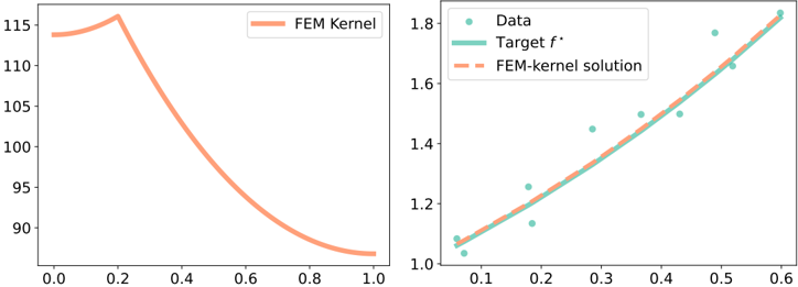<details> <summary>Image 12 Details</summary>  ### Visual Description \n ## Charts: FEM Kernel and Solution Comparison ### Overview The image presents two charts side-by-side. The left chart displays a single line representing a "FEM Kernel" plotted against an unspecified x-axis ranging from 0.0 to 1.0. The right chart shows a scatter plot of "Data" points and a line representing a "Target f*" and a dashed line representing a "FEM-kernel solution" plotted against an x-axis ranging from approximately 0.05 to 0.6. Both charts appear to be evaluating the performance of a Finite Element Method (FEM) kernel. ### Components/Axes **Left Chart:** * **Title:** Not explicitly present, but implied to be "FEM Kernel" based on the legend. * **X-axis:** Ranges from 0.0 to 1.0, unlabeled. * **Y-axis:** Ranges from approximately 90 to 115, unlabeled. * **Legend:** Located in the top-right corner. * "FEM Kernel" - represented by a solid orange line. **Right Chart:** * **Title:** Not explicitly present. * **X-axis:** Ranges from approximately 0.05 to 0.6, unlabeled. * **Y-axis:** Ranges from approximately 1.0 to 1.8, unlabeled. * **Legend:** Located in the top-left corner. * "Data" - represented by teal circles. * "Target f*" - represented by a solid teal line. * "FEM-kernel solution" - represented by a dashed orange line. ### Detailed Analysis or Content Details **Left Chart:** The "FEM Kernel" line starts at approximately 114 at x=0.0, rises to a peak of approximately 117 at x=0.2, and then decreases steadily to approximately 90 at x=1.0. The trend is initially increasing, then sharply decreasing. **Right Chart:** * **Data:** The scatter plot shows approximately 10 data points. The points are distributed roughly along a curve. Approximate coordinates: * (0.07, 1.03) * (0.11, 1.12) * (0.15, 1.21) * (0.20, 1.30) * (0.25, 1.40) * (0.30, 1.48) * (0.35, 1.56) * (0.40, 1.64) * (0.50, 1.78) * (0.55, 1.83) * **Target f*:** The solid teal line starts at approximately 1.0 at x=0.05 and increases to approximately 1.83 at x=0.55. The line appears to follow a roughly quadratic trend. * **FEM-kernel solution:** The dashed orange line starts at approximately 1.0 at x=0.05 and increases to approximately 1.8 at x=0.55. The line closely follows the "Target f*" line. ### Key Observations * The left chart shows a kernel function that initially increases and then decreases, suggesting a peak sensitivity or influence at around x=0.2. * The right chart demonstrates that the "FEM-kernel solution" closely approximates the "Target f*" function, as indicated by the overlapping lines. * The "Data" points appear to be used to define or validate the "Target f*" function. * The x-axis labels are missing, making it difficult to interpret the meaning of the x-values. ### Interpretation The charts likely represent a validation of a Finite Element Method (FEM) kernel. The left chart shows the shape of the kernel function itself, which is a key component in FEM calculations. The right chart demonstrates how well the FEM kernel can approximate a known target function ("Target f*") using available data. The close agreement between the "FEM-kernel solution" and the "Target f*" suggests that the FEM kernel is performing accurately. The data points are likely used to define the target function or to assess the accuracy of the FEM solution. The missing x-axis labels limit a deeper understanding of the context and physical meaning of the results. The initial rise and subsequent fall of the FEM Kernel suggests a localized influence or sensitivity within the domain being modeled. </details> kernel methods combined with FEM approaches come at a high computational cost, since storing the matrix K requires O ( n 2 ) memory. This becomes prohibitive for large amounts of data, as n = 10 4 already requires several gigabytes of RAM. Fourier approximation. Our primary objective in this article is to develop a more agile, flexible, and efficient method capable of handling arbitrary domains Ω . Following Doumèche et al. [Dou+24a], our methodology first requires extending the learning problem from Ω ⊆ [ -L, L ] d to the torus [ -2 L, 2 L ] d . Indeed, any function of H s (Ω) can be periodically extended into a function of H s per ([ -2 L, 2 L ] d ) [see Dou+24a, Proposition A.6 and Figure 1]. The choice of [ -2 L, 2 L ] d is commented in Appendix 4.A.2. This initial technical step allows us to use approximations with the standard Fourier basis, given for k ∈ Z d and x ∈ [ -2 L, 2 L ] d by $$\phi _ { k } ( x ) = ( 4 L ) ^ { - d / 2 } e ^ { \frac { i \pi } { 2 L } \langle k , x \rangle } ,$$ particularly adapted to periodic functions on [ -2 L, 2 L ] d . Therefore, the minimization of the risk R n defined in (4.1) over H s (Ω) can then be transferred into the minimization of the PIML risk $$\bar { R } _ { n } ( f ) = \frac { 1 } { n } \sum _ { i = 1 } ^ { n } | f ( X _ { i } ) - Y _ { i } | ^ { 2 } + \lambda _ { n } \| f \| _ { H _ { p e r } ^ { s } ( [ - 2 L , 2 L ] ^ { d } ) } ^ { 2 } + \mu _ { n } \| \mathcal { D } ( f ) \| _ { L ^ { 2 } ( \Omega ) } ^ { 2 }$$ over the periodic Sobolev space H s per ([ -2 L, 2 L ] d ) (see Appendix 4.B for an introduction to periodic Sobolev spaces). This results in a slightly modified kernel, determined by the RKHS norm $$\| f \| _ { R K H S } ^ { 2 } = \lambda _ { n } \| f \| _ { H _ { p e r } ^ { s } ( [ - 2 L , 2 L ] ^ { d } ) } ^ { 2 } + \mu _ { n } \| \mathcal { D } ( f ) \| _ { L ^ { 2 } ( \Omega ) } ^ { 2 } .$$ It is important to note that the estimators derived from the minimization of either R n or ¯ R n share the same statistical guarantees, as both kernel methods have been shown to converge to f /star at the same rate [Dou+24a, Theorem 4.6]. To implement this kernel method, a natural approach is to expand the kernel using a truncated Fourier series, i.e., K m ( x, y ) = ∑ ‖ k ‖ ∞ ⩽ m a k φ k ( x ) φ k ( y ) , with ( φ k ) ‖ k ‖ ∞ ⩽ m the Fourier basis, ( a k ) ‖ k ‖ ∞ ⩽ m the kernel coefficients in this basis, and m the order of approximation. This idea is at the core of techniques such as random Fourier features (RFF) [e.g., RR07; Yan+12]. However, unlike RFF, the Fourier features in our problem are not random quantities, as they systematically correspond to the low-frequency modes. This low-frequency approximation is particularly well-suited to the Sobolev penalty, which more strongly regularizes high frequencies (the analogous RFF algorithm would involve sampling random frequencies k according to a density that is proportional to the Sobolev decay). In addition, and more importantly, the use of such approximations bypasses the need to discretize the domain into finite elements and requires only the knowledge of the (partial) Fourier transform of 1 Ω , as will be explained later. A key milestone in the development of our method is to minimize ¯ R n not over the entire space H s per ([ -2 L, 2 L ] d ) , but rather on the finite-dimensional Fourier subspace H m = Span(( φ k ) ‖ k ‖ ∞ ⩽ m ) . This leads to the PIKL estimator, defined by $$\hat { f } ^ { P I K L } = \underset { f \in H _ { m } } { \arg \min } \, \bar { R } _ { n } ( f ) .$$ This naturally transforms the PIML problem into a finite-dimensional kernel regression task, where the associated kernel K m corresponds to a Fourier expansion of K , as will be clarified in the following paragraph. Of course, H m provides better approximates of H s per ([ -2 L, 2 L ] d ) as m increases, since for any function f ∈ H s per ([ -2 L, 2 L ] d ) , lim m →∞ min g ∈ H m ‖ f -g ‖ H s per ([ -2 L, 2 L ] d ) = 0 . Remarkably, the key advantage of using Fourier approximations in our PIKL algorithm lies in the fact that both the squared Sobolev norm ‖ f ‖ 2 H s per ([ -2 L, 2 L ] d ) and the PDE penalty ‖ D ( f ) ‖ 2 L 2 (Ω) are bilinear functions of the Fourier coefficients of f . As shown below, these bilinear forms can be represented as closed-form matrices, easing the computation of the estimator. RKHS norm in Fourier space. Suppose that the differential operator D is linear with constant coefficients, i.e., it can be expressed as D ( f ) = ∑ | α | ⩽ s a α ∂ α f for some s ∈ N /star and a α ∈ R . If f ∈ H m , then f can be rewritten in terms of its Fourier coefficients as $$f ( x ) = \left \langle z , \Phi _ { m } ( x ) \right \rangle _ { \mathbb { C } ^ { ( 2 m + 1 ) ^ { d } } } ,$$ where 〈· , ·〉 C (2 m +1) d denotes the canonical inner product on C (2 m +1) d , z is the vector of Fourier coefficients of f , and $$\Phi _ { m } ( x ) = \left ( ( 4 L ) ^ { - d / 2 } e ^ { \frac { i \pi } { 2 L } \langle k , x \rangle } \right ) _ { \| k \| _ { \infty } \leqslant m } .$$ According to Parseval's theorem, the L 2 -norm of the derivatives of f ∈ H s per ([ -2 L, 2 L ] d ) can be expressed using the Fourier coefficients of f as follows: for r ⩽ s and 1 ⩽ i 1 , . . . , i r ⩽ d , $$\| \partial _ { i _ { 1 } , \dots , i _ { r } } ^ { r } f \| _ { L ^ { 2 } ( [ - 2 L , 2 L ] ^ { d } ) } ^ { 2 } = ( 2 L ) ^ { - 2 k } \sum _ { \| j \| _ { \infty } \leqslant m } | z _ { j } | ^ { 2 } \prod _ { \ell = 1 } ^ { r } j _ { i _ { \ell } } ^ { 2 } .$$ With this notation, the Sobolev norm reads $$\| f \| _ { H _ { p e r } ^ { s } ( [ - 2 L , 2 L ] ^ { d } ) } ^ { 2 } = \sum _ { \| j \| _ { \infty } \leqslant m , \| k \| _ { \infty } \leqslant m } z _ { j } \bar { z _ { k } } \left ( 1 + \left ( \frac { \| k \| _ { 2 } ^ { 2 } } { ( 2 L ) ^ { d } } \right ) ^ { s } \right ) \delta _ { j , k } ,$$ and, similarly, $$\| \mathcal { D } ( f ) \| _ { L ^ { 2 } ( \Omega ) } ^ { 2 } = \sum _ { \| j \| _ { \infty } \leqslant m , \| k \| _ { \infty } \leqslant m } z _ { j } \bar { z _ { k } } \frac { P ( j ) \bar { P } ( k ) } { ( 4 L ) ^ { d } } \int _ { \Omega } e ^ { \frac { i \pi } { 2 L } \langle k - j , x \rangle } d x ,$$ where P ( k ) = ∑ | α | ⩽ s a α ( -iπ 2 L ) | α | ∏ d /lscript =1 ( k /lscript ) α /lscript . Therefore, introducing M m the (2 m + 1) d × (2 m +1) d matrix with coefficients indexed by j, k ∈ {-m,... , m } d , $$( M _ { m } ) _ { j , k } = \lambda _ { n } \left ( 1 + \left ( \frac { \| k \| _ { 2 } ^ { 2 } } { ( 2 L ) ^ { d } } \right ) ^ { s } \right ) \delta _ { j , k } + \mu _ { n } \frac { P ( j ) \bar { P } ( k ) } { ( 4 L ) ^ { d } } \int _ { \Omega } e ^ { \frac { i \pi } { 2 L } \langle k - j , x \rangle } d x ,$$ we obtain that the RKHS norm of f is expressed as a bilinear form of its Fourier coefficients z , i.e., $$\| f \| _ { R K H S } ^ { 2 } = \langle z , M _ { m } z \rangle _ { \mathbb { C } ^ { ( 2 m + 1 ) ^ { d } } } .$$ It is important to note that M m is Hermitian, 1 positive, 2 and definite. 3 Therefore, the spectral theorem (see Theorem 4.B.6) ensures that M m is invertible, and that its positive inverse square root M -1 / 2 m is unique and well-defined. We have now all the ingredients to define the PIKL algorithm. Remark 4.2.2 (Linear PDEs with non-constant coefficients) . This framework could be adapted to PDEs with non-constant coefficients, i.e., to operators D ( f ) = ∑ | α | ⩽ s a α ∂ α f for some s ∈ N /star and a α ∈ C 0 ( R ) . In this case, the polynomial P in (4.5) should be replaced by convolutions involving the Fourier coefficients of the functions a α . Computing the PIKL estimator. For a function f ∈ H m , one can evaluate f at x by f ( x ) = 〈 M 1 / 2 m z, M -1 / 2 m Φ m ( x ) 〉 C (2 m +1) d . This reproducing property indicates that minimizing the risk ¯ R n on H m is a kernel method governed by the kernel $$K _ { m } ( x , y ) = \langle M _ { m } ^ { - 1 / 2 } \Phi _ { m } ( x ) , M _ { m } ^ { - 1 / 2 } \Phi _ { m } ( y ) \rangle _ { \mathbb { C } ^ { ( 2 m + 1 ) ^ { d } } } .$$ Define Y = ( Y 1 , . . . , Y n ) /latticetop and K m ∈ M n ( C ) to be the matrix such that ( K m ) i,j = K m ( X i , X j ) for all 1 ⩽ i, j ⩽ n . The PIKL estimator (4.4), minimizer of ¯ R n restricted to H m , is therefore given by $$\hat { f } ^ { \text {PIKL} } ( x ) & = ( K _ { m } ( x , X _ { 1 } ) , \dots , K _ { m } ( x , X _ { n } ) ) ( \mathbb { K } _ { m } + n I _ { n } ) ^ { - 1 } \mathbb { Y } \\ & = \Phi _ { m } ( x ) ^ { ^ { * } } ( \Phi ^ { ^ { * } } \Phi + n M _ { m } ) ^ { - 1 } \Phi ^ { ^ { * } } \mathbb { Y } ,$$ where Φ =     Φ m ( X 1 ) /star . . . Φ m ( X n ) /star     is an n × (2 m +1) d matrix. The formula obtained in (4.6) is provided by the so-called kernel trick. This step offers a significant advantage to the PIKL estimator as it reduces the computational burden in large sample regimes: instead of storing and inverting the n × n matrix K m + nI n , we only need to store and invert the (2 m + 1) d × (2 m + 1) d matrix Φ /star Φ + nM m . Moreover, the computation of Φ /star Φ and Φ /star Y can be performed online and in parallel as n grows. Of course, this approach is subject to the curse of dimensionality. However, it is unreasonable to try to learn more parameters than the sample complexity n . Therefore, in practice, (2 m +1) d /lessmuch n , which justifies the preference of the (2 m +1) 2 d storage complexity over the n 2 storage complexity of the FEM-based algorithm. In addition, similar to PINNs, the PIKL estimator has the advantage that its training phase takes longer than its evaluation at certain points. In fact, once the (2 m + 1) d Fourier modes of ˆ f PIKL (given by ( Φ /star Φ + nM m ) -1 Φ /star Y ) are computed, the evaluation of Φ /star m ( x ) is straightforward. This is in 1 since M /star m = ¯ M /latticetop m = M m . 2 since 〈 z, M m z 〉 C (2 m +1) d = ‖ f ‖ 2 RKHS ⩾ 0 . 3 since 〈 z, M m z 〉 C (2 m +1) d = 0 implies ‖ f ‖ H s ([ -2 L, 2 L ] d ) = 0 , i.e., f = 0 . sharp contrast to the FEM-based strategy, which requires approximating the kernel vector ( K ( x, X 1 ) , . . . , K ( x, X n )) at each query point x . We also emphasize that the PIKL predictor is characterized by low-frequency Fourier coefficients, which, in turn, enhance its interpretability. This methodology differs significantly from PINNs, which are less interpretable and rely on gradient descent for optimization [see, e.g., WYP22]. Remark 4.2.3 (PIKL vs. spectral methods) . In the PIML context, the RFF approach resembles a well-known class of powerful tools for solving PDEs, known as spectral and pseudo-spectral methods [e.g., Can+07]. These methods solve PDEs by selecting a basis of orthogonal functions and computing the coefficients of the solution on that basis to satisfy both the boundary conditions and the PDE itself. For example, the Fourier basis ( x ↦→ exp( iπ 2 L 〈 k, x 〉 )) k ∈ Z d already used in this paper is particularly well suited for solving linear PDEs on the square domain [ -2 L, 2 L ] d with periodic boundary conditions. Spectral methods such as these have already been used in the PIML community to integrate PDEs with machine learning techniques [e.g., MQS23]. However, the basis functions used in spectral and pseudo-spectral methods must be specifically tailored to the domain Ω , the differential operator D , and the boundary conditions. For more information on this topic, please refer to Appendix 4.A.1. Computing M m for specific domains. Computing the matrix M m requires the evaluation of the integrals ( j, k ) ↦→ ∫ Ω e iπ 2 L 〈 k -j,x 〉 dx . In general, these integrals can be approximated using numerical integration schemes or Monte Carlo methods. However, it is possible to provide closed-form expressions for specific domains Ω . To do so, for d ∈ N /star , L > 0 , and Ω ⊆ [ -L, L ] d , we define the characteristic function F Ω of Ω by $$F _ { \Omega } ( k ) = \frac { 1 } { ( 4 L ) ^ { d } } \int _ { \Omega } e ^ { \frac { i \pi } { 2 L } \langle k , x \rangle } d x .$$ Proposition 4.2.4 (Closed-form characteristic functions) . The characteristic functions associated with the cube and the Euclidean ball can be analytically obtained as follows. - (Cube) Let Ω = [ -L, L ] d . Then, for k ∈ Z d , $$F _ { \Omega } ( k ) = \prod _ { j = 1 } ^ { d } \frac { \sin ( \pi k _ { j } / 2 ) } { \pi k _ { j } } .$$ - (Euclidean ball) Let d = 2 and Ω = { x ∈ [ -L, L ] , ‖ x ‖ 2 ⩽ L } . Then, for k ∈ Z d , $$F _ { \Omega } ( k ) = \frac { J _ { 1 } ( \pi \| k \| _ { 2 } / 2 ) } { 4 \| k \| _ { 2 } } ,$$ where J 1 is the Bessel function of the first kind of parameter 1. This proposition, along with similar analytical results for other domains, can be found in Bracewell [Bra00, Table 13.4], noting that F Ω is the Fourier transform of the indicator function 1 Ω and is also the characteristic function of the uniform distribution on Ω evaluated at k 2 L . We can extend these computations further since, given the characteristic functions of elementary domains Ω , it is easy to compute the characteristic functions of translation, dilation, disjoint unions, and Cartesian products of such domains (see Proposition 4.C.1 in Appendix 4.C). For instance, it is straightforward to obtain the characteristic function of the three-dimensional cylinder Ω = { x ∈ [ -L, L ] , ‖ x ‖ 2 ⩽ L } × [ -L, L ] as $$F _ { \Omega } ( k _ { 1 } , k _ { 2 } , k _ { 3 } ) = \frac { J _ { 1 } ( \pi ( k _ { 1 } ^ { 2 } + k _ { 2 } ^ { 2 } ) ^ { 1 / 2 } / 2 ) } { 4 ( k _ { 1 } ^ { 2 } + k _ { 2 } ^ { 2 } ) ^ { 1 / 2 } } \times \frac { \sin ( \pi k _ { 3 } / 2 ) } { \pi k _ { 3 } } .$$ ## 4.3 The PIKL algorithm in practice To enhance the reproducibility of our work, we provide a Python package that implements the PIKL estimator, designed to handle any linear PDE prior with constant coefficients in dimensions d = 1 and d = 2 . This package is available at https://github.com/NathanDoumeche/ numerical\_PIML\_kernel . Note that this package implements the matrix inversion of the PIKL formula (4.6) by solving a linear system using the LU decomposition. Of course, any other efficient method to avoid direct matrix inversion could be used instead, such as solving a linear system with the conjugate gradient method. Through numerical experiments, we demonstrate the performance of our approach in simulations for hybrid modeling (Subsection 4.3.1), and derive experimental convergence rates that quantify the benefits of incorporating PDE knowledge into a learning regression task (Subsection 4.3.2). ## 4.3.1 Hybrid modeling Perfect modeling with closed-form PDE solutions. We start by assessing the performance of the PIKL estimator in a perfect modeling situation (i.e., D ( f /star ) = 0 ), where the solutions of the PDE D ( f ) = 0 can be decomposed on a basis ( f k ) k ∈ N of closed-form solution functions. In this ideal case, the spectral method suggests an alternative estimator, which involves learning the coefficients a k ∈ R of f /star = ∑ k ∈ N a k f k in this basis. For example, consider the one-dimensional case ( d = 1 ) with domain Ω = [ -π, π ] , and the harmonic oscillator differential prior D ( f ) = d 2 f dx 2 + df dx + f . In this case, the solutions of D ( f ) = 0 are the linear combinations f = a 1 f 1 + a 2 f 2 , where ( a 1 , a 2 ) ∈ R 2 , f 1 ( x ) = exp( -x/ 2) cos( √ 3 x/ 2) , and f 2 ( x ) = exp( -x/ 2) sin( √ 3 x/ 2) . Thus, the spectral Fig. 4.2.: OLS and PIKL estimators for the harmonic oscillator with d = 1 , sample size n = 10 . 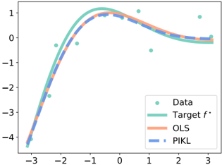<details> <summary>Image 13 Details</summary>  ### Visual Description \n ## Chart: Function Approximation Comparison ### Overview The image presents a chart comparing the performance of different function approximation methods: Data, Target function (f*), Ordinary Least Squares (OLS), and Path-Integrated Kernel Learning (PIKL). The chart displays these methods as curves plotted against an x-axis ranging from approximately -3 to 3. The y-axis represents the function values, ranging from approximately -4 to 1. ### Components/Axes * **X-axis:** Labeled with numerical values ranging from -3 to 3, with tick marks at integer values. * **Y-axis:** Labeled with numerical values ranging from -4 to 1, with tick marks at integer values. * **Legend:** Located in the top-right corner of the chart. It identifies the following data series: * "Data" (represented by light green circles) * "Target f*" (represented by a light teal solid line) * "OLS" (represented by a light orange solid line) * "PIKL" (represented by a dashed blue line) ### Detailed Analysis * **Data:** The "Data" series consists of approximately 10 scattered light green circles. The points are distributed across the x-axis, with a concentration around x = -2, x = 0, and x = 2. The y-values for these points are approximately: (-3, -2.5), (-2, -1.8), (-1, 0.8), (0, 0.9), (1, -0.5), (2, 0.1), (3, 0.6). * **Target f*:** The "Target f*" series is a smooth, light teal curve that resembles a parabola opening downwards. It reaches a maximum value of approximately 1 at x = 0. The curve is symmetrical around the y-axis. * **OLS:** The "OLS" series is a light orange solid line that closely follows the "Target f*" curve. It also resembles a parabola, with a maximum value of approximately 1 at x = 0. There is a slight deviation from the "Target f*" curve around x = 1 and x = -1. * **PIKL:** The "PIKL" series is a dashed blue line that also closely follows the "Target f*" curve. It is very similar to the "OLS" curve, with a maximum value of approximately 1 at x = 0. There is a slight deviation from the "Target f*" curve around x = -3 and x = 3. **Trend Verification:** * The "Target f*" line exhibits a parabolic shape, peaking at x=0. * The "OLS" line generally follows the "Target f*" line, showing an upward trend until x=0 and then a downward trend. * The "PIKL" line mirrors the "OLS" line's trend, closely approximating the "Target f*" curve. * The "Data" points are scattered, but generally align with the overall parabolic shape. ### Key Observations * Both "OLS" and "PIKL" methods provide very good approximations of the "Target f*" function. * The "OLS" and "PIKL" curves are almost indistinguishable from each other visually. * The "Data" points are somewhat noisy, but they generally support the shape of the "Target f*" function. * There is a slight divergence between the "OLS" and "PIKL" curves and the "Target f*" curve at the extreme ends of the x-axis (around x = -3 and x = 3). ### Interpretation The chart demonstrates the effectiveness of both OLS and PIKL methods in approximating an unknown target function (f*) based on a set of noisy data points. The close alignment of the OLS and PIKL curves with the Target f* suggests that both methods are capable of capturing the underlying functional relationship. The slight deviations at the edges of the x-axis might indicate limitations in the methods' ability to extrapolate beyond the range of the observed data. The data points themselves provide the basis for the approximation, and their distribution influences the accuracy of the resulting curves. The chart suggests that, in this particular case, PIKL and OLS perform similarly well in function approximation. </details> method focuses on learning the vector ( a 1 , a 2 ) ∈ R 2 , instead of learning the Fourier coefficients of f /star , which is the approach taken by the PIKL algorithm. A baseline that exactly leverages the particular structure of this problem, referred to as the ordinary least squares (OLS) estimator, is therefore ˆ g n = ˆ a 1 f 1 +ˆ a 2 f 2 , where $$( \hat { a } _ { 1 } , \hat { a } _ { 2 } ) = \underset { ( a _ { 1 } , a _ { 2 } ) \in \mathbb { R } ^ { 2 } } { \arg \min } \, \frac { 1 } { n } \sum _ { i = 1 } ^ { n } | a _ { 1 } f _ { 1 } ( X _ { i } ) + a _ { 2 } f _ { 2 } ( X _ { i } ) - Y _ { i } | ^ { 2 } .$$ To compare the PIKL and OLS estimators, we generate data such that Y = f /star ( X ) + ε , where X ∼ U (Ω) , ε ∼ N (0 , σ 2 ) with σ = 0 . 5 , and the target function is f /star = f 1 (corresponding to ( a 1 , a 2 ) = (1 , 0) ). We implement the PIKL algorithm with 601 Fourier modes ( m = 300 ) and s = 2 . Figure 4.2 shows that even with very few data points ( n = 10 ) and high noise levels, both the OLS and PIKL methods effectively reconstruct f /star , both incorporating physical knowledge in their own way. In Figure 4.3, we display the L 2 -error of both estimators for different sample sizes n . The two methods have an experimental convergence rate of n -1 . 1 , which is consistent with the expected parametric rate of n -1 . This sanity check shows that under perfect modeling conditions, the PIKL estimator with m = 300 performs as well as the OLS estimator specifically designed to explore the space of PDE solutions. /negationslash Fig. 4.3.: L 2 -error (mean ± std over 5 runs) of the OLS and PIKL estimators for the harmonic oscillator with d = 1 , w.r.t. n in log 10 -log 10 scale. The dashed lines represent adjusted linear models w.r.t. n , for both L 2 -errors. 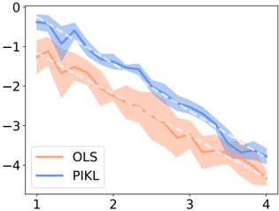<details> <summary>Image 14 Details</summary>  ### Visual Description \n ## Line Chart: Comparison of OLS and PIKL Performance ### Overview This image presents a line chart comparing the performance of two methods, Ordinary Least Squares (OLS) and Policy Iteration with Kernel Learning (PIKL), across a range of values on the x-axis. The y-axis represents a numerical score, likely an error or loss value, with lower values indicating better performance. The chart displays the mean performance of each method as a line, along with a shaded region representing the standard deviation or confidence interval around the mean. ### Components/Axes * **X-axis:** Labeled with numerical values ranging from approximately 1 to 4, with tick marks at 1, 2, 3, and 4. * **Y-axis:** Ranges from approximately 0 to -6, with tick marks at 0, -1, -2, -3, -4, -5, and -6. * **Legend:** Located in the bottom-left corner. * OLS: Represented by a light orange/peach color. * PIKL: Represented by a light blue color. ### Detailed Analysis **OLS (Orange Line):** The orange line representing OLS exhibits a consistent downward trend across the x-axis. * At x = 1, the OLS line is approximately at y = -1.5. * At x = 2, the OLS line is approximately at y = -2.2. * At x = 3, the OLS line is approximately at y = -3.0. * At x = 4, the OLS line is approximately at y = -4.5. The shaded region around the OLS line indicates a relatively wide standard deviation, particularly between x = 1 and x = 2. **PIKL (Blue Line):** The blue line representing PIKL also shows a downward trend, but it generally remains above the OLS line. * At x = 1, the PIKL line is approximately at y = -0.5. * At x = 2, the PIKL line is approximately at y = -1.3. * At x = 3, the PIKL line is approximately at y = -2.2. * At x = 4, the PIKL line is approximately at y = -3.8. The shaded region around the PIKL line appears slightly narrower than that of OLS, suggesting a smaller standard deviation. ### Key Observations * Both OLS and PIKL demonstrate decreasing performance (lower scores are better) as the x-axis value increases. * PIKL consistently outperforms OLS across the entire range of x-values, as indicated by the lower position of the blue line compared to the orange line. * The standard deviation for OLS is larger than that of PIKL, suggesting that OLS performance is more variable. ### Interpretation The chart suggests that PIKL is a more effective method than OLS for the task being evaluated. The consistent downward trend for both methods indicates that performance improves with increasing values on the x-axis (which could represent, for example, the number of iterations or the amount of data used). The smaller standard deviation for PIKL suggests that its performance is more reliable and less sensitive to variations in the input data or experimental conditions. The difference in performance between the two methods is noticeable and consistent, indicating a clear advantage for PIKL. Without knowing the context of the x-axis, it is difficult to provide a more specific interpretation, but the data strongly suggests that PIKL is a superior approach. </details> Combining the best of physics and data in imperfect modeling. In this paragraph, we deal with an imperfect modeling scenario using the heat differential operator D ( f ) = ∂ 1 f -∂ 2 2 , 2 f in dimension d = 2 over the domain Ω = [ -π, π ] 2 . The data are generated according to the model Y = f /star ( X ) + ε , where ‖ D ( f /star ) ‖ L 2 (Ω) = 0 . We assume, however, that the PDE serves as a good physical prior, meaning that ‖ f /star ‖ 2 L 2 (Ω) is significantly larger than the modeling error ‖ D ( f /star ) ‖ 2 L 2 (Ω) . The hybrid model is implemented using the PIKL estimator with parameters s = 2 , λ n = n -2 / 3 / 10 , and µ n = 100 /n . These hyperparameters are selected to ensure that, when only a small amount of data is available, the model relies heavily on the PDE. Yet, as more data become available, the model can use the data to correct the modeling error. The performance of the PIKL estimator is compared with that of a purely data-driven estimator, referred to as the Sobolev estimator, and a strongly PDE-penalized estimator, referred to as the PDE estimator. The Sobolev estimator uses the same parameter s = 2 and λ n = n -2 / 3 / 10 , but sets µ n = 0 . This configuration ensures that the estimator relies entirely on the data without considering the PDE as a prior. On the other hand, the PDE estimator is configured with parameters s = 2 , λ n = 10 -10 , and µ n = 10 10 . These hyperparameters are set to ensure that the resulting PDE estimator effectively satisfies the heat equation, making it highly dependent on the physical model. 2 We perform an experiment where ε ∼ N (0 , σ 2 ) with σ = 0 . 5 , and f /star ( t, x ) = exp( -t ) cos( x ) + 0 . 5 sin(2 x ) . This scenario is an example of imperfect modeling, since ‖ D ( f /star ) ‖ 2 L 2 (Ω) = π > 0 . However, the heat equation serves as a strong physical prior, since ‖ D ( f /star ) ‖ 2 L 2 (Ω) / ‖ f /star ‖ 2 L 2 (Ω) /similarequal 4 × 10 -3 . Figure 4.4 illustrates the performance of the different estimators. Clearly, the PDE estimator outperforms the Sobolev estimator when the data set is small ( n ⩽ 10 2 ). As expected, the performance of the Sobolev estimator improves as the sample size increases ( n ⩾ 10 3 ), but it remains consistently inferior to that of the PIKL. When Fig. 4.4.: L 2 -error (mean ± std over 5 runs) of the PDE, PIKL, and Sobolev estimators for imperfect modeling with the heat equation, as a function of n in log 10 -log 10 scale. The PDE error is the L 2 -norm between f /star and the PDE solution that is closest to f /star . 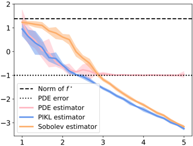<details> <summary>Image 15 Details</summary>  ### Visual Description \n ## Line Chart: Error Estimation Comparison ### Overview The image presents a line chart comparing the performance of different error estimators (PDE estimator, PIKL estimator, and Sobolev estimator) against the norm of f* and the PDE error. The chart displays the estimators' values across a range of values from approximately 1 to 5 on the x-axis. Shaded regions around each line represent uncertainty or variance in the estimator's performance. ### Components/Axes * **X-axis:** Labeled with numerical values ranging from 1 to 5, with tick marks at integer values. * **Y-axis:** Ranges from approximately -3 to 2, with tick marks at integer values. * **Lines:** Four lines are present, each representing a different estimator or error metric. * Black dashed line: "Norm of f*" * Red dotted line: "PDE error" * Pink line with shaded region: "PDE estimator" * Blue line with shaded region: "PIKL estimator" * Orange line with shaded region: "Sobolev estimator" * **Legend:** Located in the top-left corner, associating colors with each estimator/error metric. ### Detailed Analysis The chart shows the following trends and approximate data points: * **Norm of f* (Black Dashed Line):** This line is approximately horizontal, remaining relatively constant at a value of around 1.2 across the entire x-axis range. * **PDE Error (Red Dotted Line):** This line is also approximately horizontal, positioned around -1.1. * **PDE Estimator (Pink Line):** This line starts at approximately 1.1 at x=1 and slopes downward, reaching approximately -0.8 at x=5. The shaded region indicates a relatively wide range of uncertainty, particularly between x=1 and x=3. * **PIKL Estimator (Blue Line):** This line begins at approximately 0.8 at x=1 and exhibits a steeper downward slope than the PDE estimator, reaching approximately -2.5 at x=5. The shaded region is narrower than that of the PDE estimator, suggesting lower variance. * **Sobolev Estimator (Orange Line):** This line starts at approximately 0.9 at x=1 and slopes downward, similar to the PDE estimator, but with a slightly more pronounced decline. It reaches approximately -3.2 at x=5. The shaded region is comparable in width to that of the PDE estimator. ### Key Observations * All three estimators (PDE, PIKL, and Sobolev) show a decreasing trend as the x-value increases, indicating that the estimated error generally decreases with increasing values on the x-axis. * The PIKL estimator consistently estimates a lower error than the other two estimators across the entire range. * The Sobolev estimator generally estimates a lower error than the PDE estimator. * The uncertainty (as indicated by the shaded regions) is most significant for the PDE estimator. * The "Norm of f*" and "PDE error" lines provide reference levels for evaluating the performance of the estimators. ### Interpretation The chart demonstrates a comparison of different error estimation techniques. The downward trends of the estimators suggest that the error is reduced as the parameter (represented by the x-axis) increases. The PIKL estimator appears to be the most accurate, consistently providing the lowest error estimates. The wider uncertainty range for the PDE estimator suggests that it is less reliable than the PIKL and Sobolev estimators. The horizontal lines representing the "Norm of f*" and "PDE error" serve as benchmarks for assessing the quality of the error estimations. The fact that the estimators generally fall below the "PDE error" line indicates that they are successfully identifying and quantifying the error in the system. The differences between the estimators could be attributed to their underlying methodologies and assumptions. The chart suggests that the PIKL estimator is a robust and reliable method for error estimation in this context. </details> only a small amount of data is available, the PDE provides significant benefits, and the L 2 -error decreases at the super-parametric rate of n -2 for both the PIKL and the PDE estimators. However, in the context of imperfect modeling, the PDE estimator cannot overcome the PDE error, resulting in no further improvement beyond n ⩾ 100 . In addition, when a large amount of data is available, the data become more reliable than the PDE. In this case, the errors for both the PIKL and the Sobolev estimators decrease at the Sobolev minimax rate of n -2 / 3 . Overall, the PIKL estimator successfully combines the strengths of both approaches, using the PDE when data is scarce and relying more on data when it becomes abundant. ## 4.3.2 Measuring the impact of physics with the effective dimension The important question of measuring the impact of the differential operator D on the convergence rate of the PIML estimator has not yet found a clear answer in the literature. In this subsection, we propose an approach to experimentally compare the PIKL convergence rate to the Sobolev minimax rate in H s (Ω) , which is n -2 s/ (2 s + d ) [e.g., Tsy09, Theorem 2.1]. Theoretical backbone. According to Doumèche et al. [Dou+24a, Theorem 4.3], if X has a bounded density and the noise ε is sub-Gamma with parameters ( σ, M ) , the L 2 -error of both estimators (4.2) and (4.4) satisfies $$\mathbb { E } & \int _ { \Omega } | \hat { f } _ { n } - f ^ { * } | ^ { 2 } d \mathbb { P } _ { X } \\ & \leqslant C _ { 4 } \log ^ { 2 } ( n ) \left ( \lambda _ { n } \| f ^ { * } \| _ { H ^ { s } ( \Omega ) } ^ { 2 } + \mu _ { n } \| \mathcal { D } ( f ^ { * } ) \| _ { L ^ { 2 } ( \Omega ) } ^ { 2 } + \frac { M ^ { 2 } } { n ^ { 2 } \lambda _ { n } } + \frac { \sigma ^ { 2 } \mathcal { N } ( \lambda _ { n } , \mu _ { n } ) } { n } \right ) ,$$ where P X is the distribution of X . The quantity N ( λ n , µ n ) on the right-hand side of (4.7) is referred to as the effective dimension. Given the integral kernel operator L K , defined by L K : f ∈ L 2 ( P X ) ↦→ ( x ↦→ ∫ Ω K ( x, y ) f ( y ) d P X ( y )) ∈ L 2 ( P X ) , the effective dimension is the trace of the operator ( L K + Id ) -1 L K [see, e.g., CV07]. Since λ n and µ n can be freely chosen by the practitioner, the effective dimension N ( λ n , µ n ) becomes a key consideration that help quantify the impact of the physics on the learning problem. Unfortunately, bounding N ( λ n , µ n ) is not trivial. Doumèche et al. [Dou+24a] have shown that, whenever d P X dx ⩽ κ with κ ≥ 1 , $$\mathcal { N } ( \lambda _ { n } , \mu _ { n } ) \leqslant \sum _ { \lambda \in \sigma ( C \mathcal { O } _ { n } C ) } \frac { 1 } { 1 + ( \kappa \lambda ) ^ { - 1 } } \leqslant \kappa \sum _ { \lambda \in \sigma ( C \mathcal { O } _ { n } C ) } \frac { 1 } { 1 + \lambda ^ { - 1 } } ,$$ where O n is the operator O n = lim m →∞ M -1 m (where the limit is taken in the sense of the operator norm-see Definition 4.B.3) and C is the operator C ( f ) = 1 Ω f (that is, C ( f )( x ) = f ( x ) if x ∈ Ω , and C ( f )( x ) = 0 otherwise). Therefore, a natural idea to assess the effective dimension is to replace C O n C by C m M -1 m C m , where C m : H m → H m is defined by $$\forall j , k \in \{ - m , \dots , m \} ^ { d } , \quad ( C _ { m } ) _ { j , k } = \frac { 1 } { ( 4 L ) ^ { d } } \int _ { \Omega } e ^ { \frac { i \pi } { 2 L } \left \langle k - j , x \right \rangle } d x .$$ The following theorem shows that this is a sound strategy, in the sense that computing the effective dimension using the eigenvalues of C m M -1 m C m becomes increasingly accurate as m grows. Theorem 4.3.1 (Convergence of the effective dimension) . (i) One has $$\lim _ { m \rightarrow \infty } \sum _ { \lambda \in \sigma ( C _ { m } M _ { m } ^ { - 1 } C _ { m } ) } \frac { 1 } { 1 + \lambda ^ { - 1 } } = \sum _ { \lambda \in \sigma ( C \mathcal { O } _ { n } C ) } \frac { 1 } { 1 + \lambda ^ { - 1 } } .$$ - (ii) Let σ ↓ k ( C m M -1 m C m ) be the k -th highest eigenvalue of C m M -1 m C m . The spectrum of the matrix C m M -1 m C m converges to the spectrum of C O n C in the following sense: $$\forall k \in \mathbb { N } ^ { * } , \quad \lim _ { m \to \infty } \sigma _ { k } ^ { \downarrow } ( C _ { m } M _ { m } ^ { - 1 } C _ { m } ) = \sigma _ { k } ^ { \downarrow } ( C \mathcal { O } _ { n } C ) .$$ The provided Python package 4 , 5 numerical approximations of the effective dimension in dimensions d = 1 and d = 2 for any linear operator D with constant coefficients, when Ω is either a cube or a Euclidean ball. The code is available is designed to run on both CPU and GPU. The convergence of the effective dimension as m grows is studied in greater detail in Appendix 4.D.2. Comparison to the closed-form case. We start by assessing the quality of the approximation encapsulated in Theorem 4.3.1 in a scenario where the eigenvalues can be theoretically bounded. When d = 1 , s = 1 , D = d dx , and Ω = [ -π, π ] , one has [Dou+24a, Proposition 5.2] $$\frac { 4 } { ( \lambda _ { n } + \mu _ { n } ) ( k + 4 ) ^ { 2 } } \leqslant \sigma _ { k } ^ { \downarrow } ( C \mathcal { O } _ { n } C ) \leqslant \frac { 4 } { ( \lambda _ { n } + \mu _ { n } ) ( k - 2 ) ^ { 2 } } .$$ This shows that log σ ↓ k ( C O n C ) ∼ k →∞ -2 log( k ) . Figure 4.5 (Left) represents the eigenvalues of C m M -1 m C m in decreasing order, for increasing values of m , with λ n = 0 . 01 and µ n = 1 . For any fixed m , two distinct regimes can be clearly distinguished: initially, the eigenvalues decrease linearly on a log -log scale and align with the theoretical values of -2 log( k ) . Afterward, the eigenvalues suddenly drop to zero. As m increases, the spectrum progressively approaches the theoretical bound. In Appendix 4.D.2, we show that m = 10 2 Fourier modes are sufficient to accurately approximate the effective dimension when n ⩽ 10 4 . It is evident from Figure 4.5 (Right) that the effective dimension exhibits a sub-linear behavior in the log -log scale, experimentally confirming the findings of Doumèche et al. [Dou+24a], which show that N ( log( n ) n , 1 log( n ) ) = o n →∞ ( n γ ) for all γ > 0 . So, plugging this into (4.7) with λ n = n -1 log( n ) and µ n = log( n ) -1 leads to $$\mathbb { E } \int _ { [ - L , L ] } | \hat { f } _ { n } - f ^ { ^ { * } } | ^ { 2 } d \mathbb { P } _ { X } = ( \| f ^ { ^ { * } } \| _ { H ^ { 1 } ( \Omega ) } ^ { 2 } + \sigma ^ { 2 } + M ^ { 2 } ) O _ { n } \left ( n ^ { - 1 } \log ^ { 3 } ( n ) \right )$$ when D ( f /star ) = 0 , i.e., when the modeling is perfect. The Sobolev minimax rate on H 1 (Ω) is n -2 / 3 , whereas the experimental bound in this context gives a rate of n -1 . This indicates that when the target f /star satisfies the underlying PDE, the gain in terms of speed from incorporating the physics into the learning problem is n -1 / 3 . Harmonic oscillator equation. Here, we follow up on the example of Subsection 4.3.1, as presented in Figures 4.2 and 4.3. Thus, we set d = 1 , s = 2 , D ( u ) = d 2 dx 2 u + d dx u + u , and Ω = [ -π, π ] . Recall that in this perfect modeling experiment, we observed a parametric convergence rate of n -1 , which is not surprising since the regression problem essentially involves learning the two parameters a 1 and a 2 . Figure 4.6 (Left) shows the eigenvalues 4 https://github.com/NathanDoumeche/numerical\_PIML\_kernel 5 https://pypi.org/project/pikernel Fig. 4.5.: The case of D = d dx . Left: Spectrum of C m M -1 m C m . Right: Estimation of the effective dimension n ↦→ N ( log( n ) n , 1 log( n ) ) . 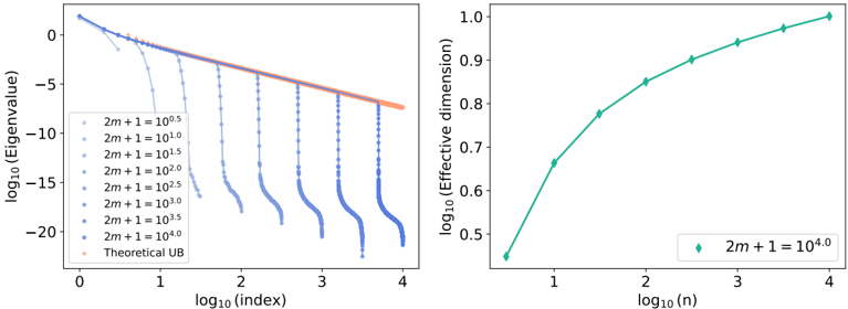<details> <summary>Image 16 Details</summary>  ### Visual Description \n ## Charts: Eigenvalue Spectrum and Effective Dimension ### Overview The image presents two charts. The left chart displays the log10 of the Eigenvalue versus the log10 of the index for different values of `2m+1`. The right chart shows the log10 of the Effective Dimension versus the log10 of n, for a single value of `2m+1`. ### Components/Axes **Left Chart:** * **X-axis:** `log10(Index)` ranging from approximately 0 to 4. * **Y-axis:** `log10(Eigenvalue)` ranging from approximately 0 to -20. * **Data Series:** Multiple lines representing different values of `2m+1`: `10^5`, `10^4`, `10^3`, `10^2`, `10^1`, `10^0`. * **Additional Line:** A line labeled "Theoretical UB" (Upper Bound). * **Legend:** Located in the top-left corner, listing the values of `2m+1` and "Theoretical UB" with corresponding colors. **Right Chart:** * **X-axis:** `log10(n)` ranging from approximately 0 to 4. * **Y-axis:** `log10(Effective dimension)` ranging from approximately 0.5 to 1.0. * **Data Series:** A single line with markers representing data points for `2m+1 = 10^6`. * **Legend:** Located in the bottom-right corner, indicating `2m+1 = 10^6` with a teal color. ### Detailed Analysis or Content Details **Left Chart:** * **`2m+1 = 10^5` (Dark Blue):** The line starts at approximately `log10(Eigenvalue) = 0` at `log10(Index) = 0` and decreases steadily to approximately `log10(Eigenvalue) = -18` at `log10(Index) = 4`. * **`2m+1 = 10^4` (Blue):** The line starts at approximately `log10(Eigenvalue) = 0` at `log10(Index) = 0` and decreases steadily to approximately `log10(Eigenvalue) = -16` at `log10(Index) = 4`. * **`2m+1 = 10^3` (Light Blue):** The line starts at approximately `log10(Eigenvalue) = 0` at `log10(Index) = 0` and decreases steadily to approximately `log10(Eigenvalue) = -14` at `log10(Index) = 4`. * **`2m+1 = 10^2` (Medium Blue):** The line starts at approximately `log10(Eigenvalue) = 0` at `log10(Index) = 0` and decreases steadily to approximately `log10(Eigenvalue) = -12` at `log10(Index) = 4`. * **`2m+1 = 10^1` (Blue):** The line starts at approximately `log10(Eigenvalue) = 0` at `log10(Index) = 0` and decreases steadily to approximately `log10(Eigenvalue) = -10` at `log10(Index) = 4`. * **`2m+1 = 10^0` (Orange):** The line starts at approximately `log10(Eigenvalue) = 0` at `log10(Index) = 0` and decreases steadily to approximately `log10(Eigenvalue) = -8` at `log10(Index) = 4`. * **Theoretical UB (Gray):** The line starts at approximately `log10(Eigenvalue) = 0` at `log10(Index) = 0` and decreases steadily to approximately `log10(Eigenvalue) = -6` at `log10(Index) = 4`. **Right Chart:** * **`2m+1 = 10^6` (Teal):** The line starts at approximately `log10(Effective dimension) = 0.5` at `log10(n) = 0` and increases to approximately `log10(Effective dimension) = 0.98` at `log10(n) = 4`. The line exhibits a curved, increasing trend. Specific data points (approximate): * `log10(n) = 1`: `log10(Effective dimension) = 0.65` * `log10(n) = 2`: `log10(Effective dimension) = 0.78` * `log10(n) = 3`: `log10(Effective dimension) = 0.90` ### Key Observations * In the left chart, as `2m+1` increases, the rate of decrease in `log10(Eigenvalue)` slows down. * The "Theoretical UB" line consistently lies above all the other lines in the left chart. * In the right chart, the effective dimension increases with `n`, approaching 1 as `n` increases. ### Interpretation The left chart illustrates the eigenvalue spectrum for different values of `2m+1`. The decreasing trend of the eigenvalues suggests a diminishing contribution from higher-order components. The "Theoretical UB" provides an upper bound on the eigenvalue distribution. The fact that the rate of decrease slows down with increasing `2m+1` suggests that larger values of `2m+1` lead to a more persistent contribution from higher-order components. The right chart shows how the effective dimension grows with `n`. The effective dimension represents the number of independent components needed to represent the data. As `n` increases, the effective dimension approaches 1, indicating that the data becomes increasingly concentrated in a lower-dimensional space. This suggests that the system is becoming more predictable or less complex as `n` increases. The relationship between the two charts is that the eigenvalue spectrum (left) influences the effective dimension (right). A slower decay of eigenvalues implies a higher effective dimension for a given `n`. The charts together provide insight into the dimensionality and complexity of the system being analyzed. </details> Fig. 4.6.: Harmonic oscillator. Left: Spectrum of C m M -1 m C m . Right: Estimation of the effective dimension n ↦→ N ( log( n ) n , 1 log( n ) ) . 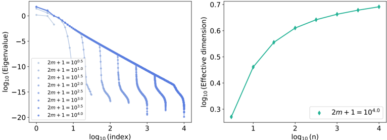<details> <summary>Image 17 Details</summary>  ### Visual Description \n ## Charts: Eigenvalue Spectrum and Effective Dimension ### Overview The image presents two charts. The left chart displays the log10 of the Eigenvalues versus the log10 of the Index for different values of '2m+1'. The right chart shows the log10 of the Effective Dimension versus the log10 of 'n', also for a specific value of '2m+1'. ### Components/Axes **Left Chart:** * **X-axis:** log10(Index), ranging approximately from 0 to 4. * **Y-axis:** log10(Eigenvalue), ranging approximately from -20 to 0. * **Legend:** Located in the top-left corner. Contains the following labels: * 2m+1 = 10^5 (Blue) * 2m+1 = 10^4 (Blue) * 2m+1 = 10^3.5 (Blue) * 2m+1 = 10^3 (Blue) * 2m+1 = 10^2.5 (Blue) * 2m+1 = 10^2 (Blue) * 2m+1 = 10^1 (Blue) **Right Chart:** * **X-axis:** log10(n), ranging approximately from 0 to 4. * **Y-axis:** log10(Effective dimension), ranging approximately from 0.3 to 0.7. * **Legend:** Located in the bottom-right corner. Contains the following label: * 2m+1 = 10^4 (Teal) ### Detailed Analysis or Content Details **Left Chart:** * **2m+1 = 10^5:** The line starts at approximately log10(Eigenvalue) = -0.5 at log10(Index) = 0, and decreases steadily to approximately log10(Eigenvalue) = -19 at log10(Index) = 4. * **2m+1 = 10^4:** The line starts at approximately log10(Eigenvalue) = -1.5 at log10(Index) = 0, and decreases steadily to approximately log10(Eigenvalue) = -18 at log10(Index) = 4. * **2m+1 = 10^3.5:** The line starts at approximately log10(Eigenvalue) = -2.5 at log10(Index) = 0, and decreases steadily to approximately log10(Eigenvalue) = -17 at log10(Index) = 4. * **2m+1 = 10^3:** The line starts at approximately log10(Eigenvalue) = -3.5 at log10(Index) = 0, and decreases steadily to approximately log10(Eigenvalue) = -16 at log10(Index) = 4. * **2m+1 = 10^2.5:** The line starts at approximately log10(Eigenvalue) = -4.5 at log10(Index) = 0, and decreases steadily to approximately log10(Eigenvalue) = -15 at log10(Index) = 4. * **2m+1 = 10^2:** The line starts at approximately log10(Eigenvalue) = -5.5 at log10(Index) = 0, and decreases steadily to approximately log10(Eigenvalue) = -14 at log10(Index) = 4. * **2m+1 = 10^1:** The line starts at approximately log10(Eigenvalue) = -6.5 at log10(Index) = 0, and decreases steadily to approximately log10(Eigenvalue) = -13 at log10(Index) = 4. **Right Chart:** * **2m+1 = 10^4:** The line starts at approximately log10(Effective dimension) = 0.32 at log10(n) = 0, increases rapidly to approximately log10(Effective dimension) = 0.65 at log10(n) = 3, and plateaus to approximately log10(Effective dimension) = 0.68 at log10(n) = 4. ### Key Observations * In the left chart, all lines exhibit a similar downward trend, indicating that the Eigenvalues decrease as the Index increases. The lines are parallel, suggesting that the rate of decrease is consistent across different values of '2m+1'. Higher values of '2m+1' correspond to higher Eigenvalues for a given index. * In the right chart, the effective dimension increases with 'n' and appears to saturate at higher values of 'n'. ### Interpretation The left chart shows the eigenvalue spectrum, which is a measure of the variance explained by each principal component. The rapid decay of the eigenvalues suggests that the data is concentrated in a few dimensions. The different curves represent the eigenvalue spectrum for different values of '2m+1', which likely represents a parameter controlling the complexity or resolution of the system. The right chart shows how the effective dimension of the data changes as the size of the data ('n') increases. The initial rapid increase in effective dimension indicates that adding more data points initially reveals more independent directions of variation. The saturation at higher values of 'n' suggests that the data eventually becomes fully spanned by the available dimensions. The relationship between the two charts is that the effective dimension is related to the number of significant eigenvalues. As 'n' increases, more eigenvalues become significant, leading to a higher effective dimension. The value of '2m+1' influences the overall scale of the eigenvalues and the rate at which the effective dimension increases. The saturation of the effective dimension suggests that the data is ultimately limited by the intrinsic dimensionality of the underlying system. </details> of C m M -1 M C m , while Figure 4.6 (Right) shows the effective dimension as a function of n . Similarly to the previous closed-form case, we observe that N ( log( n ) n , 1 log( n ) ) = o n →∞ ( n γ ) for all γ > 0 . The same argument as in the paragraph above shows that this results in a parametric convergence rate, provided D ( f /star ) = 0 . Heat equation on the disk. Let us now consider the one-dimensional heat equation D = ∂ ∂x -∂ 2 ∂y 2 , with d = 2 , s = 2 , and the disk Ω = { x ∈ R 2 , ‖ x ‖ 2 ≤ π } . Since the heat equation is known to have C ∞ solutions with bounded energy [see, e.g., Eva10, Chapter 2.3, Theorem 8], we expect the convergence rate to match that of H ∞ (Ω) , which corresponds to the parametric rate of n -1 . Once again, we observe N ( log( n ) n , 1 log( n ) ) = o n →∞ ( n γ ) for all γ > 0 , and thus an improvement over the n -2 / 3 -Sobolev minimax rate on H 2 (Ω) when D ( f /star ) = 0 . Quantifying the impact of physics. The three examples above show how incorporating physics can enhance the learning process by reducing the effective dimension, leading to a faster convergence rate. In all cases, the rate becomes parametric due to the PDE, achieving the fastest possible speed, as predicted by the central limit theorem. Our package can be directly applied to any linear PDE with constant coefficients to compute the effective convergence rate Fig. 4.7.: Heat equation. Left: Spectrum of C m M -1 m C m . Right: Estimation of the effective dimension n ↦→ N ( log( n ) n , 1 log( n ) ) . 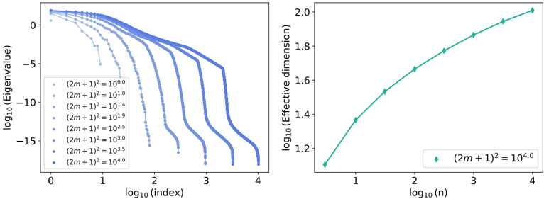<details> <summary>Image 18 Details</summary>  ### Visual Description ## Charts: Eigenvalue Spectrum and Effective Dimension ### Overview The image presents two charts. The left chart displays the log10 of the Eigenvalues versus the log10 of the index for different values of (2m+1)^2. The right chart shows the log10 of the Effective Dimension versus the log10 of n, also for (2m+1)^2 = 10^0.0. ### Components/Axes **Left Chart:** * **X-axis:** log10(index), ranging from approximately 0 to 4. * **Y-axis:** log10(Eigenvalue), ranging from approximately -15 to 0. * **Legend:** Located in the top-left corner, listing the following values for (2m+1)^2: * 10^0.0 * 10^1.4 * 10^1.9 * 10^3.0 * 10^3.5 * 10^4.0 * **Data Series:** Six curves, each representing a different value of (2m+1)^2. **Right Chart:** * **X-axis:** log10(n), ranging from approximately 0.5 to 4. * **Y-axis:** log10(Effective dimension), ranging from approximately 1.1 to 2.0. * **Legend:** Located in the bottom-right corner, indicating (2m+1)^2 = 10^0.0. * **Data Series:** A single line representing the relationship between log10(n) and log10(Effective dimension). ### Detailed Analysis or Content Details **Left Chart:** * The curves all exhibit a downward trend. The curves start near log10(Eigenvalue) = 0 and decrease to approximately log10(Eigenvalue) = -15. * (2m+1)^2 = 10^0.0: Starts at approximately log10(Eigenvalue) = 0 and decreases to approximately log10(Eigenvalue) = -15 at log10(index) = 4. * (2m+1)^2 = 10^1.4: Starts at approximately log10(Eigenvalue) = 0 and decreases to approximately log10(Eigenvalue) = -10 at log10(index) = 4. * (2m+1)^2 = 10^1.9: Starts at approximately log10(Eigenvalue) = 0 and decreases to approximately log10(Eigenvalue) = -12 at log10(index) = 4. * (2m+1)^2 = 10^3.0: Starts at approximately log10(Eigenvalue) = 0 and decreases to approximately log10(Eigenvalue) = -14 at log10(index) = 4. * (2m+1)^2 = 10^3.5: Starts at approximately log10(Eigenvalue) = 0 and decreases to approximately log10(Eigenvalue) = -14 at log10(index) = 4. * (2m+1)^2 = 10^4.0: Starts at approximately log10(Eigenvalue) = 0 and decreases to approximately log10(Eigenvalue) = -15 at log10(index) = 4. **Right Chart:** * The line exhibits an upward trend. * At log10(n) = 0.5, log10(Effective dimension) is approximately 1.15. * At log10(n) = 1, log10(Effective dimension) is approximately 1.25. * At log10(n) = 2, log10(Effective dimension) is approximately 1.5. * At log10(n) = 3, log10(Effective dimension) is approximately 1.75. * At log10(n) = 4, log10(Effective dimension) is approximately 1.9. ### Key Observations * The eigenvalue spectrum (left chart) shows that as (2m+1)^2 increases, the eigenvalues decay more slowly. * The effective dimension (right chart) increases linearly with log10(n). * The effective dimension is calculated for the case where (2m+1)^2 = 10^0.0. ### Interpretation The left chart illustrates the distribution of eigenvalues, which is a key characteristic of a matrix or operator. The different curves represent how the eigenvalue spectrum changes as the parameter (2m+1)^2 is varied. A slower decay in eigenvalues (higher values of (2m+1)^2) suggests that more dimensions are significant in representing the data. The right chart shows how the effective dimension scales with the size of the input 'n'. The linear relationship indicates that the number of effectively utilized dimensions grows logarithmically with 'n'. This suggests a dimensionality reduction or feature extraction process is at play, where the effective number of dimensions remains relatively small compared to the total number of input features. The combination of these two charts suggests a relationship between the parameter (2m+1)^2 and the effective dimensionality of the system. Increasing (2m+1)^2 leads to a slower decay of eigenvalues, which in turn implies a higher effective dimension. The right chart provides a quantitative measure of this effective dimension as a function of 'n', for a specific value of (2m+1)^2. </details> given a scaling of λ n and µ n . By identifying the optimal convergence rate, this approach can assist in determining the best parameters λ n and µ n for use in other PIML techniques, such as PINNs. ## 4.4 PDE solving: Mitigating the difficulties of PINNs with PIKL It turns out that our PIKL algorithm can be effectively used as a PDE solver. In this scenario, there is no noise (i.e., ε = 0 ), no modeling error (i.e., D ( f /star ) = 0 ), and the data consist of samples of boundary and initial conditions, as is typical for PINNs. Assume for example that the objective is to solve the Laplacian equation ∆( f /star ) = 0 on a domain Ω ⊆ [ -1 , 1] 2 with the Dirichlet boundary condition f /star | ∂ Ω = g , where g is a known function. Then this problem can be addressed by implementing the PIKL estimator, which minimizes the risk ¯ R n ( f ) = 1 n ∑ n i =1 | f ( X i ) -Y i | 2 + λ n ‖ f ‖ 2 H 2 per ([ -1 , 1] 2 ) + µ n ‖ ∆( f ) ‖ 2 L 2 (Ω) , where the X i are uniformly sampled on ∂ Ω and Y i = g ( X i ) . Of course, this example focuses on Dirichlet boundary conditions, but PIKL is a highly flexible framework that can incorporate a wide variety of boundary conditions, such as periodic and Neumann boundary conditions, as the next two examples will illustrate. Comparison with PINNs for the convection equation. To begin, we compare the performance of our PIKL algorithm with the PINN approach developed by Krishnapriyan et al. [Kri+21] for solving the one-dimensional convection equation D ( f ) = ∂ t f + β∂ x f on the domain Ω = [0 , 1] × [0 , 2 π ] . The problem is subject to the following periodic boundary conditions: $$\left \{ \begin{array} { l } { \forall x \in [ 0 , 2 \pi ] , \quad f ( 0 , x ) = \sin ( x ) , } \\ { \forall t \in [ 0 , 1 ] , \quad f ( t , 0 ) = f ( t , 2 \pi ) = 0 . } \end{array}$$ The solution of this PDE is given by f /star ( t, x ) = sin( x -βt ) . Krishnapriyan et al. [Kri+21] show that for high values of β , PINNs struggle to solve the PDE effectively. To address this challenge, we train our PIML kernel method using n = 100 data points and 1681 Fourier modes (i.e., m = 20 ). The training data set ( X i , Y i ) 1 ⩽ i ⩽ n is constructed such that X i = (0 , 2 πU i ) and Y i = sin( U i ) , where ( U i ) 1 ⩽ i ⩽ n are i.i.d. uniform random variables. To enforce the periodic boundary conditions, we center Ω at ˜ Ω = Ω -(0 . 5 , π ) , extend it to [ -1 , 1] × [ -π, π ] , and consider ˜ H m = Span(( t, x ) ↦→ e i ( π 2 k 1 t + k 2 x ) ) ‖ k ‖ ∞ ≤ m . Noting that for all ( j 1 , k 1 ) , ( j 2 , k 2 ) ∈ Z 2 , $$\int _ { [ - 1 , 1 ] \times [ - \pi , \pi ] } e ^ { i ( \frac { \pi } { 2 } ( k _ { 1 } - j _ { 1 } ) t + ( k _ { 2 } - j _ { 2 } ) x ) } d x = \frac { \sin ( \pi ( k _ { 1 } - j _ { 1 } ) / 2 ) } { \pi } \delta _ { k _ { 2 } , j _ { 2 } } ,$$ we let the matrix ( M m ) j,k be as follows: $$</text> </doctag>$$ where P is the polynomial associated with the operator D . Notice that, although f /star is a sinusoidal function, the frequency vector of f /star is ( -β, 1) , which does not belong to π 2 Z ⊕ Z . As a result, f /star does not lie in ˜ H m for any m . Table 4.1 compares the performance of various PIML methods using a sample of n = 100 initial condition points. The performance of an estimator ˆ f n on a test set ( Test ) is evaluated based on the L 2 relative error ( ∑ x ∈ Test ‖ ˆ f n ( x ) -f /star ( x ) ‖ 2 2 / ∑ y ∈ Test ‖ f /star ( y ) ‖ 2 2 ) 1 / 2 . Standard deviations are computed across 10 trials. The results show that the PIML kernel estimator clearly outperforms PINNs in terms of accuracy. Tab. 4.1.: L 2 relative error of the kernel method in solving the advection equation. | | Vanilla PINNs /diamondmath | Curriculum-trained PINNs /diamondmath | PIKL estimator | |--------|------------------------------|-----------------------------------------|------------------------------| | β = 20 | 7 . 50 × 10 - 1 | 9 . 84 × 10 - 3 | ( 1 . 56 ± 3 . 46 ) × 10 - 8 | | β = 30 | 8 . 97 × 10 - 1 | 2 . 02 × 10 - 2 | ( 0 . 91 ± 2 . 20 ) × 10 - 7 | | β = 40 | 9 . 61 × 10 - 1 | 5 . 33 × 10 - 2 | ( 7 . 31 ± 6 . 44 ) × 10 - 9 | Comparison with PINNs for the 1d-wave equation. The performance of the PIKL algorithm is compared to the PINN methodology of Wang et al. [WYP22, Section 7.3] for solving the one-dimensional wave equation D ( f ) = ∂ 2 t,t f -4 ∂ 2 x,x f on the square domain [0 , 1] 2 , with the following boundary conditions: $$\left \{ \begin{array} { l l } { \forall x \in [ 0 , 1 ] , \quad f ( 0 , x ) = \sin ( \pi x ) + \sin ( 4 \pi x ) / 2 , } \\ { \forall x \in [ 0 , 1 ] , \quad \partial _ { t } f ( 0 , x ) = 0 , } \\ { \forall t \in [ 0 , 1 ] , \quad f ( t , 0 ) = f ( t , 1 ) = 0 . } \end{array}$$ The solution of the PDE is f /star ( t, x ) = sin( πx ) cos(2 πt )+sin(4 πx ) cos(8 πt ) / 2 . This solution serves as an interesting benchmark since f /star exhibits significant variations, with ‖ ∂ t f /star ‖ 2 2 / ‖ f /star ‖ 2 2 = 16 π 2 (Figure 4.8, Left). Meanwhile, PINNs are known to have a spectral bias toward low frequencies [e.g., DAB22; Wan+22]. The optimization of the PINNs in Wang et al. [Wan+22] is carried out using stochastic gradient descent with 80 , 000 steps, each drawing 300 points at random, resulting in a sample size of n = 2 . 4 × 10 6 . The architecture of the PINNs these authors employ is a dense neural network with tanh activation functions and layers of sizes (2 , 500 , 500 , 500 , 1) , resulting in m = (2 × 500+500)+2 × (500 × 500+500)+(500 × 1+1) = 503 , 001 parameters. The training time for Vanilla PINNs is 7 minutes on an Nvidia L4 GPU (24 GB of RAM, 30.3 teraFLOPs for Float32). We obtain an L 2 relative error of 4 . 21 × 10 -1 , which is consistent with the results of Wang et al. [WYP22], who report a L 2 relative error of 4 . 52 × 10 -1 . Figure 4.8 (Middle) shows the Vanilla PINNs. We train our PIKL method using n = 10 5 data points and 1681 Fourier modes (i.e., m = 20 ). Let ( U i ) 1 ⩽ i ⩽ n be i.i.d. random variables uniformly distributed on [0 , 1] . The training data set ( X i , Y i ) 1 ⩽ i ⩽ n is constructed such that - if 1 ⩽ i ⩽ /floorleft n/ 4 /floorright , then X i = (0 , U i ) and Y i = sin( πU i ) + sin(4 πU i ) / 2 , - if /floorleft n/ 4 /floorright +1 ⩽ i ⩽ 2 /floorleft n/ 4 /floorright , then X i = ( U i , 0) and Y i = 0 , - if 2 /floorleft n/ 4 /floorright +1 ⩽ i ⩽ 3 /floorleft n/ 4 /floorright , then X i = ( U i , 1) and Y i = 0 , - if 3 /floorleft n/ 4 /floorright +1 ⩽ i ⩽ n , then X i = (1 /n, U i ) and $$\begin{array} { r l } & { Y _ { i } = f ( 0 , U _ { i } ) + \frac { 1 } { 2 n ^ { 2 } } \partial _ { t , t } ^ { 2 } f ( 0 , U _ { i } ) = f ( 0 , U _ { i } ) + \frac { 2 } { n ^ { 2 } } \partial _ { x , x } ^ { 2 } f ( 0 , U _ { i } ) } \\ & { = \left ( 1 - \frac { 2 \pi ^ { 2 } } { n ^ { 2 } } \right ) \sin ( \pi U _ { i } ) + \left ( \frac { 1 } { 2 } - \frac { 1 6 \pi ^ { 2 } } { n ^ { 2 } } \right ) \sin ( 4 \pi U _ { i } ) . } \end{array}$$ The final requirement enforces the initial condition ∂ t f = 0 in a manner similar to that of a second-order numerical scheme. Table 4.2 compares the performance of the PINN approach from Wang et al. [WYP22] with the PIKL estimator. Across 10 trials, the PIKL method achieves an L 2 relative error of (8 . 70 ± 0 . 08) × 10 -4 , which is 50% better than the performance of the PINNs. This demonstrates that the kernel approach is more accurate, requiring fewer data points and parameters than the PINNs. The training time for the PIKL estimator is 6 seconds on an Nvidia L4 GPU. Thus, the PIKL estimator can be computed 70 times faster than the Vanilla PINNs. Figure 4.8 (Right) shows the PIKL estimator. Note that in this case, the solution f /star can be represented by a sum of complex exponential functions ( f /star ∈ H 16 ), which could have biased the result in favor of the PIKL estimator by canceling its approximation error. However, the results remain unchanged when altering the frequencies in H m (e.g., taking L = 0 . 55 in (4.5) instead of L = 0 . 5 yields an L 2 relative error of (9 . 6 ± 0 . 3) × 10 -4 ). Tab. 4.2.: Performance of PINN/PIKL methods for solving the wave equation on Ω = [0 , 1] 2 | | Vanilla PINNs /diamondmath | NTK-optimized PINNs /diamondmath | PIKL estimator | |----------------------|------------------------------|------------------------------------|------------------------------| | L 2 relative error | 4 . 52 × 10 - 1 | 1 . 73 × 10 - 3 | ( 8 . 70 ± 0 . 08 ) × 10 - 4 | | Training data (n) | 2 . 4 × 10 6 | 2 . 4 × 10 6 | 10 5 | | Number of parameters | 5 . 03 × 10 5 | 5 . 03 × 10 5 | 1 . 68 × 10 3 | ## 4.5 PDE solving with noisy boundary conditions ## 4.5.1 Wave equation in dimension 2 Comparison with traditional PDE solvers. PIML is a promising framework for solving PDEs, particularly due to its adaptability to domains Ω with complex geometries, where most traditional PDE solvers tend to be highly domain-dependent. 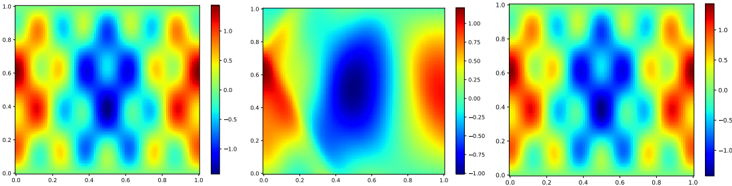However, its comparative performance <details> <summary>Image 19 Details</summary>  ### Visual Description \n ## Heatmaps: Three Comparative Distributions ### Overview The image presents three separate heatmaps displayed side-by-side. Each heatmap visualizes a two-dimensional distribution of values, represented by a color gradient. The heatmaps share the same x and y axis scales, ranging from 0.0 to 1.0. The color scale on the right indicates the value range, from approximately -1.0 to 1.0. The heatmaps appear to depict a vaguely humanoid shape in the first and third images. ### Components/Axes * **X-axis:** Ranges from 0.0 to 1.0. * **Y-axis:** Ranges from 0.0 to 1.0. * **Color Scale:** Ranges from approximately -1.0 (dark blue) to 1.0 (dark red), with intermediate colors representing values in between. The color scale is positioned on the right side of the middle heatmap. * **Heatmap 1 (Left):** Displays a distribution with a humanoid shape. * **Heatmap 2 (Center):** Displays a roughly elliptical distribution. * **Heatmap 3 (Right):** Displays a distribution with a humanoid shape, similar to the first heatmap. ### Detailed Analysis or Content Details **Heatmap 1 (Left):** * The highest values (dark red) are concentrated in the upper center and lower center of the image, forming the "head" and "legs" of the humanoid shape. * The lowest values (dark blue) are located in the central region of the body. * Approximate value ranges: * (0.2, 0.8): Values range from approximately -0.5 to 0.8. * (0.5, 0.2): Values range from approximately -0.5 to 0.8. * (0.5, 0.8): Values range from approximately -0.5 to 0.8. **Heatmap 2 (Center):** * The highest values (dark red) are concentrated in the center of the image. * The lowest values (dark blue) are located around the edges of the image. * Approximate value ranges: * (0.5, 0.5): Approximately 0.7. * (0.2, 0.2): Approximately 0.2. * (0.8, 0.8): Approximately 0.2. **Heatmap 3 (Right):** * The highest values (dark red) are concentrated in the upper center and lower center of the image, forming the "head" and "legs" of the humanoid shape. * The lowest values (dark blue) are located in the central region of the body. * Approximate value ranges: * (0.2, 0.8): Values range from approximately -0.5 to 0.8. * (0.5, 0.2): Values range from approximately -0.5 to 0.8. * (0.5, 0.8): Values range from approximately -0.5 to 0.8. ### Key Observations * Heatmaps 1 and 3 share a similar distribution pattern, resembling a humanoid shape. * Heatmap 2 exhibits a different distribution, with a central concentration of high values and lower values towards the edges. * The color scales are identical across all three heatmaps, allowing for direct visual comparison of the value distributions. * The humanoid shape in heatmaps 1 and 3 is not perfectly symmetrical. ### Interpretation The three heatmaps likely represent different data sets or different stages of a process. The humanoid shape in heatmaps 1 and 3 could represent the distribution of a certain attribute (e.g., density, probability) across a human-like form. The difference between the three heatmaps suggests that the underlying data or process has changed, resulting in the different distributions. The elliptical distribution in heatmap 2 could represent a different underlying phenomenon or a different perspective on the same data. The consistent color scale allows for a direct comparison of the magnitude of values across the three distributions. Without further context, it is difficult to determine the specific meaning of the data, but the visual patterns suggest that the data is related to spatial distributions and potentially human-related characteristics. </details> t t Fig. 4.8.: Left: ground truth solution f /star to the wave equation [taken from WYP22, Figure 6]. Middle: Vanilla PINNs from Wang et al. [WYP22]. Right: PIKL estimator. against traditional PDE solvers remains unclear in scenarios where both approaches can be easily implemented. The meta-analysis by McGreivy and Hakim [MH24] indicates that, in some cases, PINNs may be faster than traditional PDE solvers, although they are often less accurate. In our study, solving the wave equation on a simple square domain represents a setting where traditional numerical methods are straightforward to implement and are known to perform well. Table 4.3 summarizes the performance of classical techniques, including the explicit Euler, Runge-Kutta 4 (RK4), and Crank-Nicolson (CN) schemes (see Appendix 4.D.3 for a brief presentation of these methods). These methods clearly outperform both PINNs and the PIKL algorithm, even with fewer data points. Tab. 4.3.: Performance of traditional PDE solvers for the wave equation on Ω = [0 , 1] 2 . | | Euler explicit | RK4 | CN | |--------------------|------------------|----------------|----------------| | L 2 relative error | 3 . 8 × 10 - 6 | 6 . 8 × 10 - 6 | 5 . 6 × 10 - 3 | | Training data (n) | 10 4 | 10 4 | 10 4 | /negationslash Noisy boundary conditions. However, a more relevant setting for comparing the performance of these methods arises when noise is introduced into the boundary conditions. This situation is common, for instance, when the initial condition of the wave is measured by a noisy sensor. Such a setting aligns with hybrid modeling, where ε = 0 , but there is no modeling error (i.e., D ( f /star ) = 0 ). Table 4.4 compares the performance of all methods with Gaussian noise of variance of 10 -2 . In this case, the PIKL estimator outperforms all other approaches. Tab. 4.4.: Performance for the wave equation with noisy boundary conditions . | | PINNs | Euler explicit | RK4 | CN | PIKL estimator | |--------------------|-----------------|------------------|-----------------|-----------------|------------------| | L 2 relative error | 4 . 61 × 10 - 1 | 1 . 25 × 10 - 1 | 6 . 05 × 10 - 2 | 2 . 01 × 10 - 2 | 1 . 87 × 10 - 2 | | Training data (n) | 2 . 4 × 10 6 | 4 × 10 4 | 4 × 10 4 | 4 × 10 4 | 4 × 10 4 | Such PDEs with noisy boundary conditions are special cases of the hybrid modeling framework, where the data is located on the boundary of the domain. This situation arises, for example, in Cai et al. [Cai+21] which models the temperature in the core of a nuclear reactor. Fig. 4.9.: L 2 relative error of the models for the 4-dimensional heat equation with noisy boundary conditions as a function of the number of training points. Standard deviations are estimated over 5 runs. 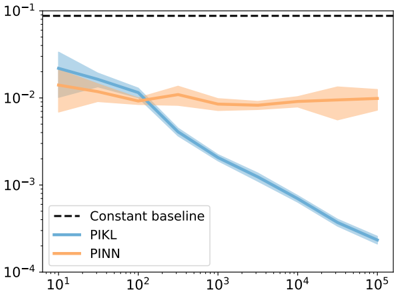<details> <summary>Image 20 Details</summary>  ### Visual Description \n ## Line Chart: Error Rate vs. Data Points ### Overview This image presents a line chart comparing the error rates of three methods – PIKL, PINN, and a Constant Baseline – as a function of the number of data points used. The error rate is plotted on a logarithmic scale (y-axis) against the number of data points on a logarithmic scale (x-axis). Each method's performance is represented by a line with a shaded area indicating the uncertainty or variance around the mean. ### Components/Axes * **X-axis:** Labeled "Data Points", with a logarithmic scale ranging from 10¹ to 10⁵. Tick marks are visible at 10¹, 10², 10³, 10⁴, and 10⁵. * **Y-axis:** Labeled "Error Rate", with a logarithmic scale ranging from 10⁻⁴ to 10⁻¹. Tick marks are visible at 10⁻⁴, 10⁻³, 10⁻², and 10⁻¹. * **Legend:** Located in the bottom-left corner. It contains the following entries: * "Constant baseline" – represented by a dashed black line. * "PIKL" – represented by a solid blue line. * "PINN" – represented by a solid orange line. ### Detailed Analysis * **Constant Baseline:** The dashed black line is horizontal and represents a constant error rate of approximately 0.1 (10⁻¹). * **PIKL (Blue Line):** The blue line starts at approximately 0.03 (3 x 10⁻²) at x = 10¹ and slopes downward, decreasing rapidly. At x = 10², the error rate is approximately 0.01 (1 x 10⁻²). The line continues to decrease, reaching approximately 0.0003 (3 x 10⁻⁴) at x = 10⁵. The shaded area around the line indicates a relatively small uncertainty, especially at higher data point values. * **PINN (Orange Line):** The orange line starts at approximately 0.04 (4 x 10⁻²) at x = 10¹ and initially increases slightly, reaching a peak around x = 10². After x = 10², the line plateaus and remains relatively constant, fluctuating between approximately 0.01 (1 x 10⁻²) and 0.02 (2 x 10⁻²). The shaded area around the line is larger than that of PIKL, indicating greater uncertainty. ### Key Observations * PIKL consistently outperforms the Constant Baseline and PINN across all data point values. * PINN's error rate does not decrease significantly with increasing data points, suggesting it may be limited by its method. * The Constant Baseline provides a fixed error rate, serving as a reference point for evaluating the performance of the other methods. * The uncertainty around PINN is significantly higher than that of PIKL, indicating greater variability in its performance. ### Interpretation The chart demonstrates that the PIKL method is significantly more effective at reducing error rates as the number of data points increases compared to PINN. PINN appears to reach a performance plateau, while PIKL continues to improve. The Constant Baseline serves as a benchmark, and both PIKL and PINN outperform it. The smaller uncertainty around PIKL suggests it is a more reliable method. This data suggests that PIKL is a more scalable and robust approach for this particular problem, as its performance improves with more data. PINN, while initially comparable, does not benefit from increased data and exhibits greater variability. The logarithmic scales on both axes emphasize the substantial reduction in error rate achieved by PIKL, particularly as the number of data points grows. The consistent performance of the Constant Baseline highlights the value of the improvements offered by PIKL and PINN. </details> ## 4.5.2 Heat equation in dimension 4 Still in the context of noisy boundary conditions, we study the feasibility and limitations of the PIKL estimator in higher dimensions. To this aim, we consider the task of learning a solution to the heat equation in dimension 4 with noisy boundary conditions. In this setting, the goal is to learn $$f ^ { * } ( x _ { 1 } , x _ { 2 } , x _ { 3 } , x _ { 4 } ) = \exp ( - 3 x _ { 1 } / \pi ^ { 2 } ) \cos ( x _ { 2 } / \pi ) \cos ( x _ { 3 } / \pi ) \cos ( x _ { 4 } / \pi )$$ on Ω = [ -0 . 5 , 0 . 5] 4 given n i.i.d. observations ( X 1 , Y 1 ) , . . . , ( X n , Y n ) such that Y = f /star ( X ) + N (0 , 10 -2 ) , and X is sampled on ( { 0 }× [ -0 . 5 , 0 . 5] 3 ) ∪ ([ -0 . 5 , 0 . 5] × ∂ [ -0 . 5 , 0 . 5] 3 ) to respectively encode the initial and boundary conditions. The function f /star is the unique solution to the heat equation ( ∂ 1 -∂ 2 2 , 2 -∂ 2 3 , 3 -∂ 2 4 , 4 ) f /star = 0 satisfying this set of initial and boundary conditions [see, e.g., Eva10, Chapter 2.3, Theorem 5]. The function f /star is flat, and close to the constant function equal to 1 . We compare the performance of our PIKL estimator with a PINN. Here, the PIKL estimator is computed with m = 3 , leading to 2401 Fourier modes. The PINN is a fully-connected neural network with three hidden layers of size 10, using tanh as activation function, and optimized on 2 × 10 5 collocation points by 2000 gradient descent steps. In this high-dimensional setting, Figure 4.9 shows that the PIKL estimator clearly outperforms the PINN both in terms of performance. Note that both methods outperform the constant model equal to ∫ Ω f /star (dotted line). Moreover, the PIKL estimator is more than 100 times faster than the PINN. The experimental convergence rate of the PIKL estimator is n -0 . 53 , which matches the parametric rate of n -1 / 2 . ## 4.6 Conclusion and future directions In this article, we developed an efficient algorithm to solve the PIML hybrid problem (4.2). The PIKL estimator can be computed exactly through matrix inversion and possesses strong theoretical properties. Specifically, we demonstrated how to estimate its convergence rate based on the PDE prior D . Moreover, through various examples, we showed that it outperforms PINNs in terms of performance, stability, and training time in certain PDE-solving tasks where PINNs struggle to escape local minima during optimization. Future work could focus on comparing PIKL with the implementation of RFF and exploring its performance against PINNs in the case of PDEs with non-constant coefficients. Another avenue for future research is to assess the effectiveness of the kernel approach compared to traditional PDE solvers, as discussed in Section 4.5. Extension to nonlinear PDEs. Extending the PIKL framework to accommodate nonlinear PDEs is an important and interesting direction for future research. From a PDE theory point of view, it is expected to be harder to deal with nonlinear PDEs, since nonlinear differential operators are challenging compared to linear operators. Even in dimension d = 1 , the solution of the ODE y ′ = y 2 with initial condition y (0) = y 0 is y ( t ) = (1 /y 0 -t ) -1 , which explodes at t = y 0 . Note that the domain of the solution y is given by the set { t ≤ y 0 } , which intricately depends on the initial condition y 0 . This prevents us from using a systematic methodology to solve this problem, and would require to design specific algorithms tailored to the condition-dependent geometry of the domain Ω . ## 4.A Comments on the PIKL estimator ## 4.A.1 Spectral methods and PIKL The Fourier approximation on which the PIKL algorithm relies resembles usual spectral methods. Spectral methods are a class of numerical techniques used to solve PDEs by representing the solution as a sum of basis functions, typically trigonometric (Fourier series) or polynomial (Chebyshev or Legendre polynomials). These methods are particularly powerful for problems with smooth solutions and periodic or well-behaved boundary conditions [e.g., Can+07]. However the basis functions used in spectral and pseudo-spectral methods must be specifically tailored to the domain Ω , the differential operator D , and the boundary conditions. This customization ensures that the method effectively captures the characteristics of the problem being solved. For example, the Fourier basis is unable to accurately reconstruct non-periodic functions on a square domain, leading to the Gibbs phenomenon at points of periodic discontinuity. A natural solution to this problem is to extend the solution of the PDE from the domain Ω to a simpler domain that admits a known spectral basis [e.g., MH16, for Fourier basis extension]. If the solution of the PDE on Ω can be extended to a solution of the same PDE on the extended domain, it becomes possible to apply a spectral method directly to the extended domain [e.g., BD01; Lui09]. However, the PDE must satisfy certain regularity conditions (e.g., ellipticity), and there must be a method to implement the boundary conditions on ∂ Ω instead of on the boundary of the extended domain. In this article, we take a slightly different approach. Although we extend Ω ⊆ [ -L, L ] d to [ -2 L, 2 L ] d , we impose the PDE only on Ω and not on the entire extended domain [ -2 L, 2 L ] d . Also, unlike spectral methods, we do not require that D ( ˆ f PIKL ) = 0 . Instead, to ensure that the problem is well-posed, we regularize the PIML problem using the Sobolev norm of the periodic extension. This Tikhonov regularization is a conventional approach in kernel learning and is known to resemble spectral methods because it acts as a low-pass filter [see, e.g., CV07]. However, given a kernel, it is non-trivial to identify the basis of orthogonal functions that diagonalize it. The main contribution of this article is to establish an explicit connection between the Fourier basis and the PIML kernel, leading to surprisingly simple formulas for the kernel matrix M m . ## 4.A.2 Choice of the extended domain Embedding Ω in a toroidal structure is necessary to consider periodic functions, which is a requirement for our Fourier expansion. Let L T define the length of the torus, i.e., such that an extension to [ -L T , L T ] is considered. Since we assume that Ω ⊆ [ -L, L ] d , we necessarily have L T > L . This condition being satisfied, any value of L T > L would be admissible for the PIKL framework. However, the choice of L T may impact the algorithmic performances. In particular, the basis functions Φ k ( x ) = exp( i π L T 〈 k, x 〉 ) depend on L T . With a fixed number m of Fourier modes, we see that for all k such that ‖ k ‖ ∞ ≤ m , and for all x ∈ Ω , lim L T →∞ Φ k ( x ) = 1 . This means that, in the case of an excessively large torus (when L T →∞ grows), our PIKL estimator will only be able to learn constant functions. Therefore, L T should not be too large relative to L . Letting L T be close to L , i.e., L T = (1 + ε ) L is not a good idea. To see this, consider the case where d = 1 and Ω = [ -1 , 1] . Then, if ε is small, the periodic extension of f /star to [ -1 -ε, 1 + ε ] will admit an exploding Sobolev norm. Indeed, for any periodic function f ∈ H 1 per ([ -1 -ε, 1 + ε ]) , we have $$\| f \| _ { H ^ { 1 } _ { p e r } ( [ - 1 - \varepsilon , 1 + \varepsilon ] ) } ^ { 2 } = \int _ { [ - 1 - \varepsilon , 1 + \varepsilon ] } f ^ { 2 } + ( f ^ { \prime } ) ^ { 2 } \geq \int _ { [ - 1 - \varepsilon , 1 + \varepsilon ] } ( f ^ { \prime } ) ^ { 2 } \geq \int _ { [ - \varepsilon , \varepsilon ] } ( f ^ { \prime } ( x + 1 + \varepsilon ) ) ^ { 2 } d x .$$ Then, the Cauchy-Schwarz inequality states that $$\int _ { [ - \varepsilon , \varepsilon ] } ( f ^ { \prime } ( x + 1 + \varepsilon ) ) ^ { 2 } d x \int _ { [ - \varepsilon , \varepsilon ] } 1 d x \geq \left ( \int _ { [ - \varepsilon , \varepsilon ] } f ^ { \prime } ( x + 1 + \varepsilon ) d x \right ) ^ { 2 } ,$$ meaning that $$\int _ { [ - \varepsilon , \varepsilon ] } ( f ^ { \prime } ( x + 1 ) ) ^ { 2 } d x \geq \varepsilon ^ { - 1 } [ f ( 1 ) - f ( - 1 ) ] ^ { 2 } .$$ All in all, denoting by E ( f /star ) the extension of f /star to [ -1 -ε, 1 + ε ] , we deduce that $$\| E ( f ^ { * } ) \| _ { H _ { p e r } ^ { 1 } ( [ - 1 - \varepsilon , 1 + \varepsilon ] ) } ^ { 2 } \geq \varepsilon ^ { - 1 } ( f ^ { * } ( 1 ) - f ^ { * } ( - 1 ) ) ^ { 2 } .$$ This computation shows that taking the extension torus to be [ -1 -ε, 1+ ε ] results in the Sobolev norm ‖ f /star ‖ 2 H 1 per ([ -1 -ε, 1+ ε ]) introducing a bias towards functions satisfying f /star (1) = f /star ( -1) , i.e., favoring periodic functions on Ω . The choice of an optimal constant L T depending on L is non-trivial, and closely relates to computing the constant in the Sobolev embedding H s (Ω) → H s per ([ -L T , L T ]) , which is known to be a difficult problem in functional analysis. Given that L T = 2 L strikes a balance by avoiding both pathological behaviors discussed earlier, we have adopted this choice throughout the paper. ## 4.A.3 Reproducing property Here, we formally prove that both properties $$( i ) \ f ( x ) = \langle M _ { m } ^ { 1 / 2 } z , M _ { m } ^ { - 1 / 2 } \Phi _ { m } ( x ) \rangle _ { \mathbb { C } ^ { ( 2 m + 1 ) ^ { d } } } , a n d$$ $$( i i ) \ \| f \| _ { R K H S } ^ { 2 } = \langle z , M _ { m } z \rangle _ { C ^ { ( 2 m + 1 ) ^ { d } } } = \| M _ { m } ^ { 1 / 2 } z \| _ { 2 } ^ { 2 }$$ are sufficient to show that minimizing ¯ R n is a kernel method. From ( i ) and ( ii ) , we deduce that the feature map is x ↦→ M -1 / 2 m Φ m ( x ) . The kernel is thus necessarily given by K ( x, y ) = 〈 M -1 / 2 m Φ m ( x ) , M -1 / 2 m Φ m ( y ) 〉 C (2 d +1) d . From ( ii ) , we deduce that the RKHS inner product is given by 〈 z, ˜ z 〉 RKHS = 〈 M 1 / 2 m z, M 1 / 2 m ˜ z 〉 C (2 d +1) d , so that ‖ z ‖ 2 RKHS = ‖ M 1 / 2 m z ‖ 2 2 . The reproducing property is then a consequence of ( i ) and ( ii ) . Indeed, let x ∈ Ω . We know that 〈 f, K ( x, · ) 〉 RKHS = 〈 M 1 / 2 m z, M 1 / 2 m ˜ z 〉 C (2 d +1) d , where z is the Fourier vector of f and ˜ z the Fourier vector of K ( x, · ) . Since the kernel K results from $$K ( x , y ) = \langle M _ { m } ^ { - 1 / 2 } \Phi _ { m } ( x ) , M _ { m } ^ { - 1 / 2 } \Phi _ { m } ( y ) \rangle _ { \mathbb { C } ^ { ( 2 d + 1 ) ^ { d } } } = \langle M _ { m } ^ { - 1 } \Phi _ { m } ( x ) , \Phi _ { m } ( y ) \rangle _ { \mathbb { C } ^ { ( 2 d + 1 ) ^ { d } } } ,$$ we know that ˜ z = M -1 m Φ m ( x ) . This means that $$\langle f , K ( x , \cdot ) \rangle _ { R K H S } = \langle M _ { m } ^ { 1 / 2 } z , M _ { m } ^ { 1 / 2 } M _ { m } ^ { - 1 } \Phi _ { m } ( x ) \rangle _ { \mathbb { C } ^ { ( 2 d + 1 ) ^ { d } } } = \langle z , \Phi _ { m } ( x ) \rangle _ { \mathbb { C } ^ { ( 2 d + 1 ) ^ { d } } } = f ( x ) ,$$ which is the reproducing property. ## 4.B Fundamentals of functional analysis on complex Hilbert spaces Let L > 0 and d ∈ N /star . We define L 2 ([ -2 L, 2 L ] d , C ) as the space of complex-valued functions f on the hypercube [ -2 L, 2 L ] d such that ∫ [ -2 L, 2 L ] d | f | 2 < ∞ . The real part of f is denoted by /Rfractur ( f ) , and the imaginary part by /Ifractur ( f ) , such that f = /Rfractur ( f ) + i /Ifractur ( f ) . Throughout the appendix, for the sake of clarity , we use the dot symbol · to represent functions. For example, ‖· ‖ denotes the function x ↦→‖ x ‖ , and 〈· , ·〉 stands for the function ( x, y ) ↦→〈 x, y 〉 . Definition 4.B.1 ( L 2 -space and ‖ · ‖ 2 -norm) . The separable Hilbert space L 2 ([ -2 L, 2 L ] d , C ) is associated with the inner product 〈 f, g 〉 = ∫ [ -2 L, 2 L ] d f ¯ g and the norm ‖ f ‖ 2 2 = ∫ [ -2 L, 2 L ] d | f | 2 . Let s ∈ N . Definition 4.B.2 (Periodic Sobolev spaces) . The periodic Sobolev space H s per ([ -2 L, 2 L ] d , R ) is the space of real functions f ( x ) = ∑ k ∈ Z d z k exp( iπ 2 L 〈 k, x 〉 ) such that the Fourier coefficients z k satisfy ∑ k | z k | 2 (1 + ‖ k ‖ 2 s ) < ∞ . The corresponding complex periodic Sobolev space is defined by $$H _ { p e r } ^ { s } ( [ - 2 L , 2 L ] ^ { d } , \mathbb { C } ) = H _ { p e r } ^ { s } ( [ - 2 L , 2 L ] ^ { d } , \mathbb { R } ) \oplus i \, H _ { p e r } ^ { s } ( [ - 2 L , 2 L ] ^ { d } , \mathbb { R } ) .$$ It is the space of complex-valued functions f ( x ) = ∑ k ∈ Z d z k exp( iπ 2 L 〈 k, x 〉 ) such that ∑ k | z k | 2 (1 + ‖ k ‖ 2 s ) < ∞ . We recall that, given two Hilbert spaces H 1 and H 2 , an operator is a linear function from H 1 to H 2 . Definition 4.B.3 (Operator norm) . [e.g., Bre10, Section 2.6] Let O : L 2 ([ -2 L, 2 L ] d , C ) → L 2 ([ -2 L, 2 L ] d , C ) be an operator. Its operator norm ||| O ||| 2 is defined by /negationslash $$| | | \mathcal { O } | | | _ { 2 } = \sup _ { g \in L ^ { 2 } ( [ - 2 L , 2 L ] ^ { d } , \mathbb { C } ) } \| \mathcal { O } g \| _ { 2 } = \sup _ { g \in L ^ { 2 } ( [ - 2 L , 2 L ] ^ { d } , \mathbb { C } ) } \| g \| _ { 2 } ^ { - 1 } \| \mathcal { O } g \| _ { 2 } .$$ The operator norm is sub-multiplicative, i.e., ||| O 1 ◦ O 2 ||| 2 ⩽ ||| O 1 ||| 2 ×||| O 2 ||| 2 . Definition 4.B.4 (Adjoint) . Let ( H , 〈· , ·〉 H ) be an Hilbert space and O : H → H be an operator. The adjoint O /star of O is the unique operator such that ∀ f, g ∈ H , 〈 f, O g 〉 H = 〈 O /star f, g 〉 H . If H = R d with the canonical scalar product, then O /star is the d × d matrix O /star = O T . If H = C d with the canonical sesquilinear inner product, then O /star is the d × d matrix O /star = ¯ O T . Definition 4.B.5 (Hermitian operator) . Let H be an Hilbert space and O : H → H be an operator. The operator O is said to be Hermitian if O = O /star . Theorem 4.B.6 (Spectral theorem) . [e.g. Rud91, Theorems 12.29 and 12.30] Let O be a positive Hermitian compact operator. Then O is diagonalizable on an Hilbert basis with positive eigenvalues that tend to zero. We denote its eigenvalues, ordered in decreasing order, by σ ( O ) = ( σ ↓ k ( O )) k ∈ N /star . We emphasize that, given an invertible positive self-adjoint compact operator O and its inverse O -1 , the eigenvalues of O -1 can also be ordered in increasing order, i.e., $$\sigma ( \mathcal { O } ^ { - 1 } ) = ( \sigma _ { k } ^ { \uparrow } ( \mathcal { O } ^ { - 1 } ) ) _ { k \in \mathbb { N } ^ { * } } = ( \sigma _ { k } ^ { \downarrow } ( \mathcal { O } ^ { - 1 } ) ) _ { k \in \mathbb { N } ^ { * } } .$$ Theorem 4.B.7 (Courant-Fischer minmax theorem ) . [Bre10, Problem 37] Let O : H → H be a positive Hermitian compact operator. Then $$\sigma _ { k } ^ { \downarrow } ( \mathcal { O } ) = \underset { \substack { d i m \, H = k \\ \text {$\theta$} } } { \max } \underset { \substack { g \in H \\ \| g \| _ { 2 } = 1 } } { \min } \langle g , \mathcal { O } g \rangle _ { \mathcal { H } } .$$ $$\sigma _ { k } ^ { \uparrow } ( \mathcal { O } ^ { - 1 } ) = \min _ { \substack { H \subseteq \mathcal { O } ( \mathcal { H } ) \\ \dim H = k } } \, \max _ { g \in H } \langle g , \mathcal { O } ^ { - 1 } g \rangle _ { \mathcal { H } } .$$ If O is injective, then Interestingly, if O is a positive Hermitian compact operator, then Theorem 4.B.7 shows that ||| O ||| 2 equals its largest eigenvalue. Definition 4.B.8 (Orthogonal projection on H m ) . We let Π m : H s per ([ -2 L, 2 L ] d , C ) → H m be the orthogonal projection with respect to 〈· , ·〉 , i.e., for all f ∈ H s per ([ -2 L, 2 L ] d , C ) , $$\Pi _ { m } f ( y ) = \sum _ { \| k \| _ { \infty } \leqslant m } \left ( \frac { 1 } { ( 4 L ) ^ { d } } \int _ { [ - 2 L , 2 L ] ^ { d } } \exp \left ( - \frac { i \pi } { 2 L } \langle k , x \rangle \right ) f ( x ) d x \right ) \exp \left ( \frac { i \pi } { 2 L } \langle k , y \rangle \right ) .$$ Note that Π m is Hermitian and that, for all f ∈ L 2 ([ -2 L, 2 L ] d , C ) , lim m →∞ ‖ f -Π m f ‖ 2 = 0 . ## 4.C Theoretical results for PIKL ## 4.C.1 Detailed computation of the Fourier expansion of the differential penalty The formula relating ‖ D ( f ) ‖ L 2 (Ω) to the Fourier coefficients of f follows from ( i ) expanding f in the Fourier basis, ( ii ) leveraging the linearity of D , ( iii ) applying the property D ( x ↦→ e -iπ 2 L 〈 k,x 〉 ) = ( x ↦→ P ( k ) e -iπ 2 L 〈 k,x 〉 ) , and (iv) recognizing that | z | 2 = z ¯ z . From these steps, we deduce that $$\| \mathcal { D } ( f ) \| _ { L ^ { 2 } ( \Omega ) } ^ { 2 } & = \int _ { \Omega } | \mathcal { D } ( f ) ( x ) | ^ { 2 } d x \\ & = \int _ { \Omega } \left | \sum _ { \| j \| _ { \infty } \leqslant m } z _ { j } \frac { P ( j ) } { ( 4 L ) ^ { d / 2 } } e ^ { - \frac { i \pi } { 2 L } \langle j , x \rangle } \right | ^ { 2 } d x , \\ & = \int _ { \Omega } \left ( \sum _ { \| j \| _ { \infty } \leqslant m } z _ { j } \frac { P ( j ) } { ( 4 L ) ^ { d / 2 } } e ^ { - \frac { i \pi } { 2 L } \langle j , x \rangle } \right ) \left ( \sum _ { \| k \| _ { \infty } \leqslant m } \bar { z } _ { k } \frac { P ( k ) } { ( 4 L ) ^ { d / 2 } } e ^ { \frac { i \pi } { 2 L } \langle k , x \rangle } d x \right ) d x \\ & = \sum _ { \| j \| _ { \infty } \leqslant m , \| k \| _ { \infty } \leqslant m } z _ { j } \bar { z } _ { k } \frac { P ( j ) \bar { P } ( k ) } { ( 4 L ) ^ { d } } \int _ { \Omega } e ^ { \frac { i \pi } { 2 L } \langle k - j , x \rangle } d x .$$ ## 4.C.2 Proof of Proposition 4.2.4 We have $$\frac { 1 } { ( 4 L ) ^ { d } } \int _ { [ - L , L ] ^ { d } } e ^ { \frac { i \pi } { 2 L } \langle k , x \rangle } d x & = \frac { 1 } { ( 4 L ) ^ { d } } \prod _ { j = 1 } ^ { d } \int _ { [ - L , L ] } e ^ { \frac { i \pi } { 2 L } k _ { j } x } d x = \prod _ { j = 1 } ^ { d } \left [ \frac { 1 } { 2 i \pi } e ^ { \frac { i \pi } { 2 L } k _ { j } x } \right ] _ { x = - L } ^ { L } \\ & = \prod _ { j = 1 } ^ { d } \frac { e ^ { \frac { i \pi } { 2 } k _ { j } } - e ^ { - \frac { i \pi } { 2 } k _ { j } } } { 2 i \pi k _ { j } } = \prod _ { j = 1 } ^ { d } \frac { \sin ( \frac { \pi } { 2 } k _ { j } ) } { \pi k _ { j } } .$$ The characteristic function of the Euclidean ball is computed in Bracewell [Bra00, Table 13.4]. ## 4.C.3 Operations on characteristic functions Proposition 4.C.1 (Operations on characteristic functions) . Consider d ∈ N /star , L > 0 , and Ω ⊆ [ -L, L ] d . - Let a ∈ [ -1 , 1] . Then a · Ω ⊆ [ -L, L ] d and $$F _ { a \cdot \Omega } ( k ) = | a | ^ { d } \times F _ { \Omega } ( a \cdot k ) .$$ - Let ˜ Ω ⊆ [ -L, L ] d be a domain such that Ω ∩ ˜ Ω = ∅ . Then Ω /unionsq ˜ Ω ⊆ [ -L, L ] d and $$F _ { \Omega \sqcup \tilde { \Omega } } ( k ) = F _ { \Omega } ( k ) + F _ { \tilde { \Omega } } ( k ) .$$ - Assume that Ω ⊆ [ -L/ 2 , L/ 2] d , and let z ∈ R d be such that ‖ z ‖ ∞ < L/ 2 . Then Ω+ z ⊆ [ -L, L ] d and $$F _ { \Omega + z } ( k ) = F _ { \Omega } ( k ) \times \exp { \left ( \frac { i \pi } { 2 L } \langle k , z \rangle \right ) } .$$ - Assume that Ω = Ω 1 × Ω 2 , where Ω 1 ⊆ [ -L, L ] d 1 , Ω 2 ⊆ [ -L, L ] d 2 , and d 1 + d 2 = d . Then F Ω ( k ) = F Ω 1 ( k 1 , . . . , k d 1 ) × F Ω 2 ( k d 1 +1 , . . . , k d ) . ## 4.C.4 Operator extensions Definition 4.C.2 (Projection on Ω ) . The projection C : L 2 ([ -2 L, 2 L ] d , C ) → L 2 ([ -2 L, 2 L ] d , C ) on Ω is defined by C ( f ) = 1 Ω f . Definition 4.C.3 (Operator extensions) . The operators C m : H m → H m , M m : H m → H m , and M -1 m : H m → H m can be extended to L 2 ([ -2 L, 2 L ] d , C ) by C m = Π m C m Π m , M m = Π m M m Π m , and M -1 m = Π m M -1 m Π m . From now on, we consider the extensions of these operators, allowing us to express equivalently $$| | | M _ { m } ^ { - 1 } | | | _ { 2 } = \sup _ { \substack { g \in H _ { m } \\ \| g \| _ { 2 } = 1 } } \| M _ { m } ^ { - 1 } g \| _ { 2 } = \sup _ { \substack { g \in L ^ { 2 } ( [ - 2 L , 2 L ] ^ { d } ) \\ \| g \| _ { 2 } = 1 } } \| M _ { m } ^ { - 1 } g \| _ { 2 } .$$ It is important to note that the extended operator M -1 m is no longer the inverse of the extended operator M m . Proposition 4.C.4 (Compact operator extension) . Let O be a positive Hermitian compact operator on L 2 ([ -2 L, 2 L ] d , R ) . Then its unique extension ˜ O to L 2 ([ -2 L, 2 L ] d , C ) is a positive Hermitian compact operator with the same real eigenfunctions and positive eigenvalues. Proof. Since ˜ O is C -linear, we necessarily have ˜ O ( f ) = O ( /Rfractur ( f )) + i O ( /Ifractur ( f )) . Therefore, the extension is unique. Since O is compact, ˜ O is also compact. According to Theorem 4.B.6, the operator O is diagonalizable in a Hermitian basis ( f k ) k ∈ N /star . Thus, for all f ∈ L 2 ([ -2 L, 2 L ] , R ) , $$\mathcal { O } ( f ) = \sum _ { k \in \mathbb { N } ^ { * } } \sigma _ { k } ^ { \downarrow } ( \mathcal { O } ) \langle f , f _ { k } \rangle _ { L ^ { 2 } ( [ - 2 L , 2 L ] , \mathbb { R } ) } f _ { k } .$$ Thus, for all f ∈ L 2 ([ -2 L, 2 L ] , C ) $$\tilde { \mathcal { O } } ( f ) & = \sum _ { k \in N ^ { * } } \sigma _ { k } ^ { \downarrow } ( \mathcal { O } ) ( \langle \Re ( f ) , f _ { k } \rangle _ { L ^ { 2 } ( [ - 2 L , 2 L ] , \mathbb { R } ) } + i \langle \Im ( f ) , f _ { k } \rangle _ { L ^ { 2 } ( [ - 2 L , 2 L ] , \mathbb { R } ) } ) f _ { k } \\ & = \sum _ { k \in N ^ { * } } \sigma _ { k } ^ { \downarrow } ( \mathcal { O } ) \langle f , f _ { k } \rangle _ { L ^ { 2 } ( [ - 2 L , 2 L ] , \mathbb { C } ) } f _ { k } .$$ This formula shows that ˜ O is Hermitian and diagonalizable with the same real eigenfunctions and positive eigenvalues as O . Recall that O n is the operator O n = lim m →∞ M -1 m , where the limit is taken in the sense of the operator norm [see Proposition B.2 Dou+24a]. Definition 4.C.5 (Operator M ) . Proposition 4.C.4 shows that the operator O n can be extended to L 2 ([ -2 L, 2 L ] , C ) . We denote the extension of O n by M -1 . The uniqueness of the extension in Proposition 4.C.4 implies that the extension of the operator C O n C : L 2 ([ -2 L, 2 L ] d ) → L 2 ([ -2 L, 2 L ] d ) to C is indeed CM -1 C : L 2 ([ -2 L, 2 L ] d , C ) → L 2 ([ -2 L, 2 L ] d , C ) . Proposition 4.C.4 shows that C O n C has the same eigenvalues as CM -1 C . ## 4.C.5 Convergence of M -1 m Lemma 4.C.6 (Bounding the spectrum of M -1 m ) . Let m ∈ N /star . Then, for all k ∈ N /star , $$\sigma _ { k } ^ { \downarrow } ( M _ { m } ^ { - 1 } ) \leqslant \sigma _ { k } ^ { \downarrow } ( M ^ { - 1 } ) .$$ Proof. Let f ∈ H m . Then, $$\langle f , M _ { m } f \rangle = \langle f , M f \rangle = \lambda _ { n } \| f \| _ { H _ { p e r } ^ { s } ( [ - 2 L , 2 L ] ^ { d } ) } ^ { 2 } + \mu _ { n } \| \mathcal { D } ( f ) \| _ { L ^ { 2 } ( \Omega ) } ^ { 2 } .$$ Thus, using Theorem 4.B.7, we deduce that $$\sigma _ { k } ^ { \uparrow } ( M _ { m } ) & = \min _ { H \subseteq H _ { m } } \max _ { g \in H } \langle g , M _ { m } g \rangle \\ & = \min _ { H \subseteq H _ { m } } \max _ { g \in H } \langle g , M g \rangle \\ & = \max _ { H \subseteq H _ { m } } \min _ { g \in H } \max _ { \| g \| _ { 2 } = 1 } \langle g , M g \rangle \begin{array} { r l } & { d u c e t h a t \sigma _ { k } ^ { \downarrow } ( M ^ { - 1 } ) \lesssim \sigma _ { k } ^ { \downarrow } ( M ^ { - 1 } ) , } \end{array} </doctag>$$ From (4.8), we deduce that σ ↓ k ( M -1 m ) ⩽ σ ↓ k ( M -1 ) . Lemma 4.C.7 (Spectral convergence of M m ) . Let m ∈ N /star . Then, for all k ∈ N /star , one has $$\lim _ { m \rightarrow \infty } \sigma _ { k } ^ { \downarrow } ( M _ { m } ^ { - 1 } ) = \sigma _ { k } ^ { \downarrow } ( M ^ { - 1 } ) .$$ Proof. By continuity of the RKHS norm f ↦→ 〈 f, Mf 〉 on H s per ([ -2 L, 2 L ] d , C ) [Dou+24a, Proposition B.1], we deduce that, for all function f ∈ H s per ([ -2 L, 2 L ] d , C ) , the quantity λ n ‖ Π m ( f ) ‖ 2 H s per ([ -2 L, 2 L ] d , C ) + µ n ‖ D (Π m ( f )) ‖ 2 L 2 (Ω , C ) converges, as m goes to the infinity, to λ n ‖ f ‖ 2 H s per ([ -2 L, 2 L ] d , C ) + µ n ‖ D ( f ) ‖ 2 L 2 (Ω , C ) . Thus, $$\forall f \in H _ { p e r } ^ { s } ( [ - 2 L , 2 L ] ^ { d } , \mathbb { C } ) , \quad \lim _ { m \to \infty } \langle f , ( M - M _ { m } ) f \rangle = 0 .$$ Next, consider f 1 , . . . , f k to be the eigenfunctions of M associated with the ordered eigenvalue σ ↑ 1 ( M ) , . . . , σ ↑ k ( M ) . Since, for any 1 ⩽ j, /lscript ⩽ k , we have that lim m →∞ 〈 f j + f /lscript , M m ( f j + f /lscript ) 〉 = 〈 f j + f /lscript , M ( f j + f /lscript ) 〉 and lim m →∞ 〈 f j + f /lscript , M m ( f j + f /lscript ) 〉 = lim m →∞ 〈 f j , M m f j 〉 + lim m →∞ 〈 f /lscript , M m f /lscript 〉 + 2lim m →∞ /Rfractur ( 〈 f j , M m f /lscript 〉 ) , we deduce that lim m →∞ /Rfractur ( 〈 f j , M m f /lscript 〉 ) = /Rfractur ( 〈 f j , Mf /lscript 〉 ) . Using the same argument by developing 〈 f j + if /lscript , M m ( f j + if /lscript ) 〉 shows that lim m →∞ /Ifractur ( 〈 f j , M m f /lscript 〉 ) = /Ifractur ( 〈 f j , Mf /lscript 〉 ) . Overall, $$\forall 1 \leqslant j , \ell \leqslant k , \quad \lim _ { m \to \infty } \langle f _ { j } , M _ { m } f _ { \ell } \rangle = \langle f _ { j } , M f _ { \ell } \rangle .$$ Now, observe that $$( g \in S p a n ( f _ { 1 } , \dots , f _ { k } ) a n d \| g \| _ { 2 } = 1 ) \Leftrightarrow ( \exists ( a _ { 1 } , \dots , a _ { k } ) \in \mathbb { C } ^ { k } , \, g = \sum _ { j = 1 } ^ { k } a _ { j } f _ { j } a n d \sum _ { j = 1 } ^ { k } | a _ { j } | ^ { 2 } = 1 ) .$$ Thus, So, $$\lim _ { m \to \infty } \max _ { g \in \text {Span} ( \Pi _ { m } ( f _ { 1 } ) , \dots , \Pi _ { m } ( f _ { k } ) ) } \langle g , M _ { m } g \rangle & = \lim _ { m \to \infty } \max _ { g \in \text {Span} ( f _ { 1 } , \dots , f _ { k } ) } \langle g , M _ { m } g \rangle \\ & = \max _ { g \in \text {Span} ( f _ { 1 } , \dots , f _ { k } ) } \langle g , M g \rangle \\ & = \sigma _ { k } ^ { \uparrow } ( M ) .$$ Note that Span(Π m ( f 1 ) , . . . , Π m ( f k )) ⊆ H m . Moreover, for m large enough, we have that dimSpan(Π m ( f 1 ) , . . . , Π m ( f k )) = k . Therefore, according to Theorem 4.B.7, $$\sigma _ { k } ^ { \uparrow } ( M _ { m } ) = \min _ { H \subseteq H _ { m } } \max _ { g \in H } \langle g , M _ { m } g \rangle \leqslant \max _ { g \in S p a n ( \Pi _ { m } ( f _ { 1 } ) , \dots , \Pi _ { m } ( f _ { k } ) ) } \langle g , M _ { m } g \rangle .$$ Combining this inequality with identity (4.10) shows that lim sup m →∞ σ ↑ k ( M m ) ⩽ σ ↑ k ( M ) . Equivalently, $$\liminf _ { m \to \infty } \sigma _ { k } ^ { \downarrow } ( M _ { m } ^ { - 1 } ) \geqslant \sigma _ { k } ^ { \downarrow } ( M ^ { - 1 } ) .$$ Finally, by Lemma 4.C.6, we have σ ↓ k ( M -1 m ) ⩽ σ ↓ k ( M -1 ) . Weconclude that lim m →∞ σ ↓ k ( M -1 m ) = σ ↓ k ( M -1 ) . Lemma 4.C.8 (Eigenfunctions convergence) . Let ( f j,m ) j ∈ N /star be the eigenvectors of M m associated with the eigenvalues ( σ ↑ j ( M m )) j ∈ N /star . Let E j = ker( M -σ ↑ j ( M )Id) . Then $$\forall j \in \mathbb { N } ^ { ^ { * } } , \quad \lim _ { m \to \infty } \min _ { y \in E _ { j } } \| f _ { j , m } - y \| _ { 2 } = 0 .$$ Proof. Let ( f j ) j ∈ N /star be the eigenvectors of M associated with the eigenvalues ( σ ↑ j ( M )) j ∈ N /star . The proof proceeds by contradiction. Assume that the lemma is false, and consider the minimum integer p ∈ N /star such that lim sup m →∞ min y ∈ E p ‖ f p,m -y ‖ 2 > 0 . Let k 1 < p be the largest integer such that σ ↑ k 1 ( M m ) < σ ↑ p ( M m ) , and let k 2 > p be the smallest integer such that σ ↑ k 2 ( M m ) > σ ↑ p ( M m ) . Observe that E p = Span( f k 1 +1 , . . . , f k 2 -1 ) . Let k 1 < j < k 2 . We know that 〈 f j , M m f j 〉 = ∑ /lscript ∈ N /star σ ↑ j ( M m ) |〈 f /lscript,m , f j 〉| 2 from diagonalizing M m . The minimality assumption on j ensures that, for all /lscript ⩽ k 1 , lim m →∞ min y ∈ E /lscript ‖ f /lscript,m -y ‖ 2 = 0 . Since E j ⊆ Span( f 1 , . . . , f k 1 ) , we deduce that ∀ /lscript ⩽ k 1 , lim m →∞ 〈 f /lscript,m , f j 〉 = 0 . Thus, $$\sum _ { \ell \geqslant k _ { 1 } } | \langle f _ { \ell , m } , f _ { j } \rangle | ^ { 2 } = 1 + o _ { m \to \infty } ( 1 ) ,$$ $$\max _ { \substack { g \in \text {Span} ( f _ { 1 } , \dots , f _ { k } ) \\ \| g \| _ { 2 } = 1 } } | \langle g , M _ { m } g \rangle - \langle g , M g \rangle | & \leqslant \max _ { \| a \| _ { 2 } = 1 } \sum _ { i , j = 1 } ^ { k } | a _ { i } a _ { j } | | \langle f _ { i } , ( M _ { m } - M ) f _ { j } \rangle | \\ & \leqslant k \max _ { 1 \leqslant i , j \leqslant k } | \langle f _ { i } , ( M _ { m } - M ) f _ { j } \rangle | \\ & \xrightarrow { n \to \infty } 0 \quad \text {according to (4.9)} .$$ and Hence, $$\sigma _ { j } ^ { \uparrow } ( M ) ( 1 - \sum _ { k _ { 1 } \leqslant \ell < k _ { 2 } } | \langle f _ { \ell , m } , f _ { j } \rangle | ^ { 2 } ) \geqslant o _ { m \rightarrow \infty } ( 1 ) + ( \sigma _ { j } ^ { \uparrow } ( M ) + \varepsilon ) \sum _ { \ell \geqslant k _ { 2 } } | \langle f _ { \ell , m } , f _ { j } \rangle | ^ { 2 } .$$ Combining this inequality with (4.11), this means that $$0 \geqslant o _ { m \rightarrow \infty } ( 1 ) + \varepsilon \sum _ { \ell \geqslant k _ { 2 } } | \langle f _ { \ell , m } , f _ { j } \rangle | ^ { 2 } .$$ Thus, lim m →∞ ∑ /lscript ⩾ k 2 |〈 f /lscript,m , f j 〉| 2 = 0 and lim m →∞ ∑ k 1 ⩽ /lscript<k 2 |〈 f /lscript,m , f j 〉| 2 = 1 . We deduce that, for all k 1 < j < k 2 , lim m →∞ min y ∈ Span( f k 1 +1 ,m ,...,f k 2 -1 ,m ) ‖ f j -y ‖ 2 = 0 . By symmetry of the /lscript 2 -distance between two spaces of the same dimension k 2 -k 1 -1 , for all k 1 < j < k 2 , lim m →∞ min y ∈ Span( f k 1 +1 ,...,f k 2 -1 ) ‖ f j,m -y ‖ 2 = 0 . This contradicts the fact that lim sup m →∞ min y ∈ E p ‖ f p,m -y ‖ 2 > 0 . Lemma 4.C.9 (Convergence of M -1 m ) . One has $$\lim _ { m \rightarrow \infty } | | | M ^ { - 1 } - M _ { m } ^ { - 1 } | | | _ { 2 } = 0 .$$ Proof. Let ( f j,m ) j ∈ N /star be the eigenvectors of M m , each associated with the corresponding eigenvalues ( σ ↑ j ( M m )) j ∈ N /star . Let ( f j ) j ∈ N /star be the eigenvectors of M , each associated with the eigenvalues ( σ ↑ j ( M )) j ∈ N /star . By Lemma 4.C.6, σ ↓ j ( M -1 m ) ⩽ σ ↓ j ( M -1 ) ; by Lemma 4.C.7, lim m →∞ σ ↓ j ( M -1 m ) = σ ↓ j ( M -1 ) ; and by Lemma 4.C.8 lim m →∞ min y ∈ E j ‖ f j,m -y ‖ 2 = 0 . Notice that M -1 m = ∑ /lscript ∈ N σ ↓ j ( M -1 m ) 〈 f j,m , ·〉 f j,m and that M -1 = ∑ /lscript ∈ N σ ↓ j ( M -1 ) 〈 f j , ·〉 f j . Let $$\sum _ { k _ { 1 } \leqslant \ell < k _ { 2 } } \sigma _ { j } ^ { \uparrow } ( M _ { m } ) | \langle f _ { \ell , m } , f _ { j } \rangle | ^ { 2 } = o _ { m \rightarrow \infty } ( 1 ) .$$ By Lemma 4.C.7, using |〈 f /lscript,m , f j 〉| 2 ⩽ 1 , we have $$\sum _ { k _ { 1 } \leqslant \ell \leqslant k _ { 2 } } \sigma ^ { \uparrow } _ { j } ( M _ { m } ) | \langle f _ { \ell , m } , f _ { j } \rangle | ^ { 2 } = \sigma ^ { \uparrow } _ { j } ( M ) \sum _ { k _ { 1 } \leqslant \ell < k _ { 2 } } | \langle f _ { \ell , m } , f _ { j } \rangle | ^ { 2 } + o _ { m \to \infty } ( 1 ) .$$ Combining (4.12) and (4.13), we deduce that $$\langle f _ { j } , M _ { m } f _ { j } \rangle = o _ { m \rightarrow \infty } ( 1 ) + \sigma _ { j } ^ { \uparrow } ( M ) \sum _ { k _ { 1 } \leqslant \ell < k _ { 2 } } | \langle f _ { \ell , m } , f _ { j } \rangle | ^ { 2 } + \sum _ { \ell \geqslant k _ { 2 } } \sigma _ { j } ^ { \uparrow } ( M _ { m } ) | \langle f _ { \ell , m } , f _ { j } \rangle | ^ { 2 } .$$ Moreover, identity (4.9) ensures that 〈 f j , M m f j 〉 = σ ↑ j ( M ) + o m →∞ (1) . Thus, $$\sigma _ { j } ^ { \uparrow } ( M ) ( 1 - \sum _ { k _ { 1 } \leqslant \ell < k _ { 2 } } | \langle f _ { \ell , m } , f _ { j } \rangle | ^ { 2 } ) = o _ { m \rightarrow \infty } ( 1 ) + \sum _ { \ell \geqslant k _ { 2 } } \sigma _ { j } ^ { \uparrow } ( M _ { m } ) | \langle f _ { \ell , m } , f _ { j } \rangle | ^ { 2 } .$$ However, according to Lemma 4.C.7, there is ε > 0 such that, for m large enough, $$\forall \ell \geqslant k _ { 2 } , \quad \sigma _ { j } ^ { \uparrow } ( M _ { m } ) \geqslant \sigma _ { k } ^ { \uparrow } ( M ) + \varepsilon .$$ g ∈ L 2 ([ -2 L, 2 L ] d , C ) be such that ‖ g ‖ 2 = 1 . Then, $$\| ( M ^ { - 1 } - M _ { m } ^ { - 1 } ) g \| _ { 2 } & \leqslant \sum _ { j \in \mathbb { N } ^ { * } } \| \sigma _ { j } ^ { \downarrow } ( M _ { m } ^ { - 1 } ) \langle f _ { j , m } , g \rangle f _ { j , m } - \sigma _ { j } ^ { \downarrow } ( M ^ { - 1 } ) \langle f _ { j } , g \rangle f _ { j } \| _ { 2 } \\ & \leqslant \sum _ { j \in \mathbb { N } ^ { * } } ( \sigma _ { j } ^ { \downarrow } ( M _ { m } ^ { - 1 } ) - \sigma _ { j } ^ { \downarrow } ( M ^ { - 1 } ) ) \| \langle f _ { j , m } , g \rangle f _ { j , m } \| _ { 2 } \\ & \quad + \sum _ { j \in \mathbb { N } ^ { * } } \sigma _ { j } ^ { \downarrow } ( M ^ { - 1 } ) \| \langle f _ { j , m } - f _ { j } , g \rangle f _ { j , m } \| _ { 2 } \\ & \quad + \sum _ { j \in \mathbb { N } ^ { * } } \sigma _ { j } ^ { \downarrow } ( M ^ { - 1 } ) \| \langle f _ { j } , g \rangle ( f _ { j , m } - f _ { j } ) \| _ { 2 } .$$ Since ‖ f j,m ‖ 2 = ‖ f j ‖ 2 = 1 , it follows that |〈 f j,m , g 〉| ⩽ 1 . Additionally, by the Cauchy-Schwarz inequality, |〈 f j , g 〉| ⩽ 1 and |〈 f j,m -f j , g 〉| ⩽ ‖ ( f j,m -f j ) ‖ 2 . Thus, the above inequality can be simplified as $$\| ( M ^ { - 1 } - M _ { m } ^ { - 1 } ) g \| _ { 2 } \leqslant \sum _ { j \in \mathbb { N } ^ { * } } ( \sigma _ { j } ^ { \downarrow } ( M _ { m } ^ { - 1 } ) - \sigma _ { j } ^ { \downarrow } ( M ^ { - 1 } ) + 2 \sigma _ { j } ^ { \downarrow } ( M ^ { - 1 } ) \| f _ { j , m } - f _ { j } \| _ { 2 } ) .$$ Thus, $$| | | M ^ { - 1 } - M _ { m } ^ { - 1 } | | | _ { 2 } \leqslant \sum _ { j \in \mathbb { N } ^ { * } } ( \sigma _ { j } ^ { \downarrow } ( M _ { m } ^ { - 1 } ) - \sigma _ { j } ^ { \downarrow } ( M ^ { - 1 } ) + 2 \sigma _ { j } ^ { \downarrow } ( M ^ { - 1 } ) \| f _ { j , m } - f _ { j } \| _ { 2 } ) .$$ Clearly, since | σ ↓ j ( M -1 m ) -σ ↓ j ( M -1 ) | ⩽ 2 σ ↓ j ( M -1 ) and ‖ f j,m -f j ‖ 2 ⩽ 2 , $$| \sigma _ { j } ^ { \downarrow } ( M _ { m } ^ { - 1 } ) - \sigma _ { j } ^ { \downarrow } ( M ^ { - 1 } ) + 2 \sigma _ { j } ^ { \downarrow } ( M ^ { - 1 } ) \| f _ { j , m } - f _ { j } \| _ { 2 } | \leqslant 4 \sigma _ { j } ^ { \downarrow } ( M ^ { - 1 } ) .$$ Moreover, ∑ j ∈ N /star σ ↓ j ( M -1 ) < ∞ [Dou+24a, Proposition B.6]. Thus, since we have that lim m →∞ | σ ↓ j ( M -1 m ) -σ ↓ j ( M -1 ) | = lim m →∞ ‖ ( f j,m -f j ) ‖ 2 = 0 , we conclude with the dominated convergence theorem that lim m →∞ ||| M -1 -M -1 m ||| 2 = 0 , as desired. ## 4.C.6 Operator norms of C m and C Lemma 4.C.10. One has ||| C ||| 2 ⩽ 1 and ||| C m ||| 2 ⩽ 1 , for all m ∈ N /star . Proof. Let g ∈ L 2 ([ -2 L, 2 L ] d , C ) . Then, by definition, Cg = 1 Ω g , and ‖ Cg ‖ 2 = ‖ 1 Ω g ‖ 2 ⩽ ‖ g ‖ 2 . Therefore, ||| C ||| 2 ⩽ 1 . Let m ∈ N /star . Then, since C m : L 2 ([ -2 L, 2 L ] d , C ) → L 2 ([ -2 L, 2 L ] d , C ) is a positive Hermitian compact operator, Theorem 4.B.7 states that $$\sigma _ { 1 } ^ { \downarrow } ( C _ { m } ) = \underset { h \in L ^ { 2 } ( [ - 2 L , 2 L ] ^ { d } , \mathbb { C } ) } { \max } \langle h , C _ { m } h \rangle = \underset { \| h \| _ { 2 } = 1 } { \max } \, \| \Pi _ { m } h \| _ { 2 } ^ { 2 } \leqslant \underset { \| h \| _ { 2 } = 1 } { \max } \| h \| _ { 2 } ^ { 2 } = 1 .$$ Since σ ↓ 1 ( C 2 m ) = σ ↓ 1 ( C m ) 2 ⩽ 1 , we deduce that $$1 \geqslant \sigma _ { 1 } ^ { \downarrow } ( C _ { m } ) ^ { 2 } = \underset { \| h \| _ { 2 } = 1 } { \max } \langle h , C _ { m } ^ { 2 } h \rangle = \underset { \| h \| _ { 2 } = 1 } { \max } \langle h , C _ { m } ^ { 2 } h \rangle = \underset { \| h \| _ { 2 } = 1 } { \max } \| C _ { m } h \| _ { 2 } ^ { 2 } .$$ This shows that ||| C m ||| 2 ⩽ 1 . ## 4.C.7 Proof of Theorem 4.3.1 Note that if H is a linear subspace of H m , then C m H is also a subspace of H m , and dim H ⩾ dim C m H . Therefore, $$\begin{array} { r l } & { \text {Therefore,} } \\ & { \sigma _ { k } ^ { \downarrow } ( C _ { m } M _ { m } ^ { - 1 } C _ { m } ) = \max _ { H \subseteq H _ { m } } \min _ { g \in H } \, \langle g , C _ { m } M _ { m } ^ { - 1 } C _ { m } g \rangle } \\ & { \quad = \max _ { H \subseteq H _ { m } } \min _ { g \in H } \, \langle ( C _ { m } g ) , M _ { m } ^ { - 1 } ( C _ { m } g ) \rangle } \\ & { \quad \leqslant \max _ { H \subseteq H _ { m } } \min _ { g \in H } \, \langle g , M _ { m } ^ { - 1 } g \rangle } \\ & { \quad \leqslant \max _ { h \subseteq H _ { m } } \min _ { g \in H } \, \langle g , M _ { m } ^ { - 1 } g \rangle } \\ & { \quad = \sigma _ { k } ^ { \downarrow } ( M _ { m } ^ { - 1 } ) } \\ & { \quad \leqslant \sigma _ { k } ^ { \downarrow } ( M ^ { - 1 } ) . } \end{array}$$ Moreover, according to Lemma 4.C.9, one has ||| M -1 m -M -1 ||| 2 → 0 . Thus, sup ‖ g ‖ 2 =1 || ( M -1 m -M -1 )( g ) || 2 → 0 . Using Lemma 4.C.10, we see that $$& \| C _ { m } M _ { m } ^ { - 1 } C _ { m } g - C M ^ { - 1 } C g \| _ { 2 } \\ & \leqslant \| ( C _ { m } - C ) M ^ { - 1 } C g \| _ { 2 } + \| C _ { m } ( M _ { m } ^ { - 1 } C _ { m } - M ^ { - 1 } C ) g \| _ { 2 } \\ & \leqslant \| | ( C _ { m } - C ) M ^ { - 1 } | | _ { 2 } + \| ( M _ { m } ^ { - 1 } C _ { m } - M ^ { - 1 } C ) g \| _ { 2 } \\ & \leqslant \| | ( C _ { m } - C ) M ^ { - 1 } | | _ { 2 } + \| ( M _ { m } ^ { - 1 } - M ^ { - 1 } ) C _ { m } g \| _ { 2 } + \| M ^ { - 1 } ( C _ { m } - C ) g \| _ { 2 } \\ & \leqslant \| | ( C _ { m } - C ) M ^ { - 1 } | | _ { 2 } + \| | M _ { m } ^ { - 1 } - M ^ { - 1 } | | _ { 2 } + \| | M ^ { - 1 } ( C _ { m } - C ) | | _ { 2 } .$$ Thus, $$| | | C _ { m } M _ { m } ^ { - 1 } C _ { m } - C M ^ { - 1 } C | | | _ { 2 } \leqslant | | | ( C _ { m } - C ) M ^ { - 1 } | | | _ { 2 } + | | | M _ { m } ^ { - 1 } - M ^ { - 1 } | | | _ { 2 } + | | | M ^ { - 1 } ( C _ { m } - C ) | | | _ { 2 } .$$ By diagonalizing M -1 and using the facts that ∑ /lscript ∈ N /star σ ↓ /lscript ( M -1 ) < ∞ and that lim m →∞ ‖ ( C m -C ) f ‖ 2 = 0 ∀ f ∈ L 2 ([ -2 L, 2 L ] d ) , it is easy to see that $$\lim _ { m \to \infty } | | | ( C _ { m } - C ) M ^ { - 1 } | | | _ { 2 } = \lim _ { m \to \infty } | | | M ^ { - 1 } ( C _ { m } - C ) | | | _ { 2 } = 0 .$$ Applying Lemma 4.C.9, we deduce that $$\lim _ { m \rightarrow \infty } | | | C _ { m } M _ { m } ^ { - 1 } C _ { m } - C M ^ { - 1 } C | | | _ { 2 } = 0 .$$ But, by Theorem 4.B.7, $$\sigma _ { k } ^ { \downarrow } ( C _ { m } M _ { m } ^ { - 1 } C _ { m } ) = \max _ { \substack { H \subseteq L ^ { 2 } ( [ - 2 L , 2 L ] ^ { d } , C ) \\ \dim H = k } } \, \min _ { g \in H } \langle g , C _ { m } M _ { m } ^ { - 1 } C _ { m } g \rangle ,$$ and $$\sigma _ { k } ^ { \downarrow } ( C M ^ { - 1 } C ) = \max _ { \substack { H \subseteq L ^ { 2 } ( [ - 2 L , 2 L ] ^ { d } , \mathbb { C } ) \\ \dim H = k } } \, \min _ { g \in H } \langle g , C M ^ { - 1 } C g \rangle .$$ Clearly, for all g ∈ L 2 ([ -2 L, 2 L ] d , C ) , $$| \langle g , C M ^ { - 1 } C g \rangle - \langle g , C _ { m } M _ { m } ^ { - 1 } C _ { m } g \rangle | & = | \langle g , ( C M ^ { - 1 } C - C _ { m } M _ { m } ^ { - 1 } C _ { m } ) g \rangle | \\ & \leqslant | | | C _ { m } M _ { m } ^ { - 1 } C _ { m } - C M ^ { - 1 } C | | | _ { 2 } .$$ Fig. 4.10.: Spectrum of C m M -1 m C m . Left: Float32 precision. Right: Float64 precision. 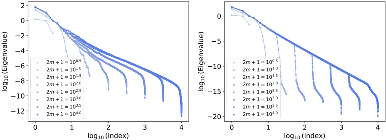<details> <summary>Image 21 Details</summary>  ### Visual Description ## Chart: Eigenvalue Spectrum ### Overview The image presents two charts displaying the eigenvalue spectrum, likely related to a matrix or operator. Both charts share the same axes and general structure, but differ in the range of the y-axis (log10(Eigenvalue)). Each chart plots several curves, each representing a different value of the parameter '2m+1'. The charts visualize how the distribution of eigenvalues changes with varying '2m+1' values. ### Components/Axes * **X-axis:** log10(Index). Scale ranges from approximately 0 to 4. * **Y-axis (Left Chart):** log10(Eigenvalue). Scale ranges from approximately 2 to -12. * **Y-axis (Right Chart):** log10(Eigenvalue). Scale ranges from approximately 2 to -20. * **Legend (Left Chart):** Located in the top-right corner. Labels are: * 2m+1 = 10^0.5 * 2m+1 = 10^1.0 * 2m+1 = 10^1.5 * 2m+1 = 10^2.0 * 2m+1 = 10^2.5 * 2m+1 = 10^3.0 * 2m+1 = 10^3.5 * 2m+1 = 10^4.0 * **Legend (Right Chart):** Located in the top-right corner. Labels are: * 2m+1 = 10^0.5 * 2m+1 = 10^1.0 * 2m+1 = 10^1.5 * 2m+1 = 10^2.0 * 2m+1 = 10^2.5 * 2m+1 = 10^3.0 * 2m+1 = 10^3.5 * 2m+1 = 10^4.0 ### Detailed Analysis or Content Details **Left Chart:** * **2m+1 = 10^0.5 (Lightest Blue):** The curve starts at approximately log10(Eigenvalue) = 1.8 and decreases monotonically, reaching approximately log10(Eigenvalue) = -11.5 at log10(Index) = 4. * **2m+1 = 10^1.0:** Starts at approximately log10(Eigenvalue) = 1.7 and decreases to approximately log10(Eigenvalue) = -11.8 at log10(Index) = 4. * **2m+1 = 10^1.5:** Starts at approximately log10(Eigenvalue) = 1.6 and decreases to approximately log10(Eigenvalue) = -11.9 at log10(Index) = 4. * **2m+1 = 10^2.0:** Starts at approximately log10(Eigenvalue) = 1.5 and decreases to approximately log10(Eigenvalue) = -12.0 at log10(Index) = 4. * **2m+1 = 10^2.5:** Starts at approximately log10(Eigenvalue) = 1.4 and decreases to approximately log10(Eigenvalue) = -12.1 at log10(Index) = 4. * **2m+1 = 10^3.0:** Starts at approximately log10(Eigenvalue) = 1.3 and decreases to approximately log10(Eigenvalue) = -12.2 at log10(Index) = 4. * **2m+1 = 10^3.5:** Starts at approximately log10(Eigenvalue) = 1.2 and decreases to approximately log10(Eigenvalue) = -12.3 at log10(Index) = 4. * **2m+1 = 10^4.0 (Darkest Blue):** Starts at approximately log10(Eigenvalue) = 1.1 and decreases to approximately log10(Eigenvalue) = -12.4 at log10(Index) = 4. **Right Chart:** * **2m+1 = 10^0.5 (Lightest Blue):** The curve starts at approximately log10(Eigenvalue) = 1.8 and decreases monotonically, reaching approximately log10(Eigenvalue) = -19.5 at log10(Index) = 4. * **2m+1 = 10^1.0:** Starts at approximately log10(Eigenvalue) = 1.7 and decreases to approximately log10(Eigenvalue) = -19.8 at log10(Index) = 4. * **2m+1 = 10^1.5:** Starts at approximately log10(Eigenvalue) = 1.6 and decreases to approximately log10(Eigenvalue) = -19.9 at log10(Index) = 4. * **2m+1 = 10^2.0:** Starts at approximately log10(Eigenvalue) = 1.5 and decreases to approximately log10(Eigenvalue) = -20.0 at log10(Index) = 4. * **2m+1 = 10^2.5:** Starts at approximately log10(Eigenvalue) = 1.4 and decreases to approximately log10(Eigenvalue) = -20.1 at log10(Index) = 4. * **2m+1 = 10^3.0:** Starts at approximately log10(Eigenvalue) = 1.3 and decreases to approximately log10(Eigenvalue) = -20.2 at log10(Index) = 4. * **2m+1 = 10^3.5:** Starts at approximately log10(Eigenvalue) = 1.2 and decreases to approximately log10(Eigenvalue) = -20.3 at log10(Index) = 4. * **2m+1 = 10^4.0 (Darkest Blue):** Starts at approximately log10(Eigenvalue) = 1.1 and decreases to approximately log10(Eigenvalue) = -20.4 at log10(Index) = 4. In both charts, all curves exhibit a similar downward trend, indicating a decreasing eigenvalue magnitude as the index increases. The curves are relatively parallel, suggesting that the overall shape of the eigenvalue spectrum remains consistent across different values of '2m+1'. ### Key Observations * The eigenvalue spectrum consistently decreases as the index increases. * Increasing the value of '2m+1' shifts the entire spectrum downwards, meaning that the eigenvalues become smaller in magnitude. * The right chart has a much larger range on the y-axis, allowing for a more detailed view of the lower eigenvalues. * The curves are closely spaced, indicating a relatively smooth distribution of eigenvalues. ### Interpretation The charts likely represent the eigenvalue spectrum of a Hamiltonian operator or a related quantum mechanical system. The parameter '2m+1' could be related to the mass or potential strength in the system. The downward trend in the eigenvalue spectrum indicates that the energy levels become more closely spaced as the index increases. The shift in the spectrum with increasing '2m+1' suggests that increasing the mass or potential strength lowers the energy levels. The difference in the y-axis range between the two charts highlights the importance of choosing an appropriate scale for visualizing data. The right chart provides a more detailed view of the lower eigenvalues, which may be important for understanding the system's behavior at low energies. The parallel nature of the curves suggests that the qualitative features of the eigenvalue spectrum are not significantly affected by changes in '2m+1', but rather the overall energy scale is shifted. This could indicate a robust relationship between the system's parameters and its energy levels. </details> Therefore, $$| \sigma _ { k } ^ { \downarrow } ( C _ { m } M _ { m } ^ { - 1 } C _ { m } ) - \sigma _ { k } ^ { \downarrow } ( C M ^ { - 1 } C ) | \leqslant | | | C _ { m } M _ { m } ^ { - 1 } C _ { m } - C M ^ { - 1 } C | | | _ { 2 } ,$$ and, in turn, lim m →∞ σ ↓ k ( C m M -1 m C m ) = σ ↓ k ( CM -1 C ) . To conclude the proof, observe that, on the one hand, $$\frac { 1 } { 1 + \sigma _ { k } ^ { \downarrow } ( C _ { m } M _ { m } ^ { - 1 } C _ { m } ) ^ { - 1 } } = \frac { \sigma _ { k } ^ { \downarrow } ( C _ { m } M _ { m } ^ { - 1 } C _ { m } ) } { 1 + \sigma _ { k } ^ { \downarrow } ( C _ { m } M _ { m } ^ { - 1 } C _ { m } ) } \leqslant \sigma _ { k } ^ { \downarrow } ( C _ { m } M _ { m } ^ { - 1 } C _ { m } ) \leqslant \sigma _ { k } ^ { \downarrow } ( M ^ { - 1 } ) ,$$ with ∑ k ∈ N /star σ ↓ k ( M -1 ) < ∞ . On the other hand, $$\lim _ { m \rightarrow \infty } \frac { 1 } { 1 + \sigma _ { k } ^ { \downarrow } ( C _ { m } M _ { m } ^ { - 1 } C _ { m } ) ^ { - 1 } } = \frac { 1 } { 1 + \sigma _ { k } ^ { \downarrow } ( C M ^ { - 1 } C ) ^ { - 1 } } ,$$ by continuity on R + of the function x ↦→ x 1+ x . Thus, applying the dominated convergence theorem, we are led to $$\lim _ { m \rightarrow \infty } \sum _ { \lambda \in \sigma ( C _ { m } M _ { m } ^ { - 1 } C _ { m } ) } \frac { 1 } { 1 + \lambda ^ { - 1 } } = \sum _ { \lambda \in \sigma ( C M ^ { - 1 } C ) } \frac { 1 } { 1 + \lambda ^ { - 1 } } .$$ ## 4.D Experiments ## 4.D.1 Numerical precision Enabling high numerical precision is crucial for efficient kernel inversion. Setting the default precision to Float32 and Complex64 can lead to significant numerical errors when approximating the kernel. For example, consider the harmonic oscillator case with d = 1 , s = 2 , and the operator D = d 2 dx 2 u + d dx u + u , with λ n = 0 . 01 and µ n = 1 . Figure 4.10 (left) shows the spectrum of C m M -1 m C m using Float32 precision, while Figure 4.10 (right) shows the same spectrum with Float64 precision. It is evident that with Float32 , the diagonalization results in lower eigenvalues compared to Float64 . In more physical terms, some energy of the matrix is lost when the last digits of the matrix coefficients are ignored. This leads to a problematic interpretation of the situation, as the Float64 estimation of the eigenvalues shows Fig. 4.11.: Convergence of the effective dimension as m grows for D = d dx . 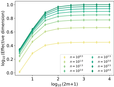<details> <summary>Image 22 Details</summary>  ### Visual Description ## Line Chart: Effective Dimension vs. 2m+1 ### Overview The image presents a line chart illustrating the relationship between the base-10 logarithm of the effective dimension (y-axis) and the base-10 logarithm of (2m+1) (x-axis). Multiple lines are plotted, each representing a different value of 'n', which appears to be a parameter influencing the effective dimension. The chart demonstrates how the effective dimension scales with (2m+1) for various 'n' values. ### Components/Axes * **X-axis Title:** log₁₀(2m+1) * **X-axis Scale:** Ranges from approximately 0 to 4. * **Y-axis Title:** log₁₀(Effective dimension) * **Y-axis Scale:** Ranges from approximately 0 to 1. * **Legend:** Located in the bottom-right corner. Contains the following entries: * Yellow: n = 10⁰.⁵ * Light Green: n = 10¹.⁰ * Green: n = 10².⁰ * Teal: n = 10².⁵ * Dark Teal: n = 10³.⁰ * Dark Green: n = 10³.⁵ * Darkest Green: n = 10⁴.⁰ ### Detailed Analysis The chart displays seven lines, each corresponding to a different 'n' value. * **n = 10⁰.⁵ (Yellow):** This line starts at approximately 0.1 at x=0 and increases to approximately 0.45 at x=4. It exhibits a concave-down trend, leveling off towards the right side of the chart. * **n = 10¹.⁰ (Light Green):** This line starts at approximately 0.3 at x=0 and increases to approximately 0.75 at x=4. It shows a similar concave-down trend as the yellow line, but is consistently higher. * **n = 10².⁰ (Green):** This line starts at approximately 0.6 at x=0 and increases to approximately 0.85 at x=4. It also exhibits a concave-down trend, remaining above the light green line. * **n = 10².⁵ (Teal):** This line starts at approximately 0.75 at x=0 and increases to approximately 0.95 at x=4. It shows a concave-down trend, consistently higher than the green line. * **n = 10³.⁰ (Dark Teal):** This line starts at approximately 0.85 at x=0 and increases to approximately 0.98 at x=4. It exhibits a concave-down trend, remaining above the teal line. * **n = 10³.⁵ (Dark Green):** This line starts at approximately 0.9 at x=0 and remains nearly constant at approximately 0.98 at x=4. It is almost flat, indicating minimal change in effective dimension with increasing (2m+1). * **n = 10⁴.⁰ (Darkest Green):** This line starts at approximately 0.95 at x=0 and remains nearly constant at approximately 1.0 at x=4. It is the flattest line, indicating the effective dimension saturates at a value of 1. All lines show an initial increase in effective dimension as (2m+1) increases. However, the rate of increase diminishes as (2m+1) becomes larger, with higher 'n' values reaching saturation more quickly. ### Key Observations * The effective dimension increases with (2m+1) for all values of 'n'. * Higher values of 'n' result in higher effective dimensions. * The increase in effective dimension diminishes as (2m+1) increases, particularly for larger 'n' values. * For n >= 10³.⁰, the effective dimension approaches 1.0 and plateaus. ### Interpretation The chart suggests that the effective dimension of a system is influenced by the parameter 'n' and the size of the input space, represented by (2m+1). As the input space grows (increasing (2m+1)), the effective dimension initially increases, but eventually saturates. This saturation point is reached more quickly for larger values of 'n'. This behavior could indicate that the system's complexity is limited by 'n', and beyond a certain point, increasing the input space does not significantly increase the system's ability to represent or process information. The saturation effect suggests a form of dimensionality reduction or a constraint on the system's capacity. The logarithmic scales used for both axes suggest that the relationship between effective dimension and (2m+1) is not linear, but rather follows a power law or a similar non-linear function. The chart is likely illustrating a theoretical concept in areas like machine learning, information theory, or statistical mechanics, where the effective dimension represents the number of independent variables needed to describe the system's behavior. </details> a clear convergence of the spectrum of C m M -1 m C m , whereas the Float32 estimation appears to indicate divergence. ## 4.D.2 Convergence of the effective dimension approximation The PIKL algorithm relies on a Fourier approximation of the PIML kernel, as developed in Section 4.2. The precision of this approximation is determined by the number m of Fourier modes used to compute the kernel. However, determining an optimal value of m for a specific regression problem is challenging. There is a trade-off between the accuracy of the kernel estimation, which improves with higher values of m , and the computational complexity of the algorithm, which also increases with m. There is a trade-off between the accuracy of the kernel approximation, which improves with higher values of m , and the computational complexity of the algorithm, which also increases with m . An interesting tool to leverage here is the effective dimension, as it captures the underlying degrees of freedom of the PIML problem and, consequently, the precision of the method. Theorem 4.3.1 states that the estimation of the effective dimension on H m converges to the effective dimension on H s (Ω) as m increases to infinity. Therefore, the smallest value m /star at which the effective dimension stabilizes is a strong candidate for balancing accuracy and computational complexity. Figures 4.11, 4.12, and 4.13 illustrate the convergence of the effective dimension estimation, using the eigenvalues of C m M -1 M C m , as m increases, for different values of n . These figures provide insights into the PIK algorithm. As expected, the Fourier approximations converge more slowly as the dimension d increases. Specifically, Figures 4.11 and 4.12 show that in dimension d = 1 , m /star /similarequal 10 2 for n ⩽ 10 4 , while Figure 4.13 indicates that in dimension d = 2 , m /star /similarequal 10 2 for n ⩽ 10 3 . ## 4.D.3 Numerical schemes We detail below the numerical schemes used as benchmarks in Section 4.4 for solving the wave equation. All these numerical schemes are constructed by discretizing the domain Ω = [0 , 1] 2 into the grid ( /lscript -1 1 Z //lscript 1 Z ) × ( /lscript -1 2 Z //lscript 2 Z ) . The initial and boundary conditions are then enforced on n = 2 /lscript 1 + /lscript 2 points, with the approximation ˆ f n defined accordingly as Fig. 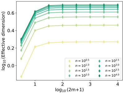4.12.: Convergence of the effective dimension as m grows for the harmonic oscillator <details> <summary>Image 23 Details</summary>  ### Visual Description \n ## Line Chart: Effective Dimension vs. Sample Size ### Overview The image presents a line chart illustrating the relationship between the logarithm base 10 of the effective dimension and the logarithm base 10 of (2m+1), where 'm' likely represents the sample size. The chart displays multiple lines, each representing a different value of 'n', also expressed as a logarithm base 10. The chart aims to demonstrate how the effective dimension scales with increasing sample size for different values of 'n'. ### Components/Axes * **X-axis Title:** log₁₀(2m+1) * **X-axis Scale:** Ranges from approximately 0.8 to 4.0, with tick marks at 1, 2, 3, and 4. * **Y-axis Title:** log₁₀(Effective dimension) * **Y-axis Scale:** Ranges from approximately 0.0 to 0.75, with tick marks at 0.2, 0.4, and 0.6. * **Legend:** Located in the bottom-right corner of the chart. * Yellow line: n = 10⁰.⁵ * Light Green line: n = 10¹.⁰ * Medium Green line: n = 10¹.⁵ * Dark Green line: n = 10².⁰ * Dark Teal line: n = 10².⁵ * Teal line: n = 10³.⁰ * Darker Teal line: n = 10³.⁵ * Darkest Teal line: n = 10⁴.⁰ ### Detailed Analysis The chart contains eight distinct lines, each representing a different value of 'n'. * **n = 10⁰.⁵ (Yellow Line):** This line starts at approximately 0.05 at x=0.8, rises sharply to approximately 0.23 at x=1.0, and then plateaus around 0.25 for x values greater than 1.5. * **n = 10¹.⁰ (Light Green Line):** This line starts at approximately 0.1 at x=0.8, rises to approximately 0.35 at x=1.0, and then plateaus around 0.4 for x values greater than 1.5. * **n = 10¹.⁵ (Medium Green Line):** This line starts at approximately 0.15 at x=0.8, rises to approximately 0.45 at x=1.0, and then plateaus around 0.5 for x values greater than 1.5. * **n = 10².⁰ (Dark Green Line):** This line starts at approximately 0.2 at x=0.8, rises to approximately 0.55 at x=1.0, and then plateaus around 0.6 for x values greater than 1.5. * **n = 10².⁵ (Dark Teal Line):** This line starts at approximately 0.25 at x=0.8, rises to approximately 0.6 at x=1.0, and then plateaus around 0.65 for x values greater than 1.5. * **n = 10³.⁰ (Teal Line):** This line starts at approximately 0.3 at x=0.8, rises to approximately 0.65 at x=1.0, and then plateaus around 0.7 for x values greater than 1.5. * **n = 10³.⁵ (Darker Teal Line):** This line starts at approximately 0.35 at x=0.8, rises to approximately 0.7 at x=1.0, and then plateaus around 0.72 for x values greater than 1.5. * **n = 10⁴.⁰ (Darkest Teal Line):** This line starts at approximately 0.4 at x=0.8, rises to approximately 0.72 at x=1.0, and then plateaus around 0.73 for x values greater than 1.5. All lines exhibit a steep increase in effective dimension for x values less than approximately 1.5, after which the increase slows down significantly, and the lines tend to converge towards a plateau. ### Key Observations * The effective dimension increases with both increasing 'm' (sample size) and increasing 'n'. * The rate of increase in effective dimension diminishes as 'm' increases, suggesting diminishing returns. * For larger values of 'm' (x > 2), the lines representing different values of 'n' converge, indicating that the effective dimension becomes less sensitive to changes in 'n'. * The yellow line (n = 10⁰.⁵) consistently exhibits the lowest effective dimension across all values of 'm'. * The darkest teal line (n = 10⁴.⁰) consistently exhibits the highest effective dimension across all values of 'm'. ### Interpretation The chart demonstrates the relationship between sample size, the parameter 'n', and the effective dimension of a system. The effective dimension represents the number of independent variables needed to describe the system. As the sample size ('m') increases, the system becomes more complex, and the effective dimension increases. However, the rate of increase diminishes, suggesting that beyond a certain point, adding more data does not significantly increase the complexity of the system. The parameter 'n' appears to control the inherent complexity of the system. Higher values of 'n' lead to higher effective dimensions, even for small sample sizes. The convergence of the lines for larger 'm' suggests that the influence of 'n' becomes less pronounced as the sample size grows, and the effective dimension is primarily determined by the sample size itself. This type of analysis is common in fields like machine learning and statistical modeling, where understanding the effective dimension is crucial for model selection, regularization, and generalization performance. The chart suggests that there is a trade-off between sample size and the inherent complexity of the system, and that choosing appropriate values for both is essential for building accurate and reliable models. </details> Fig. 4.13.: Convergence of the effective dimension as m grows for the heat equation on the disk. 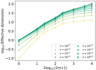<details> <summary>Image 24 Details</summary>  ### Visual Description ## Chart: Effective Dimension vs. Sample Size ### Overview The image presents a line chart illustrating the relationship between the logarithm base 10 of the effective dimension and the logarithm base 10 of (2m+1), where 'm' likely represents the number of samples. The chart displays multiple lines, each representing a different value of 'n', which appears to be a sample size parameter. Error bars are present on each data point, indicating the variability or uncertainty in the measurements. ### Components/Axes * **X-axis Title:** 2log₁₀(2m+1) * **X-axis Scale:** Ranges from approximately 0 to 4, with tick marks at 0, 1, 2, 3, and 4. * **Y-axis Title:** log₁₀(Effective dimension) * **Y-axis Scale:** Ranges from approximately -1.1 to 2.0, with tick marks at -0.5, 0, 0.5, 1.0, 1.5, and 2.0. * **Legend:** Located in the top-right corner of the chart. * n = 10⁰.⁵ (Yellow) * n = 10¹.⁰ (Orange) * n = 10¹.⁵ (Light Green) * n = 10².⁰ (Dark Green) * n = 10².⁵ (Teal) * n = 10³.⁰ (Blue) * n = 10³.⁵ (Dark Blue) * n = 10⁴.⁰ (Purple) ### Detailed Analysis The chart contains seven lines, each representing a different value of 'n'. Each line has multiple data points with error bars. * **n = 10⁰.⁵ (Yellow):** This line starts at approximately (0, -0.8) and increases slowly, reaching approximately (4, 1.3). The line is relatively flat. * **n = 10¹.⁰ (Orange):** This line starts at approximately (0, -0.3) and increases at a moderate rate, reaching approximately (4, 1.6). * **n = 10¹.⁵ (Light Green):** This line starts at approximately (0, 0.2) and increases at a moderate rate, reaching approximately (4, 1.8). * **n = 10².⁰ (Dark Green):** This line starts at approximately (0, 0.5) and increases at a moderate rate, reaching approximately (4, 1.9). * **n = 10².⁵ (Teal):** This line starts at approximately (0, 0.8) and increases at a moderate rate, reaching approximately (4, 2.0). * **n = 10³.⁰ (Blue):** This line starts at approximately (0, 1.1) and increases at a moderate rate, reaching approximately (4, 2.0). * **n = 10³.⁵ (Dark Blue):** This line starts at approximately (0, 1.4) and increases at a moderate rate, reaching approximately (4, 2.0). * **n = 10⁴.⁰ (Purple):** This line starts at approximately (0, 1.6) and increases at a moderate rate, reaching approximately (4, 2.0). All lines exhibit a generally upward trend, indicating that as 2log₁₀(2m+1) increases, the log₁₀(Effective dimension) also increases. The lines representing larger values of 'n' (10².⁵ and above) tend to converge towards the upper end of the y-axis scale. The error bars are relatively small, suggesting a reasonable degree of confidence in the measurements. ### Key Observations * The lines representing larger values of 'n' have higher effective dimensions for a given value of 2log₁₀(2m+1). * The rate of increase in effective dimension appears to slow down as 2log₁₀(2m+1) increases, particularly for the lines with larger 'n' values. * The lines converge at higher values of 2log₁₀(2m+1), suggesting that the effective dimension plateaus for large sample sizes. ### Interpretation The chart demonstrates the relationship between sample size ('m') and the effective dimension of a dataset, parameterized by 'n'. The effective dimension represents the number of independent variables needed to explain the variance in the data. As the sample size increases (as indicated by the x-axis), the effective dimension also increases, but at a decreasing rate. This suggests that with larger datasets, the information content grows, but the rate of new information gained diminishes. The different lines, each representing a different value of 'n', likely represent different scenarios or conditions under which the effective dimension is being measured. The fact that lines with larger 'n' values have higher effective dimensions suggests that 'n' is a parameter that influences the complexity or richness of the data. The convergence of the lines at higher values of 2log₁₀(2m+1) indicates that the effective dimension is ultimately limited by the parameter 'n', regardless of how large the sample size becomes. This type of analysis is common in fields like machine learning and dimensionality reduction, where understanding the effective dimension of a dataset is crucial for selecting appropriate algorithms and models. The chart provides insights into how sample size and other parameters affect the complexity and information content of a dataset. </details> - for all 0 ⩽ /lscript ⩽ /lscript 2 , ˆ f n (0 , /lscript//lscript 2 ) = sin( π/lscript//lscript 2 ) + sin(4 π/lscript//lscript 2 ) / 2 , - for all 0 ⩽ /lscript ⩽ /lscript 1 , ˆ f n ( /lscript//lscript 1 , 0) = 0 , - for all 0 ⩽ /lscript ⩽ /lscript 1 , ˆ f n ( /lscript//lscript 1 , 1) = 0 . Let the discrete Laplacian ∆ ( /lscript 1 ,/lscript 2 ) be defined for all ( a, b ) ∈ Z //lscript 1 Z × Z //lscript 2 Z by $$( \Delta _ { ( \ell _ { 1 } , \ell _ { 2 } ) } \hat { f } _ { n } ) ( a / \ell _ { 1 } , b / \ell _ { 2 } ) = \ell _ { 2 } ^ { 2 } ( \hat { f } _ { n } ( a / \ell _ { 1 } , ( b + 1 ) / \ell _ { 2 } ) - 2 \hat { f } _ { n } ( a / \ell _ { 1 } , b / \ell _ { 2 } ) + \hat { f } _ { n } ( a / \ell _ { 1 } , ( b - 1 ) / \ell _ { 2 } ) ) .$$ If f /star ∈ C 2 ([0 , 1] 2 ) , its Taylor expansion leads to (∆ ( /lscript 1 ,/lscript 2 ) f /star )( a//lscript 1 , b//lscript 2 ) = ∂ 2 x,x f /star ( a//lscript 1 , b//lscript 2 ) + o /lscript 2 → 0 (1) . Similarly, let the second-order time partial derivative operative ∂ 2 t,t, ( /lscript 1 ,/lscript 2 ) be defined for all ( a, b ) ∈ Z //lscript 1 Z × Z //lscript 2 Z by $$( \partial _ { t , t , ( \ell _ { 1 } , \ell _ { 2 } ) } ^ { 2 } \hat { f } _ { n } ) ( a / \ell _ { 1 } , b / \ell _ { 2 } ) = \ell _ { 2 } ^ { 2 } ( \hat { f } _ { n } ( ( a + 1 ) / \ell _ { 1 } , b / \ell _ { 2 } ) - 2 \hat { f } _ { n } ( a / \ell _ { 1 } , b / \ell _ { 2 } ) + \hat { f } _ { n } ( ( a - 1 ) / \ell _ { 1 } , b / \ell _ { 2 } ) ) .$$ Euler explicit. The Euler explicit scheme is initialized using the Taylor expansion f ( t, x ) = f (0 , x ) + t∂ t f (0 , x ) + t 2 ∂ 2 t,t f (0 , x ) / 2+ o t → 0 ( t 2 ) . With the initial condition ∂ t f (0 , x ) = 0 and the wave equation ∂ 2 t,t f (0 , x ) = 4 ∂ 2 x,x f (0 , x ) , this simplifies to f ( t, x ) = f (0 , x ) + 2 t 2 ∂ 2 x,x f (0 , x ) + o t → 0 ( t 2 ) . This leads to the initialization $$\forall 0 \leqslant b \leqslant \ell _ { 2 } , \quad \hat { f } _ { n } ( 1 / \ell _ { 1 } , b / \ell _ { 2 } ) = \hat { f } _ { n } ( 0 , b / \ell _ { 2 } ) + 2 \ell _ { 1 } ^ { - 2 } ( \Delta _ { ( \ell _ { 1 } , \ell _ { 2 } ) } \hat { f } _ { n } ) ( 0 , b / \ell _ { 2 } ) .$$ The wave equation ∂ 2 t,t f /star = 4 ∂ 2 x,x f /star can then be discretized as ∂ 2 t,t, ( /lscript 1 ,/lscript 2 ) ˆ f n = 4∆ ( /lscript 1 ,/lscript 2 ) ˆ f n . This leads to the explicit Euler recursive formula $$\hat { f } _ { n } ( ( a + 1 ) / \ell _ { 1 } , b / \ell _ { 2 } ) = 2 \hat { f } _ { n } ( a / \ell _ { 1 } , b / \ell _ { 2 } ) - \hat { f } _ { n } ( ( a - 1 ) / \ell _ { 1 } , b / \ell _ { 2 } ) + 4 \ell _ { 1 } ^ { - 2 } ( \Delta _ { ( \ell _ { 1 } , \ell _ { 2 } ) } \hat { f } _ { n } ) ( a / \ell _ { 1 } , b / \ell _ { 2 } ) .$$ This formula allows to compute ˆ f n (( a +1) //lscript 1 , · ) given the values of ˆ f n (0 , · ) , . . . , ˆ f n ( a//lscript 1 , · ) . Runge-Kutta 4. The RK4 scheme is a numerical scheme applied on both f /star and its derivative ∂ t f /star . Here, ˆ g n represents the approximation of ∂ t f /star . The initial condition ∂ t f (0 , · ) = 0 translates into $$\forall 0 \leqslant b \leqslant \ell _ { 2 } , \quad \hat { g } _ { n } ( 0 , b / \ell _ { 2 } ) = 0 .$$ To infer ˆ f n (( a +1) //lscript 1 , · ) and ˆ g n (( a +1) //lscript 1 , · ) given the values of ˆ f n (0 , · ) , . . . , ˆ f n ( a//lscript 1 , · ) and ˆ g n (0 , · ) , . . . , ˆ g n ( a//lscript 1 , · ) , the RK4 scheme introduces intermediate estimates as follows: - ˜ f 1 = ˆ g n ( a//lscript 1 , · ) //lscript 1 , - ˜ g 1 = 4(∆ ( /lscript 1 ,/lscript 2 ) ˆ f n )( a//lscript 1 , · ) //lscript 1 , - ˜ f 2 = (ˆ g n ( a//lscript 1 , · ) + 0 . 5 ˜ f 1 ) //lscript 1 , - ˜ g 2 = 4(0 . 5˜ g 1 +(∆ ( /lscript 1 ,/lscript 2 ) ˆ f n )( a//lscript 1 , · )) //lscript 1 , - ˜ f 3 = (ˆ g n ( a//lscript 1 , · ) + 0 . 5 ˜ f 2 ) //lscript 1 , - ˜ g 3 = 4(0 . 5˜ g 2 +(∆ ( /lscript 1 ,/lscript 2 ) ˆ f n )( a//lscript 1 , · )) //lscript 1 , - ˜ f 4 = (ˆ g n ( a//lscript 1 , · ) + ˜ f 3 ) //lscript 1 , - ˜ g 4 = 4(˜ g 3 +(∆ ( /lscript 1 ,/lscript 2 ) ˆ f n )( a//lscript 1 , · )) //lscript 1 , - ˆ f n (( a +1) //lscript 1 , · ) = ˆ f n ( a//lscript 1 , · ) + ( ˜ f 1 +2 ˜ f 2 +2 ˜ f 3 + ˜ f 4 ) / 6 , - ˆ g n (( a +1) //lscript 1 , · ) = ˆ g n ( a//lscript 1 , · ) + (˜ g 1 +2˜ g 2 +2˜ g 3 +˜ g 4 ) / 6 . 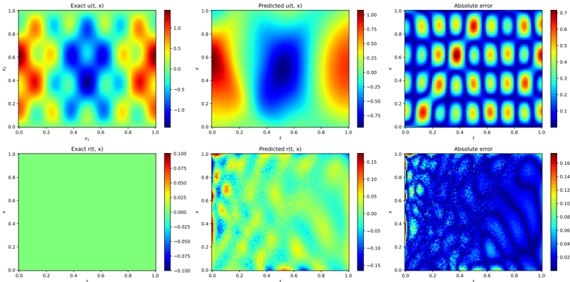<details> <summary>Image 25 Details</summary>  ### Visual Description \n ## Heatmaps: Comparison of Exact, Predicted, and Error Values ### Overview The image presents six heatmaps arranged in a 2x3 grid. Each heatmap visualizes a two-dimensional function, likely representing a time-dependent variable 't' against a spatial coordinate 'x'. The heatmaps compare the "Exact" function, a "Predicted" function, and the "Absolute Error" between the two. There are two sets of comparisons, one with a larger scale and one with a smaller scale. ### Components/Axes Each heatmap shares the following components: * **X-axis:** Labeled as 'x', ranging from approximately 0.0 to 1.0. * **Y-axis:** Labeled as 't', ranging from approximately 0.0 to 1.0. * **Colorbar:** Each heatmap has a colorbar on the right side indicating the value corresponding to each color. The colorbars have different scales for each heatmap. The heatmaps are organized as follows: 1. Top-Left: "Exact u(t, x)" - Colorbar ranges from approximately -1.0 to 1.0. 2. Top-Center: "Predicted u(t, x)" - Colorbar ranges from approximately -0.75 to 0.75. 3. Top-Right: "Absolute error" - Colorbar ranges from approximately 0.0 to 0.3. 4. Bottom-Left: "Exact r(t, x)" - Colorbar ranges from approximately -0.075 to 0.075. 5. Bottom-Center: "Predicted r(t, x)" - Colorbar ranges from approximately -0.15 to 0.15. 6. Bottom-Right: "Absolute error" - Colorbar ranges from approximately 0.0 to 0.16. ### Detailed Analysis or Content Details **Top Row:** * **Exact u(t, x):** Shows a pattern of alternating positive and negative regions, forming roughly circular or elliptical shapes. The maximum positive values are around 1.0, and the maximum negative values are around -1.0. The pattern is periodic in both 't' and 'x'. * **Predicted u(t, x):** Displays a similar pattern to the "Exact" function, but with reduced amplitude. The maximum positive values are around 0.75, and the maximum negative values are around -0.75. The predicted values appear smoothed compared to the exact values. * **Absolute Error:** Shows the difference between the "Exact" and "Predicted" functions. The error is concentrated in the regions where the "Exact" function has high amplitude. The maximum error is around 0.3. The error pattern mirrors the periodic structure of the original functions. **Bottom Row:** * **Exact r(t, x):** Shows a relatively flat green surface with small variations. The values are centered around 0.0, with a range of approximately -0.075 to 0.075. * **Predicted r(t, x):** Displays a similar pattern to the "Exact" function, but with more pronounced variations. The values range from approximately -0.15 to 0.15. * **Absolute Error:** Shows the difference between the "Exact" and "Predicted" functions. The error is more significant than in the top row, with a maximum error of around 0.16. The error pattern is more complex and less periodic than the top row. ### Key Observations * The "Predicted" functions generally follow the pattern of the "Exact" functions, but with reduced amplitude in the top row and increased variation in the bottom row. * The "Absolute Error" is highest in the regions where the "Exact" function has the largest variations. * The error in the bottom row is significantly higher than in the top row, suggesting that the prediction is less accurate for the 'r' function compared to the 'u' function. * The color scales are different for each heatmap, indicating that the functions have different ranges of values. ### Interpretation The image demonstrates a comparison between an exact solution and a predicted solution for two functions, 'u(t, x)' and 'r(t, x)'. The heatmaps visualize the accuracy of the prediction by showing the absolute error between the exact and predicted values. The top row suggests a relatively accurate prediction for 'u(t, x)', with a small error concentrated in regions of high variation. The bottom row indicates a less accurate prediction for 'r(t, x)', with a larger and more complex error pattern. The differences in error levels between the two functions could be due to several factors, such as the complexity of the functions, the quality of the prediction model, or the limitations of the numerical methods used to solve the equations. The image provides a visual representation of the prediction accuracy and highlights areas where the prediction model could be improved. The functions 'u' and 'r' may represent different physical quantities or different stages in a simulation, and the varying prediction accuracy could have implications for the overall reliability of the results. </details> t t t Fig. 4.14.: Left : Ground truth. Middle : PINN estimator. Right : Error = PINN - Ground truth. Similarly to the Euler explicit scheme, the RK4 relies on a recursive formulas to compute ˆ f n . Crank-Nicolson . The CN scheme is an implicit scheme defined as follows. Similar to the Euler explicit scheme, the ∂ t f (0 , · ) = 0 initial condition is implemented as $$\forall 0 \leqslant \ell \leqslant \ell _ { 2 } , \quad \hat { f } _ { n } ( 1 / \ell _ { 1 } , \ell / \ell _ { 2 } ) = \hat { f } _ { n } ( 0 , \ell / \ell _ { 2 } ) + 2 \ell _ { 1 } ^ { - 2 } ( \Delta _ { ( \ell _ { 1 } , \ell _ { 2 } ) } \hat { f } _ { n } ) ( 0 , \ell / \ell _ { 2 } ) .$$ Then, the recursive formula of this scheme takes the form $$\partial _ { t , t , ( \ell _ { 1 } , \ell _ { 2 } ) } ^ { 2 } \hat { f } _ { n } ( a / \ell _ { 1 } , \cdot ) = 2 ( ( \Delta _ { ( \ell _ { 1 } , \ell _ { 2 } ) } \hat { f } _ { n } ) ( a / \ell _ { 1 } , \cdot ) + ( \Delta _ { ( \ell _ { 1 } , \ell _ { 2 } ) } \hat { f } _ { n } ) ( ( a + 1 ) / \ell _ { 1 } , \cdot ) ) .$$ This leads to the recursion $$\hat { f } _ { n } ( ( a + 1 ) / \ell _ { 1 } , \cdot ) = ( I d + 2 \ell _ { 2 } ^ { 2 } \ell _ { 1 } ^ { - 2 } \Delta ) ^ { - 1 } ( 3 \hat { f } _ { n } ( a / \ell _ { 1 } , \cdot ) - \hat { f } _ { n } ( ( a - 1 ) / \ell _ { 1 } , \cdot ) ) - \hat { f } _ { n } ( ( a - 1 ) / \ell _ { 1 } , \cdot ) ,$$ $$\text {where $\Delta=\left(\begin{array} { c c c } 2 & -1 & 0 & \dots & 0 \\ -1 & 2 & -1 & \ddots & \vdots \\ 0 & -1 & 2 & \ddots & 0 \\ \vdots & \ddots & \ddots & \ddots & -1 \\ 0 & \dots & 0 & -1 & 2 \end{array}$}$$ ## 4.D.4 PINN training Figures 4.14 and 4.15 illustrate the performance of the PINNs during training while solving the 1d wave equation with noisy boundary conditions. $$\begin{array} { r l } & { 0 \, } \\ & { \vdots \, } \\ & { 0 \, } \\ & { - 1 \, } \\ & { 2 \, } \end{array}$$ Fig. 4.15.: PINN training with noisy boundary conditions. <details> <summary>Image 26 Details</summary>  ### Visual Description \n ## Line Chart: Loss vs. Iterations ### Overview The image presents a line chart illustrating the relationship between 'Loss' and 'Iterations' for three different loss functions: *L<sub>r</sub>*, *L<sub>u</sub>*, and *L<sub>v</sub>*. The chart displays how these loss values change as the number of iterations increases. The y-axis is on a logarithmic scale. ### Components/Axes * **X-axis:** 'iterations' ranging from approximately 0 to 800. * **Y-axis:** 'Loss' on a logarithmic scale, ranging from approximately 10<sup>-3</sup> to 10<sup>1</sup> (1 to 100). The scale is marked with values 10<sup>-2</sup>, 10<sup>-1</sup>, 10<sup>0</sup>, 10<sup>1</sup>. * **Legend:** Located in the top-right corner, identifying the three lines: * Blue line: *L<sub>r</sub>* * Orange line: *L<sub>u</sub>* * Green line: *L<sub>v</sub>* ### Detailed Analysis * **L<sub>r</sub> (Blue Line):** The blue line starts at approximately 10<sup>0</sup> (10) at iteration 0 and rapidly decreases to approximately 10<sup>-2</sup> (0.01) by iteration 50. It then fluctuates around this value, with some oscillations, until iteration 800, remaining relatively stable. * **L<sub>u</sub> (Orange Line):** The orange line begins at approximately 10<sup>0</sup> (10) at iteration 0 and remains relatively constant, fluctuating around 10<sup>0</sup> (10) throughout the entire range of iterations (0 to 800). There is some minor fluctuation, but it does not show a clear decreasing trend. * **L<sub>v</sub> (Green Line):** The green line starts at approximately 10<sup>-1</sup> (0.1) at iteration 0 and decreases to approximately 10<sup>-2</sup> (0.01) by iteration 50. It then fluctuates around this value, with more pronounced oscillations than the blue line, until iteration 800. It appears to stabilize around 10<sup>-2</sup> (0.01) but with higher variance than *L<sub>r</sub>*. ### Key Observations * *L<sub>r</sub>* exhibits the most significant decrease in loss, converging to a relatively stable value. * *L<sub>u</sub>* shows minimal change in loss throughout the iterations, indicating it may not be effectively learning or converging. * *L<sub>v</sub>* decreases initially but exhibits more fluctuation than *L<sub>r</sub>*, suggesting a less stable learning process. * All three loss functions start at different initial loss values. ### Interpretation The chart likely represents the training process of a machine learning model, where 'Loss' quantifies the error between the model's predictions and the actual values. 'Iterations' represent the number of times the model's parameters are updated during training. The differing behaviors of the three loss functions (*L<sub>r</sub>*, *L<sub>u</sub>*, and *L<sub>v</sub>*) suggest they may be measuring different aspects of the model's performance or represent different components of the overall loss function. *L<sub>r</sub>*’s convergence indicates successful learning for that component. *L<sub>u</sub>*'s stagnation suggests a potential issue with that component, such as a poor learning rate or a non-informative feature. *L<sub>v</sub>*'s fluctuating behavior suggests instability or sensitivity to the training data. The logarithmic scale on the y-axis is crucial for visualizing the changes in loss, especially when the loss values vary significantly in magnitude. The initial differences in loss values suggest that these loss functions are measuring different aspects of the model's performance, and their relative magnitudes are important for understanding the model's overall behavior. The fact that *L<sub>u</sub>* remains high throughout the training process could indicate a problem with the corresponding part of the model or the data used to calculate that loss. </details> ## Part II Time series forecasting in atypical periods ## Forecasting Electric Vehicle Charging Station Occupancy: Smarter Mobility Data Challenge This chapter corresponds to the following publication: Amara-Ouali et al. [AO+24]. ## 5.1 Introduction Electric mobility The transportation sector is currently one of the main contributors to greenhouse gas emissions in Europe [IEA22]. To reduce these emissions, an interesting avenue has been to foster the development of EVs. In 2021, China led global EV sales with 3.3 million units, tripling its 2020 sales, followed by Europe with 2.3 million units, up from 1.4 million in 2020 [IEA22]. The U.S. market share of electric vehicles doubled to 4.5%, with 630,000 units sold. Meanwhile, electric vehicle sales in emerging markets more than doubled [IEA22]. As a consequence, electric mobility development entails new needs for energy providers and consumers [RTE22]. Companies and researchers are proposing a large amount of innovative solutions including pricing strategies and smart charging [DW12; Wan+16; Ali+17; Mog+18; CMM20] to couple it with renewable production [HAI23]. However, their implementation requires a precise understanding of charging behaviours and better EV charging models are necessary to grasp the impact of EVs on the grid [Gop+16; Kay+22; Cio+23; AV23]. In particular, forecasting the occupancy of a charging station can be a critical need for utilities to optimise their production units according to charging demand [Zha+23]. On the user side, knowing when and where a charging station will be available is critical, but large-scale datasets on EVs are rare [CMZ21; AO+21]. Summary of the challenge This article presents the Smarter Mobility Data Challenge, which aims at testing statistical and machine learning forecasting models to predict the states of a set of charging stations in the Paris area at different geographical resolutions. This challenge was held from October, 3rd 2022 to December 5th, 2022 on the CodaLab platform https: //codalab.lisn.upsaclay.fr/competitions/7192 . It was organised by the Manifeste IA , a network of 16 French industrials and TAILOR, a European project which aims to provide the scientific foundations for Trustworthy AI. It has been pioneered following the 'AI for Humanity' French government plan launched in 2019. The challenge gathered 169 participants and was open to students from the EU. The authors (except the participants of the challenge) have collected and prepared the dataset, and organised the data challenge. Time series models Forecasting time series data is essential for businesses and governments to make informed decisions. However, the temporal structure in time series comes with specific challenges, such as non-stationarity and missing values. This is why, in addition to standard machine learning models, a wide range of models have been tailored for time series. These include auto-regressive models [Box+15], tree-based models [Fri01], and deep learning models such as recurrent neural networks [Jor97; HS97], temporal convolutional networks [BKK18] and transformers [Wen+23]. However, no one model has proven to be better than the others at predicting time series. On the one hand, although deep learning models are known to perform well with large datasets, it is still unclear how they compare to other models on small datasets, how they handle non-stationary data or how they deal with with exogenous information [Zen+23; Ksh+24]. In fact, modern machine learning models still struggle to deal with missing values and time-dependent patterns such as trends or breaks. On the other hand, tree-based models such as gradient-boosted trees are known to perform well on tabular data [McE+23], and to sometimes outperform complex deep learning models [MSA22a]. Therefore, practical insights from datasets and benchmarks are valuable [Pet+22]. In particular, a recent comprehensive benchmark [God+21] has regrouped 26 time series datasets on various domains, including energy and transport, taken from challenges [see, e.g., MSA22b] and the public domain. Other works have proposed synthetic datasets to evaluate specific properties of forecast algorithms, such as interpretability [Ism+20], outlier detection [Lai+21], and forecast performance [Kan+20]. Hierarchical forecasting The data of the Smarter Mobility Data Challenge has a hierarchical structure because it EV charging stations can be regrouped at different scales (stations, areas, and global). Hierarchical time series forecasting has been studied on various other applications where the data is directly or indirectly hierarchically organised. For example, in the retail industry, goods are often classified into categories (such as food or clothing) and inventory management can be done at different geographical (national, regional, shop) or temporal (week, month, season) scales. Moreover, electricity systems often have an explicit (electricity network) or implicit (e.g., customer types, tariff options) hierarchy. Recent work shows that exploiting this structure can improve forecasting performance at different levels of hierarchy. For instance, [Hyn+11] focuses on tourism demand, [Ath+20] on macroeconomic forecasting, and [HXB19; BH22a; TTH20; NM22] on electricity consumption data. Related works Similar to energy and transport forecasting, EV demand forecasting has received a lot of attention. The survey by Amara-Ouali et al. [AO+22] compares the classical time series methods, the statistical models, the machine learning methods and the deep learning methods that have been used to capture the temporal dependencies in EV charging data. Overall, it shows that both tree-based models and deep learning models are able to capture the complex non-linear temporal relationships in EV charging data. More recently, Ma and Faye [MF22] proposed a hybrid LSTM model that outperformed classical machine learning approaches (support vector machine, random forest, and Adaboost) and other deep learning architectures (LSTM, Bi-LSTM, and GRU) in forecasting the occupancy of 9 fast chargers in the city of Dundee. Wang et al. [Wan+23b] have investigated the use of spatial correlations to predict EV charging behaviour. They proposed a spatio-temporal graph convolutional network incorporating both geographical and temporal dependencies to predict the short-term charging demand in Beijing using a dataset of 76774 private EVs. However, such individual data is expensive and often kept private, and Wang et al. [Wan+23b] only had access to data for the month of January 2018. In fact, although datasets describing the development of EV infrastructures are common [see, e.g., FN21; Yi+22], fewer datasets document the actual use of EVs and they are often of lower spatial resolution [see, e.g., LLL19]. In fact, open datasets at the scale of individual stations, such as the one presented in this article, are still very rare [AO+21]. Such so-called EVSE-centric (for Electric Vehicle Supply Equipment) datasets are more informative and hierarchical forecasting could be useful for users and operators interested in specific EV stations. However, even with EV datasets spanning multiple years, ruptures are common and models require specific adjustments [see, e.g., KWK23]. Main Contributions The main contributions of the paper can be summarised as follows: 1. An open dataset on electric vehicle behaviors gathering both spatial and hierarchical features, available at https://gitlab.com/smarter-mobility-data-challenge/ additional\_materials . Datasets with such features are rare and valuable for electric network management. 2. An in-depth descriptive analysis of this dataset revealing meaningful user behaviors (work behaviors, daily and weekly patterns...). 3. A detailed and reproducible benchmark for forecasting the EV charging station occupancy. This benchmark compares the winning solutions of a data challenge and state-of-the-art predictive models. Overview The paper is structured as follows. Section 5.2 describes the dataset. Section 5.3 details the forecasting problem at hand and baseline models. Section 5.4 presents the methods proposed by the three winning teams. Finally, Section 5.5 summarizes the findings and discusses our results. The full dataset, baseline models, winning solutions, and aggregations, are available at https://gitlab.com/smarter-mobility-data-challenge/tutorials and distributed under the Open Database License (ODbL). A supplementary material presents the Belib's pricing and park history in Section 1, a detailed data description (collection, preprocessing, explanatory data analysis) in Section 2, some complements about the winning strategies of the challenge in Section 3, future perspectives about new datasets and benchmarks in Section 4 and a Datasheet in Section 5. ## 5.2 EV charging dataset In this section we present how the raw dataset was collected and how it was then preprocessed to make it suitable for the data challenge. General description The dataset is based on the real-time charging station occupancy information of the Belib network, available on the Paris Data platform (ODbL) [Par23]. The Belib network was composed of 91 charging stations in Paris at the time of the challenge, each offering 3 plugs for a total of 273 charging points. A process to store the data was initiated by the EDF R&D team since daily data was not stored by Paris Data. A pipeline was set up to collect this data every 15 minutes, starting July 2020, on the platform's dedicated API 1 . The data was then stored in a data lake based on Hadoop technologies (HDFS, PySpark, Hive, and Zeppelin). The storage of this information over time allows, for example, to estimate the usage of the charging stations depending on their location. 1 parisdata.opendatasoft.com/explore/dataset/belib-points-de-recharge-pour-vehicules-electriques-disponibilitetemps-reel/api Belib's history: pricing mechanism and park evolution 89% of EV users living in a house mainly charge their vehicle at home, compared to only 54% of EV users living in an apartment in 2020 [ENE21]. Paris is a very dense city that allows limited access to private residential charging points, hence the need for public charging stations. The first 5 stations of the Belib network were commissioned on 12 January, 2016 [Tor16; Cam16]. The network grew progressively in 2016 to reach 60 stations all around Paris. Users needed to buy a 15 euro badge to connect to the network. Different pricing strategies were applied depending on the time of the day and plugs. The "normal charge" of 3kW was free at night (between 8 p.m. and 8 a.m.) and cost 1 euro per hour on daytime (between 8 a.m. and 8 p.m.). The "quick charge" of 22kW cost 25 cents every 15 minutes during the first hour of charge. After the first hour, the first 15 minutes cost 2 euros. After this 1h and 15 minutes, each 15 minutes cost 4 euros. Each station contained 3 parking spots: - one dedicated to "normal charge" with an E/F electric plug, - one dedicated to "quick charge" with a ChaDeMo and a Combo2 plugs, - one where both "normal charge" and "quick charge" were possible, with an E/F, a T2, and a T3 plugs. The pricing strategy was intended to allow the usage of "normal charge" plugs as a free parking spot overnight, while "quick charge" became expensive after one hour of usage. In 2021, the city of Paris allowed the company TotalEnergies to run the Belib network for a period of 10 years. The goal is to enhance the network, increasing from 90 stations and 270 charging points, to 2300 charging points [Tot31; Liv09]. We elaborate on the new pricing mechanism in the supplementary material. Data preprocessing In the raw data, each observation reflects the status of the plugs (up to 6) within a charging point. The structure of the raw dataset is misleading as only one of these plugs can be in use at a time. Therefore, we processed the dataset to only keep the relevant rows, i.e., the rows containing the plugs in use, and we treated a charging point as a single plug. In addition, charging points are clustered in groups of three according to their geographic location in the raw data. This charging point structure was confirmed by the data provider. We grouped the three adjacent charging points into a single charging station and aggregated the data accordingly. To account for differences in timestamp synchronization between stations, we have adjusted timestamps to match the nearest 15-minute interval. The available , charging , and passive states are taken directly from the raw data. The last state other regroups several statuses including reserved (a user has booked the charging point), offline (the charging point is not able to send information to the server), and out of order (the charging point is out of order). We made this choice because of the relatively small number of reserved and out of order records. This way, the other state could be interpreted as a noisy version of the offline state. Missing timestamps in the dataset have not been filled so there is room for missing data imputation techniques. Missing values There is a significant number of missing values in the data. To illustrate, the records of the following five days are very incomplete as they contain less than 96 observations for all the 91 stations: 2020-08-06 (with 92 data points), 2020-10-27 (95), 2020-11-20 (54), 2020-12-29 (95), and 2021-01-04 (95). The distribution of missing values is highly station-dependent, as illustrated in Figure 5.1. We note that half of the stations have almost no missing data (except for the five days documented above), whereas 7 stations have around 50% missing observations. This suggests that malfunctioning behaviors are specific to some stations and could be learned. In addition, the number of non-missing stations is depicted in Fig. 5.1.: Left: Percentage of non missing observations per station. Right: Number of non missing stations in function of time on the train set. 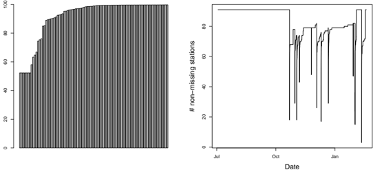<details> <summary>Image 27 Details</summary>  ### Visual Description \n ## Chart: Cumulative Number of Non-Missing Stations & Number of Non-Missing Stations Over Time ### Overview The image presents two time-series charts displayed side-by-side. The chart on the left shows the cumulative number of non-missing stations over time, while the chart on the right displays the number of non-missing stations as a function of date. Both charts appear to cover a period from approximately July to January. ### Components/Axes **Left Chart:** * **Y-axis:** Labeled "Cumulative Number of Stations", ranging from 0 to 100, with markings at 20, 40, 60, 80, and 100. * **X-axis:** Labeled "Date", with no explicit markings, but representing a time span from approximately July to January. * **Data Series:** A single series represented by vertical bars, showing the cumulative count. **Right Chart:** * **Y-axis:** Labeled "# non-missing stations", ranging from 0 to 80, with markings at 20, 40, 60, and 80. * **X-axis:** Labeled "Date", with markings for "Jul", "Oct", and "Jan". * **Data Series:** A single line plot representing the number of non-missing stations over time. ### Detailed Analysis or Content Details **Left Chart (Cumulative Number of Stations):** The cumulative number of stations starts at approximately 10 at the beginning of the period (July). It increases in a stepwise fashion, with periods of no change followed by relatively rapid increases. By approximately October, the cumulative number reaches around 50. The growth continues, and by January, the cumulative number of stations reaches approximately 95. **Right Chart (Number of Non-Missing Stations):** The number of non-missing stations fluctuates significantly over time. * **July - October:** The line starts at approximately 20 in July, increases to around 70 by October, with several dips and peaks in between. * **October - December:** The line fluctuates between approximately 60 and 80 stations. * **December - January:** A sharp decrease occurs around December, dropping to approximately 20 stations, followed by a recovery to around 75 stations by January. ### Key Observations * The cumulative number of stations (left chart) consistently increases over time, indicating a growing network of stations. * The number of non-missing stations (right chart) exhibits high variability, suggesting periods of station outages or data loss. * The sharp drop in non-missing stations around December (right chart) is a notable anomaly, potentially indicating a widespread issue affecting station availability. * The right chart shows a clear seasonal pattern, with a general increase in the number of non-missing stations from July to October, followed by a decline in December and a partial recovery in January. ### Interpretation The data suggests a network of stations is being progressively deployed or becoming operational (left chart). However, the operational stability of these stations is variable (right chart). The fluctuations in the number of non-missing stations could be due to various factors, such as maintenance, weather conditions, or technical failures. The significant drop in December warrants further investigation, as it could indicate a systemic problem affecting a large portion of the network. The seasonal pattern observed in the right chart might be related to environmental factors that impact station performance, such as winter weather. The two charts together provide a comprehensive view of both the growth and reliability of the station network. </details> Fig. 5.2.: Daily (left) and Weekly (right) profiles for each status at the Global level. 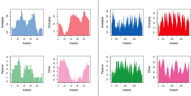<details> <summary>Image 28 Details</summary>  ### Visual Description \n ## Histograms: Battery State Over Time ### Overview The image presents a 2x2 grid of histograms, each depicting the distribution of a battery state variable over time. The x-axis of each histogram represents "Instant" (likely a time step), ranging from 0 to approximately 90 in the left column and 0 to 500 in the right column. The y-axis represents the frequency or count of occurrences for each state. The four battery states are "Available", "Charging", "Passive", and "Other". ### Components/Axes * **X-axis:** "Instant" - Represents time or a time step. Scale varies between the left and right columns. * **Y-axis:** Frequency/Count - Represents the number of occurrences of a given state at a particular instant. Scale varies between the histograms. * **Histograms:** Four histograms, each representing a different battery state. * "Available" (Blue) * "Charging" (Red) * "Passive" (Green) * "Other" (Pink) ### Detailed Analysis or Content Details **Left Column (Instant 0-90):** * **Available (Top-Left):** The histogram shows a roughly normal distribution, peaking around Instant 30. The frequency ranges from approximately 148 to 156. * **Charging (Top-Right):** The histogram shows a decreasing trend, starting with a frequency around 25 at Instant 0 and decreasing to approximately 10 at Instant 90. * **Passive (Bottom-Left):** The histogram shows a relatively stable distribution, with peaks around Instant 20 and Instant 70. The frequency ranges from approximately 18 to 22. * **Other (Bottom-Right):** The histogram shows a decreasing trend, starting with a frequency around 64 at Instant 0 and decreasing to approximately 54 at Instant 90. **Right Column (Instant 0-500):** * **Available (Top-Left):** The histogram shows a fluctuating distribution with multiple peaks and valleys. The frequency ranges from approximately 145 to 165. * **Charging (Top-Right):** The histogram shows a highly fluctuating distribution with frequent peaks and valleys. The frequency ranges from approximately 10 to 30. * **Passive (Bottom-Left):** The histogram shows a fluctuating distribution with multiple peaks and valleys. The frequency ranges from approximately 14 to 24. * **Other (Bottom-Right):** The histogram shows a fluctuating distribution with multiple peaks and valleys. The frequency ranges from approximately 50 to 70. ### Key Observations * The "Available" state generally has the highest frequency across both time ranges. * The "Charging" state has the lowest frequency, and its distribution is more volatile than the others. * The distributions in the right column (Instant 0-500) are more complex and fluctuating than those in the left column (Instant 0-90). * The "Other" state shows a clear decreasing trend in the left column, but a more fluctuating pattern in the right column. ### Interpretation The data suggests that the battery is most often in an "Available" state. The "Charging" state is relatively infrequent, indicating that the battery spends most of its time not actively charging. The "Passive" and "Other" states represent periods where the battery is neither fully available nor actively charging, potentially indicating standby or low-power modes. The difference in distributions between the left and right columns suggests a change in battery usage patterns over time. The longer time range (0-500) exhibits more variability in all states, potentially indicating a more dynamic usage scenario. The decreasing trend in the "Other" state in the left column could indicate a stabilization of the battery's operational mode over the initial 90 instants. The fluctuating nature of the "Charging" state suggests intermittent charging events, rather than a continuous charging process. The "Other" state's behavior could be related to background processes or system activities that consume battery power without actively charging or providing full availability. </details> Figure 5.1. Note that we excluded timestamps from the plot when all stations were missing. We also note that the number of missing stations starts to fluctuate a lot after October. Exploratory Data Analysis We show daily and weekly profiles with the median number of plugs as a function of time (an instant corresponding to a 15-minute interval) per status at the Global level on Figure 5.2. From these graphs, We observe the presence of a daily pattern in the data and a change in the pattern between weekdays and weekends. What we observe in Figure 5.2 matches with the pricing strategy used from 2016 to 2021, detailed in Paragraph 5.2. The pricing changed twice a day: at 8 a.m. and 8 p.m. At night, the free "normal charge regime" (7kW) explains the peak in charging states at instant 80 (corresponding to 8 p.m.) and the drop of available at the same hour. This "normal charge" mode provides a low electrical power, hence the slowness of charging. Therefore, overnight, as EV batteries become fully charged, the number of charging states decrease in favour of the number of passive states. The proportion of other states is more important at night, mainly because there is more maintenance jobs at night. Since users tend to be repelled by or ignore malfunctioning stations it explains why this excess in other comes with a slight increase of available at night. On the other hand, the price increase, after 8 a.m., induces a decrease of passive spots from 7p.m. to 9 p.m. and an increase of available (drivers parking on regular parking spots) and charging spots (drivers charging their car in front of their office after the morning ride). This analysis is consistent with the weekly scale in Figure 5.2. The number of charging stations is greater during work days, while the number of available stations is greater during week-ends, reflecting commuting behaviors. We note that the daily peaks at 8 a.m. and 8 p.m. are pronounced on the weekly charging profile. Fig. 5.3.: Empirical ACF of the 4 status at the global level. 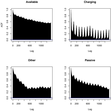<details> <summary>Image 29 Details</summary>  ### Visual Description ## Chart: Autocorrelation Function Plots for Different Device States ### Overview The image presents four autocorrelation function (ACF) plots, each representing a different device state: "Available", "Charging", "Other", and "Passive". Each plot displays the autocorrelation coefficient (ACF) on the y-axis against the lag on the x-axis. The plots are arranged in a 2x2 grid. ### Components/Axes * **X-axis:** "Lag" ranging from 0 to approximately 1000. * **Y-axis:** "ACF" (Autocorrelation Function) ranging from 0 to 1.0. * **Titles:** Each subplot has a title indicating the device state: "Available", "Charging", "Other", "Passive". * **Horizontal Blue Lines:** A horizontal blue line is present at y = 0 in each plot, representing the zero autocorrelation level. * **Data Series:** Each plot contains a black line representing the ACF values for the corresponding device state. ### Detailed Analysis Each plot will be analyzed individually. **1. Available:** * **Trend:** The ACF line starts at approximately 1.0 at lag 0 and decays rapidly to near 0 as the lag increases. The decay appears relatively smooth and monotonic. * **Data Points (approximate):** * Lag 0: ACF ≈ 1.0 * Lag 100: ACF ≈ 0.7 * Lag 200: ACF ≈ 0.4 * Lag 500: ACF ≈ 0.15 * Lag 1000: ACF ≈ 0.05 **2. Charging:** * **Trend:** The ACF line exhibits a highly oscillatory pattern with significant peaks and troughs. The peaks are concentrated at lower lags (below 200) and decay rapidly. After the initial oscillations, the ACF settles around 0. * **Data Points (approximate):** * Lag 0: ACF ≈ 1.0 * Lag 50: ACF ≈ 0.7 * Lag 100: ACF ≈ 0.2 * Lag 150: ACF ≈ -0.3 * Lag 200: ACF ≈ 0.1 * Lag 500: ACF ≈ -0.05 * Lag 1000: ACF ≈ 0.0 **3. Other:** * **Trend:** Similar to "Available", the ACF line decays from approximately 1.0 at lag 0 to near 0 as the lag increases. The decay is relatively smooth, but exhibits some minor fluctuations. * **Data Points (approximate):** * Lag 0: ACF ≈ 1.0 * Lag 100: ACF ≈ 0.6 * Lag 200: ACF ≈ 0.3 * Lag 500: ACF ≈ 0.1 * Lag 1000: ACF ≈ 0.0 **4. Passive:** * **Trend:** The ACF line starts at approximately 1.0 at lag 0 and decays to near 0 as the lag increases. The decay is initially rapid, then slows down, exhibiting some oscillations. * **Data Points (approximate):** * Lag 0: ACF ≈ 1.0 * Lag 100: ACF ≈ 0.6 * Lag 200: ACF ≈ 0.4 * Lag 500: ACF ≈ 0.2 * Lag 1000: ACF ≈ 0.1 ### Key Observations * The "Charging" state exhibits a distinctly different ACF pattern compared to the other three states, characterized by strong oscillations at low lags. This suggests a periodic or cyclical component in the data associated with the "Charging" state. * The "Available", "Other", and "Passive" states show similar decaying ACF patterns, indicating a weaker temporal dependence. * The rate of decay in the ACF differs slightly between the "Available", "Other", and "Passive" states, suggesting varying degrees of autocorrelation. ### Interpretation These ACF plots are used to analyze the temporal dependence in time series data related to device states. The ACF measures the correlation between a time series and its lagged values. * **Charging:** The strong oscillations in the ACF plot for the "Charging" state suggest that the data is highly correlated with its recent past, potentially indicating a regular charging cycle or a periodic process. The rapid decay of the oscillations suggests that this periodicity is relatively short-lived. * **Available, Other, Passive:** The decaying ACF plots for these states indicate that the data is correlated with its past, but the correlation weakens as the lag increases. This suggests that the device state at a given time is influenced by its previous states, but the influence diminishes over time. The differences in ACF patterns between the states can be used to distinguish between them and to model the temporal dynamics of the device behavior. The plots provide insights into the underlying processes governing the device states and can be used for forecasting or anomaly detection. </details> Figure 5.3 shows the empirical autocorrelation functions (ACF) at the global level. As excepted, we observe daily and weekly cycles. The daily cycle depends on the state of the plug. The non-stationnarity of the data is visible on the ACF: the available status slowly decreases on its ACF due to the low frequency component of the data. We study the distribution of the states with respect to time and stations. The barplots of the corresponding frequencies (in percent) are shown in Figure 5.4 (left). We note a major difference between the available status and the 3 others; the stations' plugs are most often available than in any other state. The distribution of the 4 states by area is shown in Figure 5.4 (right). The distribution profile is similar in all areas with a high frequency of available status, followed by other , passive then charging . We note that the other status is over represented in the north area. The west area has lower availability due to higher charging activities as well as a high representation of Other. The south and east area are very similar, with higher representation of the available status. ## 5.3 Problem description In this section, we introduce the hierarchical forecasting challenge proposed to the contestants of the Smarter Mobility Challenge. The overall goal is to forecast the occupancy of charging stations at different geographical resolutions: single station, regional and global Paris area. Accurate prediction of a single station typically benefits to EV drivers looking for available charging points, whereas forecasting the occupancy of a network of charging stations allows utility providers to optimise their production units. This can lead to significant savings for the Fig. 5.4.: Left: distribution of the 4 states over all the stations and instants. Right: distribution of the 4 states by area. 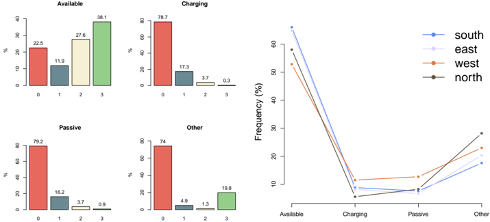<details> <summary>Image 30 Details</summary>  ### Visual Description ## Bar Charts & Line Graph: Device State Frequency by Region ### Overview The image presents a combination of four bar charts and a line graph. The bar charts display the frequency distribution of device states (Available, Charging, Passive, Other) categorized by numerical values 0, 1, 2, and 3. The line graph shows the frequency of each device state across four regions: South, East, West, and North. The y-axis of the bar charts represents frequency in percentage (%), while the x-axis represents the numerical categories 0-3. The line graph's y-axis represents frequency in percentage (%), and the x-axis represents the device states. ### Components/Axes * **Bar Charts:** * X-axis: Numerical categories 0, 1, 2, 3. * Y-axis: Frequency (%) - Scale from 0 to 80. * Four separate bar charts, each representing a device state: Available, Charging, Passive, Other. * **Line Graph:** * X-axis: Device States: Available, Charging, Passive, Other. * Y-axis: Frequency (%) - Scale from 0 to 60. * Legend: * Blue Line: South * Gray Line: East * Orange Line: West * Black Line: North ### Detailed Analysis or Content Details **Available (Bar Chart):** * Category 0: Approximately 22.5% * Category 1: Approximately 11.3% * Category 2: Approximately 27.6% * Category 3: Approximately 38.1% * Trend: The frequency increases from category 0 to 3, with a noticeable jump between 2 and 3. **Charging (Bar Chart):** * Category 0: Approximately 78.7% * Category 1: Approximately 17.3% * Category 2: Approximately 3.7% * Category 3: Approximately 0.3% * Trend: The frequency sharply decreases from category 0 to 3. **Passive (Bar Chart):** * Category 0: Approximately 79.2% * Category 1: Approximately 16.2% * Category 2: Approximately 3.7% * Category 3: Approximately 0.9% * Trend: Similar to "Charging", the frequency decreases significantly from category 0 to 3. **Other (Bar Chart):** * Category 0: Approximately 74.4% * Category 1: Approximately 4.3% * Category 2: Approximately 1.3% * Category 3: Approximately 19.8% * Trend: Frequency decreases from 0 to 2, then increases at category 3. **Line Graph:** * **South (Blue Line):** * Available: Approximately 58% * Charging: Approximately 8% * Passive: Approximately 8% * Other: Approximately 26% * **East (Gray Line):** * Available: Approximately 55% * Charging: Approximately 10% * Passive: Approximately 10% * Other: Approximately 25% * **West (Orange Line):** * Available: Approximately 45% * Charging: Approximately 15% * Passive: Approximately 15% * Other: Approximately 25% * **North (Black Line):** * Available: Approximately 40% * Charging: Approximately 20% * Passive: Approximately 20% * Other: Approximately 20% * Trend: The South and East lines show higher frequencies for "Available" and lower frequencies for "Charging" and "Passive" compared to West and North. The North line shows the lowest frequency for "Available" and the highest for "Charging" and "Passive". ### Key Observations * The "Charging" and "Passive" states have a strong concentration in category 0 across their respective bar charts. * The "Available" state shows a more even distribution across categories, with a peak at category 3. * The "Other" state has a significant frequency in category 3. * The line graph reveals regional differences in device state frequencies, with the South and East regions having more devices in the "Available" state and the North region having more devices in "Charging" and "Passive" states. ### Interpretation The data suggests a varying usage pattern of devices across different regions. The high concentration of "Charging" and "Passive" states in category 0 might indicate that most devices are either actively charging or in a standby mode. The increasing frequency of "Available" devices in higher categories could represent devices that are actively being used. The regional differences highlighted by the line graph suggest that device usage is influenced by geographical factors, potentially related to network availability, user behavior, or device deployment strategies. The "Other" state's concentration in category 3 could represent a specific device activity or a data collection anomaly that requires further investigation. The data could be used to optimize resource allocation, improve network performance, or tailor device management policies to specific regions. </details> electricity system (around 1 billion euros per year, see RTE [Sections 5.4 and 5.5, RTE19] and Lauvergne et al. [Lau+22]). Data splitting For this data challenge, we split the data between a training and a testing set. Because of the change of operator and pricing (see Section 5.2) on March 25th, 2021, we decided to study the following period: from July 3rd, 2020 to March 10th, 2021, when both the EV park and the pricing stayed unchanged. To mimic a genuine time-series forecasting problem, we preserved the time structure when partitioning the data and selected a test set of three weeks. The test set is a stable period that does not include significant changes in the data on the global level (Figure 5.5). Fig. 5.5.: Left: total number of plugs in each state in function of time on train and test (transparent color). The vertical dashed lines represents the end of the train set. Right: total of available plugs in function of time on the test set. In blue: public set. In red: private set. 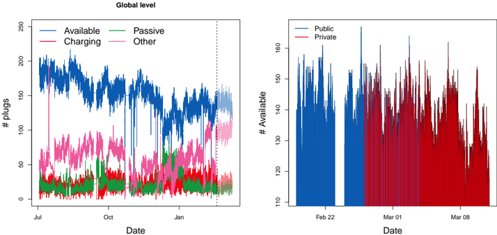<details> <summary>Image 31 Details</summary>  ### Visual Description \n ## Line Chart: Global EV Plug Availability ### Overview The image presents two line charts displaying the number of electric vehicle (EV) plugs available over time. The left chart shows a breakdown by plug status (Available, Charging, Passive, Other) at a "Global level". The right chart shows a breakdown by plug type (Public, Private) over a shorter time period. Both charts use a time-series format with 'Date' on the x-axis and '# plugs' or '# Available' on the y-axis. ### Components/Axes **Left Chart:** * **Title:** "Global level" (top-center) * **X-axis Label:** "Date" (bottom-center) * **Y-axis Label:** "# plugs" (left-center) * **Legend:** Located in the top-left corner. * Blue: "Available" * Red: "Charging" * Green: "Passive" * Pink: "Other" * **Vertical dashed line:** Approximately at the date of January 1st. **Right Chart:** * **X-axis Label:** "Date" (bottom-center) * **Y-axis Label:** "# Available" (left-center) * **Legend:** Located in the top-left corner. * Blue: "Public" * Red: "Private" ### Detailed Analysis or Content Details **Left Chart:** * **Available (Blue):** The line fluctuates between approximately 150 and 220 plugs. It generally declines from July to January, with a slight upward trend in the last few weeks of the displayed period. * July: ~210 plugs * August: ~190 plugs * September: ~170 plugs * October: ~150 plugs * November: ~160 plugs * December: ~140 plugs * January: ~150 plugs * **Charging (Red):** The line fluctuates between approximately 50 and 110 plugs. It shows a general increase from July to October, then a decline to January. * July: ~60 plugs * August: ~70 plugs * September: ~80 plugs * October: ~90 plugs * November: ~70 plugs * December: ~60 plugs * January: ~50 plugs * **Passive (Green):** The line fluctuates between approximately 20 and 60 plugs. It remains relatively stable throughout the period. * July: ~30 plugs * January: ~30 plugs * **Other (Pink):** The line fluctuates between approximately 0 and 30 plugs. It remains relatively low throughout the period. * July: ~10 plugs * January: ~10 plugs **Right Chart:** * **Public (Blue):** The line fluctuates between approximately 110 and 160 plugs. It shows a highly variable pattern with frequent peaks and troughs. * Feb 22: ~120 plugs * Mar 01: ~160 plugs * Mar 08: ~130 plugs * **Private (Red):** The line fluctuates between approximately 110 and 160 plugs. It also shows a highly variable pattern, often mirroring the Public line but with differing peak times. * Feb 22: ~110 plugs * Mar 01: ~120 plugs * Mar 08: ~150 plugs ### Key Observations * The "Available" plugs consistently represent the largest portion of the total plugs in the left chart. * The right chart shows a strong correlation between the availability of Public and Private plugs, suggesting they are often used in conjunction. * The vertical dashed line in the left chart may indicate a significant event or change in EV plug usage patterns. * The right chart shows a much shorter time frame, and a higher degree of volatility. ### Interpretation The data suggests a dynamic EV charging landscape. The left chart provides a global overview of plug status, indicating that a significant number of plugs are generally available, but a substantial portion are also in use (Charging). The decline in available plugs from July to January could be due to increased EV adoption or seasonal usage patterns. The "Passive" and "Other" categories represent a small fraction of the total, potentially indicating plugs that are temporarily unavailable or used for other purposes. The right chart focuses on the distinction between Public and Private plugs. The high variability suggests that plug availability is influenced by factors such as time of day, location, and user behavior. The correlation between Public and Private plugs suggests that users may switch between the two depending on their needs. The shorter time frame and higher volatility in the right chart could be due to the more localized nature of the data. The vertical dashed line in the left chart could represent a policy change, a major EV launch, or a significant shift in consumer behavior. Further investigation would be needed to determine the cause of this potential inflection point. Overall, the data highlights the growing demand for EV charging infrastructure and the need for continued investment and optimization. </details> The training set contains D train points from 2020-07-03 00:00 to 2021-02-18 23:45. The test set contains D test points from 2021-02-19 00:00 to 2021-03-10 23:45. As most EVSE stakeholders (e.g., EDF Group) receive the data with a delay of one to two weeks, we designed the challenge to match the operational perspective, hence the two-week forecast horizon. The test set has been divided into two subsets: a public set for validation purposes and a private set D private . The latter being used to quantify the performance of the solution while minimising the risk of overfitting. To create the public and the private sets, the test set was split into three subsets of one week each. The first week was assigned to the public set, and the third one to the private set. We randomly assigned 20% of second week to the public set and the rest to the private, as illustrated in Figure 5.5. February 23 was excluded of the test set as it contains outliers. The public and private test sets were structured to balance the preservation of the temporal structure of the data and to avoid overfitting on short forecast horizons. Target description At any given time, a plug is in one of the four states. - A station is in state c ( charging ) when it is plugged into a car and provides electricity. - In state p ( passive ) when connected to a car that is already fully charged. - In state a ( available ) when the plug is free. - In state o ( other ) when the plug is malfunctioning. We denote by y t,k = ( a t,k , c t,k , p t,k , o t,k ) ∈ { 0 , 1 , 2 , 3 } 4 the vector representing the state of station k ∈ { 1 , . . . , 91 } at time t , where a t,k is the number of available plugs, c t,k the number of charging plugs, p t,k the number of passive plugs, and o t,k the number of other plugs, at station k and time t . By definition, eq. 5.1 is always valid, $$a _ { t , k } + c _ { t , k } + p _ { t , k } + o _ { t , k } = 3 .$$ Features description To predict the state of station k at time t , the dataset contains the following variables: - Temporal information: date , tod (time of day), dow (day of week), and trend (a temporal index). - Spatial information: latitude , longitude , and area (south, north, east, and west) of the station. dow is the day of week (from 1 for Monday to 7 for Sunday) and tod the time of day, by interval of 15 minutes (0 for 00:00:00 to 95 for 23:45:00). The trend feature is the numerical conversion of the time index, and date is the corresponding string, in the ISO 8601 format. The data is then aggregated into 4 areas of about 20 stations each, as shown in Figure 5.6. Evaluation We aim to forecast the state of the different plugs at 3 hierarchical levels: - Individual stations: denoted by y t,i , for i ∈ { 1 . . . 91 } . - Areas, corresponding to the cardinal points: y t, south , y t, north , y t, east, and y t, west - At the global level: y t, global Fig. 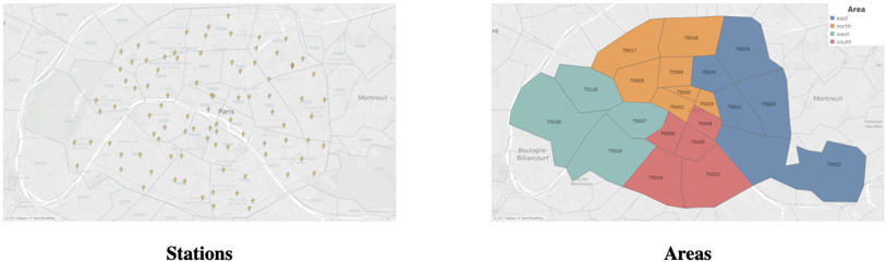5.6.: The 91 stations (yellow dots on the left) and the 4 areas of Paris (colored on the right) <details> <summary>Image 32 Details</summary>  ### Visual Description ## Map Visualization: Paris Bike Sharing System ### Overview The image presents two maps of the Paris metropolitan area, visualizing data related to a bike sharing system. The left map displays the locations of bike stations, while the right map shows the division of Paris into areas, likely representing zones or administrative districts, with associated data. ### Components/Axes **Left Map (Stations):** * **Title:** "Stations" * **Map Features:** Depicts the city of Paris and surrounding areas, including labels for "Paris", "Montreuil", and "Boulogne-Billancourt". * **Markers:** Numerous small, gold-colored markers representing bike stations are scattered throughout the map. No axis or scale is visible. **Right Map (Areas):** * **Title:** "Areas" * **Map Features:** Depicts the city of Paris and surrounding areas, including labels for "Paris", "Montreuil", and "Boulogne-Billancourt". * **Areas:** The map is divided into irregularly shaped polygons, each representing an area. Each area is filled with a different color. * **Legend (Top-Right):** * **Title:** "Area" * **Categories:** "east", "west", "north", "south" * **Colors:** * East: Blue * West: Orange * North: Teal * South: Red * **Area Labels:** Each area is labeled with a four-digit number (e.g., "75008", "75009", "75011"). ### Detailed Analysis or Content Details **Left Map (Stations):** * The stations are densely concentrated within the central areas of Paris, particularly within the inner ring of arrondissements. * Station density decreases significantly in the outer suburbs. * There are approximately 100-150 stations visible, but an exact count is difficult due to overlap and map resolution. **Right Map (Areas):** * **Area Data (Approximate, based on visual inspection):** * **75001:** Blue (East) * **75002:** Orange (West) * **75003:** Orange (West) * **75004:** Orange (West) * **75005:** Orange (West) * **75006:** Orange (West) * **75007:** Orange (West) * **75008:** Orange (West) * **75009:** Teal (North) * **75010:** Teal (North) * **75011:** Teal (North) * **75012:** Teal (North) * **75013:** Red (South) * **75014:** Red (South) * **75015:** Red (South) * **75016:** Orange (West) * **75017:** Teal (North) * **75018:** Teal (North) * **75019:** Teal (North) * **75020:** Red (South) * The areas are not uniformly sized or shaped. * The color distribution suggests a roughly quadrant-based division of Paris into East, West, North, and South zones. ### Key Observations * The bike station distribution is strongly correlated with population density and central urban areas. * The area division appears to be based on administrative or geographical boundaries. * The areas are labeled with postal codes (750xx), indicating arrondissements. * The color coding of areas provides a visual categorization, potentially representing different characteristics or data associated with each zone. ### Interpretation The data suggests a bike sharing system designed to serve the densely populated central areas of Paris. The station distribution reflects this, with a significant concentration of stations within the inner arrondissements. The division of Paris into areas (East, West, North, South) likely represents a segmentation for data analysis or operational management of the bike sharing system. The areas could be used to track usage patterns, identify areas for expansion, or manage maintenance and logistics. The correlation between area color and arrondissement number suggests a deliberate mapping of administrative boundaries to the defined zones. The lack of numerical data associated with each area (e.g., number of bikes, usage rates) limits a deeper analysis, but the visualization provides a clear overview of the system's spatial distribution and zonal organization. </details> Fig. 5.7.: Number of available (left) an passive (right) plugs in function of time for one station, its corresponding area and at the global level. 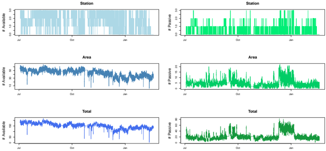<details> <summary>Image 33 Details</summary>  ### Visual Description \n ## Line Charts: Available vs. Passive Counts Over Time ### Overview The image presents six line charts arranged in a 3x2 grid. Each chart displays a time series of counts, comparing "Available" and "Passive" values over a period from approximately July to January. The charts are grouped by category: "Station", "Area", and "Total". The left column shows "# Available" on the y-axis, while the right column shows "# Passive" on the y-axis. ### Components/Axes * **X-axis:** Represents time, with labels indicating months from July to January. The scale is not explicitly marked, but appears to be roughly evenly spaced. * **Y-axis (Left Column):** "# Available" - The scale ranges from approximately 0 to 30, with no explicit tick marks. * **Y-axis (Right Column):** "# Passive" - The scale ranges from approximately 0 to 30, with no explicit tick marks. * **Chart Titles:** Each chart has a title indicating the category ("Station", "Area", "Total"). * **Data Series:** Each chart contains two data series represented by line graphs: one for "Available" (blue) and one for "Passive" (green). ### Detailed Analysis or Content Details **1. Station:** * **# Available (Blue):** The line fluctuates rapidly and consistently between approximately 0 and 30. There is no clear upward or downward trend. The data appears highly volatile. * **# Passive (Green):** The line fluctuates between approximately 0 and 25, with more frequent peaks and valleys than the "Available" series. The data also appears highly volatile. **2. Area:** * **# Available (Blue):** The line exhibits a generally decreasing trend from July to October, then stabilizes around a value of approximately 10-15, with some fluctuations. A sharp increase is observed around January. * **# Passive (Green):** The line shows a generally increasing trend from July to January, with significant fluctuations. Peaks are observed around October and January, reaching values up to approximately 25. **3. Total:** * **# Available (Blue):** The line shows a similar pattern to the "Area" chart, with a decreasing trend from July to October, stabilizing around 10-15, and a sharp increase in January. * **# Passive (Green):** The line exhibits a similar pattern to the "Area" chart's "Passive" series, with an increasing trend from July to January, significant fluctuations, and peaks around October and January, reaching values up to approximately 25. ### Key Observations * The "Station" data shows the highest degree of volatility in both "Available" and "Passive" counts. * The "Area" and "Total" data exhibit similar trends, suggesting a correlation between the two categories. * Both "Area" and "Total" show a decrease in "Available" counts and an increase in "Passive" counts from July to January. * There is a noticeable spike in both "Available" and "Passive" counts around January for "Area" and "Total". ### Interpretation The data suggests a shift in resource allocation or usage patterns over time. The "Station" data indicates a consistently high level of activity with frequent changes in availability and passivity. The "Area" and "Total" data suggest a gradual decline in available resources and a corresponding increase in passive resources from July to October, potentially indicating a seasonal change or a shift in operational priorities. The spike in January could represent a surge in demand or a change in resource allocation. The correlation between "Area" and "Total" suggests that the "Area" data may be a component of the "Total" data. Without further context, it is difficult to determine the specific meaning of "Available" and "Passive" in this scenario, but the data provides valuable insights into their temporal dynamics. </details> we also introduce y t, zone = ∑ i ∈ zone y t,i as the sum of the plugs per state in a zone (south, north, east, west, or global). Let z t = ( y t, 1 , . . . , y t, 91 , y t south , y t, north , y t, east , y t, west , y t, global ) be the aggregated matrix containing the statutes of all stations at the different hierarchical levels at time t . The goal is to provide the best estimator ˆ z of z . Performance is evaluated using the following score, encoding each hierarchical level as a penalty. $$L ( z , \hat { z } ) = | D _ { \text {private} } | ^ { - 1 } \sum _ { t \in D _ { \text {private} } } \left ( \ell _ { \text {station} } ( z _ { t } , \hat { z } _ { t } ) + \ell _ { \text {area} } ( z _ { t } , \hat { z } _ { t } ) + \ell _ { \text {global} } ( z _ { t } , \hat { z } _ { t } ) \right ) ,$$ with the different terms defined as follows: $$9 1$$ $$\ell _ { s t a t i o n } ( z _ { t } , \hat { z } _ { t } ) & = \sum _ { k = 1 } ^ { 9 1 } \| y _ { t , k } - \hat { y } _ { t , k } \| _ { 1 } , \\ \ell _ { a r e a } ( z _ { t } , \hat { z } _ { t } ) & = \sum _ { z o n e \in \mathcal { C } } \| y _ { t , z o n e } - \hat { y } _ { t , z o n e } \| _ { 1 } , \\ \ell _ { g l o b a l } ( z _ { t } , \hat { z } _ { t } ) & = \| y _ { t , g l o b a l } - \hat { y } _ { t , g l o b a l } \| _ { 1 } ,$$ where C = { south , north , east , west } is the set of cardinal points and ‖ x ‖ 1 = ∑ p k =1 | x k | is the usual /lscript 1 norm on R p . We illustrate the different hierarchical level of the data in Figure 5.7. We observe that spatial aggregation increases the signal-to-noise ratio, as the variance tends to decrease when the spatial aggregation is broader. Baseline models As a baseline, we provided two models. A first naive estimator of z t is the median per day of week and quarter-hour over the training set, in which we removed the missing values: $$\hat { z } _ { t } = \underset { t ^ { \prime } \in C a l _ { t } } { m e d i a n } \{ z _ { t ^ { \prime } } \} ,$$ where $$C a l _ { t } = \{ t ^ { \prime } \in D _ { t r a i n } , \, d o w ( t ^ { \prime } ) = d o w ( t ) \} \cap \{ t ^ { \prime } \in D _ { t r a i n } , \, t o d ( t ^ { \prime } ) = t o d ( t ) \} .$$ Notice that the Cal t corresponds to the timestamps of the same day of the week and the same hour of the day. The second baseline model is the parametric model called (CatBoost). It is a tree-based gradient boosting algorithm designed to solve regression problems on categorical data. We used its implementation in the python library CatBoost [Pro+18] and it has demonstrated excellent performance for a great variety of regression tasks [Dao19; Hua+19; HK20] and forecasting challenges [MSA22b]. The performance of these two baselines on the private test set is shown by the dotted lines in Figure 5.8, next to the solutions of the winning team. ## 5.4 Solutions of the winning teams This section describes the methods used by the three winning teams. The ranking of the top competitors is shown in Figure 5.8. The confidence intervals are constructed by time series bootstrapping (non-overlapping moving block bootstrap) [Kun89; PR94]. One subsection is dedicated to each of the winning teams, as their approaches are informative for the analysis of the dataset. In the last subsection, their strengths are combined using aggregation methods. Fig. 5.8.: Ranking of the top competitors. 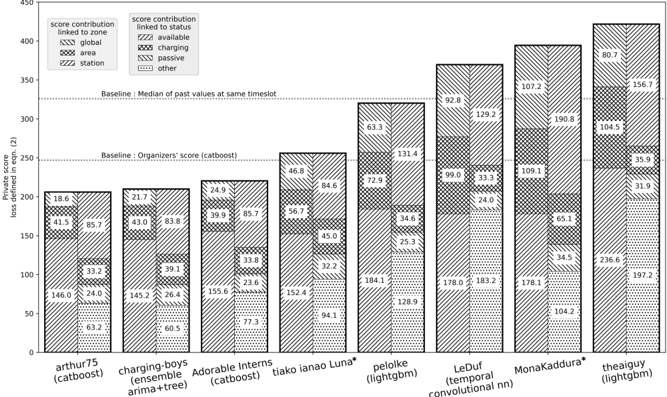<details> <summary>Image 34 Details</summary>  ### Visual Description \n ## Bar Chart: Private Score Loss Contributions by Model and Status ### Overview This image presents a bar chart comparing the "Private score loss defined in eqn. (2)" for several models, broken down by contributions linked to zone and status. The models are displayed along the x-axis, and the score loss is displayed on the y-axis, ranging from 0 to 450. Each bar is segmented to show the contribution of "global", "area", "station", "available", "charging", "passive", and "other" statuses. A baseline is indicated by a horizontal line. ### Components/Axes * **X-axis:** Model names: "arthur75 (catboost)", "charging-boys (ensemble arima+tree)", "Adorable interns (catboost)", "tiako ianao Luna", "pelolke (lightgbm)", "LeDuf (temporal convolutional nn)", "MonaKaddura", "theaiguy (lightgbm)". * **Y-axis:** "Private score loss defined in eqn. (2)", ranging from 0 to 450. * **Legend 1 (Score contribution linked to zone):** * "global" (solid fill) * "area" (diagonal stripes, 45 degrees) * "station" (dotted fill) * **Legend 2 (Score contribution linked to status):** * "available" (horizontal stripes) * "charging" (vertical stripes) * "passive" (cross-hatch) * "other" (white) * **Baseline:** A horizontal line labeled "Baseline: Organizer's score (catboost)" and "Baseline: Median of past values at same timestep". ### Detailed Analysis Here's a breakdown of the score loss for each model, with approximate values based on the chart: * **arthur75 (catboost):** Total score loss is approximately 185. * Global: ~146.0 * Area: ~33.2 * Station: ~6.2 * Available: ~18.6 * Charging: ~85.7 * Passive: ~0 * Other: ~0 * **charging-boys (ensemble arima+tree):** Total score loss is approximately 220. * Global: ~26.4 * Area: ~39.1 * Station: ~69.5 * Available: ~21.7 * Charging: ~43.0 * Passive: ~83.8 * Other: ~0 * **Adorable interns (catboost):** Total score loss is approximately 265. * Global: ~155.6 * Area: ~33.8 * Station: ~77.3 * Available: ~24.9 * Charging: ~39.9 * Passive: ~85.7 * Other: ~0 * **tiako ianao Luna:** Total score loss is approximately 235. * Global: ~94.1 * Area: ~32.2 * Station: ~45.0 * Available: ~84.6 * Charging: ~56.7 * Passive: ~0 * Other: ~0 * **pelolke (lightgbm):** Total score loss is approximately 330. * Global: ~184.1 * Area: ~25.3 * Station: ~128.9 * Available: ~72.9 * Charging: ~34.6 * Passive: ~0 * Other: ~63.3 * **LeDuf (temporal convolutional nn):** Total score loss is approximately 305. * Global: ~178.0 * Area: ~24.0 * Station: ~183.2 * Available: ~99.0 * Charging: ~33.3 * Passive: ~0 * Other: ~107.2 * **MonaKaddura:** Total score loss is approximately 395. * Global: ~178.1 * Area: ~34.5 * Station: ~104.2 * Available: ~109.1 * Charging: ~190.8 * Passive: ~0 * Other: ~102.3 * **theaiguy (lightgbm):** Total score loss is approximately 430. * Global: ~197.2 * Area: ~236.6 * Station: ~31.9 * Available: ~156.7 * Charging: ~80.7 * Passive: ~35.9 * Other: ~0 The baseline is approximately at a score loss of 250. ### Key Observations * "theaiguy (lightgbm)" has the highest total score loss, significantly exceeding the baseline. * "arthur75 (catboost)" has the lowest total score loss. * The "charging" status consistently contributes a substantial portion of the score loss for most models. * The "passive" and "other" statuses contribute very little to the score loss across all models. * "Global" is the largest contributor to the score loss for most models. ### Interpretation The chart demonstrates the performance of different models in terms of private score loss, broken down by zone and status. The varying contributions from each status suggest that the models differ in how they handle different operational conditions. The high score loss for "theaiguy (lightgbm)" indicates that this model performs relatively poorly compared to others, while "arthur75 (catboost)" performs the best. The consistent contribution of the "charging" status suggests that accurately predicting or managing charging events is a key challenge for all models. The baseline provides a reference point for evaluating the performance of each model. The differences in the composition of the score loss (e.g., the relative contributions of "global", "area", and "station") suggest that each model has different strengths and weaknesses in different zones. The lack of contribution from "passive" and "other" statuses may indicate that these statuses are less important or less frequently encountered in the dataset. </details> ∗ No information about these methods were provided by these competitors. Tab. 5.1.: Example of a data conversion to a string | Given station at a given time | Available | Charging | Passive | Other | Target | |---------------------------------|-------------|------------|-----------|---------|----------| | 14h15-16/08/2021 | 1 | 2 | 0 | 0 | 1200 | | 14h30-16/08/2021 | 0 | 1 | 1 | 1 | 0111 | | 14h45-16/08/2021 | 0 | 0 | 3 | 0 | 0030 | ## Arthur Satouf (team Arthur75) Data exploration As shown in Figure 5.1, the dataset presents a lot of missing data. Common techniques were considered to impute these [Pra+16], including computing the mean by station, forward and backward filling, simple moving average, weighted moving average, and exponential moving weighted average (EMW) [Hun86]. These techniques are evaluated by measuring the mean absolute error (MAE) on a validation subset of the training set. As a result, the EMW is the most effective technique, and it is thus implemented for both forward and backward filling approaches. Specifically, we use the last 8 known values to forward fill the first 8 missing values. The same procedure is applied to backward filling. Model description We compare usual forecasting models [Ahm+10; CG16; RSC20], such as SARIMAX, LSTM, XGBoost, random forest, and CatBoost. The evaluation metric used is the MAE, and the time series cross-validation technique is applied to evaluate the performance of the models [KP11; Ped+11]. The CatBoost algorithm is ultimately chosen for its fast optimization relying on parallelization and its ability to handle categorical data without preprocessing. As explained in Section 5.2, the states of any station k satisfy at any time t the equation a t,k + c t,k + p t,k + o t,k = 3 , which is enforced in the CatBoost estimator as follows. - At the station level, the problem is transformed from a multi-task regression problem to a classification problem. This is achieved by concatenating the values of each task as a string, resulting in 20 unique classes. In this approach, the sum of the four vectors always equals three, given that there are three plugs. After predicting a given target, the target is decomposed into four values. Table 5.1 provides an example. - At the area level, CatBoost was also used as a regression problem, as shown in Figure 5.9 and Figure 5.10. However, each area had its own model, and each area used a combination of CatBoost regressor and Regressor-Chain [Rea+09]. Regressor-Chain involves building a unique model for each task and using the result of each task as an input for the next prediction model. The output of each model, along with the previous output, is then used as input for the next task. This approach helps to keep the sum of plug equal to the right number and takes into account the correlation between tasks, making the prediction more robust. - At the global level, the approach is similar to the one applied to the area level, with only 4 models as there are no longer areas. A time series cross validation is used once again to tune the hyperparameters and to validate the models. It relies on the mean absolute percentage error [Myt+16] at the area and the global levels, and on the F-measure [CKM04] at the station level. In total, 21 CatBoost models are used to forecast the private datasets. Fig. 5.9.: Training process of the regressor Chain with CatBoost-Regressor. 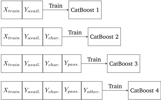<details> <summary>Image 35 Details</summary>  ### Visual Description \n ## Diagram: CatBoost Training Pipeline ### Overview The image depicts a diagram illustrating a sequential training pipeline using CatBoost models. Each stage involves training a CatBoost model with an incrementally increasing set of input features. The diagram shows four distinct CatBoost models (CatBoost 1 through 4) being trained. ### Components/Axes The diagram consists of rectangular blocks representing input features and CatBoost models, connected by arrows labeled "Train". The input features are labeled as follows: * `X_train` * `Y_avail.` (Y available) * `Y_char.` (Y character) * `Y_pass.` (Y pass) * `Y_other` The CatBoost models are labeled: * CatBoost 1 * CatBoost 2 * CatBoost 3 * CatBoost 4 ### Detailed Analysis or Content Details The diagram shows a progressive addition of features to the training process. * **CatBoost 1:** Trained using `X_train` and `Y_avail.`. * **CatBoost 2:** Trained using `X_train`, `Y_avail.`, and `Y_char.`. * **CatBoost 3:** Trained using `X_train`, `Y_avail.`, `Y_char.`, and `Y_pass.`. * **CatBoost 4:** Trained using `X_train`, `Y_avail.`, `Y_char.`, `Y_pass.`, and `Y_other`. The "Train" arrows indicate the flow of data from the input features to the respective CatBoost model. The arrangement is vertical, with each training stage stacked below the previous one. ### Key Observations The diagram illustrates a feature engineering or selection process where features are added sequentially to the training data. This suggests a strategy of incrementally improving the model's performance by incorporating additional information. The order of feature addition (`Y_avail.`, `Y_char.`, `Y_pass.`, `Y_other`) might indicate a prioritization or dependency between these features. ### Interpretation This diagram likely represents a staged approach to model building, potentially for a machine learning task involving prediction or classification. The sequential addition of features suggests a strategy to assess the contribution of each feature to the model's performance. The features themselves (`Y_avail.`, `Y_char.`, `Y_pass.`, `Y_other`) are not defined in the diagram, but their names suggest they represent different aspects or characteristics of the data. The use of CatBoost, a gradient boosting algorithm, implies a focus on achieving high predictive accuracy. The diagram doesn't provide any information about the model's performance or the criteria used for adding features, but it clearly outlines the training process. The diagram suggests a deliberate and iterative approach to model development, where each stage builds upon the previous one. </details> Fig. 5.10.: Inference process of the regressor Chain with CatBoost-Regressor. 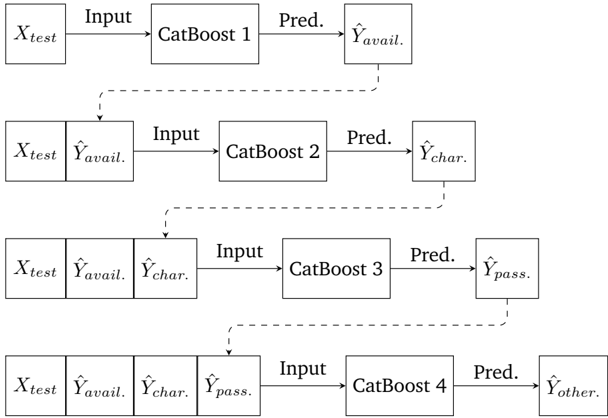<details> <summary>Image 36 Details</summary>  ### Visual Description \n ## Diagram: Cascaded CatBoost Model ### Overview The image depicts a diagram of a cascaded machine learning model using CatBoost. The model consists of four CatBoost models (CatBoost 1 through 4) arranged sequentially. Each model takes an input, makes a prediction, and the prediction is then used as an input for the next model in the cascade. ### Components/Axes The diagram consists of rectangular blocks representing the CatBoost models and input/output data. The blocks are connected by arrows indicating the flow of data. The labels within the blocks are: * **Input:** Represents the input data. * **CatBoost 1, CatBoost 2, CatBoost 3, CatBoost 4:** Represents each CatBoost model. * **Pred.:** Indicates the prediction output of each CatBoost model. * **Ŷavail:** Prediction from CatBoost 1. * **Ŷchar:** Prediction from CatBoost 2. * **Ŷpass:** Prediction from CatBoost 3. * **Ŷother:** Prediction from CatBoost 4. * **Xtest:** The initial input data. The arrows are of two types: solid arrows representing the primary data flow, and dashed arrows representing the feedback of predictions to subsequent models. ### Detailed Analysis / Content Details The diagram shows a sequential process: 1. **CatBoost 1:** Takes `Xtest` as input and produces the prediction `Ŷavail`. 2. **CatBoost 2:** Takes `Xtest` and `Ŷavail` as input and produces the prediction `Ŷchar`. 3. **CatBoost 3:** Takes `Xtest`, `Ŷavail`, and `Ŷchar` as input and produces the prediction `Ŷpass`. 4. **CatBoost 4:** Takes `Xtest`, `Ŷavail`, `Ŷchar`, and `Ŷpass` as input and produces the prediction `Ŷother`. The input data `Xtest` is consistently provided to each CatBoost model. The predictions from previous models are fed as additional inputs to subsequent models. The dashed arrows indicate that the predictions are being used as features in the next stage of the cascade. ### Key Observations The diagram illustrates a multi-stage prediction process where each CatBoost model refines the prediction based on the inputs from the previous models. This suggests a hierarchical or ensemble approach to prediction. The use of previous predictions as inputs implies that the models are learning to correct errors or improve accuracy iteratively. ### Interpretation This diagram represents a stacked generalization or cascading model. The purpose of this architecture is likely to improve prediction accuracy by leveraging the strengths of multiple CatBoost models. Each model in the cascade learns from the errors of the previous models, potentially leading to a more robust and accurate final prediction (`Ŷother`). The inclusion of `Xtest` at each stage suggests that the original features are still considered alongside the predictions from previous models. This could be to prevent error accumulation or to allow the models to revert to the original features if the predictions are unreliable. The naming of the predictions (`Ŷavail`, `Ŷchar`, `Ŷpass`, `Ŷother`) suggests that each model is focused on predicting a specific aspect or category of the target variable. Without further context, it's difficult to determine the exact meaning of these names, but they likely relate to the specific problem being solved. </details> ## Thomas Wedenig and Daniel Hebenstreit (team Charging-Boys) Data exploration Exploratory experiments did not show any signs of a trend within the time series. Regarding stationarity, we run the Augmented Dickey-Fuller test [DF79] on the daily averages of the target values for each station and find inconclusive results. Therefore, we cannot assume stationarity for all target-station pairs, which is why we employ differencing in the construction of our ARIMA model. As usual in statistical frameworks, we assume that the noise interferes with the high frequencies of the signal. To denoise, we preprocess the time series by computing a rolling window average with a window size of 2 . 5 hours [HA18]. During our data exploration, we encounter a significant change in the behavior of the individual stations in the end of October 2020, just before the COVID-19 regulations were enforced in Paris. We also assume that several stations were turned off after this event, as labels were missing over large time intervals. Thus, we experiment with different methods of missing value imputation, but find that simply dropping the timestamps with missing values performs best. We add custom features, namely a column indicating whether the current date is a French holiday, as well as sine and cosine transforms of tod , dow , the month, and the position of the day in the year. To ensure that our regression models return integer outputs that sum to 3 for each station and timestamp (since stations have exactly 3 plugs), we round and rescale these predictions in a post-processing step. Model description We train different models and then aggregate them. First, we start by considering a tree-based regression model. Using skforecast [RO23], we train an autoregressive XGBoost model [CG16] with 100 estimators. We train it on all of the 91 stations individually, each having 4 targets, resulting in 364 models. Each model receives the last 20 target values, as well as the sine/cosine transformed time information as input, and predicts the next target value. We also discard all features that are constant per station (e.g., station name, longitude, and latitude). The final regression model achieves a public leaderboard score of 177 . 67 . Then, we consider a tree-based classification model. To effectively enforce structure in the predictions (i.e., that they sum to 3 ), we transform the regression problem discussed above into a classification problem. For a given station and timestamp, consider the set of possible target values C = { x ∈ { 0 , 1 , 2 , 3 } 4 s.t. ∑ 4 i =1 x i = 3 } . We treat each element c ∈ C as a separate class and only predict class indices ∈ I = { 0 , . . . , 19 } (since |C| = 20 ). While I loses the ordinal information present in C , this approach empirically shows competitive performance. When training a single XGBoost classifier with 300 estimators for all stations, we achieve a public leaderboard score of 178 . 9 . We also experiment with autoregressive classification (i.e.,including predictions of previous timestamps), but find no improvement in the validation error. Finally, we fit a non-seasonal autoregressive integrated moving average (ARIMA) model [Box+15] for each target-station combination. To predict the value of a given target, we only consider the last p = 2 past values of the same target (in the preprocessed time series) and do not use any exogenous variables for prediction (e.g., time information). We apply first-order differencing to the time series ( d = 1 ) and design the moving average part of the model to be of first-order ( q = 1 ). On the validation and training sets, forecasts were applied recursively, using past forecasts as ground truth. We observe that the forecasts using these models have very low variance, i.e., each model outputs an approximately constant time series. These predictions achieve a competitive score on the public leaderboard (third place). The final model is an ensemble of the tree-based regression model, the tree-based classification model, and the ARIMA model. For a single target, we compute the weighted average of the individual model predictions (per timestamp). The ensemble weights are chosen to be roughly proportional to the public leaderboard score ( w reg = 0 . 35 , w class = 0 . 25 , w ARIMA = 0 . 4 ). Since the predictions of the tree-based models have high variance, we can interpret mixing in the ARIMA model's predictions as a regularizer, which decreases the variance of the final model. As the tree-based models also use time information for their predictions, we use the entirety of the available features. ## Nathan Doumèche and Alexis Thomas (team Adorable Interns) Data exploration Several challenges arise from the data, as shown in Figure 5.1. An interesting phenomenon is the emergence of a change in the data distribution on 2020-10-22, characterized by the appearance of missing data. A reasonable explanation is that the detection of missing values is due to an update in the software that communicates with the stations. The Fig. 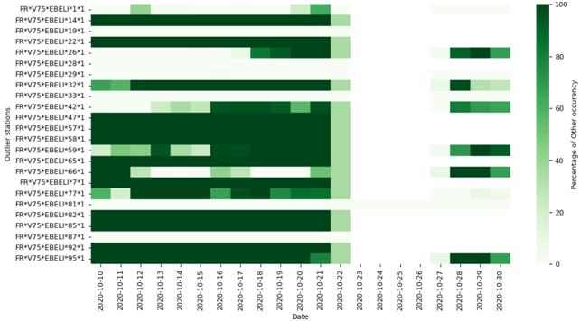5.11.: Percentage of state o occurrences per outlier per day around 2020-10-22 <details> <summary>Image 37 Details</summary>  ### Visual Description \n ## Heatmap: Outlier Station Occurrences ### Overview This image presents a heatmap visualizing the percentage of co-occurrence of outlier stations over time, specifically during the period from 2020-10-10 to 2020-10-30. The heatmap displays the relationship between 20 different outlier stations listed on the y-axis and dates on the x-axis. The color intensity represents the percentage of other occurrences, ranging from 0% (white) to 100% (dark green). ### Components/Axes * **X-axis:** Date, ranging from 2020-10-10 to 2020-10-30, with increments of approximately one day. * **Y-axis:** Outlier Stations. The following stations are listed: * FR\*V75\*EBEL\*1\*1 * FR\*V75\*EBEL\*14\*1 * FR\*V75\*EBEL\*19\*1 * FR\*V75\*EBEL\*22\*1 * FR\*V75\*EBEL\*26\*1 * FR\*V75\*EBEL\*28\*1 * FR\*V75\*EBEL\*29\*1 * FR\*V75\*EBEL\*32\*1 * FR\*V75\*EBEL\*33\*1 * FR\*V75\*EBEL\*42\*1 * FR\*V75\*EBEL\*47\*1 * FR\*V75\*EBEL\*57\*1 * FR\*V75\*EBEL\*58\*1 * FR\*V75\*EBEL\*59\*1 * FR\*V75\*EBEL\*65\*1 * FR\*V75\*EBEL\*66\*1 * FR\*V75\*EBEL\*77\*1 * FR\*V75\*EBEL\*81\*1 * FR\*V75\*EBEL\*82\*1 * FR\*V75\*EBEL\*85\*1 * FR\*V75\*EBEL\*87\*1 * FR\*V75\*EBEL\*92\*1 * FR\*V75\*EBEL\*95\*1 * **Color Scale (Right):** Percentage of Other Occurency, ranging from 0% (white) to 100% (dark green). The scale is divided into increments of approximately 20%. ### Detailed Analysis The heatmap shows varying degrees of co-occurrence between the outlier stations. Here's a breakdown of observations, noting approximate values due to the visual nature of the data: * **FR\*V75\*EBEL\*1\*1:** Shows a strong co-occurrence (approximately 80-100%) around 2020-10-29 and 2020-10-30. Very low co-occurrence (0-20%) for most other dates. * **FR\*V75\*EBEL\*14\*1:** Displays a moderate co-occurrence (approximately 40-60%) around 2020-10-29. Low co-occurrence for other dates. * **FR\*V75\*EBEL\*19\*1:** Shows a moderate co-occurrence (approximately 40-60%) around 2020-10-29. Low co-occurrence for other dates. * **FR\*V75\*EBEL\*22\*1:** Displays a moderate co-occurrence (approximately 40-60%) around 2020-10-29. Low co-occurrence for other dates. * **FR\*V75\*EBEL\*26\*1:** Shows a moderate co-occurrence (approximately 40-60%) around 2020-10-29. Low co-occurrence for other dates. * **FR\*V75\*EBEL\*28\*1:** Displays a moderate co-occurrence (approximately 40-60%) around 2020-10-29. Low co-occurrence for other dates. * **FR\*V75\*EBEL\*29\*1:** Shows a moderate co-occurrence (approximately 40-60%) around 2020-10-29. Low co-occurrence for other dates. * **FR\*V75\*EBEL\*32\*1:** Displays a moderate co-occurrence (approximately 40-60%) around 2020-10-29. Low co-occurrence for other dates. * **FR\*V75\*EBEL\*33\*1:** Shows a strong co-occurrence (approximately 60-80%) around 2020-10-11 to 2020-10-13. Low co-occurrence for other dates. * **FR\*V75\*EBEL\*42\*1:** Displays a moderate co-occurrence (approximately 40-60%) around 2020-10-21. Low co-occurrence for other dates. * **FR\*V75\*EBEL\*47\*1:** Shows a moderate co-occurrence (approximately 40-60%) around 2020-10-21. Low co-occurrence for other dates. * **FR\*V75\*EBEL\*57\*1:** Displays a moderate co-occurrence (approximately 40-60%) around 2020-10-21. Low co-occurrence for other dates. * **FR\*V75\*EBEL\*58\*1:** Shows a moderate co-occurrence (approximately 40-60%) around 2020-10-21. Low co-occurrence for other dates. * **FR\*V75\*EBEL\*59\*1:** Displays a moderate co-occurrence (approximately 40-60%) around 2020-10-21. Low co-occurrence for other dates. * **FR\*V75\*EBEL\*65\*1:** Shows a moderate co-occurrence (approximately 40-60%) around 2020-10-21. Low co-occurrence for other dates. * **FR\*V75\*EBEL\*66\*1:** Displays a moderate co-occurrence (approximately 40-60%) around 2020-10-21. Low co-occurrence for other dates. * **FR\*V75\*EBEL\*77\*1:** Shows a moderate co-occurrence (approximately 40-60%) around 2020-10-19. Low co-occurrence for other dates. * **FR\*V75\*EBEL\*81\*1:** Displays a strong co-occurrence (approximately 60-80%) around 2020-10-11 to 2020-10-13. Low co-occurrence for other dates. * **FR\*V75\*EBEL\*82\*1:** Shows a moderate co-occurrence (approximately 40-60%) around 2020-10-29. Low co-occurrence for other dates. * **FR\*V75\*EBEL\*85\*1:** Displays a moderate co-occurrence (approximately 40-60%) around 2020-10-29. Low co-occurrence for other dates. * **FR\*V75\*EBEL\*87\*1:** Shows a moderate co-occurrence (approximately 40-60%) around 2020-10-29. Low co-occurrence for other dates. * **FR\*V75\*EBEL\*92\*1:** Displays a moderate co-occurrence (approximately 40-60%) around 2020-10-29. Low co-occurrence for other dates. * **FR\*V75\*EBEL\*95\*1:** Shows a moderate co-occurrence (approximately 40-60%) around 2020-10-27 to 2020-10-30. Low co-occurrence for other dates. ### Key Observations * There's a noticeable cluster of high co-occurrence around 2020-10-29 and 2020-10-30 for several stations (FR\*V75\*EBEL\*1\*1, FR\*V75\*EBEL\*14\*1, FR\*V75\*EBEL\*19\*1, FR\*V75\*EBEL\*22\*1, FR\*V75\*EBEL\*26\*1, FR\*V75\*EBEL\*28\*1, FR\*V75\*EBEL\*29\*1, FR\*V75\*EBEL\*32\*1, FR\*V75\*EBEL\*82\*1, FR\*V75\*EBEL\*85\*1, FR\*V75\*EBEL\*87\*1, FR\*V75\*EBEL\*92\*1). * Stations FR\*V75\*EBEL\*33\*1 and FR\*V75\*EBEL\*81\*1 exhibit high co-occurrence between 2020-10-11 and 2020-10-13. * Stations FR\*V75\*EBEL\*42\*1, FR\*V75\*EBEL\*47\*1, FR\*V75\*EBEL\*57\*1, FR\*V75\*EBEL\*58\*1, FR\*V75\*EBEL\*59\*1, and FR\*V75\*EBEL\*66\*1 show moderate co-occurrence around 2020-10-21. * Most stations show very low co-occurrence for the majority of the observed period. ### Interpretation The heatmap suggests that the outlier stations do not generally co-occur frequently. However, there are specific periods where certain stations exhibit a strong tendency to occur together. The high co-occurrence around 2020-10-29 and 2020-10-30 indicates a potential shared event or condition affecting those stations. The earlier peak between 2020-10-11 and 2020-10-13 for stations FR\*V75\*EBEL\*33\*1 and FR\*V75\*EBEL\*81\*1 suggests a separate, earlier event. The moderate co-occurrence around 2020-10-21 for a different set of stations suggests yet another distinct event. This data could be used to investigate the underlying causes of these co-occurrences. For example, are these stations geographically close? Do they share similar environmental conditions? Are they subject to the same operational procedures? Further investigation is needed to understand the relationships between these outlier stations and the events that trigger their simultaneous occurrence. The heatmap provides a valuable starting point for identifying patterns and prioritizing further analysis. </details> update would have taken place on 2020-10-22, allowing the software to detect new situations in which stations were malfunctioning. This hypothesis is supported by the fact that the stations with missing values are those that were stuck in states corresponding to the absence of a car, i.e., either the state a or the state o (see Figure 5.11). In fact, 88% of the stations that were stuck in either a or o for the entire week before 2020-10-22 had missing values on 2020-10-22. Perhaps the users avoided the malfunctioning stations, or perhaps the users tried to connect to the station, but the plug was unresponsive, so the users went undetected. An important implication of this hypothesis is that the data before the change should not be invalidated, since the behaviour of the well-functioning stations did not change. Another challenge of the dataset was its shortness. In fact, we expect a yearly seasonal effect due to holidays [Xin+19] that cannot be distinguished from a potential trend because there is less than one year of data. All these observations suggest giving more weight to the most recent data. As usual in the supervised learning setting, we need to choose a model F to construct the estimator ˆ z t ∈ F . To estimate the entire D test period at once, we cannot rely on online models such as autoregressive models or hidden-state neural networks (RNN, LSTM, transformers...), although they perform well for time series forecasting [BS21], and in particular for EV charging station occupancy forecasts [MF22; Moh+23]. Once a model F is chosen, we define an empirical loss L on the training data. Then, a learning procedure, such as a gradient descent, fits the estimator ˆ z that minimizes L , with the hope that ˆ z will minimize the expectation of the test loss (5.2) [Vap91; HTF17]. Given a training set T train ⊆ D train , we consider two empirical losses. The first one corresponds to Eq. 5.4, this loss gives equal weight to all data points. $$L _ { e q u a l } ( \hat { z } ) = | T _ { t r a i n } | ^ { - 1 } \sum _ { t \in T _ { t r a i n } } \| z _ { t } - \hat { z } _ { t } \| _ { 1 }$$ The second one is given in Eq. 5.5. $$L _ { e x p } ( \hat { z } ) = \sum _ { t \in T _ { t r a i n } } \exp ( ( t - t _ { \max } ) / \tau ) \| z _ { t } - \hat { z } _ { t } \| _ { 1 } ,$$ where τ = 30 days and t max = 2021-02-19 00:00:00. Tab. 5.2.: Evaluation of the performance of the Adorable Interns' models in both phases | | Mean | Median | C (4 , 150) | C exp (5 , 200) | |------------------|--------|----------|---------------|-------------------| | Benchmark Phase | 316 | 309 | 292 | 261 | | Validation Phase | 323 | 303 | 233 | 189 | This time-adjusted loss function is common for non-stationary processes [Dit+15] because it gives more weight to the most recent observations. This makes it possible to give more credit to the data after the change in the data distribution and to capture the latest effect of the trend, while using as much data as possible. Model description To compare the performance of the models, we defined a training period T train , covering the first 95% of D train , and a validation period T val , covering the last 5% . In this benchmark phase, models are trained on T train to minimize L equal or L exp , and then their performance is evaluated on T val by L val (ˆ z ) = | T val | -1 ∑ t ∈ T val ‖ z t -ˆ z t ‖ 1 . The Mean model estimates ˆ y t,k , ˆ A t,k and ˆ G t by their mean over the training period for each value of ( tod, dow ) . Idem for the Median model. They are robust to missing values since the malfunctioning of a station k only affects ˆ y t,k . We compare them with the CatBoost model presented in Section 5.3. Let C ( d, i ) be the CatBoost model of depth d trained with i iterations using L equal , and C exp ( d, i ) the same model trained using L exp . In this setting, we train twelve CatBoost models: one for each pair of state ( a, c, p, o ) and hierarchical level. After hyperparameter tuning, we found C (4 , 150) and C exp (5 , 200) to be the best models in terms of tradeoff between performance and number of parameters, knowing that early stopping and a small number of parameters prevent overfitting [see, e.g., Yin19]. All of these models take advantage of the fact that malfunctioning stations tend to stay in specific states. The contest organizers allowed participants to test their models on a subset T val of D test . In this validation phase, we trained our best models on the entire D train period and tested them with the test loss (5.2). Table 5.2 shows that the ranking of the models is preserved. The submitted model was therefore C exp (5 , 200) . Note that this model is also interesting because its small number of parameters ensures robustness and scalability. In addition, tree-based models are quite interpretable, which is paramount for operational use [Jab+21]. ## Aggregation of forecasts from the winning teams Naive aggregations of uncorrelated estimators are known to have good asymptotic [Tsy03] and online [CBL06] properties. In practice, they often achieve better performance than the individual estimators [see, e.g., BM21; McA+21]. Table 5.3 shows the performance of the top 3 teams compared with two aggregation techniques. The Total score is the result of Equation (5.2), while the other scores are straightforward subdivisions of the loss by hierarchical level and by state. Standard deviations are estimated by moving block bootstrap. The uniform aggregation -denoted by Uniform agg. - corresponds to the mean of each team's prediction, while the weighted aggregation -denoted by Weighted agg. -is computed by gradient descent using the MLpol algorithm [GSE14] to minimise the error on the training set. Notice how the weighted aggregation outperforms the other forecasts for the total loss, as well as for all the subdivisions of the loss. Note that the weighted aggregation of the 3 teams forecasts performs better than the weighted aggregation of any subsets of it (Arthur75+Charging Boys: 199 , Arthur75+Adorable Interns: 203 , Charging Boys+Adorable Interns: 200 ). From these results, each team brings a significant contribution to the final score. Tab. 5.3.: Score by target of the top 3 teams and aggregations. | | Available | Charging | Passive | Other | Stations | Area | Global | Total | |----------------------|-------------|------------|------------|------------|-------------|------------|------------|-------------| | Arthur75 | 85.7 (2.7) | 33.1 (0.7) | 24 (0.6) | 63.3 (2.8) | 145.6 (1.4) | 41.8 (2.5) | 18.7 (4.8) | 206.1 (5.7) | | Charging Boys | 83.9 (3.3) | 38.9 (0.6) | 26.3 (0.4) | 60.7 (3.4) | 145.3 (1.8) | 42.9 (3) | 21.7 (5.7) | 209.9 (6.8) | | Adorable Interns | 85.7 (2) | 33.8 (0.7) | 23.6 (0.6) | 77.4 (2.7) | 155.4 (1.5) | 40.1 (2.8) | 25 (3.8) | 220.5 (5.1) | | Uniform Aggregation | 82.9 (2.5) | 33.1 (0.7) | 22.1 (0.5) | 63.4 (2.7) | 141.1 (1.4) | 40.5 (2.9) | 20 (4.4) | 201.5 (5.4) | | Weighted Aggregation | 82.3 (2.7) | 33 (0.7) | 22.4 (0.5) | 58.5 (2.9) | 137.1 (1.4) | 40.3 (2.9) | 18.7 (4.4) | 196.2 (5.4) | ## Neural networks Although participants proposed a wide variety of models, they mainly focused on classical time series models like ARIMA (see, e.g., charging-boys) and tree-based models (see, e.g., arthur75). Indeed, the only neural network proposed in the challenge was LeDuf's temporal convolutional neural network, inspired by Bai et al. [BKK18], and it performed poorly (see Figure 5.8). Therefore, in order to get a better overview of their potential strengths, we completed our benchmark with neural networks after the challenge. The code to reproduce these experiments is available at https://gitlab.com/smarter-mobility-data-challenge/tutorials/-/tree/master/ 2.%20Model%20Benchmark . Indeed, Fully Connected Neural Networks (FCNNs) are known to be able to forecast EV demand [Bou+22; AGG23a]. The FCNN model we implemented predicts the status of individual stations. The forecasts for the area and the global levels are then derived in a bottom-up manner by summing the forecasts of the individual stations. In contrast to the CatBoost models, this bottom-up approach performed better than training a FCNN for each hierarchical level (station, area and global). The hyperparameters of the FCNN were then optimised using the optuna package in Python [Aki+19]. As a result, the package selected a FCNN with one hidden layer, 155 neurons, a learning rate of 7 . 8 e -4 , a dropout of 0 . 012 , a batch size of 480 and 14 epochs. Similar to Ahmadian et al. [AGG23a], we found out that FCNNs with a single hidden layer were the ones that performed best. The performance of the FCNN on the test set for the hierarchical loss is 250.5 ± 3.1. The standard deviation of the score is estimated by moving block bootstrap. Thus, the FCNN is outperformed by the CatBoost model which has a loss of 246.1 ± 2.3. Graph Neural Networks (GNNs) are neural networks that encode the spatial dependencies in a dataset as a graph to capture spatial correlations. GNNs are natural candidates among neural networks for EV charging forecasting because they inherently encode the spatial hierarchical structure of the dataset [Wan+23b; Qu+24]. Among GNNs, Graph Attention Networks (GATs) are models designed for time series forecasting that exploit both temporal and spatial dependencies [Vel+18]. Contrary to Wang et al. [Wan+23b] and Qu et al. [Qu+24], the optimisation of this GNN did not converge, and its loss on the test set did not go below 400. We believe that this is due to the fact that we only had access to 91 charging stations, which is not a big data regime, as compared to Wang et al. [Wan+23b] who fitted their GNN on 76774 EVs and to Qu et al. [Qu+24] who fitted their GNN on 18061 EV charging piles. Both Wang et al. [Wan+23b] and Qu et al. [Qu+24] only had access to one month of data and focused on short-term forecasting, which may also explain this difference. ## 5.5 Summary of findings and discussion This paper presents a dataset in the context of hierarchical time series forecasting of EV charging station occupancy, providing valuable insights for energy providers and EV users alike. Models Contestants were able to train models that significantly outperformed the baseline performance (see Figure 5.8). This dataset contains many practical problems related to time series, including missing values, non-stationarity, and outliers. This explains why most contestants relied on tree-based models, which are robust enough to outperform more sophisticated machine learning methods. Data cleaning Specific techniques were developed to deal with missing data and outliers (see, e.g., Section 5.4). Data preprocessing is a crucial step, and the addition of relevant exogenous features, such as the national holidays calendar, significantly improved the results. Time dependant loss function All three of the winning solutions described in this paper were robust enough to maintain a high private test score, showing good generalization of the models. The choice of the empirical cost function to drive the training process produced the best results when more recent data points were given greater weight (see, e.g., Section 5.4). Aggregation Aggregating the forecasts of the three winning teams even yielded a better global score, with a notable improvement at the station level. The hierarchical models presented are promising and could help improve the overall EV charging network. Why publishing this dataset? This open dataset is interesting for research purpose because it encompasses many real-world problems related to time series matters, such as missing values, non-stationarities, and spatio-temporal correlations. In addition, we strongly believe that sharing the benchmark models derived from this challenge will be useful for making comparisons in future research. Two more complete datasets using new features and spanning from July 2020 to July 2022 are available at doi.org/10.5281/zenodo.8280566 and at gitlab.com/smarter-mobility-data-challenge/additional\_materials. A primary analysis is presented in the supplementary material. Perspectives Managing a fleet of EVs in the context of an increasing renewable production amount open new challenges for forecasters. We hope this dataset will allow other researchers to work on topics such as probabilistic forecasts, online learning (our challenge was "offline") or graphical models. Limitations The deployment of electric vehicles (EVs) is progressing at a remarkable pace [Sat+22], making any dataset merely a snapshot of a swiftly evolving world [see also HFS21]. To enhance forecasting accuracy, additional features could be incorporated into a dataset. Numerous covariates, such as mobility and traffic information, meteorological data, and vehicle characteristics, could be included. In a forthcoming release of the dataset, in addition to extending the observation period, we intend to incorporate traffic and meteorological data. A first attempt is proposed in the Section 4 of the supplementary material. Ethical concerns To the best of our knowledge, our work does not pose any risk of security threats or human rights violations. Knowing when and where someone plugs in their EV could lead to a risk of surveillance. However, this dataset does not contain any personal information about the user of the plug or their car, so there is no risk of consent or privacy. ## 5.A Belib's history: pricing mechanism and park evolution Though there is no official document relating the evolution of the Belib pricing mechanism, it is possible to reconstruct its history through the press. Belib pricing strategy evolved twice (on 25 March 2021 and on January 2023), and the press releases explicitly state that they do not vary between these dates [Fon31; Noe02]. This ensures that both the Belib EV park and the pricing strategy did not change during the period studied in the challenge, from 2020-07-03 to 2021-03-10. Belib creation in 2016 The 5 first stations of the Belib network were first operational on 12 January 2016 [Tor16; Cam16]. The network grew progressively during the year 2016 to reach 60 stations all around Paris. Users needed to buy a 15 euro badge to connect to the network. Different pricing strategies were applied depending on the time of the day and the plugs electric power. The "normal charge" of 3kW was free at night (between 8 p.m. and 8 a.m.) and cost 1 euro per hour on daytime (between 8 a.m. and 8 p.m.). The "quick charge" of 22kW cost 0.25 euro per 15 minutes the first hour of charge. After the first hour, the first 15 minutes cost 2 euros. After this 1h and 15 minutes, each 15 minutes slot cost 4 euros. Each station contained 3 parking spots: - one dedicated to "normal charge" with an E/F electric plug, - one dedicated to "quick charge" with a ChaDeMo and a Combo2 plugs, - one where both "normal charge" and "quick charge" were possible, with an E/F, a T2, and a T3 plugs. Therefore, this pricing strategy meant that "normal charge" plugs could serve as free parking spot at night, while "quick charge" became expensive after one hour of usage. Belib under the TotalEnergies supervision begining on 25 March 2021 In 2021, the city of Paris allowed the TotalEnergies company to run the Belib network for a period of 10 years. The goal is to develop the network from its 90 stations of 270 charging points, to 2300 charging points [Tot31; Liv09]. More precisely, our dataset accounts for 91 stations corresponding to 273 charging points. This change of the network's operator was accompanied with the following change in pricing on 25 March 2021 [Aut01]. Four programmes became available (Flex, Moto, Boost, and Boost+), with pricing depending on station's location and on the frequency of use. For occasional users, - the Flex programme allows the usage of 3.7kW and 7kW plugs. In the districts 1 to 11 of Paris, the pricing goes as follows. The first 2 hours of charging, each 15 minutes cost 0.90 euro. Then, each 15 minutes cost 1.00 euro. Then, after 3 hours of charging, each 15 minutes cost 1.10 euro. In the districts 12 to 20 of Paris, the pricing goes as follows. The first 2 hours of charging, each 15 minutes cost 0.55 euro. Then, each 15 minutes cost 0.65 euro. Then, after 3 hours of charging, each 15 minutes cost 0.75 euro. - the Moto programme allows the usage of 3.7 kW plugs for motorcycles at the cost of 0.35 euro per 15 minutes. - the Boost programme allows the usage of 22kW plugs at the cost of 1.90 euro per 15 minutes. - the Boost+ programme allows the usage of 50 kW plugs at the cost of 4.80 euros per 15 minutes. For regular users, at the condition of a yearly-7-euro subscription, - the Flex programme allows the usage of 3.7kW and 7kW plugs. In the districts 1 to 11 of Paris, the pricing goes as follows. The first 2 hours of charging, each 15 minutes cost 0.75 euro. Then, each 15 minutes cost 0.80 euro. Then, after 3 hours of charging, each 15 minutes cost 0.85 euro. In the districts 12 to 20 of Paris, the pricing goes as follows. The first 2 hours of charging, each 15 minutes cost 0.50 euro. Then, each 15 minutes cost 0.55 euro. Then, after 3 hours of charging, each 15 minutes cost 0.60 euro. - the Moto programme allows the usage of 3.7 kWh plugs for motorcycles at the cost of 0.30 euro per 15 minutes. - the Boost programme allows the usage of 22kWh plugs at the cost of 1.70 euro per 15 minutes. - the Boost+ programme allows the usage of 50 kWh plugs at the cost of 4.40 euros per 15 minutes. - at nighttime, pricing was more advantageous. The Flex programme cost 3.90 euros for the whole night, plus 0.20 euros for each consumed kWh after a 19,5 kWh consumption. The Moto programme cost 2.90 euros for the whole night, and then 0.20 euros for each kWh after a 19.5 kWh consumption. In all cases, after 14 consecutive hours of parking on a charging spot, any programme would then cost 10 euros per hour, the charging starting at the beginning of each hour. This more complex pricing was perceived as misleading for the consumers, and resulted in overall higher expenses. The pricing did not changed until 1 January 2023 [Noe02]. An price increase on January 2023 On 1 January 2023, the Belib pricing strategy evolved. It was decided to take into account that some stations were malfunctioning and did not deliver the expected electric power. Indeed, with the previous pricing strategy depending only on the charging time, some drivers were paying too much for charging their cars. Therefore, the pricing evolve to take into account both the time spent in the EV charging spot and the energy transmitted to the car. Moreover, because of the energy crisis in Europe, electricity prices had increased and TotalEnergies raised their charging price. This resulted in higher expenses for EV users, leading to a significant drop in the usage of Beilb stations [Gir27]. On 25 January 2023, to cope with the decreasing numbers of users, Belib prices were decreased [Has25]. The same pricing segmentation was kept, but with lower prices. This pricing is the same as today, on August 2023. Both the pricing on 1 January 2023 and on 25 January 2023 (in bold) are detailed in Tables 5.4, 5.5, and 5.6 [Noe02; Bel23]. Table 5.4 details the pricing for occasional users, without subscription. Table 5.5 details the pricing for regular users not living in Paris, with a yearly 7-euro subscription. Table 5.6 details the pricing for regular users living in Paris, with a yearly 7-euro subscription. Notice that the distinctions between districts was abandoned. In all cases, after 14 consecutive hours of parking on a charging spot, any programme would then cost 10 euros per hour, the charging starting at the beginning of each hour. | Pricing | Moto (3.7kW) | Flex (7kW) | Boost (22 kW) | Boost+ (50kW) | |-----------------------|----------------|---------------|-----------------|-----------------| | kWh on 01/01/2023 | 0.55C | 0.55C | 0 | 0 | | Parking on 01/01/2023 | 0.35C / 15min | 0.78C / 15min | 2.30C / 15min | 0.50C / min | | kWh on 01/25/2023 | 0.35C | 0.35C | 0 | 0 | | Parking on 01/25/2023 | 0.20C / 15min | 0.55C / 15min | 2.30C / 15min | 0.38C / min | Tab. 5.4.: Pricing for occasional users Tab. 5.5.: Pricing for regular users not living in Paris | Pricing | Moto (3.7kW) | Flex (7kW) | Boost (22 kW) | Boost+ (50kW) | |-----------------------|----------------|---------------|-----------------|-----------------| | kWh on 01/01/2023 | 0.55C | 0.55C | 0 | 0 | | Parking on 01/01/2023 | 0.30C / 15min | 0.60C / 15min | 2.15C / 15min | 0.45C / min | | kWh on 01/25/2023 | 0.35C | 0.35C | 0 | 0 | | Parking on 01/25/2023 | 0.15C / 15min | 0.35C / 15min | 2.05C / 15min | 0.35C / min | Tab. 5.6.: Pricing for regular users living in Paris | Pricing | Moto (3.7kW) | Flex (7kW) | Boost (22 kW) | Boost+ (50kW) | |-----------------------------------------------------------|---------------------------|---------------------------|-------------------|-----------------| | 8 a.m. to 8 p.m. kWh on 01/01/2023 | 0.55C | 0.55C | 0 | 0 | | Parking on 01/01/2023 kWh on 01/25/2023 | 0.30C / 15min 0.35C | 0.60C / 15min 0.35C | 2.15C / 15min 0 | 0.45C / min 0 | | Parking on 01/25/2023 | 0.15C / 15min | 0.35C / 15min | 2.05C / 15min | 0.35C / min | | 8 p.m. to 10 p.m. kWh on 01/01/2023 | 0.55C | 0.55C | 0 | 0 | | Parking on 01/01/2023 | 0.15C / 15min | 0.20C / 15min | 2.15C / 15min | 0.45C / min | | kWh on 01/25/2023 | 0.35C | 0.35C | 0 | 0 | | Parking on 01/25/2023 | | | / 15min | | | 10 p.m. to 8 a.m. | 0.10C / 15min | 0.15C / 15min | 2.05C | 0.35C / min | | kWh on 01/01/2023 Parking on 01/01/2023 kWh on 01/25/2023 | 0.30C 0.05C / 15min 0.25C | 0.30C 0.05C / 15min 0.25C | 0 2.15C / 15min 0 | 0 0.45C / min 0 | | Parking on | / 15min | / | 2.05C / | 0.35C / min | | 01/25/2023 | 0.05C | 0.05C 15min | 15min | | ## 5.B Data description ## Data set collection We set up a DataLake to collect and make available all types of data related to electric mobility. This dataset is informative about the charging stations (static data) and their use in real time (dynamic data) everywhere in France and in particular in Paris, where the operating network is called Belib. The DataLake has set up an automatic and real-time collect of Belib data as it is published on the supplier's site: https://parisdata.opendatasoft.com/explore/dataset/ belib-points-de-recharge-pour-vehicules-electriques-disponibilite-temps-reel/ api . The storage of this information over time allows, for example, to estimate the frequentation of the charging stations according to their location. The DataLake Mobility uses a big data infrastructure based on Hadoop technologies (HDFS, PySpark, Hive and Zeppelin), allowing to manipulate large volumes of data and to process massive data, including to launch machine learning algorithms. ## Data preprocessing Aggregation The raw data is structured so that each observation reflects the status of the plugs (up to 6) within a charging point. This is misleading because only one of these plugs can be in use at a time. Therefore, we have kept the relevant rows only for plugs in use and treated a charging point as a single plug. In addition, in the raw data, charging points appear in fixed geographic locations and in groups of three. This charging point structure was confirmed by the data provider. Therefore, it makes sense to regroup three adjacent charging points into a single charging station and we have aggregated the data to make each observation the status of the 3 charging points every 15 minutes. To account for discrepancies in timestamp synchronisation between stations we adjusted the timestamps to match the closest 15 minute interval. States The available , charging , and passive states are taken directly from the raw data. The last state other is regroups several statuses including reserved (a user has booked the charging point), offline (the charging point is not able to send information to the server), and out of order (the charging point is out of order). This choice was made because of the relatively small number of reserved and out of order records. Therefore, the other state could be interpreted as a noisy version of the offline state. Missing data were not filled. ## 5.C Further insights on the winning strategies ## Arthur75: time-series cross validation To select the best model, Arthur75 relied on a 4-fold time-series cross validation. More precisely, the training data is separated in six equally long subsets. The nth cross-validation step consists in training the model on the n+1 th first subsets and evaluating it on the n+2 th subset. Then, the test loss are averaged and the parameters of the models are chosen to minimize this averaged test loss. ## Charging Boys: ablation study The Charging Boys' forecast is an ensemble of models. Therefore, it is more complex than what the other teams have proposed. To better understand what each model brings to the ensemble, we conduct an ablation study. In Table 5.7, we compute the scores on the private test of each model of the ensemble. To get a better grasp of the strengths of each model, we also compute these score on each hierarchical level (station, area, and global). Interestingly, the ARIMA outperforms the other individual models at each hierarchical level. It is also clear that for each hierarchical level the ensemble outperforms the individual models meaning that each component of this complex strategy brings its contribution to the final score. Tab. 5.7.: Score by zones of Charging Boys models: ARIMA, XGB-reg, XGB-class, Ensemble. | | Stations | Area | Global | Total | |-----------|------------|--------|----------|---------| | ARIMA | 148 | 44 | 22 | 214 | | XGB-reg | 150 | 46 | 26 | 222 | | XGB-class | 149 | 49 | 23 | 221 | | Ensemble | 145 | 43 | 22 | 210 | ## 5.D Future perpectives: a longer dataset with more features To continue the endeavour initiated by the smarter mobility challenge, exogeneous data and additional occupancy records have been collected. This section details the additional resources gathered at gitlab.com/smarter-mobility-data-challenge/additional\_materials for the code and https://doi.org/10.5281/zenodo.8280566 for the datasets. ## Adding new features We present here an updated version of the data which was conducted after the smarter mobility challenge. This dataset was obtained by merging the Belib dataset with weather [Sal16] and traffic datasets [Par23]. Weather Weather data covering the same period as the charging point occupancy used for the Smarter Mobility Data Challenge, i.e., from July 2020 to March 2021, was collected using the riem package available in R [Sal16]. 3 weather stations were selected from the 3 existing Paris airports: Orly , Le Bourget , and Roissy-Charles de Gaulle . We selected the 4 weather variables the most relevant to the problem at hand, knowingly - Temperature (tmpf) in Fahrenheit, - Relative humidity (relh) in percentage, - Wind speed (sknt) in knots, - Visibility (vsby) in miles. These variables were collected on a half-hourly timestep. To match the 15 minutes timestep of the occupancy data, the missing values were filled in with linear interpolation. Furthermore, the last and first non-NA values were carried forward and backward respectively to fill in missing data at the beginning and end of the dataset. Traffic The traffic data collected on the Paris Data platform [Par23] contains information on the number of vehicles on the road at various key locations in Paris. Every hour, sensors record the number of vehicles passing through a specific location in the city of Paris. Similarly to the weather data, the data has therefore been interpolated and filled to match the 15 minute timestamp of the occupancy data. Only one sensor was kept for each charging station: the closest one according to the Haversine formula that calculates the distance between two latitudes and longitudes [Rob57].The traffic variables available are: - flow (q): number of vehicles counted - occupancy rate (k) - traffic state: 0 for unknown , 1 for fluid , 2 for pre-saturated , 3 for saturated and 4 for blocked - traffic stopped: 0 for unknown , 1 for open , 2 for blocked and 3 for invalid Benchmark We computed the catboost benchmark including the new features over the same period as the challenge. The results are shown in Table 5.8. As expected, the addition of weather and traffic information marginally improves the prediction performance when the models are trained with enough iterations. Tab. 5.8.: Losses calculated for the catboost benchmark model with 150 and 300 iterations only with temporal features and with all features (temporal, weather, traffic) | Features | Public set | Private set | Features | Public set | Private set | |------------|--------------|---------------|------------|--------------|---------------| | Temporal | 233 | 246 | Temporal | 238 | 260 | | All | 249 | 263 | All | 223 | 244 | ## Adding new observations Regarding the observation period, more data have been collected since the smarter mobility challenge. We provide a raw extraction and some initial data preparation at the following link https://doi.org/10.5281/zenodo.8280566. This new dataset runs from 28 June 2021 to 15 July 2022 at a 5-minute frequency. Data Preparation This new dataset covers the period from June 2021 to July 2022. The data preprocessing was kept minimal. It consists in simply concatenating the monthly extracts from the database, translating the statuses in English and converting the timestamp (in seconds from 1970) to a UTC datetime field. Both raw and preprocessed data are available. Fig. 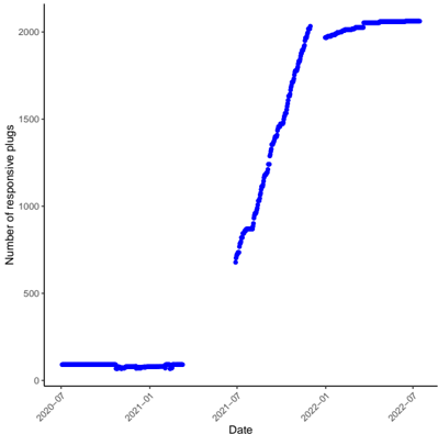5.12.: Daily EVSE count <details> <summary>Image 38 Details</summary>  ### Visual Description \n ## Line Chart: Number of Responsive Plugs Over Time ### Overview The image presents a line chart illustrating the number of responsive plugs over a period from approximately July 2020 to July 2022. The chart shows a relatively flat trend for the first year, followed by a steep increase, and then a leveling off. ### Components/Axes * **X-axis:** Labeled "Date", spanning from approximately July 2020 to July 2022. The axis is marked with approximate dates: 2020-07, 2021-01, 2021-07, 2022-01, and 2022-07. * **Y-axis:** Labeled "Number of responsive plugs", ranging from 0 to 2000, with increments of 500. * **Data Series:** A single blue line representing the number of responsive plugs. * **No Legend:** There is no explicit legend, but the Y-axis label clearly identifies the data represented by the line. ### Detailed Analysis The blue line representing the number of responsive plugs exhibits the following trend: * **2020-07 to 2021-01:** The line remains relatively flat, fluctuating between approximately 0 and 100 responsive plugs. * **2021-01 to 2021-07:** The line remains relatively flat, fluctuating between approximately 0 and 150 responsive plugs. * **2021-07 to 2022-01:** A steep upward trend is observed, increasing from approximately 600 to 2000 responsive plugs. * **2022-01 to 2022-07:** The line plateaus, fluctuating between approximately 1900 and 2000 responsive plugs. Approximate data points: * 2020-07: ~20 responsive plugs * 2021-01: ~50 responsive plugs * 2021-07: ~120 responsive plugs * 2022-01: ~1900 responsive plugs * 2022-07: ~2000 responsive plugs ### Key Observations * The most significant change occurs between July 2021 and January 2022, with a rapid increase in the number of responsive plugs. * The number of responsive plugs stabilizes after January 2022, indicating a saturation point or completion of a deployment phase. * The initial period (July 2020 - July 2021) shows minimal growth in responsive plugs. ### Interpretation The data suggests a phased rollout or adoption of "responsive plugs." The initial flat period likely represents a pilot program or limited initial deployment. The steep increase starting in July 2021 indicates a broader implementation or increased adoption rate. The subsequent leveling off suggests that the deployment has reached a significant level of completion or that the target market has been largely saturated. The data could be used to assess the success of the rollout, identify potential bottlenecks in the initial phase, and forecast future growth based on the stabilization trend. It would be useful to have additional context regarding what constitutes a "responsive plug" and the factors driving its adoption to provide a more comprehensive interpretation. </details> Statuses and missing values The statuses are different between the version V1 of the dataset (from July 2020 to March 2021) and V2 (from June 2021 to July 2022), as shown in Table 5.9. Notice that the Passive state is now part of the Available state. Indeed, after TotalEnergies Tab. 5.9.: Possible statuses of the Electric Vehicle Supply Equipment (EVSE) in the previous (V1) and current (V2) versions | Status | Description | Status | Description | |-----------|-------------------|--------------------------------------|----------------------------------| | Available | Free EVSE | Available | Free EVSE | | Charging | EV charging | Charging | EV charging at EVSE | | Passive | EV plugged | In maintenance | EVSE being fixed | | Other | EVSE out of order | Currently being commissioned Unknown | EVSE being deployed EVSE offline | became the operator of the Belib network on March 2021 (see Section 5.A), the information released regarding the stations was updated. This explains the missing values between April 2021 and June 2021 and the evolution of the states detailed in Table 5.9. For our analysis, we regroup the In maintenance and Unknown states and consider them as the Other state. The Currently being commissioned state is related to the extension of the EV park, as shown in Figure 5.12, and correspond to the fact that there were some delay between the moments when new stations were built and sent signals, and the moments when they became open to use for EV drivers. In what follows, we left this state apart. Exploratory data analysis Similarly to what we did in the EDA for the period spanning from July 2020 to March 2021, we plot the daily and weekly profiles of each status for this new period running from June 2021 to July 2022 in Figures 5.13 and 5.14. Notice that, though the pricing mechanism change on 25 March 2021 (see Section 5.A), it still was more advantageous at night (between 8 p.m. and 8 a.m.) for regular users. This explains why the daily pattern Fig. 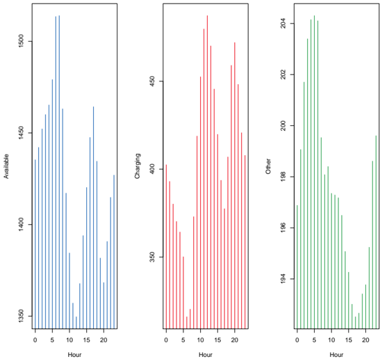5.13.: Daily profile at the Global level between July 2021 and July 2022 <details> <summary>Image 39 Details</summary>  ### Visual Description ## Bar Charts: Vehicle Availability, Charging, and Other Status Over Time ### Overview The image presents three vertically-oriented bar charts arranged side-by-side. Each chart displays a distribution of values over a 24-hour period, represented on the x-axis as "Hour" ranging from 0 to 20. The y-axes represent different vehicle statuses: "Available" (left chart), "Charging" (center chart), and "Other" (right chart). The charts appear to show the number of vehicles in each status at each hour. ### Components/Axes * **X-axis (all charts):** "Hour" ranging from 0 to 20, with tick marks at integer values. * **Y-axis (left chart):** "Available", ranging from approximately 1350 to 1500, with tick marks at 1350, 1400, 1450, and 1500. * **Y-axis (center chart):** "Charging", ranging from approximately 350 to 450, with tick marks at 350, 400, and 450. * **Y-axis (right chart):** "Other", ranging from approximately 194 to 204, with tick marks at 194, 196, 198, 200, 202, and 204. * **Colors:** Blue for "Available", Red for "Charging", and Green for "Other". ### Detailed Analysis or Content Details **Chart 1: Available Vehicles** The "Available" chart shows a generally decreasing trend from hour 0 to hour 20, with several peaks and valleys. * Hour 0: Approximately 1470 vehicles. * Hour 2: Approximately 1440 vehicles. * Hour 4: Approximately 1420 vehicles. * Hour 6: Approximately 1400 vehicles. * Hour 8: Approximately 1410 vehicles. * Hour 10: Approximately 1430 vehicles. * Hour 12: Approximately 1450 vehicles. * Hour 14: Approximately 1440 vehicles. * Hour 16: Approximately 1410 vehicles. * Hour 18: Approximately 1390 vehicles. * Hour 20: Approximately 1380 vehicles. **Chart 2: Charging Vehicles** The "Charging" chart shows an increasing trend from hour 0 to approximately hour 12, followed by a decreasing trend. * Hour 0: Approximately 360 vehicles. * Hour 2: Approximately 370 vehicles. * Hour 4: Approximately 380 vehicles. * Hour 6: Approximately 390 vehicles. * Hour 8: Approximately 400 vehicles. * Hour 10: Approximately 420 vehicles. * Hour 12: Approximately 440 vehicles. * Hour 14: Approximately 430 vehicles. * Hour 16: Approximately 410 vehicles. * Hour 18: Approximately 390 vehicles. * Hour 20: Approximately 370 vehicles. **Chart 3: Other Vehicles** The "Other" chart exhibits a similar pattern to the "Charging" chart, with an increase followed by a decrease. * Hour 0: Approximately 196 vehicles. * Hour 2: Approximately 197 vehicles. * Hour 4: Approximately 198 vehicles. * Hour 6: Approximately 200 vehicles. * Hour 8: Approximately 201 vehicles. * Hour 10: Approximately 202 vehicles. * Hour 12: Approximately 203 vehicles. * Hour 14: Approximately 202 vehicles. * Hour 16: Approximately 200 vehicles. * Hour 18: Approximately 198 vehicles. * Hour 20: Approximately 196 vehicles. ### Key Observations * The number of available vehicles generally decreases throughout the day, while the number of vehicles charging and in "Other" status increases during the first half of the day and then decreases. * The peak charging and "Other" status occur around hour 12. * The "Available" vehicle count remains significantly higher than the "Charging" and "Other" counts. ### Interpretation The data suggests a pattern of vehicle usage throughout the day. Vehicles are likely being utilized and taken off the "Available" pool during the day, with a corresponding increase in vehicles being charged or in some other state (e.g., maintenance, in use). The peak in charging and "Other" status around hour 12 could indicate a lunchtime or mid-day period where vehicles are being serviced or recharged. The consistent decline in available vehicles suggests a steady demand for the service throughout the observed period. The relatively small number of vehicles in the "Other" category suggests that most vehicles are either available or being charged. The charts provide a snapshot of vehicle fleet dynamics and could be used to optimize resource allocation and charging schedules. </details> Fig. 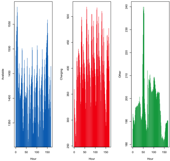5.14.: Weekly profile at the Global level between July 2021 and July 2022 <details> <summary>Image 40 Details</summary>  ### Visual Description \n ## Line Charts: Time Series Data - Available, Charging, Other ### Overview The image presents three separate line charts, each depicting a time series. The charts share a common x-axis representing "Hour" (ranging from 0 to approximately 150), but each has a unique y-axis representing a different metric: "Available" (in blue), "Charging" (in red), and "Other" (in green). All three charts appear to represent data collected over the same time period. ### Components/Axes * **X-axis (all charts):** "Hour", ranging from 0 to approximately 150. The scale is linear. * **Y-axis (Chart 1):** "Available", ranging from approximately 1450 to 1550. The scale is linear. * **Y-axis (Chart 2):** "Charging", ranging from approximately 250 to 500. The scale is linear. * **Y-axis (Chart 3):** "Other", ranging from approximately 180 to 240. The scale is linear. * **Line Color 1:** Blue, representing "Available". * **Line Color 2:** Red, representing "Charging". * **Line Color 3:** Green, representing "Other". ### Detailed Analysis or Content Details **Chart 1: Available** The blue line representing "Available" exhibits a highly oscillatory pattern. The line fluctuates rapidly between approximately 1460 and 1540. * At Hour 0, the value is approximately 1530. * Around Hour 20, the value dips to approximately 1460. * Around Hour 40, the value peaks at approximately 1540. * The pattern continues with similar amplitude fluctuations throughout the 150-hour period. **Chart 2: Charging** The red line representing "Charging" also shows a fluctuating pattern, but with a different frequency and amplitude than the "Available" chart. The line fluctuates between approximately 270 and 480. * At Hour 0, the value is approximately 320. * Around Hour 20, the value rises to approximately 400. * Around Hour 40, the value dips to approximately 280. * The fluctuations become more pronounced around Hour 100, reaching a peak of approximately 480. **Chart 3: Other** The green line representing "Other" shows a generally increasing trend with fluctuations. The line fluctuates between approximately 185 and 235. * At Hour 0, the value is approximately 190. * Around Hour 20, the value rises to approximately 200. * Around Hour 40, the value dips to approximately 185. * The line gradually increases, reaching a peak of approximately 235 around Hour 140. ### Key Observations * The "Available" and "Charging" charts exhibit high-frequency oscillations, suggesting rapid changes in these metrics over time. * The "Other" chart shows a more gradual increase, indicating a longer-term trend. * There appears to be no obvious direct correlation between the fluctuations in "Available" and "Charging". * The "Other" metric remains relatively stable compared to the other two. ### Interpretation The data suggests a dynamic system where "Available" resources and "Charging" activity fluctuate significantly over time. The "Other" metric represents a background process or resource that is increasing over the observed period. The lack of correlation between "Available" and "Charging" could indicate that these are independent processes, or that their relationship is complex and not immediately apparent. The oscillatory behavior of "Available" and "Charging" might be related to cyclical usage patterns or external events. The increasing trend in "Other" could represent a gradual accumulation of resources or a growing demand for a particular service. Further investigation would be needed to understand the underlying causes of these trends and fluctuations. The data could represent, for example, the availability of computing resources, the charging status of devices, and other system metrics in a data center or a cloud computing environment. </details> Fig. 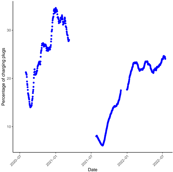5.15.: Daily percentage of Charging state smoothed on a 30-day window <details> <summary>Image 41 Details</summary>  ### Visual Description \n ## Line Chart: Percentage of Charging Plugs Over Time ### Overview The image presents a line chart illustrating the percentage of charging plugs in use over a period from approximately July 2020 to July 2022. The chart displays a fluctuating trend with two distinct periods of increased usage. ### Components/Axes * **X-axis:** Labeled "Date", spanning from approximately July 2020 to July 2022. The axis is marked with approximate dates: 2020-07, 2021-01, 2021-07, 2022-01, and 2022-07. * **Y-axis:** Labeled "Percentage of charging plugs", ranging from 0 to 35. The axis is marked with values: 0, 10, 20, 30. * **Data Series:** A single blue line representing the percentage of charging plugs. * **No Legend:** There is no explicit legend, but the Y-axis label clearly identifies the data represented by the line. ### Detailed Analysis The blue line representing the percentage of charging plugs exhibits the following trends: * **2020-07 to 2021-01:** The line starts at approximately 14% in July 2020 and increases to around 25% by January 2021, with significant fluctuations. * **2021-01 to 2021-07:** The line continues to rise, peaking at approximately 33% around March/April 2021, then declines to around 8% by July 2021. * **2021-07 to 2022-01:** The line shows a steep increase from approximately 8% in July 2021 to around 24% by January 2022. * **2022-01 to 2022-07:** The line plateaus around 24%, with minor fluctuations, reaching approximately 26% by July 2022. Approximate data points (reading from the chart): * 2020-07: 14% * 2020-12: 22% * 2021-01: 25% * 2021-03: 33% * 2021-07: 8% * 2021-12: 20% * 2022-01: 24% * 2022-07: 26% ### Key Observations * There is a clear seasonal or cyclical pattern in the data, with peaks in usage around the beginning of each year and a significant dip in the middle of 2021. * The percentage of charging plugs used has generally increased over the two-year period, despite the fluctuations. * The most significant drop in usage occurred between March and July 2021, followed by a rapid recovery. ### Interpretation The chart suggests a growing adoption of charging plugs, as indicated by the overall upward trend. The fluctuations likely represent seasonal variations in demand, potentially related to travel patterns, weather conditions, or other external factors. The sharp decline in mid-2021 could be due to a specific event or change in circumstances that temporarily reduced the need for charging. The data could represent the usage of electric vehicle charging stations, or potentially charging stations for other devices. The consistent increase in usage from late 2021 to 2022 suggests a sustained growth in demand for charging infrastructure. Further investigation would be needed to understand the underlying causes of the observed patterns and to predict future trends. </details> of the Charging state of the new period on Figure 5.13 is very similar to the one on Figure 5.2. In both cases, there are a notable peak at 8 p.m. in charging stations, a slow decay in charging stations over night until 5 a.m., and another peak in the morning around 10 p.m. corresponding to commuting behaviors. The daily pattern of the new available state is consistent with the sum of the former available and passive states. Indeed, EV charging spots becoming very attractive around 8 p.m., we observe a drop in the number of available plugs. Then, overnight, as batteries get filled, the stations come from charging to available (formerly passive ), which explains the slow increase in the number of available plugs overnight. At 10 a.m., because of commuting behaviors, EV drivers move their cars, which corresponds to the drop in Available plugs. Once again, commuting behaviors are very visible for the Charging state on Figure 5.14, with EV cars being more used during weekdays. Once again, the daily peaks and drops are very distinctive for the charging state on Figure 5.14. Seasonality Since the new dataset spans over two years, it allows to get a grasp of the seasonality of the EV charging demand. However, the EV charging station park has grown a lot during this period, as evidenced by Figure 5.12. Therefore, one needs to divide the charging demand by the number of plugs. The evolution of the daily percentage of charging station smoothed with a 30-day window is shown in Figure 5.15. Though there are missing values between April 2021 and June 2021, Figure 5.15 suggests a seasonality in the EV charging demand. Indeed, both in the end of August 2020 and August 2021, the EV charging demand is at its yearly lowest. Then, it increases until it reaches a first peak in October, and a second higher peak in the middle of December. Notice that both these peaks corresponds to holidays in France. ## Human spatial dynamics for electricity demand forecasting This chapter corresponds to the following paper: Doumèche et al. [Dou+23]. ## 6.1 Introduction From 2021 to 2023, Europe has experienced a major energy crisis with energy prices reaching levels not seen in decades [FG23]. Prices rose rapidly in the summer of 2021 as the global economy picked up following the easing of COVID-19 restrictions. Subsequently, the war in Ukraine led to a significant reduction in gas supplies, pushing gas prices even higher [Ruh+23]. In this context, the European Union adopted a series of emergency measures to mitigate the effects of this crisis, mainly by reducing electricity demand, with a binding reduction target of 5% during peak hours [Eur06]. In France, the government called for a voluntary effort to reduce energy consumption by 10% over two years and launched its own energy sobriety plan [Fre06]. Various media documented a subsequent drop in France's electricity demand in the winter of 2022-2023 [Tec22; The22; Mon23]. Energy saving is also part of France's long-term policy of ecological transition and energy sovereignty. Indeed, the energy sector's impact on climate change is forcing changes in consumption patterns, which is fueling a growing interest in energy savings and the transition to sustainable energy sources [ASM11; Roc+17; HG+19; Md+20]. In France, electricity is one of the most important components of the energy mix, accounting for 25% of its final energy consumption, and the French Ecological Transition Plan is based on massive electrification driven by decarbonised energy, coupled with energy savings [OGH22; RTE22]. While modifying human behaviour (e.g., by encouraging remote working) has been identified as an important axis of the sobriety plan, a better understanding of how this relates to energy savings is crucial for energy planning. Recently, machine learning techniques have been applied to electricity load forecasting to ensure the electricity grid remains balanced [PMF23] and to reduce electricity wastage. As France's electricity storage capacity is limited and expensive to run, electricity supply must match demand at all times. As a result, electricity load forecasting at different forecast horizons has attracted increasing interest over the last few years [Hon+20]. This article focuses on so-called short-term load forecasting, or 24-hour ahead load forecasting, which is particularly relevant for operational usage in industry and the electricity market [Nti+20; Ham+20]. We address this problem both in terms of feature selection and model design. Most state-of-the-art models rely on historical electricity load data, seasonal data such as holidays or the position of the day in the week, and meteorological data such as temperature and humidity [Nti+20]. However, such data cannot accurately account for the complex human behaviours that affect the variability of energy demand, such as holidays and remote working. As a result, traditional models struggle to account for unexpected large-scale societal events such as the COVID19 lockdowns or energy savings following economic, geopolitical, and environmental crises [OVG21]. New data capturing consumption behaviours is therefore needed to better model electricity demand. Over recent decades, datasets generated from mobile networks, locationbased services, and remote sensors in general, have been used to study human behaviour [BDK15]. Indeed, geolocation from mobile phones makes it possible to precisely characterise human flows [Dev+14; BCO15; Lor+16]. For example, such data have been used to study disease propagation [Ben+11; Blu12; RSM18; Pul+20], traffic [XCG21], the impact of human activities on biodiversity [Fil+22], and water consumption [TS+21; Smo+20]. In terms of day-ahead load forecasting, mobility data from SafeGraph, Google, and Apple mobility reports were strongly correlated with electricity load drops in the US during the COVID-19 outbreaks [CYZ20; Rua+20], as well as in Ireland [ZMM22] and in France [AGG23b]. These works show that social behaviors like lockdowns and remote working affect significantly the intensity and daily patterns of the electricity load consumption, and that these changes can be predicted by using mobility data. Although such data is quite informative about activity in urban areas, e.g., in retail stores and train stations, it does not precisely account for human presence and flows. Indeed, there is intrinsic bias in such data collection, corresponding for example to that of using (or not) a specific application. It is therefore necessary to take into account such biases when building models using this kind of data. In this context, the originality of this paper relies on the incorporation of high-quality human presence data provided by the mobile network operator Orange-representing about 40 %of the French market- in adaptive models to forecast the short-term electricity demand during France's 2022-2023 sobriety period [Bus]. This dataset is based on adjusted mobile phone traffic volume measurements collected continuously and passively at the mobile network level, unlike most location-based services data where the user is required to opt-in, which may introduce biases. As a result, our mobile network-based signal can be considered representative of the underlying population's data. Similar datasets have been used to perform dynamic census with the aim of planning the development of long-term electricity infrastructures in emerging economies [MC+15; SSS20; Sal+21], however these models were prospective and were not tested against the state-of-the-art in highly competitive tasks such as short-term electricity demand forecasting. In this article, we start by introducing the dataset at hands. We then show that our mobility data from mobile networks are correlated with other well-known socio-economic indices that capture spatial dynamics of the population. Furthermore, we show that models using mobility data outperform the state-of-the-art in electricity demand forecasting by 10% with respect to usual metrics. To better understand this result, we characterise electricity savings during the sobriety period in France. Finally, we show that the work index we have defined (see Section 6.2) has a distinctive effect on electricity demand, and is able to explain observed drops in electricity demand during holidays. Other human spatial dynamics indices such as tourism at the national level did not prove to have a significant effect on national electricity demand. The code to replicate the electricity dataset and implement the different models is available at github.com/NathanDoumeche/Mobility\_data\_assimilation. The corresponding dataset is available at zenodo.org/records/10041368. Hence, the change point results shown in Figure 6.2b, as well as the dataset and the benchmarks without mobility data of Table 6.1, are directly reproducible for future research, and can easily be updated to work for new time periods of interest. Note, however, that the mobility indices are not publicly available. ## 6.2 Using mobility data to forecast electricity demand The goal of this section is to show how using mobility data leads to better performance in forecasting the French electricity demand during the energy crisis. ## Datasets The reference dataset runs from 08/01/2013 to 28/02/2023. It consists of calendar data (dates and holidays), meteorological data (temperature), and historical data (electricity power load at different time scales). In this article, we consider this data to be a reference, because these features are commonly used to build state-of-the-art models in electricity load forecasting [Ham+20; Hon+20; Nti+20], in particular for the French electricity load [OVG21; VG22; Vil+24]. All these data are public and distributed under the Etalab open source licence. The calendar data are extracted from the French open source database [Eta23a; Eta23b]. This regroups holiday periods according to France's three holiday timetables-in France holidays depend on the region you live in-as well as the French national holidays. This calendar dataset has no missing values. The meteorological data are extracted from the SYNOP Météo-France database [MF23]. Météo-France is the French public agency responsible for the national weather and climate service. The dataset consists of 3-hourly temperature measurements from 62 meteorological stations located throughout French territory. This dataset has many missing values, which we have imputed as follows. First, if a station has a missing value at time t and the station's measurements are available 3 hours before and 3 hours after t , the missing value is imputed as the mean of these two measurements. If no such values are available, the missing temperature is imputed as the temperature of the nearest station. If however all stations in a region have missing values, the temperature of each station is imputed by taking the mean of the temperature at the same hour from the day before and the day after. Finally, the historical electricity load dataset is extracted from the RTE's public releases [RTE23b]. RTE (Réseau de Transport d'Electricité) is France's transmission system operator. It provides high quality data on regional electricity consumption in France with a frequency of 30 minutes. The national electricity load has no missing values, which is valuable since this is the final target throughout this article. In this work, the reference dataset is complemented by mobility indices. These mobile phone data were provided by Orange's Flux Vision business service [Bus], in the form of daily presence data reports. These include the number of visitors in the 101 geographical areas of mainland France, which correspond to the second level of national administrative divisions. For each location and each day, the data are stratified by the type of visitor (resident, usually present, tourist, excursionist, recurrent excursionist) and origin (foreign, local, non-local). The mobile phone data were anonymised in compliance with strict privacy requirements and audited by the French data protection authority (Commission Nationale de l'Informatique et des Libertés). Computation of the presence data reports is based on the on-the-fly processing of signalling messages exchanged between mobile phones and the mobile network, usually collected by mobile network operators to monitor and optimise mobile network activity. Such messages contain information about the identifiers of the mobile subscriber and of the antenna handling the communication, the timestamp, and the type of event (e.g., voice call, SMS, handover, data connection, location update). Knowing the location of antennas makes it possible to reconstruct the approximate position of a communication device. All these data were then used to compute the total number of individuals in a given area, without saving any residual information that could be traced back to the individual users. More specifically, at any given day, each individual was characterised based on their pattern of movement and their origin as follows. - Resident: person whose spends much of their time in the study area, and spent at least 22 nights (not necessarily consecutive) there over the past eight weeks. - Usually present: person who is not a resident of the study area but has been seen in the study area repeatedly: more than four times in different weeks during the previous eight weeks. - Tourist: person who spends the night in the study area who is neither resident nor usually present. - Excursionist: person not staying overnight the night before and the night of the study day, and present less than 5 times during the day in the last 15 days. - Recurrent excursionist: person who has not spent the night before and the current night in the study area and who has been present more than five times during the day in the previous 15 days. The night corresponding to a given day is the period between 8 p.m. of that day and 8 a.m. of the following day. Moreover, origin is categorised as follows: - Foreign: person with a foreign SIM card. - Local: person with a billing address in the study area. - Non-local: person with a billing address outside the study area. This data was then corrected by Orange Flux Vision to account for spatial and temporal biases, and so to be representative of the general population. To this end, they use spatially-stratified market share data, socio-economic data from the national statistics institute (Insee), mobile phone ownership data also from Insee, and customer socio-demographic information provided upon subscription. From these data, we constructed three indices. The work index corresponds to the number of recurrent excursionists, the tourism index to the number of foreign plus non-local tourists, and the resident index to the number of residents plus 'usually presents'. In this article, the mobility dataset covered the periods from 01/07/2019 to 01/03/2020, from 01/07/2020 to 01/03/2021, from 01/07/2021 to 01/03/2022, and from 01/07/2022 to 01/03/2023. Relying on such mobility indices is an original new way of tracking human mobility to better characterise electricity demand. Indeed, mobility is a complex signal, since the vibrancy of places varies over years, but also over the course of a day. For example, it is known that individuals circulate through a number of places throughout the day-on average between 2.5 and 4 per person in French metropolitan areas [MTE]-month, and year, whether for housing, work, education, personal relationships, and leisure. Determining the appropriate index and its level (i.e., the geographical scale at which it is aggregated) to measure a given phenomenon are both major difficulties in analysing mobility dynamics [Por23]. Our high quality dataset was designed to precisely quantify human presence over France at a very high frequency with respect to census or survey data, and has already been studied as such to account for residential behaviour [LPF23]. Its advantage is that it allows one not only to quantify with a high degree of accuracy the population present at a given time and place, but also to characterise the way they inhabit that place (i.e., residing, working, or exploring). To investigate the ability of our dataset to characterise work behaviour, we compare it to the office occupancy index from The Economist's normalcy index [The23]. This index was developed during the COVID-19 pandemic to evaluate the impact of government policies on human behaviour. It tracks eight variables (sports attendance, time at home, traffic congestion, retail footfall, office occupancy, flights, film box office, and public transport) at the national level; this open data can be found here: https://github.com/TheEconomist/normalcy-index-data . The office occupancy index is derived from Google's COVID-19 community mobility reports, which are no longer being updated as of mid-October 2022 [LLC]. Similar to our work index, the office occupancy index measures the tendency of workers to work on-site rather than remotely. As the office occupancy index is only available from February 2020 to October 2022, and mobile-network dataset only covers the periods form July to February of each year, Figure 6.1 has missing values. As illustrated in Figure 6.1, the office occupancy variable is highly correlated (87%) with the 7-day lagged work index when excluding weekends and Fig. 6.1.: Comparison of work indices. Mobile network-based work index and the normalcy index's office occupancy one. The work index in blue is lagged by 7 days. Weekends and bank holidays are excluded. Both indices have been standardised, i.e., the empirical mean has been subtracted and the result divided by the empirical standard deviation. The mobile network dataset only covers the period from July to March each year. 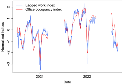<details> <summary>Image 42 Details</summary>  ### Visual Description \n ## Line Chart: Normalized Indices Over Time ### Overview This image presents a line chart comparing two normalized indices – "Lagged work index" and "Office occupancy index" – over a period spanning approximately from the beginning of 2020 to the end of 2022. The chart aims to visualize the relationship and trends of these two indices over time. ### Components/Axes * **X-axis:** Labeled "Date". The axis spans from approximately January 2020 to December 2022. The scale is not explicitly marked, but the years 2021 and 2022 are clearly indicated. * **Y-axis:** Labeled "Normalized indices". The scale ranges from approximately -3 to 2. The scale is linear with increments of 1. * **Legend:** Located in the top-left corner. * "Lagged work index" – Represented by a blue line. * "Office occupancy index" – Represented by a red line. ### Detailed Analysis The chart displays two time series. **Lagged Work Index (Blue Line):** The blue line exhibits a generally fluctuating pattern. * Early 2020: Starts around 0, dips to approximately -1.5, then recovers to around 1. * 2021: Shows significant fluctuations, ranging from approximately -2.5 to 1.8. There are multiple peaks and troughs. * 2022: Similar fluctuations to 2021, with a range of approximately -2.5 to 1.7. * Late 2022: Declines from around 0.8 to approximately -1.5. **Office Occupancy Index (Red Line):** The red line also shows fluctuations, but appears to have a stronger correlation with the blue line, particularly in the timing of major dips. * Early 2020: Starts around 0, dips to approximately -2, then recovers to around 0.5. * 2021: Fluctuates between approximately -1.5 and 1.5. * 2022: Similar fluctuations to 2021, with a range of approximately -2.5 to 1.5. * Late 2022: Declines from around 0.5 to approximately -2. **Specific Data Points (Approximate):** * January 2020: Lagged Work Index ~ 0, Office Occupancy Index ~ 0 * Mid-2020: Lagged Work Index ~ 1, Office Occupancy Index ~ 0.5 * Early 2021: Lagged Work Index ~ -2.5, Office Occupancy Index ~ -1.5 * Mid-2021: Lagged Work Index ~ 1.8, Office Occupancy Index ~ 1.5 * Early 2022: Lagged Work Index ~ -2.5, Office Occupancy Index ~ -2.5 * Mid-2022: Lagged Work Index ~ 1.7, Office Occupancy Index ~ 1.5 * December 2022: Lagged Work Index ~ -1.5, Office Occupancy Index ~ -2 ### Key Observations * **Correlation:** The two indices appear to be correlated, with similar patterns of increase and decrease. The Office Occupancy Index tends to lag slightly behind the Lagged Work Index. * **Dips:** Both indices experience significant dips in early 2020, 2021, and 2022. These dips likely correspond to periods of disruption (e.g., pandemic lockdowns). * **Volatility:** Both indices exhibit high volatility throughout the period, indicating significant fluctuations in work and occupancy levels. * **End of Period Decline:** Both indices show a clear decline towards the end of 2022. ### Interpretation The chart suggests a strong relationship between work activity (as represented by the Lagged Work Index) and office occupancy. The dips in both indices likely reflect the impact of external factors, such as the COVID-19 pandemic and associated restrictions. The correlation suggests that changes in work patterns directly influence office occupancy rates. The decline at the end of 2022 could indicate a renewed shift in work arrangements, potentially towards remote or hybrid models, or a broader economic downturn. The "Lagged Work Index" suggests that changes in work patterns are observed *before* changes in office occupancy, which is logical as work arrangements would need to shift before impacting physical office space usage. The normalization of the indices allows for a comparison of trends despite potentially different scales or units of measurement for the underlying data. The chart provides valuable insights into the dynamics of work and office space utilization over a period of significant disruption and change. </details> bank holidays. Moreover, our work index is more suitable than the office occupancy index for operational use, because it is seven days ahead of the office occupancy index, meaning that it captures the variations in office occupancy earlier. As detailed in Section I.C. of the Supplementary material, the work index is also more informative than the office occupancy index, because it captures the reduction in office occupancy during weekends and holidays. This is very valuable because holidays are known to have a significant impact on electricity demand, while their effect is difficult to evaluate. This often leads to having to analyse regular days and holidays separately [Krs22]. In addition, in Section I.B. of the Supplementary material, we demonstrate how tourism trends are related to another index from the same dataset. ## Mobility data and electricity demand forecasting We run a benchmark of state-of-the-art models to measure the benefits of incorporating mobility data into load forecasting techniques (see Section II of the Supplementary material for a more complete description of the models). In this field, the state-of-the-art is generally divided into three classes of forecasts [Sin+12; Wan+23c]: statistical models that approximate electricity demand by simple relationships between explanatory variables, data assimilation techniques that update a model using recent observations, and data-driven machine learning methods whose results may be more difficult to explain but are more expressive. Here, we focus on the state-of-the-art in French load forecasting, during the energy crisis, thereafter referred to as the sobriety period. Section 6.3 explains how this period was precisely determined. To evaluate the benefits of using mobility data to forecast France's national electricity load, we thus run a benchmark on this sobriety period, i.e., from 01/09/2022 to 28/02/2023. The training period spanned 08/01/2013 to 01/09/2022. Results are presented in Table 6.1 in terms of root mean square error (RMSE) and mean absolute percentage error (MAPE). Bold values highlight the best forecasts in each category of models. Indeed, models were evaluated according to the following test errors. Let T test be the test period, ( y t ) t ∈ T test the target, and (ˆ y t ) t ∈ T test an estimator of y . The root mean square error is defined by RMSE( y, ˆ y ) = ( 1 T test ∑ t = ∈ T test ( y t -ˆ y t ) 2 ) 1 / 2 and the mean absolute percentage Tab. 6.1.: Benchmark with and without mobility data. The numerical performance is measured in RMSE (GW) and MAPE (%). | | Without mobility | With mobility | |--------------------------------------------------------|-----------------------------------------------------------------------------------------------------|------------------------------------------------------------| | Statistical model Persistence (1 day) SARIMA GAM | 4.0 ± 0.2 GW, 5.5 ± 0.3% 2.4 ± 0.2 GW, 3.1 ± 0.2% | N.A., N.A. N.A., N.A. 2.17 ± 0.08 GW, 3.3 ± 0.1% | | Static Kalman | 2.1 ± 0.1 GW, 3.1 ± 0.2% | 1.72 ± 0.08 GW, 2.5 ± | | Dynamic | 2.3 ± 0.1 GW, 3.5 ± 0.2% | | | Data assimilation Kalman | 1.4 ± 0.1 GW, 1.9 ± 0.1% 1.5 ± 0.1 GW, 1.8 ± 0.1% 1.4 ± 0.1 GW, 1.8 ± 0.1% 2.6 ± 0.2 GW, 3.7 ± 0.2% | 0.1% 1.20 ± 0.08 GW, 1.7 ± 0.1% 1.24 ± 0.07 GW, 1.7 ± 0.1% | | Aggregation | | | | Viking | | | | Machine learning | | 1.16 ± 0.07 GW, 1.6 ± 0.1% | | GAM boosting Random forests Random forests + bootstrap | 2.5 ± 0.2 GW, 3.5 ± 0.2% 2.2 ± 0.2 GW, 3.0 ± 0.2% | 2.4 ± 0.1 GW, 3.5 ± 0.2% 2.0 ± 0.1 GW, 2.7 ± 0.2% | | | | 2.0 ± 0.1 GW, 2.7 ± 0.2% | error is defined by MAPE( y, ˆ y ) = 1 T test ∑ t ∈ T test | y t -ˆ y t | | y t | . Both errors are useful for operational uses. Since the sampling of time series are dependent, confidence intervals were obtained by time series bootstrapping [Lah03] using the tseries package [THL23] forecasting. All the models, as well as their weights and their optimization, are direct reproductions from state-of-the-art benchmarks. Indeed, the GAM model was extracted from [OVG21], the static and dynamic Kalman filters were adapted from [VG22], the Viking algorithm comes from [Vil+24], the GAM boosting is from [TH14], and the random forest and random forest with bootstrap were taken from [Goe+23]. A full description of these models can be found in Section II of the Supplementary material. Note that we have not included neural networks in this benchmark because they have not shown state-of-the-art performance in forecasting the French electricity load [Vil+24; Cam+24]. Overall, Table 6.1 shows that incorporating mobility data improves the performance of all models. In particular, the best forecast using the mobility data (aggregation of experts) has a lower error than the best forecast without mobility data, with a performance gain of about 15% in RMSE and 10% in MAPE. The NA values in the table are due to the fact that neither persistence nor SARIMA include exogenous data, making it impossible to include the mobility data in these models. These gains are statistically significant, because they leave the confidence intervals obtained by bootstrapping. Furthermore, the ranking of the models is consistent with past studies [OVG21; VG22]. We remark that the time series bootstrap in the Random forests + bootstrap improves the performance of the random forest algorithm without mobility data-confirming the results of [Goe+23]-but is not the case when adding mobility data. Moreover, holidays are known to behave differently from regular days [Krs22]. We therefore ran the same benchmark (see Table I in the Supplementary material) when excluding holidays; the results suggest that incorporating mobility data still significantly improves forecasting performance. These results all suggest that adding mobility data leads to RMSE and MAPE gains of around 10 % when forecasting French electricity demand. Fig. 6.2.: Electricity demand corrected for the effects of temperature and annual seasonality. (a) Descriptive statistics of the residuals. (b) The ten most important change points are represented by a change in the red line. The red line is the mean of the residuals between the change points. 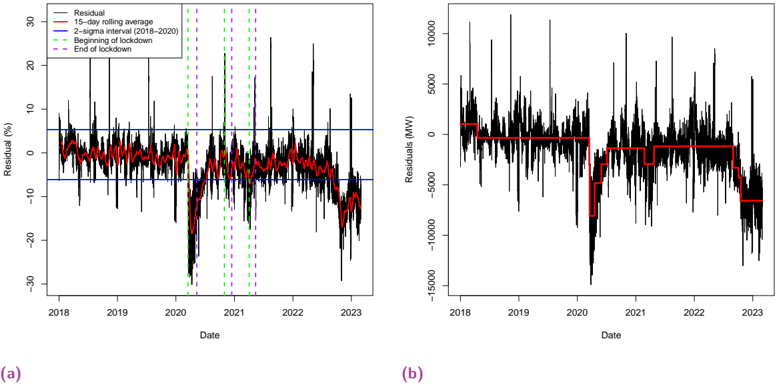<details> <summary>Image 43 Details</summary>  ### Visual Description \n ## Time Series Charts: Residual Analysis ### Overview The image presents two time series charts (labeled (a) and (b)) displaying residual analysis over time, from approximately 2018 to 2023. Chart (a) shows residuals in percentage terms, while chart (b) shows residuals in Megawatts (MW). Both charts include a 15-day rolling average (red line) and reference lines indicating the beginning and end of lockdown periods. Chart (a) also includes 2-sigma interval lines. ### Components/Axes **Chart (a):** * **X-axis:** Date (from approximately 2018 to 2023) * **Y-axis:** Residual (%) (ranging from approximately -30% to 30%) * **Legend:** * Residual (black lines) * 15-day rolling average (red line) * 2-sigma interval (2018-2020) (blue lines) * Beginning of lockdown (purple dashed vertical line) * End of lockdown (green dashed vertical line) **Chart (b):** * **X-axis:** Date (from approximately 2018 to 2023) * **Y-axis:** Residuals (MW) (ranging from approximately -150,000 MW to 100,000 MW) * **Legend:** * Residuals (black lines) * 15-day rolling average (red line) * Beginning of lockdown (purple dashed vertical line) * End of lockdown (green dashed vertical line) ### Detailed Analysis or Content Details **Chart (a): Residual (%)** The black lines representing the residuals fluctuate significantly around zero. The 15-day rolling average (red line) provides a smoothed representation of these fluctuations. The blue lines represent the 2-sigma interval (2018-2020), indicating a range within which most residuals fall. Vertical dashed lines mark the beginning and end of lockdown periods. * **2018-2019:** Residuals fluctuate within the 2-sigma interval. The rolling average remains relatively stable around 0%. * **Early 2020 (Lockdown Start):** A noticeable shift in the residual pattern occurs around the beginning of lockdown (purple line). The residuals tend to become more positive. * **2020-2021:** The residuals exhibit increased volatility. The rolling average shows a slight upward trend. * **2021-2022:** A significant negative shift in residuals is observed, with values dropping well below the 2-sigma interval. The rolling average declines sharply. * **2022-2023:** Residuals remain largely negative, with some fluctuations. The rolling average stabilizes at a negative value. **Chart (b): Residuals (MW)** The black lines representing the residuals in MW also fluctuate considerably. The 15-day rolling average (red line) smooths these fluctuations. Vertical dashed lines mark the beginning and end of lockdown periods. * **2018-2019:** Residuals fluctuate around zero. The rolling average remains relatively stable. * **Early 2020 (Lockdown Start):** A slight increase in residuals is observed around the beginning of lockdown (purple line). * **2020-2021:** The residuals show increased volatility. The rolling average exhibits a slight upward trend. * **2021-2022:** A substantial negative shift in residuals is observed, with values dropping significantly below zero. The rolling average declines sharply. * **2022-2023:** Residuals remain largely negative, with some fluctuations. The rolling average stabilizes at a negative value. ### Key Observations * Both charts show a clear impact of lockdown periods on residuals. * The negative shift in residuals observed in 2021-2022 is particularly pronounced in both charts. * The 2-sigma interval in chart (a) provides a useful reference for identifying outliers. * The rolling average effectively smooths out short-term fluctuations, revealing underlying trends. ### Interpretation The charts suggest that lockdown periods and subsequent events significantly impacted the system being modeled. The initial lockdowns (early 2020) appear to have caused a slight increase in residuals, potentially due to changes in demand patterns. However, the substantial negative shift in residuals observed in 2021-2022 indicates a more significant disruption, possibly related to broader economic or systemic changes. The fact that the rolling average remains negative in 2022-2023 suggests that this disruption has had a lasting effect. The difference in scale between the two charts (percentage vs. MW) highlights the importance of considering both relative and absolute changes when analyzing residuals. Chart (a) provides a sense of the magnitude of the residuals relative to the overall system, while chart (b) provides a sense of the absolute impact in terms of MW. The use of the 2-sigma interval in chart (a) allows for the identification of outliers, which may warrant further investigation. The consistent alignment of the lockdown markers with shifts in the residual patterns suggests a causal relationship, although further analysis would be needed to confirm this. </details> ## 6.3 Explainability of the models The goal of this section is to justify how we defined the sobriety period, and to better understand the impact of mobility on electricity demand. ## Defining the sobriety period The energy crisis in France had a significant impact on electricity demand in terms of electricity savings. To quantify the savings due to the crisis, and distinguish them from other unrelated changes, the effects of temperature and time seasonality must be removed from the French electricity demand data. The expected load given temperature and time, which we denote L ̂ oad , is estimated using a generalised additive model (GAM). Figure 6.2a shows the residuals: res = Load -L ̂ oad , where Load is the actual value of the electricity demand. This GAM was trained on the data from 01/01/2014 to 01/01/2018. The residuals were then evaluated from 01/01/2018 to 01/03/2023. Therefore, residuals measure the gap between the electricity demand at a given time and the expected demand with respect to its time and temperature dependency between 2014 and 2018. Negative residuals correspond to electricity savings. In Figure 6.2a, the blue lines represent the 2 σ variations over the period spanning 01/01/2018 to 01/01/2020, and correspond to typical variation in electricity demand around its expected value given the temperature and seasonal data. The holidays deviate strongly from the expected trend and correspond to the peaks in the residuals. Note that the 15-day rolling average in red only exits this confidence interval during the lockdowns and the 2022-2023 winter's sobriety period. This means that, during these events, the French electricity load is significantly lower than its expected values. As shown in Figure 6.2b, to detect these changes in the electricity demand, we ran a change point analysis [KE14; AC17] using binary segmentation, which detects and orders the changes in the mean of the residuals. The two most important change points of the 2018-2023 period were at the beginning of the sobriety period (04/10/2022) and the beginning of the first COVID-19 lockdown (15/03/2020). During the sobriety period from 04/10/2022 to 01/03/2023, the residuals had a mean of -10.6 % . This result was close to the assessment made by the French transmission system operator (RTE) whose estimate was of a 9 % decrease in consumption during the winter of 2022-2023 [RTE23a]. Figure 6.2b shows the ten most important change points in the residuals over the 2018-2023 period along with mean of the residuals between the change points. These results confirm that there was indeed a significant drop of around 11 % in French electricity demand during the sobriety period of 04/10/2022 to 01/03/2023. As this drop is visible in the electricity load adjusted for temperature and time, this means that temperature and seasonal data are not sufficient to accurately explain these energy savings. ## Explaining the impact of mobility on electricity demand In this section, we use variable selection to offer insights into the performance of forecasts that use mobility data. We also investigate the link between electricity demand and the work index-which emerges as the second most explanatory variable in our variable ranking (see below). Combining the calendar, meteorological, electricity, and mobile network datasets resulted in 38 features. Some of these features are highly correlated, e.g., see Section I.A of the Supplementary material for details on the correlation between the temperature and the school holidays features. Thus, to create highly explainable and robust forecasts, it is necessary to select a smaller number of highly explanatory features, in order to better understand how they relate to electricity demand. Nevertheless, typical variable selection methods based on cross-validation [WR09; HHW10; MW11] are not directly applicable to time series, because the samples are not independent. To reduce the dimensionality of the problem, one solution is to rank the features by order of importance and then select the most important ones [GPTM10]. In this paper, we considered three such ranking methods: minimum redundancy maximum relevance (mRMR), Hoeffding D-statistics, and Shapley values. For multivariate time series, feature selection can be performed using the mRMR algorithm, which consists in selecting variables that maximise mutual information with the target [PLD05; HRL15] (here the electricity load). We used the mRMRe package [Jay+13] in R for this analysis; the most important variables-in decreasing order of importance-were temperature , the work index, and the time of year . The Hoeffding D-statistic ranking and the Shapley value ranking results are detailed in Section IV.A of the Supplementary material. All three rankings gave the same results, implying that the work index is the second most inportant feature, after temperature , and is more important than the calendar data. We note also that these analyses suggest that the tourism and residents indices do not appear to be of great importance with respect to France's electricity demand (See Section IV.A of the Supplementary material). Outperforming the state-of-the-art in Table 6.1 indicates that mobility data had explanatory power when it came to electricity demand during the sobriety period. However, this result does not provide any formal insight into the future performance of the index. We therefore ran a statistical analysis of the predictive ability of this mobility data. Moreover, state-of-the-art data assimilation techniques being difficult to analyse, we restrict ourselves to explainable models of the electricity demand. Since the effect of temperature is known to be nonlinear, we consider generalized additive models (GAMs) instead of standard linear regression. As temperature and then the work index were ranked as the two most important variables in our variable selection phase, we consider the electricity demand corrected for the effect of temperature. Figures 6.3a show that the electricity demand increases with the work index, i.e., the higher the number of people at work, the higher the electricity demand. Fig. 6.3.: Effects of features on electricity demand. Each black point is an observation at 10 a.m. The effect given by the GAM regression is shown in red on both plots. Dotted red lines correspond to the 95 % confidence interval of the effects. (a) Temperature-corrected electricity load as a function of the work index. (b) Work-index corrected electricity load as a function of temperature. 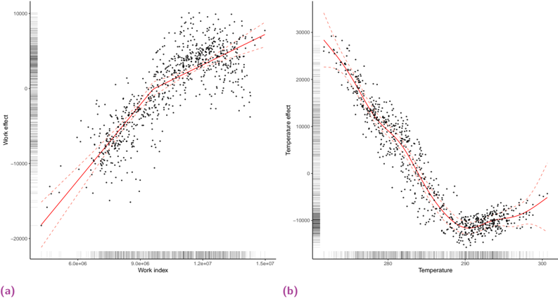<details> <summary>Image 44 Details</summary>  ### Visual Description \n ## Scatter Plots: Work Effect vs. Work Index & Temperature Effect vs. Temperature ### Overview The image presents two scatter plots, labeled (a) and (b). Plot (a) displays the relationship between "Work effect" and "Work index". Plot (b) shows the relationship between "Temperature effect" and "Temperature". Both plots include a fitted red curve attempting to model the data. The data points are represented as black dots. ### Components/Axes **Plot (a):** * **X-axis:** "Work index" ranging from approximately 5.0e+06 to 1.5e+07. * **Y-axis:** "Work effect" ranging from approximately -20000 to 10000. * No legend is present. The red line represents a fitted curve. **Plot (b):** * **X-axis:** "Temperature" ranging from approximately 270 to 300. * **Y-axis:** "Temperature effect" ranging from approximately -20000 to 30000. * No legend is present. The red line represents a fitted curve. ### Detailed Analysis or Content Details **Plot (a): Work Effect vs. Work Index** The data points show a generally upward trend, but with significant scatter. The red fitted curve appears to be a polynomial function. * At Work Index ≈ 5.0e+06, Work Effect ≈ -15000. * At Work Index ≈ 7.0e+06, Work Effect ≈ -5000. * At Work Index ≈ 9.0e+06, Work Effect ≈ 5000. * At Work Index ≈ 1.1e+07, Work Effect ≈ 15000. * At Work Index ≈ 1.3e+07, Work Effect ≈ 25000. * At Work Index ≈ 1.5e+07, Work Effect ≈ 30000. **Plot (b): Temperature Effect vs. Temperature** The data points exhibit a curved relationship, initially increasing and then decreasing. The red fitted curve appears to be a polynomial function. * At Temperature ≈ 270, Temperature Effect ≈ 25000. * At Temperature ≈ 275, Temperature Effect ≈ 20000. * At Temperature ≈ 280, Temperature Effect ≈ 15000. * At Temperature ≈ 285, Temperature Effect ≈ 10000. * At Temperature ≈ 290, Temperature Effect ≈ 5000. * At Temperature ≈ 295, Temperature Effect ≈ 0. * At Temperature ≈ 300, Temperature Effect ≈ -5000. ### Key Observations * Both plots show non-linear relationships between the variables. * The scatter in both plots is substantial, indicating a weak to moderate correlation. * The fitted curves attempt to capture the general trend but do not perfectly represent all data points. * Plot (b) shows a clear peak in "Temperature effect" around a temperature of 290. ### Interpretation The plots suggest that both "Work effect" and "Temperature effect" are influenced by their respective index/temperature values, but the relationships are complex and not strictly linear. The fitted curves represent attempts to model these relationships, but the significant scatter indicates that other factors likely contribute to the observed effects. In Plot (a), the increasing "Work effect" with increasing "Work index" could indicate a positive correlation between the two variables, but the scatter suggests that this relationship is not deterministic. In Plot (b), the bell-shaped curve suggests an optimal temperature around 290 where the "Temperature effect" is maximized. Beyond this temperature, the effect decreases. This could represent a process that is most efficient within a specific temperature range. The data suggests a parabolic relationship. The absence of error bars or statistical measures makes it difficult to assess the significance of these observations. Further analysis would be needed to determine the underlying mechanisms driving these relationships and to quantify the uncertainty associated with the fitted curves. </details> Fig. 6.4.: Dynamics captured by the work index. Each point is an observation of the electricity load corrected for temperature as a function of the work index at 10 a.m. between July 2019 and March 2022. (a) Dependence of the work index on the day of the week. (b) The holiday pattern. 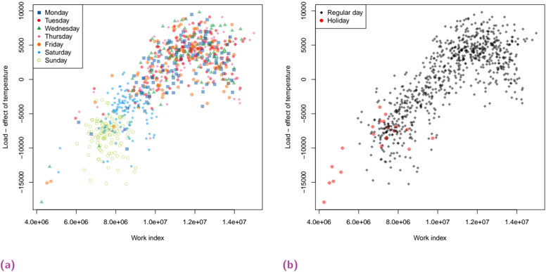<details> <summary>Image 45 Details</summary>  ### Visual Description ## Scatter Plots: Load vs. Work Index, Categorized by Day/Type ### Overview The image presents two scatter plots, labeled (a) and (b). Plot (a) displays the relationship between "Load - effect of temperature" (y-axis) and "Work index" (x-axis), with data points color-coded by day of the week. Plot (b) shows the same relationship, but categorizes data points as either "Regular day" or "Holiday". Both plots share the same axes scales. ### Components/Axes * **X-axis:** "Work index", ranging from approximately 4.0e+06 to 1.4e+07. * **Y-axis:** "Load - effect of temperature", ranging from approximately -15000 to 10000. * **Plot (a) Legend:** * Blue Square: Monday * Orange Circle: Tuesday * Green Triangle: Wednesday * Red Diamond: Thursday * Purple Cross: Friday * Yellow Dot: Saturday * Brown Plus: Sunday * **Plot (b) Legend:** * Black Dot: Regular day * Red Diamond: Holiday ### Detailed Analysis or Content Details **Plot (a): Load vs. Work Index by Day of the Week** * **Monday (Blue Squares):** Data points are clustered between Work Index values of 6.0e+06 and 1.2e+07, with Load values generally between -5000 and 5000. There's a slight upward trend as Work Index increases. * **Tuesday (Orange Circles):** Similar to Monday, clustered between 6.0e+06 and 1.2e+07, but with a wider spread in Load values, extending to approximately 8000. * **Wednesday (Green Triangles):** Data points are concentrated at lower Work Index values (around 4.5e+06) and negative Load values (between -10000 and -5000). * **Thursday (Red Diamonds):** Shows a broad distribution, with points spanning the entire Work Index range and Load values from -15000 to 8000. * **Friday (Purple Crosses):** Similar to Tuesday, clustered between 6.0e+06 and 1.2e+07, with Load values generally between -5000 and 5000. * **Saturday (Yellow Dots):** Data points are concentrated at lower Work Index values (around 4.5e+06) and negative Load values (between -10000 and -5000). * **Sunday (Brown Plus):** Data points are concentrated at lower Work Index values (around 4.5e+06) and negative Load values (between -10000 and -5000). **Plot (b): Load vs. Work Index by Day Type** * **Regular Day (Black Dots):** The majority of points are densely clustered, forming a roughly elliptical shape. The Work Index ranges from 4.0e+06 to 1.4e+07, and Load values range from -10000 to 5000. * **Holiday (Red Diamonds):** Data points are concentrated at lower Work Index values (around 4.0e+06 to 6.0e+06) and negative Load values (between -15000 and -5000). ### Key Observations * **Plot (a):** Weekdays (Monday, Tuesday, Thursday, Friday) exhibit a more dispersed pattern compared to the weekend days (Wednesday, Saturday, Sunday). Wednesday, Saturday, and Sunday show a strong concentration of data points at lower Work Index and negative Load values. * **Plot (b):** Holidays are clearly associated with lower Work Index and more negative Load values compared to regular days. * **Overall:** There appears to be a positive correlation between Work Index and Load, but this relationship is not linear and is influenced by the day of the week or day type. ### Interpretation The data suggests that "Load - effect of temperature" is influenced by both the amount of "Work index" and the day of the week/day type. The higher the Work Index, the higher the Load tends to be, but this trend is modulated by whether it's a weekday versus a weekend or holiday. The concentration of data points for Wednesday, Saturday, Sunday, and Holidays at lower Work Index and negative Load values indicates that these days are characterized by reduced work activity and potentially lower temperatures (given the "effect of temperature" component of the y-axis). The wider spread of data points for weekdays suggests more variability in work activity and temperature effects during those days. The distinction between "Regular day" and "Holiday" in Plot (b) reinforces the idea that holidays are associated with significantly different work patterns and temperature-related load profiles. The clustering of holiday data at lower Work Index and negative Load suggests a substantial reduction in activity during these periods. The plots provide insights into the relationship between work activity, temperature effects, and the resulting load, potentially useful for resource planning, energy management, or understanding system behavior under different conditions. </details> Moreover, the work index accounts for several consumption behaviours. First, Figure 6.4a shows how the index accounts for the effect of weekends, thus capturing weekly seasonality related to typical work behaviour. Indeed, we see that weekdays, Saturdays (in purple), and Sundays (in yellow) correspond to specific clusters of points with a lower work index. Figure 6.4b shows that the work index is related to consumption differences during the holidays (in red) vs other days (in black). Note that they have the same relationship as on regular days. Therefore, the work index summarises in a single feature both the effects of the day of the week and the holiday (7 features). Moreover, the analysis of the impact of our work index on electricity demand-when fixing the day of the week and excluding holidays, shows that lower work index correspond to lower electricity demand (see Section IV.B. in the Supplementary material). This shows that lower work dynamics are associated with energy savings. As expected, the effect is more pronounced during working hours. As a result, the work index is more informative than calendar information alone. In fact, models using the work index performed better on the atypical event of the sobriety period than models based on calendar data, which only capture seasonality in stationary signals (see Table IV in the Supplementary material). This suggests that the work index is explanatory of electricity demand. ## 6.4 Conclusion In this work, we have shown that the period spanning September 2022 to March 2023 was atypical in terms of France's electricity demand. During this so-called sobriety period, we observed a decrease in electricity demand similar to what happened during the first COVID-19 lockdown. However, this period of significant electricity savings lasted for over six months, which is much longer than the 1-month COVID-related period. These observations are consistent with those of French media and France's transmission system operators. These results suggest that additional phenomena to annual seasonality and temperature are responsible for the recent significant changes in the electricity consumption behaviour. As evidenced by our benchmark in Table 6.1, standard statistical models such as GAMs struggled during the sobriety period. Indeed, for the same state-of-the-art GAM, the RMSE and the MAPE when excluding holidays were respectively 55% and 87% higher than in the same test period two years earlier (September 2019 to March 2020) [OVG21]. Relying on a benchmark specific to France electricity load forecasting, we have shown that including mobile network mobility data in the analyses improves the state-of-the-art performance by around 10%. Although evaluating the cost of load forecasting error is a difficult task, it has been estimated that a 1 % reduction in load forecasting error would save an energy provider up to several hundred thousand USD per GW peak [HF16]. In 2022, the average daily load peak in France was 58 GW. According to this estimation, the gain of 0.2 % in MAPE in Table 6.1 resulting from exploiting mobility data would have amounted to tens of millions of USD per year at the national level. In addition, we have shown that the work index accounts for several consumption behaviours, including the impact of weekends and holidays on the electricity demand. Remark that these dynamics are not specific to the sobriety period, which suggests that the benefits of using mobility data would generalise to the post-crisis period. Overall, the higher the work index, the higher the electricity demand. Future lines of research include studying the work index at a 1-hour frequency, over longer periods, and at the finer geographical scale of French administrative regions. Indeed, as shown in Section I.A of the Supplementary material, mobile network data effectively capture human spatial dynamics other than those related to work, such as residence and tourism. Although in this paper we have not found a significant effect of such behaviours on national electricity demand, it might become visible when working at the regional level. Although we have shown that a reduction in the work index corresponds to a reduction in the electricity demand, further studies are needed to disentangle the effect of economic growth, employment rate, and remote working in this phenomenon. Moreover, we have focused in this work on mean forecast performance, i.e., on the ability of the forecast to predict the expected value of the electricity demand. Another interesting subject would be to evaluate the variance in the electricity demand given the work index, which would be helpful for practitioners when acting on the electricity market. Finally, in practice, it currently requires several days to clean, aggregate, and adjust the indices. For operational use, further studies are therefore needed to quantify the impact of such a delay in the use of the work index on the performance of benchmark forecasts, or conversely, to study the predictive capabilities of the work index. ## 6.A Datasets and features In this section, we provide further insight into our exploratory analysis of the mobility dataset. We show how the indices also capture holiday dynamics at the regional level by comparing the mobile network-based tourism index with official tourism statistics from Insee, and by studying the temporal evolution of the work index. ## Regional human presence indices Although for the purpose of national forecasts we have only relied on national-level indices, mobile network data were also available at the regional level, which helped to better understand the data at hand. In order to obtain a preliminary understanding of the data, we computed Pearson's product-moment correlation coefficient r between the human presence variables on the one hand, and the calendar and meteorological data on the other, for the regions of mainland France. This analysis confirmed that our indices matched several well-known human spatial dynamics. In large urban regions such as Île-de-France (IDF) we observed a negative correlation between the residence index and both of the calendar variables school holidays and summer holidays ( r = -0 . 65 and r = -0 . 84 , respectively), as well as temperature ( r = -0 . 70 ). This captures how IDF residents leave their region during the holidays and then behave as tourists. Consistently, in regions that are traditionally popular holiday destinations-such as the coastal region of Provence-Alpes-Côte d'Azur (PACA), the tourism index variable was positively correlated with the calendar variables school holidays and summer holidays ( r = 0 . 58 and r = 0 . 86 , respectively) and the meteorological variable temperature ( r = 0 . 82 ). The work index behaved similarly in both regions, with a negative correlation with the weekly holiday calendar variable ( r = -0 . 54 in IDF and r = -0 . 55 in PACA). To better characterise the seasonal changes of the indices, we show the evolution of the daily tourism , residence , and work indices in IDF (Figure 6.5a) and PACA (Figure 6.5b). In line with the Pearson correlation, in a region with a high level of economic activity such as IDF, the residence and work indices tended to increase during off-peak periods and to decrease during holidays. We observed the opposite for the tourism index in PACA, which is a very tourist-oriented region. Moreover, unlike in IDF, the work index in PACA did not decrease significantly during the summer holidays. This might be explained by the different make-up of the respective labour markets, with a high proportion of tourism workers in PACA. We can also clearly see the effects of the COVID-19 health crisis. In IDF, for example, the tourism and work indices significantly dropped during the crisis. These then gradually increased during the post-COVID period, but without reaching pre-COVID levels. This was especially pronounced for the work index, probably because of changes in work organisation triggered by the health crisis, and also as an effect of the energy crisis. In PACA, on the other hand, we observed a lower impact on tourism, partly due to tourist origin (there are more local tourists, i.e., who do not cross regional borders) than in IDF. Of note, the residence index seems to Fig. 6.5.: Regional indices. 7-day rolling average of mobility indices for the Île-de-France (a) and Provence-Alpes-Côte d'Azur (b) regions. Indices have been standardised, i.e., the empirical means have been subtracted and the result divided by the empirical standard deviations. The mobile network dataset only covers the period from July to March in each 12 -month period. Shaded areas correspond to regional school holidays, and horizontal grey lines mark the three main COVID-19 lockdowns in France. 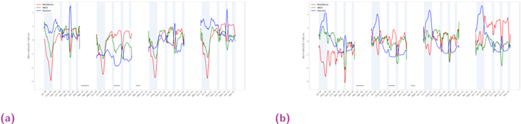<details> <summary>Image 46 Details</summary>  ### Visual Description \n ## Line Chart: Temporal Trends of Nutrient Uptake ### Overview The image presents two line charts, labeled (a) and (b), displaying temporal trends of nutrient uptake. Both charts share the same x-axis representing time points (likely days or weeks) and a y-axis representing "Nutrient Uptake (µM/h)". Each chart plots three nutrient uptake rates: Potassium (K+), Rubidium (Rb+), and Sodium (Na+). The charts are visually similar, with slight variations in the plotted lines. Vertical grey bands are present throughout both charts, likely indicating specific experimental conditions or time periods. ### Components/Axes * **X-axis:** Labeled "Time (Days)", with tick marks from approximately 0 to 35, incrementing by 5. The labels are slightly angled for readability. * **Y-axis:** Labeled "Nutrient Uptake (µM/h)", with a scale ranging from approximately 0 to 10, incrementing by 2. * **Legend:** Located in the top-left corner of each chart. * Potassium (K+) - Red line * Rubidium (Rb+) - Green line * Sodium (Na+) - Blue line * **Grey Bands:** Vertical bands spanning the entire height of the chart, appearing at regular intervals along the x-axis. ### Detailed Analysis or Content Details **Chart (a):** * **Potassium (K+):** The red line starts at approximately 2 µM/h, fluctuates significantly, reaching a peak of around 8 µM/h at day 10, then declines to around 3 µM/h by day 35. There are multiple peaks and troughs throughout the time course. * **Rubidium (Rb+):** The green line begins at approximately 3 µM/h, exhibits moderate fluctuations, peaking around 6 µM/h at day 5, and ending at approximately 2 µM/h at day 35. * **Sodium (Na+):** The blue line starts at approximately 5 µM/h, shows substantial oscillations, reaching a maximum of around 9 µM/h at day 10, and decreasing to approximately 4 µM/h at day 35. **Chart (b):** * **Potassium (K+):** The red line starts at approximately 2 µM/h, fluctuates significantly, reaching a peak of around 7 µM/h at day 10, then declines to around 3 µM/h by day 35. There are multiple peaks and troughs throughout the time course. * **Rubidium (Rb+):** The green line begins at approximately 3 µM/h, exhibits moderate fluctuations, peaking around 6 µM/h at day 5, and ending at approximately 2 µM/h at day 35. * **Sodium (Na+):** The blue line starts at approximately 5 µM/h, shows substantial oscillations, reaching a maximum of around 9 µM/h at day 10, and decreasing to approximately 4 µM/h at day 35. ### Key Observations * Both charts exhibit similar trends for all three nutrients. * Sodium (Na+) consistently shows the highest uptake rates and the most pronounced fluctuations. * Potassium (K+) and Rubidium (Rb+) uptake rates are generally lower and more stable than Sodium (Na+). * The grey bands do not appear to directly correlate with specific peaks or troughs in nutrient uptake, but they may represent periods of altered experimental conditions. * The fluctuations in nutrient uptake appear somewhat periodic, with cycles of increasing and decreasing rates. ### Interpretation The data suggests that the uptake of Sodium, Potassium, and Rubidium varies over time, potentially in response to changing environmental conditions or internal physiological processes. The higher uptake rate and greater variability of Sodium suggest it plays a more dynamic role in the system being studied. The similarity between the two charts (a) and (b) indicates that the observed trends are reproducible or consistent across different experimental runs or conditions. The periodic fluctuations could be related to circadian rhythms, nutrient availability cycles, or other time-dependent factors. The grey bands likely represent experimental manipulations or time points of interest, but their specific meaning requires additional context. The fact that Rubidium uptake is consistently lower than Potassium uptake suggests a difference in transport mechanisms or cellular requirements for these two ions. Further investigation is needed to determine the underlying causes of these observed trends and their biological significance. </details> Fig. 6.6.: Comparison of the Insee and the mobile network tourism indices. 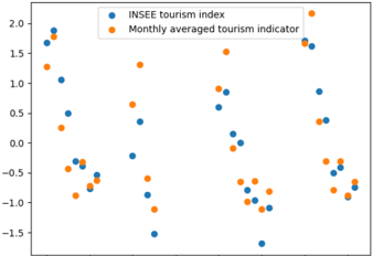<details> <summary>Image 47 Details</summary>  ### Visual Description \n ## Scatter Plot: Tourism Index vs. Monthly Indicator ### Overview The image presents a scatter plot comparing two tourism-related indicators over an unspecified time period. The plot displays the relationship between the INSEE tourism index and the monthly averaged tourism indicator. The x-axis represents the time dimension, while the y-axis represents the index/indicator values. ### Components/Axes * **X-axis:** Unlabeled, presumably representing time (months or similar). * **Y-axis:** Ranges from approximately -1.5 to 2.0, with markings at -1.5, -1.0, -0.5, 0.0, 0.5, 1.0, 1.5, and 2.0. * **Legend:** Located in the top-right corner. * **INSEE tourism index:** Represented by blue circles. * **Monthly averaged tourism indicator:** Represented by orange circles. ### Detailed Analysis The plot contains a series of data points for each indicator. **INSEE Tourism Index (Blue Circles):** The blue data points exhibit a generally fluctuating pattern. * Starting from the left, the first few points are around y = 1.7 to 1.9. * There's a dip to approximately y = 1.2. * The values then fluctuate between approximately y = 0.8 and -0.4. * Towards the right side of the plot, the values range from approximately y = -1.2 to y = 1.0. * The last few points are around y = 1.8 to 0.8. **Monthly Averaged Tourism Indicator (Orange Circles):** The orange data points also show fluctuations. * Starting from the left, the first few points are around y = 1.6 to 1.8. * The values then decrease to approximately y = 0.5. * The values fluctuate between approximately y = 0.5 and -1.3. * Towards the right side of the plot, the values range from approximately y = -1.0 to y = 0.5. * The last few points are around y = 0.4 to 0.0. There is no clear linear correlation between the two indicators. The points are scattered, suggesting a complex or weak relationship. ### Key Observations * Both indicators exhibit similar fluctuations over time, but their magnitudes and timing differ. * There are periods where both indicators are positive, and periods where both are negative. * There are no obvious outliers. * The data does not show a consistent lead or lag between the two indicators. ### Interpretation The scatter plot suggests that the INSEE tourism index and the monthly averaged tourism indicator are related, but not perfectly correlated. Both indicators likely respond to similar underlying factors (e.g., seasonality, economic conditions, global events), but they may capture different aspects of tourism activity or be calculated using different methodologies. The fluctuations in both indicators could be due to seasonal variations, unexpected events, or changes in tourism trends. The lack of a strong correlation suggests that neither indicator can be used to perfectly predict the other. However, analyzing both indicators together may provide a more comprehensive understanding of tourism trends than relying on either one alone. Further investigation would be needed to determine the specific factors driving the observed patterns and to assess the statistical significance of any observed relationships. </details> have gradually increased since the end of the COVID-19 crisis in PACA. This phenomenon of migration to certain regions of France has been documented by Insee in the report [FM23], but deserves a more in-depth analysis. ## The tourism index from mobile-phone data The evaluated number of tourists and residents has been shown to be correlated with electricity demand in highly touristic areas [BR11; Lai+11]. For this reason, we created and studied a tourism index at the national level. Traditionally, most similar assessments have been carried out on a monthly or annual basis. One strength of our mobile phone-based tourism index is that it can be calculated at finer temporal and geographical scales. To further assess the tourism index's performance as a proxy for tourism activity, we compared its monthly average with the Insee tourism index [INS23], as shown in Figure 6.6. We obtained an 87% correlation between the two signals, showing that the tourism index efficiently captures tourism trends. However, our study found that tourism had no significant impact on French electricity demand (see Section 6.D). Fig. 6.7.: Residuals as a function of the work index over the years 2019-2022. Each point is an observation between July 2019 and March 2022. 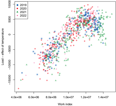<details> <summary>Image 48 Details</summary>  ### Visual Description \n ## Scatter Plot: Load vs. Work Index with Temperature Effect ### Overview The image presents a scatter plot visualizing the relationship between "Work Index" and "Load – effect of temperature" for four different years: 2019, 2020, 2021, and 2022. Each year is represented by a distinct color and marker shape. The plot appears to show a positive correlation between Work Index and Load, with variations across the years. ### Components/Axes * **X-axis:** "Work index" - Scale ranges approximately from 4.0e+06 to 1.4e+07. * **Y-axis:** "Load – effect of temperature" - Scale ranges approximately from -15000 to 10000. * **Legend:** Located in the top-left corner, identifying the years and their corresponding colors/markers: * 2019: Blue squares * 2020: Red circles * 2021: Green triangles * 2022: Pink diamonds ### Detailed Analysis The data points are distributed across the plot, with each year exhibiting a distinct pattern. * **2019 (Blue Squares):** The data points generally cluster in the lower-left quadrant, with a noticeable upward trend as the Work Index increases. The Load values range from approximately -10000 to 5000. * **2020 (Red Circles):** The data points are more dispersed than those of 2019, spanning a wider range of Load values, from approximately -15000 to 7000. There's a general upward trend, but with more scatter. * **2021 (Green Triangles):** The data points are concentrated in the upper-right quadrant, with Load values predominantly positive, ranging from approximately -5000 to 8000. The trend is strongly upward. * **2022 (Pink Diamonds):** The data points are also concentrated in the upper-right quadrant, similar to 2021, but with a slightly wider spread. Load values range from approximately 0 to 9000. **Approximate Data Points (sampled for illustration):** | Year | Work Index (approx.) | Load – effect of temperature (approx.) | |---|---|---| | 2019 | 4.5e+06 | -8000 | | 2019 | 6.0e+06 | -2000 | | 2019 | 8.0e+06 | 2000 | | 2019 | 1.2e+07 | 4000 | | 2020 | 4.2e+06 | -14000 | | 2020 | 6.5e+06 | -1000 | | 2020 | 8.5e+06 | 3000 | | 2020 | 1.3e+07 | 6000 | | 2021 | 5.0e+06 | -2000 | | 2021 | 7.0e+06 | 2000 | | 2021 | 9.0e+06 | 5000 | | 2021 | 1.4e+07 | 7000 | | 2022 | 5.5e+06 | 1000 | | 2022 | 7.5e+06 | 4000 | | 2022 | 9.5e+06 | 6000 | | 2022 | 1.4e+07 | 8000 | ### Key Observations * The relationship between Work Index and Load appears to be generally positive for all years. * The Load values tend to increase with the Work Index. * 2021 and 2022 show a more pronounced positive correlation and higher Load values compared to 2019 and 2020. * 2020 exhibits the most scatter in the data, suggesting greater variability in the Load for a given Work Index. * 2019 has the lowest Load values overall. ### Interpretation The plot suggests that as the "Work Index" increases, the "Load – effect of temperature" also tends to increase. This could indicate that higher work indices are associated with greater thermal effects. The differences between the years suggest that the relationship between Work Index and Load may be influenced by other factors that vary annually. The increasing Load values in 2021 and 2022 could be due to changes in environmental conditions, operational parameters, or other variables not explicitly shown in the plot. The wider scatter in 2020 might indicate a period of instability or greater variability in the system being measured. The data could be used to model the thermal load based on the work index, and to identify years with particularly high or low thermal effects. Further investigation would be needed to understand the underlying causes of these trends and variations. </details> Fig. 6.8.: Comparison of work indices. Comparison of the 7-day lagged mobile phone based index and the normalcy office occupancy index on all days (a), and when excluding weekends and holidays (b). 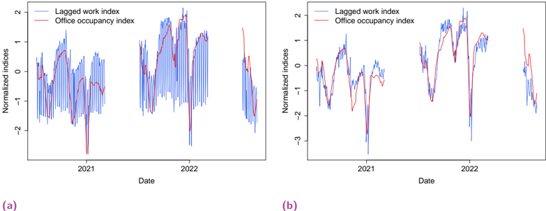<details> <summary>Image 49 Details</summary>  ### Visual Description \n ## Line Chart: Normalized Indices Over Time ### Overview The image presents two line charts, labeled (a) and (b), displaying time series data for "Lagged work index" and "Office occupancy index" from approximately 2020 to 2022. Both charts share the same axes labels and legend, but display slightly different data patterns. The y-axis represents "Normalized indices" ranging from approximately -3 to 2, while the x-axis represents "Date". ### Components/Axes * **X-axis:** "Date" - spanning from approximately early 2020 to late 2022. The scale is not explicitly marked, but the years 2021 and 2022 are clearly visible. * **Y-axis:** "Normalized indices" - ranging from approximately -3 to 2. The scale is not explicitly marked with numerical values, but the range is visually discernible. * **Legend:** Located in the top-right corner of each chart. * "Lagged work index" - represented by a blue line. * "Office occupancy index" - represented by a red line. * **Chart (a):** Displays data from approximately January 2020 to December 2022. * **Chart (b):** Displays data from approximately January 2020 to December 2022. ### Detailed Analysis or Content Details **Chart (a):** * **Lagged work index (Blue Line):** The line exhibits high-frequency oscillations throughout the period. It generally fluctuates around the 0 line. Around mid-2021, the line shows a period of sustained positive values, peaking at approximately 1.8. Towards the end of 2022, the line drops sharply to approximately -2.5. * **Office occupancy index (Red Line):** This line also oscillates, but with larger amplitude swings than the lagged work index. It spends a significant portion of 2020 and early 2021 in negative territory, reaching a minimum of approximately -2.8. It rises to positive values in mid-2021, peaking around 1.5, and then declines sharply towards the end of 2022, reaching approximately -2.5. **Chart (b):** * **Lagged work index (Blue Line):** Similar to chart (a), the line oscillates frequently. It generally fluctuates around the 0 line. Around mid-2021, the line shows a period of sustained positive values, peaking at approximately 1.7. Towards the end of 2022, the line drops sharply to approximately -3. * **Office occupancy index (Red Line):** This line also oscillates, but with larger amplitude swings than the lagged work index. It spends a significant portion of 2020 and early 2021 in negative territory, reaching a minimum of approximately -3.2. It rises to positive values in mid-2021, peaking around 1.6, and then declines sharply towards the end of 2022, reaching approximately -2.8. ### Key Observations * Both indices exhibit a strong cyclical pattern, likely reflecting weekly or monthly variations. * The Office occupancy index generally has a larger range of fluctuation than the Lagged work index. * Both indices show a similar trend of increasing in mid-2021 and then decreasing sharply towards the end of 2022. * Chart (b) shows a more pronounced dip in the Office occupancy index in early 2021 and a more significant drop at the end of 2022 compared to chart (a). ### Interpretation The charts likely depict the relationship between work activity and office usage during the COVID-19 pandemic and its aftermath. The "Lagged work index" could represent a measure of overall work activity, while the "Office occupancy index" represents the physical presence of workers in office spaces. The initial dip in the Office occupancy index in 2020 and early 2021 likely reflects the widespread shift to remote work due to the pandemic. The subsequent increase in both indices in mid-2021 suggests a partial return to office work as restrictions eased. The sharp decline at the end of 2022 could indicate a renewed shift towards remote work, potentially due to new variants or changing work policies. The fact that the Office occupancy index has a larger range of fluctuation suggests that office usage is more sensitive to external factors (like pandemic waves or policy changes) than overall work activity. The slight differences between charts (a) and (b) could be due to different data sources, methodologies, or geographical locations. The "lagged" nature of the work index suggests that changes in work activity may influence, or be influenced by, office occupancy with a delay. </details> ## Work index and calendar features As explained in the introduction, several phenomena occurred between 2020 and 2023 that significantly changed human behaviour and affected French electricity demand. To better understand the impact of the work index on electricity demand, it was therefore important to see whether this dependence has changed over time. Figure 6.7 shows that the dependence of electricity demand in the work index has been stationary over the years 2019-2022. This shows that this relationship is robust to the aforementioned events, which is an argument to believe that the results of this article will generalise well to future periods of interest. In addition, as shown in Figure 6.8a and 6.8b, unlike The Economist's office occupancy index, our work index from mobile data captures the reduction in work activity due to weekends and holidays. Furthermore, as expected, Figures 6.9a and 6.9b show that the work index is only useful for electricity demand forecasting during typical work hours. Indeed, the electricity Fig. 6.9.: Electricity demand corrected for temperature as a function of the work index for each day of the week. Each point is an observation between July 2019 and March 2022. (a) 2 a.m. (b) 10 a.m. 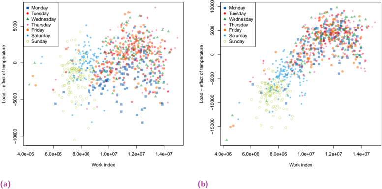<details> <summary>Image 50 Details</summary>  ### Visual Description ## Scatter Plots: Load Effect of Temperature vs. Work Index by Day of Week ### Overview The image presents two scatter plots, labeled (a) and (b), visualizing the relationship between "Load – effect of temperature" (y-axis) and "Work index" (x-axis). Each plot differentiates data points by the day of the week, using different colors and markers. The plots appear to show a positive correlation between Work Index and Load effect of temperature, with variations based on the day of the week. ### Components/Axes * **X-axis:** "Work index", ranging from approximately 4.0e+06 to 1.4e+07. * **Y-axis:** "Load – effect of temperature", ranging from approximately -10000 to 5000. * **Legend (Top-Right of both plots):** * Monday (Blue circles) * Tuesday (Orange circles) * Wednesday (Green triangles) * Thursday (Red circles) * Friday (Purple circles) * Saturday (Light-blue circles) * Sunday (Yellow circles) * **Labels:** (a) and (b) are placed below each respective plot. ### Detailed Analysis or Content Details **Plot (a):** * **Monday (Blue):** Data points are scattered, with a slight upward trend. Values range from approximately -5000 to 4000 in Load effect of temperature, and 4.5e+06 to 1.4e+07 in Work index. * **Tuesday (Orange):** Data points are concentrated in the lower-middle region, with a moderate upward trend. Values range from approximately -5000 to 3000 in Load effect of temperature, and 4.5e+06 to 1.4e+07 in Work index. * **Wednesday (Green):** Data points are clustered around the origin, with a slight upward trend. Values range from approximately -2000 to 2000 in Load effect of temperature, and 5.0e+06 to 1.2e+07 in Work index. * **Thursday (Red):** Data points are scattered, with a clear upward trend. Values range from approximately -2000 to 5000 in Load effect of temperature, and 4.5e+06 to 1.4e+07 in Work index. * **Friday (Purple):** Data points are scattered, with a moderate upward trend. Values range from approximately -5000 to 4000 in Load effect of temperature, and 4.5e+06 to 1.4e+07 in Work index. * **Saturday (Light-blue):** Data points are scattered, with a slight upward trend. Values range from approximately -5000 to 3000 in Load effect of temperature, and 4.5e+06 to 1.4e+07 in Work index. * **Sunday (Yellow):** Data points are scattered, with a moderate upward trend. Values range from approximately -5000 to 3000 in Load effect of temperature, and 4.5e+06 to 1.4e+07 in Work index. **Plot (b):** * **Monday (Blue):** Data points are scattered, with a slight upward trend. Values range from approximately -10000 to 5000 in Load effect of temperature, and 4.0e+06 to 1.4e+07 in Work index. * **Tuesday (Orange):** Data points are concentrated in the lower-middle region, with a moderate upward trend. Values range from approximately -10000 to 4000 in Load effect of temperature, and 4.0e+06 to 1.4e+07 in Work index. * **Wednesday (Green):** Data points are clustered around the origin, with a slight upward trend. Values range from approximately -5000 to 2000 in Load effect of temperature, and 4.5e+06 to 1.2e+07 in Work index. * **Thursday (Red):** Data points are scattered, with a clear upward trend. Values range from approximately -5000 to 5000 in Load effect of temperature, and 4.0e+06 to 1.4e+07 in Work index. * **Friday (Purple):** Data points are scattered, with a moderate upward trend. Values range from approximately -10000 to 4000 in Load effect of temperature, and 4.0e+06 to 1.4e+07 in Work index. * **Saturday (Light-blue):** Data points are scattered, with a slight upward trend. Values range from approximately -10000 to 3000 in Load effect of temperature, and 4.0e+06 to 1.4e+07 in Work index. * **Sunday (Yellow):** Data points are scattered, with a moderate upward trend. Values range from approximately -10000 to 3000 in Load effect of temperature, and 4.0e+06 to 1.4e+07 in Work index. ### Key Observations * Both plots exhibit a general positive correlation between Work Index and Load effect of temperature. As Work Index increases, Load effect of temperature tends to increase. * Wednesday consistently shows the lowest Load effect of temperature values for a given Work Index. * Thursday consistently shows the highest Load effect of temperature values for a given Work Index. * Plot (b) shows a generally lower range of Load effect of temperature values compared to Plot (a). * The distributions of data points for each day of the week are relatively similar between the two plots, but the overall scale of the y-axis differs. ### Interpretation These scatter plots likely represent energy consumption or load data, where "Work index" could be a measure of activity or demand, and "Load – effect of temperature" represents the additional load due to temperature variations. The differentiation by day of the week suggests that energy usage patterns vary significantly depending on the day. The consistent pattern of Wednesday having the lowest load effect and Thursday having the highest suggests that these days have fundamentally different energy usage profiles. This could be due to variations in industrial activity, commercial operations, or residential behavior. The difference in the y-axis scale between plots (a) and (b) indicates that the two plots may represent different datasets or time periods, or that a different calculation or scaling method was used for the Load effect of temperature. Plot (b) shows a more negative range of Load effect of temperature, suggesting a stronger cooling demand or a different baseline. The positive correlation between Work Index and Load effect of temperature implies that increased activity or demand leads to higher energy consumption, and that temperature plays a significant role in modulating this consumption. Further investigation would be needed to understand the specific factors driving these patterns and to develop strategies for optimizing energy usage. </details> demand corrected for the temperature effect had a significant dependence in the index at 10 a.m., but not at 2 a.m. See Section 6.D for more details. ## 6.B Benchmark and models In this section, we detail the framework and the models in Table I of the main document. ## Handling missing values in mobile network data There are two types of missing data in our datasets. First, the datasets are regularly sampled time series but with different frequencies. Indeed, recall that the calendar and the electricity datasets have 30-minute frequencies, while the meteorological dataset has a 3-hour one, while the mobile phone dataset has a 1-day frequency. A common method to deal with differences in sampling frequency is to impute the missing value by interpolation [Emm+21]. The interpolation method for meteorological data is described in the Methods section of the main paper, while the Orange indices are considered constant throughout the day. Second, the mobile network dataset only covers the periods ranging from 01/07/2019 to 01/03/2020, from 01/07/2020 to 01/03/2021, from 01/07/2021 to 01/03/2022, and from 01/07/2022 to 01/03/2023. Though various techniques have been developed to tackle sampling irregularities in time series [SM21], dealing with large sets of consecutive missing values is still very challenging. The three main approaches when studying time series with consecutive missing values are deletion, imputation, and imputation with masking [Emm+21]. First, deletion consists of discarding any observation with at least one missing value. Though this is the simplest way to deal with missing values, it can introduce a bias if the missing data are not-at-random, i.e., if the missing data are actually informative with respect to the target [LR19]. Second, in regression, imputation techniques aim to 'fill in' missing values. The state-of-the-art in time series imputation is wide-ranging and an active field of research [Ma+20]. Note that imputation that maximises a regression model's performance is not necessarily that which reconstructs missing values most accurately [Zha+21; Aym+23]. This makes it more difficult to understand and explain the true effect of imputed features on a target variable. Third, imputation with masking consists of imputing the missing values and keeping track of which observations have been imputed by adding a new feature equal to 1 if the observation comes from an actual measurement, and 0 if it was imputed. In this paper, the pattern of missing data is regular, spanning each year from March to July, and does not depend on the explanatory variables (temperature, work index, etc.). Thus, to simplify the analysis, we chose the deletion framework and have not tried to impute the missing values of the mobile network indices. Furthermore, Table I in the main text not only shows that mobile phone indices help to improve the performance of state-of-the-art forecasting algorithms, but also attests that this is still true even when comparing the complete open dataset with the incomplete mobile phone dataset. Indeed, on the one hand, models 'without mobility data' were trained on the complete calendar, weather, and electricity datasets, spanning from 08/01/2013 to 01/09/2022. On the other hand, models 'with mobility data' were created in a two-step process using the transfer learning framework presented in [AGG23b]. First, a model trained without mobility data from 08/01/2013 to 01/09/2022 provided an estimate ˆ Load of the electricity demand Load . Then, another model was trained in the deletion framework to forecast the error err = Load -ˆ Load , also known as the residual, using the mobile phone dataset. This second forecast is denoted by ˆ err . The final forecast was therefore the sum of the two forecasts ˆ Load + ˆ err . Notice that this framework gives an advantage to the reference forecast 'without mobility data'. In fact, the gains from using mobile phone data are much higher if the training periods of all models are restricted to the period for which mobile phone data are available (although we have not included these results in the paper for the sake of simplicity). However, the framework we chose allowed us to assess the interest of using mobile phone data from an operational point of view. It ensured that the best models trained using the mobile phone dataset outperformed the best models trained on the full, open datasets. Therefore, the gains of 10% we obtained are likely to be much higher if we had access to a more complete mobile phone dataset. We chose this residuals method to account for the mobile phone data because it gave better results than directly training models 'with mobility data' on all datasets restricted to the period for which the mobile phone data ere available (once again, we have not included these results in the paper for simplicity). ## Statistical models Time series models Persistence models are the simplest type of model for time series. They consist of estimating the target with its own lags and are common baselines in time series benchmarks because of their simplicity, ability to capture trends, explainability, and robustness to sudden changes in data distributions. In Table I of the main article, the persistence estimator corresponds to a 24-hour lag in electricity demand. Seasonal autoregressive integrated moving average (SARIMA) models [Box+15] are also commonly used in time series analysis. Here, we trained one model for each of the 48 halfhours in a day to capture daily seasonality in the data. Each model was then fitted with weekly seasonality by running the auto.arima method of the forecast package in R . Generalized additive models Generalized additive models (GAMs) are a generalisation of linear regression. Instead of learning linear coefficients linking certain features x = ( x 1 , . . . , x d ) to a target y , a GAM learns the nodes and coefficients of the regression of the features onto the target with respect to a spline basis. More precisely, given a target time series y = ( y t ) t ∈ T indexed by T , and some explanatory variables x = ( x t, 1 , . . . , x t,d ) t ∈ T , the response variable y is written in the form: $$y _ { t } = \beta _ { 0 } + \sum _ { j = 1 } ^ { d } f _ { j } ( x _ { t , j } ) + \varepsilon _ { t } \, ,$$ where ε = ( ε t ) t ∈ T are independent and identically distributed (i.i.d.) random noise. Though the target y t at time t is in fact a real number, each potentially explanatory time series x k = ( x t,k ) t ∈ T has a dimension d k ≥ 1 ; i.e., at time t , x t,k ∈ R d k . Therefore, nonlinear effects of multiple variables are allowed, such as, for instance, y t = β 0 + f 1 ( x t, 1 ) + ε t with x t, 1 ∈ R 2 . The goal of GAM optimisation is to find the best nonlinear functions f 1 , . . . , f d to fit y . Thus, each nonlinear effect f j is decomposed over a spline basis ( B j,k ) 1 ≤ j ≤ d, k ∈ N , with coefficients β j , such that $$f _ { j } ( x ) = \sum _ { k = 1 } ^ { m _ { j } } \beta _ { j , k } B _ { j , k } ( x ) \, ,$$ where m j corresponds to the dimension of the spline basis. The offset β 0 is chosen so that the functions f j are centred. The coefficients β 0 , β 1 , . . . , β d are then obtained by penalised least squares. The penalty term involves the second derivatives of the functions f j , forcing the effects to be smooth (see [Woo17]). The GAM model used in the experiments presented in Table 6.2 was taken from [OVG21]. As is usual in load forecasting with GAMs, we considered one model per half-hour of the day, with the 48 half-hour time series treated independently. Therefore, 48 models were fitted, one for each half-hour of each day. Given a half-hour h , our model was therefore: $$L o a d _ { h , t } & = \sum _ { i = 1 } ^ { 7 } \sum _ { j = 0 } ^ { 1 } \alpha _ { h , i , j } \, 1 _ { \text {DayType} _ { t } = i } \, 1 _ { \text {DLS} _ { t } = j } + \sum _ { i = 1 } ^ { 7 } \beta _ { h , i } \, L o a d 1 D _ { t } \, 1 _ { \text {DayType} _ { t } = i } \\ & \quad + \gamma \, L o a d 1 W _ { t } + f _ { h , 1 } ( t ) + f _ { h , 2 } ( T o Y _ { t } ) + f _ { h , 3 } ( t , \text { Temp} _ { h , t } ) + f _ { h , 4 } ( T e m p 9 5 _ { h , t } ) \\ & \quad + f _ { h , 5 } ( T e m p 99 _ { h , t } ) + f _ { h , 6 } ( T e m p M i n 9 9 _ { h , t } , \text { TempMax} 9 9 _ { h , t } ) + \varepsilon _ { h , t } \, ,$$ where the timestamp t corresponds to the day, and: - Load h,t is the electricity load on day t at time h . - DayType t is a categorical variable indicating the type of day of the week. - DLS t is a binary variable indicating whether t is daylight saving time or standard time. - Load1D and Load1W are the loads of the previous day and previous week, respectively. - ToY t is the time of year, growing linearly from 0 at midnight when January 1 begins, to 1 on December 31 at 23:30 pm. - Temp h,t is the national average temperature at time h on day t . - Temp95 h,t and Temp99 h,t are exponentially smoothed temperatures with respective factors α = 0 . 95 and 0 . 99 . For example, α = 0 . 95 corresponds to $$T e m p 9 5 _ { h , t } = \alpha T e m p 9 5 _ { h - 1 , t } + ( 1 - \alpha ) T e m p _ { h , t } .$$ - TempMin99 h,t and TempMax99 h,t are respectively the minimal and maximal values of Temp99 on day t over all time instants i such that i ≤ h . We ran these models in R using the mgcv library [Woo15]. We used the default thin-plate spline basis to represent the f j 's, except for the time of year effect f 2 for which we chose cyclic cubic splines (see [Woo17] for a full description of the spline basis). To replicate the GAM of [VG22], the dimensions of the bases were taken equal to 5 , except for f 2 which had a basis of dimension 20 . ## Data assimilation techniques State space models State space models are efficient in capturing time-varying structures (as opposed to seasonality) in time series [Han08]. In particular, the Kalman filter is a powerful mathematical and algorithmic tool introduced by [Kal60] for state space model estimation. In electricity load forecasting, Kalman filters have been used to update the output of a GAM using recent observations of electricity demand [VG22]. Following the notation of (6.1), let f ( x t ) = (1 , f 1 ( x t, 1 ) , . . . , f d ( x t,d )) /latticetop . Our goal is to estimate a time-varying vector θ t ∈ R d +1 such that E [ y t | x t ] = θ /latticetop t f ( x t ) . This corresponds to adjusting the relative importance of each nonlinear effect, while preserving their shapes. This is achieved by considering the state space model $$\begin{array} { r } { \theta _ { t } - \theta _ { t - 1 } \, \sim \mathcal { N } ( 0 , \, Q _ { t } ) , } \\ { y _ { t } - \theta _ { t } ^ { \top } x _ { t } \sim \mathcal { N } ( 0 , \, \sigma _ { t } ^ { 2 } ) , } \end{array}$$ where N ( µ, σ 2 ) is the multidimensional normal distribution with mean µ and variance matrix σ 2 , θ t is the latent state, Q t the process noise covariance matrix, and σ 2 t the observation variance. Applying the recursive Kalman filter equations as described in section A of [VG22] provides us with both θ t and the conditional expectation E [ y t | x t ] , which is known to be the best forecast, i.e., minimizes the mean square error conditional on past observations and exogenous covariates x t . As in [VG22], we ran the three variants static , dynamic , and Viking of the Kalman filter. The static version is a degenerate case where Q t is null, which leads to low adaptation. The dynamic variant supposes that Q t = Q and σ t = σ are constants obtained by grid search optimisation on past observations. Finally, the Viking version assumes that Q t and σ t are updated online (see [VG22] for more details). In Table I of the main article, the GAM model used in the state space models is that from [OVG21], while the static Kalman filter, dynamic Kalman filter, and Viking method are from [Vil+24]. Online aggregation of experts Online robust aggregation of experts [CBL06] is a model agnostic technique for time series forecasting. This approach combines various forecasts (called experts) based on their past performance, in a streaming manner. This method allows for adaptation to changes in distributions by tracking the best experts. Sequential expert aggregation assumes that the data are observed sequentially. The target variable Y (here electricity demand) is supposed a bounded sequence, i.e., Y 1 , . . . , Y T ∈ [0 , B ] , where B > 0 . Our goal is to forecast this variable step by step for each given time t . At each time t , N experts offer forecasts of Y t , denoted by ( ˆ Y 1 t , . . . , ˆ Y t N ) ∈ [0 , B ] N . These experts can be the result of any process, such as a statistical model, a physical model, or human-based expertise. Then, the aggregation algorithm generates a forecast of Y t by the weighted average of the N forecasts: $$\hat { Y } _ { t } = \sum _ { j = 1 } ^ { N } \hat { p } _ { j , t } \, \hat { Y } _ { t } ^ { j } ,$$ where the weight ˆ p j,t ∈ R depends on the performance of ˆ Y j t over the period { 1 , . . . , t -1 } . Then, Y t is observed and the next instance starts. In our study, we ran the ML-Poly algorithm, first proposed by [GSE14] and subsequently implemented in R in the opera package [GG16]. This algorithm identifies the best expert aggregation by giving more weight to experts producing the lowest forecasting error, making it noteworthy due to the absence of parameter tuning required. In Table I of the main article, all of the estimators related to data assimilation techniques are combined, i.e., the GAM, the static Kalman filter, the dynamic Kalman filter, and the Viking estimator. ## Machine learning Random forests Among the most robust machine learning techniques are random forests [Bre01]. They consist of averaging a given number of decision trees generated by applying classification and regression trees [Bre+84] to different subsets of the data obtained by bagging and random sampling of covariates. Each decision tree estimates the target by a series of logical comparisons on the feature variables. An example of a decision tree of depth 3 is 'if temperature > 30°C, if it is 10 a.m., and if it is a Wednesday, then electricity demand = 6 GW'. Random forests require very little prior knowledge about a problem, which makes them good for benchmarking in applied machine learning problems. In Table I of the main article, the random forests all had 1000 trees of depth 6 (the square root of the number of features). Random forests are usually trained on random subsets of the training sample. To take advantage of the dependence of samples in time series, the random subsets can be drawn from a given number of consecutive measures. This is what occurs in the random forest + bootstrap architecture [Goe+23]. Gradient boosting Gradient boosting [Bre97; Fri01] consists of successively fitting the errors of simple models-called weak learners-and then aggregating them. This is an ensemble technique, like random forests. Gradient boosting usually outperforms random forests [GOV22], at the cost of more parameters to calibrate. It has previously shown excellent performance on regression problems [GOV22] and in forecasting challenges [MSA22b]. In tree-based gradient boosting algorithms, weak learners are decision trees, whereas in GAM boosting algorithms [BH07], weak learners are spline regression models. ## Models with mobile phone data As explained in Section 6.B, the forecasts trained on the dataset 'with mobility data' actually consisted of two models. The first model was trained on the entire dataset 'without mobility data'. The second model estimated the error of the first model on the dataset 'with mobility data'. The GAM 'with mobility data' is the sum of the GAM 'without mobility data' and of the Tab. 6.2.: Benchmark excluding holidays. The numerical performance is measured in RMSE (GW) and MAPE (%). | | Without mobility | With mobility | |----------------------------------------|---------------------------------------------------------------------------------------------------|-----------------------------------------------------------| | Model Persistence (1 SARIMA GAM | 4.0 ± 0.2 GW, 5.0 ± 0.3% 2.0 ± 0.2 GW, 2.6 ± 0.2% ± 0.06 GW, 2.6 ± | N.A., N.A. N.A., N.A. | | day) | ± 0.05 GW, 2.20 ± | 1.07 ± 0.04 GW, 1.63 ± 0.06% | | Dynamic Kalman | 1.70 0.1% | 1.55 ± 0.05 GW, 2.43 ± 0.08% | | Data assimilation Static Kalman Viking | 1.43 0.08% 1.10 ± 0.04 GW, 1.58 ± 0.05% 0.98 ± 0.04 GW, 1.33 ± 0.04% 0.96 ± 0.04 GW, 1.36 ± 0.04% | 0.96 ± 0.03 GW, 1.39 ± 0.04% 0.98 ± 0.03 GW, 1.41 ± 0.05% | | Aggregation | | 0.88 ± 0.03 GW, 1.28 ± 0.04% | | Machine learning GAM boosting | 2.3 ± 0.1 GW, 3.3 ± 0.2% | 2.2 ± 0.1 GW, 3.1 ± 0.2% | | Random forests | 2.1 ± 0.1 GW, 3.0 ± 0.1% | 1.8 ± 0.1 GW, 2.4 ± 0.1% | | Random forests + bootstrap | 1.9 ± 0.1 GW, 2.6 ± 0.1% | 1.8 ± 0.1 GW, 2.4 ± 0.1% | following GAM: $$e r r _ { h , t } = \sum _ { i = 1 } ^ { 7 } \sum _ { j = 0 } ^ { 1 } \tilde { \alpha } _ { h , i , j } \, 1 _ { D a y T y p e _ { t } = i } + f _ { h , 7 } ( T o Y _ { t } ) + f _ { h , 8 } ( W o r k _ { t } ) + f _ { h , 9 } ( R e s i d e n c e _ { t } ) + \varepsilon _ { h , t } ,$$ with these abbreviations defined in Section 6.B. The static Kalman filter, dynamic Kalman filter, and Viking estimators 'with mobility data' were then computed by summing the effects of the two GAMs. The GAM boosting 'with mobility data' was the sum of the boosted GAM 'without mobility data' and of a boosted GAM with all variables (calendar, meteorological, electricity, and mobile phone). The random forest 'with mobility data' was the sum of the random forest + bootstrap model 'without mobility data' and of a random forest with all variables. The random forest + bootstrap 'with mobility data' was the sum of the random forest + bootstrap model 'without mobility data' and of a random forest + bootstrap with all variables. ## Excluding holidays As mentioned in Section II.B of the main paper, holidays are known to behave differently from regular days [Krs22]. Therefore, we ran the same benchmark here, but excluding holidays, as well as the days directly before and after holidays, from both training and testing. Table 6.2 shows that, when excluding holidays, incorporating mobility data improved the best performance (aggregation of experts) by 8% in RMSE and 6% in MAPE. Once again, the global performance improvement across all models was around 10 % . Note that these gains are significant, because they leave the confidence interval obtained by bootstrapping (see Methods). ## 6.C Change point detection In this section, we detail and justify the use of the model used in Section III.A of the main article to assess energy savings, as well as the change point detection algorithm subsequently applied to it. ## The seasonality model The model used in Section III.A of the main article to capture the dependence of calendar and meteorological data on electricity demand is the following direct adaptation of the GAM from Obst et al. [OVG21]: $$L o a d _ { h , t } & = \sum _ { i = 1 } ^ { 7 } \sum _ { j = 0 } ^ { 1 } \alpha _ { h , i , j } \, \mathbf 1 _ { D a y T y p e _ { t } = i } \, \mathbf 1 _ { D I S _ { t } = j } + f _ { h , 1 } ( \mathbf T o Y _ { t } ) + f _ { h , 2 } ( \mathbf Temp 9 5 _ { h , t } ) \\ & \quad + f _ { h , 3 } ( \mathbf T e m p 9 9 _ { h , t } ) + f _ { h , 4 } ( \mathbf T e m p M i n 9 9 _ { h , t } , \, \mathbf T e m p M a x 9 9 _ { h , t } ) + \varepsilon _ { h , t } .$$ We note that this corresponds to removing the dependence on the timestamp t and on the lags Load1D and Load1W from equation (6.1). On the one hand, these features were removed because they only captured the trend of the signal without explaining the phenomena at stake, which interfered with the interpretability of the model. On the other hand, the remaining features account for well-known repeated phenomena such as the effects of weekends (in DayType), holidays (in ToY), and heating and cooling (in the smoothed temperatures), thus helping to explain seasonality in the signal. This GAM was trained on data from 01/01/2014 to 01/01/2018. The residuals res = Load -ˆ Load were then evaluated from 01/01/2018 to 01/03/2023. Between 01/01/2018 and 01/01/2020, this GAM had an average MAPE of 2 . 1% and an average RMSE of 1 . 6 GW. This is comparable to the performance of the GAM in [OVG21], which had an average MAPE of 1 . 6% and an average RMSE of 1 . 2 GW. At the cost of slightly lower performance, our GAM is more interpretable because it only takes seasonal phenomena into account. We therefore consider it to be a good model for forecasting what the electricity demand should be over a multi-year time horizon, assuming that electricity consumption behaviour remains unchanged. ## Descriptive analysis of residuals In this paragraph, we focus on the period spanning from 01/01/2018 to 01/01/2020. As shown in Figure 6.10a, the residuals histogram is bell-shaped. Since we had 2 × 365 × 48 = 35040 observations, we chose the number of breaks in the histogram to be /floorleft √ 35040 /floorright = 187 , where /floorleft·/floorright is the floor function. Student's t -test showed that the expectation of the residuals was significantly lower than zero ( p < 2 . 2 × 10 -16 ) and was contained in the interval [ -0 . 16 GW , -0 . 12 GW ] with a probability of 95%. The empirical mean was -0 . 14 GW, while the empirical standard deviation was 1 . 6 GW. An Anderson-Darling normality test suggested that the residuals did not follow a normal distribution ( p < 2 . 2 × 10 -16 ). Moreover, as shown in Figure 6.10b, the autocorrelations of the residuals decreased slowly and were significantly greater than zero, suggesting that the residuals were not stationary. Further evidence for this came from a Box-Ljung test with a 1-day window ( p < 2 . 2 × 10 -16 ). Both the fact that the expectation of the residuals was significantly less than zero and the residuals were not stationary indicated that other phenomena than calendar seasonality and temperature are involved, though their impact appears to be moderate since the estimator Fig. 6.10.: Descriptive statistics of the residuals. (a) Histogram of the residuals between 01/01/2018 and 01/01/2020. (b) Autocorrelation function of the residuals between 01/01/2018 and 01/01/2020. The dotted lines correspond to a confidence interval pertaining to the precision of the auto-correlation estimators. 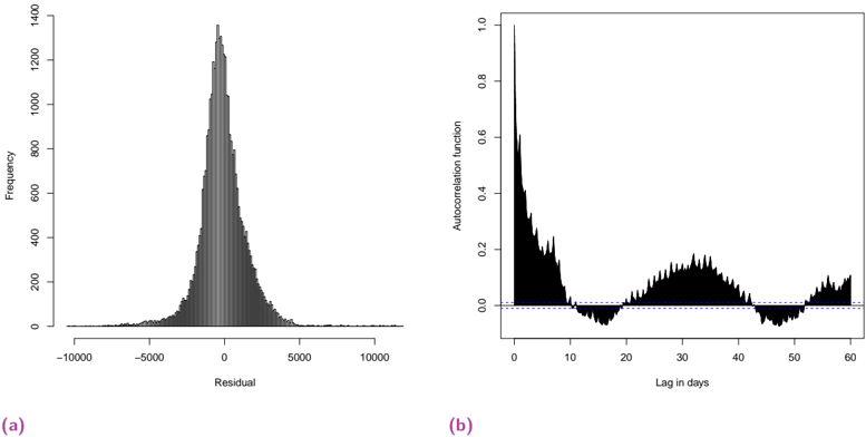<details> <summary>Image 51 Details</summary>  ### Visual Description \n ## Charts: Residual Analysis and Autocorrelation Function ### Overview The image presents two charts: (a) a histogram of residuals and (b) a plot of the autocorrelation function. Both charts are likely related to the analysis of a time series or regression model. The histogram shows the distribution of the residuals, while the autocorrelation function plot reveals the correlation between residuals at different time lags. ### Components/Axes **Chart (a): Histogram of Residuals** * **X-axis:** "Residual" - Scale ranges approximately from -10000 to 10000. * **Y-axis:** "Frequency" - Scale ranges approximately from 0 to 1400. * No legend is present. **Chart (b): Autocorrelation Function** * **X-axis:** "Lag in days" - Scale ranges from 0 to 60. * **Y-axis:** "Autocorrelation function" - Scale ranges approximately from 0 to 1.0. * A horizontal dashed line is present at y = 0. * No legend is present. ### Detailed Analysis or Content Details **Chart (a): Histogram of Residuals** The histogram is approximately symmetrical around zero. The peak frequency is around 1200, occurring at a residual value close to zero. The distribution has heavy tails, meaning there are some residuals with large absolute values (both positive and negative). The frequency decreases rapidly as the absolute value of the residual increases. Approximate values: * Residual = 0, Frequency ≈ 1200 * Residual = 2000, Frequency ≈ 600 * Residual = 4000, Frequency ≈ 200 * Residual = 6000, Frequency ≈ 100 * Residual = 8000, Frequency ≈ 50 * Residual = 10000, Frequency ≈ 20 **Chart (b): Autocorrelation Function** The autocorrelation function starts at a value of approximately 1.0 at lag 0. It then decreases rapidly to a value close to 0 around lag 10. After that, it oscillates around the zero line (dashed line) with some positive and negative values. There appears to be a slight positive autocorrelation around lag 20-30, but it remains close to zero. Approximate values: * Lag 0, Autocorrelation ≈ 1.0 * Lag 5, Autocorrelation ≈ 0.3 * Lag 10, Autocorrelation ≈ 0.05 * Lag 15, Autocorrelation ≈ -0.05 * Lag 20, Autocorrelation ≈ 0.1 * Lag 30, Autocorrelation ≈ 0.05 * Lag 40, Autocorrelation ≈ -0.05 * Lag 50, Autocorrelation ≈ -0.05 * Lag 60, Autocorrelation ≈ 0.0 ### Key Observations * The residual histogram (a) suggests that the residuals are approximately normally distributed, but with heavier tails than a normal distribution. * The autocorrelation function (b) shows a strong autocorrelation at lag 0 (as expected) and a rapid decay to near zero for higher lags. The oscillations around zero suggest that there is no significant autocorrelation remaining in the residuals. ### Interpretation The combination of these two charts suggests that the model used to generate these residuals is reasonably well-fitted to the data. The approximately normal distribution of residuals indicates that the model's assumptions are likely met. The lack of significant autocorrelation in the residuals confirms that the model is capturing the temporal dependencies in the data and that there is no remaining pattern in the errors. The heavy tails in the residual distribution might indicate the presence of outliers or that the model is not perfectly capturing all the variability in the data. The autocorrelation function plot indicates that the residuals are independent of each other over time, which is a desirable property of a well-fitted model. </details> performs well. This suggests that, even in this period without major events or decisions such as COVID-19 or sobriety, other features can be useful for better understanding electricity demand. ## Ranking changes in the data distribution The descriptive analysis shows that the residuals are not stationary. Therefore, from a statistical point of view, it is pointless to look for the change points observed in Figure 2 of the main article in absolute terms. In fact, the more precise the technique for detecting change points becomes, the more change points will be detected everywhere. This is why we need quantitative information about the importance of the change points in order to rank them and determine which are the most significant ones. A number of metrics have been developed to measure the importance of change points [AC17]. To assess the significance of the number of change points here, we sequentially compared the standard deviation of the residuals with the amplitude of the change points. This resulted in 10 change points being considered in the following analysis. The principle behind offline change-in-mean techniques is to segment the signal in such a way that approximating the signal by its mean in each segment results in the lowest possible variance. However, finding such an optimum would be computationally expensive for our time series of around 70 000 observations. Therefore, we rely on faster algorithms which have been developed to find approximations to the optimal change points, such as binary segmentation, as was used in Figure 2 of the main article. ## 6.D Statistical analysis In this section, we provide furthers analyses related to the variable selection detailed in the Results section. to further justify the study of the work index in the statistical analysis of Section III.B of the main article. ## Variable selection: Hoeffding D-stastics and Shapley values This paragraph complements the mRMR variable ranking performed in the Results section. To examine the variable selection process more closely, we computed the Hoeffding D-statistic, as shown in Table 6.3. This is a distribution-free measure of the dependence between variables Tab. 6.3.: Hoeffding D-statistic. | | Temp95 | Work | Res. | Tour. | Toy | Dow | |------------------|----------|--------|--------|---------|-------|-------| | Load | 0.3 | 0.04 | 0.09 | 0.2 | 0.07 | 0.01 | | Load \ Temp | 0.02 | 0.2 | 0.01 | 0.03 | 0.02 | 0.09 | | Load \ Temp,Work | 0.006 | 0.007 | 0.01 | 0.01 | 0.04 | 0.006 | The statistic was computed on all available days from 2019 to March 2022. Load \ Features stands for the Load corrected for the effect of the Features . Here, Res. stands for the Residence index, and Tour. for the Tourism index. [Hoe48]; the closer it is to 1, the greater the dependence. We then computed the Shapley values of the same variables using the SHAFF algorithm [B ´ +22]; results are shown in Table 6.4. We see that with the three ranking methods, the three most important variables, in order of importance, were the temperature , the work index, and the time of year . Of note, the effect of the work index only became clear after filtering out the effect of the temperature on electricity demand. We see that the importance of tourism and time of year decreases when correcting electricity demand for temperature, due to their high correlation with temperature. As a result of this analysis, the tourism and residents indices did not seem to have a significant impact on French electricity demand. Tab. 6.4.: Shapley values. | | Temp95 | Work | Res. | Tour. | Toy | Dow | |------------------|----------|--------|--------|---------|-------|-------| | Load | 0.31 | 0.05 | 0.06 | 0.14 | 0.21 | 0.03 | | Load \ Temp | 0.041 | 0.26 | 0.035 | 0.072 | 0.11 | 0.19 | | Load \ Temp,Work | 0.11 | 0.1 | 0.06 | 0.07 | 0.28 | 0.04 | Shapley values were computed on all available days from 2019 to March 2022. Load \ Features stands for the Load corrected for the effect of the Features . Here, Res. stands for the Residence index, and Tour. for the Tourism index. ## work index and calendar features The variable selection analysis in Section 6.D showed that the work indicator has a very strong effect on the electricity demand, being the second most explanatory variable. To better understand this effect, we compared-in Table 6.5-the performance of GAMs where we progressively added the features in the order of importance suggested by the variable selection analysis. The Temp GAM corresponds to the model $$L o a d _ { h , t } = f _ { h } ( T e m p 9 5 _ { h , t } ) + \varepsilon _ { h , t } .$$ The Temp + Work GAM corresponds to the model $$L o a d _ { h , t } = f _ { h , 1 } ( T e m p 9 5 _ { h , t } ) + f _ { h , 2 } ( W o r k _ { h , t } ) + \varepsilon _ { h , t } .$$ The Temp + Time GAM corresponds to the model $$L o a d _ { h , t } & = \sum _ { i = 1 } ^ { 7 } \sum _ { j = 0 } ^ { 1 } \alpha _ { h , i , j } \, 1 _ { D a y T p e _ { t } = i } \, 1 _ { D L S _ { t } = j } + \beta 1 _ { H o l i d a y s _ { t } } + f _ { h , 1 } ( T o Y _ { t } ) \\ & \quad + f _ { h , 2 } ( T e m p 9 5 _ { h , t } ) + \varepsilon _ { h , t } .$$ The Temp + Time + Work GAM corresponds to the model $$L o a d _ { h , t } & = \sum _ { i = 1 } ^ { 7 } \sum _ { j = 0 } ^ { 1 } \alpha _ { h , i , j } \, 1 _ { D a y T p e _ { t } = i } \, 1 _ { D L S _ { t } = j } + \beta 1 _ { H o l i d a y s _ { t } } + f _ { h , 1 } ( T o Y _ { t } ) \\ & \quad + f _ { h , 2 } ( T e m p 9 5 _ { h , t } ) + f _ { h , 3 } ( W o r k _ { h , t } ) + \varepsilon _ { h , t } .$$ The Temp + Work + Lags GAM corresponds to the model $$L o a d _ { h , t } & = f _ { h , 1 } ( T e m p 9 5 _ { h , t } ) + f _ { h , 2 } ( W o r k _ { h , t } ) + \sum _ { i = 1 } ^ { 7 } \alpha _ { h , i , j } \, 1 _ { D a y T y p e _ { t } = i } \, L o a d 1 D _ { h , t } \\ & \quad + \beta \, L o a d 1 W _ { h , t } + \varepsilon _ { h , t } .$$ The Temp + Time + Lags GAM corresponds to the model $$L o a d _ { h , t } & = \sum _ { i = 1 } ^ { 7 } \sum _ { j = 0 } ^ { 1 } \alpha _ { h , i , j } \, 1 _ { \text {DayType} _ { t } = i } \, 1 _ { \text {DLs} _ { t } = j } + \beta 1 _ { \text {Holidays} _ { t } } + f _ { h , 1 } ( \text {ToY} _ { t } ) + f _ { h , 2 } ( \text {Temp95} _ { h , t } ) \\ & \quad + \sum _ { i = 1 } ^ { 7 } \gamma _ { h , i , j } \, 1 _ { \text {DayType} _ { t } = i } \, L o a d 1 D _ { h , t } + \lambda L o a d 1 W _ { h , t } + \varepsilon _ { h , t } .$$ The All variables GAM corresponds to the model $$\text {Load} _ { h , t } & = \sum _ { i = 1 } ^ { 7 } \sum _ { j = 0 } ^ { 1 } \alpha _ { h , i , j } \ 1 _ { \text {DayType} _ { t } = i } \ 1 _ { \text {DLs} _ { t } = j } + \beta \mathbf 1 _ { \text {Holidays} _ { t } } + f _ { h , 1 } ( \text {ToY} _ { t } ) + f _ { h , 2 } ( \text {Temp95} _ { h , t } ) \\ & \quad + \sum _ { i = 1 } ^ { 7 } \gamma _ { h , i , j } \ 1 _ { \text {DayType} _ { t } = i } \text {Load} 1 D _ { h , t } + \lambda \text {Load} 1 W _ { h , t } + f _ { h , 3 } ( \text {Work} _ { h , t } ) + \varepsilon _ { h , t } .$$ The p-values of the Fisher tests assessing the significance of the GAM effects were below 5 % for all GAMs. We see in Table 6.5 that replacing calendar data by the work index was beneficial during atypical events whose behaviour differed from the past, i.e., the sobriety period here. Fig. 6.11.: Effect of the work index on a given day at a given hour. (a) 2d density plots of residuals as function of the work index at 10 a.m. on the Wednesdays between July 2019 and March 2022. (b) Regression coefficient of the work index on electricity demand corrected for the effect of temperature on the training set spanning July 2019 to March 2022. 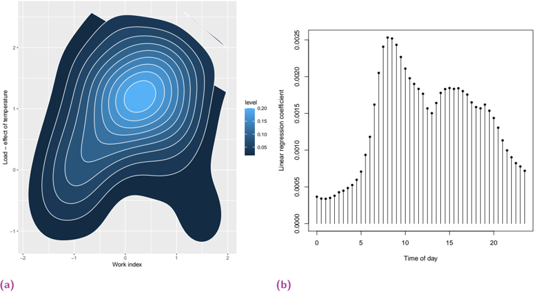<details> <summary>Image 52 Details</summary>  ### Visual Description \n ## Charts: Temperature Effect and Linear Regression Coefficient ### Overview The image presents two charts: (a) a 2D contour plot showing the relationship between "Work index" and "Load - effect of temperature", with a color scale representing the "level"; and (b) a bar chart displaying the "Linear regression coefficient" against "Time of day". ### Components/Axes **Chart (a): Contour Plot** * **X-axis:** "Work index", ranging from approximately -2 to 2. * **Y-axis:** "Load - effect of temperature", ranging from approximately -1.5 to 2.5. * **Color Scale/Legend:** "level", ranging from 0.00 to 0.20, with colors transitioning from dark blue to light blue. * **Contours:** Multiple contour lines representing different levels of the "level" variable. **Chart (b): Bar Chart** * **X-axis:** "Time of day", ranging from 0 to 22. * **Y-axis:** "Linear regression coefficient", ranging from approximately 0.000 to 0.0025. * **Bars:** Vertical bars representing the linear regression coefficient at each time of day. * **Error Bars:** Small vertical lines extending above and below each bar, indicating the uncertainty or standard error. ### Detailed Analysis or Content Details **Chart (a): Contour Plot** The contour plot shows a complex relationship between Work Index and Load - effect of temperature. The highest "level" (lightest blue) is concentrated around a Work Index of approximately 0.5 and a Load - effect of temperature of approximately 1.5. The contours become denser and darker blue as you move away from this peak, indicating lower levels. The contour lines are tightly packed in the central region, suggesting a steep gradient in the "level" variable. The lowest levels (darkest blue) are found at the extremes of both axes, particularly at Work Index values near -2 and Load - effect of temperature values near -1.5. **Chart (b): Bar Chart** The bar chart shows a clear trend in the linear regression coefficient over the course of the day. The coefficient starts at approximately 0.0002 at Time of day 0, increases rapidly to a peak around Time of day 12, reaching approximately 0.0022, and then gradually decreases to approximately 0.0005 at Time of day 22. The error bars are relatively small, indicating a consistent relationship. The error bars are largest around Time of day 0 and Time of day 22. Here's a breakdown of approximate values from the bar chart: * Time of day 0: Coefficient ≈ 0.0002, Error ≈ 0.0001 * Time of day 5: Coefficient ≈ 0.0008, Error ≈ 0.0001 * Time of day 10: Coefficient ≈ 0.0018, Error ≈ 0.0001 * Time of day 12: Coefficient ≈ 0.0022, Error ≈ 0.0001 * Time of day 15: Coefficient ≈ 0.0018, Error ≈ 0.0001 * Time of day 20: Coefficient ≈ 0.0008, Error ≈ 0.0001 * Time of day 22: Coefficient ≈ 0.0005, Error ≈ 0.0001 ### Key Observations * **Chart (a):** The highest "level" is observed at a specific combination of Work Index and Load - effect of temperature. * **Chart (b):** The linear regression coefficient exhibits a strong diurnal pattern, peaking around midday (Time of day 12) and declining towards the beginning and end of the day. The error bars suggest that the relationship is relatively stable across different time points. ### Interpretation The data suggests a complex interaction between work index and temperature effect, with an optimal combination leading to the highest "level" (presumably a desirable outcome). The diurnal pattern in the linear regression coefficient indicates that the relationship between time of day and some underlying variable is strongest around midday. This could be related to factors such as solar radiation, human activity patterns, or other time-dependent variables. The error bars provide a measure of the uncertainty in the estimated coefficients, allowing for a more robust interpretation of the results. The combination of these two charts suggests a system where both workload and time of day play a significant role in determining the outcome. The contour plot identifies optimal conditions, while the bar chart reveals how these conditions change throughout the day. </details> Indeed, the time variables were only relevant during the normal period spanning from July 2023 to September 2023, during which they still benefitted from the work index. During the sobriety period, the time variables-which only reconstruct past behaviour-were less explanatory than the work index, which did not benefit from being coupled with them. ## Work dynamics In Section III.B of the main article, we explained how the work index captures the effects of both the day of week and holidays features. However, in both Section II.B of the main paper and Section 6.D, we showed that the work index improved the performance of the forecast, beyond the effect of the calendar features. Let us briefly take a closer look at this effect. To remove the effect of time of day and holidays , we worked on a specific day (here Wednesday) and removed holidays. Figure 6.11a shows how the electricity demand on Wednesdays was still positively influenced by the work index. Furthermore, as expected, Figure 6.11b shows that the effect of the work index was more important during working hours (from 6 a.m. to 8 p.m.). These results confirm that on Wednesdays a high work index corresponded to high electricity demand. This effect could be due to economic growth (higher economic activity corresponding to both more people working which raises the work index, and to higher electricity demand) and to energy saving due to remote working (a lower office occupancy corresponding both to a lower work index and lower electricity demand). Tab. 6.5.: Integration of mobility data in GAMs. This benchmark covers all days, including holidays. The performance is measured in RMSE (GW) and MAPE(%). | | Normal period | Sobriety | |------------------------------|-----------------|-----------------| | Baseline Persistence (1 day) | 3.49 GW, 5.36% | | | Temp | | 4.03 GW, 5.26% | | GAM | | | | | 3.53 GW, 6.78% | 6.13 GW, 9.60% | | Temp+Work | 1.62 GW, 3.10% | 4.98 GW, 8.11% | | Temp+Time | 1.33 GW, 2.46% | 5.60 GW, 9.62% | | Temp+Time+Work | 1.09 GW, 2.02% | 5.24 GW, 9.00% | | Temp+Work+Lags | 1.11 GW, 1.92% | 2.11 GW, 3.13 % | | Temp+Time+Lags | 0.89 GW, 1.52% | 2.61 GW, 4.29% | | All variables | 0.80 GW, 1.38 % | 2.60 GW, 4.32% | ## Forecasting time series with constraints This chapter corresponds to the following paper: Doumèche et al. [Dou+25]. ## 7.1 Introduction Time series forecasting. Time series data are used extensively in many contemporary applications, such as forecasting supply and demand, pricing, macroeconomic indicators, weather, air quality, traffic, migration, and epidemic trends [Pet+22]. However, regardless of the application domain, forecasting time series presents unique challenges due to inherent data characteristics such as observation correlations, non-stationarity, irregular sampling intervals, and missing values. These challenges limit the availability of relevant data and make it difficult for complex black-box or overparameterized learning architectures to perform effectively, even with rich historical data [LZ21]. Constraints in time series. In this context, many modern frameworks incorporate physical constraints to improve the performance and interpretability of forecasting models. The strongest form of such constraints are typically derived from fundamental physical properties of the time series data and are represented by systems of differential equations. For example, weather forecasting often relies on solutions to the Navier-Stokes equations [Sch+21]. In addition to defining physical relationships, differential constraints can also serve as regularization mechanisms. For example, spatiotemporal regression on graphs can involve penalizing the spatial Laplacian of the regression function to enforce smoothness across spatial dimensions [Jin+24]. However, time series rarely satisfy strict differential constraints, often adhering instead to more relaxed forms of constraints [Col+23]. Perhaps the most successful example of such weak constraints are the generalized additive models [GAMs, HT86], which have been applied to time series forecasting in epidemiology [Woo17], earth sciences [Aug+09], and energy forecasting [Fas+21]. GAMs model the target time series (or some parameters of its distribution) as a sum of nonlinear effects of the features, thereby constraining the shape of the regression function. Another example of weak constraint appears in the context of spatiotemporal time series with hierarchical forecasting. Here, the goal is to combine regional forecasts into a global forecast by enforcing that the global forecast must be equal to the sum of the regional forecasts [WAH19]. Although this may seem like a simple constraint, hierarchical forecasting is challenging because of a trade-off: using more granular regional data increases the available information, but also introduces more noise as compared to the aggregated total. Another common and powerful constraint in time series forecasting arises when combining multiple forecasts [GSE14]. This is done by creating a final forecast by weighting each of the initial forecasts, with the constraint that the sum of the weights must equal one. PIML and time series. Although weak constraints have been studied individually and applied to real-world data, a unified and efficient approach is still lacking. It is important here to mention physics-informed machine learning (PIML), which offers a promising way to integrate constraints into machine learning models. Based on the foundational work of Raissi et al. [RPK19], PIML exploits the idea that constraints can be applied with neural networks and optimized by backpropagation, leading to the development of physics-informed neural networks (PINNs). PINNs have been successfully used to predict time series governed by partial differential equations (PDEs) in areas such as weather modeling [Kas+21], and stiff chemical reactions [Ji+21]. Weak constraints on the shape of the regression function have also been modeled with PINNs [Daw+22]. However, PINNs often suffer from optimization instabilities and overfitting [DBB25]. As a result, alternative methods have been developed for certain differential constraints that offer improved optimization properties over PINNs. For example, data assimilation techniques in weather forecasting have been shown to be consistent with the Navier-Stokes equations [NT24]. Moreover, Doumèche et al. [Dou+24a] showed that forecasting with linear differential constraints can be formulated as a kernel method, yielding closed-form solutions to compute the exact empirical risk minimum. An additional advantage of this kernel modeling is that the learning algorithm can be executed on GPUs, leading to significant speedups compared to the gradient-descent-based optimization of PINNs [Dou+24b]. Contributions. In this paper, we present a principled approach to effectively integrate constraints into time series forecasting. Each constrained problem is reformulated as the minimization of an empirical risk consisting of two key components: a data-driven term and a regularization term that enforces the smoothness of the function and the desired physical constraints. For nonlinear regression tasks, we rely on a Fourier expansion. Our framework allows for efficient computation of the exact minimizer of the empirical risk, which is easily optimized on GPUs for scalability and performance. In Section 7.2, we introduce a unified mathematical framework that connects empirical risks constrained by various forms of physical information. Notably, we highlight the importance of distinguishing between two categories of constraints: shape constraints, which limit the set of admissible functions, and learning constraints, which introduce an initial bias during parameter optimization. In Section 7.3, we explore shape constraints and illustrate their relevance using the example of electricity demand forecasting. In Section 7.4, we define learning constraints and show how they can be applied to tourism forecasting. This common modeling framework for shape and learning constraints allows for efficient integration of multiple constraints, as illustrated by the WeaKL-T in Section 7.4, which combines hierarchical forecasting with additive models and transfer learning. Each empirical risk can then be minimized on a GPU using linear algebra, ensuring scalability and computational efficiency. This direct computation guarantees that the proposed estimator exactly minimizes the empirical risk, preventing convergence to potential local minima-a common limitation of modern iterative and gradient descent methods used in PINNs. Our method achieves significant performance improvements over state-of-the-art approaches. The code for the numerical experiments and implementation is publicly available at https://github.com/NathanDoumeche/WeaKL . ## 7.2 Incorporating constraints in time series forecasting Throughout the paper, we assume that n observations ( X t 1 , Y t 1 ) , . . . , ( X t n , Y t n ) are drawn on R d 1 × R d 2 . The indices t 1 , . . . , t n ∈ T correspond to the times at which an unknown stochastic process ( X,Y ) := ( X t , Y t ) t ∈ T is sampled. Note that, all along the paper, the time steps need not be regularly sampled on the index set T ⊆ R . We focus on supervised learning tasks that aim to estimate an unknown function f /star : R d 1 → R d 2 , under the assumption that Y t = f /star ( X t ) + ε t , where ε is a random noise term. Without loss of generality, upon rescaling, we assume that X t := ( X 1 ,t , . . . , X d 1 ,t ) ∈ [ -π, π ] d 1 and -π ≤ t 1 ≤ · · · ≤ t n +1 ≤ π . The goal is to construct an estimator ˆ f for f /star . A simple example to to keep in mind is when Y is a stationary, regularly sampled time series with t j = j/n , and the lagged value X j = Y t j -1 serves as the only feature. In this specific case, where d 1 = d 2 , the model simplifies to Y t = f /star ( Y t -1 /n ) + ε t . Thus, the regression setting reduces to an autoregressive model. Of course, we will consider more complex models that go beyond this simple case. Model parameterization. We consider parameterized models of the form $$f _ { \theta } ( X _ { t } ) = ( f _ { \theta } ^ { 1 } ( X _ { t } ) , \dots , f _ { \theta } ^ { d _ { 2 } } ( X _ { t } ) ) = ( \langle \phi _ { 1 } ( X _ { t } ) , \theta _ { 1 } \rangle , \dots , \langle \phi _ { d _ { 2 } } ( X _ { t } ) , \theta _ { d _ { 2 } } \rangle ) ,$$ where each component f /lscript θ ( X t ) is computed as the inner product of a feature map φ /lscript ( X t ) ∈ C D /lscript , with D /lscript ∈ N /star , and a vector θ /lscript ∈ C D /lscript . The parameter vector θ ∈ C D 1 + ··· + D d 2 of the model is defined as the concatenation of θ 1 , . . . , θ d 2 . Note that f θ is uniquely determined by θ and the maps φ /lscript . To simplify the notation, we write dim( θ ) = D 1 + · · · + D d 2 . Our goal is to learn a parameter ˆ θ ∈ C dim( θ ) such that ˆ Y t = f ˆ θ ( X t ) is an estimator of the target Y t . Equivalently, f ˆ θ is an estimator of the target function f /star . To this end, the core principle of our approach is to consider ˆ θ to be a minimizer over C dim( θ ) of an empirical risk of the form $$L ( \theta ) = \frac { 1 } { n } \sum _ { j = 1 } ^ { n } \| \Lambda ( f _ { \theta } ( X _ { t _ { j } } ) - Y _ { t _ { j } } ) \| _ { 2 } ^ { 2 } + \| M \theta \| _ { 2 } ^ { 2 } ,$$ where Λ and M are complex-valued matrices with problem-dependent dimensions, which are not necessarily square. The matrix M encodes a regularization penalty, which may include hyperparameters to be tuned through validation, as we will see in several examples. Explicit formula for the empirical risk minimizer: WeaKL. The following proposition shows how to compute the exact minimizer of (7.2). (Throughout the document, ∗ denotes the conjugate transpose operation.) Proposition 7.2.1 (Empirical risk minimizer.) . Suppose both M and Λ are injective. Then, there is a unique minimizer to (7.2) , which takes the form $$\hat { \theta } = \left ( \left ( \sum _ { j = 1 } ^ { n } \Phi _ { t _ { j } } ^ { * } \Lambda ^ { * } \Lambda \Phi _ { t _ { j } } \right ) + n M ^ { * } M \right ) ^ { - 1 } \sum _ { j = 1 } ^ { n } \Phi _ { t _ { j } } ^ { * } \Lambda ^ { * } \Lambda Y _ { t _ { j } } ,$$ where Φ t is the d 2 × dim( θ ) block-wise diagonal feature matrix at time t , defined by $$\Phi _ { t } = \begin{pmatrix} \phi _ { 1 } ( X _ { t } ) ^ { * } & 0 & 0 \\ 0 & \ddots & 0 \\ 0 & 0 & \phi _ { d _ { 2 } } ( X _ { t } ) ^ { * } \end{pmatrix} .$$ This result, proven in Appendix 7.A, generalizes well-known results on kernel ridge regression [see, e.g., MRT12, Equation 10.17]. In the rest of the paper, we refer to the estimator ˆ θ as the weak kernel learner (WeaKL). The strength of WeaKL lies in its exact computation via (7.3). Unlike current implementations of GAMs and PINNs, WeaKL is free from optimization errors. Furthermore, since WeaKL relies solely on linear algebra, it can take advantage of GPU programming to accelerate the learning process. This efficiency enables effective hyperparameter optimization, as demonstrated in Section 7.3 through applications to electricity demand forecasting. Algorithmic complexity. The formula (7.3) used in this article to minimize the empirical risk (7.2) can be implemented with a complexity of O (dim( θ ) 3 + dim( θ ) 2 n ) . Note that the dimensions d 1 and d 2 of the problem only impact the complexity of WeaKL through dim( θ ) = D 1 + · · · + D d 2 . By construction, dim( θ ) ≥ d 2 , but the influence of d 1 is more subtle and depends on the chosen dimension D /lscript of the maps φ j : [ -π, π ] d 1 → C D j . In particular, if all the maps have the same dimension, i.e., D /lscript = D , then dim( θ ) = Dd 2 . Notably, this implementation runs in less than ten seconds on a standard GPU (e.g., an NVIDIA L 4 with 24 GB of RAM) when dim( θ ) ≤ 10 3 and n ≤ 10 5 . We believe that this framework is particularly well suited for time series, where data sampling is often costly, thus limiting both n and d 2 . Moreover, in many cases, the distribution of the target time series changes significantly over time, making only the most recent observations relevant for forecasting. This further limits the size of n . For example, in the Monash time series forecasting archive [God+21], 19 out of 30 time series have d 2 ≤ 10 3 and n ≤ 10 5 . However, there are relevant time series where either the dimension d 2 or the number of data points n is large. In such cases, finding an exact minimizer of the empirical risk (7.2) becomes very computationally expensive. Efficient techniques have been developed to approximate the minimizer of (7.2) in these regimes [see, e.g., Mea+20], but a detailed discussion of these methods is beyond the scope of this paper. Some important examples. Let us illustrate the mechanism with two fundamental examples. Of course, the case where φ /lscript ( x ) = x and where Λ and M are identity matrices corresponds to the well-known ridge linear regression. On the other hand, a powerful example of a nonparametric regression map is the Fourier map, defined as φ /lscript ( x ) = (exp( i 〈 x, k 〉 / 2)) /latticetop ‖ k ‖ ∞ ≤ m = (exp( i 〈 x, k 〉 / 2)) /latticetop -m ≤ k 1 ,...,k d 1 ≤ m , where the Fourier frequencies are truncated at m ≥ 0 . This map leverages the expressiveness of the Fourier basis to capture complex patterns in the data. Thus, for the /lscript -th component of f θ , we consider the Fourier decomposition $$f _ { \theta } ^ { \ell } ( x ) = \sum _ { \| k \| _ { \infty } \leq m } \theta _ { \ell , k } \exp ( - i \langle x , k \rangle / 2 ) ,$$ which can approximate any function in L 2 ([ -π, π ] d 1 , R ) as m →∞ . In this example, we have θ /lscript = ( θ /lscript,k ) /latticetop ‖ k ‖ ∞ ≤ m ∈ C (2 m +1) d . Next, for s ∈ N /star , let M be the (2 m +1) d 1 × (2 m +1) d 1 positive diagonal matrix such that $$\| M \theta _ { \ell } \| _ { 2 } ^ { 2 } = \lambda \sum _ { \| k \| _ { \infty } \leq m } \theta _ { \ell , k } ^ { 2 } ( 1 + \| k \| _ { 2 } ^ { 2 s } ) ,$$ where λ > 0 is an hyperparameter. Then, ‖ Mθ /lscript ‖ 2 is a Sobolev norm on the derivatives up to order s of f θ /lscript . When λ = 1 , we will denote this norm by ‖ f /lscript θ ‖ H s . This approach regularizes the smoothness of f /lscript ˆ θ , encouraging the recovery of smooth solutions. Moreover, choosing Λ as the identity matrix and λ = n -2 s/ (2 s + d 1 ) achieves the Sobolev minimax rate E ( ‖ f /lscript ˆ θ ( X ) -Y /lscript ‖ 2 2 ) = O ( n -2 s/ (2 s + d 1 ) ) [BM20]. This result justifies why the Fourier decomposition serves as an effective nonparametric mapping. These fundamental examples illustrate the richness of the approach, making it possible to incorporate constraints into models of chosen complexity, from very light models like linear regression, up to nonparametric models such as Fourier maps. Classification of the constraints. In order to clarify our discussion as much as possible, we find it helpful, after a thorough analysis of the existing literature, to consider two families of constraints. This distinction arises from the need to address two fundamentally different aspects of the forecasting problem. 1. Shape constraints , described in Section 7.3, include additive models, online adaption after a break, and forecast combinations (detailed in Appendix 7.B). In these models, prior information is incorporated by selecting custom maps φ /lscript . The set of admissible models f θ is thus restricted by shaping the structure of the function space through this choice of maps. Here, the matrix M serves only as a regularization term, while Λ is the identity matrix. 2. Learning constraints , described in Section 7.4, include transfer learning, hierarchical forecasting, and differential constraints (detailed in Appendix 7.B). In these models, prior information or constraints are incorporated through the matrices M and Λ . The goal is to increase the efficiency of parameter learning by introducing additional regularization. It is worth noting, however, that certain specific shape constraints cannot be penalized by a kernel norm, such as those in isotonic regression. In the conclusion, we discuss possible extensions to account for such constraints. ## 7.3 Shape constraints ## Mathematical formulation In this section, we introduce relevant feature maps φ that incorporate prior knowledge about the shape of the function f /star : [ -π, π ] d 1 → C d 2 . To simplify the notation, we focus on the one-dimensional case where d 2 = 1 and Λ = 1 . This simplification comes without loss of generality, since the feature maps developed in this section can be applied directly to (7.1). As a result, the model reduces to f θ ( X t ) = 〈 φ 1 ( X t ) , θ 1 〉 , and (7.3) simplifies to $$\hat { \theta } = ( \Phi ^ { * } \Phi + n M ^ { * } M ) ^ { - 1 } \Phi ^ { * } \mathbb { Y } ,$$ where Y = ( Y t 1 , . . . , Y t n ) /latticetop ∈ R n and the n × dim( θ ) matrix Φ takes the form $$\Phi = ( \phi _ { 1 } ( X _ { t _ { 1 } } ) | \cdots | \phi _ { 1 } ( X _ { t _ { n } } ) ) ^ { * } .$$ Note that Φ is the classical feature matrix, and that it is related to the matrix Φ t of (7.4) by Φ ∗ Φ = ∑ n j =1 Φ ∗ t j Φ t j = ∑ n j =1 φ 1 ( X t j ) φ 1 ( X t j ) ∗ . Additive model: Additive WeaKL. The additive model constraint assumes that f /star ( x 1 , . . . , x d 1 ) = ∑ d 1 /lscript =1 g /star /lscript ( x /lscript ) , where g /star /lscript : R → R are univariate functions. This constraint is widely used in data science, both in classical statistical models [HT86] and in modern neural network architectures [Aga+21]. Indeed, additive models are interpretable because the effect of each feature x /lscript is captured by its corresponding function g /star /lscript . In addition, univariate effects are easier to estimate than multivariate effects [Rav+09]. These properties allow the development of efficient variable selection methods [see, for example, MW11], similar to those used in linear regression. In our framework, the additivity constraint directly translates into the model as $$f _ { \theta } ( X _ { t } ) = \langle \phi _ { 1 } ( X _ { t } ) , \theta _ { 1 } \rangle = \langle \phi _ { 1 , 1 } ( X _ { 1 , t } ) , \theta _ { 1 , 1 } \rangle + \cdots + \langle \phi _ { 1 , d _ { 1 } } ( X _ { d _ { 1 } , t } ) , \theta _ { 1 , d _ { 1 } } \rangle ,$$ where φ 1 is the concatenation of the maps φ 1 ,/lscript , and θ 1 is the concatenation of the vectors θ 1 ,/lscript . Note that the maps φ 1 ,/lscript and the vectors θ 1 ,/lscript can be multidimensional, depending on the model. In this formulation, the effect of each feature is modeled by the function g /lscript ( x /lscript ) = 〈 φ 1 ,/lscript ( x /lscript ) , θ 1 ,/lscript 〉 , which can be either linear or nonlinear in x /lscript . The empirical risk then takes the form $$L ( \theta ) = \frac { 1 } { n } \sum _ { j = 1 } ^ { n } | f _ { \theta } ( X _ { t _ { j } } ) - Y _ { t _ { j } } | ^ { 2 } + \sum _ { \ell = 1 } ^ { d _ { 1 } } \lambda _ { \ell } \| M _ { \ell } \theta _ { 1 , \ell } \| _ { 2 } ^ { 2 } ,$$ where λ /lscript > 0 are hyperparameters and M /lscript are regularization matrices. There are three types of effects that can be taken into account: - ( i ) A linear effect is obtained by setting φ 1 ,/lscript ( x /lscript ) = x /lscript ∈ R . To regularize the parameter θ 1 ,/lscript , we set M /lscript = 1 . This corresponds to a ridge penalty. - ( ii ) A nonlinear effect can be modeled using the Fourier map φ 1 ,/lscript ( x /lscript ) = (exp( ikx /lscript / 2)) /latticetop -m ≤ k ≤ m . To regularize the parameter θ 1 ,/lscript , we set M /lscript to be the (2 m +1) × (2 m +1) diagonal matrix defined by M /lscript = Diag(( √ 1 + k 2 s ) -m ≤ k ≤ m ) , penalizing the Sobolev norm. A common choice for the smoothing parameter s , as used in GAMs, is s = 2 [see, e.g., Woo17]. - ( iii ) If x /lscript is a categorical feature, i.e., x /lscript takes values in a finite set E , we can define a bijection ψ : E → { 1 , . . . , | E |} . The effect of x /lscript can then be modeled as g /lscript ( x /lscript ) = 〈 φ 1 ,/lscript ( x /lscript ) , θ 1 〉 , where φ /lscript = φ ◦ ψ and φ is the Fourier map with m = /floorleft| E | / 2 /floorright . To regularize the parameter θ 1 ,/lscript , we set M /lscript as the identity matrix, which corresponds to applying a ridge penalty. Overall, similar to GAMs, WeaKL can be optimized to fit additive models with both linear and nonlinear effects. The parameter ˆ θ of the WeaKL can then be computed using (7.5) with $$M = \begin{pmatrix} \sqrt { \lambda _ { 1 } } M _ { 1 } & 0 & 0 \\ 0 & \ddots & 0 \\ 0 & 0 & \sqrt { \lambda _ { d _ { 1 } } } M _ { d _ { 1 } } \end{pmatrix} .$$ To stress that this WeaKL results from the enforcement of additive constraints, we call it the additive WeaKL . Note that, contrary to GAMs where identifiability issues must be addressed [Woo17], WeaKL does not require further regularization, since ˆ θ is the unique minimizer of the empirical risk L . Note that the hyperparameters λ /lscript , along with the number m of Fourier modes and the choice of feature maps φ /lscript , can be determined by model selection, as described in Appendix 7.D. Online adaption after a break: Online WeaKL. For many time series, the dependence of Y on X can vary over time. For example, the behavior of Y may change rapidly following extreme events, resulting in structural breaks. A notable example is the shift in electricity demand during the COVID-19 lockdowns, as illustrated in use case 1 . To provide a clear mathematical framework, we assume that the distribution of ( X,Y ) follows an additive model that evolves smoothly over time. Formally, considering ( t, X t ) as a feature vector, we assume that $$f ^ { ^ { * } } ( t , x _ { 1 } , \dots , x _ { d _ { 1 } } ) = h _ { 0 } ^ { ^ { * } } ( t ) + \sum _ { \ell = 1 } ^ { d _ { 1 } } ( 1 + h _ { \ell } ^ { ^ { * } } ( t ) ) g _ { \ell } ^ { ^ { * } } ( x _ { \ell } ) ,$$ where g /star /lscript and h /star /lscript are univariate functions. This model forms the core of the Kalman-Viking algorithm [VW24], which has demonstrated state-of-the-art performance in forecasting electricity demand and renewable energy production [OVG21; VG22; Vil+24]. We assume that we have at hand estimators ˆ g /lscript of g /star /lscript that we want to update over time. For example, these estimators can be obtained by fitting an additive WeaKL model, initially assuming h /star /lscript = 0 . The functions h /star /lscript are then estimated by minimizing the empirical risk $$L ( \theta ) = \frac { 1 } { n } \sum _ { j = 1 } ^ { n } \left | h _ { \theta _ { 0 } } ( t _ { j } ) + \sum _ { \ell = 1 } ^ { d _ { 1 } } ( 1 + h _ { \theta _ { \ell } } ( t _ { j } ) ) \hat { g } _ { \ell } ( X _ { \ell , t _ { j } } ) - Y _ { t _ { j } } \right | ^ { 2 } + \sum _ { 0 \leq \ell \leq d _ { 1 } } \lambda _ { \ell } \| h _ { \theta _ { \ell } } \| _ { H ^ { s } } ^ { 2 } ,$$ where λ /lscript > 0 are hyperparameters regularizing the smoothness of the functions h θ /lscript . Here, h θ ( t ) = 〈 φ ( t ) , θ 〉 , and φ is the Fourier map φ ( t ) = (exp( ikt/ 2)) /latticetop -m ≤ k ≤ m . The prior h θ /lscript /similarequal 0 reflects the idea that the best a priori estimate of Y 's behavior follows the stable additive model. Defining W t = Y t -∑ d 1 /lscript =1 ˆ g /lscript ( X /lscript,t ) , the empirical risk can be reformulated as $$L ( \theta ) = \frac { 1 } { n } \sum _ { j = 1 } ^ { n } | \langle \phi _ { 1 } ( t _ { j } , X _ { t _ { j } } ) , \theta \rangle - W _ { t _ { j } } | ^ { 2 } + \| M \theta \| _ { 2 } ^ { 2 } ,$$ with φ 1 ( t, X t ) = ((exp( ikt/ 2)) -m ≤ k ≤ m , (ˆ g /lscript ( X /lscript,t ) exp( ikt/ 2)) -m ≤ k ≤ m ) d 1 /lscript =1 ) /latticetop ∈ C (2 m +1)( d 1 +1) , $$M = \begin{pmatrix} \sqrt { \lambda _ { 0 } } D & 0 & 0 \\ 0 & \ddots & 0 \\ 0 & 0 & \sqrt { \lambda _ { d _ { 1 } } } D \end{pmatrix} ,$$ and D is the (2 m +1) × (2 m +1) diagonal matrix D = Diag(( √ 1 + k 2 s ) -m ≤ k ≤ m ) . From (7.5), we deduce that the unique minimizer of the empirical loss L is $$\hat { \theta } = ( \Phi ^ { * } \Phi + n M ^ { * } M ) ^ { - 1 } \Phi ^ { * } \mathbb { W } ,$$ where W = ( W t 1 , . . . , W t n ) /latticetop ∈ R n . This formulation allows to forecast the time series Y at the next time step, t n +1 , using $$\hat { Y } _ { t _ { n + 1 } } & = f _ { \hat { \theta } } ( t _ { n + 1 } , X _ { t _ { n + 1 } } ) = \langle \phi _ { 1 } ( t _ { n + 1 } , X _ { t _ { n + 1 } } ) , \hat { \theta } \rangle \\ & = h _ { \hat { \theta } _ { 0 } } ( t _ { n + 1 } ) + \sum _ { \ell = 1 } ^ { d _ { 1 } } ( 1 + h _ { \hat { \theta } _ { \ell } } ( t _ { n + 1 } ) ) \hat { g } _ { \ell } ( X _ { \ell , t _ { n + 1 } } ) .$$ Since the model is continuously updated over time, this corresponds to an online learning setting. To emphasize that Equation (7.9) arises from an online adaptation process, we refer to this model as the online WeaKL . Unlike the Viking algorithm of Vilmarest and Wintenberger [VW24], which approximates the minimizer of the empirical risk through an iterative process, online WeaKL offers a closed-form solution and exploits GPU parallelization for significant speedups. As shown in Section 7.3, our approach leads to improved performance in electricity demand forecasting. ## Application to electricity load forecasting In this subsection, we apply shape constraints to two use cases in electricity demand forecasting and demonstrate the effectiveness of our approach. In these electricity demand forecasting problems, the focus is on short-term forecasting, with particular emphasis on the recent non-stationarities caused by the COVID-19 lockdowns and by the energy crisis. Electricity load forecasting and non-stationarity. Accurate demand forecasting is critical due to the costly nature of electricity storage, coupled with the need for supply to continuously match demand. Short-term load forecasting, especially for 24-hour horizons, is particularly valuable for making operational decisions in both the power industry and electricity markets. Although the cost of forecasting errors is difficult to quantify, a 1% reduction in error is estimated to save utilities several hundred thousand USD per gigawatt of peak demand [HF16]. Recent events such as the COVID-19 shutdown have significantly affected electricity demand, highlighting the need for updated forecasting models [ZMM22]. Use case 1: Load forecasting during COVID. In this first use case, we test the performance of our WeaKL on the IEEE DataPort Competition on Day-Ahead Electricity Load Forecasting [Far+22]. Here, the goal is to forecast the electricity demand of an unknown country during the period following the Covid-19 lockdown. The winning model of this competition was the Viking model of Team 4 [VG22], with a mean absolute error (MAE) of 10 . 9 gigawatts (GW). For comparison, a direct translation of their model into the online WeaKL framework-using the same features and maintaining the same additive effects-results in an MAE of 10 . 5 GW. In parallel, we also apply the online WeaKL methodology without relying on the variables selected by Vilmarest and Goude [VG22]. Instead, we determine the optimal hyperparameters λ /lscript and select the feature maps φ /lscript through a hyperparameter tuning process (see Appendix 7.D). This leads to a different selected model with a MAE of 9 . 9 GW (see Appendix 7.D for a complete description of the models). Thus, the online WeaKL given by (7.9) outperforms the state-of-theart by 9% . As done in the IEEE competition [Far+22], we assess the significance of this result by evaluating the MAE skill score using a block bootstrap approach (see Appendix 7.D). It shows that the online WeaKL outperforms the winning model proposed by Vilmarest and Goude [VG22] with a probability above 90% . The updated results of the competition are presented in Table 7.1. Note that a great variety of models were benchmarked in this competition, like Kalman filters (Team 4), autoregressive models (Teams 4 and 7), random forests (Teams 4 and 6), gradient boosting (Teams 6 and 36), deep residual networks (Team 19), and averaging (Team 13). Tab. 7.1.: Performance of the online WeaKL and of the top 10 participants of the IEEE competiton. A specific bootstrap test shows that the WeaKL significantly outperform the winning team. | Team | WeaKL | 4 | 14 | 7 | 36 | 19 | 23 | 9 | 25 | 13 | 26 | |----------|---------|------|------|------|------|------|------|------|------|------|------| | MAE (GW) | 9.9 | 10.9 | 11.8 | 11.9 | 12.3 | 12.3 | 13.9 | 14.2 | 14.3 | 14.6 | 15.4 | Use case 2: Load forecasting during the energy crisis. In this second use case, we evaluate the performance of our WeaKL within the open source benchmark framework proposed by Doumèche et al. [Dou+23]. This benchmark provides a comprehensive evaluation of electricity demand forecasting models, incorporating the GAM boosting model of [TH14], the GAM of [OVG21], the Kalman models of [VG22], the time series random forests of [Goe+23], and the Viking model of [Vil+24]. The goal here is to forecast the French electricity demand during the energy crisis in the winter of 2022-2023. Following the war in Ukraine and maintenance problems at nuclear power plants, electricity prices reached an all-time high at the end of the summer of 2022. In this context, French electricity demand decreased by 10% compared to its historical trends [Dou+23]. This significant shift in electricity demand can be interpreted as a structural break, which justifies the application of the online WeaKL given by (7.9). In this benchmark, the models are trained from 8 January 2013 to 1 September 2022, and then evaluated from 1 September 2022 to 28 February 2023. The dataset consists of temperature data from the French meteorological administration Météo-France [MF23], and electricity demand data from the French transmission system operator RTE [RTE23b], sampled with a half-hour resolution. This translates into the feature variable $$X = ( L o a d _ { 1 } , L o a d _ { 7 } , T e m p , T e m p _ { \min 5 0 } , T e m p _ { \max 9 5 0 } , T e m p _ { \min 9 5 0 } , T o Y , D O W , H o l i d a y , t ) ,$$ where Load 1 and Load 7 are the electricity demand lagged by one day and seven days, Temp is the temperature, and Temp 950 , Temp max950 , and Temp min950 are smoothed versions of Temp . The time of year ToY ∈ { 1 , . . . , 365 } encodes the position within the year. The day of the week DoW ∈ { 1 , . . . , 7 } encodes the position within the week. In addition, Holiday is a boolean variable set to one during holidays, and t is the timestamp. Here, the target Y = Load is the electricity demand, so d 1 = 10 and d 2 = 1 . We compare the performance of two of our WeaKLs against this benchmark. First, our additive WeaKL is a direct translation of the GAM formula proposed by [OVG21] into the additive WeaKL framework given by (7.6). Thus, f θ ( x ) = ∑ 10 /lscript =1 g /lscript ( x /lscript ) , where: - the effects g 1 , g 2 , and g 10 of Load 1 , Load 7 , and t are linear, - the effects g 3 , . . . , g 7 of Temp , Temp 950 , Temp max950 , Temp min950 , and ToY are nonlinear with m = 10 , - the effects g 8 and g 9 of DoW and Holiday are categorical with | E | = 7 and | E | = 2 . The weights θ are learned using data from 2013 to 2021, while the optimal hyperparameters λ 1 , . . . , λ 10 are tuned using a validation set covering the period from 2021 to 2022. Once the additive WeaKL is learned, it becomes straightforward to interpret the impact of each feature on the model. For example, the effect ˆ g 3 : Temp ↦→ 〈 φ 1 , 3 (Temp) , ˆ θ 1 , 3 〉 of the rescaled temperature feature ( Temp ∈ [ -π, π ] ) is illustrated in Figure 7.1. Second, our online WeaKL is the online adaptation of f θ in response to a structural break, as described by (7.9). The hyperparameters λ 0 , . . . 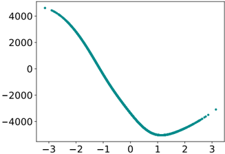, λ 10 in (7.8) are <details> <summary>Image 53 Details</summary>  ### Visual Description \n ## Chart: Polynomial Function Plot ### Overview The image displays a plot of a polynomial function. The plot shows a curve that starts at a high positive value, decreases to a negative minimum, and then increases again to a slightly positive value. The x-axis ranges from approximately -3 to 3, and the y-axis ranges from approximately -5000 to 4500. There are a few discrete data points plotted as blue dots along with the continuous curve. ### Components/Axes * **X-axis:** Labeled with numerical values ranging from -3 to 3, with tick marks at integer values. * **Y-axis:** Labeled with numerical values ranging from -5000 to 4500, with tick marks at intervals of 1000. * **Curve:** A teal-colored line representing the polynomial function. * **Data Points:** Several blue dots are scattered along the curve, indicating specific data points. ### Detailed Analysis The curve exhibits a cubic-like shape. It begins at approximately x = -3 with a y-value of around 4200. The curve then decreases, crossing the x-axis around x = -1.5. It reaches a minimum value of approximately -4800 at x = 1. The curve then increases, crossing the x-axis again around x = 2.5, and ends at approximately x = 3 with a y-value of around -300. Here's a breakdown of approximate data points: * (-3, 4200) * (-2, 3000) * (-1, 1000) * (0, 0) * (1, -4800) * (2, -2000) * (3, -300) The curve appears smooth and continuous between the plotted data points. ### Key Observations * The function has at least one local maximum and one local minimum. * The function crosses the x-axis at least twice, indicating multiple real roots. * The function is symmetric around the y-axis. ### Interpretation The plot likely represents a polynomial function of degree 3 or higher. The shape of the curve suggests a cubic function, but higher-degree polynomials could also produce similar shapes. The function's behavior indicates that it has at least two real roots, where the function's value is zero. The symmetry around the y-axis suggests that the function might be an even function, meaning f(x) = f(-x). The data points are likely samples from the continuous function, used to visualize its behavior. The function could be modeling a physical phenomenon where a quantity initially increases, then decreases, and finally increases again, such as the height of a projectile or the temperature change in a system. The exact equation of the polynomial cannot be determined from the plot alone, but it can be approximated using curve fitting techniques. </details> temperature Fig. 7.1.: Effect in MW of the temperature in the additive WeaKL. chosen to minimize the error over a validation period from 1 April 2020 to 1 June 2020 , corresponding to the first COVID-19 lockdown. Note that this validation period does not immediately precede the test period, which is uncommon in time series analysis. However, this choice ensures that the validation period contains a structural break, making it as similar as possible to the test period. Next, the functions h 0 , . . . , h 10 in (7.7) are trained on a period starting from 1 July 2020 , and updated online. The results are summarized in Table 7.2. The errors and their standard deviations are assessed by stationary block bootstrap (see Appendix 7.D). Since holidays are notoriously difficult to predict, performance is evaluated over the entire period (referred to as Including holidays ), and separately excluding holidays and the days immediately before and after (referred to as Excluding holidays ). Over both test periods, the additive WeaKL significantly outperforms the GAM, while the online WeaKL outperforms the state-of-the-art by more than 10% across all metrics. Figure 7.2 shows the errors of the WeaKLs as a function of time during the test period, which includes holidays. During the sobriety period, electricity demand decreased, causing the additive WeaKL to overestimate demand, resulting in a negative bias. Interestingly, this bias is effectively corrected by the online WeaKL, which explains its strong performance. This shows that the online update of the effects effectively corrects biases caused by shifts in the data distribution. Then, we compare the running time of the algorithms. Note that, during hyperparameter tuning, the GPU implementation of WeaKL makes it possible to train 1 . 6 × 10 5 additive WeaKL over a period of eight years in less than five minutes on a single standard GPU (NVIDIA L 4 ). As for the online WeaKL, the training is more computationally intensive because the model must be updated in an online fashion. However, training 9 . 2 × 10 3 online WeaKLs over a period of two years takes less than two minutes. This approach is faster than the Viking algorithm, which takes over 45 minutes to evaluate the same number of parameter sets on the same dataset, even when using 10 CPUs in parallel. A detailed comparison of the running times for all algorithms is provided in Appendix 7.D. Tab. 7.2.: Benchmark for load forecasting during the energy crisis | | Including holidays | Including holidays | Excluding holidays | Excluding holidays | |----------------------------|----------------------|----------------------|----------------------|----------------------| | | RMSE (GW) | MAPE (%) | RMSE (GW) | MAPE (%) | | Statistical model | | | | | | Persistence (1 day) | 4.0 ± 0.2 | 5.5 ± 0.3 | 4.0 ± 0.2 | 5.0 ± 0.3 | | SARIMA | 2.4 ± 0.2 | 3.1 ± 0.2 | 2.0 ± 0.2 | 2.6 ± 0.2 | | GAM | 2.3 ± 0.1 | 3.5 ± 0.2 | 1.70 ± 0.06 | 2.6 ± 0.1 | | Data assimilation | | | | | | Static Kalman | 2.1 ± 0.1 | 3.1 ± 0.2 | 1.43 ± 0.05 | 2.20 ± 0.08 | | Dynamic Kalman | 1.4 ± 0.1 | 1.9 ± 0.1 | 1.10 ± 0.04 | 1.58 ± 0.05 | | Viking | 1.5 ± 0.1 | 1.8 ± 0.1 | 0.98 ± 0.04 | 1.33 ± 0.04 | | Aggregation | 1.4 ± 0.1 | 1.8 ± 0.1 | 0.96 ± 0.04 | 1.36 ± 0.04 | | Machine learning | | | | | | GAM boosting | 2.6 ± 0.2 | 3.7 ± 0.2 | 2.3 ± 0.1 | 3.3 ± 0.2 | | Random forests | 2.5 ± 0.2 | 3.5 ± 0.2 | 2.1 ± 0.1 | 3.0 ± 0.1 | | Random forests + bootstrap | 2.2 ± 0.2 | 3.0 ± 0.2 | 1.9 ± 0.1 | 2.6 ± 0.1 | | WeaKLs | | | | | | Additive WeaKL | 1.95 ± 0.08 | 3.0 ± 0.1 | 1.55 ± 0.06 | 2.32 ± 0.09 | | Online WeaKL | 1.14 ± 0.09 | 1.5 ± 0.1 | 0.87 ± 0.04 | 1.17 ± 0.05 | Both use cases demonstrate that WeaKL models are very powerful. Not only are they highly interpretable-thanks to their ability to fit into a common framework and produce simple formulas-but they are also competitive with state-of-the-art techniques in terms of both optimization efficiency (they can run on GPUs) and performance (measured by MAPE and RMSE). Fig. 7.2.: Error Y t -ˆ Y t in MW of the WeaKLs on the test period including holidays. Dots represent individual observations, while the bold curves indicate the one-week moving averages. 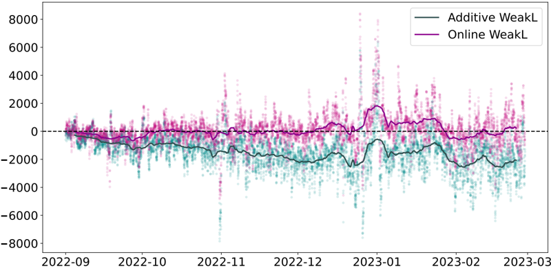<details> <summary>Image 54 Details</summary>  ### Visual Description \n ## Line Chart: WeakL Comparison ### Overview The image presents a line chart comparing two time series, labeled "Additive WeakL" and "Online WeakL", over a period from approximately September 2022 to March 2023. The chart displays fluctuations in values, with the y-axis representing the magnitude of these fluctuations and the x-axis representing time. A horizontal dashed line at y=0 is present, likely serving as a baseline for comparison. ### Components/Axes * **X-axis:** Represents time, spanning from approximately 2022-09 to 2023-03. Tick marks are present at roughly monthly intervals. * **Y-axis:** Represents the value of "WeakL", ranging from approximately -8000 to 8000. Tick marks are present at 2000-unit intervals. * **Legend:** Located in the top-right corner. * "Additive WeakL" - represented by a solid teal line. * "Online WeakL" - represented by a solid magenta line. * **Baseline:** A horizontal dashed black line at y=0. ### Detailed Analysis **Additive WeakL (Teal Line):** The teal line exhibits significant fluctuations throughout the period. The trend is generally downward from September 2022 to around November 2022, then fluctuates around a negative value. From January 2023, the line shows a slight upward trend, but remains largely negative. * Approximate values (with uncertainty of +/- 200): * 2022-09: ~ -500 * 2022-10: ~ -1500 * 2022-11: ~ -2500 * 2022-12: ~ -3000 * 2023-01: ~ -3500 * 2023-02: ~ -2000 * 2023-03: ~ -1000 **Online WeakL (Magenta Line):** The magenta line also shows substantial fluctuations, but generally remains closer to the zero baseline than the teal line. It exhibits a more erratic pattern, with frequent spikes both above and below the baseline. * Approximate values (with uncertainty of +/- 200): * 2022-09: ~ 500 * 2022-10: ~ 500 * 2022-11: ~ 1000 * 2022-12: ~ 2000 * 2023-01: ~ 4000 * 2023-02: ~ 1000 * 2023-03: ~ 0 ### Key Observations * The "Online WeakL" consistently shows higher positive values than the "Additive WeakL" for most of the observed period. * Both time series exhibit high volatility, with frequent and significant fluctuations. * The "Additive WeakL" spends a larger portion of the time below the zero baseline. * There is a notable spike in "Online WeakL" around January 2023, reaching a peak value of approximately 4000. * The "Additive WeakL" appears to be more stable in the final month (March 2023) compared to the "Online WeakL". ### Interpretation The chart likely compares the performance or error metrics ("WeakL") of two different algorithms or approaches: an "Additive" method and an "Online" method. The "Online WeakL" generally performs better (higher values) than the "Additive WeakL", suggesting it produces more accurate or desirable results. However, the "Online WeakL" is also more volatile, indicating a greater degree of instability or sensitivity to input data. The spike in January 2023 for "Online WeakL" could represent an anomaly or a specific event that significantly impacted its performance. The baseline at y=0 suggests that positive values are desirable, and the goal is to maximize the "WeakL" metric. The difference in behavior between the two lines suggests that the "Additive" approach may be more robust but less accurate, while the "Online" approach may be more accurate but less stable. Further investigation would be needed to understand the underlying causes of these differences and the implications for practical applications. </details> ## 7.4 Learning constraints ## Mathematical formulation Section 7.3 focused on imposing constraints on the shape of the regression function f /star . In contrast, the goal of the present section is to impose constraints on the parameter θ . We begin with a general method to enforce linear constraints on θ , and subsequently apply this framework to transfer learning, hierarchical forecasting, and differential constraints. Linear constraints. Here, we assume that f /star satisfies a linear constraint. By construction of f θ in (7.1), such a linear constraint directly translates into a constraint on θ . For example, the linear constraint f /star 1 ( X t ) = 2 f /star 2 ( X t ) can be implemented by enforcing θ 1 = 2 θ 2 . Thus, in the following, we assume a prior on θ in the form of a linear constraint. Formally, we want to enforce that θ ∈ S , where S is a known linear subspace of C dim( θ ) . Given an injective dim( θ ) × dim( S ) matrix P such that Im( P ) = S , then, as shown in Lemma 7.A.2, ‖ Cθ ‖ 2 2 is the square of the Euclidean distance between θ and S , where C = I dim( θ ) -P ( P ∗ P ) -1 P ∗ . In particular, ‖ Cθ ‖ 2 2 = 0 is equivalent to θ ∈ S , and ‖ Cθ ‖ 2 2 = ‖ θ ‖ 2 2 if θ ∈ S ⊥ . From this observation, there are two ways to enforce θ ∈ S in the empirical risk (7.2). On the one hand, suppose that f /star exactly satisfies the linear constraint. This happens in particular when the constraint results from a physical law. For example, to build upon the use cases of Section 7.3, assume that we want to forecast the electricity load of different regions of France, i.e., the target Y ∈ R 3 is such that Y 1 is the load of southern France, Y 2 is the load of northern France, and Y 3 = Y 1 + Y 2 is the national load. This prototypical example of hierarchical forecasting is presented in Section 7.C, where we show how incorporating even a simple constraint can significantly improve the model's performance. In this example, we know that f /star satisfies the constraint f /star 3 = f /star 1 + f /star 2 . When dealing with such exact priors, a sound approach is to consider only parameters θ such that Cθ = 0 , or equivalently, θ = Pθ ′ . Letting Π /lscript be the D /lscript × dim( θ ) projection matrix such that θ /lscript = Π /lscript θ , we have 〈 φ /lscript ( X t ) , θ /lscript 〉 = 〈 φ /lscript ( X t ) , Π /lscript θ 〉 = 〈 P ∗ Π ∗ /lscript φ /lscript ( X t ) , θ ′ 〉 . Thus, minimizing the empirical risk (7.2) over θ ′ ∈ C dim( S ) simply requires changing φ /lscript to P ∗ Π ∗ /lscript φ /lscript , which is equivalent to replacing Φ t with Φ t P in (7.3). On the other hand, suppose that the linear constraint serves as a good but inexact prior. For example, building on the last example, let X t be the average temperature in France at time t . We expect the loads Y 1 in southern France and Y 2 in northern France to behave similarly. In both regions, lower temperatures lead to increased heating usage (and thus higher loads), while higher temperatures result in increased cooling usage (also leading to higher loads). Therefore, f /star 1 and f /star 2 share the same shape, resulting in the prior f /star 1 /similarequal f /star 2 . This prototypical example of transfer learning is explored in the following paragraphs. Such inexact constraints can be enforced by adding a penalty λ ‖ Cθ ‖ 2 2 in the empirical risk (7.2), where λ > 0 is an hyperparameter. (Equivalently, this only consists in replacing M with ( √ λC /latticetop | M /latticetop ) /latticetop in (7.2).) This ensures that ‖ C ˆ θ ‖ 2 2 is small, while allowing the model to learn functions that do not exactly satisfy the constraint. These approaches are statistically sound, since under the assumption that Y t = f θ /star ( X t ) + ε t , where θ /star ∈ S , both estimators have lower errors compared to unconstrained regression. This is true in the sense that, almost surely, $$\frac { 1 } { n } \sum _ { j = 1 } ^ { n } \| f _ { \theta ^ { * } } ( X _ { t _ { j } } ) - f _ { \hat { \theta } _ { C } } ( X _ { t _ { j } } ) \| _ { 2 } ^ { 2 } + \| M ( \theta ^ { * } - \hat { \theta } _ { C } ) \| _ { 2 } ^ { 2 } \leq \frac { 1 } { n } \sum _ { j = 1 } ^ { n } \| f _ { \theta ^ { * } } ( X _ { t _ { j } } ) - f _ { \hat { \theta } } ( X _ { t _ { j } } ) \| _ { 2 } ^ { 2 } + \| M ( \theta ^ { * } - \hat { \theta } ) \| _ { 2 } ^ { 2 } ,$$ where ˆ θ is the unconstrained WeaKL and ˆ θ C is a WeaKL integrating the constraint Cθ /star /similarequal 0 (see Proposition 7.A.3 and Remark 7.A.4). Transfer learning. Transfer learning is a framework designed to exploit similarities between different prediction tasks when d 2 > 1 . The simplest case involves predicting multiple targets Y 1 , . . . , Y d 2 with similar features X 1 , . . . , X d 2 . For example, suppose we want to forecast the electricity demand of d 2 cities. Here, Y /lscript is the electricity demand of the city /lscript , while X /lscript is the average temperature in city /lscript . The general function f /star estimating ( Y 1 , . . . , Y d 2 ) can be expressed as f /star ( X ) = f /star ( X 1 , . . . , X d 2 ) = ( f /star 1 ( X 1 ) , . . . , f /stard 2 ( X d 2 )) . The transfer learning assumption is f /star 1 /similarequal · · · /similarequal f /stard 2 . Equivalently, this corresponds to the linear constraint θ ∈ Im( P ) , where P = (I 2 m +1 | · · · | I 2 m +1 ) /latticetop is a (2 m +1) d 1 × (2 m +1) matrix. Thus, one can apply the framework of the last paragraph on linear constraints as inexact prior using P . Hierarchical forecasting. Hierarchical forecasting involves predicting multiple time series that are linked by summation constraints. This approach was introduced by Athanasopoulos et al. [AAH09] to forecast Australian domestic tourism. Tourism can be analyzed at various geographic scales. For example, at time t , one could consider the total number Y A,t of tourists in Australia, and the number Y S i ,t of tourists in each of the seven Australian states S 1 , . . . , S 7 . By definition, Y A,t is the sum of the Y S i ,t , which leads to the exact summation constraint Y A,t = ∑ 7 i =1 Y S i ,t . Furthermore, since each state S i is composed of z i zones Z i, 1 , . . . , Z i,z i , an additional hierarchical level can be introduced. Note that the number of zones depends on the state, for a total of 27 zones. This results in another set of summation constraints Y S i ,t = Y Z i, 1 ,t + · · · + Y Z i,z i ,t . Overall, the complete set of summation constraints can be represented by a directed acyclic graph, as shown in Figure 7.3. Alternatively, these constraints can be expressed by a 35 × 27 summation matrix S that connects the bottom-level series Y b = ( Y Z 1 , 1 , . . . , Y Z 7 ,z 7 ) /latticetop ∈ R 27 to all hierarchical nodes Y = ( Y Z 1 , 1 , . . . , Y Z 7 ,z 7 , Y S 1 , . . . , Y S 7 , Y A ) /latticetop ∈ R 35 through the relation Y = SY b . Thus, by letting 1 = (1 , . . . , 1) /latticetop ∈ R 27 , and defining 1 ( j ) ∈ R 27 by 1 ( j ) i = { 1 if ∑ j -1 k =1 z k ≤ i ≤ ∑ j k =1 z k 0 otherwise , we have that S = (I 27 | 1 (1) | · · · | 1 (7) | 1 ) /latticetop . Fig. 7.3.: Graph representing the hierarchy of Australian domestic tourism. 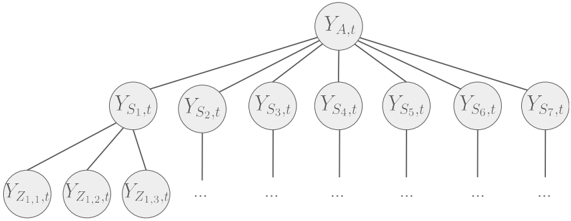<details> <summary>Image 55 Details</summary>  ### Visual Description \n ## Diagram: Hierarchical Decomposition ### Overview The image depicts a hierarchical decomposition diagram, likely representing a model or system broken down into its constituent parts. It shows a top-level node branching out into multiple intermediate nodes, which in turn branch out into further nodes. The diagram is purely schematic and does not contain numerical data. ### Components/Axes The diagram consists of interconnected nodes. The nodes are labeled with variables, indicating their role in the hierarchy. The labels are as follows: * **Top-level node:** Y_A,t * **Intermediate nodes:** Y_{S_1,t}, Y_{S_2,t}, Y_{S_3,t}, Y_{S_4,t}, Y_{S_5,t}, Y_{S_6,t}, Y_{S_7,t} * **Bottom-level nodes:** Y_{Z_1,1,d}, Y_{Z_1,2,d}, Y_{Z_1,3,d}, and so on (indicated by "...") The subscripts indicate different dimensions or indices: * 'A' likely represents a category or aspect. * 't' likely represents time. * 'S_i' likely represents sub-components or segments (i = 1 to 7). * 'Z_i,j' likely represents further sub-components or details (i = 1, j = 1 to 3 and beyond). * 'd' likely represents another dimension or detail level. The diagram uses directed arrows to show the flow or dependency from parent nodes to child nodes. ### Detailed Analysis or Content Details The diagram shows a single top-level node (Y_A,t) connected to seven intermediate nodes (Y_{S_1,t} through Y_{S_7,t}). Each of these intermediate nodes is connected to at least three bottom-level nodes (Y_{Z_1,1,d} through Y_{Z_1,3,d}), with the indication that this pattern continues ("..."). The structure suggests a hierarchical decomposition where the top-level variable is broken down into seven sub-variables, and each of those is further broken down into multiple components. The "..." notation indicates that the decomposition continues beyond the explicitly shown nodes. ### Key Observations The diagram is symmetrical in terms of the number of intermediate nodes (seven). The bottom-level nodes are shown with only a few examples, suggesting a potentially large number of such nodes for each intermediate node. The diagram does not provide any quantitative information; it is purely structural. ### Interpretation This diagram likely represents a model where a system or variable (Y_A,t) is decomposed into its constituent parts. The hierarchical structure suggests that the system can be understood by analyzing its components at different levels of detail. The time index 't' suggests that the model is dynamic and considers changes over time. The 'd' index in the bottom-level nodes could represent different dimensions or aspects of those components. The diagram could be used in various fields, such as: * **Economics:** Decomposing aggregate demand (Y_A,t) into its components (consumption, investment, government spending, etc.). * **Engineering:** Breaking down a complex system into its subsystems. * **Statistics:** Representing a hierarchical model where variables are nested within each other. * **Machine Learning:** Representing a decision tree or a hierarchical clustering structure. The diagram's simplicity suggests it is a conceptual representation rather than a detailed implementation. It serves to illustrate the hierarchical relationships between the variables without providing specific values or equations. The use of subscripts indicates that the variables are indexed by different dimensions, allowing for a more nuanced representation of the system. </details> The goal of hierarchical forecasting is to take advantage of the summation constraints defined by S to improve the predictions of the vector Y representing all hierarchical nodes. This context can be easily generalized to many time series forecasting tasks. Spatial summation constraints, which divide a geographic space into different subspaces, have been applied in areas such as electricity demand forecasting [BH22b], electric vehicle charging demand forecasting [AO+24], and tourism forecasting [WAH19]. Summation constraints also arise in multi-horizon forecasting, where, for example, an annual forecast must equal the sum of the corresponding monthly forecasts [KA19]. Finally, they also appear when goods are categorized into different groups [Pv17]. There are two main approaches to hierarchical forecasting. The first, known as forecast reconciliation, attempts to improve an existing estimator ˆ Y of the hierarchical nodes Y by multiplying ˆ Y by a so-called reconciliation matrix P , so that the new estimator P ˆ Y satisfies the summation constraints. Formally, it is required that Im( P ) ⊆ Im( S ) , where S is the summation matrix. The goal is for P ˆ Y to have less error than ˆ Y . The strengths of this approach are its low computational cost and its ability to seamlessly integrate with pre-existing forecasts. Various reconciliation matrices, such as the orthogonal projection P = S ( S /latticetop S ) -1 S on Im( S ) (see the paragraph above on linear constraints), have been shown to reduce forecasting errors and to even be optimal under certain assumptions [WAH19]. Another complementary approach is to incorporate the hierarchical structure of the problem directly into the training of the initial estimator ˆ Y [Ran+21]. While this method is more computationally intensive, it provides a more comprehensive solution than reconciliation methods because it uses the hierarchy not only to shape the regression function, but also to inform the learning of its parameters. In this paper, we build on this approach to design three new estimators, all of which are implemented in Section 7.4. As for now, we denote by /lscript 1 the total number of nodes and /lscript 2 ≤ /lscript 1 the number of bottom nodes. Thus, Y = ( Y /lscript ) /latticetop 1 ≤ /lscript ≤ /lscript 1 represents the global vector of all nodes, while Y b = ( Y /lscript ) /latticetop 1 ≤ /lscript ≤ /lscript 2 represents the vector of the bottom nodes. The /lscript 1 × /lscript 2 summation matrix S is defined so that, for all time index t , the summation identity Y t = SY b,t is satisfied. Estimator 1. Bottom-up approach: WeaKL-BU. In the bottom-up approach, models are fitted only for the bottom-level series Y b , resulting in a vector of estimators ˆ Y b . The remaining levels are then estimated by ˆ Y = S ˆ Y b , where S is the summation matrix. To achieve this, forecasts for each bottom node 1 ≤ /lscript ≤ /lscript 2 are constructed using a set of explanatory variables X /lscript ∈ R d /lscript specific to that node. Together, these explanatory variables X 1 , . . . , X /lscript 2 form the feature X ∈ R d 1 + ··· + d /lscript 2 . A straightforward choice of features are the lags of the target variable, i.e., X /lscript,t = Y /lscript,t -1 , though many other choices are possible. Next, for each bottom node 1 ≤ /lscript ≤ /lscript 2 , we fit a parametric model f θ /lscript ( X /lscript,t ) to predict the series Y /lscript,t . Each function f θ /lscript is parameterized by a mapping φ /lscript (e.g., a Fourier map or an additive model) and a coefficient vector θ /lscript , such that f θ /lscript ( X /lscript,t ) = 〈 φ /lscript ( X /lscript,t ) , θ /lscript 〉 . Therefore, the model for the lower nodes Y b,t can be expressed as Φ t θ , where θ = ( θ 1 , . . . , θ /lscript 2 ) /latticetop is the vector of all coefficients, and Φ t is the feature matrix at time t defined in (7.4). Overall, the model for all levels Y t = SY b,t is S Φ t θ , and the empirical risk corresponding to this problem is given by $$L ( \theta ) = \frac { 1 } { n } \sum _ { j = 1 } ^ { n } \| \Lambda ( S \Phi _ { t _ { j } } \theta - Y _ { t _ { j } } ) \| _ { 2 } ^ { 2 } + \| M \theta \| _ { 2 } ^ { 2 } ,$$ where Λ is a /lscript 1 × /lscript 1 diagonal matrix with positive coefficients, and M is a penalty matrix that depends on the φ /lscript mappings, as in Section 7.3. Since Λ scales the relative importance of each node in the learning process, the choice of its coefficients plays a critical role in the performance of the estimator. In the experimental Section 7.4, Λ will be learned through hyperparameter tuning. Typically, Λ /lscript,/lscript should be large when Var( Y /lscript | X /lscript ) is low-that is, the more reliable Y /lscript is as a target [WAH19]. From (7.4), we deduce that the minimizer ˆ θ of the empirical risk is $$\hat { \theta } = \left ( \left ( \sum _ { j = 1 } ^ { n } \Phi _ { t _ { j } } ^ { * } S ^ { * } \Lambda ^ { * } \Lambda S \Phi _ { t _ { j } } \right ) + n M ^ { * } M \right ) ^ { - 1 } \sum _ { j = 1 } ^ { n } \Phi _ { t _ { j } } ^ { * } \Lambda ^ { * } \Lambda Y _ { t _ { j } } .$$ We call ˆ θ the WeaKL-BU. Setting Λ = I /lscript 1 , i.e., the identity matrix, results in treating all hierarchical levels equally, which is the setup of Rangapuram et al. [Ran+21]. On the other hand, setting Λ /lscript,/lscript = 0 for all /lscript ≥ /lscript 2 leads to learning each bottom node independently, without using any information from the hierarchy. This is the traditional bottom-up approach. Estimator 2. Global hierarchy-informed approach: WeaKL-G. The context is similar to the bottom-up approach, but here models are fitted for all nodes 1 ≤ /lscript ≤ /lscript 1 , using local explanatory variables X /lscript ∈ R d /lscript , where d /lscript ≥ 1 . Thus, the model for Y t is given by Φ t θ , where θ = ( θ 1 , . . . , θ /lscript 1 ) /latticetop is the vector of coefficients and Φ t is the feature matrix at time t defined in (7.4). To ensure that the hierarchy is respected, we introduce a penalty term: $$\| \Gamma ( S \Pi _ { b } \Phi _ { t } \theta - \Phi _ { t } \theta ) \| _ { 2 } ^ { 2 } = \| \Gamma ( S \Pi _ { b } - I _ { \ell _ { 1 } } ) \Phi _ { t } \theta \| _ { 2 } ^ { 2 } ,$$ where Γ is a positive diagonal matrix and Π b is the projection operator on the bottom level, defined as Π b θ = ( θ 1 , . . . , θ /lscript 2 ) /latticetop . As in the bottom-up case, Γ encodes the level of trust assigned to each node. In Section 7.4, we learn Γ through hyperparameter tuning. This results in the empirical risk $$L ( \theta ) = \frac { 1 } { n } \sum _ { j = 1 } ^ { n } \| \Phi _ { t _ { j } } \theta - Y _ { t _ { j } } \| _ { 2 } ^ { 2 } + \frac { 1 } { n } \sum _ { j = 1 } ^ { n } \| \Gamma ( S \Pi _ { b } - I _ { \ell _ { 1 } } ) \Phi _ { t _ { j } } \theta \| _ { 2 } ^ { 2 } + \| M \theta \| _ { 2 } ^ { 2 } .$$ where M is a penalty matrix that depends on the φ /lscript mappings, as in Section 7.3. This empirical risk is similar to the one proposed by Zheng et al. [Zhe+23], where a penalty term is used to enforce hierarchical coherence during the learning process. From (7.4), we deduce that the minimizer is given by $$\hat { \theta } = \left ( \sum _ { j = 1 } ^ { n } ( \Phi _ { t _ { j } } ^ { * } \Phi _ { t _ { j } } + \mathbb { F } _ { t _ { j } } ^ { * } ( \Pi _ { b } ^ { * } S ^ { * } - I _ { \ell _ { 1 } } ) \Gamma ^ { * } \Gamma ( S \Pi _ { b } - I _ { \ell _ { 1 } } ) \Phi _ { t _ { j } } ) + n M ^ { * } M \right ) ^ { - 1 } \sum _ { j = 1 } ^ { n } \Phi _ { t _ { j } } ^ { * } Y _ { t } .$$ We refer to ˆ θ as the WeaKL-G. The fundamental difference between (7.10) and (7.11) is that the WeaKL-BU estimator only learns parameters for the /lscript 2 bottom nodes, whereas the WeaKLG estimators learns parameters for all nodes. We emphasize that WeaKL-BU and WeaKL-G follow different approaches. While WeaKL-BU adjusts the lower-level nodes and then uses the summation matrix S to estimate the higher levels, WeaKL-G relies directly on global information, which is subsequently penalized by S . In the next paragraph, we complement the WeaKL-BU estimator by adding transfer learning constraints. Estimator 3. Hierarchy-informed transfer learning: WeaKL-T. In many hierarchical forecasting applications, the targets Y /lscript are of the same nature throughout the hierarchy. Consequently, we often expect them to be explained by similar explanatory variables X /lscript and to have similar regression functions estimators f ˆ θ /lscript [e.g., Lep+23]. For this reason, we propose an algorithm that combines WeaKL-BU with transfer learning. Therefore, we assume that there is a subset J ⊆ { 1 , . . . , /lscript 2 } of similar nodes and weights ( α i ) i ∈ J such that we expect α i f ˆ θ i ( X i,t ) /similarequal α j f ˆ θ j ( X j,t ) for i, j ∈ J . In particular, there is an integer D such that θ j ∈ C D for all j ∈ J . Therefore, denoting by Π J the projection on J such that Π J θ = ( θ j ) j ∈ J ∈ C D | J | , this translates into the constraint that Π J θ ∈ Im( M J ) where M J = ( α 1 I D , . . . , α | J | I D ) /latticetop . As explained in the paragraph on linear constraints, we enforce this inexact constraint by penalizing the empirical risk with the addition of the term ‖ (I D | J | -P J )Π J θ ‖ 2 2 , where P J = M J ( M ∗ J M J ) -1 M ∗ J is the orthogonal projection onto the image of M J . This leads to the empirical risk $$L ( \theta ) = \frac { 1 } { n } \sum _ { j = 1 } ^ { n } \| \Lambda ( S \Phi _ { t _ { j } } \theta - Y _ { t _ { j } } ) \| _ { 2 } ^ { 2 } + \lambda \| ( I _ { D | J | } - P _ { J } ) \Pi _ { J } \theta \| _ { 2 } ^ { 2 } + \| M \theta \| _ { 2 } ^ { 2 } ,$$ where M is a penalty matrix that depends on the φ /lscript mappings, as in Section 7.3. We call WeaKL-T the minimizer ˆ θ of L . It is given by $$\hat { \theta } = \left ( \left ( \sum _ { j = 1 } ^ { n } \Phi _ { t _ { j } } ^ { * } S ^ { * } \Lambda ^ { * } \Lambda S \Phi _ { t _ { j } } \right ) + n \lambda \Pi _ { J } ^ { * } ( I _ { D | J | } - P _ { J } ) \Pi _ { J } + n M ^ { * } M \right ) ^ { - 1 } \sum _ { j = 1 } ^ { n } \Phi _ { t _ { j } } ^ { * } \Lambda ^ { * } \Lambda Y _ { t _ { j } } .$$ ## Application to tourism forecasting Hierarchical forecasting and tourism. In this experiment, we aim to forecast Australian domestic tourism using the dataset from Wickramasuriya et al. [WAH19]. The dataset includes monthly measures of Australian domestic tourism from January 1998 to December 2016, resulting in n = 216 data points. Each month, domestic tourism is measured at four spatial levels and one categorical level, forming a five-level hierarchy. At the top level, tourism is measured for Australia as a whole. It is then broken down spatially into 7 states, 27 zones, and 76 regions. Then, for each of the 76 regions, four categories of tourism are distinguished according to the purpose of travel: holiday, visiting friends and relatives (VFR), business, and other. This gives a total of five levels (Australia, states, zones, regions, and categories), with /lscript 2 = 76 × 4 = 304 bottom nodes, and /lscript 1 = 1 + 7 + 27 + 76 + /lscript 2 = 415 total nodes. Benchmark. The goal is to forecast Australian domestic tourism one month in advance. Models are trained on the first 80% of the dataset and evaluated on the last 20% . Similar to Wickramasuriya et al. [WAH19], we only consider autoregressive models with lags from one month to two years. This setting is particularly interesting because, although each time series can be reasonably fitted using the 216 data points, the total number of targets /lscript 1 exceeds n . Consequently, the higher levels cannot be naively learned from the lags of the bottom level time series through linear regression. The bottom-up (BU) model involves running 304 linear regressions ˆ Y BU /lscript,t = ∑ 24 j =1 a /lscript,j Y /lscript,t -j for 1 ≤ /lscript ≤ /lscript 2 , where Y /lscript,t -j is the lag of Y /lscript,t by j months. The final forecast is then computed as ˆ Y BU t = S ˆ Y BU /lscript,t , where S is the summation matrix. The Independent (Indep) model involves running separate linear regressions for each target time series using its own lags. This results in 415 linear regressions of the form ˆ Y Indep /lscript,t = ∑ 24 j =1 a /lscript,j Y /lscript,t -j for 1 ≤ /lscript ≤ /lscript 1 . Rec-OLS is the estimator resulting from OLS adjustment of the Indep estimator, i.e., taking P = S ( S ∗ S ) -1 S [WAH19]. MinT refers to the estimator derived from the minimum trace adjustment of the Indep estimator [see MinT(shrinkage) in WAH19]. PIKL-BU refers to the estimator (7.10), where, for all 1 ≤ /lscript ≤ 304 , X /lscript,t = ( Y /lscript,t -j ) 1 ≤ j ≤ 24 and φ /lscript ( x ) = x . PIKL-G is the estimator (7.11), where, for all 1 ≤ /lscript ≤ 415 , X /lscript,t = ( Y /lscript,t -j ) 1 ≤ j ≤ 24 and φ /lscript ( x ) = x . Finally, PIKL-T is the estimator (7.12), where X /lscript,t = ( Y /lscript,t -j ) 1 ≤ j ≤ 24 and φ /lscript ( x ) = x . In the latter model, all the auto-regressive effects are penalized to enforce uniform weights, which means that α /lscript = 1 and J = { 1 , . . . , /lscript 2 } in (7.12). The hyperparameter tuning process to learn the matrix Λ for the WeaKLs is detailed in Appendix 7.D. Results. Table 7.3 shows the results of the experiment. The mean square errors (MSE) are computed for each hierarchical level and aggregated under All levels. Their standard deviations are estimated using block bootstrap with blocks of length 12 . The models are categorized based on the features they utilize. We observe that the WeaKL-type estimators consistently outperform all other competitors in every case. This highlights the advantage of incorporating constraints to enforce the hierarchical structure of the problem, leading to an improved learning process. Tab. 7.3.: Benchmark in forecasting Australian domestic tourism | | ( × 10 6 ) | ( × 10 6 ) | ( × 10 6 ) | ( × 10 6 ) | ( × 10 6 ) | ( × 10 6 ) | |------------------|---------------|---------------|-----------------|-----------------|-----------------|----------------| | | Australia | States | Zones | Regions | Categories | All levels | | Bottom data BU | 5 . 3 ± 0 . 5 | 2 . 0 ± 0 . 2 | 1 . 37 ± 0 . 05 | 1 . 19 ± 0 . 02 | 1 . 17 ± 0 . 03 | 11 . 0 ± 0 . 7 | | WeaKL-BU | 4 . 5 ± 0 . 5 | 1 . 9 ± 0 . 3 | 1 . 34 ± 0 . 05 | 1 . 19 ± 0 . 03 | 1 . 17 ± 0 . 03 | 10 . 1 ± 0 . 6 | | Own lags Indep | 3 . 6 ± 0 . 6 | 1 . 8 ± 0 . 2 | 1 . 42 ± 0 . 05 | 1 . 23 ± 0 . 03 | 1 . 17 ± 0 . 03 | 9 . 2 ± 0 . 7 | | WeaKL-G | 3 . 6 ± 0 . 5 | 1 . 8 ± 0 . 2 | 1 . 37 ± 0 . 05 | 1 . 18 ± 0 . 03 | 1 . 15 ± 0 . 03 | 9 . 0 ± 0 . 7 | | All data Rec-OLS | 3 . 5 ± 0 . 5 | 1 . 8 ± 0 . 2 | 1 . 35 ± 0 . 05 | 1 . 18 ± 0 . 02 | 1 . 17 ± 0 . 03 | 8 . 9 ± 0 . 7 | | MinT | 3 . 6 ± 0 . 4 | 1 . 7 ± 0 . 1 | 1 . 29 ± 0 . 05 | 1 . 15 ± 0 . 03 | 1 . 17 ± 0 . 03 | 8 . 9 ± 0 . 5 | | WeaKL-T | 3 . 1 ± 0 . 3 | 1 . 7 ± 0 . 1 | 1 . 27 ± 0 . 05 | 1 . 15 ± 0 . 02 | 1 . 12 ± 0 . 03 | 8 . 3 ± 0 . 4 | ## 7.5 Conclusion In this paper, we have shown how to design empirical risk functions that integrate common linear constraints in time series forecasting. For modeling purposes, we distinguish between shape constraints (such as additive models, online adaptation after a break, and forecast combinations) and learning constraints (including transfer learning, hierarchical forecasting, and differential constraints). These empirical risks can be efficiently minimized on a GPU, leading to the development of an optimized algorithm, which we call WeaKL. We have applied WeaKL to three real-world use cases-two in electricity demand forecasting and one in tourism forecasting-where it consistently outperforms current state-of-the-art methods, demonstrating its effectiveness in structured forecasting problems. Future research could explore the integration of additional constraints into the WeaKL framework. For example, the current approach does not allow for forcing the regression function f θ to be non-decreasing or convex. However, since any risk function L of the form (7.2) is convex in θ , the problem can be formulated as a linearly constrained quadratic program. While this generally increases the complexity of the optimization, it can also lead to efficient algorithms for certain constraints. In particular, when d = 1 , imposing a non-decreasing constraint on f θ reduces the problem to isotonic regression, which has a computational complexity of O ( n ) [WW80]. ## 7.A Proofs The purpose of this appendix is to provide detailed proofs of the theoretical results presented in the main article. Appendix 7.A elaborates on the formula that characterizes the unique minimizer of the WeaKL empirical risks, while Appendix 7.A discusses the integration of linear constraints into the empirical risk framework. ## A useful lemma Lemma 7.A.1 (Full rank) . The matrix $$\tilde { M } = \frac { 1 } { n } \left ( \sum _ { j = 1 } ^ { n } \Phi _ { t _ { j } } ^ { * } \Lambda ^ { * } \Lambda \Phi _ { t _ { j } } \right ) + M ^ { * } M$$ is invertible. Moreover, for all θ ∈ C dim θ , θ /star ˜ Mθ ≥ λ min ( ˜ M ) ‖ θ ‖ 2 2 , where λ min ( ˜ M ) is the minimum eigenvalue of ˜ M . Proof. First, we note that ˜ M is a positive Hermitian square matrix. Hence, the spectral theorem guarantees that ˜ M is diagonalizable in an orthogonal basis of C dim( θ ) with real eigenvalues. In particular, it admits a positive square root, and the min-max theorem states that θ ∗ ˜ Mθ = ‖ ˜ M 1 / 2 θ ‖ 2 2 ≥ λ min ( ˜ M 1 / 2 ) 2 ‖ θ ‖ 2 2 = λ min ( ˜ M ) ‖ θ ‖ 2 2 . This shows the second statement of the lemma. Next, for all θ ∈ C dim θ , θ ∗ ˜ Mθ ≥ θ ∗ M ∗ Mθ . Since M is full rank, rank( M ) = dim( θ ) . Therefore, ˜ Mθ = 0 ⇒ θ ∗ ˜ Mθ = 0 ⇒ θ ∗ M ∗ Mθ = 0 ⇒ ‖ Mθ ‖ 2 2 = 0 ⇒ Mθ = 0 ⇒ θ = 0 . Thus, ˜ M is injective and, in turn, invertible. ## Proof of Proposition 7.2.1 The function L : C dim( θ ) → R + can be written as $$L ( \theta ) = \frac { 1 } { n } \left ( \sum _ { j = 1 } ^ { n } ( \Phi _ { t _ { j } } \theta - Y _ { t _ { j } } ) ^ { * } \Lambda ^ { * } \Lambda ( \Phi _ { t _ { j } } \theta - Y _ { t _ { j } } ) \right ) + \theta ^ { * } M ^ { * } M \theta .$$ Recall that the matrices Λ and M are assumed to be injective. Observe that L can be expanded as $$L ( \theta + \delta \theta ) = L ( \theta ) + 2 R e ( \langle \tilde { M } \theta - \tilde { Y } , \delta \theta \rangle ) + o ( \| \delta \theta \| _ { 2 } ^ { 2 } ) ,$$ where ˜ Y = 1 n ∑ n j =1 Φ ∗ t j Λ ∗ Λ Y t j . This shows that L is differentiable and that its differential at θ is the function dL θ : δθ ↦→ 2Re( 〈 ˜ Mθ -˜ Y , δθ 〉 ) . Thus, the critical points θ such that dL θ = 0 satisfy $$\forall \, \delta \theta \in \mathbb { C } ^ { d i m ( \theta ) } , \, R e ( \langle \tilde { M } \theta - \tilde { Y } , \delta \theta \rangle ) = 0 .$$ Taking δθ = ˜ Mθ -˜ Y shows that ‖ ˜ Mθ -˜ Y ‖ 2 2 = 0 , i.e., ˜ Mθ = ˜ Y . From Lemma 7.A.1, we deduce that θ = ˜ M -1 ˜ Y , which is exactly the ˆ θ n in (7.3). From Lemma 7.A.1, we also deduce that, for all θ such that ‖ θ ‖ 2 is large enough, one has L ( θ ) ≥ λ min ( ˜ M ) ‖ θ ‖ 2 2 / 2 . Since L is continuous, it has at least one global minimum. Since the unique critical point of L is ˆ θ n , we conclude that ˆ θ n is the unique minimizer of L . ## Orthogonal projection and linear constraints Lemma 7.A.2 (Orthogonal projection) . Let /lscript 1 , /lscript 2 ∈ N /star . Let P be an injective /lscript 1 × /lscript 2 matrix with coefficients in C . Then C = I /lscript 1 -P ( P ∗ P ) -1 P ∗ is the orthogonal projection on Im( P ) ⊥ , where Im( P ) is the image of P and I /lscript 1 is the /lscript 1 × /lscript 1 identity matrix. Proof. First, we show that P ∗ P is an /lscript 2 × /lscript 2 matrix of full rank. Indeed, for all x ∈ C /lscript 2 , one has P ∗ Px = 0 ⇒ x ∗ P ∗ Px = 0 ⇒ ‖ Px ‖ 2 2 = 0 . Since P is injective, we deduce that ‖ Px ‖ 2 2 = 0 ⇒ x = 0 . This means that ker P ∗ P = { 0 } , and so that P ∗ P is full rank. Therefore, ( P ∗ P ) -1 is well defined. Next, let C 1 = P ( P ∗ P ) -1 P ∗ . Clearly, C 2 1 = C 1 , i.e., C 1 is a projector. Since C ∗ 1 = C 1 , we deduce that C 1 is an orthogonal projector. In addition, since C 1 = P × (( P ∗ P ) -1 P ∗ ) , Im( C 1 ) ⊆ Im( P ) . Moreover, if x ∈ Im( P ) , there exists a vector z such that x = Pz , and C 1 x = P ( P ∗ P ) -1 P ∗ Pz = Pz = x . Thus, x ∈ Im( C 1 ) . This shows that Im( C 1 ) = Im( P ) . We conclude that C 1 is the orthogonal projection on Im( P ) and, in turn, that C = I /lscript 1 -C 1 is the orthogonal projection on Im( P ) ⊥ . The following proposition shows that, given the exact prior knowledge Cθ /star = 0 , enforcing the linear constraint Cθ = 0 almost surely improves the performance of WeaKL. Proposition 7.A.3 (Constrained estimators perform better.) . Assume that Y t = f θ /star ( X t )+ ε t and that θ /star satisfies the constraint Cθ /star = 0 , for some matrix C . (Note that we make no assumptions about the distribution of the time series ( X,ε ) .) Let Λ and M be injective matrices, and let λ ≥ 0 be a hyperparameter. Let ˆ θ be the WeaKL given by (7.3) and let ˆ θ C be the WeaKL obtained by replacing M with ( √ λC /latticetop | M /latticetop ) /latticetop in (7.3) . Then, almost surely, $$\frac { 1 } { n } \sum _ { j = 1 } ^ { n } \| f _ { \theta ^ { * } } ( X _ { t _ { j } } ) - f _ { \hat { \theta } _ { C } } ( X _ { t _ { j } } ) \| _ { 2 } ^ { 2 } + \| M ( \theta ^ { * } - \hat { \theta } _ { C } ) \| _ { 2 } ^ { 2 } \leq \frac { 1 } { n } \sum _ { j = 1 } ^ { n } \| f _ { \theta ^ { * } } ( X _ { t _ { j } } ) - f _ { \hat { \theta } } ( X _ { t _ { j } } ) \| _ { 2 } ^ { 2 } + \| M ( \theta ^ { * } - \hat { \theta } ) \| _ { 2 } ^ { 2 } .$$ Proof. Recall from (7.3) that $$\hat { \theta } = P ^ { - 1 } \sum _ { j = 1 } ^ { n } \Phi _ { t _ { j } } ^ { * } \Lambda ^ { * } \Lambda Y _ { t _ { j } } \quad a n d \quad \hat { \theta } _ { C } = \left ( P + \lambda n C ^ { * } C \right ) ^ { - 1 } \sum _ { j = 1 } ^ { n } \Phi _ { t _ { j } } ^ { * } \Lambda ^ { * } \Lambda Y _ { t _ { j } } ,$$ where P = ( ∑ n j =1 Φ ∗ t j Λ ∗ Λ Φ t j ) + nM ∗ M . Since Cθ /star = 0 , we see that $$\theta ^ { ^ { * } } = \left ( P + \lambda n C ^ { * } C \right ) ^ { - 1 } P \theta ^ { ^ { * } } .$$ Subtracting (7.13) to, respectively, ˆ θ and ˆ θ C , we obtain $$\theta ^ { ^ { * } } - \hat { \theta } = P ^ { - 1 / 2 } \Delta \quad a n d \quad \theta ^ { ^ { * } } - \hat { \theta } _ { C } = \left ( P + \lambda n C ^ { * } C \right ) ^ { - 1 } P ^ { 1 / 2 } \Delta ,$$ where $$\Delta = P ^ { - 1 / 2 } \left ( P \theta ^ { ^ { * } } - \sum _ { j = 1 } ^ { n } \Phi _ { t _ { j } } ^ { * } \Lambda ^ { * } \Lambda Y _ { t _ { j } } \right ) .$$ Moreover, according to the Loewner order [see, e.g., HJ12, Chapter 7.7], we have that P -1 / 2 C ∗ CP -1 / 2 ≥ 0 and ( P -1 / 2 C ∗ CP -1 / 2 ) 2 ≥ 0 . (Indeed, since P is Hermitian, so is P -1 / 2 C ∗ CP -1 / 2 .) Therefore, (I+ λnP -1 / 2 C ∗ CP -1 / 2 ) 2 ≥ I and (I+ λnP -1 / 2 C ∗ CP -1 / 2 ) -2 ≤ I [see, e.g., HJ12, Corollary 7.7.4]. Consequently, $$\| P ^ { 1 / 2 } ( \theta ^ { * } - \hat { \theta } _ { C } ) \| _ { 2 } ^ { 2 } = \Delta ^ { * } \left ( I + \lambda n P ^ { - 1 / 2 } C ^ { * } C P ^ { - 1 / 2 } \right ) ^ { - 2 } \Delta \leq \| \Delta \| _ { 2 } ^ { 2 } = \| P ^ { 1 / 2 } ( \theta ^ { * } - \hat { \theta } ) \| _ { 2 } ^ { 2 } .$$ Observing that ‖ P 1 / 2 ( θ /star -ˆ θ C ) ‖ 2 2 = 1 n ∑ n j =1 ‖ f θ /star ( X t j ) -f ˆ θ C ( X t j ) ‖ 2 2 + ‖ M ( θ /star -ˆ θ C ) ‖ 2 2 and ‖ P 1 / 2 ( θ /star -ˆ θ ) ‖ 2 2 = 1 n ∑ n j =1 ‖ f θ /star ( X t j ) -f ˆ θ ( X t j ) ‖ 2 2 + ‖ M ( θ /star -ˆ θ ) ‖ 2 2 concludes the proof. Remark 7.A.4. Taking the limit λ → ∞ in Proposition 7.A.3 does not affect the result and corresponds to restricting the parameter space to ker( C ) , meaning that, in this case, C ˆ θ C = 0 . Note also that the proposition is extremely general, as it holds almost surely without requiring any assumptions on either X or ε . Here, the error of ˆ θ is measured by $$\frac { 1 } { n } \sum _ { j = 1 } ^ { n } \| f _ { \theta ^ { * } } ( X _ { t _ { j } } ) - f _ { \hat { \theta } } ( X _ { t _ { j } } ) \| _ { 2 } ^ { 2 } + \| M ( \theta ^ { ^ { * } } - \hat { \theta } ) \| _ { 2 } ^ { 2 } ,$$ which quantifies both the error of ˆ θ at the points X t j and in the M norm. Under additional assumptions on X and ε , this discretized risk can be shown to converge to the L 2 error, E ‖ f θ /star ( X ) -f ˆ θ ( X ) ‖ 2 2 , using Dudley's theorem [see, e.g., Theorem 5.2 in the Supplementary Material of DBB25]. However, the rate of this convergence of ˆ θ to θ /star depends on the properties of C and M , as well as the growth of dim( θ ) with n . For instance, when the penalty matrix M encodes a PDE prior, the analysis becomes particularly challenging and remains an open question in physics-informed machine learning. Therefore, we leave the study of this convergence outside the scope of this article. ## 7.B More WeaKL models ## Forecast combinations To forecast a time series Y , different models can be used, each using different implementations and sets of explanatory variables. Let p be the number of models and let ˆ Y 1 t , . . . , ˆ Y p t be the respective estimators of Y t . The goal is to determine the optimal weighting of these forecasts, based on their performance evaluated over the time points t 1 ≤ · · · ≤ t n . Therefore, in this setting, X t = ( t, ˆ Y 1 t , . . . , ˆ Y p t ) , and the goal is to find the optimal function linking X t to Y t . Note that, to avoid overfitting, we assume that the forecasts ˆ Y 1 t , . . . , ˆ Y p t were trained on time steps before t 1 . This approach is sometimes referred to as the online aggregation of experts [Rem+23; Ant+24]. Such forecast combinations are widely recognized to significantly improve the performance of the final forecast [Tim06; VG22; Pet+22; AO+24], as they leverage the strengths of the individual predictors. Formally, this results in the model $$f _ { \theta } ( X _ { t } ) = \sum _ { \ell = 1 } ^ { p } ( p ^ { - 1 } + h _ { \theta _ { \ell } } ( t ) ) \hat { Y } _ { t } ^ { \ell } ,$$ where h θ /lscript ( t ) = 〈 φ ( t ) , θ /lscript 〉 , φ is the Fourier map φ ( t ) = (exp( ikt/ 2)) /latticetop -m ≤ k ≤ m , and θ /lscript ∈ C 2 m +1 . The p -1 term introduces a bias, ensuring that h θ /lscript = 0 corresponds to a uniform weighting of the forecasts ˆ Y /lscript . The function f /star is thus estimated by minimizing the loss $$L ( \theta ) = \frac { 1 } { n } \sum _ { j = 1 } ^ { n } \left | \left ( \sum _ { \ell = 1 } ^ { p } ( p ^ { - 1 } + h _ { \theta _ { \ell } } ( t _ { j } ) ) \hat { Y } _ { t _ { j } } ^ { \ell } \right ) - Y _ { t _ { j } } \right | ^ { 2 } + \sum _ { \ell = 1 } ^ { p } \lambda _ { \ell } \| h _ { \theta _ { \ell } } \| _ { H ^ { s } } ^ { 2 } ,$$ where λ /lscript > 0 are hyperparameters. Again, a common choice for the smoothing parameter is to set s = 2 . Let φ 1 ( X t ) = (( ˆ Y /lscript t exp( ikt/ 2)) -m ≤ k ≤ m ) p /lscript =1 ) /latticetop ∈ C (2 m +1) p . The Fourier coefficients that minimize the empirical risk are given by $$\hat { \theta } = ( \Phi ^ { * } \Phi + n M ^ { * } M ) ^ { - 1 } \Phi ^ { * } \mathbb { W } ,$$ where W = ( W t 1 , . . . , W t n ) /latticetop is such that W t = Y t -p -1 ∑ p /lscript =1 ˆ Y /lscript t , $$M = \begin{pmatrix} \sqrt { \lambda _ { 1 } } D & 0 & 0 \\ 0 & \ddots & 0 \\ 0 & 0 & \sqrt { \lambda _ { d _ { 1 } } } D \end{pmatrix} ,$$ and D is the (2 m +1) × (2 m +1) diagonal matrix D = Diag(( √ 1 + k 2 s ) -m ≤ k ≤ m ) . ## Differential constraints As discussed in the introduction, some time series obey physical laws and can be expressed as solutions of PDEs. Physics-informed kernel learning (PIKL) is a kernel-based method developed by Doumèche et al. [Dou+24b] to incorporate such PDEs as constraints. It can be regarded as a specific instance of the WeaKL framework proposed in this paper. In effect, given a bounded Lipschitz domain Ω and a linear differential operator D , using the model f θ ( x ) = 〈 φ ( x ) , θ 〉 , where φ ( x ) = (exp( i 〈 x, k 〉 / 2)) ‖ k ‖ ∞ ≤ m is the Fourier map and θ represents the Fourier coefficients, the PIKL approach shows how to construct a matrix M such that $$\int _ { \Omega } \mathcal { D } ( f _ { \theta } , u ) ^ { 2 } \, d u = \| M \theta \| _ { 2 } ^ { 2 } .$$ Thus, to incorporate the physical prior ∀ x ∈ Ω , D ( f /star , x ) = 0 into the learning process, the empirical risk takes the form $$L ( \theta ) = \frac { 1 } { n } \sum _ { i = 1 } ^ { n } | f _ { \theta } ( X _ { t _ { i } } ) - Y _ { t _ { i } } | ^ { 2 } + \lambda \int _ { \Omega } \mathcal { D } ( f _ { \theta } , u ) ^ { 2 } \, d u = \frac { 1 } { n } \sum _ { i = 1 } ^ { n } | f _ { \theta } ( X _ { t _ { i } } ) - Y _ { t _ { i } } | ^ { 2 } + \| \sqrt { \lambda } M \theta \| _ { 2 } ^ { 2 } ,$$ where λ > 0 is a hyperparameter. From (7.5) it follows that the minimizer of the empirical risk is ˆ θ = ( Φ ∗ Φ + nM ) -1 Φ ∗ Y . It is shown in Doumèche et al. [Dou+24a] that, as n → ∞ , f ˆ θ converges to f /star under appropriate assumptions. Moreover, incorporating the differential constraint improves the learning process; in particular, f ˆ θ converges to f /star faster when λ > 0 . ## 7.C A toy-example of hierarchical forecasting Setting. We evaluate the performance of WeaKL on a simple but illustrative hierarchical forecasting task. In this simplified setting, we want to forecast two random variables, Y 1 and Y 2 , defined as follows: $$Y _ { 1 } = \langle X _ { 1 } , \theta _ { 1 } \rangle + \varepsilon _ { 1 } , \quad Y _ { 2 } = \langle X _ { 2 } , \theta _ { 2 } \rangle - \varepsilon _ { 1 } + \varepsilon _ { 2 } ,$$ where X 1 , X 2 , ε 1 , and ε 2 are independent. The feature vectors are X 1 ∼ N (0 , I d ) and X 2 ∼ N (0 , I d ) , with d ∈ N /star . The noise terms follow Gaussian distributions ε 1 ∼ N (0 , σ 2 1 ) and ε 2 ∼ N (0 , σ 2 2 ) , with σ 1 , σ 2 > 0 . Note that the independence assumption aims at simplifying the analysis in this toy-example by putting the emphasis on the impact of the hierarchical constraints rather than on the autocorrelation of the signal, though in practice this assumption is unrealistic for most time series. This is why we will develop a use case of hierarchical forecasting with real-world time series in Section 7.4. What distinguishes this hierarchical prediction setting is the assumption that σ 1 ≥ σ 2 . Consequently, conditional on X 1 and X 2 , the sum Y 1 + Y 2 = 〈 X 1 , θ 1 〉 + 〈 X 2 , θ 2 〉 + ε 2 has a lower variance than either Y 1 or Y 2 . We assume access to n i.i.d. copies ( X 1 ,i , X 2 ,i , Y 1 ,i , Y 2 ,i ) n i =1 of the random variables ( X 1 , X 2 , Y 1 , Y 2 ) . The goal is to construct three estimators ˆ Y 1 , ˆ Y 2 , and ˆ Y 3 of Y 1 , Y 2 , and Y 3 := Y 1 + Y 2 . Benchmark. We compare four techniques. The bottom-up (BU) approach involves running two separate ordinary least squares (OLS) regressions that independently estimate Y 1 and Y 2 without using information about Y 1 + Y 2 . Specifically, $$\hat { Y } _ { 1 } ^ { B U } = \langle X _ { 1 } , \hat { \theta } _ { 1 } ^ { B U } \rangle , \quad \hat { Y } _ { 2 } ^ { B U } = \langle X _ { 2 } , \hat { \theta } _ { 2 } ^ { B U } \rangle ,$$ where the OLS estimators are $$\hat { \theta } _ { 1 } ^ { B U } = ( \mathbb { X } _ { 1 } ^ { \top } \mathbb { X } _ { 1 } ) ^ { - 1 } \mathbb { X } _ { 1 } ^ { \top } \mathbb { Y } _ { 1 } , \quad \hat { \theta } _ { 2 } ^ { B U } = ( \mathbb { X } _ { 2 } ^ { \top } \mathbb { X } _ { 2 } ) ^ { - 1 } \mathbb { X } _ { 2 } ^ { \top } \mathbb { Y } _ { 2 } .$$ Here, X 1 = ( X 1 , 1 | · · · | X 1 ,n ) /latticetop and X 2 = ( X 2 , 1 | · · · | X 2 ,n ) /latticetop are n × d matrices, while Y 1 = ( Y 1 , 1 , . . . , Y 1 ,n ) /latticetop and Y 2 = ( Y 2 , 1 , . . . , Y 2 ,n ) /latticetop are vectors of R n . To estimate Y 3 , we simply $$\begin{array} { r } { s e t \hat { Y } _ { 3 } ^ { B U } = \hat { Y } _ { 1 } ^ { B U } + \hat { Y } _ { 2 } ^ { B U } . } \end{array}$$ The Reconciliation (Rec) approach involves running three independent forecasts of Y 1 , Y 2 , and Y 3 , followed by using the constraint that the updated estimator ˆ Y Rec 3 should be the sum of ˆ Y Rec 1 and ˆ Y Rec 2 [WAH19]. To estimate Y 3 , we run an OLS regression with X = ( X 1 | X 2 ) and Y = Y 1 + Y 2 . In this approach, $$\begin{array} { r } { \left ( \hat { Y } _ { 3 , t } ^ { R e c } \right ) _ { \substack { \\ \hat { Y } _ { 1 , t } ^ { R e c } } } = S ( S ^ { T } S ) ^ { - 1 } S ^ { T } \left ( \begin{array} { r } { \langle X _ { t } , ( \mathbb { K } ^ { \top } \mathcal { K } ) ^ { - 1 } \mathbb { K } ^ { \top } \mathbb { Y } \rangle } \\ { \langle X _ { 1 , t } , \hat { \theta } _ { 1 } ^ { B U } \rangle } \\ { \langle X _ { 2 , t } , \hat { \theta } _ { 2 } ^ { B U } \rangle } \end{array} \right ) , } \end{array}$$ $$\text {with } S = \begin{pmatrix} 1 & 1 \\ 1 & 0 \\ 0 & 1 \end{pmatrix} \, a n d \, X _ { t } = ( X _ { 1 , t } | X _ { 2 , t } ) .$$ The Minimum Trace (MinT) approach is an alternative update method that replaces the update matrix S ( S /latticetop S ) -1 S T with S ( J -JWU ( U /latticetop WU ) -1 U /latticetop ) , J = ( 0 1 0 0 0 1 ) , W the 3 × 3 covariance matrix of the prediction errors on the training data, and U = ( -1 1 1 ) /latticetop [WAH19]. This approach extends the linear projection onto Im( S ) and better accounts for correlations in the noise of the time series. Finally, we apply the WeaKL-BU estimator (7.10) with M = 0 , φ 1 ( x ) = x , φ 2 ( x ) = x , and Λ = Diag(1 , 1 , λ ) , where λ > 0 is a hyperparameter that controls the penalty on the joint prediction Y 1 + Y 2 . It minimizes the empirical loss $$L ( \theta _ { 1 } , \theta _ { 2 } ) = \frac { 1 } { n } \sum _ { i = 1 } ^ { n } | \langle X _ { 1 , i } , \theta _ { 1 } \rangle - Y _ { 1 , i } | ^ { 2 } + | \langle X _ { 2 , i } , \theta _ { 2 } \rangle - Y _ { 2 , i } | ^ { 2 } + \lambda | \langle X _ { 1 , i } , \theta _ { 1 } \rangle + \langle X _ { 1 , i } , \theta _ { 2 } \rangle - Y _ { 1 , i } - Y _ { 2 , i } | ^ { 2 } ,$$ In the experiments, we set λ = σ -2 2 for simplicity, although it can be easily learned by cross-validation. Monte Carlo experiment. To compare the performance of the different methods, we perform a Monte Carlo experiment. Since linear regression is invariant under multiplication by a constant, we set σ 1 = 1 without loss of generality. Since σ 2 ≤ σ 1 , we allow σ 2 to vary from 0 to 1 . For each value of σ 2 , we run 1000 Monte Carlo simulations, where each simulation uses n = 80 training samples and /lscript = 20 test samples. In each Monte Carlo run, we independently draw θ 1 ∼ N (0 , I d ) , θ 2 ∼ N (0 , I d ) , X 1 ,i ∼ N (0 , I d ) , X 2 ,i ∼ N (0 , I d ) , ε 1 ,i ∼ N (0 , 1) , and ε 2 ,i ∼ N (0 , σ 2 2 ) , where 1 ≤ i ≤ n . Note that, on the one hand, the L 2 error of an OLS regression on Y 1 + Y 2 is σ 2 2 (1 + 2 d/n ) , while on the other hand, the minimum possible L 2 error when fitting Y 1 + Y 2 is σ 2 2 . Thus, a large 2 d/n is necessary to observe the benefits of hierarchical prediction. To achieve this, we set d = 20 , resulting in 2 d/n = 0 . 5 . The models are trained on the n training data points, and their performance is evaluated on the /lscript test data points using the mean squared error (MSE). Given any estimator ( ˆ Y 1 , ˆ Y 2 , ˆ Y 3 ) of ( Y 1 , Y 2 , Y 1 + Y 2 ) , we compute the error /lscript -1 ∑ /lscript j =1 | Y 1 ,n + j -ˆ Y 1 ,n + j | 2 on Y 1 , the error /lscript -1 ∑ /lscript j =1 | Y 2 ,n + j -ˆ Y 2 ,n + j | 2 on Y 2 , and the error /lscript -1 ∑ /lscript j =1 | Y 1 ,n + j + Y 2 ,n + j -ˆ Y 3 ,n + j | 2 on Y 1 + Y 2 . The hierarchical error is defined as the sum of these three MSEs, which are visualized in Figure 7.4. Results. Figure 7.4 clearly shows that all hierarchical models (Rec, MinT, and WeaKL) outperform the naive bottom-up model for all four MSE metrics. 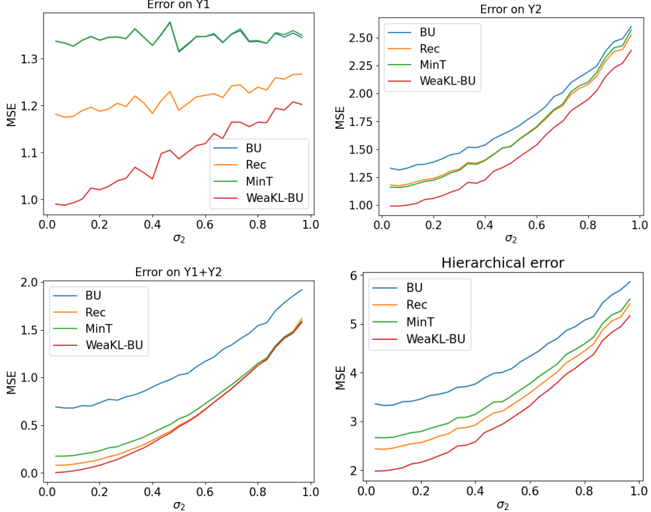Among them, our WeaKL <details> <summary>Image 56 Details</summary>  ### Visual Description \n ## Charts: Error Analysis with Noise Level ### Overview The image presents four separate line charts, each depicting the Mean Squared Error (MSE) as a function of the noise level (σ₂). The charts analyze the error performance of four different methods (BU, Rec, MinT, and WeakKL-BU) across various error metrics: Error on Y1, Error on Y2, Error on Y1+Y2, and Hierarchical error. ### Components/Axes Each chart shares the following components: * **X-axis:** Labeled "σ₂", representing the noise level, ranging from 0.0 to 1.0 with increments of 0.2. * **Y-axis:** Labeled "MSE", representing the Mean Squared Error, with varying scales depending on the chart. * **Legend:** Located in the top-right corner of each chart, identifying the four methods: * BU (Blue) * Rec (Orange) * MinT (Green) * WeakKL-BU (Red) The charts are titled as follows: * Top-left: "Error on Y1" * Top-right: "Error on Y2" * Bottom-left: "Error on Y1+Y2" * Bottom-right: "Hierarchical error" ### Detailed Analysis **1. Error on Y1:** * The blue line (BU) shows a relatively flat trend, fluctuating around a MSE of approximately 1.3, with some minor oscillations. * The orange line (Rec) starts at approximately 1.2 and gradually increases to around 1.35 as σ₂ increases to 1.0. * The green line (MinT) starts at approximately 1.1 and increases to around 1.25 at σ₂ = 1.0. * The red line (WeakKL-BU) starts at approximately 1.05 and increases to around 1.2 at σ₂ = 1.0. **2. Error on Y2:** * The blue line (BU) exhibits a strong upward trend, starting at approximately 1.0 and increasing to around 2.4 at σ₂ = 1.0. * The orange line (Rec) shows a similar upward trend, starting at approximately 1.05 and increasing to around 2.3 at σ₂ = 1.0. * The green line (MinT) also increases, starting at approximately 1.1 and reaching around 2.2 at σ₂ = 1.0. * The red line (WeakKL-BU) starts at approximately 1.0 and increases to around 1.8 at σ₂ = 1.0. **3. Error on Y1+Y2:** * The blue line (BU) shows a strong upward trend, starting at approximately 0.1 and increasing to around 1.6 at σ₂ = 1.0. * The orange line (Rec) starts at approximately 0.1 and increases to around 0.8 at σ₂ = 1.0. * The green line (MinT) starts at approximately 0.05 and increases to around 0.5 at σ₂ = 1.0. * The red line (WeakKL-BU) starts at approximately 0.05 and increases to around 0.4 at σ₂ = 1.0. **4. Hierarchical error:** * The blue line (BU) exhibits a strong upward trend, starting at approximately 2.2 and increasing to around 5.5 at σ₂ = 1.0. * The orange line (Rec) shows a similar upward trend, starting at approximately 2.3 and increasing to around 5.2 at σ₂ = 1.0. * The green line (MinT) also increases, starting at approximately 2.4 and reaching around 5.0 at σ₂ = 1.0. * The red line (WeakKL-BU) starts at approximately 2.2 and increases to around 4.5 at σ₂ = 1.0. ### Key Observations * The "BU" method consistently exhibits the highest MSE values across all error metrics, especially as the noise level (σ₂) increases. * The "WeakKL-BU" method generally performs the best, with the lowest MSE values across all error metrics. * The error increases with increasing noise level (σ₂) for all methods and all error metrics. * The "Error on Y1" chart shows the smallest range of MSE values, while the "Hierarchical error" chart shows the largest. * The "MinT" and "Rec" methods show similar performance across all charts. ### Interpretation The charts demonstrate the sensitivity of different methods (BU, Rec, MinT, WeakKL-BU) to noise when estimating errors in Y1, Y2, their combination (Y1+Y2), and a hierarchical error structure. The consistent superior performance of "WeakKL-BU" suggests that this method is more robust to noise than the others. The increasing MSE values with increasing noise level (σ₂) are expected, indicating that the accuracy of all methods degrades as the noise increases. The differences in the scales of the Y-axes across the charts suggest that the magnitude of the errors varies significantly depending on the error metric. The "Hierarchical error" is substantially larger than the errors in Y1 or Y2 individually, indicating that the hierarchical structure introduces additional complexity and potential for error. The relatively flat trend of the "BU" method in the "Error on Y1" chart might indicate that this method is less sensitive to noise when estimating errors in Y1 specifically, but it consistently performs poorly in other scenarios. This suggests that the "BU" method might be suitable only for specific applications where noise is minimal and the error metric is limited to Y1. The other methods show a more consistent increase in error with noise, suggesting a more predictable behavior. </details> Fig. 7.4.: Hierarchical forecasting performance with 2 d/n = 0 . 5 . consistently emerges as the best performing model, achieving superior results for all values of σ 2 . Our WeaKL delivers gains ranging from 10% to 50% over the bottom-up model, solidifying its effectiveness in the benchmark. The strong performance of WeaKL can be attributed to its approach, which goes beyond simply computing the best linear combination of linear experts to minimize the hierarchical loss, as reconciliation methods typically do. Instead, WeaKL directly optimizes the weights θ 1 and θ 2 to minimize the hierarchical loss. Another way to interpret this is that when the initial forecasts are suboptimal, reconciliation methods aim to find a better combination of those forecasts, but do so without adjusting their underlying weights. In contrast, the WeaKL approach explicitly recalibrates these weights, resulting in a more accurate and adaptive hierarchical forecast. Extension to the over-parameterized limit. Another advantage of WeakL is that it also works for d such that 2 n ≥ 2 d ≥ n . In this context, the Rec and MinT algorithms cannot be computed because the OLS regression of Y on X is overparameterized ( 2 d features but only n data points). To study the performance of the benchmark in the n /similarequal d limit, we repeated the same Monte Carlo experiment, but with d = 38 , resulting in d/n = 0 . 95 . The MSEs of the methods are shown in Figure 7.5. These results further confirm the superiority of the WeaKL approach in the overparameterized regime. Note that such overparameterized situations are common in hierarchical forecasting. For example, forecasting an aggregate index-such as electricity demand, tourism, or food consumption-at the national level using city-level data across d /greatermuch 1 cities (e.g., local temperatures) often leads to an overparameterized model. Extension to non-linear regressions. For simplicity, our experiments have focused on linear regressions. However, it is important to note that the hierarchical WeaKL can be applied to nonlinear regressions using exactly the same formulas. 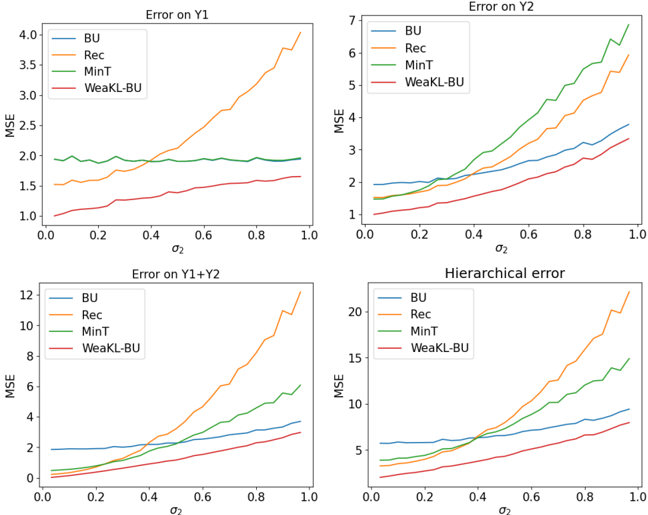Specifically, in cases where Y 1 = <details> <summary>Image 57 Details</summary>  ### Visual Description ## Line Charts: Error Analysis with Varying σ₂ ### Overview The image presents four line charts, each depicting the Mean Squared Error (MSE) as a function of σ₂ (sigma 2). The charts compare the performance of four different methods: BU, Rec, MinT, and WeakKL-BU, across different error metrics. The charts are arranged in a 2x2 grid. ### Components/Axes Each chart shares the following components: * **X-axis:** Labeled "σ₂", ranging from 0.0 to 1.0 with markers at 0.0, 0.2, 0.4, 0.6, 0.8, and 1.0. * **Y-axis:** Labeled "MSE", ranging from 0 to approximately 20, with markers at 0, 2, 4, 6, 8, 10, 12, 14, 16, 18, and 20. * **Legend:** Located in the top-left corner of each chart, identifying the four methods with corresponding colors: * BU (Blue) * Rec (Orange) * MinT (Green) * WeakKL-BU (Red) * **Titles:** Each chart has a title indicating the error metric being evaluated: * "Error on Y1" (Top-left) * "Error on Y2" (Top-right) * "Error on Y1+Y2" (Bottom-left) * "Hierarchical error" (Bottom-right) ### Detailed Analysis or Content Details **Chart 1: Error on Y1** * **BU (Blue):** The line is relatively flat initially, around MSE = 1.8, then slopes upward, reaching approximately MSE = 3.8 at σ₂ = 1.0. * **Rec (Orange):** The line starts at approximately MSE = 1.5 and increases steadily, reaching approximately MSE = 4.0 at σ₂ = 1.0. * **MinT (Green):** The line starts at approximately MSE = 1.2 and increases gradually, reaching approximately MSE = 2.5 at σ₂ = 1.0. * **WeakKL-BU (Red):** The line starts at approximately MSE = 1.1 and increases steadily, reaching approximately MSE = 3.0 at σ₂ = 1.0. **Chart 2: Error on Y2** * **BU (Blue):** The line starts at approximately MSE = 1.2 and increases steadily, reaching approximately MSE = 6.5 at σ₂ = 1.0. * **Rec (Orange):** The line starts at approximately MSE = 1.1 and increases rapidly, reaching approximately MSE = 7.0 at σ₂ = 1.0. * **MinT (Green):** The line starts at approximately MSE = 1.0 and increases gradually, reaching approximately MSE = 3.0 at σ₂ = 1.0. * **WeakKL-BU (Red):** The line starts at approximately MSE = 1.0 and increases steadily, reaching approximately MSE = 5.0 at σ₂ = 1.0. **Chart 3: Error on Y1+Y2** * **BU (Blue):** The line starts at approximately MSE = 1.5 and increases steadily, reaching approximately MSE = 10.0 at σ₂ = 1.0. * **Rec (Orange):** The line starts at approximately MSE = 1.3 and increases rapidly, reaching approximately MSE = 12.0 at σ₂ = 1.0. * **MinT (Green):** The line starts at approximately MSE = 1.1 and increases gradually, reaching approximately MSE = 4.5 at σ₂ = 1.0. * **WeakKL-BU (Red):** The line starts at approximately MSE = 1.0 and increases steadily, reaching approximately MSE = 7.0 at σ₂ = 1.0. **Chart 4: Hierarchical error** * **BU (Blue):** The line starts at approximately MSE = 1.0 and increases steadily, reaching approximately MSE = 18.0 at σ₂ = 1.0. * **Rec (Orange):** The line starts at approximately MSE = 1.0 and increases rapidly, reaching approximately MSE = 20.0 at σ₂ = 1.0. * **MinT (Green):** The line starts at approximately MSE = 1.0 and increases gradually, reaching approximately MSE = 5.0 at σ₂ = 1.0. * **WeakKL-BU (Red):** The line starts at approximately MSE = 1.0 and increases steadily, reaching approximately MSE = 8.0 at σ₂ = 1.0. ### Key Observations * Across all charts, the "Rec" method consistently exhibits the highest MSE values, especially as σ₂ increases. * The "MinT" method generally demonstrates the lowest MSE values across all charts. * The "BU" and "WeakKL-BU" methods perform similarly, with "WeakKL-BU" often slightly outperforming "BU". * The rate of MSE increase with σ₂ varies across methods and error metrics. The "Rec" method shows the most rapid increase. * The MSE values generally increase as σ₂ increases, indicating that the methods become less accurate as the variance increases. ### Interpretation The charts demonstrate the performance of four different methods for estimating or predicting values (Y1, Y2, Y1+Y2, and a hierarchical error). The parameter σ₂ likely represents a level of noise or uncertainty in the data. The results suggest that the "MinT" method is the most robust to increasing noise levels (σ₂), consistently achieving the lowest MSE across all error metrics. The "Rec" method is the most sensitive to noise, exhibiting the highest MSE values. The "BU" and "WeakKL-BU" methods offer intermediate performance. The increasing MSE values with increasing σ₂ indicate that all methods become less accurate as the uncertainty in the data grows. This is expected, as higher noise levels make it more difficult to accurately estimate the underlying values. The hierarchical error chart suggests that the methods' performance degrades more significantly when considering the combined error across multiple levels or components. The differences in performance between the methods likely stem from their underlying assumptions and approaches to handling uncertainty. The "MinT" method may incorporate a more effective regularization or noise reduction technique, while the "Rec" method may be more susceptible to overfitting or being misled by noisy data. Further investigation into the specific algorithms used by each method would be needed to fully understand these differences. </details> O2 Fig. 7.5.: Hierarchical forecasting performance with 2 d/n = 0 . 95 . f 1 ( X 1 )+ ε 1 and Y 2 = f 2 ( X 2 ) -ε 1 + ε 2 , where f 1 and f 2 represent nonlinear functions, the WeaKL approach remains valid. This is because the connection to the linear case is straightforward: the WeaKL essentially performs a linear regression on the Fourier coefficients of X 1 and X 2 , seamlessly extending its applicability to nonlinear settings. ## 7.D Experiments This appendix provides comprehensive details on the use cases discussed in the main text. Appendix 7.D describes our hyperparameter tuning technique. Appendix 7.D explains how we evaluate uncertainties. Appendix 7.D outlines our approach to handling sampling frequency in electricity demand forecasting applications. Appendix 7.D details the models used in Use case 1, while Appendix 7.D focuses on Use case 2 , and Appendix 7.D covers the tourism demand forecasting use case. ## Hyperparameter tuning Hyperparameter tuning of the additive WeaKL. Consider a WeaKL additive model $$f _ { \theta } ( X _ { t } ) = \langle \phi _ { 1 , 1 } ( X _ { 1 , t } ) , \theta _ { 1 , 1 } \rangle + \cdots + \langle \phi _ { 1 , d _ { 1 } } ( X _ { d _ { 1 } , t } ) , \theta _ { 1 , d _ { 1 } } \rangle ,$$ where the type (linear, nonlinear, or categorical) of the effects are specified. Thus, as detailed in Section 7.3, - ( i ) If the effect 〈 φ 1 ,/lscript ( X /lscript,t ) , θ 1 ,j 〉 is assumed to be linear, then φ 1 ,j ( X /lscript,t ) = X /lscript,t , - ( ii ) If the effect 〈 φ 1 ,/lscript ( X /lscript,t ) , θ 1 ,/lscript 〉 is assumed to be nonlinear, then φ 1 ,/lscript is a Fourier map with 2 m /lscript +1 Fourier modes, - ( iii ) If the effect 〈 φ 1 ,/lscript ( X /lscript,t ) , θ 1 ,/lscript 〉 is assumed to be categorical with values in E , then φ 1 ,/lscript is a Fourier map with 2 /floorleft| E | / 2 /floorright +1 Fourier modes. We let m = { m /lscript | the effect 〈 φ 1 ,/lscript ( X /lscript,t ) , θ 1 ,/lscript 〉 is nonlinear } be the concatenation of the numbers of Fourier modes of the nonlinear effects. The goal of hyperparameter tuning is to find the best set of hyperparameters λ = ( λ 1 , . . . , λ d 1 ) and m for the empirical risk (7.6) of the additive WeaKL. To do so, we split the data into three sets: a training set, then a validation set, and finally a test set. These three sets must be disjoint to avoid overfitting, and the test set is the dataset on which the final performance of the method will be evaluated. The sets should be chosen so that the distribution of ( X,Y ) on the validation set resembles as much as possible the distribution of ( X,Y ) on the test set. We consider a list of potential candidates for the optimal set of hyperparameters ( λ, m ) opt . Since we have no prior knowledge about ( λ, m ) , we chose this list to be a grid of parameters. For each element ( λ, m ) in the grid, we compute the minimizer ˆ θ ( λ, m ) of the loss (7.6) over the training period. Then, given ˆ θ ( λ, m ) , we compute the mean squared error (MSE) of f ˆ θ ( λ, m ) over the validation period. This procedure is commonly referred to as grid search. The resulting estimate of the optimal hyperparameters ( λ, m ) opt corresponds to the values of ( λ, m ) that minimize the MSE of f ˆ θ ( λ, m ) over the validation period. The performance of the additive WeaKL is then assessed based on the performance of f ˆ θ ( λ, m ) opt on the test set. Hyperparameter tuning of the online WeaKL. Consider an online WeaKL $$f _ { \theta } ( t , x _ { 1 } , \dots , x _ { d _ { 1 } } ) = h _ { \theta _ { 0 } } ( t ) + \sum _ { \ell = 1 } ^ { d _ { 1 } } ( 1 + h _ { \theta _ { \ell } } ( t ) ) \hat { g } _ { \ell } ( x _ { \ell } ) ,$$ where the effects ˆ g /lscript are known, and the updates h θ /lscript ( t ) = 〈 φ ( t ) , θ /lscript 〉 are such that φ is the Fourier map φ ( t ) = (exp( ikt/ 2)) /latticetop -m j ≤ k ≤ m j , with m j ∈ N /star . We let m = { m j | 0 ≤ j ≤ d 1 } be the concatenation of the numbers of Fourier modes. The goal of hyperparameter tuning is to find the best set of hyperparameters λ = ( λ 0 , . . . , λ d 1 ) and m for the empirical risk (7.8) of the online WeaKL. To do so, we split the data into three sets: a training set, then a validation set, and finally a test set. This three sets must be disjoint to avoid overfitting. Moreover, the training set and the validation set must be disjoint from the data used to learn the effects ˆ g /lscript . The test set must be the set on which the final performance of the method will be evaluated. The sets should be chosen so that the distribution of ( X,Y ) on the validation set resembles as much as possible the distribution of ( X,Y ) on the test set. Similarly to the hyperparameter tuning of the additive WeaKL, we then consider a list of potential candidates for the optimal hyperparameter ( λ, m ) opt , which can be a grid. Then, we compute the minimizer ˆ θ ( λ, m ) of the loss (7.8) on the training period, and the resulting estimation of ( λ, m ) opt is the set of hyperparameters ( λ, m ) such that the MSE of f ˆ θ ( λ, m ) on the validation period is minimal. The performance of the online WeaKL is thus measured by the performance of f ˆ θ ( λ, m ) opt on the test set. ## Block bootstrap methods Evaluating uncertainties with block bootstrap. The purpose of this paragraph is to provide theoretical tools for evaluating the performance of time series estimators. Formally, given a test period { t 1 , . . . , t n } , a target time series ( Y t j ) 1 ≤ j ≤ n , and an estimator ( ˆ Y t j ) 1 ≤ j ≤ n of Y , the goal is to construct confidence intervals that quantify how far RMSE n = ( n -1 ∑ n j =1 | ˆ Y t j -Y t j | 2 ) 1 / 2 deviates from its expectation RMSE = ( E | ˆ Y t 1 -Y t 1 | 2 ) 1 / 2 , and how far MAPE n = n -1 ∑ n j =1 | ˆ Y t j -Y t j || Y t j | -1 deviates from its expectation MAPE = E ( | ˆ Y t 1 -Y t 1 || Y t 1 | -1 ) . Here, we assume that Y and ˆ Y are strongly stationary, meaning their distributions remain constant over time. Constructing such confidence intervals is non-trivial because the observations Y t j in the time series Y are correlated, preventing the direct application of the central limit theorem. The block bootstrap algorithm is specifically designed to address this challenge and is defined as follows. Consider a sequence Z t 1 , Z t 2 , . . . , Z t n such that the quantity of interest can be expressed as g ( E ( Z t 1 )) , for some function g . This quantity is estimated by g ( ¯ Z n ) , where ¯ Z n = n -1 ∑ n j =1 Z t j is the empirical mean of the sequence. For example, RMSE = g ( E ( Z t 1 )) and RMSE n = g ( ¯ Z n ) for g ( x ) = x 1 / 2 and Z t j = ( Y t j -ˆ Y t j ) 2 , while MAPE = g ( E ( Z t 1 )) and MAPE n = g ( ¯ Z n ) for g ( x ) = x and Z t j = | ˆ Y t j -Y t j || Y t j | -1 . The goal of the block bootstrap algorithm is to estimate the distribution of g ( ¯ Z n ) . Given a length /lscript ∈ N /star and a starting time t j , we say that ( Z t j , . . . , Z t j + /lscript -1 ) ∈ R /lscript is a block of length /lscript starting at t j . We draw b = /floorleft n//lscript /floorright + 1 blocks of length /lscript uniformly from the sequence ( Z t 1 , Z t 2 , . . . , Z t n ) and then concatenate these blocks to form the sequence Z ∗ = ( Z ∗ 1 , Z ∗ 2 , . . . , Z ∗ b/lscript ) . Thus, Z ∗ is a resampled version of Z obtained with replacement. For convenience, we consider only the first n values of Z ∗ and compute the bootstrap version of the empirical mean: ¯ Z ∗ n = 1 n ∑ n j =1 Z ∗ j . By repeatedly resampling the b blocks and generating multiple instances of ¯ Z ∗ n , the resulting distribution of ¯ Z ∗ n provides a reliable estimate of the distribution of ¯ Z n . In particular, under general assumptions about the decay of the autocovariance function of Z , choosing /lscript = /floorleft n 1 / 4 /floorright leads to $$\sup _ { x \in \mathbb { R } } | \mathbb { P } ( T _ { n } ^ { * } \leq x | Z _ { t _ { 1 } } , \dots , Z _ { t _ { n } } ) - \mathbb { P } ( T _ { n } \leq x ) | = O _ { n \to \infty } ( n ^ { - 3 / 4 } ) ,$$ where T ∗ n = √ n ( ¯ Z ∗ n -E ( ¯ Z ∗ n | Z t 1 , . . . , Z t n )) and T n = √ n ( ¯ Z n -E ( Z t 1 )) [see, e.g. Lah03, Theorem 6.7]. Note that this convergence rate of n -3 / 4 is actually quite fast, as even if the Z t j were i.i.d., the empirical mean ¯ Z n would only converge to a normal distribution at a rate of n -1 / 2 (by the Berry-Esseen theorem). This implies that the block bootstrap method estimates the distribution of ¯ Z n faster than ¯ Z n itself converges to its Gaussian limit. /negationslash The choice of /lscript plays a crucial role in this method. For instance, setting /lscript = 1 leads to an underestimation of the variance of ¯ Z n when the Z t j are correlated [see, e.g. Lah03, Corollary 2.1]. In addition, block resampling introduces a bias, as Z t n belongs to only a single block and is therefore less likely to be resampled than Z t /floorleft n/ 2 /floorright . This explains why E ( ¯ Z ∗ n | Z t 1 , . . . , Z t n ) = ¯ Z n . To address both problems, Politis and Romano [PR94] introduced the stationary bootstrap, where the block length /lscript varies and follows a geometric distribution. Comparing estimators with block bootstrap. Given two stationary estimators ˆ Y 1 and ˆ Y 2 of Y , the goal is to develop a test of level α ∈ [0 , 1] for the hypothesis H 0 : E | ˆ Y 1 t -Y t | = E | ˆ Y 2 t -Y t | . Using the previous paragraph, such a test could be implemented by estimating two confidence intervals I 1 and I 2 for E | ˆ Y 1 t -Y t | and E | ˆ Y 2 t -Y t | at level α/ 2 using block bootstrap, and then rejecting H 0 if I 1 ∩ I 2 = ∅ . However, this approach tends to be conservative, potentially reducing the power of the test when assessing whether one estimator is significantly better than the other. To create a more powerful test, Messner et al. [Mes+20] and Farrokhabadi et al. [Far+22] suggest relying on the MAE skill score, which is defined by $$S k i l l = 1 - \frac { M A E _ { 1 } } { M A E _ { 2 } } ,$$ where MAE 1 and MAE 2 are the mean average errors of ˆ Y 1 and ˆ Y 2 , respectively. Note that Skill = (MAE 2 -MAE 1 ) / MAE 2 is the relative distance between the two MAE s. Thus, ˆ Y 1 is significantly better than ˆ Y 2 if Skill is significantly positive. A confidence interval for Skill can be obtained by block bootstrap. Indeed, consider the time series Z defined as Z t j = ( | ˆ Y 1 t j -Y 1 t j | , | ˆ Y 2 t j -Y 2 t j | ) , and let g ( x, y ) = 1 -x/y . We use the block bootstrap method over this sequence to estimate g ( E ( Z )) by generating different samples of MAE 1 and MAE 2 . In particular, in Appendix 7.D, ˆ Y 1 corresponds to WeakL, while ˆ Y 2 is the estimator of the winning team of the IEEE competition. ## Half-hour frequency Short-term electricity demand forecasts are often estimated with a half-hour frequency, meaning that the objective is to predict electricity demand every 30 minutes during the test period. This applies to both Use case 1 and Use case 2. There are two common approaches to handling this frequency in forecasting models. One approach is to include the half-hour of the day as a feature in the models. The alternative, which yields better performance, is to train a separate model for each half-hour, resulting in 48 distinct models. This superiority arises because the relationship between electricity demand and conventional features (such as temperature and calendar effects) varies significantly across different times of the day. For instance, electricity demand remains stable at night but fluctuates considerably during the day. This variability justifies treating the forecasting problem at each half-hour as an independent learning task, leading to 48 separate models. Consequently, in both use cases, all models discussed in this paper-including WeaKL, as well as those from Vilmarest and Goude [VG22] and Doumèche et al. [Dou+23]-are trained separately for each of the 48 half-hours, using identical formulas and architectures. This results in 48 distinct sets of model weights. For simplicity, and since the only consequence of this preprocessing step is to split the learning data into 48 independent groups, this distinction is omitted from the equations. ## Precisions on the Use case 1 on the IEEE DataPort Competition on Day-Ahead Electricity Load Forecasting In this appendix, we provide additional details on the two WeaKLs used in the benchmark for Use case 1 of the IEEE DataPort Competition on Day-Ahead Electricity Load Forecasting. The first model is a direct adaptation of the GAM-Viking model from Vilmarest and Goude [VG22] into the WeaKL framework. The second model is a WeaKL where the effects are learned through hyperparameter tuning. Direct translation of the GAM-Viking model into the WeaKL framework. To build their model, Vilmarest and Goude [VG22] consider four primary models: an autoregressive model (AR), a linear regression model, a GAM, and a multi-layer perceptron (MLP). These models are initially trained on data from 18 March 2017 to 1 January 2020 . Their weights are then updated using the Viking algorithm starting from 1 March 2020 [VG22, Table 3]. The parameters of the Viking algorithm were manually selected by the authors based on performance monitoring over the 2020 -2021 period [VG22, Figure7]. To further refine the forecasts, the model errors are corrected using an autoregressive model, which they called the intraday correction and implemented as a static Kalman filter. The final forecast is obtained by online aggregation of all models, meaning that the predictions from different models are combined in a linear combination that evolves over time. The weights of this aggregation are learned using the ML-Poly algorithm from the opera package [GG16], trained over the period 1 July 2020 to 18 January 2021 . The test period spans from 18 January 2021 to 17 February 2021 . During this period, the aggregated model achieves a MAE of 10 . 9 GW, while the Viking-updated GAM model alone yields an MAE of 12 . 7 GW. Here, to ensure a fair comparison between our WeaKL framework and the GAM-Viking model of Vilmarest and Goude [VG22], we replace their GAM-Viking with our online WeaKL in their aggregation. Our additive WeaKL model is therefore a direct translation of their offline GAM formulation into the WeaKL framework. Specifically, we consider the additive WeaKL based on the features X = (DoW , FTemps95 corr1 , Load 1 , Load 7 , ToY , t ) corresponding to $$Y _ { t } = & g _ { 1 } ^ { * } ( D o W _ { t } ) + g _ { 2 } ^ { * } ( F T e m p s 9 5 _ { c o r r 1 t } ) + g _ { 3 } ^ { * } ( L o a d _ { 1 t } ) + g _ { 4 } ^ { * } ( L o a d _ { 7 t } ) + g _ { 5 } ^ { * } ( T O Y _ { t } ) + g _ { 6 } ^ { * } ( t ) + \varepsilon _ { t } ,$$ where g /star 1 is categorical with 7 values, g /star 2 and g /star 6 are linear, g /star 3 , g /star 4 , and g /star 5 are nonlinear. FTemps95 corr1 is a smoothed version of the temperature, while the other features remain the same as those used in Use case 2. The weights of the additive WeaKL model are determined using the hyperparameter selection technique described in Appendix 7.D. The training period spans from 18 March 2017 to 1 November 2019 , while the validation period extends from 1 November 2019 to 1 January 2020 . During this grid search, the performance of 250 , 047 sets of hyperparameters ( λ, m ) ∈ R 7 × R 3 is evaluated in less than a minute using a standard GPU (Nvidia L4 GPU, 24 GB RAM, 30 . 3 teraFLOPs for Float32). Notably, this optimization period exactly matches the training period of the primary models in Vilmarest and Goude [VG22], ensuring a fair comparison between the two approaches. Then, we run an online WeaKL, where the effects ˆ g /lscript , 1 ≤ /lscript ≤ 7 , are inherited directly from the previously trained additive WeaKL. The weights of this online WeaKL are determined using the hyperparameter selection technique described in Appendix 7.D. The training period extends from 1 February 2020 to 18 November 2020 , while the validation period extends from 18 November 2020 to 18 January 2021 , immediately preceding the final test period to ensure optimal adaptation. During this grid search, we evaluate 625 sets of hyperparameters ( λ, m ) ∈ R 6 × R 6 in less than a minute using a standard GPU. Since t is already included as a feature, the function h ∗ 0 in Equation (7.7) is not required in this setting. Finally, we evaluate the performance of our additive WeaKL (denoted as WeaKL + ), our additive WeaKL followed by intraday correction (WeaKL + , intra ), our online WeaKL (WeaKL on ), our online WeaKL with intraday correction (WeaKL on , intra ), and an aggregated model based on Vilmarest and Goude [VG22], where the GAM and GAM-Viking models are replaced by our additive and online WeaKL models (WeaKL agg ). The test period remains consistent with Vilmarest and Goude [VG22], spanning from 18 January 2021 to 17 February 2021 . Their performance results are presented in Table 7.4 and compared to their corresponding translations within the GAM-Viking framework. Thus, GAM + refers to the offline GAM, while GAM + , intra corresponds to the offline GAM with an intraday correction. Similarly, GAM on represents the GAM-Viking model, and GAM on , intra denotes the GAM-Viking model with an intraday correction. Finally, GAM agg corresponds to the final model proposed by Vilmarest and Goude [VG22]. Tab. 7.4.: Comparing GAM-Viking with its direct translation in the WeaKL framework on the final test period | Model GAM | GAM + | GAM + , intra | GAM on | GAM on , intra | GAM agg | |-------------|---------|-----------------|----------|------------------|-----------| | MAE (GW) | 48.3 | 22.7 | 13.2 | 12.7 | 10.9 | | Model WeaKL | WeaKL + | WeaKL + , intra | WeaKL on | WeaKL on , intra | WeaKL agg | | MAE (GW) | 58.0 | 23.4 | 11.2 | 11.3 | 10.5 | Tab. 7.5.: Comparing GAM with its direct translation in the WeaKL framework on a stationary test period. | Model | GAM + | WeaKL + | GAM + , intra | WeaKL + , intra | |----------|---------|-----------|-----------------|-------------------| | MAE (GW) | 20.7 | 19.1 | 19.3 | 19.2 | The performance GAM + , GAM + , intra , WeaKL + , and WeaKL + , intra in Table 7.4 alone is not very meaningful because the distribution of electricity demand differs between the training and test periods. To address this, Table 7.5 presents a comparison of the same algorithms, trained on the same period but evaluated on a test period spanning from 1 January 2020 to 1 March 2020 . In this stationary period, WeaKL outperforms the GAMs. Moreover, in Table 7.4, the online WeaKLs clearly outperform the GAM-Viking models, achieving a reduction in MAE of more than 10% . As a result, replacing the GAM-Viking models in the aggregation leads to improved overall performance. Notably, the WeaKLs are direct translations of the GAM-Viking models, meaning that the performance gains are due solely to model optimization and not to any structural changes. Pure WeaKL. In addition, we trained an additive WeaKL using a different set of variables than those in the GAM model, aiming to identify an optimal configuration. Specifically, we consider the additive WeaKL with X = (FcloudCover \_ corr1 , Load1D , Load1W , DayType , FTemperature \_ corr1 , FWindDirection , FTemps95 \_ corr1 , Toy , t) , where - ( i ) the effects of FclouCover \_ corr1 , Load1D , and Load1W are nonlinear, - ( ii ) the effect of DayType is categorical with 7 values, - ( iii ) the remaining effects are linear. This model is trained using the hyperparameter tuning process detailed in Appendix 7.D, with the training period spanning from 18 March 2017 to 1 January 2020 , and validation starting from 1 October 2019 . Next, we fit an online WeaKL model, with hyperparameters tuned using a training period from 1 March 2020 to 18 November 2020 and a validation period extending until 18 January 2021 . To verify that our pure WeaKL model achieves a significantly lower error than the best model from the IEEE competition, we estimate the MAE skill score by comparing our pure WeaKL to the model proposed by Vilmarest and Goude [VG22]. To achieve this, we follow the procedure detailed in Appendix 7.D, using block bootstrap with a block length of /lscript = 24 and 3000 resamples to estimate the distribution of the MAE skill score, Skill . Here, ˆ Y 1 represents the WeaKL, while ˆ Y 2 corresponds to the estimator from Vilmarest and Goude [VG22]. To evaluate the performance difference, we estimate the standard deviation σ n of Skill n and construct an asymptotic one-sided confidence interval for Skill . Specifically, we define Skill n = 1 -( ∑ n j =1 | ˆ Y 1 t j -Y t j | ) / ( ∑ n j =1 | ˆ Y 2 t j -Y t j | ) and consider the confidence interval [Skill n -1 . 28 σ n , + ∞ [ , which corresponds to a confidence level of α = 0 . 1 . The resulting interval, [0 . 007 , + ∞ [ , indicates that the Skill score is positive with at least 90% probability. Consequently, with at least 90% probability, the WeaKL chieves a lower MAE than the best model from the IEEE competition. ## Precision on the use Use case 2 on forecasting the French electricity load during the energy crisis This appendix provides detailed information on the additive WeaKL and the online WeaKL used in Use case 2, which focuses on forecasting the French electricity load during the energy crisis. Additive WeaKL. As detailed in the main text, the additive WeaKL is built using the following features: $$X = ( L o a d _ { 1 } , L o a d _ { 7 } , T e m p , T e m p _ { \min 5 0 } , T e m p _ { \max 9 5 0 } , T e m p _ { \min 9 5 0 } , T o Y , D O W , H o l i d a y , t ) .$$ The effects of Load 1 , Load 7 , and t are modeled as linear. The effects of Temp , Temp 950 , Temp max950 , Temp min950 , and ToY are modeled as nonlinear with m = 10 . The effects of DoW and Holiday are treated as categorical, with | E | = 7 and | E | = 2 , respectively. The model weights are selected through hyperparameter tuning, as detailed in Appendix 7.D. The training period spans from 8 January 2013 to 1 September 2021 , while the validation period covers 1 September 2021 to 1 September 2022 . Notably, this is the exact same period used by Doumèche et al. [Dou+23] to train the GAM. The objective of the hyperparameter tuning process is to determine the optimal values for λ = ( λ 1 , . . . , λ 10 ) ∈ ( R + ) 10 and m = ( m 3 , m 4 , m 5 , m 6 , m 7 ) ∈ ( N /star ) 5 in (7.6). As a result, the additive WeaKL model presented in Use case 2 is the outcome of this hyperparameter tuning process. Online WeaKL. Next, we train an online WeaKL to update the effects of the additive WeaKL. To achieve this, we apply the hyperparameter selection technique detailed in Appendix 7.D. The training period spans from 1 February 2018 to 1 April 2020 , while the validation period extends from 1 April 2020 to 1 June 2020 . These periods, although not directly contiguous to the test period, were specifically chosen because they overlap with the COVID-19 outbreaks. This is crucial, as it allows the model to learn from a nonstationary period. Moreover, since online models require daily updates, the online WeaKL is computationally more expensive than the additive WeaKL. The training period is set to two years and two months, striking a balance between computational efficiency and GPU memory usage. Using the parameters ( λ, m ) obtained from hyperparameter tuning, we then retrain the model in an online manner with data starting from 1 July 2020 , ensuring that the rolling training period remains at two years and two months. Error quantification. Following the approach of Doumèche et al. [Dou+23], the standard deviations of the errors are estimated using stationary block bootstrap with a block length of /lscript = 48 and 1000 resamples. Model running times. Below, we present the running times of various models in the experiment that includes holidays: - GAM: 20 . 3 seconds. - Static Kalman adaption: 1 . 7 seconds. - Dynamic Kalman adaption: 48 minutes, for an hyperparameter tuning of 10 4 sets of hyperparameters [see OVG21, II.A.2]. - Viking algorithm: 215 seconds (in addition to training the Dynamic Kalman model). - Aggregation: 0 . 8 seconds. - GAM boosting model: 6 . 6 seconds. - Random forest model: 196 seconds. - Random forest + bootstrap model: 34 seconds. - Additive WeaKL: grid search of 1 . 6 × 10 5 hyperparameters: 257 seconds; training a single model: 2 seconds. - Online WeaKL: grid search of 9 . 2 × 10 3 hyperparameters: 114 seconds; training a single model: 52 seconds. ## Precisions on the use case on hierarchical forecasting of Australian domestic tourism with transfer learning The matrices Λ for the WeaKL-BU, WeaKL-G, and WeaKL-T estimators are selected through hyperparameter tuning. Following the procedure detailed in Appendix 7.D, the dataset is divided into three subsets: training, validation, and test. The training set comprises the first 60% of the data, the validation set the next 20% , and the test set the last 20% . The optimal matrix, Λ opt , is chosen from a set of candidates by identifying the estimator trained on the training set that achieves the lowest MSE on the validation set. The model is then retrained using both the training and validation sets with Λ = Λ opt , and its performance is evaluated on the test set. Given that d 1 = 415 × 24 = 19 , 920 , WeaKL involves matrices of size d 2 1 /similarequal 4 × 10 8 , requiring several gigabytes of RAM. Consequently, the grid search process is computationally expensive. For instance, in this experiment, the grid search over 1024 hyperparameter sets for WeaKL-T takes approximately 45 minutes. ## Part III Conclusion Main contributions. In this thesis, we have proven several results on the statistical properties of physics-informed machine learning. Chapter 2 focuses on the theoretical properties of physics-informed neural networks (PINNs), showing their risk consistency for linear and nonlinear PDE systems, and their strong convergence for linear PDE systems. In Chapter 3, we prove that PDE solving and hybrid modeling tasks with linear PDEs can be reframed as kernel methods, which makes it possible to characterize the impact of the physics on the convergence rate. In Chapter 4, we introduce an algorithm to efficiently implement the kernel method of Chapter 4 on GPUs. We show that this kernel method outperforms PINNs on two PDE solving tasks. Then, we have focused on forecasting energy signals during atypical periods. In Chapter 5, we present the results of the Smarter Mobility Data Challenge on forecasting the occupancy of electric vehicle charging stations. In Chapter 6, we study the integration of mobility data to forecast the French electricity demand during COVID. Finally, in Chapter 7, we adapt the kernel framework of Chapter 4 to common linear constraints in time series forecasting, and show that these new kernel methods outperform the state-of-the-art in electricity demand and tourism forecasting. Many questions remain open regarding the topics developed in this thesis. Convergence of PINNs. First, the convergence of physics-informed machine learning algorithms, and in particular of PINNs, is not well-established for nonlinear PDEs. In Doumèche et al. [DBB25], we proved the risk-consistency of the PINNs estimator, but we warned that this does not necessarily mean that the resulting PINN indeed satisfy the penalized PDE. This is due to the fact that the theoretical risk function is not weakly continuous with respect to the Sobolev norm. Some results have been proven in PDE solving, for example regarding the Navier-Stokes equation, but they mainly focus on modifications of the PINNs algorithm. For instance, De Ryck et al. [DRJM23] consider neural networks which weights are bounded during the gradient descent, and then let the bound on the weights grow, which disregards the overfitting scenarios that we pointed out in Chapter 2. Moreover, most theoretical papers consider to have at hand an exact minimizer of the empirical risk, while it is known that the gradient descent of PINNs behaves badly, especially when the penalized PDE is nonlinear [WYP22; BBC24]. Curse of the dimension. Regarding the theory of PINNs, the impact of the dimension d 1 on the theoretical performance of PINNs remains unknown. Indeed, many machine learning algorithms are known to become extremely computationally expensive as the dimension d 1 grows, while becoming less accurate. For example, our Fourier kernel method has a complexity of (2 m +1) 2 d 1 n +(2 m +1) 3 d 1 , which scales exponentially in d 1 , while the Sobolev minimax rate n -2 s/ (2 s + d 1 ) worsens exponentially in d 1 . This is known as the curse of the dimension. Meanwhile, neural networks are known to be able to overcome this issue when the data X lies in a submanifold of R d 1 of lower dimension [see, e.g., Bac24, Section 2.6]. While some experiments suggest that PINNs also alleviate the curse of the dimension [Hu+24], it has not been proven formally. Minimax convergence rates of hybrid modeling tasks. In Chapter 2, we show that the impact of linear PDEs on the convergence rate in hybrid modeling tasks can be quantified by the impact on the effective dimension of the kernel methods. In simple cases, we managed to bound the effective dimension to show that the physical prior speeds-up the learning process. In Chapter 3, we show how to approximate the effective dimension for more complex linear PDEs. Similarly, for second-order linear elliptic PDEs in dimension d = 2 , and for domains with C 2 boundary ∂ Ω , Azzimonti et al. [Azz+15] and Arnone et al. [Arn+22] showed that the hybrid modeling task outperform the Sobolev minimax rate. However, further studies should be made to determine the impact of both the PDE and the smoothness of the domain Ω on the convergence rate, in particular for classical linear and nonlinear PDEs. Adapting our kernel methods to more contexts. The kernel methods we developed are tailored to PDE solving and hybrid modeling tasks. Their main advantage is that they admit closed-form formulas for the minimizer of the empirical risk, which can be efficiently implemented on GPUs. However, to tackle high dimensional scenario, the complexity of the optimization should be reduced, and many usual techniques like gradient descent, conjugate gradient [BK10], or the Nyström method [Yan+12]. Moreover, adapting our PIKL algorithm to handle nonlinear PDEs, and developing similar kernel methods for PDE learning and operator learning are all promising avenues of research. ## Bibliography - [ASM11] E.A. Abdelaziz, R. Saidur, and S. Mekhilef. 'A review on energy saving strategies in industrial sector'. In: Renewable and Sustainable Energy Reviews 15.1 (2011), pp. 150-168 (cit. on p. 183). - [Aga+21] R. Agarwal, L. Melnick, N. Frosst, X. Zhang, B. Lengerich, et al. 'Neural Additive Models: Interpretable Machine Learning with Neural Nets'. In: Advances in Neural Information Processing Systems . Vol. 34. 2021, pp. 4699-4711 (cit. on p. 213). - [Agh+23] R. Agharafeie, J. Rodrigues C. Ramos, J.M. Mendes, and R. Oliveira. 'From Shallow to Deep Bioprocess Hybrid Modeling: Advances and Future Perspectives'. In: Fermentation 9 (2023) (cit. on p. 122). - [Agr15] M.S. Agranovich. Sobolev Spaces, Their Generalizations and Elliptic Problems in Smooth and Lipschitz Domains . Cham: Springer, 2015 (cit. on pp. 40, 87). - [AGG23a] A. Ahmadian, V. Ghodrati, and R. Gadh. 'Artificial deep neural network enables one-sizefits-all electric vehicle user behavior prediction framework'. In: Applied Energy 352 (2023), p. 121884 (cit. on p. 172). - [Ahm+10] N.K. Ahmed, A.F. Atiya, N.E. Gayar, and H. El-Shishiny. 'An empirical comparison of machine learning models for time series forecasting'. In: Econometric reviews 29.5-6 (2010), pp. 594-621 (cit. on p. 167). - [Aki+19] T. Akiba, S. Sano, T. Yanase, T. Ohta, and M. Koyama. 'Optuna: A next-generation hyperparameter optimization framework'. In: Proceedings of the 25th ACM SIGKDD international conference on knowledge discovery & data mining . 2019, pp. 2623-2631 (cit. on p. 172). - [Ali+17] M. Alizadeh, H.-T. Wai, M. Chowdhury, et al. 'Optimal Pricing to Manage Electric Vehicles in Coupled Power and Transportation Networks'. In: IEEE Transactions on Control of Network Systems 4.4 (2017), pp. 863-875 (cit. on pp. 12, 157). - [AO+24] Y. Amara-Ouali, Y. Goude, N. Doumèche, et al. 'Forecasting Electric Vehicle Charging Station Occupancy: Smarter Mobility Data Challenge'. In: Journal of Data-centric Machine Learning Research 1.16 (2024), pp. 1-27 (cit. on pp. 12, 157, 221, 228). - [AO+22] Y. Amara-Ouali, Y. Goude, B. Hamrouche, and M. Bishara. 'A benchmark of electric vehicle load and occupancy models for day-ahead forecasting on open charging session data'. In: Proceedings of the Thirteenth ACM International Conference on Future Energy Systems . 2022, 193-207 (cit. on p. 158). - [AO+21] Y. Amara-Ouali, Y. Goude, P. Massart, J.M. Poggi, and H. Yan. 'A review of electric vehicle load open data and models'. In: Energies 14.8 (2021), p. 2233 (cit. on pp. xiii, 4, 12, 157, 158). - [AC17] S. Aminikhanghahi and D.J. Cook. 'A survey of methods for time series change point detection'. In: Knowledge and Information Systems 51 (2017), 339-367 (cit. on pp. 189, 203). - [AV23] N. Andrenacci and M.P. Valentini. 'A Literature Review on the Charging Behaviour of Private Electric Vehicles'. In: Applied Sciences 13.23 (2023) (cit. on pp. 12, 157). - [Ant+24] A. Antoniadis, J. Cugliari, M. Fasiolo, Y. Goude, and J.-M. Poggi. Statistical Learning Tools for Electricity Load Forecasting . Cham: Springer, 2024, pp. 113-130 (cit. on p. 228). - [AGG23b] A. Antoniadis, S. Gaucher, and Y. Goude. 'Hierarchical transfer learning with applications to electricity load forecasting'. In: International Journal of Forecasting (2023) (cit. on pp. 13, 184, 197). - [Arn+22] E. Arnone, A. Kneip, F. Nobile, and L.M. Sangalli. 'Some first results on the consistency of spatial regression with partial differential equation regularization'. In: Stat. Sinica 32 (2022), pp. 209-238 (cit. on pp. x, 2, 20, 31, 69, 77, 83, 122, 243). - [AWD21] A. Arzani, J.-X. Wang, and R.M. D'Souza. 'Uncovering near-wall blood flow from sparse data with physics-informed neural networks'. In: Phys. Fluids 33 (2021), p. 071905 (cit. on pp. 21, 22, 24, 30, 37, 77, 122). - [AAH09] G. Athanasopoulos, R.A. Ahmed, and R.J. Hyndman. 'Hierarchical forecasts for Australian domestic tourism'. In: International Journal of Forecasting 25 (2009), pp. 146-166 (cit. on p. 220). - [Ath+20] G. Athanasopoulos, P. Gamakumara, A. Panagiotelis, R.J. Hyndman, and M. Affan. 'Hierarchical Forecasting'. In: Macroeconomic Forecasting in the Era of Big Data: Theory and Practice . Cham: Springer International Publishing, 2020, pp. 689-719 (cit. on p. 158). - [Aug+09] N.H. Augustin, M. Musio, E. Kublin K. von Wilpert, S.N. Wood, and M. Schumacher. 'Modeling Spatiotemporal Forest Health Monitoring Data'. In: Journal of the American Statistical Association 104 (2009), pp. 899-911 (cit. on pp. 14, 209). - [Aut01] AutoMoto. Paris : les tarifs des bornes de recharge Belib' augmentent . Accessed on 08/24/2023. 4/01/2021 (cit. on p. 174). - [Aym+23] A. Ayme, C. Boyer, A. Dieuleveut, and E. Scornet. 'Naive imputation implicitly regularizes high-dimensional linear models'. In: Proceedings of the 40th International Conference on Machine Learning . Vol. 202. Proceedings of Machine Learning Research. PMLR, 2023, pp. 1320-1340 (cit. on p. 197). - [Azz+15] L. Azzimonti, L.M. Sangalli, P. Secchi, M. Domanin, and F. Nobile. 'Blood flow velocity field estimation via spatial regression with PDE penalization'. In: J. Amer. Statist. Assoc. 110 (2015), pp. 1057-1071 (cit. on pp. 31, 77, 83, 243). - [Bac24] F. Bach. Learning theory from first principles . MIT press, 2024 (cit. on pp. 9, 243). - [BD01] L. Badea and P. Daripa. 'On a Boundary Control Approach to Domain Embedding Methods'. In: SIAM Journal on Control and Optimization 40 (2001), pp. 421-449 (cit. on p. 138). - [BKK18] S. Bai, J.Z. Kolter, and V. Koltun. 'An empirical evaluation of generic convolutional and recurrent networks for sequence modeling'. In: International Conference on Learning Representations (ICLR) Workshop (2018) (cit. on pp. 158, 172). - [BR11] M. Bakhat and J. Rosselló. 'Estimation of tourism-induced electricity consumption: The case study of Balearics Islands, Spain'. In: Energy Economics 33.3 (2011), pp. 437-444 (cit. on p. 194). - [Bat+25] Pau Batlle, Yifan Chen, Bamdad Hosseini, Houman Owhadi, and Andrew M. Stuart. 'Error analysis of kernel/GP methods for nonlinear and parametric PDEs'. In: Journal of Computational Physics 520 (2025), p. 113488 (cit. on pp. 77, 122). - [Bel23] Belib'. Offre Belib' . Accessed on 08/24/2023. 2023 (cit. on p. 175). - [B ´ +22] C. Bénard, G. Biau, S. Da Veiga, and Erwan Scornet. 'SHAFF: Fast and consistent SHApley eFfect estimates via random Forests'. In: Proceedings of The 25th International Conference on Artificial Intelligence and Statistics . Ed. by Gustau Camps-Valls, Francisco J. R. Ruiz, and Isabel Valera. Vol. 151. Proceedings of Machine Learning Research. PMLR, 2022, pp. 55635582 (cit. on p. 204). - [Ben+11] L. Bengtsson, X. Lu, A. Thorson, R. Garfield, and J.v. Schreeb. 'Improved response to disasters and outbreaks by tracking population movements with mobile phone network data: a post-earthquake geospatial study in Haiti'. In: PLoS Medicine 8.8 (2011), e100-1083 (cit. on p. 184). - [BPG19] E. de Bézenac, A. Pajot, and P. Gallinari. 'Deep learning for physical processes: Incorporating prior scientific knowledge'. In: J. Stat. Mech.-Theory E. (2019), p. 124009 (cit. on pp. 22, 77). - [BBM08] G. Blanchard, O. Bousquet, and P. Massart. 'Statistical performance of support vector machines'. In: The Annals of Statistics 36 (2008), pp. 489-531 (cit. on pp. xii, 4). - [BK10] G. Blanchard and N. Krämer. 'Optimal learning rates for Kernel Conjugate Gradient regression'. In: Advances in Neural Information Processing Systems . Ed. by J. Lafferty, C. Williams, J. Shawe-Taylor, R. Zemel, and A. Culotta. Vol. 23. Curran Associates, Inc., 2010 (cit. on p. 244). - [BM20] G. Blanchard and N. Mücke. 'Kernel regression, minimax rates and effective dimensionality: Beyond the regular case'. In: Analysis and Applications 18 (2020), pp. 683-696 (cit. on pp. 9, 86, 212). - [BDK15] V.D. Blondel, A. Decuyper, and G. Krings. 'Understanding vehicular routing behavior with location-based service data'. In: EPJ Data Science 4.10 (2015) (cit. on pp. 13, 184). - [Blu12] J. Blumenstock. 'Inferring patterns of internal migration from mobile phone call records: evidence from Rwanda'. In: Information Technology for Development 18.2 (2012), pp. 107125 (cit. on p. 184). - [BCO15] J. Blumenstock, G. Cadamuro, and R. On. 'Predicting poverty and wealth from mobile phone metadata'. In: Science 350.6264 (2015), pp. 1073-1076 (cit. on p. 184). - [BM21] C.S. Bojer and J.P. Meldgaard. 'Kaggle forecasting competitions: An overlooked learning opportunity'. In: International Journal of Forecasting 37.2 (2021), pp. 587-603 (cit. on p. 171). - [BBC24] Andrea Bonfanti, Giuseppe Bruno, and Cristina Cipriani. 'The Challenges of the Nonlinear Regime for Physics-Informed Neural Networks'. In: Advances in Neural Information Processing Systems . Vol. 37. Curran Associates, Inc., 2024, pp. 41852-41881 (cit. on pp. xii, 4, 6, 122, 243). - [Bon+25] A. Bonito, R. DeVore, G. Petrova, and J.W. Siegel. 'Convergence and error control of consistent PINNs for elliptic PDEs'. In: IMA Journal of Numerical Analysis (2025), draf008 (cit. on p. 122). - [BLM13] S. Boucheron, G. Lugosi, and P. Massart. Concentration Inequalities: A Nonasymptotic Theory of Independence . Oxford: Oxford University Press, 2013 (cit. on p. 82). - [Bou+22] M. Boulakhbar, M. Farag, K. Benabdelaziz, T. Kousksou, and M. Zazi. 'A deep learning approach for prediction of electrical vehicle charging stations power demand in regulated electricity markets: The case of Morocco'. In: Cleaner Energy Systems 3 (2022), p. 100039 (cit. on p. 172). - [Box+15] G.E.P. Box, G.M. Jenkins, G.C. Reinsel, and G.M. Ljung. Time series analysis: forecasting and control . John Wiley & Sons, 2015 (cit. on pp. 158, 169, 197). - [Bra00] R. Bracewell. The Fourier Transform and its Applications . 3rd ed. Electrical Engineering series. Boston: McGraw-Hill International Editions, 2000 (cit. on pp. 127, 142). - [BH22a] M. Brégère and M. Huard. 'Online Hierarchical Forecasting for Power Consumption Data'. In: International Journal of Forecasting 38 (2022), pp. 339-351 (cit. on p. 158). - [Bre97] L. Breiman. Arcing the edge . Tech. rep. Citeseer, 1997 (cit. on p. 200). - [Bre01] L. Breiman. 'Random forests'. In: Machine learning 45 (2001), pp. 5-32 (cit. on p. 200). - [Bre+84] L. Breiman, J.H. Friedman, R.A. Olshen, and C.J. Stone. Classification and regression trees . Chapman & Hall/CRC, 1984 (cit. on p. 200). - [Bre10] H. Brezis. Functional Analysis, Sobolev Spaces and Partial Differential Equations . New York: Springer, 2010 (cit. on pp. 32, 48, 67, 89, 91, 112, 140, 141). - [BS21] L. Bryan and Z. Stefan. 'Time-series forecasting with deep learning: A survey'. In: Philosophical Transactions of the Royal Society A 379 (2021), p. 20200209 (cit. on p. 170). - [BH22b] M. Brégère and M. Huard. 'Online hierarchical forecasting for power consumption data'. In: International Journal of Forecasting 38 (2022), pp. 339-351 (cit. on p. 221). - [BH07] P. Bühlmann and T. Hothorn. 'Boosting Algorithms: Regularization, Prediction and Model Fitting'. In: Statistical Science 22.4 (2007), pp. 477 -505 (cit. on p. 200). - [Bus] Orange Business. Flux Vision (cit. on pp. 184, 185). - [Cai+21] S. Cai, Z. Wang, S. Wang, P. Perdikaris, and G.E. Karniadakis. 'Physics-informed neural networks for heat transfer problems'. In: J. Heat. Transf. 143 (6 2021), p. 060801 (cit. on pp. 37, 136). - [CMZ21] L. Calearo, M. Marinelli, and C. Ziras. 'A review of data sources for electric vehicle integration studies'. In: Renewable and Sustainable Energy Reviews 151 (2021), p. 111518 (cit. on pp. 12, 157). - [Cam16] D. Camille. Bornes Bélib, les tarifs pour recharger sa voiture à Paris . Stage récupération point. Accessed on 08/24/2023. 2016 (cit. on pp. 160, 174). - [Cam+24] E. Campagne, Y. Amara-Ouali, Y. Goude, and A. Kalogeratos. 'Leveraging Graph Neural Networks to Forecast Electricity Consumption'. In: ECML PKDD 2024 - Machine Learning for Sustainable Power Systems (ML4SPS) Workshop (2024) (cit. on p. 188). - [Can+07] C. Canuto, A. Quarteroni, M.Y. Hussaini, and T.A. Zang. Spectral Methods . 1st ed. Scientific Computation. Berlin: Springer, 2007 (cit. on pp. 127, 138). - [CV07] A. Caponnetto and E. De Vito. 'Optimal Rates for the Regularized Least-Squares Algorithm'. In: Foundations of Computational Mathematics 7 (2007), 331-368 (cit. on pp. xii, 4, 9, 81, 107, 109-111, 130, 138). - [CBL06] N. Cesa-Bianchi and G. Lugosi. Prediction, learning, and games . Cambridge: Cambridge University Press, 2006 (cit. on pp. 171, 199). - [Cha+23] B. Chandrajit, L. McLennan, T. Andeen, and A. Roy. 'Recipes for when physics fails: Recovering robust learning of physics informed neural networks'. In: Mach. Learn.: Sci. Technol. 4 (2023), p. 015013 (cit. on p. 24). - [CG16] T. Chen and C. Guestrin. 'Xgboost: A scalable tree boosting system'. In: Proceedings of the 22nd acm sigkdd international conference on knowledge discovery and data mining . 2016, pp. 785-794 (cit. on pp. 167, 169). - [CKM04] T.Y. Chen, F.-C. Kuo, and R. Merkel. 'On the statistical properties of the f-measure'. In: Fourth International Conference onQuality Software, 2004. QSIC 2004. Proceedings. IEEE. 2004, pp. 146-153 (cit. on p. 167). - [Che+21] Y. Chen, B. Hosseini, H. Owhadi, and A.M. Stuart. 'Solving and learning nonlinear PDEs with Gaussian processes'. In: Journal of Computational Physics 447 (2021), p. 110668 (cit. on p. 122). - [CYZ20] Y. Chen, W. Yang, and B. Zhang. 'Using Mobility for Electrical Load Forecasting During the COVID-19 Pandemic'. In: arXiv:2006.08826 (2020) (cit. on pp. 13, 184). - [Che+22] Sibo Cheng, I. Colin Prentice, Yuhan Huang, et al. 'Data-driven surrogate model with latent data assimilation: Application to wildfire forecasting'. In: Journal of Computational Physics 464 (2022), p. 111302 (cit. on p. 3). - [Cio+23] A. Ciociola, D. Giordano, L. Vassio, and M. Mellia. 'Data driven scalability and profitability analysis in free floating electric car sharing systems'. In: Information Sciences 621 (2023), pp. 545-561 (cit. on pp. 12, 157). - [Col+23] A. Coletta, S. Gopalakrishnan, D. Borrajo, and S. Vyetrenko. 'On the Constrained TimeSeries Generation Problem'. In: Advances in Neural Information Processing Systems . Vol. 36. 2023, pp. 61048-61059 (cit. on pp. 14, 209). - [Com74] L. Comtet. Advanced Combinatorics : The Art of Finite and Infinite Expansions . Dordrecht: Springer, 1974 (cit. on p. 45). - [Cos+20] F.S. Costabal, Y. Yang, P. Perdikaris, D.E. Hurtado, and E. Kuhl. 'Physics-informed neural networks for cardiac activation mapping'. In: AIP Conf. Proc. 8 (2020), p. 42 (cit. on p. 24). - [CMM20] C. Crozier, T. Morstyn, and M. McCulloch. 'The opportunity for smart charging to mitigate the impact of electric vehicles on transmission and distribution systems'. In: Applied Energy 268 (2020), p. 114973 (cit. on pp. 12, 157). - [Cun+23] B. Cunha, C. Droz, A. Zine, S. Foulard, and M. Ichchou. 'A review of machine learning methods applied to structural dynamics and vibroacoustic'. In: Mech. Syst. Signal. Pr. (2023), p. 110535 (cit. on p. 19). - [Cuo+22] S. Cuomo, V.S. Di Cola, F. Giampaolo, et al. 'Scientific machine learning through physicsinformed neural networks: Where we are and what's next'. In: J. Sci. Comput. 92 (2022), p. 88 (cit. on pp. xi, 2, 19, 20, 22, 23, 75, 121). - [DW12] D. Dallinger and M. Wietschel. 'Grid integration of intermittent renewable energy sources using price-responsive plug-in electric vehicles'. In: Renewable and Sustainable Energy Reviews 16.5 (2012), pp. 3370-3382 (cit. on pp. 12, 157). - [Dao19] E.A. Daoud. 'Comparison between XGBoost, LightGBM and CatBoost Using a Home Credit Dataset'. In: International Journal of Computer and Information Engineering 13.1 (2019), pp. 6 -10 (cit. on p. 166). - [Dav+21] D. Davini, B. Samineni, B. Thomas, et al. 'Using physics-informed regularization to improve extrapolation capabilities of neural networks'. In: Fourth Workshop on Machine Learning and the Physical Sciences (NeurIPS 2021) . 2021 (cit. on pp. 22, 30). - [Daw+22] A. Daw, A. Karpatne, W.D. Watkins, J.S. Read, and V. Kumar. 'Physics-guided neural networks (PGNN): An application in lake temperature modeling'. In: Knowledge guided machine learning: Accelerating discovery using scientific knowledge and data . Ed. by A. Karpatne, R. Kannan, and V. Kumar. New York: Chapman and Hall/CRC, 2022, pp. 352-372 (cit. on pp. xi, 2, 22, 210). - [DRJM23] T. De Ryck, A.D. Jagtap, and S. Mishra. 'Error estimates for physics-informed neural networks approximating the Navier-Stokes equations'. In: IMA Journal of Numerical Analysis 44.1 (2023), pp. 83-119 (cit. on p. 243). - [DLM21] T. De Ryck, S. Lanthaler, and S. Mishra. 'On the approximation of functions by tanh neural networks'. In: Neural Netw. 143 (2021), pp. 732-750 (cit. on pp. 6, 23, 53, 77). - [DM22] T. De Ryck and S. Mishra. 'Error analysis for physics informed neural networks (PINNs) approximating Kolmogorov PDEs'. In: Adv. Comput. Math. 48 (2022), p. 79 (cit. on pp. 7, 20, 29, 77). - [DAB22] M. Deshpande, S. Agarwal, and A.K. Bhattacharya. 'Investigations on convergence behaviour of Physics Informed Neural Networks across spectral ranges and derivative orders'. In: 2022 IEEE Symposium Series on Computational Intelligence (SSCI) . 2022, pp. 1172-1179 (cit. on p. 134). - [Dev+14] P. Deville, C. Linard, S. Martin, et al. 'Dynamic population mapping using mobile phone data'. In: Proceedings of the National Academy of Sciences of the United States of America 111.45 (2014), pp. 15888-15893 (cit. on p. 184). - [DF79] D.A. Dickey and W.A. Fuller. 'Distribution of the estimators for autoregressive time series with a unit root'. In: Journal of the American statistical association 74.366a (1979), pp. 427431 (cit. on p. 168). - [Dit+15] G. Ditzler, M. Roveri, C. Alippi, and R. Polikar. 'Learning in Nonstationary Environments: A Survey'. In: IEEE Computational Intelligence Magazine 10.4 (2015), pp. 12-25 (cit. on p. 171). - [Dou+23] N. Doumèche, Y. Allioux, Y. Goude, and S. Rubrichi. 'Human spatial dynamics for electricity demand forecasting: The case of France during the 2022 energy crisis'. In: arXiv:2309.16238 (2023) (cit. on pp. 183, 216, 217, 235, 238). - [Dou+24a] N. Doumèche, F. Bach, G. Biau, and C. Boyer. 'Physics-informed machine learning as a kernel method'. In: Proceedings of Thirty Seventh Conference on Learning Theory . Ed. by Shipra Agrawal and Aaron Roth. Vol. 247. Proceedings of Machine Learning Research. PMLR, 2024, pp. 1399-1450 (cit. on pp. x, xii, 2, 4, 75, 122-124, 130, 131, 143, 144, 147, 210, 229). - [DBB25] N. Doumèche, G. Biau, and C. Boyer. 'On the convergence of PINNs'. In: Bernoulli 31 (2025), pp. 2127-2151 (cit. on pp. xii, 3, 19, 77, 83, 88, 122, 210, 227, 243). - [Dou+25] N. Doumèche, F. Bach, E. Bedek, et al. Forecasting time series with constraints . 2025. arXiv: 2502.10485 (cit. on p. 209). - [Dou+24b] N. Doumèche, F. Bach, G. Biau, and C. Boyer. 'Physics-informed kernel learning'. In: arXiv:2409.13786 (2024) (cit. on pp. xii, 2, 3, 121, 210, 228). - [DBB24a] N. Doumèche, G. Biau, and C. Boyer. 'Code of "On the convergences of PINNs"'. In: (2024) (cit. on p. 20). - [DBB24b] N. Doumèche, G. Biau, and C. Boyer. 'Supplement to "On the convergences of PINNs"'. In: (2024) (cit. on pp. 20, 28, 30, 31). - [Emm+21] T. Emmanuel, T. Maupong, D. Mpoeleng, et al. 'A survey on missing data in machine learning'. In: Journal of Big Data 8 (2021) (cit. on p. 196). - [ENE21] ENEDIS. Utilisation et recharge : Enquête comportementale auprès des possesseurs de véhicules électriques . Accessed on 12/08/2023. 2021 (cit. on p. 160). - [Esf23] I.C. Esfahani. 'A data-driven physics-informed neural network for predicting the viscosity of nanofluids'. In: AIP Adv. 13 (2023), p. 025206 (cit. on p. 24). - [Eta23a] Etalab. Jours fériés en France . Available: https://www.data.gouv.fr/fr/datasets/joursferies-en-france/ . [Accessed: January 9, 2025]. 2023 (cit. on p. 185). - [Eta23b] Etalab. Vacances scolaires par zones . Available: https://www.data.gouv.fr/fr/datasets/ vacances-scolaires-par-zones/ . [Accessed: January 9, 2025]. 2023 (cit. on p. 185). - [Eur06] European Commission. REPORT FROM THE COMMISSION TO THE EUROPEAN PARLIAMENT AND THE COUNCIL on the review of emergency interventions to address high energy prices in accordance with Council Regulation (EU) 2022/1854 . 5/06/2023 (cit. on p. 183). - [Eva10] L.C. Evans. Partial Differential Equations . 2nd. Vol. 19. Graduate Studies in Mathematics. Providence: American Mathematical Society, 2010 (cit. on pp. 20, 31, 40-42, 48, 53, 68, 83, 87, 88, 90, 91, 93, 94, 98, 115, 132, 137). - [FM23] O. Sanzeri F. Michailesco. Migrations résidentielles post-Covid : l'attractivité du périurbain légèrement renforcée . Tech. rep. [Accessed: January 9, 2025]. Insee, 2023 (cit. on p. 194). - [FN21] G. Falchetta and M. Noussan. 'Electric vehicle charging network in Europe: An accessibility and deployment trends analysis'. In: Transportation Research Part D: Transport and Environment 94 (2021), p. 102813 (cit. on p. 158). - [Far+22] M. Farrokhabadi, J. Browell, Y. Wang, et al. 'Day-Ahead Electricity Demand Forecasting Competition: Post-COVID Paradigm'. In: IEEE Open Access Journal of Power and Energy 9 (2022), pp. 185-191 (cit. on pp. 216, 235). - [Fas+21] M. Fasiolo, S.N. Wood, M. Zaffran, R. Nedellec, and Y. Goude. 'Fast Calibrated Additive Quantile Regression'. In: Journal of the American Statistical Association 116 (2021), pp. 1402-1412 (cit. on pp. 14, 209). - [FSF22] F. Ferraccioli, L.M. Sangalli, and L. Finos. 'Some first inferential tools for spatial regression with differential regularization'. In: J. Multivariate Anal. 189 (2022), p. 104866 (cit. on pp. 31, 77, 83). - [FG23] F. Ferriani and A. Gazzani. 'The impact of the war in Ukraine on energy prices: consequences for firms' financial performance'. In: International Economics 174 (2023), pp. 221-230 (cit. on p. 183). - [Fil+22] A. Filazzola, G. Xie, K. Barrett, et al. 'Using smartphone-GPS data to quantify human activity in green spaces'. In: PLOS Computational Biology 18.12 (2022), pp. 1-20 (cit. on p. 184). - [FS20] S. Fischer and I. Steinwart. 'Sobolev norm learning rates for regularized least-squares algorithm'. In: J. Mach. Learn. Res. 21 (2020), pp. 8464-8501 (cit. on p. 32). - [Fon31] E. Fontaine. Total revoit la grille tarifaire des bornes de recharge Belib' et fait une place à la moto électrique . Les Numériques. Accessed on 08/24/2023. 3/31/2021 (cit. on p. 174). - [Fre06] French government. Plan de sobriété énergétique . Press release. 10/06/2022 (cit. on p. 183). - [Fri01] J.H. Friedman. 'Greedy function approximation: a gradient boosting machine'. In: Annals of statistics (2001), pp. 1189-1232 (cit. on pp. 158, 200). - [GG16] P. Gaillard and Y. Goude. 'opera: Online Prediction by Expert Aggregation'. In: URL: https://CRAN. R-project. org/package= opera. r package version 1 (2016) (cit. on pp. 200, 236). - [GSE14] P. Gaillard, G. Stoltz, and T. van Erven. 'A second-order bound with excess losses'. In: Proceedings of The 27th Conference on Learning Theory . Ed. by Maria Florina Balcan, Vitaly Feldman, and Csaba Szepesvári. Vol. 35. Proceedings of Machine Learning Research. Barcelona, Spain: PMLR, 2014, pp. 176-196 (cit. on pp. 14, 171, 200, 209). - [GPTM10] R. Genuer, J.-M. Poggi, and C. Tuleau-Malot. 'Variable selection using random forests'. In: Pattern Recognition Letters 31.14 (2010), pp. 2225-2236 (cit. on p. 190). - [Gir27] J.-B. Giraud. Voiture électrique : changement surprise des tarifs de Bélib à Paris . L'EnerGEEK. Accessed on 08/24/2023. 1/27/2023 (cit. on p. 175). - [God+21] R. Godahewa, C. Bergmeir, G.I. Webb, R.J. Hyndman, and P. Montero-Manso. 'Monash Time Series Forecasting Archive'. In: Thirty-fifth Conference on Neural Information Processing Systems Datasets and Benchmarks Track (Round 2) . 2021 (cit. on pp. 158, 212). - [Goe+23] B. Goehry, H. Yan, Y. Goude, P. Massart, and J.-M. Poggi. 'Random Forests for Time Series'. In: REVSTAT-Statistical Journal 21.2 (2023), 283-302 (cit. on pp. 188, 200, 216). - [GCD22] G. Gokhale, B. Claessens, and C. Develder. 'Physics informed neural networks for control oriented thermal modeling of buildings'. In: Appl. Energ. 314 (2022), p. 118852 (cit. on p. 22). - [Gop+16] R. Gopalakrishnan, A. Biswas, A. Lightwala, et al. 'Demand Prediction and Placement Optimization for Electric Vehicle Charging Stations'. In: International Joint Conference on Artificial Intelligence . 2016 (cit. on pp. 12, 157). - [GOV22] L. Grinsztajn, E. Oyallon, and G. Varoquaux. 'Why do tree-based models still outperform deep learning on typical tabular data?' In: Advances in Neural Information Processing Systems 35 (2022), pp. 507-520 (cit. on p. 200). - [Gri11] P. Grisvard. Elliptic Problems in Nonsmooth Domains . Vol. 69. Classics in Applied Mathematics. Philadelphia: SIAM, 2011 (cit. on p. 35). - [Guo+17] C. Guo, G. Pleiss, Y. Sun, and K.Q. Weinberger. 'On calibration of modern neural networks'. In: Proceedings of the 34th International Conference on Machine Learning . Ed. by D. Precup and Y.W. Teh. Vol. 70. Proceedings of Machine Learning Research. PMLR, 2017, pp. 13211330 (cit. on p. 27). - [HAI23] A. Hafeez, R. Alammari, and A. Iqbal. 'Utilization of EV Charging Station in Demand Side Management Using Deep Learning Method'. In: IEEE Access 11 (2023), pp. 8747-8760 (cit. on pp. 12, 157). - [Ham+20] M.A. Hammad, B. Jereb, B. Rosi, and D. Dragan. 'Methods and Models for Electric Load Forecasting: a Comprehensive Review'. In: Logistics, Supply Chain, Sustainability and Global Challenges 11.1 (2020), pp. 51-76 (cit. on pp. xiii, 4, 13, 183, 185). - [HRL15] M. Han, W. Ren, and X. Liu. 'Joint mutual information-based input variable selection for multivariate time series modeling'. In: Engineering Applications of Artificial Intelligence 37 (2015), pp. 250-257 (cit. on p. 190). - [HK20] J.T. Hancock and T.M. Khoshgoftaar. 'CatBoost for big data: an interdisciplinary review'. In: Journal of Big Data 7.94 (2020) (cit. on p. 166). - [Han08] D.J. Hand. 'Forecasting with Exponential Smoothing: The State Space Approach by Rob J. Hyndman, Anne B. Koehler, J. Keith Ord, Ralph D. Snyder'. In: International Statistical Review 77 (2008), pp. 315-316 (cit. on p. 199). - [Han16] R. van Handel. Probability in High Dimension . Princeton University: APC 550 Lecture Notes, 2016 (cit. on pp. 61, 62). - [Hao+22] Z. Hao, S. Liu, Y. Zhang, et al. 'Physics-informed machine learning: A survey on problems, methods and applications'. In: arXiv:2211.08064 (2022) (cit. on pp. 19, 22, 75). - [Har06] M. Hardy. 'Combinatorics of partial derivatives'. In: Electron. J. Comb. 13 (2006), R1 (cit. on p. 42). - [Has25] B. Hasse. Paris : critiqué, Belib' fait marche arrière sur la hausse des tarifs des recharges électriques . Le Parisien. Accessed on 08/24/2023. 1/25/2023 (cit. on p. 175). - [HT86] T. Hastie and R. Tibshirani. 'Generalized additive models'. In: Statistical Science 1 (1986), pp. 297-310 (cit. on pp. 14, 209, 213). - [HTF17] T. Hastie, R. Tibshirani, and J. Friedman. The Elements of Statistical Learning . 2nd. Springer Series in Statistics. New York: Springer New York, 2017 (cit. on p. 170). - [He+20] Q. He, D. Barajas-Solano, G. Tartakovsky, and A.M. Tartakovsky. 'Physics-informed neural networks for multiphysics data assimilation with application to subsurface transport'. In: Adv. Water. Resourc. 141 (2020), p. 103610 (cit. on p. 22). - [HFS21] C. Hecht, J. Figgener, and D.U. Sauer. 'Predicting Electric Vehicle Charging Station Availability Using Ensemble Machine Learning'. In: Energies 14.23 (2021) (cit. on p. 173). - [HS97] S. Hochreiter and J. Schmidhuber. 'Long short-term memory'. In: Neural computation 9.8 (1997), pp. 1735-1780 (cit. on p. 158). - [Hoe48] W. Hoeffding. 'A non-parametric test of independence'. In: Annals of Statistics 19 (1948), pp. 293-325 (cit. on p. 204). - [HG+19] O. Hoegh-Guldberg, D. Jacob, M. Taylor, et al. 'The human imperative of stabilizing global climate change at 1.5°C'. In: Science 365.6459 (2019), eaaw6974 (cit. on p. 183). - [HF16] T. Hong and S. Fan. 'Probabilistic electric load forecasting: a tutorial review'. In: International Journal of Forecasting 32.3 (2016), pp. 914-938 (cit. on pp. 192, 216). - [Hon+20] T. Hong, P. Pinson, Y. Wang, et al. 'Energy Forecasting: A Review and Outlook'. In: IEEE Open Access Journal of Power and Energy 7 (2020), pp. 376-388 (cit. on pp. 13, 183, 185). - [HXB19] T. Hong, J. Xie, and J.D. Black. 'Global energy forecasting competition 2017: Hierarchical probabilistic load forecasting'. In: International Journal of Forecasting (2019) (cit. on p. 158). - [Hoo+23] M.V. de Hoop, N.B. Kovachki, N.H. Nelsen, and A.M. Stuart. 'Convergence rates for learning linear operators from noisy data'. In: SIAM/ASA Journal on Uncertainty Quantification 11 (2023), 480-513 (cit. on p. 77). - [HJ12] R.A. Horn and C.R. Johnson. Matrix Analysis . 2nd. Cambridge University Press, 2012 (cit. on p. 227). - [Hu+24] Z. Hu, K. Shukla, G.E. Karniadakis, and K. Kawaguchi. 'Tackling the curse of dimensionality with physics-informed neural networks'. In: Neural Networks 176 (2024), p. 106369 (cit. on p. 243). - [Hua+19] G. Huang, L. Wu, X. Ma, et al. 'Evaluation of CatBoost method for prediction of reference evapotranspiration in humid regions'. In: Journal of Hydrology 574 (2019), pp. 1029-1041 (cit. on p. 166). - [HHW10] J. Huang, J.L. Horowitz, and F. Wei. 'Variable selection in nonparametric additive models'. In: Annals of statistics 38 (2010), pp. 2282-2313 (cit. on p. 190). - [Hun86] J.S. Hunter. 'The Exponentially Weighted Moving Average'. In: Journal of Quality Technology 18.4 (1986), pp. 203-210 (cit. on p. 167). - [Hyn+11] R.J. Hyndman, R.A. Ahmed, G. Athanasopoulos, and H.L. Shang. 'Optimal combination forecasts for hierarchical time series'. In: Computational statistics & data analysis 55.9 (2011), pp. 2579-2589 (cit. on p. 158). - [HA18] R.J. Hyndman and G. Athanasopoulos. Forecasting: principles and practice . OTexts, 2018 (cit. on p. 168). - [IEA22] IEA. Electric Vehicles . Accessed on March 2nd, 2023. 2022 (cit. on pp. 12, 157). - [IEA22] IEA. Transport and environment report . Accessed on March 2nd, 2023. 2022 (cit. on p. 157). - [INS23] INSEE. Arrivées dans l'hôtellerie - Total - France métropolitaine . Available: https://www. insee.fr/fr/statistiques/serie/010598571 . ID 010598571, [Accessed: January 9, 2025]. 2023 (cit. on p. 194). - [Ism+20] A.A. Ismail, M. Gunady, H. Corrada Bravo, and S. Feizi. 'Benchmarking deep learning interpretability in time series predictions'. In: Advances in neural information processing systems 33 (2020), pp. 6441-6452 (cit. on p. 158). - [Jab+21] S.B. Jabeur, C. Gharib, S. Mefteh-Wali, and W.B. Arfi. 'CatBoost model and artificial intelligence techniques for corporate failure prediction'. In: Technological Forecasting and Social Change 166 (2021), p. 120658 (cit. on p. 171). - [JKK20] A.D. Jagtap, K. Kawaguchi, and G.E. Karniadakis. 'Adaptive activation functions accelerate convergence in deep and physics-informed neural networks'. In: J. Comput. Phys. 404 (2020), p. 109136 (cit. on p. 27). - [Jay+13] N. De Jay, S. Papillon-Cavanagh, C. Olsen, et al. 'mRMRe: an R package for parallelized mRMR ensemble feature selection'. In: Bioinformatics 29.18 (2013), pp. 2365-2368 (cit. on p. 190). - [Ji+21] W. Ji, W. Qiu, Z. Shi, S. Pan, and S. Deng. 'Stiff-PINN: Physics-Informed Neural Network for Stiff Chemical Kinetics'. In: The Journal of Physical Chemistry A 125 (2021), pp. 8098-8106 (cit. on p. 210). - [Jin+24] G. Jin, Y. Liang, Y. Fang, et al. 'Spatio-Temporal Graph Neural Networks for Predictive Learning in Urban Computing: A Survey'. In: IEEE Transactions on Knowledge and Data Engineering 36 (2024), pp. 5388-5408 (cit. on p. 209). - [Jor97] M.I. Jordan. 'Serial order: A parallel distributed processing approach'. In: Advances in psychology . Vol. 121. Elsevier, 1997, pp. 471-495 (cit. on p. 158). - [KKB20] K. Kaheman, J.N. Kutz, and S.L. Brunton. 'SINDy-PI: a robust algorithm for parallel implicit sparse identification of nonlinear dynamics'. In: Proceedings of the Royal Society A: Mathematical, Physical and Engineering Sciences 476.2242 (2020), p. 20200279 (cit. on pp. xi, 3). - [Kal60] R.E. Kalman. 'A New Approach to Linear Filtering and Prediction Problems'. In: Journal of Basic Engineering 82 (1960), pp. 35-45 (cit. on p. 199). - [Kan+20] Y. Kang, R.J. Hyndman, and F. Li. 'GRATIS: GeneRAting TIme Series with diverse and controllable characteristics'. In: Statistical Analysis and Data Mining: The ASA Data Science Journal 13.4 (2020), pp. 354-376 (cit. on p. 158). - [KM20] B. Kapusuzoglu and S. Mahadevan. 'Physics-informed and hybrid machine learning in additive manufacturing: Application to fused filament fabrication'. In: JOM-US 72 (2020), pp. 4695-4705 (cit. on p. 22). - [Kar+21] G.E. Karniadakis, I.G. Kevrekidis, L. Lu, et al. 'Physics-informed machine learning'. In: Nat. Rev. Phys. 3 (2021), pp. 422-440 (cit. on pp. x, xi, 2, 19, 20, 29, 30, 75, 121, 122). - [Kas+21] K. Kashinath, M. Mustafa, A. Albert, et al. 'Physics-informed machine learning: Case studies for weather and climate modelling'. In: Philosophical Transactions of the Royal Society A (2021) (cit. on pp. xiii, 4, 210). - [Kay+22] O. Kaya, K.D. Alemdar, A. Atalay, M.Y. Çodur, and A. Tortum. 'Electric car sharing stations site selection from the perspective of sustainability: A GIS-based multi-criteria decision making approach'. In: Sustainable Energy Technologies and Assessments 52 (2022), p. 102026 (cit. on pp. 12, 157). - [KE14] R. Killick and I. Eckley. 'Changepoint: an R package for changepoint analysis'. In: Journal of Statistical Software 58 (2014), pp. 1-19 (cit. on p. 189). - [KWK23] S. Koohfar, W. Woldemariam, and A. Kumar. 'Prediction of Electric Vehicles Charging Demand: A Transformer-Based Deep Learning Approach'. In: Sustainability 15.3 (2023) (cit. on p. 159). - [KA19] N. Kourentzes and G. Athanasopoulos. 'Cross-temporal coherent forecasts for Australian tourism'. In: Annals of Tourism Research 75 (2019), pp. 393-409 (cit. on p. 221). - [KP11] J.-P. Kreiss and E. Paparoditis. 'Bootstrap methods for dependent data: A review'. In: Journal of the Korean Statistical Society 40.4 (2011), pp. 357-378 (cit. on p. 167). - [Kri+21] A. Krishnapriyan, A. Gholami, S. Zhe, R. Kirby, and M.W. Mahoney. 'Characterizing possible failure modes in physics-informed neural networks'. In: Advances in Neural Information Processing Systems . Ed. by M. Ranzato, A. Beygelzimer, Y. Dauphin, P.S. Liang, and J. Wortman Vaughan. Vol. 34. Curran Associates, Inc., 2021, pp. 26548-26560 (cit. on pp. 20, 24, 77, 122, 133, 134). - [KH91] A. Krogh and J. Hertz. 'A simple weight decay can improve generalization'. In: Advances in Neural Information Processing Systems . Ed. by J. Moody, S. Hanson, and R.P. Lippmann. Vol. 4. Morgan-Kaufmann, 1991, pp. 950-957 (cit. on p. 27). - [Krs22] S. Krstonijevi´ c. 'Adaptive Load Forecasting Methodology Based on Generalized Additive Model with Automatic Variable Selection'. In: Sensors (Basel) (2022) (cit. on pp. 187, 188, 201). - [Ksh+24] T. Kshitij, R. Arvind, K. Vipin, and L. Dan. 'FutureTST: When Transformers Meet Future Exogenous Drivers'. In: Proceedings of the 41st International Conference on Machine Learning, Vienna, Austria. PMLR 235 . 2024 (cit. on pp. ix, 1, 158). - [Kun89] H.R. Kunsch. 'The jackknife and the bootstrap for general stationary observations'. In: The annals of Statistics (1989), pp. 1217-1241 (cit. on p. 166). - [Kur+22] S. Kurz, H. De Gersem, A. Galetzka, et al. 'Hybrid modeling: Towards the next level of scientific computing in engineering'. In: Journal of Mathematics in Industry . 8th ser. 12 (1 2022) (cit. on p. 122). - [LO+23] D. Lagomarsino-Oneto, G. Meanti, N. Pagliana, et al. 'Physics informed machine learning for wind speed prediction'. In: Energy 268 (2023), p. 126628 (cit. on pp. xiii, 4). - [Lah03] S.N. Lahiri. Resampling methods for dependent data . 1st ed. Springer Series in Statistics. Springer New York, NY, 2003 (cit. on pp. 188, 234). - [Lai+21] K.H. Lai, D. Zha, J. Xu, and Y. Zhao. 'Revisiting Time Series Outlier Detection: Definitions and Benchmarks'. In: NeurIPS Datasets and Benchmarks . 2021 (cit. on p. 158). - [Lai+11] T.M. Lai, W.M. To, W.C. Lo, Y.S. Choy, and K.H. Lam. 'The causal relationship between electricity consumption and economic growth in a Gaming and Tourism Center: the case of Macao SAR, the People's Republic of China'. In: Energy 36.2 (2011), pp. 1134-1142 (cit. on p. 194). - [Lau+22] R. Lauvergne, Y. Perez, M. Françon, and A. Tejeda De La Cruz. 'Integration of electric vehicles into transmission grids: A case study on generation adequacy in Europe in 2040'. In: Applied Energy 326 (2022), p. 120030 (cit. on p. 163). - [LLL19] Z.J. Lee, T. Li, and S.H. Low. 'ACN-Data: Analysis and Applications of an Open EV Charging Dataset'. In: Proceedings of the Tenth ACM International Conference on Future Energy Systems . e-Energy '19. New York, NY, USA: Association for Computing Machinery, 2019, 139-149 (cit. on p. 158). - [Lep+23] J. Leprince, H. Madsen, J.K. Møller, and B. Zeiler. 'Hierarchical learning, forecasting coherent spatio-temporal individual and aggregated building loads'. In: Applied Energy 348 (2023), p. 121510 (cit. on p. 223). - [Li+23] S. Li, G. Wang, Y. Di, et al. 'A physics-informed neural network framework to predict 3D temperature field without labeled data in process of laser metal deposition'. In: Eng. Appl. Artif. Intel. 120 (2023), p. 105908 (cit. on p. 23). - [Li+21] Z. Li, N. Borislavov Kovachki, K. Azizzadenesheli, et al. 'Fourier Neural Operator for Parametric Partial Differential Equations'. In: International Conference on Learning Representation . 2021 (cit. on pp. xi, 3). - [LZ21] B. Lim and S. Zohren. 'Time-series forecasting with deep learning: A survey'. In: Philosophical Transactions of the Royal Society A: Mathematical, Physical and Engineering Sciences 379 (2021), p. 20200209 (cit. on pp. ix, 1, 14, 209). - [LPK21] P. Linardatos, V. Papastefanopoulos, and S. Kotsiantis. 'Explainable AI: A review of machine learning interpretability methods'. In: Entropy 23 (2021), p. 18 (cit. on p. 19). - [Lis+23] P.J.G. Lisboa, S. Saralajew, A. Vellido, R. Fernández-Domenech, and T. Villmann. 'The coming of age of interpretable and explainable machine learning models'. In: Neurocomputing 535 (2023), pp. 25-39 (cit. on pp. ix, 1). - [LR19] R.J.A. Little and D.B. Rubin. Statistical analysis with missing data . Vol. 793. John Wiley & Sons, 2019 (cit. on p. 197). - [Liv09] D. Livois. Le géant pétrolier Total, nouveau gestionnaire du réseau parisien de bornes de recharge Belib' . Le Parisien. Accessed on 08/24/2023. 4/09/2021 (cit. on pp. 160, 174). - [LLC] Google LLC. Google COVID-19 Community Mobility Reports . [Accessed: January 9, 2025] (cit. on p. 186). - [Lor+16] G.D. Lorenzo, M.L. Sbodio, F. Calabrese, et al. 'AllAboard: Visual exploration of cellphone mobility data to optimise public transport'. In: IEEE Transactions on Visualization and Computer Graphics 22.2 (2016) (cit. on p. 184). - [LH19] I. Loshchilov and F. Hutter. 'Decoupled weight decay regularization'. In: 7th International Conference on Learning Representations . 2019 (cit. on p. 27). - [Lu+21] L. Lu, P. Jin, G. Pang, Z. Zhang, and G.E. Karniadakis. 'Learning nonlinear operators via DeepONet based on the universal approximation theorem of operators'. In: Nature Machine Intelligence 3 (2021), 218-229 (cit. on pp. xi, 3). - [LBY22] Y. Lu, J. Blanchet, and L. Ying. 'Sobolev acceleration and statistical optimality for learning elliptic equations via gradient descent'. In: arXiv:2205.07331 (2022) (cit. on p. 77). - [Lui09] S.H. Lui. 'Spectral domain embedding for elliptic PDEs in complex domains'. In: Journal of Computational and Applied Mathematics 225 (2009), pp. 541-557 (cit. on p. 138). - [LPF23] J. Lévy, J. Coldefy S. Piantoni, and J. François. 'Who Lives Where? Counting, Locating, and Observing France's Real Inhabitants.' In: SocArXiv (2023) (cit. on p. 186). - [Ma+20] J. Ma, J.C.P. Cheng, Y. Ding, et al. 'Transfer learning for long-interval consecutive missing values imputation without external features in air pollution time series'. In: Advanced Engineering Informatics 44 (2020), p. 101092 (cit. on p. 197). - [MF22] T.-Y. Ma and S. Faye. 'Multistep electric vehicle charging station occupancy prediction using hybrid LSTM neural networks'. In: Energy 244 (2022), p. 123217 (cit. on pp. 158, 170). - [Md+20] G. de Maere d'Aertrycke, Y. Smeers, H. de Peufeilhoux, and P.-L. Lucille. 'The Role of Electrification in the Decarbonization of Central-Western Europe'. In: Energies 13.18 (2020) (cit. on p. 183). - [MSA22a] S. Makridakis, E. Spiliotis, and V. Assimakopoulos. 'M5 accuracy competition: Results, findings, and conclusions'. In: International Journal of Forecasting 38.4 (2022). Special Issue: M5 competition, pp. 1346-1364 (cit. on pp. ix, 1, 158). - [MSA22b] S. Makridakis, E. Spiliotis, and V. Assimakopoulos. 'M5 accuracy competition: Results, findings, and conclusions'. In: International Journal of Forecasting 38.4 (2022), pp. 13461364 (cit. on pp. 158, 166, 200). - [MW11] G. Marra and S.N. Wood. 'Practical variable selection for generalized additive models'. In: Computational Statistics & Data Analysis 55.7 (2011), pp. 2372-2387 (cit. on pp. 190, 214). - [MC+15] E.A. Martinez-Cesena, P. Mancarella, M. Ndiaye, and M. Schläpfer. 'Using Mobile Phone Data for Electricity Infrastructure Planning'. In: arXiv:1504.03899 (2015) (cit. on p. 184). - [MH16] R. Matthysen and D. Huybrechs. 'Fast Algorithms for the Computation of Fourier Extensions of Arbitrary Length'. In: SIAM Journal on Scientific Computing 38 (2016), A899-A922 (cit. on p. 138). - [McA+21] T. McAndrew, Nutcha N. Wattanachit, G.C. Gibson, and N.G. Reich. 'Aggregating predictions from experts: A review of statistical methods, experiments, and applications'. In: WIREs Computational Statistics 13.2 (2021), e1514 (cit. on p. 171). - [McE+23] D. McElfresh, S. Khandagale, J. Valverde, et al. 'When Do Neural Nets Outperform Boosted Trees on Tabular Data?' In: Advances in Neural Information Processing Systems . Ed. by A. Oh, T. Naumann, A. Globerson, et al. Vol. 36. Curran Associates, Inc., 2023, pp. 76336-76369 (cit. on pp. ix, 1, 158). - [MH24] N. McGreivy and A. Hakim. 'Weak baselines and reporting biases lead to overoptimism in machine learning for fluid-related partial differential equations'. In: Nature Machine Intelligence 6 (2024), pp. 1256-1269 (cit. on pp. xii, 4, 136). - [Mea+20] G. Meanti, L. Carratino, L. Rosasco, and A. Rudi. 'Kernel Methods Through the Roof: Handling Billions of Points Efficiently'. In: Advances in Neural Information Processing Systems . Vol. 33. 2020, pp. 14410-14422 (cit. on p. 212). - [Mes+20] J.W. Messner, P. Pinson, J. Browell, M.B. Bjerregård, and I. Schicker. 'Evaluation of wind power forecasts - An up-to-date view'. In: Wind Energy 23 (2020), pp. 1461-1481 (cit. on p. 235). - [MQS23] B. Meuris, S. Qadeer, and P. Stinis. 'Machine-learning-based spectral methods for partial differential equations'. In: Scientific Reports 13 (2023), p. 1739 (cit. on p. 127). - [MM23] S. Mishra and R. Molinaro. 'Estimates on the generalization error of physics-informed neural networks for approximating PDEs'. In: IMA J. Numer. Anal. 43 (2023), pp. 1-43 (cit. on pp. 7, 20, 29, 77, 122). - [Mog+18] Z. Moghaddam, I. Ahmad, D. Habibi, and Q.V. Phung. 'Smart Charging Strategy for Electric Vehicle Charging Stations'. In: IEEE Transactions on Transportation Electrification 4.1 (2018), pp. 76-88 (cit. on pp. 12, 157). - [Moh+23] F. Mohammad, D.-K. Kang, M.A. Ahmed, and Y.-C. Kim. 'Energy Demand Load Forecasting for Electric Vehicle Charging Stations Network based on ConvLSTM and BiConvLSTM Architectures'. In: IEEE Access (2023), pp. 1-1 (cit. on p. 170). - [MRT12] M. Mohri, A. Rostamizadeh, and A. Talwalkar. Foundations of Machine Learning . Cambridge: MIT Press, 2012 (cit. on p. 211). - [Mon23] Le Monde. Electricité : la baisse inattendue de la consommation a permis d'éviter les coupures cet hiver . Available: https://www.lemonde.fr/planete/article/2023/03/16/electricite-la-baisseinattendue-de-la-consommation-a-permis-d-eviter-les-coupures-cet-hiver\_6165773\_3244.html. [Accessed: January 9, 2025]. 2023 (cit. on p. 183). - [MTE] MTECT. Enquête Mobilité des personnes 2018-2019 . Available: https://www.statistiques. developpement-durable.gouv.fr/resultats-detailles-de-lenquete-mobilitedes-personnes-de-2019 . [Accessed: January 9, 2025] (cit. on p. 186). - [Myt+16] A. De Myttenaere, B. Golden, B. Le Grand, and F. Rossi. 'Mean Absolute Percentage Error for regression models'. In: Neurocomputing 192 (2016), pp. 38-48 (cit. on p. 167). - [MF23] Météo-France. Données SYNOP essentielles OMM . Available: https://public.opendatasoft. com/explore/dataset/donnees- synop- essentielles- omm/ . [Accessed: January 9, 2025]. 2023 (cit. on pp. 185, 217). - [NM20] M.A. Nabian and H. Meidani. 'Physics-driven regularization of deep neural networks for enhanced engineering design and analysis'. In: J. Comput. Inf. Sci. Eng. 20 (2020), p. 011006 (cit. on pp. 20, 24). - [NS24] N.H. Nelsen and A.M. Stuart. 'Operator Learning Using Random Features: A Tool for Scientific Computing'. In: SIAM Review 66 (2024), pp. 535-571 (cit. on p. 122). - [NM22] L. Nespoli and V. Medici. 'Multivariate boosted trees and applications to forecasting and control'. In: The Journal of Machine Learning Research 23.1 (2022), pp. 11204-11250 (cit. on p. 158). - [Ngu+22] T.N.K. Nguyen, T. Dairay, R. Meunier, and M. Mougeot. 'Physics-informed neural networks for non-Newtonian fluid thermo-mechanical problems: An application to rubber calendering process'. In: Engineering Applications of Artificial Intelligence 114 (2022), p. 105176 (cit. on pp. xiii, 4). - [Nic23] R. Nickl. Bayesian non-linear statistical inverse problems . European Mathematical Society (EMS) Press, 2023 (cit. on pp. x, xi, 2, 3). - [NGW20] R. Nickl, S. van de Geer, and S. Wang. 'Convergence rates for penalised least squares estimators in PDE constrained regression problems'. In: SIAM/ASA Journal on Uncertainty Quantification 8 (2020), pp. 374-413 (cit. on pp. xii, 4, 77). - [NP07] R. Nickl and B.M. Pötscher. 'Bracketing metric entropy rates and empirical central limit theorems for function classes of Besov- and Sobolev-type'. In: J. Theor. Probab. 20 (2007), pp. 177-199 (cit. on p. 51). - [NT24] R. Nickl and E.S. Titi. 'On posterior consistency of data assimilation with Gaussian process priors: The 2D-Navier-Stokes equations'. In: The Annals of Statistics 52 (2024), pp. 18251844 (cit. on p. 210). - [Noe02] M. Noel. Voiture électrique : les tarifs des bornes de recharge Belib' revus à la hausse . Les Numériques. Accessed on 08/24/2023. 1/02/2023 (cit. on pp. 174, 175). - [Nti+20] I.K. Nti, M. Teimeh, O. Nyarko-Boateng, and A.F. Adekoya. 'Electricity load forecasting: a systematic review'. In: Journal of Electrical Systems and Information Technology 7.13 (2020), pp. 2314-7172 (cit. on pp. 13, 183, 185). - [OVG21] D. Obst, J. de Vilmarest, and Y. Goude. 'Adaptive Methods for Short-Term Electricity Load Forecasting During COVID-19 Lockdown in France'. In: IEEE Transactions on Power Systems 36.5 (2021), pp. 4754-4763 (cit. on pp. 13, 183, 185, 188, 192, 198, 199, 202, 215-217, 239). - [OGH22] H. Omar, G. Graetz, and M. Ho. 'Decarbonizing with Nuclear Power, Current Builds, and Future Trends'. In: The 4Ds of Energy Transition . John Wiley & Sons, Ltd, 2022. Chap. 6, pp. 103-151 (cit. on p. 183). - [PRP22] J.J. Pannell, S.E. Rigby, and G. Panoutsos. 'Physics-informed regularisation procedure in neural networks: An application in blast protection engineering'. In: Int. J. Prot. Struct. 13 (2022), pp. 555-578 (cit. on p. 22). - [Par23] City of Paris. Paris Data . Accessed on March 2nd, 2023. 2023 (cit. on pp. 159, 178, 179). - [Ped+11] F. Pedregosa, G. Varoquaux, A. Gramfort, et al. 'Scikit-learn: Machine Learning in Python'. In: Journal of Machine Learning Research 12 (2011), pp. 2825-2830 (cit. on p. 167). - [PLD05] H. Peng, F. Long, and C. Ding. 'Feature selection based on mutual information criteria of max-dependency, max-relevance, and min-redundancy'. In: IEEE Transactions on Pattern Analysis and Machine Intelligence 27.8 (2005), pp. 1226-1238 (cit. on p. 190). - [Pv17] C.L.P. Pennings and J. van Dalen. 'Integrated hierarchical forecasting'. In: European Journal of Operational Research 263 (2017), pp. 412-418 (cit. on p. 221). - [Pet+22] F. Petropoulos, D. Apiletti, V. Assimakopoulos, et al. 'Forecasting: Theory and practice'. In: International Journal of Forecasting 38 (2022), pp. 705-871 (cit. on pp. xiii, 4, 158, 209, 228). - [PMF23] M.G. Pinheiro, S.C. Madeira, and A.P. Francisco. 'Short-term electricity load forecasting-A systematic approach from system level to secondary substations'. In: Applied Energy 332 (2023), p. 120493 (cit. on pp. 13, 183). - [PR94] D.N. Politis and J.P. Romano. 'The stationary bootstrap'. In: Journal of the American Statistical association 89.428 (1994), pp. 1303-1313 (cit. on pp. 166, 234). - [Por23] P. Pora. 'Telework and productivity three years after the start of the pandemic'. In: Economie et Statistique / Economics and Statistics 593 (2023) (cit. on p. 186). - [Pra+16] I. Pratama, A.E. Permanasari, I. Ardiyanto, and R. Indrayani. 'A review of missing values handling methods on time-series data'. In: 2016 international conference on information technology systems and innovation (ICITSI) . IEEE. 2016, pp. 1-6 (cit. on p. 167). - [Pro+18] L. Prokhorenkova, G. Gusev, A. Vorobev, A.V. Dorogush, and A. Gulin. 'CatBoost: unbiased boosting with categorical features'. In: Advances in Neural Information Processing Systems . Ed. by S. Bengio, H. Wallach, H. Larochelle, et al. Vol. 31. Curran Associates, Inc., 2018 (cit. on p. 166). - [Pul+20] G. Pullano, E. Valdano, N. Scarpa, S. Rubrichi, and V. Colizza. 'Evaluating the effect of demographic factors, socioeconomic factors, and risk aversion on mobility during the covid19 epidemic in France under lockdown: a population-based study'. In: Lancet Digit Health 2.12 (2020), e638-e649 (cit. on p. 184). - [Qia+23] Y. Qian, Y. Zhang, Y. Huang, and S. Dong. 'Physics-informed neural networks for approximating dynamic (hyperbolic) PDEs of second order in time: Error analysis and algorithms'. In: J. Comput. Phys. 495 (2023), p. 112527 (cit. on pp. 7, 20, 77). - [Qu+24] H. Qu, H. Kuang, Q. Wang, J. Li, and L. You. 'A Physics-Informed and Attention-Based Graph Learning Approach for Regional Electric Vehicle Charging Demand Prediction'. In: IEEE Transactions on Intelligent Transportation Systems (2024), pp. 1-14 (cit. on p. 172). - [RR07] A. Rahimi and B. Recht. 'Random Features for Large-Scale Kernel Machines'. In: Advances in Neural Information Processing Systems . Ed. by J. Platt, D. Koller, Y. Singer, and S. Roweis. Vol. 20. Curran Associates, Inc., 2007 (cit. on p. 124). - [RS20] R. Rai and C.K. Sahu. 'Driven by data or derived through physics? A review of hybrid physics guided machine learning techniques with cyber-physical system (CPS) focus'. In: IEEE Access 8 (2020), pp. 71050-71073 (cit. on pp. 19, 75). - [RPK19] M. Raissi, P. Perdikaris, and G.E. Karniadakis. 'Physics-informed neural networks: A deep learning framework for solving forward and inverse problems involving nonlinear partial differential equations'. In: J. Comput. Phys. 378 (2019), pp. 686-707 (cit. on pp. x-xii, 2, 3, 19, 75, 77, 86, 121, 122, 210). - [Ram+22] M. Ramezankhani, A. Nazemi, A. Narayan, et al. 'A data-driven multi-fidelity physicsinformed learning framework for smart manufacturing: A composites processing case study'. In: 2022 IEEE 5th International Conference on Industrial Cyber-Physical Systems (ICPS) . IEEE, 2022, pp. 01-07 (cit. on pp. 22, 77). - [Ran+21] S.S. Rangapuram, L.D. Werner, K. Benidis, et al. 'End-to-End Learning of Coherent Probabilistic Forecasts for Hierarchical Time Series'. In: International Conference on Machine Learning . 2021, pp. 8832-8843 (cit. on pp. 221, 222). - [Rat+24] P. Rathore, W. Lei, Z. Frangella, L. Lu, and M. Udell. 'Challenges in Training PINNs: A Loss Landscape Perspective'. In: arXiv:2402.01868 (2024) (cit. on p. 122). - [Rav+09] P. Ravikumar, J. Lafferty, H. Liu, and L. Wasserman. 'Sparse Additive Models'. In: Journal of the Royal Statistical Society Series B: Statistical Methodology 71 (2009), pp. 1009-1030 (cit. on p. 213). - [Rea+09] J. Read, B. Pfahringer, G. Holmes, and E. Frank. 'Classifier Chains for Multi-label Classification'. In: Lecture Notes in Computer Science . Vol. 85. 2009, pp. 254-269 (cit. on p. 167). - [Rem+23] C. Remlinger, C. Alasseur, M. Brière, and J. Mikael. 'Expert aggregation for financial forecasting'. In: The Journal of Finance and Data Science 9 (2023), p. 100108 (cit. on p. 228). - [RR04] M. Renardy and R.C. Rogers. An Introduction to Partial Differential Equations . New York: Springer, 2004 (cit. on p. 101). - [RSC20] M.H.D.M. Ribeiro and L. dos Santos Coelho. 'Ensemble approach based on bagging, boosting and stacking for short-term prediction in agribusiness time series'. In: Applied soft computing 86 (2020), p. 105837 (cit. on p. 167). - [RMB21] B. Riel, B. Minchew, and T. Bischoff. 'Data-driven inference of the mechanics of slip along glacier beds using physics-informed neural networks: Case Study on Rutford Ice Stream, Antarctica'. In: J. Adv. Model. Earth Syst. 13 (2021), e2021MS002621 (cit. on pp. 22, 77). - [Rob57] C Carl Robusto. 'The cosine-haversine formula'. In: The American Mathematical Monthly 64.1 (1957), pp. 38-40 (cit. on p. 179). - [Roc+17] J. Rockström, O. Gaffney, J. Rogelj, et al. 'A roadmap for rapid decarbonization'. In: Science 355.6331 (2017), pp. 1269-1271 (cit. on p. 183). - [RO23] J. Amat Rodrigo and J. Escobar Ortiz. skforecast . Version 0.9.1. 2023 (cit. on p. 169). - [RW00] L.C.G. Rogers and D. Williams. Diffusions, Markov processes and Martingales . 2nd. Vol. 1, Foundations. Cambridge: Cambridge University Press, 2000 (cit. on p. 50). - [RTE22] RTE. Energy pathways to 2050 . Tech. rep. Réseau de Transport d'Électricité, 2022 (cit. on p. 183). - [RTE22] RTE. Futurs énergétiques 2050 : les scénarios de mix de production à l'étude permettant d'atteindre la neutralité carbone à l'horizon . Accessed on March 2nd, 2023. 2022 (cit. on p. 157). - [RTE19] RTE. Integration of electric vehicles into the power system in France . Tech. rep. Réseau de Transport d'Électricité, 2019 (cit. on p. 163). - [RTE23a] RTE. Winter 2022-2023 . Tech. rep. Réseau de Transport d'Électricité, 2023 (cit. on p. 190). - [RTE23b] RTE. éCO2mix . Available: https://www.rte- france.com/en/eco2mix/downloadindicators . [Accessed: January 9, 2025]. 2023 (cit. on pp. 185, 217). - [Rua+20] G. Ruan, D. Wu, X. Zheng, et al. 'A Cross-Domain Approach to Analyzing the Short-Run Impact of COVID-19 on the U.S. Electricity Sector'. In: Joule 4.11 (2020), pp. 2322-2337 (cit. on pp. 13, 184). - [RSM18] S. Rubrichi, Z. Smoreda, and M. Musolesi. 'A comparison of spatial-based targeted disease mitigation strategies using mobile phone data'. In: EPJ Data Science 7.17 (2018) (cit. on p. 184). - [Rud91] W. Rudin. Functional Analysis . 2nd ed. International series in Pure and Applied Mathematics. New-York: McGraw-Hill, 1991 (cit. on p. 141). - [Rue+23] L. von Rueden, S. Mayer, K. Beckh, et al. 'Informed machine learning - A taxonomy and survey of integrating prior knowledge into learning systems'. In: IEEE T. Knowl. Data. En. 35 (2023), pp. 614-633 (cit. on p. 19). - [Ruh+23] O. Ruhnau, C. Stiewe, J. Muessel, and L. Hirth. 'Natural gas savings in Germany during the 2022 energy crisis'. In: Nature energy (2023) (cit. on p. 183). - [Ryc+23] T. De Ryck, F. Bonnet, S. Mishra, and E. de Bézenac. 'An operator preconditioning perspective on training in physics-informed machine learning'. In: arXiv:2310.05801 (2023) (cit. on p. 77). - [Sal+21] H. Salat, M. Schläpfer, Z. Smoreda, and S. Rubrichi. 'Analysing the impact of electrification on rural attractiveness in Senegal with mobile phone data'. In: Royal Society Open Science 8.10 (2021), p. 201898 (cit. on p. 184). - [SSS20] H. Salat, Z. Smoreda, and M. Schläpfer. 'A method to estimate population densities and electricity consumption from mobile phone data in developing countries'. In: PLoS ONE 15.6 (2020), e0235224 (cit. on p. 184). - [Sal16] M. Salmon. riem: Accesses Weather Data from the Iowa Environment Mesonet . 2016 (cit. on p. 178). - [San21] L.M. Sangalli. 'Spatial regression with partial differential equation regularisation'. In: Int. Stat. Rev. 89 (2021), pp. 505-531 (cit. on p. 31). - [Sat+22] S.P. Sathiyan, C.B. Pratap, A.A. Stonier, et al. 'Comprehensive Assessment of Electric Vehicle Development, Deployment, and Policy Initiatives to Reduce GHG Emissions: Opportunities and Challenges'. In: IEEE Access 10 (2022), pp. 53614-53639 (cit. on p. 173). - [SW06] R. Schaback and H. Wendland. 'Kernel techniques: From machine learning to meshless methods.' In: Acta Numerica 15 (2006), pp. 543-639 (cit. on pp. 77, 122). - [Sch+21] M.G. Schultz, C. Betancourt, B. Gong, et al. 'Can deep learning beat numerical weather prediction?' In: Philosophical Transactions of the Royal Society A: Mathematical, Physical and Engineering Sciences 379 (2021), p. 20200097 (cit. on pp. 14, 209). - [Shi20] Y. Shin. 'On the convergence of physics informed neural networks for linear second-order elliptic and parabolic type PDEs'. In: Commun. Comput. Phys. 28 (2020), pp. 2042-2074 (cit. on pp. 7, 20, 29, 77, 122). - [SZK23] Y. Shin, Z. Zhang, and G.E. Karniadakis. 'Error Estimates of residual minimization using neural networks for linear PDEs'. In: Journal of Machine Learning for Modeling and Computing 4 (2023), pp. 73-101 (cit. on pp. 7, 20, 29, 77, 122). - [SM21] S.N. Shukla and B.M. Marlin. A Survey on Principles, Models and Methods for Learning from Irregularly Sampled Time Series . 2021 (cit. on p. 196). - [Shv10] P. Shvartzman. 'On Sobolev extension domains in R n '. In: J. Funct. Anal. 258 (2010), pp. 2205-2245 (cit. on p. 41). - [Sin+12] A.K. Singh, Ibraheem, S. Khatoon, Md. Muazzam, and D.K. Chaturvedi. 'Load forecasting techniques and methodologies: a review'. In: 2012 2nd International Conference on Power, Control and Embedded Systems (2012), pp. 1-10 (cit. on p. 187). - [Smo+20] K. Smolak, B. Kasieczka, W. Fialkiewicz, et al. 'Applying human mobility and water consumption data for short-term water demand forecasting using classical and machine learning models'. In: Urban Water Journal 17.1 (2020), pp. 32-42 (cit. on p. 184). - [SAW21] C. Song, T. Alkhalifah, and U.B. Waheed. 'Solving the frequency-domain acoustic VTI wave equation using physics-informed neural networks'. In: Geophys. J. Int. 225 (2021), pp. 846-859 (cit. on p. 32). - [Ste70] E.M. Stein. Singular Integrals and Differentiability Properties of Functions . Vol. 30. Princeton Mathematical Series. Princeton: Princeton University Press, 1970 (cit. on pp. 41, 50, 53, 68, 88). - [Sto82] C.J. Stone. 'Optimal global rates of convergence for nonparametric regression'. In: Ann. Stat. 10 (1982), pp. 1040-1053 (cit. on p. 37). - [TH14] S. Ben Taieb and R.J. Hyndman. 'A gradient boosting approach to the Kaggle load forecasting competition'. In: International Journal of Forecasting 30.2 (2014), pp. 382-394 (cit. on pp. 188, 216). - [TTH20] S. Ben Taieb, J.W. Taylor, and R.J. Hyndman. 'Hierarchical Probabilistic Forecasting of Electricity Demand With Smart Meter Data'. In: Journal of the American Statistical Association 116 (2020), pp. 27-43 (cit. on p. 158). - [Tay10] M.E. Taylor. Partial Differential Equations I . 2nd ed. New York: Springer, 2010 (cit. on pp. 105, 106). - [Tec22] Techniques de l'ingénieur. Consommation électrique : le plan de sobriété fournit ses premiers effets . Available: https://www.techniques-ingenieur.fr/actualite/articles/consommationelectrique-le-plan-de-sobriete-fournit-ses-premiers-effets-117348/. [Accessed: January 9, 2025]. 2022 (cit. on p. 183). - [Tem95] R. Temam. Navier-Stokes Equations and Nonlinear Functional Analysis . 2nd ed. Philadelphia: SIAM, 1995 (cit. on p. 88). - [TS+21] F. Terroso-Sáenz, A. Muñoz, J Fernández-Pedauye, and J.M. Cecilia. 'Human Mobility Prediction With Region-Based Flows and Water Consumption'. In: IEEE Access 9 (2021), pp. 88651-88663 (cit. on p. 184). - [The23] The Economist. The global normalcy index . Available: https://www.economist.com/ graphic-detail/tracking-the-return-to-normalcy-after-covid-19?utm\_medium= pr&utm\_source=inf-a . [Accessed: January 9, 2025]. 2023 (cit. on p. 186). - [The22] The New York Times. As Russia Chokes Europe's Gas, France Enters Era of Energy Sobriety . Available: https://www.nytimes.com/2022/09/05/business/russia-gas-europefrance.html . [Accessed: January 9, 2025]. 2022 (cit. on p. 183). - [Tim06] A. Timmermann. 'Chapter 4 Forecast Combinations'. In: Handbook of Economic Forecasting . Ed. by G. Elliott, C.W.J. Granger, and A. Timmermann. Vol. 1. Elsevier, 2006, pp. 135-196 (cit. on p. 228). - [Tor16] M. Torregrossa. Bornes Bélib : détails et tarifs du réseau de charge parisien . Automobile propre. Accessed on 08/24/2023. 2016 (cit. on pp. 160, 174). - [Tot31] TotalEnergies. Véhicules électriques : Total devient l ´ opérateur des 2 300 bornes de recharge du réseau Bélib' à Paris . Accessed on 08/24/2023. 3/31/2021 (cit. on pp. 160, 174). - [THL23] A. Trapletti, K. Hornik, and B. LeBaron. 'tseries: Time Series Analysis and Computational Finance'. In: URL: https://cran.r-project.org/web/packages/tseries/index.html 0.10-54 (2023) (cit. on p. 188). - [Tsy09] A.B. Tsybakov. Introduction to Nonparametric Estimation . New York: Springer, 2009 (cit. on pp. 8, 85, 130). - [Tsy03] A.B. Tsybakov. 'Optimal Rates of Aggregation'. In: Learning Theory and Kernel Machines . Ed. by Bernhard Schölkopf and Manfred K. Warmuth. Berlin, Heidelberg: Springer Berlin Heidelberg, 2003, pp. 303-313 (cit. on p. 171). - [Vap91] V. Vapnik. 'Principles of Risk Minimization for Learning Theory'. In: Advances in Neural Information Processing Systems . Ed. by J. Moody, S. Hanson, and R.P. Lippmann. Vol. 4. Morgan-Kaufmann, 1991 (cit. on p. 170). - [Vel+18] P. Velickovic, G. Cucurull, A. Casanova, et al. 'Graph attention networks'. In: stat 1050.20 (2018), pp. 10-48550 (cit. on p. 172). - [Vil+24] J. de Vilmarest, J. Browell, M. Fasiolo, Y. Goude, and O. Wintenberger. 'Adaptive Probabilistic Forecasting of Electricity (Net-)Load'. In: IEEE Transactions on Power Systems 39 (2024), pp. 4154-4163 (cit. on pp. 185, 188, 199, 215, 216). - [VW24] J. de Vilmarest and O. Wintenberger. 'Viking: Variational Bayesian Variational Tracking'. In: Statistical Inference for Stochastic Processes 27 (2024), pp. 839-860 (cit. on p. 215). - [VG22] J.d. Vilmarest and Y. Goude. 'State-Space Models for Online Post-Covid Electricity Load Forecasting Competition'. In: IEEE Open Access Journal of Power and Energy 9 (2022), pp. 192-201 (cit. on pp. 185, 188, 199, 215, 216, 228, 235-237). - [VAT21] S. Vollert, M. Atzmueller, and A. Theissler. 'Interpretable Machine Learning: A brief survey from the predictive maintenance perspective'. In: 2021 26th IEEE International Conference on Emerging Technologies and Factory Automation (ETFA ) . 2021 (cit. on pp. ix, 1). - [Wah90] G. Wahba. Spline Models for Observational Data . Society for Industrial and Applied Mathematics, 1990 (cit. on pp. x, 1). - [Wan+20a] C. Wang, E. Bentivegna, W. Zhou, L. Klein, and B. Elmegreen. 'Physics-informed neural network super resolution for advection-diffusion models'. In: Third Workshop on Machine Learning and the Physical Sciences (NeurIPS 2020) . 2020 (cit. on pp. 19, 22, 77). - [Wan+23a] H. Wang, T. Fu, Y. Du, W. Gao, K. Huang, et al. 'Scientific discovery in the age of artificial intelligence'. In: Nature 620.7972 (2023), pp. 47-60 (cit. on pp. ix, 1). - [Wan+16] Q. Wang, X. Liu, J. Du, and F. Kong. 'Smart charging for electric vehicles: A survey from the algorithmic perspective'. In: IEEE Communications Surveys & Tutorials 18.2 (2016), pp. 1500-1517 (cit. on pp. 12, 157). - [Wan+20b] R. Wang, K. Kashinath, M. Mustafa, A. Albert, and R. Yu. 'Towards physics-informed deep learning for turbulent flow prediction'. In: Proceedings of the 26th ACM SIGKDD International Conference on Knowledge Discovery & Data Mining . Association for Computing Machinery, 2020, pp. 1457-1466 (cit. on pp. 22, 77). - [Wan+23b] S. Wang, A. Chen, P. Wang, and C. Zhuge. 'Predicting electric vehicle charging demand using a heterogeneous spatio-temporal graph convolutional network'. In: Transportation Research Part C: Emerging Technologies 153 (2023), p. 104205 (cit. on pp. 158, 172). - [WYP22] S. Wang, X. Yu, and P. Perdikaris. 'When and why PINNs fail to train: A neural tangent kernel perspective'. In: Journal of Computational Physics 449 (2022), p. 110768 (cit. on pp. xii, 3, 20, 122, 127, 134-136, 243). - [Wan+23c] Z. Wang, Q. Wen, C. Zhang, et al. 'Benchmarks and Custom Package for Electrical Load Forecasting'. In: arXiv:2307.07191 (2023) (cit. on p. 187). - [Wan+22] Z. Wang, W. Xing, R. Kirby, and S. Zhe. 'Physics Informed Deep Kernel Learning'. In: Proceedings of the 25th International Conference on Artificial Intelligence and Statistics (AISTATS) 2022 . Vol. 151. PMLR, 2022, pp. 1206-1218 (cit. on p. 134). - [WR09] L. Wasserman and K. Roeder. 'High-Dimensional Variable Selection'. In: The Annals of Statistics 37 (2009), pp. 2178-2201 (cit. on p. 190). - [Wen+23] Q. Wen, T. Zhou, C. Zhang, et al. 'Transformers in time series: A survey'. In: Proceedings of the Thirty-Second International Joint Conference on Artificial Intelligence . 2023 (cit. on p. 158). - [WAH19] S.L. Wickramasuriya, G. Athanasopoulos, and R.J. Hyndman. 'Optimal Forecast Reconciliation for Hierarchical and Grouped Time Series Through Trace Minimization'. In: Journal of the American Statistical Association 114 (2019), pp. 804-819 (cit. on pp. 14, 209, 221-224, 230). - [Wil+23] J. Willard, X. Jia, S. Xu, M. Steinbach, and V. Kumar. 'Integrating scientific knowledge with machine learning for engineering and environmental systems'. In: ACM Comput. Surv. 55 (2023), p. 66 (cit. on p. 35). - [Wol+21] T. de Wolff, H. Carrillo, L. Martí, and N. Sanchez-Pi. 'Towards optimally weighted physicsinformed neural networks in ocean modelling'. In: arXiv:2106.08747 (2021) (cit. on p. 22). - [Woo15] S. Wood. 'Package 'mgcv''. In: R package version 1 (2015), p. 29 (cit. on p. 199). - [Woo17] S.N. Wood. Generalized additive models: an introduction with R . CRC press, 2017 (cit. on pp. 14, 198, 199, 209, 214). - [WW80] I.W. Wright and E.J. Wegman. 'Isotonic, convex and related splines'. In: The Annals of Statistics 8 (1980), pp. 1023-1035 (cit. on p. 225). - [Wu+23] S. Wu, A. Zhu, Y. Tang, and B. Lu. 'Convergence of physics-informed neural networks applied to linear second-order elliptic interface problems'. In: Commun. Comput. Phys. 33.2 (2023), pp. 596-627 (cit. on pp. 7, 20, 29, 77). - [Xin+19] Q. Xing, Z. Chen, Z. Zhang, et al. 'Charging Demand Forecasting Model for Electric Vehicles Based on Online Ride-Hailing Trip Data'. In: IEEE Access 7 (2019), pp. 137390-137409 (cit. on p. 170). - [Xu+21] K. Xu, M. Zhang, J. Li, et al. 'How neural networks extrapolate: From feedforward to graph neural networks'. In: International Conference on Learning Representations . 2021 (cit. on pp. 19, 24, 30, 77). - [XCG21] Y. Xu, R.D. Clemente, and M.C. González. 'Understanding vehicular routing behavior with location-based service data'. In: EPJ Data Science 10.1 (2021), pp. 1-17 (cit. on p. 184). - [Yan+12] T. Yang, Y.-F. Li, M. Mahdavi, R. Jin, and Z.-H. Zhou. 'Nyström Method vs Random Fourier Features: A Theoretical and Empirical Comparison'. In: Advances in Neural Information Processing Systems . Ed. by F. Pereira, C.J. Burges, L. Bottou, and K.Q. Weinberger. Vol. 25. Curran Associates, Inc., 2012 (cit. on pp. 124, 244). - [Yi+22] Z. Yi, X.C. Liu, R. Wei, X. Chen, and J. Dai. 'Electric vehicle charging demand forecasting using deep learning model'. In: Journal of Intelligent Transportation Systems 26.6 (2022), pp. 690-703 (cit. on p. 158). - [Yin19] X. Ying. 'An Overview of Overfitting and its Solutions'. In: Journal of Physics: Conference Series 1168 (2019) (cit. on p. 171). - [ZMM22] N. Zarbakhsh, M.S. Misaghian, and G. Mcardle. 'Human Mobility-Based Features to Analyse the Impact of COVID-19 on Power System Operation of Ireland'. In: IEEE Open Access Journal of Power and Energy 9 (2022), pp. 213-225 (cit. on pp. 13, 184, 216). - [Zen+23] A. Zeng, M. Chen, L. Zhang, and Q. Xu. 'Are transformers effective for time series forecasting?' In: Proceedings of the AAAI conference on artificial intelligence . Vol. 37. 9. 2023, pp. 11121-11128 (cit. on pp. ix, 1, 158). - [Zha+23] J. Zhang, Z. Wang, E.J. Miller, et al. 'Charging demand prediction in Beijing based on real-world electric vehicle data'. In: Journal of Energy Storage 57 (2023), p. 106294 (cit. on pp. 12, 157). - [ZLS20] R. Zhang, Y. Liu, and H. Sun. 'Physics-guided convolutional neural network (PhyCNN) for data-driven seismic response modeling'. In: Eng. Struct. 215 (2020), p. 110704 (cit. on p. 22). - [Zha+21] Y. Zhang, B. Zhou, X. Cai, et al. 'Missing value imputation in multivariate time series with end-to-end generative adversarial networks'. In: Information Sciences 551 (2021), pp. 67-82 (cit. on p. 197). - [Zhe+23] K. Zheng, H. Xu, Z. Long, Y. Wang, and Q. Chen. 'Coherent Hierarchical Probabilistic Forecasting of Electric Vehicle Charging Demand'. In: IEEE Transactions on Industry Applications (2023), pp. 1-12 (cit. on p. 222).