# Binaural Localization Model for Speech in Noise
ATF Acoustic Transfer Function AED Auto Encoder-Decoder BCCTN Binaural Complex Convolutional Transformer Network BiTasNet Binaural TasNet BMWF Binaural MWF BRIRs Binaural Room Impulse Responses BSOBM Binaural STOI-Optimal Masking BTE behind-the-ear CED Convolutional Encoder-Decoder CNN Convolutional Neural Network CRM Complex Ratio Mask CRN Convolutional Recurrrent Network CASA Computational Auditory Scene Analysis DFT Discrete Fourier Transform DNN Deep Neural Network DOA Direction of Arrival ERB Equivalent Rectangular Bandwidth EVD Eigenvalue Decomposition FAL Frequency Attention Layer FTB Frequency Transformation Block FTM Frequency Transformation Matrix fwSegSNR Frequency-weighted Segmental SNR FCIM Fixed Cylindrical Isotropic MVDR GCC-PHAT Generalized Cross-Correlation with Phase Transform method of estimating TDoA GRU Gated Recurrent Unit GOMVDR Guided OMVDR GFCIM Guided FCIM GiN Group in Noise GMVDR Guided MVDR GCC Generalized Cross-Correlation GMM Gaussian Mixture Model HATS Head and Torso Simulator HRIRs Head Related Impulse Response HSWOBM High-resolution Stochastic WSTOI-optimal Binary Mask IBM Ideal Binary Mask IDFT Inverse Discrete Fourier Transform ILD Interaural Level Difference IPD Interaural Phase Difference IRM Ideal Ratio Mask ISTFT Inverse STFT ITD Interaural Time Differences ISPD Interaural Signal Phase Difference iSNR input SNR LSA Log Spectral Amplitude LSTM Long Short-Term Memory MBSTOI Modified Binaural STOI MIMO Multiple Input Multiple Output MLP Multi-Layer Perceptrons MSC Magnitude Squared Coherence MVDR Minimum Variance Distortionless Response MWF Multichannel Wiener Filter MBCCTN Multichannel Binaural Complex Convolutional Transformer Network NCM Noise Covariance Matrix NLP Natural Language Processing NPM Normalized Projection Misalignment NH Normal Hearing OM-LSA Optimally-modified Log Spectral Amplitude OMVDR Oracle MVDR PESQ Preceptual Evalution of Speech Quality PReLU Parametric Rectified Linear Unit PSD Power Spectral Density ReLU Rectified Linear Unit RIR Room Impulse Responses RNN Recurrent Neural Network RTF Relative Transfer Function SI-SNR Scale-Invariant SNR SegSNR Segmental SNR SNR Signal-to-Noise Ratio SOBM STOI-optimal Binary Mask SPP Speech Presence Probability SSN Speech Shaped Noise STFT Short Time Fourier Transform STOI Short-Time Objective Intelligibility SRP Steered Response Power SRP-PHAT Steered Response Power with Phase Transform TF Time-Frequency TNN Transformer Neural Networks VAD Voice Activity Detector VSSNR Voiced-Speech-plus-Noise to Noise Ratio WGN White Gaussian Noise WSTOI Weighted STOI
## Abstract
Binaural acoustic source localization is important to human listeners for spatial awareness, communication and safety. In this paper, an end-to-end binaural localization model for speech in noise is presented. A lightweight convolutional recurrent network that localizes sound in the frontal azimuthal plane for noisy reverberant binaural signals is introduced. The model incorporates additive internal ear noise to represent the frequency-dependent hearing threshold of a typical listener. The localization performance of the model is compared with the steered response power algorithm, and the use of the model as a measure of interaural cue preservation for binaural speech enhancement methods is studied. A listening test was performed to compare the performance of the model with human localization of speech in noisy conditions.
Keywords: Binaural source localization, reverberation, human hearing, interaural cues, spatial hearing
## 1 Introduction
Binaural localization has garnered significant attention in the field of Computational Auditory Scene Analysis (CASA), which is influenced by principles underlying the perceptual organization of sound by human listeners. The two primary cues for sound localization are the Interaural Time Differences (ITD), also known as the time difference of arrival, and the Interaural Level Difference (ILD), which arises due to the influence of the head, torso, and outer ear. Differences between localization methods often stem from varying assumptions about environmental factors such as sound propagation, background noise, and microphone configuration. Localizing sound sources using binaural input in noise and reverberation is a challenging problem with important applications in hearing aids, spatial sound reproduction, and mobile robotics.
It is well established that the noise and reverberation in typical listening environments can mask signals and negatively affect both binaural and monaural spectral cues, leading to reduced sound localization accuracy and speech comprehension even for individuals with normal hearing [1, 2, 3]. Research has shown that localization accuracy declines as the Signal-to-Noise Ratio (SNR) decreases. For instance, [1] studied three normal hearing listeners who were asked to localize broadband click trains in an anechoic chamber under one quiet and nine noisy conditions with SNR s ranging from -13 to +14 dB. Their findings revealed that localization accuracy was poorest in the lateral horizontal plane and began to deteriorate at SNR s below +8 dB. Similarly, [2] investigated the effect of SNR on localization ability in normal hearing listeners, finding that typical environments characterized by both noise and reverberation can further degrade localization cues and impair performance. In [4], it is suggested that the combined effects of noise and reverberation could further reduce localization accuracy.
<details>
<summary>x1.png Details</summary>
### Visual Description
## Diagram: Signal Processing Pipeline for Sound Localization
### Overview
The diagram illustrates a multi-stage neural network architecture designed to process audio signals and estimate source azimuth vectors. It begins with raw left (blue) and right (red) audio signals, processes them through noise reduction, cross-correlation, and deep learning layers to output directional vectors.
### Components/Axes
1. **Input Signals**:
- **Left Channel**: Blue waveform labeled `y_L` (top-left).
- **Right Channel**: Red waveform labeled `y_R` (bottom-left).
2. **Processing Blocks**:
- **In-ear Noise**: Yellow block with internal HRTF (Head-Related Transfer Function) plots showing frequency response curves for left/right ears.
- **GCC-PHAT**: Green block computing cross-correlation (`g_LR`) between processed signals.
3. **Neural Network**:
- **Conv. 1**: 64 filters (orange).
- **Conv. 2**: 128 filters (orange).
- **Conv. 3**: 1024 filters (orange).
- **Flatten**: Transforms 3D convolutional output to 1D (pink).
- **RNN**: 128 units (green).
- **MLP**: 2-unit output layer (blue).
4. **Output**: Blue block labeled "Source Azimuth Vectors" (θ).
### Detailed Analysis
- **Signal Flow**:
- Raw audio (`y_L`, `y_R`) → Noise reduction (`ȳ_L`, `ȳ_R`) → Cross-correlation (`g_LR`) → Convolutional layers → RNN → MLP → Azimuth vectors (θ).
- **Layer Dimensions**:
- Conv. 1: Input → 64 filters.
- Conv. 2: 64 → 128 filters.
- Conv. 3: 128 → 1024 filters.
- Flatten: 1024 → 128 units.
- RNN: 128 → 128 units.
- MLP: 128 → 2 units (θ).
### Key Observations
- **Color Consistency**: Blue (left) and red (right) signals match their respective legend entries.
- **Architecture Depth**: Three convolutional layers increase channel depth exponentially (64 → 128 → 1024), followed by dimensionality reduction via flattening and sequential processing.
- **Output Specificity**: Final layer produces 2-dimensional vectors, likely representing azimuth (horizontal) and elevation (vertical) angles.
### Interpretation
This architecture combines traditional signal processing (GCC-PHAT for time-delay estimation) with deep learning to localize sound sources. The use of HRTF-informed noise reduction suggests adaptation to human auditory perception, while the CNN-RNN-MLP pipeline extracts spatial features from processed audio. The 2D output implies the model predicts both azimuth and elevation, though the diagram does not explicitly label elevation. The absence of batch size or temporal resolution details limits understanding of real-time performance constraints.
</details>
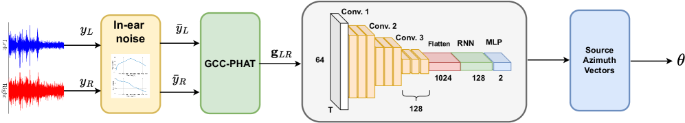
Figure 1: Block diagram of the model architecture.
<details>
<summary>x2.png Details</summary>
### Visual Description
## Line Graphs: Frequency Response Analysis
### Overview
The image contains two vertically stacked line graphs depicting frequency response characteristics. The top graph shows magnitude response in decibels (dB) across a frequency range, while the bottom graph displays phase response in radians (rad.) against the same frequency axis. Both graphs share a common frequency axis spanning 1-8 kHz.
### Components/Axes
- **X-axis (Frequency):** Labeled "Frequency (kHz)" with integer markers from 1 to 8 kHz
- **Y-axis (Top Graph):** Labeled "Magnitude (dB)" with values from 0 to 20 dB
- **Y-axis (Bottom Graph):** Labeled "Phase (rad.)" with values from -2 to 2 rad
- **No legend present**
- **Gridlines:** Present in both graphs with light gray lines and darker axis lines
### Detailed Analysis
**Top Graph (Magnitude Response):**
- Starts at 0 dB at 1 kHz
- Rises gradually to a peak of approximately 20 dB at 4 kHz
- Declines symmetrically to ~10 dB at 8 kHz
- Approximate values (with uncertainty):
- 1 kHz: 0.0 ± 0.5 dB
- 2 kHz: 15.0 ± 1.0 dB
- 3 kHz: 18.0 ± 0.8 dB
- 4 kHz: 20.0 ± 0.5 dB
- 5 kHz: 17.0 ± 0.7 dB
- 6 kHz: 14.0 ± 0.6 dB
- 7 kHz: 12.0 ± 0.5 dB
- 8 kHz: 10.0 ± 0.4 dB
**Bottom Graph (Phase Response):**
- Starts at 2.0 rad at 1 kHz
- Decreases linearly to -2.0 rad at 8 kHz
- Approximate values (with uncertainty):
- 1 kHz: 2.0 ± 0.3 rad
- 2 kHz: 1.5 ± 0.2 rad
- 3 kHz: 1.0 ± 0.1 rad
- 4 kHz: 0.5 ± 0.1 rad
- 5 kHz: -0.5 ± 0.1 rad
- 6 kHz: -1.0 ± 0.1 rad
- 7 kHz: -1.5 ± 0.1 rad
- 8 kHz: -2.0 ± 0.1 rad
### Key Observations
1. Magnitude response exhibits a resonant peak at 4 kHz with a Q-factor suggesting moderate bandwidth
2. Phase response shows a consistent -45°/radian per decade roll-off characteristic
3. Inverse relationship between magnitude peak and phase shift suggests a second-order system
4. Phase response maintains linear progression despite magnitude variations
### Interpretation
The data suggests a bandpass filter or resonant circuit behavior with:
- Center frequency at 4 kHz
- 3 dB bandwidth between 2-6 kHz (estimated from -3 dB points)
- Phase characteristics indicating a second-order system with:
- Phase lead at low frequencies
- Phase lag at high frequencies
- Maximum phase shift of -180° at resonance
The inverse relationship between magnitude and phase after the resonant peak indicates potential phase compensation requirements for stability in control systems. The consistent phase roll-off despite magnitude variations suggests the system maintains predictable phase behavior across its operational range.
</details>
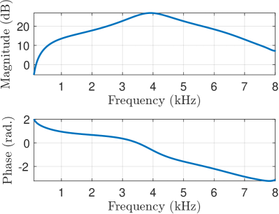
Figure 2: Magnitude and phase response of filter used to simulate the listener’s hearing threshold.
A well-known method for localisation using ITD estimation is the Generalized Cross-Correlation with Phase Transform (GCC-PHAT) approach, which assumes ideal single-path propagation. Although Generalized Cross-Correlation (GCC) and similar methods can be applied to any setup with two or more microphones, some recent research has focused on localization models specifically designed for binaural systems [5, 6]. Recent efforts have integrated azimuth-dependent models of ITD and ILD, demonstrating that jointly considering both cues enhances azimuth estimation compared to using ITD alone [7, 6, 5]. However, these models often require prior training or calibration with the binaural input due to the significant variability in the frequency-dependent patterns of ITD s and ILD s across individuals, which can lead to performance degradation in different binaural setups. Methods also differ in how they integrate interaural information across time and frequency, with these variations largely reflecting different assumptions about source activity and interaction. In [5], authors proposed a framework that determines the likelihood of each source location based on a Gaussian Mixture Model (GMM) classifier, which learns the azimuth-dependent distribution of ITD s and ILD s from joint analysis of both binaural cues. However, many binaural localization methods have focused on scenarios with minimal reverberation or background noise. One approach to improving localization in more complex environments involves using model-based information about the spectral characteristics of sound sources in the acoustic scene to selectively weight binaural cues. This involves estimating models for both target and background sources during a training stage, using spectral features derived from isolated source signals [6]. In [8], an end-to-end binaural localization algorithm that estimates the azimuth using Convolutional Neural Network (CNN)s to extract features from the binaural signal was introduced.
Human auditory cognition includes complex neurological processes for localization. Although ILD s and ITD s are widely accepted to be the primary interaural cues that influence human sound source localization [1], there is no standardized way to characterise them. Precedence effect, spectral cues, head movement and other psychoacoustical processes affect sound localization in humans. There is no universally accepted method of measuring the correlation between human sound localization and the frequency-varying interaural cues. In [9, 10], to demonstrate the preservation of spatial cues, the error in interaural cues of the enhanced speech was computed using an Ideal Binary Mask (IBM) that selects the speech-active regions in the signal.
A relevant approach to measuring the accuracy with which spatial information is preserved and the subsequent accuracy of localization of speech sources in noisy and enhanced speech signals would be to employ a model that predicts the localization of the speech-in-noise in a manner highly correlated to a human listener. This paper sets out to research methods of Direction of Arrival (DOA) estimation that are not necessarily the best-performing but specifically follow the performance of the human listener in terms of binaural localization. The paper will focus on an end-to-end binaural localization model for speech in noisy and reverberant conditions, introducing a lightweight Convolutional Recurrrent Network (CRN) that utilizes input features based on GCC-PHAT, which is a first step towards this goal. The model adds synthetic internal ear noise to an audio signal to simulate the effects of the frequency-dependent hearing threshold of a normal listener. The model is trained on binaural speech data to directly predict the source azimuth without limiting the localization to a predetermined azimuth-dependent distribution of interaural cues. The approach is evaluated using a listening test that was conducted using 15 normal hearing listeners, in which the participants were tasked to localize a target speaker in simulated noisy and reverberant conditions.
## 2 System Description
### 2.1 Signal model
A binaural system is comprises a left and a right channel. The time-domain signal $y_{L}$ received by the left channel is modeled as
$$
\displaystyle y_{L}(n)=s_{L}(n)+v_{L}(n), \tag{1}
$$
where $s_{L}$ is the anechoic clean speech signal, $v_{L}$ is the noise and $n$ is the discrete-time index. The in-ear noise added signal $\tilde{{y}_{L}}$ is given by
$$
\displaystyle\bar{y}_{L}(n)=h_{e}(n)\ast y_{L}(n)+e_{L}(n) \tag{2}
$$
where $h_{e}(n)$ is the impulse response of the filter depicted in Fig. 2 and $e_{L}(n)$ is the white noise added to the filtered noisy signal. The right channel is described similarly with a $R$ subscript. The model adds fictitious internal ear noise to an audio signal to simulate the effects of the frequency-dependent hearing threshold of a normal listener, assuming that the input speech in the stronger channel is at the normal level defined in [11] to be 62.35 dB SPL”. The noise spectrum is taken from [12, 11] and, at a particular frequency, equals the pure-tone hearing threshold minus $10\log_{10}(C)$ where $C$ is the critical ratio. The critical ratio, $C$ , is the power of a pure tone divided by the power spectral density of a white noise that masks it; this ratio is approximately independent of level. Hearing loss can also be taken into account here by modifying the filter that reduces the signal level by the hearing loss at each frequency. To avoid having to add very high noise levels at low and high frequencies, it instead filters the input signal by the inverse of the desired noise spectrum and then adds white noise with 0 dB power spectral density. Figure 1 shows the block diagram of the proposed system. The raw time-domain signal is filtered with the in-ear frequency response shown in Fig. 2. The online implementation (v_earnoise.m Matlab function) of the ear-noise filter can be found in [13]. The in-ear noise-added signal is then used as the input to the neural network, which determines the target azimuth in the frontal azimuthal plane.
### 2.2 Localization network
#### 2.2.1 Input Feature Set
The input feature of the proposed network consists of the GCC-PHAT for the pair of microphone signal frames $(\mathbf{\bar{y}_{L}},\mathbf{\bar{y}_{R})}$ , defined as
$$
\mathbf{g}_{LR}=\text{IDFT}\bigg{(}\frac{\bar{\mathbf{Y}}_{L}}{\lvert\bar{\mathbf{Y}}_{L}\rvert}\odot\frac{\bar{\mathbf{Y}}^{*}_{R}}{\lvert\bar{\mathbf{Y}}_{R}\rvert}\bigg{)}, \tag{3}
$$
the Inverse Discrete Fourier Transform (IDFT) of the element-wise product of the normalized frequency-domain frames ${\mathbf{Y}_{L}}$ and $\mathbf{{Y}}_{R}$ , where $\mathbf{\bar{{Y}}}=\text{DFT}(\bar{\mathbf{{y}}})$ and $\lvert{\mathbf{Y}}\rvert$ is the element-wise magnitude.
#### 2.2.2 Network architecture
As shown in Fig. 1, the network is composed of a set of convolutional blocks, followed by an operation of flattening of the frequency and channel dimension. The resulting tensor is then used as input for a Gated Recurrent Unit (GRU) Recurrent Neural Network (RNN). Finally, a linear layer is applied to produce a 2-D output vector, $\mathbf{\hat{v}}$ , representing the direction of the source’s azimuth.
### 2.3 Loss function
The proposed model is trained using a modification of the cosine similarity given by
$$
\displaystyle\mathcal{L}({\mathbf{v},\hat{\mathbf{v}}})=1-\lVert\frac{\mathbf{v}\cdot{\mathbf{\hat{v}}}}{|\mathbf{v}||{\mathbf{\hat{v}}}|}\rVert \tag{4}
$$
between the true and estimated directions $\mathbf{v}$ and $\hat{\mathbf{v}}$ . The loss function (4) was designed so that the absolute value of the cosine similarity between the vectors is minimized, therefore not penalizing the effects caused by the front-back ambiguity, which are expected when employing only two microphones.
## 3 Experiments
### 3.1 Dataset
To generate binaural speech data, monaural clean speech signals were obtained from the CSTR VCTK corpus [14] and spatialized using the measured Binaural Room Impulse Responses (BRIRs) from [15] for training. The VCTK corpus contains approximately 13 hours of speech data from 110 English speakers with various accents. These recordings were used to create 2 s speech utterances, which were spatialized to produce left and right ear channels. The resulting dataset comprised 20,000 speech utterances, which were divided into training (70%), validation (15%), and testing (15%) sets. Diffuse isotropic speech-shaped noise was generated using uncorrelated noise sources uniformly distributed every $5^{\circ}$ in the azimuthal plane [16], utilizing BRIRs from [15] which were recorded in a listening room with a $T_{60}$ of $460$ ms. The binaural signals were generated with the target speech positioned at a random azimuth in the frontal plane ( $-90^{\circ}$ to $+90^{\circ}$ ) with the source positioned at a distance of 100 cm. For the training process, isotropic noise was added so that the average in dB of $(SNR_{L},~SNR_{R})$ , ranged between -25 dB and 25 dB. The evaluation set comprised speech signals spatialized with BRIRs from [17] with random target azimuths and isotropic noise added at random SNR s between -25 dB and 25 dB. The speaker was positioned at a $0^{\circ}$ elevation and at a distance of 3 m. This ensured that training and evaluation sets contained binaural signals generated using different BRIRs to verify that the network generalised to different heads.
### 3.2 Training Setup
The 2 s input signals were sampled at 16 kHz, and a window size of 512 was used to generate the signal frames with a 75% overlap for a hop size of 25 ms. The parameters for the localization network are detailed in Fig. 1, which includes the tensor output shapes for each layer of the network. Convolutional layers employed a kernal size of (3, 3) throughout. Max pooling with a kernel size of 2 was applied to all convolutional layers except the last one. The Parametric Rectified Linear Unit (PReLU) activation function was utilized in all layers of the network, except for the RNN and Multi-Layer Perceptrons (MLP) output layers, which used hyperbolic tangent ( $\tanh$ ) activation, and the output layer, which employed sigmoidal activation. This architecture was taken from [18] and modified to work for binaural signals. The network has 850K parameters and is implemented using the PyTorch library, and the Adam optimizer was used for backpropagation. The network was trained for 80 epochs. The code for implementation is available online https://github.com/VikasTokala/BiL.
<details>
<summary>x3.png Details</summary>
### Visual Description
## Bar Chart: RMS Error vs. iSNR for BIL and SRP Methods
### Overview
The image contains two vertically stacked bar charts comparing RMS error (in degrees) across varying iSNR values for two methods: BIL (blue bars) and SRP (red bars). Each bar includes error bars representing uncertainty. The x-axis spans iSNR values from -25 to 25, while the y-axes for BIL and SRP range from 0–15° and 0–60°, respectively.
### Components/Axes
- **X-axis**: Labeled "iSNR" with tick marks at -25, -20, -15, -10, -5, 0, 5, 10, 15, 20, 25.
- **Y-axis (Top Chart)**: Labeled "RMS Error [deg]" (0–15°) for BIL.
- **Y-axis (Bottom Chart)**: Labeled "RMS Error [deg]" (0–60°) for SRP.
- **Legend**: Located in the top-right corner, with blue representing BIL and red representing SRP.
- **Error Bars**: Vertical lines atop each bar indicating measurement uncertainty.
### Detailed Analysis
#### BIL Method (Top Chart)
- **iSNR = -25**: RMS error ≈ 10.5° ± 3.2° (error bar length).
- **iSNR = -20**: RMS error ≈ 5.2° ± 1.8°.
- **iSNR = -15**: RMS error ≈ 4.1° ± 1.5°.
- **iSNR = -10**: RMS error ≈ 3.8° ± 1.2°.
- **iSNR = -5**: RMS error ≈ 3.0° ± 0.9°.
- **iSNR = 0**: RMS error ≈ 2.5° ± 0.7°.
- **iSNR = 5**: RMS error ≈ 2.1° ± 0.6°.
- **iSNR = 10**: RMS error ≈ 1.5° ± 0.4°.
- **iSNR = 15**: RMS error ≈ 1.0° ± 0.3°.
- **iSNR = 20**: RMS error ≈ 0.7° ± 0.2°.
- **iSNR = 25**: RMS error ≈ 0.4° ± 0.1°.
#### SRP Method (Bottom Chart)
- **iSNR = -25**: RMS error ≈ 38.0° ± 6.5°.
- **iSNR = -20**: RMS error ≈ 37.5° ± 6.2°.
- **iSNR = -15**: RMS error ≈ 25.0° ± 5.0°.
- **iSNR = -10**: RMS error ≈ 23.0° ± 4.8°.
- **iSNR = -5**: RMS error ≈ 18.0° ± 4.0°.
- **iSNR = 0**: RMS error ≈ 12.0° ± 3.5°.
- **iSNR = 5**: RMS error ≈ 13.0° ± 3.2°.
- **iSNR = 10**: RMS error ≈ 10.0° ± 2.8°.
- **iSNR = 15**: RMS error ≈ 9.0° ± 2.5°.
- **iSNR = 20**: RMS error ≈ 8.0° ± 2.2°.
- **iSNR = 25**: RMS error ≈ 9.0° ± 2.0°.
### Key Observations
1. **BIL vs. SRP**: BIL consistently shows lower RMS errors than SRP across all iSNR values.
2. **iSNR Dependency**: Both methods exhibit higher RMS errors at lower iSNR values (-25 to -5), with errors decreasing as iSNR increases.
3. **Uncertainty Trends**: Error bars are longest at lower iSNR values, indicating greater variability in measurements under poor signal conditions.
4. **SRP Anomaly**: SRP’s RMS error at iSNR = 25 (9.0°) is higher than at iSNR = 20 (8.0°), suggesting a potential non-monotonic relationship at high iSNR.
### Interpretation
The data demonstrates that the BIL method outperforms SRP in terms of RMS error across all tested iSNR values. The pronounced error reduction in BIL at lower iSNR (-25 to -5) highlights its robustness in low-signal environments. The SRP method’s higher errors and non-monotonic trend at high iSNR (20–25) may indicate overfitting or sensitivity to noise in high-signal conditions. The error bars underscore the importance of iSNR in determining measurement reliability, with lower iSNR values associated with greater uncertainty. These findings suggest BIL is preferable for applications requiring accuracy across diverse signal conditions, while SRP may require refinement for high-iSNR scenarios.
</details>
(a)
<details>
<summary>x4.png Details</summary>
### Visual Description
## Bar Chart: RMS Error by iSNR for Listeners, SRP, and BIL
### Overview
The chart compares RMS error (in degrees) across three groups—Listeners, SRP, and BIL—at three iSNR values (-15, 0, 15). Error bars represent uncertainty in measurements. SRP consistently shows the highest error, while BIL has the lowest.
### Components/Axes
- **X-axis**: iSNR (signal-to-noise ratio), labeled with ticks at -15, 0, and 15.
- **Y-axis**: RMS Error [deg], scaled from 0 to 45.
- **Legend**: Located in the top-right corner, with:
- Purple = Listeners
- Red = SRP
- Blue = BIL
- **Bars**: Grouped by iSNR, with three bars per group (one per category).
### Detailed Analysis
1. **iSNR = -15**:
- **Listeners**: ~20° (±3° uncertainty).
- **SRP**: ~28° (±5° uncertainty).
- **BIL**: ~5° (±1° uncertainty).
2. **iSNR = 0**:
- **Listeners**: ~16° (±4° uncertainty).
- **SRP**: ~27° (±6° uncertainty).
- **BIL**: ~4° (±1° uncertainty).
3. **iSNR = 15**:
- **Listeners**: ~15° (±2° uncertainty).
- **SRP**: ~17° (±3° uncertainty).
- **BIL**: ~1° (±0.5° uncertainty).
### Key Observations
- **SRP** has the highest RMS error across all iSNR values, with error bars indicating significant variability (e.g., ±6° at iSNR=0).
- **BIL** consistently shows the lowest error, with minimal uncertainty (e.g., ±0.5° at iSNR=15).
- **Listeners** exhibit a decreasing trend in error as iSNR increases (20° → 15°).
- SRP’s error bars are longest at iSNR=-15 and 0, suggesting higher measurement uncertainty in low-SNR conditions.
### Interpretation
The data suggests that **SRP** (likely a system or method) performs poorly compared to **BIL** and **Listeners**, with higher RMS error and greater variability. The trend of decreasing error with increasing iSNR implies that higher signal-to-noise ratios improve performance for all groups. However, SRP’s persistent high error—even at iSNR=15—highlights a potential flaw in its design or implementation. BIL’s near-zero error at iSNR=15 may indicate superior robustness or accuracy in high-SNR conditions. The error bars underscore the reliability of BIL’s measurements versus SRP’s inconsistency.
</details>
(b)
<details>
<summary>x5.png Details</summary>
### Visual Description
## Bar Charts: RMS Error vs. iSNR for Different Methods
### Overview
The image contains two bar charts comparing Root Mean Square (RMS) angular error (in degrees) across different signal-to-noise ratio (iSNR) values for three computational methods. The top chart compares three methods (Noisy + BIL, BCCTN + BIL, BiTasNet + BIL), while the bottom chart isolates the SpecSub + BIL method. Error bars represent standard deviation.
### Components/Axes
**Top Chart:**
- **X-axis (iSNR):** Discrete values from -15 to 15 in increments of 5 (iSNR = -15, -10, -5, 0, 5, 10, 15).
- **Y-axis (RMS Error [deg]):** Range 0–10 degrees.
- **Legend (Top-right):**
- Blue: Noisy + BIL
- Red: BCCTN + BIL
- Yellow: BiTasNet + BIL
**Bottom Chart:**
- **X-axis (iSNR):** Same values as top chart (-15 to 15).
- **Y-axis (RMS Error [deg]):** Range 0–80 degrees.
- **Legend (Top-right):**
- Cyan: SpecSub + BIL
### Detailed Analysis
**Top Chart Trends:**
1. **iSNR = -15:**
- BiTasNet + BIL (yellow) has the highest error (~9.0° ± 1.5°).
- Noisy + BIL (blue) and BCCTN + BIL (red) are similar (~4.5° ± 0.8°).
2. **iSNR = -10:**
- All methods converge (~4.0° ± 0.7° for blue/red, ~3.8° ± 0.6° for yellow).
3. **iSNR = -5 to 15:**
- Errors decrease monotonically for all methods.
- At iSNR = 15, all methods achieve ~1.5° ± 0.3° error.
**Bottom Chart Trends:**
- **SpecSub + BIL (cyan):**
- Consistent error across all iSNR values (~45° ± 5°).
- Largest error bars (up to ±7° at iSNR = -5).
### Key Observations
1. **Method Performance:**
- BiTasNet + BIL outperforms others at low iSNR but converges at high iSNR.
- SpecSub + BIL shows consistently poor performance regardless of iSNR.
2. **Error Variability:**
- SpecSub + BIL has the highest uncertainty (larger error bars).
- Noisy + BIL and BCCTN + BIL show tighter confidence intervals.
### Interpretation
The data suggests that computational methods for angular estimation exhibit SNR-dependent performance. BiTasNet + BIL demonstrates adaptive robustness, improving accuracy as SNR increases. In contrast, SpecSub + BIL fails to leverage SNR improvements, maintaining high error across all conditions. This implies that method architecture (e.g., noise handling in BiTasNet vs. static processing in SpecSub) critically impacts real-world applicability in low-SNR environments. The convergence of methods at high iSNR highlights the importance of SNR in reducing estimation errors.
</details>
(c)
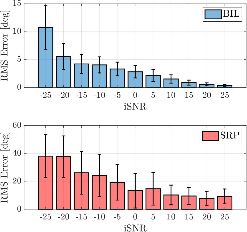
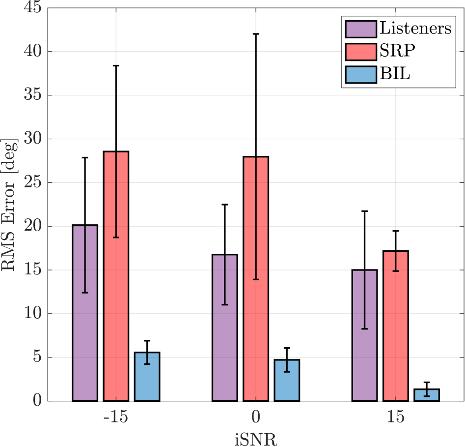
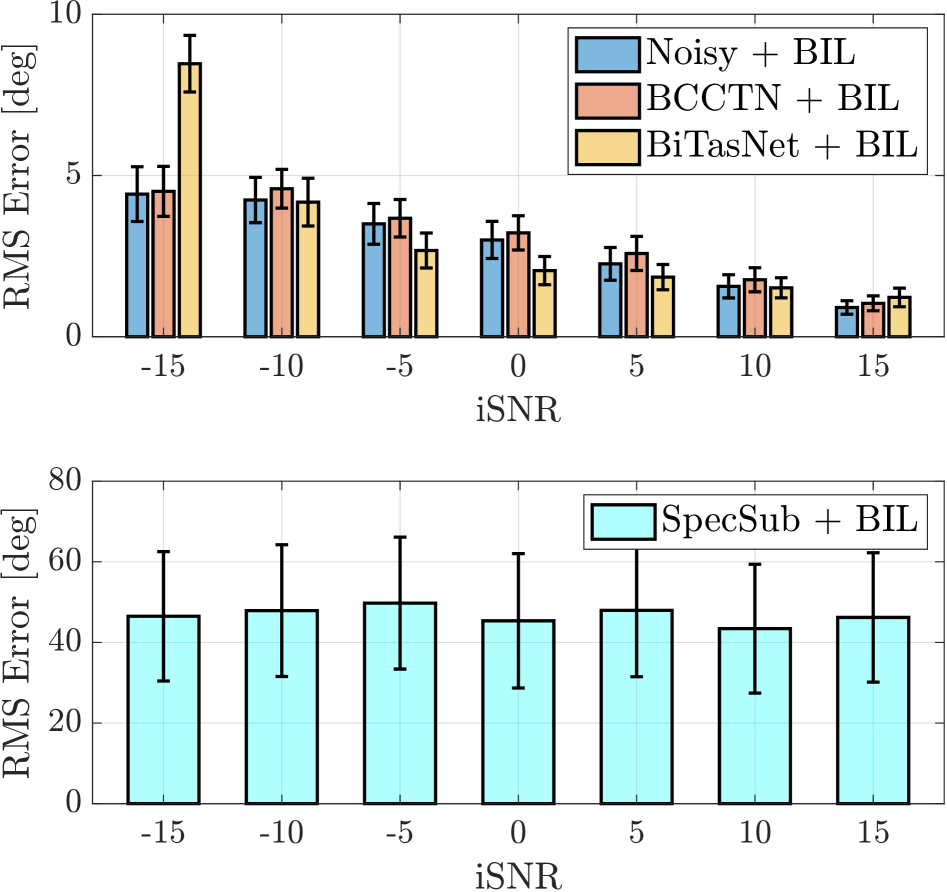
Figure 3: The plots show the localization error in noisy reverberant conditions (a) for the proposed method (BIL) and SRP, (b) for listeners compared with the proposed method and SRP and, (c) for signals processed by different enhancement methods evaluated by BIL.
### 3.3 Listening Tests
In the listening tests, 15 participants with normal hearing were tasked with localizing a target speaker within the frontal azimuthal plane. Using Beyerdynamic DT1990 Pro open-back headphones, the audio signals were delivered in a soundproof booth through an RME Fireface UCX II audio interface. The participants were required to listen to the noisy speech utterances and select the perceived azimuth using a MATLAB-based GUI. The azimuths were quantized at $15^{\circ}$ intervals. Each participant listened to 36 speech utterances, which were evenly distributed across different SNR s and randomly assigned azimuths in the frontal azimuth plane. Three conditions of input SNR (iSNR) were used in the test: -15, 0 and +15 dB iSNR corresponding to “very noisy”, “noisy” and “low noise” conditions, respectively.
## 4 Results and Discussion
| SRP-PHAT WaveLoc-GTF [8] WaveLoc-CONV [8] | $10.2^{\circ}$ $3.0^{\circ}$ $2.3^{\circ}$ |
| --- | --- |
| BIL | $1.2^{\circ}$ |
Table 1: Localization error compared to WaveLoc [8] methods.
The model was evaluated using 275 speech utterances for each noisy input SNR ranging from -25 dB to +25 dB in steps of 5 dB. The localization error for the proposed method, denoted as BIL, is shown in Fig. 3(a) for different iSNR s. The azimuth $\theta$ of the target speaker’s DOA in the frontal azimuth plane is then estimated using the Steered Response Power with Phase Transform (SRP-PHAT) algorithm [19, 20] and used for comparison. In extremely noisy conditions, such as -25 dB, the proposed method achieves a localization error of approximately $15^{\circ}$ . Under similar iSNR conditions, the localization error for Steered Response Power (SRP) is considerably higher, around $40^{\circ}$ . As the iSNR improves, the localization error for the proposed method decreases to below $5^{\circ}$ , eventually reaching just under $1^{\circ}$ at 25 dB iSNR. In contrast, the SRP method maintains an error between $10^{\circ}$ and $20^{\circ}$ even at higher iSNR s. The reduced performance of SRP at higher iSNR s can be attributed to reverberation, which causes multiple peaks in the correlation [18]. 1 shows the comparison of localization error with the WaveLoc methods proposed in [8]. These methods are also evaluated on BRIRs from [15] without the addition of external noise, and the values shown are taken from [8]. For similar conditions, the proposed method has lower error and outperforms both versions of the WaveLoc methods.
Figure 3(b) shows the localization error of human listeners compared with the proposed method and SRP for the three conditions of noisy signals as described in Sec. 3.3. The proposed method has a significantly lower localization error for all the iSNR conditions. Listeners had an average error of $20^{\circ}$ in the very noisy condition of -15 dB and an average error of $15^{\circ}$ in the low noise condition of 15 dB, given that there was no head movement to assist them. SRP -based localization had the highest localization error and standard deviation for the test samples. Previous studies have shown that human localization of speech and tones can have a localization error of up to $40^{\circ}$ when noise and reverberation are present [1, 2, 3]. If the signals processed by enhancement methods produce a low localization error with the proposed method, it is very likely that the interaural cues of the signal are preserved, and human listeners will still localize the target speaker in the same azimuth as the original noisy signal.
Figure 3(c) demonstrates how the proposed method can be used to assess the performance of binaural speech enhancement methods in preserving the interaural cues and the spatial information of the target speaker. While there are well-known objective measures to evaluate noise reduction, speech intelligibility and quality, there are no standardised measures to assess the preservation of binaural cues after they are processed by enhancement algorithms. The upper plot in Fig. 3(c) shows the localization error for noisy signals at the iSNR s from -15 dB to 15 dB and the signals processed by Binaural Complex Convolutional Transformer Network (BCCTN) [9] and Binaural TasNet (BiTasNet) [21] at the same iSNR s. The binaural enhancement algorithms are designed to preserve the interaural cues in the noisy signal while enhancement, and they show a low localization error. At -15 dB, the BiTasNet shows a higher error compared to the noisy input signal, which indicates disruption in the interaural cues, and this is expected as the method was not designed to perform enhancement at -15 dB. As the iSNR improves, all the binaural enhancement methods show localization error under $5^{\circ}$ , which signifies the preservation of interaural cues. From Fig 3(a) - Fig. 3(c), it is evident that the proposed model has a monotonic relationship to SNR, i.e., the localization error decreases with increasing iSNR. Furthermore, other studies, including [1, 2, 3], show that human localization capability is monotonically proportional to SNR. Hence, the proposed method has been seen to be, as desired, highly correlated with human binaural localization - a conclusion which is supported by the subjective listening tests conducted. The lower plot in Fig. 3(c) shows the localization error obtained when the noisy signals are processed with bilateral spectral subtraction (SpecSub) [22], where no attempt is made at preserving binaural cues. The localization error is obtained around $45^{\circ}$ as the testset contains signals which have azimuths distributed randomly between $\pm 90^{\circ}$ . If the binaural enhancement methods are being used for purposes other than human listening, the addition of in-ear noise can be omitted before performing localization.
## 5 Conclusion
This paper presented an end-to-end binaural localization model for speech in noisy and reverberant conditions. A CRN network utilizing GCC-PHAT features was introduced, and a listening test with 15 normal-hearing listeners showed that the model closely aligns with human perception, albeit with lower localization error. The model effectively evaluates the localization error of binaural speech enhancement algorithms, correlating with spatial information preservation and interaural cue retention. The key objective was to develop a DOA estimation method that mirrors human binaural localization rather than purely optimizing accuracy. The proposed method demonstrated significantly lower localization errors across all iSNR conditions. Listeners had average errors of $20^{\circ}$ at -15 dB and $15^{\circ}$ at 15 dB without head movement. SRP -based localization showed the highest error and variability and as iSNR improves, all binaural enhancement methods exhibit localization errors below $5^{\circ}$ , confirming interaural cue preservation. The model’s localization error follows a monotonic relationship with SNR, aligning with human performance trends.
## 6 Acknowledgments
This work was supported by funding from the European Union’s Horizon 2020 research and innovation programme under the Marie Skłodowska-Curie grant agreement No 956369 and the UK Engineering and Physical Sciences Research Council [grant number EP/S035842/1].
## References
- [1] M. D. Good and R. H. Gilkey, “Sound localization in noise: The effect of signal-to-noise ratio,” J Acoust Soc Am, vol. 99, pp. 1108–1117, Feb. 1996.
- [2] C. Lorenzi, S. Gatehouse, and C. Lever, “Sound localization in noise in normal-hearing listeners,” J Acoust Soc Am, vol. 105, pp. 1810–1820, Mar. 1999.
- [3] M. L. Folkerts, E. M. Picou, and G. C. Stecker, “Spectral weighting functions for localization of complex sound. II. The effect of competing noise,” J Acoust Soc Am, vol. 154, pp. 494–501, July 2023.
- [4] N. Kopčo, V. Best, and S. Carlile, “Speech localization in a multitalker mixture,” J Acoust Soc Am, vol. 127, pp. 1450–1457, Mar. 2010.
- [5] T. May, S. van de Par, and A. Kohlrausch, “A Probabilistic Model for Robust Localization Based on a Binaural Auditory Front-End,” IEEE/ACM Trans. Audio, Speech, Language Process., vol. 19, pp. 1–13, Jan. 2011.
- [6] N. Ma, J. A. Gonzalez, and G. J. Brown, “Robust Binaural Localization of a Target Sound Source by Combining Spectral Source Models and Deep Neural Networks,” IEEE/ACM Trans. Audio, Speech, Language Process., vol. 26, pp. 2122–2131, Nov. 2018.
- [7] J. Woodruff and D. Wang, “Binaural Localization of Multiple Sources in Reverberant and Noisy Environments,” IEEE/ACM Trans. Audio, Speech, Language Process., vol. 20, pp. 1503–1512, July 2012.
- [8] P. Vecchiotti, N. Ma, S. Squartini, and G. J. Brown, “End-to-end Binaural Sound Localisation from the Raw Waveform,” in Proc. IEEE Int. Conf. on Acoust., Speech and Signal Process. (ICASSP), pp. 451–455, May 2019.
- [9] V. Tokala, E. Grinstein, M. Brookes, S. Doclo, J. Jensen, and P. A. Naylor, “Binaural Speech Enhancement using Deep Complex Convolutional Recurrent Networks,” in Proc. Asilomar Conf. on Signals, Syst. & Comput., (USA), 2023.
- [10] V. Tokala, E. Grinstein, M. Brookes, S. Doclo, J. Jensen, and P. A. Naylor, “Binaural Speech Enhancement using Deep Complex Convolutional Transformer Networks,” in Proc. IEEE Int. Conf. on Acoust., Speech and Signal Process. (ICASSP), (Seoul, South Korea), 2024.
- [11] ANSI, “Methods for the calculation of the speech intelligibility index,” ANSI Standard S3.5-1997 (R2007), American National Standards Institute (ANSI), 1997.
- [12] C. V. Pavlovic, “Derivation of primary parameters and procedures for use in speech intelligibility predictions,” J Acoust Soc Am, vol. 82, pp. 413–422, Aug. 1987.
- [13] D. M. Brookes, “VOICEBOX: A speech processing toolbox for MATLAB,” 1997.
- [14] J. Yamagishi, C. Veaux, and K. MacDonald, “CSTR VCTK Corpus: English multi-speaker corpus for CSTR voice cloning toolkit (version 0.92),” University of Edinburgh. The Centre for Speech Technology Research (CSTR), 2019.
- [15] J. Francombe, “IoSR Listening Room Multichannel BRIR Dataset - University of Surrey,” 2017.
- [16] A. H. Moore, L. Lightburn, W. Xue, P. A. Naylor, and M. Brookes, “Binaural mask-informed speech enhancement for hearing aids with head tracking,” in Proc. Int. Workshop on Acoust. Signal Enhancement (IWAENC), (Tokyo, Japan), pp. 461–465, Sept. 2018.
- [17] H. Kayser, S. D. Ewert, J. Anemüller, T. Rohdenburg, V. Hohmann, and B. Kollmeier, “Database of multichannel in-ear and behind-the-Ear head-related and binaural room impulse responses,” EURASIP J. on Advances in Signal Process., vol. 2009, p. 298605, July 2009.
- [18] E. Grinstein, C. M. Hicks, T. van Waterschoot, M. Brookes, and P. A. Naylor, “The Neural-SRP Method for Universal Robust Multi-Source Tracking,” IEEE Open Journal of Signal Processing, vol. 5, pp. 19–28, 2024.
- [19] J. H. DiBiase, H. F. Silverman, and M. S. Brandstein, “Robust localization in reverberant rooms,” in Microphone Arrays (M. Brandstein and D. Ward, eds.), Digital Signal Processing, pp. 157–180, Berlin Heidelberg: Springer-Verlag, 2001.
- [20] E. Grinstein, E. Tengan, B. Çakmak, T. Dietzen, L. Nunes, T. van Waterschoot, M. Brookes, and P. A. Naylor, “Steered Response Power for Sound Source Localization: A Tutorial Review,” EURASIP J. on Audio, Speech, and Music Process., vol. submitted, May 2024.
- [21] C. Han, Y. Luo, and N. Mesgarani, “Real-Time Binaural Speech Separation with Preserved Spatial Cues,” in Proc. IEEE Int. Conf. on Acoust., Speech and Signal Process. (ICASSP), pp. 6404–6408, May 2020.
- [22] Y. Ephraim and D. Malah, “Speech enhancement using a minimum mean-square error log-spectral amplitude estimator,” IEEE Trans. Acoust., Speech, Signal Process., vol. 33, no. 2, pp. 443–445, 1985.