# Kimi K2: Open Agentic Intelligence
**Authors**: Kimi Team
Abstract
We introduce Kimi K2, a Mixture-of-Experts (MoE) large language model with 32 billion activated parameters and 1 trillion total parameters. We propose the MuonClip optimizer, which improves upon Muon with a novel QK-clip technique to address training instability while enjoying the advanced token efficiency of Muon. Based on MuonClip, K2 was pre-trained on 15.5 trillion tokens with zero loss spike. During post-training, K2 undergoes a multi-stage post-training process, highlighted by a large-scale agentic data synthesis pipeline and a joint reinforcement learning (RL) stage, where the model improves its capabilities through interactions with real and synthetic environments.
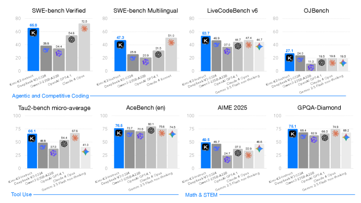
Kimi K2 achieves state-of-the-art performance among open-source non-thinking models, with strengths in agentic capabilities. Notably, K2 obtains 66.1 on Tau2-Bench, 76.5 on ACEBench (En), 65.8 on SWE-Bench Verified, and 47.3 on SWE-Bench Multilingual — surpassing most open and closed-sourced baselines in non-thinking settings. It also exhibits strong capabilities in coding, mathematics, and reasoning tasks, with a score of 53.7 on LiveCodeBench v6, 49.5 on AIME 2025, 75.1 on GPQA-Diamond, and 27.1 on OJBench, all without extended thinking. These results position Kimi K2 as one of the most capable open-source large language models to date, particularly in software engineering and agentic tasks. We release our base and post-trained model checkpoints https://huggingface.co/moonshotai/Kimi-K2-Instruct to facilitate future research and applications of agentic intelligence.
<details>
<summary>x2.png Details</summary>
### Visual Description
\n
## Bar Charts: Model Performance on Coding Benchmarks
### Overview
The image presents a series of eight bar charts comparing the performance of several large language models (LLMs) across various coding benchmarks. The models evaluated are: Kim-K2-instruct, DeepSeek-V2-024, Open-2.5B-A28, Open-A141, Claude 4 Opus, and Gemini 2.5 flash non-tuning. The benchmarks cover different aspects of coding ability, including verified code, multilingual code, competitive coding, and math/STEM tasks. Each chart displays a score, presumably representing accuracy or some other performance metric, with a "K" symbol marking a key data point.
### Components/Axes
Each chart shares the following components:
* **X-axis:** Lists the LLM models being compared.
* **Y-axis:** Represents the performance score, ranging from 0 to 100. The scale is consistent across all charts.
* **Bars:** Represent the performance of each model on a specific benchmark. The bars are color-coded, with a distinct color for each model.
* **"K" Marker:** A "K" symbol is placed on each bar, indicating a specific score.
* **Titles:** Each chart has a title indicating the benchmark being evaluated.
* **Legend:** The legend is implicit, with each model's color consistently used across all charts.
The charts are arranged in a 2x4 grid. The titles of the charts are:
1. SWE-bench Verified
2. SWE-bench Multilingual
3. LiveCode v6
4. QJBench
5. Tau-2-bench micro-average
6. AceBench (en)
7. AIME 2025
8. GPQA-Diamond
### Detailed Analysis or Content Details
Here's a breakdown of the data extracted from each chart, with approximate values and trend descriptions:
**1. SWE-bench Verified:**
* Kim-K2-instruct: ~65.8
* DeepSeek-V2-024: ~35.4
* Open-2.5B-A28: ~54.6
* Open-A141: ~72.5
* Claude 4 Opus: ~54.6
* Gemini 2.5 flash non-tuning: ~72.5
**2. SWE-bench Multilingual:**
* Kim-K2-instruct: ~47.3
* DeepSeek-V2-024: ~20.9
* Open-2.5B-A28: ~34.6
* Open-A141: ~51.0
* Claude 4 Opus: ~34.6
* Gemini 2.5 flash non-tuning: ~51.0
**3. LiveCode v6:**
* Kim-K2-instruct: ~53.7
* DeepSeek-V2-024: ~37.0
* Open-2.5B-A28: ~44.7
* Open-A141: ~44.7
* Claude 4 Opus: ~44.7
* Gemini 2.5 flash non-tuning: ~44.7
**4. QJBench:**
* Kim-K2-instruct: ~27.1
* DeepSeek-V2-024: ~11.3
* Open-2.5B-A28: ~19.5
* Open-A141: ~19.5
* Claude 4 Opus: ~19.5
* Gemini 2.5 flash non-tuning: ~19.5
**5. Tau-2-bench micro-average:**
* Kim-K2-instruct: ~75.1
* DeepSeek-V2-024: ~57.2
* Open-2.5B-A28: ~66.1
* Open-A141: ~67.6
* Claude 4 Opus: ~67.6
* Gemini 2.5 flash non-tuning: ~67.6
**6. AceBench (en):**
* Kim-K2-instruct: ~76.5
* DeepSeek-V2-024: ~60.1
* Open-2.5B-A28: ~75.6
* Open-A141: ~74.5
* Claude 4 Opus: ~74.5
* Gemini 2.5 flash non-tuning: ~74.5
**7. AIME 2025:**
* Kim-K2-instruct: ~40.5
* DeepSeek-V2-024: ~37.0
* Open-2.5B-A28: ~40.8
* Open-A141: ~40.8
* Claude 4 Opus: ~40.8
* Gemini 2.5 flash non-tuning: ~40.8
**8. GPQA-Diamond:**
* Kim-K2-instruct: ~76.1
* DeepSeek-V2-024: ~66.4
* Open-2.5B-A28: ~66.3
* Open-A141: ~74.6
* Claude 4 Opus: ~74.6
* Gemini 2.5 flash non-tuning: ~74.6
### Key Observations
* **Kim-K2-instruct** consistently performs well, often achieving the highest scores across most benchmarks.
* **DeepSeek-V2-024** generally exhibits the lowest scores across all benchmarks.
* **Open-A141, Claude 4 Opus, and Gemini 2.5 flash non-tuning** often have similar performance levels, clustering together in the higher ranges for several benchmarks.
* The performance differences between models are more pronounced in some benchmarks (e.g., SWE-bench Verified, Tau-2-bench micro-average) than in others (e.g., AIME 2025).
### Interpretation
The data suggests that Kim-K2-instruct is a strong performer across a diverse set of coding benchmarks. DeepSeek-V2-024 appears to lag behind the other models in terms of coding ability, as measured by these benchmarks. The consistent grouping of Open-A141, Claude 4 Opus, and Gemini 2.5 flash non-tuning indicates a similar level of performance for these models.
The variation in performance across benchmarks highlights the importance of evaluating models on a range of tasks to get a comprehensive understanding of their capabilities. Some benchmarks may be more sensitive to specific model architectures or training data. The "K" marker's consistent placement suggests it represents a key performance indicator, potentially a specific test case or a threshold score.
The arrangement of the charts into categories ("Agentic and Competitive Coding", "Tool Use", "Math & STEM") provides a structured view of model performance across different coding domains. This allows for a more nuanced comparison of model strengths and weaknesses. The data suggests that Kim-K2-instruct excels in both coding and math/STEM tasks, while DeepSeek-V2-024 struggles in all areas.
</details>
Figure 1: Kimi K2 main results. All models evaluated above are non-thinking models. For SWE-bench Multilingual, we evaluated only Claude 4 Sonnet because the cost of Claude 4 Opus was prohibitive.
1 Introduction
The development of Large Language Models (LLMs) is undergoing a profound paradigm shift towards Agentic Intelligence – the capabilities for models to autonomously perceive, plan, reason, and act within complex and dynamic environments. This transition marks a departure from static imitation learning towards models that actively learn through interactions, acquire new skills beyond their training distribution, and adapt behavior through experiences [64]. It is believed that this approach allows an AI agent to go beyond the limitation of static human-generated data, and acquire superhuman capabilities through its own exploration and exploitation. Agentic intelligence is thus rapidly emerging as a defining capability for the next generation of foundation models, with wide-ranging implications across tool use, software development, and real-world autonomy.
Achieving agentic intelligence introduces challenges in both pre-training and post-training. Pre-training must endow models with broad general-purpose priors under constraints of limited high-quality data, elevating token efficiency—learning signal per token—as a critical scaling coefficient. Post-training must transform those priors into actionable behaviors, yet agentic capabilities such as multi-step reasoning, long-term planning, and tool use are rare in natural data and costly to scale. Scalable synthesis of structured, high-quality agentic trajectories, combined with general reinforcement learning (RL) techniques that incorporate preferences and self-critique, are essential to bridge this gap.
In this work, we introduce Kimi K2, a 1.04 trillion-parameter Mixture-of-Experts (MoE) LLM with 32 billion activated parameters, purposefully designed to address the core challenges and push the boundaries of agentic capability. Our contributions span both the pre-training and post-training frontiers:
- We present MuonClip, a novel optimizer that integrates the token-efficient Muon algorithm with a stability-enhancing mechanism called QK-Clip. Using MuonClip, we successfully pre-trained Kimi K2 on 15.5 trillion tokens without a single loss spike.
- We introduce a large-scale agentic data synthesis pipeline that systematically generates tool-use demonstrations via simulated and real-world environments. This system constructs diverse tools, agents, tasks, and trajectories to create high-fidelity, verifiably correct agentic interactions at scale.
- We design a general reinforcement learning framework that combines verifiable rewards (RLVR) with a self-critique rubric reward mechanism. The model learns not only from externally defined tasks but also from evaluating its own outputs, extending alignment from static into open-ended domains.
Kimi K2 demonstrates strong performance across a broad spectrum of agentic and frontier benchmarks. It achieves scores of 66.1 on Tau2-bench, 76.5 on ACEBench (en), 65.8 on SWE-bench Verified, and 47.3 on SWE-bench Multilingual, outperforming most open- and closed-weight baselines under non-thinking evaluation settings, closing the gap with Claude 4 Opus and Sonnet. In coding, mathematics, and broader STEM domains, Kimi K2 achieves 53.7 on LiveCodeBench v6, 27.1 on OJBench, 49.5 on AIME 2025, and 75.1 on GPQA-Diamond, further highlighting its capabilities in general tasks. On the LMSYS Arena leaderboard (July 17, 2025) https://lmarena.ai/leaderboard/text, Kimi K2 ranks as the top 1 open-source model and 5th overall based on over 3,000 user votes.
To spur further progress in Agentic Intelligence, we are open-sourcing our base and post-trained checkpoints, enabling the community to explore, refine, and deploy agentic intelligence at scale.
2 Pre-training
The base model of Kimi K2 is a trillion-parameter mixture-of-experts (MoE) transformer [73] model, pre-trained on 15.5 trillion high-quality tokens. Given the increasingly limited availability of high-quality human data, we posit that token efficiency is emerging as a critical coefficient in the scaling of large language models. To address this, we introduce a suite of pre-training techniques explicitly designed for maximizing token efficiency. Specifically, we employ the token-efficient Muon optimizer [34, 47] and mitigate its training instabilities through the introduction of QK-Clip. Additionally, we incorporate synthetic data generation to further squeeze the intelligence out of available high-quality tokens. The model architecture follows an ultra-sparse MoE with multi-head latent attention (MLA) similar to DeepSeek-V3 [11] , derived from empirical scaling law analysis. The underlying infrastructure is built to optimize both training efficiency and research efficiency.
2.1 MuonClip: Stable Training with Weight Clipping
We train Kimi K2 using the token-efficient Muon optimizer [34], incorporating weight decay and consistent update RMS scaling [47]. Experiments in our previous work Moonlight [47] show that, under the same compute budget and model size — and therefore the same amount of training data — Muon substantially outperforms AdamW [37, 49], making it an effective choice for improving token efficiency in large language model training.
Training instability when scaling Muon
Despite its efficiency, scaling up Muon training reveals a challenge: training instability due to exploding attention logits, an issue that occurs more frequently with Muon but less with AdamW in our experiments. Existing mitigation strategies are insufficient. For instance, logit soft-cap [70] directly clips the attention logits, but the dot products between queries and keys can still grow excessively before capping is applied. On the other hand, Query-Key Normalization (QK-Norm) [12, 82] is not applicable to multi-head latent attention (MLA), because its Key matrices are not fully materialized during inference.
Taming Muon with QK-Clip
To address this issue, we propose a novel weight-clipping mechanism QK-Clip to explicitly constrain attention logits. QK-Clip works by rescaling the query and key projection weights post-update to bound the growth of attention logits.
Let the input representation of a transformer layer be $\mathbf{X}$ . For each attention head $h$ , its query, key, and value projections are computed as
$$
\mathbf{Q}^{h}=\mathbf{X}\mathbf{W}_{q}^{h},\quad\mathbf{K}^{h}=\mathbf{X}\mathbf{W}_{k}^{h},\quad\mathbf{V}^{h}=\mathbf{X}\mathbf{W}_{v}^{h}.
$$
where $\mathbf{W}_{q},\mathbf{W}_{k},\mathbf{W}_{v}$ are model parameters. The attention output is:
$$
\mathbf{O}^{h}=\operatorname{softmax}\left(\frac{1}{\sqrt{d}}\mathbf{Q}^{h}\mathbf{K}^{h\top}\right)\mathbf{V}^{h}.
$$
We define the max logit, a per-head scalar, as the maximum input to softmax in this batch $B$ :
$$
S_{\max}^{h}=\frac{1}{\sqrt{d}}\max_{\mathbf{X}\in B}\max_{i,j}\mathbf{Q}_{i}^{h}\mathbf{K}_{j}^{h\top}
$$
where $i,j$ are indices of different tokens in a training sample $\mathbf{X}$ .
The core idea of QK-Clip is to rescale $\mathbf{W}_{k},\mathbf{W}_{q}$ whenever $S_{\max}^{h}$ exceeds a target threshold $\tau$ . Importantly, this operation does not alter the forward/backward computation in the current step — we merely use the max logit as a guiding signal to determine the strength to control the weight growth.
A naïve implementation clips all heads at the same time:
$$
\mathbf{W}_{q}^{h}\leftarrow\gamma^{\alpha}\mathbf{W}_{q}^{h}\qquad\mathbf{W}_{k}^{h}\leftarrow\gamma^{1-\alpha}\mathbf{W}_{k}^{h}
$$
where $\gamma=\min(1,\tau/S_{\max})$ with $S_{\max}=\max_{h}S_{\max}^{h}$ , and $\alpha$ is a balancing parameter typically set to $0.5$ , applying equal scaling to queries and keys.
However, we observe that in practice, only a small subset of heads exhibit exploding logits. In order to minimize our intervention on model training, we determine a per-head scaling factor $\gamma_{h}=\min(1,\tau/S_{\max}^{h})$ , and opt to apply per-head QK-Clip. Such clipping is straightforward for regular multi-head attention (MHA). For MLA, we apply clipping only on unshared attention head components:
- $\textbf{q}^{C}$ and $\textbf{k}^{C}$ (head-specific components): each scaled by $\sqrt{\gamma_{h}}$
- $\textbf{q}^{R}$ (head-specific rotary): scaled by $\gamma_{h}$ ,
- $\textbf{k}^{R}$ (shared rotary): left untouched to avoid effect across heads.
Algorithm 1 MuonClip Optimizer
1: for each training step $t$ do
2: // 1. Muon optimizer step
3: for each weight $\mathbf{W}∈\mathbb{R}^{n× m}$ do
4: $\mathbf{M}_{t}=\mu\mathbf{M}_{t-1}+\mathbf{G}_{t}$ $\triangleright$ $\mathbf{M}_{0}=\mathbf{0}$ , $\mathbf{G}_{t}$ is the grad of $\mathbf{W}_{t}$ , $\mu$ is momentum
5: $\mathbf{O}_{t}=\operatorname{Newton-Schulz}(\mathbf{M}_{t})·\sqrt{\max(n,m)}· 0.2$ $\triangleright$ Match Adam RMS
6: $\mathbf{W}_{t}=\mathbf{W}_{t-1}-\eta\bigl(\mathbf{O}_{t}+\lambda\mathbf{W}_{t-1}\bigr)$ $\triangleright$ learning rate $\eta$ , weight decay $\lambda$
7: end for
8: // 2. QK-Clip
9: for each attention head $h$ in every attention layer of the model do
10: Obtain $S_{\max}^{h}$ already computed during forward
11: if $S_{\max}^{h}>\tau$ then
12: $\gamma←\tau/S_{\max}^{h}$
13: $\mathbf{W}_{qc}^{h}←\mathbf{W}_{qc}^{h}·\sqrt{\gamma}$
14: $\mathbf{W}_{kc}^{h}←\mathbf{W}_{kc}^{h}·\sqrt{\gamma}$
15: $\mathbf{W}_{qr}^{h}←\mathbf{W}_{qr}^{h}·\gamma$
16: end if
17: end for
18: end for
<details>
<summary>x3.png Details</summary>
### Visual Description
\n
## Line Chart: Max Logits vs. Training Steps
### Overview
The image presents a line chart illustrating the relationship between "Training Steps" and "Max Logits" for a "Vanilla run with Muon". The chart shows how the maximum logits value changes as the training progresses.
### Components/Axes
* **X-axis:** "Training Steps" - ranging from 0 to approximately 16000, with gridlines at 2500, 5000, 7500, 10000, 12500, and 15000.
* **Y-axis:** "Max Logits" - ranging from 0 to 1200, with gridlines at 0, 200, 400, 600, 800, and 1000.
* **Legend:** Located in the top-left corner, labeled "Vanilla run with Muon" and associated with a red line.
### Detailed Analysis
The chart displays a single data series represented by a red line. The line starts at approximately (0, 0) and exhibits a slow, almost linear increase until around 10000 Training Steps. After this point, the line begins to curve upwards more steeply, indicating an accelerating increase in Max Logits.
Here's an approximate extraction of data points:
* (0, 0)
* (2500, ~30)
* (5000, ~70)
* (7500, ~130)
* (10000, ~220)
* (12500, ~380)
* (15000, ~900)
* (16000, ~1200)
The trend is initially slow and steady, then becomes increasingly exponential.
### Key Observations
* The initial phase of training (0-10000 steps) shows a relatively gradual increase in Max Logits.
* A significant inflection point occurs around 10000 Training Steps, after which the Max Logits increase rapidly.
* The final data points suggest the model is approaching a point of convergence or saturation, as the rate of increase in Max Logits remains high.
### Interpretation
The chart likely represents the training process of a machine learning model. The "Max Logits" value could be an indicator of the model's confidence or the strength of its predictions. The initial slow increase suggests the model is learning basic features and patterns. The subsequent rapid increase indicates that the model is starting to converge and refine its predictions. The inflection point around 10000 steps could be due to a change in the learning rate, the introduction of a new optimization technique, or simply the model reaching a critical stage in its learning process. The steep increase at the end suggests the model is nearing completion of training, but further training might be needed to achieve optimal performance. The data suggests a successful training run, as the Max Logits are consistently increasing, indicating the model is improving its ability to make accurate predictions.
</details>
<details>
<summary>x4.png Details</summary>
### Visual Description
\n
## Line Chart: Kimi K2 with MuonClip - Max Logits vs. Training Steps
### Overview
The image presents a line chart illustrating the relationship between "Training Steps" and "Max Logits" for a model named "Kimi K2 with MuonClip". The chart shows how the maximum logits value changes as the model undergoes training.
### Components/Axes
* **X-axis:** "Training Steps" - ranging from approximately 0 to 225,000. The scale is linear.
* **Y-axis:** "Max Logits" - ranging from approximately 0 to 100. The scale is linear.
* **Data Series:** A single line representing "Kimi K2 with MuonClip". The line is blue.
* **Legend:** Located in the top-right corner, labeling the line as "Kimi K2 with MuonClip" and using a blue color.
* **Grid:** A light gray grid is present, aiding in reading values from the chart.
### Detailed Analysis
The blue line representing "Kimi K2 with MuonClip" exhibits the following behavior:
1. **Initial Increase (0 - ~50,000 Training Steps):** The line rapidly increases from approximately 0 to around 95-100 Max Logits. This indicates a period of rapid learning or adjustment.
2. **Plateau (~50,000 - ~80,000 Training Steps):** The line remains relatively stable at a high value (around 95-100 Max Logits) for approximately 30,000 training steps.
3. **Rapid Decrease (~80,000 - ~120,000 Training Steps):** A steep decline occurs, dropping from approximately 95-100 Max Logits to around 30 Max Logits.
4. **Stabilization and Fluctuation (~120,000 - 225,000 Training Steps):** The line stabilizes, fluctuating between approximately 25 and 40 Max Logits. There is a slight downward trend, but it is much less pronounced than the earlier decrease.
Approximate Data Points:
* (0, 0)
* (50,000, 98)
* (80,000, 95)
* (100,000, 40)
* (120,000, 30)
* (150,000, 35)
* (200,000, 32)
* (225,000, 30)
### Key Observations
* The initial rapid increase suggests the model quickly learns initial patterns.
* The plateau indicates a period where the model's performance doesn't significantly improve with further training.
* The subsequent sharp decrease suggests a potential shift in the model's learning dynamics, possibly due to overfitting or a change in the training data distribution.
* The final stabilization with fluctuations suggests the model has converged to a relatively stable state, but with some residual variability.
### Interpretation
This chart likely represents the training process of a machine learning model. The "Max Logits" value could be interpreted as a measure of the model's confidence or the strength of its predictions. The initial rapid increase and plateau suggest the model is learning effectively. The subsequent decrease could indicate that the model is starting to overfit to the training data, or that the learning rate needs to be adjusted. The final stabilization suggests that the model has reached a point of diminishing returns, and further training may not significantly improve its performance. The fluctuations in the final stage could be due to the inherent noise in the training data or the stochastic nature of the training process. The chart suggests that the training process may have benefited from early stopping or regularization techniques to prevent overfitting.
</details>
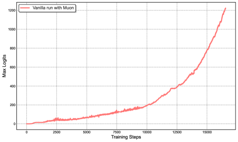
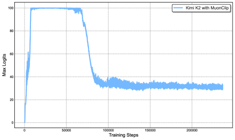
Figure 2: Left: During a mid-scale training run, attention logits rapidly exceed 1000, which could lead to potential numerical instabilities and even training divergence. Right: Maximum logits for Kimi K2 with MuonClip and $\tau$ = 100 over the entire training run. The max logits rapidly increase to the capped value of 100, and only decay to a stable range after approximately 30% of the training steps, demonstrating the effective regulation effect of QK-Clip.
MuonClip: The New Optimizer
We integrate Muon with weight decay, consistent RMS matching, and QK-Clip into a single optimizer, which we refer to as MuonClip (see Algorithm 1).
We demonstrate the effectiveness of MuonClip from several scaling experiments. First, we train a mid-scale 9B activated and 53B total parameters Mixture-of-Experts (MoE) model using the vanilla Muon. As shown in Figure 2 (Left), we observe that the maximum attention logits quickly exceed a magnitude of 1000, showing that attention logits explosion is already evident in Muon training to this scale. Max logits at this level usually result in instability during training, including significant loss spikes and occasional divergence.
Next, we demonstrate that QK-Clip does not degrade model performance and confirm that the MuonClip optimizer preserves the optimization characteristics of Muon without adversely affecting the loss trajectory. A detailed discussion of the experiment designs and findings is provided in the Appendix D.
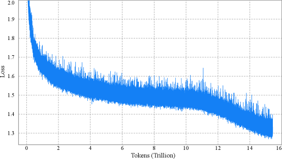
Finally, we train Kimi K2, a large-scale MoE model, using MuonClip with $\tau=100$ and monitor the maximum attention logits throughout the training run (Figure 2 (Right)). Initially, the logits are capped at 100 due to QK-Clip. Over the course of training, the maximum logits gradually decay to a typical operating range without requiring any adjustment to $\tau$ . Importantly, the training loss remains smooth and stable, with no observable spikes, as shown in Figure 3, validating that MuonClip provides robust and scalable control over attention dynamics in large-scale language model training.
<details>
<summary>x5.png Details</summary>
### Visual Description
\n
## Line Chart: Loss vs. Tokens (Trillion)
### Overview
The image presents a line chart illustrating the relationship between Loss and Tokens (measured in Trillions). The chart displays a single data series, showing how Loss changes as the number of Tokens processed increases. The chart appears to represent a training process, where Loss is expected to decrease as the model is exposed to more data.
### Components/Axes
* **X-axis:** Labeled "Tokens (Trillion)". The scale ranges from approximately 0 to 16 Trillion.
* **Y-axis:** Labeled "Loss". The scale ranges from approximately 1.3 to 2.0.
* **Data Series:** A single blue line representing the Loss value at each Token count.
* **Grid:** A light gray grid is present in the background to aid in reading values.
### Detailed Analysis
The blue line starts at approximately Loss = 1.95 when Tokens = 0. The line exhibits a steep downward slope initially, indicating a rapid decrease in Loss. This rapid decrease continues until approximately Tokens = 2 Trillion, where Loss reaches around 1.55.
From 2 to 8 Trillion Tokens, the line fluctuates around a relatively stable Loss value of approximately 1.5 to 1.6. There is significant noise in this region, with frequent small oscillations.
Between 8 and 12 Trillion Tokens, the line begins to exhibit a slight downward trend again, but the rate of decrease is much slower than the initial phase. The Loss value decreases from approximately 1.6 to 1.45.
From 12 to 16 Trillion Tokens, the line continues to decrease, reaching a final Loss value of approximately 1.35. The slope is gentle in this region.
Approximate data points:
* (0, 1.95)
* (2, 1.55)
* (4, 1.58)
* (6, 1.52)
* (8, 1.57)
* (10, 1.48)
* (12, 1.42)
* (14, 1.38)
* (16, 1.35)
### Key Observations
* **Initial Rapid Decrease:** The most significant change in Loss occurs in the first 2 Trillion Tokens.
* **Plateau:** A period of relative stability in Loss is observed between 2 and 8 Trillion Tokens.
* **Gradual Decline:** A slow and steady decrease in Loss is observed after 8 Trillion Tokens.
* **Noise:** The data is noisy, with frequent fluctuations in Loss, particularly between 2 and 8 Trillion Tokens.
### Interpretation
The chart likely represents the training process of a machine learning model. The initial rapid decrease in Loss indicates that the model is quickly learning from the data. The plateau suggests that the model has reached a point of diminishing returns, where further training provides only marginal improvements. The gradual decline after 8 Trillion Tokens suggests that the model is continuing to refine its parameters, but at a slower rate.
The noise in the data could be due to several factors, such as the stochastic nature of the training process, the variability of the data, or the presence of outliers. The overall trend suggests that the model is converging, but further training may be required to achieve optimal performance. The fact that the loss continues to decrease, even slowly, until 16 Trillion tokens suggests that the model is still benefiting from additional training data.
</details>
Figure 3: Per-step training loss curve of Kimi K2, without smoothing or sub-sampling. It shows no spikes throughout the entire training process. Note that we omit the very beginning of training for clarity.
2.2 Pre-training Data: Improving Token Utility with Rephrasing
Token efficiency in pre-training refers to how much performance improvement is achieved for each token consumed during training. Increasing token utility—the effective learning signal each token contributes—enhances the per-token impact on model updates, thereby directly improving token efficiency. This is particularly important when the supply of high-quality tokens is limited and must be maximally leveraged. A naive approach to increasing token utility is through repeated exposure to the same tokens, which can lead to overfitting and reduced generalization.
A key advancement in the pre-training data of Kimi K2 over Kimi K1.5 is the introduction of a synthetic data generation strategy to increase token utility. Specifically, a carefully designed rephrasing pipeline is employed to amplify the volume of high-quality tokens without inducing significant overfitting. In this report, we describe two domain-specialized rephrasing techniques—targeted respectively at the Knowledge and Mathematics domains—that enable this controlled data augmentation.
Knowledge Data Rephrasing
Pre-training on natural, knowledge-intensive text presents a trade-off: a single epoch is insufficient for comprehensive knowledge absorption, while multi-epoch repetition yields diminishing returns and increases the risk of overfitting. To improve the token utility of high-quality knowledge tokens, we propose a synthetic rephrasing framework composed of the following key components:
- Style- and perspective-diverse prompting: Inspired by WRAP [50], we apply a range of carefully engineered prompts to enhance linguistic diversity while maintaining factual integrity. These prompts guide a large language model to generate faithful rephrasings of the original texts in varied styles and from different perspectives.
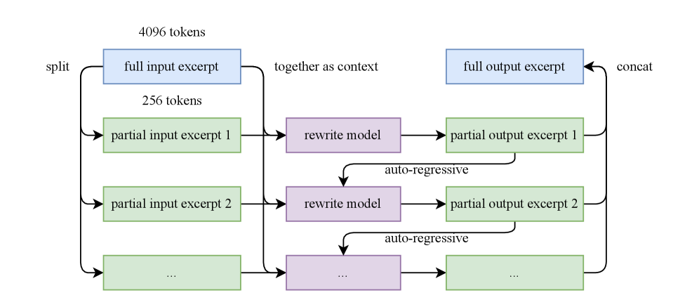
- Chunk-wise autoregressive generation: To preserve global coherence and avoid information loss in long documents, we adopt a chunk-based autoregressive rewriting strategy. Texts are divided into segments, rephrased individually, and then stitched back together to form complete passages. This method mitigates implicit output length limitations that typically exist with LLMs. An overview of this pipeline is presented in Figure 4.
- Fidelity verification: To ensure consistency between original and rewritten content, we perform fidelity checks that compare the semantic alignment of each rephrased passage with its source. This serves as an initial quality control step prior to training.
We compare data rephrasing with multi-epoch repetition by testing their corresponding accuracy on SimpleQA. We experiment with an early checkpoint of K2 and evaluate three training strategies: (1) repeating the original dataset for 10 epochs, (2) rephrasing the data once and repeating it for 10 epochs, and (3) rephrasing the data 10 times with a single training pass. As shown in Table 1, the accuracy consistently improves across these strategies, demonstrating the efficacy of our rephrasing-based augmentation. We extended this method to other large-scale knowledge corpora and observed similarly encouraging results, and each corpora is rephrased at most twice.
Table 1: SimpleQA Accuracy under three rephrasing-epoch configurations
| # Rephrasings | # Epochs | SimpleQA Accuracy |
| --- | --- | --- |
| 0 (raw wiki-text) | 10 | 23.76 |
| 1 | 10 | 27.39 |
| 10 | 1 | 28.94 |
<details>
<summary>x6.png Details</summary>
### Visual Description
\n
## Diagram: Long-Context Language Model Processing Flow
### Overview
The image depicts a diagram illustrating the process of handling long input sequences (4096 tokens) in a language model. The input is split into smaller excerpts, processed by a "rewrite model", and then concatenated to produce the final output. The process appears iterative, with multiple input excerpts being processed in parallel.
### Components/Axes
The diagram consists of rectangular blocks representing processing steps and arrows indicating the flow of data. Key components and labels include:
* **"split"**: The initial step of dividing the input.
* **"full input excerpt"**: Represents the complete input sequence.
* **"4096 tokens"**: Indicates the total length of the input sequence.
* **"256 tokens"**: Indicates the length of each partial input excerpt.
* **"partial input excerpt 1", "partial input excerpt 2", "...":** Represents individual segments of the input.
* **"rewrite model"**: A processing unit that transforms input excerpts.
* **"auto-regressive"**: Indicates the nature of the output generation process.
* **"partial output excerpt 1", "partial output excerpt 2", "...":** Represents individual segments of the output.
* **"full output excerpt"**: Represents the complete output sequence.
* **"concat"**: The final step of combining the output excerpts.
* **"together as context"**: Indicates the combination of input excerpts for processing.
### Detailed Analysis or Content Details
The diagram shows a process that begins with a 4096-token input. This input is split into excerpts of 256 tokens each. Multiple partial input excerpts are then fed into a "rewrite model". The output of the rewrite model is then processed in an "auto-regressive" manner, generating partial output excerpts. These partial output excerpts are finally concatenated ("concat") to form the full output excerpt. The diagram suggests this process is repeated iteratively, as indicated by the "...".
The flow can be summarized as follows:
1. **Input Split:** 4096 tokens -> Multiple 256-token excerpts.
2. **Rewrite & Auto-regressive Generation:** Each excerpt is processed by the "rewrite model" and then generates a partial output excerpt using an auto-regressive process.
3. **Output Concatenation:** The partial output excerpts are concatenated to form the final output.
### Key Observations
* The diagram highlights a strategy for handling long input sequences by breaking them down into smaller, manageable chunks.
* The "rewrite model" suggests a transformation or adaptation of the input excerpts before output generation.
* The auto-regressive nature of the output generation implies that each output token is generated based on the preceding tokens.
* The iterative nature of the process, indicated by the ellipsis ("..."), suggests that the input can be arbitrarily long.
### Interpretation
This diagram illustrates a technique for processing long sequences in language models, likely to overcome limitations in context window size. By splitting the input into smaller excerpts and processing them individually, the model can effectively handle inputs that exceed its maximum context length. The "rewrite model" likely plays a crucial role in maintaining coherence and consistency across the different excerpts. The auto-regressive generation ensures that the output is generated in a sequential and contextually relevant manner. The concatenation step combines the outputs from each excerpt to produce the final result. This approach is a common strategy for dealing with long-form text generation or processing tasks where the entire input cannot fit into the model's context window at once. The diagram doesn't provide specific details about the "rewrite model" or the auto-regressive process, but it clearly outlines the overall architecture and flow of the system.
</details>
Figure 4: Auto-regressive chunk-wise rephrasing pipeline for long input excerpts. The input is split into smaller chunks with preserved context, rewritten sequentially, and then concatenated into a full rewritten passage.
Mathematics Data Rephrasing
To enhance mathematical reasoning capabilities, we rewrite high-quality mathematical documents into a “learning-note” style, following the methodology introduced in SwallowMath [16]. In addition, we increased data diversity by translating high-quality mathematical materials from other languages into English.
Although initial experiments with rephrased subsets of our datasets show promising results, the use of synthetic data as a strategy for continued scaling remains an active area of investigation. Key challenges include generalizing the approach to diverse source domains without compromising factual accuracy, minimizing hallucinations and unintended toxicity, and ensuring scalability to large-scale datasets.
Pre-training Data Overall
The Kimi K2 pre-training corpus comprises 15.5 trillion tokens of curated, high-quality data spanning four primary domains: Web Text, Code, Mathematics, and Knowledge. Most data processing pipelines follow the methodologies outlined in Kimi K1.5 [36]. For each domain, we performed rigorous correctness and quality validation and designed targeted data experiments to ensure the curated dataset achieved both high diversity and effectiveness.
2.3 Model Architecture
Kimi K2 is a 1.04 trillion-parameter Mixture-of-Experts (MoE) transformer model with 32 billion activated parameters. The architecture follows a similar design to DeepSeek-V3 [11] , employing Multi-head Latent Attention (MLA) [45] as the attention mechanism, with a model hidden dimension of 7168 and an MoE expert hidden dimension of 2048. Our scaling law analysis reveals that continued increases in sparsity yield substantial performance improvements, which motivated us to increase the number of experts to 384, compared to 256 in DeepSeek-V3. To reduce computational overhead during inference, we cut the number of attention heads to 64, as opposed to 128 in DeepSeek-V3. Table 2 presents a detailed comparison of architectural parameters between Kimi K2 and DeepSeek-V3.
Table 2: Architectural comparison between Kimi K2 and DeepSeek-V3
| | DeepSeek-V3 | Kimi K2 | $\Delta$ |
| --- | --- | --- | --- |
| #Layers | 61 | 61 | = |
| Total Parameters | 671B | 1.04T | $\uparrow$ 54% |
| Activated Parameters | 37B | 32.6B | $\downarrow$ 13% |
| Experts (total) | 256 | 384 | $\uparrow$ 50% |
| Experts Active per Token | 8 | 8 | = |
| Shared Experts | 1 | 1 | = |
| Attention Heads | 128 | 64 | $\downarrow$ 50% |
| Number of Dense Layers | 3 | 1 | $\downarrow$ 67% |
| Expert Grouping | Yes | No | - |
Sparsity Scaling Law
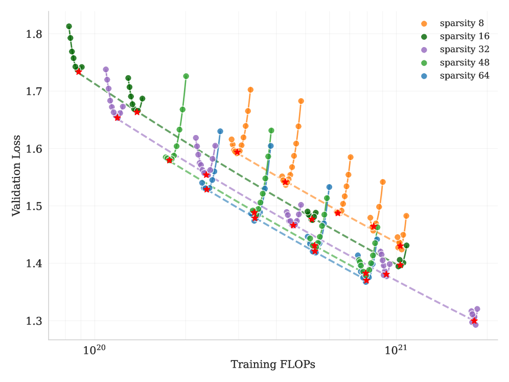
We develop a sparsity scaling law tailored for the Mixture-of-Experts (MoE) model family using Muon. Sparsity is defined as the ratio of the total number of experts to the number of activated experts. Through carefully controlled small-scale experiments, we observe that — under a fixed number of activated parameters (i.e., constant FLOPs) — increasing the total number of experts (i.e., increasing sparsity) consistently lowers both the training and validation loss, thereby enhancing overall model performance (Figure 6). Concretely, under the compute-optimal sparsity scaling law, achieving the same validation loss of 1.5, sparsity 48 reduces FLOPs by 1.69×, 1.39×, and 1.15× compared to sparsity levels 8, 16, and 32, respectively. Though increasing sparsity leads to better performance, this gain comes with increased infrastructure complexity. To balance model performance with cost, we adopt a sparsity of 48 for Kimi K2, activating 8 out of 384 experts per forward pass.
<details>
<summary>x7.png Details</summary>
### Visual Description
## Chart: Validation Loss vs. Training FLOPS with Varying Sparsity
### Overview
The image presents a line chart illustrating the relationship between Validation Loss (y-axis) and Training FLOPS (x-axis) for different levels of sparsity. The chart appears to be evaluating the performance of a model during training, with sparsity representing a regularization technique. The x-axis is on a logarithmic scale.
### Components/Axes
* **X-axis:** Training FLOPS, labeled "Training FLOPS". Scale is logarithmic, ranging approximately from 10<sup>20</sup> to 10<sup>21</sup>.
* **Y-axis:** Validation Loss, labeled "Validation Loss". Scale is linear, ranging approximately from 1.3 to 1.8.
* **Legend:** Located in the top-right corner. Contains the following sparsity levels with corresponding colors:
* sparsity 8 (Orange)
* sparsity 16 (Red)
* sparsity 32 (Purple)
* sparsity 48 (Green)
* sparsity 64 (Blue)
* **Data Series:** Five distinct lines, each representing a different sparsity level. The lines are connected by circular markers.
### Detailed Analysis
Here's a breakdown of each data series, noting trends and approximate data points. Note that due to the chart's resolution, values are approximate.
* **sparsity 8 (Orange):** The line starts at approximately (10<sup>20</sup>, 1.75) and generally decreases, with fluctuations, reaching around (8 x 10<sup>20</sup>, 1.5) before increasing again to approximately (10<sup>21</sup>, 1.55).
* **sparsity 16 (Red):** Starts at approximately (10<sup>20</sup>, 1.73) and decreases relatively smoothly to around (5 x 10<sup>20</sup>, 1.45), then plateaus and slightly increases to approximately (10<sup>21</sup>, 1.48).
* **sparsity 32 (Purple):** Begins at approximately (10<sup>20</sup>, 1.72) and shows a consistent downward trend, reaching a minimum of around (7 x 10<sup>20</sup>, 1.4) and then increasing slightly to approximately (10<sup>21</sup>, 1.43).
* **sparsity 48 (Green):** Starts at approximately (10<sup>20</sup>, 1.74) and decreases, reaching a minimum around (6 x 10<sup>20</sup>, 1.38), then increases to approximately (10<sup>21</sup>, 1.45).
* **sparsity 64 (Blue):** Starts at approximately (10<sup>20</sup>, 1.71) and decreases steadily, reaching a minimum around (8 x 10<sup>20</sup>, 1.35) and then increasing to approximately (10<sup>21</sup>, 1.33).
All lines exhibit a general downward trend initially, indicating decreasing validation loss as training FLOPS increase. However, after a certain point (around 5 x 10<sup>20</sup> FLOPS), the lines begin to fluctuate and, in some cases, increase, suggesting potential overfitting or diminishing returns from further training.
### Key Observations
* Higher sparsity levels (64 and 48) generally achieve lower validation loss values, particularly at higher FLOPS.
* The lines converge towards the right side of the chart, indicating that the impact of sparsity diminishes as training progresses.
* The orange line (sparsity 8) shows the most fluctuation, suggesting it is the least stable configuration.
* The lowest validation loss is achieved by sparsity 64, reaching approximately 1.33 at 10<sup>21</sup> FLOPS.
### Interpretation
The chart demonstrates the effect of sparsity on model validation loss during training. The results suggest that increasing sparsity can improve model performance (lower validation loss) up to a certain point. The initial decrease in validation loss with increasing FLOPS indicates that the model is learning and generalizing. The subsequent fluctuations and increases suggest that the model may be starting to overfit the training data, or that the benefits of further training are diminishing.
The convergence of the lines at higher FLOPS suggests that the impact of sparsity becomes less pronounced as the model becomes more thoroughly trained. This could be because the model has already learned the most important features, and further regularization has a smaller effect.
The fact that sparsity 64 consistently performs best suggests that a higher degree of sparsity is beneficial for this particular model and dataset. However, it's important to note that the optimal sparsity level may vary depending on the specific application and data characteristics. The chart provides valuable insights into the trade-offs between sparsity, training cost (FLOPS), and model performance (validation loss).
</details>
Figure 5: Sparsity Scaling Law. Increasing sparsity leads to improved model performance. We fixed the number of activated experts to 8 and the number of shared experts to 1, and varied the total number of experts, resulting in models with different sparsity levels.
<details>
<summary>x8.png Details</summary>
### Visual Description
\n
## Line Chart: Validation Loss vs. Training Tokens
### Overview
This chart displays the relationship between Validation Loss and Training Tokens for several models with varying computational costs (measured in FLOPS) and attention head configurations. The chart aims to demonstrate how model size and attention mechanisms affect validation performance during training.
### Components/Axes
* **X-axis:** Training Tokens, ranging from approximately 0 to 1.2e11 (120 billion). The scale is logarithmic, with a marker at 10^11.
* **Y-axis:** Validation Loss, ranging from approximately 1.35 to 1.75.
* **Legend:** Located in the bottom-left corner, detailing the different model configurations:
* `1.2e+20 FLOPS` (dotted orange line)
* `2.2e+20 FLOPS` (dotted pink line)
* `4.5e+20 FLOPS` (dotted green line)
* `9.0e+20 FLOPS` (dotted purple line)
* `models with number of attention heads equals to number of layers` (solid blue squares)
* `counterparts with doubled attention heads` (solid teal circles)
### Detailed Analysis
The chart contains six distinct data series, each representing a different model configuration.
* **1.2e+20 FLOPS (Orange):** The line starts at approximately 1.42 validation loss at 0 training tokens, decreases to a minimum of around 1.37 at approximately 5e10 training tokens, and then increases slightly to around 1.40 at 1.2e11 training tokens.
* **2.2e+20 FLOPS (Pink):** The line begins at approximately 1.62 validation loss at 0 training tokens, gradually decreases to around 1.55 at approximately 8e10 training tokens, and then plateaus around 1.56-1.60.
* **4.5e+20 FLOPS (Green):** The line starts at approximately 1.48 validation loss at 0 training tokens, decreases to a minimum of around 1.43 at approximately 6e10 training tokens, and then increases to around 1.48 at 1.2e11 training tokens.
* **9.0e+20 FLOPS (Purple):** The line begins at approximately 1.65 validation loss at 0 training tokens, decreases to around 1.60 at approximately 8e10 training tokens, and then plateaus around 1.60-1.62.
* **Models with number of attention heads equals to number of layers (Blue):** The line starts at approximately 1.73 validation loss at 0 training tokens, decreases steadily to around 1.66 at approximately 1.0e11 training tokens, and then plateaus around 1.66-1.68.
* **Counterparts with doubled attention heads (Teal):** The line begins at approximately 1.68 validation loss at 0 training tokens, decreases to around 1.65 at approximately 4e10 training tokens, and then increases to around 1.68 at 1.2e11 training tokens.
### Key Observations
* The models with fewer FLOPS (1.2e+20 and 4.5e+20) generally exhibit lower validation loss than those with more FLOPS, especially in the initial stages of training.
* The model with the fewest FLOPS (1.2e+20) shows a clear initial decrease in validation loss, followed by a slight increase, suggesting potential overfitting or reaching a local minimum.
* The models with doubled attention heads (teal) consistently perform slightly worse than their counterparts with standard attention heads (blue).
* The lines representing higher FLOPS models (2.2e+20 and 9.0e+20) show a more gradual decrease in validation loss and tend to plateau at higher loss values.
* All lines exhibit a decreasing trend in validation loss during the initial phase of training, indicating learning.
### Interpretation
The data suggests that increasing model size (FLOPS) does not necessarily lead to better validation performance. In fact, smaller models can achieve lower validation loss, potentially due to reduced overfitting or more efficient learning. The comparison between models with standard and doubled attention heads indicates that simply increasing the number of attention heads does not guarantee improved performance and may even be detrimental. The plateauing of validation loss for all models suggests that they are approaching a point of diminishing returns, where further training yields minimal improvement. The initial decrease in validation loss across all models demonstrates that the training process is effective in reducing the error on the validation set. The slight increase in validation loss for some models at later stages of training could indicate overfitting or the need for regularization techniques. The logarithmic scale of the x-axis highlights the importance of considering the rate of learning over time, as the impact of each additional training token diminishes as the training progresses.
</details>
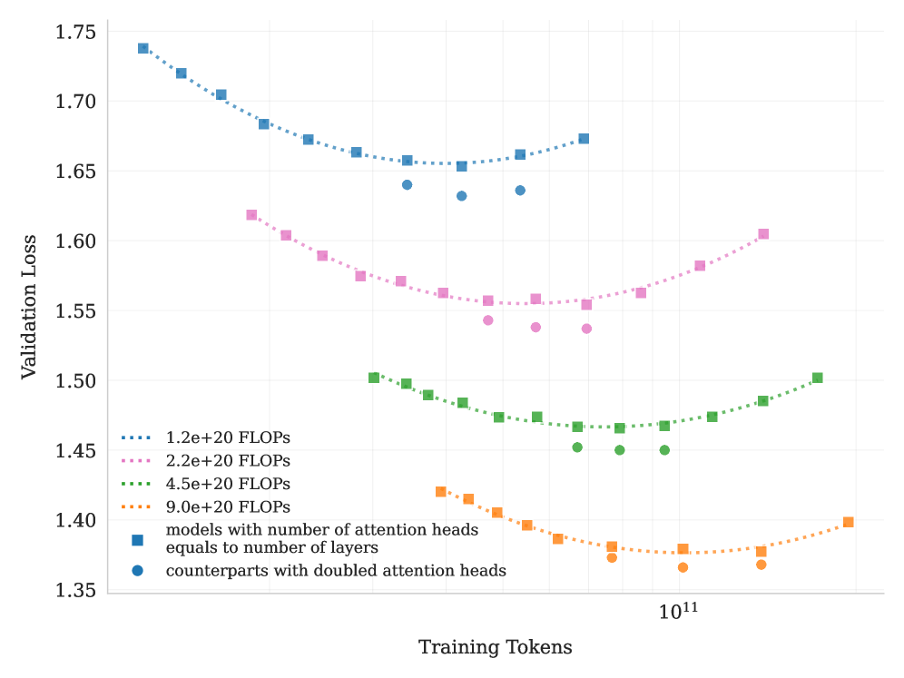
Figure 6: Scaling curves for models with number of attention heads equals to number of layers and their counterparts with doubled attention heads. Doubling the number of attention heads leads to a reduction in validation loss of approximately $0.5\%$ to $1.2\%$ .
Number of Attention Heads
DeepSeek-V3 [11] sets the number of attention heads to roughly twice the number of model layers to better utilize memory bandwidth and enhance computational efficiency. However, as the context length increases, doubling the number of attention heads leads to significant inference overhead, reducing efficiency at longer sequence lengths. This becomes a major limitation in agentic applications, where efficient long context processing is essential. For example, with a sequence length of 128k, increasing the number of attention heads from 64 to 128, while keeping the total expert count fixed at 384, leads to an 83% increase in inference FLOPs. To evaluate the impact of this design, we conduct controlled experiments comparing configurations where the number of attention heads equals the number of layers against those with double number of heads, under varying training FLOPs. Under iso-token training conditions, we observe that doubling the attention heads yields only modest improvements in validation loss (ranging from 0.5% to 1.2%) across different compute budgets (Figure 6). Given that sparsity 48 already offers strong performance, the marginal gains from doubling attention heads do not justify the inference cost. Therefore we choose to 64 attention heads.
2.4 Training Infrastructure
2.4.1 Compute Cluster
Kimi K2 was trained on a cluster equipped with NVIDIA H800 GPUs. Each node in the H800 cluster contains 2 TB RAM and 8 GPUs connected by NVLink and NVSwitch within nodes. Across different nodes, $\text{8}\!×\!\text{400}~\text{Gbps}$ RoCE interconnects are utilized to facilitate communications.
2.4.2 Parallelism for Model Scaling
Training of large language models often progresses under dynamic resource availability. Instead of optimizing one parallelism strategy that’s only applicable under specific amount of resources, we pursue a flexible strategy that allows Kimi K2 to be trained on any number of nodes that is a multiple of 32. Our strategy leverages a combination of 16-way Pipeline Parallelism (PP) with virtual stages [29, 54, 39, 58, 48, 22], 16-way Expert Parallelism (EP) [40], and ZeRO-1 Data Parallelism [61].
Under this setting, storing the model parameters in BF16 and their gradient accumulation buffer in FP32 requires approximately 6 TB of GPU memory, distributed over a model-parallel group of 256 GPUs. Placement of optimizer states depends on the training configurations. When the total number of training nodes is large, the optimizer states are distributed, reducing its per-device memory footprint to a negligible level. When the total number of training nodes is small (e.g., 32), we can offload some optimizer states to CPU.
This approach allows us to reuse an identical parallelism configuration for both small- and large-scale experiments, while letting each GPU hold approximately 30 GB of GPU memory for all states. The rest of the GPU memory are used for activations, as described in Sec. 2.4.3. Such a consistent design is important for research efficiency, as it simplifies the system and substantially accelerates experimental iteration.
EP communication overlap with interleaved 1F1B
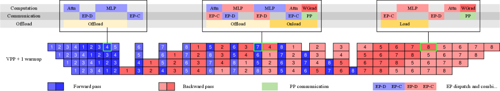
By increasing the number of warm-up micro-batches, we can overlap EP all-to-all communication with computation under the standard interleaved 1F1B schedule [22, 54]. In comparison, DualPipe [11] doubles the memory required for parameters and gradients, necessitating an increase in parallelism to compensate. Increasing PP introduces more bubbles, while increasing EP, as discussed below, incurs higher overhead. The additional costs are prohibitively high for training a large model with over 1 trillion parameters and thus we opted not to use DualPipe.
However, interleaved 1F1B splits the model into more stages, introducing non-trivial PP communication overhead. To mitigate this cost, we decouple the weight-gradient computation from each micro-batch’s backward pass and execute it in parallel with the corresponding PP communication. Consequently, all PP communications can be effectively overlapped except for the warm-up phase.
Smaller EP size
To ensure full computation-communication overlap during the 1F1B stage, the reduced attention computation time in K2 (which has 64 attention heads compared to 128 heads in DeepSeek-V3) necessitates minimizing the time of EP operations. This is achieved by adopting the smallest feasible EP parallelization strategy, specifically EP = 16. Utilizing a smaller EP group also relaxes expert-balance constraints, allowing for near-optimal speed to be achieved without further tuning.
2.4.3 Activation Reduction
After reserving space for parameters, gradient buffers, and optimizer states, the remaining GPU memory on each device is insufficient to hold the full MoE activations. To ensure the activation memory fits within the constraints, especially for the initial pipeline stages that accumulate the largest activations during the 1F1B warm-up phase, the following techniques are employed.
Selective recomputation
Recomputation is applied to inexpensive, high-footprint stages, including LayerNorm, SwiGLU, and MLA up-projections [11]. Additionally, MoE down-projections are recomputed during training to further reduce activation memory. While optional, this recomputation maintains adequate GPU memory, preventing crashes caused by expert imbalance in early training stages.
FP8 storage for insensitive activations
Inputs of MoE up-projections and SwiGLU are compressed to FP8-E4M3 in 1 $×$ 128 tiles with FP32 scales. Small-scale experiments show no measurable loss increase. Due to potential risks of performance degradation that we observed during preliminary study, we do not apply FP8 in computation.
<details>
<summary>x9.png Details</summary>
### Visual Description
\n
## Diagram: Pipeline Stage Breakdown - Computation and Communication
### Overview
The image presents a diagram illustrating the breakdown of computation and communication stages within a pipeline, likely related to a deep learning model. It compares different offloading and dispatch strategies (EP-D, EP-C, PP) for Attention (Attn), Multi-Layer Perceptron (MLP), and Weight Gradient (WGrad) operations. The diagram visualizes the stages across a timeline, represented by numbered blocks, differentiating between forward and backward passes.
### Components/Axes
The diagram is structured into three main sections, each representing a different configuration of computation and communication:
* **Section 1 (Left):** Attn and MLP, both using EP-D and EP-C offload strategies.
* **Section 2 (Center):** Attn, MLP, and WGrad, with Attn and WGrad using PP communication and MLP using EP-D offload. This section is labeled "Onload".
* **Section 3 (Right):** MLP and WGrad, both using EP-C and EP-D dispatch strategies, and labeled "Load".
The horizontal axis represents time steps, labeled "VPP + 1 warmup" and numbered 1 through 8.
A legend at the bottom-right clarifies the color coding:
* **Blue:** Forward pass
* **Red:** Backward pass
* **Green:** PP communication
* **Yellow:** EP dispatch and combi.
The top section labels the type of computation and communication strategy used in each section.
### Detailed Analysis or Content Details
Let's analyze each section and its corresponding timeline:
**Section 1 (Attn & MLP - EP-D/EP-C Offload):**
* **Attn (EP-D):** Blocks 1-4 are primarily blue (forward pass), with block 4 having a yellow overlay (EP dispatch and combi.).
* **MLP (EP-C):** Blocks 1-4 are primarily red (backward pass), with block 4 having a yellow overlay.
* **Attn (EP-C):** Blocks 5-8 are primarily red (backward pass), with block 5 having a yellow overlay.
* **MLP (EP-D):** Blocks 5-8 are primarily blue (forward pass), with block 5 having a yellow overlay.
**Section 2 (Attn, MLP, WGrad - PP/EP-D):**
* **Attn (PP):** Blocks 1-4 are primarily red (backward pass), with block 4 having a green overlay (PP communication).
* **MLP (EP-D):** Blocks 1-4 are primarily blue (forward pass), with block 4 having a yellow overlay.
* **MLP (EP-D):** Blocks 5-8 are primarily red (backward pass), with block 5 having a yellow overlay.
* **Attn (PP):** Blocks 5-8 are primarily blue (forward pass), with block 5 having a green overlay.
* **WGrad (PP):** Block 1 is blue (forward pass), block 2 is red (backward pass).
**Section 3 (MLP & WGrad - EP-C/EP-D Load):**
* **MLP (EP-C):** Blocks 1-4 are primarily red (backward pass), with block 4 having a yellow overlay.
* **WGrad (EP-D):** Blocks 1-4 are primarily blue (forward pass), with block 4 having a yellow overlay.
* **MLP (EP-D):** Blocks 5-8 are primarily blue (forward pass), with block 5 having a yellow overlay.
* **WGrad (EP-C):** Blocks 5-8 are primarily red (backward pass), with block 5 having a yellow overlay.
### Key Observations
* The diagram highlights the alternating pattern of forward and backward passes across the timeline.
* The use of yellow overlays indicates the presence of EP dispatch and combination operations, often coinciding with the end of a forward or backward pass.
* PP communication (green) appears to be concentrated in specific blocks, particularly in the Attn and WGrad sections of the "Onload" configuration.
* The "Offload" sections (left) show a more balanced distribution of forward and backward passes, while the "Load" section (right) appears to have a more staggered pattern.
### Interpretation
This diagram likely represents a performance comparison of different strategies for distributing the computational workload of a neural network across multiple devices (e.g., CPU and GPU). The EP-D, EP-C, and PP labels likely refer to different execution paradigms or communication protocols.
* **EP-D and EP-C** likely represent different forms of Early Processing with different dispatch strategies.
* **PP** likely represents Pipeline Parallelism, where different stages of the network are executed on different devices concurrently.
The diagram suggests that the choice of offloading and dispatch strategy can significantly impact the timing and balance of forward and backward passes. The presence of PP communication indicates that data needs to be transferred between devices during pipeline execution. The "Load" configuration might represent a scenario where the entire model is loaded onto a single device, while the "Offload" configurations represent scenarios where parts of the model are offloaded to other devices.
The diagram is a visual aid for understanding the trade-offs between different execution strategies and optimizing the performance of a distributed deep learning system. The "warmup" phase suggests that the initial stages of the pipeline might require some overhead to initialize the system.
</details>
Figure 7: Computation, communication and offloading overlapped in different PP phases.
Activation CPU offload
All remaining activations are offloaded to CPU RAM. A copy engine is responsible for streaming the offload and onload, overlapping with both computation and communication kernels. During the 1F1B phase, we offload the forward activations of the previous micro-batch while prefetching the backward activations of the next. The warm-up and cool-down phases are handled similarly and the overall pattern is shown in Figure 7. Although offloading may slightly affect EP traffic due to PCIe traffic congestion, our tests show that EP communication remains fully overlapped.
2.5 Training recipe
We pre-trained the model with a 4,096-token context window using the MuonClip optimizer (Algorithm 1) and the WSD learning rate schedule [26], processing a total of 15.5T tokens. The first 10T tokens were trained with a constant learning rate of 2e-4 after a 500-step warm-up, followed by 5.5T tokens with a cosine decay from 2e-4 to 2e-5. Weight decay was set to 0.1 throughout, and the global batch size was held at 67M tokens. The overall training curve is shown in Figure 3.
Towards the end of pre-training, we conducted an annealing phase followed by a long-context activation stage. The batch size was kept constant at 67M tokens, while the learning rate was decayed from 2e-5 to 7e-6. In this phase, the model was trained on 400 billion tokens with a 4k sequence length, followed by an additional 60 billion tokens with a 32k sequence length. To extend the context window to 128k, we employed the YaRN method [56].
3 Post-Training
3.1 Supervised Fine-Tuning
We employ the Muon optimizer [34] in our post-training and recommend its use for fine-tuning with K2. This follows from the conclusion of our previous work [47] that a Muon-pre-trained checkpoint produces the best performance with Muon fine-tuning.
We construct a large-scale instruction-tuning dataset spanning diverse domains, guided by two core principles: maximizing prompt diversity and ensuring high response quality. To this end, we develop a suite of data generation pipelines tailored to different task domains, each utilizing a combination of human annotation, prompt engineering, and verification processes. We adopt K1.5 [36] and other in-house domain-specialized expert models to generate candidate responses for various tasks, followed by LLMs or human-based judges to perform automated quality evaluation and filtering. For agentic data, we create a data synthesis pipeline to teach models tool-use capabilities through multi-step, interactive reasoning.
3.1.1 Large-Scale Agentic Data Synthesis for Tool Use Learning
A critical capability of modern LLM agents is their ability to autonomously use unfamiliar tools, interact with external environments, and iteratively refine their actions through reasoning, execution, and error correction. Agentic tool use capability is essential for solving complex, multi-step tasks that require dynamic interaction with real-world systems. Recent benchmarks such as ACEBench [7] and $\tau$ -bench [86] have highlighted the importance of comprehensive tool-use evaluation, while frameworks like ToolLLM [59] and ACEBench [7] have demonstrated the potential of teaching models to use thousands of tools effectively.
However, training such capabilities at scale presents a significant challenge: while real-world environments provide rich and authentic interaction signals, they are often difficult to construct at scale due to cost, complexity, privacy and accessibility constraints. Recent work on synthetic data generation (AgentInstruct [52]; Self-Instruct [76]; StableToolBench [21]; ZeroSearch [67]) has shown promising results in creating large-scale data without relying on real-world interactions. Building on these advances and inspired by ACEBench [7] ’s comprehensive data synthesis framework, we developed a pipeline that simulates real-world tool-use scenarios at scale, enabling the generation of tens of thousands of diverse and high-quality training examples.
<details>
<summary>x10.png Details</summary>
### Visual Description
\n
## Diagram: System Architecture Overview
### Overview
The image depicts a system architecture diagram illustrating the relationships between various components involved in a task-oriented system. The diagram shows a flow of information and dependencies between "Domains", "MCP tools", "Applications", "Tool Repository", "Agents", and "Tasks with rubrics".
### Components/Axes
The diagram consists of the following components:
* **Domains:** A purple rectangle at the top-center.
* **MCP tools:** A light green rectangle positioned to the left of the "Tool Repository".
* **Applications:** A light blue rectangle positioned above the "Tool Repository".
* **Tool Repository:** A larger rectangle encompassing two smaller rectangles labeled "real-world tool specs" and "synthesized tool specs". It is positioned in the lower-left quadrant.
* **Agents:** A yellow rectangle positioned in the lower-center.
* **Tasks with rubrics:** A light pink rectangle positioned to the right of the "Domains".
Arrows indicate the direction of relationships and dependencies between these components.
### Detailed Analysis or Content Details
The diagram illustrates the following relationships:
1. "Domains" have outgoing arrows to both "Applications" and "MCP tools".
2. "MCP tools" feed into the "real-world tool specs" component within the "Tool Repository".
3. "Applications" feed into the "synthesized tool specs" component within the "Tool Repository".
4. The "Tool Repository" has an outgoing arrow to "Agents".
5. "Agents" have an outgoing arrow to "Tasks with rubrics".
The "Tool Repository" is explicitly labeled and contains two sub-components: "real-world tool specs" and "synthesized tool specs". These are positioned side-by-side within the larger "Tool Repository" rectangle.
### Key Observations
The diagram highlights a system where "Domains" drive the creation of both real-world and synthesized tool specifications, which are then utilized by "Agents" to perform "Tasks with rubrics". The "Tool Repository" acts as a central storage and source for these tools. The flow is largely sequential, with information moving from higher-level concepts ("Domains") to more concrete actions ("Tasks with rubrics").
### Interpretation
This diagram likely represents a system for automated task execution or problem-solving. The "Domains" represent areas of expertise or knowledge. "MCP tools" and "Applications" are used to generate tool specifications, which are stored in the "Tool Repository". "Agents" then leverage these tools to complete "Tasks with rubrics", suggesting a focus on evaluation and quality control. The separation of "real-world" and "synthesized" tool specs indicates a hybrid approach, potentially combining existing tools with newly generated ones. The diagram suggests a pipeline where high-level domain knowledge is translated into actionable tasks through a structured tool ecosystem. The diagram does not provide any quantitative data, but rather a qualitative representation of system architecture.
</details>
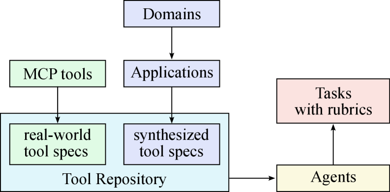
(a) Synthesizing tool specs, agents and tasks
<details>
<summary>x11.png Details</summary>
### Visual Description
\n
## Diagram: Agent Interaction Flow
### Overview
The image depicts a diagram illustrating the interaction flow between different agents and components in a system. The system involves a User Agent, an Agent, a Tool Simulator, a Judge Agent, and the concepts of Tasks, Rubrics, and Filtered Data. The diagram shows the direction of information flow between these elements using arrows labeled with the type of interaction.
### Components/Axes
The diagram consists of the following components:
* **User Agent:** Represented by a light green rectangle.
* **Agent:** Represented by a yellow rectangle.
* **Tool Simulator:** Represented by a teal rectangle.
* **Judge Agent:** Represented by a light blue rectangle.
* **Task:** Represented by a light red rectangle.
* **Rubrics:** Represented by a light orange rectangle.
* **Filtered Data:** Represented by a light green rectangle.
The following interactions are labeled on the arrows:
* **interaction:** From User Agent to Agent.
* **observation:** From Agent to Tool Simulator.
* **call:** From Agent to Tool Simulator.
* **trajectories:** From Tool Simulator to Judge Agent.
* The Judge Agent receives input from Rubrics.
* The Judge Agent outputs Filtered Data.
A dashed box encompasses the User Agent, Agent, and Tool Simulator, visually grouping them as a single unit.
### Detailed Analysis or Content Details
The diagram illustrates a closed-loop system. The User Agent initiates a process by interacting with the Agent. The Agent then observes and calls upon the Tool Simulator. The Tool Simulator generates trajectories, which are then evaluated by the Judge Agent, using Rubrics as a guide. The Judge Agent then produces Filtered Data. The User Agent receives the output of the Agent.
The diagram does not contain numerical data or specific values. It is a conceptual representation of a process.
### Key Observations
The diagram highlights the separation of concerns between the different agents. The Tool Simulator is isolated within the dashed box, suggesting it is a controlled environment. The Judge Agent acts as an evaluator, using Rubrics to assess the output of the Tool Simulator. The Filtered Data represents the refined output of the system.
### Interpretation
This diagram likely represents a system for evaluating the performance of an agent (the central yellow box) in completing tasks. The User Agent provides the task, and the Agent utilizes the Tool Simulator to generate solutions. The Judge Agent, guided by Rubrics, assesses the quality of these solutions, resulting in Filtered Data. This setup suggests a focus on iterative improvement and objective evaluation of agent behavior. The dashed box around the User Agent, Agent, and Tool Simulator indicates a self-contained unit that interacts with the external Judge Agent. The system is designed to provide a structured and measurable way to assess and refine the Agent's capabilities. The diagram is a high-level architectural overview, and does not provide details on the internal workings of each component.
</details>
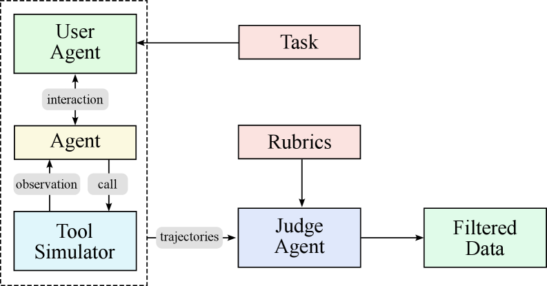
(b) Generating agent trajectories
Figure 8: Data synthesis pipeline for tool use. (a) Tool specs are from both real-world tools and LLMs; agents and tasks are the generated from the tool repo. (b) Multi-agent pipeline to generate and filter trajectories with tool calling.
<details>
<summary>x12.png Details</summary>
### Visual Description
\n
## Scatter Plot: t-SNE of MCP tools by Category
### Overview
This image presents a two-dimensional t-distributed Stochastic Neighbor Embedding (t-SNE) scatter plot visualizing the distribution of Machine Centric Productivity (MCP) tools across various categories. Each point on the plot represents a tool, and its position is determined by the t-SNE algorithm, aiming to preserve the relative similarity between tools based on their category. The plot is labeled with axes "t-SNE 1" and "t-SNE 2", and a legend on the right side identifies the color-coded categories.
### Components/Axes
* **X-axis:** t-SNE 1, ranging approximately from -15 to 75.
* **Y-axis:** t-SNE 2, ranging approximately from -60 to 65.
* **Legend:** Located in the top-right corner, listing the following categories with corresponding colors:
* databases (light blue)
* image-and-video-processing (light green)
* cloud-platforms (yellow)
* calendar-management (pale orange)
* cryptocurrency (dark orange)
* vector-databases (dark yellow)
* location-services (light purple)
* communication (pink)
* shell-access (red)
* Search (dark red)
* multimedia-processing (brown)
* file-utilities (dark brown)
* web-scraping (grey)
* ecommerce-and-retail (light grey)
* search (dark grey)
* customer-data-platforms (teal)
* app-automation (dark teal)
* developer-tools (blue)
* os-automation (dark blue)
* health-and-wellness (purple)
* virtualization (dark purple)
* version-control (olive)
* cloud-storage (dark olive)
* Research & Data (light brown)
* entertainment-and-media (beige)
* other (light beige)
* games-and-gamification (peach)
* AIGC (light peach)
* travel-and-transportation (lavender)
* note-taking (dark lavender)
* browser-automation (cyan)
* rag-systems (dark cyan)
* language-translation (sea green)
* social-media (dark sea green)
* security-and-iam (magenta)
* home-automation-and-iot (dark magenta)
* monitoring (lime)
* aiqc (dark lime)
* research-and-data (coral)
* weather-services (dark coral)
* art-and-culture (gold)
* customer-support (dark gold)
* blockchain (silver)
* finance (dark silver)
* knowledge-and-memory (bronze)
* speech-processing (dark bronze)
* marketing (rose gold)
### Detailed Analysis
The plot shows a complex distribution of points, with several clusters and overlapping regions. It's difficult to provide precise numerical values for each point without access to the underlying data. However, we can describe the general trends and approximate positions of the clusters:
* **Databases (light blue):** Concentrated in the lower-left quadrant, around t-SNE 1 = -10 and t-SNE 2 = -40.
* **Image-and-video-processing (light green):** Forms a cluster in the upper-left quadrant, around t-SNE 1 = -20 and t-SNE 2 = 50.
* **Cloud-platforms (yellow):** Located in the upper-right quadrant, around t-SNE 1 = 30 and t-SNE 2 = 40.
* **Cryptocurrency (dark orange):** A small cluster in the lower-right quadrant, around t-SNE 1 = 60 and t-SNE 2 = -50.
* **Communication (pink):** A dense cluster in the center-left, around t-SNE 1 = -10 and t-SNE 2 = 20.
* **Shell-access (red):** Overlaps with Communication, but slightly more dispersed.
* **Search (dark red):** Located in the center, around t-SNE 1 = 0 and t-SNE 2 = 0.
* **Developer-tools (blue):** Forms a cluster in the lower-center, around t-SNE 1 = -20 and t-SNE 2 = -20.
* **Health-and-wellness (purple):** Located in the lower-right quadrant, around t-SNE 1 = 40 and t-SNE 2 = -40.
* **AIGC (light peach):** Located in the lower-center, around t-SNE 1 = 0 and t-SNE 2 = -30.
* **Marketing (rose gold):** Located in the bottom-right quadrant, around t-SNE 1 = 70 and t-SNE 2 = -60.
Many other categories are scattered throughout the plot, with varying degrees of clustering. There is significant overlap between several categories, indicating that some tools may fall into multiple categories or have features that are common across categories.
### Key Observations
* The plot demonstrates a clear separation between some categories (e.g., Databases and Cloud-platforms), while others are more closely intertwined (e.g., Communication and Shell-access).
* The density of points varies across the plot, with some regions being more crowded than others. This suggests that some categories have a larger number of tools than others.
* The t-SNE algorithm has effectively captured the relationships between tools, grouping similar tools together and separating dissimilar ones.
* The "Research & Data" category appears to be spread out, suggesting a diverse range of tools within that category.
### Interpretation
The t-SNE plot provides a visual representation of the landscape of MCP tools. The clustering of categories suggests that there are distinct areas of functionality and specialization within the MCP ecosystem. The overlap between categories highlights the interconnectedness of these tools and the potential for cross-functional capabilities.
The plot can be used to identify potential gaps in the market, areas where there is a high concentration of tools, and opportunities for innovation. For example, the relatively sparse region in the upper-right quadrant might indicate a need for more tools in the Cloud-platforms and related categories.
The t-SNE algorithm is a dimensionality reduction technique, and the resulting plot should be interpreted with caution. The positions of the points are not absolute, but rather reflect the relative similarity between tools based on their category. However, the plot provides a valuable overview of the MCP tool landscape and can be used to guide further research and analysis.
</details>
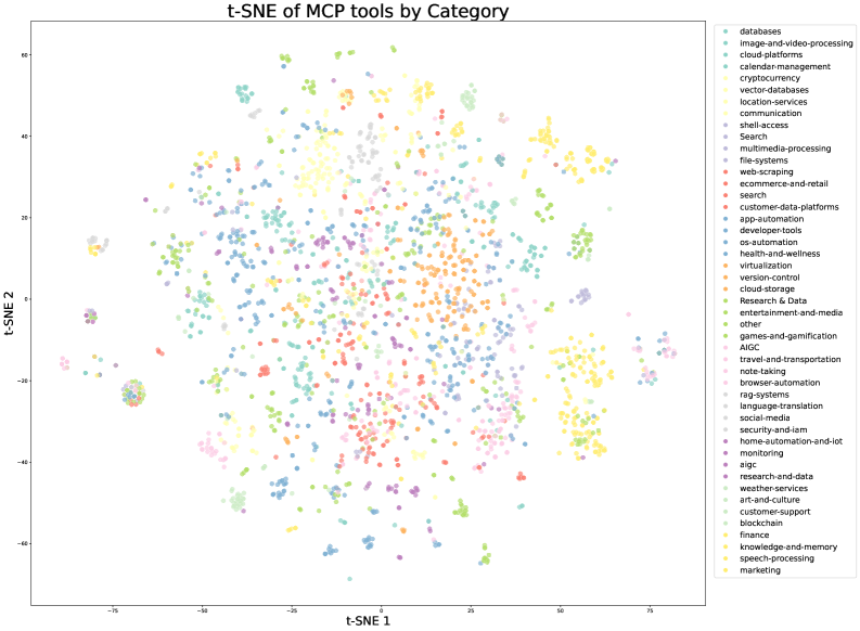
(a) t-SNE visualization of real MCP tools, colored by their original source categories
<details>
<summary>x13.png Details</summary>
### Visual Description
\n
## Scatter Plot: t-SNE of synthetic tools by Category
### Overview
This image presents a scatter plot generated using t-distributed Stochastic Neighbor Embedding (t-SNE). The plot visualizes the distribution of synthetic tools across two principal components, t-SNE 1 and t-SNE 2, and color-codes the points based on their category. The plot aims to reveal clusters and relationships between different categories of synthetic tools.
### Components/Axes
* **Title:** "t-SNE of synthetic tools by Category" (top-center)
* **X-axis:** "t-SNE 1" (bottom-center), ranging approximately from -100 to 100.
* **Y-axis:** "t-SNE 2" (left-center), ranging approximately from -75 to 100.
* **Legend:** Located in the top-right corner, listing the following categories with corresponding colors:
* enterprise\_business\_intelligence (light blue)
* transportation\_logistics (dark blue)
* iphone\_android (purple)
* smart\_home (red)
* real\_estate\_property (orange)
* unknown (grey)
* software\_apps (light green)
* legal\_compliance (dark green)
* education\_elearning (teal)
* robot\_control (yellow)
* agriculture\_environmental (brown)
* healthcare\_medical (pink)
* manufacturing\_industrial\_iot (light purple)
* desktop\_systems (cyan)
* financial\_trading (magenta)
* website\_control (olive)
* gaming\_entertainment (dark red)
### Detailed Analysis
The scatter plot shows a complex distribution of points, with several discernible clusters.
* **Enterprise\_business\_intelligence (light blue):** Forms a relatively tight cluster in the bottom-left quadrant, centered around t-SNE 1 = -50 and t-SNE 2 = -50.
* **Transportation\_logistics (dark blue):** Located adjacent to the enterprise cluster, slightly more dispersed, with a center around t-SNE 1 = -30 and t-SNE 2 = -40.
* **Iphone\_android (purple):** Occupies a large area in the center-left, extending from t-SNE 1 = -40 to t-SNE 1 = 20, and t-SNE 2 = -20 to 50.
* **Smart\_home (red):** Forms a distinct cluster in the top-right quadrant, centered around t-SNE 1 = 60 and t-SNE 2 = 70.
* **Real\_estate\_property (orange):** Located below the smart home cluster, around t-SNE 1 = 40 and t-SNE 2 = 30.
* **Unknown (grey):** Scattered throughout the plot, with a higher concentration in the center.
* **Software\_apps (light green):** Forms a cluster in the bottom-right quadrant, around t-SNE 1 = 40 and t-SNE 2 = -60.
* **Legal\_compliance (dark green):** Located near the software apps cluster, slightly more dispersed.
* **Education\_elearning (teal):** Forms a cluster around t-SNE 1 = -20 and t-SNE 2 = 30.
* **Robot\_control (yellow):** Located in the center of the plot, with a concentration around t-SNE 1 = 0 and t-SNE 2 = 0.
* **Agriculture\_environmental (brown):** Forms a cluster around t-SNE 1 = 20 and t-SNE 2 = -20.
* **Healthcare\_medical (pink):** Located near the agriculture cluster, slightly more dispersed.
* **Manufacturing\_industrial\_iot (light purple):** Forms a cluster around t-SNE 1 = -10 and t-SNE 2 = 50.
* **Desktop\_systems (cyan):** Located in the bottom-left quadrant, near the enterprise cluster.
* **Financial\_trading (magenta):** Forms a cluster around t-SNE 1 = 50 and t-SNE 2 = 0.
* **Website\_control (olive):** Located near the financial trading cluster, slightly more dispersed.
* **Gaming\_entertainment (dark red):** Forms a cluster in the top-left quadrant, around t-SNE 1 = -20 and t-SNE 2 = 80.
### Key Observations
* The "smart\_home" category is well-separated from most other categories, indicating a distinct feature space.
* The "enterprise\_business\_intelligence" and "transportation\_logistics" categories are closely clustered, suggesting similarities in their underlying characteristics.
* The "unknown" category is widely dispersed, indicating a lack of clear patterns or features.
* The "iphone\_android" category occupies a large area, suggesting a diverse range of tools within this category.
### Interpretation
The t-SNE plot effectively visualizes the relationships between different categories of synthetic tools. The clustering suggests that tools within the same category share similar characteristics, as captured by the t-SNE algorithm. The separation between clusters indicates distinct feature spaces, while the dispersion within clusters reflects the diversity of tools within each category. The "unknown" category's dispersion suggests that these tools lack clear defining features or are outliers.
The plot demonstrates the utility of dimensionality reduction techniques like t-SNE for exploring high-dimensional data and identifying underlying patterns. This visualization can be valuable for understanding the landscape of synthetic tools and identifying potential areas for further investigation or development. The relative positioning of clusters can also inform decisions about tool selection or integration. The plot suggests that the synthetic tools can be broadly categorized based on their underlying characteristics, and that further analysis could focus on understanding the specific features that differentiate these categories.
</details>
(b) t-SNE visualization of synthetic tools, colored by pre-defined domain categories
Figure 9: t-SNE visualizations of tool embeddings. (a) Real-world MCP tools exhibit natural clustering based on their original source categories. (b) Synthetic tools are organized into pre-defined domain categories, providing systematic coverage of the tool space. Together, they ensure comprehensive representation across different tool functionalities.
There are three stages in our data synthesis pipeline, depicted in Fig. 8.
- Tool spec generation: we first construct a large repository of tool specs from both real-world tools and LLM-synthetic tools;
- Agent and task generation: for each tool-set sampled from the tool repository, we generate an agent to use the toolset and some corresponding tasks;
- Trajectory generation: for each agent and task, we generate trajectories where the agent finishes the task by invoking tools.
Domain Evolution and Tool Generation.
We construct a comprehensive tool repository through two complementary approaches. First, we directly fetch 3000+ real MCP (Model Context Protocol) tools from GitHub repositories, leveraging existing high-quality tool specs. Second, we systematically evolve [83] synthetic tools through a hierarchical domain generation process: we begin with key categories (e.g., financial trading, software applications, robot control), then evolve multiple specific application domains within each category. Specialized tools are then synthesized for each domain, with clear interfaces, descriptions, and operational semantics. This evolution process produces over 20,000 synthetic tools. Figure 9 visualizes the diversity of our tool collection through t-SNE embeddings, demonstrating that both MCP and synthetic tools cover complementary regions of the tool space.
Agent Diversification.
We generate thousands of distinct agents by synthesizing various system prompts and equipping them with different combinations of tools from our repository. This creates a diverse population of agents with varied capabilities, areas of expertise, and behavioral patterns, ensuring a broad coverage of potential use cases.
Rubric-Based Task Generation.
For each agent configuration, we generate tasks that range from simple to complex operations. Each task is paired with an explicit rubric that specifies success criteria, expected tool-use patterns, and evaluation checkpoints. This rubric-based approach ensures a consistent and objective evaluation of agent performance.
Multi-turn Trajectory Generation.
We simulate realistic tool-use scenarios through several components:
- User Simulation: LLM-generated user personas with distinct communication styles and preferences engage in multi-turn dialogues with agents, creating naturalistic interaction patterns.
- Tool Execution Environment: A sophisticated tool simulator (functionally equivalent to a world model) executes tool calls and provides realistic feedback. The simulator maintains and updates state after each tool execution, enabling complex multi-step interactions with persistent effects. It introduces controlled stochasticity to produce varied outcomes including successes, partial failures, and edge cases.
Quality Evaluation and Filtering.
An LLM-based judge evaluates each trajectory against the task rubrics. Only trajectories that meet the success criteria are retained for training, ensuring high-quality data while allowing natural variation in task-completion strategies.
Hybrid Approach with Real Execution Environments.
While simulation provides scalability, we acknowledge the inherent limitation of simulation fidelity. To address this, we complement our simulated environments with real execution sandboxes for scenarios where authenticity is crucial, particularly in coding and software engineering tasks. These real sandboxes execute actual code, interact with genuine development environments, and provide ground-truth feedback through objective metrics such as test suite pass rates. This combination ensures that our models learn from both the diversity of simulated scenarios and the authenticity of real executions, significantly strengthening practical agent capabilities.
By leveraging this hybrid pipeline that combines scalable simulation with targeted real-world execution, we generate diverse, high-quality tool-use demonstrations that balance coverage and authenticity. The scale and automation of our synthetic data generation, coupled with the grounding provided by real execution environments, effectively implements large-scale rejection sampling [27, 88] through our quality filtering process. This high-quality synthetic data, when used for supervised fine-tuning, has demonstrated significant improvements in the model’s tool-use capabilities across a wide range of real-world applications.
3.2 Reinforcement Learning
Reinforcement learning (RL) is believed to have better token efficiency and generalization than SFT. Based on the work of K1.5 [36], we continue to scale RL in both task diversity and training FLOPs in K2. To support this, we develop a Gym-like extensible framework that facilitates RL across a wide range of scenarios. We extend the framework with a large number of tasks with verifiable rewards. For tasks that rely on subjective preferences, such as creative writing and open-ended question answering, we introduce a self-critic reward in which the model performs pairwise comparisons to judge its own outputs. This approach allows tasks from various domains to all benefit from the RL paradigm.
3.2.1 Verifiable Rewards Gym
Math, STEM and Logical Tasks
For math, stem and logical reasoning domains, our RL data preparation follows two key principles, diverse coverage and moderate difficulty.
Diverse Coverage. For math and stem tasks, we collect high-quality QA pairs using a combination of expert annotations, internal QA extraction pipelines, and open datasets [42, 53]. During the collection process, we leverage a tagging system to deliberately increase coverage of under-covered domains. For logical tasks, our dataset comprises a variety of formats, including structured data tasks (e.g., multi-hop tabular reasoning, cross-table aggregation) and logic puzzles (e.g., the 24-game, Sudoku, riddles, cryptarithms, and Morse-code decoding).
Moderate Difficulty. The RL prompt-set should be neither too easy nor too hard, both of which may produce little signal and reduce learning efficiency. We assess the difficulty of each problem using the SFT model’s pass@k accuracy and select only problems with moderate difficulty.
Complex Instruction Following
Effective instruction following requires not only understanding explicit constraints but also navigating implicit requirements, handling edge cases, and maintaining consistency over extended dialogues. We address these challenges through a hybrid verification framework that combines automated verification with adversarial detection, coupled with a scalable curriculum generation pipeline. Our approach employs a dual-path system to ensure both precision and robustness:
Hybrid Rule Verification. We implement two verification mechanisms: (1) deterministic evaluation via code interpreters for instructions with verifiable outputs (e.g., length, style constraints), and (2) LLM-as-judge evaluation for instructions requiring nuanced understanding of constraints. To address potential adversarial behaviors where models might claim instruction fulfillment without actual compliance, we incorporate an additional hack-check layer that specifically detects such deceptive claims.
Multi-Source Instruction Generation. To construct our training data, we employ three distinct generation strategies to ensure comprehensive coverage: (1) expert-crafted complex conditional prompts and rubrics developed by our data team (2) agentic instruction augmentation inspired by AutoIF [13], and (3) a fine-tuned model specialized for generating additional instructions that probe specific failure modes or edge cases. This multipronged approach ensures both breadth and depth in instruction coverage.
Faithfulness
Faithfulness is essential for an agentic model operating in scenarios such as multi-turn tool use, self-generated reasoning chains, and open-environment interactions. Inspired by the evaluation framework from FACTS Grounding [31], we train a sentence-level faithfulness judge model to perform automated verification. The judge is effective in detecting sentences that make a factual claim without supporting evidence in context. It serves as a reward model to enhance overall faithfulness performance.
Coding & Software Engineering
To enhance our capability in tackling competition-level programming problems, we gather problems and their judges from both open-source datasets [28, 84] and synthetic sources. To ensure the diversity of the synthetic data and the correctness of reward signals, we incorporate high-quality human-written unit tests retrieved from pre-training data.
For software engineering tasks, we collect a vast amount of pull requests and issues from GitHub to build software development environment that consists of user prompts/issues and executable unit tests. This environment was built on a robust sandbox infrastructure, powered by Kubernetes for scalability and security. It supports over 10,000 concurrent sandbox instances with stable performance, making it ideal for both competitive coding and software engineering tasks.
Safety
Our work to enhance the safety begins with a human-curated set of seed prompts, manually crafted to encompass prevalent risk categories such as violence, fraud, and discrimination.
To simulate sophisticated jailbreak attempts (e.g., role-playing, literary narratives, and academic discourse), we employ an automated prompt evolution pipeline with three key components:
- Attack Model: Iteratively generates adversarial prompts designed to elicit unsafe responses from the target LLM.
- Target Model: Produces responses to these prompts, simulating potential vulnerabilities.
- Judge Model: Evaluates the interaction to determine if the adversarial prompt successfully bypasses safety mechanisms.
Each interaction is assessed using a task-specific rubric, enabling the judge model to provide a binary success/failure label.
3.2.2 Beyond Verification: Self-Critique Rubric Reward
To extend model alignment beyond tasks with verifiable reward, we introduce a framework for general reinforcement learning from self-critic feedbacks. This approach is designed to align LLMs with nuanced human preferences, including helpfulness, creativity, depth of reasoning, factuality, and safety, by extending the capabilities learned from verifiable scenarios to a broader range of subjective tasks. The framework operates using a Self-Critique Rubric Reward mechanism, where the model evaluates its own outputs to generate preference signals. To bootstrap K2 as a competent judge, we curated a mixture of open-source and in-house preference datasets and initialize its critic capability in the SFT stage.
Self-Critiqued Policy Optimization
In the first core process of the learning loop, the K2 actor generates responses for general prompts that cover a wide range of use cases. The K2 critic then ranks all results by performing pairwise evaluations against a combination of rubrics, which incorporates both core rubrics (Appendix. F.1), which represent the fundamental values of our AI assistant that Kimi cherish, prescriptive rubrics (Appendix. F.2) that aim to eliminate reward hacking, and human-annotated rubrics crafted by our data team for specific instructional contexts. Although certain rubrics can be designated as mandatory, K2 retains the flexibility to weigh them against its internal priors. This capacity enables a dynamic and continuous alignment with its evolving on-policy behavior, ensuring that the model’s responses remain coherent with its core identity while adapting to specific instructions.
Closed-Loop Critic Refinement and Alignment
During RL training, the critic model is refined using verifiable signals. On-policy rollouts generated from verifiable-reward prompts are used to continuously update the critic, a crucial step that distills objective performance signals from RLVR directly into its evaluation model. This transfer learning process grounds its more subjective judgments in verifiable data, allowing the performance gains from verifiable tasks to enhance the critic’s judgment on complex tasks that lack explicit reward signals. This closed-loop process ensures that the critic continuously recalibrates its evaluation standards in lockstep with the policy’s evolution. By grounding subjective evaluation in verifiable data, the framework enables robust and scalable alignment with complex, non-verifiable human objectives.
Consequently, this holistic alignment yields comprehensive performance improvements across a wide spectrum of domains, including user intent understanding, creative writing, complex reasoning, and nuanced language comprehension.
3.2.3 RL Algorithm
We adopt the policy optimization algorithm introduced in K1.5 [36] as the foundation for K2. For each problem $x$ , we sample $K$ responses $\{y_{1},...,y_{k}\}$ from the previous policy $\pi_{\mathrm{old}}$ , and optimize the model $\pi_{\theta}$ with respect to the following objective:
| | $\displaystyle L_{\mathrm{RL}}(\theta)=\mathbb{E}_{x\sim\mathcal{D}}\left[\frac{1}{K}\sum_{i=1}^{K}\left[\left(r(x,y_{i})-\bar{r}(x)-\tau\log\frac{\pi_{\theta}(y_{i}|x)}{{\pi}_{\mathrm{old}}(y_{i}|x)}\right)^{2}\right]\right]\,,$ | |
| --- | --- | --- |
where $\bar{r}(x)=\frac{1}{k}\sum_{i=1}^{k}r(x,y_{i})$ is the mean rewards of the sampled responses, $\tau>0$ is a regularization parameter that promotes stable learning. As in SFT, we employ the Muon optimizer [34] to minimize this objective. As we scale RL training to encompass a broader range of tasks in K2, a primary challenge is achieving consistent performance improvements across all domains. To address this, we introduce several additions to the RL algorithm.
Budget Control
It has been widely observed that RL often results in a substantial increase in the length of model-generated responses [36, 20]. While longer responses can enable the model to utilize additional test-time compute for improved performance on complex reasoning tasks, the benefits often do not justify its inference cost in non-reasoning domains. To encourage the model to properly distribute inference budget, we enforce a per-sample maximum token budget throughout RL training, where the budget is determined based on the type of task. Responses that exceed this token budget are truncated and assigned a penalty, which incentivizes the model to generate solutions within the specified limit. Empirically, this approach significantly enhances the model’s token efficiency, encouraging concise yet effective solutions across all domains.
PTX Loss
To prevent the potential forgetting of valuable, high-quality data during joint RL training, we curate a dataset comprising hand-selected, high-quality samples and integrate it into the RL objective through an auxiliary PTX loss [55]. This strategy not only leverages the advantages of high-quality data, but also mitigates the risk of overfitting to the limited set of tasks explicitly present in the training regime. This augmentation substantially improves the model’s generalization across a broader range of domains.
Temperature Decay
For tasks such as creative writing and complex reasoning, we find that promoting exploration via a high sampling temperature during the initial stages of training is crucial. A high temperature allow the model to generate diverse and innovative responses, thereby facilitating the discovery of effective strategies and reducing the risk of premature convergence to suboptimal solutions. However, retaining a high temperature in the later stages of training or during evaluation can be detrimental, as it introduces excessive randomness and compromises the reliability and consistency of the model’s outputs. To address this, we employ a temperature decay schedule, to shift from exploration to exploitation throughout the training. This strategy ensures that the model leverages exploration when it is most beneficial, while ultimately converge on stable and high-quality outputs.
3.3 RL Infrastructure
3.3.1 Colocated Architecture
Similar to K1.5 [36], we adopt a hybrid colocated architecture for our synchronized RL training, where the training and inference engines live on the same workers. When one engine is actively working, the other engine releases or offloads its GPU resources to accommodate. In each iteration of RL training, a centralized controller first calls the inference engine to generate new data for training. It then notifies the training engine to train on the new data, and send updated parameters to the inference engine for the next iteration.
Each engine is heavily optimized for throughput. In addition, as the model scales to the size of K2, the latency of engine switching and failure recovery becomes significant. We present our system design considerations in these aspects.
3.3.2 Efficient Engine Switching
During rollout, the parameters of the training engine are offloaded to DRAM. Bringing up the training engine is therefore a simple step of H2D transmission. However, bringing up the inference engine is a bigger challenge, as it must obtain updated parameters from the training engine with a different sharding paradigm.
<details>
<summary>x14.png Details</summary>
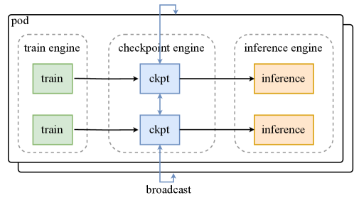
### Visual Description
\n
## Diagram: System Architecture for Model Training and Inference
### Overview
The image depicts a system architecture diagram illustrating the flow of data between a "train engine", a "checkpoint engine", and an "inference engine" all contained within a "pod". The diagram shows how training data is processed, checkpoints are created, and those checkpoints are used for inference.
### Components/Axes
The diagram consists of three main components, each enclosed in a dashed-line box:
* **Train Engine:** Contains two instances labeled "train".
* **Checkpoint Engine:** Contains two instances labeled "ckpt".
* **Inference Engine:** Contains two instances labeled "inference".
Additionally, the entire system is contained within a box labeled "pod". Arrows indicate the direction of data flow. There are two external labels: "broadcast" pointing upwards, and a connection from the "pod" to an external source.
### Detailed Analysis or Content Details
The diagram shows the following data flow:
1. **Train Engine to Checkpoint Engine:** Each of the two "train" instances in the "train engine" sends data to one of the two "ckpt" instances in the "checkpoint engine".
2. **Checkpoint Engine to Inference Engine:** Each "ckpt" instance in the "checkpoint engine" sends data to one of the two "inference" instances in the "inference engine".
3. **Broadcast:** A single arrow labeled "broadcast" points upwards from the "checkpoint engine".
4. **Pod:** The entire system is contained within a box labeled "pod".
There are no numerical values or scales present in the diagram. The diagram is purely conceptual, illustrating the relationships between the components.
### Key Observations
The diagram highlights a parallel processing architecture. There are two instances of each component ("train", "ckpt", "inference"), suggesting that the system can handle multiple training or inference tasks concurrently. The "broadcast" label suggests that checkpoint information is being disseminated to other parts of the system or to external consumers.
### Interpretation
This diagram represents a system designed for machine learning model training and deployment. The "train engine" is responsible for training the model, the "checkpoint engine" periodically saves the model's state (checkpoints), and the "inference engine" uses these checkpoints to make predictions. The "pod" likely refers to a containerization unit (like in Kubernetes), encapsulating all these components for easy deployment and scaling. The parallel instances of each component suggest a focus on scalability and throughput. The "broadcast" mechanism could be used for monitoring, model versioning, or distributing checkpoints to multiple inference servers. The diagram emphasizes a pipeline architecture where data flows sequentially through the training, checkpointing, and inference stages.
</details>
Figure 10: Parameter update utilizing a checkpoint engine
Given the scale of K2 and the vast number of devices involved, using a network file system for resharding and broadcasting parameters is impractical. The aggregate bandwidth required to keep overhead low reaches several petabytes per second. To address this challenge, we developed a distributed checkpoint engine co-located on training nodes to manage parameter states. To perform a parameter update, each checkpoint engine worker obtains a local copy of parameters from the training engine, then broadcasts the full parameter set across all checkpoint engine workers. Subsequently, the inference engine retrieves only the parameter shard it requires from the checkpoint engine. This process is illustrated in Figure 10. To enable this for a 1T model, updates are performed parameter-by-parameter in a pipelined manner, minimizing memory footprint (see Appendix G).
We opt to broadcast the full parameter set across the entire cluster, regardless of the specific sharding schemes on each inference worker. While this transfers several times more data than a theoretically optimal approach, it offers a simpler system design that is less intrusive to the training and inference engines. We chose to trade off this minor overhead to fully decouple the training engine and the inference engine, significantly simplifying maintenance and testing.
Notably, this approach outperforms the transfer-what-you-need method due to reduced synchronization overhead and higher network bandwidth utilization. Our system can complete a full parameter update for Kimi K2 with less than 30 seconds, a negligible duration for a typical RL training iteration. The source code for the checkpoint engine is available on Github https://github.com/MoonshotAI/checkpoint-engine.
3.3.3 Efficient System Startup
As large-scale training is prone to system failure, optimizing the startup time is crucial for models as large as Kimi K2.
To start the training engine, we let each training worker selectively read part or none of the parameters from disk, and broadcast necessary parameters to its peers. The design goal is to ensure all workers collectively read the checkpoint only once, minimizing expensive disk IO.
As the inference engines are independent replicas, we would like to avoid introducing extra synchronization barriers between them. Therefore, we opt to reuse checkpoint engine for startup: we let checkpoint engine collectively read the checkpoint from disk, similar to how the training engine starts. Then it updates the state of the uninitialized inference engine, using the approach introduced in the previous section. By leveraging the dedicated checkpoint engine, the system also becomes robust to single-point failures, because an inference replica can restart without communicating with other replicas.
3.3.4 Agentic Rollout
Our RL infrastructure supports the training of long-horizon, multi-turn agentic tasks. During rollout, these tasks present distinct challenges, such as complex environmental interactions and prolonged rollout durations. Here we introduce a few optimizations to alleviate these issues.
Due to the diversity of environments, certain interactions may be blocked on waiting for environment feedback (e.g., a virtual machine or a code interpreter), leaving the GPUs idle. We employ two strategies to maximize GPU utilization: (i) we deploy heavy environments as dedicated services that can scale up more easily; (ii) we employ a large number of concurrent rollouts to amortize the latency induced by certain expensive interactions.
Another challenge in agentic rollout is that individual rollout trajectories can be extremely long. To prevent long-tail trajectories from blocking the entire rollout process, we employ the partial rollout [36] technique. This strategy allows long-tail unfinished tasks to be paused, and resumed in the next RL iteration.
To improve research efficiency, we also design a unified interface inspired by the OpenAI Gym framework [5] to streamline the integration of new environments. We hope to scale our RL infrastructure to more diverse interactive environments in the future.
4 Evaluations
This section begins with the post-training evaluation of Kimi-K2-Instruct, followed by a brief overview of the capabilities of Kimi-K2-Base. We conclude with a comprehensive safety evaluation.
4.1 Post-training Evaluations
4.1.1 Evaluation Settings
Benchmarks
We assess Kimi-K2-Instruct across different areas. For coding, we adopt LiveCodeBench v6 [32] (questions from August 2024 to May 2025), OJBench [78], MultiPL-E [6], SWE-bench Verified [33, 85], TerminalBench [72], Multi-SWE-bench [87], SWE-Lancer [51], PaperBench [66], and Aider-Polyglot [17]. For tool use tasks, we evaluate performance on $\tau^{2}$ -Bench [3] and AceBench [7], which emphasize multi-turn tool-calling capabilities. In reasoning, we include a wide range of mathematical, science and logical tasks: AIME 2024/2025, MATH-500, HMMT 2025, CNMO 2024, PolyMath-en, ZebraLogic [44], AutoLogi [92], GPQA-Diamond [62], SuperGPQA [14], and Humanity’s Last Exam (Text-Only) [57]. We benchmark the long-context capabilities on: MRCR https://huggingface.co/datasets/openai/mrcr for long-context retrieval, and DROP [15], FRAMES [38] and LongBench v2 [2] for long-context reasoning. For factuality, we evaluate FACTS Grounding [31], the Vectara Hallucination Leaderboard [74], and FaithJudge [69]. Finally, general capabilities are assessed using MMLU [24], MMLU-Redux [18], MMLU-Pro [77], IFEval [91], Multi-Challenge [65], SimpleQA [79], and LiveBench [81] (as of 2024-11-25).
Baselines
We benchmark against both open-source and proprietary frontier models, ensuring every candidate is evaluated under its non-thinking configuration to eliminate additional gains from test-time compute. Open-source baselines: DeepSeek-V3-0324 and Qwen3-235B-A22B, with the latter run in the vendor-recommended no-thinking regime. Proprietary baselines: Claude Sonnet 4, Claude Opus 4, GPT-4.1, and Gemini 2.5 Flash Preview (2025-05-20). Each invoked in its respective non-thinking mode via official APIs under unified temperature and top-p settings.
Evaluation Configurations All runs query models in their non-thinking mode. Output token length is capped at 8192 tokens everywhere except SWE-bench Verified (Agentless), which is raised to 16384. For benchmarks with high per-question variance, we adopt repeated sampling $k$ times and average the results to obtain stable scores, denoted as Avg@k. For long-context tasks, we set the context window size to 128K tokens during evaluation, truncating any input that exceeds this limit to fit within the window. SWE-bench Verified is evaluated in two modes: Agentless Coding via Single Patch without Test (Acc) and Agentic Coding via bash/editor tools under both Single Attempt (Acc) and Multiple Attempts (Acc) using best-of-N selection with an internal verifier; SWE-bench Multilingual is tested only in the single-attempt agentic setting. Some data points have been omitted due to prohibitively expensive evaluation costs.
Table 3: Performance comparison of Kimi-K2-Instruct against leading open-source and proprietary models across diverse tasks. Bold denotes the global SOTA; underlined bold indicates the best open-source result. Data points marked with * are taken directly from the model’s technical report or blog.
| | Open Source | Proprietary | | | | | |
| --- | --- | --- | --- | --- | --- | --- | --- |
| Benchmark | Kimi-K2-Instruct | DeepSeek-V3-0324 | Qwen3-235B-A22B | Claude Sonnet 4 | Claude Opus 4 | GPT-4.1 | Gemini 2.5 Flash |
| Coding Tasks | | | | | | | |
| LiveCodeBench v6 (Pass@1) | 53.7 | 46.9 | 37.0 | 48.5 | 47.4 | 44.7 | 44.7 |
| OJBench (Pass@1) | 27.1 | 24.0 | 11.3 | 15.3 | 19.6 | 19.5 | 19.5 |
| MultiPL-E (Pass@1) | 85.7 | 83.1 | 78.2 | 88.6 | 89.6 | 86.7 | 85.6 |
| SWE-bench Verified Agentless-Single-Patch (Pass@1) | 51.8 | 36.6 | 39.4 | 50.2 | 53.0 | 40.8 | 32.6 |
| SWE-bench Verified Agentic-Single-Attempt (Pass@1) | 65.8 | 38.8 | 34.4 | 72.7* | 72.5* | 54.6 | — |
| SWE-bench Verified Agentic-Multi-Attempt (Pass@1) | 71.6 | — | — | 80.2* | 79.4* | — | — |
| SWE-bench Multilingual (Pass@1) | 47.3 | 25.8 | 20.9 | 51.0 | — | 31.5 | — |
| Multi-SWE-bench (Pass@1) | 18.3 | 8.0 | 9.0 | 29.2 | — | 11.7 | 14.0 |
| SWE-Lancer (Pass@1) | 39.1 | 30.5 | 24.1 | 40.8 | — | 23.0 | 38.5 |
| Paper Bench Code-Dev (Acc.) | 27.8 | 12.2 | 13.2 | 43.3 | — | 29.9 | 5.7 |
| Terminal Bench In-House (Acc.) | 30.0 | — | — | 35.5 | 43.2 | 8.3 | — |
| Terminal Bench Terminus (Acc.) | 25.0 | 16.3 | 6.6 | — | — | 30.3 | 16.8 |
| Aider-Polyglot (Acc.) | 60.0 | 55.1 | 61.8 | 56.4 | 70.7 | 52.4 | 44.0 |
| Tool Use Tasks | | | | | | | |
| Tau2 retail (Avg@4) | 70.6 | 69.1 | 57.0 | 75.0 | 81.8 | 74.8 | 64.3 |
| Tau2 airline (Avg@4) | 56.5 | 39.0 | 26.5 | 55.5 | 60.0 | 54.5 | 42.5 |
| Tau2 telecom (Avg@4) | 65.8 | 32.5 | 22.1 | 45.2 | 57.0 | 38.6 | 16.9 |
| AceBench (Acc.) | 76.5 | 72.7 | 70.5 | 76.2 | 75.6 | 80.1 | 74.5 |
| Math & STEM Tasks | | | | | | | |
| AIME 2024 (Avg@64) | 69.6 | 59.4* | 40.1* | 43.4 | 48.2 | 46.5 | 61.3 |
| AIME 2025 (Avg@64) | 49.5 | 46.7 | 24.7* | 33.1* | 33.9* | 37.0 | 46.6 |
| MATH-500 (Acc.) | 97.4 | 94.0* | 91.2* | 94.0 | 94.4 | 92.4 | 95.4 |
| HMMT 2025 (Avg@32) | 38.8 | 27.5 | 11.9 | 15.9 | 15.9 | 19.4 | 34.7 |
| CNMO 2024 (Avg@16) | 74.3 | 74.7 | 48.6 | 60.4 | 57.6 | 56.6 | 75.0 |
| PolyMath-en (Avg@4) | 65.1 | 59.5 | 51.9 | 52.8 | 49.8 | 54.0 | 49.9 |
| ZebraLogic (Acc.) | 89.0 | 84.0 | 37.7* | 79.7 | 59.3 | 58.5 | 57.9 |
| AutoLogi (Acc.) | 89.5 | 88.9 | 83.3* | 89.8 | 86.1 | 88.2 | 84.1 |
| GPQA-Diamond (Avg@8) | 75.1 | 68.4* | 62.9* | 70.0* | 74.9* | 66.3 | 68.2 |
| SuperGPQA (Acc.) | 57.2 | 53.7 | 50.2 | 55.7 | 56.5 | 50.8 | 49.6 |
| Humanity’s Last Exam (Acc.) | 4.7 | 5.2 | 5.7 | 5.8 | 7.1 | 3.7 | 5.6 |
| General Tasks | | | | | | | |
| MMLU (EM) | 89.5 | 89.4 | 87.0 | 91.5 | 92.9 | 90.4 | 90.1 |
| MMLU-Redux (EM) | 92.7 | 90.5 | 89.2* | 93.6 | 94.2 | 92.4 | 90.6 |
| MMLU-Pro (EM) | 81.1 | 81.2* | 77.3 | 83.7 | 86.6 | 81.8 | 79.4 |
| IFEval (Prompt Strict) | 89.8 | 81.1 | 83.2* | 87.6 | 87.4 | 88.0 | 84.3 |
| Multi-Challenge (Acc.) | 54.1 | 31.4 | 34.0 | 46.8 | 49.0 | 36.4 | 39.5 |
| SimpleQA (Correct) | 31.0 | 27.7 | 13.2 | 15.9 | 22.8 | 42.3 | 23.3 |
| Livebench (Pass@1) | 76.4 | 72.4 | 67.6 | 74.8 | 74.6 | 69.8 | 67.8 |
| Arena Hard v2.0 Hard Prompt (Win rate) | 54.5 | 39.9 | 39.9 | 51.6 | 59.7 | 51.7 | 48.7 |
| Arena Hard v2.0 Creative Writing (Win rate) | 85.0 | 59.3 | 59.8 | 54.6 | 68.5 | 61.5 | 72.8 |
| FACTS Grounding (Adjusted) | 88.5 | 68.3 | 68.5 | 83.6 | — | 79.2 | 86.6 |
| HHEM v2.1 (1-Hallu.) | 98.9 | 88.9 | 94.5 | 94.5 | — | 96.7 | 97.8 |
| FaithJudge (1-Hallu.) | 92.6 | 83.4 | 75.7 | 83.0 | — | 91.0 | 93.2 |
| LongBench v2 (Acc.) | 49.1 | 51.1 | — | 52.5 | — | 54.3 | 55.5 |
| FRAMES (Acc.) | 77.1 | 79.2 | — | 76.3 | — | 87.4 | 72.9 |
| MRCR (Acc.) | 55.0 | 50.8 | — | 74.4 | — | 66.9 | 81.7 |
| DROP (Acc.) | 93.5 | 91.2 | 84.3 | 92.0 | — | 79.1 | 81.7 |
4.1.2 Evaluation Results
A comprehensive evaluation results of Kimi-K2-Instruct is shown in Table 3, with detailed explanation provided in the Appendix C. Below, we highlight key results across four core domains:
Agentic and Competitive Coding
Kimi-K2-Instruct demonstrates state-of-the-art open-source performance on real-world SWE tasks. It outperforms most baselines on SWE-bench Verified (65.8%, 71.6% with multiple attemps), SWE-bench Multilingual (47.3%), and SWE-lancer (39.1%), significantly closing the gap with Claude 4 Opus and Sonnet. On competitive coding benchmarks (e.g., LiveCodeBench v6 53.7%, OJBench 27.1%), it also leads among all models, highlighting its practical coding proficiency across difficulty levels.
Agentic Tool Use
On multi-turn tool-use benchmarks, Kimi-K2-Instruct sets a new standard. It achieves 66.1 Pass@1 on $\tau^{2}$ -Bench and 76.5 on ACEBench, substantially outperforming all baselines. These results affirm its strength in grounded, controlled, and agent-driven tool orchestration across domains.
General Capabilities
Kimi-K2-Instruct exhibits strong, balanced performance across general knowledge, math, instruction following, and long-context tasks. It surpasses open-source peers on SimpleQA (31.0%), MMLU (89.5%) and MMLU-Redux (92.7%), and leads all models on instruction benchmarks (IFEval: 89.8%, Multi-Challenge: 54.1%). In math and STEM, it achieves top-tier scores (AIME 2024: 69.6%, GPQA-Diamond: 75.1%), and remains competitive on long-context factuality and retrieval (DROP: 93.5%, MRCR: 55.0%). These results position Kimi-K2-Instruct as a well-rounded and capable generalist across both short- and long-context settings.
Open-Ended Evaluation
On the LMSYS Arena leaderboard (July 17, 2025), Kimi-K2-Instruct ranks as the top-1 open-source model and 5th overall based on over 3,000 user votes. This real-world preference signal—across diverse, blind prompts—underscores Kimi-K2’s strengths in generating high-quality responses on open-ended tasks.
4.2 Pre-training Evaluations
4.2.1 Evaluation Settings
Benchmarks
We evaluate Kimi-K2-Base across diverse capability areas. For general capabilities, we assess on MMLU [24], MMLU-Pro [77], MMLU-Redux [18], BBH [68], TriviaQA [35], SuperGPQA [14], SimpleQA [79], HellaSwag [89], AGIEval [90], GPQA-Diamond [62], ARC-Challenge [9], and WinoGrande [63]. For coding capabilities, we employ EvalPlus [46] (averaging HumanEval [8], MBPP [1], HumanEval+, and MBPP+), LiveCodeBench v6 [32], and CRUXEval [19]. For mathematical reasoning, we utilize GSM8K [10], GSM8K-Platinum [75], MATH [25], and CMATH [80]. For Chinese language capabilities, we evaluate on C-Eval [30], CMMLU [41], and CSimpleQA [23].
Baselines
We benchmark against leading open-source foundation models: DeepSeek-V3-Base [11], Qwen2.5-72B-Base [60] (Note that Qwen3-235B-A22B-Base is not open-sourced, and the largest open-sourced base model in the Qwen series is Qwen2.5-72B-Base), and Llama 4-Maverick [71] (Llama 4-Behemoth is also not open-sourced). All models are evaluated under identical configurations to ensure fair comparison.
Evaluation Configurations
We employ perplexity-based evaluation for MMLU, MMLU-Redux, GPQA-Diamond, HellaSwag, ARC-Challenge, C-Eval, and CMMLU. Generation-based evaluation is used for MMLU-Pro, SuperGPQA, TriviaQA, BBH, CSimpleQA, MATH, CMATH, GSM8K, GSM8K-Platinum, CRUXEval, LiveCodeBench, and EvalPlus. To mitigate the high variance inherent to GPQA-Diamond, we report the mean score across eight independent runs. All evaluations are conducted using our internal framework derived from LM-Harness-Evaluation [4], ensuring consistent settings across all models.
4.2.2 Evaluation Results
Table 4 presents a comprehensive comparison of Kimi-K2-Base against leading open-source foundation models across diverse evaluation benchmarks. The results demonstrate that Kimi-K2-Base achieves state-of-the-art performance across the majority of evaluated tasks, establishing it as a leading foundation model in the open-source landscape.
General Language Understanding
Kimi-K2-Base achieves state-of-the-art performance on 10 out of 12 English language benchmarks. Notable results include MMLU (87.79%), MMLU-Pro (69.17%), MMLU-Redux (90.17%), SuperGPQA (44.67%), and SimpleQA (35.25%), significantly outperforming all baselines.
Coding Capabilities
On coding benchmarks, Kimi-K2-Base sets new standards with leading performance across all metrics. It achieves 74.00% on CRUXEval-I-cot, 83.50% on CRUXEval-O-cot, 26.29% on LiveCodeBench v6, and 80.33% on EvalPlus, demonstrating superior code generation and comprehension abilities, particularly in scenarios requiring step-by-step reasoning.
Mathematical Reasoning
Kimi-K2-Base exhibits exceptional mathematical capabilities, leading on three out of four benchmarks: MATH (70.22%), GSM8K (92.12%), and GSM8K-Platinum (94.21%). It maintains competitive performance on CMATH (90.26%), narrowly behind DeepSeek-V3-Base (90.53%). These results highlight the model’s robust mathematical problem-solving abilities across varying difficulty levels.
Chinese Language Understanding
The model demonstrates superior multilingual capabilities, achieving state-of-the-art results across all Chinese language benchmarks: C-Eval (92.50%), CMMLU (90.90%), and CSimpleQA (77.57%). These results establish Kimi-K2-Base as a leading model for Chinese language understanding while maintaining strong performance across other languages.
Table 4: Performance comparison of Kimi-K2-Base against leading open-source models across diverse tasks.
| | Benchmark (Metric) | #Shots | Kimi-K2-Base | DeepSeek-V3-Base | Llama4-Maverick-Base | Qwen2.5-72B-Base |
| --- | --- | --- | --- | --- | --- | --- |
| Architecture | - | MoE | MoE | MoE | Dense | |
| # Activated Params | - | 32B | 37B | 17B | 72B | |
| # Total Params | - | 1043B | 671B | 400B | 72B | |
| English | MMLU | 5-shots | 87.79 | 87.10 | 84.87 | 86.08 |
| MMLU-pro | 5-shots | 69.17 | 60.59 | 63.47 | 62.80 | |
| MMLU-redux | 5-shots | 90.17 | 89.53 | 88.18 | 87.77 | |
| SuperGPQA | 5-shots | 44.67 | 39.20 | 38.84 | 34.23 | |
| GPQA-Diamond(avg@8) | 5-shots | 48.11 | 50.51 | 49.43 | 40.78 | |
| SimpleQA | 5-shots | 35.25 | 26.49 | 23.74 | 10.31 | |
| TriviaQA | 5-shots | 85.09 | 84.11 | 79.25 | 76.03 | |
| BBH | 3-shots | 88.71 | 88.37 | 87.10 | 84.09 | |
| HellaSwag | 5-shots | 94.60 | 89.44 | 86.02 | 95.27 | |
| AGIEval | - | 84.23 | 81.57 | 67.55 | 76.87 | |
| ARC-Challenge | 0-shot | 95.73 | 93.77 | 94.03 | 95.56 | |
| WinoGrande | 5-shots | 85.32 | 84.21 | 77.58 | 84.14 | |
| Code | CRUXEval-I-cot | 0-shots | 74.00 | 62.75 | 67.13 | 61.12 |
| CRUXEval-O-cot | 0-shots | 83.50 | 75.25 | 75.88 | 66.13 | |
| LiveCodeBench(v6) | 1-shots | 26.29 | 24.57 | 25.14 | 22.29 | |
| EvalPlus | - | 80.33 | 65.61 | 65.48 | 66.04 | |
| Math | MATH | 4-shots | 70.22 | 61.70 | 63.02 | 62.68 |
| GSM8k | 8-shots | 92.12 | 91.66 | 86.35 | 90.37 | |
| GSM8k-platinum | 8-shots | 94.21 | 93.38 | 88.83 | 92.47 | |
| CMATH | 6-shots | 90.26 | 90.53 | 88.07 | 86.98 | |
| Chinese | C-Eval | 5-shots | 92.50 | 90.04 | 80.91 | 90.86 |
| CMMLU | 5-shots | 90.90 | 88.84 | 81.24 | 90.55 | |
| CSimpleQA | 5-shots | 77.57 | 72.13 | 53.47 | 50.53 | |
4.3 Safety Evaluation
4.3.1 Experiment Settings
We conducted red-teaming evaluations on Kimi K2 compare with other open-source LLMs. The evaluation covered a range of attack scenarios—including harmful content, privacy content, and security content, as well as different attack strategies such as prompt injection and iterative jailbreak.
We choose Promptfoo https://github.com/promptfoo/promptfoo to generate adversarial prompts and analyze the responses. By this way, we can evaluate model in a scalable ways.
Model Selection We compare Kimi K2 with three other open-source LLMs: DeepSeek-V3, DeepSeek-R1, and Qwen3.
Promptfoo Settings Table 5 lists plugins and strategies evaluated, with each plugin paired with all strategies to assess their performance.
Table 5: Enabled Plugins and Strategies
| Plugin | Harmful | Graphic Content, Harassment and Bullying, Hate Speech, Insults, Profanity, Radicalization, Self Harm, Sexual Content, ToxicChat |
| --- | --- | --- |
| Criminal | Chemical&Biological Weapons, Child Exploitation, Copyright Violations, Cybercrime, Illegal Activities, Illegal Drugs, Indiscriminate Weapons, Intellectual Property Violation, Non-Violent Crime, Violent Crime, Sex Crimes | |
| Misinformation | Competitor Endorsement, Unsupervised Contracts, Excessive Agency, Hallucination, Misinformation and Disinformation, Specialized Advice, Unsafe Practices, Imitation, Overreliance, Political Opinions, Religious Sensitivity | |
| Privacy | Privacy Violation, PII in API/Database, Direct PII Exposure, PII in Session Data, PII via Social Engineering | |
| Security | ASCII Smuggling, CyberSecEval, Harmbench, Debug Access, Divergent Repetition, DoNotAnswer, Malicious Code, Pliny, Prompt Extraction, Reasoning DoS, Tool Discovery | |
| Strategy | Basic, Prompt Injection, Iterative Jailbreak, Crescendo | |
Test Case Count Given the inherent non-determinism of large language model inference, single-pass outputs may exhibit variability. To account for this, we generated 3 attack prompts per plugin for each strategy.
Prompt Language Settings We pre-tested the language compatibility for each plugin-strategy combination. Some plugins support both English and Chinese, while others only support English. For combinations that support both, we generated 3 prompts in each language, resulting in 6 prompts per combination.
Manual Review We incorporated human review into the evaluation process. To minimize subjectivity problem, we conducted multiple rounds of review and assigned the same reviewer to evaluate all cases within a given test set to ensure consistency and reduce variability in judgment.
4.3.2 Safety Evaluation Results
Table 6 presents the passing rates of different models under various plugin–strategy combinations.
Table 6: Safety Evaluation Results
| Plugin | Strategy | Kimi-K2-Instruct | DeepSeek-V3-0324 | DeepSeek-R1 | Qwen3-235B-A22B |
| --- | --- | --- | --- | --- | --- |
| Harmful | Basic | 98.04 | 90.45 | 99.02 | 98.53 |
| Base64 | 100 | 90.20 | 100 | 100 | |
| Prompt Injection | 93.14 | 100 | 95.10 | 99.02 | |
| Iterative Jailbreak | 92.16 | 66.67 | 72.55 | 74.51 | |
| Crescendo | 64.71 | 64.71 | 80.39 | 86.27 | |
| Criminal | Basic | 100 | 99.62 | 95.45 | 99.24 |
| Base64 | 96.97 | 89.39 | 84.85 | 98.48 | |
| Prompt Injection | 75.76 | 91.67 | 69.70 | 98.47 | |
| Iterative Jailbreak | 57.57 | 21.21 | 25.76 | 53.03 | |
| Crescendo | 56.06 | 31.81 | 42.42 | 59.09 | |
| Misinformation | Basic | 97.28 | 92.57 | 92.46 | 94.84 |
| Base64 | 98.48 | 90.48 | 96.83 | 93.65 | |
| Prompt Injection | 98.39 | 86.51 | 93.65 | 93.65 | |
| Iterative Jailbreak | 63.97 | 53.97 | 84.13 | 69.84 | |
| Crescendo | 85.71 | 55.56 | 88.89 | 84.13 | |
| Privacy | Basic | 100 | 100 | 100 | 100 |
| Base64 | 100 | 100 | 100 | 100 | |
| Prompt Injection | 88.33 | 98.33 | 100 | 91.67 | |
| Iterative Jailbreak | 76.67 | 100 | 93.33 | 96.67 | |
| Crescendo | 96.67 | 100 | 96.67 | 100 | |
| Security | Basic | 77.84 | 75.57 | 70.46 | 90.09 |
| Base64 | 82.93 | 82.93 | 63.41 | 95.12 | |
| Prompt Injection | 87.80 | 97.56 | 65.85 | 84.13 | |
| Iterative Jailbreak | 43.90 | 60.97 | 43.90 | 78.04 | |
| Crescendo | 68.29 | 87.80 | 68.29 | 87.80 | |
Without targeted optimization for specific evaluation scenarios, the passing rate of some complex cases (e.g., Harmful–Iterative Jailbreak) was relatively higher compared to other models.
Across different attack strategies, the models exhibited varying trends. Under the Base64 strategy, passing rates generally approached or reached 100%, suggesting that encoding transformations had minimal impact on the models’ basic robustness. In contrast, the Crescendo strategy led to a general drop in passing rates, indicating stronger adversarial effectiveness.
In addition, complex attack strategies do not always outperform basic prompts. Some originally adversarial prompts may lose their intended meaning after multiple rounds of transformation, rendering the resulting model outputs less meaningful.
Automated Red-teaming Limitations Due to the involvement of human review, the evaluation results inevitably contain a degree of subjectivity. Additionally, certain plugin types involve API misuse or external tool invocation, which are more suitable for evaluating agent models with tool-calling capabilities. In the context of base LLMs, such tests may have limited relevance.
5 Limitations
In our internal tests, we have identified some limitations in current Kimi K2 models. When dealing with hard reasoning tasks or unclear tool definition, the model may generate excessive tokens, sometimes leading to truncated outputs or incomplete tool calls. Additionally, performance may decline on certain tasks if tool use is unnecessarily enabled. When building complete software projects, the success rate of one-shot prompting is not as good as using K2 under an agentic coding framework. We are working to address these issues in future releases and looking forward to more feedbacks.
6 Conclusions
We introduced Kimi K2, a 1T-parameter open-weight MoE model built for agentic intelligence. Leveraging the token-efficient MuonClip optimizer and a 15.5T-token high-quality dataset, Kimi K2 achieves stable, scalable pre-training. Post-training combines large-scale synthetic tool-use data with a unified RL framework using both verifiable rewards and self-critic feedbacks. Kimi K2 sets new state-of-the-art on agentic and reasoning benchmarks, establishing itself as the most capable open-weight LLM to date.
7 Acknowledgments
We would like to acknowledge the valuable support provided by the OpenHands and Multi-SWE-bench teams in evaluating the SWE-bench Verified and Multi-SWE-bench experimental results.
References
- [1] J. Austin, A. Odena, M. Nye, M. Bosma, H. Michalewski, D. Dohan, E. Jiang, C. Cai, M. Terry, Q. Le, and C. Sutton (2021) Program synthesis with large language models. External Links: 2108.07732, Link Cited by: §4.2.1.
- [2] Y. Bai, S. Tu, J. Zhang, H. Peng, X. Wang, X. Lv, S. Cao, J. Xu, L. Hou, Y. Dong, J. Tang, and J. Li (2025) LongBench v2: towards deeper understanding and reasoning on realistic long-context multitasks. External Links: 2412.15204, Link Cited by: §4.1.1.
- [3] V. Barres, H. Dong, S. Ray, X. Si, and K. Narasimhan (2025) $\tau^{2}$ -Bench: evaluating conversational agents in a dual-control environment. External Links: 2506.07982, Link Cited by: §4.1.1.
- [4] S. Biderman, H. Schoelkopf, L. Sutawika, L. Gao, J. Tow, B. Abbasi, A. F. Aji, P. S. Ammanamanchi, S. Black, J. Clive, et al. (2024) Lessons from the trenches on reproducible evaluation of language models. arXiv preprint arXiv:2405.14782. Cited by: §4.2.1.
- [5] G. Brockman, V. Cheung, L. Pettersson, J. Schneider, J. Schulman, J. Tang, and W. Zaremba (2016) OpenAI gym. External Links: 1606.01540, Link Cited by: §3.3.4.
- [6] F. Cassano, J. Gouwar, D. Nguyen, S. Nguyen, L. Phipps-Costin, D. Pinckney, M. Yee, Y. Zi, C. J. Anderson, M. Q. Feldman, A. Guha, M. Greenberg, and A. Jangda (2023) MultiPL-e: a scalable and polyglot approach to benchmarking neural code generation. IEEE Transactions on Software Engineering 49 (7), pp. 3675–3691. External Links: Document Cited by: §4.1.1.
- [7] C. Chen, X. Hao, W. Liu, X. Huang, X. Zeng, S. Yu, D. Li, S. Wang, W. Gan, Y. Huang, et al. (2025) ACEBench: who wins the match point in tool learning?. arXiv e-prints, pp. arXiv–2501. Cited by: §3.1.1, §3.1.1, §4.1.1.
- [8] M. Chen, J. Tworek, H. Jun, Q. Yuan, H. P. de Oliveira Pinto, J. Kaplan, H. Edwards, Y. Burda, N. Joseph, G. Brockman, A. Ray, R. Puri, G. Krueger, M. Petrov, H. Khlaaf, G. Sastry, P. Mishkin, B. Chan, S. Gray, N. Ryder, M. Pavlov, A. Power, L. Kaiser, M. Bavarian, C. Winter, P. Tillet, F. P. Such, D. Cummings, M. Plappert, F. Chantzis, E. Barnes, A. Herbert-Voss, W. H. Guss, A. Nichol, A. Paino, N. Tezak, J. Tang, I. Babuschkin, S. Balaji, S. Jain, W. Saunders, C. Hesse, A. N. Carr, J. Leike, J. Achiam, V. Misra, E. Morikawa, A. Radford, M. Knight, M. Brundage, M. Murati, K. Mayer, P. Welinder, B. McGrew, D. Amodei, S. McCandlish, I. Sutskever, and W. Zaremba (2021) Evaluating large language models trained on code. External Links: 2107.03374 Cited by: §4.2.1.
- [9] P. Clark, I. Cowhey, O. Etzioni, T. Khot, A. Sabharwal, C. Schoenick, and O. Tafjord (2018) Think you have solved question answering? try arc, the ai2 reasoning challenge. arXiv preprint arXiv:1803.05457. Cited by: §4.2.1.
- [10] K. Cobbe, V. Kosaraju, M. Bavarian, M. Chen, H. Jun, L. Kaiser, M. Plappert, J. Tworek, J. Hilton, R. Nakano, C. Hesse, and J. Schulman (2021) Training verifiers to solve math word problems. External Links: 2110.14168, Link Cited by: §4.2.1.
- [11] DeepSeek-AI (2024) DeepSeek-v3 technical report. External Links: 2412.19437, Link Cited by: §2.3, §2.3, §2.4.2, §2.4.3, §2, §4.2.1.
- [12] M. Dehghani, J. Djolonga, B. Mustafa, P. Padlewski, J. Heek, J. Gilmer, A. P. Steiner, M. Caron, R. Geirhos, I. Alabdulmohsin, et al. (2023) Scaling vision transformers to 22 billion parameters. In International conference on machine learning, pp. 7480–7512. Cited by: §2.1.
- [13] G. Dong, K. Lu, C. Li, T. Xia, B. Yu, C. Zhou, and J. Zhou (2024) Self-play with execution feedback: improving instruction-following capabilities of large language models. External Links: 2406.13542, Link Cited by: §3.2.1.
- [14] X. Du, Y. Yao, K. Ma, B. Wang, T. Zheng, K. Zhu, M. Liu, Y. Liang, X. Jin, Z. Wei, et al. (2025) Supergpqa: scaling llm evaluation across 285 graduate disciplines. arXiv preprint arXiv:2502.14739. Cited by: §4.1.1, §4.2.1.
- [15] D. Dua, Y. Wang, P. Dasigi, G. Stanovsky, S. Singh, and M. Gardner (2019) DROP: A reading comprehension benchmark requiring discrete reasoning over paragraphs. CoRR abs/1903.00161. External Links: Link, 1903.00161 Cited by: §4.1.1.
- [16] K. Fujii, Y. Tajima, S. Mizuki, H. Shimada, T. Shiotani, K. Saito, M. Ohi, M. Kawamura, T. Nakamura, T. Okamoto, S. Ishida, K. Hattori, Y. Ma, H. Takamura, R. Yokota, and N. Okazaki (2025) Rewriting pre-training data boosts llm performance in math and code. External Links: 2505.02881, Link Cited by: §2.2.
- [17] P. Gauthier (2025) Aider llm leaderboards. blog. Note: https://aider.chat/docs/leaderboards/ Cited by: §4.1.1.
- [18] A. P. Gema, J. O. J. Leang, G. Hong, A. Devoto, A. C. M. Mancino, R. Saxena, X. He, Y. Zhao, X. Du, M. R. G. Madani, et al. (2024) Are we done with mmlu?. arXiv preprint arXiv:2406.04127. Cited by: §4.1.1, §4.2.1.
- [19] A. Gu, B. Rozière, H. Leather, A. Solar-Lezama, G. Synnaeve, and S. I. Wang (2024) Cruxeval: a benchmark for code reasoning, understanding and execution. arXiv preprint arXiv:2401.03065. Cited by: §4.2.1.
- [20] D. Guo, D. Yang, H. Zhang, J. Song, R. Zhang, R. Xu, Q. Zhu, S. Ma, P. Wang, X. Bi, et al. (2025) Deepseek-r1: incentivizing reasoning capability in llms via reinforcement learning. arXiv preprint arXiv:2501.12948. Cited by: §3.2.3.
- [21] Z. Guo, S. Cheng, H. Wang, S. Liang, Y. Qin, P. Li, Z. Liu, M. Sun, and Y. Liu (2025) StableToolBench: towards stable large-scale benchmarking on tool learning of large language models. arXiv preprint arXiv:2403.07714. Cited by: §3.1.1.
- [22] A. Harlap, D. Narayanan, A. Phanishayee, V. Seshadri, N. Devanur, G. Ganger, and P. Gibbons (2018) Pipedream: fast and efficient pipeline parallel dnn training. arXiv preprint arXiv:1806.03377. Cited by: §2.4.2, §2.4.2.
- [23] Y. He, S. Li, J. Liu, Y. Tan, W. Wang, H. Huang, X. Bu, H. Guo, C. Hu, B. Zheng, et al. Chinese simpleqa: a chinese factuality evaluation for large language models, 2024a. URL https://arxiv. org/abs/2411.07140. Cited by: §4.2.1.
- [24] D. Hendrycks, C. Burns, S. Basart, A. Zou, M. Mazeika, D. Song, and J. Steinhardt (2020) Measuring massive multitask language understanding. arXiv preprint arXiv:2009.03300. Cited by: §4.1.1, §4.2.1.
- [25] D. Hendrycks, C. Burns, S. Kadavath, A. Arora, S. Basart, E. Tang, D. Song, and J. Steinhardt (2021) Measuring mathematical problem solving with the math dataset. External Links: 2103.03874, Link Cited by: §4.2.1.
- [26] S. Hu, Y. Tu, X. Han, C. He, G. Cui, X. Long, Z. Zheng, Y. Fang, Y. Huang, W. Zhao, et al. (2024) Minicpm: unveiling the potential of small language models with scalable training strategies. arXiv preprint arXiv:2404.06395. Cited by: §2.5.
- [27] J. Huang, S. S. Gu, L. Hou, Y. Wu, X. Wang, H. Yu, and J. Han (2022) Large language models can self-improve. arXiv preprint arXiv:2210.11610. Cited by: §3.1.1.
- [28] S. Huang, T. Cheng, J. K. Liu, J. Hao, L. Song, Y. Xu, J. Yang, J. Liu, C. Zhang, L. Chai, R. Yuan, Z. Zhang, J. Fu, Q. Liu, G. Zhang, Z. Wang, Y. Qi, Y. Xu, and W. Chu (2025) OpenCoder: the open cookbook for top-tier code large language models. External Links: 2411.04905, Link Cited by: §3.2.1.
- [29] Y. Huang, Y. Cheng, A. Bapna, O. Firat, D. Chen, M. Chen, H. Lee, J. Ngiam, Q. V. Le, Y. Wu, et al. (2019) Gpipe: efficient training of giant neural networks using pipeline parallelism. Advances in neural information processing systems 32. Cited by: §2.4.2.
- [30] Y. Huang, Y. Bai, Z. Zhu, J. Zhang, J. Zhang, T. Su, J. Liu, C. Lv, Y. Zhang, J. Lei, Y. Fu, M. Sun, and J. He (2023) C-eval: a multi-level multi-discipline chinese evaluation suite for foundation models. External Links: 2305.08322, Link Cited by: §4.2.1.
- [31] A. Jacovi, A. Wang, C. Alberti, C. Tao, J. Lipovetz, K. Olszewska, L. Haas, M. Liu, N. Keating, A. Bloniarz, C. Saroufim, C. Fry, D. Marcus, D. Kukliansky, G. S. Tomar, J. Swirhun, J. Xing, L. Wang, M. Gurumurthy, M. Aaron, M. Ambar, R. Fellinger, R. Wang, Z. Zhang, S. Goldshtein, and D. Das (2025) The facts grounding leaderboard: benchmarking llms’ ability to ground responses to long-form input. External Links: 2501.03200, Link Cited by: §3.2.1, §4.1.1.
- [32] N. Jain, K. Han, A. Gu, W. Li, F. Yan, T. Zhang, S. Wang, A. Solar-Lezama, K. Sen, and I. Stoica (2024) Livecodebench: holistic and contamination free evaluation of large language models for code. arXiv preprint arXiv:2403.07974. Cited by: §4.1.1, §4.2.1.
- [33] C. E. Jimenez, J. Yang, A. Wettig, S. Yao, K. Pei, O. Press, and K. R. Narasimhan (2024) SWE-bench: can language models resolve real-world github issues?. In The Twelfth International Conference on Learning Representations, External Links: Link Cited by: §4.1.1.
- [34] K. Jordan, Y. Jin, V. Boza, J. You, F. Cesista, L. Newhouse, and J. Bernstein (2024) Muon: an optimizer for hidden layers in neural networks. External Links: Link Cited by: §2.1, §2, §3.1, §3.2.3.
- [35] M. Joshi, E. Choi, D. S. Weld, and L. Zettlemoyer (2017) TriviaQA: a large scale distantly supervised challenge dataset for reading comprehension. External Links: 1705.03551, Link Cited by: §4.2.1.
- [36] Kimi Team (2025) Kimi k1. 5: scaling reinforcement learning with llms. arXiv preprint arXiv:2501.12599. Cited by: §2.2, §3.1, §3.2.3, §3.2.3, §3.2, §3.3.1, §3.3.4.
- [37] D. P. Kingma and J. Ba (2015) Adam: A method for stochastic optimization. In 3rd International Conference on Learning Representations, ICLR 2015, San Diego, CA, USA, May 7-9, 2015, Conference Track Proceedings, Y. Bengio and Y. LeCun (Eds.), External Links: Link Cited by: §2.1.
- [38] S. Krishna, K. Krishna, A. Mohananey, S. Schwarcz, A. Stambler, S. Upadhyay, and M. Faruqui (2025) Fact, fetch, and reason: a unified evaluation of retrieval-augmented generation. External Links: 2409.12941, Link Cited by: §4.1.1.
- [39] J. Lamy-Poirier (2023) Breadth-first pipeline parallelism. Proceedings of Machine Learning and Systems 5, pp. 48–67. Cited by: §2.4.2.
- [40] D. Lepikhin, H. Lee, Y. Xu, D. Chen, O. Firat, Y. Huang, M. Krikun, N. Shazeer, and Z. Chen (2020) Gshard: scaling giant models with conditional computation and automatic sharding. arXiv preprint arXiv:2006.16668. Cited by: §2.4.2.
- [41] H. Li, Y. Zhang, F. Koto, Y. Yang, H. Zhao, Y. Gong, N. Duan, and T. Baldwin (2024) CMMLU: measuring massive multitask language understanding in chinese. External Links: 2306.09212, Link Cited by: §4.2.1.
- [42] J. Li, E. Beeching, L. Tunstall, B. Lipkin, R. Soletskyi, S. Huang, K. Rasul, L. Yu, A. Q. Jiang, Z. Shen, et al. (2024) Numinamath: the largest public dataset in ai4maths with 860k pairs of competition math problems and solutions. Hugging Face repository 13 (9), pp. 9. Cited by: §3.2.1.
- [43] T. Li, W. Chiang, E. Frick, L. Dunlap, T. Wu, B. Zhu, J. E. Gonzalez, and I. Stoica (2024) From crowdsourced data to high-quality benchmarks: arena-hard and benchbuilder pipeline. arXiv preprint arXiv:2406.11939. Cited by: Appendix C.
- [44] B. Y. Lin, R. L. Bras, K. Richardson, A. Sabharwal, R. Poovendran, P. Clark, and Y. Choi (2025) ZebraLogic: on the scaling limits of llms for logical reasoning. External Links: 2502.01100, Link Cited by: §4.1.1.
- [45] A. Liu, B. Feng, B. Wang, B. Wang, B. Liu, C. Zhao, C. Dengr, C. Ruan, D. Dai, D. Guo, et al. (2024) Deepseek-v2: a strong, economical, and efficient mixture-of-experts language model. arXiv preprint arXiv:2405.04434. Cited by: §2.3.
- [46] J. Liu, C. S. Xia, Y. Wang, and L. Zhang (2023) Is your code generated by chatgpt really correct? rigorous evaluation of large language models for code generation. Advances in Neural Information Processing Systems 36, pp. 21558–21572. Cited by: §4.2.1.
- [47] J. Liu, J. Su, X. Yao, Z. Jiang, G. Lai, Y. Du, Y. Qin, W. Xu, E. Lu, J. Yan, et al. (2025) Muon is scalable for llm training. arXiv preprint arXiv:2502.16982. Cited by: §2.1, §2, §3.1.
- [48] Z. Liu, S. Cheng, H. Zhou, and Y. You (2023-11) Hanayo: harnessing wave-like pipeline parallelism for enhanced large model training efficiency. In Proceedings of the International Conference for High Performance Computing, Networking, Storage and Analysis, SC ’23, pp. 1–13. External Links: Link, Document Cited by: §2.4.2.
- [49] I. Loshchilov and F. Hutter (2019) Decoupled weight decay regularization. In International Conference on Learning Representations, External Links: Link Cited by: §2.1.
- [50] P. Maini, S. Seto, H. Bai, D. Grangier, Y. Zhang, and N. Jaitly (2024) Rephrasing the web: a recipe for compute and data-efficient language modeling. External Links: 2401.16380, Link Cited by: 1st item.
- [51] S. Miserendino, M. Wang, T. Patwardhan, and J. Heidecke (2025) SWE-lancer: can frontier llms earn $1 million from real-world freelance software engineering?. arXiv preprint arXiv:2502.12115. Cited by: §4.1.1.
- [52] A. Mitra, L. Del Corro, G. Zheng, S. Mahajan, D. Rouhana, A. Codas, Y. Lu, W. Chen, O. Vrousgos, C. Rosset, et al. (2024) Agentinstruct: toward generative teaching with agentic flows. arXiv preprint arXiv:2407.03502. Cited by: §3.1.1.
- [53] I. Moshkov, D. Hanley, I. Sorokin, S. Toshniwal, C. Henkel, B. Schifferer, W. Du, and I. Gitman (2025) Aimo-2 winning solution: building state-of-the-art mathematical reasoning models with openmathreasoning dataset. arXiv preprint arXiv:2504.16891. Cited by: §3.2.1.
- [54] D. Narayanan, M. Shoeybi, J. Casper, P. LeGresley, M. Patwary, V. Korthikanti, D. Vainbrand, P. Kashinkunti, J. Bernauer, B. Catanzaro, et al. (2021) Efficient large-scale language model training on gpu clusters using megatron-lm. In Proceedings of the international conference for high performance computing, networking, storage and analysis, pp. 1–15. Cited by: §2.4.2, §2.4.2.
- [55] L. Ouyang, J. Wu, X. Jiang, D. Almeida, C. Wainwright, P. Mishkin, C. Zhang, S. Agarwal, K. Slama, A. Ray, et al. (2022) Training language models to follow instructions with human feedback. Advances in neural information processing systems 35, pp. 27730–27744. Cited by: §3.2.3.
- [56] B. Peng, J. Quesnelle, H. Fan, and E. Shippole (2023) Yarn: efficient context window extension of large language models. arXiv preprint arXiv:2309.00071. Cited by: §2.5.
- [57] L. Phan, A. Gatti, Z. Han, N. Li, J. Hu, H. Zhang, C. B. C. Zhang, M. Shaaban, J. Ling, S. Shi, M. Choi, A. Agrawal, A. Chopra, A. Khoja, R. Kim, R. Ren, J. Hausenloy, O. Zhang, M. Mazeika, D. Dodonov, T. Nguyen, J. Lee, D. Anderson, M. Doroshenko, A. C. Stokes, M. Mahmood, O. Pokutnyi, O. Iskra, J. P. Wang, J. Levin, M. Kazakov, F. Feng, S. Y. Feng, H. Zhao, M. Yu, V. Gangal, C. Zou, Z. Wang, S. Popov, R. Gerbicz, G. Galgon, J. Schmitt, W. Yeadon, Y. Lee, S. Sauers, A. Sanchez, F. Giska, M. Roth, S. Riis, S. Utpala, N. Burns, G. M. Goshu, M. M. Naiya, C. Agu, Z. Giboney, A. Cheatom, F. Fournier-Facio, S. Crowson, L. Finke, Z. Cheng, J. Zampese, R. G. Hoerr, M. Nandor, H. Park, T. Gehrunger, J. Cai, B. McCarty, A. C. Garretson, E. Taylor, D. Sileo, Q. Ren, U. Qazi, L. Li, J. Nam, J. B. Wydallis, P. Arkhipov, J. W. L. Shi, A. Bacho, C. G. Willcocks, H. Cao, S. Motwani, E. de Oliveira Santos, J. Veith, E. Vendrow, D. Cojoc, K. Zenitani, J. Robinson, L. Tang, Y. Li, J. Vendrow, N. W. Fraga, V. Kuchkin, A. P. Maksimov, P. Marion, D. Efremov, J. Lynch, K. Liang, A. Mikov, A. Gritsevskiy, J. Guillod, G. Demir, D. Martinez, B. Pageler, K. Zhou, S. Soori, O. Press, H. Tang, P. Rissone, S. R. Green, L. Brüssel, M. Twayana, A. Dieuleveut, J. M. Imperial, A. Prabhu, J. Yang, N. Crispino, A. Rao, D. Zvonkine, G. Loiseau, M. Kalinin, M. Lukas, C. Manolescu, N. Stambaugh, S. Mishra, T. Hogg, C. Bosio, B. P. Coppola, J. Salazar, J. Jin, R. Sayous, S. Ivanov, P. Schwaller, S. Senthilkuma, A. M. Bran, A. Algaba, K. V. den Houte, L. V. D. Sypt, B. Verbeken, D. Noever, A. Kopylov, B. Myklebust, B. Li, L. Schut, E. Zheltonozhskii, Q. Yuan, D. Lim, R. Stanley, T. Yang, J. Maar, J. Wykowski, M. Oller, A. Sahu, C. G. Ardito, Y. Hu, A. G. K. Kamdoum, A. Jin, T. G. Vilchis, Y. Zu, M. Lackner, J. Koppel, G. Sun, D. S. Antonenko, S. Chern, B. Zhao, P. Arsene, J. M. Cavanagh, D. Li, J. Shen, D. Crisostomi, W. Zhang, A. Dehghan, S. Ivanov, D. Perrella, N. Kaparov, A. Zang, I. Sucholutsky, A. Kharlamova, D. Orel, V. Poritski, S. Ben-David, Z. Berger, P. Whitfill, M. Foster, D. Munro, L. Ho, S. Sivarajan, D. B. Hava, A. Kuchkin, D. Holmes, A. Rodriguez-Romero, F. Sommerhage, A. Zhang, R. Moat, K. Schneider, Z. Kazibwe, D. Clarke, D. H. Kim, F. M. Dias, S. Fish, V. Elser, T. Kreiman, V. E. G. Vilchis, I. Klose, U. Anantheswaran, A. Zweiger, K. Rawal, J. Li, J. Nguyen, N. Daans, H. Heidinger, M. Radionov, V. Rozhoň, V. Ginis, C. Stump, N. Cohen, R. Poświata, J. Tkadlec, A. Goldfarb, C. Wang, P. Padlewski, S. Barzowski, K. Montgomery, R. Stendall, J. Tucker-Foltz, J. Stade, T. R. Rogers, T. Goertzen, D. Grabb, A. Shukla, A. Givré, J. A. Ambay, A. Sen, M. F. Aziz, M. H. Inlow, H. He, L. Zhang, Y. Kaddar, I. Ängquist, Y. Chen, H. K. Wang, K. Ramakrishnan, E. Thornley, A. Terpin, H. Schoelkopf, E. Zheng, A. Carmi, E. D. L. Brown, K. Zhu, M. Bartolo, R. Wheeler, M. Stehberger, P. Bradshaw, J. Heimonen, K. Sridhar, I. Akov, J. Sandlin, Y. Makarychev, J. Tam, H. Hoang, D. M. Cunningham, V. Goryachev, D. Patramanis, M. Krause, A. Redenti, D. Aldous, J. Lai, S. Coleman, J. Xu, S. Lee, I. Magoulas, S. Zhao, N. Tang, M. K. Cohen, O. Paradise, J. H. Kirchner, M. Ovchynnikov, J. O. Matos, A. Shenoy, M. Wang, Y. Nie, A. Sztyber-Betley, P. Faraboschi, R. Riblet, J. Crozier, S. Halasyamani, S. Verma, P. Joshi, E. Meril, Z. Ma, J. Andréoletti, R. Singhal, J. Platnick, V. Nevirkovets, L. Basler, A. Ivanov, S. Khoury, N. Gustafsson, M. Piccardo, H. Mostaghimi, Q. Chen, V. Singh, T. Q. Khánh, P. Rosu, H. Szlyk, Z. Brown, H. Narayan, A. Menezes, J. Roberts, W. Alley, K. Sun, A. Patel, M. Lamparth, A. Reuel, L. Xin, H. Xu, J. Loader, F. Martin, Z. Wang, A. Achilleos, T. Preu, T. Korbak, I. Bosio, F. Kazemi, Z. Chen, B. Bálint, E. J. Y. Lo, J. Wang, M. I. S. Nunes, J. Milbauer, M. S. Bari, Z. Wang, B. Ansarinejad, Y. Sun, S. Durand, H. Elgnainy, G. Douville, D. Tordera, G. Balabanian, H. Wolff, L. Kvistad, H. Milliron, A. Sakor, M. Eron, A. F. D. O., S. Shah, X. Zhou, F. Kamalov, S. Abdoli, T. Santens, S. Barkan, A. Tee, R. Zhang, A. Tomasiello, G. B. D. Luca, S. Looi, V. Le, N. Kolt, J. Pan, E. Rodman, J. Drori, C. J. Fossum, N. Muennighoff, M. Jagota, R. Pradeep, H. Fan, J. Eicher, M. Chen, K. Thaman, W. Merrill, M. Firsching, C. Harris, S. Ciobâcă, J. Gross, R. Pandey, I. Gusev, A. Jones, S. Agnihotri, P. Zhelnov, M. Mofayezi, A. Piperski, D. K. Zhang, K. Dobarskyi, R. Leventov, I. Soroko, J. Duersch, V. Taamazyan, A. Ho, W. Ma, W. Held, R. Xian, A. R. Zebaze, M. Mohamed, J. N. Leser, M. X. Yuan, L. Yacar, J. Lengler, K. Olszewska, C. D. Fratta, E. Oliveira, J. W. Jackson, A. Zou, M. Chidambaram, T. Manik, H. Haffenden, D. Stander, A. Dasouqi, A. Shen, B. Golshani, D. Stap, E. Kretov, M. Uzhou, A. B. Zhidkovskaya, N. Winter, M. O. Rodriguez, R. Lauff, D. Wehr, C. Tang, Z. Hossain, S. Phillips, F. Samuele, F. Ekström, A. Hammon, O. Patel, F. Farhidi, G. Medley, F. Mohammadzadeh, M. Peñaflor, H. Kassahun, A. Friedrich, R. H. Perez, D. Pyda, T. Sakal, O. Dhamane, A. K. Mirabadi, E. Hallman, K. Okutsu, M. Battaglia, M. Maghsoudimehrabani, A. Amit, D. Hulbert, R. Pereira, S. Weber, Handoko, A. Peristyy, S. Malina, M. Mehkary, R. Aly, F. Reidegeld, A. Dick, C. Friday, M. Singh, H. Shapourian, W. Kim, M. Costa, H. Gurdogan, H. Kumar, C. Ceconello, C. Zhuang, H. Park, M. Carroll, A. R. Tawfeek, S. Steinerberger, D. Aggarwal, M. Kirchhof, L. Dai, E. Kim, J. Ferret, J. Shah, Y. Wang, M. Yan, K. Burdzy, L. Zhang, A. Franca, D. T. Pham, K. Y. Loh, J. Robinson, A. Jackson, P. Giordano, P. Petersen, A. Cosma, J. Colino, C. White, J. Votava, V. Vinnikov, E. Delaney, P. Spelda, V. Stritecky, S. M. Shahid, J. Mourrat, L. Vetoshkin, K. Sponselee, R. Bacho, Z. Yong, F. de la Rosa, N. Cho, X. Li, G. Malod, O. Weller, G. Albani, L. Lang, J. Laurendeau, D. Kazakov, F. Adesanya, J. Portier, L. Hollom, V. Souza, Y. A. Zhou, J. Degorre, Y. Yalın, G. D. Obikoya, Rai, F. Bigi, M. C. Boscá, O. Shumar, K. Bacho, G. Recchia, M. Popescu, N. Shulga, N. M. Tanwie, T. C. H. Lux, B. Rank, C. Ni, M. Brooks, A. Yakimchyk, Huanxu, Liu, S. Cavalleri, O. Häggström, E. Verkama, J. Newbould, H. Gundlach, L. Brito-Santana, B. Amaro, V. Vajipey, R. Grover, T. Wang, Y. Kratish, W. Li, S. Gopi, A. Caciolai, C. S. de Witt, P. Hernández-Cámara, E. Rodolà, J. Robins, D. Williamson, V. Cheng, B. Raynor, H. Qi, B. Segev, J. Fan, S. Martinson, E. Y. Wang, K. Hausknecht, M. P. Brenner, M. Mao, C. Demian, P. Kassani, X. Zhang, D. Avagian, E. J. Scipio, A. Ragoler, J. Tan, B. Sims, R. Plecnik, A. Kirtland, O. F. Bodur, D. P. Shinde, Y. C. L. Labrador, Z. Adoul, M. Zekry, A. Karakoc, T. C. B. Santos, S. Shamseldeen, L. Karim, A. Liakhovitskaia, N. Resman, N. Farina, J. C. Gonzalez, G. Maayan, E. Anderson, R. D. O. Pena, E. Kelley, H. Mariji, R. Pouriamanesh, W. Wu, R. Finocchio, I. Alarab, J. Cole, D. Ferreira, B. Johnson, M. Safdari, L. Dai, S. Arthornthurasuk, I. C. McAlister, A. J. Moyano, A. Pronin, J. Fan, A. Ramirez-Trinidad, Y. Malysheva, D. Pottmaier, O. Taheri, S. Stepanic, S. Perry, L. Askew, R. A. H. Rodríguez, A. M. R. Minissi, R. Lorena, K. Iyer, A. A. Fasiludeen, R. Clark, J. Ducey, M. Piza, M. Somrak, E. Vergo, J. Qin, B. Borbás, E. Chu, J. Lindsey, A. Jallon, I. M. J. McInnis, E. Chen, A. Semler, L. Gloor, T. Shah, M. Carauleanu, P. Lauer, T. Đ. Huy, H. Shahrtash, E. Duc, L. Lewark, A. Brown, S. Albanie, B. Weber, W. S. Vaz, P. Clavier, Y. Fan, G. P. R. e Silva, Long, Lian, M. Abramovitch, X. Jiang, S. Mendoza, M. Islam, J. Gonzalez, V. Mavroudis, J. Xu, P. Kumar, L. P. Goswami, D. Bugas, N. Heydari, F. Jeanplong, T. Jansen, A. Pinto, A. Apronti, A. Galal, N. Ze-An, A. Singh, T. Jiang, J. of Arc Xavier, K. P. Agarwal, M. Berkani, G. Zhang, Z. Du, B. A. de Oliveira Junior, D. Malishev, N. Remy, T. D. Hartman, T. Tarver, S. Mensah, G. A. Loume, W. Morak, F. Habibi, S. Hoback, W. Cai, J. Gimenez, R. G. Montecillo, J. Łucki, R. Campbell, A. Sharma, K. Meer, S. Gul, D. E. Gonzalez, X. Alapont, A. Hoover, G. Chhablani, F. Vargus, A. Agarwal, Y. Jiang, D. Patil, D. Outevsky, K. J. Scaria, R. Maheshwari, A. Dendane, P. Shukla, A. Cartwright, S. Bogdanov, N. Mündler, S. Möller, L. Arnaboldi, K. Thaman, M. R. Siddiqi, P. Saxena, H. Gupta, T. Fruhauff, G. Sherman, M. Vincze, S. Usawasutsakorn, D. Ler, A. Radhakrishnan, I. Enyekwe, S. M. Salauddin, J. Muzhen, A. Maksapetyan, V. Rossbach, C. Harjadi, M. Bahaloohoreh, C. Sparrow, J. Sidhu, S. Ali, S. Bian, J. Lai, E. Singer, J. L. Uro, G. Bateman, M. Sayed, A. Menshawy, D. Duclosel, D. Bezzi, Y. Jain, A. Aaron, M. Tiryakioglu, S. Siddh, K. Krenek, I. A. Shah, J. Jin, S. Creighton, D. Peskoff, Z. EL-Wasif, R. P. V, M. Richmond, J. McGowan, T. Patwardhan, H. Sun, T. Sun, N. Zubić, S. Sala, S. Ebert, J. Kaddour, M. Schottdorf, D. Wang, G. Petruzella, A. Meiburg, T. Medved, A. ElSheikh, S. A. Hebbar, L. Vaquero, X. Yang, J. Poulos, V. Zouhar, S. Bogdanik, M. Zhang, J. Sanz-Ros, D. Anugraha, Y. Dai, A. N. Nhu, X. Wang, A. A. Demircali, Z. Jia, Y. Zhou, J. Wu, M. He, N. Chandok, A. Sinha, G. Luo, L. Le, M. Noyé, M. Perełkiewicz, I. Pantidis, T. Qi, S. S. Purohit, L. Parcalabescu, T. Nguyen, G. I. Winata, E. M. Ponti, H. Li, K. Dhole, J. Park, D. Abbondanza, Y. Wang, A. Nayak, D. M. Caetano, A. A. W. L. Wong, M. del Rio-Chanona, D. Kondor, P. Francois, E. Chalstrey, J. Zsambok, D. Hoyer, J. Reddish, J. Hauser, F. Rodrigo-Ginés, S. Datta, M. Shepherd, T. Kamphuis, Q. Zhang, H. Kim, R. Sun, J. Yao, F. Dernoncourt, S. Krishna, S. Rismanchian, B. Pu, F. Pinto, Y. Wang, K. Shridhar, K. J. Overholt, G. Briia, H. Nguyen, David, S. Bartomeu, T. C. Pang, A. Wecker, Y. Xiong, F. Li, L. S. Huber, J. Jaeger, R. D. Maddalena, X. H. Lù, Y. Zhang, C. Beger, P. T. J. Kon, S. Li, V. Sanker, M. Yin, Y. Liang, X. Zhang, A. Agrawal, L. S. Yifei, Z. Zhang, M. Cai, Y. Sonmez, C. Cozianu, C. Li, A. Slen, S. Yu, H. K. Park, G. Sarti, M. Briański, A. Stolfo, T. A. Nguyen, M. Zhang, Y. Perlitz, J. Hernandez-Orallo, R. Li, A. Shabani, F. Juefei-Xu, S. Dhingra, O. Zohar, M. C. Nguyen, A. Pondaven, A. Yilmaz, X. Zhao, C. Jin, M. Jiang, S. Todoran, X. Han, J. Kreuer, B. Rabern, A. Plassart, M. Maggetti, L. Yap, R. Geirhos, J. Kean, D. Wang, S. Mollaei, C. Sun, Y. Yin, S. Wang, R. Li, Y. Chang, A. Wei, A. Bizeul, X. Wang, A. O. Arrais, K. Mukherjee, J. Chamorro-Padial, J. Liu, X. Qu, J. Guan, A. Bouyamourn, S. Wu, M. Plomecka, J. Chen, M. Tang, J. Deng, S. Subramanian, H. Xi, H. Chen, W. Zhang, Y. Ren, H. Tu, S. Kim, Y. Chen, S. V. Marjanović, J. Ha, G. Luczyna, J. J. Ma, Z. Shen, D. Song, C. E. Zhang, Z. Wang, G. Gendron, Y. Xiao, L. Smucker, E. Weng, K. H. Lee, Z. Ye, S. Ermon, I. D. Lopez-Miguel, T. Knights, A. Gitter, N. Park, B. Wei, H. Chen, K. Pai, A. Elkhanany, H. Lin, P. D. Siedler, J. Fang, R. Mishra, K. Zsolnai-Fehér, X. Jiang, S. Khan, J. Yuan, R. K. Jain, X. Lin, M. Peterson, Z. Wang, A. Malusare, M. Tang, I. Gupta, I. Fosin, T. Kang, B. Dworakowska, K. Matsumoto, G. Zheng, G. Sewuster, J. P. Villanueva, I. Rannev, I. Chernyavsky, J. Chen, D. Banik, B. Racz, W. Dong, J. Wang, L. Bashmal, D. V. Gonçalves, W. Hu, K. Bar, O. Bohdal, A. S. Patlan, S. Dhuliawala, C. Geirhos, J. Wist, Y. Kansal, B. Chen, K. Tire, A. T. Yücel, B. Christof, V. Singla, Z. Song, S. Chen, J. Ge, K. Ponkshe, I. Park, T. Shi, M. Q. Ma, J. Mak, S. Lai, A. Moulin, Z. Cheng, Z. Zhu, Z. Zhang, V. Patil, K. Jha, Q. Men, J. Wu, T. Zhang, B. H. Vieira, A. F. Aji, J. Chung, M. Mahfoud, H. T. Hoang, M. Sperzel, W. Hao, K. Meding, S. Xu, V. Kostakos, D. Manini, Y. Liu, C. Toukmaji, J. Paek, E. Yu, A. E. Demircali, Z. Sun, I. Dewerpe, H. Qin, R. Pflugfelder, J. Bailey, J. Morris, V. Heilala, S. Rosset, Z. Yu, P. E. Chen, W. Yeo, E. Jain, R. Yang, S. Chigurupati, J. Chernyavsky, S. P. Reddy, S. Venugopalan, H. Batra, C. F. Park, H. Tran, G. Maximiano, G. Zhang, Y. Liang, H. Shiyu, R. Xu, R. Pan, S. Suresh, Z. Liu, S. Gulati, S. Zhang, P. Turchin, C. W. Bartlett, C. R. Scotese, P. M. Cao, A. Nattanmai, G. McKellips, A. Cheraku, A. Suhail, E. Luo, M. Deng, J. Luo, A. Zhang, K. Jindel, J. Paek, K. Halevy, A. Baranov, M. Liu, A. Avadhanam, D. Zhang, V. Cheng, B. Ma, E. Fu, L. Do, J. Lass, H. Yang, S. Sunkari, V. Bharath, V. Ai, J. Leung, R. Agrawal, A. Zhou, K. Chen, T. Kalpathi, Z. Xu, G. Wang, T. Xiao, E. Maung, S. Lee, R. Yang, R. Yue, B. Zhao, J. Yoon, S. Sun, A. Singh, E. Luo, C. Peng, T. Osbey, T. Wang, D. Echeazu, H. Yang, T. Wu, S. Patel, V. Kulkarni, V. Sundarapandiyan, A. Zhang, A. Le, Z. Nasim, S. Yalam, R. Kasamsetty, S. Samal, H. Yang, D. Sun, N. Shah, A. Saha, A. Zhang, L. Nguyen, L. Nagumalli, K. Wang, A. Zhou, A. Wu, J. Luo, A. Telluri, S. Yue, A. Wang, and D. Hendrycks (2025) Humanity’s last exam. External Links: 2501.14249, Link Cited by: §4.1.1.
- [58] P. Qi, X. Wan, G. Huang, and M. Lin (2023) Zero bubble pipeline parallelism. arXiv preprint arXiv:2401.10241. Cited by: §2.4.2.
- [59] Y. Qin, S. Liang, Y. Ye, K. Zhu, L. Yan, Y. Lu, Y. Lin, X. Cong, X. Tang, B. Qian, et al. (2023) Toolllm: facilitating large language models to master 16000+ real-world apis. arXiv preprint arXiv:2307.16789. Cited by: §3.1.1.
- [60] Qwen, :, A. Yang, B. Yang, B. Zhang, B. Hui, B. Zheng, B. Yu, C. Li, D. Liu, F. Huang, H. Wei, H. Lin, J. Yang, J. Tu, J. Zhang, J. Yang, J. Yang, J. Zhou, J. Lin, K. Dang, K. Lu, K. Bao, K. Yang, L. Yu, M. Li, M. Xue, P. Zhang, Q. Zhu, R. Men, R. Lin, T. Li, T. Tang, T. Xia, X. Ren, X. Ren, Y. Fan, Y. Su, Y. Zhang, Y. Wan, Y. Liu, Z. Cui, Z. Zhang, and Z. Qiu (2025) Qwen2.5 technical report. External Links: 2412.15115, Link Cited by: §4.2.1.
- [61] S. Rajbhandari, J. Rasley, O. Ruwase, and Y. He (2020) Zero: memory optimizations toward training trillion parameter models. In SC20: International Conference for High Performance Computing, Networking, Storage and Analysis, pp. 1–16. Cited by: §2.4.2.
- [62] D. Rein, B. L. Hou, A. C. Stickland, J. Petty, R. Y. Pang, J. Dirani, J. Michael, and S. R. Bowman (2024) Gpqa: a graduate-level google-proof q&a benchmark. In First Conference on Language Modeling, Cited by: §4.1.1, §4.2.1.
- [63] K. Sakaguchi, R. L. Bras, C. Bhagavatula, and Y. Choi (2021) Winogrande: an adversarial winograd schema challenge at scale. Communications of the ACM 64 (9), pp. 99–106. Cited by: §4.2.1.
- [64] D. Silver and R. S. Sutton (2025) Welcome to the era of experience. Google AI 1. Cited by: §1.
- [65] V. Sirdeshmukh, K. Deshpande, J. Mols, L. Jin, E. Cardona, D. Lee, J. Kritz, W. Primack, S. Yue, and C. Xing (2025) MultiChallenge: a realistic multi-turn conversation evaluation benchmark challenging to frontier llms. External Links: 2501.17399, Link Cited by: §4.1.1.
- [66] G. Starace, O. Jaffe, D. Sherburn, J. Aung, J. S. Chan, L. Maksin, R. Dias, E. Mays, B. Kinsella, W. Thompson, et al. (2025) PaperBench: evaluating ai’s ability to replicate ai research. arXiv preprint arXiv:2504.01848. Cited by: §4.1.1.
- [67] H. Sun, Z. Qiao, J. Guo, X. Fan, Y. Hou, Y. Jiang, P. Xie, Y. Zhang, F. Huang, and J. Zhou (2025) ZeroSearch: incentivize the search capability of llms without searching. External Links: 2505.04588, Link Cited by: §3.1.1.
- [68] M. Suzgun, N. Scales, N. Schärli, S. Gehrmann, Y. Tay, H. W. Chung, A. Chowdhery, Q. V. Le, E. H. Chi, D. Zhou, and J. Wei (2022) Challenging big-bench tasks and whether chain-of-thought can solve them. External Links: 2210.09261, Link Cited by: §4.2.1.
- [69] M. S. Tamber, F. S. Bao, C. Xu, G. Luo, S. Kazi, M. Bae, M. Li, O. Mendelevitch, R. Qu, and J. Lin (2025) Benchmarking llm faithfulness in rag with evolving leaderboards. arXiv preprint arXiv:2505.04847. Cited by: §4.1.1.
- [70] G. Team, M. Riviere, S. Pathak, P. G. Sessa, C. Hardin, S. Bhupatiraju, L. Hussenot, T. Mesnard, B. Shahriari, A. Ramé, et al. (2024) Gemma 2: improving open language models at a practical size. arXiv preprint arXiv:2408.00118. Cited by: §2.1.
- [71] L. Team () The Llama 4 herd: The beginning of a new era of natively multimodal AI innovation — ai.meta.com. Note: https://ai.meta.com/blog/llama-4-multimodal-intelligence/ [Accessed 15-07-2025] Cited by: §4.2.1.
- [72] T. T. Team (2025-04) Terminal-bench: a benchmark for ai agents in terminal environments. External Links: Link Cited by: §4.1.1.
- [73] A. Vaswani, N. Shazeer, N. Parmar, J. Uszkoreit, L. Jones, A. N. Gomez, Ł. Kaiser, and I. Polosukhin (2017) Attention is all you need. In Advances in Neural Information Processing Systems, I. Guyon, U. V. Luxburg, S. Bengio, H. Wallach, R. Fergus, S. Vishwanathan, and R. Garnett (Eds.), Vol. 30, pp. . External Links: Link Cited by: §2.
- [74] Vectara (2024) Hallucination evaluation model (revision 7437011). Hugging Face. External Links: Link Cited by: §4.1.1.
- [75] J. Vendrow, E. Vendrow, S. Beery, and A. Madry (2025) Do large language model benchmarks test reliability?. arXiv preprint arXiv:2502.03461. Cited by: §4.2.1.
- [76] Y. Wang, Y. Kordi, S. Mishra, A. Liu, N. A. Smith, D. Khashabi, and H. Hajishirzi (2022) Self-instruct: aligning language models with self-generated instructions. arXiv preprint arXiv:2212.10560. Cited by: §3.1.1.
- [77] Y. Wang, X. Ma, G. Zhang, Y. Ni, A. Chandra, S. Guo, W. Ren, A. Arulraj, X. He, Z. Jiang, T. Li, M. Ku, K. Wang, A. Zhuang, R. Fan, X. Yue, and W. Chen (2024) MMLU-pro: a more robust and challenging multi-task language understanding benchmark. External Links: 2406.01574, Link Cited by: §4.1.1, §4.2.1.
- [78] Z. Wang, Y. Liu, Y. Wang, W. He, B. Gao, M. Diao, Y. Chen, K. Fu, F. Sung, Z. Yang, T. Liu, and W. Xu (2025) OJBench: a competition level code benchmark for large language models. External Links: 2506.16395, Link Cited by: §4.1.1.
- [79] J. Wei, N. Karina, H. W. Chung, Y. J. Jiao, S. Papay, A. Glaese, J. Schulman, and W. Fedus (2024) Measuring short-form factuality in large language models. arXiv preprint arXiv:2411.04368. Cited by: §4.1.1, §4.2.1.
- [80] T. Wei, J. Luan, W. Liu, S. Dong, and B. Wang (2023) CMATH: can your language model pass chinese elementary school math test?. External Links: 2306.16636, Link Cited by: §4.2.1.
- [81] C. White, S. Dooley, M. Roberts, A. Pal, B. Feuer, S. Jain, R. Shwartz-Ziv, N. Jain, K. Saifullah, S. Dey, Shubh-Agrawal, S. S. Sandha, S. V. Naidu, C. Hegde, Y. LeCun, T. Goldstein, W. Neiswanger, and M. Goldblum (2025) LiveBench: a challenging, contamination-free LLM benchmark. In The Thirteenth International Conference on Learning Representations, Cited by: §4.1.1.
- [82] M. Wortsman, P. J. Liu, L. Xiao, K. Everett, A. Alemi, B. Adlam, J. D. Co-Reyes, I. Gur, A. Kumar, R. Novak, et al. Small-scale proxies for large-scale transformer training instabilities, 2023. URL https://arxiv. org/abs/2309.14322. Cited by: §2.1.
- [83] C. Xu, Q. Sun, K. Zheng, X. Geng, P. Zhao, J. Feng, C. Tao, Q. Lin, and D. Jiang (2025) WizardLM: empowering large pre-trained language models to follow complex instructions. External Links: 2304.12244, Link Cited by: §3.1.1.
- [84] Z. Xu, Y. Liu, Y. Yin, M. Zhou, and R. Poovendran (2025) KodCode: a diverse, challenging, and verifiable synthetic dataset for coding. External Links: 2503.02951, Link Cited by: §3.2.1.
- [85] J. Yang, K. Lieret, C. E. Jimenez, A. Wettig, K. Khandpur, Y. Zhang, B. Hui, O. Press, L. Schmidt, and D. Yang (2025) SWE-smith: scaling data for software engineering agents. External Links: 2504.21798, Link Cited by: §4.1.1.
- [86] S. Yao, N. Shinn, P. Razavi, and K. Narasimhan (2024) Tau-bench: a benchmark for tool-agent-user interaction in real-world domains. arXiv preprint arXiv:2406.12045. Cited by: §3.1.1.
- [87] D. Zan, Z. Huang, W. Liu, H. Chen, L. Zhang, S. Xin, L. Chen, Q. Liu, X. Zhong, A. Li, et al. (2025) Multi-swe-bench: a multilingual benchmark for issue resolving. arXiv preprint arXiv:2504.02605. Cited by: §4.1.1.
- [88] E. Zelikman, Y. Wu, J. Mu, and N. Goodman (2022) Star: bootstrapping reasoning with reasoning. Advances in Neural Information Processing Systems 35, pp. 15476–15488. Cited by: §3.1.1.
- [89] R. Zellers, A. Holtzman, Y. Bisk, A. Farhadi, and Y. Choi (2019) Hellaswag: can a machine really finish your sentence?. arXiv preprint arXiv:1905.07830. Cited by: §4.2.1.
- [90] W. Zhong, R. Cui, Y. Guo, Y. Liang, S. Lu, Y. Wang, A. Saied, W. Chen, and N. Duan (2023) Agieval: a human-centric benchmark for evaluating foundation models. arXiv preprint arXiv:2304.06364. Cited by: §4.2.1.
- [91] J. Zhou, T. Lu, S. Mishra, S. Brahma, S. Basu, Y. Luan, D. Zhou, and L. Hou (2023) Instruction-following evaluation for large language models. ArXiv abs/2311.07911. External Links: Link Cited by: §4.1.1.
- [92] Q. Zhu, F. Huang, R. Peng, K. Lu, B. Yu, Q. Cheng, X. Qiu, X. Huang, and J. Lin (2025) AutoLogi: automated generation of logic puzzles for evaluating reasoning abilities of large language models. External Links: 2502.16906, Link Cited by: §4.1.1.
Appendix
Appendix A Contributions
The listing of authors is in alphabetical order based on their last names.
Yifan Bai Yiping Bao Y. Charles Cheng Chen Guanduo Chen Haiting Chen Huarong Chen Jiahao Chen Ningxin Chen Ruijue Chen Yanru Chen Yuankun Chen Yutian Chen Zhuofu Chen Jialei Cui Hao Ding Mengnan Dong Ang’ang Du Chenzhuang Du Dikang Du Yulun Du Yu Fan Yichen Feng Kelin Fu Bofei Gao Chenxiao Gao Hongcheng Gao Peizhong Gao Tong Gao Yuyao Ge Shangyi Geng Qizheng Gu Xinran Gu Longyu Guan Haiqing Guo Jianhang Guo Xiaoru Hao Tianhong He Weiran He Wenyang He Yunjia He Chao Hong Hao Hu Yangyang Hu Zhenxing Hu Weixiao Huang Zhiqi Huang Zihao Huang Tao Jiang Zhejun Jiang Xinyi Jin Yongsheng Kang Guokun Lai Cheng Li Fang Li Haoyang Li Ming Li Wentao Li Yang Li Yanhao Li Yiwei Li Zhaowei Li Zheming Li Hongzhan Lin Xiaohan Lin Zongyu Lin Chengyin Liu Chenyu Liu Hongzhang Liu Jingyuan Liu Junqi Liu Liang Liu Shaowei Liu T.Y. Liu Tianwei Liu Weizhou Liu Yangyang Liu Yibo Liu Yiping Liu Yue Liu Zhengying Liu Enzhe Lu Haoyu Lu Lijun Lu Yashuo Luo Shengling Ma Xinyu Ma Yingwei Ma Shaoguang Mao Jie Mei Xin Men Yibo Miao Siyuan Pan Yebo Peng Ruoyu Qin Zeyu Qin Bowen Qu Zeyu Shang Lidong Shi Shengyuan Shi Feifan Song Jianlin Su Zhengyuan Su Lin Sui Xinjie Sun Flood Sung Yunpeng Tai Heyi Tang Jiawen Tao Qifeng Teng Chaoran Tian Chensi Wang Dinglu Wang Feng Wang Hailong Wang Haiming Wang Jianzhou Wang Jiaxing Wang Jinhong Wang Shengjie Wang Shuyi Wang Si Wang Xinyuan Wang Yao Wang Yejie Wang Yiqin Wang Yuxin Wang Yuzhi Wang Zhaoji Wang Zhengtao Wang Zhengtao Wang Zhexu Wang Chu Wei Qianqian Wei Haoning Wu Wenhao Wu Xingzhe Wu Yuxin Wu Chenjun Xiao Jin Xie Xiaotong Xie Weimin Xiong Boyu Xu Jinjing Xu L.H. Xu Lin Xu Suting Xu Weixin Xu Xinran Xu Yangchuan Xu Ziyao Xu Jing Xu (徐) Jing Xu (许) Junjie Yan Yuzi Yan Hao Yang Xiaofei Yang Yi Yang Ying Yang Zhen Yang Zhilin Yang Zonghan Yang Haotian Yao Xingcheng Yao Wenjie Ye Zhuorui Ye Bohong Yin Longhui Yu Enming Yuan Hongbang Yuan Mengjie Yuan Siyu Yuan Haobing Zhan Dehao Zhang Hao Zhang Wanlu Zhang Xiaobin Zhang Yadong Zhang Yangkun Zhang Yichi Zhang Yizhi Zhang Yongting Zhang Yu Zhang Yutao Zhang Yutong Zhang Zheng Zhang Haotian Zhao Yikai Zhao Zijia Zhao Huabin Zheng Shaojie Zheng Longguang Zhong Jianren Zhou Xinyu Zhou Zaida Zhou Jinguo Zhu Zhen Zhu Weiyu Zhuang Xinxing Zu Kimi K2
Appendix B Token Template of Tool Calling
There are three components in the token structure for tool-calling:
- Tool declaration message: defines the list of available tools and the schema of the arguments;
- Tool invoking section in assistant message: encodes the model’s request to invoke tools;
- Tool result message: encapsulates the invoked tool’s execution result.
The raw tokens of the tool declaration message are formatted as follows:
<|im_begin|> tool_declare <|im_middle|> # Tools {{ tool declaration content }} <|im_end|>
The blue highlighted marks represent special tokens, and the green part, quoted by brackets, is the tool declaration content. We use TypeScript to express the tool declaration content, since TypeScript is a concise language with a comprehensive type system, able to express the types and constraints of tool parameters with brief text. The code 1 shows an example for two simple tools in JSON format compatible with OpenAI’s chat completion API, as a comparison, the same tools defined in TypeScript (listed in Code 2) is much shorter. To improve compatibility, part of our training data also uses JSON as the tool declaration language, so that 3rd-party frameworks need not additional development to support our tool calling scheme.
Listing 1: Tool definition with JSON in OpenAI compatible API
⬇
[{
"type": "function",
"function": {
"name": "get_weather",
"description": "Get weather for a location and date",
"parameters": {
"type": "object",
"properties": {
"location": {
"type": "string",
"description": "City and country e.g. Beijing, China"
},
"date": {
"type": "string",
"description": "Date to query, format in ‘%Y-%m-%d’"
}
},
"required": [
"location"
]
}
}
},
{
"type": "function",
"function": {
"name": "Calculator",
"description": "Simple calculator",
"parameters": {
"properties": {
"expr": {
"type": "string",
"description": "Arithmetic expression in javascript"
}
},
"type": "object"
}
}
}]
Listing 2: Tool definition in TypeScript
⬇
namespace functions {
// Get weather for a location and date
type get_weather = (_: {
// City and country e. g. Beijing, China
location: string,
// Date to query, format in ‘% Y -% m -% d ’
date?: string
}) => any;
// Simple calculator
type Calculator = (_: {
// Arithmetic expression in javascript
expr?: string
}) => any;
}
The token template of the tool invoking section in the model’s response messages is listed as follows:
<|tool_call_section_begin|> <|tool_call_begin|> // call_id part functions. {{tool name}}: {{counter}} <|tool_arguments_begin|> {{ json serialized call arguments }} <|tool_call_end|> <|tool_call_begin|> // more tool calls <|tool_call_end|> <|tool_call_section_end|>
As shown in the template, we support parallel tool calling by placing multiple tool calls in a single response turn. Each tool call has a unique call id, formatted as functions.{tool-name}:{counter}, where tool-name is the name of the tool, and counter is an auto-increasing counter of all tool calls starting from 0 in the dialog.
During inference, the model may occasionally generate unexpected tokens, leading to format errors when parsing a tool call. To solve this issue, we developed a constrained decoding module named enforcer, inspired by lm-format-enforcer https://github.com/noamgat/lm-format-enforcer. When a <tool_call_section_begin|> token is generated, it ensures that the upcoming tool-related tokens follow the predefined template, and the JSON argument string follows the declared schema.
The tool result message is simply a text message encoded with the tool’s call id and the corresponding results.
<|im_begin|> tool <|im_middle|> ## Results of {{call_id}} {{ execution result content }} <|im_end|>
Appendix C Evaluation Details
Coding Tasks.
We evaluate Kimi-K2-Instruct’s capabilities on competitive coding benchmarks, LiveCodeBench and OJBench, where Kimi-K2-Instruct attains superior performance with scores of 53.7% and 27.1%, respectively. This excellence spans both medium-level coding challenges, such as LeetCode and AtCoder, and hard-level contests like NOI and ICPC, outperforming leading open-source and proprietary models. For multilingual programming proficiency, we employ MultiPL-E, covering languages including C++, C#, Java, JavaScript, PHP, Go, Kimi-K2-Instruct surpasses top open-source models with an accuracy of 85.7%, compared with 83.1% for DeepSeek-V3-0324 and 78.2% for Qwen3-235B-A22B. In software engineering tasks, Kimi-K2-Instruct demonstrates robust performance on SWE-bench Verified (Python), SWE-lancer (Python), SWE-bench Multilingual, and Multi-SWE-bench datasets. It significantly outperforms open-source counterparts in resolving real-world code repository issues and notably narrows the performance gap with proprietary models. For example:
- SWE-bench Verified (multiple attempts): 71.6% (Kimi-K2-Instruct) vs. 80.2% (Claude 4 Sonnet)
- SWE-bench Multilingual: 47.3% (Kimi-K2-Instruct) vs. 51.0% (Claude 4 Sonnet)
- SWE-lancer: 39.1% (Kimi-K2-Instruct) vs. 40.8% (Claude 4 Sonnet)
On PaperBench, Kimi-K2-Instruct achieves an accuracy of 27.8%, closely matching GPT-4.1 and outperforming DeepSeek-V3-0324 (12.2%) and Qwen3-235B-A22B (8.2%) by a substantial margin. In terminal interaction tasks measured by TerminalBench, Kimi-K2-Instruct attains 25.0% using the default Terminus framework and rises to 30% within Moonshot’s in-house agentic framework, underscoring its capabilities in real-world agentic programming scenarios. Moreover, on the Aider-Polyglot benchmark, Kimi-K2-Instruct attains a 60.0% accuracy while employing rigorous decontamination procedures, further illustrating its strength and reliability across diverse coding environments.
Tool Use Tasks.
We evaluate multi-turn tool use with two complementary suites: $\tau^{2}$ -Bench and ACEBench. $\tau^{2}$ -Bench extends the original $\tau$ -bench single-control setup to a dual-control environment in which both the agent and an LLM-simulated user have constrained tool affordances over a shared state, adding a realistic Telecom troubleshooting domain alongside the prior Airline/Retail TAU tasks and enabling analysis of coordination vs. pure reasoning. ACEBench is a large bilingual (En/Zh) API-grounded benchmark (4.5K APIs across 8 domains; 2K annotated eval items) partitioned into Normal (basic/personalized/atomic), Special (imperfect or out-of-scope inputs), and Agent (scenario-driven multi-turn, multi-step sandbox) tracks with automated grading of calls and outcomes. All models run in non-thinking mode; we set the temperature to 0.0, use deterministic tool adapters, score $\tau^{2}$ Airline/Retail/Telecom under Avg@4 seeds with Pass@1/4, and report overall on ACEBench English. Kimi-K2-Instruct averages 66.1 micro Pass@1 across $\tau^{2}$ vs DeepSeek-V3-0324 48.8 / Qwen3-235B-A22B 37.3. On ACEBench Overall Kimi-K2-Instruct scores 76.5 vs DeepSeek 72.7 / Qwen 70.5 and remains competitive with GPT-4.1 (80.1).
Math & STEM & Logical Tasks.
For Math tasks, Kimi-K2-Instruct achieves consistently strong performance, averaging over Geimini-2.5-Flash by 5.3 percentage points, over DeepSeek-V3-0324 by 5.5 points and over GPT4.1 by 15.8 points. For example, on AIME 2024, Kimi-K2-Instruct scores 69.6%, outperforming another two top open-source models by a large margin, DeepSeek-V3-0324 by 10.2 points and Qwen3-235B-A22B by 29.5 points. In STEM evaluations, Kimi-K2-Instruct achieves 75.1% on GPQA-Diamond, outperforming DeepSeek-V3-0324 (68.4%) and all non-thinking baselines by at least 5 percentage points. On SuperGPQA, it also exceeds the previous best open-source model, DeepSeek-V3-0324, by 3.5 points. Kimi-K2-Instruct also surpasses the other two leading models in logical reasoning. It achieves 89.0% on ZebraLogic and 89.5% on AutoLogi, exceeding DeepSeek-V3-0324 (84.0%, 88.9%) and substantially outperforming Qwen3-235B-A22B (37.7%, 83.3%).
General Tasks.
Kimi-K2-Instruct ties DeepSeek-V3-0324 on MMLU and MMLU-Pro, and takes the lead on MMLU-Redux with a 92.7 EM score—slightly ahead of GPT-4.1 (92.4) and just 1.5 points behind Claude-Opus-4. Beyond multiple-choice tasks, the model achieves 31.0% accuracy on the short-answer SimpleQA—3.3 points above DeepSeek-V3-0324 and more than twice that of Qwen3-235B-A22B—though still below GPT-4.1 (42.3%). On the adversarial free-response LiveBench (2024-11-25 snapshot), it reaches 76.4%, surpassing Claude-Sonnet 4 (74.8%) and leading Gemini 2.5 Flash Preview by 8.6 points. Across this challenging triad measuring breadth, depth, and robustness of world knowledge, Kimi-K2-Instruct secures a top-tier position among open-source models. We evaluate instruction-following with IFEval and Multi-Challenge. On IFEval, Kimi-K2-Instruct scores 89.8%, higher than DeepSeek-V3-0324 (81.1%) and GPT-4.1 (88.0%). On Multi-Challenge, which involves multi-turn dialogues with conflicting instructions, it achieves 54.1%, outperforming DeepSeek-V3-0324 (31.4%), GPT-4.1 (36.4%), and Claude-Opus-4 (49.0%). These results demonstrate that Kimi-K2-Instruct integrates strong factual knowledge with consistent instruction adherence across both single- and multi-turn settings, supporting robust and reliable real-world deployment.
Long Context and Factuality Tasks.
To evaluate the factuality of Kimi-K2-Instruct, we employ three benchmarks: FACTS Grounding, which measures adherence to provided documents using the proprietary models GPT-4o, Gemini 1.5 Pro and Claude 3.5 Sonnet; HHEM, which assesses summarization quality via the open-source HHEM-2.1-Open judge; and FaithJudge, which analyzes faithfulness in RAG tasks with o3-mini as the judge. Kimi-K2-Instruct scores 88.5 on FACTS Grounding, substantially outperforming all open-source rivals and even surpassing the closed-source Gemini 2.5 Flash. With HHEM-2.1-Open it achieves a hallucination rate of 1.1 %, reported in the tables as 1 minus the rate, i.e. 98.9. On FaithJudge’s RAG tasks the hallucination rate is 7.4 %, likewise present as 92.6 for table consistency. For long-context capabilities, Kimi-K2-Instruct outperforms all open source and proprietary models on DROP (93.5%), and exceeds DeepSeek-V3-0324 on retrieval task MRCR (55.0% vs 50.8%). For long-context reasoning tasks FRAMES and LongBench v2, Kimi-K2-Instruct (77.1%, 49.1%) lags slightly behind DeepSeek-V3-0324 by around 2%.
Open-Ended Evaluation
Beyond static, closed-ended benchmarks, we evaluate the model’s performance on open-ended, nuanced tasks that more closely resemble real-world usage.
For English scenarios, we leverage the Arena-Hard-Auto v2.0 benchmark, which use LLM-as-a-judge protocols to assess generation quality across diverse, open-ended prompts [43]. These evaluations cover a wide range of high-difficulty prompts and are widely recognized in the research community. On Arena-Hard-Auto v2.0, Kimi-K2-Instruct achieves state-of-the-art win-rate on both hard prompts (54.5%) and creative writing tasks (85.0%), outperforming all open-source models and rivaling top proprietary systems such as GPT-4.1 and Claude Sonnet. These results underscore the model’s strength in handling complex reasoning and nuanced generation under diverse, unconstrained settings.
However, Arena-Hard-Auto provides limited coverage of Chinese-specific tasks. To address this gap, we developed an in-house held-out benchmark grounded in authentic user queries. To safeguard the integrity of the evaluation, the benchmark data is access-restricted, thereby eliminating the risk of overfitting.
As shown in Figure 11, Kimi-K2-Instruct shows strong performance across all comparisons on Chinese in-house benchmarks. It outperforms ChatGPT-4o-latest with a 65.4% win rate, Claude Sonnet 4 with 64.6%, and DeepSeek-V3-0324 with 59.6%. In all cases, the loss rate stays low (around 17%), indicating that Kimi-K2-Instruct rarely falls behind. The high win rates and consistent margins demonstrate its strong ability on open-ended Chinese tasks.
In addition to controlled evaluations, we also consider real-world user preference through public human assessments. As of July 17, 2025, Kimi-K2-Instruct ranked as the top open-source model and fifth overall on the LMSYS Arena leaderboard https://lmarena.ai/leaderboard/text, based on over 3,000 blind votes from real users. Unlike LLM-as-a-judge protocols, this leaderboard reflects direct human preference on diverse, user-submitted prompts, providing a complementary perspective on practical model performance.
The results on Arena-Hard-Auto, our in-house benchmark and votes from LMSYS Arena collectively offer a comprehensive view of Kimi-K2-Instruct’s open-ended capabilities, showing that it is a highly preferred model in real-world user experience across English and Chinese.
<details>
<summary>x15.png Details</summary>
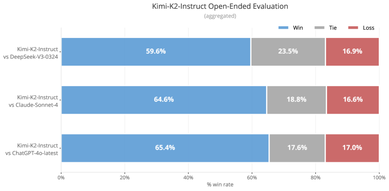
### Visual Description
## Bar Chart: Kimi-K2-Instruct Open-Ended Evaluation
### Overview
This is a horizontal bar chart comparing the win rates of Kimi-K2-Instruct against three other models: DeepSeek-V3-0324, Claude-Sonnet-4, and ChatGLM3-6b-latest. The chart displays the percentage of wins, ties, and losses for each comparison. The data appears to be aggregated.
### Components/Axes
* **Title:** Kimi-K2-Instruct Open-Ended Evaluation (aggregated) - positioned at the top-center.
* **X-axis:** "% win rate" - ranging from 0% to 100%, with tick marks at 20%, 40%, 60%, 80%, and 100%.
* **Y-axis:** Lists the comparisons:
* Kimi-K2-Instruct\_vs DeepSeek-V3-0324
* Kimi-K2-Instruct\_vs Claude-Sonnet-4
* Kimi-K2-Instruct\_vs ChatGLM3-6b-latest
* **Legend:** Located at the top-right, with three entries:
* Blue: Win
* Gray: Tie
* Red: Loss
### Detailed Analysis
The chart consists of three sets of horizontal bars, one for each comparison. Each set is divided into three segments representing Win, Tie, and Loss percentages.
**1. Kimi-K2-Instruct vs DeepSeek-V3-0324:**
* Win (Blue): Approximately 59.6% - extends to just past the 60% mark on the x-axis.
* Tie (Gray): Approximately 23.5% - extends to just past the 20% mark on the x-axis.
* Loss (Red): Approximately 16.9% - extends to just past the 15% mark on the x-axis.
**2. Kimi-K2-Instruct vs Claude-Sonnet-4:**
* Win (Blue): Approximately 64.6% - extends to just past the 65% mark on the x-axis.
* Tie (Gray): Approximately 18.8% - extends to just past the 20% mark on the x-axis.
* Loss (Red): Approximately 16.6% - extends to just past the 15% mark on the x-axis.
**3. Kimi-K2-Instruct vs ChatGLM3-6b-latest:**
* Win (Blue): Approximately 65.4% - extends to just past the 65% mark on the x-axis.
* Tie (Gray): Approximately 17.6% - extends to just past the 15% mark on the x-axis.
* Loss (Red): Approximately 17.0% - extends to just past the 15% mark on the x-axis.
### Key Observations
* Kimi-K2-Instruct consistently wins against all three models.
* The win rate is highest against ChatGLM3-6b-latest (65.4%) and Claude-Sonnet-4 (64.6%), and slightly lower against DeepSeek-V3-0324 (59.6%).
* The loss rate is relatively consistent across all three comparisons, hovering around 16-17%.
* The tie rate is lowest against Claude-Sonnet-4 (18.8%) and highest against DeepSeek-V3-0324 (23.5%).
### Interpretation
The data suggests that Kimi-K2-Instruct generally outperforms DeepSeek-V3-0324, Claude-Sonnet-4, and ChatGLM3-6b-latest in open-ended evaluation tasks. The consistent win rates across all comparisons indicate a robust advantage for Kimi-K2-Instruct. The relatively low loss rates suggest that when Kimi-K2-Instruct does not win, it rarely performs significantly worse than the other models. The variations in tie rates might indicate differences in the types of responses generated by each model – for example, DeepSeek-V3-0324 may produce more responses that are difficult to definitively categorize as wins or losses. The aggregated nature of the data obscures potential nuances in performance across different types of open-ended tasks. Further analysis, disaggregated by task type, could provide a more detailed understanding of the strengths and weaknesses of each model.
</details>
Figure 11: Chinese in-house benchmark evaluation.
Appendix D QK-Clip Does Not Impair Model Quality
The QK-Clip design follows a minimal intervention principle: it activates only when necessary, and deactivates after training stabilizes. Empirical evidence and analysis converge on its negligible impact on model quality.
Small-Scale Ablations
<details>
<summary>x16.png Details</summary>
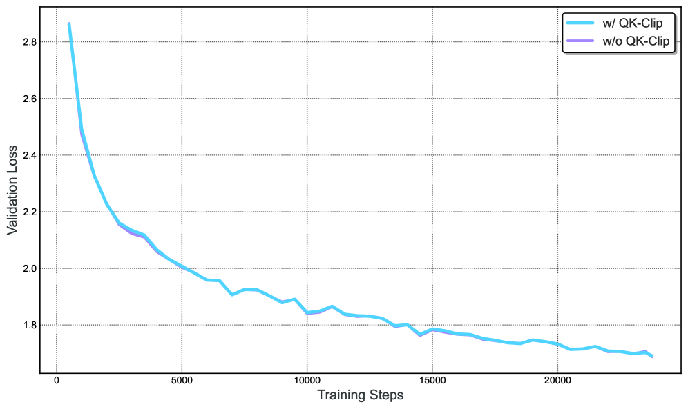
### Visual Description
\n
## Line Chart: Validation Loss vs. Training Steps
### Overview
The image presents a line chart illustrating the relationship between Validation Loss and Training Steps for two different configurations: one with "QK-Clip" and one without. The chart displays how the validation loss changes as the model undergoes training.
### Components/Axes
* **X-axis:** "Training Steps" - ranging from 0 to approximately 21,000.
* **Y-axis:** "Validation Loss" - ranging from approximately 1.7 to 2.9.
* **Legend:** Located in the top-right corner.
* "w/ QK-Clip" - represented by a light blue line.
* "w/o QK-Clip" - represented by a purple line.
* **Grid:** A light gray grid is overlaid on the chart to aid in reading values.
### Detailed Analysis
The chart contains two lines representing the validation loss over training steps.
**Line 1: w/ QK-Clip (Light Blue)**
This line demonstrates a generally decreasing trend, indicating that the validation loss decreases as training progresses.
* At Training Steps = 0, Validation Loss is approximately 2.85.
* At Training Steps = 5,000, Validation Loss is approximately 2.15.
* At Training Steps = 10,000, Validation Loss is approximately 1.9.
* At Training Steps = 15,000, Validation Loss is approximately 1.78.
* At Training Steps = 20,000, Validation Loss is approximately 1.73.
* There are some fluctuations in the line, with minor increases and decreases, but the overall trend is downward.
**Line 2: w/o QK-Clip (Purple)**
This line is almost entirely obscured by the light blue line. It appears to start at a similar validation loss as the "w/ QK-Clip" line, but it is difficult to discern its exact trajectory due to its overlap with the other line. It appears to be consistently higher than the "w/ QK-Clip" line.
* At Training Steps = 0, Validation Loss is approximately 2.8.
* At Training Steps = 5,000, Validation Loss is approximately 2.2.
* At Training Steps = 10,000, Validation Loss is approximately 2.0.
* At Training Steps = 15,000, Validation Loss is approximately 1.85.
* At Training Steps = 20,000, Validation Loss is approximately 1.8.
### Key Observations
* The "w/ QK-Clip" configuration consistently exhibits lower validation loss compared to the "w/o QK-Clip" configuration throughout the entire training process.
* Both configurations show a decreasing validation loss, suggesting that both models are learning and improving with training.
* The "w/ QK-Clip" line shows more pronounced fluctuations, potentially indicating a more sensitive or complex learning process.
### Interpretation
The data strongly suggests that incorporating "QK-Clip" into the model leads to improved performance, as evidenced by the lower validation loss. The consistent difference in validation loss between the two configurations indicates that "QK-Clip" provides a significant benefit during training. The decreasing trend for both lines demonstrates that the models are converging and learning from the training data. The fluctuations in the "w/ QK-Clip" line might suggest a more dynamic learning process, potentially requiring more careful tuning of hyperparameters. The fact that the purple line is almost entirely obscured suggests a substantial performance difference, making it difficult to analyze the "w/o QK-Clip" line in detail. This chart provides compelling evidence for the effectiveness of the "QK-Clip" technique in reducing validation loss and improving model performance.
</details>
Figure 12: Applying QK-Clip to Muon in a small-scale setting with an aggresive threshold ( $\tau$ = 30) has negligible impact on loss, indicating that it is a safe and effective method for constraining attention logits.
We train two small-scale 0.5B activated and 3B total parameters MoE models, one with vanilla Muon and the other with MuonClip using a low clipping threshold ( $\tau=30$ ). As shown in Figure 12, applying MuonClip has negligible effects on the loss curve, indicating that even aggressive clipping does not impair convergence or training dynamics with MuonClip. This demonstrates that MuonClip is a safe and effective method for bounding attention logits without degrading model performance. Furthermore, evaluation on downstream tasks reveals no statistically significant degradation in performance. These results collectively demonstrate that MuonClip is a safe and effective method for bounding attention logits without compromising model quality.
Self-deactivation
In Kimi K2, QK-Clip was only transiently active:
- Initial 70000 steps: $12.7\%$ of attention heads triggered QK-Clip for at least once, clamping $S_{\max}$ to $100$ .
- Post-70000 steps: All heads at some point reduced their $S_{\max}$ below $100$ , rendering QK-Clip inactive.
When QK-Clip is active, it is applied per-head (rather than per-layer) to minimize potential over-regularization on other heads. After training stabilizes, QK-clip is deactivated and has no effect at all.
Appendix E Why Muon is More Prone to Logit Explosion
Logit explosion occurs when the largest pre-softmax attention score
$$
S_{\max}=\max_{i,j}\bigl(q_{i}^{\vphantom{\top}}\!\cdot k_{j}\bigr) \tag{1}
$$
grows unboundedly during training. Since
$$
|q_{i}\!\cdot\!k_{j}|\leq\|q_{i}\|\|k_{j}\|\leq\|x_{i}\|\|x_{j}\|\|\mathbf{W}_{q}\|\|\mathbf{W}_{k}\|, \tag{2}
$$
and RMS-Norm keeps $\|x_{i}\|\|x_{j}\|$ bounded, the phenomenon is primarily driven by the growing spectral-norm of $\mathbf{W}_{q}$ or $\mathbf{W}_{k}$ . Empirically, we found that Muon is more susceptible to logit explosion. We give our hypothesis below.
Structural difference in updates
Muon produces a weight update coming from the $\mathrm{msign}$ operation; as a result, all singular values of the update matrix are equal — its effective rank is full. In contrast, a typical update matrix produced by Adam exhibits a skewed spectrum: a few large singular values dominate, and the effective rank is low. This low-rank assumption for Adam is not new; higher-order muP makes the same assumption.
Such phenomenon is verified on the 16 B Moonlight model, which shows weights trained with Muon exhibit higher singular-value entropy (i.e. higher effective rank) than those trained with Adam, corroborating the theoretical intuition.
SVD formulation
Let the parameter matrix at step $t-1$ have the singular value decomposition
$$
\mathbf{W}_{t-1}=\sum_{i}\sigma_{i}\,u_{i}v_{i}^{\top} \tag{3}
$$
We write the update matrices as
$$
\displaystyle\Delta\mathbf{W}_{t} \displaystyle=\sum_{j}\bar{\sigma}\,\bar{u}_{j}\bar{v}_{j}^{\top} \tag{4}
$$
The next parameter update is therefore
$$
\displaystyle\mathbf{W}_{t}\leftarrow\sum_{i}\sigma_{i}u_{i}v_{i}^{\top}+\sum_{j}\bar{\sigma}\,\bar{u}_{j}\bar{v}_{j}^{\top} \tag{5}
$$
In Muon, as both the weights and the updates have a higher effective rank than Adam, we hypothesize there is a higher probability for singular-vector pair $u_{i}v_{i}^{→p}$ to align with $\bar{u}_{j}\bar{v}_{j}^{→p}$ . This could cause the corresponding singular value of $\mathbf{W}_{t}$ to increase additively.
Attention-specific amplification
Attention logits are computed via the bilinear form
$$
q_{i}\cdot k_{j}=(x_{i}\mathbf{W}_{q})\cdot(x_{j}\mathbf{W}_{k}). \tag{6}
$$
The product $\mathbf{W}_{q}\mathbf{W}_{k}^{→p}$ squares the spectral norm, so any singular-value increase in either matrix is compounded. Muon’s tendency to enlarge singular values therefore translates into a higher risk of logit explosion.
Appendix F K2 Critic Rubrics for General RL
F.1 Core Rubrics
- Clarity and Relevance: Assesses the extent to which the response is succinct while fully addressing the user’s intent. The focus is on eliminating unnecessary detail, staying aligned with the central query, and using efficient formats such as brief paragraphs or compact lists. Unless specifically required, long itemizations should be avoided. When a choice is expected, the response should clearly offer a single, well-defined answer.
- Conversational Fluency and Engagement: Evaluates the response’s contribution to a natural, flowing dialogue that extends beyond simple question-answering. This includes maintaining coherence, showing appropriate engagement with the topic, offering relevant observations or insights, potentially guiding the conversation constructively when appropriate, using follow-up questions judiciously, handling hypothetical or personal-analogy queries gracefully, and adapting tone effectively to suit the conversational context (e.g., empathetic, formal, casual).
- Objective and Grounded Interaction: Assesses the response’s ability to maintain an objective and grounded tone, focusing squarely on the substance of the user’s request. It evaluates the avoidance of both metacommentary (analyzing the query’s structure, topic combination, perceived oddity, or the nature of the interaction itself) and unwarranted flattery or excessive praise directed at the user or their input. Excellent responses interact respectfully but neutrally, prioritizing direct, task-focused assistance over commentary on the conversational dynamics or attempts to curry favor through compliments.
F.2 Prescriptive Rubrics
- Initial Praise: Responses must not begin with compliments directed at the user or the question (e.g., “That’s a beautiful question”, “Good question!”).
- Explicit Justification: Any sentence or clause that explains why the response is good or how it successfully fulfilled the user’s request. This is different from simply describing the content.
F.3 Limitations
One potential side effect of this evaluation framework is that it may favor responses that appear confident and assertive, even in contexts involving ambiguity or subjectivity. This stems from two key constraints in the current rubric:
- Avoidance of Self-Qualification: The prescriptive rules prohibit self-assessments, explicit disclaimers, or hedging language (e.g., “this may not be accurate”, “I might be wrong”). While these phrases can reflect epistemic humility, they are often penalized as non-informative or performative.
- Preference for Clarity and Singularity: The rubric reward direct, decisive answers when users ask for a recommendation or explanation. In complex or open-ended scenarios, this may disincentivize appropriately cautious or multi-perspective responses.
As a result, the model may occasionally overstate certainty in areas where ambiguity, nuance, or epistemic modesty would be more appropriate. Future iterations of the framework may incorporate more fine-grained handling of calibrated uncertainty.
Appendix G Engine Switching Pipeline for RL Training
<details>
<summary>x17.png Details</summary>
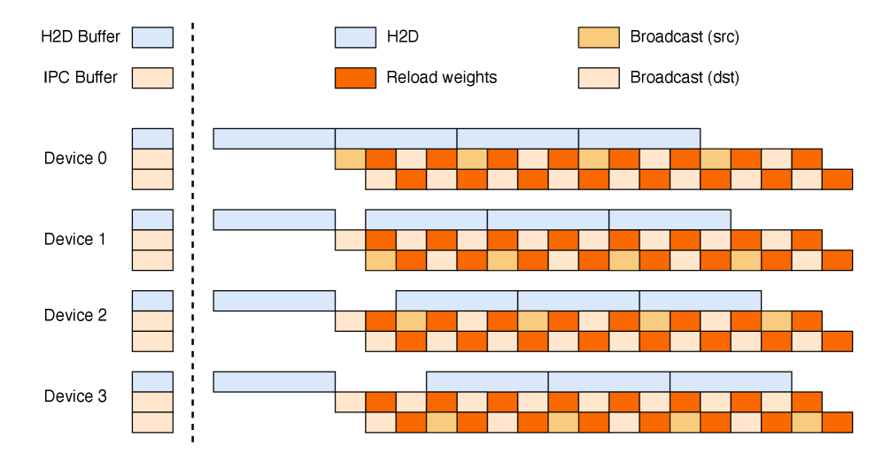
### Visual Description
\n
## Diagram: Distributed Training Data Flow
### Overview
The image depicts a diagram illustrating the data flow in a distributed training scenario, likely involving multiple devices (Device 0-3) and data transfer between a host (H2D) and devices, as well as inter-device communication. The diagram shows the sequence of operations: H2D data transfer, reloading weights, and broadcast operations (source and destination).
### Components/Axes
The diagram is structured with the following components:
* **Vertical Axis:** Represents the different devices involved in the distributed training process: Device 0, Device 1, Device 2, and Device 3. Also includes H2D Buffer and IPC Buffer.
* **Horizontal Axis:** Represents the sequence of operations or time steps.
* **Legend (Top-Right):**
* White: H2D (Host to Device)
* Yellow: Broadcast (src) - Broadcast from source
* Orange: Reload weights
* Light Yellow: Broadcast (dst) - Broadcast to destination
* **Vertical Dashed Line:** Separates the H2D Buffer and IPC Buffer from the Devices.
### Detailed Analysis
The diagram shows the following sequence of operations for each device:
* **H2D Buffer:** A white block representing data transfer from the host to the device. The length of the block is approximately the same for all devices.
* **IPC Buffer:** A white block representing data transfer from the host to the device. The length of the block is approximately the same for all devices.
* **Device 0:**
* H2D: A white block, approximately 2 units long.
* Reload weights: An orange block, approximately 1 unit long.
* Broadcast (src): A yellow block, approximately 2 units long.
* Broadcast (dst): A light yellow block, approximately 2 units long.
* **Device 1:**
* H2D: A white block, approximately 2 units long.
* Reload weights: An orange block, approximately 1 unit long.
* Broadcast (src): A yellow block, approximately 2 units long.
* Broadcast (dst): A light yellow block, approximately 2 units long.
* **Device 2:**
* H2D: A white block, approximately 2 units long.
* Reload weights: An orange block, approximately 1 unit long.
* Broadcast (src): A yellow block, approximately 2 units long.
* Broadcast (dst): A light yellow block, approximately 2 units long.
* **Device 3:**
* H2D: A white block, approximately 2 units long.
* Reload weights: An orange block, approximately 1 unit long.
* Broadcast (src): A yellow block, approximately 2 units long.
* Broadcast (dst): A light yellow block, approximately 2 units long.
The sequence of operations (H2D, Reload weights, Broadcast (src), Broadcast (dst)) is consistent across all devices. The relative lengths of the blocks representing each operation are also consistent across all devices.
### Key Observations
* The diagram illustrates a synchronous or semi-synchronous distributed training process, where all devices perform the same sequence of operations.
* The H2D transfer appears to be a necessary initial step for each device.
* The "Reload weights" operation likely refers to updating the model weights on each device.
* The "Broadcast (src)" and "Broadcast (dst)" operations suggest a communication pattern where weights or gradients are broadcast from one or more source devices to other destination devices.
* The diagram does not provide any information about the size of the data being transferred or the duration of each operation.
### Interpretation
This diagram likely represents a step in a distributed deep learning training process. The H2D transfer brings the model or data to the device. The reload weights step updates the model parameters. The broadcast operations are crucial for synchronizing the model across multiple devices, enabling parallel training. The consistent sequence of operations across all devices suggests a coordinated training process. The diagram highlights the communication overhead involved in distributed training, specifically the data transfer and broadcast operations. The diagram does not provide quantitative data, but it visually conveys the flow of data and operations in a distributed training system. The IPC buffer suggests that there is some inter-process communication happening.
</details>
(a) Theoretical perfect three-stage pipeline weight update
<details>
<summary>x18.png Details</summary>
### Visual Description
\n
## Diagram: Gantt-like Chart
### Overview
The image presents a series of four horizontal bar charts arranged vertically, resembling a simplified Gantt chart. Each chart represents a distinct process or task, visualized with three different colored segments: light blue, light orange, and a darker orange. The charts do not have explicit axis labels or numerical scales, making precise quantification difficult. The background is a uniform gray.
### Components/Axes
There are no explicit axes or scales. The diagram consists of four rows, each representing a separate entity. Each row contains a sequence of colored rectangular segments. The colors used are:
* Light Blue
* Light Orange
* Dark Orange
### Detailed Analysis or Content Details
Each row represents a different process. Let's analyze each row individually:
* **Row 1:** Starts with a light blue segment, followed by a light orange segment, then a dark orange segment, and finally a longer light orange segment.
* **Row 2:** Starts with a light blue segment, followed by a light orange segment, then a dark orange segment, and finally a longer light orange segment.
* **Row 3:** Starts with a light blue segment, followed by a light orange segment, then a dark orange segment, and finally a longer light orange segment.
* **Row 4:** Starts with a light blue segment, followed by a light orange segment, then a dark orange segment, and finally a longer light orange segment.
All four rows have the same structure: light blue, light orange, dark orange, and then a longer light orange segment. The lengths of the segments appear to be roughly consistent across all rows, although there are slight variations.
### Key Observations
The most striking observation is the uniformity across the four rows. Each row follows the same sequence of colors and a similar segment structure. There is no clear indication of time or progress, as there are no axis labels or numerical values. The diagram appears to illustrate a standardized process with three distinct phases, followed by a longer final phase.
### Interpretation
The diagram likely represents a workflow or process with four parallel instances. The consistent structure suggests that each instance follows the same steps. The light blue segment could represent an initial setup or planning phase. The light orange segment might represent a core processing phase, and the dark orange segment could represent a review or validation step. The final, longer light orange segment likely represents a completion or deployment phase.
The lack of quantitative data makes it difficult to draw definitive conclusions. However, the diagram suggests a highly standardized and repeatable process. The absence of variation between the rows implies that there are no significant bottlenecks or delays in any of the instances. It's possible this is a simplified illustration of a more complex process, focusing only on the key stages. Without additional context, it's difficult to determine the specific nature of the process or the meaning of the different color segments.
</details>
(b) A PCIE bounded three-stage pipeline
<details>
<summary>x19.png Details</summary>
### Visual Description
\n
## Diagram: Rectangular Block Arrangement
### Overview
The image presents a grid of four rows and two columns, each cell containing a series of colored rectangles. Each row begins with a light blue horizontal rectangle, followed by a sequence of smaller rectangles colored in shades of orange, yellow, and light pink. The arrangement appears to be a visual representation of some kind of data, potentially a timeline or a comparative analysis. There are no axis labels or explicit numerical values.
### Components/Axes
The diagram consists of:
* **Light Blue Rectangles:** Positioned at the beginning of each row, acting as a potential starting point or category label.
* **Orange Rectangles:** The most prominent color, appearing in varying quantities in each row.
* **Yellow Rectangles:** Present in each row, but in fewer numbers than the orange rectangles.
* **Light Pink Rectangles:** Appear in each row, but in fewer numbers than the orange and yellow rectangles.
* **Grid Structure:** Four rows and two columns, creating a structured layout.
### Detailed Analysis or Content Details
Let's analyze each row individually:
* **Row 1:** Starts with a light blue rectangle. Followed by one yellow, two orange, one light pink, and two orange rectangles.
* **Row 2:** Starts with a light blue rectangle. Followed by one yellow, two orange, one light pink, and two orange rectangles.
* **Row 3:** Starts with a light blue rectangle. Followed by one yellow, two orange, one light pink, and two orange rectangles.
* **Row 4:** Starts with a light blue rectangle. Followed by one yellow, two orange, one light pink, and two orange rectangles.
Each row has the same pattern of colored rectangles: 1 yellow, 2 orange, 1 light pink, 2 orange.
### Key Observations
* **Consistency:** All four rows exhibit the exact same sequence of colored rectangles.
* **Dominance of Orange:** The orange rectangles are the most frequent in each row.
* **Lack of Variation:** There is no variation in the pattern across the rows.
### Interpretation
The diagram likely represents a consistent process or state across four different categories or instances. The light blue rectangles could represent the categories themselves, while the sequence of colored rectangles represents the steps or components within each category. The consistent pattern suggests that the process or state is uniform across all four categories. The dominance of orange rectangles might indicate that a particular component or step is the most significant or frequent.
Without additional context, it's difficult to determine the specific meaning of the colors or the overall purpose of the diagram. It could represent anything from a workflow to a resource allocation scheme. The lack of labels or numerical data limits the depth of interpretation. It is a visual representation of a repetitive pattern, but the underlying meaning remains ambiguous.
</details>
(c) Fixed two-stage pipeline
Figure 13: pipeline for RL weight update
The checkpoint engine manages three equal-size device buffers on each GPU: an H2D buffer for loading the offloaded model parameters, and two IPC buffers for GPU-to-GPU broadcast. The IPC buffers are shared to inference engines, allowing it to directly access the same physical memory. These three buffers allow us to arrange the three steps in a pipeline.
Theoretical three-stage pipeline.
As illustrated in Figure 13(a), a three-stage pipeline is introduced. (1) H2D: a shard of the latest weights is copied into the H2D buffer asynchronously. (2) Broadcast: Once the copy completes, the shard will be copied to one IPC buffers and broadcast to all devices. (3) Reload: Inference engines simultaneously load parameters from the other IPC buffer.
Two-stage pipeline due to PCIe saturation.
On NVIDIA H800 clusters, concurrent H2D and broadcast saturate the shared PCIe fabric, collapsing the three stages into a sequential procedure (Figure 13(b)). We therefore adopt a simpler, two-stage scheme (Figure 13(c)): (1) All devices perform a single, synchronous H2D transfer. (2) The broadcast and reload proceed in parallel.
The two-stage pipeline will be bound by multiple synchronous H2D copy operations. But in large scale devices, model will be split into small shards, the entire parameter set fits into the H2D buffer in one transfer, the overhead will disappear.
By overlapping H2D, Broadcast, and Reload weights, we can obtain a high bandwidth to reshard the weights from train engines to all inference engines.