# Is Chain-of-Thought Reasoning of LLMs a Mirage? A Data Distribution Lens
**Authors**: Chengshuai Zhao, Zhen Tan, Pingchuan Ma, Dawei Li, Bohan Jiang, Yancheng Wang, Yingzhen Yang, Huan Liu
> Arizona State University
redacted {czhao93, ztan36, pingchua, daweili5, bjiang14, yancheng.wang, yingzhen.yang, huanliu}@asu.edu
## Abstract
Chain-of-Thought (CoT) prompting has been shown to improve Large Language Model (LLM) performance on various tasks. With this approach, LLMs appear to produce human-like reasoning steps before providing answers (a.k.a., CoT reasoning), which often leads to the perception that they engage in deliberate inferential processes. However, some initial findings suggest that CoT reasoning may be more superficial than it appears, motivating us to explore further. In this paper, we study CoT reasoning via a data distribution lens and investigate if CoT reasoning reflects a structured inductive bias learned from in-distribution data, allowing the model to conditionally generate reasoning paths that approximate those seen during training. Thus, its effectiveness is fundamentally bounded by the degree of distribution discrepancy between the training data and the test queries. With this lens, we dissect CoT reasoning via three dimensions: task, length, and format. To investigate each dimension, we design DataAlchemy, an isolated and controlled environment to train LLMs from scratch and systematically probe them under various distribution conditions. Our results reveal that CoT reasoning is a brittle mirage that vanishes when it is pushed beyond training distributions. This work offers a deeper understanding of why and when CoT reasoning fails, emphasizing the ongoing challenge of achieving genuine and generalizable reasoning. Our code is available at GitHub: https://github.com/ChengshuaiZhao0/DataAlchemy.
## 1 Introduction
Recent years have witnessed Large Language Models’ (LLMs) dominant role in various domains (Zhao et al., 2023; Li et al., 2025b; Zhao et al., 2025; Ting et al., 2025) through versatile prompting techniques (Wei et al., 2022; Yao et al., 2023; Kojima et al., 2022). Among these, Chain-of-Thought (CoT) prompting (Wei et al., 2022) has emerged as a prominent method for eliciting structured reasoning from LLMs (a.k.a., CoT reasoning). By appending a simple cue such as “Let’s think step by step,” LLMs decompose complex problems into intermediate steps, producing outputs that resemble human-like reasoning. It has been shown to be effective in tasks requiring logical inference Xu et al. (2024), mathematical problem solving (Imani et al., 2023), and commonsense reasoning (Wei et al., 2022). The empirical successes of CoT reasoning lead to the perception that LLMs engage in deliberate inferential processes (Yu et al., 2023; Zhang et al., 2024a; Ling et al., 2023; Zhang et al., 2024c).
However, a closer examination reveals inconsistencies that challenge this optimistic view. Consider this straightforward question: “The day the US was established is in a leap year or a normal year?” When prompted with the CoT prefix, the modern LLM Gemini responded: “The United States was established in 1776. 1776 is divisible by 4, but it’s not a century year, so it’s a leap year. Therefore, the day the US was established was in a normal year.” This response exemplifies a concerning pattern: the model correctly recites the leap year rule and articulates intermediate reasoning steps, yet produces a logically inconsistent conclusion (i.e., asserting 1776 is both a leap year and a normal year). Such inconsistencies suggest that there is a distinction between human-like inference and CoT reasoning.
An expanding body of analyses reveals that LLMs tend to rely on surface-level semantics and clues rather than logical procedures (Bentham et al., 2024; Chen et al., 2025b; Lanham et al., 2023). LLMs construct superficial chains of logic based on learned token associations, often failing on tasks that deviate from commonsense heuristics or familiar templates (Tang et al., 2023). In the reasoning process, performance degrades sharply when irrelevant clauses are introduced, which indicates that models cannot grasp the underlying logic (Mirzadeh et al., 2024). This fragility becomes even more apparent when models are tested on more complex tasks, where they frequently produce incoherent solutions and fail to follow consistent reasoning paths (Shojaee et al., 2025). Collectively, these pioneering works deepen the skepticism surrounding the true nature of CoT reasoning.
In light of this line of research, we question the CoT reasoning by proposing an alternative lens through data distribution and further investigating why and when it fails. We hypothesize that CoT reasoning reflects a structured inductive bias learned from in-distribution data, allowing the model to conditionally generate reasoning paths that approximate those seen during training. As such, its effectiveness is inherently limited by the nature and extent of the distribution discrepancy between training data and the test queries. Guided by this data distribution lens, we dissect CoT reasoning via three dimensions: (i) task —To what extent CoT reasoning can handle tasks that involve transformations or previously unseen task structures. (2) length —how CoT reasoning generalizes to chains with length different from that of training data; and (3) format —how sensitive CoT reasoning is to surface-level query form variations. To evaluate each aspect, we introduce DataAlchemy, a controlled and isolated experiment that allows us to train LLMs from scratch and systematically probe them under various distribution shifts.
Our findings reveal that CoT reasoning works effectively when applied to in-distribution or near in-distribution data but becomes fragile and prone to failure even under moderate distribution shifts. In some cases, LLMs generate fluent yet logically inconsistent reasoning steps. The results suggest that what appears to be structured reasoning can be a mirage, emerging from memorized or interpolated patterns in the training data rather than logical inference. These insights carry important implications for both practitioners and researchers. For practitioners, our results highlight the risk of relying on CoT as a plug-and-play solution for reasoning tasks and caution against equating CoT-style output with human thinking. For researchers, the results underscore the ongoing challenge of achieving reasoning that is both faithful and generalizable, motivating the need to develop models that can move beyond surface-level pattern recognition to exhibit deeper inferential competence. Our contributions are summarized as follows:
- Novel perspective. We propose a data distribution lens for CoT reasoning, illuminating that its effectiveness stems from structured inductive biases learned from in-distribution training data. This framework provides a principled lens for understanding why and when CoT reasoning succeeds or fails.
- Controlled environment. We introduce DataAlchemy, an isolated experimental framework that enables training LLMs from scratch and systematically probing CoT reasoning. This controlled setting allows us to isolate and analyze the effects of distribution shifts on CoT reasoning without interference from complex patterns learned during large-scale pre-training.
- Empirical validation. We conduct systematic empirical validation across three critical dimensions— task, length, and format. Our experiments demonstrate that CoT reasoning exhibits sharp performance degradation under distribution shifts, revealing that seemingly coherent reasoning masks shallow pattern replication.
- Real-world implication. This work reframes the understanding of contemporary LLMs’ reasoning capabilities and emphasizes the risk of over-reliance on COT reasoning as a universal problem-solving paradigm. It underscores the necessity for proper evaluation methods and the development of LLMs that possess authentic and generalizable reasoning capabilities.
## 2 Related Work
### 2.1 LLM Prompting and Co
Chain-of-Thought (CoT) prompting revolutionized how we elicit reasoning from Large Language Models by decomposing complex problems into intermediate steps (Wei et al., 2022). By augmenting few-shot exemplars with reasoning chains, CoT showed substantial performance gains on various tasks (Xu et al., 2024; Imani et al., 2023; Wei et al., 2022). Building on this, several variants emerged. Zero-shot CoT triggers reasoning without exemplars using instructional prompts (Kojima et al., 2022), and self-consistency enhances performance via majority voting over sampled chains (Wang et al., 2023). To reduce manual effort, Auto-CoT generates CoT exemplars using the models themselves (Zhang et al., 2023). Beyond linear chains, Tree-of-Thought (ToT) frames CoT as a tree search over partial reasoning paths (Yao et al., 2023), enabling lookahead and backtracking. SymbCoT combines symbolic reasoning with CoT by converting problems into formal representations (Xu et al., 2024). Recent work increasingly integrates CoT into the LLM inference process, generating long-form CoTs (Jaech et al., 2024; Team, 2024; Guo et al., 2025; Team et al., 2025). This enables flexible strategies like mistake correction, step decomposition, reflection, and alternative reasoning paths (Yeo et al., 2025; Chen et al., 2025a). The success of prompting techniques and long-form CoTs has led many to view them as evidence of emergent, human-like reasoning in LLMs. In this work, we challenge that viewpoint by adopting a data-centric perspective and demonstrating that CoT behavior arises largely from pattern matching over training distributions.
### 2.2 Discussion on Illusion of LLM Reasoning
While Chain-of-Thought prompting has led to impressive gains on complex reasoning tasks, a growing body of work has started questioning the nature of these improvements. One major line of research highlights the fragility of CoT reasoning. Minor and semantically irrelevant perturbations such as distractor phrases or altered symbolic forms can cause significant performance drops in state-of-the-art models (Mirzadeh et al., 2024; Tang et al., 2023). Models often incorporate such irrelevant details into their reasoning, revealing a lack of sensitivity to salient information. Other studies show that models prioritize the surface form of reasoning over logical soundness; in some cases, longer but flawed reasoning paths yield better final answers than shorter, correct ones (Bentham et al., 2024). Similarly, performance does not scale with problem complexity as expected—models may overthink easy problems and give up on harder ones (Shojaee et al., 2025). Another critical concern is the faithfulness of the reasoning process. Intervention-based studies reveal that final answers often remain unchanged even when intermediate steps are falsified or omitted (Lanham et al., 2023), a phenomenon dubbed the illusion of transparency (Bentham et al., 2024; Chen et al., 2025b). Together, these findings suggest that LLMs are not principled reasoners but rather sophisticated simulators of reasoning-like text. However, a systematic understanding of why and when CoT reasoning fails is still a mystery.
### 2.3 OOD Generalization of LLMs
Out-of-distribution (OOD) generalization, where test inputs differ from training data, remains a key challenge in machine learning, particularly for large language models (LLMs) Yang et al. (2024, 2023); Budnikov et al. (2025); Zhang et al. (2024b). Recent studies show that LLMs prompted to learn novel functions often revert to similar functions encountered during pretraining (Wang et al., 2024; Garg et al., 2022). Likewise, LLM generalization frequently depends on mapping new problems onto familiar compositional structures (Song et al., 2025). CoT prompting improves OOD generalization (Wei et al., 2022), with early work demonstrating length generalization for multi-step problems beyond training distributions (Yao et al., 2025; Shen et al., 2025). However, this ability is not inherent to CoT and heavily depends on model architecture and training setups. For instance, strong generalization in arithmetic tasks was achieved only when algorithmic structures were encoded into positional encodings (Cho et al., 2024). Similarly, finer-grained CoT demonstrations during training boost OOD performance, highlighting the importance of data granularity (Wang et al., 2025a). Theoretical and empirical evidence shows that CoT generalizes well only when test inputs share latent structures with training data; otherwise, performance declines sharply (Wang et al., 2025b; Li et al., 2025a). Despite its promise, CoT still struggles with genuinely novel tasks or formats. In the light of these brilliant findings, we propose rethinking CoT reasoning through a data distribution lens: decomposing CoT into task, length, and format generalization, and systematically investigating each in a controlled setting.
<details>
<summary>x1.png Details</summary>
### Visual Description
## Diagram: Conceptual Framework for Generalization in Sequence Transformation
### Overview
The image presents a structured conceptual framework for evaluating the generalization capabilities of a system (likely an AI model or algorithmic processor) regarding sequence transformation tasks. It defines foundational "atoms" and transformation functions, then categorizes generalization into three distinct domains: **Task Generalization**, **Length Generalization**, and **Format Generalization**. The diagram utilizes a color-coded legend to distinguish between input/output data and training/testing sets.
### Components/Axes
**Legend (Top Right):**
* **Red Circle:** Input
* **Blue Circle:** Output
* **Solid Red Box:** Training
* **Dashed Red Box:** Testing
**Foundational Elements (Left Column):**
* **Basic atoms A:** A grid containing the alphabet from A to Z.
* **Element l = 5:** A sequence of 5 boxes containing the letters "A P P L E".
* **$f1$: ROT Transformation:** A transformation function denoted by a double-check icon. It applies a "+13" shift to the input "A P P L E" (red), resulting in "N C C Y R" (blue).
* **$f2$: Cyclic Shift:** A transformation function denoted by a circular arrow icon. It applies a "+1" shift to the input "A P P L E" (red), resulting in "E A P P L" (blue).
### Detailed Analysis
#### 1. Task Generalization (Top Right)
This section evaluates how the system handles different types of task distributions.
**Element Table:**
| Category | Input | Output |
| :--- | :--- | :--- |
| **ID (In-Distribution)** | "A B C D" (solid red) | "A B C D" (solid red) |
| **Comp (Compositional)** | "A B C D" (solid red) | "D C B A" (dashed red) |
| **OOD (Out-of-Distribution)** | "A B C D" (solid red) | "A B C E" (dashed red) |
**Transformation Table:**
| Category | Transformation Logic |
| :--- | :--- |
| **ID** | $f1 \circ f1 \rightarrow f1 \circ f1$ |
| **Comp** | $\{f1 \circ f1 \circ f2, f2 \circ f2\} \rightarrow f2 \circ f2$ |
| **POOD** | $f1 \circ f1 \rightarrow f1 \circ f2$ |
| **OOD** | $f1 \circ f1 \rightarrow f2 \circ f2$ |
* **Visual Flow:** A set of red boxes (Training) is processed via $f_{comp}$ to produce blue boxes (Output).
#### 2. Length Generalization (Bottom Center)
This section evaluates the system's ability to handle sequences of varying lengths.
* **Text Length:**
* Input "A B C D" (solid red) is the base.
* Testing inputs include "A B C" (dashed red) and "A B C D A" (dashed red).
* **Reasoning Step:**
* $f1 \circ f1 \rightarrow f1$
* $f1 \circ f1 \rightarrow f1 \circ f1 \circ f1$
* **Visual Flow:** Red boxes (Training) are processed via $f_s$ to produce blue boxes (Output).
#### 3. Format Generalization (Bottom Right)
This section evaluates robustness against structural changes in the input.
* **Insertion:** Input "A B C D" (solid red) vs. Testing "A B ? C D" (dashed red).
* **Deletion:** Input "A B C D" (solid red) vs. Testing "A C D" (dashed red).
* **Modify:** Input "A B C D" (solid red) vs. Testing "A B C ?" (dashed red).
* **Visual Flow:** Red boxes (Training) are processed via $f_s$ to produce blue boxes (Output).
### Key Observations
* **Training vs. Testing:** The diagram consistently uses solid red boxes for training data and dashed red boxes for testing data, indicating a clear separation between seen and unseen scenarios.
* **Compositionality:** The "Task Generalization" section explicitly uses mathematical notation ($f1 \circ f1$) to represent the composition of functions, suggesting the system is being tested on its ability to combine learned operations.
* **OOD/POOD:** The inclusion of "POOD" (Presumably "Partial Out-of-Distribution") and "OOD" indicates a focus on systematic generalization—testing if the model can perform tasks that are structurally different from the training set.
### Interpretation
This diagram outlines a rigorous testing protocol for symbolic reasoning or sequence-to-sequence models.
* **Systematic Generalization:** The core intent is to determine if a model has learned the *underlying logic* (the functions $f1$ and $f2$) or if it has merely memorized specific input-output pairs. By testing on "Compositional" and "OOD" tasks, the framework probes whether the model can recombine known functions in novel ways.
* **Robustness:** The "Format Generalization" section is a stress test for input noise. It checks if the model's internal representation of the sequence is flexible enough to handle missing, inserted, or corrupted characters (the "?" symbol).
* **Peircean Investigative Perspective:** The diagram functions as a taxonomy of failure modes. By isolating Task, Length, and Format, the researchers can pinpoint exactly *where* a model fails. For example, if a model succeeds at "Task Generalization" but fails at "Length Generalization," it suggests the model has learned the logic but is overfitted to specific sequence lengths (a common issue in positional encoding in Transformers).
</details>
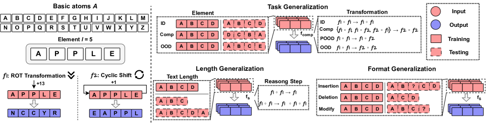
Figure 1: Framework of DataAlchemy. It creates an isolated and controlled environment to train LLMs from scratch and probe the task, length, and format generalization.
## 3 The Data Distribution Lens
We propose a fundamental reframing to understand what CoT actually represents. We hypothesize that the underlying mechanism is better understood through the lens of data distribution: rather than executing explicit reasoning procedures, CoT operates as a pattern-matching process that interpolates and extrapolates from the statistical regularities present in its training distribution. Specifically, we posit that CoT’s success stems not from a model’s inherent reasoning capacity, but from its ability to generalize conditionally to out-of-distribution (OOD) test cases that are structurally similar to in-distribution exemplars.
To formalize this view, we model CoT prompting as a conditional generation process constrained by the distributional properties of the training data. Let $D_train$ denote the training distribution over input-output pairs $(x,y)$ , where $x$ represents a reasoning problem and $y$ denotes the solution sequence (including intermediate reasoning steps). The model learns an approximation $f_θ(x)≈ y$ by minimizing empirical risk over samples drawn from $D_train$ .
Let the expected training risk be defined as:
$$
R_train(f_θ)=E_(x,y)∼D_train[\ell(f_θ(x),y)], \tag{1}
$$
where $\ell$ is a task-specific loss function (e.g., cross-entropy, token-level accuracy). At inference time, given a test input $a_test$ sampled from a potentially different distribution $D_test$ , the model generates a response $y_test$ conditioned on patterns learned from $D_train$ . The corresponding expected test risk is:
$$
R_test(f_θ)=E_(x,y)∼D_test[\ell(f_θ(x),y)]. \tag{2}
$$
The degree to which the model generalizes from $D_train$ to $D_test$ is governed by the distributional discrepancy between the two, which we quantify using divergence measures:
**Definition 3.1 (Distributional Discrepancy)**
*Given training distribution $D_train$ and test distribution $D_test$ , the distributional discrepancy is defined as:
$$
Δ(D_train,D_test)=H(D_train\parallelD_test) \tag{3}
$$
where $H(·\parallel·)$ is a divergence measure (e.g., KL divergence, Wasserstein distance) that quantifies the statistical distance between the two distributions.*
**Theorem 3.1 (CoT Generalization Bound)**
*Let $f_θ$ denote a model trained on $D_train$ with expected training risk $R_train(f_θ)$ . For a test distribution $D_test$ , the expected test risk $R_test(f_θ)$ is bounded by:
$$
R_test(f_θ)≤ R_train(f_θ)+Λ·Δ(D_train,D_test)+O≤ft(√{\frac{\log(1/δ)}{n}}\right) \tag{4}
$$
where $Λ>0$ is a Lipschitz constant that depends on the model architecture and task complexity, $n$ is the training sample size, and the bound holds with probability $1-δ$ , where $δ$ is the failure propability.*
The proof is provided in Appendix A.1
Building on this data distribution perspective, we identify three critical dimensions along which distributional shifts can occur, each revealing different aspects of CoT’s pattern-matching nature: ➊ Task generalization examines how well CoT transfers across different types of reasoning tasks. Novel tasks may have unique elements and underlying logical structure, which introduces distributional shifts that challenge the model’s ability to apply learned reasoning patterns. ➋ Length generalization investigates CoT’s robustness to reasoning chains of varying lengths. Since training data typically contains reasoning sequences within a certain length range, test cases requiring substantially longer or shorter reasoning chains represent a form of distributional shift along the sequence length dimension. This length discrepancy could result from the reasoning step or the text-dependent solution space. ➌ Format generalization explores how sensitive CoT is to variations in prompt formulation and structure. Due to various reasons (e.g., sophistical training data or diverse background of users), it is challenging for LLM practitioners to design a golden prompt to elicit knowledge suitable for the current case. Their detailed definition and implementation are given in subsequent sections.
Each dimension provides a unique lens for understanding the boundaries of CoT’s effectiveness and the mechanisms underlying its apparent reasoning capabilities. By systematically varying these dimensions in controlled experimental settings, we can empirically validate our hypothesis that CoT performance degrades predictably as distributional discrepancy increases, thereby revealing its fundamental nature as a pattern-matching rather than reasoning system.
## 4 DataAlchemy: An Isolated and Controlled Environment
To systematically investigate the influence of distributional shifts on CoT reasoning capabilities, we introduce DataAlchemy, a synthetic dataset framework designed for controlled experimentation. This environment enables us to train language models from scratch under precisely defined conditions, allowing for rigorous analysis of CoT behavior across different OOD scenarios. The overview is shown in Figure 1.
### 4.1 Basic Atoms and Elements
Let $A=\{\texttt{A},\texttt{B},\texttt{C},…,\texttt{Z}\}$ denote the alphabet of 26 basic atoms. An element $e$ is defined as an ordered sequence of atoms:
$$
e=(a_0,a_1,…,a_l-1) where a_i∈A, l∈ℤ^+ \tag{5}
$$
This design provides a versatile manipulation for the size of the dataset $D$ (i.e., $|D|=|A|^l$ ) by varying element length $l$ to train language models with various capacities. Meanwhile, it also allows us to systematically probe text length generalization capabilities.
### 4.2 Transformations
A transformation is an operation that operates on elements $F:e→\hat{e}$ . In this work, we consider two fundamental transformations: the ROT Transformation and the Cyclic Position Shift. To formally define the transformations, we introduce a bijective mapping $φ:A→ℤ_26$ , where $ℤ_26=\{0,1,…,25\}$ , such that $φ(c)$ maps a character to its zero-based alphabetical index.
**Definition 4.1 (ROT Transformation)**
*Given an element $e=(a_0,\ …,a_l-1)$ and a rotation parameter $n∈ℤ$ , the ROT Transformation $f_rot$ produces an element $\hat{e}=(\hat{a}_0,…,\hat{a}_l-1)$ . Each atom $\hat{a}_i$ is:
$$
\hat{a}_i=φ^-1((φ(a_i)+n)±od{26}) \tag{6}
$$
This operation cyclically shifts each atom $n$ positions forward in alphabetical order. For example, if $e=(\texttt{A},\texttt{P},\texttt{P},\texttt{L},\texttt{E})$ and $n=13$ , then $f_rot(e,13)=(\texttt{N},\texttt{C},\texttt{C},\texttt{Y},\texttt{R})$ .*
**Definition 4.2 (Cyclic Position Shift)**
*Given an element $e=(a_0,\ …,a_l-1)$ and a shift parameter $n∈ℤ$ , the Cyclic Position Shift $f_pos$ produces an element $\hat{e}=(\hat{a}_0,…,\hat{a}_l-1)$ . Each atom $\hat{a}_i$ is defined by a cyclic shift of indices:
$$
\hat{a}_i=a_(i-n)±od{l} \tag{7}
$$
This transformation cyclically shifts the positions of the atoms within the sequence by $n$ positions to the right. For instance, if $e=(\texttt{A},\texttt{P},\texttt{P},\texttt{L},\texttt{E})$ and $n=1$ , then $f_pos(e,1)=(\texttt{E},\texttt{A},\texttt{P},\texttt{P},\texttt{L})$ .*
**Definition 4.3 (Generalized Compositional Transformation)**
*To model multi-step reasoning, we define a compositional transformation as the successive application of a sequence of operations. Let $S=(f_1,f_2,…,f_k)$ be a sequence of operations, where each $f_i$ is one of the fundamental transformations $F=\{f_rot,f_pos\}$ with its respective parameters. The compositional transformation $f_S$ for the sequence $S$ is the function composition:
$$
f_S=f_k∘ f_k∘⋯∘ f_1 \tag{8}
$$
The resulting element $\hat{e}$ is obtained by applying the operations sequentially to an initial element $e$ :
$$
\hat{e}=f_k(f_k-1(…(f_1(e))…)) \tag{9}
$$*
This design enables the construction of arbitrarily complex transformation chains by varying the type, parameters, order, and length of operations within the sequence. At the sample time, we can naturally acquire the COT reasoning step by decomposing the intermediate process:
$$
\underbrace{f_S(e):}_Query \underbrace{e\xrightarrow{f_1}e^(1)\xrightarrow{f_2}e^(2)⋯\xrightarrow{f_k-1}e^(k-1)\xrightarrow{f_k}}_COT reasoning steps\underbrace{\boxed{\hat{e}}}_Answer \tag{1}
$$
### 4.3 Environment Setting
Through systematic manipulation of elements and transformations, DataAlchemy offers a flexible and controllable framework for training LLMs from scratch, facilitating rigorous investigation of diverse OOD scenarios. Without specification, we employ a decoder-only language model GPT-2 (Radford et al., 2019) with a configuration of 4 layers, 32 hidden dimensions, and 4 attention heads. We utilize a Byte-Pair Encoding (BPE) tokenizer. Both LLMs and the tokenizer follow the general modern LLM pipeline. During the inference time, we set the temperature to 1e-5. For rigor, we also study LLMs with various parameters, architectures, and temperatures in Section 8. Details of the implementation are provided in the Appendix B. We consider that each element consists of 4 basic atoms, which produces 456,976 samples for each dataset with varied transformations and token amounts. We initialize the two transformations $f_1=f_rot(e,13)$ and $f_2=f_pos(e,1)$ . We consider the exact match rate, Levenshtein distance (i.e., edit distance) (Yujian and Bo, 2007), and BLEU score (Papineni et al., 2002) as metrics and evaluate the produced reasoning step, answer, and full chain. Examples of the datasets and evaluations are shown in Appendix C
## 5 Task Generalization
Task generalization represents a fundamental challenge for CoT reasoning, as it directly tests a model’s ability to apply learned concepts and reasoning patterns to unseen scenarios. In our controlled experiments, both transformation and elements could be novel. Following this, we decompose task generalization into two primary dimensions: element generalization and transformation generalization.
Task Generalization Complexity. Guided by the data distribution lens, we first introduce a measure for generalization difficulty:
**Proposition 5.1 (Task Generalization Complexity)**
*For a reasoning chain $f_S$ operating on elements $e=(a_0,…,a_l-1)$ , define:
$$
\displaystyle(C)= \displaystyleα∑_i=1^mI≤ft[a_i∉E^i_train \right]+β∑_j=1^nI≤ft[f_j∉F_train \right]+γI≤ft[≤ft(f_1,f_2,…,f_k\right)∉P_train \right]+C_T \tag{11}
$$
as a measurement of task discrepancy $Δ_task$ , where $α,β,γ$ are weighting parameters for different novelty types and $C_T$ is task specific constant. $E^i_train ,F_train ,$ and $P_train$ denote the bit-wise element set, relation set and the order of relation set used during training.*
We establish a critical threshold beyond which CoT reasoning fails exponentially:
**Theorem 5.1 (Task Generalization Failure Threshold)**
*There exists a threshold $τ$ such that when $TGC(C)>τ$ , the probability of correct CoT reasoning drops exponentially:
$$
P(correct|C)≤ e^-δ(TGC(C)-τ) \tag{12}
$$*
The proof is provided in Appendix A.2.
### 5.1 Transformation Generalization
Transformation generalization evaluates the ability of CoT reasoning to effectively transfer when models encounter novel transformations during testing, which is an especially prevalent scenario in real-world applications.
<details>
<summary>x2.png Details</summary>
### Visual Description
## Scatter Plot: BLEU Score vs. Edit Distance
### Overview
This image is a scatter plot visualizing the relationship between "Edit Distance" (x-axis) and "BLEU Score" (y-axis). The individual data points are colored according to a "Distribution Shift" scale, ranging from blue (low shift) to red (high shift). The plot illustrates an inverse correlation between the similarity of the generated text to the reference (Edit Distance) and the quality of the output (BLEU Score), while also highlighting how these metrics correlate with distribution shifts.
### Components/Axes
* **X-Axis:** Labeled "Edit Distance". The scale ranges from 0.00 to 0.30, with grid lines marked at 0.05 intervals.
* **Y-Axis:** Labeled "BLEU Score". The scale ranges from 0.2 to 1.0, with grid lines marked at 0.1 intervals.
* **Legend (Color Bar):** Located on the right side of the chart, labeled "Distribution Shift".
* **Blue:** Represents low distribution shift (approx. 0.1).
* **Red:** Represents high distribution shift (approx. 0.9).
* **Purple/Pink:** Represents intermediate values.
### Detailed Analysis
The data points are distributed into two distinct regions:
1. **The "High-Performance" Cluster (Top-Left):**
* **Position:** Located at the top-left corner of the chart.
* **Values:** Edit Distance is approximately 0.00 to 0.02; BLEU Score is approximately 1.0.
* **Color:** These points are blue, indicating a very low "Distribution Shift."
* **Trend:** This represents the ideal scenario where the generated text is nearly identical to the reference.
2. **The "Degraded-Performance" Cloud (Middle-Right):**
* **Position:** Spans the center to the bottom-right of the chart.
* **Values:** Edit Distance ranges from approximately 0.10 to 0.33; BLEU Score ranges from approximately 0.2 to 0.7.
* **Color:** These points transition from purple to red, indicating a moderate to high "Distribution Shift."
* **Trend:** As the Edit Distance increases (moving right), the BLEU Score generally decreases (moving down), and the Distribution Shift increases (shifting from purple to red).
3. **Notable Data Points:**
* **Highest Edit Distance:** A single point at approximately 0.33 Edit Distance and 0.2 BLEU Score. It is colored bright red, indicating the highest level of Distribution Shift in the dataset.
* **Highest BLEU in the dispersed cloud:** A point at approximately 0.15 Edit Distance and 0.7 BLEU Score, colored light purple.
### Key Observations
* **Inverse Correlation:** There is a clear negative correlation between Edit Distance and BLEU Score. As the Edit Distance increases, the BLEU Score drops.
* **Distribution Shift Correlation:** There is a strong positive correlation between "Distribution Shift" and "Edit Distance." Higher Edit Distance values are consistently associated with higher Distribution Shift values (redder colors).
* **Bifurcation:** The data is not a continuous gradient but rather bifurcated into a high-quality cluster (blue) and a lower-quality, higher-shift cloud (purple/red). This suggests a potential threshold where model performance degrades significantly.
### Interpretation
This chart likely represents the evaluation of a Natural Language Processing (NLP) model, such as a machine translation or text generation system.
* **What the data demonstrates:** The "Distribution Shift" acts as a proxy for how "out-of-distribution" the input data is compared to the model's training data. The plot demonstrates that when the model encounters data with a higher distribution shift, it produces outputs that are further from the reference (higher Edit Distance) and of lower quality (lower BLEU Score).
* **Why it matters:** This visualization is critical for diagnosing model robustness. It shows that the model is highly sensitive to distribution shifts. The distinct separation between the blue cluster and the red/purple cloud suggests that the model maintains high performance until a certain point, after which performance degrades rapidly as the distribution shift increases.
* **Reading between the lines:** The lack of data points in the "Top-Right" (High Edit Distance, High BLEU) and "Bottom-Left" (Low Edit Distance, Low BLEU) quadrants confirms that the metrics are logically consistent: you cannot have a high BLEU score (high similarity) with a high Edit Distance (high dissimilarity), nor a low BLEU score with a low Edit Distance. The "Distribution Shift" is the primary driver of the variance in performance.
</details>
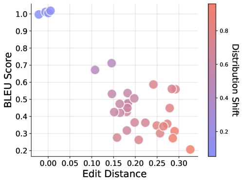
Figure 2: Performance of CoT reasoning on transformation generalization. Efficacy of CoT reasoning declines as the degree of distributional discrepancy increases.
Experimental Setup. To systematically evaluate the impact of transformations, we conduct experiments by varying transformations between training and testing sets while keeping other factors constant (e.g., elements, length, and format). Guided by the intuition formalized in Proposition 5.1, we define four incremental levels of distribution shift in transformations as shown in Figure 1: (i) In-Distribution (ID): The transformations in the test set are identical to those observed during training, e.g., $f_1∘ f_1→ f_1∘ f_1$ . (ii) Composition (CMP): Test samples comprise novel compositions of previously encountered transformations, though each individual transformation remains familiar, e.g., ${f_1∘ f_1,f_1∘ f_2,f_2∘ f_1}→ f_2∘ f_2$ . (iii) Partial Out-of-Distribution (POOD): Test data include compositions involving at least one novel transformation not seen during training, e.g., $f_1∘ f_1→ f_1∘ f_2$ . (iv) Out-of-Distribution (OOD): The test set contains entirely novel transformation types that are unseen in training, e.g., $f_1∘ f_1→ f_2∘ f_2$ .
Table 1: Full chain evaluation under different scenarios for transformation generalization.
| $f_1∘ f_1→ f_1∘ f_1$ $\{f_2∘ f_2,f_1∘ f_2,f_2∘ f_1\}→ f_1∘ f_1$ $f_1∘ f_2→ f_1∘ f_1$ | ID CMP POOD | 100.00% 0.01% 0.00% | 0 0.1326 0.1671 | 1 0.6867 0.4538 |
| --- | --- | --- | --- | --- |
| $f_2∘ f_2→ f_1∘ f_1$ | OOD | 0.00% | 0.2997 | 0.2947 |
Findings. Figure 2 illustrates the performance of the full chain under different distribution discrepancies computed by task generalize complexities (normalized between 0 and 1) in Definition 5.1. We can observe that, in general, the effectiveness of CoT reasoning decreases when distribution discrepancy increases. For the instance shown in Table 1, from in-distribution to composition, POOD, and OOD, the exact match decreases from 1 to 0.01, 0, and 0, and the edit distance increases from 0 to 0.13, 0.17 when tested on data with transformation $f_1∘ f_1$ . Apart from ID, LLMs cannot produce a correct full chain in most cases, while they can produce correct CoT reasoning when exposed to some composition and POOD conditions by accident. As shown in Table 2, from $f_1∘ f_2$ to $f_2∘ f_2$ , the LLMs can correctly answer 0.1% of questions. A close examination reveals that it is a coincidence, e.g., the query element is A, N, A, N, which happened to produce the same result for the two operations detailed in the Appendix D.1. When further analysis is performed by breaking the full chain into reasoning steps and answers, we observe strong consistency between the reasoning steps and answers. For example, under the composition generalization setting, the reasoning steps are entirely correct on test data distribution $f_1∘ f_1$ and $f_2∘ f_2$ , but with wrong answers. Probe these insistent cases in Appendix D.1, we can find that when a novel transformation (say $f_1∘ f_1$ ) is present, LLMs try to generalize the reasoning paths based on the most similar ones (i.e., $f_1∘ f_2$ ) seen during training, which leads to correct reasoning paths, yet incorrect answer, which echo the example in the introduction. Similarly, generalization from $f_1∘ f_2$ to $f_2∘ f_1$ or vice versa allows LLMs to produce correct answers that are attributed to the commutative property between the two orthogonal transformations with unfaithful reasoning paths. Collectively, the above results indicate that the CoT reasoning fails to generalize to novel transformations, not even to novel composition transforms. Rather than demonstrating a true understanding of text, CoT reasoning under task transformations appears to reflect a replication of patterns learned during training.
Table 2: Evaluation on different components in CoT reasoning on transformation generalization. CoT reasoning shows inconsistency with the reasoning steps and answers.
| $\{f_1∘ f_1,f_1∘ f_2,f_2∘ f_1\}→ f_2∘ f_2$ $\{f_1∘ f_2,f_2∘ f_1,f_2∘ f_2\}→ f_1∘ f_1$ $f_1∘ f_2→ f_2∘ f_1$ | 100.00% 100.00% 0.00% | 0.01% 0.01% 100.00% | 0.01% 0.01% 0.00% | 0.000 0.000 0.373 | 0.481 0.481 0.000 | 0.133 0.133 0.167 |
| --- | --- | --- | --- | --- | --- | --- |
| $f_2∘ f_1→ f_1∘ f_2$ | 0.00% | 100.00% | 0.00% | 0.373 | 0.000 | 0.167 |
Experiment settings. To further probe when CoT reasoning can generalize to unseen transformations, we conduct supervised fine-tuning (SFT) on a small portion $λ$ of unseen data. In this way, we can decrease the distribution discrepancy between the training and test sets, which might help LLMs to generalize to test queries.
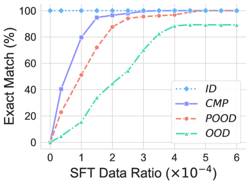
Findings. As shown in Figure 3, we can find that generally a very small portion ( $λ=1.5e^-4$ ) of data can make the model quickly generalize to unseen transformations. The less discrepancy between the training and testing data, the quicker the model can generalize. This indicates that a similar pattern appears in the training data, helping LLMs to generalize to the test dataset.
<details>
<summary>x3.png Details</summary>
### Visual Description
## Line Chart: Exact Match vs. SFT Data Ratio
### Overview
This chart illustrates the performance, measured as "Exact Match (%)", of four distinct data categories (ID, CMP, POOD, OOD) as the "SFT Data Ratio" increases. The chart demonstrates how different types of data influence model accuracy during Supervised Fine-Tuning (SFT).
### Components/Axes
* **Y-Axis:** Labeled "Exact Match (%)". The scale ranges from 0 to 100, with grid lines at intervals of 20.
* **X-Axis:** Labeled "SFT Data Ratio ($\times 10^{-4}$)". The scale ranges from 0 to 6, with grid lines at intervals of 1.
* **Legend:** Positioned in the bottom-right quadrant of the chart area.
* **ID**: Blue dotted line with diamond markers.
* **CMP**: Purple solid line with square markers.
* **POOD**: Orange-red dashed line with circle markers.
* **OOD**: Teal dash-dot line with triangle markers.
### Detailed Analysis
The chart displays four distinct learning curves, all starting at (0,0) except for the ID series.
* **ID (In-Distribution):**
* **Trend:** This series is a flat horizontal line at 100%.
* **Values:** Remains constant at 100% across the entire X-axis range (0 to 6).
* **CMP (Comparison/Compositional):**
* **Trend:** A steep, upward-sloping curve that exhibits rapid growth before plateauing.
* **Values:**
* At x=0.5: ~40%
* At x=1.0: ~80%
* At x=1.5: ~95%
* At x=2.0: ~97%
* Plateaus near 100% after x=3.0.
* **POOD (Possibly Out-of-Distribution):**
* **Trend:** A moderate, upward-sloping curve that grows steadily and plateaus later than CMP.
* **Values:**
* At x=0.5: ~23%
* At x=1.0: ~52%
* At x=1.5: ~72%
* At x=2.0: ~88%
* At x=2.5: ~94%
* At x=3.0: ~96%
* Reaches ~100% near x=5.0.
* **OOD (Out-of-Distribution):**
* **Trend:** The slowest rising curve, showing a gradual, concave-downward growth pattern.
* **Values:**
* At x=0.5: ~5%
* At x=1.0: ~15%
* At x=1.5: ~33%
* At x=2.0: ~45%
* At x=2.5: ~55%
* At x=3.0: ~70%
* At x=3.5: ~83%
* At x=4.0: ~88%
* Plateaus at approximately 90% from x=4.0 onwards.
### Key Observations
* **Performance Hierarchy:** The model's ability to achieve an "Exact Match" is strictly ordered by category: ID > CMP > POOD > OOD.
* **Data Efficiency:** The ID category requires zero additional SFT data to achieve perfect accuracy, suggesting the model was already proficient in this domain.
* **Generalization Gap:** There is a significant performance gap between ID/CMP tasks and OOD tasks. While CMP and POOD eventually reach near-perfect accuracy with enough data, the OOD category plateaus at ~90%, indicating a potential limitation in the model's ability to generalize to out-of-distribution data regardless of the SFT data ratio provided.
### Interpretation
This chart is a classic representation of model adaptation during fine-tuning.
* **ID (In-Distribution)** represents the model's baseline capability; it is already "solved" or highly familiar to the model.
* **CMP and POOD** represent tasks that are within the model's reach; they require some fine-tuning data to "unlock" the correct behavior, but they converge to high accuracy relatively quickly.
* **OOD (Out-of-Distribution)** represents the "hard" tasks. The slow, shallow slope suggests that the model struggles to map the SFT data to the correct outputs for these inputs. The fact that it plateaus at ~90% suggests that either the model lacks the capacity to fully learn these OOD patterns, or the OOD data is inherently noisy/ambiguous compared to the other categories.
In a technical context, this suggests that if the goal is to improve OOD performance, simply increasing the SFT data ratio (within this range) may yield diminishing returns, and architectural changes or different training strategies might be required.
</details>
Figure 3: Performance on unseen transformation using SFT in various levels of distribution shift. Introducing a small amount of unseen data helps CoT reasoning to generalize across different scenarios.
### 5.2 Element Generalization
Element generalization is another critical factor to consider when LLMs try to generalize to new tasks.
Experiment settings. Similar to transformation generalization, we fix other factors and consider three progressive distribution shifts for elements: ID, CMP, and OOD, as shown in Figure 1. It is noted that in composition, we test if CoT reasoning can be generalized to novel combinations when seeing all the basic atoms in the elements, e.g., $(\texttt{A},\texttt{B},\texttt{C},\texttt{D})→(\texttt{B},\texttt{C},\texttt{D},\texttt{A})$ . Based on the atom order in combination (can be measured by edit distance $n$ ), the CMP can be further developed. While for OOD, atoms that constitute the elements are totally unseen during the training.
<details>
<summary>x4.png Details</summary>
### Visual Description
## Heatmap: Performance Metrics by Scenario and Transformation
### Overview
This image displays two stacked heatmaps evaluating model performance across three distinct scenarios (ID, CMP, OOD) and six different transformations (f1, f2, f1 ∘ f1, f1 ∘ f2, f2 ∘ f1, f2 ∘ f2). The top heatmap measures performance using the "BLEU Score," while the bottom heatmap measures performance using "Exact Match (%)."
### Components/Axes
* **Shared X-Axis (Bottom):** Labeled "Transformation." The categories are: `f1`, `f2`, `f1 ∘ f1`, `f1 ∘ f2`, `f2 ∘ f1`, `f2 ∘ f2`.
* **Shared Y-Axis (Left):** Labeled "Scenario." The categories are: `ID`, `CMP`, `OOD`.
* **Top Heatmap Legend:** "BLEU Score," ranging from 0.0 (blue) to 1.0 (red).
* **Bottom Heatmap Legend:** "Exact Match (%)," ranging from 0 (blue) to 100 (red).
### Detailed Analysis
#### Top Heatmap: BLEU Score
* **ID Row:** The values are consistently **1.00** across all six transformations. The color is solid red.
* **CMP Row:**
* `f1`: 0.71
* `f2`: 0.62
* `f1 ∘ f1`: 0.65
* `f1 ∘ f2`: 0.68
* `f2 ∘ f1`: 0.32
* `f2 ∘ f2`: 0.16
* *Trend:* Performance is highest at `f1` (0.71) and degrades significantly as the transformations involve `f2` in the first position (0.32 and 0.16).
* **OOD Row:**
* `f1`: 0.00
* `f2`: 0.00
* `f1 ∘ f1`: 0.46
* `f1 ∘ f2`: 0.35
* `f2 ∘ f1`: 0.40
* `f2 ∘ f2`: 0.35
* *Trend:* Performance is non-existent (0.00) for single transformations (`f1`, `f2`) but shows moderate performance (0.35–0.46) for all composite transformations.
#### Bottom Heatmap: Exact Match (%)
* **ID Row:** The values are consistently **100** across all six transformations. The color is solid red.
* **CMP Row:** The values are consistently **0** across all six transformations. The color is solid blue.
* **OOD Row:** The values are consistently **0** across all six transformations. The color is solid blue.
### Key Observations
* **Perfect ID Performance:** The model achieves perfect scores (1.00 BLEU, 100 Exact Match) in the ID (In-Distribution) scenario regardless of the transformation applied.
* **Exact Match Failure:** The model fails to achieve any exact matches in the CMP (Comparison) and OOD (Out-of-Distribution) scenarios, resulting in a score of 0 across all transformations.
* **BLEU vs. Exact Match Discrepancy:** Despite having 0 Exact Match in CMP and OOD, the BLEU scores are non-zero (ranging from 0.16 to 0.71). This indicates that while the model is not producing identical outputs to the ground truth, it is generating text that shares significant n-gram overlap or semantic similarity.
* **Transformation Impact:** In the CMP scenario, transformations starting with `f1` yield higher BLEU scores (0.62–0.71) compared to those starting with `f2` (0.16–0.32), suggesting `f2` is a more challenging or destructive transformation for the model in this context.
### Interpretation
The data suggests a model that is highly specialized or overfitted to the "ID" (In-Distribution) data, as it handles all transformations perfectly. The complete failure to achieve "Exact Match" in CMP and OOD scenarios, contrasted with the non-zero BLEU scores, implies that the model is capable of generating "near-miss" or semantically relevant text, but lacks the precision required for exact reproduction in these more difficult scenarios. The performance drop in the CMP row when `f2` is applied suggests that `f2` introduces complexity or noise that the model is less equipped to handle compared to `f1`. The OOD scenario's inability to handle single transformations (`f1`, `f2`) but relative success with composite transformations is an anomaly that might suggest the model requires a specific "compositional" structure to trigger its generalization capabilities.
</details>
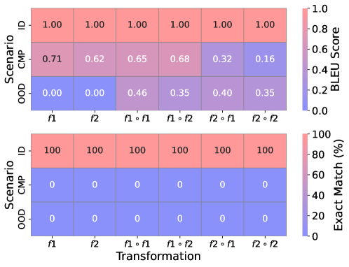
Figure 4: Element generalization results on various scenarios and relations.
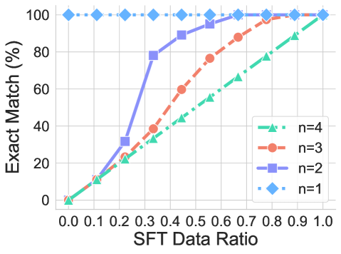
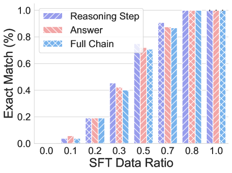
Findings. Similar to transformation generalization, the performances degrade sharply when facing the distribution shift consistently across all transformations, as shown in Figure 4. From ID to CMP and OOD, the exact match decreases from 1.0 to 0 and 0, for all cases. Most strikingly, the BLEU score is 0 when transferred to $f_1$ and $f_2$ transformations. A failure case in Appendix D.1 shows that the models cannot respond to any words when novel elements are present. We further explore when CoT reasoning can generalize to novel elements by conducting SFT. The results are summarized in Figure 5. We evaluate the performance under three exact matches for the full chain under three scenarios, CMP based on the edit distance n. The result is similar to SFT on transformation. The performance increases rapidly when presented with similar (a small $n$ ) examples in the training data. Interestingly, the exact match rate for CoT reasoning aligns with the lower bound of performance when $n=3$ , which might suggest the generalization of CoT reasoning on novel elements is very limited, even SFT on the downstream task. When we further analyze the exact match of reasoning, answer, and token during the training for $n=3$ , as summarized in Figure 5b. We find that there is a mismatch of accuracy between the answer and the reasoning step during the training process, which somehow might provide an explanation regarding why CoT reasoning is inconsistent in some cases.
<details>
<summary>x5.png Details</summary>
### Visual Description
## Line Chart: Exact Match vs. SFT Data Ratio
### Overview
This image is a line chart illustrating the relationship between the "SFT Data Ratio" (x-axis) and the "Exact Match (%)" (y-axis) across four different experimental conditions, labeled as $n=1$ through $n=4$. The chart demonstrates how increasing the data ratio improves the exact match percentage, with the rate of improvement varying significantly based on the value of $n$.
### Components/Axes
* **Y-Axis:** Labeled "Exact Match (%)". The scale ranges from 0 to 100 in increments of 20.
* **X-Axis:** Labeled "SFT Data Ratio". The scale ranges from 0.0 to 1.0 in increments of 0.1.
* **Legend:** Positioned in the bottom-right quadrant of the chart area.
* **n=4:** Teal color, triangle marker, dash-dot line style.
* **n=3:** Orange/Red color, circle marker, dashed line style.
* **n=2:** Purple color, square marker, solid line style.
* **n=1:** Light blue color, diamond marker, dotted line style.
### Detailed Analysis
The chart displays four distinct data series. Below are the approximate values extracted from the visual representation:
| SFT Data Ratio | n=1 (Light Blue) | n=2 (Purple) | n=3 (Orange) | n=4 (Teal) |
| :--- | :--- | :--- | :--- | :--- |
| **0.0** | 100% | 0% | 0% | 0% |
| **0.1** | 100% | ~12% | ~12% | ~11% |
| **0.2** | 100% | ~32% | ~24% | ~22% |
| **0.3** | 100% | ~78% | ~38% | ~33% |
| **0.4** | 100% | ~90% | ~60% | ~44% |
| **0.5** | 100% | ~95% | ~76% | ~55% |
| **0.6** | 100% | 100% | ~88% | ~66% |
| **0.7** | 100% | 100% | ~98% | ~77% |
| **0.8** | 100% | 100% | 100% | ~88% |
| **0.9** | 100% | 100% | 100% | ~95% |
| **1.0** | 100% | 100% | 100% | 100% |
**Trend Verification:**
* **n=1 (Light Blue):** This series is a horizontal line at 100%, indicating perfect performance regardless of the data ratio.
* **n=2 (Purple):** This series shows a sharp, sigmoidal upward trend. It remains low until 0.2, spikes significantly between 0.2 and 0.4, and plateaus at 100% by 0.6.
* **n=3 (Orange):** This series shows a steady, linear-to-curved upward trend, reaching 100% at approximately 0.8.
* **n=4 (Teal):** This series shows the slowest, most linear upward trend, requiring the full data ratio (1.0) to reach 100% accuracy.
### Key Observations
* **Inverse Efficiency:** There is a clear inverse relationship between the value of $n$ and the efficiency of the model (or process) in achieving an "Exact Match." Lower values of $n$ reach 100% accuracy with significantly less data.
* **Outlier:** The $n=1$ condition is an outlier, as it maintains 100% accuracy across the entire spectrum, suggesting it is either a trivial task or a baseline that does not require fine-tuning data.
* **Convergence:** All four lines converge at the (1.0, 100%) coordinate.
### Interpretation
This chart likely represents the performance of a machine learning model (such as an LLM) undergoing Supervised Fine-Tuning (SFT).
* **"SFT Data Ratio"** likely refers to the percentage of the training dataset utilized.
* **"n"** likely represents the complexity of the task or the number of "shots" (examples) provided in a prompt.
* **The Data Suggests:** As the complexity of the task ($n$) increases, the model requires a higher proportion of the fine-tuning dataset to achieve perfect "Exact Match" performance.
* **Reading Between the Lines:** The sharp jump in the $n=2$ curve suggests a "tipping point" where the model suddenly learns the task pattern effectively once a certain threshold of data (around 0.2–0.3) is provided. Conversely, $n=4$ appears to be a much harder task, requiring a linear increase in data to improve performance, suggesting that the model struggles to generalize this task without a substantial amount of training data.
</details>
(a) Performance on unseen element via SFT in various CMP scenarios.
<details>
<summary>x6.png Details</summary>
### Visual Description
## Grouped Bar Chart: Exact Match vs. SFT Data Ratio
### Overview
The image is a grouped bar chart displaying the performance of a model (likely a Large Language Model) measured by "Exact Match (%)" against varying "SFT Data Ratio" (Supervised Fine-Tuning Data Ratio) values. The chart compares performance across three distinct evaluation criteria: "Reasoning Step," "Answer," and "Full Chain."
### Components/Axes
* **Y-Axis:** Labeled "Exact Match (%)". The scale ranges from 0.0 to 1.0 in increments of 0.2.
* **X-Axis:** Labeled "SFT Data Ratio". The categories are discrete values: 0.0, 0.1, 0.2, 0.3, 0.5, 0.7, 0.8, and 1.0.
* **Legend (Positioned Top-Left):**
* **Purple (diagonal stripes):** Reasoning Step
* **Red/Pink (diagonal stripes):** Answer
* **Blue (diagonal stripes):** Full Chain
### Detailed Analysis
**Trend Verification:** All three data series exhibit a strong positive correlation with the SFT Data Ratio. As the ratio increases from 0.0 to 0.8, the Exact Match percentage increases monotonically. Performance plateaus at 1.0 (100%) for all metrics once the ratio reaches 0.8.
**Data Points (Approximate Values):**
| SFT Data Ratio | Reasoning Step (Purple) | Answer (Red) | Full Chain (Blue) |
| :--- | :--- | :--- | :--- |
| **0.0** | 0.0 | 0.0 | 0.0 |
| **0.1** | ~0.04 | ~0.06 | ~0.04 |
| **0.2** | ~0.20 | ~0.20 | ~0.20 |
| **0.3** | ~0.45 | ~0.42 | ~0.40 |
| **0.5** | ~0.75 | ~0.72 | ~0.70 |
| **0.7** | ~0.90 | ~0.87 | ~0.86 |
| **0.8** | 1.0 | 1.0 | 1.0 |
| **1.0** | 1.0 | 1.0 | 1.0 |
### Key Observations
* **Performance Saturation:** The model achieves perfect "Exact Match" scores (1.0) at an SFT Data Ratio of 0.8. Increasing the data ratio further to 1.0 yields no additional performance gain.
* **Metric Hierarchy:** In the mid-range (0.3 to 0.7), there is a consistent hierarchy in performance: "Reasoning Step" (Purple) > "Answer" (Red) > "Full Chain" (Blue). This suggests that while the model is highly capable of generating correct individual reasoning steps, the cumulative requirement of the "Full Chain" makes it the most difficult metric to satisfy.
* **Threshold Effect:** There is a significant jump in performance between the 0.1 and 0.2 ratios, suggesting a critical threshold of SFT data is required before the model begins to generalize effectively.
### Interpretation
This data demonstrates the efficacy of Supervised Fine-Tuning (SFT) in improving model performance on specific tasks. The hierarchy of metrics (Reasoning Step vs. Full Chain) provides insight into the model's failure modes: it is easier for the model to get a single step correct than to maintain correctness across the entire chain of thought.
The plateau at 0.8 suggests that for this specific dataset and task, 80% of the SFT data is sufficient to reach peak performance. This implies that the remaining 20% of the data (from 0.8 to 1.0) may be redundant or provide diminishing returns, which is a critical finding for optimizing training efficiency and reducing computational costs.
</details>
(b) Evaluation of CoT reasoning in SFT.
Figure 5: SFT performances for element generalization. SFT helps to generalize to novel elements.
## 6 Length Generalization
Length generalization examines how CoT reasoning degrades when models encounter test cases that differ in length from their training distribution. The difference in length could be introduced from the text space or the reasoning space of the problem. Therefore, we decompose length generalization into two complementary aspects: text length generalization and reasoning step generalization. Guided by instinct, we first propose to measure the length discrepancy.
Length Extrapolation Bound. We establish a power-law relationship for length extrapolation:
**Proposition 6.1 (Length Extrapolation Gaussian Degradation)**
*For a model trained on chain-of-thought sequences of fixed length $L_train$ , the generalization error at test length $L$ follows a Gaussian distribution:
$$
E(L)=E_0+≤ft(1-E_0\right)·≤ft(1-\exp≤ft(-\frac{≤ft(L-L_train \right)^2}{2σ^2}\right)\right) \tag{13}
$$
where $E_0$ is the in-distribution error at $L=L_train$ , $σ$ is the length generalization width parameter, and $L$ is the test sequence length*
The proof is provided in Appendix A.3.
### 6.1 Text Length Generalization
Text length generalization evaluates how CoT performance varies when the input text length (i.e., the element length $l$ ) differs from training examples. Considering the way LLMs process long text, this aspect is crucial because real-world problems often involve varying degrees of complexity that manifest as differences in problem statement length, context size, or information density.
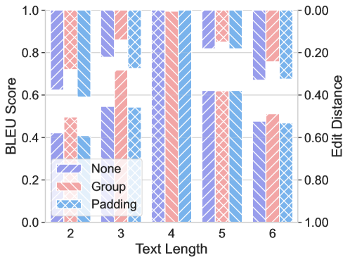
Experiment settings. We pre-train LLMs on the dataset with text length merely on $l=4$ while fixing other factors and evaluate the performance on a variety of lengths. We consider three different padding strategies during the pre-training: (i) None: LLMs do not use any padding. (ii) Padding: We pad LLM to the max length of the context window. (iii) Group: We group the text and truncate it into segments with a maximum length.
Table 3: Evaluation for text length generalization.
| 2 3 4 | 0.00% 0.00% 100.00% | 0.00% 0.00% 100.00% | 0.00% 0.00% 100.00% | 0.3772 0.2221 0.0000 | 0.4969 0.3203 0.0000 | 0.5000 0.2540 0.0000 | 0.4214 0.5471 1.0000 | 0.1186 0.1519 1.0000 | 0.0000 0.0000 1.0000 |
| --- | --- | --- | --- | --- | --- | --- | --- | --- | --- |
| 5 | 0.00% | 0.00% | 0.00% | 0.1818 | 0.2667 | 0.2000 | 0.6220 | 0.1958 | 0.2688 |
| 6 | 0.00% | 0.00% | 0.00% | 0.3294 | 0.4816 | 0.3337 | 0.4763 | 0.1174 | 0.2077 |
Findings. As illustrated in the Table 3, the CoT reasoning failed to directly generate two test cases even though those lengths present a mild distribution shift. Further, the performance declines as the length discrepancy increases shown in Figure 6. For instance, from data with $l=4$ to those with $l=3$ or $l=5$ , the BLEU score decreases from 1 to 0.55 and 0.62. Examples in Appendix D.1 indicate that LLMs attempt to produce CoT reasoning with the same length as the training data by adding or removing tokens in the reasoning chains. The efficacy of CoT reasoning length generalization deteriorates as the discrepancy increases. Moreover, we consider using a different padding strategy to decrease the divergence between the training data and test cases. We found that padding to the max length doesn’t contribute to length generalization. However, the performance increases when we replace the padding with text by using the group strategy, which indicates its effectiveness.
<details>
<summary>x7.png Details</summary>
### Visual Description
## Bar Chart: BLEU Score and Edit Distance by Text Length
### Overview
This image displays a grouped bar chart comparing the performance of three different methods ("None", "Group", and "Padding") across five distinct "Text Lengths" (2, 3, 4, 5, and 6). The chart utilizes a dual-axis system to represent two metrics simultaneously: "BLEU Score" on the left vertical axis and "Edit Distance" on the right vertical axis. The data is presented in two distinct horizontal bands: an upper band representing BLEU Scores and a lower band representing Edit Distance.
### Components/Axes
* **X-Axis:** Labeled "Text Length," with discrete categories: 2, 3, 4, 5, 6.
* **Left Y-Axis:** Labeled "BLEU Score," ranging from 0.0 to 1.0.
* **Right Y-Axis:** Labeled "Edit Distance," ranging from 0.00 (top) to 1.00 (bottom). Note that this axis is inverted.
* **Legend:** Located in the bottom-left quadrant.
* **None:** Purple bars with diagonal stripes (top-left to bottom-right).
* **Group:** Pink/Red bars with cross-hatch pattern.
* **Padding:** Blue bars with diagonal stripes (top-right to bottom-left).
### Detailed Analysis
The chart is segmented into two visual tiers. The upper tier corresponds to the BLEU Score (0.6–1.0), and the lower tier corresponds to the Edit Distance (0.4–0.6 on the left axis, which maps to 0.6–0.4 on the right axis).
**Data Points (Approximate Values):**
| Text Length | Metric | None | Group | Padding |
| :--- | :--- | :--- | :--- | :--- |
| **2** | BLEU (Upper) | ≈ 0.63 | ≈ 0.72 | ≈ 0.60 |
| **2** | Edit Distance (Lower) | ≈ 0.42 | ≈ 0.50 | ≈ 0.41 |
| **3** | BLEU (Upper) | ≈ 0.78 | ≈ 0.72 | ≈ 0.73 |
| **3** | Edit Distance (Lower) | ≈ 0.55 | ≈ 0.72 | ≈ 0.55 |
| **4** | BLEU (Upper) | 1.0 | 1.0 | 1.0 |
| **4** | Edit Distance (Lower) | 0.0 | 0.0 | 0.0 |
| **5** | BLEU (Upper) | ≈ 1.0 | ≈ 0.85 | ≈ 1.0 |
| **5** | Edit Distance (Lower) | ≈ 0.62 | ≈ 0.62 | ≈ 0.62 |
| **6** | BLEU (Upper) | ≈ 1.0 | ≈ 0.76 | ≈ 1.0 |
| **6** | Edit Distance (Lower) | ≈ 0.48 | ≈ 0.51 | ≈ 0.48 |
### Key Observations
* **The "Length 4" Anomaly:** Text Length 4 acts as a perfect performance point for all three methods, achieving a maximum BLEU score of 1.0 and a minimum Edit Distance of 0.0.
* **Method Consistency:** The "None" and "Padding" methods consistently track each other very closely across all text lengths.
* **"Group" Method Variance:** The "Group" method shows the most volatility. It outperforms the others at Length 2 (higher BLEU, higher Edit Distance) but underperforms compared to "None" and "Padding" at Lengths 3, 5, and 6.
* **Dual-Axis Inversion:** The right axis (Edit Distance) is inverted, meaning higher bars in the lower section represent a *higher* Edit Distance (worse performance), while lower bars represent a *lower* Edit Distance (better performance).
### Interpretation
The data suggests that the "Group" method introduces a specific bias or behavior that is highly sensitive to text length. While it provides a slight advantage at Length 2, it consistently degrades performance (lower BLEU, higher Edit Distance) at lengths 3, 5, and 6 compared to the baseline "None" and "Padding" methods.
The perfect performance at Text Length 4 is a significant outlier, suggesting that the underlying model or task may have a specific structural alignment or "sweet spot" at this length, rendering the differences between the methods negligible. The "None" and "Padding" methods appear to be robust, stable baselines, whereas the "Group" method appears to be an experimental intervention that does not consistently improve performance across the tested lengths.
</details>
Figure 6: Performance of text length generalization across various padding strategies. Group strategies contribute to length generalization.
### 6.2 Reasoning Step Generalization
The reasoning step generalization investigates whether models can extrapolate to reasoning chains requiring different steps $k$ from those observed during training. which is a popular setting in multi-step reasoning tasks.
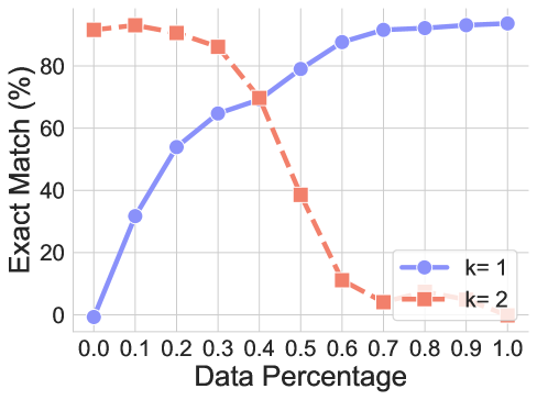
Experiment settings. Similar to text length generalization, we first pre-train the LLM with reasoning step $k=2$ , and evaluate on data with reasoning step $k=1$ or $k=3$ .
<details>
<summary>x8.png Details</summary>
### Visual Description
## Line Chart: Exact Match vs. Data Percentage
### Overview
The image displays a line chart comparing the performance of two distinct configurations, labeled $k=1$ and $k=2$, across a range of "Data Percentage" values. The chart illustrates how the "Exact Match (%)" metric evolves as the percentage of data increases from 0.0 to 1.0.
### Components/Axes
* **X-Axis:** Labeled "Data Percentage". The scale ranges from 0.0 to 1.0, with tick marks at 0.1 intervals.
* **Y-Axis:** Labeled "Exact Match (%)". The scale ranges from 0 to approximately 100, with major grid lines at 0, 20, 40, 60, and 80.
* **Legend:** Located in the bottom-right quadrant of the chart area.
* **Blue line with circle markers:** Labeled "k= 1".
* **Red/Orange dashed line with square markers:** Labeled "k= 2".
### Detailed Analysis
**Trend Verification:**
* **k=1 (Blue, solid line):** This series exhibits a monotonic upward trend. It starts at the origin (0,0), rises steeply between 0.0 and 0.4, and then continues to rise at a slower, decelerating rate, plateauing as it approaches 1.0.
* **k=2 (Red, dashed line):** This series exhibits a downward trend after an initial period of stability. It starts high, remains relatively flat between 0.0 and 0.3, drops sharply between 0.4 and 0.6, and then plateaus near zero for the remainder of the range.
**Data Points (Approximate values):**
| Data Percentage (X) | k=1 (Blue) | k=2 (Red) |
| :--- | :--- | :--- |
| 0.0 | ~0% | ~92% |
| 0.1 | ~32% | ~94% |
| 0.2 | ~54% | ~91% |
| 0.3 | ~65% | ~86% |
| 0.4 | ~70% | ~70% |
| 0.5 | ~80% | ~39% |
| 0.6 | ~88% | ~11% |
| 0.7 | ~92% | ~4% |
| 0.8 | ~93% | ~5% |
| 0.9 | ~94% | ~2% |
| 1.0 | ~95% | ~0% |
### Key Observations
* **Intersection Point:** The two data series intersect at approximately X=0.4, where both configurations achieve an "Exact Match" of roughly 70%.
* **Performance Crossover:** Before the 0.4 mark, the $k=2$ configuration significantly outperforms $k=1$. After the 0.4 mark, the $k=1$ configuration becomes the superior performer.
* **Divergence:** The gap between the two lines is widest at the extremes of the X-axis (0.0 and 1.0), indicating that the choice of $k$ is highly sensitive to the amount of data available.
### Interpretation
This chart likely represents the performance of a machine learning model or algorithm (possibly a k-Nearest Neighbors classifier or similar) where $k$ is a hyperparameter.
* **Low Data Regime (0.0 - 0.3):** The $k=2$ configuration is highly effective, suggesting it may be better at generalizing or finding patterns when data is sparse.
* **High Data Regime (0.5 - 1.0):** The $k=1$ configuration is clearly superior. The rapid decline of $k=2$ in this region suggests that as more data is introduced, the $k=2$ configuration may be suffering from increased noise, overfitting, or a fundamental mismatch in how it processes larger datasets compared to $k=1$.
* **Conclusion:** The data demonstrates a clear trade-off. If the system operates with limited data, $k=2$ is the optimal choice. If the system operates with high data availability, $k=1$ is the optimal choice. The "crossover" point at 0.4 represents the critical threshold for deciding which configuration to deploy.
</details>
(a) Reasoning step. From k=2 to k=1
<details>
<summary>x9.png Details</summary>
### Visual Description
## Line Chart: Exact Match vs. Data Percentage for k=2 and k=3
### Overview
The image is a line chart illustrating the performance of two different parameters, labeled "k=2" and "k=3," across varying "Data Percentage" levels. The chart tracks the "Exact Match (%)" metric, showing how the accuracy of these two parameters evolves as the data percentage increases from 0.0 to 1.0.
### Components/Axes
* **X-Axis:** Labeled "Data Percentage." The scale ranges from 0.0 to 1.0, with major tick marks at intervals of 0.1.
* **Y-Axis:** Labeled "Exact Match (%)." The scale ranges from 0 to 80, with major tick marks at intervals of 10.
* **Legend:** Located in the bottom-right quadrant of the chart area.
* **Blue line with circle markers:** Labeled "k=3"
* **Red/Orange dashed line with square markers:** Labeled "k=2"
* **Grid:** A light gray grid is overlaid on the chart, corresponding to the axis tick marks.
### Detailed Analysis
#### Trend Verification
* **k=3 (Blue, Solid Line):** This series exhibits a generally upward trend. It starts near zero, remains relatively flat until 0.3, experiences a minor dip at 0.5, and then accelerates sharply upward from 0.6 to 1.0.
* **k=2 (Red/Orange, Dashed Line):** This series exhibits a generally downward trend. It starts at the maximum value, drops sharply until 0.5, stabilizes/plateaus between 0.5 and 0.8, and then drops to zero at 1.0.
#### Data Extraction (Approximate Values)
| Data Percentage | k=3 (Blue, Circle) | k=2 (Red/Orange, Square) |
| :--- | :--- | :--- |
| 0.0 | ~0% | ~80% |
| 0.1 | ~0% | ~54% |
| 0.2 | ~2% | ~35% |
| 0.3 | ~6% | ~23% |
| 0.4 | ~10% | ~17% |
| 0.5 | ~9% | ~12% |
| 0.6 | ~13% | ~12% |
| 0.7 | ~29% | ~17% |
| 0.8 | ~49% | ~20% |
| 0.9 | ~63% | ~12% |
| 1.0 | ~74% | ~0% |
### Key Observations
* **Crossover Point:** The two lines intersect between 0.5 and 0.6 on the x-axis. Before this point, $k=2$ outperforms $k=3$. After this point, $k=3$ significantly outperforms $k=2$.
* **Inverse Relationship:** Between 0.0 and 0.5, the two series show a strong inverse relationship, where $k=2$ is declining while $k=3$ is slowly increasing.
* **Anomaly at 1.0:** The $k=2$ series drops abruptly to 0% at the 1.0 Data Percentage mark, which is a sharp deviation from its previous trend.
### Interpretation
This chart likely represents the performance of a machine learning model or a classification algorithm (such as K-Nearest Neighbors) where $k$ represents the number of neighbors or a similar hyperparameter.
* **Performance Characteristics:** The data suggests that $k=2$ is highly effective when the dataset is sparse (low Data Percentage) but fails to generalize or becomes unstable as the dataset grows. Conversely, $k=3$ is ineffective with sparse data but becomes increasingly accurate as more data is introduced, suggesting it is a more robust parameter for larger datasets.
* **The 1.0 Anomaly:** The sudden drop of $k=2$ to 0% at 1.0 suggests a potential edge-case failure, such as an overfitting issue, a specific boundary condition in the test set, or a computational error when the full dataset is utilized.
* **Strategic Insight:** If this were a model selection task, one would choose $k=2$ for low-data environments and $k=3$ for high-data environments. The crossover point (approx. 0.55) serves as the decision threshold for switching between these two configurations.
</details>
(b) Reasoning step. From k=2 to k=3
Figure 7: SFT performances for reasoning step generalization.
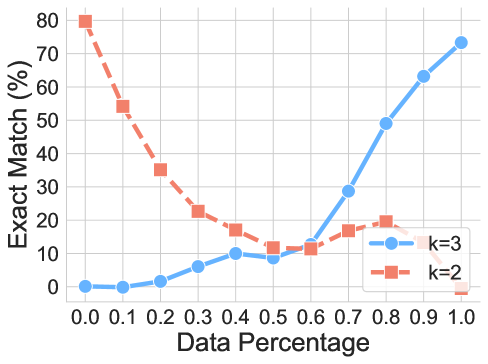
Findings. As showcased in Figure 7, CoT reasoning cannot generalize across data requiring different reasoning steps, indicating the failure of generalization. Then, we try to decrease the distribution discrepancy introduced by gradually increasing the ratio of unseen data while keeping the dataset size the same when pre-training the model. And then, we evaluate the performance on two datasets. As we can observe, the performance on the target dataset increases along with the ratio. At the same time, the LLMs can not generalize to the original training dataset because of the small amount of training data. The trend is similar when testing different-step generalization, which follows the intuition and validates our hypothesis directly.
## 7 Format Generalization
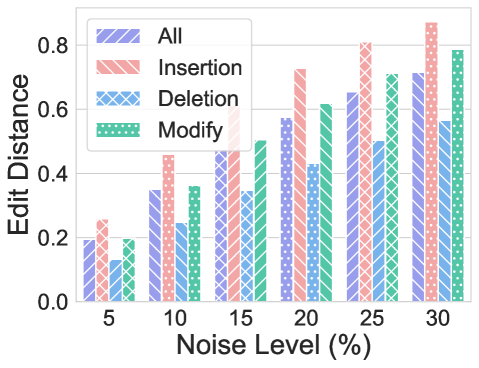
Format generalization assesses the robustness of CoT reasoning to surface-level variations in test queries. This dimension is especially crucial for determining whether models have internalized flexible, transferable reasoning strategies or remain reliant on the specific templates and phrasings encountered during training.
Format Alignment Score. We introduce a metric for measuring prompt similarity:
**Definition 7.1 (Format Alignment Score)**
*For training prompt distribution $P_train$ and test prompt $p_test$ :
$$
PAS(p_test)=\max_p∈ P_{train}\cos(φ(p),φ(p_test)) \tag{14}
$$
where $φ$ is a prompt embedding function.*
<details>
<summary>x10.png Details</summary>
### Visual Description
## Bar Chart: Edit Distance vs. Noise Level
### Overview
The image is a grouped bar chart displaying the relationship between "Noise Level (%)" and "Edit Distance" across four distinct categories: "All", "Insertion", "Deletion", and "Modify". The chart demonstrates how different types of data errors (or edits) scale as the input noise increases from 5% to 30%.
### Components/Axes
* **Y-Axis:** Labeled "Edit Distance". The scale ranges from 0.0 to 0.8, with grid lines at 0.0, 0.2, 0.4, 0.6, and 0.8.
* **X-Axis:** Labeled "Noise Level (%)". The axis displays discrete intervals: 5, 10, 15, 20, 25, and 30.
* **Legend (Positioned Top-Left):**
* **All:** Represented by purple bars with diagonal stripes.
* **Insertion:** Represented by red/pink bars with diagonal stripes.
* **Deletion:** Represented by blue bars with diagonal stripes.
* **Modify:** Represented by green bars with a dotted/stippled pattern.
### Detailed Analysis
**Trend Verification:** All four data series exhibit a clear, positive linear trend. As the "Noise Level (%)" increases from 5 to 30, the "Edit Distance" increases for every category.
**Data Points (Approximate Values):**
| Noise Level (%) | All (Purple) | Insertion (Red) | Deletion (Blue) | Modify (Green) |
| :--- | :--- | :--- | :--- | :--- |
| **5** | ~0.20 | ~0.25 | ~0.13 | ~0.20 |
| **10** | ~0.35 | ~0.45 | ~0.25 | ~0.36 |
| **15** | ~0.47 | ~0.60 | ~0.35 | ~0.50 |
| **20** | ~0.57 | ~0.72 | ~0.43 | ~0.61 |
| **25** | ~0.65 | ~0.80 | ~0.50 | ~0.71 |
| **30** | ~0.71 | ~0.87 | ~0.56 | ~0.78 |
### Key Observations
* **Highest Impact:** The "Insertion" category consistently produces the highest Edit Distance across all noise levels, indicating that insertion errors are the most significant contributor to the total edit distance in this dataset.
* **Lowest Impact:** The "Deletion" category consistently produces the lowest Edit Distance, suggesting it is the least frequent or least impactful error type among those measured.
* **Crossover/Clustering:** The "All" and "Modify" categories are clustered in the middle. At lower noise levels (5%), "All" and "Modify" are nearly identical. As noise increases, "Modify" consistently trends slightly higher than "All".
### Interpretation
The data demonstrates a predictable degradation of data integrity as noise levels increase. The system appears to be most sensitive to "Insertion" operations, which result in the highest edit distance.
From a Peircean investigative perspective, the fact that "Insertion" is consistently higher than "Deletion" and "Modify" suggests that the underlying process or algorithm being tested is inherently more prone to generating insertion errors when subjected to noise. The "All" category, which likely represents an aggregate metric, tracks closely with the "Modify" category, suggesting that "Modify" errors may be the most representative "average" error type, whereas "Insertion" acts as an outlier on the high end and "Deletion" acts as an outlier on the low end.
</details>
(a) Format generalization. Performance under various perturbation methods.
<details>
<summary>x11.png Details</summary>
### Visual Description
## Line Chart: BLEU Score vs. Noise Level
### Overview
This chart illustrates the performance degradation of four different experimental methods ("None", "Prompt", "Transformation", and "Element") as the input noise level increases from 10% to 90%. The Y-axis represents the BLEU score (a metric for evaluating text generation quality), while the X-axis represents the percentage of noise introduced.
### Components/Axes
* **Y-Axis:** Labeled "BLEU Score". The scale ranges from 0.0 to 1.0, with grid lines at 0.0, 0.2, 0.4, 0.6, 0.8, and 1.0.
* **X-Axis:** Labeled "Noise Level (%)". The scale ranges from 10 to 90, with grid lines at 10, 20, 30, 40, 50, 60, 70, 80, and 90.
* **Legend:** Positioned in the center-right of the chart area.
* **None:** Light blue line with diamond markers.
* **Prompt:** Purple line with square markers.
* **Transformation:** Orange/Coral line with circle markers.
* **Element:** Teal/Green line with triangle markers.
### Detailed Analysis
The following data points are approximate based on visual inspection of the chart markers.
**Trend Verification:**
* **None:** A perfectly horizontal line at 1.0.
* **Prompt:** A steady, slightly curved downward slope.
* **Transformation:** A steeper downward curve compared to "Prompt".
* **Element:** A sharp, rapid downward curve, reaching near-zero values quickly.
**Data Points (Approximate Values):**
| Noise Level (%) | None (Blue) | Prompt (Purple) | Transformation (Orange) | Element (Teal) |
| :--- | :--- | :--- | :--- | :--- |
| 10 | 1.0 | ~0.92 | ~0.88 | ~0.65 |
| 20 | 1.0 | ~0.85 | ~0.76 | ~0.42 |
| 30 | 1.0 | ~0.78 | ~0.66 | ~0.21 |
| 40 | 1.0 | ~0.72 | ~0.56 | ~0.12 |
| 50 | 1.0 | ~0.65 | ~0.46 | ~0.06 |
| 60 | 1.0 | ~0.58 | ~0.38 | ~0.00 |
| 70 | 1.0 | ~0.52 | ~0.30 | ~0.00 |
| 80 | 1.0 | ~0.47 | ~0.20 | ~0.00 |
| 90 | 1.0 | ~0.41 | ~0.14 | ~0.00 |
### Key Observations
* **Baseline Stability:** The "None" method maintains a perfect BLEU score of 1.0 regardless of noise, serving as the control or upper bound.
* **Robustness Hierarchy:** The "Prompt" method is the most robust against noise, maintaining the highest BLEU scores among the variable methods across all noise levels.
* **Rapid Failure:** The "Element" method is highly sensitive to noise; it loses the majority of its performance by the 30% noise level and effectively hits a BLEU score of 0.0 by the 60% noise level.
* **Divergence:** The performance gap between "Prompt" and "Transformation" increases as the noise level rises, indicating that "Prompt" scales better in high-noise environments.
### Interpretation
This chart demonstrates the comparative robustness of different data processing or model-input strategies in the presence of input noise.
* **"None"** likely represents a clean, noise-free baseline or a scenario where the model is unaffected by the specific noise injection method.
* **"Prompt"** suggests a strategy (likely prompt engineering or a specific input formatting technique) that provides significant resilience, allowing the model to maintain semantic coherence even when 90% of the input is noisy.
* **"Transformation"** appears to be a moderately effective strategy, but it degrades significantly faster than "Prompt".
* **"Element"** appears to be a fragile strategy, possibly relying on specific, granular tokens or features that are easily corrupted by noise, rendering the model unable to generate coherent output once noise exceeds 30-40%.
In summary, if the goal is to maintain performance in noisy environments, the "Prompt" strategy is clearly superior to both "Transformation" and "Element".
</details>
(b) Format generalization. Performance vs. various applied perturbation areas.
Figure 8: Performance of format generalization.
Experiment settings. To systematically probe this, we introduce four distinct perturbation modes to simulate scenario in real-world: (i) insertion, where a noise token is inserted before each original token; (ii) deletion: it deletes the original token; (iii) modification: it replaces the original token with a noise token; and (iv) hybrid mode: it combines multiple perturbations. Each mode is applied for tokens with probabilities $p$ , enabling us to quantify the model’s resilience to increasing degrees of prompt distribution shift.
Findings. As shown in Figure 8a, we found that generally CoT reasoning can be easily affected by the format changes. No matter insertion, deletion, modifications, or hybrid mode, it creates a format discrepancy that affects the correctness. Among them, the deletion slightly affects the performance. While the insertions are relatively highly influential on the results. We further divide the query into several sections: elements, transformations, and prompt tokens. As shown in Figure 8b, we found that the elements and transformation play an important role in the format, whereas the changes to other tokens rarely affect the results.
## 8 Temperature and Model Size
Temperature and model size generalization explores how variations in sampling temperature and model capacity can influence the stability and robustness of CoT reasoning. For the sake of rigorous evaluation, we further investigate whether different choices of temperatures and model sizes may significantly affect our results.
Experiment settings. We explore the impact of different temperatures on the validity of the presented results. We adopt the same setting in the transformation generalization.
Findings. As illustrated in Figure 9a, LLMs tend to generate consistent and reliable CoT reasoning across a broad range of temperature settings (e.g., from 1e-5 up to 1), provided the values remain within a suitable range. This stability is maintained even when the models are evaluated under a variety of distribution shifts.
<details>
<summary>x12.png Details</summary>
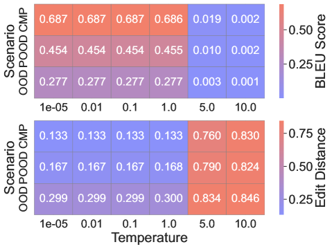
### Visual Description
## Heatmap: BLEU Score and Edit Distance vs. Temperature
### Overview
This image displays two stacked heatmaps illustrating the performance of a model under different "Temperature" settings. The top heatmap measures "BLEU Score," while the bottom heatmap measures "Edit Distance." Both charts share the same X-axis (Temperature) and Y-axis (Scenario OOD POOD CMP). The data indicates a distinct performance threshold between a Temperature of 1.0 and 5.0.
### Components/Axes
* **X-Axis (Bottom of both charts):** Temperature. Values: `1e-05`, `0.01`, `0.1`, `1.0`, `5.0`, `10.0`.
* **Y-Axis (Left of both charts):** "Scenario OOD POOD CMP". This label applies to the three rows in each heatmap.
* **Legends (Right of each chart):**
* **Top Legend (BLEU Score):** A gradient scale from Blue (low, ~0.0) to Red (high, ~0.50+).
* **Bottom Legend (Edit Distance):** A gradient scale from Blue (low, ~0.25) to Red (high, ~0.75+).
### Detailed Analysis
#### Top Chart: BLEU Score
* **Trend:** The BLEU score remains relatively stable and high (Red) for temperatures 1e-05 through 1.0. There is a sharp, drastic drop to near-zero (Blue) at temperatures 5.0 and 10.0.
* **Data Points (Rows 1-3, Columns 1-6):**
* **Row 1:** 0.687, 0.687, 0.687, 0.686, 0.019, 0.002
* **Row 2:** 0.454, 0.454, 0.454, 0.455, 0.010, 0.002
* **Row 3:** 0.277, 0.277, 0.277, 0.277, 0.003, 0.001
#### Bottom Chart: Edit Distance
* **Trend:** The Edit Distance remains relatively stable and low (Blue) for temperatures 1e-05 through 1.0. There is a sharp, drastic increase to high values (Red) at temperatures 5.0 and 10.0.
* **Data Points (Rows 1-3, Columns 1-6):**
* **Row 1:** 0.133, 0.133, 0.133, 0.133, 0.760, 0.830
* **Row 2:** 0.167, 0.167, 0.167, 0.168, 0.790, 0.824
* **Row 3:** 0.299, 0.299, 0.299, 0.300, 0.834, 0.846
### Key Observations
* **Threshold Effect:** Both metrics show a clear "cliff" or transition point between Temperature 1.0 and 5.0.
* **Inverse Relationship:** As Temperature increases beyond 1.0, the BLEU score (a measure of similarity to reference text) collapses, while the Edit Distance (a measure of dissimilarity) spikes.
* **Consistency:** The three rows in each chart exhibit very similar behavior across the temperature spectrum, suggesting that the "Scenario" variations do not alter the fundamental impact of the Temperature parameter on model output quality.
### Interpretation
The data demonstrates that the "Temperature" parameter acts as a critical control for model output quality.
* **Low Temperature (<= 1.0):** The model produces high-quality, relevant output, characterized by high BLEU scores and low Edit Distance. This is the optimal operating range.
* **High Temperature (>= 5.0):** The model's output quality degrades significantly. The near-zero BLEU scores and high Edit Distance suggest that at these temperatures, the model is likely generating incoherent, repetitive, or completely irrelevant text that bears little resemblance to the target or reference data.
The sharp transition suggests that the model's generation mechanism becomes unstable or "hallucinatory" when the temperature exceeds 1.0, rendering the output unusable for tasks requiring high fidelity to a reference.
</details>
(a) Influences of various temperatures.
<details>
<summary>x13.png Details</summary>
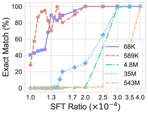
### Visual Description
## Line Chart: Exact Match vs. SFT Ratio
### Overview
This chart illustrates the relationship between the "SFT Ratio" (Supervised Fine-Tuning Ratio) and the "Exact Match (%)" performance metric across five different model sizes (68K, 589K, 4.8M, 35M, and 543M parameters). The chart demonstrates that smaller models achieve high "Exact Match" performance at significantly lower SFT ratios compared to larger models, which require higher ratios to reach 100% accuracy.
### Components/Axes
* **Y-Axis:** "Exact Match (%)", ranging from 0 to 100 in increments of 20.
* **X-Axis:** "SFT Ratio ($\times 10^{-4}$)", ranging from 1.0 to 4.0.
* **Legend:** Positioned in the middle-right quadrant of the chart. It maps the following model sizes to specific line styles and markers:
* **68K:** Solid purple line with square markers.
* **589K:** Dashed orange-red line with circle markers.
* **4.8M:** Dash-dot teal line with diamond markers.
* **35M:** Dotted blue line with diamond markers.
* **543M:** Dash-dot-dot light orange line with circle markers.
### Detailed Analysis
#### Trend Verification and Data Points
The chart displays a clear trend where smaller models (68K, 589K) show immediate performance gains at low SFT ratios, while larger models (4.8M, 35M, 543M) remain at 0% accuracy until higher SFT ratios are reached.
* **68K (Solid Purple, Square):**
* **Trend:** Starts at ~40% at 1.0. Shows a steady upward trend.
* **Data:** Reaches ~95% at 2.0; hits 100% at 2.5.
* **589K (Dashed Orange-Red, Circle):**
* **Trend:** Starts at ~30% at 1.0. Shows a rapid, steep upward trend.
* **Data:** Reaches ~95% at 1.3; hits 100% at 2.0.
* **4.8M (Dash-dot Teal, Diamond):**
* **Trend:** Remains at 0% until 2.0. Shows a very sharp, near-vertical rise between 2.0 and 3.0.
* **Data:** Hits 100% at 3.0.
* **35M (Dotted Blue, Diamond):**
* **Trend:** Remains at 0% until 1.3. Shows a gradual, stepped increase.
* **Data:** Reaches ~20% at 1.5, ~30% at 2.0, ~65% at 2.5, and hits 100% at 3.0.
* **543M (Dash-dot-dot Light Orange, Circle):**
* **Trend:** Remains at 0% for the entire duration until the very end of the x-axis.
* **Data:** Hits 100% at 4.0.
### Key Observations
* **Inverse Scaling:** There is a strong inverse correlation between model size and the SFT ratio required to achieve 100% Exact Match. The smallest model (589K) reaches 100% at a ratio of 2.0, while the largest model (543M) requires a ratio of 4.0.
* **Performance Thresholds:** The larger models exhibit a "threshold" behavior where they provide zero utility for the specific task until a critical SFT ratio is met, after which performance improves rapidly.
* **Outlier:** The 68K model starts at a higher baseline (40%) than the 589K model (30%) at the 1.0 ratio, suggesting that for very low ratios, the smallest model might be more robust or better aligned than the slightly larger 589K model.
### Interpretation
This data suggests a "phase transition" in model learning behavior during supervised fine-tuning. The larger models appear to require a higher density of training signal (SFT ratio) to "unlock" the ability to produce exact matches. This could imply that larger models are more complex and require more data to align with the specific constraints of the task, whereas smaller models may be more easily overfitted or aligned to specific, rigid output formats. The chart effectively visualizes the trade-off between model capacity and the data requirements for task-specific alignment.
</details>
(b) Influences of various sizes.
Figure 9: Temperature and model size. The findings hold under different temperatures and model sizes.
Experiment settings. We further examine the influence of model size by employing the same experimental configuration as used in the novel relation SFT study. In particular, we first pretrain models of different sizes using the transformation $f_1∘ f_1$ , and subsequently perform SFT on $f_2∘ f_2$ while varying the SFT ratios.
Finding. Fig. 9b shows the accuracy of models with different sizes using different SFT ratios, which closely matches the result of our default model size across all evaluated settings and configurations.
## 9 Discussion and Implication
Our investigation, conducted through the controlled environment of DataAlchemy, reveals that the apparent reasoning prowess of Chain-of-Thought (CoT) is largely a brittle mirage. The findings across task, length, and format generalization experiments converge on a conclusion: CoT is not a mechanism for genuine logical inference but rather a sophisticated form of structured pattern matching, fundamentally bounded by the data distribution seen during training. When pushed even slightly beyond this distribution, its performance degrades significantly, exposing the superficial nature of the “reasoning” it produces.
While our experiments utilized models trained from scratch in a controlled environment, the principles uncovered are extensible to large-scale pre-trained models. We summarize the implications for practitioners as follows.
Guard Against Over-reliance and False Confidence. CoT should not be treated as a “plug-and-play” module for robust reasoning, especially in high-stakes domains like medicine, finance, or legal analysis. The ability of LLMs to produce “fluent nonsense” —plausible but logically flawed reasoning chains—can be more deceptive and damaging than an outright incorrect answer, as it projects a false aura of dependability. Sufficient auditing from domain experts is indispensable.
Prioritize Out-of-Distribution (OOD) Testing. Standard validation practices, where the test set closely mirrors the training set, are insufficient to gauge the true robustness of a CoT-enabled system. Practitioners must implement rigorous adversarial and OOD testing that systematically probes for vulnerabilities across task, length, and format variations.
Recognize Fine-Tuning as a Patch, Not a Panacea. Our results show that Supervised Fine-Tuning (SFT) can quickly “patch” a model’s performance on a new, specific data distribution. However, this should not be mistaken for achieving true generalization. It simply expands the model’s “in-distribution” bubble slightly. Relying on SFT to fix every OOD failure is an unsustainable and reactive strategy that fails to address the core issue: the model’s lack of abstract reasoning capability.
## 10 Conclusion
In this paper, we critically examine the COT reasoning of LLMs through the lens of data distribution, revealing that the perceived structured reasoning capability largely arises from inductive biases shaped by in-distribution training data. We propose a controlled environment, DataAlchemy, allowing systematic probing of CoT reasoning along three crucial dimensions: task structure, reasoning length, and query format. Empirical findings consistently demonstrate that CoT reasoning effectively reproduces reasoning patterns closely aligned with training distributions but suffers significant degradation when faced with distributional deviations. Such observations reveal the inherent brittleness and superficiality of current CoT reasoning capabilities. We provide insights that emphasize real-world implications for both practitioners and researchers.
*
## References
- Bentham et al. (2024) O. Bentham, N. Stringham, and A. Marasovic. Chain-of-thought unfaithfulness as disguised accuracy. Transactions on Machine Learning Research, 2024. ISSN 2835-8856. URL https://openreview.net/forum?id=ydcrP55u2e. Reproducibility Certification.
- Budnikov et al. (2025) M. Budnikov, A. Bykova, and I. P. Yamshchikov. Generalization potential of large language models. Neural Computing and Applications, 37(4):1973–1997, 2025.
- Chen et al. (2025a) Q. Chen, L. Qin, J. Liu, D. Peng, J. Guan, P. Wang, M. Hu, Y. Zhou, T. Gao, and W. Che. Towards reasoning era: A survey of long chain-of-thought for reasoning large language models. arXiv preprint arXiv:2503.09567, 2025a.
- Chen et al. (2025b) Y. Chen, J. Benton, A. Radhakrishnan, J. Uesato, C. Denison, J. Schulman, A. Somani, P. Hase, M. Wagner, F. Roger, et al. Reasoning models don’t always say what they think. arXiv preprint arXiv:2505.05410, 2025b.
- Cho et al. (2024) H. Cho, J. Cha, P. Awasthi, S. Bhojanapalli, A. Gupta, and C. Yun. Position coupling: Improving length generalization of arithmetic transformers using task structure. In The Thirty-eighth Annual Conference on Neural Information Processing Systems, 2024. URL https://openreview.net/forum?id=5cIRdGM1uG.
- Garg et al. (2022) S. Garg, D. Tsipras, P. S. Liang, and G. Valiant. What can transformers learn in-context? a case study of simple function classes. Advances in neural information processing systems, 35:30583–30598, 2022.
- Guo et al. (2025) D. Guo, D. Yang, H. Zhang, J. Song, R. Zhang, R. Xu, Q. Zhu, S. Ma, P. Wang, X. Bi, et al. Deepseek-r1: Incentivizing reasoning capability in llms via reinforcement learning. arXiv preprint arXiv:2501.12948, 2025.
- Imani et al. (2023) S. Imani, L. Du, and H. Shrivastava. Mathprompter: Mathematical reasoning using large language models. In Proceedings of the 61st Annual Meeting of the Association for Computational Linguistics (Volume 5: Industry Track), pages 37–42, 2023.
- Jaech et al. (2024) A. Jaech, A. Kalai, A. Lerer, A. Richardson, A. El-Kishky, A. Low, A. Helyar, A. Madry, A. Beutel, A. Carney, et al. Openai o1 system card. arXiv preprint arXiv:2412.16720, 2024.
- Kojima et al. (2022) T. Kojima, S. S. Gu, M. Reid, Y. Matsuo, and Y. Iwasawa. Large language models are zero-shot reasoners. Advances in neural information processing systems, 35:22199–22213, 2022.
- Lanham et al. (2023) T. Lanham, A. Chen, A. Radhakrishnan, B. Steiner, C. Denison, D. Hernandez, D. Li, E. Durmus, E. Hubinger, J. Kernion, et al. Measuring faithfulness in chain-of-thought reasoning. arXiv preprint arXiv:2307.13702, 2023.
- Li et al. (2025a) H. Li, S. Lu, P.-Y. Chen, X. Cui, and M. Wang. Training nonlinear transformers for chain-of-thought inference: A theoretical generalization analysis. In The Thirteenth International Conference on Learning Representations, 2025a. URL https://openreview.net/forum?id=n7n8McETXw.
- Li et al. (2025b) Y. Li, Z. Lai, W. Bao, Z. Tan, A. Dao, K. Sui, J. Shen, D. Liu, H. Liu, and Y. Kong. Visual large language models for generalized and specialized applications. arXiv preprint arXiv:2501.02765, 2025b.
- Ling et al. (2023) Z. Ling, Y. Fang, X. Li, Z. Huang, M. Lee, R. Memisevic, and H. Su. Deductive verification of chain-of-thought reasoning. Advances in Neural Information Processing Systems, 36:36407–36433, 2023.
- Mirzadeh et al. (2024) I. Mirzadeh, K. Alizadeh, H. Shahrokhi, O. Tuzel, S. Bengio, and M. Farajtabar. Gsm-symbolic: Understanding the limitations of mathematical reasoning in large language models. arXiv preprint arXiv:2410.05229, 2024.
- Papineni et al. (2002) K. Papineni, S. Roukos, T. Ward, and W.-J. Zhu. Bleu: a method for automatic evaluation of machine translation. In Proceedings of the 40th annual meeting of the Association for Computational Linguistics, pages 311–318, 2002.
- Radford et al. (2019) A. Radford, J. Wu, R. Child, D. Luan, D. Amodei, I. Sutskever, et al. Language models are unsupervised multitask learners. OpenAI blog, 1(8):9, 2019.
- Shen et al. (2025) Z. Shen, H. Yan, L. Zhang, Z. Hu, Y. Du, and Y. He. Codi: Compressing chain-of-thought into continuous space via self-distillation. arXiv preprint arXiv:2502.21074, 2025.
- Shojaee et al. (2025) P. Shojaee, I. Mirzadeh, K. Alizadeh, M. Horton, S. Bengio, and M. Farajtabar. The illusion of thinking: Understanding the strengths and limitations of reasoning models via the lens of problem complexity. arXiv preprint arXiv:2506.06941, 2025.
- Song et al. (2025) J. Song, Z. Xu, and Y. Zhong. Out-of-distribution generalization via composition: a lens through induction heads in transformers. Proceedings of the National Academy of Sciences, 122(6):e2417182122, 2025.
- Tang et al. (2023) X. Tang, Z. Zheng, J. Li, F. Meng, S.-C. Zhu, Y. Liang, and M. Zhang. Large language models are in-context semantic reasoners rather than symbolic reasoners. arXiv preprint arXiv:2305.14825, 2023.
- Team et al. (2025) K. Team, A. Du, B. Gao, B. Xing, C. Jiang, C. Chen, C. Li, C. Xiao, C. Du, C. Liao, et al. Kimi k1. 5: Scaling reinforcement learning with llms. arXiv preprint arXiv:2501.12599, 2025.
- Team (2024) Q. Team. Qwq: Reflect deeply on the boundaries of the unknown. Hugging Face, 2024.
- Ting et al. (2025) L. P.-Y. Ting, C. Zhao, Y.-H. Zeng, Y. J. Lim, and K.-T. Chuang. Beyond rag: Reinforced reasoning augmented generation for clinical notes. arXiv preprint arXiv:2506.05386, 2025.
- Wang et al. (2024) Q. Wang, Y. Wang, Y. Wang, and X. Ying. Can in-context learning really generalize to out-of-distribution tasks? arXiv preprint arXiv:2410.09695, 2024.
- Wang et al. (2023) X. Wang, J. Wei, D. Schuurmans, Q. V. Le, E. H. Chi, S. Narang, A. Chowdhery, and D. Zhou. Self-consistency improves chain of thought reasoning in language models. In The Eleventh International Conference on Learning Representations, 2023. URL https://openreview.net/forum?id=1PL1NIMMrw.
- Wang et al. (2025a) Y. Wang, F.-C. Chang, and P.-Y. Wu. Chain-of-thought prompting for out-of-distribution samples: A latent-variable study. arXiv e-prints, pages arXiv–2504, 2025a.
- Wang et al. (2025b) Y. Wang, F.-C. Chang, and P.-Y. Wu. A theoretical framework for ood robustness in transformers using gevrey classes. arXiv preprint arXiv:2504.12991, 2025b.
- Wei et al. (2022) J. Wei, X. Wang, D. Schuurmans, M. Bosma, F. Xia, E. Chi, Q. V. Le, D. Zhou, et al. Chain-of-thought prompting elicits reasoning in large language models. Advances in neural information processing systems, 35:24824–24837, 2022.
- Xu et al. (2024) J. Xu, H. Fei, L. Pan, Q. Liu, M.-L. Lee, and W. Hsu. Faithful logical reasoning via symbolic chain-of-thought. In Proceedings of the 62nd Annual Meeting of the Association for Computational Linguistics (Volume 1: Long Papers), pages 13326–13365, 2024.
- Yang et al. (2024) J. Yang, K. Zhou, Y. Li, and Z. Liu. Generalized out-of-distribution detection: A survey. International Journal of Computer Vision, 132(12):5635–5662, 2024.
- Yang et al. (2023) L. Yang, Y. Song, X. Ren, C. Lyu, Y. Wang, J. Zhuo, L. Liu, J. Wang, J. Foster, and Y. Zhang. Out-of-distribution generalization in natural language processing: Past, present, and future. In Proceedings of the 2023 Conference on Empirical Methods in Natural Language Processing, pages 4533–4559, 2023.
- Yao et al. (2023) S. Yao, D. Yu, J. Zhao, I. Shafran, T. Griffiths, Y. Cao, and K. Narasimhan. Tree of thoughts: Deliberate problem solving with large language models. Advances in neural information processing systems, 36:11809–11822, 2023.
- Yao et al. (2025) X. Yao, R. Ren, Y. Liao, and Y. Liu. Unveiling the mechanisms of explicit cot training: How chain-of-thought enhances reasoning generalization. arXiv e-prints, pages arXiv–2502, 2025.
- Yeo et al. (2025) E. Yeo, Y. Tong, M. Niu, G. Neubig, and X. Yue. Demystifying long chain-of-thought reasoning in llms. arXiv preprint arXiv:2502.03373, 2025.
- Yu et al. (2023) Z. Yu, L. He, Z. Wu, X. Dai, and J. Chen. Towards better chain-of-thought prompting strategies: A survey. arXiv preprint arXiv:2310.04959, 2023.
- Yujian and Bo (2007) L. Yujian and L. Bo. A normalized levenshtein distance metric. IEEE transactions on pattern analysis and machine intelligence, 29(6):1091–1095, 2007.
- Zhang et al. (2024a) X. Zhang, C. Du, T. Pang, Q. Liu, W. Gao, and M. Lin. Chain of preference optimization: Improving chain-of-thought reasoning in llms. Advances in Neural Information Processing Systems, 37:333–356, 2024a.
- Zhang et al. (2024b) Y. Zhang, H. Wang, S. Feng, Z. Tan, X. Han, T. He, and Y. Tsvetkov. Can llm graph reasoning generalize beyond pattern memorization? In Findings of the Association for Computational Linguistics: EMNLP 2024, pages 2289–2305, 2024b.
- Zhang et al. (2023) Z. Zhang, A. Zhang, M. Li, and A. Smola. Automatic chain of thought prompting in large language models. In The Eleventh International Conference on Learning Representations, 2023. URL https://openreview.net/forum?id=5NTt8GFjUHkr.
- Zhang et al. (2024c) Z. Zhang, A. Zhang, M. Li, H. Zhao, G. Karypis, and A. Smola. Multimodal chain-of-thought reasoning in language models. Transactions on Machine Learning Research, 2024, 2024c.
- Zhao et al. (2025) C. Zhao, Z. Tan, C.-W. Wong, X. Zhao, T. Chen, and H. Liu. Scale: Towards collaborative content analysis in social science with large language model agents and human intervention. arXiv preprint arXiv:2502.10937, 2025.
- Zhao et al. (2023) W. X. Zhao, K. Zhou, J. Li, T. Tang, X. Wang, Y. Hou, Y. Min, B. Zhang, J. Zhang, Z. Dong, et al. A survey of large language models. arXiv preprint arXiv:2303.18223, 2023.
## Appendix A Proof of Theorems
### A.1 Proof of CoT Generalization Bound
* Proof*
Let $f_θ$ be a model trained on samples from the distribution $D_train$ using a loss function $\ell(f_θ(x),y)$ that is $Λ$ -Lipschitz and bounded. The expected test risk is given by
$$
R_test(f_θ)=E_(x,y)∼D_test≤ft[\ell(f_θ(x),y)\right]. \tag{15}
$$
We can decompose the test risk as
$$
R_test(f_θ)=R_train(f_θ)+≤ft(R_test(f_θ)-R_train(f_θ)\right). \tag{16}
$$
To bound the discrepancy between $R_test$ and $R_train$ , we invoke a standard result from statistical learning theory. Given that $\ell$ is $Λ$ -Lipschitz and the discrepancy measure $Δ(D_train,D_test)$ is an integral probability metric (e.g., Wasserstein-1 distance), we have
$$
≤ft|R_test(f_θ)-R_train(f_θ)\right|≤Λ·Δ(D_train,D_test). \tag{17}
$$
Therefore, the test risk satisfies
$$
R_test(f_θ)≤ R_train(f_θ)+Λ·Δ(D_train,D_test). \tag{18}
$$ We next account for the generalization gap between the empirical training risk $\hat{R}_train(f_θ)$ and the expected training risk $R_train(f_θ)$ . By applying a concentration inequality (e.g., Hoeffding’s inequality), with probability at least $1-δ$ , we have
$$
R_train(f_θ)≤\hat{R}_train(f_θ)+O≤ft(√{\frac{\log(1/δ)}{n}}\right), \tag{19}
$$
where $n$ is the number of training samples. Combining the above, we obtain that with high probability,
$$
R_test(f_θ)≤\hat{R}_train(f_θ)+Λ·Δ(D_train,D_test)+O≤ft(√{\frac{\log(1/δ)}{n}}\right). \tag{20}
$$
This concludes the proof. ∎
### A.2 Proof of Task Generalization Failure Threshold
We establish the exponential decay bound through a probabilistic analysis of reasoning failure modes in the presence of task generalization complexity.
Let $Ω$ denote the sample space of all possible reasoning configurations, and let $C∈Ω$ represent a specific configuration. We define the following events: $A_i$ as the event that element $a_i$ is novel, i.e., $a_i∉E^i_train$ ; $F_j$ as the event that transformation $f_j$ is novel, i.e., $f_j∉F_train$ ; and $Q$ as the event that the transformation sequence $(f_1,f_2,…,f_k)$ is novel, i.e., $(f_1,f_2,…,f_k)∉P_train$ .
Here we make the assumption that the reasoning failures induced by novel arguments, functions, and patterns contribute independently to the overall failure probability and hence we model the success probability as a product of component-wise success rates:
$$
P(correct|C)=P_0∏_i=1^mρ_a^I[A_i]∏_j=1^nρ_f^I[F_j]ρ_p^I[Q]ρ_c^C_T
$$
where $P_0∈(0,1]$ represents the baseline success probability when all components are within the training distribution, and $ρ_a,ρ_f,ρ_p,ρ_c∈(0,1)$ are the degradation factors associated with novel arguments, functions, patterns, and task-specific complexity, respectively.
$$
\displaystyle\ln P(correct\mid C) = \displaystyle\ln P_0+∑_i=1^mI[A_i] \lnρ_a+∑_j=1^nI[F_j] \lnρ_f+I[Q] \lnρ_p+C_T \lnρ_c \tag{21}
$$
For notational convenience, we define the positive constants:
$$
ξ_a:=-\lnρ_a>0,ξ_f:=-\lnρ_f>0,ξ_p:=-\lnρ_p>0,ξ_c:=-\lnρ_c>0
$$
hence we have:
$$
\ln P(correct|C)=\ln P_0-ξ_a∑_i=1^mI[A_i]-ξ_f∑_j=1^nI[F_j]-ξ_pI[Q]-ξ_cC_T \tag{22}
$$
Lemma: Relationship to TGC. The expression in equation above can be bounded in terms of $TGC(C)$ as follows:
$$
\ln P(correct|C)≤\ln P_0-δ·TGC(C) \tag{23}
$$
where $δ=\min(\frac{ξ_a}{α},\frac{ξ_f}{β},\frac{ξ_p}{γ},ξ_c)>0$ .
Proof of Lemma: From the definition of $TGC(C)$ in Eq. (11), we have:
$$
TGC(C)=α∑_i=1^mI[A_i]+β∑_j=1^nI[F_j]+γI[Q]+C_T \tag{24}
$$
By the definition of $δ$ , each term in Eq. (22) satisfies:
$$
ξ_a∑_i=1^mI[A_i]≥δα∑_i=1^mI[A_i] \tag{25}
$$
$$
ξ_f∑_j=1^nI[F_j]≥δβ∑_j=1^nI[F_j] \tag{26}
$$
$$
ξ_pI[Q]≥δγI[Q] \tag{27}
$$
$$
ξ_cC_T≥δ C_T \tag{28}
$$
Summing these inequalities establishes Eq. (23).
We now define the threshold $τ:=\frac{\ln P_0}{δ}$ . From Eq. (23), when $TGC(C)>τ$ , we have:
$$
\displaystyle\ln P(\mid C) \displaystyle≤\ln P_0-δ·(C) \displaystyle=δ(τ-(C)) \displaystyle=-δ((C)-τ) \tag{29}
$$
Exponentiating both sides yields the desired bound: $P(\mid C)≤ e^-δ(TGC(C)-τ)$
### A.3 Proof of Length Extrapolation Bound
* Proof*
Consider a transformer model $f_θ$ processing sequences of length $L$ . The model implicitly learns position-dependent representations through positional encodings $PE(i)∈ℝ^d$ for position $i∈\{1,…,L\}$ and attention patterns $A_ij=softmax≤ft(\frac{Q_iK_j^T}{√{d}}\right)$ . During training on fixed length $L_train$ , the model learns a specific distribution:
$$
p_train(h)=p(h\mid L=L_train) \tag{32}
$$
where $h=\{h_1,…,h_L\}$ represents hidden states. For sequences of length $L≠ L_train$ , we encounter distribution shift in two forms: (1) positional encoding mismatch, where the model has never seen positions $i>L_train$ if $L>L_train$ , and (2) attention pattern disruption, where the learned attention patterns are calibrated for length $L_train$ . The KL divergence between training and test distributions can be bounded:
$$
D_KL(p_test\|p_train)∝|L-L_train|^2 \tag{33}
$$ This quadratic relationship arises from linear accumulation of positional encoding errors and quadratic growth in attention pattern misalignment due to pairwise interactions. Let $E(L)$ be the prediction error at length $L$ . We decompose it as:
$$
E(L)=E_inherent(L)+E_shift(L) \tag{34}
$$
where $E_inherent(L)=E_0$ is the inherent model error (constant) and $E_shift(L)$ is the error due to distribution shift. The distribution shift error follows from the Central Limit Theorem. As the error accumulates over sequence positions, the total shift error converges to:
$$
E_shift(L)=(1-E_0)·≤ft(1-\exp≤ft(-\frac{(L-L_train)^2}{2σ^2}\right)\right) \tag{35}
$$ This form ensures that $E_shift(L_train)=0$ (no shift at training length) and $\lim_|L-L_{train|→∞}E_shift(L)=1-E_0$ (maximum error bounded by 1). The width parameter $σ$ depends on:
$$
σ=σ_0·√{\frac{d}{L_train}} \tag{36}
$$
where $σ_0$ is a model-specific constant, $d$ is the model dimension, and the $√{d/L_train}$ factor captures the concentration of measure in high dimensions. Therefore, the total error follows:
$$
E(L)=E_0+(1-E_0)·≤ft(1-\exp≤ft(-\frac{(L-L_train)^2}{2σ^2}\right)\right) \tag{37}
$$ This Gaussian form naturally emerges from the accumulation of position-dependent errors and matches the experimental observation of near-zero error at $L=L_train$ with symmetric increase in both directions. ∎
## Appendix B Experiment Details
We fine-tune a GPT-2–style decoder-only Transformer with a vocabulary size of 10,000. The model supports a maximum context length of 256 tokens. The hidden dimension is 32, the number of Transformer layers is 4, and the number of attention heads is 4. Each block includes a GELU-activated feed-forward sublayer with width $4× d_model$ .
The model is trained using the AdamW optimiser in mixed precision (FP16). The default learning rate is $3× 10^-3$ , and the schedule follows a cosine decay with a 10% warm-up ratio. Training is conducted for 10 epochs, using a batch size of 1024. A weight decay of 0.01 is applied, and gradient norms are clipped at 1.0.
## Appendix C Illustration of Datasets
Below are the examples of transformation $f_1$ and $f_2$ :
| Transformation[F1]: Transformation[F2]: | A A F Q [F1] <answer> N N S D A A L P [F2] <answer> A L P A |
| --- | --- |
aside from single transformation, we can composite transformations arbitrarily:
| Transformation[F1F2]: | A C I A [F1] [F2] <think> |
| --- | --- |
| N P V N [F2] <answer> | |
| P V N N | |
| Transformation[F2F2]: | N O V S [F2] [F2] <think> |
| O V S N [F2] <answer> | |
| V S N O | |
we use exact match, edit distance and BELU score to measure the discrepancy between generated tokens and the labels. For more than one transformation examples, we can further measure the discrepancy for reasoning and answering seperately.
## Appendix D Additional Experimental Results
### D.1 Additional Qualitative Analysis
#### D.1.1 Orthognal Transformation Caused Coincidence
The following case shows that even if the transformation is different, the model that trained on transformation $f_2∘ f_1$ can still provide correct answer through incorrect reasoning:
⬇
Prompt: ’ A A A B [F1] [F2] < answer >’
Generated:’ B A A A [F1] < answer > O N N N ’
Expected: ’ O N N N ’
#### D.1.2 Correct reasoning but failed in final answer
The following case shows that the model pretrained on the union of three transformation $f_1∘ f_2,f_2∘ f_1,f_2∘ f_2$ and test on $f_1∘ f_1$
⬇
Prompt: ’ A A A D [R1] [R1] < think >’
Generated: ’ N N N Q [R1] < answer > N N Q N ’
Expected: ’ N N N Q [R1] < answer > A A A D ’
#### D.1.3 Failure to generalize to novel element
The following case shows that the model trained on element set $a_i∈[A,M]$ can not generalize to unseen elements such as N or O
⬇
Prompt: ’ N N N O [F1] [F1] < think >’
Generated: ’ R V Q S [F1] < answer > E I D F ’
Expected: ’ A A A B [F1] < answer > N N N O ’
#### D.1.4 LLM reproduces CoT reasoning at seen lengths
The following case shows that model trained under $f_1∘ f_1$ tried to reproduce the length in training data by adding tokens in the reason chain even prompted with seen transformation $f_1$
⬇
Prompt: ’ A A B D [f1] < answer >’
Generated: ’ N O A Z N N O Q [f1]
< answer > A A B D ’
Expected: ’ N N O Q ’