# On the Theory and Practice of GRPO: A Trajectory-Corrected Approach with Fast Convergence
**Authors**:
- Lei Pang (Peking University)
- &Ruinan Jin (The Ohio State University)
> Corresponding author.
Abstract
Group Relative Policy Optimization (GRPO), recently proposed by DeepSeek, is a critic free reinforcement learning algorithm for fine tuning large language models. It replaces the value function in Proximal Policy Optimization (PPO) with group normalized rewards, while retaining PPO style token level importance sampling based on an old policy. We show that GRPO update rule in fact estimates the policy gradient at the old policy rather than the current one. However, since the old policy is refreshed every few steps, the discrepancy between the two remains small limiting the impact of this bias in practice. We validate this through an ablation study in which importance sampling is entirely removed, and updates are instead performed using the gradient estimated at a fixed old policy across multiple optimization steps. Remarkably, this simplification results in performance comparable to standard GRPO.
Motivated by these findings, we propose a new algorithm: Trajectory level Importance Corrected GRPO (TIC GRPO). TIC GRPO replaces token level importance ratios with a single trajectory level probability ratio, yielding an unbiased estimate of the current policy gradient while preserving the critic free structure. Furthermore, we present the first theoretical convergence analysis for GRPO style methods, covering both the original GRPO and our proposed variant.
1 Introduction
Reinforcement learning from human feedback (RLHF) has become a standard technique for aligning large language models (LLMs) with desired behaviors. Among RLHF methods, Proximal Policy Optimization (PPO) (Schulman et al., 2017) is widely adopted but requires training an additional value network (critic), making it resource-intensive and difficult to scale. To address this, recently proposed Group Relative Policy Optimization (GRPO) (Shao et al., 2024), a critic-free alternative that estimates advantages via group-wise reward normalization while retaining PPO-style importance sampling over an old old policy. GRPO has since been deployed in several open-source RLHF pipelines due to its simplicity and effectiveness.
Despite its empirical success, the theoretical properties of GRPO remain underexplored. In particular, GRPO employs token-level importance sampling using the old policy, but the update rule is not a direct estimator of the current policy gradient. In this work, we show that the practical GRPO update actually corresponds to the policy gradient evaluated at the old policy $\pi_{{\text{old}}}$ , plus a bias term that arises due to the mismatch between $\pi$ and $\pi_{{\text{old}}}$ . However, this bias remains small in practice, as $\pi_{{\text{old}}}$ is typically refreshed by relpaced it by current policy $\pi$ every 4–10 optimization steps. This leads to only limited divergence between the current and old policies, a finding we confirm through an ablation study: we entirely remove importance sampling and, in each inner loop where the old policy $\pi_{\text{old}}$ is held fixed before being refreshed to the current policy $\pi$ , perform all updates using gradients estimated at $\pi_{\text{old}}$ . Despite this simplification, the resulting performance remains comparable to that of standard GRPO.
Motivated by this analysis, we propose a new algorithm: Trajectory-level Importance-Corrected GRPO (TIC-GRPO). Instead of computing token-level importance ratios, TIC-GRPO uses a single trajectory-level probability ratio between the current and old policy, yielding an unbiased estimator of the current policy gradient while maintaining GRPO’s memory efficiency. Furthermore, we present the first theoretical convergence analysis for GRPO-style methods, covering both the original GRPO and our proposed variant.
We validate TIC-GRPO on two standard alignment benchmark AIME. Our experiments show that TIC-GRPO significantly outperforms standard GRPO in both accuracy and convergence speed. We also release training logs and commit history verifying that our work was completed independently prior to a concurrent similar study. Overall, TIC-GRPO offers both theoretical clarity and practical improvements for scalable reinforcement learning fine-tuning of LLMs.
Related Work
A recent concurrent work by https://arxiv.org/abs/2507.18071 proposes a similar idea of replacing token-level importance sampling in GRPO with a trajectory-level formulation. Our work was developed independently and completed concurrently; see Appendix A for supporting evidence.
In comparison, our work offers a more detailed explanation of why the original GRPO update remains effective in practice despite its inherent bias, which we attribute to the limited policy drift arising from frequent updates to the old policy. Moreover, we present the first theoretical convergence analysis for GRPO-style methods, covering both the original GRPO and our proposed trajectory-level variant.
Contributions
This paper makes the following key contributions:
- We analyze the practical update rule of GRPO and show that it estimates the policy gradient at the old policy $\pi_{\text{old}},$ not the current one. We further explain why this approximation remains effective in practice due to limited policy drift.
- We propose a new algorithm, TIC-GRPO, which replaces token-level importance sampling with a single trajectory-level ratio. This yields an unbiased estimate of the current policy gradient while preserving GRPO’s efficiency.
- We provide the first theoretical convergence analysis for GRPO-style methods, including both the original GRPO and our variant.
- We empirically validate TIC-GRPO on AIME dataset, demonstrating consistent improvements in accuracy and convergence speed over the original GRPO. Our training logs show that this work was completed independently prior to a concurrent study proposing a similar idea.
2 Preliminaries: Reinforcement Learning for LLMs and GRPO
We begin by formalizing the reinforcement learning (RL) setup used for large language model (LLM) alignment, and reviewing the GRPO algorithm proposed by DeepSeek.
2.1 Reinforcement Learning Setup
Let $s_{0}$ denote the initial prompt. At each time step $t$ , the language model generates a token $a_{t}∈\mathbb{R}^{d}$ (a column vector), forming a sequence of at most $T$ tokens. We define the state at time $t$ as
$$
s_{t}:=(s_{0},a_{1},\dots,a_{t})^{\top}\in\mathbb{R}^{t\times d}.
$$
To ensure consistent dimensionality across time steps, we embed each state into a fixed-dimensional space $\mathbb{R}^{T× d}$ via zero-padding:
$$
s_{t}:=(s_{0},a_{1},\dots,a_{t},\underbrace{0,\dots,0}_{(T-t)\ \text{tokens}})^{\top},
$$
where the final $T-t$ entries are zero vectors in $\mathbb{R}^{d}$ .
We assume the existence of a predefined reward function $r(s):\mathbb{R}^{T× d}→\mathbb{R}$ , which evaluates the quality of a complete generated sequence $s$ .
The LLM is modeled as a parameterized policy. Let
$$
\displaystyle\pi_{\theta}(a\mid s):\mathbb{R}^{T\times d}\rightarrow[0,1] \tag{1}
$$
denote the probability of generating token $a$ given current state $s$ , under model parameters $\theta∈\mathbb{R}^{T× d}$ . This policy corresponds to the LLM’s output distribution conditioned on its current context.
We adopt the standard RL formulation: the state space $S$ consists of token sequences so far, and the action space $A$ corresponds to the vocabulary. In many LLM tasks, rewards are sparse and provided only at the final step (i.e., at $t=T$ ), which aligns with the structure of post-hoc evaluation models used in practice.
We now define the trajectory probability and value function. The joint probability of generating a full trajectory under policy $\pi_{\theta}$ is given by:
$$
\operatorname{\mathbb{P}}_{\theta}(s_{T}\mid s_{0})=\prod_{t=1}^{T}\pi_{\theta}(s_{t}\mid s_{t-1}).
$$
The goal is to maximize the expected return:
$$
\displaystyle J(\theta)=\mathbb{E}_{s_{T}\sim\pi_{\theta}}\left[r(s_{T})\right]=\sum_{s_{T}\in\mathcal{S}_{T}}\operatorname{\mathbb{P}}_{\theta}(s_{T}|s_{0})r(s_{T}), \tag{2}
$$
where $\mathcal{S}_{T}$ denotes the space of all trajectories of length $T$ .
To encourage the new policy to stay close to a reference policy $\pi_{\text{ref}}$ , a KL-penalized objective is often used:
$$
\displaystyle\mathcal{J}(\theta):=J(\theta)-\beta\mathrm{KL}\bigl{(}\pi_{\theta}\|\pi_{\theta_{\text{ref}}}\bigr{)}, \tag{3}
$$
where $\beta≥ 0$ is a regularization coefficient.
The optimization of $\mathcal{J}(\theta)$ typically follows a gradient ascent (GA) scheme: We use gradient ascent as the goal is to maximize $\mathcal{J}(\theta)$ . Gradient descent is equivalent up to a sign change.
$$
\theta_{n+1}=\theta_{n}+\eta\nabla_{\theta_{n}}\mathcal{J}(\theta_{n}),
$$
with learning rate sequence $\{\eta\}_{n≥ 1}$ . Algorithms like PPO and GRPO build on this principle with various modifications to improve performance.
In our setting, since the reward $r(s_{T})$ is assigned only at the final timestep and does not depend on $\theta$ , the policy gradient simplifies as:
$$
\displaystyle\nabla J(\theta)=\sum_{s_{T}\in\mathcal{S}_{T}}\left(\nabla\operatorname{\mathbb{P}}_{\theta}(s_{T}|s_{0})\right)r(s_{T})=\mathbb{E}_{s_{T}\sim\pi_{\theta}}\left[\left(\nabla\log\operatorname{\mathbb{P}}_{\theta}(s_{T}|s_{0})\right)r(s_{T})\right]. \tag{4}
$$
Notation.
Throughout the remainder of the paper, $∇$ denotes gradients with respect to $\theta$ (or $\theta_{s}$ ), unless explicitly stated otherwise.
2.2 Review of GRPO
GRPO, recently proposed by DeepSeek, is a reinforcement learning algorithm for aligning LLMs without a value-function critic. Instead of computing global advantage estimates, GRPO uses relative rewards within a group of candidate responses to estimate local advantage.
Like PPO, GRPO employs a decoupled optimization structure: the old policy $\pi_{\theta_{\text{old}}}$ is held fixed while the current policy $\pi_{\theta}$ is updated over multiple gradient steps using the same batch of trajectories, improving sample efficiency.
Given a prompt $s_{0}$ , the old policy $\pi_{\theta_{\text{old}}}$ generates a group $G=\{s_{T}^{(1)},...,s_{T}^{(|G|)}\}$ of full responses. Each trajectory $s_{T}^{(i)}$ is scored by a reward model to obtain scalar rewards $r_{i}=r(s_{T}^{(i)})$ . GRPO then computes normalized advantages within the group as:
$$
A_{i}=\frac{r_{i}-\mu_{G}}{\sigma_{G}},\qquad\mu_{G}=\frac{1}{|G|}\sum_{i=1}^{|G|}r_{i},\qquad\sigma_{G}=\sqrt{\frac{1}{|G|}\sum_{i=1}^{|G|}(r_{i}-\mu_{G})^{2}}.
$$
These group-normalized advantages are then used to construct the objective function.
Optimisation objective
With $\pi_{\theta_{\text{old}}}$ held fixed, we optimise
$$
\displaystyle\mathcal{L}_{\text{GRPO}}(\theta,\theta_{\text{old}},\theta_{\text{ref}}) \displaystyle=\frac{1}{|G|}\sum_{i=1}^{|G|}\frac{1}{|s_{t}^{(i)}|}\sum_{t=1}^{T}\min\left\{w(s_{t}^{(i)},\theta,\theta_{\text{old}})A_{i},\operatorname{clip}\bigl{(}w(s_{t}^{(i)},\theta,\theta_{\text{old}}),\epsilon_{\text{low}},\epsilon_{\text{high}}\bigr{)}A_{i}\right\} \displaystyle\quad-\beta\mathrm{D}_{\text{KL}}\bigl{(}\pi_{\theta}\|\pi_{\theta_{\text{ref}}}\bigr{)}, \tag{5}
$$
where $|s_{t}^{(i)}|$ denotes the length of the response $s_{t}^{(i)}$ , and the importance ratio $w(s_{t}^{(i)},\theta,\theta_{\text{old}})={\pi_{\theta}(s_{t}^{(i)}\mid s_{t-1}^{(i)})}\Big{/}{\pi_{\theta_{\text{old}}}(s_{t}^{(i)}\mid s_{t-1}^{(i)})},$ and the clipping function
$$
\operatorname{clip}(x,\epsilon_{\text{low}},\epsilon_{\text{high}})=\begin{cases}1-\epsilon_{\text{low}},&x<1-\epsilon_{\text{low}},\\[4.0pt]
x,&1-\epsilon_{\text{low}}\leq x\leq 1+\epsilon_{\text{high}},\\[4.0pt]
1+\epsilon_{\text{high}},&x>1+\epsilon_{\text{high}}.\end{cases}
$$
In original GRPO, the clipping thresholds used in the surrogate objective are symmetric, i.e., $\epsilon_{\text{low}}=\epsilon_{\text{high}}$ . A subsequent study found that using asymmetric clipping ( $\epsilon_{\text{low}}≠\epsilon_{\text{high}}$ ) can lead to improved empirical performance, and accordingly renamed the modified algorithm as Decouple Clip and Dynamic Sampling Policy Optimization (DAPO) (Yu et al., 2025). Meanwhile, in DAPO, the coefficient ${1}/{|G|}\sum_{i}1/|s_{t}^{(i)}|\sum_{t}(·)$ preceding the loss function is replaced by ${1}/{\sum_{i=1}^{|G|}|s_{T}^{(i)}|}\sum_{i}\sum_{t}(·),$ where $|s_{T}^{(i)}|$ denotes the length of the response $s_{T}^{(i)}$ . In fact, since the sequence $\{|s_{T}^{(i)}|\}_{i=1}^{|G|}$ consists of independent and identically distributed random variables, the Law of Large Numbers implies that the summation in the denominator converges to $|G|·\mathbb{E}_{s_{T}\sim\pi_{\theta_{\text{old}}}}[|s_{T}|\mid\mathscr{F}_{\theta_{\mathrm{old}}}]$ as $|G|→∞$ . Consequently, analyzing this variant only introduces a different sampling error term in the gradient decomposition (shown in Section 3), without posing any essential new theoretical difficulties. Therefore, for the sake of notational simplicity, we adopt the form as original GRPO in this part throughout this paper.
In the remainder of this paper, we do not distinguish between the names DAPO and GRPO.
Eq. 2.2 can be maximized with stochastic gradient ascent (SGA) or adaptive methods such as Adam; in this paper we adopt vanilla SGA.
Update rule
We now present the update rule under a fixed old policy $\pi_{\text{old}}:$
$$
\theta_{k+1}=\theta_{k}+\eta\widehat{\nabla}\mathcal{L}_{\text{GRPO}}(\theta_{k},\theta_{\text{old}},\theta_{\text{ref}}),
$$
where $\eta$ is the learning rate Here, $n$ denotes the outer loop index (i.e., the number of major update rounds). Within each inner loop—where the old policy $\pi_{\mathrm{old}}$ remains fixed—we assume the learning rate stays constant. See Algorithm 1 for details on the outer/inner loop structure. and $\widehat{∇}\mathcal{L}_{\text{GRPO}}(\theta,\theta_{\text{old}},\theta_{\text{ref}})$ denotes a mini-batch estimate of the gradient $∇\mathcal{L}_{\text{GRPO}}(\theta,\theta_{\text{old}},\theta_{\text{ref}})$ which can be written as
$$
\displaystyle\nabla\mathcal{L}_{\text{GRPO}}(\theta,\theta_{\text{old}},\theta_{\text{ref}}) \displaystyle=\underbrace{\frac{1}{|G|}\sum_{i=1}^{|G|}\frac{1}{|s_{T}^{(i)}|}\sum_{t=1}^{T}\nabla\left(\min\left\{w(s_{t}^{(i)},\theta,\theta_{\text{old}})A_{i},\operatorname{clip}\bigl{(}w(s_{t}^{(i)},\theta,\theta_{\text{old}}),\epsilon_{\text{low}},\epsilon_{\text{high}}\bigr{)}A_{i}\right\}\right)}_{\emph{Gradient Term}} \displaystyle\quad\underbrace{-\beta\nabla\left(\mathrm{D}_{\text{KL}}\bigl{(}\pi_{\theta}\|\pi_{\theta_{\text{ref}}}\bigr{)}\right)}_{\emph{Penalty Term}}. \tag{6}
$$
After performing $K$ gradient steps under a fixed old policy $\pi_{\theta_{\text{old}}}$ , the reference is updated according to $\pi_{\theta_{\text{old}}}←\pi_{\theta}$ . The full algorithm is summarized in the following pseudocode
Input: reward function $r(·)$ ; initial parameters $\theta$ ; reference parameters $\theta_{\mathrm{ref}}$ ; group size $|G|;$ clipping threshold $\epsilon_{\text{low}},\epsilon_{\text{high}}$ ; KL coefficient $\beta$ ;
inner iterations $K$ ; learning rate $\eta$
1
2 for $n=1$ to $N$ do
3 $\pi_{\theta_{\mathrm{old}}}←\pi_{\theta}$ ;
4
5 Sample $|G|$ trajectories $\{\tau^{(i)}\}_{i=1}^{|G|}\sim\pi_{\theta_{\mathrm{old}}}$ ;
6 $r_{i}← r\!\left(s^{(i)}_{T}\right)$ ;
7
8 $\mu_{G}←\dfrac{1}{|G|}\sum_{i}r_{i}$ ,;
9 $\sigma_{G}←\sqrt{\dfrac{1}{|G|}\sum_{i}\bigl{(}r_{i}-\mu_{G}\bigr{)}^{2}}$ ,;
10 $A_{i}←\dfrac{r_{i}-\mu_{G}}{\sigma_{G}+\delta}$ ;
11
12 for $k=1$ to $K$ do
13 $w_{i,j}←\dfrac{\pi_{\theta}\bigl{(}s^{(i)}_{j}\mid s^{(i)}_{j-1}\bigr{)}}{\pi_{\theta_{\mathrm{old}}}\bigl{(}s^{(i)}_{j}\mid s^{(i)}_{j-1}\bigr{)}}$
14 $\displaystyle\mathcal{L}←\frac{1}{|G|}\sum_{i=1}^{|G|}\frac{1}{|s_{T}^{(i)}|}\sum_{j=1}^{T}\left(\min\left\{w_{i,j}A_{i},\operatorname{clip}\bigl{(}w_{i,j},\epsilon_{\text{low}},\epsilon_{\text{high}}\bigr{)}A_{i}\right\}\;-\beta\text{D}_{\mathrm{KL}}\Bigl{(}\pi_{\theta}\bigl{(}s_{j}^{(i)}\mid s^{(i)}_{j-1}\bigr{)}\|\pi_{\theta_{\mathrm{ref}}}\bigl{(}s_{j}^{(i)}\mid s^{(i)}_{j-1}\bigr{)}\Bigr{)}\right)$ ;
15
16 $\theta←\theta+\eta\hat{∇}\mathcal{L}$ ;
17
18
Algorithm 1 GRPO
Note: $\hat{∇}$ represents the stochastic gradient computed using a mini-batch of data sampled from the full dataset.
3 A Decomposition of GRPO’s Gradient Term
In this section, we analyze the Gradient Term in Eq. 2.2 and show that it can be interpreted as an asymptotically unbiased estimator of the policy gradient evaluated at $\pi_{\theta_{\text{old}}}$ . To do this, we first define the following two events:
| | $\displaystyle\mathcal{B}^{+}(s_{t}^{(i)},\theta,\theta_{\text{old}}):=\left\{w(s_{t}^{(i)},\theta,\theta_{\text{old}})≤ 1+\epsilon_{\text{high}},\ A_{i}≥ 0\right\},$ | |
| --- | --- | --- |
and the event
$$
\mathcal{B}(s_{t}^{(i)},\theta,\theta_{\text{old}})=\mathcal{B}^{+}(s_{t}^{(i)},\theta,\theta_{\text{old}})\cup\mathcal{B}^{-}(s_{t}^{(i)},\theta,\theta_{\text{old}}).
$$
Then we can get:
$$
\displaystyle\quad\text{\emph{Gradient Term}}\mathop{=}^{(*)}\frac{1}{|G|}\sum_{i=1}^{|G|}\frac{1}{|s_{T}^{(i)}|}\sum_{t=1}^{T}\bm{1}_{\mathcal{B}(s_{t}^{(i)},\theta,\theta_{\text{old}})}w(s_{t}^{(i)},\theta,\theta_{\text{old}})\nabla\log\pi_{\theta}(s_{t}^{(i)}|s_{t-1}^{(i)})\cdot A_{i} \displaystyle{=}\frac{T_{\theta_{\text{old}}}^{(-1)}}{\overline{\sigma}_{G}}\underbrace{\frac{1}{|G|}\sum_{i=1}^{|G|}\sum_{t=1}^{T}\bm{1}_{\mathcal{B}(s_{t}^{(i)},\theta,\theta_{\text{old}})}\nabla\log\pi_{\theta_{\text{old}}}(s_{t}^{(i)}|s_{t-1}^{(i)})\cdot\left(r_{i}-\overline{\mu}_{G}\right)}_{\widetilde{\nabla}J(\theta_{\text{old}})} \displaystyle\quad+\underbrace{\frac{T_{\theta_{\text{old}}}^{(-1)}}{\overline{\sigma}_{G}}\frac{1}{|G|}\sum_{i=1}^{|G|}\sum_{t=1}^{T}\bm{1}_{\mathcal{B}(s_{t}^{(i)},\theta,\theta_{\text{old}})}\frac{1}{\pi_{\theta_{\text{old}}(s_{t}^{(i)}|s_{t-1}^{(i)})}}\left(\nabla\pi_{\theta}(s_{t}^{(i)}|s_{t-1}^{(i)})-\nabla\pi_{\theta_{\text{old}}}(s_{t}^{(i)}|s_{t-1}^{(i)})\right)\cdot\left(r_{i}-\overline{\mu}_{G}\right)}_{\text{\emph{Gradient Error}}} \displaystyle\quad+\underbrace{\frac{T_{\theta_{\text{old}}}^{(-1)}}{|G|}\sum_{i=1}^{|G|}\sum_{t=1}^{T}\bm{1}_{\mathcal{B}(s_{t}^{(i)},\theta,\theta_{\text{old}})}w(s_{t}^{(i)},\theta,\theta_{\text{old}})\nabla\log\pi_{\theta}(s_{t}^{(i)}|s_{t-1}^{(i)})\cdot\left(A_{i}-\frac{r_{i}-\overline{\mu}_{G}}{\overline{\sigma}_{G}}\right)}_{Sampling\ Error_{1}} \displaystyle+\underbrace{\frac{1}{|G|}\sum_{i=1}^{|G|}\left(T_{\theta_{\text{old}}}^{(-1)}-\frac{1}{|s_{T}^{(i)}|}\right)\sum_{t=1}^{T}\bm{1}_{\mathcal{B}(s_{t}^{(i)},\theta,\theta_{\text{old}})}w(s_{t}^{(i)},\theta,\theta_{\text{old}})\nabla\log\pi_{\theta}(s_{t}^{(i)}|s_{t-1}^{(i)})\cdot A_{i}}_{Sampling\ Error_{2}} \displaystyle\quad\underbrace{-\frac{T_{\theta_{\text{old}}}^{(-1)}}{\overline{\sigma}_{G}}\frac{1}{|G|}\sum_{i=1}^{|G|}\sum_{t=1}^{T}\bm{1}_{\mathcal{B}^{c}(s_{t}^{(i)},\theta,\theta_{\text{old}})}w(s_{t}^{(i)},\theta,\theta_{\text{old}})\nabla\log\pi_{\theta}(s_{t}^{(i)}|s_{t-1}^{(i)})\cdot\left(r_{i}-\overline{\mu}_{G}\right)}_{\text{\emph{Clip Error}}}. \tag{7}
$$
In the above expression, we define
$$
\displaystyle T_{\theta_{\mathrm{old}}}^{(-1)}:=\mathbb{E}_{s_{T}\sim\pi_{\theta_{\text{old}}}}[|s_{T}|^{-1}\mid\mathscr{F}_{\theta_{\mathrm{old}}}],\ \ \overline{\sigma}_{G}:=\mathbb{E}_{s^{(1)},\ s^{(2)},...,\ s^{(|G|)}\sim\pi_{\theta_{\text{old}}}}\left[\sigma_{G}\mid\mathscr{F}_{\theta_{\mathrm{old}}}\right], \displaystyle\overline{\mu}_{G}:=\mathbb{E}_{s^{(1)},\ s^{(2)},...,\ s^{(|G|)}\sim\pi_{\theta_{\text{old}}}}\left[\mu_{G}\mid\mathscr{F}_{\theta_{\mathrm{old}}}\right]. \tag{1}
$$
Based on the decomposition above, we observe that $\tilde{∇}J(\theta_{\text{old}})$ serves as an unbiased estimator of the true policy gradient $∇ J(\theta_{\text{old}})$ , since we clearly have
$$
\displaystyle\quad\operatorname{\mathbb{E}}_{s^{(1)},\ s^{(2)},...,\ s^{(|G|)}\sim\pi_{\theta_{\text{old}}}}\left[\widetilde{\nabla}J(\theta_{\text{old}})|\mathscr{F}_{\theta_{\text{old}}}\right] \displaystyle=\operatorname{\mathbb{E}}_{s^{(1)},\ s^{(2)},...,\ s^{(|G|)}\sim\pi_{\theta_{\text{old}}}}\left[\frac{1}{|G|}\sum_{i=1}^{|G|}\left(\nabla\log\left(\prod_{t=1}^{T}\pi_{\theta_{\text{old}}}(s_{t}^{(i)}|s_{t-1}^{(i)})\right)\right)\cdot(r_{i}-\overline{\mu}_{G})\Bigg{|}\mathscr{F}_{\theta_{\text{old}}}\right] \displaystyle=\operatorname{\mathbb{E}}_{s_{T}\sim\pi_{\theta_{\text{old}}}}\left[\left(\nabla\log\operatorname{\mathbb{P}}_{\theta}(s_{T}|s_{0})\right)r(s_{T})|\mathscr{F}_{\theta_{\text{old}}}\right]-0 \displaystyle=\nabla J(\theta_{\text{old}}). \tag{1}
$$
Moreover, the remaining three error terms vanish asymptotically as both the number of iterations $N$ and the group size $|G|$ tend to infinity. This implies that the Gradient Term in GRPO serves as an asymptotically unbiased estimator of $∇ J(\theta_{\text{old}})$ .
A natural question arises:
why does GRPO remain effective in practice, given that it estimates the gradient at the stale policy $\theta_{\text{old}}$ rather than the current iterate $\theta$ ?
The key insight is that the old policy $\pi_{\theta_{\text{old}}}$ is refreshed every $K$ steps, i.e., $\pi_{\theta_{\text{old}}}←\pi_{\theta}$ . As a result, the discrepancy between $\pi_{\theta}$ and $\pi_{\theta_{\text{old}}}$ remains small throughout training, allowing the algorithm to perform reliably even with stale gradient estimates. We empirically validate our hypothesis through a controlled ablation experiment. Specifically, we remove the importance sampling mechanism entirely from DAPO and, within each inner optimization loop where the old policy $\pi_{\theta_{\mathrm{old}}}$ is held fixed, directly perform updates using the policy gradient estimated at $\pi_{\theta_{\mathrm{old}}}$ . This setting isolates the effect of importance sampling and allows us to examine how well GRPO performs when relying solely on stale gradients.
<details>
<summary>IMG_0031.jpeg Details</summary>
### Visual Description
## Line Chart: critic/rewards/mean
### Overview
The image is a line chart comparing the performance of two models, "qwen3_1.7b_grpo_only_old_policy" and "qwen3_1.7b_dapo_baseline", based on the metric "critic/rewards/mean" over a series of steps. Both lines show an upward trend, indicating increasing rewards as the steps progress.
### Components/Axes
* **Title:** critic/rewards/mean
* **X-axis:** Step, with markers at 0, 20, 40, 60, 80, 100, 120, and 140.
* **Y-axis:** Numerical values ranging from 0 to 0.25, with markers at 0, 0.05, 0.1, 0.15, and 0.2.
* **Legend:** Located at the top of the chart.
* **Green-Blue Line:** qwen3\_1.7b\_grpo\_only\_old\_policy
* **Green Line:** qwen3\_1.7b\_dapo\_baseline
### Detailed Analysis
* **qwen3\_1.7b\_grpo\_only\_old\_policy (Green-Blue Line):**
* The line starts at approximately 0.05 at Step 0.
* It generally slopes upward, reaching approximately 0.15-0.2 at Step 140.
* The line exhibits fluctuations, indicating variability in the rewards at each step.
* **qwen3\_1.7b\_dapo\_baseline (Green Line):**
* The line starts at approximately 0.06 at Step 0.
* It also generally slopes upward, reaching approximately 0.14-0.15 at Step 140.
* Similar to the other line, it shows fluctuations, but appears to have slightly higher peaks and valleys.
### Key Observations
* Both models show a positive trend in "critic/rewards/mean" as the number of steps increases.
* The "qwen3\_1.7b\_dapo\_baseline" model appears to have slightly higher rewards towards the end of the plotted steps, but the difference is not substantial.
* Both lines exhibit significant fluctuations, suggesting variability in the rewards obtained at each step.
### Interpretation
The chart suggests that both models are learning and improving their performance over time, as indicated by the increasing "critic/rewards/mean". The "qwen3\_1.7b\_dapo\_baseline" model may be performing slightly better than the "qwen3\_1.7b\_grpo\_only\_old\_policy" model, but the difference is not significant. The fluctuations in the lines indicate that the learning process is not smooth and that there is variability in the rewards obtained at each step. This could be due to the stochastic nature of the environment or the learning algorithm.
</details>
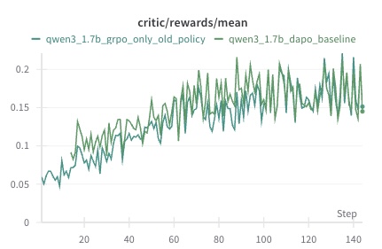
Figure 1: Ablation study based solely on old‑policy policy‑gradient estimation
We conduct this experiment using the qwen3_1.5b-base model on a hybrid dataset comprising the full DAPO-17K corpus and several hundred examples from the AIME dataset (1983–2022). The model is trained for a single epoch, with each prompt used exactly once. We use a total batch size of 128 and a mini-batch size of 32, resulting in each sample being reused for four updates before refreshing the old policy. All remaining hyperparameters follow the DAPO standard configuration. The experiment was run on an H200 GPU cluster for over 24 hours.
As shown in Figure 1, removing importance sampling does not lead to a significant drop in performance. Especially in the latter stages of the algorithm, removing importance sampling even produced a slight performance gain. This result empirically supports our earlier claim that, due to the limited drift between $\pi_{\theta}$ and $\pi_{\theta_{\text{old}}}$ within each update cycle, the policy gradient at $\pi_{\theta_{\text{old}}}$ remains a reliable update direction in practice.
This observation naturally leads to the following idea: if we could modify the importance sampling mechanism in GRPO such that the resulting estimator becomes a consistent and asymptotically unbiased estimate of the current policy gradient $∇ J(\theta)$ , then the algorithm’s performance could be further improved—both in theory and in practice.
A natural candidate for such a correction is to replace the token-level importance weights used in GRPO with a trajectory-level importance ratio. That is, instead of reweighting each token individually, we consider using the probability ratio over the entire trajectory, aligning the estimator more closely with the form of the true policy gradient. This simple yet principled modification forms the basis of our proposed algorithm, which we introduce in the next section.
4 Trajectory-Level Importance-Corrected GRPO (TIC-GRPO)
In this section, we propose our TIC-GRPO, a simple yet principled variant of GRPO. TIC-GRPO replaces the token-level importance sampling mechanism with a single trajectory-level probability ratio:
$$
w^{\prime}(s_{T}^{(i)},\theta,\theta_{\text{old}}):=\frac{\operatorname{\mathbb{P}}_{\theta}(s_{T}^{(i)}\mid s_{0}^{(i)})}{\operatorname{\mathbb{P}}_{\theta_{\text{old}}}(s_{T}^{(i)}\mid s_{0}^{(i)})}.
$$
Moreover, we employ a minor technical modification to the standard clipping mechanism used in importance sampling. The original clipping strategy, as defined in Eq. 2.2, i.e.,
$$
\min\left\{{w^{\prime}(s_{T}^{(i)},\theta,\theta_{\text{old}})}A_{i},\operatorname{clip}\bigl{(}{w^{\prime}(s_{T}^{(i)},\theta,\theta_{\text{old}})},\epsilon_{\text{low}},\epsilon_{\text{high}}\bigr{)}A_{i}\right\},
$$
treats the sign of the estimated advantage $A_{i}$ separately: when $A_{i}≥ 0$ , the importance weight is clipped from above by $1+\epsilon_{\mathrm{high}}$ , whereas when $A_{i}<0$ , it is clipped from below by $1-\epsilon_{\mathrm{low}}$ . However, we observe that retaining only the lower bound $1-\epsilon_{\mathrm{low}}$ while leaving the upper bound unconstrained fails to reduce the variance of the policy gradient estimator effectively even when $A_{i}<0.$ Motivated by this, we adopt a modified clipping scheme in which only the upper bound is enforced, as follows:
$$
\min\left\{{w^{\prime}(s_{T}^{(i)},\theta,\theta_{\text{old}})},\operatorname{clip}\bigl{(}{w^{\prime}(s_{T}^{(i)},\theta,\theta_{\text{old}})},\epsilon_{\text{low}},\epsilon_{\text{high}}\bigr{)}\right\}A_{i}.
$$
It is evident that under our modified clipping scheme, the importance sampling ratio is truncated from above at $1+\epsilon_{\mathrm{high}}$ , regardless of the sign of the estimated advantage $A_{i}$ . In particular, ratios exceeding $1+\epsilon_{\mathrm{high}}$ are clipped, while the lower bound $1-\epsilon_{\mathrm{low}}$ becomes inactive and thus plays no role in the computation. This modification leads to a more effective reduction in the variance of the policy gradient estimator, which in turn results in improved empirical performance.
For notational convenience, we denote:
| | $\displaystyle\overline{\text{clip}}(x,\epsilon_{\text{high}}):=\min\left\{x,\operatorname{clip}\bigl{(}x,\epsilon_{\text{low}},\epsilon_{\text{high}}\bigr{)}\right\}.$ | |
| --- | --- | --- |
All other components remain consistent with the original GRPO formulation. The corresponding optimization objective is given by:
$$
\displaystyle\quad\mathcal{L}_{\text{TIC-GRPO}}(\theta,\theta_{\text{old}},\theta_{\text{ref}}) \displaystyle=\frac{1}{|G|}\sum_{i=1}^{|G|}\frac{1}{|s_{T}^{(i)}|}\sum_{t=1}^{T}\overline{\text{clip}}(w^{\prime}(s_{T}^{(i)},\theta,\theta_{\text{old}}),\epsilon_{\text{high}})A_{i}-\beta\text{D}_{\text{KL}}\bigl{(}\pi_{\theta}\|\pi_{\theta_{\text{ref}}}\bigr{)}. \tag{9}
$$
All other parameters remain identical to those in GRPO and follow the same definitions provided in Section 2.2. Similarly, we present the update rule under a fixed old policy $\pi_{\text{old}}:$
$$
\theta_{n+1}=\theta_{n}+\eta\widehat{\nabla}\mathcal{L}_{\text{TIC-GRPO}}(\theta_{n},\theta_{\text{old}},\theta_{\text{ref}}),
$$
where $\{\eta_{s}\}_{s≥ 1}$ is the learning rate and $\widehat{∇}\mathcal{L}_{\text{TIC-GRPO}}(\theta,\theta_{\text{old}},\theta_{\text{ref}})$ denotes a mini-batch estimate of the gradient $∇\mathcal{L}_{\text{TIC-GRPO}}(\theta,\theta_{\text{old}},\theta_{\text{ref}})$ which can be written as
$$
\displaystyle\quad\nabla\mathcal{L}_{\text{TIC-GRPO}}(\theta,\theta_{\text{old}},\theta_{\text{ref}}) \displaystyle=\underbrace{\frac{1}{|G|}\sum_{i=1}^{|G|}\frac{1}{|s_{T}^{(i)}|}\sum_{t=1}^{T}\nabla\left(\overline{\operatorname{clip}}(w^{\prime}(s_{T}^{(i)},\theta,\theta_{\text{old}}),\epsilon_{\text{high}})\right)A_{i}}_{\emph{Gradient Term}}-\underbrace{\beta\nabla\left(\text{D}_{\text{KL}}\bigl{(}\pi_{\theta}\|\pi_{\theta_{\text{ref}}}\bigr{)}\right)}_{\emph{Penalty Term}}. \tag{10}
$$
As in GRPO, the old policy $\pi_{\theta_{\mathrm{old}}}$ is refreshed every $K$ steps by assigning $\pi_{\theta_{\mathrm{old}}}←\pi_{\theta}$ . The complete algorithm is summarized in the following pseudocode:
Input: reward function $r(·)$ ; initial parameters $\theta$ ; reference parameters $\theta_{\mathrm{ref}}$ ; group size $|G|;$ clipping threshold $\epsilon_{\text{low}},\epsilon_{\text{high}}$ ; KL coefficient $\beta$ ;
inner iterations $K$ ; learning rate $\eta$
1
2 for $n=1$ to $N$ do
3 $\pi_{\theta_{\mathrm{old}}}←\pi_{\theta}$ ;
4
5 Sample $|G|$ trajectories $\{\tau^{(i)}\}_{i=1}^{|G|}\sim\pi_{\theta_{\mathrm{old}}}$ ;
6 $r_{i}← r\!\left(s^{(i)}_{T}\right)$ ;
7
8 $\mu_{G}←\dfrac{1}{|G|}\sum_{i}r_{i}$ ,;
9 $\sigma_{G}←\sqrt{\dfrac{1}{|G|}\sum_{i}\bigl{(}r_{i}-\mu_{G}\bigr{)}^{2}}$ ,;
10 $A_{i}←\dfrac{r_{i}-\mu_{G}}{\sigma_{G}+\delta}$ ;
11
12 for $k=1$ to $K$ do
13 $w_{i,j}←\dfrac{\prod_{j=1}^{T}\pi_{\theta}\bigl{(}s^{(i)}_{j}\mid s^{(i)}_{j-1}\bigr{)}}{\prod_{j=1}^{T}\pi_{\theta_{\mathrm{old}}}\bigl{(}s^{(i)}_{j}\mid s^{(i)}_{j-1}\bigr{)}}$
14 $\displaystyle\mathcal{L}←\frac{1}{|G|}\sum_{i=1}^{|G|}\frac{1}{|s_{T}^{(i)}|}\sum_{j=1}^{T}\left(\overline{\text{clip}}(w^{\prime}(s_{T}^{(i)},\theta,\theta_{\text{old}}),\epsilon_{\text{high}})A_{i}-\beta\text{D}_{\mathrm{KL}}\Bigl{(}\pi_{\theta}\bigl{(}s^{(i)}_{j}\mid s^{(i)}_{j-1}\bigr{)}\|\pi_{\theta_{\mathrm{ref}}}\bigl{(}s^{(i)}_{j}\mid s^{(i)}_{j-1}\bigr{)}\Bigr{)}\right)$ ;
15
16 $\theta←\theta+\eta\hat{∇}\mathcal{L}$ ;
17
18
Algorithm 2 TIC-GRPO
Note: $\hat{∇}$ represents the stochastic gradient computed using a mini-batch of data sampled from the full dataset.
We now apply a decomposition analogous to that in Section 3 to the Gradient Term of TIC-GRPO. Similarly, we begin by defining two events, denoted as
| | $\displaystyle\mathcal{D}(s_{T}^{(i)},\theta,\theta_{\text{old}}):=\left\{w^{\prime}(s_{T}^{(i)},\theta,\theta_{\text{old}})≤ 1+\epsilon_{\text{high}}\right\},$ | |
| --- | --- | --- |
Then we can get:
$$
\displaystyle\quad\text{\emph{Gradient Term}}\mathop{=}^{(*)}\frac{1}{|G|}\sum_{i=1}^{|G|}\frac{1}{|s_{T}^{(i)}|}\sum_{t=1}^{T}\bm{1}_{\mathcal{D}(s_{T}^{(i)},\theta,\theta_{\text{old}})}w^{\prime}(s_{T}^{(i)},\theta,\theta_{\text{old}})\nabla\log\pi_{\theta}(s_{t}^{(i)}|s_{t-1}^{(i)})\cdot A_{i} \displaystyle{=}\frac{T_{\theta_{\text{old}}}^{(-1)}}{\overline{\sigma}_{G}}\underbrace{\frac{1}{|G|}\sum_{i=1}^{|G|}\sum_{t=1}^{T}w^{\prime}(s_{T}^{(i)},\theta,\theta_{\text{old}})\nabla\log\pi_{\theta_{\text{old}}}(s_{t}^{(i)}|s_{t-1}^{(i)})\cdot\left(r_{i}-\overline{\mu}_{G}\right)}_{\widetilde{\nabla}J(\theta)} \displaystyle\quad+\underbrace{\frac{T_{\theta_{\text{old}}}^{(-1)}}{|G|}\sum_{i=1}^{|G|}\sum_{t=1}^{T}\bm{1}_{\mathcal{D}(s_{t}^{(i)},\theta,\theta_{\text{old}})}w^{\prime}(s_{T}^{(i)},\theta,\theta_{\text{old}})\nabla\log\pi_{\theta}(s_{t}^{(i)}|s_{t-1}^{(i)})\cdot\left(A_{i}-\frac{r_{i}-\overline{\mu}_{G}}{\overline{\sigma}_{G}}\right)}_{Sampling\ Error_{1}} \displaystyle+\underbrace{\frac{1}{|G|}\sum_{i=1}^{|G|}\left(T_{\theta_{\text{old}}}^{(-1)}-\frac{1}{|s_{T}^{(i)}|}\right)\sum_{t=1}^{T}\bm{1}_{\mathcal{D}(s_{T}^{(i)},\theta,\theta_{\text{old}})}w^{\prime}(s_{T}^{(i)},\theta,\theta_{\text{old}})\nabla\log\pi_{\theta}(s_{t}^{(i)}|s_{t-1}^{(i)})\cdot A_{i}}_{Sampling\ Error_{2}} \displaystyle\quad\underbrace{-\frac{T_{\theta_{\text{old}}}^{(-1)}}{\overline{\sigma}_{G}}\frac{1}{|G|}\sum_{i=1}^{|G|}\sum_{t=1}^{T}\bm{1}_{\mathcal{D}^{c}(s_{T}^{(i)},\theta,\theta_{\text{old}})}w^{\prime}(s_{T}^{(i)},\theta,\theta_{\text{old}})\nabla\log\pi_{\theta}(s_{t}^{(i)}|s_{t-1}^{(i)})\cdot(r_{i}-\overline{\mu}_{G})}_{\text{\emph{Clip Error}}}. \tag{11}
$$
It is easy to verify that, in the above decomposition, the term $\tilde{∇}J(\theta)$ is an unbiased estimator of the true gradient $∇ J(\theta)$ . This follows from the fact that
$$
\displaystyle\quad\operatorname{\mathbb{E}}_{s^{(1)},\ s^{(2)},...,\ s^{(|G|)}\sim\pi_{\theta_{\text{old}}}}\left[\widetilde{\nabla}J(\theta_{\text{old}})|\mathscr{F}_{\theta_{\text{old}}}\right] \displaystyle=\operatorname{\mathbb{E}}_{s^{(1)},\ s^{(2)},...,\ s^{(|G|)}\sim\pi_{\theta_{\text{old}}}}\left[\frac{1}{|G|}\sum_{i=1}^{|G|}w^{\prime}(s_{T}^{(i)},\theta,\theta_{\text{old}})\left(\nabla\log\left(\prod_{t=1}^{T}\pi_{\theta_{\text{old}}}(s_{t}^{(i)}|s_{t-1}^{(i)})\right)\right)\cdot(r_{i}-\overline{\mu}_{G})\Bigg{|}\mathscr{F}_{\theta_{\text{old}}}\right] \displaystyle=\operatorname{\mathbb{E}}_{s_{T}\sim\pi_{\theta_{\text{old}}}}\left[\frac{\operatorname{\mathbb{P}}_{\theta}(s_{T}|s_{0})}{\operatorname{\mathbb{P}}_{\theta_{\text{old}}}(s_{T}|s_{0})}\left(\nabla\log\operatorname{\mathbb{P}}_{\theta}(s_{T}|s_{0})\right)r(s_{T})\Big{|}\mathscr{F}_{\theta_{\text{old}}}\right]-0 \displaystyle=\nabla J(\theta). \tag{1}
$$
Furthermore, the remaining two error terms can be shown to vanish asymptotically as the number of iterations tends to infinity. Therefore, we can interpret the Gradient Term in TIC-GRPO as a consistent and asymptotically unbiased estimator of the current policy gradient $∇ J(\theta)$ .
Intuitively, TIC-GRPO should be more sample-efficient than the original GRPO, as it directly estimates the current policy gradient rather than relying on outdated surrogate updates. However, such intuition alone is insufficient to rigorously justify the algorithm’s advantage. In the next section, we address this gap by providing formal convergence rate analyses for both GRPO and TIC-GRPO under mild assumptions—specifically, assuming the score function is Lipschitz continuous and the reward function is bounded. To the best of our knowledge, this constitutes the first theoretical convergence analysis for GRPO-style algorithms.
5 Convergence Results
To facilitate convergence analysis, we begin by rewriting both algorithms in iterative update forms:
GRPO
$$
\displaystyle\theta_{n,0}=\theta_{n-1,K}, \displaystyle\theta_{n,s+1}=\theta_{n,s}+\eta\hat{\nabla}\mathcal{L}_{\text{GRPO}}(\theta_{n,s},\theta_{n,0},\theta_{\text{ref}}),\quad(s=0,1,\dots,K). \tag{12}
$$
TIC-GRPO
$$
\displaystyle\theta_{n,0}=\theta_{n-1,K}, \displaystyle\theta_{n,s+1}=\theta_{n,s}+\eta\hat{\nabla}\mathcal{L}_{\text{TIC-GRPO}}(\theta_{n,s},\theta_{n,0},\theta_{\text{ref}}),\quad(s=0,1,\dots,K). \tag{13}
$$
We now present two key assumptions that underlie our convergence analysis for both GRPO and TIC-GRPO.
**Assumption 5.1 (Lipschitz Continuous Score Function)**
*Let $L>0$ be fixed constants. For all states $s_{t}∈\mathcal{S}$ , the score function is Lipschitz continuous in the following sense:
$$
\left\|\nabla\left(\mathrm{KL}\bigl{(}\pi_{\theta}\|\pi_{\theta_{\text{ref}}}\bigr{)}\right)-\nabla\left(\mathrm{KL}\bigl{(}\pi_{\theta^{\prime}}\|\pi_{\theta_{\text{ref}}}\bigr{)}\right)\right\|\leq L_{0}\left\|\theta-\theta^{\prime}\right\|.
$$*
**Assumption 5.2 (L0L_{0}-smooth KL Divergence Estimation Function)**
*Let $L_{0}>0$ be fixed constants. For all states $s_{t}∈\mathcal{S}$ , the KL divergence estimation function is $L_{0}-$ smooth in the following sense:
$$
\left\|\nabla\log\pi_{\theta}(s_{t}\mid s_{t-1})-\nabla\log\pi_{\theta^{\prime}}(s_{t}\mid s_{t-1})\right\|\leq L_{0}\left\|\theta-\theta^{\prime}\right\|.
$$*
In addition, we require a bounded reward assumption, stated as follows:
**Assumption 5.3 (Bounded Reward)**
*There exists a constant $R>0$ such that the absolute value of the terminal reward is uniformly bounded. Specifically, for all $s_{T}$ , we have $|r(s_{T})|≤ R.$*
This is a common and mild assumption in reinforcement learning, especially in the context of LLM-based applications.
We now present our two main theorems, which establish the convergence results for the GRPO algorithm and the TIC-GRPO algorithm, respectively, as follows:
**Theorem 5.1 (Convergence of GRPO)**
*Assume that the conditions stated in Assumptions 5.2 and 5.3 are satisfied. Let $\theta_{1,0}∈\mathbb{R}^{d}$ denote an arbitrary initialization of the algorithm, and we set $\eta_{n}\equiv\eta,\ \beta\equiv 0.$ Then the sequence $\{\theta_{t,k}\}$ generated by GRPO as defined in Eq. 5 admits the following upper bound:
$$
\frac{1}{N}\sum_{n=1}^{N}\operatorname{\mathbb{E}}\left[\|\nabla\mathcal{J}(\theta_{n,0})\|^{2}\right]=\mathcal{O}\left(\eta K\right)+\mathcal{O}\left(\frac{1}{|G|}\right)
$$*
**Theorem 5.2 (Convergence of TIC-GRPO)**
*Assume that the conditions stated in Assumptions 5.2 and 5.3 are satisfied. Let $\theta_{1,0}∈\mathbb{R}^{d}$ denote an arbitrary initialization of the algorithm, and we set $\eta_{n}\equiv\eta,\ \beta\equiv 0.$ Then the sequence $\{\theta_{t,k}\}$ generated by GRPO as defined in Eq. 5 admits the following upper bound:
$$
\frac{1}{N}\sum_{n=1}^{N}\operatorname{\mathbb{E}}\left[\|\nabla\mathcal{J}(\theta_{n,0})\|^{2}\right]=\mathcal{O}\left(\eta K\right)+\mathcal{O}\left(\frac{1}{|G|}\right)
$$*
In the above convergence result, the second term $\mathcal{O}(1/|G|)$ arises from the group-normalization procedure used in GRPO, introducing a dependency on the group size $|G|$ . However, this term becomes negligible in practice as long as each group contains a sufficiently large number of sampled responses.
6 Experiments
We conduct experiments to empirically validate the improved convergence properties of our proposed algorithm, TIC-GRPO, compared to the original GRPO.
Setup.
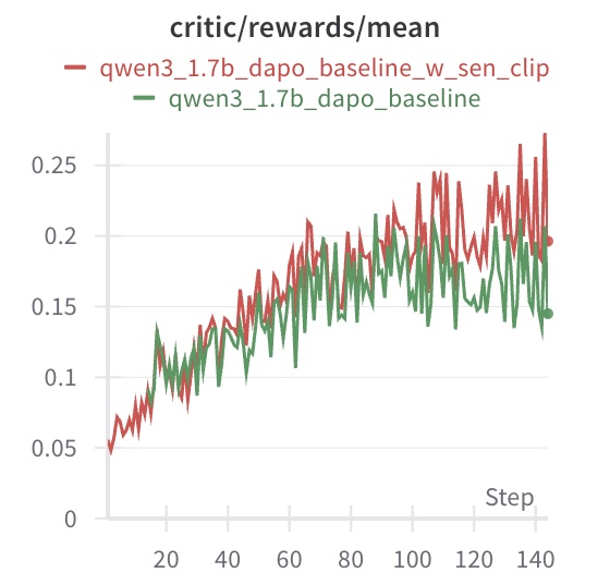
We follow the standard DAPO fine-tuning protocol and use the Qwen1.5B-base model as the backbone. Our training dataset combines the DAPO-17K corpus and a subset of AIME (1983–2022), resulting in a few hundred samples. The model is trained on an H200 GPU for over 24 hours. We set the training batch size to 128 and the mini-batch size to 32, allowing each trajectory to be reused up to 4 times. All other hyperparameters follow the default DAPO configuration. We train for a single epoch, ensuring that each prompt is used only once.
Results.
Figure 2 compares the convergence behavior of TIC-GRPO and GRPO. As shown, TIC-GRPO achieves faster improvement in reward over the same number of gradient steps. This aligns with our theoretical prediction of improved convergence rate with respect to the response length.
<details>
<summary>IMG_0032.jpeg Details</summary>
### Visual Description
## Line Chart: Critic Rewards Mean
### Overview
The image is a line chart comparing the performance of two models, "qwen3_1.7b_dapo_baseline_w_sen_clip" and "qwen3_1.7b_dapo_baseline", based on the critic/rewards/mean metric over a number of steps. The chart displays the trend of the rewards mean for each model as the steps increase.
### Components/Axes
* **Title:** critic/rewards/mean
* **X-axis:** Step, with markers at 0, 20, 40, 60, 80, 100, 120, and 140.
* **Y-axis:** Numerical values ranging from 0 to 0.25, with markers at 0, 0.05, 0.1, 0.15, 0.2, and 0.25.
* **Legend:** Located at the top-left of the chart.
* Red line: qwen3\_1.7b\_dapo\_baseline\_w\_sen\_clip
* Green line: qwen3\_1.7b\_dapo\_baseline
### Detailed Analysis
* **qwen3\_1.7b\_dapo\_baseline\_w\_sen\_clip (Red Line):**
* The line starts at approximately 0.05 at step 0.
* The line generally slopes upward, indicating an increase in the rewards mean as the steps increase.
* The line reaches approximately 0.2 at step 80.
* The line fluctuates between 0.18 and 0.27 from step 80 to 140.
* The final value at step 140 is approximately 0.2.
* **qwen3\_1.7b\_dapo\_baseline (Green Line):**
* The line starts at approximately 0.06 at step 0.
* The line generally slopes upward, indicating an increase in the rewards mean as the steps increase.
* The line reaches approximately 0.18 at step 80.
* The line fluctuates between 0.15 and 0.22 from step 80 to 140.
* The final value at step 140 is approximately 0.15.
### Key Observations
* Both models show an increasing trend in the rewards mean as the steps increase.
* The "qwen3\_1.7b\_dapo\_baseline\_w\_sen\_clip" model (red line) generally performs better than the "qwen3\_1.7b\_dapo\_baseline" model (green line), especially after step 80.
* Both models exhibit fluctuations in their rewards mean, particularly in the later steps.
### Interpretation
The chart suggests that both models improve their performance (as measured by the critic/rewards/mean metric) as they are trained over more steps. The "qwen3\_1.7b\_dapo\_baseline\_w\_sen\_clip" model appears to be more effective than the "qwen3\_1.7b\_dapo\_baseline" model, achieving higher rewards mean values, especially in the later stages of training. The fluctuations in the rewards mean could be due to the inherent variability in the training process or the exploration-exploitation trade-off in reinforcement learning.
</details>
Figure 2: Convergence comparison between TIC-GRPO and GRPO (DAPO).
Conclusion.
These results empirically confirm that TIC-GRPO exhibits a faster convergence rate than standard GRPO (DAPO), especially in the early stages of training.
References
- Schulman et al. (2017) John Schulman, Filip Wolski, Prafulla Dhariwal, Alec Radford, and Oleg Klimov. Proximal policy optimization algorithms. arXiv preprint arXiv:1707.06347, 2017.
- Shao et al. (2024) Zhihong Shao, Peiyi Wang, Qihao Zhu, Runxin Xu, Junxiao Song, Xiao Bi, Haowei Zhang, Mingchuan Zhang, YK Li, Yang Wu, et al. Deepseekmath: Pushing the limits of mathematical reasoning in open language models. arXiv preprint arXiv:2402.03300, 2024.
- Yu et al. (2025) Qiying Yu, Zheng Zhang, Ruofei Zhu, Yufeng Yuan, Xiaochen Zuo, Yu Yue, Weinan Dai, Tiantian Fan, Gaohong Liu, Lingjun Liu, et al. Dapo: An open-source llm reinforcement learning system at scale. arXiv preprint arXiv:2503.14476, 2025.
Appendix A Experimental Timeline and Evidence of Independent Work
We have uploaded our experimental logs to the following GitHub repository: https://github.com/pangleipll/dynamic_sen_clip. According to these logs, we had already completed the main experiments (those presented in Fig. 2) by July 14, which predates the posting of https://arxiv.org/abs/2507.18071 on arXiv. This evidence supports that our study was carried out independently and contemporaneously.