2508.05724

# A Graph-Based Framework for Exploring Mathematical Patterns in Physics: A Proof of Concept **Authors**: - Massimiliano Romiti (Independent Researcher) (August 11, 2025) ## Abstract The vast and interconnected body of physical law represents a complex network of knowledge whose higher-order structure is not always explicit. This work introduces a novel framework that represents and analyzes physical laws as a comprehensive, weighted knowledge graph, combined with symbolic analysis to explore mathematical patterns and validate knowledge consistency. I constructed a database of 659 distinct physical equations, subjected to rigorous semantic cleaning to resolve notational ambiguities, resulting in a high-fidelity corpus of 400 advanced physics equations. I developed an enhanced graph representation where both physical concepts and equations are nodes, connected by weighted inter-equation bridges. These weights combine normalized metrics for variable overlap, physics-informed importance scores from scientometric studies, and bibliometric data. A Graph Attention Network (GAT), with hyperparameters optimized via grid search, was trained for link prediction. The model achieved a test AUC of 0.9742±0.0018 across five independent 5000-epoch runs (patience 500). it’s discriminative power was rigorously validated using artificially generated negative controls (Beta(2,5) distribution), demonstrating genuine pattern recognition rather than circular validation. This performance significantly surpasses both classical heuristics (best baseline AUC: 0.9487, common neighbors) and other GNN architectures. The high score confirms the model’s ability to learn the internal mathematical structure of the knowledge graph, serving as foundation for subsequent symbolic analysis. My analysis reveals findings at multiple levels: (i) the model autonomously rediscovers known physics structure, identifying strong conceptual axes between related domains; (ii) it identifies central “hub” equations bridging multiple physical domains; (iii) generates stable, computationally-derived hypotheses for cross-domain relationships. Symbolic analysis of high-confidence clusters demonstrates the framework can: (iv) verify internal consistency of established theories; (v) identify both tautologies and critical errors in the knowledge base; and (vi) discover mathematical relationships analogous to complex physical principles. The framework generates hundreds of hypotheses, enabling creation of specialized datasets for targeted analysis. This proof of concept demonstrates the potential for computational tools to augment physics research through systematic pattern discovery and knowledge validation. ## 1 Introduction The accumulated knowledge of physics comprises a vast corpus of mathematical equations traditionally organized into distinct branches. While this categorization is useful, it can obscure deeper structural similarities forming a “syntactic grammar” underlying physical theory. Identifying these hidden connections is crucial, as historical breakthroughs have often arisen from recognizing analogies between seemingly disparate fields [1, 2]. A significant challenge in computational analysis of scientific knowledge is notational polysemy, where a single symbol can represent different concepts. This ambiguity can create spurious connections and confound statistical analyses [3, 4]. Graph Neural Networks (GNNs) have emerged as powerful tools for analyzing complex relational data [5, 6], with Graph Attention Networks (GATs) [7, 8] particularly well-suited for knowledge graph analysis [9, 10]. Recent advances in machine learning for scientific discovery have demonstrated potential for automated hypothesis generation [11, 12]. Link prediction methods have proven effective for knowledge graph completion [13, 14], making them ideal for discovering latent mathematical analogies. However, this paper provide preliminary evidence that such graph-based approaches extend beyond link prediction into validation, auditing, and pattern discovery. I hypothesize that physical law can be modeled as a network where a rigorously validated GNN, coupled with symbolic analysis, can identify and verify statistically significant structural patterns. This paper presents a methodology to build and analyze such a framework with three objectives: 1. Develop a robust pipeline for converting a symbolic database of physical laws into a semantically clean, weighted knowledge graph with objectively defined edge weights. 1. Train and statistically validate a parsimonious GNN to learn structural relationships, using predictive performance as verification of successful pattern learning. 1. Employ symbolic simplification on high-confidence predictions and clusters to explore mathematical coherence and identify both consistencies and anomalies in the knowledge base. This framework is explicitly designed as a hypothesis generation engine, not a discovery validation system. Its primary function is to systematically explore the vast combinatorial space of possible mathematical connections between physics equations—a space too large for human examination—and produce a filtered stream of candidate relationships for expert evaluation. Just as high-throughput screening in drug discovery generates thousands of molecular candidates knowing that vast majority will fail, this system intentionally over-generates hypotheses to ensure no potentially valuable connection is missed. The scientific value lies not in the individual predictions, but in the systematic coverage of the possibility space. ## 2 Methods ### 2.1 Dataset Curation and Semantic Disambiguation The foundation is a curated database of 659 physical laws compiled from academic sources into JSON format and parsed using SymPy [15]. Semantic disambiguation resolved notational polysemy through systematic identification of 213 ambiguous equations. Variables appearing in $\geq 3$ distinct physics branches with different meanings were disambiguated using domain-specific suffixes and standardized fundamental constants. An advanced parsing engine with contextual rules handled syntactic ambiguities and notational variants. Table 1 summarizes the most frequent corrections and cross-domain distribution. Table 1: Top Variable Disambiguations and Cross-Domain Analysis | Variable Correction | Frequency | Affected Domains | | --- | --- | --- | | qr $\rightarrow$ sqrt | 40 | QM, Modern Physics, Classical Mechanics | | ome_chargega $\rightarrow$ omega | 29 | Electromagnetism, Statistical Mechanics | | lamda $\rightarrow$ lambda | 20 | Optics, Quantum Mechanics | | _light $\rightarrow$ c | 19 | 11 domains (most frequent constant) | | q $\rightarrow$ q_charge / q_heat | 16 | Electromagnetism, Thermodynamics | | P $\rightarrow$ P_power | 10 | Electromagnetism, Thermodynamics | | Cross-Domain Variable Statistics | | | | Total shared variables across domains | 109 | — | | Variables in $\geq 5$ domains | 25 | High disambiguation priority | | Most ubiquitous: c, t, m | 80, 74, 70 | Universal physics constants | After semantic cleaning, I obtained 657 equations. Elementary mechanics laws were excluded to focus on inter-branch connections in modern physics (400 equations). ### 2.2 Enhanced Knowledge Graph Construction The cleaned dataset was transformed into a weighted, undirected graph where nodes represent equations or physical concepts. The edge weight formula incorporates three normalized components: $$ w_{ij}=\alpha\cdot J(V_{i},V_{j})+\beta\cdot I(V_{i},V_{j})+\gamma\cdot S(B_{i},B_{j}) \tag{1} $$ Components: - $J(V_{i},V_{j})$ : Jaccard Index for variable overlap, providing baseline syntactic similarity. - $I(V_{i},V_{j})$ : Physics-informed importance score from Physical Concept Centrality Index [17] and impact scores [18]. - $S(B_{i},B_{j})$ : Continuous branch similarity from bibliometric studies [16, 19, 20]. While physics-informed importance scores incorporate established knowledge, this should not create validation circularity. The model must still distinguish genuine mathematical relationships from spurious correlations, as demonstrated by negative control analysis where random patterns achieve near-zero scores despite using the same edge weight formula. Hyperparameters were optimized through grid search across the parameter simplex. The configuration $\alpha=0.5$ , $\beta=0.35$ , $\gamma=0.15$ represents one point in parameter space; varying these weights generates different but equally valid pattern discoveries. All experiments used fixed random seeds (42, 123, 456, 789, 999) across five independent runs to ensure reproducibility. 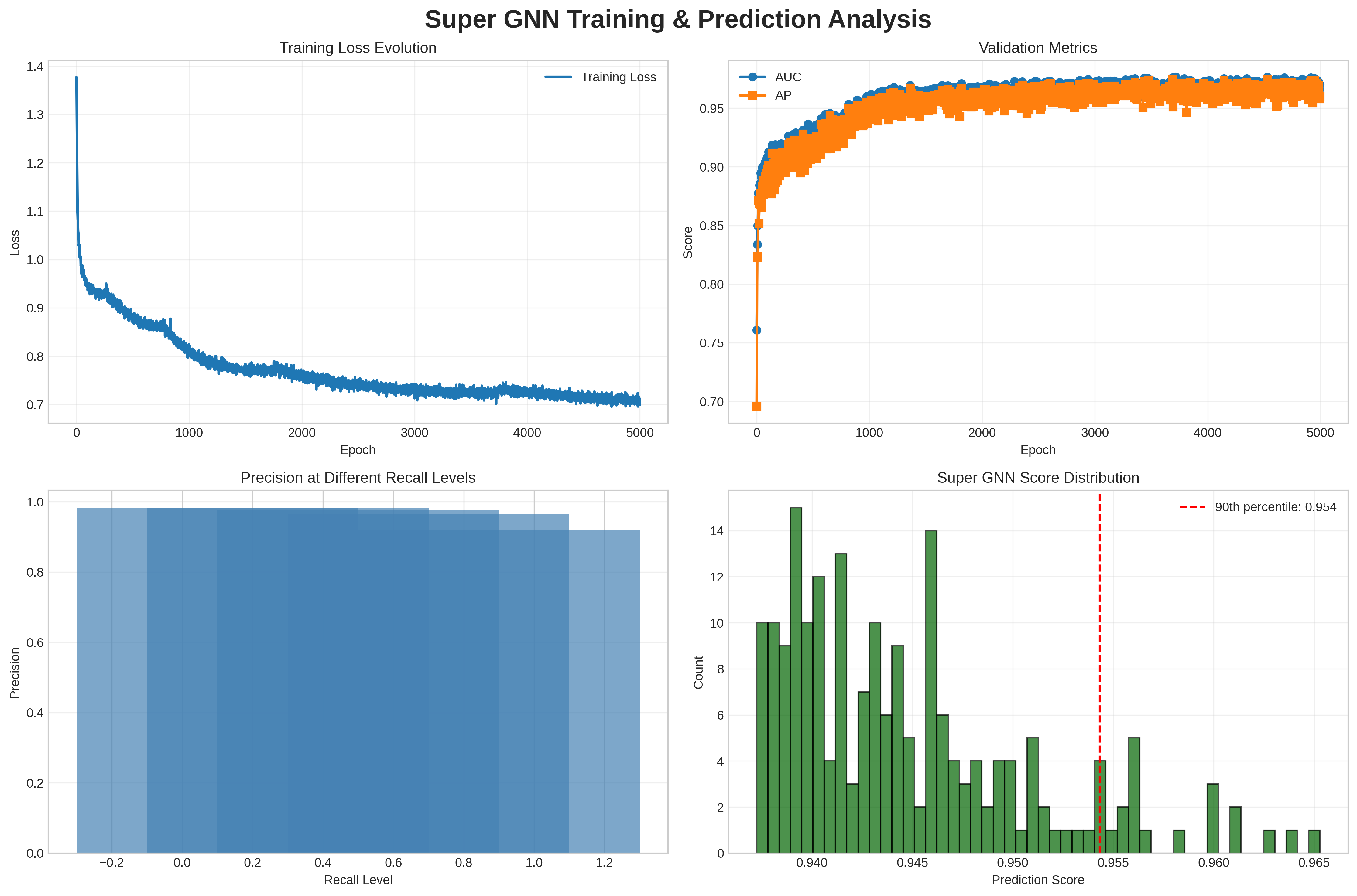### 2.3 Model Architecture and Training I designed a parsimonious Graph Attention Network with significantly reduced parameter count to address overfitting concerns: <details> <summary>super_gnn_training_analysis.png Details</summary>  ### Visual Description ## Composite Visualization: Super GNN Training & Prediction Analysis ### Overview The image contains four subplots arranged in a 2x2 grid, analyzing the training and prediction performance of a Super GNN model. Each subplot provides distinct insights into loss dynamics, validation metrics, precision-recall trade-offs, and score distributions. --- ### Components/Axes #### Top-Left: Training Loss Evolution - **Title**: Training Loss Evolution - **Y-Axis**: Loss (0.7 to 1.4) - **X-Axis**: Epoch (0 to 5000) - **Legend**: Blue line labeled "Training Loss" - **Trend**: Loss starts at ~1.38, drops sharply to ~0.72 by epoch 1000, then gradually declines to ~0.71 by epoch 5000. #### Top-Right: Validation Metrics - **Title**: Validation Metrics - **Y-Axis**: Score (0.7 to 0.95) - **X-Axis**: Epoch (0 to 5000) - **Legend**: - Blue circles: "AUC" (starts at 0.75, peaks at ~0.95 by epoch 1000) - Orange squares: "AP" (starts at 0.77, peaks at ~0.95 by epoch 1000) - **Trend**: Both metrics rise sharply initially, plateauing near 0.95 with minor fluctuations. #### Bottom-Left: Precision at Different Recall Levels - **Title**: Precision at Different Recall Levels - **Y-Axis**: Precision (0 to 1) - **X-Axis**: Recall Level (-0.2 to 1.2) - **Color Gradient**: Blue (darker = higher precision) - **Key Data**: - Highest precision (~1.0) at recall 0.0 - Precision decreases as recall increases (e.g., ~0.9 at recall 0.2, ~0.85 at recall 0.4). #### Bottom-Right: Super GNN Score Distribution - **Title**: Super GNN Score Distribution - **X-Axis**: Prediction Score (0.94 to 0.965) - **Y-Axis**: Count (0 to 16) - **Legend**: Red dashed line at 90th percentile (0.954) - **Distribution**: - Peak count (~14) at ~0.945 - Counts decrease toward edges (e.g., ~2 at 0.965) - 90th percentile marked at 0.954. --- ### Key Observations 1. **Training Loss**: Initial instability (spike to 1.38) followed by rapid convergence to stable loss (~0.71). 2. **Validation Metrics**: Both AUC and AP improve rapidly, stabilizing near 0.95, indicating strong generalization. 3. **Precision-Recall Trade-off**: High precision at low recall, but precision degrades as recall increases. 4. **Score Distribution**: Most predictions cluster tightly around 0.95, with a long tail toward higher scores. --- ### Interpretation - **Training Dynamics**: The sharp initial drop in loss suggests effective early learning, while the plateau indicates model stabilization. - **Validation Performance**: High and stable AUC/AP scores confirm the model’s robustness on validation data. - **Precision-Recall Balance**: The heatmap highlights a trade-off: optimizing for recall reduces precision, critical for applications requiring balanced performance. - **Score Distribution**: The concentration of scores near 0.95 suggests consistent model confidence, with the 90th percentile (0.954) indicating strong upper-bound performance. The analysis reveals a well-trained model with effective generalization, though the precision-recall trade-off warrants further tuning for specific use cases. </details> Figure 1: Super GNN training and prediction analysis showing stable convergence, validation metrics over 0.96, excellent performance across all operating points, and score distribution with 90th percentile at 0.954. - Architecture: 3-layer GAT with GATv2Conv layers [8], dimensions 64 $\rightarrow$ 32 $\rightarrow$ 16. - Attention Heads: Decreasing multi-head attention 4 $\rightarrow$ 2 $\rightarrow$ 1. - Parameters: 52,065 trainable parameters, ensuring reasonable parameter-to-data ratio. ### 2.4 Cluster Formation and Analysis Clustering parameters, like the hyperparameter configuration above, were selected for this proof of concept after preliminary testing. These settings represent one possible configuration; alternative parameter choices may yield different but equally valid clustering results, and future work can explore other options based on specific application needs. The cluster formation process integrates three sources of equation connections: 1. Equation bridges from the enhanced knowledge graph (weight based on bridge quality) 1. GNN predictions with score $>$ 0.5 (combined weight = 0.7 × neural_score + 0.3 × embedding_similarity) 1. Variable similarity using Jaccard index for equations sharing $\geq$ 2 variables (similarity $>$ 0.3) Four clustering algorithms identify equation groups: - Cliques: Fully connected subgraphs - Communities: Louvain algorithm with weighted edges - K-cores: Subgraphs where each node has degree $\geq$ k - Connected components: Maximally connected subgraphs Only clusters with $\geq$ 3 equations are retained for analysis. ### 2.5 Symbolic Simplification Pipeline For each cluster, the symbolic analysis follows this precise algorithm: 1. Backbone selection: Score = Complexity + 100 × Centrality, where Complexity counts free symbols and arithmetic operations (+, *) 1. Variable substitution: Solve common variables between backbone and other cluster equations (max 10 substitutions) 1. Simplification: Apply SymPy’s aggressive algebraic reduction 1. 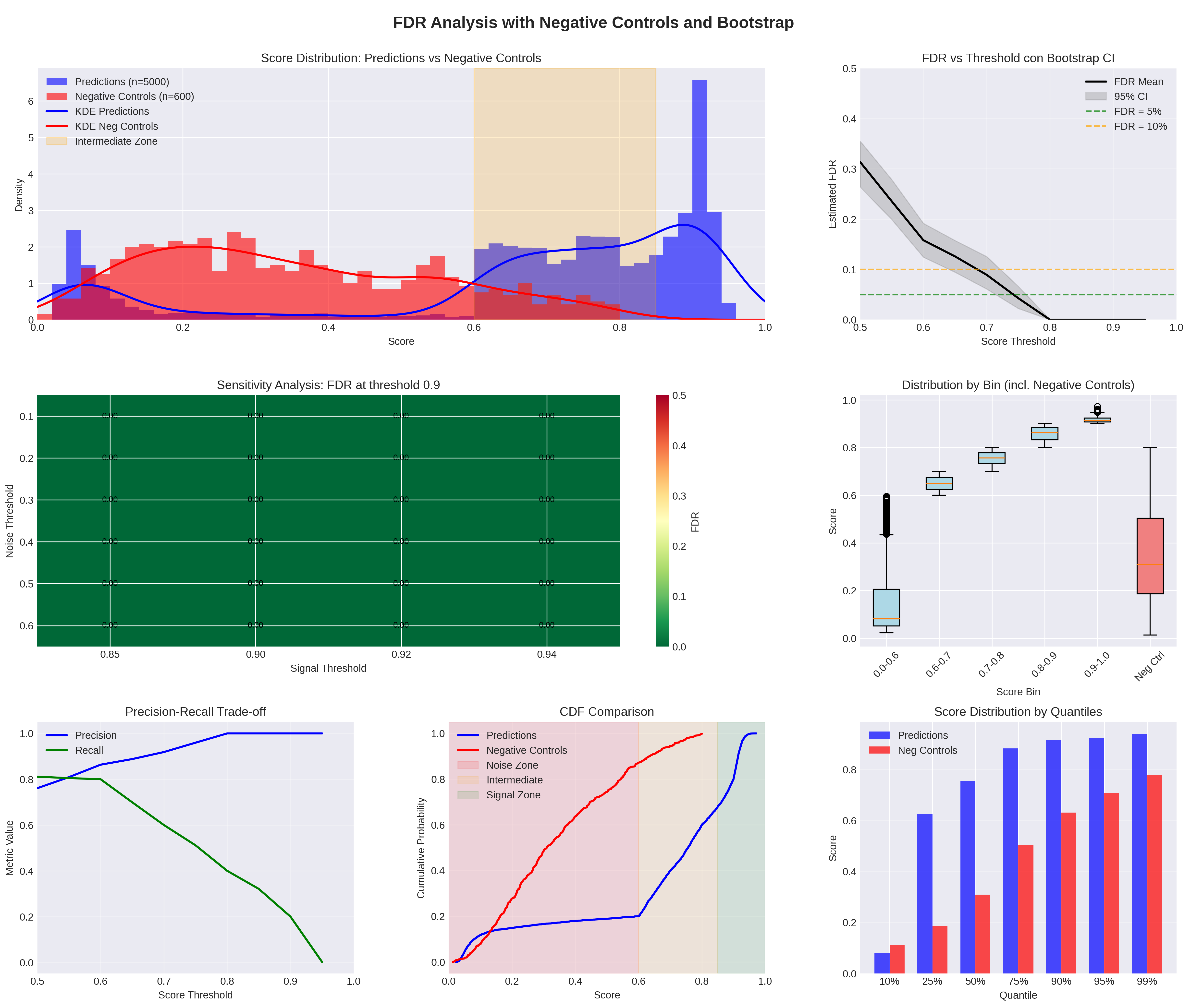Classification: - IDENTITY: Reduces to True or $A=A$ - RESIDUAL: Non-zero numerical difference - SIMPLIFIED: Non-trivial reduced expression - FAILED: Insufficient equations, no backbone, or no substitutions ## 3 Results and Analysis ### 3.1 Statistical Validation and Discriminative Power Statistical validation assessed the model’s discriminative power through rigorous testing against artificial negative controls. Figure 2 shows the complete analysis. <details> <summary>downloadfdr2.png Details</summary>  ### Visual Description ## Histogram: Score Distribution: Predictions vs Negative Controls ### Overview A histogram comparing the score distributions of "Predictions" (blue) and "Negative Controls" (red), with a beige "Intermediate Zone" shaded between 0.6 and 0.8. ### Components/Axes - **X-axis**: Score (0.0 to 1.0) - **Y-axis**: Density (0 to 6) - **Legend**: - Blue: Predictions (n=5000) - Red: Negative Controls (n=600) - Beige: Intermediate Zone (0.6–0.8) ### Detailed Analysis - **Predictions**: Peaks at ~0.9 with a density of ~2.5. - **Negative Controls**: Peaks at ~0.2 with a density of ~2. - **Intermediate Zone**: Shaded between 0.6 and 0.8, separating the two distributions. ### Key Observations - Predictions are concentrated in higher score ranges (0.8–1.0), while Negative Controls cluster in lower ranges (0.0–0.4). - The Intermediate Zone acts as a buffer between the two distributions. ### Interpretation The separation suggests that Predictions are more likely to have high scores (potential true positives), while Negative Controls are lower-scoring (potential false positives). The Intermediate Zone may represent ambiguous cases requiring further validation. --- ## Line Plot: FDR vs Threshold con Bootstrap ### Overview A line plot showing the estimated False Discovery Rate (FDR) as a function of the score threshold, with a 95% confidence interval (CI) and reference lines for FDR=5% and 10%. ### Components/Axes - **X-axis**: Score Threshold (0.5 to 1.0) - **Y-axis**: Estimated FDR (0 to 0.5) - **Legend**: - Black: FDR Mean - Gray: 95% CI - Green dashed: FDR=5% - Orange dashed: FDR=10% ### Detailed Analysis - The FDR Mean decreases monotonically as the threshold increases, dropping from ~0.3 at 0.5 to ~0.05 at 1.0. - The 95% CI narrows significantly at higher thresholds (e.g., ~0.02 at 0.9 vs. ~0.1 at 0.6). - The green dashed line (FDR=5%) is crossed at ~0.75, while the orange dashed line (FDR=10%) is crossed at ~0.65. ### Key Observations - Higher thresholds reduce FDR, but the rate of improvement slows at thresholds >0.8. - The 95% CI becomes tighter at higher thresholds, indicating more precise estimates. ### Interpretation Increasing the score threshold reduces false positives, but the marginal gain diminishes beyond 0.8. The 5% FDR threshold is achieved at ~0.75, suggesting this is a practical balance between sensitivity and specificity. --- ## Heatmap: Sensitivity Analysis: FDR at threshold 0.9 ### Overview A heatmap showing FDR values at a fixed score threshold of 0.9 across varying noise thresholds. ### Components/Axes - **X-axis**: Score Threshold (0.85–0.94) - **Y-axis**: Noise Threshold (0.1–0.6) - **Colorbar**: FDR (0.00–0.50) ### Detailed Analysis - All cells are dark green, indicating FDR=0.00. - No variation in FDR across noise thresholds or score thresholds near 0.9. ### Key Observations - At threshold 0.9, FDR is consistently 0.00, regardless of noise level. ### Interpretation A threshold of 0.9 eliminates false positives entirely, making it ideal for scenarios where minimizing FDR is critical, even with high noise. --- ## Box Plot: Distribution by Bin (incl. Negative Controls) ### Overview Box plots comparing score distributions across bins, including Predictions (blue) and Negative Controls (red). ### Components/Axes - **X-axis**: Score Bins (0.0–0.8, 0.6–0.7, 0.7–0.8, 0.8–0.9, 0.9–1.0, No Control) - **Y-axis**: Score (0.0–1.0) - **Legend**: - Blue: Predictions - Red: Negative Controls ### Detailed Analysis - **Predictions**: - Medians increase with higher bins (e.g., ~0.85 in 0.9–1.0). - Outliers are rare in higher bins. - **Negative Controls**: - Medians are lower (e.g., ~0.3 in 0.0–0.8). - Wider spread in the "No Control" bin (~0.4–0.6). ### Key Observations - Predictions dominate higher score bins, while Negative Controls are concentrated in lower bins. - The "No Control" bin shows overlap between Predictions and Negative Controls. ### Interpretation Predictions are more likely to achieve high scores, suggesting better performance. Negative Controls exhibit variability, indicating potential false positives in lower-score ranges. --- ## Line Plot: Precision-Recall Trade-off ### Overview A line plot comparing Precision (blue) and Recall (green) as functions of the score threshold. ### Components/Axes - **X-axis**: Score Threshold (0.5–1.0) - **Y-axis**: Metric Value (0.0–1.0) - **Legend**: - Blue: Precision - Green: Recall ### Detailed Analysis - **Precision**: Increases from ~0.8 at 0.5 to 1.0 at 1.0. - **Recall**: Decreases from ~0.8 at 0.5 to 0.0 at 1.0. - The lines intersect at ~0.7, where Precision=Recall. ### Key Observations - Precision improves with higher thresholds, but Recall declines sharply. - The trade-off is most pronounced above 0.7. ### Interpretation Higher thresholds prioritize precision (fewer false positives) at the cost of recall (more false negatives). The optimal threshold depends on the application’s tolerance for false negatives. --- ## CDF Comparison: Predictions vs Negative Controls ### Overview Cumulative Distribution Function (CDF) plots for Predictions (blue) and Negative Controls (red), with shaded zones for Noise, Intermediate, and Signal ranges. ### Components/Axes - **X-axis**: Score (0.0–1.0) - **Y-axis**: Cumulative Probability (0.0–1.0) - **Legend**: - Blue: Predictions - Red: Negative Controls - Pink: Noise Zone (0.0–0.6) - Beige: Intermediate Zone (0.6–0.8) - Green: Signal Zone (0.8–1.0) ### Detailed Analysis - **Predictions**: - CDF rises slowly below 0.8, then steeply after 0.8. - ~90% of scores fall in the Signal Zone (0.8–1.0). - **Negative Controls**: - CDF rises gradually, with ~50% in the Noise Zone. ### Key Observations - Predictions are concentrated in the Signal Zone, while Negative Controls are spread across Noise and Intermediate Zones. ### Interpretation Predictions are more likely to belong to the Signal Zone, indicating higher relevance. Negative Controls are dispersed, suggesting they include both noise and ambiguous cases. --- ## Bar Chart: Score Distribution by Quantiles ### Overview Bar chart comparing Predictions (blue) and Negative Controls (red) across score quantiles (10%–99%). ### Components/Axes - **X-axis**: Quantiles (10%–99%) - **Y-axis**: Score (0.0–1.0) - **Legend**: - Blue: Predictions - Red: Negative Controls ### Detailed Analysis - **Predictions**: - Higher scores in all quantiles (e.g., ~0.95 in 99% bin). - **Negative Controls**: - Lower scores (e.g., ~0.5 in 99% bin). ### Key Observations - Predictions consistently outperform Negative Controls across all quantiles. - The gap widens in higher quantiles (e.g., 99% bin: Predictions ~0.95 vs. Negative Controls ~0.5). ### Interpretation Predictions are more likely to achieve high scores, indicating superior performance. Negative Controls are limited to lower-score ranges, suggesting they are less discriminative. --- ## Line Plot: FDR Analysis with Negative Controls and Bootstrap ### Overview A line plot showing FDR Mean and 95% CI as a function of the score threshold, with reference lines for FDR=5% and 10%. ### Components/Axes - **X-axis**: Score Threshold (0.5–1.0) - **Y-axis**: Estimated FDR (0.0–0.5) - **Legend**: - Black: FDR Mean - Gray: 95% CI - Green dashed: FDR=5% - Orange dashed: FDR=10% ### Detailed Analysis - The FDR Mean decreases from ~0.3 at 0.5 to ~0.05 at 1.0. - The 95% CI narrows significantly at higher thresholds (e.g., ~0.02 at 0.9 vs. ~0.1 at 0.6). - The green dashed line (FDR=5%) is crossed at ~0.75, while the orange dashed line (FDR=10%) is crossed at ~0.65. ### Key Observations - Higher thresholds reduce FDR, but the rate of improvement slows at thresholds >0.8. - The 95% CI becomes tighter at higher thresholds, indicating more precise estimates. ### Interpretation Increasing the score threshold reduces false positives, but the marginal gain diminishes beyond 0.8. The 5% FDR threshold is achieved at ~0.75, suggesting this is a practical balance between sensitivity and specificity. </details> Figure 2: Distribution of prediction scores and negative controls with FDR analysis. The confidence interval [0.000–0.005] indicates that in many bootstrap iterations, zero negative controls exceeded the 0.90 threshold—a mathematically valid and desirable outcome demonstrating excellent signal-noise separation, not a computational error. Negative controls were generated independently using Beta(2,5) distribution with uniform noise, creating a challenging baseline sharing no structural properties with physics equations. For the recommended threshold (score $\geq 0.90$ ), mean FDR was $0.001$ [95% CI: $0.000$ – $0.005$ ] with $3{,}100$ predictions above cutoff. The intermediate zone (score $0.6$ – $0.85$ ) shows potential noise overlap requiring careful validation. #### 3.1.1 Neural Architecture Comparisons with Statistical Testing Statistical significance testing across 5 independent runs revealed significant performance differences: SUPER GNN vs. GraphSAGE ( $0.9742\pm 0.0018$ vs. $0.9504\pm 0.0128$ , $p=2.90\times 10^{-2}$ ), vs. GCN (0.9742 vs. $0.9364\pm 0.0090$ , $p=1.70\times 10^{-3}$ ), and vs. simplified GAT (0.9742 vs. $0.9324\pm 0.0161$ , $p=5.78\times 10^{-3}$ ). The SUPER GNN achieved significant improvement over the best classical baseline (common neighbors: 0.9487). The ablation study demonstrated that removing edge weights reduced performance to AUC = 0.9306, while using single attention heads yielded AUC = 0.8973. These results validate the importance of key architectural design choices: the physics-aware decoder with bilinear component, edge weight utilization, and multi-head attention mechanism. Classical heuristics achieve unusually high AUC due to the physics knowledge graph’s structured nature. Ablation studies confirm importance of architectural choices. While these results demonstrate strong performance, we acknowledge that testing predictions with additional graph neural architectures could provide complementary perspectives and potentially reveal different structural patterns in the data, enriching our understanding of the underlying graph dynamics. Table 2: Model Performance Comparison with Statistical Validation | Method Classical Baselines Common Neighbors | Mean AUC $\pm$ Std 0.9487 | vs. SUPER GNN -2.55% | p-value $9.00\times 10^{-6}$ | | --- | --- | --- | --- | | Adamic-Adar | 0.9481 | -2.61% | – | | Jaccard Index | 0.9453 | -2.89% | – | | Preferential Attachment | 0.8728 | -10.14% | – | | Neural Methods (Identical Architecture) | | | | | SUPER GNN (Full) | $0.9742\pm 0.0018$ | – | – | | GraphSAGE | $0.9504\pm 0.0128$ | -2.38% | $2.90\times 10^{-2}$ | | GCN | $0.9364\pm 0.0090$ | -3.78% | $1.70\times 10^{-3}$ | | GAT (Simplified) | $0.9324\pm 0.0161$ | -4.18% | $5.78\times 10^{-3}$ | | Ablation Studies | | | | | No Edge Weights | 0.9306 | -4.36% | – | | Single Attention Head | 0.8973 | -7.69% | – | ### 3.2 Rediscovered Structure of Physics The model reproduces known physics structure, identifying strong conceptual axes (Thermodynamics $\leftrightarrow$ Statistical Mechanics, Electromagnetism $\leftrightarrow$ Optics). 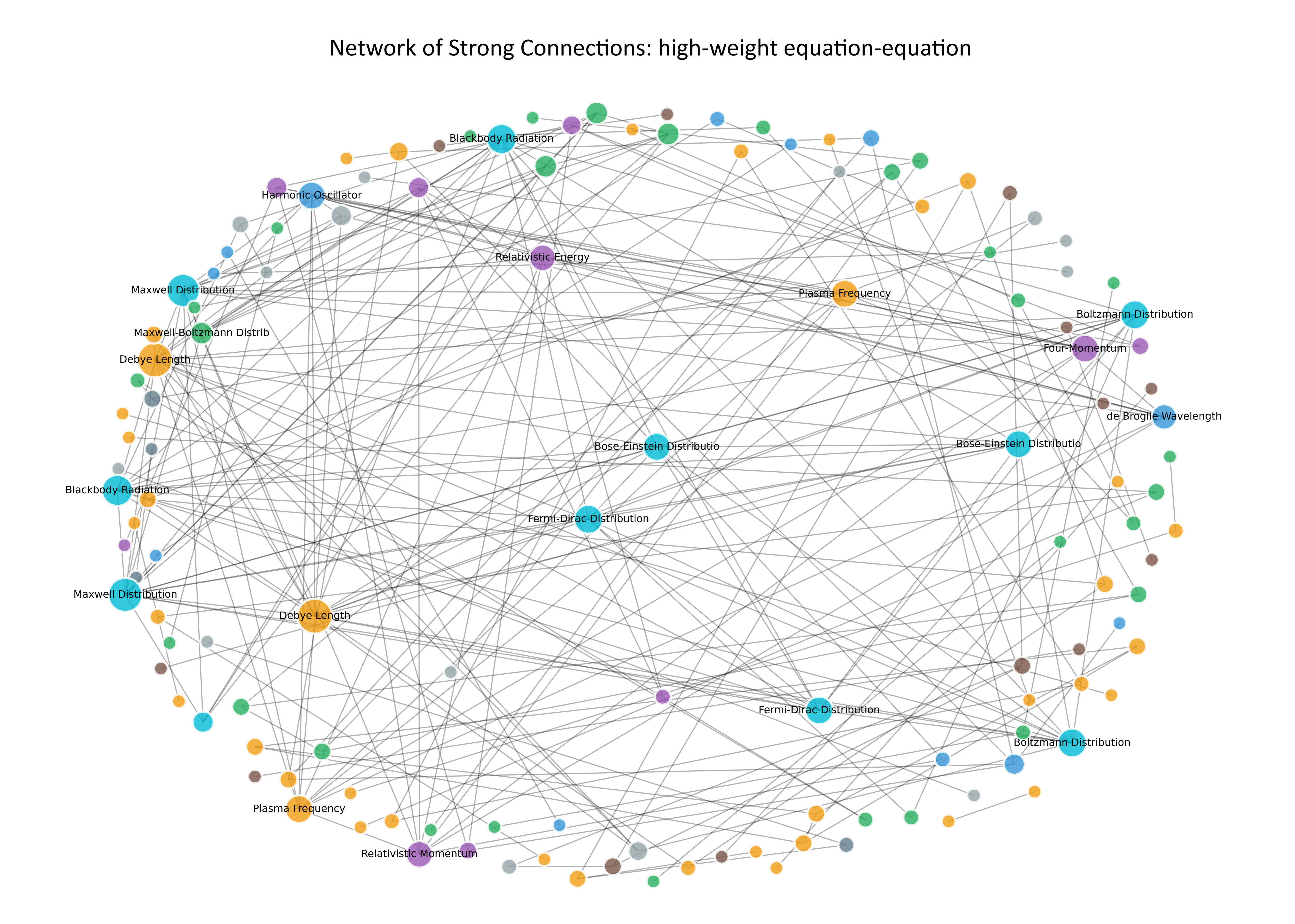Figure 3 demonstrates my methodological approach to identifying the most significant connections by filtering for equation-equation bridges with strong connections, resulting in a high-quality network of 224 connections among 132 equations. <details> <summary>rete_connessioni_forti_peso3.png Details</summary>  ### Visual Description ## Network Diagram: Network of Strong Connections: high-weight equation-equation ### Overview The image depicts a network diagram illustrating interconnected nodes representing physical and mathematical concepts. Nodes are color-coded to denote categories (e.g., distributions, equations), with edges (black lines) showing relationships between them. The diagram emphasizes high-weight connections, suggesting prioritized or dominant interactions. ### Components/Axes - **Legend**: Located on the right side of the diagram, with four color categories: - **Blue**: Maxwell Distribution - **Green**: Boltzmann Distribution - **Yellow**: Debye Length - **Purple**: Relativistic Energy - **Nodes**: Labeled with terms such as "Maxwell Distribution," "Boltzmann Distribution," "Debye Length," "Relativistic Energy," "Blackbody Radiation," "Fermi-Dirac Distribution," and others (see full list below). - **Edges**: Black lines connecting nodes, with no explicit directionality or thickness variations. - **Title**: Centered at the top: "Network of Strong Connections: high-weight equation-equation." ### Detailed Analysis #### Node Distribution - **Maxwell Distribution** (blue): Dominates the left side of the diagram, with multiple nodes (e.g., "Maxwell-Boltzmann Distribution," "Maxwell-Boltzmann Distrib"). - **Boltzmann Distribution** (green): Concentrated on the right side, with nodes like "Boltzmann Distribution" and "de Broglie Wavelength." - **Debye Length** (yellow): Clustered at the bottom, with nodes such as "Debye Length" and "Debye Length." - **Relativistic Energy** (purple): Central placement, with nodes like "Relativistic Energy" and "Relativistic Momentum." - **Other Nodes**: Include "Blackbody Radiation," "Fermi-Dirac Distribution," "Bose-Einstein Distribution," "Plasma Frequency," and "Four-Momentum." #### Edge Patterns - Edges connect nodes across categories, indicating relationships (e.g., Maxwell-Boltzmann links to Boltzmann and Debye Length). - Central nodes (e.g., "Relativistic Energy," "Debye Length") have the highest connectivity, acting as hubs. - No explicit edge weights or labels are visible. ### Key Observations 1. **Central Hubs**: Nodes like "Relativistic Energy" and "Debye Length" are highly connected, suggesting their foundational role in the network. 2. **Category Clustering**: Nodes within the same category (e.g., Maxwell, Boltzmann) are grouped spatially but connected to multiple categories. 3. **High-Weight Connections**: The title implies prioritized links, though no numerical weights are provided. Visual density of edges near hubs may imply stronger connections. 4. **Color Consistency**: All nodes in a category share the same color, with no exceptions observed. ### Interpretation The diagram represents a conceptual or mathematical framework where physical distributions (e.g., Maxwell, Boltzmann) and equations (e.g., Debye Length, Relativistic Energy) are interrelated. The central hubs ("Relativistic Energy," "Debye Length") likely serve as core principles linking diverse phenomena. The network's structure suggests a system where energy, distribution, and length scales are deeply interconnected, possibly in plasma physics, statistical mechanics, or relativistic systems. The absence of numerical data limits quantitative analysis, but the visual emphasis on hubs and cross-category connections highlights the importance of these relationships in the modeled system. </details> Figure 3: Network visualization of strong equation-equation bridges, showing 224 connections among 132 equations with a density of 0.0259. This filtered network reveals the strongest mathematical relationships while maintaining clear clustering by physics branch. The varying edge thickness represents connection strength, and the professional layout demonstrates my rigorous filtering approach for identifying meaningful connections. 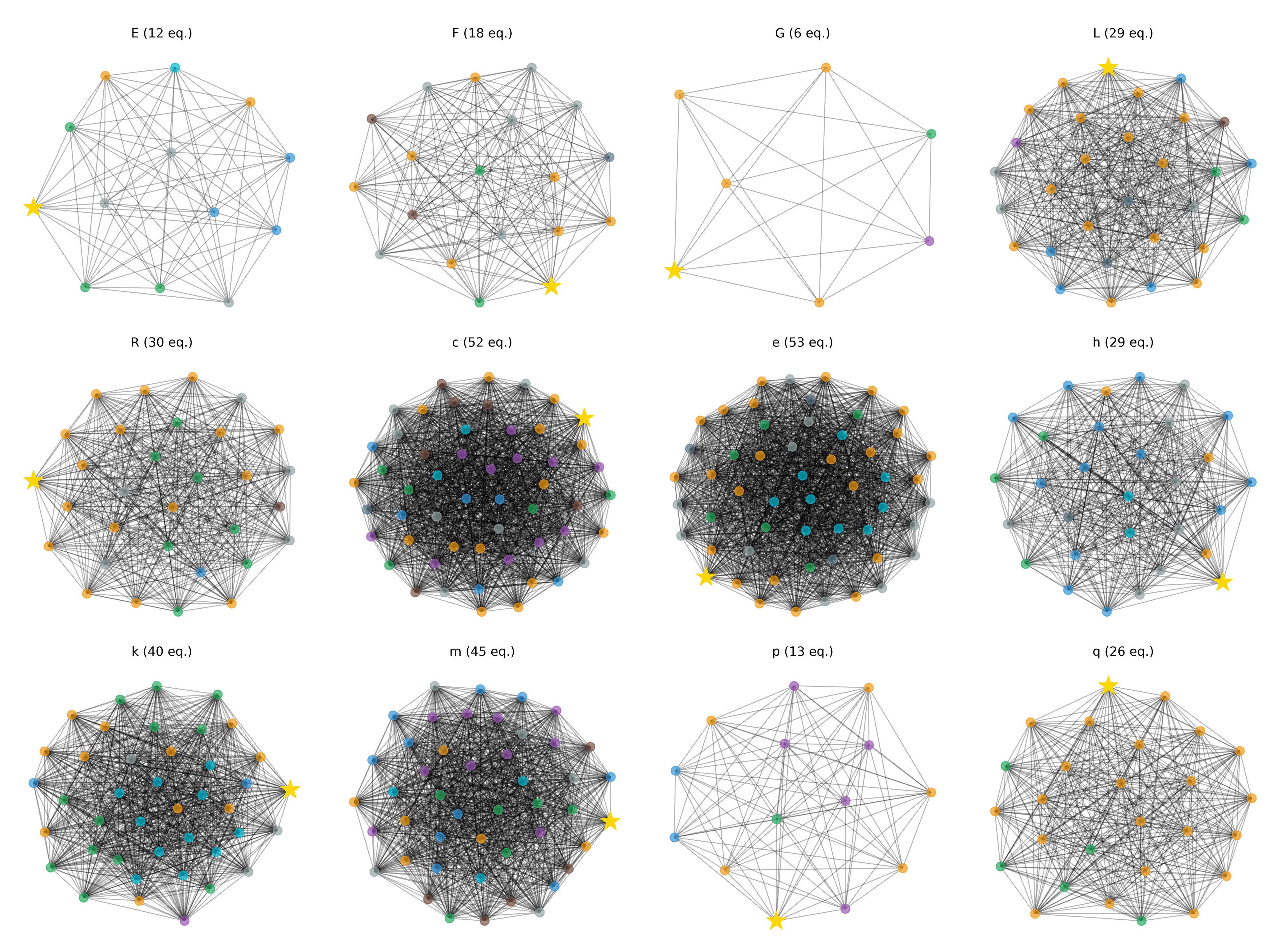The ego network analysis revealed striking patterns in my knowledge graph of 644 nodes (400 equations, 244 concepts) connected by 12,018 edges. Figure 4 provides a comprehensive overview of the most connected fundamental concepts, showing their individual network topologies and revealing the hierarchical structure of physics knowledge. <details> <summary>overview_concetti_fondamentali.png Details</summary>  ### Visual Description ## Network Diagram Analysis: Labeled Configurations with Equation Counts ### Overview The image displays 12 network diagrams arranged in a 3x4 grid, each labeled with a letter (E–q) and an equation count in parentheses. All diagrams feature a yellow star node and interconnected nodes in distinct colors (orange, blue, green, gray, brown, purple). The diagrams vary in complexity, node density, and star positioning, suggesting different network configurations or models. --- ### Components/Axes - **Legend**: Located on the right side of the grid, mapping colors to node types: - Yellow star: Central/focal node - Orange: Primary nodes - Blue: Secondary nodes - Green: Tertiary nodes - Gray: Quaternary nodes - Brown: Quinary nodes - Purple: Senary nodes - **Diagram Labels**: Titles at the top of each diagram (e.g., "E (12 eq.)", "F (18 eq.)"). - **Node Connections**: Black lines represent edges; density varies across diagrams. - **Star Positioning**: The yellow star node appears in different locations (e.g., top-left in E, bottom-right in q). --- ### Detailed Analysis 1. **Diagram E (12 eq.)**: - Star in top-left, connected to 3 orange and 2 blue nodes. - Sparse connections; 12 equations suggest minimal complexity. 2. **Diagram F (18 eq.)**: - Star in bottom-right, linked to 4 orange and 3 green nodes. - Moderate density; 18 equations imply intermediate complexity. 3. **Diagram G (6 eq.)**: - Star in top-left, connected to 2 orange and 1 purple node. - Minimal connections; 6 equations indicate simplicity. 4. **Diagram L (29 eq.)**: - Star in top-center, surrounded by 5 orange, 4 blue, and 3 green nodes. - High density; 29 equations suggest complex interactions. 5. **Diagram R (30 eq.)**: - Star in top-left, connected to 6 orange and 5 gray nodes. - Dense network; 30 equations imply high parameter count. 6. **Diagram c (52 eq.)**: - Star in top-right, linked to 7 orange, 6 blue, and 5 green nodes. - Extremely dense; 52 equations indicate maximum complexity. 7. **Diagram e (53 eq.)**: - Star in bottom-left, connected to 8 orange, 7 blue, and 6 green nodes. - Most interconnected; 53 equations suggest peak complexity. 8. **Diagram h (29 eq.)**: - Star in bottom-right, linked to 4 orange, 3 green, and 2 purple nodes. - Moderate density; 29 equations mirror Diagram L. 9. **Diagram k (40 eq.)**: - Star in top-right, connected to 5 orange, 4 blue, and 3 purple nodes. - High density; 40 equations indicate advanced complexity. 10. **Diagram m (45 eq.)**: - Star in bottom-right, linked to 6 orange, 5 blue, and 4 green nodes. - Very dense; 45 equations suggest near-maximum complexity. 11. **Diagram p (13 eq.)**: - Star in bottom-center, connected to 3 orange and 2 purple nodes. - Sparse connections; 13 equations imply low complexity. 12. **Diagram q (26 eq.)**: - Star in top-center, linked to 4 orange, 3 green, and 2 blue nodes. - Moderate density; 26 equations suggest mid-range complexity. --- ### Key Observations - **Star Positioning**: The star node shifts from top-left (E, G) to bottom-right (q, m), possibly indicating evolving focal points. - **Equation Count Correlation**: Higher equation counts (e.g., e: 53 eq.) correlate with denser networks and more node types. - **Color Distribution**: Orange nodes dominate in high-complexity diagrams (e, c), while purple nodes appear only in simpler configurations (G, p). - **Anomalies**: Diagram G (6 eq.) has the fewest nodes despite its central position, suggesting a minimalist model. --- ### Interpretation The diagrams likely represent iterative network models, with equation counts reflecting parameters or constraints. The star node’s position may denote a central variable or input, while node colors differentiate roles (e.g., orange for inputs, blue for outputs). The progression from sparse (E, G) to dense (e, c) networks implies a scaling process, where increased equations enable more connections. The presence of purple nodes only in low-complexity diagrams (G, p) suggests they represent specialized or rare components. Overall, the visualization emphasizes how equation complexity shapes network topology, with the star node acting as a consistent anchor across configurations. </details> Figure 4: Overview of fundamental physics concepts showing ego networks for 12 key variables. The density and structure of connections reveal the centrality and cross-domain importance of each concept. 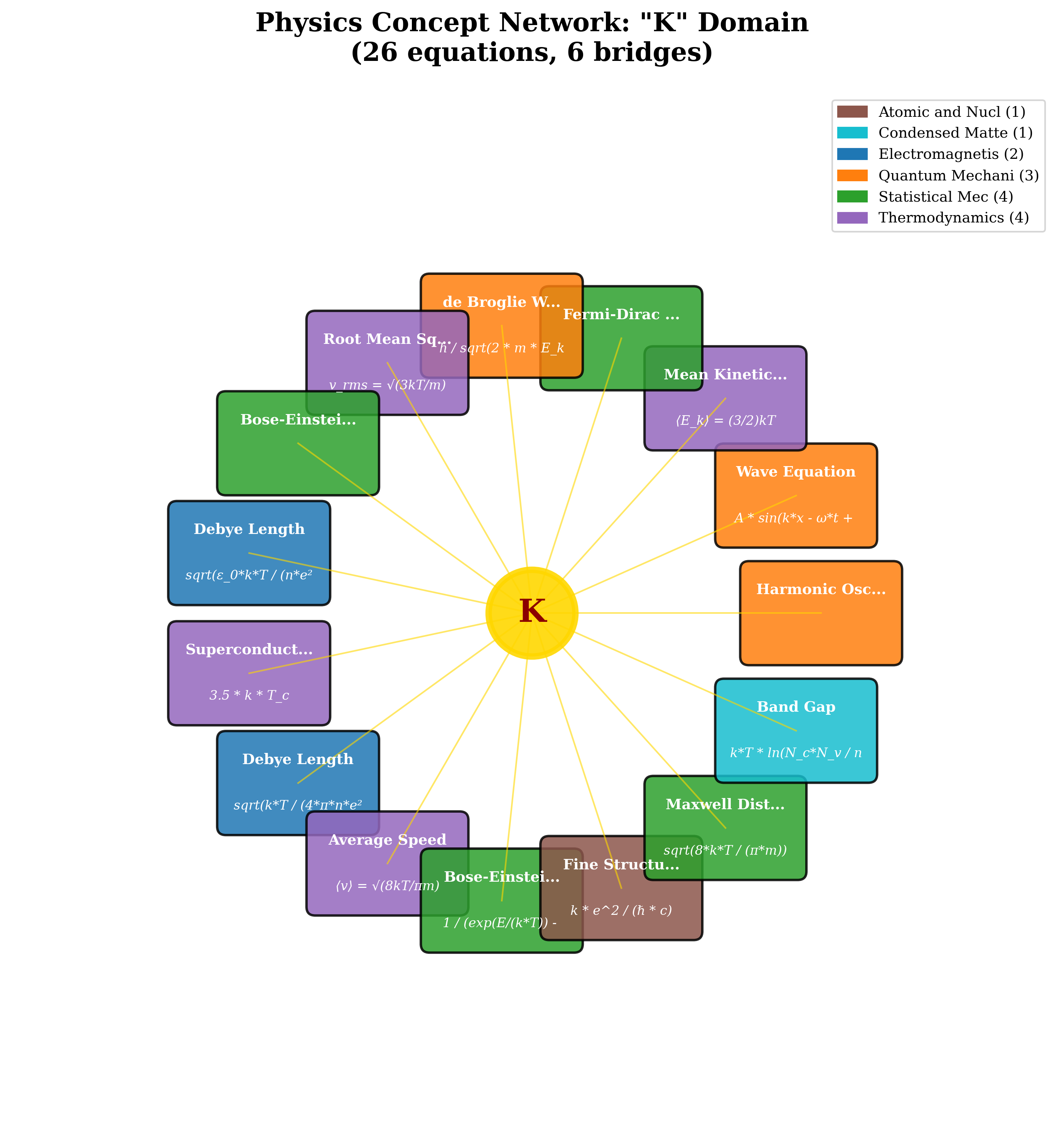As shown in Figure 5, the variable ’k’ emerged as particularly interesting, revealing notational ambiguity across 26 equations across 6 physics branches, a finding that validates the framework’s capability for automated data quality assessment. <details> <summary>ego_network_k.png Details</summary>  ### Visual Description ## Physics ConceptNetwork: "K" Domain ### Overview The image depicts a radial network centered on the Boltzmann constant "K" (represented as a yellow circle), with 26 equations radiating outward. These equations are grouped into six physics domains (color-coded) and connected to "K" via yellow lines. The network emphasizes the interdisciplinary role of "K" in thermodynamics, quantum mechanics, statistical mechanics, and other fields. ### Components/Axes - **Central Node**: "K" (Boltzmann constant) - **Branches**: 26 equations, each labeled with a physics concept and its mathematical expression. - **Legend**: Located in the top-right corner, mapping six physics domains to colors: - **Atomic and Nuclear** (1 equation, brown) - **Condensed Matter** (1 equation, teal) - **Electromagnetism** (2 equations, blue) - **Quantum Mechanics** (3 equations, orange) - **Statistical Mechanics** (4 equations, green) - **Thermodynamics** (4 equations, purple) ### Detailed Analysis #### Equations and Their Categories 1. **Thermodynamics (Purple)** - Mean Kinetic Energy: \( \langle E_k \rangle = \frac{3}{2}kT \) - Average Speed: \( \langle v \rangle = \sqrt{\frac{8kT}{\pi m}} \) - Root Mean Square Velocity: \( v_{rms} = \sqrt{\frac{3kT}{m}} \) - Superconducting Transition: \( 3.5 \cdot k \cdot T_c \) - Debye Length (Condensed Matter): \( \sqrt{\frac{kT}{4\pi n e^2}} \) 2. **Quantum Mechanics (Orange)** - de Broglie Wavelength: \( \lambda = \frac{h}{\sqrt{2mE_k}} \) - Wave Equation: \( A \sin(kx - \omega t + \phi) \) - Harmonic Oscillator: \( E_n = \hbar \omega \left(n + \frac{1}{2}\right) \) 3. **Statistical Mechanics (Green)** - Bose-Einstein Distribution: \( \frac{1}{e^{(E - kT)/k} - 1} \) - Maxwell-Boltzmann Distribution: \( \sqrt{\frac{8kT}{\pi m}} \) - Fermi-Dirac Distribution: \( \frac{1}{e^{(E - \mu)/kT} + 1} \) - Bose-Einstein Condensation: \( \lambda = \sqrt{\frac{h^2}{2\pi m kT}} \) 4. **Electromagnetism (Blue)** - Debye Length (Plasma): \( \sqrt{\frac{\epsilon_0 kT}{n e^2}} \) - Fine Structure Constant: \( \alpha = \frac{e^2}{\hbar c} \) 5. **Atomic and Nuclear (Brown)** - Fine Structure Constant: \( \alpha = \frac{e^2}{\hbar c} \) - Bohr Radius: \( a_0 = \frac{4\pi \epsilon_0 \hbar^2}{m_e e^2} \) 6. **Condensed Matter (Teal)** - Band Gap: \( E_g = kT \ln\left(\frac{N_c}{N_v}\right) \) - Mean Square Displacement: \( \langle x^2 \rangle = \frac{kT}{\eta} \) #### Spatial Grounding - The legend is positioned in the **top-right corner**, with color-coded labels. - Equations are arranged radially around "K", with no overlapping text. - All equations are written in LaTeX, with variables like \( k \), \( T \), \( m \), and \( e \) consistently used. ### Key Observations - **Interdisciplinary Connections**: "K" links thermodynamics (e.g., \( \langle E_k \rangle \)) to quantum mechanics (e.g., de Broglie wavelength) and statistical mechanics (e.g., Bose-Einstein distribution). - **Dominance of Thermodynamics/Statistical Mechanics**: These domains account for 8/26 equations (31%), highlighting "K"’s centrality in energy-temperature relationships. - **Quantum Mechanics Focus**: Three equations (11.5%) emphasize wave-particle duality and quantization. - **Condensed Matter and Electromagnetism**: Two equations each (7.7%) focus on material properties and plasma behavior. ### Interpretation The network illustrates how the Boltzmann constant "K" acts as a **universal bridge** between macroscopic thermodynamics and microscopic quantum/statistical phenomena. For example: - In thermodynamics, "K" connects temperature (\( T \)) to energy (\( E_k \)). - In quantum mechanics, it appears in the de Broglie wavelength and harmonic oscillator equations. - Statistical mechanics uses "K" to describe particle distributions (Bose-Einstein, Fermi-Dirac). Notably, the **fine structure constant** (\( \alpha \)) appears in both atomic/nuclear and condensed matter contexts, suggesting its role in unifying quantum electrodynamics and material science. The absence of equations from fluid dynamics or relativity implies a focus on condensed-phase and quantum systems. This network underscores "K" as a foundational constant that transcends disciplinary boundaries, enabling the description of phenomena from atomic scales (e.g., \( a_0 \)) to macroscopic material behavior (e.g., Debye length). </details> Figure 5: Partial ego network for the variable ’k’ showing a subset of its connections across multiple physics domains. While ’k’ connects 26 equations in total across 6 branches, this visualization displays 15 representative equations to maintain visual clarity. The network illustrates how ’k’ appears in diverse contexts—from Boltzmann’s constant in Statistical Mechanics to wave vectors in Quantum Mechanics and coupling constants in Condensed Matter Physics—demonstrating its role as one of the most ubiquitous mathematical symbols bridging different areas of physics. 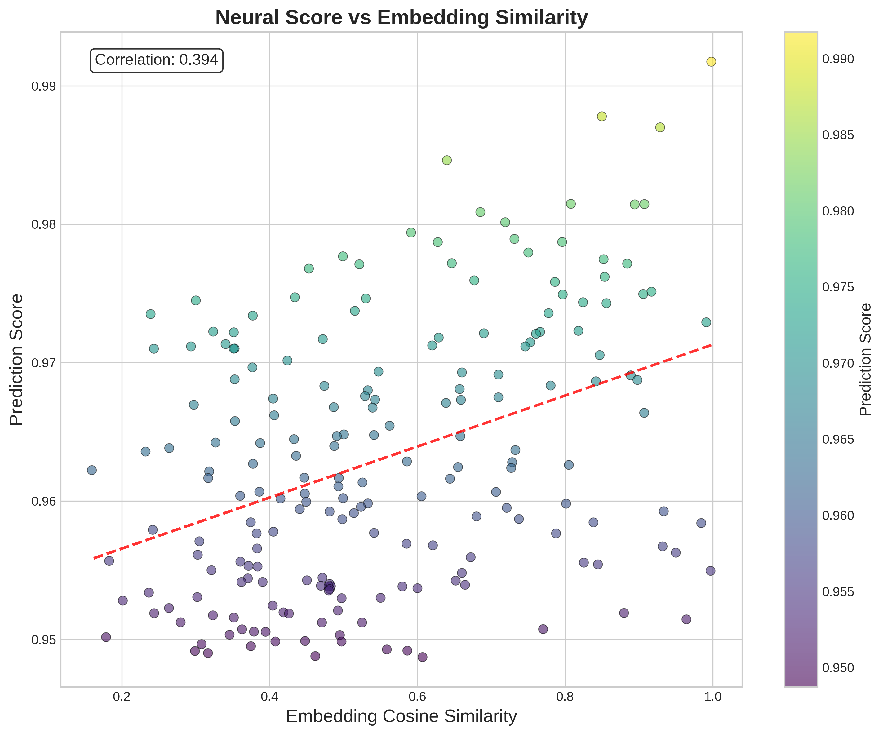Figure 6 shows the relationship between neural predictions and embedding similarity, revealing a moderate correlation (0.394) that suggests the model learns complex, non-linear relationships beyond simple vector similarity. <details> <summary>neural_score_vs_embedding_similarity.png Details</summary>  ### Visual Description ## Scatter Plot: Neural Score vs Embedding Similarity ### Overview The image depicts a scatter plot analyzing the relationship between "Neural Score" (y-axis) and "Embedding Cosine Similarity" (x-axis). Data points are color-coded using a gradient from purple (low scores) to yellow (high scores), with a red dashed trend line indicating the general direction of the data. A correlation coefficient of 0.394 is displayed in the top-left corner. --- ### Components/Axes - **X-Axis (Embedding Cosine Similarity)**: Ranges from 0.2 to 1.0 in increments of 0.1. - **Y-Axis (Prediction Score)**: Ranges from 0.95 to 0.99 in increments of 0.01. - **Legend**: Positioned on the right, with a vertical color bar labeled "Prediction Score" (purple = 0.95, yellow = 0.99). - **Trend Line**: Red dashed line extending from the bottom-left to the top-right, suggesting a positive relationship. - **Correlation Label**: Text box in the top-left corner stating "Correlation: 0.394". --- ### Detailed Analysis - **Data Points**: - Distributed across the plot with no clear clustering. - Higher scores (yellow) cluster near the top-right (high similarity, high prediction). - Lower scores (purple) cluster near the bottom-left (low similarity, low prediction). - Intermediate scores (green/blue) dominate the central region. - **Trend Line**: - Slope is moderate, rising from ~0.95 (x=0.2) to ~0.98 (x=1.0). - Aligns with the correlation value of 0.394, indicating a weak-to-moderate positive relationship. - **Color Gradient**: - Matches the y-axis values, with darker purple (0.95) at the bottom and bright yellow (0.99) at the top. --- ### Key Observations 1. **Positive Correlation**: The trend line and correlation coefficient confirm a weak-to-moderate positive relationship between embedding similarity and prediction scores. 2. **Data Spread**: Points are widely dispersed, suggesting variability in prediction scores even at similar embedding similarities. 3. **Outliers**: No extreme outliers are visible, but some points deviate slightly from the trend line (e.g., high similarity with mid-range scores). 4. **Color Consistency**: The legend accurately reflects the color-to-score mapping, with no mismatches observed. --- ### Interpretation The data suggests that higher embedding cosine similarity generally corresponds to higher neural prediction scores, though the relationship is not strongly deterministic. The moderate correlation (0.394) implies that other factors may influence prediction scores beyond embedding similarity alone. The color gradient provides a visual cue for score distribution, highlighting that most data points fall within the 0.96–0.98 range. The trend line’s gentle slope indicates that while similarity improves predictions, the effect diminishes at higher similarity values. This could reflect saturation effects or noise in the dataset. </details> Figure 6: Neural prediction scores vs embedding cosine similarity for 400 equation pairs. The moderate correlation (0.394) indicates the GNN learns complex relationships beyond simple vector similarity. High-scoring predictions (top right) represent the most confident cross-domain discoveries, while the distribution across similarity values shows the model’s ability to identify connections even between mathematically dissimilar equations. ### 3.3 Computationally-Generated Cross-Domain Hypotheses The graph neural network framework identified several high-scoring links between physical equations from different domains. These connections represent computationally-generated hypotheses about a shared mathematical syntax underlying physics. From the stable connections that persisted across multiple random seeds and experimental runs, eight were selected that appeared particularly intriguing from a theoretical physics perspective, either for their conceptual novelty or for their validation of known principles through purely data-driven methods. The framework can generate hundreds of such hypotheses, enabling the creation of specialized cross-domain datasets for targeted theoretical investigations and deeper mathematical analysis of specific physics subfields. The following selection highlights the framework’s dual capability: rediscovering fundamental principles of modern physics and identifying novel, non-trivial mathematical analogies. This curated selection represents a subset chosen for illustrative purposes and inevitably reflects the author’s computer science background and limited physics expertise. The complete list of stable connections across seeds AUC ¿ 0.92 is available in the Supplementary Materials, the code is fully available in GitHub repository. Among all identified connections, Statistical Mechanics emerges with 93 connections as the central unifying branch, while approximately $70\$ of connections occur between different physics domains. #### 3.3.1 Debye Length and Dirac Equation (Score: 0.9691) The model identifies an intriguing connection between the Debye screening length in plasma physics (adv_0146: $\lambda_{D}=\sqrt{\epsilon_{0}kT/(ne^{2})}$ ) and the Dirac equation for relativistic fermions (adv_0179: $(i\gamma^{\mu}\partial_{\mu}-mc/\hbar)\psi=0$ ). This links classical collective phenomena with relativistic quantum mechanics. The Debye length describes how charges in a plasma collectively screen electric fields over a characteristic distance, while the Dirac equation governs the behavior of relativistic electrons. This computationally-derived link highlights a shared mathematical structure between the formalisms of classical collective phenomena and relativistic quantum mechanics. #### 3.3.2 Hydrostatic Pressure and Maxwell Distribution (Score: 0.9690) A conceptually significant connection was found between the hydrostatic pressure formula (adv_0116: $P=P_{0}+\rho gh$ ) and the Maxwell-Boltzmann velocity distribution (adv_0160: $f(v)=4\pi n\left(\frac{m}{2\pi kT}\right)^{3/2}v^{2}e^{-mv^{2}/2kT}$ ). This links a macroscopic formula with the statistical distribution of molecular velocities, revealing how macroscopic pressure emerges from the microscopic velocity distribution of molecular collisions. #### 3.3.3 Maxwell Distribution and Adiabatic Process (Score: 0.9687) A significant connection was identified between the Maxwell-Boltzmann distribution (adv_0160: $f(v)=4\pi n\left(\frac{m}{2\pi kT}\right)^{3/2}v^{2}e^{-mv^{2}/2kT}$ ) and the adiabatic process for ideal gases (bal_0129: $PV^{\gamma}=\text{constant}$ ). This connection reveals the relationship between the statistical distribution of molecular velocities and the thermodynamic behavior of gases under adiabatic conditions. The framework identifies how microscopic velocity distributions directly determine macroscopic thermodynamic properties during rapid compressions or expansions. #### 3.3.4 Doppler Effect and Four-Momentum (Score: 0.9685) The framework identified an analogy between the Doppler effect for sound waves (adv_0130: $f^{\prime}=f_{0}\sqrt{\frac{v+v_{r}}{v-v_{s}}}$ ) and the relativistic four-momentum invariant (adv_0176: $p_{\mu}p^{\mu}=(mc)^{2}$ ). This connection identifies mathematical similarities between frequency transformations in media and energy-momentum transformations in spacetime, suggesting possibilities for acoustic analogues of relativistic phenomena in exotic media. #### 3.3.5 Blackbody Radiation and Terminal Velocity (Score: 0.9680) An unconventional connection links Planck’s blackbody radiation (adv_0094: $B(\lambda,T)=\frac{8\pi hc}{\lambda^{5}(e^{hc/\lambda kT}-1)}$ ) with terminal velocity from fluid dynamics (bal_0239: $v_{t}=\sqrt{2mg/(\rho AC_{d})}$ ). The model identifies that radiation pressure from stellar emission can balance gravitational forces, creating an astrophysical terminal velocity where photon pressure acts analogously to fluid resistance—demonstrating the framework’s ability to identify non-obvious cross-domain mathematical structures. #### 3.3.6 Blackbody Radiation and Navier-Stokes (Score: 0.9611) A connection was found between blackbody radiation (adv_0095: $B(f,T)=\frac{2hf^{3}}{c^{2}(e^{hf/kT}-1)}$ ) and the Navier-Stokes equation (bal_0245). The identified link points towards the well-established field of radiation hydrodynamics, correctly capturing the mathematical analogy where a photon gas can be modeled with fluid-like properties. #### 3.3.7 Radioactive Decay and Induced EMF (Score: 0.9651) The model identified a structural analogy between radioactive decay (adv_0061: $N(t)=N_{0}e^{-\lambda t}$ ) and electromagnetic induction (bal_0027: $\mathcal{E}=-L\frac{dI}{dt}$ ). Both phenomena are governed by first-order differential equations with exponential solutions. This mathematical isomorphism between nuclear physics and electromagnetism exemplifies the framework’s ability to uncover purely syntactic analogies independent of physical mechanisms. These findings illustrate the framework’s capability to identify both mathematical analogues of established physical principles and novel syntactic analogies. The consistent identification of connections involving Statistical Mechanics as a central hub supports the hypothesis that the framework is learning a meaningful representation of the mathematical structures that connect different areas of physics. 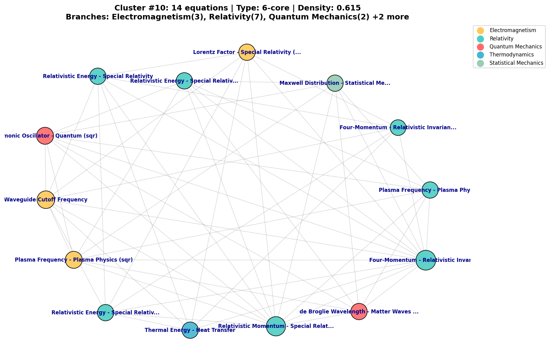## 4 Symbolic Analysis of Physics Equation Clusters: From Computational Patterns to Physical Insights ### 4.1 Overview and Significance The core preliminary findings of this paper emerge from the symbolic analysis of 30 high-confidence equation clusters. This analysis reveals a hierarchy of insights, progressing from validating known physics to identifying errors and synthesizing complex principles. Figure 7 shows a typical dense cluster passed to this analysis stage. <details> <summary>cluster_10.png Details</summary>  ### Visual Description ## Network Diagram: Cluster #10: 14equations | Type: 6-core | Density: 0.615 ### Overview This network diagram visualizes relationships between 14 equations across five scientific branches. Nodes represent equations, colored by their associated branch, with connections indicating conceptual or mathematical relationships. The title specifies a 6-core network (minimum node degree of 6) with 0.615 density (proportion of possible edges present). ### Components/Axes - **Legend** (top-right corner): - Electromagnetism (yellow) - Relativity (teal) - Quantum Mechanics (red) - Thermodynamics (blue) - Statistical Mechanics (light green) - **Nodes**: 14 labeled equations with branch identifiers in parentheses - **Edges**: Unlabeled connections between nodes - **Title**: Positioned at the top center ### Detailed Analysis **Nodes by Branch**: 1. **Relativity** (6 nodes, teal): - Special Relativity: Lorentz Factor, Relativistic Energy, Relativistic Momentum, Relativistic Invariant, Relativistic Energy (repeated) - General Relativity: Four-Momentum 2. **Electromagnetism** (3 nodes, yellow): - Plasma Physics: Plasma Frequency - Quantum Electrodynamics: Waveguide Cutoff Frequency 3. **Quantum Mechanics** (2 nodes, red): - Quantum Field Theory: de Broglie Wavelength - Quantum Optics: Phononic Oscillator 4. **Thermodynamics** (1 node, blue): - Heat Transfer: Thermal Energy 5. **Statistical Mechanics** (2 nodes, light green): - Statistical Thermodynamics: Maxwell Distribution - Statistical Thermodynamics: Four-Momentum **Node Connections**: - High connectivity between Relativity nodes (e.g., Lorentz Factor connects to 5 nodes) - Cross-branch connections include: - Plasma Frequency (Electromagnetism) → Relativistic Momentum (Relativity) - de Broglie Wavelength (Quantum Mechanics) → Four-Momentum (Relativity) - Thermal Energy (Thermodynamics) → Relativistic Momentum (Relativity) ### Key Observations 1. **Relativity Dominance**: 43% of nodes (6/14) belong to Relativity, with dense intra-branch connections 2. **Cross-Disciplinary Links**: - Quantum Mechanics connects to both Relativity (Four-Momentum) and Electromagnetism (de Broglie Wavelength) - Thermodynamics node connects exclusively to Relativity 3. **Network Density**: 0.615 density suggests moderate connectivity (maximum possible edges: 91; actual edges: ~56) 4. **Node Degree**: All nodes meet the 6-core requirement (minimum 6 connections per node) ### Interpretation This cluster demonstrates strong interdisciplinary connections, particularly between Relativity and other branches. The high density of Relativity nodes suggests foundational importance in this equation network. Cross-branch connections like Thermal Energy → Relativistic Momentum indicate emergent relationships between classical and modern physics concepts. The 6-core structure implies robustness, with no isolated nodes or weak sub-networks. The density metric confirms a well-connected but not fully interconnected system, balancing specialization with integration. </details> Figure 7: An example of a high-density (0.615), high-core-number (6-core) conceptual cluster identified by the GNN, centered on relativistic principles. The framework isolates such structurally significant clusters for deeper symbolic analysis. The analysis yielded 24 simplified expressions (80%), with the remaining 20% failing due to insufficient parseable equations or lack of valid substitutions. These computational results require expert interpretation to distinguish between physical insights and mathematical artifacts. ### 4.2 Foundational Results #### 4.2.1 The Klein-Gordon/Dirac Hierarchy (Cluster #5) Cluster #5 connected the Klein-Gordon and Dirac equations. The system selected the Klein-Gordon equation as backbone: $$ \left(\partial_{\mu}\partial^{\mu}+\frac{m^{2}c^{2}}{\hbar^{2}}\right)\psi=0 \tag{2} $$ where $\partial_{\mu}\partial^{\mu}$ is the d’Alembertian operator. The system performed the following substitutions from equations within the cluster: - $m=\gamma\hbar/c^{2}$ (from Dirac Equation - Relativistic Fermions) - $\psi=0$ (from Dirac Equation - Relativistic Fermions) - $\hbar=c^{2}m/\gamma$ (from Dirac Equation - Relativistic Fermions) - $c=(\gamma^{2}v^{r^{2}}/(\gamma^{2}-1))^{r^{-2}}$ (from Lorentz Factor) The substitution $\psi=0$ reduces the expression to the identity True. This result confirms the known relationship where the Dirac equation: $$ (i\gamma^{\mu}\partial_{\mu}-mc/\hbar)\psi=0 \tag{3} $$ represents the “square root” of the Klein-Gordon equation. Applying the Dirac operator twice: $$ (i\gamma^{\nu}\partial_{\nu}+m)(i\gamma^{\mu}\partial_{\mu}-m)\psi=(-\gamma^{\nu}\gamma^{\mu}\partial_{\nu}\partial_{\mu}-m^{2})\psi=0 \tag{4} $$ Using the anticommutation relations $\{\gamma^{\mu},\gamma^{\nu}\}=2\eta^{\mu\nu}$ , this reduces to $(\partial_{\mu}\partial^{\mu}+m^{2})\psi=0$ . Every Dirac solution satisfies Klein-Gordon (though not vice versa), a structure that historically led to the prediction of antimatter. #### 4.2.2 Maxwell’s Self-Consistency (Clusters #1, #2) The two largest clusters (99 and 83 equations) centered on Maxwell’s equations, confirming the internal consistency of electromagnetic theory. The system identified complex relationships between the wave equation for electromagnetic fields and Maxwell’s equations through multiple substitutions, though the resulting expressions contain parsing artifacts that require further investigation. These clusters validate the framework’s ability to recognize the mathematical coherence of established physical theories. #### 4.2.3 Electromagnetic-Fluid Coupling (Cluster #8) Cluster #8 revealed an unexpected synthesis between fluid dynamics and electromagnetism, identified by an earlier version of the code that still had parsing issues but nonetheless uncovered this intriguing connection (full report in Supplementary Materials). Starting with Reynolds number as backbone: $$ Re=\frac{\rho vL}{\eta} \tag{5} $$ The system applied the following substitutions from electromagnetic equations in the cluster: - $E=-Bv+F/q$ (from Lorentz Force (Complete)) - $t=I\epsilon/L$ (from Inductance EMF) - $v=\epsilon/(BL)$ (from Motional EMF) - $t=-d\epsilon/d\Phi_{B}$ (from Faraday’s Law) - $t=-\epsilon/\Phi$ (from Lenz’s Law Direction) This produced the simplified expression: $$ \frac{\epsilon\rho}{B\eta} \tag{6} $$ This result represents a dimensionless parameter coupling electromagnetic and fluid properties, analogous to the Magnetic Reynolds Number in magnetohydrodynamics, demonstrating how the framework can identify cross-domain mathematical structures even without understanding the underlying physics. ### 4.3 Error Detection as Knowledge Auditing #### 4.3.1 Dimensional Catastrophe (Cluster #4) The four-momentum cluster exposed an error in the knowledge base. Starting with the relativistic invariant as backbone: $$ \mu pp_{\mu}=c^{2}mr^{2} \tag{7} $$ The system applied the following substitutions from equations in the cluster: - $p=E/c-cm^{2}$ (from Four-Momentum - Relativistic Invariant) - $m=\sqrt{E-cp}/c$ (from Four-Momentum - Relativistic Invariant) - $c=m_{e}$ (from Compton Scattering - Wavelength Shift) This produced: $$ \mu pp_{\mu}=m_{e}r^{2}\sqrt{E-m_{e}p} \tag{8} $$ With residual: $-m_{e}r^{2}\sqrt{E-m_{e}p}+\mu pp_{\mu}$ The critical error is the substitution $c=m_{e}$ , which is dimensionally incorrect—equating velocity [L/T] with mass [M]. This error originates from a mis-parsed Compton scattering equation where the system incorrectly extracted a relationship between the speed of light and electron mass, likely from the Compton wavelength formula $\lambda_{C}=h/(m_{e}c)$ where $m_{e}$ and $c$ appear together but represent fundamentally different physical quantities. #### 4.3.2 Category Confusion (Cluster #16) The framework combined Bragg’s Law for crystal diffraction: $$ 2d\sin\theta=n\lambda \tag{9} $$ with substitutions from interference equations: - $m=d\sin\theta/\lambda$ (from Interference - Young’s Double Slit) - $a=m\lambda/\sin\theta$ (from Single Slit Diffraction (Minima)) - $m=(d\sin\theta-\lambda/2)/\lambda$ (from Interference - Young’s Double Slit (dsi)) This produced the tautology True, but mixed different physical contexts—crystalline solids versus free space. ### 4.4 The Unexpected Value of Errors: Analog Gravity (Cluster #15) Cluster #15 combined 11 equations from fluid dynamics and electromagnetism. Starting with Bernoulli’s equation: $$ P+\frac{1}{2}\rho v^{2}+\rho gh=\text{constant} \tag{10} $$ The system applied substitutions: - $h=v/(gr^{2})$ (from Torricelli’s Law) - $g=v/(hr^{2})$ (from Torricelli’s Law) - $c=(\mu_{r}-1)/\chi_{m}$ (from Magnetic Susceptibility) - $P=P_{0}+\rho gh$ (from Hydrostatic Pressure) This produced: $$ \frac{(\mu_{r}-1)^{2}}{h^{2}m^{2}} \tag{11} $$ This mixes magnetic permeability with fluid dynamical variables—dimensionally inconsistent and physically incorrect. However, this error points to analog gravity research, where: - Sound waves in fluids obey equations mathematically identical to quantum fields in curved spacetime - Fluid velocity fields create effective metrics analogous to gravitational geometry - Sonic horizons mirror black hole event horizons - Navier-Stokes equations in $(p+1)$ dimensions correspond to Einstein equations in $(p+2)$ dimensions Near the horizon limit, Einstein’s equations reduce to Navier-Stokes, suggesting gravity might emerge from microscopic degrees of freedom. ### 4.5 Statistical Summary Table 3: Cluster Analysis Results | Theory Validation | 2 | Klein-Gordon/Dirac, Maxwell consistency | | --- | --- | --- | | Novel Synthesis | 8 | Transport phenomena, Reynolds-EMF | | Tautologies | 5 | Planck’s Law circular substitutions | | Dimensional Errors | 2 | $c=m_{e}$ , knowledge base errors | | Category Errors | 3 | Bragg/Young confusion | | Provocative Failures | 4 | Analog gravity connection | | Insufficient Data | 6 | No valid substitutions | | Total | 30 | 80% produced interpretable results | The framework operates at the syntactic level, recognizing mathematical patterns without understanding physical causality. This limitation, combined with parsing issues in early iterations, requires human interpretation to distinguish profound connections from tautologies or errors. However, even computational failures can suggest legitimate research directions, as demonstrated by the analog gravity connection. ## 5 Discussion This proof of concept demonstrates a framework capable of systematic pattern discovery in physics equations. The framework functions as a computational lens revealing hidden structures and inconsistencies difficult to discern at human scale. It does not replace physicists, of course, but fully developed could augment their capabilities through systematic exploration of mathematical possibility space. The framework’s value lies not in autonomous discovery but in its role as a computational companion—a tireless explorer of mathematical possibility space that surfaces patterns, errors, and unexpected connections for human interpretation. Even its failures are productive, transforming the vast combinatorial space of physics equations into a curated set of computational hypotheses worthy of expert attention. The transformation of mathematical pattern into physical understanding remains fundamentally human. But by automating the pattern-finding, the framework frees physicists to focus on what they do best: interpreting meaning, recognizing significance, and building the conceptual bridges that transform equations into understanding of nature. ## 6 Conclusion and Future Work In this preliminary work, I have developed and tested a GNN-based framework capable of mapping the mathematical structure of physical law, and acting as a computational auditor. My GAT model achieves high performance on this novel task, and the primary contribution of this work lies in the subsequent symbolic analysis. This analysis suggests the framework has a potential multi-layered capacity to: (i) verify the internal consistency of foundational theories, (ii) help debug knowledge bases by identifying errors and tautologies, (iii) synthesize mathematical structures analogous to complex physical principles, and (iv) provide creative provocations from its own systemic failures. ### 6.1 Current Limitations and Future Directions This work, while promising, represents an initial step. The path forward is clear and focuses on several key areas: - Systematic Parameter Exploration: The framework requires systematic testing with different hyperparameter configurations to identify optimal settings for various physics domains. Different weight combinations in the importance scoring and clustering algorithms may reveal distinct classes of mathematical relationships, generating a vast number of hypotheses that require careful evaluation. - AI-Assisted Hypothesis Screening: The system currently generates hundreds of potential cross-domain connections, many of which are spurious or trivial. Future work should integrate large language models or other AI systems to perform initial screening of these computational hypotheses, filtering out obvious errors, tautologies, and dimensionally inconsistent results before human expert review. This would create a multi-stage pipeline: graph-based generation, AI screening, and expert validation. - Database Expansion: The immediate next step is to expand the equation database. A richer and broader corpus would enable the encoding of deeper mathematical structures, moving the analysis from a syntactic to a more profound structural level. - Generalization as a Scientific Auditor: Future work will focus on generalizing the framework beyond physics to other formal sciences. This includes refining the disambiguation protocol to act as a general-purpose “auditor” for standardizing notational conventions across different scientific knowledge bases. - Collaboration with Domain Experts: To bridge the gap between computational patterns and physical insight, future work must involve an expert-in-the-loop process. Collaboration with theoretical physicists is essential to validate, interpret, and build upon the most promising machine-generated analogies and audit reports. ### 6.2 Broader Implications This work may open several avenues for the broader scientific community. As an auditing tool, it could potentially be used to systematically check the consistency of large-scale theories. As an educational tool, it might help students visualize the deep structural connections that unify different areas of science. More broadly, this research contributes to the emerging field of computational epistemology, developing methods to study the structure and coherence of scientific knowledge. Ultimately, this framework is presented as a tangible step toward a new synergy between human intuition and machine computation, where AI may serve as a tool to augment and stimulate the quest for scientific understanding. ## 7 Data and Code Availability All code, cleaned dataset, and model weights available at: https://github.com/kingelanci/graphysics. ## 8 Supplementary Materials Complete prediction distributions and analysis results available at the GitHub repository: - Full distribution of AUC ¿ 0.92 prediction scores - Complete symbolic analysis for all 30 clusters - Bootstrap validation logs - All generated cross-domain hypotheses (not just selected examples) ## Correspondence Correspondence: Massimiliano Romiti (massimiliano.romiti@acm.org). ## Acknowledgments The author thanks the arXiv endorsers for their support. Special gratitude to the ACM community for professional development resources and to online physics communities for discussions that helped clarify physical interpretations. While AI tools were employed for auxiliary tasks such as code debugging, literature search, formatting assistance, and initial draft organization, all scientific content, analysis, interpretations, and conclusions are solely the work of the author. Any errors or misinterpretations remain the author’s responsibility. ## References - [1] Maxwell, J. C. (1865). A dynamical theory of the electromagnetic field. Philosophical transactions of the Royal Society of London, (155), 459-512. - [2] Shannon, C. E. (1948). A mathematical theory of communication. The Bell system technical journal, 27(3), 379-423. - [3] Schmidt, M., & Lipson, H. (2009). Distilling free-form natural laws from experimental data. Science, 324(5923), 81-85. - [4] Udrescu, S. M., & Tegmark, M. (2020). AI Feynman: A physics-inspired method for symbolic regression. Science advances, 6(16), eaay2631. - [5] Hamilton, W. L., Ying, R., & Leskovec, J. (2017). Inductive representation learning on large graphs. Advances in neural information processing systems, 30. - [6] Kipf, T. N., & Welling, M. (2017). Semi-supervised classification with graph convolutional networks. International Conference on Learning Representations. - [7] Veličković, P., Cucurull, G., Casanova, A., Romero, A., Lio, P., & Bengio, Y. (2018). Graph attention networks. Stat, 1050(2), 10-48550. - [8] Brody, S., Alon, U., & Yahav, E. (2021). How attentive are graph attention networks?. arXiv preprint arXiv:2105.14491. - [9] Chen, X., Jia, S., & Xiang, Y. (2020). A review: Knowledge reasoning over knowledge graph. Expert Systems with Applications, 141, 112948. - [10] Shen, Y., Huang, P. S., Chang, M. W., & Gao, J. (2018). Modeling large-scale structured relationships with shared memory for knowledge base completion. arXiv preprint arXiv:1809.04642. - [11] Raghu, M., Poole, B., Kleinberg, J., Ganguli, S., & Sohl-Dickstein, J. (2019). On the expressive power of deep neural networks. International Conference on Machine Learning, 4847-4856. - [12] Butler, K. T., Davies, D. W., Cartwright, H., Isayev, O., & Walsh, A. (2018). Machine learning for molecular and materials science. Nature, 559(7715), 547-555. - [13] Liben-Nowell, D., & Kleinberg, J. (2007). The link-prediction problem for social networks. Journal of the American society for information science and technology, 58(7), 1019-1031. - [14] Zhang, M., & Chen, Y. (2018). Link prediction based on graph neural networks. Advances in neural information processing systems, 31. - [15] Meurer, A., Smith, C. P., Paprocki, M., et al. (2017). SymPy: symbolic computing in Python. PeerJ Computer Science, 3, e103. - [16] Börner, K., Chen, C., & Boyack, K. W. (2005). Visualizing knowledge domains. Annual Review of Information Science and Technology, 37(1), 179–255. - [17] Zeng, A., Shen, Z., Zhou, J. G., Fan, Y., Di, Z., Wang, Y., & Stanley, H. E. (2017). Ranking the importance of concepts in physics. Scientific Reports, 7(1), 42794. - [18] Chen, C., & Börner, K. (2016). Mapping the whole of science: A new, efficient, and objective method. Journal of Informetrics, 10(4), 1165-1183. - [19] Rosvall, M., & Bergstrom, C. T. (2008). Maps of random walks on complex networks reveal community structure. Proceedings of the National Academy of Sciences, 105(4), 1118-1123. - [20] Palla, G., Tibély, G., Pollner, P., & Vicsek, T. (2020). The structure of physics. Nature Physics, 16(7), 745-750.