2508.06477v2

# Intuition emerges in Maximum Caliber models at criticality **Authors**: Lluís Arola-Fernández > lluis.arolaf@urv.catInstituto de Física Interdisciplinar y Sistemas Complejos IFISC (CSIC-UIB), Campus UIB, 07122 Palma de Mallorca, SpainDepartament d’Enginyeria Informàtica i Matemàtiques, Universitat Rovira i Virgili, 43007 Tarragona, Catalonia, SpainCurrent address. (September 26, 2025) Abstract Whether large predictive models merely parrot their training data or produce genuine insight lacks a physical explanation. This work reports a primitive form of intuition that emerges as a metastable phase of next-token prediction under future path-entropy maximization. The intuition mechanism is discovered via mind-tuning, the minimal principle that imposes Maximum Caliber in predictive models with a control temperature-like parameter $\lambda$ . Training on random walks in deterministic mazes reveals a rich phase diagram: imitation (low $\lambda$ ), rule-breaking hallucination (high $\lambda$ ), and a fragile in-between window exhibiting strong protocol-dependence (hysteresis) and multistability, where models spontaneously discover novel goal-directed strategies. These results are captured by a mechanistic low-dimensional theory and frame intuition as an emergent property at the critical balance between memorizing what is and wondering what could be. Introduction.— The rise of large-scale predictive models is reshaping artificial intelligence and transforming science and society. This progress is built upon a dominant scaling paradigm: pre-training autoregressive neural networks [1] with enormous parameter counts on big volumes of data [2] using massive compute resources [3]. When coupled with powerful search at inference time [4], this approach has yielded impressive performance in complex games [5], medical diagnosis [6] and algorithmic discovery [7]. Yet, the brute-force solution does not match the elegant efficiency of natural intelligence, which discovers intuitive shortcuts and novel, creative strategies from sparse data without rewards [8]. This contrast sharpens a foundational debate: are these models showing sparks of artificial general intelligence (AGI) [9], or are they “stochastic parrots” [10] that leverage vast experience to create an illusion of thought [5, 11]? While often addressed via complex reasoning benchmarks [12], the paradigm’s limits can be distilled into a simple Gedankenexperiment (Fig. 1). <details> <summary>Figure1.png Details</summary>  ### Visual Description ## Diagram: Simple Maze ### Overview The image is a simple, square maze. The maze is defined by black walls and a white path. The entrance appears to be on the left side, and the exit is likely on the right side, though not explicitly marked. ### Components/Axes * **Walls:** Black lines forming the boundaries and internal structure of the maze. * **Path:** White space representing the traversable route through the maze. * **Entrance:** Implied to be on the left side of the maze. * **Exit:** Implied to be on the right side of the maze. ### Detailed Analysis The maze consists of a series of right-angled turns. The path starts on the left side, moves upwards, then right, then downwards, and continues with a series of turns to navigate to the right side. The path is relatively narrow, approximately one unit wide. The walls are also approximately one unit wide. ### Key Observations * The maze is relatively simple, with a single path from left to right. * There are no dead ends or loops in the visible path. * The maze is contained within a square boundary. ### Interpretation The image represents a basic maze puzzle. The goal is to find the path from the entrance on the left to the exit on the right. The simplicity of the maze suggests it is intended for a beginner or introductory level. The black and white contrast makes the path visually clear and easy to follow. </details> Figure 1: Gedankenexperiment on emergent reasoning. A minimal environment abstracts a reasoning task into its essential components: a constrained space (a maze) and a hidden, optimal solution (to escape). The reader’s own intuition immediately grasps the task, yet a standard predictive model trained on random walk trajectories (i.e., non-intelligent data without rewards) will never discover it. This work provides a physical explanation for this leap. We introduce mind-tuning, a simple principle that balances next-token prediction against future path-entropy maximization with a temperature-like parameter $\lambda$ . To our knowledge, mind-tuning is the minimal implementation of the Maximum Caliber (MaxCal) principle [13, 14, 15] compatible with autoregressive training. It reveals the emergence of a fragile metastable phase, within a narrow temperature window between imitation and hallucination regimes, that is reminiscent of intuition. While our intuition mechanism points toward a horizon of diverse futures to explore, the prevailing paradigm remains blind, fixated only on predicting the next token. Constrained path-entropy maximization is already implicit in intrinsic motivation frameworks [16] like Causal Entropic Forces [17], Active Inference [18], Empowerment [19], or the Maximum Occupancy Principle [20]. Yet, a physical basis for such emergent behavior in pure predictive models has remained elusive. The metastable regime reported here, bounded by distinct, entropy and energy-driven transitions with strong hysteresis and multistability, explains that emergent reasoning is both rare and protocol-dependent. Furthermore, the high-dimensional mechanisms behind this phenomenology are captured analytically by a low-dimensional theory. This perspective casts intelligence as a state of computational matter [21], building on a rich history of minimal models for emergent cognitive behavior, from Hopfield’s memory [22] and Kuramoto’s synchronization [23] to phenomena in deep learning like double-descent [24], grokking [25], neural collapse [26], symmetry-breaking [27], and collective learning [28], often analyzed through spin-glass analogies [29] and phase diagrams [30, 28]. The phase-transition picture is key to research showing that intelligent systems may operate near a critical point, at the “edge of chaos” [31, 32, 33]. At criticality, fluctuations and system responsiveness peak [31, 34], creating the ideal conditions for the leap from mimicry to insight. In the learning problem, our theory points toward a critical scaling axis driven by the system’s intrinsic dynamics and suggests that current models operate in a suboptimal imitation phase, lacking the intuition that a physical mechanism unlocks. Mind-tuning.— We focus on reasoning problems solvable by generating trajectories $z=(x_{0},a_{0},x_{1},a_{1},...)$ . The system’s behavior is governed by a policy $\pi_{\theta,\beta}$ , a neural network with parameters $\theta$ that maps a data history $h_{t}=(x_{0},a_{0},...,x_{t})$ to a probability distribution over a discrete set of actions $\mathcal{A}$ via a softmax function $$ \pi_{\theta,\beta}(a_{t}\!\mid\!h_{t})=\frac{e^{\beta\,\ell_{\theta}(h_{t},a_{t})}}{\sum_{a^{\prime}\in\mathcal{A}}e^{\beta\,\ell_{\theta}(h_{t},a^{\prime})}}, \tag{1} $$ where $\ell_{\theta}$ are the network’s output logits and $\beta$ controls the policy’s stochasticity. This general setting includes state-decision spaces, standard autoregressive models where histories contain tokens and other representations (see SM Sec. S1 for implementation details). To isolate the intuition mechanism, we assume an offline, imperfect setting [35]: the model never interacts with the environment, has no external rewards, and learns from a dataset $\mathcal{D}$ of non-optimal histories. How can a purely predictive model discover a better solution than what it has seen? By biasing prediction toward futures with high causal path diversity, as prescribed by the Maximum Caliber (MaxCal) principle [13]: among all dynamics consistent with known constraints, prefer those that maximize the entropy of trajectories. The most unbiased learning objective that imposes MaxCal is the free-energy-like functional $$ \mathcal{F}_{\lambda,\beta,\tau}(\theta)=\mathcal{E}_{\beta}(\theta)-\lambda\mathcal{H}_{\tau,\beta}(\theta), \tag{2} $$ where $\lambda\!≥\!0$ is an effective temperature controlling the energy–entropy trade-off. The first term is the standard Cross-Entropy or negative log-likelihood $(\mathcal{E}$ ), measuring the cost of imitating the training data $$ \mathcal{E}_{\beta}(\theta)=\left\langle-\log\pi_{\theta,\beta}(a_{t}|h_{t})\right\rangle_{(h_{t},a_{t})\in\mathcal{D}}. \tag{3} $$ This energy $\mathcal{E}$ is traded against the causal path-entropy $\mathcal{H}$ , a Shannon entropy of self-generated futures up to a horizon of length $\tau$ $$ \mathcal{H}_{\tau,\beta}(\theta)=\left\langle\frac{1}{\tau}\left\langle-\ln P(z_{\text{future}}|h_{t})\right\rangle_{z_{\text{future}}\sim\pi_{\theta,\beta}}\right\rangle_{h_{t}\in\mathcal{D}}. \tag{4} $$ Eq.(4) is estimated over the cone of futures induced by the model itself (see SM Sec. S2B for entropy calculations), making the objective function inherently subjective and self-referential, as the internal beliefs dynamically shape the learning landscape. The gradient update $$ \theta(t+1)\leftarrow\theta(t)+\eta[{-\nabla_{\theta}\mathcal{E}_{\beta}(\theta)}+{\lambda\nabla_{\theta}\mathcal{H}_{\tau,\beta}(\theta)}] \tag{5} $$ frames learning as a competition between prediction and causal entropic forces acting on the system’s degrees of freedom, i.e. the network weights. To our knowledge, this self-contained mechanism is the minimal MaxCal implementation compatible with prevalent offline auto-regressive training. Unlike surprise-minimization [36, 37], here the entropic term rewards keeping plausible futures open, pulling toward the adjacent possible [38], without environment interaction [19, 20, 39]. The framework also admits a Bayesian interpretation [40, 41]: standard auto-regressive training use flat priors. In mind-tuning, instead, the data likelihood filters an optimistic entropic prior over futures with high diversity. Experiments.— We test this principle in the minimal sandbox of the Gedankenexperiment (Fig. 1). A model is trained on constrained random-walk trajectories, which respect the maze walls but contain no intelligent strategies for escaping. Sweeping the parameter $\lambda$ yields a rich phase diagram, with clear transitions in both genotype (Fig. 2 A) and phenotype (Fig. 2 B) metrics. <details> <summary>Figure2.png Details</summary>  ### Visual Description ## Chart/Diagram Type: Multi-Panel Figure ### Overview The image is a multi-panel figure (A-E) presenting data and diagrams related to cross-entropy, path-entropy, MFPT (Mean First Passage Time), WHR (?), and their relationship to a parameter lambda (λ). Panels A and B are plots showing the relationship between metric values/normalized MFPT/WHR and lambda. Panels C, D, and E are diagrams illustrating "Imitation", "Intuition", and "Hallucination" respectively. ### Components/Axes **Panel A:** * **Title:** Implicitly represents the relationship between cross-entropy, path-entropy, and lambda. * **Y-axis:** "Metric value", ranging from 0.6 to 1.4. * **X-axis:** Lambda (λ), implicitly on a log scale, ranging from approximately 10^-3 to 10^2. * **Data Series:** * ελ (cross-entropy): Represented by a dark red line with scattered red points. * Hλ (path-entropy): Represented by a blue line with scattered blue points. * **Inset Plot:** Located in the top-right corner, labeled "Fluctuations". * Y-axis: σ, ranging from 0.00 to 0.05. * X-axis: Lambda (λ), ranging from approximately 10^-3 to 10^1. * Data Series: Dark red and blue lines, corresponding to cross-entropy and path-entropy fluctuations, respectively. **Panel B:** * **Title:** Implicitly represents the relationship between MFPT/WHR and lambda. * **Y-axis:** "MFPT / WHR (normalized)", ranging from 0.0 to 1.0. * **X-axis:** Lambda (λ (log scale)), ranging from approximately 10^-3 to 10^2. * **Data Series:** * MFPT: Represented by a black line with scattered gray points. * WHR: Represented by a red line with scattered red points. * p_intuition: Represented by a light blue shaded region. **Panels C, D, E:** * Diagrams illustrating paths within a maze-like structure. * Paths are represented by red lines. * Maze walls are represented by black regions. * Titles: "Imitation" (C), "Intuition" (D), "Hallucination" (E). ### Detailed Analysis or ### Content Details **Panel A:** * **ελ (cross-entropy):** * Trend: Relatively constant at approximately 0.8 from λ = 10^-3 to λ ≈ 0.1. Then, it increases sharply to approximately 1.4 at λ ≈ 1, and remains relatively constant thereafter. * Values: Starts around 0.8, rises sharply around λ = 0.1, plateaus around 1.4. * **Hλ (path-entropy):** * Trend: Increases gradually from approximately 0.6 at λ = 10^-3 to approximately 1.4 at λ ≈ 1. Then, it remains relatively constant. * Values: Starts around 0.6, rises gradually, plateaus around 1.4. * **Fluctuations (Inset):** * Cross-entropy (red): Low values until λ ≈ 1, then a sharp peak, then decreases. * Path-entropy (blue): Higher values at low λ, decreases slightly, then increases slightly. **Panel B:** * **MFPT:** * Trend: Starts high (around 0.8-1.0) at low λ, decreases to a minimum around λ = 0.1, then increases slightly and plateaus around 0.3-0.4. * Values: Starts around 0.8-1.0, dips to around 0.1-0.2, plateaus around 0.3-0.4. * **WHR:** * Trend: Starts low (near 0) at low λ, increases sharply around λ = 0.1, and plateaus around 0.9-1.0. * Values: Starts near 0, rises sharply around λ = 0.1, plateaus around 0.9-1.0. * **p_intuition:** * A shaded region indicating the range of λ where intuition is most prominent, centered around λ = 0.1. **Panels C, D, E:** * **Imitation:** The red path closely follows the structure of the maze, suggesting a direct, learned route. * **Intuition:** The red path takes a more direct route, cutting corners and suggesting an understanding of the maze's overall structure. A grid of red lines extends from the exit, suggesting exploration. * **Hallucination:** The red path is highly erratic, covering much of the maze and suggesting a lack of clear direction or understanding. ### Key Observations * Cross-entropy and path-entropy converge at higher values of lambda. * MFPT and WHR exhibit inverse trends with respect to lambda. * The "intuition" region in Panel B corresponds to a transition point in the MFPT and WHR curves. * The diagrams in Panels C, D, and E visually represent different strategies for navigating the maze, corresponding to different levels of understanding or information processing. ### Interpretation The data suggests that as the parameter lambda increases, the system transitions from a state of "imitation" (low lambda) to a state of "hallucination" (high lambda), with an "intuitive" phase in between. The convergence of cross-entropy and path-entropy at higher lambda values may indicate a saturation point in the system's ability to distinguish between different paths. The inverse relationship between MFPT and WHR suggests a trade-off between the time it takes to find a solution (MFPT) and the likelihood of finding a solution (WHR). The "intuition" region represents a balance between these two factors, where the system can efficiently navigate the maze without relying solely on learned paths or random exploration. The diagrams visually reinforce these concepts, showing how the navigation strategy changes as the system transitions between these states. 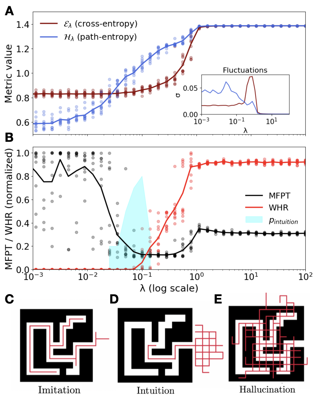</details> Figure 2: Experimental phase diagram. Sweeping $\lambda$ reveals three behavioral phases. (A) Genotype metrics: Cross-Entropy ( $\mathcal{E}$ ) and causal path-entropy ( $\mathcal{H}$ ). Inset: steady-state fluctuations $\sigma$ over different initial realizations depending on $\lambda$ . (B) Phenotype metrics: Mean First Passage Time (MFPT), Wall Hit Ratio (WHR) and intuition likelihood (see SM Sec. 4B). (C-E) Example trajectories for each phase: (C) Imitation, (D) Intuition, and (E) Hallucination. For low $\lambda$ , the system is in an imitation phase: cross-entropy is low, path-entropy is low, and trajectories reproduce the suboptimal random walks from the data, leading to a high Mean First Passage Time (MFPT) to the exit (Fig. 2 C). For high $\lambda$ , the entropic term dominates and the system enters a hallucination phase: cross- and path-entropy are high; maze rules are broken to maximize path diversity, and the Wall Hit Ratio (WHR) increases sharply (Fig. 2 E). Between these two regimes lies a narrow intuition phase, where the trade-off between $\mathcal{E}$ and $\mathcal{H}$ yields an emergent strategy: the model discovers the shortest legal path to the exit (Fig. 2 D), achieving minimal MFPT with zero WHR. The separation between the fluctuation peaks of $\mathcal{E}$ and $\mathcal{H}$ (Fig. 2 A inset) reveals distinct entropy- and energy-driven phase boundaries. <details> <summary>Figure3.png Details</summary>  ### Visual Description ## Multi-Plot Analysis of Performance Metrics vs. Lambda ### Overview The image presents four plots (A, B, C, and D) and two insets, each displaying different performance metrics as a function of the parameter lambda (λ). The plots explore forward and backward perspectives, and compare metrics like Epsilon (ε), H, MFPT (Mean First Passage Time), and WHR (Weight Histogram Ratio). The insets provide "Random baseline" comparisons for specific metrics. ### Components/Axes **Plot A:** * **Title:** (Implied) Performance Metrics vs. Lambda * **Y-axis:** "Metric values", ranging from 0.4 to 1.4. * **X-axis:** Lambda (λ), implied to be shared with other plots. * **Legend (top-left):** * Red solid line: "ελ forward" * Blue solid line: "Hλ (fwd)" * Red dashed line: "ελ backward" * Blue dashed line: "Hλ (bwd)" **Plot B:** * **Title:** MFPT / WHR (fwd) vs. Lambda * **Y-axis:** "MFPT / WHR (fwd)", ranging from 0.00 to 1.00. * **X-axis:** Lambda (λ), implied. * **Legend (center-right):** * Black solid line: "MFPT" * Red solid line: "WHR" * Light blue shaded region spans approximately from λ = 0.02 to λ = 0.07. **Plot C:** * **Title:** MFPT / WHR (bwd) vs. Lambda * **Y-axis:** "MFPT / WHR (bwd)", ranging from 0.00 to 1.00. * **X-axis:** Lambda (λ), implied. * **Legend (center-right):** * Black dashed line: "MFPT" * Red dashed line: "WHR" * Light blue shaded region spans approximately from λ = 0.02 to λ = 0.07. **Plot D:** * **Title:** (w) (mean weight) vs. Lambda * **Y-axis:** "(w) (mean weight)", ranging from 0.0 to 1.2. * **X-axis:** Lambda (λ), ranging from 10^-2 to 10^2 (log scale). * **Legend (top-right):** * Black solid line: "forward" * Black dashed line: "backward" **Inset Plots:** * **Plot A Inset:** "Random baseline" comparison for ελ. Y-axis ranges from approximately 0.5 to 1.1. X-axis is Lambda (λ), ranging from 10^-2 to 10^2 (log scale). * **Plot D Inset:** "Random baseline" comparison for (w). Y-axis ranges from approximately 0 to 1. X-axis is Lambda (λ), ranging from 10^-2 to 10^2 (log scale). ### Detailed Analysis **Plot A:** * **ελ forward (red solid line):** Starts at approximately 0.85, remains relatively constant until λ ≈ 0.1, then increases to approximately 1.1 at λ ≈ 1, and continues to increase to approximately 1.4, plateauing around λ = 10. * **Hλ (fwd) (blue solid line):** Starts at approximately 0.55, increases sharply to approximately 1.2 at λ ≈ 0.1, and then plateaus around 1.4. * **ελ backward (red dashed line):** Starts at approximately 0.85, remains relatively constant until λ ≈ 0.1, then increases to approximately 1.35, plateauing around λ = 1. * **Hλ (bwd) (blue dashed line):** Starts at approximately 0.55, increases sharply to approximately 1.1 at λ ≈ 0.1, and then plateaus around 1.4. **Plot B:** * **MFPT (black solid line):** Starts at 1.0, decreases sharply to approximately 0.1 at λ ≈ 0.05, then increases to approximately 0.3 at λ ≈ 1, and then decreases again to approximately 0.25. * **WHR (red solid line):** Starts at approximately 0.0, remains at 0 until λ ≈ 0.07, then increases sharply to approximately 0.95, plateauing around 1.0. **Plot C:** * **MFPT (black dashed line):** Starts at approximately 1.0, decreases sharply to approximately 0.1 at λ ≈ 0.05, then increases to approximately 0.3 at λ ≈ 1, and then decreases again to approximately 0.25. * **WHR (red dashed line):** Starts at approximately 0.0, remains at 0 until λ ≈ 0.07, then increases sharply to approximately 0.95, plateauing around 1.0. **Plot D:** * **Forward (black solid line):** Starts at approximately 1.0, remains relatively constant until λ ≈ 5, then decreases sharply to approximately 0.0 at λ ≈ 10, and remains at 0. * **Backward (black dashed line):** Starts at approximately 1.0, decreases gradually to approximately 0.8 at λ ≈ 1, then decreases sharply to approximately 0.0 at λ ≈ 10, and remains at 0. **Inset Plots:** * **Plot A Inset:** The data points are scattered, but the trend shows both forward and backward epsilon values starting around 0.5, increasing to approximately 0.9 around λ = 1, and then plateauing. * **Plot D Inset:** The data points are scattered, but the trend shows the mean weight starting around 1.0, decreasing to approximately 0.2 around λ = 1, and then plateauing. ### Key Observations * In Plot A, the forward and backward metrics (ελ and Hλ) converge to similar values as lambda increases. * In Plots B and C, the MFPT and WHR metrics exhibit inverse relationships, with MFPT decreasing as WHR increases. * In Plot D, the forward and backward mean weights diverge significantly as lambda increases, with the forward weight dropping sharply to zero. * The insets show the "Random baseline" performance, providing a reference point for the main plots. ### Interpretation The plots illustrate the impact of the parameter lambda (λ) on various performance metrics in forward and backward perspectives. The convergence of forward and backward metrics in Plot A suggests that as lambda increases, the system becomes more stable and less sensitive to the direction of analysis. The inverse relationship between MFPT and WHR in Plots B and C indicates a trade-off between the time it takes to reach a certain state (MFPT) and the distribution of weights (WHR). The sharp drop in forward mean weight in Plot D suggests a critical threshold for lambda, beyond which the forward perspective becomes significantly less relevant. The "Random baseline" insets provide a benchmark for evaluating the effectiveness of the system compared to a random scenario. Overall, the data suggests that lambda plays a crucial role in balancing stability, efficiency, and directionality in the system. 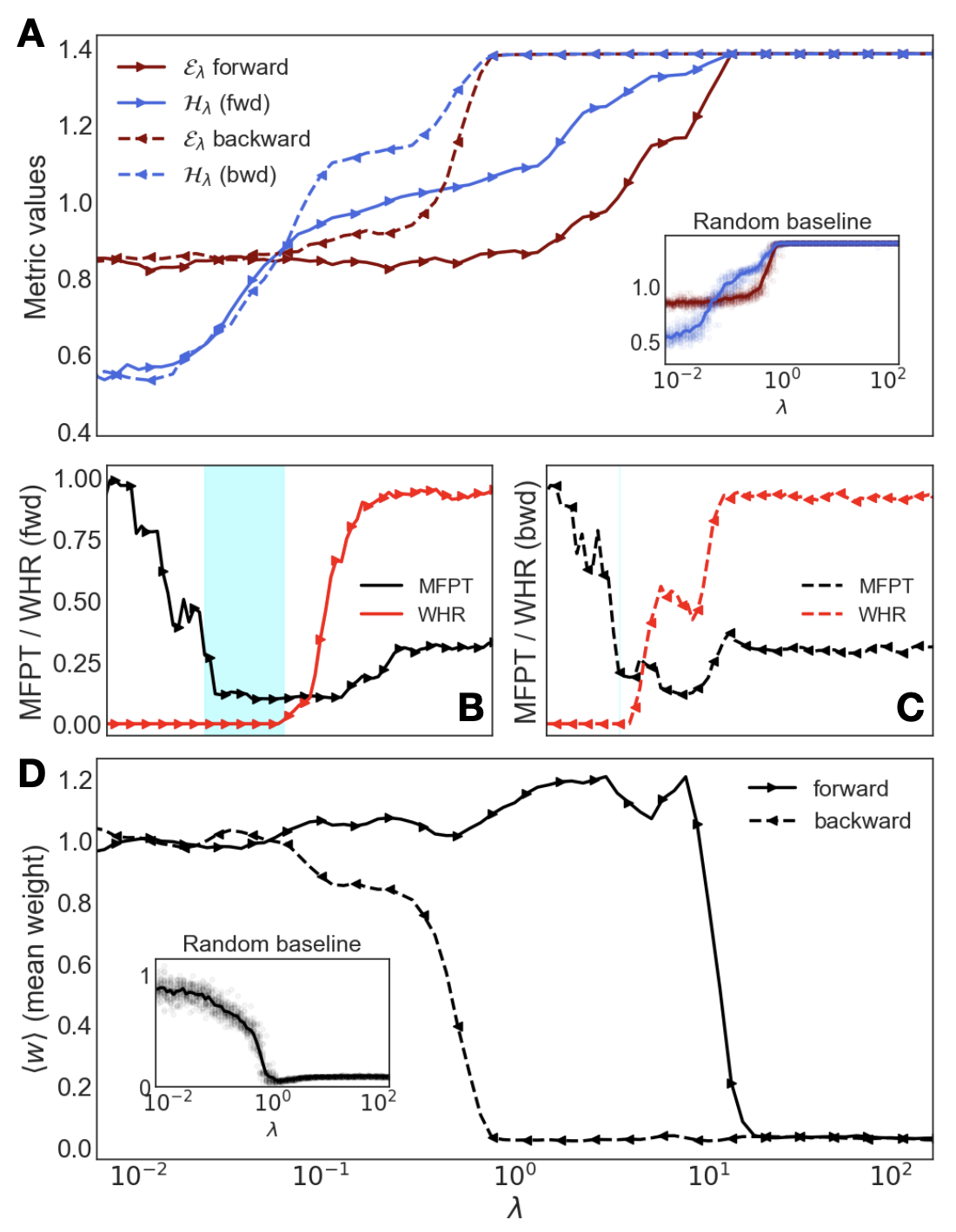</details> Figure 3: Hysteresis and protocol-dependence. Comparing a forward (solid) and backward (dashed) sweep of $\lambda$ reveals that the intuitive state is stable once found. (A) Hysteresis loop in genotype metrics ( $\mathcal{E},\mathcal{H}$ ). (B, C) Phenotype for the forward and backward sweeps, respectively, with the forward sweep showing a wider intuition window. (D) The mean network weight $\langle w\rangle$ acts as an order parameter capturing the system’s bistability. Insets show baselines without protocol. Operationally, this critical learning phase maximizes future path-entropy with minimal cross-entropy, enabling novel, goal-directed behavior at inference without interaction or explicit rewards. Reaching this phase depends on data quality and model complexity, requiring a sufficiently large future horizon and adequate model capacity (see SM Sec. S3 for a parametric study). The fragility of the mechanism is tied to multistability, as observed when applying adiabatic protocols that smoothly sweep the control parameter $\lambda$ (Fig. 3). A large hysteretic loop appears in the genotype metrics (A), which has behavioral consequences in the phenotype: while a forward sweep from $\lambda≈ 0$ opens the intuition window, with low MFPT and low WHR (B), a backward sweep starting from high $\lambda$ does not reach the desired phase (C). The bistability is captured by an effective order parameter –the mean network weight– which remains in an ordered intuitive state once the system has been guided there (D). The adiabatic protocol shows that a self-referential fine-tuning from imitation to controlled imagination allows the system to stabilize in a metastable phase, a process that motivates the term mind-tuning. Effective theory.— The phenomenology of mind-tuning emerges from a high-dimensional, multistable free-energy landscape. We capture the essential mechanism in a scalar order parameter $m∈[0,1]$ , representing the model’s rationality, and define a Boltzmann policy with an effective potential $U_{m}(a)$ : $$ p_{m,\beta}(a|h_{t})=\frac{e^{-\beta U_{m}(a)}}{\sum_{a^{\prime}\in\mathcal{A}}e^{-\beta U_{m}(a^{\prime})}}. \tag{6} $$ Actions, or decisions, are classified into optimal $a^{*}$ , rational-but-suboptimal $a^{r}$ , and non-rational $a^{n}$ and $m_{D}$ is a free parameter representing the training data’s rationality. The effective costs, $$ \displaystyle U(a^{*}) \displaystyle=0, \displaystyle U(a^{r}) \displaystyle=\frac{\max(0,m-m_{D})}{1-m_{D}}, \displaystyle U(a^{n}) \displaystyle=m, \tag{7} $$ are designed to create a trade-off: as the model’s rationality $m$ improves beyond the data’s, the cost of suboptimal-but-legal actions grows, forcing a choice between true optimality and rule-breaking. For the simple Markovian maze with a small state-space, the free energy $\mathcal{F}_{\lambda}(m)$ can be computed analytically (see SM Sec. S4A). For a given $\lambda$ , one can also explore the learning dynamics in this landscape by sampling rationality states $m$ from the equilibrium distribution $P(m)\propto e^{-\hat{\beta}\mathcal{F}(m)}$ , where the inverse temperature $\hat{\beta}$ controls the exploration-exploitation trade-off, modeling stochasticity during gradient descent. 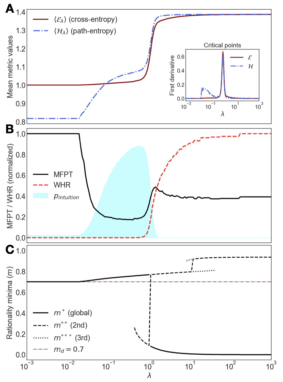This effective theory qualitatively reproduces the experimental phase diagram, including the transitions in both genotypic (Fig. 4 A) and phenotypic metrics (Fig. 4 B). The underlying mechanism is revealed by exploring the minima of the free-energy landscape, found by solving $∂\mathcal{F}_{\lambda}(m)/∂ m=0$ . This analysis confirms a smooth, entropy-driven transition followed by an abrupt, first-order energy-driven one, creating a bistable region where intuition ( $m>m_{D}$ ) and hallucination ( $m\ll m_{D}$ ) coexist (Fig. 4 C). Intriguingly, the theory further predicts a more elusive inspiration phase: a third stable solution with $m≈ 1$ , associated to a state of true creative insight. This strategy abruptly departs from data and represents internalized understanding. Unlike the subtle intuitive state, which often requires a high inference $\beta$ to be executed without error, this inspired solution would be robust even with a noisy policy. Yet, it is hidden within a tiny basin of attraction masked by the dominant hallucination phase (see SM Sec. S4.C). These predictions point to a very rich phase diagram, where intuition may be the trigger of even more exotic phenomena. <details> <summary>Figure4.png Details</summary>  ### Visual Description ## Multi-Plot Chart: Analysis of Cross-Entropy, Path-Entropy, MFPT, WHR, and Rationality Minima ### Overview The image presents three plots (A, B, and C) that analyze different metrics related to a system's behavior as a function of a parameter lambda (λ). Plot A shows the mean metric values of cross-entropy and path-entropy. Plot B displays the normalized MFPT (Mean First Passage Time) and WHR (Waiting Hit Rate), along with a shaded region representing intuition. Plot C illustrates the rationality minima. An inset in Plot A shows the first derivative of cross-entropy and path-entropy. ### Components/Axes **Plot A:** * **Title:** Mean metric values * **Y-axis:** Mean metric values, ranging from 0.8 to 1.4 * **X-axis:** Lambda (λ), implied to be logarithmic based on other plots. * **Legend (Top-Left):** * `<ελ> (cross-entropy)`: Solid brown line * `<Hλ> (path-entropy)`: Dashed blue line * **Inset Plot (Top-Right):** * **Title:** Critical points * **Y-axis:** First derivative, ranging from 0.0 to 0.6 * **X-axis:** Lambda (λ), ranging from 10^-3 to 10^3 * **Legend:** * `ε`: Solid brown line * `H`: Dashed blue line **Plot B:** * **Title:** MFPT / WHR (normalized) * **Y-axis:** MFPT / WHR (normalized), ranging from 0.0 to 1.0 * **X-axis:** Lambda (λ), ranging from 10^-3 to 10^3 (logarithmic scale) * **Legend (Left):** * `MFPT`: Solid black line * `WHR`: Dashed red line * `p_intuition`: Light blue shaded area **Plot C:** * **Title:** Rationality minima (m) * **Y-axis:** Rationality minima (m), ranging from 0.0 to 1.0 * **X-axis:** Lambda (λ), ranging from 10^-3 to 10^3 (logarithmic scale) * **Legend (Left):** * `m* (global)`: Solid black line * `m** (2nd)`: Dashed black line * `m*** (3rd)`: Dotted black line * `md = 0.7`: Dashed-dotted purple line ### Detailed Analysis **Plot A:** * **`<ελ> (cross-entropy)` (Solid brown line):** Starts at approximately 1.0 for λ < 0.1, remains relatively constant until λ ≈ 1, then increases sharply to approximately 1.38, and plateaus. * **`<Hλ> (path-entropy)` (Dashed blue line):** Starts at approximately 0.8 for λ < 0.1, increases gradually until λ ≈ 1, then increases sharply to approximately 1.38, and plateaus. * **Inset Plot:** Shows the first derivative of cross-entropy and path-entropy. Both derivatives peak around λ ≈ 1, indicating a critical point where the rate of change is highest. **Plot B:** * **`MFPT` (Solid black line):** Starts at 1.0 for λ < 0.1, decreases to approximately 0.2 around λ ≈ 1, then increases to approximately 0.4 and plateaus. * **`WHR` (Dashed red line):** Starts at 0.0 for λ < 0.1, remains at 0 until λ ≈ 1, then increases to approximately 0.9 and plateaus. * **`p_intuition` (Light blue shaded area):** Forms a bell-shaped curve centered around λ ≈ 0.1, indicating a region where intuition is most prominent. **Plot C:** * **`m* (global)` (Solid black line):** Starts at approximately 0.7 for λ < 1, then decreases sharply to approximately 0.0 for λ > 1, and plateaus. * **`m** (2nd)` (Dashed black line):** Starts at approximately 0.7 for λ < 1, then increases sharply to approximately 0.8 for λ > 1, and plateaus. * **`m*** (3rd)` (Dotted black line):** Starts at approximately 0.7 for λ < 10, then increases sharply to approximately 0.85 for λ > 10, and plateaus. * **`md = 0.7` (Dashed-dotted purple line):** Remains constant at 0.7 across all values of λ. ### Key Observations * **Critical Point:** All plots show a significant change in behavior around λ ≈ 1, suggesting a critical point in the system's dynamics. * **Entropy Transition:** In Plot A, both cross-entropy and path-entropy increase sharply around λ ≈ 1, indicating a transition in the system's entropy characteristics. * **MFPT/WHR Trade-off:** In Plot B, MFPT decreases while WHR increases around λ ≈ 1, suggesting a trade-off between the time it takes to reach a state and the frequency of hitting that state. * **Intuition Peak:** The `p_intuition` curve in Plot B peaks around λ ≈ 0.1, indicating that intuition plays a significant role in this region. * **Rationality Shift:** In Plot C, the rationality minima shift around λ ≈ 1, suggesting a change in the system's rationality characteristics. ### Interpretation The plots collectively suggest a system undergoing a phase transition or a significant change in its dynamics around λ ≈ 1. Before this point, the system exhibits different characteristics in terms of entropy, time to reach a state, frequency of hitting a state, and rationality. The peak in intuition around λ ≈ 0.1 suggests that intuitive decision-making is more prevalent in this region. The sharp changes in entropy, MFPT, WHR, and rationality minima around λ ≈ 1 indicate a shift in the system's behavior, potentially driven by a change in the underlying mechanisms or parameters. The constant `md = 0.7` line in Plot C may represent a baseline or threshold for rationality. </details> Figure 4: Theoretical predictions. The low-dimensional model reproduces the experimental findings. (A) Theoretical $\mathcal{E}$ and $\mathcal{H}$ vs. $\lambda$ . (B) Corresponding MFPT and WHR. (C) Minima of the free-energy landscape vs the control parameter $\lambda$ . The plot reveals coexisting stable states ( $m^{*},m^{**},m^{***}$ ) and a first-order transition where the global minimum jumps discontinuously, explaining the observed hysteresis. Accessing these different cognitive phases requires navigating a complex landscape. Indeed, the observed hysteresis and the success of the adiabatic protocol are explained by this multi-stability. The analytical phase-diagram (Fig. 4 C) shows that slowly increasing $\lambda$ is a safe route to guide the system into the intuition basin of attraction. In Bayesian terms, it first grounds the model with the data likelihood before introducing the entropic prior. Reaching more exotic phases in the landscape, like the predicted inspiration state, would likely demand more complex, non-equilibrium protocols. Discussion.— High-quality human data can carry an implicit drive toward path diversity, and optimization itself can induce entropic pressures that improve generalization [42], yielding an “intelligent simulator” from curated experience. This view predicts that current models should spontaneously increase their causal path entropy with scale. Our framework makes this drive explicit and grounded in MaxCal, providing a shortcut to intuition that encodes implicit search into model weights to reduce the need for expensive search at inference [43]. These results point toward a hidden axis, training-time imagination, that may be key to unlock out-of-distribution generalization in offline predictive models [35]. Our results are demonstrated in a minimal sandbox, a choice that is deliberate. The maze is the simplest non-trivial setting where the mechanism can be isolated and reproduced analytically. Many reasoning tasks can be viewed as navigation through a “conceptual maze” where a key insight unlocks a vastly larger state-space [17, 19, 20, 21]. This argument promises applications in control [17, 20], reasoning [8, 44], and planning [44]. Stefan Zweig’s The Royal Game [45] provides a compelling literary analogue: a prisoner achieves chess mastery by first studying games (imitation) and then playing against himself in his mind (imagination). His triumph occurs at the edge of madness, a state mirroring intuition coexisting with hallucination in our phase diagram. Yet, scaling mind-tuning to real-world cases faces significant challenges. Computationally, estimating path-entropy for long horizons is hard due to the combinatorial explosion of futures [13]. This requires designing clever sampling strategies [17, 46], perhaps inspired by dreaming, hierarchical reasoning [44] and unconventional methods and architectures [47, 48]. Theoretically, a full characterization of the phase diagrams and universality classe is needed to design optimal tuning protocols [49]. For uncharted domains, identifying the right spaces for entropy maximization can be difficult and the offline theory may need data augmentation from environment interaction [18]. Yet, tuning $\lambda$ for future diversity in practice can turn into an alignment problem, trading benefits for safety [50]. Despite these challenges, this work takes a high-risk, high-reward route to reframing intelligence not merely as compression and computation, but as a physical phenomenon emerging at criticality. Acknowledgments.— The author thanks many colleagues at IFISC and URV for enriching discussions. This work has been partially supported by the María de Maeztu project CEX2021-001164-M funded by the MICIU/AEI/10.13039/501100011033 and by Programa Maria Goyri URV. References - Vaswani et al. [2017] A. Vaswani et al., Attention is all you need, in Adv. in Neural Info. Processing Systems, Vol. 30 (2017). - Kaplan et al. [2020] J. Kaplan et al., Scaling laws for neural language models (2020), arXiv:2001.08361 [cs.LG] . - Hoffmann et al. [2022] J. Hoffmann et al., Training compute-optimal large language models, arXiv preprint (2022), 2203.15556 . - DeepSeek-AI et al. [2025] DeepSeek-AI et al., Deepseek-r1: Incentivizing reasoning capability in llms via reinforcement learning (2025), arXiv:2501.12948 [cs.CL] . - Shojaee et al. [2024] P. Shojaee et al., The illusion of thinking, arXiv preprint (2024), 2401.00675 . - Brodeur et al. [2024] P. G. Brodeur et al., Superhuman performance of a large language model on the reasoning tasks of a physician, arXiv preprint (2024), 2412.10849 . - Novikov et al. [2025] A. Novikov et al., Alphaevolve: A coding agent for scientific and algorithmic discovery (2025), arXiv:2506.13131 . - Chollet [2019] F. Chollet, On the measure of intelligence, arXiv preprint (2019), 1911.01547 . - Bubeck et al. [2023] S. Bubeck et al., Sparks of artificial general intelligence: Early experiments with gpt-4, (2023), 2303.12712 . - Bender et al. [2021] E. M. Bender et al., On the dangers of stochastic parrots: Can language models be too big?, in Proceedings ACM (2021) pp. 610–623. - Mitchell and Krakauer [2023] M. Mitchell and D. C. Krakauer, The debate over understanding in ai’s large language models, PNAS 120, e2215907120 (2023). - Liang et al. [2022] P. Liang et al., Holistic evaluation of language models, arXiv preprint (2022), 2211.09110 . - Jaynes [1980] E. T. Jaynes, The minimum entropy production principle, Ann. Rev.of Physical Chemistry 31, 579 (1980). - Pressé et al. [2013] S. Pressé, K. Ghosh, J. Lee, and K. A. Dill, Principles of maximum entropy and maximum caliber in statistical physics, Reviews of Modern Physics 85, 1115 (2013). - Dixit et al. [2018] P. D. Dixit et al., Perspective: Maximum caliber is a general variational principle for dynamical systems, The Journal of Chemical Physics 148, 010901 (2018). - Kiefer [2025] A. B. Kiefer, Intrinsic motivation as constrained entropy maximization, arXiv preprint (2025), 2502.02962 . - Wissner-Gross and Freer [2013] A. D. Wissner-Gross and C. E. Freer, Causal entropic forces, Physical Review Letters 110, 168702 (2013). - Wen [2025] B. Wen, The missing reward: Active inference in the era of experience (2025), arXiv:2508.05619 . - Klyubin et al. [2005] A. S. Klyubin, D. Polani, and C. L. Nehaniv, Empowerment: A universal agent-centric measure of control, in 2005 IEEE CEC, Vol. 1 (2005) pp. 128–135. - Ramirez-Ruiz et al. [2024] J. Ramirez-Ruiz et al., Complex behavior from intrinsic motivation to occupy future action-state path space, Nature Communications 15, 5281 (2024). - Friston et al. [2022] K. J. Friston et al., Designing ecosystems of intelligence from first principles, arXiv preprint (2022), 2212.01354 . - Hopfield [1982] J. J. Hopfield, Neural networks and physical systems with emergent collective computational abilities, Proceedings of the National Academy of Sciences 79, 2554 (1982). - Kuramoto [1975] Y. Kuramoto, Self-entrainment of a population of coupled non-linear oscillators, in International Symposium on Mathematical Problems in Theoretical Physics (Springer, 1975) pp. 420–422. - Belkin et al. [2019] M. Belkin, D. Hsu, S. Ma, and S. Mandal, Reconciling modern machine-learning practice and the classical bias–variance trade-off, PNAS 116, 15849 (2019). - Power et al. [2022] A. Power et al., Grokking: Generalization beyond overfitting in small neural networks, arXiv (2022), 2201.02177 . - Papyan et al. [2020] V. Papyan, X. Y. Han, and D. L. Donoho, Prevalence of neural collapse during the terminal phase of deep learning training, PNAS 117, 24927 (2020). - Liu et al. [2025] Z. Liu, Y. Xu, T. Poggio, and I. Chuang, Parameter symmetry potentially unifies deep learning theory, arXiv preprint (2025), 2502.05300 . - Arola-Fernández and Lacasa [2024] L. Arola-Fernández and L. Lacasa, Effective theory of collective deep learning, Phys. Rev. Res. 6, L042040 (2024). - Carleo et al. [2019] G. Carleo et al., Machine learning and the physical sciences, Rev. Mod. Phys. 91, 045002 (2019). - Lewkowycz et al. [2020] A. Lewkowycz et al., The large learning rate phase of deep learning: the catapult mechanism (2020), arXiv:2003.02218 [stat.ML] . - Muñoz [2018] M. A. Muñoz, Colloq.: Criticality and dynamical scaling in living systems, R. of Mod. Phys. 90, 031001 (2018). - Zhang et al. [2025] S. Zhang et al., Intelligence at the edge of chaos (2025), arXiv:2410.02536 [cs.AI] . - Jiménez-González et al. [2025] P. Jiménez-González, M. C. Soriano, and L. Lacasa, Leveraging chaos in the training of artificial neural networks (2025), arXiv:2506.08523 [cs.LG] . - Arola-Fernández et al. [2020] L. Arola-Fernández et al., Uncertainty propagation in complex networks: From noisy links to critical properties, Chaos: An Interdisciplinary Journal of Nonlinear Science 30, 023129 (2020). - Levine et al. [2020] S. Levine, A. Kumar, G. Tucker, and J. Fu, Offline reinforcement learning: Tutorial, review, and perspectives on open problems (2020), arXiv:2005.01643 [cs.LG] . - Heins et al. [2024] C. Heins et al., Collective behavior from surprise minimization, PNAS 121, e2320239121 (2024). - Friston [2010] K. Friston, The free-energy principle: A unified brain theory?, Nature Reviews Neuroscience 11, 127 (2010). - Kauffman [2000] S. A. Kauffman, Investigations (Oxford Univ. Pr., 2000). - Eysenbach and Levine [2022] B. Eysenbach and S. Levine, Maximum entropy rl (provably) solves some robust rl problems (2022), arXiv:2103.06257 [cs.LG] . - Jaynes [1957] E. T. Jaynes, Information theory and statistical mechanics, The Physical Review 106, 620 (1957). - Zdeborová and Krzakala [2016] L. Zdeborová and F. Krzakala, Statistical physics of inference: thresholds and algorithms, Adv. in Phys. 65, 453–552 (2016). - Ziyin et al. [2025] L. Ziyin, Y. Xu, and I. Chuang, Neural thermodynamics i: Entropic forces in deep and universal representation learning (2025), arXiv:2505.12387 [cs.LG] . - Belcak et al. [2025] P. Belcak et al., Small language models are the future of agentic ai (2025), arXiv:2506.02153 . - Wang et al. [2025] G. Wang et al., Hierarchical reasoning models, arXiv preprint (2025), 2506.21734 . - Zweig [1943] S. Zweig, The Royal Game (Viking Press, 1943). - Aguilar [2022] J. e. a. Aguilar, Sampling rare trajectories using stochastic bridges, Phys. Rev. E 105, 064138 (2022). - Labay-Mora et al. [2025] Labay-Mora et al., Theoretical framework for quantum associative memories, Quantum Science and Technology 10, 035050 (2025). - Brunner et al. [2025] D. Brunner et al., Roadmap on neuromorphic photonics (2025), arXiv:2501.07917 [cs.ET] . - Manzano et al. [2024] G. Manzano et al., Thermodynamics of computations with absolute irreversibility, unidirectional transitions, and stochastic computation times, Phys. Rev. X 14, 021026 (2024). - Arenas et al. [2011] A. Arenas et al., The joker effect: Cooperation driven by destructive agents, J. of Theo. Bio. 279, 113–119 (2011). - Maddison et al. [2017] C. J. Maddison, A. Mnih, and Y. W. Teh, The concrete distribution: A continuous relaxation of discrete random variables, in ICLR (2017) 1611.00712 . - Williams [1992] R. J. Williams, Simple statistical gradient-following algorithms for connectionist rl, ML 8, 229 (1992). Supplementary Material for: “Intuition emerges in Maximum Caliber models at criticality” Appendix A S1. Experimental Setup and Hyperparameters The experimental setting is a minimal yet non-trivial environment for testing emergent reasoning. It consists of a deterministic $24× 24$ maze with periodic boundary conditions, where an agent must find the path to a designated exit. This controlled testbed provides a tractable state space for analyzing the learning dynamics. The agent’s behavior is determined by a policy network that maps the current state (2D position $x_{t}$ ) to a probability distribution over the four cardinal actions: $\mathcal{A}=\{\text{Up, Down, Right, Left}\}$ . For auto-regressive training, a simple deterministic function $f(x_{t},a)$ maps the last action to the next state. The training dataset $\mathcal{D}$ is intentionally non-optimal. In our main experiments, it contains $N=100$ trajectories, each of length $T=60$ steps, generated by a constrained random walks. These walkers respect the maze walls (i.e., never collide with them) but otherwise move randomly, exhibiting no goal-directed behavior. This design ensures that the optimal exit strategy is not present in the training data, forcing the model to discover it. The model parameters $\theta$ are optimized by minimizing the free-energy functional $\mathcal{F}_{\lambda,\beta,\tau}(\theta)$ (Eq. (2) in the main text) via the Adam optimizer. The results presented in the main text (Fig. 2) are averaged over 20 independent training runs, each with a different random weight initialization, to ensure statistical robustness. The key hyperparameters used in the main experiments are: a policy network structured as a multi-layer perceptron (MLP) with one hidden layer of 128 neurons and ReLU activation; a learning rate of $1× 10^{-3}$ ; 300 training epochs per $\lambda$ value; and a future horizon of $\tau=40$ steps in the entropy calculation. The policy stochasticities are set to $\beta=1$ for training, $\beta=5$ for entropy calculation (imagination), and $\beta=10$ at inference time. A high imagination $\beta$ (compared to the training $\beta$ ) is beneficial for discovering hidden solutions that maximize causal entropy (i.e., finding the exit) with a finite $\tau$ and sparse data. A high inference $\beta$ is necessary to induce intuitive behavior in practice. In the intuition phase, the agent finds a superior solution but must execute its policy quite deterministically to follow the optimal path in the minimum time. For problems that are not Markovian or where the data representation does not contain full state information (e.g., data are sequences of moves or the agent only sees its local environment), a more advanced neural network is required. Transformers are the standard for modeling long, non-Markovian sequences of tokens. Our framework naturally extends to these sequential autoregressive architectures, albeit at the cost of more parameters and computational effort. Code availability.— PyTorch source code to reproduce the results of this paper is publicly available on GitHub: https://github.com/mystic-blue/mind-tuning. Appendix B S2. Calculation of Objective Functionals The mind-tuning objective function $\mathcal{F}_{\lambda,\beta,\tau}(\theta)=\mathcal{E}_{\beta}(\theta)-\lambda\mathcal{H}_{\tau,\beta}(\theta)$ consists of two key terms. Below we detail their calculation. B.1 A. Cross-Entropy Estimation The cross-entropy term $\mathcal{E}_{\beta}(\theta)$ , defined in Eq. (3) of the main text, measures the model’s ability to imitate the training data. It is estimated by averaging the negative log-likelihood of the actions taken in the dataset $\mathcal{D}$ given the preceding histories: $$ \hat{\mathcal{E}}_{\beta}(\theta)=\frac{1}{|\mathcal{D}|}\sum_{(h_{t},a_{t})\in\mathcal{D}}[-\log\pi_{\theta,\beta}(a_{t}|h_{t})] $$ where $|\mathcal{D}|$ is the total number of state-action pairs in the training set. This term encourages the policy to assign high probability to the trajectories observed during training. B.2 B. Causal Path-Entropy: Analytic Calculation for Markovian Systems For systems with fully-observed, discrete, and reasonably small state spaces $\mathcal{V}$ , such as our maze environment, the path-entropy can be computed analytically. Since the system is Markovian ( $h_{t}=x_{t}$ ), we can define a policy-dependent transition matrix $M_{\pi}$ . The element $(M_{\pi})_{x^{\prime},x}$ gives the probability of transitioning from state $x$ to state $x^{\prime}$ under the current policy $\pi_{\theta,\beta}$ . Specifically, $(M_{\pi})_{x^{\prime},x}=\sum_{a∈\mathcal{A}}\pi_{\theta,\beta}(a|x)\delta_{x^{\prime},f(x,a)}$ , where $f(x,a)$ is the deterministic function that returns the next state. Given a starting state $x_{start}$ , we can compute the probability distribution over future states $\vec{\rho}_{k}$ at any time step $k$ by evolving an initial occupancy vector (a point mass at $x_{start}$ ) via the recursion $\vec{\rho}_{k+1}=M_{\pi}\vec{\rho}_{k}$ . The conditional path-entropy for a trajectory starting at $x_{start}$ is then the time-averaged Shannon entropy of the policy, weighted by the occupancy probability at each future state: $$ \mathcal{H}_{\tau,\beta}(\theta|x_{start})=\frac{1}{\tau}\sum_{k=0}^{\tau-1}\sum_{x\in\mathcal{V}}(\rho_{k})_{x}\left[-\sum_{a\in\mathcal{A}}\pi_{\theta,\beta}(a|x)\log\pi_{\theta,\beta}(a|x)\right]. $$ The total functional $\mathcal{H}_{\tau,\beta}(\theta)$ is the expectation of Eq. (S2) over all starting states in the training dataset $\mathcal{D}$ . This entire calculation is fully differentiable with respect to the network parameters $\theta$ , allowing for efficient gradient-based optimization. This exact method was used to produce all experimental and theoretical results in this work. Its primary computational cost scales with the size of the state space $|\mathcal{V}|$ , making it suitable for our testbed. B.3 C. Causal Path-Entropy: Monte Carlo Estimation for High-Dimensional Systems For high-dimensional or continuous state spaces, or for non-Markovian sequence models like Transformers, the analytic approach becomes intractable. In these cases, $\mathcal{H}$ must be estimated via Monte Carlo sampling. For each starting history $h_{start}$ in a training mini-batch, we generate $K$ independent future trajectories (rollouts) of length $\tau$ by autoregressively sampling actions from the policy. The estimator for the path-entropy functional is: $$ \hat{\mathcal{H}}_{\tau,\beta}(\theta)\approx\frac{1}{|\mathcal{B}|}\sum_{h_{start}\in\mathcal{B}}\left(\frac{1}{K\tau}\sum_{k=1}^{K}\sum_{j=0}^{\tau-1}\left[-\ln\pi_{\theta,\beta}(a_{j}^{(k)}|h_{j}^{(k)})\right]_{h_{start}}\right). $$ To ensure that gradients can be backpropagated through the sampling process, especially for discrete action spaces, reparameterization techniques are required. A standard method is the Gumbel-Softmax trick [51], which provides a continuous, differentiable approximation to the sampling procedure. Alternatively, the gradient of the entropic objective can be estimated using policy gradient methods like REINFORCE [52], though this often suffers from high variance. Appendix C S3. Parametric Dependencies of the Intuition Phase The emergence of the fragile intuition phase is a critical phenomenon highly sensitive to the model, data, and learning protocol parameters. Below, we detail the key dependencies we investigated. C.1 A. 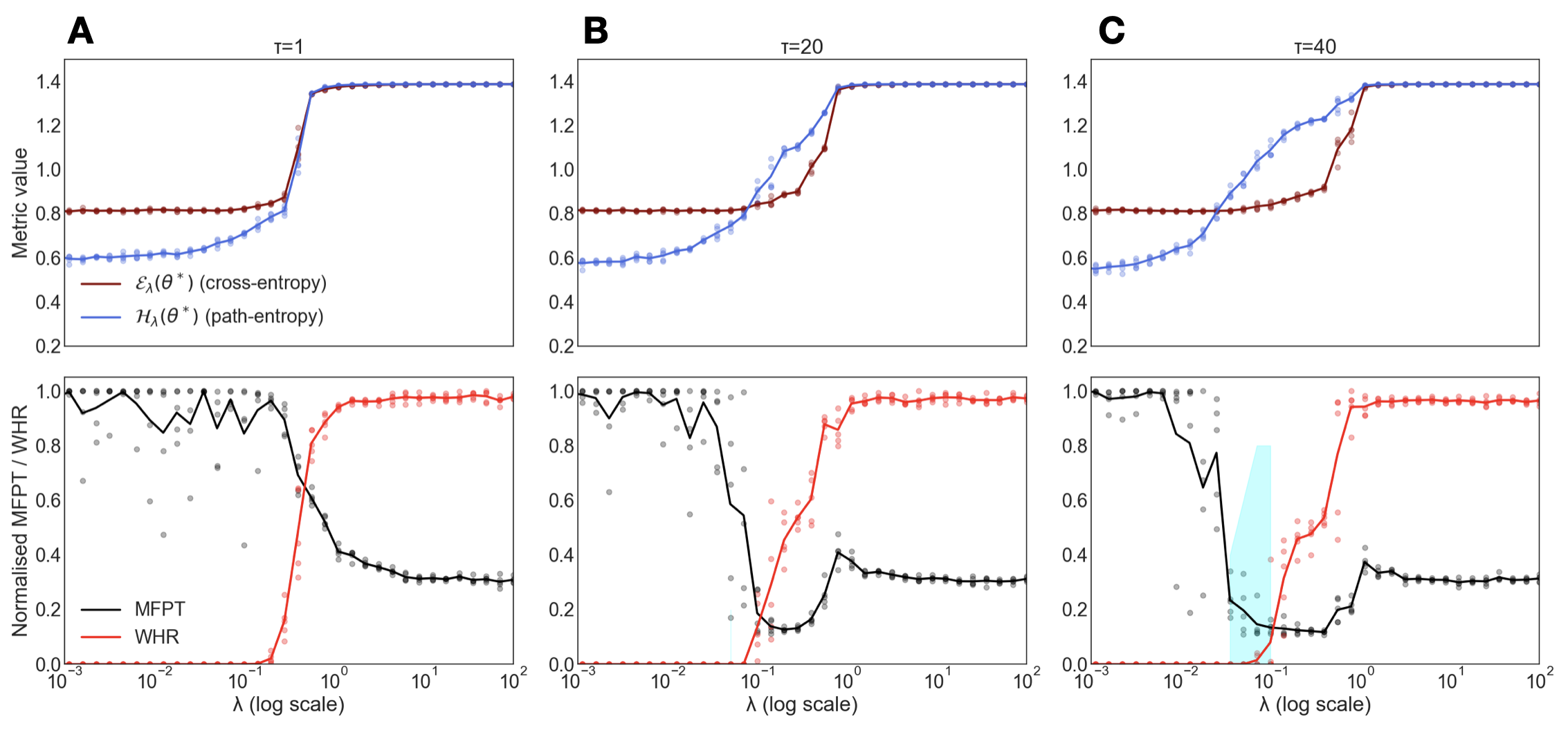Future Horizon $\tau$ The future horizon $\tau$ dictates the timescale of the model’s “imagination”. Our experiments show that the intuition phase only emerges for a sufficiently long horizon (Fig. S1). For a small $\tau$ , the model is myopic; the long-term entropic gain from escaping the maze is not visible, so the model defaults to minimizing cross-entropy and remains in the imitation phase. As $\tau$ increases, the model can foresee the vast expansion of possible futures that awaits outside the maze, creating a strong entropic incentive to find an exit. For intermediate horizons, we often observe a cheating phase—a local minimum in the free-energy landscape where the model learns to take a single illegal step through a wall. This strategy is a compromise: it incurs a small penalty for rule-breaking but gains a significant medium-term entropic advantage. Only for large $\tau$ does the incentive to find a legal path to maximal freedom dominate (i.e., virtue over vice). <details> <summary>FigureS1.png Details</summary>  ### Visual Description ## Chart: Metric Value and Normalized MFPT/WHR vs. Lambda (log scale) for Different Tau Values ### Overview The image presents three sets of two line graphs (six graphs total), arranged side-by-side, labeled A, B, and C. Each set of graphs displays the relationship between a metric value (top graph) or normalized MFPT/WHR (bottom graph) and lambda (λ) on a logarithmic scale. The three sets of graphs correspond to different values of tau (τ): 1, 20, and 40. The top graph in each set shows the cross-entropy and path-entropy, while the bottom graph shows the MFPT and WHR. ### Components/Axes **General Layout:** * The image is divided into three columns, labeled A, B, and C at the top-left of each column. * Each column contains two line graphs, one above the other. **Top Graphs (Metric Value vs. Lambda):** * **Y-axis (Metric value):** Linear scale ranging from 0.2 to 1.4. * **X-axis (λ (log scale)):** Logarithmic scale ranging from 10^-3 to 10^2. * **Legend (Top-Left of the top graph):** * Red line: ελ(θ*) (cross-entropy) * Blue line: Hλ(θ*) (path-entropy) **Bottom Graphs (Normalized MFPT/WHR vs. Lambda):** * **Y-axis (Normalized MFPT / WHR):** Linear scale ranging from 0.0 to 1.0. * **X-axis (λ (log scale)):** Logarithmic scale ranging from 10^-3 to 10^2. * **Legend (Bottom-Left of the bottom graph):** * Black line: MFPT * Red line: WHR **Titles:** * A: τ=1 * B: τ=20 * C: τ=40 ### Detailed Analysis **Graph A (τ=1):** * **Top Graph:** * Cross-entropy (red line): Starts at approximately 0.8, remains relatively constant until λ ≈ 10^-1, then increases sharply to approximately 1.35 and remains constant. * Path-entropy (blue line): Starts at approximately 0.6, remains relatively constant until λ ≈ 10^-1, then increases sharply to approximately 1.35 and remains constant. * **Bottom Graph:** * MFPT (black line): Starts at approximately 1.0, fluctuates around 1.0 until λ ≈ 10^-1, then decreases sharply to approximately 0.3 and remains constant. * WHR (red line): Starts at approximately 0.0, remains at 0.0 until λ ≈ 10^-1, then increases sharply to approximately 1.0 and remains constant. **Graph B (τ=20):** * **Top Graph:** * Cross-entropy (red line): Starts at approximately 0.8, remains relatively constant until λ ≈ 10^0, then increases sharply to approximately 1.4 and remains constant. * Path-entropy (blue line): Starts at approximately 0.6, increases gradually until λ ≈ 10^0, then increases sharply to approximately 1.4 and remains constant. * **Bottom Graph:** * MFPT (black line): Starts at approximately 1.0, fluctuates around 1.0 until λ ≈ 10^-1, then decreases sharply to approximately 0.4 and remains constant. * WHR (red line): Starts at approximately 0.0, remains at 0.0 until λ ≈ 10^-1, then increases sharply to approximately 1.0 and remains constant. **Graph C (τ=40):** * **Top Graph:** * Cross-entropy (red line): Starts at approximately 0.8, remains relatively constant until λ ≈ 10^0, then increases sharply to approximately 1.4 and remains constant. * Path-entropy (blue line): Starts at approximately 0.6, increases gradually until λ ≈ 10^0, then increases sharply to approximately 1.4 and remains constant. * **Bottom Graph:** * MFPT (black line): Starts at approximately 1.0, fluctuates around 1.0 until λ ≈ 10^-1, then decreases sharply to approximately 0.3 and remains constant. * WHR (red line): Starts at approximately 0.0, remains at 0.0 until λ ≈ 10^-1, then increases sharply to approximately 1.0 and remains constant. ### Key Observations * In all three cases, the cross-entropy and path-entropy increase sharply at a certain value of lambda. The value of lambda at which this increase occurs shifts to the right (higher values) as tau increases. * In all three cases, the MFPT decreases sharply and the WHR increases sharply at approximately the same value of lambda. * The transition point for MFPT/WHR shifts to higher lambda values as tau increases. * The shaded blue region in the bottom graph of C highlights an area of interest where the MFPT and WHR transition occurs. ### Interpretation The graphs illustrate the relationship between different metrics (cross-entropy, path-entropy, MFPT, and WHR) and the parameter lambda (λ) for different values of tau (τ). The data suggests that as lambda increases, there is a transition point where the system's behavior changes significantly. This transition point is characterized by a sharp increase in cross-entropy and path-entropy, a sharp decrease in MFPT, and a sharp increase in WHR. The shift of this transition point to higher lambda values as tau increases indicates that the system's sensitivity to lambda changes with tau. In other words, the system requires a higher value of lambda to induce the same change in behavior when tau is larger. This could be due to the system having a longer "memory" or being more resistant to changes in lambda when tau is larger. The relationship between MFPT and WHR is also notable. The inverse relationship suggests that as the mean first passage time (MFPT) decreases, the work-height ratio (WHR) increases, indicating a change in the system's efficiency or performance. </details> Figure S1: Dependence on Future Horizon $\tau$ . Phase diagram of the genotypic (top) and phenotypic (bottom) metrics as a function of $\lambda$ for different future horizons. The intuition window (sharp dip in MFPT and zero WHR, shaded blue) appears and stabilizes only for a long horizon ( $\tau=40$ ). (A) A short horizon ( $\tau=1$ ) yields only imitation and hallucination. (B) An intermediate horizon ( $\tau=20$ ) can lead to a cheating strategy, which is worse than the true intuitive solution (C). 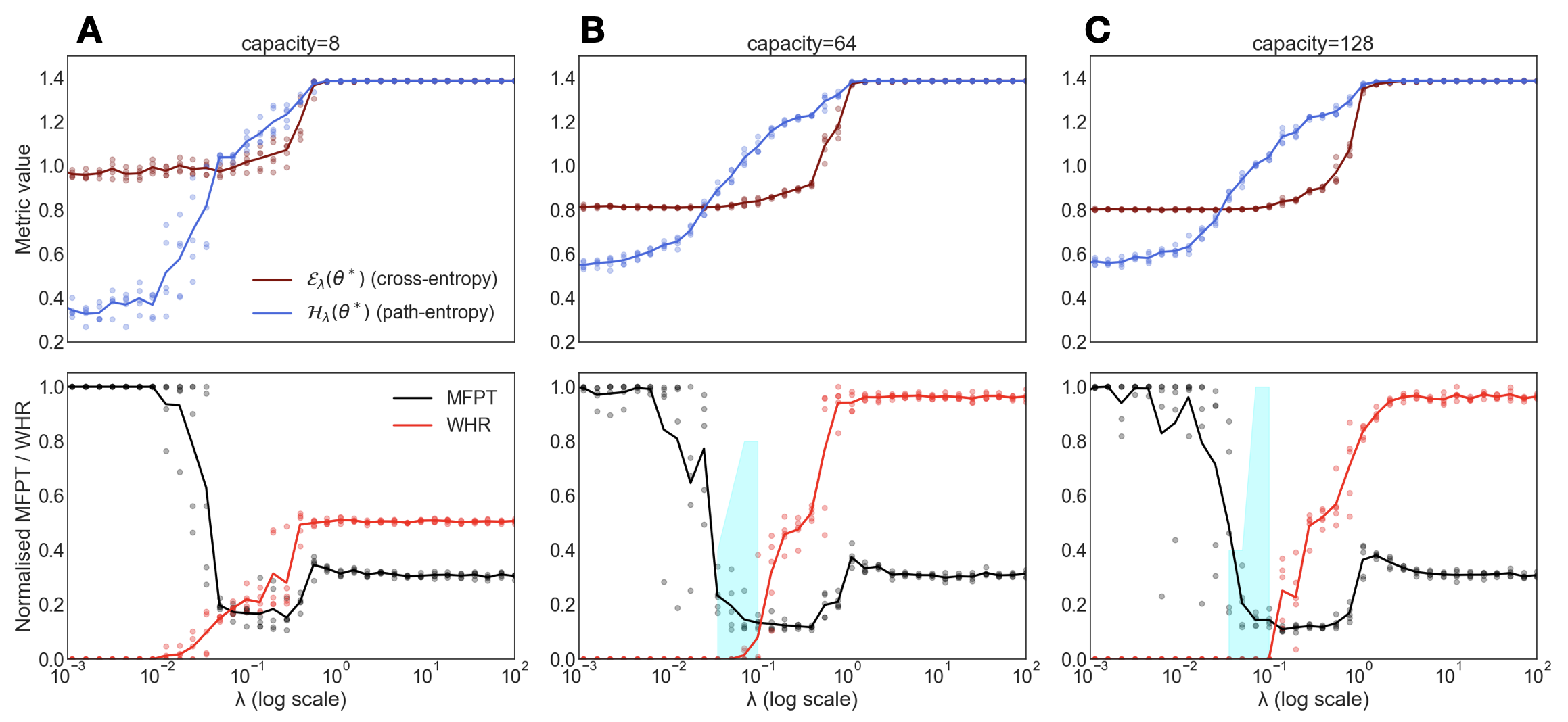C.2 B. Model Capacity The capacity of the policy network, controlled by the number of neurons, is relevant (Fig. S2). A model with insufficient capacity has high bias and lacks the representational power to learn the complex, mixed strategy required to balance maze constraints with goal-directed exploration. It cannot simultaneously represent the world model and the entropic drive, so the intuition phase does not emerge. Conversely, a model with excessive capacity relative to the task complexity is prone to overfitting. It may perfectly memorize the noisy random walks from the training data or discover trivial, non-generalizable solutions (e.g., exploiting specific numerical artifacts) to maximize entropy. The intuition phase occupies a “sweet spot” where model capacity is well-matched to the problem, enabling generalization from sparse data rather than mere memorization or unconstrained hallucination. <details> <summary>FigureS2.png Details</summary>  ### Visual Description ## Line Charts: Metric Value and Normalized MFPT/WHR vs. Lambda (Log Scale) ### Overview The image presents three sets of line charts (A, B, and C), each containing two subplots. The top subplot in each set displays the "Metric value" against "λ (log scale)" for two different metrics: cross-entropy and path-entropy. The bottom subplot in each set shows "Normalized MFPT / WHR" against "λ (log scale)" for MFPT and WHR. The three sets of charts (A, B, and C) correspond to different capacity values: 8, 64, and 128, respectively. ### Components/Axes **General Chart Elements:** * **Titles:** Each set of charts is labeled A, B, or C in the top-left corner. Above each set of charts is a "capacity" value (8, 64, or 128). * **X-axis:** The x-axis is labeled "λ (log scale)" and ranges from 10^-3 to 10^2. * **Y-axis (Top Subplot):** The y-axis is labeled "Metric value" and ranges from 0.2 to 1.4. * **Y-axis (Bottom Subplot):** The y-axis is labeled "Normalized MFPT / WHR" and ranges from 0.0 to 1.0. * **Legend (Top Subplot):** Located in the middle-right of the top subplot. * Red line: ελ(θ*) (cross-entropy) * Blue line: Hλ(θ*) (path-entropy) * **Legend (Bottom Subplot):** Located in the right of the bottom subplot. * Black line: MFPT * Red line: WHR * **Highlight:** A light blue vertical bar highlights a region on the x-axis, located around λ = 10^-1. **Specific Chart Details:** * **Chart A (capacity=8):** * Top Subplot: Metric value vs. λ (log scale) * Bottom Subplot: Normalized MFPT / WHR vs. λ (log scale) * **Chart B (capacity=64):** * Top Subplot: Metric value vs. λ (log scale) * Bottom Subplot: Normalized MFPT / WHR vs. λ (log scale) * **Chart C (capacity=128):** * Top Subplot: Metric value vs. λ (log scale) * Bottom Subplot: Normalized MFPT / WHR vs. λ (log scale) ### Detailed Analysis **Chart A (capacity=8):** * **Top Subplot:** * Cross-entropy (red): Relatively constant at approximately 1.0 from λ = 10^-3 to 10^-1, then increases to approximately 1.2 at λ = 10^0, and remains relatively constant at approximately 1.2 from λ = 10^0 to 10^2. * Path-entropy (blue): Starts at approximately 0.35 at λ = 10^-3, increases gradually to approximately 0.6 at λ = 10^-1, then increases sharply to approximately 1.4 at λ = 10^0, and remains relatively constant at approximately 1.4 from λ = 10^0 to 10^2. * **Bottom Subplot:** * MFPT (black): Constant at 1.0 from λ = 10^-3 to 10^-2, then decreases sharply to approximately 0.2 at λ = 10^-1, and remains relatively constant at approximately 0.3 from λ = 10^-1 to 10^2. * WHR (red): Starts at approximately 0.0 at λ = 10^-3, increases to approximately 0.2 at λ = 10^-1, then increases to approximately 0.5 at λ = 10^0, and remains relatively constant at approximately 0.5 from λ = 10^0 to 10^2. **Chart B (capacity=64):** * **Top Subplot:** * Cross-entropy (red): Relatively constant at approximately 0.8 from λ = 10^-3 to 10^-1, then increases to approximately 1.3 at λ = 10^0, and remains relatively constant at approximately 1.3 from λ = 10^0 to 10^2. * Path-entropy (blue): Starts at approximately 0.6 at λ = 10^-3, increases gradually to approximately 1.3 at λ = 10^0, and remains relatively constant at approximately 1.4 from λ = 10^0 to 10^2. * **Bottom Subplot:** * MFPT (black): Constant at 1.0 from λ = 10^-3 to 10^-2, then decreases sharply to approximately 0.1 at λ = 10^-1, and remains relatively constant at approximately 0.3 from λ = 10^-1 to 10^2. * WHR (red): Starts at approximately 0.0 at λ = 10^-3, increases sharply to approximately 1.0 at λ = 10^0, and remains relatively constant at approximately 1.0 from λ = 10^0 to 10^2. **Chart C (capacity=128):** * **Top Subplot:** * Cross-entropy (red): Relatively constant at approximately 0.8 from λ = 10^-3 to 10^-1, then increases to approximately 1.3 at λ = 10^0, and remains relatively constant at approximately 1.3 from λ = 10^0 to 10^2. * Path-entropy (blue): Starts at approximately 0.6 at λ = 10^-3, increases gradually to approximately 1.3 at λ = 10^0, and remains relatively constant at approximately 1.4 from λ = 10^0 to 10^2. * **Bottom Subplot:** * MFPT (black): Constant at 1.0 from λ = 10^-3 to 10^-2, then decreases sharply to approximately 0.1 at λ = 10^-1, and remains relatively constant at approximately 0.3 from λ = 10^-1 to 10^2. * WHR (red): Starts at approximately 0.0 at λ = 10^-3, increases sharply to approximately 1.0 at λ = 10^0, and remains relatively constant at approximately 1.0 from λ = 10^0 to 10^2. ### Key Observations * As capacity increases (from 8 to 64 to 128), the transition point where path-entropy increases and MFPT decreases shifts to the left (lower λ values). * The cross-entropy remains relatively constant for low λ values and then increases to a plateau for higher λ values. * The MFPT decreases sharply around λ = 10^-1, while the WHR increases sharply around λ = 10^-1. * The light blue vertical bar highlights a region around λ = 10^-1, which seems to be a critical transition point for MFPT and WHR. ### Interpretation The charts illustrate the relationship between different metrics (cross-entropy, path-entropy, MFPT, and WHR) and the regularization parameter λ for different model capacities. The data suggests that as the model capacity increases, the model becomes more sensitive to the regularization parameter λ. The transition point where the model behavior changes (as indicated by the sharp changes in MFPT and WHR) shifts to lower λ values with increasing capacity. This implies that higher capacity models require stronger regularization (lower λ) to prevent overfitting. The highlighted region around λ = 10^-1 seems to be a critical point where the model transitions from one behavior to another. The cross-entropy and path-entropy metrics also show changes around this region, indicating a shift in the model's learning dynamics. </details> Figure S2: Dependence on Model Capacity. Emergence of the intuition phase as a function of the number of neurons in the hidden layer. (A) A model with insufficient capacity (e.g., 8 neurons) cannot learn the required behavior. The intuition phase is robust for models with sufficient capacity (e.g., 64 (B) or 128 neurons (C)), which are powerful enough to discover the solution but not so powerful that they immediately overfit. 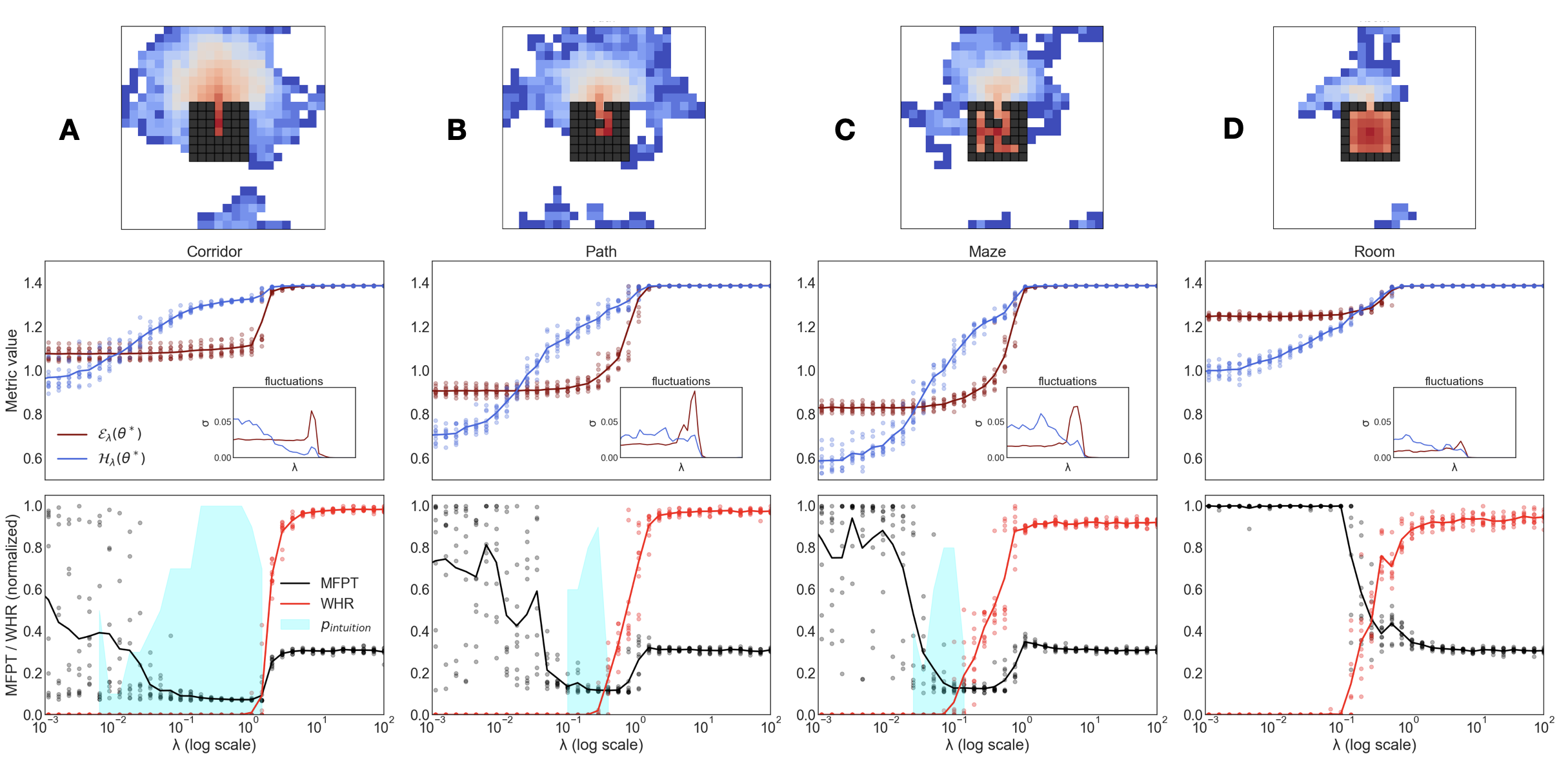C.3 C. Maze Complexity We evaluated the framework on several environments of increasing complexity (Fig. S3). In simpler environments (e.g., a straight corridor), the escape task is trivial because the data trajectories are very close to the optimal solution. The intuition window is consequently wide and appears at lower values of $\lambda$ . As maze complexity increases, finding the optimal path becomes a harder constraint-satisfaction problem. The cross-entropy term $\mathcal{E}$ more strongly penalizes deviations from valid paths. To overcome this, a stronger entropic pressure (a higher $\lambda$ ) is required to motivate the search for the distant exit. As a result, the intuition window narrows and shifts in the phase diagram, indicating that a more precise tuning of the energy-entropy balance is needed for more difficult problems. In some cases, the intuition window may disappear entirely, requiring protocols like the adiabatic sweep to be reached. <details> <summary>FigureS3.png Details</summary>  ### Visual Description ## Chart/Diagram Type: Multi-Panel Plot of Agent Navigation and Performance Metrics ### Overview The image presents a multi-panel plot analyzing agent navigation in different environments. It consists of four columns (A, B, C, D) representing different environments: Corridor, Path, Maze, and Room. Each column contains three subplots: a heatmap of agent visitation, a plot of metric values (Eλ(θ*) and Hλ(θ*)) vs. λ (log scale), and a plot of MFPT/WHR (normalized) vs. λ (log scale). The plots analyze how different metrics change with varying values of λ, providing insights into the agent's performance and behavior in each environment. ### Components/Axes **Overall Structure:** * Four columns labeled A, B, C, and D, representing different environments. * Each column has three subplots stacked vertically. **Top Row (Heatmaps):** * Each heatmap shows the agent's visitation frequency in the environment. * Color scale: Blue (low visitation) to Red (high visitation). * A black square represents the goal location. **Middle Row (Metric Value vs. λ):** * Y-axis: "Metric value", ranging from 0.6 to 1.4. * X-axis: "λ (log scale)", ranging from approximately 10^-3 to 10^2. * Two data series: * Eλ(θ*) - Red line * Hλ(θ*) - Blue line * Inset plot labeled "fluctuations" with axes ranging from 0.00 to 0.05 on the y-axis and an unlabeled x-axis. **Bottom Row (MFPT/WHR vs. λ):** * Y-axis: "MFPT / WHR (normalized)", ranging from 0.0 to 1.0. * X-axis: "λ (log scale)", ranging from approximately 10^-3 to 10^2. * Three data series: * MFPT - Black line with markers * WHR - Red line * Pintuition - Light blue shaded region **Labels:** * Column A: "Corridor" * Column B: "Path" * Column C: "Maze" * Column D: "Room" ### Detailed Analysis **Column A: Corridor** * **Heatmap:** High visitation near the starting point and the goal location. * **Eλ(θ*) (Red):** Starts around 1.1, remains relatively constant, then increases sharply to approximately 1.35 around λ = 10^0. * **Hλ(θ*) (Blue):** Starts around 0.8, increases gradually to approximately 1.4. * **MFPT (Black):** Starts around 0.4, decreases to a minimum around 0.1 at λ = 10^-1, then increases slightly. * **WHR (Red):** Starts near 0, increases sharply to 1.0 around λ = 10^0. * **Pintuition (Light Blue):** A broad peak between λ = 10^-2 and λ = 10^0. **Column B: Path** * **Heatmap:** High visitation along a direct path to the goal. * **Eλ(θ*) (Red):** Starts around 0.8, remains relatively constant, then increases sharply to approximately 1.35 around λ = 10^0. * **Hλ(θ*) (Blue):** Starts around 0.6, increases gradually to approximately 1.4. * **MFPT (Black):** Starts around 0.8, decreases to a minimum around 0.15 at λ = 10^-1, then increases slightly. * **WHR (Red):** Starts near 0, increases sharply to 1.0 around λ = 10^0. * **Pintuition (Light Blue):** A peak between λ = 10^-2 and λ = 10^0. **Column C: Maze** * **Heatmap:** High visitation in the center and near the goal, with some exploration of the maze structure. * **Eλ(θ*) (Red):** Starts around 0.8, remains relatively constant, then increases sharply to approximately 1.35 around λ = 10^0. * **Hλ(θ*) (Blue):** Starts around 0.6, increases gradually to approximately 1.4. * **MFPT (Black):** Starts around 0.9, decreases to a minimum around 0.15 at λ = 10^-1, then increases slightly. * **WHR (Red):** Starts near 0, increases sharply to 1.0 around λ = 10^0. * **Pintuition (Light Blue):** A peak between λ = 10^-2 and λ = 10^0. **Column D: Room** * **Heatmap:** High visitation concentrated near the goal location. * **Eλ(θ*) (Red):** Starts around 1.25, remains relatively constant at approximately 1.35. * **Hλ(θ*) (Blue):** Starts around 1.0, increases gradually to approximately 1.4. * **MFPT (Black):** Starts around 0.8, decreases to a minimum around 0.3 at λ = 10^-1, then increases slightly. * **WHR (Red):** Starts near 0, increases sharply to 1.0 around λ = 10^0. * **Pintuition (Light Blue):** A peak between λ = 10^-2 and λ = 10^0. ### Key Observations * **Heatmaps:** The agent's exploration strategy varies across environments. In the Corridor and Path, the agent quickly finds the goal. In the Maze, there's more exploration. In the Room, the agent focuses on the goal area. * **Eλ(θ*) and Hλ(θ*):** Both metrics generally increase with λ, with a sharp increase around λ = 10^0. The initial values and the rate of increase differ slightly across environments. * **MFPT and WHR:** The MFPT (Mean First Passage Time) generally decreases as λ increases up to a certain point, then slightly increases. The WHR (Win-stay-lose-shift Heuristic Ratio) increases sharply around λ = 10^0, indicating a shift in strategy. * **Pintuition:** The "intuition" region is consistently located between λ = 10^-2 and λ = 10^0 across all environments. ### Interpretation The data suggests that the agent's navigation strategy is influenced by the environment's complexity and the value of λ. The heatmaps show how the agent explores each environment, while the metric plots quantify the agent's performance. The sharp increase in WHR around λ = 10^0 indicates a transition from a more exploratory to a more exploitative strategy. The "intuition" region highlights a range of λ values where the agent's performance is likely driven by a balance between exploration and exploitation. The differences in the initial values and rates of change of Eλ(θ*) and Hλ(θ*) across environments suggest that the agent's internal model adapts to the specific characteristics of each environment. </details> Figure S3: Dependence on Maze Complexity. Position and width of the intuition window (measured by MFPT) for environments of varying difficulty. (A,B) For a simple corridor, the window is wide and appears at low $\lambda$ . (C) For the more complex maze used in the main text, the window is narrower, reflecting the increased difficulty. (D) For even more complex problems, the intuition window can disappear, necessitating specific protocols to reach the desired phase. Appendix D S4. Detailed Theory and Further Predictions Here we expand on the theory from the main text, providing the explicit analytical forms for the free energy functional. We also clarify the calculation of the intuition likelihood ( $p_{\text{intuition}}$ ) and discuss the existence of a more elusive inspiration phase as a further prediction of the theory. D.1 A. The Effective Free Energy Functional For the Markovian maze environment with a small state-space, the terms of the free energy functional $\mathcal{F}_{\lambda}(m)=\mathcal{E}(m)-\lambda\mathcal{H}(m)$ can be computed analytically as a function of the rationality order parameter $m$ . Note that this theory is effective: the $\beta$ of the analytical policy is distinct from the experimental one, since the former controls only three minimal analytical costs while the latter modulates the entire logit vector. The effective cross-entropy, $\mathcal{E}(m)$ , is the expectation of the negative log-likelihood over the state distribution of the given data, $\rho_{\mathcal{D}}(s)$ . For a single state $s$ , the cross-entropy is $E_{s}(m)=\log Z_{m}(s)+\beta\langle U_{m}(a)\rangle_{a\sim\text{uniform}}$ , where the average is over legal moves from $s$ . Summing over the data distribution gives $$ \mathcal{E}(m)=\left\langle\log\left(\sum_{a\in\mathcal{A}}e^{-\beta U_{m}(a|s)}\right)+\beta\frac{\sum_{a^{\prime}\in\mathcal{A}_{\text{legal}}(s)}U_{m}(a^{\prime}|s)}{|\mathcal{A}_{\text{legal}}(s)|}\right\rangle_{s\sim\rho_{\mathcal{D}}}, $$ where $U_{m}(a|s)$ is the cost of action $a$ in state $s$ (which depends on whether the move is optimal, suboptimal, or a wall collision) and $\mathcal{A}_{\text{legal}}(s)$ is the set of valid moves from $s$ . The effective path-entropy, $\mathcal{H}(m)$ , is the time-averaged Shannon entropy of the policy $p_{m,\beta}$ over trajectories of length $\tau$ starting from an initial state distribution $\rho_{0}$ (in our case, a single point at the maze start). It is calculated using the policy-dependent transition matrix $M_{m}$ $$ \mathcal{H}(m)=\frac{1}{\tau}\sum_{k=0}^{\tau-1}\left(\sum_{s\in\mathcal{V}}(\rho_{k})_{s}\cdot h_{m}(s)\right), $$ where $\vec{\rho}_{k}=(M_{m})^{k}\vec{\rho}_{0}$ is the state occupancy vector at time $k$ , and $h_{m}(s)$ is the local policy entropy at state $s$ : $$ h_{m}(s)=-\sum_{a\in\mathcal{A}}p_{m,\beta}(a|s)\log p_{m,\beta}(a|s). $$ These analytical expressions are used to generate the theoretical plots in the main text. D.2 B. Calculating the Intuition Likelihood ( $p_{\text{intuition}}$ ) The intuition metric, visualized as the cyan region in the plots, quantifies the model’s ability to spontaneously follow the optimal path. In experiments, this intuition likelihood is measured as the fraction of independent trials where the system displays the optimal solution at inference (minimal MFPT with zero WHR). The same empirical criterion can be applied to the effective theory. More interestingly, the intuition likelihood can also be calculated analytically if the optimal route is known. We define it as the joint probability of generating the true shortest path to the exit, for a horizon of $q$ steps (where $q$ depends on the maze topology). Let the optimal path be the sequence of states $z^{*}=(s_{0}^{*},s_{1}^{*},...,s_{q}^{*})$ , where $s_{0}^{*}$ is the starting position, and let $a_{t}^{*}$ be the optimal action to transition from $s_{t}^{*}$ to $s_{t+1}^{*}$ . The intuition likelihood for a given rationality level $m$ is: $$ p_{\text{intuition}}(m)=\prod_{t=0}^{q-1}p_{m,\beta}(a_{t}^{*}|s_{t}^{*}) $$ Since the system can be multistable, the final value reported in the figure for a given $\lambda$ is the Boltzmann-weighted average of this likelihood over all coexisting free energy minima ( $m^{*},m^{**},...$ ): $$ \langle p_{\text{intuition}}\rangle_{\lambda}=\sum_{i}w_{i}(\lambda)\cdot p_{\text{intuition}}(m_{i})\quad\text{where}\quad w_{i}(\lambda)=\frac{e^{-\hat{\beta}\mathcal{F}_{\lambda}(m_{i})}}{\sum_{j}e^{-\hat{\beta}\mathcal{F}_{\lambda}(m_{j})}}, $$ where $\hat{\beta}$ is an inverse temperature controlling the sampling of minima. At high $\hat{\beta}$ (low thermal noise), the system predominantly samples the global minimum, reproducing the steady-state results of the main experiments. In the numerical experiments, each run starts from a random weight initialization, and gradient descent acts as a local search that can fall into any of the attracting states. The likelihood metric is therefore zero in the imitation and hallucination phases (where the probability of following the optimal path is negligible) and peaks sharply in the narrow intuition window, provided the policy’s inference $\beta$ is sufficiently high. D.3 C. From Intuition to Inspiration: Further Predictions of the Effective Theory The intuition phase represents a significant discovery, where the model finds a hidden, optimal solution that smoothly branches from the data-driven imitation phase. It is a better way, but not a radical departure. Intriguingly, the theory predicts the existence of a distinct, more profound cognitive phase: inspiration. Inspiration is not a continuous improvement but an abrupt jump to a qualitatively different state of insight. This corresponds to the emergence of a new, globally optimal minimum in the free-energy landscape, where the rationality parameter is close to $m≈ 1$ . A model in the inspiration phase does not merely approximate the optimal policy; it knows the solution is correct. This internalized understanding would manifest through a key operational signature: the model could execute the optimal strategy robustly, even with a stochastic policy (low inference $\beta$ ), distinguishing it from the more tentative intuitive state. The theory predicts that the imagination temperature $\beta_{\text{dream}}$ —the policy stochasticity in the entropy term—is a key parameter for accessing these states (Fig. S4). At low $\beta_{\text{dream}}$ , the intuition phase ( $m>m_{D}$ ) is unstable. It emerges in a stable window only for sufficiently large $\beta_{\text{dream}}$ . At even higher values, this stable intuition branch can bifurcate into two locally stable solutions: the familiar intuition phase and this hidden inspiration phase ( $m≈ 1$ ). Both can coexist while the hallucination phase ( $m\ll m_{D}$ ) remains the global attractor. Observing this more exotic inspiration phase in practice would likely require careful tuning protocols, potentially starting from the intuition phase and employing non-equilibrium dynamics. 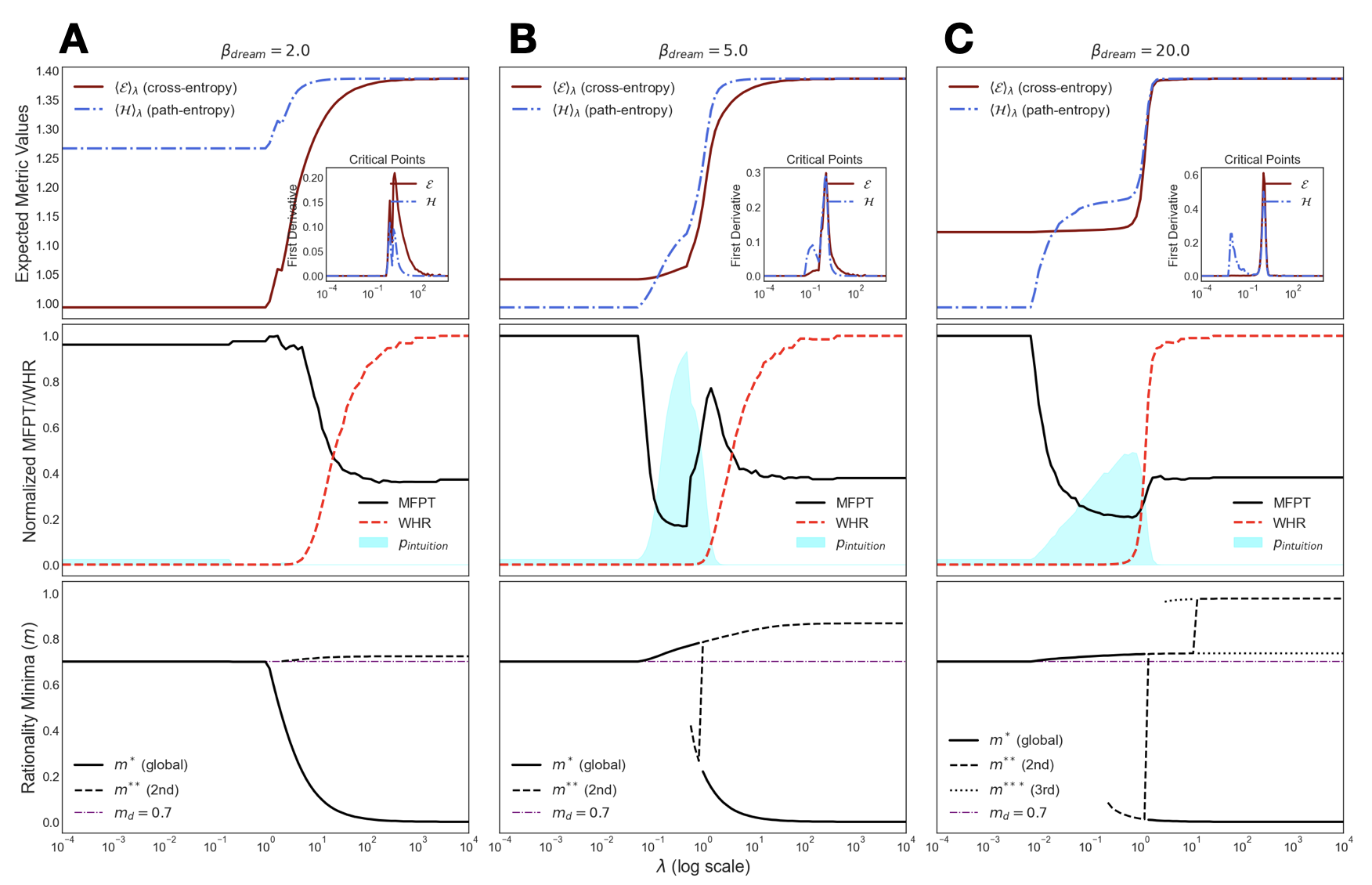<details> <summary>FigureS4.png Details</summary>  ### Visual Description ## Chart: Metric Values, Normalized MFPT/WHR, and Rationality Minima vs. Lambda ### Overview The image presents three sets of plots (A, B, and C) that illustrate the relationship between various metrics and the parameter lambda (λ) on a logarithmic scale. Each set of plots corresponds to a different value of β_dream (2.0, 5.0, and 20.0). The plots show the expected metric values (cross-entropy and path-entropy), normalized MFPT/WHR, and rationality minima as functions of lambda. Each set contains three vertically stacked plots. ### Components/Axes **General Layout:** * The image is divided into three columns labeled A, B, and C, corresponding to β_dream values of 2.0, 5.0, and 20.0, respectively. * Each column contains three vertically stacked plots. **Top Row Plots (Expected Metric Values):** * **Y-axis:** "Expected Metric Values", ranging from 1.00 to 1.40. * **Data Series:** * `(E)_λ` (cross-entropy): Solid brown line. * `(H)_λ` (path-entropy): Blue dash-dot line. * **Inset Plot (Critical Points):** * **Y-axis:** "First Derivative" * **Data Series:** * `E`: Solid brown line. * `H`: Blue dash-dot line. * **X-axis (Inset):** Same as main plot, lambda (log scale) * **X-axis:** Lambda (λ) (log scale), ranging from 10^-4 to 10^4. **Middle Row Plots (Normalized MFPT/WHR):** * **Y-axis:** "Normalized MFPT/WHR", ranging from 0.0 to 1.0. * **Data Series:** * MFPT: Solid black line. * WHR: Red dashed line. * p_intuition: Light blue shaded area. * **X-axis:** Lambda (λ) (log scale), ranging from 10^-4 to 10^4. **Bottom Row Plots (Rationality Minima):** * **Y-axis:** "Rationality Minima (m)", ranging from 0.0 to 1.0. * **Data Series:** * m* (global): Solid black line. * m** (2nd): Dashed black line. * m*** (3rd): Dotted black line (only present in plot C). * m_d = 0.7: Magenta dash-dot line. * **X-axis:** Lambda (λ) (log scale), ranging from 10^-4 to 10^4. ### Detailed Analysis **Column A (β_dream = 2.0):** * **Top Plot:** * `(E)_λ` (cross-entropy): Starts at approximately 1.00 and increases sharply around λ = 10^-1, reaching a plateau at approximately 1.38. * `(H)_λ` (path-entropy): Starts at approximately 1.27 and increases sharply around λ = 10^-1, reaching a plateau at approximately 1.38. * **Inset Plot:** The first derivative of E peaks around 10^-1 at approximately 0.18. The first derivative of H peaks around 10^-1 at approximately 0.10. * **Middle Plot:** * MFPT: Starts at approximately 0.98 and decreases sharply around λ = 10^-1, reaching a plateau at approximately 0.2. * WHR: Starts at approximately 0.0 and increases sharply around λ = 10^-1, reaching a plateau at approximately 1.0. * p_intuition: A small bump is visible around λ = 10^-1. * **Bottom Plot:** * m* (global): Starts at approximately 0.7 and decreases sharply around λ = 10^-1, reaching a plateau at approximately 0.0. * m** (2nd): Remains constant at approximately 0.7. * m_d = 0.7: Constant at 0.7. **Column B (β_dream = 5.0):** * **Top Plot:** * `(E)_λ` (cross-entropy): Starts at approximately 1.00 and increases sharply around λ = 10^-1, reaching a plateau at approximately 1.38. * `(H)_λ` (path-entropy): Starts at approximately 1.00 and increases sharply around λ = 10^-1, reaching a plateau at approximately 1.38. * **Inset Plot:** The first derivative of E peaks around 10^-1 at approximately 0.25. The first derivative of H peaks around 10^-1 at approximately 0.15. * **Middle Plot:** * MFPT: Starts at approximately 0.98 and decreases sharply around λ = 10^-1, reaching a plateau at approximately 0.2. * WHR: Starts at approximately 0.0 and increases sharply around λ = 10^-1, reaching a plateau at approximately 1.0. * p_intuition: A larger bump is visible around λ = 10^-1. * **Bottom Plot:** * m* (global): Starts at approximately 0.7 and decreases sharply around λ = 10^-1, reaching a plateau at approximately 0.0. * m** (2nd): Increases sharply around λ = 10^-1, reaching a plateau at approximately 0.7. * m_d = 0.7: Constant at 0.7. **Column C (β_dream = 20.0):** * **Top Plot:** * `(E)_λ` (cross-entropy): Starts at approximately 1.00 and increases sharply around λ = 10^-1, reaching a plateau at approximately 1.38. * `(H)_λ` (path-entropy): Starts at approximately 1.00 and increases sharply around λ = 10^-1, reaching a plateau at approximately 1.38. * **Inset Plot:** The first derivative of E peaks around 10^-1 at approximately 0.55. The first derivative of H peaks around 10^-1 at approximately 0.30. * **Middle Plot:** * MFPT: Starts at approximately 0.98 and decreases sharply around λ = 10^-1, reaching a plateau at approximately 0.2. * WHR: Starts at approximately 0.0 and increases sharply around λ = 10^-1, reaching a plateau at approximately 1.0. * p_intuition: A larger bump is visible around λ = 10^-1. * **Bottom Plot:** * m* (global): Starts at approximately 0.7 and decreases sharply around λ = 10^-1, reaching a plateau at approximately 0.0. * m** (2nd): Increases sharply around λ = 10^-1, reaching a plateau at approximately 0.7. * m*** (3rd): Increases sharply around λ = 10^-1, reaching a plateau at approximately 0.7. * m_d = 0.7: Constant at 0.7. ### Key Observations * As β_dream increases, the peak of the first derivative for both E and H in the inset plots increases. * The transition point for MFPT and WHR remains relatively constant around λ = 10^-1 across all three β_dream values. * The magnitude of p_intuition increases with increasing β_dream. * The behavior of rationality minima changes with increasing β_dream, with m*** appearing only at β_dream = 20.0. ### Interpretation The plots illustrate how different values of β_dream influence the relationship between lambda (λ) and various metrics related to cross-entropy, path-entropy, MFPT, WHR, and rationality minima. The sharp transitions observed around λ = 10^-1 suggest a critical point or threshold in the system's behavior. The increase in the peak of the first derivative for E and H with increasing β_dream indicates a more pronounced change in these metrics around the critical point. The increasing magnitude of p_intuition suggests that intuition plays a more significant role as β_dream increases. The changes in rationality minima indicate a shift in the system's rationality landscape with varying β_dream. </details> Figure S4: Dependence of theoretical predictions on the imagination temperature $\beta_{\text{dream}}$ . The theoretical phase diagram is shown for increasing values of $\beta_{\text{dream}}=\{2.0,5.0,20.0\}$ . This parameter controls the policy stochasticity in the self-referential entropy calculation. (A-C) As $\beta_{\text{dream}}$ increases, the system’s phase diagram (bottom row) changes. Higher values of this temperature can also reveal more complex phase structures, including the emergence of the inspiration phase, as discussed in the text. Insets in the first row (here and in the main text) measure the numerical first-derivatives of both the cross-entropy and path-entropy for low sampling temperature at equilibrium (thus for global attractors). The separation in the peaks of the discontinuities (B,C) signal the entropy- and energy- driven transitions that delimitate the intuition window.