2508.14313v3

# Your Reward Function for RL is Your Best PRM for Search: Unifying RL and Search-Based TTS **Authors**: Can Jin, Yang Zhou, Qixin Zhang, Hongwu Peng, Di Zhang, Zihan Dong, Marco Pavone, Ligong Han, Zhang-Wei Hong Abstract Test-time scaling (TTS) for large language models (LLMs) has thus far fallen into two largely separate paradigms: (1) reinforcement learning (RL) methods that optimize sparse outcome-based rewards, yet suffer from instability and low sample efficiency; and (2) search-based techniques guided by independently trained, static process reward models (PRMs), which require expensive human- or LLM-generated labels and often degrade under distribution shifts. In this paper, we introduce AIRL-S , the first natural unification of RL-based and search-based TTS. Central to AIRL-S is the insight that the reward function learned during RL training inherently represents the ideal PRM for guiding downstream search. Specifically, we leverage adversarial inverse reinforcement learning (AIRL) combined with group relative policy optimization (GRPO) to learn a dense, dynamic PRM directly from correct reasoning traces, entirely eliminating the need for labeled intermediate process data. At inference, the resulting PRM simultaneously serves as the critic for RL rollouts and as a heuristic to effectively guide search procedures, facilitating robust reasoning chain extension, mitigating reward hacking, and enhancing cross-task generalization. Experimental results across eight benchmarks, including mathematics, scientific reasoning, and code generation, demonstrate that our unified approach improves performance by 9% on average over the base model, matching GPT-4o. Furthermore, when integrated into multiple search algorithms, our PRM consistently outperforms all baseline PRMs trained with labeled data. These results underscore that, indeed, your reward function for RL is your best PRM for search, providing a robust and cost-effective solution to complex reasoning tasks in LLMs. footnotetext: ‡ Equal advising, Correspondence to: Can Jin <can.jin@rutgers.edu>, Tong Che <tongc@nvidia.com>. 1 Introduction Recently, test-time scaling (TTS) has been explored as an effective method to enhance the reasoning performance of large language models (LLMs) [52, 20, 62, 49, 85, 74, 30, 28, 27]. Specifically, reinforcement learning (RL) methods [52, 20, 60] and search strategies such as Monte Carlo Tree Search (MCTS), beam search, and Best-of-N sampling have been adopted to support TTS on complex reasoning benchmarks [85, 83, 82, 62, 76]. Notably, OpenAI’s o -series models [52] and DeepSeek-R1 [20] demonstrate that large-scale RL training can lengthen and refine the chains of thought (CoT) produced at inference time. The RL training of LLMs is generally guided by outcome reward models (ORMs) [9, 20, 78] and process reward models (PRMs) [35, 37, 68, 69, 60], which provide supervisory signals to improve model performance. Although DeepSeek-R1 achieves strong TTS performance using only ORMs or rule-based rewards during RL training [20], sparse outcome rewards often degrade training stability and sample efficiency [12, 37, 79, 6]. Search-based TTS methods that use static PRMs trained on labeled step-wise datasets can guide test-time search and improve reasoning performance, but building fine-grained PRMs that score each intermediate reasoning step requires extensive human annotation or LLM–generated pseudo-labels [69, 37, 12]. Furthermore, distributional shifts between a fixed PRM and the continually updated policy can lead to reward hacking [47, 16, 3], thereby undermining the stability and effectiveness of the policy model. Additionally, the reward hacking can also limit the effectiveness of PRMs in search-based TTS, where the PRM serves as a verifier during test-time search. In this paper, we investigate how to effectively combine RL-based and Search-based TTS in complex reasoning. Specifically, to reduce the cost of training high-quality PRMs and alleviate reward hacking risks from static PRMs trained on separate datasets during test time search, we propose AIRL-S , a framework that integrates adversarial inverse reinforcement learning (AIRL) [14, 13] with group relative policy optimization (GRPO) [12, 20] to support long CoT reasoning in LLMs through both RL-based and search-based TTS. During training, AIRL learns a step-wise PRM from the reference rollouts. The policy model is then updated using the combined objectives of the dense rewards in AIRL and the binary outcome rewards in GRPO. During inference, the PRM naturally serves as a verifier that guides the search procedure, extending the reasoning of the policy model. AIRL-S enables the training of generalizable PRMs without requiring any labeled process reward data, thereby significantly reducing the cost of constructing dense reward models and mitigating reward hacking under distributional shift. Furthermore, the PRM is theoretically invariant to environmental dynamics [14], allowing it to be reused during inference across different datasets and policy models in search-based TTS. We evaluate the effectiveness of the LLM policy and the PRM trained with AIRL-S on eight standard reasoning benchmarks spanning mathematics, science, and code generation. The policy model achieves an average performance improvement of 9% over the base model and matches GPT-4o across these tasks. When combined with search-based TTS methods, the PRM surpasses PRMs trained on labeled process data across multiple policy models and datasets. We further pair the PRM with widely used test-time search algorithms to demonstrate its compatibility and effectiveness under varied TTS configurations. Overall, AIRL-S provides an effective and cost-efficient approach for scaling test-time computation in LLMs for complex reasoning tasks. 2 Related Works Inverse Reinforcement Learning. Inverse reinforcement learning (IRL) [1, 58, 14, 13, 40, 41] aims to recover reward functions from expert demonstrations, enabling subsequent policy training through standard RL methods. Classic IRL methods include maximum-margin IRL [1, 58] and probabilistic maximum-entropy IRL [87, 86]. Adversarial IRL (AIRL) [14] reformulated IRL into a GAN-style adversarial game [18], improving generalization and theoretical grounding. Subsequent advances have further streamlined IRL: IQ-Learn optimizes inverse soft- $Q$ functions without explicitly modeling rewards [17]; Inverse Preference Learning uses offline pairwise preferences to avoid explicit reward modeling [21]; "IRL without RL" reframes imitation as supervised regression over trajectory data [65]. Our method leverages AIRL’s disentanglement of reward and policy, extending it to RL for large language models (LLMs) and producing a generalizable reward function suitable for guiding test-time search. RL for LLMs. Reinforcement learning from human feedback (RLHF) is standard for aligning LLM outputs with user intent [8, 54]. Nonetheless, many open-source reasoning improvement efforts still rely on imitation learning from curated Chain-of-Thought (CoT) datasets [80, 81, 84, 49, 29, 42, 43, 66]. Recent large-scale RL methods using sparse outcome rewards, such as OpenAI o1 [53] and DeepSeek-R1 [20], have achieved significant gains. Specialized RL frameworks for mathematical reasoning, such as Math-Shepherd [69] and DeepSeek-Math-7B-RL [12], utilize dense supervision or extensive RL training to match larger models. Concurrently, PRIME [11] employs "free process rewards" [61] to implicitly derive a token-level process reward from log-likelihood ratios between two LLMs. PRIME is closely related to our work, sharing the fundamental insight of utilizing an implicitly learned reward function from RL training. However, PRIME differs crucially by: - Employing per-token rewards derived from log-likelihood ratios, which reward-guided generation literatures (discrete GANs, human preference modeling, generation quality evaluation etc) [50, 57, 39] suggests is much less effective than our holistic step-wise discriminators. - Producing a policy-dependent reward function unsuitable for training new policies or guiding external search procedures. In contrast, our AIRL-based framework yields an actor-independent reward function capable of both optimal policy recovery (as shown theoretically in AIRL [14]) and direct use as a PRM for guiding search algorithms across different LLMs. Test-Time Scaling. Test-time scaling (TTS) methods enhance reasoning capabilities of fixed LLMs by allocating additional inference-time computation. Parallel TTS approaches aggregate independent samples to improve outcomes [4, 25, 70, 83]. Methods such as Self-Consistency [70], Best-of-N sampling [5, 62], and Beam Search [76, 62] utilize diversity-driven strategies for output selection. Monte-Carlo Tree Search (MCTS) integrates lookahead search guided by learned PRMs, achieving strong reasoning performance [83, 85, 82, 75, 55, 73]. Sequential TTS refines outputs iteratively based on previous attempts [49, 62, 44]. Our work integrates the AIRL-trained PRM directly into popular TTS methods, including MCTS, Beam Search, and Best-of-N sampling, demonstrating superior performance compared to static PRMs trained from labeled data. 3 Method Our objective is to learn a generalizable step-wise PRM that benefits both RL training and test-time search, thereby improving the reasoning accuracy of LLMs. We adopt AIRL and GRPO to train the PRM and the policy model jointly. The learned PRM then guides the search procedure of the policy LLM during inference, yielding additional gains in performance. The detailed pseudo-code for RL training in AIRL-S is presented in Algorithm 1. 3.1 Problem Setup Let $\mathcal{Q}$ be a dataset of questions and $q∈\mathcal{Q}$ a specific question. From the reference rollouts, we obtain a CoT, $$ C(q)=\{C_{1},C_{2},\ldots,C_{T}\}, $$ where each $C_{i}$ is a reasoning step that leads to the final answer. Our aim is to learn a PRM $r_{\phi}$ that assigns a reward to every step and provides a dense training signal for optimizing the policy model $\pi_{\theta}$ via RL. At inference time, an online-adapted $r_{\phi}$ steers the search process of $\pi_{\theta}$ , enhancing its reasoning ability on new questions. 3.2 Data Generation and Replay Buffer At the start of training, we obtain the reference rollouts for each question $q∈\mathcal{Q}$ by either sampling multiple chains of thought (CoTs) from the current policy $\pi_{\theta}$ or reusing existing CoTs. We assign a binary outcome reward, indicates whether a CoT yields the correct final answer. CoTs with a positive reward are stored in a replay buffer $\mathcal{B}$ and serve as the reference rollouts for training the AIRL reward model. To keep the reliability and diversity of $\mathcal{B}$ , we can periodically remove low-quality entries and add newly discovered high-quality CoTs during training. 3.3 Learning PRM via AIRL To avoid costly step-wise labels utilized in training static PRMs, we leverage the generative adversarial network guided reward learning in AIRL to train a discriminator that distinguishes the reference rollouts from the policy outputs [14, 18, 13, 50]. In AIRL, the discriminator $D_{\phi}$ is defined over state-action pairs. For LLM reasoning, we represent - state: the question $q$ together with the preceding reasoning steps $\{C_{1},...,C_{i-1}\}$ , and - action: the current step $C_{i}$ . The discriminator is: $$ D_{\phi}(C_{i}\mid q,C_{<i})=\frac{\exp\{f_{\phi}(q,C_{\leq i})\}}{\exp\{f_{\phi}(q,C_{\leq i})\}+\pi_{\theta}(C_{i}\mid q,C_{<i})}, $$ where $f_{\phi}$ is a learned scoring function. The step-wise reward of $C_{i}$ is then $$ r_{\phi}(C_{i}\mid q,C_{<i})=\log\frac{D_{\phi}(C_{i}\mid q,C_{<i})}{1-D_{\phi}(C_{i}\mid q,C_{<i})}. \tag{1} $$ And $r_{\phi}$ serves as the PRM. We train the discriminator by minimizing $$ {\cal L}_{\text{AIRL}}=\sum_{i=1}^{T}\Bigl[-\mathbb{E}_{q\sim\mathcal{Q},\,C\sim\pi_{e}(\cdot\mid q)}\!\bigl[\log D_{\phi}(C_{i}\mid q,C_{<i})\bigr]-\mathbb{E}_{q\sim\mathcal{Q},\,C\sim\pi_{\theta}(\cdot\mid q)}\!\bigl[\log\!\bigl(1-D_{\phi}(C_{i}\mid q,C_{<i})\bigr)\bigr]\Bigr], \tag{2} $$ where $\pi_{e}$ denotes the reference rollout distribution drawn from the replay buffer $\mathcal{B}$ and $\pi_{\theta}$ is the current policy. Updating the discriminator can be seen as updating the reward function $r_{\phi}$ . Algorithm 1 AIRL-S Input Initial LLM policy $\pi_{\theta_{\text{init}}}$ ; question set $\mathcal{Q}$ ; Total iterations $E$ ; initial replay buffer $\mathcal{B}$ Initialize policy model $\pi_{\theta}$ , reference model $\pi_{\text{ref}}$ , old policy $\pi_{\text{old}}$ , and PRM $r_{\phi}$ with $\pi_{\theta_{\text{init}}}$ Update replay buffer $\mathcal{B}$ by collecting correct rollouts for $q∈\mathcal{Q}$ using $\pi_{\theta}$ for iteration = 1, …, $E$ do Sample a batch of questions $\mathcal{B}_{i}$ from $\mathcal{B}$ Generate a group of policy rollouts: $\{C^{1},...,C^{G}\}\sim\pi_{\theta}(·|q)$ for $q∈\mathcal{B}_{i}$ Update the PRM according to AIRL loss in Equation (2) Update the policy $\pi_{\theta}$ according to the composite objectives in Equation (6) Update the old policy $\pi_{\text{old}}$ using $\pi_{\theta}$ Update the replay buffer by adding the correct rollouts to $\mathcal{B}$ end for Output Optimized policy model $\pi_{\theta}$ and PRM $r_{\phi}$ 3.4 Policy Training with Combined RL Objectives The policy model is optimized via RL. In AIRL [14], the objective of the policy model is to maximize the discriminator-derived rewards, thereby "fool" the discriminator into classifying its rollouts are reference rollouts. The AIRL objective is $$ {\cal J}_{\mathrm{AIRL}}(\theta)=\mathbb{E}_{q\sim\mathcal{Q},\,C\sim\pi_{\theta}(\cdot\mid q)}\Biggl[\sum_{i=1}^{|C|}\min\Bigl(\frac{\pi_{\theta}(C_{i}\mid q,C_{<i})}{\pi_{\mathrm{old}}(C_{i}\mid q,C_{<i})}A_{i},\mathrm{clip}\bigl(\tfrac{\pi_{\theta}(C_{i}\mid q,C_{<i})}{\pi_{\mathrm{old}}(C_{i}\mid q,C_{<i})},\,1-\epsilon,\,1+\epsilon\bigr)A_{i}\Bigr)\Biggr], \tag{3} $$ where $C$ is a chain of thought (CoT) produced by $\pi_{\theta}$ , $|C|$ is its length, $\pi_{\text{old}}$ is the sampling policy, and $A_{i}$ is the advantage at step $i$ , estimated with a REINFORCE-style method [72]. DeepSeek-R1 achieves strong reasoning performance by pairing binary outcome rewards with group relative policy optimization (GRPO) [20]. For a group of $G$ CoTs $\{C^{k}\}_{k=1}^{G}$ , we utilize the same outcome rewards based GRPO, and the objective is $$ \mathcal{J}_{\mathrm{GRPO}}(\theta)=\;\mathbb{E}_{q\sim\mathcal{Q},\,\{C^{k}\}_{k=1}^{G}\sim\pi_{\mathrm{old}}(\cdot\mid q)}\\ \Biggl[\frac{1}{G}\sum_{k=1}^{G}\bigl(\min\Bigl(\frac{\pi_{\theta}(C^{k}\mid q)}{\pi_{\mathrm{old}}(C^{k}\mid q)}A^{k},\mathrm{clip}\bigl(\tfrac{\pi_{\theta}(C^{k}\mid q)}{\pi_{\mathrm{old}}(C^{k}\mid q)},\,1-\epsilon,\,1+\epsilon\bigr)A^{k}\Bigr)-\beta\,\mathrm{D}_{\mathrm{KL}}\!\bigl(\pi_{\theta}\|\pi_{\mathrm{ref}}\bigr)\Bigr)\Biggr], \tag{4} $$ $$ \mathrm{D}_{\mathrm{KL}}\!\bigl(\pi_{\theta}\|\pi_{\mathrm{ref}}\bigr)=\frac{\pi_{\mathrm{ref}}(C^{k}\mid q)}{\pi_{\theta}(C^{k}\mid q)}-\log\!\frac{\pi_{\theta}(C^{k}\mid q)}{\pi_{\mathrm{ref}}(C^{k}\mid q)}-1, \tag{5} $$ where $\pi_{\text{ref}}$ is a frozen reference model, and $\epsilon$ and $\beta$ are hyper-parameters. The advantage $A^{k}$ for each CoT in the group is computed from the binary outcome rewards. We define a composite objective that combines the AIRL objective and GRPO objective to incorporate both the intermediate step rewards and the outcome rewards, and update the policy model to maximize the combined RL objectives: $$ {\cal J}(\theta)=\lambda\,{\cal J}_{\mathrm{AIRL}}(\theta)+(1-\lambda)\,{\cal J}_{\mathrm{GRPO}}(\theta), \tag{6} $$ where $\lambda$ is a hyperparameter to balance the outcome rewards and process rewards. The training alternates between (i) updating the discriminator $D_{\phi}$ to distinguish reference rollouts from policy rollouts, and (ii) optimizing the policy by maximizing the composite objectives of AIRL and GRPO in Equation (6). <details> <summary>x1.png Details</summary>  ### Visual Description \n ## Diagram: TTS Architecture Comparison - RL Base vs. Search Base ### Overview This diagram illustrates a comparison between two Text-to-Speech (TTS) architectures: Reinforcement Learning (RL) Base TTS and Search Base TTS. The diagram visually represents the flow of information and processes within each architecture, highlighting the key components and differences. The diagram is divided into two main sections, one for each TTS approach, separated by a dashed horizontal line. ### Components/Axes The diagram consists of several interconnected blocks representing different components. Key components include: * **Policy πθ**: Represents the policy network in the RL Base TTS. * **Question q**: Represents the input question for both architectures. * **CoTs (Chain of Thoughts)**: Represent the intermediate reasoning steps. * **AIRL Discriminator**: A component in the RL Base TTS used for reward shaping. * **Outcome Reward JGRPO**: The final reward signal in the RL Base TTS. * **Step-wise Reward rρ**: The reward signal at each step in the RL Base TTS. * **Policy Update**: The process of updating the policy network in the RL Base TTS. * **Best-of-N**: A component in the Search Base TTS that generates multiple solutions. * **Beam Search**: A component in the Search Base TTS that explores multiple paths. * **MCTS (Monte Carlo Tree Search)**: A component in the Search Base TTS used for decision-making. * **Selection, Expansion, Simulation, Backpropagation**: The four phases of MCTS. * **PRM (Probabilistic Reasoning Model)**: Used for ranking and selecting solutions in the Search Base TTS. The diagram also includes a legend explaining the symbols used: * Dashed boxes: Apply PRM * Red circles: Rejected Step * Solid circles: Selected Step * White circles: Intermediate Step * Black circles: Full Solution ### Detailed Analysis or Content Details **RL Base TTS (Top Section):** 1. A "Question q" enters a "Policy πθ" block. 2. The policy generates "Sampled CoTs". 3. These CoTs are compared to "Reference CoTs". 4. The difference is fed into an "AIRL Discriminator", which outputs a "Step-wise reward rρ". 5. The "Step-wise reward" and an "Outcome Reward JGRPO" are combined to generate a "Policy Update". **Search Base TTS (Bottom Section):** 1. A "Question q" is input into both "Best-of-N" and "Beam Search" blocks. 2. "Best-of-N" generates N solutions and uses PRM to select the best. The solutions are represented by a series of dashed boxes with circles indicating steps. 3. "Beam Search" ranks and retains top-N steps per decision, also using PRM. The solutions are represented by a series of dashed boxes with circles indicating steps. 4. The selected solutions are then fed into the "MCTS" process, which consists of four phases: * **Selection**: Nodes are selected based on the UCT score. * **Expansion**: The tree is expanded by generating steps. * **Simulation**: The value is simulated by extending nodes. * **Backpropagation**: The tree is updated based on the simulation results. **Legend:** * Dashed boxes represent the application of PRM. * Red circles indicate rejected steps. * Solid circles indicate selected steps. * White circles represent intermediate steps. * Black circles represent full solutions. ### Key Observations * The RL Base TTS relies on a reward-based learning approach, while the Search Base TTS utilizes a search-based approach. * The Search Base TTS incorporates MCTS for decision-making, which involves iterative selection, expansion, simulation, and backpropagation. * PRM plays a crucial role in both Search Base TTS components (Best-of-N and Beam Search) for ranking and selecting solutions. * The diagram highlights the iterative nature of the Search Base TTS, with the MCTS process continuously refining the search tree. ### Interpretation The diagram demonstrates a comparison of two distinct approaches to TTS. The RL Base TTS leverages reinforcement learning to optimize a policy for generating CoTs, guided by rewards from an AIRL discriminator. This approach aims to learn a policy that produces high-quality CoTs. In contrast, the Search Base TTS employs search algorithms (Best-of-N and Beam Search) combined with MCTS to explore a space of possible solutions. PRM is used to evaluate and rank these solutions, guiding the search process. The use of MCTS in the Search Base TTS suggests a more deliberate and exploratory approach, where the algorithm actively searches for the best solution by simulating different paths. The RL Base TTS, on the other hand, relies on learning a policy that implicitly encodes the search strategy. The diagram suggests that the Search Base TTS may be more suitable for complex problems where a clear reward signal is difficult to define, while the RL Base TTS may be more efficient for problems where a well-defined reward function can be used to guide learning. The diagram does not provide quantitative data, but it effectively illustrates the conceptual differences between the two architectures. The dashed line separating the two sections emphasizes the distinct nature of the approaches. 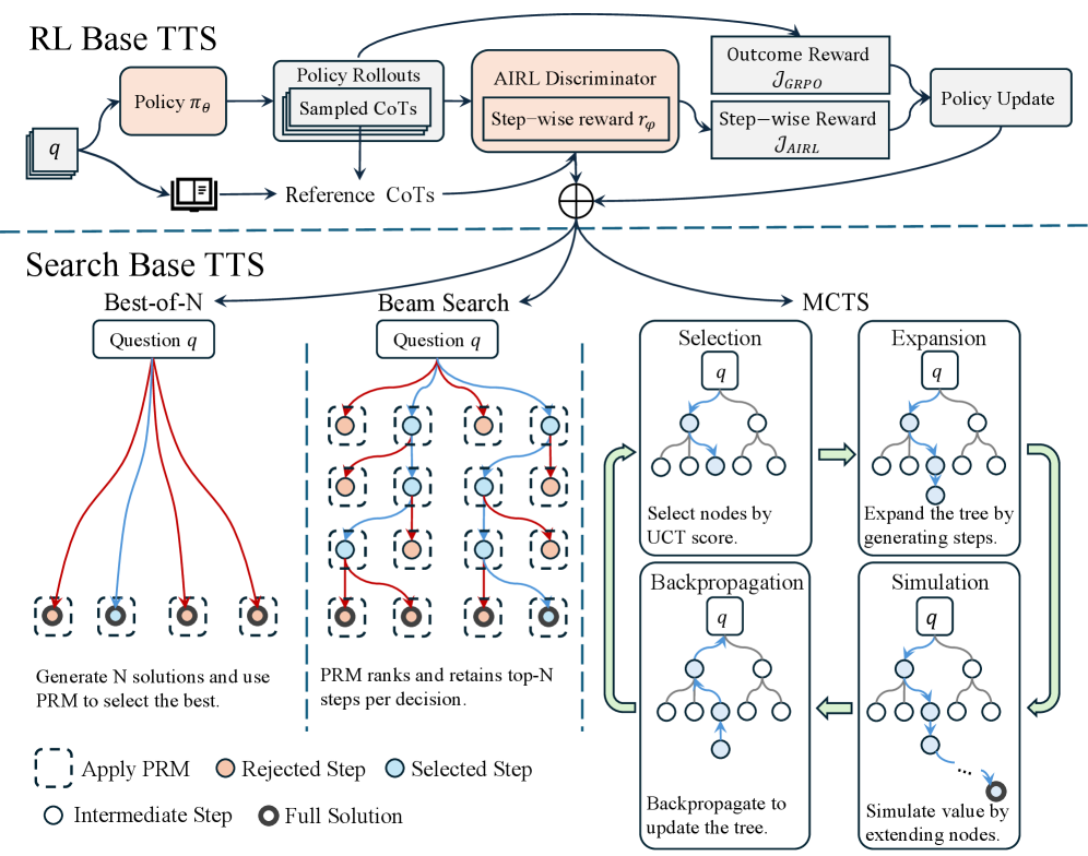</details> Figure 1: Overview of AIRL-S . During training, AIRL-S uses the AIRL discriminator to learn a PRM and optimizes the policy with both dense rewards from AIRL and outcome rewards from GRPO. At test time, the trained policy and PRM jointly guide downstream search algorithms. 3.5 PRM-guided Test-Time Search Test-Time Search. At inference time, search-based TTS explores multiple CoTs rather than generating a single pass. Approaches such as Best-of- N [62], beam search [76], and Monte Carlo Tree Search (MCTS) [85] improve reasoning by leverage outcome or process reward models to guide exploration. Because our reward function $r_{\phi}$ is learned and adapted on the policy LLM during RL, we can seamlessly reuse it as a PRM to steer the search procedure. When the policy proposes several actions, either intermediate steps or complete solutions, we score each candidate with $r_{\phi}$ and retain those with the highest scores according to the chosen search strategy. Figure 1 illustrates how $r_{\phi}$ integrates with Best-of-N, beam search, and MCTS; implementation details are provided in Appendix A. - Best-of- N. For a question $q$ , we sample $N$ full solutions from $\pi_{\theta}(·\mid q)$ and select the one with the highest PRM aggregation score (defined below). - Beam Search. With beam size $N$ and beam width $M$ , we extend each beam node by $M$ candidate steps, rank those steps by $r_{\phi}$ , and keep the top $N$ nodes. The process continues until we obtain $N$ complete solutions. - MCTS. Using expansion width $M$ , we select a node by the upper confidence bound for trees (UCT) criterion, which combines PRM rewards with visit counts [63, 31]. We then generate $M$ child steps, simulate rollouts using $r_{\phi}$ to estimate node values, and back-propagate the rewards. The search returns $N$ full solutions. PRM Aggregation. After search, we obtain $N$ candidate solutions $\{C^{k}\}_{k=1}^{N}$ for each question $q$ . Following Snell et al. [62], for every solution $C^{k}$ we compute a step-wise aggregation score $$ s\!\bigl(C^{k}\bigr)=\min_{i}r_{\phi}\!\bigl(C^{k}_{i}\bigr), $$ namely, the smallest PRM reward among its steps. Let $A^{k}$ be the final answer produced by $C^{k}$ . For inter-answer aggregation, we aggregate the step-wise scores of all solutions that yield the same distinct answer $a$ : $$ S(a)=\sum_{k:\,A^{(k)}=a}\,s\!\bigl(C^{(k)}\bigr). $$ The answer with the largest $S(a)$ is selected as the model’s prediction; we term this method PRM-Min-Sum. Further implementation details and the definition of other PRM aggregation methods appear in Appendix A. 4 Experiments To evaluate the effectiveness of the unified RL-based and search-based TTS technique in AIRL-S , we conduct extensive experiments to (i) compare the performance of our policy model to current state-of-the-art (SoTA) comparable size models on eight reasoning tasks, (ii) compare our PRM to PRMs trained on labeled datasets and implicit PRMs, (iii) combine our policy model and PRM with various search-based TTS techniques, (iv) conduct additional experiments to investigate the effect of the combined AIRL and GRPO objectives in RL training and the impact of various answer aggregation techniques in search-based TTS. 4.1 Experimental Details LLMs. Policy Baselines: We select SoTA open-source and API models as baselines for our policy model. The open-source LLMs encompass models specifically designed for or excelling in reasoning through RL training, such as Math-Shepherd-Mistral-7B-RL [71], DeepSeek-Math-7B-RL [60], Qwen2.5-Math-7B-Instruct [24], and Eurus-2-7B-PRIME [11]. We also include Qwen2.5-7B-Instruct [56] and Phi-4-14B [2] as general-purpose open-source baselines. We further include s1.1-7B [49] as a baseline trained through direct imitation learning on DeepSeek-R1 demonstrations instead of AIRL. For API models, we select DeepSeek-R1 [20], DeepseekV3 (2025-03-24) [38] and GPT-4o (2024-11-20) [51] as baselines. PRM Baselines: We select Math-Shepherd-Mistral-7B-PRM [69] and Llama3.1-8B-PRM-Deepseek-Data [77] as PRM baselines trained on labeled step-wise data. We choose the recent EurusPRM-Stage2 [79] as an implicit PRM baseline trained through ORM. More details of the baseline models are expanded in Appendix B. Tasks. Mathematical/Scientific Reasoning: We evaluate on AIME2024 [45], AMC [46], MATH500 [23], and GPQA-Diamond [59] to validate the effectiveness of AIRL-S in mathematical or scientific reasoning tasks. Coding: We further evaluate the reasoning capabilities of our model in coding tasks on four benchmarks, including HumanEval [7], MBPP [19], LeetCode [10], and LiveCodeBench (v4) [26]. Details of all the tasks are introduced in Appendix B. Training. Our full training dataset contains 160K questions, mostly sampled from NuminaMATH [33]. We use the LLM policy self-generated responses as the reference rollouts, and the rollouts are generated using rollout prompts, and more details are shared in Appendix B. We initialize both $\pi_{\theta}$ and $f_{\phi}$ using Qwen2.5-7B-Instruct, while we modify the head of $f_{\phi}$ into a scalar-value prediction head. The training is conducted on 8 NVIDIA A100 GPUs with Pytorch FSDP. We use a learning rate of 2e-6 for the reward model and 5e-7 for the policy model, maximum output length is set to 8,192, and the training batch size is 1024. For each question, we sample 8 outputs using the rollout prompts. The KL coefficient is set to 0.001, $\lambda$ is set to 0.5, and the total training epochs are 2. Evaluation. For results where search-based TTS is not applied, we report zero-shot Accuracy@1 for math and science tasks, and Pass@1 for coding tasks using a temperature of 0 for reproducibility. For results where search-based TTS is applied, we use a temperature of 0.7 to enable step exploration, tree width $M$ is set to 4, and the performance of the PRM aggregated solution is reported. The main results are averaged over three runs. 4.2 Main Results Effectiveness of the Policy Model. To comprehensively validate the performance of our policy model Qwen2.5-7B-AIRL-S , we compare it to ten SoTA LLMs (open- and closed-source) on eight reasoning tasks. The results in Table 1 lead to the following observations: (i) AIRL-S can effectively enhance the reasoning performance of the base model. When trained on Qwen2.5-7B-Instruct, our policy achieves an average improvement of 9% across eight benchmarks and a 13% improvement on mathematical and scientific reasoning tasks. (ii) Our policy exhibits strong performance compared to existing LLMs trained through RL. AIRL-S outperforms Math-Shepherd-Mistral-7B-RL, DeepSeek-Math-7B-RL, and Qwen2.5-Math-7B-Instruct (trained with PRMs from labeled step-wise datasets) and Eurus-2-7B-PRIME (trained with an implicit PRM derived from its policy). Compared to these models, AIRL-S consistently achieves higher reasoning accuracy on all tasks by learning a policy-independent step-wise reward function through AIRL. (iii) Our approach surpasses direct imitation learning on reference rollouts. Compared to s1.1-7B trained via supervised fine-tuning on DeepSeek-R1 demonstrations, AIRL-S yields an average improvement of 15% by learning a reward function from reference rollouts and maximizing the rewards instead of direct imitation learning. (iv) Finally, AIRL-S outperforms the recently released Phi-4-14B on average despite having half its parameter count and matches the performance of the general-purpose model GPT-4o. Table 1: Comparison of our policy model with ten SoTA open- and closed-source LLMs across eight reasoning benchmarks. Boldface indicates the top result within each model category; green highlighting denotes the best result among local models. Our policy achieves the highest average performance among local models and matches GPT-4o overall. (GPQA: GPQA-Diamond; LCB-v4: LiveCodeBench-v4) | Model | Mathematical/Scientific Reasoning | Coding | Avg. | | | | | | | | --- | --- | --- | --- | --- | --- | --- | --- | --- | --- | | AIME2024 | AMC | MATH500 | GPQA | HumanEval | Leetcode | LCB-v4 | MBPP | | | | API Models | | | | | | | | | | | DeepSeek-R1 | 79.8 | 85.5 | 96.5 | 71.2 | 97.6 | 90.4 | 71.1 | 95.8 | 86.0 | | DeepSeek-V3 | 36.7 | 81.9 | 90.2 | 61.1 | 93.3 | 88.3 | 67.0 | 88.9 | 75.9 | | GPT-4o | 13.3 | 50.6 | 65.8 | 43.9 | 90.2 | 60.6 | 44.2 | 87.3 | 57.0 | | Local Models (RL with PRMs) | | | | | | | | | | | Math-Shepherd-Mistral-7B-RL | 0.0 | 7.2 | 28.6 | 9.6 | 32.3 | 5.6 | 3.9 | 51.1 | 17.3 | | DeepSeekMath-7B-RL | 3.3 | 18.1 | 48.6 | 23.2 | 58.5 | 11.2 | 6.2 | 73.1 | 30.3 | | Qwen2.5-Math-7B-Instruct | 13.3 | 50.6 | 79.6 | 29.3 | 57.9 | 11.7 | 9.3 | 46.0 | 37.2 | | Eurus-2-7B-PRIME | 20.0 | 56.6 | 79.2 | 33.8 | 70.7 | 31.1 | 24.3 | 70.1 | 48.2 | | Local Models (Other Baselines) | | | | | | | | | | | s1.1-7B | 16.7 | 38.6 | 72.6 | 35.4 | 76.8 | 11.1 | 9.3 | 76.7 | 42.2 | | Qwen2.5-7B-Instruct | 16.7 | 33.7 | 72.0 | 32.5 | 81.7 | 47.4 | 28.0 | 79.4 | 48.9 | | Phi-4-14B | 13.3 | 44.6 | 78.6 | 55.6 | 84.1 | 45.6 | 31.2 | 74.3 | 53.4 | | Qwen2.5-7B-AIRL-S (Ours) | 26.7 | 59.0 | 80.2 | 40.2 | 85.1 | 54.4 | 31.3 | 83.3 | 57.5 | 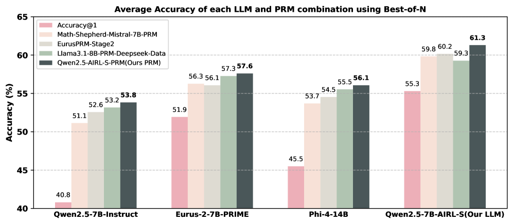Effectiveness of the PRM. We assess the generalizability of our PRM, Qwen2.5-AIRL-S-PRM, by comparing it to PRMs trained on labeled step-wise datasets. We evaluate four PRMs using Best-of-N search with 64 rollouts on AIME2024, AMC, and MATH500 across four generative LLMs. The average performance of each LLM–PRM pair is shown in Figure 2, and detailed results are provided in Appendix C. Our observations are: (i) Qwen2.5-AIRL-S-PRM improves Best-of-N performance for all LLMs and datasets, outperforming Math-Shepherd-Mistral-7B-PRM and EurusPRM-Stage2 by 2.4% and 1.4%, respectively. (ii) Combining Qwen2.5-7B-AIRL-S with Qwen2.5-AIRL-S-PRM yields the best performance among all LLM–PRM combinations, with an 11% gain over Qwen2.5-7B-Instruct with Math-Shepherd-Mistral-7B-PRM. These results demonstrate that AIRL-S effectively unifies RL-based TTS and Search-based TTS and that our PRM generalizes across different models and datasets. <details> <summary>x2.png Details</summary>  ### Visual Description ## Bar Chart: Average Accuracy of LLM and PRM Combinations ### Overview This bar chart displays the average accuracy of different Large Language Model (LLM) and Program-aided Reasoning Model (PRM) combinations, evaluated using a Best-of-N approach. The accuracy is measured in percentage (%). The chart compares four different LLM/PRM pairings. ### Components/Axes * **Title:** "Average Accuracy of each LLM and PRM combination using Best-of-N" (Top-center) * **X-axis:** LLM/PRM Combinations: "Qwen2.5-7B-Instruct", "Eurus-2-7B-PRIME", "Phi-4-14B", "Qwen2.5-7B-AIRL-S(Our LLM)" (Bottom-center) * **Y-axis:** Accuracy (%) - Scale ranges from 40 to 65, with increments of 5. (Left-side) * **Legend:** Located in the top-left corner, identifying the color-coded data series: * Accuracy@1 (Pink) * Math-Shepherd-Mistral-7B-PRM (Light Green) * EurusPRM-Stage2 (Gray) * Llama3.1-8B-PRM-Deepseek-Data (Dark Green) * Qwen2.5-AIRL-S-PRM(Ours PRM) (Teal) ### Detailed Analysis The chart consists of four groups of bars, each representing one LLM/PRM combination. Each group contains five bars, one for each PRM. * **Qwen2.5-7B-Instruct:** * Accuracy@1: 51.1% * Math-Shepherd-Mistral-7B-PRM: 52.6% * EurusPRM-Stage2: 53.8% * Llama3.1-8B-PRM-Deepseek-Data: 40.8% * Qwen2.5-AIRL-S-PRM(Ours PRM): 51.9% * **Eurus-2-7B-PRIME:** * Accuracy@1: 56.1% * Math-Shepherd-Mistral-7B-PRM: 57.3% * EurusPRM-Stage2: 56.3% * Llama3.1-8B-PRM-Deepseek-Data: 57.6% * Qwen2.5-AIRL-S-PRM(Ours PRM): 56.1% * **Phi-4-14B:** * Accuracy@1: 54.5% * Math-Shepherd-Mistral-7B-PRM: 55.5% * EurusPRM-Stage2: 53.7% * Llama3.1-8B-PRM-Deepseek-Data: 45.5% * Qwen2.5-AIRL-S-PRM(Ours PRM): 56.1% * **Qwen2.5-7B-AIRL-S(Our LLM):** * Accuracy@1: 59.8% * Math-Shepherd-Mistral-7B-PRM: 60.2% * EurusPRM-Stage2: 59.3% * Llama3.1-8B-PRM-Deepseek-Data: 61.3% * Qwen2.5-AIRL-S-PRM(Ours PRM): 55.3% ### Key Observations * The "Qwen2.5-7B-AIRL-S(Our LLM)" combination consistently achieves the highest accuracy across most PRMs, with Llama3.1-8B-PRM-Deepseek-Data reaching 61.3%. * "Llama3.1-8B-PRM-Deepseek-Data" generally performs the worst, especially with "Qwen2.5-7B-Instruct" (40.8%). * "Math-Shepherd-Mistral-7B-PRM" and "EurusPRM-Stage2" consistently show relatively high performance across all LLM combinations. * The accuracy values are relatively close for many combinations, suggesting that the choice of PRM has a significant impact on performance. ### Interpretation The data suggests that the "Qwen2.5-7B-AIRL-S" LLM, when paired with different PRMs, demonstrates superior performance compared to the other LLM models tested. The "Llama3.1-8B-PRM-Deepseek-Data" pairing consistently underperforms, indicating a potential incompatibility or limitation within this combination. The relatively small differences in accuracy between the PRMs for a given LLM suggest that the PRM selection is crucial for optimizing performance. The chart highlights the importance of carefully selecting both the LLM and PRM components to achieve the best possible accuracy in a combined system. The "Our PRM" (Qwen2.5-AIRL-S-PRM) shows competitive results, but doesn't consistently outperform the other PRMs. The data implies that the "Best-of-N" approach is effective in improving accuracy, as evidenced by the higher values achieved compared to a single prediction. </details> Figure 2: Average performance of four PRMs applied to four generative LLMs using Best-of-N with 64 rollouts on AIME2024, AMC, and MATH500. Our PRM (Qwen2.5-AIRL-S-PRM) consistently delivers the highest test-time search performance across all models and datasets. 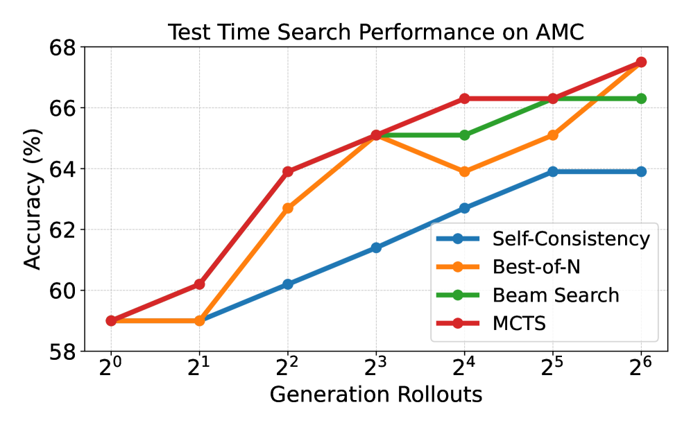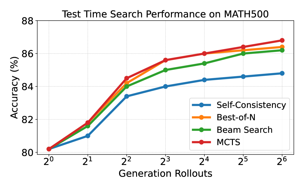Effectiveness on Different Search-Based TTS Methods. We evaluate our PRM within three search-based TTS methods, MCTS, beam search, and Best-of-N, using Qwen2.5-7B-AIRL-S as the generative LLM and Qwen2.5-AIRL-S-PRM as the verifier. We include Self-Consistency [70] as a baseline for sanity check: it generates multiple complete solutions and uses majority vote to select the final answer without any PRM or ORM. Results on AMC and MATH500 in Figure 3 show that: (i) Our PRM effectively guides the search, selection, and aggregation processes for all search algorithms. It improves performance across all search-based methods as the number of rollouts increases and outperforms Self-Consistency under the same rollouts. This result indicates that reward-guided step generation and selection produce more accurate intermediate decisions than majority voting on final answers. (ii) The PRM is especially effective for value-based methods like MCTS. By estimating step values during tree expansion and selecting nodes by UCT score, MCTS benefits more from the PRM’s guidance, leading to more accurate intermediate steps. <details> <summary>x3.png Details</summary>  ### Visual Description ## Line Chart: Test Time Search Performance on AMC ### Overview The image presents a line chart illustrating the performance of four different search algorithms (Self-Consistency, Best-of-N, Beam Search, and MCTS) on the AMC task, measured by accuracy as a function of generation rollouts. The chart displays how accuracy changes as the number of generation rollouts increases from 2⁰ to 2⁶. ### Components/Axes * **Title:** "Test Time Search Performance on AMC" (centered at the top) * **X-axis:** "Generation Rollouts" (bottom-horizontal). Markers are at 2⁰, 2¹, 2², 2³, 2⁴, 2⁵, and 2⁶. * **Y-axis:** "Accuracy (%)" (left-vertical). Scale ranges from 58% to 68%. * **Legend:** Located in the top-right corner. Contains the following entries with corresponding colors: * Self-Consistency (Blue) * Best-of-N (Orange) * Beam Search (Green) * MCTS (Red) ### Detailed Analysis The chart displays four distinct lines, each representing a search algorithm's accuracy as generation rollouts increase. * **Self-Consistency (Blue):** The line starts at approximately 58% accuracy at 2⁰ rollouts. It increases slowly to around 61% at 2¹, then rises more steeply to approximately 63% at 2². It plateaus around 63-64% for the remaining rollouts (2³ through 2⁶). * **Best-of-N (Orange):** The line begins at approximately 58% accuracy at 2⁰ rollouts. It dips to around 59% at 2¹, then increases rapidly to approximately 64% at 2². It continues to increase, reaching around 66% at 2⁴ and finally approximately 67% at 2⁶. * **Beam Search (Green):** The line starts at approximately 58% accuracy at 2⁰ rollouts. It increases steadily to around 62% at 2¹, then rises more sharply to approximately 65% at 2². It continues to increase, reaching approximately 66% at 2³ and 67% at 2⁶. * **MCTS (Red):** The line begins at approximately 58% accuracy at 2⁰ rollouts. It increases rapidly to approximately 63% at 2¹, then continues to increase sharply to approximately 65% at 2². It continues to increase, reaching approximately 67% at 2⁴ and approximately 68% at 2⁶. ### Key Observations * MCTS consistently demonstrates the highest accuracy across all generation rollout values. * Self-Consistency shows the slowest improvement in accuracy and plateaus at a lower level compared to the other algorithms. * Best-of-N and Beam Search exhibit similar trends, with Beam Search slightly outperforming Best-of-N at higher rollout values. * All algorithms show a significant performance boost between 2⁰ and 2² rollouts. * The performance gains diminish as the number of rollouts increases beyond 2³. ### Interpretation The data suggests that increasing the number of generation rollouts generally improves the accuracy of all four search algorithms on the AMC task. However, the extent of improvement varies significantly between algorithms. MCTS appears to be the most effective algorithm, consistently achieving the highest accuracy. Self-Consistency, while improving with rollouts, reaches a performance ceiling relatively quickly. The diminishing returns observed at higher rollout values suggest that there is a point of diminishing returns where further increasing rollouts does not yield substantial accuracy gains. This could be due to factors such as computational cost or the inherent limitations of the algorithms themselves. The initial rapid improvement likely reflects the algorithms' ability to explore the search space more effectively with increased computational effort. The differences in performance between the algorithms highlight the importance of algorithm selection for optimal performance on this task. </details> <details> <summary>x4.png Details</summary>  ### Visual Description \n ## Line Chart: Test Time Search Performance on MATH500 ### Overview This line chart depicts the performance of four different search algorithms (Self-Consistency, Best-of-N, Beam Search, and MCTS) on the MATH500 dataset, measured by accuracy as a function of Generation Rollouts. The x-axis represents the number of Generation Rollouts, expressed as powers of 2 (from 2⁰ to 2⁶). The y-axis represents the Accuracy in percentage (from 80% to 88%). ### Components/Axes * **Title:** "Test Time Search Performance on MATH500" (centered at the top) * **X-axis Label:** "Generation Rollouts" (centered at the bottom) * **X-axis Markers:** 2⁰, 2¹, 2², 2³, 2⁴, 2⁵, 2⁶ * **Y-axis Label:** "Accuracy (%)" (left side) * **Y-axis Scale:** Linear, ranging from approximately 80% to 88% with increments of 2%. * **Legend:** Located in the top-right corner. * **Self-Consistency:** Blue line with circle markers. * **Best-of-N:** Orange line with circle markers. * **Beam Search:** Green line with circle markers. * **MCTS:** Red line with circle markers. ### Detailed Analysis * **Self-Consistency (Blue):** The line starts at approximately 80% at 2⁰, rises sharply to around 83% at 2¹, then plateaus, reaching approximately 85% at 2² and remaining relatively stable around 85% for the rest of the rollouts. * **Best-of-N (Orange):** The line begins at approximately 80% at 2⁰, increases steadily to around 86% at 2³, and then plateaus, reaching approximately 87% at 2⁶. * **Beam Search (Green):** The line starts at approximately 80% at 2⁰, increases rapidly to around 86% at 2³, and then plateaus, reaching approximately 86.5% at 2⁶. * **MCTS (Red):** The line begins at approximately 80% at 2⁰, increases steadily to around 86.5% at 2³, and continues to increase, reaching approximately 87.5% at 2⁶. Here's a breakdown of approximate accuracy values at each Generation Rollout: | Generation Rollouts | Self-Consistency (%) | Best-of-N (%) | Beam Search (%) | MCTS (%) | |---|---|---|---|---| | 2⁰ | 80 | 80 | 80 | 80 | | 2¹ | 83 | 82 | 82 | 82 | | 2² | 85 | 84 | 84 | 84 | | 2³ | 85 | 86 | 86 | 86.5 | | 2⁴ | 85 | 86 | 86 | 86.5 | | 2⁵ | 85 | 86 | 86 | 87 | | 2⁶ | 85 | 87 | 86.5 | 87.5 | ### Key Observations * All four algorithms start with the same accuracy at 2⁰. * Self-Consistency shows the earliest plateau in performance. * MCTS consistently achieves the highest accuracy, especially at higher Generation Rollouts. * Best-of-N and Beam Search exhibit similar performance trends, plateauing around similar accuracy levels. ### Interpretation The chart demonstrates the impact of increasing Generation Rollouts on the accuracy of different search algorithms for solving MATH500 problems. The algorithms initially show significant performance gains as the number of rollouts increases, indicating that exploring more possibilities improves solution quality. However, the gains diminish as the number of rollouts grows, suggesting a point of diminishing returns. MCTS appears to be the most effective algorithm, consistently outperforming the others, particularly at higher rollout numbers. This suggests that MCTS's tree search strategy is well-suited for this type of problem. Self-Consistency, while simple, plateaus quickly, indicating it may not benefit as much from increased exploration. The similar performance of Best-of-N and Beam Search suggests they offer comparable trade-offs between exploration and computational cost. The plateauing behavior of all algorithms indicates that the MATH500 problems may have inherent limitations in terms of how much accuracy can be achieved through search alone. Further improvements might require more sophisticated algorithms or problem-specific knowledge. </details> Figure 3: Comparison of test-time search performance with our PRM applied to MCTS, Beam Search, and Best-of-N across varying rollout counts. Our PRM consistently improves performance for all search techniques. 4.3 Ablation Study Impact of Our PRM on RL Training. 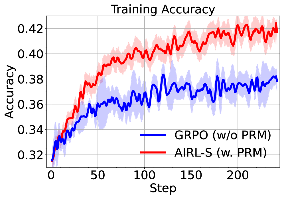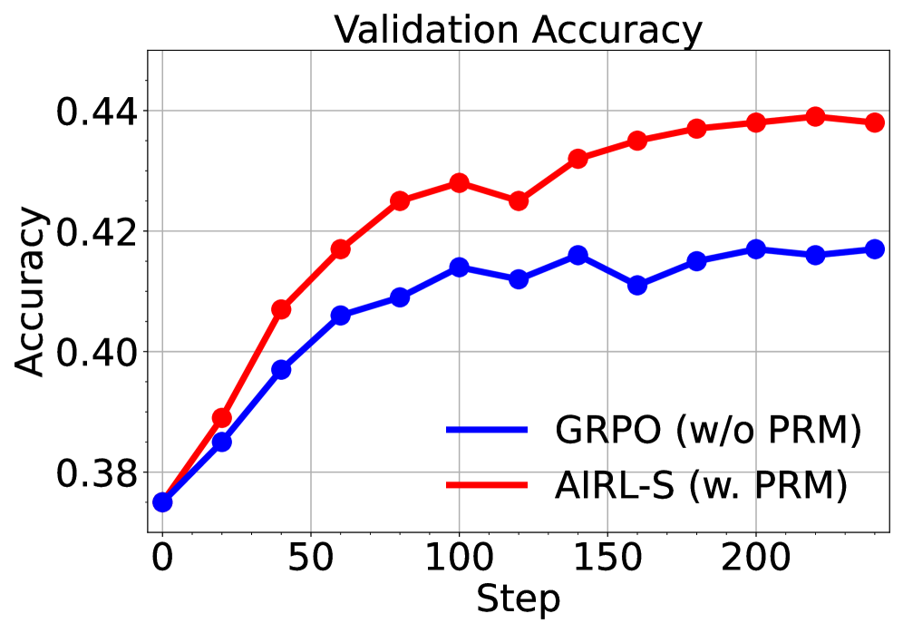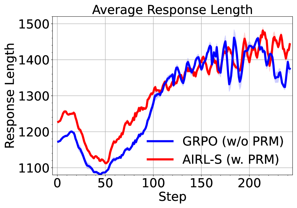To assess the contribution of our reward function on RL training, we compare AIRL-S to GRPO trained with outcome rewards only (no PRM), while keeping all other settings identical to AIRL-S . The results in Figure 4 show that adding our PRM improves both training and validation accuracy. Furthermore, as training progresses, AIRL-S enables longer response generation at test time, demonstrating its ability to scale inference computation. <details> <summary>x5.png Details</summary>  ### Visual Description \n ## Line Chart: Training Accuracy ### Overview This line chart displays the training accuracy of two different models, GRPO (without PRM) and AIRL-S (with PRM), over a series of training steps. The chart shows the mean accuracy for each model, along with a shaded region representing the standard deviation around the mean. ### Components/Axes * **Title:** "Training Accuracy" - positioned at the top-center of the chart. * **X-axis:** "Step" - ranging from approximately 0 to 220, with tick marks at intervals of 50. * **Y-axis:** "Accuracy" - ranging from approximately 0.32 to 0.42, with tick marks at intervals of 0.02. * **Legend:** Located in the bottom-center of the chart. * **Blue Line:** "GRPO (w/o PRM)" * **Red Line:** "AIRL-S (w. PRM)" * **Shaded Regions:** Light blue around the blue line, and light red around the red line, representing the standard deviation. ### Detailed Analysis **AIRL-S (w. PRM) - Red Line:** The red line representing AIRL-S shows an upward trend throughout the training process. * At Step 0, the accuracy is approximately 0.33. * At Step 50, the accuracy is approximately 0.39. * At Step 100, the accuracy is approximately 0.40. * At Step 150, the accuracy is approximately 0.41. * At Step 200, the accuracy is approximately 0.41. * At Step 220, the accuracy is approximately 0.41. The shaded region around the red line indicates a relatively consistent standard deviation, ranging from approximately 0.01 to 0.02. **GRPO (w/o PRM) - Blue Line:** The blue line representing GRPO shows a more fluctuating trend, with periods of increase and decrease. * At Step 0, the accuracy is approximately 0.33. * At Step 50, the accuracy is approximately 0.36. * At Step 100, the accuracy is approximately 0.37. * At Step 150, the accuracy is approximately 0.37. * At Step 200, the accuracy is approximately 0.38. * At Step 220, the accuracy is approximately 0.38. The shaded region around the blue line indicates a larger and more variable standard deviation, ranging from approximately 0.01 to 0.03. ### Key Observations * AIRL-S consistently outperforms GRPO in terms of training accuracy. * The standard deviation of AIRL-S is smaller than that of GRPO, indicating more stable training. * GRPO exhibits more volatility in its training accuracy, suggesting it may be more sensitive to variations in the training data or hyperparameters. * Both models appear to converge towards a stable accuracy level after approximately 150 steps. ### Interpretation The data suggests that incorporating PRM (as in AIRL-S) leads to improved and more stable training accuracy compared to not using PRM (as in GRPO). The consistent upward trend and smaller standard deviation of AIRL-S indicate that it learns more effectively and is less prone to overfitting or instability during training. The fluctuating behavior of GRPO suggests that it may require more careful tuning or regularization to achieve comparable performance. The convergence of both models after 150 steps implies that the training process is reaching a point of diminishing returns, and further training may not yield significant improvements in accuracy. The difference in performance between the two models highlights the importance of the PRM component in achieving optimal results. </details> <details> <summary>x6.png Details</summary>  ### Visual Description \n ## Line Chart: Validation Accuracy ### Overview This image presents a line chart illustrating the validation accuracy of two different models, GRPO (without PRM) and AIRL-S (with PRM), over a series of steps. The chart displays how the accuracy of each model changes as the training progresses, measured by the 'Step' value on the x-axis. ### Components/Axes * **Title:** "Validation Accuracy" - positioned at the top-center of the chart. * **X-axis:** "Step" - ranging from approximately 0 to 220, with tick marks at intervals of 50. * **Y-axis:** "Accuracy" - ranging from approximately 0.38 to 0.44, with tick marks at intervals of 0.02. * **Legend:** Located in the top-right corner of the chart. * **GRPO (w/o PRM):** Represented by a blue line. * **AIRL-S (w. PRM):** Represented by a red line. ### Detailed Analysis **AIRL-S (w. PRM) - Red Line:** The red line representing AIRL-S exhibits an upward trend, starting at approximately 0.38 at Step 0. It increases relatively quickly to around 0.42 by Step 50, then continues to rise more gradually, reaching approximately 0.435 by Step 100. The line plateaus around 0.438-0.44 between Steps 150 and 200, with a slight fluctuation. * Step 0: ~0.38 * Step 50: ~0.42 * Step 100: ~0.435 * Step 150: ~0.438 * Step 200: ~0.44 **GRPO (w/o PRM) - Blue Line:** The blue line representing GRPO also shows an upward trend, but it is less pronounced than that of AIRL-S. It starts at approximately 0.38 at Step 0 and increases to around 0.41 by Step 50. The line then plateaus, with minor fluctuations, reaching approximately 0.425 by Step 100 and remaining around that level until Step 200, with a slight increase to ~0.428. * Step 0: ~0.38 * Step 50: ~0.41 * Step 100: ~0.425 * Step 150: ~0.426 * Step 200: ~0.428 ### Key Observations * AIRL-S consistently outperforms GRPO throughout the entire training process. * The accuracy of AIRL-S increases rapidly in the initial stages (Steps 0-50) and then stabilizes. * GRPO shows a slower and less significant increase in accuracy, plateauing at a lower level than AIRL-S. * Both models start with the same accuracy at Step 0. ### Interpretation The data suggests that incorporating PRM (as in AIRL-S) significantly improves the validation accuracy compared to not using PRM (as in GRPO). The faster initial increase in accuracy for AIRL-S indicates that PRM helps the model learn more effectively in the early stages of training. The plateauing of both lines suggests that the models are converging, and further training may not yield substantial improvements. The consistent difference in accuracy between the two models highlights the benefit of using PRM in this context. The chart demonstrates the effectiveness of the AIRL-S model with PRM in achieving higher validation accuracy compared to the GRPO model without PRM. </details> <details> <summary>x7.png Details</summary>  ### Visual Description \n ## Line Chart: Average Response Length ### Overview This image presents a line chart illustrating the average response length over a series of steps for two different models: GRPO (without Preference Ranking Model - PRM) and AIRL-S (with PRM). The chart displays how the average response length changes as the step number increases. ### Components/Axes * **Title:** Average Response Length * **X-axis:** Step (ranging from approximately 0 to 220) * **Y-axis:** Response Length (ranging from approximately 1100 to 1500) * **Legend:** * Blue Line: GRPO (w/o PRM) * Red Line: AIRL-S (w. PRM) * **Grid:** A light gray grid is present in the background to aid in reading values. ### Detailed Analysis The chart shows two distinct lines representing the average response length for each model over the steps. **GRPO (w/o PRM) - Blue Line:** The blue line starts at approximately 1200 at step 0. It initially decreases to a minimum of around 1130 at step 10. From step 10 to approximately step 100, the line exhibits a generally upward trend, increasing to around 1380. Between steps 100 and 220, the line fluctuates significantly, oscillating between approximately 1400 and 1500. **AIRL-S (w. PRM) - Red Line:** The red line begins at approximately 1250 at step 0. It also initially decreases, reaching a minimum of around 1150 at step 10. From step 10 to approximately step 100, the red line shows a consistent upward trend, increasing to around 1400. Between steps 100 and 220, the red line also fluctuates, but its oscillations are less pronounced than those of the blue line, generally staying between approximately 1400 and 1480. **Approximate Data Points (extracted visually):** | Step | GRPO (Blue) | AIRL-S (Red) | |---|---|---| | 0 | 1200 | 1250 | | 10 | 1130 | 1150 | | 50 | 1280 | 1320 | | 100 | 1380 | 1400 | | 150 | 1450 | 1430 | | 200 | 1480 | 1460 | | 220 | 1430 | 1440 | ### Key Observations * Both models exhibit an initial decrease in average response length followed by an increase. * AIRL-S (with PRM) consistently demonstrates a higher average response length than GRPO (without PRM) after step 50. * The fluctuations in average response length are more pronounced for GRPO (without PRM) in the later stages (steps 100-220). * The difference in average response length between the two models appears to stabilize around 100-200 units after step 100. ### Interpretation The data suggests that incorporating a Preference Ranking Model (PRM), as done in AIRL-S, leads to a higher average response length compared to not using a PRM (GRPO). The initial decrease in response length for both models could be due to a learning phase where the models are initially calibrating. The subsequent increase suggests that the models are learning to generate more comprehensive or detailed responses. The fluctuations in the later stages might indicate a degree of instability or variance in the response generation process. The more pronounced fluctuations in GRPO suggest that the absence of a PRM makes the response length more sensitive to variations in the input or the learning process. The consistent higher response length of AIRL-S indicates that the PRM is effectively guiding the model to produce longer, potentially more informative, responses. </details> Figure 4: Comparison of AIRL-S and GRPO trained with outcome rewards only. AIRL-S improves training and validation performance and enables longer response generation at test time. 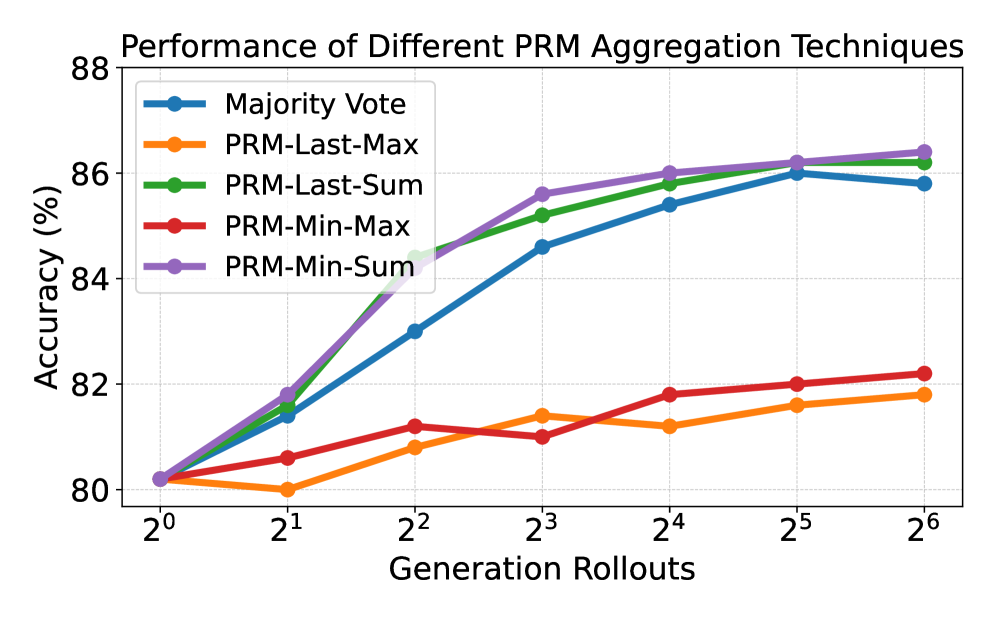Impact of PRM Aggregation Techniques. As described in Section 3.5 and Appendix A, different PRM aggregation techniques can select the final answer from multiple rollouts. We evaluate these techniques using our policy and PRM with Best-of-N search on MATH500; results of five aggregation techniques (defined in Appendix A) appear in Figure 5. PRM-Min-Vote and PRM-Last-Vote achieve the highest accuracy, showing that step-level rewards enable effective answer aggregation. In contrast, PRM-Min-Max and PRM-Last-Max achieve the worst performance, demonstrating the importance of inter-answer aggregation via PRM weighted voting to integrated the answers from various rollouts. <details> <summary>x8.png Details</summary>  ### Visual Description \n ## Line Chart: Performance of Different PRM Aggregation Techniques ### Overview This line chart illustrates the performance, measured in accuracy (%), of five different Prompt Response Modeling (PRM) aggregation techniques across varying numbers of generation rollouts. The x-axis represents the generation rollouts (from 2⁰ to 2⁶), and the y-axis represents the accuracy percentage (from 80% to 88%). Each line represents a different aggregation technique, and the chart aims to compare their performance as the number of generation rollouts increases. ### Components/Axes * **Title:** "Performance of Different PRM Aggregation Techniques" (Top-center) * **X-axis Label:** "Generation Rollouts" (Bottom-center) * **Markers:** 2⁰, 2¹, 2², 2³, 2⁴, 2⁵, 2⁶ * **Y-axis Label:** "Accuracy (%)" (Left-center) * **Scale:** 80 to 88, with increments of approximately 2. * **Legend:** Located in the top-left corner. * **Labels & Colors:** * Majority Vote (Blue) * PRM-Last-Max (Orange) * PRM-Last-Sum (Green) * PRM-Min-Max (Red) * PRM-Min-Sum (Purple) ### Detailed Analysis Here's a breakdown of each line's trend and approximate data points, verified against the legend colors: * **Majority Vote (Blue):** The line slopes upward, showing a consistent increase in accuracy with increasing generation rollouts. * 2⁰: ~80% * 2¹: ~81% * 2²: ~83% * 2³: ~85% * 2⁴: ~86% * 2⁵: ~86% * 2⁶: ~86.5% * **PRM-Last-Max (Orange):** The line shows a relatively flat trend with some fluctuations. * 2⁰: ~80% * 2¹: ~80.5% * 2²: ~81% * 2³: ~81.5% * 2⁴: ~82% * 2⁵: ~82% * 2⁶: ~82.5% * **PRM-Last-Sum (Green):** The line slopes upward, similar to Majority Vote, but starts slightly lower and ends slightly lower. * 2⁰: ~80% * 2¹: ~81% * 2²: ~82.5% * 2³: ~85% * 2⁴: ~85.5% * 2⁵: ~86% * 2⁶: ~86% * **PRM-Min-Max (Red):** The line shows an initial increase, then plateaus, and has some fluctuations. * 2⁰: ~80% * 2¹: ~80.5% * 2²: ~81% * 2³: ~82% * 2⁴: ~82% * 2⁵: ~82% * 2⁶: ~82.5% * **PRM-Min-Sum (Purple):** The line slopes upward, showing a consistent increase in accuracy with increasing generation rollouts. It starts lower than Majority Vote but reaches a similar level. * 2⁰: ~80% * 2¹: ~81% * 2²: ~82.5% * 2³: ~84.5% * 2⁴: ~85.5% * 2⁵: ~86% * 2⁶: ~86% ### Key Observations * **Majority Vote and PRM-Min-Sum** demonstrate the highest accuracy, reaching approximately 86-86.5% at 2⁶. * **PRM-Last-Max, PRM-Min-Max** show the lowest and most stable accuracy, hovering around 82-82.5%. * **PRM-Last-Sum** performs intermediately, with a steady increase but not reaching the levels of Majority Vote or PRM-Min-Sum. * The most significant accuracy gains occur between 2⁰ and 2³, after which the improvements become marginal for most techniques. ### Interpretation The data suggests that the "Majority Vote" and "PRM-Min-Sum" aggregation techniques are the most effective for improving accuracy as the number of generation rollouts increases. These techniques consistently outperform "PRM-Last-Max" and "PRM-Min-Max". The relatively flat performance of the latter two suggests they are less sensitive to the number of rollouts or may have reached a performance ceiling. The initial rapid increase in accuracy across all techniques indicates that early generation rollouts provide the most significant improvements. Beyond a certain point (around 2³ or 2⁴), the marginal gains diminish, suggesting diminishing returns. The difference between "PRM-Last-Sum" and the top performers ("Majority Vote" and "PRM-Min-Sum") could be due to the way the last responses are aggregated. The "Sum" approach might be more susceptible to outliers or less effective at capturing the consensus of multiple responses compared to the "Majority Vote" or "Min-Sum" approaches. This data is valuable for optimizing the PRM process by informing the choice of aggregation technique and the optimal number of generation rollouts to balance accuracy and computational cost. Further investigation could explore why "Majority Vote" and "PRM-Min-Sum" are superior and whether the performance differences are statistically significant. </details> Figure 5: Performance of different PRM aggregation techniques evaluated on MATH500. Table 2: Comparison of our policy model and PRM with PRIME [11] train on the same setting. AIRL-S consistently outperforms PRIME both with and without test-time search. AIME, MATH, and BoN denote AIME2024, MATH500, and Best-of-N, respectively. | PRIME PRIME w. BoN AIRL-S | 16.7 20.0 26.7 | 55.4 62.7 59.0 | 78.4 84.2 80.2 | 50.2 55.6 55.3 | | --- | --- | --- | --- | --- | | AIRL-S w. BoN | 30.0 | 67.5 | 86.4 | 61.3 | Comparison with Concurrent Implicit PRM Methods. We compare AIRL-S with PRIME [11], which trains a policy-dependent dense reward function based on [79]. Both methods are trained on Qwen2.5-7B-Instruct under identical settings. At inference, we apply Best-of-N search under 64 rollouts with each method’s PRM. Results on AIME2024, AMC, and MATH500 in Table 2 show that our policy and PRM combination outperforms PRIME, further confirming that AIRL-S unifies RL-based and search-based TTS. 5 Conclusion In this paper, we present AIRL-S , a framework that unifies RL-based and search-based TTS for LLMs. AIRL-S integrates AIRL with GRPO to learn a step-wise PRM from reference rollouts without any labeled data. This PRM guides both RL training by improving training stability and sample efficiency, and inference search by extending reasoning chains and mitigating reward hacking. We evaluate AIRL-S on eight benchmarks covering mathematics, scientific reasoning, and code generation. The results show that AIRL-S significantly improves the performance of base models and outperforms existing RL-trained and imitation-based methods. The PRM generalizes across different LLMs, datasets, and search algorithms, consistently enhancing test-time search performance. These findings validate that unifying RL-based and search-based TTS offers an efficient and robust approach for complex reasoning. References - [1] P. Abbeel and A. Y. Ng (2004) Apprenticeship learning via inverse reinforcement learning. In Proceedings of the twenty-first international conference on Machine learning, pp. 1. Cited by: §2. - [2] M. Abdin, J. Aneja, H. Behl, S. Bubeck, R. Eldan, S. Gunasekar, M. Harrison, R. J. Hewett, M. Javaheripi, P. Kauffmann, et al. (2024) Phi-4 technical report. arXiv preprint arXiv:2412.08905. Cited by: Appendix D, §4.1. - [3] Y. Bai, A. Jones, K. Ndousse, A. Askell, A. Chen, N. DasSarma, D. Drain, S. Fort, D. Ganguli, T. Henighan, et al. (2022) Training a helpful and harmless assistant with reinforcement learning from human feedback. arXiv preprint arXiv:2204.05862. Cited by: §1. - [4] B. Brown, J. Juravsky, R. Ehrlich, R. Clark, Q. V. Le, C. Ré, and A. Mirhoseini (2024) Large language monkeys: scaling inference compute with repeated sampling. arXiv preprint arXiv:2407.21787. Cited by: §2. - [5] D. Carraro and D. Bridge (2024) Enhancing recommendation diversity by re-ranking with large language models. ACM Transactions on Recommender Systems. Cited by: §2. - [6] A. J. Chan, H. Sun, S. Holt, and M. Van Der Schaar (2024) Dense reward for free in reinforcement learning from human feedback. In Proceedings of the 41st International Conference on Machine Learning, pp. 6136–6154. Cited by: §1. - [7] M. Chen, J. Tworek, H. Jun, Q. Yuan, H. Pinto, J. Kaplan, et al. (2021) Evaluating large language models trained on code. arXiv preprint arXiv:2107.03374. External Links: Link Cited by: Table 5, §4.1. - [8] P. F. Christiano, J. Leike, T. B. Brown, M. Martic, S. Legg, and D. Amodei (2017) Deep reinforcement learning from human preferences. In Advances in Neural Information Processing Systems 30 (NIPS 2017), pp. 4299–4307. External Links: Link Cited by: §2. - [9] K. Cobbe, V. Kosaraju, M. Bavarian, M. Chen, H. Jun, L. Kaiser, M. Plappert, J. Tworek, J. Hilton, R. Nakano, et al. (2021) Training verifiers to solve math word problems. arXiv preprint arXiv:2110.14168. Cited by: §1. - [10] T. Coignion, C. Quinton, and R. Rouvoy (2024) A performance study of llm-generated code on leetcode. arXiv preprint arXiv:2407.21579. External Links: Link Cited by: Table 5, §4.1. - [11] G. Cui, L. Yuan, Z. Wang, et al. (2025) Process reinforcement through implicit rewards. arXiv preprint arXiv:2502.01456. External Links: Link Cited by: Table 3, §2, §4.1, §4.3, Table 2. - [12] DeepSeek-AI (2024) DeepSeek-math-7b-rl: reinforcement learning enhanced math reasoning model. Note: GitHub repository External Links: Link Cited by: §1, §1, §2. - [13] C. Finn, P. Christiano, P. Abbeel, and S. Levine (2016) A connection between generative adversarial networks, inverse reinforcement learning, and energy-based models. arXiv preprint arXiv:1611.03852. Cited by: §1, §2, §3.3. - [14] J. Fu, K. Luo, and S. Levine (2018) Learning robust rewards with adverserial inverse reinforcement learning. In International Conference on Learning Representations, Cited by: §1, §2, §2, §3.3, §3.4. - [15] B. Gao, F. Song, Z. Yang, Z. Cai, Y. Miao, Q. Dong, L. Li, C. Ma, L. Chen, R. Xu, Z. Tang, B. Wang, D. Zan, S. Quan, G. Zhang, L. Sha, Y. Zhang, X. Ren, T. Liu, and B. Chang (2024) Omni-math: a universal olympiad level mathematic benchmark for large language models. External Links: 2410.07985, Link Cited by: §B.3, Table 4. - [16] L. Gao, J. Schulman, and J. Hilton (2023) Scaling laws for reward model overoptimization. In International Conference on Machine Learning, pp. 10835–10866. Cited by: §1. - [17] D. Garg, S. Chakraborty, C. Cundy, J. Song, and S. Ermon (2021) IQ-learn: inverse soft-$q$ learning for imitation. In NeurIPS 2021 Spotlight, External Links: Link Cited by: §2. - [18] I. Goodfellow, J. Pouget-Abadie, M. Mirza, B. Xu, D. Warde-Farley, S. Ozair, A. Courville, and Y. Bengio (2020) Generative adversarial networks. Communications of the ACM 63 (11), pp. 139–144. Cited by: §2, §3.3. - [19] Google Research, J. Austin, A. Odena, M. Nye, M. Bosma, H. Michalewski, D. Dohan, E. Jiang, C. Cai, M. Terry, Q. Le, et al. (2021) MBPP-sanitized. Note: Hugging Face DatasetsSanitized split of the MBPP benchmark External Links: Link Cited by: Table 5, §4.1. - [20] D. Guo, D. Yang, H. Zhang, J. Song, R. Zhang, R. Xu, Q. Zhu, S. Ma, P. Wang, X. Bi, et al. (2025) Deepseek-r1: incentivizing reasoning capability in llms via reinforcement learning. arXiv preprint arXiv:2501.12948. Cited by: Table 3, §1, §1, §1, §2, §3.4, §4.1. - [21] J. Hejna and D. Sadigh (2023) Inverse preference learning: preference-based rl without a reward function. Vol. 36, pp. 18806–18827. Cited by: §2. - [22] D. Hendrycks, S. Basart, S. Kadavath, M. Mazeika, A. Arora, E. Guo, C. Burns, S. Puranik, H. He, D. Song, and J. Steinhardt (2021) Measuring coding challenge competence with APPS. CoRR abs/2105.09938. External Links: Link, 2105.09938 Cited by: §B.3, §B.4, Table 4. - [23] D. Hendrycks, C. Burns, S. Kadavath, A. Arora, S. Basart, E. Tang, D. Song, and J. Steinhardt (2021) Measuring mathematical problem solving with the math dataset. In Advances in Neural Information Processing Systems (NeurIPS), External Links: Link Cited by: Table 5, §4.1. - [24] B. Hui, J. Yang, Z. Cui, J. Yang, D. Liu, L. Zhang, T. Liu, J. Zhang, B. Yu, K. Lu, et al. (2024) Qwen2. 5-coder technical report. arXiv preprint arXiv:2409.12186. Cited by: Table 3, §4.1. - [25] R. Irvine, D. Boubert, V. Raina, A. Liusie, Z. Zhu, V. Mudupalli, A. Korshuk, Z. Liu, F. Cremer, V. Assassi, et al. (2023) Rewarding chatbots for real-world engagement with millions of users. arXiv preprint arXiv:2303.06135. Cited by: §2. - [26] I. Jain, F. Zhang, W. Liu, et al. (2025) LiveCodeBench: holistic and contamination-free evaluation of llms for code. In International Conference on Learning Representations (ICLR) 2025, External Links: Link Cited by: Table 5, §4.1. - [27] C. Jin, T. Che, H. Peng, Y. Li, D. Metaxas, and M. Pavone (2024) Learning from teaching regularization: generalizable correlations should be easy to imitate. Advances in Neural Information Processing Systems 37, pp. 966–994. Cited by: §1. - [28] C. Jin, H. Peng, Q. Zhang, Y. Tang, D. N. Metaxas, and T. Che (2025) Two heads are better than one: test-time scaling of multi-agent collaborative reasoning. arXiv preprint arXiv:2504.09772. Cited by: §1. - [29] M. Jin, W. Luo, S. Cheng, X. Wang, W. Hua, R. Tang, W. Y. Wang, and Y. Zhang (2024) Disentangling memory and reasoning ability in large language models. arXiv preprint arXiv:2411.13504. Cited by: §2. - [30] M. Jin, Q. Yu, D. Shu, H. Zhao, W. Hua, Y. Meng, Y. Zhang, and M. Du (2024) The impact of reasoning step length on large language models. In Findings of the Association for Computational Linguistics ACL 2024, pp. 1830–1842. Cited by: §1. - [31] L. Kocsis and C. Szepesvári (2006) Bandit based monte-carlo planning. In European conference on machine learning, pp. 282–293. Cited by: 3rd item. - [32] J. Li, E. Beeching, L. Tunstall, B. Lipkin, R. Soletskyi, S. C. Huang, K. Rasul, L. Yu, A. Jiang, Z. Shen, Z. Qin, B. Dong, L. Zhou, Y. Fleureau, G. Lample, and S. Polu (2024) NuminaMath. Numina. Note: https://huggingface.co/datasets/AI-MO/NuminaMath-CoT Cited by: §B.3, §B.4, Table 4. - [33] J. LI, E. Beeching, L. Tunstall, B. Lipkin, R. Soletskyi, S. C. Huang, K. Rasul, L. Yu, A. Jiang, Z. Shen, Z. Qin, B. Dong, L. Zhou, Y. Fleureau, G. Lample, and S. Polu (2024) NuminaMath. Numina. Note: [https://huggingface.co/AI-MO/NuminaMath-CoT](https://github.com/project-numina/aimo-progress-prize/blob/main/report/numina_dataset.pdf) Cited by: §4.1. - [34] R. Li, J. Fu, B. Zhang, T. Huang, Z. Sun, C. Lyu, G. Liu, Z. Jin, and G. Li (2023) TACO: topics in algorithmic code generation dataset. arXiv preprint arXiv:2312.14852. Cited by: §B.3, Table 4. - [35] Y. Li, Z. Lin, S. Zhang, Q. Fu, B. Chen, J. Lou, and W. Chen (2023) Making language models better reasoners with step-aware verifier. In Proceedings of the 61st Annual Meeting of the Association for Computational Linguistics (Volume 1: Long Papers), pp. 5315–5333. Cited by: §1. - [36] Y. Li, D. Choi, J. Chung, N. Kushman, J. Schrittwieser, R. Leblond, T. Eccles, J. Keeling, F. Gimeno, A. D. Lago, T. Hubert, P. Choy, C. de Masson d’Autume, I. Babuschkin, X. Chen, P. Huang, J. Welbl, S. Gowal, A. Cherepanov, J. Molloy, D. J. Mankowitz, E. S. Robson, P. Kohli, N. de Freitas, K. Kavukcuoglu, and O. Vinyals (2022) Competition-level code generation with alphacode. Science 378 (6624), pp. 1092–1097. External Links: Document, Link Cited by: §B.3, §B.4, Table 4. - [37] H. Lightman, V. Kosaraju, Y. Burda, H. Edwards, B. Baker, T. Lee, J. Leike, J. Schulman, I. Sutskever, and K. Cobbe (2023) Let’s verify step by step. In The Twelfth International Conference on Learning Representations, Cited by: §1, §1. - [38] A. Liu, B. Feng, B. Xue, B. Wang, B. Wu, C. Lu, C. Zhao, C. Deng, C. Zhang, C. Ruan, et al. (2024) Deepseek-v3 technical report. arXiv preprint arXiv:2412.19437. Cited by: Table 3, §4.1. - [39] F. Liu et al. (2020) Learning to summarize from human feedback. In Proceedings of the 58th Annual Meeting of the Association for Computational Linguistics, pp. 583–592. Cited by: item (a). - [40] S. Liu and M. Zhu (2022) Distributed inverse constrained reinforcement learning for multi-agent systems. Advances in Neural Information Processing Systems 35, pp. 33444–33456. Cited by: §2. - [41] S. Liu and M. Zhu (2024) In-trajectory inverse reinforcement learning: learn incrementally before an ongoing trajectory terminates. Advances in Neural Information Processing Systems 37, pp. 117164–117209. Cited by: §2. - [42] Y. Liu, H. Gao, S. Zhai, X. Jun, T. Wu, Z. Xue, Y. Chen, K. Kawaguchi, J. Zhang, and B. Hooi (2025) GuardReasoner: towards reasoning-based llm safeguards. arXiv preprint arXiv:2501.18492. Cited by: §2. - [43] Y. Liu, S. Zhai, M. Du, Y. Chen, T. Cao, H. Gao, C. Wang, X. Li, K. Wang, J. Fang, J. Zhang, and B. Hooi (2025) GuardReasoner-vl: safeguarding vlms via reinforced reasoning. arXiv preprint arXiv:2505.11049. Cited by: §2. - [44] A. Madaan, N. Tandon, P. Gupta, S. Hallinan, L. Gao, S. Wiegreffe, U. Alon, N. Dziri, S. Prabhumoye, Y. Yang, et al. (2023) Self-refine: iterative refinement with self-feedback. Advances in Neural Information Processing Systems 36, pp. 46534–46594. Cited by: §2. - [45] Mathematical Association of America (2024) 2024 american invitational mathematics examination (aime i). Technical report Mathematical Association of America. External Links: Link Cited by: Table 5, §4.1. - [46] Mathematical Association of America (2025) American Mathematics Competitions (AMC). Note: https://www.maa.org/student-programs/amc Accessed: 2025-05-05 Cited by: Table 5, §4.1. - [47] Y. Miao, S. Zhang, L. Ding, R. Bao, L. Zhang, and D. Tao (2024) Inform: mitigating reward hacking in rlhf via information-theoretic reward modeling. In The Thirty-eighth Annual Conference on Neural Information Processing Systems, Cited by: §1. - [48] N. Muennighoff, Z. Yang, W. Shi, X. L. Li, L. Fei-Fei, H. Hajishirzi, L. Zettlemoyer, P. Liang, E. Candès, and T. Hashimoto (2025) S1: simple test-time scaling. External Links: 2501.19393, Link Cited by: §B.3, Table 4. - [49] N. Muennighoff, Z. Yang, W. Shi, X. L. Li, L. Fei-Fei, H. Hajishirzi, L. Zettlemoyer, P. Liang, E. Candès, and T. Hashimoto (2025) S1: simple test-time scaling. arXiv preprint arXiv:2501.19393. Cited by: Table 3, §1, §2, §2, §4.1. - [50] W. Nie, N. Narodytska, and A. Patel (2018) Relgan: relational generative adversarial networks for text generation. In International conference on learning representations, Cited by: item (a), §3.3. - [51] OpenAI (2024-11-20) GPT-4o system card. Technical report OpenAI. External Links: Link Cited by: Table 3, §4.1. - [52] OpenAI (2024-09) Learning to reason with llms. External Links: Link Cited by: §1. - [53] OpenAI (2024-12) OpenAI o1 system card. Technical report OpenAI. External Links: Link Cited by: §2. - [54] L. Ouyang, J. Wu, X. Jiang, D. Almeida, C. L. Wainwright, P. Mishkin, C. Zhang, S. Agarwal, K. Slama, A. Ray, J. Schulman, J. Hilton, F. Kelvin, L. Miller, M. Simens, A. Askell, P. Welinder, P. Christiano, J. Leike, and R. Lowe (2022) Training language models to follow instructions with human feedback. arXiv preprint arXiv:2203.02155. External Links: Link Cited by: §2. - [55] S. Park, X. Liu, Y. Gong, and E. Choi (2024) Ensembling large language models with process reward-guided tree search for better complex reasoning. Cited by: §2. - [56] Qwen Team, A. Yang, B. Yang, B. Zhang, B. Hui, B. Zheng, B. Yu, C. Li, D. Liu, et al. (2024) Qwen2.5 technical report. arXiv preprint arXiv:2412.15115. External Links: Link Cited by: Table 3, §4.1. - [57] A. Rashid, R. Wu, J. Grosse, A. Kristiadi, and P. Poupart (2024) A critical look at tokenwise reward-guided text generation. arXiv preprint arXiv:2406.07780. Cited by: item (a). - [58] N. D. Ratliff, J. A. Bagnell, and M. A. Zinkevich (2006) Maximum margin planning. In Proceedings of the 23rd international conference on Machine learning, pp. 729–736. Cited by: §2. - [59] D. Rein, B. Li, A. C. Stickland, J. Petty, R. Y. Pang, J. Dirani, J. Michael, and S. R. Bowman (2023) GPQA: a graduate-level google-proof q&a benchmark. arXiv preprint arXiv:2311.12022. External Links: Link Cited by: Table 5, §4.1. - [60] Z. Shao, P. Wang, Q. Zhu, R. Xu, J. Song, X. Bi, H. Zhang, M. Zhang, Y. Li, Y. Wu, et al. (2024) Deepseekmath: pushing the limits of mathematical reasoning in open language models. arXiv preprint arXiv:2402.03300. Cited by: Table 3, §1, §4.1. - [61] C. Snell, J. Lee, K. Xu, and A. Kumar (2024) Free process rewards without process labels. arXiv preprint arXiv:2412.01981. External Links: Link Cited by: §2. - [62] C. V. Snell, J. Lee, K. Xu, and A. Kumar (2025) Scaling test-time compute optimally can be more effective than scaling LLM parameters. In The Thirteenth International Conference on Learning Representations, External Links: Link Cited by: §A.1, §1, §2, §3.5, §3.5. - [63] N. Srinivas, A. Krause, S. M. Kakade, and M. W. Seeger (2012) Information-theoretic regret bounds for gaussian process optimization in the bandit setting. IEEE transactions on information theory 58 (5), pp. 3250–3265. Cited by: 3rd item. - [64] M. Studio (2024) Codeforces–python submissions. Note: https://huggingface.co/datasets/MatrixStudio/Codeforces-Python-Submissions Cited by: §B.3, §B.4, Table 4. - [65] G. Swamy, D. Wu, S. Choudhury, D. Bagnell, and S. Wu (2023) Inverse reinforcement learning without reinforcement learning. pp. 33299–33318. Cited by: §2. - [66] J. Tan, K. Zhao, R. Li, J. X. Yu, C. Piao, H. Cheng, H. Meng, D. Zhao, and Y. Rong (2025) Can large language models be query optimizer for relational databases?. arXiv preprint arXiv:2502.05562. Cited by: §2. - [67] G. Team, A. Kamath, J. Ferret, S. Pathak, N. Vieillard, R. Merhej, S. Perrin, T. Matejovicova, A. Ramé, M. Rivière, et al. (2025) Gemma 3 technical report. arXiv preprint arXiv:2503.19786. Cited by: Appendix D. - [68] J. Uesato, N. Kushman, R. Kumar, F. Song, N. Siegel, L. Wang, A. Creswell, G. Irving, and I. Higgins (2022) Solving math word problems with process-and outcome-based feedback. arXiv preprint arXiv:2211.14275. Cited by: §1. - [69] P. Wang, L. Li, Z. Shao, R. Xu, D. Dai, Y. Li, D. Chen, Y. Wu, and Z. Sui (2024) Math-shepherd: verify and reinforce llms step-by-step without human annotations. In Proceedings of the 62nd Annual Meeting of the Association for Computational Linguistics (Volume 1: Long Papers), pp. 9426–9439. Cited by: §1, §1, §2, §4.1. - [70] X. Wang, J. Wei, D. Schuurmans, Q. Le, E. Chi, S. Narang, A. Chowdhery, and D. Zhou (2022) Self-consistency improves chain of thought reasoning in language models. Cited by: §2, §4.2. - [71] Z. Wang, X. Liu, H. Chen, S. Ermon, et al. (2023) Math-shepherd: verify and reinforce llms step-by-step. Note: arXiv preprint arXiv:2312.08935 External Links: Link Cited by: Table 3, §4.1. - [72] R. J. Williams (1992) Simple statistical gradient-following algorithms for connectionist reinforcement learning. Machine learning 8, pp. 229–256. Cited by: §3.4. - [73] Y. Wu, Z. Sun, S. Li, S. Welleck, and Y. Yang (2024) Inference scaling laws: an empirical analysis of compute-optimal inference for problem-solving with language models. arXiv preprint arXiv:2408.00724. Cited by: §2. - [74] Y. Wu, Z. Sun, S. Li, S. Welleck, and Y. Yang (2025) Inference scaling laws: an empirical analysis of compute-optimal inference for LLM problem-solving. In The Thirteenth International Conference on Learning Representations, External Links: Link Cited by: §1. - [75] Y. Xie, A. Goyal, W. Zheng, M. Kan, T. P. Lillicrap, K. Kawaguchi, and M. Shieh (2024) Monte carlo tree search boosts reasoning via iterative preference learning. arXiv preprint arXiv:2405.00451. Cited by: §2. - [76] Y. Xie, K. Kawaguchi, Y. Zhao, J. X. Zhao, M. Kan, J. He, and M. Xie (2023) Self-evaluation guided beam search for reasoning. Advances in Neural Information Processing Systems 36, pp. 41618–41650. Cited by: §1, §2, §3.5. - [77] W. Xiong, H. Zhang, N. Jiang, and T. Zhang (2024) An implementation of generative prm. GitHub. Note: https://github.com/RLHFlow/RLHF-Reward-Modeling Cited by: §4.1. - [78] F. Yu, A. Gao, and B. Wang (2023) Outcome-supervised verifiers for planning in mathematical reasoning. arXiv preprint arXiv:2311.09724 2 (6). Cited by: §1. - [79] L. Yuan, W. Li, H. Chen, G. Cui, N. Ding, K. Zhang, B. Zhou, Z. Liu, and H. Peng (2024) Free process rewards without process labels. arXiv preprint arXiv:2412.01981. Cited by: §1, §4.1, §4.3. - [80] S. Yuan, Z. Chen, Z. Xi, J. Ye, Z. Du, and J. Chen (2025) Agent-r: training language model agents to reflect via iterative self-training. arXiv preprint arXiv:2501.11425. Cited by: §2. - [81] X. Yue, X. Qu, G. Zhang, Y. Fu, W. Huang, H. Sun, Y. Su, and W. Chen (2023) Mammoth: building math generalist models through hybrid instruction tuning. Cited by: §2. - [82] D. Zhang, J. Wu, J. Lei, T. Che, J. Li, T. Xie, X. Huang, S. Zhang, M. Pavone, Y. Li, et al. (2024) Llama-berry: pairwise optimization for o1-like olympiad-level mathematical reasoning. arXiv preprint arXiv:2410.02884. Cited by: §1, §2. - [83] S. Zhang, Z. Chen, Y. Shen, M. Ding, J. B. Tenenbaum, and C. Gan (2023) Planning with large language models for code generation. arXiv preprint arXiv:2303.05510. Cited by: §1, §2. - [84] X. Zhang, C. Du, T. Pang, Q. Liu, W. Gao, and M. Lin (2024) Chain of preference optimization: improving chain-of-thought reasoning in llms. Advances in Neural Information Processing Systems 37, pp. 333–356. Cited by: §2. - [85] A. Zhou, K. Yan, M. Shlapentokh-Rothman, H. Wang, and Y. Wang (2024) Language agent tree search unifies reasoning, acting, and planning in language models. In Proceedings of the 41st International Conference on Machine Learning, pp. 62138–62160. Cited by: §1, §2, §3.5. - [86] B. D. Ziebart, J. A. Bagnell, and A. K. Dey (2010) Modeling interaction via the principle of maximum causal entropy. Cited by: §2. - [87] B. D. Ziebart, A. L. Maas, J. A. Bagnell, and A. K. Dey (2008) Maximum entropy inverse reinforcement learning. In Proceedings of the 23rd AAAI Conference on Artificial Intelligence (AAAI ’08), pp. 1433–1438. External Links: Link Cited by: §2. Appendix A Details for Search-based TTS A.1 PRM Aggregation Techniques Answer Aggregation. After search, we obtain $N$ candidate reasoning chains for each question $q$ . Following Snell et al. [62], we compute a step-wise aggregation score for each chain by either taking the minimum PRM reward across its steps or using the reward of its final step. For inter-answer aggregation, we either select the answer whose chain has the highest step-wise score (Maximum Score) or sum the step-wise scores of all chains that produce the same answer and choose the answer with the highest total (Sum Score). Step-wise Aggregation. For each reasoning chain, we compute its score by one of two methods: - Minimum Step Reward: Use the minimum PRM reward among all steps in the chain. - Last Step Reward: Use the PRM reward at the chain’s final step. Inter-answer Aggregation. After computing step-wise scores, we aggregate across chains that yield the same final answer using one of two methods: - Maximum Score: Select the answer of the chain with the highest step-wise score. - Sum Score: Sum the step-wise scores of all chains with the same answer and select the answer with the highest total. These choices yield four PRM aggregation methods: - PRM-Min-Max: Minimum Step Reward + Maximum Score. - PRM-Min-Sum: Minimum Step Reward + Sum Score. - PRM-Last-Max: Last Step Reward + Maximum Score. - PRM-Last-Sum: Last Step Reward + Sum Score. In addition, we include Majority Vote, which selects the final answer that appears most frequently among all reasoning chains. A.2 Test-Time Search Techniques Best-of-N Sampling. We sample $N$ complete chains of thought (CoTs) from the policy $\pi_{\theta}(·\mid q)$ . By default, we aggregate candidates using the PRM-Min-Sum method described in Section 3.5. Beam Search. We adopt the BFS-V implementation with beam size $N$ and beam width $M$ : 1. Generate $N$ initial proposals from $\pi_{\theta}$ . 1. Score each proposal using the PRM’s step-wise reward. 1. Retain the top $\tfrac{N}{M}$ proposals. 1. For each surviving proposal, sample $M$ next-step candidates and return to Step 2. Repeat until $N$ complete solutions are generated. By default, we aggregate candidates with PRM-Min-Sum (Section 3.5). Monte Carlo Tree Search (MCTS). MCTS combines exploration via UCT with PRM-based value estimation: 1. Selection. From the root, traverse by choosing the child $n$ that maximizes $$ \mathrm{UCT}(n)=\mu_{n}+\alpha\sqrt{\frac{\ln N_{\mathrm{parent}}}{N_{n}}}, $$ where $\mu_{n}$ is the cumulative PRM reward of all future steps, $N_{\mathrm{parent}}$ and $N_{n}$ are the visit counts of the parent and current node, respectively, and $\alpha=1.25$ by default. 1. Expansion. At a leaf node, generate $M$ new steps from $\pi_{\theta}$ . 1. Simulation. Roll out each new node to completion (temperature 0) and use the terminal PRM reward as the node’s value. 1. Backpropagation. Update $\mu_{n}$ , $N_{\mathrm{parent}}$ , and $N_{n}$ along the selected path. Terminate when $N$ complete solutions are obtained. By default, we use PRM-Min-Sum to aggregate candidates (Section 3.5). Self-Consistency. We sample $N$ CoTs from $\pi_{\theta}$ without PRM guidance and aggregate answers by majority vote (see Appendix A). Self-Consistency exploits output diversity but does not use any PRM feedback. Appendix B Implementation Details B.1 Prompts By defaul, we the same CoT prompts for both training and evaluation. The CoT prompt in our experiments are indicated in Table B.1. | Mathematical/Scientific Reasoning Coding | Please reason step by step, and put your final answer within \\boxed{Your answer}. Write Python code to solve the problem. Please reason step by step and present the code in ’’’python YOUR CODE’’’ at the end. | | --- | --- | B.2 Models To clarify the context of our empirical study, Table 3 summarises the LLMs we utilized in our experiments, detailing their backbone architectures and key training procedures. Table 3: Overview of LLMs used in our experiments. | Eurus-2-7B-PRIME | Qwen2.5-Math-7B | Training by two stages: (i) supervised fine-tuning on the Eurus instruction corpus; (ii) online RL with PRIME implicit process reward using GSM8K, MATH, and synthetic Chain-of-Thought data [11]. | | --- | --- | --- | | DeepSeek-Math-7B-RL | DeepSeek-R1-7B | SFT on DeepSeekMath-Instruct (800 K math CoT pairs) followed by GRPO reinforcement learning [60]. | | Math-Shepherd-Mistral-7B-RL | Mistral-7B | PRM-guided step-wise PPO training on MetaMATH and MATH Level-5 problems [71]. | | Qwen-2.5-Math-7B-Instruct | Qwen-2.5 | Supervised fine-tuning on 200 K math instructions plus RLHF preference optimization [24]. | | DeepSeek-R1 | - | Four-stage pipeline: pre-training on 1.2T tokens, SFT, RLHF, and DPO. Public endpoint deepseek-ai/DeepSeek-R1. We use this model for inference based on the togather API [20]. | | DeepSeek-V3 | - | Continued bilingual web-scale pre-training on DeepSeek-R1, followed by alignment stages; version tag 0324. We use this model for inference based on the togather API [38]. | | s1.1-7B | Qwen2.5-7B-Instruct | Few-shot SFT and low-resource RL on $≈$ 1K GPT-4–generated reasoning tasks (s1K-1.1) [49]. | | Qwen-2.5-7B-Instruct | - | 2M general instruction pairs plus RLHF; supports 131K-token context [56]. | | DeepSeek-R1-Distill-Qwen-7B | Qwen2.5-Math-7B | Distillation of DeepSeek-R1 pseudo-labels into Qwen-7B for reduced inference cost. | | GPT-4o | - | OpenAI RLHF pipeline; accessed via chat/completions with model gpt-4o-2024-11-20. We use this model for inference based on the OpenAI API [51]. | B.3 Training Datasets Our training datasets consist of math questions sampled from NuminaMath [32], openaimath [48], Omni-MATH [15], and code questions sampled APPS [22], CodeContests [36], TACO [34], and Codeforces [64]. The detailed information of our training dataset is indicated in Table 4. Table 4: Training dataset source in our experiments. | Dataset | # Questions | Introduction | | --- | --- | --- | | Mathematical Reasoning | | | | NuminaMath | 125K | Olympiad-level competition problems with chain-of-thought solutions; the metric is exact-match accuracy [32]. | | Openaimath | 12K | Competition-style questions released by OpenAI, spanning algebra, combinatorics, geometry, etc.; metric is exact-match accuracy [48]. | | Omni-MATH | 4K | Universal Olympiad-level problems covering 8 subjects and 6 difficulty tiers; evaluated via exact-match correctness [15]. | | Coding | | | | APPS | 3K | Real-world programming challenges of varying difficulty; graded by hidden unit tests— metric is Pass@1 [22]. | | CodeContests | 3K | Codeforces-style contest tasks curated for AlphaCode; metric is Pass@1 [36]. | | TACO | 10K | Algorithmic coding problems grouped by topic and difficulty; metric is Pass@1 [34]. | | Codeforces | 3K | A cleaned subset of Python submissions from Codeforces transformed into standalone tasks; metric is Pass@1 [64]. | B.4 Validation Datasets Our validation dataset is sampled from NuminaMath [32], APPS [22], CodeContests [36], and Codeforces [64] with a total of 2K mathematical and coding questions. B.5 Evaluation Tasks For completeness, Table 5 enumerates the evaluation tasks—covering mathematical/scientific reasoning, and code generation—on which we evaluate all systems throughout this paper. Table 5: Introduction of evaluation tasks used in our experiments. | Dataset Mathematical/Scientific Reasoning AIME2024 | Introduction American Invitational Mathematics Examination 2024. Two papers (AIME I & II) with 15 questions each, for a total of 30 short-answer problems. We evaluate exact‐match answer accuracy and average across three random seeds for stability [45]. | | --- | --- | | AMC | All come from AMC12 2022, AMC12 2023 with 83 multiple-choice questions. Models must output the correct option; metric is accuracy [46]. | | MATH500 | A subset of the MATH benchmark containing 500 competition problems spanning seven topics and five difficulty levels. We report accuracy [23] . | | GPQA-Diamond | High-quality slice of GPQA with 198 graduate-level multiple-choice questions in biology, chemistry and physics [59]. We report accuracy. | | Coding Tasks | | | HumanEval | Classic Python code-generation set with 164 functions, each graded by unit tests. We report Pass@1 [7]. | | MBPP | Sanitized version of Mostly Basic Python Problems comprising 427 hand-verified tasks; Pass@1 is reported [19]. | | LeetCode | 180 LeetCode tasks including 45 Easy, 91 Medium and 44 Hard; we convert to Python and grade with official test cases, reporting Pass@1 [10]. | | LiveCodeBench | Continually-updated contest benchmark. We use releases v4 with 776 tasks; metric is Pass@1 [26]. | Appendix C Additional Results The detailed performance of each LLM-PRM combination using Best-of-N with 64 rollouts on AIME2024, AMC, and MATH500 are shown in Figure 6, Figure 7 and Figure 8, respectively. Our policy model combined with our PRM consistently achieves the best performance in all datasets and LLM-PRM combinations, demonstrating the effectiveness of AIRL-S in unifying RL-based and Search-based TTS. 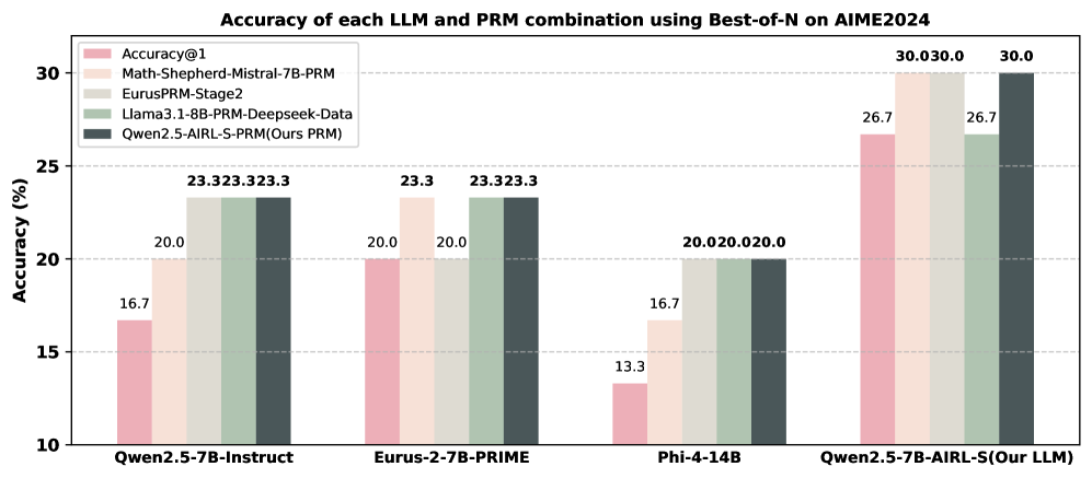<details> <summary>x9.png Details</summary>  ### Visual Description ## Bar Chart: Accuracy of LLM and PRM Combinations on AIME2024 ### Overview This bar chart displays the accuracy of different Large Language Model (LLM) and Program-aided Reasoning Model (PRM) combinations when evaluated on the AIME2024 dataset, using a Best-of-N approach. Accuracy is measured as a percentage. The chart compares four different LLM/PRM combinations. ### Components/Axes * **Title:** "Accuracy of each LLM and PRM combination using Best-of-N on AIME2024" (positioned at the top-center) * **X-axis:** LLM/PRM combinations: "Qwen2.5-7B-Instruct", "Eurus-2-7B-PRIME", "Phi-4-14B", "Qwen2.5-7B-AIRL-S(Our LLM)" (positioned at the bottom) * **Y-axis:** Accuracy (%) - Scale ranges from 10 to 30, with increments of 5. (positioned on the left) * **Legend:** Located in the top-left corner, identifying the color-coded LLM/PRM combinations: * "Accuracy@1" (light red) * "Math-Shepherd-Mistral-7B-PRM" (light green) * "EurusPRM-Stage2" (light blue) * "Llama3.1-8B-PRM-Deepseek-Data" (medium green) * "Qwen2.5-AIRL-S-PRM(Ours PRM)" (dark grey) ### Detailed Analysis The chart consists of four groups of bars, one for each LLM/PRM combination on the x-axis. Each group contains five bars, representing the accuracy of each of the five LLM/PRM combinations. * **Qwen2.5-7B-Instruct:** * Accuracy@1: Approximately 16.7% * Math-Shepherd-Mistral-7B-PRM: Approximately 20.0% * EurusPRM-Stage2: Approximately 20.0% * Llama3.1-8B-PRM-Deepseek-Data: Approximately 23.3% * Qwen2.5-AIRL-S-PRM(Ours PRM): Approximately 23.3% * **Eurus-2-7B-PRIME:** * Accuracy@1: Approximately 20.0% * Math-Shepherd-Mistral-7B-PRM: Approximately 23.3% * EurusPRM-Stage2: Approximately 23.3% * Llama3.1-8B-PRM-Deepseek-Data: Approximately 23.3% * Qwen2.5-AIRL-S-PRM(Ours PRM): Approximately 20.0% * **Phi-4-14B:** * Accuracy@1: Approximately 13.3% * Math-Shepherd-Mistral-7B-PRM: Approximately 16.7% * EurusPRM-Stage2: Approximately 20.0% * Llama3.1-8B-PRM-Deepseek-Data: Approximately 20.0% * Qwen2.5-AIRL-S-PRM(Ours PRM): Approximately 20.0% * **Qwen2.5-7B-AIRL-S(Our LLM):** * Accuracy@1: Approximately 26.7% * Math-Shepherd-Mistral-7B-PRM: Approximately 30.0% * EurusPRM-Stage2: Approximately 30.0% * Llama3.1-8B-PRM-Deepseek-Data: Approximately 26.7% * Qwen2.5-AIRL-S-PRM(Ours PRM): Approximately 26.7% ### Key Observations * The "Qwen2.5-7B-AIRL-S(Our LLM)" combination consistently achieves the highest accuracy across all PRM models, particularly with "Math-Shepherd-Mistral-7B-PRM" and "EurusPRM-Stage2", reaching 30.0%. * "Phi-4-14B" consistently shows the lowest accuracy across all PRM models. * The "Llama3.1-8B-PRM-Deepseek-Data" and "Qwen2.5-AIRL-S-PRM(Ours PRM)" combinations often yield similar accuracy scores. * The "Accuracy@1" baseline is consistently lower than the accuracy achieved when combined with any of the PRM models. ### Interpretation The data suggests that combining LLMs with PRM models significantly improves accuracy on the AIME2024 dataset. The "Qwen2.5-7B-AIRL-S" LLM, when paired with "Math-Shepherd-Mistral-7B-PRM" or "EurusPRM-Stage2", demonstrates the highest performance, indicating a strong synergy between these models. The consistently low performance of "Phi-4-14B" suggests it may not be as well-suited for this particular task or dataset. The improvement observed when using PRM models compared to the "Accuracy@1" baseline highlights the benefit of program-aided reasoning in enhancing LLM capabilities. The fact that the "Qwen2.5-AIRL-S-PRM(Ours PRM)" performs well, but not always the best, suggests that while the team's PRM is effective, other PRM models like "Math-Shepherd-Mistral-7B-PRM" and "EurusPRM-Stage2" may offer further improvements when combined with their LLM. 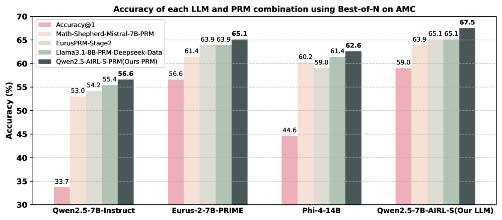</details> Figure 6: Performance of applying four PRMs on four different generation LLMs using Best-of-N with 64 rollouts on AIME2024 <details> <summary>x10.png Details</summary>  ### Visual Description ## Bar Chart: Accuracy of LLM and PRM Combinations ### Overview This bar chart displays the accuracy of different Large Language Models (LLMs) combined with different Program-aided Reasoning Models (PRMs) when evaluated using a Best-of-N approach on an AMC (presumably, a multiple-choice question answering dataset). The accuracy is measured in percentage points. The chart compares four LLM/PRM combinations. ### Components/Axes * **Title:** "Accuracy of each LLM and PRM combination using Best-of-N on AMC" (Top-center) * **X-axis:** LLM/PRM combinations: "Qwen2.5-7B-Instruct", "Eurus-2-7B-PRIME", "Phi-4-14B", "Qwen2.5-7B-AIRL-S(Our LLM)" (Bottom-center) * **Y-axis:** Accuracy (%) - Scale ranges from 30 to 70, with increments of 5. (Left-side) * **Legend:** Located in the top-left corner, identifying the data series: * "Accuracy@1" (Pink) * "Math-Shepherd-Mistral-7B-PRM" (Red) * "EurusPRM Stage2" (Green) * "Llama3.1-8B-PRM-Deepseek-Data" (Gray) * "Qwen2.5-AIRL-S-PRM(Ours PRM)" (Dark Green) ### Detailed Analysis The chart consists of four groups of bars, one for each LLM/PRM combination on the x-axis. Each group contains five bars, representing the accuracy of each of the five models/combinations listed in the legend. * **Qwen2.5-7B-Instruct:** * Accuracy@1: ~33.7% * Math-Shepherd-Mistral-7B-PRM: ~53.0% * EurusPRM Stage2: ~54.2% * Llama3.1-8B-PRM-Deepseek-Data: ~55.6% * Qwen2.5-AIRL-S-PRM(Ours PRM): ~56.6% * **Eurus-2-7B-PRIME:** * Accuracy@1: ~61.4% * Math-Shepherd-Mistral-7B-PRM: ~63.9% * EurusPRM Stage2: ~65.1% * Llama3.1-8B-PRM-Deepseek-Data: ~63.9% * Qwen2.5-AIRL-S-PRM(Ours PRM): ~56.6% * **Phi-4-14B:** * Accuracy@1: ~44.6% * Math-Shepherd-Mistral-7B-PRM: ~59.0% * EurusPRM Stage2: ~60.2% * Llama3.1-8B-PRM-Deepseek-Data: ~61.4% * Qwen2.5-AIRL-S-PRM(Ours PRM): ~62.6% * **Qwen2.5-7B-AIRL-S(Our LLM):** * Accuracy@1: ~59.0% * Math-Shepherd-Mistral-7B-PRM: ~63.9% * EurusPRM Stage2: ~65.1% * Llama3.1-8B-PRM-Deepseek-Data: ~65.1% * Qwen2.5-AIRL-S-PRM(Ours PRM): ~67.5% ### Key Observations * The "Accuracy@1" consistently shows the lowest accuracy across all LLM/PRM combinations. * "Qwen2.5-AIRL-S-PRM(Ours PRM)" generally yields the highest accuracy, especially when combined with "Qwen2.5-7B-AIRL-S(Our LLM)". * "EurusPRM Stage2" and "Llama3.1-8B-PRM-Deepseek-Data" often perform similarly, with accuracies clustered around the 60-65% range. * "Math-Shepherd-Mistral-7B-PRM" consistently improves accuracy compared to "Accuracy@1" but is often lower than the other PRMs. * The largest performance gap for a single LLM/PRM combination is observed for "Qwen2.5-7B-Instruct", where "Accuracy@1" is ~33.7% and "Qwen2.5-AIRL-S-PRM(Ours PRM)" is ~56.6%. ### Interpretation The data suggests that incorporating PRMs significantly improves the accuracy of LLMs on the AMC dataset. The "Qwen2.5-AIRL-S-PRM(Ours PRM)" consistently demonstrates the best performance, indicating that the researchers' PRM is particularly effective. The relatively low accuracy of "Accuracy@1" suggests that the Best-of-N approach, utilizing multiple reasoning steps, is crucial for achieving higher accuracy. The variations in performance across different LLM/PRM combinations highlight the importance of selecting compatible models for optimal results. The fact that the "Our PRM" consistently performs well with different LLMs suggests it is a robust and generalizable improvement. The data does not provide information on the computational cost or efficiency of these combinations, only their accuracy. 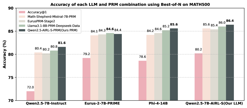</details> Figure 7: Performance of applying four PRMs on four different generation LLMs using Best-of-N with 64 rollouts on AMC <details> <summary>x11.png Details</summary>  ### Visual Description ## Bar Chart: Accuracy of LLM and PRM Combinations on MATH500 ### Overview This bar chart displays the accuracy of different Large Language Models (LLMs) combined with different Program-aided Reasoning Models (PRMs) on the MATH500 dataset, using a Best-of-N evaluation method. The accuracy is measured as Accuracy@1, representing the percentage of correct answers on the first attempt. The chart compares four different LLM/PRM combinations. ### Components/Axes * **Title:** "Accuracy of each LLM and PRM combination using Best-of-N on MATH500" (Top-center) * **X-axis:** LLM/PRM Combinations: "Qwen2.5-7B-Instruct", "Eurus-2-7B-PRIME", "Phi-4-14B", "Qwen2.5-7B-AIRL-S(Our LLM)" (Bottom-center) * **Y-axis:** Accuracy (%) - Scale ranges from 70 to 90, with increments of 5. (Left-side) * **Legend:** Located in the top-left corner, identifying the color-coded data series: * Accuracy@1 (Pink) * Math-Shepherd-Mistral-7B-PRM (Green) * EurusPRM-Stage2 (Gray) * Llama3.1-8B-PRM-Deepseek-Data (Light Gray) * Qwen2.5-AIRL-S-PRM(Ours PRM) (Dark Green) ### Detailed Analysis The chart consists of four groups of bars, one for each LLM/PRM combination. Each group contains four bars, representing the accuracy of each PRM when paired with the corresponding LLM. * **Qwen2.5-7B-Instruct:** * Accuracy@1: Approximately 72.0% * Math-Shepherd-Mistral-7B-PRM: Approximately 80.4% * EurusPRM-Stage2: Approximately 80.2% * Llama3.1-8B-PRM-Deepseek-Data: Approximately 81.6% * Qwen2.5-AIRL-S-PRM(Ours PRM): Approximately 80.8% * **Eurus-2-7B-PRIME:** * Accuracy@1: Approximately 79.2% * Math-Shepherd-Mistral-7B-PRM: Approximately 84.1% * EurusPRM-Stage2: Approximately 84.3% * Llama3.1-8B-PRM-Deepseek-Data: Approximately 84.6% * Qwen2.5-AIRL-S-PRM(Ours PRM): Approximately 84.4% * **Phi-4-14B:** * Accuracy@1: Approximately 78.6% * Math-Shepherd-Mistral-7B-PRM: Approximately 84.2% * EurusPRM-Stage2: Approximately 84.6% * Llama3.1-8B-PRM-Deepseek-Data: Approximately 85.6% * Qwen2.5-AIRL-S-PRM(Ours PRM): Approximately 85.2% * **Qwen2.5-7B-AIRL-S(Our LLM):** * Accuracy@1: Approximately 80.2% * Math-Shepherd-Mistral-7B-PRM: Approximately 85.6% * EurusPRM-Stage2: Approximately 85.4% * Llama3.1-8B-PRM-Deepseek-Data: Approximately 86.0% * Qwen2.5-AIRL-S-PRM(Ours PRM): Approximately 86.4% ### Key Observations * The "Qwen2.5-7B-AIRL-S(Our LLM)" combination consistently achieves the highest accuracy across all PRMs. * "Accuracy@1" consistently shows the lowest accuracy compared to the other PRMs for each LLM. * The "Llama3.1-8B-PRM-Deepseek-Data" and "Qwen2.5-AIRL-S-PRM(Ours PRM)" PRMs generally perform better than "Math-Shepherd-Mistral-7B-PRM" and "EurusPRM-Stage2". * The accuracy scores are relatively close for most combinations, suggesting that the choice of PRM has a significant impact, but the LLM also plays a role. ### Interpretation The data suggests that combining LLMs with PRMs significantly improves performance on the MATH500 dataset compared to using the LLMs alone (as indicated by the lower "Accuracy@1" scores). The "Qwen2.5-7B-AIRL-S" LLM, when paired with various PRMs, consistently demonstrates the highest accuracy, indicating its superior capability in this task. The "Llama3.1-8B-PRM-Deepseek-Data" and "Qwen2.5-AIRL-S-PRM(Ours PRM)" PRMs appear to be particularly effective in enhancing the reasoning abilities of the LLMs. The relatively small differences in accuracy between the PRMs suggest that the optimal PRM choice may depend on the specific LLM being used. The consistent trend of higher accuracy with PRM integration highlights the benefit of program-aided reasoning for complex mathematical problem-solving. The data points to a synergistic relationship between LLMs and PRMs, where each component complements the other to achieve better results. </details> Figure 8: Performance of applying four PRMs on four different generation LLMs using Best-of-N with 64 rollouts on MATH500 Appendix D Limitations While our experiments demonstrate that AIRL-S effectively unifies RL-based and search-based TTS across multiple test-time search algorithms using a single policy model and PRM, we have not tested its scalability on other base model architectures such as Phi-4 [2] and Gemma-3 [67]. We also have not studied how training dataset size affects AIRL-S ’s performance. Future work will evaluate AIRL-S on larger language models and more extensive datasets, including tasks with more difficult reasoning questions. Appendix E Broader Impacts Large‐scale reward-model-guided reinforcement learning (RL) and test-time search (TTS) can amplify the reasoning power of language models, lowering the barrier to advanced problem solving. Positive impacts include: (i) Scientific acceleration —open-sourced PRMs provide a drop-in verifier for symbolic mathematics and formal-methods research, potentially shortening proof discovery cycles; (ii) Educational equity —a modest-sized model fine-tuned with our AIRL-S pipeline attains near-GPT-4o performance, enabling free or low-cost tutoring tools in under-resourced regions; (iii) Software reliability —the PRM can rank candidate patches during code repair, reducing latent defects in safety-critical systems. Negative impacts and misuse scenarios. Disinformation : stronger mathematical/verbal reasoning could automate generation of persuasive but false technical content. Fairness & bias : reward models inherit biases present in demonstrations; these biases can be amplified by MCTS selection. Dual-use : chain-level reward shaping may help adversaries explore large search spaces (e.g. exploit generation, surveillance analytics). Labour displacement : automating competitive-programming-style tasks might displace junior software-engineering roles.