# Bridging the Analog and the Probabilistic Computing Divide: Configuring Oscillator Ising Machines as P-bit Engines
**Authors**: E.M.Hasantha Ekanayake, Nikhat Khan, Nikhil Shukla
> University of Virginia, Charlottesville, VA, USA
## Abstract
Oscillator Ising Machines (OIMs) and probabilistic bit (p-bit) platforms have emerged as promising non-Von Neumann paradigms for tackling hard computational problems. While OIMs realize gradient-flow dynamics, p-bit platforms operate through stochastic sampling. Although traditionally viewed as distinct approaches, this work presents a theoretically grounded framework for configuring OIMs as p-bit engines. We demonstrate that this functionality can be enabled through a novel interplay between first- and second harmonic injection to the oscillators. Our work identifies new synergies between the two methods and broadens the scope of applications for OIMs beyond combinatorial optimization problems to those that entail stochastic sampling. We further show that the proposed approach can be applied to other analog dynamical systems, such as the Dynamical Ising Machine.
preprint: APS/123-QED
## I Introduction
The endeavor to devise efficient solutions to complex computational problems has been a longstanding focus of science and technology research owing to its far-reaching implications for practical applications. A particularly promising direction is the design of special-purpose hardware that accelerates such tasks while improving energy efficiency, especially for problems that remain challenging for conventional digital platforms. Within this context, two emerging approaches have attracted significant attention: analog oscillator Ising machines (OIMs) and probabilistic bit (p-bit) based computing engines– the focus of the present work.
OIMs, first proposed by Wang et al. [1] exploit the elegant equivalence between the ’energy function’ characterizing the dynamics of a network of coupled oscillators under second harmonic injection (SHI) and the Ising Hamiltonian. Minimizing the Ising Hamiltonian is an archetypal combinatorial optimization problem (COP) where the goal is to find spin configurations $s∈\{-1,+1\}$ that minimizes the Ising Hamiltonian given by $H=-∑{J_ijs_is_j}$ , where $J_ij$ is the interaction between spin $i$ and $j$ . OIMs realize gradient-flow dynamics on a continuous relaxation of the Ising model and have been extensively explored for solving combinatorial optimization problems (COPs) [2, 3]. They have been experimentally realized across diverse platforms, including optical [4, 5], acoustic [6], electronic [7, 8, 9, 10, 11, 12], spin-wave [13], and quantum systems [14]. These demonstrations have been complemented by extensive theoretical studies [15, 16, 17].
P-bit-based computing engines, on the other hand, are a complementary computing paradigm uniquely capable of Boltzmann sampling. A p-bit can be viewed as a tunable random number generator whose output probability depends on the synaptic input. At the network level, this yields a binary stochastic neural network (BSNN) [18], with spin updates governed by,
$$
s_i^+=sgn≤ft[\tanh≤ft(β∑_\begin{subarray{c}j=1\\
j≠ i\end{subarray}}^NJ_ijs_j\right)-μ\right] \tag{1}
$$
where, $μ$ is a random number typically selected from a uniform distribution between $[-1,1]$ , and $β$ is the equivalent of inverse temperature [19]. Furthermore, if we interpret the spins as the phases of oscillators—a perspective that is useful in the context of this work—then the state update rule can be expressed as,
$$
s_i^+=\cosφ_i=sgn≤ft[\tanh≤ft(β∑_\begin{subarray{c}j=1\\
j≠ i\end{subarray}}^NJ_ij\cosφ_j\right)-μ\right] \tag{2}
$$
where, $φ∈\{0,π\}$ (wrapped phase form). In both Eqs. (1) and (2), the self bias term has not been considered although it is relatively straightforward to include it into the approach presented here.
The intrinsic stochastic sampling capability of p-bit engines offers a complementary approach to OIMs in the context of solving COPs [20, 21, 22, 23, 24, 25, 26, 27]. In addition, the stochastic sampling can be exploited in other application such as probabilistic inference and learning. Establishing such a capability within OIMs—hitherto not demonstrated—could therefore significantly broaden their functional scope beyond combinatorial optimization. To date, OIMs and p-bit engines have largely been pursued as independent approaches, with limited exploration of their potential synergies [28, 29]. In this work, we bridge this gap by demonstrating the feasibility of configuring OIMs as p-bit engines, thereby establishing them as an alternative analog platform for probabilistic computing.
<details>
<summary>Figure1r.png Details</summary>
### Visual Description
This document provides a technical analysis of the provided image, which illustrates the dynamics of an oscillator system influenced by harmonic injections and synaptic inputs, visualized through phase diagrams, heatmaps, and energy landscapes.
## Diagram: Oscillator Dynamics and Energy Landscapes
### Overview
The image is a composite figure containing four distinct panels (labeled a, b, c, and d) and a schematic diagram. It characterizes the behavior of a dynamical system—likely a neural oscillator or similar physical system—subject to First Harmonic Injection (FHI) and Second Harmonic Injection (SHI). The figure explores how parameters $\gamma$ (a bias or control parameter) and $\epsilon$ (a phase-related variable) affect the system's energy landscape and phase trajectory.
### Components/Axes
**1. Schematic (Top-Left):**
* **Components:** A block diagram showing "SHI" (Second Harmonic Injection) passing through a switch, and "FHI" (First Harmonic Injection) entering a node. The node outputs $V_{out}(\phi)$.
* **Text:**
* "FHI: First Harmonic Injection"
* "SHI: Second Harmonic Injection"
**2. Panel (a) - Phase Diagram (Middle-Left):**
* **Visual:** A circular representation of phase.
* **Labels:**
* $\pi$ (left pole), $0$ (right pole), $\epsilon=0$ (top pole).
* Arrows labeled $-\gamma$ (pointing left) and $+\gamma$ (pointing right).
* Text: "Noise", "Synaptic input", "Trajectory of $\phi, \epsilon$".
**3. Panel (b) - Heatmap (Top-Right):**
* **Axes:**
* X-axis: $\gamma$ (range: -0.5 to 0.5).
* Y-axis: $\epsilon$ (range: -0.5 to 0.5).
* **Colorbar:** Represents $-\nabla E = \dot{\epsilon}$ (gradient of energy), ranging from -0.5 (dark blue) to 0.5 (yellow).
* **Annotations:**
* Dashed line labeled "$\dot{\epsilon} = 0$".
* Text: "$K_S = 0.15$".
* Yellow arrows and wave patterns labeled "Phase trajectory resulting from synaptic input".
**4. Panel (c) - 3D Surface Plot (Bottom-Left):**
* **Axes:**
* X-axis: $\epsilon(\pi)$ (range: -0.5 to 0.5).
* Y-axis: $\gamma$ (range: -0.2 to 0.2).
* Z-axis: Energy (a.u.) (range: -0.2 to 0.1).
* **Colorbar:** "Energy" (range: -0.25 to 0.1).
**5. Panel (d) - Line Plots (Bottom-Right):**
* **Axes:**
* X-axis: $\epsilon(\pi)$ (range: -0.5 to 0.5).
* Y-axis: Energy (a.u.) (range: -0.30 to 0.15).
* **Legend/Series:**
* Top plot ($\gamma < 0$): Pink ($\gamma = -0.1$), Purple ($\gamma = -0.15$), Green ($\gamma = -0.2$).
* Middle plot ($\gamma = 0$): Orange ($\gamma = 0$).
* Bottom plot ($\gamma > 0$): Pink ($\gamma = 0.1$), Purple ($\gamma = 0.15$), Green ($\gamma = 0.2$).
* **Text:** "$K_S = 0.15$".
---
### Detailed Analysis
**Panel (a) - Phase Dynamics:**
The diagram depicts a circular phase space. The "Trajectory of $\phi, \epsilon$" is shown as a curved arrow along the top arc of the circle. The system is perturbed by "Noise" and "Synaptic input," which shift the trajectory along the $\gamma$ axis.
**Panel (b) - Gradient Heatmap:**
* **Trend:** The heatmap shows a diagonal transition from yellow (positive $\dot{\epsilon}$) to dark blue (negative $\dot{\epsilon}$).
* **Dashed Line:** The line $\dot{\epsilon} = 0$ acts as a separatrix.
* **Synaptic Input:** Three vertical dotted lines indicate specific cross-sections where synaptic input causes the phase trajectory to jump or shift, indicated by the yellow arrows.
**Panel (c) - 3D Energy Landscape:**
* **Trend:** The surface shows a "hill" and "valley" structure. As $\gamma$ increases (moving along the y-axis), the energy landscape deforms. The energy is highest (yellow) at the peak and lowest (blue) in the deep wells.
**Panel (d) - Energy vs. Phase:**
* **Top Plot ($\gamma < 0$):** The curves show a peak near $\epsilon = 0$ and a dip near $\epsilon = 0.5$. As $\gamma$ becomes more negative (moving from -0.1 to -0.2), the peak height decreases slightly, and the depth of the well increases.
* **Middle Plot ($\gamma = 0$):** A single orange curve shows a symmetric oscillation with a peak at $\epsilon \approx 0$ and a minimum at $\epsilon \approx 0.5$.
* **Bottom Plot ($\gamma > 0$):** The curves are inverted compared to the top plot. As $\gamma$ increases (0.1 to 0.2), the energy well deepens significantly.
---
### Key Observations
* **Symmetry Breaking:** The transition from $\gamma < 0$ to $\gamma > 0$ in panel (d) demonstrates a clear symmetry breaking in the energy landscape.
* **Correlation:** The heatmap in (b) is the gradient representation of the energy surface in (c). Where the energy surface is flat (peaks/valleys), the gradient $\dot{\epsilon}$ is zero (the dashed line in b).
* **Synaptic Influence:** The synaptic input acts as a forcing function that pushes the system across the energy barriers defined in the landscape.
### Interpretation
This figure describes the **bifurcation and control of an oscillator**.
* **The System:** The combination of FHI and SHI suggests a system where the phase ($\phi$) is controlled by external harmonic signals.
* **The Energy Landscape:** The energy plots (c and d) represent the potential function of the system. The system naturally seeks the lowest energy state (the "wells").
* **The Role of $\gamma$:** $\gamma$ acts as a control parameter that tilts the energy landscape. When $\gamma$ is negative, the system is biased toward one state; when positive, it is biased toward another.
* **Synaptic Input:** The synaptic input (visualized in b) provides the energy or "kick" required to move the system's state from one basin of attraction to another across the energy barrier.
* **Peircean Investigative Note:** The visual language suggests this is a study in **bistability**. The system can exist in different states, and the "Synaptic input" is the mechanism for switching between these states. The "Noise" mentioned in (a) likely represents stochastic fluctuations that could cause spontaneous switching if the energy barrier is low enough.
</details>
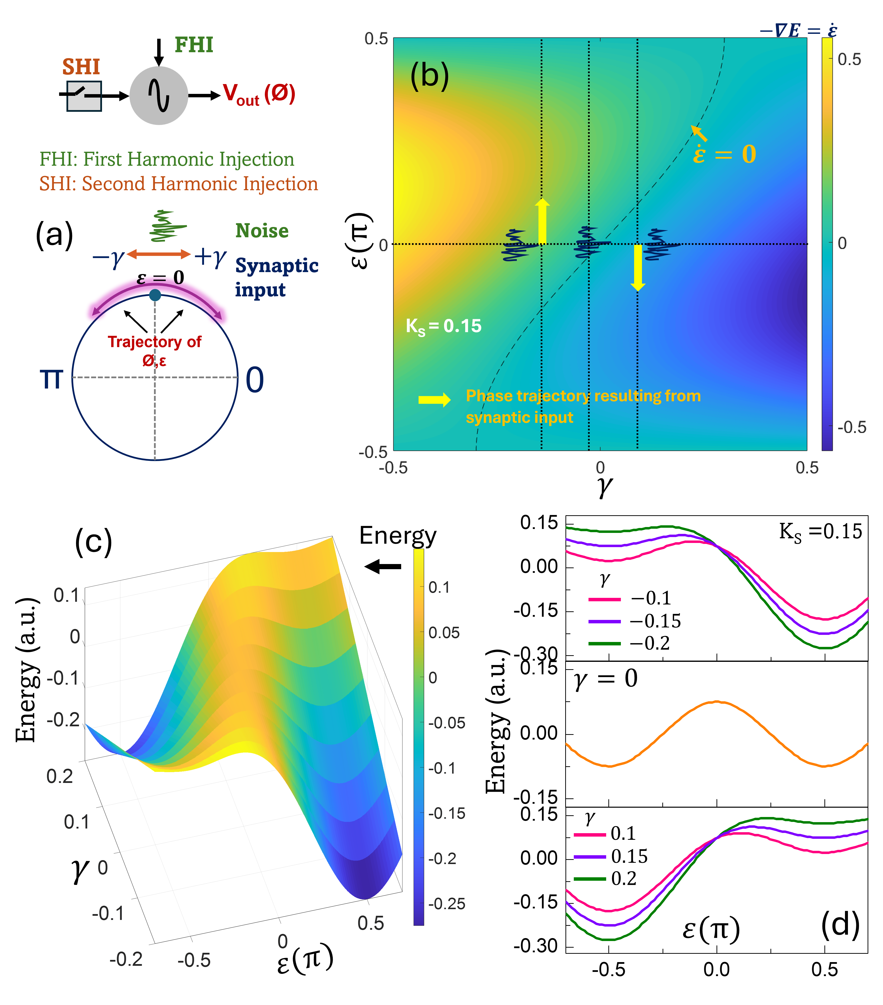
Figure 1: Dynamics of a harmonic oscillator under SHI (a) Schematic illustration of the signals required to program an harmonic oscillator as a p-bit. (b) Force field as a function of $γ$ ( $K_s=0.15$ , where $K_s$ is the strength of SHI.). (c) Corresponding energy landscape demonstrating its evolution with the synaptic input, $γ$ . (d) Specific cuts of the energy landscape at $γ=\{0, ± 0.1, ± 0.15, ± 0.2\}$ ( $K_s=0.15$ ).
To establish the foundation of our oscillator-based p-bit engine, we begin by demonstrating two key properties of harmonic oscillators (the class of harmonic oscillators considered in this study) and their networks operating under SHI: (a) An oscillator subjected to first- and second harmonic injection can function as a binary stochastic neuron (BSN); and (b) A network of such coupled oscillators—specifically an OIM—can operate as a binary stochastic neural network (BSNN). These two properties form the conceptual and mathematical basis for designing an oscillator-based p-bit engine.
## II Configuring Oscillators as Stochastic Neurons
To design a binary stochastic neuron (BSN) using an oscillator, we first examine the dynamics of a harmonic oscillator subjected to two external inputs (Fig. 1 (a)). (a) The first input is a signal with a frequency nearly equal to the oscillator’s natural frequency—a condition commonly referred to as injection locking. Within a specific locking range, this external signal entrains the oscillator, steering its output toward the phase and frequency of the injected signal, effectively synchronizing the oscillator’s behavior with the input. An energetics-based explanation of the relevant phase behavior is provided in Appendix A. We refer to this signal as the fundamental harmonic injection (FHI). All phase values are defined with respect to a common reference signal. (b) The second input is SHI, operating at twice the oscillator’s natural frequency. SHI drives the oscillator phase toward either $φ=0$ or $φ=π$ .
The resulting phase dynamics of such an oscillator can be described by,
$$
\begin{split}\frac{dφ}{dt}&=-K_c\sin{≤ft(φ-θ\right)}-K_s\sin(2φ)\\
\end{split} \tag{3}
$$
where, $φ$ denotes the output phase of the oscillator, while $θ$ represents the phase offset of the FHI signal input. The parameters $K_c$ and $K_s$ are coupling constants of the FHI and SHI signals, with the first and the second terms on the RHS of Eq. (LABEL:neuron1) capturing the influence of the FHI and SHI, respectively.
In this work, we will restrict our attention to cases where $θ∈\{0,\frac{π}{2},π\}$ . Initially, we will focus on the analysis where $θ∈\{0,π\}$ , with the case $θ=\frac{π}{2}$ becoming relevant further on. Under this constraint, we can recast Eq. (LABEL:neuron1) as,
$$
\begin{split}\frac{dφ}{dt}=-γ\sin{≤ft(φ\right)}-K_s\sin(2φ)\end{split} \tag{4}
$$
where $γ (=± K_c)$ denotes the scaled synaptic input; $γ=K_c$ when $θ=0$ and $γ=-K_c$ when $θ=π$ . For simplicity, we will generally refer to $γ$ as the synaptic input in the following discussion. The details of the scaling factor will be elaborated in the subsequent section.
Furthermore, for convenience, we perform a frame rotation by $0.5π$ , redefining the phase as $φ=\frac{π}{2}+ε$ . We also note that the relevant values of $θ$ for this rotated frame shift to $θ^{^\prime}∈\{-\frac{π}{2},0,\frac{π}{2}\}$ . Under this transformation, equation (4) becomes,
$$
\frac{dε}{dt}=-γ\cos{≤ft(ε\right)}+K_s\sin(2ε) \tag{5}
$$
We now analyze the properties and the behavior of Eq. (5). First, the fixed points of this system lie at $ε_1^*=± 0.5π$ , and at values satisfying $\sin(ε_2^*)=\frac{γ}{2K_s}$ . A detailed stability analysis of all the fixed points has been presented in Appendix B.
Next, we investigate the expected dynamical behavior of the system by analyzing the effective force field $(-∇ E=\dot{ε})$ driving the phase evolution as a function of $γ$ , as shown in Fig. 1 (b). The dotted line in the figure represents the set of phase points where the phase velocity vanishes, i.e., $\frac{dε}{dt}=0$ , and is described by the equation:
$$
-γ+2K_s\sin(ε)=0
$$
This curve defines the nullcline of the system, separating regions of positive and negative phase flow.
Interestingly, when the system is initialized at $ε=0$ , the direction of phase evolution depends entirely on the sign of $γ$ . For $γ<0$ , the dynamics flow toward $ε=\frac{π}{2}$ (corresponding to $φ=π$ ). Conversely, for $γ>0$ , the dynamics flow toward $ε=-\frac{π}{2}$ (i.e., $φ=0$ ). Moreover, the magnitude of $γ$ determines the steepness of the phase flow at $ε=0$ . At the critical point $γ=0$ , the direction of phase evolution becomes entirely stochastic in the presence of noise.
Figure 1 (c) shows the evolution of the oscillator’s energy landscape with the synaptic input, $γ$ , with Fig. 1 (d) showing cuts at specific values of $γ=\{0, ± 0.1, ± 0.15, ± 0.2\}$ . In Fig. 1 (d), the relative symmetry about $ε=0$ is evident across all cases, with the energy profiles for $γ=\{+0.1, +0.15, +0.2\}$ and $γ=\{-0.1, -0.15, -0.2\}$ appearing as mirror images, respectively, and the $γ=0$ case exhibiting a perfectly symmetric landscape.
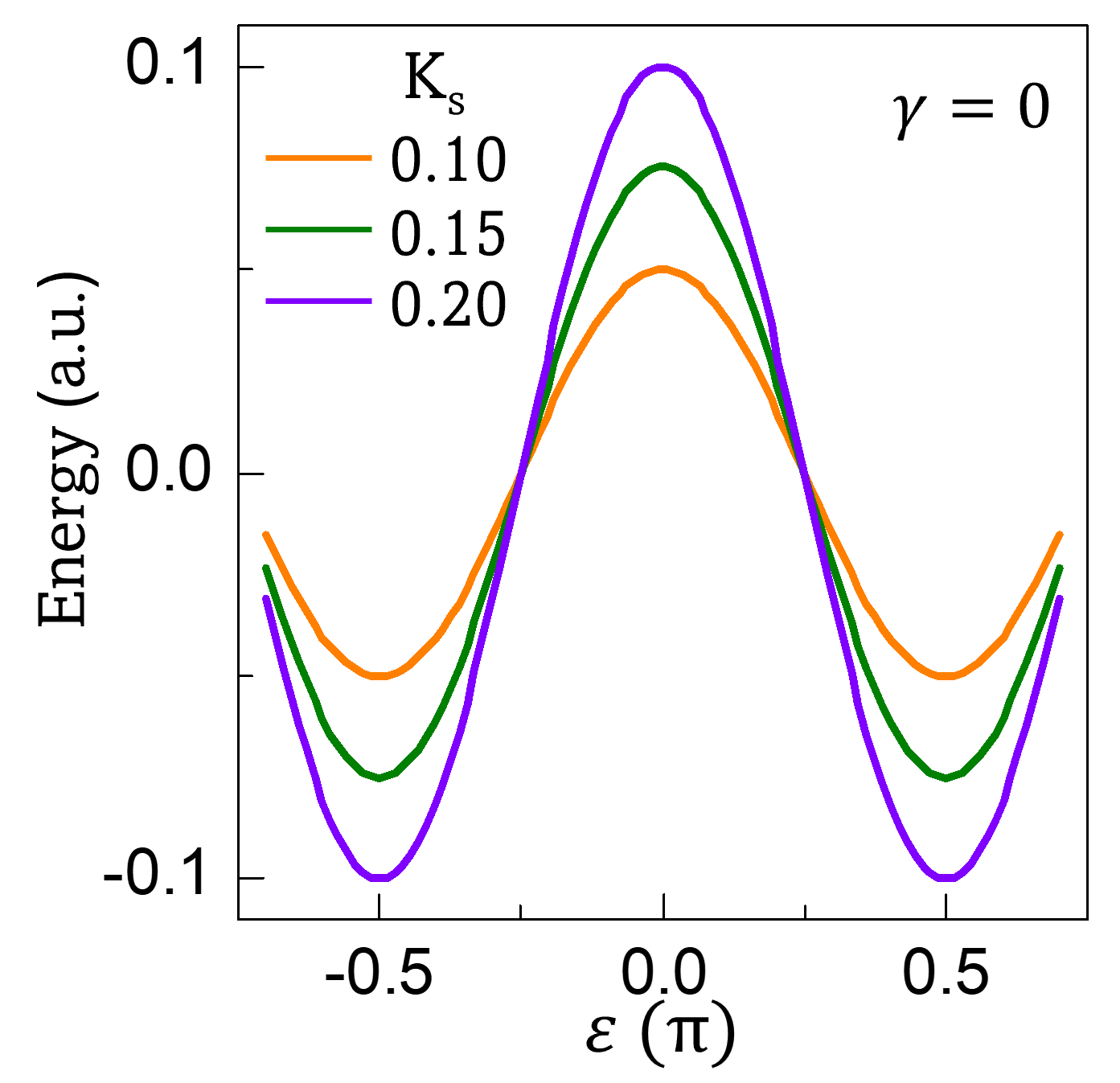
In alignment with prior work on magnetic tunnel junctions (MTJs)-based p-bits [30], we engineer our oscillator-based BSN to operate within the low energy barrier regime. Since the height of the barrier is controlled by $K_s$ (see Appendix C for details), this is achieved by tuning $K_s$ to a small value ( $K_s\ll 1$ ) during the sampling event. Thus, the oscillator-based approach can enable a BSN with a tunable barrier.
From 1 (b) as well as from the form of Eq. (5), it can be observed that the system exhibits a unique symmetry at $ε=0$ , within the domain $ε∈≤ft[-\frac{π}{2},\frac{π}{2}\right]$ , whereby the magnitude of the (scaled) synaptic input has a symmetric effect for $+γ$ and $-γ$ , but induces phase flows in opposite directions. This symmetry plays a critical role in enabling the oscillator to function as a BSN, as it defines a neutral point from which the system can stochastically evolve toward one of two stable states depending on the sign of the synaptic input. As we will show later, this stochastic response is also highly non-linear. In practical settings, the oscillator can be driven to this neutral point $ε=0$ using an FHI signal with a phase offset of $θ^{^\prime}=0$ (we refer to this input as $FHI^0$ ), and without applying the SHI.
Thus, operating the oscillator as a BSN entails the following steps:
(i) Set oscillator phase to the neutral point using $FHI^0$ . (ii) Remove $FHI^0$ followed by application of the synaptic input (also an FHI signal when considering a single oscillator) and SHI signal (applied as a ramp) to evaluate the (stochastic) neuron’s state—this constitutes a sampling event. As we will demonstrate later, in the OIM network, such synaptic input is effectively generated by other connected oscillators within the network.
## III Dynamics of an Oscillator-based BSN
To quantitatively analyze the stochastic nonlinear response of the oscillator-based BSN, we begin with the oscillator dynamics described in Eq. (5). We first define the updated spin state in terms of $ε$ , which, in the context of the continuous time dynamics considered here, is given by,
$$
s^+=sgn≤ft(\cos(φ^+)\right)=-sgn≤ft(\sin(ε^+)\right)
$$
where, $φ^+$ and $ε^+$ refer to the phase of the system at a small time increment $Δ t→ 0$ after the sampling has been initiated.
We now evaluate the solution to the dynamics presented in Eq. (5). Although deriving an explicit solution is challenging, Eq. (5) has an implicit analytical solution given by,
$$
\frac{ζ(ε)-γ\tanh^-1(\sin(ε))}{γ^2-4K_s^2}=t \tag{6}
$$
where,
$$
\begin{split}ζ(ε)&=K_s\big(-2\log(γ-2K_s\sin(ε))\\
&+\log(1-\sin(ε))+\log(\sin(ε)+1)\big)\\
\end{split} \tag{7}
$$
For it’s applications as a BSN, we focus on the direction of the initial phase trajectory. To understand and evaluate the system dynamics at the sampling instant—defined as the moment when (FHI 0) is suppressed and the SHI and the synaptic input are asserted —we adopt the following approximation: (i) The dynamics are evaluated in the limit $t→ 0$ . (ii) We model the noise as Gaussian white noise with $⟨η(t)⟩=0, ⟨η(t)η(t^\prime)⟩=2K_nδ(t-t^\prime),$ with $K_n$ denoting the noise intensity i.e., $η(t) dt=√{2K_n} dW_t,$ where $W_t$ is a Wiener process. Equivalently, over a finite timestep $Δ t$ , $∫_t^t+Δ tη(τ) dτ ∼ N\big(0, 2K_n Δ t\big).$ (iii) At the onset of sampling ( $t→ 0$ ) , we assume $K_s→ 0$ such that $K_s\ll|γ|$ . This reflects the requirement for a low energy barrier in the probabilistic regime. Subsequently, $K_s$ must be ramped up for reasons discussed in the following section.
Under these approximations, the oscillator phase can be expressed as:
$$
\begin{split}\sin(ε_i)&≈\tanh≤ft(-γ t+ε^η(t)\right)\\
\\
&≈\tanh≤ft(-γ t\right)+ε^η(t).sech^2(γ t)\\
\\
\end{split} \tag{8}
$$
Here, $ε^η(t)∼N\big(0, 2K_n t\big)$ , and is small such that the $\tanh(.)$ term can be linearized. Accordingly, at a small time increment $Δ t→ 0$ after the onset of sampling at t=0, the updated state of the oscillator-based BSN can be described as,
$$
\begin{split}s^+&≈sgn≤ft[\tanh(γΔ t)-ε^η(Δ t).sech^2(γΔ t)\right]\\
\\
&≡sgn≤ft[\tanh(γΔ t)-ϑ\right]\end{split} \tag{9}
$$
where, $ϑ≡ε^η(Δ t).sech^2(γΔ t)$ . Since $sech^2(γΔ t)∈(0,1]$ , and noise intensity is assumed to be small, $ϑ$ has a high probability of being in the interval [-1,+1]. The infinitesimal time ( $Δ t$ ) can be interpreted as the time duration required by the oscillator phase to reach a critical threshold magnitude $|ε_th|$ , beyond which the oscillator phase cannot ‘reverse’ trajectory. $Δ t$ can be tuned through properties of the SHI pulse, such as its slew rate. Additional details on $Δ t$ are discussed in the following sections. The derivation of Eqs. (8) and (9) has been presented in Appendix D. Furthermore, while Eq. (8) addresses the regime where $γ\gg K_s$ , we also consider (in Appendix D) the complementary case where both $γ$ and $K_s$ are small and comparable. In this setting, the synaptic bias $γ$ and the stochastic perturbations act as competing drivers of the phase dynamics. A large $|γ|$ produces a predictable exponential drift, whereas strong noise leads to rapid amplification of fluctuations and broad dispersion of trajectories. The observed evolution is therefore governed by the balance between deterministic drive and stochastic forcing.
We note that the actual synaptic input to the BSN would be applied as the voltage (or current) amplitude, $V_inj$ , and phase (in-phase or out-of-phase) of the injected signal, which relate to $γ$ and the coupling constant $K_c$ as $γ=± K_c ≈± \frac{ω_0}{2Q}·\frac{V_inj}{V_osc}$ [31, 32], where $Q$ is the quality factor of the oscillator, $ω_0$ is the natural frequency, and $V_osc$ represents the amplitude of the oscillator, respectively. This formulation implies that $γ$ serves as a scaled representation of the synaptic input, as noted earlier. Furthermore, the effective inverse temperature is then given by $β_eff=\frac{ω_0Δ t}{2V_osc}.\frac{1}{Q}$ implying that $β_eff$ can be modulated using the quality factor, $Q$ , of the oscillator as well as other parameters such as the oscillation amplitude among others. This tunability provides a practical mechanism for controlling the stochastic behavior of the system. The updated state is then expressed as
$$
\begin{split}s^+&≈sgn≤ft[\tanh≤ft(\frac{ω_0Δ t}{2QV_osc}· V_inj\right)-ϑ\right]\\
\\
&≡sgn≤ft[\tanh≤ft(β_eff· V_inj\right)-ϑ\right]\end{split} \tag{10}
$$
<details>
<summary>Figure2r.png Details</summary>
### Visual Description
## Charts: Probability vs. Injection Voltage ($V_{inj}$)
### Overview
The image displays two side-by-side line charts, labeled (a) and (b). Both charts plot the probability ($p$) as a function of injection voltage ($V_{inj}$). The data in both charts follows a sigmoidal (S-shaped) curve, modeled by the equation $p = \frac{1 + \tanh(\beta_{eff}V_{inj})}{2}$. The charts illustrate how varying parameters ($K_n$ in chart (a) and $\beta_{eff}$ in chart (b)) affect the steepness of the probability transition.
### Components/Axes
* **Common Y-Axis:** "Probability, $p$", ranging from 0.0 to 1.0.
* **Chart (a) X-Axis:** "$V_{inj}$", ranging from -0.8 to 0.8.
* **Chart (b) X-Axis:** "$V_{inj}$", ranging from -1.0 to 1.0.
* **Equation:** Both charts display the same formula: $p = \frac{1 + \tanh(\beta_{eff}V_{inj})}{2}$.
---
### Detailed Analysis
#### Chart (a): Effect of $K_n$ on Probability
* **Constant:** $K_{s,max} = 0.15$.
* **Legend/Data Table:** Located in the center-right of the chart area. It maps colors to $K_n$ values and their corresponding $\beta_{eff}$ values derived from the fit.
| Color | $K_n$ | $\beta_{eff}$ |
| :--- | :--- | :--- |
| Dark Blue | 0.01 | 88.76 |
| Orange | 0.05 | 12.631 |
| Green | 0.10 | 6.289 |
| Purple | 0.15 | 3.837 |
| Olive/Brown | 0.20 | 2.704 |
* **Trend:** All curves are sigmoidal and intersect at $(0, 0.5)$. As $K_n$ increases (from 0.01 to 0.20), the $\beta_{eff}$ value decreases, and the slope of the curve at the center decreases (the transition becomes less sharp/more gradual). The Dark Blue curve is the steepest (approaching a step function), while the Olive curve is the shallowest.
#### Chart (b): Effect of $\beta_{eff}$ on Probability
* **Constants:** $K_{s,max} = 0.15$, $K_n = 0.15$.
* **Legend:** Located on the right side of the chart. It maps colors to $\beta_{eff}$ values.
| Color | $\beta_{eff}$ |
| :--- | :--- |
| Purple | $\approx 8$ |
| Orange | $\approx 6$ |
| Green | $\approx 4$ |
| Dark Blue | $\approx 2$ |
* **Trend:** All curves are sigmoidal and intersect at $(0, 0.5)$. As $\beta_{eff}$ increases (from 2 to 8), the slope of the curve at the center increases (the transition becomes sharper). The Purple curve is the steepest, while the Dark Blue curve is the shallowest.
---
### Key Observations
* **Symmetry:** All curves in both charts are symmetric around the origin $(0, 0.5)$.
* **Parameter Relationship:** In chart (a), there is an inverse relationship between $K_n$ and $\beta_{eff}$. As $K_n$ increases, the effective gain ($\beta_{eff}$) drops, resulting in a flatter curve.
* **Visual Consistency:** The colors used in the legends are consistent with the data points on the lines, though the values they represent differ between chart (a) and chart (b).
* **Transition Sharpness:** The parameter $\beta_{eff}$ acts as a gain control for the transition. Higher values of $\beta_{eff}$ force the system toward a binary state (0 or 1) more rapidly as $V_{inj}$ deviates from 0.
### Interpretation
The data demonstrates a system governed by a logistic function where the probability of an event is determined by an injection voltage ($V_{inj}$).
The parameter $\beta_{eff}$ functions as the "steepness" or "gain" factor. When $\beta_{eff}$ is high, the system behaves like a digital switch (a step function), where the probability jumps from 0 to 1 almost instantly at $V_{inj} = 0$. When $\beta_{eff}$ is low, the system behaves more probabilistically, with a wider range of $V_{inj}$ values resulting in intermediate probabilities between 0 and 1.
Chart (a) provides a practical application of this, showing how a physical parameter $K_n$ can be used to tune the system's sensitivity (the effective gain $\beta_{eff}$). Chart (b) isolates the gain parameter itself, confirming that $\beta_{eff}$ is the direct determinant of the transition's sharpness.
</details>
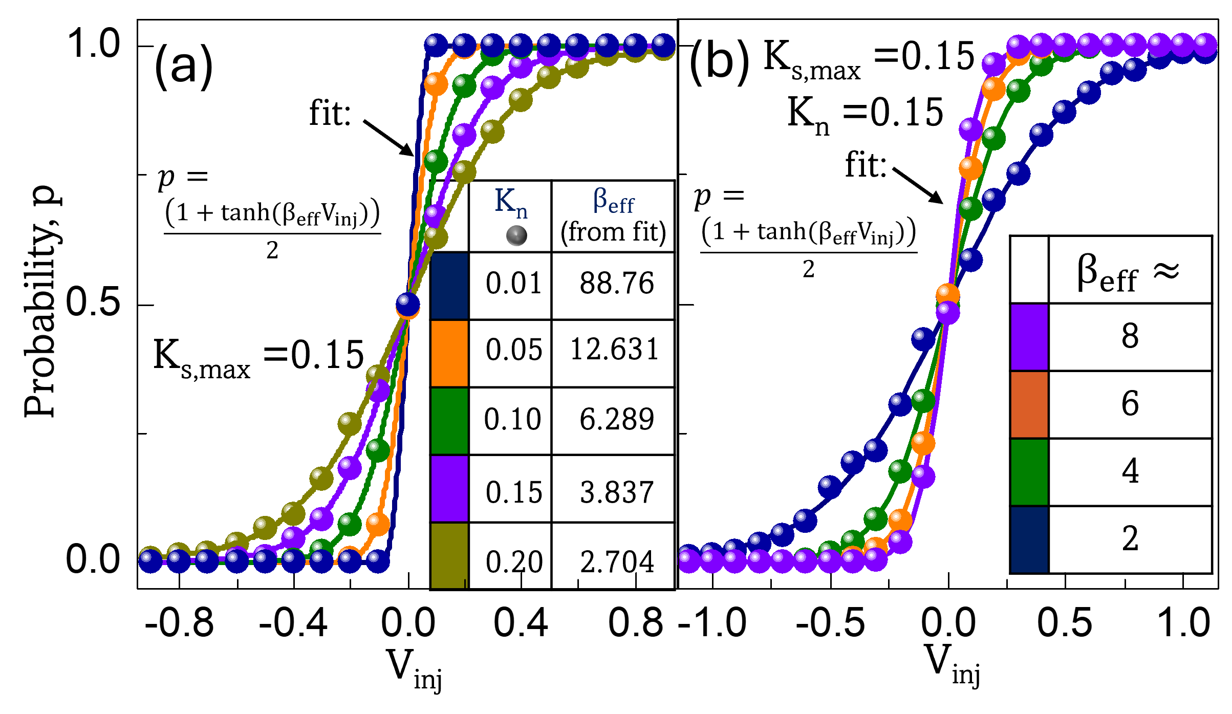
Figure 2: Oscillator-based BSN. Firing probability (symbols) as a function of the synaptic input for: (a) varying levels of noise ( $K_n$ ). (b) different values of $β_eff$ derived for $K_n=0.15$ . We note that the $β_eff$ profile will change for a different $K_n$ . The lines in the plot indicate fits using the equation $p=\frac{1+\tanh(β_effV_inj)}{2}$ along with the calculated $β_eff$ ; $p:$ firing probability. All fits exhibit $R^2>0.999$
Equation (LABEL:final_BSN) showcases the BSN’s capability to perform Boltzmann sampling, and consequently, function as a p-bit when initialized at the critical phase point, $ε=0$ . In the following section, we show that, in OIMs, $V_inj$ —and consequently $γ$ —is generated and regulated through the mutual feedback among the coupled oscillators. To validate the dynamics derived above, we simulate the oscillator-based BSN’s switching using a stochastic differential equation solver implemented in MATLAB ®. We first examine the evolution of stochastic behavior under varying noise levels. The phase is initialized at $ε=0$ and allowed to evolve in the presence of different noise intensities and synaptic inputs. The firing probability is then estimated over 2000 such cycles. Figure 2 (a) presents the simulation results (symbols) for the output firing probability of the oscillator-based BSN as a function of $V_inj$ . These results are fitted using the function $p=\frac{1+\tanh(β_effV_inj)}{2}$ (solid lines), showing excellent agreement with the simulated data ( $R^2>0.999$ ); p is the probability of the neuron firing i.e., switching to $s=+1$ .
In practical implementations, modulating external noise to control temperature and stochasticity may not be feasible. Instead, the effective inverse temperature—and thus the degree of stochastic behavior—can be tuned by adjusting $β_eff$ , which is achievable through modulation of the oscillator’s quality factor $Q$ . Figure 2 (b) illustrates the evolution of firing probability (symbols) for different values of $β_eff$ , where the switching probability again exhibits tanh(.) dependence on $V_inj$ as confirmed by the corresponding fitted curves (solid lines) with $R^2>0.999$ . A noise strength of $K_n=0.15$ was used in the simulation. These simulation results further support that the oscillator exhibits the characteristic behavior of a BSN capable of performing Boltzmann sampling.
A key consideration in engineering the oscillator’s dynamics for BSN functionality is the relative magnitude of $γ$ and the SHI strength, $K_s$ . Realizing effective Boltzmann sampling behavior requires a small energy barrier, which corresponds to the regime $K_s→ 0$ such that $K_s\ll|γ|$ . If this condition is not satisfied, the system may still operate as a BSN; however, its dynamics may deviate from the Boltzmann sampling behavior. This is detailed in the analysis in Appendix D.
In contrast, to preserve the oscillator’s phase trajectory after sampling and to enable reliable readout, a lower bound on $K_s$ must be satisfied. Specifically, this bound ensures that once the phase magnitude exceeds a certain threshold ( $|ε_th|$ ), the phase continues to evolve in the same direction until it reaches the corresponding fixed point.
While a detailed analytical derivation is provided in Appendix E, we offer here a qualitative explanation of the origin of this constraint by examining the dynamics described by Eq. (5). Within the interval $ε∈(-\frac{π}{2},\frac{π}{2})$ , the cosine term satisfies $\cos(ε)>0$ , and the synaptic input term $-γ\cos(ε)$ therefore drives the phase evolution in the direction opposite to the sign of $γ$ . This implies that the synaptic input alone tends to push the phase toward the fixed point opposite to the sign of $γ$ , unless counteracted by the SHI term.
If noise initially drives $\frac{dε}{dt}$ in the direction not favored by the synaptic input (Fig. 8 (b)), and $K_s$ is too small, the oscillator may reverse its trajectory to align with the trajectory favored by the synaptic input. In such cases, the final state may not reflect the oscillator’s initial trajectory or the intended output $s^+$ . The SHI term— specifically, the $K_s\sin(2ε)$ component in Eq. (5), acts to reinforce the initial direction of $\frac{dε}{dt}$ generated by the stochastic sampling process, provided $K_s$ is sufficiently large. This reinforcement helps ensure that the phase continues toward the correct fixed point.
The critical condition to ensure that an oscillator at $ε=|ε_th|$ maintains its trajectory is given by:
$$
|γ|<2K_s\sin(|ε_th|)
$$
It is important to note that due to the presence of noise, this threshold is inherently probabilistic, resulting in a diffuse rather than deterministic boundary. This condition appears to contradict the earlier requirement concerning the relative magnitudes of $γ$ and $K_s$ . To reconcile these seemingly opposing constraints, we propose implementing the SHI input as a ramp signal with a carefully engineered slew rate. Specifically, the SHI can be initialized at a low amplitude—ensuring that $K_s\ll|γ|$ —to facilitate stochastic sampling in the low-barrier regime. Subsequently, the amplitude of the SHI is increased to reinforce the resulting phase trajectory. Additionally, as noted above the characteristics of the applied SHI input, particularly its slew rate, also modulate $Δ t$ . A smaller slew rate increases $Δ t$ , which in turn modifies the inverse temperature and also makes the system less stochastic (see Appendix F for details).
The analysis presented in this section reveals that the competition between synaptic input and noise gives rise to a stochastic bifurcation, which constitutes the core operating principle of the proposed oscillator-based BSN.
## IV Configuring OIMs As Binary Stochastic Neural Networks
Building upon the ability to configure an oscillator as a BSN capable of performing Boltzmann sampling, we now investigate the possibility of configuring an OIM as a p-bit engine, or in other words, a BSNN. The core premise of this idea is that after the system reaches steady state, i.e., $ε∈\{-\frac{π}{2},\frac{π}{2}\}$ , the dynamics of a randomly sampled oscillator driven to the phase point $ε=0$ (i.e., $φ=\frac{π}{2}$ ) still approximate Boltzmann sampling. Steady state initialization at $ε∈\{-\frac{π}{2},\frac{π}{2}\}$ can be achieved by applying an SHI signal prior to the onset of stochastic sampling. As noted earlier, in the OIM, the feedback from other coupled oscillators acts as the effective synaptic input, which subsequently modulates the oscillator’s stochastic dynamics.
To establish this result, in the following sections, we divide the oscillators in the network into two categories and analyze their dynamics:
(i) Randomly sampled oscillator $i$ initialized to $ε_i=0$ . The phase evolution of an oscillator in the OIM network can be described by the equation,
$$
\frac{dφ_i}{dt}=-K∑_\begin{subarray{c}j=1\\
j≠ i\end{subarray}}^NJ_ij\sin(φ_i-φ_j)-K_s\sin(2φ_i)\\
$$
which, in the rotated frame of reference, can be expressed as,
$$
\frac{dε_i}{dt}=-K∑_\begin{subarray{c}j=1\\
j≠ i\end{subarray}}^NJ_ij\sin(ε_i-ε_j)+K_s\sin(2ε_i) \tag{11}
$$
As alluded to earlier, we assume that:
(i) The selected oscillator is initialized at $ε=0$ . This can be accomplished using $FHI^0$ signal with large amplitude. (ii) Since we begin performing stochastic sampling after the OIM network has achieved steady state, all other oscillators are at $ε=±\frac{π}{2}\>\>\big(φ∈\{0,π\}\big)$ . Furthermore, we will ensure that the oscillators maintain their state during the sampling event by applying a sufficiently large $K_s$ . This condition is required to ensure that the oscillator dynamics map to Gibbs sampling (see Appendix G). In the subsequent sections, we will discuss how these conditions can be implemented.
Under the constraints outlined above, the phase dynamics of the selected oscillator simplify to:
$$
\begin{split}\frac{dε_i}{dt}&=≤ft(K∑_\begin{subarray{c}j=1\\
j≠ i\end{subarray}}^NJ_ij\sin(ε_j)\right)\cos(ε_i)+K_s\sin(2ε_i)\\
\\
&≡-γ_i\cos(ε_i)+K_s\sin(2ε_i)\end{split} \tag{12}
$$
where,
$$
γ_i=-K∑_\begin{subarray{c}j=1\\
j≠ i\end{subarray}}^NJ_ij\sin(ε_j)
$$
We now show that $γ_i$ , as defined above, represents the synaptic input to oscillator $i$ from the other connected oscillators in the network. To establish this, we consider the relationship between $ε$ and $φ$ , and the fact that $s=\cos(φ)$ when $φ∈\{0,π\}$ :
$$
\begin{split}γ_i=-K∑_\begin{subarray{c}j=1\\
j≠ i\end{subarray}}^NJ_ij\sin(ε_j)&=-K∑_\begin{subarray{c}j=1\\
j≠ i\end{subarray}}^NJ_ij\sin≤ft(φ_j-\frac{π}{2}\right)\\
=K∑_\begin{subarray{c}j=1\\
j≠ i\end{subarray}}^NJ_ij\cos(φ_j)&=K∑_\begin{subarray{c}j=1\\
j≠ i\end{subarray}}^NJ_ijs_j\end{split}
$$
This establishes that $γ_i$ represents the net synaptic input received by oscillator $i$ from the connected oscillators under the conditions described above. Additionally, we note that the self-biasing term can be incorporated by injecting an FHI signal to oscillator with the strength and phase of the signal representing the self-bias input.
The updated state of oscillator $i$ can then be expressed as,
$$
\begin{split}s_i^+&≈-sgn≤ft[\tanh(-γ_iΔ t)+ε^η(Δ t).sech^2(γΔ t)\right]\\
\\
&≈sgn≤ft[\tanh≤ft(KΔ t∑_\begin{subarray{c}j=1\\
j≠ i\end{subarray}}^NJ_ijs_j\right)-ϑ\right]\end{split} \tag{13}
$$
which closely resembles the state update rule for p-bits (Eq. (1)), with the factor $β_eff=KΔ t$ serving as the effective inverse temperature. As detailed in [1], the value of K depends on the perturbation projection vector function for the oscillator as well as the amplitude of the perturbation from the oscillators in the network, which can be tuned via the coupling element in the network. This equivalence implies that even in the OIM, the oscillator can approximate Boltzmann sampling thereby enabling the network to function as a p-bit platform.
One of the critical requirements of realizing the above dynamics is to drive the randomly selected oscillator $i$ to $ε_i=0\>\>\big(φ_i=\frac{π}{2}\big)$ . This can be achieved by applying a large FHI signal, $FHI^0$ , while suppressing the SHI signal $(K_s=0)$ . The resulting dynamics can be described by:
$$
\frac{dε_i}{dt}=-K_c,i\sin(ε_i)-K∑_\begin{subarray{c}j=1\\
j≠ i\end{subarray}}^NJ_ij\sin(ε_i-ε_j) \tag{14}
$$
The largest magnitude of the second term is $D_i$ —the degree of the node (oscillator) $i$ in the network. By designing $K_c,i\gg KD_i$ ensures that the contributions of the second term are small. Consequently, the phase will be driven to $ε_i≈ 0$ , thereby preparing it for the subsequent stochastic sampling event.
(ii) Oscillators not being sampled Under steady state, such oscillators have phases $ε=±\frac{π}{2}$ , and the goal is to maintain the configuration when oscillator $i$ is sampled. To achieve this, we apply a strong SHI signal. The corresponding dynamics for an oscillator $j$ that is not being sampled can be then described as follows:
$$
\begin{split}\frac{dε_j}{dt}=-K∑_\begin{subarray{c}k=1\\
k≠ j\end{subarray}}^NJ_jk\sin(ε_j-ε_k)+K_s\sin(2ε_j)\\
\\
∀ j∈\{1,2,\dots,i-1,i+1,\dots,N\}\end{split} \tag{15}
$$
Furthermore, $\sin(ε_j-ε_k)≈ 0$ since
$$
ε_k∈≤ft\{-\frac{π}{2},\frac{π}{2}\right\} ∀ j,k∈\{1,2,\dots,i-1,i+1,\dots,N\}
$$
Consequently, the dynamics can be reduced to,
$$
\begin{split}\frac{dε_j}{dt}=-KJ_ji\sin(ε_j-ε_i)+K_s\sin(2ε_j)\\
\\
∀ j∈\{1,2,\dots,i-1,i+1,\dots,N\}\end{split} \tag{16}
$$
The maximum magnitude of the first term is $|KJ_ji|$ . Thus, by using $2K_s,j\gg KJ_ji$ , the phase can be maintained at $ε_j≈\{-\frac{π}{2},\frac{π}{2}\}$ . These assumptions are further validated through simulations presented in the following section.
Based on the above analysis, algorithm 1 presents the scheme for configuring OIMs as p-bit engines. Although the analysis above was conducted in a rotated frame of reference, we present the operational scheme in terms of the original phase variable $φ$ , to maintain consistency with the prevailing conventions in the OIM literature, where the spin states are defined as $φ∈\{0,π\}$ . As previously noted, the relationship between the two frames is given by $φ=\frac{π}{2}+ε$ .
Table 1: Operating OIM as a p-bit platform
| 1: 2: 3: | Initialize all oscillators. Apply SHI signal to all oscillators. The OIM performs gradient descent and achieves a steady state characterized by $φ∈\{0,π\}$ . while not converged or for a fixed number of iterations do |
| --- | --- |
| 4: | Randomly select an oscillator $i$ . |
| {Step (i): Prepare oscillator for stochastic sampling} | |
| 5: | Apply $FHI^0$ signal to oscillator $i$ with appropriate amplitude and set SHI signal to oscillator $i$ to $0$ . |
| {Step (ii): Initiate probabilistic evolution} | |
| 6: | Reduce $FHI^0$ signal to $0$ . |
| 7: | Ramp SHI signal to oscillator $i$ . |
| 8: | Let $φ_i$ probabilistically relax to $φ=0$ or $φ=π$ based on synaptic feedback from connected nodes and intrinsic noise. |
| 9: | end while |
## V Computing with OIMs configured as P-bit engines
### V.1 5-Node Adder
<details>
<summary>Figure_sampling.png Details</summary>
### Visual Description
## Mixed Diagram: Truth Table and Probability Distribution Chart
### Overview
The image presents a combined data visualization consisting of a truth table (top-left) and a grouped bar chart (bottom). The chart compares theoretical probability values ("Boltzmann law") against experimental measurements ("Measured (oscillators)") for specific binary states. The truth table defines the binary inputs and outputs ($C_i, B, A, S, C_o$) and their corresponding decimal values, which serve as the X-axis coordinates for the bar chart.
### Components/Axes
**1. Truth Table (Top-Left)**
| $C_i$ | $B$ | $A$ | $S$ | $C_o$ | Decimal |
| :--- | :--- | :--- | :--- | :--- | :--- |
| 0 | 0 | 0 | 0 | 0 | 0 |
| 0 | 0 | 1 | 1 | 0 | 6 |
| 0 | 1 | 0 | 1 | 0 | 10 |
| 0 | 1 | 1 | 0 | 1 | 13 |
| 1 | 0 | 0 | 1 | 0 | 18 |
| 1 | 0 | 1 | 0 | 1 | 21 |
| 1 | 1 | 0 | 0 | 1 | 25 |
| 1 | 1 | 1 | 1 | 1 | 31 |
**2. Bar Chart**
* **Y-Axis:** Labeled "Probability". The scale ranges from 0 to 0.2, with major ticks at 0, 0.05, 0.1, 0.15, and 0.2.
* **X-Axis:** Labeled "[C_i B A S C_o]". The axis displays the decimal values corresponding to the truth table: 0, 6, 10, 13, 18, 21, 25, 31.
* **Legend (Top-Right):**
* **Blue Bar:** "Boltzmann law" (Theoretical prediction).
* **Orange Bar:** "Measured (oscillators)" (Experimental data).
### Detailed Analysis
**Data Series Trends:**
* **Boltzmann law (Blue):** The blue bars are consistent in height across all eight labeled X-axis points (0, 6, 10, 13, 18, 21, 25, 31), maintaining a probability of approximately 0.12.
* **Measured (oscillators) (Orange):** The orange bars closely track the blue bars at all labeled points. At most points, the orange bar is nearly identical in height to the blue bar. At points 21 and 25, the orange bar is slightly lower than the blue bar. At point 31, the orange bar is slightly lower than the blue bar.
* **Noise/Intermediate States:** Between the primary labeled points (e.g., between 0 and 6, 6 and 10), there are very small, non-zero bars visible for both the Boltzmann law and the Measured data. These represent states with very low probability (near 0.005).
**Data Points (Approximate Probability Values):**
* **At 0:** Both ~0.12
* **At 6:** Both ~0.12
* **At 10:** Both ~0.12
* **At 13:** Both ~0.12
* **At 18:** Both ~0.12
* **At 21:** Blue ~0.12, Orange ~0.115
* **At 25:** Blue ~0.12, Orange ~0.125
* **At 31:** Blue ~0.12, Orange ~0.12
### Key Observations
* **High Correlation:** The experimental "Measured" data shows a very high degree of correlation with the theoretical "Boltzmann law" prediction.
* **Uniform Distribution:** The system appears to be designed to favor the eight specific states listed in the truth table, as these are the only states with significant probability mass.
* **State Leakage:** The presence of tiny bars between the primary states suggests "leakage" or transient states where the system briefly exists outside of the eight defined "valid" states.
### Interpretation
This visualization demonstrates the validation of a physical system (likely a network of coupled oscillators) against a theoretical model (Boltzmann law).
The truth table defines the "valid" states of a logic system. The bar chart shows that the system spends the vast majority of its time in these valid states, with a probability distribution that is nearly uniform across them. The close alignment between the blue (theoretical) and orange (measured) bars indicates that the oscillator system successfully mimics the statistical mechanics predicted by the Boltzmann law. The small, non-zero bars between the main peaks likely represent thermal noise or transient switching states in the physical hardware, which are expected in real-world implementations of such systems.
</details>
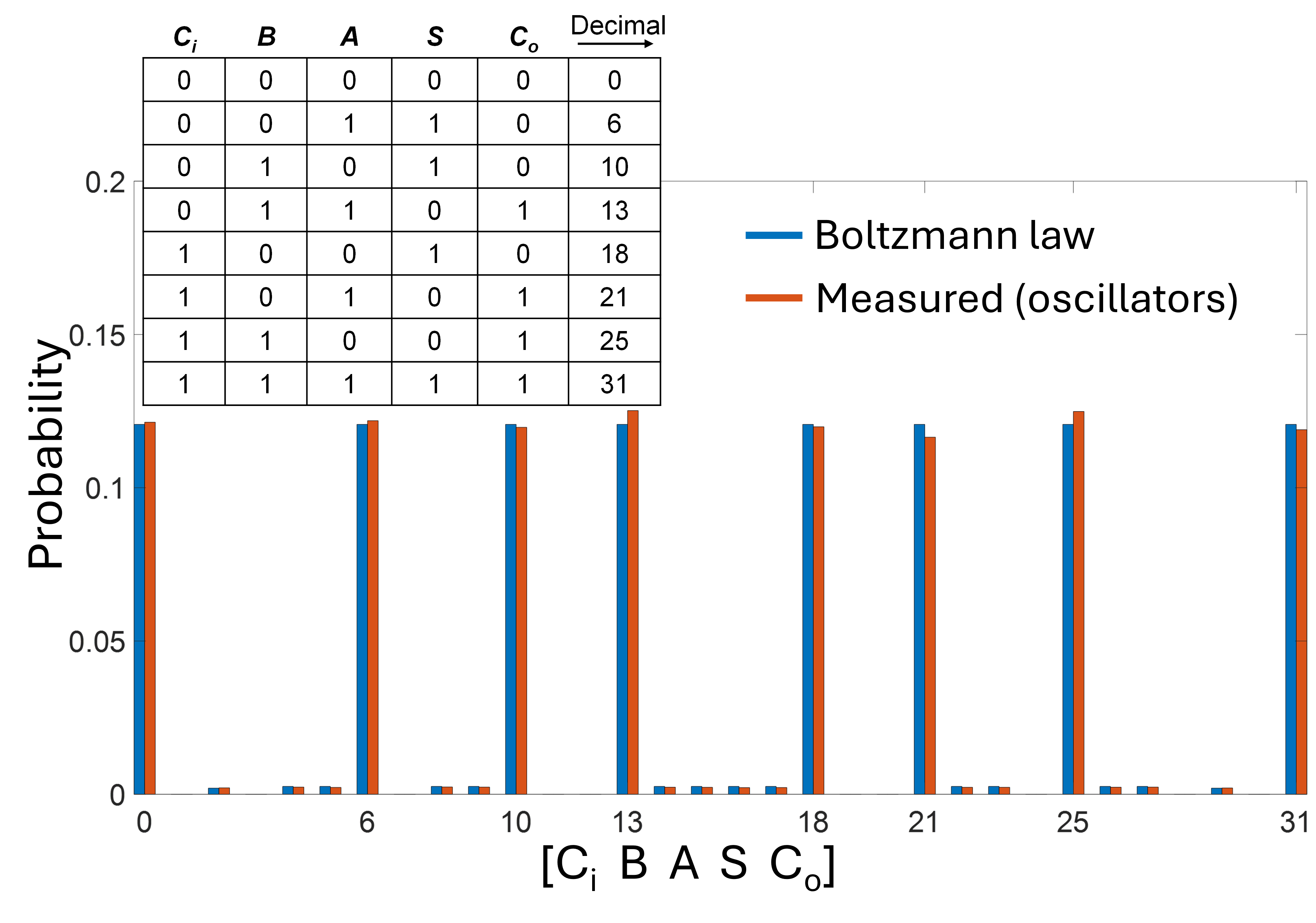
Figure 3: Full adder Probability histogram measured using the oscillators (orange bars, obtained using $5× 10^5$ sweeps) compared with the target Boltzmann distribution (blue bars). Following the convention of Ref. [19], states are indexed by the decimal value of the binary word $[C_in A B S C_out]$ . The dominant peaks correspond to the valid entries of the full-adder truth table, as highlighted in the inset. The two distributions show excellent agreement, with a measured KL divergence of $7.68× 10^-4$ . Simulation parameters: $K=0.18$ ; $K_s(t)=K_s,max(1-e^-\frac{t{10^-2}})$ ; $K_n=0.1$ .
To evaluate the sampling capability of our oscillator-based BSN, we benchmark its output distribution against the target Boltzmann distribution for a full adder, following the approach presented by Camsari et al. [19]. For this purpose, we construct the corresponding $14× 14$ adjacency matrix with the following assignment of nodes: 1–9 represent auxiliary and handle bits, 10 corresponds to $C_in$ , 11 to $A$ , 12 to $B$ , 13 to the sum $S$ , and 14 to the carry-out $C_out$ . The network is operated in the so-called truth table mode, where all input and output terminals are left floating. Under this condition, the distribution obtained using the oscillator-based BSN (using $5× 10^5$ sweeps) aligns closely with the target Boltzmann distribution, thereby confirming its ability to perform correct stochastic sampling. Here, we note that simulating the analog dynamics of all oscillators for $5× 10^5$ sweeps (corresponding to a total simulated time of $∼ 2× 10^7$ per oscillator) within the stochastic differential equation (SDE) framework (to account for noise) is computationally prohibitive. Therefore, we only simulate the dynamics of oscillator being sampled, while the remaining oscillators are held at their fixed phase values. However, in the following example—computing MaxCut—which requires a smaller number of sweeps, we simulate the entire oscillator network.
Figure 3 presents the resulting probability histogram, showing an excellent match to the target Boltzmann distribution (KL divergence= $7.68× 10^-4$ ). Each state is labeled by the decimal value of the binary string $[ C_in A B S C_out ]$ and the inset highlights the valid truth-table states of the full adder, which appear as the tallest peaks in the distribution.
### V.2 Computing MaxCut
<details>
<summary>Figure3r.png Details</summary>
### Visual Description
## [Diagram]: Oscillator Sampling and Optimization Dynamics
### Overview
This image presents a multi-panel technical figure (labeled a, b, and c) illustrating the dynamics of an oscillator-based system, likely used for solving combinatorial optimization problems (such as the Max-Cut problem). The figure includes a specific sampling sequence, a binary state switching plot, a phase evolution plot, and a "Cut" value optimization plot featuring an inset network graph.
### Components/Axes
* **Top Text Block:** "Oscillator sampling sequence:" followed by a sequence of numbers.
* **Panel (a):** A pulse train/square wave plot.
* **Y-axis:** Binary states. Top label: "FHI⁰>0, K_s=0"; Bottom label: "FHI⁰=0, K_s>0".
* **Panel (b):** A time-series plot.
* **Y-axis:** $\phi$ ($\pi$). Scale ranges from -1 to 1.
* **X-axis:** Shared "Time" axis (0 to 80+).
* **Panel (c):** A step-function plot.
* **Y-axis:** "Cut". Scale ranges from 35 to 40.
* **X-axis:** "Time".
* **Inset:** A network graph with nodes labeled 1 through 15.
* **Annotations:** Red arrows appear in panels (b) and (c) at approximately Time = 35 and Time = 60.
### Detailed Analysis
#### 1. Oscillator Sampling Sequence
The sequence is provided as follows:
5 $\rightarrow$ 6 $\rightarrow$ 15 $\rightarrow$ 7 $\rightarrow$ 1 $\rightarrow$ 3 $\rightarrow$ 9 $\rightarrow$ 4 $\rightarrow$ 11 $\rightarrow$ 8 $\rightarrow$ 14 $\rightarrow$ 12 $\rightarrow$ 13 $\rightarrow$ 10 $\rightarrow$ 2 $\rightarrow$ 14 $\rightarrow$ 9 $\rightarrow$ 12 $\rightarrow$ 8 $\rightarrow$ 5 $\rightarrow$ 11 $\rightarrow$ 3 $\rightarrow$ 15 $\rightarrow$ 10 $\rightarrow$ 13 $\rightarrow$ 6 $\rightarrow$ 4 $\rightarrow$ 7 $\rightarrow$ 2 $\rightarrow$ 1
#### 2. Panel (a): Switching States
This panel displays a high-frequency square wave. The signal alternates between two states:
* **State 1 (Top):** FHI⁰ > 0, K_s = 0
* **State 2 (Bottom):** FHI⁰ = 0, K_s > 0
The transitions are perfectly synchronized, indicating a switching mechanism between two distinct operational modes or parameters.
#### 3. Panel (b): Phase Evolution ($\phi$)
This plot tracks the phase ($\phi$) of multiple oscillators over time.
* **Trend:** Most lines oscillate or remain near 0.
* **Outlier:** One distinct purple line drops sharply from 0 to -1 at the very beginning (Time $\approx$ 0) and remains at -1 for the duration of the plot.
* **Dynamics:** There are periodic spikes and transitions in the other colored lines. Two specific time points (marked by red arrows at Time $\approx$ 35 and Time $\approx$ 60) show distinct phase shifts or re-alignments.
#### 4. Panel (c): Cut Optimization and Network Graph
* **Main Plot:** A green line representing the "Cut" value. The value starts at approximately 34, increases in steps, and reaches 40.
* **Step Increases:** The "Cut" value increases at specific intervals. Notably, the red arrows at Time $\approx$ 35 and Time $\approx$ 60 align with the upward steps in the "Cut" value.
* **Inset Network Graph:** Located in the bottom-right. It depicts a graph with 15 nodes (labeled 1-15). The nodes are interconnected by a dense web of blue lines (edges). The graph appears to be a complete or near-complete graph, representing the structure being optimized.
### Key Observations
* **Correlation:** The red arrows in panels (b) and (c) are vertically aligned. This suggests that the phase shifts observed in panel (b) are the direct cause of the increases in the "Cut" value in panel (c).
* **Optimization Progress:** The "Cut" value increases over time, suggesting an iterative optimization process (OIM - likely "Oscillator-based Ising Machine" or "Oscillator-based Optimization Method") that improves the solution quality as the system evolves.
* **System Stability:** The purple line in panel (b) suggests that one oscillator (or a subset) locks into a stable phase of -1, while others remain dynamic.
### Interpretation
This figure demonstrates the operational mechanics of an oscillator-based computing system solving a graph optimization problem (specifically, the Max-Cut problem).
1. **The Process:** The system uses a specific sampling sequence to update oscillators.
2. **The Mechanism:** Panel (a) shows the system switching between two modes (FHI and K_s), which likely controls the coupling strength or the Hamiltonian parameters of the system.
3. **The Result:** As the system evolves, the oscillators adjust their phases (panel b). When the system reaches specific states (indicated by the red arrows), the "Cut" value—a metric of the optimization quality—increases (panel c).
4. **The Goal:** The system is attempting to maximize the "Cut" value, which corresponds to finding the optimal partition of the network graph shown in the inset. The step-wise increase indicates that the system is successfully finding better solutions over time.
</details>
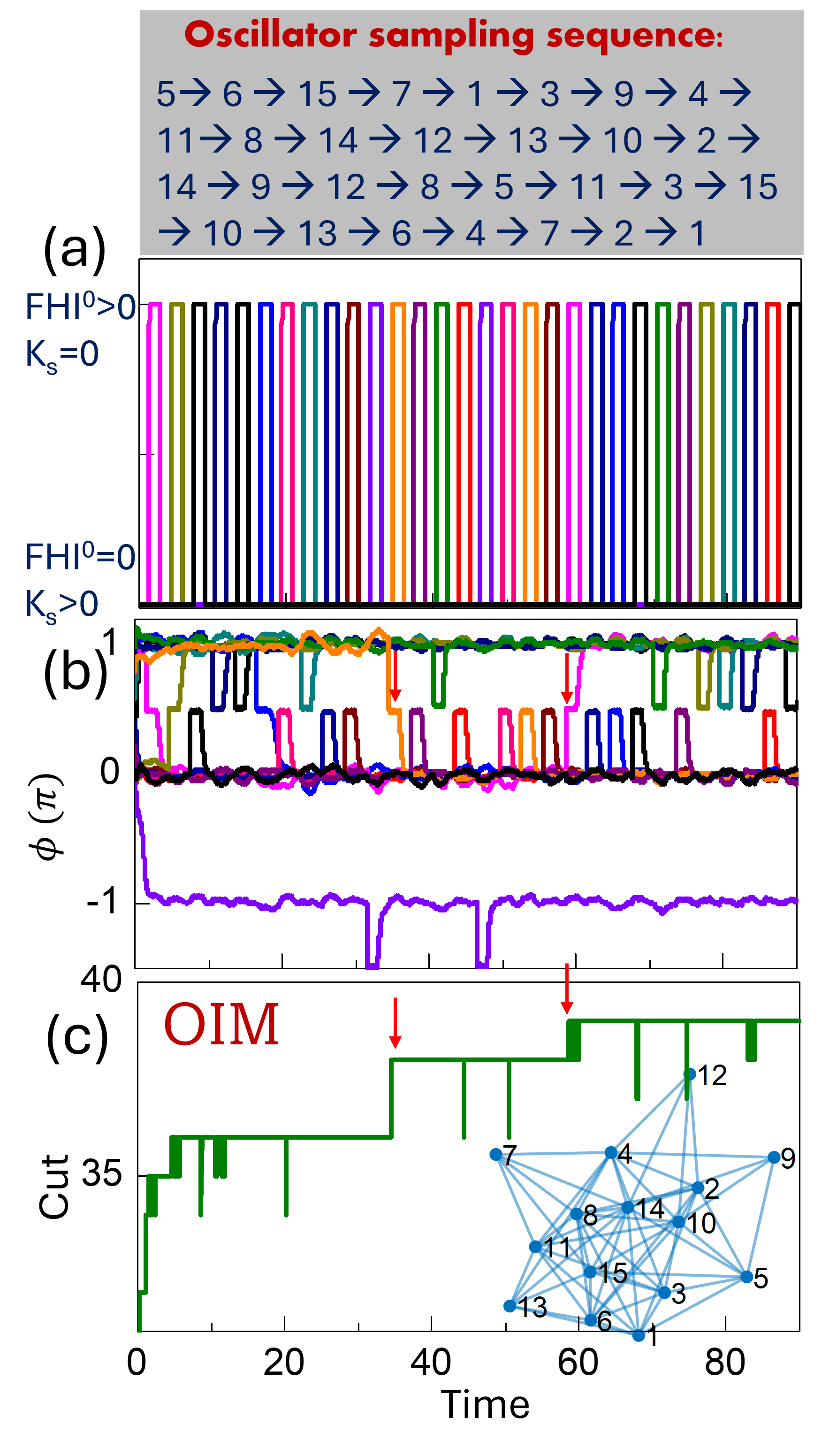
Figure 4: Operating OIMs as p-bit platforms. (a) Randomly generated FHI sequence to the oscillators. The application of FHI to the oscillator is accompanied by the suppression of SHI, and vice-versa. (b) Phase response of the oscillators over time. (c) Evolution of the computed graph cut over time/iterations. With stochastic sampling, the system is able to reach the globally optimal solution (MaxCut =39). The red arrows highlight sampling events that improved cut. Simulation parameters: $K=1;K_s,max=2;\>FHI^0=50;\>K_n for sampled oscillator=0.04$ ; ramping schedule of the SHI signal: $K_s(t)=K_s,max\big(1-e^-\frac{t{τ}}\big)$ , where $K_s,max=2$ and $τ=10^-2$ .
We now evaluate the archetypal MaxCut problem using the OIM’s stochastic sampling mode. Computing the MaxCut of a graph is a NP-hard problem where the objective is to partition the nodes such that the weight of the edges shared among the two sets (i.e., intersect the cut) is maximized. The MaxCut problem directly maps to the solution of the corresponding anti-ferromagnetic Ising Hamiltonian i.e., $J_ij=-W_ij$ , where $\>W_ij$ represents the weight of the edges in the graph to be partitioned. While the MaxCut problem has been used as a representative example, the above approach can be applied to other COPs such as graph coloring and finding maximum independent sets, among others.
We demonstrate the functionality using a randomly generated graph with 15 nodes and 59 edges. Figure 4 (a) illustrates the sequence of $FHI^0$ inputs applied to various randomly sampled oscillators in a sequential manner. The assertion of $FHI^0$ is accompanied by suppression of the SHI signal to that oscillator. The resulting phase dynamics of the oscillators are shown in Fig. 4 (b). It can be observed that during each sampling event, the sampled oscillator is first driven to a phase of $φ_i=\frac{π}{2}$ by the application of the $FHI^0$ signal, while the phases of the other (non-sampled) oscillators remain at $φ∈\{0,π\}$ . Subsequently, the $FHI^0$ signal is suppressed, and the corresponding SHI input is reasserted (not shown in Fig. 4 (a) for clarity). As observed in the dynamics, the sampled oscillator then stochastically relaxes toward either $φ_i=0$ or $φ_i=π$ , with the direction of phase relaxation determined by the competition between the synaptic input and the noise, as noted earlier. Arrows in Fig. 4 (b) indicate representative cases where the oscillator flips its state. It is noteworthy that in traditional OIMs, such transitions are likely to have a low probability of occurrence once all oscillator phases have settled to $φ_i=0$ or $φ_i=π$ since $\frac{dφ}{dt}$ , which effectively represents the diving force ( $-∇ E=\frac{dφ}{dt}$ ) on the oscillator phase is close to zero for all oscillators i.e., $\frac{dφ}{dt}≈ 0$ . Figure 4 (c) shows the corresponding evolution of the graph cut. The red arrows in Figs. 4 (c) highlight the sampling events that lead to an increase in the graph cut allowing the system to compute the optimal MaxCut. Simulation results on 10 additional randomly generated graphs have been presented in Appendix H.
<details>
<summary>Figure_MaxCutBZ.png Details</summary>
### Visual Description
## Scatter Plots: Energy Distribution and Autocorrelation Function (ACF)
### Overview
The image displays two distinct scatter plots, labeled (a) and (b), which analyze the relationship between three data series identified by color (Purple, Orange, Green).
* **Plot (a)** illustrates a linear relationship between "log (p)" and "Energy," including a data table with $\beta$ and $R^2$ values.
* **Plot (b)** illustrates the decay of the "ACF" (Autocorrelation Function) over "lag."
Both plots share the same color-coded series, which correspond to specific $\beta$ values:
* **Purple:** $\beta = 1.145$
* **Orange:** $\beta = 0.662$
* **Green:** $\beta = 0.362$
---
### Components/Axes
#### Plot (a) - Left
* **Y-Axis:** Labeled "log (p)". Scale ranges from 0 to -15, with major ticks at 0, -5, -10, -15.
* **X-Axis:** Labeled "Energy". Scale ranges from -20 to 10, with major ticks at -20, -10, 0, 10.
* **Legend/Table:** Located in the top-right quadrant of the plot area. It is a 3x2 table (excluding headers) mapping the color-coded $\beta$ values to $R^2$ values.
| Series | $\beta$ | $R^2$ |
| :--- | :--- | :--- |
| Purple | 1.145 | 0.99 |
| Orange | 0.662 | 0.977 |
| Green | 0.362 | 0.99 |
#### Plot (b) - Right
* **Y-Axis:** Labeled "ACF". Scale ranges from 0.0 to 1.0, with major ticks at 0.0, 0.5, 1.0.
* **X-Axis:** Labeled "lag". Scale ranges from 0 to 30, with major ticks at 0, 10, 20, 30.
* **Legend:** Located in the top-right quadrant of the plot area. It lists the color-coded $\beta$ values:
* Purple: $\beta = 1.145$
* Orange: $\beta = 0.662$
* Green: $\beta = 0.362$
---
### Detailed Analysis
#### Plot (a): log(p) vs. Energy
All three series exhibit a strong negative linear trend (downward slope).
* **Purple Series ($\beta = 1.145$):** Shows the steepest negative slope. It starts at approximately (-19, -2.5) and terminates at approximately (-9, -14.5).
* **Orange Series ($\beta = 0.662$):** Shows an intermediate negative slope. It starts at approximately (-19, -4) and terminates at approximately (-2, -15.5).
* **Green Series ($\beta = 0.362$):** Shows the shallowest negative slope. It starts at approximately (-19, -5) and terminates at approximately (8, -14.5).
#### Plot (b): ACF vs. lag
All three series exhibit an exponential-like decay starting from (0, 1.0).
* **Purple Series ($\beta = 1.145$):** Exhibits the slowest decay rate. At lag 30, the ACF value is approximately 0.3.
* **Orange Series ($\beta = 0.662$):** Exhibits an intermediate decay rate. At lag 30, the ACF value is approximately 0.1.
* **Green Series ($\beta = 0.362$):** Exhibits the fastest decay rate. At lag 30, the ACF value is approximately 0.05.
---
### Key Observations
* **Inverse Correlation:** There is a clear inverse relationship between the $\beta$ value and the rate of decay in the ACF plot. A higher $\beta$ (Purple) results in slower decay (higher persistence/memory), while a lower $\beta$ (Green) results in faster decay.
* **Slope Sensitivity:** In the log(p) vs. Energy plot, higher $\beta$ values correspond to steeper negative slopes.
* **High Linearity:** The $R^2$ values in plot (a) (0.99, 0.977, 0.99) confirm that the linear fit for these energy distributions is extremely high across all three parameters.
---
### Interpretation
This data likely represents the analysis of a stochastic process or a physical system (such as a time series or a particle distribution) where $\beta$ acts as a scaling exponent or a parameter governing the system's "memory" or "persistence."
* **Reading between the lines:** The Purple series ($\beta = 1.145$) demonstrates "long-range correlation" or "long memory," as evidenced by the ACF remaining significantly above zero even at high lag values. Conversely, the Green series ($\beta = 0.362$) behaves more like a system with short-range correlation, losing its autocorrelation rapidly.
* **System Behavior:** The plots suggest that as the parameter $\beta$ increases, the system becomes more ordered or persistent (slower decay in ACF) and exhibits a more concentrated energy distribution (steeper slope in log(p)). This is a classic signature of systems undergoing phase transitions or exhibiting critical behavior, where the scaling exponent $\beta$ dictates the structural properties of the data.
</details>
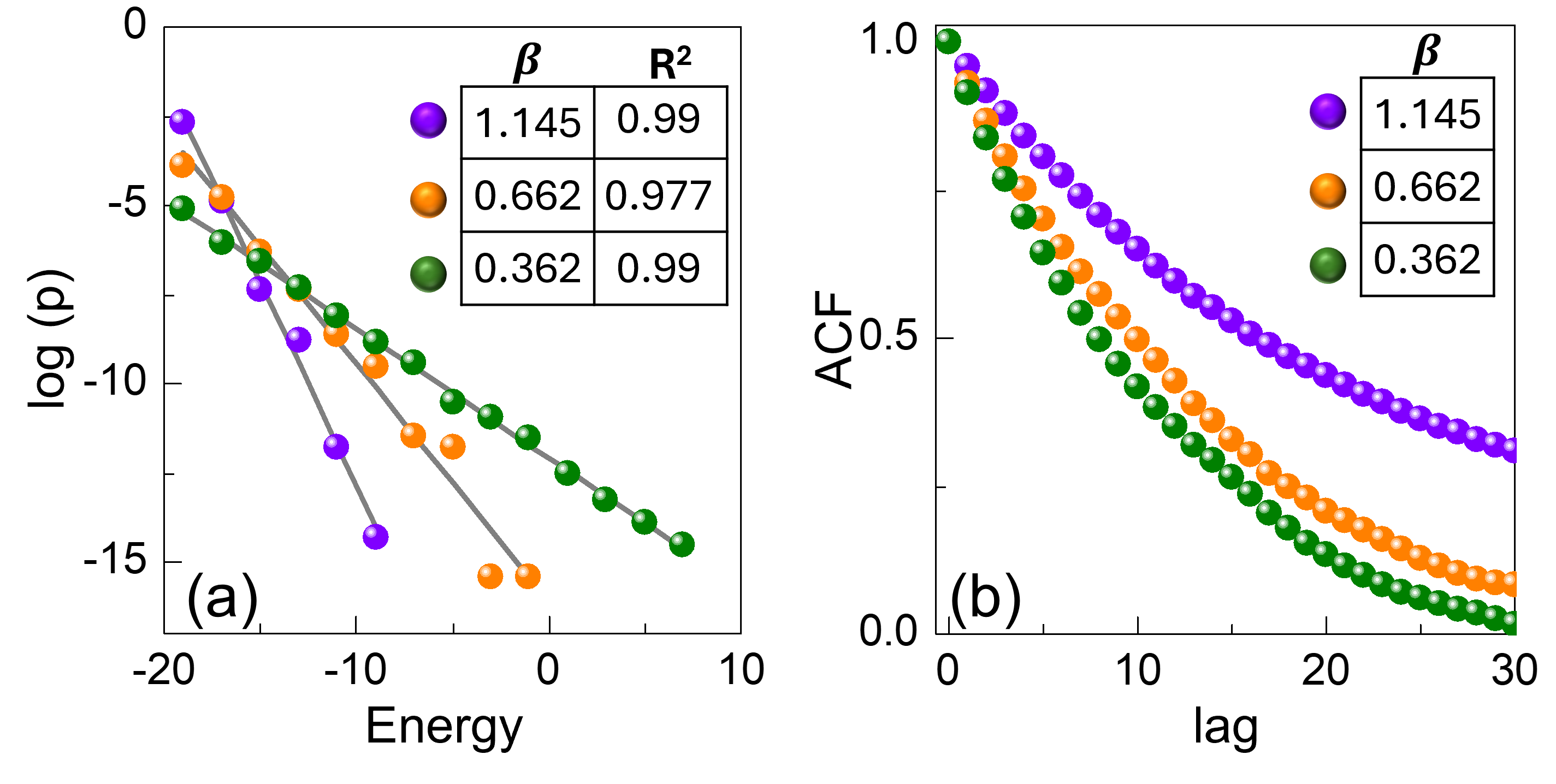
Figure 5: Boltzmann sampling behavior. (a) Plot of $\log$ (p) (p: probability) versus energy for varying noise intensities ( $K_n=0.05$ , 0.1, 0.15), corresponding to different effective temperatures. The extracted effective inverse temperatures ( $β$ ) and the quality of the linear fits ( $R^2$ ) are shown in the inset. (b) Autocorrelation function (ACF) of the system energy as a function of lag, exhibiting a decay toward zero, confirming that the stochastic dynamics effectively decorrelate successive configurations.
While the above simulations demonstrate the application of the OIM’s stochastic sampling capability in solving COPs such as MaxCut, we also employ the same example to further corroborate their Boltzmann sampling behavior. Specifically, we perform simulations on the 15-node graph considered in Fig. 4 under varying noise intensities, which effectively correspond to different effective temperatures. Similar to the five-state adder analysis, we simulate only the dynamics of the oscillator being sampled, while the remaining oscillator phases are held fixed. Figure 5 (a) shows the resulting $\log$ (p) (p: probability) versus energy distributions obtained over 5000 sweeps. The observed linear dependence confirms that the sampled state probabilities follow the expected Boltzmann relation, with the slope yielding the effective inverse temperature ( $β$ ). Furthermore, Fig. 5 (b) presents the normalized autocorrelation function (ACF) [33] of the system energy as a function of the lag. In all cases, the autocorrelation decays toward zero with increasing delay, indicating that the stochastic dynamics efficiently decorrelate successive configurations.
<details>
<summary>Figure4r.png Details</summary>
### Visual Description
## Stacked Time-Series Line Charts: Bifurcation and State Dynamics
### Overview
This image displays two vertically stacked line charts sharing a common horizontal axis labeled "Time" (ranging from 0 to 300). The charts illustrate the temporal evolution of a system, likely a dynamical or multi-agent system, undergoing a bifurcation event.
* **Top Chart (a):** Tracks the phase variable $\Phi (\pi)$ for multiple entities over time.
* **Bottom Chart (b):** Tracks a variable labeled "Cut" over time.
A light blue shaded region on the far left (Time 0 to ~15) is annotated as "Before Bifurcation." Red arrows at Time $\approx 220$ indicate a synchronized event across both charts.
### Components/Axes
**Shared Horizontal Axis:**
* **Label:** "Time"
* **Scale:** 0 to 300, with major ticks every 50 units.
**Top Chart (a):**
* **Vertical Axis:** Labeled "$\Phi (\pi)$". Scale ranges from 0.0 to 1.0.
* **Data Series:** Multiple overlapping lines of various colors (red, blue, green, purple, orange, cyan, dark red). These lines represent the state of individual agents or components.
* **Annotations:** A red arrow points downward at Time $\approx 220$.
**Bottom Chart (b):**
* **Vertical Axis:** Labeled "Cut". Scale ranges from 35 to 40.
* **Data Series:** A single green line representing the "Cut" value.
* **Annotations:** A red arrow points upward at Time $\approx 220$. The text "DIM" appears in the bottom-right corner.
### Detailed Analysis
**1. Phase 1: Pre-Bifurcation (Time 0 to ~15)**
* **Chart (a):** All colored lines are clustered at a value of 0.5.
* **Chart (b):** The "Cut" value starts at 0, then exhibits a sharp, vertical jump to approximately 36.
**2. Phase 2: Post-Bifurcation (Time ~15 to ~220)**
* **Chart (a):** The system bifurcates. The lines diverge from the 0.5 state, splitting into distinct groups: some lines jump to 1.0, others drop to 0.0, and some remain at 0.5. Throughout this period, the lines exhibit discrete "switching" behavior, jumping between 0.0, 0.5, and 1.0 at various time intervals.
* **Chart (b):** The "Cut" value remains relatively stable at ~36, then steps up to ~37 at Time $\approx 55$. It remains at ~37 until the next event.
**3. Phase 3: Event at Time $\approx 220$**
* **Chart (a):** Marked by the red arrow. There is a noticeable reorganization of the lines. Several lines that were at 0.5 or 0.0 shift to 1.0, and others shift to 0.5.
* **Chart (b):** Marked by the red arrow. The "Cut" value steps up from ~37 to approximately 38.5.
### Key Observations
* **Correlation:** There is a clear correlation between the "Cut" value and the state of the $\Phi$ variables. Increases in the "Cut" value (the green line) appear to trigger or coincide with state transitions in the $\Phi$ variables.
* **Bifurcation:** The transition at Time $\approx 15$ is the most significant event, where the system moves from a uniform state (0.5) to a bifurcated state (0.0, 0.5, 1.0).
* **Discrete States:** The $\Phi$ variable is quantized, restricted to three distinct levels: 0.0, 0.5, and 1.0.
* **Step-wise Progression:** The "Cut" variable behaves as a step function, suggesting it may be a control parameter that is incremented periodically.
### Interpretation
The data suggests this is a simulation of a complex system, possibly related to **network synchronization, community detection, or phase transitions in coupled oscillators**.
* **"Cut" as a Control Parameter:** The "Cut" variable likely represents a global constraint or a threshold parameter (common in graph partitioning or community detection algorithms). As this parameter increases, the system is forced to reorganize its internal states ($\Phi$).
* **Bifurcation:** The initial jump at Time $\approx 15$ represents a phase transition where the system loses its initial symmetry.
* **DIM:** The label "DIM" in the bottom right likely refers to "Dimensionality" or the specific model/algorithm name (e.g., a Dimensionality reduction technique or a specific simulation model).
* **System Stability:** The system appears to reach a quasi-stable state after each "Cut" increment, where the $\Phi$ values fluctuate within a specific band until the next "Cut" increment forces a new configuration.
</details>
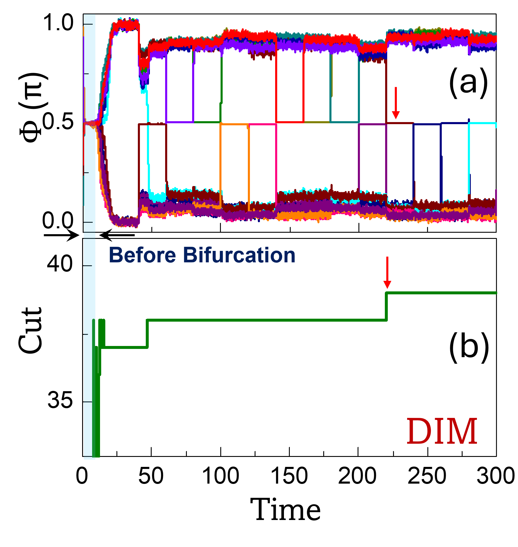
Figure 6: Operating DIMs as p-bit platforms. Evolution of (a) phases in the DIM model; and (b) corresponding graph cut over time. The same graph shown in Fig. 4 has been considered in the simulation. With stochastic sampling, the system is able to compute the MaxCut (=39) ( $K=1;K_s,max=4;\>\>FHI^0=50;\>\>K_n for sampled oscillator=0.006$ ).
## VI Realizing P-bit Engines Using Other Analog Ising Machines
Beyond conventional OIMs, the proposed sampling methodology exhibits potential for generalization to a broader class of analog dynamical systems. As a case in point, we evaluate the implementation of the proposed sampling mode in the Dynamical Ising Machine (DIM) recently introduced by the authors [34]. Unlike the traditional Kuramoto model, which relies on phase differences, the DIM employs additive phase interactions. The DIM dynamics can be described by:
$$
\begin{split}\frac{dφ_i}{dt}&=-K∑_\begin{subarray{c}j=1\\
j≠ i\end{subarray}}^NJ_ij\sin(φ_i\bm{+}φ_j)-K_s\sin(2φ_i)\end{split} \tag{17}
$$
Specifically, when $K_s$ is below a certain threshold, the system stabilizes at the trivial state $φ=\frac{π}{2}$ . As $K_s$ increases beyond this threshold, the system undergoes a bifurcation, leading to the emergence of stable phase configurations at $φ∈\{0,π\}^N$ , which can subsequently be mapped to a spin configuration. The phase dynamics of the DIM, without stochastic sampling, are presented in Appendix I for the graph considered in Fig. 4 .
While a detailed analysis of the DIM dynamics has been presented in [34], it is worth noting that the system exhibits a pitchfork bifurcation, qualitatively similar to that observed in the other popular Ising machine models such as the simulated bifurcation machine (SBM) [35]. This similarity suggests the feasibility of performing stochastic sampling in a broad class of analog dynamical systems beyond the OIM.
Similar to the OIM, the DIM dynamics in the rotated frame of reference are given by,
$$
\begin{split}\frac{dε_i}{dt}&=K∑_\begin{subarray{c}j=1\\
j≠ i\end{subarray}}^NJ_ij\sin(ε_i+ε_j)+K_s\sin(2ε_i)\\
\\
&=\cos(ε_i)≤ft(K∑_\begin{subarray{c}j=1\\
j≠ i\end{subarray}}^NJ_ij\sin(ε_j)\right)+K_s\sin(2ε_i)\\
\\
&≡-γ_i\cos(ε_i) +K_s\sin(2ε_i)\end{split} \tag{18}
$$
where $γ_i$ has the same definition and meaning as that in the case of the OIM. Moreover, equation (18) is exactly the same as the corresponding equation (12) derived for the OIM. Therefore, by employing the same approach and constraints used for the OIM, the updated spin state using the DIM can be derived as follows:
$$
\begin{split}s_i^+&≈-sgn≤ft[\tanh(-γ_iΔ t)+ε^η(Δ t).sech^2(γΔ t)\right]\\
\\
&≈sgn≤ft[\tanh≤ft(KΔ t∑_\begin{subarray{c}j=1\\
j≠ i\end{subarray}}^NJ_ijs_j\right)-ϑ\right]\end{split} \tag{19}
$$
Figure 6 presents a simulation demonstrating the operation of the DIM in sampling mode to compute the MaxCut of the same graph considered in Fig. 4. As shown in Fig. 6 (a), the phase dynamics initially exhibit a bifurcation as $K_s$ is ramped up from $K_s=0$ to $K_s=4$ (not shown in the figure). At this stage, however, the system has not yet reached the optimal solution. With the onset of stochastic sampling, the system begins to sample the solution space and eventually converges to the optimal MaxCut value of 39, as shown in Fig. 6 (b).We note that while both the models exhibit Gibbs sampling, the characteristics (e.g., effective temperature) obtained for a specific set of parameters ( $K,K_s,K_n$ ) will depend on the choice of exact dynamics.
## VII Conclusion
This work builds a conceptual bridge between two paradigms that have traditionally been regarded distinct: analog oscillator-based Ising machines (OIMs) and stochastic sampling-based p-bit engines. By leveraging the natural dynamics of coupled oscillators—specifically through the interplay of SHI and FHI signals—we demonstrate that analog OIMs can perform stochastic sampling without requiring explicit computation of energy functions or the synaptic feedback.
An intrinsic feature of this approach is the initial phase evolution, during which the oscillator network naturally performs gradient descent that involves the oscillator phases evolving simultaneously. Starting from random initial conditions, the phases converge to discrete states ( $φ_i≈ 0$ or $φ_i≈π$ ), effectively settling into a local minimum of the Ising energy landscape. In certain applications such as combinatorial optimization, this simultaneous evolution has the potential to offer a potential speed-up, positioning the system in a low-energy configuration even before the onset of the sampling-mode operation. However, these promising features come with the trade-off of requiring physical connectivity among oscillators—digital p-bit designs are better suited to implement the interaction between p-bits. From an implementation standpoint, this makes the analog approach more appropriate for sparse architectures which aligns well with the operational regimes where traditional p-bit platforms are expected to perform well.
Nevertheless, it is important to recognize several key factors that must be optimized to ensure reliable operation: (a) The SHI pulse characteristics (amplitude and slew rate) must be carefully designed, as they determine $Δ t$ , which in turn governs the effective temperature, the effective noise, and the validity of the approximations used in Eq. (8) to achieve Gibbs sampling. In practice, a high slew-rate SHI signal (resulting in a small $Δ t$ ) is generally desirable to simultaneously satisfy these requirements. (b) Beyond $Δ t$ , the effective temperature also depends on the coupling strength, $K$ , among oscillators. Therefore, the coupling strength must be co-designed with $Δ t$ to realize the desired temperature range, while maintaining frequency locking and satisfying the weak-coupling condition implicit in the dynamics considered here. Since $K$ itself is determined by factors such as the natural frequency, oscillation amplitude, and the magnitude of the physical quantity (e.g., coupling resistance) characterizing the coupling element, these parameters must also be carefully considered to ensure robust operation. (c) Finally, the present analysis does not account for parameter variations or natural frequency mismatches–effects that may play a critical role in determining whether robust operation can be achieved. These design aspects and challenges will need to be systematically investigated going forward.
From an algorithmic standpoint, we note that since Gibbs sampling is inherently sequential, incorporating techniques such as the graph-coloring method proposed by Niazi et al. [36] which enables multiple spins to be updated simultaneously— need exploration to further enhance performance, and represents a compelling direction for future exploration. Looking ahead, the capability of OIMs—when configured as p-bit engines—to perform stochastic sampling opens promising avenues for neural network applications, including the training of restricted Boltzmann machines.
The overlaps between the analog and probabilistic paradigms identified in this work motivate the extension of this framework to more generalized computational models, including higher-order Ising machines [37, 38], p-bits with more than two states [39, 22], as well as to other analog systems [35, 40, 41, 42, 43, 44] beyond those explored here.
## ACKNOWLEDGEMENTS
We gratefully acknowledge Prof. Kerem Camsari for providing valuable insights on the sampling properties of p-bits. This material is based upon work supported in part by ARO award W911NF-24-1-0228 and National Science Foundation grants ( $\#$ 2422333, #2433871).
## APPENDIX A INJECTION LOCKING IN SINGLE OSCILLATOR
We analyze the impact of FHI on oscillator dynamics from an energy-based perspective. For an oscillator driven by an FHI signal at its natural frequency but with a phase offset $θ$ , the phase dynamics can be described using Adler’s equation [31, 32] as follows:
$$
\frac{dφ}{dt}=-K_c\sin(φ-θ) \tag{20}
$$
The corresponding energy function that the above dynamics minimize can be expressed as:
$$
E(φ)=-K_c\cos(φ-θ) \tag{21}
$$
For this system, the relationship $-\frac{dE}{dφ}=\frac{dφ}{dt}$ holds, implying that:
$$
\frac{dE}{dt}=\frac{dE}{dφ}·\frac{dφ}{dt}=-≤ft(\frac{dφ}{dt}\right)^2≤ 0
$$
Thus, the energy monotonically decreases over time, and the system evolves toward a stable fixed point.
The minimum of the energy function occurs at $φ^*=θ$ , where $\frac{dE}{dt}=0$ . Within the domain $φ∈[θ,θ+2π)$ , the only other fixed point satisfying $\frac{dE}{dt}=\frac{dφ}{dt}=0$ is at $φ^*=θ+π$ , which corresponds to a local maximum, and is therefore unstable. For all other values of $φ$ in this domain, $\frac{dE}{dt}<0$ . Consequently, the oscillator phase converges to the stable fixed point $φ=θ$ , although perturbations may be necessary to prevent the dynamics from settling at the unstable fixed point $φ^*=θ+π$ .
## APPENDIX B STABILITY OF THE FIXED POINTS OF THE DYNAMICS
We analyze the stability of the fixed points associated with the dynamics described in Eq. (5) of the main text. As previously discussed, the fixed points of the dynamics are given by, $ε_1^*=±\frac{π}{2}$ and $\sin(ε_2^*)=\frac{γ_i}{2K_s}$ .
To investigate the local stability of the system, we analyze the sign of the second derivative:
$$
H(ε_i)=\frac{d^2ε_i}{dt^2}=γ_i\sin(ε_i)+2K_s\cos(2ε_i)
$$
We seek conditions under which $H(ε_i)<0$ , indicating local stability.
- Stability of $ε_1^*=\frac{π}{2}$ At this point, $\sin(ε_1^*)=1$ , $\cos(2ε_1^*)=-1$ , so:
$$
H(ε_1^*)=γ_i+(-2K_s)=γ_i-2K_s
$$
Hence, $H(ε_1^*)<0$ when $γ_i<2K_s$ .
- Stability of $ε_1^*=-\frac{π}{2}$ Here, $\sin(ε_1^*)=-1$ , $\cos(2ε_1^*)=-1$ , therefore:
$$
H(ε_1^*)=-γ_i-2K_s
$$
Thus, $H(ε_1^*)<0$ when $γ_i+2K_s>0$ .
- Combined Condition: Both fixed points $ε_1^*=±\frac{π}{2}$ are stable when:
$$
γ_i^2<4K_s^2
$$
- Stability of $\sin(ε_2^*)=\frac{γ_i}{2K_s}$ Substituting into $H(ε_i)$ , we find that:
$$
H(ε_2^*)<0 when γ_i^2>4K_s^2
$$
## APPENDIX C TUNING ENERGY BARRIER WITH SHI STRENGTH ( $K_s$ )
<details>
<summary>Figure5r.png Details</summary>
### Visual Description
## Line Chart: Energy vs. $\epsilon$ for varying $K_s$ values
### Overview
This image displays a scientific line plot illustrating the relationship between Energy (in arbitrary units) and a variable $\epsilon$ (in units of $\pi$). The plot compares three distinct curves, each corresponding to a specific value of the parameter $K_s$ (0.10, 0.15, and 0.20), while holding the parameter $\gamma$ constant at 0.
### Components/Axes
* **Y-Axis:** Labeled "Energy (a.u.)". The scale ranges from -0.1 to 0.1, with major ticks at -0.1, 0.0, and 0.1.
* **X-Axis:** Labeled "$\epsilon$ ($\pi$)". The scale ranges from approximately -0.7 to 0.7, with major ticks at -0.5, 0.0, and 0.5.
* **Legend:** Located in the top-left quadrant. It defines the color-coding for the parameter $K_s$:
* **Orange line:** $K_s = 0.10$
* **Green line:** $K_s = 0.15$
* **Purple line:** $K_s = 0.20$
* **Annotation:** Located in the top-right corner: "$\gamma = 0$".
### Detailed Analysis
The plot displays three oscillatory curves that are symmetric about the vertical axis ($\epsilon = 0$).
**Trend Verification:**
* All three curves exhibit a local maximum at $\epsilon = 0$.
* All three curves exhibit local minima at $\epsilon \approx \pm 0.5$.
* The curves intersect at approximately $\epsilon \approx \pm 0.25$ and $\epsilon \approx \pm 0.75$.
**Data Points (Approximate Values):**
| Parameter ($K_s$) | Color | Energy at $\epsilon = 0$ (Max) | Energy at $\epsilon = \pm 0.5$ (Min) |
| :--- | :--- | :--- | :--- |
| **0.10** | Orange | $\approx +0.05$ | $\approx -0.05$ |
| **0.15** | Green | $\approx +0.07$ | $\approx -0.07$ |
| **0.20** | Purple | $\approx +0.10$ | $\approx -0.10$ |
*Note: The values are estimated based on visual alignment with the grid lines.*
### Key Observations
* **Amplitude Scaling:** The amplitude of the energy oscillation is directly proportional to the value of $K_s$. As $K_s$ increases from 0.10 to 0.20, the peak-to-trough distance increases significantly.
* **Crossover Points:** The curves are not parallel; they intersect at specific points ($\epsilon \approx \pm 0.25$ and $\epsilon \approx \pm 0.75$). At these points, the energy value is independent of the $K_s$ parameter.
* **Symmetry:** The system demonstrates perfect mirror symmetry across the y-axis ($\epsilon = 0$).
### Interpretation
This plot is characteristic of a dispersion relation in condensed matter physics, likely representing the energy band structure of a periodic system (such as a 1D lattice).
* **Physical Significance:** The parameter $K_s$ likely represents a coupling strength or a hopping parameter. Increasing $K_s$ increases the bandwidth (the difference between the maximum and minimum energy), suggesting stronger interaction or tighter binding as $K_s$ increases.
* **The Crossover:** The intersection points at $\epsilon \approx \pm 0.25$ suggest a "node" or a point of degeneracy where the energy state is invariant to changes in the coupling parameter $K_s$.
* **Context:** The plot describes a system where energy is periodic with respect to $\epsilon$. The behavior is consistent with a tight-binding model where the energy dispersion is modulated by the parameter $K_s$. The condition $\gamma = 0$ implies this is a specific slice of a larger parameter space, likely representing a system without a specific type of asymmetry or bias (e.g., no external field or specific phase factor).
</details>
Figure 7: Tuning energy barrier with $K_s$ . Evolution of the energy barrier with $K_s$
We analyze the impact of $K_s$ on the energy barrier. The function corresponding to the dynamics described by Eq. (5) is,
$$
E=γ\sin(ε)+\frac{1}{2}K_s\cos(2ε) \tag{22}
$$
Figure 7 shows the resulting energy landscape for different values of $K_s$ ( $γ=0$ ). The energy difference between the peak energy (at $ε=0$ ) and either valley (at $ε=±\frac{π}{2}$ ) is given by $(Δ E)_max=|K_s|$ .
## APPENDIX D TEMPORAL EVOLUTION OF THE PHASE
We now analyze the dynamics presented in Eq. (5). The implicit analytical solution is given by,
$$
\frac{ζ(ε)-γ\tanh^-1(\sin(ε))}{γ^2-4K_s^2}=t+C \tag{23}
$$
where,
$$
\begin{split}ζ(ε)&=K_s\big(-2\log(γ-2K_s\sin(ε))\\
&+\log(1-\sin(ε))+\log(\sin(ε)+1)\big)\\
\end{split} \tag{24}
$$
and $C$ is the constant of integration. $C=0$ since $ε(t=0)=0$ , and $K_s=0$ at $t=0$ .
We now analyze the dynamics under the constraints specified in the main text, which are also restated below for reference: (i) The dynamics are evaluated in the limit $t→ 0$ . (ii) We model the noise as Gaussian white noise with $⟨η(t)⟩=0, ⟨η(t)η(t^\prime)⟩=2K_nδ(t-t^\prime),$ with $K_n$ denoting the noise intensity i.e., $η(t) dt=√{2K_n} dW_t,$ where $W_t$ is a Wiener process. Equivalently, over a finite timestep $Δ t$ , $∫_t^t+Δ tη(τ) dτ ∼ N\big(0, 2K_n Δ t\big).$ (iii) At the onset of sampling ( $t→ 0$ ) , we assume $K_s→ 0$ such that $K_s\ll|γ|$ . This reflects the requirement for a low energy barrier in the probabilistic regime.
Eq. (23) can be rearranged to yield,
$$
\begin{split}\sin(ε_i)&=\tanh≤ft(-γ t+\frac{4K_s^2t+ζ(ε)}{γ}+ε^η(t)\right)\\
\\
&=\tanh≤ft(-γ t+\frac{4K_s^2t+ζ(ε)}{γ}+ε^η(t)\right)\end{split}\ \tag{25}
$$
Here, $ε^η(t)$ represents the perturbation induced by noise. We note that in the above analysis, we approximate the impact of noise as phase jitter; a more exhaustive treatment would model the phase dynamics as a stochastic differential equation.
From the above equation, we group all the terms dependent on $K_s$ as,
$$
\begin{split}&Θ=\frac{4K_s^2t+ζ(ε)}{γ}\\
\\
⇒ &\sin(ε_i)=\tanh≤ft(-γ t+Θ+ε^η(t)\right)\end{split}
$$
and evaluate $Θ$ under the constraints stated above.
We begin by simplifying the following terms: $\log(1-\sin(ε))+\log(1+\sin(ε))=\log(\cos^2(ε))$ . Thus, $ζ(ε)=2K_s≤ft(\log≤ft(\cos(ε)\right)-\log≤ft(γ-2K_s\sin(ε)\right)\right)$
Next, we apply the following approximations (applicable under the constraints stated above), $\bullet$ $\cos(ε)≈ 1-\frac{ε^2}{2}⇒\log(\cos(ε))≈-\frac{ε^2}{2}$ $\bullet$ $\sin(ε)≈ε$ $\bullet$ $\log(γ-2K_s\sin(ε))≈\log(|γ|)-\frac{2K_sε}{γ}$
Substituting these approximations into expression for $ζ$ yields,
$$
ζ≈ 2K_s≤ft(\frac{-ε^2}{2}-\log(|γ|)+\frac{2K_sε}{γ}\right)
$$
Subsequently, $Θ$ can be approximated as,
$$
\begin{split}Θ&=\frac{4K_s^2t+2K_s≤ft(\frac{-ε^2}{2}-\log(|γ|)+\frac{2K_sε}{γ}\right)}{γ}\\
\\
&=\frac{4K_s^2t}{γ}-\frac{K_sε^2}{γ}-\frac{2K_s\log(|γ|)}{γ}+\frac{4K_s^2ε}{γ^2}\end{split}
$$
The above expression shows the leading-order behavior of terms dependent on $K_s$ in the phase behavior. Moreover, when $K_s→ 0$ such that $K_s\ll|γ|$ , $Θ→ 0$ . Nevertheless it is important that the system parameters be carefully designed to ensure that the dynamics emulate Boltzmann sampling as close as possible.
<details>
<summary>Figure6r.png Details</summary>
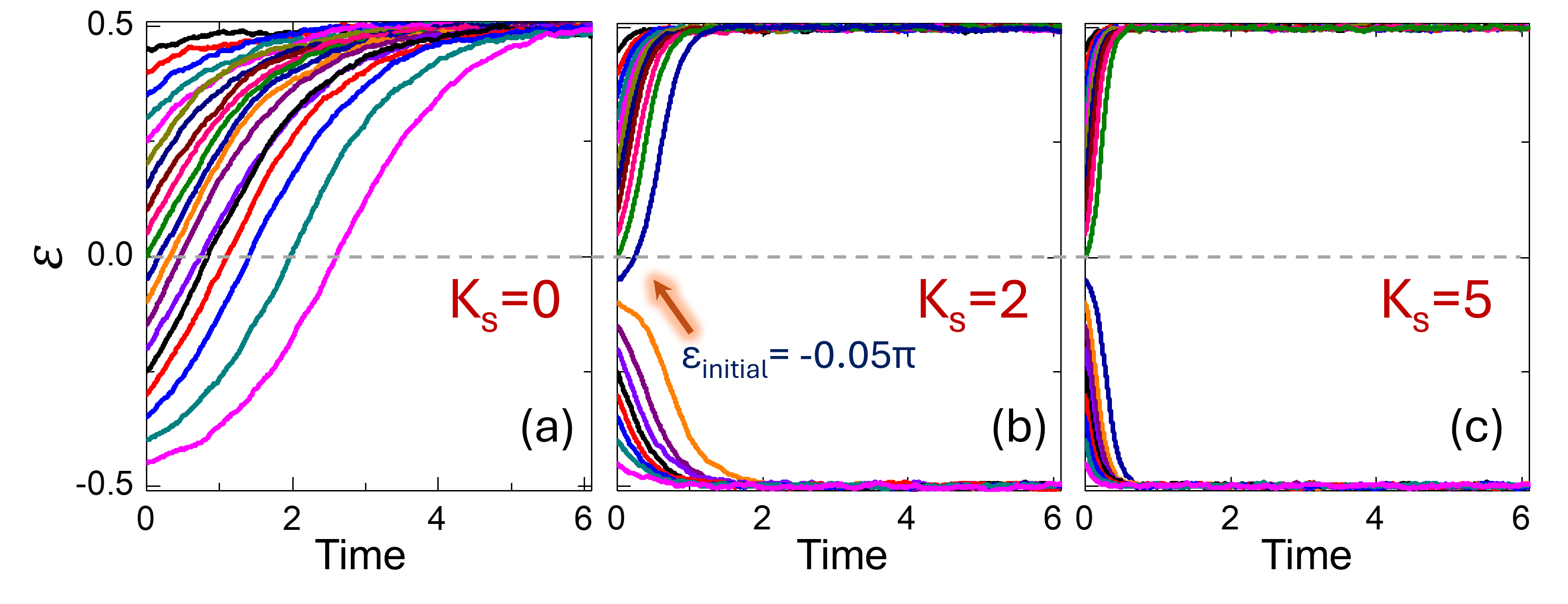
### Visual Description
## Line Charts: Evolution of $\epsilon$ over Time for varying $K_s$
### Overview
The image displays three side-by-side line charts, labeled (a), (b), and (c), illustrating the temporal evolution of a variable $\epsilon$ (epsilon) over time. Each chart represents the system's behavior under a different parameter value, $K_s$. The charts demonstrate a transition in system dynamics as $K_s$ increases, moving from a single-attractor state to a bistable state with rapid convergence.
### Components/Axes
* **Y-Axis:** Labeled "$\epsilon$". The scale ranges from -0.5 to 0.5. A dashed horizontal line is drawn at $\epsilon = 0.0$ across all three panels.
* **X-Axis:** Labeled "Time". The scale ranges from 0 to 6.
* **Panel (a):** Located on the left. Contains the label "$K_s=0$" in red text in the bottom-right quadrant.
* **Panel (b):** Located in the center. Contains the label "$K_s=2$" in red text in the bottom-right quadrant. It includes an annotation: "$\epsilon_{initial} = -0.05\pi$" written in blue text, with an orange arrow pointing toward the cluster of lines starting below the zero line.
* **Panel (c):** Located on the right. Contains the label "$K_s=5$" in red text in the bottom-right quadrant.
### Detailed Analysis
#### Panel (a) [$K_s=0$]
* **Trend:** All colored trajectories exhibit an upward slope.
* **Behavior:** Regardless of the starting position (which varies between -0.5 and 0.5), all trajectories converge toward the upper steady state of $\epsilon = 0.5$.
* **Convergence Rate:** The convergence is gradual, with most lines reaching the steady state between time $t=2$ and $t=6$.
#### Panel (b) [$K_s=2$]
* **Trend:** The system exhibits bifurcation. Trajectories starting above the zero line trend upward to 0.5; trajectories starting below the zero line trend downward to -0.5.
* **Annotation:** The text "$\epsilon_{initial} = -0.05\pi$" (blue) with an orange arrow indicates the starting condition for the group of trajectories that converge to the negative steady state.
* **Convergence Rate:** The convergence is significantly faster than in panel (a), with most trajectories reaching their respective steady states by $t=1$.
#### Panel (c) [$K_s=5$]
* **Trend:** Similar to panel (b), the system is bistable, with trajectories splitting toward 0.5 or -0.5.
* **Convergence Rate:** The convergence is extremely rapid. The trajectories appear almost vertical, reaching their steady states almost immediately after $t=0$.
### Key Observations
* **Bistability Transition:** As $K_s$ increases from 0 to 2, the system transitions from a single-attractor state (where all values converge to 0.5) to a bistable state (where values converge to either 0.5 or -0.5 depending on initial conditions).
* **Coupling Strength:** The parameter $K_s$ appears to act as a coupling strength or control parameter. Higher values of $K_s$ result in steeper, faster convergence to the steady states.
* **Symmetry:** The system shows symmetry around the $\epsilon=0$ axis in panels (b) and (c), suggesting that the basins of attraction for the positive and negative states are balanced.
### Interpretation
The data suggests this is a visualization of a dynamical system, likely related to synchronization or phase-locking (such as the Kuramoto model or a similar oscillator network).
* **At $K_s=0$:** The system lacks the coupling strength required to maintain a negative state, causing all trajectories to be "pulled" toward the positive attractor at 0.5.
* **At $K_s \ge 2$:** The coupling strength is sufficient to create two distinct basins of attraction. The system becomes sensitive to initial conditions; if a trajectory starts below the threshold (indicated by the $\epsilon_{initial}$ annotation), it is captured by the negative attractor (-0.5). If it starts above, it is captured by the positive attractor (0.5).
* **The Role of $K_s$:** The increase in $K_s$ effectively "sharpens" the potential landscape of the system, making the steady states more stable and the transition to them more aggressive. The annotation $\epsilon_{initial} = -0.05\pi$ highlights the specific starting condition required to enter the negative basin of attraction.
</details>
Figure 8: Role of SHI in maintaining phase trajectory. Phase deviation $ε$ as a function of time for: (a) $K_s=0$ ; (b) $K_s=2$ ; (c) $K_s=5$ . The results in the illustrative example show that a critical SHI is needed to help the oscillator phase continue to evolve along the direction of its initial perturbation. $|γ_1|=1$ has been considered in this example.
Under these conditions, Eq. (LABEL:appendix4-2) can be approximated as,
$$
\begin{split}\sin(ε_i)&≈\tanh≤ft(-γ t+ε^η(t)\right)\\
\\
&≈\tanh≤ft(-γ t\right)+ε^η(t).sech^2(γ t)\\
\\
\end{split}
$$
Here, $ε^η(t)∼N\big(0, 2K_n t\big)$ , and is small such that the $\tanh(.)$ term can be linearized. The noise term, $ε^η(t).sech^2(γ t)$ , can be considered as a gaussian distribution representing white noise, and scaled by a function of the synaptic input—sech ${}^2(γ t)$ . The updated spin state, $s^+=-sgn≤ft(\sin(ε^+)\right)$ , at a short time instant $Δ t→ 0$ after sampling has been initiated (at $t=0$ ), can be expressed as,
$$
\begin{split}s^+&≈sgn≤ft[\tanh(γΔ t)-ε^η(Δ t).sech^2(γΔ t)\right]\\
\\
&≡sgn≤ft[\tanh(γΔ t)-ϑ\right]\end{split}
$$
where, $ϑ≡ε^η(Δ t).sech^2(γΔ t)$ . Since $sech^2(γΔ t)∈(0,1]$ , and noise power is assumed to be small, $ϑ$ has a high probability of being in the interval [-1,+1]. We also note that for $Δ t→ 0$ , $sech^2(γΔ t)→ 1⇒ϑ≈eqε^η(Δ t)$ . Moreover, the gaussian distribution is more representative of the thermal noise found in physical devices.
We also consider the case when both $γ$ and $K_s$ are small. Under this assumption, the dynamics for $ε\ll 1$ can be approximated as,
$$
\frac{dε}{dt}≈-γ+2K_sε
$$
Unlike the previous case, using the SDE framework here yields a tractable and elegant solution that offers a clear and intuitive picture of the relative competition between the stochastic and deterministic components.
We begin by considering the linear Itô SDE
$$
\begin{split}&dε(t)=\big(-γ+2K_sε(t)\big) dt+√{2K_n} dW_t,\\
\\
&where we note that ε(0)=0, K_s>0.\end{split} \tag{0}
$$
Integrating factor: Let $M(t)=e^-2K_st$ . Since $M$ is deterministic,
$$
\displaystyle d\big(M(t)ε(t)\big) \displaystyle=M(t) dε(t)+ε(t) dM(t) \displaystyle=-γ M(t) dt+√{2K_n} M(t) dW_t. \tag{27}
$$
Integration from $0$ to $t$ yields
$$
\displaystyle M(t)ε(t) \displaystyle=-γ∫_0^tM(s) ds \displaystyle +√{2K_n}∫_0^tM(s) dW_s. \tag{28}
$$
Since
$$
∫_0^te^-2K_ss ds=\frac{1-e^-2K_st}{2K_s}, M(t)^-1=e^2K_st,
$$
we obtain
$$
ε(t)=\frac{γ}{2K_s} (1-e^2K_st)+√{2K_n}∫_0^te^2K_s(t-s) dW_s. \tag{29}
$$
Mean: The stochastic integral in (29) has zero mean:
$$
E[ε(t)]=\frac{γ}{2K_s} (1-e^2K_st). \tag{30}
$$
Variance: By Itô isometry,
$$
\displaystyleVar[ε(t)] \displaystyle=2K_n∫_0^te^4K_s(t-s) ds \displaystyle=\frac{K_n}{2K_s} \big(e^4K_st-1\big). \tag{31}
$$
The above results imply that for $K_s>0$ , both mean and variance diverge exponentially. Thus, no stationary distribution exists. Two limiting cases further clarify the dynamics:
- Case $γ=0$ . In the absence of the synaptic input, the deterministic contribution reduces to $dε=2K_sε dt$ . With $ε(0)=0$ , this term alone would maintain $ε(t)≡ 0$ . However, in the presence of Gaussian noise, random perturbations are continuously injected and then exponentially amplified by the unstable drift. Consequently, the growth of $ε(t)$ is seeded by stochastic fluctuations and deterministically amplified over time.
- Case $γ≠ 0$ . When $γ≠ 0$ , both deterministic and stochastic contributions govern the dynamics. As seen from Eq. (30) and Eq. (31), both the drift-induced component and the noise-driven fluctuations diverge as $t$ increases. The relative dominance of these two effects depends on the balance between the deterministic drive, set by $|γ|$ , and the stochastic forcing, quantified by $K_n$ . A stronger deterministic bias leads to more predictable exponential growth, whereas larger noise intensity results in greater dispersion across trajectories.
## APPENDIX E ROLE OF SHI DURING STOCHASTIC SAMPLING
To analyze how the SHI can help the oscillator maintain the phase trajectory resulting from the stochastic sampling process, we examine Eq. (5):
$$
\frac{dε}{dt}=-γ\cos(ε)+K_s\sin(2ε)
$$
As discussed in the main text, the role of SHI is particularly critical when the initial direction of phase relaxation is counter to that expected from synaptic feedback, owing to noise. As noted earlier, the synaptic input (alone) tends to push the phase toward the fixed point opposite to the sign of $γ$ . In other words, we seek to analyze the conditions under which the initial flow of the dynamics is towards $ε=+\frac{π}{2}(-\frac{π}{2})$ , even when though the synaptic input is $γ>0\>\>≤ft(γ<0\right)$ , respectively.
Assuming that the initial perturbation results in a phase magnitude given by $|ε_th|$ , the critical condition on $K_s$ to ensure that the phase continues to flow in the same direction can be expressed as,
$$
2K_s\sin(|ε_th|)>≤ft|γ\right| \tag{32}
$$
This condition ensures the RHS of Eq. (5) maintains the same sign as the phase at $ε=ε_th$ . Further, since $\sin(.)$ is monotonic in the region, $|ε|∈\{0,\frac{π}{2}\}$ , the sign of the RHS terms will not change until dynamics reach the corresponding fixed point. We note that in the presence of noise, the above condition should be interpreted in a probabilistic sense.
We also illustrate this behavior using a simple example: a negatively coupled two-oscillator system (with $K=1$ ) in which the phase of oscillator 2 is fixed at $ε_2=-\frac{π}{2}$ yielding $γ_1=-1⇒|γ_1|=1$ . In this configuration, the energetically favorable state for oscillator 1 is $ε_1=\frac{π}{2}$ , and synaptic feedback is expected to drive the system toward this fixed point. To explore the system’s dynamics, oscillator 1 is initialized at various discrete phase values within the range $ε_th∈[-0.45π, 0.45π]$ . Figures 8 (a–c) show the evolution of $ε$ for different values of $K_s$ .
In the absence of synaptic hysteresis (i.e., $K_s=0$ ), the phase does not preserve the direction of its initial perturbation. Instead, it eventually aligns with the direction of the synaptic input, converging to $ε=\frac{π}{2}$ . This behavior is expected, as the inequality in Eq. (32) is never satisfied in this regime.
Introducing SHI (i.e., $K_s>0$ ) enables the oscillator phase to continue evolving along the direction of $ε_th$ . However, the magnitude of $K_s$ must exceed a certain threshold. This behavior is illustrated in Figs. 8 (b) and 8 (c). In Fig. 8 (b), when $K_s$ is below the threshold required for that $ε_th=-0.05π$ , the phase evolution eventually aligns with the direction favored by the synaptic input. In contrast, when $K_s$ is sufficiently, as in Fig. 8 (c)), all initial phase values considered here evolve along the direction of their original perturbation. Thus, the SHI injection strength, $K_s$ , must be carefully engineered to ensure that one phase magnitudes beyond a certain threshold evolve continue to evolve in the direction of their initial perturbation.
## APPENDIX F TIME INCREMENT $Δ t$ AND IMPACT OF SLEW RATE OF THE SHI SIGNAL
As described in the main text, the infinitesimal time $Δ t$ is defined as the interval required for the oscillator phase to reach the critical threshold $|ε_th|$ , beyond which the phase trajectory cannot reverse and the sampling event is effectively complete. The value of $Δ t$ is determined by properties of the SHI signal, most notably its slew rate. Qualitatively, this dependence can be understood as follows: a higher slew rate drives the oscillator phase more rapidly toward the fixed points $ε∈\{-\tfrac{π}{2},\tfrac{π}{2}\}$ , thereby reducing $Δ t$ .
To provide a quantitative illustration, we consider the SHI signal implemented as a linear ramp with slew rate $ρ$ , such that $K_s=ρ t$ . For this case, the phase dynamics (Eq. (5)), under the assumption $|ε|\ll 1$ , can be expressed as:
$$
\begin{split}&\frac{dε}{dt}=-γ+(ρ t)(2ε)\\
\\
⇒\>&\frac{dε}{dt}-2ρ ε t=-γ\end{split} \tag{33}
$$
where, $\sin(2ε)∼ 2ε$ since $|ε|\ll 1$ .
Using the integrating factor, $μ(t)=e^-ρ t^2$ , Eq. (33) can be expressed as,
$$
\frac{d}{dt}≤ft(ε e^-ρ t^2\right)=-γ e^-ρ t^2 \tag{34}
$$
With the initial condition $ε(0)=0$ , the resulting phase evolution is described by,
$$
ε(t)=-\frac{√{π}γ e^ρ t^2 erf(√{ρ}t)}{2√{ρ}} \tag{35}
$$
Using Eq. 35, we compute the time, $Δ t$ taken by the oscillator phase to reach $|ε_th|≈\frac{γ}{2K_s,th}$ $(|ε_th|\ll 1), where K_s,th=ρ(Δ t)$ . Equating Eq. (35) to $|ε_th|$ yields,
$$
\begin{split}\frac{γ}{2ρ(Δ t)}=\frac{√{π}γ e^ρ(Δ t)^2 erf(√{ρ}Δ t)}{2√{ρ}}\\
\\
⇒√{ρ} Δ t π e^ρΔ t^2 erf(√{ρ}Δ t)=1\end{split} \tag{36}
$$
Note that the relationship between $ρ$ and $Δ t$ does not depend on $γ$ . To express this relationship in terms of $ρ$ , we define $y=√{ρ} Δ t⇒ρ=\frac{y^2}{(Δ t)^2}$ where $y$ obeys the relationship,
$$
√{π} y e^y^2 erf(y)=1 \tag{37}
$$
which is Eq. (36) expressed in terms of $y$ .
Equation (37) implies that $y$ is a constant, whose value can be approximated as $y≈ 0.62$ . Thus, the relationship between the ramp rate of the SHI signal and $Δ t$ , can be approximated as,
$$
\begin{split}ρ≈\frac{0.3844}{(Δ t)^2}\\
\\
≡Δ t≈\frac{0.62}{√{ρ}}\end{split} \tag{38}
$$
Equation (38) shows that $Δ t$ is inversely proportional to the square root of the slew rate, under the approximations stated above. While this relationship was derived assuming a linear ramp signal for analytical convenience, we expect the same qualitative dependence of $Δ t$ on $ρ$ to hold for other SHI signal schemes as well.
<details>
<summary>FigureKLD.png Details</summary>
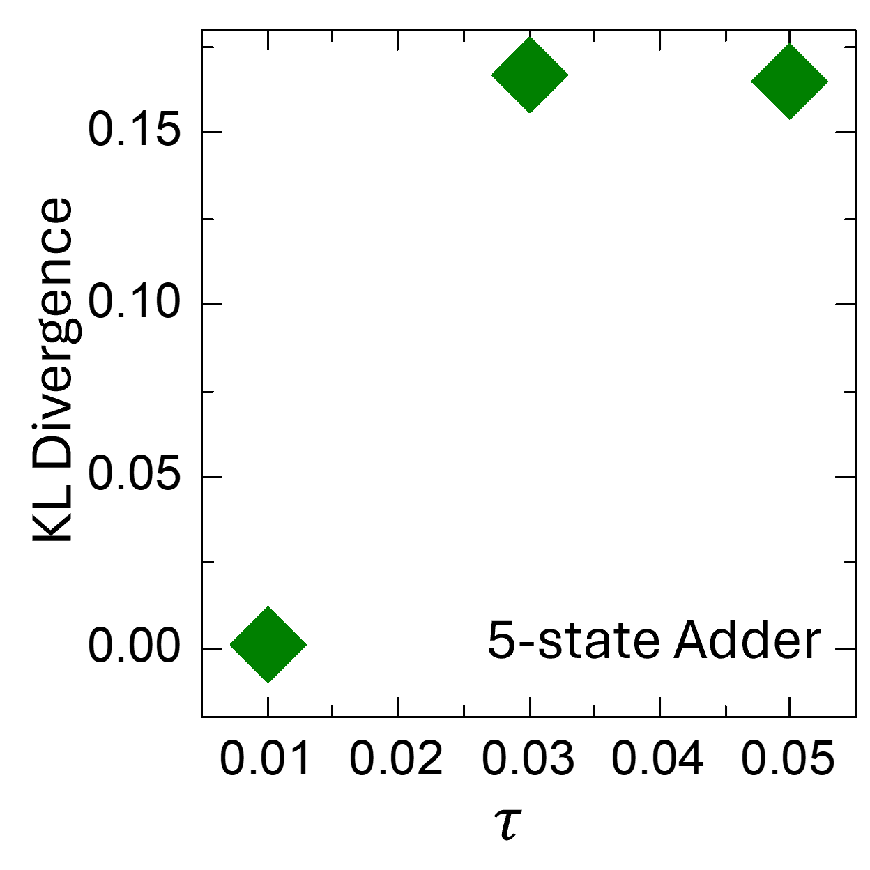
### Visual Description
## Scatter Plot: KL Divergence vs. $\tau$ for 5-state Adder
### Overview
This image is a scatter plot illustrating the relationship between a parameter $\tau$ (tau) and "KL Divergence" for a system identified as a "5-state Adder." The plot contains three distinct data points represented by green diamonds.
### Components/Axes
* **Y-Axis:** Labeled "KL Divergence." The scale ranges from 0.00 to 0.15, with major tick marks at 0.00, 0.05, 0.10, and 0.15.
* **X-Axis:** Labeled "$\tau$." The scale ranges from 0.01 to 0.05, with major tick marks at 0.01, 0.02, 0.03, 0.04, and 0.05.
* **Data Markers:** Three large, solid green diamond-shaped markers.
* **Text Label:** "5-state Adder" is positioned in the bottom-right quadrant of the plot area.
### Detailed Analysis
The data series consists of three points. The visual trend shows a sharp increase in KL Divergence between $\tau = 0.01$ and $\tau = 0.03$, followed by a plateau between $\tau = 0.03$ and $\tau = 0.05$.
* **Point 1 (Bottom-Left):**
* **Position:** X-axis value of 0.01, Y-axis value of 0.00.
* **Status:** The marker is centered exactly on the intersection of the 0.01 X-axis tick and the 0.00 Y-axis tick.
* **Point 2 (Top-Middle):**
* **Position:** X-axis value of 0.03, Y-axis value of approximately 0.17.
* **Status:** The marker is centered above the 0.03 X-axis tick. Vertically, it sits above the 0.15 Y-axis tick mark.
* **Point 3 (Top-Right):**
* **Position:** X-axis value of 0.05, Y-axis value of approximately 0.17.
* **Status:** The marker is centered above the 0.05 X-axis tick. It is horizontally aligned with Point 2, indicating the same Y-axis value.
### Key Observations
* **Threshold Effect:** The system exhibits a distinct threshold behavior. At $\tau = 0.01$, the KL Divergence is zero, indicating perfect alignment or convergence.
* **Saturation:** The KL Divergence increases significantly as $\tau$ moves from 0.01 to 0.03, but then remains constant (plateaus) as $\tau$ increases further to 0.05.
* **Data Sparsity:** The plot only provides data for three specific values of $\tau$ (0.01, 0.03, 0.05), leaving the behavior between these points undefined.
### Interpretation
The data demonstrates that the "5-state Adder" system is sensitive to the parameter $\tau$.
* **KL Divergence Significance:** KL Divergence (Kullback-Leibler divergence) is a measure of how one probability distribution differs from a reference distribution. A value of 0.00 at $\tau = 0.01$ suggests that at this specific parameter value, the system's output distribution perfectly matches the target distribution.
* **System Instability:** The sharp rise in divergence at $\tau = 0.03$ suggests that increasing $\tau$ beyond 0.01 introduces significant error or deviation in the system's state distribution.
* **Steady State Error:** The plateau at $\tau = 0.03$ and $\tau = 0.05$ suggests that once the system deviates from the target distribution, it reaches a maximum level of divergence (approximately 0.17) within this parameter range. It does not appear to diverge further as $\tau$ increases from 0.03 to 0.05, implying the system reaches a stable, albeit inaccurate, state.
</details>
Figure 9: Impact of SHI rise time and $Δ t$ . Measured KL Divergence as a function of $τ$ , where $K_s(t)=K_s,max(1-e^-\frac{t{τ}})$ . $τ$ impacts the time scale over which the SHI signal is asserted.
The practical implications of the relationship between $Δ t$ and $ρ$ are: (a) $Δ t$ directly impacts the effective inverse temperature ( $β$ ) of the oscillator-based BSN and sets the requirements on the required slew rate. (b) Increasing $Δ t$ suppresses the effect of noise, thereby making the system “less” stochastic. To elucidate this, we consider the expression for the updated spin state given by:
$$
s^+=sgn≤ft[\tanh(γΔ t)-ε^η(Δ t) sech^2(γΔ t)\right]
$$
The noise term, $ε^η(Δ t) sech^2(γΔ t)$ , indicates that the noise perturbation is scaled by $sech^2(γΔ t)$ which has a maximum value (=1) when $γΔ t=0$ , and diminishes (with the value approaching 0) as the value of the argument of the $sech^2(.)$ increases. Consequently, a large value of $Δ t$ (for a given $γ$ ), effectively diminishes the impact of noise making the system less stochastic.
We evaluate the impact of the time-scale over which the SHI signal is asserted (and consequently, $Δ t$ ) on the sampling properties. Fig. 9 shows the measured KL divergence parameter for a 5-state adder (considered above) as a function of $τ$ – the time-constant associated with the SHI signal; $K_s(t)=K_s,max(1-e^-\frac{t{τ}})$ . As noted above, this also impacts $Δ t$ . Consistent with the preceding analysis, an increase in $τ$ leads to a corresponding rise in the KL divergence, indicating degraded sampling quality at longer $τ$ durations.
## APPENDIX G PHASE CONFIGURATION OF NON-SAMPLED OSCILLATORS
As noted in the main text, it is important to ensure that the phases of the non-sampled oscillators are maintained at
$$
ε_j∈≤ft\{-\tfrac{π}{2},\tfrac{π}{2}\right\} ≡ φ_j∈\{0,π\}, ∀ j∈\{1,2,\dots,N\}∖\{i\},
$$
(where, $i$ is the sampled oscillator) to ensure that the oscillator dynamics map to Gibbs sampling. To explain this requirement, we being with Eq. (11), which is rewritten below for reference:
$$
\frac{dε_i}{dt}=-K∑_\begin{subarray{c}j=1\\
j≠ i\end{subarray}}^NJ_ij\sin(ε_i-ε_j)+K_s\sin(2ε_i) \tag{39}
$$
Expanding the $\sin(ε_i-ε_j)$ term, Eq. (39) can be expressed as,
$$
\begin{split}&\frac{dε_i}{dt}=\\
&-K\bigg(-\cos(ε_i)∑_\begin{subarray{c}j=1\\
j≠ i\end{subarray}}^NJ_ij\sin(ε_j)+\sin(ε_i)∑_\begin{subarray{c}j=1\\
j≠ i\end{subarray}}^NJ_ij\cos(ε_j)\bigg)\\
&+K_s\sin(2ε_i)\end{split} \tag{40}
$$
When $ε_j∈\{-\frac{π}{2},\frac{π}{2}\}≡φ_j∈\{0,π\}$ ,
$$
\sin(ε_i)∑_\begin{subarray{c}j=1\\
j≠ i\end{subarray}}^NJ_ij\cos(ε_j)=0
$$
reducing Eq. (40) to Eq. (12) in the main text, which in turn establishes that the OIM dynamics can perform Gibbs sampling.
In contrast, when $ε_j∉\{-\frac{π}{2},\frac{π}{2}\}≡φ_j∉\{0,π\}$ , then
$$
\sin(ε_i)∑_\begin{subarray{c}j=1\\
j≠ i\end{subarray}}^NJ_ij\cos(ε_j)≠ 0
$$
which introduces an additional component orthogonal to $\cos(ε_i)$ that breaks the direct Gibbs mapping (except in special cases where $∑_\begin{subarray{c}j=1\ j≠ i\end{subarray}}^NJ_ij\cos(ε_j)$ vanishes or averages to zero).
## APPENDIX H ADDITIONAL MAXCUT RESULTS
We present the MaxCut results for ten additional randomly generated 15-node graphs. Figure 10 shows the distribution of the obtained cut values using a box plot, where each cut value is normalized with respect to the corresponding Maximum Cut. Each graph is simulated 10 times.
<details>
<summary>FigureMC_distribution.png Details</summary>
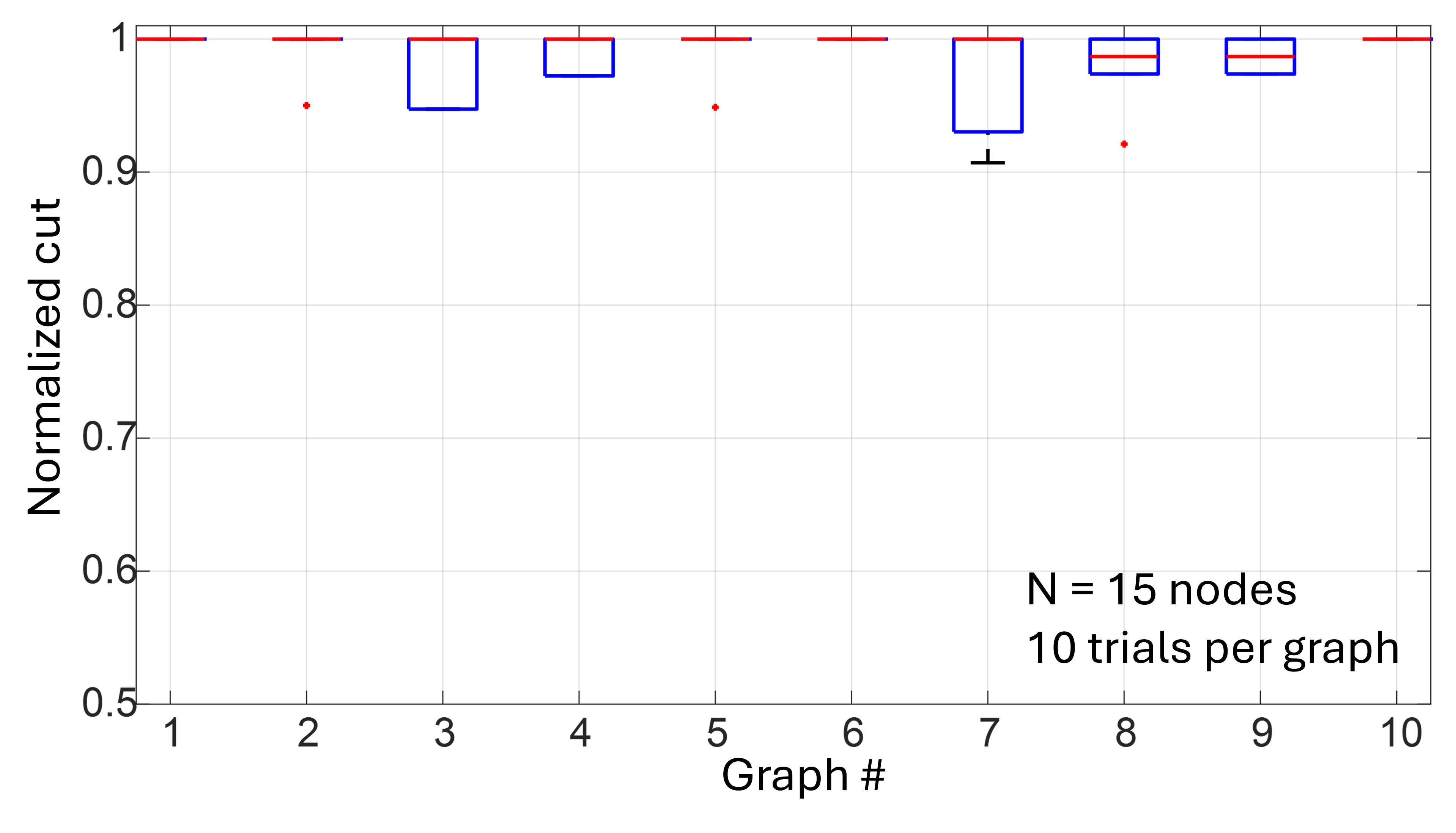
### Visual Description
## Box Plot: Normalized Cut Performance across 10 Graphs
### Overview
This image displays a box-and-whisker plot illustrating the "Normalized cut" performance metric across 10 distinct graphs. The chart indicates that for a set of 15 nodes, the algorithm or method being tested consistently achieves high performance, with most trials resulting in a normalized cut value of 1.0.
### Components/Axes
* **Y-Axis:** Labeled "Normalized cut". The scale ranges from 0.5 to 1.0, with major tick marks at 0.1 intervals.
* **X-Axis:** Labeled "Graph #". The scale ranges from 1 to 10, representing the specific graph being tested.
* **Annotations:** Located in the bottom-right quadrant of the plot area, the text reads:
* "N = 15 nodes"
* "10 trials per graph"
* **Visual Elements:**
* **Blue Boxes:** Represent the interquartile range (IQR) of the data.
* **Red Horizontal Lines:** Represent the median value within the boxes.
* **Black Lines (Whiskers):** Represent the range of the data (excluding outliers).
* **Red Dots:** Represent statistical outliers.
### Detailed Analysis
The data is plotted for 10 distinct graphs. Below is the breakdown of the distribution for each:
* **Graph 1:** Median at 1.0. No box or whiskers visible, indicating all 10 trials resulted in 1.0.
* **Graph 2:** Box spans approximately 0.95 to 1.0. Median at 1.0. A red outlier dot is present at approximately 0.95.
* **Graph 3:** Box spans approximately 0.95 to 1.0. Median at 1.0.
* **Graph 4:** Box spans approximately 0.97 to 1.0. Median at 1.0.
* **Graph 5:** Median at 1.0. No box visible. A red outlier dot is present at approximately 0.95.
* **Graph 6:** Median at 1.0. No box or whiskers visible.
* **Graph 7:** Box spans approximately 0.93 to 1.0. Median at 1.0. A lower whisker extends down to approximately 0.91.
* **Graph 8:** Box spans approximately 0.97 to 1.0. Median is slightly below 1.0, at approximately 0.98. A red outlier dot is present at approximately 0.92.
* **Graph 9:** Box spans approximately 0.97 to 1.0. Median at 1.0.
* **Graph 10:** Median at 1.0. No box or whiskers visible.
### Key Observations
* **High Performance Ceiling:** The vast majority of trials across all graphs result in a normalized cut of 1.0, suggesting the method is highly effective for these specific graph configurations.
* **Variance:** Graph 7 exhibits the most significant spread in data, with the lowest whisker reaching down to ~0.91.
* **Outliers:** Graphs 2, 5, and 8 contain outliers, indicating that while the method is generally consistent, there are occasional trials where the performance drops significantly compared to the median.
* **Median Shift:** Graph 8 is the only instance where the median line is visibly lower than 1.0 (approx. 0.98), suggesting it may be the most difficult graph configuration among the set.
### Interpretation
The "Normalized cut" is a standard metric used in graph theory and computer vision to evaluate the quality of graph partitioning or clustering. A value of 1.0 typically represents an optimal or near-optimal cut.
The data demonstrates that the algorithm is highly robust for 15-node graphs, as it achieves the optimal score of 1.0 in the median case for 9 out of 10 graphs. The presence of outliers and the slight performance dip in Graph 8 suggest that the algorithm's performance is dependent on the specific topology of the graph being analyzed. The "N = 15 nodes" constraint implies a relatively small graph size, which likely contributes to the high success rate. The consistency across most graphs suggests that the method is reliable, though the outliers in graphs 2, 5, 7, and 8 indicate that certain graph structures may occasionally challenge the algorithm's convergence or partitioning logic.
</details>
Figure 10: Computing MaxCut using OIM-based p-bit engine. Box plot showing distribution of graph cuts obtained for 10 randomly generated 15-node graphs. Each graph is simulated 10 times. The SHI scheme is the same as that used in the main text.
## APPENDIX I DYNAMICS OF DYNAMICAL ISING MACHINE
Figure 11 evaluates the graph considered in Fig. 4 using the analog dynamics of the DIM (without stochastic sampling). A bifurcation similar to that exhibited by other models such as SBM [35] is observed.
<details>
<summary>Figure7r.png Details</summary>
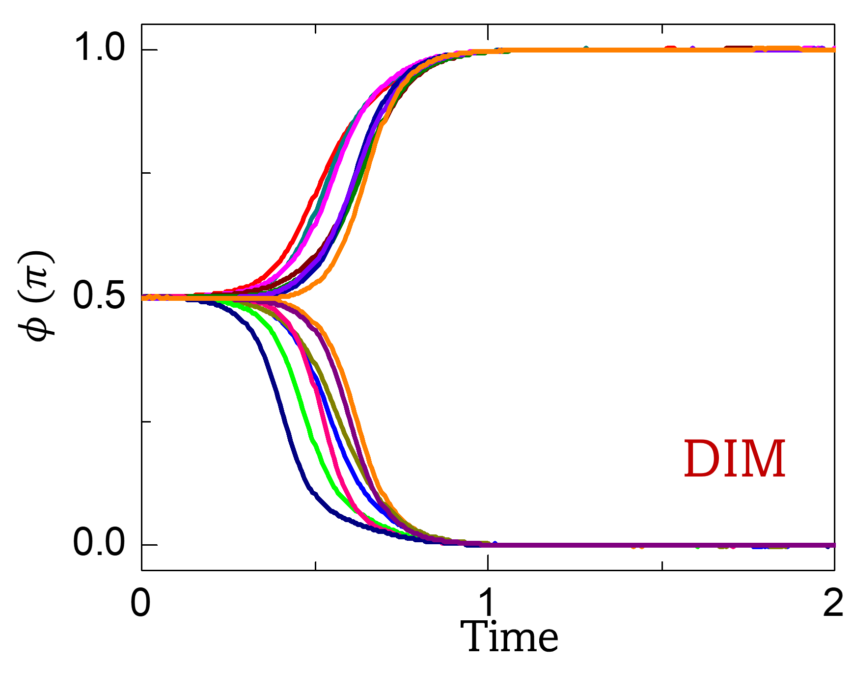
### Visual Description
## Line Chart: Bifurcation of $\phi (\pi)$ over Time
### Overview
The image displays a line chart illustrating the temporal evolution of a variable, denoted as $\phi (\pi)$, starting from a neutral state of 0.5. The chart demonstrates a bifurcation process where multiple trajectories, initially clustered at 0.5, diverge over time to settle into one of two stable states: 0.0 or 1.0. The chart includes the annotation "DIM" in the lower-right quadrant.
### Components/Axes
* **Y-Axis**: Labeled "$\phi (\pi)$". The scale ranges from 0.0 to 1.0. Major tick marks are present at 0.0, 0.5, and 1.0.
* **X-Axis**: Labeled "Time". The scale ranges from 0 to 2. Major tick marks are present at 0, 1, and 2.
* **Data Series**: Multiple colored lines (magenta, light blue, green, dark blue, orange, brown) representing different simulation runs or parameter variations.
* **Annotation**: The text "DIM" is written in red, positioned in the lower-right area of the chart (approximately at x=1.5, y=0.25).
### Detailed Analysis
* **Initial State (t = 0 to ~0.3)**: All data series originate at the coordinate (0, 0.5). The lines remain tightly clustered, showing no significant deviation from the 0.5 value during this initial phase.
* **Divergence Phase (~0.3 to ~0.8)**: Starting at approximately t=0.3, the lines begin to diverge.
* **Upper Branch**: A subset of lines (magenta, light blue, orange, brown) curves upward, increasing monotonically toward the value of 1.0.
* **Lower Branch**: A subset of lines (dark blue, green, brown, orange) curves downward, decreasing monotonically toward the value of 0.0.
* **Steady State (~0.8 to 2.0)**: By t=0.8, all lines have reached their respective steady states. The lines remain flat at either 0.0 or 1.0 for the remainder of the time axis (up to t=2.0).
* **Symmetry**: The bifurcation appears largely symmetric around the horizontal line $\phi = 0.5$.
### Key Observations
* **Bistability**: The system exhibits clear bistable behavior. The state $\phi = 0.5$ acts as an unstable equilibrium point, while 0.0 and 1.0 act as stable attractors.
* **Transition Speed**: The transition from the unstable equilibrium to the stable attractors is rapid, occurring over a time interval of approximately 0.5 units.
* **Annotation**: The red "DIM" label is isolated from the axes and data, suggesting it is a label for the specific dataset or model configuration being plotted, rather than a variable on the axes.
### Interpretation
The data suggests a phase transition or a bifurcation event in a dynamical system. The system is initially in a state of unstable equilibrium ($\phi = 0.5$). As time progresses, the system is forced to "choose" between two stable outcomes (0.0 or 1.0).
The "DIM" label likely stands for "Dimensionality" or refers to a specific parameter set (e.g., "Dimension 1" or "Dimensionality reduction"). In computational or physical modeling, this type of plot is characteristic of systems undergoing symmetry breaking, where small variations in initial conditions or parameters lead to divergent macroscopic outcomes. The fact that all lines converge to exactly 0.0 or 1.0 indicates that the system is highly constrained or "saturated" once the transition is complete.
</details>
Figure 11: Dynamical Ising Machine. Evolution of $φ$ in the DIM model for the graph considered in Fig. 4 (K=1; $K_s(t)=0.4t$ ).
## References
- [1] T. Wang, L. Wu, P. Nobel, and J. Roychowdhury. Solving combinatorial optimisation problems using oscillator based Ising machines. Natural Computing 20 (2), 287–306 (2021).
- [2] N. Mohseni, P. L. McMahon, and T. Byrnes. Ising machines as hardware solvers of combinatorial optimization problems. Nature Reviews Physics 4 (6), 363–379 (2022).
- [3] A. Lucas, Ising formulations of many NP problems, Frontiers in Physics 2, 5 (2014).
- [4] R. Hamerly, T. Inagaki, P. L. McMahon, D. Venturelli, A. Marandi, T. Onodera, E. Ng, C. Langrock, K. Inaba, T. Honjo, et al. Experimental investigation of performance differences between coherent Ising machines and a quantum annealer. Science Advances 5 (5), eaau0823 (2019).
- [5] T. Honjo, T. Sonobe, K. Inaba, T. Inagaki, T. Ikuta, Y. Yamada, T. Kazama, K. Enbutsu, T. Umeki, R. Kasahara, et al. 100,000-spin coherent Ising machine. Science Advances 7 (40), eabh0952 (2021).
- [6] A. Litvinenko, R. Khymyn, R. Ovcharov, and J. Åkerman. A 50-spin surface acoustic wave Ising machine. Communications Physics 8 (1), 1–11 (2025).
- [7] A. Mallick, M. K. Bashar, D. S. Truesdell, B. H. Calhoun, and N. Shukla. Overcoming the accuracy vs. performance trade-off in oscillator ising machines. In 2021 IEEE International Electron Devices Meeting (IEDM), 40–2 (2021).
- [8] W. Moy, I. Ahmed, P.-W. Chiu, J. Moy, S. S. Sapatnekar, and C. H. Kim. A 1,968-node coupled ring oscillator circuit for combinatorial optimization problem solving. Nature Electronics 5 (5), 310–317 (2022).
- [9] M. K. Bashar, A. Mallick, D. S. Truesdell, B. H. Calhoun, S. Joshi, and N. Shukla. Experimental demonstration of a reconfigurable coupled oscillator platform to solve the max-cut problem. IEEE Journal on Exploratory Solid-State Computational Devices and Circuits 6 (2), 116–121 (2020).
- [10] J. Vaidya, R. S. Kanthi, and N. Shukla. Creating electronic oscillator-based Ising machines without external injection locking. Scientific Reports 12 (1), 981 (2022).
- [11] O. Maher, M. Jiménez, C. Delacour, N. Harnack, J. Núñez, M. J. Avedillo, B. Linares-Barranco, A. Todri-Sanial, G. Indiveri, and S. Karg. A CMOS-compatible oscillation-based VO 2 Ising machine solver. Nature Communications 15 (1), 3334 (2024).
- [12] H. Cılasun, W. Moy, Z. Zeng, T. Islam, H. Lo, A. Vanasse, M. Tan, M. Anees, A. Kumar, S. S. Sapatnekar, et al. A coupled-oscillator-based Ising chip for combinatorial optimization. Nature Electronics 1–10 (2025).
- [13] A. Litvinenko, R. Khymyn, V. H. González, R. Ovcharov, A. A. Awad, V. Tyberkevych, A. Slavin, and J. Åkerman. A spinwave Ising machine. Communications Physics 6 (1), 227 (2023).
- [14] A. D. King, S. Suzuki, J. Raymond, A. Zucca, T. Lanting, F. Altomare, A. J. Berkley, S. Ejtemaee, E. Hoskinson, S. Huang, et al. Coherent quantum annealing in a programmable 2,000 qubit Ising chain. Nature Physics 18 (11), 1324–1328 (2022).
- [15] M. K. Bashar, Z. Lin, and N. Shukla. Stability of oscillator Ising machines: Not all solutions are created equal. J. Appl. Phys. 134 (14), 144901 (2023).
- [16] Y. Cheng, M. K. Bashar, N. Shukla, and Z. Lin. A control theoretic analysis of oscillator Ising machines. Chaos: An Interdisciplinary Journal of Nonlinear Science 34 (7) (2024).
- [17] A. Allibhoy, A. N. Montanari, F. Pasqualetti, and A. E. Motter. Global Optimization Through Heterogeneous Oscillator Ising Machines. arXiv preprint arXiv:2505.17027 (2025).
- [18] K. Y. Camsari, B. M. Sutton, and S. Datta. P-bits for probabilistic spin logic. Applied Physics Reviews 6 (1) (2019).
- [19] K. Y. Camsari, R. Faria, B. M. Sutton, and S. Datta. Stochastic p-bits for invertible logic. Physical Review X 7 (3), 031014 (2017).
- [20] N. A. Aadit, A. Grimaldi, M. Carpentieri, L. Theogarajan, J. M. Martinis, G. Finocchio, and K. Y. Camsari. Massively parallel probabilistic computing with sparse Ising machines. Nature Electronics 5 (7), 460–468 (2022).
- [21] S. Chowdhury, A. Grimaldi, N. A. Aadit, S. Niazi, M. Mohseni, S. Kanai, H. Ohno, S. Fukami, L. Theogarajan, G. Finocchio, et al. A full-stack view of probabilistic computing with p-bits: Devices, architectures, and algorithms. IEEE Journal on Exploratory Solid-State Computational Devices and Circuits 9 (1), 1–11 (2023).
- [22] W. Whitehead, Z. Nelson, K. Y. Camsari, and L. Theogarajan. CMOS-compatible Ising and Potts annealing using single-photon avalanche diodes. Nature Electronics 6 (12), 1009–1019 (2023).
- [23] C. Duffee, J. Athas, Y. Shao, N. D. Melendez, E. Raimondo, J. A. Katine, K. Y. Camsari, G. Finocchio, and P. K. Amiri. Integrated probabilistic computer using voltage-controlled magnetic tunnel junctions as its entropy source. arXiv preprint arXiv:2412.08017 (2024).
- [24] W. A. Borders, A. Z. Pervaiz, S. Fukami, K. Y. Camsari, H. Ohno, and S. Datta. Integer factorization using stochastic magnetic tunnel junctions. Nature 573 (7774), 390–393 (2019).
- [25] N. S. Singh, K. Kobayashi, Q. Cao, K. Selcuk, T. Hu, S. Niazi, N. A. Aadit, S. Kanai, H. Ohno, S. Fukami, et al. CMOS plus stochastic nanomagnets enabling heterogeneous computers for probabilistic inference and learning. Nature Communications 15 (1), 2685 (2024).
- [26] J. Si, S. Yang, Y. Cen, J. Chen, Y. Huang, Z. Yao, D.-J. Kim, K. Cai, J. Yoo, X. Fong, et al. Energy-efficient superparamagnetic Ising machine and its application to traveling salesman problems. Nature Communications 15 (1), 3457 (2024).
- [27] J. Jhonsa, W. Whitehead, D. McCarthy, S. Chowdhury, K. Camsari, and L. Theogarajan. A CMOS Probabilistic Computing Chip With In-situ hardware Aware Learning. arXiv preprint arXiv:2504.14070 (2025).
- [28] F. Böhm, D. Alonso-Urquijo, G. Verschae, and G. Van der Sande. Noise-injected analog Ising machines enable ultrafast statistical sampling and machine learning. Nature Communications 13 (1), 5847 (2022).
- [29] K. Lee, S. Chowdhury, and K. Y. Camsari. Noise-augmented chaotic Ising machines for combinatorial optimization and sampling. Communications Physics 8 (1), 35 (2025).
- [30] R. Faria, K. Y. Camsari, and S. Datta. Low-barrier nanomagnets as p-bits for spin logic. IEEE Magnetics Letters 8, 1–5 (2017).
- [31] R. Adler. A study of locking phenomena in oscillators. Proceedings of the IRE 34 (6), 351–357 (2006).
- [32] P. Bhansali and J. Roychowdhury. Gen-Adler: The generalized Adler’s equation for injection locking analysis in oscillators. In 2009 Asia and South Pacific Design Automation Conference, 522–527 (2009).
- [33] G. E. P. Box, G. M. Jenkins, G. C. Reinsel, and G. M. Ljung, Time Series Analysis: Forecasting and Control, 5th ed. (John Wiley & Sons, 2015).
- [34] E. M. H. E. B. Ekanayake and N. Shukla. Different paths, same destination: Designing physics-inspired dynamical systems with engineered stability to minimize the Ising Hamiltonian. Phys. Rev. Appl. 24 (2), 024008 (2025).
- [35] H. Goto, K. Tatsumura, and A. R. Dixon. Combinatorial optimization by simulating adiabatic bifurcations in nonlinear Hamiltonian systems. Science Advances 5 (4), eaav2372 (2019).
- [36] S. Niazi, S. Chowdhury, N. A. Aadit, M. Mohseni, Y. Qin, and K. Y. Camsari, Training deep Boltzmann networks with sparse Ising machines, Nature Electronics 7 (7), 610–619 (2024).
- [37] M. K. Bashar and N. Shukla. Designing Ising machines with higher order spin interactions and their application in solving combinatorial optimization. Scientific Reports 13 (1), 9558 (2023).
- [38] D. Kleyko, D. Nikonov, A. Khosrowshahi, B. Olshausen, C. Bybee, and F. Sommer. Efficient optimization with higher-order ising machines. Nature Communications 14 (1) (2023).
- [39] C. Duffee, J. Athas, A. Grimaldi, D. Volpe, G. Finocchio, E. Wei, and P. K. Amiri. Extended-variable probabilistic computing with p-dits. arXiv preprint arXiv:2506.00269 (2025).
- [40] M. Honari-Latifpour and M.-A. Miri. Optical Potts machine through networks of three-photon down-conversion oscillators. Nanophotonics 9 (13), 4199–4205 (2020).
- [41] N. Berloff and J. Cummins. Vector Ising Spin Annealer for Minimizing Ising Hamiltonians. (2025), Nature Portfolio.
- [42] A. Mallick, M. K. Bashar, Z. Lin, and N. Shukla. Computational models based on synchronized oscillators for solving combinatorial optimization problems. Physical Review Applied 17 (6), 064064 (2022).
- [43] C. Delacour, B. Haverkort, F. Sabo, N. Azemard, and A. Todri-Sanial. Lagrange Oscillatory Neural Networks for Constraint Satisfaction and Optimization. arXiv preprint arXiv:2505.07179 (2025).
- [44] M. Ercsey-Ravasz and Z. Toroczkai. Optimization hardness as transient chaos in an analog approach to constraint satisfaction. Nature Physics 7 (12), 966–970 (2011).